New consonantal acoustic parameters for forensic speaker ...

New consonantal acoustic parameters for forensic speaker comparison

Colleen Marie Kavanagh

Submitted in partial fulfillment of the requirements for the degree of Doctor of Philosophy

University of York

Department of Language and Linguistic Science

Submitted September 2012

1

Abstract

This thesis examines acoustic parameters of five consonants /m, n, ŋ, l, s/ in

two dialects of British English: Standard Southern British English and Leeds

English. The research aims to explore population distributions of the acoustic

features, gauge cross-dialectal variation, and discover new parameters for

application in forensic speaker comparison casework. The five parameters

investigated for each segment are:

For /m, n, ŋ, l/: For /s/: Normalised duration Centre of gravity Standard deviation Frequency at peak amplitude Frequency at minimum amplitude

Normalised duration Centre of gravity Standard deviation Skewness Kurtosis

The work contributes firstly to the general phonetic literature by presenting

acoustic data for a number of parameters and consonant segments that have not

been previously studied in depth in these dialects. Secondly, the research informs

the forensic phonetic literature by considering the intra- and inter-speaker

variability and gauging the relative speaker-specificity of each acoustic feature.

Discriminant analysis and likelihood ratio estimation assess the discrimination

ability of each feature, and results highlight several promising parameters with

potential for application in forensic speaker comparison casework.

3

Table of Contents

Abstract ................................................................................................................... 1

Table of Contents .................................................................................................... 3

List of Tables ........................................................................................................ 14

List of Figures ....................................................................................................... 17

List of Appendices ................................................................................................. 27

Acknowledgements ................................................................................................ 28

Declaration ............................................................................................................ 31

Chapter 1 Introduction ........................................................................................... 33

1.1 Forensic speaker comparison background .......................................... 33

1.1.1 Expression of forensic speaker comparison conclusions ............. 34

1.2 Research aims ...................................................................................... 36

1.3 Thesis outline ....................................................................................... 38

Chapter 2 Literature Review .................................................................................. 41

2.0 Overview .............................................................................................. 41

2.1 Segmental duration research ................................................................ 41

2.2 Other acoustic parameters of consonants ............................................ 50

2.2.1 Segmental acoustic literature: Nasal consonants ......................... 51

2.2.1.1 Nasal consonant production .................................................. 51

2.2.1.2 Nasal acoustic literature ........................................................ 51

2.2.2 Segmental acoustic literature: /l/ .................................................. 54

2.2.2.1 /l/ production .......................................................................... 54

2.2.2.2 /l/ acoustic literature .............................................................. 55

2.2.3 Segmental acoustic literature: /s/ .................................................. 58

2.2.3.1 /s/ production ......................................................................... 58

2.2.3.2 /s/ acoustic literature .............................................................. 59

2.3 Speaker discrimination literature ......................................................... 68

2.3.1 Discriminant analysis .................................................................... 68

4

2.3.1.1 Speaker comparison research using discriminant analysis ... 71

2.3.2 Likelihood ratios ........................................................................... 77

2.3.2.1 Limitations ............................................................................. 80

2.3.2.2 Likelihood ratios in forensic speaker comparison ................ 81

2.4 Chapter summary ................................................................................. 90

Chapter 3 Pilot Study ............................................................................................. 91

3.0 Overview.............................................................................................. 91

3.1 Materials .............................................................................................. 91

3.2 Segmentation ....................................................................................... 93

3.2.1 Nasal segmentation ....................................................................... 94

3.2.2 Lateral segmentation .................................................................... 95

3.2.3 Fricative segmentation .................................................................. 98

3.2.4 Excluded data ............................................................................. 100

3.3 Data .................................................................................................... 103

3.4 Results and Analysis ......................................................................... 106

3.4.1 Dialectal Variation ...................................................................... 106

3.4.2 Position and Context Effects ...................................................... 107

3.4.3 Variability by Speaker ................................................................ 113

3.4.3.1 Discriminant Analysis ......................................................... 118

3.5 Conclusions ........................................................................................ 123

Chapter 4 Materials and Methodology ................................................................. 125

4.0 Overview............................................................................................ 125

4.1 Materials ............................................................................................ 125

4.1.1 Corpora ....................................................................................... 125

4.1.1.1 The DyViS corpus ............................................................... 126

4.1.1.2 The IViE corpus .................................................................. 126

5

4.1.1.3 The Morley corpus .............................................................. 127

4.1.2 Speech tasks ................................................................................ 128

4.1.3 Segments ..................................................................................... 128

4.1.3.1 Segmentation........................................................................ 129

4.2 Methodology ...................................................................................... 132

4.2.1 Acoustic parameters .................................................................... 133

4.2.1.1 Normalised duration ............................................................ 133

4.2.1.2 Centre of gravity .................................................................. 134

4.2.1.3 Standard deviation ............................................................... 135

4.2.1.4 Peak frequency ..................................................................... 136

4.2.1.5 Minimum frequency ............................................................ 137

4.2.1.6 Skewness .............................................................................. 138

4.2.1.7 Kurtosis ................................................................................ 138

4.2.2 Nasal and lateral spectral analysis .............................................. 139

4.2.3 Fricative spectral analysis ........................................................... 142

4.2.4 Speaker and dialect significance testing ..................................... 145

4.2.5 Discriminant analysis .................................................................. 145

4.2.6 Likelihood ratios ......................................................................... 147

4.2.6.1 Likelihood ratio calculation ................................................. 147

4.2.6.2 Assessment of LR performance .......................................... 148

Chapter 5 Results: /m/ ......................................................................................... 151

5.0 Overview ............................................................................................ 151

5.1 Intra- and inter-speaker variability .................................................... 151

5.1.1 Normalised duration ................................................................... 152

5.1.2 Centre of gravity ......................................................................... 154

6

5.1.2.1 COG Band 1: 0-500 Hz ....................................................... 154

5.1.2.2 COG Band 2: 500-1000 Hz ................................................. 156

5.1.2.3 COG Band 3: 1-2 kHz ......................................................... 157

5.1.2.4 COG Band 4: 2-3 kHz ......................................................... 159

5.1.2.5 COG Band 5: 3-4 kHz ......................................................... 161

5.1.2.6 Global centre of gravity ...................................................... 162

5.1.3 Standard Deviation ..................................................................... 164

5.1.3.1 SD Band 1: 0-500 Hz .......................................................... 164

5.1.3.2 SD Band 2: 500-1000 Hz .................................................... 165

5.1.3.3 SD Band 3: 1-2 kHz ............................................................ 167

5.1.3.4 SD Band 4: 2-3 kHz ............................................................ 168

5.1.3.5 SD Band 5: 3-4 kHz ............................................................ 169

5.1.3.6 Global standard deviation .................................................... 171

5.1.4 Peak frequency ........................................................................... 172

5.1.4.1 Peak Band 1: 0-500 Hz ....................................................... 172

5.1.4.2 Peak Band 2: 500-1000 Hz ................................................. 173

5.1.4.3 Peak Band 3: 1-2 kHz ......................................................... 174

5.1.4.4 Peak Band 4: 2-3 kHz ......................................................... 176

5.1.4.5 Peak Band 5: 3-4 kHz ......................................................... 177

5.1.4.6 Global Peak frequency ........................................................ 179

5.1.5 Minimum frequency ................................................................... 180

5.1.5.1 Minimum Band 1: 0-500 Hz ............................................... 180

5.1.5.2 Minimum Band 2: 500-1000 Hz ......................................... 181

5.1.5.3 Minimum Band 3: 1-2 kHz ................................................. 183

5.1.5.4 Minimum Band 4: 2-3 kHz ................................................. 184

7

5.1.5.5 Minimum Band 5: 3-4 kHz ................................................. 186

5.1.5.6 Global Minimum frequency ................................................ 188

5.2 Dialect effects .................................................................................... 189

5.3 Discriminant analysis ......................................................................... 190

5.4 Likelihood ratio analysis ................................................................... 195

5.4.1 ±4 log10LRs ............................................................................... 196

5.4.2 False positives and false negatives ............................................. 197

5.4.3 Equal error rate ........................................................................... 198

5.4.4 Log likelihood ratio cost ............................................................. 198

5.4.5 Best performing tests .................................................................. 199

5.5 Chapter summary ............................................................................... 201

Chapter 6 Results: /n/ .......................................................................................... 202

6.0 Overview ............................................................................................ 202




6.1.2.1 COG Band 1: 0-500 Hz ....................................................... 205

6.1.2.2 COG Band 2: 500-1000 Hz ................................................. 206

6.1.2.3 COG Band 3: 1-2 kHz ......................................................... 208

6.1.2.4 COG Band 4: 2-3 kHz ......................................................... 209

6.1.2.5 COG Band 5: 3-4 kHz ......................................................... 211

6.1.2.6 Global centre of gravity ....................................................... 212

6.1.3 Standard deviation ...................................................................... 213

6.1.3.1 SD Band 1: 0-500 Hz .......................................................... 214

6.1.3.2 SD Band 2: 500-1000 Hz .................................................... 215

8

6.1.3.3 SD Band 3: 1-2 kHz ............................................................ 217

6.1.3.4 SD Band 4: 2-3 kHz ............................................................ 218

6.1.3.5 SD Band 5: 3-4 kHz ............................................................ 220


6.1.4 Peak frequency ........................................................................... 222

6.1.4.1 Peak Band 1: 0-500 Hz ....................................................... 222

6.1.4.2 Peak Band 2: 500-1000 Hz ................................................. 224

6.1.4.3 Peak Band 3: 1-2 kHz ......................................................... 225

6.1.4.4 Peak Band 4: 2-3 kHz ......................................................... 226

6.1.4.5 Peak Band 5: 3-4 kHz ......................................................... 228



6.1.5.1 Minimum Band 1: 0-500 Hz ............................................... 231

6.1.5.2 Minimum Band 2: 500-1000 Hz ......................................... 231

6.1.5.3 Minimum Band 3: 1-2 kHz ................................................. 232

6.1.5.4 Minimum Band 4: 2-3 kHz ................................................. 234

6.1.5.5 Minimum Band 5: 3-4 kHz ................................................. 236


6.2 Dialect effects .................................................................................... 238

6.3 Discriminant analysis ........................................................................ 239


6.4.1 ±4 log10LRs ............................................................................... 247


6.4.3 Equal error rate ........................................................................... 248

6.4.4 Log likelihood ratio cost ............................................................ 249

9


6.5 Chapter summary ............................................................................... 251

Chapter 7 Results: /ŋ/ .......................................................................................... 252

7.0 Overview ............................................................................................ 252




7.1.2.1 COG Band 1: 0-500 Hz ....................................................... 255

7.1.2.2 COG Band 2: 500-1000 Hz ................................................. 257

7.1.2.3 COG Band 3: 1-2 kHz ......................................................... 258

7.1.2.4 COG Band 4: 2-3 kHz ......................................................... 259

7.1.2.5 COG Band 5: 3-4 kHz ......................................................... 261

7.1.2.6 Global centre of gravity ....................................................... 263


7.1.3.1 SD Band 1: 0-500 Hz .......................................................... 264

7.1.3.2 SD Band 2: 500-1000 Hz .................................................... 266

7.1.3.3 SD Band 3: 1-2 kHz ............................................................ 268

7.1.3.4 SD Band 4: 2-3 kHz ............................................................ 269

7.1.3.5 SD Band 5: 3-4 kHz ............................................................ 270


7.1.4 Peak frequency ............................................................................ 273

7.1.4.1 Peak Band 1: 0-500 Hz ........................................................ 274

7.1.4.2 Peak Band 2: 500-1000 Hz .................................................. 274

7.1.4.3 Peak Band 3: 1-2 kHz .......................................................... 275

7.1.4.4 Peak Band 4: 2-3 kHz .......................................................... 276

10

7.1.4.5 Peak Band 5: 3-4 kHz ......................................................... 278



7.1.5.1 Minimum Band 1: 0-500 Hz ............................................... 280

7.1.5.2 Minimum Band 2: 500-1000 Hz ......................................... 281

7.1.5.3 Minimum Band 3: 1-2 kHz ................................................. 282

7.1.5.4 Minimum Band 4: 2-3 kHz ................................................. 284

7.1.5.5 Minimum Band 5: 3-4 kHz ................................................. 285


7.2 Dialect effects .................................................................................... 287

7.3 Chapter summary ............................................................................... 289

Chapter 8 Results: /l/ ........................................................................................... 290

8.0 Overview............................................................................................ 290




8.1.2.1 COG Band 1: 0-500 Hz ....................................................... 293

8.1.2.2 COG Band 2: 500-1000 Hz ................................................. 294

8.1.2.3 COG Band 3: 1-2 kHz ......................................................... 296

8.1.2.4 COG Band 4: 2-3 kHz ......................................................... 297

8.1.2.5 COG Band 5: 3-4 kHz ......................................................... 299

8.1.2.6 Global centre of gravity ...................................................... 300


8.1.3.1 SD Band 1: 0-500 Hz .......................................................... 303

8.1.3.2 SD Band 2: 500-1000 Hz .................................................... 304

11

8.1.3.3 SD Band 3: 1-2 kHz ............................................................ 306

8.1.3.4 SD Band 4: 2-3 kHz ............................................................ 307

8.1.3.5 SD Band 5: 3-4 kHz ............................................................ 309


8.1.4 Peak frequency ............................................................................ 312

8.1.4.1 Peak Band 1: 0-500 Hz ........................................................ 312

8.1.4.2 Peak Band 2: 500-1000 Hz .................................................. 313

8.1.4.3 Peak Band 3: 1-2 kHz .......................................................... 314

8.1.4.4 Peak Band 4: 2-3 kHz .......................................................... 316

8.1.4.5 Peak Band 5: 3-4 kHz .......................................................... 317

8.1.4.6 Global Peak frequency......................................................... 318


8.1.5.1 Minimum Band 1: 0-500 Hz ............................................... 320

8.1.5.2 Minimum Band 2: 500-1000 Hz ......................................... 321

8.1.5.3 Minimum Band 3: 1-2 kHz ................................................. 322

8.1.5.4 Minimum Band 4: 2-3 kHz ................................................. 324

8.1.5.5 Minimum Band 5: 3-4 kHz ................................................. 325


8.2 Dialect effects .................................................................................... 328

8.3 Discriminant analysis ......................................................................... 331


8.4.1 ±4 log10LRs ............................................................................... 340


8.4.3 Equal error rate ........................................................................... 342

8.4.4 Log likelihood ratio cost ............................................................. 342

12


8.5 Chapter summary ............................................................................... 345

Chapter 9 Results: /s/ ........................................................................................... 346

9.0 Overview............................................................................................ 346

9.1 Intra- and inter-speaker variability: Static measures ........................ 346

9.1.1 Normalised Duration .................................................................. 348

9.1.2 Centre of Gravity ........................................................................ 350

9.1.3 Standard Deviation ..................................................................... 351

9.1.4 Skewness ..................................................................................... 353

9.1.5 Kurtosis ....................................................................................... 354

9.1.6 Filter effects ................................................................................ 356

9.1.7 Dialect effects ............................................................................. 360

9.1.8 Static discriminant analysis ........................................................ 361

9.1.9 Static likelihood ratio analysis ................................................... 373

9.1.9.1 ±4 log10LRs ........................................................................ 376

9.1.9.2 False positives and false negatives ...................................... 376

9.1.9.3 Equal error rate .................................................................... 377

9.1.9.4 Log likelihood ratio cost ..................................................... 377

9.1.9.5 Best performing tests ........................................................... 378

9.2 Dynamic variability ........................................................................... 378

9.2.1 Dynamic discriminant analysis .................................................. 382

9.3 Chapter summary ............................................................................... 386

Chapter 10 Discussion ......................................................................................... 387

10.0 Overview.......................................................................................... 387

10.1 Summary of speaker-specificity and discrimination findings ........ 387

10.1.1 ANOVA findings ...................................................................... 387

13

10.1.1.1 Segments ............................................................................ 387

10.1.1.2 Parameters .......................................................................... 388

10.1.2 Discriminant analysis and likelihood ratio findings ................ 390

10.1.2.1 /m/ ...................................................................................... 390

10.1.2.2 /n/ ....................................................................................... 391

10.1.2.3 /l/ ........................................................................................ 391

10.1.2.4 /s/ ........................................................................................ 392

10.1.2.5 Overall findings ................................................................. 393

10.2 Limitations ....................................................................................... 395

10.3 Implications for forensic speaker comparison casework ................ 396

Chapter 11 Conclusion ........................................................................................ 398

11.1 Thesis summary ............................................................................... 398

11.2 Research aims revisited ................................................................... 401

11.3 Opportunities for future research .................................................... 401

11.4 Conclusion ....................................................................................... 403

Appendices .......................................................................................................... 404

Bibliography ........................................................................................................ 417

14

List of Tables

Table 2.1. Intervocalic consonant durations (ms) across word position and syllable stress conditions. Adapted from Umeda (1977:848). ........................... 44

Table 2.2. Duration of /m, n, l, s/ in word-initial pre-stress position and /ŋ/ in word-final position (American English: Klatt, 1979; American English and Swedish: Carlson & Granström, 1986; Australian English: Fletcher & McVeigh, 1993). ..................................................................................... 47

Table 2.3. Intervocalic consonant durations (in ms) in four word-stress conditions. Adapted from Lavoie (2001:110-111). ................................................... 49

Table 2.4. Results of ANOVAs for single and whole spectrum measures (Stuart-Smith et al., 2003:1852-1853). Results significant at p<.05 level indicated by *. ......................................................................................... 65

Table 2.5. Results of ANOVAs for duration and spectral parameters for /s/. Significant results indicated by * (p<.05), highly significant results by ** (p<.001). (Stuart-Smith, 2007:75). .................................................. 67

Table 2.6. Correct classification rates for DA using F1, F2, and F3 of Australian English /aI/. (McDougall, 2004:118). ..................................................... 74

Table 3.1. Total segmented and excluded tokens. .................................................. 103

Table 3.2. Results of ANOVAs for effect of Dialect on segment durations. ......... 107

Table 3.3. Coding of syllable position and phonological context. ......................... 109

Table 3.4. Mean segment durations (ms) and token numbers by Syllable Position and Phonological Context for all speakers. .......................................... 110

Table 3.5. ANOVA results for Syllable Position and Phonological Context effects on segment duration. Asterisks indicate effects significant at the level p<.05. ................................................................................................... 110

Table 3.6. Results of ANOVAs for effect of Speaker on segment durations. Significant effects are indicated by an asterisk. ................................... 117

Table 3.7. Cross-validated classification rates for single-predictor DA................. 119

Table 3.8. Individual classification rates with predicted group membership for all SSBE data (in percent). Correct classifications are highlighted. ......... 120

Table 3.9. Individual classification rates with predicted group membership for all Leeds data (in percent). Correct classifications are highlighted. ......... 122

Table 4.1. Token numbers by dialect, speaker, and segment. ................................ 132

Table 4.2. Summary of five parameters and 21 measurements taken for all nasal and lateral segments /m, n, ŋ, l/. ........................................................... 139

Table 4.3. Summary of datasets analysed and filters applied in analysis of /s/. .... 144

15

Table 5.1. Results of univariate ANOVAs for Speaker (N=30) for each acoustic feature of /m/ (x19). Bold text indicates significant p values at the level .05. ......................................................................................................... 152

Table 5.2. Mann-Whitney U test findings for effect of Dialect on acoustic features of /m/. Bold text indicates results significant at the level .05. ............. 189

Table 5.3. Cross-validated classification rates for DA with 1-8 predictors for /m/ and 30 speakers; chance=3.3%. Asterisks indicate tests excluding Peak Band 2 and Minimum Band 1............................................................... 193

Table 5.4. Summary of LR performance for /m/ in 19 test combinations, showing percentage of SS and DS comparisons yielding log10LRs≥±4, percentage of false positives and negatives, equal error rate (EER), and Cllr. Asterisks indicate tests where Minimum Band 1 and Peak Band 2 were excluded. The darkest shade of each colour indicates the highest value per column, with progressively lighter shades denoting lower values. .................................................................................................... 196

Table 6.1. Results of univariate ANOVAs for Speaker (N=30) for each acoustic feature of /n/ (x17). Bold text indicates significant p values at the level .05. ......................................................................................................... 203

Table 6.2. Mann-Whitney U test findings for effect of Dialect on acoustic features of /n/. Bold text indicates results significant at the level .05. .............. 239

Table 6.3. Cross-validated classification rates for DA with 1-5 predictors for /n/ and 28 speakers; chance=3.6%. Asterisks indicate tests from which Peak in Bands 2 and 5 and Minimum in Bands 1 and 2 were excluded. ......... 243

Table 6.4. Summary of LR performance for /n/ in 17 test combinations, showing percentage of same-speaker (SS) and different-speaker (DS) comparisons yielding log10LRs≥±4, percentage of false positives and negatives, equal error rates (EER), and Cllr. Asterisks indicate tests from which Peak in Bands 2 and 5, and Minimum in Bands 1 and 2, were excluded. ...................................................................................... 246

Table 7.1. Results of univariate ANOVAs for Speaker (N=29) for each acoustic feature of /ŋ/ (x15). Bold text indicates results significant at the level .05. ......................................................................................................... 253

Table 7.2. Mann-Whitney U test findings for effect of Dialect on acoustic features of /ŋ/. Bold text indicates results significant at the level .05. .............. 288

Table 8.1. Results of univariate ANOVAs for Speaker (N=30) on each acoustic feature of /l/ (x16). Bold text indicates results significant at the level .05. ......................................................................................................... 291

16

Table 8.2. Mann-Whitney U test findings for effect of Dialect on acoustic features of /l/. Bold text indicates results significant at the level .05................ 328

Table 8.3. Cross-validated classification rates for DA with 1-6 predictors for /l/ and 26 speakers; chance=3.8%. Asterisks indicate tests from which Peak in Bands 1, 2 and 5, and Minimum in Bands 1 and 5, were excluded. ... 336

Table 8.4. Summary of LR performance for /l/ in 17 test combinations, showing percentage of same-speaker (SS) and different-speaker (DS) comparisons yielding log10LRs≥±4, percentage of false positives and negatives, equal error rates (EER), and Cllr. Asterisks indicate tests from which normalised duration, Peak in Bands 1, 2, and 5, and Minimum in Bands 1 and 5 were excluded. ........................................ 340

Table 9.1. Results of univariate ANOVAs for Speaker (N=30 in 4 and 8 kHz, N=18 in 16 and 22.05 kHz) on each acoustic parameter of /s/ (x5) and in each filter condition (x4). Bold text indicates significant p values at the level .05. .......................................................................................... 348

Table 9.2. Mann-Whitney U test findings for effect of Dialect on acoustic features of /s/. Bold text indicates results that are significant at the level .05. . 360

Table 9.3. Cross-validated classification results for static discriminant analyses with 1-5 predictors for /s/ and 30 speakers, in 500-4000 Hz and 500-8000 Hz filter conditions; chance=3.3% ........................................................... 368

Table 9.4. Cross-validated classification results for static DA with 1-5 predictors for /s/ with 18 speakers (DyViS and Morley only), filtered at 500-4000, 500-8000, 500-16000, and 500-22050 Hz; chance=5.6% .................. 371

Table 9.5. Summary of LR performance for /s/, showing percentage of same-speaker (SS) and different-speaker (DS) comparisons yielding log10LRs≥±4, percentage of false positives and negatives, equal error rates (EER), and Cllr. All tests include all five acoustic parameters. .. 374

Table 9.6. Number of parameters and predictors tested in dynamic discriminant analysis. F-ratios were used to select predictors in tests indicated by asterisks. ................................................................................................ 383

Table 9.7. F-ratios for all predictors in all filter conditions, in both 30-speaker and 18-speaker data sets. The darkest blue cells indicate the highest F-ratio within each filter condition per data set. .............................................. 383

Table 9.8. Classification rates for dynamic DA of /s/ for 8 kHz tests only. .......... 385

Table 10.1. Summary of best-performing DA and LR tests per segment. ............. 390

17

List of Figures

Figure 2.1. Mean durations of pooled vowels in 12 consonant environments (House & Fairbanks, 1953:108). ......................................................................... 42

Figure 2.2. Energy contours for the nasal consonants [m] and [n]. Upper panels: uncompressed 16 kHz sampling rate. Lower panels: compressed (ITU-T G.729 codec). Reproduced from Amino and Arai (2009:24, 26). ........ 53

Figure 2.3. Illustrations of distributions with positive and negative skewness (left) and positive, negative, and normal kurtosis (right) (reproduced from MVP Programs, 2008). ........................................................................... 62

Figure 2.4. Spectrogram of /aI/ in bike, showing the 10% steps at which formant measurements were taken between markers 1 and 2 (McDougall 2004:108). ............................................................................................... 73

Figure 2.5. Tippett plots of LR discrimination using /aI/ showing „readword‟ and „spellword‟ results with all data (red solid line), and with F1 of T2 omitted (dotted black line). Reproduced from Rose, Kinoshita and Alderman (2006:333). ............................................................................. 86

Figure 3.1. Spectrogram and textgrid for sentence W1 Where is the manual? spoken by speaker MC, showing segmentation of /m/. ...................................... 95

Figure 3.2. Spectrogram and textgrid showing a segmented final /l/ in the word meal, from sentence I2 May I leave the meal early? produced by speaker RP............................................................................................... 97

Figure 3.3. Example of segmented clear initial /l/ in live in sentence I3 Will you live in Ealing? (speaker PT). .................................................................. 98

Figure 3.4. Spectrogram and textgrid for the sentence C3 Did you say mellow or yellow? produced by speaker TG, showing segmentation of /s/. .......... 99

Figure 3.5. Example of nasalised vowel in sentence W2 When will you be in Ealing? (speaker JP). The interval labelled „n X‟ marks the duration of the nasalised vowel. .............................................................................. 100

Figure 3.6. Example of /mm/ sequence with no intermediate boundary in sentence C2 Is his name Miller or Mailer? (speaker JI). .................................... 101

Figure 3.7. Example of elision of /l/ in sentence W2 When will you be in Ealing? (speaker TG). Marked interval indicates the preceding vowel. .......... 102

Figure 3.8. Mean and standard deviation of segment durations compared across dialects. .................................................................................................. 106

Figure 3.9. Means and ranges of /m/ durations for both SSBE and Leeds speakers, in descending order of mean. ................................................................ 114

18

Figure 3.10. Means and ranges of /n/ durations for both SSBE and Leeds speakers, in descending order of mean. ............................................................... 114

Figure 3.11. Means and ranges of /ŋ/ durations for both SSBE and Leeds speakers, in descending order of mean. ............................................................... 115

Figure 3.12. Means and ranges of /l/ durations for both SSBE and Leeds speakers, in descending order of mean. ............................................................... 116

Figure 4.1. Sample spectrum of /l/ in They live on the same street produced by speaker 1 (DyViS, Task 3), with Peak and Minimum frequencies highlighted. ........................................................................................... 137

Figure 5.1. Mean (represented by green markers) and range (black vertical lines) of normalised /m/ durations by speaker, in descending order of mean. .. 153

Figure 5.2. Mean and range for COG of /m/ in Band 1 by speaker, in descending order of mean. ....................................................................................... 155




Figure 5.6. Mean and range for COG of /m/ in Band 5 (3-4 kHz) by speaker, in descending order of mean. .................................................................... 161

Figure 5.7. Mean and range of COG of /m/ by speaker across the entire spectrum, 0-4 kHz. Solid lines above and below each marker line signify speakers‟ ranges within the Band by indicating maximum and minimum values. ................................................................................................... 163

Figure 5.8. Mean and range of SD of /m/ in Band 1 by speaker, in descending order of mean. ................................................................................................ 165

Figure 5.9. Mean and range of SD of /m/ in Band 2 by speaker, in descending order of mean. ................................................................................................ 166

Figure 5.10. Mean and range of SD of /m/ in Band 3 by speaker, in descending order of mean. ....................................................................................... 167



Figure 5.13. Mean SD of /m/ by speaker across the entire spectrum, 0-4 kHz. .... 171

19

Figure 5.14. Mean and range of Peak frequency of /m/ in Band 1 (0-500 Hz) by speaker, in descending order of mean. ................................................. 173

Figure 5.15. Mean and range of Peak frequency of /m/ in Band 2 by speaker, in descending order of mean. .................................................................... 174




Figure 5.19. Mean and range of Peak frequency for /m/ by speaker across the entire spectrum, 0-4 kHz. Solid lines above and below each marker line signify speakers‟ ranges within the Band by indicating maximum and minimum values. Band 2 was excluded, as noted in §5.1.4.2. ............ 179

Figure 5.20. Mean and range of Minimum frequency of /m/ in Band 1 by speaker, in descending order of mean. ................................................................ 181





Figure 5.25. Mean and range of Minimum frequency for /m/ by speaker across the entire spectrum, 0-4 kHz. Solid lines above and below each marker line signify speakers‟ ranges within the Band by indicating maximum and minimum values. Band 1 was excluded, as noted in §5.1.5.1. ............ 188

Figure 5.26. Discriminant function plot for first two discriminant functions in the „Best 8 F-ratios‟ test (COG 1, 4, 5; SD 1, 3, 4; Peak 1, 4). Individual cases are indicated by open coloured circles, and group centroids by filled blue squares. ................................................................................ 191

Figure 5.27. Individual speaker classification rates for Best 8 F-ratios and COG+SD. ............................................................................................ 194

Figure 5.28. Tippett plot of log10LR values in same- and different-speaker comparisons for Best 8 F-ratios and COG+SD tests. ......................... 200

20

Figure 6.1. Mean and range of normalised /n/ durations by speaker, in descending order of mean. ....................................................................................... 204

Figure 6.2. Mean and range for COG of /n/ in Band 1 by speaker, in descending order of mean. ....................................................................................... 206





Figure 6.7. Mean and range of COG for /n/ by speaker across the entire spectrum, 0-4 kHz. Solid lines above and below each marker line signify speakers‟ ranges within the Band by indicating maximum and minimum values. ................................................................................................... 213

Figure 6.8. Mean and range of SD of /n/ in Band 1 by speaker, in descending order of mean. ................................................................................................ 214

Figure 6.9. Mean and range of SD of /n/ in Band 2 by speaker, in descending order of mean. ................................................................................................ 216

Figure 6.10. Mean and range of SD of /n/ in Band 3 by speaker, in descending order of mean. ....................................................................................... 217



Figure 6.13. Mean SD of /n/ by speaker across the entire spectrum, 0-4 kHz. ..... 222

Figure 6.14. Mean and range of Peak frequency of /n/ in Band 1 by speaker, in descending order of mean. .................................................................... 223





21

Figure 6.19. Mean and range of Peak frequency for /n/ by speaker across the entire spectrum, 0-4 kHz. Solid lines above and below each marker line signify speakers‟ ranges within the Band by indicating maximum and minimum values. Peak in Bands 2 and 5 were excluded, as noted in §6.1.4.2 and §6.1.4.5. ............................................................................ 230

Figure 6.20. Mean and range of Minimum frequency of /n/ in Band 1 by speaker, in descending order of mean. .................................................................... 231





Figure 6.25. Mean and range of Minimum frequency for /n/ by speaker across the entire spectrum, 0-4 kHz. Solid lines above and below each marker line signify speakers‟ ranges within the Band by indicating maximum and minimum values. Bands 1 and 2 were excluded, as noted in §6.1.5.1 and §6.1.5.2. .......................................................................................... 238

Figure 6.26. Discriminant function plot showing the first two discriminant functions for the 5-predictor COG+SD/Best 5 F-ratios test. Individual cases and group centroids are shown. ................................................................... 241

Figure 6.27. Individual cross-validated classification rates in the Best 5 F-ratios test (COG in Bands 1, 3, and 4 + SD in Bands 1 and 4) and COG Bands 1-5 for /n/, with 28 speakers (chance=3.6%). ........................................ 245

Figure 6.28. Tippett plot showing log10LR values for same-speaker (SS) and different-speaker (DS) comparisons for Best 5 F-ratios and COG+Peak tests. ....................................................................................................... 251

Figure 7.1. Mean and range of normalised /ŋ/ durations by speaker, in descending order of mean. ....................................................................................... 254

Figure 7.2. Mean and range for COG of /ŋ/ in Band 1 by speaker, in descending order of mean. ....................................................................................... 256



22



Figure 7.7. Mean and range of COG for /ŋ/ by speaker across the entire spectrum, 0-4 kHz. Solid lines above and below each marker line signify speakers‟ ranges within the Band by indicating maximum and minimum values. ................................................................................................... 264

Figure 7.8. Mean and range for SD of /ŋ/ in Band 1 by speaker, in descending order of mean. ................................................................................................ 265

Figure 7.9. Mean and range for SD of /ŋ/ in Band 2 by speaker, in descending order of mean. ................................................................................................ 267

Figure 7.10. Mean and range for SD of /ŋ/ in Band 3 by speaker, in descending order of mean. ....................................................................................... 268



Figure 7.13. Mean and range of SD of /ŋ/ by speaker across the entire spectrum, 0-4 kHz. .................................................................................................... 272

Figure 7.14. Mean and range for Peak frequency of /ŋ/ in Band 1 by speaker, in descending order of mean. .................................................................... 274





Figure 7.19. Mean and range of Peak frequency of /ŋ/ by speaker across the spectrum, 0-4 kHz. Solid lines above and below each marker line signify speakers‟ ranges within the Band by indicating maximum and minimum values. Bands 1, 2, and 3 were excluded, as noted in §7.1.4.1-7.1.4.3 above. ........................................................................................ 280

Figure 7.20. Mean and range for Minimum frequency of /ŋ/ in Band 1 by speaker, in descending order of mean. ............................................................... 281

23

Figure 7.21. Mean and range for Minimum frequency of /ŋ/ in Band 2 by speaker, in descending order of mean. ................................................................ 282




Figure 7.25. Mean and range of Minimum frequency for /ŋ/ by speaker across the spectrum, 0-4 kHz. Solid lines above and below each marker line signify speakers‟ ranges within the Band by indicating maximum and minimum values. Bands 1, 2, and 4 were excluded, as noted in §7.1.5.1, 7.1.5.2, and 7.1.5.4. ............................................................................... 287

Figure 8.1. Mean and range of normalised /l/ durations by speaker, in descending order of mean. ....................................................................................... 292

Figure 8.2. Mean and range for COG of /l/ in Band 1 by speaker, in descending order of mean. ....................................................................................... 294





Figure 8.7. COG for /l/ by speaker across the entire spectrum, 0-4 kHz. Markers indicate speakers‟ mean values in each Band; solid lines above and below each marker line signify speakers‟ ranges within the Band by indicating maximum and minimum values. ......................................... 301

Figure 8.8. Mean and range for SD of /l/ in Band 1 by speaker, in descending order of mean. ................................................................................................. 304

Figure 8.9. Mean and range for SD of /l/ in Band 2 by speaker, in descending order of mean. ................................................................................................. 305

Figure 8.10. Mean and range for SD of /l/ in Band 3 by speaker, in descending order of mean. ....................................................................................... 307


24


Figure 8.13. SD for /l/ by speaker across the entire spectrum, 0-4 kHz. Markers indicate speakers‟ mean values in each Band. ..................................... 311

Figure 8.14. Mean and range for Peak frequency of /l/ in Band 1 by speaker, in descending order of mean. .................................................................... 313





Figure 8.19. Peak frequency for /l/ by speaker across the spectrum, 0-4 kHz. Markers indicate speakers‟ mean values in each Band; solid lines above and below each marker line signify speakers‟ ranges within the Band by indicating maximum and minimum values. Bands 1, 2, and 5 were excluded, as noted in §8.1.4.1, §8.1.4.2, and §8.1.4.5. ........................ 319

Figure 8.20. Mean and range for Minimum frequency of /l/ in Band 1 by speaker, in descending order of mean. ............................................................... 320





Figure 8.25. Minimum frequency for /l/ by speaker across the entire spectrum, 0-4 kHz. Markers indicate speakers‟ mean values in each Band; solid lines above and below each marker line signify speakers‟ ranges within the Band by indicating maximum and minimum values. Bands 1 and 5 were excluded, as noted in §8.1.5.1 and §8.1.5.5. ........................................ 327

Figure 8.26a and b. Boxplots showing COG in Bands 1 (Figure a, left) and 2 (Figure b, right), grouped by Dialect (1=SSBE, 2=Leeds). .............. 329

25

Figure 8.27. Discriminant function plot showing first two discriminant functions for the Best 6 F-ratios test. Individual cases and group centroids are shown. ................................................................................................... 333

Figure 8.28. Discriminant function plot showing the first two discriminant functions for the 6-predictor COG+SD test. Individual cases and group centroids are shown. ............................................................................. 334

Figure 8.29. Individual cross-validated classification rates in the Best 6 F-ratios, COG+SD, and SD+Peak tests for /l/, with 26 speakers. Chance=3.8%....................................................................................... 338

Figure 8.30. Tippett plot showing log10LRs for same-speaker and different-speaker comparisons for COG (Bands 1-5), COG+Peak, SD+Peak, and Best 6 F-ratios. ................................................................................................. 344

Figure 9.1. Mean and range of normalised /s/ durations by speaker, in descending order of mean. ....................................................................................... 349

Figure 9.2. Mean and range of COG of /s/ by speaker, in descending order of mean. Spectra were bandpass filtered at 500-8000 Hz. .................................. 351

Figure 9.3. Mean and range of SD of /s/ by speaker, in descending order of mean. Spectra were bandpass filtered at 500-8000 Hz. .................................. 352

Figure 9.4. Mean and range of skewness of /s/ by speaker, in descending order of mean. Spectra were filtered at 500-8000 Hz. ....................................... 354

Figure 9.5. Mean and range of kurtosis of /s/ by speaker, in descending order of mean. Spectra were bandpass filtered at 500-8000 Hz. ....................... 355

Figure 9.6. Mean COG by speaker and filter condition. ........................................ 357

Figure 9.7. Mean SD by speaker and filter condition. ............................................ 357

Figure 9.8. Mean skewness by speaker and filter condition. .................................. 358

Figure 9.9. Mean kurtosis by speaker and filter condition. .................................... 358

Figure 9.10. Discriminant scores on the first two discriminant functions for all 30 speakers in the five-predictor, 4-kHz analysis. Individual cases are represented by open circles, group centroids by filled blue squares. .. 362

Figure 9.11. Discriminant scores on the first two discriminant functions for all 30 speakers in the five-predictor, 8-kHz analysis. .................................... 363

Figure 9.12. Discriminant scores on the first two discriminant functions for 18-speaker subset in the five-predictor, 4-kHz analysis. ........................... 365

Figure 9.13. Discriminant scores on the first two discriminant functions for 18-speaker subset in the five-predictor, 8-kHz analysis. ........................... 366

Figure 9.14. Discriminant scores on the first two discriminant functions for 18-speaker subset in the five-predictor, 16-kHz analysis. ......................... 366

26

Figure 9.15. Discriminant scores on the first two discriminant functions for 18-speaker subset in the five-predictor, 22.05-kHz analysis. ................... 367

Figure 9.16. Individual speakers‟ cross-validated classification rates in the five-predictor, 30-speaker tests. Results from the 4 kHz filter condition are shown in blue and those from the 8 kHz condition in red. ................. 370

Figure 9.17. Individual speakers‟ cross-validated classification rates in the 5-predictor, 18-speaker tests. 4 kHz filter condition results are shown in blue, 8 kHz in red, 16 kHz in green, and 22.05 kHz in purple. .......... 372

Figure 9.18. Tippett plot showing log10LR scores for 30-speaker, five-predictor tests in 4 and 8 kHz conditions. Red lines=DS tests, blue lines=SS tests. ............................................................................................................... 374

Figure 9.19. Tippett plot showing log10LR scores for 18-speaker, five-predictor tests in 4, 8, 16, and 22.05 kHz conditions. ................................................. 375

Figure 9.20. Mean COG of /s/ at onset, midpoint, and offset, showing dynamic movement throughout production. Each line represents a single speaker. ............................................................................................................... 379

Figure 9.21. Mean SD of /s/ at onset, midpoint, and offset, per speaker. .............. 380

Figure 9.22. Mean skewness of /s/ at onset, midpoint, and offset, per speaker. .... 380

Figure 9.23. Mean kurtosis of /s/ at onset, midpoint, and offset, per speaker. ..... 381

27

List of Appendices

1. IViE Corpus Sentence List (Grabe, Post & Nolan, 2001)………………..404

2. Text of news report reading passage for DyViS Task 3 (Nolan, McDougall, de Jong, & Hudson, 2009: 50-51)………………………………………...405

3. Text of IViE Cinderella reading passage (Grabe, Post & Nolan, 2001)…407

4. Text of Morley word and sentence list (Richards, 2008)…………………409

5. Mean and range of centre of gravity, standard deviation, skewness, and

kurtosis of /s/ by speaker, in descending order of mean. Spectra filtered at 500-4000 Hz, 500-16000 Hz, and 500-22050 Hz………………………...411

28

Acknowledgements

To my husband Patrick: Thank you for making me do this. From tears on the couch to starting my career the day my PhD registration ends – I wouldn‟t have even started this journey if it weren‟t for you. I‟m grateful for every kick out of bed, every hug when it became too much, and every milestone celebration with you. It's all just part of our marathon together... Also, thanks for the iPad. I told you I would use it! To my Parents: Thank you for investing in my nerdiness. I hope I've proved you'll get a decent ROI, and maybe even a cushy suite at the Winchester apartments when you finally retire. And thank you for tricking me into reading more books with your cassette tape bribes. I think I've read enough to inherit Dad's record collection by now. To Paul, Ghada, and Maya: Thanks first to Paul for introducing me to the world of forensic phonetics and putting up with me in my awkward stage. I've held on to a little of that awkwardness for kicks, but you've played a huge part in pushing me through it, convincing me I‟m not a total imposter. Many thanks to the whole Khattab-Foulkes clan for all the Maya time I could handle (and enough spirits to paralyse a small army). To Peter French and Dom Watt: Thank you both for all your advice and encouragement, especially during my imposter syndrome phase (which, granted, lasted through most of my PhD). I‟m grateful for you sharing your amazing brains with me over the past five years, and supporting me through my degrees and beyond. To Lisa Roberts and Rich Rhodes: Thank you for being excellent office mates and keeping me mildly sane. I‟m glad you were there to stop me talking to myself in our open plan office and to keep me from hurling my computer through the window on more than one occasion. Thank you for every tea break, Brown‟s excuse, and coffee-shop-writing date. To Sam Hellmuth and all my undergraduate students: Thank you, Sam, for helping me get over my gripping fear of crowds of 18 year olds and believe I had

29

something to offer them. To those crowds of 18 year olds, too, for being less terrifying in real life than you were in my head. To Twitter: For connecting me with so many other nutters grad students, for giving me a legitimate venue to talk to myself under the guise of "tweeting", for helping me solve so many of my #thesiswriting dilemmas, I am ever grateful. To Coffee Culture, The House of the Trembling Madness, and many a York cafe/bar: I appreciate you enduring hours of me loitering and getting jittery/tipsy on too many coffees/afternoon pints while I wrote this thesis. Thank you for your patience (and wifi and power outlets). To all my friends: You‟re all beautiful people. Thank you for making my five years in England so enjoyable. I‟m so happy I got to see you find love, get married, have gorgeous babies, find great new jobs, go on adventures, and achieve all you have. I‟m thankful I could be part of your lives, and now I‟m really stoked to have you all visit me in Canada...

31

Declaration

This thesis has not previously been submitted for any degree other than

Doctor of Philosophy of the University of York. This thesis is only my original

work, except where otherwise stated. Other sources are acknowledged by explicit

references.

Signed:

Colleen Kavanagh

Date: May 16, 2013

33

Chapter 1 Introduction

The research presented in this thesis explores a number of acoustic

parameters of five consonants /m, n, ŋ, l, s/ in two dialects of British English, with

the aim of assessing population distributions, cross-dialect variation, and speaker-

specificity of the parameters and segments. This chapter frames the contribution of

the thesis within forensic speech science, providing a short overview of forensic

speaker comparison and reference to other relevant issues in the field. The central

aims of the research will then be detailed, and an overview of the following

chapters given.

1.1 Forensic speaker comparison background

Forensic speaker comparison (FSC) is the most common task performed by

forensic phoneticians (Foulkes & French, 2012:558). This involves analysis and

comparison of typically two recordings, a known sample and a disputed sample.

The known sample is usually a recording of a police interview with the suspect; the

disputed sample is an evidential recording of an unknown speaker, and might or

might not include a crime taking place. The goal of the forensic analysis is to

provide the court with an opinion regarding the probability of obtaining the

evidence (the set of similarities and differences between the two samples) under the

assumption that the samples were produced by the same speaker, versus the

probability of obtaining that same evidence under the assumption that two different

speakers produced the known and disputed samples. How this goal is achieved

may vary greatly between experts; however, a recent international survey of FSC

experts found that 24/34 used a combined auditory-acoustic phonetic methodology

34

(Gold & French, 2011). In this combined method, auditory judgments about

phonetic features of the speech are made in combination with acoustic analysis of

features such as fundamental frequency and vowel formants (French, 1994). The

parameters selected for analysis are determined on a case-by-case basis: ideal

features are typically those with low intra-speaker variability and high inter-speaker

variability. Some commonly analysed features in forensic speaker comparison are

listed in French, Nolan, Foulkes, Harrison, and McDougall (2010:146-147).

Observations of the selected features are compared across the recordings, and the

total extent of similarities and differences between them are assessed, taking into

account that some variation can always be expected within an individual.

1.1.1 Expression of forensic speaker comparison conclusions

The expression of conclusions also varies between experts, as shown in the

results of the international survey mentioned above. Gold and French (2011:752)

found experts employed a variety of conclusion frameworks in speaker comparison

casework. These included a binary decision (i.e. „same speaker‟ or „different

speakers‟), a classical probability scale (expressing the “likelihood of identity

between criminal and suspect”), likelihood ratios (either numerical or verbal,

expressing the probability of the evidence given „same-speaker‟ versus „different-

speaker‟ hypotheses), and the framework advocated in the UK Position Statement

(French & Harrison, 2007; a two-part decision assessing „consistency‟ and

„distinctiveness‟ of the samples).

The findings of Gold and French‟s survey demonstrate the lack of

agreement within the field regarding the expression of conclusions in FSC

casework, in addition to the diversity of methodological approaches. Experts

35

conduct analysis and express opinions in several different ways, and those

employing the same analysis methods do not always apply the same conclusion

frameworks (see Table 2 in Gold & French, 2011:752, for a breakdown of methods

versus conclusion frameworks). This lack of consistency has recently become a

significant focus of discussion within the field of forensic speech science.

Although the classical probability scale and UK Position Statement were reportedly

used most often in the 2011 survey, recent research has seen a growing trend

towards the incorporation of likelihood ratios (LRs) into the evaluation of potential

speaker comparison parameters. Rose and Morrison in particular advocate the use

of LRs in a response to the UK Position Statement, describing LR estimation as the

“logically and legally correct framework” for evaluating FSC evidence (2009:143).

At the 2012 meeting of the International Association for Forensic Phonetics and

Acoustics (IAFPA), approximately 20% of papers presented included calculation

and/or discussion of LRs, as did approximately 45% of papers presented at the

2011 meeting of the Forensic Acoustics subcommittee of the Acoustical Society of

America (ASA).

While the use of LRs in speaker comparison is explored from a research

standpoint, some concerns regarding their applicability to speech evidence have

been raised. In particular, in a rejoinder to Rose and Morrison (2009), French et al.

(2010) identify the absence of reliable population statistics for many features of

speech as a major limitation, particularly when considering the diversity of possible

speaker populations that may be relevant in different cases (2010:146-147). The

authors provide a lengthy but inevitably incomplete list of acoustic, phonetic, and

other linguistic and non-linguistic features that are commonly analysed in FSC

cases. If a wholly quantitative LR approach were applied, only a very limited set

36

of these features could be analysed as a result of the limited availability of

population statistics and the difficulty in collecting sufficient and timely data for

every feature in the relevant population. This sort of approach, as French et al.

observe, “runs the very real risk of producing an opinion that could lead to a

miscarriage of justice” (2010:149), by ignoring many of the available features that,

if analysed, might otherwise have an effect on the conclusions drawn by the expert.

The motivation for exploring acoustic properties of consonants from a

forensic perspective stems precisely from this lack of population statistics for many

analysable features. The focus from an acoustic standpoint has largely been on

vowel formants/trajectories and fundamental frequency, perhaps as a result of the

perceived ease of gathering such data (Loakes, 2006:205). On the other hand,

analysis of consonant segments within speaker comparison casework tends to be

from an auditory perspective (Gold & French, 2011:753). The present study takes

a step towards broadening the literature by extending acoustic analysis to consonant

segments in an effort to discover new parameters for FSC.

1.2 Research aims

The main aims of this study are, first, to expand the body of forensic speech

science literature relating to consonant acoustics by assessing the intra- and inter-

speaker variability in acoustic data for a select set of parameters from an explicitly

speaker-specific perspective. However speaker-specific the parameters are, a

current illustration of their distributions within the examined population can

nonetheless contribute to the forensic phonetic literature and inform speaker

comparison casework. In light of the argument put forward in French et al. (2010),

this thesis takes a step towards compiling population statistics for a number of

37

acoustic parameters of consonants. It begins with five relatively common

consonants in English, in an attempt to broaden the set of features that may be

analysed using a quantitative LR approach. Much additional work is required in

order to obtain a fuller picture of the distribution of these acoustic parameters in the

English-speaking population (or in other languages) in general, but this research

represents a first step on that path.

The second main aim of the thesis is to explore the role of dialect and what

effect, if any, it has on the acoustic properties of the consonant segments being

investigated. The dialect-dependence of these features might have bearing on how

population statistics arising from the analysis may be used in speaker comparison

casework. Knowledge of features that are independent (as far as possible) of

dialect may serve to broaden the relevance of population statistics for those

features. As a starting point, the present work examines the five selected

consonants in two British dialects: Standard Southern British English with speakers

from Cambridge, and Leeds English.

The third aim of the present work is to discover whether any of the

consonants and acoustic parameters being investigated are, in fact, highly speaker-

specific, and thus whether they have strong potential to contribute to the

discrimination of individual speakers. This is achieved by assessing the

performance of individual parameters and combinations thereof in speaker

discrimination/comparison tasks through discriminant analysis (DA) and the

calculation of LRs.

38

1.3 Thesis outline

In Chapter 2, an overview is presented of the existing literature relating to

durational and acoustic parameters of the five consonant segments under

investigation. The statistical methods employed in the assessment of the speaker

discrimination potential of the acoustic parameters are then described, and the

literature in which these methods have been applied from a forensic speaker

comparison perspective is surveyed.

In Chapter 3, a pilot study examining the duration properties of the five

segments is reported. This study was conducted to inform both the segmentation

methodology and analysis of consonant duration, specifically in which positional

and phonological contexts duration should be considered in the larger study.

The materials used and methodology employed in the thesis are detailed in

Chapter 4. The corpora from which recordings were obtained are described and the

dataset used in the analysis is outlined. A discussion of the set of acoustic

parameters of each of the five consonants is also given, along with an explanation

of the motivation behind the selection of the parameters, in §4.2.1. Finally, the

statistical analysis methods (discriminant analysis and LRs) used to evaluate the

speaker discrimination potential of each parameter are explained in detail. The

acoustic parameters examined for /m, n, ŋ/, and /l/ are:

Normalised duration Centre of gravity Standard deviation Frequency at peak amplitude Frequency at minimum amplitude

39

And those examined for /s/:

Normalised duration Centre of gravity Standard deviation Skewness Kurtosis

The four spectral parameters (centre of gravity, standard deviation, skewness, and

kurtosis) examined for /s/, along with centre of gravity and standard deviation for

the nasals and /l/, are common parameters in fricative acoustic analysis, typically

referred to as spectral moments (though standard deviation is actually the square

root of the second spectral moment, variance). Further details are given in §4.2.1.

Results for the analysis of /m, n, ŋ, l/, and /s/ are presented in Chapters 5-9

respectively. Intra- and inter-speaker variation in each measured parameter is

discussed along with an assessment of the potential speaker-specificity. Results of

all discriminant analysis (DA) and LR tests are presented for each segment, with

the most promising speaker discriminating parameters highlighted and discussed in

additional detail.

The results presented in Chapters 5-9 for each individual segment are

brought together and discussed in Chapter 10. A comparative analysis of the

various acoustic parameters and the five segments is offered, examining both the

acoustic measurements and speaker discrimination performance. Some limitations

of the methodology are then outlined, as well as implications of the results of the

study with respect to forensic speaker comparison.

40

Finally, Chapter 11 summarises the overall findings of the thesis and

highlights some opportunities for future research to build on the outcomes of the

present study.

41

Chapter 2 Literature Review

2.0 Overview

In this chapter, an overview is presented of the body of literature

surrounding segmental duration and other consonantal acoustic parameters, with

particular consideration given to the five consonants that are the focus of the

present thesis: /m, n, ŋ, l, s/. In addition, a general background is given of the two

statistical approaches applied in evaluating the speaker-specificity of the segments,

as well as a survey of the forensic literature in which these approaches have been

previously applied.

2.1 Segmental duration research

Early research on segment durations focused on the effect of adjacent

consonants on vowel durations. Among the earliest to explore the issue

systematically, House and Fairbanks (1953) examined the effects of voicing,

manner, and place of articulation of consonants on the duration of adjacent vowels.

Six American English vowels in 12 consonant environments, including voiced and

voiceless stops and fricatives, and two nasals, were analysed. Ten adult male

speakers produced a word list comprising disyllabic nonsense words with an initial

unstressed syllable [hə] and the stressed target vowel between identical consonants,

for example, „hupeep‟, „huteet‟ (1953:106). Figure 2.1 (reproduced from House &

Fairbanks, 1953:108) shows mean durations of all six vowels pooled in each of the

12 consonant environments, with duration on the vertical axis and environment on

42

the horizontal axis. Consonants produced at the same place of articulation are

arranged vertically.

Figure 2.1. Mean durations of pooled vowels in 12 consonant environments (House & Fairbanks, 1953:108).

The effect of voicing was consistent across all voiced-voiceless pairs:

vowels in a voiced consonant environment were found to be significantly longer

than those between voiceless consonants. Fricatives lengthened vowels relative to

those in stop or nasal environments with the same voicing value. The two nasals

that were examined, /m/ and /n/, appeared to exert a similar influence to that of the

voiced stops at the same place of articulation. Acknowledging that the consonants

included in the analysis were not balanced for place of articulation, House and

Fairbanks cautiously reported a significant effect of place on vowel duration

(1953:108). As the two labio-dental consonants are both fricatives (/f, v/), and the

two velars are both stops (/k, g/), it is difficult to separate the place effect from the

effects reported for voicing and manner.

A similar study by Peterson and Lehiste (1960) reported comparable results.

The authors investigated the influence of word-initial and final consonants on 15

43

vowels in recordings of six American English speakers. The data came from

mono- and disyllabic minimal pairs read in a carrier sentence rather than

symmetrical nonsense syllables as in House and Fairbanks (1953).

The findings for the pattern of influence of word-final consonants on

preceding vowels in real words are identical to those reported by House and

Fairbanks (1953) for nonsense words. Peterson and Lehiste reported that vowels

with a following voiced consonant were longer than those with a following

voiceless one with a ratio of approximately 3:2 (1960:700). Similar vowel

durations were found preceding nasals and homorganic voiced stops, in both cases

significantly longer than before voiceless stops. Vowels were also longer before a

fricative than a plosive with the same voicing value (1960:700).

The effect of preceding consonants on vowel durations was not quite so

clear. In contrast with the effect of following-consonant voicing, vowels were

shorter when preceded by a voiced stop than by a voiceless stop including the

period of aspiration. With a preceding nasal, vowels were shorter still relative to

those following voiced stops (1960:701). Within the nasals, vowels following /n/

were on average longer than those following /m/. It is within the set of fricatives

that the pattern was most irregular. No duration difference was found between

vowels following /f/ and /v/; however, average vowel durations were longer

following /s/ than /z/ as expected, but shorter following /tʃ/ than /dƷ/ (1960:700).

In Umeda (1977), the focus shifted from vowel durations to the consonants

themselves. Umeda investigated the variability in duration of 21 English

consonants as a function of position within the word and relative to the stressed

syllable, and of vowel versus consonant environments. Among the consonants

being considered were voiced and voiceless stops, affricates, fricatives, nasals, and

44

one approximant. These included the five segments that are the subject of study in

the present thesis: /m, n, ŋ, l, s/. Attempts were made to measure durations of

consonants in all possible combinations of word and syllable stress positions, and

phonological context environments. Segments were measured in the onset of

stressed and unstressed syllables in word-initial and medial positions, in unstressed

word-final position, as well as with preceding and following vowels, other

consonants, and pauses in all positions (where possible).

Umeda found that in an intervocalic environment, consonants in a stressed

syllable tended to be longer than in an unstressed syllable both word-initially and

medially. Initial consonants were also typically longer than both medial and final

ones across both stress conditions. Within the unstressed condition, segments were

shorter word-medially than finally, with the exception of three of the eight

fricatives: /f, v, z/. The 21 consonants examined were therefore found to be

generally longest in word-initial stressed position, and shortest in medial unstressed

position (1977:848).

Table 2.1. Intervocalic consonant durations (ms) across word position and syllable stress conditions. Adapted from Umeda (1977:848).

Umeda (1977)

Segment VˈCV (ˈ)VCV

Initial Medial Initial Medial Final /m/ 86 74 80 70 73 /n/ 71 38 60 34 48 /ŋ/ - - - 58 67 /l/ 66 47 - 40 - /s/ 129 120 106 90 95

Table 2.1 summarises Umeda‟s duration measures for the five segments

examined in the present thesis in intervocalic environments in stressed (VˈCV, with

45

stress on the following vowel, e.g. I must) and unstressed ((ˈ)VCV, no stress on the

following vowel, with or without stress on the preceeding vowel, e.g. unaware)

positions. It can be noted that the fricative /s/ was longest across all conditions,

while /m/ was consistently the longest of the nasals.

Consonant durations were also found to be affected by phonological

environment. Adjacent consonants, both within the word and across word

boundaries, tended to shorten the duration of the target segments relative to their

mean durations in intervocalic word-initial stressed position. The main exception

occurred when word-final consonants, particularly stops and nasals, were followed

by a nasal, lateral, or glide across the word boundary, when target consonant

durations were lengthened by up to 43 ms (1977:853).

Contextual effects on /m/ duration were mixed: some consonants shortened

the duration of an adjacent /m/ while others lengthened it. In initial position with a

preceding consonant across the word boundary, /m/ was shortened by /t, v/ and /s/

but lengthened by /k/ and /z/. Word-medially, a following homorganic stop

shortened the duration of /m/, but all other following stops and fricatives

lengthened it. /m/ was also lengthened in final position by a following liquid or

glide (1977:852-854). While the effect of following consonants in medial and final

positions was apparent, a clear pattern for the effects of preceding consonants on

/m/ duration was lacking for this particular speaker.

In initial and final positions, the effect of phonological context on /n/ was

clear: preceding consonants shortened duration of /n/, while following consonants

lengthened it. Medial /n/ was lengthened only by a following /d/ or /s/. The

difference in duration between medial /n/ when followed by any other consonant

and intervocalic medial /n/ was 5 ms or less (1977:852-854).

46

Similar to medial /m/, word-final /ŋ/ was also shortened only by a following

homorganic stop but lengthened by all other following consonants, both within

word-final clusters and across word boundaries (1977:853).

In word-initial stressed consonant clusters (e.g. sleek) versus intervocalic

initial stressed position (e.g. the leak), /l/ was shortened most by preceding

voiceless fricatives, less so by voiced stops, and lengthened very slightly by

preceding voiceless stops (1977:851), though the effect was less than 5 ms

difference.

At the head of a stressed syllable, whether word-initial or medial, following

voiceless stops shortened the duration of /s/ relative to intervocalic stressed position

(e.g. sting vs. I sing) (1977:851). All other adjacent stops, nasals, and some

fricatives shortened /s/ durations in all positions; the only exceptions were

preceding /f, v/ across a word boundary in initial position, and preceding or

following /l/ in medial position, which lengthened durations by 7-24 ms relative to

/s/ in an intervocalic environment in the same position (1977:852-854).

In terms of the effect of manner of articulation on consonant duration, labial

stops and nasals were longest, alveolars were shorter, and velar stops shortest in the

word-initial stressed condition (1977:848). Across all position and context

conditions, velar consonants generally showed the narrowest range of durations

while alveolars employed the widest range.

These results were limited, however, as Umeda‟s analysis was based largely

on a 20-minute recording of one American male speaker‟s reading of an essay, with

some additional data obtained from a recording of another male speaker reading a

different text. No assessment was possible of the speaker-specificity of consonant

durations or the effect of speaking rate, nor was it possible to evaluate the typicality

47

of these speakers‟ durations within the population with so few subjects. This study

does, however, lay the groundwork for investigating contextual effects on

consonant durations, as previous research had focused largely on vowel durations

and the influence of adjacent consonants, with occasional secondary consideration

given to the consonants themselves.

Table 2.2. Duration of /m, n, l, s/ in word-initial pre-stress position and /ŋ/ in word-final position (American English: Klatt, 1979; American English and Swedish: Carlson & Granström, 1986; Australian English: Fletcher & McVeigh, 1993).

Segment Klatt Carlson & Granström Fletcher

& McVeigh AmEng Swedish /m/ 70 81 65 92 /n/ 65 72 70 85 /ŋ/ 80 - 80 - /l/ 80 74 65 87 /s/ 125 127 100 135

Inherent durations of 52 English consonants and vowels were estimated by

Klatt (1979) for use in a speech synthesis-by-rule system. The values reported for

/m, n, ŋ, l, s/ in word-initial pre-stressed position are presented in Table 2.2,

alongside values reported in two other studies aimed at generating segmental

duration rules for speech synthesis.

Carlson and Granström (1986) report consonant durations for American

English and Swedish, in the context of extending the development of durational

rule systems for speech synthesis models to Swedish. The Swedish data were

collected from 150 read sentences produced by one adult male, and the American

English data from 10 sentences produced by each of 50 male and 50 female

speakers. Durations for both English and Swedish of the five segments of interest

in the present thesis are presented in Table 2.2.

48

The English consonant durations were in line with those reported by Klatt

(1979). Swedish consonant durations were typically shorter than English durations

reported both in the same study and by Klatt, with the exception of /n/ and /ŋ/.

Carlson and Granström found consonants were shortened in clusters, including

across word boundaries (1986:145). They also observed that /s/ in the English data

was longer in word-initial position than word-finally regardless of context or stress


Another model of segment duration was proposed by Fletcher and McVeigh

(1993), for Australian English. Durations of all consonants and vowels were

calculated from 498 sentences produced by a single adult male speaker of

Australian English. Durations of the consonants of present interest, also in initial

pre-stress position, are also summarised in Table 2.2. There is broad agreement

between the findings of Fletcher and McVeigh, Klatt, and Carlson and Granström.

Fletcher and McVeigh‟s values were the highest reported, though both their data

and the Swedish data were obtained from a single speaker. Data from multiple

speakers would be required to produce a more representative picture of the

durational patterns of each language variety.

In her research on consonant strength, Lavoie (2001) examined durations of

20 English consonants and two stop+r clusters with respect to word position and

position relative to syllabic stress. Among the 20 stops, fricatives, affricates,

nasals, and liquids were four of the five segments investigated in this thesis: /m, n,

l, s/. The analysis considered the duration of each consonant or cluster in pre-stress

and non-pre-stress conditions in both word-initial and word-medial positions. All

target consonants were in intervocalic position either within the word or across

word boundaries. The subjects, three female and two male American English

49

speakers, read target words in carrier sentences, with four repetitions of each

sentence.

A summary of the mean durations across the four word-stress conditions for

/m, n, l, s/ is given in Table 2.3. As in the Umeda (1977) data, /m, n, l/ were found

to be longest in the word-initial pre-stress condition, and shortest in medial non-

pre-stress position. Mean durations of initial /m, n, l/ were also longer than medial

durations within each stress condition, (Lavoie, 2001:111).

Two-factor ANOVAs revealed that both word and stress position had a

significant effect on the durations of /m, n, l/, while only stress position had a

significant effect on /s/ duration (2001:118-119). The analysis did not include

tokens in word-final position, however, which might or might not have revealed a

word position effect for /s/ as well.

Table 2.3. Intervocalic consonant durations (in ms) in four word-stress conditions. Adapted from Lavoie (2001:110-111).

Segment Pre-Stress Non-Pre-Stress

Initial Medial Initial Medial /m/ 81 71 69 60 /n/ 79 59 56 36 /l/ 94 61 81 52 /s/ 120 120 104 107

Across all conditions, /n/ showed the widest variation in durations, with 43

ms between initial pre-stress and medial non-pre-stress. /l/ showed the greatest

variability between initial and medial positions within each stress condition (29-33

ms difference), while /n/ varied most within each word position (23 ms difference

in both pre-stress and non-pre-stress) (2001:111).

50

As word position did not have a significant effect on /s/ duration, the pattern

was somewhat different. Pre-stress consonants were still longer than non-pre-stress

ones, but within each stress condition, the means were equal regardless of word


The data in both Lavoie (2001) and Umeda (1977) appeared to follow

similar patterns across word-stress positions as well as segments, even though

Umeda‟s data were obtained mainly from a single speaker. In both studies, of the

five consonants of present interest, /s/ durations were longest overall, /m/ was

consistently the longest of the nasals, while /n/ and /l/ were most variable across

conditions. Mean duration values as well as the relationships between initial and

medial, and stressed and unstressed consonants also appeared comparable.

Consequently, there does not appear to be substantial change over time in the

duration of consonants. A known limitation of, for example, vowel formant

population statistics is the scope for relatively rapid change over time. Based on

the studies examined above, this might not be a relevant factor with respect to

consonant duration statistics; however, the small number of speakers in Umeda‟s

study in particular limits the strength of any conclusions that might be drawn.

2.2 Other acoustic parameters of consonants

An overview is presented here of the literature surrounding a number of

acoustic parameters other than duration of the consonant segments investigated in

the thesis.

51

2.2.1 Segmental acoustic literature: Nasal consonants

2.2.1.1 Nasal consonant production

In producing nasal consonants, the lowering of the velum and simultaneous

closure in the oral tract creates a coupling of the nasal and oral cavities. The

resultant formants (concentrated bands of energy around particular frequencies) are

the product of a combination of the resonant frequencies of the nasal and oral tracts

(Stevens, 1997:486). Although the effects of the nasal and oral resonances cannot

be wholly separated, the relative immovability of the nasal cavity compared with

the oral cavity suggests that nasal sounds might be of significant value in the search

for speaker-specific acoustic measures (Nolan, 1997:750-751). The nasal cavity

and the passage of air through it can, however, be temporarily affected by illness or

environmental allergies, for example, or permanently by cosmetic or medical

surgery. Even so, the substantial variability between speakers in nasal cavity size

and shape implies a similarly high degree of inter-speaker acoustic variability worth

exploring (Nolan, 1997; Stevens, 1997).

2.2.1.2 Nasal acoustic literature

Compared with oral stops and fricatives, nasal sounds have been found to

show greater inter-speaker acoustic differences and be more useful in perceptual

identification of speakers (Amino, Sugawara & Arai, 2006). Amino et al. (2006)

performed a perceptual test and acoustic analysis of a set of Japanese consonants

including both oral and nasal sounds. Ten male speakers recorded each of the nine

consonants – [t, d, s, z, ɾ, j, m, n], and [ɲ] – in the sequence „aCaCaCa‟ in a carrier

sentence, and the fourth syllable of each was extracted to form the pool of stimuli

in the perception experiment. In a closed set test, five listeners who were all

52

familiar with the ten speakers gave a total of 250 judgments per consonant (10

speakers x 5 tokens x 5 listeners), by attempting to identify the speaker. The best

results were elicited by [m, n, ɲ, z], with 80-86% correct identification of speakers.

Of the remaining consonants, it was noted that voiced segments performed better

than the corresponding voiceless segment (2006:233). Acoustic analyses of the

spectral properties of six of the consonants allowed quantification of the differences

in performance observed in the perceptual test. The six consonants selected were

[m, n, t, d, s], and [z]; distances between pairs of tokens were calculated, as well as

average intra- and inter-speaker distances, and ratios of intra- to inter-speaker

distances. Results showed that inter-speaker distances and distance ratios were

lowest for the oral stops and highest for the nasals [m] and [n] as predicted

(2006:234); a high ratio and inter-speaker distance reflects better discrimination

power of a given segment. The proposal that nasal sounds should be more speaker-

dependent than oral sounds is supported by the results of both the speaker

identification experiment and the acoustic analysis; this suggests nasal acoustics are

a potentially useful parameter for FSC.

Amino and Arai (2009) continued exploration of Japanese nasals and oral

consonants as speaker discriminators, also observing idiosyncrasies in the acoustic

properties of nasals. Using the same six consonants from the acoustic section of

Amino et al.‟s (2006) study, further analysis was carried out on speech samples

from four male Japanese speakers. „Energy transitions‟ across time were computed

for each consonant from the speech materials at 16 kHz and 8 kHz sampling rates

(uncompressed), and in a compressed format.

The „energy transitions‟ of each token were plotted by segment as contours

of normalized energy over time. Examples are given in Figure 2.2, showing

53

contours for the nasals sampled at 16 kHz and in compressed format (using ITU-T

G.729 codec). Contours from the uncompressed samples showed relatively low

within-speaker variability and visibly speaker-specific contour shapes. ANOVAs

revealed significant differences between speakers for all types of consonant at both

16 kHz and 8 kHz sampling rates, nasals showing the greatest degree of

significance at 16 kHz (p<.0001), and contributing most to the differentiation of

speakers at 8 kHz (2009:25-26). Compression reduced the speaker-specificity of

the energy contours, underlining the importance of using uncompressed speech

materials when possible in forensic cases.

Figure 2.2. Energy contours for the nasal consonants [m] and [n]. Upper panels: uncompressed 16 kHz sampling rate. Lower panels: compressed (ITU-T G.729 codec). Reproduced from Amino and Arai (2009:24, 26).

54

The positive results regarding the speaker-specificity of nasals in Japanese

from the two studies presented above have led to the current consideration of nasal

segments as potential speaker comparison parameters in English as well.

2.2.2 Segmental acoustic literature: /l/

2.2.2.1 /l/ production

Articulation of the lateral approximant /l/ involves raising the tongue blade

towards the alveolar ridge with one or both of the lateral edges of the tongue

lowered, allowing air to pass around the sides of the constriction (Stevens,

1998:543). This effectively creates a side branch in the oral cavity, altering the

resonant frequencies of the vocal tract. Ladefoged and Maddieson note that F1 of

voiced lateral segments for male speakers can be expected below approximately

400 Hz, regardless of place of articulation, and that F2 can vary across a wide

frequency range, while F3 is typically very strong and found at a relatively high

frequency (1996:193-194). Produced with the tongue blade raised towards the

alveolar ridge and the back of the tongue lowered, canonical „clear‟ or „light‟ /l/

can be expected to have low F1 and high F2 frequencies, similar to a high front

vowel. Conversely, canonical „dark‟ /l/ is produced with a similar tongue position

as for a high back vowel; it is therefore expected to have low F1 and F2

frequencies (Fry, 1979:120). The lowering of F2 between clear and dark /l/ reflects

the retraction of the tongue dorsum in the velarisation gesture characteristic of dark

/l/ (Sproat & Fujimura, 1993).

55

2.2.2.2 /l/ acoustic literature

Sproat and Fujimura (1993) proposed the existence of a continuum of

darkness in /l/ before a linguistic boundary and a correlation with rime duration for

American English. They hypothesised that the longest /l/ realisations would also be

the darkest in quality, while the shortest /l/s may be as light as syllable-initial /l/.

Using simultaneously recorded acoustic and articulatory data from two male

and two female adult speakers of American English, plus one British English

speaker with significant American English influence (one of the authors, R. Sproat),

the first two formants of word-initial and pre-boundary /l/ were measured, as well

as the duration of the pre-boundary rime which was always /il/. Articulatory data

were collected using an X-Ray Microbeam System, with pellets placed near the tip

of the tongue, on the tongue blade, and on the dorsum of the tongue. Reference

pellets were also placed on the upper and lower incisors, the bridge of the nose, and

the lower lip (Sproat & Fujimura, 1993:294).

Comparing articulatory and acoustic data, Sproat and Fujimura claimed that

dark-light allophonic variation was not categorical, but relative to the degree of

dorsal retraction and the timing between the dorsal and apical gestures. The tongue

dorsum was retracted in all /l/s, but „dark‟ /l/ had a greater degree of retraction than

„light‟ /l/ (1993:298). Additionally, the dorsal gesture (retraction of the dorsum and

lowering of the middle of the tongue) reached its extreme in dark /l/ before the

apical gesture (raised tongue tip) was completed. In light /l/, the timing

relationship was reversed: the apical gesture reached its extreme before the dorsum

was retracted and the tongue middle lowered (1993:300).

Strong correlations were observed between the duration of the rime /il/ and

the acoustic and articulatory indicators of /l/ quality: F2-F1 values, degree of

56

tongue retraction and lowering, and the timing difference between dorsal and apical

gestures (1993:300). The data also supported the hypothesis of a continuum of /l/

qualities and durations: the shortest rimes did contain the lightest /l/s, while the

longest rimes contained the darkest /l/s (1993:301-302).

Huffman (1997) investigated the variation in backness of syllable-onset /l/

between intervocalic and post-consonantal environments, and the relationship

between backness and duration, building on Sproat and Fujimura‟s study of

syllable-final /l/. Onset /l/ was segmented in read speech data from eight adult

female American English speakers. The stimuli consisted of four pairs of target

words embedded in short passages. The target words formed two groups: one with

post-consonantal /l/ in Cl words (e.g. blow) and one with intervocalic /l/ in Cəl

words (e.g. below). In each of the four pairs, a different vowel followed /l/; the

effect of the vowels ([i, ʌ, o, ɑ]) on /l/ acoustics was also considered.

The first two formants at the midpoint of /l/ tokens were measured and

tested for the effects of word type (Cl vs. Cəl), speaker identity, and following

vowel identity (V2). Results of ANOVAs revealed significant effects of Speaker

and Word type on F1 and F2 values, while V2 identity had a significant effect on

F1 values only. Significant effects on F1 and F2 means were also found for the

interactions V2*Speaker and Word type*Speaker; the interaction of Word type*V2

had a significant effect on F1 only (1997:125).

Looking across word types, mean F2 values were generally lower in Cəl

words than in Cl words, suggesting a more retracted tongue position for /l/ in Cəl

words (1997:125). A raised tongue position reflected in generally lower F1 means

in Cəl type words was also apparent, which Huffman suggests might be consistent

57

with velarisation of /l/, particularly within the context of an adjacent low vowel

(1997:129).

Closer inspection of individual speakers suggested some could be

characterized as „velarisers‟ and some as „centralisers‟, while others showed no

systematic variation between contexts. Three of the eight speakers had lower F2

means in Cəl versus Cl words in at least one of the three back V2 environments [ʌ,

o, ɑ]. In these contexts, Huffman attributes the lowering of F2 to a velarisation

gesture of the tongue for /l/ in the intervocalic environment (1997:128). In a front

vowel context, a lowered F2 could be interpreted as centralisation rather than

velarisation (although both involve tongue retraction to some degree and lowering

of F2), so speakers who only had lowered F2 values in Cəl words in this front

vowel environment were not considered „velarisers‟. Centralisation of /l/ was noted

in two of the remaining five speakers, with more central F1 and F2 values in Cəl

words than in Cl words, in both front and back vowel contexts. The final three

speakers showed no systematic differences in formant values between word types,

though they did make use of much narrower F2 ranges than the first five speakers.

The durations of /l/ tokens were also measured, and significant effects of

Speaker and Word type were found, as well as interactions of Speaker*Word type,

and Word type*V2 (Huffman, 1997:133). /l/ was found to be consistently longer in

intervocalic position than post-consonantally.

In light of Sproat and Fujimura‟s (1993) proposal that greater tongue

retraction in /l/ production is correlated with increased duration, Huffman also

examined the relationship between duration and backness of /l/. It was observed

that backer /l/ articulations, those with lower F2 values, were indeed longer than

fronter ones, but longer /l/s were not necessarily backer. In comparisons of the

58

four word pairs for individual speakers, there were five instances where /l/ duration

was significantly different across word types. In four of these five cases, the longer

intervocalic /l/s were actually fronter than the shorter post-consonantal ones.

Conversely, in all of the cases where F2 was significantly lower in Cəl words than

in Cl words, the backer /l/ (with a lower F2) was longer (1997:136).

While the relationship between duration and darkness appears

straightforward for syllable-final /l/, in syllable-initial position it is less clear. A

confounding factor in Huffman‟s study might be the effect of the preceding

consonant on /l/ durations. As Umeda (1977) observed, /l/ durations were

shortened by a preceding voiced stop relative to their durations in intervocalic

position. The preceding consonants were /b, g/ in Huffman‟s Cl stimuli, whereas in

Sproat and Fujimura‟s study, the target /l/s were always postvocalic. A clearer

picture of this relationship will be particularly important in establishing across what

contexts the acoustics and duration of /l/ can be directly compared for the purpose

of FSC.

2.2.3 Segmental acoustic literature: /s/

2.2.3.1 /s/ production

Fricatives are produced with a narrow constriction somewhere along the

vocal tract causing turbulence in the airflow which results in frication noise

(Strevens, 1960; Shadle, 1990). Production of /s/ in English involves a constriction

between the tongue tip or blade and the roof of the mouth in the region of the

alveolar ridge; turbulent noise is generated as the airstream contacts the upper teeth

(Stuart-Smith, 2007:66). Changes in the precise location and length of the

constriction will alter the size and shape of the cavities behind and in front of the

59

constriction. This in turn produces changes in the values of the acoustic features

connected to these cavities. High frequency peaks (above about 4000 Hz for males,

5000 Hz for females) in the fricative spectrum of /s/ are related to the resonances of

the front cavity, while low frequency peaks are related to the back cavity (Stuart-

Smith, 2007:67). A number of zeros are also produced which are related to the

noise source and its location within the vocal tract, and the distance between the

noise source and the constriction (2007:67). As a result, there might be a capacity

for inter-speaker variability in /s/ acoustics attributable to variation in length and

location of individuals‟ constrictions, tongue body shape, and the consequent cavity

dimensions.

2.2.3.2 /s/ acoustic literature

The study of fricative acoustics has incorporated a wide variety of methods

and parameters for analysis, including single spectral measures and whole spectrum

measures (e.g. Wrench, 1995; Stuart-Smith, 2007), as well as absolute and relative

duration and amplitude measures (e.g. Jongman, Wayland & Wong, 2000). One

common aim of fricative acoustic investigations has been to identify any possible

acoustic correlates of phonetic features such as place of articulation and voicing

(e.g. Jongman et al., 2000; Gordon, Barthmaier & Sands, 2002). Another aim,

perhaps more recently, has been to discover whether social identities such as

gender are reflected in acoustic properties of /s/ in particular (Stuart-Smith,

Timmins & Wrench, 2003; Stuart-Smith, 2007). An overview of some of the

fricative acoustic literature is presented below, with particular attention paid to

results reported for /s/.

60

In an early exploration of the acoustic cues to fricative identity, Hughes and

Halle (1956) examined the spectra of six English fricatives in three vowel

environments. Spectral peaks were measured as they were noted to be related to

the size of the front cavity, between the point of constriction and the lips

(1956:306). It was hypothesized that the frequency of the highest amplitude peak

would rise as the point of constriction moved forward from post-alveolar /ʃ, ʒ/ to

labio-dental /f, v/, and the size of the front cavity was reduced (1956:306-307).

Word list data containing the fricatives /f, v, s, z, ʃ, ʒ/ in initial and non-

initial position with an adjacent front, central, or back vowel were produced by two

male speakers and one female. Peaks of each segment in each environment were

compared across individuals. The relationship between the peaks held across

speakers, with those of /s, z/ consistently higher than those of /ʃ, ʒ/. For the labio-

dentals, however, often no peaks were visible below 10 kHz as the front cavity

between the teeth and the opening of the lips is so small (1956:307). Instead,

relatively flat distributions of energy were observed in the spectra of /f, v/.

Interestingly, the location of the peaks differed considerably between

individuals. One speaker‟s /s, z/ peak frequencies were lowered relative to those of

the other two speakers, such that his /s, z/ overlapped with the other two speakers‟

/ʃ, ʒ/ frequencies (1956:307). Although the number of subjects was quite low and

mixed male and female speakers, Hughes and Halle demonstrated the capacity for

interspeaker variation in spectral properties of /s/ owing to individual differences in

cavity size and shape that result from differences in physiology and the exact

location of the constriction (1956:307).

Jongman et al. (2000) also examined place of articulation by testing how

well eight American English fricatives could be discriminated using a series of

61

acoustic measures, in an attempt to isolate any correlates of place of articulation.

Adult male and female speakers produced three repetitions of each of the eight

fricatives /f, v, θ, ð, s, z, ʃ, ʒ/ in initial position in a monosyllabic CVC word

followed by each of six vowels /i, e, æ, ɑ, o, u/. Measurement parameters included

the peak with the highest amplitude in the fricative spectrum, both relative and

absolute amplitude and duration, and the four spectral moments (centre of gravity,

variance, skewness, and kurtosis). Absolute amplitude values were normalised for

differences in intensity between speakers by subtracting the fricative amplitude

from that of the following vowel. Relative amplitude was calculated as the

difference between fricative and following vowel amplitudes in the F3 region for

sibilants and the F5 region for non-sibilants (2000:1256). Absolute durations were

normalised by taking the ratio of the fricative noise duration over the duration of

the CVC word, as absolute durations may be sensitive to variations in speaking rate

(2000:1260). Centre of gravity, also called mean, refers to the frequency at which

energy under the curve is equal on either side (Stuart-Smith et al., 2003:1852).

Variance refers to the dispersion of energy around the mean, and skewness to the

degree of symmetry of the distribution: a positive skewness value is obtained when

the right tail of the distribution is wider than the left tail and a negative value when

the left tail is wider than the right (Jongman et al., 2000:1253). Kurtosis reflects

how peaked or flat the distribution is: negative values are obtained for relatively

flat distributions, and positive values for distributions with more well-defined peaks

(Jongman et al., 2000:1253). Illustrations of distributions with positive and

negative skewness, as well as positive, normal, and negative kurtosis are given in

Figure 2.3.

62

Figure 2.3. Illustrations of distributions with positive and negative skewness (left) and positive, negative, and normal kurtosis (right) (reproduced from MVP Programs, 2008).

Mean peak values differentiated place of articulation well, with values

lowering as the constriction moved farther back in the mouth. The mean peak for

/s/ for all males and females combined was just below 7000 Hz (2000:1256,

estimated from Fig. 1). When males and females were separated, however, a

gender effect was evident: females‟ mean peak value for /s/ was significantly

higher at approximately 7500 Hz than the males‟ at just above 6000 Hz

(2000:1256, estimated from Fig. 2).

Results of the spectral moment analysis showed /s/ and /z/ for all speakers

combined had the highest mean centre of gravity and the highest kurtosis values, as

well as the lowest variance and skewness values of the eight fricatives (2000:1257,

Table 1). This means the alveolar fricatives had energy concentrated at the highest

frequencies and the most peaked distribution of the four pairs of fricatives. As was

the case for peak frequencies, female speakers were also significantly different

from males in the moment analysis, with higher mean, variance, and kurtosis

values, and lower skewness values than the male speakers (2000:1257), reflected by

better defined peaks in the females‟ spectra and a concentration of energy at higher

frequencies.

63

Relative amplitude (the difference between fricative and vowel amplitudes

within a specific frequency range) and normalised amplitude (the difference

between fricative and vowel amplitudes across the whole spectrum) emerged as

good measures for discriminating place of articulation and voicing. Relative

amplitude measures also revealed a significant gender effect with smaller values for

females than males across all fricatives (2000:1259-1260).

Absolute durations of sibilant fricatives were significantly longer than non-

sibilant durations, but this was not a good measure for distinguishing place of

articulation. /s/ and /ʃ/ were longest in terms of absolute duration, at 178 ms each,

but normalisation revealed /ʃ/ was relatively longer. Voicing and gender were also

significant factors for normalised durations, with pooled voiceless fricatives being

longer than voiced ones, and females having shorter durations than males overall

(2000:1260). It was not made clear whether the gender effect was significant or

patterned in the same way for each fricative individually.

Gordon, Barthmaier, and Sands (2002) reported results of a cross-linguistic

study of voiceless fricatives also with the aim of identifying acoustic measures for

distinguishing place of articulation. The study examined various voiceless

fricatives in the inventories of seven endangered languages, analysing read speech

from between two and 12 male and female native speakers of each. The authors

measured duration, centre of gravity, and average spectral peaks for each speaker.

/s/ was included in the analysis for all seven languages (Chickasaw, Western

Apache, Scottish Gaelic, Western Aleut, Montana Salish, Hupa, and Toda

(2002:142)). In this study, unlike Jongman et al. (2000), individuals were

considered separately, allowing the degree of inter-speaker variation to be

evaluated.

64

Gordon et al. (2002) found /s/ to have the longest mean duration in four of

the seven languages (Chickasaw, Gaelic, W. Aleut, Hupa), and the second longest

following /ʃ/ in W. Apache (all results summarized from §3, pp 143-166).

Differences between males and females were found, though not all were

statistically significant. In five of the languages (Chickasaw, W. Apache, W. Aleut,

Hupa, Toda), female speakers‟ /s/ durations were longer than those of the male

speakers, reaching significance in Chickasaw and W. Apache. In the remaining

two, gender differences were negligible, with just 1-3 ms difference between male

and female speakers‟ mean durations.

In all of the languages except Toda, /s/ was also found to have the highest

average centre of gravity, with significant differences from nearly all other

fricatives, the exception being /ɬ/ in Montana Salish. As with durations, female

speakers‟ centres of gravity were higher than the males‟ in four languages; in the

other three, males‟ values were higher. It should be noted, though, that for one

language (Hupa), data from only two speakers – one male, one female – were used.

Substantial inter-speaker variation was observed in peaks of /s/ for both

males and females in W. Apache, Gaelic, and W. Aleut, and for males only in

Chickasaw and Toda. The set of Hupa speakers consisted of just one male and one

female, so examination of inter-speaker variability within each gender was not

possible for that language. Nonetheless, that such inter-speaker variability has been

found across a number of languages (Hughes & Halle, 1956; Gordon et al., 2002)

suggests further investigation of the speaker-specificity of acoustic measures of /s/

is warranted and potentially valuable in FSC.

Stuart-Smith, Timmins, and Wrench (2003) extended study of the

differences between male and female speakers‟ /s/ acoustics to explore „sex‟ and

65

„gender‟ as separate factors. They hypothesized that the indexing of socio-cultural

gender identity was likely to occur beyond the expected acoustic effects resulting

from physiological differences associated with biological sex (2003:1851).

To explore this hypothesis, the authors examined data from equal numbers

of older and younger, working class and middle class, male and female speakers of

Glaswegian English. Four whole spectrum measures – mean, spread, skewness,

and kurtosis – were analysed, along with three single spectral measures: minimum,

cutoff, and peak. Minimum and cutoff measures were taken at the points where

fricative energy was first visible in the spectrogram and where the main band of

energy was first visible, respectively. Peak, as above, was defined as the highest

amplitude peak in the spectrum (2003:1852). The analysis was conducted using

wide-band spectrograms (8 ms Hanning window, 128 points), and DFT spectra (25

ms Hanning window) (2003:1852).

Table 2.4. Results of ANOVAs for single and whole spectrum measures (Stuart-Smith et al., 2003:1852-1853). Results significant at p<.05 level indicated by *.

Factor Min Cutoff Peak Mean Spread Skewness Kurtosis Age ns * * * * * ns Class * ns ns * ns ns ns Sex * * * * * * * Age*Class * ns * * * * ns Age*Sex * ns ns ns * ns ns Class*Sex * ns * ns ns ns ns Age*Class*Sex ns ns * * ns * ns

Table 2.4 summarizes the results of ANOVAs conducted to test the effects

of the factors Age, Class, and Sex on the seven single and whole spectrum

parameters examined. The factor Sex was significant for all parameters. All

parameters except kurtosis had at least one additional main effect and most showed

66

significant interactions as well. The authors interpret the coincident effects of Sex

with Age and Class and the frequent interactions between them as evidence for

additional group identity differences being marked by speakers‟ production of /s/

(2003:1854). They suggest the group with the clearest evidence to support this

interpretation is the working class girls, who patterned with the male speakers

rather than with the other female speakers in peak, mean, and skewness values,

(2003:1854). The authors concluded that while some aspects of the acoustic signal

result from anatomical differences between the sexes, biological sex provides an

acoustic „frame‟ for other social factors to work within (2003:1854).

Stuart-Smith (2007) re-examined the data in Stuart-Smith et al. (2003) with

different parameters. The original recordings were also re-digitized at a higher

sampling rate (48 kHz compared to 16 kHz in Stuart-Smith et al. (2003)) and

filtered to produce recordings with a range of 500 to 22 000 Hz. It was noted in

Stuart-Smith et al. (2003) that spectral peaks of /s/ may be higher than 8000 Hz, so

the sampling rate of 16 000 Hz was probably too low for the analysis.

As in Stuart-Smith et al.‟s (2003) study, peak, mean, and spread were

measured, along with front slope and absolute duration. Front slope captures the

steepness of the slope of the energy from the lower limit of the spectrum, 500 Hz,

to the highest amplitude peak (2007:72). Results of ANOVAs for the effects of

Class, Age, and Sex are displayed in Table 2.5.

Sex was once again significant for all parameters, but in this study it was

never the only factor affecting any given measure. Interactions with either Age or

Class and with both were found for four of the five parameters, again interpreted as

evidence for „gender‟ as a social identity separate from biological sex.

67

Table 2.5. Results of ANOVAs for duration and spectral parameters for /s/. Significant results indicated by * (p<.05), highly significant results by ** (p<.001). (Stuart-Smith, 2007:75).

Factor Duration Peak Front Slope Mean Spread Class ** ** ns ** * Age ** ** ** ** ns Sex * ** ** ** ** Class*Age ns ** ns ** ns Class*Sex ns ** ** ** ns Age*Sex ** ** ns ns ns Class*Age*Sex ns ** ** ** ns

The working class girls (aged 13-14) were still found to pattern with the

group of male speakers in mean, peak, and front slope despite the physiological

differences in vocal tract size resulting from both sex and age. The male speakers

were also all very similar in their range of peak frequency values despite the same

age-related physiological differences, the adults having fully mature and thus larger

vocal tracts (2007:77). For the group of female speakers, a much wider range of

peak values was evident, approximately twice that of the males (from about 5200 to

9000 Hz for females, 4200 to 6000 Hz for males) (2007:77).

In light of the findings presented above, it would be prudent to treat male

and female speakers separately when analyzing acoustic parameters of /s/, including

duration. This is especially important when the focus of study is to determine the

degree of inter-speaker variability in acoustic measures. Therefore, in the present

investigation, subjects were limited to male speakers. This is of particular forensic

relevance, as subjects in forensic investigations are commonly adult males;

consequently, research designed to expand the body of population statistics for

male speakers rather than females is arguably of greater value to FSC casework.

68

2.3 Speaker discrimination literature

In order to evaluate the speaker discrimination potential of acoustic

parameters of the five consonants discussed above, two statistical tests will be

employed: discriminant analysis (DA) and likelihood ratios (LR). DA and LR

estimation are common methods for testing the power of various features of speech

in discriminating between speakers and, in the case of LRs, evaluating the strength

of the evidence for FSC. This section presents an overview of the principles of the

two methods and their application and limitations within FSC. In addition, a

survey is presented of studies that have been significant in establishing the

relevance of these types of analysis in the same context.

2.3.1 Discriminant analysis

DA is a statistical method used to test how well group membership can be

predicted from a set of variables, known as predictors. In the context of speaker

comparison, discriminant analysis can be used to assess the speaker-specificity of a

given variable and how useful it might be as a parameter in forensic casework. In

this context, each „group‟ consists of a sample of utterances from a single speaker,

so predictions about group membership of each utterance are essentially predictions

of the identity of the speaker. The utterances from which measurements are taken

are known as „cases‟, and predictors may be any number of auditory or acoustic

parameters such as formant measurements or segment durations. The predictors

must be related in some way, so that a value for every predictor may be obtained

from each individual case. However, the number of predictors that can be included

in analysis is limited by the size of the samples. The number of predictors must be

smaller than the number of cases in the smallest group (Tabachnick & Fidell,

69

2007:381). For example, if the smallest group contains 20 cases, the maximum

number of predictors allowed is 19. If the number of predictors exceeds the

smallest number of cases, the power of the analysis will be lowered (2007:250).

DA involves two parts: in the first, linear combinations of predictors called

discriminant functions are constructed. The discriminant functions maximize the

separation between groups to determine the best way to combine the predictors and

to describe the between-group differences (Tabachnick & Fidell, 2007:376-377).

The functions can be plotted against each other in scatterplots in order to depict

regions for each speaker visually. The better the separation between groups, the

better the predictors are able to discriminate between speakers. This step tests

whether the whole discriminant model is significant and if it can reliably predict

group membership from the given set of predictors (Garson, 2008).

In the second part, classification is used to assess how well group

membership can actually be predicted using the data provided. Cases are assigned

to a group based on classification equations derived from the data in each group;

one equation is calculated for each group in the analysis (Tabachnick & Fidell,

2007:387). Individual cases are inserted into each equation in turn to produce a

classification score for each group, and cases are then assigned to the group for

which the highest score was obtained. Classification can also be cross-validated at

this stage using the „leave-one-out‟ method, which leaves each case out in turn

while the classification equations are calculated (2007:405). This enables testing of

the equations‟ ability to generalize to new data, as the case being classified at any

given time was not included in the reference sample used in the derivation of the

classification equation.

70

As DA is highly sensitive to outliers, any univariate and multivariate

outliers in the data must be identified for each group individually prior to analysis

(2007:382). Univariate outliers are cases with extreme values on a single variable,

resulting in a non-normal distribution for the given variable. They can be identified

by calculating a z-score for each data point for each group separately. Z-scores are

standardized scores of the within-group variability. Cases with a z-score greater

than 3.29 on a single predictor are considered outliers (2007:73). These must be

either eliminated or the variable‟s distribution transformed to improve normality

before searching for multivariate outliers (2007:74).

Multivariate outliers, cases with highly unusual combinations of scores on

two or more variables, can be detected using Mahalanobis distance. This is a

measure of the distance from a particular case to the centroid of the cluster of the

remaining cases in the group; the centroid is the point of intersection of the means

of all the variables (2007:74). The distances are compared to a critical value

determined by a 2 table with the appropriate number of degrees of freedom. The

critical value with the relevant degrees of freedom represents the Mahalanobis

distance at the p=.001 level. Data points with Mahalanobis distance values above

this threshold are considered multivariate outliers (Pallant, 2007:280; Tabachnick &

Fidell, 2007:99).

DA is used often in forensic speech science research as a means of gauging

the inter-speaker variability of a particular feature and whether that feature might

prove to be a good parameter for FSC casework. It is not a method for evaluating

the strength of the speech evidence, but is a valuable research tool for exploring the

speaker-specificity of features. To date, the focus has been largely on vowels and

71

discovering which formants measured at which points carry the most speaker-

specific characteristics. A survey of this body of literature is presented below.

2.3.1.1 Speaker comparison research using discriminant analysis

McDougall (2004) sought to address an issue relevant to FSC by

investigating the dynamics of vowel formants in the Australian English diphthong

/aI/ and whether they might reveal more inter-speaker differences than static vowel

midpoint measurements. The dynamic quality of diphthongs and the involvement

of the tongue, lips, and jaw independently in their production suggest greater

potential for speaker-specific productions and inter-speaker variability than static

formant measures. It was predicted that, although the relationship between tongue

positions or phonetic targets must be achieved as determined by the language, there

might be a variety of pathways for different speakers to take in order to achieve

these targets (McDougall, 2004:105). The study examined the first three formants

of /aI/ in five words – bike, hike, like, Mike, and spike – in pairs of sentences. The

first of each pair contained the target word with nuclear stress, the second with

non-nuclear stress; within each pair, the phonemes surrounding the target word

were the same. Each pair was read five times first at a normal speaking rate, then a

further five times at a faster rate, by five adult male Australian English speakers

from Queensland. These four rate-stress conditions were designed to reflect

common differences between known and disputed speech samples in FSC cases.

Recording conditions are often very different between police interviews and

criminal recordings, for example, and the samples might be very short, limiting the

amount of material available for analysis and direct comparison. McDougall

attempted to address the question of whether vowel formants can be compared

72

directly across these varying conditions, or whether greater speaker-specific

information is revealed by any particular speaking rate or stress level.

Tokens were divided into ten intervals, as in Figure 2.4, and measurements

were taken of the first three formants at 10% steps, from 10% to 90% of the

duration of the diphthong in order to normalize for duration differences of

individual tokens.

McDougall observed visibly low within-speaker and higher between-speaker

variability across the different rate-stress conditions in examining the mean

frequency contours of the first three formants. Analysis of variance (ANOVA)

revealed that Speaker was significant at all points on the mean F2 and F3 contours,

and the first half of the points on the F1 contour. Stress was significant at different

sections of each mean formant contour: mean F1 frequency between 40% and 80%

of nuclear stressed /aI/ was higher, F2 frequency between 10% and 50% was lower,

and F3 frequency between 10% and 70% was higher than the same sections of non-

nuclear stressed /aI/. Speaking Rate was not significant for any of the contours

(2004:109). Some of the variation in standard deviations was attributed to the

effect of different consonants preceding the target segment in the test sentences

(2004:110). It was also acknowledged that dialect differences might be the source

of some of the visible differences between speakers‟ trajectories, as two speakers

spoke with dialects nearer the „broad‟ end of the Australian English spectrum than

the others (for discussion of Australian English variation, see e.g. Harrington, Cox

& Evans, 1997; Cox, 1998; Rose, 2002, Ch. 7).

73

Figure 2.4. Spectrogram of /aI/ in bike, showing the 10% steps at which formant measurements were taken between markers 1 and 2 (McDougall 2004:108).

DA was performed to quantify the variation observed between speakers in

formant contours and trajectories, and the effects of the four rate-stress conditions

on speaker discrimination. The predictors for each condition were F1-F3 at the 10-

90% measurement points; the total number of predictors was 27 (3 formants x 9

points). However, the maximum number of predictors permitted was 20, as this

number must be smaller than the sample size of the smallest group which in this

case was 21 following deletion of outliers and missing values (2004:119). The

seven 10% interval predictors with the smallest F-ratios (as determined by

ANOVAs) for each rate-stress condition were eliminated, as a large F-ratio is taken

to indicate a predictor with a high ratio of inter- to intra-speaker variability

(McDougall, 2005:38). The majority of excluded measurement points came from

F1, and some from F2. The remaining intervals were included in the DA in various

combinations with single and multiple formants.

74

Table 2.6. Correct classification rates for DA using F1, F2, and F3 of Australian English /aI/. (McDougall, 2004:118). Darker shades of grey indicate progressively higher correct classification rates within each rate-stress condition.

Formant(s) N Predictors Normal-nuclear

Fast-nuclear

Normal- non-nuclear

Fast-non-nuclear

F1

1 43 25 40 40 3 62 71 55 51 5 62 72 63 54 9 68 74 62 68

F2

1 31 42 47 44 3 61 54 69 62 5 75 68 74 68 9 77 80 70 73

F3

1 41 46 44 42 3 66 67 60 53 5 71 69 61 55 9 71 73 65 61

F1+F2

2 51 43 50 60 6 83 78 72 69 10 81 81 80 75 18 88 88 81 83

F2+F3

2 55 57 65 60 6 83 84 86 81 10 90 87 85 84 18 94 94 89 87

F1+F2+F3

3 68 57 60 57 9 90 88 87 87 15 95 92 91 90 20 95 95 88 89

Percentages of cases assigned to the correct group for all tests are displayed

in Table 2.6. The inclusion of more predictors generally yielded better

discrimination, with the best rates of classification occurring in three-formant, 15-

and 20-predictors tests: between 88% and 95% of cases in these tests were assigned

to the correct speaker. Single-formant, one-predictor tests resulted in only 25% to

75

47% correct classification, emphasizing that a single measurement from any

formant is not sufficient for discrimination of speakers.

McDougall concluded that speakers do differ in their articulatory pathways

in reaching a particular phonetic target, and that inspection of formant dynamics

can highlight some of these speaker-specific differences. She noted that F3

contributed most to discrimination, though all three formants carried some speaker-

specific information, reinforcing the importance of placing attention on the higher

formants when performing speaker comparisons. In addition, classification was

more successful with nuclear stress at both speaking rates. As a result, McDougall

also suggests that differing speaking rates might be comparable, but tokens with

differences in prosodic or sentence stress should be treated carefully and compared

separately (2004:124).

Eriksson and Sullivan (2008) investigated the discriminatory power of the

trajectories of the first four formants in the Swedish glide-vowel sequence /jœ:/,

also with the hypothesis that speakers would employ different pathways between

the two phonetic targets. The authors analysed read speech from five young adult

male Swedish speakers; all five speakers were from differing dialect backgrounds

from various regions of Sweden. The sequence /jœ:/ was reportedly selected

because of its frequency in the text; this also allowed for evaluation of the

methodology reported in McDougall (2004) for speaker discrimination based on

dynamic formant values and its applicability to other languages. McDougall‟s DA

methodology was adopted but modified by the inclusion of F4 measures. It was

hypothesized that including F4 values would reveal greater between-speaker

variation than F3 values for Swedish, as Swedish was said to have more vowel

phonemes than English and F3 is therefore of more importance in the production of

76

vowel qualities (Eriksson & Sullivan, 2008:55). This, however, poses a problem in

the method‟s application to forensic casework, as F4 is rarely available for analysis

in forensic data, due to the frequently poor quality of recordings and telephone

transmission bandpass effects (Künzel, 2001).

The first four formants were tracked semi-automatically in each of the seven

repetitions of the target variable per speaker. Formant values were then extracted

at 10% intervals from 10-90% of the duration of each production as described in

McDougall‟s study, forming a pool of 36 possible predictors for DA. This time-

alignment eliminated any duration differences between speakers. The maximum

number of predictors permitted in the analysis was six as each group contained

seven tokens of the target sequence. Eriksson and Sullivan employed the leave-

one-out cross-validation method for deriving the classification equations described

in §2.3.1.

Results of the discriminant analysis classification tests were presented

alongside McDougall‟s results, allowing all tests except those with predictors from

F4 to be directly compared between the two experiments. The highest correct

classification rate achieved was 88% for F2+F3+F4 with six predictors; this is

similar to McDougall‟s (2004) results for three-formant tests with more than six

predictors, which achieved approximately 70-95% correct classification. The

„optimal‟ set, with the six best predictors from F2 and F3 as determined by

statistical tests earlier in the study, yielded a classification rate of only 65%.

Discrimination generally improved when the higher formants and greater numbers

of predictors were included. F3 and F4 were found to contribute most to

discrimination, with F1 contributing least, lending weight to the notion that most

speaker-specific information is contained in the higher formants.

77

Overall, correct classification was around 60%, which the researchers

considered low for this leave-one-out DA method. It was suggested that there

might be too little data with only seven cases of the target segment per speaker, or

that the number of predictors was insufficient; thus, increasing the sample size to

allow more predictors to be included might improve discrimination. It was noted,

however, that the speakers‟ dialects might have had as much of an effect on

discrimination as individual speaker variation. The authors acknowledge that

dialect might play a role and suggest examining this role more closely in future

research of this kind.

2.3.2 Likelihood ratios

The second statistical approach employed in the thesis in evaluation of the

speaker-specificity of consonant features is the likelihood ratio (LR) approach.

The LR constitutes one of the terms in the odds form of Bayes‟ Theorem for

calculating the odds in favour of one hypothesis over its opposite, given the

observed evidence (Aitken & Taroni, 2004). The formula for calculating this, the

posterior odds, is expressed at (1) where p stands for probability, Hp and Hd

represent the prosecution and defense hypotheses respectively, and E represents the

evidence to be considered (Rose & Morrison, 2009). The second term in the

formula is the prior odds or the odds in favour of the hypothesis Hp before any

information about the evidence E is known (Rose, 2002:63).

(1) Posterior Odds Prior Odds Likelihood Ratio p(Hp|E) = p(Hp) x p(E|Hp) p(Hd|E) p(Hd) p(E|Hd)

78

However, it is not the work of the forensic scientist to make judgments

about the guilt or innocence of a suspect by calculating the probability of a certain

hypothesis given the evidence observed (i.e. by calculating posterior odds). Nor is

it likely that the forensic scientist will have full knowledge of or access to

information about the prior odds (Champod & Meuwly, 2000). The role of any

forensic expert including phoneticians is to assess the evidence provided and

estimate the probability of observing that evidence given the competing hypotheses

(Aitken & Taroni, 2004:4). For this reason, some forensic speech scientists argue

that the „logically and legally correct‟ way of assessing speaker comparison

evidence is through the use of LRs (e.g. Rose, 2002; Kinoshita, Ishihara, & Rose,

2009; Morrison, 2009).

In the FSC context, the evidence is normally presented in the form of a

known speech sample and a disputed speech sample, and the similarities and

differences between the two samples are quantified. LRs can be used to evaluate

the strength of this type of evidence by calculating the probability of observing that

particular set of similarities and differences between the samples under the same-

speaker hypothesis (or prosecution hypothesis, Hp) versus under the different-

speaker hypothesis (or defense hypothesis, Hd) (Rose, 2002:57).

The numerator p(E|Hp) in the LR term in the formula at (1), which

represents the probability of the evidence given the same-speaker hypothesis,

gauges the degree of similarity between the two speech samples for a given

variable. The greater the similarity between them, the higher the value for p(E|Hp)

will be. The probability of obtaining the evidence under the assumption of the

different-speaker hypothesis, represented by the denominator p(E|Hd), is calculated

by assessing the typicality of the samples within the relevant population. This

79

represents the probability of observing the evidence – the measured similarities and

differences between the two samples – by chance in the relevant population (Rose,

2002:58).

A LR of 1 means the known and disputed samples are equally similar to

each other and to the reference sample, providing no support for either same- or

different-speaker hypotheses (Rose, 2002:59). If the known and disputed samples

are similar for a particular parameter, the LR value calculated will be above 1 and

in support of the same-speaker hypothesis. However, a LR value below 1 will be

obtained if the known and disputed samples differ with respect to the parameter

being considered, and will provide support to the different-speaker hypothesis. The

values will be close to 1 if the samples, whether similar or different from each

other, are still typical of the reference population. LR values move farther away

from 1 as typicality decreases, when both samples diverge from the reference

sample, whatever the degree of similarity between them (Rose, 2002:58-59).

In order to assess typicality, a reference sample must be constructed from

the relevant population. What constitutes the relevant population is conditioned by

the identity of the perpetrator in the case, not the person being accused of the crime

(Aitken & Taroni, 2004:275-276). The relevant population therefore includes all

and only those who could potentially have been involved in the crime, given what

is known about the speaker in the disputed sample, and the reference sample used

in LR estimation must accurately represent that population. Firstly, some mention

of language and sex must be made (Rose, 2002:65). In a case involving a criminal

recording of a male speaker of French, for example, a reference sample of female

English speakers is not appropriate. It might also be the case that a reference

sample containing speakers of another dialect of the same language is not

80

representative of the population to which the perpetrator belongs with respect to a

particular variable (Loakes, 2006:196). Secondly, the wording of the defense

hypothesis should be considered. The formulation of the defense hypothesis has

bearing on the identification of the relevant population, the construction of the

reference sample, and consequently the distributions of features within that sample,

all of which affects the resultant LR value. The relevant population under a

hypothesis that the disputed sample was produced by „someone other than the

suspect‟ could conceivably incorporate the world‟s population; narrowing the

hypothesis to „someone who sounds like the suspect‟ also narrows the relevant

population to those speakers with similar-sounding voices to the suspect (Rose,

2002:64-65).

2.3.2.1 Limitations

Application of the LR approach in forensic phonetics is limited by the lack

of population statistics for many of the parameters that may be used in speaker

comparison, as noted in §1.1.1. Knowledge of language- and dialect-specific

distributions of comparison parameters is required to be able to delimit the

reference population in any given case. As the reference sample and the features

chosen for analysis should be tailored to the details of each case, compiling a new

reference sample on a case-by-case basis in order to gather these statistical data

would prove time-consuming and costly. This is especially so considering the

extensive list detailed by French et al. (2010) of the features regularly examined in

speaker comparison cases. In addition to the difficulty of gathering sufficient

reference data, the inherently variable nature of speech complicates the issue

further. Population statistics for speech need to be updated regularly in order to

81

account for changes over time in various features of languages and dialects (French

et al., 2010:148).

To date, much of the research involving this LR approach has focused on

the role of vowel formants and F0 statistics in discriminating speakers as a

consequence of the availability of and relative ease of gathering population

statistics for these features (Loakes, 2006:205). A selection of such studies

employing LRs for the evaluation of speech evidence is reviewed below.

2.3.2.2 Likelihood ratios in forensic speaker comparison

A LR approach was used in an experiment by Rose, Osanai, and Kinoshita

(2003) to assess the strength of evidence that could be achieved from analysis of a

number of segmental parameters. This study examined how well same- and

different-speaker pairs of speech samples could be discriminated using LRs

estimated for formants or spectral peaks of three Japanese sounds: the syllable-final

mora nasal, the voiceless fricative [ɕ], and the long vowel [ɔ:].

Data were obtained from read speech for 60 speakers from a database of

300 adult male Japanese speakers from 11 prefectures (thus presumably different

dialect regions, although the dialect background of the selected 60 speakers is not

stated explicitly). All recordings were made over a landline telephone, recorded in

a central location, with a bandpass of approximately 250 to 4500 Hz (2003:185).

Each speaker provided four samples: two non-contemporaneous sessions separated

by three to four months, with two repetitions of the material per session, each

treated separately. With 60 speakers and four samples per speaker, 240 same-

speaker comparisons were possible, as well as 28,320 different-speaker

comparisons (2003:182). Within each sample, the first five formants of each of

82

seven tokens of the mora nasal, 10 tokens of [ɔ:], and the first five spectral peaks in

10 tokens of [ɕ] were measured and mean values calculated (2003:183-184). The

authors do acknowledge that measuring five nasal or vowel formants is not

necessarily realistic forensically, particularly for recordings made outside of the

Japanese telephone network. Although they argue their formant values appear

reasonably unaffected (2003:194), it is unlikely that five formants or fricative peaks

will be measureable in telephone recordings made on other networks where a more

typical bandpass might be 350-3400 Hz (Künzel, 2001), or even in directly

recorded criminal samples where the acoustic quality is frequently low.

For all same- and different-speaker pairs of samples, LR values were

calculated for each formant or peak (all labelled F1-F5) separately for each of the

three segments (5 formants/peaks x 3 segments = 15 single-formant LRs); for all

formants combined per segment (1 combined-formant LR x 3 segments = 3

combined-formant LRs); and for all formants of all segments combined (Rose et

al., 2003:184). The best rate of discrimination was achieved in this test of all

formant data from all three segments combined. With all data combined,

approximately 41% of same-speaker comparisons had a LR above 1, meaning 41%

were correctly identified as being same-speaker pairs. Only 0.8% of different-

speaker pairs were incorrectly identified as being same-speaker pairs, with LR

values greater than 1 (2003:189, Table 3). Although the rate of false negatives

appears high (59% of same-speaker pairs incorrectly rejected as different-speaker

pairs), a false negative might be more acceptable than a false positive in a legal

system where the burden of proof lies with the prosecution (Goodin, 1985;

Thompson, Taroni & Aitken, 2003; Aitken & Taroni, 2004). As with any forensic

83

analysis, a false positive result has the effect of falsely incriminating an innocent

person; thus, a false positive rate of only 0.8% is promising.

In order to assess the strength of the evidence that was obtained, a LRtest

value was calculated for each test by dividing the percentage of same-speaker pairs

with LR values greater than 1 by the percentage of different-speaker pairs with LRs

greater than 1. For the test that produced the best discrimination rate, with all

formant data for all segments combined, the LRtest was approximately 50

(41.3%/0.8%), meaning “one would be about 50 times more likely, on average, to

observe a LR greater than 1 … if the pair of samples were from the same rather

than different speakers” (2003:192). The strength of the evidence is therefore

interpreted as „moderate‟ support for the same-speaker (prosecution) hypothesis.

The authors hypothesized that the strength of evidence would improve with the

inclusion of more segments in the analysis, as would be typical in a real forensic

case (2003:193).

The Australian English diphthong /aI/ was also the subject of a study by

Rose, Kinoshita and Alderman (2006), evaluating speaker discrimination using LRs

rather than DA, as the authors argued that LRs are the “logically and legally

correct way to estimate the strength of forensic identification evidence” (2006:329),

following the example of the LR-based method of evaluating DNA evidence. This

experiment incorporated a reference population independent of the dataset being

tested with the aim of producing more realistic results than tests in which the

dataset forms both the test data and the reference population. 25 male Australian

English speakers, between ages 19 and 64, were each recorded in two sessions, 10

to 14 days apart; these non-contemporaneous samples gave additional forensic

relevance to the study, as speaker comparison samples are usually recorded with

84

some time delay between them. Six words carried the target segment – buy, bide,

high, hide, bite, height – and were first read, then spelled and repeated by the

participants, twice per session. These two repetitions within each utterance, labeled

„readword‟ and „spellword‟, were analysed separately. F1, F2, and F3 were

measured at two points in each token, representative of the two targets of the

diphthong, at the earliest point of F2 stability („T1‟), and at the maximum point of

F2 („T2‟). This is in contrast to McDougall‟s (2004) approach, capturing

information only at the two phonetic targets, and leaving out dynamic and

potentially speaker-specific information from the pathways between those targets.

The reference sample for comparison consisted of 166 male Australian

English speakers from a corpus created in 1967 each producing two

contemporaneous samples of hide, with the first three formants measured at two

points again representative of the two diphthongal targets. The appropriateness of

this corpus as reference material is questionable given the nearly 40-year gap

between its creation and the recording of the 25 speakers for Rose et al.‟s (2006)

study. The purpose of the reference sample is to determine the typicality of the

values for a particular parameter in the two speech samples being compared

relative to the relevant population as a whole (Rose, 2002). In defining what the

relevant population is for a particular case, knowledge about sociolinguistic

variability should be considered; in this case, the possibility for sound change over

time and regional variation within the population of Australian English speakers

might mean that the 1967 corpus was no longer representative of the relevant

population in 2006.

LR-based discrimination tests were carried out, comparing same- and

different-speaker pairs against the reference sample. All 25 non-contemporaneous

85

same-speaker comparisons were performed, as well as 600 of the possible 1200

different-speaker comparisons (the number was reduced by performing only

contemporaneous comparisons). Separate analyses were conducted on the

„readword‟ and „spellword‟ sets, each under two conditions – one with all formants

included, and another with F1 values at the T2 timepoint omitted („no T2F1‟

condition). The intent of this „no T2F1‟ condition was to reflect the realistic

forensic condition in which F1 of high vowels is typically affected by the bandpass

effect of telephone transmission, rendering the values unreliable for comparison

(Rose et al., 2006:333).

The Tippett plots below (Figure 2.5) display „readword‟ and „spellword‟

log10LR results for both „all data‟ and „no T2F1‟ conditions. The curves rising

towards the right represent results of same-speaker comparisons, while those rising

towards the left represent results of different-speaker comparisons. The point

where each curve crosses the vertical 0 line indicates the proportion of false

positives (different-speaker pairs incorrectly identified as same-speakers) and false

negatives (same-speakers incorrectly identified as different-speakers). Results were

slightly better for the tests including all formant measurements than in the „no

T2F1‟ condition. Equal error rates (EER), where the false acceptance rate equals

the false rejection rate, were approximately 8% for both „readword‟ and

„spellword‟ sets, compared with EERs of approximately 10% for the two sets under

the „no T2F1‟ condition. EERs can be read from the Tippett plots in Figure 2.5 by

finding the point of intersection on the y-axis of the two curves in the same test

condition. When the two curves cross at 0.08 on the y-axis, 8% of tests have been

falsely identified as either same- or different-speaker pairs.

86

Figure 2.5. Tippett plots of LR discrimination using /aI/ showing „readword‟ and „spellword‟ results with all data (red solid line), and with F1 of T2 omitted (dotted black line). Reproduced from Rose, Kinoshita and Alderman (2006:333).

In estimating the strength of the evidence, a log10LR≥±4 is interpreted as

„very strong‟ evidence for the appropriate hypothesis (2006:333). In other words, a

log10LR of 4 means one would be 10,000 times more likely to observe the evidence

assuming the same-speaker hypothesis than the different-speaker hypothesis; a

log10LR of -4 means one would be 10,000 times more likely to observe the

evidence assuming the different-speaker hypothesis than the same-speaker

hpothesis. The point on the y-axis in the Tippett plots in Figure 2.5 where each

curve intersects 4 or -4 log10LR indicates the proportion of comparisons that lie

below the threshold for „very strong‟ evidence; the remaining proportion of

comparisons is considered to yield very strong LRs. Approximately 70% of all

different-speaker „readword‟ tests and 80% of different-speaker „spellword‟ tests

achieved the level of -4 log10LR (different-speaker test results are rising towards the

left in the two Tippett plots). Only 10-20% of same-speaker comparisons (curves

87

rising towards the right) lie above this threshold. However, this is reported to be

typical for same-speaker tests as a pair of samples cannot be any more similar than

identical, while some pairs may be more different than others (2006:334). The

omission of T2F1 information appeared to affect different-speaker tests more than

same-speaker tests in terms of strength of evidence, though no suggestions are

given by the authors for why this is the case.

The discrimination performance of these results is reflected in the EER, but

the authors also discuss the benefit of being able to provide a probability of error

for any given threshold, citing, for example, a 1% chance of error at log10LR≥2 for

„readword‟ different-speaker comparisons. The importance of this in the forensic

context is highlighted, as a statement of probability of error may lend support for

the reliability and strength of evidence presented in court. In light of these results,

Rose and colleagues conclude that LR-based discrimination of non-

contemporaneous speech samples using the diphthong /aI/ is feasible, and suggest

extending testing to additional diphthongs and formant dynamics and accounting

for variation in phonation type.

Morrison (2009) continued exploration of LR-based evaluation of speaker

comparison evidence using Australian English diphthong trajectories. Parametric

curves were used to model the trajectories of the first three formants of five vowels

/aI, eI, oʊ, aʊ, ɔI/, using the same corpus as in Rose et al. (2006). 27 adult male

Australian English speakers produced four tokens of each vowel in two sessions,

approximately two weeks apart. A number of different systems were tested to

determine the optimal system for measuring and testing each vowel: formants were

measured in Hz and logHz, at 2-ms intervals of their absolute duration, at 2-ms

intervals of time-normalized durations (all vowels scaled to 250 ms), and modeled

88

using polynomials and discrete cosine transforms (Morrison, 2009:2389). Tests

were conducted with data from F1-F3, and with data from only F2 and F3,

emulating the common forensic condition in which F1 of vowels is compromised

by the telephone bandpass effect (2009:2390).

The reference sample consisted of data from all the speakers except those

being compared at any given time. This allowed the testing procedure to be cross-

validated, as the system was not being trained on the same data that it was

subsequently testing. This is similar to the cross-validation method used in DA

classification, which leaves each case out of the training data set in turn while the

classification equations are derived. Non-contemporaneous comparisons were

performed, so each speaker‟s session 1 data were compared with his own session 2

data for same-speaker tests, and with session 2 data from all other speakers for

different-speaker tests.

The results of the best-performing two- and three-formant systems for each

vowel were presented; the best systems were then fused to produce LRs for all five

vowels combined. Of the individual vowels, the best results were achieved with

two-formant tests of /eI/. The two-formant F2-F3 and three-formant F1-F3 systems

produced roughly equal results for /aI, ɔI/. The three-formant system was slightly

better than two formants for /oʊ, aʊ/; however, for /eI/, two formants were

substantially better than three at discriminating speakers, particularly in the

different-speaker comparisons (2009:2394). In the fused tests, two- and three-

formant systems were nearly equal in their performance for both same- and

different-speaker pairs. Morrison considers this an indication that good results

could still be obtained if measurement of F1 is hindered by the telephone bandpass

effect (2009:2395).

89

In all single vowel tests, same-speaker comparisons had a very low error

rate, with very few obtaining LR values below 1. The same-speaker errors that did

occur only reached a LR value of 17 in favour of the different-speaker hypothesis,

which would not be considered to give strong support to the different-speaker

hypothesis. Conversely, the worst different-speaker error, for three-formant tests of

/aI/, was a LR of 863 in favour of the same-speaker hypothesis (2009:2394),

indicating one would be 863 times more likely to observe the evidence given the

same-speaker hypothesis, despite the data being produced by different speakers.

When the five best single-vowel systems were fused, error rates for both

same- and different-speaker comparisons were reduced. Complete separation of

same- and different-speaker curves was achieved, and no same-speaker pairs

produced LR values less than 1, meaning all were correctly identified as same-

speaker pairs. The proportion of different-speaker comparisons with three formants

producing LRs greater than 1 (erroneously identifying them as same-speaker pairs)

was less than approximately 2% and only reached LRs of less than 3 in favour of

the same-speaker hypothesis (2009:2395).

Morrison acknowledges that the small sample size (4 tokens per vowel x

two sessions) or the presence of outliers might have resulted in unusually high LR

values for same-speaker comparisons for single vowels, with a maximum LR of

147x109 in the two-formant /eI/ system (2009:2394). The maximum same-speaker

LRs for the fused systems, however, were much more conservative and realistic for

speech data at 229 (F1-F3) and 437 (F2-F3). As a result, there may be “little

danger of the expert witness overstating the degree of support for one or other of

the hypotheses when using LRs generated by the fused system” (2009:2396).

90

2.4 Chapter summary

This chapter provided an outline of previous work investigating acoustic

properties of consonants, with particular attention paid to the five consonants of

interest in the present thesis: /m, n, ŋ, l, s/. Early segment duration literature often

considered consonants in the context of their effects on adjacent vowel durations

only. The focus later shifted to understanding the constraints on durations of

consonants themselves for the purpose of developing speech synthesis systems.

The potential for high inter-speaker variability in acoustic properties of nasal

consonants has been explored in a specifically forensic context, most notably in

Japanese. Exploration of /l/ has frequently focussed on acoustic correlates of

articulatory differences between „light‟ and „dark‟ /l/, as well as contextual effects

on backness and its relationship to /l/ duration. The existing fricative literature

employs a range of single- and whole-spectrum measures in addition to duration

and amplitude parameters in the investigation of acoustic correlates of place of

articulation and sociophonetic variation in /s/.

In §2.3 the two statistical methods (DA and LR estimation) employed in the

thesis for evaluating the speaker discrimination potential of acoustic parameters of

the selected consonant segments were outlined. The literature applying these two

methods in the forensic context was also reviewed, illustrating the role they play in

forensic speech science research.

The proceeding chapter describes a pilot study conducted to explore

consonant duration in SSBE and Leeds English in light of the findings of the

literature discussed in this chapter. The following chapters detail the methodology

employed in the main study and the findings of the present research, as well as the

implications of those results with respect to forensic speaker comparison casework.

91

Chapter 3 Pilot Study

3.0 Overview

The study reported in this chapter investigates the duration patterns of a

number of English consonants across two dialects and within and between speakers

in an exploratory analysis of duration as a parameter for FSC. An assessment is

made of the independence of segment durations from the two dialects under

investigation. Contextual effects of syllable position and phonological environment

are then considered. This will allow some of the variation attributed to factors

other than speaker to be identified and compensated for in further research. In the

final section, speaker-specificity of segment durations is examined, and the capacity

of duration to distinguish individual speakers is tested using DA.

3.1 Materials

Recordings of twelve young male British English speakers from the IViE

corpus (Grabe, Post, & Nolan, 2001) were analysed. The IViE corpus consists of

recordings of young male and female speakers of nine urban dialects of English

from centres across England, Wales, Ireland, and Northern Ireland, including two

bilingual speaker groups (Welsh-English speakers in Cardiff and Punjabi-English

speakers in Bradford). The corpus was created for the purpose of studying

intonational variation across a number of speaking styles and varieties of English.

Speakers performed tasks in five styles including paired casual conversations, a

map task, reading the story of Cinderella and retelling it from memory, and reading

a list of short sentences. Read sentence data for the six male Cambridge (SSBE)

and six male Leeds speakers were analysed for the present study. Participants read

92

22 sentences in all, in five categories designed to elicit different patterns of

intonation: Statements (e.g. We live in Ealing), Questions without morphosyntactic

markers (He is on the lilo?), Inversion questions (May I lean on the railings?), WH-

questions, (Why are we in a limo?), and Coordinations (Did he say lino or lilo?)

(Grabe, Post, & Nolan, 2001). The read sentences were selected for this

exploratory stage of the current research to maintain, between speakers, control

over the numbers of available tokens and the contexts in which they occur. The

full sentence list is included in Appendix 1.

The IViE corpus was selected for analysis as it allowed direct comparison

of data across dialects, as equal numbers of age- and gender-matched speakers

produced the same read speech data in each dialect. The Cambridge (SSBE) and

Leeds dialects were chosen partly because of the availability of additional materials

for extended study, and also as representative „southern‟ and „northern‟ varieties of

British English as a starting point for the comparison of dialects.

The segments analysed were the nasals /m, n, ŋ/, the lateral approximant /l/,

and the voiceless fricative /s/. Durations of these and other consonants have been

studied previously, mainly in American English, in the context of speech synthesis

with the aim of modelling the factors affecting segment and syllable durations to

create natural-sounding synthetic speech (Carlson & Granström 1986; Fletcher &

McVeigh, 1993). Others (House & Fairbanks, 1952; Peterson & Lehiste, 1960;

Luce & Charles-Luce, 1985) have examined these and other consonants,

particularly the English plosives, in research on variability in vowel duration as a

function of preceding and following consonants. Sociolinguistic research on the

duration of /s/ has centred on the effects of factors such as sex/gender, age, and

socioeconomic class on speakers‟ productions of the fricative (Munson, 2004;

93

Stuart-Smith, 2007). A detailed survey of the literature is provided in Chapter 2.

In general, consonant durations have not been investigated systematically in a

forensic context with the express aim of identifying any speaker-specific properties

that might exist.

With relatively low token numbers at this investigative stage, segments in

all phonological contexts and syllable positions were considered collectively in the

DA section. No distinction was made between phonetic variants that occur in

different contexts, such as clear and dark allophones of /l/. While the formants of

clear and dark realisations of /l/ are expected to differ (Fry, 1979:120), the

relationship between /l/ quality and duration is somewhat less clear, as noted in

Chapter 2. If duration contrasts are found between phonetic variants, syllable

positions, or phonological contexts for any of the segments under investigation in

§3.4.2, these may be treated separately in subsequent research.

3.2 Segmentation

Each sound file was segmented using Praat v.5.1.08 and the target segment

and word boundaries marked in a textgrid file, as shown in the lower half of the

examples in Figure 3.1-3.7 below. Segmentation of target sounds was conducted

on the basis of oral constriction criteria, as described in Turk, Nakai, and Sugahara

(2006). Using both the waveform and spectrogram, major changes in the acoustic

signal corresponding to articulatory events were used to identify the boundaries of

the target segments. Tokens were labelled with the appropriate marker „m‟, „n‟,

„ŋ‟, „l‟, or „s‟. All possible tokens were marked, although only those in which the

target segment was produced and for which start and end points could be clearly

established were included in the analysis. The criteria used in segmentation of each

94

of the segments under investigation are described in §3.2.1-3.2.3 below. It should

be noted that the frequency range of the spectrograms used in segmentation was 0-8

kHz, not the 0-5 kHz range shown in Figures 3.1-3.7. The difficulties encountered

in segmentation and details of the rejected tokens are discussed in §3.2.4 and §3.3.

3.2.1 Nasal segmentation

Nasal segments are characterised acoustically by periodicity, lowered

amplitude relative to adjacent vowels, stronger energy in the low frequency range

than at higher frequencies, as well as a very low F1 in the region of 250 to 300 Hz

for male speakers (Fry, 1979; Stevens, 1998). For adult males, an anti-resonance is

expected between approximately 1000 and 1200 Hz for labial nasals and between

1600 and 1900 Hz for alveolar nasals, with a second anti-resonance at about three

times the frequency of the first; for velar nasals, no zero is expected below about

3000 Hz (Stevens, 1998). Start points were placed at the zero crossing of the

waveform nearest the onset of the oral constriction typically indicated by the

coincident onset of the anti-resonances and offset of preceding vowel formants.

End points were marked at the release of the oral closure, indicated either by the

onset of vowel formants with increased amplitude or a burst observed in the

spectrogram as a narrow vertical band of energy. Figure 3.1 shows an example of

a segmented initial /m/, with a duration of 106 ms, produced by speaker MC in the

sentence W1 Where is the manual?.

The bilabial nasal portion of the utterance is labelled „m‟ in the textgrid

below the spectrogram. Formants (marked by the red dots) can be found at

approximately 330 Hz, 1240 Hz, and 2230 Hz, with zeros at approximately 855 Hz

and 2975 Hz indicated by arrows in the highlighted section of the spectrogram.

95

The onset of these zeros, the relatively sudden decrease in intensity of the

preceding vowel formants, and a fairly clear change in the periodic pattern of the

waveform are taken to indicate the start point of the nasal segment. An increase in

complexity of the waveform and intensity in the spectrogram can be observed at the

point of release of the nasal and onset of formants in the following vowel.

Figure 3.1. Spectrogram and textgrid for sentence W1 Where is the manual? spoken by speaker MC, showing segmentation of /m/.

3.2.2 Lateral segmentation

Lateral approximants are acoustically similar to vowels, except for the

presence of an anti-resonance typically around 2000 Hz (Bladon & Al-Bamerni,

1976:139) or below (Jassem, 1962:126). This anti-resonance may have the effect

of weakening F3 and causing the higher formants to cluster close together (Bladon

& Al-Bamerni, 1976:139). The F1 and F2 of clear and dark realisations of /l/ are

96

expected to be similar to those of front and back vowels respectively (Fry,

1979:120). There may be overlap in F1 space of the two variants, with the first

formant of each expected in the region of approximately 350-500 Hz, but it is

suggested (e.g. Bladon and Al-Bamerni, 1976; Carter & Local, 2007) that F2 is the

most important acoustic correlate of the perceptual quality of /l/ articulations. For

male speakers, F2 in the region of 1100-1600 Hz may be associated with a clear /l/

quality, while an F2 in the region of approximately 700-1000 Hz is typical of dark

/l/ (values estimated from Bladon & Al-Bamerni, 1976:141, Fig. 2). This lowered

F2 reflects the velarisation gesture of the tongue dorsum retraction characteristic of

dark /l/ articulation (Sproat & Fujimura, 1993; Carter, 2003). SSBE (Cambridge) is

noted as having clear /l/ in syllable onset position and dark /l/ in the rime, while

onset /l/ in Leeds English has been found to be acoustically similar to rime /l/ in

other English varieties that have positional clear/dark variants (Carter & Local,

2007). Carter and Local, in a study of F2 variation in liquids in Leeds and

Newcastle English, found the mean F2 frequencies of Leeds initial /l/ and

Newcastle final /l/ to be nearly identical (Leeds: 1028 Hz, Newcastle: 1024 Hz)

(2007:191-192). Leeds initial /l/ was also found to have a similar range of F2–F1

means to that of the American English „dark‟ final laterals reported by Sproat and

Fujimura (1993) (Carter & Local, 2007:196).

In segmenting /l/, start and end points were positioned at either end of the

anti-resonance and the relative steady state of the second formant. An example of a

segmented word-final intervocalic /l/ with a duration of 47 ms is given in Figure

3.2. The onset and offset of the lateral are indicated by the sudden weakening of

energy in F3 at the end of the preceding vowel, and by the abrupt onset of F3 in the

following vowel; slight falling and rising transitions in F2 are also visible at onset

97

and offset of the /l/. In the highlighted section, an anti-resonance is visible centring

on approximately 1913 Hz (indicated by an arrow), along with F1 at approximately

410 Hz and F2 at 1170 Hz. The lateral consonant portion is slightly lower in

intensity relative to the adjacent vocalic segments, particularly above F2.

Figure 3.2. Spectrogram and textgrid showing a segmented final /l/ in the word meal, from sentence I2 May I leave the meal early? produced by speaker RP.

Segmentation of /l/ in initial position is illustrated in Figure 3.3. In

comparison with the /l/ in Figure 3.2, F2 in this example is much higher, at

approximately 1815 Hz, suggesting this is a „clear‟ /l/. The anti-resonance,

indicated by the arrow and centring on approximately 1100 Hz, is lower than that

of the previous example, and the energy above F2 is substantially stronger. In this

instance, the point of decrease in energy in F2 and higher formants of the preceding

98

vowel was marked as the onset of the /l/ segment, and the sudden increase in F2

energy and change in the shape of the waveform indicated the offset.

Figure 3.3. Example of segmented clear initial /l/ in live in sentence I3 Will you live in Ealing? (speaker PT).

3.2.3 Fricative segmentation

Voiceless fricatives are characterised by an aperiodic distribution of sound

energy within a frequency range determined by the filtering effect of the vocal tract

when the constriction is made at different places of articulation (Fry, 1979). The

frication energy of a /s/ can range from approximately 2000-8000 Hz or higher

(Strevens, 1960; Fry, 1979; Stuart-Smith, Timmins, & Wrench, 2003). The onset

and offset of this energy, in conjunction with the onset and offset of aperiodicity in

the waveform, were the main criteria used in the segmentation of tokens of /s/ in

the data. Where a token was partially voiced as a result of the voicing of the

preceding segment extending beyond the onset of fricative energy, the start point

99

was placed at the onset of the high frequency fricative energy observable in the

spectrogram, as suggested by Munson (2001:1205). Endpoints were marked at the

onset of the second formant of the following vowel.

An example of a segmented /s/ with a duration of 121 ms, produced by

speaker TG, is given in Figure 3.4. Although some formant structure may be

observed in the spectrogram in the highlighted portion labelled „s‟, the onset and

offset of aperiodicity in the waveform and high frequency aperiodic energy in the

spectrogram indicate the boundaries of the /s/. Little energy is found below

approximately 1600 Hz, while the fricative energy is strongest above 3300 Hz.

Figure 3.4. Spectrogram and textgrid for the sentence C3 Did you say mellow or yellow? produced by speaker TG, showing segmentation of /s/.

100

3.2.4 Excluded data

This section details problems encountered in segmentation and the types of

tokens that were rejected from the analysis. Nasalised vowels and voiceless nasals,

elided segments, and adjacent segments of the same place or manner of articulation

(the first of which was unreleased) were excluded as clear boundaries of the target

consonant segment could not be established. Details of the numbers of each type of

exclusion are discussed further in §3.3.

Figure 3.5. Example of nasalised vowel in sentence W2 When will you be in Ealing? (speaker JP). The interval labelled „n X‟ marks the duration of the nasalised vowel.

Voiceless nasals were rare in the data, but nasalised vowels were frequent in

sentence final position and in unstressed function words. The example in Figure

3.5 shows a nasalised vowel labelled „n X‟ in sentence W2 When will you be in

101

Ealing?; the highlighted interval marks the duration of the nasalised portion of the

vowel (segmented auditorily) in when as no nasal consonant was produced.

Figure 3.6. Example of /mm/ sequence with no intermediate boundary in sentence C2 Is his name Miller or Mailer? (speaker JI).

As a result of the sentence construction, the sequences /mm/ and /ŋm/

occurred once each (C2 Is his name Miller or Mailer? and S7 You are feeling

mellow). This meant a total of 24 nasal-nasal sequences (12 speakers x 2

sentences) would be excluded if no boundary could be located between the

segments. An example of this is provided in Figure 3.6 of the /mm/ sequence from

sentence C2. In the highlighted portion, a constant, steady first formant is visible

with little energy above; no break is detectable in the waveform or spectrogram

which would correspond to a release of the final /m/ in name. Intermediate interval

102

boundaries were marked for reference only, to indicate the occurrence of two

possible tokens, though no measurements were taken.

No instances of /l/ vocalisation were observed in the data. The example in

Figure 3.7 illustrates a case where the /l/ in will was elided before a palatal glide.

In this instance, as in nasalised vowels, there was no consonant segment available

to measure; the interval in Figure 3.7 marks the duration of the vowel in will.

Figure 3.7. Example of elision of /l/ in sentence W2 When will you be in Ealing? (speaker TG). Marked interval indicates the preceding vowel.

Additional details of all excluded tokens and their frequency are discussed

further in §3.3. Although they have been excluded from the present study, the type

and frequency of these realisations of the target segments might also be relevant to

FSC, if individuals exhibit differing usage patterns of these particular non-canonical

103

consonant realisations. For this reason, the excluded data have been retained for

possible inclusion in further studies.

3.3 Data

The total number of tokens marked, those excluded, the number of

remaining tokens available for DA, and the mean number per speaker for each

dialect are displayed in Table 3.1.

Table 3.1. Total segmented and excluded tokens.

Dialect Segment Total Excluded N for analysis Mean/speaker

SSBE

/m/ 102 21 81 13 /n/ 108 12 96 16 /ŋ/ 66 18 48 8 /l/ 246 32 214 36 /s/ 12 0 12 2

Leeds

/m/ 102 29 73 12 /n/ 108 14 94 16 /ŋ/ 66 20 46 8 /l/ 246 36 210 35 /s/ 12 0 12 2

Totals 1068 182 886

Twelve tokens of /m/ from each dialect set were excluded as no clear

boundaries could be identified for any speaker between the two adjacent /m/

segments in sentence C2 Is his name Miller or Mailer?. A further six SSBE and

five Leeds /m/ tokens from sentence S7 You are feeling mellow were excluded for

the same reason, as no clear boundary between the velar and labial nasals could be

established. This also meant the velar nasals in sentence S7 were rejected for the

same 11 speakers as a result of assimilation to the following labial nasal. Of the

104

remaining rejected /ŋ/ tokens, approximately 75% were in sentence-final position

and realised mainly as nasalised vowels or occasionally as voiceless nasal

consonants.

Of the 26 total excluded /n/ tokens, 10 SSBE and 13 Leeds tokens occurring

in word-final position and realised as nasalised vowels were excluded; all occurred

in the unstressed function words in and when. Of the remaining three rejected /n/

tokens, two were produced by SSBE speakers word-initially following a voiceless

fricative in his name, and the third by a Leeds speaker intervocalically in lino. At

least one /n/ token was rejected per speaker, though SSBE speaker MA and Leeds

speaker SU had the highest numbers of excluded tokens (five and six respectively).

All speakers had at least some /l/ tokens rejected: between four and eight

per speaker for SSBE, and between two and 12 for Leeds. Approximately 80% of

Leeds and 90% of SSBE excluded /l/ tokens occurred in word-medial or final

position; all medial tokens were in intervocalic environments, and word-final

tokens occurred before vowels or glides or phrase-finally. Laterals in these

positions in British English are typically dark or darker than canonically clear

articulations (Bladon & Al-Bamerni, 1976; Sproat & Fujimura, 1993). Those

which occurred before glides were often elided altogether: 14 of a possible 24 were

elided in sentences I3 Will you live in Ealing? and W2 When will you be in

Ealing?. The remaining excluded tokens, all in word-initial position, occurred

either intervocalically or following a velar nasal, again suggesting a potentially

darker articulation than might be expected in word-initial position (Sproat &

Fujimura, 1993; Huffman, 1997). Additionally, initial /l/ in the variety of English

spoken in Leeds is typically dark (Carter & Local, 2007). These dark /l/

articulations could be considered more vocalic in nature than clear /l/ articulations

105

as a result of the stronger dorsal gesture associated with their production (Sproat &

Fujimura, 1993). The slow F2 transition related to this gesture of velarisation

(Carter, 2003) renders the onset and offset of the lateral oral constriction difficult to

identify acoustically, making segmentation of dark /l/ more difficult than canonical

clear /l/. Although the /l/ was always audible in these rejected initial tokens, the /l/

segments were indistinguishable from the surrounding vowels or nasals in the

waveform and spectrogram, and were consequently rejected. Turk, Nakai, and

Sugahara advise against analysis of /l/ in durational studies because of its relatively

low segmentability and the frequent absence of “spectral discontinuity at

constriction onset and release” (2006:15). The typically poor quality of recordings

in real forensic cases might also limit the useful application of /l/ duration data in

speaker comparison. However, in the present study, 75% of segmented /l/ tokens

were retained for analysis, with the majority of excluded tokens occurring in medial

or final position. It might be the case that initial /l/ is more „segmentable‟ than in

other positions and should thus be the focus of additional studies of /l/ duration.

Although all 12 tokens per dialect could be segmented reliably, /s/ was

excluded from further analysis at this stage as a result of the low number of

available tokens in this data set (two per speaker). The reason for the dearth of /s/

tokens in the IViE corpus is unclear, though it could be a result of the corpus being

designed to permit study of intonational variability in dialects of English, which

perhaps required more voiced sounds than voiceless ones. At a minimum, the

methodology for segmenting /s/ tokens is informed by the pilot study, despite there

being insufficient data for statistical analysis at this stage. Investigation of /s/

durations will continue in further studies with additional data, however, as it is a

common sound in English and relatively easily segmented.

106

3.4 Results and Analysis

Durations of all segmented tokens were extracted from the textgrids

automatically using a Praat script written by the author. The script recorded the

start and end times of each labelled segment, and calculated the duration by

subtracting the start time from the end time. Segment durations were investigated

for variability by dialect, position and phonological context, and speaker.

3.4.1 Dialectal Variation

In order to assess the dialect-independence of segment durations, data for all

speakers were pooled within each dialect set. Figure 3.8 displays means and

standard deviations for each segment.

Figure 3.8. Mean and standard deviation of segment durations compared across dialects.

107

SSBE means (in blue on the left of each pair of bars) were higher than those

for Leeds (in green) for /m, n/, though the differences within each pair appear small

(2-7 ms). SSBE standard deviations were also slightly higher than those of Leeds

speakers for /m, n, l/ with differences of 3-5 ms between dialects. The largest

difference is in /ŋ/, with the Leeds standard deviation at 36 ms and that for SSBE at

28 ms.

The effect of Dialect on segment durations was tested by conducting

separate univariate analyses of variance (ANOVAs) on each of the four segments,

with Dialect considered the independent variable and each of the segments /m, n, ŋ,

l/ the dependent variable. Although /n/ approaches significance, Dialect was found

not to be statistically significant at the p<.05 level for any of the segments (see

Table 3.2 for F-ratios and p-values). As a result, duration may be regarded as

independent of dialect within these data. More comprehensive study involving

more speakers and dialects is required to confirm the generalisability of these

findings.

Table 3.2. Results of ANOVAs for effect of Dialect on segment durations.

Segment Dialect

F p /m/ 0.594 .442 /n/ 3.762 .054 /ŋ/ 0.081 .776 /l/ 0.538 .464

3.4.2 Position and Context Effects

In light of the substantial research on contextual effects on vowel durations

(reviewed in Chapter 2; see e.g. House & Fairbanks, 1952; Peterson & Lehiste,

1960; van Santen, 1992; Tauberer & Evanini, 2009), it follows that a deeper

108

understanding of the influence of adjacent sounds on the duration of consonants is

essential. If consonant duration information is to be used in a forensic context, all

factors affecting duration should be known and accounted for, leaving only

variation attributable to the individual speaker. This is especially important

considering the often limited lexical content and low technical quality of criminal

recordings. In order to apply any knowledge gained about the speaker-specificity

of segmental duration, it should be known whether the potentially few available

tokens in a forensic recording may be compared directly across different contexts,

or whether sources of contextual variation must be taken into account. In this

section, the four segments /m, n, ŋ, l/ are examined with respect to syllable position

and phonological context to discover what, if any, contextual factors should be

considered in subsequent research.

Tokens were coded first for their position within the syllable (Onset versus

Coda). Segments in word-initial and word-final position were labelled as Onset

and Coda respectively. Syllabification of word-medial segments was carried out

using the maximal onset principle following Aylett and Turk (2004), so that

syllable onsets contained the maximum number of consonants allowed by English

phonotactics (Fallows, 1981). The second code assigned to each token conveyed

information about adjacent segments, using a single code that incorporated both

preceding and following phonological context. Phonological Context was coded in

terms of „Vowel‟ versus „Non Vowel‟, where Non Vowel included both

consonantal segments and pauses. Initially, the intention was to assess contextual

effects of Vowel versus Consonant Manner of Articulation versus Pause, following

Umeda (1977) (see Chapter 2 for further discussion). However, the distribution of

consonant manners and pauses was too sparse in the data to allow reliable separate

109

analysis of each. As a result, consonants and pauses were grouped together at this

stage. Better control over the distribution of segments with more even token

numbers in all contexts would be required to allow contextual effects on duration of

consonant manner and place of articulation as well as pause to be separated.

Table 3.3. Coding of syllable position and phonological context.

Syllable Position V_V V_C V_#

C_V #_V

Onset OnVV I leave

(OnVC) (the music)1

OnCV growing limes

Coda CoVV Ealing or

CoVC remembered

(CoCV) (film on)

Each Syllable Position-Phonological Context environment is referred to with

a code in the format (Syllable Position)(Preceding Context)(Following Context).

The complete set of codes with lexical examples (from the IViE stimuli where

possible) is presented in Table 3.3. In coding for context, segments across word

boundaries were included; thus, only sentence-initial and sentence-final tokens were

considered to be preceded or followed by a pause. Tokens did not occur in every

context possible for each segment. None occurred in OnVC or CoCV for any

speaker, although these are not necessarily impossible environments for these

segments; they are simply not represented in the stimuli.

1 It should be noted that not all authors consider /j/ as in /mjuzIk/ a

consonant in English. Stevens and Blumstein (1981), for example, identify glides

as „nonconsonantal‟ because they lack the rapid spectral changes associated with

„consonantal‟ segments (1981:23).

110

Table 3.4 summarises the pooled token numbers and mean durations for all

speakers of each dialect and in each Syllable Position-Phonological Context

environment occurring in the data.

Table 3.4. Mean segment durations (ms) and token numbers by Syllable Position and Phonological Context for all speakers.

Dialect Segment OnVV OnCV CoVV CoVC

Mean N Mean N Mean N Mean N

SSBE

/m/ 85 52 48 12 - - 84 17 /n/ 46 6 64 4 57 41 87 45 /ŋ/ - - - - 101 6 100 42 /l/ 68 183 60 5 55 22 44 4

Leeds

/m/ 78 51 53 10 - - 87 12 /n/ 45 5 56 6 50 39 79 44 /ŋ/ - - - - 69 5 106 41 /l/ 69 176 77 4 62 22 53 8

Table 3.5. ANOVA results for Syllable Position and Phonological Context effects on segment duration. Asterisks indicate effects significant at the level p<.05.

Dialect Segment Syllable Position Phonological Context

F p F p

SSBE

/m/ .717 .400 13.104 .000* /n/ 5.428 .022* 27.407 .000* /ŋ/ - - .006 .940 /l/ 10.706 .001* 2.260 .107

Leeds

/m/ 3.422 .068 8.266 .001* /n/ 4.288 .041* 37.402 .000* /ŋ/ - - 5.317 .026* /l/ 8.216 .005* 3.712 .026*

Analyses of variance (ANOVAs) were conducted on each of the four

variables /m, n, ŋ, l/ with duration as the dependent variable and Syllable Position

and Phonological Context as independent variables. The results are presented in

Table 3.5, with significant effects at p<.05 level indicated by an asterisk. A

111

significant main effect of Syllable Position was found for durations of /n/ and /l/ for

both SSBE and Leeds speakers. Phonological Context was also found to be

significant for SSBE /m/ and /n/, and for all four segments for Leeds speakers. No

interaction effects were found.

Post-hoc tests (Tukey, Bonferroni) were also conducted for each segment

within each dialect set. Data for /m/ were available in three contexts: OnVV,

OnCV and CoVC. Pairwise comparisons showed /m/ was significantly shorter in

OnCV position than in both OnVV and CoVC for both SSBE and Leeds. No

significant difference was found between OnVV and CoVC, suggesting

Phonological Context is more influential than Syllable Position in determining /m/

durations; a different picture might emerge, however, if data were present in more

contexts or if word position were taken into account as well.

Comparisons of /n/ means revealed significant differences between Leeds

CoVC and all other contexts (OnVV, OnCV, CoVV). SSBE CoVC was also

significantly different from OnVV and CoVV. For both dialects, /n/ in CoVC

position had the highest mean (SSBE: 87 ms, Leeds: 79 ms) and OnVV the lowest

(SSBE: 46 ms, Leeds: 45 ms). Looking across comparable Syllable Positions, data

were available in both Onset and Coda in intervocalic position (OnVV and CoVV).

Intervocalic Coda means were consistently higher than Onset means, though the

difference was not significant for either dialect. With regard to Phonological

Context, means were consistently lower in intervocalic position than preceding or

following a consonant or pause, although also not significantly.

As /ŋ/ is limited to Coda position in English, no Syllable Position effect was

possible. The effect of Phonological Context was found to be significant for Leeds

but not for SSBE. Although overall segment means were not significantly different

112

(SSBE: 100 ms, Leeds: 102 ms), it appears that speakers of these dialects might

need to be treated separately for /ŋ/ following closer inspection of Context effects.

Contexts may be combined for SSBE speakers; however, for Leeds speakers, mean

durations were 69 ms in CoVV position and 106 ms in CoVC position, suggesting

/ŋ/ tokens occurring before a consonant or pause should be treated separately from

those before a vowel.

Post-hoc comparisons also revealed differing contextual effects across

dialects for /l/. Overall Syllable Position means were higher in the Onset than in

the Coda for both dialects (SSBE p<.0001, Leeds p=.001). However, different

patterns emerged for the two dialects when Phonological Context was considered.

For SSBE speakers, /l/ in OnVV position was significantly longer than in CoVV.

For Leeds speakers, the only significant difference occurred between OnVV and

CoVC positions, the OnVV mean again being higher. No other comparisons were

found to be significant. Huffman‟s (1997) findings for onset /l/ durations in

American English (discussed in Chapter 2, §2.2.2) are supported here by the SSBE

results, but not by those for Leeds English. She observed that onset /l/ was

consistently longer intervocalically than following a consonant (1997:134), as is the

case for SSBE speakers here (OnVV=68 ms, OnCV=60 ms). For Leeds speakers,

however, the relationship is reversed: /l/ is on average shorter in OnVV position

than in OnCV (69 ms and 77 ms respectively). It should be noted here that

analysis of /l/ is based on highly unequal group sizes, with 183 and 176 tokens in

OnVV and four to eight in other contexts, which might be confounding the results.

There are discrepancies in group size among the other segments, but none as

extreme as that within the /l/ data.

113

The factors that may require separate treatment in further research vary

between segments. For /m/, it appears that tokens which follow a consonant or

pause might be inherently shorter than those following vowels and require

independent consideration. For /n/, phonological context again appears to have a

greater effect: /n/ in coda position preceding a consonant is significantly longer

than in any other context. SSBE /ŋ/ may be compared directly across different

contexts, but for Leeds, phonological context must be considered as intervocalic /ŋ/

was significantly shorter than preceding a consonant or pause. Considering the

highly discrepant group sizes within the /l/ data, additional data should be collected

in contexts with adjacent consonants before drawing any conclusions regarding the

effects of Syllable Position and Phonological context on /l/ durations.

3.4.3 Variability by Speaker

Maximum, minimum, mean, and range of segment durations were

calculated for each speaker. Figures 3.9-3.12 display individuals‟ means and

ranges, with speakers arranged from left to right in descending order of mean for

each segment. Dialect group membership is indicated by either C (for Cambridge

= SSBE) or L (for Leeds) after each individual‟s initials.

For /m/ in Figure 3.9, means varied over 23 ms, from 66-89 ms. Ranges

varied more noticeably between speakers, however: speaker JI (SSBE) produced

the widest range of /m/ durations (135 ms), while speaker TG (SSBE) produced the

narrowest range (53 ms).

114

Figure 3.9. Means and ranges of /m/ durations for both SSBE and Leeds speakers, in descending order of mean.

Figure 3.10. Means and ranges of /n/ durations for both SSBE and Leeds speakers, in descending order of mean.

115

Figure 3.10 displays means and ranges for /n/ in both dialects. Mean

durations were quite similar to those for /m/, with 21 ms separating the lowest and

highest of 59 ms and 80 ms. Three speakers produced ranges of more than 100 ms

(JE, JI, and MD), while the narrowest range was 40 ms (speaker ST, Leeds).

Mean and ranges of /ŋ/ durations are displayed in Figure 3.11. Inter-

speaker variability in mean appeared highest for this segment, with 51 ms between

the highest and lowest values. Ranges also varied substantially between speakers.

99 ms separated the widest and narrowest ranges of 143 ms and 44 ms (JW and RP,

respectively, both Leeds).

Figure 3.11. Means and ranges of /ŋ/ durations for both SSBE and Leeds speakers, in descending order of mean.

Figure 3.12 displays means and ranges of /l/ durations. Similar to /n/,

means were distributed over 21 ms, from 61 ms (speaker TG) to 82 ms (JI). The

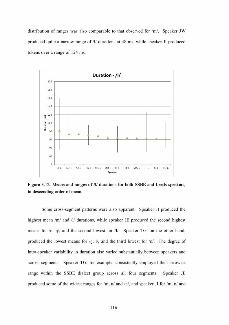
116

distribution of ranges was also comparable to that observed for /m/. Speaker JW

produced quite a narrow range of /l/ durations at 48 ms, while speaker JI produced

tokens over a range of 124 ms.

Figure 3.12. Means and ranges of /l/ durations for both SSBE and Leeds speakers, in descending order of mean.

Some cross-segment patterns were also apparent. Speaker JI produced the

highest mean /m/ and /l/ durations, while speaker JE produced the second highest

means for /n, ŋ/, and the second lowest for /l/. Speaker TG, on the other hand,

produced the lowest means for /ŋ, l/, and the third lowest for /n/. The degree of

intra-speaker variability in duration also varied substantially between speakers and

across segments. Speaker TG, for example, consistently employed the narrowest

range within the SSBE dialect group across all four segments. Speaker JE

produced some of the widest ranges for /m, n/ and /ŋ/, and speaker JI for /m, n/ and

117

/l/. Speaker MD‟s ranges were amongst the widest for /n/ and /ŋ/, and amongst the

narrowest for /m/ and /l/.

Table 3.6. Results of ANOVAs for effect of Speaker on segment durations. Significant effects are indicated by an asterisk.

Dialect Segment Speaker

F p

SSBE

/m/ 1.423 .226 /n/ 1.492 .200 /ŋ/ 3.126 .017* /l/ 5.272 .000*

Leeds

/m/ /n/ /ŋ/ /l/

.769

.568 1.471 3.335

.575

.724

.221 .006*

ANOVAs were conducted to test the effect of Speaker identity on durations

of each segment. Significant effects were found for Speaker on SSBE /ŋ, l/ and

Leeds /l/ durations. F-ratios and p values are summarised in Table 3.6. It is

surprising that Leeds /ŋ/ was found not to be significant for Speaker, considering

the disparity in ranges and means evident in Figure 3.11.

Post-hoc tests revealed no significant comparisons between individuals

within either dialect for /m/ or /n/, and none for Leeds /ŋ/. In comparisons for

SSBE /ŋ/ durations, speaker TG was found to be significantly different from JE and

MC, the two speakers with the highest means for that segment in the SSBE group.

For /l/, one significant comparison was found within the Leeds set, between

speakers RP and SU, although comparison of RP and ST was approaching

significance. Within the SSBE test of /l/, for which the Speaker effect was highly

significant, speaker JI was found to be significantly different from four others: JE,

MA, PT, and TG.

118

These results appear promising in terms of the speaker-specificity of

segment durations and the application of such data in forensic speaker comparison:

although many speakers‟ durations may fall within a similar range, it is those that

lie at the extremes which may be useful in forensic work. This may be similar to

the patterns found for other common speaker comparison parameters such as

fundamental frequency (e.g. Hudson, de Jong, McDougall, Harrison & Nolan,

2007) and articulation rate (e.g. Künzel, 1997; Jessen, 2007), where it is the

speakers who employ values at the extreme highs or lows relative to what is typical

of the general population that are of greatest interest.

3.4.3.1 Discriminant Analysis

Discriminant analyses (DA) were conducted on both dialect sets, with the

two dialects being treated separately at first; they were subsequently combined to

create a third dialect-independent set containing all 12 speakers for additional DA

testing. The aim of DA was to determine how well individual speakers could be

identified by a set of predictors. The predictors in this case were the durations of

/m, n, ŋ/, and /l/.

Outliers first needed to be identified and eliminated from the data set, as DA

is highly sensitive to outliers and non-normal distributions (Tabachnick & Fidell,

2007:382; further discussion of DA methodology is given in Chapter 2, §2.3.1).

Identification of univariate outliers was carried out in SPSS v.17.0 by standardising

the values of the predictors for each speaker independently, and eliminating any for

which z>±3.29 (Tabachnick & Fidell, 2007:73). This resulted in only two tokens

of /l/, one per dialect, and no nasal tokens being discarded from the data; these

outliers accounted for 0.2% of the total data set.

119

Single-predictor discriminant analyses were performed in SPSS using the

leave-one-out method of cross-validation described in Chapter 2. The results are

summarised in Table 3.7 below (SSBE and Leeds sets chance=17%; Combined

chance=8%). Classification rates indicate the percentage of the total number of

tokens per predictor for which group membership was correctly predicted. Tests of

the six SSBE speakers generally yielded the highest classification rates, with tests

of the Combined set consistently producing the lowest rates. The highest overall

rate was achieved in the test of /ŋ/ within the SSBE set, with 25% of cases being

correctly classified. The lowest overall rate of 8% occurred in the Combined tests

of /m/ and /n/.

Classification was highest in tests of /ŋ/ across all three datasets, although it

should be noted that this segment had the lowest token numbers with between five

and ten per speaker. The remaining three segments performed little or no better

than chance; the Leeds /l/ test in fact produced a classification rate below the level

of chance (13%).

Table 3.7. Cross-validated classification rates for single-predictor DA.

Predictor Correct Classification (%)

SSBE (6) Leeds (6) Combined (12) /m/ 17 19 8 /n/ 19 19 8 /ŋ/ 25 22 15 /l/ 19 13 10

Overall, classification rates were relatively low as this analysis was based

on data from a single predictor. It is hypothesised that correct classification rates

will improve with the addition of more predictors, such as formant data, as

120

McDougall (2004), Eriksson and Sullivan (2008), and Atkinson (2009), for

example, have shown.

Table 3.8. Individual classification rates with predicted group membership for all SSBE data (in percent). Correct classifications are highlighted.

Segment Speaker Predicted Group Membership

JE JI MA MC PT TG

/m/

JE 15 23 8 0 46 8 JI 0 14 0 36 29 21 MA 0 38 0 0 62 0 MC 0 57 14 0 21 7 PT 0 15 8 0 69 8 TG 0 36 7 7 43 7

/n/

JE 0 12 24 0 6 59 JI 18 12 41 0 0 29 MA 8 46 15 0 0 31 MC 6 0 24 24 0 47 PT 13 7 13 13 0 53 TG 6 0 18 18 0 59

/ŋ/

JE 33 17 0 33 0 17 JI 11 11 33 22 11 11 MA 25 13 25 0 13 25 MC 50 13 38 0 0 0 PT 38 13 0 0 0 50 TG 0 0 11 0 11 78

/l/

JE 0 14 6 22 8 50 JI 0 36 3 18 6 36 MA 0 17 0 28 8 47 MC 0 38 0 11 14 38 PT 0 23 0 9 3 66 TG 0 14 0 11 11 64

Closer inspection of individual cross-validated classification statistics

revealed some interesting patterns. Tables 3.8 and 3.9 provide individual

classification rates for SSBE and Leeds respectively, showing the percentage of

each speaker‟s tokens that were assigned to each group. Correct classification rates

121

are highlighted for each segment; all other percentages represent errors. Amongst

the SSBE speakers, PT‟s /m/ tokens were classified correctly in 69% of cases,

while up to 15% of other individuals‟ tokens were classified correctly. Speaker PT,

along with JI, was also frequently selected incorrectly in classification of other

speakers‟ tokens of /m/: 21-62% of others‟ tokens were wrongly classified as

being produced by PT, and 15-57% as JI. Only one speaker (JE) was never

selected incorrectly, but two (MA and MC) were never selected correctly.

A similar pattern is evident in the SSBE /n/ statistics: again two speakers

were never correctly selected (JE and PT), and one achieved a high correct

classification rate but was also frequently selected incorrectly. In this case, it was

speaker TG who was selected correctly in 59% of cases but was also wrongly

selected in classification of 29-59% of others‟ tokens of /n/. The remaining

incorrect classifications were spread more evenly across all other speakers, except

PT who was wrongly selected in only one case.

Speaker TG again achieved the highest individual classification rates for /ŋ/

at 78%, and for /l/ at 64%. Unfortunately, he was also selected wrongly in a large

number of cases: 11-50% of /ŋ/ and 36-66% /l/ cases. Speaker JE was never

selected, correctly or incorrectly, in the classification of /l/ durations. Speakers JI

and TG were the only ones to have at least some tokens correctly classified for

each segment.

Amongst the Leeds speakers in Table 3.9, RP stood out as the most easily

classified speaker across three of the segments: 64% of /m/, 59% of /n/, and 61%

of /l/ tokens were correctly classified as being produced by this speaker. In the /ŋ/

test, speaker MD achieved the highest individual classification rate. As in the

SSBE set, several speakers had no correct classifications in at least one test. RP

122

was the only speaker to be selected correctly for at least some cases for every

segment; however, he was also frequently selected incorrectly. A high proportion

of other speakers‟ cases, up to 63%, were incorrectly allocated to RP‟s group.

Table 3.9. Individual classification rates with predicted group membership for all Leeds data (in percent). Correct classifications are highlighted.

Segment Speaker Predicted Group Membership

JP JW MD RP ST SU

/m/

JP 0 0 0 40 0 60 JW 15 23 0 31 0 31 MD 8 31 0 23 8 31 RP 7 0 7 64 0 21 ST 0 0 0 36 0 64 SU 8 8 25 42 0 17

/n/

JP 0 12 29 53 6 0 JW 0 0 47 35 12 6 MD 6 13 38 38 0 6 RP 6 0 24 59 6 6 ST 0 0 33 47 13 7 SU 0 0 58 42 0 0

/ŋ/

JP 33 0 44 11 11 0 JW 0 0 43 57 0 0 MD 14 0 57 29 0 0 RP 0 13 0 25 38 25 ST 20 0 40 40 0 0 SU 20 0 10 60 0 10

/l/

JP 0 5 16 47 26 5 JW 0 9 17 29 46 0 MD 3 3 0 63 28 3 RP 0 5 16 61 18 0 ST 0 10 7 28 7 48 SU 3 14 11 30 43 0

It is worthy of note that the three speakers who were correctly classified at

least some of the time for every segment were also the three found to have

significant results in the post-hoc comparisons for Speaker effects discussed in the

123

previous section. Differences were found between JI and four of the five other

SSBE speakers for /l/, and between TG and two others for /ŋ/. For Leeds /l/,

comparison of RP and SU was significant, while comparison of RP and ST was

approaching significance. These three speakers JI, TG, and RP were also

frequently at the extremes in terms of the range of durations used, as is evident in

Figures 3.9-3.12 in §3.4.3. It is clear that some speakers, in particular those who

make use of either very wide or very narrow ranges of duration, are better

discriminated than others.

3.5 Conclusions

Findings presented in this chapter will inform further research design in

terms of establishing what contextual factors must be taken into account when

analysing consonant durations. Durations of /m, ŋ, l/ may be considered

independent of dialect within these data. Each segment investigated appears to

require separate treatment for different contextual factors in subsequent research.

Phonological Context is most influential in determining /m/ and /n/ durations. /m/

was found to be shortest following a consonant or pause, while /n/ was found to be

longer preceding a consonant in coda position than anywhere else. An additional

dialect difference surfaced in analysis of contextual effects on /ŋ/ durations:

different phonological contexts are comparable for SSBE speakers, but not for

Leeds speakers. SSBE /ŋ/ means in both CoVV and CoVC contexts were similar to

Leeds /ŋ/ in CoVC position; intervocalic /ŋ/ was significantly shorter than in CoVC

position for Leeds speakers, however. Results for /l/ appeared to be confounded by

the highly discrepant group sizes, so additional data should be collected before

drawing conclusions regarding contextual effects for /l/.

124

DA results showed /ŋ/ obtained the highest classification rates across all

three data sets, while classification of /m, n, l/ achieved rates little better than

chance. With regard to individual classification, at least some data for three

speakers were classified correctly for every segment; these were the same speakers

who had statistically significant differences from others, revealed by post-hoc

comparisons following Speaker ANOVAs. It has been shown that some speakers

do exhibit a relatively low degree of intra-speaker variability for each of the

segments investigated. There is also some degree of inter-speaker variability,

particularly in the /ŋ/ and /l/ data. These results suggest segment duration is

potentially a useful parameter for FSC and warrants further investigation.

125

Chapter 4 Materials and Methodology

4.0 Overview

In this chapter, the materials analysed in the remainder of the thesis are

described in detail. The three corpora from which data were obtained are

discussed, and the method of segmentation revisited. The methodology applied in

analysis is then presented, with detailed explanations of the acoustic parameters of

interest and motivations for exploring these parameters. Analysis procedures

specific to each consonant type are also provided. Finally, DA and LR analysis

methods are detailed further.

4.1 Materials

The data analysed in the following chapters were obtained from 30 young

adult male speakers of two regional varieties: SSBE and Leeds English. This

section provides details of each of the three corpora from which recordings were

obtained, with reference to the type and amount of speech elicited and the

recording methods used in each corpus. The consonant segments that are the focus

of the study are discussed, the segmentation method used is illustrated, and finally,

the data used in the analysis are summarised.

4.1.1 Corpora

The three corpora from which recordings were obtained are the DyViS

database, the IViE corpus, and the Morley corpus. Each is presented in turn below

with details of the participants and content of each corpus.

126

4.1.1.1 The DyViS corpus

Of the 21 SSBE speakers, 15 were recorded as part of the DyViS database

(Nolan, McDougall, de Jong, & Hudson, 2009). The DyViS corpus consists of

recordings of 100 young male Standard Southern British English speakers

producing two samples of spontaneous speech under simulated forensic conditions,

including a mock police interview (Task 1) and a telephone conversation with an

„accomplice‟ (Task 2). Speakers also produced two samples of read speech: a

passage written in the form of a fictional news report detailing the alleged crime

(Task 3), and a list of short sentences (Task 4). 20 of the 100 speakers returned for

a second session to record the two reading tasks, approximately two months after

the first session, to provide non-contemporaneous samples for the corpus.

Recordings from the second session were not used at this time, as no non-

contemporaneous samples were available for the remaining 15 speakers from the

two additional corpora.

The DyViS studio recordings were made using a Marantz PMD670 portable

solid state recorder with a sampling rate of 44.1 kHz; each speaker had a

Sennheiser ME64-K6 cardioid condenser microphone positioned approximately 20

cm from his mouth. Recording was conducted in a sound-treated room in the

Phonetics Laboratory at the University of Cambridge (Nolan et al., 2009:40).

4.1.1.2 The IViE corpus

Data for an additional six SSBE speakers, as well as six of the Leeds

speakers, were acquired from the IViE corpus (SSBE is called Cambridge in IViE,

described further in Chapter 3), with subjects reading a passage relating the story of

Cinderella. Again, this controlled for the content of recordings and the number of

127

possible instances of the target segments. The IViE corpus was recorded in urban

secondary schools (Grabe, Post, & Nolan, 2001). The quality of the recordings was

relatively high, with a sampling rate of 16 kHz and minimal background noise.

4.1.1.3 The Morley corpus

The remaining three Leeds speakers were recorded as part of the Morley

corpus (Richards, 2008). This corpus contains samples of spontaneous and read

speech produced by young, working-aged, and retired speakers from the Morley

area of Leeds. The corpus was balanced for age and sex of speakers. For the

present thesis, only the male speakers were used. Additionally, because speakers in

the first two corpora were between approximately 15 and 25 years of age at the

time of recording, the (older) retired speakers in the Morley corpus were not

included in the present study in order to control broadly for age. Two of the young

speakers and one of the working-aged speakers were selected based on quality of

the recordings. The Morley corpus was recorded either in speakers' homes or in

empty school classrooms, while the DyViS and IViE recordings were studio-quality

or similar. The level of background noise in some of the Morley recordings meant

acoustic measurements would have been significantly affected.

This corpus was recorded using a Sharp portable MD831 minidisc player

with TDK-80 minidiscs and an Electret Condenser EM-400 lapel microphone.

Recordings were digitised using Audacity 1.22 with a sampling rate of 44.1 kHz

(Richards, 2008:77). However, in the three Morley recordings used, due to

background noise and recording quality, very little speech signal information was

encoded in the spectrum above approximately 16 kHz.

128

In the following chapters, SSBE DyViS speakers are labelled with numbers

1-15, SSBE IViE speakers 16-21, Leeds IViE speakers 22-27, and Leeds Morley

speakers 28-30.

4.1.2 Speech tasks

The use of read speech tasks from each corpus allowed for relative control

over the position within the word and phonological context, as well as the number

of tokens of each of the target segments. There was still some variation in token

numbers as the nature of the reading tasks differed between the three corpora. For

this thesis, the DyViS Task 3 materials were selected, which consisted of a read

passage in the form of a fictional news report. The 15 recordings used in the

analysis were between 2m40s and 4m09s in length. The 12 speakers from the IViE

corpus read a passage telling the story of Cinderella, with recordings being between

approximately 3m30s and 4m45s in length. In the Morley corpus, the reading task

consisted of a word list and a list of short sentences; these recordings each lasted

between approximately 3m16s and 4m0s. The texts of the reading materials used

in the DyViS, IViE, and Morley tasks are given in Appendices 2, 3, and 4,

respectively.

4.1.3 Segments

The consonant segments under investigation are those described in the pilot

study in Chapter 3: /m, n, ŋ, l, s/. The acoustic properties of consonants are

significantly understudied in general, particularly from a forensic perspective of

identifying highly speaker-dependent parameters. However, these nasal, liquid, and

fricative segments are relatively common in spoken English, and are predicted to be

129

relatively easily segmentable, potentially leading to new acoustic comparison

parameters for analysis in FSC casework. Following French et al. (2010), the

importance of exploring the speaker discrimination performance of as many

parameters as possible (including acoustic ones) is noted, as the more parameters

available for analysis in a FSC case, the stronger the resulting evidence might be.

Little cross-dialectal variation in acoustic parameters of the nasal consonants

is predicted as nasal acoustics are strongly dependent on individual physiology

(Stevens, 1998). There is perhaps more scope for dialectal variation in /l/ and /s/

given the sociophonetic variability attested in the literature for both (see Chapters 2

and 3), with clear /l/ in initial position in SSBE, and a darker initial /l/ in Leeds

English (Carter & Local, 2007); some social factors affecting /s/ acoustics have

been attested in Glasgow English (Stuart-Smith, et al., 2003; Stuart-Smith, 2007),

though none are reported in the literature for SSBE or Leeds. However, acoustic

properties of /s/ are also noted to be strongly linked to anatomy, which might

reduce the scope for cross-dialect variation in this segment.

4.1.3.1 Segmentation

In the pilot study described in Chapter 3, word position and phonological

context were found to affect the duration of consonants. Consequently, data for the

present study were collected only from segments in specific contexts in order to

ensure the data were directly comparable. For four of the target segments, /m, n, l,

s/, only tokens occurring in word-initial position were analysed. Word-initial

tokens of these consonants were found to be notably easier to segment than word-

medial and word-final tokens. It was noted that in medial position, tokens of /l/

especially were often difficult to segment, as they frequently lacked clear

130

boundaries with adjacent segments. Word-finally, the nasals were occasionally not

realised as consonants, but rather as nasalised vowels, while /l/ was sometimes

vocalised. Additionally, adjacent consonants in all positions were found to affect

the duration of segments relative to intervocalic environments. Consequently, for

/m, n, l, s/, the target segment was always followed by a stressed vowel, and

preceded by either a pause or a vowel across the word boundary. All tokens of /ŋ/

occurred in word-final position, as this segment does not occur in word-initial

position in English. In this case, /ŋ/ was always preceded by a vowel, and followed

by a pause at the end of a phrase, or by a vowel across the word boundary.

The segmentation of all data was performed manually following the

methodology described in Chapter 3. Start points of the word-initial nasals /m, n/

were marked at the zero crossing of the waveform nearest the onset of the oral

constriction. In tokens preceded by a vowel, this was indicated by the onset of

nasal anti-resonances and the coincident offset of preceding vowel formants. In

tokens preceded by a pause, this was marked by the onset of voicing and the nasal

formants. In the case of /ŋ/, which always occurred word-finally, start points were

marked by the onset of anti-resonances and the offset of preceding vowel formants.

For all three segments, /m, n, ŋ/, end points were marked by the onset of vowel

formants with increased amplitude, or by a short burst of energy in the spectrogram

at the release of the oral closure.

In segmentation of word-initial /l/ following a pause, onsets were marked by

the onset of /l/ formants and voicing. For tokens following a vowel, a decrease in

energy relative to the preceding vowel formants and the onset of lateral anti-

resonances indicated /l/ onset. A sudden change in the shape of the waveform and

an increase in energy in the F2 region indicated the offset of /l/.

131

Start points for word-initial /s/ were marked at the onset of aperiodic high-

frequency fricative noise observable in the spectrogram and aperiodicity in the

waveform. End points were marked at the offset of frication and the onset of

periodicity in the waveform at the beginning of the following vowel. Chapter 3,

§3.2 provides sample spectrograms showing segmented tokens from the IViE

corpus. The segmentation criteria were simplified from those used in the pilot

study in Chapter 3, as no partially voiced tokens were observed in the main study

(see §3.2.3 for details of /s/ segmentation in the pilot study). Total token numbers

collected for each of the 30 speakers and five segments are displayed in Table 4.1.

For all segments, only (roughly) canonical articulations were included,

meaning that, for example, realisations of /ŋ/ as alveolar [n] or as a nasalized vowel

were not considered. These non-canonical realisations might have some forensic

value in themselves, as the frequency of variants and their acoustic properties could

potentially be highly speaker-specific. However, it was decided to limit the scope

of the thesis to near-canonical variants in order to focus the analysis on specific

acoustic properties of the five selected consonants themselves. It is for this reason

that token numbers, particularly for /ŋ/, were quite variable between speakers, as

different numbers of tokens were excluded for each individual.

132

Table 4.1. Token numbers by dialect, speaker, and segment. Dialect Speaker /m/ /n/ /ŋ/ /l/ /s/

SSBE

1 10 10 3 8 15 2 12 13 6 12 15 3 11 12 5 8 14 4 11 13 4 8 15 5 10 13 7 9 16 6 10 10 7 11 15 7 10 12 7 4 14 8 10 12 7 8 15 9 10 11 5 5 15 10 10 6 6 4 16 11 11 12 8 8 16 12 9 12 4 8 16 13 10 11 5 5 14 14 11 11 6 7 15 15 10 12 5 9 17 16 14 6 5 9 11 17 12 7 6 11 11 18 12 6 5 12 10 19 12 5 3 13 11 20 11 6 7 12 10 21 11 6 7 8 10

Leeds

22 13 7 3 12 10 23 12 5 2 11 10 24 12 7 3 9 10 25 12 7 5 11 10 26 13 7 2 10 10 27 12 6 1 8 10 28 14 8 2 13 6 29 14 7 5 12 7 30 14 8 12 12 7

Total 343 268 153 277 371

4.2 Methodology

For each of the five segments, five acoustic parameters were analysed.

Normalised duration, centre of gravity, and standard deviation of the distribution of

energy in the spectrum were calculated for all five segments. In the nasal and

133

lateral segment analysis, frequency at peak amplitude and frequency at minimum

amplitude were also measured. Analysis of /s/ also considered skewness and

kurtosis. Section 4.2.1 defines each acoustic parameter in turn, including details

specific to each segment type. The data collection methods employed in spectral

analysis of nasals and /l/ (§4.2.2) and /s/ (§4.2.3) are then illustrated.

4.2.1 Acoustic parameters

4.2.1.1 Normalised duration

A consideration arising from the pilot study, and during collection of the

data for the main study, was the issue of how to control for differences in speaking

tempo between individuals, and for variations in tempo within a single speaker‟s

recording. Variations in speaking rate can be expected to result in relative

lengthening or shortening of syllables and the segments within them, depending on

a variety of factors including phrase length, as well as external factors such as sex

and age ( , 2008). As a result, in order to make direct comparisons of

segment durations across speakers, differences in individual speaking rates should

be normalised. A method was developed for the present study using local Average

Syllable Duration (ASD) as a normalisation parameter, and implemented using the

formula at (2).

(2) Normalised Duration = TokenDur (ms) (IPDur (ms)/IPSyll)

Absolute durations of tokens were obtained first using a Praat script written

by the author, by calculating the duration of the interval between the marked onset

134

and offset points of each token. These absolute durations were then normalised to

attempt to control for differences in articulation rate between speakers. ASD,

measured in ms/syllable, was calculated by dividing the duration of the local

intonation phrase containing the token to be normalised (IPDur) by the number of

phonological syllables in the phrase (IPSyll). The absolute duration of the token

(TokenDur) was then divided by the ASD. The resulting Normalised Duration (no

units) expresses the segment duration as a proportion of the individual speaker‟s

local ASD. Normalised duration was analysed for all five segments.

4.2.1.2 Centre of gravity

The centre of gravity (COG) of fricative segments was discussed in detail in

Chapter 2, §2.2.3, with respect to the acoustic literature surrounding /s/. This

measure is also applicable to other segments including nasal and lateral consonants,

as it is simply a measure of the distribution of energy in the spectrum.

Consequently, this parameter was analysed for all five segments. COG gives the

frequency at which the distribution of spectral energy is equal on either side; it is

also known as the mean. Energy concentrated at lower frequencies in the spectrum

results in a low COG, and concentrated at higher frequencies, a high COG.

In the case of nasal and lateral consonants, COG may be influenced by the

frequency and amplitude of poles and zeros in the acoustic signal. COG does not

attempt to measure the poles, zeros, or any formants directly; rather it measures the

concentration of energy within a specified frequency range. Speakers with longer

vocal tracts are expected to have energy concentrated at lower frequencies, and thus

lower COGs, than speakers with shorter vocal tracts (Reetz & Jongman, 2009:194-

195). Stevens also notes “considerable variability” between individuals in terms of

135

nasal cavity size and shape, which is reflected in inter-speaker variability in the

acoustic properties of nasals (1998:189-190).

In the production of fricatives, energy distribution in the spectrum is related

to the shape and size of the resonance cavity in front of the oral constriction

(Jongman et al., 2000:1253). Speakers with smaller vocal tracts are expected to

have smaller cavities in front of the point of constriction than speakers with larger

vocal tracts (Stuart-Smith et al., 2003:1851). Such physiological differences

between individuals are expected to result in a relatively high degree of speaker-

specificity in acoustic properties (particularly COG) of nasals, laterals, and

fricatives.

4.2.1.3 Standard deviation

Standard deviation (SD) is another measure of the distribution of energy in

the spectrum which was also analysed for all five segments. This parameter is

measured as the square root of the second spectral moment (variance); it refers to

the dispersion or bandwidth of energy around the COG (Stuart-Smith et al.,

2003:1852). A low SD value is obtained if the energy is densely concentrated

around the COG; conversely, if energy is dispersed across a wider frequency range,

higher SD values will be obtained.

Inter-speaker variability in SD in consonant segments may result from

differing surface areas of individuals‟ nasal and oral cavities involved in the

production of each. In the production of nasals, the increase in surface area

introduced by coupling the nasal and oral cavities (described in Chapter 2,

§2.2.1.1), introduces a damping effect on the transmitted sound energy. The soft

nasal passage walls absorb more of the energy, causing the bandwidth of poles and

136

zeros to increase, thus distributing the energy over a wider frequency range. The

nasal passages of individuals, however, vary in size and shape; consequently, the

resulting damping effects of the passage walls on sound energy are expected to

vary. The overall size and shape of the oral cavity and side branch in the

production of /l/ is expected to have a similar damping effect on the transmitted

sound energy (Stevens, 1998). SD is not a measure of pole-zero bandwidths

directly, but a measure of the spread of energy around the COG. As such, pole-

zero bandwidth variation may affect the dispersion of energy in the spectrum, in

turn affecting SD.

4.2.1.4 Peak frequency

Peak frequency was analysed for /m, n, ŋ, l/ only. This parameter gives the

frequency at the point of maximum amplitude within the spectrum. Figure 4.1

shows a sample spectrum (0-4 kHz) of the word-initial /l/ in live from the sentence

They live on the same street (DyViS Task 3) produced by speaker 1. The left edge

of the pink highlighted area marks the highest Peak, the point of maximum

amplitude, at approximately 345 Hz. Several other high-amplitude peaks can be

seen across the spectrum. These peaks are related to poles in the signal, the

location and spacing of which are related to the total length of the nasal+oral

cavity for nasals, or the oral+side branch cavities for /l/ (Stevens, 1998).

137

Figure 4.1. Sample spectrum of /l/ in They live on the same street produced by speaker 1 (DyViS, Task 3), with Peak and Minimum frequencies highlighted.

4.2.1.5 Minimum frequency

Minimum frequency, the point of lowest amplitude in the spectrum, was

measured for the three nasals and /l/ only. Minimum may be related to the zeros or

anti-resonances in the spectrum, though it is not a measure of the zeros directly, but

rather indicates the point at which spectral energy is lowest within the frequency

range being investigated. In the case of nasals, zeros are introduced by the

coupling of the nasal and oral cavities, as noted above and in Chapter 2, §2.2.1.1.

Similarly, zeros occur in the spectrum of /l/ as a result of the side branch in the

vocal tract created by lowering one or both sides of the tongue body during the

alveolar constriction (Stevens, 1998). The predicted locations of the zeros in the

spectra of /m, n, ŋ, l/ for adult male speakers are noted in Chapter 3, §3.2. Figure

4.1 above also illustrates this parameter: the right edge of the pink highlighted

138

section marks the point of lowest amplitude in the spectrum from 0-4 kHz, at

approximately 689 Hz.

4.2.1.6 Skewness

Skewness was analysed for /s/ only. This parameter is the third spectral

moment; it is a measure of the symmetry of the distribution of energy in the

spectrum of a sound. A perfectly symmetrical distribution, such as a normal

distribution, will have a skewness value of zero. Asymmetrical skewness values

can be positive or negative: a positive skewness above zero indicates a distribution

in which the right tail is longer than the left, while a negative skewness indicates a

distribution with a longer left tail (Jongman et al., 2000:1253).

4.2.1.7 Kurtosis

Kurtosis was also analysed for /s/ only. The fourth spectral moment,

kurtosis is a measure of the relative peakedness or flatness of the energy

distribution. Relatively flat distributions are indicated by negative kurtosis values,

and relatively peaked ones by positive values (Jongman et al., 2000:1253). Like

skewness, a normal distribution will have a kurtosis value of zero. Both skewness

and kurtosis provide measures of the shape of the fricative energy, while COG and

SD illustrate the location and diffusion of the energy. Further discussion of all four

measures and their role in fricative acoustic research is provided in §2.2.3. See

Chapter 2, Figure 2.3 for illustrations of distributions demonstrating positive and

negative forms of both skewness and kurtosis.

139

4.2.2 Nasal and lateral spectral analysis

In analysis of the three nasals /m, n, ŋ/ and the lateral /l/, a Praat script

automatically obtained measurements for the four spectral parameters (COG, SD,

Peak, and Minimum). Data were extracted from a single 40-ms Kaiser 2 window at

the midpoint of each nasal token, and from a 20-ms window at the midpoint of

tokens of /l/. The Kaiser 2 window was selected as potentially the best

approximation of a Gaussian window (Jalal Al-Tamimi, personal communication).

The four spectral parameters were each measured in five frequency bands

from 0 to 4 kHz: 0-500 Hz, 500-1000 Hz, 1-2 kHz, 2-3 kHz, and 3-4 kHz. This

resulted in a total of 20 spectral variables (4 parameters x 5 bands). Examining

parameters in narrower bands rather than the entire spectrum allowed assessment of

the distribution of energy and the speaker-specificity of acoustic measures in other

regions, not only the lowest portion of the spectrum, as nasal spectra in particular

are typically dominated by a concentration of energy in the region of 250-300 Hz

for male speakers. The measurements taken for each token of /m, n, ŋ, l/ are

summarised in Table 4.2.

Table 4.2. Summary of five parameters and 21 measurements taken for all nasal and lateral segments /m, n, ŋ, l/.

Parameter Measurements NormDuration Single measure COG Band 1

(0-0.5 kHz)

Band 2 (0.5-1 kHz)

Band 3 (1-2 kHz)

Band 4 (2-3 kHz)

Band 5 (3-4 kHz)

SD Peak Minimum

The selection of this frequency range (0-4 kHz) also attempts to address an

issue that could have implications for the use of acoustic parameters of consonants

140

in forensic casework. Criminal samples are frequently recorded via a telephone

line or using mobile telephone technology; others might be recorded at a relatively

low sampling rate resulting in a limited frequency bandwidth similar to that of a

telephone line. Telephone transmission has a band-pass filter effect on the speech

signal, limiting the frequency range of the transmitted signal to between

approximately 300 Hz and 3-4.5 kHz depending on the system (see e.g. Enbom &

Kleijn, 1999; Künzel, 2001; Kent & Read, 2002; Rose, Osanai, & Kinoshita, 2003;

and Cannizzaro et al., 2005). This limitation means that acoustic energy near the

edges of the telephone band may be attenuated, resulting in reliable measurements

not being available in the lowest band (0-500 Hz) and potentially the highest (3-4

kHz). The intermediate bands might not be significantly affected by telephone

transmission, however, so any potentially speaker-specific features in these regions

might still be of use, permitting analysis of these parameters in forensic cases

involving telephone or mobile phone recordings.

Motivation

The motivation for exploring the speaker-specificity of these four spectral

parameters derives from Pruthi‟s (2007) study of nasalised vowels. In his thesis,

Pruthi investigated a number of acoustic parameters for the automatic detection of

nasalised vowels for potential application in speech and speaker recognition and

speech enhancement.

As noted in §4.2.1.5 and in Chapter 2, zeros are introduced into the acoustic

signal by the coupling of the nasal and oral cavities in the production of nasals, or

by the oral side branch in production of lateral consonants (Stevens, 1998). As a

result, pole-only formant tracking methods such as the one employed by Praat are

141

likely to produce errors when applied to pole-zero signals (Pruthi, 2007), as in

nasals and laterals. Consequently, alternative acoustic measures were sought in the

absence of an appropriate pole-zero formant tracker. The alternative proposed by

Pruthi and recommended by Alex Cristia (personal communication) was to examine

the distribution of energy, by measuring COG and SD, as well as visible peaks and

minima across the spectrum.

Pruthi‟s thesis investigated SD of energy around the COG in four 1-kHz

frequency bands from 0-4 kHz, in an attempt to capture the „diffuse nature‟ of the

nasalised vowel spectrum (2007:111-113). For the present study, the lowest band

was divided into two 500 Hz bands instead. This was intended to allow

investigation of the low-frequency energy associated with the strong nasal formant

typically found in the 250-300 Hz region of nasal consonants for male speakers,

without it dominating the distribution of energy up to 1 kHz. Additionally, this

division allows bands to be examined individually, if analysis of the same

parameters were to be conducted in FSC casework. This would be particularly

useful if, for example, low frequency background noise or telephone transmission

significantly affected the lowest and highest frequency bands; in that case, the rest

of the frequency range could be analysed independently of the affected bands.

Pruthi also counted the number of peaks in the spectrum up to 4 kHz.

While the number might not necessarily differ between speakers, for forensic

purposes the location of these peaks might have some speaker discrimination

potential, as the location and spacing of the associated poles are related to the

overall length of the pharyngeal and nasal cavities of the speaker. For example, in

the signal of /m/, a male speaker with a vocal tract length of 19.6 cm is expected to

have one pole at approximately 250 Hz with further poles spaced on average 900

142

Hz apart (Stevens, 1998:495). Additionally, inspection of Figures 9.6, 9.10, and

9.15 in Stevens (1998:497-509) suggests at least one peak may be expected in each

of the frequency bands for the three nasals.

Similarly, Pruthi examined the number and amplitude of „dips‟ in the

spectra of nasalised vowels relating to the additional zeros introduced by the nasal

cavity (2007:110-111). Again, for forensic purposes, the location of minima in the

spectrum of nasal and lateral consonants might show some inter-speaker variability,

owing to the distinct size and shape of each individual‟s nasal cavity or oral side

branch in the case of /l/. Differences in physiology between individuals are

predicted to give rise to differences in acoustic features (Stevens, 1998:189-190)

which might in turn be used to discriminate speakers.

4.2.3 Fricative spectral analysis

Acoustic data for COG, SD, skewness, and kurtosis of /s/ were also

extracted automatically using a Praat script. No pre-emphasis was applied to the

spectra as voiceless sounds are not subject to the same -6dB/octave loss as voiced

sounds (Munson, 2001). There does not appear to be a standard window length for

fricative analysis in the existing literature. Windows used in previous studies range

from 10 ms (Munson, 2004) to 100 ms (Wrench, 1995; Jones & Nolan, 2007);

however, the most common window lengths appear to be between 20 ms and 50 ms

(e.g. Hughes & Halle, 1956; Forrest, Weismer, Milenkovic, & Dougall, 1988;

Stuart-Smith et al., 2003). For the present study, spectral measures were first

calculated from a single 40-ms Kaiser 2 window centred on the midpoint of the

segment, giving static measures. A series of three sets of measurements was then

calculated from 20-ms windows at the onset, midpoint, and offset of each segment

143

to give dynamic measures. This provided additional predictors for statistical

analysis (3 x 4 spectral parameters + normalised duration), and allowed for

examination of dynamic changes in spectral shape over time during the course of

production. Static and dynamic data were collected from two datasets and

statistical analyses were conducted for both.

Dataset 1

The first dataset contained the complete set of 30 speakers from all three

corpora. This 30-speaker set was analysed in two filter conditions: 500-8000 Hz

and 500-4000 Hz. A 500 Hz high-pass filter was first applied to all spectra to

eliminate low frequency background noise, as suggested by Stuart-Smith (2007:71).

8 kHz was selected as the maximum frequency as the IViE corpus recordings were

sampled at a lower rate than the DyViS and Morley recordings (noted in §4.1.1).

Therefore, to allow comparison across all three corpora, a low-pass filter was

applied at 8 kHz (half the IViE sampling rate of 16 kHz) to each spectrum before

acoustic measures were calculated.

The second filter condition (500-4000 Hz) again attempted to approximate

the telephone band-pass effect described in §4.2.2. The acoustic energy associated

with the alveolar fricative /s/ is typically concentrated around 4-5 kHz (Jongman et

al., 2000:1253). Much of this is likely to be removed during telephone

transmission. Despite this, the distribution of energy in production of the alveolar

fricative /s/ can in fact extend to lower frequencies, within the range of telephone

transmission (Stuart-Smith et al., 2003:1852). The 4 kHz filter permitted

exploration of how effective acoustic measures of /s/ might be in discriminating

speakers in forensic cases involving telephone recorded speech.

144

Dataset 2

The second dataset contained a subset of 18 speakers from the DyViS and

Morley corpora only. In this subset, four filter conditions were tested as a result of

the wider frequency bandwidth available due to the 44.1 kHz sampling rate (see

§4.1.1). The four conditions were 500-4000 Hz, 500-8000 Hz, 500-16000 Hz, and

500-22050 Hz. A 500 Hz high-pass filter was again applied to remove background

noise in the low-frequency range, and the same low-pass filters were applied at 4

and 8 kHz as in the 30-speaker set. Two additional low-pass filters were then

applied to the spectra at 16 and 22.05 kHz. The 22.05 kHz condition made use of

the full spectrum available. The 16 kHz filter was selected as there appeared to be

little speech signal information above this point in the Morley recordings (noted in

§4.1.1.3). This condition allowed assessment of whether the high-frequency energy

between 16 and 22.05 kHz affects acoustic measurements. Filtering the data at

multiple frequencies in this way allowed comparison of speaker discrimination

performance of the spectral parameters with varying amounts of acoustic

information from a single dataset. Table 4.3 summarises the number of speakers

(and from which corpora) and the filter conditions applied in analysis of the two

datasets.

Table 4.3. Summary of datasets analysed and filters applied in analysis of /s/. Dataset 1 Dataset 2 N Speakers 30 18

Corpora DyViS IViE

Morley

DyViS -

Morley

Filters

500-4000 Hz 500-8000 Hz

- -

500-4000 Hz 500-8000 Hz 500-16000 Hz 500-22050 Hz

145

4.2.4 Speaker and dialect significance testing

The effect of speaker identity on each of the acoustic features was assessed

to explore whether speakers differed from each other in their acoustic realisations

and were thus likely to be discriminated by any of the parameters. Univariate

ANOVAs were conducted with Speaker as a fixed factor for each dependent

variable. The potential degree of speaker-specificity of each variable is reflected in

the magnitude of the F-ratio and the significance of the p-value. Additionally,

Gabriel and Hochberg‟s GT2 post-hoc tests highlighted significant differences

between individual speakers. These tests were selected as they are recommended

when sample sizes are slightly different (Gabriel) or very different (Hochberg), as

was the case in the present study (Field, 2009:374-375). The post-hoc test

employed was selected based on token numbers available for each segment and is

indicated in each of the subsequent results chapters.

Dialect was also investigated for significance as a factor in acoustic

realisations of the consonant features described above. Parametric tests of

significance were found to be inappropriate as the data did not meet the

assumptions of normality and homogeneity of variance. There were also fewer

Leeds speakers (9) than SSBE speakers (21), resulting in highly unequal sample

sizes. Therefore, the non-parametric Mann-Whitney U statistic was employed to

test the effect of dialect group membership on each variable.

4.2.5 Discriminant analysis

Direct discriminant analyses (DA) were conducted on individual features

and combinations of parameters to explore how well acoustic data could predict

speaker identity. The principles of DA and its use in forensic phonetic literature

146

are described in additional detail in §2.3. DA with cross-validated classification

was carried out with both static and dynamic data for the full 30-speaker dataset

and the 18-speaker subset for /m, n, l, s/. /ŋ/ data were analysed descriptively and

not statistically as a result of the low token numbers obtained per speaker (see

Table 4.1); DA was therefore not conducted for /ŋ/.

DA explored individual predictors, single Bands (e.g.

COG+SD+Peak+Minimum of /m/ in Band 1), single parameters (e.g. COG of /n/

in Bands 1-5), and combinations of two or more parameters to discover which

predictors showed the most discrimination potential. As observed in the DA

literature survey presented in Chapter 2, the number of predictors permitted in DA

is limited by the smallest sample size. In tests where the number of potential

predictors exceeded this limit, the F-ratios resulting from the Speaker ANOVAs

were used to eliminate predictors. Only the predictors with the highest F-ratios for

the given parameters, up to the limit determined by the smallest sample size, were

included; those with lower F-ratios were eliminated. An additional „Best F-ratios‟

test was performed for each segment, which included predictors with the highest F-

ratios across all parameters up to the number permitted by the smallest sample size.

The number of tests conducted and the predictors included in each are given in

each of the relevant results chapters. The predictor combinations yielding the

highest correct classification percentages overall for each segment are highlighted

and examined further.

147

4.2.6 Likelihood ratios

4.2.6.1 Likelihood ratio calculation

Likelihood ratios were calculated for combinations of features for four of

the five consonant segments: /m, n, l, s/; as in the DA, token numbers for /ŋ/ in the

present dataset were not sufficient for the calculation of LRs. Chapter 2, §2.3.2

describes LR analysis and limitations in the context of FSC in detail, along with an

overview of the implementation of LR analysis in existing forensic phonetic

literature.

In the present study, LR estimation was conducted using a script2 based on

Aitken and Lucy‟s (2004) Multivariate Kernel Density (MVKD) formula and

implemented in MATLAB. Testing was carried out intrinsically, with no external

reference sample. The 30 speakers were separated into two groups; LRs were

calculated for half the speakers while the other half formed the reference sample,

and groups were then reversed to calculate LRs for the remaining speakers. As no

non-contemporaneous data were available in the dataset, separate „suspect‟ and

„criminal‟ samples were created by dividing individual speakers‟ samples in two.

The first half was consistently tested as the „suspect‟ sample, and the second half as

the „criminal‟ sample. This ensured same-speaker tests did not involve comparison

of identical data samples.

The same predictor combinations tested in the DA described above were

also tested in the LR analysis for each segment, and the raw LR scores were then

transformed to log10LRs. This logarithmic transformation maps a raw LR of 1,

2 Many thanks to Philip Harrison who wrote the MATLAB script for iterative

LR estimation used in the present study.

148

indicating equal support for both same- and different-speaker hypotheses, to a

log10LR of 0. Raw LRs greater than 1, indicating support for the same-speaker

hypothesis, are mapped to the positive values between 0 and ∞, while raw LRs

between 0 and 1 are mapped to the negative values between 0 and -∞, indicating

support for the different-speaker hypothesis. The predictors included in each test

are also given in the relevant sections of each following results chapter. The best

performing tests for each segment are highlighted and illustrated further.

Performance was assessed using the four measures described below.

4.2.6.2 Assessment of LR performance

The performance of each LR test was gauged using a series of four

measures: proportion of log10LRs≥±4, proportions of false negatives and false

positives, equal error rate, and log likelihood ratio cost.

The proportion of log10LRs≥±4 was selected as an indication of the

strength of evidence. A log10LR of ±4 is equivalent to a raw LR score of 10 000

(same-speaker) or 0.0001 (different-speaker). This is considered to be 'very strong'

evidence in support of the relevant conclusion following the Forensic Science

Service‟s verbal scale for the interpretation of LRs as described by Champod and

Evett (2000:240). Ideally, a high proportion of speaker comparisons would

produce log10LR scores of a magnitude of ±4 or higher as this would indicate the

predictors are producing strong evidence. A higher proportion of different-speaker

tests than same-speaker tests may be expected to produce scores beyond this

threshold, though. While some different-speaker pairs may be more different than

others, there is a limit to how similar two individuals can be; that is, a same-

speaker pair cannot be any more similar than identical.

149

Second, false positive and false negative rates were calculated for each LR

test. False positives occur when a different-speaker comparison produces a log10LR

greater than 0, incorrectly identifying the different speakers as a same-speaker pair.

Conversely, false negatives occur when a same-speaker pair is incorrectly identified

as a different-speaker pair, with a negative log10LR score. The lower the rate both

of false positives and of false negatives the better, as this indicates fewer errors.

Equal error rate (EER; discussed previously in Chapter 2, §2.3.2.2) was also

calculated for each LR test. EER gives an indication of the total proportion of

errors in the speaker comparison system, in both same- and different-speaker

comparisons, though it does not give any indication of the magnitude of errors.

This is measured at the point where false acceptance equals false rejection, and is

expressed as a percentage of all same- and different-speaker comparisons.

The fourth measure used to gauge LR performance was log likelihood ratio

cost (Cllr). Cllr is a measure of the validity of the speaker comparison system

(Morrison, 2011:92), developed initially for evaluation of automatic speaker

recognition systems by Brümmer and du Preez (2006). A high level of validity will

be achieved in a system with no errors, or only a small proportion of errors of low

magnitude. Cllr is essentially a mean of two separate means: one calculated from

the „penalty values‟ contributed by same-speaker errors, the other from those

contributed by different-speaker errors. Large log10LRs in the wrong direction (i.e.

positive log10LRs in DS comparisons, or negative log10LRs in SS comparisons)

contribute higher „penalty values‟ than small errors. Therefore, unlike EER or the

proportion of false positives and negatives, Cllr takes into account the magnitude of

the errors in a test. A Cllr of 1 would be obtained in a system which gave no

support to either the same- or different-speaker hypotheses. Values greater than 1

150

indicate systems with poor validity, though these may be improved with calibration

(Morrison, 2011:94). The closer the Cllr value to 0 the better, as this indicates an

overall lower magnitude of errors and better validity in the system. Cllr is, however,

dependent on both the system and the samples in the database used in the

calculation of LRs. For further discussion of the method of calculating this metric,

see Morrison (2011).

151

Chapter 5 Results: /m/

5.0 Overview

This chapter details results of acoustic analysis of /m/. Intra- and inter-

speaker variability in each of the five parameters is described, including reference

to the results of analyses of variance (ANOVAs) for Speaker. For each of the four

spectral parameters, the five Bands are discussed independently, followed by a

global view of each parameter across the entire spectrum. Results of significance

testing for the effect of Dialect are then discussed. Findings of the DA and LR

analysis are evaluated, and the best performing predictor combinations in each

analysis are highlighted and illustrated in detail.

5.1 Intra- and inter-speaker variability

This section presents intra- and inter-speaker variability in normalised

duration and the four spectral parameters analysed for /m/. In obtaining

measurements for centre of gravity, standard deviation, peak and minimum

frequencies, the spectrum was divided into five „Bands‟ so that each could be

examined individually, as described in Chapter 4. As acoustic energy is typically

concentrated around 250-300 Hz in nasal consonants (Stevens, 1998:489), this

approach allowed the shape of the entire spectrum to be considered without

measures being dominated by the lowest nasal formant. Data for each of the 21

variables are presented separately, with figures displaying mean and range of

values by speaker, in descending order of mean.

152

Univariate ANOVAs were conducted in order to test the effects of Speaker

identity on the five acoustic parameters, with separate analyses performed on data

from each frequency Band for the four spectral parameters. Speaker was found to

be highly significant for all dependent variables. Gabriel post-hoc tests examined

pairwise speaker comparisons, highlighting which individuals were most distinct

from the group and therefore likely to be discriminated best. F-ratios and p-values

are summarised in Table 5.1, and post-hoc results are discussed further in each

subsection below. Empty cells indicate data that were excluded from analysis;

details are given and the data illustrated in the relevant sections.

Table 5.1. Results of univariate ANOVAs for Speaker (N=30) for each acoustic feature of /m/ (x19). Bold text indicates significant p values at the level .05.

Parameter Band 1 Band 2 Band 3 Band 4 Band 5 NormDur F=3.050, p<.0001

COG F=19.996 p<.0001

F=2.694 p<.0001

F=7.129 p<.0001

F=18.027 p<.0001

F=11.942 p<.0001

SD F=12.636 p<.0001

F=2.570 p<.0001

F=8.847 p<.0001

F=7.507 p<.0001

F=6.817 p<.0001

Peak F=8.837 p<.0001 - F=2.733

p<.0001 F=10.876 p<.0001

F=5.287 p<.0001

Minimum - F=5.290 p<.0001

F=2.700 p<.0001

F=3.949 p<.0001

F=5.130 p<.0001

5.1.1 Normalised duration

Duration of tokens of /m/ was normalised for local speaking rate using the

average syllable duration (ASD) of the intonation phrase in which each token

occurred (see Chapter 4, §4.2.1.1 for details). Speakers‟ means and ranges for

mean normalised duration (no units) are given in Figure 5.1. There appears to be

relatively little inter-speaker variability in mean, as the vast majority fell within

±0.1 of 0.4. The two speakers at the low extreme (28 and 29), stood out quite

153

neatly and might therefore be discriminated from the group easily. The ranges of

normalised durations were noticeably variable between speakers, however. The

vertical lines in Figure 5.1 indicate ranges from observed minimum to observed

maximum values. Some individuals were remarkably consistent, while others

produced durations over quite wide ranges. The lowest range of .16 was produced

by speaker 7, and the highest of .67 by speaker 22; this indicates these two

speakers varied by 16% and 67% of their own local ASDs respectively.

Figure 5.1. Mean (represented by green markers) and range (black vertical lines) of normalised /m/ durations by speaker, in descending order of mean.

Normalised duration appears unlikely to be a good speaker discriminator in

statistical tests that compare only means; it is actually the intra-speaker variability

that best distinguishes speakers from each other and is the source of the most inter-

speaker variability. Although this does not fit the description of the idealised

154

speaker discriminator with high inter-speaker and low intra-speaker variability, it is

still very important to note that much of the population sample examined here is so

consistent in terms of mean normalised duration. Deviations from this norm may

provide strong evidence for or against the same-speaker hypothesis.

ANOVA results showed Speaker to be a highly significant factor (F=3.050,

p<.0001) affecting normalised duration. Gabriel post-hoc tests, however, showed

that the speakers with the two highest and two lowest means were the only

individuals who stood out statistically. Speaker 28 was significantly different from

all others except speaker 29; the only other significant comparisons occurred

between speaker 29 and speakers 5 and 21. It is predicted that discrimination rates

will be highest for speakers 28 and 29 in particular, and perhaps speakers 5 and 21

as well; the remaining individuals are not expected to be very well discriminated

from the group with mean normalised duration as the sole predictor, unless

individual differences in range can be taken into account as well.

5.1.2 Centre of gravity

Centre of gravity (COG), as described in Chapter 4, §4.2.1.2, is measured as

the point at which the acoustic energy is equal on either side of the distribution.

This section describes COG data for /m/ in the five frequency Bands from 0-4 kHz

and presents a discussion of the degree of intra- and inter-speaker variation and

speaker discrimination potential.

5.1.2.1 COG Band 1: 0-500 Hz

Figure 5.2 presents a picture for COG in Band 1 similar to that of the

normalised duration data above. While the difference between the highest and

155

lowest mean COG values was 112 Hz, 25 of the 30 speakers lie within 50 Hz of

each other, between 200 and 250 Hz. Similar to duration, it might be that only

speakers at the extremes are likely to be discriminated from the population by this

parameter. In this case, good discrimination rates may be expected for the five

speakers with means below 200 Hz.

Although all ranges were less than 100 Hz, range appears to contribute

relatively well to the overall level of inter-speaker variability. Ranges varied from

29 Hz (speaker 23) to 93 Hz (speaker 1). Low variability in general may be

expected in this band, though, given the relative inflexibility of the nasal cavity and

of the location of the oral constriction in labial nasal articulations (Stevens, 1998).

Figure 5.2. Mean and range for COG of /m/ in Band 1 by speaker, in descending order of mean.

156

Speaker was a highly significant factor with the highest overall F-ratio of

the 21 variables presented in this chapter (F=19.996, p<.0001). Post-hoc tests

showed each speaker differed significantly from at least three others, with the

highest numbers of significant comparisons for the speaker with the highest mean

(speaker 16 with 17 significant comparisons) and the four individuals with the

lowest means. Speaker 30 had the lowest mean COG and was significantly

different from all others except speaker 14. Likewise, speaker 14 was significantly

different from all but those immediately around him (speakers 12, 21, and 30). 17

and 19 significant pairs were found for speakers 12 and 21 respectively. In all

cases, significant differences occurred within and across both dialect groups.

5.1.2.2 COG Band 2: 500-1000 Hz

In Band 2, COG means and ranges showed more variability both within and

between speakers than in Band 1. 180 Hz separated the highest and lowest means,

as shown in Figure 5.3. It appears as though the speakers are divided into three

groups with a gap of approximately 25 Hz between them: one with means above

700 Hz, one between 650 and 700 Hz, and a third with means below 650 Hz. The

two smaller groups of speakers above 700 Hz and below 650 Hz are perhaps most

promising in terms of discrimination, being somewhat distinct from the majority in

the middle group with slightly more separation between them.

There was also substantial variation in ranges of COG values in Band 2.

Most produced ranges of approximately 200-300 Hz, though the lowest was 65 Hz

(speaker 30), and the highest reached 394 Hz (speaker 13). Speakers with the

narrowest ranges tended also to have low means, though the pattern does not hold

157

firmly: speaker 12 had one of the lower ranges but a high mean, while speaker 19

had a very low mean but a high range.


The effect of Speaker was also found to be highly significant for COG in

Band 2 (F=2.694, p<.0001). However, post-hoc tests revealed few significant

pairwise comparisons. Speaker 17, with the highest mean, was significantly

different from each of the five speakers with the lowest means: 14, 19, 28, 29, and

30. No other pairwise comparisons were found to be significant.

5.1.2.3 COG Band 3: 1-2 kHz

A further increase in both inter- and intra-speaker variability in mean and

range of COG is found in Band 3 compared with Band 2. The difference between

158

the highest and lowest means in Band 3 was 375 Hz, more than double the

difference found in Band 2. However, the observed values were almost entirely in

the lower half of the spectral band from which measurements were taken, as shown

in Figure 5.4. All but one of the means were below 1500 Hz (speaker 14,

mean=1512 Hz), while a single speaker produced a maximum value of over 1700

Hz (speaker 21, max=1705 Hz).


As noted previously, an important difference between speakers is in fact the

intra-speaker variability individuals are capable of producing. In the present Band,

COG ranges varied from 111 Hz (speaker 13) to 629 Hz (speaker 26), with most

speakers producing ranges of around 200-400 Hz. Looking at where in the

spectrum these ranges lay, six individuals produced maximum COG values above

159

1600 Hz, though interestingly, not all of these six had high mean values. Speaker

23‟s mean was 1273 Hz, yet his maximum COG was 1619 Hz. Similarly, eight

speakers produced minimum values at or below 1100 Hz, though not all had low

means. Speakers 2 and 26 produced minima of 1100 and 1057 Hz respectively,

despite having some of the higher means within the group.

Speaker was found to be a significant factor in univariate ANOVA test

results (F=7.129, p<.0001), with post-hoc tests showing at least one significant

pairwise comparison per speaker. Speaker 14 with the highest mean was,

predictably, significantly different from all others but the six immediately closest to

him in terms of mean COG (speakers 2, 4, 6, 12, 19, and 21). Speaker 22, with the

lowest mean, had the second highest number of significant comparisons, with 14

from across both dialect sets.

5.1.2.4 COG Band 4: 2-3 kHz

Inter-speaker variability in mean COG in Band 4 was similar to that found

in Band 3, with approximately 400 Hz between the extreme means. Also similar to

Band 3, COG values in Band 4 were generally found in the lower portion of the

spectrum as shown in Figure 5.5. The average of all speakers‟ means was

approximately 2350 Hz, and only two had means over 2500 Hz. Additionally, two

speakers (2 and 20) produced maximum values over 2700 Hz, while three (4, 6,

and 14) had minima below 2100 Hz.

There was slightly less disparity between the highest and lowest ranges of

COG in Band 4 than in Band 3: the lowest was similar at 117 Hz (speaker 19), but

the highest range was over 100 Hz less, reaching 511 Hz (speaker 2). There was a

160

little less intra-speaker variability generally, but the variation that did exist in terms

of range contributed well to the overall level of inter-speaker variability.


ANOVA results once again showed Speaker to be a highly significant factor

(F=18.027, p<.0001), and post-hoc tests confirmed the high level of inter-speaker

variability predicted from the data in Figure 5.5. Speaker 20 had the most

significant pairwise comparisons at 22, followed by speakers 4, 6, and 18 who each

had 19. However, a minimum of six significant pairs were found for each speaker,

and over a third of speakers had 12 or more significant comparisons. This is

important as it shows that it is not only the speakers at the extremes that have the

potential to be discriminated, but that many of the speakers nearer the middle of the

161

distribution may also be distinguished from others using COG in the 2-3 kHz

range.

5.1.2.5 COG Band 5: 3-4 kHz

Analysis of Band 5 revealed the highest degree of inter-speaker variability

in mean COG of all five Bands. 470 Hz separated the highest mean (speaker 12,

3714 Hz), and the lowest (speaker 17, 3244 Hz). In this Band, data were spread

across most of the frequency range from 3100 to just under 3900 Hz.

Figure 5.6. Mean and range for COG of /m/ in Band 5 (3-4 kHz) by speaker, in descending order of mean.

Speakers also differed widely in their ranges of values, from 191 Hz for

speaker 2 to 730 Hz for speaker 9. As shown in Figure 5.6, these two individuals

had similar means near the high end of the distribution, despite being at opposite

162

extremes in terms of range, demonstrating a lack of correlation between mean and

range for COG in Band 5. Although there was already good inter-speaker

variability in mean values, a further contribution is made by such differences

between individuals in their levels of intra-speaker variability.

As in the four previous Bands, Speaker was a highly significant factor for

COG in Band 5 (F=11.942, p<.0001). Interestingly, post-hoc tests showed fewer

significant comparisons per speaker than in COG in Band 4, contrary to what might

have been expected from the observed inter-speaker variation in mean and range

discussed above. At least two significant comparisons were found per speaker,

with nine of 30 speakers having 10 or more. The two speakers at the extremes in

terms of mean, 12 and 17, had 20 significant comparisons each, the highest number

within the group. The other seven speakers with 10 or more significant pairs were,

however, also those at the extremes (speakers 3, 5, 8, 13, 14, 16, and 23),

suggesting it is still only speakers with extreme mean values, and not also those in

the middle of the distribution, who are likely to be successfully discriminated from

the group with COG in Band 5 as a predictor.

5.1.2.6 Global centre of gravity

An overall view of COG of /m/ in the five frequency Bands is shown in

Figure 5.7. Each colour denotes a different Band; within each, the marker lines

indicate mean COG for each speaker, while solid lines above and below indicate

the maximum and minimum values observed. This view permits observation of

patterns across Bands and for individual speakers. It can be seen that COG was

relatively central within Bands 1 and 5, and generally low within the frequency

ranges of Bands 2, 3 and 4.

163

Figure 5.7. Mean and range of COG of /m/ by speaker across the entire spectrum, 0-4 kHz. Solid lines above and below each marker line signify speakers‟ ranges within the Band by indicating maximum and minimum values.

A number of individuals stood out with values at or near the extremes in

terms of mean, range, or both across several Bands. Speaker 6, for example,

produced amongst the highest mean COGs in Bands 2 and 3 and the lowest in Band

4, in addition to producing amongst the highest and lowest ranges in Bands 1 and 4

respectively. Speaker 14‟s mean was near the extremes in all five Bands (low in 1,

2, and 4; high in 3 and 5). Speaker 17, on the other hand, produced means near the

low extreme in Bands 3 and 5, and near the high extreme in Band 2. Finally,

speaker 30‟s means and ranges were amongst the lowest in Bands 1 and 2, while

his mean COG was third highest in Band 4.

164

5.1.3 Standard Deviation

In this section, variation observed in standard deviation (SD) is presented.

SD is a measure of the dispersion of energy around the COG, described in detail in

Chapter 4, §4.2.1.3.

5.1.3.1 SD Band 1: 0-500 Hz

SD data from Band 1 for all speakers are displayed in Figure 5.8. Much

like COG in Band 1, inter-speaker variability appears to be relatively low, as 23 of

the 30 speakers‟ means fell within a narrow 20 Hz range, from 60 to 80 Hz. The

highest and lowest means were separated by 51 Hz. However, a good level of

discrimination may be expected for the four speakers with means above 80 Hz as a

result of the slight separation amongst them, as well as between this group and the

remaining speakers.

There also appears to be relatively low within-speaker variability, as ranges

varied from 9 Hz to 58 Hz. Speaker 12, with the lowest range, and speaker 10,

with a range of 12 Hz, were both remarkably consistent within themselves in terms

of their SD values. This could result in these speakers achieving high individual

rates of discrimination along with those at the extremes in terms of mean SD.

Speaker was a highly significant factor for SD in Band 1 and yielded the

third highest F-ratio of all variables for /m/ (F=12.636, p<.0001). Post-hoc

pairwise comparisons showed each speaker was significantly different from at least

three others. Many individuals had a high number of significant comparisons,

however: four speakers had at least 20 significant pairs, and a further three had at

least 10. The three individuals who had the most significant comparisons were the

three with the highest means, speakers 5, 6, and 24, with 24 or 25 each. It appears,

165

then, that SD in Band 1 might prove to be a relatively good speaker discrimination

parameter.

Figure 5.8. Mean and range of SD of /m/ in Band 1 by speaker, in descending order of mean.

5.1.3.2 SD Band 2: 500-1000 Hz

SD in Band 2 exhibited slightly more inter-speaker variability in mean

values than in Band 1; means at the extremes were separated by approximately 65

Hz. The majority of speakers still fell within a fairly narrow range, though, with 27

of 30 means between 100 and 150 Hz, as shown in Figure 5.9. The three speakers

with means above and below this region may be expected to achieve the best rates

of discrimination, particularly speakers 9 and 12. These two had the highest

means, but also a narrow range of SD values, indicating relatively high consistency

in their realisations with regard to the spread of energy around the COG in Band 2.

166

In fact, speaker 12, along with speaker 30, again produced the lowest range

of SD values at 46 Hz, as in Band 1. Wider ranges, up to 154 Hz (speaker 6), also

indicate increased intra-speaker variability. However, the lowest ranges indicate

that individuals differed in the degree of intra-speaker variability they are capable

of producing, resulting in range contributing further to overall inter-speaker

variability for this parameter.


While Speaker was found to be a highly significant factor for SD in Band 2

(F=2.570, p<.0001), post-hoc tests suggest it might not be a highly effective

speaker discriminator. Speaker 29, with the lowest mean, was significantly

different from just five others (speakers 6, 9, 12, 26, and 27). Of these five, only

167

speaker 9, with the highest mean, had a second significant comparison. The

remaining 23 speakers did not differ significantly from any other individuals.

5.1.3.3 SD Band 3: 1-2 kHz

Good inter-speaker variability in mean SD in Band 3 is visible in Figure

5.10; means in this Band varied from 117 to 301 Hz, a difference of 184 Hz. The

majority fell in the 150-250 Hz region, with two small groups at either extreme

above and below this region.


Ranges of SD values increased in Band 3 over those observed in Band 2. In

this Band, ranges extended from 98 Hz for speaker 21, to 293 Hz for speaker 15, a

difference of 195 Hz. Although this indicates an increase in intra-speaker

168

variability in general, the spread of ranges might again contribute to overall inter-

speaker variability.

ANOVA results showed that Speaker was also a highly significant factor for

SD in Band 3 (F=8.847, p<.0001), and each individual was found to have at least

two significant pairwise comparisons in Gabriel post-hoc tests. The speakers with

the highest and lowest means had the highest numbers of significant pairs: speakers

4, 13, 17, 18, 22, and 26 each differed significantly from between 14 and 18 other

individuals. Differences were consistently found between speakers both within and

across dialect groups, with no disproportionate differences between SSBE and

Leeds speakers.

5.1.3.4 SD Band 4: 2-3 kHz

A relatively linear relationship between SD means was found for the

majority of speakers in Band 4, shown in Figure 5.11. Aside from a distinct group

of four above 200 Hz, 26 speakers' means lie within a 100 Hz range. However, the

highest and lowest means were separated by 145 Hz, from 94 to 239 Hz, suggesting

a good degree of inter-speaker variability exists in this Band.

An important difference between speakers again appears to come from the

variation in range. The low of just 29 Hz by speaker 10 along with 10 other ranges

of less than 100 Hz indicate that several individuals were quite consistent with

respect to SD values in this frequency Band. Some speakers, on the other hand,

varied widely, as indicated by the widest range of 283 Hz (speaker 17).

Speaker was found to have a significant main effect for SD in Band 4 with a

moderate F-ratio (F=7.507, p<.0001). Post-hoc tests showed one speaker (15)

had no significant comparisons, but all others differed significantly from at least

169

one other. The two speakers with the highest means (23 and 30), however, had at

least 20 significant pairs each. Speakers 21 and 26 were also near the high extreme

in terms of mean, and differed significantly from 14 and 19 others, respectively.


5.1.3.5 SD Band 5: 3-4 kHz

In the fifth frequency Band, the difference between the highest and lowest

means (143 Hz) was similar to that in Band 4. There were two sets of speakers at

either extreme separated from the middle group by approximately 25 Hz each, as

shown in Figure 5.12. Within each of these three groups, though, there was

relatively little separation between speakers.

There was some variability between speakers in terms of range, though the

extremes were less disparate than in Band 4. The widest range was 274 Hz for

170

speaker 9, while the narrowest was 69 Hz for speaker 30 (who also had the highest

mean). Unlike in Bands 1, 2, and 4, none of the speakers was particularly

consistent in terms of their target SD values. In fact, most ranges were in the

region of 125-190 Hz, with few below 100 Hz. This might not be particularly

beneficial for FSC purposes, as this low variability in range of SD values between

speakers contributes less to the overall level of inter-speaker variability.


Speaker was nonetheless found to be a highly significant factor for SD in

Band 5 (F=6.817, p<.0001), despite six speakers having no significant post-hoc

pairwise comparisons. All others differed from at least one other individual. Only

three speakers (5, 17, and 19 – with the three lowest means) had 10 or more

171

significant pairs. Speaker 30, with the highest mean and lowest range, was

significantly different from nine other individuals.

5.1.3.6 Global standard deviation

Figure 5.13 shows mean SD by speaker in all five Bands. SD was clearly

lowest in Band 1 for all but speaker 6. For 18 of the 30 speakers, Band 2 SD

values were second lowest overall. Interestingly, though, for two others SD was

lower in Band 3, and for the remaining 10 speakers SD was lower in Band 4 than

in Band 2. Speaker means in Bands 3 and 5 were fairly similar in general, with a

similar level of inter-speaker variability.

Figure 5.13. Mean SD of /m/ by speaker across the entire spectrum, 0-4 kHz.

As in the discussion of global COG in §5.1.2.6, a number of speakers

appeared to display cross-Band patterns in mean and range of SD. Speaker 8, for

172

instance, produced mean SD values amongst the lowest in Bands 1, 3, 4, and 5.

Speaker 10 also produced amongst the highest and lowest means in Bands 2 and 4

respectively, as well as some of the lowest ranges in Bands 1 and 4, and one of the

highest in Band 5. Additionally, speaker 29 was near the extreme in terms of either

mean or range of SD in each of the five Bands: he produced the lowest mean in

Band 2 and the second highest in Band 5, as well as amongst the highest ranges in

Bands 1 and 3, and the lowest in Band 4.

5.1.4 Peak frequency

Peak is a measure of the frequency at the point of maximum amplitude

within a Band; further details are given in Chapter 4, §4.2.1.4. This section

presents analysis of the intra- and inter-speaker variability observed in Peak

frequency of /m/.

5.1.4.1 Peak Band 1: 0-500 Hz

As shown in Figure 5.14, there was a broadly linear relationship between

speaker means in Peak in Band 1. The only exception was speaker 30, who in this

case had the lowest mean; a gap of approximately 35 Hz separated speaker 30 from

speaker 14 with the next lowest mean, while the difference between the overall

lowest and highest means was 124 Hz, from 140 to 264 Hz.

Several speakers were quite consistent in terms of range of Peak values.

The lowest range, of 27 Hz, was produced by speaker 29; 15 others produced

ranges under 100 Hz. Still, there was fairly good inter-speaker variability in range,

as the highest extended to 196 Hz (speaker 19).

173

Figure 5.14. Mean and range of Peak frequency of /m/ in Band 1 (0-500 Hz) by speaker, in descending order of mean.

ANOVA results showed Speaker to be a significant factor affecting Peak

frequency in Band 1 with a moderate F-ratio (F=8.837, p<.0001). As expected,

speaker 30 had the highest number of significant post-hoc comparisons (24). Four

other individuals had at least 10 significant pairs, while all speakers had a

minimum of one.

5.1.4.2 Peak Band 2: 500-1000 Hz

Data for Peak in Band 2 are displayed in Figure 5.15. This is included for

completeness, but the data were not analysed as the measurements were unreliable.

Although inspection of a sample of the spectra showed these measurements did not

correspond to actual peaks, 22 of the 30 speakers had minimum Peak values at 550

Hz, and 13 had maximum values at 950 Hz. As manual inspection showed the

174

automatically obtained measurements for this Band were not accurate, the data

were excluded from all statistical analyses.

Figure 5.15. Mean and range of Peak frequency of /m/ in Band 2 by speaker, in descending order of mean.

5.1.4.3 Peak Band 3: 1-2 kHz

Figure 5.16 displays means and ranges for Peak frequency in Band 3. With

a wider frequency range from which to obtain measurements, there was increased

variability between speakers, including a difference of 369 Hz between high and

low means. However, the highest mean value was 1461 Hz, signifying that means

for all speakers were found in the lower half of this spectral Band. 11 of the 30

speakers did produce maximum Peak values above 1500 Hz, so it is certainly

possible for high amplitude peaks to occur in the upper half of Band 3. Results

from this sample of 30 speakers, though, suggest that in the wider population (at

175

least for speakers of these two dialects) Peak frequency can be expected below

1500 Hz, and any above this threshold may be considered unusual or distinctive.


The narrowest range of 177 Hz produced by speaker 22 indicates that

speakers were less consistent overall in terms of the location of the highest

amplitude peak. In fact, three speakers‟ ranges spanned nearly the entire Band:

speakers 4 and 15 had ranges of 935 and 920 Hz respectively, in addition to

speaker 26 who had the highest range at 981 Hz. Such disparity in ranges, in

addition to the variation in mean values, suggests Peak in Band 3 is potentially a

good speaker discriminator, although this might be most effective in statistical tests

that consider both mean and range, rather than mean alone.

176

ANOVA results showed Speaker to be highly significant for Peak frequency

in Band 3 (F=2.733, p<.0001), although not all individuals had significant post-

hoc comparisons. Of the 30 speakers, 19 were not significantly different from any

others. Only speaker 14, with the highest mean value, had more than two

significant comparisons. These were all between speaker 14 and the nine others

with the lowest means (speakers 1, 9, 16, 17, 22, 23, 25, 27, and 29).

5.1.4.4 Peak Band 4: 2-3 kHz

Inter-speaker variability in Peak in Band 4 was substantially higher than in

Band 3, with means varying from 2084 Hz to 2626 Hz, a difference of 542 Hz.

Additionally, means did extend above the midpoint of this Band; the four highest

means (on the far left in Figure 5.17) were above the 2500 Hz mark. Unlike in

Band 3, then, mean values in the wider population might be expected across more

of the frequencies in this region of the spectrum for /m/, not only in the lower half.

The inter-speaker variability in ranges in Band 4 was similar to that

observed in Band 3. The extreme ranges were slightly lower on the whole than in

Band 3 at 157 Hz (by speaker 19), and 836 Hz (by speaker 13), but the difference

between them was still quite high at 679 Hz. 50% of individual ranges lay between

300 Hz and 500 Hz; nine speakers had ranges above 500 Hz, and six under 300 Hz.

This relatively high degree of inter-speaker variability in both mean and range

suggests Peak in Band 4 might also have good speaker discrimination potential.

ANOVA results lend support to this prediction, as Speaker was again found

to be a highly significant factor, with the fifth highest F-ratio amongst the variables

examined for /m/ (F=10.876, p<.0001). Post-hoc tests also showed each

individual to be significantly different from at least one other, though most had

177

many more significant pairs. 18 of the 30 speakers had at least five, and seven of

those individuals had more than 10: speaker 21 had the highest number of

significant comparisons at 20, followed by speakers 14 and 20 with 14 significant

pairs each, all of whom were at or near the extremes in terms of mean Peak

frequencies. What is important to note, however, is that individuals throughout the

distribution had multiple significant comparisons, not only those at the extremes.


5.1.4.5 Peak Band 5: 3-4 kHz

Analysis of Peak frequency in Band 5 revealed another substantial increase

in inter-speaker variability in mean values: as shown in Figure 5.18, means spanned

nearly 700 Hz, from 3145 Hz to 3843 Hz.

178


This wide spread of means should prove promising for speaker

discrimination tests; however, it is accompanied by a marked increase in range

across all speakers, reducing the possible contribution to inter-speaker variability of

range compared to that observed for Peak in Band 4. Though the lowest range was

234 Hz produced by speaker 17, few individuals had ranges below 500 Hz (six of

30). Nearly two-thirds of speakers (19 of 30) had ranges of more than 700 Hz,

including 14 over 800 Hz and the highest of 944 Hz (speaker 18). Such a high

level of intra-speaker variability, particularly as the majority of individuals had

similarly high degrees of within-speaker variability, suggests Peak in Band 5 might

not be as strong a speaker discriminator as Peak in Band 4.

Speaker was, in fact, found to be a highly significant factor for Peak

frequency values in Band 5 (F=5.287, p<.0001). However, post-hoc tests showed

179

that 12 of the 30 speakers (40%) were not significantly different from any others.

Speaker 12, with the highest mean, had 11 significant comparisons; he was the only

individual with at least 10.

5.1.4.6 Global Peak frequency

Figure 5.19. Mean and range of Peak frequency for /m/ by speaker across the entire spectrum, 0-4 kHz. Solid lines above and below each marker line signify speakers‟ ranges within the Band by indicating maximum and minimum values. Band 2 was excluded, as noted in §5.1.4.2.

Means and ranges of Peak frequency across the four Bands for which data

were available (excluding Band 2) are displayed in Figure 5.19. Means were

relatively central within Bands 1 and 5, and relatively low within Bands 3 and 4.

Ranges increased sharply in higher Bands, covering much of the frequency span of

Band 5 in particular, compared to the markedly narrow ranges of Band 1.

180

The most notable individual cross-Band patterns were those exhibited by

speakers 14 and 17. Speaker 14 produced mean Peak frequencies amongst the

lowest in Bands 1 and 4, and amongst the highest in Bands 3, and 5. Speaker 17

was near the low extremes of both mean and range in Bands 3 and 5, in addition to

producing amongst the highest means in Band 1 and the highest ranges in Band 4.

5.1.5 Minimum frequency

Minimum frequency, detailed further in Chapter 4, §4.2.1.5, measures the

frequency at the point of lowest amplitude within the spectral Band specified. This

section presents analysis of the intra- and inter-speaker variability observed in

Minimum frequency of /m/.

5.1.5.1 Minimum Band 1: 0-500 Hz

Similar to Peak in Band 2, data for Minimum in Band 1 were unreliable and

therefore excluded from analysis. A large proportion of measurements were

reported to be 50 Hz from the upper and lower limits of the Band: 23 speakers had

maximum values at 450 Hz, while 24 had minimum values at 50 Hz. Four

individuals had a range of 0 Hz as all data were reported at either 50 Hz or 450 Hz,

as shown in Figure 5.20. These values did not correspond to visible minima in a

sample of the spectra, and so all Minimum data for Band 1 were excluded.

181

Figure 5.20. Mean and range of Minimum frequency of /m/ in Band 1 by speaker, in descending order of mean.

5.1.5.2 Minimum Band 2: 500-1000 Hz

In Band 2, means for Minimum frequency lay mostly in the upper half of

the spectrum, at 750 Hz or above, though six speakers‟ means were below this

point. There was a good level of inter-speaker variability in mean values as they

spanned 306 Hz from the lowest of 637 Hz to the highest of 943 Hz. Mean and

range data for Minimum in Band 2 are displayed in Figure 5.21.

There was an even greater difference between the two extremes in terms of

range than in terms of mean for Minimum in Band 2. The narrowest range was

110 Hz (speaker 6), and the widest 447 Hz (speaker 20), a difference of 337 Hz.

However, further inspection shows there was relatively little inter-speaker

variability in range, as only seven individuals had ranges under 300 Hz. The

remaining 23 ranges fell between 300 and 447 Hz. This might not be a particularly

182

strong speaker discriminator, then, despite the degree of inter-speaker variability

found in mean values. As the spread of Minimum values was relatively wide and

differed little between individuals, range did not contribute to overall inter-speaker

variability, but instead resulted in a relatively high level of intra-speaker variability.


ANOVA results indicated that Speaker was a highly significant factor for

Minimum in Band 2 with a moderate F-ratio (F=5.290, p<.0001). Nonetheless,

10 speakers were found to have no significant pairs in post-hoc comparisons. Four

speakers differed significantly from at least five other individuals: speakers 28, 29,

and 30 each had 12 significant pairs, while speaker 6 had eight.

183

5.1.5.3 Minimum Band 3: 1-2 kHz

Similar to Band 2, Minimum frequency means were found largely in the

upper half of Band 3, with only one mean below 1500 Hz (speaker 14, on the far

right in Figure 5.22). It could be hypothesised, then, that in the wider population,

few means might be expected below 1500 Hz, and any that are may be considered

distinctive. The lowest and highest means differed by 629 Hz (1308-1937 Hz).

Three speakers at the extremes – 17 and 18 at the high end, 14 at the low end –

were very clearly separated from the rest of the group by mean values. As such,

there may be good potential for discrimination of individuals using Minimum in

Band 3 as a predictor of speaker identity.


184

Although mean values were almost exclusively above 1500 Hz, ranges did

extend to cover much of the Band. Several speakers had extremely wide ranges,

the highest being 973 Hz by speaker 28. Others were much more consistent in

their productions, particularly speakers 7, 17, and 18, who each had ranges of just

over 200 Hz. There was a relatively high degree of variation between speakers in

terms of range values, which suggests that range could also be contributing to the

overall inter-speaker variability.

Univariate ANOVA results found Minimum in Band 3 to be highly

significant for the effects of Speaker, but this predictor also had one of the lowest

F-ratios amongst the 21 variables (F=2.700, p<.0001). Post-hoc comparisons

revealed that 14 of the 30 speakers had no significant pairs at all. The only

individuals with more than one significant comparison were the two at the extremes

in terms of mean: speakers 14 and 17, with 13 and three significant pairs,

respectively.


As in Band 3, Minimum frequency means were clearly concentrated in the

upper half of Band 4. Figure 5.23 shows that only three speakers‟ means were

below the midpoint of the Band. Still, means varied highly between speakers, from

2468 Hz at the lowest to 2935 Hz at the highest, a difference of 467 Hz.

Many speakers‟ ranges did extend well below the 2500 Hz point, even

though means were generally in the upper portion of the Band. The widest range

observed was 976 Hz, for speaker 18. This speaker also produced the lowest

individual measurement, at 2007 Hz, just above the lower frequency limit of the

Band. The highest individual Minimum was produced by speaker 25 at just under

185

the upper limit of 3000 Hz. Speaker 25 also had one of the narrowest ranges in the

distribution, at just over 200 Hz. Several others produced relatively low ranges of

around 200 Hz or less, including speaker 10 with the narrowest range of 113 Hz.


Speaker was a highly significant factor for Minimum in Band 4, albeit with

a fairly low F-ratio (F=3.949, p<.0001). Additionally, Gabriel post-hoc tests

found that 13 of the 30 speakers were not significantly different from any others.

14 of the remaining speakers had between one and three significant comparisons, in

all cases with one or more of speakers 18, 20, and 30. These three individuals were

the only ones with more than three significant pairs, having between 10 and 14

each. Perhaps unsurprisingly, speakers 18, 20, and 30 had the three lowest means;

186

they formed a distinct group separated from the remaining 27 speakers by

approximately 100 Hz, as illustrated in Figure 5.23.


Minimum frequency means were much more evenly distributed across the

spectrum in Band 5 than they were in Bands 2, 3, and 4. Means were spread across

739 Hz, from 3102 Hz to 3841 Hz. There also appeared to be several smaller

groups of speakers, separated by 50 Hz or more, within the whole dataset, which

can be seen in Figure 5.24.

The difference between the highest and lowest ranges (987 Hz and 278 Hz

by speakers 26 and 17 respectively) was also substantial at 709 Hz. However,

range was not highly variable between speakers overall: 26 of the 30 speakers

produced values spanning 700 Hz or more. This indicates a very high degree of

intra-speaker variability for this parameter, with range not contributing to the total

inter-speaker variability as per a number of the parameters discussed above. A

possible explanation for this wide variation might be the non-linear relationship

between the location of the first nasal anti-resonance and the second. As described

in Chapter 3, zeros are predicted to occur in /m/ at frequencies with a ratio of 1:3,

with the first zero at approximately 1000-1200 Hz (Stevens, 1998), which would

fall within Band 3. This would result in the second zero occurring between

approximately 3000 and 3600 Hz, in Band 5. However, presuming that the

predicted 1:3 relationship holds, the high intra-speaker variability observed in

Minimum values in Band 3 may result in increased intra-speaker variability in

Band 5 as well. In reality, some of the second nasal anti-resonances may occur at

even higher frequencies than the upper limit of 4 kHz in Band 5. It must be noted

187

again that Minimum is not intended to be a measure of the zeros directly, but it is

expected to be heavily influenced by any zeros present in the frequency range from

which measurements are obtained.


In spite of the generally high degree of intra-speaker variability, Speaker

was again a highly significant factor for Minimum in Band 5 (F=5.130, p<.0001).

The relatively low F-ratio, in addition to the 12 speakers who had no significant

post-hoc pairwise comparisons, suggests this parameter might not be a particularly

strong speaker discriminator. Of the remaining 18 individuals, speaker 12, who

had the lowest mean and one of the lowest ranges, also had the highest number of

significant comparisons (10). Speakers 8, 17, and 26 had eight significant pairs

each; speaker 5 had just seven. Although speaker 5 had a more extreme mean than

188

speaker 26, he had fewer significant comparisons, likely as a result of speaker 26‟s

extremely wide range in addition to his relatively high mean.

5.1.5.6 Global Minimum frequency

Figure 5.25. Mean and range of Minimum frequency for /m/ by speaker across the entire spectrum, 0-4 kHz. Solid lines above and below each marker line signify speakers‟ ranges within the Band by indicating maximum and minimum values. Band 1 was excluded, as noted in §5.1.5.1.

A global view of Minimum frequency in the four available Bands

(excluding Band 1) is shown in Figure 5.25. Speaker 17 again had the most

notable cross-Band pattern for Minimum as he did for COG and Peak. He

produced mean Minimum frequencies near the low extremes in Bands 2 and 4, and

near the high extremes in Bands 3 and 5; he also produced amongst the lowest

ranges in Bands 3 and 5, and amongst the highest in Band 4. Speaker 30 was also

189

interesting in that he produced some of the highest means in Bands 2 and 3 and one

of the lowest in Band 4, in addition to one of the lowest ranges in Band 2 and one

of the highest in Band 4.

5.2 Dialect effects

The effect of Dialect on the 19 variables presented above, excluding

Minimum in Band 1 and Peak in Band 2, was measured using the non-parametric

Mann-Whitney U test. This was selected as the Dialect sample sizes were

substantially different: the SSBE sample included 21 speakers and 227 tokens,

while the Leeds sample contained nine speakers and a total of 116 tokens.

Parametric tests of significance that are sensitive to unequal sample sizes are not

valid in this case.

Table 5.2. Mann-Whitney U test findings for effect of Dialect on acoustic features of /m/. Bold text indicates results significant at the level .05.

Parameter Band 1 Band 2 Band 3 Band 4 Band 5 NormDur .000 COG .713 .082 .011 .000 .207 SD .003 .048 .385 .000 .001 Peak .752 - .002 .082 .362 Minimum - .000 .637 .001 .634

Results of the Mann-Whitney U tests are displayed in Table 5.2; results

significant at the 5% level are indicated in bold. Ten of the 19 variables were

found to be significant for Dialect, though no single parameter was significant in all

five Bands, nor were all parameters in a single Band. However, it is unclear

whether the significant findings are actually the result of Dialect differences or if

they are at least partially attributable to the highly significant Speaker effects noted

190

in §5.1. The post-hoc tests conducted following Speaker ANOVAs did not show a

disproportionate difference between speakers from the two dialect groups.

Significant pairwise comparisons were frequently found both within and between

dialects. Similarly, inspection of the figures in §5.1 found that speakers were

relatively well interspersed with each other, with no apparent clustering of either

dialect group. As a result, Dialect effects were not considered further, and SSBE

and Leeds speakers were analysed together in the DA and LR tests that follow.

5.3 Discriminant analysis

Direct discriminant analyses (DA) were conducted for the 19 available

acoustic parameters (excluding Minimum Band 1 and Peak Band 2), as well as a

number of combinations of these parameters. DA methodology is described in

detail in Chapters 2 and 4. Discriminant functions were first derived, from which

the individual contribution of each predictor in a test could be interpreted. Cross-

validated classification was then conducted with each of the 19 individual

predictors and a number of combinations for a total of 40 separate tests, given in

Table 5.3. The classification process assigned each case to its predicted group;

correct classification rates reported in Table 5.3 indicate the percentage of cases

that were assigned to the correct speaker group in each test. In this instance, each

„case‟ is a single token of /m/ and each 'group' is an individual speaker. Predictor

combinations tested included all four spectral parameters in each Band („single-

Band‟) and all five Bands for each parameter (e.g. COG Bands 1-5), both with and

without normalised duration. Six two-parameter combinations and the eight

parameters with the highest F-ratios overall (as calculated in Speaker ANOVAs)

were also tested.

191

In DA, the number of cases in the smallest group limits the number of

predictors permitted in the analysis (see Chapter 4). In the present dataset, the

smallest group contained nine tokens of /m/; the number of predictors was therefore

limited to a maximum of eight. In some tests, several predictors had to be

eliminated as a result. For the given parameters in each test combination, the

predictors with the highest F-ratios were included, up to the maximum of eight.

The predictors that were included in each test are also noted in Table 5.3 below.

Figure 5.26. Discriminant function plot for first two discriminant functions in the „Best 8 F-ratios‟ test (COG 1, 4, 5; SD 1, 3, 4; Peak 1, 4). Individual cases are indicated by open coloured circles, and group centroids by filled blue squares.

Figure 5.26 displays discriminant scores on the first two discriminant

functions in the 8-predictor test of the highest overall F-ratios: COG Bands 1, 4 and

5; SD Bands 1, 3, and 4; and Peak Bands 1 and 4. Dark blue squares represent

group centroids for each speaker. There was a good level of separation between

192

groups generally, and a few individuals were quite well discriminated by one or

both of the functions. Speaker 14 was separated from the rest of the group by the

first function and speaker 30 by both the first and second functions. In this test, the

first two functions accounted for a total of 49% of the variation. COG and Peak

made the largest contribution to discrimination, as structure coefficients showed

that COG in Band 1 correlated with the first function, and COG and Peak in Band

4 both correlated with the second function.

Table 5.3 displays all predictors and combinations tested, and results of

cross-validated classification (chance=3.3%). Of all single-predictor tests, COG in

Band 1 (with the highest F-ratio overall) produced the highest classification rate as

14% of cases were assigned to the correct speaker group. While this is not a

particularly high rate, single predictors are not expected to discriminate individuals

exceptionally well, as shown by the discriminant function plots above, and noted in

§2.3.1.1. A single function does not separate individual speakers very well, but the

addition of a second function corresponding to a second predictor improves

discrimination; the addition of further predictors is expected to continue this

improvement.

In tests of all predictors within a single Band, Band 1 (excluding Minimum)

produced the highest classification rates both with and without normalised duration

(24% and 25%, respectively), despite having one fewer predictor than tests of

Bands 3-5. Band 4 produced the second highest rates in tests with and without

normalised duration, with 20% and 24% of cases being correctly classified. Band 2

excluding Peak was the least successful of the single-Band tests, while Bands 3 and

5 performed similarly.

193

Table 5.3. Cross-validated classification rates for DA with 1-8 predictors for /m/ and 30 speakers; chance=3.3%. Asterisks indicate tests excluding Peak Band 2 and Minimum Band 1.

Parameter(s) Band(s) N Pred

% Classification Band

1 2 3 4 5 NormDur - 1 8 COG 1-5 1 14 9 8 8 8 SD 1-5 1 10 7 10 7 8 Peak 1-5 excl. 2 1 10 - 7 8 8 Minimum 2-5 1 - 7 10 5 6 Single-Band 1-5 3-4 25* 12* 13 24 13 Dur+Band 1-5 4-5 24* 13* 17 20 17 COG 1-5 5 34 SD 1-5 5 30 Peak 1-5 excl. 2 4* 25 Min 2-5 4* 16 Dur+COG 1-5 6 36 Dur+SD 1-5 6 28 Dur+Peak 1-5 excl. 2 5* 26 Dur+Min 2-5 5* 18 COG+SD 1, 3, 4, 5 8 53 COG+Peak 1, 3, 4, 5 8 40

COG+Min COG 1, 3, 4, 5, Min 2, 3, 4, 5 8 39

SD+Peak 1, 3, 4, 5 8 41

SD+Min SD 1, 3, 4, 5, Min 2, 3, 4, 5

8 38

Peak+Min Peak 1, 3, 4, 5, Min 2, 3, 4, 5 8 29

Best 8 F-ratios COG1,4,5, SD1,3,4, Peak1,4 8 49

Classification rates in single-parameter tests (e.g. COG 1-5) were generally

better than in single-Band tests. COG performed best, achieving 34% correct

classification, improving to 36% with the addition of normalised duration. Peak

and Minimum, each with one predictor excluded, produced the lowest rates in

194

single-parameter tests with and without normalised duration. Generally, the

addition of duration improved classification slightly, except for the SD test where

classification lowered from 30% to 28% when duration was included.

Figure 5.27. Individual speaker classification rates for Best 8 F-ratios and COG+SD.

In the 8-predictor „Best F-ratio‟ test, correct classification was quite high, at

49%. This combination of COG+SD+Peak appears promising for speaker

discrimination. However, the highest overall rate of classification was actually

achieved in the eight-predictor test of COG+SD Bands 1, 3, 4, and 5. In this test,

53% of cases were assigned to the correct speaker (group in DA terms). Correct

classification rates for all individual speakers in these two tests are given in Figure

5.27. A number of speakers were quite well discriminated: 21 speakers had at least

50% of tokens correctly classified in one or both tests. Only speaker 1 had no

195

tokens correctly identified in the Best 8 F-ratios test. Six individuals had more than

80% correct classification in at least one test, including speaker 30 who had 100%

of his tokens classified correctly in the COG+SD test. Rates were equal in the two

tests for four individuals. For 17 others, COG+SD produced better rates of

classification, while the Best 8 F-ratios produced better results for the final nine.

5.4 Likelihood ratio analysis

LRs were calculated for the same multiple-predictor combinations tested in

the DA above to permit comparison of the results. In each test, LRs were

calculated for 30 same-speaker (SS) and 420 different-speaker (DS) comparisons

using an implementation of Aitken and Lucy‟s (2004) MVKD formula, noted in

§4.2.6.1. 19 separate tests were conducted: 17 of the 40 DA tests reported in §5.3

plus a combination of all available predictors, and another of all spectral predictors

(excluding normalised duration). The predictors included in each test are given in

Table 5.4; asterisks indicate tests from which Minimum Band 1 and Peak Band 2

were excluded.

In the two-parameter tests, all five Bands could be included for each

parameter, as the number of predictors is not limited by the smallest sample size in

LR analyses, as it is in DA. Therefore, the COG+SD test, for example, included

10 predictors instead of eight. Table 5.4 also shows the proportion of log10LRs

with a magnitude of ±4 or higher for SS and DS comparisons (in shades of blue),

the proportion of false positives and false negatives (in orange), equal error rates

(EERs, in purple), and log likelihood ratio cost (Cllr, in red) for each test. Within

each column, white indicates the lowest value for the given measure, and darker

shades of each colour indicate progressively higher values.

196

Table 5.4. Summary of LR performance for /m/ in 19 test combinations, showing percentage of SS and DS comparisons yielding log10LRs≥±4, percentage of false positives and negatives, equal error rate (EER), and Cllr. Asterisks indicate tests where Minimum Band 1 and Peak Band 2 were excluded. The darkest shade of each colour indicates the highest value per column, with progressively lighter shades denoting lower values.

Predictor(s) ±4 Log10LR % False Neg % False Pos %

EER % Cllr SS DS SS DS

Duration 0 0 83 19 51 1.25 Band 1* 0 23 17 21 17 0.54 Band 2* 0 0 33 45 40 1.04 Band 3 0 2 17 38 23 0.74 Band 4 0 15 17 29 26 0.70 Band 5 0 9 13 35 23 0.69 COG 7 38 10 15 13 0.51 SD 0 22 10 18 16 0.58 Peak* 0 36 13 13 13 0.57 Min* 0 0 23 44 33 0.84 COG+SD 13 56 13 10 13 0.48 COG+Peak* 3 40 3 16 13 0.38 COG+Min* 0 39 7 17 13 0.56 SD+Peak* 0 36 13 13 13 0.57 SD+Min* 0 23 13 18 16 0.68 Peak+Min* 0 12 3 28 20 0.57 All* 3 77 60 4 30 12.19 All excl Dur* 3 74 53 4 24 7.25 Best 8 F-ratios 10 49 7 8 7 0.32

5.4.1 ±4 log10LRs

As noted in Chapter 4, §4.2.6.2, ideally a high proportion of SS and DS

tests would result in log10LRs over the „very strong‟ evidence threshold of ±4,

though DS comparisons are generally expected to produce stronger evidence than

SS comparisons. In fact, only six of the 19 tests conducted for /m/ generated SS

log10LR scores of magnitude 4 or higher. COG+SD and the Best 8 F-ratios tests

had the highest proportions with 13% and 10%, respectively. However, 16 tests

197

yielded DS scores of -4 or lower. The highest percentages of scores constituting

„very strong‟ evidence were produced in the „All-predictor‟, „All excluding

duration‟, COG+SD, and „Best 8 F-ratios‟ tests: 77%, 74%, 56%, and 49%,

respectively. Single-parameter tests of COG and Peak, as well as several two-

parameter combinations, also produced relatively high proportions of high-

magnitude log10LRs (36-40%).

5.4.2 False positives and false negatives

All tests had at least a small percentage of false positives and false

negatives, as shown in Table 5.4; the darkest shade of orange indicates the highest

rates of both, with lower rates marked by progressively lighter shades. The lowest

false positive rate was obtained in the test of all 19 predictors: just 4% of the 420

DS comparisons resulted in positive log10LR values. The COG+SD and Best 8 F-

ratios tests produced relatively low rates as well. However, a number of other

predictor combinations yielded high proportions of false positives, in particular the

single-Band tests. In these tests, 21-45% of DS comparisons resulted in positive

log10LR values, incorrectly indicating that the samples were produced by the same

speaker. With the exception of Minimum, single-parameter tests produced fewer

false positives than single-Band tests.

Despite the small proportion of false positives, the All-predictor and All

excluding Duration tests also produced very high rates of false negatives (60% and

53% respectively), some with extremely high magnitudes of up to -44 log10LR. A

similar discrepancy between SS and DS discrimination performance was found in

tests of normalised duration alone. In all three tests, discrimination was relatively

good in DS comparisons, but extremely poor in SS comparisons. In most other

198

tests, false negative rates were substantially lower, the lowest being between 3-7%

in the COG+Peak, COG+Min, Peak+Min, and Best 8 F-ratios tests.

5.4.3 Equal error rate

EERs are also given in Table 5.4. EER indicates the point at which the

false acceptance rate equals the false rejection rate. In the present study, false

acceptance refers to DS pairs being accepted as SS pairs, and false rejection refers

to SS pairs being wrongly judged as DS pairs. A low EER, therefore, signifies a

low proportion of errors. The darkest shade of purple in Table 5.4 indicates the

highest EER; lower rates are marked by progressively lighter shades. The highest

EER of 51% occurred in the single-predictor test of normalised duration. Tests of

Band 2, Minimum, and All 19 predictors also produced fairly high EERs between

30% and 40%. Otherwise, rates were comparatively good: six tests produced EERs

of 13%, most notably all one- and two-parameter tests involving COG. The lowest

overall was 7% in the Best 8 F-ratios test. This can be identified in the Tippett plot

below (Figure 5.28), at the point where the solid red and blue lines cross.

5.4.4 Log likelihood ratio cost

In Table 5.4, the darkest shade of red highlights the highest Cllr value

obtained in the 19 test combinations; lighter shades mark progressively lower, thus

better, values (as the closer Cllr is to 0, the better). The highest Cllr values of 12.19

and 7.25 were obtained in the All-predictor and All excluding Duration tests;

normalised duration and Band 2 tests also produced Cllr values above 1 (1.25 and

1.04, respectively). On the surface these appear to indicate extremely poor results.

However, these do obscure the good performance in DS comparisons in three of the

199

tests: normalised duration, All predictors, and All excluding Duration. The vast

majority of errors in these three tests occurred in SS comparisons, often with

extremely high magnitudes as noted above, resulting in extremely poor Cllr values.

The lowest Cllr overall of 0.32 was obtained in the Best 8 F-ratios test, in

line with the strong results observed in the three measures of LR performance

discussed above. Relatively good results were also achieved in COG+SD and

COG+Peak tests, with Cllr values of 0.48 and 0.38 respectively. The remaining

tests produced fair results with Cllr values less than 1, though better values were

generally obtained in one- and two-parameter tests than in single-Band tests.

5.4.5 Best performing tests

The predictor combinations that achieved the highest classification rates in

DA were also the best performing combinations in the LR analysis: COG+SD and

the Best 8 F-ratios. In this case, all five Bands could be included for each of

COG+SD, as the number of predictors is not limited by the smallest sample size in

LR analysis. The COG+SD test, therefore, included 10 predictors. The Best 8 F-

ratios test included the same predictors indicated in §5.3: COG Bands 1, 4, and 5;

SD Bands 1, 3, and 4; and Peak Bands 1 and 4. Figure 5.28 displays log10LR

results for these two tests. The blue lines rising to the right indicate SS test results,

and the red lines rising to the left, the DS results. The Best 8 F-ratios test is

represented by solid lines and the COG+SD test by dashed lines. The farther

away from vertical the lines are, the stronger the evidence overall, as a larger

proportion of tests will have scores beyond the ±4 log10LR threshold. In SS

comparisons, the Best 8 F-ratios test performed slightly better than COG+SD, in

that a lower rate of false negatives was obtained (7% versus 13%). Additionally,

200

the solid blue line (representing the Best 8 F-ratios SS tests) is slightly farther from

the vertical zero line than the dashed blue line is. This indicates that LR values in

the Best 8 F-ratios SS comparisons were generally higher than the COG+SD

comparisons, giving stronger support for the SS conclusion, though the proportions

of log10LRs over the +4 threshold were similar in each (10% versus 13%).

Figure 5.28. Tippett plot of log10LR values in same- and different-speaker comparisons for Best 8 F-ratios and COG+SD tests.

In DS comparisons, the Best 8 F-ratios and COG+SD tests again performed

quite similarly, though in this case, COG+SD gave slightly stronger evidence.

56% of COG+SD comparisons surpassed the -4 log10LR „very strong evidence‟

threshold, compared to 49% of the Best 8 F-ratios comparisons. For both, the false

positive rate was relatively low: 8% of Best 8 F-ratios and 10% of COG+SD DS

201

pairs were incorrectly identified as SS pairs. EER, the point at which the blue and

red lines intersect in Figure 5.28, was lower in the Best 8 F-ratios test (7%) than in

the COG+SD test (13%), indicating that fewer errors were made when the eight

predictors with the highest F-ratios were analysed. Cllr was also lower in the Best 8

F-ratios test at 0.32, as compared to 0.48 in the COG+SD test. This reflects both

the lower proportion and the lower magnitude of the errors in the Best 8 F-ratios

test.

5.5 Chapter summary

In this chapter, the intra- and inter-speaker variability observed in acoustic

features of /m/ was described in detail, along with results of significance testing for

the effects of both Speaker and Dialect. Speaker was found to be a highly

significant factor for all variables. The effect of Dialect was less clear and was

ultimately not pursued in the DA and LR analysis. DA and LR results showed a

number of promising predictors amongst the acoustic parameters measured for /m/.

Overall, the eight predictors with the highest F-ratios (COG Bands 1, 4, and 5 +

SD Bands 1, 3, and 4 + Peak Bands 1 and 4) and COG+SD appeared to be the

most promising combinations for the discrimination of speakers in both DA and

using a LR approach.

202

Chapter 6 Results: /n/

6.0 Overview

This chapter examines the intra- and inter-speaker variability in acoustic

measures of /n/. The 21 acoustic variables selected for nasal consonant analysis are

discussed, and the effects of both Speaker and Dialect on these measures are

described. Results of both discriminant analysis and likelihood ratio analysis are

then summarised, and the best performing predictor combinations with the greatest

speaker discrimination potential in each statistical analysis are illustrated in detail.


This section explores the intra- and inter-speaker variability observed in the

21 acoustic variables measured for /n/. As in Chapter 5 for /m/, these included

normalised duration and four spectral parameters measured in each of five

frequency Bands: 0-500 Hz, 500-1000 Hz, 1-2 kHz, 2-3 kHz, and 3-4 kHz. Data

for each are presented separately below. Figures 6.1-6.24 display individuals‟

means and ranges of values for each variable, as well as a global representation of

each parameter across the whole spectrum from 0-4 kHz.

Univariate ANOVAs were conducted to measure the effect of Speaker

identity on each acoustic variable, and Hochberg post-hoc tests identified

significant comparisons between individual speakers. The Hochberg test was

employed as it is recommended in cases where sample sizes are very different

(Field, 2009:375). In the present dataset, individual speaker samples varied from

five to 13 tokens; as the largest sample was more than double the size of the

203

smallest, and all samples were relatively small, the Hochberg post-hoc test was

deemed most appropriate. A summary of ANOVA results for all parameters is

provided in Table 6.1, with significant findings indicated in bold. Empty cells

signify variables that were excluded from analysis as a result of unreliable data;

these are discussed in more detail in the relevant sections below.

Table 6.1. Results of univariate ANOVAs for Speaker (N=30) for each acoustic feature of /n/ (x17). Bold text indicates significant p values at the level .05.

Parameter Band 1 Band 2 Band 3 Band 4 Band 5 NormDur F=1.137, p=.295

COG F=10.416 p<.0001

F=6.883 p<.0001

F=12.528 p<.0001

F=17.856 p<.0001

F=4.779 p<.0001

SD F=12.024 p<.0001

F=5.017 p<.0001

F=3.812 p<.0001

F=10.102 p<.0001

F=4.371 p<.0001

Peak F=4.396 p<.0001 - F=7.555

p<.0001 F=6.430 p<.0001 -

Minimum - - F=2.791 p<.0001

F=9.611 p<.0001

F=2.381 p<.0001


Normalised duration of /n/, measured as a proportion of the local average

syllable duration (ASD), does not appear to be a promising speaker discriminator

on its own. Duration was the only variable for /n/ found not to be significant for

the effect of Speaker in univariate ANOVA results (F=1.137, p=.295). Hochberg

post-hoc tests, conducted for full exploration of the data, also showed no significant

differences between any individuals. However, the data do provide an indication of

duration norms within the relevant populations. Deviations from these norms may

be informative and potentially quite useful for speaker comparison work.

It can be seen in Figure 6.1 that means were not particularly variable

between speakers; the distribution was relatively flat and concentrated close to 0.3,

204

with two to three speakers at either end diverging from the main group. The

average across all speakers was .325. Range was somewhat more varied than

mean: speaker 17 produced normalised durations over a range of 0.728, i.e.

approximately 73% of his ASD, while the lowest range was 0.158, i.e.

approximately 16% of speaker 23‟s ASD. Two thirds of individuals, however,

produced ranges of between 0.3 and 0.5.

Figure 6.1. Mean and range of normalised /n/ durations by speaker, in descending order of mean.


In this section, data for centre of gravity – the mean of the distribution of

energy – for /n/ are analysed in each of the five spectral Bands. Further discussion

of this parameter is provided in Chapter 4, §4.2.1.2.

205

6.1.2.1 COG Band 1: 0-500 Hz

Figure 6.2 displays speakers‟ means and ranges for COG in Band 1. 113

Hz separated the highest and lowest mean values, at 257 Hz and 144 Hz

respectively, nearly identical to the spread of mean values for COG of /m/ in Band

1 presented in Chapter 5 (§5.1.2.1). Interestingly, the five speakers with the lowest

means for /n/ in Figure 6.2 also had the five lowest mean COG values for /m/.

Similarly, speakers 8, 16, and 19 were amongst those with the highest mean COG

values for both /m/ and /n/. This might be a result of individual differences in total

vocal tract length or nasal cavity volume. As Stevens suggests, the lowest natural

frequency of the nasal tract and the frequency of pole-zero pairs in nasal

consonants, below approximately 1.3 kHz, is highly dependent on the volume of

the sinuses and the size of the sinus openings, which may vary considerably

between individuals (1998:189-190).

Range also contributed to the overall inter-speaker variability in COG in

this frequency Band. Three speakers had ranges of over 100 Hz, the highest being

149 Hz (speaker 28); the lowest observed range was just 18 Hz for speaker 23.

Several others were also very consistent in their COG productions, as 12 of the 30

speakers had ranges of under 50 Hz.

ANOVA results showed that COG in Band 1 was highly significant for

Speaker, with the fourth highest F-ratio overall for /n/ (F=10.416, p<.0001).

Post-hoc tests revealed three speakers (20, 23, and 27) were significantly different

from one other individual; all others had at least two significant comparisons.

Speaker 30, who was clearly separated from the remaining speakers with the lowest

mean, was significantly different from all others except speakers 14 and 21.

Speakers 1, 12, and 14 each had between 10 and 18 significant pairwise

206

comparisons. Importantly, though, multiple significant comparisons were found for

speakers throughout the distribution, not only those at the extremes. Differences

were also found both within and between dialect groups, so that SSBE speakers had

significant comparisons with both Leeds speakers and other SSBE speakers, and

vice versa.

Figure 6.2. Mean and range for COG of /n/ in Band 1 by speaker, in descending order of mean.

6.1.2.2 COG Band 2: 500-1000 Hz

In Band 2, inter-speaker variation in mean COG increased from Band 1,

with 224 Hz separating the highest and lowest values, as shown in Figure 6.3. The

slope from the highest mean at 797 Hz (speaker 20) to the lowest at 573 Hz

(speaker 15) was steeper than that in Band 1, shown in Figure 6.2. The relationship

between means was also less linear, with relatively more separation between

207

individuals, particularly at the high end of the distribution. However, all but two of

the speakers‟ means were below 750 Hz, in the lower half of the Band, though

several maximum COG values did extend above this point.


The lowest ranges in Band 2 were not as narrow as those in Band 1, though

the overall spread of ranges was much higher. The lowest observed range in Band

2 was 59 Hz, and the highest 278 Hz, a difference of 219 Hz. Range values were

very evenly distributed, too: 14 speakers had ranges of 100-200 Hz, eight of less

than 100 Hz, and eight of more than 200 Hz. This distribution of ranges may

contribute to the overall inter-speaker variability in COG.

Speaker was a highly significant factor for COG in Band 2 (F=6.883,

p<.0001); post-hoc comparisons showed one speaker (18) was not significantly

208

different from any others, but the remaining 29 had a minimum of one significant

pair. The two individuals with the highest means (both SSBE) also had the most

significant pairs (speaker 5 had 19, and speaker 20 had 22), with several speakers

from both dialect groups.

6.1.2.3 COG Band 3: 1-2 kHz

At the same time as the frequency span from which acoustic data were

measured increased from 500 Hz in the first two Bands to 1000 Hz in Band 3, the

spread of mean COG values and ranges also increased. 439 Hz separated the

highest mean of 1609 Hz from the lowest of 1170 Hz. Amongst the speakers with

higher means, there were two small groups of three and six individuals separated

slightly from the remaining speakers by approximately 50-60 Hz, which can be

seen in Figure 6.4.

Some degree of inter-speaker variability was contributed by individuals‟

ranges in addition to their mean COGs. Ranges varied from 102 Hz (speaker 28) to

534 Hz (speaker 2), a difference of 432 Hz. Speakers‟ ranges were also distributed

fairly well: seven speakers had ranges of less than 200 Hz, 14 of between 200-300

Hz, five of 300-400 Hz, and 4 of 400 Hz or more.

ANOVA results showed COG in Band 3 to be highly significant for Speaker

with the second highest F-ratio of all 21 variables (F=12.528, p<.0001). At least

two significant pairs per speaker were found in post-hoc comparisons, while 14 of

the 30 speakers had a minimum of 10 significant pairs. With the highest mean,

speaker 26 was significantly different from 20 others, followed by speakers 19 and

27, with 18 and 17 significant differences, respectively. It is worth noting that, in

addition to speakers with means at the extremes, those nearer the middle of the

209

distribution differed significantly from several others as well. As a result of this

relatively high degree of speaker specificity, COG in Band 3 was predicted to

contribute strongly to discrimination in the analyses presented in §6.3 and 6.4.


6.1.2.4 COG Band 4: 2-3 kHz

Figure 6.5 displays mean and range data for COG in Band 4. ANOVA

results showed this variable to be highly significant for Speaker, with the highest F-

ratio of all the acoustic measures analysed for /n/ (F=17.856, p<.0001). The

highest (2668 Hz) and lowest (2241 Hz) means differed by 427 Hz, which is

comparable to the difference found in Band 3. The distribution of means was

centred near the midpoint of the Band (average across all speakers was 2481 Hz).

210

The spread of ranges found in Band 4 was much higher than in Band 3. 503

Hz separated the highest and lowest ranges. 23 of 30 were between 100 and 300

Hz, while six speakers produced ranges of 300 Hz or more. However, speakers 11

and 17 stood out most clearly. Speaker 11 produced COG values over a range of

588 Hz, the widest observed in this Band. Speaker 17, on the other hand, produced

the narrowest range of 85 Hz, the only one less than 100 Hz.


Each speaker had a minimum of three significant post-hoc comparisons, and

two-thirds had at least 10 significant pairs. Speaker 6, with the lowest mean and a

relatively narrow range, had the highest number of significant pairs with 25, while

speakers 12, 14, and 20 also had 19-20 significant pairs each. As in Band 3, it is

important to note that speakers throughout the distribution in terms of mean had

211

multiple significant differences; it is not only the speakers at the extremes who

differed from each other. In particular, speaker 11 (with the highest range) had

eight significant pairs, despite being very near the centre of the distribution of

means. Significant differences were also evenly spread between the two dialect

groups, so that there was no disproportionate difference between SSBE and Leeds

speakers. Differences were found both within and across groups.

6.1.2.5 COG Band 5: 3-4 kHz

Speaker means for COG in Band 5 were again centred roughly around the

middle of the Band, as shown in Figure 6.6. Means varied from 3239 Hz (speaker

20) to 3694 Hz (speaker 16), a difference of 455 Hz. Several smaller, distinct

clusters of means each separated by approximately 25-50 Hz can be seen in Figure

6.6, in particular the lowest mean and the three highest.

Although the difference between the highest and lowest ranges (505 Hz)

was very similar to that found in Band 4, ranges were generally higher overall in

Band 5. The lowest was 180 Hz (speaker 4), the highest 685 Hz (speaker 3).

Whereas the majority of ranges were between 100-300 Hz in Band 4, only 11 of

the 30 were less than 300 Hz in Band 5. While mean might have contributed a

high degree of inter-speaker variability, the generally wide ranges which varied

little between speakers suggest that COG in Band 5 might not be a particularly

strong speaker discriminator. This is supported by the low F-ratio found in the

ANOVA results, although Speaker was still found to be a highly significant factor

(F=4.779, p<.0001). Post-hoc tests revealed that eight of the 30 speakers were

not significantly different from any others; the remaining 22 had a minimum of one

significant comparison. The majority had fewer than five significant differences,

212

however. The only individuals with more than five were those at the extremes:

speakers 1, 16, and 20, who each differed significantly from 9-12 others.



An overall view of COG of /n/ is provided in Figure 6.7, showing

individuals‟ means and ranges in each of the five Bands. COG appears relatively

low within each of Bands 1, 2, and 3, and relatively central in Bands 4 and 5.

Ranges were fairly narrow in all Bands, though slightly wider in Band 5, between

3-4 kHz. The most notable cross-Band patterns belonged to speakers 13, 16, and

20. Speaker 13 produced mean COGs near the low extremes in Bands 3 and 4 and

near the high extreme in Band 5. He also produced some of the widest ranges in

Bands 1, 2, and 5, and one of the narrowest in Band 4. Speaker 16 produced

213

ranges amongst the widest in Bands 2 and 4, and one of the lowest in Band 3. His

Band 1 and 5 means were also some of the highest, while his Band 4 mean was

amongst the lowest. Additionally, speaker 20 produced the highest mean COG in

Bands 2 and 4, amongst the lowest in Bands 3 and 5, along with some of the lowest

ranges in Bands 3 and 4.

Figure 6.7. Mean and range of COG for /n/ by speaker across the entire spectrum, 0-4 kHz. Solid lines above and below each marker line signify speakers‟ ranges within the Band by indicating maximum and minimum values.

6.1.3 Standard deviation

The SD data presented below are given as a measure of the spread of energy

around the centre of gravity in each frequency Band, for each token of /n/. SD as a

parameter is discussed further in Chapter 4, §4.2.1.3. Mean and range of SD values

produced by each speaker are presented below.

214

6.1.3.1 SD Band 1: 0-500 Hz

Means and ranges for SD in Band 1 are displayed in Figure 6.8 below.

Means were spread across 67 Hz, from the highest of 107 Hz to the lowest of 40

Hz. There was a broadly linear relationship between means within the main group

of speakers, although the three individuals at the high extreme and two at the low

extreme were clearly separated from this main group. These five speakers are

expected to achieve the highest rates of discrimination with the present variable as

a predictor of identity.

Figure 6.8. Mean and range of SD of /n/ in Band 1 by speaker, in descending order of mean.

A number of speakers were remarkably consistent in their acoustic patterns

for SD: five speakers had ranges of less than 20 Hz, including speaker 10 with the

lowest overall range of 13 Hz (in addition to speakers 9, 11, 16, and 27). Although

215

COG values in Band 1 did vary, SD (the spread of energy around the COG) for

realisations of /n/ remained relatively constant, for these five individuals in

particular. Even the highest range of 65 Hz, by speaker 17, suggests that speakers

in general were quite consistent with respect to SD in the lowest Band. This low

intra-speaker variability is desirable in a FSC context, especially in conjunction

with the relatively high level of inter-speaker variability in mean SD values.

ANOVA results showed Speaker was a highly significant factor for SD in

Band 1, with the third highest F-ratio overall (F=12.024, p<.0001). At least two

significant differences per speaker were found in post-hoc comparisons, though

most speakers had four to five. However, four individuals had at least 20

significant pairs (speakers 5, 6, 16, and 24). Notably, speaker 16, who had the

lowest mean and a range of less than 20 Hz, was significantly different from all

others except speaker 12.

6.1.3.2 SD Band 2: 500-1000 Hz

SD in Band 2 showed an increase in the frequency and spread of mean

values, displayed in Figure 6.9, from those found in Band 1. Means varied from 89

Hz (speaker 16) to 175 Hz (speaker 6), a difference of 86 Hz. Although there were

no individuals clearly separated from the rest as in Band 1, the spread of means

may still indicate a relatively high level of inter-speaker variability.

Ranges were also more variable than those observed in Band 1. In this

case, six speakers produced ranges of less than 50 Hz; the lowest was 32 Hz

produced by speaker 19. The highest was 128 Hz (speaker 15), nearly double the

highest SD range found in Band 1. Ranges were fairly evenly distributed, however.

In addition to the six under 50 Hz, seven speakers produced ranges of over 100 Hz,

216

with the remaining 17 between 50 and 100 Hz. Although the level of intra-speaker

variability appears to be higher than in Band 1, both mean and range in Band 2

may be contributing to the overall inter-speaker variation in SD.


Speaker was found to be a highly significant factor for SD in Band 2

(F=5.017, p<.0001), though post-hoc tests revealed that 10 speakers were not

significantly different from any others. The remaining 20 had at least one

significant comparison, but only three individuals differed significantly from more

than five others (speakers 6, 7, and 9). Speaker 6 (who had the highest mean and

second highest range) had the highest number of significant pairs (16), equally

divided between SSBE and Leeds speakers. SD in Band 2 might be somewhat less

speaker-specific than in Band 1, but the inter-speaker variability observed and the

217

significance of the factor Speaker do suggest that SD might still contribute to

discrimination, perhaps in combination with additional acoustic variables.

6.1.3.3 SD Band 3: 1-2 kHz

Figure 6.10 displays speakers‟ means and ranges of SD in Band 3. The

spread of means increased again from that found in Band 2: the highest (298 Hz by

speaker 23) and lowest means (144 Hz by speaker 22) were separated by 154 Hz.

Speakers 13 and 22, with the lowest means on the far right of the graph, were

separated slightly from the remaining speakers by approximately 25 Hz.


A wider spread of ranges was found in Band 3 than for SD in Bands 1 and 2

discussed above. 195 Hz separated the highest range (246 Hz, speaker 13) from the

218

lowest range (51 Hz, speaker 17). As in the lower Bands, ranges were fairly evenly

distributed: six ranges were of less than 100 Hz, while four were of over 200 Hz,

and the remaining 20 were between 100-200 Hz. This concentration between 100-

200 Hz, however, might mean that range does not contribute greatly to the overall

level of inter-speaker variability for this measure.

Despite being highly significant for Speaker (F=3.812, p<.0001), post-hoc

tests for SD in Band 3 found that 18 of the 30 speakers had no significant

comparisons. 10 of the remaining 12 speakers had one to three significant

differences each; only speakers 13 and 22 had more (six and nine significant

comparisons, respectively). As a result, SD in Band 3 appears not to be a

particularly promising speaker discriminator.

6.1.3.4 SD Band 4: 2-3 kHz

SD means in Band 4 were spread across 170 Hz, from the low of 105 Hz to

the high of 275 Hz, the largest difference between extreme mean values for SD in

all five Bands. Means were well distributed across this frequency range, with four

somewhat distinct groups visible in Figure 6.11. Small groups of five and two

individuals respectively on the far left of the figure, and a group of five on the far

right, can be seen, in addition to the main group in the centre; each group is

separated from adjacent ones by approximately 20-30 Hz.

A good degree of inter-speaker variation was found in range as well. 184

Hz separated the high of 234 Hz (speaker 9), and the low of 50 Hz (speaker 19).

Only two individuals had ranges over 200 Hz, however, while 12 had ranges of less

than 100 Hz, and 16 between 100-200 Hz. Along with mean SD values, this may

indeed make an important contribution to inter-speaker variability, as several

219

speakers had relatively narrow ranges, and fewer were concentrated between 100-

200 Hz than in Band 3.

ANOVA results showed SD in Band 4 was also highly significant for

Speaker, and had the fifth highest F-ratio overall (F=10.102, p<.0001). One

individual (speaker 27) had no significant post-hoc comparisons, though all others

had at least one. The speakers with the lowest mean (15) and the four highest

means (3, 7, 23, and 30) had the most significant comparisons, with between 12

and 20 each. Speakers 7 and 30 were each significantly different from 20 other

individuals throughout the distribution and across both dialect groups.


220

6.1.3.5 SD Band 5: 3-4 kHz

Figure 6.12 displays speakers‟ means and ranges for SD in the fifth Band.

The highest and lowest means (294 Hz and 148 Hz respectively) differed by 146

Hz; however, the differences between individuals appeared to be slightly larger

amongst those with lower means, on the far right of the figure, than those with

higher means. In addition to the slight gap between speakers 13 and 7, the two

speakers with the lowest means (1 and 14) were separated from the remaining

individuals and from each other by approximately 25 Hz.


The difference between the highest and lowest ranges was comparatively

high at 221 Hz: speaker 20 produced the widest range of 268 Hz, while speakers 22

and 29 both produced quite narrow ranges of 47 Hz. These extremes would appear

221

to indicate a good level of inter-speaker variation in range, but in fact, most of

those in between were quite similar. 24 of the 30 speakers‟ ranges were between

100-200 Hz; just four had ranges of under 100 Hz, and two of over 200 Hz. Such

similarity amongst the majority of the sample might actually reduce inter-speaker

variability overall.

Although Speaker was found to be a highly significant factor, SD in Band 5

had one of the lowest overall F-ratios (F=4.371, p<.0001). Post-hoc comparisons

also showed that 11 of 30 speakers had no significant differences; the remaining 19

had at least one. Speakers 1 and 14, with the two lowest means, had the highest

number of significant comparisons, with 17 and 11 respectively. Nonetheless, as in

Band 2, SD in Band 5 did show a degree of speaker-specificity that might

contribute to discrimination, in combination with other variables.


Speakers‟ mean SD values for all five Bands are displayed in Figure 6.13.

Similar to the findings for /m/ (Chapter 5, §5.1.3.6), SD means in Bands 1 and 2

were generally lowest, Bands 3 and 5 were comparatively high and fairly similar,

while Band 4 was closer to Band 2 for many speakers. On the whole, Bands 3, 4,

and 5 displayed the highest level of inter-speaker variability in mean. The two

most interesting individuals were speakers 1 and 30. Speaker 1‟s mean SD was

amongst the lowest in Bands 1 and 5 and the highest in Band 2, while his ranges in

Bands 1 and 4 were also amongst the highest in those Bands. Speaker 30 was

notable as he produced means at or near the high extreme in Bands 3, 4, and 5, as

well as ranges near the low extreme in all Bands except Band 2.

222

Figure 6.13. Mean SD of /n/ by speaker across the entire spectrum, 0-4 kHz.


This section presents analysis of the intra- and inter-speaker variability in

Peak frequency of /n/. Peak frequency was measured at the point of maximum

amplitude within the frequency Band; additional details are given in Chapter 4,

§4.2.1.4.

6.1.4.1 Peak Band 1: 0-500 Hz

Mean Peak values in Band 1 varied over 142 Hz, from 144 Hz (speaker 30)

to 286 Hz (speaker 17). It is predicted that the speakers at the extremes will be

discriminated best by this variable. Otherwise, the majority of speakers were fairly

close in terms of mean, often with very little separation between individuals, as can

be seen in Figure 6.14.

223

Figure 6.14. Mean and range of Peak frequency of /n/ in Band 1 by speaker, in descending order of mean.

Range might be making a greater contribution than mean to the overall

inter-speaker variability in Peak in Band 1. Ranges varied from just 15 Hz

(speaker 16) to 284 Hz (speaker 28), a difference of 269 Hz. Compared to the

difference between extreme mean values for the present variable, the difference

between extreme ranges was quite high. Additionally, more than half the speakers

(17 of 30) produced ranges of less than 100 Hz, including two with extremely

narrow ranges of 15-25 Hz. Another three had ranges of more than 200 Hz, and

the remaining 10 were between 100-200 Hz.

Speaker was a highly significant factor for Peak in Band 1, although a

similarly low F-ratio to that for SD in Band 5 was obtained (F=4.396, p<.0001).

The majority of speakers had one to two significant post-hoc pairwise comparisons;

three individuals had more than two significant pairs, while four were found not to

224

be significantly different from any others. As predicted, it was speakers 1, 17, and

30 at the extremes in terms of mean who had the highest number of significant

pairs: 6, 11, and 15, respectively. Despite this, it is important to note that 26

speakers were significantly different from at least one other. Therefore, in

combination with other variables, the inter-speaker variability present in Peak

measures in Band 1 might still contribute to the discrimination of individuals.

6.1.4.2 Peak Band 2: 500-1000 Hz

Mean and range data obtained for Peak in Band 2 are shown in Figure 6.15.


As was the case for the same variable for /m/ in Chapter 5, data for many of

the speakers were not reliable. As shown in the figure, the majority of speakers

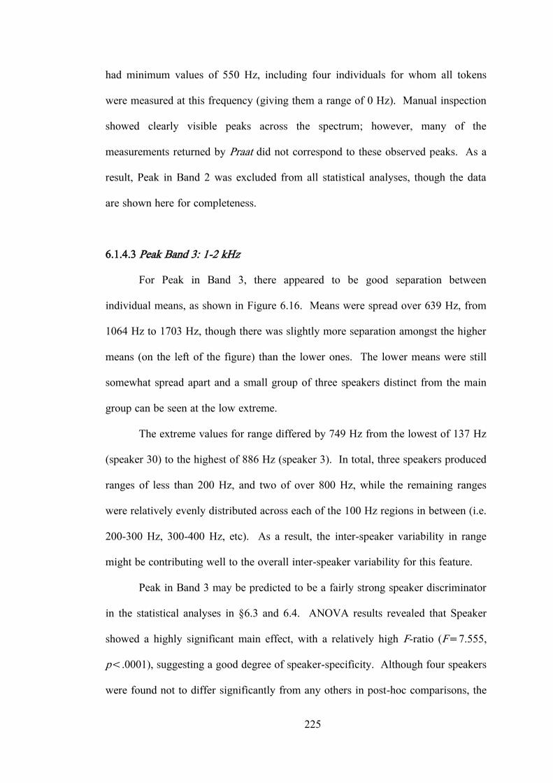
225

had minimum values of 550 Hz, including four individuals for whom all tokens

were measured at this frequency (giving them a range of 0 Hz). Manual inspection

showed clearly visible peaks across the spectrum; however, many of the

measurements returned by Praat did not correspond to these observed peaks. As a

result, Peak in Band 2 was excluded from all statistical analyses, though the data

are shown here for completeness.

6.1.4.3 Peak Band 3: 1-2 kHz

For Peak in Band 3, there appeared to be good separation between

individual means, as shown in Figure 6.16. Means were spread over 639 Hz, from

1064 Hz to 1703 Hz, though there was slightly more separation amongst the higher

means (on the left of the figure) than the lower ones. The lower means were still

somewhat spread apart and a small group of three speakers distinct from the main

group can be seen at the low extreme.

The extreme values for range differed by 749 Hz from the lowest of 137 Hz

(speaker 30) to the highest of 886 Hz (speaker 3). In total, three speakers produced

ranges of less than 200 Hz, and two of over 800 Hz, while the remaining ranges

were relatively evenly distributed across each of the 100 Hz regions in between (i.e.

200-300 Hz, 300-400 Hz, etc). As a result, the inter-speaker variability in range

might be contributing well to the overall inter-speaker variability for this feature.

Peak in Band 3 may be predicted to be a fairly strong speaker discriminator

in the statistical analyses in §6.3 and 6.4. ANOVA results revealed that Speaker

showed a highly significant main effect, with a relatively high F-ratio (F=7.555,

p<.0001), suggesting a good degree of speaker-specificity. Although four speakers

were found not to differ significantly from any others in post-hoc comparisons, the

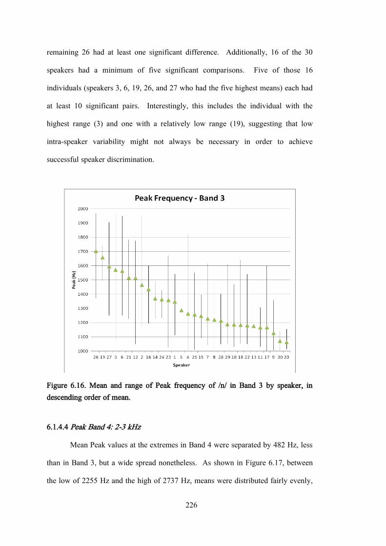
226

remaining 26 had at least one significant difference. Additionally, 16 of the 30

speakers had a minimum of five significant comparisons. Five of those 16

individuals (speakers 3, 6, 19, 26, and 27 who had the five highest means) each had

at least 10 significant pairs. Interestingly, this includes the individual with the

highest range (3) and one with a relatively low range (19), suggesting that low

intra-speaker variability might not always be necessary in order to achieve

successful speaker discrimination.


6.1.4.4 Peak Band 4: 2-3 kHz

Mean Peak values at the extremes in Band 4 were separated by 482 Hz, less

than in Band 3, but a wide spread nonetheless. As shown in Figure 6.17, between

the low of 2255 Hz and the high of 2737 Hz, means were distributed fairly evenly,

227

with several small groups distinguishable throughout the distribution, each

separated by approximately 25-50 Hz.

The disparity between the highest and lowest ranges in Band 4 was even

higher than that found in Band 3. 765 Hz separated the extreme ranges of 157 Hz

(speaker 6) and 922 Hz (speaker 11). As in Band 3, range values were quite evenly

distributed: three speakers produced ranges of less than 200 Hz, three to six

speakers had ranges in each of the 100-Hz regions up to 800 Hz, and three had

ranges higher than 800 Hz. This wide variation and even distribution may suggest

a good degree of speaker-specificity and good discrimination potential, similar to

Peak in Band 3.


228

Speaker was a highly significant factor for Peak in Band 4, with a

moderately high F-ratio (F=6.430, p<.0001). Post-hoc comparisons revealed that

eight speakers had no significant differences from other speakers, though all others

had at least one. Three speakers had at least 10 significant pairs, including speaker

12 with the highest mean and a relatively low range, who differed from 12 other

individuals. Importantly, though, 10 speakers – including some nearer the middle

of the distribution in terms of mean (e.g. speakers 2, 3, and 13) – were each

significantly different from six to seven others. This indicates that it is not only the

speakers at the extremes who differ, but also those who produced Peak frequencies

near the mean for the entire data set, which might point towards strong speaker

discrimination performance in statistical testing.

6.1.4.5 Peak Band 5: 3-4 kHz

Figure 6.18 displays mean and range data for Peak in Band 5. As in Band

2, Peak measurements in this frequency Band were inaccurate for many speakers,

so this variable was also excluded from all statistical analyses, though it is included

here for completeness. Speaker 24's data in particular were highly problematic, as

all of his tokens were measured at 3050 Hz. Others had minimum Peak

frequencies measured at 3050 Hz and maximum values at 3950 Hz, out of line with

actual peaks visible in the spectra.

229



Figure 6.19 displays mean and range data by speaker for Peak frequency

across the entire spectrum, from 0-4 kHz, excluding Bands 2 and 5. Peak in Band

1 was noticeably less variable than in Bands 3 and 4, and was fairly central within

the frequency Band. Peak was also relatively centred within Band 4, and mostly in

the lower half of Band 3.

A number of notable cross-Band patterns were apparent for Peak. Speaker

19 produced amongst the highest means in Bands 1 and 3, and amongst the lowest

in Band 4, while speaker 20 did the opposite: his means were near the low extreme

in Bands 1 and 3, and the high extreme in Band 4. Speaker 19 also produced

amongst the highest and lowest ranges in Bands 1 and 3 respectively, and speaker

20 amongst the lowest in the same Bands. Speakers 26 and 30 both produced some

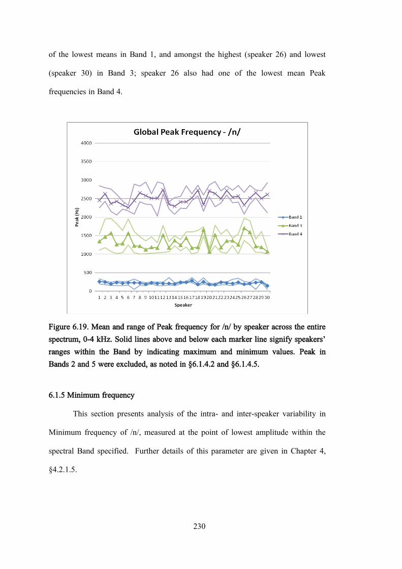
230

of the lowest means in Band 1, and amongst the highest (speaker 26) and lowest

(speaker 30) in Band 3; speaker 26 also had one of the lowest mean Peak

frequencies in Band 4.

Figure 6.19. Mean and range of Peak frequency for /n/ by speaker across the entire spectrum, 0-4 kHz. Solid lines above and below each marker line signify speakers‟ ranges within the Band by indicating maximum and minimum values. Peak in Bands 2 and 5 were excluded, as noted in §6.1.4.2 and §6.1.4.5.


This section presents analysis of the intra- and inter-speaker variability in

Minimum frequency of /n/, measured at the point of lowest amplitude within the

spectral Band specified. Further details of this parameter are given in Chapter 4,

§4.2.1.5.

231


Minimum in Band 1 was also excluded from all statistical analyses but is

again included here for completeness. A large proportion of the data was

questionable, as many of the measurements returned by Praat were either 50 Hz or

450 Hz, as shown in Figure 6.20. Seven of the 30 speakers recorded data solely at

frequencies of 450 Hz or 50 Hz. Most of the remaining speakers‟ data ranged

between these two frequencies only. As a result, the data were deemed unreliable

and excluded from further analysis.

Figure 6.20. Mean and range of Minimum frequency of /n/ in Band 1 by speaker, in descending order of mean.

6.1.5.2 Minimum Band 2: 500-1000 Hz

Though it is perhaps less evident from Figure 6.21 than from Figure 6.20,

data for Minimum in Band 2 were also problematic for many speakers. 18% of all

232

tokens, from 16 different speakers, were measured at 950 Hz despite not

corresponding to an actual peak at this frequency in the spectrum following manual

inspection. As in Band 1, as well as Bands 2 and 5 for Peak frequency, such a high

proportion of erroneous data rendered this variable unreliable and therefore not

suitable for inclusion in any further statistical analysis.



Means for Minimum frequency in Band 3 shown in Figure 6.22 were widely

variable, spread over 605 Hz. The lowest mean observed was 1265 Hz for speaker

19; speaker 28 produced the highest mean at 1870 Hz, approximately 100 Hz

higher than the next highest. A number of small groups can be distinguished

233

throughout the rest of the distribution, with gaps of approximately 40-50 Hz

between speakers 18 and 8, 23 and 26, and 3 and 25.


The lowest range, for speaker 24, was 234 Hz, while the highest was 942

Hz for speaker 3. Despite this disparity between extreme values for range, intra-

speaker variability in Minimum frequencies in Band 3 was quite high for most

individuals. Only six speakers produced ranges of less than 500 Hz. As a result,

ranges appear unlikely to contribute to overall inter-speaker differences for the

present variable, as they are too consistently high across the majority of speakers.

Although the spread of means is promising, the inter-speaker variability contributed

by mean values might be obscured by the wide ranges employed by many

individuals. If ranges were similar across individuals but generally narrow, the

234

inclusion of this variable as a predictor might improve discrimination. However,

generally wide ranges mean that speakers with very different means still overlap

greatly, reducing the overall potential contribution of range to discrimination.

Speaker was found to be highly significant for Minimum in Band 3, but

with one of the lowest overall F-ratios (F=2.791, p<.0001). Post-hoc

comparisons showed that 24 of the 30 speakers had no significant differences.

Speaker 28, with the highest mean and a relatively low range, was significantly

different from four others, and speaker 2 from two others. The four remaining

speakers with one significant comparison each were speakers 3, 12, 19, and 27.

Despite the significant effect of Speaker, the wide variation exhibited by the

majority of speakers and few differences between individuals in post-hoc testing

suggest that Minimum in Band 3 might not be a promising speaker discriminator,

perhaps even in combination with other predictor variables.


For Minimum in Band 4, means were again spread across a wide frequency

range of 857 Hz, as shown in Figure 6.23. Means extended from 2098 Hz (speaker

24) to 2955 Hz (speaker 5), covering most of the frequency span of the Band.

There was particularly good separation between individuals in the lower half of the

distribution, amongst the speakers on the right side of the figure. Several

individuals and small groups were separated from adjacent speakers by

approximately 50-120 Hz.

The ranges of Minimum frequencies produced by individual speakers varied

widely, from 25 Hz (speaker 5) to 968 Hz (speaker 12), a difference of 943 Hz.

There did not appear to be a very even distribution of ranges, however: a small

235

number of speakers had very narrow ranges (seven under 200 Hz), while many had

very wide ranges (17 over 600 Hz), with few in between. Interestingly, though, 11

speakers never produced values below 2500 Hz, the midpoint of the Band, and two

speakers never above this point.


ANOVA results showed that Minimum in Band 4 was highly significant for

Speaker, with a relatively high F-ratio (F=9.611, p<.0001). Post-hoc comparisons

showed that only speaker 23 was not significantly different from any others, and

the remaining 29 speakers had at least two significant comparisons. Six individuals

had a minimum of 10 significant pairs, including speakers 12 and 24 who had 20

each. Significant comparisons occurred both within and across dialect groups for

all but one speaker (8, whose significant differences were only within the SSBE

236

group). These ANOVA results suggest that Minimum in Band 4 is potentially a

good speaker discriminator, perhaps best in combination with additional predictors.


Minimum in Band 5 was quite similar to Band 3, and did not appear to be a

particularly promising speaker discriminator despite a wide distribution of means

and a significant effect of Speaker. Means and ranges for Band 5 are shown in

Figure 6.24. Means were relatively evenly spread across 574 Hz, from 3243 Hz

(speaker 1) to 3817 Hz (speaker 22), with slightly more separation between the

lowest three means than within the main group.


237

Ranges were consistently wide and very similar across the majority of

speakers, however. The lowest range was 316 Hz (speaker 20), one of only three

under 500 Hz. The remaining 27 varied from 501 Hz to the highest range of 948

Hz (speaker 4). As in Band 3, these consistently wide ranges might obscure

differences between speakers with otherwise disparate means, hindering

discrimination.

As stated above, Speaker was a highly significant factor for Minimum in

Band 5, albeit with the second lowest F-ratio overall (F=2.381, p<.0001). Post-

hoc tests showed that 24 of the 30 speakers had no significant comparisons with

any other individuals. The only significant differences were between speaker 1

(with the lowest mean and second highest range) and speakers 2, 7, 18, 22, and 28.


In Figure 6.25, means and ranges for Minimum in Bands 3, 4, and 5 are

displayed to provide a global view of this parameter across the spectrum. Bands 1

and 2 are excluded for the reasons noted in §6.1.5.1 and §6.1.5.2 above. Minimum

ranges in Bands 3-5 were relatively high overall, though Band 4 ranges appear most

variable between speakers, as a number of individuals can be seen to have quite

narrow ranges. In all three Bands, Minimum data covered most of the frequency

range, with slight concentration in the upper half of each.

Speakers 24 and 28 had interesting cross-Band patterns. Speaker 24

produced the third highest mean in Band 3, the lowest mean in Band 4, and low

ranges in both. Speaker 28 notably produced amongst the highest means and

lowest ranges in Bands 3 and 5, in addition to one of the lowest means and highest

ranges in Band 4.

238

Figure 6.25. Mean and range of Minimum frequency for /n/ by speaker across the entire spectrum, 0-4 kHz. Solid lines above and below each marker line signify speakers‟ ranges within the Band by indicating maximum and minimum values. Bands 1 and 2 were excluded, as noted in §6.1.5.1 and §6.1.5.2.

6.2 Dialect effects

The effect of Dialect on all parameters was tested using the Mann-Whitney

U test for non-parametric data, as sample sizes were unequal (21 speakers and 206

tokens for SSBE, 9 speakers and 62 tokens for Leeds). As described above, four of

the 21 predictors were excluded (Peak 2 and 5, Minimum 1 and 2) because of

unreliable data. Of the remaining 17 predictors, 11 were not significant for Dialect,

while six were. Mann-Whitney U test results are given in Table 6.2.

As was the case with /m/ in Chapter 5, despite the statistical significance, it

is not entirely clear whether the effect is actually due to cross-dialectal variation in

acoustic productions, or a result of the highly significant Speaker effects observed

for all 16 variables tested. Inspection of the distribution of speakers from the two

239

dialect groups in Figures 6.1-6.24 shows neither group was disproportionately high

or low when compared with the other in terms of mean values. Speakers of the two

dialects were not grouped distinctly either. The nine Leeds speakers were

relatively evenly interspersed with the SSBE speakers for all variables, including

those found to be significant for Dialect (COG in Bands 4 and 5, SD in 2 and 5,

Peak in 4, and Minimum in 4). Post-hoc comparisons in Speaker ANOVAs did not

reveal disproportionate differences between SSBE and Leeds speakers either.

Speakers regularly had significant differences both within and across dialect

groups. It is suspected that strong individual speaker differences are contributing

greatly to the significance of Dialect for some parameters. This warrants further

exploration in future research, to clarify the role of Dialect; however, in light of the

observations noted here, Dialect was not pursued any further in analysis of /n/ in

the present study.

Table 6.2. Mann-Whitney U test findings for effect of Dialect on acoustic features of /n/. Bold text indicates results significant at the level .05.

Parameter Band 1 Band 2 Band 3 Band 4 Band 5 NormDur .364 COG .400 .115 .665 .000 .027 SD .353 .000 .076 .172 .000 Peak .724 - .497 .020 - Minimum - - .742 .036 .125


DA was conducted on /n/ acoustic data, as described in Chapter 4. Peak in

Bands 2 and 5, and Minimum in Bands 1 and 2, were excluded from DA testing for

the reasons noted in §6.1. Normalised duration was also not tested, as it was not

found to be significant for Speaker, and was thus not predicted to contribute to

240

speaker discrimination. In addition, two speakers were excluded from the DA

testing data, although they were retained for the discussion of intra- and inter-

speaker variability in §6.1. Data for speakers 19 and 23 (one from each dialect

group) were reliable and worth including in analysis of the distributions for each

variable, but these two individuals produced five tokens of /n/ each, making them

the smallest samples in the dataset. This would have limited DA to four predictors,

as the number of predictors in a single test must be less than the smallest sample

size. However, with speakers 19 and 23 excluded, the next smallest sample was six

tokens, which allowed a maximum of five predictors; this permitted testing of

combinations of all five Bands for a single parameter (e.g. COG Bands 1-5).

These exclusions resulted in a total of 28 speakers (20 for SSBE, eight for

Leeds) and 16 predictors available for analysis. Each predictor was tested

individually and in a number of combinations, for a total of 31 separate DA tests.

As in Chapter 5, in combinations where the total number of predictors exceeded the

maximum of five, F-ratios for Speaker reported in Table 6.1 were used to select the

five predictors to be included. In two-parameter combinations, at least two

predictors from each parameter were selected to ensure that tests would not consist

entirely of predictors from just one of the parameters. Table 6.3 gives the

predictors included in each of the 31 tests, along with cross-validated classification

rates. The same Band and parameter combinations were tested as for /m/ in

Chapter 5, with the exception of those that included normalised duration. The

„Best 5 F-ratios‟ test was identical to the two-parameter COG+SD combination

(COG in Bands 1, 3, and 4, SD in Bands 1 and 4), as indicated in Table 6.3.

Discriminant functions were derived for each test, allowing interpretation of

the contribution to discrimination of each predictor. Figure 6.26 displays

241

discriminant scores on the first two functions for the Best 5 F-ratios test. The dark

blue squares indicate group centroids for individual speakers; the vertical and

horizontal spread of these centroids suggests there is a relatively high degree of

separation between speakers with good contributions from the first two

discriminant functions. Speakers 6 on the far left and 12, 18, and 20 on the far

right were separated quite well from the remaining speakers by the first function,

which was strongly correlated with COG in Band 4. The second discriminant

function separated speaker 30 from the main group, and also separated speakers 12,

18, 20, and 21 from each other fairly well. COG in Band 1 and SD in Band 4 had

relatively strong correlations with the second function, although both were more

strongly and significantly correlated with the fifth discriminant function. In total,

the first two functions accounted for approximately 55% of the variation.

Figure 6.26. Discriminant function plot showing the first two discriminant functions for the 5-predictor COG+SD/Best 5 F-ratios test. Individual cases and group centroids are shown.

242

Cross-validated classification rates for all DA tests are given in Table 6.3;

chance level was approximately 3.6%. Of the 16 single-predictor tests, the highest

classification rate was achieved by SD in Band 1, as 17% of cases were assigned to

the correct speaker group. Several predictors produced very low classification

rates, below 10%, particularly SD in Band 5 and Minimum in Band 3, which

achieved just 5% correct classification each, only just above the level of chance.

This is not unexpected, though, given the low F-ratios obtained for these two

predictors, and that a single predictor is unlikely to produce a high level of

discrimination on its own.

Classification generally improved in multiple-predictor tests. 27% of cases

were classified correctly in the Band 1 test despite having fewer predictors than

other single-Band tests, as Minimum was excluded. Band 4 (with all four

predictors) performed fairly well too, with 23% correct classification. Bands 2 and

5 each had one to two predictors excluded and consequently produced relatively

low classification rates.

The single-parameter test results were also split: COG and SD produced

good results, with 42% and 28% correct classification respectively, but Peak and

Minimum were not as successful in discriminating speakers. However, these two

tests did have two fewer predictors than the five-predictor COG and SD tests.

COG with Bands 1-5 in fact achieved the second highest classification rate overall.

243

Table 6.3. Cross-validated classification rates for DA with 1-5 predictors for /n/ and 28 speakers; chance=3.6%. Asterisks indicate tests from which Peak in Bands 2 and 5 and Minimum in Bands 1 and 2 were excluded.

Parameter(s) Band N Pred % Classification COG 1 1 13 2 1 10 3 1 9 4 1 14 5 1 8 SD 1 1 17 2 1 7 3 1 10 4 1 9 5 1 5 Peak 1 1 11 3 1 7 4 1 8 Minimum 3 1 5 4 1 11 5 1 7 Band 1 excl. Min 3* 27 2 excl. Peak, Min 2* 12 3 4 16 4 4 23 5 excl. Peak 3* 12 COG 1 thru 5 5 42 SD 1 thru 5 5 28 Peak 1, 3, 4 3* 15 Min 3 thru 5 3* 10 COG + SD (Best 5 F-ratios) COG 1, 3, 4, SD 1, 4 5 45 COG + Peak COG 1, 3, 4, Peak 3, 4 5 35 COG + Min COG 1, 3, 4, Min 3, 4 5 32 SD + Peak SD 1, 2, 4, Peak 3, 4 5 31 SD + Min SD 1, 2, 4, Min 3, 4 5 30 Peak + Min Peak 1, 3, 4, Min 3, 4 5 19

The best performing combinations generally were the two-parameter tests.

All but Peak+Min achieved between 30% and 45% correct classification, well

244

above chance level, particularly considering the five-predictor limit. The highest

overall rate of 45% was obtained in the Best 5 F-ratios/COG+SD test; this is

similar to the DA results for /m/ presented in Chapter 5 where the two highest

classification rates overall were produced by the COG+SD and Best 8 F-ratios

tests. Higher rates might be achieved for /n/ with increased token numbers

allowing the inclusion of more predictors, as demonstrated by the eight-predictor

DA results for /m/ which reached 53% correct classification. Although 45% might

not appear to be a remarkable result, it should be noted for all DA results that

classification is not necessarily expected to reach 100% when so many speakers are

included and a small number of predictors is used. With 30 speakers and a

maximum of five predictors, the rates achieved for /n/ simply serve to highlight the

most promising predictor combinations for speaker discrimination.

Individual cross-validated classification rates for the two highest scoring

tests were generally quite good. Figure 6.27 shows correct classification rates for

individual speakers in the tests of Best 5 F-ratios and COG Bands 1-5. For 16 of

the 30 speakers, at least 50% of tokens were correctly classified in one or both

tests. Six of these 16 individuals reached at least 80%, including three who

achieved 100% classification in at least one of the tests. For 11 speakers, COG

Bands 1-5 produced better classification than the Best 5 F-ratios test. For 12

speakers, higher rates were achieved in the Best 5 F-ratios test, while results of the

two tests were equal for the remaining five individuals. Only speaker 11 had no

tokens correctly classified with either combination of predictors. On the other

hand, speaker 30 was extremely well discriminated from the group, being the only

speaker to achieve 100% classification in both tests. Inspection of the errors (not

shown) revealed that four tokens were incorrectly assigned to speaker 30 in the

245

COG Bands 1-5 test, and he was selected incorrectly only once in the Best 5 F-

ratios test. This indicates a very high level of discrimination, as not only were all

of speaker 30‟s tokens correctly classified, he was rarely confused with other

individuals.

Figure 6.27. Individual cross-validated classification rates in the Best 5 F-ratios test (COG in Bands 1, 3, and 4 + SD in Bands 1 and 4) and COG Bands 1-5 for /n/, with 28 speakers (chance=3.6%).


LR analysis was conducted as described in Chapter 4. Peak in Bands 2 and

5, and Minimum in Bands 1 and 2, were again excluded. Normalised duration was

also not tested, as it was found not to be significant for the effect of Speaker.

Additionally, all data for speakers 19 and 23 were excluded as a result of small

sample sizes, as in the DA above. Although this reduced the size of the reference

246

sample, it allowed for consistency between the DA and LR analyses. The

exclusion of these two speakers, with just five tokens each, increased the smallest

sample size to six tokens. The smallest samples could, therefore, be divided evenly

to create the two separate samples required for comparison.

Table 6.4. Summary of LR performance for /n/ in 17 test combinations, showing percentage of same-speaker (SS) and different-speaker (DS) comparisons yielding log10LRs≥±4, percentage of false positives and negatives, equal error rates (EER), and Cllr. Asterisks indicate tests from which Peak in Bands 2 and 5, and Minimum in Bands 1 and 2, were excluded.

Predictors ±4 Log10LR % False Neg % False Pos % EER

% Cllr SS DS SS DS

Band 1* 0 17 18 27 21 0.70 Band 2* 0 2 21 41 29 0.87 Band 3 0 11 29 33 29 0.77 Band 4 0 27 18 21 19 0.65 Band 5* 0 2 57 16 36 0.98 COG 4 39 25 12 14 0.50 SD 0 18 29 24 25 0.66 Peak* 0 8 18 29 25 0.75 Min* 0 7 57 17 32 0.96 COG+SD 4 61 36 7 18 1.45 COG+Peak* 0 46 25 8 11 0.47 COG+Min* 0 46 29 11 14 0.55 SD+Peak* 0 33 32 15 18 0.61 SD+Min* 0 34 29 12 18 0.66 Peak+Min* 0 18 39 14 25 0.86 All* 14 73 50 10 24 13.35 Best 5 F-ratios 4 46 14 11 14 0.47

28 same-speaker (SS) comparisons and 364 different-speaker (DS)

comparisons were performed. Individual Bands and parameters were tested as well

as combinations of two parameters, as in the DA above, for a total of 17 tests. For

two-parameter combinations, however, all available predictors were included as LR

247

analysis is not limited by sample size, as DA is. A separate Best 5 F-ratios test was

also conducted, as in this case the COG+SD test included 10 predictors instead of

the five tested in the DA. Finally, all available predictors were combined in a

single test. Table 6.4 provides a summary of LR results for all 17 tests, showing

the proportion of SS and DS comparisons with log10LR scores≥±4, rates of false

positives and negatives, equal error rates, and Cllr (detailed in Chapter 4, §4.2.6.2).

6.4.1 ±4 log10LRs

The proportion of log10LR scores at or beyond the ±4 threshold provides an

indication of the strength of the evidence obtained in the LR analysis (for further

details, see Chapter 4, §4.2.6.2). The All-predictor test achieved the highest

proportion of both SS and DS comparisons (14% and 73% respectively) above (or

below) this threshold, equivalent to a raw LR score of 10,000 in support of either

hypothesis. In DS comparisons, the Best 5 F-ratios, COG+SD, COG+Peak, and

COG+Min all achieved very high rates as well, up to 61%. In SS comparisons,

COG, COG+SD, and the Best 5 F-ratios tests were the only additional tests with

scores above the +4 threshold. These SS results are not unexpected, however. DS

pairs are expected to achieve higher scores overall than SS pairs, as there is a limit

to how similar speakers may be, though the degree to which they may differ can be

greater.


The false negative column in Table 6.4 indicates the percentage of SS pairs

that were wrongly identified as DS pairs, i.e. those with a negative log10LR value (a

raw LR of less than 1). The darkest shade of orange indicates the highest false

248

negative proportion, with lower rates marked in progressively lighter shades. The

highest rates were obtained in the Band 5, Minimum, and All-predictor tests, where

50% or more of the SS comparisons produced negative log10LR values. A number

of other tests produced relatively high rates as well, particularly the two-parameter

combinations, in which false negative percentages ranged from 29% to 39%. The

lowest rate overall was 14% in the Best 5 F-ratios test.

False positive rates are also indicated in shades of orange in Table 6.4, with

the highest rates marked by the darkest shades. More false positives occurred in

single-parameter or Band tests than in two-parameter combinations. The highest

rate was obtained in the Band 2 test, where 41% of DS comparisons incorrectly

produced log10LR values greater than 0 (a raw LR value greater than 1). This is a

particularly poor result, as it means that nearly half of all DS pairs (151 of 364)

were incorrectly identified as SS pairs. In an ideal LR system, the false positive

rate would be 0, as the impact of obtaining false positives in real forensic casework

can be severe, potentially contributing to a wrongful conviction. The tests which

produced the lowest false positive rates were COG+SD and COG+Peak, where 7-

8% of DS comparisons resulted in positive log10LR values. Relatively low rates of

10-11% were also obtained in the COG+Min, Best 5, and All-predictor tests.


The highest equal error rates are marked in the darkest shade of purple in

Table 6.4, and lower values in progressively lighter shades. EERs were generally

higher in single-Band and single-parameter tests than combined-parameter tests.

The highest rates were produced in tests of Band 5 and Minimum (36% and 32%

respectively), which also produced the two highest rates of false negatives.

249

However, amongst the single-parameter tests, COG (Bands 1-5) had one of the

lowest EERs (14%). When parameters were combined, COG+Min and Best 5 F-

ratios tests had equally low EERs (14%), and the lowest overall (11%) was

obtained in the COG+Peak test.


While EER describes the proportion of errors produced in a given test, it

does not say anything about the magnitude of the errors. The fourth statistic

presented in Table 6.4 is Cllr or log likelihood ratio cost, which does reflect the

magnitude of errors in the context of measuring the validity of the LR system, as

described in Chapter 4. Errors of high magnitude contribute more to Cllr than those

of low magnitude, and the proximity of the Cllr to 0 indicates the validity of the

system. The highest Cllr value obtained for the present dataset was 13.35 in the All-

predictor test. This reflects the extremely high proportion and magnitude of SS

errors in the All-predictor test, similar to the finding for the same test for /m/ in

Chapter 5. The lowest values, signifying the tests with the greatest validity, were

obtained in the COG+Peak and Best 5 F-ratios tests (both 0.47).


Considering the results of all four measures presented above, the best

performing tests overall appear to be COG+Peak and the Best 5 F-ratios. The

Tippett plot below (Figure 6.28) displays log10LR values for all SS and DS pairs in

these two tests.

In DS comparisons, indicated by the red lines rising to the left, COG+Peak

and Best 5 F-ratios tests were roughly equal. Both had the same proportion of

250

results (46%) over the -4 log10LR threshold for „very strong‟ evidence, though the

Best 5 F-ratios test produced slightly more false positives (11% versus 8% for

COG+Peak). In SS comparisons, however, the Best 5 F-ratios test (indicated by

the solid blue line rising to the right) appears to perform slightly better than

COG+Peak. While none of the SS pairs in the COG+Peak test reached the +4

log10LR threshold, 4% of the Best 5 F-ratios SS comparisons did.

The false negative rate in the Best 5 F-ratios test was also much lower, at

14%, than in COG+Peak, where 25% of SS comparisons incorrectly resulted in a

negative log10LR value. The proportions of false positives and negatives are

represented in Figure 6.28 by the proportion of the red curves which lay to the right

of the vertical zero line, and of the blue curves which lay to the left of the zero line,

respectively. COG+Peak produced the lowest overall EER (11%) and Best 5 F-

ratios the second lowest (14%). These can be identified in the Tippett plot as the

point at which the SS and DS curves for each test cross; the solid lines

(representing the Best 5 F-ratios results) cross slightly higher than the dashed

(COG+Peak) lines on the vertical axis. These two tests also shared the lowest

overall Cllr value of 0.47 reported above. Other tests might have produced better

results on one or more of these four measures, such as COG+SD and All-predictor

tests having lower percentages of false positives and higher proportions of „very

strong‟ results over ±4 log10LR. However, those tests also produced more errors

on other measures, in particular high false negative rates and extremely high Cllr

values. On balance, COG+Peak and the Best 5 F-ratios produced few false

positives, relatively few false negatives, low EERs and Cllr, and a fairly good

strength of evidence, making them the best performing predictor combinations for

/n/ in the LR analysis.

251

Figure 6.28. Tippett plot showing log10LR values for same-speaker (SS) and different-speaker (DS) comparisons for Best 5 F-ratios and COG+Peak tests.

6.5 Chapter summary

This chapter explored the intra- and inter-speaker variability observable in

acoustic properties of /n/ and the effects of both Speaker and Dialect on these

features. Speaker was found to be highly significant for all parameters except

normalised duration, while the effect of Dialect was unclear. Results of both DA

and LR analysis suggested that the investigated parameters showed strong speaker

discrimination potential. DA and LR results both determined that the Best 5 F-

ratios test was one of the best-performing predictor combinations; relatively

promising results were also obtained in the COG Bands 1-5 DA test and the

COG+Peak LR test.

252

Chapter 7 Results: /ŋ/

7.0 Overview

This chapter presents analysis of the intra- and inter-speaker variability in

acoustic features of /ŋ/, along with an assessment of the effect of Speaker and

Dialect on those features. As Table 4.1 in Chapter 4 showed, token numbers of /ŋ/

were relatively low. As a result, analysis in the present chapter is largely

descriptive, and DA and LR estimation were not conducted. Statistical results

should be considered in this light and treated with a degree of caution until

additional data can be analysed.


This section examines the five acoustic parameters of /ŋ/ with a view to

assessing the intra- and inter-speaker variability of each parameter in each of the

five frequency Bands. Each is discussed independently below, along with a global

view of each parameter across the whole spectrum. Means and ranges for each

individual are displayed in Figures 7.1-7.25.

Token numbers were more limited than for /m/ and /n/ in previous chapters:

speaker 27 was removed from the analysis as he produced only one phonetically

velar nasal consonant. The remaining 29 speakers produced a minimum of two and

a maximum of 12 tokens, with a mean of five across all speakers. Token numbers

for each individual are given in Table 4.1 (Chapter 4).

Results of univariate ANOVAs for Speaker are summarised in Table 7.1.

Where no results are reported, the variable was excluded from analysis as a

253

consequence of unreliable data. Further details are provided in the relevant

subsections below. The effect of Speaker was found to be significant for all

variables, with the exception of Minimum in Band 5. Speaker effects are examined

in more detail in each subsection, along with the results of Hochberg post-hoc

pairwise comparisons. However, this general finding indicates that the acoustic

properties of /ŋ/ under investigation, in addition to those of /m/ and /n/, may have

the potential to contribute to speaker discrimination.

Table 7.1. Results of univariate ANOVAs for Speaker (N=29) for each acoustic feature of /ŋ/ (x15). Bold text indicates results significant at the level .05.

Parameter Band 1 Band 2 Band 3 Band 4 Band 5 NormDur F=2.263 p=.001

COG F=9.706 p<.0001

F=4.676 p<.0001

F=5.539 p<.0001

F=10.858 p<.0001

F=3.585 p<.0001

SD F=14.288 p<.0001

F=4.873 p<.0001

F=4.921 p<.0001

F=9.146 p<.0001

F=3.495 p<.0001

Peak - - - F=4.785 p<.0001

F=2.015 p=.005

Minimum - - F=2.773 p<.0001 - F=1.548

p=.055


Means and ranges of normalised /ŋ/ durations for all speakers are displayed

in Figure 7.1, arranged in descending order of mean. Speaker 26, with the highest

mean (0.806), was clearly markedly different from the remainder of the group;

however, it must be noted that he produced only two measureable tokens of

phonetically velar nasal consonants, with normalised durations of 0.805 and 0.806.

Additional data would be required to determine the degree of intra-speaker

variability he is actually capable of producing beyond what was captured in the

present dataset. The difference between extreme means was 0.502, equivalent to

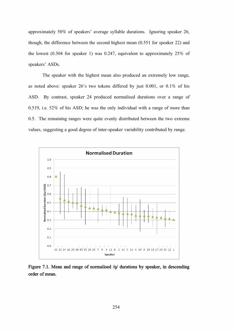
254

approximately 50% of speakers‟ average syllable durations. Ignoring speaker 26,

though, the difference between the second highest mean (0.551 for speaker 22) and

the lowest (0.304 for speaker 1) was 0.247, equivalent to approximately 25% of

speakers‟ ASDs.

The speaker with the highest mean also produced an extremely low range,

as noted above: speaker 26‟s two tokens differed by just 0.001, or 0.1% of his

ASD. By contrast, speaker 24 produced normalised durations over a range of

0.519, i.e. 52% of his ASD; he was the only individual with a range of more than

0.5. The remaining ranges were quite evenly distributed between the two extreme

values, suggesting a good degree of inter-speaker variability contributed by range.

Figure 7.1. Mean and range of normalised /ŋ/ durations by speaker, in descending order of mean.

255

Speaker was found to be highly significant, although as a result of the

highly skewed distribution of means, normalised duration produced one of the

lowest F-ratios overall (F=2.263, p=.001). Hochberg post-hoc tests showed that

only speaker 26 was significantly different from other individuals, with 16

significant pairs. The remaining 12 speakers had no significant comparisons.

However, ignoring speaker 26, the spread of means for /ŋ/ was similar to that for

/m/, which was also significant for Speaker. This suggests that with additional data

normalised duration might be able to contribute to speaker discrimination.


This sections details intra- and inter-speaker variation in COG

measurements in each of the five frequency Bands from 0 to 4 kHz. Further details

are given in Chapter 4, §4.2.1.2.

7.1.2.1 COG Band 1: 0-500 Hz

Mean and range data for COG in Band 1 are displayed in Figure 7.2. The

highest mean of 259 Hz (speaker 8) was similar to that for both /m/ and /n/, though

the lowest mean was 120 Hz (speaker 30), which was 24 Hz lower than that for /m/

and /n/. This spread of 139 Hz suggests a relatively high level of variation between

individuals, with slightly more separation between means nearer the low extreme.

Speakers were largely very consistent in their COG realisations, as 15 of 29

ranges were smaller than 50 Hz, including the lowest, at 19 Hz (speaker 14). Four

individuals produced ranges of more than 100 Hz, the highest being 142 Hz

(speaker 11). Some inter-speaker variation might be contributed by range, but this

256

generally low level of intra-speaker variability is notable, as low intra-speaker

variability is highly desirable with respect to FSC parameters.

Figure 7.2. Mean and range for COG of /ŋ/ in Band 1 by speaker, in descending order of mean.

In line with the findings for /m/ and /n/ in Chapters 5 and 6, COG in Band 1

for /ŋ/ was highly significant for Speaker, yielding the third highest F-ratio of the

15 /ŋ/ variables (F=9.706, p<.0001). In post-hoc comparisons, all speakers were

found to be significantly different from at least one other. Eight individuals had at

least five significant comparisons; two of these speakers differed significantly from

more than 10 others. Speaker 30, with the lowest mean and a very low range, was

significantly different from 23 others, and speaker 21 from 14 others.

257

7.1.2.2 COG Band 2: 500-1000 Hz

In Band 2, shown in Figure 7.3, COG means were all below the midpoint of

the Band. The highest mean observed was 748 Hz by speaker 12, though several

speakers had individual measurements of above 750 Hz. Means were spread over

169 Hz, as the lowest was 579 Hz for speaker 10.


Ranges in Band 2 were generally wider than in Band 1, though the

narrowest was identical at 19 Hz (speaker 26). Two ranges, however, were above

200 Hz, including the highest at 215 Hz for speaker 21. Additionally, a total of 19

of the 29 ranges were above 100 Hz, while in Band 1 the majority were below 50

Hz. This increase in intra-speaker variability suggests COG in Band 2 might be

258

slightly less speaker-specific than in Band 1, though the spread of means does still

indicate a relatively high level of inter-speaker variability.

ANOVA results showed Speaker to be a highly significant factor for COG

in Band 2 with a moderate F-ratio (F=4.676, p<.0001). In post-hoc pairwise

comparisons, however, 17 speakers were found not to be significantly different

from any others; the remaining 12 differed from at least one other individual.

However, 10 of the remaining 12 speakers each had five to six significant pairs,

suggesting that this parameter might still contribute well to discrimination,

particularly in combination with additional predictors.

7.1.2.3 COG Band 3: 1-2 kHz

Speakers‟ means and ranges for COG in Band 3 are displayed in Figure 7.4.

Means were again concentrated in the lower half of the Band, though in this case

six were above the midpoint of 1500 Hz. The highest mean reached 1602 Hz

(speaker 14), while the lowest was 1184 Hz (speaker 7), a difference of 418 Hz. A

relatively high degree of inter-speaker variation is evident, as individuals are fairly

well separated and several distinct groups are visible, separated by approximately

40-100 Hz.

Ranges were highly varied, as the widest (718 Hz, speaker 17) and

narrowest (14 Hz, speaker 16) differed by 704 Hz, a marked increase over Bands 1

and 2. Most were relatively narrow, however: 21 of 29 ranges were under 300 Hz,

including six under 100 Hz. The remaining eight were distributed between 319 Hz

and 718 Hz. This suggests that some degree of inter-speaker variability may be

contributed by range, in addition to that found in mean COG.

259

The inter-speaker variability noted above was reflected in the ANOVA

results, as COG in Band 3 was highly significant for Speaker, with the fifth highest

F-ratio overall (F=5.539, p<.0001). In post-hoc comparisons, however, 11

speakers were found not to differ significantly from any others, though the

remaining 18 had at least one significant comparison. The two individuals with the

highest means, speakers 4 and 14, also had the most significant comparisons (9 and

11 respectively); four others at the extremes in terms of mean each differed from

five to seven individuals.


7.1.2.4 COG Band 4: 2-3 kHz

COG in Band 4 patterned similarly to Band 3, with means spread over 474

Hz, largely in the lower half of the Band. Means extended from 2147 Hz (speaker

260

14) to 2621 Hz (speaker 28); in total, seven means were above 2500 Hz, the

midpoint of the Band. Though there were fewer distinct groups of means than in

Band 3, the spread and general separation between speakers was greater in Band 4,

as shown in Figure 7.5.

Ranges were generally narrower and less variable between speakers than in

Band 3, in contrast to the increased inter-speaker variability found in mean COG.

Seven speakers produced ranges of less than 100 Hz, including speaker 26, with the

narrowest range of 20 Hz. In all, 22 of the 29 speakers‟ ranges were under 300 Hz,

similar to the findings for Band 3. Unlike in Band 3, though, the widest range was

400 Hz (speaker 8). As a result, there was still relatively high inter-speaker

variability with less overall intra-speaker variability.


261

Speaker was found to be highly significant for COG in Band 4, with the

second highest F-ratio overall for /ŋ/ (F=10.858, p<.0001). With the limited data

available, this parameter appears to be relatively highly speaker-specific, as it was

for /m/ and /n/, which both obtained very high F-ratios in Speaker ANOVAs for

COG in this Band. All speakers had a minimum of two significant post-hoc

comparisons. 15 of 29 speakers differed significantly from at least five others,

seven of whom had at least 10 significant differences. The two speakers with the

lowest means (6 and 14) shared the highest number of significant comparisons (18

each). Notably, speakers 5, 11, and 17, who had means nearing the centre of the

distribution, also had multiple significant comparisons with five to six each. This is

important, as has been shown in Chapters 5 and 6 for COG of /m/ and /n/ in Band

4, because it demonstrates that speakers throughout the population distribution –

not only those at the extremes – can potentially be discriminated by this feature.

7.1.2.5 COG Band 5: 3-4 kHz

Means and ranges for COG in Band 5 are displayed in Figure 7.6. Means

were more evenly distributed across the 3-4 kHz spectrum than in lower Bands: the

lowest observed was 3251 Hz for speaker 28, and the highest 3752 Hz for speaker

12, with an average across all speakers of 3507 Hz. This represents the widest

spread of COG means for /ŋ/, at 501 Hz. The greatest separation between

individuals was at the extremes; the single highest and lowest means were each

clearly separated from the group by approximately 70 Hz.

In Band 5, ranges were wider in general than in Band 4, although the spread

of ranges was similar. Speaker 28 again produced the lowest range of 36 Hz, and

speaker 17 the highest at 520 Hz, a difference of 484 Hz. However, only speaker

262

28‟s was under 100 Hz. 14 of 29 ranges were between 200-300 Hz, with a total of

five individuals producing ranges of over 400 Hz. As a result, the overall level of

inter-speaker variability might be somewhat reduced by the large number of very

similar and generally wide ranges.


ANOVA results found Speaker to be a highly significant factor for COG in

Band 5, albeit with a low F-ratio (F=3.585, p<.0001). Post-hoc tests showed 18

of the 29 individuals did not differ significantly from any others. The remainder

had at least one significant comparison, though only one individual had more than

five. Speaker 12 differed significantly from eight others, as he had the highest

mean and a relatively low range. These findings suggest that COG in Band 5

263

might not be a particularly speaker-specific feature or a strong speaker

discriminator.


A global view of COG of /ŋ/ across the whole spectrum from 0-4 kHz is

shown in Figure 7.7. Markers indicate speakers‟ means in each Band, while solid

lines in the same colour above and below each marker line denote speakers‟

maximum and minimum values, and therefore their ranges. COG measures in

Bands 1, 2, and 3 were generally low within each frequency Band, while they were

quite central within Band 5. In Band 4, COG values were also largely below the

midpoint; however, a number of speakers from the IViE corpus (speakers 20-26,

representing both dialects) produced quite central means with very narrow ranges.

As in the previous chapters for /m/ and /n/, several speakers produced

interesting cross-Band patterns in COG of /ŋ/. Speaker 12, for instance, produced

means near the low extremes in Bands 1 and 3, and at or near the high extremes in

Bands 2, 4, and 5. He also produced ranges amongst the lowest in Bands 1, 3, and

5, and amongst the highest in Band 4. Speaker 14 was at or near the low extreme

for both mean and range in Band 1, as well as for mean in Bands 4 and 5. He also

produced the highest mean COG of all speakers in Band 3. Speaker 26‟s means

and ranges were amongst the lowest in Bands 1 and 2. He produced one of the

highest means in Band 3, as well as the lowest ranges in Bands 3 and 4. Finally,

along with speaker 26, speaker 28 was one of the most internally consistent

individuals. He produced low ranges in Bands 2, 3, 4, and 5, in addition to the

highest mean in Band 4 and the lowest in Band 5. Such cross-Band patterns

264

suggest speakers might be relatively well discriminated by combinations of

multiple COG predictors.

Figure 7.7. Mean and range of COG for /ŋ/ by speaker across the entire spectrum, 0-4 kHz. Solid lines above and below each marker line signify speakers‟ ranges within the Band by indicating maximum and minimum values.


The section discusses intra- and inter-speaker variability in SD of /ŋ/. SD is

a measure of the spread of energy in the spectrum around the COG; this is

described further in Chapter 4, §4.2.1.3.

7.1.3.1 SD Band 1: 0-500 Hz

Means and ranges of SD in Band 1 are displayed in Figure 7.8. Means were

spread over 69 Hz, from 44 Hz (speaker 3) to 113 Hz (speaker 5), with the majority

under 100 Hz. These extreme frequencies and the difference between them were

265

quite similar to those for /m/ and /n/, and indicate a relatively narrow dispersion of

energy around the COG of /ŋ/ in Band 1 in general. There was still a good level of

separation between individuals throughout the distribution, however, as well as a

gap of 10 Hz between speakers 15 and 24.

Figure 7.8. Mean and range for SD of /ŋ/ in Band 1 by speaker, in descending order of mean.

SD ranges were low overall, indicating speakers were internally consistent

in their SD values in Band 1. Only the widest range (56 Hz, speaker 11) was over

50 Hz; the lowest range was just 1 Hz by speaker 19 (who produced three tokens of

/ŋ/). In fact, 17 of 29 individuals had ranges of 25 Hz or less. This generally low

level of intra-speaker variability is notable particularly in addition to the inter-

speaker variability observed in mean, and suggests that SD in Band 1 might be a

promising speaker discriminator, as it was for both /m/ and /n/ in Chapters 5 and 6.

266

Following similar findings for /m/ and /n/, SD in Band 1 was highly

significant for the effect of Speaker, with the highest F-ratio overall for /ŋ/

(F=14.288, p<.0001). Post-hoc tests showed that all speakers were significantly

different from at least one other, though most differed from several others. 20

individuals had five or more significant comparisons; six had 10 or more. Speakers

3 and 16, who had the two lowest means, also had the highest numbers of

significant pairs, with 21 and 19 respectively. Importantly, as was the case for

COG in Band 4, speakers throughout the distribution in terms of mean had

numerous significant comparisons: speakers 2, 8, 9, and 14 in particular each

differed significantly from five to six others, despite being near the centre of the

distribution.

7.1.3.2 SD Band 2: 500-1000 Hz

SD means were slightly higher in Band 2 than in Band 1, indicating an

increase in the spread of energy around the COG of /ŋ/. As shown in Figure 7.9,

the lowest observed mean was 78 Hz (speaker 4) and the highest 167 Hz (speaker

11), a difference of 89 Hz. This spread of means was slightly wider than in Band 1

as well. The separation between speakers appears consistent throughout most of

the distribution, with slightly more separation amongst means near the low extreme.

Ranges in Band 2 were higher in general than in Band 1 as well: although

one speaker produced identical SD values leading to a range of 0 Hz (speaker 28),

only 10 in total were below 50 Hz. 18 ranges were between 50-100 Hz, with the

final speaker (1) producing a 101 Hz range of SD values. It must be noted that

speaker 28 had only two tokens of phonetically velar productions of /ŋ/ that were

included in the present dataset, so additional data might reveal greater intra-speaker

267

variation for this individual. Regardless, the relatively low inter-speaker variability

in range in general might suggest lower speaker-specificity in SD in Band 2 than in

Band 1.


SD in Band 2 was highly significant for Speaker, but yielded a moderate F-

ratio (F=4.873, p<.0001). Accordingly, post-hoc comparisons showed that 13 of

the 29 speakers did not differ significantly from any others; all others had at least

one significant comparison. Four individuals had more than five significant pairs:

the speakers with the two highest and two lowest means (4, 5, 11, and 29) each

differed significantly from between six and 10 other individuals.

268

7.1.3.3 SD Band 3: 1-2 kHz

Speakers‟ means and ranges for SD in Band 3 are displayed in Figure 7.10.

Mean SD increased again over Bands 1 and 2, as the lowest was 143 Hz (speaker

13) and the highest 341 Hz (speaker 23). The difference between extreme values

was also higher, at 198 Hz, indicating increased inter-speaker variability.

Separation between individual means was relatively consistent, though the two

highest and three lowest were clearly distinguished from the main group by

approximately 20-40 Hz.


A number of speakers had relatively wide ranges, as the highest was 227 Hz

(speaker 15), though many others had very narrow ranges as well. 15 of 29 ranges

were less than 100 Hz, including seven under 50 Hz and the lowest overall of 11

269

Hz (speaker 28). The remaining 13 were between 100-200 Hz. This distribution

suggests that range might contribute somewhat to the overall level of inter-speaker

variability in SD in Band 3.

Speaker was a highly significant factor, with a moderate F-ratio (F=4.921,

p<.0001), as in Band 2. 10 individuals had no significant post-hoc comparisons,

while the remainder had at least one. The three speakers with the lowest means

were the only individuals with more than five significant pairs: speakers 7 and 16

each differed from 16 others, and speaker 8 from seven others.

7.1.3.4 SD Band 4: 2-3 kHz

SD means decreased in Band 4 relative to Band 3, as the highest observed

was 262 Hz (speaker 26) and the lowest 99 Hz (speaker 1), a difference of 163 Hz.

The greatest separation between individual means appears to be in the upper half of

the distribution, as shown in Figure 7.11.

The majority of ranges were relatively narrow, as in Band 3, as 20 were less

than 100 Hz, including seven under 50 Hz and the narrowest range overall of 6 Hz

(speaker 28). Speaker 12 produced the widest range of 178 Hz, one of five over

150 Hz. Range might contribute somewhat to the overall inter-speaker variability

in SD in Band 4, though the generally low level of intra-speaker variability also

suggests relatively high speaker-specificity in this feature.

ANOVA results found SD in Band 4 to be highly significant for Speaker,

with the fourth highest F-ratio overall (F=9.146, p<.0001). In post-hoc tests, six

individuals had no significant comparisons, while all others had at least one. 15 of

29 speakers were significantly different from five or more others, including four

with at least 10 significant comparisons. Speakers 30 and 21 had the highest

270

numbers of significant pairs (17 and 13, respectively), as well as two of the three

highest means. As a result, SD in Band 4 is expected to be another promising

speaker discriminator warranting further attention.


7.1.3.5 SD Band 5: 3-4 kHz

In Band 5, mean SD values increased over Band 4 as they varied from 155

Hz (speaker 28) to 318 Hz (speaker 18). The majority of means were above 200

Hz (only four were below) indicating that the energy in Band 5 was relatively

diffuse. The spread of means was similar to Band 4, though the absolute values

were higher. The separation between individual means was broadly consistent

across the distribution, as no distinct groups were visible in Figure 7.12.

271

SD ranges were slightly wider than in Band 4, and somewhat similar to

those in Band 3. Two speakers produced ranges of over 200 Hz, the widest being

211 Hz (speaker 17). Although the lowest range was 17 Hz (speaker 24), this was

one of only four under 50 Hz. 11 of the remaining 23 ranges were between 50-100

Hz, and the final 12 between 100-200 Hz. This distribution of ranges is similar to

that in Band 3, but the spread of means was lower, which might result in SD in

Band 5 being less speaker-specific than it was in Band 3.


Speaker was found to be a highly significant factor for SD in Band 5, albeit

yielding a low F-ratio (F=3.495, p<.0001). In post-hoc tests, 21 individuals were

found not to be significantly different from any others. Of the eight speakers with

272

significant comparisons, only speakers 17 and 18 (with the highest range and mean,

respectively) had more than one. Each was significantly different from four others.


Figure 7.13. Mean and range of SD of /ŋ/ by speaker across the entire spectrum, 0-4 kHz.

In Figure 7.13, speaker means from all five Bands are displayed to give an

overall view of SD in the spectrum from 0-4 kHz. Band 1 had the narrowest

concentration of energy around the COG, as SD values were generally lowest in the

0-500 Hz region. SD in Band 2 was slightly higher on average, though three

speakers (4, 19, and 29) produced lower means in Band 2 than in Band 1. Band 4

means were similar to those for Band 2 for many speakers, and slightly higher for

others. In particular, a number of speakers between 18 and 30 (both SSBE and

273

Leeds speakers who belonged to the IViE and Morley corpora) produced higher SD

means in Band 4 than Band 2. Speakers 1-17 (SSBE, from the DyViS and IViE

corpora) were relatively close across the two Bands. For speakers 1, 5, and 6,

mean SD in Band 4 was nearly as low as in Band 1. As detailed in §7.1.3.3 and

§7.1.3.5, means were fairly similar in Bands 3 and 5. The relationship between

these two Bands was divided, however, as 16 speakers‟ means were higher in Band

3, 11 were higher in Band 5, and two were equal.

Acoustic analysis of /ŋ/ revealed fewer notable cross-Band patterns than

were found for /m/ and /n/. Still, a few speakers did produce interesting patterns:

speaker 3 produced the lowest mean in Band 1 and amongst the highest in both

Bands 4 and 5, as well as the third highest range in Band 2. Speaker 6‟s was

amongst the highest means in Bands 1 and 2, and amongst the lowest in Band 4, in

addition to this speaker having one of the higher ranges in Band 3. Speaker 18

produced amongst the lowest means in Band 1 and some of the highest in Bands 4

and 5, and amongst the highest ranges in Bands 1 and 4. Finally, speaker 23

produced means at opposite extremes in Bands 3 and 5, in addition to ranges near

the low extreme in Bands 1 and 2. Such observations should be treated with

caution, however, as token numbers for some speakers were very low, as reported

in Table 4.1.


Peak frequency was measured at the point of maximum amplitude in the

spectrum of each frequency Band. Further details of this parameter are provided in

Chapter 4, §4.2.1.4.

274

7.1.4.1 Peak Band 1: 0-500 Hz

Data for Peak in Band 1 were rejected as a number of speakers‟

measurements appeared unreliable. Figure 7.14, showing mean and range data, is

included here for completeness. It can be seen that 12 of the 29 speakers had

minimum Peak values at 50 Hz or 150 Hz; these did not correspond to visible

peaks in the spectra for a sample of these measurements. Consequently, all data for

Peak in Band 1 were excluded.

Figure 7.14. Mean and range for Peak frequency of /ŋ/ in Band 1 by speaker, in descending order of mean.

7.1.4.2 Peak Band 2: 500-1000 Hz

Peak in Band 2 was also excluded, as above; Figure 7.15 shows individuals‟

means and ranges, for comprehensiveness. The majority of speakers‟ Peak

measurements were questionable: 24 of 29 speakers had minima at 550 Hz, and

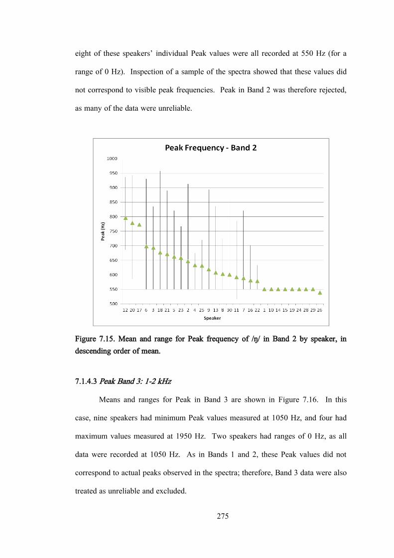
275

eight of these speakers‟ individual Peak values were all recorded at 550 Hz (for a

range of 0 Hz). Inspection of a sample of the spectra showed that these values did

not correspond to visible peak frequencies. Peak in Band 2 was therefore rejected,

as many of the data were unreliable.


7.1.4.3 Peak Band 3: 1-2 kHz

Means and ranges for Peak in Band 3 are shown in Figure 7.16. In this

case, nine speakers had minimum Peak values measured at 1050 Hz, and four had

maximum values measured at 1950 Hz. Two speakers had ranges of 0 Hz, as all

data were recorded at 1050 Hz. As in Bands 1 and 2, these Peak values did not

correspond to actual peaks observed in the spectra; therefore, Band 3 data were also

treated as unreliable and excluded.

276


7.1.4.4 Peak Band 4: 2-3 kHz

The spread of mean Peak frequency values in Band 4 was quite wide,

covering most of the Band. 704 Hz separated the maximum of 2758 Hz (speaker

18) from the minimum of 2054 Hz (speaker 14). Means were generally well

separated throughout the distribution, and the two highest means and the lowest

were clearly distinct from the group, as shown in Figure 7.17. Additionally,

speakers 22 and 5, near the centre of the distribution, were separated by

approximately 50 Hz. This distribution of means suggests a potentially high degree

of speaker-specificity for Peak frequency in Band 4.

The spread of ranges was also high, with 741 Hz between the highest at 757

Hz (speaker 7) and the lowest at 16 Hz (speaker 28). Speaker 28‟s was one of

three ranges under 100 Hz; it should be borne in mind that he produced just two

277

tokens of /ŋ/, however. 20 of the 29 ranges were relatively evenly distributed

between 16 Hz and 500 Hz, with the final nine over 500 Hz. With about one third

of speakers producing Peak measurements across at least half of the frequency

Band, this high level of intra-speaker variability might hinder the potential speaker-

specificity of Peak in Band 4.


Speaker was found to be a highly significant factor for Peak in Band 4 but

yielded a moderate F-ratio (F=4.785, p<.0001) as a result of the level of intra-

speaker variability. Post-hoc comparisons found that four speakers were

significantly different from at least five other individuals. The two speakers at the

extremes in terms of mean (14 and 18) had the highest numbers of significant

278

comparisons (10 and 11, respectively). In all, 21 speakers differed from at least

one other; the remaining eight returned no significant comparisons.

7.1.4.5 Peak Band 5: 3-4 kHz

Mean and range data for Peak in Band 5 are displayed in Figure 7.18. As in

Band 4, means were spread over a large proportion of the Band: the highest (3859

Hz, speaker 22) and lowest means (3215 Hz, speaker 24) were separated by 644

Hz. In this case, means were generally centred within the Band, and a number of

distinct groups were visible. The six highest means were separated from the rest by

125 Hz, while gaps of approximately 50-60 Hz can be seen between speakers 3 and

26, and between speakers 1, 6, and 14. Similar to Band 4, Peak in Band 5 may be

relatively speaker-specific as a result of this distribution of means.

The disparity between extreme ranges was even higher in Band 5 than in

Band 4: speakers 8 and 29 both produced ranges of 900 Hz, while speaker 22 was

much more consistent, with a range of 22 Hz (too small to be visible in Figure

7.18). Despite this great difference between extremes, the majority of ranges were

in fact relatively wide. More than half of speakers (16 in total) produced ranges of

over 500 Hz, and speaker 22‟s was the only one under 100 Hz.

As a consequence of the generally wide ranges, Peak in Band 5 produced

the second lowest F-ratio overall, although it was found to be significant for

Speaker (F=2.015, p=.005). Interestingly, post-hoc tests found no significant

comparisons between any individuals, suggesting that, despite the significance of

Speaker, Peak in Band 5 might not be a particularly good discriminator.

279



Figure 7.19 shows mean and range data for Peak frequency in the two

available Bands. It can be seen that Peak values were generally lower within Band

4, while they were roughly centred in Band 5. Ranges were also somewhat wider

in Band 5, as indicated by the distance between the solid lines of the same colour

above and below the Band marker lines in Figure 7.19. Although none was

expected, no dialect effect was apparent, as Leeds and SSBE speakers appeared

similarly variable in both regions of the spectrum.

Although data were available from only two of the five Bands, Peak

frequency for /ŋ/ is not predicted to be a strong speaker discriminator based on the

data presented here. Increased token numbers might improve the level of speaker-

specificity; however, in the present dataset, Peak appears to be less speaker-specific

280

for /ŋ/ than for /m/ and /n/ (as seen in Chapters 5 and 6) as intra-speaker variability

was comparatively high in general. As a result, this parameter is not expected to be

a strong predictor of speaker identity.

Figure 7.19. Mean and range of Peak frequency of /ŋ/ by speaker across the spectrum, 0-4 kHz. Solid lines above and below each marker line signify speakers‟ ranges within the Band by indicating maximum and minimum values. Bands 1, 2, and 3 were excluded, as noted in §7.1.4.1-7.1.4.3 above.


Minimum frequency was measured at the point of lowest amplitude within

each spectral Band. This parameter is detailed further in Chapter 4, §4.2.1.5.


Minimum frequency data in Band 1 are displayed in Figure 7.20, included

here for completeness, as it is clear that data in this Band were inaccurately

281

measured by the Praat script, as was Peak in Bands 1-3. Nearly all speakers had

minimum or maximum values recorded at 50 Hz from the edges of the Band.

Seven of 29 speakers had ranges of 0 Hz, as all their values were recorded at either

50 Hz or 450 Hz. Another 14 speakers had ranges of 400 Hz, all of which

extended from 50 Hz to 450 Hz. A sample of the spectra showed that these

measurements did not correspond to actual troughs. The data were consequently

deemed unreliable and were excluded from analysis.

Figure 7.20. Mean and range for Minimum frequency of /ŋ/ in Band 1 by speaker, in descending order of mean.

7.1.5.2 Minimum Band 2: 500-1000 Hz

Minimum in Band 2 yielded fewer inaccurate measurements than in Band 1,

but was also excluded as a result of unreliable data (displayed in Figure 7.21). A

number of speakers again had Minimum values recorded at 50 Hz from the upper

282

and lower limits of the frequency Band, including two speakers (4 and 28) with all

tokens at 950 Hz. As these were not consistent with observable Minimum

frequencies in the spectra, all Band 2 data were excluded.



Mean Minimum frequencies in Band 3 were roughly centred in the

frequency region, perhaps skewed slightly towards the upper half of the Band, as

shown in Figure 7.22. 621 Hz separated the highest mean of 1760 Hz (speaker 12)

from the lowest of 1139 Hz (speaker 14). A broadly linear relationship amongst

the majority of means can be seen. Two were clearly separated, though: at the low

extreme, speaker 2 was separated from speaker 26 by approximately 75 Hz, and

283

speaker 14‟s mean was 154 Hz below speaker 2‟s. Without these two individuals,

the remaining 27 means were distributed across less than 400 Hz.

The disparity between extreme ranges was high at 909 Hz: the lowest

observed was 37 Hz (speaker 23) and the highest 946 Hz (speaker 21). Speaker

23‟s, however, was one of two under 100 Hz; 14 individuals produced ranges over

500 Hz, covering at least half the Band. Such a high proportion of very wide

ranges indicates a high level of intra-speaker variability for many individuals,

which might reduce the overall speaker-specificity of this parameter.


Minimum in Band 3 was highly significant for the effect of Speaker, despite

a low F-ratio (F=2.773, p<.0001). 18 of 29 speakers did not differ significantly

from any others in post-hoc tests; the remaining 11 had at least one significant

284

comparison. Speaker 14 (who had the lowest mean by over 150 Hz) had nine

significant comparisons; the only other individual with more than one was speaker

30, who differed significantly from speakers 2 and 14. This suggests that

Minimum frequency of /ŋ/ in Band 3 perhaps does not have strong potential to be a

good speaker discriminator.



Similar to Bands 1 and 2, Minimum data from Band 4 appeared unreliable.

Speakers‟ means and ranges are included in Figure 7.23 for completeness. More

than a third of individuals had Minimum values recorded at 50 Hz from the upper

and lower limits of the Band, despite not corresponding to Minimum frequencies in

285

the spectra. One speaker (23) also had a range of 0 Hz, as all tokens were reported

at 2950 Hz. As a result, Minimum in Band 4 was also excluded from analysis.


Mean and range data for Minimum frequency in Band 5 are displayed in

Figure 7.24. Means were widely distributed and roughly centred within the Band,

with 718 Hz separating the extremes of 3835 Hz (speaker 28) and 3117 Hz

(speaker 1). Several distinct individuals and groups of means are visible: means

near the low extreme were quite well separated, while the highest mean was

approximately 125 Hz higher than the next.


286

Much like in Band 3, extreme ranges were highly disparate, although many

individuals produced very wide ranges and only a few produced narrow ones.

Minimum values for speakers 2 and 30 were distributed over 921 Hz, while speaker

23‟s range was just 13 Hz, the only one under 100 Hz. 20 speakers‟ data were

distributed over at least 500 Hz, or half the frequency Band.

Despite the wide distribution of means, ANOVA results showed that

Speaker was not a significant factor for Minimum in Band 5 (F=1.548, p=.055)

with, predictably, no significant post-hoc comparisons. The high level of intra-

speaker variability displayed by many individuals obscures the high inter-speaker

variability observed in mean Minimum frequencies. As it was not significant for

Speaker, Minimum in Band 5 is not expected to contribute to speaker

discrimination.


Data for Minimum in the two available Bands are displayed in Figure

7.25, showing mean, maximum, and minimum values by speaker. It is clear that

intra-speaker variability was quite high in Band 5, with data covering much of the

frequency range. In Band 3, two-thirds of means were in the upper half of the

Band, though most speakers had some individual Minimum values below 1500 Hz.

No correlation was found between the two Bands, and no dialect differences were

apparent. As was noted for Peak frequency in §7.1.4.6, Minimum frequency of /ŋ/

also appears unlikely to contribute considerably to speaker discrimination given the

low degree of speaker-specificity indicated by ANOVA results for both Bands.

287

Figure 7.25. Mean and range of Minimum frequency for /ŋ/ by speaker across the spectrum, 0-4 kHz. Solid lines above and below each marker line signify speakers‟ ranges within the Band by indicating maximum and minimum values. Bands 1, 2, and 4 were excluded, as noted in §7.1.5.1, 7.1.5.2, and 7.1.5.4.

7.2 Dialect effects

The effect of Dialect on the acoustic parameters of /ŋ/ was evaluated using

the non-parametric Mann-Whitney U test. The six Peak and Minimum variables

excluded above were also excluded from significance testing in this section.

Results for the 15 included variables are summarised in Table 7.2; results

significant at the 5% level are indicated in bold.

Findings for /ŋ/ were similar to those for /m/ and /n/ in that six of the 15

variables were found to be significant for the effect of Dialect: normalised duration,

COG in Bands 1 and 4, SD in Bands 2 and 4, and Peak in Band 4. However, as

with both of the nasals discussed in Chapters 5 and 6, the highly unequal sample

sizes and strong significance of Speaker for all predictors but Minimum in Band 5

288

suggest these findings should also be treated with caution. As speaker 27 was

excluded from all analysis, there were six Leeds speakers producing 35 tokens in

total, compared with 21 SSBE speakers producing 118 tokens of /ŋ/. Additional

data for Leeds might give a clearer picture of the variation in acoustic features of

/ŋ/ in that dialect.

Table 7.2. Mann-Whitney U test findings for effect of Dialect on acoustic features of /ŋ/. Bold text indicates results significant at the level .05.

Parameter Band 1 Band 2 Band 3 Band 4 Band 5 NormDur .000 COG .001 .408 .870 .000 .542 SD .482 .022 .086 .000 .122 Peak - - - .001 .915 Minimum - - .145 - .996

Further, just as in Chapters 5 and 6, post-hoc comparisons in Speaker

ANOVA tests for /ŋ/ showed no disproportionate differences between dialect

groups. Significant comparisons regularly occurred both within and across groups.

Similarly, the distribution of means in Figures 7.1-7.25 does not give a clear

indication that speakers from each dialect were grouping separately.

It may be possible to attribute significant findings for Dialect to Speaker

and sample size effects, as no Dialect effect was expected and results were not

consistent across all Bands and parameters. It is clear, though, that additional data

are required in order to draw firm conclusions regarding all acoustic analysis of /ŋ/

presented in this chapter.

289

7.3 Chapter summary

In this chapter, a descriptive analysis of intra- and inter-speaker variability

in acoustic features of /ŋ/ was presented. ANOVAs were conducted to assess the

effects of Speaker identity on acoustic parameters; findings showed that all

variables were highly significant for Speaker, with the exception of Minimum in

Band 5. F-ratios were, in general, lower than those obtained in ANOVAs for /m/

and /n/, though F-ratios for COG and SD in Bands 1 and 4 were relatively high,

suggesting that these parameters might have strong speaker discrimination

potential. Dialect effects were inconsistent, and like those for /m/ and /n/, may be

attributable to other sources of variation. DA and LR analysis were not conducted

as a result of limited token numbers. Ultimately, the limited data available for /ŋ/

rendered analysis challenging, so findings should be treated with caution and

regarded as indicators of potential which might alter with additional data.

290

Chapter 8 Results: /l/

8.0 Overview

In this chapter, the results of acoustic analysis of onset /l/ are discussed,

with speaker-specificity of data in each of the five frequency Bands assessed

independently. A global view of each parameter across the entire spectrum is also

provided. Results of significance testing for the effect of Dialect on /l/‟s acoustic

parameters are then discussed. Finally, results of DA and LR analysis are

summarised, and the best performing DA and LR predictor combinations are

highlighted and illustrated further.


This section details findings from the acoustic analysis of /l/ in onset

position and examines the degree of intra- and inter-speaker variability found for

each parameter. The speaker-specificity of each feature and predictions about its

potential value in FSC tasks are discussed. Univariate ANOVAs assessed the effect

of Speaker identity on each feature individually; results are summarised in Table

8.1 and are discussed further in §8.1.1-8.1.5.6. All acoustic variables except

normalised duration were found to be highly significant for Speaker. Where no

results are given, the data were excluded from analysis for reasons discussed in the

relevant subsections.

291

Table 8.1. Results of univariate ANOVAs for Speaker (N=30) on each acoustic feature of /l/ (x16). Bold text indicates results significant at the level .05.

Parameter Band 1 Band 2 Band 3 Band 4 Band 5 NormDur F=1.224, p=.206

COG F=7.521 p<.0001

F=4.347 p<.0001

F=8.755 p<.0001

F=7.674 p<.0001

F=3.920 p<.0001

SD F=4.496 p<.0001

F=4.466 p<.0001

F=3.067 p<.0001

F=7.183 p<.0001

F=8.332 p<.0001

Peak - - F=8.668 p<.0001

F=7.335 p<.0001 -

Minimum - F=4.057 p<.0001

F=3.826 p<.0001

F=4.931 p<.0001

-


Normalised duration was the only feature of /l/ for which the effect of

Speaker was found not to be significant (F=1.224, p=.206), and is therefore not

expected to contribute to speaker discrimination. However, as for /n/, the data do

give an indication of the expected distribution of normalised /l/ durations, expressed

here as a proportion of each speaker‟s local average syllable duration (ASD).

Means and ranges for all speakers are shown in Figure 8.1. Individual means

varied from 0.190 (speaker 28) to 0.418 (speakers 25 and 26), a difference of

0.228. The majority of speakers – 23 of 30 – produced mean durations within

±0.05 of the cross-speaker mean of 0.311 (i.e. within ±5% of 31% of the ASD).

Small tails are visible at both extremes in Figure 8.1 where a few speakers were

separated slightly from the main group. There was no clear division between the

two dialect groups, however. Although the four highest mean normalised durations

were produced by Leeds speakers, so too was the lowest mean; additionally, Leeds

speakers 22, 29, and 30 shared similar means near the middle of the distribution.

Ranges appeared to be relatively variable across speakers, the highest and

lowest ranges differing by 0.520 (or 52%) of speakers‟ ASDs. Speaker 25 was

292

most variable, with a range of 0.735; speaker 28, with the lowest mean, also

produced the narrowest range of durations, at 0.215. Despite Speaker not being a

significant factor, Hochberg post-hoc comparisons (conducted for thoroughness)

showed the only significant difference was between these two individuals, speakers

25 and 28.

Figure 8.1. Mean and range of normalised /l/ durations by speaker, in descending order of mean.


COG data for /l/ in each of the five frequency Bands are presented in this

section, followed by a global overview across the whole spectrum. The observed

intra- and inter-speaker variability is described, along with the potential of COG in

each Band as a predictor of speaker identity.

293

COG for /l/, like that for the three nasals discussed in previous chapters,

may be related to formants in the acoustic structure, although it does not attempt to

be a measure of the formants directly. Rather, COG is a measure of the mean of

the energy in the spectrum, which will certainly be influenced by any formants

located in the spectrum from which measurements are taken. For /l/ in initial

position, one formant may be expected between approximately 350 and 500 Hz,

and a second anywhere from 700-1000 Hz or 1100-1600 Hz (Bladon & Al-

Bamerni, 1976), as noted in Chapter 3.

8.1.2.1 COG Band 1: 0-500 Hz

Mean and range data for COG in Band 1 are displayed in Figure 8.2. COG

in the lowest frequency Band was higher on average for /l/ than for the nasals /m,

n, ŋ/ examined in Chapters 5-7. Means varied from 172 Hz (speaker 30) to 331 Hz

(speaker 29) with an average across all speakers of 269 Hz. By comparison, /m/

averaged 219 Hz, /n/ 220 Hz, and /ŋ/ 206 Hz. The majority of individual means for

/l/ were clustered between 200 and 300 Hz, with slightly more separation between

those at the extremes. Only speaker 30 produced a mean COG value below 200

Hz, while four speakers (2, 23, 26, and 29) had means above 300 Hz.

Several speakers produced relatively low ranges: speakers 10 and 13 shared

the lowest overall at 57 Hz, while 11 speakers in total produced ranges of less than

100 Hz. There was also a fairly high level of inter-speaker variability in range, as

values spanned 144 Hz to the highest observed range of 201 Hz, (speaker 26). The

combined inter-speaker variation in means and ranges suggest that COG in Band 1

might be a relatively strong speaker discriminator for /l/, as it was for /m/ and /n/.

294

Univariate ANOVA results showed COG in Band 1 to be highly significant

for Speaker, with the fifth highest F-ratio overall for /l/ (F=7.521, p<.0001). All

speakers had at least one significant post-hoc comparison. Five individuals (12, 23,

26, 29, and 30) each differed significantly from at least five others, including two

who differed from more than 10. Speaker 30, with the lowest mean and one of the

lowest ranges (76 Hz), was significantly different from 24 others.

Figure 8.2. Mean and range for COG of /l/ in Band 1 by speaker, in descending order of mean.

8.1.2.2 COG Band 2: 500-1000 Hz

Data for COG in Band 2 are shown in Figure 8.3. The spread of means was

wider than in Band 1 at 189 Hz, with a high of 771 Hz (speaker 13) and a low of

582 Hz (speaker 19). The greatest separation between individuals occurred

between the two highest means and the remainder of the group, as each was

295

separated from adjacent means by at least 30 Hz. Additionally, all but speaker 13

were below the midpoint of the Band, and a third of speakers never produced

individual COG values above this point.

Range provided a moderate level of inter-speaker variation as well. One

individual produced a range of over 300 Hz (speaker 4, at 305 Hz), while six

produced ranges of less than 100 Hz, including speaker 29 with the lowest at 51

Hz. 14 of the remaining ranges were between 100-200 Hz, and the final nine were

between 200-300 Hz.


Speaker was a highly significant factor for COG in Band 2, with a

moderately high F-ratio relative to other features of /l/ (F=4.347, p<.0001). Post-

hoc comparisons, however, showed that 13 speakers were not significantly different

296

from any others, while the remaining 17 had at least one significant pair. Three

individuals had more than five significant comparisons: speaker 19, with the lowest

mean, had seven, and the two with the highest means (speakers 13 and 23) had 10

and eight respectively.

8.1.2.3 COG Band 3: 1-2 kHz


Figure 8.4 displays mean and range data for COG in Band 3. As in Band 2,

the majority of means were in the lower half of the Band, below 1500 Hz. Three

means were above this point, though 14 of the 30 speakers never produced COG

values above 1500 Hz. Nevertheless, means were spread over 476 Hz, from 1106

297

Hz (speaker 23) to 1582 Hz (speaker 20). Greater separation can be observed

amongst the higher means than the lower ones in Figure 8.4.

The highest and lowest ranges also differed substantially. The lowest

observed was 127 Hz (speaker 24), and the highest 642 Hz (speaker 16). Across

this 515 Hz spread, ranges were relatively evenly distributed. Three were less than

200 Hz and five were more than 500 Hz, with 13 ranges between 300 and 400 Hz,

and the remaining nine between 400 and 500 Hz.

ANOVA results revealed COG in Band 3 to be highly significant for

Speaker, with the highest overall F-ratio for /l/ (F=8.755, p<.0001). 26 speakers

were significantly different from at least one other in post-hoc testing, though four

had no significant comparisons. Six speakers in total had more than five significant

pairs; three of these individuals (18, 19, and 20) each had more than 10. Speaker

20, who had the highest mean, differed significantly from 19 others. For all three,

significant comparisons were evenly divided across the two dialect groups so that

no individual was disproportionately different from speakers of one dialect or the

other.

8.1.2.4 COG Band 4: 2-3 kHz

In contrast to the pattern observed in Bands 2 and 3, mean COGs in Band 4

were largely in the upper half of the Band, above 2500 Hz. The lowest mean COG

was 2396 Hz (speaker 5), and an additional six speakers returned means below

2500 Hz. Means were spread over 415 Hz, slightly less than in Band 3, with a

maximum of 2811 Hz (speaker 23). Data for Band 4 are displayed in Figure 8.5.

Ranges for COG in this Band were quite evenly distributed between the

lowest of 129 Hz (speaker 7) and the highest of 581 Hz (speaker 6). In total, five

298

speakers produced ranges of less than 200 Hz, nine in each of the 100 Hz regions

from 200-300 Hz and 300-400 Hz, five between 400 and 500 Hz, and two over 500

Hz. This relatively uniform distribution of ranges contributed to the overall inter-

speaker variability in COG, in combination with the spread of means.


Speaker was again found to be a highly significant factor for COG in Band

4, with the fourth highest F-ratio for /l/ (F=7.674, p<.0001). Only one speaker

(7) was not significantly different from any others; the remaining 29 had at least

one significant pair each, though many had more than one. In all, 12 speakers had

more than five significant comparisons, including two with more than 10. Speaker

23, with the highest mean and a relatively low range of 183 Hz, had the highest

number of significant comparisons overall, at 21.

299

8.1.2.5 COG Band 5: 3-4 kHz

Means and ranges for COG in Band 5 are shown in Figure 8.6. Means were

much more evenly distributed around the centre of the frequency range than in

lower Bands. The average across all means was 3511 Hz, just above the midpoint,

and equal numbers of speakers produced means above and below 3500 Hz. Those

at the extremes differed by 343 Hz: the highest observed was 3693 Hz (speaker

26), and the lowest 3350 Hz (speaker 6). Inter-speaker differences were slightly

wider amongst those at the high extreme, on the left of the figure, than amongst

those in the middle or at the low extreme of the distribution.


Although the difference between extreme values was lower than in Bands 3

and 4, COG ranges themselves were somewhat higher in Band 5. 404 Hz separated

300

the widest range of 619 Hz (speaker 23) and the narrowest of 215 Hz (speaker 30).

Band 5 was the only one in which no speaker produced a range of under 200 Hz.

These generally wider ranges do not contribute as much to the overall inter-speaker

variability as a mix of some very narrow and some very wide ranges might. As a

result, the inter-speaker variability observed for mean COG might be somewhat

hindered by the findings for range.

Speaker was a highly significant factor for COG in Band 5, although the F-

ratio obtained was amongst the lowest overall (F=3.920, p<.0001). Post-hoc

comparisons also showed that 15 of 30 speakers were not significantly different

from any other individuals. The remaining 15 had at least one significant

comparison, though only three individuals had more than five. Speaker 17 had the

most, with nine; speakers 6 and 26 were significantly different from six and seven

others, respectively. As suggested by the generally wide ranges, COG in Band 5

appears to be comparatively less speaker-specific than in lower frequency Bands

and consequently a less promising speaker discriminator.


COG data across all five Bands are displayed in Figure 8.7. Coloured

markers indicate each speaker‟s mean COG in each Band; solid lines in the same

colour above and below each marker line represent speakers‟ maximum and

minimum values in a given Band (thereby indicating each speaker‟s range).

It can be seen that both intra- and inter-speaker variability were higher in

the three uppermost frequency Bands than in the two lowest. Not only did speakers

differ more from each other at higher frequencies, but internal variability was also

higher than in the lowest two Bands. Intra-speaker variability was slightly higher

301

in Bands 3 and 5 than in Band 4, as demonstrated by the wider ranges in Bands 3

and 5 marked in Figure 8.7.

Figure 8.7. COG for /l/ by speaker across the entire spectrum, 0-4 kHz. Markers indicate speakers‟ mean values in each Band; solid lines above and below each marker line signify speakers‟ ranges within the Band by indicating maximum and minimum values.

Although there was a substantial amount of variation between speakers,

trends can be seen in terms of the location of the COG within the Bands. COG was

generally centred on the middle of Bands 1 and 5, in the lower half of Bands 2 and

3, and in the upper half of Band 4. To relate this to predicted formant frequencies

for /l/, as discussed in Chapter 3, §3.2.2, COG in Band 1 was generally lower than

the 350-500 Hz expected for F1. F2 of „dark‟ /l/ is predicted to be approximately

700-1000 Hz, within the limits of Band 2. With a concentration of energy at higher

frequencies in this Band, speakers with darker initial /l/ (Leeds speakers, according

302

to Carter and Local (2007:196)) may be expected to have a higher mean COG than

speakers with clear initial /l/. In fact, there was no clear difference between SSBE

and Leeds speakers‟ mean COG in Band 2; all were generally low within the Band.

Additionally, „clear‟ /l/ was expected to have an F2 of approximately 1100-1600

Hz, which lies within Band 3. Despite expected formant frequency differences

between SSBE and Leeds speakers, there was again no clear difference between the

two groups in mean COG; all means in Band 3 fell between 1100-1600 Hz.

A number of speakers exhibited patterns across multiple Bands that may

signal strong discrimination potential if COG measures are used in combination.

Speaker 6, for example, produced some of the lowest means in Bands 4 and 5,

along with the highest range in Band 4. Speaker 13 had the highest and second

lowest means in Bands 2 and 4 respectively, as well as the lowest range in Band 1.

Speaker 23 might have the most potential to be discriminated from other

individuals using a combination of COG predictors. He was at one extreme or the

other in mean COG in all of the first four Bands, in addition to having the highest

range in Band 5. Speaker 26 also produced mean values at or near the extremes in

each of Bands 1, 3, and 5. Overall, COG of /l/ appears to exhibit a relatively high

degree of inter-speaker variability in both mean and range across the spectrum, and

consequently is predicted to contribute strongly to speaker discrimination.


SD was measured for /l/ as described in Chapter 4. Each SD measurement

indicates the spread of energy around the COG for an individual token of /l/. A

narrow spread results in a small SD value (in Hz), while a large SD indicates more

diffuse energy. Intra- and inter-speaker variability in SD are presented in this

303

section in the five Bands individually as well as globally across the spectrum. The

speaker-specificity of SD in each Band and the discrimination potential of each

variable are evaluated.

8.1.3.1 SD Band 1: 0-500 Hz

Mean SD values in Band 1 were spread across 46 Hz, as shown in Figure

8.8, with a high of 118 Hz (speaker 24) and a low of 72 Hz (speaker 13). Means

nearer the low end of the distribution were separated slightly more than at the high

end. This spread of means was lower than that found for /m/ and /n/ in Chapters 5

and 6 (51 and 67 Hz, respectively). However, the SD means themselves were

generally higher for /l/ than for /m/ and /n/ in Band 1, meaning the distribution of

energy around the COG was generally wider for /l/.

In addition to the increased means, ranges were also higher in general for /l/

than for /m/ and /n/. While the lowest was 14 Hz (speaker 7), the highest reached

85 Hz (speaker 18), a spread of 71 Hz. Four individuals had quite wide ranges:

speakers 2, 12, 18, 25 all produced ranges of more than 75 Hz. Many others had

much narrower ranges, contributing well to overall inter-speaker variability: 16 of

30 were less than 50 Hz, including five under 30 Hz.

SD in Band 1 was highly significant for Speaker with the median F-ratio

(F=4.496, p<.0001); however, post-hoc tests found that 14 speakers had no

significant comparisons. All others had at least one, and five speakers had a

minimum of five significant differences each. Most of these individuals were

amongst those with the highest means. Speaker 24 had the highest mean and

highest number of significant comparisons, with nine. Additionally, Speakers 5,

23, and 28 had between five and eight significant differences each, as well as three

304

of the five highest means. Speaker 8, with the second lowest mean, was the final

speaker with at least five significant pairs. Although a number of individuals were

not significantly different from any others, the moderate F-ratio and strong

significance of Speaker in addition to the relatively strong inter-speaker variability

observed in both mean and range suggest that SD in Band 1 might make an

important contribution to speaker discrimination in combination with other

predictors.

Figure 8.8. Mean and range for SD of /l/ in Band 1 by speaker, in descending order of mean.

8.1.3.2 SD Band 2: 500-1000 Hz

SD means in Band 2, shown in Figure 8.9, were divided into three clear

groups. Three speakers shared the highest mean of 170 Hz (5, 13, and 23), on the

far left of the figure. A group of seven means is visible, adjacent to the three

305

highest; these speakers all returned means between 151 and 159 Hz, and were

separated from the other two groups of individuals by approximately 10 Hz.

Speaker 22 produced the lowest mean SD, at 107 Hz. This difference of 63 Hz

between extremes represents an increase in the spread of means over Band 1.

Ranges were also more variable between speakers in Band 2 than in Band 1.

120 Hz separated the lowest of 11 Hz (speaker 9) from the highest of 131 Hz

(speaker 27). In Band 2, however, four speakers produced ranges of less than 50

Hz, compared to 16 ranges of less than 50 Hz in Band 1. Four others produced

ranges of over 100 Hz, with the remaining 22 relatively evenly spread between 50

and 100 Hz.


306

SD in Band 2 was again found to be highly significant for Speaker, with a

similar F-ratio to that for Band 1 (F=4.466, p<.0001). 16 of 30 speakers were

found to have no significant pairs; all others had at least one. Two speakers at each

extreme in terms of mean (5, 19, 22, and 23: two from each dialect group) each had

a minimum of five significant differences. Speakers 5 and 23 were again amongst

those with the highest means, and had the highest numbers of significant

comparisons (seven and nine, respectively). At the other extreme, speakers 19 and

22 were each found to be significantly different from five others.

8.1.3.3 SD Band 3: 1-2 kHz

In Band 3, 131 Hz separated the extreme mean SD values: the highest was

226 Hz for speaker 30, and the lowest 95 Hz for speaker 28, as shown in Figure

8.10. However, the two highest means were clearly distinguished from the

remainder of the group; without them, the other 28 means were spread across 73

Hz. As a result, speakers 3 and 30 were predicted to achieve the best individual

discrimination rates in the statistical analyses in §8.3 and §8.4.

The spread of ranges was also relatively high, but more evenly distributed

than the means were, indicating that a good degree of inter-speaker variability

might be contributed by range. 229 Hz separated the high of 265 Hz (speaker 2)

and the low of 36 Hz (speaker 14). Several speakers stood out in Figure 8.10 by

virtue of their extremely high ranges, as seven were over 200 Hz. Eight others had

ranges of less than 100 Hz, while the remaining 15 were distributed across the

region in between.

Although SD in Band 3 was highly significant for Speaker, it also had a

relatively low F-ratio (F=3.067, p<.0001). Post-hoc differences were also

307

minimal, as suggested by the distribution of mean values. No significant

comparisons were found for eight speakers; of the remaining 22, only two

individuals were significantly different from more than one other. Speaker 30, who

had the highest mean, was predictably found to differ from most others, with a total

of 20 significant pairs. Additionally, speaker 28, with the lowest mean overall, was

significantly different from both speakers 3 and 30.


8.1.3.4 SD Band 4: 2-3 kHz

Figure 8.11 displays mean and range data for SD in Band 4. Means were

spread over 155 Hz and were more evenly distributed than in Band 3. The lowest

was 131 Hz returned by speaker 17, and the highest 286 Hz, by speaker 30.

Interestingly, the speakers with the three highest means in Band 3 also produced the

308

three highest in Band 4 (30, 3 and 21). Several small, distinct groups are visible in

Figure 8.11 too, particularly amongst the higher means, though the three lowest

means were also separated from the central group by approximately 20 Hz.


Speaker 27 produced the lowest range at 40 Hz, one of eight under 100 Hz.

Three ranges were over 200 Hz, including the highest of 220 Hz for speaker 6.

Equally distributed between 100-200 Hz were the 19 remaining ranges. Though

ranges in Band 4 were relatively high in general, particularly in comparison with

Bands 1 and 2, this wide and even distribution of ranges might still contribute to

discrimination by increasing overall inter-speaker variability.

Speaker was indeed found to be highly significant for SD in Band 4, with a

relatively high F-ratio (F=7.183, p<.0001); this parameter may therefore have

309

strong speaker discrimination potential. In post-hoc pairwise tests, 12 speakers had

a minimum of five significant pairs, and while five speakers were found not to

differ significantly from anyone else, all others had at least one significant

comparison. Speakers 3 and 30, with the two highest means, had the highest

number of significant pairs (15 and 17 respectively). Speaker 19 was also worth

noting, as he was significantly different from five others despite having a mean SD

nearer the middle of the distribution than the extremes. Speakers 5, 12, and 15

were closer to the low extreme in terms of mean than speaker 19, but actually had

fewer significant comparisons. Importantly, for all speakers with five or more

significant comparisons, differences were found both within and across dialect

groups.

8.1.3.5 SD Band 5: 3-4 kHz

On the whole, mean SD for /l/ was highest in Band 5, with a relatively wide

spread of frequencies, as shown in Figure 8.12. Means were distributed over 133

Hz from the minimum of 173 Hz (speaker 9) to the maximum of 306 Hz (speaker

23). The widest separation between individuals was found in the middle of the

distribution, where the slope was steepest between speakers 17, 2, and 28.

The distribution of ranges in Band 5 was very similar to that found in Band

4. Eight speakers produced ranges of less than 100 Hz, including the narrowest of

56 Hz (speaker 29). 20 ranges were evenly distributed between 100 and 200 Hz,

with the two widest ranges produced by speakers 22 and 24 (232 Hz and 213 Hz,

respectively). Similar to Band 4, then, SD in Band 5 appears to have a high level

of inter-speaker variability in both mean and range and is therefore a potentially

good speaker discriminator.

310


ANOVA testing revealed SD in Band 5 to be highly significant for Speaker,

and had the third highest F-ratio of all 21 variables for /l/ (F=8.332, p<.0001).

Significant post-hoc comparisons were found for all but three speakers. Almost

two thirds of individuals, 19 in total, had five or more significant differences.

Speaker 23, a Leeds speaker with the highest mean, was significantly different from

15 other individuals from both dialect groups. An additional six individuals had

between 10 and 14 significant pairs, each with speakers from across both dialect

groups. Most importantly, however, the group of speakers with five or more

significant comparisons included several near the centre of the distribution in terms

of mean, such as speakers 4, 12, and 28. This suggests SD in Band 5 has the

potential to contribute to the discrimination of speakers throughout the distribution,

not only those at the extremes.

311


Speakers‟ mean SD values for all five frequency Bands are displayed in

Figure 8.13. Means were generally lowest in Band 1, with an average of 96 Hz

across all speakers. Bands 2 and 3 were similar, with averages of 138 Hz and 134

Hz respectively, across all speakers; however, a higher degree of inter-speaker

variability in mean was found for Band 3. Means in Bands 4 and 5 were generally

highest and fairly similar for most speakers.

Figure 8.13. SD for /l/ by speaker across the entire spectrum, 0-4 kHz. Markers indicate speakers‟ mean values in each Band.

Similar to observations for global COG, a number of speakers produced SD

means and ranges near the extremes of the distribution across multiple Bands.

Speaker 3, for example, had the third lowest mean in Band 1 and the second

highest in Bands 3 and 4, as well as having amongst the lowest ranges in Bands 1,

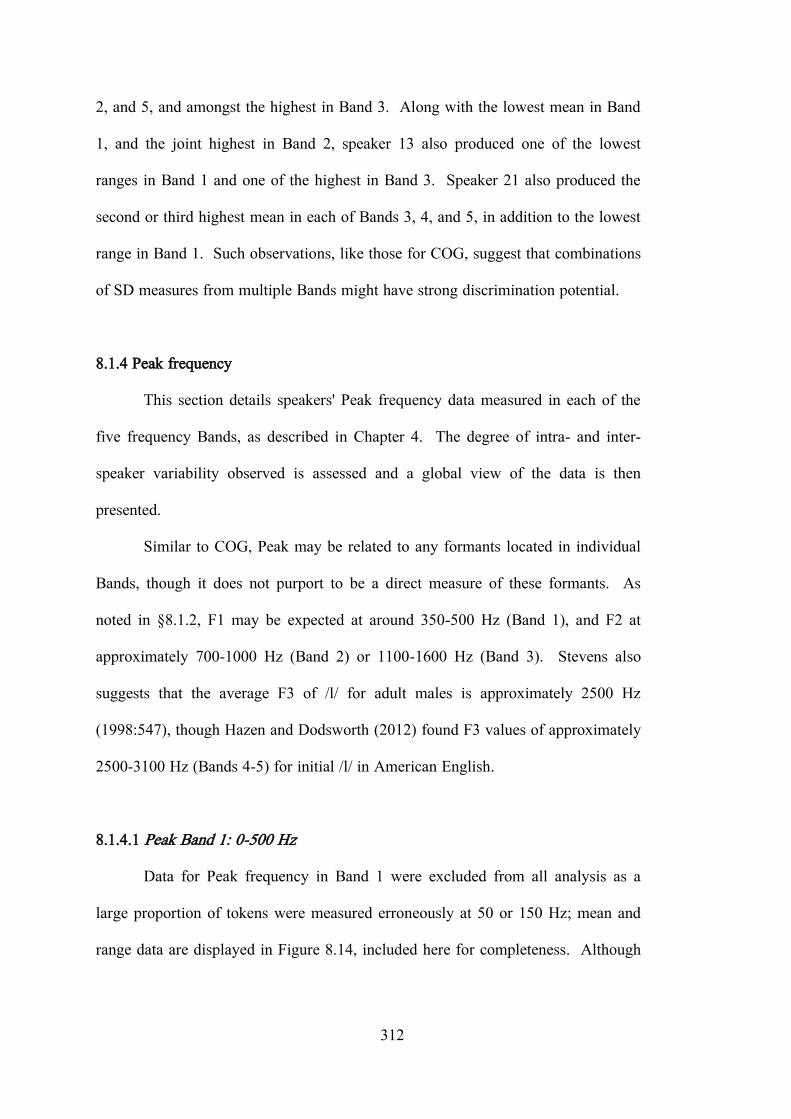
312

2, and 5, and amongst the highest in Band 3. Along with the lowest mean in Band

1, and the joint highest in Band 2, speaker 13 also produced one of the lowest

ranges in Band 1 and one of the highest in Band 3. Speaker 21 also produced the

second or third highest mean in each of Bands 3, 4, and 5, in addition to the lowest

range in Band 1. Such observations, like those for COG, suggest that combinations

of SD measures from multiple Bands might have strong discrimination potential.


This section details speakers' Peak frequency data measured in each of the

five frequency Bands, as described in Chapter 4. The degree of intra- and inter-

speaker variability observed is assessed and a global view of the data is then

presented.

Similar to COG, Peak may be related to any formants located in individual

Bands, though it does not purport to be a direct measure of these formants. As

noted in §8.1.2, F1 may be expected at around 350-500 Hz (Band 1), and F2 at

approximately 700-1000 Hz (Band 2) or 1100-1600 Hz (Band 3). Stevens also

suggests that the average F3 of /l/ for adult males is approximately 2500 Hz

(1998:547), though Hazen and Dodsworth (2012) found F3 values of approximately

2500-3100 Hz (Bands 4-5) for initial /l/ in American English.

8.1.4.1 Peak Band 1: 0-500 Hz

Data for Peak frequency in Band 1 were excluded from all analysis as a

large proportion of tokens were measured erroneously at 50 or 150 Hz; mean and

range data are displayed in Figure 8.14, included here for completeness. Although

313

the measured frequencies did not correspond to actual peaks in the spectra, 12

speakers had minima at 50 or 150 Hz.

Figure 8.14. Mean and range for Peak frequency of /l/ in Band 1 by speaker, in descending order of mean.

8.1.4.2 Peak Band 2: 500-1000 Hz

Peak data for Band 2 are shown in Figure 8.15. It can be seen that a

majority of speakers' minimum values were measured at 550 Hz, and a number had

maximum values at 950 Hz. Several speakers had ranges of 0 Hz as all tokens

were recorded at 550 Hz. Manual inspection found that these measurements did

not align with peaks in the spectra. As a result, all data for Peak in this Band were

rejected and excluded from analysis.

314


8.1.4.3 Peak Band 3: 1-2 kHz

In Band 3, the majority of Peak frequency means were found in the lower

half of the Band; only the three highest means were above 1500 Hz. Means were

spread over 540 Hz, however, from 1059 Hz (speaker 30) to 1599 Hz (speaker 19).

The separation of individual means was relatively high as a result. Four distinct

groups can be seen in Figure 8.16, each separated from adjacent groups by

approximately 45-100 Hz. This wide distribution of means suggests a high level of

inter-speaker variability and the strong potential of Peak in Band 3 as a speaker

discriminator.

The difference between extreme range values was similarly high, at 710 Hz.

The maximum was 826 Hz (speaker 16) and the minimum 116 Hz (speaker 24).

The remainder varied greatly, as two ranges under 200 Hz and two over 700 Hz

315

were found, in addition to between three and seven ranges in each of the 100 Hz

regions in between. Such high inter-speaker variability in both mean and range

points toward Peak in Band 3 being quite a strong speaker discriminator.

ANOVA results revealed Peak in Band 3 to be highly significant, with the

second highest F-ratio overall for Speaker (F=8.668, p<.0001). Post-hoc analysis

showed that five speakers had no significant comparisons, but all others had at least

one. In total, 10 individuals differed significantly from at least five others.

Unsurprisingly, the three speakers with means over 1500 Hz had the greatest

number of differences within the group: speakers 18, 19, and 20 had 13-16

significant pairs each. It is notable that for these three speakers, differences were

found with individuals from both dialect groups equally.


316

8.1.4.4 Peak Band 4: 2-3 kHz

Mean Peak frequencies in Band 4, as shown in Figure 8.17, were generally

found in the upper half of the Band, although seven of 30 means were below the

midpoint of 2500 Hz. The highest mean, 2938 Hz for speaker 23, was clearly

separated from the remainder of the group, by 155 Hz. Within this main group, the

greatest separation between individuals was found amongst the lower means. The

lowest mean observed was 2285 Hz by speaker 13, indicating a spread of 653 Hz,

which was higher than that found for Peak in Band 3.


Several speakers stood out because of their extremely wide or narrow

ranges. Speaker 6 returned the widest range at 894 Hz, while speakers 14 and 29

also had ranges of over 800 Hz. At the other extreme, the lowest range was 147

317

Hz (speaker 9), one of four ranges under 200 Hz. The remaining 23 were

concentrated between 200 and 300 Hz or 500 and 700 Hz, with very few in

between.

As a result of the wide spread of both mean and range values, Peak in Band

4 was highly significant for Speaker, with a relatively high F-ratio (F=7.335,

p<.0001). One individual (12) had no significant comparisons in post-hoc tests,

while the rest had at least one. Several speakers had many more, however, as a

total of 12 individuals each differed significantly from at least five others. This

included speaker 23, who had the greatest number of significant comparisons (17)

as well as having the highest mean value and one of the lowest ranges.

Additionally, the three individuals at the low extreme in terms of mean (5, 6, and

13) each had 12-14 significant comparisons. A dialect split was not clear, even for

speakers with fewer significant pairs; differences were generally found both within

and between the two dialect groups. For those with fewer than five significant

pairs, differences were often within a speaker‟s own dialect rather than across

dialect groups.

8.1.4.5 Peak Band 5: 3-4 kHz

Data for Peak in Band 5 are displayed in Figure 8.18. Again, as in Bands 1

and 2, a large number of tokens were measured erroneously near the edges of the

Band. Several speakers had maximum and minimum values recorded at 3950 Hz

or 3050 Hz. Peak in Band 5 was consequently excluded from all statistical

analyses.

318



Peak data for the two available Bands are displayed in Figure 8.19, showing

the relationship between the two sets of measurements. It can be seen that Band 3

Peaks were largely in the lower half of the frequency range, while Peaks were

generally higher within Band 4. In Band 3, the six SSBE speakers from the IViE

corpus appeared to have the highest means, while the DyViS and Leeds (from both

Morley and IViE corpora) speakers‟ means were similarly low in the Band. No

correlation was found between the two Bands.

Despite having three fewer Bands available than in COG and SD, some

patterns are still noticeable with respect to individuals‟ distributions across the

spectrum. Speaker 21 produced mean Peak frequencies amongst the top five in

Bands 3 and 4, as well as one of the highest ranges in Band 3 and one of the lowest

319

in Band 4. Speaker 23 had the second lowest mean in Band 3 in addition to the

highest mean and a very low range in Band 4. The lowest range and third lowest

mean in Band 3, and the third highest mean in Band 4, were all produced by

speaker 24. Along with those observed for COG and SD above, such patterns

indicate good potential for discrimination for a number of speakers, particularly

when Peak data from both Bands are combined.

Figure 8.19. Peak frequency for /l/ by speaker across the spectrum, 0-4 kHz. Markers indicate speakers‟ mean values in each Band; solid lines above and below each marker line signify speakers‟ ranges within the Band by indicating maximum and minimum values. Bands 1, 2, and 5 were excluded, as noted in §8.1.4.1, §8.1.4.2, and §8.1.4.5.


Minimum frequency data are presented in this section, along with discussion

of the level of intra- and inter-speaker variability in each Band and the potential of

320

Minimum as an effective speaker discriminator. Data from two of the five Bands

were excluded from analysis, but as in the previous section for Peak, they are

presented here for completeness, with an explanation of the reasons for their

exclusion being detailed in the relevant sections.


Data for Minimum in Band 1 were problematic, as was the case for /m, n/

and /ŋ/ in Chapters 5-7. As shown in Figure 8.20, nearly all speakers had

minimum values of 50 Hz and maxima of 450 Hz. For seven individuals, all

tokens were reported at 50 Hz, giving them a range of 0 Hz. Manual inspections of

spectra showed that this was not accurate, and the data were rejected as a result.

Figure 8.20. Mean and range for Minimum frequency of /l/ in Band 1 by speaker, in descending order of mean.

321

8.1.5.2 Minimum Band 2: 500-1000 Hz

Means and ranges for Minimum frequency in Band 2 are shown in Figure

8.21. The majority of means (all but eight) were in the upper half of the Band,

above 750 Hz. Despite this, the spread of means appears relatively high, with 240

Hz between the extreme values of 918 Hz (speaker 17) and 678 Hz (speaker 13).

Four groups of means were also distinguishable in Figure 8.21: two small groups of

three and five means at the high extreme, plus one group of three at the low

extreme, in addition to the main group forming the bulk of the distribution. Each

group was separated from adjacent ones by approximately 25-40 Hz.


In contrast with the apparently high inter-speaker variability in mean, ranges

appeared generally wide and less variable between individuals. Of the three ranges

322

that were under 200 Hz, the narrowest was 81 Hz, for speaker 14. The highest

observed was 396 Hz for speaker 20, one of 15 ranges over 300 Hz, and the

remaining 12 were between 200 and 300 Hz. Consistently wide ranges such as this

might obscure some of the inter-speaker variability contributed by mean Minimum

frequencies, reducing the overall discriminatory potential of this feature.

Minimum in Band 2 was found to be highly significant for Speaker, albeit

with a moderate F-ratio (F=4.057, p<.0001), in spite of the generally wide ranges

observed. Post-hoc tests, however, revealed that 19 of 30 speakers had no

significant differences from any others. Two speakers, 5 and 23, each had seven

significant comparisons with individuals at the opposite extreme in terms of mean.

Interestingly, these two speakers had more significant pairs than speaker 13, who

had the lowest overall mean and a similar range to speaker 5. The final nine

speakers each had one to four significant differences.


Mean Minimum frequencies in Band 3 were also largely in the upper half of

the Band, above 1500 Hz, similar to Band 2. As shown in Figure 8.22, only two

were below 1500 Hz: speakers 19 and 20 produced the lowest means of 1459 Hz

and 1411 Hz, respectively. Even so, means were still spread over more than 500

Hz, as the highest observed was 1914 Hz (speaker 25).

Variation in range was even higher than for mean in Band 3. The narrowest

range, 140 Hz (speaker 7), was 826 Hz less than the widest range of 966 Hz

(speaker 19). This disparity could potentially contribute to the overall level of

inter-speaker variability; however, a large proportion of speakers had very wide

ranges. 14 of 30 individuals had ranges of more than 500 Hz, including four of

323

over 900 Hz. This might reduce the contribution of range to inter-speaker

variability, as nearly 50% of speakers produced Minimum frequency values across

more than half the Band. Noticeably, though, the 16 speakers with narrower ranges

were the same 16 speakers who never produced individual Minimum values below

1500 Hz.


Speaker was found to be highly significant for Minimum in Band 3

(F=3.826, p<.0001); however, the low F-ratio and few significant post-hoc

comparisons suggest that speaker-specificity was relatively low and that Minimum

in Band 3 might not have strong discrimination potential. In post-hoc tests, 16 of

30 speakers were not significantly different from any others. Of the 14 who were,

12 had one to two significant pairs; only two individuals had more. Speakers 19

324

and 20 differed significantly from 10 and 12 others, respectively, in addition to

having the two lowest means and two of the highest ranges overall.


Unlike in Band 3, mean Minimum frequencies covered most of Band 4.

Means were spread over nearly 800 Hz from 2067 Hz (speaker 8) at one extreme to

2864 Hz (speaker 5) at the other. The separation between means was generally

good, with several distinct groups and individuals, as shown in Figure 8.23. This

spread of means alone might suggest strong speaker discrimination potential for

Minimum in Band 4.


325

As in Band 3, the disparity between extremes in terms of range was also

quite high. Speaker 15 produced the highest range of 963 Hz, and speaker 8 the

lowest of 118 Hz, a difference of 845 Hz. However, 12 speakers – more than a

third of the sample – produced ranges of more than 900 Hz. Despite the huge

difference between high and low values, ranges were generally high, with little

variation amongst the majority of speakers. Such wide ranges might obscure some

of the inter-speaker variability observed in mean values for Minimum in Band 4,

reducing its potential as a speaker discrimination parameter.

Minimum in Band 4, in spite of the substantial number of very wide ranges,

was highly significant for Speaker, with a moderate F-ratio (F=4.931, p<.0001).

16 speakers had a minimum of one significant post-hoc comparison, while 14 had

none. Five individuals had five or more significant pairs: 2, 5, 8, 17, and 18.

Speaker 5 had the highest number of significant differences with nine, and also had

the highest mean overall. The other four individuals all had mean values at the low

extreme for Minimum in Band 4.


As in Band 1, Minimum data in Band 5 were largely inaccurate and

therefore excluded from all analysis; Figure 8.24 displays mean and range data,

included here for completeness. A large proportion of tokens were reported at

either 3050 Hz or 3950 Hz, although in this case no speaker had a range of 0 Hz.

326



Mean and range data for the three Bands to be included in DA and LR

analysis of Minimum frequency are shown in Figure 8.25. The pale solid lines

above and below each mean line indicate maximum and minimum values, thereby

representing each individual‟s range. No significant correlations were found

between any of the three Bands. Data in Bands 2 and 3 were largely found in the

upper half of each frequency region, though the trend is perhaps most obvious in

Band 3. Leeds speakers displayed somewhat lower internal variability than the

majority of SSBE speakers in Band 3. Speakers 22-30 (the nine Leeds speakers)

had relatively narrower ranges, on the whole, than SSBE speakers 1-21. Band 4,

however, provided the highest intra-speaker and inter-speaker variability, with no

clear dialect difference.

327

Figure 8.25. Minimum frequency for /l/ by speaker across the entire spectrum, 0-4 kHz. Markers indicate speakers‟ mean values in each Band; solid lines above and below each marker line signify speakers‟ ranges within the Band by indicating maximum and minimum values. Bands 1 and 5 were excluded, as noted in §8.1.5.1 and §8.1.5.5.

Fewer individuals exhibited striking cross-Band patterns for Minimum than

for COG and SD in particular, but a few were worth noting. Speaker 5 produced

the lowest mean in Band 2, the highest in Band 4, and the fifth highest range in

Band 3. Speaker 14 had the lowest range in Band 2 as well as the third highest

mean in Bands 3 and 4. Finally, speaker 20 had the highest range and the fifth

highest mean in Band 2, along with the lowest mean and third highest range in

Band 3, and the second highest range in Band 4.

328

8.2 Dialect effects

The effect of Dialect was assessed using the Mann-Whitney U test as

sample sizes were highly unequal; all variables were tested except those rejected

for unreliable data. Normalised duration was examined even though it was not

significant for Speaker, as the effect of Dialect on segment duration may still

inform population statistics for /l/ and be relevant to forensic applications of the

data.

Table 8.2. Mann-Whitney U test findings for effect of Dialect on acoustic features of /l/. Bold text indicates results significant at the level .05.

Parameter Band 1 Band 2 Band 3 Band 4 Band 5 NormDur .205 COG .016 .148 .000 .048 .005 SD .000 .015 .105 .268 .000 Peak - - .000 .016 - Minimum - .041 .001 .291 -

Mann-Whitney U test results are given in Table 8.2; significant results are

indicated in bold. 11 of the 16 variables were found to be significant for Dialect.

These findings are not unexpected given previous literature relating to acoustic

features of /l/ in British English dialects (e.g. Carter & Local, 2007; see Chapters 2

and 3 for further discussion). Formant analysis of /l/ in initial position indicates a

relatively darker realisation in Leeds English than in Newcastle English (Carter &

Local, 2007:196), while RP/SSBE is noted as having clear /l/ in initial position (e.g.

West, 1999:407; Carter & Local, 2007:185). Although the present analysis does

not attempt to measure formants directly, COG, Peak, and Minimum frequencies in

particular may be expected to vary across these dialects as formants and zeros

would (as noted in §8.1.2, §8.1.4, §8.1.5, and Chapter 4). However, although mean

329

values for each dialect group might differ slightly, a degree of variation within a

dialect can also be expected; this is demonstrated by the fact that all features but

normalised duration were found to be highly significant for the effect of Speaker,

with significant differences both within and between dialect groups. Inspection of

the figures in §8.1.1-8.1.5 suggests that speakers from the two dialect groups were

clustering somewhat, but that there were also individuals from each group at both

extremes in terms of mean. For example, COG in Band 1 shown in Figure 8.2 was

significant for Dialect (p=.016), but the individuals with the highest and lowest

mean values were both from Leeds (29 and 30). Leeds speakers 22, 24, 25, and 28

were dispersed throughout the distribution. SSBE speakers also fell at both

extremes of the distribution of COG means in Band 1. A similar picture can be

seen for COG in Band 2, which was not significant for Dialect (p=.148): Leeds

speakers 23 and 24 produced means at the high extreme, while means for speakers

22 and 25 were at the low extreme.

Figure 8.26a and b. Boxplots showing COG in Bands 1 (Figure a, left) and 2 (Figure b, right), grouped by Dialect (1=SSBE, 2=Leeds).

330

Figure 8.26 shows boxplots for COG in Bands 1 and 2 grouped by Dialect

(1=SSBE, 2=Leeds). It is clear that there was substantial overlap between the

two groups, even for COG in Band 1, for which Dialect was a significant factor.

To explore the possible effect of Dialect on the outcome of DA and LR

analysis, tests of individual predictors were conducted and the results of variables

found to be significant and non-significant for Dialect were compared. Findings

for COG in Bands 1 and 2 are discussed here as an example. In DA classification,

errors would be expected to occur more frequently within dialect groups than

between them for significant predictors, e.g. COG in Band 1. In other words,

Leeds speakers should be confused with other Leeds speakers more often than with

SSBE speakers, and vice versa. This was not evident in the individual

classification rates for COG in Band 1, however. Inspection of errors found that

misclassifications were no more frequent within dialects than between them.

Confusion occurred more often between individuals who were proximate in terms

of mean COG than amongst those from the same dialect group. Additionally, the

pattern and proportion of errors was nearly identical for both significant (e.g. COG

in Band 1) and non-significant (e.g. COG in Band 2) predictors, suggesting that

Speaker identity plays a more important role than Dialect in discrimination.

Similarly, if Dialect were to interfere with discrimination in LR analysis,

higher-magnitude different-speaker LRs would be expected in cross-dialect

comparisons than within-dialect ones; that is, LRs (for different speakers only)

would be higher in SSBE-Leeds comparisons than in Leeds-Leeds or SSBE-SSBE

comparisons for predictors for which Dialect was a significant factor. In fact, the

pattern of LR magnitude was counter-intuitive for significant and non-significant

predictors. For COG in Band 1, LRs were higher in comparisons where a Leeds

331

speaker provided the „suspect‟ sample, regardless of whether the „criminal‟ sample

was from a Leeds or an SSBE speaker. Additionally, the highest LRs on average

were found in Leeds-Leeds comparisons, as speakers 29 and 30 were very different,

with means at opposite extremes in Band 1. For COG in Band 2, which was not

significant for Dialect, LRs were in fact marginally higher on average in cross-

dialect comparisons than within dialects. As both features were highly significant

for Speaker, with relatively high F-ratios (indicating high speaker-specificity), this

pattern of LR results again suggests that Speaker is the more important factor than

Dialect in LR analysis. It was decided, therefore, to combine the Dialect groups in

order to conduct DA and LR analysis with the dataset as a whole, rather than with

each group independently.


Direct discriminant analyses (DA) were conducted as described in Chapter 4

with the acoustic data for /l/ presented above. As noted in §8.1.4-8.1.5 above, five

spectral variables were excluded as a result of problematic data: Peak in Bands 1, 2,

and 5, and Minimum in Band 1 and 5. In §8.1.1, it was reported that Speaker was

found not to be significant for normalised duration in ANOVA results. This

parameter was, therefore, not predicted to contribute to speaker discrimination.

These six variables were excluded from both DA and LR analysis, resulting in 15

variables being available for testing. Additionally, in order to improve the

robustness of the statistical analysis and to allow combinations of predictors to be

tested, speakers who had produced five or fewer tokens were excluded from the

dataset. As in Chapter 6, data for these speakers were still worth including in the

discussion of intra- and inter-speaker variability presented in §8.1; however, the

332

small sample sizes would likely result in reduced statistical power. Speakers 7, 9,

10, and 13 each produced four or five tokens of /l/ and were thus excluded, leaving

26 speakers in total. The smallest sample size following these exclusions was

seven tokens, allowing a maximum of six predictors to be combined. This ensured

that all five Bands for a single parameter (e.g. COG in Bands 1-5) could be tested,

and it allowed combinations of more than one acoustic parameter.

In total, 31 tests were performed, on data produced by all 26 speakers from

both dialect groups. Each of the 15 individual predictors was tested, in addition to

16 combinations of up to six predictors. Single-Band, single-parameter, and two-

parameter tests were conducted, as well as a „Best 6 F-ratios‟ test of the six

individual predictors with the highest F-ratios determined by the ANOVAs reported

in §8.1: COG in Bands 1, 3, and 4, SD in Band 5, and Peak in Bands 3 and 4. In

two-parameter combinations, the six predictors to be tested were determined by

selecting the three predictors with the highest F-ratios from each acoustic

parameter, following the same procedure as in Chapters 5 and 6. As Peak

frequency had fewer than three predictors available, the sixth predictor was selected

from the second parameter in combinations involving Peak. All DA test

combinations for /l/ are given in Table 8.3.

Discriminant functions were derived for each of the tests. Discriminant

scores for the first two functions for the Best 6 F-ratios test are displayed in Figure

8.27, and for the COG+SD test in Figure 8.28. The vertical and horizontal spread

of the group centroids (dark blue squares) suggests that several speakers can be

quite well discriminated by the first two functions in each test. In particular, in

both plots speaker 30 was very well discriminated from the group by the first

function, and speakers 18 and 20 by the second. Approximately 61% of the total

333

variation in the Best 6 F-ratios test was accounted for by the first two functions:

35% by the first function, and 26% by the second. Interestingly, though, none of

the six predictors correlated most strongly with the first discriminant function. All

six contributed relatively well, but all were more strongly (and significantly)

correlated with another discriminant function. COG and Peak in Band 3 both

correlated significantly with the second function, however. The third of six

functions derived for this test accounted for approximately 18% of the variation

and correlated strongly with COG in Bands 1 and 4 as well as Peak in Band 4. SD

in Band 5 correlated with the fourth function, to which approximately 13% of the

total variation was attributable. The remaining 8% of variation was accounted for

by the fifth and sixth discriminant functions, although neither was significantly

correlated with any particular predictor.

Figure 8.27. Discriminant function plot showing first two discriminant functions for the Best 6 F-ratios test. Individual cases and group centroids are shown.

334

Similarly, in the COG+SD test, the first two discriminant functions

accounted for approximately 60% of the total variation. Although SD in Bands 4

and 5 were similarly correlated with the first function, both correlated significantly

with other functions; no individual predictor correlated most strongly with the first.

The second function, however, was significantly correlated with COG in Band 3.

COG in Bands 1 and 4 correlated most strongly with the third discriminant

function, which accounted for 16% of the variation. The final three functions

accounted for the remaining 24% of variation, and correlated with SD in Band 5

(fourth function), Band 4 (fifth function), and Band 1 (sixth function).

Figure 8.28. Discriminant function plot showing the first two discriminant functions for the 6-predictor COG+SD test. Individual cases and group centroids are shown.

Cross-validated classification of data was also performed for the 26

speakers, with a chance level of 3.8%. Correct classification rates for all tests are

335

given in Table 8.3. Although many of the single-predictor results were only

marginally above chance, COG in Bands 1 and 4 and Peak in Band 4 performed

slightly better and achieved between 10% and 12% correct classification. As these

tests all involved just one predictor, even the best rates were not exceptionally high,

but they do in fact give an indication of the potential contribution individual

predictors might make to speaker discrimination.

In the single-Band tests, the highest classification rates were, predictably,

obtained in the four-predictor Band 3 and Band 4 tests. These Bands were the only

ones with all four acoustic parameters included, as Peak and Minimum were both

excluded from Bands 1 and 5, and Peak from Band 2. 17% of Band 4 tokens were

assigned to the correct speaker group, and 15% for Band 3.

Amongst the single-parameter tests, the highest classification rates were

obtained in the tests with all five predictors, especially COG, which achieved 30%

correct classification, and SD, which achieved 23%. Although Peak had only two

predictors available (Bands 3 and 4), 20% of tokens were still assigned to the

correct speaker groups in that test, due to the relatively high level of speaker-

specificity indicated by the high F-ratios obtained for these two predictors. In spite

of producing one of the lowest single-parameter test classification rates, Peak

appears nonetheless to be a very promising parameter for FSC. If data were

available for all five Bands, it might be predicted that the classification rate for

Peak would be similar to, or higher than, that obtained for COG.

336

Table 8.3. Cross-validated classification rates for DA with 1-6 predictors for /l/ and 26 speakers; chance=3.8%. Asterisks indicate tests from which Peak in Bands 1, 2 and 5, and Minimum in Bands 1 and 5, were excluded.

Parameter(s) Band N Pred % Classification COG 1 1 12 2 1 7 3 1 9 4 1 10 5 1 6 SD 1 1 6 2 1 4 3 1 9 4 1 9 5 1 7 Peak 3 1 9 4 1 11 Minimum 2 1 9 3 1 5 4 1 9 Band 1 excl. Peak, Min 2* 14 2 excl. Peak 3* 11 3 4 15 4 4 17 5 excl. Peak, Min 2* 12 COG 1 thru 5 5 30 SD 1 thru 5 5 23 Peak 3 thru 4 2* 20 Min 2 thru 4 3* 16 COG + SD COG 1, 3, 4, SD 1, 4, 5 6 37 COG + Peak COG 1, 2, 3, 4, Peak 3, 4 6 29 COG + Min COG 1, 3, 4, Min 2, 3, 4 6 30 SD + Peak SD 1, 2, 4, 5, Peak 3, 4 6 33 SD + Min SD 1, 4, 5, Min 2, 3, 4 6 26 Peak + Min Peak 3, 4, Min 2, 3, 4 5* 27 Best 6 F-ratios COG 1, 3, 4, SD 5, Peak 3, 4 6 30

The highest rates in general were obtained in the two-parameter

combination tests. The best classification rate overall was 37%, in the COG+SD

337

test, while 33% of tokens in the SD+Peak test were assigned to the correct speaker

group. The remaining two-parameter tests performed similarly, with between 26%

and 30% correct classification in each. Importantly, all two-parameter tests

obtained classification rates well above the level of chance, with a relatively high

level of discrimination in several tests. Although the rates achieved were not as

high as those for /m/ and /n/ in Chapters 5 and 6, these DA findings do point to a

number of predictor combinations for /l/ that appear quite promising and warrant

further investigation for use in FSC.

Similar to the DA findings for /m/ presented in Chapter 5, the Best 6 F-

ratios test did not produce the highest overall classification rate. Regardless, it was

still amongst the best-performing tests, producing the joint third-highest rate, with

30% of tokens correctly classified. This was in line with results for the majority of

two-parameter combinations, and was only marginally lower than the best overall

classification rate.

Although the best-performing tests achieved 30-37% correct classification

for the whole dataset, rates for individual speakers were frequently higher.

Individual cross-validated classification rates for the COG+SD and SD+Peak tests

are displayed in Figure 8.29. Rates for the Best 6 F-ratios test are also displayed

for reference, as this predictor combination was theoretically expected to be the

most speaker-specific, according to the ANOVA results for Speaker presented

above. In total, 13 of the 26 speakers had at least 50% of their tokens correctly

classified in one or more of these three tests. Speakers 23 and 30 reached 80%

correct classification in both the Best 6 F-ratios and COG+SD tests. At the other

end of the scale, speakers 11 and 25 had no tokens classified correctly in any of the

three tests. Neither was confused with any other individual in particular, as tokens

338

for both speakers were misclassified across multiple speaker groups in all tests.

Interestingly, speaker 11 was also not discriminated well in the analysis of /n/

presented in Chapter 6, as none of his tokens was correctly classified in the two

best-performing tests for /n/ (Best 5 F-ratios and COG in Bands 1-5).

Figure 8.29. Individual cross-validated classification rates in the Best 6 F-ratios, COG+SD, and SD+Peak tests for /l/, with 26 speakers. Chance=3.8%.

For five individuals, the best results were obtained in the Best 6 F-ratios

test; for three speakers, the COG+SD test produced the highest rates; and for six

individuals, the highest rates were achieved in the SD+Peak test. For nine of the

10 remaining speakers, two of the three tests shared the highest classification rates,

while speaker 24 was equally well discriminated by each of the three predictor

combinations (44% correct classification).

339

While the classification rates obtained using acoustic parameters of /l/ were

not quite as high as those for /m/ and /n/ overall, the findings presented in this

section do indicate a number of promising features. As per the results for /m/ and

/n/, increased token numbers, and therefore increased predictor numbers, would

likely improve discrimination. Extended investigation of the role of dialect might

also be beneficial, particularly if an equal number of speakers of each dialect were

used.


Intrinsic LR testing (meaning no external reference sample was used as it is

in „extrinsic‟ testing) was also conducted using the 15 acoustic predictors available

for /l/. The same six predictors were excluded from LR analysis as were excluded

from the DA, as described in §8.3. Speakers 7, 9, 10, and 13 were excluded as

well, in order to maintain consistency with the DA. With 26 speakers in the

sample, then, 26 same-speaker (SS) comparisons were conducted, in addition to

312 different-speaker (DS) comparisons. 17 separate single-Band, single-

parameter, and multiple-parameter tests were performed, with between five and 15

predictors in each; these are given in Table 8.4, along with a summary of the

performance of each test. In the two-parameter combinations, all available

predictors were included, unlike in the DA, as predictor numbers were not limited

by the smallest sample size. A test of all 15 predictors was also conducted to

observe the effect on discrimination when all available acoustic information was

used. Finally, the Best 6 F-ratios test included the same six predictors as in the DA

presented in §8.3: COG in Bands 1, 3, and 4, SD in Band 5, and Peak in Bands 3

and 4. Table 8.4 summarises the performance of each test as gauged by four

340

statistics: percentage of log10LRs at or beyond the ±4 „very strong evidence‟

threshold, percentage of false negatives and positives, equal error rate (EER), and

log likelihood ratio cost (Cllr).

Table 8.4. Summary of LR performance for /l/ in 17 test combinations, showing percentage of same-speaker (SS) and different-speaker (DS) comparisons yielding log10LRs≥±4, percentage of false positives and negatives, equal error rates (EER), and Cllr. Asterisks indicate tests from which normalised duration, Peak in Bands 1, 2, and 5, and Minimum in Bands 1 and 5 were excluded.

Predictors ±4 Log10LR % False Neg % False Pos % EER

% Cllr SS DS SS DS

Band 1* 0 4 12 35 23 0.70 Band 2* 0 2 27 40 35 1.10 Band 3 4 11 15 36 27 0.80 Band 4 0 7 27 30 30 1.11 Band 5* 0 4 15 38 27 0.74 COG 0 10 15 27 23 0.62 SD 0 16 23 24 23 0.76 Peak* 0 7 23 33 30 0.91 Min* 0 1 19 30 27 0.74 COG+SD 0 33 35 17 23 1.32 COG+Peak* 4 17 23 20 20 0.80 COG+Min* 0 15 42 26 31 1.80 SD+Peak* 0 21 19 21 19 0.75 SD+Min* 0 22 31 20 23 1.46 Peak+Min* 0 9 31 25 27 0.97 All* 0 56 77 10 38 14.88 Best 6 F-ratios 4 19 31 26 29 0.86

8.4.1 ±4 log10LRs

In the first two columns of Table 8.4, the darkest blue cells indicate the tests

with the highest percentage of ±4 log10LRs. In SS tests, very few comparisons

reached this strength of evidence, although this is not particularly unusual. In DS

comparisons, however, all tests produced at least a small percentage of „very

341

strong‟ LRs. The highest rate was obtained in the All-predictor test, where 56% of

DS comparisons produced a log10LR of at least –4. DS evidence was generally

fairly strong in most multiple-parameter tests, in particular COG+SD, SD+Peak,

and SD+Min, each of which produced 21-33% of scores beyond this threshold.


The third and fourth columns contain false negative and false positive rates,

where the darkest shade of orange indicates the highest percentage of each. False

negative rates, when a SS comparison incorrectly produced a negative log10LR

value, were generally higher in multiple-parameter than single-parameter tests. The

highest rate overall was obtained in the All-predictor test, where more than three-

quarters of SS pairs were wrongly judged as DS pairs. The lowest rate was 12%,

in the Band 1 test with only COG and SD included, which is still relatively high

considering that false negative rates for /m/ in Chapter 5 were as low as 3%. False

positive rates, on the other hand, were generally higher in single-Band and single-

parameter tests than in multiple-parameter tests. 35-40% of all DS comparisons

resulted in positive log10LR values in the five single-Band tests. In contrast with its

77% false negative rate, the All-predictor test actually had the fewest false positives

(10%). This follows the pattern observed for both /m/ and /n/ when all available

predictors were combined, perhaps surpassing a point of diminishing returns:

results for DS comparisons were relatively strong, while SS comparisons produced

a high proportion of high-magnitude errors.

342


With such high false negative and false positive findings in general,

relatively high EERs may be expected. The highest EER at 38% was,

unsurprisingly, found in the All-predictor test. Rates were also fairly high in

single-Band tests: Band 2 had the second highest EER, at 35%. The Best 6 F-ratios

test, which might have been predicted to perform quite well due to the expected

speaker-specificity of the six predictors, produced another relatively high EER, at

29%. The lowest rates were not particularly low, however. Five tests, including

single-Band, single-parameter, and multiple-parameter combinations, shared one of

the lower EERs, at 23%. The SD+Peak test produced an EER of 19%, the lowest

overall for /l/, although this was nearly three times higher than the lowest EER

observed in LR analysis of /m/ (7%) and nearly double that for /n/ (11%).


The final column in Table 8.4 displays Cllr values, with the highest indicated

by the darkest shade of red. Progressively lighter shades denote tests with a lower

proportion and magnitude of errors; the closer the Cllr is to 0 the better the validity

of the system (Morrison, 2011:94). It is clear, then, that Cllr values for LR analysis

of /l/ were all quite high. The lowest observed were 0.62 in the single-parameter

test of COG, and 0.70 in the Band 1 test. Conversely, a Cllr of 14.88 was found for

the All-predictor test, an extremely high value resulting from the high number of

errors, particularly in SS comparisons, and from the strength of those errors. SS

errors reached a log10LR of magnitude -88.69, equivalent to a raw LR of 4.9x1088 in

favour of the (incorrect) different-speaker hypothesis. The reason for such large SS

errors is unclear, particularly when the DS results for the All-predictor test were

343

comparatively good. This is, however, consistent with findings for /m/ and /n/, as

All-predictor tests returned extremely high Cllr values for both of those segments as

well. Overall, LR analysis of acoustic features of /l/ returned higher Cllr values than

/m/ and /n/, indicating lower validity than the analyses of /m/ and /n/ reported in

Chapters 5 and 6.


No test stands out as clearly producing the best results, nor do the LR

findings appear to be in line with the DA results presented in §8.3. The DA

classification rates suggested that COG+SD and SD+Peak discriminated

individual speakers best; on balance, however, it appears that COG (Bands 1-5),

COG+Peak, and SD+Peak were most successful in the LR analysis for /l/. SS

and DS log10LRs for these three tests are represented in Figure 8.30. The Best 6 F-

ratios test results are also included for reference, to facilitate comparison with the

best-performing DA results.

The lowest EER (19%) and fourth lowest Cllr (0.75) overall were obtained in

the SD+Peak test, which also produced relatively low false negative and false

positive rates (19% and 21%, respectively). The magnitude of LRs was also fairly

high in DS comparisons for SD+Peak. COG+Peak generated the second lowest

EER (20%) and a relatively low Cllr (0.80); additionally, the false positive rate

(20%) was comparable to that of the SD+Peak test, albeit with a slightly higher

false negative rate (23%). COG in Bands 1-5 produced somewhat mixed results:

despite a fairly high rate of false positives (27%), the EER was relatively low (one

of five tests with an EER of 23%), and this test had the lowest Cllr overall (0.62),

and thus the highest validity. A small proportion of DS comparisons (10%) and no

344

SS comparisons produced log10LRs over the „very strong evidence‟ threshold of

±4 in the COG Bands 1-5 test, though.

Figure 8.30. Tippett plot showing log10LRs for same-speaker and different-speaker comparisons for COG (Bands 1-5), COG+Peak, SD+Peak, and Best 6 F-ratios.

It can be seen from the Tippett plot above (Figure 8.30) that the Best 6 F-

ratios results were in line with the others, although they did not appear quite as

strong from the statistics summarised in Table 8.4. The EER (29%), false negative

rate (31%), and false positive rate (26%) were all slightly higher in the Best 6 F-

ratios test than in the other three tests represented in Figure 8.30. The Cllr and

proportion of log10LRs above the „very strong evidence‟ threshold were comparable

to those of the COG+Peak test. These findings, along with the DA results, do

345

serve to highlight a number of features that might hold some evidentiary value, but

certainly require further investigation.

8.5 Chapter summary

In this chapter, intra- and inter-speaker variability in acoustic parameters of

/l/ was investigated, and ANOVA results found that Speaker was a highly

significant factor for all variables except normalised duration. The effect of Dialect

on the acoustic parameters of /l/ was once again mixed, following similar findings

for /m/, /n/, and /ŋ/. Both DA and LR analysis pointed to SD+Peak as a very

promising parameter combination for speaker comparison. DA results also

indicated that the six-predictor COG+SD test discriminated speakers well, while

further promising results were obtained in the LR tests of COG in Bands 1-5,

COG+Peak, and the Best 6 F-ratios.

346

Chapter 9 Results: /s/

9.0 Overview

Analysis of /s/ is presented in two parts in this chapter. First, static acoustic

measures of five parameters are analysed; intra- and inter-speaker variability and

speaker-specificity of each parameter is investigated in an 8 kHz filter condition,

and the effects of each of four filter conditions on acoustic measurements are then

assessed. The role of Dialect is then explored, and finally, results of DA and LR

estimation with static measures are detailed. The second part presents results of

dynamic analysis of /s/: inter-speaker variability is explored in the 8 kHz filter

condition again, and further DA was conducted to examine whether discrimination

of speakers might be improved by analysis of dynamic versus static predictors.

9.1 Intra- and inter-speaker variability: Static measures

This section provides detailed discussion of the intra- and inter-speaker

variability observed in /s/ as measured in five acoustic parameters: normalised

duration, centre of gravity, standard deviation, skewness, and kurtosis. The four

spectral measures are a standard set of parameters that are commonly analysed in

the study of fricative acoustics, known as spectral moments (note that standard

deviation is actually the square root of the second spectral moment, variance). It

was not necessary to divide the spectrum into bands for /s/ as was done for the

nasals and /l/: the division of the spectrum into bands for those consonants was

proposed as an alternative to measuring the formants directly, in the absence of an

appropriate pole-zero formant tracker (see §4.2.2 for more detail). Unlike nasal

347

and liquid spectra, the fricative spectrum consists of high-frequency broadband

noise, rather than formants. As such, it was preferable to examine the distribution

of energy for /s/ as a whole, rather than in individual frequency bands.

It was noted in Chapter 4 that 8 kHz was the upper frequency limit of the

IViE recordings, so to permit comparison of all speakers‟ recordings, all DyViS

and Morley recordings were low-pass filtered at this frequency; an additional filter

was applied at 4 kHz to explore the effect of a bandpass filter similar to that found

in telephone transmission. The DyViS and Morley recordings were also filtered at

16 kHz and 22.05 kHz, and in all cases, a high-pass filter was also applied at 500

Hz, as described in §4.2.3. For the four spectral parameters, results are presented

for static midpoint measures in the 8 kHz filter condition only. Figures displaying

data from 4 kHz, 16 kHz, and 22.05 kHz conditions can be found in Appendix 5.

A summary of the effects of all four filter conditions on spectral measures is

presented in §9.1.6 below.

Means and ranges of values for each of the parameters are displayed in

Figures 9.1-9.5. In each, speakers are ordered from left to right in descending

order of mean, indicated by a green marker, with vertical lines indicating the actual

range of values employed by each speaker. Range is considered in addition to

mean as vastly different ranges of values can be obscured by very similar means. It

is potentially more informative to observe the spread of values that an individual is

capable of producing on a given parameter than to refer to the mean alone.

Univariate analyses of variance (ANOVAs) were conducted to test the effect

of speaker identity on each of the five parameters in each filter condition. Speaker

was found to be a highly significant factor in all cases (p<.0001), suggesting that

these might indeed be useful parameters for speaker discrimination. Results are

348

summarised in Table 9.1. Hochberg post-hoc tests revealed significant differences

between individuals; this test was selected as sample sizes were unequal. Post-hoc

comparison results in the 8 kHz filter condition are discussed in each relevant

section below.

Table 9.1. Results of univariate ANOVAs for Speaker (N=30 in 4 and 8 kHz, N=18 in 16 and 22.05 kHz) on each acoustic parameter of /s/ (x5) and in each filter condition (x4). Bold text indicates significant p values at the level .05.

Parameter Filter

4 kHz 8 kHz 16 kHz 22.05 kHz NormDur F=5.111, p<.0001

COG F=19.563 p<.0001

F=23.172 p<.0001

F=9.326 p<.0001

F=9.378 p<.0001

SD F=12.183 p<.0001

F=11.092 p<.0001

F=9.119 p<.0001

F=8.885 p<.0001

Skewness F=13.827 p<.0001

F=16.603 p<.0001

F=7.200 p<.0001

F=5.807 p<.0001

Kurtosis F=7.414 p<.0001

F=6.888 p<.0001

F=6.208 p<.0001

F=15.132 p<.0001

9.1.1 Normalised Duration

Figure 9.1 shows speakers‟ means and ranges of normalised duration,

expressed as a proportion of the average syllable duration (ASD, measured in

ms/syllable) of the local intonation phrase. Considering mean values alone, the

highest and lowest values differed by approximately 0.3, i.e. 30%, of speakers‟

ASD. The individuals at the extremes may be somewhat better discriminated from

the group than those closer to the middle of the distribution. Only one speaker (15,

on the far right of the figure) had a mean normalised duration of less than 0.5. This

indicates that the duration of speaker 15‟s productions of /s/ was, on average, less

than half his ASD, while other speakers‟ /s/ durations typically constituted more

349

than half the local ASD. Conversely, speaker 25 on the far left of the figure was

the only individual with a mean value greater than 0.8, signifying that his mean

segment duration was more than 80% of his average syllable duration.

A number of individuals, however, were notable for the ranges of

normalised duration values employed, rather than for their mean values. In

particular, speakers 4, 7, and 10 (SSBE), and 29 and 30 (Leeds), all had extremely

wide ranges of more than 0.5. Speaker 24, on the other hand, had the narrowest

range at 0.23, meaning his segment durations varied by 23% of his ASD.

Figure 9.1. Mean and range of normalised /s/ durations by speaker, in descending order of mean.

Maximum and minimum durations might also prove interesting. Two of the

30 speakers (10 and 25) had maximum durations greater than 1, indicating a token

of /s/ that was actually longer than the ASD in the local intonation phrase. Another

350

two speakers (28 and 30) had minimum normalised durations of less than 25% of

the local ASD.

Speaker was a highly significant factor for normalised duration of /s/

(F=5.111, p<.0001). However, six speakers had no significant post-hoc

comparisons; all others had at least one. The speakers with the greatest number of

significant differences were the two with the highest and lowest means, speakers 15

and 25, with 11 and 13 significant pairs, respectively.

9.1.2 Centre of Gravity

Mean and range of COG in the 8 kHz filter condition is shown in Figure

9.2, with a difference of 2349 Hz between the highest and lowest values (speaker

4=6610 Hz; speaker 24=4261 Hz). Although just under two thirds of speakers

lay between 5 kHz and 6 kHz, the remaining speakers above and below this band

could potentially be discriminated relatively well.

With such disparate means, speakers‟ maximum and minimum values also

differ greatly. Only speaker 4 produced a maximum value greater than 7 kHz;

likewise, only speaker 24 from Leeds produced a minimum COG value below 4

kHz in this filter condition.

Range was once again an interesting source of inter-speaker variability for

COG. Speaker 30 from Leeds had the smallest range at 653 Hz, even though he

had one of the highest means. In total, nine of 30 individuals had ranges under 1

kHz. At the other extreme, speaker 19 produced COG values across a range of

2078 Hz, despite his having a mean nearer the centre of the distribution, showing

the lack of correlation between mean and range.

351

Figure 9.2. Mean and range of COG of /s/ by speaker, in descending order of mean. Spectra were bandpass filtered at 500-8000 Hz.

ANOVA results showed COG to be highly significant for Speaker, with the

highest F-ratio overall for /s/ (F=23.172, p<.0001). Post-hoc comparisons

confirmed the high degree of inter-speaker variability observed. Each individual

was found to be significantly different from at least six others. Speaker 24, who

had the lowest mean COG overall, also had the highest number of significant

speaker pairs, at 26. 22 of the 30 speakers had 10 or more significant pairs, while

eight individuals had 15 or more.

9.1.3 Standard Deviation

SD means and ranges in the 8 kHz condition are displayed in Figure 9.3.

SD is measured as the spread of energy in the spectrum around the COG, and is

detailed further in Chapter 4, §4.2.1.3. The majority of means (26 of 30) were

352

within ±200 Hz of 1 kHz, though the extreme high (1785 Hz, speaker 19) and low

(789 Hz, speaker 24) means differed by 996 Hz. One speaker (27) produced a

minimum SD value below 500 Hz, and six speakers had maxima above 1500 Hz.

Speaker 19 made use of the widest spread of SD values, with a range of

1388 Hz. Along with speaker 17, only these two individuals had ranges of over 1

kHz. The narrowest range of SD values was produced by speaker 26 at 263 Hz,

resulting in a difference of 1125 Hz between the extreme ranges.

Figure 9.3. Mean and range of SD of /s/ by speaker, in descending order of mean. Spectra were bandpass filtered at 500-8000 Hz.

Speaker was also found to be highly significant for SD of /s/, with a

relatively high F-ratio (F=11.092, p<.0001). Speaker 19 was particularly well

differentiated from the group, with significant post-hoc differences between him

and all 29 other individuals, as expected from examination of Figure 9.3. Speaker

353

6 had the second-highest number of significant comparisons (16), in addition to the

second-highest mean SD. However, as the majority of the group had somewhat

similar mean values, eight speakers had only one significant comparison (all with

speaker 19).

9.1.4 Skewness

Mean skewness values, which measure the symmetry of the distribution of

energy in the spectrum of /s/ per speaker, were fairly evenly distributed above and

below 0 (14 speakers had positive skewness, 16 had negative), as shown in Figure

9.4. The majority of speakers generally displayed relatively normal distributions,

with 13 of 30 means within ±0.5 of 0 skewness: 0 indicates a symmetrical, normal

distribution of energy within the spectrum, as described in Chapter 4, §4.2.1.6.

Better discrimination might therefore be achieved for speakers with non-normal

distributions, and therefore mean skewness values further away from 0.

Variation in the range of skewness values might also be an important factor

to consider. Ranges varied from less than 1 (speaker 28=0.89) to over 3 (speakers

12, 17, 18, and 20). However, what is most interesting is that, despite the great

range of possible values, there were several individuals who produced only positive

or only negative skewness values. For example, speaker 23 had the highest mean

and never produced tokens with negative skewness. At the other extreme, four

speakers (6, 19, 25 and 30) never produced tokens with positive skewness.

Skewness of /s/ was also highly significant for Speaker, with the second

highest F-ratio in the 8 kHz filter condition (F=16.603, p<.0001). In post-hoc

tests, all speakers had at least five significant comparisons, while some had up to

354

19. The speakers with the two highest and two lowest means (speakers 23 and 9, 6

and 30 respectively) were each found to differ significantly from 15 others.

Figure 9.4. Mean and range of skewness of /s/ by speaker, in descending order of mean. Spectra were filtered at 500-8000 Hz.

9.1.5 Kurtosis

Kurtosis reflects the relative peakedness or flatness of the distribution of

energy in the spectrum (see §4.2.1.7 for more detail). Figure 9.5 shows means and

ranges of kurtosis values in the 8 kHz condition. Mean kurtosis results displayed

relatively little inter-speaker variation. No negative means were observed, and 26

of 30 fell between 0 and 5. Very few negative kurtosis values were found in

general, and nine individuals consistently produced positive kurtosis measures.

Additionally, only two speakers had maxima greater than 10. Knowing that the

population could be expected to be somewhat invariable in this respect, observing

355

suspect or criminal data in a FSC case outside this norm could provide relatively

strong evidence for the appropriate same- or different-speaker hypothesis.

Kurtosis ranges were highly variable, however, as three individuals

produced ranges greater than 10, while 10 others produced ranges of less than 5.

The highest observed was 15.74 (speaker 27) and the lowest 2.81 (speaker 2), a

difference of 12.93.

Figure 9.5. Mean and range of kurtosis of /s/ by speaker, in descending order of mean. Spectra were bandpass filtered at 500-8000 Hz.

ANOVA results showed Speaker to be a highly significant factor for

kurtosis of /s/, though this parameter produced the second lowest F-ratio in the 8

kHz condition (F=6.888, p<.0001). Post-hoc test results were similar to those for

SD: the speakers with the highest means had the greatest number of significant

comparisons. Between 13 and 22 statistically significant differences were found for

356

the four speakers with the highest mean kurtosis values (18, 24, 29, and 30).

Conversely, 10 individuals had two or fewer, including three individuals with no

significant comparisons at all (speakers 16, 20, and 27).

9.1.6 Filter effects

A comparison of mean values for the four spectral parameters in all four

bandpass filter conditions (0.5-4 kHz, 0.5-8 kHz, 0.5-16 kHz, and 0.5-22.05 kHz) is

presented below and illustrated in Figures 9.6-9.9. Ideally, the relationship between

speakers would be preserved independently of the effect the filters have on absolute

values. When the spectra were bandpass filtered at 0.5-16 kHz and 0.5-22.05 kHz,

speakers‟ means for COG and SD were nearly identical (16 kHz and 22.05 kHz

data are represented by red and green markers respectively in the figures), with as

little as 4 Hz difference between them. The relationships between individuals as

well as absolute values were extremely well maintained between 16 kHz and 22.05

kHz for skewness and kurtosis, too, with the exception of speakers 28-30 from the

Morley corpus (on the far right of the figures). This was expected, however, as a

result of the difference in recording quality between the Morley and DyViS

corpora; there was little acoustic energy visible above 16 kHz in the three Morley

recordings (see Chapter 4, §4.1.1.3). Still, positive correlations significant at the

.01 level were found between the 16 kHz and 22.05 kHz conditions for all four

spectral parameters.

357

Figure 9.6. Mean COG by speaker and filter condition.

Figure 9.7. Mean SD by speaker and filter condition.

358

Figure 9.8. Mean skewness by speaker and filter condition.

Figure 9.9. Mean kurtosis by speaker and filter condition.

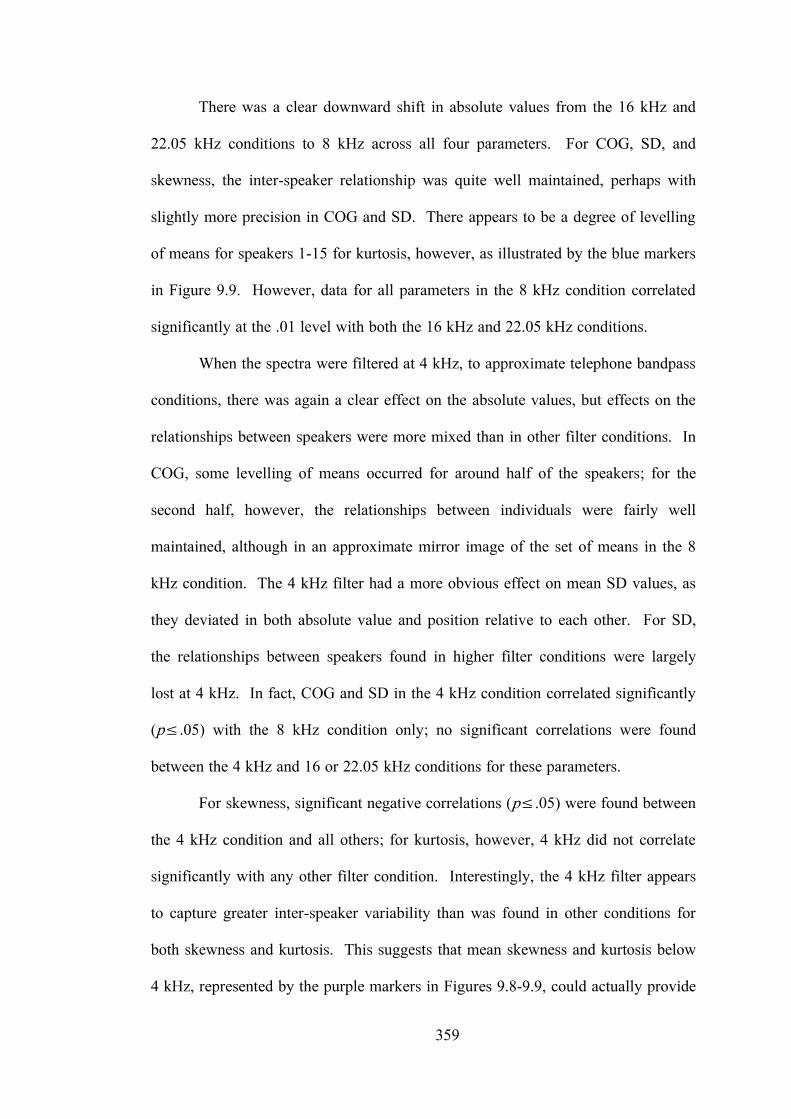
359

There was a clear downward shift in absolute values from the 16 kHz and

22.05 kHz conditions to 8 kHz across all four parameters. For COG, SD, and

skewness, the inter-speaker relationship was quite well maintained, perhaps with

slightly more precision in COG and SD. There appears to be a degree of levelling

of means for speakers 1-15 for kurtosis, however, as illustrated by the blue markers

in Figure 9.9. However, data for all parameters in the 8 kHz condition correlated

significantly at the .01 level with both the 16 kHz and 22.05 kHz conditions.

When the spectra were filtered at 4 kHz, to approximate telephone bandpass

conditions, there was again a clear effect on the absolute values, but effects on the

relationships between speakers were more mixed than in other filter conditions. In

COG, some levelling of means occurred for around half of the speakers; for the

second half, however, the relationships between individuals were fairly well

maintained, although in an approximate mirror image of the set of means in the 8

kHz condition. The 4 kHz filter had a more obvious effect on mean SD values, as

they deviated in both absolute value and position relative to each other. For SD,

the relationships between speakers found in higher filter conditions were largely

lost at 4 kHz. In fact, COG and SD in the 4 kHz condition correlated significantly

(p≤.05) with the 8 kHz condition only; no significant correlations were found

between the 4 kHz and 16 or 22.05 kHz conditions for these parameters.

For skewness, significant negative correlations (p≤.05) were found between

the 4 kHz condition and all others; for kurtosis, however, 4 kHz did not correlate

significantly with any other filter condition. Interestingly, the 4 kHz filter appears

to capture greater inter-speaker variability than was found in other conditions for

both skewness and kurtosis. This suggests that mean skewness and kurtosis below

4 kHz, represented by the purple markers in Figures 9.8-9.9, could actually provide

360

strong discrimination evidence in recordings with lower frequency bandwidths.

Counter to what might have been predicted based on assumptions about the

acoustic structure of /s/, there appears to be sufficient acoustic information and,

crucially, sufficient inter-speaker variation in the spectrum of /s/ below 4 kHz to

permit analysis of this segment in recordings with limited bandwidth.

9.1.7 Dialect effects

The effect of Dialect on acoustic parameters is difficult to evaluate given

the disparity in token numbers between the two samples. As more SSBE than

Leeds speakers were included, the resulting data contained more than three times as

many SSBE tokens as Leeds ones (291 versus 80). Consequently, statistical tests

such as ANOVA that are sensitive to highly unequal sample sizes cannot be

applied. The nonparametric independent samples Mann-Whitney U test was

conducted, as in Chapters 5-8.

Table 9.2. Mann-Whitney U test findings for effect of Dialect on acoustic features of /s/. Bold text indicates results that are significant at the level .05.

Parameter Filter

4 kHz 8 kHz 16 kHz 22 kHz NormDur .000 COG .932 .000 .080 .084 SD .720 .002 .000 .000 Skewness .949 .578 .140 .574 Kurtosis .604 .000 .007 .000

Results of the Mann-Whitney U test revealed a mixed picture of the effect

of Dialect, as shown in Table 9.2. Dialect was a significant factor for each acoustic

parameter in only some of the filter conditions tested; in others, no effect was

observed. Notably, none of the four spectral parameters was significant in the 4

361

kHz condition. Inspection of the distribution of SSBE and Leeds speakers‟ data

along the x-axes in Figures 9.1-9.5 for the 8 kHz condition, and in Appendix 5 for

the additional three conditions, suggests that the significant results might be

attributable to the highly unequal sample sizes and to the highly significant effect

of Speaker identity on all parameters, similar to the findings for /m, n, ŋ, l/. Leeds

speakers appeared to be relatively evenly interspersed among the SSBE speakers,

with individuals from both dialect sets at both extremes on each parameter. As in

previous chapters for the nasals and /l/, significant post-hoc comparisons were also

frequently found between individuals within and across dialect groups.

Consequently, Dialect was not considered further in the DA and LR analysis

presented below, as no effect was predicted and results were unclear.

9.1.8 Static discriminant analysis

DA was conducted with the five acoustic parameters of /s/ to explore which

predictors or combinations of predictors were the most speaker-specific and

therefore likely to be the best speaker discriminators. DA takes both intra- and

inter-speaker variability into account. As a number of speakers produced means

and ranges at or near the extremes on more than one parameter, DA will show

whether discrimination is improved by combining this information.

DA was performed using both the total set of 30 speakers with data from

the 4 kHz and 8 kHz filter conditions, and using the subset of 18 speakers from

DyViS and Morley only, with data from all four filter conditions. Thirty-one tests

were conducted on each data set, with between one and five predictors per test.

The maximum number of predictors permitted is limited by the number of tokens in

the smallest sample size, as noted in Chapter 4. For tests of the static measures in

362

the present analysis, this did not present a problem, even though the smallest

sample contained six tokens: 5 acoustic parameters x 1 measurement point = 5

possible predictors. However, this does have implications for DA with dynamic

acoustic measures of /s/, which will be discussed in §9.2 below.

The maximum number of discriminant functions available is either equal to

the total number of predictors, or the number of groups minus 1, whichever is

fewer (Tabachnick & Fidell, 2007:398). As the maximum number of predictors

available for testing was five, while the number of groups minus 1 was 29, up to

five discriminant functions were derived in the present analysis. The first function

accounts for the largest proportion of variance between groups, with each

subsequent function accounting for progressively less.

Figure 9.10. Discriminant scores on the first two discriminant functions for all 30 speakers in the five-predictor, 4-kHz analysis. Individual cases are represented by open circles, group centroids by filled blue squares.

363

Discriminant scores on the first two functions for the 30-speaker, five-

predictor tests in the 4 kHz and 8 kHz conditions are displayed in the scatterplots in

Figures 9.10 and 9.11. Scatterplots of discriminant scores for the five-predictor

tests in all four filter conditions for the 18-speaker subset are given in Figures 9.12-

9.15.

Figure 9.11. Discriminant scores on the first two discriminant functions for all 30 speakers in the five-predictor, 8-kHz analysis.

COG appears to be contributing most to discrimination in both filter

conditions for the complete 30-speaker set and at 4 kHz in the 18-speaker subset.

In the five-predictor, 30-speaker test at 4 kHz, both COG and skewness correlated

with the first discriminant function, but at 8 kHz, only COG correlated with the

first function. The discriminant function plots for these two tests are shown in

Figures 9.10 and 9.11. In both tests, the first function accounted for approximately

364

51% of the total variance; the second function, for 20% at 4 kHz, and 30% at 8

kHz. Normalised duration and kurtosis made the smallest contributions to

discrimination. Duration correlated with the third and fourth functions at 4 and 8

kHz, respectively, and kurtosis with the fifth function in both filter conditions.

Between 4% and 13% of variance was attributable to each of these functions.

Inspection of classification rates in one- and two-predictor tests of skewness

and kurtosis suggests these parameters may be contributing more at 4 kHz than at 8

kHz (see Table 9.3 below). This is consistent with observations made in §9.1.6

regarding increased inter-speaker variability in the lowest filter condition for both

skewness and kurtosis. As indicated, skewness correlated with the first

discriminant function in the five-predictor test at 4 kHz, but with only the third

function at 8 kHz. This does support the hypothesis of a greater contribution to

discrimination by skewness at 4 kHz than in higher filter conditions. However,

structure coefficients indicated that kurtosis was correlated with the fifth

discriminant function in both 4 kHz and 8 kHz five-predictor tests, which

accounted for the smallest proportion of inter-speaker variance. So, the

contribution of kurtosis to discrimination does not appear to be affected, either

positively or negatively, by the filter settings.

In the 18-speaker tests (see discriminant function plots in Figures 9.12-

9.15), COG still appears to be contributing strongly to discrimination, correlating

with the first discriminant function at 4 kHz, and with the second function at 8, 16,

and 22.05 kHz. Skewness was correlated with the first function in both 4 kHz and

8 kHz five-predictor tests, which accounted for approximately 57% of between-

group variance in each case. In the two highest filter conditions, however,

skewness contributed less, correlating with the fourth discriminant function. SD

365

correlated variably with the second, third, and fourth discriminant functions in each

of the four conditions, suggesting the contribution of SD has some importance in

discrimination, but not a major role.

Figure 9.12. Discriminant scores on the first two discriminant functions for 18-speaker subset in the five-predictor, 4-kHz analysis.

The role of normalised duration, on the other hand, seems to be fairly

minor: duration correlated only with the fourth discriminant function at 4 kHz and

with the fifth function at 8, 16, and 22.05 kHz, in five-predictor tests. At 4, 8, and

16 kHz, kurtosis correlated with the third, fourth, and fifth functions, which

accounted for between 2% and 11% of variance. At 22.05 kHz, though, kurtosis

was strongly correlated with the first discriminant function, to which 53% of the

total variance was attributable.

366



367

Figure 9.15. Discriminant scores on the first two discriminant functions for 18-speaker subset in the five-predictor, 22.05-kHz analysis.

Cross-validated classification rates were calculated for all filter conditions

in both the 30-speaker and 18-speaker sets. Results of the 30-speaker tests are

presented in Table 9.3. The highest rate of classification achieved in the 30-

speaker tests was 29% in the 8 kHz condition, meaning 29 percent of tokens were

assigned to the correct speaker. Rates were generally better in the 8 kHz condition

than in the 4 kHz one, and particularly noticeably so in the four- and five-predictor

test, supported by a significant paired-sample t-test result (p=.016). However,

performance at 4 kHz was still above chance, and a strong positive correlation

between 4 kHz and 8 kHz classification rates indicated a similar trend in the two

conditions: including more predictors results in better discrimination, and individual

predictors and combinations performed similarly.

368

Table 9.3. Cross-validated classification results for static discriminant analyses with 1-5 predictors for /s/ and 30 speakers, in 500-4000 Hz and 500-8000 Hz filter conditions; chance=3.3%

Predictor(s) % Classification

4 kHz 8 kHz Duration 7 COG 10 11 SD 7 8 Skewness 10 6 Kurtosis 9 5 Dur + COG 12 15 Dur + SD 12 11 Dur + Skewness 14 10 Dur + Kurtosis 12 11 COG + SD 14 18 COG + Skewness 10 19 COG + Kurtosis 10 16 SD + Skewness 14 14 SD + Kurtosis 9 14 Skewness + Kurtosis 12 11 Dur + COG + SD 19 22 Dur + COG + Skew 14 22 Dur + COG + Kurt 13 18 Dur + SD + Skew 17 20 Dur + SD + Kurt 13 17 Dur + Skewness + Kurt 14 14 COG + SD + Skew 16 28 COG + SD + Kurt 14 24 COG + Skewness + Kurtosis 15 17 SD + Skewness + Kurtosis 13 20 Dur + COG + SD + Skewness 20 28 Dur + COG + SD + Kurtosis 19 25 Dur + COG + Skewness + Kurtosis 17 25 Dur + SD + Skewness + Kurtosis 18 22 COG + SD + Skewness + Kurtosis 16 28 Dur + COG + SD + Skewness + Kurtosis 20 29

Despite the relatively low average classification rates across all 30 speakers,

a number of individuals were extremely well discriminated by various

369

combinations of predictors. Figure 9.16 displays individual rates for each of the 30

speakers in the five-predictor tests only. Rates for both 4 kHz and 8 kHz

conditions are given in blue and red respectively. The height of each bar indicates

the percentage of a speaker‟s tokens that was correctly classified. Where a bar is

missing, all of the speaker‟s tokens were misclassified. The average classification

rates for these tests were 20% (4 kHz) and 29% (8 kHz), as indicated in Table 9.3.

Eight speakers achieved rates of 50% or higher in at least one of the two filter

conditions, and speaker 21 reached or surpassed this level in both conditions. The

individual who stood out most clearly was speaker 24 with 90% correct

classification at 8 kHz, the highest individual rate overall in the five-predictor tests.

Interestingly, no other speakers‟ tokens were incorrectly attributed to him. This is

important to note as it demonstrates that speaker 24‟s 90% classification rate was

not obtained by chance, as he was never confused with any other speaker. This

individual, at least, was very well discriminated from the group, as Figure 9.11

suggests (speaker 24‟s group centroid is on the far left of the plot, clearly separated

from the other groups along the dimension of the first discriminant function).

Another interesting aspect of speaker 24‟s individual rates is that, at 4 kHz,

none of his tokens was correctly attributed to him. This likely results from the fact

that none of his mean values across all spectral parameters in the 4 kHz condition

were near the extremes of the distributions. In the 8 kHz condition, however, his

mean COG and SD values were very low, and his mean kurtosis value was very

high, relative to the other speakers, leading to more accurate classification in the 8

kHz condition. This seems to indicate that all of this individual‟s speaker-specific

acoustic properties are to be found in the frequency band between 4-8 kHz. This is

not the case for all speakers, however. Although the highest average classification

370

percentages were achieved in the 8 kHz condition, for 16 of the 30 speakers, 4 kHz

classification rates were actually equal to or higher than 8 kHz rates.

Figure 9.16. Individual speakers‟ cross-validated classification rates in the five-predictor, 30-speaker tests. Results from the 4 kHz filter condition are shown in blue and those from the 8 kHz condition in red.

Classification rates in the four filter conditions for the 18-speaker subset are

given in Table 9.4. 8 kHz again yielded the highest classification rates generally,

with the highest overall rate of 32% being achieved in the five-predictor test. The

lowest rates were obtained in the 4 kHz condition again; 16 and 22.05 kHz results

were overall very similar.

371

Table 9.4. Cross-validated classification results for static DA with 1-5 predictors for /s/ with 18 speakers (DyViS and Morley only), filtered at 500-4000, 500-8000, 500-16000, and 500-22050 Hz; chance=5.6%

Predictor(s) % Cross-Validated Classification

4 kHz 8 kHz 16 kHz 22.05 kHz Duration 9 COG 15 13 11 11 SD 12 8 10 9 Skewness 16 15 15 9 Kurtosis 12 7 14 14 Dur + COG 16 15 16 16 Dur + SD 17 13 16 15 Dur + Skewness 17 18 14 11 Dur + Kurtosis 14 12 17 15 COG + SD 21 20 21 20 COG + Skewness 15 23 16 16 COG + Kurtosis 14 17 19 19 SD + Skewness 21 19 19 19 SD + Kurtosis 13 19 15 15 Skewness + Kurtosis 16 17 21 21 Dur + COG + SD 24 21 23 21 Dur + COG + Skew 20 25 19 20 Dur + COG + Kurt 16 19 21 19 Dur + SD + Skew 23 24 20 19 Dur + SD + Kurt 16 19 17 18 Dur + Skewness + Kurt 17 19 25 22 COG + SD + Skew 22 30 22 21 COG + SD + Kurt 19 28 23 23 COG + Skewness + Kurtosis 18 23 22 23 SD + Skewness + Kurtosis 21 27 25 24 Dur + COG + SD + Skew 24 31 26 22 Dur + COG + SD + Kurt 25 29 25 26 Dur + COG + Skew + Kurt 19 26 25 27 Dur + SD + Skew + Kurt 23 28 25 27 COG + SD + Skew + Kurt 21 31 27 27 Dur+ COG + SD + Skew + Kurt 25 32 29 29

Individual classification rates for the five-predictor, 18-speaker tests are

displayed in Figure 9.17. Blue and red again represent the 4 kHz and 8 kHz

372

conditions; green bars represent 16 kHz, and purple bars, 22.05 kHz. Seven of the

18 speakers obtained rates of 50% or higher in at least one filter condition,

including two speakers, 29 and 30, who each exceeded 50% in two conditions.

These two had the highest individual rates overall: speaker 29 achieved 71%

correct classification in the 8 kHz test, and speaker 30 achieved the same rate in

both 4 kHz and 16 kHz tests.

Figure 9.17. Individual speakers‟ cross-validated classification rates in the 5-predictor, 18-speaker tests. 4 kHz filter condition results are shown in blue, 8 kHz in red, 16 kHz in green, and 22.05 kHz in purple.

The highest average rates across all speakers were obtained in the 8 kHz

filter condition, but it is not clear that this condition provides the most speaker-

specific information for all individuals. Different speakers were affected by the

filters in different ways. 8 kHz did provide the highest level of discrimination for

373

nine of the 18 speakers. However, for the remaining nine speakers, the top

classification rates were distributed across the other three filter conditions.

Although there is significant room for improvement, it is promising that the

rates achieved were all well above the level of chance, particularly considering the

low number of predictors and, for some speakers, low token numbers as well.

Scores did improve when predictors were combined suggesting that increasing the

number of predictors further might continue to improve discrimination.

Tabachnick and Fidell indicate that low classification rates might be the result of

violations of a number of assumptions, including the assumption of multivariate

normality (2007:381). In tests with five or fewer predictors, it is suggested that a

minimum of 20 tokens per group should ensure robustness to violations of

normality (2007:382). The present study includes a maximum of five predictors

and just six tokens in the smallest group. It would, therefore, be beneficial to

increase the minimum number of tokens per speaker, which would allow more

predictors to be included and would likely improve discrimination performance.

9.1.9 Static likelihood ratio analysis

LR analysis was conducted to test performance of the five static acoustic

measures in actual speaker comparison tests. Testing was done intrinsically, as

described in Chapter 4, §4.2.6.1, with the 30- and 18-speaker sets forming both test

and reference samples. As all data had been recorded in a single session, no non-

contemporaneous samples were available to form a comparison sample. Therefore,

each speaker's data were divided in half to create two separate samples for

comparison.

374

Table 9.5. Summary of LR performance for /s/, showing percentage of same-speaker (SS) and different-speaker (DS) comparisons yielding log10LRs≥±4, percentage of false positives and negatives, equal error rates (EER), and Cllr. All tests include all five acoustic parameters.

Dataset Filter ±4 Log10LR % False Neg % False Pos % EER

% Cllr SS DS SS DS

30Spkr 4K 3 25 17 31 23 0.79 8K 3 22 3 41 23 1.08

18Spkr

4K 0 36 6 20 17 0.55 8K 0 10 6 34 28 0.64 16K 0 15 6 24 17 0.52 22K 11 20 17 29 17 0.77

Figure 9.18. Tippett plot showing log10LR scores for 30-speaker, five-predictor tests in 4 and 8 kHz conditions. Red lines=DS tests, blue lines=SS tests.

375

Figure 9.19. Tippett plot showing log10LR scores for 18-speaker, five-predictor tests in 4, 8, 16, and 22.05 kHz conditions.

LRs were calculated for 30 same-speaker and 420 different-speaker

comparisons. LRs were also calculated for the 18-speaker subset, for which 18 SS

tests and 144 DS tests were conducted. Table 9.5 summarises results in all filter

conditions for both datasets on the four measures used to gauge LR performance:

proportion of log10LRs≥±4, false positives and false negatives, EER, and Cllr.

Figure 9.18 displays log10LR results for the five-predictor 30-speaker 4 kHz and 8

kHz tests, and Figure 9.19 displays results for all four filter conditions in the 18-

speaker subset. Blue lines rising towards the right represent SS results; red lines

rising towards the left represent DS results. Log10LR values are indicated on the x-

axes; the y-axes show the cumulative proportion of results with a given log10LR.

376

9.1.9.1 ±4 log10LRs

From Figure 9.18, 8 kHz results would appear to give slightly stronger

evidence than 4 kHz in SS tests, and vice-versa in DS tests. The proportion of SS

tests which yielded scores at or above +4 log10LR was in fact equal at 3% in both

4 kHz and 8 kHz conditions, as shown in Table 9.5; in DS tests, however, the 4

kHz condition did yield a higher proportion of scores at or beyond –4 (25%) than

the 8 kHz tests (22%). It should be noted that SS results are not expected to be as

strong as those in DS tests; speakers cannot be more similar than identical, while

they can differ to more varied degrees.

In the 18-speaker subset, the 4 kHz scores appear to give the strongest

evidence in DS tests: 36% of tests produced scores at or beyond –4 log10LR, as

compared to 10-20% in other conditions. SS results were very similar across the

four conditions, though slightly stronger in the 22.05 kHz condition, which was the

only one to yield scores above the +4 log10LR threshold (11% of SS tests).

9.1.9.2 False positives and false negatives

False positives occur when DS pairs are incorrectly identified as being SS

pairs, i.e. where the log10LR score is greater than 0 (a raw LR greater than 1); false

negatives indicate a SS pair incorrectly identified as a DS pair, with a negative

log10LR. In the 30-speaker dataset, the false negative rate was higher in the 4 kHz

test (17%), while the 8 kHz test produced a very low rate of false negatives (3%).

For false positives, the 8 kHz rate (41%) was higher than the 4 kHz rate (31%),

though both were considerably higher than is desirable.

In the 18-speaker subset, false negatives were highest in the 22.05 kHz

condition (17%), with relatively low rates in all other filter conditions (6%). False

377

positive rates were notably higher than false negatives in the subset, as well as in

the full dataset. 34% of DS comparisons produced false positives in the 8 kHz test,

and 20-29% in the three additional tests. It is unclear what the cause of these

exceptionally high false positive rates is, particularly when same-speaker

comparisons yielded far fewer false negatives, and Speaker was found to be highly

significant for all predictors, often with rather high F-ratios.

9.1.9.3 Equal error rate

EER is measured as the point where false acceptance equals false rejection,

and is described further in Chapter 4, §4.2.6.2. EERs can be identified in Figures

9.18 and 9.19 as the points where each pair of red (DS) and blue (SS) lines cross.

Both 4 kHz and 8 kHz 30-speaker tests produced EERs of 23%, shown in Figure

9.18. In the 18-speaker subset, shown in Figure 9.19, the 8 kHz condition

produced the highest overall EER at 28%, though the rates for 4, 16, and 22.05 kHz

tests were comparatively low, at 17%. Overall, the highest EERs for LR analysis

of /s/ were not as high as those obtained in tests of /m, n, l/, but the lowest rates for

/s/ were also not as low as those reported in the preceding chapters.

9.1.9.4 Log likelihood ratio cost

Cllr is a measure of the validity of the LR system, which takes into account

both the proportion and magnitude of errors. A Cllr close to 0 indicates high

validity, and a value of over 1 indicates particularly poor validity. Further details

are provided in Chapter 4, §4.2.6.2. In the 30-speaker full dataset, Cllr was

relatively high in both tests (4 kHz=0.79, 8 kHz=1.08). Validity improved in

tests of the 18-speaker subset, which produced fewer errors overall. The lowest Cllr

378

observed was 0.52 in the 16 kHz five-predictor test, while the highest in this subset

was 0.77, similar to the value obtained in the 4 kHz 30-speaker test.

9.1.9.5 Best performing tests

In the 30-speaker tests, LR performance was similar, on the whole, in both

4 kHz and 8 kHz conditions. The 4 kHz test results, however, might be considered

slightly better than the 8 kHz results, in particular because of the lower false

positive rate and the lower Cllr, which indicates better validity in the system

(although both were still quite high in general).

Similarly, in the 18-speaker subset, the 4 kHz results appear to be strongest

overall, with a high proportion of log10LRs≥4, relatively low false positives (20%),

false negatives (6%), and EER (17%), and the second-lowest Cllr (0.55). Results in

the 16 kHz filter condition were quite similar to these, although false positives were

slightly more frequent (24%) and the percentage of log10LRs≥4 was lower (15%).

On the whole, the results of the LR analysis of /s/ appear quite promising,

particularly for data from the low frequency region below 4 kHz, indicating

potential application of these parameters in FSC even in band-limited recordings.

9.2 Dynamic variability

The four spectral variables – COG, SD, skewness, and kurtosis – were also

measured in three separate, smaller windows to capture dynamic movements in the

spectrum over time. Onset, midpoint, and offset measures were obtained from 20-

ms windows rather than 40-ms windows to avoid overlap in the shortest tokens of

/s/, giving a picture of the paths taken from onset to offset in each production.

Means in the three measurement windows for each parameter in the 8 kHz filter

379

condition only are displayed in Figures 9.20-9.23. Each coloured line represents a

single speaker.

Figure 9.20. Mean COG of /s/ at onset, midpoint, and offset, showing dynamic movement throughout production. Each line represents a single speaker.

If there were no dynamic movement over the course of /s/ production, the

lines would be expected to be horizontal from onset to offset. From the figures, it

is clear that there was some dynamic variability in all four acoustic parameters.

However, for dynamic measures to contribute more to discrimination than static

midpoint measures, the paths employed by each speaker must vary in addition to

their absolute values. Absolute values certainly varied between speakers for both

COG and SD (Figures 9.20 and 9.21): the vertical spread at each measurement

point was approximately 2000 Hz for COG and 1000 Hz for SD. Yet the paths

followed by individuals were for the most part very similar.

380

Figure 9.21. Mean SD of /s/ at onset, midpoint, and offset, per speaker.

Figure 9.22. Mean skewness of /s/ at onset, midpoint, and offset, per speaker.

381

Conversely, the variability in both absolute values and direction of change

in dynamic skewness and kurtosis measures indicates a potential for improved

discrimination performance over static midpoint measures (see Figures 9.22 and

9.23). In dynamic skewness, some individuals curved sharply upwards from onset

to offset, others arched downwards, and some displayed a more linear upward

movement from onset through to offset. In kurtosis, the contrast was not quite as

obvious. Several speakers displayed a sharp rise from onset to midpoint with a

roughly symmetrical fall from midpoint to offset; some produced a gentler rise and

fall, while others still displayed more consistent downward movement throughout

their productions.

Figure 9.23. Mean kurtosis of /s/ at onset, midpoint, and offset, per speaker.

382

9.2.1 Dynamic discriminant analysis

DA using dynamic measures of /s/ was conducted as described in Chapter 4,

and in §9.1.8. Tests were performed on the complete 30-speaker data set in the 4

kHz and 8 kHz filter conditions, and on the 18-speaker subset in 4, 8, 16, and 22.05

kHz filter conditions. Classification rates are given in Table 9.8. Despite the

increased amount of acoustic information available and higher number of potential

predictors, discrimination did not improve over the rates obtained using static

midpoint measurements only (Tables 9.3 and 9.4).

The lack of improvement is likely due to the limitations on the number of

predictors that could be included in any given test; as noted in §9.1.8, the smallest

group contained six tokens, meaning the maximum number of predictors allowed

was five. With a total of 13 possible predictors (4 acoustic parameters x 3 intervals

+ normalised duration = 13), this meant that several had to be eliminated from

many of the possible test combinations given in Table 9.6. The number of acoustic

parameters tested is given, along with the total number of possible predictors per

test, when data from one (midpoint), two (onset+offset), and three

(onset+midpoint+offset) measurement windows were included. Tests with and

without normalised duration as a predictor are listed separately, as only a single

measure of duration per token is possible. Asterisks signify tests in which the

number of predictors was restricted by the number of tokens in the smallest group.

383

Table 9.6. Number of parameters and predictors tested in dynamic discriminant analysis. F-ratios were used to select predictors in tests indicated by asterisks.

N Parameters Midpoint Onset+Offset On+Mid+Off 1 (duration) 1 1 (acoustic variable) 1 2 3 2 (with duration) 2 3 4 2 (without duration) 2 4 6* 3 (with duration) 3 5 7* 3 (without duration) 3 6* 9* 4 (with duration) 4 7* 10* 4 (without duration) 4 8* 12* 5 5 9* 13* Best 5 F-ratios 5

Table 9.7. F-ratios for all predictors in all filter conditions, in both 30-speaker and 18-speaker data sets. The darkest blue cells indicate the highest F-ratio within each filter condition per data set.

Filter Parameter 30 Speakers 18 Speakers

Onset Midpoint Offset Onset Midpoint Offset

4 kHz

COG 7.54 15.59 8.24 8.41 15.36 9.22 SD 3.27 10.65 2.86 5.19 10.80 2.58 Skewness 7.24 10.71 6.31 8.54 10.43 6.73 Kurtosis 4.71 5.30 1.18 6.64 4.85 1.28

8 kHz

COG 14.63 18.92 11.15 4.65 11.13 12.56 SD 5.06 9.55 6.44 4.36 6.64 4.22 Skewness 2.85 13.60 6.18 4.41 16.41 9.16 Kurtosis 1.43 4.59 1.62 2.52 5.78 1.79

16 kHz

COG

- - -

2.55 8.71 11.21 SD 4.97 7.45 4.19 Skewness 3.61 6.25 5.20 Kurtosis 2.13 4.56 1.93

22.05 kHz

COG

- - -

2.35 8.76 11.08 SD 6.95 7.38 6.00 Skewness 3.67 5.25 8.30 Kurtosis 3.71 11.78 4.47

NormDur 5.89 2.50

384

In order to limit the number of predictors to the maximum of five, F-ratios

were calculated for each parameter at each measurement point and used to select

the predictors to be tested; separate F-ratios were calculated in each filter condition

in both the 30-speaker and 18-speaker data sets. The predictor with the highest F-

ratio for each parameter in a given test was included in the analysis, followed by

the predictor(s) with the next highest ratios overall for that test. So, in a 3-

predictor test of onset+midpoint+offset, at least one predictor from each

parameter (for example, one from each of COG+SD+kurtosis), plus two of the

remaining predictors with the next highest F-ratios were included. The

combinations of parameters tested were the same as those in Tables 9.3 and 9.4,

with an additional test of the top 5 F-ratios overall within each filter condition and

dataset. All F-ratios are presented in Table 9.7; the darkest shades of blue indicate

the highest F-ratios within the filter condition per dataset.

Classification rates for the 30- and 18-speaker 8 kHz conditions only are

given in Table 9.8. The highest rates in the 30-speaker set were obtained in the

five-parameter tests, with 28% in both midpoint and onset+midpoint+offset tests.

In the 18-speaker set, the highest rate of 32% was achieved in the five-predictor

Best 5 F-ratios test. This represents a minor decrease in performance from the

highest rates of classification obtained in the static DA (29% and 32% at 8 kHz in

the 30- and 18-speaker sets, respectively). In fact, rates were slightly lower almost

universally in the dynamic DA midpoint tests when compared with the static DA

results, suggesting perhaps more speaker-specific information can be captured by

measuring acoustic parameters in a longer 40-ms window, as in the static analysis,

than in the shorter 20-ms window used in the dynamic analysis here.

385

Table 9.8. Classification rates for dynamic DA of /s/ for 8 kHz tests only.

Parameter(s)

30 Speakers 18 Speakers

Mid On + Off

On + Mid

+ Off Mid On +

Off

On + Mid

+ Off Duration 7 9 COG 8 13 19 7 16 22 SD 9 9 12 11 12 18 Skewness 6 6 13 10 11 23 Kurtosis 4 5 7 7 10 12 Dur + COG 12 13 20 13 17 21 Dur + SD 12 13 18 13 17 20 Dur + Skewness 11 13 16 16 18 23 Dur + Kurtosis 8 7 9 9 11 13 COG + SD 16 20 26 19 22 30 COG + Skewness 17 22 26 19 27 31 COG + Kurtosis 11 17 23 17 22 24 SD + Skewness 13 12 22 18 24 29 SD + Kurtosis 13 12 18 18 20 29 Skewness + Kurtosis 11 11 18 16 15 26 Dur + COG + SD 20 19 24 20 22 24 Dur + COG + Skewness 20 24 24 23 26 30 Dur + COG + Kurtosis 15 15 21 17 22 23 Dur + SD + Skewness 16 18 23 21 23 28 Dur + SD + Kurtosis 17 16 21 21 22 24 Dur + Skewness + Kurtosis 14 12 18 16 18 26 COG + SD + Skewness 24 23 27 23 29 32 COG + SD + Kurtosis 22 21 27 22 26 29 COG + Skewness + Kurtosis 18 26 25 23 27 30 SD + Skewness + Kurtosis 19 15 26 24 25 31 Dur + COG + SD + Skew 26 24 26 27 25 29 Dur + COG + SD + Kurt 23 23 24 24 24 28 Dur + COG + Skew + Kurt 21 19 23 24 20 28 Dur + SD + Skew + Kurt 21 19 27 27 20 31 COG + SD + Skew + Kurt 24 23 27 27 26 31 Dur+COG+SD+Skew+Kurt 28 21 28 29 27 25 Top 5 F-Ratios 27 32

386

Discrimination rates are likely to improve with significantly higher token

numbers, so that all 13 predictors could be included without violating any

constraints of the statistical analysis. This would require further investigation in a

larger data set. Consequently, given these results, the focus should remain on static

midpoint measurements presented in §9.1, particularly as discrimination was

somewhat better in the static analysis.

9.3 Chapter summary

This chapter first presented acoustic analysis of the five parameters of /s/

using static midpoint measures. All parameters were found to be highly significant

for the effect of Speaker in all four filter conditions: 4, 8, 16, and 22.05 kHz. The

effect of Dialect was mixed, as it was for /m, n, ŋ/ and /l/, but ultimately was set

aside for DA and LR analysis. In both the 30-speaker and 18-speaker datasets, DA

classification results were highest in the five-predictor 8 kHz condition, though

results in the other three conditions were comparable. LR analysis findings

suggested that the best overall results in both datasets were obtained in the 4 kHz

filter condition. This is notable, as it might have implications for the use of

acoustic parameters of /s/ in forensic cases involving telephone-transmitted speech.

In the second part, dynamic analysis of the five parameters showed that

while absolute values differed between speakers, the paths taken from onset to

offset were generally similar across speakers for, COG and SD in particular. DA

classification rates with dynamic measures were found to be no better than those

with static measures, though further analysis with additional data and therefore

more predictors might improve dynamic DA results.

387

Chapter 10 Discussion

10.0 Overview

In this chapter, the results presented in the preceding five chapters are

brought together and summarised in a discussion of the overall findings of the

research. The relative speaker-specificity and performance of each consonant

segment and parameter in the discrimination of speakers are discussed with a view

to highlighting the parameters with the greatest potential for use in forensic speaker

comparison casework.

10.1 Summary of speaker-specificity and discrimination findings

This section evaluates the speaker-specificity and discrimination

performance in both DA and LR analysis of the five consonant segments under

investigation, and the parameters measured for each. The most promising

parameters and individual consonants will be highlighted, and the implications of

the data for forensic speaker comparison casework will then be considered.

10.1.1 ANOVA findings

10.1.1.1 Segments

Univariate ANOVA results for the factor Speaker provided a first indication

of which parameters were most speaker-specific and had the most potential for

application in speaker discrimination tasks. The highest F-ratios in general were

obtained for /m/ and /s/, as shown in Tables 5.1 and 9.2; these two segments were

also the only ones for which all predictors were found to be highly significant for

388

the effect of Speaker. F-ratios for /n/ and /ŋ/ were somewhat comparable, though

more predictors were excluded from analysis of /ŋ/ as a result of unreliable data.

One predictor for each was found not to be significant for Speaker: normalised

duration of /n/ (F=1.137, p=.295) and Minimum in Band 5 of /ŋ/ (F=1.548,

p=.055). Normalised duration of /l/ was also not significant for Speaker

(F=1.224, p=.206), and /l/ produced the lowest F-ratios of all five consonants.

These ANOVA findings suggest that the acoustic features of /l/ analysed in the

present study are the least speaker-specific and might therefore be the least useful

in discriminating individual speakers. This might be surprising, given the socio-

phonetic variation in /l/ attested in the literature (see §2.2.2.2 and §3.2.2), which is

not found for nasals. While social factors have been noted to affect acoustic

properties of /s/ in Glasgow (Stuart-Smith, Timmins, & Wrench, 2003; Stuart-

Smith, 2007), this is not attested in the literature for SSBE and Leeds English.

However, individual differences in anatomy are cited as a major source of acoustic

variability in nasals and /s/ (e.g. Hughes & Halle, 1956; Fry, 1979; Stevens, 1998).

This division might explain the comparatively lower level of speaker-specificity in

/l/. Conversely, ANOVA results for /m/ and /s/ mark these as the most speaker-

specific segments with the greatest potential for speaker discrimination.

10.1.1.2 Parameters

In terms of the most promising individual parameters, COG and SD

appeared to be most speaker-specific for the three nasals, while COG of /s/ had the

highest F-ratios in three of the four filter conditions. These findings are in line

with observations in the nasal and fricative acoustic literature (see also Chapter 2).

In their investigation of /s/ in Glasgow English, Stuart-Smith, Timmins, and

389

Wrench found considerable inter-speaker variation in mean and spread (equivalent

to COG and SD): amongst males, means were distributed over nearly 2 kHz, and

spread values over approximately 700 Hz (2003:1853, Fig. 2). As noted in Chapter

4, COG and SD in nasals are strongly linked to the size and shape of the coupled

nasal and oral cavities. As nasal cavities are relatively inflexible and “differ

considerably among individuals” (Amino, Sugawara, & Arai, 2006:235), it follows

that COG and SD of nasals appear to be relatively highly speaker-dependent.

There was no clear best spectral parameter for /l/ as the highest F-ratios

were spread across COG, SD, and Peak. In the main, though, it appears that COG

for all five segments is a very promising, highly speaker-specific parameter.

For /s/, normalised duration and skewness in the 22.05 kHz condition

produced the lowest overall F-ratios for that segment, though all parameters were

highly significant for Speaker. However, kurtosis had the lowest F-ratios in three

of the four filter conditions and the highest in the 22.05 kHz condition.

On the whole, normalised duration and Minimum appeared to be the

weakest (least speaker-specific) parameters for the three nasals and /l/. As noted,

normalised duration was not significant for Speaker for two of the segments, while

Minimum in Band 5 of /ŋ/ was the only other predictor found not to be significant.

Minimum and normalised duration produced the lowest F-ratios in general, while

Minimum data in several Bands for each of the nasal and lateral segments were

excluded from analysis as a consequence of unreliable measurements. These two

parameters in particular, then, are not anticipated to contribute strongly to speaker

discrimination. What they do provide is an indication of the population

distributions of each parameter in SSBE and Leeds dialects. Even if neither is

highly speaker-specific, having a body of population statistics for the given

390

parameters still allows those speakers who deviate from the population‟s norm to

be identified readily. Similar to F0 distributions for male speakers, such as that

reported by Hudson et al. (2007), in which speakers were relatively normally

distributed, the speakers who differ greatly from the mean can be discriminated

easily from the group on the given parameter. So, parameters that were not

significant for the factor Speaker could still be informative in forensic speaker

comparison work.

10.1.2 Discriminant analysis and likelihood ratio findings

The tests that produced the best DA and LR results per segment are

summarized in Table 10.1, while each segment is assessed individually in

§10.1.2.1-10.1.2.4. Overall findings of the research are discussed in §10.1.2.5.

Table 10.1. Summary of best-performing DA and LR tests per segment. Segment DA LR

/m/ Best 8 F-ratios COG+SD

Best 8 F-ratios COG+SD

/n/ COG+SD

COG Bands 1-5 COG+SD

COG+Peak

/l/ COG+SD SD+Peak

COG Bands 1-5 COG+Peak SD+Peak

Best 6 F-ratios

/s/ 8 kHz 4 kHz (30-speaker set)

4 kHz, 16 kHz (18-speaker set)

10.1.2.1 /m/

In the DA and LR analysis, /m/ performed exceptionally well, achieving

quite high rates of classification in the DA, considering the high number of

speakers and the limited number of predictors. The tests of COG+SD and the Best

391

8 F-ratios (COG in Bands 1, 4, 5; SD in Bands 1, 3, 4; Peak in Bands 1, 4) were

most successful overall. These two tests gave the highest DA classification rates

(53% and 49%, respectively), as well as the best results across the four statistics

used to evaluate LR performance.

10.1.2.2 /n/

DA results for /n/ were slightly lower on the whole than for /m/ but were

still comparable as the difference in classification rates might be a result of the

difference in predictor numbers. In five-predictor tests for /n/, classification rates

were similar to or slightly higher than those achieved in the same five-predictor

tests for /m/. Still, the COG+SD and COG in Bands 1-5 tests performed quite

well (45% and 42%, respectively). In the LR analysis of /n/, COG+SD and

COG+Peak appeared to be the strongest predictor combinations. In this respect,

the DA and LR findings differed somewhat for /n/, as the test of COG in Bands 1-5

did not perform as well in LR analysis as it did in DA.

10.1.2.3 /l/

Following predictions based on the Speaker ANOVA findings, /l/ was found

not to perform as well as the two nasals (two, as no DA or LR analysis was

conducted for /ŋ/). DA classification rates and LR findings were still relatively

good, but somewhat less speaker-specific than for /m/ and /n/. COG+SD once

again produced one of the highest DA classification rates (37%), along with

SD+Peak (33%); however, analysis of /l/ included more predictors than the

analysis of /n/, but correct classification of data for /l/ was actually lower than for

/n/. As was demonstrated in Chapters 5-9, increasing the number of predictors in

392

DA tests (within a single segment) typically increased the classification rate.

Although this is a cross-segment comparison, the lower rates for /l/ (despite its

having more predictors) suggest that /l/ is a less promising speaker discriminator on

the whole than /m/ and /n/ might be. Similarly, LR analysis of /l/ found a higher

proportion of false negatives and false positives, higher EERs, and higher Cllr

values than were observed in LR analysis of /m/ and /n/. The best-performing

predictor combination was also not as clear for /l/ as it was for /m/ and /n/. The

COG in Bands 1-5, COG+Peak, SD+Peak, and Best 6 F-ratio tests all performed

relatively well, as suggested in Chapter 8, but none performed exceptionally across

all four evaluation statistics discussed.

10.1.2.4 /s/

DA and LR results varied somewhat across the four filter conditions

examined in the analysis of /s/, though some findings were relatively consistent. In

the DA, classification rates were always highest in the five-predictor test of all the

acoustic parameters under investigation. The four-predictor test of the four spectral

parameters (COG, SD, skewness, and kurtosis) also produced similarly high

classification rates in several filter conditions, indicating that normalised duration

did not contribute greatly to discrimination. In general, discrimination of speakers

was most successful in tests that included COG and SD along with various

combinations of the other three parameters. Although tests in the 8 kHz condition

frequently produced higher DA classification rates than in the other filter

conditions, LR results for /s/ were quite different. In the full 30-speaker data set,

the 4 kHz test of all five parameters produced a lower false positive rate and a

lower Cllr than the 8 kHz test, although EERs were identical. In the 18-speaker

393

subset, the 4 kHz and 16 kHz tests performed quite similarly and relatively well,

with lower EERs, lower Cllr values, and fewer false positives than in any other test

from either data set.

10.1.2.5 Overall findings

Results of the DA and LR analysis appear to corroborate predictions based

on the results of the Speaker ANOVAs. COG and SD of all segments look to be,

on the whole, the most promising acoustic parameters for speaker comparison

amongst all those examined. In terms of individual segments, /m/ in particular

appears very promising, with good potential as a speaker discriminator, along with

both /n/ and /s/. Less promising but still perhaps worth further exploration was /l/,

the properties of which seemed to be least speaker-specific from the ANOVA

findings.

DA and LR results also highlight the need for multiple predictors when

attempting to discriminate individuals. Within each segment, better DA

classification and more accurate LR results were obtained when several predictors

were combined. Although neither achieved perfect discrimination of individual

speakers, the DA and LR results are indicative of the level of speaker-specificity of

each parameter examined, and the potential contribution to FSC evidence overall.

In comparison with previous studies using DA to test speaker discrimination of

acoustic features, such as McDougall (2004, 2005) and Eriksson and Sullivan

(2008), which had fewer speakers, more tokens per speaker, and more predictors,

classification rates obtained in the present study are still relatively promising. The

thesis included a high number of speakers (26-30 per segment) and token numbers

limited predictors to between five and eight. By comparison, McDougall (2004)

394

tested five speakers with 20 acoustic predictor variables, achieving up to 95%

correct classification. As the number of speakers increases, discrimination is

expected to decrease, while as the number of predictors increases, discrimination is

also expected to increase, at least to a point. McDougall demonstrated that a “point

of diminishing returns” exists, beyond which additional predictors will not improve

discrimination accuracy (2004:119). She does, however, show that increasing the

number of parameters as well as the total number of predictors can indeed improve

classification. For the present study, therefore, it may be predicted that

discrimination would improve if more predictors could be included and more

parameters combined. In FSC in general, analysis of multiple consonant segments,

in addition to a wealth of other acoustic and auditory phonetic features, may serve

to improve discrimination further, just as combining multiple predictors within a

segment does.

The thesis also highlights the need to explore both interpersonal and

intrapersonal variability when analysing speech. Both mean and range appear to

contribute to the overall level of inter-speaker variability observed in Chapters 5-9,

though this might seem contrary to the ideal speaker discriminator (one with high

inter-speaker and low intra-speaker variability). Consequently, some level of intra-

speaker variability is not necessarily a negative finding, as it is worth noting that it

is often not of the same magnitude for every individual. Some speakers are capable

of a wide range of acoustic realisations, while others remain much more consistent.

Such observations could provide useful evidence in FSC cases. For example,

similar means may be observed for a given acoustic parameter in both suspect and

criminal samples, but if one is particularly consistent with a small range, and the

395

other is highly variable, this might be interpreted as evidence in favour of the

different-speaker hypothesis.

10.2 Limitations

This section outlines some limitations of the present study. Some ecological

validity was lost by analysing read speech instead of spontaneous speech as would

typically be found in a forensic speaker comparison case. Additionally, samples

were obtained from a single recording session for each speaker, so that no non-

contemporaneous data were available. In casework, it is likely that several weeks,

months, or even years might have passed between the recording of the criminal and

suspect samples. Non-contemporaneity of samples has been a particularly frequent

topic of discussion in the field of forensic speech science in recent years, with

increasing numbers of studies incorporating recordings made several weeks,

months, or even years apart (e.g. Loakes, 2006; Nolan et al., 2009; Rhodes, 2012).

However, the present research was intended to be exploratory, investigating new

acoustic parameters under somewhat idealised conditions to obtain a kind of

baseline of discrimination performance, before examining them under more realistic

but less than ideal conditions. Indeed, the findings presented in Chapters 5-9 do

give an indication of the potential of the investigated parameters as speaker

discriminators and point to a number that might be found, after further study, to be

robust to the conditions found in real forensic case settings.

A limitation particular to the LR analysis is the lack of an extrinsic

reference sample. LRs were calculated with the data set of 30 speakers forming

both test and reference samples, with data for each speaker divided into two sets.

This might somewhat overestimate the actual LR values. Rose, Kinoshita, and

396

Alderman suggest that LRs calculated with independent test and reference samples

generally produce “more realistic and defensible results” (2006:329). This requires

compilation of a much larger database, however, with many more speakers than

were available in the present study. It should be noted that the relationships

between the performances of each separate LR test are still informative: certain

predictor combinations performed better than others. Even if the LR values might

be overestimated, they should be so for all parameters equally. Nevertheless, an

extrinsic study of this type would be an important next step in the research.

10.3 Implications for forensic speaker comparison casework

The results presented in Chapters 5-9, while exploratory, may guide future

research with respect to consonant acoustics as speaker discriminators. The present

study highlights parameters of a number of consonant segments which appear to be

highly speaker-specific. In particular, COG and SD (of /m/ and /s/ especially, and

perhaps to a similar extent /n/) look to be the most promising parameters for

discrimination of individual speakers for these variables. The relative ease of

segmenting nasal consonants and sibilant fricatives in recorded speech (Turk, Nakai

& Sugahara, 2006) means that these new parameters could be incorporated into the

set of acoustic features to be analysed in FSC work, even in recordings with limited

bandwidth.

It is particularly notable that, in statistical analyses of /s/, acoustic

parameters still discriminated speakers relatively well in the 4 kHz filter condition,

despite much of the acoustic energy of /s/ typically being concentrated above 4

kHz. Although DA results were higher in the 8 kHz condition, data in the 4 kHz

condition looked to achieve better LR results. This is important because DA is not

397

directly applicable in FSC tasks; it simply gives an indication of the speaker-

specificity of predictors. LR estimation, on the other hand, is argued to be the

“logically and legally correct” method for evaluating evidence in FSC casework

(Rose & Morrison, 2009:143). The performance of parameters in the 4 kHz filter

condition in LR analysis indicates relatively strong potential for these parameters to

be robust to the filtering effects of telephone transmission. As noted in Chapter 4,

forensic recordings made over the telephone or using mobile phone technology in

some way are exceptionally common. Because telephone bandwidth is limited, it is

crucial to find acoustic parameters for speaker comparison within the frequencies

capable of being transmitted. The findings for /s/ in the 4 kHz filter condition

indicate that acoustic information below 4 kHz is still highly speaker-specific and

potentially applicable to forensic work involving telephone-transmitted speech.

The actual telephone bandwidth can vary between countries or telephone networks,

however, and a number of frequency ranges have been reported, e.g. 500-3500 Hz

(Kent & Read, 2002:13) or 300-3000 Hz (2002:78) for general North American

landline systems; 350-3200 Hz in an American landline system (Cannizzaro et al.,

2005:656); 350-3400 Hz for a German digital landline system (Künzel, 2001:80),

and 250-4500 Hz for a Japanese landline system (Rose, Osanai, & Kinoshita,

2003:185). As such, findings from the 4 kHz condition might not apply in all

cases, though they do indicate that acoustic parameters of /s/ should certainly not

be discounted as speaker discriminators in cases involving telephone or mobile

phone recordings.

398

Chapter 11 Conclusion

11.1 Thesis summary

Chapter 1 situated the research within the field of forensic speech science

and introduced the aims of the thesis. This chapter provided some relevant

background to the task of forensic speaker comparison and current issues

surrounding analysis and expression of conclusions. The consonant segments and

acoustic parameters investigated in the thesis were also introduced.

A survey of the literature surrounding the five consonant segments of

interest was presented in Chapter 2. To provide context for the research conducted

for the present thesis, previous studies exploring segmental duration and other

acoustic parameters of consonants were summarised. Additionally, an overview of

existing forensic literature employing discriminant analysis and likelihood ratio

estimation in the assessment of new speaker comparison parameters served to

inform the methodology employed in the present research.

A pilot study exploring duration in the five segments of interest was

reported in Chapter 3. This preliminary study examined the effects of phonological

context and position within the word on the absolute durations of each consonant.

The aim was ultimately to discover across which word positions and contexts

consonant duration properties are comparable. The outcome of this pilot study

resulted in the main part of the research focussing only on those occurrences of

each segment in post-pausal/post-vocalic, word-initial (or word-final in the case of

/ŋ/), pre-vocalic environments.

In Chapter 4, the materials used and the final methodology employed in the

research were laid out. This chapter provided detailed explanations of the acoustic

399

parameters investigated and the data collection methods used for each segment.

§4.2.5 and §4.2.6 detailed the discriminant analysis and likelihood ratio estimation

methods employed, including discussion of the four measures that were used to

gauge performance of the predictors in the LR analysis.

Chapters 5 through 9 presented results of the analyses of /m, n, ŋ, l, s/,

respectively, as outlined in Chapter 4. For each of the five segments, the degree of

intra- and inter-speaker variability in each parameter was assessed by examining

means and ranges of values produced by each speaker. Analyses of variance were

also conducted to test the effect of speaker identity on each acoustic parameter.

These ANOVA findings showed that nearly all parameters yielded significant or

highly significant effects for Speaker. This generally high degree of speaker-

specificity observed indicated that many of the acoustic parameters showed

potential for use in discrimination of individual speakers.

Dialect effects on acoustic measures of the five segments were assessed.

Though significant effects were predicted for /l/ only, results were mixed for all

segments, as Dialect was found to be a significant factor for between six and 11

acoustic variables per consonant. It was asserted that these mixed results may be at

least partially attributable to the highly significant findings for Speaker, and

potentially also to the unequal sample sizes. As no single parameter was significant

for Dialect, and nor were all parameters in a single Band or filter condition, these

varied findings were not pursued.

Results of discriminant analyses and likelihood ratio estimation were

reported in Chapters 5, 6, 8, and 9 for /m, n, l/ and /s/, respectively; the limited data

available for /ŋ/ meant that DA and LR analysis could not be conducted for this

segment. For /m/ in Chapter 5, the most promising DA and LR results for forensic

400

speaker comparison occurred in the eight-predictor Best F-ratios test (COG in

Bands 1, 4, 5 + SD in Bands 1, 3, 4 + Peak in Bands 1, 4). Similarly, for /n/ in

Chapter 6, the five-predictor Best F-ratios test (COG in Bands 1, 3, 4 + SD in

Bands 1, 4) achieved the highest DA classification rate and was amongst the best-

performing LR tests. DA and LR findings differed slightly in Chapter 8 for /l/,

though the combination of SD+Peak appeared quite promising in both analyses.

Overall, tests including COG of /l/ in both DA and LR analysis achieved relatively

good results. In Chapter 9, static DA classification rates for /s/ were highest in the

five-predictor 8 kHz condition, in both the 30-speaker and 18-speaker datasets.

Dynamic DA results did not improve on those obtained in DA testing of static

measures. Interestingly, LR analysis found that the five-predictor test achieved the

best results in the 4 kHz condition in both datasets, a finding that has important

implications for the application of acoustic parameters of /s/ in cases involving

telephone- or mobile phone-recorded speech.

The discussion presented in Chapter 10 brought together the findings of the

five Results chapters. This allowed comparison of acoustic analyses across the five

consonant segments and assessment of which parameters and which segments are

most promising for application in forensic speaker comparison casework. Overall,

COG and SD of acoustic energy in all five segments were noted as having

promising speaker discrimination potential. Results were strongest on the whole

for /m/, while /n/ and /s/ similarly appeared promising. DA and LR analysis of /l/

produced somewhat mixed findings, though results do suggest that further

exploration of acoustic parameters of this segment might be warranted.

401

11.2 Research aims revisited

The aims of this thesis were to contribute population statistics for a set of

five acoustic parameters of the five selected consonant segments, to assess the

dialect-independence of those parameters, and to identify any that might be highly

speaker-specific and have strong speaker discrimination potential. The research

conducted addressed each of these by (i) describing the distribution of each feature

within the sample of speakers, with reference to each speaker‟s mean and range of

data, (ii) evaluating the statistical effect of dialect as a factor in the distribution of

each acoustic feature, and (iii) testing the speaker-specificity of features using

ANOVA and the discrimination potential of each as a predictor of speaker identity

through discriminant analysis and the calculation of LRs.

The results presented in Chapters 5-9 show that some consonant acoustic

features can indeed be highly speaker-specific, and may therefore be useful in

forensic speaker comparison. Centre of gravity and standard deviation of the

distribution energy in the spectrum in each of the five frequency Bands from 0-4

kHz for /m, n, ŋ, l/, and in each of the four filter conditions for /s/, appear to be

very promising parameters for speaker comparison. The overall findings of this

thesis indicate that acoustic properties of consonants are not to be ignored in favour

of vowel formants or auditory judgments of consonants in forensic speaker

comparison casework.

11.3 Opportunities for future research

The findings presented in the preceding chapters give rise to a number of

opportunities to build on the research conducted. Notably, further study should

expand the application of the methodology to spontaneous, casual speech and non-

402

contemporaneous speech samples. The incorporation of materials of this type

would allow assessment of the practicability of the analysis of acoustic parameters

examined in this thesis in conditions more closely approximating those of forensic

casework.

In order to establish the dialect-independence of the examined features more

widely, the methodology may also be extended to additional dialects of English,

within and beyond Britain, as well as to other languages. The present study

considered two dialects, but the immense regional phonetic variation in English is

well documented, particularly in vowels; less clear is the regional variation in

consonant acoustics. Whether the population statistics gathered as part of the thesis

may be extrapolated to other varieties of English depends on the wider dialect-

independence of the acoustic parameters. The dependence on anatomy of acoustic

features of nasals and /s/, in particular, also suggests that the parameters might be

to some extent language-independent, further broadening their application in FSC.

Extension of the methodology to additional data might also allow LR analysis to be

conducted with an external reference sample, as this requires a more substantial

database of speakers.

Another interesting (though to the thesis tangential) opportunity for further

research is exploration of the tokens that were excluded from analysis. The thesis

focussed solely on the near-canonical consonantal realisations of the five segments

in order to examine the potential contribution of consonant acoustics to speaker

discrimination. However, the non-canonical realisations might themselves be of

interest in a forensic speaker comparison case. In the process of segmenting the

recordings, a number of possible patterns were observed. In productions of /m/ and

/n/, some speakers occasionally elided the word-initial nasal altogether, while

403

others sometimes produced a sort of nasalised approximant in place of the nasal

stop. Word-final velar nasal realisations varied from canonical velar consonants to

the occasional alveolar nasal, and more frequently nasalised vowels. Some

speakers elided the consonant altogether, without producing a nasalised vowel

either. The excluded tokens of /l/ were quite interesting: some speakers

occasionally elided the word-initial /l/, while a few in particular frequently

produced a devoiced /l/, despite it being in a word-initial, intervocalic, stressed

position. Such observations, though not within the scope of this thesis, have the

potential to be useful parameters for speaker comparison in themselves. Further

analysis should reveal the frequency and distribution of each type of non-canonical

realisation, providing another potentially speaker-specific comparison parameter.

11.4 Conclusion

The thesis has demonstrated that acoustic properties of consonants can be

highly speaker-specific and therefore of potentially great value in discriminating

individuals. The work has highlighted a number of very promising new parameters

with exciting potential for application in FSC casework. It is hoped that these

findings will contribute not only to the general acoustic phonetic literature, but also

to further exploration of additional consonants and acoustic features as valuable

speaker discriminators in English and beyond.

404

Appendices

1. IViE Corpus Sentence List (Grabe, Post & Nolan, 2001).

S1 We live in Ealing. S2 You remembered the lilies. S3 We arrived in a limo. S4 They are on the railings. S5 We were in yellow. S6 He is on the lilo. S7 You are feeling mellow. S8 We were lying. Q1 He is on the lilo? Q2 You remembered the lilies? Q3 You live in Ealing? I1 May I lean on the railings? I2 May I leave the meal early? I3 Will you live in Ealing? W1 Where is the manual? W2 When will you be in Ealing? W3 Why are we in a limo? C1 Are you growing limes or lemons? C2 Is his name Miller or Mailer? C3 Did you say mellow or yellow? C4 Do you live in Ealing or Reading? C5 Did he say lino or lilo?

405

2. Text of news report reading passage for DyViS Task 3 (Nolan, McDougall, de Jong, & Hudson, 2009: 50-51).

Report: Hoards of Heroin in Parkville last Thursday Police announced last night that they have arrested one of two men believed

to be responsible for selling large quantities of heroin at the Parkville petrol station at 10:15 pm last Thursday.

The suspect, who cannot be named, works as a hairdresser in Carter Town. He is employed by Mr Eugene Burke at Eugene‟s Hairdressers on Reeve Causeway, opposite the city tour bus stop. Reeve Causeway is north of the hypermarket on Pighty Road. This part of town is known for Cooper‟s kite shop, Hogan‟s Bookshop, a DIY shop and the Bear Pub on Harper Passage, between the High Street and Curtis Avenue. The Pipeworks on Hope Avenue provides work for many residents of Carter Town. Eugene‟s Hairdressers has a fine reputation due to the long-standing service of Peter Beard and Barbara Detman. Beard is a friend of the suspect: they go to Deacon Steak House together. Barbara Detman is well known in the community for her poodles and for driving a scooter. Eugene Burke is also a friend of the suspect: it is understood that they play sports together.

The man in question went to Buckley School, where he became acquainted with a certain Scott Weadon, a tour guide; they have been in touch since schooldays thanks to „Skype‟. Our suspect is also known to be a good friend of Miss Pat Weasley, a typesetter at Butler Press. They live on the same street (Hatfield Avenue in Hatfield) and often meet at Hobbs Passage Inn.

On normal weekdays our suspect drives to work, taking Boyd Street, the A40 and then Carter Road. Last Thursday however, he spent the night at his sister‟s house in Dixon, though he has no solid alibi for the time of the crime. He is suspected to have left the house around 8:30, and driven to Parkville on the Westlake Bypass, where he made an untraceable phone call and waited for forty minutes before meeting up with his accomplice to deal out the class A drug. He drives a sky-coloured VW Beetle of the new type, which the police have identified, though he denies that one of the headlights is damaged. CCTV footage from the Tightrope Services on the A40 shows him driving with his accomplice last Thursday.

That night he would have passed the Peartree Court Apartments, Weekes Toytown, the Boyd Theatre, „Courgette Capers‟ restaurant and Reef Hotel. The suspected accomplice was sighted soon afterwards in the deer park, near Baxter‟s sports ground and the boathouse on the River Hike. The suspect‟s sister (a teacher)

406

lives in a house on Dexter Road, opposite Pat Hobbs‟ butchery, Kit Burgess‟ bakery and the Pike and Eel pub, on the way to the Heights Hotel. Dexter Road is known to many as the way to visit Dr Tyke and Mrs Dowdy the cook, on Badger Pass. It was in this area that our man had met with his accomplice the day before the crime at Yewtree Reservoir (there is a footpath opposite Coot Avenue and the Church of St Eustace). Police also believe that the suspect‟s brother-in-law might have been involved.

The day after the crime, the suspect drove on to Dexter, where he apparently visited Hooper‟s Bike Shop and Dickie Reed the ticket tout, before taking lunch in The Cow Pub with his colleague, Eugene Burke. However, it is not certain what role, if any, Burke played in the crime.

407

3. Text of IViE Cinderella reading passage (Grabe, Post & Nolan, 2001). Once upon a time there was a girl called Cinderella. But everyone called her

Cinders. Cinders lived with her mother and two stepsisters called Lily and Rosa. Lily and Rosa were very unfriendly and they were lazy girls. They spent all their time buying new clothes and going to parties. Poor Cinders had to wear all their old hand-me-downs! And she had to do the cleaning!

One day, a royal messenger came to announce a ball. The ball would be held at the Royal Palace, in honour of the Queen's only son, Prince William. Lily and Rosa thought this was divine. Prince William was gorgeous, and he was looking for a bride! They dreamed of wedding bells!

When the evening of the ball arrived, Cinders had to help her sisters get ready. They were in a bad mood. They'd wanted to buy some new gowns, but their mother said that they had enough gowns. So they started shouting at Cinders. 'Find my jewels!' yelled one. 'Find my hat!' howled the other. They wanted hairbrushes, hairpins and hair spray.

When her sisters had gone, Cinders felt very down, and she cried. Suddenly, a voice said: 'Why are you crying, my dear?' It was her fairy godmother!

The girl poured her heart out: 'Lily and Rosa have it all!' she cried, 'even though they're awful, and fat, and they're dull! And I want to go to the ball, and meet Prince William!'

'You will, won't you?' laughed her fairy godmother. 'Go into the garden and find me a pumpkin'. Cinders went, and found a splendid pumpkin which the fairy changed into a dazzling carriage.

'Now bring me four white mice,' the godmother said. The girl went, and found one... two...three...four mice. The fairy godmother changed the mice into four lovely horses to pull the carriage.

Then the girl looked at her old rags. 'Oh dear!' she sighed. 'Where will I find something to wear? I don't have a gown!' 'Hmmm...' said the fairy : 'Let's see, what do you need? You'll need a ballgown... you need jewellery... you need shoes, and... something needs to be done about your hair. And would you like a blue gown or a green gown?'

For the third time, Cinders' godmother waved her magic wand. A ballgown, a robe and jewels appeared. And there were some elegant glass slippers.

'You look wonderful,' her fairy godmother said, smiling. 'Just remember one thing - the magic only lasts until midnight!' And off Cinders went to the ball.

408

In the Royal Palace, everyone was amazed by the radiant girl in the beautiful ballgown. 'Who is she?' they asked. Prince William thought Cinders was the most beautiful girl he had ever seen. 'Have we met?' he asked. 'And may I have the honour of this dance?

Prince William and Cinders danced for hours. Cinders was so glad that she failed to remember her fairy godmother's warning. Suddenly the clock chimed midnight!

Cinders ran from the ballroom. 'Where are you going?' Prince William called. In her hurry, Cinders lost one of her slippers. The Prince wanted to find Cinderella, but he couldn't find the girl. 'I don't even know her name,' he sighed. But he held on to the slipper.

After the ball, the Prince was resolved to find the beauty who had stolen his heart. The glass slipper was his only clue. So he declared: 'The girl whose foot will fit this slipper shall be my wife'. And he began to search the kingdom.

Every girl in the land was willing to try on the slipper. But the slipper was always too small. When the Royal travellers arrived at Cinders' home, Lily and Rosa tried to squeeze their feet into the slipper. But it was no use; their feet were enormous!

'Do you have any other girls?' the Prince asked Cinders' mother. 'One more,' she replied. 'Oh no,' cried Lily and Rosa. 'She is much too busy!' But the Prince insisted that all girls must try the slipper.

Cinders was embarrassed. She didn't want the Prince to see her in her old apron. And her face was dirty! 'This is your daughter?' the Prince asked, amazed. But then Cinders tried on the glass slipper, and it fitted perfectly!

The Prince looked carefully at the girl's face, and he recognised her. 'It's you, my darling isn't it?' he yelled. 'Will you marry me?' Lily and Rosa were horrified. 'It was you at the ball, Cinders?' they asked. They couldn't believe it! Then Cinders married William, and they lived happily ever after.

409

4. Text of Morley word and sentence list (Richards, 2008). Fleece Face Dress Trap Palm Lot Thought Goat Foot Kit Mouth Nurse Goose Fatal Better Classy Star Bother Draw Kettle True Crow Blur Little South Turtle Metre Booth Metal Poor Smelly Batting Pray Thanks Dirty Courting

Bloater Outer Thunder Written Foamy Myth Later Tricky Murky Threw Moth Eighty Below Startle Tatty Rotting Broody Naughty Beetle Globe Pouting Butter Easy Lucky Curtain Pour Lilting Thirsty Sure Brutal Clue Goatee Plough Mother Litter Hooter

Mouthy Now Birth Pure Fitting Blue Greeting Truth Flirty Motor Daughter Regretting Potter Crew Toffee Skating Play Atheist Raw Sweaty Sea Shatter Bellow Parting Throat Author Nutty Brittle Tool Rather Skirting-board Think Cure Booty Law Third

Boating Meaty Shuttle Slow Lay Party Lousy Total Cutting Both Thread Shore Rattle Method Bitty Claw Path Spotty All Barmy Lazy Chortle Hearth Battle Splinter Far Morley Starter Berry Portal Thousand Nathan Hurtle Looting Bottle Flea

410

I beat it. Take a seat at the table. I hate it. A plate of chips. I bet it rains. Let it be. I sat in it. The cat is dead. I start at four. A heart of gold. I got it. Not on Sunday. I thought it over. I wrote it. Make a note of it. I put it in. Shut any open doors. I hit it. Sit on the floor. It‟s out in the garden. Shout out loud. I hurt it. Shirt and tie. Suit of armour. Root around in the bag.

411

5. Mean and range of centre of gravity, standard deviation, skewness, and kurtosis of /s/ by speaker, in descending order of mean. Spectra were bandpass filtered at 500-4000 Hz, 500-16000 Hz, and 500-22050 Hz.

417

Bibliography

Acoustical Society of America (2011). Program of the 162nd Meeting of the Acoustical Society of America. Retrieved from http://acousticalsociety.org/meetings/san_diego/san_diego_program

Aitken, C. G. G., & Lucy, D. (2004). Evaluation of trace evidence in the form of

multivariate data. Applied Statistics. 53(1), 109-122. Aitken, C. G. G., & Taroni, F. (2004). Statistics and the Evaluation of Evidence for

Forensic Scientists (2nd ed.). Chichester: John Wiley & Sons, Ltd. Amino, K., & Arai, T. (2009). Speaker-dependent characteristics of the nasals.

Forensic Science International, 185, 21-28. Amino, K., Sugawara, T., & Arai, T. (2006). Idiosyncrasy of nasal sounds in

human speaker identification and their acoustic properties. Acoustical Science and Technology, 27(4), 233-235.

Atkinson, N. (2009). The Discriminatory Powers of Formant Dynamics in SSBE

Monophthongs. Unpublished MSc thesis, University of York. Aylett, M., & Turk, A. (2004). The smooth-signal redundancy hypothesis: A

functional explanation for relationships between redundancy, prosodic prominence, and duration in spontaneous speech. Language and Speech, 47(1), 31-56.

Bladon, R. A. W., & Al-Bamerni, A. (1976). Coarticulation resistance in English

/l/. Journal of Phonetics, 4(2), 137-150. Brümmer, N., & du Preez, J. (2006). Application-independent evaluation of speaker

detection. Computer Speech and Language, 20, 230-275. Cannizzaro, M. S., Reilly, N., Mundt, J. C., & Snyder, P. J. (2005). Remote capture

of human voice acoustical data by telephone: A methods study. Clinical Linguistics & Phonetics, 19(8), 649-658.

418

Carlson, R., & Granström, B. (1986). A search for durational rules in a real-speech data base. Phonetica, 43(1-3), 140-154.

Carter, P. (2003). Extrinsic phonetic interpretation: spectral variation in English

liquids. In J. Local, R. Ogden, & R. Temple (Eds.), Phonetic Interpretation: Papers in laboratory phonology VI (pp. 237-252). Cambridge: CUP.

Carter, P., & Local, J. (2007). F2 variation in Newcastle and Leeds English liquid

systems. Journal of the International Phonetic Association, 37(2), 183-199. Champod, C., & Evett, I. W. (2000). Commentary on “A. P. A. Broeders (1999)

„Some observations on the use of probability scales in forensic identification‟, Forensic Linguistics, 6(2): 228-41”. International Journal of Speech, Language and the Law, 7(2), 238-243.

Champod, C., & Meuwly, D. (2000). The inference of identity in forensic speaker

recognition. Speech Communication, 31(2-3), 193-203. Cox, F. (1998). The Bernard data revisited. Australian Journal of Linguistics, 18(1),

29-55. Enbom, N., & Kleijn, W. B. (1999). Bandwidth expansion of speech based on

vector quantization of the mel frequency cepstral coefficients. Proceedings of the IEEE Workshop on Speech Coding, Porvoo, Finland, 171-173.

Eriksson, E. J., & Sullivan, K. P. H. (2008). An investigation of the effectiveness of

a Swedish glide+vowel segment for speaker discrimination. International Journal of Speech, Language and the Law, 15(1), 51-66.

Fallows, D. (1981). Experimental evidence for English syllabification and syllable

structure. Journal of Linguistics, 17(2), 309-317. Field, A. (2009). Discovering Statistics using SPSS (3rd ed.). London: Sage. Fletcher, J., & McVeigh, A. (1993). Segment and syllable duration in Australian

English. Speech Communication, 13(3-4), 355-365.

419

Forrest, K., Weismer, G., Milenkovic, P., & Dougall, R. N. (1988). Statistical analysis of word-initial voiceless obstruents: Preliminary data. Journal of the Acoustical Society of America, 84(1), 115-123.

Foulkes, P., & French, J. P. (2012). Forensic Speaker Comparison: A Linguistic-

Acoustic Perspective. In P. M. Tiersma & L. M. Solan (Eds.), The Oxford Handbook of Language and Law (pp. 557-572). Oxford: Oxford UP.

French, J. P., & Harrison, P. (2007). Position statement concerning use of

impressionistic likelihood terms in forensic speaker comparison cases. International Journal of Speech, Language and the Law, 14(1), 137-144.

French, J. P., Nolan, F., Foulkes, P., Harrison, P., & McDougall, K. (2010). The

UK position statement on forensic speaker comparison: a rejoinder to Rose and Morrison. International Journal of Speech, Language and the Law, 17(1), 143-152.

French, J. P. (1994). An overview of forensic phonetics with particular reference to

speaker identification. International Journal of Speech, Language and the Law. 1(2), 197-206.

Fry, D. B. (1979). The Physics of Speech. Cambridge: CUP. Garson, G. D. (2008). Discriminant Function Analysis. Retrieved from

http://faculty.chass.ncsu.edu/garson/PA765/discrim.htm Gold, E., & French, J. P. (2011). An international investigation of forensic speaker

comparison practices. Proceedings 17th ICPhS, Hong Kong, 751-754. Goodin, R. E. (1985). Erring on the Side of Kindness in Social Welfare Policy.

Policy Sciences, 18(2), 141-156. Gordon, M., Barthmaier, P., & Sands, K. (2002). A cross-linguistic acoustic study

of voiceless fricatives. Journal of the International Phonetic Association, 32(2), 141-174.

420

Grabe, E., Post, B. & Nolan, F. (2001). The IViE Corpus. Department of Linguistics, University of Cambridge. http://www.phon.ox.ac.uk/IViE.

Harrington, J., Cox, F., & Evans, Z. (1997). An acoustic phonetic study of broad,

general, and cultivated Australian English vowels. Australian Journal of Linguistics, 17(2), 155-184.

Hazen, K., & Dodsworth, R. (2012). Going to L in Appalachia: Language change

for L-vocalization in the Mountain State. Paper presented at LSA 2012, Portland, OR.

House, A. S., & Fairbanks, G. (1953). The Influence of Consonant Environment

upon the Secondary Acoustical Characteristics of Vowels. Journal of the Acoustical Society of America, 25(1), 105-113.

Hudson, T., de Jong, G., McDougall, K., Harrison, P., & Nolan, F. (2007). F0

statistics for 100 young male speakers of Standard Southern British English. Proceedings 16th ICPhS, Saarbrücken, 1809-1812.

Huffman, M. K. (1997). Phonetic variation in intervocalic onset /l/‟s in English.

Journal of Phonetics, 25, 115-141. Hughes, G. W., & Halle, M. (1956). Spectral properties of fricative consonants.

Journal of the Acoustical Society of America, 28(2), 303-310. IAFPA (2012). Conference Programme. Retrieved from

http://www.iafpa2012.com/?page_id=235 Jassem, W. (1962). The acoustics of consonants. In Fry, D. B. (Ed.) (1976).

Acoustic Phonetics. Cambridge: CUP. Jessen, M. (2007). Forensic reference data on articulation rate in German. Science

and Justice, 47(2), 50-67. Jones, M. J., & Nolan, F. J. (2007). An acoustic study of north Welsh voiceless

fricatives. Proceedings 16th ICPhS cken, 873-876.

421

Jongman, A., Wayland, R., & Wong, S. (2000). Acoustic characteristics of English fricatives. Journal of the Acoustical Society of America, 108(3), 1252-1263.

Kent, R. D., & Read, C. (2002). Acoustical analysis of speech (2nd ed.). Canada:

Singular. Kinoshita, Y., Ishihara, S., & Rose, P. (2009). Exploring the discriminatory

potential of F0 distribution parameters in traditional forensic speaker recognition. International Journal of Speech, Language and the Law, 16(1), 91-111.

Klatt, D. H. (1979). Synthesis by rule of segmental durations in English sentences.

In B. Lindblom & S. Öhman (Eds.), Frontiers of Speech Communication Research (pp. 287-299). New York: Academic.

Künzel, H. (2001). Beware of the „telephone effect‟: the influence of telephone

transmission on the measurement of formant frequencies. International Journal of Speech, Language and the Law, 8(1), 80-99.

Künzel, H. J. (1997). Some general phonetic and forensic aspects of speaking

tempo. International Journal of Speech, Language and the Law, 4(1), 48-83. Ladefoged, P., & Maddieson, I. (1996). The Sounds of the World‟s Languages.

Oxford: Blackwell. Lavoie, L. (2001). Consonant Strength: Phonological Patterns and Phonetic

Manifestations. New York: Garland. Loakes, D. (2006). A forensic phonetic investigation into the speech patterns of

identical and non-identical twins. Unpublished PhD thesis. University of Melbourne.

Luce, P. A., & Charles-Luce, J. (1985). Contextual effects on vowel duration,

closure duration, and the consonant/vowel ratio in speech production. Journal of the Acoustical Society of America, 78(6), 1949-1957.

422

McDougall, K. (2004). Speaker-specific formant dynamics: An experiment on Australian English /aI/. International Journal of Speech, Language and the Law, 11(1), 103-130.

McDougall, K. (2005). The Role of Formant Dynamics in Determining Speaker

Identity. PhD Dissertation, University of Cambridge. Morrison, G. S. (2011). Measuring the validity and reliability of forensic

likelihood-ratio systems. Science and Justice, 51, 91-98. Morrison, G. S. (2009). Likelihood-ratio forensic voice comparison using

parametric representations of the formant trajectories of diphthongs. Journal of the Acoustical Society of America, 125(4), 2387-2397.

Munson, B. (2004). Variability in /s/ production in children and adults: Evidence

from dynamic measures of spectral mean. Journal of Speech, Language, and Hearing Research, 47(1), 58-69.

Munson, B. (2001). A method for studying variability in fricatives using dynamic

measures of spectral mean. Journal of the Acoustical Society of America, 110(2), 1203-1206.

MVP Programs. (2008). MVPStats – Help: Skewness/Kurtosis. Retrieved from

http://mvpprograms.com/help/mvpstats/distributions/SkewnessKurtosis Nolan, F. (1997). Speaker Recognition and Forensic Phonetics. In W. J. Hardcastle

& J. Laver (Eds.), The Handbook of Phonetic Sciences (pp. 744-767). Oxford: Blackwell.

Nolan, F., McDougall, K., de Jong, G., & Hudson, T. (2009). The DyViS database:

style-controlled recordings of 100 homogeneous speakers for forensic phonetic research. International Journal of Speech, Language and the Law, 16(1), 31-57.

Pallant, J. (2007). SPSS Survival Manual. (3rd ed.). Maidenhead: Open University

Press.

423

Peterson, G. E., & Lehiste, I. (1960). Duration of syllable nuclei in English. Journal of the Acoustical Society of America, 32(6), 693-703.

Pruthi, T. (2007). Analysis, vocal-tract modeling and automatic detection of vowel

nasalization. Unpublished PhD thesis. University of Maryland.

, H. (2008). Multilevel modelling of between-speaker and within-speaker variation in spontaneous speech tempo. Journal of the Acoustical Society of America, 123(2), 1104-1113.

Reetz, H., & Jongman, A. (2009). Phonetics: Transcription, production, acoustics,

and perception. Chichester: Wiley-Blackwell. Rhodes, R. (2012). Assessing the strength of of non-contemporaneous forensic

speech evidence. Unpublished PhD thesis. University of York. Richards, H. (2008). Mechanisms, motivations and outcomes of change in Morley

(Leeds) English. Unpublished PhD thesis. University of York. Rose, P. (2002). Forensic Speaker Identification. London: Taylor & Francis. Rose, P., Kinoshita, Y., & Alderman, T. (2006). Realistic extrinsic forensic speaker

discrimination with the diphthong /aI/. In P. Warren & C. I. Watson (Eds.), Proceedings of the 11th Australasian International Conference on Speech Science & Technology, Auckland, New Zealand, Canberra, Australia (pp. 329-334). Australasian Speech Science & Technology Association.

Rose, P., & Morrison, G. S. (2009). A response to the UK Position Statement on

forensic speaker comparison. International Journal of Speech, Language and the Law, 16(1), 139-163.

Rose, P., Osanai, T., & Kinoshita, Y. (2003). Strength of forensic speaker

identification evidence: multispeaker formant- and cepstrum-based segmental discrimination with a Bayesian likelihood ratio as threshold. International Journal of Speech, Language and the Law, 10(2), 179-202.

424

Shadle, C. (1990). Articulatory-acoustic relationships in fricative consonants. In W. J. Hardcastle & A. Marchal (Eds.), Speech Production and Speech Modelling (pp. 187-209). Dordrecht, Netherlands: Kluwer.

Sproat, R., & Fujimura, O. (1993). Allophonic variation in English /l/ and its

implications for phonetic implementation. Journal of Phonetics, 21(3), 291-311.

Stevens, K. N. (1997). Articulatory-Acoustic-Auditory Relationships. In W. J.

Hardcastle & J. Laver (Eds.), The Handbook of Phonetic Sciences (pp. 462-506). Oxford: Blackwell.

Stevens, K. N. (1998). Acoustic Phonetics. Cambridge, Massachusetts: MIT Press. Stevens, K. N. & Blumstein, S. E. (1981). The Search for Invariant Acoustic

Correlates of Phonetic Features. In P. D. Eimas & J. L. Miller (Eds.), Perspectives on the study of speech (pp. 1-38). Hillsdale, NJ: Lawrence Erlbaum Associates, Inc.

Strevens, P. (1960). Spectra of fricative noise in human speech. Language and

Speech, 3(1), 32-49. Stuart-Smith, J. (2007). Empirical evidence for gendered speech production: /s/ in

Glaswegian. In J. Cole, & J. I. Hualde (Eds.), Laboratory Phonology 9 (pp. 65-86). Berlin: Mouton de Gruyter.

Stuart-Smith, J., Timmins, C., & Wrench, A. (2003). Sex and gender differences in

Glaswegian /s/. Proceedings 15th ICPhS, Barcelona, 1851-1854. Tabachnick, B. G. & Fidell, L. S. (2007). Using Multivariate Statistics (5th ed.).

New York: Harper Collins. Tauberer, J., & Evanini, K. (2009). Intrinsic vowel duration and the post-vocalic

voicing effect: Some evidence from dialects of North American English. In Proceedings of Interspeech 2009, 2211-2214.

425

Thompson, W. C., Taroni, F., & Aitken, C. G. G. (2003). How the Probability of a False Positive Affects the Value of DNA Evidence. Journal of Forensic Science, 48(1), 47-54.

Turk, A. E., Nakai, S., & Sugahara, M. (2006). Acoustic segment durations in

prosodic research: A practical guide. In S. Sudhoff, D. Lenertova, R. Meyer, S. Pappert, P. Augurzky, I. Mleinek, N. Richter, & J. Schliesser (Eds.), Methods in empirical prosody research (pp. 1-28). Berlin: Mouton.

Umeda, N. (1977). Consonant duration in American English. Journal of the

Acoustical Society of America, 61(3), 846-858. van Santen, J. P. H. (1992). Contextual effects on vowel duration. Speech

Communication, 11(6), 513-546. West, P. (1999). Perception of distributed coarticulatory properties of English /l/

and /ɹ/. Journal of Phonetics, 27(4), 405-426. Wrench, A. A. (1995). Analysis of fricatives using multiple centres of gravity.

Proceedings 13th ICPhS, Stockholm, 460-463.

New consonantal acoustic parameters for forensic speaker ...

Documents

Transcript of New consonantal acoustic parameters for forensic speaker ...