1

Griffiths, M (2010) “Did he have an accent?”

Forensic speaker descriptions of unknown voices In S. Tomblin, N. MacLeod, R. Sousa-Silva, M. Coulthard, (eds), Proceedings of the

International Association of Forensic Linguists Tenth Biennial Conference Birmingham:

Centre for Forensic Linguistics (pp245-259)

ABSTRACT This paper addresses the issue of forensic speaker description: cases where the voice

of the suspect may form a part of a police investigation, but where no voice recording exists. There is

currently no established reliable procedure for eliciting earwitness descriptions of voices. When

dealing with earwitnesses, evidence gathering is restricted to the police asking for descriptions of the

voice(s) encountered, which are then written down. There is no synthetic reconstruction of the voice.

Much doubt has existed over nonlinguists’ abilities to provide voice descriptions, yet every day

nonlinguist police officers engage nonlinguist earwitnesses in the process of eliciting linguistic data.

This paper offers evidence that whilst nonlinguist ideologies of language are often at odds with those

of the linguist, there are nevertheless consistencies and patterns in the nonlinguist’s perceptions and

descriptions of accents and voices. A case is made that it is possible, with the right framework, to

elicit data that can be meaningful and make a contribution to the investigative process and that there is

the potential to develop an audiofit.

KEYWORDS forensic speaker description, audiofit, nonlinguists, accent, voice, police

Context

The aim of this paper is to focus on an area of research that has yet to be identified as a single

body of study within applied or forensic linguistics, which I entitle forensic speaker

description (FSD): the elicitation for forensic purposes of descriptions of known or unknown

voices by members of the public by police officers. Nolan and Grabe (1996) paint an

illustrative picture of the type of linguistic evidence where FSD may be relevant.

Criminals, contrary to the ideal for children in Victorian England, are often heard but not

seen. Victims may not have seen attackers, but may have heard them speak; witnesses may

have seen little of masked armed robbers, but have overheard their interactions; and

recipients of obscene telephone calls have been exposed only to the voice of the

perpetrator. (Nolan and Grabe 1996:74)

This is distinct from the far more widely-researched forensic speaker identification (FSI) in

both the source of the evidence -- recorded (FSI) vs. unrecorded (FSD) -- and the personnel

handling the evidence -- recordings are passed on to professional linguists for analysis (FSI)

vs. recordings are elicited and processed primarily by police officers. Employing forensic

speaker description as a method for handling voice evidence is always likely to present

problems not encountered in other lines of investigation. A simple table comparison of FSD

with other forms of audiovisual evidence -- visual identification via closed circuit television

(CCTV), eyewitness description (EYW) and forensic speaker identification (FSI) -- illustrates

some of the major difficulties facing forensic speaker description work:

Table 1: Comparison of visual and linguistic evidence sources

2

As the table above illustrates, FSD is what we might call the most impoverished source of

evidence. FSD is what researchers and legal professionals are likely to be reduced to when no

video or audio recording exist and there is no data from an electronic source that can be

technically analysed or enhanced. In these scenarios, when there is simply no recorded voice

evidence available, it is likely that the only distinctive evidential feature of the perpetrator --

the voice -- may be manifest solely in the memory of the earwitness, that is, the direct victims

of or audially present bystanders to a crime.

The problem of accessing descriptions from earwitnesses is further exacerbated by the fact

that few of the people who are likely to be earwitnesses will hardly ever have had any

linguistic training. There is a weak diffusion of linguistic expertise (referring to the analysis

of language rather than the ability to speak other languages) throughout a given population

and professional linguists are few and far between. Linguistics is not frequently studied to

any depth students in by students in schools or colleges and the proportion of the adult

general public in any given country that has ever undergone any language awareness training

is extremely small. The lack of awareness or experience of linguistic issues is of course not

uniformly low. Whilst there will be a few people with a general interest in language at least at

an anecdotal level, it is clear that most of the general public are ‘non-linguists’. Ergo,

excepting an improbable mass global persecution of linguists, most earwitnesses are likely to

be members of the general public untrained in the science of linguistics, people who,

according to Shuy, do not ‘have the metalanguage to describe his/her own language.’ (Shuy

1993:14)

Interestingly, the term ‘general public’ is used in the police context to contrast those who

work in law enforcement with those who do not. From the linguist’s perspective, the contrast

here is between those with formal linguistic training and those without, regardless of a

person’s relationship to the criminal justice system. It would seem clear that despite being

tasked with eliciting evidence and solving crimes, the training received by police officers

offers no linguistic advantage. In preparation for this paper, interviews were conducted with

police officers (a Police Constable and a Detective Inspector) from South Wales Police, who

identified that aside from being given training in general questioning techniques, such as the

cognitive interview, few if any police officers have any specific linguistic training, and

receive no training courses or guidelines on the elicitation or provision of voice descriptions,

excepting the general guidelines for taking and providing statements. Given that the police

offers assumed this would be the pattern countrywide, the UK police are from the linguist’s

point of view as likely to be members of the nonlinguist general public as the suspects,

victims and witness they deal with. This assumption can also be extended to those staffing the

courts who also receive no specific linguistic training. Philippon et al (2007) also observes

that police officers are no more efficient at dealing with, organising and collecting linguistic

CCTV EYW FSI FSD

A recorded sample of evidence is available

The evidence has a technical source

The evidence can be technically

assisted/enhanced

3

evidence than ordinary members of the public, indicating that even work experience does not

make up for a lack of specific linguistic training.

The resultant situation is that suspects, victims, witnesses, arresting officers and legal

professionals are therefore almost exclusively nonlinguists, accessing an identical linguistic

resource for the provision, elicitation and interpretation of voice descriptions. Moreover,

there may be little difference in terms of technical linguistic sophistication between a

description of a voice in a pub, a police station or a law court, being that all the venues are

populated almost exclusively by nonlinguists. We can easily surmise that every hour of every

day, up and down the country and around the world, nonlinguist members of the general

public are appointed to elicit the best possible linguistic evidence, from other nonlinguist

members of the general public, which other nonlinguists then represent in law courts. Yet so

long as there are earwitnesses to crimes that have no aural recordings, eliciting forensic

speaker descriptions will continue to be a necessary part of the legal investigative process.

Research aims

Given the picture painted above, the aims of the research described in this paper are to

address five research questions:

1) Do nonlinguists have the ability to perceive regional and social accents?

2) Is accent perception a function of respondent origin?

3) Is there any other way of eliciting accent perceptions from nonlinguists?

4) What do nonlinguists notice in voices?

5) Is there the potential to build an audiofit?

Method

The research was designed around eliciting respondents’ impressions and descriptions of

unknown voices. A direct approach was employed, whereby recordings of real voices were

played to respondents. Of course, ethically, we are not able to expose respondents to the

trauma of earwitnessing voices whilst committing real crimes. Instead, the respondents were

told that the voices they heard were recordings of interviews that took place with speakers

who were being held in custody in relation to the same crime.

Voice donors were recruited to play the role of the interviewees recorded in the police station.

As one of the first studies of its kind, we have little guidance in the literature as to the ideal

number of voice tokens to present in forensic speaker description research. Good practice

used in forensic voice identification line-ups suggests a maximum of nine voices, as

recommended by the McFarlane guidelines (Nolan 2003). However, the nine-voice

recommendation pertains to the field of forensic speaker identification, where the respondent

is passive and has only to recognise/identify the speaker. Providing forensic speaker

descriptions is active by nature, with the earwitness providing the evidence in their

descriptions, rather than responding to recorded or live speakers as one might expect in, for

example, a voice identification line-up. With this in mind, the potential for listener

fatigue/cognitive overload must be acknowledged. It was decided therefore, to reduce the

number of voice samples in order to reduce the cognitive load on the respondents. It was

decided to work with a bank of five exemplar voices.

It was essential that the recordings of the voices did not rouse any suspicions in the

respondents in terms of them not being ‘authentic’ police recordings. To this end, three

considerations were designed into the voice recording process. First, is the consideration of

4

community authenticity -- the voice donors need to sound like native speakers of their

presented accents but should not sound like emblematic stereotypes of the accent; second is

the consideration of style authenticity – if the respondents are to believe that the recordings

are taken from police interviews as planned, the speakers must spontaneous, unrehearsed and

that their statements are freely spoken, rather than read from a printed text. If respondents

suspect at any point that the speakers have donated their voices or have falsified their accents

or have been coached for use in a social experiment, the validity of the research would be

compromised. These considerations underlie the selection of the speakers and the content and

delivery of the voice samples set out below.

Background to the voice donors: To ensure style authenticity, this research observed Broeders’ (1996:9) emphatic stance not to

use actors or ‘professional speakers’ in forensic speaker research. Broeders argues that

linguists and phoneticians will be fully aware that features of the speech of actors and other

professional speakers can be manifestly different from the speech of other language users.

Only ordinary members of the public were approached to be voice donors and all voice

donors were recruited on the basis of their accents. There is a solid body of research that

suggests that accent and voice features of a speaker could be largely responsible for the

varied impressions that nonlinguists may have of the same voice (e.g. Seggie 1983; van

Bezooijen and Ytsma 1999; Dixon and Mahoney 2004) and in experimenting with possible

design of an audiofit, we require stimulus material that will be meaningfully different to the

nonlinguists. The first three voice donors were selected on the basis of their native regional

accents, which were likely to be salient to the respondents. They were not, however, assumed

to be absolute tokens of the dialect of their origin, and this was specifically left to the

respondents to evaluate.

There needed to be a strong likelihood of the voice donors’ accents being recognisably and

authentically associated with five regional or social groups found in the south of the UK.

Those groups were: the regional accents of South Wales, South West of England and South

East England (often associated with Estuary English); the accent of public-school educated

RP-like speakers -- an accent that has been transplanted to private schools around the world,

and is more of a social than a regional accent; and an accent which is commonly found in the

south of the UK but which is neither particular marked for regionality or social background.

This accent might, in nonlinguists’ terms, be called ‘neutral’. A map indicating the

geographical provenance of the voice donors is given in Figure 1.

Speaker 1 -- 26 year-old male from Cardiff, Wales: Cardiff is the largest city in Wales with

its own recognised distinct accent. More recently, the accent has been popularised in the

television sitcom ‘Gavin and Stacey’. In preparatory interviews for this paper, the speaker

exhibited a great many features associated with the Cardiff urban accent.

Speaker 2 -- 27 year-old male from Bristol South West England: Bristol is the principle city

of South West England and is known for a distinct regional accent. A stereotypical urban

Bristol accent has also been popularised in the television sketch comedy ‘Little Britain’ as the

accent of the character Vickie Pollard. In preparatory interviews, the speaker showed many of

the stereotypical features associated with this accent.

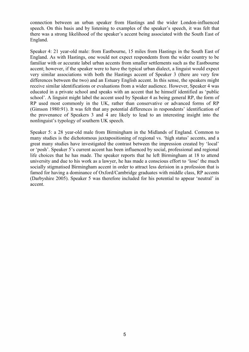
Speaker 3 -- 30 year-old male from Hastings, South East England some 60 miles south of

London: Whilst not being a very large urban settlement and as such unlikely to have a distinct

accent recognisable to the wider country, the town lies in the dialect area heavily influenced

by the spread of Estuary English and a linguist would expect respondents to make a

5

connection between an urban speaker from Hastings and the wider London-influenced

speech. On this basis and by listening to examples of the speaker’s speech, it was felt that

there was a strong likelihood of the speaker’s accent being associated with the South East of

England.

Speaker 4: 21 year-old male: from Eastbourne, 15 miles from Hastings in the South East of

England. As with Hastings, one would not expect respondents from the wider country to be

familiar with or accurate label urban accents from smaller settlements such as the Eastbourne

accent; however, if the speaker were to have the typical urban dialect, a linguist would expect

very similar associations with both the Hastings accent of Speaker 3 (there are very few

differences between the two) and an Estuary English accent. In this sense, the speakers might

receive similar identifications or evaluations from a wider audience. However, Speaker 4 was

educated in a private school and speaks with an accent that he himself identified as ‘public

school’. A linguist might label the accent used by Speaker 4 as being general RP, the form of

RP used most commonly in the UK, rather than conservative or advanced forms of RP

(Gimson 1980:91). It was felt that any potential differences in respondents’ identification of

the provenance of Speakers 3 and 4 are likely to lead to an interesting insight into the

nonlinguist’s typology of southern UK speech.

Speaker 5: a 28 year-old male from Birmingham in the Midlands of England. Common to

many studies is the dichotomous juxtapositioning of regional vs. ‘high status’ accents, and a

great many studies have investigated the contrast between the impression created by ‘local’

or ‘posh’. Speaker 5’s current accent has been influenced by social, professional and regional

life choices that he has made. The speaker reports that he left Birmingham at 18 to attend

university and due to his work as a lawyer, he has made a conscious effort to ‘lose’ the much

socially stigmatised Birmingham accent in order to attract less derision in a profession that is

famed for having a dominance of Oxford/Cambridge graduates with middle class, RP accents

(Darbyshire 2005). Speaker 5 was therefore included for his potential to appear ‘neutral’ in

accent.

6

Figure 1 Geographical provenance of voice donors

The content of the voice donors’ speech: A verbal guise technique (Gallois and Callan 1981) was employed, whereby the five recruited

voice donors were asked to produce carefully-controlled, content-neutral texts: all speakers

were required to be discussing the same series of events as if they had been co-witnesses.

Each speaker gave an account of a series of events on a ‘night out’, visiting bars and

socialising in a group, telling the same set of facts, produced as responses to questions. (The

questions were edited out in order to focus attention only on the exemplar voices.)

Respondents were presented with the five recordings, in any one of five randomised

sequences to offset any order effects and asked to record their responses on a questionnaire.

Gender was seen as an area of research in itself and it was decided therefore to stay with

voice samples from one sex, male, as the social stereotype of possible male crimes may lend

more credibility to the possibility that the voice donors were potential criminal.

The participants consisted of two cohorts: Group 1 n=144 (116 female/24 male/6 no

information given) and Group 2 n=122 (91 female/31 male). Following evidence from Braun

(1996) and Hollien and Schwartz (2000), suggesting no difference in respondent performance

in speaker identification tasks as a function of respondent sex, no distinction was drawn

between the responses of either sex.

All respondents were undergraduate students, living in South Wales, between the ages of 18

and 24. In Group 1 (G1), 98.6% of the participants were aged between 18 and 21; in Group 2

(G2) the figure was 95.5%. Findings from Braun (1996) and Bull and Clifford (1984) suggest

Speaker 2

Bristol

Speaker 5

Birmingham

l

Speaker 4

Eastbourne

Speaker 3

Hastings

Speaker 1

Cardiff

7

that for speaker identification research, respondents over 16 and under 40 may yield the most

reliable results. Given the lack of research in the field of forensic speaker description, this

guidance was applied to the current research, and all participants fell within an age range of

predicted competence for the tasks. All respondents were not formally selected but were a

convenience sample, based on availability and willingness to participate.

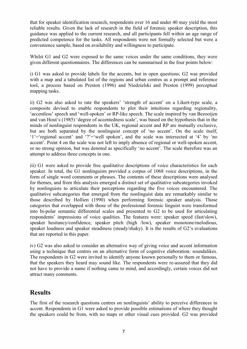
Whilst G1 and G2 were exposed to the same voices under the same conditions, they were

given different questionnaires. The differences can be summarised in the four points below:

i) G1 was asked to provide labels for the accents, but in open questions; G2 was provided

with a map and a tabulated list of the regions and urban centres as a prompt and reference

tool, a process based on Preston (1996) and Niedzielski and Preston (1999) perceptual

mapping tasks.

ii) G2 was also asked to rate the speakers’ ‘strength of accent’ on a Likert-type scale, a

composite devised to enable respondents to plot their intuitions regarding regionality,

‘accentless’ speech and ‘well-spoken’ or RP-like speech. The scale inspired by van Bezooijen

and van Hout’s (1985) ‘degree of accentedness scale’, was based on the hypothesis that in the

minds of nonlinguist respondents in the UK, regional accent and RP are mutually exclusive,

but are both separated by the nonlinguist concept of ‘no accent’. On the scale itself,

‘1’=‘regional accent’ and ‘7’=‘well spoken’, and the scale was intersected at ‘4’ by ‘no

accent’. Point 4 on the scale was not left to imply absence of regional or well-spoken accent,

or no strong opinion, but was denoted as specifically ‘no accent’. The scale therefore was an

attempt to address three concepts in one.

iii) G1 were asked to provide free qualitative descriptions of voice characteristics for each

speaker. In total, the G1 nonlinguists provided a corpus of 1068 voice descriptions, in the

form of single word comments or phrases. The contents of these descriptions were analysed

for themes, and from this analysis emerged a distinct set of qualitative subcategories invoked

by nonlinguists to articulate their perceptions regarding the five voices encountered. The

qualitative subcategories that emerged from the nonlinguist data are remarkably similar to

those described by Hollien (1990) when performing forensic speaker analysis. Those

categories that overlapped with those of the professional forensic linguist were transformed

into bi-polar semantic differential scales and presented to G2 to be used for articulating

respondents’ impressions of voice qualities. The features were: speaker speed (fast/slow),

speaker hesitancy/confidence, speaker pitch (high /low), speaker monotone/melodious,

speaker loudness and speaker steadiness (steady/shaky). It is the results of G2’s evaluations

that are reported in this paper.

iv) G2 was also asked to consider an alternative way of giving voice and accent information

using a technique that centres on an alternative form of cognitive elaboration: soundalikes.

The respondents in G2 were invited to identify anyone known personally to them or famous,

that the speakers they heard may sound like. The respondents were re-assured that they did

not have to provide a name if nothing came to mind, and accordingly, certain voices did not

attract many comments.

Results

The first of the research questions centres on nonlinguists’ ability to perceive differences in

accent. Respondents in G1 were asked to provide possible estimations of where they thought

the speakers could be from, with no maps or other visual cues provided. G2 was provided

8

with a map of the UK, demarcated and labelled into regions, plus a separate tabulated list

version of the UK regions with each region’s largest urban centres listed:

Table 2 Nonlinguists’ labelling of speaker accents - % ‘recognition’ rates

G1 G2

Speaker 1 labelled as ‘Wales’ 66% 71%

Speaker 1 labelled as ‘the city of Cardiff’ 36% 39%

Speaker 2 labelled as ‘South West’ 67% 70%

Speaker 2 labelled as ‘the city of Bristol’ 20% 43%

Speaker 3 labelled as ‘South East’ 72% 72%

Speaker 3 labelled as the ‘city of London’ 62% 52%

Speaker 4 labelled as South/South East/London 49% 20%

Speaker 4 labelled as London 13% 7%

Speaker 4 labelled as Oxford/Cambridge 0% 44%

Speaker 4 ‘don’t know’ 44% 24%

Speaker 5 labelled as South/South East/London 34% 14%

Speaker 5 labelled as the Midlands 14% 18%

Speaker 5 labelled as Oxford/Cambridge 0% 24%

Speaker 5 ‘don’t know’ 44% 21%

Taking first Speakers 1-3, we see that at least 2/3 of the respondents in both groups identify

the speakers as having accents that match their native regions -- this, despite the two groups

having completed alternative questionnaires, and G1 not being given any maps or tabulated

lists of regions or cities. At the regional level, the results remain in percentage terms, very

similar across the two groups. (Nb. Due to the nature of the experiment, it is not possible to

run independent or repeated measure statistical treatments, and for now we must satisfy

ourselves with percentages.) This would suggest that rather than being bereft of intuitions

regarding the origins of a speaker accent, the nonlinguists bring with them a relatively strong

areal taxonomy of accent variation in the regions under investigation. However, there is more

to this picture -- Speaker 3 is estimated as coming from the city of London, despite being

from the south coast of England, some 60 miles away. We can only speculate at this stage as

to what might direct people’s focus to the largest conurbation in the region: it may be that

nonlinguists from outside any one particular region are not sensitised to the range of intra-

region accent variation. Alternatively, it may be that if pressed for the name of a town/city,

nonlinguists will simply identify the largest, best-known urban centre in any particular

region. Certainly, this could form a revealing line if enquiry in future research designs.

Regardless of the possible explanations, however, it must be noted that the nonlinguists could

have suggested any urban centre in the UK, but did not, and the cities that were selected were

remarkably accurate, given the range of urban centres within the country.

For Speaker 4, we see quite a different picture. The data appear to suggest that the regional

label provided by the respondents to describe social accents such that of Speaker 4 are

function of the question and questionnaire. G1, which was provided only with open

questions, estimated Speaker 4 to be from somewhere in the South -- a potentially very large

region encompassing both the South West and South East -- or London. The use of London

9

as a label for the accent also exemplifies the semantic duality of labels like London, where

the name can connote a traditional regional accent as seen for Speaker 3, or an accent

associated with social/political/educational prestige such as RP-like accent of Speaker 4 as

both accents are apparently seen to cohabit the same urban space.

However, it is the data from G2, who were provided with a guided perceptual mapping task,

that are perhaps most intriguing. We see that in this task when the cities of Oxford and

Cambridge are provided on the questionnaire in map and tabulated form, nearly 50% of

respondents choose these cities as the label they associate with the accent, markedly different

from the South/London labels from the respondents in G1. We can certainly speculate that

what we are seeing here is the Oxford/Cambridge labels serving as a convenient shorthand

for nonlinguists to articulate the accent’s RP-ness -- that RP has a particular sociourban

associations in the minds of nonlinguists, even if these associations are not based on linguist

fact. If this is the case, this is of value to researchers/legal professionals, as the use of the

Oxford/Cambridge labels as a repository for accent associations also serves as a strategy for

disambiguating nonlinguist responses.

The data for Speaker 5 in some ways shows similar tendencies as those data for Speaker 4, in

that we see that the Oxford/Cambridge label has been utilised by a quarter of respondents

from G2 in contrast to none from G1. We can also see that where guided perceptual mapping

has been utilised for G2, there are 50% fewer ‘don’t know’ responses. But what is also clear

is that the nonlinguists do not agree on a label which articulates their associations with a large

spread of associations. What is needed is to investigate an alternative paradigm for

articulating accent associations. To explore an alternative paradigm, the nonlinguists in G2

were also presented with an instrument, upon which they were invited to plot their intuitions

regarding the strength of the speakers’ accents.

Figure 2 Means for ‘strength of accent’

The results of an ANOVA on the differences between the mean ratings for these speakers

show that in all cases, the differences were significantly different ( < 0.05), with the

exception of between Speakers 1-3 and 2-3, where no significant differences were found.

The ‘accent strength’ attributions for Speakers 1, 2 and 3 are remarkably loaded towards the

‘regional’ end of the scale whilst for Speaker 4, 86% of respondents placed on the ‘well-

spoken’ side of the scale. Speaker 5 is the only example of the five speakers where neither

points 1 nor 7 are employed by the respondents and Speaker 5 was viewed differently from

other speakers: over 75% of the respondents rated the speaker around the middle three points

Speaker 1 Speaker 2 Speaker 3 Speaker 4 Speaker 5

Accent Strength 2.55 2.81 2.71 5.26 4.31

0

1

2

3

4

5

6

7

Me

an

sco

re

10

on the scale, suggesting that Speaker 5 is seen as somehow less ‘well-spoken’ than Speaker 4,

but also less ‘regional’ than Speakers 1, 2 and 3. The results of the ANOVA and the data in

the bar chart suggest that the ‘no accent’ scale was meaningful to the respondents and

methodologically valid, and that it may have a role to play in any future audiofit.

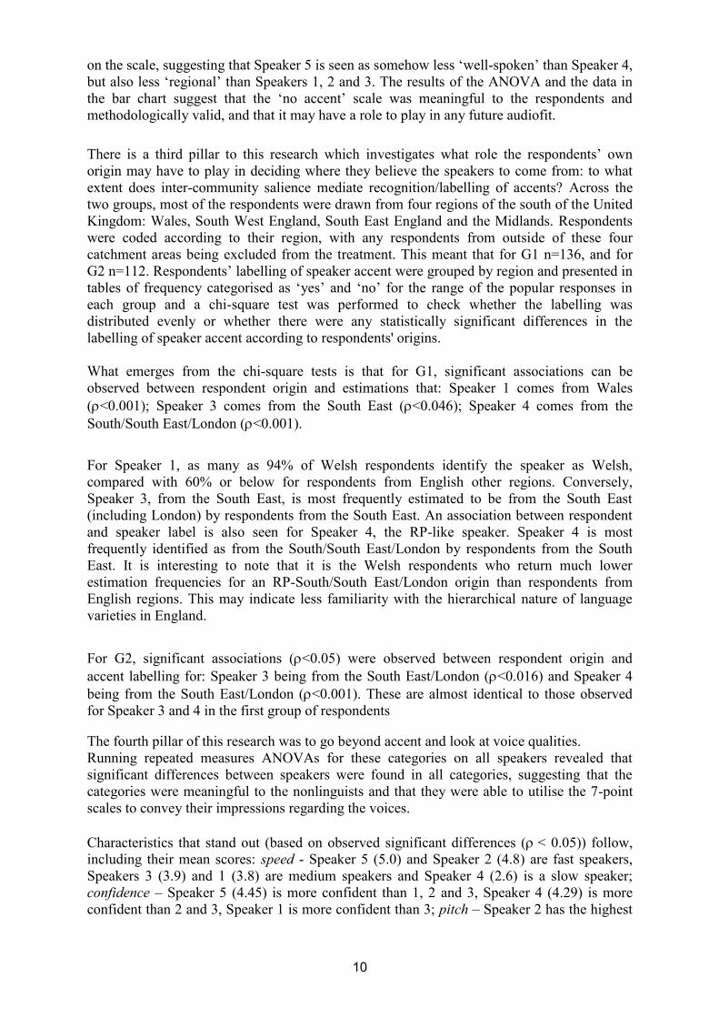
There is a third pillar to this research which investigates what role the respondents’ own

origin may have to play in deciding where they believe the speakers to come from: to what

extent does inter-community salience mediate recognition/labelling of accents? Across the

two groups, most of the respondents were drawn from four regions of the south of the United

Kingdom: Wales, South West England, South East England and the Midlands. Respondents

were coded according to their region, with any respondents from outside of these four

catchment areas being excluded from the treatment. This meant that for G1 n=136, and for

G2 n=112. Respondents’ labelling of speaker accent were grouped by region and presented in

tables of frequency categorised as ‘yes’ and ‘no’ for the range of the popular responses in

each group and a chi-square test was performed to check whether the labelling was

distributed evenly or whether there were any statistically significant differences in the

labelling of speaker accent according to respondents' origins.

What emerges from the chi-square tests is that for G1, significant associations can be

observed between respondent origin and estimations that: Speaker 1 comes from Wales

(<0.001); Speaker 3 comes from the South East (<0.046); Speaker 4 comes from the

South/South East/London (<0.001).

For Speaker 1, as many as 94% of Welsh respondents identify the speaker as Welsh,

compared with 60% or below for respondents from English other regions. Conversely,

Speaker 3, from the South East, is most frequently estimated to be from the South East

(including London) by respondents from the South East. An association between respondent

and speaker label is also seen for Speaker 4, the RP-like speaker. Speaker 4 is most

frequently identified as from the South/South East/London by respondents from the South

East. It is interesting to note that it is the Welsh respondents who return much lower

estimation frequencies for an RP-South/South East/London origin than respondents from

English regions. This may indicate less familiarity with the hierarchical nature of language

varieties in England.

For G2, significant associations (<0.05) were observed between respondent origin and

accent labelling for: Speaker 3 being from the South East/London (<0.016) and Speaker 4

being from the South East/London (<0.001). These are almost identical to those observed

for Speaker 3 and 4 in the first group of respondents

The fourth pillar of this research was to go beyond accent and look at voice qualities.

Running repeated measures ANOVAs for these categories on all speakers revealed that

significant differences between speakers were found in all categories, suggesting that the

categories were meaningful to the nonlinguists and that they were able to utilise the 7-point

scales to convey their impressions regarding the voices.

Characteristics that stand out (based on observed significant differences (< 0.05)) follow,

including their mean scores: speed - Speaker 5 (5.0) and Speaker 2 (4.8) are fast speakers,

Speakers 3 (3.9) and 1 (3.8) are medium speakers and Speaker 4 (2.6) is a slow speaker;

confidence – Speaker 5 (4.45) is more confident than 1, 2 and 3, Speaker 4 (4.29) is more

confident than 2 and 3, Speaker 1 is more confident than 3; pitch – Speaker 2 has the highest

11

pitch (4.6), followed by Speakers 5 (4.3) and 3, (4.2) followed by Speaker 1 (2.8) with a

relatively low voice and Speaker 3 (2.1) rated as having a deep voice; melodiousness –

Speaker 5 (4.8) is more than average and therefore melodious, followed by Speaker 2 (4.4),

followed by Speakers 1 (3.9) and 3 (3.8) with Speaker 1 rated at a low (monotonous) 2.5.

Loudness – each was significantly different from each other: Speaker 1 (5.1), Speaker 5 (4.6),

Speaker 2 (4.2), Speaker 3 (3.7) and Speaker 4 (3.3); steadiness – again, each was

significantly different from each other: Speaker 4 (5.35), Speaker 1 (4.95), Speaker 5 (4.6),

Speaker 3 (4.0) and Speaker 2 (3.5).

Elaborating on this further, we can turn the data into boxplots for each speaker:

Figure 3 Boxplot for Speaker 1 voice characteristics

Speaker1 Shaky-Steady

Speaker1 Soft-Loud

Speaker1 Monotone- Melodious

Speaker1 Deep Voice - High-Pitched

Speaker1 Hesitant- Confident

Speaker1 Slow-Fast

7

6

5

4

3

2

1

12

Figure 4 Boxplot for Speaker 2 voice characteristics

Figure 5 Boxplot for Speaker 3 voice characteristics

Speaker 2

Speaker3

Shaky - Steady

Shaky-Steady

Speaker 2

Speaker 3

Soft - Loud

Soft-Loud

Speaker 2

Speaker 3

Monotone -

Monotone-

Melodious

Melodious

Speaker 2

Speaker 3

Deep voice -

Deep voice -

High-Pitched

High-pitched

Speaker2

Speaker 3

Hesitant-

Hesitant -

Confident

Confident

Speaker 2

Speaker 3

Slow-Fast

Slow - Fast

7

7

6

6

5

5

4

4

3

3

2

2

1

1

13

Figure 6 Boxplot for Speaker 4 voice characteristics

Figure 7 Boxplot for Speaker 5 voice characteristics

Speaker4

Speaker5

Shaky-Steady

Shaky- Steady

Speaker4

Speaker5

Soft-Loud

Soft-Loud

Speaker4

Speaker5

Monotone-

Monotone-

Melodious

Melodious

Speaker4

Speaker5

Deep Voice-

Deep voice-

High-pitched

High-pitched

Speaker4

Speaker5

Hesitant-

Hesitant-

Confident

Confident

Speaker4

Speaker5

Slow-Fast

Slow-Fast

7

7

6

6

5

5

4

4

3

3

2

2

1

1

14

The boxplot for Speaker 1 demonstrates that ‘deep voice -- high-pitched’ provokes a very

clear reaction, with 50% of respondents placing the voice between points 2 and 3, and we can

observe the direct opposite for evaluations of the speaker on ‘soft -- loud’, with the speaker

attracting ratings between 5 and 6. For Speaker 2, the boxplot is a little less dramatic showing

fewer extremes of ratings although higher than medium ratings for speed, pitch,

melodiousness and loudness. There is quite a wide range of opinion for hesitant/confident.

The boxplot for Speaker 3 indicates a concentration of opinion on three features: medium

hesitancy/confidence and loudness, but a higher pitched voice. For Speaker 4 we see some

strong characterisation of a slow speaker with a deep, monotonous generally steady voice and

for Speaker 5 there is quite a range of opinion on some points, but there is certainly a

characterisation of the speaker as having a higher than medium voice, louder than medium

and steadier than medium voice.

The fifth and final pillar of this research is to consider an alternative way of eliciting voice

and accent information from nonlinguists using a technique that uses an alternative form of

cognitive elaboration: soundalikes. Where soundalikes were provided, the names associated

with the voices provide interesting reading.

Speaker 1 was compared with ‘Goldie Lookin’ Chain’ (rap group from Newport, South

Wales), ‘Dirty Sanchez’ (South Wales 'stunt' TV show), ‘Kelly Jones from Stereophonics'

(South Wales pop group), a friend (respondent was from South Wales), ‘my brother’

(respondent was from South Wales). What is clear is that every soundalike mentioned has an

association with South Wales and the three famous people mentioned all have accents that

would be associated with industrialised urban areas of South Wales.

Speaker 2 was compared with Gareth from 'The Office' (British TV comedy), ‘Vickie

Pollard’ (Bristol character from 'Little Britain'), ‘Little Britain woman’ (presumably the same

character from the TV comedy programme), ‘a farmer’, ‘people from my hometown’ (the

respondent was from South West), ‘a friend’ (the respondents were from the South West,

although we cannot be certain where the friends are from). The regional identification data in

the earlier sections confirm that most respondents believed Speaker 2 to be from the South

West of England, many of them from Bristol. An obvious connection appears in that all the

famous soundalikes identified are famous for their regional accents, in particular their

realisation of the postvocalic [r] shibboleth that can so readily identify those southern English

speakers that come from the West or South West of England. This accent is also readily

stereotyped as a ‘farmer’s’ accent, an example of which also appears.

Speaker 3 attracted by far the highest frequency of single soundalike: ‘David Beckham’

(English footballer), with 36 comparisons. Also included were ‘Frank Lampard’ (English

Footballer) ‘Mike Skinner’ (rapper from 'The Streets' pop group) and ‘my parents from

London.’

The 36 soundalikes for David Beckham is a remarkably figure for a non-essential category

within the questionnaire. But what was it in Speaker 3’s voice that was so salient to the

respondents? It would be uncontroversial to say that Beckham, a famous footballer from just

outside London (Essex) is well known for his strong regional, estuary English speech variety.

And these are the very same features that have been identified with Speaker 3 throughout by

both groups of respondents. The choice of Frank Lampard may echo the same reasoning as

for David Beckham. It may be that the respondent perceives Lampard to share similar, high-

pitched estuary English tones. All three of these soundalikes, but David Beckham as a label

could therefore be conveying more than simple accent information: Beckham in particular is

impersonated on television by comedians, etc., and a constant characteristic to be mimicked

15

is not just his accent but soft, high, voice; and these are features described by a number of

respondents in the polar voice descriptions.

Speaker 4, who was characterised as having a deep monotonous voice with an RP-like accent

was compared to famous TV comedian with an RP-like voice, Stephen Fry, and the famously

dead-pan, monotonous deep-voiced comedian Jack Dee. The comparison with voice can also

be seen with the TV actor/comedian David Walliams and the singer Damon Albarn from the

pop group ‘Blur’. Dee, Albarn and Walliams can all be characterised as having a somewhat

understated and unmelodious delivery and again, it would appear that the respondents are

conveying more than accent information with their soundalikes.

Speaker 5, whose accent had been identified with his home region by very few people and

who appears to be more likely to be identified as having no accent -- neither strongly

regional, nor RP -- on the accent scale, was identified as sounding like just two people: Frank

Skinner (TV comedian) and Scott Mills (radio presenter) who many would describe as having

an ‘average’ to ‘high’ pitched voice, and it may be these salient features noted by the

respondent that suggested this soundalike. It is also worth noting that in this research, the

speaker without an overt regionally or socially marked accent attracted the fewest

soundalikes.

Discussion and conclusion

Given the need for the police and legal professionals to be able to elicit accent descriptions

from nonlinguists, the first research question in this article was to investigate whether

nonlinguists have the ability to perceive regional and social accents. The data from this study

demonstrate that the nonlinguist respondents in this research are capable of perceptual

discrimination between the accents of the speakers presented. However, variation was

observed in the accuracy and focus of the estimations of speaker origin, with those speakers

using traditional regional accents (Speakers 1, 2 and 3) receiving the highest frequency of

accurate estimations of origin. Those speakers who were not strongly associated with any one

region (Speakers 4 and 5) received more disparate estimations of origin.

Moreover, the introduction in this study of guided perceptual mapping as an elaboration of

Preston’s (1996) and Niedzielski and Preston’s (1999) approach to folk linguistics research

has shown itself to have applications in the forensic field, in that it assists not only in the

perceptual differentiation of regions and accents, but also in the expression of social

associations with an accent that has no overt geographical origin. Researchers and legal

professionals may wish to draw upon and further develop such a technique.

With regard to the second research question -- whether accent perception is a function of

respondent origin -- this study has provided evidence that social and perceptual distance and

not just Euclidian measures between a respondent and a speaker’s origin have a role to play

in the accuracy of the identification. The evidence of perceptual asymmetry between, for

example, Wales and England and the South East of England compared with other regions is

consistent with other data from the UK context (Williams et al. 1996; Kerswill and Williams

2002; Garrett et al. 2004). Perceptual distance and within community variation and salience

should play a role in future research designs.

The use of the ‘strength of accent’ scale served to illustrate a non-geographical medium for

eliciting accent perceptions and labels from nonlinguists, addressing the third research

question. For example, Speaker 5 was identified as having ‘no accent’, and whilst linguists

16

will know it to be impossible to speak a language without communicating some regional or

social information about oneself, the data from the ‘strength of accent’ scale lend support to

the conclusion that, in the UK, the concept of ‘no accent’ is a very real nonlinguist alternative

to, on the one hand, the socially-marked RP/well-spoken/Oxford/‘posh’ English and on the

other hand, regional/accented English.

Turning to the fourth of the research questions regarding what nonlinguists notice about a

voice, inviting nonlinguists to rely on their own cognitive representations and processes when

describing voices and accents endows resultant descriptions with a level of community

authenticity essential to the field of forensic speaker description. Identifying and engaging

with nonlinguists’ own perceptual scales should inform practice amongst forensic linguists

and legal professionals. Additionally, Kerswill (2002) has suggested that the recognition of

non-community accents may be mediated by whether the voice sounds like someone the

judge happens to know. The data in this study have shown that there is a clear potential for

nonlinguists to articulate their perceptions by describing a person known to them -

soundalikes. The remarkably high rate of ‘David Beckham’ soundalike descriptions served as

an overwhelmingly powerful alternative to description through other, more technically-

oriented channels of accent and voice description. Linguists may baulk at the idea of

introducing such non-technical opinions into research but it is nonlinguist police and

nonlinguist earwitnesses that we are focusing on, and so long as such terms are universally

salient and have wide currency, they remain viable ways of communicating what has been

heard from one nonlinguist to another. A further avenue of research may be to investigate

what role linguists could play in relating the description of the earwitnesses to technical

descriptions of language.

In conclusion, I discussed at the beginning how around the world, nonlinguist police officers

routinely take statements from nonlinguist earwitnesses in relation to linguistic issues,

meaning witnesses to and victims of crime are being questioned by almost exclusively

linguistically untrained people. In answer to the fifth research question, whilst only a first

step in researching the potential for FSD, the data presented here suggest that there is indeed

potential for the creation of an audiofit to augment current practice. The data suggest that the

illustrated gap between current practices and nonlinguist abilities should be reviewed and that

researchers should assume that nonlinguists are capable of perceiving linguistic detail and

providing relatively meaningful data.

No doubt, this first venture into researching FSD cannot be assumed to be presenting a

finished methodology and further testing on a range of respondents populations, using a

wider cabinet of exemplars is required in order to arrive at a reliable and valid audiofit

instrument. However, if the situation is to be improved, researchers, police and legal

professionals need to acknowledge the weaknesses in the current system and in order to

develop a co-ordinated and systemic typology for eliciting descriptive forensic linguistic data

-- an appropriate audiofit instrument with which enhance the evidence gathering process and

affect the course of social justice.

References

Braun, A. (1996) Age estimation by different listener groups. Forensic Linguistics: The International

Journal of Speech, Language and Law 3(1): pp. 65--73.

Broeders, A.P. (1996) Earwitness identification: common ground, disputed territory and uncharted

areas. Forensic Linguistics: The International Journal of Speech, Language and Law 3(1): pp. 3--15.

17

Bull, R. and Clifford, B. (1984) Earwitness voice recognition accuracy. In G. L. Wells and E. F.

Loftus (eds.) Eyewitness Testimony: Psychological Perspectives pp. 92--123. Cambridge: Cambridge

University Press

Dixon, J.A. and Mahoney, B. (2004) The effect of accent evaluation and evidence on a suspect's

perceived guilt and criminality. Journal of Social Psychology 144(1): pp. 63--73.

Gallois, C. and Callan, V. (1981) Personality impression elicited by English accented speech. Journal

of Cross-Cultural Psychology 12: pp. 347--359.

Garrett, P., Coupland, N. and Williams, A. (2004) Adolescents' lexical repertoires of peer evaluation:

boring prats and English snobs. In A. Jaworski, N. Coupland and D. Galasinski (eds.) The

Sociolinguistics of Metalanguage 193--226. Berlin: Mouton de Gruyer.

Hollien, H. (1990). The Acoustics of Crime. New York: Plenum Press.

Hollien, H. and Schwartz, R. (2000) Aural-perceptual speaker identification: problems with non-

contemporary samples. Forensic Linguistics: The International Journal of Speech, Language and Law

7(2): pp. 199--211.

Kerswill, P. and Williams, A. (2002) Dialect Recognition and Speech Community Focussing in New

and Old Towns in England. In D. Long and D. Preston (eds.) Handbook of Perceptual Dialectology.

Vol. 2 pp. 173—204. Michigan: John Benjamins Publishing Company.

Niedzielski, N. and Preston, D. (1999) Folk Linguistics. Berlin: Mouton de Gruyer.

Nolan, F. (2003) A recent voice parade International Journal of Speech, Language and the Law

10(2): 277--291.

Nolan, F. and Grabe, E. (1996) Preparing a voice lineup. Forensic Linguistics: The International

Journal of Speech, Language and Law 3(1): pp. 74--94.

Philippon, A.C., Cherryman, J., Bull, R. and Vrij, A. (2007) Lay people's and police officers’ attitudes

towards the usefulness of perpetrator voice identification. Applied Cognitive Psychology Volume

21(1): pp. 103--115.

Preston, D. (1996) Whaddayaknow? The modes of linguistic awareness. Language Awareness 5(1):

pp. 40--74.

Seggie, I. (1983) Attribution of guilt as a function of ethnic accent and type of crime. Journal of

Multilingual and Multicultural Development 4(2): pp. 197--206.

Shuy, R. (1993) Language Crimes: The Use and Abuse of Language Evidence in the Courtroom.

Cambridge MA: Blackwell.

van Bezooijen, R. and Ytsma, J. (1999) Accents of Dutch: Personality impression, divergence and

identifiability. Belgian Journal of Linguistics 13(1): pp. 105--129.

van Bezooijen, R. and van Hout, R. (1985) Accentedness ratings and phonological variables as

measures of variation in pronunciation. Language and Speech 28(2): pp. 129--142.