Rendaku and Proto-Japanese Accent

Classes

J. MARSHALL UNGER

The Ohio State University

1. Introduction

Rendaku (or sequential voicing) in Japanese refers to the voicing of the

initial obstruent of a morpheme when it comes second in a compound. It

never occurs in non-mimetic native compounds when there is a medial

voiced obstruent in the second morpheme (Lyman 1894), but no one has

found a rule that predicts when it does occur. Contrasting pairs like hanazi

‘nosebleed’ (< hana + ti) vs. hanasaki ‘tip of the nose’ and hiragana

‘cursive syllabic script’ (< hira + kana) vs. katakana ‘angular syllabic

script’, compounds like Nakata ~ Nakada (family name), and the fact that

some neologisms do exhibit rendaku while others do not all make it

doubtful that a purely phonological explanation for the distribution of

rendaku in the modern language will ever be found. The same is true for

earlier stages of the language (Unger [1977] 1993).

Consequently, if we tabulate all the noun-compounds attested in Old

Japanese documents by some phonological feature of their constituents, we

expect to find rendaku distributed randomly over all combinations.

Using a list of 908 noun compounds culled from Omodaka 1967 by

Timothy J. Vance, my research assistant Yu Hirata created a “flat” database

for testing this prediction. For each compound, he checked Vance’s data,

entered the meaning of the constituent nouns (to facilitate separation of

homophones), and looked up their reconstructed accent classes (Martin

1987). I used Excel 97 to analyze this database.

2. Findings

In 826 (90.97%) of the 908 OJ compounds, the second noun lacked a

medial b, d, g, or z, which would have blocked rendaku (Lyman’s Law).

Of those 826 compounds, the first and second nouns in 683 (82.69%)

contained one or two syllables each. In fact, no second-position noun

contained more than two syllables whereas 143 compounds had

first-position nouns of three or more syllables. Because such long nouns

fall into a large number of low-frequency accent classes and because the

accent of first- with second-position nouns must be compared, I restricted

my attention to the 683 compounds with mono- and dissyllabic constituents.

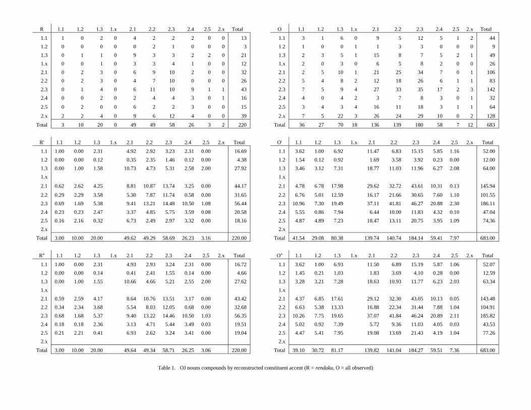
Table 1 shows how these are distributed with respect to the accent

classes of their constituents. The 220 compounds that exhibit rendaku are

tabulated in array R; all 683 observed compounds are tabulated in array O.

In both arrays, the rows (columns) correspond to the accent classes of the

nouns in first (second) position. In the accent class designator n.k, the

number to the left of the point counts the syllables in the noun; the number

to the right is its class number. An x instead of a number means that, for

these nouns, Martin could not narrow down the reconstruction to one

specific class. Thus 1.x and 2.x are not actual classes, like 1.1, 2.1, etc.

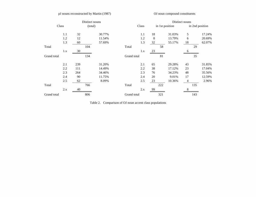
Instead of discarding the n.x data, we can distribute them over the real

classes. There are two ways to do this (Table 2). One is to use the accent

class percentages found in Martin’s 1987 noun inventory (excluding

borrowings); the other is to use percentages based on the set of all

constituents actually found in OJ compounds. The advantage of using

Martin’s inventory is that we get a larger sample, including many nouns that

do not begin with voiceless obstruents, as all the second-position nouns in

the OJ data must. To obtain array R (O) in Table 3, we multiply the

numbers in the 1.x and 2.x rows (columns) of R (O) by the percentage of

nouns in each class 1.1–1.3 (2.1–2.5) and add the product to the

corresponding cells in that row (column). The advantage of using only the

constituents found in OJ compounds is that we can obtain separate

percentages for each class in first and second position; however, the sample

size is smaller. To obtain R (O) in Table 4, we proceed as before but use

separate factors for the rows and columns as appropriate. It turns out that

the results of the two procedures are in good agreement.

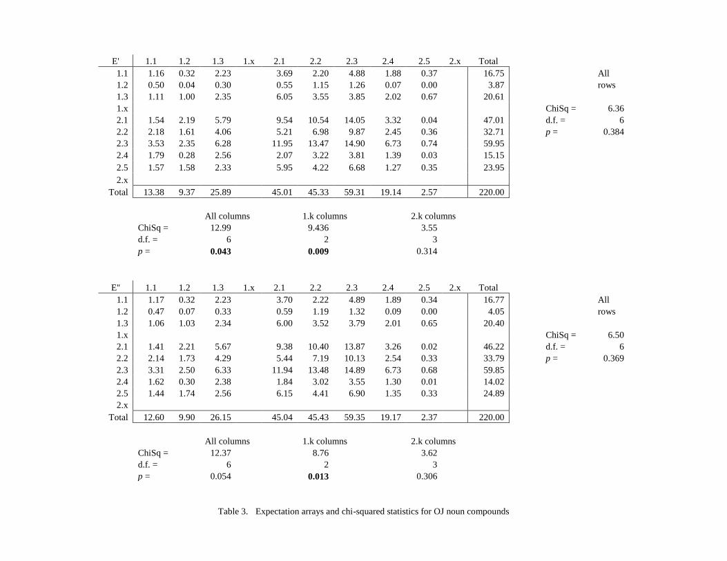
To compute the expectation arrays E (Table 5) and E (Tables 6), we

multiply the entries in arrays O and O, respectively, by 220/683 (32.21%),

the ratio of rendaku compounds to all compounds. These arrays therefore

reflect the hypothesis H0 that rendaku is distributed randomly regardless of

constituent accent. To check H0, we perform χ2 tests on the row and

column sums of arrays E, R and E, R, respectively. As shown in

Tables 5 and 6, H0 was confirmed for the row sums in both cases, but not

for the column sums.1 The probability that the column sums differed from

the expected values by chance alone is less than 5 percent for R and E, and

only slightly more than 5 percent for R and E. In both cases, the number

of rendaku compounds with a monosyllabic noun in second position was

significantly lower than expected.

3. Accounting for the discrepancy

3.1 Merging mono- and dissyllabic nouns

This is a puzzling result because it suggests some sort of phonological

conditioning of rendaku, yet the presence of a monosyllabic noun in second

position does not preclude the occurrence of rendaku; it just makes it less

likely. Moreover, since the number of syllables in the second constituent

seems to affect the occurrence of rendaku significantly, one would expect

that the number of syllables in the first constituent would too—but it

doesn’t. Finally, why should we get fewer cases of rendaku than expected?

If there were a preference for inserting no in X-Y compounds when Y was

monosyllabic, then we would expect to find more cases (because of OJ

reductions from X.no.Y added to lexicalized rendaku compounds).

Conversely, if there were a preference for avoiding no when Y was

monosyllabic, then why do we find rendaku randomly distributed when it

isn’t?

All these problems can be solved if we rearrange the data in accord

with two ideas developed in Martin 1987. One is that class 1.3 is the result

of a merger of two classes, 1.3a and 1.3b, that were distinct in

proto-Japanese.

Though the modern dialects require the reconstruction of only three accent

types for monosyllabic nouns, both evidence from [Ruiju] Myōgi-shō and

structural considerations indicate that earlier kinds of Japanese must

have had four types. (Martin 1987, 180)

The other is that all pJ monosyllabic nouns were bimoraic, as they are in

many Western Japanese dialects even now. When uttered in isolation,

1 Although there are eight rows and columns, degrees of freedom equals 6, not 7,

because no expected value can be less than 5; hence, the 1.1 and 1.2 row sums and

2.4 and 2.5 column sums must be combined.

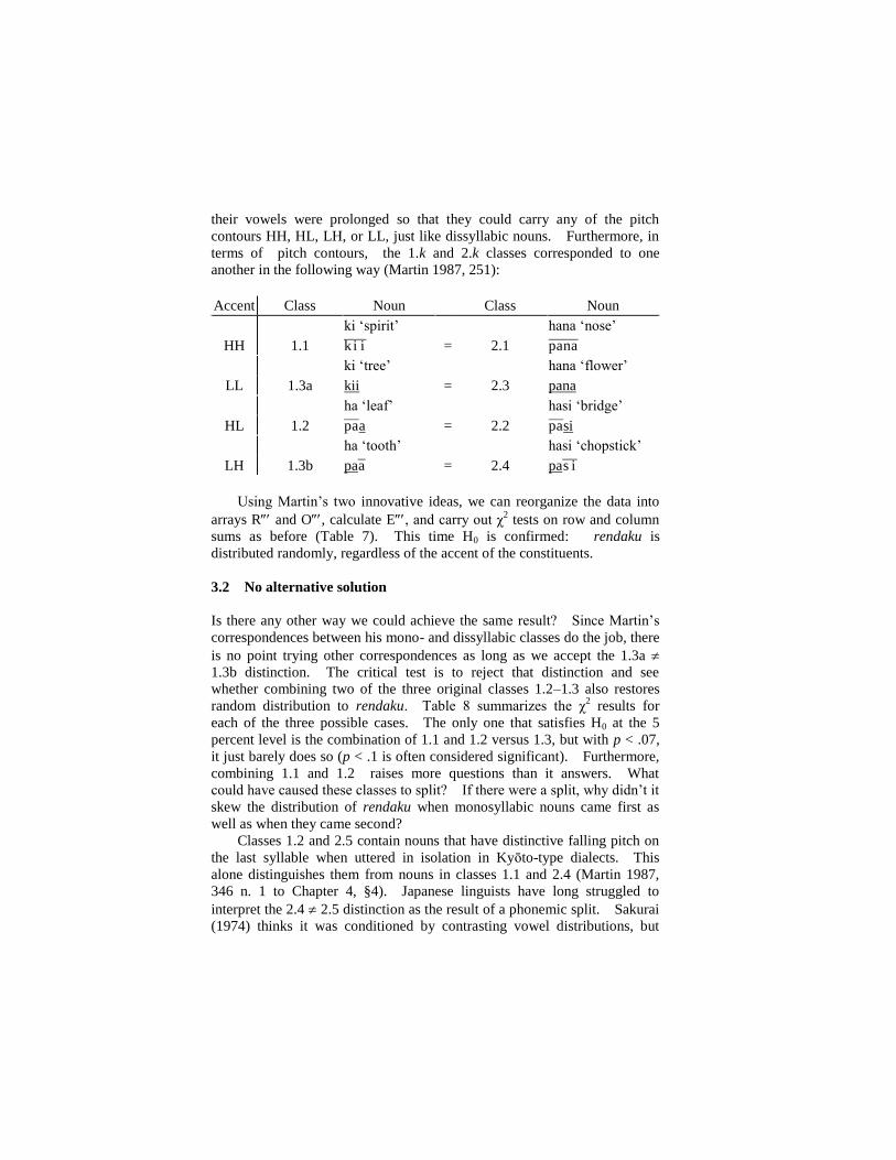
their vowels were prolonged so that they could carry any of the pitch

contours HH, HL, LH, or LL, just like dissyllabic nouns. Furthermore, in

terms of pitch contours, the 1.k and 2.k classes corresponded to one

another in the following way (Martin 1987, 251):

Accent

Class

Noun

Class

Noun

HH

1.1

ki ‘spirit’

=

2.1

hana ‘nose’

k i i pana

LL

1.3a

ki ‘tree’

=

2.3

hana ‘flower’

kii pana

HL

1.2

ha ‘leaf’

=

2.2

hasi ‘bridge’

paa pasi

LH

1.3b

ha ‘tooth’

=

2.4

hasi ‘chopstick’

paa pas i

Using Martin’s two innovative ideas, we can reorganize the data into

arrays R and O, calculate E, and carry out χ2 tests on row and column

sums as before (Table 7). This time H0 is confirmed: rendaku is

distributed randomly, regardless of the accent of the constituents.

3.2 No alternative solution

Is there any other way we could achieve the same result? Since Martin’s

correspondences between his mono- and dissyllabic classes do the job, there

is no point trying other correspondences as long as we accept the 1.3a

1.3b distinction. The critical test is to reject that distinction and see

whether combining two of the three original classes 1.2–1.3 also restores

random distribution to rendaku. Table 8 summarizes the χ2 results for

each of the three possible cases. The only one that satisfies H0 at the 5

percent level is the combination of 1.1 and 1.2 versus 1.3, but with p < .07,

it just barely does so (p < .1 is often considered significant). Furthermore,

combining 1.1 and 1.2 raises more questions than it answers. What

could have caused these classes to split? If there were a split, why didn’t it

skew the distribution of rendaku when monosyllabic nouns came first as

well as when they came second?

Classes 1.2 and 2.5 contain nouns that have distinctive falling pitch on

the last syllable when uttered in isolation in Kyōto-type dialects. This

alone distinguishes them from nouns in classes 1.1 and 2.4 (Martin 1987,

346 n. 1 to Chapter 4, §4). Japanese linguists have long struggled to

interpret the 2.4 2.5 distinction as the result of a phonemic split. Sakurai

(1974) thinks it was conditioned by contrasting vowel distributions, but

fares no better than the earlier scholars whose studies he reviews in detail.

The Russian linguist Polivanov speculated that final falling pitch is a trace

of a “truncated” nasal phoneme. Martin (1987, 361 n. 1 to Chapter 4, §14)

thinks he got the idea by comparing Korean achom ‘morning’ with Japanese

asa id., which is 2.5 and could be taken back to an earlier *asa.m.2

However, Martin found that the handful of Ryūkyū words with final nasals

unreflected in main-island cognates are scattered randomly across

reconstructed accent classes, and Hirata and I have hunted in vain for

additional Korean matches with final nasals for Japanese 2.5 nouns.

Polivanov’s explanation for class 2.5 is therefore dubious. (In any case, he

suggests no link between classes 1.2 and 2.5, and apart from falling pitch in

Kyōto-type dialects, there seems to be none.) The present study adds to

the doubt by showing that 2.5 nouns are unexceptional with respect to the

distribution of rendaku. On that basis at least, the fact that class 2.5 is

relatively small and distinctive only in one dialect group suggests that its

origins should be sought in relatively recent developments within that

group.

4. Significance of the results

If we don’t adopt Martin’s reconstruction of OJ monosyllabic noun accent,

we cannot explain the non-random distribution of rendaku in those OJ noun

compounds in which the second constituent is monosyllabic. Since we

have strong independent reasons for thinking that rendaku has always been

fundamentally lexical, this strongly supports Martin’s reconstruction, even

though it was based solely on unrelated “evidence from Myōgi-shō and

structural considerations.” This surprising congruence of results has

far-reaching implications for the reconstruction of early stages of the

Japanese language.

2 Actually, as Murayama shows, Polivanov got the final-nasal idea from an article

by E. A. Meyer (1906), a phonetician interested in the origins of tones in Northern

Germanic.

In Unger ([1977] 1993), I showed that the internal reconstruction of OJ

verb paradigms requires rules for reducing vowel sequences that depend on

whether a vowel belongs to a mono- or polysyllabic morpheme. I also

showed that the so-called -ramu forms of OJ verbs are evidence of a pre-OJ

stage during which the rentaikei of yodan and rahen verbs ended in *-uru,

which shortened to -u in Old Japanese.3 Whitman (1985, 1990) proposed

that this change was a special case of a more general rule of r-deletion

conditioned by the length of the preceding vowel. He found a correlation

between the pre-OJ long vowels, which had to be reconstructed to block this

change, and rising pitch in the corresponding syllables of Middle Korean

cognates. But if vowels could be distinctively long or short before *r in

pre-Old Japanese, there is no reason that vowel length could not be

distinctive in other environments, and, in Unger 1998, I explained how the

rules of vowel sequence reduction could be recast in terms of vowel length

under the assumption that every monosyllabic morpheme was bimoraic.

In fact, unless they are recast in this way, there is an unresolvable conflict

between the internal reconstruction of pre-OJ verb forms and other sound

changes postulated by Whitman on the basis of Korean-Japanese matches.

These changes—pre-OJ *ti > OJ si, *ni > i, and *ri > i—not only play a role

in Korean-Japanese etymologies but also explain how the collapse of the

so-called kō-otsu (or A-B) distinctions among OJ i-ending syllables was

initiated.

Thus, the assumption that vowels were automatically lengthened in

pre-OJ monosyllabic morphemes is a vital link between Korean-Japanese

comparisons and the internal reconstruction of pre-OJ verb paradigms.

The fact that it is supported by observations about the seemingly unrelated

distribution of rendaku over OJ noun compounds is quite unexpected and

therefore strengthens our confidence that the proto-Korean-Japanese

reconstruction reflects a real prehistoric language.

References

Lyman, Benjamin Smith. 1894. Change from surd to sonant in Japanese

compounds. Philadelphia: Oriental Club of Philadelphia.

Martin, Samuel E. 1987. The Japanese language through time. New

Haven: Yale University Press.

Meyer, Ernst Alfred. 1906. “Nihongo ni okeru ongakuteki go-akusento.”

Nihongo kenkyū, Murayama Shichirō (trans.), 1–10. Tōkyō:

3 OJ nahen, sahen, kahen, and nidan verbs all have rentaikei in -uru. Likewise,

they have izenkei in -ure, to which yodan and rahen answers with -e. The -rasi

forms also preserve the *-ur- sequence.

Kōbundō, 1976. Original in Le monde oriental (Uppsala: A.B.

Lubdequistska Bokhandeln, 1906–41), 77–86.

Omodaka Hisataka et al., comps. 1967. Jidaibetsu kokugo daijiten, jōdai

hen. Tōkyō: Sanseidō.

Sakurai Shigeharu. 1974. Kodai kokugo akusento-shi ronkō. Tōkyō:

Ōfūsha.

Unger, J. Marshall. 1977. Studies in Early Japanese morphophonemics.

Second edition, 1993. Bloomington: Indiana Linguistics Club.

────. 1998. “Reconciling comparative and internal reconstruction:

the case of Old Japanese /ti, ri, ni/.” Linguistics Society of America

annual meeting (New York).

Whitman, John Bradford. 1985. “The phonological basis for the

comparison of Japanese and Korean.” Cambridge, MA: Harvard

University dissertation.

────. 1990. “A rule for medial *-r- loss in pre-Old Japanese.”

Linguistic change and reconstruction methodology, ed. Philip Baldi,

511–45. Berlin: Mouton de Gruyter.

R 1.1 1.2 1.3 1.x 2.1 2.2 2.3 2.4 2.5 2.x Total

O 1.1 1.2 1.3 1.x 2.1 2.2 2.3 2.4 2.5 2.x Total

1.1 1 0 2 0 4 2 2 2 0 0 13

1.1 3 1 6 0 9 5 12 5 1 2 44

1.2 0 0 0 0 0 2 1 0 0 0 3

1.2 1 0 0 1 1 3 3 0 0 0 9

1.3 0 1 1 0 9 3 3 2 2 0 21

1.3 2 3 5 1 15 8 7 5 2 1 49

1.x 0 0 1 0 3 3 4 1 0 0 12

1.x 2 0 3 0 6 5 8 2 0 0 26

2.1 0 2 3 0 6 9 10 2 0 0 32

2.1 2 5 10 1 21 25 34 7 0 1 106

2.2 0 2 3 0 4 7 10 0 0 0 26

2.2 5 4 8 2 12 18 26 6 1 1 83

2.3 0 1 4 0 6 11 10 9 1 1 43

2.3 7 5 9 4 27 33 35 17 2 3 142

2.4 0 0 2 0 2 4 4 3 0 1 16

2.4 4 0 4 2 3 7 8 3 0 1 32

2.5 0 2 0 0 6 2 2 3 0 0 15

2.5 3 4 3 4 16 11 18 3 1 1 64

2.x 2 2 4 0 9 6 12 4 0 0 39

2.x 7 5 22 3 26 24 29 10 0 2 128

Total 3 10 20 0 49 49 58 26 3 2 220

Total 36 27 70 18 136 139 180 58 7 12 683

R' 1.1 1.2 1.3 1.x 2.1 2.2 2.3 2.4 2.5 2.x Total

O' 1.1 1.2 1.3 1.x 2.1 2.2 2.3 2.4 2.5 2.x Total

1.1 1.00 0.00 2.31 4.92 2.92 3.23 2.31 0.00 16.69

1.1 3.62 1.00 6.92 11.47 6.83 15.15 5.85 1.16 52.00

1.2 0.00 0.00 0.12

0.35 2.35 1.46 0.12 0.00

4.38

1.2 1.54 0.12 0.92

1.69 3.58 3.92 0.23 0.00

12.00

1.3 0.00 1.00 1.58

10.73 4.73 5.31 2.58 2.00

27.92

1.3 3.46 3.12 7.31

18.77 11.03 11.96 6.27 2.08

64.00

1.x

1.x

2.1 0.62 2.62 4.25

8.81 10.87 13.74 3.25 0.00

44.17

2.1 4.78 6.78 17.98

29.62 32.72 43.61 10.31 0.13

145.94

2.2 0.29 2.29 3.58

5.30 7.87 11.74 0.58 0.00

31.65

2.2 6.76 5.01 12.59

16.17 21.66 30.65 7.60 1.10

101.55

2.3 0.69 1.69 5.38

9.41 13.21 14.48 10.50 1.08

56.44

2.3 10.96 7.30 19.49

37.11 41.81 46.27 20.88 2.30

186.11

2.4 0.23 0.23 2.47

3.37 4.85 5.75 3.59 0.08

20.58

2.4 5.55 0.86 7.94

6.44 10.00 11.83 4.32 0.10

47.04

2.5 0.16 2.16 0.32

6.73 2.49 2.97 3.32 0.00

18.16

2.5 4.87 4.89 7.23

18.47 13.11 20.75 3.95 1.09

74.36

2.x

2.x

Total 3.00 10.00 20.00 49.62 49.29 58.69 26.23 3.16 220.00

Total 41.54 29.08 80.38 139.74 140.74 184.14 59.41 7.97 683.00

R'' 1.1 1.2 1.3 1.x 2.1 2.2 2.3 2.4 2.5 2.x Total

O'' 1.1 1.2 1.3 1.x 2.1 2.2 2.3 2.4 2.5 2.x Total

1.1 1.00 0.00 2.31 4.93 2.93 3.24 2.31 0.00 16.72

1.1 3.62 1.00 6.93 11.50 6.89 15.19 5.87 1.06 52.07

1.2 0.00 0.00 0.14

0.41 2.41 1.55 0.14 0.00

4.66

1.2 1.45 0.21 1.03

1.83 3.69 4.10 0.28 0.00

12.59

1.3 0.00 1.00 1.55

10.66 4.66 5.21 2.55 2.00

27.62

1.3 3.28 3.21 7.28

18.63 10.93 11.77 6.23 2.03

63.34

1.x

1.x

2.1 0.59 2.59 4.17

8.64 10.76 13.51 3.17 0.00

43.42

2.1 4.37 6.85 17.61

29.12 32.30 43.05 10.13 0.05

143.48

2.2 0.34 2.34 3.68

5.54 8.03 12.05 0.68 0.00

32.68

2.2 6.63 5.38 13.33

16.88 22.34 31.44 7.88 1.04

104.91

2.3 0.68 1.68 5.37

9.40 13.22 14.46 10.50 1.03

56.35

2.3 10.26 7.75 19.65

37.07 41.84 46.24 20.89 2.11

185.82

2.4 0.18 0.18 2.36

3.13 4.71 5.44 3.49 0.03

19.51

2.4 5.02 0.92 7.39

5.72 9.36 11.03 4.05 0.03

43.53

2.5 0.21 2.21 0.41

6.93 2.62 3.24 3.41 0.00

19.04

2.5 4.47 5.41 7.95

19.08 13.69 21.43 4.19 1.04

77.26

2.x

2.x

Total 3.00 10.00 20.00 49.64 49.34 58.71 26.25 3.06 220.00

Total 39.10 30.72 81.17 139.82 141.04 184.27 59.51 7.36 683.00

Table 1. OJ nouns compounds by reconstructed constituent accent (R = rendaku, O = all observed)

pJ nouns reconstructed by Martin (1987)

OJ noun compound constituents

Distinct nouns

Distinct nouns

Class

(total)

Class

in 1st position

in 2nd position

1.1

32

30.77%

1.1

18

31.03%

5

17.24%

1.2

12

11.54%

1.2

8

13.79%

6

20.69%

1.3

60

57.69%

1.3

32

55.17%

18

62.07%

Total

104

Total

58

29

1.x

30

1.x

23

6

Grand total

134

Grand total

81

35

2.1

239

31.20%

2.1

65

29.28%

43

31.85%

2.2

111

14.49%

2.2

38

17.12%

23

17.04%

2.3

264

34.46%

2.3

76

34.23%

48

35.56%

2.4

90

11.75%

2.4

20

9.01%

17

12.59%

2.5

62

8.09%

2.5

23

10.36%

4

2.96%

Total

766

Total

222

135

2.x

40

2.x

99

8

Grand total

806

Grand total

321

143

Table 2. Comparison of OJ noun accent class populations

E' 1.1 1.2 1.3 1.x 2.1 2.2 2.3 2.4 2.5 2.x Total

1.1 1.16 0.32 2.23 3.69 2.20 4.88 1.88 0.37 16.75

All

1.2 0.50 0.04 0.30

0.55 1.15 1.26 0.07 0.00

3.87

rows

1.3 1.11 1.00 2.35

6.05 3.55 3.85 2.02 0.67

20.61

1.x

ChiSq = 6.36

2.1 1.54 2.19 5.79

9.54 10.54 14.05 3.32 0.04

47.01

d.f. = 6

2.2 2.18 1.61 4.06

5.21 6.98 9.87 2.45 0.36

32.71

p =

0.384

2.3 3.53 2.35 6.28

11.95 13.47 14.90 6.73 0.74

59.95

2.4 1.79 0.28 2.56

2.07 3.22 3.81 1.39 0.03

15.15

2.5 1.57 1.58 2.33

5.95 4.22 6.68 1.27 0.35

23.95

2.x

Total 13.38 9.37 25.89 45.01 45.33 59.31 19.14 2.57 220.00

All columns 1.k columns

2.k columns

ChiSq = 12.99

9.436

3.55

d.f. =

6

2

3

p =

0.043

0.009

0.314

E'' 1.1 1.2 1.3 1.x 2.1 2.2 2.3 2.4 2.5 2.x Total

1.1 1.17 0.32 2.23 3.70 2.22 4.89 1.89 0.34 16.77

All

1.2 0.47 0.07 0.33

0.59 1.19 1.32 0.09 0.00

4.05

rows

1.3 1.06 1.03 2.34

6.00 3.52 3.79 2.01 0.65

20.40

1.x

ChiSq = 6.50

2.1 1.41 2.21 5.67

9.38 10.40 13.87 3.26 0.02

46.22

d.f. = 6

2.2 2.14 1.73 4.29

5.44 7.19 10.13 2.54 0.33

33.79

p =

0.369

2.3 3.31 2.50 6.33

11.94 13.48 14.89 6.73 0.68

59.85

2.4 1.62 0.30 2.38

1.84 3.02 3.55 1.30 0.01

14.02

2.5 1.44 1.74 2.56

6.15 4.41 6.90 1.35 0.33

24.89

2.x

Total 12.60 9.90 26.15 45.04 45.43 59.35 19.17 2.37 220.00

All columns 1.k columns

2.k columns

ChiSq = 12.37

8.76

3.62

d.f. =

6

2

3

p =

0.054

0.013

0.306

Table 3. Expectation arrays and chi-squared statistics for OJ noun compounds

R''' 2.1+ 2.2+ 2.3+ 2.4+ 2.5+ 2.x+ Total

O''' 2.1+ 2.2+ 2.3+ 2.4+ 2.5+ 2.x+ Total

2.1+ 15.36 16.43 23.54 5.56 0.00

61.20

2.1+ 49.50 47.38 75.02 24.67 1.40

198.28

2.2+ 5.98 12.56 15.97 1.71 0.00

36.35

2.2+ 26.26 30.47 45.86 9.85 1.34

113.91

2.3+ 17.24 18.01 24.74 13.88 3.07

77.29

2.3+ 62.46 56.34 75.83 31.84 4.70

231.52

2.4+ 7.05 7.51 8.96 3.74 0.07

27.46

2.4+ 19.53 17.87 21.83 5.56 0.33

65.24

2.5+ 7.00 4.78 3.50 3.36 0.00

18.71

2.5+ 23.59 18.18 27.02 4.81 1.38

75.05

2.x+

2.x+

Total 52.62 59.28 76.70 28.25 3.14 220.00

Total 181.34 170.24 245.55 76.72 9.14 683.00

E''' 2.1+ 2.2+ 2.3+ 2.4+ 2.5+ 2.x+ Total

2.1+ 15.95 15.26 24.17 7.95 0.45

63.77

All

2.2+ 8.46 9.82 14.77 3.17 0.43

36.65

rows

2.3+ 20.12 18.15 24.43 10.26 1.51

74.46

2.4+ 6.29 5.76 7.03 1.79 0.11

20.97

ChiSq = 3.44

2.5+ 7.60 5.86 8.70 1.55 0.45

24.15

d.f. =

4

2.x+

p =

0.487

Total 58.41 54.84 79.09 24.71 2.94 220.00

All columns

ChiSq = 1.51

d.f. = 3

p =

0.680

Table 4. Chi-squared statistics after merging 1- and 2-syllable classes

Classes Class

Classes Class

Classes Class

1.1 &

1.2

1.3

1.1 &

1.3

1.2

1.2 &

1.3

1.1

E'

22.75

25.89

39.27

9.37

35.26

13.38

R'

13.00

20.00

23.00

10.00

30.00

3.00

E''

22.49

26.15

38.74

9.90

36.04

12.60

R''

13.00

20.00

23.00

10.00

30.00

3.00

p' = 0.063

0.034

0.012

p'' = 0.066

0.041

0.016

Table 5. Chi-squared probabilities assuming accent splits for 1-syllable nouns in 2nd position