arX

iv:h

ep-p

h/06

1038

1v1

28

Oct

200

6

Neutrino masses in the economical 3-3-1 model

P. V. Dong∗†

Department of Physics and NCTS, National Tsing Hua University, Hsinchu, Taiwan, R.O.C.

H. N. Long‡

Department of Physics, Kobe University, Nada, Kobe 657-8501, Japan and

Institute of Physics, VAST, P.O. Box 429, Bo Ho, Hanoi 10000, Vietnam§

D. V. Soa¶

Department of Physics, Hanoi University of Education, Hanoi, Vietnam

(Dated: February 2, 2008)

We show that, in frameworks of the economical 3-3-1 model, the suitable pattern of neutrinomasses arises from the three quite different sources - the lepton-number conserving, the spontaneouslepton-number breaking and the explicit lepton-number violating, widely ranging over the massscales including the GUT one: u ∼ O(1) GeV, v ≈ 246 GeV, ω ∼ O(1) TeV and M ∼ O(1016) GeV.At the tree-level, the model contains three Dirac neutrinos: one massless, two large with degeneratemasses in the order of the electron mass. At the one-loop level, the left-handed and right-handedneutrinos obtain Majorana masses ML,R in orders of 10−2−10−3 eV and degenerate in MR = −ML,while the Dirac masses get a large reduction down to eV scale through a finite mass renormalization.In this model, the contributions of new physics are strongly signified, the degenerations in the massesand the last hierarchy between the Majorana and Dirac masses can be completely removed by heavyparticles. All the neutrinos get mass and can fit the data.

PACS numbers: 14.60.St, 14.60.Pq, 12.15.Lk, 11.30.Qc

I. INTRODUCTION

Until now the unique evidence supported physics beyond the standard model (SM) is nonzero neutrino massesthrough their oscillation. The recent experimental results of SuperKamiokande Collaboration [1], KamLAND [2] andSNO [3] confirm that neutrinos have tiny masses and oscillate. This implies that the standard model must be extended.Among the beyond-SM extensions, the models based on the SU(3)C ⊗ SU(3)L ⊗ U(1)X (3-3-1) gauge group [4, 5]have some intriguing features: First, they can give partial explanation of the generation number problem. Second,the third quark generation has to be different from the first two, so this leads to the possible explanation of why topquark is uncharacteristically heavy.

In one of the 3-3-1 models, three lepton triplets are of the form (νL, lL, νcR), where the third members are related

to the right-handed (RH) components of neutrino fields ν. The scalar sector in this model is minimal with just twoHiggs triplets, hence it has been called the economical 3-3-1 model [6, 7]. The general Higgs sector is very simple andconsists of three physical scalars (two neutral and one charged) and eight Goldstone bosons - the needed number formassive gauge bosons [8]. The model is consistent and possesses the key properties: (i) There are three quite differentscales of the vacuum expectation values (VEVs): u ∼ O(1) GeV, v ≈ 246 GeV, and ω ∼ O(1) TeV; (ii) There existtwo types of the Yukawa couplings with very different strengths: the lepton-number conserving (LNC) h’s and thelepton-number violating (LNV) s’s satisfying s≪ h. The resulting model yields interesting physical phenomenologiesdue to mixings in the Higgs [8], gauge [6, 9] and quark [10] sector.

At the tree level, the neutrino spectrum in this model contains three Dirac fields with one massless and twodegenerate in mass ∼ hνv, where the Majorana fields νL and νR are massless. This spectrum is not realistic under thedata because there is only one squared-mass splitting. Moreover, since the observed neutrino masses are so small, theDirac mass is unnatural, and then one must understand what physics gives hνv ≪ hlv - the mass of charged leptons.

∗ On leave from Institute of Physics, VAST, P.O. Box 429, Bo Ho, Hanoi 10000, Vietnam§ Permanent address†Electronic address: pvdong@iop.vast.ac.vn‡Electronic address: hnlong@iop.vast.ac.vn¶Electronic address: dvsoa@assoc.iop.vast.ac.vn

2

In contrast to usual cases [11], in which the problem can be solved, in this model the neutrinos including RH onescan only get small masses through radiative corrections.

The aim of this work is carrying out radiative corrections for the neutrino masses and gives a possible explanationof why the neutrino Dirac masses are small. This is not the result of a seesaw [11], however, is due to a finite massrenormalization arising from a very different radiative mechanism. We will show that the neutrinos can get mass notonly from the standard symmetry breakdown, but also from the electroweak SU(3)L ⊗ U(1)X breaking associatedwith spontaneous lepton-number breaking (SLB), and even through the explicit lepton-number violating processes ofa new physics.

At the one-loop level the Dirac neutrinos can get a large reduction in mass, the fields νL and νR obtain Majoranamasses ML,R. The degeneration of MR = −ML is removed by heavy particles. The total mass spectrum for theneutrinos are therefore neat and can fit the data.

The rest of this paper is organized as follows: In Section II, we give a brief review of the economical 3-3-1 model, themass mechanisms of neutrinos are represented. Section III devotes detailed calculations and analysis of the neutrinomass spectrum. We summarize our results and make conclusions in the last section - Sec. IV.

II. A REVIEW OF THE ECONOMICAL 3-3-1 MODEL

The particle content in this model, which is anomaly free, is given as follows

ψaL = (νaL, laL, (νaR)c)T ∼ (3,−1/3), laR ∼ (1,−1), a = 1, 2, 3,

Q1L = (u1L, d1L, UL)T ∼ (3, 1/3) , QαL = (dαL,−uαL, DαL)

T ∼ (3∗, 0), α = 2, 3,

uaR ∼ (1, 2/3) , daR ∼ (1,−1/3) , UR ∼ (1, 2/3) , DαR ∼ (1,−1/3) , (1)

where the values in the parentheses denote quantum numbers based on the (SU(3)L,U(1)X) symmetry. The electriccharge operator in this case takes a form

Q = T3 −1√3T8 +X, (2)

where Ti (i = 1, 2, ..., 8) and X , respectively, stand for SU(3)L and U(1)X charges. The electric charges of the exoticquarks U and Dα are the same as of the usual quarks, i.e., qU = 2/3, qDα

= −1/3.The spontaneous symmetry breaking in this model is obtained by two stages:

SU(3)L ⊗ U(1)X → SU(2)L ⊗ U(1)Y → U(1)Q. (3)

The first stage is achieved by a Higgs scalar triplet with a VEV given by

χ =(

χ01, χ

−2 , χ

03

)T ∼ (3,−1/3) , 〈χ〉 =1√2

(u, 0, ω)T. (4)

The last stage is achieved by another Higgs scalar triplet needed with the VEV as follows

φ =(

φ+1 , φ

02, φ

+3

)T ∼ (3, 2/3) 〈φ〉 =1√2

(0, v, 0)T. (5)

The Yukawa interactions which induce masses for the fermions can be written in the most general form:

LY = LLNC + LLNV, (6)

in which, each part is defined by

LLNC = hU Q1LχUR + hDαβQαLχ

∗DβR

+hlabψaLφlbR + hν

abǫpmn(ψcaL)p(ψbL)m(φ)n

+hdaQ1LφdaR + hu

αaQαLφ∗uaR +H.c., (7)

LLNV = suaQ1LχuaR + sd

αaQαLχ∗daR

+sDα Q1LφDαR + sU

α QαLφ∗UR +H.c., (8)

where p, m and n stand for SU(3)L indices.

3

The VEV ω gives mass for the exotic quarks U , Dα and the new gauge bosons Z ′, X, Y , while the VEVs u andv give mass for the quarks ua, da, the leptons la and all the ordinary gauge bosons Z, W [10]. In the next sectionswe will provide the detailed analysis of neutrino masses. To keep a consistency with the effective theory, the VEVsin this model have to satisfy the constraint

u2 ≪ v2 ≪ ω2. (9)

In addition we can derive v ≈ vweak = 246 GeV and |u| ≤ 2.46 GeV from, the mass of W boson and the ρ parameter[6], respectively. From atomic parity violation in cesium, the bound for the mass of new natural gauge boson is givenby MZ′ > 564 GeV (ω > 1400 GeV) [9]. From the analysis on quark masses, higher values for ω can be required, forexample, up to 10 TeV [10].

The Yukawa couplings of (7) possess an extra global symmetry [12, 13] which is not broken by v, ω but by u. Fromthese couplings, one can find the following lepton symmetry L as in Table I (only the fields with nonzero L are listed;all other fields have vanishing L). Here L is broken by u which is behind L(χ0

1) = 2, i.e., u is a kind of the SLB

scale [14]. It is interesting that the exotic quarks also carry the lepton number (so-called lepton quarks); therefore,

TABLE I: Nonzero lepton number L of the model particles.

Field νaL laL,R νcaR χ0

1 χ−2 φ+

3 UL,R DαL,R

L 1 1 −1 2 2 −2 −2 2

this L obviously does not commute with the gauge symmetry. One can then construct a new conserved charge Lthrough L by making a linear combination L = xT3 + yT8 + LI. Applying L on a lepton triplet, the coefficients willbe determined

L =4√3T8 + LI. (10)

Another useful conserved charge B which is exactly not broken by u, v and ω is usual baryon number: B = BI. Boththe charges L and B for the fermion and Higgs multiplets are listed in Table II. Let us note that the Yukawa couplings

TABLE II: B and L charges of the model multiplets.

Multiplet χ φ Q1L QαL uaR daR UR DαR ψaL laR

B-charge 0 0 1

3

1

3

1

3

1

3

1

3

1

30 0

L-charge 4

3− 2

3− 2

3

2

30 0 −2 2 1

31

of (8) conserve B, however, violate L with ±2 units which implies that these interactions are much smaller than thefirst ones [10]:

sua , s

dαa, s

Dα , s

Uα ≪ hU , hD

αβ , hda, h

uαa. (11)

In this model, the most general Higgs potential has very simple form

V (χ, φ) = µ21χ

†χ+ µ22φ

†φ+ λ1(χ†χ)2 + λ2(φ

†φ)2

+λ3(χ†χ)(φ†φ) + λ4(χ

†φ)(φ†χ). (12)

It is noteworthy that V (χ, φ) does not contain trilinear scalar couplings and conserves both the mentioned globalsymmetries, this makes the Higgs potential much simpler and discriminative from the previous ones of the 3-3-1models [12, 13, 15]. The non-zero values of χ and φ at the minimum value of V (χ, φ) can be obtained by

χ+χ =λ3µ

22 − 2λ2µ

21

4λ1λ2 − λ23

≡ u2 + ω2

2, (13)

φ+φ =λ3µ

21 − 2λ1µ

22

4λ1λ2 − λ23

≡ v2

2. (14)

4

Any other choice of u, ω for the vacuum value of χ satisfying (13) gives the same physics because it is related to (4)by an SU(3)L ⊗U(1)X transformation. It is worth noting that the assumed u 6= 0 is therefore given in a general case.This model of course leads to the formation of Majoron [8, 14, 16]. The analysis in [8] shows that, after symmetrybreaking, there are eight Goldstone bosons and three physical scalar fields - the SM like H0, the new neutral H0

1 andthe charged bilepton H±

2 with the masses:

m2H ≃ 4λ1λ2 − λ2

3

2λ1

v2, m2H1

≃ 2λ1ω2, m2

H2≃ λ4

2ω2. (15)

Let us remind the reader that the couplings λ4,1,2 are positive and fixed by the Higgs boson masses and the λ3, wherethe last one λ3 is constrained by |λ3| < 2

√λ1λ2 and gives the splitting ∆m2

H ≃ −[λ23/(2λ1)]v

2 from the SM prediction.In the considering model, the possible different mass-mechanisms for the neutrinos can be summarized through the

three dominant SU(3)C ⊗ SU(3)L ⊗ U(1)X -invariant effective operators as follows [17]:

OLNCab = ψc

aLψbLφ, (16)

OLNVab = (χ∗ψc

aL)(χ∗ψbL), (17)

OSLBab = (χ∗ψc

aL)(ψbLφχ), (18)

where the Hermitian adjoint operators are not displayed. It is worth noting that they are also all the performableoperators with the mass dimensionality d ≤ 6 responsible for the neutrino masses. The difference among the mass-mechanisms can be verified through the operators. Both (16) and (18) conserve L, while (17) violates this charge withtwo units. Since d(OLNC) = 4 and L〈φ〉 = 0, (16) provides only Dirac masses for the neutrinos which can be obtainedat the tree level through the Yukawa couplings in (7). Since d(OSLB) = 6 and (L〈χ〉)p 6= 0 for p = 1, vanishes forother cases, (18) provides both Dirac and Majorana masses for the neutrinos through radiative corrections mediatedby the model particles. The masses induced by (16) are given by the standard SU(2)L ⊗ U(1)Y symmetry breakingvia the VEV v. However, those by (18) are obtained from both the stages of SU(3)L ⊗ U(1)X breaking achieved bythe VEVs u, ω and v.

Let us recall that, except the unconcerned LNV couplings of (8), all the remaining interactions of the model (leptonYukawa couplings (7), Higgs self-couplings (12), and etc.) conserve L, this means that the operator (17) cannot beinduced mediated by the model particles. As a fact, the economical 3-3-1 model including the alternative versions[4, 5] are only extensions beyond the SM in the scales of orders of TeV [9, 18]. Such processes are therefore expectedmediated by heavy particles of an underlined new physics at a scale M much greater than ω which have been followedin various of grand unified theories (GUTs) [17, 19, 20]. Thus, in this model the neutrinos can get mass from threevery different sources widely ranging over the mass scales: u ∼ O(1) GeV, v ≈ 246 GeV, ω ∼ O(1) TeV, andM ∼ O(1016) GeV.

We remind that, in the former version [5], the authors in [21] have considered operators of the type (17), however,under a discrete symmetry [22]. As shown by us [10], the current model is realistic, and such a discrete symmetry isnot needed, because, as a fact that the model will fail if it enforces. In addition, if such discrete symmetries are notdiscarded, the important mass contributions for the neutrinos mediated by model particles are then suppressed; forexample, in this case the remaining operators (16) and (18) will be removed. With the only operator (17) the threeactive neutrinos will get effective zero-masses under a type II seesaw [11] (see below); however, this operator occupiesa particular importance in this version.

Alternatively, in such model, the authors in [12] have examined two-loop corrections to (17) by the aid of explicitLNV Higgs self-couplings, and using a fine-tuning for the tree-level Dirac masses of (16) down to current values.However, as mentioned, this is not the case in the considering model, because our Higgs potential (12) conserves L.We know that one of the problems of the 3-3-1 model with RH neutrinos is associated with the Dirac mass term ofneutrinos. In the following, we will show that, if such a fine-tuning is done so that these terms get small values, thenthe mass generation of neutrinos mediated by model particles is not able to be done or trivially, this is in contradictionwith [12]. In the next, the large bare Dirac masses for the neutrinos, which are as of charged fermions of a naturalresult from standard symmetry breaking, will be studied.

For the sake of convenience in further reading, we present the lepton Yukawa couplings and the relevant Higgsself-couplings in terms represented by Feynman diagrams in Figs. (1) and (2), where the Hermitian adjoint ones arenot displayed.

III. NEUTRINO MASS MATRIX

The operators OLNC, OSLB and OLNV (including their Hermitian adjoint) will provide the masses for the neutrinos:the first responsible for tree-level masses, the second for one-loop corrections, and the third for contributions of heavyparticles.

5

χp φq

iλ4δp

qδm

n

φm

χn

χp χq

iλ3δp

qδm

n

φm

φn

FIG. 1: Relevant Higgs self-couplings.

lb ψna

φm

ihlabδ

mn PR

ψbm ψcap

φn

ihνabǫ

pmnPL

FIG. 2: Lepton Yukawa couplings.

A. Tree-level Dirac masses

From the Yukawa couplings in (7), the tree-level mass Lagrangian for the neutrinos is obtained by [23]

LLNCmass = hν

abνaRνbL〈φ02〉 − hν

abνcaLν

cbR〈φ0

2〉 +H.c.

= 2〈φ02〉hν

abνaRνbL +H.c. = −(MD)abνaRνbL +H.c.

= −1

2(νc

aL, νaR)

(

0 (MTD)ab

(MD)ab 0

)(

νbL

νcbR

)

+H.c.

= −1

2Xc

LMνXL +H.c., (19)

where hνab = −hν

ba is due to Fermi statistics. The MD is the mass matrix for the Dirac neutrinos:

(MD)ab ≡ −√

2vhνab = (−MT

D)ab =

0 −A −BA 0 −CB C 0

, A,B,C ≡√

2hνeµv,

√2hν

eτv,√

2hνµτv. (20)

This mass matrix has been rewritten in a general basis XTL ≡ (νeL, νµL, ντL, ν

ceR, ν

cµR, ν

cτR):

Mν ≡(

0 MTD

MD 0

)

. (21)

The tree-level neutrino spectrum therefore consists of only Dirac fermions. Since hνab is antisymmetric in a and

b, the mass matrix MD gives one neutrino massless and two others degenerate in mass: 0, −mD, mD, wheremD ≡ (A2 +B2 +C2)1/2. This mass spectrum is not realistic under the data, however, it will be severely changed bythe quantum corrections, the most general mass matrix can then be written as follows

Mν =

(

ML MTD

MD MR

)

, (22)

6

νcaL

νbL ldR lcLhl

×φ02

hl

hν

φ+3φ+

1

××χ0

3 χ01

λ4

νcaL

νbL lcdL lccRhν

×φ02

hl

hl

φ+1φ+

3

××χ0

1 χ03

λ4

FIG. 3: The one-loop corrections for the mass matrix ML.

where ML,R (vanish at the tree-level) and MD get possible corrections.If such a tree-level contribution dominates the resulting mass matrix (after corrections), the model will provide an

explanation about a large splitting either ∆m2atm ≫ ∆m2

sol or ∆m2LSND ≫ ∆m2

atm,sol [12, 24]. We then, however, must

need a fine-tuning at the tree-level [12] either mD ∼ (∆m2atm)1/2 (∼ 5×10−2 eV) or mD ∼ (∆m2

LSND)1/2 (∼ eV) [24].Without lose the generality we can assume hν

eµ ∼ hνeτ ∼ hν

µτ which give us then hν ∼ 10−13 (or 10−12). The couplinghν in this case is so small and therefore this fine-tuning is not natural [25]. Indeed, as shown below, since hν enter thedominant corrections from (18) for ML,R, these terms ML,R get very small values which are not large enough to splitthe degenerate neutrino masses into a realistic spectrum. (The largest degenerate splitting in squared-mass is stillmuch smaller than ∆m2

sol ∼ 8 × 10−5 eV2 [24].) In addition, in this case the Dirac masses get corrections trivially.The status of this problem can be changed with the induced operator (17) (see below), however, not interested in

this work, because as mentioned the operator (18) that obtains the contributions of model particles is then discarded.This implies that the tree-level Dirac mass term for the neutrinos by its naturalness should be treated as those as ofthe usual charged fermions resulted of the standard symmetry breaking, say, hν ∼ he (∼ 10−6) [25]. It turns out thatthis term is regarded as a large bare quantity and unphysical. Under the interactions, they will of course change tophysical masses. In the following we will obtain such finite renormalizations in the masses of neutrinos.

B. One-loop level Dirac and Majorana masses

The operator (18) and its Hermitian adjoint arise from the radiative corrections mediated by the model particles,and give contributions to Majorana and Dirac mass terms ML, MR and MD for the neutrinos. The Yukawa couplingsof the leptons in (7) and the relevant Higgs self-couplings in (12) are explicitly rewritten as follows

LleptY = 2hν

abνcaLlbLφ

+3 − 2hν

abνaRlbLφ+1 + hl

abνaLlbRφ+1 + hl

abνcaRlbRφ

+3 +H.c.,

LrelvH = λ3φ

−1 φ

+1 (χ0∗

1 χ01 + χ0∗

3 χ03) + λ3φ

−3 φ

+3 (χ0∗

1 χ01 + χ0∗

3 χ03)

+ λ4φ−1 φ

+1 χ

0∗1 χ

01 + λ4φ

−3 φ

+3 χ

0∗3 χ

03 + λ4φ

−3 φ

+1 χ

0∗1 χ

03 + λ4φ

−1 φ

+3 χ

0∗3 χ

01. (23)

The one-loop corrections to the mass matrices ML of νL, MR of νR and MD of ν are therefore given in Figs. (3), (4)and (5), respectively.

7

νaRνcbR ldR lcLhl

×φ02

hl

hν

φ+1φ+

3

××χ0

1 χ03

λ4

νaRνcbR lcdL lccRhν

×φ02

hl

hl

φ+3φ+

1

××χ0

3 χ01

λ4

FIG. 4: The one-loop corrections for the mass matrix MR.

νaRνbL ldR lcLhl

×φ02

hl

hν

φ+1φ+

1

××χ0

3,1 χ03,1

λ3,4

νaRνbL lcdL lccRhν

×φ02

hl

hl

φ+3φ+

3

××χ0

1,3 χ01,3

λ3,4

FIG. 5: The one-loop corrections for the mass matrix MD.

1. Radiative corrections to ML and MR

With the Feynman rules at hand [23], ML is obtained by

− i(ML)abPL =

∫

d4p

(2π)4(i2hν

acPL)i(p/+mc)

p2 −m2c

(

ihlcd

v√2PR

)

i(p/+md)

p2 −m2d

× (ihl∗bdPL)

−1

(p2 −m2φ1

)(p2 −m2φ3

)

(

iλ4

uω

2

)

+

∫

d4p

(2π)4(

ihl∗acPL

) i(−p/+mc)

p2 −m2c

(

ihldc

v√2PR

)

i(−p/+md)

p2 −m2d

× (i2hνbdPL)

−1

(p2 −m2φ1

)(p2 −m2φ3

)

(

iλ4

uω

2

)

. (24)

For the sake of simplicity, in the following, we suppose that the Yukawa coupling of charged leptons hl is flavordiagonal, thus lc and ld are mass eigenstates respective to the mass eigenvalues mc and md. The equation (24)becomes then

(ML)ab =i√

2λ4uω

vhν

ab

[

m2bI(m

2b ,m

2φ3,m2

φ1) −m2

aI(m2a,m

2φ3,m2

φ1)]

, (a, b not summed), (25)

where the integral I(a, b, c) is given in Appendix A.In the effective approximation (9), identifications are given by φ±3 ∼ H±

2 and φ±1 ∼ G±W [8], where H±

2 and G±W

as above mentioned, are the charged bilepton Higgs boson and the Goldstone boson associated with W± boson,

8

respectively. For the masses, we have also m2φ3

≃ m2H2

(≃ λ4

2ω2) and m2

φ1≃ 0. Using (A5), the integrals are given by

I(m2a,m

2φ3,m2

φ1) ≃ − i

16π2

1

m2a −m2

H2

[

1 −m2

H2

m2a −m2

H2

lnm2

a

m2H2

]

, a = e, µ, τ. (26)

Consequently, the mass matrix (25) becomes

(ML)ab ≃√

2λ4uωhνab

16π2v

[

m2H2

(m2a −m2

b)

(m2b −m2

H2)(m2

a −m2H2

)+

m2am

2H2

(m2a −m2

H2)2

lnm2

a

m2H2

−m2

bm2H2

(m2b −m2

H2)2

lnm2

b

m2H2

]

≃√

2λ4uωhνab

16π2vm2H2

[

m2a

(

1 + lnm2

a

m2H2

)

−m2b

(

1 + lnm2

b

m2H2

)]

, (27)

where the last approximation (27) is kept in the orders up to O[(m2a,b/m

2H2

)2]. Since m2H2

≃ λ4

2ω2, it is worth noting

that the resulting ML is not explicitly dependent on λ4, however, proportional to tθ = u/ω (the mixing angle between

the W boson and the singly-charged bilepton gauge boson Y [6]),√

2vhνab (the tree-level Dirac mass term of neutrinos),

and mH2in the logarithm scale. Here the VEV v ≈ vweak, and the charged-lepton masses ma (a = e, µ, τ) have the

well-known values. Let us note that ML is symmetric and has vanishing diagonal elements.For the corrections to MR, it is easily to check that the relationship (MR)ab = −(ML)ab is exact at the one-loop

level. (This result can be derived from Fig. (4) in a general case without imposing any additional condition on hl,hν , and further.) Combining this result with (27), the mass matrices are explicitly rewritten as follows

(ML)ab = −(MR)ab ≃

0 f rf 0 tr t 0

, (28)

where the elements are obtained by

f ≡(√

2vhνeµ

)

{

(

tθ8π2v2

)

[

m2e

(

1 + lnm2

e

m2H2

)

−m2µ

(

1 + lnm2

µ

m2H2

)]}

,

r ≡(√

2vhνeτ

)

{(

tθ8π2v2

)[

m2e

(

1 + lnm2

e

m2H2

)

−m2τ

(

1 + lnm2

τ

m2H2

)]}

,

t ≡(√

2vhνµτ

)

{

(

tθ8π2v2

)

[

m2µ

(

1 + lnm2

µ

m2H2

)

−m2τ

(

1 + lnm2

τ

m2H2

)

]}

. (29)

It can be checked that f, r, t are much smaller than those of MD. To see this, we can take me ≃ 0.51099 MeV,mµ ≃ 105.65835 MeV, mτ ≃ 1777 MeV, v ≃ 246 GeV, u ≃ 2.46 GeV, ω ≃ 3000 GeV, andmH2

≃ 700 GeV (λ4 ∼ 0.11)[6, 8, 9], which give us then

f ≃(√

2vhνeµ

)

(

3.18 × 10−11)

, r ≃(√

2vhνeτ

)

(

5.93 × 10−9)

, t ≃(√

2vhνµτ

)

(

5.90 × 10−9)

, (30)

where the second factors rescale negligibly with ω ∼ 1− 10 TeV and mH2∼ 200− 2000 GeV. This thus implies that

|ML,R|/|MD| ∼ 10−9, (31)

which can be checked with the help of |M | ≡ (M+M)1/2. In other words, the constraint is given as follows

|ML,R| ≪ |MD|. (32)

With the above results at hand, we can then get the masses by studying diagonalization of the mass matrix (22),in which, the submatrices ML,R and MD satisfying the constraint (32), are given by (28) and (20), respectively. Incalculation, let us note that, since MD has one vanishing eigenvalue, Mν does not possess the pseudo-Dirac propertyin all three generations [26], however, is very close to those because the remaining eigenvalues do. As a fact, we willsee that Mν contains a combined framework of the seesaw [11] and the pseudo-Dirac [27]. To get mass, we can supposethat hν is real, and therefore the matrix iMD is Hermitian: (iMD)+ = iMD (20). The Hermitianity for ML,R is alsofollowed by (28). Because the dominant matrix is MD (32), we first diagonalize it by biunitary transformation [28]:

νaR = νiR(−iU)+ia, νbL = UbjνjL, (i, j = 1, 2, 3), (33)

Mdiag ≡ diag(0,−mD,mD) = (−iU)+MDU, mD =√

A2 +B2 + C2, (34)

9

where the matrix U is easily obtained by

U =1

mD

√

2(A2 + C2)

C√

2(A2 + C2) iBC −AmD BC − iAmD

−B√

2(A2 + C2) i(A2 + C2) (A2 + C2)

A√

2(A2 + C2) iAB + CmD AB + iCmD

. (35)

Resulted by the anti-Hermitianity of MD, it is worth noting that Mν in the case of vanishing ML,R (21) is indeeddiagonalized by the following unitary transformation:

V =1√2

(

U U−iU iU

)

. (36)

A new basis (ν1, ν2, ..., ν6)TL ≡ V +XT

L , which is different from (νjL, νciR)T of (33), is therefore performed. The

neutrino mass matrix (22) in this basis becomes

V +MνV =

(

Mdiag ǫǫ −Mdiag

)

, (37)

ǫ ≡ U+MLU, ǫ+ = ǫ, (38)

where the elements of ǫ are obtained by

ǫ11 = ǫ22 = ǫ33 = 0, (39)

ǫ12 = iǫ∗13 ={

[ABmD + iC(A2 −B2 + C2)]f + [(C2 −A2)mD + 2iABC]r

+[iA(A2 −B2 + C2) −BCmD]t}

[m2D

√

2(A2 + C2)]−1, (40)

ǫ23 ={

(A2 + C2) [(CmD − iAB)t− (AmD + iBC)f ]

−[

B(A2 − C2)mD + iAC(A2 + 2B2 + C2)]

r} [

m2D(A2 + C2)

]−1. (41)

Let us remind the reader that (39) is exactly given at the one-loop level ML (25) without imposing any approximationon this mass matrix. Interchanging the positions of component fields in the basis (ν1, ν2, ..., ν6)

TL by a permutation

transformation P+ ≡ P23P34, that is, νp → (P+)pqνq (p, q = 1, 2, ..., 6) with

P+ =

1 0 0 0 0 00 0 0 1 0 00 1 0 0 0 00 0 1 0 0 00 0 0 0 1 00 0 0 0 0 1

, (42)

the mass matrix (37) can be rewritten as follows

P+(V +MνV )P =

0 0 0 0 ǫ12 ǫ130 0 ǫ12 ǫ13 0 00 ǫ21 −mD 0 0 ǫ230 ǫ31 0 mD ǫ32 0ǫ21 0 0 ǫ23 mD 0ǫ31 0 ǫ32 0 0 −mD

. (43)

It is worth noting that in (43) all the off-diagonal components |ǫ| are much smaller than the eigenvalues | ±mD|due to the condition (32). The degenerate eigenvalues 0, −mD and +mD (each twice) are now splitting into threepairs with six different values, two light and four heavy. The two neutrinos of first pair resulted by the 0 splittinghave very small masses as a result of exactly what a seesaw does [11], that is, the off-diagonal block contributions tothese masses are suppressed by the large pseudo-Dirac masses of the lower-right block. The suppression in this caseis different from the usual ones [11] because it needs only the pseudo-Dirac particles [27] with the masses mD of theelectroweak scale instead of extremely heavy RH Majorana fields, and that the Dirac masses in those mechanismsare now played by loop-induced f, r, t (29) as a result of the SLB u/ω. Therefore, the mass matrix (43) is effectivelydecomposed into MS for the first pair of light neutrinos (νS) and MP for the last two pairs of heavy pseudo-Diracneutrinos (νP):

(ν1, ν4, ν2, ν3, ν5, ν6)TL → (νS, νP)T

L = V +eff(ν1, ν4, ν2, ν3, ν5, ν6)

TL , V +

eff(P+V +MνV P )Veff = diag (MS,MP) , (44)

10

where Veff, MS and MP get the approximations:

Veff ≃(

1 E−E+ 1

)

, E ≡(

0 0 ǫ12 ǫ13ǫ12 ǫ13 0 0

)

−mD 0 0 ǫ230 mD ǫ32 00 ǫ23 mD 0ǫ32 0 0 −mD

−1

,

MS ≃ −E

0 ǫ210 ǫ31ǫ21 0ǫ31 0

, MP ≃

−mD 0 0 ǫ230 mD ǫ32 00 ǫ23 mD 0ǫ32 0 0 −mD

. (45)

The mass matrices MS and MP, respectively, give exact solutions as follows

mS± = ±2Im(ǫ13ǫ13ǫ32)

m2D − ǫ223

≃ ±2Im

(

ǫ13ǫ13ǫ32m2

D

)

, (46)

mP± = −mD ± |ǫ23|, mP′± = mD ± |ǫ23|. (47)

In this case, the mixing matrices are collected into (νS±, νP±, νP′±)TL = V +

± (νS, νP)TL, where the V± is obtained by

V± =1√2

1 −1 0 0 0 01 1 0 0 0 00 0 κ −κ 0 00 0 0 0 1 10 0 0 0 κ −κ0 0 1 1 0 0

, κ ≡ ǫ23|ǫ23|

= exp(i arg ǫ23). (48)

It is noted that the degeneration in the Dirac one | ±mD| is now splitting severally.From (47) we see that the four large pseudo-Dirac masses for the neutrinos are almost degenerate. In addition,

the resulting spectrum (46), (47) yields two largest squared-mass splittings, respectively, proportional to m2D and

4mD|ǫ23|. Resulted by (41) and (30), we can evaluate |ǫ23| ≃ 3.95 × 10−9 mD ≪ mD (where A ∼ B ∼ C ∼ mD/√

3is understood), this therefore implies that the fine-tuning as mentioned is not realistic because the splitting 4mD|ǫ23|is still much smaller than ∆m2

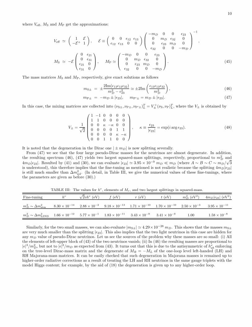
sol. (In detail, in Table III, we give the numerical values of these fine-tunings, wherethe parameters are given as before (30).)

TABLE III: The values for hν , elements of Mν , and two largest splittings in squared-mass.

Fine-tuning hν√

2vhν (eV) f (eV) r (eV) t (eV) m2D (eV2) 4mD|ǫ23| (eV2)

m2D ∼ ∆m2

atm 8.30 × 10−14 2.88 × 10−2 9.18 × 10−13 1.71 × 10−10 1.70 × 10−10 2.50 × 10−3 3.95 × 10−11

m2D ∼ ∆m2

LSND 1.66 × 10−12 5.77 × 10−1 1.83 × 10−11 3.43 × 10−9 3.41 × 10−9 1.00 1.58 × 10−8

Similarly, for the two small masses, we can also evaluate |mS±| ≃ 4.29×10−28 mD. This shows that the masses mS±

are very much smaller than the splitting |ǫ23|. This also implies that the two light neutrinos in this case are hidden forany mD value of pseudo-Dirac neutrinos. Let us see the sources of the problem why these masses are so small: (i) Allthe elements of left-upper block of (43) of the two neutrinos vanish; (ii) In (46) the resulting masses are proportional to|ǫ|3/m2

D, but not to |ǫ|2/mD as expected from (43). It turns out that this is due to the antisymmetric of hνab enforcing

on the tree-level Dirac-mass matrix and the degenerate of MR = −ML of the one-loop level left-handed (LH) andRH Majorana-mass matrices. It can be easily checked that such degeneration in Majorana masses is remained up tohigher-order radiative corrections as a result of treating the LH and RH neutrinos in the same gauge triplets with themodel Higgs content; for example, by the aid of (18) the degeneration is given up to any higher-order loop.

11

2. Radiative corrections to MD

As mentioned, the mass matrix MD requires the one-loop corrections as given in Fig. 5, and the contributions areeasily obtained as follows

− i(M radD )abPL =

∫

d4p

(2π)4(−i2hν

acPL)i(p/+mc)

p2 −m2c

(

ihlcd

v√2PR

)

i(p/+md)

p2 −m2d

× (ihl∗bdPL)

−1

(p2 −m2φ1

)2

(

iλ3

u2 + ω2

2+ iλ4

u2

2

)

+

∫

d4p

(2π)4(

ihl∗acPL

) i(−p/+mc)

p2 −m2c

(

ihldc

v√2PR

)

i(−p/+md)

p2 −m2d

× (i2hνbdPL)

−1

(p2 −m2φ3

)2

(

iλ3

u2 + ω2

2+ iλ4

ω2

2

)

. (49)

We rewrite

(M radD )ab = − i

√2hν

ab

v

{[

λ3(u2 + ω2) + λ4u

2]

m2bI(m

2b ,m

2φ1

)

+[

λ3(u2 + ω2) + λ4ω

2]

m2aI(m

2a,m

2φ3

)}

, (a, b not summed), (50)

where I(a, b) is given in (A6). With the help of (A7), the approximation for (50) is obtained by

(M radD )ab ≃ − hν

ab

8√

2π2v

{

[

λ3(u2 + ω2) + λ4u

2]

+[

λ3(u2 + ω2) + λ4ω

2] m2

a

m2H2

}

= −√

2hνab

(

λ3ω2

16π2v

)

[

1 +

(

1 +λ4

λ3

)(

u2

ω2+

m2a

m2H2

)

+ O(

u4

ω4,m4

a,b

m4H2

)]

. (51)

Because of the constraint (9) the higher-order corrections O(· · ·) can be neglected, thus M radD is rewritten as follows

(M radD )ab = −

√2hν

ab

(

λ3ω2

16π2v

)

(1 + δa) , δa ≡(

1 +λ4

λ3

)(

u2

ω2+

m2a

m2H2

)

, (52)

where δa is of course an infinitesimal coefficient, i.e., |δ| ≪ 1. Again, this implies also that if the fine-tuning is donethe resulting Dirac-mass matrix get trivially. It is due to the fact that the contribution of the term associated withδa in (52) is then very small and neglected, the remaining term gives an antisymmetric resulting Dirac-mass matrix,that is therefore unrealistic under the data.

With this result, it is worth noting that the scale

∣

∣

∣

∣

λ3ω2

16π2v

∣

∣

∣

∣

(53)

of the radiative Dirac masses (52) is in the orders of the scale v of the tree-level Dirac masses (20). Indeed, if oneputs |(λ3ω

2)/(16π2v)| = v and takes |λ3| ∼ 0.1 − 1, then ω ∼ 3 − 10 TeV as expected in the constraints [9, 18]. Theresulting Dirac-mass matrix which is combined of (20) and (52) therefore gets two typical examples of the bounds:(i) (λ3ω

2)/(16π2v)+ v ∼ O(v); (ii) (λ3ω2)/(16π2v)+ v ∼ O(0). The first case (i) yields that the status on the masses

of neutrinos as given above is remained unchanged and therefore is also trivial as mentioned. In the last case (ii), thecombination of (20) and (52) gives

(MD)ab =√

2hνab(vδa). (54)

It is interesting that in this case the scale v for the Dirac masses (20) gets naturally a large reduction, and we arguethat this is not a fine-tuning. Because the large radiative mass term in (52) is canceled by the tree-level Dirac masses,we mean this as a finite renormalization in the masses of neutrinos. It is also noteworthy that, unlike the case of thetree-level mass term (20), the mass matrix (54) is now nonantisymmetric in a and b . Thus all the three eigenvaluesof this matrix are nonzero. Let us recall that in the first case (i) the zero eigenvalue is, however, retained because thecombination of (20) and (52) is proportional to hν

abv.

12

In contrast to (31), in this case there is no large hierarchy between ML,R and MD. To see this explicitly, let us takethe values of the parameters as given before (30), thus λ3 ≃ −1.06 and the coefficients δa are evaluated by

δe ≃ 6.03 × 10−7, δµ ≃ 6.23 × 10−7, δτ ≃ 6.28 × 10−6. (55)

Hence, we get

|ML,R|/|MD| ∼ 10−2 − 10−3. (56)

With the values given in (55), the quantities hν and mD can be evaluated through the mass term (54); the neutrinodata imply that hν and mD are in the orders of he and me - the Yukawa coupling and mass of electron, respectively.It is worth checking that the two largest squared-mass splittings as given before can be applied on this case of (56),and seeing that they fit naturally the data.

C. Mass contributions from heavy particles

There remain now two questions not yet answered: (i) The degeneration of MR = −ML; (ii) The hierarchy of ML,R

and MD (56) can be continuously reduced? As mentioned, we will prove that the new physics gives us the solution.The mass Lagrangian for the neutrinos given by the operator (17) can be explicitly written as follows

LLNVmass = sν

abM−1(〈χ∗〉ψcaL)(〈χ∗〉ψbL) +H.c.

= sνabM−1

(

u√2νc

aL +ω√2νaR

)(

u√2νbL +

ω√2νc

bR

)

+H.c.

= −1

2Xc

LMnewν XL +H.c., (57)

where the mass matrix for the neutrinos is obtained by

Mnewν ≡ −

(

u2

Msν uω

Msν

uωMsν ω2

Msν

)

, (58)

in which, the coupling sνab is symmetric in a and b. Because of the hierarchies u2 ≪ uω ≪ ω2 corresponding of the

submatrices MnewL , Mnew

D and MnewR of (58), the two questions as mentioned are solved simultaneously. Intriguing

comparisons between sν and hν are given in order

1. hν conserves the lepton number; sν violates this charge.

2. hν is antisymmetric and enforcing on the Dirac-mass matrix; sν is symmetric and breaks this property.

3. hν preserves the degeneration of MR = −ML; sν breaks the MR = −ML.

4. A pair of (sν , hν) in the lepton sector will complete the rule played by the quark couplings (sq, hq) [10].

5. hν defines the interactions in the SM scale v; sν gives those in the GUT scale M.

Let us now take the values M ≃ 1016 GeV, ω ≃ 3000 GeV, u ≃ 2.46 GeV and sν ∼ O(1) (perhaps smaller), thesubmatrices Mnew

L ≃ −6.05 × 10−7sν eV and MnewD ≃ −7.38 × 10−4sν eV can give contributions (to the diagonal

components of ML and MD, respectively) but very small. It is noteworthy that the last one MnewR ≃ −0.9sν eV can

dominate MR.To summarize, in this model the neutrino mass matrix is combined by Mν +Mnew

ν where the first term is definedby (22), and the last term by (58); the submatrices of Mν are given in (28) and (54), respectively. Dependence on thestrength of the new physics coupling sν , the submatrices of the last term, Mnew

L and MnewD , are included or removed.

IV. CONCLUSIONS

The basic motivation of this work is to study neutrino mass in the framework of the model based on SU(3)C ⊗SU(3)L ⊗U(1)X gauge group contained minimal Higgs sector with right-handed neutrinos. In this paper, the massesof neutrinos are given by three different sources widely ranging over the mass scales including the GUT’s and the

13

small VEV u of spontaneous lepton breaking. We have shown that, at the tree-level, there are three Dirac neutrinos:one massless and two degenerate with the masses in the order of the electron mass. At the one-loop level, a possibleframework for the finite renormalization of the neutrino masses is obtained. The Dirac masses obtain a large reduction,the Majorana mass types get degenerate in MR = −ML, all these masses are in the bound of the data. It is emphasizedthat the above degeneration is a consequence of the fact that the left-handed and right-handed neutrinos, in this model,are in the same gauge triplets. The new physics including the 3-3-1 model are strongly signified. The degenerationsand the hierarchies among the mass types are completely removed by heavy particles.

We have shown that the three couplings λ1,2,4 of the Higgs potential are constrained by the scalar masses, theremainder λ3 is free, negative [8] and now fixed by the neutrino masses. This means also that the generation ofthe neutrino masses leads to a shift (down) in mass of the Higgs boson from the SM prediction. In this model, theGoldstone boson GX ∼ χ0

1 of the non-Hermitian neutral bilepton gauge boson X0 [8] is also a Majoron associated withthe neutrino Majorana masses. The coupling of HGXGX is given at the tree-level [8] and will provide a considerablecontribution in the invisible modes of decay of the SM Higgs boson.

The resulting mass matrix for the neutrinos consists of two parts Mν +Mnewν : the first is mediated by the model

particles, and the last is due to the new physics. Upon the contributions of Mnewν , the different realistic mass textures

can be produced such as pseudo-Dirac patterns associated with the seesaw one are obtained in case of the last termhidden (neglected). In another scenario, that the bare coupling hν of Dirac masses get higher values, for example, inorders of hµ,τ , the VEV ω can be picked up to an enough large value (∼ O(104−105) TeV) so that the type II seesawspectrum is obtained. Such features deserves further study.

Acknowledgments

P. V. D is grateful to the National Center for Theoretical Sciences of the National Science Council of the Republicof China for financial support. He thanks Kingman Cheung and Members of the Focus Group on Particle Physics atNational Tsing Hua University for their kind help and support. H. N. L. is supported by JSPS grant No: S-06185,he would also like to thank C. S. Lim and Members of Department of Physics, Kobe University for warm hospitalityduring his visit where this work was completed. The work was also supported in part by National Council for NaturalSciences of Vietnam.

APPENDIX A: FEYNMAN INTEGRATION

In this Appendix, we present evaluation of the integral

I(a, b, c) ≡∫

d4p

(2π)4p2

(p2 − a)2(p2 − b)(p2 − c), (A1)

where a, b, c > 0 and I(a, b, c) = I(a, c, b) should be noted in use.In the case of b 6= c and b, c 6= a, we introduce a well-known integral as follows

∫

d4p

(2π)41

(p2 − a)(p2 − b)(p2 − c)=

−i16π2

{

a lna

(a− b)(a− c)+

b ln b

(b− a)(b − c)+

c ln c

(c− b)(c− a)

}

. (A2)

Differentiating two sides of this equation with respect to a we have

∫

d4p

(2π)41

(p2 − a)2(p2 − b)(p2 − c)=

−i16π2

{

ln a+ 1

(a− b)(a− c)− a(2a− b − c) ln a

(a− b)2(a− c)2

+b ln b

(b− a)2(b − c)+

c ln c

(c− a)2(c− b)

}

. (A3)

Combining (A2) and (A3) the integral (A1) becomes

I(a, b, c) =

∫

d4p

(2π)4

[

1

(p2 − a)(p2 − b)(p2 − c)+

a

(p2 − a)2(p2 − b)(p2 − c)

]

=−i

16π2

{

a(2 lna+ 1)

(a− b)(a− c)− a2(2a− b− c) ln a

(a− b)2(a− c)2+

b2 ln b

(b − a)2(b− c)+

c2 ln c

(c− a)2(c− b)

}

. (A4)

14

If a, b≫ c or c ≃ 0, we have an approximation as follows

I(a, b, c) ≃ − i

16π2

1

a− b

[

1 − b

a− blna

b

]

. (A5)

In the other case with b = c and b 6= a, we have also

I(a, b) ≡ I(a, b, b) = − i

16π2

[

a+ b

(a− b)2− 2ab

(a− b)3lna

b

]

, (A6)

where, also, I(a, b) = I(b, a) should be noted in use.If b≫ a or a ≃ 0, we have the following approximation

I(a, b) ≃ − i

16π2b. (A7)

Let us note that the above approximations aI(a, b, c) (or bI(a, b, c)) and bI(a, b) are kept in the orders up toO(c/a, c/b) and O(a/b), respectively.

[1] SuperKamiokande Collaboration, Y. Fukuda et al., Phys. Rev. Lett. 81, 1158 (1998); 81, 1562 (1998); 82, 2644 (1999);85, 3999 (2000); Y. Suzuki, Nucl. Phys. B, Proc. Suppl. 77, 35 (1999); S. Fukuda et al., Phys. Rev. Lett. 86, 5651 (2001);Y. Ashie et al., Phys. Rev. Lett. 93, 101801 (2004).

[2] KamLAND Collaboration, K. Eguchi et al., Phys. Rev. Lett. 90, 021802 (2003); T. Araki et al., Phys. Rev. Lett. 94,081801(2005).

[3] SNO Collaboration, Q. R. Ahmad et al., Phys. Rev. Lett. 89, 011301 (2002); 89, 011302 (2002); 92, 181301 (2004); B.Aharmim et al., Phys. Rev. C 72, 055502 (2005).

[4] F. Pisano and V. Pleitez, Phys. Rev. D 46, 410 (1992); P. H. Frampton, Phys. Rev. Lett. 69, 2889 (1992); R. Foot, O. F.Hernandez, F. Pisano and V. Pleitez, Phys. Rev. D 47, 4158 (1993).

[5] M. Singer, J. W. F. Valle and J. Schechter, Phys. Rev. D 22, 738 (1980); R. Foot, H. N. Long and Tuan A. Tran, Phys.Rev. D 50, 34(R) (1994); J. C. Montero, F. Pisano and V. Pleitez, Phys. Rev. D 47, 2918 (1993); H. N. Long, Phys. Rev.D 54, 4691 (1996); 53, 437 (1996).

[6] P. V. Dong, H. N. Long, D. T. Nhung and D. V. Soa, Phys. Rev. D 73, 035004 (2006).[7] W. A. Ponce, Y. Giraldo and L. A. Sanchez, Phys. Rev. D 67, 075001 (2003).[8] P. V. Dong, H. N. Long and D. V. Soa, Phys. Rev. D 73, 075005 (2006).[9] P. V. Dong, H. N. Long and D. T. Nhung, Phys. Lett. B 639, 527 (2006).

[10] P. V. Dong, Tr. T. Huong, D. T. Huong and H. N. Long, Phys. Rev. D 74, 053003 (2006).[11] P. Minkowski, Phys. lett. B 67, 421 (1977); M. Gell-Mann, P. Ramond and R. Slansky, Complex spinors and unified

theories, in Supergravity, edited by P. van Nieuwenhuizen and D. Z. Freedman (North Holland, Amsterdam, 1979), p. 315;T. Yanagida, in Proceedings of the Workshop on the Unified Theory and the Baryon Number in the Universe, edited by O.Sawada and A. Sugamoto (KEK, Tsukuba, Japan, 1979), p. 95; S. L. Glashow, The future of elementary particle physics,in Proceedings of the 1979 Cargese Summer Institute on Quarks and Leptons, edited by M. Levy et al. (Plenum Press,New York, 1980), pp. 687-713; R. N. Mohapatra and G. Senjanovic, Phys. Rev. Lett. 44, 912 (1980); See also the type IIseesaw: R. N. Mohapatra and G. Senjanovic, Phys. Rev. D 23, 165 (1981); G. Lazarides, Q. Shafi and C. Wetterich, Nucl.Phys. B 181, 287 (1981); J. Schechter and J. W. Valle, Phys. Rev. D 25, 774 (1982).

[12] D. Chang and H. N. Long, Phys. Rev. D 73, 053006 (2006).[13] M. B. Tully and G. C. Joshi, Phys. Rev. D 64, 011301 (2001).[14] G.B. Gelmini and M. Roncadelli, Phys. Lett. B 99, 411 (1981); S. Bertolini and A. Santamaria, Nucl. Phys. B 310, 714

(1988); Y. Chikashige, R. N. Mohapatra and R. D. Peccei, Phys. Lett. B 98, 265 (1981); Phys. Rev. Lett. 45, 1926 (1980);D. Chang, W. Y. Keung and P. B. Pal, Phys. Rev. Lett. 61, 2420 (1988).

[15] R. A. Diaz, R. Martinez and F. Ochoa, Phys. Rev. D 69, 095009 (2004).[16] F. Pisano and S. S. Sharma, Phys. Rev. D 57, 5670 (1998); J. C. Montero, C. A. de S. Pires and V. Pleitez, Phys. Rev.

D 60, 098701 (1999); J. C. Montero, C. A. de S. Pires and V. Pleitez, Phys. Rev. D 64 096001 (2001); C. A. de S. Piresand P. S. Rodrigues da Silva, Eur. Phys. J. C 36, 397 (2004); A. G. Dias, A. Doff, C. A. de S. Pires and P. S. Rodriguesda Silva, Phys. Rev. D 72, 035006 (2005).

[17] S. Weinberg, Phys. Rev. Lett. 43, 1566 (1979); F. Wilczek and A. Zee, Phys. Rev. Lett. 43, 1571 (1979).[18] A. Carcamo, R. Martinez and F. Ochoa, Phys. Rev. D 73, 035007 (2006); F. Ochoa and R. Martinez, Phys. Rev. D 72,

035010 (2005).[19] L. A. Sanchez, W. A. Ponce and R. Martinez, Phys. Rev. D 64, 075013 (2001); R. Martinez, W. A. Ponce and L. A.

Sanchez, Phys. Rev. D 65, 055013 (2002); S. Sen and A. Dixit, Phys. Rev. D 71, 035009 (2005); D. A. Gutierrez, W. A.Ponce and L. A. Sanchez, Eur. Phys. J. C 46, 497 (2006); and in Ref.[22].

15

[20] J. C. Pati and A. Salam, Phys. Rev. D 10, 275 (1974); H. Geogri and S. L. Glashow, Phys. Rev. Lett. 32, 438 (1974); H.Georgi, H. R. Quinn and S. Weinberg, Phys. Rev. Lett. 33, 451 (1974); H. Georgi, in Particles and Fields, edited by C. E.Carlson (A.I.P., New York, 1975); H. Fritzsch and P. Minkowski, Ann. Phys. 93, 193 (1975); F. Gursey, P. Ramond andP. Sikivie, Phys. Lett. B 60, 177 (1975).

[21] A. G. Dias, C. A. de S. Pires and P. S. Rodrigues da Silva, Phys. Lett. B 628, 85 (2005).[22] J. C. Montero et. al. in Ref. [5]; D. A. Gutierrez, W. A. Ponce and L. A. Sanchez, Int. J. Mod. Phys. A 21, 2217 (2006).[23] Conventions of the charge-conjugation, the mass-matrices, and the Feynman-rules given in this work can find in: S. M.

Bilenky, C. Giunti and W. Grimus, Prog. Part. Nucl. Phys. 43, 1 (1999); A. Denner, H. Eck, O. Hahn and J. Kublbeck,Nucl. Phys. B 387, 467 (1992).

[24] W. -M. Yao et. al. (Particle Data Group), J. Phys. G: Nucl. Part. Phys. 33, 1 (2006), and references therein.[25] See also: R. D. Peccei, hep-ph/0609203; A. Yu. Smirnov, hep-ph/0411194.[26] M. Kobayashi and C. S. Lim, Phys. Rev. D 64, 013003 (2001).[27] S. M. Bilenky and B. Pontecorvo, Phys. Rept. 41, 225 (1978); L. Wolfenstein, Nucl. Phys. B 186, 147 (1981); S. T. Petcov,

Phys. Lett. B 110, 245 (1982); S. M. Bilenky and B. Pontecorvo, Sov. J. Nucl. Phys. 38, 248 (1983); S. M. Bilenky and S.T. Petcov, Rev. Mod. Phys. 59, 671 (1987); M. Kobayashi, C. S. Lim and M. M. Nojiri, Phys. Rev. Lett. 67 1685 (1991);C. Giunti, C. W. Kim and U. W. Lee, Phys. Rev. D 46, 3034 (1992); J. P. Bowes and R. R. Volkas, J. Phys. G 24, 1249(1998); M. Kobayashi and C. S. Lim in Ref. [26]; K. R. Balaji, A. Kalliomaki and J. Maalampi, Phys. Lett. B 524, 153(2002); J. F. Beacom et al., Phys. Rev. Lett. 92, 011101 (2004).

[28] Ta-Pei Cheng and Ling-Fong Li, Gauge Theory of Elementary Particle Physics (Clarendon Press, Oxford, 2004), p. 357.