Economical & Physical Justification For Canals - Lectures on ...
69
CHAPTER – 5 Economical & Physical Justification For Canals Dr. M. R. Kabir Professor and Head, Department of Civil Engineering University of Asia Pacific (UAP), Dhaka
-
Upload
khangminh22 -
Category
Documents
-
view
0 -
download
0
Transcript of Economical & Physical Justification For Canals - Lectures on ...
CHAPTER – 5
Economical & Physical
Justification For Canals
Dr. M. R. Kabir Professor and Head, Department of Civil Engineering
University of Asia Pacific (UAP), Dhaka

LECTURE 12
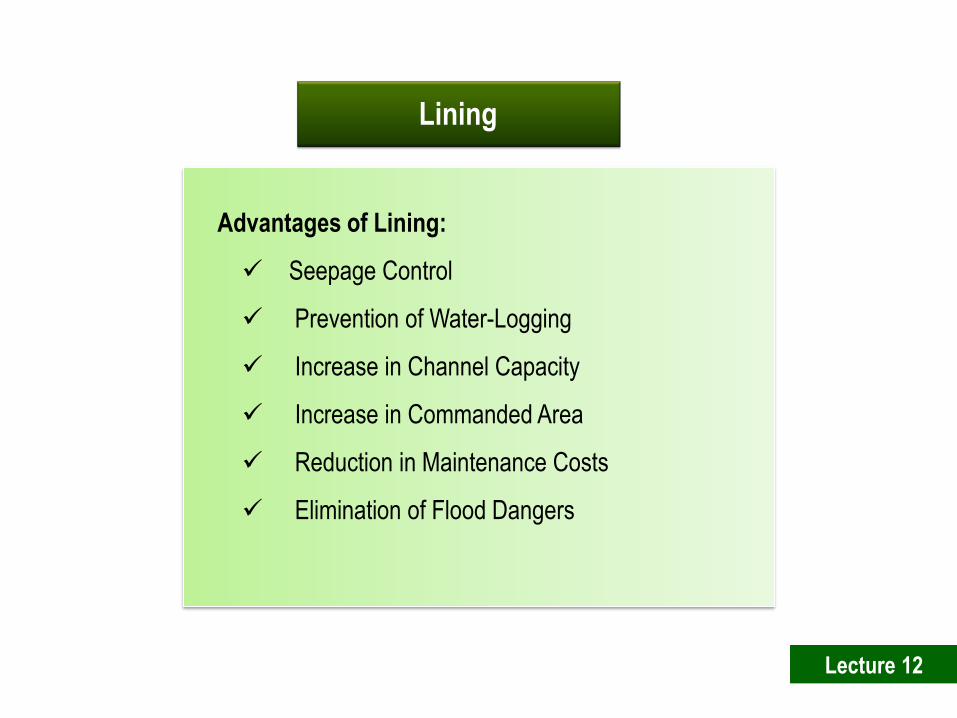
Lining
Advantages of Lining:
Seepage Control
Prevention of Water-Logging
Increase in Channel Capacity
Increase in Commanded Area
Reduction in Maintenance Costs
Elimination of Flood Dangers
Lecture 12
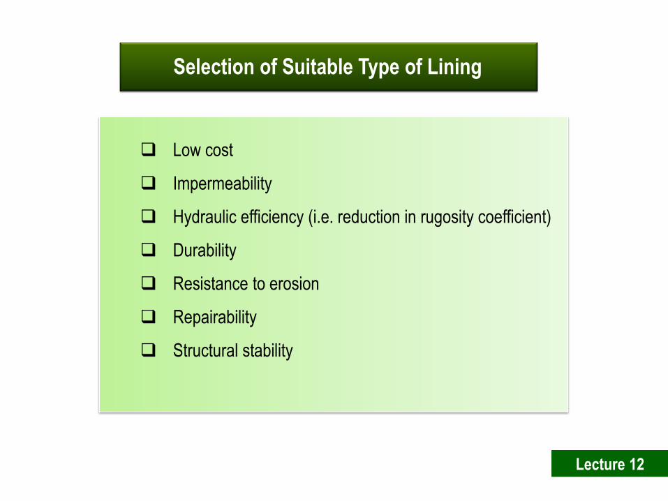
Selection of Suitable Type of Lining
Low cost
Impermeability
Hydraulic efficiency (i.e. reduction in rugosity coefficient)
Durability
Resistance to erosion
Repairability
Structural stability
Lecture 12

Financial Justification & Economics of Canal Lining
Annual benefits:
(a) Saved seepage water by lining:
Let, the rate of water is sold to the cultivators = Tk. R1/cumec
If m cumecs of water is saved by lining the canal annually, then the money saved by
lining = Tk. m R1
(b) Saving in maintenance cost:
Let, the average cost of annual upkeep of unlined channel = Tk. R2
If p is the percentage fraction of the saving achieved in maintenance cost by lining the
canal, then the amount saved = pR2 Tk.
The total annual benefits = mR1 + p R2
Lecture 12

Annual costs:
Let, the capital expenditure is C Tk. & the lining has a life of Y years
Annual depreciation charges = C/Y Tk.
Interest of the capital C = C(r/100) [r = percent of the rate of annual interest]
Average annual interest = C/2(r/100) Tk.
[Since the capital value of the asset decreases from C to zero in Y years]
The total annual costs of lining = C/Y + C/2(r/100)
Benefit cost ratio = =
If p is taken as 0.4, then
Benefit cost ratio =
Costs Annual
Benefits Annual
1002
4.0 21
rC
Y
C
RmR
Lecture 12
1002
21
rC
Y
C
pRmR
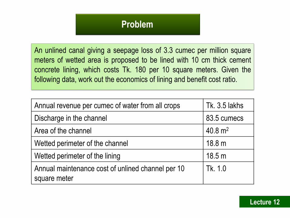
An unlined canal giving a seepage loss of 3.3 cumec per million square
meters of wetted area is proposed to be lined with 10 cm thick cement
concrete lining, which costs Tk. 180 per 10 square meters. Given the
following data, work out the economics of lining and benefit cost ratio.
Problem
Annual revenue per cumec of water from all crops Tk. 3.5 lakhs
Discharge in the channel 83.5 cumecs
Area of the channel 40.8 m2
Wetted perimeter of the channel 18.8 m
Wetted perimeter of the lining 18.5 m
Annual maintenance cost of unlined channel per 10
square meter
Tk. 1.0
Lecture 12
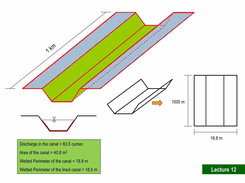
Discharge in the canal = 83.5 cumec
Area of the canal = 40.8 m2
Wetted Perimeter of the canal = 18.8 m
Wetted Perimeter of the lined canal = 18.5 m
18.8 m
1000 m
Lecture 12
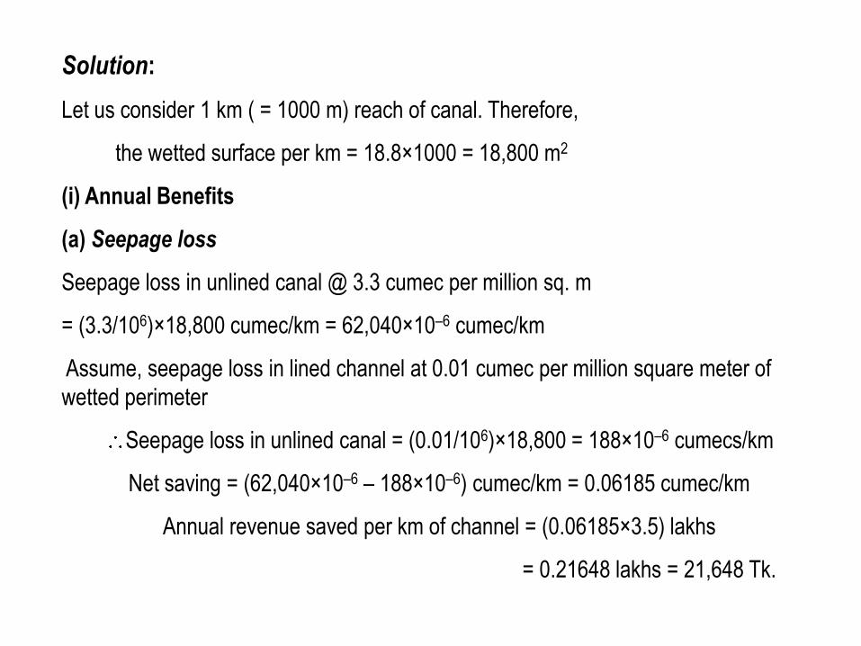
Solution:
Let us consider 1 km ( = 1000 m) reach of canal. Therefore,
the wetted surface per km = 18.8×1000 = 18,800 m2
(i) Annual Benefits
(a) Seepage loss
Seepage loss in unlined canal @ 3.3 cumec per million sq. m
= (3.3/106)×18,800 cumec/km = 62,040×10–6 cumec/km
Assume, seepage loss in lined channel at 0.01 cumec per million square meter of
wetted perimeter
Seepage loss in unlined canal = (0.01/106)×18,800 = 188×10–6 cumecs/km
Net saving = (62,040×10–6 – 188×10–6) cumec/km = 0.06185 cumec/km
Annual revenue saved per km of channel = (0.06185×3.5) lakhs
= 0.21648 lakhs = 21,648 Tk.
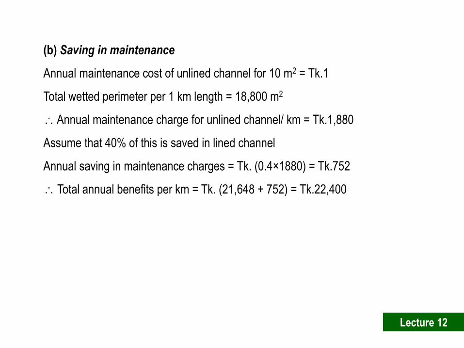
(b) Saving in maintenance
Annual maintenance cost of unlined channel for 10 m2 = Tk.1
Total wetted perimeter per 1 km length = 18,800 m2
Annual maintenance charge for unlined channel/ km = Tk.1,880
Assume that 40% of this is saved in lined channel
Annual saving in maintenance charges = Tk. (0.4×1880) = Tk.752
Total annual benefits per km = Tk. (21,648 + 752) = Tk.22,400
Lecture 12
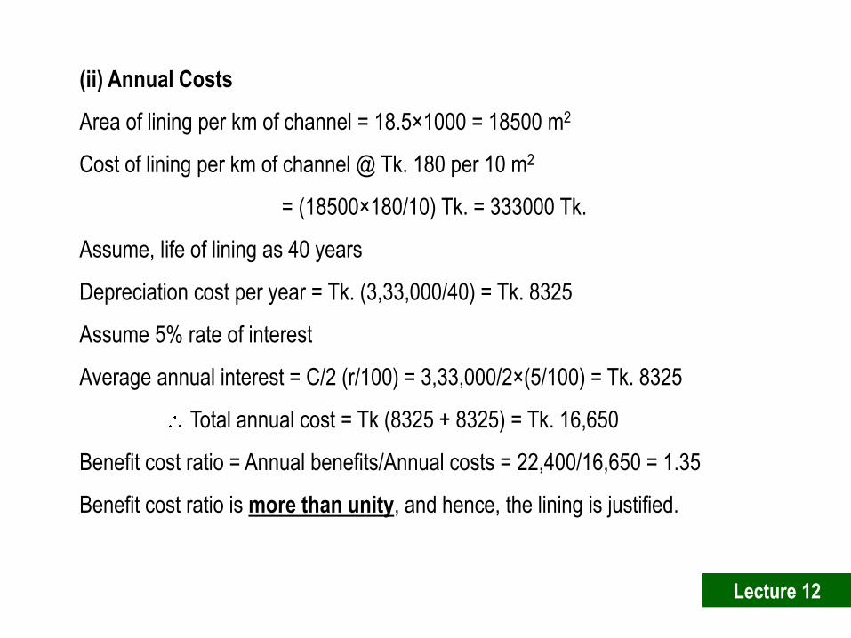
(ii) Annual Costs
Area of lining per km of channel = 18.5×1000 = 18500 m2
Cost of lining per km of channel @ Tk. 180 per 10 m2
= (18500×180/10) Tk. = 333000 Tk.
Assume, life of lining as 40 years
Depreciation cost per year = Tk. (3,33,000/40) = Tk. 8325
Assume 5% rate of interest
Average annual interest = C/2 (r/100) = 3,33,000/2×(5/100) = Tk. 8325
Total annual cost = Tk (8325 + 8325) = Tk. 16,650
Benefit cost ratio = Annual benefits/Annual costs = 22,400/16,650 = 1.35
Benefit cost ratio is more than unity, and hence, the lining is justified.
Lecture 12

LECTURE 13
Failure due to Subsurface Flow
(a) Failure by Piping or Undermining
(b) Failure by Direct Uplift
Failure by Surface Flow
(a) By Hydraulic Jump
(b) By Scouring
Lecture 13
Causes of failure of weir or barrage on
permeable foundation
The water from the upstream side continuously percolates through
the bottom of the foundation and emerges at the downstream end of
the weir or barrage floor. The force of percolating water removes the
soil particles by scouring at the point of emergence.
Lecture 13
(a) Failure by Piping or undermining
The percolating water exerts an upward pressure on the foundation of the
weir or barrage. If this uplift pressure is not counterbalanced by the self
weight of the structure, it may fail by rapture.
(b) Failure by Direct uplift
Lecture 13
When the water flows with a very high velocity over the crest of the weir or
over the gates of the barrage, then hydraulic jump develops. This
hydraulic jump causes a suction pressure or negative pressure on the
downstream side which acts in the direction uplift pressure. If the
thickness of the impervious floor is sufficient, then the structure fails by
rapture.
(a) Failure by Hydraulic Jump
Lecture 13

During floods, the gates of the barrage are kept open and the water flows
with high velocity. The water may also flow with very high velocity over the
crest of the weir. Both the cases can result in scouring effect on the
downstream and on the upstream side of the structure. Due to scouring of
the soil on both sides of the structure, its stability gets endangered by
shearing.
(b) Failure By Scouring
Lecture 13
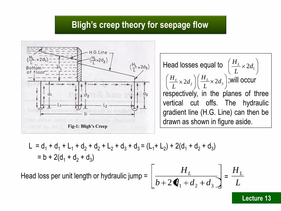
L = d1 + d1 + L1 + d2 + d2 + L2 + d3 + d3 = (L1+ L2) + 2(d1 + d2 + d3)
= b + 2(d1 + d2 + d3)
Head loss per unit length or hydraulic jump = 3212 dddb
H L
L
H L=
22dL
H L32d
L
H L
12dL
HL
Head losses equal to
;will occur
respectively, in the planes of three
vertical cut offs. The hydraulic
gradient line (H.G. Line) can then be
drawn as shown in figure aside.
Bligh’s creep theory for seepage flow
Lecture 13
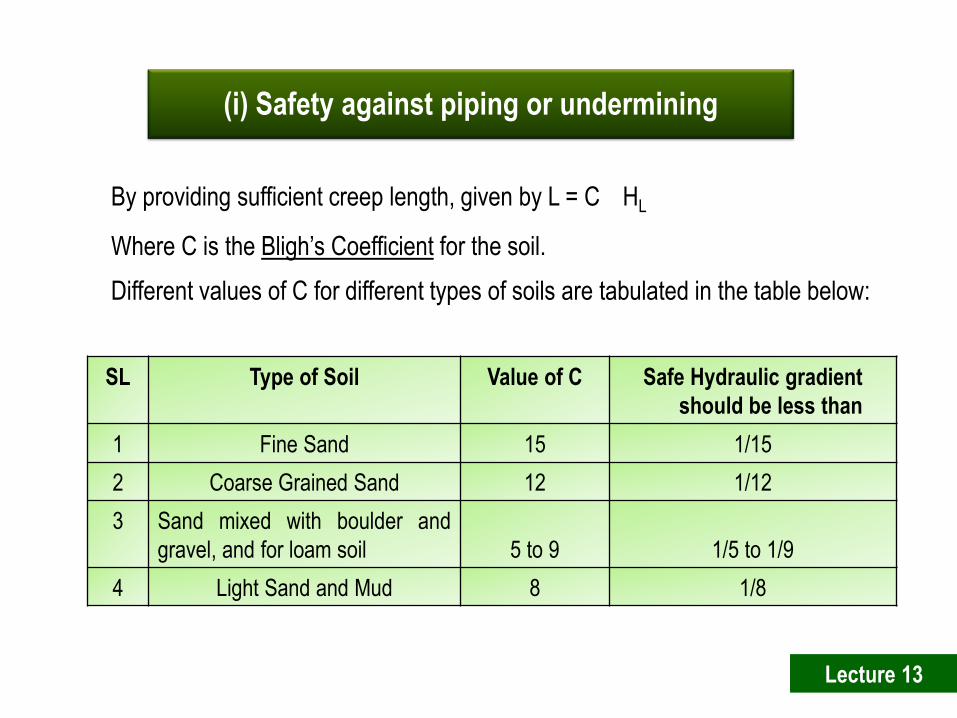
By providing sufficient creep length, given by L = C
HL
Where C is the Bligh’s Coefficient for the soil.
Different values of C for different types of soils are tabulated in the table below:
SL Type of Soil Value of C Safe Hydraulic gradient
should be less than
1 Fine Sand 15 1/15
2 Coarse Grained Sand 12 1/12
3 Sand mixed with boulder and
gravel, and for loam soil
5 to 9
1/5 to 1/9
4 Light Sand and Mud 8 1/8
(i) Safety against piping or undermining
Lecture 13

The ordinates of the H.G line above the bottom of the floor represent the residual
uplift water head at each point. Say for example, if at any point, the ordinate of
H.G line above the bottom of the floor is 1 m, then 1 m head of water will act as
uplift at that point. If h′ meters is this ordinate, then water pressure equal to h′
meters will act at this point, and has to be counterbalanced by the weight of the
floor of thickness say t.
Uplift pressure = γw
h′
[where γw is the unit weight of water]
Downward pressure = (γw
G).t
[Where G is the specific gravity of the floor material]
For equilibrium,
γw
h′ = (γw
G). t
h′ = G
t
(i) Safety against uplift pressure
Lecture 13

Where, h′ – t = h = Ordinate of the H.G line above the top of the floor
G – 1 = Submerged specific gravity of the floor material
Subtracting t on both sides, we get
(h′ – t) = (G
t – t) = t (G – 1)
t = = 1
'
G
th
1G
h
Lecture 13
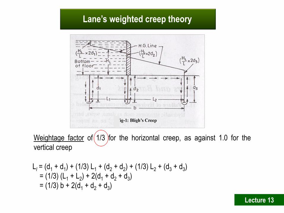
Ll = (d1 + d1) + (1/3) L1 + (d2 + d2) + (1/3) L2 + (d3 + d3)
= (1/3) (L1 + L2) + 2(d1 + d2 + d3)
= (1/3) b + 2(d1 + d2 + d3)
Weightage factor of 1/3 for the horizontal creep, as against 1.0 for the
vertical creep
Lane’s weighted creep theory
Lecture 13
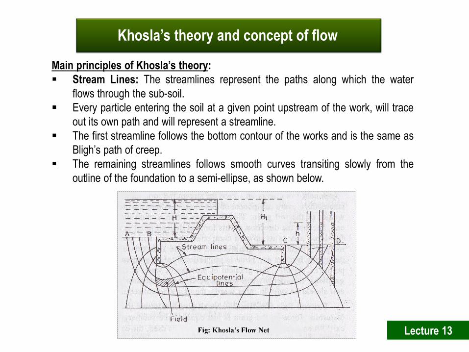
Khosla’s theory and concept of flow
Main principles of Khosla’s theory:
Stream Lines: The streamlines represent the paths along which the water
flows through the sub-soil.
Every particle entering the soil at a given point upstream of the work, will trace
out its own path and will represent a streamline.
The first streamline follows the bottom contour of the works and is the same as
Bligh’s path of creep.
The remaining streamlines follows smooth curves transiting slowly from the
outline of the foundation to a semi-ellipse, as shown below.
Lecture 13
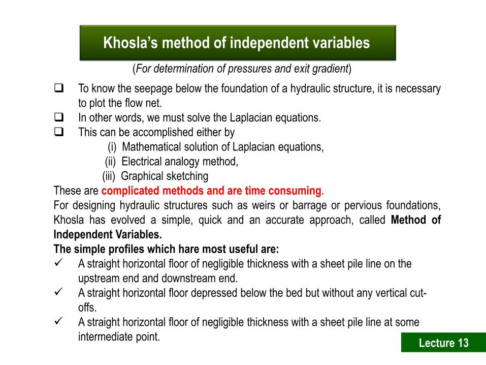
To know the seepage below the foundation of a hydraulic structure, it is necessary
to plot the flow net.
In other words, we must solve the Laplacian equations.
This can be accomplished either by
(i) Mathematical solution of Laplacian equations,
(ii) Electrical analogy method,
(iii) Graphical sketching
These are complicated methods and are time consuming.
For designing hydraulic structures such as weirs or barrage or pervious foundations,
Khosla has evolved a simple, quick and an accurate approach, called Method of
Independent Variables.
The simple profiles which hare most useful are:
A straight horizontal floor of negligible thickness with a sheet pile line on the
upstream end and downstream end.
A straight horizontal floor depressed below the bed but without any vertical cut-
offs.
A straight horizontal floor of negligible thickness with a sheet pile line at some
intermediate point.
(For determination of pressures and exit gradient)
Khosla’s method of independent variables
Lecture 13

a) Correction for the Mutual interference of Piles
b) Correction for the thickness of floor
c) Correction for the slope of the floor
Three corrections in Khosla’s theory
Lecture 13
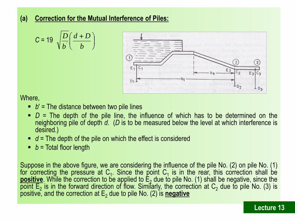
(a) Correction for the Mutual Interference of Piles:
Where,
b′ = The distance between two pile lines
D = The depth of the pile line, the influence of which has to be determined on the neighboring pile of depth d. (D is to be measured below the level at which interference is desired.)
d = The depth of the pile on which the effect is considered
b = Total floor length
Suppose in the above figure, we are considering the influence of the pile No. (2) on pile No. (1) for correcting the pressure at C1. Since the point C1 is in the rear, this correction shall be positive. While the correction to be applied to E2 due to pile No. (1) shall be negative, since the point E2 is in the forward direction of flow. Similarly, the correction at C2 due to pile No. (3) is positive, and the correction at E2 due to pile No. (2) is negative
C = 19 b
Dd
b
D'
Lecture 13

(b) Correction for thickness of floor:
The corrected pressure at E1 should be less than the calculated pressure at E1′
The correction to be applied for the joint E1 shall be negative.
The pressure calculated C1′ is less than the corrected pressure at C1
The correction to be applied at point C1 is positive.
Lecture 13
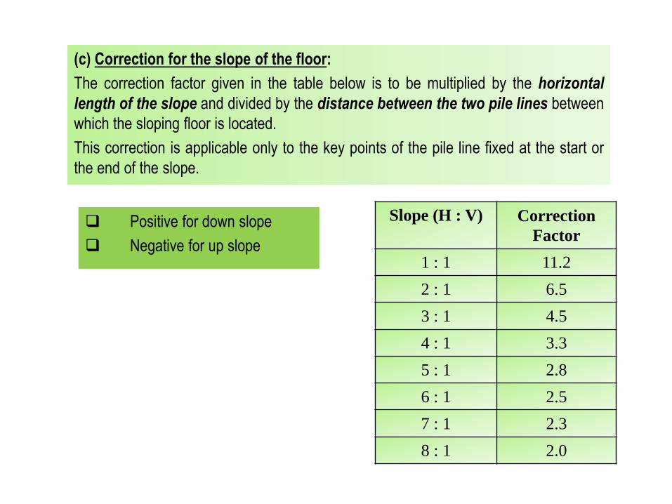
Slope (H : V) Correction
Factor
1 : 1 11.2
2 : 1 6.5
3 : 1 4.5
4 : 1 3.3
5 : 1 2.8
6 : 1 2.5
7 : 1 2.3
8 : 1 2.0
Positive for down slope
Negative for up slope
(c) Correction for the slope of the floor:
The correction factor given in the table below is to be multiplied by the horizontal
length of the slope and divided by the distance between the two pile lines between
which the sloping floor is located.
This correction is applicable only to the key points of the pile line fixed at the start or
the end of the slope.
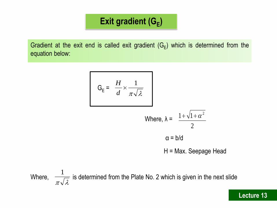
2
11 2
Where, λ =
α = b/d
H = Max. Seepage Head
GE = 1
d
H
Exit gradient (GE)
Gradient at the exit end is called exit gradient (GE) which is determined from the
equation below:
Where, is determined from the Plate No. 2 which is given in the next slide 1
Lecture 13
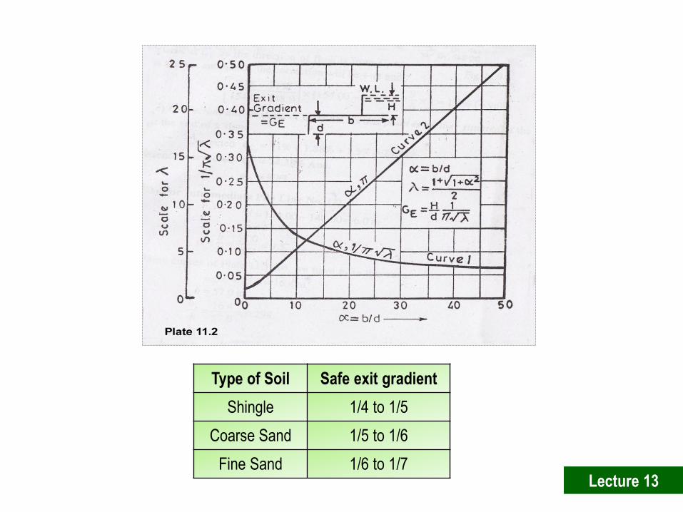
Type of Soil Safe exit gradient
Shingle 1/4 to 1/5
Coarse Sand 1/5 to 1/6
Fine Sand 1/6 to 1/7 Lecture 13

LECTURE 14
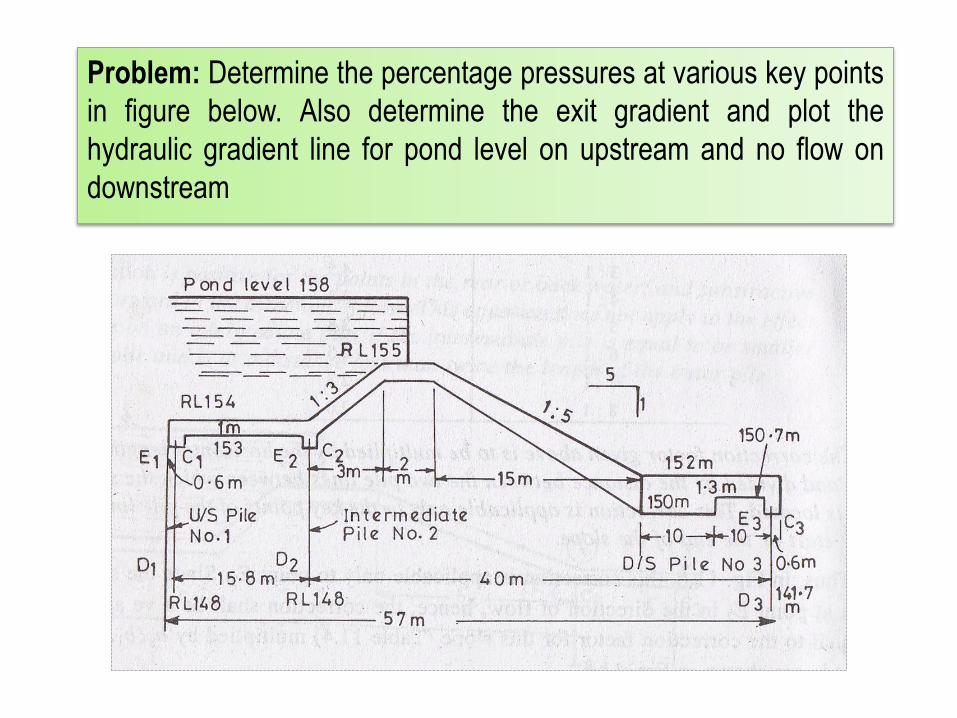
Problem: Determine the percentage pressures at various key points
in figure below. Also determine the exit gradient and plot the
hydraulic gradient line for pond level on upstream and no flow on
downstream
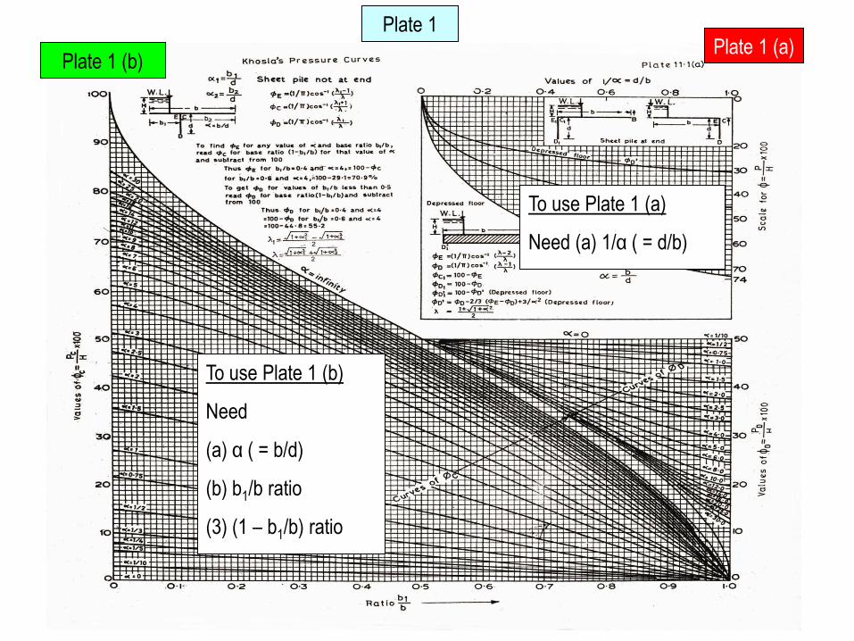
Plate 1 (a) Plate 1 (b)
Plate 1
To use Plate 1 (b)
Need
(a) α ( = b/d)
(b) b1/b ratio
(3) (1 – b1/b) ratio
To use Plate 1 (a)
Need (a) 1/α ( = d/b)
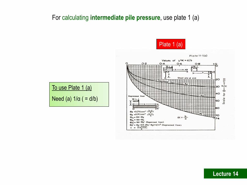
Plate 1 (a)
To use Plate 1 (a)
Need (a) 1/α ( = d/b)
For calculating intermediate pile pressure, use plate 1 (a)
Lecture 14
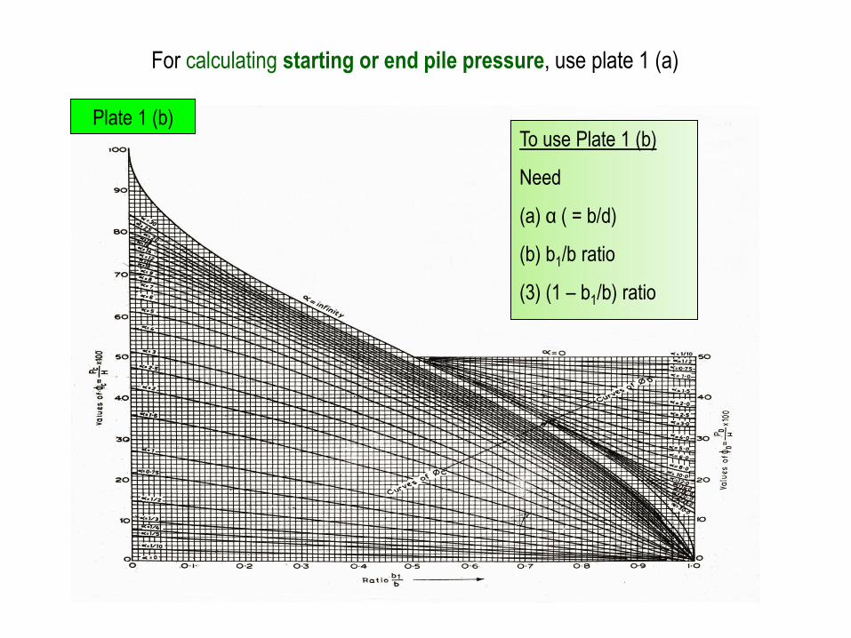
Plate 1 (b) To use Plate 1 (b)
Need
(a) α ( = b/d)
(b) b1/b ratio
(3) (1 – b1/b) ratio
For calculating starting or end pile pressure, use plate 1 (a)
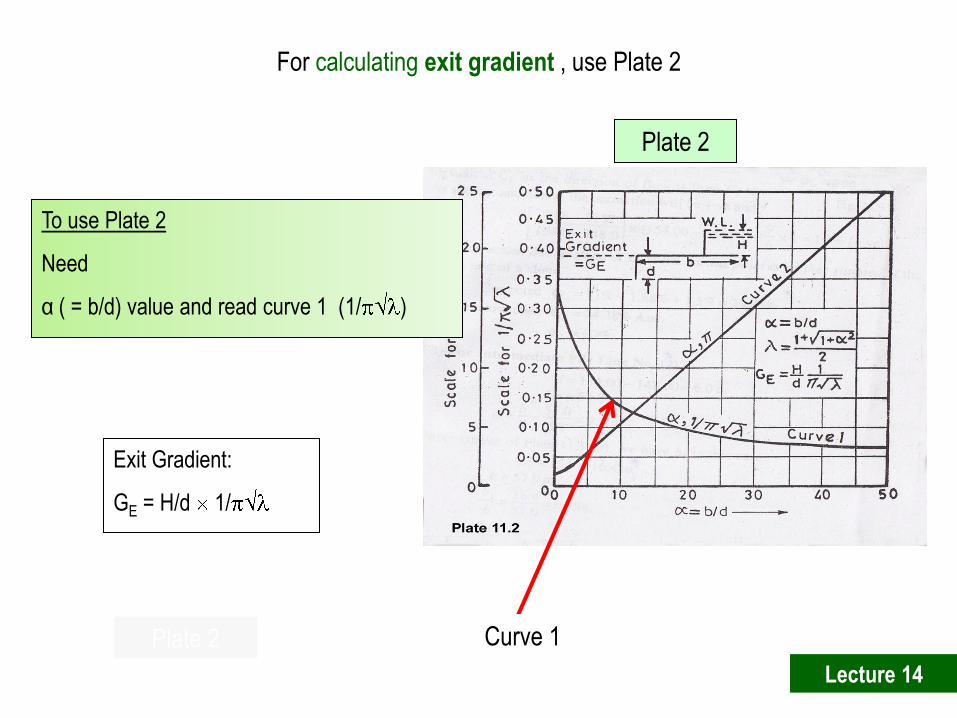
Plate 2
Plate 2
For calculating exit gradient , use Plate 2
To use Plate 2
Need
α ( = b/d) value and read curve 1 (1/ )
Exit Gradient:
GE = H/d 1/
Curve 1
Lecture 14
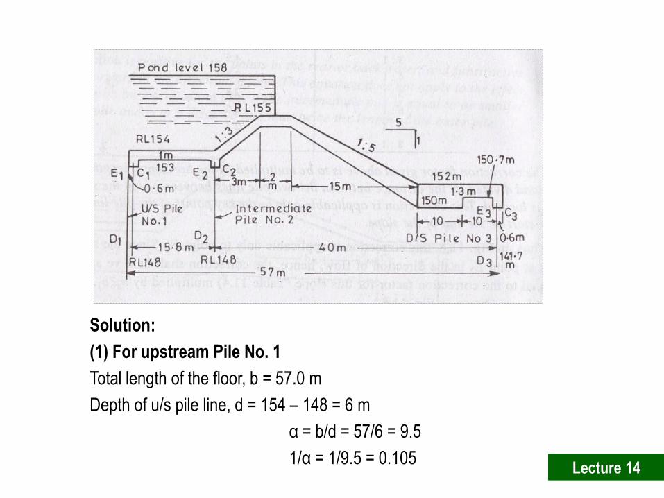
Solution:
(1) For upstream Pile No. 1
Total length of the floor, b = 57.0 m
Depth of u/s pile line, d = 154 – 148 = 6 m
α = b/d = 57/6 = 9.5
1/α = 1/9.5 = 0.105 Lecture 14
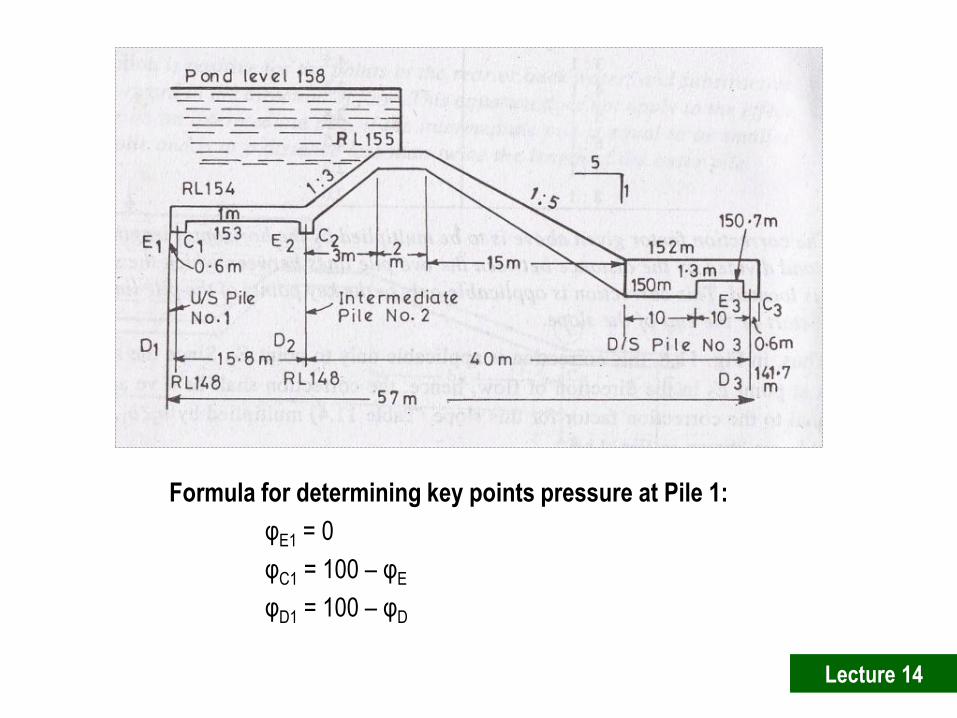
Formula for determining key points pressure at Pile 1:
φE1 = 0
φC1 = 100 – φE
φD1 = 100 – φD
Lecture 14

Plate 1 (a) Plate 1 (a)
0.105
φE = 29 %
φD = 20 %
Lecture 14
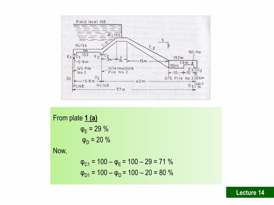
From plate 1 (a)
φE = 29 %
φD = 20 %
Now,
φC1 = 100 – φE = 100 – 29 = 71 %
φD1 = 100 – φD = 100 – 20 = 80 %
Lecture 14
At point C1 only
Corrections
Now
Lecture 14
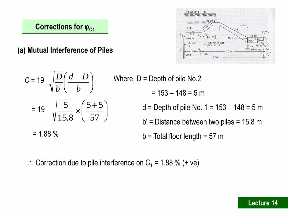
Corrections for φC1
(a) Mutual Interference of Piles
Where, D = Depth of pile No.2
= 153 – 148 = 5 m
d = Depth of pile No. 1 = 153 – 148 = 5 m
b′ = Distance between two piles = 15.8 m
b = Total floor length = 57 m
C = 19 b
Dd
b
D'
= 19
57
55
8.15
5
= 1.88 %
Correction due to pile interference on C1 = 1.88 % (+ ve)
Lecture 14
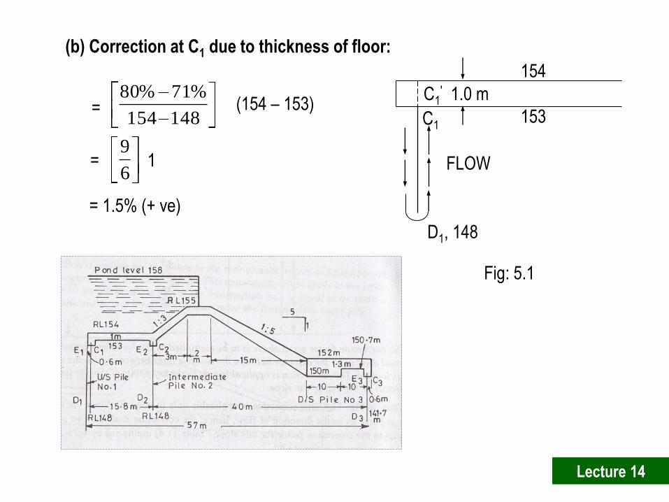
(b) Correction at C1 due to thickness of floor:
FLOW
C1
C1′ 1.0 m
153
154
D1, 148
Fig: 5.1
(154 – 153)
=
1 6
9
148154
%71%80=
= 1.5% (+ ve)
Lecture 14

After Corrections (For Pile No.1)
φE1 = 100 %
φD1= 80 %
φC1 = 74.38 %
(c) Correction due to slope at C1 is nil
Corrected (φC1) = 71 % + 1.88 % + 1.5 %
= 74.38 %
Lecture 14
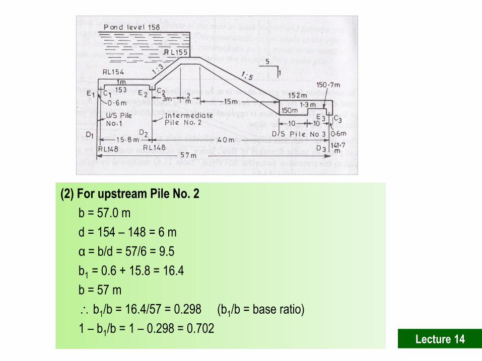
(2) For upstream Pile No. 2
b = 57.0 m
d = 154 – 148 = 6 m
α = b/d = 57/6 = 9.5
b1 = 0.6 + 15.8 = 16.4
b = 57 m
b1/b = 16.4/57 = 0.298 (b1/b = base ratio)
1 – b1/b = 1 – 0.298 = 0.702 Lecture 14

Formula for determining key points pressure at Pile 2:
φE2 = 100 – φC (1 – b1/b value & α )
φC2 = Direct value from chart (b1/b value & α )
φD2 = 100 – φD (1 – b1/b value & α )
Lecture 14
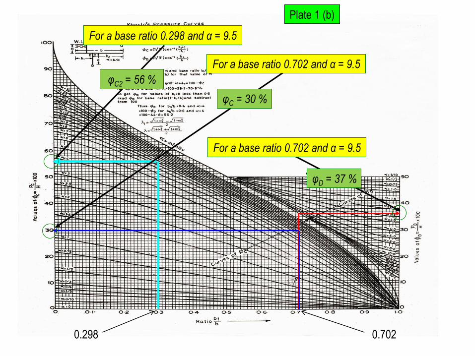
For a base ratio 0.298 and α = 9.5
φC2 = 56 %
For a base ratio 0.702 and α = 9.5
φC = 30 %
For a base ratio 0.702 and α = 9.5
φD = 37 %
Plate 1 (b)
0.702 0.298
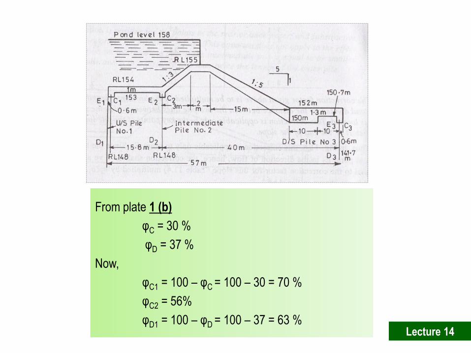
From plate 1 (b)
φC = 30 %
φD = 37 %
Now,
φC1 = 100 – φC = 100 – 30 = 70 %
φC2 = 56%
φD1 = 100 – φD = 100 – 37 = 63 %
Lecture 14
At points E2 & C2
Corrections
Now
Lecture 14
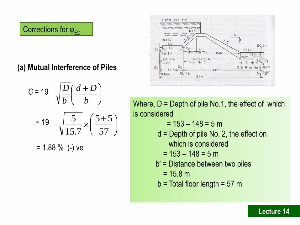
Corrections for φE2
Where, D = Depth of pile No.1, the effect of which
is considered
= 153 – 148 = 5 m
d = Depth of pile No. 2, the effect on
which is considered
= 153 – 148 = 5 m
b′ = Distance between two piles
= 15.8 m
b = Total floor length = 57 m
C = 19 b
Dd
b
D'
= 19
57
55
7.15
5
= 1.88 % (-) ve
(a) Mutual Interference of Piles
Lecture 14

(b) Thickness correction (φE2 )
=
Thickness of floor 22
D22
DEbetween Distance
Obs - Obs E
148154
%63%70=
1.0 = (7/6)
1.0 = 1.17 %
This correction is negative, E2
′ C2
′
E2 C2
Fig: 5.2
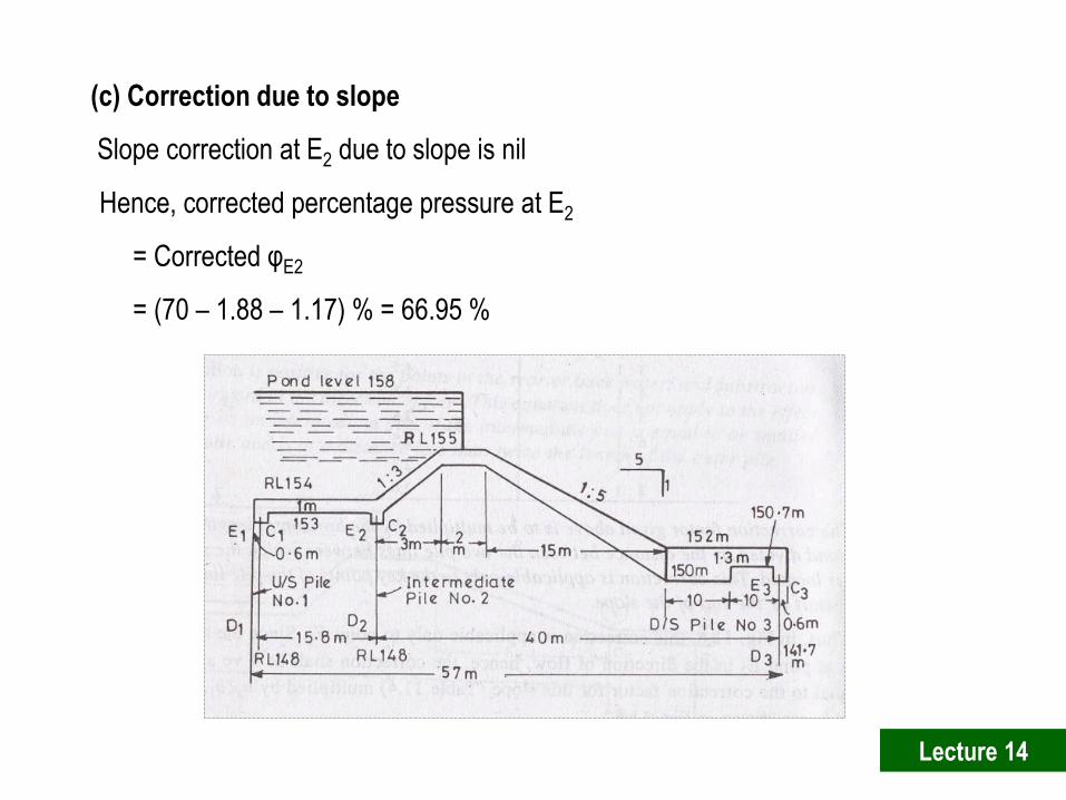
(c) Correction due to slope
Slope correction at E2 due to slope is nil
Hence, corrected percentage pressure at E2
= Corrected φE2
= (70 – 1.88 – 1.17) % = 66.95 %
Lecture 14

Corrections for φC2
Where, D = Depth of pile No.3, the effect of which is
considered
= 153 – 141.7 = 11.3 m
d = Depth of pile No. 2, the effect on which is
considered
= 153 – 148 = 5 m
b′ = Distance between two piles (2 &3)
= 40 m
b = Total floor length = 57 m
C = 19 b
Dd
b
D'
= 19
57
511
40
11
= 2.89 % (+) ve
(a) Mutual Interference of Piles
Lecture 14
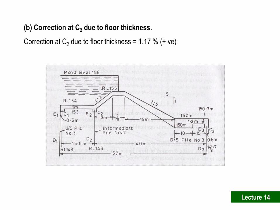
(b) Correction at C2 due to floor thickness.
Correction at C2 due to floor thickness = 1.17 % (+ ve)
Lecture 14
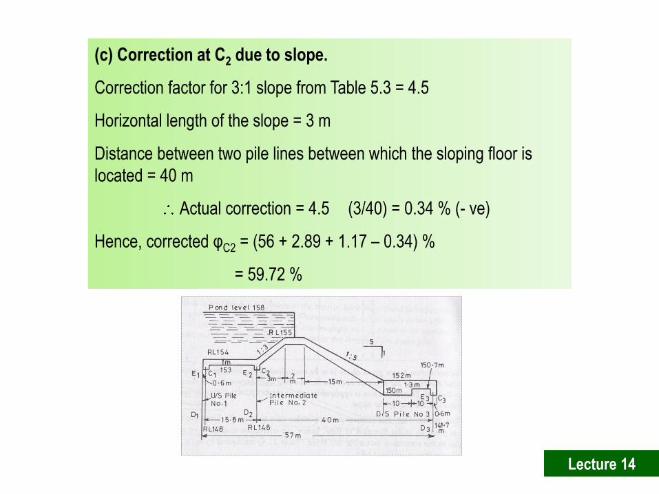
(c) Correction at C2 due to slope.
Correction factor for 3:1 slope from Table 5.3 = 4.5
Horizontal length of the slope = 3 m
Distance between two pile lines between which the sloping floor is
located = 40 m
Actual correction = 4.5
(3/40) = 0.34 % (- ve)
Hence, corrected φC2 = (56 + 2.89 + 1.17 – 0.34) %
= 59.72 %
Lecture 14
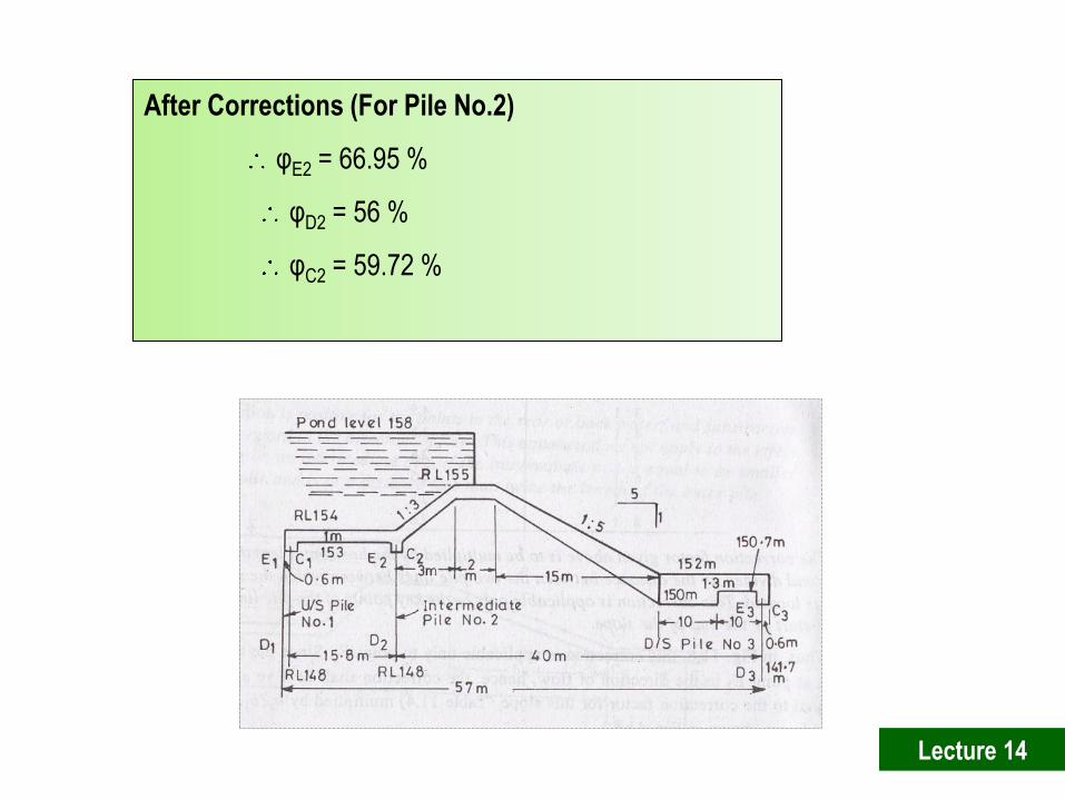
After Corrections (For Pile No.2)
φE2 = 66.95 %
φD2 = 56 %
φC2 = 59.72 %
Lecture 14

(3) For upstream Pile Line No. 3
b = 57 m
d = 152 – 141.7 = 10.3 m
1/α = d/b = 10.3/57 = 0.181
Lecture 14
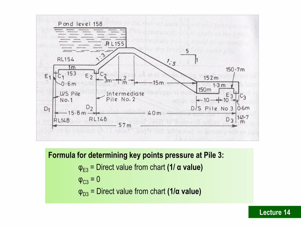
Formula for determining key points pressure at Pile 3:
φE3 = Direct value from chart (1/ α value)
φC3 = 0
φD3 = Direct value from chart (1/α value)
Lecture 14
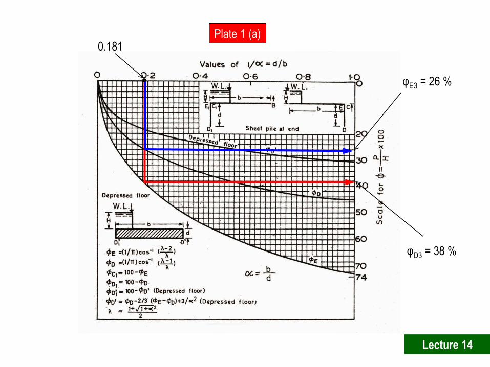
Plate 1 (a) Plate 1 (a)
0.181
φE3 = 26 %
φD3 = 38 %
Lecture 14

From plate 1 (a)
φE3 = 38 %
φD3 = 26%
Lecture 14

At point E3 only
Corrections
Now
Lecture 14
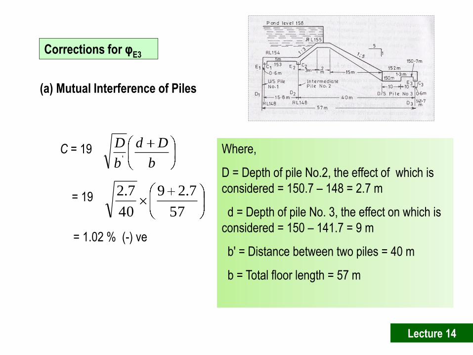
Corrections for φE3
C = 19 b
Dd
b
D'
= 19
57
7.29
40
7.2
= 1.02 % (-) ve
Where,
D = Depth of pile No.2, the effect of which is
considered = 150.7 – 148 = 2.7 m
d = Depth of pile No. 3, the effect on which is
considered = 150 – 141.7 = 9 m
b′ = Distance between two piles = 40 m
b = Total floor length = 57 m
(a) Mutual Interference of Piles
Lecture 14
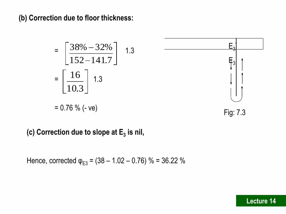
(b) Correction due to floor thickness:
=
1.3
=
1.3
= 0.76 % (- ve)
7.141152
%32%38
3.10
16
E3′
E3
Fig: 7.3
(c) Correction due to slope at E3 is nil,
Hence, corrected φE3 = (38 – 1.02 – 0.76) % = 36.22 %
Lecture 14
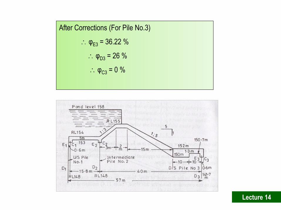
After Corrections (For Pile No.3)
φE3 = 36.22 %
φD3 = 26 %
φC3 = 0 %
Lecture 14
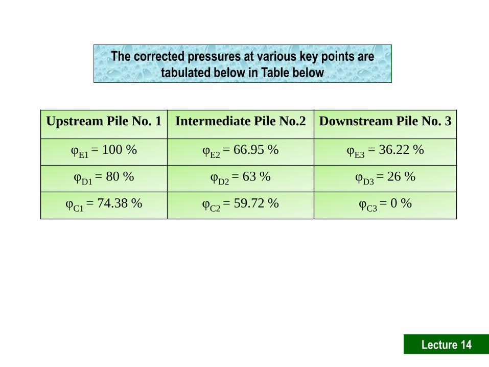
The corrected pressures at various key points are
tabulated below in Table below
Upstream Pile No. 1 Intermediate Pile No.2 Downstream Pile No. 3
φE1 = 100 % φE2 = 66.95 % φE3 = 36.22 %
φD1 = 80 % φD2 = 63 % φD3 = 26 %
φC1 = 74.38 % φC2 = 59.72 % φC3 = 0 %
Lecture 14
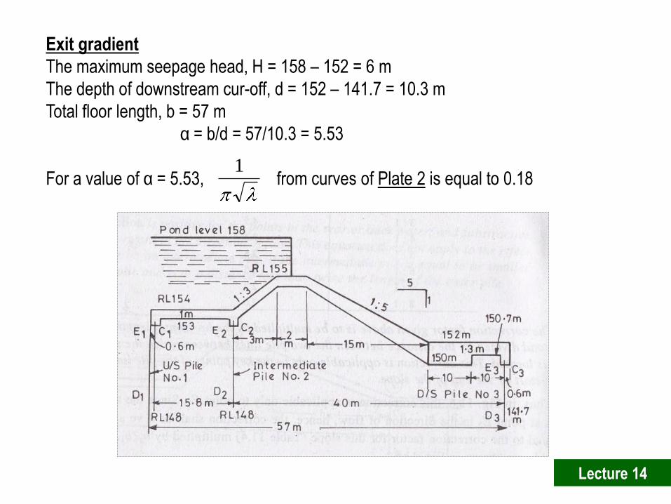
1
Exit gradient
The maximum seepage head, H = 158 – 152 = 6 m
The depth of downstream cur-off, d = 152 – 141.7 = 10.3 m
Total floor length, b = 57 m
α = b/d = 57/10.3 = 5.53
For a value of α = 5.53, from curves of Plate 2 is equal to 0.18
Lecture 14
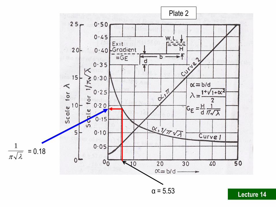
= 0.18 1
Plate 2
α = 5.53 Lecture 14
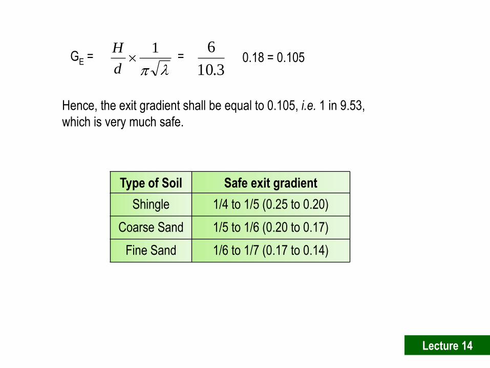
Hence, the exit gradient shall be equal to 0.105, i.e. 1 in 9.53,
which is very much safe.
1
d
H
3.10
6GE = =
0.18 = 0.105
Type of Soil Safe exit gradient
Shingle 1/4 to 1/5 (0.25 to 0.20)
Coarse Sand 1/5 to 1/6 (0.20 to 0.17)
Fine Sand 1/6 to 1/7 (0.17 to 0.14)
Lecture 14
End of Chapter – 5