
NEURAL NETWORKS - School of Computer Science
126
NEURAL NETWORKS Ivan F Wilde Mathematics Department King’s College London London, WC2R 2LS, UK [email protected]
-
Upload
khangminh22 -
Category
Documents
-
view
1 -
download
0
Transcript of NEURAL NETWORKS - School of Computer Science

NEURAL NETWORKS
Ivan F Wilde
Mathematics Department
King’s College London
London, WC2R 2LS, UK

Contents
1 Matrix Memory . . . . . . . . . . . . . . . . . . . . . . . . . . 1
2 Adaptive Linear Combiner . . . . . . . . . . . . . . . . . . . . 21
3 Artificial Neural Networks . . . . . . . . . . . . . . . . . . . . 35
4 The Perceptron . . . . . . . . . . . . . . . . . . . . . . . . . . 45
5 Multilayer Feedforward Networks . . . . . . . . . . . . . . . . . 75
6 Radial Basis Functions . . . . . . . . . . . . . . . . . . . . . . 95
7 Recurrent Neural Networks . . . . . . . . . . . . . . . . . . . . 103
8 Singular Value Decomposition . . . . . . . . . . . . . . . . . . 115
Bibliography . . . . . . . . . . . . . . . . . . . . . . . . . . . . . 121
Chapter 1
Matrix Memory
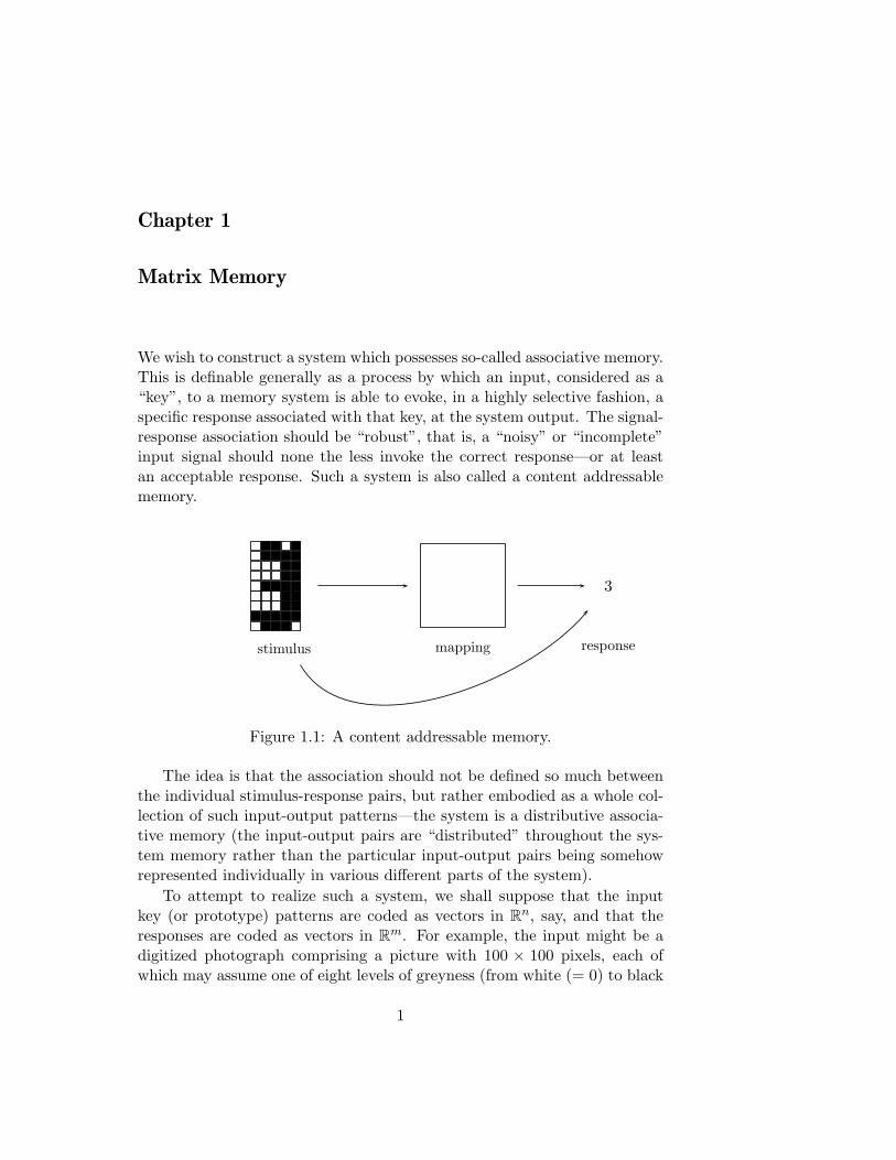
We wish to construct a system which possesses so-called associative memory.This is definable generally as a process by which an input, considered as a“key”, to a memory system is able to evoke, in a highly selective fashion, aspecific response associated with that key, at the system output. The signal-response association should be “robust”, that is, a “noisy” or “incomplete”input signal should none the less invoke the correct response—or at leastan acceptable response. Such a system is also called a content addressablememory.
3
stimulus mapping response
Figure 1.1: A content addressable memory.
The idea is that the association should not be defined so much betweenthe individual stimulus-response pairs, but rather embodied as a whole col-lection of such input-output patterns—the system is a distributive associa-tive memory (the input-output pairs are “distributed” throughout the sys-tem memory rather than the particular input-output pairs being somehowrepresented individually in various different parts of the system).
To attempt to realize such a system, we shall suppose that the inputkey (or prototype) patterns are coded as vectors in R
n, say, and that theresponses are coded as vectors in R
m. For example, the input might be adigitized photograph comprising a picture with 100 × 100 pixels, each ofwhich may assume one of eight levels of greyness (from white (= 0) to black
1
2 Chapter 1
(= 7)). In this case, by mapping the screen to a vector, via raster order, say,the input is a vector in R
10000 and whose components actually take valuesin the set {0, . . . , 7}. The desired output might correspond to the name ofthe person in the photograph. If we wish to recognize up to 50 people, say,then we could give each a binary code name of 6 digits—which allows up to26 = 64 different names. Then the output can be considered as an elementof R
6.Now, for any pair of vectors x ∈ R
n, y ∈ Rm, we can effect the map
x 7→ y via the action of the m × n matrix
M (x,y) = y xT
where x is considered as an n×1 (column) matrix and y as an m×1 matrix.Indeed,
M (x,y)x = y xT x
= α y,
where α = xT x = ‖x‖2, the squared Euclidean norm of x. The matrixyxT is called the outer product of x and y. This suggests a model for our“associative system”.
Suppose that we wish to consider p input-output pattern pairs, (x(1), y(1)),(x(2), y(2)), . . ., (x(p), y(p)). Form the m × n matrix
M =
p∑
i=1
y(i) x(i)T .
M is called the correlation memory matrix (corresponding to the given pat-tern pairs). Note that if we let X = (x(1) · · ·x(p)) and Y = (y(1) · · · y(p)) bethe n×p and m×p matrices with columns given by the vectors x(1), . . . , x(p)
and y(1), . . . , y(p), respectively, then the matrix∑p
i=1 y(i) x(i)T is just Y XT .Indeed, the jk-element of Y XT is
(Y XT )jk =
p∑
i=1
Yji(XT )ik =
p∑
i=1
YjiXki
=
p∑
i=1
y(i)j x
(i)k
which is precisely the jk-element of M .When presented with the input signal x(j), the output is
Mx(j) =
p∑
i=1
y(i) x(i)T x(j)
= y(j)x(j)T x(j) +
p∑
i=1i6=j
(x(i)T x(j))y(i).
Department of Mathematics

Matrix Memory 3
In particular, if we agree to “normalize” the key input signals so thatx(i)T x(i) = ‖x(i)‖2 = 1, for all 1 ≤ i ≤ p, then the first term on the righthand side above is just y(j), the desired response signal. The second term onthe right hand side is called the “cross-talk” since it involves overlaps (i.e.,inner products) of the various input signals.
If the input signals are pairwise orthogonal vectors, as well as beingnormalized, then x(i)T x(j) = 0 for all i 6= j. In this case, we get
Mx(j) = y(j)
that is, perfect recall. Note that Rn contains at most n mutually orthogonal
vectors.
Operationally, one can imagine the system organized as indicated in thefigure.
inputsignal ...
∈ Rn
...
∈ Rm
output
key patterns are loaded at beginning
↓ ↓ ↓
Figure 1.2: An operational view of the correlation memory matrix.
• start with M = 0,
• load the key input patterns one by one
M ← M + y(i)x(i)T , i = 1, . . . , p,
• finally, present any input signal and observe the response.
Note that additional signal-response patterns can simply be “added in”at any time, or even removed—by adding in −y(j)x(j)T . After the secondstage above, the system has “learned” the signal-response pattern pairs. Thecollection of pattern pairs (x(1), y(1)), . . . , (x(p), y(p)) is called the trainingset.
King’s College London
4 Chapter 1
Remark 1.1. In general, the system is a heteroassociative memory x(i)Ã
y(i), 1 ≤ i ≤ p. If the output is the prototype input itself, then the systemis said to be an autoassociative memory.
We wish, now, to consider a quantitative account of the robustness ofthe autoassociative memory matrix. For this purpose, we shall suppose thatthe prototype patterns are bipolar vectors in R
n, i.e., the components of
the x(i) each belong to {−1, 1}. Then ‖x(i)‖2 =∑n
j=1 x(i)j
2 = n, for each
1 ≤ i ≤ p, so that (1/√
n)x(i) is normalized. Suppose, further, that theprototype vectors are pairwise orthogonal (—this requires that n be even).The correlation memory matrix is
M =1
n
p∑
i=1
x(i) x(i)T
and we have seen that M has perfect recall, Mx(j) = x(j) for all 1 ≤ j ≤ p.We would like to know what happens if M is presented with x, a corruptedversion of one of the x(j). In order to obtain a bipolar vector as output, weprocess the output vector Mx as follows:
Mx à Φ(Mx)
where Φ : Rn → {−1, 1}n is defined by
Φ(z)k =
{1, if zk ≥ 0
−1, if zk < 0
for 1 ≤ k ≤ n and z ∈ Rn. Thus, the matrix output is passed through
a (bipolar) signal quantizer, Φ. To proceed, we introduce the notion ofHamming distance between pairs of bipolar vectors.
Let a = (a1, . . . , an) and b = (b1, . . . , bn) be elements of {−1, 1}n, i.e.,bipolar vectors. The set {−1, 1}n consists of the 2n vertices of a hypercubein R
n. Then
aT b =n∑
i=1
aibi = α − β
where α is the number of components of a and b which are the same, and βis the number of differing components (aibi = 1 if and only if ai = bi, andaibi = −1 if and only if ai 6= bi). Clearly, α + β = n and so aT b = n − 2β.
Definition 1.2. The Hamming distance between the bipolar vectors a, b,denoted ρ(a, b), is defined to be
ρ(a, b) = 12
n∑
i=1
|ai − bi|.
Department of Mathematics

Matrix Memory 5
Evidently (thanks to the factor 12), ρ(a, b) is just the total number of
mismatches between the components of a and b, i.e., it is equal to β, above.Hence
aT b = n − 2ρ(a, b).
Note that the Hamming distance defines a metric on the set of bipolarvectors. Indeed, ρ(a, b) = 1
2‖a − b‖1, where ‖ · ‖1 is the ℓ1-norm definedon R
n by ‖z‖1 =∑n
i=1 |zi|, for z = (z1, . . . , zn) ∈ Rn. The ℓ1-norm is also
known as the Manhatten norm—the distance between two locations is thesum of lengths of the east-west and north-south contributions to the journey,inasmuch as diagonal travel is not possible in Manhatten.
Hence, using x(i)T x = n − 2ρ(x(i), x), we have
Mx =1
n
p∑
i=1
x(i)x(i)T x
=1
n
p∑
i=1
(n − 2ρi(x))x(i),
where ρi(x) = ρ(x(i), x), the Hamming distance between the input vector xand the prototype pattern vector x(i).
Given x, we wish to know when x à x(m), that is, when x à Mx Ã
Φ(Mx) = x(m). According to our bipolar quantization rule, it will certainlybe true that Φ(Mx) = x(m) whenever the corresponding components of Mx
and x(m) have the same sign. This will be the case when (Mx)j x(m)j > 0,
that is, whenever
1
n(n − 2ρm(x)) x
(m)j x
(m)j︸ ︷︷ ︸
= 1
+1
n
p∑
i=1i6=m
(n − 2ρi(x))x(i)j x
(m)j > 0
for all 1 ≤ j ≤ n. This holds if
∣∣∣∣p∑
i=1i6=m
(n − 2ρi(x))x(i)j x
(m)j
∣∣∣∣ < n − 2ρm(x) ((∗))
for all 1 ≤ j ≤ n (—we have used the fact that if s > |t| then certainlys + t > 0).
We wish to find conditions which ensure that the inequality (∗) holds.By the triangle inequality, we get
∣∣∣∣p∑
i=1i6=m
(n − 2ρi(x))x(i)j x
(m)j
∣∣∣∣ ≤p∑
i=1i6=m
|n − 2ρi(x)| (∗∗)
King’s College London

6 Chapter 1
since |x(i)j x
(m)j | = 1 for all 1 ≤ j ≤ n. Furthermore, using the orthogonality
of x(m) and x(i), for i 6= m, we have
0 = x(i)T x(m) = n − 2ρ(x(i), x(m))
so that
|n − 2ρi(x)| = |2ρ(x(i), x(m)) − 2ρi(x)|= 2|ρ(x(i), x(m)) − ρ(x(i), x)|≤ 2ρ(x(m), x),
where the inequality above follows from the pair of inequalities
ρ(x(i), x(m)) ≤ ρ(x(i), x) + ρ(x, x(m)) and
ρ(x(i), x) ≤ ρ(x(i), x(m)) + ρ(x(m), x).
Hence, we have|n − 2ρi(x)| ≤ 2ρm(x) (∗∗∗)
for all i 6= m. This, together with (∗∗) gives
∣∣∣∣p∑
i=1i6=m
(n − 2ρi(x))x(i)j x
(m)j
∣∣∣∣ ≤p∑
i=1i6=m
|n − 2ρi(x)|
≤ 2(p − 1)ρm(x).
It follows that whenever 2(p − 1)ρm(x) < n − 2ρm(x) then (∗) holds whichmeans that Mx = x(m). The condition 2(p − 1)ρm(x) < n − 2ρm(x) is justthat 2pρm(x) < n, i.e., the condition that ρm(x) < n/2p.
Now, we observe that if ρm(x) < n/2p, then, for any i 6= m,
n − 2ρi(x) ≤ 2ρm(x) by (∗∗∗), above,
<n
p
and so n − 2ρi(x) < n/p. Thus
ρi(x) >1
2
(n − n
p
)=
n
2
(p − 1
p
)
≥ n
2p,
assuming that p ≥ 2, so that p − 1 ≥ 1. In other words, if x is withinHamming distance of (n/2p) from x(m), then its Hamming distance to ev-ery other prototype input vector is greater (or equal to) (n/2p). We havethus proved the following theorem (L. Personnaz, I. Guyon and G. Dreyfus,Phys. Rev. A 34, 4217–4228 (1986)).
Department of Mathematics

Matrix Memory 7
Theorem 1.3. Suppose that {x(1), x(2), . . . , x(p)} is a given set of mutuallyorthogonal bipolar patterns in {−1, 1}n. If x ∈ {−1, 1}n lies within Ham-ming distance (n/2p) of a particular prototype vector x(m), say, then x(m)
is the nearest prototype vector to x.
Furthermore, if the autoassociative matrix memory based on the patterns{x(1), x(2), . . . , x(p)} is augmented by subsequent bipolar quantization, thenthe input vector x invokes x(m) as the corresponding output.
This means that the combined memory matrix and quantization sys-tem can correctly recognize (slightly) corrupted input patterns. The non-linearity (induced by the bipolar quantizer) has enhanced the system performance—small background “noise” has been removed. Note that it could happen thatthe output response to x is still x(m) even if x is further than (n/2p) fromx(m). In other words, the theorem only gives sufficient conditions for x torecall x(m).
As an example, suppose that we store 4 patterns built from a grid of8× 8 pixels, so that p = 4, n = 82 = 64 and (n/2p) = 64/8 = 8. Each of the4 patterns can then be correctly recalled even when presented with up to 7incorrect pixels.
Remark 1.4. If x is close to −x(m), then the output from the combinedautocorrelation matrix memory and bipolar quantizer is −x(m).
Proof. Let M = 1n
∑pi=1(−x(i))(−x(i))T . Then clearly M = M , i.e., the
autoassociative correlation memory matrix for the patterns −x(1), . . . ,−x(p)
is exactly the same as that for the patterns x(1), . . . , x(p). Applying the abovetheorem to the system with the negative patterns, we get that Φ(Mx) =−x(m), whenever x is within Hamming distance (n/2p) of −x(m). But thenΦ(Mx) = x(m), as claimed.
A memory matrix, also known as a linear associator, can be pictured asa network as in the figure.
x1
x2
x3
xn
...
input vector(n components)
y1
y2
ym
...output vector(m components)
M11
M21
Mm1
Mmn
Figure 1.3: The memory matrix (linear associator) as a network.
King’s College London
8 Chapter 1
“Weights” are assigned to the connections. Since yi =∑
j Mijxj , thissuggests that we assign the weight Mij to the connection joining input node jto output node i; Mij = weight(j → i).
The correlation memory matrix trained on the pattern pairs (x(1), y(1)),. . . ,(x(p), y(p)) is given by M =
∑pm=1 y(m)x(m)T , which has typical term
Mij =
p∑
m=1
(y(m)x(m)T )ij
=
p∑
m=1
y(m)i x
(m)j .
Now, Hebb’s law (1949) for “real” i.e., biological brains says that if the exci-tation of cell j is involved in the excitation of cell i, then continued excitationof cell j causes an increase in its efficiency to excite cell i. To encapsulatea crude version of this idea mathematically, we might hypothesise that theweight between the two nodes be proportional to the excitation values ofthe nodes. Thus, for pattern label m, we would postulate that the weight,
weight(input j → output i), be proportional to x(m)j y
(m)i .
We see that Mij is a sum, over all patterns, of such terms. For this reason,the assignment of the correlation memory matrix to a content addressablememory system is sometimes referred to as generalized Hebbian learning, orone says that the memory matrix is given by the generalized Hebbian rule.
Capacity of autoassociative Hebbian learning
We have seen that the correlation memory matrix has perfect recall providedthat the input patterns are pairwise orthogonal vectors. Clearly, there canbe at most n of these. In practice, this orthogonality requirement may notbe satisfied, so it is natural ask for some kind of guide as to the numberof patterns that can be stored and effectively recovered. In other words,how many patterns can there be before the cross-talk term becomes so largethat it destroys the recovery of the key patterns? Experiment confirms that,indeed, there is a problem here. To give some indication of what might bereasonable, consider the autoassociative correlation memory matrix basedon p bipolar pattern vectors x(1), . . . , x(p) ∈ {−1, 1}n, followed by bipolarquantization, Φ. On presentation of pattern x(m), the system output is
Φ(M x(m)) = Φ( 1
n
p∑
i=1
x(i)x(i)T x(m)).
Department of Mathematics
Matrix Memory 9
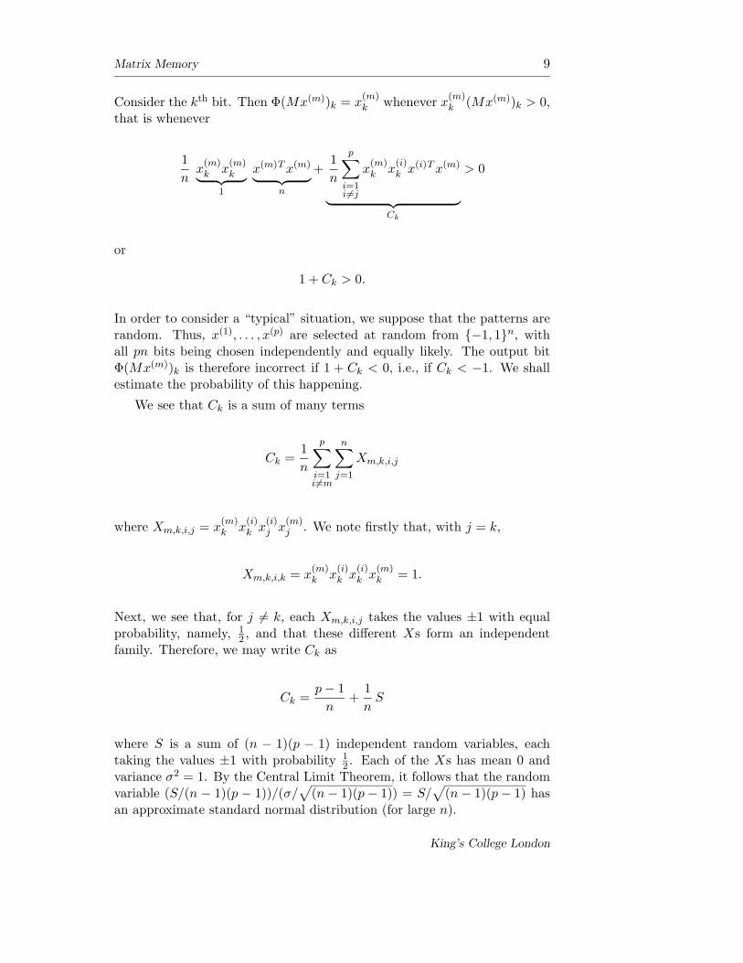
Consider the kth bit. Then Φ(Mx(m))k = x(m)k whenever x
(m)k (Mx(m))k > 0,
that is whenever
1
nx
(m)k x
(m)k︸ ︷︷ ︸
1
x(m)T x(m)
︸ ︷︷ ︸n
+1
n
p∑
i=1i6=j
x(m)k x
(i)k x(i)T x(m)
︸ ︷︷ ︸Ck
> 0
or
1 + Ck > 0.
In order to consider a “typical” situation, we suppose that the patterns arerandom. Thus, x(1), . . . , x(p) are selected at random from {−1, 1}n, withall pn bits being chosen independently and equally likely. The output bitΦ(Mx(m))k is therefore incorrect if 1 + Ck < 0, i.e., if Ck < −1. We shallestimate the probability of this happening.
We see that Ck is a sum of many terms
Ck =1
n
p∑
i=1i6=m
n∑
j=1
Xm,k,i,j
where Xm,k,i,j = x(m)k x
(i)k x
(i)j x
(m)j . We note firstly that, with j = k,
Xm,k,i,k = x(m)k x
(i)k x
(i)k x
(m)k = 1.
Next, we see that, for j 6= k, each Xm,k,i,j takes the values ±1 with equalprobability, namely, 1
2 , and that these different Xs form an independentfamily. Therefore, we may write Ck as
Ck =p − 1
n+
1
nS
where S is a sum of (n − 1)(p − 1) independent random variables, eachtaking the values ±1 with probability 1
2 . Each of the Xs has mean 0 andvariance σ2 = 1. By the Central Limit Theorem, it follows that the randomvariable (S/(n − 1)(p − 1))/(σ/
√(n − 1)(p − 1)) = S/
√(n − 1)(p − 1) has
an approximate standard normal distribution (for large n).
King’s College London
10 Chapter 1
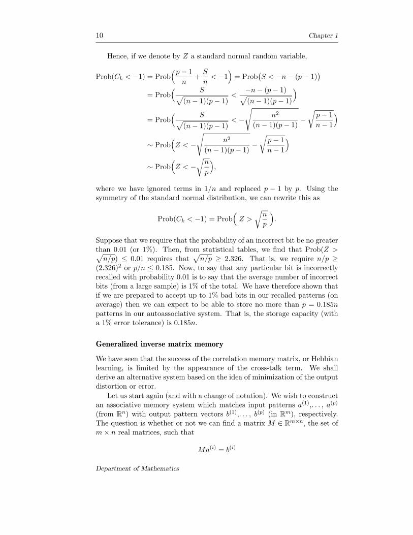
Hence, if we denote by Z a standard normal random variable,
Prob(Ck < −1) = Prob(p − 1
n+
S
n< −1
)= Prob
(S < −n − (p − 1)
)
= Prob( S√
(n − 1)(p − 1)<
−n − (p − 1)√(n − 1)(p − 1)
)
= Prob( S√
(n − 1)(p − 1)< −
√n2
(n − 1)(p − 1)−
√p − 1
n − 1
)
∼ Prob(Z < −
√n2
(n − 1)(p − 1)−
√p − 1
n − 1
)
∼ Prob(Z < −
√n
p
),
where we have ignored terms in 1/n and replaced p − 1 by p. Using thesymmetry of the standard normal distribution, we can rewrite this as
Prob(Ck < −1) = Prob(
Z >
√n
p
).
Suppose that we require that the probability of an incorrect bit be no greaterthan 0.01 (or 1%). Then, from statistical tables, we find that Prob(Z >√
n/p) ≤ 0.01 requires that√
n/p ≥ 2.326. That is, we require n/p ≥(2.326)2 or p/n ≤ 0.185. Now, to say that any particular bit is incorrectlyrecalled with probability 0.01 is to say that the average number of incorrectbits (from a large sample) is 1% of the total. We have therefore shown thatif we are prepared to accept up to 1% bad bits in our recalled patterns (onaverage) then we can expect to be able to store no more than p = 0.185npatterns in our autoassociative system. That is, the storage capacity (witha 1% error tolerance) is 0.185n.
Generalized inverse matrix memory
We have seen that the success of the correlation memory matrix, or Hebbianlearning, is limited by the appearance of the cross-talk term. We shallderive an alternative system based on the idea of minimization of the outputdistortion or error.
Let us start again (and with a change of notation). We wish to constructan associative memory system which matches input patterns a(1),. . . , a(p)
(from Rn) with output pattern vectors b(1),. . . , b(p) (in R
m), respectively.The question is whether or not we can find a matrix M ∈ R
m×n, the set ofm × n real matrices, such that
Ma(i) = b(i)
Department of Mathematics
Matrix Memory 11
for all 1 ≤ i ≤ p. Let A ∈ Rn×p be the matrix whose columns are the vectors
a(1), . . . , a(p), i.e., A = (a(1) · · · a(p)), and let B ∈ Rm×p be the matrix with
columns given by the b(i) s, B = (b(1) · · · b(p)), thus Aij = a(j)i and Bij = b
(j)i .
Then it is easy to see that Ma(i) = b(i), for all i, is equivalent to MA = B.The problem, then, is to solve the matrix equation
MA = B,
for M ∈ Rm×n, for given matrices A ∈ R
n×p and B ∈ Rm×p.
First, we observe that for a solution to exist, the matrices A and Bcannot be arbitrary. Indeed, if A = 0, then so is MA no matter what Mis—so the equation will not hold unless B also has all zero entries.
Suppose next, slightly more subtly, that there is some non-zero vectorv ∈ R
p such that Av = 0. Then, for any M , MAv = 0. In general, it neednot be true that Bv = 0.
Suppose then that there is no such non-zero v ∈ Rp such that Av = 0,
i.e., we are supposing that Av = 0 implies that v = 0. What does thismean? We have
(Av)i =
p∑
j=1
Aijvj
= v1Ai1 + v2Ai2 + · · · + vpAip
= v1a(1)i + v2a
(2)i + · · · + vpa
(p)i
= ith component of (v1a(1) + · · · + vpa
(p)).
In other words,
Av = v1a(1) + · · · + vpa
(p).
The vector Av is a linear combination of the columns of A, considered aselements of R
n.
Now, the statement that Av = 0 if and only if v = 0 is equivalent to thestatement that v1a
(1) + · · ·+ vpa(p) = 0 if and only if v1 = v2 = · · · = vp = 0
which, in turn, is equivalent to the statement that a(1),. . . ,a(p) are linearlyindependent vectors in R
n.
Thus, the statement, Av = 0 if and only if v = 0, is true if and only ifthe columns of A are linearly independent vectors in R
n.
Proposition 1.5. For any A ∈ Rn×p, the p × p matrix ATA is invertible if
and only if the columns of A are linearly independent in Rn.
Proof. The square matrix ATA is invertible if and only if the equationATAv = 0 has the unique solution v = 0, v ∈ R
p. (Certainly the invertibilityof ATA implies the uniqueness of the zero solution to ATAv = 0. For theconverse, first note that the uniqueness of this zero solution implies that
King’s College London

12 Chapter 1
ATA is a one-one linear mapping from Rp to R
p. Moreover, using linearity,one readily checks that the collection ATAu1, . . . , ATAup is a linearly in-dependent set for any basis u1, . . . , up of R
p. This means that it is a basisand so ATA maps R
p onto itself. Hence ATA has an inverse. Alternatively,one can argue that since ATA is symmetric it can be diagonalized via someorthogonal transformation. But a diagonal matrix is invertible if and only ifevery diagonal entry is non-zero. In this case, these entries are precisely theeigenvalues of ATA. So ATA is invertible if and only if none of its eigenvaluesare zero.)
Suppose that the columns of A are linearly independent and that ATAv =0. Then it follows that vT ATAv = 0 and so Av = 0, since vT ATAv =∑n
i=1(Av)2i = ‖Av‖22, the square of the Euclidean length of the n-dimensional
vector Av. By the argument above, Av is a linear combination of the columnsof A, and we deduce that v = 0. Hence ATA is invertible.
On the other hand, if ATA is invertible, then Av = 0 implies that ATAv =0 and so v = 0. Hence the columns of A are linearly independent.
We can now derive the result of interest here.
Theorem 1.6. Let A be any n × p matrix whose columns are linearly inde-pendent. Then for any m × p matrix B, there is an m × n matrix M suchthat MA = B.
Proof. LetM = B︸︷︷︸
m×p
(ATA)−1
︸ ︷︷ ︸p×p
AT
︸︷︷︸p×n
.
Then M is well-defined since ATA ∈ Rp×p is invertible, by the proposition.
Direct substitution shows that MA = B.
So, with this choice of M we get perfect recall, provided that the inputpattern vectors are linearly independent.
Note that, in general, the solution above is not unique. Indeed, for anymatrix C ∈ R
m×n, the m × n matrix M ′ = C(1ln − A(ATA)−1AT
)satisfies
M ′A = C(A − A(ATA)−1ATA
)= C(A − A) = 0 ∈ R
m×p.
Hence M + M ′ satisfies (M + M ′)A = B.Can we see what M looks like in terms of the patterns a(i), b(i)? The
answer is “yes and no”. We have A = (a(1) · · · a(p)) and B = (b(1) · · · b(p)).Then
(ATA)ij =n∑
k=1
ATikAkj =
n∑
k=1
AkiAkj
=n∑
k=1
a(i)k a
(j)k
Department of Mathematics
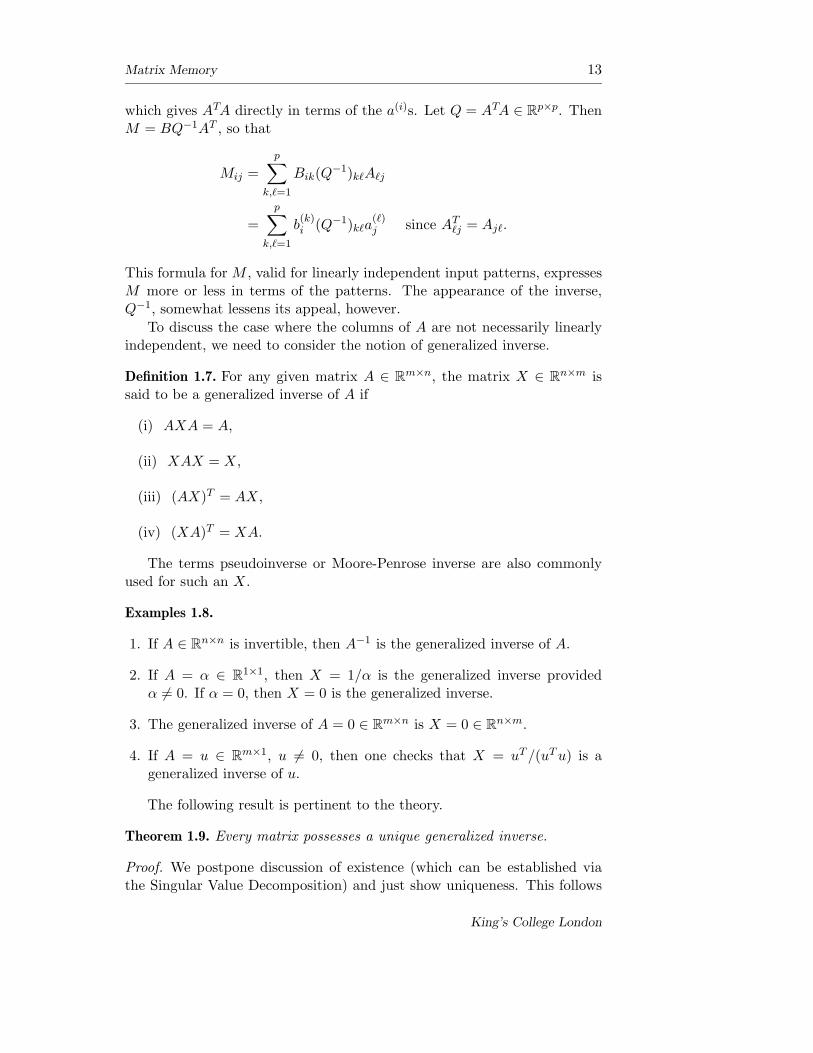
Matrix Memory 13
which gives ATA directly in terms of the a(i)s. Let Q = ATA ∈ Rp×p. Then
M = BQ−1AT , so that
Mij =
p∑
k,ℓ=1
Bik(Q−1)kℓAℓj
=
p∑
k,ℓ=1
b(k)i (Q−1)kℓa
(ℓ)j since AT
ℓj = Ajℓ.
This formula for M , valid for linearly independent input patterns, expressesM more or less in terms of the patterns. The appearance of the inverse,Q−1, somewhat lessens its appeal, however.
To discuss the case where the columns of A are not necessarily linearlyindependent, we need to consider the notion of generalized inverse.
Definition 1.7. For any given matrix A ∈ Rm×n, the matrix X ∈ R
n×m issaid to be a generalized inverse of A if
(i) AXA = A,
(ii) XAX = X,
(iii) (AX)T = AX,
(iv) (XA)T = XA.
The terms pseudoinverse or Moore-Penrose inverse are also commonlyused for such an X.
Examples 1.8.
1. If A ∈ Rn×n is invertible, then A−1 is the generalized inverse of A.
2. If A = α ∈ R1×1, then X = 1/α is the generalized inverse provided
α 6= 0. If α = 0, then X = 0 is the generalized inverse.
3. The generalized inverse of A = 0 ∈ Rm×n is X = 0 ∈ R
n×m.
4. If A = u ∈ Rm×1, u 6= 0, then one checks that X = uT /(uT u) is a
generalized inverse of u.
The following result is pertinent to the theory.
Theorem 1.9. Every matrix possesses a unique generalized inverse.
Proof. We postpone discussion of existence (which can be established viathe Singular Value Decomposition) and just show uniqueness. This follows
King’s College London
14 Chapter 1
by repeated use of the defining properties (i),. . . ,(iv). Let A ∈ Rm×n be
given and suppose that X, Y ∈ Rn×m are generalized inverses of A. Then
X = XAX, by (i),
= X(AX)T , by (iii),
= XXT AT
= XXT AT Y T AT , by (i)T ,
= XXT AT AY, by (iii),
= XAXAY, by (iii),
= XAY, by (ii),
= XAY AY, by (i),
= XAAT Y T Y, by (iv),
= AT XT AT Y T Y, by (iv),
= AT Y T Y, by (i)T ,
= Y AY, by (iv),
= Y, by (ii),
as required.
Notation For given A ∈ Rm×n, we denote its generalized inverse by A#.
It is also often written as Ag, A+ or A†.
Proposition 1.10. For any A ∈ Rm×n, AA# is the orthogonal projection onto
ranA, the linear span in Rm of the columns of A, i.e., if P = AA# ∈ R
m×m,then P = P T = P 2 and P maps R
m onto ranA.
Proof. The defining property (iii) of the generalized inverse A# is preciselythe statement that P = AA# is symmetric. Furthermore,
P 2 = AA#AA# = AA#, by condition (i),
= P
so P is idempotent. Thus P is an orthogonal projection.For any x ∈ R
m, we have that Px = AA#x ∈ ranA, so that P : Rm →
ranA. On the other hand, if x ∈ ranA, there is some z ∈ Rn such that
x = Az. Hence Px = PAz = AA#Az = Az = x, where we have usedcondition (i) in the penultimate step. Hence P maps R onto ranA.
Proposition 1.11. Let A ∈ Rm×n.
(i) If rankA = n, then A# = (ATA)−1AT .
(ii) If rankA = m, then A# = AT (AAT )−1.
Department of Mathematics

Matrix Memory 15
Proof. If rankA = n, then A has linearly independent columns and we knowthat this implies that ATA is invertible (in R
n×n). It is now a straightforwardmatter to verify that (ATA)−1AT satisfies the four defining properties of thegeneralized inverse, which completes the proof of (i).
If rankA = m, we simply consider the transpose instead. Let B = AT .Then rankB = m, since A and AT have the same rank, and so, by theargument above, B# = (BT B)−1BT . However, AT # = A#T , as is easilychecked (again from the defining conditions). Hence
A# = A#TT = (AT )#T
= B#T = B(BT B)−1
= AT (AAT )−1
which establishes (ii).
Definition 1.12. The ‖ · ‖F -norm on Rm×n is defined by
‖A‖2F = Tr(ATA) for A ∈ R
m×n,
where Tr(B) is the trace of the square matrix B; Tr(B) =∑
i Bii. Thisnorm is called the Frobenius norm and sometimes denoted ‖ · ‖2.
We see that
‖A‖2F = Tr(ATA) =
n∑
i=1
(ATA)ii
=
n∑
i=1
m∑
j=1
ATijAji
=
n∑
i=1
m∑
j=1
A2ij
since ATij = Aji. Hence
‖A‖F =√
(sum of squares of all entries of A) .
We also note, here, that clearly ‖A‖F = ‖AT ‖F .Suppose that A = u ∈ R
m×1, an m-component vector. Then ‖A‖2F =∑m
i=1 u2i , that is, ‖A‖F is the usual Euclidean norm in this case. Thus
the notation ‖ · ‖2 for this norm is consistent. Note that, generally, ‖A‖F
is just the Euclidean norm of A ∈ Rm×n when A is “taken apart” row
by row and considered as a vector in Rmn via the correspondence A ↔
(A11, A12, . . . , A1n, A21, . . . , Amn).The notation ‖A‖2 is sometimes used in numerical analysis texts (and
in the computer algebra software package Maple) to mean the norm of
King’s College London

16 Chapter 1
A as a linear map from Rn into R
m, that is, the value sup{‖Ax‖ : x ∈R
n with ‖x‖ = 1}. One can show that this value is equal to the square rootof the largest eigenvalue of ATA whereas ‖A‖F is equal to the square rootof the sum of the eigenvalues of ATA.
Remark 1.13. Let A ∈ Rm×n, B ∈ R
n×m, C ∈ Rm×n, and X ∈ R
p×p. Thenit is easy to see that
(i) Tr(AB) = Tr(BA),
(ii) Tr(X) = Tr(XT ),
(iii) Tr(ACT ) = Tr(CT A) = Tr(AT C) = Tr(CAT ).
The equalities in (iii) can each be verified directly, or alternatively, onenotices that (iii) is a consequence of (i) and (ii) (replacing B by CT ).
Lemma 1.14. For A ∈ Rm×n, A#AAT = AT .
Proof. We have
(A#A)AT = (A#A)T AT by condition (iv)
= (A(A#A))T
= AT by condition (i)
as required.
Theorem 1.15. Let A ∈ Rn×p and B ∈ R
m×p be given. Then X = BA# isan element of R
m×n which minimizes the quantity ‖XA − B‖F .
Proof. We have
‖XA − B‖2F = ‖(X − BA#)A + B(A#A − 1lp)‖2
F
= ‖(X − BA#)A‖2F + ‖B(A#A − 1lp)‖2
F
+ 2 Tr(AT (X − BA#)T B(A#A − 1lp)
)
= ‖(X − BA#)A‖2F + ‖B(A#A − 1lp)‖2
F
+ 2 Tr((X − BA#)T B (A#A − 1lp)A
T
︸ ︷︷ ︸= 0 by the lemma
).
Hence
‖XA − B‖2F = ‖(X − BA#)A‖2
F + ‖B(A#A − 1lp)‖2F
which achieves its minimum, ‖B(A#A − 1lp)‖2F , when X = BA#.
Department of Mathematics
Matrix Memory 17
Note that any X satisfying XA = BA#A gives a minimum solution.If AT has full column rank (or, equivalently, AT has no kernel) then AAT
is invertible. Multiplying on the right by AT (AAT )−1 gives X = BA#. Sounder this condition on AT , we see that there is a unique solution X = BA#
minimizing ‖XA − B‖F .
In general, one can show that BA# is that element with minimal ‖ · ‖F -norm which minimizes ‖XA − B‖F , i.e., if Y 6= BA# and ‖Y A − B‖F =‖BA#A − B‖F , then ‖BA#‖F < ‖Y ‖F .
Now let us return to our problem of finding a memory matrix which storesthe input-output pattern pairs (a(i), b(i)), 1 ≤ i ≤ p, with each a(i) ∈ R
n
and each b(i) ∈ Rm. In general, it may not be possible to find a matrix
M ∈ Rm×n such that Ma(i) = b(i), for each i. Whatever our choice of
M , the system output corresponding to the input a(i) is just Ma(i). So,failing equality Ma(i) = b(i), we would at least like to minimize the errorb(i) − Ma(i). A measure of such an error is ‖b(i) − Ma(i)‖2
2 the squaredEuclidean norm of the difference. Taking all p patterns into account, thetotal system recall error is taken to be
p∑
i=1
‖b(i) − Ma(i)‖22.
Let A = (a(1) · · · a(p)) ∈ Rn×p and B = (b(1) · · · b(p)) ∈ R
m×p be the matriceswhose columns are given by the pattern vectors a(i) and b(i), respectively.Then the total system recall error, above, is just
‖B − MA‖2F .
We have seen that this is minimized by the choice M = BA#, where A# isthe generalized inverse of A. The memory matrix M = BA# is called theoptimal linear associative memory (OLAM) matrix.
Remark 1.16. If the patterns {a(1), . . . , a(p)} constitute an orthonormal fam-ily, then A has independent columns and so A# = (ATA)−1AT = 1lpA
T , sothat the OLAM matrix is BA# = BAT which is exactly the correlationmemory matrix.
In the autoassociative case, b(i) = a(i), so that B = A and the OLAMmatrix is given as
M = AA#.
We have seen that AA# is precisely the projection onto the range of A, i.e.,onto the subspace of R
n spanned by the prototype patterns. In this case,we say that M is given by the projection rule.
King’s College London

18 Chapter 1
Any input x ∈ Rn can be written as
x = AA#x︸ ︷︷ ︸OLAM system output
+ (1l − AA#)x︸ ︷︷ ︸“novelty”
.
Kohonen calls 1l − AA# the novelty filter and has applied these ideas toimage-subtraction problems such as tumor detection in brain scans. Non-null novelty vectors may indicate disorders or anomalies.
Pattern classification
We have discussed the distributed associative memory (DAM) matrix asan autoassociative or as a heteroassociative memory model. The first ismathematically just a special case of the second. Another special case isthat of so-called classification. The idea is that one simply wants an inputsignal to elicit a response “tag”, typically coded as one of a collection oforthogonal unit vectors, such as given by the standard basis vectors of R
m.
• In operation, the input x induces output Mx, which is then associatedwith that tag vector corresponding to its maximum component. In otherwords, if (Mx)j is the maximum component of Mx, then the output Mxis associated with the jth tag.
Examples of various pattern classification tasks have been given by T. Koho-nen, P. Lehtio, E. Oja, A. Kortekangas and K. Makisara, Demonstration ofpattern processing properties of the optimal associative mappings, Proceed-ings of the International Conference on Cybernetics and Society, Washing-ton, D. C., 581–585 (1977). (See also the article “Storage and Processing ofInformation in Distributed Associative Memory Systems” by T. Kohonen,P. Lehtio and E. Oja in “Parallel Models of Associative Memory” editedby G. Hinton and J. Anderson, published by Lawrence Erlbaum Associates,(updated edition) 1989.)
In one such experiment, ten people were each photographed from fivedifferent angles, ranging from 45◦ to −45◦, with 0◦ corresponding to a fullyfrontal face. These were then digitized to produce pattern vectors witheight possible intensity levels for each pixel. A distinct unit vector, a tag,was associated with each person, giving a total of ten tags, and fifty patterns.The OLAM matrix was constructed from this data.
The memory matrix was then presented with a digitized photographof one of the ten people, but taken from a different angle to any of theoriginal five prototypes. The output was then classified according to thetag associated with its largest component. This was found to give correctidentification.
The OLAM matrix was also found to perform well with autoassociation.Pattern vectors corresponding to one hundred digitized photographs were
Department of Mathematics

Matrix Memory 19
used to construct the autoassociative memory via the projection rule. Whenpresented with incomplete or fuzzy versions of the original patterns, theOLAM matrix satisfactorily reconstructed the correct image.
In another autoassociative recall experiment, twenty one different pro-totype images were used to construct the OLAM matrix. These were eachcomposed of three similarly placed copies of a subimage. New pattern im-ages, consisting of just one part of the usual triple features, were presentedto the OLAM matrix. The output images consisted of slightly fuzzy versionsof the single part but triplicated so as to mimic the subimage positioninglearned from the original twenty one prototypes.
An analysis comparing the performance of the correlation memory ma-trix with that of the generalized inverse matrix memory has been offered byCherkassky, Fassett and Vassilas (IEEE Trans. on Computers, 40, 1429 (1991)).Their conclusion is that the generalized inverse memory matrix performsbetter than the correlation memory matrix for autoassociation, but thatthe correlation memory matrix is better for classification. This is contraryto the widespread belief that the generalized inverse memory matrix is thesuperior model.
King’s College London

20 Chapter 1
Department of Mathematics

Chapter 2
Adaptive Linear Combiner
We wish to consider a memory matrix for the special case of one-dimensionaloutput vectors. Thus, we consider input pattern vectors x(1), . . . , x(p) ∈ R
ℓ,say, with corresponding desired outputs y(1), . . . , y(p) ∈ R and we seek amemory matrix M ∈ R
1×ℓ such that
Mx(i) = y(i),
for 1 ≤ i ≤ p. Since M ∈ R1×ℓ, we can think of M as a row vector M =
(m1, . . . , mℓ). The output corresponding to the input x = (x1, . . . , xℓ) ∈ Rℓ
is just
y = Mx =ℓ∑
i=1
mixi .
Such a system is known as the adaptive linear combiner (ALC).
input signalcomponents
x1
x2
xn
...
m1
m2
mn
weights on connections
∑
“adder”forms
∑ni=1 mixi
y
output
Figure 2.1: The Adaptive Linear Combiner.
We have seen that we may not be able to find M which satisfies theexact input-output relationship Mx(i) = y(i), for each i. The idea is to lookfor an M which is in a certain sense optimal. To do this, we seek m1, . . . , mℓ
21
22 Chapter 2
such that (one half) the average mean-squared error
E ≡ 12
1p
p∑
i=1
|y(i) − z(i)|2
is minimized—where y(i) is the desired output corresponding to the inputvector x(i) and z(i) = Mx(i) is the actual system output. We already know,from the results in the last chapter, that this is achieved by the OLAMmatrix based on the input-output pattern pairs, but we wish here to developan algorithmic approach to the construction of the appropriate memorymatrix. We can write out E in terms of the mi as follows
E = 12p
p∑
i=1
|y(i) −ℓ∑
j=1
mjx(i)j |2
= 12p
p∑
i=1
(y(i)2 +
ℓ∑
j,k=1
mjmkx(i)j x
(i)k − 2
ℓ∑
j=1
y(i)mjx(i)j
)
= 12
ℓ∑
j,k=1
mjAjkmk −ℓ∑
j=1
bjmj + 12c
where Ajk = 1p
∑pi=1 x
(i)j x
(i)k , bj = 1
p
∑pi=1 y(i)x
(i)j and c = 1
p
∑pi=1 y(i)2.
Note that A = (Ajk) ∈ Rℓ×ℓ is symmetric. The error E is a non-negative
quadratic function of the mi. For a minimum, we investigate the equalities∂E/∂mi = 0, that is,
0 =∂E∂mi
=ℓ∑
k=1
Aikmk − bi ,
for 1 ≤ i ≤ ℓ, where we have used the symmetry of (Aik) here. We thusobtain the so-called Gauss-normal or Wiener-Hopf equations
ℓ∑
k=1
Aikmk = bi , for 1 ≤ i ≤ ℓ,
or, in matrix form,Am = b ,
with A = (Aik) ∈ Rℓ×ℓ, m = (m1, . . . , mℓ) ∈ R
ℓ and b = (b1, . . . , bℓ) ∈ Rℓ.
If A is invertible, then m = A−1b is the unique solution. In general, theremay be many solutions. For example, if A is diagonal with A11 = 0, thennecessarily b1 = 0 (otherwise E could not be non-negative as a function ofthe mi) and so we see that m1 is arbitrary. To relate this to the OLAMmatrix, write E as
E = 12p‖MX − Y ‖2
F ,
Department of Mathematics

Adaptive Linear Combiner 23
where X = (x(1) · · ·x(p)) ∈ Rℓ×p and Y = (y(1) · · · y(p)) ∈ R
1×p. This, weknow, is minimized by M = Y X# ∈ R
1×ℓ. Therefore m = MT must be asolution to the Wiener-Hopf equations above. We can write A, b and c interms of the matrices X and Y . One finds that A = 1
pXXT , bT = 1pY XT
and c = 1pY TY . The equation Am = b then becomes XXT m = XY T giving
m = (XXT )−1XY T , provided that A is invertible. This gives M = mT =Y XT (XXT )−1 = Y X#, as above.
One method of attack for finding a vector m∗ minimizing E is that ofgradient-descent. The idea is to think of E(m1, . . . , mℓ) as a bowl-shapedsurface above the ℓ-dimensional m1, . . . , mℓ-space. Pick any value for m.The vector grad E , when evaluated at m, points in the direction of maximumincrease of E in the neighbourhood of m. That is to say, for small α (and avector v of given length), E(m+αv)−E(m) is maximized when v points in thesame direction as grad E (as is seen by Taylor’s theorem). Now, rather thanincreasing E , we wish to minimize it. So the idea is to move a small distancefrom m to m − α grad E , thus inducing maximal “downhill” movement onthe error surface. By repeating this process, we hope to eventually reach avalue of m which minimizes E .
The strategy, then, is to consider a sequence of vectors m(n) given algo-rithmically by
m(n + 1) = m(n) − α grad E , for n = 1, 2, . . . ,
with m(1) arbitrary and where the parameter α is called the learning rate.If we substitute for grad E , we find
m(n + 1) = m(n) + α(b − Am(n)
).
Now, A is symmetric and so can be diagonalized. There is an orthogonalmatrix U ∈ R
ℓ×ℓ such that
UAUT = D = diag(λ1, . . . , λℓ)
and we may assume that λ1 ≥ λ2 ≥ · · · ≥ λℓ. We have
E = 12mT Am − bT m + 1
2c
= 12mT UTUAUTUm − bT UTUm + 1
2c
= 12zT Dz − vT z + 1
2c
where z = Um and v = Ub
= 12
ℓ∑
i=1
λiz2i −
ℓ∑
i=1
vizi + 12c.
King’s College London
24 Chapter 2
Since E ≥ 0, it follows that all λi ≥ 0—otherwise E would have a negativeleading term. The recursion formula for m(n), namely,
m(n + 1) = m(n) + α(b − Am(n)
),
givesUm(n + 1) = Um(n) + α
(Ub − UAUTUm(n)
).
In terms of z, this becomes
z(n + 1) = z(n) + α(v − Dz(n)
).
Hence, for any 1 ≤ j ≤ ℓ,
zj(n + 1) = zj(n) + α(vj − λjzj(n)
)
= (1 − αλj)zj(n) + αvj .
Setting µj = (1 − αλj), we have
zj(n + 1) = µjzj(n) + αvj
= µj(µjzj(n − 1) + αvj) + αvj
= µ2jzj(n − 1) + (µj + 1)αvj
= µ2j (µjzj(n − 2) + αvj) + (µj + 1)αvj
= µ3jzj(n − 2) + (µ2
j + µj + 1)αvj
= · · ·= µn
j zj(1) + (µn−1j + µn−2
j + · · · + µj + 1)αvj .
This converges, as n → ∞, provided |µj | < 1, that is, provided −1 <1 − αλj < 1. Thus, convergence demands the inequalities 0 < αλj < 2 forall 1 ≤ j ≤ ℓ. We therefore have shown that the algorithm
m(n + 1) = m(n) + α(b − Am(n)
), n = 1, 2, . . . ,
with m(1) arbitrary, converges provided 0 < α <2
λmax, where λmax is the
maximum eigenvalue of A.Suppose that m(1) is given and that α does indeed satisfy the inequalities
0 < α < 2/λmax. Let m∗ denote the limit limn→∞ m(n). Then, lettingn → ∞ in the recursion formula for m(n), we see that
m∗ = m∗ + α(b − Am∗
),
that is, m∗ satisfies Am∗ = b and so m(n) does, indeed, converge to a valueminimizing E . Indeed, if m∗ satisfies Am∗ = b, then we can complete thesquare and write 2E as
2E = mT Am − 2bT m + c
= mT Am − mT∗ Am − mT Am∗ + c, using bT m = mT b
= (m − m∗)T A(m − m∗) − mT
∗ m∗ + c,
which is certainly minimized when m = m∗.
Department of Mathematics
Adaptive Linear Combiner 25
The above analysis requires a detailed knowledge of the matrix A. Inparticular, its eigenvalues must be determined in order for us to be able tochoose a valid value for the learning rate α. We would like to avoid havingto worry too much about this detailed structure of A.
We recall that A = (Ajk) is given by
Ajk =1
p
p∑
i=1
x(i)j x
(i)k .
This is an average of x(i)j x
(i)k taken over the patterns. Given a particular
pattern x(i), we can think of x(i)j x
(i)k as an estimate for the average Ajk.
Similarly, we can think of bj = 1p
∑pi=1 y(i)x
(i)j as an average, and y(i)x
(i)j as
an estimate for bj . Accordingly, we change our algorithm for updating thememory matrix to the following.
Select an input-output pattern pair, (x(i), y(i)), say, and use the previousalgorithm but with Ajk and bj “estimated” as above. Thus,
mj(n + 1) = mj(n) + α(y(i)x
(i)j −
ℓ∑
k=1
x(i)j x
(i)k mk(n)
)
for 1 ≤ j ≤ n. That is,
mj(n + 1) = mj(n) + αδ(i)x(i)j
where
δ(i) =(y(i) −
ℓ∑
k=1
x(i)k mk(n)
)
= (desired output − actual output)
is the output error for pattern pair i. This is known as the delta-rule, or theWidrow-Hoff learning rule, or the least mean square (LMS) algorithm.
The learning rule is then as follows.
King’s College London
26 Chapter 2
Widrow-Hoff (LMS) algorithm
• First choose a value for α, the learning rate (in practice, this might be 0.1or 0.05, say).
• Start with mj(1) = 0 for all j, or perhaps with small random values.
• Keep selecting input-output pattern pairs x(i), y(i) and update m(n) bythe rule
mj(n + 1) = mj(n) + αδ(i)x(i)j , 1 ≤ j ≤ ℓ,
where δ(i) = y(i) − ∑ℓk=1 mk(n)x
(i)k is the output error for the pattern
pair (i) as determined by the memory matrix in operation at iterationstep n. Ensure that every pattern pair is regularly presented and con-tinue until the output error has reached and appears to remain at anacceptably small value.
• The actual question of convergence still remains to be discussed!
Remark 2.1. If α is too small, we might expect the convergence to be slow—the adjustments to m are small if α is small. Of course, this is assuming thatthere is convergence. Similarly, if the output error δ is small then changesto m will also be small, thus slowing convergence. This could happen if menters an error surface “valley” with an almost flat bottom.
On the other hand, if α is too large, then the ms may overshoot andoscillate about an optimal solution. In practice, one might start with alargish value for α but then gradually decrease it as the learning progresses.These comments apply to any kind of gradient-descent algorithm.
Remark 2.2. Suppose that, instead of basing our discussion on the errorfunction E , we present the ith input vector x(i) and look at the immediateoutput “error”
E(i) = 12
∣∣y(i) −ℓ∑
k=1
mkx(i)k
∣∣2.
Then we calculate
∂E(i)
∂mj= −
(y(i) −
ℓ∑
k=1
mkx(i)k
︸ ︷︷ ︸δ(i)
)x
(i)j ,
for 1 ≤ j ≤ ℓ. So we might try the “one pattern at a time” gradient-descentalgorithm
mj(n + 1) = mj(n) + αδ(i)x(i)j , 1 ≤ j ≤ ℓ,
Department of Mathematics

Adaptive Linear Combiner 27
with m(1) arbitrary. This is exactly what we have already arrived at above.It should be clear from this point of view that there is no reason a priori tosuppose that the algorithm converges. Indeed, one might be more inclinedto suspect that the m-values given by this rule simply “thrash about all overthe place” rather than settling down towards a limiting value.
Remark 2.3. We might wish to consider the input-output patterns x and yas random variables taking values in R
ℓ and R, respectively. In this context,it would be natural to consider the minimization of E((y − mT x)2). Theanalysis proceeds exactly as above, but now with Ajk = E(xjxk) and bj =E(yxj). The idea of using the current, i.e., the observed, values of x and yto construct estimates for A and b is a common part of standard statisticaltheory. The algorithm is then
mj(n + 1) = mj(n) + α(y(n)x
(n)j −
ℓ∑
k=1
x(n)j x
(n)k mk(n)
)
where x(n) and y(n) are the input-output pattern pair presented at stepn. If we assume that these patterns presented at the various steps areindependent, then, from the algorithm, we see that mk(n) only depends onthe patterns presented before step n and so is independent of x(n). Takingexpectations we obtain the vector equation
E m(n + 1) = E m(n) + α( b − A E m(n) ).
It follows, as above, that if 0 < α < 2/λmax, then E m(n) converges to m∗
which minimizes the mean square error E((y − mT x)2).
We now turn to a discussion of the convergence of the LMS algorithm(see Z-Q. Luo, Neural Computation 3, 226–245 (1991)). Rather than justlooking at the ALC system, we shall consider the general heteroassociativeproblem with p input-output pattern pairs (a(1), b(1)), . . . , (a(p), b(p)) witha(i) ∈ R
ℓ and b(i) ∈ Rm, 1 ≤ i ≤ p. Taking m = 1, we recover the ALC,
as above. We seek an algorithmic approach to minimizing the total system“error”
E(M) =
p∑
i=1
E(i)(M) =
p∑
i=1
12‖b
(i) − Ma(i)‖2
where E(i)(M) = 12‖b(i) − Ma(i)‖2 is the error function corresponding to
pattern i.
We have seen that E(M) = 12‖B −MA‖2
F , where ‖ · ‖F is the Frobenius
norm, A = (a(1) · · · a(p)) ∈ Rℓ×p and B = (b(1) · · · b(p)) ∈ R
m×p and that asolution to the problem is given by M = BA#.
King’s College London
28 Chapter 2
Each E(i) is a function of the elements Mjk of the memory matrix M .Calculating the partial derivatives gives
∂E(i)
∂Mjk=
∂
∂Mjk
12
m∑
r=1
(b(i)r −
ℓ∑
s=1
Mrsa(i)s
)2
= −(b(i)j −
ℓ∑
s=1
Mjsa(i)s
)a
(i)k
=((
Ma(i) − b(i))a(i)T
)jk
.
This leads to the following LMS learning algorithm.
• The patterns (a(i), b(i)) are presented one after the other, (a(1), b(1)),(a(2), b(2)),. . . , (a(p), b(p))—thus constituting a (pattern) cycle. This cycleis to be repeated.
• Let M (i)(n) denote the memory matrix just before the pattern pair(a(i), b(i)) is presented in the nth cycle. On presentation of (a(i), b(i))to the network, the memory matrix is updated according to the rule
M (i+1)(n) = M (i)(n) − αn
(M (i)(n)a(i) − b(i)
)a(i)T
where αn is the (n-dependent) learning rate, and we agree that thematrix M (p+1)(n) = M (1)(n + 1), that is, presentation of pattern p + 1in cycle n is actually the presentation of pattern 1 in cycle n + 1.
Remark 2.4. The gradient of the total error function E is given by the terms
∂E∂Mjk
=
p∑
i=1
∂E(i)
∂Mjk.
When the ith example is being learned, only the terms ∂E(i)/∂Mjk, forfixed i, are used to update the memory matrix. So at this step the value ofE(i) will decrease but it could happen that E actually increases. The pointis that the algorithm is not a standard gradient-descent algorithm and sostandard convergence arguments are not applicable. A separate proof ofconvergence must be given.
Remark 2.5. When m = 1, the output vectors are just real numbers and werecover the adaptive linear combiner and the Widrow-Hoff rule as a specialcase.
Remark 2.6. The algorithm is “local” in the sense that it only involves in-formation available at the time of each presentation, i.e., it does not needto remember any of the previously seen examples.
Department of Mathematics

Adaptive Linear Combiner 29
The following result is due to Kohonen.
Theorem 2.7. Suppose that αn = α > 0 is fixed. Then, for each i = 1, . . . , p,
the sequence M (i)(n) converges to some matrix M(i)α depending on α and i.
Moreover,
limα↓0
M (i)α = BA#,
for each i = 1, . . . , p.
Remark 2.8. In general, the limit matrices M(i)α are different for different i.
We shall investigate a simple example to illustrate the theory (followingLuo).
Example 2.9. Consider the case when there is a single input node, so thatthe memory matrix M ∈ R
1×1 is just a real number, m, say.
inM ∈ R
1×1
out
Figure 2.2: The ALC with one input node.
We shall suppose that the system is to learn the two pattern pairs (1, c1)and (−1, c2). Then the total system error function is
E = 12(c1 − m)2 + 1
2(c2 + m)2
where M11 = m, as above. The LMS algorithm, in this case, becomes
m(2)(n) = m(1)(n) − α(m(1)(n) − c1)
m(3)(n) = m(1)(n + 1) = m(2)(n) − α(m(2)(n) + c2)
with the initialization m(1)(1) = 0. Hence
m(1)(n + 1) = (1 − α)m(2)(n) − αc2
= (1 − α)((1 − α)m(1)(n) + αc1
)− αc2
= (1 − α)2︸ ︷︷ ︸= λ, say
m(1)(n) + (1 − α)αc1 − αc2︸ ︷︷ ︸= β, say
King’s College London
30 Chapter 2
giving
m(1)(n + 1) = λm(1)(n) + β
= λ(λm(1)(n − 1) + β
)+ β
= λ2m(1)(n − 1) + λβ + β
= · · ·= λnm(1)(1)︸ ︷︷ ︸
= 0
+(λn−1 + · · · + λ + 1)β
=(1 − λn)
(1 − λ)β.
We see that limn→∞ m(1)(n + 1) = β/(1 − λ), provided that |λ| < 1. Thiscondition is equivalent to (1 − α)2 < 1, or |1 − α| < 1, which is the same as0 < α < 2. The limit is
m(1)α ≡ β
1 − λ=
(1 − α)αc1 − αc2
1 − (1 − α)2
which simplifies to
m(1)α =
(1 − α)c1 − c2
2 − α.
Now, for m(2)(n), we have
m(2)(n) = m(1)(n)(1 − α) + αc1
→ m(2)α ≡ m(1)
α (1 − α) + αc1
=c1 − (1 − α)c2
2 − α
as n → ∞, provided 0 < α < 2. This shows that if we keep the learning
rate fixed, then we do not get convergence, m(1)α 6= m
(2)α , unless c1 = −c2.
The actual optimal solution m∗ to minimizing the error E is got from solvingdE/dm = 0, i.e., −(c1−m)+(c2+m) = 0, which gives m∗ = 1
2(c1−c2). This
is the value for the OLAM “matrix”. If c1 6= c2 and α 6= 0, then m(1)α 6= m∗
and m(2)α 6= m∗. Notice that both m
(1)α and m
(2)α converge to the OLAM
solution m∗ as α → 0, and also the average 12(m(1)(n) + m(2)(n)) converges
to m∗.
Next, we shall consider a dynamically variable learning rate αn. In thiscase the algorithm becomes
m(2)(n) = (1 − αn)m(1)(n) + αnc1
m(1)(n + 1) = (1 − αn)m(2)(n) − αnc2.
Department of Mathematics

Adaptive Linear Combiner 31
Hence
m(1)(n + 1) = (1 − αn)[(1 − αn)m(1)(n) + αnc1
]− αnc2,
giving
m(1)(n + 1) = (1 − αn)2m(1)(n) + (1 − αn)αnc1 − αnc2.
We wish to examine the convergence of m(1)(n) (and m(2)(n)) to m∗ =(c1 − c2
2
). So if we set yn = m(1)(n) −
(c1 − c2
2
), then we would like to
show that yn → 0, as n → ∞. The recursion formula for yn is
yn+1 +(c1 − c2
2
)= (1 − αn)2
(yn +
(c1 − c2
2
))+ (1 − αn)αnc1 − αnc2.
which simplifies to
yn+1 = (1 − αn)2yn − α2n
(c1 + c2
2
).
Next, we impose suitable conditions on the learning rates, αn, which willensure convergence.
• Suppose that 0 ≤ αn < 1, for all n, and that
(i)∞∑
n=1
αn = ∞ , (ii)∞∑
n=1
α2n < ∞ ,
that is, the series∑∞
n=1 αn is divergent, whilst the series∑∞
n=1 α2n is
convergent.
An example is provided by the assignment αn = 1/n. The intuition is thatcondition (i) ensures that the learning rate is always sufficiently large topush the iteration towards the desired limiting value, whereas condition (ii)ensures that its influence is not too strong that it might force the schemeinto some kind of endless oscillatory behaviour.
Claim The sequence (yn) converges to 0, as n → ∞.
Proof. Let rn = −(c1 + c2
2
)α2
n . Then, by condition (ii),∑∞
n=1 |rn| < ∞.
The algorithm for yn is
yn+1 = (1 − αn)2yn + rn
= (1 − αn)2((1 − αn−1)2yn−1 + rn−1) + rn
= (1 − αn)2(1 − αn−1)2yn−1 + (1 − αn)2rn−1 + rn
= · · ·= (1 − αn)2(1 − αn−1)
2 · · · (1 − α1)2y1 + (1 − αn)2 · · · (1 − α2)
2r1
+ (1 − αn)2 · · · (1 − α3)2r2 + · · · + (1 − αn)2rn−1 + rn .
King’s College London
32 Chapter 2
For convenience, set y1 = r0 and βj = (1−αj)2. Then we can write yn+1 as
yn+1 = r0β1β2 · · ·βn + r1β2 · · ·βn + r2β3 · · ·βn + · · · + rn−1βn + rn.
Let ε > 0 be given. We must show that there is some integer N such that|yn+1| < ε whenever n > N . The idea of the proof is to split the sum in theexpression for yn+1 into two parts, and show that each can be made smallfor sufficiently large n. Thus, we write
yn+1 = (r0β1β2 · · ·βn + · · · + rmβm+1 · · ·βn)
+ (rm+1βm+2 · · ·βn + · · · + rn−1βn + rn)
and seek m so that each of the two bracketed terms on the right hand sideis smaller than ε/2.
We know that∑∞
j=1 |rj | < ∞ and so there is some integer m such that∑nj=m+1 |rj | < ε/2, for n > m. Furthermore, the inequality |1 − αj | ≤ 1
implies that 0 < βj ≤ 1 and so, with m as above,
|(rm+1βm+2 · · ·βn + · · · + rn−1βn + rn)| ≤ |rm+1| + · · · + |rn|
=n∑
j=m+1
|rj | <ε
2
which deals with the second bracketed term in the expression for yn+1.To estimate the first term, we rewrite it as
(r′0 + r′1 + · · · + r′m)β1β2 · · ·βn ,
where we have set r′0 = r0 and r′j =rj
β1 · · ·βj, for j > 0.
We claim that β1 · · ·βn → 0 as n → ∞. To see this, we use the inequality
log(1 − t) ≤ −t, for 0 ≤ t < 1,
which can be derived as follows. We have
− log(1 − t) =
∫ 1
1−t
dx
x
≥∫ 1
1−tdx, since
1
x≥ 1 in the range of integration,
= t,
which gives log(1 − t) ≤ −t, as required. Using this, we may say thatlog(1 − αj) ≤ −αj , and so
∑nj=1 log(1 − αj) ≤ −∑n
j=1 αj . Thus
log(β1 · · ·βn) = logn∏
j=1
(1 − αj)2 = 2
n∑
j=1
log(1 − αj) ≤ −2n∑
j=1
αj .
But∑n
j=1 αj → ∞ as n → ∞, which means that log(β1 · · ·βn) → −∞ asn → ∞, which, in turn, implies that β1 · · ·βn → 0 as n → ∞, as claimed.
Department of Mathematics
Adaptive Linear Combiner 33
Finally, we observe that for m as above, the numbers r′0, r′1, . . . , r
′m do
not depend on n. Hence there is N , with N > m, such that
|(r′0 + r′1 + · · · + r′m)β1β2 · · ·βn| <ε
2
whenever n > N . This completes the proof that yn → 0 as n → ∞.
It follows, therefore, that m(1)(n) → m∗ =(c1 − c2
2
), as n → ∞. To
investigate m(2)(n), we use the relation
m(2)(n) = (1 − αn)︸ ︷︷ ︸→ 1
m(1)(n)︸ ︷︷ ︸→m∗
+ αn︸︷︷︸→ 0
c1
to see that m(2)(n) → m∗ also.
Thus, for this special simple example, we have demonstrated the con-vergence of the LMS algorithm. The statement of the general case is asfollows.
Theorem 2.10 (LMS Convergence Theorem). Suppose that the learning rate αn
in the LMS algorithm satisfies the conditions
∞∑
n=1
αn = ∞ and
∞∑
n=1
α2n < ∞.
Then the sequence of matrices generated by the algorithm, initialized by thecondition M (1)(1) = 0, converges to BA#, the OLAM matrix.
We will not present the proof here, which involves the explicit form ofthe generalized inverse, as given via the Singular Value Decomposition. Forthe details, we refer to the original paper of Luo.
The ALC can be used to “clean-up” a noisy signal by arranging it asa transverse filter. Using delay mechanisms, the “noisy” input signal issampled n times, that is, its values at time steps τ, 2τ, . . . , nτ are collected.These n values form the fan-in values for the ALC. The output error isε = |d− y|, where d is the desired output, i.e., the pure signal. The networkis trained to minimize ε, so that the system output y is as close to d aspossible (via the LMS error). Once trained, the network produces a “clean”version of the signal.
The ALC has applications in echo cancellation in long distance telephonecalls. The ’phone handset contains a special circuit designed to distinguishbetween incoming and outgoing signals. However, there is a certain amountof signal leakage from the earpiece to the mouthpiece. When the callerspeaks, the message is transmitted to the recipient’s earpiece via satellite.
King’s College London

34 Chapter 2
Some of this signal then leaks across to the recipient’s mouthpiece and issent back to the caller. The time taken for this is about half a second, sothat the caller hears an echo of his own voice. By appropriate use of theALC in the circuit, this echo effect can be reduced.
Department of Mathematics
Chapter 3
Artificial Neural Networks
By way of background information, we consider some basic neurophysiology.It has been estimated that the human brain contains some 1011 nerve cells, orneurons, each having perhaps as many as 104 interconnections, thus forminga densely packed web of fibres.
The neuron has three major components:
• the dendrites (constituting a vastly multibranching tree-like structurewhich collects inputs from other cells),
• the cell body (the processing part, called the soma),
• the axon (which carries electrical pulses to other cells).
Each neuron has only one axon, but it may branch out and so may beable to reach perhaps thousands of other cells. There are many dendrites(the word dendron is Greek for tree). The diameter of the soma is of theorder of 10 microns.
The outgoing signal is in the form of a pulse down the axon. On arrivalat a synapse (the junction where the axon meets a dendrite, or indeed, anyother part of another nerve cell) molecules, called neurotransmitters are re-leased. These cross the synaptic gap (the axon and receiving neuron do notquite touch) and attach themselves, very selectively, to receptor sites on thereceiving neuron. The membrane of the target neuron is chemically affectedand its own inclination to fire may be either enhanced or decreased. Thus,the incoming signal can be correspondingly either excitatory or inhibitory.Various drugs work by exploiting this behaviour. For example, curare de-posits certain chemicals at particular receptor sites which artificially inhibitmotor (muscular) stimulation by the brain cells. This results in the inabilityto move.
35

36 Chapter 3
The containing wall of the cell is the cell membrane—a phospholipidbilayer. (A lipid is, by definition, a compound insoluble in water, such asoils and fatty acids.) These bilayers have a phosphoric acid head which isattracted to water and a glyceride tail which is repelled by water. Thismeans that in a water solution they tend to line up in a double layer withthe heads pointing outwards.
The membrane keeps most molecules from passing either in or out ofthe cell, but there are special channels allowing the passage of certain ionssuch as Na+, K+, Cl− and Ca++. By allowing such ions to pass in andout, a potential difference between the inside and the outside of the cell ismaintained. The cell membrane is selectively more favourable to the passageof potassium than to sodium so that the K+ ions could more easily diffuseout, but negative organic ions inside tend to pull K+ ions into the cell. Thenet result is that the K+ concentration is higher inside than outside whereasthe reverse is true of Na+ and Cl− ions. This results in a resting potentialinside relative to outside of about −70mV across the cell wall.
When an action potential reaches a synapse it causes a change in thepermeability of the membrane of the cell carrying the pulse (the presynapticmembrane) which results in an influx of Ca++ ions. This leads to a releaseof neurotransmitters into the synaptic cleft which diffuse across the gap andattach themselves at receptor sites on the membrane of the receiving cell(the postsynaptic membrane). As a consequence, the permeability of thepostsynaptic membrane is altered. An influx of positive ions will tend todepolarize the receiving neuron (causing excitation) whereas an influx ofnegative ions will increase polarization and so inhibit activation.
Each input pulse is of the order of 1 millivolt and these diffuse towardsthe body of the cell where they are summed at the axon hillock. If thereis sufficient depolarization the membrane permeability changes and allowsa large influx of Na+ ions. An action potential is generated and travelsdown the axon away from the main cell body and off to other neurons.The amplitude of this signal is of the order of tens of millivolts and itspresence prevents the axon from transmitting further pulses. The shapeand amplitude of this travelling pulse is very stable and is replicated at thebranching points of the axon. This would indicate that the pulse seems notto carry any information other than to indicate its presence, i.e., the axoncan be thought of as being in an all-or-none state.
Once triggered, the neuron is incapable of re-excitation for about onemillisecond, during which time it is restored to its resting potential. Thisis called the refractory period. The existence of the refractory period limitsthe frequency of nerve-pulse transmissions to no more than about 1000 persecond. In fact, this frequency can vary greatly, being mere tens of pulsesper second in some cases. The impulse trains can be in the form of regularspikes, irregular spikes or in bursts.
Department of Mathematics
Artificial Neural Networks 37
The big question is how this massively interconnected network constitut-ing the brain can not only control general functional behaviour but also giverise to phenomena such as personality, sleep and consciousness. It is alsoamazing how the brain can recognize something it has not “seen” before.For example, a piece of badly played music, or writing roughly done, say, cannevertheless be perfectly recognized in the sense that there is no doubt inone’s mind (sic) what the tune or the letters actually “are”. (Indeed, surelyno real-life experience can ever be an exact replica of a previous experience.)This type of ability seems to be very hard indeed to reproduce by computer.One should take care in discussions of this kind, since we are apparentlytalking about the functioning of the brain in self-referential terms. After all,perhaps if we knew (whatever “know” means) what a tune “is”, i.e., how itrelates to the brain via our hearing it (or, indeed, seeing the musical scorewritten down) then we might be able to understand how we can recognizeit even in some new distorted form.
In this connection, certain cells do seem to perform as so-called “featuredetectors”. One example is provided by auditory cells located at either sideof the back of the brain near the base and serve to locate the direction ofsounds. These cells have two groups of dendrites receiving inputs originating,respectively, from the left ear and the right ear. For those cells in the left sideof the brain, the inputs from the left ear inhibit activation, whereas thosefrom the right are excitatory. The arrangement is reversed for those in theright side of the brain. This means that a sound coming from the right, say,will reach the right ear first and hence initially excite those auditory cellslocated in the left side of the brain but inhibit those in the right side. Whenthe sound reaches the left ear, the reverse happens, the cells on the leftbecome inhibited and those on the right side of the brain become excited.The change from strong excitation to strong inhibition can take place withina few hundred microseconds.
Another example of feature detection is provided by certain visual cells.Imagine looking at a circular region which is divided into two by a smallerconcentric central disc and its surround. Then there are cells in the visualsystem which become excited when a light appears in the centre but forwhich activation is inhibited when a light appears in the surround. Theseare called “on centre–off surround” cells. There are also corresponding “offcentre–on surround” cells.
We would like to devise mathematical models of networks inspired by(our understanding of) the workings of the brain. The study of such artificialneural networks may then help us to gain a greater understanding of theworkings of the brain. In this connection, one might then strive to makethe models more biologically realistic in a continuing endeavour to modelthe brain. Presumably one might imagine that sooner or later the detailedbiochemistry of the neuron will have to be taken into account. Perhaps one
King’s College London

38 Chapter 3
might even have to go right down to a quantum mechanical description.This seems to be a debatable issue in that there is a school of thought whichsuggests that the details are not strictly relevant and that it is the overallcooperative behaviour which is important for our understanding of the brain.This situation is analogous to that of the study of thermodynamics andstatistical mechanics. The former deals essentially with gross behaviour ofphysical systems whilst the latter is concerned with a detailed atomic ormolecular description in the hope of explaining the former. It turned outthat the detailed (and quantum) description was needed to explain certainphenomena such as superconductivity. Perhaps this will turn out to be thecase in neuroscience too.
On the other hand, one could simply develop the networks in any di-rection whatsoever and just consider them for their own sake (as part ofa mathematical structure), or as tools in artificial intelligence and expertsystems. Indeed, artificial neural networks have been applied in many areasincluding medical diagnosis, credit validation, stock market prediction, winetasting and microwave cookers.
To develop the basic model, we shall think of the nervous system asmediated by the passage of electrical impulses between a vast web of inter-connected cells—neurons. This network receives input from receptors, suchas the rods and cones of the eye, or the hot and cold touch receptors of theskin. These inputs are then processed in some way by the neural net withinthe brain, and the result is the emission of impulses that control so-calledeffectors, such as muscles, glands etc., which result in the response. Thus,we have a three-stage system: input (via receptors), processing (via neuralnet) and output (via effectors).
To model the excitatory/inhibitory behaviour of the synapse, we shallassign suitable positive weights to excitatory synapses and negative weightsto the inhibitory ones. The neuron will then “fire” if its total weightedinput exceeds some threshold value. Having fired, there is a small delay,the refractory period, before it is capable of firing again. To take this intoaccount, we consider a discrete time evolution by dividing the time scaleinto units equal to the refractory period. Our concern is whether any givenneuron has “spiked” or not within one such period. This has the effect of“clocking” the evolution. We are thus led to the caricature illustrated in thefigure.
The symbols x1, . . . , xn denote the input values, w1, . . . , wn denote theweights associated with the connections (terminating at the synapses). u =∑n
i=1 wixi is the net (weighted) input, θ is the threshold, v = u− θ is calledthe activation potential, and ϕ(·) the activation function. The output y isgiven by
y = ϕ(u − θ︸ ︷︷ ︸v
).
Department of Mathematics

Artificial Neural Networks 39
x1
x2
xn
inputs
...
∑
summation
w1
w2
wn
uϕ( · )
θ
−1 threshold
y
output
Figure 3.1: A model of a neuron as a processing device.
Typically, ϕ(·) is a non-linear function. Commonly used forms for ϕ(·) arethe binary and bipolar threshold functions, the piece-wise linear function(“hard-limited” linear function), and the so-called sigmoid function. Exam-ples of these are as follows.
Examples 3.1.
1. Binary threshold function:
ϕ(v) =
{1, v ≥ 0
0, v < 0.
v
ϕ
0
1
Thus, the output y is 1 if u − θ ≥ 0, i.e., if u ≥ θ, or, equivalently, if∑wixi ≥ 0. A neuron with such an activation function is known as
a McCulloch-Pitts neuron. It is an “all or nothing” neuron. We willsometimes write step(v) for such a binary threshold function ϕ(v).
2. Bipolar threshold function:
ϕ(v) =
{1, v ≥ 0
−1, v < 0.
v
ϕ
0
1
−1
This is just like the binary version, but the “off” output is representedas −1 rather than as 0. We might call this a bipolar McCulloch-Pittsneuron, and denote the function ϕ(·) by sign(·).
King’s College London
40 Chapter 3
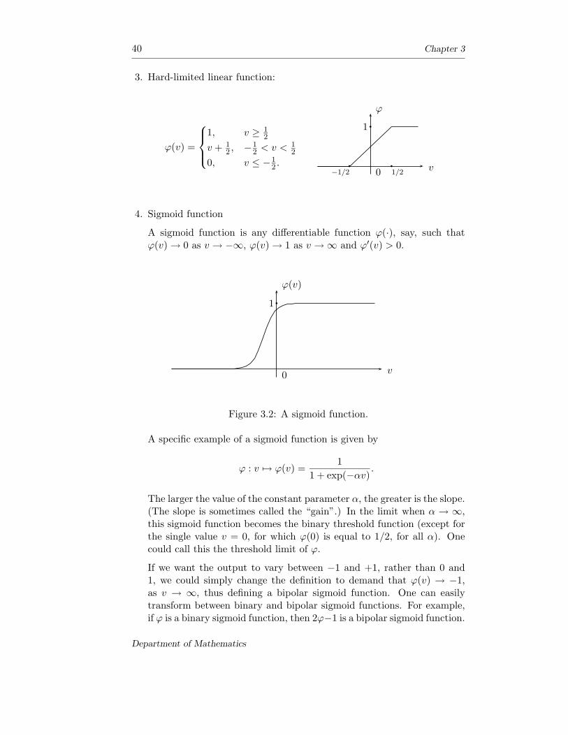
3. Hard-limited linear function:
ϕ(v) =
1, v ≥ 12
v + 12 , −1
2 < v < 12
0, v ≤ −12 . v
ϕ
0
1
−1/2 1/2
4. Sigmoid function
A sigmoid function is any differentiable function ϕ(·), say, such thatϕ(v) → 0 as v → −∞, ϕ(v) → 1 as v → ∞ and ϕ′(v) > 0.
v
ϕ(v)
0
1
Figure 3.2: A sigmoid function.
A specific example of a sigmoid function is given by
ϕ : v 7→ ϕ(v) =1
1 + exp(−αv).
The larger the value of the constant parameter α, the greater is the slope.(The slope is sometimes called the “gain”.) In the limit when α → ∞,this sigmoid function becomes the binary threshold function (except forthe single value v = 0, for which ϕ(0) is equal to 1/2, for all α). Onecould call this the threshold limit of ϕ.
If we want the output to vary between −1 and +1, rather than 0 and1, we could simply change the definition to demand that ϕ(v) → −1,as v → ∞, thus defining a bipolar sigmoid function. One can easilytransform between binary and bipolar sigmoid functions. For example,if ϕ is a binary sigmoid function, then 2ϕ−1 is a bipolar sigmoid function.
Department of Mathematics

Artificial Neural Networks 41
For the explicit example above, we see that
2ϕ(v) − 1 =1 − exp(−αv)
1 + exp(αv)= tanh
(αv
2
).
We turn now to a slightly more formal discussion of neural network. Wewill not attempt a definition in the axiomatic sense (there seems little pointat this stage), but rather enumerate various characteristics that typify aneural network.
• Essentially, a neural network is a decorated directed graph.
• A directed graph is a set of objects, called nodes, together with a collectionof directed links, that is, ordered pairs of nodes. Thus, the ordered pairof nodes {u, v} is thought of as a line joining the node u to the node vin the direction from u to v. A link is usually called a connection (orwire) and the nodes are called processing units (or elements), neuronsor artificial neurons.
• Each connection can carry a signal, i.e., to each connection we may assigna real number, called a signal. The signal is thought of as travelling inthe direction of the link.
• Each node has “local memory” in the form of a collection of real numbers,called weights, each of which is assigned to a corresponding terminatingi.e., incoming connection and represents the synaptic efficacy.
• Moreover, to each node there is associated some activation function whichdetermines the signals along its outgoing connections based only on localmemory—such as the weights associated with the incoming connectionsand the incoming signals. All outgoing signals from a particular nodeare equal in value.
• Some nodes may be specified as input nodes and others as output nodes.In this way, the neural network can communicate with the external world.One could consider a node with only outgoing links as an input node(source) and one with only incoming links as an output node (sink).
• In practical applications, a neural network is expected to be an intercon-nected network of very many (possibly thousands) of relatively simpleprocessing units. That is to say, the effectiveness of the network is ex-pected to come about because of the complexity of the interconnectionsrather than through any particularly clever behaviour of the individualneurons. The performance of a neural network is also expected to berobust in the sense of relative insensitivity to the removal of a smallnumber of connections or variations in the values of a few of the weights.
King’s College London
42 Chapter 3
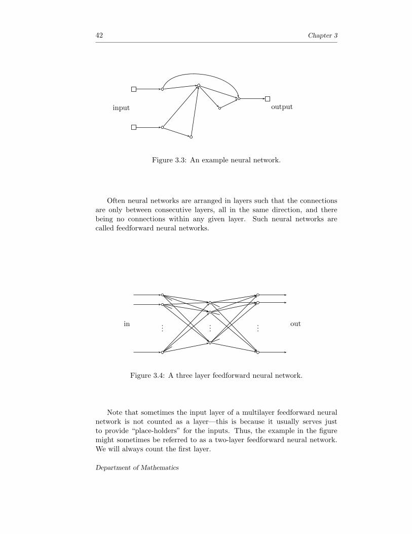
input output
Figure 3.3: An example neural network.
Often neural networks are arranged in layers such that the connectionsare only between consecutive layers, all in the same direction, and therebeing no connections within any given layer. Such neural networks arecalled feedforward neural networks.
in ......
...out
Figure 3.4: A three layer feedforward neural network.
Note that sometimes the input layer of a multilayer feedforward neuralnetwork is not counted as a layer—this is because it usually serves justto provide “place-holders” for the inputs. Thus, the example in the figuremight sometimes be referred to as a two-layer feedforward neural network.We will always count the first layer.
Department of Mathematics
Artificial Neural Networks 43
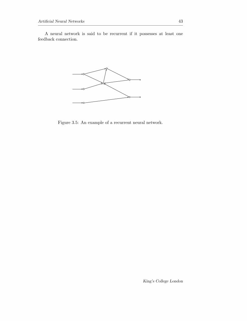
A neural network is said to be recurrent if it possesses at least onefeedback connection.
Figure 3.5: An example of a recurrent neural network.
King’s College London

44 Chapter 3
Department of Mathematics

Chapter 4
The Perceptron
The perceptron is a simple neural network invented by Frank Rosenblatt in1957 and subsequently extensively studied by Marvin Minsky and SeymourPapert (1969). It is driven by McCulloch-Pitts threshold processing unitsequipped with a particular learning algorithm.
“Retina”
A1
A2
...
An
Associator units
∑
w1
w2
wn
θoutput
∈ {0, 1}
︸ ︷︷ ︸
Threshold decision unit
Figure 4.1: The perceptron architecture.
The story goes that after much hype about the promise of neural net-works in the fifties and early sixties (for example, that artificial brains wouldsoon be a reality), Minsky and Papert’s work, elucidating the theory andvividly illustrating the limitations of the perceptron, was the catalyst forthe decline of the subject and certainly (which is almost the same thing) thewithdrawal of U. S. government funding. This led to a lull in research intoneural networks, as such, during the period from the end of the sixties to thebeginning of the eighties, but work did continue under the headings of adap-
45
46 Chapter 4
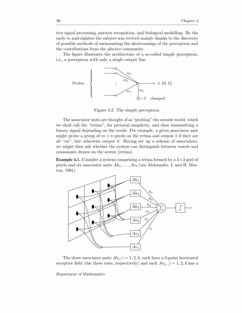
tive signal processing, pattern recognition, and biological modelling. By theearly to mid-eighties the subject was revived mainly thanks to the discoveryof possible methods of surmounting the shortcomings of the perceptron andthe contributions from the physics community.
The figure illustrates the architecture of a so-called simple perceptron,i.e., a perceptron with only a single output line.
...
w1
w2
wnw0
−1 clamped
∈ {0, 1}Probes
Figure 4.2: The simple perceptron.
The associator units are thought of as “probing” the outside world, whichwe shall call the “retina”, for pictorial simplicity, and then transmitting abinary signal depending on the result. For example, a given associator unitmight probe a group of m × n pixels on the retina and output 1 if they areall “on”, but otherwise output 0. Having set up a scheme of associators,we might then ask whether the system can distinguish between vowels andconsonants drawn on the screen (retina).
Example 4.1. Consider a system comprising a retina formed by a 3×3 grid ofpixels and six associator units Ah1, . . . , Av3 (see Aleksander, I. and H. Mor-ton, 1991).
Ah1
Ah2
Ah3
Av3
Av2
Av1
∑
h1
h2
h3
v3
v2
v1
The three associator units Ahi, i = 1, 2, 3, each have a 3-point horizontalreceptive field (the three rows, respectively) and each Avj , j = 1, 2, 3 has a
Department of Mathematics

The Perceptron 47
3-point vertical receptive field (the three columns). Each associator fires ifand only if a majority of its probes are “on”, i.e., each produces an output of1 if and only if at least 2 of its 3 pixels are black. We wish to assign weightsh1, . . . , v3, to the six connections to the binary threshold unit so that thesystem can successfully distinguish between the letters T and H so that thenetwork has an output of 1, say, corresponding to T, and an output of 0corresponding to H.
Associator
Ah1 Ah2 Ah3 Av1 Av2 Av3
! T 1 0 0 0 1 0
H 1 1 1 1 0 1 !
To induce the required output, we seek values for h1, . . . , v3 and θ suchthat
1h1 + 0h2 + 0h3 + 0v1 + 1v2 + 0v3 > θ,
but
1h1 + 1h2 + 1h3 + 1v1 + 0v2 + 1v3 < θ.
That is, h1 + v2 > θ and h1 + h2 + h3 + v1 + v3 < θ.
This will ensure that the binary decision output unit responds correctly.There are many possibilities here. One such is to try h1 = v2 = 1. Then thefirst of these inequalities demands that 2 > θ, whereas the second inequalityrequires that 1 + h2 + h3 + v1 + v3 < θ. Setting h2 = h3 = v1 = v3 = −1and θ = 0 does the trick.
The retina image corresponds to the associator output vector
given by (Ah1, . . . , Av3) = (1, 0, 0, 0, 1, 0), which we see induces the weightednet input h1 + v2 = 1 + 1 = 2 to the binary decision unit. Thus the outputis 1, which is associated with the letter T.
On the other hand, the retina image leads to the associator output
vector (Ah1, . . . , Av3) = (1, 1, 1, 1, 0, 1) which induces the weighted net inputh1 + h2 + h3 + v1 + v3 = 1− 1− 1− 1− 1 = −3 to the binary decision unit.The output is 0 which is associated with the letter H.
King’s College London

48 Chapter 4
It is of interest to look at an example of the limitation of the perceptron(after Minsky and Papert). We shall illustrate an example of a global prop-erty (connectedness) that cannot be measured by local probes. Let us saythat an associator unit has diameter d if the smallest square containing itssupport pixels (i.e., those pixels in the retina on whose values it depends)has side of d pixels. We shall now see that if a perceptron has diameter d,then, no matter how many associator units it has, there are tasks it simplycannot perform, such as check for connectedness.
Theorem 4.2. It is impossible to implement “connectedness” on a retina ofwidth r > d by a perceptron whose associator units have diameter no greaterthan d.
Proof. The proof is by contradiction. Suppose that we have a perceptronwhose probes have diameters not greater than d and that this perceptroncan recognise connectedness, that is, its output is 1 when it sees a connectedfigure on the retina and 0 otherwise. Consider the four figures indicated ona retina of width r > d.
width ≥ d + 1
1 2 3 4
Figure 4.3: Figures to fox the perceptron.
The perceptron associator units can be split into three distinct groups:
A — those which probe the left-hand end of the figure,
B — those which probe neither end,
C — those which probe the right-hand end of the figure.
The contribution to the output unit’s activation can therefore be representedas a sum of the three corresponding contributions, symbolically,
Σ = ΣA + ΣB + ΣC .
Department of Mathematics

The Perceptron 49
∑
∑A
∑B
∑C
Figure 4.4: Contributions to the output activation.
On presentation of pattern (1), the output should be 0, so that Σ(1) < θ,that is,
Σ(1)A + Σ
(1)B + Σ
(1)C < θ.
On presentation of patterns (2) or (3), the output should be 1, so
Σ(2)A + Σ
(2)B + Σ
(2)C > θ
Σ(3)A + Σ
(3)B + Σ
(3)C > θ.
Finally, presentation of pattern (4) should give output 0, so
Σ(4)A + Σ
(4)B + Σ
(4)C < θ.
However, the contributions Σ(1)B , Σ
(2)B , Σ
(3)B and Σ
(4)B are all equal because
the class B probes cannot tell the difference between the four figures.
Similarly, we see that Σ(1)A = Σ
(2)A and Σ
(1)C = Σ
(3)C , and Σ
(2)C = Σ
(4)C and
Σ(3)A = Σ
(4)A . To simplify the notation, let X, X ′ and Y, Y ′ denote the two
different A and C contributions, respectively, and set α = θ − Σ(1)B . Then
King’s College London

50 Chapter 4
we can write our four inequalities as
X + Y < α from figure (1)
X + Y ′ > α from figure (2)
X ′ + Y > α from figure (3)
X ′ + Y ′ < α from figure (4).
Clearly, the first two inequalities imply that Y ′ > Y which together with thethird gives X ′ + Y ′ > X ′ + Y > α. This contradicts the fourth inequality.We conclude that there can be no such perceptron.
Two-class classification
We wish to set up a network which will be able to differentiate inputs fromone of two categories. To this end, we shall consider a simple perceptroncomprising many input units and a single binary decision threshold unit.We shall ignore the associator units as such and just imagine them as pro-viding inputs to the binary decision unit. (One could imagine the systemcomprising as many associator units as pixels and where each associator unitprobes just one pixel to see if it is “on” or not.) However, we shall allow theinput values to be any real numbers, rather than just binary digits.
Suppose then that we have a finite collection of vectors in Rn, each of
which is classified as belonging to one of two categories, S1, S2, say. Ifthe vector (x1, . . . , xn) is presented to a linear binary threshold unit withweights w1, . . . , wn and threshold θ, then the output, z, say, is
z = step(∑n
i=1 wixi − θ)
=
{1, if
∑ni=1 wixi ≥ θ
0, otherwise.
We wish to find values of w1, . . . , wn and θ such that inputs in one of thecategories give output z = 1, whilst those in the other category yield outputz = 0. The means of attempting to achieve this will be to modify the weightswi and the threshold θ via an error-correction learning procedure—the so-called “perceptron learning rule”.
For notational convenience, we shall reformulate the problem. Let w0 =θ and set x0 = −1. Then
n∑
i=1
wixi − θ =n∑
i=0
wixi.
For given x ∈ Rn, let y = (x0, x) = (−1, x) ∈ R
n+1 and let w ∈ Rn+1 be the
vector given by w = (w0, w1, . . . , wn). The two categories of vectors S1 andS2 in R
n determine two categories, C1 and C2, say, in Rn+1 via the above
Department of Mathematics

The Perceptron 51
augmentation, x 7→ (−1, x). The problem is to find w ∈ Rn+1 such that
w · y > 0 for y ∈ C1 and w · y < 0 for y ∈ C2, where
w · y = wT y = w0y0 + · · · + wnyn
is the inner product of the vectors w and y in Rn+1.
To construct an error-correction scheme, suppose that y is one of theinput pattern vectors we wish to classify. If y ∈ C1, then we want w · y > 0for correct classification. If this is, indeed, the case, then we do not changethe value of w. However, if the classification is incorrect, then we must havew · y < 0. The idea is to change w to w′ = w + y. This leads to
w′ · y = (w + y) · y = w · y + y · y > w · y
so that even if w′ ·y still fails to be positive, it will be less negative than w ·y(note that y = (x0, x) 6= 0, since x0 = −1). In other words, w′ is “nearer”to giving the correct classification for the particular pattern y than w was.
Similarly, for y ∈ C2, misclassification means that w · y ≥ 0 rather thanw · y < 0. Setting w′ = w − y, gives
w′ · y = (w − y) · y = w · y − y · y,
so that w′ is nearer to the correct classification than w.
The perceptron error-correction rule, then, is to present the pattern vec-tor y and leave w unchanged if y is correctly classified, but otherwise changew to w′, where
w′ =
{w + y, if y ∈ C1
w − y, if y ∈ C2.
The discussion can be simplified somewhat by introducing
C = C1 ∪ (−C2) = {y : y ∈ C1, or − y ∈ C2}.
Then w · y > 0 for all y ∈ C would give correct classification. The error-correction rule now becomes the following.
The perceptron error-correction rule:
• present the pattern y ∈ C to the network;
• leave the weight vector w unchanged if w · y > 0,
• otherwise change w to w′ = w + y.
King’s College London
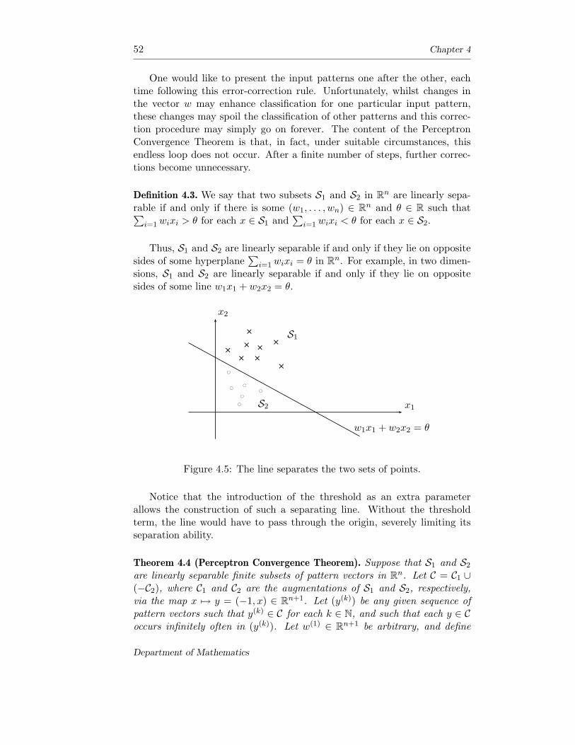
52 Chapter 4
One would like to present the input patterns one after the other, eachtime following this error-correction rule. Unfortunately, whilst changes inthe vector w may enhance classification for one particular input pattern,these changes may spoil the classification of other patterns and this correc-tion procedure may simply go on forever. The content of the PerceptronConvergence Theorem is that, in fact, under suitable circumstances, thisendless loop does not occur. After a finite number of steps, further correc-tions become unnecessary.
Definition 4.3. We say that two subsets S1 and S2 in Rn are linearly sepa-
rable if and only if there is some (w1, . . . , wn) ∈ Rn and θ ∈ R such that∑
i=1 wixi > θ for each x ∈ S1 and∑
i=1 wixi < θ for each x ∈ S2.
Thus, S1 and S2 are linearly separable if and only if they lie on oppositesides of some hyperplane
∑i=1 wixi = θ in R
n. For example, in two dimen-sions, S1 and S2 are linearly separable if and only if they lie on oppositesides of some line w1x1 + w2x2 = θ.
x1
x2
++++
++ +
+bcbc
bc
bc
bc
bc
bc
S1
S2
w1x1 + w2x2 = θ
Figure 4.5: The line separates the two sets of points.
Notice that the introduction of the threshold as an extra parameterallows the construction of such a separating line. Without the thresholdterm, the line would have to pass through the origin, severely limiting itsseparation ability.
Theorem 4.4 (Perceptron Convergence Theorem). Suppose that S1 and S2
are linearly separable finite subsets of pattern vectors in Rn. Let C = C1 ∪
(−C2), where C1 and C2 are the augmentations of S1 and S2, respectively,via the map x 7→ y = (−1, x) ∈ R
n+1. Let (y(k)) be any given sequence ofpattern vectors such that y(k) ∈ C for each k ∈ N, and such that each y ∈ Coccurs infinitely often in (y(k)). Let w(1) ∈ R
n+1 be arbitrary, and define
Department of Mathematics

The Perceptron 53
w(k+1) by the perceptron error-correction rule
w(k+1) =
{w(k), if w(k) · y(k) > 0,
w(k) + y(k), otherwise.
Then there is N such that w(N) · y > 0 for all y ∈ C, that is, after at mostN update steps, the weight vector correctly classifies all the input patternsand no further weight changes take place.
Proof. The perceptron error-correction rule can be written as
w(k+1) = w(k) + α(k)y(k),
where α(k) =
{0, if w(k) · y(k) > 0
1, otherwise,for k = 1, 2, . . . .
Notice that α(k)y(k) · w(k) ≤ 0, for all k. We have
w(k+1) = w(k) + α(k)y(k)
= w(k−1) + α(k−1)y(k−1) + α(k)y(k)
= · · ·= w(1) + α(1)y(1) + α(2)y(2) + · · · + α(k)y(k).
By hypothesis, S1 and S2 are linearly separable. This means that there issome w ∈ R
n+1 such that w ·y > 0 for each y ∈ C. Let δ = min{w ·y : y ∈ C}.Then δ > 0 and w · y(k) ≥ δ for all k ∈ N. Hence
w(k+1) · w = w(1) · w + α(1)y(1) · w + α(2)y(2) · w + · · · + α(k)y(k) · w≥ w(1) · w + (α(1) + α(2) + · · · + α(k))δ.
However, by Schwarz’ inequality, |w(k+1) · w| ≤ ‖w(k+1)‖‖w‖ and so
(w(1) · w + (α(1) + α(2) + · · · + α(k))δ
)≤ ‖w(k+1)‖ ‖w‖. (∗)
On the other hand,
‖w(k+1)‖2 = w(k+1) · w(k+1)
= (w(k) + α(k)y(k)) · (w(k) + α(k)y(k))
= ‖w(k)‖2 + 2α(k)y(k) · w(k)
︸ ︷︷ ︸≤ 0
+α(k)2‖y(k)‖2
≤ ‖w(k)‖2 + α(k)‖y(k)‖2, since α(k)2 = α(k),
≤ · · ·≤ ‖w(1)‖2 + α(1)‖y(1)‖2 + α(2)‖y(2)‖2 + · · · + α(k)‖y(k)‖2
≤ ‖w(1)‖2 +(α(1) + α(2) + · · · + α(k)
)K (∗∗)
King’s College London
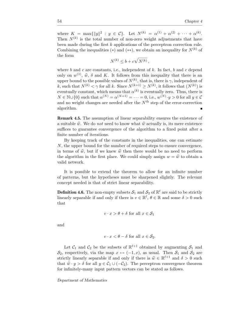
54 Chapter 4
where K = max{‖y‖2 : y ∈ C}. Let N (k) = α(1) + α(2) + · · · + α(k).Then N (k) is the total number of non-zero weight adjustments that havebeen made during the first k applications of the perceptron correction rule.Combining the inequalities (∗) and (∗∗), we obtain an inequality for N (k) ofthe form
N (k) ≤ b + c√
N (k) ,
where b and c are constants, i.e., independent of k. In fact, b and c dependonly on w(1), w, δ and K. It follows from this inequality that there is anupper bound to the possible values of N (k), that is, there is γ, independent ofk, such that N (k) < γ for all k. Since N (k+1) ≥ N (k), it follows that (N (k)) iseventually constant, which means that α(k) is eventually zero. Thus, there isN ∈ N∪{0} such that α(N) = α(N+1) = · · · = 0, i.e., w(N) ·y > 0 for all y ∈ Cand no weight changes are needed after the N th step of the error-correctionalgorithm.
Remark 4.5. The assumption of linear separability ensures the existence ofa suitable w. We do not need to know what w actually is, its mere existencesuffices to guarantee convergence of the algorithm to a fixed point after afinite number of iterations.
By keeping track of the constants in the inequalities, one can estimateN , the upper bound for the number of required steps to ensure convergence,in terms of w, but if we knew w then there would be no need to performthe algorithm in the first place. We could simply assign w = w to obtain avalid network.
It is possible to extend the theorem to allow for an infinite numberof patterns, but the hypotheses must be sharpened slightly. The relevantconcept needed is that of strict linear separability.
Definition 4.6. The non-empty subsets S1 and S2 of Rℓ are said to be strictly
linearly separable if and only if there is v ∈ Rℓ, θ ∈ R and some δ > 0 such
that
v · x > θ + δ for all x ∈ S1
and
v · x < θ − δ for all x ∈ S2.
Let C1 and C2 be the subsets of Rℓ+1 obtained by augmenting S1 and
S2, respectively, via the map x 7→ (−1, x), as usual. Then S1 and S2 arestrictly linearly separable if and only if there is w ∈ R
ℓ+1 and δ > 0 suchthat w · y > δ for all y ∈ C1 ∪ (−C2). The perceptron convergence theoremfor infinitely-many input pattern vectors can be stated as follows.
Department of Mathematics

The Perceptron 55
Theorem 4.7. Let C be any bounded subset of Rℓ+1 such that there is some
w ∈ Rℓ+1 and δ > 0 such that w ·y > δ for all y ∈ C. For any given sequence
(y(k)) in C, define the sequence (w(k)) by
w(k+1) = w(k) + α(k)y(k), where α(k) =
{0, if w(k) · y(k) > 0
1, otherwise,
and w(1) ∈ Rℓ+1 is arbitrary. Then there is M (not depending on the par-
ticular sequence (y(k))) such that N (k) = α(1) + α(2) + · · · + α(k) ≤ M forall k. In other words, α(k) = 0 for all sufficiently large k and so there canbe at most a finite number of non-zero weight changes.
Proof. By hypothesis, C is bounded and so there is some constant K suchthat ‖y‖2 < K for all y ∈ C. Exactly as before, we obtain an inequality
N (k) ≤ b + c√
N (k)
where b and c only depend on w(1), w, K and δ.
Remark 4.8. This means that if S1 and S2 are strictly linearly separable,bounded subsets of R
ℓ, then there is an upper bound to the number ofcorrections that the perceptron learning rule is able to make. This does notmean that the perceptron will necessarily learn to separate S1 and S2 in afinite number of steps—after all, the update sequence may only “sample”some of the data a few times, or perhaps not even at all! Indeed, havingchosen w(1) ∈ R
ℓ+1 and the sequence y(1), y(2), . . . of sample data, it may bethat w(1) ·y(j) > 0 for all j, but nonetheless, if y(1), y(2), . . . does not exhaustC, there could be (possibly infinitely-many) points y ∈ C with w(1) · y <0. Thus, the algorithm, starting with this particular w(1) and based onthe particular sample patterns y(1), y(2), . . . will not lead to a successfulclassification of S1 and S2.
King’s College London
56 Chapter 4
Extended two-class classification
So far, we have considered classification into one of two possible classes. Byallowing many output units, we can use a perceptron to classify patterns asbelonging to one of a number of possible classes. Consider a fully connectedneural network with n input and m output threshold units.
x1
x2
x3
xn
−1
...
...
m units
θ1
θ2
θm output ∈ { 0, 1 }m
Figure 4.6: A perceptron with m output units.
The idea is to find weights and thresholds such that presentation ofpattern j induces output for which only the jth unit is “on”, i.e., all outputunits are zero except for the jth which has value 1. Notice that the systemis equivalent to m completely independent simple perceptrons but with eachbeing presented with the same input pattern. We are led to the followingmulticlass perceptron error-correction rule. As usual, we work with theaugmented pattern vectors.
The extended two-class perceptron error-correction algorithm
• start with arbitrary weights (incorporating the threshold as zerothcomponent);
• present the first (augmented) pattern vector and observe the outputvalues;
• using the usual (simple) perceptron error-correction rule, update allthose weights which connect to an output with incorrect value;
• now present the next input pattern and repeat, cycling through allthe patterns again and again, as necessary.
Department of Mathematics
The Perceptron 57
Of course, the question is whether or not this procedure ever leads tothe correct classification of all m patterns. The relevant theorem is entirelyanalogous to the binary decision case—and is based on pairwise mutuallinear separability. (We will consider a less restrictive formulation later.)
Theorem 4.9. Let S = S1 ∪ · · · ∪ Sm be a collection of m classes of patternvectors in R
n and suppose that the subsets Si and S ′i = S \ Si are linearly
separable, for each 1 ≤ i ≤ m. Then the extended two-class perceptronerror-correction algorithm applied to an n-input m-output perceptron reachesa fixed point after a finite number of iterations and thus correctly classifieseach of the m patterns.
Proof. As we have already noted, the neural network is equivalent to mindependent simple perceptrons, each being presented with the same inputpattern. By the perceptron convergence theorem, we know that the jth ofthese will correctly distinguish the jth pattern from the rest after a finitenumber Nj , say, of iterations. Since there are only a finite number of pat-terns to be classified, the whole set will be correctly classified after at mostmax{N1, . . . , Nm} updates.
It is therefore of interest to find conditions which guarantee the linearseparability of m patterns as required by the theorem. It turns out thatlinear independence suffices for this, as we now show.
Definition 4.10. A linear map ℓ from Rn to R is called a linear functional.
Remark 4.11. Let ℓ be a linear functional on Rn, and let e1, . . . , en be a basis
for Rn. Thus, for any x ∈ R
n, there is α1, . . . , αn ∈ R such that
x = α1e1 + · · · + αnen.
Then we have
ℓ(x) = ℓ(α1e1 + · · · + αnen)
= ℓ(α1e1) + · · · + ℓ(αnen)
= α1ℓ(e1) + · · · + αnℓ(en).
It follows that ℓ is completely determined by its values on the elements of anybasis in R
n. In particular, if {e1, . . . , en} is the standard orthonormal basisof R
n, so that x = (x1, . . . , xn) = x1e1+ · · ·+xnen, then ℓ(x) = v ·x ( = vT x,in matrix notation), where v ∈ R
n is the vector v =(ℓ(e1), . . . , ℓ(en)
).
On the other hand, for any u ∈ Rn, it is clear that the map x 7→ u · x
( = uT x) defines a linear functional on Rn.
King’s College London
58 Chapter 4
Proposition 4.12. For any linearly independent set of vectors {x(1), . . . , x(m)}in R
n, the augmented vectors {x(1), . . . , x(m)}, with x(i) = (−1, x(i)) ∈ Rn+1,
form a linearly independent collection.
Proof. Suppose that∑m
j=1 αjx(j) = 0. This is a vector equation and so each
of the n+1 components of the left hand side must vanish,∑m
j=1 αjx(j)i = 0,
for 0 ≤ i ≤ n. Note that the first component of x(j) has been given theindex 0.
In particular,∑m
j=1 αjx(j)i = 0, for 1 ≤ i ≤ n, that is,
∑mj=1 αjx
(j) = 0.
By hypothesis, x(1), . . . , x(m) are linearly independent and so α1 = · · · =αm = 0 which means that x(1), . . . , x(m) are linearly independent, as re-quired.
Remark 4.13. The converse is false. For example, if x(1) = (1, 1, . . . , 1) ∈ Rn,
and x(2) = (2, 2, . . . , 2) ∈ Rn, then clearly x(1) and x(2) are not linearly
independent. However, x(1) and x(2) are linearly independent.
Proposition 4.14. Suppose that x(1), . . . , x(m) ∈ Rn are linearly independent
pattern vectors. Then, for each k = 1, 2, . . . , m, there is w(k) ∈ Rn and
θk ∈ R such that
w(k) · x(k) > θk
and
w(k) · x(j) < θk
for j 6= k.
Proof. By the previous result, the augmented vectors x(1), . . . , x(m) ∈ Rn+1
are linearly independent. Let y(m+1), . . . , y(n+1) be n − m linearly inde-pendent vectors such that the collection {x(1), . . . , x(m), y(m+1), . . . , y(n+1)}forms a basis for R
n+1.Define the linear functional ℓ1 : R
n+1 → R by assigning its values on thebasis given above according to ℓ1(x
(1)) = 1 and ℓ1(x(2)) = · · · = ℓ(yn+1) =
−1. Now, we know that there is v = (v0, v1, . . . , vn) ∈ Rn+1 such that ℓ1
can be written asℓ1(x) = v · x
for all x ∈ Rn+1. Set θ1 = v0 and w(1) = (v1, . . . , vn) ∈ R
n. Then
1 = ℓ1(x(1)) = v · x(1)
= v0x(1)0 + v1x
(1)1 + · · · + vnx(1)
n
= −θ1 + w(1) · x(1), since x(1)0 = −1,
so that w(1) · x(1) > θ1.Similarly, for any j 6= 1, −1 = ℓ1(x
(j)) = −θ1 + w(1) · x(j) giving w(1) ·x(j) < θ1. An identical argument holds for any x(k) rather than x(1).
Department of Mathematics

The Perceptron 59
This tells us that an m-output perceptron is capable of correctly classify-ing m linearly independent pattern vectors. For example, we could correctlyclassify the capital letters of the alphabet using a perceptron with 26 outputunits by representing the letters as 26 linearly independent vectors. Thismight be done by drawing each character on a retina (or grid) of sufficientlyhigh resolution (perhaps 6× 6 pixels) and transforming the resulting imageinto a binary vector whose components correspond to the on-off state of thecorresponding pixels. Of course, one should check that the 26 binary vectorsone gets are, indeed, linearly independent.
The multi-class error correction algorithm
Suppose that we have a collection of patterns S in Rn comprising m classes
S1, . . . ,Sm. The aim is to construct a network which can correctly classifythese patterns. To do this, we set up a “winner takes all” network builtfrom m linear units.
x1
x2
xn
input
...
∑
∑
...
∑
m unitscomputesthe winning unit
j
Figure 4.7: Winner takes all network.
There are n inputs which feed into m linear units, i.e., each unit simplyrecords its net weighted input. The network output is the index of the unitwhich has maximum such activation. Thus, if w1, . . . , wm are the weightsto the m linear units and the input pattern is x, then the system output isthe “winning unit”, i.e., that value of j with
wj · x > wi · x for all i 6= j.
In the case of a tie, one assigns a rule of convenience. For example, onemight choose one of the winners at random, or alternatively, always choosethe smallest index possible, say.
King’s College London

60 Chapter 4
Multi-class error correction algorithm
• Choose the initial set of weight vectors w(1)1 , . . . , w
(m)m , arbitrarily.
• Step k: Present a pattern x(k) from S and observe the winning unit.Suppose that x(k) ∈ Si. If the winning unit is unit i, then donothing. If the winning unit is j 6= i, then update the weightsaccording to
w(k+1)i = w
(k)i + x(k) reinforce unit i
w(k+1)j = w
(k)j − x(k) anti-reinforce unit j
. . . and repeat.
The question is whether or not the algorithm leads to a set of weights whichcorrectly classify the patterns. Under certain separability conditions, theanswer is yes.
Theorem 4.15 (Multi-class error-correction convergence theorem). Supposethat the m classes Si are linearly separable in the sense that there exist weightvectors w∗
1, . . . , w∗m ∈ R
n such that
w∗i · x > w∗
j · x for all j 6= i
whenever x ∈ Si. Suppose that the pattern presentation sequence (x(k)),from the finite set S = S1 ∪ · · ·∪Sm, is such that every pattern in S appearsinfinitely-often. Then, after a finite number of iterations, the multi-classerror-correction algorithm provides a set of weight vectors which correctlyclassify all patterns in S.
Proof. The idea of the proof (Kesler) is to relate this system to a two-classproblem (in a high dimensional space) solved by the usual perceptron error-correction algorithm.
For any given i ∈ {1, . . . , m} and x ∈ Si, we construct m − 1 vectors,x(j) ∈ R
mn, 1 ≤ j ≤ m but j 6= i, as follows. Set
x(j) = u1 ⊕ u2 ⊕ · · · ⊕ um ∈ Rmn
where ui = x, uj = −x and all other uℓs are zero in Rn. Let
w∗ = w∗1 ⊕ · · · ⊕ w∗
m ∈ Rmn.
Thenw∗ · x(j) = w∗
i · x − w∗j · x > 0
by (the separation) hypothesis. Let C denote the set of all possible x(j)s asx runs over S. Then C is “linearly separable” in the sense of the perceptronconvergence theorem;
w∗ · y > 0 for all y ∈ C.
Department of Mathematics
The Perceptron 61
Suppose we start with w = w(1)1 ⊕ · · · ⊕w
(1)m and apply the perceptron error
correction algorithm with patterns drawn from C:
w(k+1) = w(k) + α(k)x(j)
where α(k) = 0 if w(k) · x(j) > 0, and otherwise α(k) = 1. The correctionα(k)x(j) gives
w(k+1) = (w(k)1 + v1) ⊕ . . . (w(k)
m + vm)
where
vi = α(k)x, assuming x ∈ Si
vj = −α(k)x,
vℓ = 0, all ℓ 6= i, j.
Thus, the components of w(k+1) are given by
w(k+1)i = w
(k)i + α(k)x
w(k+1)j = w
(k)j − α(k)x
w(k+1)ℓ = w
(k)ℓ , ℓ 6= i, ℓ 6= j
which is precisely the multi-class error correction rule when unit j is thewinning unit. In other words, the weight changes given by the two systemalgorithms are the same. If one is non-zero, then neither is the other. Itfollows that every misclassified pattern (from S) presented to the multi-class system induces a misclassified “super-pattern” (in C ⊂ R
mn) for theperceptron system thus triggering a non-zero weight update.
However, the perceptron convergence theorem assures us that the “super-pattern” system can accommodate at most a finite number of non-zeroweight changes. It follows that the multi-class algorithm can undergo atmost a finite number of weights changes. We deduce that after a finite num-ber of steps, the winner-takes-all system must correctly classify all patternsfrom S.
King’s College London

62 Chapter 4
Mapping implementation
Let us turn now to the perceptron viewed as a mechanism for implementingbinary-valued mappings, f : x 7→ f(x) ∈ {0, 1}.
Example 4.16. Consider the function f : {0, 1}2 → {0, 1} given by
f :
(0, 0) 7→ 0
(0, 1) 7→ 0
(1, 0) 7→ 0
(1, 1) 7→ 1.
If we think of 0 and 1 as “off” and “on”, respectively, then f is “on” if andonly if both its arguments are “on”. For this reason, f is called the “and”function.
We wish to implement f using a simple perceptron with two input neu-rons and a binary threshold output neuron. Thus, we seek weights w1, w2
and a threshold θ such that step(w1x + w2y − θ) = 1 for (x, y) = (1, 1),but otherwise is zero, that is, we require that w1x + w2y − θ is positive for(x, y) = (1, 1), but otherwise is negative. Geometrically, this means that thepoint (1, 1) lies above the line w1x + w2y − θ = 0 in the two-dimensional(x, y)-plane, whereas the other three points lie below this line. The linew1x + w2y − θ = 0 is a “hyperplane” linearly separating the two classes{(1, 1)} and {(0, 0), (0, 1), (1, 0)}. There are many possibilities—one such isshown in the figure.
(0,0)
(0,1)
(1,0)
(1,1)
separating hyperplane
θ = 3
w1 = 2
w2 = 2
Figure 4.8: A line separating the classes, and the correspondingsimple perceptron which implements the “and” function.
Department of Mathematics
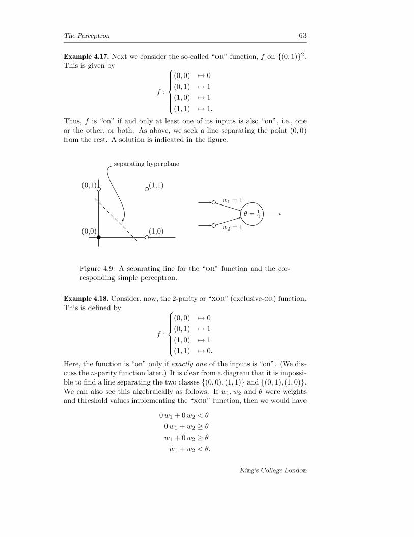
The Perceptron 63
Example 4.17. Next we consider the so-called “or” function, f on {(0, 1)}2.This is given by
f :
(0, 0) 7→ 0
(0, 1) 7→ 1
(1, 0) 7→ 1
(1, 1) 7→ 1.
Thus, f is “on” if and only at least one of its inputs is also “on”, i.e., oneor the other, or both. As above, we seek a line separating the point (0, 0)from the rest. A solution is indicated in the figure.
(0,0)
(0,1)
(1,0)
(1,1)
separating hyperplane
θ = 1
2
w1 = 1
w2 = 1
Figure 4.9: A separating line for the “or” function and the cor-responding simple perceptron.
Example 4.18. Consider, now, the 2-parity or “xor” (exclusive-or) function.This is defined by
f :
(0, 0) 7→ 0
(0, 1) 7→ 1
(1, 0) 7→ 1
(1, 1) 7→ 0.
Here, the function is “on” only if exactly one of the inputs is “on”. (We dis-cuss the n-parity function later.) It is clear from a diagram that it is impossi-ble to find a line separating the two classes {(0, 0), (1, 1)} and {(0, 1), (1, 0)}.We can also see this algebraically as follows. If w1, w2 and θ were weightsand threshold values implementing the “xor” function, then we would have
0 w1 + 0w2 < θ
0 w1 + w2 ≥ θ
w1 + 0w2 ≥ θ
w1 + w2 < θ.
King’s College London
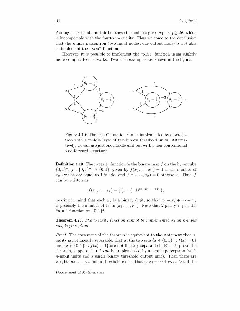
64 Chapter 4
Adding the second and third of these inequalities gives w1 +w2 ≥ 2θ, whichis incompatible with the fourth inequality. Thus we come to the conclusionthat the simple perceptron (two input nodes, one output node) is not ableto implement the “xor” function.
However, it is possible to implement the “xor” function using slightlymore complicated networks. Two such examples are shown in the figure.
θ1 = 1
21
1
θ2 = 3
2
1
1
θ3 = 1
2
1
−1
θ1 = 3
2
1
1θ3 = 3
2
−3
2
2
Figure 4.10: The “xor” function can be implemented by a percep-tron with a middle layer of two binary threshold units. Alterna-tively, we can use just one middle unit but with a non-conventionalfeed-forward structure.
Definition 4.19. The n-parity function is the binary map f on the hypercube{0, 1}n, f : {0, 1}n → {0, 1}, given by f(x1, . . . , xn) = 1 if the number ofxk s which are equal to 1 is odd, and f(x1, . . . , xn) = 0 otherwise. Thus, fcan be written as
f(x1, . . . , xn) = 12
(1 − (−1)x1+x2+···+xn
),
bearing in mind that each xk is a binary digit, so that x1 + x2 + · · · + xn
is precisely the number of 1 s in (x1, . . . , xn). Note that 2-parity is just the“xor” function on {0, 1}2.
Theorem 4.20. The n-parity function cannot be implemented by an n-inputsimple perceptron.
Proof. The statement of the theorem is equivalent to the statement that n-parity is not linearly separable, that is, the two sets {x ∈ {0, 1}n : f(x) = 0}and {x ∈ {0, 1}n : f(x) = 1} are not linearly separable in R
n. To prove thetheorem, suppose that f can be implemented by a simple perceptron (withn-input units and a single binary threshold output unit). Then there areweights w1, . . . , wn and a threshold θ such that w1x1 + · · ·+wnxn > θ if the
Department of Mathematics
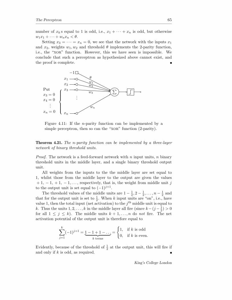
The Perceptron 65
number of xk s equal to 1 is odd, i.e., x1 + · · · + xn is odd, but otherwisew1x1 + · · · + wnxn < θ.
Setting x3 = · · · = xn = 0, we see that the network with the inputs x1
and x2, weights w1, w2 and threshold θ implements the 2-parity function,i.e., the “xor” function. However, this we have seen is impossible. Weconclude that such a perceptron as hypothesized above cannot exist, andthe proof is complete.
x1
x2
x3
xn
Putx3 = 0x4 = 0
...xn = 0
−1
...
∑
θw1
w2
w3
wn
Figure 4.11: If the n-parity function can be implemented by asimple perceptron, then so can the “xor” function (2-parity).
Theorem 4.21. The n-parity function can be implemented by a three-layernetwork of binary threshold units.
Proof. The network is a feed-forward network with n input units, n binarythreshold units in the middle layer, and a single binary threshold outputunit.
All weights from the inputs to the the middle layer are set equal to1, whilst those from the middle layer to the output are given the values+ 1, − 1, + 1, − 1, . . . , respectively, that is, the weight from middle unit jto the output unit is set equal to (−1)j+1.
The threshold values of the middle units are 1 − 12 , 2 − 1
2 , . . . , n − 12 and
that for the output unit is set to 12 . When k input units are “on”, i.e., have
value 1, then the total input (net activation) to the jth middle unit is equal tok. Thus the units 1, 2, . . . , k in the middle layer all fire (since k− (j− 1
2) > 0for all 1 ≤ j ≤ k). The middle units k + 1, . . . , n do not fire. The netactivation potential of the output unit is therefore equal to
k∑
j=1
(−1)j+1 = 1 − 1 + 1 − . . .︸ ︷︷ ︸k terms
=
{1, if k is odd
0, if k is even.
Evidently, because of the threshold of 12 at the output unit, this will fire if
and only if k is odd, as required.
King’s College London
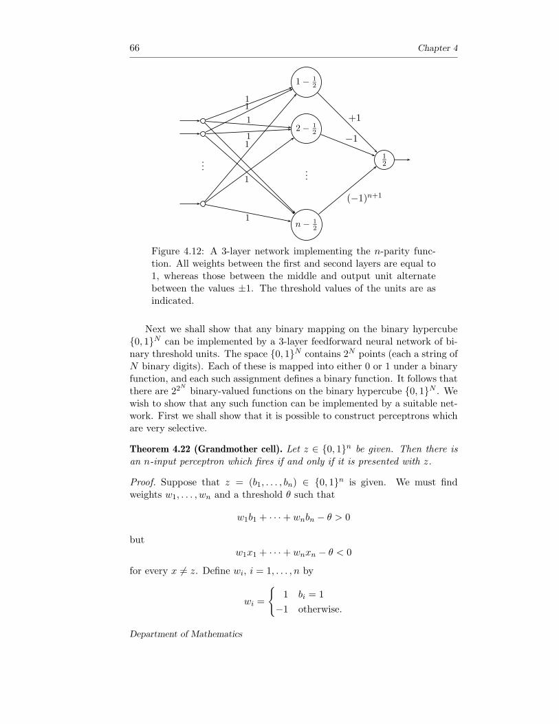
66 Chapter 4
...
1 − 1
2
2 − 1
2
...
n − 1
2
1
1
1
1
1
1
1
12
+1
−1
(−1)n+1
Figure 4.12: A 3-layer network implementing the n-parity func-tion. All weights between the first and second layers are equal to1, whereas those between the middle and output unit alternatebetween the values ±1. The threshold values of the units are asindicated.
Next we shall show that any binary mapping on the binary hypercube{0, 1}N can be implemented by a 3-layer feedforward neural network of bi-nary threshold units. The space {0, 1}N contains 2N points (each a string ofN binary digits). Each of these is mapped into either 0 or 1 under a binaryfunction, and each such assignment defines a binary function. It follows thatthere are 22N
binary-valued functions on the binary hypercube {0, 1}N . Wewish to show that any such function can be implemented by a suitable net-work. First we shall show that it is possible to construct perceptrons whichare very selective.
Theorem 4.22 (Grandmother cell). Let z ∈ {0, 1}n be given. Then there isan n-input perceptron which fires if and only if it is presented with z.
Proof. Suppose that z = (b1, . . . , bn) ∈ {0, 1}n is given. We must findweights w1, . . . , wn and a threshold θ such that
w1b1 + · · · + wnbn − θ > 0
but
w1x1 + · · · + wnxn − θ < 0
for every x 6= z. Define wi, i = 1, . . . , n by
wi =
{1 bi = 1
−1 otherwise.
Department of Mathematics
The Perceptron 67
This assignment can be rewritten as wi = (2bi − 1). Then we see that
n∑
i=1
wixi =n∑
i=1
(2bi − 1)xi
=n∑
i=1
(2bixi − xi).
Now, if x = z, then xi = bi, 1 ≤ i ≤ n, so that bixi = b2i = bi, since
bi ∈ {0, 1}. Hence, in this case,
n∑
i=1
wixi =n∑
i=1
(2bi − bi) =n∑
i=1
bi.
On the other hand, if x 6= z, then there is some j such that xj 6= bj sothat bjxj = 0 (since one of bj , xj must be zero). But, for such a term,(2bj − 1)xj = −xj < bj (because bj + xj = 1). Hence, if x 6= z, we have
n∑
i=1
wixi =n∑
i=1
(2bi − 1)xi <n∑
i=1
bi.
Now, both sides of the above inequality are integers, so if we set θ =∑ni=1 bi − 1
2 , it follows that
n∑
i=1
wixi < θ <n∑
i=1
bi =n∑
i=1
wibi
for any x 6= z and the construction is complete.
In the jargon, a neuron such as this is sometimes called a grandmothercell (from the biological idea that some neurons might serve just a singlespecialized purpose, such as responding to precisely one’s grandmother). Itis not thought that such neurons really exist in real brains.
Theorem 4.23. Any mapping f : {0, 1}N → {0, 1} can be implemented by a3-layer feedforward neural network of binary threshold units.
Proof. Let f : {0, 1}N → {0, 1} be given. We construct the appropriateneural network as follows.
The neural network has N inputs, a middle (hidden) layer of 2N binarythreshold units and a single binary threshold output unit. The output unitis assigned threshold 1
2 . Label the hidden units by the 2N elements z in{0, 1}N and construct each to be the corresponding grandmother unit forthe binary vector z. The weight from each such unit to the output unit isset to the value f(z).
Then if the input is z, only the hidden unit labelled by z will fire. Thetotal input to the output unit will then be precisely f(z). The output unitwill fire if and only if the value of f(z) is 1 (and not 0).
King’s College London
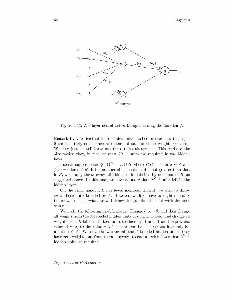
68 Chapter 4
x1
x2
xi
xn
...
...
θ1
...
θj
...
θ2N
2N units
wj1
wji
wjN
12
f(b1, . . . , bN )
f
Figure 4.13: A 3-layer neural network implementing the function f .
Remark 4.24. Notice that those hidden units labelled by those z with f(z) =0 are effectively not connected to the output unit (their weights are zero).We may just as well leave out these units altogether. This leads to theobservation that, in fact, at most 2N−1 units are required in the hiddenlayer.
Indeed, suppose that {0, 1}N = A ∪ B where f(x) = 1 for x ∈ A andf(x) = 0 for x ∈ B. If the number of elements in A is not greater than thatin B, we simply throw away all hidden units labelled by members of B, assuggested above. In this case, we have no more than 2N−1 units left in thehidden layer.
On the other hand, if B has fewer members than A, we wish to throwaway those units labelled by A. However, we first have to slightly modifythe network—otherwise, we will throw the grandmother out with the bathwater.
We make the following modifications. Change θ to −θ, and then changeall weights from the A-labelled hidden units to output to zero, and change allweights from B-labelled hidden units to the output unit (from the previousvalue of zero) to the value −1. Then we see that the system fires only forinputs x ∈ A. We now throw away all the A-labelled hidden units (theyhave zero weights out from them, anyway) to end up with fewer than 2N−1
hidden units, as required.
Department of Mathematics
The Perceptron 69
Testing for linear separability
The perceptron convergence theorem tells us that if two classes of patternsare linearly separable, then the perceptron error-correction rule will eventu-ally lead to a set of weights giving correct classification. Unfortunately, itsheds no light on whether or not the classes actually are linearly separable.Of course, one could ignore this in practice, and continue with the hope thatthey are. We have seen that linear independence suffices and so, providedwe embed our patterns into a space of sufficiently high dimension, therewould seem to be a good chance that the classes will be linearly separableand so we can run the perceptron algorithm with abandon. It would be nice,however, if it were possible to somehow discover, as we go along, whetheror not our efforts are doomed to failure. We will discuss now the so-calledHo-Kashyap algorithm, which does precisely that.
The problem is to classify two sets of patterns S1 and S2 in Rℓ. As usual,
these are augmented to give C1 and C2, and then we set C = C1 ∪ (−C2).Thus, we seek w ∈ R
ℓ+1 such that w · y > 0 for all y ∈ C. SupposeC = {y(1), . . . , y(N)}. Then we want w ∈ R
ℓ+1 such that w · y(j) > 0 foreach 1 ≤ j ≤ N . Evidently, this problem is equivalent to that of finding aset of real numbers b1 > 0, . . . , bN > 0 such that w · y(j) = bj , 1 ≤ j ≤ N .Expressing this in matrix form, we seek w ∈ R
ℓ+1 and b ∈ RN such that b
has strictly positive entries, and
Y w = b, where Y =
y(1)T
y(2)T
...
y(N)T
∈ R
N×(ℓ+1),
where we have used the equality w · y(j) = y(j)T w.To develop an algorithm for finding such vectors w and b, we observe
that, trivially, any such pair minimizes the quantity
J = 12‖Y w − b‖2 = 1
2‖Y w − b‖2F .
So to attempt to find a suitable w and b, we employ a kind of gradient-descent based technique. Writing
J = 12‖Y w − b‖2 = 1
2(Y w − b)T (Y w − b)
= 12
N∑
j=1
(y(j)T w − bj)2
we see that ∂J/∂bj = −(y(j)T w − bj), 1 ≤ j ≤ N , and so the gradient of J ,as a function of the vector b, is
∂J
∂b= −(Y w − b) ∈ R
N .
King’s College London

70 Chapter 4
Suppose that w(1), w(2), . . . , and b(1), b(2), . . . are iterations for w and b,respectively. Then a gradient-descent technique for b might be to constructthe b(k) s by the rule
b(k+1) = b(k) − α∂J
∂b
= b(k) + α(Y w(k) − b(k)), k = 1, 2, . . . ,
where α is a positive constant. Given b(k), we choose w(k) so that J isminimized (for given Y and b(k)). This we know, from general theory, to beachieved by w(k) = Y #b(k). Indeed, for given matrices A and B, ‖XA−B‖F
is minimized by X = BA# and so, for given Y and b, ‖Y w− b‖F = ‖(Y w−b)T ‖F = ‖wT Y T − bT ‖F is minimized by wT = bT Y T # = bT Y #T , that is,for w = Y #b.
However, we want to ensure that b(k) has strictly positive components.To this end, we modify the formula for b(k+1) above, to the following. Weset
b(k+1) = b(k) + α∆b(k)
where ∆b(k)j =
{(Y w(k) − b(k))j , if (Y w(k) − b(k))j > 0
0, otherwiseand where b(1) is
such that b(1)j > 0 for all 1 ≤ j ≤ N . Note that b(k+1)
j ≥ b(k)j for each
1 ≤ j ≤ N , that is, the components of b(k) never decrease at any step of theiteration. The algorithm then is as follows.
The Ho-Kashyap algorithm
Let b(1) be arbitrary subject to b(1)j > 0, 1 ≤ j ≤ N . For each k = 1, 2, . . .
set w(k) = Y #b(k) and
b(k+1) = b(k) + α∆b(k)
where the constant α > 0 will be chosen to ensure convergence, and where∆b(k) is given as above.
For notational convenience, let e(k) = Y w(k) − b(k). Then ∆b(k) is thevector with components given by ∆b(k)
j = e(k)j if e(k)
j > 0, but otherwise∆b(k)
j = 0. It follows that e(k)T ∆b(k) = ∆b(k)T ∆b(k).
Theorem 4.25. Suppose that S1 and S2 are linearly separable classes. Then,for any k, the inequalities e(k)
j ≤ 0 for all j = 1, . . . , N imply that e(k) = 0.
Proof. By hypothesis, there is some w ∈ Rℓ+1 such that w · y > 0 for all
y ∈ C, i.e., w · y(j) > 0 for all 1 ≤ j ≤ N . In terms of the matrix Y , this
Department of Mathematics
The Perceptron 71
implies that the vector Y w has strictly positive components, (Y w)j > 0,1 ≤ j ≤ N . Now, from the definition of e(k), we have
Y T e(k) = Y T (Y w(k) − b(k))
= Y T (Y Y #b(k) − b(k))
= (Y T Y Y # − Y T )b(k).
But Y Y # = (Y Y #)T and so
Y T Y Y # = Y T (Y Y #)T
=((Y Y #Y
)T
= Y T .
Hence Y T e(k) = 0, and so e(k)T Y = 0. (We will also use this last equalitylater.) It follows that e(k)T w = 0, that is,
N∑
j=1
e(k)j(Y w)j = 0.
The inequalities (Y w)j > 0 and e(k)j ≤ 0, for all 1 ≤ j ≤ N , force e(k)
j = 0for all 1 ≤ j ≤ N .
Remark 4.26. This result means that if, during execution of the algorithm,we find that e(k) has strictly negative components, then S1 and S2 are notlinearly separable.
Next we turn to a proof of convergence of the algorithm under the as-sumption that S1 and S2 are linearly separable.
Theorem 4.27. Suppose that S1 and S2 are linearly separable, and let 0 <α < 2. The algorithm converges to a solution after a finite number of steps.
Proof. By definition,
e(k) = Y w(k) − b(k)
= (Y Y # − 1lN )b(k)
= (P − 1lN )b(k)
where P = Y Y # satisfies P = P T = P 2, i.e., P is an orthogonal projection.Therefore
e(k+1) = (P − 1lN )b(k+1)
= (P − 1lN )(b(k) + α∆b(k))
= e(k) + α(P − 1lN )∆b(k).
King’s College London

72 Chapter 4
Hence
‖e(k+1)‖2 = ‖e(k)‖2 + α2‖(P − 1lN )∆b(k)‖2
+ 2αe(k)T (P − 1lN )∆b(k).
To evaluate the right hand side, we calculate
‖(P − 1lN )∆b(k)‖2 = ∆b(k)T P T P∆b(k)
− 2∆b(k)P∆b(k) + ∆b(k)T ∆b(k)
= −‖P∆b(k)‖2 + ‖∆b(k)‖2, using P = P T P .
Furthermore,
e(k)T (P − 1lN )∆b(k) = e(k)T (Y Y # − 1lN )∆b(k)
= −e(k)T ∆b(k), since e(k)T Y = 0,
= −∆b(k)T ∆b(k)
= −‖∆b(k)‖2.
Therefore, we can write ‖e(k+1)‖2 as
‖e(k+1)‖2 = ‖e(k)‖2 − α2‖P∆b(k)‖2 − α(2 − α)‖∆b(k)‖2 (∗)
Choosing 0 < α < 2, we see that
‖e(k+1)‖ ≤ ‖e(k)‖, for k = 1, 2, . . . .
The sequence (‖e(k)‖)k∈N is a non-increasing sequence of non-negative terms,and so converges as k → ∞. In particular, it follows from (∗) that ‖∆b(k)‖ →0, i.e., ∆b(k) → 0 in R
N as k → ∞. (The difference ‖e(k)‖2 − ‖e(k+1)‖2
converges to 0. By (∗), this is equal to a sum of two non-negative terms,both of which must therefore also converge to 0.)
Moreover, the sequence (e(k))k∈N is a bounded sequence in RN and so
has a convergent subsequence. That is, there is some f ∈ RN and a sub-
sequence (e(kn))n∈N such that e(kn) → f in RN as n → ∞. In particular,
the components e(kn)j converge to the corresponding component fj of f , as
n → ∞. From its definition, we can write down the components of ∆b(k) as
∆b(k)j = 1
2(e(k)j + |e(k)
j |), j = 1, 2, . . . , N.
Hence
∆b(kn)j = 1
2(e(kn)j + |e(kn)
j |)→ 1
2(fj + |fj |)
Department of Mathematics

The Perceptron 73
as n → ∞, for each 1 ≤ j ≤ N . However, we know that the sequence(∆b(k))k∈N converges to 0 in R
N , and so, therefore, does the subsequence(∆b(kn))n∈N. It follows that fj + |fj | = 0 for each 1 ≤ j ≤ N . In otherwords, all components of f are non-positive.
By hypothesis, S1 and S2 are linearly separable and so there is w ∈ Rℓ+1
such that Y w has strictly positive components. However, e(k)T Y = 0 for allk, and so, in particular,
fT Y w = limn→∞
e(kn)T Y w = 0,
i.e.,∑N
j=1 fj(Y w)j = 0, where (Y w)j > 0 for all 1 ≤ j ≤ N . Since fj ≤ 0,
we must have fj = 0, j = 1, . . . , N , and we conclude that e(kn) → 0 asn → ∞. But then the inequality ‖e(k+1)‖ ≤ ‖e(k)‖, for all k = 1, 2, . . . ,implies that the whole sequence (e(k))k∈N converges to 0. (For any givenε > 0, there is N0 such that ‖e(kn)‖ < ε whenever n > N0. Put N1 = kN0+1.Then for any k > N1, we have ‖e(k)‖ ≤ ‖e(kN0+1)‖ < ε.)
Let µ = max{b(1)j : 1 ≤ j ≤ N} be the maximum value of the com-
ponents of b(1). Then µ > 0 by our choice of b(1). Since e(k) → 0, ask → ∞, there is k0 such that ‖e(k)‖ < 1
2µ whenever k > k0. In particular,
−12µ < e(k)
j < 12µ for each 1 ≤ j ≤ N whenever k > k0. But for any
j = 1, . . . , N , b(k)j ≥ b(1)
j , and so
(Y w(k))j = b(k)j + e(k)
j
> µ − 12µ = 1
2µ
> 0
whenever k > k0. Therefore the vector w(k0+1) satisfies y(j)T w(k0+1) > 0for all 1 ≤ j ≤ N and determines a separating vector for S1 and S2 whichcompletes the proof.
King’s College London

74 Chapter 4
Department of Mathematics
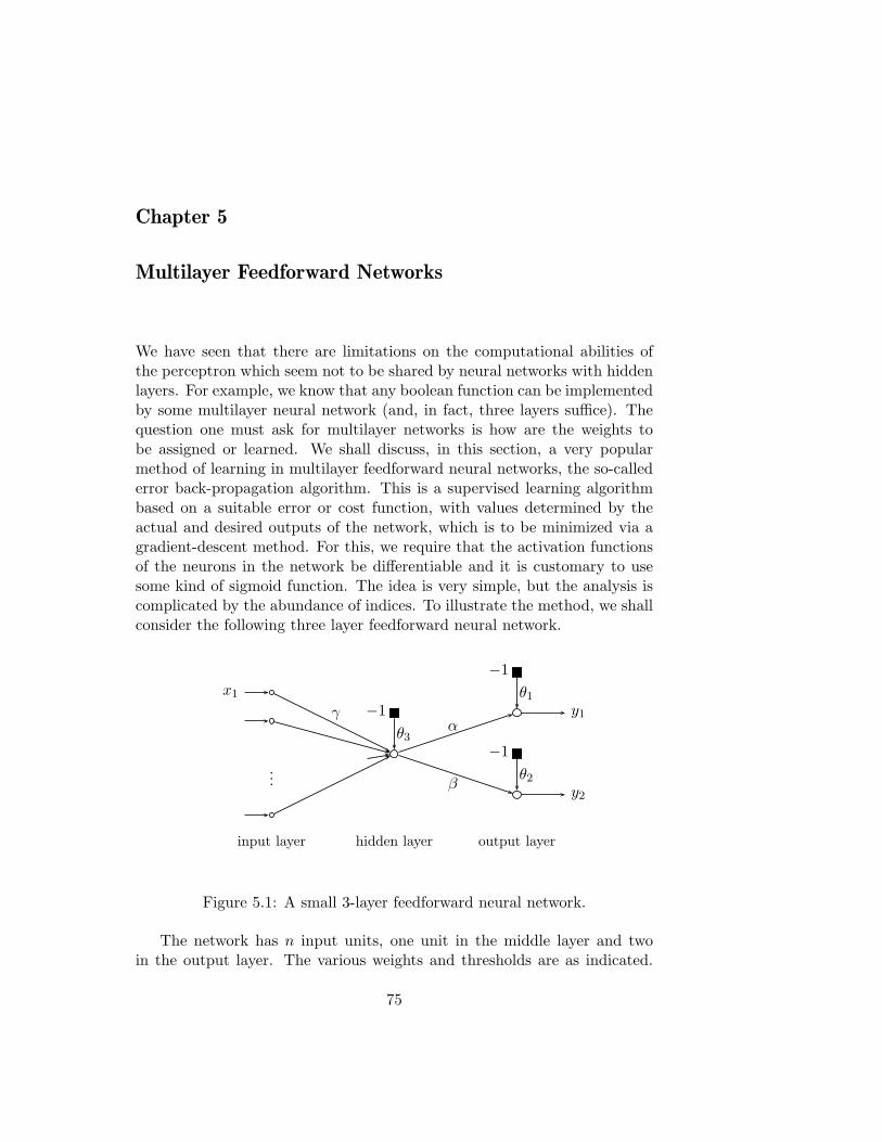
Chapter 5
Multilayer Feedforward Networks
We have seen that there are limitations on the computational abilities ofthe perceptron which seem not to be shared by neural networks with hiddenlayers. For example, we know that any boolean function can be implementedby some multilayer neural network (and, in fact, three layers suffice). Thequestion one must ask for multilayer networks is how are the weights tobe assigned or learned. We shall discuss, in this section, a very popularmethod of learning in multilayer feedforward neural networks, the so-callederror back-propagation algorithm. This is a supervised learning algorithmbased on a suitable error or cost function, with values determined by theactual and desired outputs of the network, which is to be minimized via agradient-descent method. For this, we require that the activation functionsof the neurons in the network be differentiable and it is customary to usesome kind of sigmoid function. The idea is very simple, but the analysis iscomplicated by the abundance of indices. To illustrate the method, we shallconsider the following three layer feedforward neural network.
x1
...
input layer
−1
hidden layer
θ3
γ
−1
θ1
−1
output layer
θ2
α
β
y1
y2
Figure 5.1: A small 3-layer feedforward neural network.
The network has n input units, one unit in the middle layer and twoin the output layer. The various weights and thresholds are as indicated.
75
76 Chapter 5
We suppose that the activation functions of the neurons in the second andthird layers are given by the sigmoid function ϕ, say. The nodes in theinput layer serve, as usual, merely as placeholders for the distribution of theinput values to the units in the second (hidden) layer. Suppose that theinput pattern x = (x1, . . . , xn) is to induce the desired output (d1, d2). Lety = (y1, y2) denote the actual output. Then the sum of squared differences
E = 12
((d1 − y1)
2 + (d2 − y2)2)
is a measure of the error between the actual and desired outputs. We seekto find weights and thresholds which minimize this. The approach is to usea gradient-descent method, that is, we use the update algorithm
w 7→ w + ∆w,
with ∆w = −λ grad E , where w denotes the “weight” vector formed by allthe individual weights and thresholds of the network. (So the dimension ofw is given by the total number of connections and thresholds.) As usual,λ is called the learning parameter. To find grad E , we must calculate thepartial derivatives of E with respect to all the weights and thresholds.
Consider ∂E/∂α first. We have y1 = ϕ(v1), with v1 = u1 − θ1 andu1 = (
∑w1izi) = αz where z is the output from the (single) middle unit
(so that there is, in fact, no summation but just the one term). Thusy1 = ϕ(αz − θ1). Hence
∂E∂α
= −(d1 − y1)∂y1
∂α
= −(d1 − y1)ϕ′(v1)∂v1
∂α= −(d1 − y1)ϕ′(v1) z
= −∆1 z
where we have set ∆1 = (d1 − y1)ϕ′(v1). In an entirely similar way, we get
∂E∂β
= −(d2 − y2)ϕ′(v2) z
≡ −∆2 z
where we have used v2 = βz − θ2. Further,
∂E∂θ1
= −(d1 − y1)ϕ′(v2) (−1)
and
∂E∂θ2
= −(d2 − y2)ϕ′(v2) (−1).
Department of Mathematics

Multilayer Feedforward Networks 77
Next, we must calculate
∂E∂γ
= −(d1 − y1)∂y1
∂γ− (d2 − y2)
∂y2
∂γ.
Now,
∂y1
∂γ=
∂ϕ(v1)
∂γ= ϕ′(v1)
∂v1
∂γ
= ϕ′(v1)α∂z
∂γ= ϕ′(v1)α
∂ϕ(v3)
∂γ
= ϕ′(v1)αϕ′(v3)∂v3
∂γ
= ϕ′(v1)αϕ′(v3)x1, using v3 = u3 − θ3 = (x1γ + . . . ) − θ3.
Similarly, we find∂y2
∂γ= ϕ′(v2)βϕ′(v3)x1.
Hence
∂E∂γ
= −(d1 − ϕ(v1)
)ϕ′(v1)αϕ′(v3)x1
−(d2 − ϕ(v2)
)ϕ′(v2)αϕ′(v3)x1
= −(∆1α + ∆2β)ϕ′(v3)x1
= −∆1 x1
where ∆1 ≡ (∆1α + ∆2β)ϕ′(v3).In the same way, we calculate
∂E∂θ3
= −∆1 (−1).
Thus, the gradient-descent algorithm is to update the weights according to
α −→ α + λ∆1z,
β −→ β + λ∆2z,
θi −→ θi − λ∆i, i = 1, 2,
γ −→ γ + λ∆1x1, and
θ3 −→ θ3 − λ∆1.
We have only considered the weight γ associated with the input to secondlayer, but the general case is clear. (We could denote these n weights byγi, i = 1, . . . , n, in which case the adjustment to γi is +λ∆1xi.) Noticethat the weight changes are proportional to the signal strength along the
King’s College London

78 Chapter 5
corresponding connection (where the thresholds are considered as weightson connections with inputs clamped to the value −1). The idea is to picturethe ∆s as errors associated with the respective network nodes. The values ofthese are computed from the ouput layer “back” towards the input layer bypropagation, with the appropriate weights, along the “backwards” networkone layer at a time. Hence the name “error back-propagation algorithm”,although it is simply an implementation of gradient-descent.
Now we shall turn to the more general case of a three layer feedforwardneural network with n input nodes, M neurons in the middle (hidden) layerand m in the third (output) layer. A similar analysis can be carried out ona general multilayer feedforward neural network, but we will just considerone hidden layer.
x1
x2
xn
...
......
y1
y2
ym
w s w s
hidden layer
Figure 5.2: The general 3-layer feedforward neural network.
First, we need to set up the notation. Let x1, . . . , xn denote the inputvalues and d1, . . . , dm the desired outputs. Let the weight from input uniti to hidden layer neuron j be denoted by wji and that from hidden layerneuron k to output neuron ℓ by wℓk. All neurons in layers two and three areassumed to have differentiable (usually sigmoid) activation function ϕ(·).
The activation potential (net input to the activation function) of neuron jin the hidden layer is vh
j =∑n
i=0 wjixi, where x0 = −1 and wj0 = θj is thethreshold value.
The output from the neuron j in the hidden layer is ϕ(vhj ) ≡ zj , say.
The activation potential of the output neuron ℓ is voutℓ =
∑Mk=0 wℓkzk, where
z0 = −1 and wℓ0 = θℓ, the threshold for the unit.
The output from the neuron ℓ in the output layer is yℓ = ϕ(voutℓ ).
Department of Mathematics
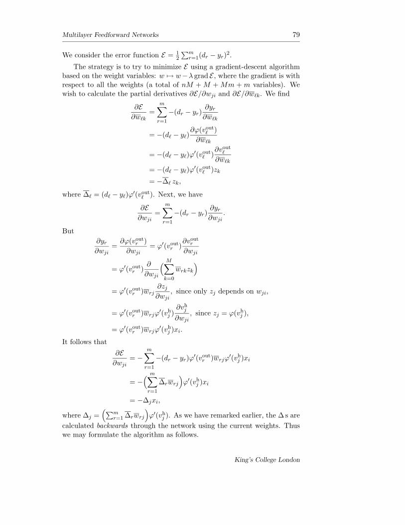
Multilayer Feedforward Networks 79
We consider the error function E = 12
∑mr=1(dr − yr)
2.
The strategy is to try to minimize E using a gradient-descent algorithmbased on the weight variables: w 7→ w−λ grad E , where the gradient is withrespect to all the weights (a total of nM + M + Mm + m variables). Wewish to calculate the partial derivatives ∂E/∂wji and ∂E/∂wℓk. We find
∂E∂wℓk
=m∑
r=1
−(dr − yr)∂yr
∂wℓk
= −(dℓ − yℓ)∂ϕ(vout
ℓ )
∂wℓk
= −(dℓ − yℓ)ϕ′(vout
ℓ )∂vout
ℓ
∂wℓk
= −(dℓ − yℓ)ϕ′(vout
ℓ )zk
= −∆ℓ zk,
where ∆ℓ = (dℓ − yℓ)ϕ′(vout
ℓ ). Next, we have
∂E∂wji
=m∑
r=1
−(dr − yr)∂yr
∂wji.
But
∂yr
∂wji=
∂ϕ(voutr )
∂wji= ϕ′(vout
r )∂vout
r
∂wji
= ϕ′(voutr )
∂
∂wji
( M∑
k=0
wrkzk
)
= ϕ′(voutr )wrj
∂zj
∂wji, since only zj depends on wji,
= ϕ′(voutr )wrjϕ
′(vhj )
∂vhj
∂wji, since zj = ϕ(vh
j ),
= ϕ′(voutr )wrjϕ
′(vhj )xi.
It follows that
∂E∂wji
= −m∑
r=1
−(dr − yr)ϕ′(vout
r )wrjϕ′(vh
j )xi
= −( m∑
r=1
∆rwrj
)ϕ′(vh
j )xi
= −∆jxi,
where ∆j =(∑m
r=1 ∆rwrj
)ϕ′(vh
j ). As we have remarked earlier, the ∆ s are
calculated backwards through the network using the current weights. Thuswe may formulate the algorithm as follows.
King’s College London
80 Chapter 5
The Error Back-Propagation algorithm:
• set all weights to small random values;
• present an input-output pattern pair from the training set andthen compute all activation potentials and internal unit outputspassing forward through the network, and the network outputs;
• compute all the ∆ s by propagation backwards through the networkand hence determine the partial derivatives of the error functionwith respect to all the weights using the current values of theweights;
• update all weights by the gradient-descent rule w 7→ w − λ grad E ,where λ is the learning rate;
• select another pattern repeating steps 2, 3 and 4 above until theerror function is acceptably small for all patterns in the giventraining set.
It must be noted at the outset that there are no known general convergencetheorems for the back-propagation algorithm (unlike the LMS algorithm dis-cussed earlier). This is a game of trial and error. Nonetheless, the methodhas been widely applied and it could be argued that its study in the mid-eighties led to the recent resurgence of interest (and funding) of artificialneural networks. Some of the following remarks are various cook-book com-ments based on experiment with the algorithm.
Remarks 5.1.
1. Instead of changing the weights after each presentation, we could take a“batch” of pattern pairs, calculate the weight changes for each (but donot actually make the change), sum them and then make an accumulatedweight change “in one lump”. This would be closer in spirit to a “pure”gradient-descent method. However, such batch updating requires storingthe various changes in memory which is considered undesirable so usuallythe algorithm is performed with an update after each step. This is calledpattern mode as distinct from batch mode.
2. The learning parameter λ is usually selected in the range 0.05—0.25.One might wish to vary the value of λ as learning proceeds. A furtherpossibility would be to have different values of the learning parameterfor the different weights.
3. It is found in practice that the algorithm is slow to converge, i.e., it needsmany iterations.
Department of Mathematics
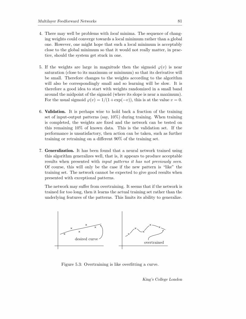
Multilayer Feedforward Networks 81
4. There may well be problems with local minima. The sequence of chang-ing weights could converge towards a local minimum rather than a globalone. However, one might hope that such a local minimum is acceptablyclose to the global minimum so that it would not really matter, in prac-tice, should the system get stuck in one.
5. If the weights are large in magnitude then the sigmoid ϕ(v) is nearsaturation (close to its maximum or minimum) so that its derivative willbe small. Therefore changes to the weights according to the algorithmwill also be correspondingly small and so learning will be slow. It istherefore a good idea to start with weights randomized in a small bandaround the midpoint of the sigmoid (where its slope is near a maximum).For the usual sigmoid ϕ(v) = 1/(1+exp(−v)), this is at the value v = 0.
6. Validation. It is perhaps wise to hold back a fraction of the trainingset of input-output patterns (say, 10%) during training. When trainingis completed, the weights are fixed and the network can be tested onthis remaining 10% of known data. This is the validation set. If theperformance is unsatisfactory, then action can be taken, such as furthertraining or retraining on a different 90% of the training set.
7. Generalization. It has been found that a neural network trained usingthis algorithm generalizes well, that is, it appears to produce acceptableresults when presented with input patterns it has not previously seen.Of course, this will only be the case if the new pattern is “like” thetraining set. The network cannot be expected to give good results whenpresented with exceptional patterns.
The network may suffer from overtraining. It seems that if the network istrained for too long, then it learns the actual training set rather than theunderlying features of the patterns. This limits its ability to generalize.
++
+
+ +
desired curve
bc
bcbc
bcbc
++
+
+ +
overtrained
Figure 5.3: Overtraining is like overfitting a curve.
King’s College London
82 Chapter 5
8. If we take the activation function to be the standard sigmoid functiongiven as ϕ(v) = 1/(1 + exp(−v)), then
ϕ′(v) =e−v
(1 + e−v)2= ϕ(v)
e−v
(1 + e−v)= ϕ(v)
(1 − 1
(1 + e−v)
)
= ϕ(v)(1 − ϕ(v)
).
This means that it is not necessary to compute ϕ′(v) separately once wehave found ϕ(v). That is to say, the update algorithm can be rewrittenso that the ∆s can be calculated from the knowledge of ϕ(v) directly.This saves computation time.
9. To picture how the network operates, it is usual to imagine that somehowcertain characteristic features of the training set have been encapsulatedin the network weights. The network has extracted the essence of thetraining set.
Data compression. Suppose the network has 100 input units, say, 10hidden units and 100 output units, and is trained on a set of input-outputpatterns where the output is the same as the input, i.e., the network istrained to learn the identity function. Such a neural network will havelearned to perform 10:1 data compression. Instead of transmitting the100 signal values, one would transmit the 10 values emitted by the hiddenunits and only on arrival at the receiving end would these values bepassed into the final third layer (so there would be two neural networks,one at each end of the transmission line).
10. We could use a different error function if we wish. All that is requiredby the logic of the procedure is that it have a (global) minimum whenthe actual output and desired output are equal. The only effect on thecalculations would be to replace the terms −2(dr − yr) by the moregeneral expression ∂E/∂yr. This will change the formula for the “outputunit ∆ s”, ∆ℓ, but once this has been done the formulae for the remainingweight updates are unchanged.
Instead of just the weight update ∆wji(t + 1) = −λ∂E(t)/∂wji at the iter-ation step (t + 1), it has often been found better to incorporate a so-calledmomentum term, α∆wji(t), giving
∆wji(t + 1) = −λ∂E(t)
∂wji+ α∆wji(t),
where ∆wji(t) is the previous weight increment and α is called the momen-tum parameter (chosen so that 0 ≤ α ≤ 1, but often taken to be 0.9). Tosee how such a term may prove to be beneficial, suppose that the weights
Department of Mathematics
Multilayer Feedforward Networks 83
correspond to a “flat” spot on the error surface, so that ∂E(t)/∂wji is nearlyconstant (and small). In this situation, we have
∆wji(t) = −λ∂E
∂wji+ α∆wji(t − 1)
= −λ∂E
∂wji+ α
(−λ
∂E∂wji
+ α∆wji(t − 2))
= −λ∂E
∂wji
(1 + α + α2 + · · · + αt−2
)+ αt−1∆wji(1).
We see that
∆wji(t) → − λ
(1 − α)
∂E∂wji
,
as t → ∞, giving an effective learning rate of λ/(1−α) which is larger thanλ if α is close to 1. Indeed, if we take α = 0.9, as suggested above, then theeffective learning rate is 10λ. This helps to speed up “convergence”.
Now let us suppose that ∂E(t)/∂wji fluctuates between successive posi-tive and negative values. Then
∆wji(t + 2) = −λ∂E(t + 1)
∂wji+ α∆wji(t + 1)
= −λ∂E(t + 1)
∂wji− αλ
∂E(t)
∂wji+ α2∆wji(t)
= −λ(∂E(t + 1)
∂wji+ α
∂E(t)
∂wji
)+ α2∆wji(t).
If α is close to 1 and if ∂E(t + 1)/∂wji ∼ −∂E(t)/∂wji then the first (brack-eted) term on the right hand side, above, is small and so the inclusion of themomentum term helps to damp down oscillatory behaviour of the weights.
On the other hand, if ∂E/∂wji has the same sign for two consecutivesteps, then the above calculation shows that including the momentum term“accelerates” the weight change.
A vestige of mathematical respectability can be conferred on such useof a momentum term according to the following argument. The idea isnot to use just the error function for the current pattern, but rather toincorporate all the error functions for all the patterns presented throughoutthe history of the iteration process. Denote by E(1), E(2), . . . , E(t) the errorfunctions associated with those patterns presented at steps 1, 2, . . . , t. LetEt = E(1)(w(t))+· · ·+E(t)(w(t)) be the sum of these error functions evaluatedat the current time step t. Now base the gradient-descent method on thefunction Et.
King’s College London
84 Chapter 5
We get
∆wji(t + 1) = −λ∂Et
∂wji
= −λ∂E(t)
∂wji− λ
∂
∂wji
(E(1)(w(t)) + · · · + E(t−1)(w(t))
).
The second term on the right hand side above is like ∂Et−1/∂wji = ∆wji(t),a momentum contribution, except that it is evaluated at step t not t − 1.
Function approximation
We have thought of a multilayer feedforward neural network as a networkwhich learns input-output pattern pairs. Suppose such a network has n unitsin the input layer and m in the output layer. Then any given function f ,say, of n variables and with values in R
m determines input-output patternpairs by the obvious pairing (x, f(x)). One can therefore consider trying totrain a network to learn a given function and so it is of interest to know ifand in what sense this can be achieved.
It turns out that there is a theorem of Kolmogorov, extended by Sprecher,on the representation of continuous functions of many variables in terms oflinear combinations of a continuous function of linear combinations of func-tions of one variable.
Theorem 5.2 (Kolmogorov). For any continuous function f : [0, 1]n → R (onthe n-dimensional unit cube), there are continuous functions h1, . . . , h2n+1
on R and continuous monotonic increasing functions gij, for 1 ≤ i ≤ n, and1 ≤ j ≤ 2n + 1, such that
f(x1, . . . , xn) =2n+1∑
j=1
hj
( n∑
i=1
gij(xi)).
The functions gij do not depend on f .
Theorem 5.3 (Sprecher). For any continuous function on the n-dimensionalunit cube, f : [0, 1]n → R, there is a continuous function h and continuousmonotonic increasing functions g1, . . . , g2n+1 and constants λ1, . . . , λn suchthat
f(x1, . . . , xn) =2n+1∑
j=1
h( n∑
i=1
λigj(xi)).
The functions gj and the constants λi do not depend on f .
This theorem implies that any continuous function f from a compactsubset of R
n into Rm can be realized by some four layer feedforward neural
network.
Department of Mathematics
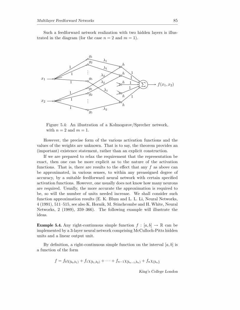
Multilayer Feedforward Networks 85
Such a feedforward network realization with two hidden layers is illus-trated in the diagram (for the case n = 2 and m = 1).
x1
x2
...
1
1
1
g1
g2
g5
...
1
1
1
g1
g2
g5
λ1
λ2
λ1
λ2
λ1
λ2
h
h
h
h
h
∑
11
1
1
1
f(x1, x2)
Figure 5.4: An illustration of a Kolmogorov/Sprecher network,with n = 2 and m = 1.
However, the precise form of the various activation functions and thevalues of the weights are unknown. That is to say, the theorem provides an(important) existence statement, rather than an explicit construction.
If we are prepared to relax the requirement that the representation beexact, then one can be more explicit as to the nature of the activationfunctions. That is, there are results to the effect that any f as above canbe approximated, in various senses, to within any preassigned degree ofaccuracy, by a suitable feedforward neural network with certain specifiedactivation functions. However, one usually does not know how many neuronsare required. Usually, the more accurate the approximation is required tobe, so will the number of units needed increase. We shall consider suchfunction approximation results (E. K. Blum and L. L. Li, Neural Networks,4 (1991), 511–515, see also K. Hornik, M. Stinchcombe and H. White, NeuralNetworks, 2 (1989), 359–366). The following example will illustrate theideas.
Example 5.4. Any right-continuous simple function f : [a, b] → R can beimplemented by a 3-layer neural network comprising McCulloch-Pitts hiddenunits and a linear output unit.
By definition, a right-continuous simple function on the interval [a, b] isa function of the form
f = f0χ[b0,b1) + f1χ[b1,b2) + · · · + fn−1χ[bn−1,bn) + fnχ{bn}
King’s College London
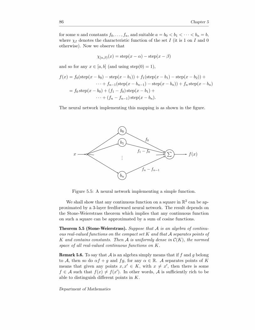
86 Chapter 5
for some n and constants f0, . . . , fn, and suitable a = b0 < b1 < · · · < bn = b,where χI denotes the characteristic function of the set I (it is 1 on I and 0otherwise). Now we observe that
χ[α,β)(x) = step(x − α) − step(x − β)
and so for any x ∈ [a, b] (and using step(0) = 1),
f(x) = f0(step(x − b0) − step(x − b1)) + f1(step(x − b1) − step(x − b2)) +
· · · + fn−1(step(x − bn−1) − step(x − bn)) + fn step(x − bn)
= f0 step(x − b0) + (f1 − f0) step(x − b1) +
· · · + (fn − fn−1) step(x − bn).
The neural network implementing this mapping is as shown in the figure.
x
b0
b1
...
bn
∑
f0
f1 − f0
fn − fn−1
f(x)
Figure 5.5: A neural network implementing a simple function.
We shall show that any continuous function on a square in R2 can be ap-
proximated by a 3-layer feedforward neural network. The result depends onthe Stone-Weierstrass theorem which implies that any continuous functionon such a square can be approximated by a sum of cosine functions.
Theorem 5.5 (Stone-Weierstrass). Suppose that A is an algebra of continu-ous real-valued functions on the compact set K and that A separates points ofK and contains constants. Then A is uniformly dense in C(K), the normedspace of all real-valued continuous functions on K.
Remark 5.6. To say that A is an algebra simply means that if f and g belongto A, then so do αf + g and fg, for any α ∈ R. A separates points of Kmeans that given any points x, x′ ∈ K, with x 6= x′, then there is somef ∈ A such that f(x) 6= f(x′). In other words, A is sufficiently rich to beable to distinguish different points in K.
Department of Mathematics
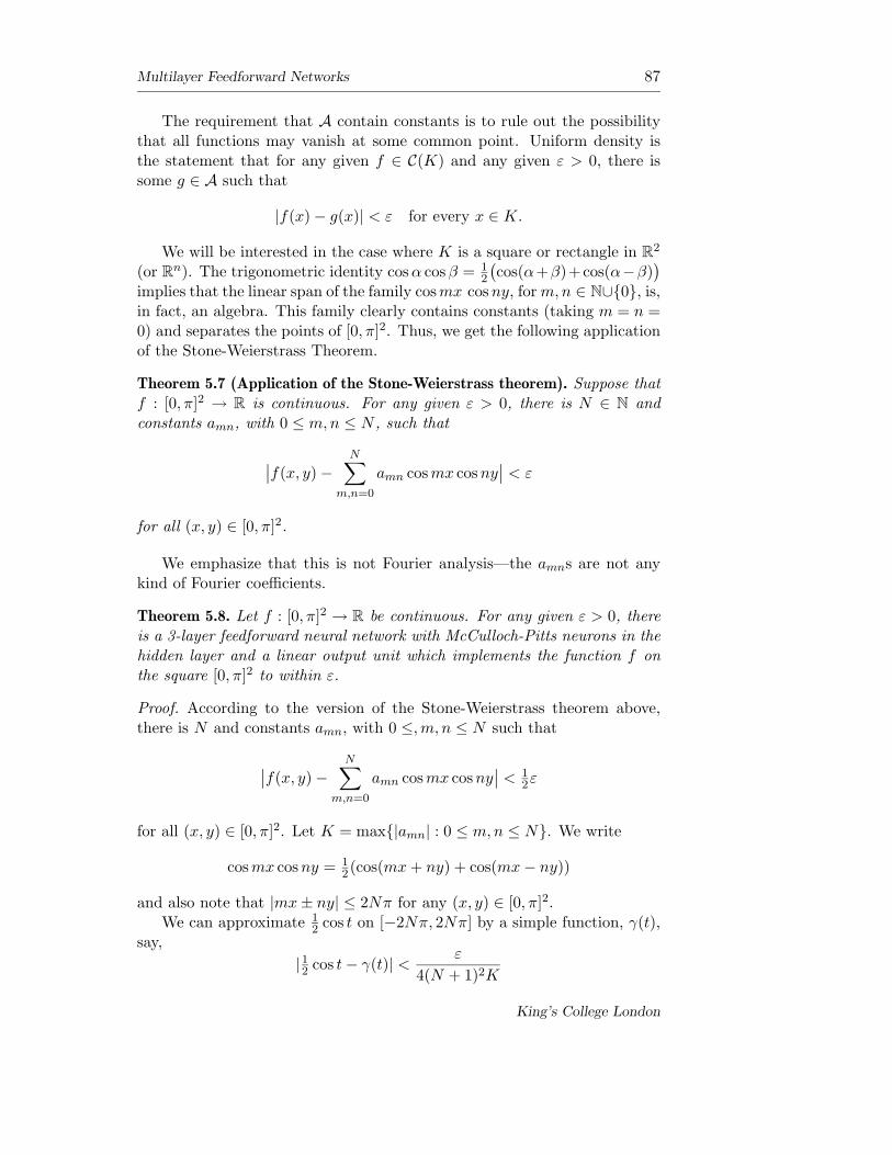
Multilayer Feedforward Networks 87
The requirement that A contain constants is to rule out the possibilitythat all functions may vanish at some common point. Uniform density isthe statement that for any given f ∈ C(K) and any given ε > 0, there issome g ∈ A such that
|f(x) − g(x)| < ε for every x ∈ K.
We will be interested in the case where K is a square or rectangle in R2
(or Rn). The trigonometric identity cosα cos β = 1
2
(cos(α+β)+cos(α−β)
)
implies that the linear span of the family cosmx cos ny, for m, n ∈ N∪{0}, is,in fact, an algebra. This family clearly contains constants (taking m = n =0) and separates the points of [0, π]2. Thus, we get the following applicationof the Stone-Weierstrass Theorem.
Theorem 5.7 (Application of the Stone-Weierstrass theorem). Suppose thatf : [0, π]2 → R is continuous. For any given ε > 0, there is N ∈ N andconstants amn, with 0 ≤ m, n ≤ N , such that
∣∣f(x, y) −N∑
m,n=0
amn cos mx cos ny∣∣ < ε
for all (x, y) ∈ [0, π]2.
We emphasize that this is not Fourier analysis—the amns are not anykind of Fourier coefficients.
Theorem 5.8. Let f : [0, π]2 → R be continuous. For any given ε > 0, thereis a 3-layer feedforward neural network with McCulloch-Pitts neurons in thehidden layer and a linear output unit which implements the function f onthe square [0, π]2 to within ε.
Proof. According to the version of the Stone-Weierstrass theorem above,there is N and constants amn, with 0 ≤, m, n ≤ N such that
∣∣f(x, y) −N∑
m,n=0
amn cos mx cos ny∣∣ < 1
2ε
for all (x, y) ∈ [0, π]2. Let K = max{|amn| : 0 ≤ m, n ≤ N}. We write
cos mx cos ny = 12(cos(mx + ny) + cos(mx − ny))
and also note that |mx ± ny| ≤ 2Nπ for any (x, y) ∈ [0, π]2.We can approximate 1
2 cos t on [−2Nπ, 2Nπ] by a simple function, γ(t),say,
|12 cos t − γ(t)| <ε
4(N + 1)2K
King’s College London
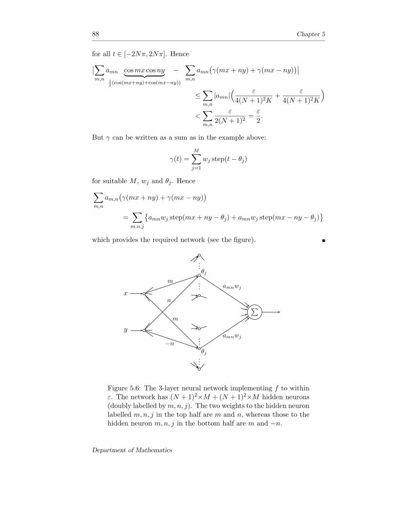
88 Chapter 5
for all t ∈ [−2Nπ, 2Nπ]. Hence
∣∣∑
m,n
amn cos mx cos ny︸ ︷︷ ︸12(cos(mx+ny)+cos(mx−ny))
−∑
m,n
amn
(γ(mx + ny) + γ(mx − ny)
)∣∣
≤∑
m,n
|amn|( ε
4(N + 1)2K+
ε
4(N + 1)2K
)
<∑
m,n
ε
2(N + 1)2=
ε
2.
But γ can be written as a sum as in the example above:
γ(t) =M∑
j=1
wj step(t − θj)
for suitable M , wj and θj . Hence
∑
m,n
am,n
(γ(mx + ny) + γ(mx − ny)
)
=∑
m,n,j
{amnwj step(mx + ny − θj) + amnwj step(mx − ny − θj)
}
which provides the required network (see the figure).
x
y
...
...
...
...
θj
θj
m
n
m
−n
∑
amnwj
amnwj
Figure 5.6: The 3-layer neural network implementing f to withinε. The network has (N + 1)2×M + (N + 1)2×M hidden neurons(doubly labelled by m, n, j). The two weights to the hidden neuronlabelled m, n, j in the top half are m and n, whereas those to thehidden neuron m, n, j in the bottom half are m and −n.
Department of Mathematics

Multilayer Feedforward Networks 89
Remark 5.9. The particular square [0, π]2 is not crucial—one can obtain asimilar result, in fact, on any bounded region of R
2 by rescaling the variables.Also, there is an analogous result in any number of dimensions (products ofcosines in the several variables can always be rewritten as cosines of sums).The theorem gives an approximation in the uniform sense. There are variousother results which, for example, approximate f in the mean square sense.It is also worth noting that with a little more work, one can see that sigmoidunits could be used instead of the threshold units. One would take γ aboveto be a sum of “smoothed” step functions, rather a sum of step functions.
A problem with the above approach is with the difficulty in actuallyfinding the values of N and the amns in any particular concrete situation. Byadmitting an extra layer of neurons, a somewhat more direct approximationcan be made. We shall illustrate the ideas in two dimensions.
Proposition 5.10. Let f : R2 → R be continuous. Then f is uniformly
continuous on any square S ⊂ R2.
Proof. Suppose that S is the square S = [−R, R] × [−R, R] and let ε > 0be given. We must show that there is some δ > 0 such that |x−x′| < δ andx, x′ ∈ S imply that
|f(x) − f(x′)| < ε.
Suppose that this is not true. Then, no matter what δ > 0 is, there will bepoints x, x′ ∈ S such that |x − x′| < δ but |f(x) − f(x′)| ≥ ε. In particular,if, for any n ∈ N, we take δ = 1/n, then there will be points xn and x′
n in Swith |xn − x′
n| < 1/n but |f(xn) − f(x′n)| ≥ ε.
Now, (xn) is a sequence in the compact set S and so has a convergentsubsequence, xnk
→ x as k → ∞, with x ∈ S. But then
|x′nk
− x| ≤ |x′nk
− xnk| + |xnk
− x| <1
nk+ |xnk
− x| → 0
as k → ∞, i.e., x′nk
→ x, as k → ∞.By the continuity of f , it follows that
|f(xnk) − f(x′
nk)| → |f(x) − f(x)| = 0
which contradicts the inequality |f(xnk) − f(x′
nk)| ≥ ε and the proof is
complete.
The idea of the construction is to approximate a given continuous func-tion by step-functions built on small rectangles. Let B be a rectangle of theform
B = (a, b] × (α, β].
Notice that B contains its upper and right-hand edges, but not the loweror left-hand ones. It is a bit of a nuisance that we have to pay attention tothis minor detail.
King’s College London

90 Chapter 5
Let S denote the collection of finite linear combinations of functions ofthe form χB, for various Bs, where
χB(x) =
{1, x ∈ B
0, x /∈ B
is the characteristic function of the rectangle B. Thus, S consists of functionsof the form a1χB1 + · · · + amχBm
, with a1, . . . , am ∈ R.
Theorem 5.11. Let f : R2 → R be continuous. Then for any R > 0 and any
ε > 0 there is g ∈ S such that
|f(x) − g(x)| < ε, for all x ∈ (−R, R) × (−R, R),
i.e., f can be uniformly approximated on the square (−R, R) × (−R, R) byelements of S.
Proof. By our previous discussion, we know that f is uniformly continuouson the square A = [−R, R] × [−R, R]. Hence there is δ > 0 such that|f(x) − f(x′)| < ε whenever x, x′ ∈ A and |x − x′| < δ. Subdivide A into nsmaller squares as shown.
B1 B2 . . .
Bn
...
. . .
Figure 5.7: Divide A into many small rectangles, B1, . . . , Bn.
Choose n so large that each Bm has diagonal smaller than δ and let xm
be the centre of Bm. Then |x − xm| < δ for any x ∈ Bm.
Department of Mathematics

Multilayer Feedforward Networks 91
Put gm = f(xm), and set
g(x) =n∑
m=1
gmχBm(x).
Then, for any x ∈ (−R, R) × (−R, R),
|g(x) − f(x)| = |gj − f(x)|, where j is such that x ∈ Bj ,
= |f(xj) − f(x)|< ε
since |xj − x| < δ.
We see that f is approximated on each Bm by its value at the centre.Notice that the approximation is rather more explicit than that of the pre-vious scheme using the Stone-Weierstrass theorem. As a matter of fact, wecould use that theorem here also, but as we have just remarked, there wouldthen be no indication as to the value of n nor of the constants am.
To construct the appropriate network, we shall need two types of McCulloch-Pitts threshold units—differing on the value they take at the jumppoint. Let
H(s) =
{1, s ≥ 0
0, s < 0and H0(s) =
{1, s > 0
0, s ≤ 0.
Thus, H(·) is just the function step(·) used already. H0 differs from H onlyin its value at 0—it is 0 there. The purpose of introducing these differentversions of the step-function will soon become apparent. Indeed, H0(s−a) =χ(a,∞)(s) and H(−s + b) = χ(−∞,b](s) so that
χ(a,b](s) = H0(s − a)︸ ︷︷ ︸
χ(a,∞)(s)
H(−s + b)︸ ︷︷ ︸χ(−∞,b](s)
.
This means that we can implement the function χ(a,b] by the networkshown.
King’s College London
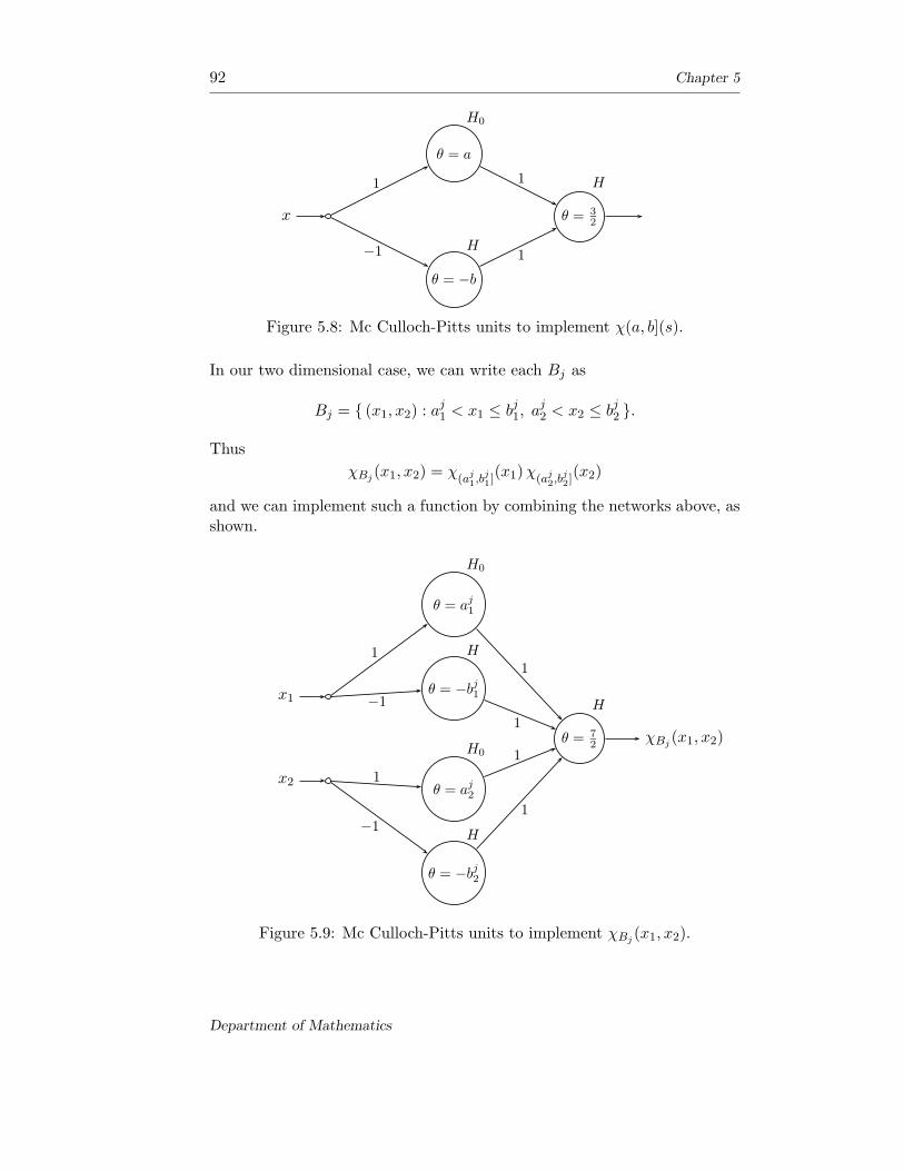
92 Chapter 5
x
θ = a
θ = −b
H0
H
1
−1
θ = 3
2
H1
1
Figure 5.8: Mc Culloch-Pitts units to implement χ(a, b](s).
In our two dimensional case, we can write each Bj as
Bj = { (x1, x2) : aj1 < x1 ≤ bj
1, aj2 < x2 ≤ bj
2 }.
Thus
χBj(x1, x2) = χ
(aj1,bj
1](x1)χ
(aj2,bj
2](x2)
and we can implement such a function by combining the networks above, asshown.
x1
θ = aj1
θ = −bj1
H0
H1
−1
x2θ = aj
2
θ = −bj2
H
H0
1
−1
θ = 7
2
H
1
1
1
1
χBj(x1, x2)
Figure 5.9: Mc Culloch-Pitts units to implement χBj(x1, x2).
Department of Mathematics

Multilayer Feedforward Networks 93
Theorem 5.12. Suppose that f : R2 → R is continuous. Then for any
given R > 0 and ε > 0 there is a 4-layer feedforward neural network withMc Culloch-Pitts units in layers 2 and 3 and with a linear output unit whichimplements f to within error ε uniformly on the square (−R, R)× (−R, R).
Proof. We have done all the preparation. Now we just piece together thevarious parts. Let g, B1, . . . , Bn etc. be an approximation to f (to within ε)as given above. We shall implement g using the stated network. Each χBj
is implemented by a 3-layer network, as above. The outputs of these areweighted by the corresponding gj and then fed into a linear (summation)unit.
x1
x2
...
H0 aj1
H−bj1
H0
aj2
H−bj2
...
...
1
1
11
H
θ=7/2
...
∑
g1
gj
gn
f(x1, x2)
Figure 5.10: The network to implement f to within ε uniformlyon the square (−R, R) × (−R, R).
The first layer consists of place holders for the input, as usual. Thesecond layer consists of 4n threshold units (4 for each rectangle Bj , j =1, . . . , n). The third layer consists of n threshold units, required to completethe implementation of the n various χBj
s. The final output layer consists ofa single linear unit.
For any given input (x1, x2) from the rectangle (−R, R) × (−R, R) pre-cisely one of the units in the third layer will fire—this will be the jth corre-sponding to the unique j with (x1, x2) ∈ Bj . The system output is thereforeequal to
∑ni=1 giχBi
(x1, x2) = gj = g(x1, x2), as required.
See the work of K. Hornik, M. Stinchecombe and H. White, for example,for further results on function approximation.
King’s College London

94 Chapter 5
Department of Mathematics
Chapter 6
Radial Basis Functions
We shall reconsider the problem of implementing the mapping of a given setof input vectors x(1), . . . , x(p) in R
n into target values y(1), . . . , y(p) in R,
x(i)Ã y(i), i = 1, . . . , p.
We seek a function h which not only realizes this association,
h(x(i)) = y(i), i = 1, . . . , p,
but which should also “predict” values when applied to new but “similar”input data. This means that we are not interested in finding a mapping hwhich works precisely for just these x(1), . . . , x(p). We would like a mappingh which will “generalize”.
We will look at functions of the form ϕ(‖x− x(i)‖), i.e., functions of thedistance between x and the prototype input x(i)—so-called basis functions.Thus, we try
h(x) =
p∑
i=1
wiϕ(‖x − x(i)‖)
and require y(j) = h(x(j)) =∑p
i=1 wiϕ(‖x(j) − x(i)‖). If we set (Aji) =(Aij) = (ϕ(‖x(j) − x(i)‖)) ∈ R
p×p, then our requirement is that
y(j) =
p∑
i=1
Ajiwi = (Aw)j ,
that is, y = Aw. If A is invertible, we get w = A−1y and we have found h.
A common choice for ϕ is a Gaussian function:
ϕ(s) = e−s2/2σ2
—a so-called localized basis function.
95

96 Chapter 6
With this choice, we see that
h(x(j)) =
p∑
i=1
wiϕ(‖x(j) − x(i)‖)
= wj ϕ(‖x(j) − x(j)‖)︸ ︷︷ ︸= 1
+
p∑
i=1i6=j
wi ϕ(‖x(j) − x(i)‖)
= wj + ε
where ε is small provided that the prototypes x(j) are reasonably well-separated. The various basis functions therefore “pick out” input patternsin the vicinity of specified spatial locations.
To construct a mapping h from Rn to R
m, we simply construct suitablecombinations of basis functions for each of the m components of the vector-valued map h = (h1, . . . , hm). Thus,
hk(x) =
p∑
i=1
wki ϕ(‖x − x(i)‖).
This leads to
y(j)k = hk(x
(j)) =
p∑
i=1
wki ϕ(‖x(j) − x(i)‖)︸ ︷︷ ︸Aji
=
p∑
i=1
wkiAij
= (WA)kj
giving Y = WA, where Y = (y(1), . . . , y(p)) ∈ Rm×p.
The combination of basis functions has been constructed so that it passesthrough all input-output data points. This means that h has “learned” theseparticular pairs—but we really want a system to learn the “essence” of theinput-output association rather than the intricate details of a number ofspecific examples. We want the system to somehow capture the “features”of the data source, rather than any actual numbers—which may well be“noisy” (or slightly inaccurate) anyway.
Department of Mathematics

Radial Basis Functions 97
Radial basis network
A so-called radial basis network is designed with the hope of incorporatingthis idea of realistic generalization ability. It has the following features.
• The number M of basis functions is chosen to be typically much smallerthan p.
• The centres of the basis functions are not necessarily constrained to beprecisely at the input data vectors. They may be determined during thetraining process itself.
• The basis functions are allowed to have different widths (σ)—these mayalso be determined by the training data.
• Biases or thresholds are introduced into the linear sum.
Thus, we are led to consider mappings of the form
x 7→ yk(x) =M∑
j=1
wkjϕj(x) + wk0 k = 1, 2, . . . , m,
where ϕj(x) = exp(−‖x−µj‖2/2σ2j ) and µj ∈ R
n. The corresponding 3-layernetwork is shown in the diagram. The first layer is the usual place-holderlayer. The second layer has units with activation functions given by thebasis functions ϕj , and the final layer consists of linear (summation) units.
x1
x2
...
xn
ϕ0 = 1
ϕ11
1
1
ϕ2
...
ϕM
∑y1
∑y2
...
∑ym
w10
w11
w21
w12
w1M
Figure 6.1: A radial basis network.
King’s College London
98 Chapter 6
Training
To train such a network, the layers are treated quite differently. The secondlayer is subjected to unsupervised training—the input data being used toassign values to µj and σj . These are then held fixed and the weights to theoutput layer are found in the second phase of training.
Once a suitable set of values for the µjs and σjs has been found, we seeksuitable wkjs. These are given by
yk(x) =M∑
j=0
wkjϕj(x) (with ϕ0 ≡ 1)
i.e., y = Wϕ. This is just a linear network problem—for given x, we calculateϕj(x), so we know the hidden layer to output pattern pairs. We can thereforefind W by minimizing the mean square error à generalized inverse memory(OLAM) (or we can use the LMS algorithm to find this).
Returning to the problem of assigning values to the µjs and σjs—this canbe done using the k-means clustering algorithm (MacQueen), which assignsvectors to one of a number of clusters.
k-means clustering algorithm
Suppose that the training set consists of N data vectors, each in Rn, which
are assumed to constitute k clusters. The centroid of a cluster is, by defini-tion, the mean of its members.
• Take the first k data points as k cluster centres (giving clusters each withone member).
• Assign each of the remaining N − k data points one by one to the clusterwith the nearest centroid. After each assignment, recompute the centroidof the gaining cluster.
• Select each data point in turn and compute the distances to all clustercentroids. If the nearest centroid is not that particular data point’sparent cluster, then reassign the data point (to the cluster with thenearest centroid) and recompute the centroids of the losing and gainingclusters.
• Repeat the above step until convergence—that is, until a full cycle throughall data points in the training set fails to trigger any further clustermembership reallocations.
• Note: in the case of ties, any choice can be made.
Department of Mathematics

Radial Basis Functions 99
This algorithm actually does converge, as we show next. The idea is tointroduce an “energy” or “cost” function which decreases with every clusterreallocation.
Theorem 6.1 (k-means convergence theorem). The k-means algorithm isconvergent, i.e., the algorithm induces at most a finite number of clustermembership reallocations and then “stops”.
Proof. Suppose that after a number of steps of the algorithm the data setis partitioned into the k clusters A1, . . . , Ak with corresponding centroidsa1, . . . , ak, so that
aj =1
nj
∑
x∈Aj
x,
where nj is the number of data points in Aj , j = 1, . . . , k. Let
E = E(A1) + · · · + E(Ak)
where E(Aj) =∑
x∈Aj‖x− aj‖2, j = 1, . . . , k. Suppose that the data point
x′ is selected next and that x′ ∈ Ai. If ‖x′ − ai‖ ≤ ‖x′ − aj‖, all j, then thealgorithm makes no change.
On the other hand, if there is ℓ 6= i such that ‖x′− aℓ‖ < ‖x′− ai‖, thenthe algorithm removes x′ from Ai and reallocates it to Am, say, where m issuch that
‖x′ − am‖ = min{ ‖x′ − aj‖ : j = 1, 2, . . . , k }.In this case, ‖x′ − am‖ < ‖x′ − ai‖.
We estimate the change in E. To do this, let A′i = Ai \ {x′} and let
A′m = Am ∪ {x′}, the reallocated clusters, and let a′i and a′m denote their
centroids, respectively. We find
E(Ai) + E(Am) =∑
x∈Ai
‖x − ai‖2 +∑
x∈Am
‖x − am‖2
=∑
x∈A′
i
‖x − ai‖2 + ‖x′ − ai‖2 +∑
x∈Am
‖x − am‖2
>∑
x∈A′
i
‖x − ai‖2 + ‖x′ − am‖2 +∑
x∈Am
‖x − am‖2
≥∑
x∈A′
i
‖x − a′i‖2 +∑
x∈A′
m
‖x − a′m‖2 = E(A′i) + E(A′
m),
since∑
‖x−α‖2 is minimized when α is the centroid of the xs. Thus, every“active” step of the algorithm demands a strict decrease in the “energy” Eof the overall cluster arrangement.
Clearly, a given finite number of data points can be assigned to k-clustersin a finite number of ways, and so E can assume only a finite number ofpossible values. It follows that the algorithm can only trigger a finite numberof reallocations, and the result follows.
King’s College London

100 Chapter 6
Having found the centroids c1, . . . , ck, via the k-means algorithm, we setµ1 = c1, . . . , µk = ck. The values of the various σjs can then be calculatedas the standard deviation of the data vectors in the appropriate cluster j,i.e.,
σ2j =
1
nj
nj∑
i=1
‖x(i) − cj‖2, j = 1, 2, . . . , k,
where nj is the number of data vectors in cluster j.
We see that radial basis function networks are somewhat different fromthe standard feedforward sigmoidal-type neural network and are simpler totrain. As some reassurance regarding their usefulness, we have the following“universal approximation theorem”.
Theorem 6.2. Suppose that f : Rn → R is a continuous function. Then
for any R > 0 and ε > 0 there is a radial basis function network whichimplements f to within ε everywhere in the ball {x : ‖x‖ ≤ R }.
Proof. Let ϕ(x, µ, σ) = exp(−(x − µ)2/2σ2). Then we see that
ϕ(x, µ, σ)ϕ(x, µ′, σ′) = c ϕ(x, λ, ν),
for suitable c, λ and ν. It follows that the linear span S of 1 and Gaussianfunctions of the form ϕ(x, µ, σ) is, in fact, an algebra. That is, if S denotesthe collection of functions of the form
w0 + w1ϕ(x, µ1, σ1) + · · · + wjϕ(x, µj , σj)
for j ∈ N and wi ∈ R, 0 ≤ i ≤ j, then S is an algebra.
x1
x2
...
xn
ϕ0 = 1
ϕ1
...
ϕN
∑
w0
w1
wN
Figure 6.2: The radial basis network approximating the functionf uniformly on the ball {x : ‖x‖ ≤ R }.
Department of Mathematics

Radial Basis Functions 101
Clearly, S contains constants and also S separates points of Rn. Indeed,
if z 6= z′ in Rn, then
ϕ(z, z, 1) = 1 6= ϕ(z′, z, 1).
We can now apply the Stone-Weierstrass theorem to conclude that f can beuniformly approximated on any ball {x : ‖x‖ ≤ R } by an element from S.Thus, for given ε > 0, there is N ∈ N and w0, w1, . . . , wN , µi and σi fori = 1, . . . , N such that
∣∣∣f(x) −N∑
i=0
wiϕi(x)∣∣∣ < ε
for all x with ‖x‖ ≤ R, where ϕ0 = 1 and ϕi(x) = ϕ(x, µi, σi) for i =1, . . . , N . Such an approximating sum is implemented by a radial basisnetwork, as shown.
King’s College London

102 Chapter 6
Department of Mathematics

Chapter 7
Recurrent Neural Networks
In this chapter, we reconsider the problem of content addressable memory(CAM). The idea is to construct a neural network which has stored (orlearned) a number of prototype patterns (also called exemplars) so thatwhen presented with a possible “noisy” or “corrupt” version of one of these,it nonetheless correctly recalls the appropriate pattern—autoassociation.
Figure 7.1: A recurrent neural network with 5 neurons.
We consider a recurrent neural network of n bipolar threshold units.Once the exemplars are loaded, the system is fixed, that is, the weights andthresholds are kept fixed—there is no further learning. The purpose of thenetwork is to simply recall a suitable pattern appropriate to the input. Thestate of the network is just the knowledge of which neurons are firing andwhich are not. We shall model such states of the system by elements of thebipolar hypercube {−1, 1}n, where the value 1 corresponds to “firing” and−1 to “not firing”.
103
104 Chapter 7
If the state of the system is x = (x1, . . . , xn), then the net internalactivation potential of neuron i is equal to
∑nk=1 wikxk − θi, where wik is
the connection weight from neuron k to neuron i, and θi is the thresholdof neuron i. Passing this through the bipolar threshold function gives thesignal value sign(
∑nk=1 wikxk − θi), where
sign(v) =
{1, v ≥ 0
−1, v < 0.
The neural network can be realized as a dynamical system as follows. Con-sider the state of the system at discrete time steps t = 0, 1, 2, . . . . Ifx(t) = (x1(t), . . . , xn(t)) in {−1, 1}n denotes the state of the system attime t, we define the state at time t + 1 by the assignment
xi(t + 1) = sign( n∑
k=1
wikxk(t) − θi
),
1 ≤ i ≤ n, with the agreement that xi(t+1) = xi(t) if∑n
k=1 wikxk(t)−θi = 0.Thus, as time goes by, the state of the system hops about on the verticesof the hypercube [−1, 1]n. The time evolution set out above is called thesynchronous (or parallel) dynamics, because all components xi are updatedsimultaneously.
An alternative possibility is to update only one unit at a time, that is,to consider the neurons individually rather than en masse. This is calledsequential (or asynchronous) dynamics and is defined by
xi(t + 1) = sign( i−1∑
k=1
wikxk(t + 1) +n∑
k=i
wikxk(t) − θi
),
for 1 ≤ i ≤ n. Thus, first x1 and only x1, is updated, then just x2 is updatedusing the latest value of x1, then x3, using the latest values of x1 and x2,and so on. Then the transition (x1(t), . . . , xn(t)) to (x1(t+1), . . . , xn(t+1))proceeds in n intermediate steps. At each such step, the state change ofonly one neuron is considered. As a consequence, the state vector x hopsabout on the vertices of the hypercube [−1, 1]n but can either remain whereit is or only move to a nearest-neighbour vertex at each such step. If wethink of n such intermediate steps as constituting a cycle, then we see thateach neuron is “activated” once and only once per cycle. (A variation onthis theme is to update the neurons in a random order so that each neuronis only updated once per cycle on average.)
Such systems were considered by J. Hopfield in the early eighties andthis provided impetus to the study of neural networks. A recurrent neuralnetwork as above and with the asynchronous (or random) mode of operationis known as the Hopfield model.
Department of Mathematics
Recurrent Neural Networks 105
There is yet a further possibility—known as block-sequential dynamics.Here the idea is to divide the neurons into a number of groups and thenupdate each group synchronously, but the groups sequentially, for example,synchronously update group one, then likewise group two, but using thelatest values of the states of the neurons in group one, and so on.
So far we have not said anything about the values to be assigned tothe weights. Before doing this, we first consider the network abstractlyand make the following observation. The state vector moves around in thespace {−1, 1}n which contains only finitely-many points (2n, in fact) andits position at t + 1 depends only on where it is at time t (and, in thesequential case, which neuron is to be updated next). Thus, either it willreach some point and stop, or it will reach a configuration for a second timeand then cycle repeatedly forever.
To facilitate further investigation, we define
E(x) = 12xT Wx + xT θ
= −12
n∑
i,j=1
xiwijxj +n∑
i=1
xiθi
where x = (x1, . . . , xn) is the state vector of the network, W = (wij) andθ = (θi).
The function E is called the energy associated with x (by analogy withlattice magnetic (or spin) systems). We can now state the basic result forsequential dynamics.
Theorem 7.1. Suppose that the synaptic weight matrix (wij) is symmetricwith non-negative diagonal terms. Then the sequential mode of operation ofthe recurrent neural network has no cycles.
Proof. Consider a single update xi 7→ x′i, and all other xj s remain un-
changed. Then we calculate the energy difference
E(x′) − E(x) = −12
n∑
j=1j 6=i
(x′iwijxj + xjwjix
′i) − 1
2x′iwiix
′i + x′
iθi
+ 12
n∑
j=1j 6=i
(xiwijxj + xjwjixi) + 12xiwiixi − xiθi
King’s College London
106 Chapter 7
(all terms not involving xi or x′i cancel out)
= −n∑
j=1j 6=i
x′iwijxj − 1
2x′iwiix
′i + x′
iθi
+n∑
j=1j 6=i
xiwijxj + 12xiwiixi − xiθi
using the symmetry of (wij)
= −n∑
j=1
x′iwijxj + x′
iwiixi − 12x′
iwiix′i + x′
iθi
+n∑
j=1
xiwijxj − xiwiixi + 12xiwiixi − xiθi
= (xi − x′i)
n∑
j=1
wijxj + 12wii(2x′
ixi − x′ix
′i − xixi) + (x′
i − xi)θi
= −(x′i − xi)
n∑
j=1
wijxj − 12wii(x
′i − xi)
2 + (x′i − xi)θi
= −12wii(x
′i − xi)
2 − (x′i − xi)
( n∑
j=1
wijxj − θi
).
Suppose that x′i 6= xi. Then x′
i − xi = 2 if x′i = 1 but x′
i − xi = −2 ifx′
i = −1. It follows that sign(x′i) = sign(x′
i −xi). Furthermore, by definitionof the evolution, x′
i = sign(∑n
j=1 wijxj − θi), and so we see that (x′i − xi)
and (∑n
j=1 wijxj − θi) have the same sign.
By hypothesis, wii ≥ 0, and so if x′i 6= xi then E(x′) < E(x). This means
that any asynchronous change in x leads to a strict decrease in the energyfunction E. It follows that the system can never leave and then subsequentlyreturn to any state configuration. In particular, there can be no cycles.
This leads immediately to the following corollary.
Corollary 7.2. A recurrent neural network with symmetric synaptic weightmatrix with non-negative diagonal elements reaches a fixed point after afinite number of steps when operated in sequential mode.
Proof. The state space is finite (and there are only a finite number of neuronsto be updated), so if there are no cycles the iteration process must simplystop, i.e., the system reaches a fixed point.
Department of Mathematics
Recurrent Neural Networks 107
We turn now to the question of choosing the synaptic weights. We setall thresholds to zero, θi = 0, 1 ≤ i ≤ n. Consider the problem of storinga single pattern z = (z1, . . . , zn). We would like input patterns (startingconfigurations) close to z to converge to z via the asynchronous dynamics.In particular, we would like z to be a fixed point. Now, according to theevolution, if x(0) = z and the ith component of x(0) is updated first, then
xi(1) = sign( n∑
k=1
wikxk(0))
= sign( n∑
k=1
wikzk
).
For z to be a fixed point, we must have zi = sign(∑n
k=1 wikzk
)(or possibly
∑nk=1 wikzk = 0). This requires that
n∑
k=1
wikzk = αzi
for some α ≥ 0. Guided by our experience with the adaptive linear combiner(ALC) network, we try wik = αzizk, that is, we choose the synaptic matrixto be (wik) = αzzT , the outer product (or Hebb rule). We calculate
n∑
k=1
wikzk =n∑
k=1
αzizkzk = αnzi
since z2k = 1. It follows that the choice (wik) = αzzT , α ≥ 0, does indeed
give z as a fixed point.
Next, we consider what happens if the system starts out not exactly inthe state z, but in some perturbation of z, say z. We can think of z as zbut with some of its bits flipped. Taking x(0) = z, we get
xi(1) = sign( n∑
k=1
wikzk
).
The choice α = 0 would give wik = 0 and so xi(1) = zi and z (and indeedany state) would be a fixed point. The dynamics would be trivial—nothingmoves. This is no good for us—we want states z sufficiently close to zto “evolve” into z. Incidentally, the same remark applies to the choice ofsynaptic matrix (wik) = 1ln, the unit n × n matrix. For such a choice, itis clear that all vectors are fixed points. We want the stored patterns toact as “attractors” each with non-trivial “basin of attraction”. Substituting
King’s College London
108 Chapter 7
(wik) = αzzT , with α > 0, we find
xi(1) = sign( n∑
k=1
αzizkzk
)
= sign(zi
n∑
k=1
zkzk
), since α > 0,
= sign(zi(n − 2ρ(z, z))
),
where ρ(z, z) is the Hamming distance between z and z, i.e., the number ofdiffering bits. It follows that if ρ(z, z) < n/2, then sign
(zi(n − 2ρ(z, z))
)=
sign(zi) = zi, so that x(1) = z. In other words, any vector z with ρ(z, z) <n/2 is mapped onto the fixed point z directly, in one iteration cycle. (When-ever a component of z is updated, either it agrees with the correspondingcomponent of z and so remains unchanged, or it differs and is then mappedimmediately onto the corresponding component of z. Each flip moves z to-wards z.) We have therefore shown that the basin of direct attraction of zcontains the disc {z : ρ(z, z) < n/2}.
Can we say anything about the situation when ρ(z, z) > n/2? Evidently,sign
(zi(n − 2ρ(z, z))
)= sign(−zi) = −zi, and so x(1) = −z. Is −z a fixed
point? According to our earlier discussion, the state −z is a fixed point if wetake the synaptic matrix to be given by (−z)(−z)T . But (−z)(−z)T = zzT
and we conclude that −z is a fixed point for the network above. (Alterna-tively, we could simply check this using the definition of the dynamics.)
We can also use this to see that z is directly attracted to −z wheneverρ(z, z) > n/2. Indeed, ρ(z, z) > n/2 implies that ρ(−z, z) < n/2 and so,arguing as before, we deduce that z is directly mapped onto the fixed point−z. If ρ(z, z) = n/2, then there is no change, by definition of the dynamics.
How can we store many patterns? We shall try the Hebbian rule,
W ≡ (wik) =
p∑
µ=1
z(µ)z(µ)T
so that wik =∑p
µ=1 z(µ)i z
(µ)k , where z(1), . . . , z(p) are the patterns to be
stored. Starting with x(0) = z, we find
zi(1) = sign((Wz)i) = sign( n∑
k=1
wikzk
)
= sign( n∑
k=1
p∑
µ=1
z(µ)i z
(µ)k zk
).
Department of Mathematics
Recurrent Neural Networks 109
Notice that if z(1), . . . , z(p) are pairwise orthogonal, then
p∑
µ=1
z(µ)z(µ)T z(j) = z(j)‖z(j)‖2
so that if z = z(j), then
zi(1) = sign(‖z(j)‖2z
(j)i
)
= sign(z(j)i )
= z(j)i .
It follows that each exemplar z(1), . . . , z(p) is a fixed point if they are pairwiseorthogonal. In general (not necessarily pairwise orthogonal), we have
n∑
k=1
wikz(j)k =
p∑
µ=1
n∑
k=1
z(µ)i z
(µ)k z
(j)k
= z(j)k
n∑
k=1
z(j)i z
(j)k +
p∑
µ 6=j
z(µ)i
n∑
k=1
z(µ)k z
(j)k
= n(z(j)i +
1
n
p∑
µ 6=j
z(µ)i
n∑
k=1
z(µ)k z
(j)k
)(∗)
The right hand side has the same sign as z(j)i whenever the first term is
dominant. To get a rough estimate of the situation, let us suppose that theprotoype vectors are chosen at random—this gives an “average” indicationof what we might expect to happen (a “typical” situation). Then the secondterm in the brackets on the right hand side of (∗) involves a sum of n(p− 1)terms which can take on the values ±1 with equal probability. By theCentral Limit Theorem, the term
1
n
p∑
µ 6=j
z(µ)i
n∑
k=1
z(µ)k z
(j)k
has approximately a normal distribution with mean 0 and variance (p−1)/n.This means that if p/n is small, then this term will be small with highprobability, so that the pattern z(j) will be stable.
King’s College London

110 Chapter 7
Consider now a recurrent neural network operating under the synchronous(parallel) mode,
xi(t + 1) = sign( n∑
k=1
wikxk(t) − θi
).
The dynamics is described by the following theorem.
Theorem 7.3. A recurrent neural network with symmetric synaptic matrixoperating in synchronous mode converges to a fixed point or to a cycle ofperiod two.
Proof. The method uses an energy function, but now depending on the stateof the network at two consecutive time steps. We define
G(t) = −n∑
i,j=1
xi(t)wijxj(t − 1) +n∑
i=1
(xi(t) + xi(t − 1)
)θi
= −xT (t)Wx(t − 1) +(xT (t) + xT (t − 1)
)θ.
Hence
G(t + 1) − G(t) = −xT (t + 1)Wx(t) +(xT (t + 1) + xT (t)
)θ
+ xT (t)Wx(t − 1) −(xT (t) + xT (t − 1)
)θ
=(xT (t − 1) − xT (t + 1)
)Wx(t)
+(xT (t + 1) − xT (t − 1)
)θ, using W = W T ,
= −(xT (t + 1) − xT (t − 1)
)(Wx(t) − θ)
= −n∑
i=1
(xi(t + 1) − xi(t − 1)
)( n∑
k=1
wikxk(t) − θi
).
But, by definition of the dynamics,
xi(t + 1) = sign( n∑
k=1
wikxk(t) − θi
),
which means that if x(t + 1) 6= x(t− 1) then xi(t + 1) 6= xi(t− 1) for some iand so
(xi(t + 1) − xi(t − 1)
)( n∑
k=1
wikxk(t) − θi
)> 0
and we conclude that G(t + 1) < G(t). (We assume here that the thresholdfunction is strict, that is, the weights and threshold are such that x =(x1, . . . , xn) 7→ ∑
k wikxk − θi never vanishes on {−1, 1}n.) Since the state
Department of Mathematics

Recurrent Neural Networks 111
space {−1, 1}n is finite, G cannot decrease indefinitely and so eventuallyx(t + 1) = x(t − 1). It follows that either x(t + 1) is a fixed point or
x(t + 2) = the image of x(t + 1) under one iteration
= the image of x(t − 1), since x(t + 1) = x(t − 1)
= x(t)
and we have a cycle x(t) = x(t+2) = x(t+4) = . . . and x(t−1) = x(t+1) =x(t + 3) = . . . , that is, a cycle of period 2.
We can understand G and this result (and rederive it) as follows. Weshall design a network which will function like two copies of our original. Weconsider 2n nodes, with corresponding state vector (z1, . . . , z2n) ∈ {0, 1}2n.
The synaptic weight matrix W ∈ R2n×2n is given by
W =
(0 WW 0
)
so that Wij = 0 and W(n+i)(n+j) = 0 for all 1 ≤ i, j ≤ n and Wi(n+j) = wij
and W(n+i)j = wij . Notice that W is symmetric and has zero diagonal
entries. The thresholds are set as θi = θn+i = θi, 1 ≤ i ≤ n.
. . .
. . .n + 1 n + 2 n + 3 2n
1 2 3 n
Figure 7.2: A “doubled” network. There are no connections be-tween nodes 1, . . . , n nor between nodes n + 1, . . . , 2n. If we wereto “collapse” nodes n+i onto i, then we would recover the originalnetwork.
King’s College London
112 Chapter 7
Let x(0) be the initial configuration of our original network (of n nodes).Set z(0) = x(0) ⊕ x(0), that is, zi(0) = xi(0) = zn+i(0) for 1 ≤ i ≤ n.
We update the larger (doubled) network sequentially in the order noden+1, . . . , 2n, 1, . . . , n. Since there are no connections within the set of nodes1, . . . , n and within the set n + 1, . . . , 2n, we see that the outcome is
z(0) = x(0) ⊕ x(0) 7−→ x(2) ⊕ x(1) = z(1)
7−→ x(4) ⊕ x(3) = z(2)
7−→ x(6) ⊕ x(5) = z(3)
...
7−→ x(2t) ⊕ x(2t − 1) = z(t)
where x(s) is the state of our original system run in parallel mode. By thetheorem, the larger system reaches a fixed point so that z(t) = z(t + 1) forall sufficiently large t. Hence
x(2t) = x(2t + 2) and x(2t − 1) = x(2t + 1)
for all sufficiently large t—which means that the original system has a cycleof length 2 (or a fixed point).
The energy function for the larger system is
E(z) = −12zT Wz + zT θ
= −12
(x(2t) ⊕ x(2t − 1)
)T W
(x(2t) ⊕ x(2t − 1)
)
+(x(2t) ⊕ x(2t − 1)
)T θ
= −12
(x(2t) ⊕ x(2t − 1)
)T(Wx(2t − 1) ⊕ Wx(2t)
)
+(x(2t) ⊕ x(2t − 1)
)T θ
= −12
(x(2t)T Wx(2t − 1)x(2t − 1)T Wx(2t)
)
+ x(2t)T θ + x(2t − 1)T θ
= −x(2t)T Wx(2t − 1) +(x(2t)
= x(2t − 1))T θ
= G(2t)
since W = W T . We know that E is decreasing. Thus we have shown thatparallel dynamics leads to a fixed point or a cycle of length (at most) 2without the extra condition that the threshold function be “strict”.
Department of Mathematics
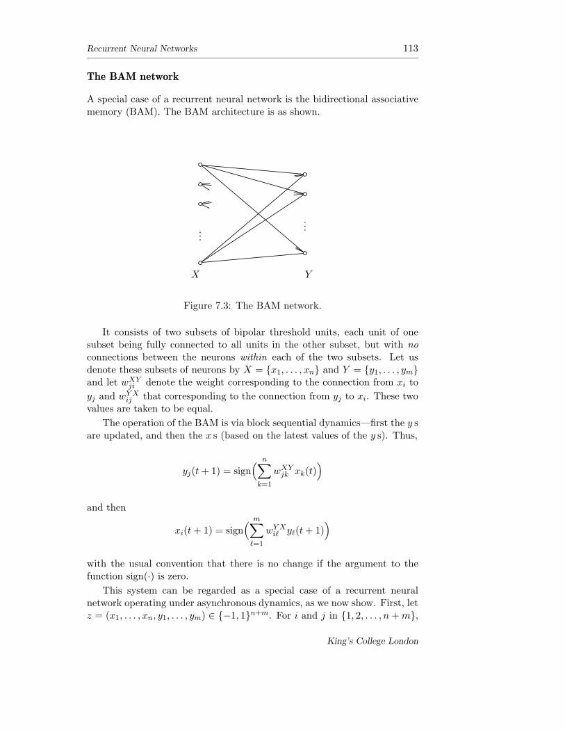
Recurrent Neural Networks 113
The BAM network
A special case of a recurrent neural network is the bidirectional associativememory (BAM). The BAM architecture is as shown.
...
X
...
Y
Figure 7.3: The BAM network.
It consists of two subsets of bipolar threshold units, each unit of onesubset being fully connected to all units in the other subset, but with noconnections between the neurons within each of the two subsets. Let usdenote these subsets of neurons by X = {x1, . . . , xn} and Y = {y1, . . . , ym}and let wXY
ji denote the weight corresponding to the connection from xi to
yj and wY Xij that corresponding to the connection from yj to xi. These two
values are taken to be equal.
The operation of the BAM is via block sequential dynamics—first the y sare updated, and then the x s (based on the latest values of the y s). Thus,
yj(t + 1) = sign( n∑
k=1
wXYjk xk(t)
)
and then
xi(t + 1) = sign( m∑
ℓ=1
wY Xiℓ yℓ(t + 1)
)
with the usual convention that there is no change if the argument to thefunction sign(·) is zero.
This system can be regarded as a special case of a recurrent neuralnetwork operating under asynchronous dynamics, as we now show. First, letz = (x1, . . . , xn, y1, . . . , ym) ∈ {−1, 1}n+m. For i and j in {1, 2, . . . , n + m},
King’s College London

114 Chapter 7
define wji as follows
w(n+r)i = wXYri , for 1 ≤ i ≤ n and 1 ≤ r ≤ m,
wi(n+r) = wY Xir , for 1 ≤ i ≤ n and 1 ≤ r ≤ m
and all other wji = 0. Thus
(wji) =
(0 W T
W 0
)
where W is the m × n matrix Wri = wXYri . Next we consider the mode of
operation. Since there are no connections between the y s, the y updatescan be considered as the result of m sequential updates. Similarly, the xupdates can be thought of as the result of n sequential updates. So we canconsider the whole y and x update as m+n sequential updates taken in theorder of y s first and then the x s. It follows that the dynamics is governedby the asynchronous dynamics of a recurrent neural network whose synapticmatrix is symmetric and has nonnegative diagonal terms (zero in this case).Hence, in particular, the system converges to a fixed point.
One usually considers the patterns stored by the BAM to consist of pairsof vectors, corresponding to the x and y decomposition of the network,rather than as vectors in {−1, 1}n+m, although this is a mathematicallytrivial distinction.
Department of Mathematics
Chapter 8
Singular Value Decomposition
We have discussed the uniqueness of the generalized inverse of a matrix,but have still to demonstrate its existence. We shall turn to a discussionof this problem here. The solution rests on the existence of the so-calledsingular value decomposition of any matrix, which is of interest in its ownright. It is a standard result of linear algebra that any symmetric matrixcan be diagonalized via an orthogonal transformation. The singular valuedecomposition can be thought of as a generalization of this.
Theorem 8.1 (Singular Value Decomposition). For any given non-zero ma-trix A ∈ R
m×n, there exist orthogonal matrices U ∈ Rm×m, V ∈ R
n×n andpositive real numbers λ1 ≥ λ2 ≥ · · · ≥ λr > 0, where r = rankA, such that
A = U D V T
where D ∈ Rm×n has entries Dii = λi, 1 ≤ i ≤ r and all other entries are
zero.
Proof. Suppose that m ≥ n. Then ATA ∈ Rn×n and ATA ≥ 0. Hence there
is an orthogonal n × n matrix V such that
ATA = V Σ V T
where Σ ∈ Rn×n is given by Σ =
µ1 0. . .
0µn
where µ1 ≥ µ2 ≥ · · · ≥ µn
are the eigenvalues of ATA, counted according to multiplicity. If A 6= 0,then ATA 6= 0 and so has at least one non-zero eigenvalue. Thus, thereis 0 < r ≤ n such that µ1 ≥ µ2 ≥ · · · ≥ µr > µr+1 = · · · = µn = 0.
Write Σ =
(Λ 00 0
), where Λ =
λ1 0. . .
0λn
, with λ2
1 = µ1, . . . , λ2r = µr.
Partition V as V =(V1 V2
)where V1 ∈ R
n×r and V2 ∈ Rn×(n−r). Since V is
115

116 Chapter 8
orthogonal, its columns form pairwise orthogonal vectors, and so V T1 V2 = 0.
We have
ATA = V Σ V T
=(V1 V2
) (Λ2 00 0
)V T
=(V1Λ
2 0) (
V T1
V T2
)
= V1Λ2V T
1 .
Hence V T2 ATAV2 = V T
2 V1︸ ︷︷ ︸(V T
1 V2)T =0
Λ2 V T1 V2︸ ︷︷ ︸=0
, so that V T2 AT AV2 = 0 and so it follows
that AV2 = 0.Now, the equality ATA = V1Λ
2V T1 suggests at first sight that we might
hope that A = ΛV T1 . However, this cannot be correct, in general, since
A ∈ Rm×n, whereas ΛV T
1 ∈ Rr×n, and so the dimensions are incorrect.
However, if U ∈ Rk×r satisfies UT U = 1lr, then V1Λ
2V T1 = V1ΛUT UΛV T
1
and we might hope that A = UΛV T1 . We use this idea to define a suitable
matrix U . Accordingly, we define
U1 = AV1Λ−1 ∈ R
m×r,
so that A = U1ΛV T1 , as discussed above. We compute
UT1 U1 = Λ−1 V T
1 ATAV1Λ−1
︸ ︷︷ ︸Λ2
= 1lr.
This means that the r columns of U1 form an orthonormal set of vectorsin R
m. Let U2 ∈ Rm×(m−r) be such that U = (U1 U2) is orthogonal (in
Rm×m)—thus the columns of U2 are made up of (m−r) orthonormal vectors
such that these, together with those of U1, form an orthonormal set of mvectors. Thus, UT
2 U1 = 0 ∈ R(m−r)×r and UT
1 U2 = 0 ∈ Rr×(m−r). Hence we
have
UT AV =
(UT
1
UT2
)A (V1 V2)
=
(UT
1 AUT
2 A
)(V1 V2)
=
(UT
1 AV1 UT1 AV2
UT2 AV1 UT
2 AV2
)
=
(UT
1 AV1 0UT
2 AV1 0
), since AV2 = 0,
=
(Λ 0
UT2 U1Λ 0
),
Department of Mathematics

Singular Value Decomposition 117
using U1 = AV1Λ−1 and UT
1 U1 = 1lr so that Λ = UT1 AV1,
=
(Λ 00 0
), using UT
2 U1 = 0.
Hence,
A = U
(Λ 00 0
)V T ,
as claimed. Note that the condition m ≥ n means that m ≥ n ≥ r, and sothe dimensions of the various matrices are all valid.
If m < n, consider B = AT instead. Then, by the above argument, weget that
AT = B = U ′
(Λ′ 00 0
)V ′T ,
for orthogonal matrices U ′ ∈ Rn×n, V ′ ∈ R
m×m and where Λ′2 holds thepositive eigenvalues of AAT . Taking the transpose, we have
A = V ′
(Λ′ 00 0
)U ′T .
Finally, we observe that from the given form of the matrix A, it is clear thatthe dimension of ranA is exactly r, that is, rankA = r.
Remark 8.2. From this result, we see that the matrices ATA = U
(Λ2 00 0
)V T
and AAT = V
(Λ2 00 0
)UT have the same non-zero eigenvalues, counted
according to multiplicity. We can also see that
rankA = rankAT = rankAAT = rankATA .
Theorem 8.3. Let A ∈ Rm×n and let U ∈ R
m×m, V ∈ Rn×n, Λ ∈ R
r×r be asgiven above via the singular value decomposition of A, so that A = UDV T
where D =
(Λ 00 0
)∈ R
m×n. Then the generalized inverse of A is given by
A# = V
(Λ−1 00 0
)
︸ ︷︷ ︸n×m
UT .
Proof. We just have to check that A#, as given above, really does satisfythe defining conditions of the generalized inverse. We will verify two of thefour conditions by way of illustration.
King’s College London
118 Chapter 8
Put X = V HUT , where H =
(Λ−1 00 0
)∈ R
n×m. Then
AXA = UDV T V HUT UDV T
= U
(1lr 00 0
)
︸ ︷︷ ︸m×m
(Λ 00 0
)
︸ ︷︷ ︸m×n
V T = A.
Similarly, one finds that XAX = X. Next, we consider
XA = V HUT UDV T
= V
(Λ−1 00 0
)
︸ ︷︷ ︸n×m
UT U︸ ︷︷ ︸1lm
(Λ 00 0
)
︸ ︷︷ ︸m×n
V T
= V
(1lr 00 0
)
︸ ︷︷ ︸n×n
V T
which is clearly symmetric. Similarly, one verifies that AX = (AX)T , andthe proof is complete.
We have seen how the generalized inverse appears in the construction ofthe OLAM matrix memory, via minimization of the output error. Now wecan show that this choice is privileged in a certain precise sense.
Theorem 8.4. For given A ∈ Rm×n and B ∈ R
ℓ×n, let ψ : Rℓ×m → R be
the map ψ(X) = ‖XA − B‖F . Among those matrices X minimizing ψ, thematrix X = BA# has the least ‖ · ‖F -norm.
Proof. We have already seen that the choice X = BA# does indeed minimizeψ(X). Let A = UDV T be the singular value decomposition of A with thenotation as above—so that, for example, Λ denotes the top left r × r blockof D. We have
ψ(X)2 = ‖XA − B‖2F
= ‖XUDV T − B‖2F
= ‖XUD − BV ‖2F , since V is orthogonal,
= ‖Y D − C‖2F , where Y = XU ∈ R
ℓ×m, C = BV ∈ Rℓ×n,
=∥∥(Y1 Y2)
(Λ 00 0
)− (C1 C2)
∥∥2
F,
Department of Mathematics

Singular Value Decomposition 119
where we have partitioned the matrices Y and C into (Y1 Y2) and (C1 C2)with Y1, C1 ∈ R
ℓ×r,
= ‖(Y1Λ 0) − (C1 C2)‖2F
= ‖(Y1Λ − C1... − C2)‖2
F
= ‖Y1Λ − C1‖2F + ‖C2‖2
F .
This is evidently minimized by any choice of Y (equivalently X) for which
Y1Λ = C1. Let Y = (C1Λ−1
... 0) and let Y = (C1Λ−1
... Y2), where Y2 ∈R
ℓ×m−r is subject to Y2 6= 0 but otherwise is arbitrary. Both Y and Ycorrespond to a minimum of ψ(X), where the X and Y matrices are relatedby Y = XU , as above. Now,
‖Y ‖2F = ‖C1Λ
−1‖2F < ‖C1Λ
−1‖2F + ‖Y2‖2
F = ‖Y ′‖2F .
It follows that among those Y matrices minimizing ψ(X), Y is the one withthe least ‖ · ‖F -norm. But if Y = XU , then ‖Y ‖F = ‖X‖F and so X givenby X = Y UT is the X matrix which has the least ‖ ·‖F -norm amongst thosewhich minimize ψ(X). We find
X = Y UT
= (C1Λ−1 ... 0)UT
= (C1 C2)
(Λ−1 00 0
)UT
= BV
(Λ−1 00 0
)UT
= BA#
which completes the proof.
King’s College London

120 Chapter 8
Department of Mathematics
Bibliography
We list, here, a selection of books available. Many are journalistic-styleoverviews of various aspects of the subject and convey little quantitativefeel for what is supposed to be going on. Many declare a deliberate attemptto avoid anything mathematical.
For further references a good place to start might be the bibliography ofthe book of R. Rojas (or that of S. Haykin).
Aarts, E. and J. Korst, Simulated Annealing and Boltzmann Machines,J. Wiley 1989. Mathematics of Markov chains and Boltzmann machines.
Amit, D. J., Modeling Brain Function, The World of Attractor NeuralNetworks, Cambridge University Press 1989. Statistical physics.
Aleksander, I. and H. Morton, An Introduction to Neural Computing, 2nded., Thompson International, London 1995.
Anderson, J. A., An Introduction to Neural Networks, M.I.T. Press 1995.Minimal mathematics with emphasis on the uses of neural network algorithms.
Indeed, the author questions the appropriateness of using mathematics in this
field.
Arbib, M. A., Brains, Machines and Mathematics, 2nd ed., Springer-Verlag1987. Nice overview of the perceptron.
Aubin, J.-P., Neural Networks and Qualitative Physics, Cambridge Univer-sity Press 1996. Quite abstract.
Bertsekas, D. P. and J. N. Tsitsiklis, Parallel and Distributed Computation–Numerical Methods, Prentice-Hall International Inc. 1989.
Bishop, C. M., Neural networks for Pattern Recognition, Oxford UniversityPress 1995. Primarily concerned with Bayesian statistics.
Blum, A., Neural Networks in C++—An Object Oriented Framework forBuilding Connectionist Systems, J. Wiley 1992. Computing hints.
121
122 Bibliography
Bose, N. K. and P. Liang, Neural Network Fundamentals with Graphs,Algorithms and Applications, McGraw-Hill 1996. Emphasises the use of
graph theory.
Dayhoff, J., Neural Computing Architectures, Van Nostrand Reinhold 1990.A nice discussion of neurophysiology.
De Wilde, P., Neural Network Models, 2nd ed., Springer 1997. Gentle
introduction.
Devroye, L., Gyorfi, G. and G. Lugosi, A Probabilistic Theory of PatternRecognition, Springer 1996. A mathematics book, full of inequalities to do
with nonparametric estimation.
Dotsenko, V., An Introduction to the Theory of Spin Glasses and NeuralNetworks, World Scientific 1994. Statistical physics.
Duda, R. O. and P. E. Hart, Pattern Classification and Scene Analysis,J. Wiley 1973. Well worth looking at. It puts later books into perspective.
Fausett, L., Fundamentals of Neural Networks, Prentice Hall 1994. Nice
detailed descriptions of the standard algorithms with many examples.
Freeman, J. A., Simulating Neural Networks with Mathematica, Addison-Wesley 1994. Set Mathematica to work on some algorithms.
Freeman, J. A. and D. M. Skapura, Neural Networks: Algorithms, Applica-tions, and Programming Techniques, Addison-Wesley 1991. Well worth a
look.
Golub, G. H. and C. F. van Loan, Matrix Computations, The John HopkinsUniversity Press 1989. Superb book on matrices; you will discover entries in
your matrix you never knew you had.
Hassoun, M. H., Fundamentals of Artificial Neural Networks, The MITPress 1995. Quite useful to dip into now and again.
Haykin, S., Neural Networks, A Comprehensive Foundation, Macmillan1994. Looks very promising, but you soon realise that you need to spend a lot
of time tracking down the original papers.
Hecht-Nielsen, R., Neurocomputing, Addison-Wesley 1990.
Department of Mathematics
Bibliography 123
Hertz, J., A. Krogh and R. G. Palmer, Introduction to the Theory of NeuralComputation, Addison-Wesley 1991. Quite good account but arguments are
sometimes replaced by references.
Kamp, Y. and M. Hasler, Recursive Neural Networks for Associative Mem-ory, J. Wiley 1990. Well-presented readable account of recurrent networks.
Khanna, T., Foundations of Neural Networks, Addison-Wesley 1990.
Kohonen, T., Self-Organization and Associative Memory, Springer 1988.Discusses the OLAM.
Kohonen, T., Self-Organizing Maps, Springer 1995. Describes a number of
algorithms and various applications. There are hundreds of references.
Kosko, B., Neural Networks and Fuzzy Systems, Prentice-Hall 1992. Disc
included.
Kung, S. Y., Digital Neural Networks, Prentice-Hall 1993. Very concise
account for electrical engineers.
Looney, C. G., Pattern Recognition Using Neural Networks, Oxford Uni-versity Press 1997. Quite nice account—concerned with practical application
of algorithms.
Masters, T., Practical Neural Network Recipes in C++, Academic Press1993. Hints and ideas about implementing algorithms; with disc.
McClelland J. L., D. E. Rumelhart and the PDP Research Group, ParallelDistributed Processing, Vols 1 and 2, MIT Press 1986. Has apparently sold
many copies.
Minsky, M. L. and S. A. Papert, Perceptrons, Expanded ed. MIT Press1988. Everyone should at least browse through this book.
Muller, B. and J. Reinhardt, Neural Networks: An Introduction, Springer1990. Quite a nice account; primarily statistical physics.
Pao, Y-H., Adaptive Pattern Recognition and Neural Networks, Addison-Wesley 1989.
Peretto, P., An Introduction to the Modeling of Neural Networks, CambridgeUniversity Press 1992. Heavy-going statistical physics.
King’s College London

124 Bibliography
Ritter, H., T. Martinez and K. Schulten, Neural Computation and Self-Organizing Maps, Addison-Wesley 1992.
Rojas, R., Neural Networks – A Systematic Introduction, Springer 1996. A
very nice introduction—but do not expect too many details.
Simpson, P. K., Artificial Neural Systems: Foundations, Paradigms, Appli-cations, and Implementations, Pergamon Press 1990. A compilation of
algorithms.
Vapnik, V., The Nature of Statistical Learning Theory, Springer 1995. An
overview (no proofs) of the statistical theory of learning and generalization.
Wasserman, P. D., Neural Computing, Theory and Practice, Van NostrandReinhold 1989.
Welstead, S., Neural Network and Fuzzy Logic Applications in C/C++,J. Wiley 1994. Programmes built around Borland’s Turbo Vision; disc
included.
Department of Mathematics