Network Optimisation Package for the Design and Analysis of

Survivable SDH Networks

James O'Hara B. Eng.

A thesis submitted as a requirement for the degree of Masters of Engineering in Electronic Engineering

Dublin City University Supervisor - Dr. T. Curran

September 1998

DeclarationI hereby certify that this material, which I now submit for assessment on the programme of study leading to the award of Masters of Engineering, is entirely my own work and has not been taken from the work of others save and to the extent that such work has been cited and acknowledged within the text of this work.

ID Number: 93701365James O’Hara

Date: 11th September, 1998

AcknowledgementsThe author would like to express his gratitude and thanks to the

following people who contributed to and made this work possible:

• To Dr. Tommy Curran for providing the opportunity to pursue this

research, and for his technical advice and expertise throughout.

• To Broadcom Hireann Research Ltd., for its assistance and continued

support.

• To my colleagues, both at DCU and Broadcom, for listening to my

concepts and for their enthusiasm for offering advice. In particular,

thanks is due to Mandy, for her - as she put it - "amazing patience,

incredible eye fo r detail, limitless generosity, ..."

• To my parents for their constant support throughout my studies.

• And finally, to Fiona, for being there when the going got tough, and

for her encouragement and unflagging desire to see this labour of

love concluded.

Abstract

Title: N etw ork O ptim isation Package for the D esign and A nalysis o fSurvivable SDH N etw orks

Author: Jam es O'Hara B. Eng.

The advancements in digital technology and the resultant economies o f scale offered by high

capacity fibre transmission systems have enabled network operators to provide more cost-effective

telecommunications services to their increasing customer base. However, with the deployment o f

such systems, the emphasis on service quality and network reliability has increased considerably.

To address this and many other network management issues, the SDH digital transmission standard

was established. While supporting enhanced network management functionality, it was only through

the subsequent development o f highly intelligent Network Elements (NEs) that the inherent cost

benefits o f SDH have been realised. Each NE is characterised by its own topology and associated

restoration schemes. As the economic viability o f these survivable topologies are dependent on

varying network conditions, it has been shown that the most cost-effective networks will be based on

a combination o f these topologies. The complexity o f these highly integrated networks and the

immense capital investment involved suggests that much consideration should be given to the

design and optimisation o f such networks. This research work concerns an investigation into this

particular area o f network optimisation. It involves the developm ent o f an optimisation design

package that facilita tes the generation and analysis o f survivable SDH networks through the

implementation o f highly efficient optimisation techniques. Existing optimisation techniques are

utilised to this end, and enhanced upon to address aspects o f the SDH design model that were

previously not taken into consideration. This results in the development o f innovative and highly

efficient algorithmic procedures fo r solving this particu lar design problem, and "NetOpt" - a

prototype design tool fo r implementing such procedures. Based on a set o f generated test case

networks, a detailed analysis and evaluation o f these procedures and the resultant network

solutions is presented. In conclusion, it is shown that CAD-based tools are essential fo r the

generation and analysis o f survivable SDH networks.

Table of Contents

C h a p te r 1 - I n t r o d u c t io n ........................................................................... 11.1 M otivation........................................................................................................................... 11.2 O bjectives............................................................................................................................ 21.3 Thesis Structure................................................................................................................. 41.4 Associated Publications....................................................................................................4

C h a p te r 2 - S D H N e tw o rk D esig n C o n c e p ts ...............................................................52.1 Emergence of SD H ............................................................................................................5

2.1.1 SDH Standardisation Proccss.................................................. 62.1.2 SDH Frame Structure...................................... 82.1.3 Layer Concept and SDH Overhead Channels............................................................. 92.1.4 STM-1 Pay load.............................................................................................................102.1.5 Benefits of SDH........................................................................................................... 12

2.2 Review of SDH-Based Network Elem ents.................................................................132.2.1 Terminal Multiplexer (TM)........................................................................................ 132.2.2 Add-Drop Multiplexer (ADM) ..................................................................... 142.2.3 Digital Cross-Connect (DXC).................................................................................... 15

2.3 SDH Survivable Topologies..........................................................................................162.3.1 TM Point-to-Point Topologies.................................................................................... 162.3.2 ADM Ring Topologies............................................................................................. 17

2.3.2.1 Line-level restoration.................................................................................................182.3.2.2 Path-level restoration.................................................................................................19

2.3.3 DXC-based Mesh Topologies.....................................................................................202.3.4 Hybrid ADM-ring/DXC Topology.................................................... 222.3.5 Comparison of Survivable Topologies......................................................................22

2.4 SDH Network Architectures and Deployment S trategies..................................... 232.4.1 SDH Network Architecture............................................................. 23

2.4.1.1 National trunk network................................................................................. 242.4.1.2 Regional junction network.........................................................................................242.4.1.3 Local access network................................................................................................ 24

2.4.2 SDH Deployment Strategies.......................................................................................252.4.3 Considerations Affecting SDH Deployment............................................................26

Chapter 3 - SDH N etw ork O ptim isation................................................................ 273.1 Problem Formulation and Network Representation.................................... 27

3.1.1 Input data and network representation.......................................................................273.1.2 Output data and solution representation................................................................... 283.1.3 Design constraints........................................................................................................293.1.4 Formulation of Cost Function........................................................................ 30

3.1.4.1 Nodal cost function................................................................................................... 303.1.4.2 Link cost function.................................. ......................... ................ ..................... . 3 1

3.1.5 Reformulation as a Combinatorial Optimisation Problem......................................343.2 Joint Optimal Routing and W orking Capacity Assignment Problem ..................35

3.2.1 Problem Formulation...................................................................................................353.2.2 Adoption of a Minimum-Hop Routing Constraint.................................... 353.2.3 Routing Algorithm and Computational Complexity................................................ 40

3.3 Optimal Spare Capacity Assignment Problem ......................................................... 403.3.1 Problem Formulation.................................................................................................. 403.3.2 Generation of Optimal Flow Constraints.................................................. 413.3.3 Optimisation Phase and Problem Complexity..........................................................463.3.4 Proposed Solution M ethod..........................................................................................47

3.3.4.1 Initial spare capacity assignment algorithm...............................................................473.3.4.2 Global spare capacity assignment algorithm............................................................. 503.3.4.3 Adaptive minimisation algorithm........................................................................,..... 51

3.3.5 Spare Capacity Assignment based on Path-Level Restoration...............................523.3.5.1 Initial spare capacity assignment algorithm............................................................... 533.3.5.2 Global spare capacity assignment algorithm............................................................. 543.3.5.3 Overall complexity.................................................................................................... 55

3.4 Network Optimisation Solution M ethod ................................................................... 563.4.1 Review of Solution M ethods......................................................................................56

3.4.1.1 Local search methodology............... 563.4.1.2 Greedy algorithms............................................................................................ 573.4.1.3 Modem methods....................................................................................................... 573.4.1.4 Comparison of solution methods ....................................................... 58

3.4.2 Proposed Solution M ethod..................................................................................... 603.4.2.1 Initial optimisation phase.......................................................................................... 603.4.2.2 Refinement phase...................................................................................................... 62

Chapter 4 - Im plem entation o f D esign P rocedure............................................. 634.1 Optimal Design P rocedure............................................................................................634.2 Network Optimisation Algorithm ................................................................................ 64

4.2.1 Initial Optimisation Algorithm.................................................................................. 654.2.2 Dual Optimisation Algorithm.....................................................................................674.2.3 Network Cost Algorithms...........................................................................................70

4.2.3.1 Basic network cost algorithm.....................................................................................704.2.3.2 Total network cost algorithm.....................................................................................71

4.3 Joint Optimal Routing & W orking Capacity Assignment A lgorithm .................714.3.1 Optimal Routing Algorithm........................................................................................72

4.3.1.1 Dijkstra's shortest-path algorithm....................................................... 724.3.1.2 Improvements to existing algorithm..........................................................................744.3.1.3 Imposing minimum-hop routing constraint................................................................754.3.1.4 Overall routing algorithm.......................................................................................... 76

4.3.2 Interpretation of Paths Matrix and Path-Trace Algorithm...................................... 774.3.3 Connectivity Test Algorithm......................................................................................794.3.4 Working Capacity Assignment Algorithm............................................................... 80

4.4 Optimal Spare Capacity Assignment A lgorithm ......................................................804.4.1 Initial Spare Capacity Assignment Algorithm..........................................................814.4.2 Global Spare Capacity Assignment Algorithm........................................................834.4.3 Adaptive Minimisation Algorithm....................................................................... 844.4.4 Release Phase Algorithm............................................................................................ 85

C h a p te r 5 - N e tO p t D esig n T o o l ....................................................................................865.1 Overview of N etO pt.......................................................................................................86

5.1.1 Active Design Field................................................... 865.1.1.1 Network representation.............................. 875.1.1.2 Zoom setting.............................................................................................................. 885.1.1.3 Gridlines.................................................................................................................... 885.1.1.4 Network coordinates.......................................................................................... 885.1.1.5 Scrollbars................................................................................................................. 895.1.1.6 Network rendering..................................................................................................... 905.1.1.7 Changing the zoom setting.............................................................................. 90

5.1.2 Menu B ar......................................................................................................................915.1.2.1 File menu................................................................................................................... 915.1.2.2 Edit menu............................................................................. 925.1.2.3 View menu ................................................................................................... 935.1.2.4 Optimisation menu ................................................................................................94

5.1.3 Tool B ar........................................................................................................................955.1.4 Status Bar......................................................................................................................955.1.5 Dialog Boxes.................................................................................................................96

5.1.6 Interaction with the Network Solution.......................................................................965.1.6.1 Link options........................... 965.1.6.2 Node options............................................................................................................. 96

5.2 Initialising a New Input N etw ork................................................................................ 975.2.1 Initialise the Active Network Domain.......................................................................975.2.2 Initialise the Number of Nodes................................................ 975.2.3 Initialise the Nodal Characteristics............................................................................ 985.2.4 Initialise the Inter-Nodal Constraints.........................................................................985.2.5 Initialise the Cost Components.............................. 995.2.6 Initialise the Network Description........................................................................... 1005.2.7 Save the Network to F ile ...........................................................................................100

5.3 Network Editing U tilities ............................................................................................ 1005.3.1 Editing Inter-Nodal Constraints (Locally) .............................. 1005.3.2 Editing Inter-Nodal Constraints (Globally)............................................................ 1025.3.3 Updating the Network Solution................................................................................102

5.4 Network Optimisation U tilities..................................................................................1025.4.1 Design Constraints............................................... 1025.4.2 Cost Components....................................................................................................... 1035.4.3 Network Optimisation...............................................................................................1035.4.4 Initial Optimisation.................................................................................................... 1045.4.5 Dual Optimisation...................................................................................................... 1045.4.6 Optimal Spare Capacity.............................................................................................104

C hapter 6 - Results and A n alysis............................................................................ 1056.1 Generation of Test Case N etw orks............................................................................ 1056.2 Solution Characteristics................................................................................................107

6.2.1 Network Connectivity................................................................................................1076.2.2 Working Capacity Solution Characteristics.............................................................1086.2.3 Working and Spare Capacity Cost Characteristics.................................................1156.2.4 Validation of Initial Optimisation Phase.................................................................1206.2.5 Optimal Solution Characteristics..............................................................................121

6.3 Optimisation Complexity and Efficiency................................................................ 1236.3.1 Initial Optimisation Phase......................................................................................... 1246.3.2 Refinement Phase...................................................................................................... 124

6.4 Optimal Routing S trategies.........................................................................................1276.4.1 Working Capacity Cost Characteristics...................................................................1276.4.2 Spare Capacity Cost Characteristics........................................................................ 128

6.5 Spare Capacity Assignment Algorithm...........................................................1296.5.1 Quality of Near-Optimal Solution................................................................ 1296.5.2 Path-level and Line-level Restoration...................................................................... 130

C hapter 7 - Conclusions................................................................ 1327.1 Overall Discussion of Results..........................................................................132

7.1.1 Solution Characteristics.............................................................................................1327.1.2 Optimal Routing Strategies.................................................. 1357.1.3 Optimal Spare Capacity Assignment Algorithm....................................................1357.1.4 Overall Optimisation Procedure...............................................................................136

7.1.4.1 Initial optimisation phase......................................................................................................1367.1.4.2 Refinement phase................................................................................................................... 136

7.1.5 NetOpt and the Optimal Design Procedure............................................................1387.2 Recommendations and Scope for Future Work.............................................. 139

7.2.1 Further Validation of Results...................................................................................1397.2.2 Further Development of the Optimal Design Procedure...................................... 139

R eferences.............................................................................................................. 140

Appendix A1 - DXC-based R estoration C o n tro l....................................... I

Appendix A2 - D istributed Restoration T im e.................................................I l l

Appendix A3 - O ptim al Routing A lgorithm s................................................ V IIA3.1 Implementation of Dijkstra's Shortest-Path Algorithm................................ VIIA3.2 Implementation of Modified Shortest-Path Algorithm..................................IXA3.3 Implementation of Minimum-hop/Shortest-path Algorithm...........................X

v i i i

Chapter 1 - Introduction

1.1 M otivation

Synchronous Digital Hierarchy (SDH) has evolved to address the limitations of the existing

Plesiochronous Digital Hierarchy (PDH) networks. It has surpassed PDH in the following aspects:

• defines a set of high-capacity hierarchical signal rates, ranging from 155 Mb/s to 2.4 Gb/s, with

easy accommodation of higher order rates, such as 10 Gb/s, as technology evolves.

• represents a worldwide standard which unifies European, North American, and Japanese

transmission rates, and supports interconnection of existing PDH networks.

• provides advanced network management capabilities allowing network operators to provide

enhanced and highly reliable services through pre-emptive maintenance and dynamic service

restoration.

• supports a simplified method of synchronous multiplexing which enables signals to be

extracted/inserted directly into higher order signal rates, overcoming the inefficiency of the

multi-step PDH-based process.

• precipitated the development and standardisation of advanced and highly intelligent Network

Elements (NEs), i.e. Terminal Multiplexers (TMs), Add-Drop Multiplexers (ADMs), and Digital

Cross-Connects (DXCs). Associated with each NE are characteristic topologies and restoration

schemes, i.e. TM-based point-to-point, ADM-based ring, and DXC-based mesh topologies.

These NEs and their topologies provide dynamic routing and restoration capabilities needed for

distributed network management control.

• provides improved network performance and flexibility enabling network operators to meet

customer’s growing demands for better quality of service. The initial costs of such a new

network infrastructure are offset by the consequent reduction in operating costs and return in

revenue that result from the highly reliable and cost effective services that can be provided.

• offers easy accommodation of new broadband services, such as B-ISDN and ATM.

With the deployment of these high capacity fibre transmission systems, the emphasis on service

quality and network reliability has increased substantially. For network operators, improved

1

network reliability is essential from the perspective of lost revenue and the fact that their customers,

particularly business users, are now themselves demanding a higher level of service quality.

Addressing this issue, SDH has resulted in the development of enhanced self-healing techniques

which are supported by the various NEs and their characteristic topologies and restoration schemes.

These topologies are each dependent to a varying degree on restoration time, relative cost, network

characteristics, and the required level of survivability. It has been shown that survivable SDH

transmission networks are expected to be based on a combination of these topologies. Due to the

difficulty of planning such complex SDH integrated restoration schemes, computer-aided design

tools are essential to ensure reasonable and cost-effective network solutions that utilise the merits of

each restoration topology.

1.2 O bjectives

The overall objective of this work was to develop a network optimisation package that would

facilitate the design and analysis of optimal SDH network solutions through the implementation of

highly efficient and effective optimisation techniques. The realisation of this objective involved the

following procedural steps:

Step 1. The formulation of the optimal design problem in terms of the:

• notation and data structures used to represent both the input network and the resultant

network solution

• design constraints which must be satisfied in order to realise a feasible solution

• cost model adopted for this particular problem

Step 2. The development of an optimal design procedure for solving this problem.

Step 3. The development of a prototype design tool that would facilitate the implementation of this

design procedure.

Step 4. The evaluation of SDH network solutions resulting from the application of this procedure.

The inputs to the design problem include node locations, potential links, and inter-nodal demands,

fixed costs, and distances. The objective being to generate a network solution that minimises the

total network cost while allocating sufficient network capacity to route all inter-nodal demands and

satisfy a required level of survivability. This problem is characterised by large dimensionality even

where small networks are concerned and it turns out that the overall problem is completely

intractable. However, based on the network model adopted, it will be shown that the problem can be

2

reformulated as a combinatorial optimisation problem. This enables the natural decomposition of

the problem into a number of sub-problems that can be solved sequentially.

The basic sub-problem is, given a network configuration, how should capacity be assigned in order

to route all inter-nodal demands and satisfy a required level of survivability at the minimum cost.

This is composed of two sequential solution steps. The first concerns the optimal routing of

demands and the assignment of working capacity based on the optimal routes generated. While

well-established shortest-path routing algorithms could be used to realise this solution, it was found

that the routing strategy needed to be refined to take into consideration component costs specific to

the SDH network model. Further modifications were also made to improve the overall performance

of the algorithm. Based on the solution derived from this step, the second step involves the optimal

assignment of spare capacity across the network that ensures 100 % restoration against all single

link failures. While an exact solution to this problem can be found, the computational complexity of

the technique used increases dramatically with the number of nodes in the network, and it turns out

that this problem is itself deemed intractable for networks with more than 20 nodes. As a

consequence, considerable work was devoted to this problem in an attempt to find a feasible

solution method. This has resulted in the development and implementation of an innovative and

highly efficient technique which, in its basic form, is capable of finding near-optimal cost solutions

that are proportional representations of the optimal cost solutions.

Given that the minimum cost solution for any network configuration can be found, the objective of

the overall optimisation problem is to find the configuration that represents the optimal solution.

However, as the number of potential solutions grows exponentially with the number of input nodes,

this problem is classified as /VP-hard, for which no realistic time solution can be found. In recent

years, a number of heuristic-based solution methods have been developed to effectively solve this

class of problem. Based on the concept of a local search methodology, the most efficient of these

solution methods are based on well-established Greedy algorithms, while, more recently, a number

of more advanced algorithms have emerged. In general, while the latter are capable of finding better

solutions, a considerable increase in the computational time requirement is incurred. Following a

review of these algorithms, it was found that, due to the incorporation of the spare capacity

assignment problem, no single algorithm could efficiently and/or effectively solve the overall

optimisation problem. As a result, a two-phase solution approach was adopted. The first phase

utilises a highly efficient Greedy algorithm to reduce the initial complexity of the problem by

finding a more practical starting solution, while the second phase concerns the refinement of this

solution and is based on a more advanced and computationally intensive algorithm. To accelerate

the optimisation process and improve its overall effectiveness, perturbation techniques, such as user

3

interaction with the refinement phase, are also employed. These form part of the overall optimal

design procedure facilitated by the design tool.

1.3 Thesis Structure

An introduction to SDH network design concepts is presented in Chapter 2. Following a discussion

on the benefits of SDH and how it will form the infrastructure for future transmission networks, the

various SDH-based network elements and their characteristic topologies and restoration schemes

are reviewed. Finally, the current trends in SDH deployment are reviewed.

Chapter 3 concerns the formulation of the optimal design problem. Based on the network model

defined, it is shown how the problem can be decomposed into the various sub-problems identified in

Section 1.2. The solution methods developed to efficiently solve these individual sub-problems are

then presented.

Chapter 4 concerns the implementation of these solution methods in terms of the algorithmic

procedures involved and how these form part of the overall optimal design procedure facilitated by

the design tool.

An overview of the design tool and how it facilitates the generation, editing and optimisation of

survivable SDH networks is presented in Chapter 5.

Chapter 6 concerns an evaluation of the optimal design procedure facilitated by the design tool.

Based on the analysis of a set of test case networks that model variations in the input constraints, it

will be shown how these input conditions impact on the solution characteristics for each network. It

will also be shown how these characteristics have a residual effect on the computational complexity

of each phase of the respective optimisation processes. Finally, a cost analysis of alternative routing

strategies and restoration techniques is presented.

An overall discussion of results and scope for further work is presented in Chapter 7.

1.4 A ssociated Publications

A summary of part of this work was published in "Technology Ireland 1995", a magazine

supplement published by TELTEC Ireland.

4

Chapter 2 - SDH Network Design Concepts

2.1 Em ergence o f SDH

As digital networks increased in size and complexity over the last decade, there was a growing need

from both network operators and their customers for facilities not readily or economically supported

by the existing Plesiochronous Digital Hierarchy (PDH) transmission networks. PDH was

developed in the early 70s to provide increased routing capacity to meet the rapid growth in both

residential and business telephony traffic. Although based on digital transmission over coaxial

cables, the high cost of bandwidth and digital components at that time put constraints on the

operations and management facilities PDH networks could offer. While PDH standards have

evolved in a step-by-step basis to support the growing demand in voice traffic and data services, the

inherent lack of facilities has left it a costly, outmoded, and difficult-to-manage network, whose

inefficiencies, both in equipment and operations, have inhibited the progression toward a more

flexibly controlled and fully managed broadband network.

PDH is based on a complex multiplex/demultiplex scheme which enables lower order primary rate

signals, i.e. 2 Mb/s, to be multiplexed into successively higher order rates, i.e. 8 Mb/s, 34 Mb/s, 140

Mb/s and, later, up to the proprietary 565 Mb/s line rate. At each multiplexing step, the bit rate of

the individual signal rates is controlled within specified limits and synchronised by the process of

bit stuff justification. In order to extract/insert an individual 2 Mb/s signal at any level of the

hierarchy, i.e. 140 Mb/s, the whole signal structure must be demultiplexed (i.e. from 140 to 34, 34

to 8, and 8 to 2) and then reassembled (i.e. 2 to 8, 8 to 34, and 34 to 140) for onward transmission.

This highlights one of the major drawbacks of using PDH in high capacity networks.

Another serious limitation of the PDH systems is the lack of management and maintenance

information passed along with the signal. The standard approach to managing these networks is to

use manual distributed frames (MDFs) which provide cross-connection of channels using coaxial

patching leads. This severely limits the flexibility required by network operators to respond to

network failures and the rapidly changing demands of their customers. In addition, within the

European PDH system, higher order line rates lack a common standard above 140 Mb/s. While

proprietary signal rates do operate above this level, due to their proprietary nature, interworking

between systems is impossible. At an international level, incompatibilities between line rates are

5

even more significant. In Japan and North America, the PDH hierarchies differ considerably from

those defined in Europe. A comparison of the various PDH hierarchies is shown in Figure 2.1.

(a) Japan (b) North America (c) Europe

Figure 2.1 International PDH hierarchies

Recognising these problems, the telecommunications industry has formulated a worldwide digital

transmission standard, the Synchronous Digital Hierarchy.

2.1.1 SDH Standardisation Process

The initial standardisation process began in 1985, when the American National Standards Institute

(ANSI) established the SONET (Synchronous Optical NETwork) standard [1]. This standard

defined a set of hierarchical transport structures which utilise pointers to provide a more flexible

and simplified technique for the multiplexing and mapping of the various PDH signal rates and

SONET composite rates into payloads within a synchronised frame structure. Also defined within

these frame structures are a set of overhead channels and signalling protocols that are used to

support enhanced operations and management functionality. The hierarchy of frame rates, known as

the Synchronous Transport Signal (STS) frame rates, is shown in Table 2.1.

6

SONET SDH Frame RateSTS-1 - 52 Mb/s

STS-3 (STS-3c) STM-1 155 Mb/s

STS-9 - 466 Mb/s

STS-12 STM-4 622 Mb/s

STS-18 - 933 Gb/s

STS-24 - 1244 Gb/s

STS-36 1866 Gb/s

STS-48 STM-16 2488 Gb/s

Table 2.1 SONET and SDH frame rates

In 1988, the first phase of international standardisation began, when the ITU-T, formally CCITT,

released its initial recommendations [2]. These recommendations, which were drawn up by the

CCITT Study Group and the regional standardisation bodies (ANSI - in North America, and

CEPT/ETSI1 - in Europe), merged the existing transmission rates with the enhanced operations and

management facilities defined by SONET to form the SDH standards. These included standards for

new transmission signal rates (Recommendation G.707 [3]), optical interfaces (G.708 [4]), and

synchronous multiplexing structures (G.709 [5])2. As shown in Table 2.1, SDH adopted the term

STM (Synchronous Transport Module) to define the hierarchy of transmission rates and

corresponding frame structures.

The aim of the SDH recommendations was to reach a high degree of compatibility with SONET and

therefore define a truly world-wide standard. However, in reality the transmission structure defined

by SONET differs significantly from the ITU-T recommendations for SDH. In Table 2.1, it can be

seen that a common rate exists at 155 Mb/s and this has been recommended as the lowest common

rate for international SDH traffic. However, the SONET 155 Mb/s rate (STS-3) is constructed from

a byte interleaved version of the STS-1 frame, with the result that the pointers and associated

overheads do not correspond directly to that of an equivalent STM-1 frame. To accommodate this,

an alternative SONET frame (STS-3c) was defined based on the SDH frame structure. The STS-3c

Conference of European Postal Telecommunications/European Telecommunications Standards Institute.

Additional recommendations have since been drawn up: G.781, G.782 and G.783 (Equipment), G.957 and G.958 (Optical and line interfaces), and G.784 (SDH network management functions) [6],

7

can thus be transported and byte interleaved to higher rates in the same fashion as an STM-1 for

transport over common bearers.

2.1.2 SDH Fram e Structure

The Synchronous Transmission Mode-level 1 (STM-1) is the basic frame structure and the first

level of the SDH transmission hierarchy. This 155 Mb/s frame structure, as depicted in Figure 2 .2 ,

consists of 270 columns by 9 rows of bytes. Bytes are transmitted row by row from left to right, and

the basic time constant of 8,000 frames/sec (125 (ts/frame) is preserved3. Since one frame is

transmitted every 125 (ts, each byte is equivalent to a 64 Kb/s channel.

The STM-1 frame is partitioned into various functional regions. The first nine columns contain the

Section OverHead (SOH) and the frame pointer bytes (see Section 2.1.3). The remaining 261

columns are used to carry the synchronous information payload which includes an extra nine bytes

for Path OverHead (POH) (see Section 2.1.3).

9 Columns (Bytes) 261 Columns (Bytes)

9 Rows

IS h--------------------------------- / ------------------------------------H

RegeneratorSOH

AU Pointer P

»MultiplexerSOH

OH

Payload

125 us

1 Byte

Figure 2.2 STM-1 frame structure

3This is consistent with Pulse Coded Modulation (PCM) techniques used to transform analog voice signals to digital bit streams. In accordance with Nyquist’s Law, each voice signal requires a 64 Kb/s stream (the product o f 8 kHz sampling by an 8-bit (byte) per sample coding).

8

2.1.3 Layer Concept and SDH Overhead Channels

The SDH signal is transmitted hierarchically via path, multiplexer, and regenerator sections, with

each transmission section forming a layer. To reflect this layering concept, SDH overhead channels

are divided into Path OverHead (POH) and Section OverHead (SOH), with the SOH being further

divided into the Regenerator-SOH (RSOH) and the Multiplexer-SOH (MSOH). Figure 2.3 identifies

the various overhead bytes and their relative positions within the frame structure. The division of

overhead bytes according to layer functionality reflects the separation of processing functions

within the various network elements.

IJ1

B3

C2

G1

F2

H4

Z3

Z4

Z5

(a) SOH channels (b) POH channels

Figure 2.3 SDH overhead channels

The RSOH contains the overhead channels processed by all SDH network elements. These RSOH

channels include framing bytes (A ls, A2s), which indicate the start of each frame, an STM-1

identification byte (Cl), an 8-bit Bit-Interleaved Parity (BIP-8) check for error monitoring (BL), an

orderwire channel (E l) for network maintenance personnel communications, a channel for

unspecified operator applications (FI), and a three-byte data communication channel to carry

maintenance and provisioning information (D l, D2, D3).

The MSOH channels are processed by all SDH equipment except regenerators. They include the

STM-1 pointer bytes (His, H2s, H3s), a BIP-24 for line error monitoring (B l, B2, B3), a two-byte

Automatic Protection Switch (APS) message channel (K l, K2), a nine-byte line data

communications channel (D4-D12), six bytes reserved for future growth (Zls, Z2s), and a line

orderwire channel (E2).

The POH channels are processed at the STM-1 payload terminating equipment and are used for end-

to-end path communications. They include a path trace byte (Jl), a path BIP-8 for end-to-end

1 2 3 4 5 6 7 8 9

1 A1 A1 A1 A2 A2 A2 Cl X X

2 Bl El FI X x

3 Dl D2 D3

4 HI HI HI H2 H2 H2 H3 H3 H3

5 B2 B2 B2 Kl K3

6 D4 D5 D6

7 D7 D8 D9

8 DI O Dl l D12

9 Z1 Z1 Z1 Z2 Z2 Z2 E 2 X X

9

payload error monitoring (B3), a signal label to identify the type of payload being carried (C2), a

path status byte to carry maintenance information (G l), a network user channel (F2), a multiframe

alignment byte for position indication (H4), and three bytes (Z3-Z5) for use by path user and

network operator.

2.1.4 STM-1 Payload

The recommendation G.707 specifies the technique for mapping, aligning and multiplexing lower

order PDH tributary rates (G.703) into a synchronous signal carried within the STM-1 payload. The

various PDH interface rates supported by SDH are shown in Figure 2.4. The acronyms C

(Container), VC (Virtual Container), TU (Tributary Unit), TUG (Tributary Unit Group), AU

(Administrative Unit), and AUG (Administrative Unit Group) define various stages of the required

signal processing.

Figure 2.4 SDH multiplex structure

Container, C-n (n = lx-4): A Container is an information structure which forms the synchronous

payload for each VC. There is a Container defined for each PDH rate.

Virtual Container (VC): A VC is an information structure which consists of an information payload

and POH channels, and is used to support path-layer connections. Two types of VCs are defined:

lower order VCs (VC-n, n=l;c,2), which comprise of a single C-n (n=lx,2) plus a lower order VC

POH appropriate to that level; and higher order VCs (VC-n, n=3,4), which comprise of either a

single C-n (n=3,4) or an assembly of TUG-2s or TUG-3s, together with a VC POH appropriate to

that level.

Tributary Unit (TU): A TU is an information structure which provides adaptation between the

lower and higher order path-layers. The TUs (TU-n, n=l,2,3) consist of an information payload (a

10

V C -n ) together w ith a T U pointer. The T U p ointer in d icates the o ffse t o f the p ayload fram e relative

to the h igher order V C fram e.

Tributary Unit Group (TUG): O ne or m ore T U s o ccu p y in g f ix ed /d efin ed p o sitio n s in a h igher

order V C p ayload is term ed a T U G . T w o types o f T U G s are defined: a T U G -2, w hich co n sis ts o f a

h om ogen eou s a ssem b ly o f identical T U - ls or a T U -2; and a T U G -3 , w h ich co n sis ts o f a

h om ogen eou s assem b ly o f T U G -2 s or a T U -3 .

A dm inistrative Unit (AU): A n A U is an inform ation structure w h ich p rovid es adaptation b etw een

the h igher order path-layer and the m u ltip lex section -layer. T h e A U s (A U -n , n = 3 ,4 ) co n sis t o f an

inform ation p ayload (a V C -n ) and an A U pointer. T h e A U p oin ter indicates the o ffse t o f the

payload fram e w ith respect to the ST M -1 m u ltip lex section fram e (i.e . p hase a lign m en t). T w o A U s

are defined: an A U -4 , w hich co n sists o f a V C -4 p lus an A U pointer; and an A U -3 , w h ich c o n sis ts o f

a V C -3 plus an A U pointer.

Adm inistrative Unit Group (AUG): A n A U G co n sis ts o f a h om ogen eou s, b yte-in terleaved ,

assem b ly o f three A U -3 s or an A U -4 occu p y in g fix ed /d efin ed p o sitio n s in an S T M payload.

Pointers: Poin ters en ab le the f le x ib le and d ynam ic a lign m en t o f V C s w ith in the A U and low er

order T U fram e structures. D yn am ic a lignm ent im p lies that the V C is a llow ed to "Float" w ith in the

A U fram e. T hus the pointer is adaptive to ch an ges in V C p hase and fram e rates. T h e h igh est order

pointer, the A U -4 pointer, is con ta ined in b ytes H I, H 2 and H 3. In the case o f three A U -3 s , there are

three pointers (each ava ilin g o f a s in g le H I , H 2, H 3 b yte). T h e application o f pointers and their

detailed sp ec ifica tio n s are g iven in G .709 .

M apping SDH: A procedure by w hich tributaries are adapted in to V C s at the boundary o f an S D H

netw ork.

A ligning SDH: A procedure by w h ich the fram e o ffse t in form ation is incorporated into a T U or A U

w hen adapting to the fram e reference o f the supporting layer.

M ultiplexing SDH: A procedure by w h ich m u ltip le lo w er order path layer sign a ls are adapted into a

higher order path, or the m ultip le high order Path L ayer S ign a ls are adapted into a m u ltip lex section .

Concatenation: A procedure w hereby m ultip le V C s are a ssoc ia ted w ith on e another and their

com b ined cap acity can be u sed as a s in g le C ontainer.

11

M ultiplexing to higher order STM -N rates: H igher order S D H rates are obtained by byte

in terleaving N fram e-aligned S T M -Is to form an STM -/V fram e structure, w here N = 4 (6 2 2 M b /s)

and 16 (2 .4 G b/s). Fram e a lignm ent and byte-

in terleaving en ab les ST M -N fram es to carry

broadband payloads o f approxim ately 5 6 0 and 2 2 4 0

M b/s resp ective ly . F igure 2 .5 sh o w s h ow an S T M -4

is constructed from four S T M -ls . T he S T M -1 6 is

created in m uch the sam e w ay, either by

in terleaving sixteen S T M -ls or four S T M -4s.

A lthou gh the S T M -16 (2 .4 G b/s rate) is the h ighest

rate defined so far, h igher rates are proposed , the

on ly restricted b ein g tech n o logy .

2.1.5 Benefits o f SDH

Worldwide Standard: S D H is a w orld w id e standard w hich u n ifie s European, N orth A m erican and

Japanese transm ission rates, and supports the in terconnection o f ex is tin g P D H netw orks. T his

m eans that S D H can be overla id on the ex is tin g P D H infrastructure, thus perm itting new serv ices to

be d evelop ed and introduced gradually. T h e u tilisa tion o f the e x istin g fa c ilit ie s a lso a llo w s for an

effic ien t and co st-e ffec tiv e evolu tion ary strategy towards S D H .

Enhanced OA&M Capabilities: S D H overcom es m any o f the p rob lem s assoc ia ted w ith the ex istin g

P D H system s. It d efin es a com p reh en sive range o f ea s ily a cc ess ib le overhead b ytes w hich can

support advanced netw ork m anagem ent ca p ab ilities. B ased on th ese m anagem ent fa c ilitie s , netw ork

operators can p rovide en h anced and h igh ly reliab le serv ices to cu stom ers through p re-em ptive

m aintenance and dynam ic serv ice restoration.

Enhanced Network E lem ents: T he s im p lified m ethod o f syn ch ron ous m u ltip lex in g defined by S D H

en ab les the extraction and in sertion o f tributary sign als d irectly in to h igher order sign al rates

w ithout in term ediate m ultip lex ing . T h is has led to the d evelop m en t and standardisation o f advanced

and h igh ly in te lligen t netw ork e lem en ts , i.e . T erm inal M u ltip lexers (T M s), A dd-D rop M u ltip lexers

(A D M s), and D ig ita l C ross-C on n ects (D X C s). T h ese netw ork e lem en ts p rovide dynam ic routing

and restoration cap ab ilities through the distributed m anagem ent o f n etw ork fa c ilitie s (see section

, 4 x 9 b y ie s ^ ___________ 4 x 2 7 0 bytes____________

O us tim e

Pointers n

125 i

Figure 2.5 S T M -4 fram e structure

12

2.2 ). T he standardisation o f th ese netw ork elem en ts should a lso fa c ilita te the interw orking o f S D H

equipm ent from different ven d ors4.

Im proved Performance & F lexibility: T he im proved n etw ork p erform an ce and flex ib ility offered

by S D H w ill enab le netw ork operators to respond qu ick ly to m eet custom ers' short or lo n g term

dem ands, w h ile provid ing a m ore reliab le and resilien t n etw ork infrastructure for those user serv ices

that require a h igh d egree o f n etw ork integrity. Thus, the in itial capital co sts , attributed to the

introduction o f n ew netw ork elem en ts , sh ou ld be o ffse t by reduced op eratin g costs and increased

reven ues from h igh ly reliab le and co st e ffe c tiv e serv ices.

Broadband Networks: W h ile the short term fo cu s is lik ely to be on co st sav in gs, the lon g term goal

is to provide a m ore flex ib ly m anaged and resilien t netw ork for h igh cap acity broadband serv ices.

S D H offers easy accom m od ation o f n ew serv ices and tech n o lo g ie s , su ch as B -IS D N and A T M , w ith

the planned m igration to h igh er order sign a l rates, such as S T M -6 4 (1 0 G b /s), as tech n o logy

ev o lv es.

2.2 Review o f SD H -Based N etw ork Elem ents

A s m entioned in the p revious sectio n , the sim p lified m u ltip lex in g /d em u ltip lex in g technique offered

by S D H elim inates the n eed for the in e ffic ie n t m ulti-step P D H -b ased p rocess. A s a co n seq u en ce ,

netw ork elem en t structures h ave b eco m e m ore s im p lified and eco n o m ic a lly v iab le. T h is has led to

the d evelop m en t and standardisation o f h igh ly in telligen t netw ork elem en ts , such as T M s, A D M s

and D X C s, w hich support a cc ess to the e x istin g netw ork infrastructure as w e ll as form ing the

infrastructure for a fu lly operational S D H netw ork (see S ection 2 .4 ). W h ile h igh capacity optical

lin e system s, and to a le sser ex ten t radio relay system s, w ill p rovid e the transm ission m edium , it is

these netw ork elem en ts that w ill p rov id e the distributed sw itch in g , routing and m anagem ent

fun ction s n eeded to d eliver broadband serv ices. M oreover, it is on ly through these netw ork

elem en ts that the cost b en efits o ffered b y S D H can be fu lly rea lised .

2.2.1 Term inal M ultiplexer (TM )

T he T M is the m ost b asic S D H n etw ork elem en t. It p rov id es p o in t-to -p o in t a ccess to the core

netw ork for low er order traffic rates in clu d in g ex istin g P D H rates (G .7 0 3 ). F orm ing a tree or star-

4In practice this is not yet the case. Differing interpretation of the standards by different manufacturers has, as yet, prevented true interpretability between SDH equipment from different vendors [7]

13

type top o lo g y , the T M is u sed to aggregate low er order traffic rates at the periphery o f the a ccess

netw ork. A s dep icted in F igu re 2 .6 (b), the T M can a lso be con figu red to o ffer regeneration

fun ction ality on lon g d istance fibre spans, i.e . greater than 7 0 K m [8 ]. T h e fo llo w in g is a description

o f the T M equipm ent sp ec ifica tion s at the various STM -/V le v e ls (F igure 2 .6 (a)).

TM (STM -1): provides sim p le G .703 to S T M -1 m u ltip lex /d em u ltip lex fun ctionality; 63 (2 M b /s)

sign a ls, 3 (45 M b /s) sign a ls, or a com b ination o f th ese or other G .7 0 3 lin e rates can b e

m u ltip lexed /d em u ltip lexed to form an S T M -1 at the input/output port.

TM (STM-4, 16): provide the sam e fu n ction a lity excep t at the 140 M b /s and/or STM -1 to STM -/V

rates. H ow ever, this can be exten d ed to the lo w er order G .703 rates b y ap p ly in g an additional G .703

to ST M -1 m u ltip lex /d em u ltip lex operation . T h is ex ten sion can b e eq u a lly ap p lied to the operations

o f A D M and D X C equipm ent.

^ STM-N

MUX

- f l VG.703 (STM-1)

140Mb/s - STM-1 (STM-4, 16)

(a) Term inal M u ltip lexer (b) T M con figu red as a regenerator

Figure 2.6 T erm inal M u ltip lexer (T M )

2.2.2 A dd-D rop M ultiplexer (AD M )

T h e A D M provides the sam e m u ltip lex in g fun ction ality as the T M . H ow ever , it a lso p rovid es lo w

co st a ccess to traffic on the core netw ork. T h e A D M is the k ey com p on en t in ring-type to p o lo g ies ,

w h ich in troduce increased serv ice fle x ib ility in both urban and rural areas. A group o f A D M s,

form ing a ring-type top o logy , can be m anaged as a separate en tity and thus o ffer distributed

con figuration and restoration. T h e fo llo w in g is a descrip tion o f A D M eq u ipm en t sp ec ifica tion s at

the various S T M -N le v e ls (F igure 2 .7 ).

A D M (STM -1): has tw o I/O ports w h ich en ab les signal rates to b e either routed through or

add/dropped at each A D M . L ik e its T M counterpart, the S T M -1 b ased A D M provides G .703 to

S T M -1 m ultip lex /d em u ltip lex fu n ction a lity .

14

A D M (STM-4, 16): p rovide the sam e m u ltip lex /d em u ltip lex fu n ction a lity excep t at the 140 M b /s

and/or S T M -1 leve l.

STM-W<-

MUX

MUX

STM-N-+•

y \rG.703 (STM-1)

140Mb/s - STM-1 (STM-4, 16)

Figure 2.7 A d d /D rop M u ltip lexer (A D M )

2.2.3 D igital Cross-Connect (D XC)

T h e D X C supports cross-con n ection o f S D H and ex istin g P D H sign a l rates through m apping and

m u ltip lex in g at the STM -/V lin e rates. It has the cap ab ility o f m on itorin g O A & M overhead ch an nels,

and thus supports d istributed con trol and en h anced netw ork m anagem ent operations. T ogeth er w ith

its transparent sw itch in g characteristic, th ese cap ab ilities can p rov id e f lex ib le and distributed

restoration and reconfiguration. T h e D X C is the k ey com p on en t in the core netw ork, form in g a

m esh -typ e top o logy w hich serves to groom /con so lid a te traffic in the a cc ess netw ork. T h e fo llo w in g

is a description o f D X C eq uipm ent sp ec ifica tio n s at the various S T M -N le v e ls , (F igure 2 .8 ).

D X C (STM -1): can have up to 2 5 6 I/O ports w h ich a llo w signal rates to be either term inated or

rem ultip lexed back (cross-con n ected ) into an appropriate ou tgo in g sign a l. T h e S T M -1 based D X C ,

a lso know n as a w ideband D X C , p rovid es cross-con n ection at the G .7 0 3 le v e ls .

D X C (STM -4, 16): a lso know n as broadband D X C s, these D X C s p rov id e the sam e cross-con n ect

fu n ction a lity as the w ideband D X C ex c ep t at the 140 M b /s and/or S T M -1 leve l. It is noted that

additional ports can b e con figu red w ith in each D X C , but th is in cu rs m uch h igher costs per port

relative to the standard cross-con n ect con figuration .

15

140Mb/s - STM-1 (STM-4, 16)

Figure 2.8 D ig ita l C ross-C on n ect (D X C )

2.3 SDH Survivable Topologies

A s the d ep loym ent o f h igh cap acity fibre tran sm ission system s esca la tes , em p h asis on serv ice

quality and netw ork reliab ility has increased con sid erab ly . For the n etw ork operator, im proved

netw ork reliab ility is essen tia l both from the p ersp ective o f lo st reven ue and the fact that their

custom ers, particularly b u sin ess users, are n ow d em and ing a h igher le v e l o f serv ice quality.

M oreover, as the deregulation o f the te leco m s industry nears and operator com p etition b eco m es

m ore prevalent, these cu stom ers can d ictate their c h o ic e in serv ice , and dem and better overall

quality.

O ne o f the m ain aim s o f the S D H standardisation p rocess w as to address the issu e o f netw ork

survivab ility . It has resu lted in the d evelop m en t o f en h anced se lf-h ea lin g tech n iq u es w h ich are

supported b y the various n etw ork e lem en ts and their characteristic to p o lo g ies . A rev iew o f these

su rvivab le to p o lo g ies and restoration techn iqu es is presented in the fo llo w in g su b -section s.

2.3.1 T M Point-to-Point Topologies

A T M to p o lo g y p rovid es p oin t-to -p o in t co n n ectio n s b etw een any pair o f n od es in the netw ork. A s

such , it is sa id to h ave a con n ectiv ity requirem ent o f on e, w here the co n n ectiv ity requirem ent

d efin es the num ber o f n od e d isjo in t paths that ex is t b etw een any pair o f n od es. In term s o f

su rvivab ility , the con n ectiv ity requirem ent a lso d efin es the m in im u m num ber o f lin k s that m ust be

rem oved b efore a n od e b eco m es d iscon n ected . A s a resu lt, T M -b ased p o in t-to -p o in t survivab le

to p o lo g ie s m ust u se d iversely routed spare cap acity lin k s to p rovid e p rotection again st link fa ilures.

A s show n in F igu re 2 .9 , the spare cap acity link can be con figured in a l:N or 1:1 arrangem ent. In

16

the case o f l.N protection , on e spare capacity channel is a ssign ed to N w ork ing ch an n els. In the

even t o f a link failure, w ork in g ch an nels are restored on a priority b asis w ith the serv ices carried on

AM channels b ein g lost. A s the em p hasis on serv ice quality in creases, this arrangem ent is n o lon ger

acceptable, and the u se o f 1:1 p rotection has b eco m e the prerequisite. In this to p o lo g y , a spare

capacity link is a ssign ed to each w ork in g capacity link. T h e restoration techn ique it s e lf is based on

autom atic protection sw itch in g (A P S ). It w orks by transm itting the w ork ing sign a l on both links

sim u ltan eou sly . T h e rece iv in g n ode then m onitors the w ork in g sign a l and if it is lo st or degraded it

autom atically sw itch es to the spare cap acity sign al. S in ce the sw itch in g tim e is n eg lig ib le , this is

regarded as static instantaneous restoration. W h ile this has an e x c e llen t response tim e, the draw back

to this survivab le to p o lo g y is that it requires a large am ount o f redundant cap acity on d ed icated

d iversely installed links.

3 3

Working Capacity Channels

(a) 1 :N protection (b) 1:1 protection

Figure 2.9 T M p oin t-to -p o in t to p o lo g ie s

Spare Capacity Channels

2.3.2 A D M Ring Topologies

A n A D M ring to p o lo g y is com p osed o f a group o f n od es that support tw o w ay co n n ectio n s. In this

case, each node (or nodal pair) w ill h ave a co n n ectiv ity requirem ent o f exactly tw o . T hat is, a

m inim um o f tw o links m ust b e rem oved b efore any n od e b eco m e s d iscon n ected (or tw o node

d isjo in t paths ex ist b etw een each pair o f nodes on the ring). S evera l ring con figu ration s, such as

U ni-d irection al, B i-d irection a l and tw o/fou r fibre, have b een p rop osed [9 -16 ]. T h e A D M ring

top o logy supports m any o f the en h anced features offered by S D H and is regarded as on e o f the m ost

p rom isin g and co st e ffe c tiv e restoration sch em es. For exam p le, an A D M ring can be m anaged as an

entity and thus offers d istributed con figuration m anagem ent. D u e to this ch aracteristic, this

survivab le to p o lo g y is o ften referred to as an A D M se lf-h ea lin g ring (SH R ). In general, th is form o f

restoration is con sid ered static (pre-determ ined) restoration, i.e . - 5 0 m s. In this to p o lo g y , spare

cap acity is assign ed to each link in a d istributed fash ion and is shared by all w ork in g links on the

ring. A s a result, there is a sav in g on the spare cap acity requirem ent com pared w ith the T M -based

17

1:1 A P S schem es. T here are tw o b asic form s o f d istributed restoration proposed for A D M SH R

topologies: L in e -lev e l and P ath -leve l.

2.3.2.1 Line-level restoration

In lin e-lev e l restoration, restored routes are form ed around the fa iled lin k at the lin e -le v e l upon

detection o f lin e alarm s, su ch as L O S (L oss O f S ign a l) and lin e A IS (A larm Indication S ig n a l)5.

S in ce spare capacity is d iverse ly d istributed and shared b y all w ork in g traffic on the ring, the

am ount o f redundant spare cap acity is reduced. In order to coord in ate this sharing, a set o f m essa g e s

m ust be transm itted b etw een each n ode on the ring so that the spare cap acity can be su itably

assigned. S in ce th ese m essa g es are d efin ed at the lin e -le v e l, th ey are accom m od ated w ith in the S D H

SO H .

T o illustrate the con cep t o f lin e -le v e l restoration, con sid er the s ix n od e ring top o lo g y d ep icted in

Figure 2 .10 , w ith all in ter-nodal paths6 show n clearly . W e sh a ll n ow con sid er the potentia l lin k

fa ilu re b etw een n o d es 1 and 6. T h e ob jective o f the restoration p rocess is to reroute the inter-nodal

dem ands traversing this fa ile d link.

3

Figure 2.10 A D M ring to p o lo g y

5In a more simplified point-to-point based technique, each sending node on the ring transmits two copies o f the same signal simultaneously in opposite directions around the ring, and if the working signal is lost or degraded, the receiving node automatically switches to the spare channel. However, this requires a dedicated (redundant) protection ring (spare capacity) for each working line.

6The method of routing inter-nodal demands is discussed in Chapter 3, Network Optimisation.

18

In the case o f lin e -lev e l restoration , the p rocess is in itia ted by the term inating n odes o f the fa iled link

(design ated as the sender and ch o o ser resp ective ly7). In th is ex a m p le , n ode 1 d en otes the sender and

node 6 the ch ooser. A s d ep icted in F igure 2 .1 1 , s in ce restored routes are con figu red b etw een these

n od es, the inter-nodal paths u s in g the fa iled link do n ot n eed to be reconfigured . T h e restoration

process can therefore perform revertive sw itch in g in a sim p le w ay w hen the failure is repaired.

H ow ever, sin ce reconfiguration o f inter-nodal paths is n ot supported , the restoration p rocess is

lim ited to link failures, i.e . it cannot protect against nodal fa ilu res. T h e so lu tion to this prob lem is to

use p ath -level restoration, w h ich is a relatively m ore co m p lex but even m ore b an d w id th -efficien t

technique.

3 3

Figure 2.11 L in e -le v e l restoration

2.3.2.2 Path-level restoration

In the ca se o f path -level restoration , F igure 2 .1 2 , i f the w ork in g sign a l on any g iven path is lo st or

degraded, the fa iled traffic is restored b etw een the term inating n od es at the path le v e l. In other

w ords, the term inating n od es o f each inter-nodal path traversing th e fa iled lin k in itiates their ow n

independent restoration p rocess. T h e m essage p assin g ch an n els are therefore accom m od ated w ith in

the S D H PO H , and the d etection o f the path A IS is the trigger for the process.

7The restoration is initiated at the sender and terminated at the chooser. A simple rule can be applied to determine the pair, i.e. the node with the smaller address is the sender and the other, the chooser [10].

19

Figure 2.12 P ath -leve l restoration

In regard to the v iab ility o f th is techn iqu e, s in ce restored routes are form ed at the path lev e l, the

spare capacity requirem ent is reduced con sid erab ly . T h is can b e reduced even further by perform ing

a p re-p rocessing phase, know n as the re lease phase, w hich en ab les the w ork in g capacity on the

fa iled paths to be released and therefore u sed to reroute fa iled cap acity . M oreover, protection

against nodal failures is a lso supported. T he netw ork can therefore protect again st m ost netw ork

failures, and thus guarantee a better quality o f serv ice . H ow ever, sin ce the m anagem ent o f path-

le v e l restoration is relatively m ore co m p lex , additional p ro cessin g cap ab ilities m ust b e em bedded

w ithin each netw ork elem ent. In order to ju stify the d ep loym ent o f netw ork sy stem s based on this

restoration schem e, the overall co st b en efits m ust o ffse t the additional m anagem ent and operational

costs . In regard to the latter, it is exp ected that ad vances in netw ork m anagem ent system s and

reduced equipm ent costs w ill ensure that p ath -level restoration w ill b ecom e the standard technique

in future S D H netw orks.

2.3.3 D X C-based M esh Topologies

A D X C -b ased m esh top o logy is form ed by a group o f n od es that h ave a co n n ectiv ity requirem ent

that ex ceed s tw o. That is , at least three n ode d isjo in t paths ex ist b etw een each pair o f n od es in the

netw ork configuration . A s stated in S ectio n 2 .2 .3 , D X C s can p rovide distributed control for

enhanced configuration m anagem ent op eration s, such as distributed restoration and dynam ic

reconfiguration. A s such , it is a lso referred to as a se lf-h ea lin g techn iqu e and is regarded as the m ost

f le x ib le restoration sch em e [10], p rov id in g re la tive ly fast restoration (~ 2 s), at either the lin e or path

lev e l. In this top o lo g y , spare cap acity is a ssig n ed in a distributed fash ion across the netw ork and is

shared by a greater num ber o f failure scen arios. In the ca se o f a link fa ilure, the fa iled w ork ing

cap acity can therefore be rerouted over a variety o f d iverse paths. T h is is in contrast to the sin gle

alternative path o ffered by poin t-to-point and ring to p o lo g ies . A s a result, th is to p o lo g y p rovid es a

20

higher leve l su rvivab ility against m ultip le link as w e ll as nodal fa ilu res, w h ile m in im is in g the spare

capacity requirem ent.

D X C -b ased se lf-h ea lin g is d efined as a distributed restoration sch em e w h o se control is in itiated and

execu ted lo c a lly at each D X C in an autonom ous distributed fash ion [9]. A n alternative restoration

sch em e u sin g centralised control cou ld a lso be u sed , although the overall restoration tim e m ay take

upw ards o f 10 m inutes, w h ich is totally u n ex cep ta b le8. W h ile d istributed con tro l is m ore effic ien t,

econ om ic con sid erations m ust a lso be con sid ered . T h ese issu es are d ealt w ith in A p p en d ix A l ,

w here a com parison o f both techn iqu es is provided .

D istributed control in v o lv es the exch an ge o f m essa g e s b etw een D X C s in resp on se to a netw ork

request/event su ch as a link fa ilu re9. S in ce in te llig en ce resid es lo c a lly at each D X C , the D X C

controllers act lik e parallel p rocessors com p u tin g alternative routes d yn am ica lly in real-tim e.

S everal restoration sch em es h ave been p rop osed and studied. A lth ou gh th ese stu d ies c ite that

distributed restoration techn iqu es can restore serv ices w ith in 2 s, actual restoration tim es m ay range

from 150 m s up to tens o f secon d s d ep en din g on, am ong other factors, n etw ork s iz e and the severity

o f the failure. A s m ost serv ices are im pacted b y a serv ice outage greater than 2 s, the ob jective

w ould be for the restoration o f all s in g le link fa ilu res T h ese issu es are addressed in m ore detail in

A pp en dix A 2 , w here techn iques used to im prove restoration tim es are presented.

In general, the D X C -m esh top o logy can p rovid e a h igher le v e l o f su rvivab ility again st m ultip le link

as w ell as nodal failures, w h ile m in im isin g the spare cap acity requirem ent. H ow ever , d ue to its

m ore com p lex restoration and sw itch in g p rocess, there is a need for m ore sop h istica ted C P U and

m em ory storage cap ab ilities. A s such, it is d eem ed too ex p en siv e and u nsu itab le for sparse traffic

[9, 10, 17]. D X C -b ased m esh to p o lo g ies are therefore m ore ap p licab le to the core n etw ork (see

section 2 .4 .1 ) , w here traffic has already b een con centrated from the lo w er n etw ork le v e ls , w hile

A D M and T M to p o lo g ie s tend to be m ore appropriate to the access netw ork, w here traffic m ust be

groom ed and aggregated up to the various S T M sign a l rates.

8 Studies show that most service are impacted by a service outage greater than 2 s [see Appendix A l] ,

9The concept of request/event message passing can also be applied to other forms o f management processing, such as dynamic network reconfiguration (DNR) in response to significant changes in traffic patterns across the network 118].

21

2.3.4 Hybrid ADM-ring/DXC Topology

In reality, h ow ever, no such clearly d efin ed boundary b etw een the various to p o lo g ie s and their

applications w ill ex ist. In particular, in the region b etw een the core and a ccess netw orks there ex ists

an interm ediary n etw ork hierarchy, the reg ion al ju n ction netw ork (see section 2 .4 .1 ) , w hich

facilitates the in terconn ection b etw een these netw orks. D u e to the variance in its netw ork

characteristics, it is ex p ec ted that the m ost co st e ffe c tiv e so lu tion w ithin this reg ion al ju n ction

network w ill co n sis ts o f a hybrid top o logy w hich m ax im ises the sim p lic ity o f A D M s and the

flex ib ility o f D X C s [9, 16, 19].

O ne o f the m ain aim s o f the S D H standardisation p rocess w as to d efin e a com m on netw ork

in terface that a llo w s d irect in terconnection o f d ifferen t netw ork elem en ts . T h is en su res that D X C -

based m esh and A D M -b a sed ring to p o lo g ie s can o ffer com plem entary rather than alternative

network to p o lo g ies . S in c e each top o logy is dep en dent to varying d egrees on n etw ork ch aracteristics,

relative costs , and the required lev e l o f su rvivab ility , m any d ifferen t scen arios can be en v isaged . In

one such scenario , know n as a "logical ring application" [16 ], a set o f partial rings (ch ains o f

A D M s) are in terconn ected by D X C s, see F igure 2 .1 3 . T raffic from an A D M can term inate at A D M s

either on the sam e chain or on any other in terconn ected chain , w ith the D X C s p rovid in g the

in terconnection cap ab ilities. D ep en d in g on the netw ork characteristics, it can be seen h ow

variations on the ab ove top o lo g y cou ld b e used .

Figure 2.13 H ybrid to p o lo g y ( lo g ica l ring application)

2.3.5 Comparison of Survivable Topologies

From a netw ork d esign ers p erspective, the u n iq ue ch aracteristics and inherent co st b en efits o f the

various netw ork to p o lo g ie s m ust be taken in to con sid eration in order to rea lise an optim um co st-

effec tiv e so lu tion . A sum m ary o f the various restoration techn iqu es is p rovided in T ab le 2 .2 .

22

TM-1:1 APS ADM-Ring DXC-Mesh

Restoration Time E xcellen t G ood ( - 5 0 m s) Fair (2 -3 s)

Flexibility Poor G ood E x ce llen t

Failures Handled Fair G ood E x ce llen t

Spare Capacity P oor G ood E x cellen t

Table 2.2 Survivab le to p o lo g y characteristics

2.4 SDH N etw ork Architectures and D eploym ent Strategies

In this section , the current trends in S D H d ep loym en t as d iscu ssed in som e o f the m any papers and

articles p ub lish ed in this area are rev iew ed [7, 8, 16, 2 0 -2 6 ]. A s w ill b e sh ow n , there is n o universal

strategy for early S D H d ep loym en t b ecau se the b en efits o f such w ill vary from operator to operator,

depending on, for exam p le, the ex ten t and age o f the ex istin g netw ork infrastructure, the serv ice

aspirations and forecasted grow th in traffic, and im p lica tion s o f future com p etition . W hat is c lear is

that S D H b en efits and tech n o lo g y are accepted , to the ex ten t that a lm ost all netw ork operators h ave

been en gaged in ex te n s iv e trials o f S D H products and various n etw ork con figurations, as a b asis for

form ulating and p lann in g w id esca le d ep loym en t strateg ies. It sh ou ld b e n oted that the inform ation

pertaining to the various papers and articles referenced in this and p revious sectio n s d o es not

present or quantify ex a c t S D H netw ork so lu tion s, but p rov id es in tu itive and in valu ab le inform ation

regarding general n etw ork characteristics and p otentia l so lu tions.

2.4.1 SDH Network Architecture

T he ex istin g P D H n etw ork architecture is b ased on the ex ch a n g e hierarchy it in terconn ects,

n am ely10: the national trunk netw ork, w hich in tercon n ects the Trunk E xch an ges (S X ) and

International E xch an ges (IX ); the regional ju n ction netw ork, w hich in terconn ects the T andem

E xchanges (T X ) and the L oca l E xch an ges (L X ); and the loca l a ccess netw ork, w hich p rov id es the

link b etw een the L X s and the custom er p rem ises. E ach netw ork le v e l is characterised b y d ifferent

traffic load s and n etw ork con figurations. W h ile S D H w ill p rovid e a m ore reliab le and f lex ib ly

m anaged netw ork infrastructure, practical con sid era tion s d ictate that m ost o f the ex istin g fibre optic

10It should be noted that, while the naming conventions for the various network hierarchies may vary from operator to operator their characteristics and general attributes are the same.

23

cab le and, in particular, n ode infrastructure b e used . T h is w ill resu lt in a h ierarchy that w ill still

c lo se ly relate to the ex ch a n g e hierarchy it supports.

2.4.1.1 National trunk network

In the national trunk netw ork, the traffic has already b een con centrated from the low er n etw ork

le v e ls and serves to transport h igh -cap acity aggregated traffic b etw een the trunk n od es. T he

top o logy o f this netw ork w ill gen erally co n sis t o f a fu lly m esh ed netw ork at the S T M -4 /S T M -16 ,

and, later, S T M -64 sign al le v e ls , w ith broadband D X C s and A D M s p rovid in g restoration and

groom ing at the ST M -1 sign al le v e l. T h e netw ork acts as a gatew ay for the in terconn ection o f the

various regional ju n ction netw orks, and w ill provide a restoration sch em e w ith at least tw o d iverse

routes to tw o independent n odes in each o f these netw orks.

2.4.1.2 Regional junction network

T h e regional ju n ction netw ork co n sis ts o f tandem n odes w hich co n so lid a te and groom traffic

b etw een the loca l a ccess netw ork and lo ca l exch an ges it serves. In general, the to p o lo g y o f this

netw ork w ill con sist o f a hybrid netw ork at the S T M -1 /S T M -4 sign a l le v e ls , w ith w ideband D X C s

and A D M s provid ing restoration and groom in g at the G 703 sign al le v e l. The A D M rings w ill serve

m inor transm ission centres a ssoc ia ted w ith L X s, w h ile the w id eb and D X C s w ill serve m ajor

transm ission centres a ssoc ia ted w ith T X s and p rovide in tercon n ection b etw een the rings. T he

practical ch o ice and com b ination o f th ese tw o alternatives w ill depend on the n etw ork

characteristics and under w hat con d ition s is it eco n o m ica l to d ep lo y D X C s. In the case o f large

m etropolitan areas, the to p o lo g y m ight co n sis t o f broadband D X C s, w id eb and D X C s and A D M s,

p rovid ing h igh-cap acity aggregated links b etw een m ajor sw itch in g centres w ith the in terconn ection

o f A D M ring netw orks serving the m inor sw itch in g centres. A restoration sch em e based on dual

parenting is also assum ed.

2.4.1.3 Local access network

T he loca l a ccess n etw ork le v e l w ill co n sis t ex te n siv e ly o f A D M ring to p o lo g ies , w h ile other

to p o lo g ies , such as T M /A D M star/hub to p o lo g ie s , w ill b e u sed to aggregate the low er order traffic

rates at the periphery o f the a ccess netw ork. T h e A D M ring top o lo g y w ill p rovide con so lid a tion and

flex ib le routing b etw een n od es at the ST M -1 sign al le v e l. In addition , it o ffers fast and au ton om ou s

restoration at the G .703 sign al rates and o ffers substantial ad vantages over the traditional p o in t-to-

point and star/hub to p o lo g ies .

24

2.4.2 SDH Deployment Strategies

A s m en tion ed ab ove, there is no u niversa l strategy for early S D H d ep loym en t b ecau se the ben efits

o f such w ill vary from operator to operator. H ow ever, the fo llo w in g is a rev iew o f the m ain

d ep loym en t strategies currently b e in g used .

Top-down: T h e top-dow n approach in v o lv es the dep loym ent o f broadband D X C s and high capacity

lin e system s into the regional and core n etw orks. It is a lso p rovin g attractive to th ose operators

look in g to in crease their fibre cap acity /u tilisa tion and overall re liab ility .

Bottom -up: T h e bottom -up strategy is b ased on the d ep loym en t o f sm all "islands" o f S D H , such as

ST M -1 access rings, in itia lly in terconn ected by S D H /P D H tran sm ission links. Its m ain application

is for netw ork exp an sion in k ey areas, such as m ajor b u sin ess sites.

W ith both approaches, the fu ll en d -to-end b en efits o ffered by S D H are lim ited to traffic w hich is

originated, transported, and term inated w h o lly w ithin these S D H n etw ork reg ion s. A s a result, a

further tw o op tion s are b ein g adopted.

Overlay: T h e overlay option in v o lv es the creation o f n ew region al or national S D H netw orks w hich

can later be extend ed to a m ore general netw ork. T h is m ight, in itia lly , be d ep loyed to provide high

integrity prem ium serv ices for m ajor n etw ork users and p rovid e the fou n d ation for m ore general

netw ork d ep loym ent.

Rip-out: T h is approach in v o lv es the co m p lete rep lacem ent o f the e x is tin g infrastructure, over a

relatively short period, on the assum ption that the overall return on in vestm en t w ill b e m ore quickly

realised than from a hybrid P D H /S D H netw ork.

A ll four strategies h ave their m erits, w ith the bottom -up approach b ein g favoured by m any operators

on the b asis o f return on in vestm en t [8, 24 ], A ltern atively , for sm aller netw ork operators, such as

u tilities, the rip-out approach m ay b e m ore e ffec tiv e . In practice, early n etw ork dep loym ent

strategies tended to be ev en ly sp lit b etw een the first tw o approaches, although the trend appears to

be m ov in g m ore tow ards the over lay netw ork.

In G erm any [20], D eu tsch e T e lek o m first b egan the con stru ction o f an S D H core netw ork in 1990.

It is based on h igh-cap acity broadband D X C s, in terconn ected by S T M -4 ,1 6 lin e system s. T his was

fo llo w e d by their V IS Y O N p ilo t program in 1994 , w hich in vo lved the introduction o f A D M rings

based on ST M -1 and S T M -4 lin e system s.

25

In France [7 ], F rance T e leco m adopted the top-dow n approach by in itia lly targeting their core

netw ork, fo llo w e d later by the introduction o f S D H rings in the ju n ction and a cc ess netw orks. T heir

m ain drivers w ere perform ance and cost-re la ted b en efits , w hich they b e lie v e are essen tia l in an

in creasingly com p etitive g lob al m arket.

In the U K [7], the estab lish m en t o f an already lib era lised environm ent g o e s further to illustrate the

d ifferent approaches and busin ess drivers in d ep lo y in g S D H , as start-up operators attem pt to attract

custom ers and reven ue aw ay from the U K 's estab lish ed operators, B T and M ercury. For exam p le,

C able T V operators are fo cu sin g on the c o s t-e ffec tiv e p rovision o f te lep h on y and broadband

in teractive serv ices , such as v id eo on dem and to residentia l cu stom ers. S in c e they are starting w ith a

"green field" scen ario , they can take advantage o f the en h anced ca p ab ilities and operating cost

im provem ents o f a fu lly integrated S D H netw ork. In resp onse, B T has begu n an in ten sive S D H

d ep loym ent program , w hich in clu d es D X C s, A D M s and lin e system s, as w e ll as an overall netw ork

S D H m anagem ent system .

In the U S [25 , 26 ], sim ilar d ep loym en t strateg ies relating to S O N E T -b ased equ ipm ent h ave a lso

been w itn essed . O ther areas o f in terest in clu d e the Far E ast and the P a c ific B asin [23], w hich

represent on e o f the fastest grow in g te lecom m u n ica tion s reg ion s in the w orld . T h ese region s have

already seen a h igh d egree o f S D H activ ity , w ith cou n tries lik e H on g K on g , S ingap ore, A ustralia ,

and N ew Z ealand all m ovin g from tech n ica l trials to im m inent d ep loym ent.

2.4.3 Considerations Affecting SDH Deployment

W h ile it is accep ted that S D H w ill form the infrastructure for future tran sm ission netw orks, a

num ber o f issu e s a ffectin g the early in troduction o f S D H have em erged . A s w as d iscu ssed in the

p revious section , there is no on e strategy for rea lis in g a fu lly integrated S D H netw ork. W hat is clear

is the fact that it w ill h ave to, to som e d egree, w ork w ithin the ex istin g P D H netw ork. T his presents

additional con sid eration s for n etw ork operators in m anaging and op eratin g these interw orking

netw orks. T h ese in clu d e the transm ission o f S D H m anagem ent inform ation over P D H lin e system s,

interaction o f P D H and S D H restoration sch em es, and the syn ch ron isation o f fragm ented S D H

island s. A lthou gh som e o f the b en efits o f S D H are lo st in in terfacing w ith ex is tin g segm ents o f the

PD H netw ork, it is still fea sib le to d o so . T h is w ill rem ain a lim itation until S D H can b e d ep loyed

throughout the netw ork.

26

Chapter 3 - SDH Network Optimisation

In Chapter 2, the b en efits o f S D H and h ow it w ill form the infrastructure for future transm ission

netw orks w ere covered . In particular, the various S D H -b ased n etw ork e lem en ts and their

characteristic to p o lo g ie s and restoration sch em es w ere rev iew ed . A s d iscu ssed , the em p h asis on

serv ice quality has m ade netw ork su rvivab ility an im portant d esign criterion. W h ile the overall

ob jective is to d ev elo p an autom ated d esign too l that w ill aid n etw ork planners in d es ig n in g and

op tim isin g th ese netw orks, the und erly in g d esign m eth od o logy m ust first be d evelop ed .

S ection 3.1 con cern s the form ulation o f the optim al d esign p rob lem in term s o f the n otation and

data structures u sed to represent both the input n etw ork and the resultant n etw ork so lu tion . It a lso

sp ec ifies the d esign constraints w hich m ust b e sa tisfied in order to rea lise a fea s ib le so lu tion . T h e

cost m odel adopted for this particular p rob lem covered is then p resented . F in ally , based on this cost

m odel, it w ill b e sh ow n that the prob lem can b e reform ulated as a com binatorial optim isation

problem . T his en ab les the natural d eco m p o sitio n o f the p rob lem into various sub-problem s that can

then be so lved sequ en tia lly . T he rem aining sec tio n s concern the d evelop m en t o f the so lu tion

m ethods u sed to e ffic ien tly so lv e th ese individual sub-problem s.

3.1 Problem Form ulation and N etw ork R epresentation

T his section con cern s the form ulation o f the optim al d esign prob lem . It is n oted that, w h ile the

netw ork m odel d efin ed is sp ec ific to the S D H d esign problem , the data structures and notation are

based on the p rin cip les o f graph theory and are con sisten t w ith th ose adopted for m ost netw ork

optim isation p rob lem s [2 7 -3 0 ].

3.1.1 Input data and network representation

T he netw ork is d en oted as an undirected Graph G — (N , L ) , w here N = { I , . . . , n) represents the set

o f all n od es, and L = ( / ;. ) ( ;=1 n represents the se t o f all inter-nodal links. A sso c ia ted w ith each link

I j b etw een n od es i and j is a n on -n egative d istan ce d j j , a dem and requirem ent r{ j and a fix ed co st

com ponent . T h ese e lem en ts form part o f th e inter-nodal d istance m atrix, D = (d^j ) i j=y n, the

dem and requirem ent m atrix, R = (ri j ) l j = l n , and the f ix ed co s t m atrix, F J'X“‘ = ( f ^ ed); ,

resp ectively .

27

A s stated in Chapter 2, it is assu m ed that the geograph ical loca tion o f each n ode is k now n in

advance and is subm itted as an input param eter to the p rocess. T h e in ter-nodal dem ands are a lso

predeterm ined valu es obtained from forecasted traffic m od els (se e section 3 .1 .3 ) . The fix ed cost

com p onent represents the co st o f in sta llin g a link b etw een any tw o n od es irrespective o f the

capacity on that link (see section 3 .1 .4 ) . It is assum ed that all lin k s m ay be present in the in itia l

so lu tion . If a link is not d eem ed ec o n o m ic a lly feasib le , then this is reflected by the f ix ed co st

com p onent o f that link. In addition , it is not assum ed that the d istan ce m atrix sa tisfies the triangular

inequality. That is, for any i , j , k e N , d tj + d Jk > d i k d oes not h ave to hold.

In d en otin g the netw ork as b e in g undirected , it can be assu m ed that m atrices D, R and F 1,xcd are

sym m etric. T his is a rea listic assu m p tion and can be applied to m ost n etw ork types in clu d in g S D H

[1 1 -1 3 , 17]. T his im p lies that th ese m atrices can b e m ade upper triangular w ithout lo ss o f

gen era lity11. T h is is an im portant property s in ce it reduces both the com p utational tim e and m em ory

requirem ent o f the op tim isation problem .

3.1.2 Output data and solution representation

T he ob jective o f the optim al netw ork d esign problem is to gen erate a m inim um cost top o lo g y ,

d efined as a set o f links and the optim al cap acity assignm en t on each link to route all inter-nodal

dem ands and satisfy the required le v e l o f survivab ility . W e d efin e an ad jacency m atrix,

A = ( a , j ) iJ=l n, a w ork ing cap acity m atrix, W C = (w c i y ) ij=1 „, and a spare cap acity m atrix,

S C = ( sc j j ) ij=l n, to represent the so lu tion . T he ad jacency m atrix is b asica lly a sub-set o f L, the

set o f all inter-nodal links: w here a i; — y' i f a link is present in the optim al so lu tion and 7 — ri

otherw ise . M atrices A, WC, and S C are all sym m etric fo llo w in g the assum ption m ade above. In

addition to these m atrices, w e d efin e a paths m atrix P = ( p j J)i j=i n, w hich stores the optim al paths

u sed to route the inter-nodal dem and s. T h is is generated during the jo in t optim al routing and

w orking capacity assignm en t p hase o f the d esign p rocess and is u sed in other sub-routines, e .g . the

netw ork con n ectiv ity test and spare cap acity assignm en t b ased on p a th -level restoration.

n For example, the demand between nodes i and j denoted by matrix element rf j or is equal and is the

sum of the demands in either direction. Similarly, the distance and fixed cost associated with each link or relevant matrix element is the same in both directions.

28

3.1.3 Design constraints

D em and Requirements: A s d iscu ssed in C hapter 2, practical con sid era tion s d ictate that m ost o f the

e x istin g netw ork infrastructure b e u tilised . T h is is particularly true o f n od e locations and the

exch an ge hierarchy they support. E ach hierarchy is characterised b y d ifferen t traffic load s and

netw ork con figurations. T here is a clear d istinction b etw een the a c c e ss and core netw ork h ierarchies

w ith the regional netw ork p rov id in g the in terconn ection . H en ce w e can co n sid er the d esign and

op tim isation o f the a ccess and core netw orks separately by in c lu d in g the regional netw ork

infrastructure in both d esign prob lem s. It is assum ed that traffic fo reca stin g and route d im en sion in g

(inter-nodal dem ands) are estim ated in the pre-planning p h ase o f the tran sm ission d esign problem

and are therefore g iven as input data [9, 2 9 , 3 1 ]. D em ands w ill d ep en d on forecasted traffic grow th

and the serv ice asp irations o f operators, e .g . narrowband and broadband data serv ices. For the jo in t

reg ion a l/access netw ork problem , each n od e in the a ccess n etw ork w ill h ave a dem and requirem ent,

g iven in E l s , for every other n od e in the sam e region and a dem and requirem ent for every other

region . In the ca se o f the jo in t core/reg ion a l netw ork, each n ode w ill h ave a dem and requirem ent,

g iven in S T M -Is , for all other n o d es in the netw ork.

Survivability. O ne o f the m ost im portant d esign constraints in S D H netw ork op tim isation is

survivab ility . T h e m ajor issu e in d es ig n in g and p lanning S D H n etw ork s is h ow to b est u tilise the

unique attributes o f the various netw ork to p o lo g ie s and their a sso c ia tiv e netw ork elem en ts to satisfy

the various netw ork constraints at a m in im u m cost. D u e to the variance in th ese characteristics, an

optim al so lu tion w ould co n sist o f a hybrid o f these to p o lo g ies . T h e overa ll op tim isation process

m ust therefore be capable o f eva lu a tin g the m inim um co st o f p rov id in g a required lev e l o f

su rvivab ility for any g iven n etw ork con figuration in order to com p are and derive an optim al

n etw ork solu tion .

Connectivity. For a so lu tion to be fea s ib le , all n od es (or in ter-nodal paths) m ust sa tisfy a m inim um

con n ectiv ity requirem ent o f on e. That is , at least on e n od e d isjo in t path m ust ex ist b etw een each

pair o f n od es in the netw ork. A s d iscu ssed in C hapter 2, the T M , A D M , and D X C netw ork elem en ts

and their corresponding to p o lo g ies h ave a co n n ectiv ity requirem ent o f on e, tw o , and greater than

tw o , resp ective ly . S in ce an optim al so lu tion w ill con sist o f a hybrid o f th ese to p o lo g ies , it is m ore

appropriate to d escribe the so lu tion in term s o f its average co n n ectiv ity requirem ent or con n ectiv ity

characteristic, w here the co n n ectiv ity characteristic d efin es the num ber o f links in any g iven

so lu tion . T his is an im portant n etw ork characteristic s in ce it im p acts d irectly on the netw ork co st

com p on en ts. For exam p le, as n etw ork co n n ectiv ity increases, the f ix e d c o s t com p onent, w hich is a

fu n ction o f the num ber o f lin k s, w ill in crease . Inversely , the variab le cap acity dependent co st

com p on en t (see n ext section ) w ill d ecrease as in ter-nodal dem ands are routed over shorter link paths

29

and the spare capacity is shared and distributed over a greater num ber o f d iversely routed paths. In

S ection 3 .4 .2 , it w ill be sh ow n how this attribute can be u sed as a constrain t in redu cing the in itial

com p lex ity o f the d esign problem .

N etwork Cost F unction : T o evaluate the cost o f any g iven n etw ork so lu tion , w e m ust be ab le to

m odel its cost. T h e c h o ic e o f n etw ork co st fu n ction is the k ey to d efin in g an e ff ic ien t op tim isation

design p rocess. T h is in flu en ces the ch o ic e o f routing m ethod and contributes to the overall

com p lex ity o f the problem .

3.1.4 Formulation of Cost Function

D u e to the range and com p lex ity o f the various cost com p on en ts contributing to the overall co st o f a

netw ork, the ob jective o f m in im isin g such co st can be very com p lica ted . A n a ly sis o f co s t fun ction s

has show n that the im position o f su itab le assum ptions can result in good approxim ations w hich

sim p lify the overall op tim isation problem [12 , 13, 27 , 2 8 , 3 1 -3 3 ]. D en otin g so lu tion sp ace S as the

set o f all fea sib le so lu tion s, let us in itia lly d efin e the general co st fun ction for the in sta lla tion o f a

g iven netw ork so lu tion , s € S , in term s o f nodal and link costs:

F(s) = F(A, WC,SC) = ^ f n(wc„+scn)+ ^ f,(w c ,+ sc ,) .a , (3 .1 )VneAZ V/eL

In this equation , f n(wcn+ scn) and f t{wct +sc,).al d efin e general fu n ction s for the cap acity

sw itch ed (nodal) and capacity routed (lin k) costs , resp ective ly . T h ese co st fu n ction s shall n ow be

rev iew ed separately in the con tex t o f approxim ating the overall co st m odel.

3.1.4.1 Nodal cost function

O ne o f the key features o f S D H w as the d evelop m en t o f h igh ly in te lligen t n etw ork elem en ts . A s the

o b jectiv e is to d esign an optim al n etw ork so lu tion based on the cost/su rv ivab ility trad e-o ff b etw een

the various netw ork elem en ts and their characteristic to p o lo g ies , their c o s t ch aracteristics m ust

som eh ow b e m odelled . W h ile m ost netw ork op tim isation techn iqu es fo cu s ex c lu s iv e ly on link co st

op tim isation [17, 28 , 3 2 -3 5 ], th ose that do con sid er nodal co s ts m odel all or part o f the c o s t as link

co sts [31]. T h is is in k eep in g w ith the form o f this c o s t m od el. T o ju stify this p o ss ib ly gross

assum ption , the co st com p on en ts in v o lv ed shall exam in ed .

In general, the nodal cost fu n ction can be rather com p licated . H ow ever , it is a reason able

assum ption to approxim ate the cost as co n sis tin g o f a f ix e d set-up co st and a variable, cap acity

dependent, cost. T he nodal co st fun ction therefore b ecom es:

30

f n ( w C „ + S C j = [ f nfiXed + /„Var. (WC, , + SCn )] (3 .2 )

T h e fix ed cost com p onent relates to the set-up co st assoc ia ted w ith each n etw ork elem en t. It is

com p rised o f the b asic n od e structure and hardware com p on en t co sts . S in ce all N n od es w ill be

present in each potential so lu tion , w e can n eg le c t th is cost com p on en t. T h e sam e can n ot be said o f

the variable co st com p on en t s in ce it is a fun ction o f the n etw ork e lem en t type and the sign a l rate at

w hich it operates. A correlation o f th ese co s ts [9, 12, 13] is sh ow n in T ab le 3 .1 , w here X represents

a reference cost based on the co st o f a T M (S T M -1).

Signal Rate TM Cost ADM Cost DXC Cost

ST M -1 X X 3 .9 4 X*

S T M -4 1.77 X 1.77 X 6 .9 8 X

S T M -16 2 .9 7 X 2 .9 7 X 19.58 X

Table 3.1 C orrelation o f netw ork e lem en t costs

It can be seen that the relative co st at each sign a l le v e l is the sam e for T M s and A D M s, w h ile the

corresp ond ing co st o f D X C s is su bstan tia lly greater (due to the m ore co m p lex sw itch in g and control

hardware required for groom in g and cro ss-co n n ectio n ). T h is cost com p on en t is therefore a function

o f n etw ork con n ectiv ity , i.e . the num ber o f links that term inate at each node, and represents the cost

o f lin e term ination and in terface cards. S in c e the ch o ic e o f sign al rate w ill depend on the cap acity

b ein g sw itch ed at each node, i.e . term inating link cap acities, w e can m od el th ese co s ts as a d istance

independent com p onent o f lin k co sts b y in troducing a term inal c o s t com p on en t f 'erm"ial. S in ce each

link has tw o term inating end points, the cap acity sw itch ed com p on en t o f the link co st fu n ction can

b e g iven by:

fe n c ed (wCi +SC]) = 2 . ( WC/ + sc , ). f — ' (3 .3 )

3.1.4.2 Link cost function

A rev iew o f the w ork p u b lish ed in th is area w as presented in [27 ]. T h is d efin es a num ber o f

gen era lised cost fun ction s w h ich can be ap plied to the various fa c ility types, such as fibre op tics,

coax ia l cab le , and copper. In [27] and other recent w orks relating to fac ility d esign and p lann in g

(for both te lecom m u n ication s and data netw orks) [28 , 3 2 -3 5 ], resu lts in d icate that the ec o n o m ie s-o f-

sca le associa ted w ith h igh -cap acity tran sm ission system s m ake the d ep loym en t and u tilisa tion o f

* Configured for 240 (2 Mb/s) ports, with a cost o f 0.84 X for each additional bay (60 ports).

31

fibre-optic lin e system s a v iab le ch o ic e in netw ork so lu tion s. S in c e S D H is predom inantly based and

d efin ed for transm ission over fibre o p tic s12, in th is sectio n w e con sid er the m ain cost fu n ction s

relating to this facility type. T h ese are dep icted in F igure 3.1 b e low .

f r ,ed{wcl+ S ct ) f r >e\ w c , + Sc,)

(a) D iscrete cost (b) L inear cost

Figure 3.1 L ink co st fu n ction s

In both cases, cost is an in creasin g function o f d istance. A s w ith nodal cost fun ction , the lin k co st

function can be rather com p lica ted . T he sam e assu m p tion as b efore can be applied and this c o s t can

be approxim ated as co n sis tin g o f a f ix ed set up co s t and a variable, capacity dependent, cost. T h is

gives:

f , O c , + s c ,) = d r [ f ^ d + f r . (WC, + « : , ) ] (3 .4 )

T he fixed co st com p onent, w h ich is often a s ign ifican t p ercen tage o f the total cost, represents the

cost o f in sta llin g a fibre cab le over link / irrespective o f the cap acity on that link. It co n sis ts o f the

cost o f obtain ing right o f w ay, and the labour and m aterial co sts assoc ia ted w ith d ig g in g a trench

and laying dow n a co n d u it13. D ep en d in g on the path and the nature o f the in stallation , th ese costs

m ay vary dram atically , i.e . d ig g in g up a street in a c ity centre w ill b e m uch m ore ex p en siv e than

w orking in an open fie ld . In addition , i f the fibre is in tend ed as an upgrade over an ex is tin g link,

then the ex istin g con d uit sh ou ld b e u tilised w here p o ssib le . It w ill be assu m ed that th ese co sts w ill

be know n in advance and g iv en as input data to the d esig n p rocess. A s d efin ed in section 3 .1 .1 , the

12It is noted that SDH is also defined for transmission over radio (microwave). However, this form of transmission is more applicable to remote sections o f the network where land-based links are not feasible. As such, the apparent economic justification and installation of such systems will generally be known in advance and are therefore omitted from the overall design process.

,3Due to the compact dimensions o f fibre cables these costs are assumed to be independent of the number o f cables being routed, i.e. the cost is not a function o f capacity routed.

32

resp ective fixed costs com p on en ts, f / ' xed, assoc ia ted w ith each lin k / e L , are represented by the

fix ed co st m atrix, F }‘xed = ( / / ' W ) /E/ .

T h e variable cost com p on en t o f any link I is a n on -d ecreasin g fu n ction o f the total cap acity b ein g

routed over that link. T h e step w ise co st function , sh ow n in F igu re 3.1 (a), w here co s t is a

d iscon tinu ous function o f cap acity , m ost c lo se ly represents r e a lity 14. W h ile this form o f cost

function has been applied to som e netw ork op tim isation prob lem s [31], the spare cap acity

assignm ent problem has n ot b een con sid ered , and even for the optim al routing and a llocation o f

w ork in g capacity, this leads to in e ffic ie n c ie s in m em ory requirem ents and com putational tim e. T his

is due to the fact that, as p roven in [27], optim al sp litting o f in ter-nod al dem ands across the netw ork

m ust b e considered . T he p rob lem is com p licated by the num ber o f d iverse routes and inter-nodal

paths vy in g for m in im u m co st routes.

T h is has led to the m ore w id e ly accep ted u se o f con tinu ous co st ap proxim ations, as sh ow n in Figure

3.1 (b), where the variable co st com p on en t is linearly proportional to cap acity . It w as a lso p roven in

[27], that the jo in t optim al rou tin g and assignm en t o f w ork in g cap acity d oes not require the sp litting

o f dem and, and can b e foun d by im plem en ting w ell-e sta b lish ed shortest-path routing algorithm s.

H ow ever, these a lgorithm s on ly con sid er the cap acity routing c o s ts , i.e . the d istance dependent

costs . A n additional m in im u m -h op constraint is therefore im p osed in order to m in im ise the cap acity

sw itch in g costs (see S ectio n 3 .2 .3 ) . U sin g th ese w ork ing cap acity assignm en ts, the optim al spare

cap acity assignm ents, that en su re 100% restoration against all s in g le link fa ilures, can then be

calcu lated .

A d op tin g the linear co st ap proxim ation , the cap acity routed com p on en t o f the link cost fu n ction is

g iven by:

f r ,ed(w c l + sc ,) = d ,.f / '* ed + d r (w c, + s c , ) . f f i bre (3 .5 )

In this equation, the variable co st com p onent is d enoted as f J'hn . C om b in in g eq uations 3 .4 and 3 .5 ,

the m od ified link cost fu n ction b ecom es:

f t (w c , + SCl) = d r f [ ' xed + d , . (w c, + sc , ). f fihre + 2 .(w c , + sc ,). f ~ d , if a , =' y' (3 .6 )

T he total cost o f in sta llin g a g iv e n n etw ork so lu tion is therefore g iv en by:

14This is due to the fact that fiber cables are generally defined for a set o f discrete capacities, which is related to the grade of fiber and the optical equipment used.

33

F (s) = X K ■■ f , fmd + 4 . (w c, + sc, ). f fibre + 2 . (w c , + j c , ). / “ ]. a , (3 .7 )V/eLw/jere a,=]

T he ob jective o f the op tim isation problem is therefore to find the n etw ork so lu tion , s e S , w h ich

m in im ises this cost.

3.1.5 Reformulation as a Combinatorial Optimisation Problem

A natural d ecom p osition o f th e op tim isation d esign p rob lem is as fo llo w s:

(i) G iven a netw ork con figuration , h ow sh ould cap acity b e a ssig n ed in order to route all inter-

nodal dem ands and satisfy a g iven le v e l o f su rvivab ility at the m in im u m cost?

(ii) G iven any input netw ork, w hat link con figu ration represents the op tim al so lu tion?

B ased on the co st m od el g iven in equation 3 .7 , i f sub-problem (i) can b e so lv ed in p o lyn om ia l tim e,

then sub-problem (ii) w ill co n sis t o f a fin ite , although large, set o f fea s ib le so lu tion s. In other

w ords, i f the so lu tion space S can b e v ie w e d as d iscrete w ith a f in ite num ber o f p o ss ib le link

con figurations, then sub-problem (ii) can be con sid ered a com b inatoria l op tim isation problem [27],

H ow ever, even i f the p rob lem can b e reduced to a com binatorial prob lem , a large set o f fea sib le

so lu tion s m ust still be con sid ered . G iven an n n od e netw ork, there are n(n — 1) / 2 potential links,2

and the num ber o f p otentia l con figurations is o f the order 0 ( 2 " ) . S in c e the problem grow s

exp on en tia lly w ith resp ect to n, it is c la ss ified as N P-hard, for w h ich no p o lyn om ia l tim e so lu tion

can be found [27 , 30 ]. Fortunately, a num ber o f h eu ristic -b ased algorithm s h ave b een d evelop ed to

so lv e these prob lem s. T h e desirab le ch aracteristics o f th ese algorithm s are that they run in

reasonable tim e, w h ile p rov id in g satisfactory near-optim al so lu tio n s. T he m ost e ffec tiv e o f these

algorithm s are based on a local search m eth od o logy . A rev iew o f these a lgorithm s, and

con seq u en tly the so lu tion approach u sed for so lv in g this op tim isation p rob lem , is presented in the

S ectio n 3 .4 .1 .

For the ab ove con d ition to h old , it is assu m ed that a m in im u m co s t so lu tion can b e found for each

potentia l configuration , i.e . su b-problem (i) can b e so lved . T h is su b-prob lem is com p osed o f tw o

sequential so lu tion steps. T h e first step con cern s the jo in t optim al routing and w ork in g capacity

assignm en t problem . T hen, b ased on this so lu tion , the secon d step con cern s the optim al spare

cap acity assignm en t problem . A s stated in the p rev iou s section , the so lu tion to the first step can be

foun d by im plem en ting a m in im u m -hop/shortest-path routing algorithm . S in c e th is algorithm is o f

p olyn om ia l tim e com p lex ity , the ab ove con d ition h o ld s (see S ectio n 3 .2 .3 ). A n exact solu tion to the

secon d step can a lso b e foun d , h ow ever its com p utational co m p lex ity in creases dram atically w ith

34

the num ber o f nodes in any g iven netw ork, and it turns out that the p rob lem itse lf is deem ed

intractable for netw orks w ith m ore than 2 0 n od es [10]. C onsiderab le w ork has therefore been

d evoted to this prob lem in an attem pt to find a fea sib le so lu tion m ethod. T h ese sub-prob lem s w ill

n ow be con sid ered in m ore detail.

3.2 Joint O ptim al Routing and W orking Capacity A ssignm ent Problem

3.2.1 Problem Formulation

T he input to the jo in t optim al routing and w ork in g cap acity assignm en t p rob lem is the current

netw ork con figuration , d efined by the ad jacen cy m atrix A. B ased on th is con figuration , the

ob jective is to generate the optim al paths for routing the inter-nodal dem and requirem ents. Paths are

se lected in accord ance w ith the m in im u m -h op/sh ortest path constraint and are stored in the paths

m atrix P. B ased on th ese paths, w ork ing cap acity is then assign ed to each link to sa tisfy the inter-

nodal dem and requirem ents.

3.2.2 Adoption of a Minimum-Hop Routing Constraint

T h is problem on ly con cern s the m in im isation o f the w ork in g cap acity com p on en ts o f the cost

function . A s stated in section 3 .1 .2 , for a linear co st fu n ction w ith a fix ed o ffse t, optim al routes can

be found by im plem en ting w ell-estab lish ed shortest-path algorithm s. H ow ever , th is d o es not

con sid er the d istance-ind ep en dent cap acity sw itch ed com p on en t o f the co st fun ction and the

residual e ffec t on the spare capacity requirem ent. T o m in im ise the form er, a m in im u m -h op routing

constraint is adopted. T h is m in im ises the average num ber o f w ork ing cap acity ch an nels per link and

results in a m ore balanced distribution o f cap acity . A s a con seq u en ce , the overa ll spare capacity

requirem ent is a lso m in im ised .

T h e m inim um -hop routing constraint w orks on the co n cep t o f ch o o sin g in ter-nodal paths w ith the

m inim um num ber o f h ops, i.e . links. If m ore than on e path o f equal h op-cou nt ex ists , then the path

representing the shortest d istance w ou ld b e se lec ted . T o illustrate the b en efits o f m inim um -hop

routing over standard shortest-path routing, con sid er the n etw ork exam p le sh ow n in F igure 3 .2 .

35

[71

36 121 7 121 8 ------- P p

[8]

Figure 3 .2 8 -n od e network, exam p le (note: link d istan ces are sh ow n in square brackets)

A s an in itia l exam p le, both routing techn iqu es are u sed to find the optim al paths b etw een n ode one

and all other n od es in the netw ork. T h e so lu tio n s are sh ow n in F igu re 3 .3 . For the b en efit o f this

exam p le, all inter-nodal dem ands are set at u nity to in d icate the num ber o f paths traversing each

link, i.e . rx 4 = 1 is routed over Z16 —> l61 —» /78 —» /84 u sin g the standard shortest-path constraint,

and v ia /, 5 —> /5 4 u sin g the m in im um -hop/shortest-path constraint.

Notation: Source ' Termination

(a) Standard shortest-path routing (b) M inim u m -hop /sh ortest-path routing

Figure 3.3 O ptim al routing from n od e on e to every other n od e in the n etw ork

T o com pare the co st d ifferen ces, the cap acity routed and sw itch ed com p on en ts w ill be lo o k ed at

separately. A s all links w ill be present in the overa ll so lu tion s, the fix ed co st com p on en ts can be

n eg lected . T h e o b jectiv e therefore is to m in im ise the variable cap acity dep en dent co sts . T h ese costs

are sh ow n in T able 3 .2 , where:

routed ~ ^ ¿ a i-d i-C r f flbre , d en otes the cap acity routed costs (3 .8 )V/eL

Fswitched = X a , .c l . f ,ermmal, d en otes the cap acity sw itch ed co sts (3 .9 )V/eL

36

X tar cic, — v;^-,------- , d en otes the average num ber o f cap acity ch an nels per link (3 .1 0 )

Z j aiVleL

p wcvrouted

p ”cuswitched ¿ I

Standard shortest-path 4 5 / f i b r e ^ 2 J te rm in a l 2.3

Minimum-hop/shortest-path 5 0 f fibre j r terminal 1.7

Table 3.2 W ork in g capacity dep en dent co sts resu lting from n ode one

It can be seen from th ese resu lts that m in im um -hop routing m in im ises the term inal co sts w h ile

standard shortest-path routing m in im ises the d istan ce-d ep en d en t fibre costs. T h e so lu tio n s a lso

illustrate how the d istribution o f capacity d iffers b etw een both routing m ethods. T h e shortest-path

algorithm se lec ts paths o f m in im u m accu m u lative lin k d istance, irrespective o f the num ber o f

individual links (hop s) in vo lved . A s a result, the average num ber o f w ork ing cap acity ch an nels

increases and certain lin k s and n od es b eco m e overload ed . T h is d istribution characteristic is said to

be "unbalanced" [18 ]. C on seq u en tly , w h ile there is an apparent co st sav in g in term s o f fibre span

costs, the unbalanced d istribution in creases the term inal sw itch in g costs . It a lso has a residual e ffec t

on the overall spare cap acity requirem ent. S in ce th is relates to the overall routing characteristics,

con sid er the resp ective so lu tion s d ep icted in F igu re 3 .4 .

(a) Standard shortest-path routing (b) M in im um -hop/shortest-path routing

Figure 3.4 O ptim al routing and w ork in g cap acity assignm en t so lu tion s

T he overall cap acity routed and sw itch ed co sts b ased on b oth routing m ethods are sh o w n in T able

3.3. A s exp ected , the m inim um -hop and standard shortest-path algorithm s h ave m in im ised the

term inal and fibre co sts , resp ective ly .

37

Table 3.3 T otal w ork in g cap acity d ep en dent costs

T he standard shortest-path algorithm has a lso resu lted in a h ig h ly unbalanced d istribution o f

capacity. That is, links ll 6, /6 7 , /7 8 , /83, and their interm ediary n o d es are overload ed w h ile th ose on

the periphery, representing lon ger path d istances, rem ain u nd er-u tilised . T h e residual e ffec t o f th is

on the overall spare cap acity requirem ent can n ow be con sid ered .

T h e spare cap acity assign m en t prob lem and so lu tion m ethod s are presented in S ectio n 3 .3 . T h e

ob jective is to take the optim al w ork in g cap acity so lu tion s = (A , W C ) , and to op tim ally assign

spare capacity that guarantees 100% restoration against all s in g le lin k fa ilures. A p p ly in g this to the

so lu tions above resu lts in the overa ll capacity a ssign m en t so lu tion s sh ow n in F igure 3 .5 . T h e spare

capacity assignm en ts are sh ow n in parentheses.

(a) Standard shortest-path routing (b) M in im u m -hop/shortest-path routing

Figure 3.5 O p tim ised w ork ing and spare cap acity a ssign m en t so lu tions

T h e cost d ifferen ces b etw een both so lu tion s can n ow be com p ared in term s o f the total n etw ork

cost, i.e . the sum o f w ork ing and spare cap acity assign m en ts. T h e overall capacity routed and

sw itch ed costs for both so lu tion s are g iven in T ab le 3 .4 . F or the so lu tion based on the standard

shortest-path routing, both the cap acity routed and sw itch ed co sts are n ow greater than th ose o f the

m inim um -hop so lu tion . T h is is attributed to the in crease in the average num ber o f w ork ing cap acity

channels and their d istribution characteristic.

38

TfWC+SCrouted

rpWC+SCswitched Cl

Standard shortest-path 426 . f fihre2 4 4 J terminal 11.1

Minimum-hop/shortest-path 358 J fihrej : terminal 8.3

Table 3.4 T otal netw ork capacity dep en dent co sts

In the first in stance, shortest-path routing has resu lted in a 16% in crease in the average num ber o f

w orking capacity ch an nels per link. T h is is eq u iva len t to the in crease in the average num ber o f links

(hop s) per path, i.e. overload ing . I f on e o f th ese links fa ils , then each cap acity ch an nel traversing

that lin k m ust b e rerouted back over its in itia l path and then over th e lon ger d istan ce link paths

w hich w ere n eg lected in the first p lace . T h is in its ow n right lead s to an in crease in the average

num ber o f spare cap acity ch an n els, but o f greater con seq u en ce is the e ffe c t on the optim al

utilisation o f these assignm en ts.

A s stated in S ectio n 2 .3 .3 , spare cap acity is a d ecreasin g fu n ction o f netw ork con n ectiv ity s in ce it is

assign ed in a distributed fash ion across the netw ork and is shared by a greater num ber o f p o ssib le

link fa ilures. In other w ords, fa iled cap acity , w h ich is it s e lf red u ced 15, can b e rerouted over a greater

num ber o f d iverse paths. M oreover, as the n etw ork b ecom es m ore b alanced , spare capacity is shared

m ore optim ally . T h is is based on the con cep t o f netw ork f lo w and link cu t-sets , w h ich is d efin ed in

section 3 .3 .2 . T h e b asic con cep t is: for each lin k that fa ils , the w ork in g cap acity (flo w requirem ent)

m ust b e rerouted over the set o f a lternative paths (lin k cu t-sets), such that the con servation o f f lo w

is sa tisfied . In other w ords, the sum o f spare cap acity (potentia l f lo w ) on th ese paths m ust b e greater

than or equal to the f lo w requirem ent. O ptim al f lo w is a m easure o f the d ifferen ce b etw een these

tw o va lu es. In the ca se o f an overload ed link, the f lo w requirem ent w ou ld represent an upper bound

on the f lo w across certain portions o f the n etw ork. H ow ever, i f an u nd er-u tilised link fa ils , there is

an e x c ess o f f lo w across th ese portions o f the netw ork, i.e . the f lo w attributed to the overload ed link

is not b ein g op tim ally u tilised b y the other lin k failures. A s the netw ork b eco m es m ore balanced , the

ex c e ss f lo w is decreased and the spare cap acity requirem ent is m in im ised .

T he im position o f the m inim um -hop constraint therefore m in im ises the total cap acity routed and

sw itch ed costs. T h e ab ove netw ork con figu ration ex e m p lifie s the overa ll co s t b en efits o f u sin g this

routing m ethod. W h ile the standard shortest-path routing m ethod can result in the sam e so lu tion ,

this is on ly p o ss ib le i f the netw ork con figu ration is such that th is routing m ethod se lec ts the sam e

15As network connectivity increases, inter-nodal demands are routed over shorter path distances and the average number of working capacity channels decreases.

39

optim al paths as the m inim um -hop routing m ethod. T h is w ou ld b e the ca se in sparse netw orks,

w here the shortest-path w ill gen erally represent the m inim um -hop path. A fu ll an a lysis o f these

routing m ethod s under varying n etw ork con d ition s is g iven in C hapter 6.

3.2.3 Routing Algorithm and Com putational Com plexity

S in ce the routing algorithm m ust be ap p lied to each netw ork con figu ration con sid ered , e ffic ien t

m ethods for im plem en ting this algorithm m ust a lso be con sid ered . T h e shortest-path algorithm

applied here is d ue to D ijkstra [30 , 36 , 37 ]. It p rovid es the basis for the m ost e ffic ien t algorithm s

know n for so lv in g this problem . T h e algorithm is based on a la b e llin g criterion and is u sed to find

the shortest-path b etw een any tw o n od es in a netw ork. D ep en d in g on the re la tive p roxim ity o f these

n odes, the p rocess can vary from 1 to n — 1 iterations, w ith a p o ly n o m ia l tim e co m p lex ity o f order

n, O (n ), for each iteration. S in ce the p rocess has a m axim u m run tim e o f (n — l ) .O ( n ) , w hich is

approxim ately 0 (n 2), by setting th is as the prerequisite, the shortest-path from any n ode to all other

n odes in the netw ork can be found. A p p ly in g this to all n nodes resu lts in an overall com putational

tim e co m p lex ity o f order 0 ( n 3). T h e m in im u m -h op constraint can then b e introduced w ithout

incurring any additional com putational overhead. T he d evelop m en t and im plem en tation o f this

algorithm is p resen ted in Chapter 4.

3.3 O ptim al Spare Capacity A ssignm ent Problem

In order to com pare and derive an optim al n etw ork so lu tion , the overa ll op tim isation p rocess m ust

be capable o f evaluatin g the m in im u m c o s t o f p rovid in g a required lev e l o f su rvivab ility for any

fea s ib le n etw ork configuration. U nfortu nately , d ue to the nature and co m p lex ity o f th is problem ,

e ffic ien t and/or optim al techn iqu es are lack in g in this area. O ne tech n iq u e that is cap ab le o f fin d in g

an optim al so lu tion is d iscu ssed in [17] and p resented in [10 ]. It u ses a lin ear program m ing

procedure in con jun ction w ith a m axim u m flo w algorithm . H ow ever , it is sh ow n that its

com putational co m p lex ity and m em ory requirem ent in crease dram atically w ith n etw ork s ize and it

is deem ed intractable for netw orks w ith m ore than 2 0 n odes. T h is has led to the d evelop m en t o f an

in n ovative and h ighly e ffic ien t so lu tion m ethod , w hich , in its b asic form , is cap ab le o f find in g

fea sib le near-optim al netw ork so lu tion s.

3.3.1 Problem Form ulation

T he input to the optim al spare cap acity assign m en t problem is the current n etw ork con figuration

and the optim al w ork ing cap acity assign m en t so lu tion d enoted as s = (A , W C ) . T h e paths m atrix is

40

also u sed to com p ute the spare cap acity requirem ent based on p a th -leve l restoration. S in ce this

in troduces additional co m p lex ity into the prob lem , the b asic p rob lem form ulation in term s o f the

lin e -lev e l restoration constraint w ill first b e con sid ered . T h e o b jectiv e is to m in im ise the sum o f the

spare cap acity assignm en ts across the netw ork w hich guarantee 100% restoration (survivab ility )

against all s in g le link failures.

B ased on u nd erlying m eth od o logy u sed in [10 ], the so lu tion approach is co m p o sed o f tw o p hases.

The first p hase in v o lv es the generation o f optim al f lo w constraints, w h ich d efin e the optim al paths

u sed to reroute the w orking capacity on each lin k failure in a d istributed fash ion across the n etw ork

infrastructure. T h e secon d p hase then con cern s the op tim isation tech n iq u e u sed to m in im ise the sum

o f the spare cap acity requirem ents subject to th ese f lo w constraints.

3.3.2 G eneration o f O ptim al Flow Constraints

T o generate the optim al f lo w constrain ts, e ff ic ie n t m ax im u m -flow a lgorithm s, su ch as Ford and

Fulkerson's, cou ld be u tilised [30, 36 , 37 ], T h e b asic con cep t is to fin d the optim al path(s) from a

source to a term inal a lon g w hich the p oten tia l f lo w sa tisfies the current f lo w requirem ent. In the

ca se o f the spare cap acity assignm ent prob lem , the source and term inal represent the term inating

n odes o f a p otentia l link failure; the fa iled w ork in g cap acity , the f lo w requirem ent; and the spare

capacity assign m en ts on each link, the potentia l flo w . T h e ob jectiv e therefore is to m ax im ise the

utilisation o f the p otentia l f lo w , i.e . m in im ise its requirem ent, w h ile sa tisfy in g the various f lo w

requirem ents.

The m axim u m -flow algorithm that is con sid ered here is based on the p reflow -p u sh con cep t o f

K arzanov [38], C onsidered on e o f the m ost e ff ic ien t techn iqu es, it u ses lin k cu t-sets and partial

cu ts-sets to com p ute the f lo w across the netw ork. A cut is d efin ed as a set o f links in a con n ected

netw ork w h o se rem oval d iscon n ects the su b set o f n odes on either s id e o f the cut. M oreover, the

capacity assign ed to th ese links d efin es the p oten tia l f lo w across that portion o f the netw ork. In the

ca se o f a partial cut, the w ork ing cap acity on o n e o f these lin k s represents the f lo w requirem ent and

the spare cap acity on the rem ain ing lin k s represents the p otentia l flo w . T o reroute the f lo w

requirem ent, the resu lting link f lo w eq u ation m ust satisfy the con servation o f f lo w , su ch that:

\ sc. . . a . , > w c r w here I. „ is the fa iled link (3 .1 1 )y CUt

where a{ j *a X Y

Starting w ith the source node, the o b jectiv e is to cut each n od e in turn from the netw ork and to

com p ute the link f lo w equation assoc ia ted w ith that cut. U s in g a la b e llin g criterion to record the

41

status and input f lo w o f each n od e, as each n ode is cut, the input f lo w on that n ode is pushed across

the netw ork tow ards its adjacently con n ected n odes. A t each iteration, the o b jectiv e is to ca lcu la te

w hich n ode represents the optim al f lo w and to cut that n od e from the netw ork. T h e p rocess

con tinu es until all interm ediary n odes b etw een the sou rce and the term inal h ave b een cut. T he link

flow equations a ssoc ia ted w ith each o f th ese cuts then d efin e the optim al paths u sed to reroute the

f lo w requirem ent o f the fa iled link.

Figure 3.6 N etw ork so lu tion (w ith optim al w ork in g and spare capacity a ssign m en ts)

Figure 3.7 N etw ork ex a m p le (sh o w in g the set o f partial-cuts attributed to a fa ilu re on Z6 7)

T o illustrate h ow this process w orks, con sid er the netw ork so lu tion (w ith optim al w ork in g and spare

capacity a ssign m en ts) sh ow n in F igu re 3 .6 . In th is exam p le, le t lin k /67 represent the fa iled link.

N o d es 6 and 7 therefore represent the sou rce and term inal, and w c6 7 = 7 the f lo w requirem ent. T he

flo w requirem ent is in itia lly a ssign ed to the sou rce and a ll other n od es are lab elled as b e in g uncut

with a zero input f lo w assignm en t. T h e p rocess is in itiated b y m akin g the first partial-cut Q l around

the source node, see F igure 3 .7 . T h e o b jectiv e is to push the input f lo w assign ed to this n ode over

the cut links to its adjacent n o d es, i.e . n od es 1 and 5. T h e lin k f lo w eq u ation assoc ia ted w ith th is cut

is g iven by:

5 C 6.1 + ‘VC6,5 - W C 6,7 ( 3 ‘ 1 2 )

42

Inserting the values g iven , it can be seen that this equation sa tis f ie s the con servation o f flo w . An

input f lo w corresponding to the p otentia l f lo w (spare capacity assign m en t) on each o f the cut links

is then assigned to the resp ective adjacent n odes. There are n o w tw o p o ss ib le paths to reroute the

f lo w requirem ent, w here the num ber o f paths is equal to the num ber o f n od es that have an input

f lo w assignm en t. T h e ob jective therefore is to find the n od e w h ich represents the optim al f lo w and

to cut that n od e from the netw ork.

T ak in g n od e 1, the input f lo w is currently 3 and the output f lo w is 7 , i.e . sc l 2 + sc , 5 . T h is n od e is

said to h ave an e x c ess potentia l o f 7 — 3 = 4 . S im ilarly , the e x c e s s p otentia l around n ode 5 is 0. T he

node w h ich exh ib its the m inim al e x c e s s p otentia l is said to represent the optim al flo w , s in ce it

m ax im ises the potential f lo w across that portion o f the netw ork. S in c e th is is exh ib ited by n od e 5,

the n ext partial cut Q2 is m ade around th is n ode and the corresp ond ing lin k f lo w equation is g iven

by:

sc 6 , + s c 5 , + sc54 > w c 6 7 (3 .1 3 )

In regard to inter-nodal f lo w , an input f lo w corresponding to the p otentia l f lo w on any n ew ly cut

link is then added to that already assign ed to the resp ective adjacent n od es. That is, node 1 w ill n ow

have an accum u lative input f lo w o f 5 units, w h ile node 4 w ill h ave an in itia l input f lo w o f 2 units.

S in ce tw o alternative paths ex ist, the e x c e s s potential at the resp ectiv e n od es m ust be calcu lated .

N o d e 1 n ow has an e x c ess o f 0 , d ue to the n ew flo w co n d itio n s around it, w h ile n ode 4 has an

e x c e s s o f 4 . T h e next partial-cut Q3 is therefore m ade around n od e 1 and the resu lting link f lo w

equation is g iven by:

sc , 2 + s c 5 4 > w c 6 7 (3 .1 4 )

T h is p rocess is applied to each o f the rem ain ing nodes in the netw ork. T h e order in w hich these

n od es are cut and the corresp ond ing link f lo w equations are as fo llo w s:

(3 .1 5 )

(3 .1 6 )

(3 .1 7 )

(3 .1 8 )

e 4 (n od e 2): SC2,3+SC5A >W C e?

to L/l (n od e 3): s c 3 4 + SC3 g + SC5 4 >

(n od e 4): sc3g+ s c 4 s > w c 6J

e 7 (n od e 8): SCS,1 — WC6,1

43

T h e ob jective o f rerouting the fa iled cap acity has n ow b een attained and the optim al lin k f lo w

eq u ation s found. Indexing each lin k as an ordered lis t16, th ese eq u ation s are represented by the cut­

set m atrix Q z = ( q zxy) , w here z is the in d ex o f fa iled link, i.e . z = 1 0 , x is the cut in dex , i.e .

x = 1 , . . , « — 1, and y is the link in d ex , i.e . y = l,..,rum, w here l"um is the num ber o f lin k s in the

so lu tion . T hen, for each cut x, q zxy = \ i f link I is partially cut, and q zx y = 0 o th erw ise . A p p ly in g

this to the lin k f lo w equations resu lts in the fo llo w in g m atrix representation:

q !° 0 0 1 0 0 0 0 0 1 0 0 < d w c [nd

£ 2° 0 1 1 0 0 0 1 0 0 0 0 < d

Q '° 1 0 0 0 0 0 1 0 0 0 0 < d wc“

<21° S C md = 0 0 0 1 0 0 1 0 0 0 0 < d > <

Q l° 0 0 0 0 1 1 1 0 0 0 0 < d » c

0 0 0 0 0 1 0 1 0 0 0 s c “-------■

0Q? 0 0 0 0 0 0 0 0 0 0 1 s c ’9nd

sc.J n d

SC-,J n d

SC,J n d10

sc\ind

It is noted that the spare capacity and w ork in g cap acity in d ex correspond to the ordered lin k list. For exam p le, the link f lo w equation attributed to the partial cut QA, i.e . z — 4 is g iv en by:

Q l° . S C md — sc ind + sc M = w c M, [w h ich is eq u iva len t to the f lo w eq u ation 3 .1 5 ] (3 .1 9 )‘4 H MO

16An ordered list is used to efficiently reference the matrix elements. Each link is indexed according to the

index of its terminating nodes, i.e. l[nd — ll 2 . = h,5> ^ = h,6' ^ ~ 2,3 ’ 5'^ = 3,4 ’ ^ =

ljnd — /4 5 , l%d — l4 8 , l'gd = /5 6 , l ‘"d — l6 7 and l[nd = l l s - The alternative would be to use an N x N matrix

to represent each cut, which would be totally inefficient.

44

Inserting the corresponding spare cap acity assignm en ts, it can b e sh ow n that the con servation o f

f lo w for each equation is satisfied:

Q ' ° . S C ind __

7

8

7

7

7

7

It can b e seen from this that the potentia l f lo w across the m ajority o f partial-cuts is exactly equal to

the capacity f lo w requirem ent. T h ese cuts are referred to as b ein g saturated, i.e . they ex h ib it no

e x c e s s f lo w . A s d iscu ssed in S ection 3 .2 .3 , this represents the optim al u tilisa tion o f spare cap acity

across th ose portions o f the netw ork. It has a lso been sh ow n from th is exam p le that the num ber o f

f lo w eq uations is equal to the num ber o f n od es cut, i.e . n — 1. H ow ever , in the ca se o f u n iform ly

distributed flo w , w here the m ajority o f cuts are saturated, additional f lo w constraints m ay be

required in order to generate a fea sib le so lu tion . T his is an in ev itab le lim itation o f any f lo w

algorithm w here the ex iste n c e o f e x c e s s f lo w in on e equation m ight b e carried forw ard and

contribute to the saturated f lo w o f another. In term s o f com putational tim e co m p lex ity , the

m axim um flo w algorithm requires a m inim um o f n - l iterations w ith each iteration h av in g a

p olyn om ial tim e co m p lex ity o f order 0 ( n ) . A p p ly in g th is to all /'""" links in any g iven n etw ork

con figuration resu lts in an overall com p utational tim e co m p lex ity o f order 0 ( n 2). . In other

w ords, the overall tim e com p lex ity attributed to this p hase o f the so lu tion m ethod is a fu n ction o f

the num ber o f links (or con n ectiv ity characteristic).

In this exam p le, the so lu tion w as u sed to generate the f lo w constrain ts. H ow ever, in the actual spare

capacity assignm en t problem , the ob jectiv e w ou ld be to find this so lu tion . T o generate th ese f lo w

constraints, e ffic ien t m axim u m flo w algorithm s, such as the p reflow -p u sh algorithm , cou ld b e u sed .

H ow ever, th ese a lgorithm s require som e form o f referen ce f lo w . In [10 ], the w ork ing cap acity

assignm en ts on each lin k w ere u sed . T h is p rocess w orks in versely to the p rocess ab ove, i.e . the n ode

exh ib itin g the h ighest e x c e s s f lo w is se lec ted at each iteration. H ow ever , s in ce the w ork in g cap acity

assign m en ts are not in versely proportional to the op tim u m spare cap acity assign m en ts, th is cou ld

result in sub-optim al f lo w constraints. A n alternative m ethod d evelop ed here is d iscu ssed in S ection

3 .3 .4 . It in troduces an in itia l spare cap acity a ssign m en t p hase b ased on the lo ca l op tim isation o f

45

f lo w around each node. U sin g th ese va lu es, the ab ove p rocess can then be u sed to gen erate the

optim al f lo w constraints.

3.3.3 Optimisation Phase and Problem Complexity

A ssu m in g that the f lo w constrain ts h ave b een generated , the o b jectiv e o f the secon d p h ase is to

m inim ise the sum o f the spare cap acity assignm en ts su bject to th ese constraints. T h is is stated as

fo llow s:

such as the S im p lex M ethod , h ave b een d evelop ed [30 , 39 ]. U nfortunately , sin ce its com p utational

tim e and m em ory requirem ent increase dram atically w ith n etw ork s ize , it is d eem ed intractable for

netw orks with m ore than 2 0 nodes.

In regard to the m em ory requirem ent, a m atrix o f ( ft — 1). e lem en ts is required for each lin k

failure, w hich resu lts in an overa ll requ irem ent17 o f — 1)./'"™. A t this p oint each f lo w

equation is represented as a lin ear in eq u a lity18. T o apply a L P techn iqu e, th ese eq u ation s m ust first

be transform ed into eq u ation form by subtracting a n on -n egative surplus or slack variable sv, w here

v = 1 , . . , (ft - 1 ) . lnum. T h e ob jectiv e fu n ction w ou ld then b e su bject to:

order o f com p lex ity can be even greater, th is techn iqu e w ou ld therefore b e u nsu itable for th is d esign

problem . A n alternative techn iqu e is presented in the n ex t section .

17This does not account for the presence o f additional flow constraints.

O bject Function: V sc M. a lM —> m iny *v (3 .2 0 )

Subject to: (3 .2 1 )y —1

T his is the general form o f a lin ear program m ing p rob lem for w h ich effic ien t so lu tion m ethod s,

(3 .2 2 )y=\

T h is introduces an additional m atrix (m em ory) requ irem ent o f [(ft — l ) . / m'm]2 e lem en ts . S in c e the

18Prior to the optimisation process the existence o f an inequality (excess flow) will not be known, so each equation must be treated as being a potential inequality.

46

3.3.4 Proposed Solution Method

In the ab ove approach, a so lu tion is on ly found after p erform ing the L P technique on the optim al

f lo w constraints. T h e so lu tion m ethod proposed here o v erco m es th is prob lem by gen erating a

so lu tion at each stage o f the p rocess. It w orks by in itia lly a ss ig n in g spare capacity lo c a lly around

each node. T his h igh ly e ff ic ie n t techn iqu e ex p lo its the u n iq u e properties o f optim al netw ork f lo w

and the distribution o f w ork ing capacity assignm en ts to approxim ate a fea sib le near-optim al

so lu tion . T aking th ese in itia l assign m en ts as reference va lu es, the m axim um flo w algorithm is then

u sed to generate the optim al f lo w constraints for each link fa ilu re . D urin g this step, additional spare

capacity can be assigned in order to sa tisfy the con servation o f f lo w for each constraint. T h is resu lts

in a fea sib le near-optim al so lu tion that can then b e op tim ised u s in g an adaptive m in im isation

techn ique. T his is an exh au stive p rocess that incurs a re la tive ly large com putational overhead and

m em ory requirem ent. T h e b asic spare capacity generator, w h ich is com p osed o f the first tw o step s,

is therefore u sed in the overa ll op tim isation p rocess. It is n oted that the overall spare capacity

generator, in clu d ing the m in im isation step, is a lso offered as a stand -a lone p rocess to eva lu ate exact

su rvivab ility costs. T h ese so lu tion steps w ill n ow b e d escrib ed in m ore detail.

3.3.4.1 Initial spare capacity assignment algorithm

T h e input to this p rocess is the current netw ork con figuration and the optim al w ork in g cap acity

assignm en t so lu tion s = (A , W C ) . T h e ob jective is to op tim ally a ssign spare cap acity around each

node. A lthough the p rocess is lo ca lised , s in ce each link is present in tw o separate nodal p rocesses,

interaction b etw een f lo w assign m en ts w ill ex ist. In tu itively , b y u sin g this property, the fa iled

cap acity on any link (flo w requirem ent) can b e distributed (p u sh ed ) to som e d egree across the

netw ork from on e p rocess (n od e) to th e n ext. T h ese assign m en ts w ou ld then p rovid e the near-

optim al reference f lo w s required for the generation o f th e op tim al f lo w constraints.

It w as found that the assign m en t o f optim al f lo w is d ep en d en t on the order in w h ich n od es are

se lected . S in ce the d istribution o f spare cap acity is a fu n ction o f n etw ork co n n ectiv ity and the

distribution o f w ork in g cap acity (se e S ection 3 .2 .3 ) , the p rop osed se lec tio n criterion w orks by

evaluatin g the potential f lo w around each n ode in accord ance w ith the fo llo w in g equation:

^po ten tia l _ flow _ yvL'j 23)n"’" - 1

In this equation, w c (max d en otes the m axim u m link cap acity term inating at n ode i, and n c°n the

con n ectiv ity o f that node, i.e . num ber o f term inating lin k s. T h e o b jectiv e is to m o v e from region s

(n od es) o f h igh p otentia l, w h ich represent the upper b ounds on the spare capacity requirem ent, to

47

th ose o f low er potential and thus push the f lo w requirem ents to som e d egree across the network.

N o d es are therefore sorted accord in g to the m axim um va lu e, to sp ec ify the order in w hich they are

selected .

H avin g determ ined this, the in itia l spare cap acity assignm en t p rocess is ap p lied to each n od e in turn.

The ob jective is to cu t each link around the n ode and to assign spare cap acity to the rem aining links,

such that the corresponding f lo w requirem ent is op tim ally rerouted. H ow ever , s in ce interaction

b etw een p rocesses ex ists , the spare capacity assign m en ts from p rev iou s p ro cesses m ust a lso be

taken into account. T h e first step therefore is to ascertain the f lo w requirem ent on each link

accord ing to the fo llo w in g constraint:

f - eq = m a x {w c . j , sc i ] } (3 .2 4 )

In this equation, i represents the current n ode and j any adjacent node. T o illustrate this con cept,

con sid er the netw ork so lu tion sh ow n in F igu re 3 .8 . In th is so lu tion , spare cap acity from three

p revious nodal p ro cesses has b een assign ed , i.e . around n o d es 7 , 2 , and 6. A cco rd in g to equation

3 .22 , the n ext process is to be applied to n od e 8. L ook in g at the w ork in g and spare capacity

assignm ents on each o f the term inating links, it can be seen that the spare cap acity on link Zg7

represents the upper bound on its f lo w requirem ent, i.e . f 7reg = m a x { w c 87, s c 87} = 7 . T his

illustrates the push con cep t, w ith the spare cap acity requirem ent attributed to the failure on lin k /7 6

n ow b ein g rerouted across another region o f the netw ork.

Figure 3.8 In itial spare capacity assign m en ts around n od es 7, 2 , and 6

H avin g determ ined the flo w requirem ents on each link, each o f th ese links m ust be cut in turn and

spare capacity assign ed over the rem ain ing lin k s, su ch that the corresp ond ing f lo w requirem ent is

op tim ally rerouted (pushed). T h e m ethod u sed here is to assign spare cap acity in proportion to the

w orking cap acity assignm en t on each o f the rem ain ing links, such that the sum o f the total cap acity

(w orking and spare) is balanced . T o illustrate th is con cep t con sid er the spare capacity assignm ent

p rocess around n ode 8, as sh ow n in F igure 3 .9 .

48

(a) in itial process so lu tion (b) rounding-up (c) f in a l p rocess so lu tion

Figure 3 .9 Spare cap acity a ssign m en t p rocess around n od e 8

N eg le c tin g p revious spare capacity assign m en ts, the in itia l so lu tion is sh ow n in F igu re 3 .9 (a). It can

be seen that the total cap acity on each link is ex a ctly eq u al to 6 .5 units. S in c e w e are d ea lin g with

in tegral lin e rates, th ese va lu es m ust be rounded to the nearest integer. If, as in th is case , the ex c ess

is even ly distributed, the general rule is to round up on links that represent the upper bound. The

so lu tion to th is is sh ow n in F igure 3 .9 (b). H ow ever, th ese are regarded as ten tative assignm en ts,

sin ce the spare cap acity assign m en ts from p rev iou s iterations m ust be con sid ered . A s each link is

cut, the fo llo w in g constraint is therefore applied:

sc^ - max{.vci ; ,.vcjt} (3.25)

T hat is, the spare cap acity assignm en t on any link is on ly updated i f the current requirem ent

represents the upper bound. I f the spare cap acity a ssign m en t e x c ee d s the current requirem ent, then

th is ex c ess f lo w can b e u sed to reduce the requirem ents on the other links. A n y lin k that sa tisfies

th is condition is therefore rem oved from the p rocess, the e x c e s s f lo w is subtracted from the f lo w

requirem ent, and the p rocess is applied again . T o illustrate th is con cep t, con sid er th e ten tative spare

capacity assign m en ts attributed to the cut on link /83:

sc4 = m ax{.sc8 4 , s c 4 } = m a x { 0 ,3 } - 3 (3 .2 6 )

sc7 = m a x { s c 7 , s c } = m a x { 7 ,1} = 7 (3 .2 7 )

In this case, s in ce the spare cap acity requirem ent on /8 7 e x c ee d s the current requirem ent, this link is

rem oved from the p rocess and the e x c ess f lo w is subtracted from the f lo w requirem ent. A s the f lo w

requirem ent is n o w < 0, the p rocess term inates and the spare cap acity assign m en ts are le ft

u nchanged, i.e. s c 84 = 0 and scs l = 7 . Spare cap acity is then assign ed for each o f the other cut

links. T he so lu tion is sh ow n in F igure 3 .9 (c).

T h e so lu tion after ap p ly in g the in itia l spare cap acity a ssign m en t p rocess to all 8 n od es is sh ow n in

F igure 3 .1 0 b e lo w . W e can see that it is a g o o d approxim ation o f the optim al netw ork so lu tion

sh ow n p rev iou sly in F igure 3 .6 . T h ese assign m en ts n ow p rovide the near-optim al reference f lo w s

49

required for the n ext so lu tion step. In term s o f com p utational com p lex ity , each nodal p rocess has a

polynom ial tim e com p lex ity o f 0 ( n 2), w h ich resu lts in an overall tim e co m p lex ity for th is so lu tion

step o f 0 ( n 3).

Figure 3.10 Initial spare cap acity a ssign m en t solu tion

3.3.4.2 Global spare capacity assignment algorithm

W h ile the m eth od o logy u sed in the p revious step w as capable o f rerouting (p u sh in g) the f lo w

requirem ents to som e d egree across the netw ork, as th ese f lo w requirem ents get d issip ated (sp lit) at

each node, the con servation o f flo w across the entire netw ork m ay not b e sa tisfied . T h is p hase

therefore con cern s the near-optim al assignm en t o f spare cap acity across the entire n etw ork through

the generation o f optim al f lo w constraints.

The near-optim al reference f lo w from the in itia l spare cap acity assignm en t p hase p rov id es the input

to this p hase. U s in g th ese reference va lu es, the optim al f lo w constraints for each p o ss ib le link

failure can then b e generated u sin g the m axim u m f lo w algorithm presented in S ectio n 3 .3 .2 . S in ce

the w ork ing cap acity assignm en t on certain lin k s represents the upper bound on the f lo w across

regions o f the netw ork, links are in itia lly sorted accord in g to the m axim u m valu e. T h is then

sp ec ifies the order in w hich the m axim um flo w a lgorithm is applied to each link.

A s the con servation o f f lo w across certain reg ion s o f the netw ork m ay not b e sa tisfied , each tim e a

partial cut is m ade, the potentia l f lo w across that cu t m ust b e evaluated . I f th is is n ot sa tisfied , then

additional spare cap acity is assigned to the relevant lin k s in accordance w ith the m ethod o f

proportionality d iscu ssed in the p revious sectio n . It is noted that, for the b asic spare cap acity

assignm ent a lgorithm it is n ot necessary to gen erate the cu t-set m atrix Q, s in ce th ese constrain ts are

only u sed in the adaptive m inim isation step.

A p p ly in g this to our 8 n od e netw ork resu lts in the so lu tion show n in F igure 3 .1 1 . C om paring this to

the optim al n etw ork so lu tion , F igure 3 .6 , w e can se e that the output o f the b asic spare cap acity

generator represents a fea s ib le near-optim al so lu tion . It is th is jo in t p rocess that w ill be u sed in the

50

overall solu tion m ethod. In this case , s in ce the m in im isation step is n ot co n sid ered , the f lo w

constraints do not n eed to be stored, i.e . m em ory requirem ent is reduced.

Figure 3.11 G lobal spare cap acity assign m en t so lu tion

3.3.4.3 Adaptive minimisation algorithm

T his algorithm , w hich is o ffered as a stand -a lone p rocess, is u sed to m in im ise the su m o f the spare

capacity assignm en ts subject to the optim al f lo w constrain ts. T ak in g the fea s ib le near-optim al

so lu tion from the p revious phase, th is adaptive tech n iq u e w orks on the princip le o f in creasin g the

spare capacity requirem ent over certain links in order to reduce the requirem ent over a greater

num ber o f links w h ile still sa tisfy in g f lo w constrain ts. T h e criterion used to se lec t w hich links are

increased and w h ich are d ecreased stem s from an in tu itive study o f the optim al f lo w constraints.

In S ection 3 .3 .2 , it w as sh ow n that the p otentia l f lo w across certain cuts w ere saturated and that

these cuts represented the optim al u tilisa tion o f spare cap acity across th ese portions o f the netw ork.

U sin g this property, the first step is to an alyse each o f the f lo w constraints in order to eva lu ate the

utilisation characteristics o f each link, i.e . h ow m any saturated cuts d oes each lin k contribute to.

T he ob jective is to in crease the spare cap acity requirem ent over links that are h igh ly u tilised and

decrease the spare cap acity requirem ent on links that are under u tilised . In itially on ly im provem ents

(reductions) in th e overall spare capacity requirem ent are accepted; that is, i f the in crease over a

certain num ber o f lin k s resu lts in the reduction over a greater num ber o f links. U s in g this adaptive

technique, a so lu tion is fin a lly found, w here no ad d ition al im provem ents can b e m ade. A p p ly in g

this to the 8 n ode n etw ork resu lts in the optim al so lu tion sh ow n in F igu re 3 .1 2 b elow .

51

Figure 3.12 A d ap tive m in im isation (o f cap acity sw itch ed co sts)

W e h ave - in e ffec t - m in im ised the total cap acity sw itch ed co sts o f the netw ork. The n ext step is to

m in im ise the capacity routed co sts . T ak in g each link in turn, w e find th e su bset o f lin k s that appear

in all o f the saturated cuts that this link contributes to . T h e link that represents the shortest d istance

is then com pared to the current lin k d istance, and if th is is foun d to be shorter, then its requirem ent

is increased w h ile the requirem ent on the current link is d ecreased . T h is sub-routine con tinu es until

no additional im provem ents can b e m ade. A p p ly in g this to the 8 n od e netw ork resu lts in the so lu tion

in Figure 3 .13 . C om paring this to the p revious so lu tion , w e can se e that s c 45 ( d 45 = 8 ) has b een

decreased and sc l2 ( d ]2 = 6 ) in creased . S in c e the LP tech n iq u e d o es n ot co n sid er d istance as a

constraint, this so lu tion m ethod is therefore cap ab le o f fin d in g even lo w er co st so lu tions.

Figure 3.13 A d ap tive m in im isation ( o f capacity routed co sts)

3.3.5 Spare Capacity Assignment based on Path-Level Restoration

A s d efin ed in S ectio n 2 .3 .2 , in p ath -level restoration w ork in g cap acity is rerouted b etw een the

term inating n odes o f each in ter-nodal path u sin g the fa iled link. T h e resu lt is a reduction in the

overall spare cap acity requirem ent, w hich can b e reduced even further b y re leasin g and m aking

availab le the w ork ing capacity on all paths u s in g the fa iled link.

52

3.3.5.1 Initial spare capacity assignment algorithm

T o assign spare cap acity based on p ath -level restoration, a path-trace a lgorithm is applied to the

paths m atrix P to find all inter-nodal paths u sin g the fa iled link. For each path foun d , a secon d path-

trace sub-routine is then u sed to trace a lon g the inter-nodal path and re lease the w ork in g capacity on

each lin k found (see Chapter 4 , S ection 4 .4 .4 ) .

T aking the 8 n ode netw ork as an exam p le, the in itia l spare cap acity a ssign m en t around n od e 7 is

again con sid ered . A s b efore, the f lo w requirem ent on each link em an atin g from this n od e is

evaluated accord in g to equation 3 .2 2 . T hen, taking each link in turn, w e reroute the f lo w

requirem ent over the rem aining links. A t th is point, w e in troduce the re lease p hase. A ll inter-nodal

paths u sin g that link are found and the w ork in g cap acity a lon g th ese paths is traced and released . A

released cap acity m atrix R C = (rc, X jeN is u sed to store the aggregated w ork in g cap acity re leased

on each link. T aking lin k Z67 as an exam p le, a graphical representation o f th is is d ep icted in F igure

3 .14 . T he released capacity on each o f th ese lin k s is stored in the relevant m atrix elem en t, i.e .

rc7,8 = 3 .

(i)O 3

□ 4

Figure 3.14 R elea sed cap acity illustration

W e are on ly interested in the re leased cap acity on each o f the rem aining lin k s in the nodal p rocess,

i.e . rc1% = 3 . S in ce the f lo w requirem ent on the fa iled link can n ow be o ff-se t by the re leased

cap acity , a n ew flo w requirem ent is ca lcu la ted accord in g to the fo llo w in g constraint:

f r = f r (3 .2 8 )

In this equation , i represents the current n od e, i.e . node l , j the term inating n od e o f the current lin k

failure, i.e. n ode 6, and k any other n od e adjacent to i, i.e . n ode 8. In the c a se o f link /67, the n ew

flo w requirem ent is 1 unit, i.e . f * q — f™q - 2 ,r c 78 = 7 - 6 = 1. T he rem ainder o f the process is

then the sam e as that d efined in S ection 3 .3 .4 .1 .

53

S in ce the original f lo w requirem ent has b een reduced quite con sid erab ly , it is appropriate at this

point to ver ify equation 3 .28 . T ak in g the restoration o f the inter-nodal path b etw een n od es 1 and 8

as an exam p le, the d ifferen ce b etw een lin e and p ath -level restoration is sh ow n in F igures 3 .15 (a)

and (b).

2 2

(a) L in e -lev e l restoration (b) P ath -leve l restoration

Figure 3.15 C om parison o f lin e and p ath -level restoration

In the ca se o f lin e -lev e l restoration, the dem and is routed over the orig inal path tow ards the source

node o f the fa iled link, i.e . n ode 6 . T h e sou rce n od e in itiates the restoration p rocess and reroutes the

dem and to the term inal node, i.e. n ode 7. W h en it reaches the term inal it is routed over its original

path again . T he restoration path in this ca se is: /6 j —> /, 2 —■> l2 3 > ■

In the ca se o f p ath -level restoration, the sou rce node o f the fa iled path, i.e . n od e 1, in itia tes the

p rocess and reroutes the dem and requirem ent to the corresponding term inal node, i.e. n od e 8 . T he

restoration path in this ca se is: S in ce tw o links h ave b een rem oved from the

restoration path, the corresponding spare cap acity requirem ent on th ese lin k s is reduced. In addition,

the w ork in g capacity on the orig inal path is re leased and m ade ava ilab le . T h is is eq u iva len t to

subtracting tw ice the released cap acity from the f lo w requirem ent on each o f th ese links as g iven by

equation 3 .28 .

3.3.5.2 Global spare capacity assignment algorithm

A s before, the so lu tion from the p revious step provides the reference f lo w valu es. T h e order in

w hich the m axim um flo w algorithm is ap p lied is a lso the sam e. H o w ev er , to generate the f lo w

constraints b ased on p ath -level restoration, a num ber o f m od ifica tion s to th is p rocess m ust b e m ade.

T ak in g each lin k in turn, the first step is to apply the release phase. A s w as the ca se in the p revious

p rocess, all inter-nodal paths u sin g that fa iled link are found and the w ork in g cap acity a lon g each

path is traced and released . T he m axim u m f lo w algorithm is n ow applied . A s before, the ob jectiv e is

to cu t on e n ode at a tim e from the netw ork and to com p ute the lin k f lo w equation a ssoc ia ted w ith

that partial-cut. In the ca se o f p a th -level restoration , the released cap acity on each link contributing

54

I

to that f lo w equation can n ow b e u sed to reduce the f lo w requirem ent, i.e . the fa iled w ork in g

capacity . B ased on the p rin cip les applied in th e p revious section , the resu lting lin k f lo w eq u ation

m ust n ow sa tisfy the fo llo w in g con servation o f flow :

/ , sc ¡.a , ; > w c r v — / , 2 . rc, ¡.a . , , w here l r v d en otes the fa iled lin k (3 .2 9 )/ 1J IfJ ' >J *1 J

Vo,- j cut Vat j cutai . j* ax, y ai J * as.y

A s w as the ca se w ith the original p rocess, each tim e a partial-cut is m ade the p otentia l f lo w across

this link cu t-set is com pared to the f lo w requirem ent. I f it is foun d n ot to sa tisfy the con servation o f

flo w , then additional spare cap acity is assign ed to th ese links accord in g to the m ethod o f

proportionality.

3.3.5.3 Overall complexity

The adaptive m inim isation techn iqu e can then b e applied to this so lu tion as before. A p p ly in g the

n ew three-step p rocess to our 8 n od e n etw ork resu lts in the so lu tion sh ow n in F igu re 3 .16 .

Figure 3.16 P ath -leve l R estoration

C om paring this to the so lu tion based on lin e - le v e l restoration (see F igure 3 .6 ), it w as fou n d that

there is a 37 % reduction in the su m o f the overa ll spare cap acity requirem ent:

Line-level Restoration: ^ sc i-a , = 4 3 , Path-level Restoration: ^ , sc ,.a , = 2 7V/eL V/eZ.

A s d iscu ssed in Chapter 2 , w h ile th is reduction can b e translated into a reduction in the total

cap acity routed and sw itch ed co sts , it m ust o ffse t the additional p ro cessin g co sts (em b ed d ed in each

n ode) n eed ed to coord inate th is m ore co m p lex restoration p rocess. In a sim ilar w ay, the evaluation

o f spare cap acity based on p ath -level restoration incurs additional com p utational co m p lex ity that

m ay b e d eem ed too tim e con su m in g for the overa ll op tim isation process.

55

3.4 Netw ork O ptim isation Solution M ethod

3.4.1 Review of Solution Methods

A n an alysis o f the m ost e ffe c tiv e so lu tion m ethods, both estab lish ed and recently d ev elo p ed , for

so lv in g com binatorial op tim isation prob lem s w as con d u cted b y M cG ib n ey [27]. W h ile that w ork

con cern ed the general con cep ts o f netw ork op tim isation , n ot con sid er in g the survivab ility constraint

or ex p lic itly d efin in g the transm ission infrastructure, its fin d in gs h ave som e bearing on the se lec tio n

o f the overall so lu tion m ethod adopted in this work. S in c e all m ethod s under con sid eration are

b ased on a loca l search m eth o d o lo g y , a general in troduction to this and related issu es is presented.

3.4.1.1 Local search methodology

A s d efin ed in [27], "local search (a lso ca lled n eigh bou rh ood search) is a general approach to so lv in g

optim isation problem s w here there is a fin ite , but large, set o f fea s ib le solutions" . T h is approach is

therefore w e ll su ited to the present com binatorial op tim isation p rob lem . G iven an in itia l starting

so lu tion , the idea is to generate a set (neighb ourhood ) o f fea s ib le so lu tion s that are, in som e sen se ,

near to the current so lu tion . A n ew so lu tion is then se lec te d from this set in som e m anner, i.e . the

m axim um cost im provem ent. T h e se lec tio n p rocess is term ed a move and the loca l search routine

con tinu es m aking a series o f m o v es from the in itia l so lu tion until so m e stop criterion is sa tisfied .

That is, it m akes a lo ca lly optim al ch o ic e at each step in the h op e that this w ill lead to a g lo b a lly

optim al solu tion . A s stated in [27 ], "the num ber o f lo ca l op tim a and their p roxim ity (in term s o f

cost) to the g lob al op tim u m in flu en ces the relative e ffe c tiv e n e ss o f these algorithm s". E ach

algorithm can b e d efined accord in g to the fo llo w in g procedure constraints:

• ch o ic e o f in itial starting so lu tion

• d efin ition o f a n eigh bou rh ood

• se lec tion criteria

T h e ch o ic e o f in itial starting so lu tion w ill depend on the loca l search m ethod. In the d efin ition o f

neighbourhoods, a c lear trad e-o ff ex ists b etw een com putational tim e and quality o f lo ca l optim a.

Larger neigh bou rh oods m ight m ean that a better so lu tion co u ld b e found, but at the ex p en se o f

increased com putational com p lex ity .

For all so lu tion m ethod s under con sid eration , the neigh bou rh ood o f a so lu tion is d efin ed as the set

o f so lu tions d ifferin g in link arrangem ent from the current on e b y the presence or absence o f on e

link. S e lectin g a so lu tion from this neigh bou rh ood im p lies that a move con sists o f a link insertion or

56

removal. T he criteria for se lec tin g a n ew so lu tion from th is n eigh b ou rh ood is then determ ined by

the algorithm .

3.4.1.2 Greedy algorithms

For Greedy algorithm s, the ch o ic e o f in itia l starting so lu tion is sh ow n to b e that o f a fu lly con n ected

netw ork. In its pure form , a greedy algorithm alw ays se lec ts the m o v e that represents the b est cost

im provem ent at that m om ent. In other w ords, it opts for the path o f steep est d escen t from the in itia l

so lu tion and con tinu es in th is fash ion u ntil a lo ca l op tim a is reached. H ow ever, th is is re la tively

tim e-con sum in g, as the co st o f every so lu tion in the n eigh b ou rh ood m ust be evaluated at every

iteration, i.e . n(n — 1) / 2 n ew so lu tion s. T h e alternative is to u se M inou x's Accelerated Greedy algorithm [40], T h is h igh ly e ff ic ien t algorithm takes ad vantage o f a monotonicity property w h ich

requires a sm all num ber (often ju st on e) o f the all so lu tion s to b e eva lu a ted at each iteration.

T h e algorithm , w hich on ly h o ld s for link rem ovals, w orks on the p rin cip le that g iven an in itia l

starting so lu tion , the set o f all p otentia l link rem oval so lu tion s is eva lu ated . T h ese so lu tion s are then

sorted according to the m axim u m cost im provem ent, and the b est so lu tion is then selected . B ased on

the n ew so lu tion , the m on oton icity property h olds that, i f the su b -set o f link rem oval so lu tion s is

again evaluated , then their re sp ectiv e co sts w ill n ever b e le s s than that o f the previous iteration.

T herefore, instead o f eva lu atin g th is n ew so lu tion set, the link rem oval so lu tion that represented the

n ext best cost im provem ent in the orig inal set is on ly evalu ated . In accordance w ith the

m on oton icity property, i f its co st is unchanged , or is at least lo w er than the n ext b est so lu tion , then

it is rem oved, sin ce no other lin k rem oval w ill result in a better so lu tion . On the other hand, i f its

cost has changed and it is n o lon ger better than the n ex t b est so lu tion , then it is inserted back into

the so lu tion set and resorted. T h e p rocess con tinu es until n o further co st im provem ents can b e

found.

3.4.1.3 Modern methods

M ore recently , a num ber o f ad vanced so lu tion m ethods h ave b een d ev elo p ed . T h ese a lgorithm s are

characterised by their ab ility to avo id gettin g trapped in lo ca l optim a. T h e advantage o f th is is that

better so lu tions can be found than w ith pure greedy m ethods. H ow ever , in com parison to the greed y

approach, m ore com putational tim e is required for th ese a lgorithm s to con verge. Tabu Search and

Simulated Annealing are am ongst the m ost prom isin g o f th ese algorithm s.

Tabu Search is essen tia lly a greed y algorithm , w ith the ex cep tio n that this approach can accep t the

lea st-cost non-im proving m ove in the even t that n o im provin g m o v es are p o ssib le . In other w ord s, it

57

avo id s gettin g trapped in loca l optim a by adopting a steep est d ecen t/m ild est ascen t procedure. S in ce

it is very lik e ly that the p rocess w ill revert back to the lo ca l op tim a at the n ext m ove, in order to

gu id e the process out o f this, reverse m oves are tem porarily forb idden (T abu). T h e ab ility o f this

algorithm to find a better so lu tion depends on the s iz e o f the Tabu list, i.e . the lis t o f m ost recent

m o v es, and the num ber o f additional iterations (non -im p rov in g m o v es) it is a llow ed to m ake.

S im u lated A n n ea lin g is another n ew ly d ev elo p ed algorithm . It is b ased on the an alogy b etw een the

p rocess o f annealing so lid s and the p rob lem o f so lv in g large com b inatoria l prob lem s. In the p h ysica l

annealin g p rocess, a m aterial is in itia lly m elted and is then s lo w ly c o o led so that the particles in its

crysta llised form can arrange th em se lv es in a state o f m inim um en ergy . I f the m aterial is c o o led too

fast, then lo ca lly sub-optim al con figu ration s w ill b e in troduced into the crysta llised m aterial. In the

sim ulated annealing algorithm , the set o f fea sib le so lu tion s are an a logou s to the various c o o lin g

stages o f the physica l system . A t each iteration o f the p rocess, a random link is se lec ted . D ep en d in g

on its current status, its co st o f rem oval or insertion is ca lcu la ted . T h e n ew so lu tion can b e accepted

even i f it represents a non-im proving m ove. T he d egree to w h ich a non-im proving m ove is accep ted

relates to the d ecreasing c o o lin g sch ed u le. T h e algorithm term inates w hen n on -im proving m oves are

no lon ger accepted and no im provin g m oves are p o ssib le . G enerally , the longer the algorithm is

a llo w ed to run, i.e. the lon ger the c o o lin g sch ed u le , the better the so lu tion generated.

3.4.1.4 Comparison of solution methods

B ased on resu lts obtained from [27], T able 3 .5 sh ow s a com p arison o f the various lo ca l search

algorithm s in term s o f the quality o f so lu tion . A 2 0 n ode netw ork w ith 3 variations on the ratio o f

f ix ed to variable cost com p on en ts w ere se lec ted for this ca se study.

58

Cost

Algorithm K h a r = 0 - 1 ^ = 1 -0 ^ = 1 0 . 0

Accelerated Greedy X X 1.008 X

Pure Greedy X X 1 .0 1 0 X

Tabu Search X X 1 .0 0 4 X

Simulated Annealing X X X

k c h a r = 0 .1 : fixed costs are on average 10 tim es less than variable costs

Ie c h a r = fixed costs are the sam e as the variable costs

K h a r = fixed costs are on average 10 tim es greater than variable costs

X : the best cost solution for that ratio characteristic

Table 3.5 C om parison o f b est co st so lu tion s

It can b e seen from these resu lts that all so lu tion m ethods tend tow ard the sam e overall cost. T h is is

a characteristic o f m any d esign p rob lem s w here the g lob a l optim a are re la tively flat and all loca l

optim a lead to about the sam e co st [32 ], If this is the case , then the e ff ic ie n c y o f th ese a lgorithm s is

o f m ore relevance. A com parison o f the average com putational tim e requirem ents for each

algorithm is sh ow n in F igure 3 .1 7 b e lo w .

Accelerated Greedy

1 Standard Greedy

Tabu Search 500

Simulated Annealing 920 | |

Time

Figure 3.17 C om p arison o f com putational tim e requirem ents

T he results in dicate that the relative c o s t redu ction s resu lting from the m od em so lu tion m ethods

m ay n ot ju stify the con sid erab le in crease in com p utational tim e required for th ese algorithm s to

con verge. M oreover, su rvivab ility w as not con sid ered in the ab ove d esign prob lem , the e ffe c t o f

w h ich w ou ld have resulted in ev en greater co n v erg en ce tim es. D u e the additional co m p lex ity

attributed to th is constraint, som e form o f greed y approach, preferably A ccelerated G reedy, w ould

be b est adopted. H ow ever, it w as fou n d that the con d ition s n eed ed for these algorithm s to w ork

e ffe c tiv e ly and e ffic ien tly d id not h o ld for the present problem . In particular, it w as ob served that

the so lu tion sp ace con sisted o f a large num ber o f lo c a lly su b-optim al so lu tion s, and that th ese

algorithm s tended to get trapped in th ese lo ca l optim a. A s a result, m o d em so lu tion m ethods, such

59

as Tabu Search, had to be con sid ered in order to refine this so lu tion . T h is has led to the adoption o f

a tw o-p h ase so lu tion approach, w h ich is presented in the n ext section .

3.4.2 Proposed Solution Method

A s w ith all netw ork d esign prob lem s, there is a trad e-o ff b etw een d esign tim e and the quality o f

so lu tion returned. A s d iscu ssed in the p rev iou s sectio n , the p rop osed so lu tion m ethod attem pts to

address this issu e by adopting a tw o-p hase so lu tion approach. T h e first p hase con cern s the initial

optim isation o f the problem . B a sed on a m o d ified A ccelera ted G reedy algorithm , this p h ase is u sed

to reduce the in itia l co m p lex ity o f the p rob lem b y fin d in g a m ore practical starting so lu tion . T he

secon d p hase then con cern s the refinem ent o f this so lu tion and is b ased on the m ore

com p utationally in ten sive Tabu Search algorithm . A n o v erv iew o f each p hase is p resen ted in the

fo llo w in g su bsection s.

3.4.2.1 Initial optimisation phase

T aking som e form o f in itia l n etw ork con figuration as its input, the ob jective o f th is p h ase is to find

a m ore practical starting so lu tion , w h ich w ill then be fed in to the refinem ent phase. S in ce

com putational e ff ic ie n c y is the m ain con cern , the so lu tion m ethod is based on the A ccelerated

G reedy algorithm . A s stated in the p revious sectio n , for greedy algorithm s the c h o ic e o f initial

starting so lu tion w as fou n d to b e that o f a fu lly con n ected netw ork. T h is is particu larly true o f the

A ccelerated G reedy algorithm , w hich on ly con sid ers lin k rem ovals. H ow ever, th e im p osition o f the

spare capacity assignm en t problem has an ad verse e ffe c t on the e ff ic ie n c y o f th is algorithm . For

in stance, sin ce the tim e co m p lex ity attributed to this sub-problem is a fu n ction o f netw ork

con n ectiv ity , starting w ith a fu lly con n ected n etw ork w ou ld p rove tota lly in effic ien t. O f m ore

s ig n ifica n ce is the fact that the m on oton icity property no lon ger h olds, and a m uch greater num ber

o f so lu tions m ust be evaluated at each iteration. T o o vercom e th ese prob lem s, a m o d ified techn iqu e

has b een d evelop ed w h ich takes advantage o f th e correlation b etw een n etw ork co n n ectiv ity and the

various cost characteristics.

A s d iscu ssed in S ection 3 .1 .3 , as netw ork co n n ectiv ity d ecreases, the f ix ed co s ts com p on en t w ill

d ecrease w h ile the cap acity d ependent variable c o s ts w ill in crease. T h is is illustrated in F igu re 3 .18 ,

w hich sh ow s the so lu tion cost characteristics fo r a range o f benchm ark to p o lo g ie s . E ach benchm ark

top o logy represents the m in im u m cost so lu tion (in term s o f w ork in g cap acity c o s ts ) that sa tisfies a

g iven con n ectiv ity requirem ent, i.e . in the range 1 - 4 . T h e total netw ork co st so lu tion (in term s o f

w orking and spare cap acity co sts) is a lso sh o w n for each top o logy . It can be seen that the w ork ing

cap acity so lu tion cost is a d ecreasin g fu n ction o f n etw ork con n ectiv ity . A s the resu lts in C hapter 6

60

w ill verify, d ep en din g on the input netw ork constrain ts, the average con n ectiv ity requirem ent o f the

loca l optim a for this op tim isation problem w ill range b etw een 1.0 and 3 .0 . T he results w ill a lso

sh ow that the loca l optim a for the total netw ork co st so lu tion w ill range b etw een 2 .5 and 4 .5 . A s can

be seen from this exam p le, the total network so lu tion co st for each benchm ark top o lo g y p rov id es a

good indication as to the approxim ate location o f the lo c a l optim a. It is th is con cep t that is adopted

for the m odified algorithm .

■ F(A,WC,SC) - F(A,WC)

Connectivity Req.

Figure 3.18 S olu tion costs for the resp ectiv e benchm ark to p o lo g ies

Starting w ith a fu lly co n n ected netw ork and on ly co n sid er in g w ork in g cap acity so lu tion co sts , the

A ccelerated G reedy algorithm is applied as p rev iou sly d escrib ed , w ith the excep tion that, for each

potential cost im provem ent, i.e . lin k rem oval, a sp ec ia l co n n ectiv ity -test algorithm is u sed to ver ify

that the resu lting con figuration sa tisfies an in itia l co n n ectiv ity requirem ent o f fou r19. T he link

rem oval (m ove) is on ly a ccep ted i f this con n ectiv ity constrain t is sa tisfied and the p rocess con tin u es

until no further links can be rem oved. T he resu ltin g so lu tion represents the first benchm ark

top o logy and the total netw ork so lu tion cost is ca lcu la ted . T h e con n ectiv ity requirem ent is then

decrem ented by on e and the n ext benchm ark to p o lo g y is foun d . T h is con tinu es until all benchm ark

top o log ies and their corresp on d in g cost so lu tion s h ave b een found. T h e benchm ark to p o lo g y that

represents the m in im u m reference cost is then u sed as the input to the refinem ent phase.

19This represents the upper bound for the connectivity characteristic o f any local optim a (see C hapter 6).

3.4.2.2 Refinement phase

T aking the so lu tion resu ltin g from the p revious p hase as its input, the ob jectiv e o f this p hase is to

find the m inim um co st so lu tion . A s stated ab ove, the so lu tion m ethod adopted for th is p hase is

based on the m ore com p utationally in ten sive Tabu Search algorithm . S in ce both the w ork ing and

spare cap acity assign m en t so lu tion s are evaluated for each p otentia l con figuration , th is p hase is a lso

know n as the dual op tim isation phase. A s d iscu ssed in the p rev iou s sectio n , the ability o f this

algorithm to find a better co st so lu tion d ep en ds on the s iz e o f the Tabu lis t and the num ber o f

additional iterations (non -im p rovin g m oves) it is a llo w ed to m ake. T h e d esign too l a lso facilita tes

user interaction w ith the refinem ent p hase (se e C hapter 4 ). O n ce the loca l optim al has b een found,

the design er can m anually ed it the corresp ond ing so lu tion b y in sertin g or rem ovin g any num ber o f

links. T he dual op tim isation algorithm can then be ap p lied to th is n ew con figuration to se e i f an

im proved so lu tion can b e found. T h is user interaction procedure form s the b asis for the h ighly

e ffec tiv e perturbation techn iqu e u sed to accelerate the p ro cess . T h e im plem en tation o f th is and all

other so lu tion m ethod s describ ed in this chapter are presented in the n ext chapter.

62

Chapter 4 - Implementation of Design Procedure

Chapter 3 con cern ed the form ulation o f the optim al d esign prob lem and the d evelop m en t o f the

overall solu tion m ethod. A s d iscu ssed , due to the co st m od el adopted , th e p rob lem co u ld be

reform ulated as a com binatorial op tim isation problem . T h is en ab led the natural d ecom p osition o f

the problem into a num ber o f sub-problem s for w h ich e ff ic ien t so lu tion m ethod s w ere prop osed and

described . In this chapter, the im plem entation o f th ese in d iv idu al so lu tion m ethods is con sid ered in

term s o f the algorithm ic procedures in v o lv ed and h ow th ese form part o f the overa ll optim al d esign

procedure facilita ted b y the d esig n tool.

4.1 Optim al D esign Procedure

W h ile the NetOpt d esig n to o l it s e lf w ill b e presented in the n ext chapter, it is appropriate at this

stage to g iv e a general o v erv iew o f the optim al d esig n procedure facilita ted by the application.

T h e first step in any d esig n procedure is to in itia lise the input netw ork to b e op tim ised . T h is is

facilitated by an interactive procedure w hich en ab les the n etw ork d esign er to input the fo llo w in g

constraints:

• N um ber o f n odes n : A s w ith all input constrain ts, it is assu m ed that the num ber o f n odes w ill be

know n in advance and therefore g iv en as an in itia l input param eter. T h is constraint w ill d efin e

the d im en sion s o f the various data structures u sed to represent both the input netw ork and output

solution.

• N o d e locations: T h e ap plication has fu ll m ou se support w hich , in con ju n ction w ith various

disp lay features, fa c ilita tes the p lacem en t o f each n od e w ith in a virtual d esign fie ld . T h e (* , ,)>,■)

coordinates o f each n od e loca tion are then stored in the resp ective nodal arrays, X =

and Y — (}'; ) /=1 n. T h ese are u sed to d isp lay the n etw ork so lu tion .

• Inter-nodal constraints: O n ce the n odal infrastructure has b een d efin ed th e u ser m ust then

in itia lise the inter-nodal constraints:

i) F ixed costs, F r'ml =

ii) D em and requirem ents, R = (f*

iii) D istan ces, D = (d t ] ) u=l „

63

• C ost com ponents: O nce the inter-nodal constraints h ave been in itia lised the d esign er m ust then

sp ecify the netw ork co st com ponents: f fihn and f ' erminal

W ith the input netw ork in itia lised 20 the netw ork optim isation p rocess can b e applied . A s d efined in

S ection 3 .4 .2 , this so lu tion m ethod is com p osed o f tw o p hases. T h e first phase con cern s the in itial

optim isation o f the problem . B ased on a m od ified A ccelera ted G reedy algorithm , this p hase reduces

the in itial com p lex ity o f the p rob lem by fin d in g a m ore practical starting so lu tion . T h e secon d phase

con cern s the refinem ent o f this so lu tion and is based on the m ore com p utationally in ten sive Tabu

Search algorithm . T h e m ain ob jective o f this p hase is to gu id e the p ro cess toward the g lob a l optim a.

A s m en tion ed in the p revious chapter, the u ser in teraction p rocedure facilita ted by the d esign tool

also en ab les the netw ork d esign er to m anually gu id e the process tow ard the g lob a l optim al solu tion .

A s a result, the com putational tim e co m p lex ity o f the Tabu Search a lgorithm can b e reduced and its

effec tiv e n e ss im proved substantially (see S ection 4 .2 .2 ).

W h ile this d escrib es the b asic d esign procedure, it m ust be appreciated that any rea listic d esign

procedure can iterate through any num ber o f c y c le s , w h ich in clu d e the ed itin g and refinem ent o f the

netw ork constraints and the optim al so lu tion states. W ith this in m ind, the rem ainder o f this chapter

con cern s the im plem entation o f the a lgorithm s u sed to rea lise the op tim al so lu tion .

4.2 Netw ork O ptim isation A lgorithm

T h e N e t w o r k O p t im is a t io n A l g o r i t h m is in itia lly d efin ed in term s o f the input constraints, the

output so lu tion , and the ob jective fu n ction u sed to rea lise the so lu tion . For co n sis ten cy , this form at

is applied to the in dividu al so lu tion steps d escrib ed in subsequent sectio n s . D efin in g the algorithm

w e have:

Input: A fu lly con n ected netw ork con figuration d efin ed by the ad jacen cy m atrix A , and the d esign

constraints d efin ed b y the netw ork d esign er. T h ese in clu d e the optim al routing strategy and

restoration sch em e em p loyed b y the relevant su b -p rocesses. T he d efault settin gs are m inim um -

hop/shortest-path routing and lin e -le v e l restoration.

Process C onstraints: In regard to the refinem ent phase, the netw ork d esign er m ust sp ec ify the Tabu

lis t s iz e and the num ber o f additional n on -im p rov in g m o v es it is a llo w ed to m ake.

20As will be discussed in Chapter 5, the application offers various utilities which enable the network designer to access and edit the network constraints at any point during the design procedure.

64

Output. T he optim al c o s t solution.

Process Variables: L et d en ote the m in im u m so lu tion cost, A 1""’ = (a""" ),• -e y v the so lu tion

configuration , and c the con n ectiv ity requirem ent, resp ective ly . W ith this n otation in m ind, the

algorithm can n ow be stated:

O bjective: To find the optimal cost solution.

A l g o r i t h m 4.1 : N e t w o r k O p t im is a t io n A l g o r i t h m

Step 1. Initialise = 0 0 and c req = 4 .

Step 2. A pply the I n i t ia l O p tim isa tio n A lg o r it h m (see Section 4 .2 .1 ) to the current network to generate the m inim um cost solution, S = (A , W C ) , that satisfies C .

(a) Apply the TOTAL NETWORK COST ALGORITHM (see Section 4.2.3.2) to this benchmark topology

to calculate the overall solution cost, Scast = F ( A , W C , S C ) .

(b) If Scos < C n , then this benchmark topology represents the minimum reference solution cost.

Set C ' = ^ 01' and A min= A .

i) if C > 1, then the next benchmark topology must be checked. Let Creq —> Creq — 1 and

return to Step 2.

ii) otherwise, no further reduction in network connectivity can be made. Go to Step 3.

(c) Else, the previous benchmark topology represented the minimum reference solution cost. Reset

A = A ™ and go to Step 3.

Step 3. The initial network configuration has therefore been reduced to a more practical starting solution. Themore computationally intensive DUAL OPTIMISATION ALGORITHM (see Section 4.2.2) is now appliedto this solution in order to find the optimal cost solution.

step 4. End.

4.2.1 Initial O ptim isation Algorithm

A s d escrib ed in C hapter 3, the INITIAL OPTIMISATION ALGORITHM is b ased on a m od ified

A ccelerated G reedy algorithm and is u sed to fin d the optim al cost so lu tion (in term s o f w ork ing

capacity co sts) that sa tisfies a g iven co n n ectiv ity requirem ent. It is u sed in con ju n ction w ith the

NETWORK OPTIMISATION ALGORITHM to fin d the starting so lu tion for the m ore com p utationally

in ten sive DUAL OPTIMISATION ALGORITHM. D efin in g the algorithm :

Input'. T h e current netw ork con figuration d efin ed by the adjacency m atrix A , and the current

con n ectiv ity requirem ent c req.

O bjective: T o find the m inim um co st so lu tion s = ( A , W C ) that sa tisfies c req.

65

Process Variables: L et S cosl = (.sfOTf) ,c , d en ote the set o f all potentia l lin k rem oval so lu tion co sts ,1 l(=lnum

and I'ndex - (i',ndex),p, and J mdex = (j',ndex ) ,p, the inter-nodal in d ex o f each link . In addition , let1 ‘ fc‘nnm 1 ii=tnninthe variables s™ ', l mm, and k represent the m in im u m so lu tion cost, the num ber o f potentia l links,

and the d elim iter variable, resp ective ly . U s in g th is n otation , the a lgorithm ic procedure can be stated

as fo llo w s:

Output: The minimum cost solution s = (A , W C ) .

A l g o r it h m 4 .2: In it ia l O p t im is a t io n A l g o r it h m

Step 1. Calculate the cost o f the current network solution and set it equal to the minimum solution cost, i.e. let

C n = F(S0)) = F(A(i\WC0)) [sec Note 1].

Step 2. For each link in the current configuration A (1), calculate its cost o f removal and store those valuesthat correspond to a potential cost improvement. Since the number of potential links is initially

unknown, we set l m,m — 0 . Then, V /, j e N , where I < j and a :. j — y ' :

(a) Set flf j — r i , i.e. remove link /■ . from the current network configuration, and calculate the new

solution cost .v™' = F ( s (1 ,|j)) [see Note 2],(b) If s c,,st < then this represents a cost improvement: let l num 4— l num + 1 , and set

„ cost „cost • index * •, •indexS p m = -y > = 1 and = J .

(c) Reset U, . — y .

Step 3. Initialise the delimiter (iteration) variable k = I.

Step 4. Sort the set o f solution costs and their corresponding index array values (within the range k —> l mtm)according to the minimum cost solution.

Step 5. For each iteration k, = F(s(k}) denotes the cost o f the minimum solution.

(a) If s ‘k°sl < , then confirm that this still represents the minimum cost solution:

cost (k—l.jndejjinrfex)i) set a.index — n', and calculate the new solution cost s'" — F(s * ’* ) [see Note

‘k <jk2], Update the solution status field and analysis QuitEvent [see Note J].

ii) if Scosl < s™ ' and s C0Sl < Sk°sl (the next-best solution cost), then update the solution status

fields [see Note 3], let k — > k 4-1 , set = scost, and return to Step 5.. . . . ! . /> „cost ^ „cost J „ cost ^ „ cost ^ „ 1 _ J 1 , _ cost „cost j .in) else if s < 5min and s > Sk , reset a .index .index — y , update s k — S and return to

lk »JkStep 4.

iv) else if s C0Sl > .v™” , then the link removal is no longer feasible: let k —» k + 1 and return to Step 4.

(b) Else if s ck°5t > , then end. In accordance to the monotonicity property, no further cost

improvements can be found.

Step 6. End.

66

Note 1. Calls the B asic N etw ork Co st A lgorithm (see Section 4.2.3.1)

Note 2. Calls the B asic N etw ork Co st A lg o rith m . The connectivity requirem ent and terminating nodes o f each link are also passed as constraints.

Note 3. A procedural call to the application which updates a number o f status fields to indicate the current solution status while the process is running. In addition, the application provides the facility to quit a process at any time. These application specific facilities are discussed in Chapter 5.

4.2.2 Dual Optimisation Algorithm

A s described in C hapter 3, the DUAL OPTIMISATION ALGORITHM is based on the Tabu Search

m ethod ology and is used in the refinem ent p hase o f the op tim isation procedure. C onsidered on e o f

the m ore advanced so lu tion m ethods, it is characterised by its ab ility to avo id getting trapped in

loca l optim a.

T h e solu tion m ethod w orks by ex cep tin g least-cost n on-im proving m o v es i f no im proving m o v e is

p ossib le , i.e . w hen a lo ca l optim um is reached, and by p reventin g the p rocess from reverting back to

th is loca l optim um . T h is latter con d ition , w hich is a lso k n ow n as cy c lin g , is prevented by creating a

Tabu list o f the m ost recent non-im proving m oves. S in ce a num ber o f sub-optim al link

configurations m ay e x is t21, the s iz e o f the Tabu list is an im portant p rocess constraint. If it is too

sm all, the p rocess m ay not be ab le to escap e from the lo ca l optim a, w h ile i f it is too large, the

p rocess m ay be restricted in its search for optim al so lu tion s. R esu lts from [27] in dicate that the best

so lu tions can b e a ch ieved w ith Tabu lists ranging b etw een 5 and 2 0 m o v es.

W h ile the Tabu list prevents im m ediate cy c lin g , lo n g term cy c lin g can still occur. T his is w here a

local optim um is reached m ore on e than on ce. S in c e this w ill con tin u e for the rem ainder o f the

process, it is im portant to d etect and break th ese c y c le s . T h e m ost e ffe c tiv e techn iqu e d oin g so is to

introduce som e form o f perturbation into the p rocess, hi [27 ], tw o alternatives w ere investigated .

T he first in v o lv es altering the status o f a sm all num ber o f links ch o sen at random . T h e secon d

alternative is to generate a co m p lete ly n ew random starting so lu tion . T he p rocess then con tin u es

w ith this n ew so lu tion until another c y c le is d etec ted or the lim it on the num ber o f iterations is

reached. D uring in itia l trials o f the Tabu Search p rocess, it w as foun d that cy c lin g did not occu r that

21This is particularly true of larger networks where a number o f sub-optimal configurations may exist in the overall network configuration.

67

often for this particular prob lem , i.e . 1000 iterations22. A s this corresp ond s to a run tim e o f ~ 9 .5

hours on a 100 M H z Pentium ™ PC , there w as n o apparent n eed for th ese tech n iq u es. H ow ever, the

con cep t o f in troducing so m e form o f perturbation to accelerate the p rocess w as investigated .

T ak in g the sam e test ca se n etw orks, the Tabu Search p rocess w a s again applied . H ow ever, in this

ca se the p rocess w as tem porarily su spend ed after 100 iterations and the status o f a num ber o f links

altered. T h e p rocess then resum ed w ith this n ew so lu tion for the n ex t 100 iterations and the sam e

procedure w as applied . T h is con tin u ed for 10 separate runs, i.e . an overa ll run tim e o f 1000

iterations. In com parison to the b asic p rocess, th is procedure w a s co n sisten tly ab le to find a better

cost so lu tion after le s s than 5 runs. In e ffec t, the perturbation p rov id ed the im petus to litera lly jum p

from the current loca l optim a and, as a result, the p rocess w as ab le to perform a m uch w id er search

o f the solu tion space.

T he e ffec tiv e n e ss o f th is tech n iq u e is to ta lly dependent on the su b -set o f lin k s ch osen at the en d o f

each run, sin ce they h ave the e ffe c t o f d isp la c in g the sub-optim al structures in the current so lu tion .

A s they are se lec ted at random , there is no guarantee that the resu ltant m oves w ill be e ffec tiv e .

In tu itively , an alternative is to a llo w the u ser to interact w ith th is p rocess. A s an ex p erien ced

n etw ork d esign er w ou ld h ave the ab ility to v isu a lise w hat a g o o d so lu tion lo o k s lik e , he w ou ld be

able to d etect potentia l su b-optim al structures. A s m en tion ed in p rev iou s section s, the d esig n tool

facilita tes this procedure by en ab lin g the netw ork d esign er to interact w ith a graphical

representation o f the so lu tion . T he d esign er can then insert or rem ove any num ber o f links and

apply the Tabu Search p rocess to se e i f a better co st so lu tion can be fou n d . A s the resu lts in C hapter

6 w ill sh ow , th is procedure proved h ig h ly e ffe c tiv e in gu id in g the dual op tim isation p rocess toward

the g lob a l optim al so lu tion , w h ile redu cing the overall com p u tation a l requirem ent con sid erably .

W ith th is in m ind, the a lgorithm ic p rocedure for the DUAL OPTIMISATION ALGORITHM can n o w be

defined .

Input: T h e current n etw ork con figuration d efin ed by the ad jacen cy m atrix A and the p rocess

constraints.

Process C onstraints: T h e T abu lis t s iz e lsize and the num ber o f additional (Tabu) iterations ?max.

Objective'. T o find the m in im u m co st so lu tion s = (A , WC,SC).

O utput: T h e m in im u m co st so lu tion s — (A , WC,SC).

22These were conducted on three independent 24 node networks. From these results, it was deduced that the solution space consisted of a large number o f well distributed sub-optimal solution states.

68

Process Variables'. L et d en ote the m inim um so lu tion c o s t and A min = ( a ™ ) ,jeW its

configuration . For each m ove (iteration), let s ch°e3't d en ote the so lu tion c o s t o f the best m ove, ihest and

Jbesi inter-nodal in dex o f the m o v e (lin k), and m besl the status o f the m o v e (i.e . insert or rem ove).

T o m aintain the Tabu list, let l tabu = )xsl and J labu = ( j '“hu ) xel d en ote the set o f inter-nodal

in d ices o f the m ost recent n on -im p rov in g m o v es. In addition , le t k represent the overall iterative

variable and t the num ber o f non-im proving m oves (iteration s). F in a lly , let the m atrix

s ,abu = (s\aj “ ),-je/v represent the Tabu status o f each inter-nodal link . U s in g this notation , the

algorithm can n ow be stated as fo llo w s:

A l g o r it h m 4 .3 : D u a l O p t im is a t io n A l g o r it h m

Step 1. Initialise all entries in Tabu status matrix to f a l s e and set k = t = 1. Calculate the total cost o f the initial network solution [see Note 1] and set this equal to the minimum solution cost, i.e.

S £ = F is m).

Step 2. For each iteration k, let s (k) denote the minimum cost solution. Set = °° and search the

neighbourhood o f this solution for the best-cost solution (move)23. That is, V i , j E N , where i < j , then:

(a) If a, j — y and s ‘abu — f a l s e , then:

i) set a { j — r i and calculate the new solution cost Scost = F ( s (* ,,j)) [see Note 7],

• * \ ■ r „ COSt ^ „ C O S t . _ C O St ___ „ C O S t * ' ___ ■ , ___In) if s < s hest, then set s besl - s , ihesl - i , j hesl - j , and m best - n .

iii) reset a f . — y ' .

iv) update solution status field and analyse QuitEvent [see N ote 2],

(b) If a . j — r i and s\abu = f a l s e , then:

i) set a t j — y and calculate the new solution cost Scost = F ( s (t ,,j)) [see Note 7],

■c „cost / „ cost ^ , _cost „cost ■ ' ___ ’ J _ t11) if .y < she5t, then set s hest - s , ihesl - i , Jhest - j and m hesl - y .

iii) reset a ( , — r i .

iv) update solution status field and analyse QuitEvent [see N ote 2).

Step 3. With the solution neighbourhood searched, implement the move that represents the best cost. That is, set a , , = m, .besi 'Jbesi best

Step 4. Check if this represents a non-improving m ove and update the relevant variables accordingly.

(a) If sb™[ < s “"r, then this represents a new minimum solution cost. Set .S'™,'/ = and

A mn = A . Update the solution status fields [see Note 2].

- ’Represents the largest cost im provem ent or, in the case o f a non-im proving m ove, the sm allest loss.

69

(b) Else if, S cb°sl > and t < l . , then the current move24 is pushed onto the Tabu list. Set

S'hlh',, = trUe' i‘abU = 'best and j ’tabU = ibesr and let t —» t +1.■cost ^ cost(c) Else if, Scb°sst > s™ and t < ls. then the least recent move is removed from the top o f the list;

all other m oves are iterated up one place; and the current move is pushed onto the list. That is:

i) set s'“hb“ .,„h„ = false, i.e. reinstate the least recent non-improving m ove (link).<> j i

ii) for x = 1 , . . . , ( l , ze - 1 ) , set i f “ = C , and j ? ' = .

set = true' C " = hes, and f iT = jbest’ and let t -> t +1.

Step 5. Consider the next iteration:

(a) I f t < fmax, then let k —> k + 1 and return to Step 2.

(b) Else, end. N o further non-improving m oves are permitted. Set A = A™n.

Step 6. End.

Note 1. C alls the To tal N etw ork COST A lg o rith m (see Section 4 .2 .3 )

Note 2. S ee Note 3 o f the INITIAL OPTIMISATION ALGORITHM

4.2.3 Network Cost Algorithms

G iven any netw ork con figuration , the co st o f the netw ork so lu tion m ust b e ca lcu la ted . T h is m ay

represent the w ork ing cap acity so lu tion co st or the w ork in g and spare cap acity so lu tion cost. A s

such , there are tw o co st a lgorithm s d efin ed for the overall d esign problem .

4.2.3.1 Basic network cost algorithm

The BASIC NETWORK COST ALGORITHM is d efin ed as fo llo w s:

In p u t T he current n etw ork con figuration d efin ed by the ad jacency m atrix A .

A dditional Constraints: In the ca se o f the INITIAL OPTIMISATION ALGORITHM, the con n ectiv ity

requirem ent c req and the term inating n od es o f the rem oved link are g iv e n as input constraints.

Objective: T o generate the optim al w ork in g cap acity so lu tion s = (A , W C ) .

Output: T h e so lu tion co s t F ( s ) g iven by E q uation 3.7.

24The Tabu list must be full before we can iterate through it (see Step 4. (c))

7 0

Process V ariables: Let scosl represent the co st o f the so lu tion and connected a b oo lean status

variable. B ased on this notation , the a lgorithm ic procedure is stated as fo llow s:

A l g o r it h m 4 .4 : B a s ic N e t w o r k C o s t A l g o r it h m

Step 1. Apply the Jo in t O p t im a l W o r k in g C a p a c it y A s s ig n m e n t A l g o r it h m based on the input parameters. Set the return value equal to connected.

(a) If connected — true, then calculate the cost o f this solution sC0Sl = F(A, WC).

(b) Else if connected = fa lse , then the current solution is not feasible. Set s€OSt = 00.

Step 2. Return Scost.

4.2.3.2 Total network cost algorithm

T h e T o t a l N e t w o r k c o s t A l g o r i t h m is d efin ed as fo llo w s:

Input: T he optim al w ork ing cap acity so lu tion s = (A , WC) and the restoration constraint.

Objective-. T o generate the overall n etw ork so lu tion s = ( A,W C,SC ) .

O utput: T he so lu tion co st F(s) g iv e n by Equation 3 .7 .

Process Variables-. L et sC0St represent the cost o f the so lu tion . T h e algorithm ic p rocedure is stated

as fo llow s:

A l g o r it h m 4 .5 : T o t a l N e t w o r k C o s t A l g o r it h m

S te p l . Apply the B a s ic S p a re C a p a c ity A s s ig n m e n t A lg o r i t h m to s = (A,WC) and generate the overall network solution S — (A,WC,SC ) based on the current restoration constraint. Then

calculate the cost o f this solution sCOit = F(s).

Step 2. Return Scost.

4.3 Joint O ptim al R outing & W orking Capacity A ssignm ent A lgorithm

T h e J o in t O p t im a l R o u t in g a n d W o r k in g C a p a c i t y A s s ig n m e n t A lg o r i t h m is co m p o sed o f

various sub-routines and fu n ction ca lls to other a lgorithm s. A h ig h -le v e l v ie w o f the a lgorithm w ill

be con sid ered b efore lo o k in g at the in dividu al step s. D efin in g the problem :

Input: T he current netw ork con figu ration , d efin ed by the ad jacen cy m atrix A and the in ter-nodal

d istance m atrix D.

71

A dditional Constraints: For the INITIAL OPTIMISATION ALGORITHM, in order to verify that the

rem oval o f a g iven lin k represents a fea sib le so lu tion , the co n n ectiv ity requirem ent and the inter-

nodal index o f the link are p rovided as additional input param eters.

Objective: T o generate the optim al w ork ing capacity a ssign m en t so lu tion s = (A , W C ).

Output: T he con n ectiv ity status o f the netw ork represented by the b oo lean variable, connected, and

the solu tion s = (A , W C ).

Process Variables: B oo lean status variable, connected. B a sed on this notation, the h ig h -lev e l

algorithm ic procedure is stated as fo llow s:

A l g o r it h m 4.6: J o in t O p t im a l R o u t in g & W o r k in g C a p a c it y A s s ig n m e n t A l g o r it h m

Step 1. Generate the optimal paths by calling the OPTIMAL ROUTING ALGORITHM. Set the return value equal to connected. If connected = true, continue. Else, go to Step 4.

Step 2. [Optional] Call the CONNECTIVITY TEST ALGORITHM based on the additional input constraints. Set the return value equal to connected. If connected = true, continue. Else, go to Step 4.

Step 3. Based on the optimal routes generated in Step 1, assign working capacity by calling the WORKING C a p a c i ty A s s ig n m e n t A lg o r i th m .

Step 4. Return connected to the calling function.

4.3.1 Optimal Routing Algorithm

T h e O pt im a l ROUTING ALGORITHM, is d evelop ed in the fo llo w in g su b -section s.

4.3.1.1 Dijkstra's shortest-path algorithm

T his algorithm is based on a lab ellin g con cep t and is an e ff ic ie n t m ethod for find in g the shortest-

path b etw een any pair o f n od es in a netw ork. T he fo llo w in g d efin es the problem :

Input: The current netw ork con figuration d efined by the ad jacen cy m atrix A and the inter-nodal

d istance m atrix D.

Objective: C om pute the shortest-path b etw een any pair o f n o d es, denoted as s (source) and t

(iterminal).

Output: A boolean variable connected, w hich in d icates i f a path ex ists . I f a path d o es ex ist, then it

w ill be stored in the s th row o f the paths m atrix, Ps ( p s i ) i&N-

Process Variables: L et D parh = (d?“lh )jeN d en ote the set o f path d istan ces b etw een the sou rce and

all other n odes in the n etw ork, and S checked = ( s f ,ecked)ieN the status (lab el) o f each node. In addition,

72

le t w node represent the w ork in g node, d ^ the m inim um -path d istan ce, nmm the m in im u m -n ode

in dex , and wfound a b oo lean status variable. U sin g this n otation , the a lgorithm can n ow b e stated as

fo llo w s:

A l g o r it h m 4 .7: D ij k s t r a 's Sh o r t e s t -P a t h A l g o r it h m

Step 1. Since no paths are known, initialise d [’“,h = 00 , s^hecke — f a l s e (unchecked), and p s i — X

(undefined), V i , i G N . Then start out by labelling source node s as being checked. That is, letdpath _ q^ checked _ tm e an(j p — s [ et w ngde = S be the initial working node.

Step 2. Let w found = fa ls e and dj™ = 00 , and V i, i e N , where i s and s f ccked = f a l s e :

(a) If Clw d i — y ' , then recompute d f>a,h, such that d f ’a,h = iTlin{d jK"h , d 1“"1] + ^ ¡} represents

the minimum shortest-path distance between Wnode and i. That is, each o f the nodes adjacent to

w node 316 examined.

(b) If m in {d f)a,h ,d ^ ath + d m ,} = d ,’‘“h + d w ., then an improved shortest-path distancev 7 w no,le w node'* ' w m iIt w node’> r r

between nodes s and i has been found. The corresponding path matrix element is also updated, such that p ■ = Wnode, in order to later reconstruct the final path.

(c) If d!’a,h < d imn, then a new working node has been found. Set Wj,nmd — tr u e , and let

d £ = d r « « l n ^ = i .

Step 3. Consider the next iteration:

(a) If t * n mm and w found = t r u e , then set Wnode = n mm and s c d = t r u e , and return to Step 2.

(b) Else if t = ftrnin and Wj,ound = tru e , then end. The shortest-path from .V to t has been found.

(c) Else if Hm[n and Wftnmd = fa ls e , then end. N o path exists between S and t.

Step 4. Return c o n n e c te d — w fgund

T o illustrate how this is im p lem en ted , con sid er the n etw ork to p o lo g y sh ow n in F igure 4.1 b e lo w .

T h e ob jective is to find the shortest-path b etw een n od es 1 and 8 , i.e . s = 1 and t — 8 .

Figure 4.1 E xam p le n etw ork (note: link d istan ces are sh ow n in square brackets)

73

T he fu ll im plem entation o f the algorithm , sh o w in g the resu lts and status o f the netw ork at each

iteration, is g iven in A p p en d ix A 3 .1 . T h e shortest-path w as fou n d during the fifth iteration o f the

process. T h e fo llo w in g is the status o f the so lu tion , in term s o f the various nodal sets:

/> = [ 1 ,1 ,2 ,5 ,1 ,1 ,6 , 7 ] , D pa,h = [ 0 ,6 , 1 3 ,1 2 , 4 ,3 , 5 ,7 ] , and S c" = [ 1 ,1 ,0 ,0 ,1 ,1 ,1 ,1 ]

A graphical representation o f th is so lu tion is sh ow n in F igu re 4 .2 b e low .

2

1 - m^ [3] 6 [2] 7 [2] ' »

- 4

Figure 4.2 G raphical representation o f so lu tion (ch eck ed n od es are sh ow n in bold)

It is n oted that, s in ce f iv e iterations w ere required, and sin ce a shortest-path w as foun d at each

iteration, w e h ave, in e ffec t, a lso found the shortest-path b etw een n ode 1 and n od es 6 , 5 , 7 , and 2

resp ective ly . In addition, although n od es 3 and 4 h ave path d istan ces a ssign ed to them , these

d istances rem ain tentative as they are still la b e lled as b e in g u n ch eck ed .

Com putational Com plexity. E ach iteration has a com putational tim e co m p lex ity o f the order o f

O (n)*. S in ce the shortest-path to n od e 8 w as foun d during the fifth iteration, the run tim e for this

p rocess w as 5 , 0 ( n ) . T h e com p utational co m p lex ity therefore varies b etw een 0 ( n ) and

(n — 1 ). O (n ) d ep en din g on the proxim ity o f the term inating node.

4.3.1.2 Improvements to existing algorithm

S in ce the ob jective is to generate optim al routes b etw een all nodal pairs, ap p ly in g this p rocess to

each individual pair o f n odes w ou ld p rove very in effic ien t. H ow ever, the constraint that term inates

the p rocess on receip t o f t can b e rem oved and th e p rocess con tin u ed until the shortest-paths from s

to all other n od es are foun d . T h is w ou ld resu lt in a m axim u m run tim e o f 0 ( n 2). T o im p o se this

n ew constraint, an iteration variable k is in troduced and the m o d ified a lgorithm b ecom es:

* For each iteration all n nodes must be probed to ascertain their current status.

74

A l g o r it h m 4 .8 : M o d if ie d S h o r t e s t -P a t h A l g o r it h m

Step 1. Same as before, except: initialise k = 1.

Step 2. Same as before.

Step 3. Consider the next iteration:

(a) If k < n — 1 and w }ouml — true, then let k k + 1 , Wnode = n mm and sn ^ kc‘' = tr u e > and

return to Step 2.

(b) Else if k = ft — 1 and Wf0und = true, then end. The shortest path between node s and all other

nodes in the network has been found.

(c) Else if k < n — [ and W , nd = f a l s e , then end. N o path exists between node s and the

remaining unchecked nodes.

Step 4. Return co n n ected = w foum, .

A p p ly in g this to the n etw ork ex a m p le g iv e s the fo llo w in g so lu tion [see A p p en d ix A 3 .2 ]:

Px = [1,1,8 , 8 , 1,1,6 , 7 ] , D pa,h = [ 0 ,6 , 1 0 ,1 0 ,4 , 3 , 5 ,7 ] , and S checked = [1,1,1,1,1,1,1,1]

A g ra p h ica l r e p r e se n ta t io n o f th is s o lu t io n is s h o w n in F ig u r e 4 .3 b e lo w .

Figure 4.3 G raphical representation o f so lu tion

4.3.1.3 Imposing minimum-hop routing constraint

T h e m inim um -hop routing constraint is n ow in troduced. It w orks on the prin cip le o f ch o o s in g paths

based on the m inim um num ber o f h ops, i.e . links. I f m ore than on e m in im u m -h op path ex ists

betw een any tw o n od es, then the path represen tin g the shortest d istance is se lec ted .

Initialisation P h ase: L et H cmm> = (h .om' ) jEN d en ote the m in-hop cou n t b etw een the sou rce and all

other n odes in the netw ork, and w hop the hop cou n t o f the current w ork in g n od e. T h e optim al

routing algorithm then b ecom es:

75

A l g o r it h m 4 .9: M in im u m -h o p /s h o r t e s t -p a t h a l g o r it h m

Step I. Same as before, except: set hc“""' = w hop = 0 .

Step 2. Same as before, except: V f , i e N , where i ^ S, and ( s f tcke(l = true or li" “"1 > w hnp):

<«> if * r > ^ . and ihen

P s j = W node /l“ “™ = W hop + 1.

(b) Else if a HWii = 1 , h r ' > W lmp+ l , then df’a,h = + ^ lf. ^ = ^ 1, and

^ ' " ' ' = ^ + 1.

(c) If d r " < , then lei = irw e, d g = d r" ' and ftmin = i .

S/e/? 3. Same as before, except: let WA(J?) = h'n"""'.

Step 4. Return co n n ected = w found ■

A p p ly in g this to the network exam p le g iv e s the fo llo w in g so lu tion [see A ppendix A 3 .3 ]:

Px = [ 1 ,1,2,5, U 6,7], D '”“h = [ 0 , 6 ,2 ,2 ,4 ,3 ,5 ,7], and S c“ = [1 ,1 ,1 ,1 ,1 ,1 ,1 ,1 ]

A g ra p h ica l re p r esen ta tio n o f th is so lu t io n is s h o w n in F ig u r e 4 .4 b e lo w .

171

1 3B l ■ 6 121 7 [21

8

[8]

Figure 4.4 G raphical represen tation o f so lu tion

4.3.1.4 Overall routing algorithm

S in ce the com putational co m p lex ity o f the ab ove algorithm is 0 ( n 2), i f th is m ethod is applied to all

n n odes, then the run tim e fo r the overa ll rou ting p rocess is o f the order 0 ( n 3). T h is is the

m inim um com putational requirem ent for f in d in g the shortest-path b etw een all n od al pairs in a

76

netw ork and is com parable to other e ffic ien t algorithm s such as F loyd [30, 36 , 4 1 ]. T h e overall

algorithm can n ow be stated as fo llo w s:

A l g o r it h m 4.10: O p t im a l R o u t in g A l g o r it h m

Step 1. V i E N :

(a) Apply the m in im UM-HOP/SHORTEST-PATH a l g o r it h m to the current source node i.

i) if connected. - tru e , then continue.

ii) else if co n n ected — f a l s e , then the current network configuration is unconnected and the process is terminated.

Step 2. Return co n n e c te d .

It is noted that, in Step I the process is term inated i f the current n etw ork con figuration is foun d to

be u nconn ected . In other w ords, i f a link rem oval resu lts in any portion o f the n etw ork b ein g

discon nected then the p rocess is autom atically term inated and this resu lt is returned to the ca llin g

function . U sin g a separate p rocess for each n od e im p lies that an u n con n ected netw ork w ill be

d etected during the first iteration. T his is an im provem en t on F lo y d w hich requires the entire

p rocess to b e perform ed b efore the status o f n etw ork co n n ectiv ity can b e ascertained.

4.3.2 Interpretation of Paths Matrix and Path-Trace Algorithm

A s show n in the ab o v e im plem entations, the optim al path from any g iven n ode £ to all other nodes

in a netw ork can b e represented by the s'h row o f the paths m atrix, i.e . Ps = ( p sj ) jEN. T h is h ighly

effic ien t m ethod for storin g optim al routes is due to the tree-type (inheritance) routing structure

generated. From F igu re 4 .4 it can be seen that, for n od e t, the corresp ond ing path e lem en t p i t = x

represents the in d ex to the n od e im m ediately p reced in g t on the path from t to s. S im ilarly , n od e y,

w here y = p-t t , represents the p reced in g node on the path b etw een a: and s, and is therefore the n ext

n ode on the path b etw een t and s. U sin g this recu rsive step , the path b etw een n ode s and any other

node in the netw ork can be traced. The algorithm can n o w be d efin ed as fo llo w s:

Input: T he paths m atrix P and the index to any in ter-nodal link denoted 5 and t.

O bjective: T o trace all n od es (links) a lon g the path b etw een 5 and t. In addition, d ep en d in g on the

ca llin g function , an appropriate sub-routine can a lso b e ap plied to each lin k found.

Process Variables: L et x and y denote the trace variables.

77

A l g o r it h m 4.11: P a t h -T r a c e A l g o r it h m

Step 1. Initialise the trace variables by setting X = y = t .

Step 2. W hile y t - S :

(a) Let X = p s x.

(b) Nodes X and y now define the current link (I ) on the path between nodes S and t. A [S u b ­

r o u t in e ] can now be applied to this link.

(c) Let y = x .

T aking P] = [ 1 ,1 ,2 ,5 ,1 ,1 ,6 , 7 ] from the last so lu tion , it can be illustrated h ow this algorithm is

im plem en ted by tracing the path b etw een n od es 1 and 4 , i.e . 5 = 1 and t = 4 .

E x a m p l e 4.1: Im p l e m e n t a t io n o f P a t h -T r a c e A l g o r it h m

Step 1. Let X — y = 4. In terms of terminating and intermediate nodes, the known path is: 1—...—4.

Step 2. Let X = p s x = p l 4 = 5 . Then link l5 4 is the first link on the path between nodes 1 and 4, and we

have 1—__ —5 — 4. Let y = X = 5 . Since y £ 1, repeat.

Step 2. Let X = p l5 = 1. Then 5 is the next link on the path between nodes 1 and 4, and the path becomes

1—___— 1 — 5 — 4 . Let y = X = 1. Since y — s = 1, the path between nodes 1 and 4 has been traced,i.e. 1 — 5 — 4 or Z15 —> l54. Note that, using the standard shortest-path solution the equivalent path

would be /, 6 —> /6 7 —> Z7 g —> Z7 g — Zg 4 .

T h e path-trace algorithm is on e o f the m ost u tilised sub-routines in the overall d esign and

op tim isation process. It is ca lled by num erous a lgorithm s and other sub-routines, including:

. T he WORKING CAPACITY ASSIGNMENT ALGORITHM (se e S ection 4 .3 .4 ) .

• T h e p ath -level SPARE CAPACITY ASSIGNMENT ALGORITHM (see S ectio n 4 .4 .4 ) .

• PATH TRACE : A N etO p t u tility that en ab les d esign ers to d isp lay the routing tree from any g iven

n od e to all other n od es o n the netw ork (see C hapter 5).

• PATHS USING: A N etO p t u tility that en ab les d esign ers to lis t and d isp lay a ll paths b ein g routed

over any g iven lin k in the current netw ork so lu tion (see C hapter 5).

78

4.3.3 Connectivity Test Algorithm

C alled in con jun ction w ith the MODIFIED ACCELERATED GREEDY ALGORITHM, this algorithm is

u sed to generate a benchm ark to p o lo g y that sa tis f ies a g iven co n n ectiv ity requirem ent. T he problem

is d efin ed as fo llo w s:

Input. T he inter-nodal d istance and paths m atrices D and P, the term inating n od es o f any link s and

t, and the con n ectiv ity requirem ent c req.

Objective: T o verify that creq n ode d isjo in t paths ex ist b etw een n od es s and t.

Output'. V erification : co n n ected is true or fa lse .

Process Variables: Let m atrix D pa,h = (d 'm,h) (6/v d en ote the set o f path d istan ces b etw een the

source and all other n odes, and S = (s, ).eN the status o f each node. In ad dition , let p coun, d en ote the

path counter, p found a b oolean status variable, and c scount and c ‘count the co n n ectiv ity counter for the

source and term inating node, resp ective ly . U s in g this notation, the a lgorithm can n ow be stated:

A l g o r it h m 4 .12 : C o n n e c t iv it y -T e s t A l g o r it h m

Step 1. Initialise Cc'oimf = c'cgml = 0 and p fmlnd = f a l s e . Then V i, i £ N :

(a) If a u — ÿ and i ^ t , then let S, — a' (adjacent) and Cscount <— c ’C0Unl + 1 , otherwise set

5, — u (unchecked). Similarly, if as j — ÿ and i ^ .V, then let c ‘C0unt <r- c'cmml + 1 .

(b) If Cscounl < Creq or c'count < Creq, then go to Step 4, i.e. the current configuration fails the basic

requirement of having Creq node disjoint paths if C adjacent nodes do not exist at either end.

Otherwise, initialise p count — 0 and set Ss — c' (checked).

Step 2. ( iteration p cmm, ) V i, i E N , let d!‘uth = 0 (the accumulative path distance), if S: — u' and i ^ t,compute the path distance between nodes i and t using the PATH TRACE ALGORITHM with sub-routine: if Sy — u (confirm it is node disjoint), then let d[mlh — d[M,h + dxy, else, reset d[,alh = 0 to denote a

non-disjoint path exists between i and t.

Step 3. V i , i E N :

<a) if s,^d.drh>o.,«ids>d,J+dr\^nMds:=d,J+dr. Pjomd=tn*e,= i, and / mir| = i (Adjacent and Intermediary path nodes).

(b) Else if S; — a' and d ipath = 0 , then a non-disjoint path exists between adjacent node i and

terminal node t. A new path must therefore be sought between node i and any intermediate node j E N , such that j is unchecked and specifies a node disjoint path between itself and the node t.

That is, V; 6 N , if Sj — u and d pa> > 0 , compute the path distance between i and j using

the p a t h TRACE a l g o r i t h m with the same sub-routine used in Step 2. If d ^ ’ > d si + d path,

set d Z h = dsJ+ d r lh, Pfound = tru e , A min = i, and / min = j .

19

S te p 4 . Consider the next iteration:

(a) If Pfound = tr u e and P amM < c req — 1, let P amnl < - p cnunl + 1 , and label all nodes on this path

as checked. That is, set .V, = S, — c' , and using the PATH t r a c e ALGORITHM with™min minsubroutine: s — c ' , label all nodes on the two sub-paths p ( A mm, / inin ) and / i ( / min, e n d ) as

checked. Set p ]ound — f a l s e and return to Step 2.

(b) Else if P j ound = t r u e and p cmmt = c req — 1, then end. c req node disjoint paths exist.

(c) Else if p fmmd = f a l s e and p coun, < Creq — 1 then end. c req node disjoint paths do not exist.

S te p 5. Return c o n n e c t e d - Pfound.

4.3.4 Working Capacity Assignment Algorithm

T he W o r k in g C a p a c it y A s s ig n m e n t p roblem is d efin ed as fo llo w s:

Input: T h e inter-nodal dem and requirem ent and paths m atrices R and P.

O bjective: In accordance w ith the optim al paths, assign w ork in g cap acity on each lin k in order to

satisfy (route) all inter-nodal dem ands.

O utput: T he optim al w ork ing capacity so lu tion 5 = (A , W C ) .

T h e algorithm is stated as fo llow s:

A l g o r it h m 4.13: W o r k in g C a p a c it y A s s ig n m e n t A l g o r it h m

Step 1. Since the existing entries in the working capacity matrix are no longer valid, reset them to zero.

Step 2. V /, j s N , where i < j , apply the P a th - T r a c e A lg o r i t h m between nodes i and j with the

following subroutine: w c v = WCx + rt j (i.e. increment the capacity on each link along the path).

Step 3. End.

4.4 Optimal Spare Capacity Assignment Algorithm

A s presented in C hapter 3, the so lu tion m ethod to the OPTIMAL SPARE CAPACITY ASSIGNMENT

problem is co m p o sed o f three sequ en tia l so lu tion step s. T h e prob lem is d efin ed as fo llo w s:

Input: T he current netw ork con figuration and op tim al w ork in g cap acity so lu tion s — (A , W C ). T he

paths m atrix P is a lso u sed to assign spare cap acity b ased on p ath -level restoration . In addition , the

inter-nodal d istan ces m atrix D is u sed during the adaptive m in im isation step to m in im ise the

capacity routing costs .

80

Objective: G enerate the optim al netw ork spare cap acity so lu tion s = (A , W C ,S C ), that ensures

100% restoration against any s in g le link failure.

Optional C onstrain ts: D u e to the com putational requirem ent, the fin a l adaptive m in im isation step is

only ca lled by a stand-alone process. In addition , there is the op tion o f a ssig n in g spare cap acity

based on lin e - le v e l or p ath -level restoration.

Output: T h e optim al spare capacity so lu tion 5 = (A , W C ,S C ) .

B ased on the various so lu tion steps, the fo llo w in g is a h ig h -lev e l v ie w o f the OPTIMAL SPARE

C a p a c it y A s s ig n m e n t A l g o r it h m :

A l g o r it h m 4 .14 : O p t im a l S p a r e C a p a c it y A s s ig n m e n t A l g o r it h m

Step 1. A p p ly the I n it ia l Sp a r e C a p a c it y A s s ig n m e n t A l g o r it h m .

Step 2. Using the resultant assignments as reference flows, apply the G l o b a l Sp a r e C a p a c it y A s s ig n m e n t A l g o r it h m .

Step 3. [Optional] Apply the A d a p t iv e M in im is a t io n A l g o r it h m to minimise the sum o f the spare capacity assignments subject to the optimal flow constraints.

Step 4. [Optional] Confirm that the current flow assignments are feasible. If not, add new constraints and return to Step 3.

Step 5. End.

It is noted that, in the ca se o f the BASIC SPARE CAPACITY ASSIGNMENT ALGORITHM, on ly Steps 1, 2

and 5 are im plem en ted .

4.4.1 Initial Spare Capacity Assignment Algorithm

In S ection 3 .3 .4 , the so lu tion m ethod to the op tim al spare cap acity

assignm ent p rob lem w as illustrated u sin g an 8 n od e netw ork

configuration . In that exam p le, all links in the netw ork supported

distributed restoration , i.e . at least tw o n od e d isjo in t paths ex isted

b etw een each n od e. H ow ever, s in ce p o in t-to -p o in t co n n ectio n s m ay

ex ist, w e m ust in itia lly rem ove th ese lin k s from th e p rocess and assign spare cap acity on a poin t-to-

point b asis. T o illustrate this con cep t con sid er the s im p le 6 n od e n etw ork con figuration sh ow n here.

It is co m p o sed o f tw o ring to p o lo g ies in tercon n ected by a s in g le link. N o w , i f a lin k on either ring

fa ils, then there is n o u se in rerouting the fa iled cap acity over the in terconn ecting lin k s in ce there is

no return path. H en ce , w e m ust rem ove th is lin k from the p rocess.

81

T o find w hich links support distributed restoration, each link is tem porarily rem oved from the

current configuration and a m o d ified 25 version o f DIJKSTRA'S ALGORITHM is applied to the lin k to

see i f an alternative path ex ists . I f the rem oval resu lts in an u n con n ected netw ork, i.e . the return

valu e con n ected = f a l s e , then the link is rem oved from the p rocess by settin g a, — f . In addition,

spare capacity is assign ed to this link on a poin t-to-point b asis, i.e . sc, = w c r In versely , i f the return

valu e con n ected = tru e , then the link supports d istributed restoration and set a , — t' to reflect this.

S in ce this is a valid link, the lin k in d ex arrays and the various n odal arrays (process variables) are

updated. W ith this in m ind, the overall problem can b e d efin ed as fo llo w s:

Input: T he current netw ork so lu tion s = (A , W C ).

O bjective: T o op tim ally assign spare capacity loca lly around each node.

Output: T he approxim ate so lu tion s = (A , W C ,S C ).

Process Variables: L et the fo llo w in g arrays d en ote the various n odal characteristics d efin ed for the

process: N po,en,ial~flow = ^ , N con = (n ‘on) ieN, N™ K~WC = (n™ ~wc) ieN, and N i,,dex. Let

F req = ( f tnq)ieN d en ote the f lo w requirem ents on each lin k during the various nodal p ro cesses . In

addition, let l num d en ote the num ber o f links that support d istributed restoration, and I mdex and J index

the in dex arrays o f th ese lin k s (used in the n ext S o lu tion S tep). U sin g th is notation , the algorithm

can n ow b e stated as fo llo w s:

A l g o r i t h m 4.15: I n i t i a l S p a r e C a p a c i t y A s s ig n m e n t A l g o r i t h m

Step 1. Initially, the number o f links supporting distributed restoration, the spare capacity matrix, and the various nodal arrays are set to zero. Then, V l , j e N , where i < j and a . . — y ' :

(a) Apply DIJKSTRA'S ALGORITHM to ascertain if the link supports distributed restoration. The result is given by the return value connected.

(b) If co n n ected = tr u e , let a, . — f to reflect this. Since this is a valid link, the various arrays

and control variables must be updated (for both terminating nodes): letIX WC _ 1

’ i.j } ’_ m ax_wc r „ m ax_w c ____ i •index • •index ■ , im un . inum , iHj = m a x {n j ,w c Lj}, ir ,m = i , j r „ = 7 , a n d / - > / + 1 .

(c) Otherwise no alternative route exists, so we must remove this link from the process and assign spare capacity on a point-to-point basis: let a, j — f ' and SC, ■ — w cj j.

Step 2. The potential flow characteristic n P°tential-flow arounci each node is then evaluated according to

equation 3.22. Nodes are then sorted according to the maximum value to specify the order in which

n co" n con + j n con ^ con + j =

25In this modification, the standard DIJKSTRA'S ALGORITHM (see Section 4.3.1.1) is applied to find the shortest- path between the terminating nodes o f the link, with the exception that the paths matrix is not updated.

82

they are selected. During this process, the nodal index array ¡\J"‘dex js usecj to store the ordered list o f sorted nodes.

Step 3. Each node is then visited in accordance with the above index list and spare capacity is assigned locally. That is, V l e N :

(a) Initialise k = 0 , where k is used to denote the number o f adjacently connected nodes to n'"dex

that support distributed restoration. A nodal index array ]\jflow-mdex ¡s a[so uscd to store the reference to these nodes26. In other words, V / G N:

i) if a mda — t ' , then evaluate the inter-nodal flow requirement / ¡ eq according to equation

3.23, set n flnw~mdex — j and let k —> k + 1.

(b) Cut each of these links in turn and optimally reroute the corresponding flow requirement over the remaining links. That is, V / e k :

i) [Optional] apply the R e le a s e P h a se A lg o r i t h m to this link, i.e. I j,m_wdfX, if sparerij ,t i j

capacity is to be assigned according to path-level restoration (see Section 3.3.5).

ii) assign spare capacity in accordance with the method o f proportionality presented in Chapter 3, Section 3.3.4.1.

Step 4. End.

4.4.2 Global Spare Capacity Assignment Algorithm

B ased on the so lu tion generated in the p rev iou s step, the GLOBAL SPARE CAPACITY ASSIGNMENT

problem can n ow b e d efined .

I n p u t : T he approxim ate spare cap acity so lu tion s = (A , W C, S C ), the num ber o f links in the current

p rocess l "“m, and their corresp ond ing in dex arrays g iven b y I ‘"dex and J"“k x .

O bjective-. T o generate the op tim al f lo w constraints and assign ad dition al spare capacity to sa tisfy

these constraints. It is n oted that the optim al f lo w constrain ts are on ly stored i f the fin a l

m inim isation step is to b e applied .

O u tp u t: A fea sib le near-optim al so lu tion s — (A ,W C ,S C ), and i f required the optim al f lo w

constraints represented by the partial cu t-se t m atrix Q.

P ro c e ss variables-. L et S v,sited = (sJ,s"ed) leN and Schecked = ( .s fecked) i6N d en ote the status o f each n od e

during the various link p ro cesses . In ad dition , let f nq d en ote the f lo w requirem ent on each link, and

26These links are only o f interest for the remainder o f this sub-routine. Since they represent a sub-set o f all possible links, i.e. adjacent nodes, these reference parameters are used to reduce the computational requirement, i.e. remove redundant iterations.

83

pexcess _ (y- excess ancj f ,npu! = ( f ! nput ).<_N the status o f f lo w around each node. U sin g this

notation , the algorithm can b e stated as fo llo w s:

A l g o r i t h m 4.16: G l o b a l S p a r e C a p a c i t y A s s i g n m e n t A l g o r i t h m

Step 1. If required, all entries in the cut-set matrix Q are set to zero. The link index arrays, J mdex and J mdex, are initially sorted according to maximum working capacity on each link, to specify the order in which they are selected (see Section 3.4.2.2).

Step 2. For each link, compute the optimal flow equations. That is, V k , k e /

(a) [Optional] Apply the RELEASE PHASE ALGORITHM to this link, i.e. ,,w„ , if spare capacity is'A •Jk

to be assigned according to path-level restoration (see Section 3.3.5).

(b) Let f req = WC.M„- .¡„de, be the current flow requirement. Assign f " q to node i'kneex, i.e. the‘k .71-

source node, and reset the input flow assignments on all other nodes to zero. In addition, label

node i'k"dex as being visited and checked, and all other nodes as unvisited and unchecked.

(c) For all nodes that are visited but not checked, calculate the excess potential. That is, V i, i € N ,

if s f ,eJ = s f ecked = f a l s e , then let f excess = - ( f mpul) and then:

V / , 7 e N, if a ltJ = t and s f ecked = f a l s e , then f excess = f excess + s c . / .

(d) Label the node with the minimum excess potential as being checked, and make a partial cutaround this node to generate the corresponding flow constraint (see Section 3.4.2). V / , i £ N , if

s f ecked = tr u e hen:

V j , j £ N , if a, j — t ’ and s^hecked = f a l s e , then label [Optional] the corresponding link entry

in the cut-set matrix as being cut and reduce f req, such that f req — f " q —SC. .** . If this link

has not yet been cut, assign input flow to this node as follows: f ‘npu' — f ”'1"" + s c Lj .

(e) If f req > 0 , i.e. the current link cut-set does not satisfy the conservation o f flow, additionalspare capacity is assigned on all the relevant links with accordance to the method ofproportionality (see Section 3.3.4.1). Return to (c).

Step 3. End.

4.4.3 Adaptive Minimisation Algorithm

T his so lu tion step is on ly im p lem en ted in the stand -a lone spare cap acity assign m en t procedure. T he

p rob lem is d efin ed as fo llo w s:

* In the case o f path-level restoration: f . CM ess — f . excess + sc , ■ + 2 . r c , j

** In the case o f path-level restoration: f req = f req — (s c , j + 2 . rc , -)

84

Input. T h e near-optim al so lu tion s = (A , WC, SC) and the optim al f lo w constraints d efin ed by the

partial cu t-set m atrix Q.

Objective. T o m in im ise the capacity sw itch in g and routing costs .

Output. T he m inim um spare cap acity co st so lu tion s = (A , WC, SC).

A s the overall ADAPTIVE MINIMISATION ALGORITHM is quite deta iled , on ly the m ain fun ction al

steps w ill b e presented here.

A l g o r it h m 4 .17: A d a p t iv e M in im is a t io n A l g o r it h m

Step 1. The flow constraints are analysed and the utilisation characteristics o f each link evaluated. Links are then sorted in accordance of the highest utilisation.

Step 2. An iterative process is then applied to these links to minimise the capacity switching costs. The objective is to increment the spare capacity requirement on the most utilised links and decrement the requirement on a greater number o f least utilised links. The process continues until no further cost improvements can be found.

Step 3. A second iterative process is then applied to each link to minimise the capacity routing costs. The objective is to decrement the spare capacity requirement on longer span lengths, by incrementing the requirement on shorter distance links. This continues until no further cost improvements can be found.

Step 4. End.

4.4.4 Release Phase Algorithm

U sed in the assignm en t o f spare cap acity based on p ath -level restoration, the RELEASE PHASE

ALGORITHM is d efined as fo llo w s:

Input: T he path m atrix P — (p j .), jeN and the term inating n od es o f the fa iled link, s and t.

Objective: T o find all paths u sin g ls l and to re lease the w ork in g cap acity a lon g each path.

Output: T h e released spare cap acity on each link represented by m atrix RC — (rc^. )(J.e/v.

A l g o r it h m 4 .18 : R e l e a s e P h a s e A l g o r it h m

Step 1. Initialise all entries in the released capacity matrix at zero.

Step 2. V i , j e N . where i > j , apply the P a t h T r a c e A l g o r i t h m between nodes i and j with the

following subroutine: if X = s and y = t (or vice versa), then the path between nodes i and j is

routed over the failed link. If this condition holds, then retrace the path between nodes i and j , this time releasing the working capacity on each link along the path. In other words, now use the subroutine: r c x = r c xy + rx .

Step 3. End.

85

Chapter 5 - NetOpt Design Tool

T he p revious chapters dealt w ith the form ulation o f the optim al d esign p rob lem and the

d evelop m en t o f the d esign m eth od o logy u sed to so lv e this p rob lem . In this chapter, an o v erv iew o f

the N etO pt d esign too l and h ow it facilita tes the gen eration , ed itin g , and op tim isation o f su rvivab le

S D H netw orks is presented.

5.1 Overview of NetOpt

N etO pt is an event-driven application that offers users a w id e range o f m enu com m and s and

associa ted u tilities that facilita te all a sp ects o f the optim al d esig n procedure. T h e ap plication has a

D O S-based graphical u ser in terface (G U I) w ith fu ll m o u se support. E x ten siv e u se o f co lou r graphics

and d ia log b o x es (sim ilar to th ose o f Windows-based ap p lica tion s) aids u ser in teraction throughout

the d esign procedure (Figure 5 .1 ). T h e m ain area o f the ap plication w in d ow is assign ed to the active

d esign fie ld . W ith fu ll scro ll bar and zo o m fun ction ality , it is u sed to d isp lay and render sp ec ified

regions o f the netw ork con figuration w ith in the active netw ork dom ain (see S ectio n 5 .1 .1 ) . A p u ll­

dow n m enu and push-button too l bar are located a lon g the top o f the d esign fie ld , w ith a status bar

is a lon g the bottom . T h e m enu and too l bar p rovid e a ccess to the various N etO p t com m and s (see

S ection 5 .1 .2 and 5 .1 .3 ) , w h ile the status bar is u sed to d isp lay inform ation required for the

generation and evaluation o f the active netw ork.

5.1.1 Active Design Field

T he active d esign fie ld is a scro llab le w in d o w that en ab les the n etw ork d esign er to v ie w any area o f

the active network domain at the current zo o m settin g. It a lso has fu ll m ouse support, w h ich en ab les

the user to interact w ith the active d esign fie ld . D urin g the in itia lisa tion p hase o f a n ew input

netw ork, this facilita tes the p lacem en t o f n odes w ith in the activ e netw ork dom ain (se e S ection

5 .1 .1 .1 ). O n ce d efin ed , for all su bsequ en t stages o f the d esig n procedure, the current netw ork

so lu tion is d isp layed . T he u ser can a lso interact w ith this so lu tion and c lick on any active n etw ork

elem en t d isp layed and apply the various edit and view com m and s offered by the ap plication (see

S ection 5 .1 .2 ).

86

183.46 K m2 1 8 .1 7 Km

Descript ion

network.net

I !■ ■ ■ M H■ I; T o t a l = 3 1 6 7 9

Figure 5 .1 N etO p t application

T h e u tilities and d esign features assoc ia ted w ith the active d esig n f ie ld w ill n ow b e con sid ered in

m ore detail.

5 .1 .1 .1 Network representation

It is appropriate at this po in t to recall h ow the input n etw ork infrastructure is in itia lly d efin ed . A s

stated in Chapter 3, the input netw ork is d en oted as an u nd irected Graph G = ( N , L ) , w here

N = represents the set o f all n od es, and L = (li j ) ijeN represents the set o f all inter-nodal

links. S in ce it is assu m ed that the geograph ica l loca tion o f each n o d e w ill be know n in advance, the

u ser m ust therefore d efin e their loca tion s w ithin a p red efin ed netw ork domain*. In con jun ction with

other u tilities, the active d esig n f ie ld facilita tes this in itia l d esign step by en ab lin g the u ser to d efin e

* The Access and Core network domains are given default settings o f (100 x 100) km2 and (400 x 400) km2 respectively, although these values can be increased at any point during the design process to accommodate larger network domains.

87

the required netw ork dom ain , and then based on this active dom ain , p lace each n od e at the desired

geographical location . T h e (*,,)',■) coord inates o f each n od e location are then stored in the

resp ective nodal arrays, X = ( * , ) , e/v and Y = ( y .) ieN. O n ce the nodal infrastructure has been

d efin ed , the user m ust then in itia lise the various inter-nodal constrain ts. T h ese operations form part

o f the overall in teractive p rocedure u sed to generate and d efin e a n ew input n etw ork (see S ection

5 .2 ).

5.1.1.2 Zoom setting

T h e Zoom setting relates to the reso lu tion o f the v ie w , w here the reso lu tion represents a unit o f

distance. At each reso lu tion , the active d esign f ie ld m easures ap proxim ately (6 0 0 x 3 5 0 ) u n its2. A t

the lo w est resolu tion (Z oom 1:1), N etO pt can d isp lay the a ctiv e netw ork to the nearest m eter. In

other w ords, the u ser can v ie w any area o f the active n etw ork dom ain m easuring approxim ately

(6 0 0 x 350 ) m 2. For each su bsequent lev e l, the reso lu tion in creases by a factor o f 10. In other w ords,

the user can zo o m out and v ie w in creasing areas o f the active n etw ork dom ain m easuring

approxim ately (6 x 3 .5 ) km 2, (6 0 x 3 5 ) km 2 and (6 0 0 x 3 5 0 ) km 2, resp ective ly .

5.1.1.3 Gridlines

A t each zoom lev e l, the active netw ork dom ain is d iv id ed in to a m atrix o f c e lls m easuring (1 0 0 x

100) units2. H en ce, there are approxim ately 6 x 3 .5 c e lls in the active d isp lay fie ld at any on e tim e.

A gridline m arking sch em e is then u sed to in d icate the boundaries o f these ce lls .

In Figure 5 .1 , the zo o m settin g is at its secon d h igh est reso lu tion and the d isp lay fie ld therefore

represents an area m easuring (6 0 x 35 ) km 2. T h is in turn im p lies that each c e ll (grid) represents an

area o f (10 x 10) km 2. A t th is reso lu tion , the grid lines p rov id e a v isu al aid for d eterm in in g the

approxim ate location o f each n od e in relation to the overall n etw ork dom ain . In addition, the grid

sch em e enables the u ser to zo o m in on a particular region o f the active netw ork dom ain (see S ection

5 .1 .1 .7 ).

5.1.1.4 Network coordinates

W h ile the gridlines p rovid e the in itia l v isu al reference (to w ith in 100 units o f the current v ie w ), the

arrow pointer can b e u sed to determ ine the exact location (coord in ates) o f any g iven n ode to the

nearest unit. T o facilita te th is, the ( x , y ) coord inates o f the arrow pointer w ithin the active d isp lay

fie ld are d isp layed on the status bar (se e S ection 5 .1 .4 ) . A s the active d isp lay area m ay represent any

scro llab le region o f the active netw ork dom ain , th ese coord inates are translated into ab solu te va lu es

in relation to the overall netw ork dom ain . S in ce the reso lu tion , grid lines and n etw ork coord inate

88

d isp lay features are all fun ction s o f the zo o m setting, the fo llo w in g tab le p rovid es a sum m ary o f the

e ffec tiv e d isp lay characteristics at each lev e l.

Zoom Setting Resolution Display Area Cell Area

Zoom [1] = 1:1 0 .001 km (0 .6 0 0 x 0 .3 5 0 ) k m 2 ( 0 .1 0 0 x 0 .1 0 0 ) km 2

Zoom [2] = 1:10 0.01 km (6 .0 0 x 3 .5 0 ) km 2 (1 .0 0 x 1 .00) km 2

Zoom [3] = 1:100 0.1 km (6 0 .0 x 3 5 .0 ) km 2 (1 0 .0 x 10 .0) km 2

Zoom [4] = 1:1000 1 km (6 0 0 x 3 5 0 ) km 2 (1 0 0 x 100) km 2

Table 5.1 A ctiv e d isp lay characteristics for each zo o m le v e l

5.1.1.5 Scroll bars

D isp layed a lon g the right and b ottom ed g es o f the active d esig n fie ld , the scro ll bars en ab le the user

to m o v e anyw here w ithin the active netw ork d om ain (se e F igure 5 .1 ). T h e floa tin g b o x es in sid e the

scroll bars in dicate the vertica l and horizontal p osition o f the current v ie w in relation to the overall

n etw ork dom ain. T h e scroll bars can b e activated either b y m o u se or keyboard. T o illustrate,

con sid er the exam p le o f the vertica l scro ll bar as sh ow n b e lo w . It is n oted that all scro ll operations

are in proportion to the current zoom setting.

<- C lick in g on the arrow button or p ressin g the up arrow k ey scro lls up on e c e ll

<- C lick in g on the scroll bar or p ressin g the p a g e up k ey scro lls up on e fu ll screen

<- T he floa tin g b ox in d icates the vertical loca tion w ith in the netw ork d esign fie ld

C lick in g on the scro ll bar or pressin g the p a g e d ow n k ey scrolls d ow n on e fu ll screen

0 <- C lick in g on the arrow button or p ressin g th e d ow n arrow k ey scro lls d ow n on e c e ll

T h e horizontal scro ll bar is u sed in the sam e m anner to m o v e le ft or right. In addition, to p rovide a

v isu a l reference to the user, the scro ll bars are co lo u r coordinated w ith the grid lines and the running

d isp lay o f the netw ork coordinates.

g

I3

I

89

5.1.1.6 Network rendering

T he active netw ork is d isp layed in term s o f the nodal infrastructure and the current n etw ork so lu tion

j ( A , W C ) *. That is, the n odes, the inter-nodal links, and the corresp ond ing cap acity assignm en ts on

these links are d isp layed . T h is is illustrated by the netw ork exam p le sh ow n in F igure 5 .1 . R eferring

to this exam p le, the fo llo w in g object notation is u sed to d en ote the various n etw ork elem ents:

— d en otes 3. D^CC netw ork elem en t (n od e)

flPM i 4- d en otes an A D M netw ork elem en t (n od e)

™ I <- d en otes a TM netw ork elem en t (nod e)

El d en otes a su b-netw ork4* (group o f n od es)

T he con n ectiv ity characteristic o f each n od e d icta tes w h ich netw ork e lem en t is rendered. In

addition, a four character nam e tag is a lso a ssoc ia ted and d isp layed w ith each node. T h ese tags are

d efined during the in itia lisation p hase o f the input n etw ork (see S ection 5 .2 .3 ) . A s stated above, the

user can interact w ith the netw ork so lu tion and c lic k on all active netw ork e lem en ts d isp layed .

5.1.1.7 Changing the zoom setting

The user can zo o m in or out o f the current v ie w by se lec tin g the relevant zo o m com m and from

either the View m enu or the tool bar (see S ec tio n s 5 .1 .2 and 5 .1 .3 ) . In the c a se o f the zo o m out

com m and, sin ce th is in creases the current v ie w by a factor o f 10 , the ap plication autom atica lly takes

this v ie w as the referen ce point and d isp lays all reg ion s around it. In the ca se o f the zo o m in

com m and, the u ser m ust sp ec ify the region o f the current v ie w h e w ish es to zo o m in on. That is, the

user m ust p osition the arrow pointer and c lic k on the region he w ish es to zo o m in on. In both cases,

the gridlines and d isp lay coordinates are re-sca led in accord ance w ith the n ew zo o m setting. A

slid in g bar located on the too l bar is a lso u sed to in d icate the current zo o m setting.

* If the optimal spare capacity solution s (A ,W C ,S C ) has been evaluated, then the corresponding capacity

assignments are also displayed.

** Due to the area a rendered node occupies, which is independent o f the zoom setting, a number o f nodes may overlap within a certain region of the display. If this is the case, then this network element is used to denote a sub-network o f at least two nodes exists in this particular region o f the network. The sub-network can be viewed by clicking on the network element

90

5.1.2 Menu Bar

L ocated a lon g the top o f the application w in d ow , the p u ll-d ow n m enu bar p rov id es the n etw ork

design er w ith a com p reh en sive range o f com m and s and assoc ia ted fu n ction s to generate, ed it,

op tim ise , and v ie w potential netw ork con figurations. A ll com m and s are grouped by fu n ction a l type

under the appropriate m enu button. T o activate a m enu:

1. C lick on the appropriate m enu button u sin g the m ou se , or

2. Press Ctrl -¡-hotkey, w h ere the hotkey is the underlined letter in the m enu nam e

O n ce the m enu bar has been activated , the u ser m ay scro ll right or left, to activate a n ew m enu list.

A lternatively , the u ser can sim p ly click a d ifferen t m enu button. T o se lec t a m enu com m and:

1. C lick on the appropriate com m and, or

2. Press Cix\+hotkey, w here the hotkey is the u nd erlined letter in the com m and nam e, or

3. Scroll up or d ow n the m enu list and hit return on the appropriate com m and

A brief descrip tion o f the various m enu com m an d s is presented in fo llo w in g su b -section s.

5.1.2.1 File menu

New: in itiates the in teractive process u sed to create a n ew n etw ork in N etO pt (se e S ectio n 5 .2 ,

In itia lising a N e w Input N etw ork ).

Open: en ab les the u ser to open an ex istin g netw ork that has b een created in N etO p t and saved to

file . A n input d ia lo g b ox prom pts the u ser to se le c t the appropriate filen am e. W h en op en ed the

design fie ld is recon figured to the saved settin gs (se e S ave).

Save: en ab les the u ser to save the active netw ork to file . T h e fo llo w in g netw ork data is stored:

• the various nodal arrays

• the in ter-nodal data structures (m atrices) u sed to d efin e the input netw ork

91

• the inter-nodal data structures u sed to d efin e the current n etw ork so lu tion

• the current d esign , d isp lay , and optim isation settin gs

D u e to the form at in w hich data is stored, the ap plication adopts a .N E T ex ten sio n to d en ote

com patib le file s . S in c e the current netw ork con figuration is saved , the ap plication p rovid es a Save

d ia log box to en ab le the u ser to sp ec ify a n ew filen a m e i f required.

Settings: en ab les the u ser to a ccess and update inform ation relating to the active netw ork, i.e . the

current d esign area and n etw ork type.

Exit: en ab les the user to quit the application . U pon se lec tio n , the ap plication w ill prom pt the user to

save the active n etw ork w ith u n saved ch an ges.

5.1.2.2 Edit menu

File Edit J Uieu Opt inisation

□ E l & Undo ^ Zoo¿nsertRenoueEdit Link Edit Node Edit Network

Undo: en ab les the u ser to reverse the last ed itin g action i f p o ss ib le . T h is on ly ap p lies to the

insertion or rem oval o f either a link or node. A s w ith any com m and or resultant operation that

m od ifies the n etw ork characteristics, an a lgorithm ic procedure is ca lled to update the netw ork

solu tion and refresh the d isp lay (see S ectio n 5 .3 .3 ) .

Insert: p rovid es the user w ith the option to insert a netw ork e lem en t into the current n etw ork

configuration. U p on se lec tio n , a d ia lo g b ox is presented to the u ser o ffer in g h im the c h o ic e o f

netw ork elem en ts. In the ca se o f link insertion, the u ser is prom pted to c lick on the nodal pair he

w ish es to in ter-con nect. In the ca se o f n od e in sertion , the u ser is p rovided w ith a drag and drop n od e

w hich he can p la ce anyw here w ithin the d esign fie ld (see S ection 5 .2 .3 ) . It is n oted that th ese

options are a lso ava ilab le on the to o l bar (se e S ectio n 5 .1 .3 ).

Remove: p rovid es the u ser w ith the op tion to rem ove a netw ork e lem en t from the current n etw ork

configuration. U p on se lec tio n , the u ser is prom pted to c lick on the relevant n etw ork elem en t. In the

92

case o f n ode rem oval, the various nodal arrays and inter-nodal m atrices m ust a lso b e updated. T h ese

op tions are a lso availab le b y c lick in g on the relevant n etw ork elem en t (se e S ection 5 .1 .6 ) .

Edit Link: p rovid es the u ser with a cross reference o f lin k ed itin g features, i.e . insert and rem ove.

Edit Node: provides the user w ith a cross reference o f n ode ed itin g features. B e s id es the basic

insert/rem ove option , the u ser can a lso ed it the nodal characteristics and inter-nodal constraints (see

S ection 5 .3 , N etw ork E d itin g U tilit ie s ). It is n oted that m ost o f th ese op tion s are a lso ava ilab le by

c lick in g the relevant n ode (se e section 5 .1 .6 ).

Edit Network: offers the facility to update the netw ork d escrip tion or, in the ca se o f netw ork

sim ulation, vary the inter-nodal constraints on a g lob a l b asis (see S ection 5 .3 ).

5.1.2.3 View menu

File Edit Uieu f\| Opt inisation

UsM ^ s RefreshDisplay Capacity Path Trace Paths Using

; Network AnalysisZoon I n Zoom Outi

Refresh: redraws the active netw ork w ithin the active d isp lay fie ld and is u sed to over-ride the path

trace feature or any other procedure that m ay h ave h igh lighted segm en ts o f the active network.

Display Capacity: p rov id es the u ser w ith the option o f d isp lay in g in ter-nodal cap acity assignm en ts

o f the current netw ork so lu tion .

Path Trace: en ab les the u ser to v ie w (h igh ligh t) the optim al routes from a sp ec ified node to all

other n odes in the netw ork. U pon se lec tio n , the user is prom pted to c lick on the relevant node.

A lternatively , this op tion is ava ilab le by c lick in g d irectly on the relevant node. It is n oted that the

various routes rem ain h igh ligh ted until the netw ork is refreshed or another n od e is se lected .

Paths Using: en ab les the user to v ie w all paths b e in g routed over a sp ec ified link . U pon se lec tio n ,

the u ser is prom pted to c lic k on the relevant link. O n ce the lin k has b een se lec ted , a lis t o f all inter-

93

nodal paths (and corresponding dem ands) b e in g routed over that lin k is presented in the form o f a

scro llab le d ia log b ox . A lternatively , th is option is ava ilab le by c lick in g d irectly on the relevant link.

Network Analysis: en ab les the user to obtain statistical in form ation relatin g to the n etw ork

characteristics for any g iven so lu tion . T h is is d iscu ssed in Chapter 6 , R esu lts and A n a lysis .

Zoom In: en ab les the user to zo o m in on a sp ec ified region o f the d esig n fie ld . U p on se lec tion , the

user is prom pted to c lick on the region he w ish es to zo o m in on.

Zoom Out: en ab les the user to zo o m out o f the current v iew .

5.1.2.4 Optimisation menu

Fi le Edit Uieu Qptinisation^ Network De

U M & B 3 e l - = - j Design ConstraintsCost Conponents

iNetwork OptinisationInitial Optinisation Dual Opt inisat ionOptinal Spare Capacity

1

Design Constraints: en ab les the u ser to a cc ess and ed it the d esign constrain ts, i.e . the optim al

routing and restoration constraints (see S ectio n 5 .4 , N etw ork O p tim isation ).

Cost Components: en ab les the u ser to a ccess and ed it the current co s t com p on en ts settin gs (see

S ection 5 .4 ).

Network Optimisation: en ab les the u ser to apply the NETWORK OPTIMISATION ALGORITHM to the

active netw ork (see S ection 5 .4 ).

Initial Optimisation: en ab les the u ser to apply the INITIAL OPTIMISATION ALGORITHM to the

current netw ork configuration (se e S ectio n 5 .4 ).

Dual Optimisation: en ab les the u ser to apply the DUAL OPTIMISATION ALGORITHM to the current

netw ork con figuration (see S ection 5 .4 ).

Opt. Spare Capacity: en ab les the u ser to apply the OPTIMAL SPARE CAPACITY ASSIGNMENT

ALGORITHM to the current n etw ork con figu ration (se e S ection 5 .4 ).

94

5.1.3 Tool Bar

L ocated a lon g the top o f the application w in d o w and b e lo w the m enu bar, the m ou se driven tool bar

p rovid es q uick a ccess to m any o f the com m and s provided by the m enu bar. T h e fo llo w in g is a lis t o f

the to o l bar buttons:

In itia lise a n ew a ccess network: (se e S ectio n 5 .2 )

In itia lise a n ew core network: (see S ection 5 .2 )

O pen file

S a v e file

=X =I Insert node

:______stJ Insert lin k

r

Z o o m in

Z o o m out

Z o o m

Z oom setting: a s lid in g bar u sed to in d icate the current zo o m setting

R eferring to F igure 5 .1 , tw o tex t fie ld s are a lso located a lon g the top o f th e ap plication w in dow .

The first is u sed to d isp lay a 30-character d escrip tion o f the active netw ork. T h is is provided b y the

u ser during the in itia lisation p hase and can be ed ited at any point during the d esig n process. The

secon d fie ld is u sed to d isp lay the filen am e o f the active netw ork.

5.1.4 Status Bar

T h e status bar is located a lon g the b ottom o f the application w in d o w and d isp lays in form ation

relating to the active netw ork and various ap p lication p rocesses. R eferrin g to F igure 5 .1 , these

in form ation f ie ld s include:

X, Y coordinates: p rovide a running d isp lay o f the arrow p ointer coord inates w ith in the active

d esign field .

Network connectivity status: a slid in g bar u sed to in dicate the co n n ectiv ity o f th e current netw ork

so lu tion as a percen tage o f the overall n etw ork con n ectiv ity . D urin g an active op tim isation process,

the slid in g bar is updated d ynam ically to in d icate that the process is running in the background.

95

Solution status: a status button which enables the user to quit an active process (see Section 4 .2 .1 ).

Network cost: used to in dicate the co st o f the current n etw ork so lu tion . A s w ith the slid in g bar, this

fie ld is d yn am ica lly updated during an active op tim isation p rocess.

5.1.5 Dialog Boxes

A d ia lo g b ox takes the form o f a pop-up w in d o w w hich en ab les the u ser to a ccess or sp ec ify

inform ation relating to an active d esign procedure, e .g . o p en in g f ile s , ed itin g in ter-nodal constrain ts,

etc. U sed ex te n siv e ly throughout the ap plication , they can contain con trol fu n ction a lity , such as

option buttons, in form ation ed itin g fie ld s , and scro ll bars. T h ey are a lso u sed to d isp lay error

m essages and u ser prom pts.

5.1.6 Interaction with the Network Solution

A s d iscu ssed in S ectio n 5 .1 .1 , the netw ork d esign er can interact w ith the n etw ork so lu tion by

c lick in g on any active netw ork elem en t d isp layed . A s a resu lt, all relevant ed it and v ie w op tion s can

be provided to the user by c lick in g on a netw ork elem en t. W hen click ed , the n etw ork e lem en t is

high lighted and a list o f op tion s is presented in the form o f a pop-up m enu. W h ile som e op tion s,

such as rem ove, are im plem en ted upon se lec tio n , others, such as edit constrain ts, require additional

user interaction. T h e fo llo w in g is the list o f op tion s for each e lem en t type.

5.1.6.1 Link options

Remove: (se e S ection 5 .1 .2 .2 ).

Paths Using: (see S ection 5 .1 .2 .3 ) .

5.1.6.2 Node options

Remove: (se e S ectio n 5 .1 .2 .2 ).

Move: U p on se lec tio n , the u ser can drag and drop the n od e to a n ew location w ith in the d esign

field . It is n oted that the inter-nodal d istance m atrix m ust a lso be updated (see A lgorith m 5 .1 ).

Path Trace: (see S ectio n 5 .1 .2 .3 )

Rename: U p on se lec tio n , the u ser is p resented w ith an input d ia lo g b o x w h ich en ab les h im to ed it

the current n am e tag.

96

Edit Constraints: U pon se lec tio n , a sp ecia l ed itin g d ia log b ox is op en ed . It con ta ins a lis tin g o f all

adjacent n odes and a ch o ic e o f ed itin g fu n ction s (see S ectio n 5 .3 ).

5.2 Initialising a New Input Network

T his section presents an o v erv iew o f the in teractive p rocedure u sed to create and in itia lise a n ew

input n etw ork in N etO pt. A s d iscu ssed in the p rev iou s section , the u ser has a ch o ic e o f tw o netw ork

types, i.e . A c c e ss or C ore, w h ich can b e se lec ted from either the File m enu or too l bar. O n ce the

netw ork type has b een se lec ted , the user is gu ided through the fo llo w in g interactive step s to

in itia lise and d efin e the input network:

Step 1. In itia lise the A ctiv e N etw ork D om ain

Step 2. In itia lise the N um ber o f N o d es

Step 3. In itia lise the N od al C haracteristics

Step 4. In itia lise the Inter-N odal C onstraints

Step 5. In itia lise the N etw ork C ost C om p onents

Step 6. In itia lise the N etw ork D escrip tion

Step 7. S ave the N etw ork to F ile

5.2.1 Initialise the Active Network Domain

A lthough the A c c e ss and C ore n etw ork dom ain s are g iven d efault settin gs o f (1 0 0 x 100) km 2 and

(4 0 0 x 4 0 0 ) km 2 , resp ective ly , th ese d im en sion s can be in creased to accom m od ate larger netw ork

dom ains. A n input d ia lo g b ox , w hich prom pts the u ser to con firm or update the d efault settin gs, i.e .

x max x > max km 2, is therefore presented. F or both netw ork types, the d im en sion s are rounded up to

the nearest 100 km . That is, for a netw ork d om ain m easuring (1 4 0 x 3 3 0 ) km 2, the d esign er w ou ld

sp ec ify a dom ain m easuring (2 0 0 x 4 0 0 ) km 2. T h e active d esign f ie ld is then con figured accord in g

to these settin gs. A lth ou gh fix ed for the rem ainder o f the in itia lisa tion p rocess, th ese d im en sion s

can b e in creased at any su bsequ en t poin t in the d esign p rocess i f required.

5.2.2 Initialise the Number of Nodes

O nce the active dom ain has b een d efin ed , the u ser is presented w ith a n ew input d ia lo g b ox ,

prom pting sp ec ifica tio n o f the num ber o f netw ork nodes. T h e input va lu e is saved as the active n ode

variable n. T h is va lu e is u sed to d efin e the d im en sion s o f the various nodal arrays and inter-nodal

97

m atrices for the rem ainder o f the p rocess. W h ile it is assu m ed that the num ber o f n od es w ill rem ain

constant over the entire d esign p rocess, N etO p t d oes fa c ilita te the option to insert or rem ove any

num ber o f n odes after the in itia lisation p rocess has b een com p leted .

5.2.3 Initialise the Nodal Characteristics

O n ce the num ber o f n od es has b een d efin ed , the netw ork d esign er m ust sp ec ify the location o f each

node based on the active n etw ork dom ain d efin ed in Step 1. N etO p t p rov id es tw o op tions for nodal

placem ent: User Defined or Random.

In norm al operation, sin ce it is assu m ed that the nodal location s are know n in advance, the n etw ork

d esign er w ould se lec t the User Defined op tion . In this m ode o f operation , the u ser m ust p osition the

arrow pointer and c lick on the d esired location w ithin active n etw ork dom ain . A s d iscu ssed in

S ection 5 .1 .1 , the active d esign fie ld and various d isp lay features, su ch as zoom , scro ll and pointer

coordinates, facilita te this procedure. In addition to these d isp lay features, a drag and :

drop node (as show n op p osite) is tagged to the arrow pointer to p rovid e a v isu a l aid. j

F or each nodal p lacem ent i, th e ( x ^ y j coord inates are translated and stored in the {

resp ective nodal arrays. A t th is p oin t, an input d ia log b ox is presented w hich enab les

the user to sp ec ify a four-character nam e tag for each node. A s a defau lt, the nam e tag is the letter N

fo llo w ed b y the current nodal in d ex num ber i. A s w ith p revious step s, on ce the in itia lisation p rocess

has b een com p leted the u ser can ed it th ese nodal characteristics.

T h e Random option for the p lacem en t o f n odes w as incorporated into N etO p t to facilita te the

generation o f random test ca se netw ork infrastructures. O n se lec tin g th is option , N etO p t w ill

generate the coordinates for each n od e accord in g to the fo llo w in g algorithm ic procedure:

A l g o r it h m 5 .1: R a n d o m N o d e P l a c e m e n t A l g o r it h m

Step I. For all nodes I, let the ( X , y j ) coordinates be uniformly distributed on the 2-dimensional space,

[0 , ] x [0 , }'m.[x ]. Note: all coordinates are given to the nearest meter.

Step 2. End.

5.2.4 Initialise the Inter-Nodal Constraints

T h is step o f the p rocess en ab les the netw ork d esign er to in itia lise the various inter-nodal input

constraints, i.e. dem and requirem ents, f ix ed costs , and d istan ces. A s w ith the previous step , the user

is g iven the option o f sp ec ify in g real input data or random ly generating this data.

98

If the u ser-d efin ed option is se lec ted , the inter-nodal constrain ts are in itia lised to d efault va lu es

accord in g to the fo llo w in g a lgorithm ic procedure:

A l g o r it h m 5 .2: D e f a u l t In it ia l is a t io n A l g o r it h m

Step 1. For all inter-nodal links /( ., where i, j = I , . . , n , then:

(i) Let r( j = 1 E - 1 or S T M - 1 (for Access or Core networks, respectively)

(ii) Let f i j Md = 1 0 ,0 0 0 £ /k m

(iii) Let d u = yj ( x i - x j )2 + ( y i - y j )2 k m

Step 2. End.

O n ce the in itia lisation p rocess has b een com p leted , the u ser can ed it these constraints u s in g the

n od e ed itin g u tilities d iscu ssed in section 5 .3 .2 .

For the random option , th ese constrain ts are in itia lised accord in g to the fo llo w in g algorithm ic

procedure:

A l g o r it h m 5 .3: R a n d o m In it ia l is a t io n A l g o r it h m

Step 7. Through a series of input dialog boxes, the user is requested to input the upper and lower bounds on the various inter-nodal constraints. The following input parameters are specified:(i) rmin and rmax, given in E - l s or S T M - I s for Access or Core networks, respectively

(“ ) fm T' and f * * d, given in 1 ,0 0 0 £ /K m

(iii) d mjn and d max, which must be between the range [1 , 1 .5 ]

Step 2. For all inter-nodal links Z( ., where i , j = 1 then:

(i) Let r. j have a uniform distribution on [ fmin > rnlax ]

(ii) Let f f f ed have a uniform distribution on f I

(iii)Letfi?i; = ■yj ( x j — Xj ) 2 + ( y i — y j ) 2 . 8 , where 8 hasauniform distribution on

Step 3. End.

5.2.5 Initialise the Cost Com ponents

O n ce the inter-nodal constrain ts h ave b een in itia lised , the d esign er m ust sp ec ify the netw ork co st

com p onents: f f,hre and j '""'""“1. D e fin e d to the nearest £ 1 0 0 /S T M - 1 , th e fibre and term inal cost

c o m p o n e n ts are g iv e n d e fa u lt s e t t in g s o f £ 1 0 0 0 /S T M -1 an d £ 5 0 0 0 / S T M - l , resp ective ly . For

each co st com ponent, an input d ia lo g b o x is presented to the u ser w h ich prom pts h im to con firm or

99

update these d efault settings. A ga in , th ese settin gs can be m o d ified at any point after the

in itia lisation process has b een com p leted .

5.2.6 Initialise the Network Description

T h e u ser is p rovided with an input d ia log b o x that en ab les him to enter the netw ork descrip tion.

5.2.7 Save the Network to File

B efore the user is requested to save the netw ork to f ile , the fo llo w in g a lgorithm ic procedure is

ca lled to generate the in itial n etw ork solution:

A l g o r it h m 5 .4: I n it ia l N e t w o r k S o l u t io n A l g o r it h m

Step 1. For all Z; ., let a, j — y ' , i.e. initialise a fully connected network configuration.

Step 2. Apply the BASIC NETWORK COST ALGORITHM to generate the cost o f the initial network solution,

s cost = F (A ,W C ) .

Step 3. Initialise the network cost and connectivity status fields, and refresh the display.

Step 4. End.

A S ave A s d ia lo g box is then presented, w h ich en ab les the u ser to save the n ew ly d efined n etw ork

to f ile . C ontrol is then returned to the u ser and the active netw ork is d isp layed .

5.3 Network Editing Utilities

T h e various netw ork ed itin g u tilities en ab le the n etw ork d esign er to interact w ith the overall

op tim isation procedure. The b asic ed itin g u tilities, such as in sert/rem ove, h ave b een d escrib ed in

p revious section s and are not repeated here. H ow ever, a num ber o f en h an ced ed itin g u tilities w ere

a lso referred to in th ese section s. T h ese o ffer the n etw ork d esign er the fa c ility to a ccess and m od ify

the various inter-nodal constraints both lo c a lly and on a g lob a l basis.

5.3.1 Editing Inter-Nodal Constraints (Locally)

T he fo llo w in g u tility en ab les the u ser to ed it the inter-nodal constrain t on a n od e-b y-n od e b asis. It

can be activated from the m enu bar, in w hich c a se the user is prom pted to c lick on the relevant

n od e. A lternatively , the user can c lick on the relevant n od e and se lec t the op tion from the pop-up

m enu presented. O n ce activated, the relevant n ode rem ains h igh ligh ted and a sp ec ia l ed itin g d ia log

100

b ox is opened. A s sh ow n in F igure 5 .2 (a), this pop-up w in d o w con ta in s a scro llab le lis t o f th e inter-

nodal links b etw een the se lec ted n od e and all other n o d es in the netw ork. A sso c ia ted w ith each lin k

is a constraint fie ld . T h e various constraints are p rovid ed by w ay o f buttons located b e lo w the

scro llable region. T h e u ser can therefore ch o o se w h ich constrain t h e w ish es to a ccess and d isp lay by

c lick in g on the relevant button. O n ce se lec ted , the con strain t button is h igh lighted and the constraint

fie ld associated w ith each lin k is updated. T o ed it th ese constrain ts the user m ust c l ic k the 'Edit'

button. In ed it m ode, as sh ow n in F igure 5 .2 (b), the 'Edit' op tion is replaced by an 'Update' option ,

the constraint and 'Quit' op tion s are d isabled , and the constrain t f ie ld is m ade active . T h e user can

then scro ll up or dow n the lis t and se lec t the in ter-nodal con stra in t(s) he w ish es to ed it. O n ce the

required m od ifica tion s have b een m ade, the u ser sim p ly se lec ts 'Update' and the relevant m atrix

entries are updated. I f n o further ch an ges are required the u ser can 'Quit' the p rocess and c lo se the

ed itin g w in dow .

Node Infornation

Distance given in Kn

l : n l_ -> n2_ 4 5 . 2 8

a]

2 : n l_ -> m3 _ 1 0 3 . 3 4

3 : n l_ -> n4 _ 1 1 2 . 4 5

4 : n l_ -> n5 __ 1 2 5 . 2 1

5 : n l_ -> 116_ 1 5 3 . 4 7»i

Select Constraint V

Qu i t Ed i tu

Fi>DJ.

Denand F ixedCost Distance

Node Infornation

Distance given in Kn

DenandUpdate FixedCost■" “ K Distance

(a) S e le c t m ode (b) Edit m ode

Figure 5.2 N o d e ed itin g w in d o w

In practical n etw ork d esign p rob lem s, th is is an im portant u tility . A s d iscu ssed in sectio n 5 .2 .4 ,

w hen in itia lisin g a netw ork b ased on real input data, the in itia lisa tion p rocess sim p ly sets the

various inter-nodal constrain ts to d efault va lu es. T h is u tility can then be u sed to a cc ess these

constraints and set them to their proper va lu es. It a lso p rov id es the netw ork d esig n er w ith the

fac ility to update th ese constrain ts at a later stage i f required.

101

5.3.2 Editing Inter-Nodal Constraints (Globally)

T he g lob al ed iting u tility w as incorporated into the d esign too l to fa c ilita te the generation o f random

test ca se netw orks and eva lu ate the e ffec t these constrain ts h ave on the various co st com p on en ts and

netw ork characteristics. T h is u tility w as used ex te n siv e ly for gen erating the test ca se netw orks

presented in Chapter 6, R esu lts and A n a lysis .

T h is netw ork ed itin g option is ava ilab le as a com m and on the m en u bar. U p on se lec tio n , the u ser is

provided with the list o f constrain ts. O n ce the relevant con stra in t has been se lec ted , the u ser is

requested to set the range on w hich the n ew in ter-nodal con stra in ts w ill be uniform ly distributed.

T h e algorithm ic procedure is sim ilar to that u sed in in itia lis in g random input data, see ALGORITHM

5.3.

5.3.3 Updating the Network Solution

A s w as m entioned earlier, for any ed itin g operation that m o d ifie s the netw ork constraints or co st

characteristics, an algorithm ic procedure is ca lled to update and d isp lay the n ew netw ork so lu tion .

T his algorithm is stated as fo llo w s:

A l g o r i t h m 5.5: U p d a te d N e t w o r k S o l u t i o n A l g o r i t h m

Step 1. Apply the B a s ic N e tw o r k C o s t A lg o r i th m to generate the cost o f the new network solution,

s cm‘ = F (A , W C).

Step 2. Update the network cost and connectivity status fields, and refresh the display.

Step 3. End.

5.4 Network Optimisation Utilities

T his section provides an o v er v ie w o f the netw ork op tim isation related m enu com m ands supported

by the application, see S ectio n 5 .1 .2 .

5.4.1 Design Constraints

T h is com m and en ab les the netw ork d esign er to a ccess and ed it the d esign constraints, i.e . the

optim al routing and restoration constrain ts. U pon se lec tio n , an ed itin g d ia log b ox is presented to the

user. It con sists o f tw o text f ie ld s w h ich sh ow th e current constrain t settin gs. L ocated n ext to each

text fie ld is an 'Edit' button. L ocated b elow th ese is a button prom pting the u ser to 'Confirm' the

102

current settings. T o ed it a constraint, the user sim p ly c lick s on th e re levan t 'Edit' button. D ep en d in g

on w hich constraint is se lec ted , an additional c h o ic e layer is presen ted . T h is en ab les the u ser to

se lec t from the alternative op tion s assoc ia ted w ith each constrain t. I f a constrain t is ed ited , then the

constraint fie ld is au tom atically updated. O n ce sa tisfied w ith the current settin gs, the u ser sim ply

se lec ts 'Confirm'.

T he alternative op tions a ssoc ia ted w ith each constraint are as fo llo w s:

• O ptim al R outing Strategy

(a) M inim um -hop/shortest-path routing

(b) Standard shortest-path routing

• O ptim al R estoration S ch em e

(a) L in e -lev el restoration

(b) P ath -level restoration

5.4.2 Cost Components

T his com m and en ab les the n etw ork d esign er to access and ed it the current co st com p on en ts, i.e.

f i>bre and f termmal. U p on se lec tio n , an in teractive procedure sim ilar to that u sed to in itia lise the cost

com p onents is fo llo w e d (see S ectio n 5 .2 .5 ) . In the ca se o f in ter-nodal fix ed co sts , th ese constraints

can b e ed ited u sin g the n etw ork ed itin g u tilities d escribed in S ectio n 5 .3 .

5.4.3 Network Optimisation

T h is com m and en ab les the netw ork d esign er to apply the NETWORK OPTIMISATION ALGORITHM to

the active netw ork. U p on se lec tio n , the u ser is asked to con firm the op tim isation constraints and

cost com p onents. T h e u ser is then asked to in itia lise the p rocess constrain ts, i.e . the Tabu lis t s ize

and the num ber o f n on -im proving m o v es (iteration s) a llo w ed . O n ce these constrain ts h ave been

confirm ed , the ap plication c a lls the NETWORK OPTIMISATION ALGORITHM. It is n oted that,

irrespective o f the current netw ork con figuration , the input to th is p rocess w ill a lw ays be a fu lly

con n ected netw ork con figuration . A s such , i f the netw ork d esign er w ish es to refin e an optim al

so lu tion and evaluate the e ffe c t o f m anual ch an ges, the stand -alone DUAL OPTIMISATION

ALGORITHM w ou ld b e se lec ted (se e S ection 5 .4 .5 ) . A s w ith all op tim isation p ro cesses , the u ser can

quit any active p rocess by c lick in g on the p ro cess indicator button loca ted on the status bar.

103

5.4.4 Initial Optimisation

T h is com m and en ab les the n etw ork d esign er to apply the INITIAL OPTIMISATION A l g o r it h m to the

active network. A s d efined in C hapter 4, th is m od ified A ccelera ted G reedy a lgorithm is u sed to find

optim al netw ork so lu tion s that sa tisfy a required le v e l o f con n ectiv ity . A s such , the u ser is requested

to sp ec ify this constraint. T h e u ser is a lso requested to se lec t the starting so lu tion . In regard to this,

the user has the option o f "Continuing" w ith the current netw ork so lu tion , or to "Reset" the netw ork

as b ein g a fu lly con n ected netw ork. W h ile this stand -alone p rocess d o es not form part o f the

optim isation procedure, it w as incorporated into the p ack age to sim u late and an a lyse the in itial

phase o f this procedure (see n ext chapter).

5.4.5 Dual Optimisation

T h is com m and en ab les the n etw ork d esign er to apply the DUAL OPTIMISATION ALGORITHM to the

current netw ork so lu tion . A s d iscu ssed in S ectio n 4 .2 .2 , this d esign feature fa c ilita tes user

interaction w ith the refinem ent p hase o f the op tim isation procedure. O n ce the lo c a l op tim u m has

been found, the n etw ork d esign er can m anually ed it the corresp ond ing so lu tion b y in serting or

rem ovin g any num ber o f lin k s. T h e DUAL OPTIMISATION ALGORITHM can then be applied to this

n ew con figuration to se e i f an im proved so lu tion can b e found. A s w ill be sh ow n in the n ext

chapter, this form s the b asis for the h igh ly e ffe c tiv e in teractive procedure u sed in the refinem ent

p hase o f the overall op tim isation procedure.

5.4.6 Optimal Spare Capacity

T h is com m and en ab les the user to apply the OPTIMAL SPARE CAPACITY ASSIGNMENT ALGORITHM

to the current netw ork con figuration . A s d efin ed in C hapter 4 , th is in clu d es the re la tively exh au stive

adaptive m in im isation step and is o ffered as a stand -a lone p rocess to eva lu ate the exact spare

capacity assign m en t costs for any g iven n etw ork con figuration .

N o te : a tim ing m ech an ism has a lso b een incorporated in to each op tim isation p rocess, to evaluate

and analyse the com putational tim es.

104

Chapter 6 - Results and Analysis

T his chapter con cern s an evaluation o f the optim al d esign p rocedure facilita ted by the d esign too l,

based on the an alysis o f a set o f test ca se n etw orks that m od el variations in the input constraints.

T h ese netw orks are d efin ed in S ection 6 .1 . S ection 6 .2 presents a d etailed an a lysis o f the im pact

these input con d ition s h ave on the so lu tion co st ch aracteristics for each netw ork, and h ow th ese in

turn h ave a residual e ffe c t on con n ectiv ity ch aracteristics and so the optim al so lu tion co st

characteristics. S ectio n 6 .3 con cern s an eva lu ation o f the op tim isation p rocess u sed to rea lise the

resp ective so lu tion s presented in S ection 6 .2 . It w ill be sh ow n h ow variations in the input

constraints and the optim al so lu tion ch aracteristics im pact on the com putational co m p lex ity o f each

phase o f the resp ective op tim isation p ro cesses . In particular, it w ill be sh ow n h ow the inherent

characteristics o f the optim al so lu tion s ob served in S ectio n 6 .2 , can be u sed to substan tia lly im prove

the e ff ic ien cy and e ffec tiv e n e ss o f the com p u tation a lly in ten siv e refinem ent p hase. F in a lly , a cost

an alysis o f the alternative routing strategies and restoration techn iqu es is presented in S ectio n s 6 .4

and 6 .5 , resp ective ly .

6.1 Generation of Test Case Networks

T he o b jectiv e is to m od el a range o f p oten tia l n etw ork con d ition s by varying the input constraints.

T w o base n etw orks are in itia lly d efin ed , i.e . N etw ork s 1.0 and 2 .0 . A p p ly in g th e in teractive p rocess

u sed to create and in itia lise n ew input n etw orks (se e S ectio n 5 .2 ), the fo llo w in g input constraints

w ere d efin ed for each network:

• D om ain area: ( 1 0 0 x 1 0 0 ) k m 2 and ( 2 0 0 x 2 0 0 ) k m 2, resp ectively .

• N um ber o f nodes: 12 and 24 , resp ective ly .

• Node locations: The R andom NODE PLACEMENT ALGORITHM [5 .1] was used to generate the

respective network infrastructures, i.e. the set o f nodal locations within the respective network

domains.

• Inter-nodal constraints: The RANDOM INITIALISATION ALGORITHM [5 .3 ] was used to generate the

inter-nodal constraints based on the following parameter settings:

i) D em ands: [rmn, rmax ] = [0 ,1 ] , g iven in S T M - Is

ii) F ixed costs: [ f ^ d = [ 1 0 ,2 0 ] , g iv e n in 1 ,0 0 0 £ /k m

105

• C ost com ponents: f 1>hre = 1 ,0 0 0 £ /k m an d f termmal = 1 0 , 0 0 0 £ /k m

T he netw ork infrastructure and inter-nodal dem and requirem ent settin gs for the resp ectiv e netw orks

are typical representations o f sm all to m ed iu m -sized m etropolitan area netw orks [9, 10, 17]. The

variations in th ese netw orks are u sed to an a lyse th e e ffe c t that netw ork s iz e and d om ain area have

on the results, and to sh ow h ow th ese resu lts can b e ex ten d ed to other netw ork infrastructures. It is

also noted that the co st com p on en t settings, in c lu d in g th ose d efin ed for the in ter-nodal f ix ed costs,

represent a correlation o f rea listic co st va lu es [9, 10, 12, 13, 33 ].

W h ile these netw orks m od el variations in the netw ork infrastructure, it is a lso im portant to an a lyse

the effec t that variations in the inter-nodal constrain ts h ave on the resp ective resu lts. A s such , tw o

alternative version s o f each b ase netw ork, i.e . N etw ork s x .l and x.2, w ere generated u sin g the

network ed itin g u tility describ ed in S ection 5 .3 .2 . T h ese netw orks m odel in creases in the average

inter-nodal dem and and the f ix ed costs, resp ective ly . T h e fo llo w in g param eters w ere sp ec ified for

each:

• D em ands: [ r ^ , fmax] = [ 0 ,5 ] , g iven in S T M - l s . A s the dem and requirem ents contribute to the

variable cap acity dep en dent co sts , th ese in creases can a lso m od el in creases in the fibre and

term inal costs, or, a lternatively , d ecreases in the f ix e d costs.

• F ixed costs: [ f ^ ed = [ 2 0 ,4 0 ] , g iven in 1 ,0 0 0 £ /k m . U sin g the sam e reason in g as above,

these in creases can a lso m odel d ecreases in the fibre and term inal co sts , or, alternatively ,

d ecreases in the dem and requirem ents that con trib ute to th ese costs .

A set o f six test ca se n etw orks h ave therefore b een d efin ed . T h ese are sum m arised in T ab le 6 .1 .

iii)D istances: , <5max ] = [1.1 - 1 .3 ]

Nodesn

Domain

[^"max >y max ]

Demands ir r 1L min 9 ' max -*

Fixed Costsr ^ fixed j? fixed -1

min * J max J

Network 1.0 1 2 [ 1 0 0 , 1 0 0 ] [ 0 ,1 ] [ 1 0 , 2 0 ]

Network 1.1 1 2 [ 1 0 0 , 1 0 0 ] [ 0 ,5 ] [ 1 0 , 2 0 ]

Network 1.2 1 2 [ 1 0 0 , 1 0 0 ] [ 0 ,1 ] [ 2 0 , 4 0 ]

Network 2.0 2 4 [ 2 0 0 , 2 0 0 ] [ 0 ,1 ] [ 1 0 , 2 0 ]

Network 2.1 2 4 [ 2 0 0 , 2 0 0 ] [ 0 ,5 ] [ 2 0 , 4 0 ]

Network 2.2 2 4 [ 2 0 0 , 2 0 0 ] [ 0 ,1 ] [ 1 0 , 2 0 ]

Table 6.1 T est case networks

106

6.2 Solution Characteristics

In this section , the correlation b etw een netw ork co n n ectiv ity and the various netw ork cost

characteristics are exam in ed . T h ese correlations are exp erim en ta lly ver ified through the an a lysis o f

the k ey benchm ark so lu tion s generated for each test ca se netw ork. In particular, it w ill be sh ow n

how variations in the input constraints im pact on the n etw ork c o s t characteristics and h ow these

have a residual e ffec t on the con n ectiv ity characteristics o f the resp ec tiv e benchm ark so lu tions.

B ased on this d etailed an a lysis, the e ffec tiv e n e ss o f the in itia l op tim isation p hase shall be verified .

T o con clu d e this an a lysis, the optim al so lu tion s characteristics are con sid ered .

6.2.1 Network Connectivity

B efore an alysin g the test resu lts, th is section p rovid es som e in sigh t into the correlation b etw een the

con n ectiv ity characteristic assoc ia ted w ith each benchm ark so lu tion and som e general netw ork

characteristics. A s d efin ed p rev iou sly , a benchm ark to p o lo g y represents the m inim um co st so lu tion

(in term s o f w ork ing cap acity assignm en t co sts) that sa tisfies a required le v e l o f con n ectiv ity . T h e

con n ectiv ity requirem ent it s e lf d efin es the m inim um num ber o f n od e d isjo in t paths that m ust ex ist

b etw een any pair o f n odes in the so lu tion . In term s o f su rvivab ility , th is requirem ent a lso d efin es the

m inim um num ber o f lin k s that m ust be rem oved b efore any set o f n od es in the netw ork b eco m e

d iscon nected . T he m inim um num ber o f links n eed ed to sa tisfy a required le v e l o f con n ectiv ity is

given by:

I = n — 1, i f c - 1num 7 ieq

f \ (6 -1)= otherwise

2

A s can be seen from this equation , the co n n ectiv ity characteristic (num ber o f lin k s) is a fun ction o f

netw ork size (num ber o f n od es). T h e p ro o f is quite straight forw ard. A fu lly con n ected netw ork

sa tisfies a con n ectiv ity requirem ent o f n — 1. That is, a m inim um o f n — 1 links m ust be rem oved

b efore any tw o n od es b eco m e d iscon n ected . Inserting this in to eq u ation (6 .1 ) g ives: n(n —1 ) / 2 ,

w hich is, as exp ected , the num ber o f lin k s in a fu lly con n ected netw ork.

A p p ly in g this to the b ase netw ork infrastructures d efin ed in S ectio n 6 .1 , the m inim um num ber o f

links in each benchm ark so lu tion is sh ow n b e lo w in T ab le 6 .2 .

107

12-Nodes 24-Nodes

C req Inum .num

4 2 4 48

3 18 36

2 12 24

1 11 23

Table 6.2 M in im u m num ber o f lin k s for each benchm ark so lu tion

In practice, as the in itia l op tim isation p rocess on ly con sid ers m oves (lin k rem ovals) that im prove the

so lu tion cost, the actual num ber o f links in each benchm ark so lu tion w ill tend to ex c ee d the

m inim um requirem ent. T h e extent b y w hich th ese va lu es are ex c ee d e d d ep en ds on the required level

o f con n ectiv ity , n etw ork s ize and the so lu tion c o s t characteristics. W e can an a lyse the correlation

b etw een th ese characteristics by ca lcu la tin g the average co n n ectiv ity requirem ent (see S ection

6 .2 .2 ). T h is is g iven by the fo llo w in g equation:

2.1req n

(6.2)

In term s o f the so lu tion cost ch aracteristics, as n etw ork co n n ectiv ity d ecreases, the fix ed cost

com p onent w ill d ecrease, w h ile the variable cap acity dependent co s ts w ill in crease. T o understand

the correlation b etw een netw ork co n n ectiv ity and these co st ch aracteristics, con sid er the fo llow in g:

G iven any netw ork so lu tion , i f a lin k is rem oved , i.e . the co n n ectiv ity ch aracteristic is d ecreased , the

fix ed cost a ssoc ia ted w ith that lin k w ill n o lon ger contribute to the n ew so lu tion co st, i.e . the fixed

cost com p onent w ill d ecrease. H ow ever, the dem and requirem ents b e in g routed over that link m ust

then be routed over alternative paths. S in c e the orig inal paths represented the m in im um -hop/

shortest-path routes, the average h op-cou nt and d istance o f th ese n ew paths w ill in crease. A s a

resu lt, both the w ork in g cap acity sw itch ed and routing costs w ill in crease. T h e spare capacity

sw itch ed and routing co sts w ill a lso in crease, s in ce the num ber o f alternative paths for rerouting the

fa iled w ork in g cap acity on each lin k has d ecreased and the average fa iled w ork in g capacity on each

o f the resp ective links has it s e lf in creased . T h ese is su e s form the b asis for the resu lts and an alysis

presented in the fo llo w in g section s .

6.2.2 Working Capacity Solution Characteristics

In this section , the correlation b etw een netw ork con n ectiv ity and the w ork in g cap acity so lu tion cost

characteristics is exam in ed . T h e fo llo w in g netw ork and cost characteristics w ill b e analysed:

108

Average connectivity requirement: c = ■ num-n

Number of links in each benchmark solution: lnum = ^ a,VleL

Note: the minimum num ber of links for each benchm ark solution will also be shown in parenthesis beside the actual solution value.

dj •Average link distance: d, = ------

num

Average hop-count: hcounl

Note: this solution characteristic represents the average num ber o f links each inter-nodal path traverses, i.e. the sum o f the hop counts for each inter-nodal path divided by the num ber o f inter-nodal paths. It is also noted that, the average number o f paths traversing each link in the solution could also be derived from this sum by dividing it by the num ber of links. W hile the w orking capacity switched and routed costs depend on the actual dem ands being routed and the link distances involved, the basic relationship between netw ork connectivity and these cost characteristics can be extrapolated from these routing characteristics. M ore significantly, these routing characteristics can be used to evaluate the effect network size has on the key benchm ark solutions.

Working capacity solution cost: F(A, WC) — FJixed + F^al

Total working capacity costs: F™a, = ^ [d,. wc , . f tf,xed + 2. wc,. f [ermmat]. a,VleL

Total fixed costs: F}jxed = ^ a,.dr f [ 'xedVleL

W e shall in itia lly con sid er the 12-nod e netw ork infrastructure, i.e . N etw ork s 1.x, and an a lyse the

e ffec t that variations in the input dem and and f ix ed co st constrain ts h ave on these benchm ark

so lu tion characteristics. T h ese resu lts are p resen ted in T ab les 6 .3 (a) - (c ). G raphs o f the benchm ark

co st characteristics for the resp ective n etw ork s are a lso sh ow n in F igu res 6.1 (a) - (c).

Network 1.0

C req C req ^num d , ^countFfixed F wctotal

F(A,WC)

4 4 .1 6 7 25 (24 ) 4 5 .3 1.76 14 288 4 138 18 426

3 3 .0 0 0 18 (18) 4 0 .6 2.11 9 3 3 8 4 834 14 172

2 2 .1 6 7 13 (12) 3 2 .2 2 .77 5 803 5 2 4 6 11 049

1 2 .0 0 0 1 2 (1 1 ) 3 2 .0 2 .8 3 4 844 5 4 2 5 1 1 8 8 8

W [ w ' • ™ J = [ 0 ,1 ] , = [ 1 0 ,2 0 ]

109

Network 1.1

C req Creq Hum d< icount F fixedpvc

totalF(A,WC)

4 4 .3 3 3 26 (24) 46 .2 1.67 15 806 19 051 34 857

3 3 .5 0 0 21 (18 ) 4 1 .9 1.98 11 172 2 0 4 4 8 31 620

2 2 .6 6 7 1 6 (1 2 ) 3 5 .8 2 .2 6 7 5 1 3 2 2 145 29 658

1 2 .5 0 0 1 5 (1 1 ) 35 .7 2 .2 9 6 8 1 4 2 2 505 29 319

0 » [ r m i n > r m a x ] = [ 0 , 5 ] , [ Æ ' , Æ ' ] = [ 1 0 , 2 0 ]

Network 1.2

Creq Creq Inum d tL

count F fixed rtotal

F (A ,W C )

4 4 .1 6 7 25 (24) 45 .1 1.71 3 0 679 4 139 34 818

3 3 .1 6 7 19 (1 8 ) 4 0 .8 2.11 21 963 4 4 0 9 26 248

2 2 .1 6 7 13 (12) 3 1 .8 2 .8 5 12 773 5 148 17 980

1 1 .000 1 1 (1 1 ) 30 .9 2 .9 3 1 0 6 1 2 5 6 5 9 16 257

(0 rm ] = [0,l], = [20,40]

Table 6 .3 B enchm ark so lu tion characteristics

Fixed — 0 — Working — 9 — F(A,WC)

Cost

1 2 3 4

Connectivity Req.

35000

C 25000 o 20000 s 15000 t

1 2 3 4

Connectivity Req.

35000 30000

C 25000 o 20000 s t

1 2 3 4

Connectivity Req.

20000

15000

(a) N etw ork 1.0 (b) N etw ork 1.1 (c ) N etw ork 1.2

Figure 6.1 B en ch m ark cost characteristics

A s exp ected , the so lu tion cost, F (A ,W C ), is a d ecreasin g fu n ction o f netw ork co n n ectiv ity in all

cases. In other w ord s, w ithout the im p osition o f the con n ectiv ity requ irem ent constraint, the loca l

optim a fo r th is op tim isation prob lem w ou ld tend toward a con n ectiv ity characteristic o f one. W h ile

this w as exp ected , it is o f m ore in terest to an a lyse the e ffe c t that variations in the input constraints

110

h ave on the average con n ectiv ity requirem ent o f th ese loca l-o p tim a and the p reced in g benchm ark

so lu tions. T o understand th is relation ship , it is m ore appropriate to con sid er the e ffe c t these

constraints h ave on the in d iv idu al co st com p on en ts o f the resp ec tiv e so lu tion s.

In all ca ses , as n etw ork con n ectiv ity d ecreases, the f ix ed c o s t com p on en t d ecreases, w h ile the

w orking capacity cost com p on en t in creases. H ow ever, due to the variations in the input constrain ts,

the relative contribution each co st com p on en t m akes to the resp ec tiv e benchm ark so lu tion s varies

dram atically. B y com paring the e ffe c t each constraint has on th ese c o s t characteristics, the residual

e ffec t on the overall co sts and the con n ectiv ity ch aracteristics can b e derived . T aking N etw ork 1.0

as the basis for this com p arison , it can be seen that the fix ed c o s t com p on en t dom inates at the h igher

con n ectiv ity lev e ls . It can a lso be seen that the rate o f ch an ge in th is co st com p on en t is m uch greater

than that o f the w ork ing cap acity cost com p onent. In other w ords, as netw ork co n n ectiv ity

d ecreases, the cost b en efit o f rem ovin g a link, in term s o f its f ix e d co st com p onent, is far greater

than the additional co st o f rerouting the original lin k dem ands. A s a result, the num ber o f lin k s in

each benchm ark so lu tion ten ds tow ard the m inim um requirem ent. F in a lly , as the fix ed co s ts are

stead ily decreasing and the w ork in g cap acity co sts are gradually in creasin g , there is a p o in t w here

the latter b ecom es the dom inant co st com p onent. T h e average co n n ectiv ity requirem ent for this

transition is approxim ately tw o .

R eferring to the resu lts for N etw ork 1.1, an alyse the e ffe c t that an in crease in the average dem and

requirem ents has on these characteristics can n ow b e an alysed . It can b e seen that the w ork in g

cap acity cost com p on en t d om in ates over the entire range o f so lu tio n s and, s in ce the rem oval o f any

lin k increases th is co st com p on en t and redu ces the fix ed co sts , th is d om in ance increases as n etw ork

con n ectiv ity d ecreases. T h is has a residual e ffe c t on the actual co n n ectiv ity characteristic o f the

resp ective so lu tion s. It can b e seen that the num ber o f lin k s in each so lu tion ex c ee d s th e m in im u m

requirem ent quite su bstantially , and as the co n n ectiv ity requirem ent d ecreases, th is characteristic

increases. A s a result, the average con n ectiv ity requirem ent for the loca l optim a is m uch greater

than that o f the b ase netw ork.

C onsiderin g to the resu lts for N etw ork 1.2, the e ffe c t that an in crease in the average f ix ed co s ts has

on th ese characteristics can n ow b e con sid ered . A s exp ected , in com p arison to the base n etw ork, the

f ix ed co st com p onent o f each benchm ark so lu tion has in creased substantia lly and is therefore

dom inant over the entire range o f so lu tion s. In other w ords, the co st o f rem oving a link a lw ays

represents a co st im provem ent. A s a result, the co n n ectiv ity characteristic for the loca l op tim a a lso

represents the m in im u m requirem ent. H ow ever, it is in teresting to n ote that the co n n ectiv ity

characteristic for the p reced in g benchm ark so lu tion s d o es n ot con verge to the m inim um

requirem ent. T h is is due to the fea s ib le layout o f the netw ork. T o illustrate this, con sid er the

111

netw ork so lu tion s show n in F igu re 6 .2 . F igure 6 .2 (a) sh ow s the actual d u a l-con n ected benchm ark

so lu tion for N etw ork 1.2, w h ile F igure 6 .2 (b) represents the m in im u m co n n ectiv ity requirem ent

so lu tion . D u e to the d om in ance o f the f ix ed co st com p onent, it w ou ld b e assu m ed that this w ou ld

represent the optim al so lu tion . H ow ever, due to the exaggeration o f its lin k configuration , i.e . trying

to adopt a ring top o logy , the form er so lu tion actually represents the optim al con figuration .

M oreover, as netw ork s iz e in creases th is characteristic b eco m es even m ore pronounced. T h is is

illustrated in F igure 6 .3 , w here the corresp ond ing so lu tion s for the 2 4 -n o d e netw ork are sh ow n , i.e.

N etw ork 2 .2 .

(a) A ctual (b ) P otentia l

F ig u r e 6 .2 D u a l-co n n ec ted benchm ark so lu tion s for N etw ork 1.2

(a) A ctu a l (b ) P otentia l

F ig u r e 6 .3 D u al-con n ected benchm ark so lu tion s for N etw ork 2 .2 (see results b e lo w )

F in a lly , in term s o f the average h op-cou nt and average lin k d istan ce characteristics, the fo llo w in g

ob servation s can b e made: A s ex p ected , the average hop-count is an in creasin g function o f netw ork

con n ectiv ity in all cases (see S ectio n 6 .2 .1 ) . In regard to the average lin k d istances, in general, for

each m ove, links representing lon ger span len gth s w ill tend to b e rem oved . H ence the average link

112

d istance is a decreasing fun ction o f con n ectiv ity . For a fix ed n etw ork infrastructure, it is im portant

to n ote that these characteristics are in depend en t o f variations in th e input dem and and fix ed cost

constraints. That is, g iven any lin k con figuration , the routing ch aracteristics and lin k d istances w ill

b e the sam e irrespective o f the d em ands b ein g routed over th ese lin k s or the fix ed co sts in vo lved .

A s such , these characteristics are m ore u sefu l in an alysin g the e ffe c t n etw ork s iz e and dom ain s ize

h ave on the so lu tion characteristics. W ith this in m ind, the 24 -n od e n etw ork infrastructure w ill n ow

be con sid ered , i.e . N etw ork s 2.x. T h ese resu lts are presented in T a b les 6 .4 (a) - (c ), w ith graphs o f

the benchm ark cost characteristics for the resp ective netw orks sh ow n in F igu res 6 .4 (a) - (c).

Network 2.0

C req Creq ^num d, ^count F fixedp w c

totalF(A,WC)

4 4 .1 6 7 5 0 (48 ) 6 4 .4 2 .49 4 7 221 28 834 76 055

3 3 .417 41 (36 ) 6 0 .8 2 .75 33 9 3 9 3 0 5 9 4 64 533

2 2 .5 8 3 31 (24 ) 5 4 .6 3 .26 23 117 33 268 56 384

1 2 .0 0 0 24 (23 ) 51 .1 3 .47 17 4 8 5 3 4 285 51770

(a) [ W I - _ J = [ 0 ,1 ] , l f £ r ‘ , f £ dl = l 1 0 ,2 0 ]

Network 2.1

Creq Creq 1num d , count F fixedpwc

totalF (A ,W C )

4 4 .5 0 0 5 2 (48 ) 65 .3 2 .47 49 8 1 0 134 7 9 2 184 602

3 3 .7 5 0 4 4 (36 ) 6 2 .2 2 .67 38 321 139 377 177 698

2 3 .0 8 3 37 (24 ) 58 .3 2 .97 3 0 5 2 3 145 105 175 628

1 3 .083 37 (2 4 ) 5 8 .3 2 .97 30 5 2 3 145 105 175 628

(b) [r„i ,,rm ] = [0,5], [/_£".Æ ' ] = [10,20]

Network 2.2

C req Creq ^num d, icount F fixedp w c

totalF (A ,W C )

4 4 .0 8 3 4 9 (4 8 ) 59 .1 2 .75 85 2 6 4 2 7 951 113 215

3 3 .2 5 0 3 9 ( 3 6 ) 58 .8 2 .9 4 65 965 3 0 7 5 2 96 717

2 2 .4 1 7 29 (24 ) 5 3 .4 3 .4 6 43 2 6 2 3 4 138 77 525

1 1.000 23 (2 3 ) 50 .8 3 .47 64 9 4 8 3 6 281 69 352

<0 [ w r _ ] = [0,l], U T , / , T ] = [20,40]

Table 6.4 B enchm ark so lu tion characteristics

113

- Fixed -Working ■ F(A,WC)

Cost

Cost

200000

100000

50000

01 2 3 4

Connectivity Req.

(b) N etw ork 2.1

120000

100000

80000

60000

20000 0

1 2 3 4

Connectivity Req.

(c ) N etw ork 2 .2(a) N etw ork 2 .0

Connectivity Req.

80000 70000

c 60000

° 40000S 30000 t

F ig u r e 6 .4 B enchm ark co st characteristics

The m ain observation is that, in com p arison to th e p revious n etw ork infrastructure, the relative

contribution o f the w ork in g cap acity co s ts has in creased in all ca ses . A s a result, th e con n ectiv ity

characteristics o f the resp ective benchm ark so lu tion s has increased, i.e . com p arin g N etw ork 1.0

w ith N etw ork 2 .0 , etc . T h is is due to the e ffec t n etw ork s iz e has on the routing ch aracteristics. T o

illustrate this, con sid er the benchm ark so lu tion s that sa tisfy the in itia l co n n ectiv ity requirem ent for

the inter-related N etw ork s 1.0 and 2 .0 . In both so lu tion s, the average con n ectiv ity requirem ent is the

sam e, i.e . 4 .1 6 7 . In term s o f the routing characteristics, the average h op -cou n t for each so lu tion is

1.76 and 2 .4 9 , resp ective ly . H ow ever, these va lu es are relative to the netw ork, i.e . the num ber o f

in ter-nodal paths27. T h e total num ber o f cap acity ch an n els b e in g routed in each ca se is therefore 116

and 6 9 4 , resp ective ly . T h is represents a ratio o f 1:6. S in ce the actual w ork in g cap acity co st ratio is

1:7, the relative increase can b e related to the in crease in the routing characteristic. In addition,

sin ce the actual co sts depend on the average lin k d istan ces in vo lved , the variance in th ese va lu es

can b e attributed to th is characteristic.

T h e correlation b etw een the resp ectiv e fix ed co st com p on en ts can a lso be derived from the average

link d istan ce characteristics. T ak in g the ab ove tw o so lu tion s again , it can b e seen that the num ber o f

links in them is 25 and 5 0 resp ec tiv e ly . A ssu m in g that the u n iform d istribution o f f ix ed costs

associa ted w ith th ese links is ap proxim ately the sam e, the fix ed co st ratio w ou ld b e at least 1:2.

H ow ever , the netw ork dom ain s iz e and the d istribution o f the n etw ork infrastructure w ith in the

27Thc number o f inter-nodal paths for the 12 and 24 node networks are 66 and 276 respectively , i.e. the number o f links in the fully connected networks.

114

resp ective dom ains m ust a lso be con sid ered . A s the d om ain s iz e o f the 24-n od e n etw ork is four

tim es that o f the 12-node netw ork, and s in ce tw ice the num ber o f n od es are b ein g distributed w ith in

th is dom ain, the average link d istance ratio w ould b e ap proxim ately 1:1.5. A u gm en tin g this w ith the

link ratio, the fix ed co st ratio w ou ld be ap proxim ately 1:3, w h ich is verified by the resu lts. F in a lly ,

as the corresponding w ork in g capacity co st ratio is approxim ately 1:6, it can be seen h ow the

relative contribution o f the w ork in g cap acity co sts has in creased over the range o f benchm ark

so lu tions.

Im plem entation : A ll benchm ark so lu tion s w ere generated u sin g the stand-alone in itia l op tim isation

p rocess (see S ection 5 .4 .4 ) , w h ile the netw ork an a lysis u tility w as u sed to obtain all the relevant

netw ork and cost characteristics (see S ection 5 .1 .2 .3 ).

6.2.3 Working and Spare Capacity Cost Characteristics

In this section , the an a lysis o f the benchm ark so lu tion s is ex ten d ed , and the residual e ffe c t that

netw ork con n ectiv ity and the w ork ing capacity c o s t characteristics h ave on the spare cap acity co st

characteristics under varying n etw ork con d ition s is con sid ered . T h e fo llo w in g netw ork and co st

characteristics w ill be analysed:

2.1Average connectivity requirement: c = — mL

n

Working capacity routed costs: Kited = Y j al .d r wcl . f l,herV/eL

Working capacity switched costs: F™itcheJ = ^ 2. a ,. wc, . f ' e,"unalVleL

Total working capacity switched costs: F™, = Frwoculed + Fswwcitched

Spare capacity routed costs: F™uted — ^ a,. d , . sc ,. f J,berVleL

Spare capacity switched costs: F^Uched — ^ 2 .a ,,sc , . f ' e'mmalVI<eL

Total spare capacity switched costs: Fts0c[al = Frsoculed + F^itched

Percentage of spare capacity redundancy: R* = 100.F™gl / F™a,

Note: this solution characteristic is used to express the am ount o f redundant spare capacity needed to be placed

in the network as a percentage o f the working capacity requirem ent.

115

A s w ith the p revious an a lysis , the 12-node n etw ork infrastructure w ill be con sid ered in itia lly and

the effec t that variations in the inter-nodal constraints h ave on th ese so lu tion ch aracteristics w ill be

analysed . T h ese resu lts are presented in T ab les 6 .5 (a) - (c ) , w ith graphs o f the benchm ark cap acity

cost characteristics for the resp ective netw orks sh o w n in F igu res 6 .5 (a) - (c).

Network 1.0 Working Capacity Costs Spare Capacity Costs

Creq C reqp w c

routedp w c

switchedp w c

totalp s c

routedp s c

switchedp s c

total K c

4 4 .1 6 7 2 8 1 8 1 3 2 0 4 138 1 521 6 6 0 218 1 53 %

3 3 .0 0 0 3 2 3 4 1 6 0 0 4 834 2 308 1 120 3 428 71 %

2 2 .1 6 7 3 2 0 6 2 0 4 0 5 246 4 0 8 9 2 5 8 0 6 669 127 %

1 2 .0 0 0 3 345 2 0 8 0 5 425 4 178 2 7 2 0 6 898 165 %

(a) \v • v 1L rmn 5 max J = m h r f f,xed f fixed lI J min '»J max J = [ 1 0 ,2 0 ]

Network 1.1 Working Capacity Costs Spare Capacity Costs

C req Creqp w c

routedp w c

switchedp w c

totalp s c

routedp s c

switchedp s c

total C

4 4 .3 3 3 13 251 5 800 19 051 6 2 6 9 2 875 9 144 48 %

3 3 .5 0 0 13 628 6 820 20 448 9 0 5 4 4 2 8 0 13 334 65 %

2 2 .6 6 7 14 005 8 140 22 145 1 0 5 1 9 6 6 0 0 17 119 77 %

1 2 .5 0 0 14 245 8 2 6 0 22 505 11 0 3 4 6 9 2 0 17 954 80 %

(b) \ r . y 1 :L nun 5 max -l = [ 0 ,5 ] , [ / rfixed .c fixed i niri ’ J max J = [ 1 0 ,2 0 ]

Network 1.2 Working Capacity Costs Spare Capacity Costs

Creq C reqp w c

routedp w c

switched \p w c

totalp s c

routedp s c

switchedp s c

total r :

4 4 .1 6 7 2 859 1 2 8 0 4139 1 3 1 9 5 8 0 1 899 45 %

3 3 .1 6 7 2 949 1 4 6 0 4 404 2 2 4 6 1 0 6 0 3 306 75 %

2 2 .1 6 7 3 169 1 9 8 0 5 149 3 3 0 6 2 4 6 0 6 450 125 %

1 1 .000 3 619 2 0 4 0 5 659 3 6 1 9 2 0 4 0 5 659 1 0 0 %

(C) [ rH > rw ] = [ 0 .II. I / r ' . Æ ' I = [2 0 .4 0 ]

Table 6.5 B enchm ark cap acity characteristics

116

-W orking Capacity -Spare Capacity

7000Q q

6000 C 5000< o 4000 S 3000t 2000 <3

1000 0

1 2 3

Connectivity Req.

(a) N etw ork 1.0

25000

20000c0 15000

s 10000 t

5000

2 3 4

Connectivity Req.

(b) N etw ork 1.1

7000 j

6000( W c xc 5000 To 4000 Os 3000 D wt 2000

10000 1 1

1 2 3

Connectivity Req.

(c) N etw ork 1.2

F ig u r e 6 .5 B enchm ark w ork ing and spare cap acity cost characteristics

In the previous section , the e ffe c t that variations in the input constraints had on the relative

contribution the fix ed and w ork in g cap acity cost com p on en ts m ade to the resp ective benchm ark

so lu tions, and h ow th ese variations had a residual e ffec t on the con n ectiv ity characteristics o f these

so lu tion s, w as analysed . A s th ese benchm ark so lu tion s p rov id e the input to the optim al spare

cap acity assignm en t p rocess, the residual e ffec t o f th ese ch aracteristics on the spare cap acity costs

can be show n.

A s exp ected , the spare cap acity c o s t characteristics and the corresp ond ing le v e ls o f redundancy are

in creasing fun ction s o f n etw ork con n ectiv ity in all ca ses . In other w ords, as n etw ork con n ectiv ity

d ecreases, the spare cap acity co sts increase, s in ce the am ount o f w ork ing cap acity b e in g routed over

each link in the resp ective so lu tion s has increased . M oreover, s in ce the num ber o f alternative paths

for rerouting this fa iled cap acity has decreased , the spare cap acity is shared by a reduced num ber o f

failure scenarios and the corresp ond ing le v e l o f redundancy has a lso increased.

In term s o f netw ork redundancy, it can be seen that th e redundancy ex c ee d s 100 %, as n etw ork

con n ectiv ity tends tow ard tw o . In other w ords, the co st o f p rotectin g the netw ork is greater than the

norm al cost o f operation . T h is is a direct con seq u en ce o f lin e -le v e l restoration. T o illustrate this,

con sid er the d u a l-con n ected so lu tion for N etw ork 1.2 sh ow n in F igure 6 .6 . T h is represents a lo g ic a l-

ring top o logy . It can b e seen that w c 34 — 9 se ts the upper bound on the spare cap acity requirem ent

on partial-ring (A ), w h ile the sam e is true o f w c 4 5 = w c 10 U = 11 on partial-ring (B ).

117

n2

Figure 6 .6 D u al-con n ected benchm ark so lu tion for N etw ork 1.2

Finally , it can be seen that for an average co n n ectiv ity requirem ent o f ex a ctly on e, i.e . N etw ork 1.2,

the redundancy characteristic reverts back to a m in im u m o f 100 %. In other w ords, th is represents a

tree-type to p o lo g y w here all lin k s are protected on a poin t-to-point b asis. T h e draw back to this is

that, in order to protect against link cuts, spare cap acity m ust b e assign ed to d ed icated d iversely

installed links. A s a result, the fix ed cost com p on en t o f this so lu tion in creases dram atically .

T he 24 -n od e netw ork infrastructure w ill n ow b e con sid ered and the e ffe c t that netw ork s iz e and

dom ain area h ave on th ese characteristics w ill b e an alysed . T h ese resu lts are presented in T ab les 6 .6

(a) - (c), w ith graphs o f the benchm ark cap acity co st characteristics for the resp ectiv e netw orks

sh ow n in F igures 6 .7 (a) - (c).

Network 2.0 Working Capacity Costs Spare Capacity Costs

CreV Creqp w c

routedp w c

switched■pwc

totalp SC

routedp s c

switchedp s c

total K c

4 4 .1 6 7 21 9 1 4 6 920 28 834 10 349 3 3 6 0 13 709 47 %

3 3 .4 1 7 2 2 8 9 4 7 7 0 0 30 594 15 164 4 9 4 0 20 104 6 6 %

2 2 .5 8 3 2 4 328 8 9 4 0 33 268 23 333 8 6 0 0 31 933 96 %

1 2 .0 0 0 25 0 4 5 9 2 4 0 34 285 2 9 179 10 9 4 0 40 119 117 %

118

N etw o rk 2.1 W o r k in g C a p a c ity C o sts S p a r e C a p a c ity C o sts

C req C reqp w c

routedp w c

switchedp w c

totalp s c

routedp s c

switchedp s c

total R i

4 4 .5 0 0 101 6 9 2 33 100 134 792 5 8 3 8 2 2 0 140 78 522 58 %

3 3 .7 5 0 103 197 36 180 139 377 7 0 7 9 9 2 2 100 92 899 6 6 %

2 3 .0 8 3 105 665 39 4 4 0 145 105 7 6 123 2 8 100 104 223 72 %

1 3 .0 8 3 105 665 39 4 4 0 145 105 7 6 123 28 100 104 223 72 %

(b) \ r . k 1L nun ’ max J = m 51 \ f f ix e J f f,xed 1L 9 J > X.J min max J = [ 1 0 ,2 0 ]

N etw o rk 2.2 W o r k in g C a p a c ity C o sts S p a r e C a p a c ity C o sts

C req Creqp w c

routedpwc

switchedp w c

totalp s c

routedp s c

switchedp s c

totaln %K sc

4 4 .0 8 3 2 0 711 7 2 4 0 27 951 11 0 0 5 3 7 4 0 14 745 53 %

3 3 .2 5 0 2 2 812 7 9 4 0 30 752 14 5 6 0 4 9 6 0 19 520 63 %

2 2 .4 1 7 2 4 4 8 5 9 6 8 0 34 138 25 4 4 0 9 9 2 0 35 360 103 %

1 1.000 2 6 578 10 3 0 0 36 878 2 6 578 10 3 0 0 36 878 100 %

Table 6 .6 B enchm ark cap acity characteristics

-W orking Capacity -Spare Capacity

Cost

Connectivity Req. Connectivity Req.

(a) N etw ork 2 .0 (b) N etw ork 2.1 (c) N etw ork 2 .2

Figure 6.7 B enchm ark w ork in g and spare capacity co s ts characteristics

It can b e seen that the spare cap acity co st ch aracteristics are sim ilar to th ose obtained for the 12-

n odc netw ork infrastructure. H ow ever, due to the in crease in the co n n ectiv ity characteristics o f the

resp ective benchm ark so lu tion s (see p rev iou s sectio n ), the corresp ond ing redundancy le v e ls h ave

d ecreased proportionally .

2 3 4

Connectivity Req.

119

160000 140000

100000 80000 60000 40000 20000

01 2 3 4

40000

c 30000 25000 20000

s 15000 1 10000

5000 0

1 2 3 4

Im plem entation : T he stand-alone optim al spare cap acity a ssign m en t p rocess w as u sed to evaluate

the spare capacity assignm en t co sts for each benchm ark top o lo g y (see S ectio n 5 .4 .6 ).

6.2.4 Validation of Initial Optimisation Phase

T o valid ate the in itial op tim isation p hase, a com p arison o f the w ork in g cap acity and total netw ork

solu tion cost characteristics for each test ca se n etw ork is presented . T h ese are sh ow n in F igu res 6 .8

(a) - (f).

F(A,WC,SC) -F(A,WC)

Cost

Cost

25000

20000c0 15000 s t

5000

01 2 3 4

Connectivity Req.

(a) N etw ork 1.0

50000

40000

20000

10000

01 2 3 4

Connectivity Req.

(b) N etw ork 1.1

4000035000300002500020000

10000 5000

01 2 3 4

Connectivity Req.

(c) N etw ork 1.2

cost

250000200000150000100000

500000

2 3

Connectivity Req.

(e) N etw ork 2.1

600004000020000

o1 2 3 4

Connectivity Req.

(d) N etw ork 2 .0

120000 100000 80000 60000 40000 20000

01 2 3 4

Connectivity Req.

(f) N etw ork 2 .2

cost

F ig u r e 6 .8 S o lu tion co sts characteristics

T he ob jective o f the in itia l op tim isation p hase is to find a m ore practical starting so lu tion for the

m ore com p utationally in ten sive refinem ent phase. A s d iscu ssed p rev iou sly , w ithout the im position

o f the con n ectiv ity requirem ent constraint, the lo c a l optim a for the w ork in g cap acity op tim isation

problem w ou ld tend tow ard a co n n ectiv ity characteristic o f one in all ca ses . It is th is cond ition that

en ab les the in itia lisa tion op tim isation p rocess to generate the se t o f benchm ark to p o lo g ies and

evaluate the corresp ond ing total netw ork co st ch aracteristics. A s a resu lt, the benchm ark top o logy

120

representing the m inim um reference co st can be determ ined and u sed as the input to the refinem ent

phase. D ep en d in g on the input constrain ts, it can b e seen h o w the average con n ectiv ity

characteristic o f the resp ective reference so lu tion s can vary.

T h e m ain observation is that the characteristic co st curves for each pair o f in ter-related netw orks are

quite sim ilar. For both base n etw orks, i.e . N etw ork s 1.0 and 2 .0 , it can be seen that benchm ark

top o lo g y -3 represents the m inim um referen ce so lu tion . H ow ever, it is n oted that, due to the relative

in crease in netw ork size , the average co n n ectiv ity characteristic o f th ese so lu tio n s is 3 .0 0 0 and

3 .4 1 7 , resp ective ly . In the ca se o f N etw ork s 1.1 and 2 .1 , due to the in crease in the dem and

requirem ents, benchm ark top o lo g y -4 represents the m inim um referen ce so lu tion , w h ile the average

con n ectiv ity characteristics are 4 .3 3 3 and 4 .5 0 0 , resp ective ly . F in a lly , in the ca se o f N etw ork s 1.2

and 2 .2 , due to the in crease in f ix ed co sts , benchm ark to p o lo g y -2 represents the m in im u m reference

so lu tion , w h ile the average co n n ectiv ity characteristics are 2 .1 6 7 and 2 .4 1 7 , resp ective ly . A

sum m ary o f th ese results is presented in T ab le 6 .7 .

E ssen tia lly , in term s o f the so lu tion sp ace, the referen ce so lu tion s p rov id e a g o o d indication as to

the approxim ate location o f the optim al so lu tion , i.e . the ob jective o f the in itia l op tim isation p hase

is satisfied .

C req Inum F ( s )

Network 1.0 3 .0 0 0 18 17 7 1 8

Network 2.0 3 .4 1 7 41 84 637

Network 1.1 4 .3 3 3 26 4 4 001

Network 2.1 4 .5 0 0 54 2 6 3 124

Network 1.2 2 .1 6 7 13 2 4 4 3 0

Network 2.2 2 .4 1 7 29 112 885

Table 6.7 M in im u m referen ce so lu tion characteristics

6.2.5 Optimal Solution Characteristics

T o con clu d e this an alysis sectio n , the op tim al so lu tion characteristics are n o w con sid ered . T he

average con n ectiv ity and cost ch aracteristics for th e resp ective n etw orks are presented in T able 6 .8 ,

w ith graphical representations o f th e corresp on d in g so lu tion to p o lo g ie s d ep icted in F igures 6 .9 (a) -

(f). A n evaluation o f the refin em en t p ro cess u sed to rea lise th ese so lu tio n s is p resen ted in S ectio n

6 .3 .2 .

121

Creq ^num F ( s )

Network 1.0 2 .6 6 7 16 16 421

Network 2.0 2 .9 1 7 35 82 125

Network 1.1 4 .1 6 7 25 4 0 2 2 9

Network 2.1 4 .3 3 3 5 2 24 3 4 2 2

Network 1.2 2 .3 3 3 14 2 4 068

Network 2.2 2 .5 8 3 31 110 363

T a b le 6 .8 O ptim al so lu tion characteristics

(a) N etw ork 1.0 (b) N etw ork 1.1 (c ) N etw ork 1.2

(d) N etw ork 2 .0 (e ) N etw ork 2 .1 (f) N etw ork 2 .2

F ig u r e 6 .9 O ptim al n etw ork to p o lo g ies

A s in the p rev iou s section , due to the correlation b etw een the resp ectiv e so lu tion characteristics, it

is appropriate to con sid er each pair o f in ter-related netw orks separately.

122

Networks 1.0 and 2.0: In com parison to the m inim um referen ce so lu tion s, the average con n ectiv ity

requirem ents for both base netw orks h ave d ecreased p roportionally . In term s o f the optim al

con figurations, it can be seen that both so lu tion s represent hybrid netw orks o f in terconn ected ring

top o lo g ies . W h ile th is cou ld h ave been d educed from the co n n ectiv ity characteristics, it is

in teresting to n ote that the link arrangem ents w ith in the resp ectiv e to p o lo g ie s are w ell balanced .

T his is co n sisten t for all optim al so lu tion s foun d , and is related to the optim al assignm en t and

utilisation o f spare capacity . A s d iscu ssed in S ectio n 3 .2 .3 , as a n etw ork b eco m es m ore balanced ,

spare cap acity is assign ed and shared m ore op tim ally across the netw ork. In S ectio n 6 .3 .2 , it w ill be

show n h ow this con d ition can be used to im prove the e ff ic ie n c y and e ffe c tiv e n e ss o f the refinem ent

process.

Networks 1.1 and 2.1: A s w as the ca se w ith the base n etw orks, com paring the optim al and

reference so lu tion s, the average con n ectiv ity requirem ents h ave decreased proportionally . H ow ever,

due to the relative increase in the cap acity dep en dent costs , the co n n ectiv ity characteristics are still

substantially greater than th ose o f the b ase n etw orks. A s a resu lt, both optim al so lu tion s represent a

m ore m esh ed netw ork top o logy .

Networks 1.2 and 2.2: In com p arison to the referen ce so lu tion ch aracteristics, the average

con n ectiv ity requirem ents for both so lu tion s h ave increased th is tim e. H ow ever , due to the relative

increase in the fix ed co sts , these characteristics are still le ss than th ose o f the resp ective base

netw orks. A s a result, the num ber o f in terconn ected ring to p o lo g ie s has d ecreased in both cases.

A sum m ary o f th ese results and the overall co n c lu sio n s drawn w ill b e presented in the n ext chapter.

6.3 Optimisation Complexity and Efficiency

T his section con cern s an evaluation o f the overall op tim isation procedure in term s o f the e ff ic ie n c y

and e ffec tiv e n e ss o f the individual so lu tion p h ases. T ak in g the set o f test ca se netw orks as the b ases

for this evaluation , it w ill be sh ow n h ow variations in the input constrain ts im pact on the co m p lex ity

o f each problem .

In regard to the com putational tim es presented in the fo llo w in g su b -section s, all op tim isation

p rocesses w ere perform ed on a 100 M H z P entium ™ PC.

123

6.3.1 Initial Optimisation Phase

T he in itia l op tim isation p hase is an integral part o f the overa ll op tim isation process. B a sed on the

h igh ly e ffic ien t A ccelerated G reedy algorithm , it is u sed to reduce the in itia l co m p lex ity o f the

problem by fin d in g a m ore practical starting so lu tion for the m ore com p utationally in ten sive

refinem ent p hase. B ased on the resu lts presented in S ection 6 .3 .4 , the e ffec tiv e n e ss o f th is so lu tion

phase has been verified . In term s o f the com p utational tim e co m p lex ity o f this p rocess, the average

run tim es for the 12 and 2 4 -n o d e netw orks are presented in T ab le 6 .9 b e lo w . It is n oted that

variations in the inter-nodal constrain ts had a n eg lig ib le im pact on th ese tim es and are not

con sid ered . C om paring these tim es to the refinem ent tim es (se e T ab le 6 .1 1 ) illustrates the e ff ic ie n c y

o f th is so lu tion phase.

Networks 1 jc Networks 2a:

Average time (s) 1.8 41 .1

Table 6.9 In itial optim isation p rocess tim es

6.3.2 Refinement Phase

T he o b jectiv e o f the refinem ent p h ase is to gu ide the op tim isation p rocess out o f loca l op tim a in

order to find a better co st so lu tion . T h e fo llo w in g step s h ave b een id en tified:

Step 1. A s part o f the n etw ork op tim isation algorithm , the dual op tim isation p rocess is ap p lied to

the m in im u m reference so lu tion . B a sed on the p rocess constrain ts in itia lised by the user, i.e .

the Tabu list s iz e and the num ber o f n on -im p rov in g m o v es a llo w ed , an optim al so lu tion is

returned.

Step 2 . O n ce the lo ca l optim al has b een fou n d , the user can ed it the corresponding so lu tion by

in serting or rem oving any num ber o f links. T he stand -a lone dual op tim isation p rocess can

then b e applied to th is n ew con figuration to see i f a better co s t so lu tion can b e foun d . T h is

can b e applied any num ber o f tim es, w ith n ew p rocess constrain ts in itia lised for each step.

It w ill be sh ow n that the com p utational tim e requirem ent and co m p lex ity o f this p hase is h igh ly

dependent on n etw ork s iz e and the co n n ectiv ity characteristics o f the optim al so lu tion s. That is , the

c h o ic e o f p rocess constraints se lec te d for each refinem ent step , and the num ber o f steps required,

depends on th ese netw ork ch aracteristics. T h e criteria u sed to se lec t w hich links to ed it is another

im portant factor. H ow ever, it w ill b e sh ow n that th is is re la tively co n sisten t for all n etw orks, and is

based on the balanced netw ork con d ition ob served in S ectio n 6 .2 .5 .

124

T he b asic unit o f com p lex ity is con sid ered first. For each potentia l m ove, i.e . iteration o f the dual

optim isation p rocess, the co st o f every so lu tion in the n eigh b ou rh ood o f the current solu tion m ust be

evaluated . T his represents a com p utational tim e co m p lex ity o f order 0 ( n 4).lnum, w here the num ber

o f so lu tion s is proportional to n2 and the tim e co m p lex ity for eva lu a tin g each so lu tion is o f order

0 (n 2).lnum. T he latter is attributed to the co m p lex ity o f the m axim u m flo w algorithm (see S ection

3 .3 .2 ). T he tim e co m p lex ity fo r each iteration is therefore a fu n ction o f netw ork s iz e and

con n ectiv ity o f the current so lu tion . A s the search o f the so lu tion sp ace w ill b e concentrated around

the optim al so lu tion , the average tim e co m p lex ity w ill b e a fu n ction o f th is solution's con n ectiv ity

characteristic. A s show n in T ab le 6 .1 0 , th is is con sisten t w ith the average iteration tim es foun d for

the resp ective netw orks. A s the total com putational tim e is a fu n ction o f the num ber o f p rocess

iterations (m oves), the ob jectiv e w o u ld b e to m in im ise th is con stra in t w ithou t reducing the

effec tiv e n e ss o f the p rocess. T h is relates to the ch o ic e o f p rocess constrain ts and the perturbation

techn iqu es u sed to accelerate the p rocess.

Network Index 1 .0 1 . 1 1 .2 2 .0 2 .1 2 .2

Average time (s) 0 .6 0 .7 0 .6 2 6 .4 3 1 .2 24.1

T a b le 6 .1 0 A verage iteration tim es

C onsider Step 1 o f the refinem ent p hase. A s the in teractive procedure proved h igh ly e ffec tiv e , the

ob jective o f this step w as to ap ply a b asic refinem ent o f the referen ce so lu tion . A s such , the

num ber o f n on-im proving m o v es w as set to zero and a lo ca l op tim a c lo ser to the g lob al optim al

so lu tion w as returned. T h e com p utational tim e for each n etw ork p ro cess can , therefore, be d erived

from the resp ective d ifferen ces b etw een the reference and optim al so lu tions' con n ectiv ity

characteristics m ultip lied by the average iteration tim e, e .g . (3 x 0 .4 = 1.2) s for N etw ork 1.0.

Step 2 o f the refinem ent p hase is n o w con sid ered . T o p rovid e a better understanding o f th is step , the

in teractive procedure and the c h o ic e o f p rocess constraint are d ealt w ith separately.

Link selection criteria: B a sed on the b alanced netw ork con d ition , the in itia l ob jective is to d etect

and rem ove sub-optim al structures that e x is t w ith in the so lu tion to p o lo g y resu ltin g from Step 1. For

each subsequent step , as the b asic su b-optim al structures that v io la te the b alance con d ition w ill no

lon ger ex ist, the ob jective is to p rov id e som e form o f perturbation to accelerate the p rocess. T he

m ost e ffec tiv e techn iqu e in v o lv ed in creasin g the con n ectiv ity b etw een lo c a lly adjacent n od es w h ile

m aintain ing the balance con d ition . For exam p le, N etw ork 1.0 w ou ld b e ed ited in such a w ay that a

n ew con figuration sim ilar to that represented by the optim al so lu tion for N etw ork 1.1 w ou ld result.

T h is enabled the p rocess to search a w id er range o f the so lu tion sp ace, w h ile redu cing the

125

com putational tim e con sid erab ly . M oreover, better co st so lu tio n s w ere co n sisten tly found in

com p arison to any other techn iqu e con sid ered , i.e . the random se lec tio n criterion.

Tabu list size : In all cases, b est resu lts w ere obtained for a Tabu lis t o f 5 e lem en ts.

Number o f non-improving m oves allowed: D u e to the e ffe c tiv e n e ss o f the in teractive procedure, it

w as found that the num ber o f ad d ition al iterations for the p ro cess co u ld be reduced sign ifican tly .

D ep en d in g on the relative co n n ectiv ity characteristics, the op tim u m settin gs varied b etw een 10 and

3 0 iterations. It m ust be em p h asised that th ese are the num ber o f ad d ition al iterations and not the

total num ber o f iterations for each p rocess. In other w ords, i f 10 lin k s are inserted during the

in teractive procedure, then ap proxim ately this num ber o f m o v es (iteration s) w ill be perform ed

b efore any non-im proving m o v e is in itia lly found.

Number o f interactive refinement steps: It w as found that the num ber o f in teractive refinem ent steps

required for each netw ork d ep en d ed on the s iz e o f the netw ork and the con n ectiv ity characteristics

o f the so lu tion space around the resp ec tiv e optim al so lu tion s. In the ca se o f N etw ork s 1 .0 and 1.2,

the optim al so lu tion w as foun d after o n ly on e interactive step . In the ca se o f N etw ork 1.1, s in ce the

con n ectiv ity o f the optim al so lu tio n is greater, tw o in teractive step s w ere required. In other w ords,

due to the increased co n n ectiv ity characteristic, there are a greater num ber o f lo c a l optim a based

around the optim al so lu tion to b e con sid ered . T his con d ition a lso im p acts on the total num ber o f

iterations per p rocess and the average tim e per iteration, i.e . both in crease. In the ca se o f N etw ork s

2 .0 and 2 .2 , although the co n n ectiv ity characteristics, i.e . va lu es, o f the optim al so lu tion s are

com parab le to their 12-node counterparts, due to the in crease in n etw ork size , these va lu es represent

a relative increase in inter-nodal co n n ectiv ity and at least tw o in teractive step s w ere required.

F in a lly , in the case o f N etw ork 2 .1 , as the con n ectiv ity ch aracteristic represents a h igh ly m esh ed

netw ork, at least three in teractive step s w ere required. A sum m ary o f th ese resu lts, sh o w in g the

refinem ent p hase process tim es for each n etw ork, is presented in T ab le 6 .11 .

N etw o rk In d ex 1 .0 1 .1 1.2 2 .0 2 .1 2 .2

A v e r a g e t im e (s) 47 .1 7 8 .8 191.2 3 9 7 0 .4 7 1 0 3 .9 3 0 4 8 .5

T a b le 6 .1 1 R efin em en t p rocess tim es

A d iscu ssio n o f these resu lts and overa ll co n c lu sio n s drawn w ill b e presented in the n ext chapter.

126

In this section , an an alysis o f the a lternative routing strategies is presen ted . A s d iscu ssed in S ectio n

3 .2 .3 , the standard shortest-path algorithm d oes not take in to accoun t the d istan ce independent

w ork in g cap acity sw itch ed com p on en t o f the so lu tion co s ts or the residual e ffec t o f the spare

cap acity co sts . It w as sh ow n that the form er co u ld be m in im ised by im p o sin g a m inim um -hop

routing constraint, w hich m in im ises the average num ber o f paths b e in g routed over each lin k and

resu lts in a m ore balanced distribution o f the cap acity assign m en ts. C on seq u en tly , the overall spare

cap acity requirem ent is a lso m in im ised . A s th ese ob servation s w ere based on a s in g le in stance o f a

netw ork, th is an a lysis is n ow ex ten d ed to co n sid er the e ffe c t n etw ork con n ectiv ity has on th ese

so lu tion characteristics.

6.4.1 Working Capacity Cost Characteristics

T he d ifferen ces in the w orking cap acity co st ch aracteristics w ill first b e con sid ered . T h e set o f

benchm ark so lu tion s for N etw ork 2 .0 are u sed for th is an alysis. T h ese resu lts are presented in T ab le

6 .12 . It is noted that although the e ffe c t o f variations in the input constrain ts w ill a lso be referred to,

it is im practical to sh ow all re levant resu lts.

6.4 Optimal Routing Strategies

Network 2.0

C req Routing Strategycount

F wcrouted

p w cswitched

p w ctotal

M inim um -H op/Shortest-P ath 2 .4 9 21 9 1 4 6 9 2 0 28 8 3 4

4 Standard Shortest-Path 2 .6 2 21 7 3 6 7 3 0 0 29 0 3 6

% Difference + 5 .2 % - 0 .7 % + 5 .5 % + 0 .7 %

M inim um -H op/Shortest-P ath 2 .7 5 2 2 8 9 4 7 7 0 0 30 598

3 Standard Shortest-Path 2 .8 7 2 2 7 5 0 8 0 4 0 30 7 9 0

% Difference + 4 .4 % - 0 .6 % + 4 .4 % + 0 .6 %

M inim um -H op/Shortest-P ath 3 .2 6 2 4 328 8 9 4 0 33 2 6 8

2 Standard Shortest-Path 3 .2 6 24 3 2 0 8 9 6 0 33 2 8 0

% Difference + 0 .0 - 0 .0 + 0 .0 + 0 .0

M inim um -H op/Shortest-P ath 3 .4 7 25 0 4 5 9 2 4 0 3 4 2 8 5

1 Standard Shortest-Path 3 .47 25 045 9 2 4 0 34 2 8 5

% Difference 0 .0 0 .0 0 .0 0 .0

Table 6.12 W ork in g cap acity co s t characteristics

127

T h e standard shortest-path routing strategy se lec ts paths o f m in im u m accu m u lative lin k d istance

irrespective o f the num ber o f in dividu al lin k s (h op s) in vo lved . In com p arison to the m in im um -hop

routing strategy, th is resu lts in an increase in the cap acity sw itch ed co sts and a d ecrease in the

cap acity routed costs . T h e form er can be d irectly related to the in crease in the average h op-cou nt. It

can b e seen that, the relative d ifferen ces in the routing and co st characteristic are a d ecreasin g

fun ction o f netw ork con n ectiv ity . In effec t, the h igher the co n n ectiv ity characteristic, the greater the

percentage d ifferen ce , s in ce there are a greater num ber o f alternative paths for routing the inter-

nodal dem ands. H ow ever, as th is characteristic d ecreases, both routing m ethods w ill tend tow ard the

sam e so lu tion , s in ce the op tim al path w ill gen era lly represent the m in im u m -h op path.

In term s o f variations in the input constraints, it w as foun d that the p ercen tage d ifferen ce in the cost

characteristics w ere proportional to the co n n ectiv ity characteristic o f the resp ective so lu tion s.

6.4.2 Spare Capacity Cost Characteristics

T h e d ifferen ces in the spare cap acity co st ch aracteristics shall n o w be con sid ered . A ga in , taking

N etw ork 2 .0 as the b asis for th is an a lysis, the relevant resu lts are presented in T ab le 6 .13 .

N e tw o r k 2 .0

Creq Routing Strategy TTSCrouted

p s cswitched

p s ctotal F ( s )

4

M inim um -H op/Shortest-P ath 10 349 3 3 6 0 13 7 0 9 89 7 6 4

Standard Shortest-Path 11 357 3 6 8 0 15 0 3 7 9 0 993

% Difference + 9 .7 % + 9 .5 % + 9 .7 % + 1.4 %

3

M inim um -H op/Shortest-P ath 15 164 4 9 4 0 20 104 84 6 3 7

Standard Shortest-Path 15 778 5 0 6 0 2 0 838 85 568

% Difference + 4 .0 % + 2 .4 % + 3 .6 % + 1.1 %

2

M inim um -H op/Shortest-P ath 23 333 8 6 0 0 31 9 3 3 88 317

Standard Shortest-Path 23 747 8 7 2 0 3 2 4 6 7 88 8 6 4

% Difference + 1.8 % + 1 .4 % + 1.7 % + 0 .6 %

1

M inim u m -H op/Shortest-P ath 2 9 179 10 9 4 0 4 0 119 105 4 0 8

Standard Shortest-Path 2 9 179 10 9 4 0 4 0 119 105 4 0 8

% Difference 0 .0 % 0 .0 % 0 .0 % 0 .0 %

Table 6.13 Spare cap acity c o s t characteristics

A s sh ow n in S ectio n 3 .2 .3 , the standard shortest-path routing strategy resu lts in an unb alanced

distribution o f w ork in g cap acity assignm en ts. In com p arison to the m inim um -hop rou ting strategy,

128

th is results in an in crease in both the spare cap acity sw itch ed and routed costs . A s w as the ca se w ith

w orking capacity co sts , the percen tage d ifferen ce in the resp ectiv e spare cap acity co sts is a

d ecreasing function o f n etw ork con n ectiv ity . W h ile the standard shortest-path routing m ethod can

resu lt in the sam e so lu tion co sts as netw ork co n n ectiv ity co n v erg es to on e, by d efau lt it can be

con clud ed that m in im u m -h op routing represents the op tim al routing strategy.

In terms o f the total so lu tion co sts , the overall co st b en efits w ill d ep en d on the contribution o f the

capacity dependent co st com p on en ts, and the relative co n n ectiv ity characteristics. For ex a m p le , in

the case o f N etw ork 2 .1 , w here the w ork ing and spare cap acity co s ts dom inate the entire range o f

so lu tion s, the overall co st b en efits are substantially greater even at the lo w er co n n ectiv ity le v e ls .

6.5 Spare Capacity Assignment Algorithm

6.5.1 Quality of Near-Optimal Solution

O ne o f the m ost im portant asp ects o f this w ork w as the d evelop m en t o f an in n ovative and h igh ly

effic ien t so lu tion m ethod for so lv in g the optim al spare cap acity a ssign m en t problem . In its b asic

form , th is so lu tion m ethod is cap ab le o f gen erating fea s ib le near-optim al co st so lu tio n s. A s th is is

u sed to generate the set (neighb ourhood ) o f fea s ib le so lu tion s for each iteration o f the refinem ent

phase, it is im portant to verify that these co st so lu tion s are proportional representations o f the

optim al cost so lu tions.

C onsider the m in im u m c o s t so lu tion for N etw ork 1.0, as sh ow n in F igure 6 .9 (a). For this an alysis,

the set o f optim al and near-optim al spare cap acity so lu tion s w ith in the n eigh bou rh ood o f this

solu tion w ere evaluated . B a sed on these resu lts, a graph o f the n eigh bou rh ood so lu tion co s ts w orthy

o f consideration , i.e. w ith in a fea s ib le range o f the m in im u m so lu tion cost, is sh ow n in F igu re 6 .10 .

It can be seen that the near-optim al co sts are, in fact, a proportional representation o f the optim al

costs. In other w ords, the order o f potentia l m o v es is the sam e for b oth sets o f so lu tions.

129

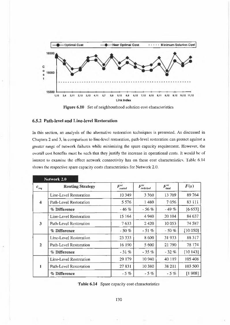
Optimal Cost — ♦ — Near Optimal Cost Minimum Solution Cost

Link Index

Figure 6.10 S et o f n eighbourhood so lu tion c o s t characteristics

6.5.2 Path-level and Line-level Restoration

In this section , an an a lysis o f the alternative restoration tech n iq u es is presented. A s d iscu ssed in

Chapters 2 and 3, in com p arison to lin e -le v e l restoration, p a th -leve l restoration can protect again st a

greater range o f n etw ork fa ilu res w h ile m in im isin g the spare cap acity requirem ent. H ow ever, the

overall cost b en efits m ust b e su ch that they ju stify the in crease in operational costs. It w ou ld be o f

interest to exam in e the e ffec t n etw ork con n ectiv ity has on th ese cost characteristics. T ab le 6 .1 4

sh ow s the resp ective spare cap acity co sts characteristics for N etw o rk 2 .0 .

N etw o rk 2 .0

Creq Routing Strategy p s crouted

p s cswitched

p s ctotal F ( s )

4

L in e-L eve l R estoration 10 3 4 9 3 3 6 0 13 7 0 9 89 7 6 4

P ath -L evel R estoration 5 5 7 6 1 4 8 0 7 0 5 6 83 111

% Difference - 4 6 % - 5 6 % - 4 9 % [6 6 5 3 ]

3

L in e-L eve l R estoration 15 164 4 9 4 0 2 0 104 84 637

P ath -L evel R estoration 7 633 2 4 2 0 10 053 7 4 5 8 7

% Difference - 5 0 % - 5 1 % - 5 0 % [1 0 0 5 0 ]

2L in e-L ev e l R estoration 23 333 8 6 0 0 31 933 88 317

P ath -L evel R estoration 16 190 5 6 0 0 21 7 9 0 78 174

% Difference - 3 1 % - 3 5 % - 3 2 % [10 143]

1L in e-L eve l R estoration 2 9 179 10 9 4 0 4 0 119 105 4 0 8

P ath -L evel R estoration 2 7 831 10 3 8 0 38 211 103 5 0 0

% Difference - 5 % - 5 % - 5 % [1 908]

Table 6.14 Spare cap acity c o s t characteristics

130

It can be seen that the p ercen tage d ifferen ce b etw een the spare cap acity cost characteristics is a

d ecreasing function o f network con n ectiv ity , w h ile the overall cost b en efits tend to increase to som e

d egree. T h is is due to the increase in the corresp ond ing le v e ls o f redundancy (see S ection 6 .2 .3 ) . It

is, how ever, noted that as netw ork con n ectiv ity tends toward on e, the relative co st b en efits b ecom e

n eg lig ib le . A correlation b etw een the cost b en efits , netw ork co n n ectiv ity , and the corresp ond ing

le v e ls o f redundancy can therefore be m ade. In term s o f the v iab ility o f p ath -level restoration, as

research and d evelop m en t in th is area is on go in g , it is o u ts id e (he scop e o f th is w ork to p rovide a

d efin itive cost an a lysis, b eyon d q uantifying the potential ga in s.

131

Chapter 7 - Conclusions

7.1 Overall Discussion of Results

7.1.1 Solution Characteristics

B ased on the co st m odel d efin ed for th is prob lem , it w as sh ow n that the so lu tion c o s t for any g iven

netw ork configuration cou ld be represented by a lin k -d ep en dent f ix e d c o s t com p on en t and a

variable cap acity-depend en t-cost com p onent. It w as a lso show n h ow th ese c o s t com p onents w ere

con verse fun ction s o f netw ork con n ectiv ity (th e num ber o f lin k s in the n etw ork so lu tion ). That is , as

netw ork co n n ectiv ity decreased , the fix ed co sts d ecreased , w h ile the variable cap acity dependent

costs increased . C onsequ en tly , the co n n ectiv ity characteristic o f the optim al so lu tion d epended on

the relative contribution (i.e . s ig n ifica n ce) o f th ese co st com p on en ts. T h e correlation b etw een these

so lu tion characteristics form ed the b asis for th e h igh ly d etailed an a lysis p resen ted in S ection 6 .2 . In

particular, it w as sh ow n h ow variations in the input constraints im pacted on th ese characteristics,

and h ow th ese in turn had a residual e ffec t on the optim al so lu tion ch aracteristics. T h e fo llo w in g is

a sum m ary o f the m ain observations:

• Inter-nodal demand sensitivity: G iven the optim al so lu tion for any input netw ork, i f the inter-

nodal dem ands for that netw ork are in creased , then, due to the relative in crease in the capacity

dependent co sts that result, the co n n ectiv ity characteristic o f the op tim al so lu tion w ill a lso

increase. In other w ords, w h ile the optim al paths rem ain u nchanged , d ue to the increase in the

dem ands b ein g routed over these paths, b oth the w ork ing capacity sw itch ed and routed costs w ill

increase. In addition , s in ce the average w ork in g cap acity b e in g routed o v er each p otentia l link

fa ilu re has in creased , the spare cap acity sw itch ed and routed costs w ill a lso increase. A s a result,

the cost b en efits o f inserting a link, in term s o f redu cing the variable cap acity d ependent costs,

w ill be greater than the additional f ix e d c o s t o f in sta llin g that link. O b v io u sly , the d egree by

w hich the co n n ectiv ity characteristic in creases depends on the relative in crease in dem ands. In

addition, s in ce the dem ands im pact on the variable cap acity dep en dent co sts , an in crease in this

input constraint a lso m od els the im pact o f in creases in the fibre and term inal costs, or,

alternatively , d ecreases in the fix ed costs.

• Inter-nodal fixed cost sensitivity: G iven th e optim al so lu tion for any input netw ork, i f the inter-

nodal fix ed co s ts for that netw ork are in creased , then, due to the relative in crease in the overall

f ix ed co st com p onent, the con n ectiv ity ch aracteristic o f the optim al so lu tion w ill d ecrease. That

132

is , the co st b en efits o f rem ovin g a link , in term s o f redu cing the f ix ed c o s t com p on en t, w ill b e

greater than the additional costs attributed to rerouting the original link d em and s. A s b efore , the

d egree by w h ich the con n ectiv ity characteristic d ecreases w ill d epend on the relative increase in

this input constraint. In addition, u sin g the sam e reason in g as ab ove, an in crease in this input

constraint a lso m od els the im pact o f d ecreases in the fibre and term inal c o s ts , or, alternatively ,

d ecreases in the dem and requirem ents that contribute to th ese costs.

• Network infrastructure sensitivity: M ain ta in in g the sam e param eter settin gs for the inter-nodal

dem and requirem ents and fix ed co sts , i f th e num ber o f input n od es and dom ain area are

increased, then, due to the relative in crease in the cap acity dep en dent co sts , the con n ectiv ity

characteristic o f the optim al so lu tion a lso in creases. T h is is attributed to th e e ffe c t an increase in

the num ber o f n od es has on the routing ch aracteristics. B a s ica lly , as the num ber o f nodes

increases, the num ber o f the inter-nodal paths and the average h op -cou n t per path increase

proportionally . C on seq u en tly , both the w ork in g and spare cap acity sw itch ed and routed costs

w ill in crease. W h ile it is noted that the average link d istan ces a lso in crease, their relative im pact

on the fix ed co st com p on en t is not as s ign ifican t. H en ce , the overall resu lt is an in crease in the

con n ectiv ity characteristic. A s before, the d egree by w h ich this characteristic in creases depends

on the relative in crease in the input constrain ts under con sid eration .

D ue to the variance in th ese input constrain ts, it w as sh ow n that the co n n ectiv ity characteristics o f

the optim al w ork in g cap acity assignm en t so lu tio n s varied b etw een 1.0 and 3 .0 . That is, as the

relative s ig n ifica n ce o f the fix ed co st com p on en t in creased , the co n n ectiv ity characteristic o f the

so lu tion tended tow ard the lo w er bound, w h ile the in verse w as true o f the cap acity d ep en dent cost

com ponent. In the ca se o f the optim al netw ork so lu tio n s, s in ce the spare cap acity a ssign m en t costs

w ere a lso con sid ered , the relative s ig n ifica n ce o f the cap acity dependent co s t com p on en t increased.

C onsequ en tly , the resp ective con n ectiv ity characteristics in creased p rop ortionally , i.e . they varied

betw een 2 .5 and 4 .5 . A s d iscu ssed , it w as th is con d ition , i.e . the fact that the optim al w ork ing

cap acity assign m en t so lu tion tended tow ard a lo w er bound in com p arison to the optim al netw ork

so lu tion , that en ab led the in itia l op tim isation p ro cess to generate the set o f benchm ark to p o lo g ies

and evaluate the corresp ond ing reference so lu tion co sts (se e S ection 7 .1 .4 .1 ).

In term s o f the optim al netw ork con figu ration s, the to p o lo g ica l representation o f th ese so lu tion s can

b e ded uced from th e corresp ond ing co n n ec tiv ity ch aracteristics, i.e . th e so lu tio n s ranged from

hybrid netw orks o f in terconn ected ring to p o lo g ie s to h igh ly m esh ed netw ork to p o lo g ie s . H ow ever,

as the d esign too l a lso provided a v isu a l representation o f th ese to p o lo g ies , it w as s ig n ifica n t to note

that, irrespective o f the num ber o f lin k s in th ese optim al so lu tion s, their arrangem ent w ith in the

resp ective to p o lo g ie s w as h igh ly balanced . A s d iscu ssed , th is form ed the b asis for the h igh ly

133

effec tiv e se lec tio n criterion u sed in the in teractive procedure o f the refinem ent p h ase (see S ection

7 .1 .4 .2 ).

F inally , con sid erations con cern in g the practical realisation and eco n o m ic v iab ility o f the various

survivable to p o lo g ies are sum m arised:

• DXC-based mesh topologies: W h ile the resu lts sh ow that D X C -b ased m esh to p o lo g ie s b eco m e

m ore eco n o m ica lly v iab le as the relative s ig n if ica n ce o f the cap acity dep en dent co st com p on en t

increases, it is n oted that som e con sid eration sh ou ld be g iven to the practical rea lisa tion o f th ese

so lu tions. T h is con cern s the relative in crease in m anagem ent co s ts and restoration tim es. For

exam p le, in term s o f restoration tim es, as the netw ork s iz e in creases, it m ay not b e p o ss ib le for

the current restoration sch em es to m eet the 2 -s serv ice ob jectiv e for all s in g le lin k fa ilu res (see

A pp en dix A .2 ). M oreover, due to the m ore sop h istica ted m anagem ent sy stem s required, an

additional nodal co st com p on en t sh ou ld b e im p osed on all D X C s w ith in an optim al so lu tion .

T his cou ld be m od elled b y a fix ed , d istan ce in dependent, lin k co st com p on en t w hich w ou ld

effec tiv e ly reduce the num ber o f sw itch ed term ination p o in ts across the netw ork, i.e . d ecrease

the con n ectiv ity characteristic o f the optim al so lu tion . A lth ou gh this cost characteristic w as not

analysed in the resu lts , its e ffec t can b e correlated w ith the e ffe c t in creases in the inter-nodal

f ix ed costs h ave on the optim al solu tion .

• TM-based point-to-point topologies: It w as in teresting to n ote that T M -b ased point-to-point

su rvivab le to p o lo g ie s did n ot feature in any o f the optim al so lu tion s found. T h is w a s attributed to

the fact that, in order to protect again st lin k cuts, T M -b ased p oin t-to -p o in t to p o lo g ie s m ust be

protected b y routing d ed icated spare cap acity over d iversely in sta lled lin k s. A s a resu lt, both the

fix ed co st and cap acity d ependent c o s t com p on en ts w ere such that A D M ring to p o lo g ie s proved

m ore eco n o m ica lly v iab le.

• Path-level restoration: In p ath -level restoration , s in ce fa iled cap acity is rerouted b etw een the

term inating n od es o f the orig inating path, it w as sh ow n that the spare capacity requirem ent can

be reduced con sid erab ly . M oreover, th is restoration sch em e a lso p rovid es p rotection against

nodal fa ilu res. H ow ever , con sid eration sh ou ld be g iven to the additional m anagem ent co sts and

in crease in restoration tim es attributed to th is re la tively m ore co m p lex restoration sch em e. A s

d iscu ssed , w h ile current netw ork m anagem ent sy stem s and assoc ia ted eq u ipm en t co sts m ay not

ju stify near-term d ep loym ent, it is ex p ec ted that en h ancem en ts in the form er and reductions in

the latter w ill m ake this restoration sch em e a v iab le alternative for future S D H n etw orks.

134

7.1.2 Optimal Routing Strategies

It w as show n that, in com p arison to the standard shortest-path routing strategy, the im p osition o f the

m inim um -hop routing constraint resu lted in the m in im isation o f the total cap acity sw itch ed and

routed costs. In particular, it w as sh ow n that, by im p osin g this constraint, the average num ber o f

paths b ein g routed across the n etw ork w as m in im ised and the d istribution characteristic o f w ork in g

capacity assignm ents b ecam e m ore balanced . A s a resu lt, the overall spare cap acity requirem ent w as

a lso m inim ised . A s d iscu ssed , the overall co st b en efits w ere d ep en dent on the contribution o f the

capacity dependent co st com p on en ts and the relative co n n ectiv ity ch aracteristics o f the optim al

netw ork so lu tions under consideration .

In terms o f the im plem entation o f the a lgorithm ic procedure, it w as sh ow n that a separate routing

p rocess, having a p o lyn om ia l tim e co m p lex ity o f order 0 (n 2), w as u sed to find the optim al path

from any node in the netw ork to a ll other n od es. A s th is w as applied to all n n od es in the netw ork,

the overall tim e co m p lex ity w as o f order 0 ( n 3). T h is is com parable to the m ost e ff ic ien t a lgorithm s

u sed for so lv in g this problem . In addition , due to the iterative rou tine u sed , the ex iste n c e o f an

u nconn ected n etw ork so lu tion can be determ ined during the first iteration. T h is represents an

im provem ent in perform ance o v er ex istin g algorithm s.

7.1.3 Optimal Spare Capacity Assignment Algorithm

T o com pare and d erive an optim al netw ork so lu tion , the overall op tim isation p rocess m ust at least

be capable o f generating the optim al spare cap acity assignm en t so lu tion for any fea s ib le netw ork

configuration con sid ered . A s d iscu ssed , due to the co m p lex ity o f th is problem , e ffic ien t and/or

e ffec tiv e techn iques w ere lack in g in th is area. T h is resu lted in the d evelop m en t and im plem entation

o f an in novative and h igh ly e ff ic ien t so lu tion m ethod. It w as sh ow n that, in its b asic form , this

so lu tion m ethod w as cap ab le o f fin d in g fea sib le near-optim al co st so lu tion s that w ere proportional

representations o f th e optim al co st so lu tion s. It w as th is p rocess, w h ich represents a p o lyn om ia l

tim e com p lex ity o f order 0 (n 2).lnum, that w as u sed in the overa ll op tim isation procedure.

A n additional so lu tion step w as a lso d ev elo p ed to eva lu ate the optim al co st so lu tion . B a sed on an

adaptive m in im isation techn iqu e, it w as cap ab le o f m in im is in g the cap acity sw itch ed and routed

costs. H ow ever, as th is incurred a re la tively large com p utational overhead, it w as on ly incorporated

as a stand-alone p rocess.

F in ally , it is noted that both the stand -alone and b asic spare cap acity assignm en t p ro cesses w ere

a lso capable o f fin d in g optim al and near-optim al c o s t so lu tion s b ased on p ath -level restoration.

135

7.1.4 Overall Optimisation Procedure

W h ile som e w ork in the area o f S D H netw ork optim isation has con sid ered the im pact o f netw ork

reliab ility and the evaluation o f spare cap acity assignm en t co sts for a s in g le in stan ce o f an optim al

w ork in g cap acity assignm ent so lu tion , n on e has con sid ered the su rv ivab ility constraint ex p lic itly as

part o f the overall op tim isation p rocess. A s such , in regard to eva lu a tin g the w ork presented in th is

th esis, there w as no real b asis for com p arison . H ow ever, it is n otew orth y that, irrespective o f th is,

con sid erab le effort w as m ade to refin e the overa ll op tim isation p rocedu re w ith particular em p hasis

p laced on e ff ic ien cy and effec tiv e n e ss .

7.1.4.1 Initial optimisation phase

A s the resu lts ver ify , th is p hase o f the op tim isation procedure p roved h igh ly e ffe c tiv e in redu cing

the in itia l co m p lex ity o f the problem . E ssen tia lly , in term s o f the so lu tio n sp ace , it w as u sed to find

the approxim ate location o f the g lo b a l op tim al so lu tion , i.e . to narrow the search o f the so lu tion

sp ace to the region around the g lob a l op tim al so lu tion . T h e resu ltin g so lu tion w as then u sed as the

input to the m ore com p utationally in ten s iv e refin em en t phase.

For the in itial optim isation p rocess, the m ain em p hasis w as p la ced on e ff ic ie n c y . B ased on a

m od ified A ccelerated G reedy algorithm , the p rocess took advantage o f the fact that the optim al

w orking cap acity assignm en t so lu tion ten ded tow ard a low er bound in com p arison to the optim al

n etw ork so lu tion , to generate the set o f k ey benchm ark to p o lo g ie s and eva lu ate the corresponding

reference so lu tion costs . T he m in im u m referen ce co st so lu tion w a s then u sed as the input to the

refinem ent phase. In terms o f the com p utational tim e requirem ent, s in ce the w orking cap acity

assignm en t co sts w ere on ly con sid ered for each iteration o f the p ro cess , and sin ce the m on oton icity

property h eld , it w as sh ow n that the average run tim es w ere n e g lig ib le in com parison to the run

tim es o f the overall optim isation procedures.

7.1.4.2 Refinement phase

H avin g found the m inim um referen ce so lu tion , the ob jective o f th e refin em en t p hase w as to gu id e

the op tim isation p rocess tow ard the g lo b a l op tim al so lu tion . A s d iscu sse d , d ue to the im p osition o f

the spare capacity assignm en t p rob lem and the so lu tion co st ch aracteristics that resu lt, it w as foun d

that the so lu tion sp ace con sisted o f a large num ber o f w ell-d istrib u ted sub-optim al so lu tion states.

M oreover, it w as sh ow n that the com p u tation a l tim e co m p lex ity o f th is p hase w as h igh ly dependent

on the num ber o f input n odes and the co n n ectiv ity characteristic o f the optim al so lu tion . A s such , in

term s o f its e ff ic ien cy and e ffe c tiv e n e ss , the refinem ent procedure had to b e adapted to the input

n etw ork under con sid eration . T h is related to the lin k se lec tio n criteria u sed in the interactive

136

procedure, the ch o ic e o f p rocess constrain ts se lec ted for each refinem ent step , and the num ber o f

refinem ent steps required. T h e ob jectiv e w as to m in im ise the latter con stra in ts, w h ile m axim isin g

the e ffec tiv e n e ss o f the p rocess through the in teractive procedure.

D u e to the e ffec tiv e n e ss o f the in teractive procedure, the first step con cern ed the b asic refinem ent o f

the m inim um referen ce so lu tion . It in v o lv ed fin d in g a loca l optim al so lu tion c lo ser to the g lobal

optim al so lu tion . T h is was ach ieved b y settin g the p rocess constraints, i.e . the Tabu lis t s iz e and the

num ber o f n on -im proving m oves, to zero. A s a result, the com p utational tim e requirem ent for th is

refinem ent step w as kept to a m inim um .

W ith the in itia l loca l optim al so lu tion foun d , the in teractive refinem ent p rocedu re w as then applied .

It w as sh ow n that, d ep en din g on the input netw ork under con sid eration , th is procedure con sisted o f

on e or m ore in teractive refinem ent step s w ith variations in the in teractive procedure and ch o ic e o f

p rocess constraints appropriate to that netw ork. T h e fo llo w in g is a sum m ary o f th ese results:

• Interactive procedure: It w as sh ow n that the criteria used to se le c t w h ich links to ed it w as

relatively con sisten t for all n etw orks, and w as based on the b alanced n etw ork con dition . For the

in itia l in teractive step , the o b jectiv e w as to d etect and rem ove sub-optim al lin k structures. For

each su bsequ en t step, the ob jectiv e w as to p rovide the perturbation m echan ism . A s d iscu ssed ,

the m ost e ffe c tiv e techn ique in v o lv ed in creasin g the con n ectiv ity b etw een lo c a lly adjacent nodes

w h ile m aintain ing the b alanced n etw ork con d ition . E ssen tia lly , this en ab led the p rocess to search

a w id er range o f the so lu tion sp ace c lo s e to the g lob a l optim a, w h ile red u cin g the com putational

tim e requirem ent considerably . T h is tech n iq u e actually h igh ligh ts the m ain lim itation o f random -

based perturbation techn iqu es. T hat is, s in ce links are se lec ted at random , their e ffec tiv e n e ss in

acceleratin g the p rocess can n ot b e guaranteed . H en ce, a greater num ber o f iterations per p rocess

and p rocess runs w ould b e required. T h is ap p lies eq u ally to any so lu tio n m ethod b ased on a

random se lec tio n m eth od o logy , e .g . S im u lated A n n ea lin g and G en etic algorithm s.

• Process constraints: D u e to the e ffe c tiv e n e ss o f the in teractive procedure it w as found that the

p rocess constraints cou ld b e kept to a m in im u m .

• Number o f interactive refinement steps and computational time requirem ent: T h e num ber o f

in teractive refinem ent step s w as h igh ly d ependent on the num ber o f input n odes and the

con n ectiv ity characteristic o f the optim al so lu tion . That is, as th ese netw ork characteristics

in creased , the num ber o f lo ca l op tim a b ased around the optim al so lu tion in creased sign ifican tly .

A s a resu lt, a greater num ber o f in teractive refinem ent step s w ere required to guarantee that the

b est co st so lu tion w as found. It w as a lso sh o w n h o w increases in th ese netw ork characteristics

im pacted on the num ber o f iterations p er p ro cess and the average run tim e per iteration, i.e . both

137

in creased sign ifican tly . C on seq u en tly , the overall com p utational tim e requirem ents for the

resp ective in teractive refinem ent procedures varied quite dram atically , i.e . from on e m inute for a

sparsely con n ected 12-nod e netw ork to approxim ately tw o hours for a h ig h ly m esh ed 2 4 -n o d e

netw ork.

7.1.5 NetOpt and the Optimal Design Procedure

A s d efin ed , the d esign too l N etO pt w as d evelop ed to facilita te the overall optim al d esign procedure,

i.e . to support the key fun ction al requirem ents o f this procedure. B a sed on this, the fo llo w in g is a

sum m ary o f the m ain features and u tilities supported by the too l.

• Basic Features-. N etO p t is an event-driven G U I application w ith fu ll m ou se support.

• Active Design Field: A scro llab le w in d ow w hich en ab les the u ser to in itia lise , v ie w , and ed it a

to p o lo g ica l representation o f an active netw ork at varied reso lu tion s.

• Dialog Boxes: U sed ex te n siv e ly , they can contain control fu n ction a lity , such as option buttons,

in form ation ed itin g fie ld s, and scro ll bars. T h ey are a lso u sed to d isp lay u ser prom pts and error

m essages.

• Menu and Tool Bar: P rovide a ccess to an ex te n siv e range o f N etO p t com m and s and assoc ia ted

u tilities w hich are grouped accord in g to the fu n ction a l area they support, i.e . F ile , Edit, V ie w ,

and O ptim isation .

• Status Bar: D isp la y s inform ation relatin g to the active netw ork and ap p lication p rocesses.

• User Interaction: T he u ser can interact w ith the current n etw ork so lu tion by c lick in g on any o f

the a ctiv e netw ork e lem en ts d isp layed , i.e . n od es and links. W h en click ed , the n etw ork e lem en t

is h igh ligh ted and a lis t o f relevant com m an d op tion s is presented in the form o f a pop-up m enu.

In co n clu sio n , th is w ork has sh ow n that C A D -b ased to o ls , su ch as N etO pt, are essen tia l for

generating and an a lysin g c o s t-e ffec tiv e su rvivab le S D H netw orks. It is a lso n otew orthy that, w h ile

the prim ary ob jectiv e o f this prototype d esig n too l w as to fac ilita te the optim al d esign procedure, it

a lso p rovid ed the fram ew ork (i.e . en vironm en t) and im petus n eed ed to d evelop , eva lu ate, and refine

every asp ect o f th is procedure.

138

7.2 Recommendations and Scope for Future Work

7.2.1 Further Validation of Results

A s defined , the infrastructure and the inter-nodal dem and requirem ent settin gs for the b ase test ca se

netw orks w ere typical representations o f sm all to m ed iu m -sized m etropolitan area netw orks. It w as

also stated that the cost com p on en t settin gs, in c lu d in g th ose d efin ed for the inter-nodal f ix ed co sts ,

represented a correlation o f rea listic cost va lu es. H ow ever, it w as foun d that variances in th e input

constraints and, in particular, the co st com p on en ts d id ex ist. W h ile the netw ork an alysis attem pted

to m odel th ese variances, it is recom m en ded that further va lid ation o f resu lts sh ould b e b ased on

real input data and cost com p on en t va lu es. H ow ever, as w as foun d during the cou rse o f th is w ork,

due to the com p etitive nature o f the te lecom m u n ication s industry, it is d ifficu lt to obtain , let a lon e

publish , su ch con fid en tia l in form ation .

7.2.2 Further Development of the Optimal Design Procedure

It w as sh ow n that the overall com p utational tim e requirem ent for the op tim isation procedure w as

m ainly attributed to the refin em en t phase, i.e . the tim e requirem ent o f the in itia l op tim isation p hase

w as n eg lig ib le in com parison . It w as a lso sh ow n that this tim e requirem ent increased d ram atically

as the num ber o f input n od es and co n n ectiv ity characteristic o f the optim al so lu tion in creased .

G iven this dram atic in crease, as n etw ork s iz e in creases, the op tim isation prob lem soon b eco m es

intractable. A s such , further d evelop m en t o f the d esign procedure sh ou ld take into con sid eration

techn iques that cou ld b e u sed to m ake the p rob lem m ore m anageable .

T he m ost e ffe c tiv e o f th ese techn iqu es, and on e w h ich is a c tiv e ly em p lo y ed for so lv in g large-sca le

netw ork d esign prob lem s, is b ased on the co n cep t o f fa c ility hubbing and nodal h ierarchies [17].

S im ilar to the co n cep t o f the a cc ess , reg ion al, and core n etw ork ex ch a n g e h ierarchies d escrib ed in

S ection 2 .4 , the id ea is to in troduce further p artition ing (or layerin g) o f th ese netw ork h ierarchies by

grouping n odes accord ing to so m e p red efin ed criteria, e .g . geograp h ica l location , com m u n ity o f

interest, or traffic load s. T h e prob lem w ith this techn iqu e is that the n odal h ierarchies (i.e . sub­

netw ork infrastructures) and their resp ective inter-nodal dem ands m ust b e estim ated in the pre­

p lanning p hase o f the d esign p rob lem and therefore g iv en as input data. C on seq u en tly , w h ile the

d esign procedure can b e ap plied to each sub-netw ork to fin d the optim al so lu tion , as th ese are

p rocessed in depend en tly o f each other, they m ay actually represent sub-optim al structures w ith in

the overall n etw ork infrastructure. H ow ever, as w as the ca se w ith th e b asic d esign procedure, d u e to

the reduction in the com p utational tim e requirem ent, th is m ore m odular procedure co u ld b e ap p lied

a num ber o f tim es and therefore u sed to refine the input constrain ts and the optim al so lu tion states.

139

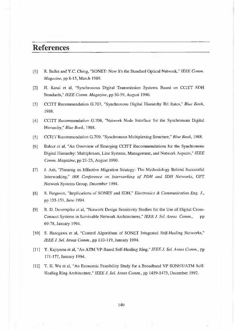
References

[1] R. B a llet and Y .C . C hing, "SO NET: N o w It's the Standard O p tica l N etw ork," IEEE Comm.

Magazine, pp 8 -1 5 , M arch 1989.

[2] H. K asai et al, "Synchronous D ig ita l T ransm ission S y stem s B ased on C C ITT S D H

Standards," IEEE Comm. Magazine, pp 5 0 -5 9 , A u gu st 1990.

[3] C C ITT R ecom m en dation G .7 0 7 , "Synchronous D ig ita l H ierarchy B it Rates," Blue Book,

1988.

[4] C C ITT R ecom m en dation G .7 0 8 , "N etw ork N o d e Interface for the S ynchronous D ig ita l

Hierarchy," Blue Book, 1988.

[5] C C ITT R ecom m en d ation G .7 0 9 , "Synchronous M u ltip lex in g Structure," Blue Book, 1988.

[6] B a lcer et al, "An O v erv iew o f E m erg in g C C ITT R ecom m en d ation s for the S ynchronou s

D ig ita l Hierarchy: M u ltip lexers, L in e S ystem s, M an agem ent, and N etw ork A spects," IEEE

Comm. Magazine, pp 2 1 -2 5 , A u g u st 1990.

[7] J. A sh , "Planning an E ffe c tiv e M igration Strategy: T h e M eth o d o lo g y B eh ind S u ccessfu l

Interworking," IRR Conference on Interworking o f PDH and SDH Networks, G PT

N etw ork S ystem s G roup, D ecem b er 1994.

[8] S . Ferguson, "Im plications o f S O N E T and SD H ," Electronics & Communication Eng. J.,

pp 133-151 , June 1994.

[9] R. D . D oversp ik e et al, "N etw ork D esig n S en sitiv ity S tu d ies for the U se o f D ig ita l C ross­

C onnect S ystem s in S u rv ivab le N etw ork A rchitectures," IEEE J. Sei. Areas Comm., pp

69 -7 8 , January 1994.

[10] S. H asegaw a et al, "Control A lgorith m s o f S O N E T Integrated S e lf-H ea lin g N etw orks,"

IEEE J. Sei. Areas Comm., pp 1 1 0 -1 1 9 , January 1994.

[11] Y . K ajiyam a et al, "An A T M V P -B a sed S e lf-H ea lin g R ing," IEEE J. Sei. Areas Comm., pp

171-177 , January 1994.

[12] T. H. W u et al, "An E co n o m ic F ea sib ility Study for a B roadband V P S O N E T /A T M S e lf-

H ealin g R in g A rchitecture," IEEE J. Sei. Areas Comm., pp 1 4 5 9 -1 4 7 3 , D ecem b er 1992.

140

[13] T . H . W u and M . E. B u rrow es, "Feasib ility Study o f a H ig h -S p eed S O N E T S e lf-H ea lin g

R in g A rchitecture in Future In teroffice N etw orks," IEEE Comm. Magazine, pp 3 3 -5 1 ,

N ovem b er 1990.

[14] J. S osn osk y , "Service A p p lica tion s for S O N E T D C S D istrib u ted R estoration," IEEE J. Sei.

Areas Comm., pp 5 9 -6 8 , January 1994.

[15] T. H. W u et al, "The Im pact o f S O N E T D ig ita l C ross-C on n ect S y stem A rchitecture on

D istributed R estoration," IEEE J. S e i Areas Comm., pp 7 9 -8 7 , January 1994.

[16] T. H. W u et al, "SO N ET Im plem entation," IEEE Comm. M agazine, pp 3 4 -4 0 , Septem ber

1993.

[17] T. H . W u et al, "Survivable S O N E T N etw ork s - D esign M eth od o logy ," IEEE J. Sei. Areas

Comm., pp 2 0 5 -2 1 2 , January 1994.

[18] I. H aw ker and C .P. B otham , "D istributed C ontrol in S D H Transport N etw orks," B T

L aboratories, 1994.

[19] R. H olter, "M anaging S O N E T Equipm ent," IEEE Networks M agazine, pp 36 -4 1 , January

1992.

[20] S. A llm is , "Im plem enting a F le x ib le Synchronou s N etw ork," IEEE Comm. Magazine, pp

5 2 -5 5 , Septem ber 1993.

[21] U . M azzei et al, "E volution o f the Italian T eleco m m u n ica tio n s N etw ork T ow ards SDH ,"

IEEE Comm. M agazine, pp 4 4 -4 9 , A u gu st 1990.

[22] N .B . Sandesara et al, "Plans and C onsideration s for S O N E T D ep loym en t," IEEE Comm.

Magazine, pp 26 -3 3 , A u gu st 1990.

[23] M . S h afi and B . M ortim er, "The E vo lu tion o f SDH : A V ie w from T e le c o m N ew Zealand,"

IEEE Comm. Magazine, pp 6 0 -6 6 , A ugu st 1990.

[24] B . G. L ee et al, "Synchronous D ig ita l T ransm ission," Broadband Telecommunications

Technology, Chapter 3, pp 1 0 5 -2 3 2 , A rtech H ou se Inc., 1993 .

[25] T. J. A prille , "Introducing S O N E T into the L ocal E x ch a n g e Carrier N etw ork," IEEE

Comm. Magazine, pp 3 4 -4 3 , A u gu st 1990.

[26] R. G. G areiss and P. H . H e y w o o d , "SO N E T /SD H : T om orrow 's N etw ork s Today," Data

Comm. - on the Web, S ep tem b er 1993.

[27] J. M cG ib n ey , "M odem G lob a l O p tim isation H euristics in the lo n g term P lanning o f

networks", M.Eng. Thesis, D ub lin C ity U n iversity , June 1995.

141

[28] T. H. W u et al, "C om puter-A ided D esig n Procedures for S urvivab le F ibre N etw orks,"

IEEE J. Sel. Areas Comm., pp 1 1 8 8 -1 1 9 7 , O ctober 1989.

[29] M . M in ou x , "N etw ork S yn th esis and O ptim um N etw ork D es ig n Problem s: M od els ,

S olu tion M ethod s and A pplications," Networks, V o l. 19, pp 3 1 3 -3 6 0 , 1989.

[30] J. R. E vans and E. M inieka, Optimization Algorithms fo r Networks and Graphs, Chapters

1-6, D ekker, 1992.

[31] G. A . G rover et al, "M EN TO R :A n A lgorith m for M esh N etw ork T o p o lo g ic a l O ptim ization

and R outing," IEEE Trans, on Comm., V o l. 39 , pp 5 0 3 -5 1 3 , A pril 1991.

[32] A . Gersht and R. W eihm ayer, "Joint O ptim ization o f D ata N etw ork D esig n and F acility

S election ," IEEE J. Sel. Areas Comm., pp 1 6 6 7 -1 6 8 1 , D ecem b er 1990.

[33] M . K em er et al, "An A n a ly s is o f A lternative A rch itectures for the In teroffice N etw ork,"

IEEE J. Sel. Areas Comm., pp 1 4 0 4 -1 4 1 3 , D ecem b er 1986.

[34] M . G erla et al, "On the T o p o lo g ica l D esig n o f D istrib u ted C om puter N etw orks," IEEE

Trans, on Comm., pp 4 8 -6 0 , January 1977.

[35] B . G avish et al, "Fiberoptic C ircuit N etw ork D esig n U nd er R eliab ility C onstraints," IEEE

J. Sel. Areas Comm., pp 1 1 8 1 -1 1 8 7 , O ctober 1989.

[36] D . B ertsekas and R. G allager, "Routing in D ata N etw orks," Data Networks, C hapter 5, pp

3 6 3 -4 7 9 , P rentice-H all, 1992.

[37] T .H . C orm en et al, Introduction to Algorithms, Chapters 17, 2 5 , and 2 7 , M cG raw -H ill,

1990.

[38] A . V . G old b erg and R. E . Tarjan, "A N e w A pp roach to the M ax im u m -F low Problem ," J.

fo r Computing Machinery, V o l. 3 5 , pp 9 2 1 -9 4 0 , O ctob er 1988.

[39] M . S. Bazaraa et al, Linear Programming and Network Flows, Chapters 1-3, 8 -9 , and 12,

W iley , 1990.

[40] M . M inou x, "A ccelerated G reedy A lgorith m s for M a x im iz in g Subm odular S et Functions,"

Proc. IFIP, pp 2 3 4 -2 4 3 , 1977.

[41] J.F. M ondou et al, "Shortest Path A lgorithm s: A C om putational Study w ith the C

P rogram m ing L anguage," Computer Ops. Res., V o l. 18, pp 7 6 7 -7 8 6 , 1991.

142

Appendix A1 - DXC-based Restoration Control

D X C -b ased se lf-h ea lin g is d efin ed as a d istributed restoration sch em e w h o se control is in itiated and

execu ted lo ca lly at each D X C in an au ton om ou s distributed fash ion . An alternative restoration

techn ique u sing centralised control cou ld a lso b e em p loyed . B oth tech n iq u es d efin e the m ech an ism

u sed in reconfiguring the D X C s in order to reroute fa iled cap acity . In th e ca se o f centra lised control,

as dep icted in F igure A l . l (a), D X C reconfiguration is perform ed at a centra lised con troller (or

O perating S ystem ), w ith a large database con ta in in g all the relevant netw ork inform ation . In this

sch em e, w hen a failure is d etected , a fau lt n o tifica tion m essa g e is sen t from each o f the a ffected

D X C s to the centralised controller. T h e O S then p ro cesses th ese m essa g es, extrapolates the fault

location , com p utes an optim al routing table and then d ow n load s reconfiguration requests to the

relevant D X C s. W h ile th is sch em e m ay op tim ally reroute the fa iled cap acity , the overall process

m ay take upw ards o f 10 m and cau se u n accep tab le degradation o f serv ices for m ost custom ers

affected by the fa ilu re1 [9, 10, 14, 15, 18]. In fact, as the s iz e and co m p lex ity o f these netw orks

increase, centralised control b eco m es even le ss attractive, incurring greater resp on se tim es w h ich in

turn reduce the overall re silien ce o f the netw ork.

M essag ePassing

M essag ePassing

(a) C entralised (b) D istributed

F ig u r e A l . l D X C -b a sed restoration control

h o w e v er , this is still much faster than manual DXC reconfiguration (as is the case in PDH-based cross connects in the event o f a failure) which may disrupt services for hours or more [14],

A s m ost serv ices are im pacted by a serv ice ou tage greater than 2 s, as d iscu ssed in [14 , 15], the

ob jective w ould be to reduce the restoration tim e d ow n to th is perm itted le v e l. T h is w as the m ain

m otivation for con sid er in g alternative D X C recon figuration sch em es such as th o se b ased on

distributed control. T h e v iab ility o f u sin g D X C -b ased m esh to p o lo g ie s w ith d istributed control (to

m eet the 2-s serv ice restoration o b jectiv e) has b een ex te n s iv e ly stud ied [15 , 18, 19]. It has been

sh ow n that this alternative approach exh ib its m uch faster restorational tim es and a h igh er d egree o f

flex ib ility com pared to the centralised control techn iqu e.

D istributed control, as d ep icted in F igure A l . l (b ), in v o lv es the exch an ge o f m essa g es b etw een

adjacent D X C s in resp on se to a netw ork req u est/even t such as a link fa ilu re. T h is con cep t o f

requ est/even t m essage p assin g can be applied to other form s o f m anagem ent p rocessin g , such as

dynam ic netw ork reconfiguration (D N R ) in resp on se to s ign ifican t ch an ges in traffic patterns across

the netw ork [18]. W ith distributed control, the in te llig en ce resid es lo c a lly at each D X C . A s such ,

the D X C controllers act lik e parallel p rocessors com p u tin g alternative routes d yn am ica lly in real­

tim e. Each D X C is a lso cap ab le o f storing loca l in form ation such as the w ork in g and spare capacity

assignm en ts assoc ia ted w ith each o f its term inating links. E m b ed ded in each con tro ller is a set o f

rules/a lgorithm s that interprets alarm s or m essa g e s rece iv ed from its adjacent n od es. In other w ords,

there is no n eed for a large netw ork database or control softw are as the netw ork acts as its ow n

database2. In addition, any n ew lin e system or n od e added to the netw ork is au tom atica lly protected,

subject to spare cap acity availab ility , s in ce there are no p rotection plans to m od ify .

2W hile each DXC operates in an autonomous and distributed manner, controlling its entire cross-connect system, interfaces with external operating systems will still exist. This will provide the necessary management facilities used to monitor and administrate the network remotely by the local operators.

Appendix A2 - Distributed Restoration Time

T he im pact on n etw ork serv ices (and cu stom ers) a sso c ia ted w ith serv ice d ow n tim e is d irectly

related to restoration tim e. V ariou s param eters that can a ffec t the total restoration tim e per STM -1

path have b een h igh ligh ted . In accordance w ith the relevant stud ies, such as B e llcore 's industry­

w id e standardisation in itia tive3, th ese param eters and their re la tive tim es are g iven b elow :

• A larm D etection T im e 10 m s

• C P U - M e ssa g e P rocess in g T im e 1-10 m s

• M essage Transfer T im e 1-10 m s

• C ross-C onn ect T im e 100 m s per S T M -1 path

T h ese param eter va lu es relate to the current D X C sy stem architectures and cross-con n ect

tech n o log ies w h ich o n ly a llo w for serial m essa g e p ro cess in g and serial cross-con n ection . A

schem atic representation o f the D X C system is sh ow n in F igu re A 2 .1.

T he alarm d etection tim e is the duration b etw een alarm occurrence and recogn ition b y the C P U . A

tim e constraint o f 10 m s is gen erally assum ed for this param eter. T h e m essage p ro cessin g tim e is

part o f the restoration algorithm execu tion tim e and is largely dependent on the C P U and the

required le v e l o f p rocessin g . A ccord in g to the stu d ies, the average C P U m essa g e p ro cessin g tim e is

5 m s, i.e . 1 -10 m s. M e ssa g e transfer tim e through the D X C d ep en ds on the q ueue d elay , the tim e

from input q ueue to C P U m em ory and from C P U m em ory to output queue. T h is tim e is assu m ed to

be in the sam e reg ion as the C P U p ro cessin g tim e. It is n oted that, each D X C has a received

m essage (input) q ueue and a sen d in g m essage (output) q ueue for each co n n ected link. F in ally , the

cross-con n ect tim e per S T N -1 is 100 m s, w here m ap transfer cro ss-co n n ectio n 4 is assu m ed. R esults

from the various stud ies in d icate that the cro ss-co n n ect tim e is the m ost dom inant factor and that

m ainly this param eter w ill d ictate the total restoration tim e.

3This is consistent with other independent studies, such as those conducted by NEC [10].

4The cross-connect time includes two phases: 1) the time for computing the new configuration map within the CPU controller; and 2) the time to transfer the new map and update the current configuration map. The latter phase includes spare port verification and testing, and finally the reconfiguration o f the cross-connect matrix based on this new map.

in

Input Queue

A I S , L O S

IA la r m D e te c to r

I/O Port AV

J t

Output Queue

Serial Control Bus

Restoration Message

Cross-Connect Message

- NV -► I/O Port

CPURestoration Message

Cross-Connect Message

Serial Control Bus$

M e m o r y

Figure A2.1 Serial p ro cessin g /cro ss-co n n ec t sy stem

T he ob jective o f th ese stud ies w as to analyse the v iab ility o f d istributed con tro l sch em es to m eet the

2-s restoration o b jectiv e in D X C -b ased m esh netw orks. T h e netw ork m od els w ere based on core

netw orks, w ith b etw een 11 and 15 n odes, an average co n n ectiv ity o f 3 .5 , and traffic dem ands

ranging from 5 to 4 0 S T M -ls per link. Spare cap acity assign m en ts w ere op tim ised to en su re 100%

restoration against any s in g le lin k failure. T h e stud ies co n c lu d e that, u sin g the present serial

p rocessin g /cross-con n ect D X C system , it is not p o ss ib le to m eet the 2 -s restoration o b jectiv e for all

sin g le link failure scen arios.

T o im prove the restoration tim e, tw o b asic en h ancem en ts to the p rocess h ave b een id en tified . The

first is to m in im ise the num ber o f restoration m essa g es or paths n eed ed to be p rocessed . T h e secon d

is to enhance the D X C p rocessin g /cross-con n ect ca p a b ilitie s . In the first approach, there are tw o

p o ssib le w ays to reduce the num ber o f paths or restoration m essa g es n eed ed to b e processed: bundle

restoration or priority restoration. B u nd le and priority restoration op tion s prim arily im pact the

ex istin g operation system s, that is, p rovision in g , adm in istration , and bandw idth m anagem ent, w h ile

the D X C system en h an cem en ts w ill im pact on d ev elo p m en ts in D X C tech n o lo g y , i.e . it is vendor

sp ecific .

Bundle R estoration : T h e con cep t o f bundle restoration is to restore a group o f S T M -ls that h ave

the sam e path term ination n od es w ith a s in g le restoration m essa g e instead o f on e for each in d iv idu al

STM -1 path. T hus the num ber o f restoration m essa g e s and paths n eed in g to b e p rocessed w ith in

D X C s is s ign ifican tly reduced. T h e id ea is to create an STM -/V fram e at the end n od es (for path

restoration) to accom m od ate a m axim um o f N a ffected S T M -ls , w here N m ay b e equal to 1, 4 , or

16. H ow ever, in form ation regarding w h ich S T M -ls sh ou ld b e bundled together during the

IV

restoration p rocess n eed s to b e created during the serv ice p ro v is io n in g phase, and d ow n load ed and

stored in each D X C . Thus a database is n eed ed in each D X C to store th is in form ation , w hich m ust

also be updated con tin u ou sly to ensure the correct paths are restored. A s such , k eep in g track o f

these dynam ic ST M -1 assign m en ts and correctly updating the relevant databases m ay put a strain on

the netw ork operations system .

Priority restoration : Priority restoration is a m ore rea listic short term so lu tion . T he id ea is to restore

the ST M -1 paths on priority b asis. T h is redu ces both m essa g e p ro cessin g and D X C cross-con n ect

delay and m ay p rovide 2 -se c restoration to h igh-priority serv ices. U nfortu nately , w h ile this con cep t

m ay b e sim p le to im plem en t in a v en d o r-sp ecific sub-netw ork, it m ay p rove m ore co m p lex in larger

m ulti-vendor netw orks. In turn, th is m ay add sign ifican t co m p lex ity to ex is tin g operation system s

and require enhanced bandw idth m anagem ent cap ab ilities. A num ber o f stud ies have been proposed

to determ ine the exact im pact o f u sin g priority restoration on ex istin g operations system s.

D X C system architecture enhancements-. T h e p rop osed en h ancem en ts to the present D X C system

for fast restoration in clu d e parallel m essa g e p ro cessin g w ith in the C P U , and the p arallel path cross-

con n ection and/or faster reconfiguration cap ab ilities. It is ex p ec ted that the n ex t generation o f

D X C s w ill o ffer cross-con n ect tim es in the reg ion o f 10 m s per ST M -1 path. B a sed on e x istin g

D X C tech n o logy , on ly sm all gains w ere actu ally ach ieved u sin g parallel m essa g e p rocessin g . A s

exp ected , the cross-con n ect p rocessin g tim e is the dom inant factor. A s a resu lt, in creasin g the batch

size , i.e . the num ber o f parallel p rocesses, in the cross-con n ect p rocessor resu lts in a linear sp eed-up

o f cross-con n ect tim es. For exam p le, a 4 0 -ch an n el S T M -1 link co u ld b e restored w ith in 2 if the

batch s ize w as greater than 6.

In sim u lations, it w as a lso foun d that u s in g n ext generation cro ss-co n n ect tech n o lo g y (1 0 m s) there

is a point b eyon d w hich n o sign ifican t ga in s in restoration tim e can b e m ade b y in creasin g the batch

size. A t this point, the m essa g e p rocessors b eco m e the dom inant factor (or the b ottlen eck ). T o

overcom e this, m ore p rocessors h ave to be added or the p rocessin g tim e reduced.

Other short-to-m edium term solutions: A ltern atively , the 2 -s restoration ob jectiv e m ay b e m et by

overlay in g hybrid netw ork restoration to p o lo g ie s . T h ese hybrid n etw orks w ou ld be based on point-

to-point A P S or A D M rings to p o lo g ie s p rov id in g fast restoration to m eet sp ec ific cu stom er n eed s.

The D X C -b ased se lf-h ea lin g netw ork w ou ld then p rovide m ore f le x ib le restoration w ith enhanced

survivab ility again st n od e fa ilu res, and adequate restoration tim e for m ost other cu stom er

requirem ents.

V

A nother alternative w ou ld b e to u se prep lanned D X C restoration. Preplanned restoration m ay resu lt

in faster algorithm execu tion and, m ore s ig n ifica n tly , faster cro ss-co n n ectio n s in ce the cross-

con n ect tim e m ay be reduced i f the internal route for th e cross-con n ect sw itch in g m atrix is k n ow n in

advance. H ow ever, the preplanned con figu ration m aps in each D X C m ust b e syn ch ron ised and

com p licated u pdating procedures ap p lied , th e latter putting a large overhead on the n etw ork

adm inistration and m aintenance system . E ach D X C w ou ld a lso require a large database in order to

store a ll the relevant failure scen arios. M oreover, sh ou ld the netw ork state ch a n g e sign ifican tly

s in ce the last update, then this approach can n ot guarantee the required le v e l o f re silien ce .

O ne so lu tion , as p rop osed in [18 ], w o u ld b e to com b in e the d ynam ic and prep lanned techn iqu es in a

w ay that w ou ld com p lem en t each other. H o w ev er , it is p o ss ib le that the ad dition al overhead co sts in

equ ipm ent w ou ld n ot ju stify the ex p en se . W h ich approach sh ould be u sed d ep en d s on the co st for

th ese system en h ancem en ts, and the reven u e ex p ec ted from serv ices supported by the distributed

control D X C n etw ork restoration system s.

VI

Appendix A3 - Optimal Routing Algorithms

A3.1 Implementation of Dijkstra's Shortest-Path Algorithm

e x a m p l e 1: Im p l e m e n t a t io n o f D i j k s t r a 's s h o r t e s t -p a t h a l g o r it h m

[Must Modify] - To illustrate how this algorithm is implemented consider the network shown in Figure A3.1. The objective is to find the shortest-path between nodes 1 and 8, i.e. s = 1 and t = 8.

Figure A3.1 Example network (note: link distances are shown in square brackets)

Step 1. Start out by labelling node s as being checked. Set d p“lh = 0 , she°ked = t r u e , p1} — 1.

At this point D palh = [0 , oo, oo, oo, oo) 00, 00, 00] , Px = [1, x , x , x , x , x , x , x ] an d

S checked = [ 1 , 0 , 0 , 0 , 0 , 0 , 0 , 0 ] . Let w node = s = \ .

Step 2. Iteration (k = 1):Set Winund = fa ls e and d min — 0 0 . V i , i £ TV, where i * 1 and s .he,:ked = f a l s e :

d 2a,h — m m {d pa,h , d palh + d i 2} = m in {o o ,0 + 6 } = 6 and let pu2 = 1 (improved)d 5palh = m in {d 5pa,h, d r + < 5 } = m in {oo , 0 + 4 } = 4 and let Pl 5 = 1 {improved}

d r = m in {d r ,d r = m in { o o ,0 + 3} = 3 and let p]6 — 1 {improved}Result: D pa,h = [ 0 , 6 , 00, 00, 4 , 3 , 00, 00] , Pl = [ l , l , x , x , l , l , x , x ] , Wfound= tr u e ,

‘C * = ‘C * = 3 and 6.

Step 3. Since t ^ 6 and wfound = true, set Wnode = 6 and sc6hecked = t r u e , and return to Step 2.Step 2. (k = 2):

d p“'H = 6 {unchanged}d r = m in { d pr > d pr + d 6 5 } = m in { 4 ,3 + 3} = 4 {unchanged}

d pa,h = vd m {d pa,h, d r + d (sl} = m in { o o ,3 + 2 } = 5 and let pi7 —6 {improved)

vn

Result: Dra,l‘ = [ 0 , 6 , 4 , 3 , 5 , ■»], Pt = [1,l,x,x, 1,1,6,x], wfamd = true

< C ‘ = ‘ Ç " * = 4 a n d n „ i I = 5 .

Step 3. Since t & 5 and Wfgund = true, set W,wdc = 5 and s°5 ec e = tr u e , and return to Step 2.

Step 2. (k = 3):

d p‘"h = 6 and d pa,h — 5 (unchanged}

d%ath = , d%arh + d 5 4} = m in { ° ° , 4 + 8} = 12 and let p XA = 5 ( improved}

Result: D pa,h = [ 0 ,6 , » 0 ,1 2 ,4 ,3 ,5 ,° ° ] , Pi = [1 ,1 , * ,5 ,1 ,1 ,6 , x ], w found = tr u e ,

<«f=</r*=5andl l - 1 =7.

Step 3. Since t ^ l and W/UIim/ = true, set w node = 1 and s'{"’(k,'d = tr u e , and return to Step 2.

Step 2. (k = 4):

d%a,h = 6 and = 1 2 f unchanged}

dga,H = m in {d('“"‘, d }p“,h + d 7g} = m in{«= , 5 + 2 } = 7 and let p ] & = 1 (improved}

Result: D pa,h = [ 0 , 6 , » , 1 2 , 4 , 3 , 5 , 7 ] , P x = [ 1 ,1 , x , 5 , 1 ,1 ,6 ,7 ] , w found = tru e ,

d ! T = d r h = 6 a n d « min= 2 .

Step 3. Since t & 2 and w found = true, set w node = 2 and s f ecke — tr u e , and return to Step 2.

Step 2. (k = 5 ):

dpath = min{dpath,dparh + d2 3} = m in { ° ° ,6 + 7 } = 13 and let p i3 = 2 (improved}d 4 “h = 1 2 and d p‘"h - 7 {unchanged}

Result: O'"“ = [0 ,6 ,1 3 ,1 2 ,4 ,3 ,5 ,7 1 , = [1 ,1 ,2 ,5 ,1 ,1 ,6 ,7 ] , u \ = true,

42* =<C* = 7aMnmln=8.

Sie/? i . Since t = ttmin = 8 , then end. The shortest path between nodes 1 and 8 has thus been found (see Figure A3.2).

Step 4. Return co n n ec ted = w found = tr u e .

Figure A 3.2 Graphical representation o f optimal path

vm

A3.2 Implementation of Modified Shortest-Path Algorithm

E x a m p l e 2: Im p l e m e n t a t io n o f M o d if ie d Sh o r t e s t -P a t h A l g o r it h m

Continuing from Step 3 iteration (k = 5 ) o f EXAMPLE 1:

The status o f the various inter-nodal variables and routing constraints up to this point are: Wjlmnd — true,d parH = d pa,h = 7 r i m n = S J c = 5i D !>ath = [ 0 , 6 , 1 3 , 1 2 , 4 ,3 , 5 ,7 ] and = [ 1 ,1 ,2 ,5 ,1 ,1 ,6 ,7 ] .

Step 3. Since k < n — 1 and Wfuund = true, let k <r-6 , set Wnode = 8 and = tr u e , and return to

Step 2.

Step 2. (k = 6 ):

d pa,h = vr\m{d^ath, dg“lh + d s 3 } = m i n { l 3 ,7 + 3} = 1 0 and let p l3 = 8 (improved)

d%alh = m in {d 4at' \d g “'1' — m in { 1 2 ,7 + 3} = 10 and let p l4 = 8 (improved}

Result: D pa,h = [ 0 , 6 , 1 0 , 1 0 , 4 , 3 , 5 , 7 ] , P, = [ 1 ,1 ,8 , 8 ,1 , 1 ,6 , 7 ] , w found = true,

d pa,h= d f a,h = 10 and n = 3 .m in 3 nu n

Step 3. Since k < n — 1 and Wimmd — true, let k <r— 7 , set Wngde = 3 and s f il'cked — tr u e , and return to

Step 2.

Step 2. (k = ly .

d%alh = mill {d4 "h, d pa,h + d 34] = m in{10,10 + 4] = 10 (unchangedj

Result: O'"* = [0 ,6 ,1 0 ,1 0 ,4 ,3 ,5 ,7 ] , P, = [1 ,1 ,8 ,8 ,1 ,1 ,6 ,7 ], > « _ = » ,

4 2 * = d , “h = 10 and »„,„ = 4 .

Step 3. Since k = n — 1 = 7 and w found = true, then end. The shortest path from s = 1, to all other nodes

in the network has been found (see Figure A3.3).

Step 4. Return co n n ected - w found - tr u e .

Figure A 3.3 Graphical representation o f solution

IX

A3.3 Implementation of Minimum-hop/Shortest-path Algorithm

E x a m p le 3: I m p le m e n t a t io n o f M o d i f i e d S h o r t e s t - P a t h A l g o r i t h m

Continuing from S tep 3 iteration (k = 5) of EXAMPLE 1:

The status of the various inter-nodal sets and routing constraints up to this point are: W jound = true,

dj** = d P°‘h = l , n ^ = 8 , D pa,h = [ 0 ,6 ,1 3 ,1 2 ,4 ,3 ,5 ,7 ] (same), /> = [1 ,1 ,2 ,5 ,1 ,1 ,6 ,7 ] (same) andRcoum = [ 0 , i , 2 , 2 ,1 ,1 ,2 ,3 ],

Step 3. Since k < n — 1 and w found = true, let k <— 6 , set Wlwde = 8 , w hop = = 3 and^checked _ ^ u e , a n ( j r c | u r n t 0 Step 2 .

Step 2. (k — 6 ):

¿ p a th _ ^ 2 a n (] / j3 = 2 (unchanged)

dP“ih — 12 and h4 —2 {unchanged)It is noted that, using the standard shortest-path algorithm, optimal paths were routed via node 8. However, these improvements in the shortest-path distance are ignored by this algorithm, since theresultant paths would have twice the current hop-count in both cases.

Result: D path = [ 0 ,6 ,2 ,2 ,4 ,3 ,5 ,7 ] , = [1 ,1 ,2 ,5 ,1 ,1 ,6 ,7 ], w found= tr u e ,

d Z h = d r h = 1 2 and « ^ = 4 .

Step 3. Since k < n — 1 and Wjound = true, let k <— 7 , set WntWe = 4 , = /i4°wnr = 2 andchecked _ tm e , and return to Sfep 2.

5fep2. (fc = 7):

= 1 3 and h3 = 2 (unchanged}

Result: D pa,h = [ 0 , 6 , 2 , 2 , 4 , 3 , 5 , 7 ] , /> = [ 1 , 1 , 2 , 5 , 1 , 1 , 6 , 7 ] , w /o„nd = ir u e , = d 3#"rt and

«min = 3 -

Step 3. Since k = n — 1 = 7 and Wf0und = irwe, then end. The minimum-hop/shortest-path from node s = 1 to all other nodes in the network has been found.

Step 4. Return connected. - w found = tr u e .

X

Figure A3.4 G raphical Representation o f Solution

XI