Network-Level Analysis of Cortical Thickness of the EpilepticBrain

A Raj1, S.G Mueller2, K Young2, K.D. Laxer3, and M Weiner21 Department of Radiology, Weill Cornell Medical College, New York, NY 100212 Department of Radiology and Biomedical Imaging, University of California at San Francisco andCenter for Imaging of Neurodegenerative Diseases, San Francisco, CA 941213 Pacific Epilepsy Program, California Pacific Medical Center, San Francisco, CA, 94115

AbstractTemporal lobe epilepsy (TLE) characterized by an epileptogenic focus in the medial temporal lobeis the most common form of focal epilepsy. However, the seizures are not confined to the temporallobe but can spread to other, anatomically connected brain regions where they can cause similarstructural abnormalities as observed in the focus. The aim of this study was to derive whole brainnetworks from volumetric data and obtain network-centric measures which can capture corticalthinning characteristic for TLE and can be used for classifying a given MRI into TLE or normal,and to obtain additional summary statistics which relate to the extent and spread of the disease. T1weighted whole brain images were acquired on a 4T magnet in 13 patients with TLE with mesialtemporal lobe sclerosis (TLE-MTS), 14 patients with TLE with normal MRI (TLE-no) and 30controls. Mean cortical thickness and curvature measurements were obtained using the Freesurfersoftware. These values were used to derive a graph, or network, for each subject. The nodes of thegraph are brain regions, and edges represent disease progression paths. We show how to obtainsummary statistics like mean, median and variance defined for these networks and to performexploratory analyses like correlation and classification. Our results indicate that the proposednetwork approach can improve accuracy of classifying subjects into 2 groups (control and TLE),from 78% for non-network classifiers to 93% using the proposed approach. We also obtainnetwork “peakiness” values using statistical measures like entropy and complexity - this appearsto be a good characterizer of the disease, and may have utility in surgical planning.

IntroductionTemporal lobe epilepsy (TLE) is characterized by an epileptogenic focus in the mesialtemporal lobe structures and is the most common form of partial epilepsy with a prevalenceof 0.1% in the general population. Based on imaging and histopathology two types of non-lesional TLE can be distinguished: 1. TLE with mesial-temporal lobe sclerosis (TLE-MTS,about 60–70%), characterized by an atrophied hippocampus with clear MRI abnormalitiesand severe neuronal loss. Depth EEG shows a relatively circumscribed epileptogenic zone inmesial temporal structures. 2. TLE with normal appearing hippocampus on MRI (TLE-no,

Address correspondence to: Ashish Raj, ashish@med.cornell.edu, Weill Medical College of Cornell University, 1300 York Avenue,New York, NY 10044, (office): 212-746-3925.Publisher's Disclaimer: This is a PDF file of an unedited manuscript that has been accepted for publication. As a service to ourcustomers we are providing this early version of the manuscript. The manuscript will undergo copyediting, typesetting, and review ofthe resulting proof before it is published in its final citable form. Please note that during the production process errors may bediscovered which could affect the content, and all legal disclaimers that apply to the journal pertain.

NIH Public AccessAuthor ManuscriptNeuroimage. Author manuscript; available in PMC 2011 October 1.

Published in final edited form as:Neuroimage. 2010 October 1; 52(4): 1302–1313. doi:10.1016/j.neuroimage.2010.05.045.

NIH

-PA Author Manuscript

NIH

-PA Author Manuscript

NIH

-PA Author Manuscript

about 30–40%) and mild or no neuronal loss on histological examination. In TLE-no depthEEG shows a more widespread, less well defined epileptogenic area in the mesial temporallobe extending into the inferior and lateral temporal lobe (Vossler et al. 2004). In both TLEtypes however, seizures are not restricted to the temporal lobe but can spread to otheranatomically connected extratemporal brain regions, and can cause similar if less severeabnormalities. The pathophysiology of these extratemporal changes is not entirely clear andpossible mechanisms include secondary neuronal loss due to deafferentiation and neuronalloss/dysfunction due to local excitotoxic effects of seizure spread with propagation ofepileptogenic activity to secondary regions (Zumsteg et al., 2006; Huppertz et al., 2001).

The anatomically defined projections of the epileptogenic focus to other temporal andextratemporal regions will determine the distribution and severity of extrafocalabnormalities. Therefore, a description of the distribution of extratemporal abnormalitiesmight provide additional information regarding the exact location of the epileptogenic focus.Recently regionally unbiased whole brain cortical thickness measurements based on T1weighted images were reported (Fischl and Dale, 2000; Thompson et al., 2005), and theiruse in TLE have shown them to be very sensitive for the detection of distributed atrophiceffects in TLE-MTS and TLE no (Lin et al., 2007; MacDonald et al., 2008; Bernhardt et al.,2008; Mueller et al. 2009a).

However, these studies have not considered the network-level architecture (i.e. topology) ofthe observed pattern of extrafocal cortical thinning. The overall goal of this study wastherefore to test if it is possible to derive, for each patient, a TLE-related network within thebrain by looking at extrafocal abnormalities in cortical thinning. The nodes of this networkare the regions significantly affected by the disease, and the link between any two nodesrepresents the probability of the two regions having a disease progression path betweenthem. Prior studies have already demonstrated that it is possible to derive connectivitybetween cortical regions in terms of statistical associations between brain regions acrosssubjects in terms of cortical thickness (Lerch et al., 2006; He et al., 2007 and 2008; Chen etal., 2008) or volume (Bassett, et al., 2008).

In this work we propose a generalized Gibbs probability model for network connectivity,attempt to derive individual brain networks from this model (rather than group networksproposed by previous authors), and propose a graph-theoretic method for performingconventional statistical analysis like correlation and classification using network-levelinformation. Finally we explore traditional network features such as degree distribution andclustering, and novel features such as network entropy and complexity. Our chosen diseasemodel is TLE, for which the following questions were addressed. 1. Do networks derived bythis approach differ between TLE-MTS and TLE-no? 2. How do these networks contributeto the focus localization in TLE-MTS and TLE-no? 3. Can the information contained in thestructure of these networks be used to correctly classify a subject into disease group?

TheoryA Generalized Gibbs Probability Distribution Model For Cortical Thickness

Our input consists of the 68 cortical ROIs provided by Freesurfer (Fischl et al., 2004) and 4sub-cortical ROIs from hippocampal volumetry – details are in the Methods section. Each ofthese ROIs is mapped to a node in our hypothesized network. Suppose we are given Nsubjects each of whom belongs to one of the three groups {control, TLE-MTS, TLE-no}.Let a subject k ∈ {1, …, N}, have a (n × n) table Tk of cortical thickness values, where Tk (i)denotes the cortical thickness of the i-th ROI of the k-th subject, and i ∈{1,.., n}. Let themean and standard deviations of each ROI thickness over all known healthy subjects be μT(i) and σT (i). Define the normalized z-scores of these subjects as follows

Raj et al. Page 2

Neuroimage. Author manuscript; available in PMC 2011 October 1.

NIH

-PA Author Manuscript

NIH

-PA Author Manuscript

NIH

-PA Author Manuscript

(1a)

Observations of TLE subjects indicated significant cortical thinning, and also higher surfaceirregularity reflected by higher average curvature. In Figure 1 a scatter plot of corticalthickness versus curvature (normalized z-scores) indicates a moderate negative correlationbetween the two for TLE patients and almost no correlation for healthy subjects. Thereforewe define the z-scores corresponding to cortical curvature, given curvature tables Ck:

(1b)

For subcortical structures, thickness is difficult and/or inappropriate to measure. Instead weobtain their volume tables Volk using Freesurfer and from hippocampal subfield volumetry(see Methods), and normalize them in the same way as thickness and curvature:

(1c)

Since the data have been normalized by noise variance of each ROI, it is now possible to usethese values irrespective of whether they came from thickness, curvature or volume.

Given the preponderance of evidence that statistical association of cortical thickness orvolume denotes cortical connectivity (Lerch et al., 2006; He et al., 2007 and 2008; Chen etal., 2008) or volume (Bassett, et al., 2008), we now attempt to fit a probabilistic model tothis data and ask whether individual networks can be created from this model that capturesthe network properties of the disease. We hypothesize that there exists a function χ: R × R→ R such that the probability of a disease progression path between any two nodes i and j ofthe k-th subject is given by

(2)

The distribution over the entire brain network is given by

(3)

Where is the normalizing constant and is called Partition Function. This is a generalizedversion of Gibbs distributions defined over a Markov Random Field (Geman and Geman,1984; Li, 1995). Gibbs distributions were originally used in statistical mechanics, and havesince appeared in diverse fields to capture the statistics of images (Geman and Geman 1984;Besag, 1986), chaotic systems (Beck and Schlogl, 1993), and as natural spatial priors inMRI image reconstruction (Raj et al., 2007).

Clearly from equations (2) and (3), the set of pairwise potentials χ(Zi, Zj) form a sufficientstatistic for the entire distribution, and have a special connotation as Potential Functions instatistical mechanics. This paper treats them simply as a matrix of connection strengthbetween nodes, but their meaning should always be understood in terms of the probabilitydistribution shown in equations (2,3).

Raj et al. Page 3

Neuroimage. Author manuscript; available in PMC 2011 October 1.

NIH

-PA Author Manuscript

NIH

-PA Author Manuscript

NIH

-PA Author Manuscript

A New Proposal To Create Networks Characteristic of TLEThe correct form of χ, which depends on the disease process, may be chosen from a set ofcandidate formulas by optimizing over some reasonable objective function, for instanceusing a Gibbs learning algorithm (Li, 1995). In Appendix A we show that a particular choiceof the model, with χ(Zi, Zj) = Zi · Zj amounts to the Pearson correlation which has appearedin previous reports. Here we do not rigorously go into the problem of model selection. Wecreated a short list (Appendix B) of so-called robust L1-norm models (e.g. Raj et al., 2007)and selected the following formula for χ that gave the highest classifying power, as shown inFigure 6. Define a (n × n) connectivity matrix ℂk of subject k, for each pair of nodes i and jin the network as

(4a)

For subcortical regions we have volume but not thickness or curvature, and a comparableconnectivity score is defined as

(4b)

Network Pruning—Noise reduction is accomplished by imposing the condition thataffected regions exhibit both thinning and curvature increase:

(5a)

For subcortical regions:

(5b)

Finally, nodes which have zero or very small connections (using a user-defined threshold) toother nodes are eliminated.

Graph Theoretical Features of an Individual NetworkSeveral network-level summary measures are known (Watts et al., 1998). The degree of anode is the average number of connections to that node. The clustering coefficient of a nodeis the average number of connections between the node’s neighbors divided by all theirpossible connections. Chen et al. (2008), Bassett et al. (2008) and He et al. (2007, 2008)found these measures to indicate so-called small world properties in the brain. In this studydegree is computed as the sum of connectivity weights. In contrast to prior work ourindividual subjects’ networks obtained from cortical thickness data simply do not showenough group-wise differences in terms of the above popular network metrics to make themuseful for classification (see Figure 7). We therefore propose three additional summaryfeatures that do capture relevant group differences and measure the “peakiness” of thenetwork: Network Entropy, Statistical Complexity (Crutchfield and Young, 1989), andMono-exponential decay of degree curve.

Raj et al. Page 4

Neuroimage. Author manuscript; available in PMC 2011 October 1.

NIH

-PA Author Manuscript

NIH

-PA Author Manuscript

NIH

-PA Author Manuscript

First we transform a given network into a Markovian transition matrix, where the sum of theconnectivity exiting any node adds up to 1, and therefore each edge weight can be thought ofas the probability of moving from that node to its neighbor. Define a new connectivitymatrix ℂ̃k from ℂk whose rows have been normalized to sum to 1. The transitionprobabilities between any two nodes are given directly by the edge weights of thisnormalized matrix: pij = ℂ̃k (i, j). It is well-known (Zhang et al., 2008) that the left-mosteigenvector v1 of ℂ̃k represents the stationary distribution of the network, and gives nodeprobabilities according to pi = v1 (i). Then the new summary features are:

a.Network Entropy: . Low entropy denotes a “peaky” connectivitycurve.

b.Network Statistical Complexity: . Complexity is aninformation measure representing uniformity in connection weights, thus lowcomplexity denotes higher “peakiness”.

c. Mono-exponential decay constant τ of sorted degree curve: s(i) ∝ smax e−i/τ,where s(i) is the sorted connectivity sum for node i, and smax is its largest value.Small τ denotes peakiness.

A Proposal For Classifying NetworksLet the TLE network of subject k be given by the graph Gk = {Vk, Ek}, where Vk is the set ofnodes or vertices of the graph, and Ek is the set of edges. Denote the set of all such graphs byΩ. Since the epileptogenic network of different subjects may vary in terms of affectednodes, severity and spatial distribution, we allow graphs to have varying number of nodes,edges and topologies, in particular, |Gk|≠|Gk′|, Vk≠Vk′. This is to be contrasted withtraditional similarity measures defined on scalars or vectors, which require equal size of allconstituents.

We propose a new method for specifying the “distance” between individual networks, asfollows. Suppose we start with the network Gk, and insert or delete nodes as well as edgesone by one, until we match the network Gk′ - such that there exists a graph isomorphismbetween Gk and Gk′. Each of these modifications comes at a pre-defined cost, in our case, aunit cost for inserting or deleting a node, and a cost of |eij| for inserting or deleting an edgeof weight |eij|, and a cost of |eij − e′ij| for modifying the cost of edge eij to e′ij. Let us definethe edit cost of this edit path from Gk to Gk′ as the sum of all these pre-defined costs addedover all the insert/delete/modify steps. Then the Graph Edit Distance (GED) between Gk andGk′ is the edit cost of the edit path from Gk to Gk′ which gives the minimum cost:

(6)

Details are in Appendix C. The GED allows us to treat individual networks like randomvariables, by a mapping from graphs to non-negative scalar variables, as described inAppendix C. Pairwise GED distances are then embedded into a Cartesian feature spaceusing a popular algorithm called MultiDimensional Scaling (MDS) (Seber, 1984). MDS hasbeen successful in several biomedical data analysis problems, particularly genomic dataanalysis (Tzeng et al., 2008).

The entire process beginning with FreeSurfer analysis on MR images, to network formation,to GED distance to the MDS mapping is depicted in a flowchart in Figure 2. Finally, the

Raj et al. Page 5

Neuroimage. Author manuscript; available in PMC 2011 October 1.

NIH

-PA Author Manuscript

NIH

-PA Author Manuscript

NIH

-PA Author Manuscript

Cartesian feature vectors are fed to a classification routine to obtain class labels for eachsubject. We chose a classical clustering method for this purpose, called linear discriminantanalysis (LDA) (Krzanowski, 1988; Appendix C).

New TLE-Specific Measures: Dispersion, Severity and Temporal Lobe SpecificityDispersion—We define a new network measure of “peakiness” called Dispersion. Formaximum descriptive power we propose the first Principal Component (PC1) of the 3previously defined peakiness measures (entropy, complexity, exponential decay), eachnormalized to have unit variance. PC1 is determined simply as follows (Jolliffe, 2002).

(7)

In order to convert PC1 in the range (0,1), we perform the logit transform (Ashton, 1972)

(8)

Severity—Overall brain atrophy or severity can be defined as the sum of connectivity overall nodes

(9)

Temporal Lobe Specificity—The clinician is also interested in assessing how specificthe disease is to the temporal lobe, and how much it has dispersed outside the temporal lobe.A simple measure of TL specificity, as a ratio of connectivity within ipsilateral temporallobe, over the entire brain is:

(10)

TL specificity could be an important measure for patients slated for temporal lobe resectionsurgery.

MethodsStudy Population

This study was approved by our institution’s IRB and written informed consent wasobtained from each subject according to the Declaration of Helsinki. Twenty-seven patientssuffering from drug resistant TLE were recruited between mid 2005 and end of 2007 fromthe Pacific Epilepsy Program, California Pacific Medical Center and the Northern CaliforniaComprehensive Epilepsy Center, UCSF, where they underwent evaluation for epilepsy

Raj et al. Page 6

Neuroimage. Author manuscript; available in PMC 2011 October 1.

NIH

-PA Author Manuscript

NIH

-PA Author Manuscript

NIH

-PA Author Manuscript

surgery. Thirteen patients had evidence for MTS on 1.5T MRI (TLE-MTS) and 14 patientshad normal appearing hippocampi and normal reads on 1.5T MRI (TLE-no). The presenceof MTS in TLE-MTS was confirmed by hippocampal subfield volumetry using highresolution T2 weighted images aimed at the hippocampus. The absence of MTS wasconfirmed in all but one TLE-no who had a significant volume loss in the ipsilateralsubiculum. TLE groups were matched for lateralization: 9 left/8right (female), and 5 left/5right (male). Subjects were grouped into ipsilateral and contralateral, by side-flipping onegroup, so that all patients had the focus on the left side. Identification of epileptogenic focuswas based on seizure semiology and prolonged ictal and interictal Video/EEG/Telemetry(VET) in all patients. The control population consisted of 30 healthy volunteers. Table 1displays subject characteristics.

MRI acquisitionAll imaging was performed on a Bruker MedSpec 4T system controlled by a Siemens Trio™

console and equipped with an eight channel array coil (USA Instruments). The followingsequences were acquired: 1. For cortical thickness and thalamus measurements a volumetricT1-weighted gradient echo MRI (MPRAGE) TR/TE/TI = 2300/3/950 ms, 1.0 × 1.0 × 1.0mm3 resolution, acquisition time 5.17 min. 2. For the measurement of hippocampalsubfields, a high resolution T2 weighted fast spin echo sequence (TR/TE: 3500/19 ms, 0.4 ×0.4 mm in plane resolution, 2 mm slice thickness, 24 slices acquisition time 5:30 min., and3. For the determination of intracranial volume (ICV), a T2 weighted turbospin echosequence (TR/TE 8390/70 ms, 0.9 × 0.9 × 3 mm nominal resolution, 54 slices, acquisitiontime 3.06 min).

Cortical Thickness MeasurementAll T1 images were segmented using EMS (van Leemput et al., 1999a,b). The bias fieldmaps and tissue maps obtained during this process were used for bias correction and skullstripping of the T1 image. FreeSurfer (version 3.05, https://surfer.nmr.mgh.harvard.edu) wasused for cortical surface reconstruction and cortical thickness estimation. The procedure hasbeen extensively described elsewhere (Fischl et al., 1999a,b; Fischl and Dale, 2000; Fischl etal., 2001; Fischl et al., 2002; Fischl et al., 2004a,b; Dale et al., 1999; Segonne et al., 2005).Visual inspection by raters unaware of the clinical diagnosis was used to manually correcterrors due to segmentation miss-classification, if necessary. An automatic parcellationtechnique was used to subdivide each hemisphere into 34 gyral labels (Desikan et al., 2006).

Hippocampal subfield volumetryThe method used for subfield marking has been described previously (Mueller et al. 2009b).The marking scheme depends on anatomical landmarks, particularly on a hypointense linerepresenting myelinated fibers in the stratum moleculare/lacunosum (Eriksson et al. 2008)which can be reliably visualized on high resolution images. Therefore external and internalhippocampal landmarks are used to further subdivide the hippocampus into subiculum, CA1,CA1-2 transition zone and CA3 dentate gyrus.

Network-level ProcessingMeans of healthy male and female controls were subtracted from all gender-groupeddatasets in order to remove systematic gender-related bias. Since gender-specific healthymean values are available, it was not necessary to perform the usual correction involvingintra-cranial volume as a covariate. Our subjects are approximately age-matched, andtherefore no age effect adjustment was needed. A connectivity matrix was then obtainedeach subject’s tables using Eqs. (4–5).

Raj et al. Page 7

Neuroimage. Author manuscript; available in PMC 2011 October 1.

NIH

-PA Author Manuscript

NIH

-PA Author Manuscript

NIH

-PA Author Manuscript

Group networks—A summary network for the entire group (c.f. He et al., (2007)) wasobtained as follows. Across the entire group, a count was maintained of all non-zero edgeweights and the strongest 15-percentile of edges were retained. The summary network hasthe same nodes as an individual network, and its edge weight are given by the number oftimes that edge appeared in individual networks.

Classification—Euclidean embedding of proposed Graph Edit distance between subjectswas performed using the MDS algorithm. Classification using linear discriminant analysisyielded TLE-MTS, TLE-no and Control groups. In order to avoid using the same data forboth training and classification, we adopted the jack-knife or leave-one-out approach. Eachsubject, whether control or TLE, was classified by using the remaining subjects as trainingset. Results of this leave-one-out validation were summarized by the Receiver OperatorCharacteristics (ROC) curve (Kraemer et al., 1992).

Lateralization—The sum of outgoing connectivities (“severity”) of each node wascomputed and sorted. Then a lateralization label (“left” or “right”) was assigned to eachsubject, depending on which hemisphere had the larger number of such highly-connectednodes. A concordance score (from 0–100%) was computed by comparing with thelateralization obtained by VET.

Network-level metrics—Traditional network measures (degree, clustering), new ones(network entropy, statistical complexity and monoexponential decay parameter fit), andTLE-specific ones (Dispersion, Severity, TL-specificty) were computed. Histograms ofthese features were compiled, a 2-sample one-sided student’s T-test was performed betweeneach group pair, and their p-values were obtained.

ResultsCortical Thickness and Curvature

Normalized thickness maps are consistent with earlier reports (Mueller et al., 2009a) and arenot shown here. Briefly, TLE-MTS was associated with prominent cortical thinning inipsilateral medial posterior temporal and lateral prestriatal structures, additional regions withless severe cortical thinning were found in superior frontal, pre/postcentral and superiortemporal regions bilaterally. TLE-no was associated with prominent cortical thinning inipsilateral anterior inferior, lateral and superior temporal, opercular and insular regions. Lessprominent cortical thinning was also found in superior frontal regions and pre/postcentralregions bilaterally. As reported before, there was more widespread contralateral involvementin TLE-no than in TLE-MTS. We did not find significant (p<0.05) curvature changes as astand-alone measure, however Figure 1 shows that moderate correlation exists betweenthickness and curvature in TLE but none in healthy subjects.

Summary Group NetworkFigure 3 shows summary networks for TLE-MTS and TLE-no groups, displayed using anovel illustration method whereby cortical nodes are mapped to an ellipse except for thecingulate which are mapped as arcs within the ellipse for ease of visualization. Highthreshold (85-percentile) and low threshold (70-percentile) cases are shown separately inorder to give a sense of how frequently the edges appear in their group. Localized nature ofTLE-MTS is easily distinguished from more diffuse TLE-no. While TLE-no has a largernumber of edges at low threshold than TLE-MTS, the opposite is true at high threshold. Thisimplies that TLE-MTS has a few very strong edges, while TLE-no has more, well-distributed, but weaker edges. Table 2 shows that node connectivity strength is distributed in

Raj et al. Page 8

Neuroimage. Author manuscript; available in PMC 2011 October 1.

NIH

-PA Author Manuscript

NIH

-PA Author Manuscript

NIH

-PA Author Manuscript

the brain as expected from prior studies, with dominant ipsilateral temporal involvement inTLE-MTS and bilateral involvement in TLE-no.

Classification Using Individual NetworksFigure 4 shows 2-way (Control vs. TLE) and 3-way (Control vs. TLE-MTS vs. TLE-no)ROC classification curves from the leave-one-out analysis. Best accuracy is obtained bygraph edit distance measure (93% area under ROC Curve, compared to 78% for vectordistance classifier). The classification performance is higher for the 2-group case comparedto the 3-group case, as expected. Figure 6 shows that the max() function (Eq. 4) produces thebest classifier AUC of all alternatives listed in Appendix B. Supplementary Figure S1 showsthat classification accuracy increases substantially when one uses both thickness andcurvature rather than thickness alone.

LateralizationConcordance between lateralization from VET with the network approach is plotted inFigure 5 against the number of highest-connected nodes used in the calculation of laterality.Only 40% concordance is achieved by looking at the first 3 most well-connected nodes inthe networks, rising to 100% with increasing number of nodes.

Summary Network MeasuresDegree distribution, clustering coefficient, and sum of outgoing connection weights arepresented in Figure 7 after sorting from highest to lowest. Only the last measure showedsignificant group differences. The 3 new summary measures (network entropy, networkstatistical complexity and mono-exponential decay of sorted degree curve are shown inFigure 8. The p-values corresponding to a 2-tailed t-test between the 3 groups aresignificant, as shown between each group pair. Note how these measures impose a specificorder on the 3 groups: the TLE-MTS patients are distinguished by “peaky” summary curves,which indicate a well-localized epileptic focus. The TLE-no patients show greatly reducedpeakiness in their curves, as expected. Healthy subjects show the least amount of peakiness,indicating no specific focus, as expected.

TLE-Specific measuresA scatter plot of severity versus dispersion is shown in Figure 9, which demonstrates thatwhile all TLE-MTS fall comfortably within the expected quadrant of high-severity-low-dispersion, the TLE-no is more dispersed as well as less severe. Figure 10 shows a scatterplot of dispersion versus TL specificity, and again indicates that TLE-MTS subjects fall inthe expected quadrant of low-dispersion-high TL specificity.

DiscussionSummary of findings

Network-centric results of Figure 3 and Table 2 are consistent with prior findings of Muelleret al., (2007,2009a, McDonald et al. 2008, Lin et al. 2008) and that TLE-MTS showssignificant focal cortical thinning in the ipsilateral temporal lobe, and TLE-no shows weakerbut more widespread bilateral involvement. However, the network approach brings addedvalue by improving classification and providing new metrics like degree distribution,clustering coefficient, entropy and complexity. New metrics like severity and dispersionmay also improve characterization of epilepsy. Network analysis seems to provideespecially better characterization of TLE-no, which was traditionally problematic due tolack of measureable sclerosis on MRI exams. Voxel-based morphometry on the 1.5T(Mueller et al., 2006) found no significant hippocampal or cortical atrophy in TLE-no

Raj et al. Page 9

Neuroimage. Author manuscript; available in PMC 2011 October 1.

NIH

-PA Author Manuscript

NIH

-PA Author Manuscript

NIH

-PA Author Manuscript

compared to healthy subjects. Mueller et al., 2009b confirmed the absence of hippocampalatrophy in TLE-no using high resolution T2 subfield mapping at 4T but reported about 17%of TLE-no to have non-specific abnormalities which were inadequate for focus localization.Network-based classification results in Figure 4 are significantly improved compared to thepresented volumetric assessment based conventional classifier using the same volumetricdata. However, we have not investigated other contrast mechanisms like T2 relaxation(Mueller et al., 2007) and MRSI (Mueller et al. 2004) which might provide additionalinformation not possible by volumetrics alone. The laterality result in Figure 5 showing100% concordance with VET, if replicated in future studies, might be significant for clinicalpractice.

Comparison with previous network studiesNetwork methods have been utilized in different biomedical fields, e.g. to study biochemicaland metabolic interactions, epidemiological relationships or protein interaction and geneexpression interactions (Guimera et al., 2007; Price et al., 2007; Steuer et al., 2007; Beneitoet al., 2008; Charbonier et al., 2008; Liang et al., 2008). Similar network methods have alsobeen applied to MR diffusion tractography (Hagmann et al., 2008), functional MRI (fMRI)(Achard et al., 2006) and magnetoencephalography (MEG) (Kujala et al., 2008). In priorthickness- or volume-based studies (Lerch et al., 2006; He et al., 2007; Chen et al., 2008; Heet al., 2008; Bassett et al., 2008) anatomical connection was defined as statistical associationbetween brain regions, as measured by the Pearson correlation coefficient across subjects.

Properties of an unweighted version of their network were characterized in terms of degree,clustering coefficient, and path length, and confirmed so-called “small-world” attributes inthe brain as well as modular architecture in healthy development (Chen et al., 2008). Thereare several important differences between our approach and these papers, which provideinsight into disease groups but little practical diagnostic information or exploratory analysisof individual subjects.

GED methods have recently appeared in the graph processing and machine learning (Robleset al., 2005) where they were mainly used for hand-writing detection, face recognition, linedrawing matching and feature matching. GED does not previously appear to have beenreported in biomedical imaging. Its use in performing statistical analysis in any context alsoappears to be novel.

The Individual TLE-Specific Network ApproachUnlike previous group networks where ensemble correlation signifies connectivity, links inour networks come from potential functions (Eq 4) between a pair of ROIs, and must beinterpreted as the probability of disease path (Eq 2–3) rather than anatomic connectivity.Since they come from a single pair of thickness values, not ensemble average, theseprobabilities can be very noisy due to substantial noise embedded at various points in thedata pipeline - in the MRI signal, in the segmentation step, inhomogeneity correction step, orthe registration step, and finally in the cortical measurement step. Further uncertainty isintroduced by natural anatomic variations present in human brains. Yet we are able to inferindividual networks reliably enough to perform accurate classification and to obtainlateralization information. Why? First, only significantly atrophied ROIs show up asnetwork nodes due to normalization to z-scores, and are further pruned by joint thicknessand curvature constraints. Second, even if individual links in the network are noisy, thenetwork as a whole should still be informative. Since all subsequent computations, whetheredit distance classification or aggregate network measures like degree, clustering, entropyand complexity, are performed on whole networks and depend on overall network topology,they are quite reliable.

Raj et al. Page 10

Neuroimage. Author manuscript; available in PMC 2011 October 1.

NIH

-PA Author Manuscript

NIH

-PA Author Manuscript

NIH

-PA Author Manuscript

What explains the suitability of max() function over other potential functions for epilepsyclassification? Progression of atrophy in epilepsy is likely caused by excitotoxicityaccompanied by grey-matter loss and damage of the white matter tracts which channel thedisease from one cortical or subcortical region to another (Shin et al., 1994; Zumsteg et al.,2006; Huppertz et al., 2001). We speculate that since the more affected node in the node pairwill dominate atrophic progression in this model, the likelihood of a pathway to become adisease propagation path depends only on the more affected region irrespective of whetherthe other terminal is healthy or atrophic. However, we stress that the proposed network-centric approach does not rely on a particular connectivity formula – we simply chose theone that was demonstrably the most informative.

Interpreting TLE-Specific measures—Histograms of network peakiness measures(Entropy, statistical complexity, exponential decay) shown in Figure 8 strongly suggest thatthe TLE-no group shows network characteristics somewhat between the TLE-MTS andHealthy groups. Due to this mixture effect, neither conventional summary network statistics(Figure 7) nor conventional vector distance metrics appear to give good 3-way classification.Figure 8 further suggests that the TLE-no group might in fact be a mixture of MTS-like andHealthy-like subgroups, as indicated in the figure by blue and pink. The “Healthy-like”subgroup show high dispersion of epileptic focus in terms of their network properties moreakin to the Healthy group. This conclusion is also supported by Figure 9, where TLE-MTSsubjects uniformly appear to have high-severity and low-dispersion, but TLE-no subjects aremore dispersed and less severe. Figure 10 indicates that TLE-MTS subjects fall in theexpected quadrant of low-dispersion-high TL specificity. Within the temporal lobe, thesepatients have high severity, but the disease has not dispersed outside of the TL. However, alook at the TLE-no shows that while some of these subjects display TLE-MTS-likeproperties, others possess high dispersion.

Significance, Limitations and Future WorkClassification results in Figure 4 show added clinical value of TLE networks compared tovolumetric data, but cannot serve as replacement for ictal EEG recordings which is the goldstandard for focus localization. Instead, our intent was to show how to quantify and analyzethe information contained in networks derived from volumetry, whether for epilepsy or (inthe future) for diseases with more challenging clinical diagnoses, like Alzheimer’s disease,Parkinson’s disease, schizophrenia and multiple sclerosis. Networks analysis could be usedto obtain an initial indication of TLE-MTS, or TLE-no or of a different from of epilepsy,and a strong indication of lateralization. This information may prevent unnecessary invasiveEEG recordings in inappropriate subjects. It will be interesting to see if there is a differencein success rate of resection surgery between the TLE-no in the high dispersion versus lowdispersion regions of Figure 9. If network measures are indeed shown to be predictive ofsurgical outcome, then they could provide another tool for surgical planning. These ideas arespeculative and need to be carefully validated through a larger study with sufficientstatistical power and long-term post-surgical follow-up. Future cortical parcellationtechniques with more ROIs might produce more localized node information. Functional(fMRI and MEG) data as well as DTI data elucidating fiber architecture perhaps incombination with cortical thickness might yield larger, more reliable brain networks.Proposed graph edit distance-based network analysis technique will continue to be useful inthese applications. We also note that applying proposed technique to TLE is just a first step.The ultimate goal is to use such techniques for focus localization in types of partial epilepsywhere the standard methods fail, e.g. non lesional neocortical epilepsy.

Limitations—Many attendant limitations of preprocessing steps that may adversely affectour results were described by Mueller et al., (2009a). Other limitations include:

Raj et al. Page 11

Neuroimage. Author manuscript; available in PMC 2011 October 1.

NIH

-PA Author Manuscript

NIH

-PA Author Manuscript

NIH

-PA Author Manuscript

1. Cortical atrophy is the macro-structural irreversible endpoint of apathophysiological cascade induced by epilepsy. Therefore proposed approach isnot promising for early detection or characterization of more subtle alterations inthe brain. Other MRI contrasts (T2, DTI, ASL, MRSI) might be more sensitive inthis respect. T2 relaxation (Mueller et al., 2007) and MRSI (Mueller et al. 2004)were shown to provide sensitive characterization of epilepsy but it is unclear howto apply proposed network approach on these datasets. However, DTI may be idealfor this purpose and will be undertaken in future studies.

2. Cortical networks inherit the errors and inconsistencies of Freesurfer. Preliminaryanalysis of back-to-back scans (unpublished) indicate up to 10% variation inthickness of smaller cortical structures even in healthy subjects. Accuracy ofcortical parcellation depends on MR image quality – Freesurfer did not succeed ona 1.5T data set from Cornell due to lower SNR and diffuse grey-white boundary.

3. Initial classification into 3 groups (healthy, TLE-MTS, TLE-no) was based on MRIexams at 1.5T, which has limited SNR and resolution. This classification wassubsequently supported by 1) histopathological exam on a subset of 10 patients thathas undergone surgery, and 2) All subjects also had subfield volumetry asdescribed in Mueller et al. 2009. The presence of MTS was confirmed in all TLE-MTS. Except for one TLE-no who had a significant volume loss in the ipsilateralsubiculum, absence of MTS was confirmed in all TLE-no. However, the goldstandard to determine if pathology and VET focus lateralization were correct arethe histopathological examination of the resected tissue and seizure-freedom aftersurgery. Since not all patients have undergone surgery yet, we cannot eliminate thepossibility that the 3 groups are less distinct than initially assessed based on 1.5Tscans.

Supplementary MaterialRefer to Web version on PubMed Central for supplementary material.

ReferencesAchard S, Salvador R, Whitcher B, Suckling J, Bullmore E. A resilient, low-frequency, small-world

human brain functional network with highly connected association cortical hubs. J Neurosci2006;26(1):63–72. [PubMed: 16399673]

Ashton, WD. The logit transformation: with special reference to its uses in bioassay. Griffin; London:1972.

Bassett DS, Bullmore E, Verchinski BA, Mattay VS, Weinberger DR, Meyer-Lindenberg A.Hierarchical organization of human cortical networks in health and schizophrenia. J Neurosci2008;28(37):9239–48. [PubMed: 18784304]

Beck, C.; Schlogl, F. Therodynamics of Chaotic Systems. Cambridge University Press; 1993.Besag J. On the statistical analysis of dirty pictures (with discussion). J Royal Statistical Society

1986;B48:259–302.Charbonnier S, Gallego O, Gavin AC. The social network of a cell: Recent advances in interactome

mapping. Biotechnol Annu Rev 2008;14:1–28. [PubMed: 18606358]Chen ZJ, He Y, Rosa-Neto P, Germann J, Evans AC. Revealing Modular Architecture of Human Brain

Structural Networks by Using Cortical Thickness from MRI. Cerebral Cortex 2008;18:2374–81.[PubMed: 18267952]

Clauset A, Moore C, Newman ME. Hierarchical structure and the prediction of missing links innetworks. Nature 2008;453(7191):98–101. [PubMed: 18451861]

Collins DL, Neelin P, et al. Data in Standardized Talairach Space. J Comput Assist Tomogr1994;18(2):292–205. [PubMed: 8126285]

Raj et al. Page 12

Neuroimage. Author manuscript; available in PMC 2011 October 1.

NIH

-PA Author Manuscript

NIH

-PA Author Manuscript

NIH

-PA Author Manuscript

Eriksson SH, Thom M, Bartlett PA, Symms MR, McEvoy AW, Sisodiya SM, Duncan JS.PROPELLER MRI visualizes detailed pathology of hippocampal sclerosis. Epilepsia 2008;49:33–39. [PubMed: 17877734]

Fischl B, Dale AM. Measuring the Thickness of the Human Cerebral Cortex from MagneticResonance Images. Proceedings of the National Academy of Sciences 2000;97:11044–49.

Fischl B, Sereno MI, Dale AM. Cortical Surface-Based Analysis I: Segmentation and SurfaceReconstruction. NeuroImage 1999;9(2):179–194. [PubMed: 9931268]

Fischl B, van der Kouwe A, Destrieux C, Halgren E, Segonne F, Salat D, Busa E, Seidman L,Goldstein J, Kennedy D, Caviness V, Makris N, Rosen B, Dale A. Automatically Parcellating theHuman Cerebral Cortex. Cerebral Cortex 2004;14:11–22. [PubMed: 14654453]

Geman S, Geman D. Stochastic relaxation, Gibbs distributions, and the Bayesian restoration of images.IEEE Trans Patt Anal Machine Intel 1984;6:721–741.

Guimerà R, Sales-Pardo M, Amaral LA. Classes of complex networks defined by role-to-roleconnectivity profiles. Nat Phys 2007;3(1):63–69. [PubMed: 18618010]

Hagmann P, Cammoun L, Gigandet X, Meuli R, Honey CJ, Wedeen VJ, Sporns O. Mapping theStructural Core of Human Cerebral Cortex. PLoS Biol 2008;6(7):59.

He Y, Chen ZJ, Evans AC. Small-World Anatomical Networks in the Human Brain Revealed byCortical Thickness from MRI. Cerebral Cortex 2007;17:2407–2419. [PubMed: 17204824]

He Y, Chen ZJ, Evans AC. Structural Insights into Aberrant Topological Patterns of large scalecortical networks in Alzheimer’s Disease. J Neuroscience 2008;28:4756–4766.

Hsu Y, Schuff N, Du AT, Mark K, Zhu X, Hardin D, Weiner MW. Comparison of automated andmanual MRI volumetry of hippocampus in normal aging and dementia. J Magnetic ResonanceImaging 2002;16:305–310.

Huppertz HJ, Hoegg S, Sick C, Lucking CH, Zentner J, Schulze-Bonhage A, et al. Cortical currentdensity reconstruction of interictal epileptiform activity in temporal lobe epilepsy. ClinNeurophysiol 2001;112:1761–72. [PubMed: 11514259]

Jolliffe, IT. Principal Component Analysis. 2. Springer; 2002.Kale R. Bringing epilepsy out of the shadows. BMJ 1997;315:2–3. [PubMed: 9233309]Kraemer, HC. Evaluating medical tests: objective and quantitative guidelines. Newbury Park, CA:

Sage Publications; 1992.Krzanowski, WJ. Principles of Multivariate Analysis. Oxford University Press; 1988.Kujala J, Gross J, Salmelin R. Localization of correlated network activity at the cortical level with

MEG. Neuroimage 2008;39(4):1706–20. [PubMed: 18164214]Large-Scale Cortical Networks in Alzheimer’s Disease. The Journal of Neuroscience 28(18):4756–66.Lerch JP, Worsley K, Shaw WP, Greenstein DK, Lenroot RK, Giedd J, Evans AC. Mapping

anatomical correlations across cerebral cortex (MACACC) using cortical thickness from MRI.NeuroImage 2006;31:993–1003. [PubMed: 16624590]

Li, S. Markov random field modeling in computer vision. Springer-Verlag; Berlin: 1995.Liang KC, Wang X. Gene regulatory network reconstruction using conditional mutual information.

EURASIP J Bioinform Syst Biol 2008:253894. [PubMed: 18584050]Martínez-Beneito MA, Conresa D, López-Quílez A, López-Maside A. Bayesian Markov switching

models for the early detection of influenza epidemics. Stat Med 2008;27(22):4455–68. [PubMed:18618414]

Mueller SG, Laxer KD, Barakos J, Cashdollar N, Flenniken DL, Vermathen P, Matson GB, WeinerMW. Identification of the epileptogenic lobe in neocortical epilepsy with proton MR spectroscopicimaging. Epilepsia 2004;45:1580–1589. [PubMed: 15571516]

Mueller SG, Laxer KD, Cashdollar N, Buckley S, Paul C, Weiner MW. Voxel-based optimizedMorphometry (VBM) of Gray and White Matter in Temporal Lobe Epilepsy (TLE) with andwithout Mesial Temporal Sclerosis. Epilepsia 2006;47:900–907. [PubMed: 16686655]

Mueller SG, Laxer KD, Schuff N, Weiner MW. Voxel-based T2 relaxation rate measurements intemporal lobe epilepsy (TLE) with and without mesial temporal sclerosis. Epilepsia 2007;48(2):220–8. [PubMed: 17295614]

Raj et al. Page 13

Neuroimage. Author manuscript; available in PMC 2011 October 1.

NIH

-PA Author Manuscript

NIH

-PA Author Manuscript

NIH

-PA Author Manuscript

Mueller SG, Laxer KD, Barakos J, Cheong I, Garcia P, Weiner MW. Widespread neocorticalabnormalities in temporal lobe epilepsy with and without mesial sclerosis. Neuroimage2009;46(2):353–9. [PubMed: 19249372]

Mueller SG, Laxer KD, Barakos J, Cheong I, Garcia P, Weiner MW. Subfield atrophy pattern intemporal lobe epilepsy with and without mesial sclerosis detected by high-resolution MRI at 4Tesla: preliminary results. Epilepsia 2009;50(6):1474–83. [PubMed: 19400880]

Price ND, Shmulevich I. Biochemical and statistical network models for systems biology. Curr OpinBiotechnol 2007;18(4):365–70. [PubMed: 17681779]

Rademacher J, Galaburda AM, Kennedy DN, Filipek PA, Caviness VS. Human cerebral cortex:localization, parcellation and morphometry with magnetic resonance imaging. J Cogn Neurosci1992;4:352–374.

Raj A, Singh G, Zabih R, Kressler B, Wang Y, Schuff N, Weiner M. Bayesian Parallel Imaging WithEdge-Preserving Priors. Magn Reson Med 2007;57(1):8–21. [PubMed: 17195165]

Robles-Kelly A, Hancock ER. Graph edit distance from spectral seriation. IEEE Trans Pattern AnalMach Intell 2005;27(3):365–78. [PubMed: 15747792]

Seber, GA. Multivariate Observations. John Wiley; 1984.Shin C, McNamara JO. Mechanisms of Epilepsy. Annual Review of Medicine 1994;45:379.Sled JG, Zijdenbos AP, Evans AC. A nonparametric method for automatic correction of intensity

nonuniformity in MRI data. IEEE Trans Med Imaging 1998;17:87–97. [PubMed: 9617910]Steuer R. Computational approaches to the topology, stability and dynamics of metabolic networks.

Phytochemistry 2007;68(16–18):2139–51. [PubMed: 17574639]Thompson PM, Lee AD, et al. Abnormal Cortical Complexity and Thickness Profiles Mapped in

Williams Syndrome. Journal of Neuroscience 2005;25(16):4146–58. [PubMed: 15843618]Tzeng J, Lu HH, Li WH. Multidimensional scaling for large genomic data sets. BMC Bioinformatics

2008;9:179. [PubMed: 18394154]Vossler DG, Kraemer DL, Haltiner AM, Rostad SW, Kjos BO, Davis BJ, Morgan JD, Caylor LM.

Intracranial EEG in temporal lobe epilepsy: location of seizure onset relates to degree ofhippocampal pathology. Epilepsia 2004;45(5):497–503. [PubMed: 15101831]

Watts D, Strogatz SH. Collective dynamics of ‘small-world’ networks. Nature 1998;393(6684):440–2.[PubMed: 9623998]

Wiebe S, Bellhouse DR, Fallahay C, Eliasziw M. Burden of epilepsy: the Ontario Health Survey. CanJ Neurol Sci 1999;26:263–270. [PubMed: 10563210]

Crutchfield JP, Young K. Inferring statistical complexity. Phys Rev Lett 10 1989;63(2):105–108.Zhang F, Hancock ER. Graph spectral image smoothing using the heat kernel. Pattern Recognition

2008;41(11):3328–3342.Zumsteg D, Friedman A, Wieser HG, Wennberg RA. Propagation of interictal discharges in temporal

lobe epilepsy: Correlation of spatiotemporal mapping with intracranial foramen ovale electroderecordings. Clinical Neurophysiology 2006;117:2615–2626. [PubMed: 17029950]

APPENDIX A: CONNECTION BETWEEN GIBBS POTENTIAL ANDCORRELATION

Let us write the thickness correlation between two cortical regions as ,

where is the ensemble expectation over all subjects, and bydefinition. Now consider a candidate Gibbs potential formula χ(Zi, Zj) = ZiZj, and assumethat data from different subjects are independently distributed. Then the joint probability

over all subjects is given by

Raj et al. Page 14

Neuroimage. Author manuscript; available in PMC 2011 October 1.

NIH

-PA Author Manuscript

NIH

-PA Author Manuscript

NIH

-PA Author Manuscript

In other words, the Pearson correlation computed in previous anatomical connectivity workreduces to a special case of our proposed Gibbs potential, when χ(Zi, Zj) = Zi · Zj.

APPENDIX B: IDENTIFYING THE BEST CONNECTIVITY FORMULAThe results described in this paper were obtained using a specific potential formula: Eq. (4)because it was found to give the best classification results. In fact, a number of otherformulas were evaluated, as summarized below.

(A1)

(A2)

(A3)

(A4)

(A5)

Each of these is a heuristic, and the “correct” formula is at this point only justifiable by itsclassification performance in terms of area under the ROC curve (Figure 6) though somearguments for its suitability were given in Discussion. Area under ROC is a good measure offitness because it measures how informative any network is regarding the diseasemechanism it is supposed to capture.

APPENDIX C: CLASSIFYING NETWORKS USING GRAPH EDIT DISTANCE

Specifying a Distance Between Two NetworksStarting with network Gk, and inserting or deleting nodes as well as edges one by one, untilwe arrive at an isomorphism of Gk′, we define the minimum cost of this edit path as theGraph Edit Distance (GED) between Gk and Gk′:

(C1)

Where each insert/delete modification comes at a pre-defined cost, in our case, a unit costfor inserting or deleting a node, and a cost of |eij| for inserting or deleting an edge of weight |eij|, and a cost of |eij − e′ij| for modifying the cost of edge eij to e′ij. Note that as defined, thisdistance is not commutative: dGED (Gk, Gk′) ≠ dGED (Gk′, Gk).

The GED allows us to treat individual networks like random variables, by the followingmapping from graphs to non-negative scalar variables:

Raj et al. Page 15

Neuroimage. Author manuscript; available in PMC 2011 October 1.

NIH

-PA Author Manuscript

NIH

-PA Author Manuscript

NIH

-PA Author Manuscript

(C2)

where Ḡ is a centroid graph defined below, and σGED is the variance of dGED (Gk, Ḡ) for allk. The mapping Z: Ω → ℜ converts a given network into a distance from some centroidgraph. The centroid graph is a graph such that the sum of its GED distances from allsubjects’ graphs is smallest:

(C3)

Converting pairwise distances to points in Euclidean spaceIn order to completely convert individual networks into random vectors for the purpose ofstatistical analysis, a geometric embedding of the pairwise GED distances into Euclideanspace is performed via a popular algorithm called Multi-Dimensional Scaling (MDS)(Seber84). MDS has been successful in several biomedical data analysis problems,particularly genomic data analysis (Tzeng et al., 2008). MDS converts a matrix of pairwiseGED distances, DGED = {dGED (Gk, Gk′)|} into a matrix Δ of size ndims × N, ndims < N, suchthat its columns represent Cartesian coordinates of the geometric embedding of i-th subject’snetwork. The coordinate vectors given by the columns of Δ, i.e. δi = Δ(:, i), faithfully satisfythe GED distance criteria between every subject, such that

(C4)

Further statistical analysis can be performed on Cartesian vectors δi. This procedure is usefulfor classification algorithms that can only take feature vectors as input, rather than pairwisedistances between points in feature space. Given a database of graphs, the procedure forGaussian statistical analysis will proceed as follows.

1. Obtain pairwise distance matrix DGED for all graphs in database.

2. Perform MDS to obtain Δ = MDS(DGED)

3. Determine covariance matrix C = (ΔΔH)

A number of routine statistical tasks can now be performed, for example any supervised orunsupervised (clustering) algorithm that utilizes distance measurements. For instance,suppose it is determined that the graphs belong to 2 distinct groups, such that in Cartesianspace

A given graph Gk can be assigned to either group A or B according to which of

Raj et al. Page 16

Neuroimage. Author manuscript; available in PMC 2011 October 1.

NIH

-PA Author Manuscript

NIH

-PA Author Manuscript

NIH

-PA Author Manuscript

is smaller. Hypothesis testing to determine whether two graphs Gk and Gk′ belong to thesame Gaussian distribution can similarly be performed.

Classification Using Linear Discriminant AnalysisMultiple-group classification on δi is performed via. Linear Discriminant Analysis (LDA),which is a classical method for separating data points into groups. It works by fitting normaldistributions to each group and finding the classification which maximizes the lineardiscriminant between groups (Krzanowski, 1988). Suppose there are ng groups, and themean and covariance of the embedded coordinates (e.g. δk) for each group are given by μ1,…, μng, and C1, …, Cng. Let the overall mean of the data set be given by μ̄ = mean(μ1, …,μng). Then the LDA method finds the classification Ψ: ℝndims → ℤng that maximizes the so-called linear discriminant:

(C5)

where the between-class and within-class scatter matrices SB, SW are defined by

(C6)

In this work LDA was solved using standard eigen-decomposition method (Krzanowski,88).

Raj et al. Page 17

Neuroimage. Author manuscript; available in PMC 2011 October 1.

NIH

-PA Author Manuscript

NIH

-PA Author Manuscript

NIH

-PA Author Manuscript

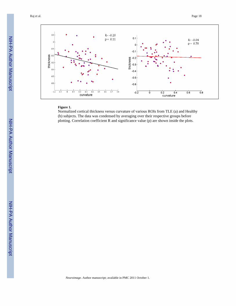
Figure 1.Normalized cortical thickness versus curvature of various ROIs from TLE (a) and Healthy(b) subjects. The data was condensed by averaging over their respective groups beforeplotting. Correlation coefficient R and significance value (p) are shown inside the plots.

Raj et al. Page 18

Neuroimage. Author manuscript; available in PMC 2011 October 1.

NIH

-PA Author Manuscript

NIH

-PA Author Manuscript

NIH

-PA Author Manuscript

Figure 2.Summary flowchart of GED-based network classification. Various MR brain volumes fromdifferent subjects are processed by FreeSurfer to get cortical thickness and curvature ofparcellated cortical structures. A network is built for each subject. These networks are fedinto the GED algorithm to compute pairwise distances between them. The MDS (multi-dimensional scaling) algorithm is applied to convert these pairwise distances into Cartesiancoordinates in the embedded Euclidean space. Finally, LDA (linear discriminant analysis) isperformed to get disease class for each subject.

Raj et al. Page 19

Neuroimage. Author manuscript; available in PMC 2011 October 1.

NIH

-PA Author Manuscript

NIH

-PA Author Manuscript

NIH

-PA Author Manuscript

Figure 3.Epilepsy-derived brain network connectivity of TLE subjects. For visual conveniencecortical networks are depicted as 2D circular rings, with cortical ROIs residing on thecircumference, except for cingulate structures which are shown as brown arcs within thecircle.Following a dorsal view, frontal lobe is represented in light blue arc, temporal lobe (darkblue), parietal lobe (green) and occipital lobe (orange). A histogram of the 5 most popularconnections across all subjects was compiled and this histogram was then thresholded toobtain the connectivities above. The straight lines between ROIs denote the presence of themost frequently occurring connections among all subjects in the specified group. Plots on

Raj et al. Page 20

Neuroimage. Author manuscript; available in PMC 2011 October 1.

NIH

-PA Author Manuscript

NIH

-PA Author Manuscript

NIH

-PA Author Manuscript

the left ((a) and (b)) show the first few most frequent connections by setting a highthreshold, and on the right (c) and (d) show a few more of these frequent connections byrelaxing the threshold a little.

Raj et al. Page 21

Neuroimage. Author manuscript; available in PMC 2011 October 1.

NIH

-PA Author Manuscript

NIH

-PA Author Manuscript

NIH

-PA Author Manuscript

Figure 4.Receiver Operator Characteristic (ROC) curves for the GED-distance based classification, aswell as the standard difference norm-based classification. (a) corresponds to 2-groupclassification (TLE vs Healthy), and (b) corresponds to 3-group classification (TLE-MTS vsTLE-no vs Healthy). Note that there is some loss of performance from the 2-group case tothe 3-group case, but the GED-based method consistently outperforms the standard non-graph approach.

Raj et al. Page 22

Neuroimage. Author manuscript; available in PMC 2011 October 1.

NIH

-PA Author Manuscript

NIH

-PA Author Manuscript

NIH

-PA Author Manuscript

Figure 5.Concordance between VET-based lateralization of epileptic focus and MRI-basedlateralization. The x-axis depicts the number of highly-connected nodes used to estimatelateralization.

Raj et al. Page 23

Neuroimage. Author manuscript; available in PMC 2011 October 1.

NIH

-PA Author Manuscript

NIH

-PA Author Manuscript

NIH

-PA Author Manuscript

Figure 6.Area under ROC curves, for 5 different edge weight formulas. The formula producing bestclassification power is indicated by red arrows and boxes. Note the, max() function appearsto be most informative edge weight for Epilepsy.

Raj et al. Page 24

Neuroimage. Author manuscript; available in PMC 2011 October 1.

NIH

-PA Author Manuscript

NIH

-PA Author Manuscript

NIH

-PA Author Manuscript

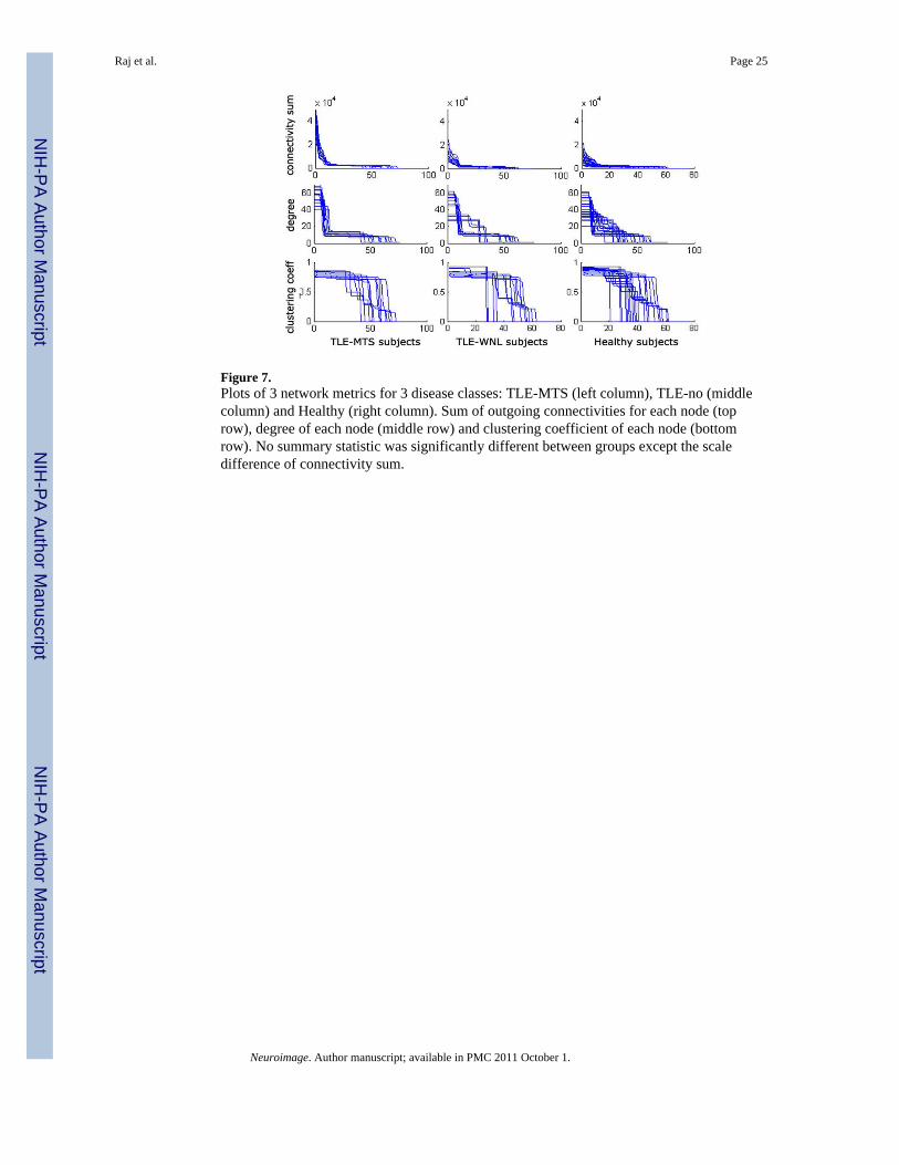
Figure 7.Plots of 3 network metrics for 3 disease classes: TLE-MTS (left column), TLE-no (middlecolumn) and Healthy (right column). Sum of outgoing connectivities for each node (toprow), degree of each node (middle row) and clustering coefficient of each node (bottomrow). No summary statistic was significantly different between groups except the scaledifference of connectivity sum.

Raj et al. Page 25

Neuroimage. Author manuscript; available in PMC 2011 October 1.

NIH

-PA Author Manuscript

NIH

-PA Author Manuscript

NIH

-PA Author Manuscript

Figure 8.Histograms of network metrics. TLE-MTS (left column), TLE-no (middle column) andHealthy (right column). Network entropy for each subject (top row), statistical complexity(2nd row), monoexponential decay parameter fit (3rd row), and area under the connectivitysum curves shown in top row of figure 6 (bottom row). The p-values corresponding to a 2-way T-test between the 3 groups, for each of these 4 summary metrics, are shown betweencorresponding group pairs. TLE-no group shows network characteristics somewhat betweenthe TLE-MTS and Healthy groups. We conjecture that the TLE-no group can be separatedinto TLE-MTS-like and Healthy-like subgroups, as shown by the two colors in the middlecolumn: blue for TLE-MTS-like subgroup, and pink for Healthy-like subgroup. The“Healthy-like” subgroup show high dispersion of epileptic focus in terms of their networkproperties more akin to the Healthy group.

Raj et al. Page 26

Neuroimage. Author manuscript; available in PMC 2011 October 1.

NIH

-PA Author Manuscript

NIH

-PA Author Manuscript

NIH

-PA Author Manuscript

Figure 9.Network-derived measures of epilepsy severity and dispersion. These measures can proveuseful to a clinician interested in surgical planning.

Raj et al. Page 27

Neuroimage. Author manuscript; available in PMC 2011 October 1.

NIH

-PA Author Manuscript

NIH

-PA Author Manuscript

NIH

-PA Author Manuscript

Figure 10.Scatter plot of Dispersion versus Temporal Lobe Specificity of cortical atrophy. The inverserelationship between dispersion and TL specificity of most TLE subjects indicates that thedispersion is a result of out-migration of epileptogenic regions from TL to other regions ofthe brain. Among TLE-MTS patients this out-migration is limited. However, some TLE-nosubjects, as indicated in the figure, exhibit high dispersion as well as low TL specificity.

Raj et al. Page 28

Neuroimage. Author manuscript; available in PMC 2011 October 1.

NIH

-PA Author Manuscript

NIH

-PA Author Manuscript

NIH

-PA Author Manuscript

NIH

-PA Author Manuscript

NIH

-PA Author Manuscript

NIH

-PA Author Manuscript

Raj et al. Page 29

Table 1

Study subject characteristics. Number of subjects (age range, mean ± stdev)

Gender Control TLE-MTS TLE-no

Female 20 (38.8 ± 9.7) 8 (39.6 ± 9.9) 9 (35.0 ± 7.5)

Male 10 (37.9 ± 9.7) 5 (44.4 ± 6.4) 5 (37.0 ± 5.8)

Neuroimage. Author manuscript; available in PMC 2011 October 1.

NIH

-PA Author Manuscript

NIH

-PA Author Manuscript

NIH

-PA Author Manuscript

Raj et al. Page 30

Table 2

Total node strength in each lobe, as percentage of total. Connections weights lower than the low threshold inFig. 2 were not counted.

Lobe

TLE-MTS TLE-no

Ipsi Contra Ipsi Contra

Occipital 0 3 0 5

Parietal 3 3 3 5

Temporal 47 3 25 20

Cingulate 8 8 10 6

Frontal 14 11 14 12

Total 72 28 52 48

Neuroimage. Author manuscript; available in PMC 2011 October 1.