ORIGINAL RESEARCH ARTICLEpublished: 24 February 2015

doi: 10.3389/fninf.2015.00002

Network dynamics with BrainX3: a large-scale simulationof the human brain network with real-time interactionXerxes D. Arsiwalla1*, Riccardo Zucca1, Alberto Betella1, Enrique Martinez1, David Dalmazzo1,

Pedro Omedas1, Gustavo Deco2,3 and Paul F. M. J. Verschure1,3*

1 Synthetic Perceptive Emotive and Cognitive Systems Lab, Center of Autonomous Systems and Neurorobotics, Universitat Pompeu Fabra, Barcelona, Spain2 Computational Neuroscience Group, Center for Brain and Cognition, Universitat Pompeu Fabra, Barcelona, Spain3 Institució Catalana de Recerca i Estudis Avançats , Barcelona, Spain

Edited by:

Mihail Bota, University of SouthernCalifornia, USA

Reviewed by:

Bruce Graham, University of Stirling,UKOlusola Ajilore, University of Illinoisat Chicago, USA

*Correspondence:

Xerxes D. Arsiwalla and Paul F. M. J.Verschure, Synthetic PerceptiveEmotive and Cognitive Systems Lab,Center of Autonomous Systems andNeurorobotics, Universitat PompeuFabra, La Nau Building, Roc Boronat138, 08018 Barcelona, Spaine-mail: x.d.arsiwalla@gmail.com;paul.verschure@upf.edu

BrainX3 is a large-scale simulation of human brain activity with real-time interaction,rendered in 3D in a virtual reality environment, which combines computational powerwith human intuition for the exploration and analysis of complex dynamical networks. Weground this simulation on structural connectivity obtained from diffusion spectrum imagingdata and model it on neuronal population dynamics. Users can interact with BrainX3 inreal-time by perturbing brain regions with transient stimulations to observe reverberatingnetwork activity, simulate lesion dynamics or implement network analysis functions froma library of graph theoretic measures. BrainX3 can thus be used as a novel immersiveplatform for exploration and analysis of dynamical activity patterns in brain networks,both at rest or in a task-related state, for discovery of signaling pathways associatedto brain function and/or dysfunction and as a tool for virtual neurosurgery. Our resultsdemonstrate these functionalities and shed insight on the dynamics of the resting-stateattractor. Specifically, we found that a noisy network seems to favor a low firing attractorstate. We also found that the dynamics of a noisy network is less resilient to lesions.Our simulations on TMS perturbations show that even though TMS inhibits most of thenetwork, it also sparsely excites a few regions. This is presumably due to anti-correlationsin the dynamics and suggests that even a lesioned network can show sparsely distributedincreased activity compared to healthy resting-state, over specific brain areas.

Keywords: connectomics, virtual reality, neural dynamics, large-scale brain networks, big data, virtual

neurosurgery

1. INTRODUCTIONHow should one visualize and simulate the large amounts of databeing generated nowadays in neurobiology, in ways that couldinform our understanding of the structure and function of thebrain? Would that also link to clinical applications? Over theyears, the cumulative spate of studies in structural and functionalneuroimaging, electrophysiology, genetic imaging and axonal-tracing studies have generated enormous amounts of data (foundin online repositories such as http://www.neuroscienceblueprint.nih.gov/connectome/ and http://www.brain-map.org to name afew), which, on one hand have led to many insights on the intri-cate patterns of signaling and connectivity, as well as the existenceof multi-scale processes in the brain; on the other hand, it hasexposed the need for an integrative framework for modelingand simulating whole-brain dynamics and function. To addressthis need, neuroscientists started using ideas from network engi-neering, thinking of the brain as a complex dynamical networkof neurons, thus giving rise to the field of brain connectomics(Hagmann, 2005; Sporns et al., 2005). Akin to the genome, whichis a map of the genetic sequence of an organism, the connectomeis a map of the neuronal circuitry of an organism emphasizing thenodes and their connections where nodes can represent volumesof neuronal tissue to single neurons. Of course, merely a map

of this network is not sufficient to predict or understand func-tion. Being a dynamic network, signaling processes in the brainoperate across a range of spatial and temporal scales. Therefore, amechanistic understanding of these processes is essential to gaininsight into cognitive function. At the same time, the complexityof the connectome means that these signaling circuits cannot beunderstood in isolation or even in a serial manner, but necessarilyhave to be seen in the functional context of the whole network.This calls for a large-scale network level analysis and simulationof whole-brain activity and an associated immersive visualiza-tion and interaction system. This is the challenge BrainX3 aimsto tackle.

BrainX3 is a large-scale simulation of the human cerebral con-nectome, which uses both anatomical structure and biophysicaldynamics in order to reconstruct activity and predict function.Structural connectivity of the network is obtained from humanDiffusion Spectrum Imaging (DSI) data (Hagmann et al., 2008).Each node of the connectivity matrix corresponds to a popula-tion of neurons. For simulating dynamics, BrainX3 offers the usera choice of dynamical models that can be implemented, namely,population dynamics based on a linear-threshold transfer func-tion, or a non-linear sigmoidal transfer function with decay, ordynamical mean-field models (Wong and Wang, 2006; Deco et al.,

Frontiers in Neuroinformatics www.frontiersin.org February 2015 | Volume 9 | Article 02 | 1

NEUROINFORMATICS

Arsiwalla et al. BrainX3

2013). The last of these models are the most interesting as theycome closest to biology; they compute aggregate neural activitytaking into account synaptic dynamics and stochasticity.

Until the advent of the connectome (Hagmann, 2005; Spornset al., 2005), the traditional method of choice for investigat-ing non-invasive human resting-state dynamics has heavily reliedon back-inference of neural mechanisms from BOLD signals.Despite the many successes of this approach, a few drawbacksremain; for instance, it does not provide precise temporal infor-mation on the flow of activity through the network, and beinga signal based on haemodynamic responses, it is at best only aproxy for neural activity. However, the birth of the field of con-nectomics has helped turn this around. Combining structuralconnectivity data with detailed neuronal dynamics made it pos-sible to instead predict functional activity (Honey et al., 2009).These predictions have been validated for both spiking neuron aswell as dynamical mean-field models, when compared to empir-ical BOLD data (Deco et al., 2013). In this work we implementmean-field dynamics in BrainX3 using Hagmann et al.’s DSI net-work to reconstruct neurodynamic activity for the entire cortexwithin a 3D virtual environment, for the purpose of investigat-ing temporal patterns of whole-brain neural activity when thebrain is in the resting-state. The resting-state refers to the stateof spontaneous neural activity recorded in the absence of anyspecific tasks being instructed to the subject. In computationalmodels, this corresponds to no specific (or localized) externalinput currents being injected into the network above the overallbaseline current. The activity in this spontaneous state is far fromrandom. Hence, understanding the biophysical dynamics of theresting-state constitutes an important challenge.

The technology of BrainX3 is layered on four modular compo-nents: an input module, a data processing module, a visualizationand interaction module, and a simulation and analysis module.The integration of these modules generates the full user expe-rience. Simulations run in the eXperience Induction Machine(XIM), an enclosed virtual/mixed reality chamber, which enablesuser-immersion and exploration of virtually rendered scenarios(refer to Figure 1) (Bernardet et al., 2010; Betella et al., 2014c).Based on DSI data, a 3D model of the connectome network isreconstructed within the XIM, providing users with an inside-out perspective of the brain connectome and allowing them tonavigate through pathways in the network. Additionally, the XIMsupports a custom-built large-scale neural simulator, iqr, whichcommunicates bi-directionally with the virtual brain networkand imposes dynamics on it (Bernardet and Verschure, 2010).Furthermore, BrainX3 is based on a natural user interactionparadigm, such that using natural gestures, i.e., hand gestures,body posture, etc., users can navigate the virtual space, select andbookmark brain areas, perform surgeries, stimulate any region ofthe network to investigate the dynamics of the neuronal activityreverberating through associated areas. Finally, for data analysis,BrainX3 communicates bi-directionally, using standard protocolssuch as UDP or YARP (Metta et al., 2006), with external networkanalysis tools, including the Brain Connectivity Toolbox (BCT)(Rubinov and Sporns, 2010) running on a MATLAB client.

What is BrainX3 capable of? It provides the possibilityof analyzing and interacting in real-time with the simulated

FIGURE 1 | Computer rendering of BrainX3 within the eXperience

Induction Machine (XIM). The 3D connectome network and its simulateddynamics are projected on the frontal screen. The screen on the right displaysregional information of selected brain areas from a curated database, whilethe left screen shows 2D axial slices of the brain and indicates regions ofactivity. The user can navigate and interact with the model with predefinedhand gestures.

activity. Compared to functional correlations, dynamical anal-ysis of causal activity serves as a powerful tool to unravelmechanisms of large-scale neural circuits. Indeed, couplingstructural connectivity data with detailed enough populationdynamics should be sufficient in predicting functional corre-lations and large-scale activity patterns. As examples, we useBrainX3 to demonstrate the dynamics of the brain in theresting-state as well as under perturbations due to evoked stim-uli. We investigate how neural activity reorganizes followingsimulated lesions. Additionally, using graph theoretic measuresfrom the BCT we can also determine shortest paths betweennodes.

At this point, it is also worth drawing attention to the growingeco-system of ‘big brain projects’ and other neuroinformat-ics tools which complement BrainX3. Among these are theConnectome Workbench of the Human Connectome Project(http://www.humanconnectome.org/connectome/connectome-workbench.html) (Marcus et al., 2013), the Brain Explorer 2 ofthe Allen Institute for Brain Science (http://www.brain-map.

org), the Glass Brain Project (http://neuroscapelab.com/projects/glass-brain/) (Mullen et al., 2013), the VisNEST tool (Nowkeet al., 2013) and The Virtual Brain (Jirsa et al., 2010; Sanz-Leonet al., 2013). While many of them are 3D visualization tools, someof them also include dynamics and interaction. In that sense,The Virtual Brain comes closest to the objectives of BrainX3, butfor example, it does not include real-time interaction. Unlikethe aforementioned, BrainX3 runs in a completely immersivevirtual reality chamber, facilitating real-time interaction with thesimulation using natural gestures. For the benefit of the neu-roinformatics community, a portable laptop version, includinginteraction (but without user immersion), is currently underdevelopment. Besides, visualization, interaction and simulation,BrainX3 has been developed with a vision toward a “smart explo-ration space for big data” as part of the European Union CEEDS

Frontiers in Neuroinformatics www.frontiersin.org February 2015 | Volume 9 | Article 02 | 2

Arsiwalla et al. BrainX3

(Collective Experience of Empathic Data Systems) project (http://ceeds-project.eu and http://www.brainx3.com).

2. MATERIALS AND METHODS2.1. HARDWARE AND SYSTEM ARCHITECTUREThe virtual reality environment supporting BrainX3 is the eXpe-rience Induction Machine (XIM) (Bernardet et al., 2010; Betellaet al., 2014c; Omedas et al., 2014). The XIM is a 25 m2 humanaccessible space (schema in Figure 1) equipped with 360◦ sur-round screens, an interactive luminous floor with pressuresensors, a marker-free tracking system, a KinectTM, micro-phones, a sonification system and wearable sensors, that sup-port human-machine interaction in the exploration of complexdatasets. The computational platform running BrainX3 in theXIM includes four latest generation machines that communi-cate bi-directionally using the YARP protocol within a highspeed LAN connection: 2 PCs dedicated to graphical render-ing (INTEL CORE i7 2600K 3,4GHZ/8mb/LGA1155, two DDR3s4GB 1333Mhz KINGSTON, AMD FirePro V7900 Professionalwith AMD Eyefinity technology) with a total of eight display portoutputs, each of which is connected to an HD projector (EpsonPowerLite Pro G5450WUNL), thus creating a 360◦ projectiondisplay that surrounds the user; 1 server dedicated to sensorsrecording and real-time interaction (HP proliant DL160 G6, XeonE5506, 2.13 GHz) that is connected to the XIM sensors and effec-tors, including a Microsoft Kinect2™, the sonification system andthe interactive floor; 1 server dedicated to simulation and com-putation (HP proliant DL160 G6, Xeon E5506 at 2.13 GHz) that

runs the neural network simulator iqr (http://iqr.sourceforge.net) and MATLAB.

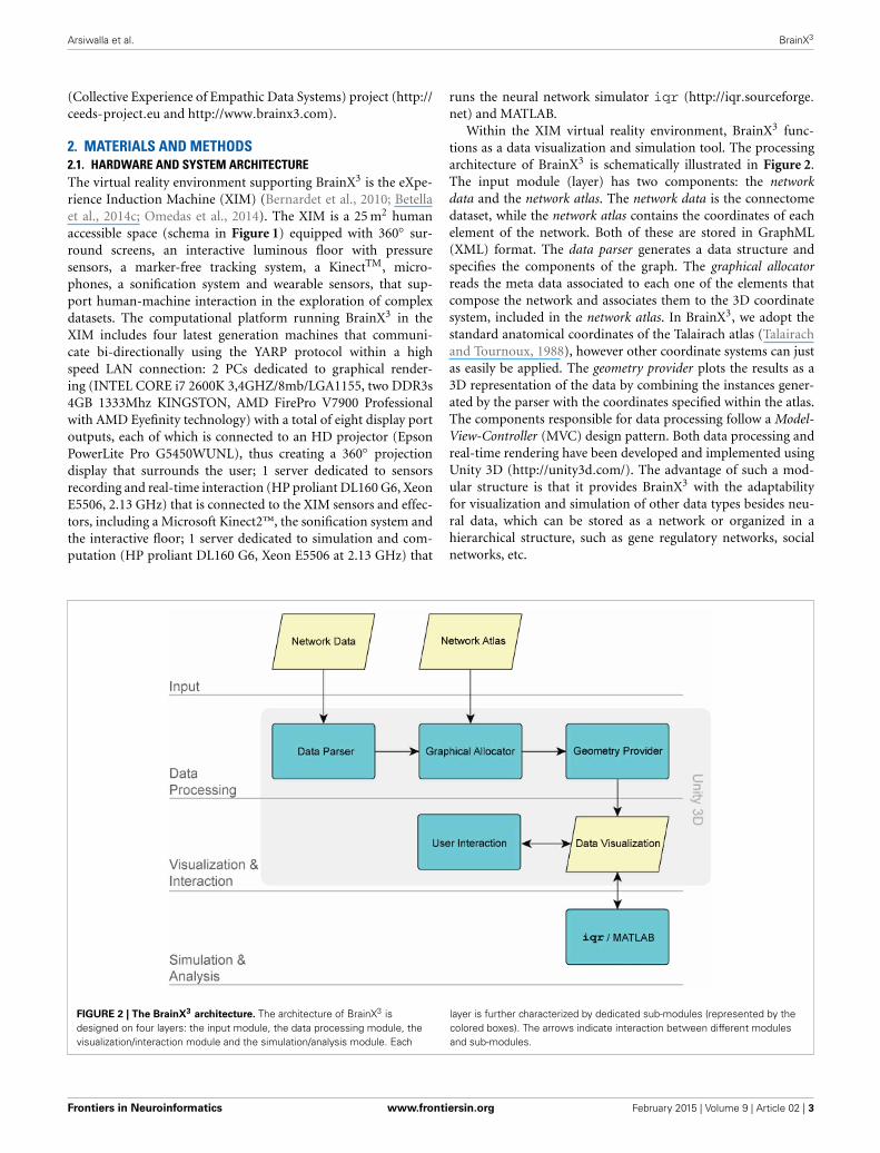
Within the XIM virtual reality environment, BrainX3 func-tions as a data visualization and simulation tool. The processingarchitecture of BrainX3 is schematically illustrated in Figure 2.The input module (layer) has two components: the networkdata and the network atlas. The network data is the connectomedataset, while the network atlas contains the coordinates of eachelement of the network. Both of these are stored in GraphML(XML) format. The data parser generates a data structure andspecifies the components of the graph. The graphical allocatorreads the meta data associated to each one of the elements thatcompose the network and associates them to the 3D coordinatesystem, included in the network atlas. In BrainX3, we adopt thestandard anatomical coordinates of the Talairach atlas (Talairachand Tournoux, 1988), however other coordinate systems can justas easily be applied. The geometry provider plots the results as a3D representation of the data by combining the instances gener-ated by the parser with the coordinates specified within the atlas.The components responsible for data processing follow a Model-View-Controller (MVC) design pattern. Both data processing andreal-time rendering have been developed and implemented usingUnity 3D (http://unity3d.com/). The advantage of such a mod-ular structure is that it provides BrainX3 with the adaptabilityfor visualization and simulation of other data types besides neu-ral data, which can be stored as a network or organized in ahierarchical structure, such as gene regulatory networks, socialnetworks, etc.

FIGURE 2 | The BrainX3 architecture. The architecture of BrainX3 isdesigned on four layers: the input module, the data processing module, thevisualization/interaction module and the simulation/analysis module. Each

layer is further characterized by dedicated sub-modules (represented by thecolored boxes). The arrows indicate interaction between different modulesand sub-modules.

Frontiers in Neuroinformatics www.frontiersin.org February 2015 | Volume 9 | Article 02 | 3

Arsiwalla et al. BrainX3

2.2. VISUALIZATION AND SIMULATIONVisualization and reconstruction of the connectome withinBrainX3 is based on DSI data of white matter fiber structural con-nectivity averaged from five healthy right-handed male humansubjects (Hagmann et al., 2008). The dataset contains 998 vox-els (nodes) belonging to 33 cortical areas per hemisphere (referTable 1), for a total of 66 areas. The 998 Regions of Interest(ROIs) have an average size of 1.5 cm2 and each ROI is associ-ated with {x, y, z} coordinates as per the Talairach coordinates ofROIs (Talairach and Tournoux, 1988). Since tractography doesnot determine the directionality of the fibers, the connectivitymatrix (approximately 17000 bi-directional connections) is sym-metric at the ROI level. Connection strengths within the networkrefer to normalized number of white matter fiber tracts betweenROIs.

To introduce dynamics into the visualization, the large-scale multi-level neural networks simulator, iqr (http://iqr.

sourceforge.net/), is bi-directionally interfaced to Unity. iqrallows the user to design complex neuronal models througha graphical interface and to visualize, analyze and modify themodel’s parameters in real-time (Bernardet and Verschure, 2010).The architecture of iqr is modular, providing the possibility todefine custom neurons and synapses. iqr can simulate large neu-ronal systems up to 500k neurons and connections and can bedirectly interfaced to external sensors and effectors. In order toenable real-time user interaction with the reconstructed data, userinput from Unity is sent to iqr (Arsiwalla et al., 2013). The neu-ronal simulator computes the processes and broadcasts the outputof the simulation back to the Unity engine in the XIM. The sim-ulation runs with iqr receiving commands through Unity atany time during the simulation. Upon receiving input from iqr,Unity updates the visualized population activity on each node. Inits current form, BrainX3 can accommodate networks of up to4000 nodes (albeit with a slower simulation time).

Table 1 | 33 brain regions on each hemisphere (ID), abbreviated name (Abbr.), anatomical name (Brain region) and ROI node numbers for each

region on right (R) and (L) hemispheres.

ID Abbr. Brain region Nodes (R) Nodes (L)

1 BSTS Bank of the superior temporal sulcus 463–469 961–965

2 CAC Caudal anterior cingulate cortex 191–194 692–695

3 CMF Caudal middle frontal cortex 126–138 628–640

4 CUN Cuneus 335–344 835–842

5 ENT Entorhinal cortex 419–420 918–920

6 FP Frontal pole 26–27 527–528

7 FUS Fusiform gyrus 391–412 890–911

8 IP Inferior parietal cortex 284–311 787–811

9 IT Inferior temporal cortex 424–442 925–941

10 ISTC Isthmus of the cingulate cortex 202–209 703–710

11 LOCC Lateral occipital cortex 355–373 852–873

12 LOF Lateral orbitofrontal cortex 1–19 501–520

13 LING Lingual gyrus 374–390 874–889

14 MOF Medial orbitofrontal cortex 28–39 529–540

15 MT Middle temporal cortex 443–462 942–960

16 PARC Paracentral lobule 175–186 677–687

17 PARH Parahippocampal cortex 413–418 912–917

18 POPE Pars opercularis 48–57 548–558

19 PORB Pars orbitalis 20–25 521–526

20 PTRI Pars triangularis 40–47 541–547

21 PCAL Pericalcarine cortex 345–354 843–851

22 PSTC Postcentral gyrus 210–240 711–740

23 PC Posterior cingulate cortex 195–201 696–702

24 PREC Precentral gyrus 139–174 641–676

25 PCUN Precuneus 312–334 812–834

26 RAC Rostral anterior cingulate cortex 187–190 688–691

27 RMF Rostral middle frontal cortex 58–79 559–577

28 SF Superior frontal cortex 80–125 578–627

29 SP Superior parietal cortex 257–283 760–786

30 ST Superior temporal cortex 470–497 966–994

31 SMAR Supramarginal gyrus 241–256 741–759

32 TP Temporal pole 421–423 921–924

33 TT Transverse temporal cortex 498–500 995–998

Frontiers in Neuroinformatics www.frontiersin.org February 2015 | Volume 9 | Article 02 | 4

Arsiwalla et al. BrainX3

2.3. DYNAMICAL MODELS IN BRAINX3

As the connectivity data currently being used by BrainX3 isderived from neuroimaging sources, it is more appropriate tomodel network dynamics by means of neuronal population mod-els. At present, BrainX3 allows to run simulations with either ofthe three models: (i) the linear-threshold model, (ii) non-linear(sigmoidal) model and (iii) dynamical mean-field model. Thelinear-threshold model simply sums up all the input signals toa population module from various dendrites (within a fixed timewindow) and fires an output signal to neighboring modules onlyif the summed inputs cross a designated threshold. Additionallyeach neuronal population module is stochastic, having Gaussiannoise. This was demonstrated in earlier work (Arsiwalla et al.,2013). The non-linear model is similar to above except that thelinear-threshold filter is replaced by a sigmoidal filter with decay.This was used in Betella et al. (2014b).

The dynamical mean-field model is a mathematical reductionof a spiking attractor network consisting of integrate and fire neu-rons with excitatory and inhibitory synapses (Wong and Wang,2006; Deco et al., 2013). Global brain dynamics of the network ofinterconnected local networks is described by the following set ofdifferential equations derived in Deco et al. (2013):

Table 2 | List of parameters of the dynamical mean-field model

implemented in BrainX3 from Deco et al. (2013).

Parameter Description Value Unit

measure

N Number of nodes 998

w Local recurrent excitation 0.9

a Input-output function 270 n/C

b Input-output function 108 Hz

d Input-output function 0.154 s

γ Kinetic parameter 0.641 s

τS Kinetic parameter 100 ms

JN Synaptic coupling 0.2609 nA

I0 Overall external input 0.3 nA

σ Noise amplitude 0.01, 0.05, 0.07, 0.1

dSi

dt= −Si

τs+ (1 − Si)γ H(xi) + σ vi(t) (1)

H(xi) = axi − b

1 − exp( − d(axi − b))(2)

xi = wJN Si − GJN

∑

j

CijSj + I0 (3)

where H(xi) and Si respectively correspond to the populationrate and the average synaptic gating variable at each local nodei, w is the local recurrent excitation, G is a global scaling param-eter, Cij is the matrix of structural connectivity expressing theneuroanatomical connections between areas i and j, vi is uncor-related Gaussian noise. All parameters values, with the exceptionof σ , which was systematically varied in the present simulationstudy, are as in Deco et al. (2013) and have been summarized inTable 2.

Among the three types of models described above, mean-fieldmodels are the most interesting as they come closest to biol-ogy. They compute aggregate neural activity taking into accountsynaptic dynamics and stochasticity. Hence, in this paper, oursimulations will be based on the dynamical mean-field model.However, compared to Deco et al. (2013), where the dynamics wasparametrized on 66 regions, in this work we scale the dynamics to998 ROIs.

2.4. REAL-TIME INTERACTION FRAMEWORKBrainX3 allows users to interact in real-time with the simula-tion (the simulation itself is not real-time, each millisecond ofsimulation takes between 20 and 50 ms, being slower during inter-action). This is a form of on-line interaction, as opposed to apre-programed off-line mode of interaction. It provides users thepossibility to perturb the simulated activity (by injecting cur-rents using predefined hand gestures) mid-way through the run.Gesture recognition and signaling within the XIM is supportedvia the Social Signal Interpretation (SSI) framework (Wagneret al., 2013) and is based on the Microsoft KinectTM v2 tech-nology. The KinectTM detects body joints and two main handactions: the closed hand and pointing with a finger. All high

FIGURE 3 | Interaction within BrainX3. User immersion and interaction within BrainX3.

Frontiers in Neuroinformatics www.frontiersin.org February 2015 | Volume 9 | Article 02 | 5

Arsiwalla et al. BrainX3

FIGURE 4 | Simulation of resting-state activity vs. noise showing

that increased noise suppresses network activity. Snapshot ofresting-state neural activity at a single time-point (after thedynamics stabilizes around the attractor) for different levels of noiseamplitude within BrainX3. From top to bottom, noise amplitudes:(A) 0.01, (B) 0.05, (C) 0.07, and (D) 0.1. Each row shows

screenshots from the posterior, superior and lateral perspectives.The color bar on the right represents neuronal activity in Hz(warmer colors represent higher activation of the nodes). The fullsimulation can be seen on videos 01 and 02 of the followinglink: https://www.youtube.com/playlist?list=PL-BcYpSz98wqVAKuI-ymqDII-6nXK_8uq.

FIGURE 5 | Analysis of resting-state activity vs. noise. 2D plots ofresting-state neural activity for the same four simulation runs shown in Figure 4.Subplots (A–D) respectively refer to noise amplitudes 0.01, 0.05, 0.07, and 0.1.Each subplot shows three graphics: 2D distribution of nodes with activity

indicated by colors from the color bar (warmer colors refer to higher activation),mean firing rate for all 998 nodes over the last 2 s of simulation and time-seriessignals extracted for three seed ROIs rCAC (node 193, shown in black), rISTC(node 205, shown in green) and lPCUN (node 830, shown in magenta).

Frontiers in Neuroinformatics www.frontiersin.org February 2015 | Volume 9 | Article 02 | 6

Arsiwalla et al. BrainX3

level mapping and interpretation of gestures is performed bySSI. In order to rotate the network sideways, the user simply hasto clench her/his fist and make a sideways arm movement. Forzooming into the network, the user moves directly toward thescreen and the visualization becomes immersive placing the user“inside” the 3D reconstruction (refer to Figure 3). For stimulat-ing or inhibiting brain areas, the user simply has to control thecursor with a hand movement, select a node or region in thenetwork with a grabbing gesture, then drag and drop the cursoron the icon in the graphical user interface, associated to stim-ulation or inhibition. This respectively corresponds to injectingexternal excitatory or inhibitory currents into the dynamics. Thestrength of the stimulation current is pre-defined in the iqrconfiguration file (but can be arbitrarily chosen). Stimulationscan be performed on one or more brain areas simultaneously.BrainX3 then reconstructs reverberating neural activity propa-gating through the connectome. Furthermore, in order to equipthe user with tools for analysis of the outcome of the simulation,BrainX3 is also interfaced with the MATLAB Brain ConnectivityToolbox, which enables several graph-theoretic operations to beperformed on the reconstructed network such as finding theshortest path between any two nodes or detecting communitystructure in the data (Rubinov and Sporns, 2010). BrainX3 alsoincludes customized interaction functionalities that allow the userto bookmark areas of interest, to tag and visually highlight cho-sen pathways, to filter network complexity and to model lesions

by disabling nodes in order to obtain altered activity associated tothe lesion.

3. RESULTSWe now put to test the functional capabilities of BrainX3 togain valuable insights on the large-scale dynamics of the humanconnectome. We start by simulating the global dynamics of theresting-state. Then we lesion the structural network and studyaberrant cortical activity for both focal lesions as in strokepatients as well as for diffuse lesions as in multiple sclerosispatients. Next, we study the effect of external perturbationssuch as trans-cranial magnetic stimulations on the network andits resulting evoked activity. Finally, we demonstrate an exer-cise in tracing pathways within the cortex in order to extractfunctional circuits as well as to analyze them. Videos explic-itly demonstrating these results in BrainX3 have been uploadedon the following link: https://www.youtube.com/playlist?list=PL-BcYpSz98wqVAKuI-ymqDII-6nXK_8uq.

3.1. DYNAMICS OF THE RESTING-STATEFigures 4, 5 show results from 10 s of simulation of resting-statedynamics. An important observation made in Deco et al. (2013)was that the resting-state network operates at the edge of a bifur-cation. This fixes the global coupling parameter of the model.Analogously, for the scaled model we implement here, the valueof the global coupling G is determined to be 2.3 using the same

FIGURE 6 | Simulation of lesioned (focal) brain activity vs. noise.

Snapshot of neural activity at a single time-point in BrainX3 following afocal lesion in areas rCUN, rLOCC, and rPCUN. From top to bottom,noise amplitudes: (A) 0.01, (B) 0.05, (C) 0.07, and (D) 0.1. Each rowshows screenshots from the posterior, superior and lateral perspectives.

The color bar on the right represents neuronal activity in Hz (warmercolors represent higher activation of the nodes and lesioned nodes areshown in black). The full simulation can be seen on videos 03 and 04 ofthe following link: https://www.youtube.com/playlist?list=PL-BcYpSz98wqVAKuI-ymqDII-6nXK_8uq.

Frontiers in Neuroinformatics www.frontiersin.org February 2015 | Volume 9 | Article 02 | 7

Arsiwalla et al. BrainX3

observation. Besides that, all other mean-field model parameters(except the noise amplitude σ ) are held at exactly the same valuesas in Deco et al. (2013). The numerics run in time steps of 0.1 msbut we sample data every 1 ms giving 10K points for a run of 10 s.Figure 4 shows screenshots from the front display of BrainX3 atthe end of four runs of the simulation. Each run was chosen witha different value of noise amplitude, shown in rows A, B, C and Dwith σ 0.01, 0.05, 0.07, and 0.1 respectively. The four snapshotsin each row (from left to right) correspond to the posterior, supe-rior and lateral views respectively. Since BrainX3 is interfaced toMATLAB via YARP/UDP, in addition to the 3D reconstruction,we also obtained time-series data that can be analyzed using anystatistical tool. This is shown in Figure 5. This analysis was per-formed off-line using MATLAB. Each of the four subplots A, B,C, and D refer to the same four noise levels. Further, each subplotincludes three graphics: a 2D distribution of ROIs with colorednodes indicating activity level at the end of the simulation, a plotshowing the mean firing rate of every ROI over the last 2 s and aplot showing the full time-series signal of three randomly chosennodes. The mean firing activity represents the stable fixed point ofthe dynamics and in fact the attractor of the resting-state network.The seed ROIs corresponding to the three time-series signals referto nodes 193, 205, and 830 located in regions rCAC (black), rISTC(green) and lPCUN (magenta) respectively. Table 1 shows themapping of ROI identities to anatomical region names.

An interesting insight that we gain upon comparing the resultsof these simulations is the way noise affects the network attractors

themselves. This is summarized in the histogram on the left-hand side of Figure 11, showing the total mean firing rate of theresting-state network integrated over all ROIs. Each column of thehistogram refers to a given noise amplitude. What is interesting isthat rather than jumping into a hyperactive or chaotic state, uponincreasing intrinsic noise, the dynamics of the network seems toquiet down. For σ 0.07, mean activity for each node is around40 Hz and for σ 0.1, it almost goes to zero. Remarkably, this hap-pens without the use of any ROI to ROI inhibitory connections.Noise seems to reverse the stability of the previously unstable lowfiring attractor state.

3.2. DYNAMICS OF STROKE AND MULTIPLE SCLEROSISHaving looked at the healthy resting-state network above, we nowshow how lesions can be simulated in BrainX3. We consider twolesion types, (i) focal lesions, which occur in the case of strokepatients, and (ii) diffuse lesions, which typically occur in patientswith multiple sclerosis. Figures 6, 7 shows results for the formerlesion type with the same four levels of noise as above. Figures 8,9 shows results with diffuse lesions. The focal lesion is constructedon the right hemisphere by severing all white matter fibers con-nections from all nodes in regions rCUN, rLOCC, and rPCUN.These are a total of 52 disconnected ROIs, amounting to 6.64% ofthe total connections. The diffuse lesions are constructed by ran-domly disconnecting individual ROIs distributed throughout thenetwork. To compare with the focal case, we chose 50 scatteredROIs, which amount to 4.91% of the total connections.

FIGURE 7 | Analysis of lesioned (focal) brain activity vs. noise. 2D plotsfor neural activity following a focal lesion in areas rCUN, rLOCC and rPCUNfor the same four simulation runs shown in Figure 6. Subplots (A–D)

respectively refer to noise amplitudes 0.01, 0.05, 0.07, and 0.1. Each subplotshows three graphics: 2D distribution of nodes with activity indicated by

colors from the color bar (warmer colors refer to higher activation andlesioned nodes are shown in black), mean firing rate for all nodes over thelast 2 s of simulation and time-series signals extracted for the three seedROIs rCAC (node 193, shown in black), rISTC (node 205, shown in green) andlPCUN (node 830, shown in magenta).

Frontiers in Neuroinformatics www.frontiersin.org February 2015 | Volume 9 | Article 02 | 8

Arsiwalla et al. BrainX3

In Figure 10, we compare differences between healthy resting-state activity (Figure 4) and the lesioned activity (Figure 6). Thefour plots on the left side of Figure 10 show the difference in meanfiring rate between the healthy and focally lesioned networks (onthe y-axis) in the attractor state at every ROI (on the x-axis),for the four noise amplitudes (in increasing order from top tobottom). From this we see that for the lowest noise amplitude(0.01), the lesion mostly affects activity in its anatomical vicinity.However, by the time we reach noise amplitude 0.07, the spanof the network affected by the lesion has dramatically increased.Furthermore, the histogram shown in the center of Figure 11integrates the differences in mean firing over all ROIs to give thetotal difference in mean firing between the healthy and focallylesioned network for each noise amplitude. The columns of thehistogram are on the positive side of the x-axis (except for noiseamplitude 0.1, when the activity in both networks is just noise).By the time the noise amplitude rises to 0.07, the lesioned net-work dramatically differs from the healthy network in total firing.These observations suggest that noisy networks are less resilientto focal lesions.

On the other hand, a comparison of mean activity between thefocally lesioned (Figure 6) and diffuse lesioned (Figure 8) net-works is shown in the four plots on the right side of Figure 10.The y-axis denotes the difference in mean firing rate between thediffuse and focally lesioned networks in the attractor state. Thex-axis runs over all 998 ROIs. Though the number of disablednodes in both cases is almost the same, we find activity levels incase of diffuse lesions to be markedly higher than in the case of a

focal lesion (of course, both conditions have diminished activitycompared to the healthy network). The same thing can be seenfrom the histogram on the right-hand side of Figure 11, showingthe total difference in mean firing between the diffuse and focallesion activity for each noise amplitude, integrated over all ROIs.Again, the columns are on the positive side of the x-axis. Thus, theconnectome network shows more resilience to diffuse rather thanfocal lesions with the same number of nodes. This is presumablydue to the wiring architecture of the brain that allows for alternatepassages in order to protect against random abrasions.

3.3. CAUSAL EFFERENTS OF TMS PERTURBATIONSNon-invasive physiological perturbations of specific brain areasusing transcranial magnetic stimulations (TMS) have successfullybeen used for probing neural circuits and their functions. Theycan be operated either to excite or completely inhibit a given brainarea both in the presence or absence of a task. What we wantto computationally reconstruct in BrainX3 are the causal effer-ents of the evoked activity due to this stimulation. In Figure 12we show results for an inhibitory stimulation applied to all thenodes in areas rCUN, rLOCC and rPCUN (the same regions onwhich we earlier simulated a focal lesion and with network noiseamplitude of 0.01). TMS is applied during the first 5 s of the sim-ulation and the network returns to resting-state once stimulationis discontinued. The bottom right plot in Figure 12 shows howthis affects the time-series of the same three seed nodes we used(rCAC (black), rISTC (green) and lPCUN (magenta)), which areconnected to but not part of the perturbed regions. The change

FIGURE 8 | Simulation of lesioned (diffuse) brain activity vs. noise.

Snapshot of neural activity at a single time-point in BrainX3 following a diffuselesion. The lesion was simulated by disconnecting 50 randomly selectednodes. From top to bottom, noise amplitudes: (A) 0.01, (B) 0.05, (C) 0.07, and

(D) 0.1. Each row shows screenshots from the posterior, superior and lateralperspectives. The color bar on the right represents neuronal activity in Hz(warmer colors represent higher activation of the nodes and lesioned nodesare shown in black).

Frontiers in Neuroinformatics www.frontiersin.org February 2015 | Volume 9 | Article 02 | 9

Arsiwalla et al. BrainX3

FIGURE 9 | Analysis of lesioned (diffuse) brain activity vs. noise. 2D plotsfor neural activity following a diffuse lesion for the same four simulation runsshown in Figure 8. Again, subplots (A–D) respectively refer to noiseamplitudes 0.01, 0.05, 0.07, and 0.1. Each subplot shows three graphics: 2Ddistribution of nodes with activity indicated by colors from the color bar

(warmer colors refer to higher activation and lesioned nodes are shown inblack), mean firing rate for all nodes over the last 2 s of simulation andtime-series signals extracted for the three seed ROIs rCAC (node 193, shownin black), rISTC (node 205, shown in green) and lPCUN (node 830, shown inmagenta).

in the firing rate is of the order of 10–20 Hz and upon removingthe stimulation, we find that the network returns to resting-stateactivity in about 40 ± 10 ms. The left diagram in Figure 12 showsall 998 nodes, with the stimulated nodes in gray and the colorsin all other nodes denoting the difference in the average firingrate (averaged over 2 s) for each node after and before the per-turbation. The averaging is done to take in account variationsdue to noise. The plot on the top right of Figure 12 shows theexact differences (in red) in average firing rate, after minus before,for each of the 998 nodes (the stimulated areas are shaded ingray), with the black, green and magenta markers referring tothe seed nodes. Hence, above the zero difference, we see effer-ent areas of the network that are inhibited during TMS, whereas,below the zero line refers to efferents that are actually excitedduring TMS.

Clearly, the results show that areas anatomically closer to theperturbed regions are most affected, but they also show spe-cific long range connections in the frontal, temporal and limbiclobes that are affected by stimulating areas rCUN, rLOCC, andrPCUN (in the occipital and parietal lobes). Figure 12 showsROIs in regions rPARC, rCAC, rISTC, rPC, rSP, rIP, and rLINGare strongly inhibited. Since the stimulated areas here are exactlythe same that we lesioned for simulating stroke dynamics, themap of efferents we find after TMS are also part of the affectedpathways following the lesion. As described in the next subsectionand Figure 13, in BrainX3 we can extract these efferents explicitlyin a 3D reconstruction.

Though most of the TMS efferents are inhibited during thestimulation phase, interestingly, a small number of them are alsoexcited, showing an average firing rate higher than the non-perturbed (resting-state) value. These occur sparsely in regionsrLOF, rRMF, rCMF, lLOF, lPOPE, and lFUS. A possible explana-tion for the occurrence of these excitations is that these ROIs werethe ones that were anti-correlated to the stimulated nodes, whenthe network was in the resting-state.

3.4. PATHFINDING IN THE BRAINBesides simulation, another utility in BrainX3 is that it canbe customized for real-time analysis and circuit extraction.This can be done either by analyzing output signals of neu-ral activity from the simulation or by implementing graph-theoretic algorithms on the network. Here, we provide a exam-ple of bookmarking pathways efferent to the focal lesion dis-cussed above. Bookmarking in BrainX3 can simply be doneusing natural gestures. In Figure 13 we trace the connectivityspan (within the healthy dataset) of all the three areas thatwe had lesioned earlier. All edges emanating from the previ-ously lesioned ROIs are bookmarked in thick black giving aclear spatial impression of the extent of the lesion on the net-work. Though the lesion lies only in the occipital and pari-etal lobes, its effects are felt as far as the frontal, temporaland limbic lobes. Extracting circuits this way is intuitive anduser controllable, compared to automated processes based oncorrelation data.

Frontiers in Neuroinformatics www.frontiersin.org February 2015 | Volume 9 | Article 02 | 10

Arsiwalla et al. BrainX3

FIGURE 10 | Firing rate differences � FR between healthy and lesioned

brains. The left-hand side shows the difference in mean firing rate betweenthe healthy and focally lesioned networks (plotted on the y-axis) in theattractor state at each ROI (plotted on the x-axis), for the four noise

amplitudes (in increasing order, starting at 0.01 on top to 0.1 at the bottom).The gray columns in the figures indicate the lesioned areas rCUN, rLOCC,and rPCUN. The right-hand side shows the same difference but for thediffuse vs. the focally lesioned network.

4. DISCUSSIONAs techniques of quantitative analysis and measurement devicesin neuroscience make improvements, it is becoming more evi-dent that the role of large-scale dynamics and whole-brainmeasures cannot be ignored. Functional correlations by them-selves are insufficient for inference of mechanisms and principlesunderlying brain function. Large-scale temporal activity mapsacross structurally connected brain areas are more informative

of whole-brain circuit mechanisms. Being able to predict thesemaps by implementing realistic biophysical dynamics brings usa small step closer to identifying the neural correlates of cog-nitive functions. BrainX3 is a small step in this direction. Itopens the possibility of analyzing neural activity propagationdue to causal dynamics. Being immersive, it gives a much bet-ter intuitive anatomical perspective of the brain, than a 2D atlaswould.

Frontiers in Neuroinformatics www.frontiersin.org February 2015 | Volume 9 | Article 02 | 11

Arsiwalla et al. BrainX3

FIGURE 11 | Comparison of total mean firing rates between healthy and

lesioned brains. The histogram on the left shows the total mean firing rateof the healthy resting-state network (Total RSFR ), integrated over all ROIs, foreach value of noise amplitude. The histogram at the center shows the total

difference in mean firing between the healthy and focally lesioned networks(Total RSFR - Total FLFR ) for each noise amplitude, integrated over all ROIsand the histogram on the right shows the same difference but for the diffusevs. the focally lesioned networks (Total DLFR - Total FLFR ).

FIGURE 12 | Results from TMS perturbations applied upon regions

rCUN, rLOCC, and rPCUN. The left figure shows a 2D distribution ofnodes with colors indicating difference in mean firing after and beforeinhibition. The gray nodes indicate regions where TMS is applied. Thetop right plot quantifies these differences (here the perturbed areas areindicated by the gray columns), while the bottom right plot extracts the

firing rate over time for seed nodes 193 (rCAC), 205 (rISTC) and 830(lPCUN). ROIs in regions rPARC, rCAC, rISTC, rPC, rSP, rIP, and rLINGwere found to be strongly inhibited as a result of the TMS perturbationin rCUN, rLOCC, and rPCUN. The full simulation can be seen on video05 of the following link: https://www.youtube.com/playlist?list=PL-BcYpSz98wqVAKuI-ymqDII-6nXK8uq.

BrainX3, as we have shown in this paper, is a platform for datavisualization, simulation, analysis and interaction, which com-bines computational power with human intuition in representingand interacting with large complex data. For the human connec-tome network above, we have shown an anatomically-spaced 3Dsimulation of whole-brain neural activity, based on the dynam-ical mean-field model, which was earlier tested in Deco et al.(2013) for resting-state dynamics. The results shown included theresting-state network, lesioned brains as well as externally stim-ulated networks. Our simulations above shed some insight onthe spatial distribution of activity in the attractor state, how itmaintains a level of resilience to damage, effects of noise andphysiological perturbations. Specifically, we found that a noisy

network seems to favor a low firing attractor. This is simply a con-sequence of the detailed biophysics of our model. Interestingly,both, computational and empirical studies in the literature haveclaimed that an increase in neural noise (in the form of randombackground activity) is associated with aging brains, which showa lower signal-to-noise ratio and less distinctive cortical repre-sentations leading to reduced information processing (Li et al.,2001; Li and Sikström, 2002; Hong and Rebec, 2012). In partic-ular, fMRI data in D’Esposito et al. (1999), Huettel et al. (2001)show fewer activated voxels and an increase in noise in older par-ticipants, compared to younger ones. Our observation about theeffect of noise on neural firing corroborates with the literatureand as future research we plan to model neural dynamics in aging

Frontiers in Neuroinformatics www.frontiersin.org February 2015 | Volume 9 | Article 02 | 12

Arsiwalla et al. BrainX3

FIGURE 13 | Pathfinding in the brain. Extracting efferents of selectedregions in BrainX3, shown in the top figure. The selected regions are therCUN, rLOCC, and rPCUN. All paths emerging from these regions are tracedin thick black. Screenshots refer to the posterior (top left) and superior view

(top right). The bottom figure shows a reference atlas with labels of brainregions in the posterior (bottom left) and superior (bottom right) sides of thenetwork. The colors in the atlas refer to major lobes: frontal (blue), temporal(green), occipital (red), parietal (orange) and cingulate cortex (purple).

brains. We also found that a noisy network is less resilient tofocal lesions. Between diffuse and focal lesions, the connectomenetwork shows more resilience to the former, suggesting thatthe brain’s wiring architecture is such that it provides alternatepathways for propagation of activity in order to protect againstnon-localized damage. Our results on TMS perturbations, gener-ate temporal sequence of causal activations, which in the exampleof stimulating regions in the occipital and parietal lobes, map toefferent areas that presumably constitute a functional pathway.Interestingly, we also noticed that even though TMS inhibits mostof the network, it also sparsely excites a few regions. Presumably,these are the regions anti-correlated to the perturbed ROIs. Thissuggests that even a lesioned network can show increased activ-ity over sparsely distributed brain areas, compared to healthybrain networks. Knowledge of these active areas can be clini-cally useful for assessing levels of consciousness in patients withsevere brain injury. These observations demonstrate the role ofBrainX3 as a hypothesis generator. As is often the case with com-plex data, one might not always have a specific hypothesis to startwith. Instead, discovering meaningful patterns and associationsin big data might be a necessary incubation step for formulatingwell-defined hypotheses.

BrainX3 is not only a generator of simulated data of dynamicalprocesses in complex networks, but it also provides a natural user

interaction paradigm (including user immersion and gesture-based inputs) for the visualization and exploration of complexnetwork datasets. In previous work, we have validated BrainX3

vs. standard desktop-based visualization and simulation toolsand found that our system is better at structural understand-ing of the data based on the performance of subjects on amemory task (Betella et al., 2013, 2014a,b). As future applica-tions of our technology, we foresee online user-interaction withsimulations as a step toward virtual brain surgery, enabling asurgeon to try out several surgical procedures and assessing riskfactors on models based on the patient’s data before actuallyperforming the surgery. However, to be useful for any formof precision surgery, besides improving usability and integra-tion with other input/output devices relevant for surgery, thesize of the simulation will have to be significantly scaled tomuch finer resolutions matching those of surgical standards andeven more detailed biophysical models will have to be used(including plasticity and pharmacological inputs). This wouldmean working with networks having millions of nodes andproportionately many more connections (such as from preci-sion microscopy), which would require optimizing BrainX3 withparallel computing. This is the next step in the developmentBrainX3, scaling and optimizing the simulation for very largenetworks.

Frontiers in Neuroinformatics www.frontiersin.org February 2015 | Volume 9 | Article 02 | 13

Arsiwalla et al. BrainX3

AUTHOR CONTRIBUTIONSXA, RZ, AB, and PV contributed to the design, analysis, inter-pretation and writing of the manuscript. EM, PO, and DD con-tributed to the technical implementation. GD contributed to theanalysis.

FUNDINGThis research has been supported by the EC FP7 project, CEEDS(FP7-ICT-2009-5), under grant agreement n. 258749.

ACKNOWLEDGMENTSWe thank Olaf Sporns and Chris Honey for sharing the DSIdata, Microsoft Inc. for the KinectTM v2 sensor and SDK, pro-vided under the Developer Preview Program and Laura Serra fortechnical support.

REFERENCESArsiwalla, X., Betella, A., Martínez, E., Omedas, P., Zucca, R., and Verschure, P.

(2013). “The dynamic connectome: a tool for large scale 3D reconstructionof brain activity in real time,” in 27th European Conference on Modeling andSimulation (Alesund). doi: 10.7148/2013-0865

Bernardet, U., Badia, S., Duff, A., Inderbitzin, M., Le Groux, S., Manzolli, J., et al.(2010). “The eXperience induction machine: a new paradigm for mixed-realityinteraction design and psychological experimentation,” in The Engineering ofMixed Reality Systems, Human-Computer Interaction Series, eds E. Dubois, P.Gray, and L. Nigay (London: Springer), 357–379.

Bernardet, U., and Verschure, P. F. M. J. (2010). iqr: a tool for the construction ofmulti-level simulations of brain and behaviour. Neuroinformatics 8, 113–134.doi: 10.1007/s12021-010-9069-7

Betella, A., Cetnarski, R., Zucca, R., Arsiwalla, X. D., Martinez, E., Omedas, P., et al.,(2014b). “BrainX3: embodied exploration of neural data,” in Virtual RealityInternational Conference (Laval: ACM), 37:1–37:4.

Betella, A., Martinez, E., Kongsantad, W., Zucca, R., Arsiwalla, X. D., Omedas, P.,et al. (2014a). “Understanding large network datasets through embodied inter-action in virtual reality,” in Proceedings of the 2014 Virtual Reality InternationalConference (Laval: ACM), 23.

Betella, A., Martínez, E., Zucca, R., Arsiwalla, X. D., Omedas, P., Wierenga, S., et al.(2013). “Advanced interfaces to stem the data deluge in mixed reality: plac-ing human (un) consciousness in the loop,” in ACM SIGGRAPH 2013 Posters(Anaheim, CA: ACM), 68.

Betella, A., Zucca, R., Cetnarski, R., Greco, A., Lanatà, A., Mazzei, D., et al.(2014c). Inference of human affective states from psychophysiological measure-ments extracted under ecologically valid conditions. Front. Neurosci. 8:286. doi:10.3389/fnins.2014.00286

Deco, G., Ponce-Alvarez, A., Mantini, D., Romani, G. L., Hagmann, P., andCorbetta, M. (2013). Resting-state functional connectivity emerges from struc-turally and dynamically shaped slow linear fluctuations. J. Neurosci. 33,11239–11252. doi: 10.1523/JNEUROSCI.1091-13.2013

D’Esposito, M., Zarahn, E., Aguirre, G. K., and Rypma, B. (1999). The effect of nor-mal aging on the coupling of neural activity to the bold hemodynamic response.Neuroimage 10, 6–14. doi: 10.1006/nimg.1999.0444

Hagmann, P. (2005). From Diffusion MRI to Brain Connectomics. Ph.D. the-sis, Institut de Traitement des Signaux Programme Doctoral en Informatiqueet Communications Pour L’obtention du Grade de Docteur ès Sciences parDocteur en Médecine, Université de Lausanne.

Hagmann, P., Cammoun, L., Gigandet, X., Meuli, R., Honey, C. J., Wedeen, V. J.,et al. (2008). Mapping the structural core of human cerebral cortex. PLoS Biol.6:15. doi: 10.1371/journal.pbio.0060159

Honey, C., Sporns, O., Cammoun, L., Gigandet, X., Thiran, J.-P., Meuli,R., et al. (2009). Predicting human resting-state functional connectivityfrom structural connectivity. Proc. Natl. Acad. Sci. 106, 2035–2040. doi:10.1073/pnas.0811168106

Hong, S. L., and Rebec, G. V. (2012). A new perspective on behavioral inconsistencyand neural noise in aging: compensatory speeding of neural communication.Front. Aging Neurosci. 4:27. doi: 10.3389/fnagi.2012.00027

Huettel, S. A., Singerman, J. D., and McCarthy, G. (2001). The effects of agingupon the hemodynamic response measured by functional MRI. Neuroimage 13,161–175. doi: 10.1006/nimg.2000.0675

Jirsa, V. K., Sporns, O., Breakspear, M., Deco, G., and McIntosh, A. R. (2010).Towards the virtual brain: network modeling of the intact and the damagedbrain. Arch. Ital. Biol. 148, 189–205.

Li, S.-C., Lindenberger, U., and Sikström, S. (2001). Aging cognition: from neuro-modulation to representation. Trends Cogn. Sci. 5, 479–486. doi: 10.1016/S1364-6613(00)01769-1

Li, S.-C., and Sikström, S. (2002). Integrative neurocomputational perspectives oncognitive aging, neuromodulation, and representation. Neurosc. Biobehav. Rev.26, 795–808. doi: 10.1016/S0149-7634(02)00066-0

Marcus, D. S., Harms, M. P., Snyder, A. Z., Jenkinson, M., Wilson, J. A., Glasser,M. F., et al. (2013). Human connectome project informatics: quality con-trol, database services, and data visualization. Neuroimage 80, 202–219. doi:10.1016/j.neuroimage.2013.05.077

Metta, G., Fitzpatrick, P., and Natale, L. (2006). Yarp: yet another robot platform.Int. J. Adv. Robo. Syst. 3, 43–48. doi: 10.5772/5761

Mullen, T., Kothe, C., Chi, Y. M., Ojeda, A., Kerth, T., Makeig, S., et al. (2013). Real-time modeling and 3D visualization of source dynamics and connectivity usingwearable EEG. Conf. Proc. IEEE Eng. Med. Biol. Soc. Conf. 2013, 2184–2187. doi:10.1109/EMBC.2013.6609968

Nowke, C., Schmidt, M., van Albada, S. J., Eppler, J. M., Bakker, R., Diesrnann,M., et al. (2013). “VisNEST—Interactive analysis of neural activity data,” inBiological Data Visualization (BioVis), 2013 IEEE Symposium on (Atlanta, GA:IEEE), 65–72.

Omedas, P., Betella, A., Zucca, R., Arsiwalla, X. D., Pacheco, D., Wagner, J.,et al. (2014). “XIM-engine: a software framework to support the developmentof interactive applications that uses conscious and unconscious reactions inimmersive mixed reality,” in Proceedings of the 2014 Virtual Reality InternationalConference (Laval: ACM), 26:1–26:4.

Sanz-Leon, P., Knock, S. A., Woodman, M. M., Domide, L., Mersmann, J.,McIntosh, A. R., et al. (2013). The Virtual Brain: a simulator of primate brainnetwork dynamics. Front. Neuroinform. 7:10. doi: 10.3389/fninf.2013.00010

Rubinov, M., and Sporns, O. (2010). Complex network measures of brainconnectivity: uses and interpretations. Neuroimage 52, 1059–1069. doi:10.1016/j.neuroimage.2009.10.003

Sporns, O., Tononi, G., and Kötter, R. (2005). The human connectome: a structuraldescription of the human brain. PLoS Comput. Biol. 1:e42. doi: 10.1371/jour-nal.pcbi.0010042

Talairach, J., and Tournoux, P. (1988). Co-Planar Stereotaxic Atlas of the HumanBrain. 3-Dimensional Proportional System: An Approach to Cerebral Imaging.New York, NY: Thieme Medical Publishers.

Wagner, J., Lingenfelser, F., Baur, T., Damian, I., Kistler, F., and André, E. (2013).“The social signal interpretation (SSI) framework: multimodal signal process-ing and recognition in real-time,” in Proceedings of the 21st ACM InternationalConference on Multimedia (New York, NY: ACM), 831–834.

Wong, K.-F., and Wang, X.-J. (2006). A recurrent network mechanism oftime integration in perceptual decisions. J. Neurosci. 26, 1314–1328. doi:10.1523/JNEUROSCI.3733-05.2006

Conflict of Interest Statement: The authors declare that the research was con-ducted in the absence of any commercial or financial relationships that could beconstrued as a potential conflict of interest.

Received: 12 September 2014; accepted: 02 February 2015; published online: 24February 2015.Citation: Arsiwalla XD, Zucca R, Betella A, Martinez E, Dalmazzo D, Omedas P, DecoG and Verschure PFMJ (2015) Network dynamics with BrainX3: a large-scale simu-lation of the human brain network with real-time interaction. Front. Neuroinform.9:02. doi: 10.3389/fninf.2015.00002This article was submitted to the journal Frontiers in Neuroinformatics.Copyright © 2015 Arsiwalla, Zucca, Betella, Martinez, Dalmazzo, Omedas, Deco andVerschure. This is an open-access article distributed under the terms of the CreativeCommons Attribution License (CC BY). The use, distribution or reproduction in otherforums is permitted, provided the original author(s) or licensor are credited and thatthe original publication in this journal is cited, in accordance with accepted academicpractice. No use, distribution or reproduction is permitted which does not comply withthese terms.

Frontiers in Neuroinformatics www.frontiersin.org February 2015 | Volume 9 | Article 02 | 14