Grouping parts with a neural network

Journal of Manu]acturing Systems Volume 13/No. 4

Grouping Parts with a Neural Network Yunkung Chung, Yuan-Ze Institute of Technology, Nei-Li, Taiwan Andrew Kusiak, University of Iowa, Iowa City

Abstract Recognition of objects is used for identification,

classification, verification, and inspection tasks in manufacturing. Neural networks are well suited for this application. In this paper, an application of a back- propagation neural network for the grouping of parts is presented. The back-propagation neural network is provided with binary images describing geometric part shapes, and it generates part families. To decrease the chance of reaching a local optimum and to speed up the computation process, three parameters--bias, momentum, and learning rate--are taken into consideration. The contribution of this paper is in design of a neuro-based system to group parts. The network groups all the training and testing parts into part families with perfect accuracy. Performance of the system has been tested on a benchmark example and then by experimenting with 60 parts.

Keywords: Group Technology, Manufacturing, Neural Networks, Artificial Intelligence

Introduction Group technology (GT) allows design and man-

ufacturing to take advantage of similarities between parts. A design engineer facing the task of devel- oping a new part can use a GT code or an image of the part to determine whether similar parts exist in a computer-aided design (CAD) database. Making limited changes to the drawing of an existing part is less time consuming than designing the part from scratch. A manufacturing engineer may improve the efficiency of manufacturing operations by using GT to identify machine cells and part families.

Similarity between parts can be determined based on design and/or manufacturing attributes. Design attributes may include the part's geometric shape or dimensions; manufacturing attributes may involve

part routes, tools, or production time and volume. In this paper shape similarity is the attribute considered. To group parts, a back-propagation neural network is used.

The back-propagation neural network Lz is a multiple-layer network with an input layer, output layer, and some hidden layers between the input and output layers. Its learning procedure is based on gradient search with the least-sum-square optimality criterion. Calculation of the gradient is done by a partial derivative of the sum of the squared error with respect to the weights, as shown in Eq. (3) presented later in this paper. After the initial weights have been randomly specified and an input has been presented to the neural network, each neuron in the current layer sums up outputs from all neurons in the preceding layer. The sums and activation (output) values for each neuron in each layer are propagated forward through the entire network to compute an actual output and error of each neuron in the output layer. The error for each neuron is computed as the difference between an actual output and its corresponding target output, and then the partial derivative of the sum-squared error of all neurons in the output layer is propagated backward through the entire network and the weights are updated.

Generally speaking, the learning process of a back-propagation neural network takes place in two phases. In the forward phase, the output of each neuron in each layer and the errors between the actual outputs from the output layer and the target outputs are computed; in the backward phase, weights are modified by the back-propagated errors that occurred in each layer of the network. As this learning process is distributed, that is, each neuron operates its own computation, the neural network can be structurally implemented in parallel.

262

Journal of Manufacturing Systems Volume 13"/No. 4

By knowing some topology and the learning properties of a neural network, one can determine whether a specific neural network architecture is appropriate for a problem. Using the back- propagation learning procedure for GT, the initial weights (small values) of connections are generated at random, and an input vector representing the envelope (shape) of a standard part propagates forward through the entire network to compute the output of each neuron in the hidden and output layer. The output of a neuron in the network is the value of the activation function, shown later in Eq. (1).

For each neuron in the output layer, its (actual) output value is compared with the corresponding target value to calculate the error of each neuron of the output layer. If the output error of the training part geometry is within a predefined tolerance, the training of the network is accomplished; otherwise the learning continues, that is, the weights are modified by calculating and propagating the error of each neuron in the output layer backward through the entire network. A similar computation is performed for the output value of each neuron in a forward phase by using the new (modified) weights. In a target pattern representing a part family (a group of parts), only one neuron value is defined as 1 and all other values are 0. For example, the target pattern (0 1 0 0 0) represents part family 2 because the value of its second neuron is 1 and the remaining values are 0. After the neural network has been trained, it assigns an input part in the form of a binary image to a family, even if the shape is incomplete.

Literature related to the problem is discussed in the next section. Background of a back-propagation neural network and its learning process are then addressed. Next the application of the back- propagation neural network to GT and a benchmark experiment are discussed. Performance of the system is investigated, conclusions are given.

Literature Review The basic idea of GT is to decompose a manu-

facturing system into subsystems. There are two fundamental approaches used in GT: classification and clustering. 3 In the classification approach, parts are grouped into part families based on their geom-

etry and other part features such as function or operation. In the clustering approach, part families and machine cells are obtained by processing a machine-part incidence matrix.

Kaparthi and Suresh 4 applied neural networks for classification and coding of rotational parts using a three-digit part description. Awwal et al.S applied a Hopfield neural network to recognize part shapes in the form of binary images. Four part shapes were used to train a neural network, and nine partial input shapes were provided to test the recognition capability of the network. The tested shapes were correctly identified.

Kamarthi et al. 6 applied a back-propagation neural network for retrieval of part data. The approach presented in this paper differs from the latter approach in a number of ways. First, implementation of the neural network discussed in this paper is based on the epoch (a set of patterns) principle, while Kamarthi et al. applied the pattern-by-pattern principle. The training time of the epoch approach is shorter than that of the pattern-by-pattern principle. Secondly , Kamarthi et al. used the back- propagation neural network to recognize incomplete part shapes to obtain some part information; in this paper, the network is used to group parts into part families. Third, several important concepts related to the implementation of a back-propagation neural network, such as selection of learning parameters, the number of neurons in a hidden layer, and the number of hidden layers, are not discussed in Kamarthi et al.

In this paper, machine parts are classified based on their geometry using a back-propagation neural network. A part geometry in the form of a binary image is extracted by the network, and parts are grouped into families. The software implementation of the network discussed in the paper offers the means to automate the process of grouping physical parts or their geometries.

Back-Propagation Neural Networks The back-propagation neural network includes

one or more layers of hidden neurons, that is, the neurons between the input and output layer. While training the neural network, target outputs should be taken into account as a portion of the training set to evaluate the error between each target output and

263

Journal of Manufacturing Systems Volume 13/No. 4

actual output. Actual outputs are generalized during the learning process, and target outputs, which are regarded as a teacher, are provided in the training set. If the teacher determines that the error between itself and each actual output is larger than a tolerance, the learning process continues until the error is within the tolerance. Due to this learning virtue, the back-propagation neural network belongs to the category of supervised learning networks.

In contrast, a neural network learning process is called unsupervised if its training set does not include target outputs. This means that there is no teacher used to check the error associated with actual outputs of the neural network. The determination and comparison of outputs is performed by the neural network itself, not by the teacher (target output), to guide whether the learning process has been accomplished.

Figure 1 shows a three-layer back-propagation neural network. To make the figure readable, only some of the connections are shown. Each circle

Feedback error

Input layer

Figure 1 Three-Layer Back-Propagation Neural Network

represents a neuron, and each arrow represents a connection and its associated weight. Neurons marked with the letter b are the bias neurons. They exist in each layer except the output layer. Each bias neuron serves as a threshold unit and has a constant activation value (output value) of 1.

The concept of using bias neurons as threshold units is shown in Figure 2. 7 The sigmoid function3" in Figure 2a is used as the continuous activation function in a back-propagation neural network. On the other hand, the activation (output) of a neuron y in the current layer is the value of the sigmoid function of the weighted sum of the neuron, that is

f(iy) = Oy = 1/[1 + e x p ( - [ 3 i y ) ] (1)

where the weighted sum iy = ~ WyxO x represents

x = O

an input value to neuron y in the current layer. The value nq denotes the number of neurons in the previous layer q, whereas Wy x is the weight between neuron y in the current layer and the neuron x in the previous layer q; o x is the output value of the neuron x in the previous layer q. The parameter 13 is a constant affecting the shape of the sigmoid function. The larger the value of [3, the steeper the curve shape. Normally, in a back-propagation neural network, the value of 13 is 1. It needs to be mentioned here that the output value of the neuron in the input layer is the same as its corresponding input value, not the activation of the corresponding input value.

In Figure 2a, when the weighted (iy) sum or the input value of the neuron y reaches a large negative (large positive) value, its activation (output) approaches 0 (1). The activation value of the weighted sum of an input to a neuron is 0.5 when the sum equals 0. The subscript of a bias neuron is represented by 0. Therefore, the value 0 of the subscript x (x-- 0) in the equation for calculating the weighted sum of a neuron indicates that the neuron is a bias providing a threshold value WyoO o to the neuron y in the current layer. As a result, the equation for computing the weighted sum can be

rewritten as iy = ~ WyxO x + WyoO o, where oo =

x - = l

1 (the output value of a bias equals 1) and Wy o is a constant functioning as a threshold. This constant results in shifting of the sigmoid curve.

264

Journal of Manufacturing Systems V o l u m e 13/No. 4

Figure 2b shows a shifted curve to the right by the distance wy o because the activation and the weight of the bias are supposed to be 1 and positive, respectively. (When the value of Wyo is negative, the sigmoid curve shifts to the left.) Consequently, the threshold point of the sigmoid curve is moved from the origin point 0 to Wyo. In this way, the bias neurons provide adjustable thresholds for each neuron connected to them. In other words, the threshold for a certain neuron comes from the adjustable value of Wy o, the connection weight between the neuron and the bias. The concepts of the other two parameters, which are momentum and learning rate, are explained next.

In the course of back-propagation learning, a gradient search procedure is used to find connection weights of the network, but it tends to trap into local minima. The local minima may be avoided by adjusting the value of the momentum. In the training process formulated by Rumelhart et al. ~ for learning input patterns, the procedure for finding the

f ( i y )

1.0

0.5

(a) The sigmoid function for various values of constant

f(iy)

1.0

iy o wy0

(b) A sigmoid function shifted Wy 0 distance to the left and to threshold at Wy 0

0.5

correct set of weights is to change the weights by reducing the error 81, as rapidly as possible, where

!1 k

8k = 0.5 >](t,--Ok) 2 (2)

k = l

As shown in Figure 3, the error 8, occurring in the output layer k is defined as a difference, called sum-squared error, between the actual output o k and the target output t,.

The goal of the learning process is to minimize this sum-squared error over the entire training set and converge to the optimal solution. The approach used to achieve this goal is the gradient search, which is based on a partial derivative of the sum of the squared error with respect to the weights. The convergence toward improved values of the weights and thresholds is accomplished by taking an incre-

-08 , mental change Aw,y proportional to - - , that is

Ow ,j

-08 k -08 k Oi__ K :Xw, : : ) Ow, j

n

= ,qE k OWkj ( wkpj) = "qEko j k = l

(3)

where ~q is a constant called a learning rate, which is an adjustable step and is used to speed up convergence to a local minimum, and nq denotes the

o=i i wji oj =f(ij) Wkj Ok=f{ik)

w 0 b ~ Ek Target J . , 9 .~ t i

i l W f ~ wlJ OI jl

• w2J ~ {2 i2 w 2 : Ej • 02 •

: w~j • Wjn

in °k ~1~-- t k

Input Hidden Output layer layer layer

Figure 2 Sigmoid Function and Its Characteristics

Figure 3 Weights and Errors in Back-Propagation Network

265

Journal qf Man@wturing Systems Volume 13/No. 4

number of neurons in the output layer q. Note that wt, j is the weight of the connection between the neuron in the current layer k and the previous layer j. The value E k in Eq. (3), called the error of neuron k in the output layer, has the following form:

E k -- O~k O3k Ook Oi k 3ok Oit,

= (tk--Ok) f ' (it,) = (t k- Ok)ok(l--ok) (4)

Eq. (4) is derived from Eqs. (1) and (2) (for details refer to Rumelhart et al. ~ and WassermanS). The procedure for deriving weight changes (Awji) and errors (Ej) in the hidden layers is similar to that for the output layer and is not presented here. The final expressions for computing the weight change and error in each neuron in the hidden layer are as follows:

A w j i = ~qEjo i ( 5 )

and

Ej = oj(l-oj) ~ wkjE k (6) k = l

respectively. So far, it has not been mentioned how a momen-

tum is used to find a better local minimum (perhaps the global minimum). The parameter involved in Eqs. (3) and (5) is only the learning rate xl, which is explained next. The essence of the momentum is similar to the physical momentum created, for example, by a sled sliding down a hill. Once the sled has built up enough speed to overcome small bumps on the downhill run, the speed generates physical momentum to overcome perturbations and allow the sled to keep sliding toward the downhill direction. 9 This physical action implies that a local minimum of the back-propagation network may be improved by adapting a momentum to force the minimum to bounce out of its local position and then to have the network continue toward a better solution.

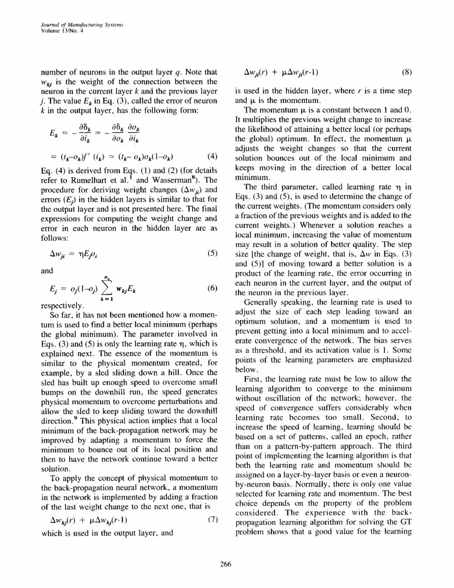
To apply the concept of physical momentum to the back-propagation neural network, a momentum in the network is implemented by adding a fraction of the last weight change to the next one, that is

Awl,j(r ) + IxAwkj(r- 1) (7)

which is used in the output layer, and

Awji(r ) + IXAWji(r - 1) (8)

is used in the hidden layer, where r is a time step and tz is the momentum.

The momentum IX is a constant between 1 and 0. It multiplies the previous weight change to increase the likelihood of attaining a better local (or perhaps the global) optimum. In effect, the momentum IX adjusts the weight changes so that the current solution bounces out of the local minimum and keeps moving in the direction of a better local minimum.

The third parameter, called learning rate ~1 in Eqs. (3) and (5), is used to determine the change of the current weights. (The momentum considers only a fraction of the previous weights and is added to the current weights.) Whenever a solution reaches a local minimum, increasing the value of momentum may result in a solution of better quality. The step size [the change of weight, that is, Aw in Eqs. (3) and (5)] of moving toward a better solution is a product of the learning rate, the error occurring in each neuron in the current layer, and the output of the neuron in the previous layer.

Generally speaking, the learning rate is used to adjust the size of each step leading toward an optimum solution, and a momentum is used to prevent getting into a local minimum and to accel- erate convergence of the network. The bias serves as a threshold, and its activation value is 1. Some points of the learning parameters are emphasized below.

First, the learning rate must be low to allow the learning algorithm to converge to the minimum without oscillation of the network; however, the speed of convergence suffers considerably when learning rate becomes too small. Second, to increase the speed of learning, learning should be based on a set of patterns, called an epoch, rather than on a pattern-by-pattern approach. The third point of implementing the learning algorithm is that both the learning rate and momentum should be assigned on a layer-by-layer basis or even a neuron- by-neuron basis. Normally, there is only one value selected for learning rate and momentum. The best choice depends on the property of the problem considered. The exper ience with the back- propagation learning algorithm for solving the GT problem shows that a good value tbr the learning

266


rate is . 1 and for the momentum is .25; however, this does not mean that there are not other values that may provide better results. Minai and Williams l° investigated the impact of the two parameters on back-propagation learning.

In addition to the above three issues related to back-propagation learning, network size is also critical. If there are not enough hidden neurons, the network is not able to learn the training parts; however, if too many hidden neurons are assigned to a network, the network loses the ability to generalize. 8 The back-propagation neural network learning algorithm and its application to form part families are illustrated in the Appendix.

A back-propagation neural network has some strengths and weaknesses. One weakness is that the performance of back propagation degrades when the size of the problem increases. The second weakness is its slow learning. When the global minima are well hidden among the local minima, the back- propagation network can end up bouncing between local minima without significant improvement, thus causing slow learning.

Nevertheless, back propagation allows expansion of the range of problems to which neural networks can be applied. For example, the back-propagation network can solve the XOR (exclusive-or) logic problem that could not be solved by earlier neural networks. For a more complete description of neural networks, the readers can refer to Hecht-Nielsen 1~ and Wasserman. 8

Neural Network Solution Approach In this section, the back-propagation neural net-

work is applied to produce part families. Figure 4a shows three parts from the same family, iz Their binarized image (12 × 16 pixels) is shown in Figure 4b.

A training set of five standard part shapes (12 × 16 pixels) is shown in Figure 5A. Another set of testing parts has been divided into two types, five parts with partial geometry shown in Figure 5B and 10 parts with distorted geometry shown in Figure 5C. Each part geometry is represented by a 5 × 5 binary image and is used as an input to the back- propagation neural network. Each output neuron of the network represents a distinct part family. The five training parts are assigned to five different part families, that is, the first training part is trained to

Figure 4 Representation of Parts

(a) Three sample parts, (b) pattern (12 x 32 pixels) representing parts in (a)

. . | . . . . .

. . . | . . . . . u ,

. . . . |

. . . . . . n , . | . .

. l . . . n . | . | . . n .

(a)

B)

iiiii::i::iiiii

[i++ . . . . HIii i-,:, ,,,i

""iiiiii i::: ["[[[[ | . . . . .

I : i I l I : l i I | | I I

. . 1 . . . . . . . . . . ¢ . , , . . . . . . . . . . . . . . , iiiiii iiiiii • . . . . . . . . . H -"-'If-" "-'-I'-'-'-

(b) (c) (d) (e)

(P~)

ii:i"iill ii=i:ii iiiiii"+tu!!

i+.::: [i[[i[iiiiiiiiii

(Da)

( D n

iiiiiiiiiiii (Pb) (Pc) (Pd) (Pc)

++++I+,IIHitUH (Db) (De) (Dd) (De)

i!! :!!!!!++ :":+:- . . . . . . . . ;; ;i;i iii l | l - ' - ' - ' | l l l l | l l l l I - ' I |

(Dg) (Dh) (Di) (D j )

Figure 5 20 Part Geometries

(A) Five training parts, (B) five testing parts with partial geometry, (C) 10 testing parts with distorted geometry

be classified as part family 1, the second training part is trained to be classified as part family 2, and so on (see Figure 6).

Determining the number of hidden layers and the number of neurons in each hidden layer is a con- siderable task. Cybenko 13 stated that one hidden

267


Input layer

(193neurons)

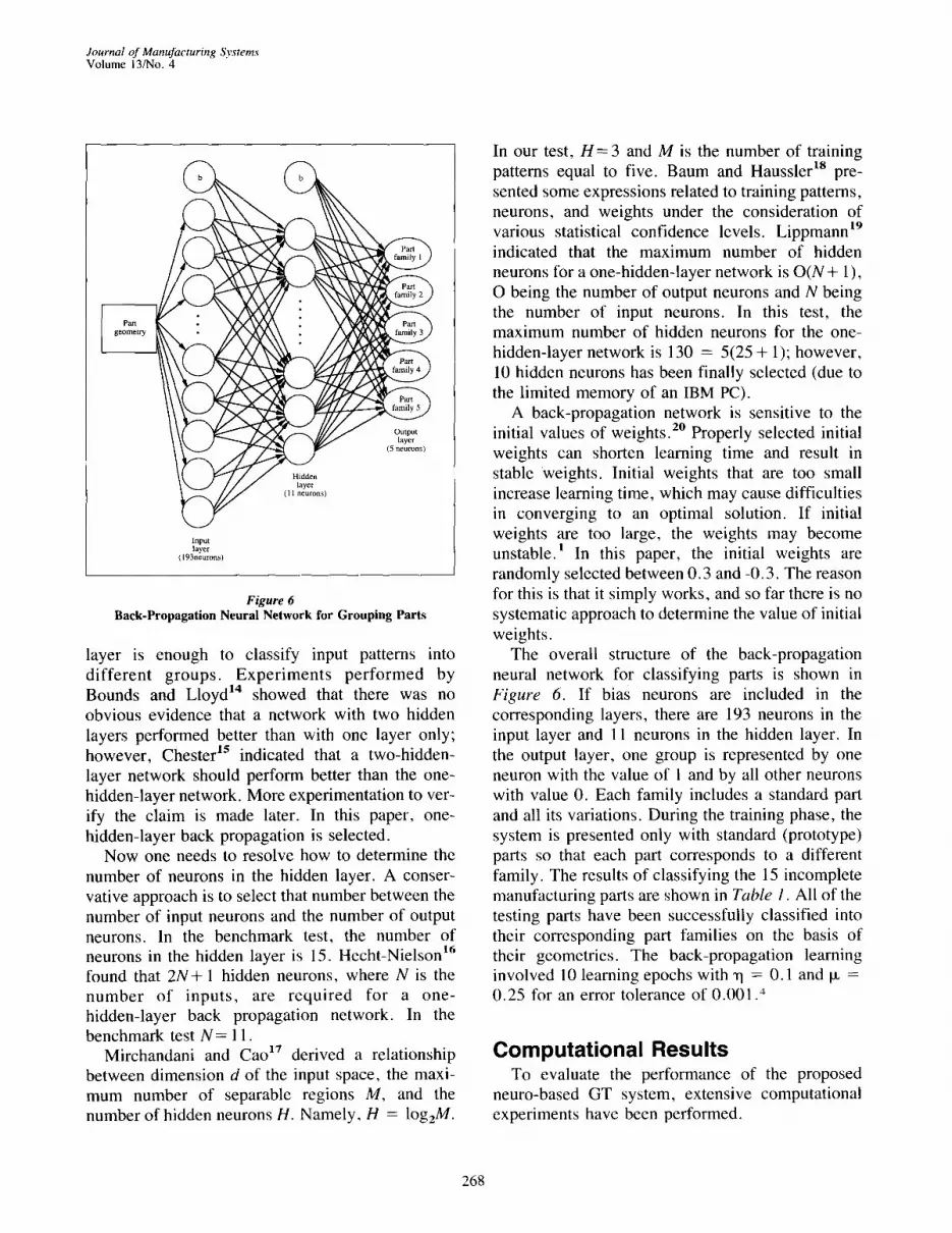
Figure 6 Back-Propagation Neural Network for Grouping Parts

layer is enough to classify input patterns into di f ferent groups. Exper iments pe r fo rmed by Bounds and Lloyd 14 showed that there was no obvious evidence that a network with two hidden layers performed better than with one layer only; however, Chester js indicated that a two-hidden- layer network should perform better than the one- hidden-layer network. More experimentation to ver- ify the claim is made later. In this paper, one- hidden-layer back propagation is selected.

Now one needs to resolve how to determine the number of neurons in the hidden layer. A conser- vative approach is to select that number between the number of input neurons and the number of output neurons. In the benchmark test, the number of neurons in the hidden layer is 15. Hecht-Nielson 16 found that 2N+ 1 hidden neurons, where N is the number of inputs, are required for a one- hidden-layer back propagation network. In the benchmark test N = 11.

Mirchandani and Cao ~7 derived a relationship between dimension d of the input space, the maximum number of separable regions M, and the number of hidden neurons H. Namely, H -- log2M.

In our test, H = 3 and M is the number of training patterns equal to five. Baum and Haussler ~8 presented some expressions related to training patterns, neurons, and weights under the consideration of various statistical confidence levels. Lippmann ~9 indicated that the maximum number of hidden neurons for a one-hidden-layer network is O(N + 1 ), O being the number of output neurons and N being the number of input neurons. In this test, the maximum number of hidden neurons for the one- hidden-layer network is 130 -- 5(25 + 1); however, 10 hidden neurons has been finally selected (due to the limited memory of an IBM PC).

A back-propagation network is sensitive to the initial values of weights. 2° Properly selected initial weights can shorten learning time and result in stable weights. Initial weights that are too small increase learning time, which may cause difficulties in converging to an optimal solution. If initial weights are too large, the weights may become unstable. ~ In this paper, the initial weights are randomly selected between 0.3 and -0.3. The reason for this is that it simply works, and so far there is no systematic approach to determine the value of initial weights.

The overall structure of the back-propagation neural network for classifying parts is shown in Figure 6. If bias neurons are included in the corresponding layers, there are 193 neurons in the input layer and 11 neurons in the hidden layer. In the output layer, one group is represented by one neuron with the value of 1 and by all other neurons with value 0. Each family includes a standard part and all its variations. During the training phase, the system is presented only with standard (prototype) parts so that each part corresponds to a different family. The results of classifying the 15 incomplete manufacturing parts are shown in Table 1. All of the testing parts have been successfully classified into their corresponding part families on the basis of their geometries. The back-propagation learning involved 10 learning epochs with 1] = 0.1 and i x = 0.25 for an error tolerance of 0.001.4

Computational Results To evaluate the performance of the proposed

neuro-based GT system, extensive computational experiments have been performed.

268

Journal of Manufacturing Systems V o l u m e 13/No. 4

Table 1 R e s u l t of Part C l a s s i f i c a t i o n P r o d u c e d by

N e u r o - B a s e d G T System

Training Part Partial Part pa~ geometry family part geometry family

a 1 Pa 1

b 2 Pb 2

c 3 Pc 3

d 4 Pd 4

e 5 Pe 5

Distorted Part Distorted Part part geometry family part geometry family

Da 5 Df 4

Db 5 Dg 3

Dc 3 Dh 2

Dd 5 Di 4

De 5 Dj 1

In the computational experiment, a data set of 60 binary parts (Figure 7) was used in which 10 and 7, respectively, standard parts were selected as the training parts (see Tables 2 and 3). The results of the grouping experiment are interpreted as follows: in a 10-neuron (and 7-neuron) output layer, the output neuron with the value above 0.5 indicates the family membership for the input part. In general, the output neuron with the highest value represents a part family.

Most of the time, the value of the output neurons serves as an indicator of the strength of the part family generated. If the vector of output neurons contains one neuron with a value very close to 1 and the other neurons are very close to 0, one concludes that the system has achieved a high level of dissimilarity among the families. If the output values are very close to each other, a low level of dissimilarity is indicated. In this case, the output neuron with the highest value determines the family an input part belongs to, and this interpretation results in the assignment of parts to the corresponding families as shown in Tables 2 and 3. In ART learning, an input pattern is classified into an output neuron with the highest activation value. The neuron is called a winning neuron.

To generalize the above grouping strategy, the values of output neurons can be used as scores to produce an ordered ranking; in other words, the

II

/

35

I

Figure 7 Sample P a r t s U s e d in E x p e r i m e n t

neuron with the output value closest to 1 can be intepreted as the most likely correct grouping neuron, the next closest value to 1 as the second most likely correct grouping neuron, and so on.

Using the grouping strategy with 15 learning epoches, a 100% satisfactory grouping can be obtained with x I = 0.1, ix = 0.25, and 10 one- hidden-layer neurons for both training and testing parts (see Tables 2 and 3).

Effects of Learning Rate and Momentum As stated previously, back-propagation learning

is influenced by two parameters, -q and ix. Proper values for qq and ix must be determined empirically, and these are problem dependent. It is generally accepted that rl and ix should become smaller over a training time.

Figures 8-10 show the learning curves for three different values of the momentum. It is obvious that the learning algorithm in Figure 10 has difficulty in converging to the expected minimum output error if

269

Journal of Mam4fiwturing Systems Volume 13/No. 4

Table 2 10 Part Families Produced by Neuro-Based GT System

Part family I Part family 2 Part family 3 Part family 4 Part family 5

59

Tab~ 2 conanued

part family 6 part family 7 Part family 8 Par~ family 9 Part family 10

Table 3 Seven Part Families Produced by Neuro-Based GT System Table 3 continued

part family 1 pan family 3 Part family 4 part family 5 Part family 6 Part family 7

270

Journal of Manufacturing Systems' V o l u m e 1 3 / N o . 4

05oi °00, 0,45 1 : learning rate • 0 . 4 0 I R = 0 .05

0.351 ~ ~ • R=0.10 0.30 1 " K . ' ~ . ' . ~ . _ - - - ' - - - R = 0.20

" 0.25 1 "~:~L~X,...~ ~ _ R=°3° 0201

8 0.151 0 . 1 0 1

0.05 1

0.00 I • , - , • ~ . , . , • , - , • , • , ' , • , • , • , • , " , • ,

0 1 2 3 4 5 6 7 8 9 10 11 12 13 14 15 16 M o m e n t u m = 0 .1

0 . 5 0

0 .45

0 . 4 0

0 .35

0 . 3 0

0 .25

0 . 2 0

0 .15

0 . 1 0 1

0 .05 1

0.0[3

~ R = 0.01

8 R = 0.05

R: l e a r n i n g rate • R = 0. l 0

R = 0.20

• i

1 2 3 4 5 6 7 8 9 10 11 12 13 14 15 16 M o m e n t u m = 0 . 5

Figure 8 Learning Curves of the System with Different Learning Rates


0.50 - 1 R = 0 . 0 l

0.45 " ~ . , • R = 0.05

0 . 4 0 - ~ R: learning rate • R = 0.10 0 . 3 5 - . ' - x . - - - . . - - - -

R = 0 . 2 0 0.30 "

0.25 " = ~

0.20 "

0.15 "

0.10 "

0.05 "

0.00

0 1 2 3 4 5 6 7 8 9 10 11 12 13 14 15 16 M o m e n t u m = 0 . 9


IX is large; however, the convergence might be reached if the value of "q is very small. This observation implies that the two parameters have a reverse relationship.

On the other hand, if the value of Ix would be small, then ~q could be large; however, the convergence would be difficult to obtain if values of the two parameters were small. Figure 9 shows that the large value of "q could also be used if the value of Ix was kept at medium. Based on these observations, it is recommended that the ratio of the learning rate and momentum be about 1.5 to 2.5 for the GT application discussed in this paper.

Determination of Network Topology Figure 11 shows the output error (sum-squared

error) versus the number of learning epochs of the neural network for various numbers of one- hidden-layer neurons. In the figure, the number of neurons was changed to 1, 5, 10, 20, and 30 in a single hidden layer.

050

045 "t ~

040-1

035-1

030 -1

025 -I

020 -1

015"1 - - H=I ~- t t=5 • H = I 0

010-1 ¢ I-1=20 "d 005-1 = = t nn ns

000 I • , . , - i - , • , • , • , • , • , • , • , • , . , • i • , - , 0 I 2 3 4 5 6 7 8 9 10 11 12 13 14 15 16

Number of learning epochs

l Figure 11

Learning Curves f o r O n e - H i d d e n - L a y e r Network

For each case shown in Figure 11, the convergence could be obtained regardless of the number of hidden neurons; however, in the case when there is only one hidden neuron, the neural network could not be trained for all 60 parts. As the number of hidden neurons increases, the number of learning epochs needed to train all parts decreases. With more than 10 hidden neurons, the output error decreases rather fast until it reaches 11 learning epochs, and then it converges to the expected minimum output error. The network with 5 hidden neurons learns the shape of 60 parts slowly and does not converge to the expected minimum output error until 15 epochs. Similar results were recorded for different learning parameters. Thus, in our GT application, the number of hidden neurons was fixed at 15.

Figure 12 shows the output values of two testing parts for different hidden neurons in a single hidden layer. The two examples illustrate, first, how the

271


a)

Output value

Training pair

Input Target part family

T

Part family

Hidden neurons

10 20 30

0 0.03 0.03 0.01 1

0 0.11 0.11 0.00 2

0 0.05 0.03 0.00 3

0 0.01 0.00 0.00 4

0 0.22 0.08 0.08 5

1 0.82 0.89 0.92 6

0 0.02 0.00 0.00 7

0 0.05 0.05 0.05 8

0 0.21 0.03 0.01 9

0 0.01 0.01 0.00 10

6 6 6 Ten familie

b)

Output value

Training pair

Input Target part family

W

Part family

Hidden neurons .~

10 20 30

0 0.01 0.02 0.06 1

0 0.56 0.56 0.60 2

.2 0 0 .12 0.01 0.01 3

0 0.05 10.02 0.06 4

0 0.04 0.01 0.01 5

0 0.61 0.61 0.63 6

0 0.52 0.34 0.32 7

0 0.01 0.01 0.00 8

0 0.31 0.30 0.26 9

1 0.68 0.68 0.71 10

10 10 10 ten familie

Figure 12 Output Values of One-Hidden-Layer Network for Two Testing Parts

(a) Example 1, (b) Example 2

family of an input (training or testing) part is determined. By the proposed grouping strategy, the output neuron with the highest value (bold printed) represents the part family of the testing part. Regardless the number of hidden neurons, the two parts were correctly classified into their corresponding part families trained (families 6 and 10 in Tables 2 and 3). Second, the values of the " w i n n e r s " are strenghtened as the number of hidden neurons increases. This shows that the grouping accuracy increases as more hidden neurons are used, and this result is consistent with the analysis of Figure 11.

Figure 12 shows the output values of the parts ment ioned above for different number of hidden layers. Each hidden layer contains 10 neurons. It is apparent from the two examples in the figure that a more definite assignment of an input part is accomplished when multiple hidden layers are used; how-

ever, this takes a long time to train the network due

to the increase of layers. Figure 13 shows that the winner neuron is altered

if more than one hidden layer is used. The input part was assigned to family 10, the same as used in the training, if one hidden layer was employed. The input part, however, was assigned to part family 6 when two or three hidden layers were used. This is most likely due to the use of the proposed grouping strategy because the strategy does not consider " l o s e r s . " For example, in each case of the three different hidden layers in Figure 13b, the value of output neurons 6 and 10 are close to each other. These values were originally regarded as one, the input part was not identified; however, after the grouping decision has been taken, only a larger value of the two output neurons was used to determine the family.

272


a)

Output value Hidden layers

Training pair 1 2 3

Input Target 0 0.03 0.12 0.01 1 part family

0 0.11 0.18 0.11 2

0 0.05 0.12 0.00 3

0 0.01 0.01 0.06 4

0 0.22 0.13 0.01 5

1 0.82 0.91 0.94 6

0 0.02 0.00 0.00 7

0 0.05 0.06 0.00 8

Part family

I 0 0.21 10.00 0.01 9

0 0.01 0.00 0.00 10

6 6 6 ten ramilie.~

b) Output value

Training pair

Input Target 0 part family

Part family

Hidden layers

1 2 3

0.0 0.00 0.00 1

0 .056 0.37 0.60 2

0 .012 0.07 0.08 3

0 0.05 0.01 0.01 4

0 0.04 0.00 0.00 5

0 0.61 0.78 0.78 6

0 0.52 0.51 0.55 7

0 0.01 0.01 0.00 8

0 0.31 0.32 0.41 9

1 0.68 0.70 0.74 10

10 6 6 ten familie.,

Figure 13 Output Values for Two Testing Parts Using a Different Number of Hidden Layers

(a) Example 1, (b) Example 2

Based on above " re laxed" grouping discipline, all input parts (including training and test parts) can be grouped into families satisfactorily. Generally speaking, the network classifies any number of input parts with a 100% certainty if the number of learning epochs is sufficiently large.

Conclusions The research presented in the paper was moti-

vated by the interest in shape recognition using neural networks and its application in group technology.

A number of experiments has been carried out to investigate the performance of the neural network to classify parts based on their shape. The experiments involved investigation of the effects of learning rate "q and momentum coefficient ix and the number of hidden neurons and hidden layers. The strategy for

grouping parts resulted in satisfactory grouping all of training and test parts into families. The findings of the experiments are as follows:

1. The formation result of part families depends on the predetermined number of part families.

2. The learnability of grouping increases as the number of hidden neurons increases.

3. The result of grouping may be different if the number of hidden layers is altered.

4. The relationship between learning rate and momentum coefficient may be reversed.

5. The capability of grouping parts using the proposed grouping strategy is 100% satisfactory.

Acknowledgment This research by the second author has been

partially supported by grant DAAE07-C-R080 from the US Army Tank Automotive Command.

273


References 1. D.E. Rumelhart, G.E. Hinton, and R.J. Williams, "Learning

Representations by Back-Propagation Errors," Nature (n323, 1986), pp533-536.

2. D.E. Rumelhart, G.E. Hinton, and R.J. Williams, "Learning Internal Representation by Error Propagation," Parallel Distributed Processing, Vol. I: Foundations, D.E. Rumelhart, G. E. Hinton, and R. J. Williams, ed. (Cambridge, MA: MIT Press, 1989), pp318-362. 3. A. Kusiak, Intelligent Manufacturing Systems (Englewood Cliffs,

NJ: Prentice Hall, 1990). 4. S. Kaparthi and N.C. Suresh, "A Neural Network System for

Shape-Based Classification and Coding of Rotational Parts," Interna- tional Journal of Production Research (v29, n9, 1991 ), pp 1771 - 1784. 5. A.A.S. Awwal and M.A. Karim, "Machine Parts Recognition

Using a Trinary Associative Memory," Optical Engineering (v28, n5, 1989), pp537-543. 6. S.V. Kamarthi, S.R.T. Kumara, F.T.S. Yu, and I. Ham,

"Neural Networks and Their Application in Component Design Data Retrieval," Journal of Intelligent Manufacturing (vl, n2, 1990), ppl25-140. 7. J. Dayhoff, Neural Network Architectures: An Introduction (New

York: Van Nostrand Reinhold, 1990). 8. P.D. Wasserman, Neural Computing: Theory and Practice (New

York: Van Nostrand Reinhold, 1989). 9, M. Caudill and C. Butler, Naturally Intelligent Systems (Cam-

bridge, MA: MIT Press, 1990). 10. A.A. Minai and R.D. Williams, "Acceleration of Back- Propagation through Learning Rate and Momentum Adaptation," Proceedings of the 4th IEEE Annual International Conference on Neural Networks, Washington, DC (1990), ppi.676-1.679. 1 I. R. Hecht-Nielsen, "Theory of the Backpropagation Neural Net- works," Proceedings of the 3rd IEEE Annual International Confer- ence on Neural Networks, San Diego (1989), ppi.593-I.626. 12. D.D. Bedworth, M.R. Henderson, and P.M. Wolfe, Computer Integrated Design and Manufacturing (New York: McGraw-Hill, 1991). 13. G. Cybenko, "Approximation by Superpositions of a Sigmoidal Function," Mathematics of Control, Signals and Systems (v2, n4, 1989), pp303-314. 14. D.G. Bounds and P.J. Lloyd, "A Multilayer Perceptron Network for the Diagnosis of Low Back Pain," Proceedings of the 2nd IEEE Annual International Conference on Neural Networks, San Diego (1988), ppll.481 -II.489. 15. D.L. Chester, "Why Two Hidden Layer are Better than One?" Proceedings of the 4th IEEE Annual International Conference on Neural Networks, Washington, DC (1990), ppi.265-I.268. 16. R. Hecht-Nielsen, "Kolmogorov's Mapping Neural Network Existence Theorem," Proceedings of the 1st IEEE Annual Interna- tional Conference on Neural Networks, San Diego (1987), pplll. 1 I- Ill. 14. 17. G. Mirchandani and W. Cao, "On Hidden Nodes for Neural Nets," IEEE Transactions on Circuits and Systems (v36, n5, 1989), pp661-664. 18. E.B. Baum, D. Haussler, and H.K. Liu, "What Size Net Gives Valid Generalization'?" Neural Computation (v 1, n2, 1989), ppl 51 - 160. 19. R.P. Lippmann, "An Introduction to Computing with Neural Nets" IEEE Acoustics, Speech, and Signal Processing (April 1987), pp4-22. 20. J.F, Kolen and J.B. Pollack, "Backpropagation is Sensitive to Initial Conditions," Complex Systems (v4, n3, 1990), pp269-280.

Appendix This appendix illustrates how to apply the back-

propagation learning algorithm to group parts into families. The learning algorithm discussed here was o r i g i n a l l y p r e s e n t e d in L i p p m a n n ~9 and Wasserman. 8 The notation used in the algorithm is

explained first. The subscripts i, j , and k represent a neuron i, j , and k in the input layer, hidden layer, and in the output layer, respectively. The letters (plain) i, o, and t represent an input to a layer, an output from a layer, and a target to the output layer, respectively. The same letters typed in bold represent their corresponding vectors. The letters w, n, and E represent the weight, number of neurons, and error, respectively. For example, i i is the input (letter) to the neuron i (subscript) in the input layer; i i is the input vector set to the neuron i the input layer; oj is the output from the neuronj in the hidden layer; n k is a constant denoting the number of neurons in the output layer. The steps of the back-propagation algorithm are presented next.

Step 1 Set the initial values of all weights to small real

numbers. Input the value of the learning rate -q, the value of

the momentum Ix, and the value of the error tolerance 3.

Step 2 Present a training pattern i i to the input layer

neurons and specify the desired target output pattern t k. The vector (i k, tk) is used to describe the training patterns.

Step 3 Calculate

n i

0 : ~ WJ iOi' Oj i=O

= 1/[1 + exp( -o) ]

and n.

ik = ~ i wkJ°J ' ° k = 1 / [ 1 + e x p ( - i k ) ]

j = o

T h e c a l c u l a t i o n i n v o l v e the inputs f r o m the b ias

n e u r o n s i n d i c a t e d by the subsc r ip t O; fo r e x a m p l e ,

o o m e a n s the o u t p u t o f n e u r o n 0 (bias) .

T h e a c t i v a t i o n v a l u e o f a b ias n e u r o n is 1.

S t e p 4

C a l c u l a t e

El, = (tk--Ok)Ok(1--Ok)

274

Input

0 1 1

1 0 I

1 0 0

If E k is less than ~, then stop; otherwise, continue learning, that is calculate

n k

Ey = oy(1-oj) ~ wkjE k k = l

Step 5 Calculate the weight adjustments

Awkj = -qEkoj, Awji : qqEj .o i

Step 6 Repeat steps 2-5 for each training pair (i k, tk).

Step 7 Calculate new weights

wkj(r + 1) = wkj(r ) + Awkj(r ) + p~Awkj(r-1 )

and

wji(r + 1) = wji(r ) + Awji(r ) + txAwji(r-1 )

where r is a time step.

Step 8 Repeat step 7 until the network learns all (it,, tk). Go back to step 3. The concept of grouping parts is illustrated with

a GT problem in Figure 14. The training set for this problem contains three patterns shown in Figure 14a. The solution to the GT problem is shown in Figure 14b. The shadowed portion of a part shape corresponds to 1; the blank portion corresponds to 0. In the course of learning, each of the three parts is classified into a separate part family. The pattern used to represent part family 1 is (1 0 0), in which the value of neuron 1 is 1 and 0 for all other neurons. Similarly, (0 1 0) and (0 0 1) represent part families 1 and 2, respectively. Figure 14c shows the

Output

1 0 0

0 1 0

0 0 1

Part shape

H

0.1 Q ~ 0 . 2

-02 0.2 0.1

Part family

1

2

3


Figure 14 Illustration of GT Problem and Neural Network

(a) Three training patterns, (b) assignment of parts to families, (c) neural network for the GT problem

neural network needed to group the three input parts into part families. The numbers on the connections in the network are the randomly generated initial weights.

Authors' Biographies Dr. Yunkung Chung is an assistant professor in the Department

of Industrial Engineering at Yuan-Ze Institute of Technology in Taiwan. He graduated from the Department of Industrial Engi- neering at the University of Iowa. Dr. Chung is interested in applications of artificial intelligence in manufacturing.

Dr. Andrew Kusiak is professor and chairman of the Department of Industrial Engineering at the University of Iowa. He is interested in engineering design and manufacturing. Dr. Kusiak has authored and edited numerous books, including Intelligent Manufacturing Systems and Concurrent Engineering: Automation, Tools, and Techniques, and published research papers in various journals. He serves on the editorial boards of several journals and is editor-in-chief of the Journal of Intelligent Manufacturing.

275

Grouping parts with a neural network

Documents

Transcript of Grouping parts with a neural network