i

Environmental Independent

Research Project

Variations in Fallow deer (Dama dama) group size

between habitats and seasons.

Richard I. M. Guy

BSc (Hons.) Environmental Conservation

14th March 2013

ii

Abstract:

This study aimed to determine significant links between changes in fallow deer (Dama dama) group size,

the habitat they occupy and the season. A population was chosen on a site with two main habitat types,

woodland and grassland, allowing between habitat comparisons. Data were collected through direct

observation from June 2012 through February 2013. A secondary data source, recorded between

January 2008 and December 2011, supplemented this limited data set and allowed more representative

analysis. Results showed significant differences between habitats, although not as expected based on

literary examples and hypotheses describing habitat selection and use. There were also significant

differences between seasons, largely in keeping with well described patterns from the literature.

Interaction between the two variables was marginal significant, but not conclusive. Additional study is

required to describe the mechanisms creating unexpected habitat use at this location. It is thought that

high levels of disturbance from human activity, and poor structured habitat areas may play a role.

Acknowledgements:

For assisting in the production of this dissertation, and the completion of the project, I would like to

thank:

Dr P. Mitchell, for advice and guidance throughout the project.

The Deer Study and Wildlife Centre, for access to information, use of resources and site specific

expertise, especially Russell Mander (Chairman), Jeanette Lawton (Founder) and Jack Ward

(Volunteer); specifically for permission to use prior records of deer sightings which made this

research topic feasible.

The Trentham Estate; for permission to use the estate as a study site and putting me in touch with

The Deer Study and Wildlife Centre.

Those who have read and commented on drafts at various stages, namely; E. Guy, M. Guy, T. Guy,

G. Guy and Dr Mitchell.

Those who accompanied me on data gathering visits, namely; E. Guy, M. Guy and R. Guy.

C. Mann for advice and assistance regarding the statistical analysis of data.

R. Duncan for advice and assistance with the production of maps.

iii

Contents:

List of Figures, Tables and Graphs

Chapter 1 - Introduction pg. 1

1.1 Deer in the UK

1.2 Ecological Impacts of Deer

1.3 Deer Behaviour

1.4 Factors affecting group size

1.5 Hypotheses explaining social behaviour

1.6 Summary of literature and statement of project aims

1.7 Hypotheses

1.8 Fallow Deer

Chapter 2 - Study Specifics and Methods pg. 15

2.1 Study Population

2.2 Site Description

2.3 Methodology

Chapter 3 - Results pg. 22

Chapter 4 - Discussion pg. 27

4.1 Variation between habitats

4.2 Seasonal variation

4.3 Evaluation of methods

Chapter 5 - Conclusion pg. 34

Bibliography pg. 36

Figure Sources pg. 39

Appendices pg. 40

Appendix 1: Summarised Mean Group Size Data tables and graphs (Seasonal)

Appendix 2: Tables of means used in SPSS analysis

Appendix 3: Seasonal variation in group size between habitats

Appendix 4: Seasonal habitat use

iv

List of Figures, Tables and Graphs:

Chapter 1 - Introduction

Figure 1.1 - Fallow Deer Distribution Map, Staffordshire pg. 8

Figure 1.2 - Fallow Deer Distribution Map, UK pg. 11

Figure 1.3 - Fallow Buck and Fawn (Common Colouration), Richmond Park, London pg. 12

Figure 1.4 - Mixed Colour Herd of Fallow Does, Cannock Chase, Staffordshire pg. 12

Table 1.1 - Table of variables affecting group size of deer; their effects and interactions pg. 9

Chapter 2 - Study Specifics and Methods

Figure 2.1 - Location of study site within UK pg. 15

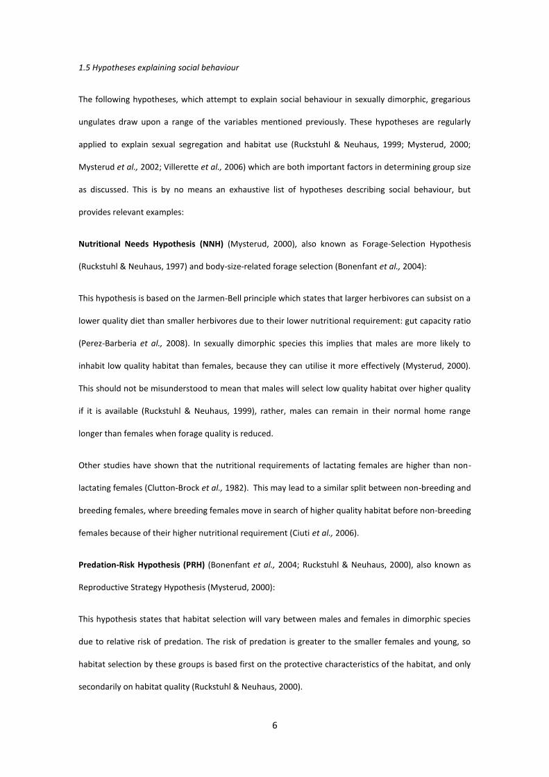
Figure 2.2 - Study Area Map pg. 16

Figure 2.2a (Overlay) - Study Methods descriptive overlay Overlay to pg. 16

Chapter 3 - Results

Table 3.1 - Table of Results (Two-way repeated measures ANOVA) pg. 23

Table 3.2 - Mean group size by habitat pg. 23

Table 3.3 – Woodland-Grassland differences in mean group size pg. 24

Table 3.4 - Table of results (Pair-wise comparison test - Seasons) pg. 25

Table 3.5 - Seasonal variation in mean group size pg. 25

Graph 3.2 – Habitat Mean Group Size pg. 23

Graph 3.3 – Woodland-Grassland differences in mean group size pg. 24

Graph 3.5 – Seasonal variation in mean group size pg. 25

Chapter 4 - Discussion

Graph 4.1 - Average number of groups seen per sector on each visit pg. 31

Graph 4.2 - Average number of deer seen per visit pg. 32

1

Chapter 1: Introduction

1.1 Deer in the UK

There are six species of deer living wild in the UK. Red Deer, Cervus elaphus, and Roe Deer, Capreolus

capreolus, have both been present since the last glacial retreat (Prior, 1987b; Maroo & Yalden, 2000).

The four remaining species: Fallow Deer, Dama dama, Sika, Cervus nippon, Chinese Water Deer,

Hydropotes inermis, and Reeves Muntjac, Muntiacus reevesii, have been introduced (Prior, 1987b;

Putman & Langbein, 2003). With the lack of natural predators deer numbers have increased rapidly over

the last two centuries, now presumed as high or higher than any time since the glacial retreat (Prior,

1987b).

While population figures are very difficult to establish with any accuracy, Battersby (2005) estimated

that collectively, there are approximately 1,018,000 individual deer within the mainland UK, with the

native Red and Roe by far the most abundant (355,500 and 501,000 respectively). The British Deer

Society, in the most recent British Deer Survey (2011), calculated that the distribution of all species has

extended by between 5.9% and 18.4% (mean: 10.6%) between 2008 and 2011, implying that this

number is increasing (Hailstone, 2012).

1.2 Ecological Impacts of Deer

Populations of these sizes, growing at these rates, present potential problems. As large herbivorous

mammals, deer can do significant damage to vegetation communities. These may be agricultural crops

(Wywialowski, 1996; Cote et al., 2004), forestry plantations (Prior, 1987a; Reimoser, Armstrong &

Suchant, 1999; Quine, Shore & Trout, 2004), conservation habitats (Gill, 2000; Fuller, 2001; Pellerin,

Huot & Cote, 2004; Sage et al., 2004; Symes & Currie, 2005) or domestic areas (Chapman & Harris,

1996). Researchers have been attempting to understand the impacts of this damage on habitats and

other species for some time. While the effects are being researched, deer populations are also

managed; to maintain healthy deer populations but also to reduce the financial losses of agricultural

and commercial forestry companies (Gordon, Hester & Festa-Bianchet, 2004; MacMillan & Leitch, 2008).

2

The type of impact depends upon the species of deer. Herding species such as Red deer, Fallow deer and

Sika can form large aggregations, which together in arable agriculture areas can cause huge financial

damage to a crop in a very short space of time (Griffith, 2011). Similarly large groups can also cause

significant damage in woodland, both commercial and conservation (Gill & Beardall, 2001).

In contrast, the damage done by solitary species such as Roe or Muntjac may be less significant in

overall scale but more significant to specific habitats or species. Cooke (1997) describes how the

Bluebell, Hyacinthoides non-scripta, is selected by the Muntjac as a favoured food item. As a result, in

some bluebell woods where Muntjac are present, stocks of this native flower are being severely affected

(Cooke & Farrell, 2001). One study found that 98% of bluebell inflorescences in an area of woodland

were eaten (Chapman & Harris, 1996).

Roe deer can also seriously damage woodland areas, particularly young conifer plantations or coppice

areas, where regrowth shoots are browsed and coppice stools can be killed (Fawcett, 1997). Browse

(leaves and twigs) forms a large part of their diet, especially during spring and summer. The bucks also

‘fray’ trees with their antlers as territorial marking behaviour (Fawcett, 1997).

In some conservation woodland, natural regeneration can be completely supressed, leading to reduced

floral diversity (Kirby, 2001), but also altered woodland structure over time (Fuller, 2001), indirectly

affecting a range of species which rely on specific habitat characteristics (Gill & Fuller, 2007; Newson et

al., 2012). However, some areas benefit from a low level of grazing, as this can create a more diverse

ground flora composition and structure (Kirby, 2001; Watkinson et al., 2001). The level of damage

considered as ‘acceptable’ is heavily dependent on use of the land. Commercial land managers generally

accept far lower damage levels before seeking mitigation through deer management (Prior, 1987a).

Bonenfant et al (2005) describes the concept of an economic carrying capacity, above which the

financial damage is unsustainable. Fencing and culling are the two most commonly employed methods

of deer control (Anon., 2011; Griffiths, 2011).

3

1.3 Deer Behaviour

Levels of damage are often used to determine the sustainability of deer densities (Morellet et al., 2007).

However, it is not always the density of the population that is the causal factor in levels of damage

(Griffiths, 2011). There are many different factors affecting the behaviour of deer species. Population

density, species, the type of habitat, forage availability and quality, and time of year all affect the

behaviour of the deer, and therefore the impacts of those deer on their habitat (Prior, 1987a).

One factor that is particularly significant in determining impacts on a habitat is the size of the groups

that are formed. Larger groups will obviously do more damage than smaller groups, but large groups do

not always mean high density (Reimoser et al., 1999; Scott, Bacon & Irvine, 2002). Some species are

more likely to form groups than others, for a variety of reasons, but at a landscape scale, the density

may remain relatively low (Griffiths, 2011). It is this particular behavioural trait that is the topic of this

study.

Grouping behaviour is very common among a range of animals. This social behaviour is particularly

common among prey species, where grouping reduces predation risks to the group as a whole and the

individuals who comprise it (Manning & Dawkins, 2012). The successful detection of an approaching

predator, and therefore survival, increases with the number of vigilant individuals (Fawcett, 1997).

Shared vigilance allows each individual to engage in productive activities for a proportionately higher

amount of time (Elgar, 1989). Other benefits include a reduced risk of being selected for predation, due

to the increased choice of potential prey (Morgan & Godin, 1985). This strategy is utilised by a wide

variety of species including invertebrates (Uetz et al., 2002), fish (Morgan & Godin, 1985), birds and

mammals (Elgar, 1989). Many ungulate species exhibit grouping behaviour including Red deer (Clutton-

Brock, Major & Guinness, 1985), Fallow deer (Apollonio et al., 1998), Moose, Alces alces gigas, (Molvar

& Bowyer, 1994), and White-tailed deer, Odocoileus virginianus, (Sorensen & Taylour, 1995). Other deer

species do not exhibit this trait of aggregation, remaining solitary or only forming small, often family

based, groups (Anon., 2011), but this study will focus on gregarious species.

Sexual segregation is another social behaviour prevalent among deer (Mysterud, 2000; Villerette et al.,

2006). Sexual segregation refers to the spatial or associational separation of adult males and females

4

(Mysterud et al., 2002). As with grouping behaviour, there are many factors that affect this behaviour

and it is exhibited differently from species to species (Ruckstuhl & Neuhaus, 2000).

In some circumstances this segregation is only social; the males will remain within the same

geographical area as the females, but will not associate with them (Langbein & Chapman, 2003). The

males may remain solitary or in some species, such as Red and Fallow deer, form bachelor herds

(Chapman & Chapman, 1997; Putman & Langbein, 2003). During the breeding season, these bachelor

herds will break up and the individual males will seek out receptive females (Borkowski & Pudelko,

2007). In some cases, males will remain with females for extended periods before separating until the

following breeding season (Langbein & Chapman, 2003). In other cases, the segregation is also

geographical; males may move into completely different areas, not overlapping with female territory at

all (Langbein & Chapman, 2003; Borkowski & Pudelko, 2007). In these cases the males will move back

into female areas in time for the mating season. In these species, adult females will commonly form

groups comprising other females and their young (Bonenfant et al., 2005).

Sexual segregation is a factor in determining potential group size. The mating season, when females

come into oestrous, is the time of year when the largest groups of gregarious deer species are usually

seen, not only because the males join the females, but often because multiple female groups will gather

at mating sites (Prior, 1987b; Chapman & Chapman, 1997).

1.4 Factors affecting group size

The size, demographic composition and spatial locality of aggregations are dictated by a range of social,

biological and ecological factors. Both the size and demographic composition of groups are largely

affected, at certain times of year, by the exhibition of sexual segregation as discussed above. Variation

between seasons is another major factor in determining social behaviour (Sorensen & Taylour, 1995).

There are two main factors which vary with the season. The first element of seasonality is the effect of

the annual breeding cycle, which is correlated with seasonal change; the second relates to habitat and

food availability. Generally speaking for gregarious deer in the UK, the mating period or ‘rut’ coincides

5

with late autumn and parturition, or the fawning period, falls in early summer (Chapman & Chapman,

1997). In the rut, as mentioned with regards to sexual segregation, large aggregations may be seen

(Putman, 2000).

Dependent on species, females will either remain as a group (e.g. Fallow, Langbein & Chapman, 2003) or

separate after the rut (e.g. Sika, Putman, 2000). However, even in gregarious species, as the parturition

season approaches, pregnant does will leave the group to find a suitable site to give birth. The most

common time to see females of these species on their own coincides with this fawning period (Chapman

& Chapman, 1997). These females leave their young in a sheltered spot, returning regularly to suckle

(Langbein & Chapman, 2003; Ciuti et al., 2006). Barren females and yearlings remain in groups, albeit

smaller in size, during this time (Bonenfant et al., 2005; Ciuti et al., 2006).

The second variable, seasonal changes in habitat characteristics and food availability, affects grouping

behaviour in a wide range of ways (Mysterud et al., 2000; Sims et al., 2007). This makes ascertaining

which variable is most significant very difficult; it also makes it impractical to discuss all factors here.

High-productivity habitats can support higher population densities because the nutritional value of the

vegetation is correspondingly higher (Ruckstuhl & Neuhaus, 2000). This is not a solely seasonal variable,

relying also on soil type, precipitation levels, altitude, aspect and others (Rose, 2004). It is generally

recognised that higher productivity habitats will support a higher population, and therefore, higher

group sizes of gregarious species (Apollonio et al., 1998; Yokoyama & Shibata, 1998).

If these areas are open then large groups may congregate to take advantage of the resources, while

gaining the anti-predator advantages of feeding in a group (Prior, 1987a). In equally productive, but

more closed structural habitats, density may be similar; group size may be smaller however, because the

protective characteristics of the habitat offset the need for the protection of a group (Langbein &

Chapman, 2003). This commonly means that in winter, when very little ground vegetation is present in

any habitat, group sizes tend to be larger (Apollonio et al., 1998; Chapman & Chapman, 1997).

6

1.5 Hypotheses explaining social behaviour

The following hypotheses, which attempt to explain social behaviour in sexually dimorphic, gregarious

ungulates draw upon a range of the variables mentioned previously. These hypotheses are regularly

applied to explain sexual segregation and habitat use (Ruckstuhl & Neuhaus, 1999; Mysterud, 2000;

Mysterud et al., 2002; Villerette et al., 2006) which are both important factors in determining group size

as discussed. This is by no means an exhaustive list of hypotheses describing social behaviour, but

provides relevant examples:

Nutritional Needs Hypothesis (NNH) (Mysterud, 2000), also known as Forage-Selection Hypothesis

(Ruckstuhl & Neuhaus, 1997) and body-size-related forage selection (Bonenfant et al., 2004):

This hypothesis is based on the Jarmen-Bell principle which states that larger herbivores can subsist on a

lower quality diet than smaller herbivores due to their lower nutritional requirement: gut capacity ratio

(Perez-Barberia et al., 2008). In sexually dimorphic species this implies that males are more likely to

inhabit low quality habitat than females, because they can utilise it more effectively (Mysterud, 2000).

This should not be misunderstood to mean that males will select low quality habitat over higher quality

if it is available (Ruckstuhl & Neuhaus, 1999), rather, males can remain in their normal home range

longer than females when forage quality is reduced.

Other studies have shown that the nutritional requirements of lactating females are higher than non-

lactating females (Clutton-Brock et al., 1982). This may lead to a similar split between non-breeding and

breeding females, where breeding females move in search of higher quality habitat before non-breeding

females because of their higher nutritional requirement (Ciuti et al., 2006).

Predation-Risk Hypothesis (PRH) (Bonenfant et al., 2004; Ruckstuhl & Neuhaus, 2000), also known as

Reproductive Strategy Hypothesis (Mysterud, 2000):

This hypothesis states that habitat selection will vary between males and females in dimorphic species

due to relative risk of predation. The risk of predation is greater to the smaller females and young, so

habitat selection by these groups is based first on the protective characteristics of the habitat, and only

secondarily on habitat quality (Ruckstuhl & Neuhaus, 2000).

7

Under this hypothesis non-breeding females again occupy a ‘middle ground’, being at higher risk than

males, but lower than females with young. They may therefore occupy a different habitat niche, being

more protective in nature than that selected by females with fawns, but less than male selected areas.

This assumption was supported by Ciuti et al. (2006) who found that this was the case in a Fallow deer

population in Italy.

While many ungulates have co-evolved with predators and therefore developed these and other anti-

predator strategies, it is unclear to what extent these strategies are still exhibited in areas where natural

predators have long been removed (Apollonio et al., 1998).

This hypothesis conflicts with the NNH in some scenarios, suggesting females may select lower quality

but safer habitat than males in contrast to seeking higher quality as the NNH suggests.

Incisor-Breadth Hypothesis (IBH) (Mysterud, 2000):

This hypothesis is related to the NNH and is also based upon the Jarmen-Bell principle. It is a limited

scope hypothesis, applying only when forage availability is very low. It states that females are more

competitive than males in these conditions because their smaller body size relates to a lower incisor

breadth, allowing them to exploit limited food sources, such as grazing on areas with a reduced sward

height, more efficiently than males (Mysterud, 2000).

1.6 Summary of literature and statement of project aims

The literature discussed in this review suggests that there are many factors which collectively produce

considerable variation in the social behaviour of gregarious ungulates. Table 1.1 attempts to summarize

these data while also illustrating the inter-connectivity between these variables. With so many variable

factors, making accurate predictions of expected group size in a given area is unfeasible, but some

general assumptions can be applied when all the variables are properly considered.

8

Aff

ect

ed

by:

Has

eff

ect

on

:

Seas

on

(C

limat

e)

Spri

ng

- M

id-s

ized

gro

up

s

Sum

mer

- S

ma

ller

gro

up

s

Au

tum

n -

La

rge

Gro

up

s

Win

ter

- La

rge

Gro

up

s

Ha

bit

at

stru

ctu

re,

Foo

d a

vail

ab

ilit

y /

qu

ali

ty,

Sta

ge o

f b

reed

ing

cycl

e

NN

H

PR

H

Bo

rko

wsk

i &

Pu

del

ko, 2

00

7,

Sore

nse

n &

Ta

ylo

ur,

19

95

,

Hab

itat

Typ

eW

oo

dla

nd

- S

ma

ller

gro

up

s

Op

en -

La

rger

gro

up

s

Foo

d a

vail

ab

ilit

y /

qu

ali

ty,

Ha

bit

at

stru

ctu

re

NN

H

PR

H

Ap

oll

on

io e

t a

l., 1

99

8,

Bo

rko

wsk

i &

Pu

del

ko, 2

00

7,

Vil

lere

tte

et a

l., 2

00

6

Hab

itat

Str

uct

ure

Clo

sed

, Pro

tect

ive

- Sm

all

gro

up

s

(pre

do

m. D

oes

an

d f

aw

ns)

Op

en -

La

rger

gro

up

s (p

red

om

. Ma

le

an

d n

on

-bre

edin

g d

oes

)

Sea

son

,

Ha

bit

at

Typ

e

Foo

d a

vail

ab

ilit

y /

qu

ali

ty,

PR

H

Ap

oll

on

io e

t a

l., 1

99

8,

Bo

rko

wsk

i &

Pu

del

ko, 2

00

7,

Vil

lere

tte

et a

l., 2

00

6,

Ru

ckst

uh

l &

Neu

ha

us,

20

00

Foo

d a

vaila

bili

ty /

qu

alit

y

Go

od

qu

ali

ty -

Fem

ale

an

d y

ou

ng

bia

s

Po

or

qu

ali

ty -

Ma

le b

ias

Hig

h a

vail

ab

ilit

y -

Ma

le b

ias

Low

ava

ila

bil

ity

- Fe

ma

le b

ias

Sea

son

,

Ha

bit

at

Typ

e,

Ha

bit

at

Stru

ctu

re

Bre

edin

g st

atu

sN

NH

IBH

Ap

oll

on

io e

t a

l., 1

99

8,

Bo

rko

wsk

i &

Pu

del

ko, 2

00

7,

Yoko

yam

a &

Sh

ibu

ta, 1

99

8

Bre

ed

ing

stat

us

(ad

ult

s)

All

: Ga

ther

fo

r ru

t

Ma

le: S

exu

all

y se

greg

ate

d f

rom

fem

ale

s m

ost

of

yea

r,

Fem

ale

(B

reed

ing)

: Sp

lit

du

rin

g

faw

nin

g

Fem

ale

(B

arr

en):

Sta

ys i

n g

rou

ps

du

rin

g fa

wn

ing

Age

,

Foo

d a

vail

ab

ilit

y /

qu

ali

ty

PR

H

NN

H

Ciu

ti e

t a

l., 2

00

6,

Mys

teru

d e

t a

l., 2

00

2,

Ru

ckst

uh

l &

Neu

ah

us,

20

00

Stag

e o

f B

ree

din

g

Cyc

le (

Do

es

&

Faw

ns)

Faw

nin

g: D

oes

so

lita

ry

Lact

ati

on

: Do

es g

ath

er w

hen

fa

wn

s

act

ive

Ru

t: A

ll a

ggre

gate

to

bre

ed

Pre

gna

ncy

: Do

es r

ema

in i

n g

rou

ps

Sea

son

PR

H

Bo

nen

fan

t et

al.,

20

05

,

Ciu

ti e

t a

l., 2

00

6,

Clu

tto

n-B

rock

et

al.,

19

82

,

Age

Faw

ns

- R

ema

in w

ith

mo

ther

Yea

rlin

gs -

Fem

ale

s re

ma

in w

ith

do

es,

pri

cket

s jo

in a

du

lt m

ale

s

Ad

ult

s -

gro

up

wit

h s

am

e se

x

Bre

edin

g st

atu

sP

RH

IBH

Mys

teru

d e

t a

l., 2

00

0,

Sore

nse

n &

Ta

ylo

ur,

19

95

- N

NH

: Nu

trio

na

l N

eed

s H

ypo

thes

is

- P

RH

: Pre

da

tio

n R

isk

Hyp

oth

esis

- I

BH

: In

ciso

r B

rea

dth

Hyp

oth

esis

Hyp

oth

esis

Ab

bre

via

tio

ns:

Table 1.1 - Table of variables affecting group size of deer; their effects and interactionsIn

tera

ctio

n w

ith

oth

er

vari

able

s:

Var

iab

le:

Effe

cts

on

Gro

up

siz

e:

Re

late

d

Hyp

oth

ese

s:Sp

eci

fic

Lite

ratu

re S

ou

rce

(s):

9

Fig 1.1 - Fallow Deer Distribution,

Staffordshire (Source: NBN [Online], 2013a)

© Crown copyright and database rights 2011

Ordnance Survey [100017955]

Key:

- 2km square with Fallow deer

recorded

- Staffordshire county boundary

Scale:

0km 10 20km N

This study will aim to test two of these general assumptions, the effect of habitat type and season, on

group sizes. Also attempting to establish any significant interaction between these two variables. The

study must be conducted in Staffordshire, ideally close to Stoke-on-Trent. Red, Fallow, and Roe deer and

Muntjac are all present in Staffordshire. Roe and Muntjac are not gregarious species, are not common in

Staffordshire and are not found in the required locality. Red deer exhibit the required grouping

behaviour, but are not present in the area immediately accessible to Stoke-on-Trent. Fallow deer are

gregarious, and can be found in this area (see Fig. 1.1). The following hypotheses of gregarious cervid

behaviour will be tested using Fallow deer as a representative species.

10

1.7 Hypotheses

Null Hypothesis 1:

There is no significant difference in the average group size of Fallow deer using different

habitats. (Habitat types: Woodland, Grassland).

Alternative:

The average size of Fallow deer groups is significantly larger in grassland than in woodland.

Null Hypothesis 2:

There is no significant difference in the average group size of Fallow deer in different seasons

(Seasons: Spring, Summer, Autumn, Winter).

Alternative:

There is a significant difference in the average group size of Fallow deer in different seasons.

Null Hypothesis 3:

There is no significant link between season and habitat use in determining group size in Fallow

deer. (Season: Spring, Summer, Autumn, Winter; Habitat Type: Woodland and Grassland).

Alternative:

There is a significant link between season and habitat use in determining group size in Fallow

deer.

11

Fig 1.2 - Fallow Deer Distribution, UK (Source: NBN [Online],

2013b)

Red squares indicate Fallow Deer Present - 10km Resolution

1.8 Fallow Deer

As Fallow deer have been selected as a representative and feasible subject for this study, below is a brief

review of Fallow Deer biology and ecology, related to what has been discussed regarding social

behaviour.

Native to the eastern Mediterranean, Fallow deer have been introduced in many countries globally and

extensively throughout Europe (Chapman & Chapman, 1997). In the British Isles, there is evidence of the

presence of Fallow deer prior to the last glaciation, but they did not naturally recolonize after the glacial

retreat (Prior, 1987b). Originally re-introduced

to Britain by the Romans, they did not

establish wild populations and were absent

from the record again until re-introduced by

the Normans in the 12th

century (Fletcher,

2010). Fallow deer have been present in feral

populations of varying sizes, alongside captive

populations since this time (Chapman &

Chapman, 1997). They are now considered to

be naturalised to the British Isles (Acevedo et

al., 2010). They are the most common of the

introduced species, both in abundance and

distribution (see Figure 1.2) (Aebischer, Davey,

& Kingdon, 2011). Battersby (2005) estimated

their population in 2005 at 108,000 individuals

in the mainland UK, and this is likely to have

increased. Between 2008 and 2011 their range

expanded by 9.4% (Hailstone, 2012).

N

0km 100 200km

12

Fig 1.3 - Fallow Buck and Fawn (Common Colouration), Richmond

Park, London. Source: Author, Oct. 2012

Fig 1.4 - Mixed Colour Herd of Fallow Does (Black and Common

Colouration), Cannock Chase, Staffordshire

Source: Author, June 2011

Appearance

Fallow are a relatively large deer species in the

UK context; adult males’ average 53-90kg in

weight with adult females (exhibiting sexual

dimorphism) averaging 35-55kg (Langbein &

Chapman, 2003). This is smaller than Red deer,

similar to Sika, and significantly larger than the

other deer species (Anon., 2011).

Fallow deer exhibit a range of pelage variants.

There are four main varieties, known as

common, ‘menil’, black & white (Langbein &

Chapman, 2003) (See Fig 1.3). It is believed this

variety is as a result of generations of breeding in

deer parks with restricted genetic diversity

leading to inbreeding. All varieties interbreed

freely in the wild and many populations consist

of several or all colour variants (Chapman &

Chapman, 1997) (See Fig. 1.4).

Reproduction

Fallow are a polygynous species; males compete during the rut (normally late October - November

(Langbein & Chapman, 2003)) to gain dominance, giving them access to receptive does (Prior, 1987b).

Competition may be at rutting stands where does are herded and defended by a dominant buck or a

transient group followed and protected by a dominant buck (Langbein & Chapman, 2003). Dominance

will change through the rutting period as bucks are challenged and defeated or grow weary from the

exertion of maintaining their harem (Chapman & Chapman, 1997).

13

Fawns are born in June or early July; single births are the norm, though twin and even triple foetuses

have been observed (Chapman & Chapman, 1997; Langbein & Chapman, 2003). For the first few weeks

fawns are left alone in cover. The doe does not move far from the hiding place, Chapman and Chapman

(1997) suggests never further than 200-300m which is perceived as close enough to hear a distress call.

This is supported by Ciuti et al. (2006) who found that summer home range sizes of calving does were

significantly smaller than non-calving does. The mother returns regularly to suckle, Chapman &

Chapman (1997) quote 4 hour intervals between visits. When the fawn is strong enough (approx. 3

weeks (Langbein & Chapman, 2003)) it will join the mother in feeding and moving, and the pair will then

join with other does, fawns and sub-adults of both sexes (Apollonio et al., 1998).

Habitat selection and use

Fallow deer are most commonly associated, across both their natural and introduced range, with

mature broadleaf woodland (Appollonio et al, 1998; Langbein & Chapman, 2003). They also use

agricultural land with small patches of woodland, coniferous plantations, marshes and grassland

(Borkowski & Pudelko, 2007; Chapman & Chapman, 1997; Langbein & Chapman, 2003). Despite this

association, woodlands are used predominantly for shelter with feeding taking place on rides or glades

within the woodland or on adjacent land (Langbein & Chapman, 2003). Borkowski & Pudelko (2007)

found that habitat use was not proportional to habitat availability, illustrating bias in habitat selectivity,

corroborating the earlier literature evidence.

Feeding Habits

Feeding is by ‘preferential grazing’: grazing on forage sources specifically selected as higher value

(Chapman & Chapman, 1997). The preferred vegetation type alters with availability through the year.

When available, grass species form the majority of the diet (Borkowski & Pudelko, 2007); 60 - 95% from

spring to autumn (Langbein & Chapman, 2003). Despite this significant preferential selection of grass,

Fallow deer are capable of utilising a wide range of other food sources when grass is unavailable or

14

nutritionally insufficient; these include acorns, beech mast, apples, cereal crops, rushes and leaves and

twigs of a variety of trees and shrubs and others (Langbein & Chapman, 2003).

Social Behaviour

Fallow deer are both gregarious, and exhibit sexual segregation similar to other ungulate species

mentioned (Chapman & Chapman, 1997; Mysterud, 2000; Ciuti, et al, 2006). Large groups of up to 200

may be observed in areas where population density and habitat type are favourable (Langbein &

Chapman, 2003). Large groups such as these are transient, with individuals or smaller groups frequently

joining or leaving the group (Chapman & Chapman, 1997). Chapman & Chapman (1997) suggest that the

largest group sizes will be seen around the rut, with the smallest group sizes observed in the summer

around the time of fawning (Supported by Apollonio et al., 1998, and Ciuti et al., 2006).

Home range size effects social integration and aggregation. Borkowski & Pudelko (2007) found during a

study in Poland, that the average annual home range of adult males was 9.75km2 compared to 2.1km

2

for adult females, 4.5 times larger. The difference between breeding and non-breeding female range

sizes, discussed by Ciuti et al. (2006), has already been mentioned (see: Section 1.8, Reproduction, pg.

10).

Finally, several studies indicate the effect of habitat in determining group size. Langbein & Chapman

(2003) suggest that average Fallow deer group sizes in open habitats are up to four times larger than in

woodland. Apollonio et al. (1998) observed ‘a marked tendency to form larger groups as the habitat

becomes more open’ (pg. 230).

15

Chapter 2: Study Specifics and Methods

2.1 Study Population

The subject of the study was a population of Fallow

Deer (ca. 60–100; R. Mander, pers. comm.) at the

Trentham Estate in Staffordshire, south of Stoke-on-

Trent (see Figure 2.1). Fallow deer are the only

species of deer present on the estate, and the herd

exhibits the ‘black’ pelage colouration. This trait is

maintained through selective culling (J. Lawton, pers.

comm.).

2.2 Site Description (See Figure 2.2):

The estate, ca. 295 hectares / 725 acres total area

(Anon., Undated - a), includes a variety of land

uses. A large portion of the estate contains a

number of commercial properties and areas including a garden centre, hotel, retail village and the

Trentham Gardens and Monkey Forest tourist attractions and Trentham Lake. This area is fenced off

from access by the deer. The remaining area, where this studies observation were recorded, is

comprised of a mixture of habitat types, including a river corridor, small marsh area, un-grazed

meadows and a range of mixed woodlands. An area (45 hectares, 111 acres) of the woodland on the

estate is designated as a SSSI (Anon., Undated - b).

The deer herd is wild, not a park herd; there are no physical restraints to their movements on or off the

estate. Some local man-made features unintentionally limit movement to a degree. The M6 to the west,

Figure 2.1 - Location of study site within the UK.

- Study Site

16

17

separated by ca. 500m of mixed agricultural land, presents a barrier. Observations by local researchers

suggest migration across the M6 has reduced over the last few decades (J. Lawton, pers. comm.), and is

currently low. Observations during the study support this; deer were seen using the area between the

estate boundaries and the M6 only twice during the study period. On these occasions forestry

operations were underway on the estate. This disturbance may have altered normal habitat use. Use of

fields in this area as grazing pasture for sheep may also affect the favourability of this area; deer may be

reluctant to use land occupied or recently vacated by domestic livestock (DeGabriel et al, 2011; Prior,

1987a).

The A34 dual-carriageway to the east presents another barrier, although does not prevent movements

entirely. Deer were seen crossing this road twice during the study period. To the north, deer fencing has

been installed to prevent movement of deer onto a golf course. To the south a residential area,

Tittensor village, borders the estate. None of these features are wholly restrictive but together result in

a moderately stable population.

Supporting this assumption is the low numbers of non-black pelage individuals observed. Another

population of fallow deer - of common colouration - reside a short distance to the south in Tittensor

woods (J. Lawton, pers. comm.). Only one common coloured individual, a Pricket, was seen during the

study period, suggesting low levels of immigration, and, in return, emigration.

One goal of the deer management plan on the estate is to reduce or prevent over-grazing in the

woodland areas. The area of woodland designated as SSSI is currently designated as ‘unfavourable

recovering’ (Bickerton, 2013). Reasons for this assessment include the lack of ground flora diversity and

very low levels of natural-regeneration of tree species as a result of over-grazing. Currently in woodland

areas the ground vegetation is dominated by bracken, Pteridium aquilinum, and in some areas,

Rhodendedron ponticum (Bickerton, 2013); neither species are eaten by the deer (G. Williamson, pers.

comm.).

18

2.3 Methodology:

2.3.1 Data Collection

The data required for analysis were gathered through primary and secondary methods. First-hand

observations were made from June 2012 through February 2013. On average, three or four visits to the

study site were made per month. Initial plans of visiting twice a week were made impractical by a

number of factors, the temporary closure of parts of the estate during the normal survey time window

due to culling activities was particularly restrictive. Each visit began within 2 hours of dawn and a set

circular route was walked around the estate with some variations allowing for confirmation of distant

sightings. The direction and start point of the route was altered regularly to allow all areas to be

surveyed at a range of times (see Fig 2.2a).

For the purposes of this study the estate was considered in three sectors; two woodland sectors

(‘Monument Hill’ (MH) and ‘Kings Wood’ (KW)) and one predominantly pastoral sector (‘A34 Meadows’

(AM)). The set route allowed observation of the highest possible percentage of each sector, allowing for

site topography and visibility due to vegetation, and covered approx. 4.6 miles (7.5 km) (See Figure

2.2a). Several site visits were made previous to the data gathering period to assess areas where deer

were likely to be seen, both through identification of sign (Bang & Dahlstrøm, 2001) and through

conversations with estate staff. Dependent on sightings, each visit took 2 - 3 ½ hours. The extra time

involved in some visits was due to periods spent stationary, to limit disturbance to the deer, both from a

welfare perspective, and to collect data reflecting natural behaviour. These methods are similar to those

employed by Villerette et al. (2006) in surveying a Fallow deer population in France; also Sorenson and

Taylour (1995) suggestions regarding direct counting of groups were useful.

On each visit the following information was recorded:

- Date of visit

- Size of group(s) seen

- Gender and age group (Buck, Pricket, Doe, Fawn) of individuals within group(s)

- Location of group(s) or individuals seen (MH, KW or AM)

- Overall number of deer seen

19

These records allowed comparison with the secondary data source (see below), while providing

additional detail on group size. Initially methodological plans included the collection of additional

variables, such as climatic conditions; smaller, more habitat specific area identification; activity of

individuals in the group and time of day. Unfortunately, the secondary data did not go into such depth

making comparison of these additional factors impossible and this more simplistic approach was used so

comparisons could be made.

Care was taken to ensure that groups and individuals were not recounted during a visit. If a group

moved out of sight in the direction being travelled, then a group of similar size and gender composition

seen further along the route would not be counted, based on the assumption that it was the same

group. Often individual bucks can be identified by antler morphology aiding this process. If observed

deer could not be accurately counted or identified as a specific gender they were not included. Minimal

equipment (Binoculars and notepad) was required for data collection.

The secondary data comprised a record of previous sightings, documenting 4 years (minus four months

with no data) from January 2008 until December 2011. This additional data allowed a more

representative analysis of behaviour, given a range of years. This source is an informal, unpublished

record made by Jack Ward, a volunteer for the Deer Study and Resource Centre, located on the

Trentham Estate. Permission for full access and use of this resource was given by Russell Mander,

Chairman of the Study Centre, and Jack Ward, the researcher.

The data collected includes

- Date of visit

- Number of deer seen

- Gender and age group of deer seen

- Location of deer seen (1 of 3 estate sectors)

20

2.3.2 Standardisation of data sets

The secondary data did not allow for direct comparison with the primary figures. To enable statistical

testing, two assumptions were applied to the data set.

Within the literature (see Chapter 1) sexual segregation is exhibited to varying degrees. In some areas

adult males reside exclusively as individuals or in all-male groups outside of the rut period (October -

November), however, it is recognised that this varies with habitat type and size, population size and

density, and other factors (Chapman & Chapman, 1997; Apollonio et al., 1998; Mysterud, 2000;

Ruckstuhl & Neuhaus, 2000; Langbein & Chapman, 2003; Ciuti et al., 2006; Borkowski & Pudelko, 2007).

During this study, bucks were recorded in mixed sex groups from September until January. No mixed

adult groups were observed during February 2013, or between June and August 2012. It is suggested

that aggregation centres on the rut period (October - November); implying if the bucks have split by

February, they will remain segregated until the rut (Prior, 1987b; Chapman & Chapman, 1997; Langbein

& Chapman, 2003; Ciuti et al., 2006). It is therefore reasonable to assume in these circumstances that

during the un-surveyed months (March - June), the bucks remain segregated.

The first assumption applies this monthly pattern of segregation, as stated above, to the secondary data.

For seasonal analysis, this pattern will be interpreted as bucks remaining separate during spring and

summer, and congregating with the female groups during autumn and winter. All other individuals

(adult females, sub-adults of both sexes and fawns) are assumed to form groups together during spring

and summer, based on first-hand observation, Prior (1987b), Langbein & Chapman (2003) and Villerette

et al. (2006).

For analysis, this assumption will be considered in two perspectives:

- All groups containing adult males (A1-B)

- All groups containing adult females (A1-D).

This is required because of the overlapping of groups, with some in autumn and winter (those

comprising both male and female adults) requiring analysis under both conditions.

21

As reliable patterns cannot be accurately determined from nine months of observations, this pattern of

segregation cannot be applied with absolute confidence. The data was also been tested under an

additional assumption; that all deer recorded in a sector on an individual visit were in one group (A2).

Assumption 1: Adults males are considered to be segregated from female groups during spring and

summer; aggregated during autumn and winter (A1-B: Male groups; A1-D: Female groups).

Assumption 2: All deer recorded in a sector are considered to be in one group.

For the purposes of this study, seasons are considered as follows (calendar months):

Spring: March, April and May

Summer: June, July, August

Autumn: September, October, November

Winter: December, January, February

2.3.3 Statistical Analysis

The hypotheses were tested using two-way repeated measure ANOVA (Analysis of Variance). This

analyses the effect of the variables (season and habitat) on the size of the group to determine

significance levels. It also analyses any interaction between the variables. This test requires the data to

exhibit sphericity (Field, 2009). The sphericity of all data was tested using Machlys’ test for Sphericity. In

addition, the seasonal variable was tested using pair-wise comparison tests, which test for significant

differences between the individual means for each of the four levels within the variable. Lastly, the

paired-samples t test was used to compare the habitat mean group size for each season, to determine

significant differences between the grouping behaviour at the seasonal level.

22

Chapter 3 - Results

This analysis is based on the means of all group or individual sightings seen during 172 site visits

between January 2008 and February 2013. 29 were primary data collection visits between June 2012

and February 2013, observing 64 groups; the sightings from the remaining 143 visits were recorded in

the secondary data source. A summary of this data over the entire study period is included in Appendix

1.

The seasonal mean group size was calculated for each condition, for each year (see Appendix 2).

Sightings from 2012 and 2013 were combined and used as a single year (listed as 2012 in tables). The

analysis was carried out using SPSS software (v. 19).

The data were checked for violations of sphericity, to ensure the results of the test could be considered

reliable. This was tested using Mauchlys’ test for Sphericity (Field, 2009). For the assumption of

sphericity to be met, the test result must be non-significant, i.e. p. > 0.05. If sphericity is violated a

correction must be applied, the appropriate correction depends on the Ɛ value. The habitat variable,

with only two levels, automatically meets the assumption of sphericity as three or more levels are

required for it to be violated (Field, 2009).

Results were initially tested for significance at the 95% confidence limit. However there were some

results which, though not significant at this limit, proved significant at the 90% confidence limit. These

will also be discussed.

The results for the tests are shown in the following tables and graphs; some further details are found in

appendices:

- Table 3.1 is a tabulated summary of the two-way repeated measure ANOVA test results for each

hypothesis in each assumed scenario.

- Table and Graph 3.2 illustrate the differences in group size between habitats for each assumption

(Hypothesis 1).

- Table 3.3 shows the result of the paired-samples t test carried out on individual seasons and

illustrates the differences between mean group sizes in woodland and grassland by season

(Hypothesis 1 and 3).

23

- Table 3.4 is a tabulated summary of the pair-wise comparison test results for the seasonal variable

(Hypothesis 2).

- Table and Graph 3.5 illustrate the mean group size for each season for each assumption

(Hypothesis 2).

- Appendix 3 contains the tables and graphs comparing the mean group size in each habitat by

season (Hypothesis 3).

Hypothesis Assumption Sphericity (Met if p. > 0.05) Results (Sig. if p. < 0.05) Null Hypothesis

1 - B N/A F (3, 9) = 15.029, p. = 0.030 Rejected^

1 - D N/A F (1, 3) = 4.426, p. = 0.126 Accepted

2 N/A F (1, 3) = 13.981, p. = 0.033 Rejected^

1 - B χ2 (5) = 13.421, p. = 0.039 F (1.228, 3.684) = 10.065, p. = 0.036* Rejected

1 - D χ2 (5) = 0.419, p. = 0.996 F (3, 9) = 12.926, p. = 0.001 Rejected

2 χ2 (5) = 0.587, p. = 0.990 F (3, 9) = 8.609, p. = 0.005 Rejected

1 - B χ2 (5) = 16.766, p. = 0.012 F (1.010, 3.031) = 0.545, p. = 0.515* Accepted

1 - D χ2 (5) = 2.343, p. = 0.829 F (3, 9) = 3.540, p. = 0.061 Rejected

2 χ2 (5) = 4.676, p. = 0.519 F (3, 9) = 3.314, p. = 0.080 Rejected

- Rejected, but alternative cannot be accepted; see Section 4.1

Fields highl ighted green are s igni ficant at 95% confidence level

Fields highl ighted yel low are s igni ficant at 90% confidence level

Table 3.1 - Table of Results (Two-way repeated measure ANOVA)

1 - Effect of

Habitat

2 - Effect of

Season

3 - Link between

Habitat and

Season

* - Greenhouse-Geisser Correction appl ied; Ɛ was < 0.75 in both cases (Field, 2009).

Red highl ighted fields did not meet conditions of Spherici ty

NB:

Mean

95% Con.

(+/-) Mean

95% Con.

(+/-)

Ass 1 - B 14.69 7.77 10.42 4.62

Ass 1 - D 17.18 3.17 15.27 3.45

Ass 2 17.71 3.71 15.81 3.31

Table 3.2 - Habitat Mean Group Size

Woodland Grassland

14

.69

17

.18

17

.71

10

.42

15

.27

15

.81

0

5

10

15

20

25

30

Ass 1 - B Ass 1 - D Ass 2

Me

an G

rou

p S

ize

Assumed Grouping Behaviour

Graph 3.2: Habitat Mean Group Size

Woodland

Grassland

24

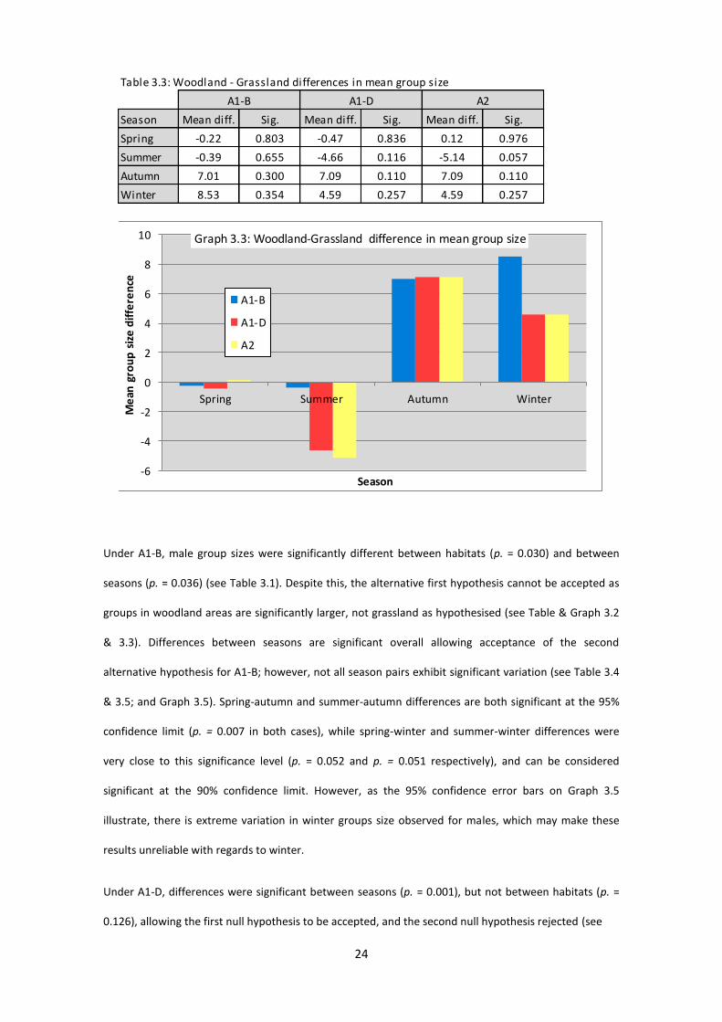
Under A1-B, male group sizes were significantly different between habitats (p. = 0.030) and between

seasons (p. = 0.036) (see Table 3.1). Despite this, the alternative first hypothesis cannot be accepted as

groups in woodland areas are significantly larger, not grassland as hypothesised (see Table & Graph 3.2

& 3.3). Differences between seasons are significant overall allowing acceptance of the second

alternative hypothesis for A1-B; however, not all season pairs exhibit significant variation (see Table 3.4

& 3.5; and Graph 3.5). Spring-autumn and summer-autumn differences are both significant at the 95%

confidence limit (p. = 0.007 in both cases), while spring-winter and summer-winter differences were

very close to this significance level (p. = 0.052 and p. = 0.051 respectively), and can be considered

significant at the 90% confidence limit. However, as the 95% confidence error bars on Graph 3.5

illustrate, there is extreme variation in winter groups size observed for males, which may make these

results unreliable with regards to winter.

Under A1-D, differences were significant between seasons (p. = 0.001), but not between habitats (p. =

0.126), allowing the first null hypothesis to be accepted, and the second null hypothesis rejected (see

Table 3.3: Woodland - Grassland differences in mean group size

Season Mean diff. Sig. Mean diff. Sig. Mean diff. Sig.

Spring -0.22 0.803 -0.47 0.836 0.12 0.976

Summer -0.39 0.655 -4.66 0.116 -5.14 0.057

Autumn 7.01 0.300 7.09 0.110 7.09 0.110

Winter 8.53 0.354 4.59 0.257 4.59 0.257

A1-B A1-D A2

-6

-4

-2

0

2

4

6

8

10

Spring Summer Autumn Winter

Me

an g

rou

p s

ize

dif

fere

nce

Season

Graph 3.3: Woodland-Grassland difference in mean group size

A1-B

A1-D

A2

25

Mean

95% Con.

(+/-) Mean

95% Con.

(+/-) Mean

95% Con.

(+/-)

Spring 2.48 1.05 18.20 5.41 19.28 7.77

Summer 2.89 .39 8.25 2.59 9.29 2.71

Autumn 19.72 7.94 18.92 6.83 18.92 6.83

Winter 25.14 22.22 19.54 4.50 19.54 4.50

Ass 1 - B Ass 1 - D Ass 2

Table 3.5 - Seasonal variation in mean group size for each assumed scenario

0

5

10

15

20

25

30

Spring Summer Autumn Winter

Me

an G

rou

p S

ize

Season

Graph 3.5: Seasonal variation in mean group size

Ass 1 - B

Ass 1 - D

Ass 2

Mean Diff Sig. Mean Diff Sig. Mean Diff Sig.

Summer -0.42 0.176 9.95 0.022 10.00 0.033

Autumn -17.24 0.007 -0.72 0.788 0.36 0.909

Winter -22.67 0.052 -1.35 0.518 -0.26 0.923

Spring 0.42 0.176 -9.95 0.022 -10.00 0.033

Autumn -16.83 0.007 -10.67 0.016 -9.63 0.025

Winter -22.25 0.051 -11.29 0.012 -10.26 0.018

Spring 17.24 0.007 0.72 0.788 -0.36 0.909

Summer 16.83 0.007 10.67 0.016 9.63 0.025

Winter -5.43 0.481 -0.62 0.745 -0.62 0.745

Spring 22.67 0.052 1.35 0.518 0.26 0.923

Summer 22.25 0.051 11.29 0.012 10.26 0.018

Autumn 5.43 0.481 0.62 0.745 0.62 0.745

NB:Fields highlighted green are significant at 95% confidence level

Fields highlighted yellow are significant at 90% confidence level

Table 3.4 - Table of Results (Pair-wise Comparison - Seasons)

Autumn

Winter

Ass 1 - DAss 1 - B Ass 2

Spring

Summer

26

Table 3.1). Similarly to A1-B not all season pairs exhibited significant variations. The average group size

observed in summer was significantly different to each other season (p. = 0.022, 0.016 and 0.012 for

summer-spring, summer-autumn and summer-winter respectively; see Table 3.4 & 3.5).

Under A2 both habitat (p. = 0.033) and season (p. = 0.005) had a significant effect on the size of the

group. There was a significant difference between the mean group size in summer and all other seasonal

means. This assumption exhibited the same pattern as A1-D, with spring, autumn and winter means

showing significant differences from summer, but not from each other (see Table 3.3 & 3.4).

Interaction between variables (Hypothesis 3) was not significant under any of the three assumed

conditions at the 95% confidence limit. However, the interaction was significant for female groups under

the first assumption and groups under the second assumption were significant at a 90% confidence level

(p. = 0.061 and p. = 0.080 respectively). When differences between habitats are considered for each

season individually, there are differences in group size, but only one difference shows any significance,

and that at the 90% level; under A2 in summer (p. = 0.057; see Table 3.3).

27

Chapter 4 - Discussion

4.1 Variation between habitats

The results show that group sizes in some cases did exhibit significant variation, both between habitats

and between seasons. However, the expected differences between habitat types as discussed by

Chapman & Chapman (1997), Langbein & Chapman (2003), Ciuti et al. (2006), Bonenfant et al. (2006),

Borkowski & Pudelko (2007); of smaller groups being found in woodland or closed habitats than in open

areas was contradicted on this occasion, with significantly larger groups more commonly found in

woodland areas throughout the year (see Table & Graph 3.2).

When each season is considered separately this pattern is not universal (see Table & Graph 3.3 and

Appendix 3). At a seasonal level none of the differences between habitats are significant at the 95%

level, despite visual analysis of data shows considerable variation (Graph 3.3). The expected patterns

were based largely on the predation-risk hypothesis, as described by Ruckstuhl & Neuhaus (2000) and

Villerette et al. (2006), which predicts that populations in closed or protective habitats will form smaller

groups because of the reduced risk of predation in these protective areas. Correspondingly, those

groups in open areas would form larger groups because of the higher risk of predation.

In the summer months, woodland areas are at their most ‘closed’ due to the peak vegetation growth.

During this period average group sizes (A1-D and A2) show this expected pattern, with larger groups

present in grassland areas, although the differences under A1-D are not significant, under A2 the

difference is significant just outside of the level (p. = 0.057; see Table & Graph 3.3), so can be considered

significant at the 90% confidence limit.

Adult males (A1-B), which are most commonly segregated from adult females and young at this time of

year (Langbein & Chapman, 2003), form small single-sex groups or live independently and the difference

between habitats is negligible as would be expected.

Visual examination of autumn and winter trends for both assumptions appear to show a bias for higher

group sizes in woodland, although none of these differences is significant at 95% or 90% confidence

28

limits (see Table and Graph 3.3). Spring groups are very similar between habitats under all conditions

(see Table & Graph 3.3).

Inconsistency between expected and observed patterns may be affected by a range of factors. The rut

during autumn, for which deer will gather in large groups to rutting stands (Chapman & Chapman, 1997;

Langbein & Chapman, 2003), may also affect habitat selection. At the study site the rutting stands are

known to be in woodland areas (J. Ward, pers. comm.), and this draw may create atypical habitat

selection. If this is the case, the combined effects on larger groups gathering in the woodland, may be

sufficient to significantly alter observed patterns. This cannot be quantified with the existing data,

further study would be required; comparison between areas where rutting stands may be in contrasting

habitat types would be particularly useful.

The predation-risk hypothesis discusses ‘closed’ in comparison to ‘open’ habitats in establishing general

trends. Initially, for this study, woodland was considered closed and grassland open, in keeping with

habitat description by Langbein and Chapman (2003). In reality, habitat areas need to be considered

individually to establish what comprises closed or open habitats. Other studies have used a more

complex habitat-type breakdown than this study, allowing more in depth analysis of habitat use

patterns. Borkowski and Pudelko (2007) divided woodland into four separate stages of growth during a

radio-tracking study on Fallow deer in Poland. Ciuti et al. (2006) divided their study site in Italy into

fourteen distinct types of vegetation cover. A higher resolution of data collection was considered for this

study, but the need for compliance with secondary data gathering system made this approach

unprofitable in this instance.

Borkowski and Pudelko (2007) discovered that thicket stage woodland was an especially important

habitat for the deer, both as a food source and for cover. In contrast, the expected favoured habitat of

mature forest areas were used relatively little. It was believed that the lack of under storey in the study

area made these areas unfavourable, providing little in the way of food or cover. A similar effect may be

present in this instance during winter and spring due to the poor under storey conditions, providing an

explanation for the grouping patterns seen. More in depth data collection would be required to fully

establish the pattern in this specific location, and the causes for the departure from normally expected

behaviour.

29

The characteristics of the area considered as grassland area (‘A34 Meadows’: see Figure 2.2 & 2.2a) in

this study may also lead to a loss of comparative distinction between sectors. Although the majority of

this area is meadow, and therefore ‘open’ land, there are some small blocks of woodland and at the

south of this sector is a marshy area adjacent to the river Trent. During winter floods this area is of

limited use to the deer. However, during the summer this area dries sufficiently for easy access by deer

and the vegetation grows very high providing both food and cover. During summer and early autumn

visits to the site, before water levels rose, it was very common to observe deer in this area, including

fawns ‘lying up’ in the concealing vegetation. As this area may be considered a closed habitat by that

evidence, its inclusion in the open estate sector may lead to inaccurate representation of patterns.

Chapman & Chapman (1997) suggest that disturbance can be a significant factor in determining group

sizes. The public footpaths and commercial operations on the estate and the surrounding roads and

residential areas exert a perhaps higher than normal pressure on the deer. This may bias habitat

selection in favour of the more protective habitat areas; and although woodland on the estate may be

considered open by comparison to other woodland, it may retain enough protective characteristics to

rate higher than meadows. Any increased use of these habitats may create the impression of larger

group sizes when considered under the assumed grouping behaviour in this study.

Initial analysis of habitat use does not indicate such a bias. The studied area was comprised of

approximately two thirds woodland. Female habitat use was 61.8% use of woodland over the year;

roughly in proportion to the amount of habitat available (~66%). Male woodland use was only 48.6%,

showing preference of open areas compared to females (see Appendix 4). The predation-risk hypothesis

predicts this, stating that males will use open areas more than females as, due to their larger body size,

the risk of predation to themselves is lower (Mysterud, 2000; Villerette et al., 2006).

Borkowski and Pudelko (2007) discovered a marked difference between habitat use and habitat

availability in their study. This may indicate that the proportional use of habitat as observed for females

in this location is actually not what should be expected under normal conditions. It is also uncertain to

what extent deer populations still retain anti-predatory behaviours where predators have been absent

for extended periods, such as the British Isles (Apollonio et al., 1998). It may be the case that some anti-

30

predator responses are retained due to the perceived threat from man, thus the principles may still be

valid (Ruckstuhl & Neuhaus, 2000).

4.2 Seasonal Variation

Some elements of seasonality have been mentioned above in relation to differences in group size

between habitats. However, when seasonal differences are considered isolation from habitat use, much

clearer patterns are seen, with seasonal differences significant for each assumed condition at the 95%

confidence limit (see Table 3.1). As can be seen from Tables 3.4 and 3.5, and Graph 3.5 summer is the

season most different from other seasons, with significantly smaller group sizes evident among females

(A1-D) and overall groups (A2). Fawning coincides with summer (Langbein & Chapman, 2003) and this

reduction in mean group size is likely a result of does separating to give birth to fawns in safe areas of

high vegetation, again predicted by the predation-risk hypothesis (Ciuti et al., 2006). After parturition,

does will seldom travel far from their fawn, restricting their range, and therefore the likelihood that they

will form groups (Chapman & Chapman, 1997). Female group sizes show very little variation between

the other seasons, indicating that the fawning period may have the greatest influence on female group

size determination.

Male groups, while showing close similarities between spring and summer and autumn and winter (see

Table 3.4), show significant variation between these season-pairs (see Graph 3.5). While this pattern is

expected in Fallow deer, in this case it could simply be a result of the assumed scenario placed on the

data (A1-B) and so cannot be treated as an independently significant result. However, when the primary

observations are considered in isolation this pattern is still evident (Male Average Groups Sizes 2012/13:

Summer - 1.83, Autumn - 8.83, Winter - 10.33), strongly suggesting this assumption is valid.

It was expected that the largest groups would be seen in the autumn, coinciding with the rut period

(Langbein & Chapman, 2003). However, the results show no significant differences between autumn and

winter under any of the three assumptions (see Table 3.3). Under A1-D and A2 there was also no

significant difference between spring and autumn group sizes. Chapman & Chapman (1997), state that

in some areas groups remain together after the rut through the winter into the spring. It is unclear as to

31

what dictates this behaviour in comparison with those areas where rutting groups dissipate immediately

after the rut, although the structure of winter habitats may be a factor, as discussed (Borkowski &

Pudelko, 2007). Appendix 4 illustrates the average annual habitat use patterns of the study population,

showing significantly higher use of woodlands from autumn to spring compared with summer under all

conditions, potentially supporting this presumption.

4.3 Evaluation of methods

The methodology used for this project was deemed to be the most suitable for gathering and analysing

the required data given the time scale, logistic constraints and secondary data detail. Some

compromises were required, but the described methods were considered the most appropriate despite

these minor drawbacks.

The assumptions applied by necessity to the secondary data (see Chapter 2), need to be understood in

order to accurately interpret the exhibited patterns. All group sizes should be considered as maximum

rather than real as it is assumed that all individuals seen in a sector congregate in a single group. In

reality it was very common during primary data collection to observe numerous distinct groups within a

single sector; four separate groups were seen in a single sector on two occasions (30/08/2012, in ‘A34

Meadows’ and 10/09/2012, in ‘Kings Wood’). These multiple group sightings were more common during

0

0.5

1

1.5

2

2.5

June July Aug Sept Oct Nov Dec Jan Feb

Ave

rage

Nu

mb

er o

f gr

ou

ps

seen

Month

Graph 4.1 - Average number of groups seen per sector on each visit - Primary survey period

32

the late summer and autumn months (see Graph 4.1).

Population sizes and behaviour assessed through direct counting methods, as in this study, can limit the

accuracy of recorded data. In some habitat types, particular in summer, vegetation cover makes it

difficult to accurately observe deer and their behaviour. This can lead to a bias in detectability between

habitats and between seasons. Borkowski & Pudelko (2007) and Bonenfant et al. (2005) both state that

direct observation methods may underestimate the use of closed habitats, and the numbers of animals

using them.

The viewing figures from this study support this statement (see Graph 4.2); numbers of deer seen each

visit in summer months, when habitats are most ‘closed’ by peak vegetation growth, were lower than

other times in the year. This method also risks disturbance of the study subjects. This can lead to

unnatural behaviour, including changed grouping behaviour. When disturbed, groups may split up into

smaller groups, move from one habitat type into another, or multiple groups merge to form larger

groups (Chapman & Chapman, 1997).

Fallow deer are often active throughout the day and night (Langbein & Chapman, 2003).Without the

resources of night vision or thermal imaging equipment, which is often the method for professional deer

surveys (Mayle, Peace & Gill, 2008); this observation was limited to daylight hours. Dawn was chosen as

the time of day allowing the most regular opportunity to visit the site, while also limiting the effects of

33

disturbance from other sources such as dog walkers or estate staff. Safety considerations made dusk

visits inadvisable. As all primary data was collected at this time of day, the data may not give a full

representation of overall grouping patterns. Borkowski & Pudelko (2007) found significant differences

between diurnal and nocturnal behaviour, including the grouping habits, of fallow deer. As mentioned,

these limitations were understood in advance and the chosen methods represent the data collection

system deemed most suitable. There is no record of the time of day that secondary data source visits

were made, and so this cannot be taken into account for these data either. Despite these drawbacks, it

is believed that the patterns observed and the conclusions drawn from this study are still robust and the

result relevant within the parameters considered.

34

Chapter 5: Conclusion

It was expected that a difference would be observed between habitat types, however the actual

difference observed was contrary to what had been expected. Group sizes in woodland were

significantly larger for two of the three tested scenarios, with no significant difference for the third (A1-

D). Langbein and Chapman (2003) suggested that the opposite would be true, stating than groups in

open areas were typically two to four times larger than woodland groups; this was supported by the

predation-risk hypothesis (Ruckstuhl & Neuhaus, 2000).

It was considered, based on findings by Borkowski and Pudelko (2007) that the variance from normally

expected behaviour may be due to the type of woodland found at the study site. Due to prolonged

overgrazing, some woodland areas are very open in structure, with little or no shrub layer, and only very

large trees. In these areas, the protective character of habitats normally considered closed is lacking.

Groups in these areas may be more likely to exhibit behaviour normally expected in open habitats as a

result. Additional analysis, with higher resolution recording of habitat type and condition could be

undertaken to establish whether this assumption is correct.

Seasonal variation in group sizes was significant, and largely followed the expected pattern, with

summer group sizes significantly smaller than all other seasons for all scenarios, with one exception. It

was expected that autumn group size would be the largest due to the population congregating at rutting

stands. While large groups were observed in autumn, they were not significantly larger than groups in

winter for any assumption, and for two of the three assumptions showed no significant difference to

spring groups. The third assumption only demonstrated a significant difference at the 90% level.

While it was expected that winter and spring groups may have been smaller, this was assumed as an

intermediary stage between autumn highs and summer lows. The evidence suggests instead that group

sizes remain high throughout the year, with breakup of groups seen in summer for the fawning period,

followed by groups aggregating again in time for the rut period. This showed that the most significant

seasonal variation relates to the reproductive cycle, specifically during the fawning period in summer.

However, these conclusions need to be understood in the context of the assumptions applied to the

data; that all group sizes should be considered maximum possible group sizes. Within this assumption is

35

the possibility that actual group sizes were significantly lower, and that undetectable differences may

render these analyses void for some conclusions.

Interaction between habitat and season was indecisive; two scenarios (A1-D & A2) showed significance

at 90% for this hypothesis. The third (A1-B) showed no significance at all. This suggests a weak link

between the two in determining group size, predominantly for female groups. What interaction does

exist is considered to be a result of the changing nature of woodland through the seasons. Woodland

areas providing significant cover during summer may provide very little cover during winter and early

spring, affecting the habitat use of the deer and by association, their grouping behaviours.

The two variables tested are both very broad in scope; in further study could be broken down to allow

more in depth analysis. With a greater number of variable factors recorded, a regression model could be

used to rank these determining factors. This level of analysis was not possible in this instance; time

constraints restricted the opportunity to gather sufficient data at this depth, and the secondary data

used to supplement results had not been gathered with this use in mind, so the data did not allow

analysis of this type.

Overall the project has fulfilled aims to determine what variation can be observed in group size between

variations in habitat and season, confirming that groups do change according to variation with a number

of ecological variables.

36

Bibliography:

Acevedo, P., Ward, A., Real, R. & Smith, G. (2010) Assessing biogeographical relationships of

ecologically related species using favourability functions: a case study on British deer, Diversity and

Distributions, Vol. 16, pg. 515–528

Aebischer, N. J., Davey, P. D. & Kingdon, N. G. (2011). National Gamebag Census: Mammal Trends to

2009. Game & Wildlife Conservation Trust, Fordingbridge (Available at:

http://www.gwct.org.uk/ngcmammals).

Anonymous (2011) Training Manual for Deer Stalkers, The British Deer Society, Fordingbridge

Anonymous (Undated - b) The Trentham Estate [Online], Available from -

http://www.trentham.co.uk/the-trentham-estate [Accessed on: 4/3/2012]

Apollonio, M., Focardi, S., Toso, S. & Nacci, L. (1998) Habitat selection and group formation pattern of

fallow deer Dama dama in a submediterranean environment, Ecography, Vol. 21, pg. 225-234

Bang, P. & Dahlstrøm, P. (2001) Animal Tracks and Signs, Oxford University Press, Oxford

Battersby, J. (2005) UK Mammals: Species Status and Population Trends. Joint Nature Conservation

Committee/Tracking Mammals Partnership, Peterborough

Bickerton, K. (2013) Condition of SSSI Units: Kings and Hargreaves Woods, Natural England [Online],

Available at -

http://www.sssi.naturalengland.org.uk/special/sssi/reportAction.cfm?report=sdrt13&category=S&refer

ence=1000991, [Accessed on: 4/3/2013]

Bonenfant, C., Loe, L. E., Mysterud, A., Langvatn, R., Stenseth, N. C., Gaillard, J-M. & Klein, F. (2004)

Multiple causes of sexual segregation in European red deer: enlightenments from varying breeding

phenology at high and low latitude, Proc. R. Soc. Lond. B., Vol. 271, pg. 883-892

Bonenfant, C., Gaillard, J-M., Klein, F. & Hamann, J-L. (2005) Can we use young : female ratio to infer

ungulate population dynamics? An empirical test using red deer Cervus elaphus as a model, Journal of

Applied Ecology, Vol. 42, pg. 361-370

Borkowski, J. & Pudelko, M. (2007) Forest Habitat use and home-range size in radio-collared fallow

deer, Annales Zoologici Fennici, Vol. 44, pg. 107 - 114

Chapman, D. & Chapman, N. (1997) Fallow Deer, Coch-y-Bonddu Books, Machynlleth

Chapman, N. G. & Harris, S. (1996) Muntjac, The Mammal Society & The British Deer Society, UK

Chapman, N. G. & Hecker, K. (Eds.) (2008) Proceedings of the International Symposium "Enclosures: A

Dead End?", CIC (International Council for Game and Wildlife Conservation), Sopron, Hungary

Ciuti, S., Bongi, P., Vassale, S. & Apollonio, M. (2006) Influence of fawning on the spatial behaviour and

habitat selection of female fallow deer (Dama dama) during late pregnancy and early lactation, Journal

of Zoology, Vol. 268, pg. 97–107

Clutton-Brock, T. H., Iason, G. R., Albon, S. D. & Guinness, F. E. (1982) Effects of lactation on feeding

behaviour and habitat use in wild Red deer hinds, Journal of Zoology, Vol. 198, 2, pg. 227-236

Clutton-Brock, T. H., Major, M. & Guinness, F. E. (1985) Population Regulation in Male and Female Red

Deer, Journal of Animal Ecology, Vol. 54, 3, pg. 831-846

37

Cooke, A. S. & Farrell, L. (2001) Impact of muntjac deer (Muntiacus reevesii) at Monks Wood National

Nature Reserve, Cambridgeshire, eastern England, Forestry, Vol. 74, 3, pg. 241-250

Cooke, A. S. (1997) Effects of grazing by muntjac (Muntiacus reevesii) on bluebells (Hyacinthoides non-

scripta) and a field technique for assessing feeding activity, Journal of Zoology, Vol. 242, 2, pg. 365-369

Cote, S. D., Rooney, T. P., Tremblay, J-P., Dussault, C. & Waller, D. M. (2004) Ecological Impacts of Deer

Overabundance, Annual Review of Ecology, Evolution, and Systematics, Vol. 35, pg. 113-147

DeGabriel, J. L., Albon, S. D., Fielding, D. A., Riach, D. J., Westaway, S. & Irvine, R. J. (2011) The

presence of sheep leads to increases in plant diversity and reductions in the impact of deer on heather,

Journal of Applied Ecology, Vol. 48, pg. 1269-1277

Elgar, M. A. (1989) Predator vigilance and group size in mammals and birds: A critical review of the

empirical evidence, Biological Review, Vol. 64, 1, pg. 13-33

Fawcett, J. K. (1997) Roe Deer, The Mammal Society & The British Deer Society, UK

Field, A. (2009) Discovering Statistics using SPSS (3rd Ed.), Sage Publications Ltd., London

Fletcher, J. (2010) Deer Parks and Deer Farming in Great Britain - History and Current Status, In:

Chapman, N. G. & Hecker, K. (eds.): Proceedings of the International Symposium “Enclosures: a Dead-

End?” Sopron, Hungary 2008, pg. 54-61.

Fuller, R. J. (2001) Responses of woodland birds to increasing numbers of deer: a review of evidence and

mechanisms, Forestry, Vol. 74, 3, pg. 289-298

Gill, R. (2000) The Impact of Deer on Woodland Biodiversity, Forestry Commission, Edinburgh

Gill, R. M. A. & Beardall, V. (2001) The impact of deer on woodlands: the effects of browsing and seed

dispersal on vegetation structure and composition, Forestry, Vol. 74, 3, pg. 209-218

Gill, R. M. A. & Fuller, R. J. (2007) The effects of deer browsing on woodlands structure and songbirds in

lowland Britain, Ibis, Vol. 149, pg. 119-127

Gordon, I. J., Hester, A. J. & Festa-Bianchet, M. (2004) The management of wild large herbivores to

meet economic, conservation and environmental objectives, Journal of Applied Ecology, Vol. 41, pg.

1021-1031

Griffith, D. (2011) Deer Management in the UK, Quiller, Shrewsbury

Hailstone, M. (2012) The Great British Deer Survey, Deer, Vol. 16, 6, pg. 12-15

Kirby, K. J. (2001) The impact of deer on the ground flora of British broadleaved woodland, Forestry, Vol.

74, 3, pg. 219-229

Langbein, J. & Chapman, N. (2003) Fallow Deer, The Mammal Society & The British Deer Society, UK

MacMillan, D. C. & Leitch, K. (2008) Conservation with a Gun: Understanding Landowner Attitudes to

Deer Hunting in the Scottish Highlands, Human Ecology, Vol. 36, pg. 473-484

Manning, A. & Dawkins, M. S. (2012) An Introduction to Animal Behaviour (6th Ed.), Cambridge

University Press, Cambridge

38

Maroo, S. & Yalden, D. W. (2000) The Mesolithic Mammal Fauna of Great Britain, Mammal Review, Vol.

30, pg. 243-248

Mayle, B., Peace, A. & Gill R. (2008) How Many Deer? A field guide to estimating deer population size,

Field Book 18, Forestry Commission, Norwich

Molvar, E. M. & Bowyer, R. T. (1994) Costs and benefits of group living in a recently social ungulate: The

Alaskan Moose, Journal of Mammology, Vol. 75, 3, pg. 621-630

Morellet, N., Gaillard, J-M., Hewison, A. J. M., Ballon, P., Boscardin, Y., Duncan, P., Klein, F. & Maillard,

D. (2007) Indicators of ecological change: new tools for managing populations of large herbivores,

Journal of Applied Ecology, Vol. 44, pg. 634-643

Morgan M. J. & Godin, J. J. (1985) Anti-predator benefits of schooling behaviour in a Cyprinodontid fish,

the Banded Killfish (Fundulus diaphanus), Ethology, Vol. 70, 3, pg. 236-246

Mysterud, A. (2000) The relationship between ecological segregation and sexual body size dimorphism

in large herbivores, Oecologia, Vol. 124, pg. 40–54

Mysterud, A., Coulson, T., & Stenseth, N. (2002) Essay Review: The role of males in the dynamics of

ungulate populations, Journal of Animal Ecology, Vol. 71, pg. 907–915

Mysterud, A., Yoccoz, N. G., Stenseth, N. C. & Langvatn, R. (2000) Relationships between sex ratio,

climate and density in red deer: the importance of spatial scale, Journal of Animal Ecology, Vol. 69, pg.

959-974

Natural England (Undated) Kings and Hargreaves Wood SSSI Notification [Online], Available from -

http://www.sssi.naturalengland.org.uk/citation/citation_photo/1000991.pdf [Accessed on: 4/3/2013]

Newson, S. E., Johnston, A., Renwick, A. R., Baillie, S. R. & Fuller, R. J. (2012) Modelling large-scale

relationships between changes in woodland deer and bird populations, Journal of Applied Ecology, Vol.

49, pg. 278-286

Pellerin, S., Huot, J. & Cote, S. D. (2006) Long term effects of deer browsing and trampling on the

vegetation of peatlands, Biological Conservation, Vol. 128, pg. 316-326

Perez-Barberia, F. J., Perez-Fernandez, E., Robertson, E. & Alvarez-Enriquez, B. (2008) Does the Jarmen-

Bell principle at intra-specific level explain sexual segregation in polygynous ungulates? Sex difference in

forage digestibility in Soay sheep, Oecologia, Vol. 157, 1, pg. 21-30

Prior, R. (1987a) Deer Management in Small Woodlands, The Game Conservancy, Fordingbridge

Prior, R. (1987b) Deer Watch, Swan Hill Press, Shrewsbury

Putman, R. & Langbein, J. (2003) The Deer Manager’s Companion, Swan Hill Press, UK

Putman, R. (2000) Sika Deer, The Mammal Society & The British Deer Society, UK

Quine, C. Shore, R. & Trout, R. (2004) Managing Woodlands and their Mammals, Forestry Commission,

Edinburgh

Reimoser, F., Armstrong, H. & Suchant, R. (1999) Measuring forest damage of ungulates: what should

be considered, Forest Ecology and Management, Vol. 120, pg. 47-58

Rose, R. (2004) Working with Nature: Memoirs of a Wildlife Manager, David A H Grayling, Penrith

39

Ruckstuhl, K. & Neuhaus, P. (2000) Sexual Segregation in Ungulates: A new approach, Behaviour, Vol.

137, pg. 361-377

Sage, R. B., Hollins, K., Gregory, C. L., Woodburn, M. I. A. & Carroll, J. P. (2004) Impact of roe deer

Capreolus capreolus browsing on understorey vegetation in small farm woodlands, Wildlife Biology, Vol.

10, pg. 115-120

Scott, D., Bacon, P. & Irvine, J. (2002) Management of Deer in Woodlands: Literature reviews of

woodland design, and techniques for assessing populations and damage, Report to the Deer

Commission for Scotland, Centre for Ecology and Hydrology, Banchory

Sorensen, V. & Taylor, D. (1995) The Effect of Seasonal Change on the Group Size, Group Composition,

and Activity Budget of White-Tailed Deer (Odocoileus virginianus), Ohio Journal of Science, Vol. 95 (5),

pg. 321-324

Symes, N. & Currie, F. (2005) Woodland management for birds: a guide to managing for declining

woodland birds in England, The RSPB, Sandy and Forestry Commission England, Cambridge

Uetz, G. W., Boyle, J., Hieber, C. S. & Wilcox, R. S. (2002) Anti-predator benefits of group living in

colonial web-building spiders: the early warning effect, Animal Behaviour, Vol. 63, 3, pg. 445-452

Villerette, N.; Helder, R.; Angibault, J. Cargnelutti, B. & Gerard, J-F (2006) Sexual segregation in fallow

deer: are mixed-sex groups especially unstable because of asynchrony between the sexes?, C. R.

Biologies, Vol. 329, pg. 551–558

Watkinson, A. R.; Riding, A. E. & Courie, N. R. (2001) A community and population perspective of the

possible role of grazing in determining the ground flora of ancient woodlands, Forestry, Vol. 74, 3, pg.

231-239

Wywialowski, A. P. (1996) Wildlife Damage to Field Corn in 1993, Wildlife Socitey Bulletin, Vol. 24., 2,

pg. 264-271

Yokoyama, S. & Shibata, E. (1998) Characteristics of Sasa nipponica grassland as a summer forage for

sika deer on Mt. Ohdaigahara, central Japan, Ecological Research, Vol. 13, pg. 193-198

Figure Sources:

Figure 1.1 - NBN (National Biodiversity Network) (2013a) Fallow Deer Distribution Grid Map,

Staffordshire [Online], Available at: http://www.searchnbn.net/gridMap/gridMap.jsp#topOfMap,

Customisable Maps, [Accessed on 2/03/2013]

Figure 1.2 - NBN (National Biodiversity Network) (2013b) Fallow Deer Distribution Grid Map, UK

[Online], Available at: http://www.searchnbn.net/gridMap/gridMap.jsp#topOfMap, Customisable Maps,

[Accessed 2/03/2013)

Figure 2.2 - Google Maps Image (2012) Untitled Image [Online], Available at:

https://maps.google.co.uk/maps?hl=en, centred at 52.9517N, -2.2031W [Accessed 19/01/2013]

40

Appendix 1: Summarised Mean Group Size Tables and Graphs by Season

Tab

le A

1.1

- C

om

bin

ed H

ab

ita

t Fi

gure

s -

by

sea

son

Mea

nSt

d D

evM

ean

Std

Dev

Mea

nSt

d D

ev

Spri

ng

2.6

31

.69

18

.66

12

.46

20

.04

15

.21

Sum

mer

2.8

32

.01

7.6

05

.52

8.3

96

.32

Au

tum

n2

1.5

11

6.7

11

5.9

01

4.5

81

4.8

31

4.5

5

Win

ter

24

.89

17

.62

19

.93

15

.89

19

.74

15

.90

Tab

le A

1.2

- W

oo

dla

nd

on

ly h

ab

ita

t fi

gure

s -

by

sea

son

Mea

nSt

d D

evM

ean

Std

Dev

Mea

nSt

d D

ev

Spri

ng

2.2

41

.44

17

.98

13

.38

19

.22

16

.94

Sum

mer

2.2

71

.12

6.0

04

.20

6.4

64

.42

Au

tum

n2

3.2

61

7.9

71

8.2

41

6.2

41

6.8

21

6.1

6

Win

ter

28

.17

19

.94

21

.52

17

.55

21

.22

17

.56

Tab

le A

1.3

- G

rass

lan

d o

nly

ha

bit

at

figu

res

- b

y se

aso

n

Mea

nSt

d D

evM

ean

Std

Dev

Mea

nSt

d D

ev

Spri

ng

2.9

01

.80

19

.76

10

.70

21

.49

11

.39

Sum

mer

3.1

52

.30

9.3

96

.24

10

.44

7.3

1

Au

tum

n1

7.0

09

.43

11

.79

9.8

11

1.5

61

0.6

5

Win

ter

18

.33

8.4

91

6.0

09

.65

16

.00

9.6

5

Ass

um

pti

on

1-B

Ass

um

pti

on

1-D

Ass

um

pti

on

2

Ass

um

pti

on

1-B

Ass

um

pti

on

1-D

Ass

um

pti

on

2

Ass

um

pti

on

1-B

Ass

um

pti

on

1-D

Ass

um

pti

on

2

05

10

15

20

25

30

35

40

45

Spri

ng

Sum

me

rA

utu

mn

Win

ter

Mean Group Size

Seas

on

Gra

ph

A1.

2 -

Ave

rage

Gro

up

Siz

e -

Wo

od

lan

d (S

eas

on

al)

Ass

um

pti

on

1-B

Ass

um

pti

on

1-D

Ass

um

pti

on

2

05

10

15

20

25

30

35

40

45

Spri

ng

Sum

me

rA

utu

mn

Win

ter

Mean Group Size

Seas

on

Gra

ph

A1.

1 -

Ave

rage

Gro

up

Siz

e -

Co

mb

ine

d H

abit

at (

Seas

on

al)

Ass

um

pti

on

1-B

Ass

um

pti

on

1-D

Ass

um

pti

on

2

05

10

15

20

25

30

35

40

45

Spri

ng

Sum

me

rA

utu

mn

Win

ter

Mean Group Size

Seas

on

Gra

ph

A1.

3 -

Ave

rage

Gro

up

Siz

e -

Gra

ssla

nd

(Se

aso

nal

)

Ass

um

pti

on

1-B

Ass

um

pti

on

1-D

Ass

um

pti

on

2

41

Appendix 2: Tables of means used in SPSS analysis

Table A2.1 - Seasonal mean group size for each habitat as used in analysis (Assumption 1 - B)

Season

Year / Habitat Woodland Grassland Woodland Grassland Woodland Grassland Woodland Grassland

2008 1.17 2.46 2.29 2.80 27.30 19.00 33.80 22.00

2009 2.29 3.89 1.67 4.40 28.13 20.60 26.21 16.13

2010 3.00 3.00 2.50 3.67 27.20 0.00 0.00 18.00

2011 3.00 1.00 4.00 1.80 13.50 22.00 59.00 26.00

2012 2.00 1.75 10.00 9.50 11.75 6.00

Table A2.2 - Seasonal mean group size for each habitat as used in analysis (Assumption 1 - D)

Season

Year / Habitat Woodland Grassland Woodland Grassland Woodland Grassland Woodland Grassland

2008 15.70 21.88 4.71 8.00 19.65 9.20 27.00 13.50

2009 23.00 22.44 7.10 8.78 24.73 18.33 23.71 16.13

2010 15.07 15.00 7.18 13.43 25.25 7.20 11.75 19.50

2011 18.09 14.40 2.00 14.80 25.00 22.00 25.00 19.75

2012 6.29 5.56 5.88 8.31 10.36 6.00

Table A2.3 - Seasonal mean group size for each habitat as used in analysis (Assumption 2)

Season

Year / Habitat Woodland Grassland Woodland Grassland Woodland Grassland Woodland Grassland

2008 15.83 23.76 5.65 9.27 19.65 9.20 27.00 13.50

2009 25.60 26.33 7.60 12.30 24.73 18.33 23.71 16.13

2010 14.93 15.30 7.64 15.00 25.25 7.20 11.75 19.50

2011 21.00 11.50 3.00 13.83 25.00 22.00 25.00 19.75

2012 6.00 5.18 5.88 8.31 10.36 6.00

Spring Summer Autumn Winter

Spring Summer Autumn Winter

Spring Summer Autumn Winter

42

Appendix 3: Seasonal variation in group size between habitats

Mean

95% Con.

(+/-) Mean

95% Con.

(+/-)

Spring 2.37 1.38 2.59 1.93

Summer 2.62 1.57 3.17 1.79

Autumn 24.03 11.19 15.40 16.45

Winter 29.75 38.65 20.53 6.99

Mean

95% Con.

(+/-) Mean

95% Con.

(+/-)

Spring 17.97 5.73 18.43 6.87

Summer 5.25 3.90 11.25 5.36

Autumn 23.66 4.26 14.18 11.32

Winter 21.87 10.94 17.22 4.74

Mean

95% Con.

(+/-) Mean

95% Con.

(+/-)

Spring 19.34 7.89 19.22 11.11

Summer 5.97 3.48 12.60 3.95

Autumn 23.66 4.26 14.18 11.32

Winter 21.87 10.94 17.22 4.74

Error Bars represent 95% confidence limits

Table A3.1: Variation in Habitat use by season

(Assumption 1 - Buck groups)

Table A3.3 - Variation in Habitat use by season

(Assumption 2)

Table A3.2: Variation in Habitat use by season

(Assumption 1 - Doe Groups)

Woodland Grassland

Woodland Grassland

Woodland Grassland

19.3

4

5.97

23.6

6

21.8

7

19.2

2

12.6

0

14.1

8

17.2

2

0

5

10

15

20

25

30

Spring Summer Autumn Winter

Me

an

Gro

up

Siz

e

Season

Graph A3.3: Variation in Habitat use by season (A2)

Woodland

Grassland

2.37

2.62

24.0

3

29.7

5

2.59

3.1

7

15

.40

20.5

3

0

5

10

15

20

25

30

Spring Summer Autumn Winter

Me

an G

rou

p S

ize

Season

Graph A3.1: Variation in Habitat use by season (A1-B)

Woodland

Grassland

17.9

7

5.2

5

23.6

6

21.8

7

18.4

3

11.2

5

14.1

8

17.2

2

0

5

10

15

20

25

30

Spring Summer Autumn Winter

Me

an G

rou

p S

ize

Season

Graph A3.2: Variation in Habitat use by season (A1-D)

Woodland

Grassland

43

Appendix 4: Seasonal habitat use

Woods Fields

Spring 35.4% 64.6%

Summer 22.3% 77.7%

Autumn 63.3% 36.7%

Winter 73.3% 26.7%

Woods Fields

Spring 63.2% 36.8%

Summer 40.1% 59.9%

Autumn 67.1% 32.9%

Winter 76.8% 23.2%

Woods Fields

Spring 60.0% 40.0%

Summer 38.7% 61.3%

Autumn 67.4% 32.6%

Winter 76.1% 23.9%

48.6% 51.4%

Annual

Average:61.8% 38.2%

Table A4.3: Habitat Use

Averages - Combined

Table A4.1: Habitat Use

Averages - Males

Table A4.2: Habitat Use

Averages - Females

Average

Average

Average

Annual

Average:

Annual

Average:60.6% 39.5%

0%

10%

20%

30%

40%

50%

60%

70%

80%

90%

100%

Spring Summer Autumn Winter

% H

abit

at U

se

Season

Graph A4.3: Habitat Use Averages - Combined

Fields

Woods

0%

10%

20%

30%

40%

50%

60%

70%

80%

90%

100%

Spring Summer Autumn Winter

% H

abit

at U

se

Season

Graph A4.1: Habitat Use Averages - Males

Fields

Woods

0%

10%

20%

30%

40%

50%

60%

70%

80%

90%

100%

Spring Summer Autumn Winter

% H

abit

at U

se

Season

Graph A4.2: Habitat Use Averages - Females

Fields

Woods