arX

iv:1

302.

1595

v1 [

astr

o-ph

.SR

] 6

Feb

201

3

Accepted by AJ

Near-IR Periodic and Other Variable Field Stars in the Field of the Cygnus

OB7 Star Forming Region

Scott J. Wolk

Harvard–Smithsonian Center for Astrophysics, 60 Garden Street, Cambridge, MA 02138

Thomas S. Rice

Harvard–Smithsonian Center for Astrophysics, 60 Garden Street, Cambridge, MA 02138

Colin A. Aspin

Institute for Astronomy, University of Hawaii at Manoa, 640 N Aohoku Pl, Hilo, HI 96720

ABSTRACT

We present a subset of the results of a three season, 124 night, near-infrared moni-

toring campaign of the dark clouds Lynds 1003 and Lynds 1004 in the Cygnus OB7 star

forming region. In this paper, we focus on the field star population. Using three seasons

of UKIRT J, H and K band observations spanning 1.5 years, we obtained high-quality

photometry on 9,200 stars down to J=17 mag, with photometric uncertainty better

than 0.04 mag. After excluding known disk bearing stars we identify 149 variables –

1.6% of the sample. Of these, about 60 are strictly periodic, with periods predominantly

< 2 days. We conclude this group is dominated by eclipsing binaries. A few stars have

long period signals of between 20 and 60 days. About 25 stars have weak modulated

signals, but it was not clear if these were periodic. Some of the stars in this group may

be diskless young stellar objects with relatively large variability due to cool star spots.

The remaining ∼60 stars showed variations which appear to be purely stochastic.

Subject headings: stars: eclipsing binaries – stars: variables – infrared: stars

1. Introduction

Two crucial experiments for identifying Young Stellar Objects (YSOs) are near-infrared (NIR)

disk studies and variability studies. We have combined these two techniques in a three season, 124

night NIR monitoring campaign of the star forming region Cyg OB7 (Rice et al. 2012; hereafter

Paper I). The first result of this experiment was the identification of 30 YSOs in the region and the

discovery that about a quarter of them were seen to transition in JHK color-color space from the

– 2 –

“photospheric” region of the NIR color-color diagram to the region of the diagram corresponding

to disk bearing stars (Lada & Adams 1992). In a follow-up paper, we study the periodic nature of

the YSOs and the observed systematic color changes (Wolk et al. 2013; hereafter Paper III).

Disk-bearing young stars, also known as classical T Tauri stars (cTTs), have long been iden-

tified as optically variable (Joy 1945; Herbig 1962). At a minimum the variability is due to a

combination of starspots, accretion and circumstellar disk occultations (Herbst et al. 1994). The

study of near-infrared variability in young stars allows us to directly study changes in those disk

structures. Studies of the Orion A and Chameleon I molecular clouds established that variability is

related to the presence of an inner accretion disk (Carpenter et al. 2001, 2002). In Orion, as many

as 93% of the variable stars are identified to be young stars, and a strong connection is established

between variability and near-infrared excess. Studies of individual YSOs such as AA Tau and

its analogs reveal insights into magnetospheric accretion processes linked to inner-disk dynamics

(Bouvier et al. 2003, 2007; Donati et al. 2010). Other types of stars such as EX Lup (Aspin et al.

2010) and V1118 Ori (Audard et al. 2010) exhibit large, eruptive mass-accretion events due to

mass infall events of M > 0.1M⊕ that are easily studied in the near-infrared; during outburst, their

near-infrared emission is dominated by hotspot radiation and emission reprocessed in the disk.

Recent mid-IR variability surveys such in the IC 1396A and Orion star forming regions provide key

insights into physical processes of young stars over short (∼40 day) timescales, finding that 70% of

YSOs with infrared excess are variable (Morales-Calderon et al. 2009, 2011). Scholz (2012) studied

the NIR variability of several young clusters including the ONC, NGC 1333, IC 348 and σ Orionis.

He finds variability amplitudes are largest in NGC 1333, presumably because it has the youngest

sample of YSOs. The frequency of highly variable objects also increases with the time window of

the observations.

Although the focus of our observing campaign was to study YSOs, our observed field contains

about 9200 background and foreground stars for which variability analysis were carried out. Of

these, 158 were found to be variable via the Stetson index (Stetson 1996). Variable field stars

provide important information about the nature and evolution of stars in various regions of our

galaxy. For example, eclipsing binary stars provide us information about the masses and radii of

stars (see e.g. Huang & Struve 1956; Popper et al. 1985). Pulsating variables, such as Cepheids and

RR Lyrae, serve as distance indicators (see e.g. Benedict et al. 2007). A common type of pulsators

known as δ Scuti stars offer unique insight into the internal structure and evolution of main-sequence

objects (Thompson et al. 2003). Pietrukowicz et al. (2009) recently performed a deep four night

monitoring campaign of about 50,000 stars in Carina with the VLT and found a 0.7% variability

fraction. The main goal of their program was the optical follow-up of OGLE planetary transit

candidates. They found 43% of the variables were eclipsing systems while a statistically identical

number were pulsating systems. About 2/3 of the pulsating systems were δ Scuti stars.

The goal of this paper is simple: to document the rate, and to a lesser extent the types, of NIR

variability seen in the field stars. We will then use the result of the field star analysis as a point

of comparison for the results found in star forming regions. In the next section (§2) we will briefly

– 3 –

review the source data. In §3 we discuss two techniques for period analysis: a fast χ2 minimization

algorithm and Lomb-Scargle periodogram analysis. In §4 we present the results of our periodicity

study of the field stars. The field stars divide into four types. First – regular periodic variables

which are either eclipsing or pulsating; second – less regular periodic stars; third – long duration

variables which, despite a strong signal, defied description by a single period and fourth – weak

signal, stochastic variables. We summarize the results in §5.

2. Observation and Data Reduction

The constellation Cygnus contains many rich and complex star-forming regions, including the

North America and Pelican nebulae and the Cygnus X star forming region (Reipurth & Schneider

2008). In the Cygnus region, nine OB associations have been found. Cygnus OB7 is the nearest

at a distance of around 800 pc (Aspin et al. 2009, distance modulus µ = 9.5). Cygnus OB7 is

along the line-of-sight of the large dark cloud Kh 141 (Khavtasi 1955) – also called the northern

coal sack; this cloud is over 5o across. While a physical connection has not been confirmed, the

dark clouds Lynds 1003-1004, the target of this study, lie near the middle of Kh 141. The dark

clouds were first studied in the context of star formation by Cohen (1980) who found a diffuse

red nebula he named RNO 127. This nebula was later determined to be a bright Herbig-Haro

(HH) object by Melikian & Karapetian (HH 428 2001, 2003). Further study in the optical and

near-infrared identified a number of Herbig-Haro objects (Devine et al. 1997; Movsessian et al.

2003) and multiple IRAS sources (Dobashi et al. 1996) that reveal the presence of a young stellar

population and significant star formation activity. The field of view of the study is about a 1 degree

square centered near 21h00m +52o30′ (J2000.) near the “Braid Nebula Star”. While Aspin et al.

(2009) and Rice, Wolk & Aspin (2012) have identified over 40 disked YSOs in the region, to date

no deep X-ray studies have been made to identify the disk-free young stellar population.

The dataset used here was fully described in Paper I. In brief, J , H, and K observations of

the Cygnus OB7 region were obtained using the Wide Field Camera (WFCAM) instrument on

the United Kingdom InfraRed Telescope (UKIRT), an infrared-optimized 3.8 meter telescope atop

Mauna Kea, Hawaii at 4200 meters elevation. Our data consist of WFCAM observations taken from

May 2008 to October 2009 in three observing seasons as part of a special observation program.

Data were taken on a total of 124 nights during this period. For each night, we extracted data

from the archive for all stars with photometric uncertainties less than 0.1 mag in J band and no

processing error flags. Starting from about 100,000 detected objects, over 38,000 stars met this

criterion every night. The typical errors of these stars for one night are shown in Figure 1. Out of

the 124 nights in the original survey, 24 nights were rejected due to deviations in the mean color of

& 1%, leaving 100 nights for our analysis (Table 1) (see also Rice, Wolk & Aspin 2012). To assure

the best quality data we require J . 17.3 which limits errors to ≤ 4% at J; we also excluded stars

brighter than J =11 as bright stars would saturate in epochs with especially good seeing or if the

star brightened. We also required no quality error bit flags on any of the observations. In the end

– 4 –

we obtained high-quality photometry on 9,200 stars.

Fig. 1.— Errors vs. magnitude in all three bands shown for one night of data. This is about 38,000

stars with J errors < 0.1 mag.

Variability was quantified for all sources in the field using the Stetson index (S; Stetson 1996)1.

This is a method for quantifying variability within a sample which includes multiple colors each

with different error characteristics. The resultant value is zero for a constant source and exceeds 1

for a source with significant correlated variability; high values indicate greater variability.2

1This index is referred to by the letter J in the original article, we use S to avoid confusion with the filter band.

2Carpenter et al. (2001) compared the Stetson index to χ2 fits and concluded that S > 0.55 was sufficient to confirm

variability. In Paper I we concluded that S > 1.0 was preferable for our analysis because the more conservative value

prevented false detections in large samples.

Table 1. Observing Log

Epoch Start Date End Date Number of observations

Season 1 26-Apr-2008 22-May-2008 19

Season 2 19-Sep-2008 27-Nov-2008 39

Season 3 28-Aug-2009 13-Oct-2009 41

Total 26-Apr-2008 13-Oct-2009 100

– 5 –

3. Period Analysis

3.1. Automated Period Searches

To investigate whether the variable stars were periodic, we used two period-finding algorithms:

the Lomb-Scargle periodogram (also knonwn as the Lomb Normalized Periodogram – LNP; cf.

Press & Rybicki 1989) and the Fast χ2 (Fχ2) algorithm (Palmer 2009), both suited for period

analysis on unevenly sampled data such as ours. The Lomb-Scargle method is a useful and pop-

ular way to analyze periodicity with an easily interpreted periodogram, which identifies multiple

candidate periods and their relative probability. This method essentially takes the Fast Fourier

Transform of the input signal and reinterprets it (with certain restrictions) as the periodogram.

The signal in the periodogram with the maximum power is generally interpreted as the true signal.

The method uses the number and spacings of samples to determine the frequency domain to be

explored. Spurious detections can be produced at frequencies where the sample times have signif-

icant periodicity (i.e. nightly samples); power from harmonics above the fundamental sine wave is

lost, and the algorithm ignores point-to-point variations in the measurement error.

Given the long baselines in our data, the LNP method can determine very precise periods.

The formal error on derived (linear) frequencies is: δf = 3σN/2TA√N0 (Horne & Baliunas 1986),

where σN is the variance of noise remaining after the periodic signal is subtracted, N0 is the number

of independent points (about 100), T is the length of time baseline (about 500 days), and A is the

amplitude of signal (typically 10%). For our data, the formal error is typically less than 0.001 days,

an indication of the tremendous leverage gained by long term monitoring of very stable periods.

On the other hand the step size of the period search algorithms is a function of the square of the

period and while the step size is ∼ 0.001 day for periods < 2 days, the step size is about 0.014

days for a period of 10 days. We list measures of period to the nearest 0.01 days (∼ 15 minutes)

which is well within the precision for periods < 10 days and reasonable for all listed periods. This

precision is consistent with our purposes, which is to identify the field variables, not to physically

evaluate each one in detail.

Among non-variables in our data, our LNP analysis often found spurious periods near 0.5

and 1.0 days, likely due to the ∼ 1 day separation between nightly observations. Because of our

sampling rate and the induced aliasing in our dataset, we chose to reject certain windows of periods

from our LNP analysis. These were periods shorter than 0.55 days, longer than 250 days, and the

interval 0.9 - 1.1 days. Further, the LNP method favors sinusoidal variability and had a difficulty

with sharp eclipsing systems. This happens because the Fourier transform is at the core of the

signal decomposition. Hence the signal is decomposed into sines and cosines, no matter what the

shape of the true signal.

To overcome these limitations, we also used the Fχ2 algorithm. The Fχ2 method uses a

truncated Fourier expansion. Since a limited number of harmonics are explored, it allows the

frequencies searched to have arbitrary range and density so that periods are not missed by the

– 6 –

Table 2. Period search parameters.

Description Parameter

J Range ∼11.0-17.3 mag

H Range ∼11.0-16.5 mag

K Range ∼11.0-16.0 mag

Typical errors 0.02 mag

Stars Monitored ∼ 9,200

Range of sensitivity 0.1- 250 days

Range of completeness 0.2 - 50 days

Amplitude Limit 0.02

Typical σPeriod < 0.01 days

– 7 –

search. Fχ2 is sensitive to power in higher harmonics of the fundamental sinusoid meaning it

can identify structures more complex than sinusoids. Further, there is insensitivity to the sample

timing including periods less than one day and near one day. The frequency search is gridded more

tightly than the traditional integer number of cycles over the span of observations, eliminating

power loss from peaks that fall between the grid points. Using the (Fχ2) algorithm we were able to

explore periods as short as 0.1 days and found very stable results across the three bands. However,

simulations with test data indicated that period near 0.1 days still tended to get lost in aliasing

with the sampling rate, especially in the single season data. Empirically, the Fχ2 method is more

reliable for complex variables such pulsating stars and for short-period (. 1 day), highly stable, but

non-sinusoidal variability, such as detached eclipsing binaries. Table 2 lists the overall parameters

of the periodicity search.

Data from each filter and each season were independently analyzed by both the Fχ2 and LNP

techniques. This analysis was followed by analysis of the combined three epochs of data (4 seasonal

divisions × 3 filters × 2 methods = 24 light curves generated for each star). Results of the combined

data set were given primacy as dynamic periods, either due to eclipses or pulsations, should be

stable over 500 days. The individual seasonal measurements were more important for the pre-main

sequence stars in which the mechanisms inducing the periodicity, whether cool star spots, accretion

spots or disk features, are thought to be only quasi-stable in nature.

3.2. Manual Validation

Even when it appears a period is present, the algorithms often disagree on the preferred period.

We manually graded the light curves of each star on a 5 point empirical scale. A grade of 5 was

given to the subset of periods which appeared beyond question; usually these were clear eclipsing

systems or other systems which varied sinusiodally with periods under a day. A grade of 4 was

given to stars with periods of similar consistency in results, but in which the noise in the individual

measurements was nearly at the level of the signal and hence less reliable. A grade of 3 was given

when the various techniques returned clear aliases of each other an hence the positive determination

of the true period was not possible. Periods longer than 60 days often fall into this category. A

grade of 2 was given when the various methods returned different periods of similar quality and

hence the period list was not considered to be reliable. A grade of 1 was assigned to cases in which

the rise and fall in the data were clear, but no period could be established, perhaps simply due

to unlucky sampling. Finally, a 0 is used for stars which are variable, but have no evidence of

periodicity.

For the intermediate cases, Figure 2 shows an example of the follow-up analysis. The individual

periodograms show multiple peaks. In this case, they are near 0.78 days, 1.55 days and 3.55 days.

The peaks are sharpest in the combined three season data, indicating a very stable long term

signal. Though the signal peaks are similar in size, inspection of the three fits shows the 1.55 day

period has the smallest deviations from a smooth fit to the data. Further, we note, in the 1.55 day

– 8 –

decomposition there are two peaks of different sizes and hence when they are folded on top of each

other the apparent noise is enhanced. This is a contact eclipsing system, similar to W UMa.

This approach does not work when the data are too symmetric. Many of the minimum χ2

phase-folded light curves showed a single fall and rise (see the third panel of Figure 2). This is

surprising as we expected eclipses to be common but most eclipse lightcurves have both a primary

a secondary eclipse. In addition, when we compared the periods of systems with a single rise fall

to those that showed two, the periods of the single cycle objects where shorter than those which

showed both a primary a secondary eclipse – this indicated a bias in the period finding. Formally,

the difference in χ2 between a lightcurve showing a single event and dual events very small. Hence

the period finding codes will tend to favor, incorrectly, the shorter period showing a single eclipse.

Because of this, we manually reviewed all periodic sources and doubled the period of those which

indicated a single eclipse. We corrected only systems that showed highly stable periods consistent

with eclipse induced variations. We do not apply the correction to more stochastic systems since

other phenomena, especially pulsation and star spots, could induce a periodic single dip modulation.

4. Results

We divided the field variable stars into four groups based on their periodic signatures. About

60 appeared to be eclipsing systems with strong regular variations on time scales usually less than

two days. Around 20 had weak modulation on the order of a few days – consistent with star

spots. Three appear to have long term cycles of between 20 and 60 days. The remainder, about

60 variables, showed no signs of periodic behavior. We labeled these stochastic variables. About

90% of these had S < 2 and none had S > 2.7. A cursory examination found 17 lay along the

Lynds 1003-1004 dust ridge, consistent with a random spatial distribution. There was an over

abundance of the stochastic sources south of the dust lane, compared to north, but this was not

found to be statistically significant.

In Tables 3–5, we quantify the variability observed in these sources. The first two columns

of these tables list the position of the sources. Later, we will refer to particular star by the

position, contracted by the removal of the colons. Columns 3-5 list the median of the 10 brightest

measurements of the star in the respective filters, J , H and K. This gives the relevant brightness

of the star out of eclipse while minimizing observational biases. Columns 6 and 7 list the range

seen in the J and K filters. Similarly, columns 8 and 9 list the peak to floor change in the J −H

and H −K colors. Column 10 lists the Stetson index for the star. Tables 3 and 5 have an eleventh

column listing the period of the star. Table 3 adds a final column to indicate the classification

of the binary which we discuss in §4.1. Table 5 adds a final column to indicate the grade of that

period which we discussed in §3.2.

– 9 –

Fig. 2.— An example period analysis for 205928.56+521010.4. Top-left: The raw K-band lightcurve

for all three seasons. Top-right: The raw K-band lightcurve for season 2 shown for clarity. Second-

left: The result of folding over the strongest signal in the K-band LNP using data for all three

seasons LNP is best suited to finding single sinusoidal periods. Second-Right: The result of folding

over the strongest signal in the K-band data found in the χ2 minimization data, this is also one of

the harmonics in the LNP (bottom-left). Note the RMS on the curve exceeds the nominal error.

Third-Left: Now folded on the intermediate harmonic – season 3 only. Double sine wave pattern is

evident with very low residuals. Third-Right: The result of folding all K-band data over 1.56 days.

Note that the peaks are unequal indicative of an eclipsing contact binary system. Bottom-left:

The periodogram of the K-band data for all three seasons, the peaks labeled “1”,“2” and “3” refer

to the peaks of 0.78, 1.56, 3.56 days respectively. Bottom-right: Phased color-magnitude diagram

shows little color dependence as a function of brightness or phase.

– 10 –

Table 3. Strongly periodic stars in the monitored field.

R.A. Decl. J H K ∆J ∆K ∆J −H ∆H −K S Period Type

(J2000) (J2000) mag mag mag mag mag mag mag (days)

Simple eclipse

20:58:25.76 +52:22:48.0 16.98 15.54 14.83 0.30 0.19 0.15 0.14 1.69 26.34 EA

20:58:52.56 +52:26:23.5 15.33 14.08 13.33 0.21 0.18 0.08 0.07 3.84 1.80 E

20:59:08.17 +52:45:31.6 16.70 15.82 15.38 0.80 0.74 0.39 0.31 10.12 0.92 E

20:59:14.13 +52:53:30.6 15.90 15.20 14.83 0.18 0.17 0.09 0.10 2.19 2.36 E

20:59:26.53 +52:52:47.3 14.04 13.49 13.17 0.24 0.23 0.08 0.06 4.40 3.90 E

20:59:39.90 +52:03:43.4 14.68 14.08 13.85 0.16 0.16 0.06 0.07 2.09 1.10 E

20:59:56.53 +52:48:44.4 16.24 15.35 14.91 0.79 0.70 0.27 0.22 12.61 0.76 E

21:00:33.27 +52:14:24.6 16.58 15.52 14.95 0.55 0.56 0.16 0.17 6.92 2.72 E

21:00:43.81 +52:13:02.2 16.84 15.32 14.57 0.44 0.25 0.25 0.10 4.58 4.20 EB

21:00:51.23 +52:50:35.5 15.43 14.75 14.39 0.45 0.45 0.10 0.09 5.48 6.84 E

21:01:49.79 +52:52:35.9 16.02 15.24 14.91 0.92 0.78 0.20 0.21 18.89 0.74 EB

21:02:18.28 +52:26:08.4 14.81 14.18 13.90 0.29 0.30 0.10 0.10 2.13 0.76 E

21:02:23.06 +52:50:56.6 16.73 16.04 15.59 0.52 0.63 0.20 0.24 5.87 1.94 EA

21:02:40.50 +52:43:52.3 16.71 15.95 15.53 0.69 0.42 0.28 0.28 4.19 1.36 E

21:03:10.79 +52:22:04.3 15.68 14.61 13.96 0.45 0.47 0.08 0.08 9.16 2.40 E

21:03:16.39 +52:14:48.6 16.42 15.59 15.13 0.58 0.64 0.14 0.15 7.71 3.30 E

21:03:19.74 +52:40:26.2 13.26 12.77 12.57 0.15 0.24 0.12 0.15 2.36 1.56 E

Continual change

20:57:40.61 +52:30:38.5 15.87 15.07 14.72 0.42 0.40 0.17 0.15 10.56 0.26 EW

20:57:42.55 +52:49:22.3 15.73 14.92 14.43 0.20 0.23 0.21 0.19 5.69 1.11 EW

20:57:56.91 +52:40:19.7 15.73 15.03 14.69 0.32 0.33 0.10 0.11 9.78 0.38 EW

20:58:01.46 +52:22:37.2 16.09 15.45 15.14 0.21 0.23 0.19 0.13 4.28 0.28 EW

20:58:01.70 +52:20:09.3 13.54 13.14 12.93 0.14 0.13 0.08 0.07 3.19 0.30 EW

20:58:14.05 +52:47:24.7 15.06 14.44 14.10 0.24 0.34 0.18 0.08 7.94 0.93 EW

20:58:15.20 +52:53:57.8 17.26 16.20 15.76 0.51 0.43 0.40 0.30 5.19 0.20 EW

20:58:42.87 +52:44:29.6 16.71 15.72 15.31 0.90 0.79 0.35 0.33 14.37 0.28 EB

20:59:05.47 +52:07:11.3 15.38 14.72 14.39 0.32 0.31 0.10 0.07 9.58 0.50 EW

20:59:38.03 +52:17:02.5 16.88 15.42 14.61 0.46 0.35 0.19 0.13 9.72 0.44 EW

20:59:42.46 +52:37:40.0 17.00 16.14 15.72 0.56 0.45 0.25 0.17 8.15 0.38 EW

20:59:45.69 +52:07:16.3 15.96 15.26 14.98 0.42 0.42 0.14 0.19 13.19 0.36 EW

20:59:51.01 +52:03:48.1 14.98 14.19 13.76 0.15 0.15 0.07 0.05 3.32 0.92 EW

20:59:53.48 +52:08:09.3 15.09 14.52 14.34 0.12 0.15 0.09 0.10 2.92 0.30 EW

21:00:29.43 +52:11:47.1 17.02 15.31 14.36 0.42 0.26 0.23 0.09 6.77 0.40 EW

21:00:37.56 +52:17:53.9 15.69 14.77 14.36 0.23 0.23 0.10 0.09 7.30 0.28 EW

21:00:38.51 +52:31:46.1 17.10 15.94 15.31 0.35 0.30 0.33 0.23 5.57 0.36 EW

21:01:07.03 +52:24:41.8 14.12 13.12 12.63 0.32 0.26 0.08 0.08 9.71 0.43 EW

21:01:27.73 +52:42:55.8 16.70 15.72 15.27 0.40 0.33 0.20 0.23 7.31 0.40 EW

21:01:31.13 +52:47:10.0 16.22 15.36 14.90 0.24 0.17 0.17 0.09 2.89 0.42 EW

21:01:35.18 +52:09:16.7 16.40 15.24 14.66 0.40 0.35 0.20 0.14 9.03 0.40 EW

21:01:45.39 +52:40:59.9 14.81 14.15 13.92 0.33 0.34 0.15 0.15 11.90 0.28 EA

21:02:01.04 +52:43:13.8 16.84 15.85 15.42 0.35 0.34 0.20 0.17 6.04 0.24 EW

21:02:09.77 +52:47:29.4 15.75 14.83 14.40 0.24 0.24 0.11 0.10 5.20 1.40 EW

21:02:09.93 +52:31:35.4 17.11 16.19 15.59 0.29 0.23 0.24 0.16 2.60 1.04 EB

21:02:24.97 +52:46:14.0 16.86 16.03 15.64 0.55 0.54 0.40 0.35 10.88 0.32 EW

– 11 –

Table 3—Continued

R.A. Decl. J H K ∆J ∆K ∆J −H ∆H −K S Period Type

(J2000) (J2000) mag mag mag mag mag mag mag (days)

21:02:31.31 +52:11:08.9 16.04 15.13 14.72 0.34 0.30 0.12 0.11 8.84 0.36 EW

21:02:40.60 +52:34:48.4 12.39 11.86 11.57 0.49 0.45 0.11 0.07 16.91 0.94 EW

21:03:05.18 +52:55:01.1 16.86 15.96 15.57 0.43 0.31 0.24 0.35 4.14 0.24 EW

Other periodic

20:58:24.90 +52:30:31.5 17.19 15.15 14.12 0.74 0.42 0.37 0.13 8.10 10.12 P

20:59:31.39 +52:28:02.1 16.37 15.33 14.76 0.48 0.33 0.26 0.15 9.02 0.61 RRab

21:00:02.10 +52:17:26.1 16.57 15.52 14.91 0.17 0.12 0.14 0.13 1.61 23.08 EA?

21:02:05.76 +52:22:53.9 16.21 14.04 12.92 0.24 0.16 0.13 0.08 4.70 24.29 P?

21:02:23.22 +52:49:51.0 16.34 15.55 15.08 0.64 0.54 0.17 0.21 8.75 0.25 δ Scu

Lower quality

20:57:46.71 +52:03:02.3 14.13 13.53 13.28 0.09 0.11 0.06 0.08 1.85 0.40 EW

20:57:49.45 +52:36:13.6 16.64 15.81 15.33 0.21 0.22 0.18 0.20 1.30 3.52 E

20:57:50.41 +52:33:28.0 13.02 11.93 11.39 0.28 0.28 0.09 0.08 1.52 0.16 E

20:58:20.99 +52:23:00.8 16.90 16.09 15.66 0.29 0.23 0.23 0.22 1.42 1.72 E

20:58:21.17 +52:54:45.1 16.43 15.63 15.28 0.25 0.23 0.16 0.19 3.99 0.29 EW

20:58:33.79 +52:30:33.0 16.22 14.32 13.12 0.20 0.11 0.15 0.07 2.36 2.19 EW

20:59:22.81 +52:23:38.4 15.59 14.67 14.20 0.09 0.08 0.08 0.08 2.10 0.40 EW

20:59:28.88 +52:45:44.1 15.20 12.89 11.50 0.26 0.18 0.09 0.08 2.43 2.06 E

20:59:36.91 +52:54:11.1 16.08 15.13 14.73 0.15 0.09 0.14 0.09 1.18 2.93 E

21:00:54.62 +52:32:13.4 16.53 15.59 15.01 0.39 0.28 0.39 0.18 2.31 8.12 E

21:00:58.93 +52:38:10.7 14.72 13.97 13.56 0.13 0.11 0.12 0.12 1.61 0.38 EW

21:01:22.54 +52:37:52.0 16.30 15.55 15.10 0.40 0.33 0.28 0.13 4.56 1.64 EA

21:01:58.81 +52:50:41.6 15.62 14.94 14.59 0.10 0.12 0.08 0.08 2.27 0.36 EW

21:02:44.91 +52:42:51.3 16.20 15.31 14.92 0.21 0.20 0.14 0.15 4.46 0.16 EW

Note. — Typical photometric errors are ∼ 2%

– 12 –

Table 4. Stochastically variable stars in the monitored field.

R.A. Decl. J H K ∆J ∆K ∆J −H ∆H −K S

(J2000) (J2000) mag mag mag mag mag mag mag

20:57:33.38 +52:02:51.9 15.65 14.81 14.34 0.18 0.22 0.13 0.19 2.12

20:57:33.82 +52:16:57.1 14.04 13.51 13.30 0.10 0.09 0.07 0.09 1.04

20:57:47.82 +52:35:24.6 13.35 12.60 12.23 0.07 0.08 0.10 0.07 1.16

20:57:51.99 +52:52:33.7 13.91 13.08 12.75 0.05 0.08 0.05 0.08 1.04

20:58:08.27 +52:22:24.4 16.39 15.48 15.07 0.13 0.11 0.14 0.10 1.30

20:58:18.83 +52:13:07.4 15.68 14.65 14.20 0.10 0.14 0.09 0.07 1.60

20:58:18.92 +52:10:10.1 16.26 15.44 15.13 0.12 0.14 0.12 0.12 1.18

20:58:22.06 +52:26:47.8 14.83 14.18 13.90 0.07 0.12 0.07 0.09 1.07

20:58:27.66 +52:18:31.9 15.55 14.47 13.94 0.11 0.05 0.09 0.07 1.57

20:58:35.47 +52:42:41.0 14.05 13.06 12.65 0.11 0.06 0.09 0.07 1.11

20:58:35.74 +52:43:53.1 15.20 14.59 14.26 0.12 0.09 0.09 0.07 1.26

20:58:37.31 +52:28:08.2 16.91 15.52 14.82 0.23 0.14 0.20 0.12 1.64

20:58:41.61 +52:42:45.8 15.62 14.64 14.24 0.14 0.07 0.14 0.10 1.02

20:58:45.02 +52:42:59.0 15.39 14.63 14.37 0.17 0.10 0.10 0.10 1.28

20:58:46.47 +52:29:41.6 13.20 11.83 11.07 0.20 0.12 0.10 0.10 1.34

20:58:46.95 +52:08:23.5 14.70 14.09 13.87 0.09 0.08 0.10 0.13 1.28

20:58:47.02 +52:41:40.6 16.69 16.13 15.62 0.97 0.57 1.01 0.44 1.35

20:58:48.88 +52:22:31.6 16.89 14.86 13.77 0.22 0.07 0.19 0.10 1.38

20:58:52.78 +52:19:39.1 15.98 15.24 14.95 0.10 0.11 0.10 0.10 1.20

20:58:53.16 +52:42:46.7 14.88 14.07 13.72 0.16 0.09 0.11 0.09 1.05

20:59:03.46 +52:02:33.9 15.16 14.27 13.92 0.08 0.15 0.06 0.10 1.18

20:59:04.29 +52:33:02.6 16.94 14.21 12.78 0.21 0.05 0.19 0.06 1.05

20:59:11.42 +52:46:41.9 14.82 13.87 13.45 0.11 0.08 0.07 0.07 2.20

20:59:12.17 +52:09:42.0 14.78 14.21 14.02 0.08 0.07 0.05 0.05 1.07

20:59:13.54 +52:03:59.1 16.45 15.20 14.65 0.16 0.10 0.14 0.10 1.27

20:59:17.76 +52:46:12.3 15.75 14.81 14.36 0.11 0.09 0.11 0.07 1.80

20:59:22.91 +52:35:13.8 14.55 13.63 13.25 0.08 0.08 0.08 0.12 1.01

20:59:32.26 +52:32:47.4 13.93 13.31 12.97 0.07 0.08 0.05 0.05 1.21

20:59:33.88 +52:10:16.8 13.15 12.67 12.60 0.07 0.07 0.04 0.05 1.11

20:59:41.00 +52:23:49.2 16.98 15.26 14.23 0.23 0.06 0.21 0.10 1.26

20:59:49.14 +52:04:42.7 16.53 15.39 14.94 0.13 0.09 0.11 0.09 1.13

20:59:57.42 +52:38:57.2 15.82 14.20 13.36 0.09 0.04 0.09 0.11 1.20

20:59:59.71 +52:10:43.1 16.17 15.34 15.10 0.12 0.12 0.13 0.14 1.14

21:00:01.78 +52:25:45.3 16.56 14.98 14.10 0.17 0.07 0.17 0.09 1.11

21:00:13.31 +52:02:24.6 16.30 15.24 14.69 0.14 0.18 0.19 0.19 1.43

21:00:15.00 +52:30:06.0 14.07 13.43 13.30 0.12 0.10 0.08 0.07 1.18

21:00:19.16 +52:27:16.0 17.15 15.13 14.02 0.20 0.07 0.20 0.08 1.05

21:00:20.48 +52:31:08.4 14.19 12.70 11.89 0.11 0.13 0.08 0.08 1.14

21:00:22.53 +52:42:53.7 15.94 15.14 14.79 0.27 0.17 0.14 0.15 1.43

21:00:22.81 +52:07:33.7 15.86 14.96 14.68 0.11 0.12 0.12 0.13 1.48

21:00:23.12 +52:04:32.7 16.10 14.59 13.77 0.12 0.10 0.12 0.06 1.03

21:00:23.32 +52:42:58.4 15.79 14.62 14.12 0.21 0.13 0.12 0.13 1.47

21:00:23.49 +52:54:18.2 15.83 14.91 14.50 0.11 0.12 0.12 0.10 1.10

21:00:23.97 +52:42:20.5 15.09 14.00 13.55 0.18 0.15 0.11 0.12 1.05

21:00:37.50 +52:07:04.1 16.88 15.65 15.03 0.60 0.12 0.60 0.13 2.40

– 13 –

4.1. Candidate Eclipsing Systems

Eclipsing binaries are among the easiest periodic objects to detect due to their highly stable

periodicity and their conspicuous sudden drops by 0.2 mag or more. Eclipsing binaries can provide

fundamental mass and radius measurements for the component stars (see the extensive review by

Andersen 1991). These mass and radius measurements allow for accurate tests of stellar evolution

models (e.g., Pols et al. 1997; Schroder, Pols, & Eggleton 1997; Guinan et al. 2000; Torres & Ribas

2002). In their Kepler survey, Prsa et al. (2011) identify 1879 such objects in the 105o2 field. There

are over 100 variability types listed in the Variable Star Catalog (GCVS) (Samus & Durlevich,

2009). It is not our purpose to precisely identify each variable with its exact type; however, their

short periods, large amplitudes and stability generally rule out most varieties of pulsating stars.

Because our observations span a year and a half, we can highly constrain the shapes of these stars’

periodic light curves despite not observing with a cadence of more than once per night.

Among the 149 diskless variable stars, we identified about 60 candidate eclipsing binaries. The

determining factors for the assignment of eclipsing as the reason for the variation were a) strong

period detections which were consistent between the seasons with no phase shift and b) generally

short periods. We visually inspected each folded light curve and found 51 of these with very clear

periods, consistent, season to season and filter to filter. Since their periods tended to be short,

usually Fχ2 fitting was more appropriate. The GCVS divides eclipsing binary systems into four

observational classes based on the shape of their light curves. The general classes are: 1) ‘E’ for

eclipsing systems in which the stars are well separated with very sharp eclipses. 2) ‘EA’ for Algol-

like system in which we can notice some rounding of the edges near the time of the eclipses. 3)

‘EB’ for β Lyrae-like system in which the eclipse edges are so rounded as to make it difficult to tell

when the eclipses begin and end, and they have one minimum much deeper than the other. 4) ‘EW’

for W UMa-like near contact systems with nearly sinusoidal signals and period . 1 day. We note

these classes in the last column of Table 3. There are a few stars in Table 3 identified as pulsators;

these are usually identified with ‘P’ except for one suspected RR Lyrae (‘RR’). We do not attempt

to classify the lightcurves by the physical characteristics of the stars as we lack sufficient data.

Periods for the remaining stars were less certain due to either lower signal strength or aliasing

which made it difficult to select the correct period out of a few candidates. Usually this was resolved

by using the ∼ 500 day photometric base-line. In some cases, the signal levels were close to the

noise, so single-peaked and double-peaked signals were difficult to distinguish. While some of the

reported periods are below our formal sensitivity for periods given the sampling of our data, the

period-folded lightcurves are convincing enough that we are confident enough to include them. We

do not make classifications for Table 5 as the quality of the folded lightcurves was not high enough.

Just under 40% of the eclipsing systems showed clean, sharp eclipses, in which the star deviated

from its nominal flux level for a fixed time period in which it dropped sharply and then returned

to the original flux. These are detached systems where the separation of both components is large

compared to their radii. The stars interact gravitationally, but the distortion of their surfaces due

– 14 –

Table 4—Continued

R.A. Decl. J H K ∆J ∆K ∆J −H ∆H −K S

(J2000) (J2000) mag mag mag mag mag mag mag

21:01:03.61 +52:20:42.8 15.58 14.56 14.13 0.11 0.09 0.06 0.06 1.45

21:01:06.83 +52:04:32.1 17.11 16.27 15.79 0.76 0.23 0.71 0.22 2.15

21:01:13.48 +52:09:01.3 14.72 13.92 13.54 0.07 0.10 0.04 0.05 1.22

21:01:36.23 +52:21:44.2 13.61 12.86 12.46 0.09 0.15 0.07 0.11 2.62

21:01:41.63 +52:02:17.7 15.17 13.60 12.90 0.19 0.14 0.18 0.11 1.10

21:01:55.68 +52:26:59.6 17.21 14.07 12.42 0.26 0.07 0.23 0.08 1.26

21:01:57.61 +52:04:30.3 16.87 15.85 15.44 0.24 0.17 0.27 0.23 1.25

21:02:06.63 +52:07:31.0 16.32 15.31 14.70 0.11 0.12 0.16 0.16 1.02

21:02:17.82 +52:07:31.5 16.87 15.97 15.61 0.18 0.42 0.38 0.29 1.40

21:02:19.35 +52:04:46.1 13.57 12.85 12.55 0.07 0.08 0.05 0.09 1.40

21:02:34.21 +52:09:33.8 14.66 13.76 13.43 0.07 0.07 0.06 0.05 1.30

21:03:14.00 +52:03:37.9 16.85 15.40 14.77 0.30 0.19 0.24 0.13 1.09

21:03:14.92 +52:03:58.5 14.66 13.90 13.49 0.09 0.16 0.12 0.13 1.12

21:03:17.92 +52:16:38.0 12.91 12.41 12.34 0.13 0.14 0.07 0.11 1.04

21:03:18.27 +52:17:46.6 15.48 14.23 13.64 0.09 0.14 0.08 0.09 1.07

21:03:18.42 +52:03:36.9 15.55 14.12 13.46 0.11 0.18 0.17 0.16 1.00

21:03:18.56 +52:15:06.5 14.09 13.38 13.11 0.15 0.14 0.11 0.09 1.09

Note. — Typical photometric errors are ∼ 2%

– 15 –

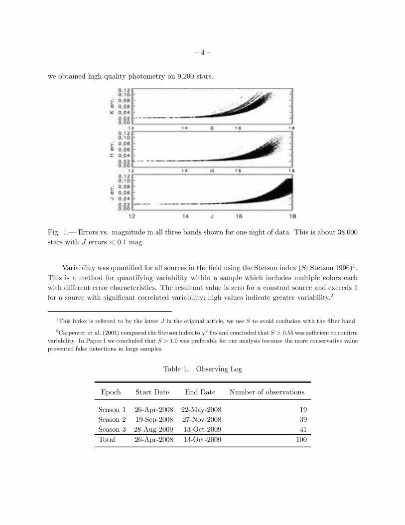
Table 5. Other possibly periodic stars in the monitored field.

R.A. Decl. J H K ∆J ∆K ∆J −H ∆H −K S Period Gr.

(J2000) (J2000) mag mag mag mag mag mag mag (days) 1− 5

Long period

20:59:41.783 +52:39:10.2 16.52 15.22 14.52 0.40 0.28 0.20 0.16 5.30 61 or 122* 3

21:00:00.453 +52:24:50.5 13.92 12.42 11.72 0.19 0.15 0.07 0.07 3.16 59.20 3

21:02:22.239 +52:44:57.9 15.53 14.23 13.60 0.17 0.10 0.16 0.07 2.04 72.60 2

Moderate period

20:57:47.04 +52:43:57.6 14.74 13.88 13.50 0.10 0.17 0.10 0.09 1.12 2.78 4

20:57:51.19 +52:31:54.6 14.92 13.75 13.21 0.13 0.10 0.09 0.05 2.30 17.85 5

20:58:11.02 +52:26:53.4 15.58 14.32 13.68 0.09 0.08 0.06 0.07 1.02 12.43 3

20:58:16.96 +52:47:34.7 12.30 11.95 11.75 0.08 0.09 0.07 0.07 1.83 12.80 2

20:58:19.12 +52:21:40.6 14.83 13.72 13.20 0.12 0.09 0.09 0.07 2.31 multi* 2

20:58:23.86 +52:20:10.1 13.33 12.80 12.47 0.07 0.07 0.06 0.08 1.50 9.84 4

20:58:27.49 +52:36:42.6 16.58 15.28 14.61 0.19 0.10 0.21 0.09 1.03 25.80 2

20:58:30.78 +52:06:39.0 14.10 13.42 13.16 0.12 0.09 0.08 0.10 1.68 4.52 4

20:58:42.08 +52:20:03.5 13.95 13.03 12.65 0.12 0.08 0.09 0.08 1.36 4.70 4

20:59:17.76 +52:46:12.3 15.72 14.79 14.33 0.11 0.09 0.11 0.07 1.80 3.07 3

20:59:28.56 +52:10:10.4 15.88 15.04 14.70 0.18 0.15 0.09 0.09 3.24 3.56 3

21:00:14.89 +52:14:58.0 12.80 12.08 11.90 0.09 0.07 0.10 0.10 1.62 1.25, 4.96* 1

21:00:16.18 +52:47:59.6 16.28 15.39 15.00 0.16 0.11 0.13 0.18 1.28 7.70 1

21:00:42.28 +52:20:10.5 12.37 11.56 11.22 0.11 0.09 0.06 0.08 2.06 6.19 5

21:00:42.84 +52:46:16.3 15.43 14.45 14.01 0.13 0.13 0.12 0.09 2.68 9.46 4

21:01:21.18 +52:43:43.7 16.01 15.13 14.73 0.24 0.10 0.25 0.12 1.52 4.7 , 3.1* 3

21:01:34.27 +52:47:41.2 14.99 14.14 13.83 0.12 0.11 0.11 0.06 2.37 2.29† 2

21:02:02.70 +52:39:29.0 15.74 14.55 14.00 0.12 0.09 0.07 0.08 1.06 12.50 1

21:02:16.70 +52:02:19.9 15.23 14.30 13.96 0.30 0.10 0.31 0.14 1.72 4.59 3

21:02:35.59 +52:43:53.6 14.38 13.46 13.07 0.17 0.13 0.09 0.08 3.64 7.29 5

21:03:02.06 +52:53:49.4 15.98 15.12 14.84 0.22 0.15 0.24 0.12 1.26 8.11 3

Note. — Typical photometric errors are ∼ 2%.

∗Noted stars did not have a unique period identified.

†Period only noted in Season 2.

– 16 –

to tidal deformation and rotation is minimal. These constitute the first group of stars in Table 3,

identified as “simple eclipse”. These systems have periods ranging from around 0.4 days to a little

over 13 days. For the best examples, these stars ranged from an average J magnitude of 13.3 to 16.8

mag with a median average J ∼ 16.2. Eclipse depth ranges from 0.15 to 0.92 mag with a median

of 0.45 mag. The color changes are small, but measurable, with the median shift in J −K color

of about 0.18 and and a maximum shift of about ∆J −K ∼ 0.5. We show 10 of these in Figure 3.

The nominal level when the system is out of eclipse indicates limited tidal distortion effects – with

a few exceptions, 210149.79+525235.9 being the most conspicuous.

4.2. Ellipsoidal/Contact systems

Slightly over 60% of the lightcurves in this sample had continuous flux variations. There have

been several recent surveys focused on finding variable stars. A long baseline study covering up

to 8 years is a galactic field monitoring program by Paczynski et al. (2006). It is more common

that these studies last an observing season (e.g.Weldrake & Bayliss 2008 and Miller et al. 2010).

Pietrukowicz et al. (2009) and Pietrukowicz et al. (2011) focused on deep monitoring program of

a few days which included NIR and optical photometry. The results of these programs are that

between 0.06 and 0.30 % of the field stars show systems with continuous flux variations, indicative

of contact binaries or elliptical stars. An exception is the result from the Kepler mission which

indicates the rate of such stars may be as high as 1.2% when the precision in the photometric is

high enough (e.g.mmag, Prsa et al. 2011).

While it is possible the continuous signal variation is due to the stars being ellipsoidal in shape,

it is more likely that two stars are in or near contact with each other and there is a continuous

variation of flux. In contact binary systems all cycles contain two maxima and two minima and this

was enforced by the period finding algorithm. We show 10 of these in Figure 4. We would expect

that the periods of these contact binaries are shorter than other binaries. Indeed the periods range

from about 0.2 days to 3 days for these kinds of systems. The median period found was around 0.4

days. Periodic phenomena are also expected in young spotted stars, but the short periods and and

long term stability argue against this interpretation. Some of the qualitatively weaker sources, such

as 205922.81+522338.4, 205746.71+520302.3 and 210058.93+523810.7, were explicitly examined at

high order peaks in their periodograms, but no convincing signal was found. The periods shown in

Figure 4 here are the strongest periods for these stars, but the two algorithms occasionally returned

alias frequencies. These stars ranged from an average J magnitude of 12.5 to 17.3 with a median of

J ∼ 16.1. Eclipse depth ranges from ∆J = 0.1 to 0.9 with a median of 0.35. The color changes are

small but measurable with the median shift in J−H color of about 0.2 and and a maximum shift of

about ∆J−H ∼ 0.4. A few systems had clear color patterns. 205945.69+520716.3 tends to become

redder as it becomes fainter and bluer as it become brighter; 210029.43+521147.1 showed a similar

pattern. 205905.47+520711.3 and 205746.71+520302.3 appear reddest when they are faintest, but

the effect is weak, perhaps 0.02 in H −K. A detailed statistical analysis would be needed to prove

– 17 –

the color patterns noted in these stars were significant.

Most of the contact systems are probably W UMa type systems, consisting of a pair of stars

in a tight, circular orbit, with each star in contact with and eclipsing the other. W UMa type

contact binary stars are surprisingly common in the solar neighborhood. The apparent relative

frequency of W UMa type stars was estimated at about 1/130 of the frequency of the common

solar-neighborhood FGK-type disc population dwarfs with an age of 5 − 11 × 109 years (OGLE

Rucinski 1998). This is similar to the detection rate found here, which was about 32/9200 (≈1/240

or 0.04%) Because the formation of contact systems by the gradual loss of angular momentum due

to the combined effects of tidal coupling and braking by the stellar wind W UMa type systems are

not observed in clusters younger than about 1 billion years old.

4.3. Longer period stars

About 20 stars showed sinusoidal variations on timescales of about 2 to 25 days. These are

indicated as “moderate period/ weak signal” variables in Table 5. Many of these show significantly

more deviation from the computed signal than the typical short period system. This is not an effect

of low peak to trough signal (and hence higher noise) – the best examples of stars with period from

2-25 days ranged from and average J magnitude of 12.4 to 15.5 with a median average J ∼ 14.1 -

brighter than either of the eclipsing subgroups.

The confidence of most of the periods in the lower portion of Table 5 is not very high as noted

by the relatively low grades. We show 10 examples of these in Figure 5. Most of these objects

have light curves dominated by a single peak and single trough. Unlike the previous group of

objects, doubling the periods did not improve the signal to noise. Several stars in the group showed

periodicity in only some of the observing seasons. Other stars showed several signals at similar

strength and we chose to list the strongest two. One star, 205819.12+522140.6, has five equally

probable signals. This might be a sign that some of these are pulsating stars, such stars would

show relatively colorless changes as observed here.

Another possibility is that some of these stars may be diskless, low-mass YSOs, alternatively

called Class III objects or weak T Tauri stars. As this is a region of star formation with about 40

previously identified disk and envelope bearing stars, it would be surprising if the number of diskless

objects was much less than 20; it could possibly exceed 40. Diskless YSOs are often variable due to

surface spots induced by dynamo behavior in their evolving interiors (e.g. Feigelson & Montmerle

1999).

Cool spots, like those on the Sun, were first identified as a contributor to the variability

of PMS stars in the 1980s (Vrba et al. 1985). Static stellar spots induce variability because of

the rotation of the star. Starspots have been used regularly as a method of measuring stellar

periods (e.g. Attridge & Herbst 1992). Typical rotation periods of weak T Tauri stars are between

1 and 10 days (Grankin et al. 2008). In the I band, the luminosity change is typically < 15%

– 18 –

Fig. 3.— Some examples of detached systems. K-band data are shown. Phase 0 is arbitrary based

on the time of the first observation. Names are indicated in each panel. In the bottom two rows,

ellipsoidal effects are clearly seen.

– 19 –

Fig. 4.— Some example contact systems. Names are indicated in each panel.

– 20 –

(Cohen, Herbst, & Williams 2004). The implied color change due to a lower effective temperature

is < 5%. The median magnitude change of the moderate period stars in our data is ∼ 10%, quite

consistent with the spot interpretation. Typical color changes are a bit higher than expected, about

8% at J −H and H−K, however color measurements are more sensitive to measurement precision

so we do not consider this result inconsistent with the spot interpretation – at least for some of the

sources.

4.4. Other periodic stars

A small number of stars showed very strong periodic light curves which neither corresponded

to eclipse events or symmetric signals. These are indicated as “other periodic” stars in Table 3.

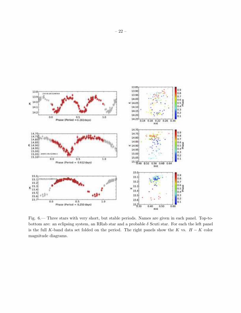
Two examples are shown in Figure 6. Star 210145.39+524059.9 has a period of just 6.8 hours with a

one flat minima which lasts about an hour ∆J ∼ ∆K ≈ 0.33. There is a clear pattern in the color-

magnitude diagram indicating the star changes color, becoming bluer the longer it is in the faint

state, reddening somewhat as it brightens and then becoming fainter with little noticeable color

change. This appears to be an eclipsing binary. Star 205931.39+522802.1 has a period of about

14.7 hours with a smooth rapid rise coming about 1/3 of the cycle and the decline lasting the other

2/3 ∆J = 0.48 and ∆J −K ∼ 0.15. This appears to be an RR Lyrae sub-type known as an RRab

star which has a large amplitude, hours long, asymmetric light curve. Star 210223.22+524951.0

shows a combination of these effects: a short (∼ 6 hour) period, a sustained minimum, a rapid rise

and a slow fall. For this star ∆J = 0.64 and ∆J −K ∼ 0.10. This may be a δ Scuti star.

There are a few stars which appear to vary on longer times scales. Because there are only

three, and the periods are at least of order the duration of the observing season, it is hard to tell

if they share any characteristics. There are also a few objects with very regular, non-sinusoidal

variations. Some of these may instead be tidally distorted stars or perhaps pulsating stars.

Since our period detection algorithms were designed to find stable periods we may have missed

δ Scuti stars - these are among the most common pulsating stars (Pietrukowicz et al. 2009). One of

the key distinguishing characteristic of common pulsating stars is irregular change signal strength

on a regular period. The typical δ Scuti star has an amplitude of 0.003 - 0.9 magnitudes. The

variations in luminosity are due to both radial and non-radial pulsations of the star’s surface. They

sometimes have beat patterns which make the light curves difficult to fold as the amplitude of

adjoining cycles is often modulated. Further the periods are typically < 6 hours which is much

below our sampling. δ Scutis are early A to late F range and hence are generally warm with respect

to the near-IR studied here, with color changes more obvious in optical wavelengths. The J-K color

shouldn’t change much at all. Given the 0.2% fraction observed in Carina (Pietrukowicz et al. 2009)

we expect about 18 of these stars in our dataset; however, given their typical periods of 0.25 days

and typical amplitudes, including amplitude modulation, many of these may have gone undetected

or noted as stochastic systems.

– 21 –

Fig. 5.— Three–season K band period-folded lightcurves of stars with quasi-sinusoidal periods

longer than 2 days which were stable across the three seasons including 2 long period variables.

Names are indicated in each panel.

– 22 –

Fig. 6.— Three stars with very short, but stable periods. Names are given in each panel. Top-to-

bottom are: an eclipsing system, an RRab star and a probable δ Scuti star. For each the left panel

is the full K-band data set folded on the period. The right panels show the K vs. H − K color

magnitude diagrams.

– 23 –

5. Conclusions

In this contribution, we present the results of an approximately 100 night, NIR photometric

monitoring campaign. While the program itself was focused on the pre-main sequence population

of the very young star forming region Cyg OB7, we report here on the field star population. The ∼9,200 non-disked stars surveyed were in a band from 11 < J < 17.3, 11 < H < 16.5, and 11 < K <

16. About 1.6% of the non-disked stars variable. This is significantly less than the rate for disked

YSO’s which have variability rates > 90% (Carpenter et al. 2001, 2002; Morales-Calderon et al.

2009, 2011; Rice, Wolk & Aspin 2012; Scholz 2012). Of the variables, about 1/3 are weakly variable

with stochastic changes.

We used two period finding algorithms on the variables, Fast χ2 and the Lomb-Scargle peri-

odogram. About one-third of the variables are clearly eclipsing systems with highly stable periods.

The greater half of the eclipsing systems are contact or near contact binaries with continous flux

changes. The detection rate of contact/ellipsoidal binary systems is 0.4%, about 25% higher than

other ground-based surveys, but about one-third the rate found by Kepler.

Among the remaining variables, some of these have very stable, very short periods and appear

to be pulsators. There are intermediate length periodic variables with less stable variability, with

nearly colorless luminosity changes of about 0.1 magnitudes. These stars have periods between 2

and 25 days and may be spotted. Follow-up deep X-ray or optical Hα observations could be used

to ascertain the evolutionary status of these stars and the likelihood that these changes do indeed

arise from spots.

6. Acknowledgements

S.J.W. is supported by NASA contract NAS8-03060 (Chandra). T.S.R. was supported by

Grant #1348190 from the Spitzer Science Center and also the NSF REU site grant #0757887. The

United Kingdom Infrared Telescope is operated by the Joint Astronomy Centre on behalf of the

Science and Technology Facilities Council of the U.K. We thank A. Nord, L. Rizzi, and T. Carroll for

assistance in obtaining these observations. We also thank the University of Hawaii Time Allocation

Committee for allocating the nights during which these observations were made. The authors wish

to recognize and acknowledge the very significant cultural role and reverence that the summit of

Mauna Kea has always had within the indigenous Hawaiian community. We are most fortunate to

have the opportunity to conduct observations from this sacred mountain. Special thanks to Nancy

Evans, Margarita Karovska and Matthew Templeton for helping us assess the lightcurves.

– 24 –

REFERENCES

Andersen, J. 1991, A&A Rev., 3, 91

Aspin, C., et al. 2009, AJ, 137, 431

Aspin, C., Reipurth, B., Herczeg, G. J., & Capak, P. 2010, ApJ, 719, L50

Attridge, J. M., & Herbst, W. 1992, ApJ, 398, L61

Audard, M., et al. 2010, A&A, 511, A63

Benedict, G. F., et al. 2007, AJ, 133, 1810

Bouvier, J., et al. 2003, A&A, 409, 169

Bouvier, J., et al. 2007, A&A, 463, 1017

Carpenter, J. M., Hillenbrand, L. A., & Skrutskie, M. F. 2001, AJ, 121, 3160

Carpenter, J. M., Hillenbrand, L. A., Skrutskie, M. F., & Meyer, M. R. 2002, AJ, 124, 1001

Cohen, M. 1980, AJ, 85, 29

Cohen, R. E., Herbst, W., & Williams, E. C. 2004, AJ, 127, 1602

Devine, D., Reipurth, B., & Bally, J. 1997, Herbig-Haro Flows and the Birth of Stars, 182, 91P

Dobashi, K., Bernard, J.-P., & Fukui, Y. 1996, ApJ, 466, 282

Donati, J.-F., et al. 2010, MNRAS, 409, 1347

Feigelson, E.D., & Montmerle, T. 1999, ARAA, 37, 363

Grankin, K. N., Bouvier, J., Herbst, W., & Melnikov, S. Y. 2008, A&A, 479, 827

Guinan, E. F., Ribas, I., Fitzpatrick, E. L., Gimenez, A., Jordi, C., McCook, G. P., & Popper,

D. M. 2000, ApJ, 544, 409

Herbig, G. H. 1962, Advances in Astronomy and Astrophysics, 1, 47

Herbst, W., Herbst, D. K., Grossman, E. J., & Weinstein, D. 1994, AJ, 108, 1906

Horne, J.H., Baliunas S.L. 1986, ApJ, 302, 757

Hodgkin, S. T., Irwin, M. J., Hewett, P. C., & Warren, S. J. 2009, MNRAS, 394, 675

Huang, S. S., & Struve, O. 1956, AJ, 61, 300

– 25 –

Joy, A. H. 1945, ApJ, 102, 168

Khavtasi, D. S. 1955, Abastumanskaia Astrofizicheskaia Observatoriia Byulleten, 18, 29

Lada, C. J., & Adams, F. C. 1992, ApJ, 393, 278

Melikian, N. D., & Karapetian, A. A. 2003, Astrophysics, 46, 282

Melikian, N. D., & Karapetian, A. A. 2001, Astrophysics, 44, 216

Miller, V. R., Albrow, M. D., Afonso, C., & Henning, Th. 2010, A&A, 519, A12

Morales-Calderon, M., et al. 2011, ApJ, 733, 50

Morales-Calderon, M., et al. 2009, ApJ, 702, 1507

Movsessian, T., Khanzadyan, T., Magakian, T., Smith, M. D., & Nikogosian, E. 2003, A&A, 412,

147

Paczynski, B., Szczygie l, D. M., Pilecki, B., & Pojmanski, G. 2006, MNRAS, 368, 1311

Palmer, D. M. 2009, ApJ, 695, 496

Parihar, P., Messina, S., Distefano, E., Shantikumar, N. S., & Medhi, B. J. 2009, MNRAS, 400, 603

Pietrukowicz, P., et al. 2009, A&A, 503, 651

Pietrukowicz, P., et al. 2011, arXiv:1110.3453

Pols, O. R., Tout, C. A., Schroder, K.-P., Eggleton, P. P., & Manners, J. 1997, MNRAS, 289, 869

Popper, D. M., Andersen, J., Clausen, J. V., & Nordstrom, B. 1985, AJ, 90, 1324

Press, W. H., & Rybicki, G. B. 1989, ApJ, 338, 277

Prsa, A., et al. 2011, AJ, 141, 83

Reipurth, B., & Schneider, N. 2008, Handbook of Star Forming Regions, Volume I, 36

Rice, T. S., Wolk, S. J., & Aspin, C. 2012, ApJ, 755, 65

Rieke, G. H., & Lebofsky, M. J. 1985, ApJ, 288, 618

Rucinski, S. M. 1998, AJ, 115, 1135

Samus, N. N., Durlevich, O. V., & et al. 2009, VizieR Online Data Catalog, 1, 2025

Scholz, A. 2012, MNRAS, 420, 1495

Schroder, K.-P., Pols, O. R., & Eggleton, P. P. 1997, MNRAS, 285, 696

– 26 –

Stetson, P. B. 1996, PASP, 108, 851

Tokunaga, A. T., Simons, D. A., & Vacca, W. D. 2002, PASP, 114, 180

Torres, G., & Ribas, I. 2002, ApJ, 567, 1140

Thompson, S. E., Clemens, J. C., van Kerkwijk, M. H., & Koester, D. 2003, ApJ, 589, 921

Vrba, F. J., Rydgren, A. E., Zak, D. S., & Schmelz, J. T. 1985, AJ, 90, 326

Weldrake, D. T. F., & Bayliss, D. D. R. 2008, AJ, 135, 649

Wolk, S. J., Rice, T. S., & Aspin, C. 2013, in prep.

This preprint was prepared with the AAS LATEX macros v5.2.