Bachelor Thesis in Statistics, 15 ECTS

Music Recommendations

Approximating user distributions to address thecold start problem

Johan Hammarstedt

Department of StatisticsLund University

Fall Semester, 2019

Supervisor: Krzysztof Podgórski

Abstract

In today’s data driven society the world is at a point of information overload. As people relyon Google for information and other platforms such as Netflix and Spotify for entertainment,the need for relevant filtering of content has never been higher. As a result, recommendationsystems have seen a great surge in demand. One can divide the space of recommendationalgorithms into primarily two approaches. In the context of music,a collaborative based onewhere underlying correlations between users dictate the model, and the content based ap-proach which examines the more specific relationship each user has to the songs. This paperaims to highlight the issues many collaborative models face when there is a lack unevenamount of interactions with the songs; this is usually the case for less popular or new items.To address this, a content based approach is suggested based on music feature data with thegoal to distinguish unique user distributions based on song characteristics. After evaluatingthis method against a popularity based baseline model, there was a small but not significantdifference in the error. This suggested that there are a lot of room for improvement in theapproximation of user distributions, leading to the conclusion that with more elaborativemethods one could most likely expand upon this research and build strong recommendationsbased on the idea of probabilistic user distributions.

Keywords— Content-Based Recommendations, Collaborative Filtering, Matrix Factoriza-tion, User-Feature distribution

i

Acknowledgements

I would like to thank my supervisor Krzysztof Podgórski for our interactive discussions andhis commitment to help me complete this paper. I am also thankful to Spotify and theresearchers behind the Million Song Dataset for their excellent API’s and accessible data.Finally I would extend my gratitude to my parents and my grandpa for all their supportthroughout my academic career.

ii

Contents

1 Introduction 11.1 Background . . . . . . . . . . . . . . . . . . . . . . . . . . . . . . . . . . . . 11.2 The cold start problem . . . . . . . . . . . . . . . . . . . . . . . . . . . . . . 21.3 Goal and scope of this paper . . . . . . . . . . . . . . . . . . . . . . . . . . . 3

2 Spotify and EchoNest Datasets 5

3 Methodology 133.1 Collaborative filtering - a model based method . . . . . . . . . . . . . . . . . 13

3.1.1 Matrix factorization models - Singular Value Decomposition . . . . . 133.2 Content Based filtering methods . . . . . . . . . . . . . . . . . . . . . . . . . 17

3.2.1 The Yeo-Johnson Transformation . . . . . . . . . . . . . . . . . . . . 173.2.2 Multivariate Gaussian Distribution . . . . . . . . . . . . . . . . . . . 18

3.3 Proposed evaluation method . . . . . . . . . . . . . . . . . . . . . . . . . . . 18

4 Evaluation and Results 224.1 Collaborative filtering Results . . . . . . . . . . . . . . . . . . . . . . . . . . 224.2 Content Based Results . . . . . . . . . . . . . . . . . . . . . . . . . . . . . . 26

4.2.1 Results on users with more songs . . . . . . . . . . . . . . . . . . . . 31

5 Discussion 33

6 Conclusion and final words 37

A Appendix - Optimization Algorithms IA.1 Cost Function . . . . . . . . . . . . . . . . . . . . . . . . . . . . . . . . . . . IA.2 Gradient Decent . . . . . . . . . . . . . . . . . . . . . . . . . . . . . . . . . . II

A.2.1 Stochastic Gradient Decent . . . . . . . . . . . . . . . . . . . . . . . IVA.3 Regularization . . . . . . . . . . . . . . . . . . . . . . . . . . . . . . . . . . . IV

iii

B Appendix - Yeo-Johnson transformations VI

iv

List of Figures

2.1 Distribution of full dataset with only users who has listened to more than tensongs . . . . . . . . . . . . . . . . . . . . . . . . . . . . . . . . . . . . . . . . 8

2.2 Raw sample user feature data . . . . . . . . . . . . . . . . . . . . . . . . . . 9

2.3 Listen Count . . . . . . . . . . . . . . . . . . . . . . . . . . . . . . . . . . . 11

4.1 Listening pattern prediction . . . . . . . . . . . . . . . . . . . . . . . . . . . 24

4.2 Example of transformed variables with Recommendations. The diagonal dis-plays the distribution for that user’s features. Green: Recommended songs.Orange: The distribution of the users top ten songs. Blue: the rest of thatuser’s songs. . . . . . . . . . . . . . . . . . . . . . . . . . . . . . . . . . . . . 27

4.3 Error in relation to user information . . . . . . . . . . . . . . . . . . . . . . 29

4.4 Likelihood model: Relationship between Error, Listen Count and Unique songs 30

A.1 Gradient Decent Visualization . . . . . . . . . . . . . . . . . . . . . . . . . . III

A.2 The dilemma of choosing learning rate . . . . . . . . . . . . . . . . . . . . . IV

B.1 Transformation results: Energy (left) and Danceability (right) . . . . . . . . VI

B.2 Transformation results: Acousticness (left) and Instrumentalness (right) . . VI

B.3 Transformation results: Loudness (left) and Liveness (right) . . . . . . . . . VII

B.4 Transformation results: Tempo (left) and Valence (right) . . . . . . . . . . . VII

v

List of Tables

2.1 General data information . . . . . . . . . . . . . . . . . . . . . . . . . . . . 6

2.2 Top-10 most listened songs by users in dataset . . . . . . . . . . . . . . . . . 10

2.3 Cumulative Percentage . . . . . . . . . . . . . . . . . . . . . . . . . . . . . . 10

2.4 Distribution of Listen Counts . . . . . . . . . . . . . . . . . . . . . . . . . . 11

2.5 Distribution of Listen Counts for users with >10 songs. . . . . . . . . . . . . 12

3.1 User-Song Matrix (R) . . . . . . . . . . . . . . . . . . . . . . . . . . . . . . 14

3.2 Factor Matrix example - Songs . . . . . . . . . . . . . . . . . . . . . . . . . . 15

4.1 SVD results . . . . . . . . . . . . . . . . . . . . . . . . . . . . . . . . . . . . 22

4.2 Best Predictions for SVD model . . . . . . . . . . . . . . . . . . . . . . . . . 23

4.3 Worst predictions for SVD model . . . . . . . . . . . . . . . . . . . . . . . . 25

4.4 Overall Results . . . . . . . . . . . . . . . . . . . . . . . . . . . . . . . . . . 28

4.5 Results for users with most songs after 10 cross-validations . . . . . . . . . . 31

4.6 Example of a decentile distribution for one user . . . . . . . . . . . . . . . . 32

vi

1. Introduction

1.1 Background

In today’s data driven society we are at a point of information overload. The availability ofinformation has created an environment where haystacks are everywhere and user’s barelyknow how to spot the needle. This has generated a surge of recommendation systems withthe task to filter relevant content for the user. Tech-companies such as Amazon, Spotify,Netflix and Youtube are constantly developing algorithms to identify user behavior and cre-ate relevant content for each consumer. "Recommendation systems are defined as decisionmaking strategy for users under complex information environments" [11]. This paper aim toelaborate on the algorithms used in today’s industry, more specifically the two approachesknown as collaborative filtering and content based filtering which will be discussed in detail inthe upcoming sections. Collaborative filtering aims to use the ratings provided by a networkof users to make predictions for what to recommend, refereed to as user-to-user. On the otherhand, a content based approach looks at the specific user and the attributes of each item sheprefers, i.e user-to-item [15]. Today, collaborative filtering is the most popular technologyused and has seen a lot of success due to the power of user profiling and big platforms suchas Spotify, having 124 million paid subscriptions and 271 million active monthly users, allwith their own unique profiles [1] [3].

The authors of the article "Current challenges and visions in music recommender systemsresearch" [16] identifies many important particularities with music recommendations, andthe following are especially relevant for this paper:

1. "Consumption behavior": A lot of music is consumed passively as background music,

1

which we pay no attention to. This can cause a problem to identify actual preferenceand implicit feedback, leading to false assumption about the users taste.

2. "Listening context": A user can have very different taste for any given situation. Onone hand creating a calm playlist for studying but then also a death-metal album forworking out. User may also change their preferences over time.

1.2 The cold start problem

A well known obstacle with many recommendation systems is the cold start problem, wherethe lack of information makes it difficult to create proper assumptions of user preference[10] [16]. Collaborative models tend to have a strong bias towards music with a lot of userinteraction and thus favor more popular music. In the article "A collaborative filteringapproach to mitigate the new user cold start problem" [6], the authors identifies three typesof cold start problems:

1. New Community: Difficulties obtaining data when first creating a recommendation sys-tem environment. With a few users and bad recommendations, keeping them becomesdifficult and further weakens the models.

2. New User: The problem of limited information from new users is one of the moredifficult problems, which in some cases can be addressed by asking a new user toprovide information upon entering the platform.

3. New item: Newly created songs or not popular ones lack interactions from users andwill therefore have a hard time being labeled.

Another complication of music recommendations is sparsity : "the inverse ratio between givenand possible ratings" [16]. With a lot of content available and millions of users, individualswill only be able to rate a fraction of available songs. This also leads to more unreliablerecommendations [12].

Nevertheless, in order to address the cold start problem, a lot of research has been doneon Ensemble Based Recommender Systems. The idea is to combine collaborative models

2

and content models by different methods and thus address their respective weaknesses withthe others strengths [16] [8]. There are many approaches to combine these models such ascomputing weighed averages between predictions or switching between models in a scenariobased setting [4]. As this paper mainly will elaborate on the use of the models separately,combining them to a hybrid would be an intriguing topic for further research.

1.3 Goal and scope of this paper

In this paper I aim to do the following:

1. Give an overview of the state of the art collaborative filtering approaches being usedin the industry today, then create and evaluate a collaborative model.

2. Attempt to address the cold start problem (mainly the new item) recommendationsystems face by proposing a content based solution.

3. Introduce a method to objectively evaluate the content model for each user.

The collaborative filtering model is a technique utilizing Matrix Factorization and is a wellknown approach within recommendation systems. The goal is to predict user ratings givenother user behavior by exploiting hidden correlations between users and their respective rat-ings. Further details of this are provided in later sections of this paper (see 3.1.1).

As previously mentioned, it will be difficult for the above method to recommend songs thatthat many users have yet to interact with, known as the Cold start problems of new items.The main focus of this paper will therefore be on the content based approach and its evalua-tion. Content based methods do not require ratings of other users to recommend and insteadextract features from the songs themselves. [16]. The paper suggests a probabilistic modelbased on identifying underlying user distributions. The intuition is the rather simple ideathat, given the set of song features, each user has their own distribution which would corre-spond to one’s taste. A user frequently listening to dance music would correspondingly see

3

the features clustering towards high scores in characteristic features of that genre, like danca-bility and energy. By approximating the feature distribution for songs that a user prefers toa multivariate Gaussian distribution (see 3.2.2=, and then computing the likelihood of othersongs in the dataset, new songs with similar features would be recommended. Consequently,ignoring aspects such as popularity and other user preferences that are the main sources ofbias when dealing with the new item problem.

Evaluating a music recommendation system presents many problems as it becomes difficultto objectively address each user’s unique taste. A good recommendation for one might bepoor for another. Furthermore, the content model will not output a predictive and compa-rable rating for each song but rather rank them in terms of likelihood that it fits the userdistribution. This means that there are originally no true label to evaluate on. There are nonatural translation between the likelihood of a song in a user distribution and the amountof times the user has listened to a given song. The paper therefore suggest an alternativeapproach where the goal is to compute the distance from each song to the user-distribution.Since the model will, given a certain amount of mixed songs, recommend strictly based onlikelihood, one can compare how much the user’s preferences matches the user distribution.

4

2. Spotify and EchoNest Datasets

There will be two data sets be used to build the models and make recommendations. Thefirst is raw data obtained from Spotify’s API. Due to user privacy, only public playlists areavailable here and no user data could be gathered. The dataset consists of 83 450 songswhich are divided into 1453 public playlists. In addition to general info such as title, releasedate and artists, Spotify has also enabled a feature extraction for each song. This introducesthe following variables, who are continuous if not otherwise mentioned. Further note thatthese values were later normalized from [0, 1]. [18]:

1. Danceability - how suitable a track is for dancing in range [0, 1].

2. Acousticness - a confidence measure in range [0.0, 1.0] of whether the track is acoustic.

3. Energy - represents a perceptual measure of intensity and activity in range [0.0, 1.0].

4. Instrumentalness - predicts whether a track contains vocals or not from [0.0, 1.0]. Highervalues indicate less presence of vocals.

5. Key - the key the track is in. Categorical using standard Pitch Class notation. −1

indicates no pitch detected.

6. Liveness - detects the presence of an audience in the recording, higher values indicatea higher probability that the track was performed live, range: [0, 1].

7. Loudness - the overall loudness of a track in decibels (dB), usually in range [−60, 0].

8. Mode - the modality (major or minor) of a track (binary), the type of scale from whichits melodic content is derived.

5

9. Tempo - the overall estimated tempo of a track in beats per minute (BPM).

10. Valence - a measure in range [0.0, 1.0] describing the musical positiveness conveyed bya track.

Due to the lack of user data in the Spotify dataset another one was obtained which is a subsetof the Million Song Dataset (MSD) from the Echo Taste Profile subset [5] [19]. The MSD isa very extensive dataset and widely used within research on recommendation systems sinceit has real and authenticated user data. Since the processing of the full 280 GB dataset andeven the full Echo subset would have required further data management, it is outside of thescope of this paper, and the final data gathered consists of 2 · 106 entries, containing 10000

unique songs and 76353 unique users. Each entry holds:

1. User ID

2. Listen Count

3. Song ID

4. Title

5. Release Date

6. Artist Name

Table 2.1: General data information

Unique songs Unique users Features Total Rows

EchoNest 10000 76353 User listen count 2000000Spotify Set 83 450 No user data Song features 83450

Table 2.1 displays the initial information obtained from each dataset. Using Spotify’s querymethod in their web API, the feature extraction was made for the EchoNest subset as well,leaving 1550027 rows. Since the focus mainly will be on the new item problem, and not

6

the new user problem, users who had listened to fewer than ten songs were then removedin order to better estimate the user-feature-distributions, resulting in 1347089 entries. TheEchoNest set will be used to build the models since it contains the user information needed.The recommendation library can then be expanded by the songs in the Spotify Set.

Figure 2.1 displays the distributions of the different features for users who have listened tomore than ten songs. As can be observed, some are Gaussian-like and will fit the generateddistribution properly while others will not. For this model binary and categorical valuespresents an issue, therefore the categorical key and the binary mode will be removed for theapproximation.

7

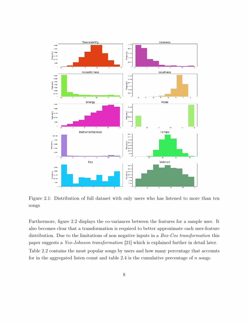
Figure 2.1: Distribution of full dataset with only users who has listened to more than tensongs

Furthermore, figure 2.2 displays the co-variances between the features for a sample user. Italso becomes clear that a transformation is required to better approximate each user-featuredistribution. Due to the limitations of non negative inputs in a Box-Cox transformation thispaper suggests a Yeo-Johnson transformation [21] which is explained further in detail later.

Table 2.2 contains the most popular songs by users and how many percentage that accountsfor in the aggregated listen count and table 2.4 is the cumulative percentage of n songs.

8

Figure 2.2: Raw sample user feature data

9

Table 2.2: Top-10 most listened songs by users in dataset

Title Listen Count Percentage of the aggregated listen count1 Undo 7032 0.4536142 You’re The One 6729 0.4340683 Revelry 6145 0.3963964 Secrets 5841 0.3767865 Fireflies 4795 0.3093126 Tive Sim 4548 0.2933787 Use Somebody 3976 0.2564808 Drop The World 3879 0.2502239 Marry Me 3578 0.23080610 Canada 3526 0.227452

Table 2.3: Cumulative Percentage

Songs 10 20 30 40 50Cumulative Percentage 3.4 5.4 6.9 8.3 9.6

As displayed in Table 2.3, the first 50 songs account for 10% of the total 155027 for the fulldataset, where the top 10 is 3.4%. Figure 2.3 then illustrates the distribution of the listencount. The x-axis displays how many times a single song has been listened to mapped to they-axis by the amount of users. As seen roughly in Figure 2.3, the majority of listen countsare users who have listened to a song a fewer times. This is also confirmed by the listencount distribution in Table 2.4. This can present problems, especially for the collaborativemodel, since the recommendations in a environment could lead to overfitting and minimizethe error by rating all songs as one.

10

Table 2.4: Distribution of Listen Counts

Listen Count 1 2 3 4 5 6 7 8 9 10 <10

Total (thousands) 890 242 110 63 71 35 23 17 12 14 71Total (%) 57 16 7 4 4.5 2.2 1.5 1.1 0.8 0.9 4

Figure 2.3: Listen Count

After removing the users with less than ten songs, this resulted in 1347089 entries with 42288

unique users. Table 2.5 displays the new distribution which is similar to Table 2.4 and thuswill not change any other aspect of the analysis.

11

Table 2.5: Distribution of Listen Counts for users with >10 songs.

Listen Count 1 2 3 4 5 6 7 8 9 10 <10

Total (thousands) 772 212 97 56 60 30 20 15 11 12 608Total (%) 57 15.8 7.2 4.1 4.4 2.2 1.5 1.1 .8 .9 4.4

12

3. Methodology

The methods used in this paper are divided into several subsections covering the statisticalmethods and the proposed implementation. The more detailed mathematical notations ofoptimization using stochastic gradient decent and the idea behind regularization can be foundin the Appendix (see A).

3.1 Collaborative filtering - a model based method

Collaborative filtering usually falls into two types of techniques, Memory-Based and Model-Based. As the name suggests, Memory based stores a lot of information which it then mapsto each user. This is effective but in many cases not scalable enough for a substantial amountof users. The model based technique implies that a generalized model will be implemented topredict good songs. The focus of the collaborative section will be on model based approachesand for further readings on memory based approaches the reader is referred to [11]. To betterexplain the intuition behind these methods, the listen count is being defined as rating.

3.1.1 Matrix factorization models - Singular Value Decomposition

As previously mentioned, many of the other techniques have difficulties in terms of scala-bility. Latent factor models or matrix factorization models uses a dimensionality reductiontechnique called matrix factorization to efficiently create a model which will be introducedbelow. The full approach is known as singular value decomposition (SVD). So given a matrixcontaining all users and all songs, we approximate the scalar product between these vectorsand thus fill in the ’blanks’ as displayed in Table 3.1.

13

Table 3.1: User-Song Matrix (R)

S1 S2 S3 S4

User 1 3 1 3

User 2 1 4 1

User 3 3 1 1 3

User 4 3 5 4

Matrix R displayed in Table 3.1 is what one wish to compute. Realistically this matrixis missing values since most users have not listened to all songs. The goal is to predict thesemissing entries and recommend those with high scores to respective user. The problem isthat matrix R quickly gets very large, for the data set consisting of 10000 songs and 76353

users it would be a 76353 × 10000 matrix. This is dealt with by matrix factorization. Theidea is to exploit the fact that there exists high correlations between the rows and columnsin the matrix.

Now we introduce a user matrix U and an song matrix S. The user matrix is of size Nu×Nh

where Nu is the amount of users and Nh is the amount of so called hidden features we choose(the idea behind these features will be explained in the next paragraph). The song matrix Sis similar and of dimension Ns ×Nh where Ns is the number of songs. The goal of singularvalue decomposition is to compute:

U · ST ≈ R (3.1)

In words, finding the optimal matrix multiplication between two feature matrices that ap-proximates the whole user-song matrix R the best. This is done by finding hidden featuresthat exploits the correlations as previously mentioned. These hidden features are not intu-itively easy to explain since they are generated to find the best fit and might be the genre ofthe song, the popularity or something uninterpretable. [15].

14

Table 3.2: Factor Matrix example - Songs

Hidden Feature 1 (e.g. Genre) Hidden Feature 2 (e.g. key) ... Hidden feature Nh

Song 1 0.4 0.6 ... 0.5

Song 2 0.2 0.8 ... 0.2

... ... ... ... ..

... ... ... ... ..

Song Ns 0.5 0.3 ... 0.3

The user factor matrix looks similar with users {1, 2, ..., Nu} instead of songs. In the graphabove each song j has its own vector that suggests how well the song j possesses these fea-tures. In the user matrix, corresponding interpretation for user i would be the level of interestthe user has shown in songs with high values for given features [15]. An example would bethat a user has high values of hidden features that could corresponds to Pop or Dance music,meaning he tends to rate those songs high.

To quote from C.Aggrawal’s book on recommender systems [4], the inner dot product ofmatrices U and S, ui · sj "captures the interaction between user i and item j, the overallinterest of the user in characteristics of the item." The vectors ui and sj thus both has di-mension 1×Nh. From 3.1 it follows that rating ri,j can be approximated by the dot productof the jth song vector and ith user vector in their respective matrix. So the basic predictionfor the rating ri,j on song j by user i would be:

ri,j = uTi · sj. (3.2)

In the models used for this paper we will also incorporate baseline predictors as suggestedby [4] on their model for Netflix recommendations. The baseline predictors are meant tocapture systematic biases, like some users giving too high ratings. However, our ratings arebased on listens which are less likely to be biased in such a way (or a user could listen toan extensive amount of music compared to the rest and boost a song too much). To explainthese baselines used for dealing with bias, let µ be the average rating for all songs, vi and wj

15

be the observed standard deviation of user i and song j from the average. Then the baselineprediction bi,j for an unknown rating ri,j is:

bi,j = µ+ vi + wj (3.3)

Hence, to find the baseline for ex Happy with Pharell Williams one would do as follows: Ifthe average rating (listen count) for all songs was 3, but given the popularity of the songusers listen to it on average 1.5 times more. Then user X barely listen to music at all, onaverage he only listens to any song 1 time, 2 less than average. The baseline would thereforebe bi,j = 3 + 1.5− 2.

The updated rating for song j by user i will accordingly be computed by:

ri,j = bi,j + uTi sj = µ+ vi + wj + uTi sj. (3.4)

We wish to estimate vi, wj, uj, si, using a regularized (see A.2) squared error as our costfunction, as recommended by [4]. We first define a set with the known rating pairs (i, j) asη. So: η = {(i, j)|ri,j is known}. Then we minimize the cost function:

minb∗,u∗,s∗

∑i,j∈η

(rj,i − bi,j − uTj si)2 + λ(v2i + w2j + ||sj||2 + ||ui||2). (3.5)

The minimization is done by stochastic gradient decent [A.2.1]. A very successful SGDapproached created by Funk [17] is used to update the parameters:

• wj := wj + γ(ei,j − λwj)

• vi := vi + γ(ei,j − λvi)

• ui := ui + γ(ei,j · sj − λui)

• sj := sj + γ(ei,j · ui − λsj)

The error term is defined by computing the prediction ri,j and then comparing it to the truerating ri,j which is possible since we are optimizing a training set with the true ratings knownin η [15]:

ei,j = ri,j − ri,j, (i, j) ∈ η. (3.6)

16

3.2 Content Based filtering methods

Content based models are using the analysis between user item rather than user to user. Theapproach suggested in this paper originates from the idea that each user has a correspondingfeature distribution which, independent of popularity and previous ratings, can be usedto make more individual recommendations. The features are transformed by Yeo-Johnsontransformation with the goal to better fit the approximated multivariate normal distributionfor each user and then the likelihood of each song is computed to recommend the songsfitting the distribution the best.Below follows the methodology necessary to perform thesecomputations. The last section contains the proposed method to evaluate these results.

3.2.1 The Yeo-Johnson Transformation

Examining the initial data it was clear that some transformation was necessary to betterallow for normality. The Yeo-Johnson transformation was suggested by In-Kwon Yeo andRichard A. Johnson as a way to deal with the limitations of the Box-Cox transformation, asit only allows for strictly positive numbers [22]. The transformation was chosen as a way todeal with potential skewness and allow for better analysis. The transformations on a featurevector X with parameter λ is given by:

ψ(λ, x) =

((x+ 1)λ − 1)/λ, if λ 6= 0, x ≥ 0

log (x+ 1), if λ = 0, x ≥ 0

−[(−x+ 1)2−λ − 1)

]/(2− λ), if λ 6= 2, x < 0

− log (−x+ 1), if λ = 2, x < 0

(3.7)

The transformation is used to better allow for normality in the feature data and lambda is ahyper-parameter used for selecting the set of transformation on X. The optimal lambda (λ)for each feature is determined by the following method [2]:

L(X;λ, σ) =N

2log(σ2) + (λ− 1)

∑i

sign (xi) log(|xi|+ 1).

17

3.2.2 Multivariate Gaussian Distribution

The multivariate normal distribution is said to be defined when the random variable Z =

[Z1, ..., ZN ]T with mean µ ∈ Rn and the co-variance matrix Σ ∈ Sn++ have the probabilitydensity function:

p(z;µ,Σ) =1

(2π)n2 |Σ| 12

exp

(−1

2(z − µ)TΣ−1(z − µ)

)This is written as Z ∼ N (µ,Σ). The co-variance matrix Σ, for any random vector Z isdefined as:

Σ = E[(Z − µ)(Z − µ)T ] = E[ZZT ]− µµT .

The co-variance Σ for the multivariate Gaussian distribution, it is required to be positivedefinite, meaning that all its corresponding eigenvalues are positive.

For the k given features, each user-feature distribution will be approximated with a k × 1

vector µi and k × k matrix Σi. Since songs has different listen counts, both the co-variancematrix and µi will be weighted accordingly. Then, the likelihood of each song is calculatedfor each user and the top ten recommendations will be given by the ten with the highestlikelihood, given that the user has not listened to the song previously.

3.3 Proposed evaluation method

The following definitions are introduced below to be referred to in this section:

• LetNu be the total amount of users and useri denote the i-th user where i = {0, 1, ....Nu}.

• Let Ns be the total amount of songs and songj refer to the j-th song wherej = {0, 1..., Ns}.

• Let k be the number of features evaluated.

• µi,Σi: The k × 1 weighted average vector and the k × k weighted co-variance matrixfor useri.

18

• Si: The set of songs in the full dataset which useri has listened too.

• Li,j: The number of times useri has listened to songj assuming that songj ∈ Si.

1. Li: total listen count for useri ∈ Si.Li =

∑Sij=0 Li,j , j ∈ Si

• Fj: The k× 1 vector containing the corresponding k features for that song, so each Fjconsists of k numerical values representing the characteristics of that song.

• Pi: Refers to the overall listen count by all users in Si. Pi,j is then the overall listencount for song j by all users in Si.

Due to the difficulties of measuring model performance for a user on songs he/she has notgiven any information on, the evaluation will be performed on Si.

For useri, the idea is to compute the Mahalanobis squared distance (M2) from each songvector Fj to µi, thus the center of useri’s approximated user distribution. Then the aim is toexamine the distribution of these distances in relation to the listening preferences for useri.Mahalanobis Squared Distance is defined as follows: Let Fj be a k × 1-dimensional vectorcorresponding to a song with k- features. Let µi,Σi be the mean vector and co-variancematrix for user i between k features. Then the Mahalanobis squared distance between Fjand µi is defined as [14]:

M2 = (Fj − µi)TΣ−1(Fj − µi). (3.8)

As Σ−1 is the inverse of the co-variance matrix it is assumed that the matrix is invertibleand positive definite. As a result, it is then possible to show that M2 ∼ χ2(k), for k degreesof freedom corresponding to the number of song features1.

By using that M2 ∼ χ2k we compute the decentiles for that distribution and construct

intervals to check the total listen count for that user in each decentile interval. By definition,the distribution of the songs from our likelihood model will be 0.1 in each decentile. Let Li,m

1The actual derivation is out of scope of this paper, see [20]

19

be the listen count for useri in decentile m. The squared error for useri in decentile m isthen then defined as:

SEModeli,m =

[0.1− Li,m

Li

]2(3.9)

The mean squared error for useri and the total for all users then becomes:

MSEModeli =

1

10

10∑m=1

SEModeli,m ,m = {1, ..., 10} (3.10)

=⇒ MSEModel =1

Nu

Nu∑i=0

MSEModeli (3.11)

For comparison, a popularity model is also introduced. Defined as follows:

SEPopularityi,m =

[0.1− Pi,m

Pi

]2(3.12)

MSEPopularityi and MSEPopularity are determined similarly as (3.12) and (3.13).

For example, examining 8 features. Given the song vectors F1,F2,F3 for useri with a respec-tive listen count of 10, 12, 20. mean vector µi and co-variance matrix Σi. The Public Countfor the songs are (1020, 950, 2000). AllM2 values were then calculated to 6.55, 6.6, 3.8. Fora chi square distribution with 8 degrees of freedom: both F1 and F2 belongs to P50 and F3

is in P20. Thus:

SEModeli,2 = (0.1− 20

10 + 12 + 20 + rest)2 ≈ 0.09

SEModeli,5 = (0.1− 22

10 + 12 + 20 + rest)2 ≈ 0.11

=⇒ MSEModeli =

1

10

[0.09 + 0.11 +

10∑m=1

SEModeli,m

],m 6= {2, 5}

Where the rest denotes the remaining listen count for useri.

20

The step-by-step evaluation is done as follows:

1. Compute all decentiles for χ2k.

2. For each user:

(a) Randomly split the dataset into a training set of 80% and a test set of 20%.

(b) Approximate the multivariate Gaussian user distribution (µi,Σi) on the trainingset.

(c) Compute the Mahalanobis distance for each song vector Fj in the test set.

(d) For all decentiles, determine Li,m and Pi,m

(e) Calculate SEModeli and SEPopularity

i

3. Calculate MSEModel and MSEPopularity

Given that the whole dataset is transformed to approximately be normally distributed, thefollowing key point is made regarding the aim of this method:

The goal off the evaluation method is to test if each user distribution is distinctenough to make personalized recommendations based on feature data alone.

21

4. Evaluation and Results

4.1 Collaborative filtering Results

To create meaningful recommendations the listen count was scaled down to ’ratings’ from0 − 10.The initial scaling was just performed to merge values larger than 10. So the ratingfor songj by useri would be computed:

Ri,j = min(Li,j, 10)

Table 4.1 contains the after training the model on first a sample of 100000 entries with defaultvalues and a grid-search on number of epochs, hidden features,the overall learning rate andoverall regularization term. The optimal parameters where then used to train the full datasetwhich is also displayed below.

Table 4.1: SVD results

Hidden Features Epochs LR RT MSE MAE

SampleDefault 100 20 0.005 0.02 6.243 1.816

Gridsearch 100 25 0.03 0.6 6.23 1.815

Full Gridsearch 100 25 0.03 0.6 4.8 1.4

LR: Learning Rate, RT: Regularization term

Examining the sample results, one can see that the after grid-search, the model did slightlybetter after training for 5 more epochs with a different learning rate and regularization term.

22

Given more data on the full training set the model improves further with the optimal grid-search parameters from the sample. The final precision and recall scores for a five foldcross-validated model was:

PRAll =Recommended items that are relevant

Recommended items= 0.845

RCAll =Recommended items that are relevant

Relevant items= 0.594

However, given the uneven distribution of the data these results might be misleading. Table4.2 shows the best results for the full model. As seen the highest scores are all ones whichmatches are assumptions given the highly skewed data. The common trend is that all songshave all been ’rated’ by a large amount of users with an average Pi of 368.9 and Ii of 85.Although some might be more of lucky guesses with a low Pi and also a not very active usercorresponding to a low Ii value.

Table 4.2: Best Predictions for SVD model

User ID Song ID TR Pr Ii Pi Error

1 54a3... spotify:track:0kXeKglrzFU3w5J9nQWX0N 1.0 1.0 113 1360 0.02 3cec... spotify:track:56mAv6TVHL4QXcD4B4Ezvg 1.0 1.0 178 468 0.03 4a25... spotify:track:7BukHDlNfu4Ql7NATH6YIz 1.0 1.0 42 61 0.04 c6dd... spotify:track:57PqYPpY9sB8IQlRlnDVnN 1.0 1.0 145 171 0.05 9442... spotify:track:1pJS4rS12iA5MryQSAP2kQ 1.0 1.0 70 268 0.06 90ee... spotify:track:5UWwZ5lm5PKu6eKsHAGxOk 1.0 1.0 22 814 0.07 67db... spotify:track:2GGnAVuaaKklRJ67QZClzW 1.0 1.0 21 81 0.08 b075... spotify:track:6Y6f7LSvHxUA61ItYiSMKE 1.0 1.0 118 118 0.09 c766... spotify:track:029O4HWI1pVXLfFdfQd1Jb 1.0 1.0 130 104 0.010 72e5... spotify:track:3gNynXzWWUBDm9u4FLywaC 1.0 1.0 11 244 0.0

Ii: the set of songs listened to by user i

Pi: The set of all users who have listened to the songTR: True Rating, Pr: Prediction

23

Looking further into one of the top predictions, the left histogram in in Figure 4.1, one cansee that the majority of listenings are one, which then gives the model a lot of incentive torate this song accordingly.

Figure 4.1: Listening pattern prediction

Examining the worst predictions in table 4.3 the trend is also very clear as the maximal errorwill inevitable be when a low prediction corresponds to a high true rating and vice versa. Allsongs displayed here also have a high average P of 1020. The average I of 69 is also lowerthan for the best predictions, implying less information and thus harder to predict. Sincemost songs in the dataset are only listened to once we will examine one of the songs that waspredicted a high score.

24

Table 4.3: Worst predictions for SVD model

User ID Song ID TR Pr Ii Pi Error

1 87f7... spotify:track:1NhPKVLsHhFUHIOZ32QnS2 10.0 1.0 53 3634 9.02 b8f6... spotify:track:2vO1wr5wIEHqQmY4jWbuhi 10.0 1.0 158 397 9.03 06c4... spotify:track:1R6lhY5PqoxQJU5hsMDvjg 10.0 1.0 130 488 9.04 3da9... spotify:track:2cOCunrzyHVpTrTwSIKRbt 1.0 10.0 65 195 9.05 567b... spotify:track:2CR62nxWDw8ZRmJLCpm5PD 1.0 10.0 50 122 9.06 e647... spotify:track:3MJdjsfekFs4kh04g2l6Zg 10.0 1.0 12 1518 9.07 2a1f... spotify:track:43OjswTQMkuvQQEP38Roxl 10.0 1.0 32 64 9.08 4e6d... spotify:track:11LmqTE2naFULdEP94AUBa 10.0 1.0 138 378 9.09 3604... spotify:track:05NMSR0sSrCZxTHDRV415A 10.0 1.0 39 2637 9.010 8f8c8... spotify:track:31I3Rt1bPa2LrE74DdNizO 10.0 1.0 14 335 9.0

Ii: the set of songs listened to by user i

Pi: The set of all users who have listened to the songTR: True Rating, Pr: Prediction

The right histogram in 4.1 shows the song corresponding to index 5 in table 4.3. Again,the majority has listened to the song once but here a lot of users has also listened to thesong more than 10 times and thus the model makes the prediction on the wrong side of thespectrum.

25

4.2 Content Based Results

The figures in Appendix B displays the features after the Yeo-Johnson transformation. Sev-eral features are improved slightly to better fit a Gaussian distribution but many of them,especially instrumentalness and acousticness (see B.2) are still facing problems due to itsnon-symmetric properties.

Figure 4.2 shows the same user with respective feature scatter plot but now with the trans-formed values. As mentioned in the data exploration section (see 2), key and mode wereremoved to better allow for the Gaussian approximation. Furthermore, all values that ac-count for the users top ten most listened songs are plotted in terms of their listen count. Inaddition, the top ten recommendations from the model are marked green in each plot. Therecommendations tend to cluster around the center together with the top songs which indicatethat the likelihood estimation will give recommendations that most likely will correspond tothe user distribution and by assumption then be good recommendations. Acousticness andinstrumentallness still have difficulties to fit the distributions but the recommendations stilllay relatively close to them to the center.

26

Figure 4.2: Example of transformed variables with Recommendations. The diagonal dis-plays the distribution for that user’s features. Green: Recommended songs. Orange: Thedistribution of the users top ten songs. Blue: the rest of that user’s songs.

27

Table 4.4 displays the overall results. As seen in the table, the model fails to outperformthe baseline over all the 35000 users. One important note is that the the users are sorted onthe number of songs in descending order. As seen, the difference is increasing between eachinterval which calls for further analysis regarding relationship between the number of songs(listen count) and the evaluation.

Table 4.4: Overall Results

MSE Likelihood Model MSE Popularity Model Difference0-5000 0.0145 0.0098 0.00475000-10000 0.0276 0.0131 0.014510000-15000 0.0389 0.0131 0.014520000-25000 0.0493 0.0117 0.037520000-25000 0.0603 0.0098 0.050525000-30000 0.0699 0.0067 0.063330000-35000 0.09 0.0 0.09Overall 0.0450 0.0088 0.0361

Figure 4.3 displays this relationships further, showing the users listening information in rela-tion to the error. Again since the users are sorted from the most amount of songs and highestlisten count it can clearly be seen that the error increases linearly for the model in absenceof enough information.

28

Figure 4.3: Error in relation to user information

Figure 4.4 evaluates this relationship further to determine if the strong linear trend comesmainly from a lack of unique songs or listen count. Each dot represents a user with itsrespective error, listen count and unique songs. As shown, the number of unique songsstrongly determine the error. This is expected from the definition of the evaluation methodsince a decentile cannot have any listen count if there is no song there to begin with. This isdiscussed further in the later sections of this paper.

29

Figure 4.4: Likelihood model: Relationship between Error, Listen Count and Unique songs

30

4.2.1 Results on users with more songs

Table 4.5 shows the first ten users average results after ten cross validations. The overallerror of the model has dropped significantly as a result of better on average approximationsdue to more songs. Here the model outperforms the baseline with a decreased MSE of 7.2%

when examining the mean for both of them, the differences for all the 100-pairwise values is,however not significantly different from zero with a t-value of 0.51.

Table 4.5: Results for users with most songs after 10 cross-validations

User MSE_model MSE_public Listen Count Songs (Test Set) Difference

0 0.00575 0.00562 556 113 -0.000121 0.00177 0.00153 196 106 -0.000252 0.00181 0.00284 178 96 0.001033 0.00248 0.00137 182 89 -0.001124 0.00179 0.0035 227 88 0.001715 0.00206 0.00105 165 84 -0.0016 0.00188 0.00274 264 83 0.000867 0.00246 0.00247 178 83 1e-058 0.00185 0.0014 129 81 -0.000449 0.00158 0.00235 116 80 0.00076

Mean 0.0023 0.00248 219 90 0.00014

Table 4.6 is an example of one user’s decentile distributions. As shown, the model is fairlyaccurate since the mean user frequency, which can be interpreted as the true label, is close to0.1. Here the model manages to outperform the popularity baseline model with an averageerror of 0.0011 compared to 0.0033.

31

Table 4.6: Example of a decentile distribution for one user

User User LC Public LC Model Freq User Freq Public Freq Model SE Public SE

P10 30 7773 0.1 0.13393 0.27898 0.00115 0.02104P20 15 986 0.1 0.06696 0.03539 0.00109 0.001P30 29 2246 0.1 0.12946 0.08061 0.00087 0.00239P40 31 3338 0.1 0.13839 0.1198 0.00147 0.00035P50 20 3694 0.1 0.08929 0.13258 0.00011 0.00187P60 25 2566 0.1 0.11161 0.0921 0.00013 0.00038P70 15 1685 0.1 0.06696 0.06048 0.00109 4e-05P80 10 1157 0.1 0.04464 0.04153 0.00306 1e-05P90 25 1074 0.1 0.11161 0.03855 0.00013 0.00534

Mean 22 2931 0.1 0.098 0.1052 0.0011 0.0033

LC: Listen Count (Li),Freq: Frequency

In this example it is also worth noting that the first decentile is very off for the Public Count,creating a large error which affected the final result.

32

5. Discussion

To start out, the dataset provides a realistic environment in terms of listen counts. In mostcases there will be information on songs but users will only have listened to the song once orsome will also have listened to a few songs many times. This creates a difficult environmentfor especially the collaborative model where the fundamental idea is to make recommen-dations based on user information only. Using baselines (3.1) to account for user specificscenarios can partly help the model but not enough.This was displayed in the predictions asthe model did perform well on songs with a lot of ratings from other users where the userrating matched the popular opinion. Also, the true conversion from listen counts to ratingsmight not be completely accurate, a user can still enjoy a song he has listened to only once.But the assumption that a users tend to listen more to song they like was made to enablefurther analysis given the data.

This asymmetry of low ratings also creates difficulties to correctly assert high ratings, as dis-played in 4.3. The example showcased in 4.1 for a specific user provides a good intuition forthis. When the relative frequency of top ratings are higher than usual the model determinesthis to be a good song, despite the actual users opinion. This implies that there could bea bias towards more popular songs and thus a need for a more objective recommendationin some cases. Due to the nature of the model relying heavily on user interaction, in anenvironment with a majority of the users who have listened to songs only once and thereforegiven ’low ratings’, the model could in this case be accurate but still have a hard time makingany substantial recommendations.

After examining the content based results it is clear why the model performs poorly on userswith a few songs since the definition of the evaluation method does not take this into account.

33

When calculating MSEModeli in the test set for users with less than 50 total songs, hence

Si ≤ 50 =⇒ Testi ≤ 10 since the test set only will hold 20% of the data. Since the userhas not listened to enough songs there will not, per definition, be enough to understand theuser distribution and thus one can see that if, for user i in decentile m:

Li,m = 0 =⇒ SEModeli,m = (0.1− 0)2 = 0.01.

Meaning that the model will be punished for not having enough information on each user.This can be clearly observed in both table 4.4 but more clearly in figure 4.3 where the almostlinear trend between error and amount of songs is displayed. This is also confirmed in 4.4where one can see that the set of unique songs for each user has a stronger impact on theerror. Listen count and unique songs are per definition correlated but referring to the aboveimplication, if Unique Songsi,m = 0 =⇒ Li,m = 0 per definition of the evaluation method.This is not necessarily discouraging for the purpose of this paper, as the main focus wason dealing with new items rather than new users. Furthermore, to comment on the tradeoff between choosing the ratio between training and test set: a smaller training set allowsfor better estimation of the true label1 but will worsen the approximation of the user dis-tribution. Focusing optimization on this matter is on the verge of overfitting and thereforestandard practice of 80 : 20 split was chosen.

The cross-validated result for the users with the most songs (4.5) is approximating the true la-bel well enough to give the model a chance to occasionally outperform the baseline popularity-model. The purpose of the baseline model was not only to get comparable results, but insome sense to tell how much a users listening preferences, in terms of features, matches themainstream opinion. If the true label and the public frequency are close it means that theycome from similar distributions.

Figure 4.2 illustrates the basic idea of this approach, that the recommendations will lie closeto the center of the user distribution. Thus representing features that the user on averageprefers. It is also intuitive to understand why this approach requires a lot of information

1Li,m, the listen count for user i in decentilem, for each m = {1, ..., 9} (3.9) will be refereed to as the truelabel since this is the actual user distribution.

34

about each user but does not, in comparison to the collaborative model, require any infor-mation about other users. Since popularity is not a variable in the feature space, songswill be assessed only based on ’closeness’ to the estimated distribution. The collaborativestruggles to recommend songs that a few users have interacted with but can spot underly-ing correlations between users and thus make good recommendations based on user-to-userprofiling. One core assumption of this paper was the normality of each user distributions.This assumption led to the removal of categorical and binary values that possibly could haveprovided useful information if extracted properly. One could argue that both acousticenessand instrumentalness neither are close to normal as well (B) and should thus be removed.But examining the clustered recommendations in figure 4.2 and cross-validating the resultswith and without the mentioned variables, they were kept as they actually provided someadditional information and created better results. Nevertheless, since the difference betweenthe model and the baseline average was not significantly different from zero one can argueone of the following:

1. A majority of the user’s distributions are not significantly unique from that off thegeneral public.

2. Given that users do have a different taste in music, the feature approximation is notfully captured by the methods used in this paper.

First, the reasoning that all users would have very similar taste and therefore existing astrong bias towards more popular music cannot be disregarded. However, it is more likely,given the results in this paper and previous research on collaborative models, that userswould rather have grouped preferences than all go with the popular opinion. Second, boththe method and evaluation has a lot of room for improvement. The Yeo Johnson transfor-mation was arguably not the optimal method to use for this data. Both Box Cox and YeoJohnsson are primarily to deal with outliers and tails in the distributions [7]. In terms ofnormality, the problem with the feature data was not necessarily the tails but rather thatsome were not particularly close to normal to begin with. There are several other methodsone could use but this is currently outside the scope of this paper and left for further research.

Elaborating on further possibilities for improvement, as briefly mentioned in the introductorysection, there are a lot of other factors to consider rather than just the raw listen counts and

35

features (1.1) outside the scope of dataset. Different consumption behaviour of users wouldcould have big impact on the current method, as a song listened to passively still would resultin false assumptions both by the likelihood and collaborative model. Moreover, the contextualaspect of different playlists could imply a lot of inner distributions for each user, making theassumption of a single distribution more difficult. This is followed by the aspect of time sincemusic taste can change a lot over short periods. One could included a more details timeseries forecasting over listening patterns to further detect changing preference and thus alsoa shifting distribution. Both timing and playlist contexts could potentially enable strongerapproximations and other, more substantial clustering-methods could be relevant to betteraddress the feature data [16].

36

6. Conclusion and final words

This paper has been elaborating on two aspect of the recommendation system. First, theuser to user dimension, where clusters of users tell a lot of information and recommendationsare based on that basis. This approach requires a lot of user interaction to accurately build aproper profile and cluster it with like-minded individuals. The collaborative model strugglesto recommend items that are not rated by many, but also in the environment of highly skeweddata. However, given its scalability and capability to map a large amount of users to eachother, one can understand how platforms such as Spotify can capitalize on detailed user dataand thus use these methods to their full potential.

Given the extensive research on collaborative models, this paper aimed to address someof its issues by exploring the second dimension of user to item based recommendations.The strength and weakness of the likelihood model lies in its ability to disregard otheruser’s preferences to make more independent selection on the actual context of the songs.These feature recommendations might not be songs one normally would have discovered,but they still matches the characteristics of songs the user has interacted with, allowing formore exploration in terms of both new ’under-the-radar’ songs and artists. In future work,combining both models to a hybrid would present the opportunity to deal with the coldstart problem through feature data but at the same time exploit the hidden correlationscollaborative model identifies between users. Despite the non significant difference betweenthe popularity and likelihood model, the small difference in performance after cross-validationsuggests that with some improvements, one could still utilize the feature data to make morepersonalized recommendations.

37

A. Appendix - Optimization Algorithms

The point of many machine learning algorithms is to optimize a function f(x) of some sort.This implies either minimizing or maximizing the function with respect to x in this example.The optimization function is called the objective function. Usually referred to in terms ofminimization as the cost function [9]. This section aims to explain the concept of stochasticgradient decent which is used for optimizing the Probabilistic Matrix Factorization model. Abrief explanation of gradient decent is given first to then ’explain’ how it is performed witha stochastic approach.

A.1 Cost Function

A cost function as explain above is the function we seek to minimize, commonly written asJ(x,w) with the goal to minimize w. In words, the cost function tells us how far away theprediction is from the actual value, and intuitively one want this function to be as small aspossible since this implies that our model predictions corresponds well to the actual reality.A common cost function taught in early statistic courses is the mean squared error:

J(x,w) =1

N

N∑i=1

(yi − gw(xi))2

N is the number of training examples, yi is the real value for training example i, xi is theinput parameters for the training example i and gw(xi) is the predicted value for trainingexample i using the parameter(s) w. The objective is then to solve: argminx J(x,w) whichis done using gradient decent.

I

A.2 Gradient Decent

Let f(x) be a function defined on all R with derivative f ′(x). The derivative tells us how wecan scale the input to obtain corresponding change in output: f(x+ γ) ≈ f(x) + γf ′(x) fora small enough γ [9]. With this in mind the following also holds:

limγ→0

f(x− γ sign(f ′(x))) < f(x).

We can thus reduce f(x) by subtracting the derivative, this is called gradient descent [13].Gamma is used as the notation for the learning rate or the step-size, hence how much we will’move’ the function in one direction. Even though practically impossible our goal is to findthe global minimum, where no change would result in a lower value of f(x).

In a multidimensional setting with several inputs one must take the the partial derivativeof each of the inputs at the current location. So δ

δxif(x) yields the change in f as only the

variable xi changes at point x. The vector consisting of all partial derivatives of all variablesevaluated at x is called the gradient and is written as ∇xf(x).

∇xf(x) =

δf

δx1(x)

...

...

...δf

δxn(x)

(A.1)

The direction to move f(x) in order to descent the fastest is the gradient itself.This can be showed if we let −→v be a unit vector (implying that |−→v |2 = 1) and project it on∇xf(x).

−→v · ∇xf(x) = |∇xf(x)|2|−→v |2 cos θ = |∇xf(x)|2 cos θ =⇒ min(−→v · ∇xf(x)) = −∇xf(x).

Thus, to decent from point x to x* using a gradient based approach one would compute:

x∗ = x− γ∇xf(x)

II

To describe how x is updated to x∗ we will use the notation := which implies that x will bereplaced by the computed value to the right.

x := x− γ∇xf(x)

Gamma, as previously mentioned, is the learning rate. This is a parameter usually set by theresearcher as a small constant in a trail- and error setting. If the learning rate is too big theupdated values would cover too large intervals, most likely skipping the minimum. With atoo big small learning rate the computations would take too much time. Figure 3.1 displaysa the gradient decent process with an appropriate learning rate.

Figure A.1: Gradient Decent Visualization

Figure 3.2 shows the trade-off and difficulties of selecting a proper learning rate.

III

Figure A.2: The dilemma of choosing learning rate

A.2.1 Stochastic Gradient Decent

One problem with the general gradient decent approach is how it scales poorly on largeproblems as the computational cost becomes too high. The idea of Stochastic GradientDecent (SGD) is to approximate the gradient using a uniformly drawn sample from thetraining set, also referred to as a minibatch [9]. Instead of computing the gradient formillions of examples we estimate the gradient with our minibatch of size n drawn from thepopulation of size N :

g =1

n′∇w

n∑i=1

J(x(i), y(i),w)

Where n is the sample from the whole population of examples,J(x, y,w) is the cost functionwhich we want to minimize for w. As Figure 3.1 the gradient descent technique is appliedwith the estimated gradient g:

w := w − γg

A.3 Regularization

Overfitting is a very common problem in all machine learning areas; creating a model thatis too adapted to the training data, consequently providing a model unable to generalize for

IV

any out of the sample observations. One of the means to reduce overfitting is regularization.By introducing a bias in the cost function with the aim to stabilize the model by penalize bigvalues of the coefficients in our matrices U and V, which will be covered in detail later. Byadding the below regularization term to our cost function which we wish to optimize later:

λ(||U ||2 + ||V ||2), λ > 0. (A.2)

λ is the regularization parameter, a hyper parameter we tune ourselves as we try to find thebest model [4]. ||U ||2 is the squared Frobenius norm, or euclidean distance which is definedas the square root of the sum of the squares of all the matrix entries. Let A be a matrix ofsize n×m, then the norm is defined as:

||A|| =

√√√√ m∑i=1

n∑j=1

a2ij (A.3)

V

B. Appendix - Yeo-Johnson transformations

Figure B.1: Transformation results: Energy (left) and Danceability (right)

Figure B.2: Transformation results: Acousticness (left) and Instrumentalness (right)

VI

Figure B.3: Transformation results: Loudness (left) and Liveness (right)

Figure B.4: Transformation results: Tempo (left) and Valence (right)

VII

Bibliography

[1] Spotify. https://newsroom.spotify.com/company-info/. Accessed: 2020-02-10.

[2] Scipy. https://github.com/scipy/scipy/blob/v1.4.1/scipy/stats/morestats.py#L1273-L1363, 2020.

[3] G. Adomavicius and A. Tuzhilin. Toward the next generation of recommender systems: asurvey of the state-of-the-art and possible extensions. IEEE Transactions on Knowledgeand Data Engineering, 17(6):734–749, June 2005.

[4] C. C. Aggarwal et al. Recommender systems. Springer, 2016.

[5] T. Bertin-Mahieux, D. P. Ellis, B. Whitman, and P. Lamere. The million song dataset.In Proceedings of the 12th International Conference on Music Information Retrieval(ISMIR 2011), 2011.

[6] J. Bobadilla, F. Ortega, A. Hernando, and J. Bernal. A collaborative filtering approachto mitigate the new user cold start problem. Knowledge-based systems, 26:225–238, 2012.

[7] G. E. Box and D. R. Cox. An analysis of transformations. Journal of the Royal StatisticalSociety: Series B (Methodological), 26(2):211–243, 1964.

[8] R. Burke. Hybrid recommender systems: Survey and experiments. User modeling anduser-adapted interaction, 12(4):331–370, 2002.

[9] I. Goodfellow, Y. Bengio, and A. Courville. Deep learning. MIT Press, 2016.

[10] J. L. Herlocker, J. A. Konstan, L. G. Terveen, and J. T. Riedl. Evaluating collaborativefiltering recommender systems. ACM Transactions on Information Systems (TOIS),22(1):5–53, 2004.

VIII

[11] F. O. Isinkaye, Y. Folajimi, and B. A. Ojokoh. Recommendation systems: Principles,methods and evaluation. Egyptian Informatics Journal, 16(3):261–273, 2015.

[12] M. Kaminskas and F. Ricci. Contextual music information retrieval and recommenda-tion: State of the art and challenges. Computer Science Review, 6(2-3):89–119, 2012.

[13] C. Lemaréchal. Cauchy and the gradient method. Doc Math Extra, 251:254, 2012.

[14] G. J. McLachlan. Mahalanobis distance. Resonance, 4(6):20–26, 1999.

[15] F. Ricci, L. Rokach, and B. Shapira. Recommender systems handbook. Springer, 2011.

[16] M. Schedl, H. Zamani, C.-W. Chen, Y. Deldjoo, and M. Elahi. Current challenges andvisions in music recommender systems research. International Journal of MultimediaInformation Retrieval, 7(2):95–116, 2018.

[17] Simon Funk. Netflix update: Try this at home. https://sifter.org/ si-mon/journal/20061211.htmll, 2006.

[18] Spotify. Spotify: Spotify Web API Surface library. https://developer.spotify.com/documentation/web-api/, 2020.

[19] B. W. P. L. Thierry Bertin-Mahieux, Daniel P.W. Ellis. The Million Song Dataset,inproceedings of the 12th international society for music information retrieval conference,2011.

[20] M. Thill. The relationship between the mahalanobis distance and the chi-squared dis-tribution. https://markusthill.github.io/mahalanbis-chi-squared/, 2017.

[21] S. Weisberg. Yeo-Johnson power transformations. Department of Applied Statistics,University of Minnesota. Retrieved June, 1:2003, 2001.

[22] I.-K. Yeo and R. A. Johnson. A new family of power transformations to improve nor-mality or symmetry. Biometrika, 87(4):954–959, 2000.

IX