Framing sexual assault in Japan - Lund University Publications
Upload
khangminh22Category
view
1download
0
Carl Eriksson Hampus Henåker Thesis for the degree of Master of Science in Engineering Division of Thermal Power Engineering Department of Energy Sciences Faculty of Engineering | Lund University
Centrifugal Turbopumps
Flow Physics and Modelling


Centrifugal TurbopumpsFlow Physics and Modelling
by Carl Eriksson and Hampus Henåker
Thesis for the degree of Master of ScienceThesis advisor: Prof. Magnus Genrup
To be presented, with the permission of the Faculty of Engineering of Lund University, for public criticismon the online meeting at the Department of Energy Sciences on Monday, the 7th of June 2021 at 10:00.
This degree project for the degree ofMaster of Science in Engineering has been conductedat the Division of Thermal Power Engineering, Department of Energy Sciences, Facultyof Engineering, Lund University.
Supervisor at the Division of Thermal Power Engineering was Professor Magnus Genrup.Supervisor at GKN Aerospace Sweden AB was Jonathan Mårtensson.
Examiner at Lund University was Associate Professor Marcus Thern.
The project was carried out in cooperation with GKN Aerospace Sweden AB inTrollhättan.
© Carl Eriksson and Hampus Henåker 2021Division of Thermal Power EngineeringDepartment of Energy SciencesFaculty of Engineering, Lund UniversityBox 118SE–221 00 LUNDSweden
issn: <0282-1990>LUTMDN/TMHP-21/5485-SE
Typeset in LATEXLund 2021

Preface
This thesis deals with the flow-physics and all components of a centrifugal pump, bothsingle- and multi-stage. The physics and engineering aspects of these components havebeen studied thoroughly throughout the years. To fully grasp and model the intricateflow phenomena of a single of these components could warrant a thesis of its own. Or,indeed, an entire professional career. The challenge, therefore, has primarily been tocondense the vast amount of (sometimes contradicting) material into something usefuland applicable.
We would like to thank prof. Magnus Genrup for encouraging us and shining a light onareas within the realm of fluid mechanics and turbomachinery that he knew we wouldfind interesting. His passion for engineering and teaching is something we have seenevery day.
We would also like to thank GKN Aerospace Sweden AB for the opportunity to pursueour interest in turbomachinery. Especially our point of contact, Jonathan Mårtensson,for his insights and feedback.
Lastly, we would like to thank our families and loved ones. Not only for their supportduring this thesis, but for all encouragement during the years leading up to it.
To summarise five years of studies at university is no easy task. Time has flown by andit is first at the end of the journey one sees what the accumulation of experiences hasproduced. Perhaps it is best left to the greek philosopher Plutarch in the 1st century AD:
"...and Alexander wept, seeing as he had no more worlds to conquer"
iii


Abstract
Choices made in the early stages of a design process are crucial. They dictate many ofthe limitations and freedoms the designer has in later stages of the design. Informeddecisions are therefore crucial at this stage. With the increasing computational power ofmodern computers, more and more designers utilise CFD software to design and evaluateperformance of turbopumps. The simulations allow the designer to visualise intricateflow patterns and simulate effects of advanced 3D geometry. However, even with moderncomputers, CFD simulations are relatively slow and should, therefore, mainly be used toimprove an already decent design.
Centrifugal pumps are complicated, and in order to perform fast calculations the flow ismodelled in a simplified fashion. Analogies from the field of centrifugal compressors areutilised since research within this field has progressed further in certain areas. Generally,the flow in radial turbomachinery is not well understood, and many empirical correlationsare still in use, at least in open literature. An extensive literature review has been made,detailing the flow through the pump. Ways to model these flows are presented anddiscussed.
The main aim of this degree project is to develop a computer-program for the early stagesof new centrifugal turbopump development. In order to develop this software, the flowphysics of a centrifugal pump has been studied and broken down in a way that allows thevital parts to be easily implemented in computer code. The developed tool achieves itsmain purpose, being able to quickly deliver a preliminary design with analysis regardingoff-design performance.
The software developed from these models allows generation of a preliminary design,from specified design criteria, in less than a second. The program has been validatedagainst a similar, commercial, program, with satisfactory results. All geometry createdwithin the software can also be analysed in off-design, i.e. varied mass-flow androtational speed. Another aspect regarding off-design is the stable operating-range,which is included in the analysis.
v


Sammanfattning
Val som görs tidigt i en designprocess kan vara avgörande. De dikterar många avde begränsningar och friheter som konstruktörer har i senare skeden av processen.Informerade beslut är därmed viktiga i detta skede. Med den ökande beräkningskraftenhos moderna datorer använder fler och fler konstruktörer CFD-programvara för attutforma och utvärdera prestanda hos turbopumpar. Simuleringarna gör det möjligt förkonstruktören att visualisera invecklade flödesmönster och simulera effekter av avancerad3D-geometri. Även med moderna datorer är CFD-simuleringar relativt långsamma ochbör därför huvudsakligen användas för att förbättra en befintlig design.
Centrifugalpumpar är komplicerade och för att kunna göra snabba beräkningar behöverflödet modelleras på ett förenklat sätt. Analogier från centrifugalkompressorer haranvänts eftersom forskningen har kommit längre där i vissa avseenden. Flödet i radiellaturbomaskiner saknar en tydlig beskrivning, och många empiriska samband användsfortfarande, åtminstone i allmänt tillgänglig litteratur. En omfattande litteraturstudie hargenomförts, i vilken flödet genom pumpen beskrivs. Alternativ för att modellera dessaflöden presenteras och diskuteras.
Huvudsyftet med detta examensarbete är att utveckla ett datorprogram för de tidigastadierna i utformningen av en ny centrifugal turbopump. För att utveckla dennaprogramvara har flödesfysiken för en centrifugalpump studerats och förenklats på ettsätt som möjliggjort implementering i datorkod. Programmet uppnår sitt huvudsyfte,att snabbt kunna leverera en preliminär design med analys av prestanda vid varierandemassflöden och rotationshastigheter.
Programvaran som utvecklats från dessa modeller möjliggör generering av en preliminärdesign, från specificerade designkriterier, på mindre än en sekund. Programmet harvaliderats mot ett liknande, kommersiellt, program med tillfredsställande resultat. Allgeometri som skapas i programvaran kan även analyseras vid olika operationspunkter.Ytterligare en aspekt som utvärderas är vilka operationspunkter som ligger inom detstabila arbetsområdet.
vii


Popular Science Summary
During the 15th and 16th century mankind started exploring Earth. She sought out richeson far-away shores and thus required ships that could travel the oceans. The shipbuildersof the day had to develop new concepts in order for these vessels to withstand the voyage.Progress was made. This progress increased rapidly during the 18th and 19th centurythrough marvellous engineering breakthroughs such as the piston-, and steam enginethat paved the way for more daring explorations onto shores even farther away.
It lies in our nature to seek out the unknown and find answers to questions that troubleour minds. We are a curious specie and as such we cannot hinder progress - nor shouldwe. In the 1950s we resumed our obsession for exploration and a new shore had emerged.Space. John F. Kennedy said: "We choose to go to the Moon in this decade and do theother things, not because they are easy, but because they are hard...". He captured theessence of engineering and what mankind is all about.
Space is still our frontier as far as exploration goes. In recent years, travelling to otherplanets is viewed by some as a calling. Some go as far as saying it is our destiny as aspecie. Leaving Earth’s atmosphere is no simple feat and requires shuttles with enginescapable of immense thrust and power. These are known as rocket engines and lie at theforefront of engineering. At the heart of the rocket lies the turbopump, a centrifugalmachine capable of high rotational speeds and flows. If we want to explore space and findthe next shore, we will need advanced turbo-pumps. The task of developing a turbopumpcan seem daunting and good design tools are needed.
Developing a design tool able to capture the advanced flows with turbopumps requireknowledge and experience within the field of fluid dynamics. The thesis accompanyingthis text serves as an introduction as well as a deep-dive into models and flow phenomenain turbopumps. More specifically, centrifugal pumps.
A new age of exploration is upon us and who knows what the consequences may. Willspace-travel further our knowledge of the universe or will we spend a vast amount ofEarths resources chasing dreams? It may be that the development of turbo-pumps willactually help us back here on Earth. There are many similarities between turbo-pumpsand regular pumps used in the electric power generation and industry. An expected 20%of the electricity produced is spent pumping water. If these pumps can be replaced withmore efficient ones, created with the knowledge gained from turbo-pump development, itwill be a significant step in the combat of climate change.
ix


Populärvetenskaplig sammanfattning
Under 1400- och 1500-talet började mänskligheten utforska jorden. Hon sökte rikedomari fjärran och behövde därmed fartyg som kunde klara långa sträckor till havs. Dåtidensskeppsbyggare utvecklade nya koncept för att bygga dessa skepp vilket ledde till nyaframsteg. Utvecklingen ökade snabbt under 1700- och 1800-talet med fantastiska tekniskagenombrott som t.ex. kolv- och ångmotorn som banade väg för djärvare utforskningar.
Det ligger i vår natur att utforska det okända och hitta svar på våra frågor. Vi är en nyfikenart och som sådan bör vi inte hindra framsteg. På 1950-talet återupptog vi vår besatthetför utforskning och en ny dörr hade öppnats. Rymden. John F. Kennedy sa: Åe choose togo to the Moon in this decade and do the other things, not because they are easy, butbecause they are hard...". Han fångade ingenjörskonstens kärna och vad mänsklighetenkan åstadkomma.
Det är fortfarande rymden som vi håller på att utforska. Under de senaste åren har resortill andra planeter börjat bli en upprepad realitet. Vissa går så långt som att säga attdet är vår arts öde att bilda kolonier på andra planeter. Att lämna jordens atmosfär äringen enkel bedrift och kräver raketer med motorer som har enorm kraft och effekt.Dessa raketmotorer ligger i framkant av dagens teknik. I hjärtat av raketen hittar manen turbopump, ofta en centrifugalmaskin, som har höga rotationshastigheter och flöden.Om vi vill fortsätta utforska rymden behöver vi turbopumpar som är än mer avancerade.Uppgiften att utveckla en turbopump kan verka omöjlig och det behövs därför bradesignverktyg.
Att utveckla ett designverktyg som kan beskriva de avancerade flödena i turbopumparkräver kunskap och erfarenhet inom fluidmekanik. Uppsatsen som medföljer denna textfungerar som en introduktion till, och en djupdykning i, modeller och flödesfenomen icentrifugala turbompumpar.
En ny era av utforskning ligger framför oss och vem vet vilka konsekvenser det kan få.Kommer rymdresor att öka vår kunskap om universum eller kommer vi att spendera enstor mängd av jordens resurser till att jaga drömmar? Det kan vara så att utvecklingenav turbopumpar faktiskt kan hjälpa oss här nere på jorden. Det finns många likhetermellan turbopumpar och vanliga pumpar som används i elproduktion och industri. Enuppskattning är att 20 % av den el vi producerar går åt till att pumpa vatten. Om dessapumpar ersätts av pumpar med högre verkningsgrad, skapade med kunskapen frånturbopumpens utveckling, är det ett viktigt steg i kampen mot klimatförändringarna.
xi


Contents
Preface iii
Abstract v
Sammanfattning vii
Popular Science Summary ix
Populärvetenskaplig sammanfattning xi
List of Figures xix
List of Tables xxi
Nomenclature xxiii
1 Introduction 11.1 Turbomachinery . . . . . . . . . . . . . . . . . . . . . . . . . . . . . . 1
1.1.1 What are Turbomachines? . . . . . . . . . . . . . . . . . . . . 11.1.2 Centrifugal Pumps . . . . . . . . . . . . . . . . . . . . . . . . 11.1.3 Geometry . . . . . . . . . . . . . . . . . . . . . . . . . . . . . 21.1.4 Rocket Science . . . . . . . . . . . . . . . . . . . . . . . . . . 5
1.2 Aim of the study . . . . . . . . . . . . . . . . . . . . . . . . . . . . . 71.2.1 Delimitations . . . . . . . . . . . . . . . . . . . . . . . . . . . 7
1.3 Outline . . . . . . . . . . . . . . . . . . . . . . . . . . . . . . . . . . 7
2 Fluid Mechanics in Turbomachinery 92.1 Frame of Reference . . . . . . . . . . . . . . . . . . . . . . . . . . . . 9
2.1.1 Fluid elements . . . . . . . . . . . . . . . . . . . . . . . . . . 92.1.2 Coordinates . . . . . . . . . . . . . . . . . . . . . . . . . . . . 102.1.3 Rotating System . . . . . . . . . . . . . . . . . . . . . . . . . 11
2.2 Equations of State . . . . . . . . . . . . . . . . . . . . . . . . . . . . . 142.3 Governing equations . . . . . . . . . . . . . . . . . . . . . . . . . . . 15
2.3.1 Continuity . . . . . . . . . . . . . . . . . . . . . . . . . . . . 152.3.2 Momentum . . . . . . . . . . . . . . . . . . . . . . . . . . . . 152.3.3 Energy . . . . . . . . . . . . . . . . . . . . . . . . . . . . . . 162.3.4 Essential Concepts in Turbomachinery . . . . . . . . . . . . . . 19
xiii

Contents
2.4 Evaluation of Performance . . . . . . . . . . . . . . . . . . . . . . . . 202.4.1 Efficiency . . . . . . . . . . . . . . . . . . . . . . . . . . . . . 202.4.2 Loss Models . . . . . . . . . . . . . . . . . . . . . . . . . . . 212.4.3 Off-Design . . . . . . . . . . . . . . . . . . . . . . . . . . . . 22
2.5 Pump Consideration . . . . . . . . . . . . . . . . . . . . . . . . . . . . 222.5.1 Head . . . . . . . . . . . . . . . . . . . . . . . . . . . . . . . 222.5.2 Pump Curve . . . . . . . . . . . . . . . . . . . . . . . . . . . 222.5.3 Cavitation . . . . . . . . . . . . . . . . . . . . . . . . . . . . . 232.5.4 Specific Suction Speed . . . . . . . . . . . . . . . . . . . . . . 242.5.5 Rotational Pressure . . . . . . . . . . . . . . . . . . . . . . . . 24
2.6 Additional Flow Phenomena . . . . . . . . . . . . . . . . . . . . . . . 252.6.1 Turbulence . . . . . . . . . . . . . . . . . . . . . . . . . . . . 252.6.2 Pipe Flow . . . . . . . . . . . . . . . . . . . . . . . . . . . . . 25
3 Inlet Design 273.1 Basic Principles . . . . . . . . . . . . . . . . . . . . . . . . . . . . . . 27
3.1.1 Upstream of impeller . . . . . . . . . . . . . . . . . . . . . . . 273.1.2 Inducer . . . . . . . . . . . . . . . . . . . . . . . . . . . . . . 293.1.3 Cavitation at Inlet . . . . . . . . . . . . . . . . . . . . . . . . . 29
3.2 Modelling and Performance . . . . . . . . . . . . . . . . . . . . . . . . 303.2.1 At Impeller . . . . . . . . . . . . . . . . . . . . . . . . . . . . 313.2.2 Empirical Cavitation . . . . . . . . . . . . . . . . . . . . . . . 323.2.3 Brumfield Criteria . . . . . . . . . . . . . . . . . . . . . . . . 33
3.3 Design Choices . . . . . . . . . . . . . . . . . . . . . . . . . . . . . . 343.4 Design Procedure . . . . . . . . . . . . . . . . . . . . . . . . . . . . . 353.5 Off-Design Considerations . . . . . . . . . . . . . . . . . . . . . . . . 38
4 Impeller Flow Physics 414.1 Detailed Impeller Geometry . . . . . . . . . . . . . . . . . . . . . . . 414.2 Basic Principles . . . . . . . . . . . . . . . . . . . . . . . . . . . . . . 41
4.2.1 Outlet State . . . . . . . . . . . . . . . . . . . . . . . . . . . . 424.3 Internal Flow . . . . . . . . . . . . . . . . . . . . . . . . . . . . . . . 44
4.3.1 Primary Flow . . . . . . . . . . . . . . . . . . . . . . . . . . . 444.3.2 Secondary Flow . . . . . . . . . . . . . . . . . . . . . . . . . 444.3.3 Mixing Flow . . . . . . . . . . . . . . . . . . . . . . . . . . . 48
5 Impeller Modelling 495.1 One-Zone Modelling . . . . . . . . . . . . . . . . . . . . . . . . . . . 49
5.1.1 Slip Models . . . . . . . . . . . . . . . . . . . . . . . . . . . . 495.1.2 One-Zone Calculations . . . . . . . . . . . . . . . . . . . . . . 50
5.2 Two-Zone Model . . . . . . . . . . . . . . . . . . . . . . . . . . . . . 515.2.1 TEIS . . . . . . . . . . . . . . . . . . . . . . . . . . . . . . . 525.2.2 Primary Zone . . . . . . . . . . . . . . . . . . . . . . . . . . . 565.2.3 Secondary Zone . . . . . . . . . . . . . . . . . . . . . . . . . 58
xiv

Contents
5.2.4 Mixing . . . . . . . . . . . . . . . . . . . . . . . . . . . . . . 595.2.5 Additional Losses . . . . . . . . . . . . . . . . . . . . . . . . . 62
5.3 Design Procedure . . . . . . . . . . . . . . . . . . . . . . . . . . . . . 665.3.1 Design Criteria . . . . . . . . . . . . . . . . . . . . . . . . . . 665.3.2 Optimisation . . . . . . . . . . . . . . . . . . . . . . . . . . . 66
5.4 Additional Considerations . . . . . . . . . . . . . . . . . . . . . . . . 685.4.1 Unified Loss-Correlation . . . . . . . . . . . . . . . . . . . . . 685.4.2 Blade Loading . . . . . . . . . . . . . . . . . . . . . . . . . . 685.4.3 Axial Force . . . . . . . . . . . . . . . . . . . . . . . . . . . . 70
6 Vaneless Diffuser 736.1 Basic Principle . . . . . . . . . . . . . . . . . . . . . . . . . . . . . . 73
6.1.1 Purpose of Vaneless Diffuser . . . . . . . . . . . . . . . . . . . 736.1.2 Evaluation of Performance . . . . . . . . . . . . . . . . . . . . 74
6.2 Governing Equations . . . . . . . . . . . . . . . . . . . . . . . . . . . 746.2.1 Code Implementation . . . . . . . . . . . . . . . . . . . . . . . 76
6.3 Design Options . . . . . . . . . . . . . . . . . . . . . . . . . . . . . . 776.3.1 Pinch . . . . . . . . . . . . . . . . . . . . . . . . . . . . . . . 776.3.2 Matching the Flow . . . . . . . . . . . . . . . . . . . . . . . . 78
6.4 Off-Design Considerations . . . . . . . . . . . . . . . . . . . . . . . . 786.4.1 Rotating Stall . . . . . . . . . . . . . . . . . . . . . . . . . . . 78
7 Vaned Diffusers 837.1 Basic Principle . . . . . . . . . . . . . . . . . . . . . . . . . . . . . . 837.2 Airfoils . . . . . . . . . . . . . . . . . . . . . . . . . . . . . . . . . . 84
7.2.1 NACA 65 . . . . . . . . . . . . . . . . . . . . . . . . . . . . . 847.2.2 Alternative Airfoils . . . . . . . . . . . . . . . . . . . . . . . . 877.2.3 Transformation to Match the Flow . . . . . . . . . . . . . . . . 88
7.3 Performance . . . . . . . . . . . . . . . . . . . . . . . . . . . . . . . . 897.3.1 Design Mass-Flow . . . . . . . . . . . . . . . . . . . . . . . . 897.3.2 Off-Design Mass-flow . . . . . . . . . . . . . . . . . . . . . . 93
7.4 Design . . . . . . . . . . . . . . . . . . . . . . . . . . . . . . . . . . . 947.4.1 Procedure . . . . . . . . . . . . . . . . . . . . . . . . . . . . . 94
8 Return Channel 978.1 Basic Principles . . . . . . . . . . . . . . . . . . . . . . . . . . . . . . 97
8.1.1 Purpose of Return Channel . . . . . . . . . . . . . . . . . . . . 978.1.2 Detailed Return Channel Geometry . . . . . . . . . . . . . . . 978.1.3 Flow Structures . . . . . . . . . . . . . . . . . . . . . . . . . . 98
8.2 Performance . . . . . . . . . . . . . . . . . . . . . . . . . . . . . . . . 998.2.1 Modelling of First Bend . . . . . . . . . . . . . . . . . . . . . 998.2.2 Modelling of Deswirl Vanes . . . . . . . . . . . . . . . . . . . 998.2.3 Modelling of Second Bend . . . . . . . . . . . . . . . . . . . . 102
xv

Contents
8.3 Design . . . . . . . . . . . . . . . . . . . . . . . . . . . . . . . . . . . 1038.3.1 First Bend . . . . . . . . . . . . . . . . . . . . . . . . . . . . . 1038.3.2 De-swirl Vanes . . . . . . . . . . . . . . . . . . . . . . . . . . 1038.3.3 Second Bend . . . . . . . . . . . . . . . . . . . . . . . . . . . 106
8.4 Off-Design Considerations . . . . . . . . . . . . . . . . . . . . . . . . 106
9 Volute 1079.1 Basic Principles . . . . . . . . . . . . . . . . . . . . . . . . . . . . . . 107
9.1.1 Detailed Volute Geometry . . . . . . . . . . . . . . . . . . . . 1079.2 3D Flow Structures . . . . . . . . . . . . . . . . . . . . . . . . . . . . 111
9.2.1 At Design Mass-Flow . . . . . . . . . . . . . . . . . . . . . . 1119.2.2 At Off-Design Mass-Flow . . . . . . . . . . . . . . . . . . . . 112
9.3 Performance . . . . . . . . . . . . . . . . . . . . . . . . . . . . . . . . 1139.3.1 Meridional Loss . . . . . . . . . . . . . . . . . . . . . . . . . 1159.3.2 Tangential Loss . . . . . . . . . . . . . . . . . . . . . . . . . . 1159.3.3 Frictional Loss . . . . . . . . . . . . . . . . . . . . . . . . . . 1169.3.4 Exit Loss . . . . . . . . . . . . . . . . . . . . . . . . . . . . . 116
9.4 Design . . . . . . . . . . . . . . . . . . . . . . . . . . . . . . . . . . . 1179.4.1 CAM-model . . . . . . . . . . . . . . . . . . . . . . . . . . . 1179.4.2 Implementation . . . . . . . . . . . . . . . . . . . . . . . . . . 117
10 Hub-to-Shroud Analysis 11910.1 Basic Principles . . . . . . . . . . . . . . . . . . . . . . . . . . . . . . 119
10.1.1 Purpose of SCM . . . . . . . . . . . . . . . . . . . . . . . . . 11910.1.2 Flow Description . . . . . . . . . . . . . . . . . . . . . . . . . 120
10.2 Geometric Description . . . . . . . . . . . . . . . . . . . . . . . . . . 12210.2.1 Intrinsic Coordinates . . . . . . . . . . . . . . . . . . . . . . . 12210.2.2 Lean/Rake . . . . . . . . . . . . . . . . . . . . . . . . . . . . 12310.2.3 Differentiation of Unit-vectors . . . . . . . . . . . . . . . . . . 124
10.3 Governing Equations . . . . . . . . . . . . . . . . . . . . . . . . . . . 12610.3.1 Acceleration . . . . . . . . . . . . . . . . . . . . . . . . . . . 12610.3.2 Force . . . . . . . . . . . . . . . . . . . . . . . . . . . . . . . 127
10.4 Modelling . . . . . . . . . . . . . . . . . . . . . . . . . . . . . . . . . 12810.4.1 Discretization . . . . . . . . . . . . . . . . . . . . . . . . . . . 12910.4.2 Entropy Generation . . . . . . . . . . . . . . . . . . . . . . . . 130
10.5 Calculation Procedure . . . . . . . . . . . . . . . . . . . . . . . . . . . 130
11 Validation 13311.1 Validation against Japikse . . . . . . . . . . . . . . . . . . . . . . . . . 133
11.1.1 Sources of Error . . . . . . . . . . . . . . . . . . . . . . . . . 13411.1.2 Inlet . . . . . . . . . . . . . . . . . . . . . . . . . . . . . . . . 13511.1.3 Impeller . . . . . . . . . . . . . . . . . . . . . . . . . . . . . . 13511.1.4 Vaneless Diffuser . . . . . . . . . . . . . . . . . . . . . . . . . 13611.1.5 Vaned Diffuser . . . . . . . . . . . . . . . . . . . . . . . . . . 137
xvi

Contents
11.1.6 Volute & Return Channel . . . . . . . . . . . . . . . . . . . . . 137
12 Conclusions 13912.1 Conclusions . . . . . . . . . . . . . . . . . . . . . . . . . . . . . . . . 13912.2 Future Work . . . . . . . . . . . . . . . . . . . . . . . . . . . . . . . . 139
A State Function 145
B Bezier Curves 147
C Numeric Methods 149C.1 Newton-Raphson . . . . . . . . . . . . . . . . . . . . . . . . . . . . . 149C.2 Runge-Kutta . . . . . . . . . . . . . . . . . . . . . . . . . . . . . . . . 150
xvii


List of Figures
1.1 Meridional cross section of a centrifugal pump, with volute. . . . . . . 31.2 Axial cross section of a centrifugal pump, with volute. . . . . . . . . . 41.3 Meridional cross section of a centrifugal pump, with return channel. . . 51.4 Simple schematic of a rocket engine. . . . . . . . . . . . . . . . . . . 6
2.1 Fluid element in a cartesian coordinate system. . . . . . . . . . . . . . 102.2 Example of a Velocity Triangle . . . . . . . . . . . . . . . . . . . . . . 122.3 The path of a stationary disk and the relative path of a fluid element on a
rotating disk. . . . . . . . . . . . . . . . . . . . . . . . . . . . . . . . 142.4 The effect blades on the impeller has on the flow path . . . . . . . . . . 142.5 Example of a pump curve. . . . . . . . . . . . . . . . . . . . . . . . . 23
3.1 Inlet velocity diagrams with different level of inlet swirls . . . . . . . . 283.2 Relation of Specific suction speed and flow coefficient, for different
values of blade cavitation coefficient. The Brumfield criteria is also shown. 343.3 The variation of relative velocity at tip and the NPSHR for different
geometries. Calculated for water for an arbitrary pump in the design tool. 353.4 Flow chart for the numerical design procedure . . . . . . . . . . . . . . 363.5 Brumfield plots showing the numerical calculation, the Brumfield design
point and the actual design point. Both cases have the same specifiedparameters, with exception for the velocity profile, AK. . . . . . . . . . 38
3.6 Flow chart of inlet design . . . . . . . . . . . . . . . . . . . . . . . . . 39
4.1 Meridional view of an impeller, including seals. . . . . . . . . . . . . . 424.2 Arbitrary velocity triangle created by the design tool created by the
authors. (Text on x-axis wrong) . . . . . . . . . . . . . . . . . . . . . . 434.3 A 90 °bend used in the two scenarios. The rotation is around the z-axis,
in the second scenario. . . . . . . . . . . . . . . . . . . . . . . . . . . 46
5.1 Conceptual representation of the primary zone and secondary zone.Reworked from [2]. . . . . . . . . . . . . . . . . . . . . . . . . . . . . 52
5.2 Principle sketch of the TEIS-model. Reworked from [2]. . . . . . . . . 535.3 Flow chart of TEIS-model calculations. . . . . . . . . . . . . . . . . . 555.4 Flow chart describing the procedure for one Two-Zone calculation. . . . 635.5 The impeller design procedure, containing both the TEIS and Two-Zone
models. . . . . . . . . . . . . . . . . . . . . . . . . . . . . . . . . . . 67
xix

List of Figures
5.6 Preliminary blade loading. The red line is the relative velocity wherecavitation would occur. The increase in this velocity is due to the increasein pressure due to work supplied by the impeller. . . . . . . . . . . . . 69
5.7 Control volume showing pressure forces acting on the impeller . . . . . 70
6.1 Pressure and velocity of fluid within the vaneless diffuser. . . . . . . . . 776.2 The effects friction has on the flow path within the diffuser. The orange
curve is friction-less while the blue has friction. However, the frictionhas been exaggerated in order for clearer visualisation. . . . . . . . . . 78
6.3 Effects on critical flow angle. Digitised plots from [2]. . . . . . . . . . 80
7.1 Two different models of the NACA65 airfoil. . . . . . . . . . . . . . . . 857.2 Top view of cascade diffuser with 15 NACA65-0406 airfoils. . . . . . . 867.3 Design Procedure vaned diffusers . . . . . . . . . . . . . . . . . . . . . 95
8.1 Meridional view of the return channel. . . . . . . . . . . . . . . . . . . 988.2 LC5−6 as a function of A4@/15. Reworked from data by [26] presented in
[2]. . . . . . . . . . . . . . . . . . . . . . . . . . . . . . . . . . . . . . 998.3 Flow angle out of bend can be determined from this graph. Reworked
from data by [26] presented in [2]. . . . . . . . . . . . . . . . . . . . . 1008.4 View of de-swirl vanes, from Aungier’s construction. . . . . . . . . . . 105
9.1 Top-view of a volute . . . . . . . . . . . . . . . . . . . . . . . . . . . 1089.2 Axial view of internal and external volutes from the developed design
program. . . . . . . . . . . . . . . . . . . . . . . . . . . . . . . . . . . 1099.3 Tangential view of overhung and symmetric volutes. . . . . . . . . . . . 1109.4 Cross-section of volute with swirl velocities at design mass-flow. Re-
worked from Braembussche [17] . . . . . . . . . . . . . . . . . . . . . 1129.5 Cross-section of volute with swirl velocities at low mass-flow. . . . . . 1149.6 Cross-section of volute with swirl velocities at high mass-flow. . . . . . 114
10.1 S1 and S2 surfaces in quasi-three-dimensional analysis, from Wu [35]. . 12010.2 Radial equilibrium of a fluid element in cylindrical coordinates (Courtesy
of Magnus Genrup). . . . . . . . . . . . . . . . . . . . . . . . . . . . . 12210.3 Relationship between intrinsic coordinates, cylindrical coordinates, and q.12310.4 Description of lean angle. . . . . . . . . . . . . . . . . . . . . . . . . . 12310.5 Differentiation of meridional unit vector. . . . . . . . . . . . . . . . . . 12410.6 Discretization of impeller geometry. . . . . . . . . . . . . . . . . . . . 12910.7 Hub(green) - and shroud(blue) contours with Bezier points and generated
quasi-normal(red). . . . . . . . . . . . . . . . . . . . . . . . . . . . . 13010.8 Calculation procedure for the hub-shroud analysis. . . . . . . . . . . . . 131
C.1 Newton-Raphson method, from Hoffman [39]. . . . . . . . . . . . . . . 149
xx

List of Tables
11.1 Input data for validation of pump-design . . . . . . . . . . . . . . . . . 13411.2 Comparison for inlet data . . . . . . . . . . . . . . . . . . . . . . . . . 13511.3 Comparison for impeller data . . . . . . . . . . . . . . . . . . . . . . . 13511.4 Comparison for vaneless data at radial location r = 0.222m for our
designed pump and r = 0.224m for the reference pump. . . . . . . . . . 13611.5 Comparison for vaneless data at radial location r = 0.2616m for our
designed pump and r = 0.2644m for the reference pump. . . . . . . . . 13611.6 Comparison for vaneless data at radial location r = 0.3015m for our
designed pump and r = 0.3048m for the reference pump . . . . . . . . . 137
xxi


Nomenclature
Overall
� Area, constant in axial force calculations
� Velocity profile coefficient
�' Area Ratio
0 Acceleration
02
Point of maximum camber
®� General vector quantity
� Blockage � = 1 − (�4 5 5 /�64>)
1 Width
� Absolute velocity
�� Discharge coefficient �� = �4 5 5 /�64> = 1 − �
� 5 Fricition coefficient
�ℎ Enthalpy recovery coefficient
�!0 Design lift coefficient
�? Static pressure recovery coefficient
�) Through-flow velocity in volute
�slip Slip velocity
2 Chord length
�' Diffusion Ratio
xxiii

Nomenclature
3 Diameter
3� Hydraulic diameter
� Energy
4 Specific energy
®4 Unit vector
� Force
5 Frictional coefficient; specific force (throughflow)
6 Gravitational acceleration
� Enthalpy; head
ℎ Specific enthalpy
� Rothalpy
8 Incidence angle
! Length; blade loading
!B Length of streamline
!� Loss coefficient
" Mach Number
¤< Mass flow rate
< Mass; inverse swirl parameter
#%(� Net positive suction head
#%(�� Net positive suction head availiable
#%(�' Net positive suction head required
#BB Suction specific speed
? Pressure
xxiv

Nomenclature
?) Total rotational pressure
& Heat flux
'2 Radius of curvature
'4 Reynolds number
A Radial coordinate in cylindrical coordinate system
( Entropy
B Specific entropy
) Absolute temperature
)foil Thickness altering constant for an airfoil
C Time; thickness
Cclr Tip clearance
* Internal energy; blade speed
D Specific internal energy
+ Volume
E Specific Volume
¤+ Volume flow
, Relative velocity; work
¤, Power
F Specific work
G Cartesian coordinate; distance along chord
G< Location along chord for maximum thickness
H Cartesian coordinate
/ Number of blades or vanes
xxv

Nomenclature
H) Airfoil thickness
I Height; axial direction in cylindrical coordinates; cartesian coordinate
Greek Symbols
U Absolute flow angle axially defined
V Relative flow angle axially defined
W Local camberline slope angle of airfoil
Δ Denotes difference
X Deviation angle; boundary layer thickness
Y Secondary zone area fraction; surface roughness
n Limiting factor for the Wiesner slip model
[ Efficiency; effectiveness in TEIS-model
Θ Total energy of flowing fluid
\ Tangential coordinate in cylidrical coordinate system; specific energy of flowingfluid; camber angle
\� Divergence angle
^ Curvature
_ Swirl parameter, �\/�<
` Work input coefficient; dynamic viscosity
b Relative distance along impeller blade
d Density
f Slip factor; solidity
f1 Blade cavitation coefficient
g Torque
Φ Inclination angle of flow; sweep angle
xxvi
Nomenclature
q Flow coefficient; general property of fluid
j Secondary flow mass flow fraction
l Rotational speed
Subscripts
0 Total condition; plenum
1 Impeller inlet
2 Impeller outlet
3 Diffuser leading edge
4 Vaned diffuser throat
5 Diffuser exit; volute entry; return channel entry
6 180° from volute cutwater; return bend exit
7 Volute exit, Exit de-swirl vanes
8 Pump exit; stage exit
0 Element a in TEIS-model
0E4 Average
BL Blade loading
1 Blade property; element b in TEIS-model
2 Property of camberline; cross-sectional property in volute
corr Corrected value
crit Critical value
dyn Dynamic property
� Front property axial force
5 Flow property
xxvii

Nomenclature
ℎ Hub
8 Ideal; incidence
kin Kinetic property
! Lower coordinate of airfoil
< Mixed-out property; meridional direction
max Denotes max property
mix Property at mixing
= Normal direction
% Polytropic
? Primary zone
pot Potential property
' Rear property axial force
A Radial property (cylindrical coordinate system)
(� Skin friction
B Insentropic property; secondary zone
seal Seal
sep Separation
Bℎ Shroud
stall Property at stall
C Tip
th Throat location
CB Total-to-static
CC Total-to-total
xxviii

Nomenclature
D Upper coordinate of airfoil
E Vapour
F Wake position
I Axial property in cylindrical coordinate system
\ Tangential component in cylindrical coordinate system
Superscripts and Overscripts
− Average value
→ Vector
′ Property behind seal; modified coordinate
∗ Property at lowest incidence loss
xxix


Chapter 1
Introduction
1.1 Turbomachinery
1.1.1 What are Turbomachines?
Turbomachines are devices that transfer energy to or from a fluid in a continuousflow with a rotating part. This general description results in a lot of machines beingclassified as turbomachines, be it a feed-water pump in a power plant, a wind turbinesupplying electrical energy, or a turbopump launching satellites to orbit earth. Evenbefore the industrialisation, mankind has relied upon the work transfer made possibleby turbomachines to aid them in their daily lives. The first wind-mill, for instance, isdocumented to have been in use around 500-900 AD in Persia or Mesopotamia [1]. Thefirst record of a turbomachine to make use of thermodynamic principles, however, wasperhaps the radial reaction steam-turbine showcased by Hero of Alexandria in the firstcentury BC. The wind-mill and Hero’s turbine operate on a different set of principlesand thus they are divided into different sub-categories of turbomachinery.
One way to categorise these machines is to look at the path of the flow through themachine. A machine in which the flow enters and leaves in the axial direction istermed an ’axial’ turbomachine. A machine in which the flow enters or leaves in theradial direction is termed a ’radial’ turbomachine. To further classify turbomachines,a distinction is usually made between devices that extract energy from the flow anddevices that transfer energy to the flow. The way energy is transferred to/from theflow is by decreasing/increasing the pressure level of the flow. Machines that lower thepressure level, thus extracting energy, are classified as turbines. Machines that increasethe pressure level, thus increasing the energy level, are classified as compressors/pumps.
1.1.2 Centrifugal Pumps
Radial turbomachines that increase pressure are also known as ’centrifugal’ turbomachinesdue to the influence of centrifugal effect on the pressure increase. This centrifugal effect
1

Chapter 1 Introduction
stems from an increase in radius and will be presented in detail in section 2.1.3. Thedifference between compressors and pumps is the state of the working fluid. Compressoris the term chosen for pressure increasing turbomachines that operate on gases whilepumps operate on liquids. Compressors are commonly found in both the axial and radialsub-category of turbomachines while pump-designers usually favour the radial flow path.This is due to the higher density of the working fluid in pumps which leads to a lowervolume-flow which corresponds to a low specific suction speed, section 2.5 goes intodetail on this.
Gases have a lower density than liquids and thus, for a given pressure-ratio, experience ahigher relative change in density. Liquids can, generally speaking, be considered incom-pressible i.e. constant density. This assumption has lead to different implementations ofthe governing equations for centrifugal turbomachinery. For most applications this is aperfectly reasonable assumption but for certain liquids experiencing significant pressureratios the density variations become significant and compressible analysis is required.Designing compressible pumps, then, utilises techniques from both traditional pump andcompressor design.
Given the complex 3D motion of the flow inside centrifugal turbomachinery, a completedesign would require the full set of Navier-Stokes equations. These equations requireadvanced numerical methods in order to analyse fluid flows. Software running numericalsolvers of the Navier-Stokes equation, also known as computational fluid dynamics(CFD), often require long computational times and can be an inefficient approach to anew problem. In order to simplify the fluid motion and obtain a first approximation ofthe design, the assumption is usually made that the flow is uniform over a given crosssection. This reduces the description of the flow from 3D to 1D, for which simple modelscan be used. By choosing these cross sections carefully, the flow through the pump canbe calculated and with loss models, gathered from empirical data, the design can berelated to real pump performance. In the end, the result of both CFD and 1D-modelsdepend on models and empirical data.
1.1.3 Geometry
During system or cycle design each component is often viewed as a control volume sinceengineers often only concern themselves with the input and output of each component.When designing components, however, it is useful to divide the component into partssince models are often developed separately for each part. The notations of the centrifugalpump geometry presented here will be used throughout this text. What each number isreferencing, however, depends on whether it is a single- or a multistage pump.
2

1.1 Turbomachinery
Single-stage
Figure 1.1 shows the meridional cross-section of a single-stage pump featuring a vaneddiffuser and figure 1.2 the axial cross-section featuring a vaneless diffuser. If the pumpdoes not feature a vaned diffuser, sections 2-5 represents the vaneless diffuser. Whateach cross-section represents is described below.
1 Inlet to Impeller
2 Impeller outlet
3 Leading edge of vaned diffuser
4 Trailing edge of vaned diffuser
5 Volute entry
6 180 ° from volute cutwater
7 Volute exit
8 Pump exit
2
Axis of rotation
1
3
4
56
Figure 1.1: Meridional cross section of a centrifugal pump, with volute.
3

Chapter 1 Introduction
ω
6
7
8Cutwater
Figure 1.2: Axial cross section of a centrifugal pump, with volute.
Multistage
Figure 1.3 shows the division of a pump-stage for a pump with multiple stages. Whatseparates the division of a single- and multistage pump is what happens after cross-section5. In the single-stage pump, section 5 is the entry to the volute which collects the flowand leads it out of the pump at section 8. In the multistage pump, section 5 is the entry tothe return-channel which guides the flow to the next stage. The last stage of a multistagepump has the same division as a single-stage. What each cross-section represents isdescribed below.
1 Inlet to Impeller
2 Impeller outlet
3 Leading edge of vaned diffuser
4 Trailing edge of vaned diffuser
5 Return channel entry
6 Exit of first bend, entry to de-swirl vanes
7 Exit de-swirl vanes
8 Stage exit
4

1.1 Turbomachinery
2
Axis of rotation
1
3
4
56
7
8
Figure 1.3: Meridional cross section of a centrifugal pump, with return channel.
The Concept of Pump Design
Each cross section depicted in figures 1.1, 1.2, and 1.3 represents the borders of a controlvolume, i.e. 1-2 is the first control volume and 2-3 the second control volume. The totalcontrol volume of the pump, then, is described by seven smaller control volumes. Todesign and determine the performance of a centrifugal pump each control volume mustbe solved sequentially. This is a simplified view of the design procedure for centrifugalpumps. As will be shown later, each control volume is often divided into separate regions(e.g. primary and secondary zone in the impeller). Nevertheless, for a first, holistic, viewit can be helpful to regard the pump as a series of control volumes.
1.1.4 Rocket Science
Due to export control on rocket turbopumps, some details have been omitted from thisreport. Furthermore, water has been chosen as the working fluid of the pump due to
5

Chapter 1 Introduction
these restrictions. However, the design process described in the report is valid for anycentrifugal pump.
Rockets are mainly utilised in the field of space exploration. A main identifier for arocket is that both fuel and oxidiser is brought with the vehicle, i.e. not supplied fromthe surroundings as is standard for the air-supply to many engines, both automotive andaeroplanes.
Thrust is needed to propel a rocket and it is achieved by accelerating the fluid leavingthe combustion chamber through a nozzle, see figure 1.4 . The force exerted to achievethis acceleration is equal and opposite the force acting on the rocket itself, i.e. the thrust.This is in line with Newton’s third law.
Fuel Pump
Oxidizer Pump
Combustion Chamber
Figure 1.4: Simple schematic of a rocket engine.
The velocity and mass flow are both important parameters to generate thrust. In order toburn fuel and increase the energy level of the fluid, utilised in the acceleration, fuel andoxidiser need to be supplied to the combustion chamber at a desired state (pressure). Aconventional way of achieving this is by using pumps, or turbopumps to be exact.
Turbopumps differ from ordinary pumps. For one, the turbopump is often driven by aturbine, hence its name, but electrically driven rocket-pumps also exist. It usually hasa high rotational speed, compared to stationary pumps. Additionally, life time has notbeen as important, since the rocket stages were left to burn when they had done their partof the launch. A pump that constantly is pumping water, i.e. in a district heating systemhas high requirements on life time, since a high number of operating hours is desired.However, with the current trend of landing and reusing rockets, the life time of rocketturbo-pumps may be of a greater importance in the near future.
6

1.2 Aim of the study
Restrictions regarding weight is put on the whole rocket engine. To reduce the weightof the fuel-, and oxidiser tanks it is desirable to have low pressure in the tanks as thisreduces the required thickness of the tank and thus the weight. Low pressure in the tankcan pose a problem for the inlet section of the pump, an area further discussed in chapter3.
1.2 Aim of the study
The objective of this master’s thesis is to develop a 1D design tool for preliminarydesign of centrifugal pumps. Preliminary design is meant to aid heavy 3D calculationsperformed in software running CFD. The idea is that the complex 3D flow field shouldonly be solved for geometry having passed the 1D design phase. As the tool will be usedin an iterative manner, emphasis is put on speed and stability. In order to develop thistool, the authors seek to:
• Understand the flow physics in each element of a centrifugal pump.
• Perform a literary review of models describing these flow physics.
• Implement these models in computer-code and create an interface for control.
1.2.1 Delimitations
Due to time restrictions the scope of this thesis has been limited. The authors havefocused on rapid 1D calculations, neglecting aspects such as e.g. boundary layers,turbulence, and transient aspects. The focus have been on the theory and modelling ofthe centrifugal pump components depicted in figures 1.1, 1.2, and 1.3.
1.3 Outline
The report will start with a chapter on relevant concepts for fluid flow in centrifugalturbomachinery. Following chapters will focus on the different components of themachine, tracing a fluid-element’s path. Chapter 10 will detail a quasi-three-dimensionalmodel for a more detailed design of the rotating part of the impeller. Chapter 11 comparesand validates the developed design program against Japikse [2].
7

Chapter 2
Fluid Mechanics in Turbomachinery
In order to describe the one dimensional fluid flow through a centrifugal turbomachine,something must be said about how the fluid and the flow is modelled. This chapter startswith a review of these models before introducing the governing equations and equationsof state. The chapter ends with a section relevant for pump considerations.
2.1 Frame of Reference
2.1.1 Fluid elements
Consider the infinitesimal fluid element shown in figure 2.1. It has a differential volumemGmHmI but contains enough molecules so that it can be viewed as a continuous medium.In this macroscopic point of view the fluid element can be described by macroscopicproperties such as pressure, density, and temperature. Now consider a region in spacewith volume + constructed of fluid elements. This region is known as a control volumeand can either be fixed in space or moving with the fluid. If the volume is fixed in space,also known as the Eulerian approach, fluid elements are constantly moving across thesurface ( of the control volume. Otherwise the fluid elements inside + remains constantbut their properties change, this is known as the Lagrangian approach [3] [4].
In a three dimensional description of the flow field, the macroscopic properties vary inevery direction inside the flow field. This means each fluid element inside the controlvolume has its own unique set of properties. In a cartesian coordinate system a fluidproperty can be described by q = q(G, H, I, C), where q is the property (density, pressure,temperature etc.) and C is time. Changes to the property inside the fluid element can bedescribed by its total derivative, see equation (2.1).
�q
�C=mq
mC+ mqmG
3G
3C+ mqmH
3H
3C+ mqmI
3I
3C(2.1)
A three dimensional level of detail is necessary to grasp the complicated flow phenomena
9

Chapter 2 Fluid Mechanics in Turbomachinery
δy δx
δz
Figure 2.1: Fluid element in a cartesian coordinate system.
and to determine critical regions inside the flow field. However, for preliminary designand understanding of the fundamental flow it is often sufficient to consider a 2D or a 1Dflow field. In a 1D flow field the fluid properties are constant for each cross-section ofthe control volume and are only subject to change in the flow direction i.e q = q(G, C)taking G as the flow direction. Furthermore, if the flow is assumed to be steady there areno changes to the flow with respect to time and hence properties are constant for a givenposition along the flow path. In such cases, changes to properties are given by equation(2.2).
�q
�C=mq
mG
3G
3C(2.2)
2.1.2 Coordinates
Before diving any further into the theory of centrifugal pumps something must be saidabout the coordinate system often employed when working with turbomachines and, inaddition, the relative reference frame. As turbomachines include a rotating part (rotor) itis common to introduce a cylindrical coordinate system when describing them.
Cylindrical Coordinates
As for a great number of objects and machinery, the cartesian coordinate system (x, y, z)is not always the most suitable. For turbomachinery, amongst other things, the cylindricalcoordinate system is beneficial to use. The cylindrical coordinate system is given by (r,\, z). The radial coordinate, r, is the distance from a centre-axis. The angular coordinate,\, is the angle which the radial coordinate is at, compared to a chosen reference state.
10

2.1 Frame of Reference
Lastly, the axial coordinate, z, is the distance away from the chosen origin along thecentre-axis.
The benefit from using cylindrical coordinate is due to the approximate axi-symmetricdesign of turbomachines. It is therefore easier to describe using cylindrical, e.g. theouter radius is given by a coordinate r (angular coordinate needed if a specific point onouter radius is to be specified), whereas in cartesian coordinates two coordinates aregenerally needed G2 + H2 = A2. This is just one of many examples where this coordinatesystem is useful.
The velocity of a fluid flow through a turbomachine has components of velocity in alldirections and its quantity can be calculated through equation (2.3).
� =
√�2I + �2
A + �2\
(2.3)
The turbomachinery-flow is often considered axi-symmetric meaning there is no variationin velocity in the tangential direction. The component of velocity normal to an axi-symmetric surface is called meridional velocity and it can be calculated through equation(2.4). When the velocity has components in the tangential direction, the flow is said tohave swirl and the angle between the tangential and meridional components of velocityis termed the swirl angle, U. The swirl angle can be calculated through equation (2.5).
�< =
√�2I + �2
A (2.4)
U = tan−1(�\
�<
)(2.5)
2.1.3 Rotating System
Due to the rotating nature of turbomachinery it is helpful to have a coordinate systemthat fits into this. Cylindrical coordinates, describing radius, tangential angle and axialdepth is a suitable choice, as mentioned above. The rotating coordinate system can bevisualised as what the blades of the turbomachine experiences, and will therefore bedependent on the speed of rotation.
Greitzer et. al [5] mentions that working with such a coordinate system allows one towork with steady fluid motions, but the price one has to pay is that the system is notinertial. In an inertial coordinate system, the acceleration of a fluid particle and theforce acting upon it can be related by Newton’s second law, shown in equation (2.11). Inthe rotating coordinate system, which is about to be described, Coriolis and centrifugalaccelerations must also be accounted for when using Newton’s second law in a rotating
11

Chapter 2 Fluid Mechanics in Turbomachinery
frame of reference. The velocity in the absolute frame, and the perceived velocity inthe relative frame is related below, in equation (2.6). Where ®� denotes the absolutevelocity vector, ®, is the relative velocity vector, l is the rotational speed of the relativecoordinate system and ®A is the position vector from the origin of rotation. The productl®A is the local blade speed. This is easily visualised with help of velocity diagrams.
®� = ®, + l®A (2.6)
Velocity diagrams
One common tool for analysing the flow through a turbomachine is to look at thevelocity diagrams for the flow through the machine. Velocity diagrams are constructedby inserting the absolute and relative velocities into the same diagram. As the absoluteand relative velocities are related by the blade speed, the diagram closes and forms atriangle which is why velocity diagrams are also known as velocity triangles. Figure 2.2shows an example of a velocity diagram for the inlet section of a centrifugal pump at thetip position. In the figure it can be seen that there is a difference between the blade angle(V11C) and the relative flow angle (V1C). This difference is called incidence (8) and is ameasure of how well the geometry matches an oncoming fluid. When the flow angle ofthe fluid leaving the blade section differs from the angle of the blade the flow is said todeviate and hence the difference between the blade angle and the relative flow angle iscalled deviation.
Figure 2.2: Example of a Velocity Triangle
12

2.1 Frame of Reference
Mathematical Description
To accurately describe and model objects and machinery a common notation is needed,whether it is a drawing sent to manufacturing or a CAD-model created and translated toa mesh for use in CFD. The most common system is the cartesian, which the reader maybe familiar with, described by the spatial coordinates (x, y, z), where all three axis lieorthogonal to each other. There are other systems which may be beneficial and easier touse for certain geometries, e.g. polar coordinates when describing circular objects.
The general transformation, as described by Greitzer [5], is shown in equation (2.7)below. If ®� is set to be the positional vector ®A , equation (2.6) is obtained.
(� ®��C
)01B>;DC4
=
(� ®��C
)A4;0C8E4
+ l × ®� (2.7)
The substantial derivative for a scalar quantity is, as shown by Greitzer [5], the samein both absolute and relative frames. This includes density and entropy amongst otherscalar properties.
To give the reader a good intuition about Coriolis acceleration, and an intuitive acceptance,an illustrative example will be conducted, rather than just deriving equations and watchthe term fall out due to maths.
Imagine standing on a disk, which is able to rotate around its centre point, as a merry-go-round. In this first scenario, you are standing on the outer rim of the disk, facing inwards,with the disk being stationary. You will now throw a ball, aiming for the centre. In thiscase the ball will go in a straight line in your frame of reference (which is the same as theabsolute frame). In the next scenario the disk will be spinning with a constant angularvelocity l, and you, standing on the disk, will follow along as it rotates. In your frameof reference, the disk is stationary and the world is spinning the other direction, i.e. in arelative sense.
If you now throw the ball again, aiming for the centre, the ball will curve in your frameof reference. It will start with a tangential velocity, equal to rotational speed multipliedwith the distance from the centre. As the ball moves inward, the local relative velocity ofthe disk will be lower than that for the ball, and the ball will seem to speed up. In theabsolute frame of reference the ball will be seen travelling in a straight line.
The Coriolis acceleration can be visualised with the help of figures 2.3 and 2.4, depictingthe reverse situation of the analogy above. The change in velocity can then be calculated,see equation (2.8).
3�\
3C= 2l, (2.8)
13

Chapter 2 Fluid Mechanics in Turbomachinery
ω
Free path
Path when ω = 0
Figure 2.3: The path of a stationary disk and the relative path of a fluid element on a rotatingdisk.
ω
Free path
Forced path
Figure 2.4: The effect blades on the impeller has on the flow path
There are other forces at play inside an impeller and the intuitive Coriolis accelerationrequires some alteration. The Coriolis acceleration works normal to the relative velocity,towards the pressure surface of the blades. This creates a pressure gradient towards thepressure surface and thus a secondary flow towards the suction-side. Without the blades,the Coriolis acceleration would have moved the fluid in the opposite direction to therotational speed but due to the pressure build-up on the blades, the fluid will move in thesame direction as the rotational speed.
2.2 Equations of State
Once two properties of a substance (not in the saturated region) are known, the stateof the fluid is fixed. This is useful in thermodynamic analysis as it closes a system ofequations containing fluid elements. As described earlier in this chapter, a fluid elementis defined such that it can only have one specified state, i.e. only one temperature,pressure, enthalpy, etc. This allows for iterative solutions, when the state does notchange considerably between calculation points (with allowable tolerance) the solutionhas converged. For information about how fluids are modelled and choices made in thedeveloped design program the reader is directed towards appendix A.
14

2.3 Governing equations
2.3 Governing equations
The laws of the universe applies to everything. Conservation of energy and mass aretwo fundamental cornerstones to all of science, and many useful expression can beobtained from combining and re-casting equations describing fundamental acceptedlaws. With knowledge about fluid elements and control volumes it is possible to look atthe governing equations for one dimensional flow in a centrifugal pump.
2.3.1 Continuity
Continuity represents the notion that mass can neither be created nor destroyed. If acertain amount of fluid enters the region, the same amount must exit the region as well.The continuity equation is given in equation 2.9, where ¤< is mass flow, � 5 flow area,d density, and � velocity of the fluid. The flow area � 5 is the area normal to the flowdirection, i.e the direction of �.
¤< = d� 5� (2.9)
For an incompressible assumption, the mass continuity can be re-written to volume-continuity, see equation (2.10). This is usually an assumption made for many pumps ina preliminary design stage. However, it is useful to have the continuity-equation on amass basis to account for compressible effects in the flow. The volume flow through amachine in which the density changes (compressible effects) will not be constant, as thevolume of each fluid element change as the density change. The mass flow, however,will always be constant when dealing with steady flows.
¤+ = � 5� (2.10)
2.3.2 Momentum
The momentum equation is Newton’s second law applied to fluid elements. Newton’ssecond law, see equation (2.11), states that the resulting force on a body is equal to itsmass times the acceleration.
� = <0 (2.11)
The momentum equation can be written in a more general sense with equation (2.12).For a fluid element with constant mass, equation (2.12) reduces to Newton’s second lawsince acceleration is the time derivative of velocity. The change in momentum over time
15

Chapter 2 Fluid Mechanics in Turbomachinery
for a fluid element, which is equal to the force exerted on the fluid, is thus proportionalto the change in velocity.
The forces � that cause a change in momentum inside a pump are primarily surfaceforces, stemming from the rotating impeller, that acts on the surface of the controlvolume.
� =3
3C(<�) = ¤<Δ� (2.12)
2.3.3 Energy
The energy is a vital property of the flow and fluid elements. To properly model the flow,laws governing the transfer of energy will be summarised in this section. For detaileddescriptions of these fundamental laws, the reader is directed towards any textbook inthermodynamics e.g. Çengel and Boles [6].
First Law of Thermodynamics
The first law of thermodynamics describes the conservation of energy. The reader mayfamiliar with the expression: "Energy cannot be created, nor destroyed", which capturesthe essence of the first law. The equation below, equation (2.13), describes the change ofenergy in the system as the difference of the heat supplied to the system and the workdone by the system.
Δ* = & −, (2.13)
Total Enthalpy
The first law of thermodynamics states that energy cannot be created or destroyed, onlyconverted. Energy exists as internal energy*, kinetic energy �kin or as potential energy�pot. For fluid flow there is an additional form of energy: flow energy. Flow energy, orflow work,, 5 is the work required to push the fluid element into the control volume.Imagine a control volume full of fluid elements, in order for a fluid element to enter thecontrol volume it must push out an already existing fluid element. The force required topush the fluid element is pressure times area and the resulting flow work thus becomespressure times volume, see equation (2.14).
� = ?� 5 , , 5 = ?�! = ?+ (2.14)
16

2.3 Governing equations
The total energy of a flowing fluid (Θ) can then be described as the sum of internal,kinetic, potential, and flow energy see equation (2.15). Enthalpy (�) is defined as* + ?+which reduces the total energy of a flowing fluid to equation (2.16). Potential energy isoften neglected when considering the flow through a machine thus reducing equation(2.16) into � + � . Specific properties are obtained by dividing both sides with themass of the fluid element, see equation (2.17). The combination specific enthalpy andspecific kinetic energy is denoted stagnation (or total) enthalpy (ℎ0) which is the energylevel of the fluid flow if it would be isentropically put to rest i.e. without losses.
Θ = * + �kin + �pot + ?+ = * +<�2
2+ �pot + ?+ (2.15)
Θ = � + <�2
2+ �pot (2.16)
\ = ℎ + �2
2+ 4pot = ℎ0 + 4pot (2.17)
Energy can either be transferred as heat or as work. Heat is the energy transfer associatedwith a change in temperature, whilst work is the energy transfer associated with a forceacting over a distance. In pumps, work is supplied in order to increase the pressure levelof the fluid. If the pump is assumed to be adiabatic (i.e no heat transfer) the specific worksupplied to the fluid is equal to the increase in stagnation enthalpy, F = Δℎ0.
Second Law of Thermodynamics
The first law only describes the fundamental outline of a process. In order for a processto occur it must also satisfy the second law of thermodynamics [6]. An inequality ofgreat importance is the Clausius inequality, see equation (2.18). It states that the cyclicintegral of X&
)is always less or equal to zero, which is valid for both reversible and
irreversible cycles [6]. ∮X&
)≤ 0 (2.18)
Consider a traditional heat engine where heat is supplied and work extracted. Moreunits of heat needs to be supplied to the engine than the units of work we are able toretrieve from it. This is due to irreversibilities within the engine, such as i.e. friction.These irreversibilities makes it impossible to reverse the process. Entropy is a usefulproperty which quantifies the irreversibility of a process. If more entropy is generated,the efficiency of said process is lower. It is the change in entropy that is of interest duringanalysis. Entropy is defined in equation (2.19) and is used to evaluate the quality ofenergy [6].
17

Chapter 2 Fluid Mechanics in Turbomachinery
3( =
(X&
)
)int rev
(2.19)
Hence, the change in entropy can be described by equation (2.20). If the entropy of asystem increases, there have been more irreversibilities at work, and we have lost someof the potential work from our initial state.
Δ( = (2 − (1 =
∫ 2
1
(X&
)
)int rev
(2.20)
The differential form of equation (2.13) for a closed and stationary system is describedin equation (2.21), for an internally reversible process.
X&int rev − X,int rev, out = 3* (2.21)
With the following expressions known
X&int rev = )3(
,int rev, out = ?3+
equation (2.21) can now be re-written, with intensive properties, in equation (2.22),known as the first Gibbs equation.
)3B = 3D + ?3E (2.22)
3ℎ = )3B + E3? (2.23)
The second Gibbs equation, seen in equation (2.23), is obtained by eliminating 3D fromthe first Gibbs equation, utilising the definition of enthalpy in differential form, seeequation (2.24).
ℎ = D + ?E3ℎ = 3D + ?3E + E3?
(2.24)
18

2.3 Governing equations
2.3.4 Essential Concepts in Turbomachinery
Euler’s equation
One additional physical principle that can be derived from Newton’s second law is theconservation of angular momentum. Consider a control volume in which the fluid flowenters at radius A1 and tangential velocity �\1 and leaves at radius A2 with tangentialvelocity �\2. The force that the fluid exerts on its surrounding is, according to equation(2.12) �\ = ¤<Δ�\ and hence the angular momentum g = �\A = ¤<Δ(�\A). In the caseof no force acting on the fluid element, the change in angular momentum is zero andthus A�\ = 2>=BC0=C, which is the conservation of angular momentum principle.
For centrifugal pumps, work is being exerted on the fluid and the work transfer can becalculated through the change in angular momentum: ΔF = Δ(gl). The work transfermultiplied by the mass flow yields the required pumping power, ¤, = ¤<ΔF. Combiningthese principles yields an expression for the pumping power described by the change inangular velocity, tangential velocity and radius shown in equation (2.25).
¤, = ¤<Δ(lA�\) (2.25)
As the angular velocity multiplied by the radii gives the blade speed of the rotor (* = Al)equation (2.25) can be rewritten as: ¤, = ¤<Δ(*�\). Combining angular momentumwith the definition for stagnation enthalpy yields the Euler work equation:
F = Δ(*�\) = Δℎ0 (2.26)
The Euler work equation is one of the principle equations for centrifugal turbomachineryas it links the energy equation to the momentum equation. The Euler equation is validfor adiabatic steady flows and holds for any streamline through the turbomachine.
Rothalpy
One implication of the Euler work equation is that the difference between stagnationenthalpy and the product of blade speed and tangential velocity stays constant along astreamline, see equation (2.27). This constant quantity is often referred to as rothalpy (ortrothalpy in some texts) and is useful for analysing fluid flows through any turbomachine.
ℎ0 −*�\ = constant = � (2.27)
19

Chapter 2 Fluid Mechanics in Turbomachinery
Bernoulli equation
The Bernoulli equation is helpful in describing flow-diffusion for incompressible flowbetween two points in space. It can be derived from both the momentum and energyequation. Equation (2.28) shows the Bernoulli equation between points 1 and 2.Neglecting changes in potential energy it is clear that a reduction in velocity at point 2implies an increase in static pressure at the same point. This coupling between velocityand pressure is fundamental in the analysis of turbomachinery.
?1 +d�2
12+ 6I1 = ?2 +
d�22
2+ 6I2 (2.28)
2.4 Evaluation of Performance
2.4.1 Efficiency
The second law of thermodynamics covers that which the first law does not; The qualityof energy. In an adiabatic flow, there is no heat transfer from the surrounding to thesystem. Any heat generated within the system is due to irreversibilities occurring withinthe flow e.g. friction. The magnitude of these irreversibilities determine how much heatis generated and in the end how much work potential is lost during the process. Entropyis a thermodynamic property that is used to determine how much work potential hasbeen lost during a process.
Since entropy is a function of the state once two other properties of the state are known sois the entropy. Assuming an adiabatic process the lost work potential can be calculated asthe increase in entropy between two states. In an isentropic process the entropy remainsconstant i.e. there are no irreversibilities. To determine the performance of a real processit can be compared to the ideal, isentropic, process. From the Euler work equation it canbe seen that the stagnation enthalpy increases for a fluid as it moves through the pump.Hence, to determine the isentropic efficiency of a pump, one can compare the isentropicincrease in enthalpy to the actual increase, see (2.29) in which B denotes the isentropicincrease.
[% =Δℎ0BΔℎ0
(2.29)
When calculating the efficiency it is important to know if the kinetic energy leaving theimpeller is useful or not. If the kinetic energy is not useful and cannot be recovered itshould be considered a loss. In that case, one should use the static enthalpy at impellerexit instead of the total enthalpy. Considering the total-to-static change in enthalpy
20

2.4 Evaluation of Performance
results in the total-to-static efficiency, equation (2.30). The total-to-total efficiency isshown in equation (2.31), between general stations 0 and 1.
[CB,0−1 =ℎ1B − ℎ00ℎ1 − ℎ00
(2.30)
[CC,0−1 =ℎ01B − ℎ00ℎ01 − ℎ00
(2.31)
2.4.2 Loss Models
When analysing the components inside a centrifugal pump and determining theirindividual performance one needs to look at the losses generated inside the component.In order to compare different pumps and different flow conditions dimensionless loss-coefficients are commonly used to relate the generated losses. Loss-coefficients providethe designer with a criteria for optimisation but one must avoid sub-optimising thecomponents. The overall performance of the pump outweighs the performance ofindividual components. In preliminary design, loss-coefficients are necessary to relatethe state between different components. These loss-coefficients are obtained fromempirical data and the available data is scarce as performance of individual componentsare tightly kept secrets of pump-manufacturers. The most common loss-coefficients incentrifugal turbomachinery is the total pressure loss coefficient which relates a drop intotal pressure to the initial dynamic pressure, see equation (2.32).
!�0−1 =?00 − ?01?00 − ?0
(2.32)
Another coefficient, commonly accompanying the loss-coefficient, is the pressure recoverycoefficient. Velocity and pressure are closely linked, a reduction in velocity leads to anincrease in pressure and vice versa. The pressure-recovery coefficient relates the changein static pressure to the dynamic pressure, see equation (2.33). As it is possible for thestatic pressure to either increase or decrease in a component, �? can be both negativeand positive.
�?,0−1 =?1 − ?0?00 − ?0
(2.33)
21

Chapter 2 Fluid Mechanics in Turbomachinery
2.4.3 Off-Design
How a turbomachine behaves at mass-flows and rotational speeds different from designvalues is an important aspect during performance evaluation. Within which mass-flowthe machine is able to operate is known as its range. Section 2.5.2 goes into more detailabout how the range of the pump must match the range of the system it is placed in.
2.5 Pump Consideration
The core of this chapter has been describing the general flow physics coupled to aradial turbomachine, containing both compressors and pumps. However, when solelyconsidering pumps, a number of simplifications can be made, but there is also a need forextra consideration of some aspects that are not a problem for compressors.
An assumption, leading to multiple simplifications down the line, is the assumption ofa incompressible working fluid, i.e. the density is considered constant. This is a validassumption in many pump cases, but not all. Some cases, when a high pressure/head riseis needed, the compressible effects have a greater impact, and may need to be considered.
2.5.1 Head
In the field of pumps, pressure and mass flow are often mentioned in terms of headand volume flow, which is done by dividing by the density. This is possible due to theincompressible nature of fluids. Because of this convention, several useful parametersare defined from head, instead of a pressure, and it is important for a designer to take thisinto account.
2.5.2 Pump Curve
A benefit that pump curves, and the notation of using volume flow and head, is that thepump performance is not dependant on the fluid used. If the same volume per unit timeof oil and water is pumped by the same pump, they may be pumped to the same height.However, both the mass flow through the pump and the pressure ratio over the pump willdiffer, due to the working fluid. When fitting a pump to a system, the pump will operateat that point where the system’s curve intersects with the pump’s curve. In figure 2.5pump curves for different rotational speeds are shown. The design point is shown as ared star.
22

2.5 Pump Consideration
Figure 2.5: Example of a pump curve.
2.5.3 Cavitation
One phenomenon that needs to be considered in pump design, due to the working fluidbeing a liquid, is cavitation. Cavitation occurs when the static pressure decreases belowthe vapour pressure, for the current temperature, and vapour forms. When the pressureis increased again, the vapour bubble implodes, quickly. The implosion may imposestresses on the impeller and cause erosion.
The initiation of cavitation is often defined as when 3 % drop-off of the total deliveredhead (TDH) occurs. An increase of cavitation entails a rapidly lowered delivered head,and the pump is basically out of its range. The detrimental effects of cavitation, both inperformance and life time deterioration, makes it needed to be considered from start ofthe pump design.
Since cavitation occurs when the static pressure falls beneath a certain pressure, cavitationis most likely to occur at inlet to the pump, before the impeller has put in work into thefluid and raised the pressure. It is, therefore, crucial to design the inlet with cavitation inmind.
One important parameter for pumps are the net positive suction head, NPSH. The requiredNPSH, NPSHR, is a parameter of the pump. It is the head the working fluid needs tohave to just be at cavitation. A safety margin is recommended.
23

Chapter 2 Fluid Mechanics in Turbomachinery
2.5.4 Specific Suction Speed
A useful parameter in pump design is the specific suction speed, #BB, defined in equation(2.34). It it used to define the suction characteristics for pumps. The NPSH of two pumpscan not be used directly to compare their suction performance. However, the specificsuction speed allows these two pumps to be compared from a suction performanceperspective.
#BB =l ¤+1/2
(6NPSHR)3/4(2.34)
2.5.5 Rotational Pressure
As previously mentioned, the working fluid for a pump can in many cases be consideredincompressible. From this assumption the rothalpy can be rewritten to something namedrotational pressure, used by Japikse [2].
Let us once again divert our attention to one of the most fundamental equations inthermodynamics, the 2nd Gibbs equation, stated before in equation (2.23). If theassumption of incompressibility is made, the dynamic pressure can be expressed by thekinetic energy of the flow times the density. The total pressure is re-iterated below, inequation (2.35).
?0 = ? + ?dyn = ? + d12�2 (2.35)
Thus making it possible to rewrite (2.23) in terms of total states.
The total enthalpy can now be rewritten to rothalpy, by subtracting work input on bothsides, see equation (2.36).
3� = 3ℎ0 − l3 (A�\) = 3?0 + )3B − l3 (A�\) (2.36)
Rothalpy is constant along a streamline, as mentioned previously in this chapter. It cannow be seen, that in the case of an isentropic streamline, the left hand side terms will beequal to the rothalpy, i.e. constant along the stream line. In simple terms, the rotationalpressure can be seen as the incompressible version of rothalpy, where we have multipliedit with the density. It is, however, only valid for isentropic streamlines.
24

2.6 Additional Flow Phenomena
2.6 Additional Flow Phenomena
2.6.1 Turbulence
Turbulence is a property of the flow and a measure of turbulence is the dimensionlessReynolds number '4. It is a measure of the inertial forces to the viscous forces. A higher'4 indicates a more turbulent flow. '4 is an important parameter when modelling theflow, since it is incorporated in many models. It is defined in equation (2.37) where 3 isthe characteristic length and ` the dynamic viscosity.
'4 =d�3
`(2.37)
2.6.2 Pipe Flow
The flow in pipes have been extensively researched and empirically tested. Whenanalysing other flow regions it can be helpful to correlate the flow to pipe-flow for thesereasons. The friction coefficient in pipe-flow can be modelled in numerous ways. Twoof the most common modelling formulas are those of Haaland and Coolebrook, seeequations (2.38) and (2.39) [7].
1√5= −1.8;>6
[(Y/3�3.7
)1.11+ 6.9'4
](2.38)
1√5= −2;>6
(Y
3.73�+ 2.51'4
√5
)(2.39)
The hydraulic diameter, �ℎ, used to calculate the friction factor is given by equation(2.40). For a circle the equation for the hydraulic diameter would yield the actual diameterof the circle and for a square it would yield the length of one of the sides. The hydraulicdiameter is a measure to utilise non-circular cross-section in pipe-flow calculations.
3� = 4� 5
!wet,per(2.40)
25


Chapter 3
Inlet Design
3.1 Basic Principles
The purpose of the inlet-section of the pump is to guide the flow towards the impellerentry and ensure stable operation and a sufficiently wide range in mass flow. The inletsection starts at Plenum, station 0 in figure 1.1. The inlet guide vanes (IGVs) are locatedat station 0.5, their role is to impart swirl of the incoming flow. It is not always desiredto increase the swirl of the incoming flow and thus the IGVs are not always includedin design. Between the IGVs and the inducer the flow is generally accelerated, due tothe reduction of flow area due to impeller/inducer eye. At the start of the impeller theinteraction between fluid and blade may cause cavitation of the fluid, and the designershould take these aspects into consideration.
3.1.1 Upstream of impeller
Upstream of the impeller there may be a tank, pool or similar, containing the workingfluid at a certain thermodynamic state. For a compressor that may be the ambient air,i.e. no tank and atmospheric conditions apply. However, for a pump connected to atank, the configuration may be of great importance. The location of the tank may addor subtract to the head available (NPSHA) by either being located at a higher or lowerelevation relative to the pump. The thermodynamic state within the tank is also of greatimportance for the designer, due to the safe operational range outside cavitating range isaltered due to these.
In power plants, it is not rare to have the feed-water tanks a couple of floors above thepumps, which are most commonly placed at or below ground level. This creates a fluid(water) column, increasing the pressure/head at the inlet of the pump.
The inlet guide vanes (IGVs), if present, may induce a swirl to the flow. Looking at theEuler turbomachine equation (2.26), this may either increase of decrease the amountof work that is possible to input into the fluid. Having a variable guide vane may also
27

Chapter 3 Inlet Design
increase the range of operation. However, it is not only the work input that is of interestfor the designer. By inducing a swirl, the relative velocity, i.e. the velocity experiencedby the impeller, is also changed. The impact the relative velocity has on cavitation willbe shown later in this chapter. In figure 3.1 velocity triangles at inlet are shown fordifferent level of swirl. The velocity triangles are created from the design tool created aspart of this master thesis.
(a) Negative swirl
(b) Positive swirl
Figure 3.1: Inlet velocity diagrams with different level of inlet swirls
The effect of swirling the flow can be seen in the velocity triangles shown in figure 3.1.A positive swirl, i.e. in the direction of blade rotation, will decrease the relative velocity,
28

3.1 Basic Principles
experienced by the blade, but the amount of work input available will also be reduced,as mentioned above. If instead the swirl is in opposite direction of blade rotation, theamount of work the impeller may transfer to the fluid is increased. However, the relativevelocity is increased, which may present other problems to the designer, which will bediscussed below (low W1C desired, and large cavitation margin). If the IGVs are variable,i.e. able to move, the amount of swirl may be changed to suit the current mass flow.
In the above paragraphs, different velocity depending on radius has not been discussed.The effect of boundary layer build-up, components up-stream and interaction with theimpeller may cause an uneven velocity profile. The effects of these are hard to simulatein 1D, and simplifications about the velocity field will be made in the preliminary designtool created.
3.1.2 Inducer
Firstly, a note regarding terminology must be made. In pump terminology an inducer is,often, a separate set of blades which may allow a cavitating flow. However, in centrifugalcompressor terminology all blade inlet regions are referred to as inducers [2]. NASA [8]describes the inducer as the axial inlet portion of the turbopump rotor. This subsectionwill mainly refer to the additional structure for pump impellers.
The inducer may have several different roles, depending on what turbomachine it ismounted on [2]. It is the first rotating part that interacts with the working fluid, whichmeans it has a critical role in e.g. guiding the flow.
Pumps having a high specific speed, often has separate inducers, designed to accepta cavitating flow, i.e. a two-phase flow. Japikse [2] mentions that in a well-designedinducer the first mode of cavitation occurs as tip vortex cavitation, followed by sheetcavitation at the leading edge which then is led into the core of the flow, in the middle ofthe flow passage. Due to this design, blade damage can be avoided, since the collapsingbubbles are not attached to the blade surface.
The main objective for cavitation accepting inducers are to capture the flow in therelative frame of reference and increase the pressure gradually, until the pressure exceedscavitation pressure everywhere. Therefore, little blade turning is used, and the mostcommon configuration is of a helical or screw shape, according to Japikse [2].
3.1.3 Cavitation at Inlet
Even though cavitation is a crucial phenomenon, it has not yet been fully understood,and modelling of cavitation uses many empirical correlations.Inlet optimised for best efficiency is done by minimising the relative tip velocity. However,if the designer wishes to design the inlet for best performance in an NPSH-perspective,
29

Chapter 3 Inlet Design
this mindset needs to be altered, i.e minimising NPSHR.At inlet the flow accelerate to pass through the impeller passage, which has someblockage from the blades. During this acceleration the static pressure is decreased, andas mentioned above, if this pressure is reduced below vapour pressure cavitation mayoccur.
The cavitation is an effect of the required NPSH exceeding the available. It is thereforeof importance for the designer to know what the constraints and freedoms are beforedesigning the pump. The absolute value of NPSHR of the pump does not single-handedlytell if the pump will cavitate. If the supplies fluid has an inlet head of a NPSH, i.e. hasan available NPSH (NPSHA), that is equal to the NPSHR, that pump will remain at theinception of cavitation, assuming the cavitation coefficient, f1, was correctly chosen.The cavitation coefficient will be described in section 3.2.2 where cavitation is modelled.
NPSHA, i.e. the head above vapour pressure, is dependent on temperature. A highertemperature leads to boiling at a higher pressure, and an increased temperature of theworking fluid would therefore entail a lower NPSHA. This is of utmost importance to thedesigner when determining the margin to cavitation. A pump designed to pump lakewater at 10 °C might have problem if the temperature is increased to 20 °a hot summerday. It is important to consider cases that lie outside what the pump is designed for, i.e.off-design.
Another case of off-design is a varied mass flow. An increased mass flow will increasethe velocity of fluid through the pump and reduce the static pressure. This results in anincrease of NPSHR. At a certain mass flow, cavitation will occur and the upper limit forthe pump is reached.
3.2 Modelling and Performance
In this section, equations based on both laws of conservation and empirical data describingthe flow at inlet are presented. However, before the effects of the impeller are implementedthe state of the fluid approaching the impeller must be determined.
The flow state at the impeller inlet can be calculated from the specified thermodynamicstate upstream of the pump. However, before the fluid reaches the impeller it mayaccelerate or decelerate and encounter losses. Therefore the state at impeller inlet maynot be the same as the state prescribed in the tank. The velocity is calculated in equation(3.1). The loss is described by a prescribed loss coefficient, see equation (3.2).
�<1 =d0d1
AR01�<0 (3.1)
?01 = ?00 − LC1(?00 − ?0) (3.2)
30

3.2 Modelling and Performance
For a general case, some iterations may be needed to correctly determine the state atstation 1, due to the unknown density in equation (3.1).
3.2.1 At Impeller
The speed of the impeller is calculated by multiplying the rotational speed with theradius, as seen in equation (3.3).
*1 = A1l (3.3)
The meridional velocity is obtained in equation (3.4), which is obtained by re-casting thecontinuity equation. The flow area utilised to calculate the meridional velocity is foundthrough equations (3.5) and (3.6), by a specified inlet blockage factor and inlet sweepangle.
�<1 =¤<
d1� 5 1(3.4)
� 5 1 =��c(A2
1C − A21ℎ)
sinΦ1(3.5)
�� = 1 − � (3.6)
For a more realistic description of the flow field, the meridional component will beallowed to vary in the radial direction. The meridional velocity at inlet tip radius iscalculated in equation (3.7). � may be empirically determined by experiments andsimulations conducted. According to Japikse [2], a common range of � is between 1.0and 1.25.
�<1C = � × �<1 (3.7)
Since �\1 is set from guide vanes, both components of the absolute flow velocity isknown. The magnitude of this velocity is calculated by the Pythagorean theorem, seen inequation (3.8). The relative velocity is calculated in a similar manner, seen in equation(3.9).
�1 =√�2<1 + �
2\1 (3.8)
31

Chapter 3 Inlet Design
,1 =√(�\1 −*1)2 + �2
<1 (3.9)
Once the relative velocity is known, the relative flow angle may be calculated by equation(3.10). The blade angle may then be calculated, for a set value of incidence, in equation(3.11).
sin V =�<1,1
(3.10)
8 = V1 − V (3.11)
It should be noted, that the local blade speed depends on the radial location. This impliesthat an even absolute flow field will result in a relative flow field which varies in radialdirection.
3.2.2 Empirical Cavitation
An empirical approach correlating acceleration effects to the cavitation phenomenonexists and is essential for preliminary design [2]. The static pressure at inlet tip isdescribed by equation (3.12).
? = ?1C − f1(12d,2
1C
)(3.12)
f1 is the blade cavitation coefficient. It represents the fraction of the relative dynamicpressure which contributes to cavitation, by reducing the static pressure. At cavitation,the coefficient is defined according to equation (3.13). Some recommended values of f1are shown below [2].
? = ?E = ?1C − f1(12d,2
1C
)(3.13)
0.2 ≤ f1 ≤ 0.4 Dixon (1978)0.1 ≤ f1 ≤ 1.0 Practice
f1 ≤ 0.1 Rocket Turbopumps
32

3.2 Modelling and Performance
The static pressure at tip can be rewritten, assuming incompressible flow, as seen inequation (3.14). Due to the low mach numbers experienced by liquids, and the empiricalnature of cavitation modelling, this is deemed sufficient, even for a liquid of morecompressible nature.
?1C = ?01 −12d�2
1C = ?E + f1(12d,2
1C
)(3.14)
To calculate the margin to cavitation, the difference of total pressure of fluid and vapourpressure is analysed, seen in equation (3.15) described by the blade cavitation coefficientand velocities.
NPSH = NPSHR =?01 − ?Ed6
=
12�
21C + f1
12,
21C
6=
12�
21C (1 + f1) +
12f1*
21C
6(3.15)
We can now optimise the inlet for a minimum of required NPSH, and be further awayfrom cavitation at a given NPSHA. Optimising according to a minimum NPSHR will bein conflict with minimising the relative tip velocity, which can be shown analytically fora incompressible fluid.
3.2.3 Brumfield Criteria
If the performance parameters are known for the pump to be designed, i.e. l, ¤+ andNPSHR, then the specific suction speed is known. For this specific suction speed thereis a maximum value of cavitation coefficient at a specific flow coefficient, see figure 3.2.This relationship is obtained from equation (3.16). One might say that we could chooseanother, lower cavitation coefficient, if our blades allow it, however, from the definitonof NPSHR in equation (3.15) it can be observed that a higher value of f1 allows for alower relative tip velocity. The lower tip velocity is desired as it is the design goal foroptimum efficiency.
The optimum cavitation coefficient can be found as a function of flow coefficient, i.e. theBrumfield criteria, see equation (3.17).
#BB√1 − ( A1ℎ
A1C)2=
23/4c1/2q1/2
(f1 + (f1 + 1)q2)3/4(3.16)
f1 =2q2
1 − 2q2 (3.17)
33

Chapter 3 Inlet Design
Figure 3.2: Relation of Specific suction speed and flow coefficient, for different values of bladecavitation coefficient. The Brumfield criteria is also shown.
The NPSHR for the current inlet design can be found by using equation (3.15) togetherwith the calculated velocities. An estimate for f1 is required. An example of how thevariations may look like is presented in figure 3.3. It should be obvious to the reader thatthe two ways of optimising the impeller does not coincide. To summarise, for a set #BB,a maximum f1 is obtained from the Brumfield criteria. This also results in obtainingthe corresponding flow coefficient, q. The flow coefficient can be used, together withthe specified performance parameters, to calculate the dimensions of the impeller inlet.Thus the inlet design is achieved from this #BB.
3.3 Design Choices
The inlet of the impeller can, in machines operating on a liquid working fluid, beoptimised in two aspects. Either to minimise the relative tip speed, i.e. optimise for bestefficiency, or to optimise for minimum NPSHR, i.e. being as far away from cavitationas possible. These two conditions does not coincide, and for a first stage pump, theNPSHR optimisation is often chosen, due to the detrimental effects of cavitating flow,both in performance and life time. However, if a multistage pump is to be designed, theinlet of the following stages may be optimised in an best efficiency aspect, due to thepressure of the working fluid being far from vapour pressure. This design procedure willbe explained further in the following section.
A high efficiency is always desired. However, if cavitation occurs, both life time andperformance of the pump is severely reduced. Thus, a cavitating pump does not have highefficiency. An impeller designed for best efficiency will be the design which corresponds
34

3.4 Design Procedure
Figure 3.3: The variation of relative velocity at tip and the NPSHR for different geometries.Calculated for water for an arbitrary pump in the design tool.
to the lowest relative tip velocity,1C .
The parameter NPSHR has already been discussed above. A popular design choice is tooptimise the impeller to have the lowest NPSHR possible for the given parameters. Apumpwith set volume flow rate and rotational speedwill have increased #BB for decreasingNPSHR since NPSHR is in the denominator in equation (2.34). This relationship is alsoshown in figure 3.2, and discussed above.
However, the designer always desire an impeller with as high efficiency as possible, i.e.a low relative tip velocity,1C , which is discussed above. It can be seen that, when thecavitation coefficient f1 is reduced, the relative tip velocity must increase to maintainthe NPSHR, see equation (3.15).
3.4 Design Procedure
To find a design yielding either a minimum NPSHR or a minimum relative velocity,a number of designs are computed and evaluated. The design corresponding to thechosen method of optimisation is then chosen. It is possible to solve for the inlet designanalytically, if simplifications are made, e.g. incompressible flow. Explicit equations arepresented by Japikse [2] for both efficiency and NPSHR optimisation. The Brumfieldcriteria could also be utilised to determine the design of the inlet. These designs, althoughderived from a simplified case, could provide decent starting values to quickly find thesought optimum, which will be described below.
35

Chapter 3 Inlet Design
When the above equations are used, the state is needed at all radial locations used, i.e. thecomputational points. These are often hub, mean, and tip radius. However, the specifiedthermodynamic state is often the state of the fluid far upstream, in a relative manner.Therefore, an iterative procedure is done to find the state just upstream the blades, due tolosses and changes in flow are in the inlet duct.
Numerical Approach
In order to find the the inlet design suitable for the chosen design criteria a parametricstudy is conducted. A velocity is set upstream of the impeller eye, at station 0, wherethe thermodynamic state is specified. By specified loss and area ratio the density andvelocity of the fluid at impeller inlet is found through some iteration.
Once the fluid velocity at impeller inlet is determined, equations (3.4) to (3.6) are utilisedto calculate the inlet dimensions, given either the hub radius or the hub-tip-ratio. Ameridional velocity profile may be acquired from equation (3.7) before calculating theabsolute and relative velocities at desired radii. The NPSHR is computed with equation(3.15). A new velocity is then set upstream of the impeller and the procedure is repeated.
The relative velocity at tip radius and the NPSHR is then compared for the differentcases, shown in figure 3.3 In figure 3.4 a flow chart for the design procedure is shown.
Input:T00, p00, AR01,LC1, AK, α
set Cm0
Calculate staticstate at station 1
Did itconverge?
update ρ
Calculate velocities
Calculate NPSHR
Run for arange ofvelocities
update Cm
Evaluate designswith respect to
chosen design criteriaDone
no yes
Figure 3.4: Flow chart for the numerical design procedure
36

3.4 Design Procedure
Combining with Brumfield-Criteria
Another mean to determine the inlet geometry is to utilise the Brumfield graph, shownin figure 3.2. However, the pump will then be designed with a simplistic approach,assuming an incompressible working fluid, an even velocity profile and no blockagefrom impeller blades.
If the designer wishes to maintain a realistic view, the Brumfield criteria may serve as anapproximation. In figure 3.5 the effect of these parameters are shown. E.g. in figure 3.5bthe difference of the design points achieved from Brumfield and numerical computationsare clearly seen. A velocity profile is applied, which entails a higher velocity of the fluidat the tip, following from equation (3.7). This would result in a higher NPSHR, given byequation (3.15) and therefore a lower specific suction speed. In the figure shown water isused a working fluid, which does not experience much compressibility. However, forliquid hydrogen, a fuel used in rocket propulsion [8], the compressibility causes the linesto diverge.
According to NASA [8] there are several starting points when designing, i.e. combinationsof input parameters. The Brumfield criteria provides a useful tool when translatingthese different input parameters to another set of quantities which can be utilised in theequations above.
The numerical approach, described by the equations above, is always solving for tipvelocities, with rotational speed and mass flow/volume flow known. However, these maynot be known by the designer, but an NPSHR may be chosen as input instead. NASAdescribes two cases, A and B, [8]. In case A, all performance parameters, (rotationalspeed, mass- or volume flow and NPSHR) are all specified by the designer and thespecific suction speed is known. The Brumfield plot can then be utilised by drawing a linefrom the corrected specific suction speed to find the flow coefficient, q, which correlatesto the maximum cavitation coefficient, f1. The numerical approach, however, will notutilise the specified NPSHR. Instead, the cavitation coefficient, f1 found with Brumfieldcriteria will be utilised relating the velocity to NPSHR. The numerical approach usesrotational speed and flow to determine the velocity and NPSHR.
In the other case (B), where not all three performance parameters are known, anotherapproach is needed. When two of the three parameters are specified by the designer, thespecific speed becomes a function which is only dependant on the last parameter. Thespecific speed will be related to the flow coefficient, according to the Brumfield criteria.To do this, an estimated value of f1 is required. This allows to calculate the specificsuction speed, and therefore the last remaining unknown. The numerical approachcan now be conducted in the same way as above, due to rotational speed and flow aredetermined through Brumfield, if they were not specified by the designer.
The flow chart of inlet design calculation is seen in figure 3.6.
37

Chapter 3 Inlet Design
(a) With AK
(b) No AK
Figure 3.5: Brumfield plots showing the numerical calculation, the Brumfield design pointand the actual design point. Both cases have the same specified parameters, withexception for the velocity profile, AK.
3.5 Off-Design Considerations
At higher than design mass flows the absolute velocity is increased, following thecontinuity equation. The dimensions are set from the generated geometry, and theperformance may be calculated for a given absolute velocity. At high mass flows
38

3.5 Off-Design Considerations
the NPSHR will be increased, and cavitation may be encountered. Considering thedetrimental effects of cavitation, the off-design range should be considered early in thedesign process.
At lower than design mass flows, the absolute velocity is reduced which alters theaerodynamic performance of the blades. The flow will begin to separate on the suctionside of the blade if the flow is further reduced. The flow separation creates zones ofre-circulation and if conditions worsen, the inlet may stall [2].
Known&
Designer input
Known&
Designer input
Case A Case B
Brumfield criteria
Numerical
Design chosen onfigure of merit
Done
(Additional information)
Figure 3.6: Flow chart of inlet design
39


Chapter 4
Impeller Flow Physics
The impeller, also known as the rotor, is the part of the pump that supplies work to theworking fluid. The aim of this chapter is to initially explain the geometry of the impeller,followed by a simplified view of how the fluid is affected, i.e. the fluid at station 2. Lastlya more thorough view of the internal flow physics will be described.
The modelling of the flow will be conducted in the subsequent chapter.
4.1 Detailed Impeller Geometry
To obtain a complete view of the impeller and possible interactions with other part ofthe pump the impeller and surrounding components will be discretised. A meridionalview of an impeller is shown in figure 4.1. The sketch shows a shrouded impeller, but itis possible to use an un-shrouded impeller, also known as an open impeller. The openimpeller does not have a shroud, and is thereby open to the front cavity.
As seen in the figure 4.1, it is possible to have a sweep-angle (q1 < 90°) resulting ina mixed flow into the impeller. Similarly for station 2, the designer has the option tohave the discharge going in a more axial direction. Seals are present both between theshroud-cavity and inlet, i.e. front seal, and between rear of the disk and shaft, i.e. rearseal. Pumps are often designed with a blade angle at impeller tip, called back sweep dueto being in the opposite direction of rotation. This is utilised to minimise the effect ofslip, discussed later in this chapter.
4.2 Basic Principles
The main purpose of the impeller in a pump is to increase the pressure of the workingfluid by supplying work to it. The impeller is driven by an external machine, be it anelectrical motor or a turbine. Torque is transferred through the shaft to the fluid. Asdescribed above, the outlet of the pump impeller, i.e. the impeller tip, lies at a greater
41

Chapter 4 Impeller Flow Physics
Axis of rotation
1
2
3
Φ1
Figure 4.1: Meridional view of an impeller, including seals.
radius than the inlet. This increase of radius may be of benefit as it aids in the process ofwork input, as explained earlier in Euler’s turbomachine equation (see equation (2.26)).
When visualising the flow through the impeller it can be beneficial to work in a relativecoordinate system, i.e. one rotating at same speed as the impeller. The flow can then bedescribed in terms of relative velocities. The relative flow of the impeller may be allowedto diffuse through the impeller, in order to obtain a flow closer to the desired state.
4.2.1 Outlet State
At the impeller tip, where the flow leaves the impeller, the flow can be visualised byutilising velocity triangles. For an ideal flow, in which the flow completely follows theblades, the relative flow angle is equal to the exit blade angle, given by the back-sweep.The velocities are dependant on the work supplied and the relative diffusion taking placewithin the impeller. This will be related with modelling and equations in the next chapter.
Deviation/Slip Phenomenon
The relative flow leaving the impeller will deviate from the blade angle, even in ideal(inviscid and isentropic) conditions due to lack of guidance from the blades [9]. Aperfectly guided flow could theoretically be achieved by an infinite number of infinitelythin blades, thus giving perfect guidance. This is practically impossible, but this reasoningshould distinguish slip from other losses and inefficiencies.
Dixon [9] mentions a concept to visualise the origin of slip. Imagine inviscid fluid
42

4.2 Basic Principles
entering the impeller without swirl. The absolute flow at outlet should maintain thezero swirl from inlet. The impeller is rotating with rotational speed l and relativeto the impeller the fluid has a rotation of −l. This is called the relative eddy. Theoutlet flow can be viewed as a through-flow following the blading with the relative eddysuperimposed, thus creating a difference in flow angle and blade angle.
This difference in angles is referred to as deviation. This deviation is present, even in aloss-free case, and as seen in figure 4.2, it reduces the tangential velocity in the absoluteframe. The slip factor is defined as the ratio of the actual and theoretical absolutetangential velocities.
Velocity Diagram
In figure 4.2 an arbitrary velocity triangle of the mixed-out, average, state flow leavingthe impeller is visualised. The blade speed is from left to right, i.e. a clockwise turningimpeller. The slip is visualised in the figure through the difference between ideal andactual relative velocity. The actual velocity does not follow the blading, resulting in asubsequent decrease of the tangential absolute velocity, �\ .
Figure 4.2: Arbitrary velocity triangle created by the design tool created by the authors. (Texton x-axis wrong)
43

Chapter 4 Impeller Flow Physics
4.3 Internal Flow
The reader should now have a general view of the overall achievements accomplished bythe impeller. The flow within the impeller is, however, of great importance to accuratelydescribe and understand the impeller and pump as whole.
During the passage, centrifugal and Coriolis forces affect the flow and distorts the flowfield. Later in this chapter it will be shown that low-momentum fluid is relocated tocertain areas within the passage. This phenomenon will be utilised in the modelling ofthe flow in chapter 5.
4.3.1 Primary Flow
The primary flow in the impeller, or in any other flow, can be thought of as the flowdoing what is intuitive [10]. For the impeller this means following the blades throughthe passage. Experiments has shown the presence of a virtually loss-free (isentropic)zone at the outlet of the impeller, referred to as the primary zone [2].
4.3.2 Secondary Flow
The secondary flow is defined as all non-primary flow. This implies that the secondaryflow is not a unified state, but a multitude of velocities combined. The reader may getan intuitive feel for secondary flows from the following example. When reading thisthesis, the primary flow could be thought of the direction along which the page numbersincrease. The other movements such as going to nomenclature or another section, be itfor clarification or repetition, could be seen as a secondary flow of reading.
Another famous example of visualising secondary flows was done by Edward S. Taylor[10]. He describes a cup of tea, with tea leaves, and what happens if one were to stir it.A first intuition would be that the leaves would be thrown outwards onto the cup edgedue to centrifugal force. However, the leaves goes towards the middle of the cup. Thisphenomenon is described by secondary flows. As the denser leaves are brought to thebottom, the secondary flows carry them towards the centre.
The secondary flows inside the centrifugal impeller is extremely difficult to describe. Inorder to obtain a grasp of this concept, the inviscid and incompressible case is discussed atfirst, originally done by Johnson [11]. Consider a velocity triangle, described in equation(4.1) in vector notation and the definition of absolute vorticity, shown in equation (4.2).
®� = ®, + ®* (4.1)
44

4.3 Internal Flow
ΩB = ®∇ × ®� = ®∇ × ®, + 2l (4.2)
Substituting equation (4.1) into equation (4.2), taking the divergence and some furthermanipulation yields the expression shown in equation (4.3). The equation describes thestreamwise vorticity, and the parameters inside the equation are given below [11]:
• ΩB = streamwise vorticity
• G = direction along the rotational axis
• 1 = binormal to the relative streamline
m
mB
(ΩB
d,
)=
2d,2
(1'2
m?)
m1− l,
m?)
mG
)(4.3)
By fixing the coordinate system to the rotating fluid element, described in section 2.1,the following expression, seen in equation (4.4) is obtainable. This equation describesthe twisting of the secondary flow field, q, in terms of the angular coordinate along theflow path.
m2q
m\2 = (rtp
[cos q − 1
'>(lG sin q2>B\ + lH cos q + lI sin q sin \)
]− 1'>(lG cos \ + lI sin \)
(4.4)
Where:
(rtp = Strength of the relative total pressure gradient =Δ?)
d,2'2
�
'> = Rossby Number =,
l'2
The Rossby Number, '>, can be seen as the fraction of relative influence that either thecurvature or rotational effects has. As Johnson mentions, if the Rossby number is low,the flow will be dominated by rotational effects, and a large Rossby number tells of aflow dominated by curvature.
Johnson [11] has applied these equations to simplified cases in order to increase theunderstanding of secondary flow development.
45

Chapter 4 Impeller Flow Physics
Flow in Bends
Johnson [11] mentions that, for a potential flow, the rotational total pressure, ?) , isuniform in the flow field. However, for a real flow, even for a flow with uniform rotationalrelative pressure, areas of low ?) will develop, either due to separation of flow or viscouslosses in boundary layers. In the report by Johnson, however, the consideration is forinviscid flow and how an already developed gradient of ?) is convected through the flow.The geometry of the rotating bend is depicted in figure 4.3.
Change in radius
Radius of curvature
r
z
Figure 4.3: A 90 °bend used in the two scenarios. The rotation is around the z-axis, in the secondscenario.
Johnson [11] presents stable locations for fluid having low ?) , and the movementassociated when not being in this stable position. The stable location of low ?) is definedby Johnson as the point on the wall of a passage, either rotating or stationary, wherethe gradient of ?) may exist in the boundary layer without any creation of streamwisevorticity. Three main points about stable locations, according to Johnson, are:
• At the stable position, the value of mmB
(ΩBd,
)is zero.
• The stable location of low ?) is also the point where all fluid with low relativepressure tends to move.
• The stable location for low ?) coincides with the position of minimum reducedstatic pressure, ?A = ? − 1
2l2A2
The reduced static pressure and and total rotational pressure are related in equation (4.5).
?) = ?A +12d,2 (4.5)
Below, two examples from Johnson will be presented. The first is a stationary bend andthereafter a rotating bend. The flow is still assumed inviscid.
46

4.3 Internal Flow
For a stationary bend, i.e. having no rotational speed l = 0, equation (4.4) above can bereduced. The simplified equation is presented below in equation (4.6).
m2q
m\2 = (rtp cos q =Δ?)
d,2'2
�cos q (4.6)
In this scenario, flow is going through a 90° bend, and a fluid particles path thoughthe bend is analysed. The flow path depends on the initial conditions, especially thepressure gradient. For a flow, with initial pressure gradient pointing (positive) in oppositedirection of the upcoming bend, the flow will be stable.
This stable location is intuitive by the following reasoning. The turning of the flowrequires a force acting upon it, this equates to having a pressure side on the outside ofthe bend. If the same bend now rotates around the axial direction the second scenario isreached. Applying equation (4.4) to this scenario equation (4.7) is obtained.
m2q
m\2 = (rtp cos q −(rtp
'>sin q sin \ − 1
'>sin \ (4.7)
The stable locus position is now dependent on the Rossby number. For Rossby numbersgreater than unity it will be located on the suction surface, otherwise the stable locationis located on the pressure surface.
By comparing equation (4.7) to the equation of the stationary bend, equation (4.6), theeffects of the Rossby number can be easily visualised, and a general intuition made.E.g. for large values of '>, the two equations will be approximately the same, i.e.rotational effects are in that case negligible. To obtain a grasp how this is connected tosecondary flows inside an impeller passage it is important to note the several bends theflow experiences though the impeller.
Eckardt’s Impeller
For the impeller passage in a centrifugal machine three main contributors of streamwisevorticity generation is mentioned [2].
Firstly the inlet, or inducer, bend is mentioned, where the low momentum fluid isconvected from the boundary layers of the shroud and hub walls to the suction surface,due to secondary flows caused by the bend’s curvature.
The exact location is dependent on the influence from either of these parts. Johnson alsomentions that the Rossby number is about 0.25 for this initial bend for most impellers.Since '> is small, rotational effects will dominate the secondary flow. The stable locationshould therefore be closer to the centre of the suction surface for the inlet bend.
47

Chapter 4 Impeller Flow Physics
In the axial to radial bend the curvature induces secondary flows which carries low ?)fluid towards the shroud. The rotation of the passage also generates secondary flows,caused by Coriolis acceleration, which moves low ?) fluid to the suction surface. TheRossby number is around unity for this part of the impeller, for Eckardt’s impeller'> = 0.7. Which entails that aspects of curvature is of the same significance as rotationalaspects in terms of secondary flow generation.
Thirdly, the basic passage rotation increases in strength as the flow passes through theimpeller to the radial direction. Secondary flow is generated by coriolis forces, whichmoves low momentum fluid from hub and shroud walls, and from the unstable pressuresurface, onto the suction surface.
It has now been shown that both the curvature of the flow and rotational aspects generatesecondary flow, which in turn move low ?) fluid to certain areas. This fluid is mostcommonly found within boundary layers, as it is there friction causes a reduction in ?) .This gives rise to what is called the secondary zone. At the tip of the impeller, i.e. outlet,there will be both a primary zone and a secondary zone.
4.3.3 Mixing Flow
After leaving the impeller, there is no phenomena that collects low momentum fluidin separate, stable locations, i.e. there is no active segmentation of the flow. Due toturbulence, viscosity etc. the two zones will eventually mix and merge into one mixed-outstate. Japikse [2] mentions that the separate zones may continue their formation after theimpeller. At a radius, about 30 % greater than impeller outlet, the flow field can be seenas essentially mixed-out. The mixing of the two zones is associated with a loss of totalpressure and an increase in static pressure.
48

Chapter 5
Impeller Modelling
In the preceding chapter the impeller and the flow within was presented. To obtain aquantitative measure of the pump and its performance, these flow phenomena need tobe modelled. This chapter will introduce two ways of modelling the impeller. Firstly, awell known simplistic approach will be presented. Thereafter, a more realistic way ofmodelling, taking the internal flow physics into account, is presented.
5.1 One-Zone Modelling
In this way of describing the impeller, all fluid entering the control volume is describedby a single state. The same is true for the exit stage. Conservation equations, Euler workequation and impeller efficiency is utilised to determine the exit state of the fluid fromthe inlet state.
The simplicity stems from the neglection of the internal flow, i.e. no information isgained about the internal flow field. It is required to describe the inlet and outlet as oneaveraged thermodynamic state each. It can easily be distinguished, that this simplisticway of describing the impeller is inferior to more advanced models. However, it doesprovide a mean to quickly determine the exit state, even possible to do by hand. It is awell know procedure, mentioned in most turbomachinery literature and utilised by bothstudents and engineers to estimate an exit state [2].
5.1.1 Slip Models
The slip phenomenon described in section 4.2.1 can be modelled in a multitude of ways.They apply to different scenarios and ranges.
Stanitz slip model [9] is shown in equation (5.1).
f = 1 − 0.63c//1 − q2 tan V21
(5.1)
49

Chapter 5 Impeller Modelling
A popular slip model, originally proposed by Wiesner, is seen in equation (5.2). Thismodel is valid within a limited range, defined in equation (5.3). If the radius ratio exceedsn a correction for the slip factor may be obtained through equation (5.4) [9].
f = 1 −√
cos V21
/0.7(1 − q2 tan V21)(5.2)
A1A2≤ n = exp
(−8.16 cos V21
/
)(5.3)
fcorr = f
[1 −
(A1/A2 − n
1 − n
)3]
(5.4)
A slip model proposed by Stodola is shown in equation (5.5) [9].
f = 1 − (c//) cos V211 − q2 tan V21
(5.5)
5.1.2 One-Zone Calculations
The outlet is described as an averaged mixed-out state [2]. To calculate this state, theEuler turbomachine equation, conservation of mass, velocity triangles and definition ofimpeller efficiency is utilised.
The meridional velocity at impeller outlet is found in equation (5.6), where the wholecircumferential area is used, i.e. no blockage from vanes [2]. The impeller tip speedmay be calculated in equation (5.7). The slip velocity, described in section 4.2.1, iscalculated in equation (5.8), utilising the slip factor from a slip model of choice. Withthese velocities now known, the actual absolute tangential velocity may be calculated,see equation (5.9).
�<2< =¤<
d2� 5 2(5.6)
*2 = lA2 (5.7)
�slip = *2(1 − f) (5.8)
50

5.2 Two-Zone Model
�\2< = *2 −�<2<tan V21
− �slip (5.9)
The velocity triangle at outlet is now fully defined. Using this velocity triangle andknown inlet state in the Euler turbomachine equation (5.10) and applying it in the energyequation (5.11), together with parasitic losses, the total enthalpy rise through the impelleris acquired.
FEuler = *2�\2 −*1�\1 (5.10)
F = Δℎ0 = FEuler + Ffriction + Fbackflow + Fleakage (5.11)
Below, in equation (5.12), is an incompressible description of the isentropic efficiency.The equation may also be used to find the total pressure after the impeller if the efficiencyis specified.
[0−2 =(?02< − ?00)/d
F(5.12)
By utilising the equations above the state at impeller exit may be approximated.
5.2 Two-Zone Model
In traditional meanline design seen above, the work transferred from impeller to thefluid may be described by isentropic efficiency, which may be found from loss models.In the following section, however, it will be described how the impeller flow can bemodelled by utilising characteristics of the flow physics described in section 4.3. Losseswill naturally arise from this method of modelling.
The flow through the impeller has, as previously stated, a primary and a secondary zone.A conceptual representation of these zones is shown in figure 5.1. However, it shouldbe noted that this figure is just a concept, and does not necessarily represent the exactlocations of physical zones within the impeller. It indicates the presence of a primaryzone with isentropic streamlines, and an averaged secondary zone with non-isentropicstreamlines. This is the essential concept behind two-zone modelling. Actual flowphysics are considered, unlike the calculations for single-zone modelling.
The state after the impeller cannot be easily described by one of these zones. Someform of mixing is needed to reach a reasonable flow characteristic. This mixing can bereached in a multitude of ways, e.g. mixing by taking a mass average of the primary
51

Chapter 5 Impeller Modelling
Primary
Secondary
Figure 5.1: Conceptual representation of the primary zone and secondary zone. Reworked from[2].
and secondary flow conditions or by performing mixing calculations, which is describedlater, in section 5.2.4.
To find the thermodynamic state of the fluid exiting the impeller from either zone,conservation equations are utilised. The relative velocity out of the impeller, for theisentropic streamlines, are calculated by the diffusion ratio for the impeller. This diffuisionratio may be calculated by utilising the Two Elements In Series model (TEIS-model).
5.2.1 TEIS
The knowledge about an isentropic core flow permits the definition of parametersdescribing the acceleration or deceleration of the core. A convenient parameter for thispurpose is the ratio of relative velocities at impeller inlet and exit. It is conventional touse the relative velocity at inlet tip [2].
,1C/,2?
This ratio gives a good description of the the most critical streamlines in the impeller. Ifthis ratio is greater than one, the core flow has been decelerated, i.e. diffused. If the ratiois less than one, it has been accelerated. To achieve a good design, the designer wishesto have considerable diffusion of the core flow within the impeller.
The impeller passage may be seen as a rotating diffuser. For a conventional diffuser,parameters as area ratio and length to width, for each stream tube, are important. Toobtain a sufficient description of the flow diffusion through the impeller passage a twostep diffusion model is employed. A principle sketch of these two elements are visualisedin figure 5.2.
52

5.2 Two-Zone Model
Element A
Element B
Figure 5.2: Principle sketch of the TEIS-model. Reworked from [2].
The first element can be either a nozzle or diffuser in character, as it has a variablegeometry, depending on the level of incidence. The second element most often has adiffusive character. The first element is described by an inlet area and a throat area,whilst the second element is described by the same throat area and exit area.
The inlet area to the impeller passage, i.e. to the first element, is dependent on the flow.At high flow the relative flow angle is reduced and flow area is increased, thus makingthe first element into a nozzle, accelerating the flow. At low flows, the relative flow angleis increased and the inlet area is reduced accordingly. The reduction of the flow areameans that a diffusive character is obtained in the first element.
The second element, which is being fed by the first one, is of constant geometry, i.e. theflow areas are not dependant of the flow. However, Japikse [2] mentions that the actualfluid dynamic throat is able to move to various positions in the vicinity of the geometricthroat, depending to the particular flow. To relate the exit and inlet tip the diffusion ratioparameter can be utilised.
�'2 = ,1C/,2?
A higher value of the diffusion ratio indicates that more diffusion has occurred. If thevalue is below unity, the flow has accelerated in the impeller passage. If the passage ismodelled without effects of viscosity and a flow that follows the blading perfectly anideal diffusion ratio is obtained. A comparison of the ideal and actual values may beinstructive to the pump designer.
A simple analytical model can be written for these two elements. Each of the elements istreated as a diffuser with constant effectiveness ([). The following equations are validfor a compressible flow. If an incompressible assumption is sufficient, coefficients ofpressure recovery may be used instead of coefficients of enthalpy recovery. This is
53

Chapter 5 Impeller Modelling
described by having the density ratio set to unity. The ideal diffusion ratio, for element a,is described in equation (5.13). It can be seen that the diffusion ratio is a function of therelative flow angle at inlet.
�'08 =d1d0
�0==D;0A,1 cos(V1C)�Cℎ
=,08
,1C(5.13)
The ideal enthalpy recovery coefficient can be found with the ideal diffusion ratio, seeequation (5.14). As previously mentioned, in the case of incompressible fluid assumptionthis reduces to the pressure recovery coefficient, as the ideal diffusion ratio is describedsolely by the area ratio.
�ℎ,08 = 1 − �'208 (5.14)
The actual diffusion ratio in the first element, equation (5.15), is obtained from the idealcoefficient of enthalpy recovery and an effectiveness, which is assumed constant throughthe element.
�'20 =
11 − [0�ℎ,08
=
(,0
,1C
)2
(5.15)
The relative velocity in the throat is now found, and can be utilised to determine thethermodynamic state in this position. By utilising the isentropic definition of the primaryzone, only one other property is needed to determine the thermodynamic state, asmentioned in chapter 2. By utilising the constant property rothalpy, the enthalpy in thethroat may be found. The density can now be calculated as a function of the state. Theabove equation can be repeated with the newly calculated density and the process isrepeated until the state has converged.
The second element, element b, is described in a similar manner, where the ideal diffusionis obtained from the ratios of densities and flow areas in equation (5.16). The idealenthalpy recovery coefficient in element b is then obtained by equation (5.17), which isused in equation (5.18) together with the constant effectiveness of element b to obtainthe actual diffusion ratio of the second element.
�'18 =d0
d1
�Cℎ
�annular,exit cos(V21 + X2?)=,18
,0
(5.16)
�ℎ,18 = 1 − �'218 (5.17)
54

5.2 Two-Zone Model
�'21 =
11 − [1�ℎ,18
=
(,1
,0
)2
(5.18)
In a similar manner as above, the state at outlet may now be found, to calculate thedensity, and iterate until convergence.
When the actual diffusion ratios are found for each element, the total diffusion ratio forthe impeller passage may be calculated, according to equation (5.19).
�'22 = �'
20�'
21 =
(,1
,1C
)2
(5.19)
A flow chart for computational process for TEIS is shown below in figure 5.3. Theiterative method it not needed in an incompressible case.
Knownηaηb
Inlet Geometry
Element a
Calculate Ath
Did itconverge?
Element b
update ρa
Did itconverge?
update ρb
Done
no yes
no
yes
Figure 5.3: Flow chart of TEIS-model calculations.
55

Chapter 5 Impeller Modelling
5.2.2 Primary Zone
With known isentropic relative velocity leaving the impeller, the property known asrothalpy or, in the case for incompressible flow, rotational pressure may be utilised todetermine the enthalpy or pressure at the outlet, since the state at inlet is completelyknown. This in done by re-arranging either equation (5.20) or (5.21), for compressibleand incompressible case, respectively.
� = ℎ2? +12,2
2? −12*2
2 = ℎ1C +12,2
1C −12*2
1C (5.20)
?) = ?2 +12d2? (,2
2? −*22) = ?1C +
12d1C�
21C − d1C*1C�\1C (5.21)
Where*2 is the wheel speed at impeller tip, shown in equation (5.22).
*2 = lA2 (5.22)
With the enthalpy or pressure known, the thermodynamic state is fully defined, due tothe isentropic nature of the primary zone streamlines. The entropy is constant from inletand can be used to calculate other properties of the primary zone, e.g. density.
With blade angle known, and a set deviation, the complete velocity triangle can bedetermined. The meridional velocity component is related to the relative velocity inequation (5.23). The relative tangential velocity is found in the samemanner, see equation(5.24). The absolute tangential velocity can now be calculated from the blade speed andrelative tangential velocity, equation (5.25), and thereafter, the total absolute velocity iscalculated with the Pythagorean theorem in equation (5.26).
�<2? = ,<2? = ,2? cos V2? (5.23)
,\2? = ,2? sin V2? (5.24)
�\2? = *2 +,\2? (5.25)
�2? =√�2<2? + �
2\2? (5.26)
The relative flow angle, used in the equations above, is calculated in equation (5.27),with blade angle and deviation known.
56

5.2 Two-Zone Model
V2? = V21 + X2? (5.27)
The geometric area at impeller outlet is given by the circumferential area, minus the areaattributed to blade thickness, given by equation (5.28).
� 5 2 = 2cA212 −/'12C21cos V21
(5.28)
In order to evaluate the flow, both containing primary and secondary flow, descriptionsof the sizes of them are required. The size of the secondary zone is described by thefraction of mass flow and flow area, defined by equations (5.29) and (5.30), respectively.The mass fraction in secondary zone is, usually, the specified parameter. A commonvalue in preliminary design is 0.15, but it may be altered if more knowledge is acquired,e.g. from similar pumps.
The value of Y may be calculated from j and continuity equation applied to the primaryzone at impeller outlet, described below in equation (5.31).
j =¤<B
¤< (5.29)
Y =�B
� 5 2(5.30)
Y = 1 − ¤<(1 − j)(d2?,<2?� 5 2)
(5.31)
With the absolute velocity and static enthalpy known, the total enthalpy can be foundthrough equation (5.32). With the pre-made assumption about isentropic streamlines inthe primary zone, the complete state can be found at outlet of the primary zone. For theincompressible case the total pressure may be calculated directly by equation (5.33).
ℎ02? = ℎ2? +�2
2?
2(5.32)
?02? = ?2? + d2?�2
2?
2(5.33)
In order to close this system without the assumption that the primary zone occupies allof the impeller a description of the secondary zone and mixing process is needed.
57

Chapter 5 Impeller Modelling
5.2.3 Secondary Zone
The secondary zone contains losses, and is therefore not isentropic. The thermodynamicstate can not be defined by the known entropy (at inlet) as in the primary zone. Becauseof this, some iteration may be necessary to achieve a converged solution. In theses cases,when a state property is needed, the initial guess will be the same value as for the primaryzone. Subsequent values for these parameters are taken from the previous iteration, untilconvergence.
An assumption made, is that the tip is unloaded, i.e. the static pressures in primary andsecondary zones are equal, seen in equation (5.34).
?2? = ?2B = ?2 (5.34)
The meridional velocity of the fluid in the secondary zone can be determined by the useof the continuity equation and the secondary zone flow area fraction, Y, shown below inequation (5.35).
d2B�<2BY + d2?�<2? (1 − Y) =¤<� 5 2
(5.35)
The average flow angle describing the secondary zone is given in a similar manner as forthe primary zone and can be seen in equation (5.36).
V2B = V21 + X2B (5.36)
With the calculated meridional velocity, the velocity triangle can be determined fromthe secondary zone flow angle. The relative velocity in the tangential direction is foundfrom the trigonometric relationship, seen in equation (5.37), and the relative velocity ofthe secondary zone is acquired from the Pythagorean theorem, in equation (5.38). Theabsolute velocities are described in equations (5.39) and (5.40), in a similar manner asfor the primary zone.
,\2B = ,<2B tan V2B (5.37)
,2B =√,2<2B +,
2\2B (5.38)
�\2B = *2 +,\2B (5.39)
58

5.2 Two-Zone Model
�2B =√�2<2B + �
2\2B (5.40)
The energy equation, seen in equation (5.41), relates the inlet state of the impeller to theoutlet by utilising Euler turbo machinery equation from inlet tip to outlet of secondaryzone and ascribing losses from front cover to the secondary zone.
ℎ02B = ℎ00 +*2�\2B −*1C�\1C + Ffront cover (5.41)
The front cover friction for shrouded impellers, seen in equation (5.41), is hard toestimate [2]. Even though the number of studies is limited, it has been shown that a goodapproximation is to equate it with the rear disk friction, described by Daily and Nece[12]. The rear disk friction is described in section 5.2.5.
With the definition of total enthalpy, the static enthaply for the secondary zone may becalculated, as shown in equation (5.42).
ℎ2B = ℎ02B −�2
2B2
(5.42)
The static thermodynamic state is now fully defined for the secondary zone, both staticenthalpy and pressure is know. This allows for a computation of the density and iterationuntil density convergence is necessary as previously mentioned.
When the primary and secondary zones are fully defined, the mixing process tying themtogether must be described.
5.2.4 Mixing
As previously stated, the isentropic core flow or the secondary flow is not sufficient tosingle handedly described the mixed out state. The mixed state can be obtained either bymass averaging of the two states obtained by primary and secondary flow calculations orby performing mixing calculations, stated by Japikse [2].
These methods are not the same, because the mixing calculations includes entropygeneration. The mixing method allows to evaluate the losses associated to the mixingand attribute these to the impeller, which is the cause of primary and secondary flowzones.
It should be noted, again, that mixing is not an instantaneous process and the mixingprocess may extend into the diffuser. Japikse [2] mentions that the flow field issubstantially mixed out at a radius approximately 30 % greater of the impeller tip radius.Therefore, the mixing equations must be thought of giving an effective mixed-out station,
59

Chapter 5 Impeller Modelling
needed to proceed with the calculations.
The direct result of this mixing process is a loss in total pressure and an increase in staticpressure. The loss in total pressure can be found if the mixed out state is compared to thestate of mass averaged properties from the primary and secondary zone.
Mixing Equations
The exit process may be calculated correctly by setting up a control volume. This wasdone by Johnston and Dean, later by Dean, Wright and Runstadler, and later corrected byJapikse [2].
The following mixed-out state equations are obtained. Momentum, continuity and energyequations.
∫ C
0
{∯2.E.
d(C) ®� (C)[ ®� (C) · 3 ®�]}3C = ∫ C
0
∑®� (C)3C (5.43)
∫ C
0
{∯2.E.
d(C) ®� (C)3 ®�}3C = < (5.44)
∫ C
0
{∯2.E.
Δℎ0(C)[d(C) ®� (C) · 3 ®�
]}3C =
∑8
�8 (5.45)
where,
®� (C) = �< (C) ®4< + �\ (C) ®4\
and
3 ®� = 3IA3\ ®4<
Taking the scalar product of the velocity and the infinitesimal area, results in the followingexpression:
®� (C) · 3 ®� = ±�< (C)A3\3I
When integrating over time, themeridional velocity is partially described by the secondaryzone and partially by the primary zone. This is due to the temporal dependency of
60

5.2 Two-Zone Model
the rotating impeller passage. The computation of the mixing process is essential. Itprovides closure to the system of equation and allows important parameters, describingthe flow field, to be calculated.
From the integrals equations of momentum, in both meridional and tangential direction,continuity and energy are derived. The final thermodynamic state is unknown and someiteration may be needed, as for the secondary zone. An initial guess for the density is themass averaged density of the primary and secondary zone, described by equation (5.46).
By manipulating the radial momentum, shown in equation (5.47), the static pressureafter mixing may be obtained, seen in equation (5.48).
d2< = d2? (1 − j) + d2Bj (5.46)
¤<?�<2? + ¤<B�<2B = ¤<�<2< + (?2< − ?2)2cA212 (5.47)
?2< = ?2 +¤<?�<2? + ¤<B�<2B − ¤<�<2<
�2<(5.48)
However, in order to calculate this pressure, the meridional velocity is needed. This canbe calculated by the continuity equation applied to the mixing zone, seen in equation(5.49).
¤< = 2cA212�<2<d2< (5.49)
By conserving angular momentum, the tangential velocity after mixing can be foundfrom equation (5.50). The complete velocity triangle can now be decided with the thePythagorean theroem, shown again in equation (5.51).
¤<?�\2? + ¤<B�\2B = ¤<�\2< (5.50)
�2< =√�2<2< + �
2\2< (5.51)
By utilising the energy equation and attributing losses connected to the impeller atthis stage, the total enthalpy of the mixed state can be found, through equation (5.52).Through total enthalpy and velocity, the static enthalpy may be calculated with equation(5.53). This provides information about the thermodynamic state since both staticpressure and static enthalpy is known. Density for this state may now be calculated andthe procedure can be repeated until convergence is achieved.
61

Chapter 5 Impeller Modelling
¤<?ℎ02? + ¤<Bℎ02B + ¤,disk friction + ¤,re-circulation = ¤<ℎ02< (5.52)
ℎ02< = ℎ2< +�2
2<2
(5.53)
Once convergence is achieved, the impeller flow may be evaluated by some dependentvariables shown below. A slip factor, found from velocity triangles and dependent on thechosen deviation angles, is seen in equation (5.54). This may be related to a chosen slipfactor to evaluate whether the deviation chosen is correct.
Another useful variable is the swirl parameter, described in equation (5.55). It is ameasure of the swirl leaving the the impeller. This parameter may be used by the designerto quickly evaluate the impeller performance.
A third parameter obtainable at this stage is the work input coefficient, seen in equation(5.56).
f2< =�\2<
�\2< + �slip2<(5.54)
_2< =�\2<�<2<
(5.55)
`2< =�\2<*2− �\1*1
*22
(5.56)
A flow chart for the calculations for the two-zone-model is presented in figure 5.4.
5.2.5 Additional Losses
The losses within the impeller passage are ascribed to the secondary zone and mixingprocess. These losses stem from boundary layer growth, leakage, viscous forces etc.
Disk Friction
Disk friction on the rear of the impeller is complicated to describe, due to the incrediblycomplicated flow field arising between the rotating impeller and the stationary wall.The model used for this is by Daily and Nece [12] and is thought to be a reasonableassumption. The friction is described in equation (5.57), with friction coefficient andReynolds number given in equations (5.58) and (5.59), respectively.
62

5.2 Two-Zone Model
Known:State at inlet,χ, δ2p, δ2sW2p, r2, b2
Primary ZoneCalculations
Secondary ZoneCalculations
Did itconverge?
update ρ2s
Mixing Calculations
Did itconverge?
updateρ2m
Done
no yes
no
yes
Figure 5.4: Flow chart describing the procedure for one Two-Zone calculation.
Frear disk =�35 d2< (*2/A2)3A5
2¤< (5.57)
� 5 =0.0402'40.2
2<(5.58)
'42< =*2A2d2<`2<
(5.59)
Seal Leakage
Leakage is caused by a pressure gradient over the seals. The theory behind leakageloss, is that the mass flow going through the seal already has some work attributed to it.The pressure is lost, but temperature increased, i.e. more energy is needed to obtain aspecified pressure rise for a given mass of fluid. The leakage through an arbitrary seal isdiscussed below. A simple model is used to create an estimate of the leakage through thefront seal, as presented by Japikse [2].
63

Chapter 5 Impeller Modelling
Firstly, a relationship between pressure and velocity at impeller tip and seal locationis written in terms of total relative pressures, see equation (5.60), i.e. the fluid isapproximated as incompressible.
?) = ?2 +(,2
22−*2
22
)d = ?′1 +
(,′21
2−*′212
)d (5.60)
The relative velocities, at both stations, are difficult to describe and accurately model. Asimple approach is made by approximating the relative velocity to a fraction of the localwheel speed, see equation (5.61). This fraction is, for the sake of simplicity, set to be thesame for both stations.
,8 = �*8 (5.61)
Combining equations (5.60) and (5.61) yields the expression seen in equation (5.62).
?) = ?2 +((�*2)2
2−*2
22
)d = ?′1 +
((�*1)′2
2−*′212
)d (5.62)
Recasting equation (5.62) to solve for the pressure just before the seal finally gives us theexpression seen in equation (5.63).
?′1 = ?2 +d
2
[*2
2 (�2 − 1) −*′21 (�
2 − 1)]
(5.63)
The static pressure difference across the field, i.e. the pressure gradient driving theleakage flow, can now be solved for and related to a pressure loss in a similar manneras described earlier, as a fraction of the dynamic head/pressure through the seal. Thefollowing relationship may be found, seen in equation (5.64), using equation (5.63) andthe general expression of pressure loss, mentioned before.
?′1 − ?1
d=?2 − ?1d
+ 12
[*2
2 (�2 − 1) −*′21 (�
2 − 1)]=Δ?
d=!�seal�
2seal
2(5.64)
Where the loss term can be written on its own, as seen below in equation (5.65).
!�seal�2seal =
[2(?2 − ?1)
d+ (*2
2 −*′21 ) (�
2 − 1)]
(5.65)
The value of the fraction �, relating wheel speed to relative velocity, is important as it
64

5.2 Two-Zone Model
describes how the fluid behaves inside the cavity. A general understanding regarding theimplications of � is critical to a pump designer using these simplifications. As seen inequation (5.66) � is in the range of zero to negative one. If � is set to zero the relativevelocity will equate to zero as well, indicating that the absolute velocity is equal to theblade velocity, thus resulting in a solid body rotation. If � is negative one, the relativevelocity is equal to the blade speed, but in opposite direction. The absolute velocity isthen zero, analogous to a simple stagnation cavity flow, according to Japikse [2].
� = −1 Cavity� = −0.5 Couette� = 0 solid body rotation
(5.66)
For pumps the value of F may vary between 0.3 and 0.9 (sign not important and isdropped). Through pressure-measurements inside the cavity a reasonable value of Fmay be deduced. A suggested, initial, value for preliminary design is somewhere around0.75-0.85 [2].
The mass flow through the seal is obtained by applying the continuity equation to theseal, see equation (5.67).
¤<seal = d�seal�seal (5.67)
The area of the seal is described by the annulus area, see equation (5.68).
�seal = 2cAsealCclr,seal (5.68)
The mass flow through seals, i.e. the leakage, may be in both direction, i.e. there maybe either inwards-leakage or outwards-leakage. The generally accepted sign conven-tion, adopted by Japikse [2], is positive mass flow when fluid is flowing away fromimpeller tip, i.e. outwards leakage, and negative mass flowwhen there is inwards-leakage.
The direction of leakage may be of great importance depending on the fluid requirements.Outwards leakage means that no external fluid is allowed to penetrate the seals tocontaminate the working fluid, if the seal is separating two different fluids.
This general, simplistic approach does not account for additional effect that leakage maycause. If there is a big mass flow through the front seal, the leakage will have an effect onthe velocity field of the incoming fluid, hence affecting the inlet performance. Japikse [2]advises that the impeller diffusion should be reduced if significant leakage is obtained.
65

Chapter 5 Impeller Modelling
The general approach for seal leakage above, which has been visualised for the frontseal, may also be applied to the rear seal. The pressure behind the seal, which may bedifferent from the front should be adjusted if that is the case. However, this is rare.
5.3 Design Procedure
The flow leaving the impeller may now be mathematically described for a given impellerand set deviation. In the design process, the designer will specify a pressure ratio and avalue for the swirl parameter _2<, which the design process will search for. The searchcontains three nested loops, i.e. loops within loops. This design procedure is essentiallyan off-design analysis, where the program will try different geometries and with helpfrom numerical algorithms change the design to get closer and closer to the desiredperformance. The procedure and the logic is visualised in figure 5.5.
The deviation is changed to match the estimated slip from a chosen slip model. Whencorrect slip is acquired, the particular geometry is evaluated in terms of pressure ratio.The impeller tip radius is varied, and therefore the deviation analysis is repeated, untilcorrect pressure ratio is found.
Once the pressure ratio is found, the width of the impeller tip is varied to match thedesired swirl parameter. This changes in geometry entails that both a new radius isneeded to find the correct pressure ratio (for this new width), and for each radius triedthe deviation is matched to the slip for the current geometry.
Once the geometry yielding the desired performance is found the design process is done.
5.3.1 Design Criteria
The design criteria, briefly mentioned above, is chosen by the pump designer. Theperformance of the pump is specified (some information is already specified at inlet) andthe particular parameters for impeller design is pressure ratio and swirl parameter.
5.3.2 Optimisation
The numerical method used for finding correct values of e.g. deviation is the Newton-Raphson method. The local derivative is used to estimate where the correct value shouldbe. This method is described in deeper detail in appendix C.1.
The iteration for correct deviation runs the most, since it is deepest among the nestedloops. A quicker convergence of this loop would entail a massive improvement of the
66

5.3 Design Procedure
Known:State at inlet,
PRdesign, λ2m, σ2m
δ2s
TEIS calculations
Two Zonecalculations
σ2m con-verged?
update δ2m
PR con-verged?
update r2
λ2m con-verged?
update b2
Done
no
yes
no
yes
no
(Off-design)
yes
yes
Figure 5.5: The impeller design procedure, containing both the TEIS and Two-Zone models.
overall computational time.
Relaxation, to ensure stable operation, may be tweaked to improve the computationaltime. The same can be said for tolerances, although the latter may lower the accuracy ofthe solution.
Analysis
As previously mentioned, the equations used in the design process describe the per-formance of a specific geometry. This means that the analysis for a given impeller, e.g.for a varied mass flow, utilises a similar procedure. To obtain an accurate value of themixed-out state, the deviation is altered to match the slip with a chosen slip model.Afterwards, the performance can be analysed.
67

Chapter 5 Impeller Modelling
5.4 Additional Considerations
In this section additional information about the designed impeller is presented. Theseprovide the designer with a means to compare the data to other analyses conducted.Some of the aspects mentioned is approximate due to the design only being preliminary.For instance, blade loading depends on the 3-D shape of the blade and axial force maybe handled with various techniques, although this is out of the scope for a preliminarydesign.
5.4.1 Unified Loss-Correlation
Once the impeller is designed and the outlet state is calculated loss coefficients andefficiencies can be determined. This can be useful when comparing the performance toanalyses done in other software.
The total-to-total efficiency, described in equation (2.31), may be applied to the mixedout state. This is shown in equation (5.69) for clarity.
[0−2 =ℎ02<,B − ℎ00
ℎ02< − ℎ00(5.69)
A loss coefficient stemming from the two zone model is shown in equation (5.70).
!�impeller =,2
2?
,21C
(1 −
,22B
,22?
)j (5.70)
5.4.2 Blade Loading
When the system of equation is solved for the primary, secondary, and mixing zones theinternal flow physics of the impeller can be estimated. The blade loading of the impellercan be visualised in a plot, see figure 5.6.
Aungier [13] describes the flow from impeller inlet tip to outlet by following equations.The max velocity reached is described in equation (5.71), from the relative velocities atinlet tip and outlet primary zone, respectively. `2m is the work-input factor, which canbe calculated according to equation (5.56).
,max =,1C +,2? + Δ,
2(5.71)
68

5.4 Additional Considerations
�'eq =,max,2?
(5.72)
∫ !1
0(,suction −,pressure)3b = 2c
A2�\2? − A1C�\1C
/
,suction −,pressure = Δ,
[1 −
����2b!1 − 1����]
Δ, =2c32*2`2<
/!1
(5.73)
By assuming incompressibility, which allows the use of rotational pressure, the staticpressure can be found as a function of the relative velocity found above. This results inthe blade loading figure being described by pressures. If the temperature is assumed tobe constant, which is a fairly good assumption, the vapour pressure can be shown. Thiscan be seen in figure 5.6. The aim of this figure is to give the designer an idea of theperformance and flow physics in the impeller passage.
Figure 5.6: Preliminary blade loading. The red line is the relative velocity where cavitationwould occur. The increase in this velocity is due to the increase in pressure due towork supplied by the impeller.
It should be re-iterated that the velocity/pressure distribution shown in the plots aboveare highly approximate, but give the designer a preliminary view of the blade loading.For a more thorough description of the internal flow it is recommended to use a throughflow solver and finally 3-D CFD solver to obtain an accurate flow field and blade loading.
69

Chapter 5 Impeller Modelling
5.4.3 Axial Force
Axial thrust may be of great importance when designing pumps. There are severalingenious ideas where axial forces are lowered by redirecting pressures or creatingspecific configurations of several impellers. However, a preliminary estimate of the axialthrust produced can be computed.
The axial thrust can be calculated by considering the impeller as a control volume andanalysing the momentum equation in axial direction. The shaft force is found by knowingthat the impeller is axially stationary. Figure 5.7 shows the control volume over theimpeller. Pressure forces are acting at inlet, outlet and in both front and rear cavity. Thepressures at inlet and outlet are determined in other steps of the design calculations,and will be treated as known quantities here. The static pressure in the cavities will bedescribed in a similar manner as for seal leakage. Since the wheel speed varies withradius, the static pressure in the cavity will be a function of radius.
Axis of rotation
Rear CavityPressure
Front CavityPressure
p
p
1
2
Cm1
Cm2
Figure 5.7: Control volume showing pressure forces acting on the impeller
?(A) = ?′1 + (1 − �2)
(d
2
)[*2(A) −*′21 ] (5.74)
or rewritten as
?(A) =(d
2
)(1 − �2)*2(A) +
[?′1 −
(d
2
)(1 − �2)*′21
]= �A2 + �
(5.75)
70

5.4 Additional Considerations
Where A and B are constants, described for each cavity in equation (5.77). Themomentum equation in axial direction also needs the change in velocity occurring withinthe control volume, i.e. the acceleration, applied in the axial direction. Combining thepressure forces and change in velocity equation (5.76) is acquired.
�I = ¤<�<1 sin q1 − ¤<�<2 sin q2 + ?0cA21ℎ +
?1ℎ + ?1C2
c(A21C − A
21ℎ)
+c2�� (A4
2C − A41C) + c�� (A
22C − A
21C) −
c
2�' (A4
2ℎ − A48ℎ)
−c�' (A22ℎ − A
28ℎ) − ?2c(A2
2C − A22ℎ)
(5.76)
�� =d
2(1 − �2
�) (2cl)2
�' =d
2(1 − �2
') (2cl)2
�� = ?′1 −
d
2(1 − �2
�)*′21
�' = ?′8 −
d
2(1 − �2
')*′28
(5.77)
71


Chapter 6
Vaneless Diffuser
6.1 Basic Principle
The kinetic energy leaving the impeller is roughly 20% to 40% of the total work inputaccording to Japikse [2] and Braembussche [14] mentions that it can be as high as 50 %.This kinetic energy must be recovered in an efficient way if an efficient stage is desired.
6.1.1 Purpose of Vaneless Diffuser
Diffusers convert kinetic energy of the fluid into a rise of static pressure. There are twomain principles that govern the diffusion of the flow, continuity and conservation ofmomentum. Diffusers are able to utilise both of these principles.
• Increasing the flow area, thus reducing the average velocity and increasing staticpressure, e.g. see Bernoulli equation (2.28).
• Changing the mean flow path and giving an recovery in angular velocity accordingto conservation of angular momentum, A�\ � constant.
The designer has several choices to utilise these methods to obtain a pressure recovery,which will be described in this chapter and chapter 7. This chapter will focus on vanelessdiffusers, their usage, mathematical description and role in the pump. The range of stableoperation and the effect design choices has on the range will also be described.
The vaneless diffuser is employed in various industries, as it is a cheap way to reacha reasonable pressure recovery. The absence of a geometric throat leads to a wideroperation range. However, stall in a vaneless diffuser may still occur and will be discussedlater in this chapter.
When designing a diffuser, it is important to note what exit state is desired. AsBraembussche [14] expresses, there is no reason to reduce the velocity below what isneeded in the pipe transporting the fluid or the sought velocity field to the next stage.
73

Chapter 6 Vaneless Diffuser
Japikse [2] mentions that the field of diffuser design in pumps is comparatively weak incomparison to centrifugal compressors. Technology, theory and advancements in thefield of compressors will therefore be applied to pumps, which has been done by rocketturbopump designers for decades.
A simple vaneless diffuser is described by two parallel walls forming an open annularpassage from the impeller tip to some limiting outer radius [2]. The lack of vanes alsomeans that the vaneless diffuser will not cause any vane driven oscillation.
It should be noted that the flow coming into the vaneless diffuser is highly non-uniformas stated by Braembussche [14]. This is because of the boundary layers developingalong walls and the secondary flow and flow separation in the impeller. The axialnon-uniformity of the relative flow is responsible for the skewness of the absolute flow atdiffuser inlet. This non-uniformity is enhanced by radial pressure gradient in the diffuserthat can cause return flow and stall in the diffuser. This phenomenon will be discussedfurther in section 6.4.
6.1.2 Evaluation of Performance
Braembussche [14] states that diffuser performance is usually not stated in an efficiency,but rather a pressure coefficient and a loss coefficient, described in section 2.4.2 andre-iterated below in equations (6.1) and (6.2) for clarity.
�?,0−1 =?1 − ?0?00 − ?0
(6.1)
!�0−1 =?00 − ?01?00 − ?0
(6.2)
Some designers, when designing pumps with highly backswept blades, might completelyomit the diffuser and use the volute as a diffuser to save cost and space. This approachcomes at the expense of efficiency and pressure recovery.
6.2 Governing Equations
To efficiently describe the diffuser, a number of simplifications are made. These are inaccordance with the literature and are deemed sufficient by the authors for a preliminarydesign. The following equations describe a vaneless diffuser:
A�\ � constant (6.3)
74

6.2 Governing Equations
d�<2cA1 = ¤< (6.4)
_ = tanU =�\
�<�
constant/A¤</(d2cA1) = constant × d1¤< (6.5)
Equation (6.3) and (6.4) shows the conservation of angular momentum and mass,respectively. Equation (6.5) shows that the flow angle in the vaneless diffuser dependson the density, passage width and mass flow rate. If a constant width vaneless diffuser isconsidered, and the assumption of incompressibility is made, the flow angle is constantfor a given mass flow rate. The flow path will then form a logarithmic spiral throughthe diffuser. This logarithmic path will be longer than a flow path in a vaned diffuser,and may therefore give greater losses [2], due to frictional losses to the walls. To form abetter understanding of the flow in a general vaneless diffuser, the conservation equationsgoverning the flow will be integrated through the diffuser. The vaneless diffuser isgoverned by the following partial differential equations.
The following form of conservation equation is finally reached, from Stanitz [15].
1d
md
mA+ 1�<
m�<
mA+ 11
m1
mA+ 1A= 0 (6.6)
�<m�<
mA−�2\
A+ � 5
�2 cosU1 sinΦ
+ 1d
m?
mA= 0 (6.7)
�<m�\
mA− �\�<
A+ � 5
�2 sinU1 sinΦ
= 0 (6.8)
The levels of skin friction is approximated by using equation (6.9), where : is usuallyset to 0.010, according to [2].
� 5 = :
(1.8 × 10⁵
'4
)0.2
(6.9)
Where Reynolds number is based on the flow at the inlet of the diffuser, seen in equation(6.10).
'4 =d2<�2�\2<
`(6.10)
75

Chapter 6 Vaneless Diffuser
6.2.1 Code Implementation
The above governing equation can be re-cast in a manner shown below, and be directlyused to calculate the flow state in the vaneless diffuser by numerically integrating withthe Runge-Kutta method. By using a fourth order Runge-Kutta, a good approximationof the next step can be obtained and the end state can be calculated with a reasonableaccuracy with relatively large step-size. For a more in-depth description of the numericalintegration by the Runge-Kutta method the interested reader can see appendix C.2.
m�<
mA= −�<
(1d
md
mA+ 11
m1
mA+ 1A
)(6.11)
m?
mA= d
(�2\
A− �<
m�<
mA− � 5
�2 cosU1 sinΦ
)(6.12)
m�\
mA= − 1
�<
(�\�<
A+ � 5
�2 sinU1 sinΦ
)(6.13)
From the results, i.e. the last step of the Runge-Kutta, a loss coefficient can be calculatedin a similar manner as losses are described in other sections, as a fraction of the dynamicpressure. The values of pressure and velocity at different radii through the diffuser canbe seen in figure 6.1.
The difference of a reversible and ireversible flow path through the diffuser can also bevisualised by plotting the path for each of them, see figure 6.2.
The effect of compressibility is expressed in the term md/mA , and was initially neglectedwith the assumption of incompressibility. However, the compressible effect can have animmense effect on the fluid behaviour.
When testing the incompressible version geometry for a vaneless diffuser applied to acompressor normally working on R-134a was utilised. When air was supplied to thesame geometry, at the same conditions, the diffuser acted as a nozzle, accelerating theflow.
The compressible effects of water and other liquids are smaller than for the aforementionedgasses. However, for some liquids it can be of significant proportion. The application ofthe pump may also be of importance, where in some applications the level of accuracy ishigher and the assumption of incompressibility may not be suitable.
For a less compressible working fluid, the convergence is faster. An assumption ofincompressibility is not necessary because it will not significantly increase the speed ofcalculation and the compressible case can be used as a default setting, at least when using
76

6.3 Design Options
(a) Static pressure at different radii. Note theincrease. (b) Meridional velocity at different radii.
(c) Tangential velocity at different radii.
Figure 6.1: Pressure and velocity of fluid within the vaneless diffuser.
a pre-made matrix describing the thermodynamic properties (which is recommended forall fluids).
6.3 Design Options
This section will briefly mention some of the many options the designer may consider.
6.3.1 Pinch
Pinch is the notion used for the design option of varying the width of the diffuser tocontrol the change of flow area. For an unpinched diffuser, the circumferential area isgiven by 2cA1. For a diffuser utilising pinch, the circumferential area can be expressedas 2cA1(A), where the width is a function of the radius.
77

Chapter 6 Vaneless Diffuser
Figure 6.2: The effects friction has on the flow path within the diffuser. The orange curve isfriction-less while the blue has friction. However, the friction has been exaggeratedin order for clearer visualisation.
6.3.2 Matching the Flow
An additional effect of the diffuser is matching of flows between the impeller to somedesired flow state downstream, either at a volute or a vaned diffuser. As mentionedpreviously, the flow leaving the impeller is highly-non uniform. By letting the flow gothrough a vaneless part, the flow is allowed to stabilise and a more stable flow field isobtained.
6.4 Off-Design Considerations
The governing equations are applicable for various types of inflow and can be usedto determine the performance while within operating range. The lower limit of theoperating range is estimated as the flow condition where the diffuser stalls.
6.4.1 Rotating Stall
At low flow rates the pump may experience stall in one or several of its components.This section aims to discuss rotating stall in the vaneless diffuser (VDRS).
Jansen [16] made the following main conclusions about rotating stall in a vanelessdiffuser:
78

6.4 Off-Design Considerations
• Rotating stall is triggered by local return flow in the diffuser.
• It can exist with uniform inlet and outlet flows.
• The rotational speed, lf, is between 5% and 22% of l.
It is likely that these local return flows will first occur in the boundary layer. These returnflows will create perturbations, which are damped by the core flow. This destabilisingmechanism is confirmed by Fringe and Braembussche [17].
The theory Jansen [16] forged, combined with calculations of viscous flow combinesinto a practical stability limit. These calculations, of the boundary layer, was repeated bySenoo and Kinoshita [18] with the following modifications.
• The flow is no longer assumed to be symmetric with respect to the center of thediffuser.
• The inlet conditions account for distortions of radial and tangential velocity overthe diffuser width.
• The boundary layer profiles are modified in such a way that merging of the twoboundary layers does not necessarily lead to return flow.
The wall stream line angle, U∞ + W is seen to increase initially and then decrease whenboundary layers have fully developed. Return flow occurs when the wall streamline angleexceeds 90 degrees, according to Senoo and Kinoshita [18]. Return flow will occur for agiven inlet flow angle, when the free stream angle is high enough.
The geometric effect of the vaneless diffuser with parallel walls, i.e. various (12/A2) andA5/A2 can be analysed. A segmentation may be made, distinguishing short diffusers fromlong diffusers. Short diffusers are considered to have a radius ratio of A5/A2 = 1.2, whilstlong diffusers are defined as A5/A2 →∞, but more commonly A5/A2 > 2.
Different aspects, such as inletMach number, Reynolds number and velocity perturbationsall have an impact on the critical inlet angle where VDRS will occur. The relativeinfluence from each parameter is decided from the diffuser geometry, as seen in figure6.3. If a vaneless diffuser without parallel walls is employed, i.e. pinching is used, acorrection is needed to find the inlet angle where VDRS starts to occur. This is also truefor diffusers employing different types of inlet shapes, due to e.g. stabilising/destabilisingeffects on the boundary layers.
Senoo and Kinoshita [18] has claimed that VDRS will occur when the flow angle enteringthe diffuser exceeds a critical value Ucrit, described by equation (6.14), for an infinitelylong diffuser i.e. radii ratio of more than 2.
90° − Ucrit90° − UA
= 0.88 (6.14)
79

Chapter 6 Vaneless Diffuser
0.0 0.2 0.4 0.6 0.8 1.0 1.2Re 1e7
72
74
76
78
802c
2c = f(Re, b2/r2)
b2/r2 = 0.05b2/r2 = 0.1b2/r2 = 0.2b2/r2 = 0.3b2/r2 = 0.4
(a) Critical angle for different Re
0.0 0.2 0.4 0.6 0.8 1.0 1.2 1.4M2
55
60
65
70
75
80
2c
2c = f(M2, b2/r2)
b2/r2 = 0.05b2/r2 = 0.1b2/r2 = 0.2b2/r2 = 0.3b2/r2 = 0.4
(b) Critical angle for different Mach-number
0.00 0.05 0.10 0.15 0.20 0.25 0.30Cr/Cr
55
60
65
70
75
80
85
2c
2c = f( Cr/Cr, b2/r2)
b2/r2 = 0.05b2/r2 = 0.1b2/r2 = 0.2b2/r2 = 0.3b2/r2 = 0.4
(c) Critical angle for different ΔCA /CA
0.00 0.05 0.10 0.15 0.20 0.25 0.30C /C
55
60
65
70
75
80
85
2c
2c = f( C /C , b2/r2)
b2/r2 = 0.05b2/r2 = 0.1b2/r2 = 0.2b2/r2 = 0.3b2/r2 = 0.4
(d) Critical angle for different ΔC\ /C\
Figure 6.3: Effects on critical flow angle. Digitised plots from [2].
UA is the inlet flow angle for which local return flow begins to occur.
Experiments conducted by Senoo and Kinoshita [18] has resulted in the expressionshown in equation (6.14). In these experiments it was shown that the radius ratio is ofgreat importance, as seen in figure 6.3. Braembussche [14] states that stabilising effectof a fully developed flow starts close to the inlet of a narrow diffuser and further downthe passage for a wider one.
The multiple aspects that causes VDRS all need to be considered in a performanceanalysis, where geometrical aspects are of great importance, both radii ratio and width toinlet ratio. Flow perturbations and Reynolds number are also important. However, theflow perturbation may be difficult to estimate, and even measure.
Up until now, the stability has only been discussed for vaneless diffusers with parallelwalls. However, as described above, the designer may choose to have a pinch, i.e. a
80

6.4 Off-Design Considerations
width reduction along an increasing radius. If a pinched diffuser is utilised the criticalangle for stable operation has to be corrected to account for the pinching. Braembussche[14] proposes a correction angle according to equation (6.15) in which 1� denotes widthat diffuser exit.
U2,crit,corr = 76 + (U2,crit − ΔU − 76) 1�12
(6.15)
Other geometrical parameters that could have an effect on stability is the shape of theentry to the diffuser, e.g. round-off or a sharp edge. These aspects have not beenconsidered for a preliminary design.
81


Chapter 7
Vaned Diffusers
Similar to vaneless diffusers, vaned diffusers are tasked with recovering the kineticenergy leaving the impeller. Vaned diffusers achieve this recovery in a shorter distance byturning the flow. There are primarily two kinds of vaned diffusers: channel and cascades.The channel type diffuser has, according to Japikse, the longest history out of all types ofdiffusers. However, the simple conical and simple wedge diffuser had not been appliedto advanced pumps and compressors until more recent times. The range for this type ofdiffuser is, however, narrow, and is not as extensively used in pumps as other types ofvaned diffuser. They are mentioned here to inform the reader that other types of diffusersexists, but they will not be covered.
This chapter deals with cascade diffusers of the NACA65 and circular arc type. Theirgeometric construction is described along with performance models, both at design andoff-design mass-flows.
7.1 Basic Principle
From the continuity equation it is clear that an increase in flow area leads to a diffusionof the flow. The flow leaving the impeller has a large component of its velocity in thetangential direction and hence the flow area is equal to the annular area multiplied bythe cosine of the flow angle. Thus, a turning of the flow in the radial direction leads toan increase in flow area and thus more rapid diffusion. This is the general idea behindvaned diffusers. Their purpose is to increase the diffusion compared to the vanelessdiffuser by increasing the flow area more rapidly. This leads to shorter diffusers since thesame pressure ratio can be achieved for a smaller radial increase. This is useful when theapplication calls for high pressure ratios or when the overall dimensions of the pump is alimiting factor. In many applications vaned diffusers often lead to increases in efficiencyas well. This chapter deals with vaned diffusers and the two main designs commonlyadopted; wedge diffusers and cascade diffusers.
Cascade diffusers, similar to axial turbomachinery, utilises airfoil profiles to turn theflow. There is vast amount of test data available for different categories of airfoil-proiles
83

Chapter 7 Vaned Diffusers
but the ones most commonly adopted in cascade diffusers are the NACA65 airfoils.The design process of cascade diffusers include determining a desired flow path andthen selecting a corresponding airfoil. Implementing cascade diffusers in a design toolrequires knowledge about airfoil theory, geometric construction, and how to evaluatetheir performance.
7.2 Airfoils
Airfoil theory finds its origin in the early days of the airplane industry. Horatio F. Phillipswas a British aviation enthusiast who experimented on airfoils in a wind tunnel and wasable to patent the first airfoil shape in 1884. The Wright brothers followed soon after withtheir own experiments which resulted in their first flight in 1903. These first iterationsof airfoils relied upon trial-and-error and were primitive in nature. In the 1930s NACA(now NASA) started a systematic design process which relied upon a numbering systemto describe the geometry of the airfoils [3].
7.2.1 NACA 65
Figure 7.1a shows the basic geometry of a symmetric airfoil, namely the NACA65-0010.The mean camber line sits halfway between the upper and lower side of the foil and thechord is the minimum distance between the leading and trailing edge. For a symmetricairfoil the camberline and chord-line coincide. The flow approaches the airfoil in thefigure from left to right and often at an angle to the chord-line. This angle is known as theangle of attack (�>�). Figure 7.1b shows the NACA65-1210 airfoil at 6° �>�. Anotherimportant angle in airfoil-theory is the incidence-angle, which is the angle between theflow and the camberline at the leading edge. The difference in direction between theflow and the camberline at the trailing edge is called deviation [3].
An airfoil turns the flow which generates a lift force through the moment of momentumequation. The difference in blade angles at the leading and trailing edge along withhow well the flow follows the airfoil (i.e. the magnitude of the incidence an deviation)determines how much lift is generated. Airfoils performance in guiding the flow is whythey are implemented in applications not requiring a lift-force to be generated. Thenumbers in the NACA65-serie represents the following:
• 1st: The name of the serie.
• 2nd: Location of minimum pressure along the chord.
• 3rd: Lift coefficient.
• 4th & 5th: Thickness of the foil.
84

7.2 Airfoils
(a) NACA65-0010 profile (b) NACA65-1210 profile
Figure 7.1: Two different models of the NACA65 airfoil.
Geometric Construction
To construct the geometry of a selected NACA65 airfoil one needs to modify thecoordinates of a given airfoil. The coordinates of a profile with unity lift coefficientand a thickness distribution of 10% are usually given. The thickness (H) ) is given asa percentage of the chord, distributed along the camberline. In order to distribute thethickness, the slope of the camber line (3H2/3G2) must be known. This slope is predefinedfor the NACA65 with zero slope at 50% of the chord. The thickness distribution is givenin equations (7.1) through (7.4).
GD = G2 − H) sin(3H2
3G2
)(7.1)
G! = G2 + H) sin(3H2
3G2
)(7.2)
HD = H2 + H) cos(3H2
3G2
)(7.3)
H! = H2 − H) cos(3H2
3G2
)(7.4)
The coordinates are rotated by the angle of attack (�>�) and in order for the leadingand trailing edge to be placed on A3 and A5 respectively the length of the chord, given inequation (7.5), must be known. The parameter < is the inverse of the swirl parameter, _.
85

Chapter 7 Vaned Diffusers
2 =<2 + 1
< cos(�>�) + sin(�>�) ln(A5A3
)(7.5)
The coordinates are modified for the lift-coefficient and the chord according to equations(7.6) through (7.9). The parameter )foil is used to alter the thickness and is determinedby the chosen NACA65 airfoil.
G′2 = 2G2 (7.6)
H′2 = �!02H2 (7.7)
H′) = 2)foilH) (7.8)
tan(W ′) = �!0 (7.9)
Figure 7.2 shows the top-view of a vaned diffuser constructed using the method describedabove. The diffuser has 15 NACA65-0406 airfoils.
Figure 7.2: Top view of cascade diffuser with 15 NACA65-0406 airfoils.
86

7.2 Airfoils
7.2.2 Alternative Airfoils
An alternative approach to the NACA65 airfoils is to adopt the vane design suggestedin Aungier [19]. Much like the NACA65 airfoils, Aungier constructs a mean camberline and places a thickness along the camber. The camberline is described by a naturallogarithm in combination with a cubic polynomial and thus needs 4 boundary conditions.
Geometric construction
Defining [ as [ = A/A3 the camberline is described by:
\ ([) = � ln([) + �([ − 1) + � ([2 − 1) + � ([3 − 1) (7.10)
Two of the boundary conditions are chosen so as to yield the blade angles at the leadingand trailing edges. The angles along the camberline is given by equation (7.11) and(7.12).
tanU1 = [3\
3[(7.11)
3\
3[=�
[+ � + 2�[ + 3�[2 (7.12)
The two remaining equations necessary to close the system of equations are provided bythe blade loading. Aungier introduces a parameter to control the distribution of theblade loading, see equation (7.13). Whether U1 is set to either U31 or U41 determines if is 3 or 4.
=
A4A3− 1
tanU41 − tanU31
3 (tanU1)3[
(7.13)
The constants in equation (7.10) are now fully defined, see equation (7.14)
87

Chapter 7 Vaned Diffusers
� =(tanU41 − tanU13) ( 3 + 4 − 2)
3( A4A3− 1)3
� =(tanU41 − tanU13) ( 4 − 3)
4( A4A3− 1)2
−9� ( A4
A3+ 1)
4
� = 3(tanU41 − tanU13)
A4A3− 1
− 4� − 9�
� = tan V3 − � − 2� − 3�
(7.14)
With the camberline fully defined, a thickness distribution is all that remains for thegeometric description. Aungier proposes two options: constant thickness with linearreduction towards leading and trailing edge or a thickness distribution resembling theNACA66006 airfoil. The thickness distribution for the latter is given by the equations in(7.15).
C0 =C13 + (C14 − C13
G2)
C1,max
C1
C1,max= C0 + (1 − C0)
(2G
2
)=for
(G
2
)≤ 0.5
C1
C1,max= C0 + (1 − C0)
(2 − 2
G
2
)=for
(G
2
)> 0.5
= = 0.755(0.57 − G
2
)for
(G
2
)≤ 0.539
= = 1.225(G
2− 0.52
)for
(G
2
)> 0.539
(7.15)
7.2.3 Transformation to Match the Flow
It should be noted that airfoil theory and cascade testing has mostly been done on axialflow. To account for this in the swirling flow inside the diffuser, the airfoil needs to bedistorted somewhat. The flow needs to experience the vaned diffuser in a similar manneras it would an axial airfoil during purely axial flow. The airfoil relative to the flow shouldhave the same aerodynamic properties regardless of flow structure. This distortion isdone by transforming the airfoil.
On a similar note, the solidity of a vaned diffuser is dependent on the distance betweentwo adjacent foils. This distance varies with radii and in the developed program anaverage value has been utilised between leading and trailing edge. Solidity is key in themodelling of vaned diffusers, and if only one of the leading- and trailing edge valueswould be used, the empirical data could yield unrealistic performance.
88

7.3 Performance
7.3 Performance
The performance of the vaned diffuser is determined by the increase in static pressureas well as the losses in total pressure. The losses are due to friction and sub-optimalguidance of the flow by the airfoils. Approximations are needed to implement advancedeffects such as boundary layer growth and friction losses. The model presented belowrelies upon the work presented in Aungier [13], and has been verified empirically. Thissection strictly deals with the performance of specified flow and geometry. Designconsiderations are detailed in section 7.4.
The procedure is iterative in nature. Initial estimations about blockage, deviation etc.which affect the velocities and losses must be updated. The process continues until thevelocity leaving the diffuser satisfies continuity.
7.3.1 Design Mass-Flow
The performance of vaned diffusers is described in Aungier [13]. Aungier uses continuityand conservation of angular momentum alongside loss models to predict the state of thefluid leaving the vaned diffuser. The loss models predict losses stemming from incidence,blockage, and flow-mixing with the wake. Once the individual loss coefficients have beenestimated, the total loss coefficient can be added together using equation (7.16). Similarto older performance prediction (e.q. Lieblein [20]) Aungier uses Howell’s models forestimating the deviation of the flow leaving the vanes [21]. Furthermore, Aungier usesa blockage factor to factor in the effect of divergence angle and blade-loading on thedischarge area from the vanes.
!� =∑8=1
!�8 (7.16)
Blockage
The divergence angle \� is estimated from equation (7.17) with F given by equation(7.18).
2\� = 2 arctan[
2!B14 (F4−C14)
13 − F3 + C13
](7.17)
F =2cA cosU1
/(7.18)
From empirical data it has been noted that the performance of vaned diffusers rapidly
89

Chapter 7 Vaned Diffusers
decrease for 2\� > 11°. To account for this in the model, Aungier defines a correctionfactor, �\,corr, described by the relation in (7.19). For divergence angles smaller than thecritical value �\,corr is set to 1.
�\,corr ≥2\�11
(7.19)
To estimate the blade loading parameter, the blade-to-blade velocity difference is required,see equation (7.20). The blade loading parameter, !, is then given by equation (7.21).
Δ� =2c(A3�\3 − A4�\4)
/!B(7.20)
! =Δ�
�3 − �4(7.21)
Similar to \� , the performance has been noted to deteriorate for ! > 13 . A correction
factor �!,corr is introduced according to the relation in (7.22).
�!,corr ≥ 3! (7.22)
With divergence angle, blade loading, and correction factors introduced the blockagefactor can be defined, see equation (7.23) through (7.26).
�4 =!B
[ 1 + 2(�2
'− 1)
]F4
(7.23)
1 = 0.2(1 − 1
�!,corr�\,corr
)(7.24)
2 =2\2
125�\,corr
(1 − 2\2
22�\,corr
)(7.25)
�' =12
(�<3 cosU14�<4 cosU13
+ 1)
(7.26)
Skin Friction
The loss coefficient for the skin friction of an airfoil is given by (7.27). It is takenfrom fully developed pipe-flow and corrected with the thickness of the boundary layer,
90

7.3 Performance
X. The boundary layer thickness is estimated using flat-plate correlations and furtherapproximated by taking the value at mid-passage, see equation (7.28). The hydraulicdiameter, 3� , in equation (7.27) is taken as the average values of the hydraulic diameterat throat and exit of a cascade passage. The hydraulic diameter is calculated usingequation (2.40).
!�SF =4� 5
( 2X3�)0.25
(�
�3
)2!B
3�(7.27)
X =5.142� 5 !B
2(7.28)
Incidence Loss
The incidence loss represents the losses stemming from flow adjustment at entry to thecascade passage. At entry, the flow needs to be adjusted both with respect to the bladeangle and the throat area. The optimum incidence is the incidence which would yield thelowest losses. It is defined in equation (7.29). The flow angle at throat is calculated from�3 and �Cℎ, both of which are known for a specified geometry.
cosU∗ =√
cosU31 cosUth =�<3�∗3
(7.29)
At entry to the passage the flow-area is both contracted due to introduction of the vanesand expanded from the flow turning. The incidence loss coefficient, see equation (7.30),is a balancing of these two concepts and the model approximates the loss as 80% of asudden expansion loss in addition to the reduction in flow area.
!�80 = 0.8(�∗3 − �th
�3
)2+
(/C132cA3
)2(7.30)
Wake Mixing Loss
At exit to the vane passage there is a sudden increase in area. In this region the flow hasseparated from the blade due to boundary layer growth. The velocity of the separatedflow is estimated from the inlet velocity and �\ from the blockage calculations, seeequation (7.31).
�sep =�3
1 + 2�\(7.31)
91

Chapter 7 Vaned Diffusers
The meridional velocity in the wake of the vane is given by the velocity triangle in whichthe tangential velocity is given by the conservation of angular momentum:
�<,wake =√�2sep − �2
\4 (7.32)
The mixed meridional flow is given by continuity from the core flow and the change inflow area:
�<,mix =�4�<42cA414
(7.33)
The losses associated with mixing of the wake and the core flow can then be estimatedusing equation (7.34).
!�mix =
[�<,wake − �<,mix
�3
]2(7.34)
Fluid Deviation
The angle of the flow leaving the diffuser differs from the vane exit angle by the deviation.To close the system of equations describing the performance of vaned diffusers, thedeviation and thus the flow angle must be estimated. Models for fluid deviation havebeen studied thoroughly for axial compressors and they are commonly used in vaneddiffuser calculations as well. Both Aungier [13] and Japikse [22] implement the deviationmodel by Howell [21], given in equation (7.35). The point of maximum camber (0
2) is
0.5 for NACA65 profiles. For circular arcs they need to be calculated from the generatedgeometry. The solidity (f) is given by equation (7.36).
X∗ =\ [0.92( 0
2)2 + 0.02U41]√
f − 0.02\(7.35)
f =/ (A4 − A3)2cA3 cos U1
(7.36)
Another option to calculate the fluid deviation is to use Carter’s rule [9], described belowin equation (7.37).
92

7.3 Performance
X∗ = <\√f+ G
< = 0.23(20
2
)2+ U5
∗
500
(7.37)
7.3.2 Off-Design Mass-flow
To predict the off-design performance, the choking and stall-limits of the design mustbe known. As choking will not be a factor in the design-program for the pump, onlystall will be considered. The stall-limit of the vaned diffusor is described in Aungier[13] through the parameter given by equation (7.38). is evaluated between inlet andthroat and the average value is taken, hence the approximation.
= −A m sinUmA
≈ A3ℎCℎ
[sinU3sinUCℎ
− 1
](7.38)
An additional parameter 0 is introduced in order to implement Mach-number effectsin centrifugal compressors, see equation (7.39). 0 tends towards zero for small Mach-numbers which will be the case in pump-analysis due to the high speed of sound inliquids.
0 ="2
3 cos2 U31 sinU31
1 − "23 cos2 U31
(7.39)
The stall limit has empirically been found to be well approximated by the criteria + 0 = 0.39, according to Aungier [13].
Incidence Loss
The value for at which stall ensues yields a corresponding flow angle U3B which makesit possible to estimate a loss coefficient for the off-design incidence loss based on thevelocities [13]. At velocities lower than stall-velocity, the losses are related to the velocityat optimum incidence through equation (7.40).
!�8 = 0.8
[�3 − �∗3�3
]2
(7.40)
If, on the other hand, the velocity is higher than stall-velocity the loss coefficient is given
93

Chapter 7 Vaned Diffusers
by equation (7.41) in which it is assumed that 80% of the ideal pressure recovery is lost.
!�8 = 0.8
[�2th
�23
((�3
�3,stall
)2− 1
)+(�3,stall − �∗3)
2
�23,stall
](7.41)
Fluid Deviation
At off-design the deviation must be adjusted for the change in incidence. Aungierimplements a method derived from the data presented by Johnsen and Bullock [23] whichexpresses the relationship between deviation and incidence according to equation (7.42).
mX
m8= exp
[f
((1.5 − U31
60) − 3.3
)](7.42)
7.4 Design
This chapter has previously dealt with the basic principles, geometric construction ofairfoils, and the performance of an already set design. A design procedure is required,however, to generate a geometry for a given flow. Much of the flow structures in a pumpis dictated by the impeller and subsequent components are usually designed for the flowdelivered by the impeller at design point.
7.4.1 Procedure
The design procedure follows the path shown in figure 7.3
Initial Guesses
The design process starts with a selection of geometric quantities at position 3, diffuserleading edge:
• A3
• 13
• U31
A good starting point would be to select the same height of the diffusor as at impeller tipand a sufficiently large vaneless space. According to Rodgers [24], the minimum radius
94

7.4 Design
Input:State, velocities,
and angles at pos.2
Set: r3, b3, α3b
Sizing: r4, b4, α4b, Z
OKSizing?
updateLE data
Choose Vane-design
OK Per-formance?
updateLE data
Done
no
yes
no
Figure 7.3: Design Procedure vaned diffusers
ratio for the vaneless space lie in the range 1.1 to 1.15. The blade angle at the leadingedge is usually specified from the absolute flow angle leaving the impeller with somedesign angle of attack. Japikse [22] suggests an �>� around 5-6° if NACA65 airfoilsare used.
Sizing
There might be restrictions affecting the designer when the overall shape of the vaneddiffuser is to be selected. The radial length of the pump might be a limiting factor andthe number of vanes dictated by the number of impeller blades as to avoid resonance.Analysis of resonance is usually conducted in a later part of the design phase.
Too short of a vaned diffuser with too few blades will lead to poor guidance of the flow.A long vaned diffuser with many vanes, however, will lead to large friction losses andblockage of the flow. A trade-off is required.
The parameters to be decided are:
• A4
• 14
95

Chapter 7 Vaned Diffusers
• /
• U41
The blade angle at the trailing edge can be initially estimated using the correlationpresented by Horlock, according to Japikse [22], where the camber angle was correlatedto lift coefficient of a NACA65 airfoil. A rough approximation of the correlationpresented suggests:
\ ≈ 20�!0
A designer may use the correlations presented in equations (7.19) and (7.22) to evaluatethe parameters chosen so as not to exceed the limits. The solidity of of the vaned diffusercan also guide the designer towards good starting values. Senoo et. al [25] detail thebenefit of low solidity cascades in their study. Additional information that strengthensthe claims made by Senoo et. al are presented in Japikse [22].
In preliminary design the width of the cascade exit can be set equal to the width at theleading edge. The number of vanes should be an uneven number and, as mentionedearlier, be set as to avoid the natural frequencies of the impeller blades at the specifiedrotational speed.
Vane Design
When the overall flow path and size are chosen, the designer may choose a suitable airfoilprofile and construct the geometry in accordance with the method described in section7.2. Once the geometry has been constructed the performance can be evaluated usingthe method described above.
96

Chapter 8
Return Channel
The basic functionality of the return channel is to bring the flow from one stage of thepump to the next. Furthermore, the flow entering the next stage should be without swirl,which is an additional target in the design of the return channel. The reasoning behindthe no-swirl aspiration lies in the Euler turbomachine equation (2.26), with positiveswirl-components reducing the work-input of the impeller.
There are variants of return channels available, not implemented in the design tool, wherea vaned diffuser is continued over the bend and transformed into de-swirl vanes. Thistype of return channel system is more advanced and not thoroughly covered in the openliterature.
8.1 Basic Principles
8.1.1 Purpose of Return Channel
The aim of the return channel is to supply the inlet of the next stage with the workingfluid, preferably with no swirl. This process should be done with as low loss as possible.
8.1.2 Detailed Return Channel Geometry
The flow is guided through a bend, a 180° turn, before being introduced to the vanedsection, which aims to remove all swirl from the flow. Following the vaned section liesthe 90° bend, turning the flow from a radially inwards direction, to an axial direction,into the next stage. An overview of the return channel can be seen in figure 8.1.
In the current study, only an initial design of the return channel is generated, due tothe lack of models evaluating differences in designs. The geometry generated can beextracted and further manipulated using other software for a more in depth analysis e.g.using CFD.
97

Chapter 8 Return Channel
Figure 8.1: Meridional view of the return channel.
8.1.3 Flow Structures
The flow in the return channel is dominated by secondary flows. Vortices as big as thechannel width may exist due to boundary layer roll-up of fluid in front of vane leadingedge, according to Japikse [2].
The swirl in the flow coming into the return bend aids in the turning of the flow in the180° bend. Visualise a purely radial flow at diffuser exit, a high pressure can then beimagined along the outer perimeter of the bend with separation and low pressure at theinner perimeter. Adding swirl to the flow could have a smoothing effect, creating betteradhesion to the inner perimeter. This can be seen in data presented by Japikse [2], seefigure 8.2. A certain level of swirl gives a minimum loss coefficient for a prescribed bendgeometry. If the swirl is increased above this level the loss coefficient also increases.This is most likely due to the longer flow path required and the associated frictionallosses.
As mentioned in chapter 2, conservation of tangential momentum states that rC\ isconstant if no forces are involved. This implies an increase in tangential velocity whenradius is reduced. The flow physics are therefore in opposition to the desired end state ofthe return channel, in contrast to the vaneless diffuser.
98

8.2 Performance
101
req/b5
10 1
LC5
6
Loss coefficient vs. req/b5
Figure 8.2: LC5−6 as a function of A4@/15. Reworked from data by [26] presented in [2].
8.2 Performance
The losses here are, as usual, defined from the dynamic pressure. The reader shouldnow realise the importance of a good diffusion prior to the return channel, to reduce theamount of dynamic head entering the return channel. If a designer were to employ aninferior diffuser but still have the same loss coefficient in the return channel, the absoluteloss would be greater since dynamic head entering return channel is larger.
8.2.1 Modelling of First Bend
Using the data from the experiment performed by Rothstein [26], see figures 8.2 and 8.3,the loss-coefficient for the bend and the flow angle after the bend can be approximatedusing curve-fitting. The equivalent radius of the bend is calculated in equation (8.1).
Aeq =A5
cosU5(8.1)
8.2.2 Modelling of Deswirl Vanes
As mentioned above in section 8.1.2, Japikse [2] proposes two sets of deswirl vanes toreduce the swirl of the flow. Some studies including different setups of return channelshas yielded empirical data that could be utilised, in the same manner as for the 180°
99

Chapter 8 Return Channel
2 4 6 8 10 12 14req/b5
0
10
20
30
40
50
60
70
80
6
6 vs. req/b5
5 = 40°5 = 50°5 = 60°5 = 70°5 = 80°
Figure 8.3: Flow angle out of bend can be determined from this graph. Reworked from data by[26] presented in [2].
bend, to determine the performance of the vaned section.
Another mean of modelling the losses and performance is presented by Aungier [27].Many similarities to Aungier’s description of vaned diffuser performance, discussed insection 7.3, can be seen. However, the bend of the return channel causes flow distortionswhich affects the interactions between fluid and return channel downstream. This bendis not present in a vaned diffuser, and therefore this performance modelling of incidenceon the vaned section will differ.
Aerodynamic area blockage factors are estimated in two ways, see equations (8.2) and(8.3), ^ave is the average curvature of the vanes. Equation (8.2) is an estimate utilisinginviscid flow and the average radius of curvature of the crossover bend. The estimationdone in equation (8.3) is based of blockage due to stall. The estimation that yields theminimum aerodynamic area blockage factor is used.
�6 =(^ave16)2
12 + (^ave16)2(8.2)
�6 =Amax1maxA616
(8.3)
When the flow angle in the vane throat is equal to the flow inlet angle, the incidenceloss is assumed to be at a minimum, according to Aungier [27]. Since area blockageis not directly utilised in return channel analysis, the minimum loss incidence angle iscorrected to account for aerodynamic entrance blockage, described in equation (8.4).
100

8.2 Performance
tan(90 − U∗) = (1 − �6) tan[90 − arcsin
(�th�6
)](8.4)
The loss coefficient stemming from incidence of the flow, can now be determined, seeequation (8.5).
!�8 = 0.8[1 − �<6
�6 sin(90 − U∗)
]2(8.5)
The skin friction, due to viscous shear forces on the perimeter of the channels, aredescribed in equation (8.6). The friction coefficient may be estimated by either Haalandsor Colebrook, see section 2.6.2. The hydraulic diameter 3� is estimated in a similar waydone in performance of vaned diffuser, see section 7.3.
!�(� =
(4!B� 5
3�
) (�ave�6
)2(8.6)
The average velocity, needed to estimate the skin friction loss coefficient, is based on theaverage of the maximum of �6 and �th, and �7. See equation (8.7).
� = max(�6, �th)
�ave =� + �7
2(8.7)
The loss due to blade loading, described by the blade loading loss coefficient, is modelledin equation (8.9). It is based on the blade-to-blade velocity difference, calculated fromvane re-circulation in equation (8.8).
Δ� =2c(A6�\6 − A7�\7)
/!B(8.8)
!�BL =
[Δ�
6�6
]2(8.9)
In a similar fashion to the impeller blade loading, mentioned for relative velocitiesin section 5.4.2, the maximum velocity on the vane surface is approximated throughequation (8.10). It is assumed to occur halfway along the passage, in accordance withAungier [27].
�max =�6 + �7
2+ Δ� (8.10)
101

Chapter 8 Return Channel
The separation velocity, the velocity where boundary layer is assumed to separate isassumed to be �sep =
�max2 if �max > 2�7. Otherwise the separation velocity is set to �7.
The velocity after mixing of the wake, following the vane, is approximated by equation(8.11).
�$ =
√(�7�7�$
)2+ �2
\7 (8.11)
Where the flow areas are described below in equation (8.12). �7 accounts for blockage ofvanes, whilst �$ is assumed to be just after the trailing edge of the vanes, and thereforedescribed by the complete circumferential area.
�7 =
(2cA7 −
/C7cosU7
)17
�$ = 2cA717
(8.12)
The mixing of the wake and primary flow results in some losses, as described in earlierchapters. However, in the return channel the loss will be described by a loss coefficient,given by equation (8.13).
!�mix =
[�sep − �$
�6
]2(8.13)
The actual flow angle leaving the vaned section can be estimated in the same manner asfor the vaned diffuser, see section 7.3.
8.2.3 Modelling of Second Bend
The final task of the return channel is to turn the flow into the axial direction towardsthe impeller eye of the next stage. The loss associated with this turning is described inAungier [27] and calculated through equation (8.14). It is under the assumption that theflow is turned 90°, i.e. from the radial direction to the axial direction.
!�$ = 0.1(�<7�6
)2(8.14)
102

8.3 Design
8.3 Design
8.3.1 First Bend
The first bend, which turns the flow 180° is defined by a circular arc on the hub side andan ellipse on the shroud side.
8.3.2 De-swirl Vanes
The de-swirl vanes are situated in a section described by straight line segments. The de-swirl vanes themselves may be described in a multitude of ways. Japikse [2] proposes twomethods on how to remove the swirl of the flow and the construction of the camberlines.The first way proposed is to linearly reduce the tangential velocity from an inlet tangentialvelocity to a desired value. The other way of achieving de-swirl of the flow is by linearlyreducing the tangential momentum, A�\ . The thickness distribution of the first two ofthese cascades have the thickness distribution described by NACA65-series profile.
CCR
The circumferential component reduction (CCR) cascade, yields a linear change in thetangential velocity component. The camber coordinate \ is described in equation (8.15).'7 = A7/A6, '8 = A8/A6 and 8 is denoting a local condition. P is the fraction of initialangular momentum left in the cascade. \ is given in radians.
\8 =
('8 − 1)('7 + '8 %−1
2 −%+1
2
)('7 − 1) tan(90 − U61)
(8.15)
Additionally, Japikse [2] features a study on CCR cascades performed by Japikse andOsborne. CCR was chosen in the study as it was hypothesised that it would provide moreuniform turning of the flow over the passage. A correlation for the losses as a functionof the diffuser outlet flow angle, for the different return channels, was developed. Theeffect of incidence onto the de-swirl vane was also evaluated.
MMR
Another cascade mentioned by Japikse is a cascade which linearly reduces the angularmomentum A�\ . This is called a moment of momentum reduction (MMR) cascade. Thecamber line for this vane is described in equation (8.16).
103
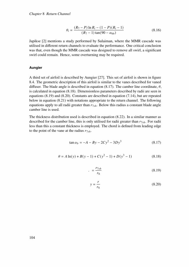
Chapter 8 Return Channel
\8 =('7 − %) ln '8 − (1 − %) ('8 − 1)('7 − 1) tan(90 − U61)
(8.16)
Japikse [2] mentions a study performed by Sulaiman, where the MMR cascade wasutilised in different return channels to evaluate the performance. One critical conclusionwas that, even though the MMR cascade was designed to remove all swirl, a significantswirl could remain. Hence, some overturning may be required.
Aungier
A third set of airfoil is described by Aungier [27]. This set of airfoil is shown in figure8.4. The geometric description of this airfoil is similar to the vanes described for vaneddiffuser. The blade angle is described in equation (8.17). The camber line coordinate, \,is calculated in equation (8.18). Dimensionless parameters described by radii are seen inequations (8.19) and (8.20). Constants are described in equation (7.14), but are repeatedbelow in equation (8.21) with notations appropriate to the return channel. The followingequations apply to all radii greater than A7Bℎ. Below this radius a constant blade anglecamber line is used.
The thickness distribution used is described in equation (8.22). In a similar manner asdescribed for the camber line, this is only utilised for radii greater than A7Bℎ. For radiiless than this a constant thickness is employed. The chord is defined from leading edgeto the point of the vane at the radius A7Bℎ.
tanU1 = −� − �H − 2�H2 − 3�H3 (8.17)
\ = � ln(H) + �(H − 1) + � (H2 − 1) + � (H3 − 1) (8.18)
. =A7BℎA6
(8.19)
H =A
A6(8.20)
104

8.3 Design
(a) Top view of de-swirl vanes. Note that flow is going radiallyinwards. The camber line (red) is drawn for one of the vanes.
(b) A single de-swirl vane. The green line is the chord. The lastpart is described by a straight segment with constant width.
Figure 8.4: View of de-swirl vanes, from Aungier’s construction.
� =(tanU61 − tanU71) ( 6 + 7 − 2)
3(. − 1)3
� =(tanU61 − tanU71) ( 7 − 6)
4(. − 1)2− 9� (. + 1)
4
� = 6(tanU61 − tanU71)
. − 1− 4� − 9�
� = tan V6 − � − 2� − 3�
(8.21)
105

Chapter 8 Return Channel
C = C0 + (Cmax − C0)H4CC0 = C6 + (C7 − C6)
G
2
HC =G
G<, for G < G<
HC =1 − G/2
1 − G</2, for G > G<
4 =
√0.4G<2
[0.95
(1 + G
2
)(1 − HC) + 0.05
](8.22)
8.3.3 Second Bend
The second bend, turning the flow 90° to axial direction is described by a circular arc onthe shroud side and an ellipse on the hub side.
8.4 Off-Design Considerations
At off-design conditions the flow will approach the bend with a flow angle different fromthe design conditions. At low mass-flows the diffuser, provided that it has not stalled,will deliver a higher than design flow angle to the return channel. At high mass-flowsthis angle will, correspondingly, be lower. If the pump features a vaned diffuser it mayprovide better guidance for the flow leaving the diffuser, resulting in a flow closer tothe design conditions for the return channel. The flow deviation at off-design may bemodelled utilising Carters rule, shown below in equation (8.23). This may result in aflow having swirl at the end of the return channel. This swirl will affect the performanceof the upcoming stage. The same equation can be used when designing, to iterativelyobtain a vaned section yielding a desired level of swirl, often zero.
X∗ = <\√f+ G
< = 0.23(20
2
)2 (8.23)
106

Chapter 9
Volute
The volute is situated after the diffusor in the last stage of the pump. Occasionally, thevolute is regarded as part of the diffusor, or alternatively, the diffuser regarded as part ofthe volute. The purpose of the volute is to gather the flow leaving the diffusing elementsand send it towards the exit of the pump with as low loss as possible. This chapter startswith a description of the volute geometry which is necessary to grasp the flow-structureinside the volute. The chapter ends with a model predicting the performance of thevolute and design aspects.
9.1 Basic Principles
9.1.1 Detailed Volute Geometry
Figure 9.1 shows the general layout of a single vane volute with a circular cross-sectionin the r\-plane in which the impeller is rotating anti-clockwise. The flow enters thevolute circumferentially at position 6 and leaves tangentially at section 8. This resultsin an uneven circumferential mass-flow distribution as the fluid elements closest tosection 8 need not travel as far in the volute as the fluid-elements entering the volute at asmaller \-coordinate. To accommodate this increase in mass-flow there is a need forincreased flow area along the circumferential direction. The point in the volute wherethe \-coordinate is zero, i.e. where the smallest flow area occurs, is called cut-water ortongue, see figure 9.1.
The performance of a volute is evaluated by the increase in static pressure and the loss intotal pressure, as mentioned in section 2.4.2. The loss arise from wall friction, shearforces between fluid elements as they mix in the flow, and exit/entry loss. These arecomplicated 3D-phenomena involving vortex structures and they will be described inlater sections in this chapter. However, to understand the flow field and the origin of thevortex structures one should first consider the different geometric aspects of the volute.
A designer need to navigate among the main geometric parameters to find a combination
107

Chapter 9 Volute
ω
6
7
8Cutwater
Figure 9.1: Top-view of a volute
that yields the best performance [14]. The parameters are:
• the connection to the diffuser
• the shape of the cross-sections
• change in flow area
• size of the volute
Connection to the Diffuser
Volutes are commonly defined as internal, external, or central [28]. The differencebetween external and internal volutes lies in how much space the volute occupies inthe radial direction. An internal volute folds behind the impeller in the axial directionwhereas an external volute continues radially outward after the diffuser, thus taking upmore space in the radial direction. Figure 9.2a shows a principle sketch of an internalvolute and figure 9.2b an external. It can be seen that the centre-radius for the internal
108
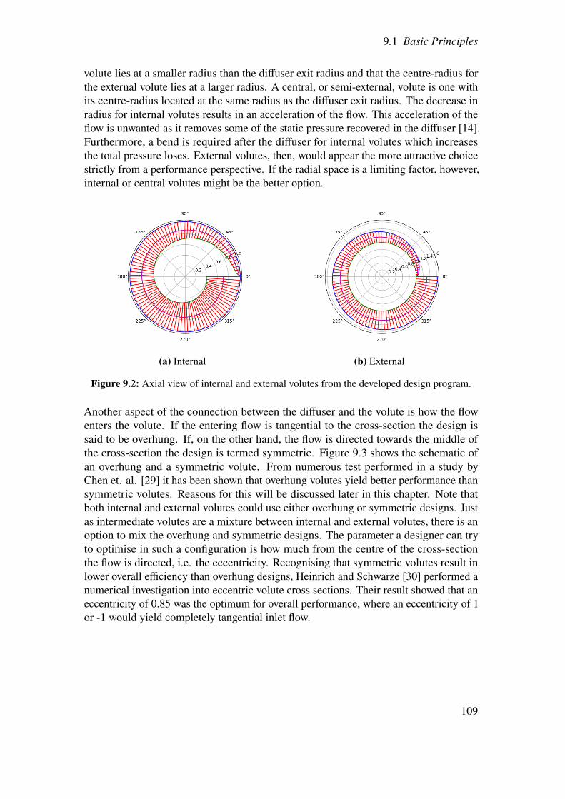
9.1 Basic Principles
volute lies at a smaller radius than the diffuser exit radius and that the centre-radius forthe external volute lies at a larger radius. A central, or semi-external, volute is one withits centre-radius located at the same radius as the diffuser exit radius. The decrease inradius for internal volutes results in an acceleration of the flow. This acceleration of theflow is unwanted as it removes some of the static pressure recovered in the diffuser [14].Furthermore, a bend is required after the diffuser for internal volutes which increasesthe total pressure loses. External volutes, then, would appear the more attractive choicestrictly from a performance perspective. If the radial space is a limiting factor, however,internal or central volutes might be the better option.
(a) Internal (b) External
Figure 9.2: Axial view of internal and external volutes from the developed design program.
Another aspect of the connection between the diffuser and the volute is how the flowenters the volute. If the entering flow is tangential to the cross-section the design issaid to be overhung. If, on the other hand, the flow is directed towards the middle ofthe cross-section the design is termed symmetric. Figure 9.3 shows the schematic ofan overhung and a symmetric volute. From numerous test performed in a study byChen et. al. [29] it has been shown that overhung volutes yield better performance thansymmetric volutes. Reasons for this will be discussed later in this chapter. Note thatboth internal and external volutes could use either overhung or symmetric designs. Justas intermediate volutes are a mixture between internal and external volutes, there is anoption to mix the overhung and symmetric designs. The parameter a designer can tryto optimise in such a configuration is how much from the centre of the cross-sectionthe flow is directed, i.e. the eccentricity. Recognising that symmetric volutes result inlower overall efficiency than overhung designs, Heinrich and Schwarze [30] performed anumerical investigation into eccentric volute cross sections. Their result showed that aneccentricity of 0.85 was the optimum for overall performance, where an eccentricity of 1or -1 would yield completely tangential inlet flow.
109

Chapter 9 Volute
(a) Overhung (b) Symmetric
Figure 9.3: Tangential view of overhung and symmetric volutes.
Shape of Cross-Sections
Besides choosing between internal/external and overhung/symmetric volutes a designerhas to decide upon the shape of the cross-sections. The options are rectangular, circular,or elliptic [14]. For readers familiar with aerodynamic design the intuitive choice mightbe the circular or elliptical designs. Mishina and Gyobo [31] investigated rectangularand circular cross-sections for tangential inflow volutes which showed a small favourfor circular cross-sections. Ayder et. al. [32] conducted experiments on volutes withelliptical and rectangular cross-shapes. The results showed better performance for therectangular volutes which the authors attribute to the rectangular volute being betteradapted to the impeller and vaneless diffuser. The conclusion one can draw from thesestudies is that circular/eliptical shapes generally perform better than rectangular onesand that the most important factor is that the system is designed as a whole.
Flow Area
Apart from studying the shape of the cross-sections, Mishina and Gyobo [31] investigatedhow the loss was affected by area distribution. Through trial-and-error they found theoptimum area distribution and related that to the area distribution obtained from ananalysis employing conservation of angular momentum. The effect of area-distributionwas shown to have more impact on loss-coefficient than choice of cross-sectional shape.Their study also showed a clear drop in performance when moving from external tointernal volutes.
110
9.2 3D Flow Structures
Besides deciding upon the proper area distribution, the designer is tasked with choosingthe overall size of the volute. The choice between a larger/smaller volute is closelylinked to the desired effects at off-design conditions. Larger volutes generally provide alarger operating range for high mass-flows but are sensitive to surge at low mass flows.Furthermore, at rotational speeds exceeding design large volutes show unsteady flowbehaviour. Small volutes are stable at all rotational speeds but lack the operating rangeof large volutes, dropping rapidly in pressure-ratio for increased mass-flows [14]. Thevolutes behaviour at design and off-design conditions will be detailed later in this chapter.
9.2 3D Flow Structures
The through-flow velocity in the volute (�) ) is primarily made up of the tangential flowleaving the diffusor (�\6), with absolute flow angles generally around 60-70°. �) iswhat drives the fluid-element through the volute and out of the pump. This leaves theradial velocity component, �A6, which is often modelled as completely lost. Consider afluid element entering an overhung volute close to the cut-water. As there are no otherfluid-elements in the volute, the fluid elements fill the flow area completely. The radialvelocity component of this initial flow encounters a wall and can safely be assumedto be lost due to frictional forces and dissipation. Hence, these initial fluid elementsonly have tangential velocity. As these fluid-elements travel along their respectivestreamlines, the flow area increases and other fluid-elements are fed into the flow. Aswe are dealing with an overhung volute the radial velocity components of the addedflow enters tangentially to the original streamline. The added flow starts swirling aroundthe original streamline, creating a vortex tube. What was a tangential-radial flow hastransformed into a tangential flow with swirl. This process continues throughout thevolute, each step in the circumferential direction adds a vortex-tube with ever increasingradius around the original streamline.
9.2.1 At Design Mass-Flow
From the previous explanation of the flow structure it can be understood that the swirl-component of the flow depends on �A6. At design operation �A6 is constant out of thediffusing elements as there are no disturbances to the flow. Hence, the resulting swirlvelocity inside the volute would be uniform assuming no loss, as seen in figure 9.4a.This corresponds to a free-vortex flow. However, this flow structure cannot exist as thevelocity gradients in the centre would generate large shear forces. A real structure wouldapproach the shape depicted in figure 9.4b, with a linear decrease in swirl towards thecentre. Thus, a vortex tube experience a decrease in swirl as it moves through the volute.This is intuitive as there is a continuous mixing of the flow where kinetic energy iscontinuously dissipated. Experiments have validated this flow structure inside the volute
111

Chapter 9 Volute
and has shown that the swirl-velocity is close to uniform at the outer vortex tubes, i.e.low initial dissipation of the kinetic energy.
(a) Ideal (b) Real
Figure 9.4: Cross-section of volute with swirl velocities at design mass-flow. Reworked fromBraembussche [17]
Due to the energy dissipation, the total pressure is lower at the centre of the cross-section.From radial equilibrium and energy balance, equation (9.1) and (9.2), it can be shownthat the decrease in total pressure and swirl velocity leads to a lower static pressure andan increase in tangential velocity towards the centre of a cross-section.
3?
3A= d
�2swirlA
(9.1)
d+2tanA= ?0 − ? − d
�2swirlA
(9.2)
9.2.2 At Off-Design Mass-Flow
The flow in the volute at off-design conditions is a key piece of the puzzle in theunderstanding of why a pump behaves in a certain way during off-design operations.
112

9.3 Performance
Low Mass-Flows
At lower than design mass-flow the tangential velocity out of the impeller is increasedand the radial velocity reduced compared to design conditions. This is due to continuityand increased diffusion in the impeller combined with constant blade speed. The increasein tangential velocity implies an increase in �) , as �\6 fed into �) . Continuity betweenvolute inlet and exit, however, demands a lower �) than at design-conditions. Hence, �\6is decelerated upon entry to the volute which increases the static pressure. As velocitiesand pressures need to be continuous throughout the volute there is a build-up in staticpressure between start and exit of the volute. With a circumferential increase in staticpressure towards volute exit, there is an accompanying decrease in radial velocity.
High Mass-Flows
At higher than design mass-flow the tangential velocity out of the impeller is decreasedand the radial velocity increased compared to design conditions. A low tangentialvelocity implies a low �) , but as more fluid needs to pass through the geometry of thevolute for a given time, �) needs to be larger than at design mass-flow. Hence �) needsto accelerate through the volute which leads to a decrease in static pressure. Through thesame analogy as in the low mass-flow case (continuous pressure-field), the static pressurewill be highest at the start of the volute and lowest at volute exit. The circumferentialdistribution of mass-flow will be low where the static pressure is high and thus �A6 willincrease from volute start to exit.
Implications for Cross-Sections
The link between �A6 and swirl-velocity in vortex tubes was described earlier in thischapter. At off-design mass-flows, �A6 was seen to decrease/increase from start to end ofthe volute. The swirl-velocity of a vortex tube, then, will be larger towards the centre ofthe cross section for low mass-flows and smaller towards the centre for high mass-flows.Assuming isentropic flow, the cross-sectional velocity distributions would approach theshapes shown in figures 9.5a and 9.6a, respectively. However, as at design-conditions,the shear-forces at the centre would be too great. The distribution instead approaches theones depicted in figures 9.5b and 9.6b.
9.3 Performance
With knowledge about the flow structure inside the volute, the assumptions made in theprediction of performance of the volute becomes more intuitive. The performance of thevolute can be described by an increase in static pressure and an inevitable decrease in
113

Chapter 9 Volute
(a) Ideal (b) Real
Figure 9.5: Cross-section of volute with swirl velocities at low mass-flow.
(a) Ideal (b) Real
Figure 9.6: Cross-section of volute with swirl velocities at high mass-flow.
total pressure. These are described by the static pressure recovery coefficient �%,5−7 andthe total pressure loss coefficient !�5−7. These have already been presented in section2.4.2 but are re-iterated here for clarity, see equations (9.3) and (9.4).
114

9.3 Performance
�?,5−7 =?7 − ?5?05 − ?5
(9.3)
!�5−7 =?05 − ?07?05 − ?5
(9.4)
Japikse [33] presented a method for estimating the loss-coefficient and it has beenimproved by Weber and Koronowski [28]. The model includes:
• !�<, meridonal velocity loss
• !�\ , tangential velocity loss
• !� 5 , frictional loss
• !�4, exit loss
The accumulated loss coefficient is given by:
!�5−7 = !�< + !�\ + !� 5 + !�4 (9.5)
9.3.1 Meridional Loss
The meridional component of the loss predicts how much of the meridional kineticenergy entering the volute is lost. Relating this to the flow structure described in section9.2 means that some of the kinetic energy associated with the swirl is destroyed by theshear forces. !�< can be calculated through equation (9.6). Selecting �1 = 1 makesthe assumption that all of the swirl has dissipated i.e. all of the meridional velocityhas been lost. This is a common (and pessimistic) assumption in predicting the voluteperformance [22].
!�< = �1�2<5
�25
(9.6)
9.3.2 Tangential Loss
The tangential component of the loss depends on whether the through-flow velocityaccelerates or decelerates through the volute i.e. if the mass-flow is higher or lower thandesign. Considering the swirl-velocities detailed in 9.2.2 reveals the reasons for this. Foran accelerating flow, the swirl-velocities in the centre of the cross-section where found tobe small. Small swirl-velocities require only a small level of dissipation (low kineticenergy loss) in order to reach a forced vortex structure. A decelerating flow, on the other
115

Chapter 9 Volute
hand, where found to yield higher swirl-velocities towards the centre of the cross-sectionand thus require a lot of dissipation to reach a forced vortex structure, according toBraembussche [14]. For geometries where the central position of the cross-sectionincreases from start to end of the volute (A5 < A6) some free vortex diffusion is possible.To allow for this in the loss-model Japikse [22] introduces another correction factor, �2.The tangential loss coefficient for decelerating flows is described by equation (9.7). Foraccelerating flow, the loss is assumed negligible (�2 = 0) and for decelerating flow theloss is modelled like sudden expansion loss (�2 = 1).
!�\ = �2
(A5A6
)2�2\5(1 − �5/�7)2
12d�
25
(9.7)
9.3.3 Frictional Loss
The frictional loss is modelled by a friction coefficient dependent on the Reynolds numberand wall roughness, the hydraulic diameter of the volute and the length of the fluid path.The friction coefficient is usually taken from pipe-flow charts [14]. Equation (9.8) showsthe definition for the loss coefficient.
!� 5 = � 5
!B
3�(9.8)
9.3.4 Exit Loss
The exit loss, according to Weber and Koronowski [28], is modelled as a conical diffuser,see equation (9.9). The opening angle from the volute to exit should not exceed 10-11°so as to avoid flow separation. For moderate opening angles a constant value of 0.15 for�3 is proposed. For values of fully separated flow, �3 may reach values exceeding 1.
!�4 = �3
12d(�)5 − �)6)2
12d�
25
(9.9)
Aungier [13] suggests that the proceeding exit loss from Weber and Koronowski is tooptimistic and instead proposes an exit loss coefficient according to equation (9.10).
!�4 =
(�6 − �7�5
)2(9.10)
116

9.4 Design
9.4 Design
The description of volute flow shows that external slightly eccentric overhung volutes arepreferable if the available space allows it. Apart from basic geometric choices, the maintask in designing a volute is to specify the circumferential variation in cross-sectionalarea. Aungier [13] describes two approaches: the simple area schedule (SAS) and theconservation of angular momentum (CAM-model). In SAS-design the area of the fullycollected flow is specified and the cross-sectional area varies linearly.
9.4.1 CAM-model
The conservation of angular momentum combined with the continuity equation specifiesthe cross-sectional area as a function of mean passage radius A2, see equation (9.11).
A2� = A5�\5
d2�2�2 = d5�5�<5
�2 = \A215
tanU5
(9.11)
The CAM-model can be updated with predictions about loss in angular momentum dueto e.g. friction. Karassik [34] suggests a correction factor in the magnitude 0.9 to 0.95which can be implemented for a more realistic model.
9.4.2 Implementation
Restrictions of A2 may be found if, for instance, the shape of the cross-sections are definedor some other restrictions put on the overall geometry of the pump. The distribution ofA2 in the design-tool is calculated from predefined cross-sections and symmetry.
Undersized volutes are associated with a loss penalty, according to Aungier [13], and asizing parameter (SP) may be introduced to enlargen the volute somewhat. Values of SPin the range 1-1.2 are common.
117


Chapter 10
Hub-to-Shroud Analysis
10.1 Basic Principles
Chapters 4 and 5 detail the flow inside the impeller and preliminary flow models. Theoutput from a design-program operating on the principles described in chapter 3 and5 is the axisymmetric geometry at cross-sections 1 and 2, with reference to figure 1.1.The preliminary design does not provide information about the streamlines betweenstation 1 and 2. However, this is of great importance in the design and a common tool touse in the preliminary phase (pre-CFD) is a quasi-three-dimensional flow analysis [13],sometimes referred to as the streamline curvature method (SCM). Wu [35] is commonlyreferenced as the creator of the quasi-three-dimensional flow analysis and his ideas havebeen implemented in numerous commercial codes. Before CFD, quasi-three-dimensionalflow analysis was the primary tool used in the design of turbomachinery. The techniquesof Wu guided the advances within radial turbomachines between the 1950’s and 1980’s.In the original report by Wu he presents two axisymmetric stream surfaces on whichthe flow field is calculated. These are termed the S1 and S2 surfaces, see figure 10.1.The S1 surface lies between two blade rows and the S2 surface lies in the hub-to shroudplane. The S2 surface is the most common starting point in preliminary design. Japikse[22] deems the additional detail supplied by the S1 surface unnecessary in relation to theadded complexity and recommends that designers move on to viscid 3D solvers after theS2 surface have been solved. The S2 stream surface, also known as the hub-to-shroudplane, was prioritised and this chapter details the derivation and implementation of theSCM-equations on this plane.
10.1.1 Purpose of SCM
The designers choice of pressure ratio, swirl parameter, and blade angles decide theoverall geometry of the impeller in the preliminary design. The models, however, provideno information about how section 1 and 2 is connected, or how the velocity changesbetween these sections. The velocity distribution on the S2 surface provides informationabout the blade loading which, through empirical correlations and previous experience,
119

Chapter 10 Hub-to-Shroud Analysis
Figure 10.1: S1 and S2 surfaces in quasi-three-dimensional analysis, from Wu [35].
can guide the designer towards good aerodynamic design. Blade loading is normallyevaluated through the local blade loading coefficient and the local rate of diffusion [22].The blade loading coefficient is given by the change in relative velocity divided by theaverage value: Δ,/, .
The rate of diffusion and the resulting pressure field within the flow passage must bewithin certain limits. If the rate of diffusion is to high, i.e. sharp increases in pressurealong the hub- and shroud contours, the boundary layers will grow leading to an increaseof the secondary flows [22]. Large secondary zones imply a relatively small primary zoneand inefficient work-input to the fluid. Restricting the rates of diffusion along hub andshroud, then, is an essential part of the design process. Knowledge about boundary layergrowth within the impeller is required and some models for this have been presented, forinstance by Aungier [13]. In absence of such models, empirical data and experience willhave to suffice. The purpose of the hub-shroud-analysis, then, is to evaluate blade- andpassage profiles through trial-and-error until a candidate geometry for CFD has emerged.
10.1.2 Flow Description
The problem to be solved on S2 is described by the Navier-Stokes equations. In thepreliminary design, only the inviscid parts of these equations are considered, what isknown as the Euler equations. The continuity equation is re-iterated here on vectornotation, see equation (10.1).
120

10.1 Basic Principles
md
mC+ ®∇ · (d ®�) = 0 (10.1)
The first part of equation (10.1) represents the temporal term and it is neglected duringsteady state, i.e. when there is no change to the flow over time. The momentum Eulerequation can be derived from Newtons second law and has been presented in numeroustexts, for instance Young [7] or Anderson [3]. It is presented here in equation (10.2) onvector notation. The steady momentum Euler equation is given in equation (10.3).
d
[m ®�mC+ ( ®� · ®∇) ®�
]= −®∇? + ®� (10.2)
( ®� · ®∇) ®� = −1d®∇? + ®5 (10.3)
The derivation of the acceleration and force terms for the impeller fluid flow will bedetailed in section 10.3. The pressure terms can be elaborated through radial equilibrium.Consider the fluid element shown in figure 10.2, it is described in cylindrical coordinatesby (A, \, I). A balance of forces on the surface of the fluid yields the expression inequation (10.4) [36].
�A3�A
3A+ �I
3�A
3I− �\A= −1
d
3?
3A(10.4)
The second Gibbs equation can be differentiated with regard to 3A, see equation (10.5).Rewriting the enthalpy in terms of total enthalpy and velocity allows for an expressionconnection the velocity distribution to the work transfer and entropy generation. Therewritten version of the radial equilibrium equation is shown in equation (10.6) [36], inwhich quantities are assumed constant in the \-direction.
1d
3?
3A=3ℎ
3A− ) 3B
3A(10.5)
3ℎ03A− ) 3B
3A= −�I
3�A
3I+ �I
3�I
3A+ �\
3�\
3A+�2\
A(10.6)
The flow physics presented in this section shows that the velocity field in the hub-shroud-analysis is a matter of modelling the fluid acceleration and force-terms. In order toimplement these models, a discretisation of the impeller geometry is needed.
121

Chapter 10 Hub-to-Shroud Analysis
Figure 10.2: Radial equilibrium of a fluid element in cylindrical coordinates (Courtesy ofMagnusGenrup).
10.2 Geometric Description
A well-defined geometry lies at the heart of the hub-shroud-analysis. This section seeksto introduce the reader to the domain used in later part of this chapter.
10.2.1 Intrinsic Coordinates
The SCM utilises one key aspects of streamlines: there is no velocity-component normalto a streamline as streamlines are defined as being tangent to the velocity vector [7].When performing computations on streamlines it is helpful to define a coordinate systemthat follows the streamline. These coordinates are known as intrinsic coordinates, givenin (<, =, \). Figure 10.3 shows how the intrinsic coordinates can be expressed in termsof cylindrical coordinates given the local flow angle, q.
Also shown in figure 10.3 is @, C, and W, which is the quasi-normal to the streamline, theorthogonal direction to the quasi-normal, and their angle to the radial and axial directionrespectively. Quasi-normals are used to describe the flow field from a supplied geometry.
The relative flow direction F is described by < and the relative flow angle V. Sincethe only components of velocity lies in the <\-plane, so does F. Since no fluidcan pass through the blades, F will follow the blades if incidence and deviation areneglected. However, there are models to incorporate incidence and deviation within thecomputational domain, for instance Aungier [13].
122

10.2 Geometric Description
Figure 10.3: Relationship between intrinsic coordinates, cylindrical coordinates, and q.
10.2.2 Lean/Rake
Apart from the hub- and shroud contours, the blades are what defines the computationaldomain on the S2 surface. The blades can be tilted somewhat in the tangential direction,and this angle is often termed lean or rake. This implies that two corresponding pointson the hub- and shroud surfaces do not share the same \-coordinate. Lean/rake isrepresented by Y, shown in figure 10.4. The 4-direction can be described as @ rotated Ydegrees around C.
Figure 10.4: Description of lean angle.
The force exerted by the blades on the fluid acts normal to the blade surface. As theF and C directions both lie tangential to the plane, the direction normal to the blade
123

Chapter 10 Hub-to-Shroud Analysis
surface, ? is given by the cross-product shown in equation (10.7), and the unit vector inp-direction is obtained by normalising.
®#? = ®4F × ®4C
®4? =®#?|#? |
(10.7)
10.2.3 Differentiation of Unit-vectors
Rc
Rc
i
i+1
αα
em
e men
e n
Figure 10.5: Differentiation of meridional unit vector.
When moving from point i to i+1 along a streamline, a distance Δ<, the meridionaldirection changes, from ®4<8 to ®4<8+1 . This change can be seen as a rotation aroundthe \-axis, which is orthogonal to the paper. Let us now describe the unit vectors indirections from point i, in intrinsic coordinates (n, \, m).
®4<8 = [0, 0, 1] ®4<8+1 = [sinU, 0, cosU]
Note that both vector has the length of unity, as they are unit-vectors.
To obtain the relative change of the direction from point i to i+1 the diffence is taken.
Δ®4< = ®4<8+1 − ®4<8 = [sinU, 0, cosU − 1]
124

10.2 Geometric Description
The trigonometric expressions can be rewritten by utilising Taylor expansion:
sinU = U − U3
3!+ U
5
5!− U
7
7!+ ...
cosU = 1 − U2
2!+ U
4
4!− U
6
6!+ ...
Truncating terms of second order and greater yields the following expression of therelative change of the meridional direction.
Δ®4< = [U, 0, 0]
The change in the unit vector is meridional direction is described by the angle U in thenormal direction, n. The change of the meridional unit vector over the change in distancemay be desribed as:
Δ®4<Δ<
=[U, 0, 0]Δ<
=U ®4=Δ<
The distance along the streamline, Δ< can be described by a circular arc, with the angleU and the radius '2.
Δ< = U'2
Combined with the expression above, yields.
Δ®4<Δ<
=U ®4=U'2
=®4='2
The example is derived from a streamline having a macroscopic curvature, thus makingit easy to visualise. However, if the limit of the fraction is taken one obtains the partialderivative seen below. It should be obvious that this equation is true for an arbitrarystreamline.
m ®4<m<
=®4='2
125

Chapter 10 Hub-to-Shroud Analysis
10.3 Governing Equations
With the geometry fully defined, the acceleration and force terms can be derived.
10.3.1 Acceleration
The acceleration term in the steady momentum equation was given by:
( ®� · ®∇) ®�
in which the velocity vector and the nabla operator in cylindrical coordinates is given by[3]:
®� =�< ®4A + �\ ®4\ + �I ®4I®∇ = m
mA®4A +
1A
m
m\®4\ +
m
mI®4I
Expanding the acceleration terms yields the following expression:[(�< ®4A + �\ ®4\ + �I ®4I)
(®4Am
mA+ ®4\
1A
m
m\+ ®4I
m
mI
)](�< ®4A + �\ ®4\ + �I ®4I)
Within the blade impeller, the fluid is best described by the relative velocity. Below thecomponents of velocity is related from the absolute frame to the relative frame.
�< = ,<
�\ = ,\ + lA
The nabla-operator in intrinsic coordinates are given by
®∇ = ®4<m
m<+ ®4\A
m
m\+ ®4=
m
m=
The acceleration, for steady state, is shown in the left-hand-side of equation (10.2).Applying the nabla operator to the velocity vector, all given in intrinsic coordinates,results in the following expression.
126

10.3 Governing Equations
®0 = ( ®, · ®∇) ®, = ®4<,<
m,<
m<+,2
<
m ®4<m<+ ®4\,<
m (,\ + lA)m<
+,< (,\ + lA)m ®4\m<+ (,\ + lA)
A,<
m ®4<m\+ ®4<(,\ + lA)
A
m,<
m\
+ (,\ + lA)2A
m ®4\m\+ (,\ + lA)
A®4\m (,\ + lA)
m\
By assuming axi-symmetric flow, i.e. no variation in tangential direction, and utilisingthe following expressions below, equation (10.8) is obtained.
m ®4<m<
=®4='
m ®4<m\
= 0m ®4\m<
= 0m ®4\m\
= −®4A
®0 = ®4<,<
m,<
m<+ ®4=
,2<
'2+ ®4\,<
m (,\ + lA)m<
− ®4A(,\ + lA)2
A(10.8)
The acceleration in the quasi-normal directionmay now be calculated as the scalar-productbetween the unit vector and acceleration.
0@ = ®4@ · ®0 = sin(q + W),<
m,<
m<+ cos(q + W)
,2<
'2− cos(W) (,\ + lA)2
A
The acceleration can, with use of the Euler equations, be written as below, when appliedin quasi-normal direction.
0@ =−1d
m?
m@+ �@
Where the pressure gradient can be rewritten in a similar fashion as above, utilising Gibbsand the definition of total enthalpy. The force-term, however, will be derived below.
10.3.2 Force
The acceleration in the tangential direction can be described, utilising theEulermomentumequation. Since axi-symmetry is assumed, the pressure gradient in tangential direction iszero, −1
d
m?
m\= 0. Thus resulting in:
0\ = 5\
127

Chapter 10 Hub-to-Shroud Analysis
This specific force equates to the turning of the flow in tangential direction, and cantherefore be found from the change in velocities.
In the meridional direction the following expression is reached.
0< =−1d
m?
m<+ 5<
,<
m,<
m<− (,\ + lA)2
2sin(q) =
)mB
m<−mℎ0m<+,<
m,<
m<+(,< tan(V)+lA
) (tan(V) m,<
m<+,<
m tan(V)m<
+l2A sin(q))+ 5<
The specific force applied to the fluid by the blades, 5? are acting normal to the bladesurface, in the direction given by ®4?. 5? may be described by components in the intrinsiccoordinate system.
5=,? = ®5? · ®4=
5\,? = ®5? · ®4\
Since the tangential specific force can be found through the tangential acceleration, allforces may be calculated if the directions are known.
Finally the force in the quasi-normal direction may be calculated as
5@ = sin(q + W) 5< + cos(q + W) 5=
10.4 Modelling
The section above describes the inviscid flow terms to be caluclated in the hub-to-shroudanalysis. The geometry needs to be discretized in order to implement the equations incomputer code and some of the quantities within the flow require models to provide agood estimation.
128

10.4 Modelling
10.4.1 Discretization
The impeller is discretized according to figure 10.6. The quasi-orthogonals go in thej-direction and the streamlines move in the i-direction. The computational nodes are theintersections between the streamlines and the quasi-orthogonals. The hub represents j=0and the shroud j=n, where n is the number of streamlines. The impeller inlet representsi=0, and the outlet i=k, where k is the number of quasi-orthogonals. The area generatedbetween four computational points, for instance [i,j], [i,j+1], [i+1,j], and [i+1,j+1] istermed a stream-tube.
Axis of rotation
i
j
j = 0
j = n
Figure 10.6: Discretization of impeller geometry.
The hub-, and shroud contours are normally specified through Bezier curves [22]. Thisallows the designer to specify both angles at leading-, and trailing edge, as well as thecurvature. For more information about how the Bezier polynomials can be implemented,the reader is directed to appendix B. The points created along hub and shroud arethen moved to be equidistant, and the quasi-orthogonals can be created by connectingrespective points on the hub- and shroud contours [13]. Figure 10.7 shows how Beziercurves and quasi-normals can be implemented in a design program.
The starting point for the calculation procedure, described below, can then be initiated bycreation of the initial streamlines. For this, the number of desired streamlines must beprovided by the designer. The initial computational points are then distributed along the
129

Chapter 10 Hub-to-Shroud Analysis
Figure 10.7: Hub(green) - and shroud(blue) contours with Bezier points and generated quasi-normal(red).
quasi-normal to give equal flow area for each stream-tube. This is done by placing thecomputational points on the RMS-value.
The curvature can be computed for each node on the hub- and shroud contours, as wasshown in section 10.2. Along streamlines inside the impeller, however, the curvaturecannot be computed as easily. A linear approximation between the contours of hub-andshroud have therefore been implemented.
10.4.2 Entropy Generation
In order to close the system of equations described in sections above a model is requiredfor the generation of entropy, both along the quasi-normal and the meridional direction.A simple model mentioned by Casey [37] is to model the entropy generation with aspecified polytropic efficiency. Another model mentioned by Casey is the dissipationloss coefficient to estimate the viscous losses.
10.5 Calculation Procedure
The implementation of the equations described in section 10.3 and the discretizedgeometry described in section 10.4 follow the procedure shown in figure 10.8. Thecomputations starts with a calculation of the inlet condition and a two-zone model,following the procedures described in chapters 3 and 5. This fixes the inlet and outlet
130
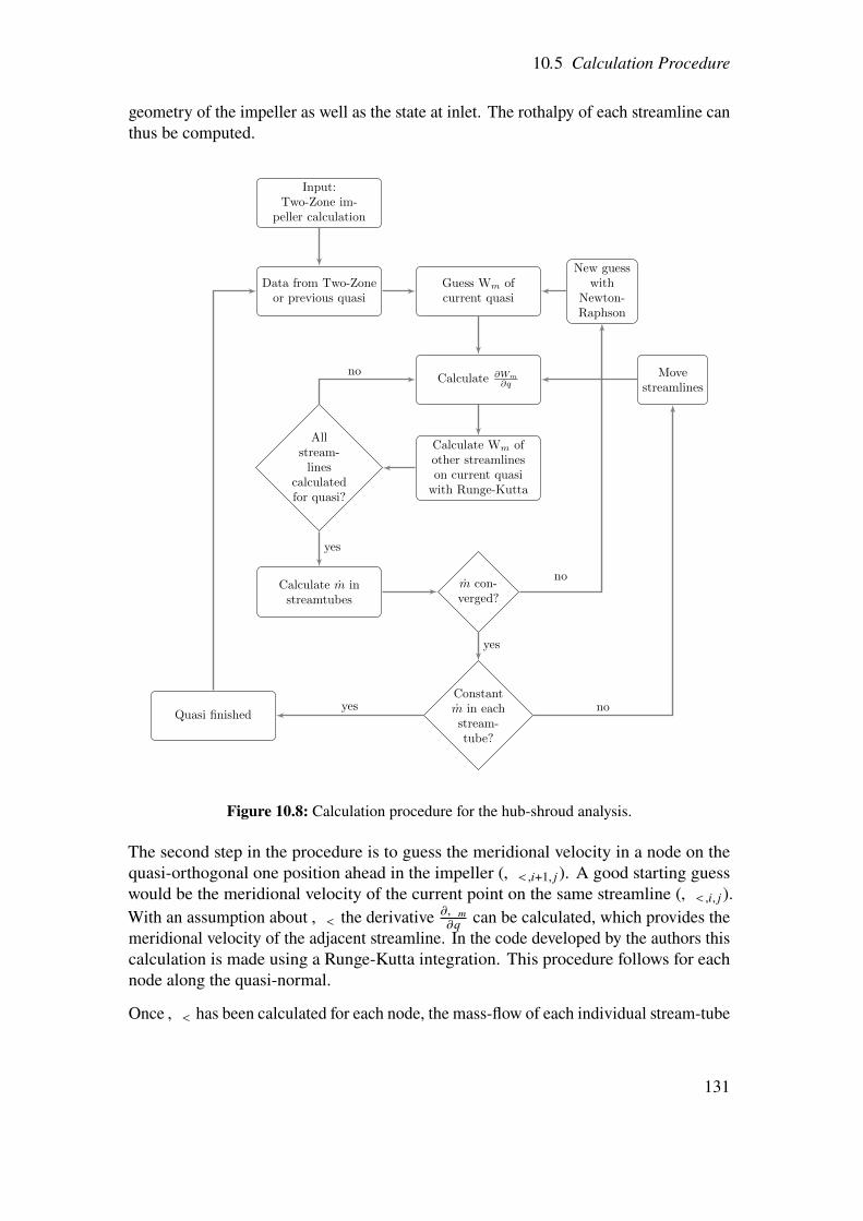
10.5 Calculation Procedure
geometry of the impeller as well as the state at inlet. The rothalpy of each streamline canthus be computed.
Input:Two-Zone im-
peller calculation
Data from Two-Zoneor previous quasi
Guess Wm ofcurrent quasi
Calculate ∂Wm
∂q
Calculate Wm ofother streamlineson current quasi
with Runge-Kutta
Allstream-
linescalculatedfor quasi?
Calculate m instreamtubes
m con-verged?
New guesswith
Newton-Raphson
Constantm in eachstream-tube?
Movestreamlines
Quasi finished
no
yes
no
yes
noyes
Figure 10.8: Calculation procedure for the hub-shroud analysis.
The second step in the procedure is to guess the meridional velocity in a node on thequasi-orthogonal one position ahead in the impeller (,<,8+1, 9 ). A good starting guesswould be the meridional velocity of the current point on the same streamline (,<,8, 9 ).With an assumption about,< the derivative m,<
m@can be calculated, which provides the
meridional velocity of the adjacent streamline. In the code developed by the authors thiscalculation is made using a Runge-Kutta integration. This procedure follows for eachnode along the quasi-normal.
Once,< has been calculated for each node, the mass-flow of each individual stream-tube
131

Chapter 10 Hub-to-Shroud Analysis
can be calculated, summed, and checked against the prescribed total mass-flow. Thisprovides a means of validating the initial guess of ,<. ,< is updated in the codedeveloped by the authors using the Newton-Rahpson method.
When the mass-flow has converged, the position of each computational node can beevaluated. If the mass-flow inside a stream-tube ( ¤<BC) differs from ¤<BC upstream, thedistance between two nodes must be updated. If the mass-flow inside a stream-tubehas changed it implies that there has been flow across a streamline, which violates thedefinition of a streamline. The re-positioning of nodes means that the computation muststart from the top, but the values of,< are kept from the last iteration as a first guess.
With converged ,<, ¤<, and ¤<BC the calculation procedure is finished for the currentquasi-normal. The data from the current-quasi-normal becomes the input value for thenext quasi-normal.
132

Chapter 11
Validation
The developed program needs to be validated in order to be trusted as a preliminarydesign-tool. Validation is preferably done against a myriad of experimental data, toensure flexibility. However, due to lack of experimental data during this thesis, validationis conducted against a theoretical pump developed in a similar tool. Further testing andtweaking of the program during use is essential to have a versatile and accurate program.
11.1 Validation against Japikse
The validation is conducted against an example given by Japikse [2]. The program istherefore validated against another computational program. However, the results fromJapikse are deemed to be a good benchmark. In the data presented by Japikse, the densityof the fluid is calculated to be around 2300 kg/m3. The density is found from dynamicpressure and kinetic energy. Through this knowledge the pump performance in headmay be calculated, and reasonable input data chosen to match the given case. Other fluidproperties, e.g. viscosity, are not known, but assumed to be similar to water as that is thefluid stated.
All of the initial data is not readily available. Total pressure at plenum, is calculatedbackwards from the loss coefficient. From this estimated pressure, the sought pressureratio is found by dividing the result at impeller tip with the plenum pressure. Mass flowis also estimated, calculated from the provided volume flow and estimated density. Anestimation of blade thickness was made to 1mm, which is deemed reasonable. Inputdata used is shown in table 11.1.
The relative error is calculated according to equation (11.1).
Relative Error =����Our Value − Reference ValueReference Value
���� (11.1)
133

Chapter 11 Validation
11.1.1 Sources of Error
There are a few sources of error in the validation process. The most prominent sourcesare presented below:
• Small errors in each component are likely to add up. Another way of presentingthis validation could have been component-wise. However, it was thought to be abetter validation if the program as a whole was tested.
• The reference pump did not converge to exactly _2< = 4.35. This might causesome of the discrepancies. Furthermore, this raises questions about the numericaltolerances in the reference program.
• The lack of information both in design input and numerical controls may introducesources of error, stemming from slightly different data.
• All of the models implemented in the developed design-program may not beexactly the same as for the program behind the reference pump. Important to noteis that all models are merely approximations of reality.
Parameter Value Unitr1ℎ 0.0857 mf1 0.2 (-)N 1000 RPM¤< 315 kg/s
incidenceℎ 2.61 °incidence< 2.66 °incidenceC 2.68 °_2<,desired 4.35 (-)
Pressure ratio 4.253889 (-)q1 40 °AK 1.07 (-)LC01 0.1 (-)
BLCK1 0.03 (-)V21 -67.5 °r5/r2 1.36 (-)b5/b2 1 (-)p00 79701.7 PaT00 310.93 KLC01 0.1 (-)
Table 11.1: Input data for validation of pump-design
134

11.1 Validation against Japikse
11.1.2 Inlet
Results from the inlet portion are presented in table 11.2. Overall the relative errors aresmall.
Parameter Our Reference Unit Rel. Error [%]r1C 0.159 0.158 m 0.63
NPSH 3.80 3.80 m 0C1C 4.00 4.07 m/s 1.7W1C 17.12 17.03 m/s 0.53V1C -76.5 -76.2 ° 0.39C1< 3.73 3.80 m/s 1.8W1< 13.88 13.84 m/s 0.29V1< -74.4 -74.1 ° 0.40C1ℎ 3.49 3.56 m/s 2.0W1ℎ 9.63 9.65 m/s 0.21V1ℎ -68.8 -68.4 ° 0.58
Table 11.2: Comparison for inlet data
11.1.3 Impeller
The results regarding the impeller are seen in table 11.3. Note that the developed programconverges on the value _2< = 4.35, the desired value. This is not the case for thereference data.
Parameter Our Reference Unit Rel. Error [%]r2 0.222 0.224 m 0.89b2 0.080 0.080 m 0p2? 260438 257055 Pa 1.3p02? 329887 324803 Pa 1.6W2? 13.16 14.19 m/s 7.3p02B 484760 485091 Pa 0.068W2B 2.14 2.28 m/s 6.1p2< 263789 261401 Pa 0.91p02< 344740 339042 Pa 1.7W2< 11.15 11.65 m/s 4.3f2< 0.763 0.807 (-) 5.5_2< 4.35 4.33 (-) 0.46
Table 11.3: Comparison for impeller data
135

Chapter 11 Validation
11.1.4 Vaneless Diffuser
The data for the vaneless diffuser will be givan at three different radial locations. The firstcorresponds to inlet to vaneless diffuser, see table 11.4. The second at the mid-radius,table 11.5, and the last one at outlet, table 11.6. The radial locations do not line upperfectly. due to differences in previous components.
The large relative error for the losses are likely due to the difference in friction coefficients.For the reference pump a value of 0.006 compared to the calculated value in our designtool of 0.0047. The friction coefficient is calculated in equation (6.9), and the differenceis likely due to different '4, stemming from different fluid properties.
Parameter Our Reference Unit Rel. Error [%]C< 2.86 2.81 m/s 1.8C\ 12.45 12.16 m/s 2.4T 310.95 310.98 K 0.0096p 263789 261401 Pa 0.91p0 344739 339042 Pa 1.7U 77.05 76.98 ° 0.09C? 0 0 (-) 0LC 0 0 (-) 0
(A�\)8/(A�\)2< 1 1 (-) 0
Table 11.4: Comparison for vaneless data at radial location r = 0.222m for our designed pumpand r = 0.224m for the reference pump.
Parameter Our Reference Unit Rel. Error [%]C< 2.43 2.40 m/s 1.3C\ 10.44 10.17 m/s 2.7T 310.95 310.99 K 0.013p 286294 282985 Pa 1.2p0 343331 337543 Pa 1.7U 76.92 76.76 ° 0.21C? 0.278 0.278 (-) 0LC 0.017 0.021 (-) 19
(A�\)8/(A�\)2< 0.99 0.987 (-) 0
Table 11.5: Comparison for vaneless data at radial location r = 0.2616m for our designed pumpand r = 0.2644m for the reference pump.
136

11.1 Validation against Japikse
Parameter Our Reference Unit Rel. Error [%]C< 2.10 2.08 m/s 0.96C\ 9.00 8.71 m/s 3.3T 310.95 310.99 K 0.013p 300217 296175 Pa 1.4p0 342323 336344 Pa 1.8U 76.79 76.54 ° 0.33C? 0.45 0.448 (-) 0.45LC 0.030 0.037 (-) 19
(A�\)8/(A�\)2< 0.980 0.975 (-) 0.51
Table 11.6: Comparison for vaneless data at radial location r = 0.3015m for our designed pumpand r = 0.3048m for the reference pump
11.1.5 Vaned Diffuser
The reference pump does not have a vaned diffuser, and thus it could not be validatedagainst. However, there is a reference compressor in Japikse [22] that feature a vaneddiffuser with 11 NACA65-0406 airfoils. The solidity, loss-coefficient, and pressurerecovery are similar to the vaned diffuser developed in the developed program.
11.1.6 Volute & Return Channel
Due to lack of information regarding the volute, e.g. shape and model, it is omitted fromthe validation.
The reference pump does not contain a return channel, which is why this part of thedeveloped program cannot be validated. However, the performance of return channelsdesigned are on par with experimental performance-data presented in [2].
137


Chapter 12
Conclusions
12.1 Conclusions
A tool for preliminary design of radial pumps, named RaPID (Radial Pump InitialDesign), has been developed. The tool is able to produce designs with a variety ofcomponents to choose from with satisfactory results, as shown in chapter 11. The speedof design generation and off-design analysis is quick. It takes only seconds to read, runthe calculations, and produce a report presented in either excel or as a text-file.
With increasing computational power, full 3D simulations become increasingly accessible,even for simple problems. However, old and proven methods utilised when computerswere quite weak, should not be underestimated. In these preliminary designs, only themost vital aspects of the flow are considered. If a pump is designed poorly in respectto these vital aspects, the project as a whole will suffer since it is more costly to use atrial-and-error approach during 3D-simulations. The benefit of a trustworthy and rapiddesign tool, then, should not be overlooked. Once an accepted preliminary design isobtained, it may be transferred to 3D simulations to alter details not accessible in 1D or2D simulations. The designer should use the most suitable tool available for the currentphase of the design process.
12.2 Future Work
The models presented in this text can be developed further. They rely on empirical dataand assumptions about the flow. With more knowledge about flow structures in radialturbomachinery and more empirical data it is possible to create more accurate modelsthat can improve the preliminary design.
One assumption about the flow made in this text is that it is axi-symmetric. Modelsdescribing flow-interactions between impeller, diffuser, and volute that look at non-symmetric flow structures could give the designer a better insight into how the pump
139
Chapter 12 Conclusions
would perform at off-design mass-flows. Such models are available in the open literature,see for instance [14].
A handful of possible topics that could improve the preliminary design tool are:
• Connect the output data from the return channel to the input data of a followingstage, thus having the possibility to easily design a multistage pump. This step hasto be done manually in the current program.
• Two-zone model applied to the vaneless difuser, see for example Japikse andDubitsky [38].
• A impeller-diffuser-volute response model
• Parallelisation, mainly for faster off-design computation. However, if moresophisticated models are to be implemented, it might be necessary to incorporateparallel processing to keep computational times low.
140

Bibliography
[1] C. Anderson,Wind Turbines: Theory and Practice. Cambridge University Press,2020, isbn: 9781108478328.
[2] D. Japikse, W. D. Marscher and R. B. Furst, Centrifugal Pump Design andPerformance. 2006, isbn: 0-933283-09-1.
[3] J. Andersson, Fundamentals of Aerodynamics. McGraw-Hill, 2011.[4] H. Versteeg and W. Malalasekera, An Introduction to Computational Fluid
Dynamics: The Finite Volume Method. Pearson Education Limited, 2007, isbn:9780131274983.
[5] E.M. Greitzer, C. S. Tan andM. B. Graf, Internal Flow: Concepts and Applications.Cambridge University Press, 2004.
[6] Y. A. Cengel and M. A.Boles, Thermodynamics an Engineering Approach,8th ed. 2 Penn Plaza, New York, NY 10121: McGraw-Hill Education, 2015, isbn:978-981-4595-29-2.
[7] D. Young, Introduction to Fluid Mechanics. Wiley, 2012, isbn: 9780470902158.[8] Liquid Rocket Engine Turbopump Inducers. NASA SP-8052. 1971, vol. 8052.[9] S. L. Dixon and C. A. Hall, Fluid Mechanics and Thermodynamics of Turboma-
chinery. 2014, isbn: 978-0-12-415954-9.[10] E. S. Taylor, “Film notes for secondary flow”, Massachusetts Institute of Techno-
logy, Report 21612, 1968.[11] M. Johnson, “Secondary flow in rotating bends”, Journal of Engineering for
Power, vol. 100, pp. 553–560, 1978.[12] J. Daily and R. Nece, “Chamber dimension effects on induced flow and frictional
resistance of enclosed rotating disks”, Journal of Basic Engineering, vol. 82,pp. 217–230, 1978.
[13] R. Aungier, Centrifugal Compressors: A Strategy for Aerodynamic Design andAnalysis. ASME Press, 2000, isbn: 9780791800935.
[14] R. Van den Braembussche, Design and Analysis of Centrifugal Compressors,ser. Wiley-ASME Press Series. Wiley, 2019, isbn: 9781119424109.
[15] J. D. Stanitz, “One-dimensional compressible flow in vaneless diffusers of radial-,and mixed-flow centrifugal compressors including effects of friction, heat transferand area change”, Lewis Flight Propulsion Laboratory, Technical Note 2610,1952.
141

Bibliography
[16] W. Jansen, “Rotating stall in a radial vaneless diffuser”, Journal of Basic Engin-eering, vol. 86, pp. 750–758, 1964.
[17] P. Fringe and R. Van den Braembussche, “A theoretical model for rotating stallin the vaneless diffuser of a centrifugal compressor”, Journal of Engineering forGas Turbines and Power, vol. 107, pp. 507–513, 1985.
[18] Y. Senoo and Y. Kinoshita, “Influence of inlet flow conditions and geometries ofcentrifugal vaneless diffusers on critical flow angle for reverse flow”, Journal ofFluid Engineering, vol. 99, pp. 98–102, 1977.
[19] R. H. Aungier, “A systematic procedure for the aerodynamic design of vaneddiffusers”, ASME FED, vol. 69, pp. 27–34, 1988.
[20] S. Lieblein, “Analysis of experimental low-speed loss and stall characteristics oftwo-dimensional compressor blade cascades”, Lewis Flight Propulsion Laboratory,Technical Note RM E57A28, 1957.
[21] A.R.Howell, “Fluid dynamics of axial compressors”,Proceedings of the Institutionof Mechanical Engineers, vol. 153, no. 1, pp. 441–452, 1945.
[22] D. Japikse, Centrifugal Compressor Design and Performance. 1996, isbn: 978-0-933283-03-9.
[23] I. Johnsen, R. Bullock, N. Aeronautics, S. Space Administration and L. R. C.Technical Information Division, Aerodynamic Design of Axial-flow Compressors:Ed. U.S. Government Printing Office, 1965.
[24] C. Rodgers, “The Performance of Centrifugal Compressor Channel Diffusers”,ser. Turbo Expo: Power for Land, Sea, and Air, V001T01A003, vol. Volume 1:Turbomachinery, Apr. 1982.
[25] Y. Senoo, H. Hayami and K. Utsunomiya, “Application of a low-solidity cascadediffuser to transonic centrifugal compressor”, Journal of Turbomachinery, vol. 112,pp. 25–29, 1990.
[26] E. Rothstein, Experimentelle und theoretische Untersuchung der Strömungs-vorgänge in Rückführkanälen von Radialverdichterstufen, insbesondere sol-cher mit geringen Kanalbreiten. Fakultät für Maschinenwesen der Rheinisch-Westfählischen Technischen Hochschule Aachen, 1984.
[27] R. H. Aungier, “Aerodynamic design and analysis of vaneless diffusers and returnchannels”, Turbo Expo: Power for Land, Sea, and Air, vol. Volume 1: AircraftEngine; Marine; Turbomachinery; Microturbines and Small Turbomachinery, May1993.
[28] C. R. Weber and M. E. Koronowski, “Meanline Performance Prediction of Volutesin Centrifugal Compressors”, ser. Turbo Expo: Power for Land, Sea, and Air,vol. Volume 1: Turbomachinery, Jun. 1986.
[29] H. Chen, D. Tong and X. Wang, “Vortices and performance of internal andexternal volutes”, Jun. 2015.
142
Bibliography
[30] M. Heinrich and R. Schwarze, “Genetic optimization of the volute of a centrifugalcompressor”, 2017.
[31] H. Mishina and I. Gyobu, “Performance Investigations of Large Capacity Centri-fugal Compressors”, ser. Turbo Expo: Power for Land, Sea, and Air, vol. Volume1A: General, Apr. 1978.
[32] E. Ayder and R. Braembussche, “Numerical analysis of the 3d swirling flow incentrifugal compressor volutes”, May 1993.
[33] D. Japikse, “Advanced diffusion levels in turbocharger compressors and compon-ent matching.”, I Mech E Conference Publications (Institution of MechanicalEngineers), pp. 143–155, Jan. 1982.
[34] I. Karassik, Pump Handbook, ser. Mechanical engineering. McGraw-Hill, 1976,isbn: 9780070333017.
[35] C. Wu, P. Beck and U. S. N. A. C. for Aeronautics, A General Theory of Three-dimensional Flow in Subsonic and Supersonic Turbomachines of Axial-, Radial-,and Mixed-flow Types, ser. Technical note. National Advisory Committee forAeronautics, 1952.
[36] D. Japikse and N. Baines, Introduction to Turbomachinery, ser. A Concepts ETIBook Series. Concepts ETI, 1994, isbn: 9780933283060.
[37] M. Casey and C. Robinson, Radial Flow Turbocompressors. Cambridge UniversityPress, 2021, isbn: 9781108416672.
[38] O. Dubitsky and D. Japikse, “Vaneless diffuser advanced model”, Journal ofTurbomachinery, vol. 130, 2008.
[39] J. Hoffman and S. Frankel, Numerical Methods for Engineers and Scientists,Second Edition, Taylor & Francis, 2001, isbn: 9780824704438.
143

Appendix A
State Function
Equations of state (EOS) was introduced in chapter 2 and it was noted that twothermodynamic properties was required to fix the state. Once the state is fixed theother properties linked to the state can be determined using EOS. There are softwareavailable, e.g. REFPROP, that lets the user insert state-properties and receive any otherthermodynamic property or dependant property of the state. The state must be fullydefined by the input properties.
Using EOS-software is useful when the number of state calculations are limited. TheEOS-calculations require significant computational effort and as the number of callsto the software increase so does the computational time. With large number of state-calculations it is often more efficient to access the properties of a state through propertytables. One common file-type that contains property tables are RGP-files (Real GasProperty). RGP-files have a predictable structure which make them easy to implement.
The thermodynamic properties in a RGP-file are sorted by temperature and pressure. Thefile contains both single phase properties and saturation properties. The thermodynamicproperties available, besides temperature and pressure, are:
• Specific enthalpy, ℎ
• Specific entropy, B
• density, d
The dependent properties available in a RGP-file are:
• Specific heat at constant pressure, 2?
• Specific heat at constant volume, 2E
• Speed of sound, 0
• Dynamic viscosity, `
• Thermal conductivity, :
145

Appendix A State Function
In order for the program to use RGP-files instead of an EOS-software the program mustbe able to read the files and interpolate between values. The program should be ableto find all of the properties no matter which thermodynamic properties are given. Thetrivial case is when T and p are known, as the tables are already sorted by T and p.Any other set of thermodynamic properties require table inversion, which is a moresophisticated search. The search that involves the most computations is to supply ℎ, B, ord to find the other properties of the state, e.g T = T(ℎ, B).
The problem with table-inversion was solved in a recursive manner, to minimise thecomputational time and effort. The algorithm that searches through the tables dividesthe table into quadrants and checks whether one of the input properties lie within oneof these quadrants. If it does, the algorithm checks weather the other input propertyalso lies within the aforementioned quadrant. If both values are found within a quadrant,that specific quadrant is subdivided into 4 new quadrants and the process starts anew.One key aspect of the search is that tables are continuous, this enables the algorithm todetermine whether the sought value exists within a certain quadrant.
The search-algorithm stops when the two input properties are found in, or between, fourpoints in the table. Then, bi-linear interpolation is used to yield an estimation of thethermodynamic-state and return the sought properties.
146

Appendix B
Bezier Curves
ABezier curve is a curve defined by N points, and gives a curve described by a polynomialof order N-1. I.e. two points give a straight line, three points gives a second degree curveetc. For a general Bezier curve, the curve starts in the first control point and ends in thelast point. It is guided by the other points, but does not generally pass through them. Theeasiest way of describing the process of obtaining the Bezier curve, is to start with twopoints. The Bezier curve can easily be obtained from linear interpolation from the firstpoint to the other, described below in equation (B.1)
&(C) = %0(1 − C) + %1C 0 ≤ C ≤ 1 (B.1)
When adding an additional point, the complexity is increased. Between the first andsecond point a line is described, as done above. Similarly is done between the secondpoint and the third point. Now, the Bezier curve may be obtained from linear interpolation,from the two already interpolated lines, as described below in equations (B.2). It shouldbe clear to the reader that a simple substitution of the Q-expressions into the third line ofequation (B.2) will result in a single, second-order polynomial, seen in equation (B.3).
&0(C) = %0(1 − C) + %1C 0 ≤ C ≤ 1&1(C) = %1(1 − C) + %2C 0 ≤ C ≤ 1'(C) = &0(1 − C) +&1C 0 ≤ C ≤ 1
(B.2)
'(C) = %0(1 − C)2 + 2%1C (1 − C) + %2C2 (B.3)
The reader should now have a clear picture of how a greater number of points form aBezier curve, i.e. through a recursive process of linear interpolation until a single curveis left. If a fourth point were to be added to the example above, three Q-expressionswould be obtained, which in turn results in two R-expressions. These two expressionscan then be used to obtain a single third-order polynomial, which describes the singleBezier curve.
147


Appendix C
Numeric Methods
C.1 Newton-Raphson
The Newton-Raphson method utilises the derivative of the function to estimate thenext guess in the iteration. It is one of the most popular method for solving non-linearequations due to its fast and reliable convergence [39]. The convergence-rate is quadratic.
G8+1 = G8 −5 (G8)5 ′(G8)
(C.1)
The drawback of the Newton-Raphson model is that the derivative must be calculated,which adds a computational point from the start. The method can be visualised accordingto figure C.1.
Figure C.1: Newton-Raphson method, from Hoffman [39].
149

Appendix C Numeric Methods
C.2 Runge-Kutta
Differential equations are encountered in many fields. In this thesis they were introducedin chapter 6. To solve differential equations numerically the Runge-Kutta method wasused. This text relies upon the work by Hoffman [39].
Consider equation (C.2), where a non-linear first order ordinary differential equation(ODE) is given.
H′ =3H
3C= 5 (C, H) (C.2)
If the initial value is known for the equation, the solution can be estimated throughmarching through the solution one step at the time. A simple approach of doing this isassuming the function to be piece-wise linear, i.e. holding the slope constant from point= to = + 1, based on the slope value of point =.
H=+1 = H= + ΔH (C.3)
where:
ΔH = H′(H=)ΔC (C.4)
However, by using this method, the time step, ΔC, must be kept small to minimise theerrors. The fourth order Runge-Kutta method is shown in equation (C.5), where the nextstep value is described by a weighted sum of all four ΔH.
H=+1 = H= +16(ΔH1 + 2ΔH2 + 2ΔH3 + ΔH4
)(C.5)
The differences, ΔH, are described at different points between C= and C=+1, where themidpoint differences are weighted heavier. The differences are described below inequation (C.6).
ΔH1 = ΔC 5 (C=, H=)
ΔH2 = ΔC 5
(C= +
ΔC
2, H= +
ΔH12
)ΔH3 = ΔC 5
(C= +
ΔC
2, H= +
ΔH32
)ΔH4 = ΔC 5 (C= + ΔC, H= + ΔH1)
(C.6)
150

C.2 Runge-Kutta
The ODEs presented in chapter 6 for the diffuser are shown below for simplicity. Theycan be solved in a similar manner as mentioned above, with the exception that theydepend on each other. The equations can either be solved simultaneously in a matrix orsequentially, the latter was chosen by the authors.
3?
3A= d
(�2\
A− �<
3�<
3A− � 5
�2 cos(U)1 sin(q)
)(C.7)
3�\
3A= − 1
�<
(�<�\
A+ � 5
�2 sin(U)1 sin(q)
)(C.8)
3�<
3A= −�<
(1d
3d
3A+ 11
31
3A+ 1A
)(C.9)
To solve the flow state in each point, but most importantly at the last point, i.e. outletfrom the diffuser, these equations are solved iteratively with the Runge-Kutta method.
Since this is an initial valued problem, the flow state, and fluid state, is completely knownat inlet to the diffuser. Each of the three ODEs above can be evaluated at station 2. Anapproximation can be made at the mid-way point similar to equations (C.3) and (C.4),between the start point and next point. The same ODEs are evaluated at this mid-point,but with new values. Next, new derivatives are obtained. These are used to acquire newvalues at the mid-point. From these values a third set of derivatives are calculated andfrom these, values of the next point are approximated. These values are used at this pointto get a fourth set of derivatives.
At this stage, four set of derivatives exist. These are used in a weighted average to obtainthe difference of the current point and the next one, see equations (C.5) and (C.6). Thismeans that the next point is now approximated. The same procedure can now be repeateduntil the final radius is reached.
151
Copyright © 2022 FDOKUMEN