Measuring Portfolio Value at Risk

Chao Xu1 , Huigeng Chen2

Supervisor: Birger Nilsson

Department of Economics

School of Economics and Management, Lund University

May 2012

1saintlyjinn@hotmail.com2chenhuigeng@gmail.com

Abstract

On estimating portfolio Value at Risk, the application of traditionalunivariate VaR models is limited. Under specific circumstance, the VaRestimation could be inadequate. Facing the financial crises and increasinguncertainty in financial markets, effective multivariate VaR models havebecome crucial. This paper gives an overview of various multivariate VaRmodels. The main aim is to compare the one day out-of-sample predictiveperformances of different models, including basic multivariate VaR models,volatility weighted multivariate VaR models and copula-based multivari-ate VaR models. Performance is evaluated in terms of Christoffersen test,quadratic probability score and root mean squared error. The findings showthat basic multivariate VaR models such as multivariate normal VaR modeland multivariate t VaR model behave poorly and fail to generate reliableVaR estimations. By contrast, volatility weighted multivariate VaR modelsand copula-based multivariate VaR models show notable improvements inthe predictive performance.

Keywords: Multivariate Value at Risk, portfolio risk measures, Copu-la, Monte Carlo simulation, DCC-GARCH, multivariate EWMA, Christof-fersen test, quadratic probability score, root mean squared error, R software.

i

Acknowledgements

We wish to thank our supervisor, Professor Mr. Birger Nilsson for his usefulcomments, suggestions and valuable guidance.

ii

Contents

1 Introduction 1

2 Theory 4

2.1 Value at Risk . . . . . . . . . . . . . . . . . . . . . . . . . . . . . . 4

2.1.1 Definition . . . . . . . . . . . . . . . . . . . . . . . . . . . . 4

2.1.2 Parameters . . . . . . . . . . . . . . . . . . . . . . . . . . . 4

2.1.3 Attractions and criticism of Value at Risk . . . . . . . . . . 5

2.2 Multivariate Value at Risk . . . . . . . . . . . . . . . . . . . . . . . 5

2.3 Approaches of multivariate Value at Risk . . . . . . . . . . . . . . . 6

2.3.1 Multivariate historical simulation . . . . . . . . . . . . . . . 6

2.3.2 Age-weighted multivariate historical simulation . . . . . . . 7

2.3.3 VaR under multivariate normal distribution . . . . . . . . . 8

2.3.4 VaR under multivariate t-distribution . . . . . . . . . . . . . 10

2.3.5 Monte Carlo simulation method . . . . . . . . . . . . . . . . 11

2.4 Modelling Volatility . . . . . . . . . . . . . . . . . . . . . . . . . . . 12

2.4.1 Multivariate EWMA model . . . . . . . . . . . . . . . . . . 13

2.4.2 Conditional Correlation GARCH Model . . . . . . . . . . . 13

2.5 Copula-based Monte Carlo approach . . . . . . . . . . . . . . . . . 15

2.5.1 Introduction . . . . . . . . . . . . . . . . . . . . . . . . . . . 15

2.5.2 Some families of Copula . . . . . . . . . . . . . . . . . . . . 16

2.5.3 Marginal distribution of copula function . . . . . . . . . . . 19

2.5.4 Pseudo observations: An alternative for marginal distribution 19

2.5.5 Estimation: Inference functions for margins method . . . . . 20

2.5.6 Copula-based Monte Carlo approach . . . . . . . . . . . . . 21

2.6 Evaluation Methods . . . . . . . . . . . . . . . . . . . . . . . . . . 21

2.6.1 Christoffersen frequency test . . . . . . . . . . . . . . . . . . 21

2.6.2 Ranking alternative VaR models . . . . . . . . . . . . . . . . 23

3 Data 25

3.1 Data description . . . . . . . . . . . . . . . . . . . . . . . . . . . . 25

3.2 Setting of rolling window periodic sampling . . . . . . . . . . . . . . 25

3.3 Static and dynamic analysis on probability distributions . . . . . . 26

4 Methodology: VaR models and notations 28

iii

5 Modelling Volatility 30

5.1 Time series properties . . . . . . . . . . . . . . . . . . . . . . . . . 30

5.2 DCC-GARCH model . . . . . . . . . . . . . . . . . . . . . . . . . . 32

5.3 Multivariate EWMA . . . . . . . . . . . . . . . . . . . . . . . . . . 33

5.4 Dependence structure . . . . . . . . . . . . . . . . . . . . . . . . . . 33

6 Empirical Results 35

7 Conclusion 39

References 40

Appendix A 43

Appendix B 49

iv

1 Introduction

Value at Risk (VaR) is a widely used measurement of financial risk and playsa decisive role in risk management. In recent years, globalization of financialmarkets, financial integration and more complex derivatives have caused a morevolatile environment. Firms and investors are exposed to more financial risks thanbefore. A better and more liable risk management is demanded as the enlarge-ment of financial risks. Although VaR is a simple measurement and easy to beinterpreted, it is not easy to be estimated. The estimation of VaR is sensitiveto the model assumption. Any deviations from the assumption would lead to aninadequate estimation. Facing the financial crises and increasing uncertainty infinancial markets, effective measures of market risks have become crucial.

Traditional studies of VaR focus their attention on the univariate approaches. Uni-variate VaR models are easily constructed, but ignore the time varying covarianceor correlation between financial assets. Assuming constant time-varying volatilitymay lead to an inadequate estimation of VaR in the long-run if changes in the de-pendence structure are not taken into account. Moreover, in some circumstances,univariate approaches are inapplicable as some of the portfolio returns are not ob-servable. Furthermore, estimating portfolio VaR simply by aggregating the VaRof each portfolio component can be problematic. On one hand, due to the diver-sification effects, the portfolio VaR can be smaller than the sum of the portfoliocomponents’ VaR; on the other hand, the portfolio VaR can be larger than thesum of the portfolio components’ VaR, as a result of non-subadditive propertyof VaR (In specific cases, V aRA+B > V aRA + V aRB, the diversification effectsare ignored). Both of them can lead to an inadequate result from the regulatorypurposes or users’ perspective.

Compared with the univariate approaches of VaR, the multivariate approachesof VaR are far from well-developed. Up to now, there are several multivariateapproaches for estimating VaR, such as the variance-covariance approach, histor-ical simulation and the Monte Carlo method. But most of them are developeddirectly from the univariate approaches and work with unrealistic and inadequateassumptions. In addition, newly developed statistical tools such as the advancedvolatility model and the advanced kernel density estimation method are seldomapplied to the estimation of VaR. The theory of multivariate VaR models is stillnot mature and faces many problem when they are applied. For example, thevariance-covariance approach or analytical approach assumes a multivariate nor-mal distribution of portfolio returns and estimation is made based on the expectedreturn and sample standard deviation: It is widely used after the publishing ofRiskmetricsTM technology. However, the multivariate normality is rarely an ade-quate assumption in finance. Sheikh and Qiao (2010) found evidence that in manycases, financial returns were not independent and not normally distributed. If onefinancial model incorporates non-normality, standard deviation would become anineffective measurement of risk. In this case, the portfolio could be riskier thandesired.

In this paper, we discuss various approaches of estimating multivariate VaR andpropose a copula-based Monte Carlo approach. In order to model VaR adequately,some recent advanced techniques are employed. The performance of both multi-

1

variate VaR models are evaluated by an application on the portfolio that consistsof S&P 500 stock index and Hang Seng stock index (HSI). This paper contributesto the literature on multivariate approach VaR models, giving a detailed summaryof various multivariate models and offering several ways on computational realiza-tions. In addition, it expands the application of statistical software R to the areaof multivariate VaR models.

In summary, our research on the multivariate VaR models is trying to answer fourresearch questions,

• What is the performance of basic multivariate VaR models?(Including historical simulation, parametric VaR model based on multivari-ate normal/t distribution, age-weighted historical simulation)

• How to construct multivariate volatility models? How is the accuracy?

• Do volatility adjusted multivariate VaR models have better predictive per-formances than the basic multivariate VaR models?

• Do VaR models based on copula theory and Monte Carlo simulation methodhave better predictive performances than the basic multivariate VaR models?

The conclusive evidence of this study indicates that the basic multivariate VaRmodels do not perform well in estimating future losses. Most of them estimatesVaR inadequately, which leads to an unacceptable number of violations in thetest period and a failure in passing the christoffersen test. By contrast, bothvolatility adjusted multivariate VaR models and copula-based multivariate VaRmodels perform well in VaR estimation. Both of them show notable improvementson the predictive performance than the basic multivariate VaR models.

The paper is organized as follow. The first section introduces the theoreticalbackground of various multivariate VaR models which will be followed by a copula-based Monte Carlo VaR model. Section 3 gives a description of the data as well asbasic analysis of the data. The methodology is presented in section 4. The time-varying volatilities are modelled in section 5. In section 6, the empirical results ofboth models are presented. Finally, section 7 concludes our study.

The time frame is limited for this study, and quite understandably, it is difficultto cover all aspects of multivariate VaR models. Detailed analysis on this topicwould require extensive research; therefore, several aspects of this paper have tobe delimited.

• The methodology discussed in the theory part can be applied to the multi-variate case when the portfolio is consist of more than two financial assets.But for simplicity, we only focus on the bivariate case and choose a portfoliothat consists of two assets as an illustration.

• There are a considerable number of VaR models or assumptions on distri-bution that are available; however we are limited to the 22 models we areusing.

2

• Multivariate DCC-GARCH with leverage effects and conditional copula meth-ods are not employed. We believe they can significantly improve the esti-mation results, but they are rather time-consuming and computationallyintensive. Due to the restriction on the time-horizon of this study, we haveto abandon them. However, they are available for future study and they canbe easily realized by extending the models discussed in this paper(originalDCC-GARCH model and unconditional copula theory).

3

2 Theory

In this section, the theoretical background of multivariate VaR models is present-ed. It starts with the definition of univariate and multivariate Value at Risk.In addition, the advantages and the shortcomings of VaR models are discussed.Next, four different types of multivariate VaR models are introduced, includingnon-parametric VaR models, VaR model under multivariate normal distribution,VaR model under multivariate t distribution and copula-based multivariate VaRmodels. Furthermore, the multivariate volatility models are introduced as an im-provement on the basic multivariate VaR models. In the end, the backtesting andevaluation methodologies are presented.

2.1 Value at Risk

2.1.1 Definition

In 1994, J.P morgan published a risk control methodology known as RiskmetricsTM,which was mainly based on a newly developed financial risk measurement namedValue at Risk. It was regarded as a masterpiece in financial risk management, andsoon became popular. Over the last few years, VaR has become a key componentin the management of market risk for many financial institutions. It is used as aninternal risk management tool, as well as chosen by the Basel Committee as theinternational standard for regulatory purposes.

Given confidence level α ∈ (0, 1) and holding period (H), the Value at Risk of aportfolio is defined as the smallest number l, such that the probability of a futureportfolio loss L exceeds l is no larger than 1−α. It measures the risk of future lossesfrom a specific financial assets for a certain holding period. In probabilistic terms,VaR is simply a quantile of the loss distribution (McNeil et al, 2002). Formally,

V aRα(L) = inf{l ∈ R : Pr(L > l) ≤ 1− α} = inf{l ∈ R : FL(l) ≥ α}

In the equation, inf is short for infimum and inf(S) represents the greatest lowerbound of a subset S, i.e. the biggest number that is smaller than or equal to everynumber in S.

2.1.2 Parameters

VaR involves two arbitrarily chosen parameters, confidence level (α) and holdingperiod (H). The confidence level indicates the probability that we will get a futureoutcome no worse than estimated VaR. Holding period determines the length ofinterval within which the loss is calculated.

Dowd (2005) shows VaR is contingent on the choice of confidence level and isnon-decreasing with the confidence level. VaR cannot fall when the confidencelevel rises. In choosing confidence levels, investors or managers should consider

4

”the worst-case loss amounts that are large enough to be material” (Laubsch 1999,p.10). On the contrary, for a capital adequacy purpose, a relatively high confi-dence level is recommended. Basel Committee recommends the 99% confidencelevel (Basel Committee, 1996). Higher confidence level would benefit when facedwith a unexpected high market risk. However, choosing an unnecessary high levelof confidence, such as 99.9%, would lead to a false sense of risk management asthe losses will rarely exceed that level. Moreover, due to fat-tailed distribution ofmarket returns, it is difficult to select a proper theoretical probability distributionand a high confidence level VaR is both time consuming and costly to be correctlymodelled (Laubsch, 1999). As a result, lower confidence levels are often used forinternal management purpose. For example, J.P Morgan uses a 95% confidencelevel, Citibank uses a level of 95.4% (Dowd, 1998). Furthermore, confidence lev-el also varies with the different risk attitudes of managers. A risk averse andconservative manager would prefer a higher confidence level.

In practice, holding periods (H) are usually defined as one day or one month. ButVaR can also operate on other length of holding period, depend on investmenthorizons of the investors or managers. For model validation or backtesting pur-poses, a short holding period is preferable. Reliable validation requires a largedataset and thus requires a short holding period.

2.1.3 Attractions and criticism of Value at Risk

The reasons behind the popularity of VaR can be concluded into three main at-tractions. The primary reason is, it provides a common consistent measurementof risk across different positions and risk factors. As a result, VaR can be appliedto all asset classes (stocks, bonds, derivatives etc.). In addition, VaR makes itpossible to measure the risk in both portfolio components level and overall level,which enables managers to take a detailed measurement of portfolio risks. Finally,VaR is conceptual simplicity and its results are easy to be interpreted.

From among the critics, Einhorn and Brown (2008) argue that VaR focus on themanageable risks near the center of the distribution, but ignore the tails. Taleb(1997) claims that VaR is impossible to estimate the risks of rare events. As aresult, VaR could be destabilizing during a crisis. Another criticism of VaR is itsnon-coherence due to its non-subadditive property. In specific conditions, VaRincreases when financial assets are aggregated into portfolio. VaR does not alwaysencourage diversification. It is seen as the most serious drawback of VaR as a riskmeasurement.

2.2 Multivariate Value at Risk

The portfolio Value at Risk can be seen as a combination of the multivariateValue at Risk of portfolio components. In this part, we discuss the definition andfeatures of multivariate Value at Risk, as well as its implication on the portfolioValue at Risk. From the definition in the univariate VaR model, we know theVaR is provided by a quantile function QX(α) which accumulates a probability α

5

to the left tail or 1 − α to the right tail. The definition of multivariate VaR issimilar. Embrechts and Puccetti (2006), Nappo and Spizichino (2009) propose todefine an intuitive and immediate generalization of the VaR models in the case ofa d -dimensional loss distribution. According to their researches, multivariate VaRis denoted as the α quantile curves of the d -dimensional loss distribution.

V aRiα(X) = E[Xi|F (X) = α]

Cousin and Bernardino (2011) point out some characters of multivariate VaR.Before presenting their results, the definition of regularity condition has to beintroduced: A random vector satisfies regularity conditions, when the vector isnon-negative absolutely-continuous and with partially increasing multivariate dis-tribution function F .

With the definition, considering a random vector X satisfying the regularity condi-tions and assuming its multivariate distribution function F is a quasi concave (theupper level sets of function F are convex sets), for all α ∈ (0, 1), the estimation ofmultivariate VaR is always greater than or equal to the estimation of univariateVaR,

V aRiα(X) ≥ V aRα(Xi)

According to the results, multivariate V aRiα(X) is a more conservative measure-

ment than the vector consists of the univariate VaR (V aRα(Xi)). As a result, theportfolio VaR estimated with multivariate VaR model is more conservative thanthe VaR estimations from univariate VaR models. From an empirical point ofview, multivariate VaR takes the correlation between asset returns into accoun-t. Compared with univariate VaR, more information and more risk factors areconsidered in the estimation.

2.3 Approaches of multivariate Value at Risk

Traditional univariate VaR models focus on a financial asset or portfolio individ-ually. Portfolio losses are assumed to be observable. However, we can not alwaysobserve portfolio return directly in the practice. In order to study a generalizedportfolio VaR, we have to use multivariate approaches of VaR which explicitlymodel the correlation structure or covariance structure between portfolio compo-nents. Similar with univariate VaR models, there exists a vast number of waysof multivariate VaR calculation which differ in their assumptions and have theirown advantages and disadvantages. In this paper, we review major approachesof multivariate VaR estimation and we believe that addressing the problem ofcomparison of various VaR would offer useful information for VaR users.

2.3.1 Multivariate historical simulation

The most widely used non-parametric approach of multivariate VaR models is themultivariate historical simulation (multivariate HS). Under this approach, the es-

6

timation of VaR is based on the empirical loss distribution. All informations aboutthe distribution of future returns are assumed to be reflected by the empirical lossdistribution. This assumption enables forecasting future VaR directly from thehistorical observation of portfolio returns, instead of estimating the loss distribu-tion under some explicit statistical models. The multivariate version of historicalsimulation is similar with the univariate basic historical simulation. But beforedoing the procedures of historical simulation, the assets returns are transformedinto portfolio returns.

Rp = wRa

where Rp denotes the composed portfolio returns, w denotes the weights of finan-cial assets in the portfolio, Ra denotes the vector of historical returns of portfoliocomponents.

Afterwards, the VaR of the next day (V aRt+1) is estimated by the 1− α quantile(Q1−α) of historical distribution of portfolio returns Rp, multiplied by the currentvalue of the portfolio (P ).

V aRt+1 = −Q1−α(Rp(t), Rp(t− 1), · · · , Rp(1))P (1)

Taking a sliding windows of 1000 observations as the illustration, V aR0.99 at (t+1)is simply the negative of the 10th (1000×0.01) lowest portfolio return in the sortedobservations multiply by current value of the portfolio P .

The historical simulation method has obvious attractions: it is easy to implementand does not depend on certain assumptions of loss distribution. It is an appealingfeature among the risk measurements on portfolio level. As in some circumstances,it is not possible to model the dependence structure between portfolio componentsand the joint probability distribution is hard to be constructed. In that case,multivariate historical simulation method is the only choice of risk measurement.

However the success of this approach is highly dependent on the user’s abilityto collect sufficient quantities of relevant, synchronized data for all risk factors(McNeil, 2005). An insufficient dataset would lead to the destabilizing of theempirical loss distribution. Furthermore, historical simulation approaches of VaRmodels suffer from the so-called ghost effect. Namely, when a large loss observationfalling out of the sample, there would be a jump in the estimated VaR. Hence,multivariate historical simulation could perform well only if there are no gaps inthe volatility of portfolio returns overtime.

2.3.2 Age-weighted multivariate historical simulation

In order to reduce the ghost effects of basic historical simulation approach, Boudoukhet al (1998) suggested weighting the observations according to their age, instead ofgiving equal weights 1/N for all historical observations. Accordingly, observation-s farther away from today are given lower weights, while latest observations aregiven higher weights. In practice, the weights are often defined as exponentially

7

decreasing, with the form:

w1 =1− λ1− λn

w2 = λw1

· · ·wN = λN−1w1

N∑i=1

wi = 1

where wi represents the adjusted weights according to the ’age’ of the observedreturns. Constant λ lies between 0 and 1, a λ close to zero will make olderobservations irrelevant quickly and a λ close to one will transform the age weightedsimulation into the equally weighted basic historical simulation. In our research,λ is set to 0.94, which is consistent with major previous researches on AWHS.

Dowd (2005) gives a summary of improvement of age weighted historical simulationagainst basic historical simulation,

• It provides a generalisation of basic historical simulation models. Basic his-torical simulation can be regarded as a special case with zero decay (λ = 1).

• A suitable choice of λ can make the VaR estimates more responsive to largeloss observations. It also makes this approach better at handling clusters oflarge losses (Volatility clustering).

• Age-weighting reduces the so-called ghost effects.

2.3.3 VaR under multivariate normal distribution

VaR under multivariate normal distribution is the most widely used parametricapproach of multivariate VaR models. This approach assumes the returns of port-folio components are multivariate normally distributed with mean vector µ andcovariance matrix Σ,

µ =

µ1

µ2...µn

and Σ =

σ2

1 σ12 · · · σ1n

σ21 σ22 · · · σ2n

......

. . ....

σn1 σn2 · · · σ2n

The mean vector µ captures the average level of returns, while the covariancematrix Σ captures the interactions between the returns to different assets. Addi-tionally, the current value of the portfolio is defined as P . Given the weights ofthe portfolio components w = (w1, w2, · · · , wn), the portfolio expected return (µp)

8

and the portfolio return variance σ2p are given by,

µp = wµ

σ2p = wΣw′

Then, VaR under the assumption of multivariate normal distribution returns canbe estimated by equation (2).

V aRα(L) = P (−µp − σpz1−α) (2)

In the equation, the mean vector and the covariance matrix are usually unknownand we have to explicitly model them based on the actual observations.

The simplest way to estimate the mean vector and the covariance matrix is usingthe sample mean vector µ and sample covariance matrix Σ directly. Denotes Nvectors of portfolio component’s return as r1, · · · , rN ,

µ =1

N − 1

N∑i=1

ri

Σ =1

N − 1(ri − µ)(ri − µ)′

An alternative method for estimating parameters µ and Σ of multivariate nor-mal distribution is the well-known maximum likelihood estimation (MLE). Themethod of maximum likelihood is widely used in statistical inference to estimateparameters. Maximum likelihood estimation begins with the mathematical ex-pression known as a likelihood function of the sample data. Recall the probabilitydensity function of a d-dimensional multivariate normal distribution N(µ,Σ),

p(x|µ,Σ) =1

(2π)d/2|Σ|1/2e−

(x−µ)′Σ(x−µ)2

Given observed returns (r1, r2, · · · , rn), the log-likelihood function is defined as,

l(µ,Σ|(r1, r2, · · · , rn)) = −Nd2log(2π)− N

2log(det Σ)− 1

2

N∑i=1

(ri − µ)′Σ−1(ri − µ)

Parameters of the multivariate normal distribution can be estimated by maxi-mizing the log-likelihood function l(µ,Σ|(r1, r2, · · · , rn)). The maximizing processwith multiple variables is a bit complex. One widely used numerical optimizationalgorithm is L-BFGS-B algorithm. It is a class of hill-climbing numerical opti-mization techniques that seeks a stationary point of a function. As the aim ofthe L-BFGS-B is to minimize the objective function, the log-likelihood functionshould be multiplied by (−1) to make the algorithm applicable, when applied

9

to parameters estimation of multivariate normal distribution. Hence, the targetfunction can be defined as,

f(µ,Σ) = −l(µ,Σ|(r1, r2, · · · , rn))

=Nd

2log(2π) +

N

2log(det Σ) +

1

2

N∑i=1

(ri − µ)′Σ−1(ri − µ)

The L-BFGS-B algorithm proceeds roughly as follow. Before the approximation,a starting point is chosen. At each iteration, the Cauchy point is first computedby algorithm CP. Then a search direction is computed by either the direct primalmethod, or the conjugate gradient method. Afterwards, a line search is performedalong the search direction, subject to the bounds on the problem. The optimumpoint is find after several repeating of the process above. (For a detailed algorithm,see Byrd et al, 1995, p.17)

2.3.4 VaR under multivariate t-distribution

Empirical studies show that financial returns do not follow the normal distribution.An estimation under the multivariate normality can be inadequate. As a result,multivariate student’s t-distribution is introduced into VaR modelling to dealingwith fat-tailed and leptokurtic features of portfolio returns.

Similar with the multivariate normal distribution approach, denote P as the cur-rent price of the portfolio. VaR under the multivariate t-distribution is given bythe equation (3).

V aRα(L) = P [−µp −√v − 2

vσpt1−α,v] (3)

whereµp = wµ

σp =√wΣw′

In the equation, portfolio return matrix (µ), portfolio covariance matrix (Σ) anddegree of freedom (v) is unknown and needed to be estimated. Exactly as theapproaches of multivariate normal distribution, we have to estimate parametersof the multivariate t distribution.

Aeschliman et al (2010) developed a Batch approximation algorithm for estimatingparameters of multivariate t distribution. At the expense of a slightly decreasedaccuracy, the proposed algorithm is significantly faster and easier to implement.The algorithm starts with the estimation of sample mean vector µ, simply bytaking median of the portfolio returns.

µ = median(ri)

10

With the estimated µ, we can get the degree of freedom v afterwards.

b =1

n

n∑i=1

(log‖xi − µ‖2 − 1

n

n∑i=1

log‖xi − µ‖2)2 − ψ1(p

2)

v =1 +√

1 + 4b

b

where ψ1(x) is the trigamma function (ψ1(x) = d2

dx2 lnΓ(x) = ddxψ(x)) and p is the

number of portfolio components.

Afterwards, the covariance matrix Σ can be derived by

Σ =exp{ 1

n

∑ni=1 log‖xi − µ‖2 − logv + ψ0( v

2)− ψ0(p

2)}

tr( 1n

∑ni=1

(xi−µ)(xi−µ)′

‖xi−µ‖2log2p/(v2+2log2p)

)

n∑i=1

(xi − µ)(xi − µ)′

‖xi − µ‖2log2p/(v2+2log2p)

where ψ0(x) is the digamma function (ψ0(x) = ddxlnΓ(x) = Γ′(x)

Γ(x))

An alternative for estimating the parameters of multivariate t-distribution is Max-imum likelihood estimation (MLE). Recall the probability density function for amultivariate t-distribution with mean vector µ, covariance matrix Σ and degreesof freedom parameter v is,

f(x, µ,Σ, v) =Γ[(v + n)/2]√

det Σ[(v − 2)π]n/2Γ(v/2)[1 +

1

v − 2(x− µ)′Σ−1(x− µ)]−(v+n)/2

The corresponding target log-likelihood function can be derived as,

l(µ,Σ, v|(x1, x2, · · · , xn)) =n∑i=1

log(f(xi, µ,Σ, v))

The vector µ, covariance matrix Σ and degrees of freedom v can be estimated bymaximizing the log-likelihood function. The procedure of MLE is similar with themultivariate normal approach.

2.3.5 Monte Carlo simulation method

Monte Carlo simulation methods are by far the most flexible and powerful toolsfor estimating Value at Risk. They are able to take into account all non-linearitiesof the portfolio value with respect to its underlying risk factors. However, Thismethod still has one potential weakness. Specific stochastic processes need to beselected before the simulation. As a result, this method is very sensitive to theselection of stochastic processes.

The basic idea of this approach is to simulate repeatedly from a stochastic pro-cesses which governing the returns of the financial assets. Dowd (2005) gives a

11

general simulation process for Monte Carlo simulation.

1. Select a model for the stochastic variables of interest.

2. Construct fictitious or simulated paths for the stochastic variables

3. Repeat these simulations enough times to be confident that the simulationdistribution is sufficiently close to the ’true’ distribution of actual portfoliovalues to be a reliable proxy for it.

4. Infer the VaR from this proxy distribution

Consider a simple case that we have two financial assets. The return vector µ,covariance matrix Σ and portfolio weights w vector are assumed to be,

µ =

(0.11

)Σ =

(1 0.4

0.4 1

)w =

(0.5 0.5

)The simulation procedure starts with defining the path to generate possible scenar-ios of portfolio return. For simplicity, the path is specified as the random numbergenerated from the multivariate distribution with mean (µ) and covariance matrix(Σ). In each iteration, we get a simulated portfolio return. And after repeating theiteration 100000 times, we get the probability distribution of simulated portfolioreturns (Figure 10, see Appendix A). V aR0.99 can be inferred from the figure asthe 99% quantile of the loss distribution.

2.4 Modelling Volatility

Both approaches discussed in section 2.3 are under the assumption of constantvolatility overtime. Hence, recent changes in the volatility of financial assets arenot taken into account. However, under constant volatility assumption, estimatedVaR would not incorporate the observed volatility clustering of financial returns.And the model may fail in generating the adequate VaR estimations.

Hull and White (1998) suggest one possible solution to the historical simulationapproach. The basic idea is to adjust the return to take account of recent changesin volatility. For example, in forecasting VaR for day T+1, we transform the his-torical return (rt) into volatility weighted return (r∗t ) before performing historicalsimulation approach.

r∗t =σT+1

σtrt t = 1, 2, 3, · · · , T

where σt denotes the volatility associated with the observed losses and σT+1 de-notes the forecast volatility (conditional volatility) based on the historical changesin volatility.

For parametric approaches (multivariate Normal/t VaR models), forecast volatilityσT+1 enters the VaR formula directly and replace the portfolio volatility σp asso-

12

ciated with the observed losses. The task is thus to forecast conditional volatilityσT+1 for each day.

In the univariate volatility weighted VaR models, volatility σT+1 is estimated byunivariate GARCH model or univariate exponentially weighted moving average(EWMA) model. Similar with the univariate case, we use multivariate GARCHmodels or multivariate EWMA model to take the historical changes in volatilityinto account. In practice, there are numerous multivariate GARCH models can bechosen from, such as VEC model (Bollerslev et al, 1988) and BEKK model (Engleet al, 1995). In this paper, we just focus on (extended) dynamic conditionalcorrelation GARCH model and Multivariate EWMA model.

2.4.1 Multivariate EWMA model

EWMA is developed on the basis of equally weighted moving average and cap-tures the dynamic features of volatility. But different with the equally weightedestimator of volatility, the most recent observations of returns are assigned withhigher weights. As a result, the volatility reacts faster to shocks in the market.

In practice, it is more reasonable to use EWMA and assume today’s volatility ismore affected by the most recent events. Previous research based on the EWMAvolatility model shows its reliable performance in VaR estimation.

In the univariate EWMA volatility model, the estimator of conditional variancedefines variance of next period σt+1 as a weighted average of the current period’svariance σ2

t and squared current deviations from the average loss ε2t .

σ2t+1 = λσ2

t + (1− λ)ε2t

The equation can be expanded to the multivariate EWMA, with the definition ofcovariance matrix (Σt). The future covariance of portfolio components Σt can beestimated by today’s changes in returns εt and covariance of portfolio componentsat t-1, Σt−1.

Σt = λΣt−1 + (1− λ)εtε′t

where λ is a fixed constant and with the range from 0 to 1. A lower λ makes olderchanges in volatility irrelevant quickly and vice versa. In this paper, we prefer touse λ = 0.94 which is consistent with the choice of RiskmetricsTM.

2.4.2 Conditional Correlation GARCH Model

An alternative for multivariate EWMA model is conditional correlation GARCHmodel. It can be viewed as a non-linear combination of univariate GARCH models.And the model can be separated into two parts, GARCH models (conditional vari-ance) and correlation matrices. In the model, any individual conditional variancecan be specified separately and a conditional correlation matrix can be constructedto describe the dependence structure between the individual series.

13

Bollerslev (1990) proposes a constant conditional correlation GARCH (CCC-GARCH)model in which the conditional correlations are constant. The conditional covari-ances are proportional to the product of the corresponding conditional standarddeviations. The CCC-GARCH model is defined as,

Ht = DtRDt

where Dt is the k × k diagonal matrix of time varying standard deviations fromunivariate GARCH models with

√hii on the ith diagonal, and Rt is the time

varying correlation matrix.

Dt = diag(h1/211t · · ·h

1/2NNt)

Rt =

ρ11 ρ12 · · · ρ1n

ρ21 ρ22 · · · ρ2n...

.... . .

...ρn1 ρn2 · · · ρnn

hiit in matrix Dt is the conditional variances and can be defined as any univariateGARCH model, taking GARCH(1,1) as example,

hiit = wi + αiε2i,t−1 + βihii,t−1

However, in practice, the assumption that conditional correlations are constantovertime, is unrealistic. As an improvement on the CCC-GARCH model, Engel(2002), Christodoulakis and Satchell (2002) and Tse and Tsui (2002) propose ageneralization of the CCC-GARCH model called dynamic conditional correlationGARCH (DCC-GARCH) model.

In this paper, we only focus on the Engel’s DCC-GARCH model which define theconditional correlation matrix as time-varying. Mathematically,

Rt = Q∗−1t QtQ

∗−1t

where Qt is the unconditional covariance of standardized residuals resulting fromthe univariate GARCH models and Q∗t is a diagonal matrix consists of the squareroot of the diagonal elements of Qt

Q∗t = Diag(√q11,√q22, · · · ,

√qnn)

Engel (2002) performed a comparison of several conditional covariance and showedthat DCC-GARCH model was overall best in estimation. Despite its accurateestimation of future covariances, potential weaknesses still exist. One potentialdrawback of the DCC-GARCH model is that all conditional correlations followthe same dynamic structure is unrealistic in practice.

14

2.5 Copula-based Monte Carlo approach

2.5.1 Introduction

As discussed in section 2.3.5, Monte Carlo approaches of multivariate VaR esti-mation require the joint distributions of portfolio component returns to be known.In addition, the accuracy of Monte Carlo method is very sensitive to the assump-tion of joint distribution. A deviation from the actual distribution may lead toinadequate VaR estimations. Thus, the feasibility of the approach highly dependson an accurate modelling of joint distribution.

The copula theory was first developed in Sklar (1959). It is a very powerful toolfor modelling joint distribution because it does not require any assumptions on theselection of distribution function and allows us to decompose any n-dimensionaljoint distribution into n marginal distributions and a copula function.

In this section, we take the advantage of copula theory and develop a copula-based Monte carlo approach. In consistent with the other parts of our research,only bivariate copula is introduced in this paper.

The study starts with a definition of the bivariate copula functions.

Definition 1 A 2-dimensional copula is a function C(u, v) defined in the domain

[0, 1]× [0, 1] and with the range of [0, 1], i.e. [0, 1]2 → [0, 1]. The copula function

satisfied following properties,

(1) Boundary condition

For all u, v ∈ [0, 1],C(u, 0) = C(0, v) = 0

C(u, 1) = u,C(1, v) = v

(2) Monotonic condition

For all u1, u2, v1, v2 ∈ [0, 1], when u1 ≤ u2, v1 ≤ v2

C(u2, v2) + C(v1, u1)− C(u2, v1)− C(u1, v2) ≥ 0

With the definition of copula function, Sklar (1959) proposes the sklar’s theoremthat shows the importance and usefulness of copula function.

Theorem 1 (Sklar’s Theorem) Let H(x, y) = P [X ≤ x, Y ≤ y] be a joint distri-

bution function with marginal distribution F (x) = P (X ≤ x) and G(y) = P (Y ≤

y). Then there exists a copula function C: [0, 1]2 → [0, 1] such that,

H(x, y) = C(F (x), G(y))

15

If F (x) and G(y) are continuous, then copula function C is unique. Namely, if C isa copula and F (x) and G(y) are distribution functions, then the function H(x, y)is a joint distribution function with margins F (x) and G(y).

The main implication of Sklar’s theorem is that a joint distribution can be de-composed into two univariate marginal distributions F (x) and G(y). Conversely,we can link any group of two univariate distributions with a copula function andconstruct a valid joint distribution for the two variables. This implication offersan effective way for modelling joint distributions.

Despite its convenience of constructing joint probability distribution, bivariatecopula function is also a measurement of dependence structure between two ran-dom variables. Each bivariate copula functions has its specific features of describ-ing the dependence structure. Some of them focus on the linear correlations, whilethe others focus on the tail dependence/independence. As a result, VaR modelswith different assumptions on the copula functions are expected to have differentresults.

2.5.2 Some families of Copula

Five families of copula functions are introduced in this paper: Gaussian copula,Student’s t-copula, Gumbel copula, Clayton copula and Frank copula. In addition,Gumbel copula, Clayton copula and Frank copula are also known as Archimedeanclass copulas. In this part, both the definitions of copula functions and theirfeatures are discussed.

Bivariate Gaussian Copula

The bivariate Gaussian copula is a dependence function associated with bivariatenormality and is given by,

CGa(u, v) = Φρ(Φ−1(u),Φ−1(v))

=

∫ Φ−1(u)

−∞

∫ Φ−1(v)

−∞

1

2π√

1− ρ2exp(

2ρst− s2 − t2

2(1− ρ2))dsdt

where Φ−1 is the quantile function of the corresponding standard normal cumu-lative distribution function and Φρ(x, y) is the standard bivariate normal distri-bution with correlation parameter ρ. Since it is parametrized by the correlationcoefficient ρ, we can also write the bivariate Gaussian copula function as CGa

ρ .

In the bivariate Gaussian copula function, the dependence structure is describedby the linear correlation coefficient ρ. As a result, the bivariate Gaussian copulagives an overall description of the dependence structure between the stochasticvariables.

Figure 1 illustrates the joint density function constructed with bivariate normalcopula and standard normal marginal distributions. The correlation coefficientρ = 0.5

16

x

y

z

0.02

0.04

0.06

0.08

0.1

0.12

0.14

0.16

0.18

−2 −1 0 1 2

−2

−1

01

2

Figure 1: Density and level curves of the Gaussian Copula with ρ = 0.5

Bivariate Student’s t-Copula

The student’s t-copula function is defined as,

Tρ,v(u, z) = tρ,v(t−1v (u), t−1

v (z))

=

∫ t−1v (u)

−∞

∫ t−1v (z)

−∞

1

2π√

1− ρ2(1 +

s2 + t2 − 2ρst

v(1− ρ2))−

v+22 dsdt

where ρ and v are the parameters of the copula, t−1v (v) is the inverse of the standard

student t-distribution with degrees of freedom v. The stronger correlation ρ andthe lower the degree of freedom v, the stronger is the tail dependence. As a result,the student’s t copula consider both the tail dependence and overall dependencein composing joint distributions.

Figure 2 shows the joint density function constructed with bivariate student’s t-copula and standard normal marginal distributions. The correlation coefficientρ = 0.5 and degree of freedom df = 3.

x

y

z

0.02

0.04

0.06

0.08

0.1

0.12

0.14

0.16

0.18

0.2

−2 −1 0 1 2

−2

−1

01

2

Figure 2: Density and level curves of the Student’s t-Copula with ρ = 0.5 anddf = 3

17

Archimedean Copulas

Archimedean copulas is an important class of copula functions that are easy toconstruct and have good analytical properties. Before introducing it, two im-portant concepts have to be defined: generator function φ and pseudo-inverse ofgenerator function φ[−1].

Definition 2 Function φ can be a generator function, if it satisfies,

• φ : [0,∞)→ [0, 1], φ(0) = 1, limx→∞ φ(x) = 0

• φ is continuous

• φ is strictly decreasing on [0, φ−1(0)]

• φ−1 is given by φ−1(x) = inf{u : φ(u) ≤ x}

Definition 3 The pseudo-inverse of generator function φ is defined as,

φ[−1](v) =

{φ−1(v) 0 ≤ v ≤ φ(0)

0 φ(0) ≤ v ≤ +∞

With the definitions above, an bivariate Archimedean copula function can be ’gen-erated’ by the generator function:

CA(u, v) = φ[−1](φ(u) + φ(v))

Numerous Archimedean copula functions can be generated, with different assump-tions of generator functions. In this paper, we will present three widely usedArchimedean family copula functions. Figure 3 shows the level curves of the prob-ability density function of them with standard normal margins and α = 2.

Gumbel Copula

0.02 0.04

0.06

0.08

0.1

0.12

0.14

0.16

0.18

0.2

0.22

−2 −1 0 1 2

−2

−1

01

2

Clayton Copula

0.02

0.04 0.06

0.08

0.1

0.12 0.14

0.16

0.18

0.2

0.2

2

−3 −2 −1 0 1 2

−3

−2

−1

01

2

Frank Copula

0.02

0.04

0.06

0.08

0.1

0.12

0.14

0.16

−2 −1 0 1 2

−2

−1

01

2

Figure 3: Level curves of the Archimedean Copula density with α = 2

The first Archimedean copula employed is the Gumbel copula. It was first pro-posed by Gumbel (1960). The generator function is in the form of φα(t) =(−ln(t))α. The Gumbel copula is an asymmetric copula but exhibits greater

18

greater tail dependence in the upper tail (Figure 3, left). This copula functionis give by,

C(u, v) = exp{−[(−ln(u))α + (−ln(v))α]1/α}

The parameter α determines the degree of dependency. Independence is obtainedwhen α = 1, while perfect dependence is obtained as α→∞.

The second Archimedean copula used is the Clayton copula. It is also asymmetricbut exhibits greater tail dependence in the lower tails (Figure 3, middle). Itwas first proposed by Clayton (1978). The generator function of Clayton copulaφα(t) = 1

α(t−α − 1). And the copula function is,

C(u, v) = max[(u−α + v−α − 1)−1/α), 0]

When α → ∞, perfect tail dependence is obtained. When α → 0 implies tailindependence.

The third Archimedean copula is Frank copula which is first introduced in Frank(1979). The generator function is φα(t) = −ln exp(−αt)−1

exp(−α)−1. Different with Gumbel/-

Clayton copula, Frank copula exhibits tail independence (Figure 3, right). Thecopula function,

C(u, v) = − 1

αln(1 +

(exp(−αu)− 1)(exp(−αv)− 1)

exp(−α)− 1)

2.5.3 Marginal distribution of copula function

Marginal distribution plays an important role in copula theory. As the bivariatecopula functions are defined in the space [0, 1]× [0, 1], the real observations cannotbe substituted into the copula function directly. The marginal distributions canwork as a proxy between copula function and the real observations. In a portfoliocase, the marginal distribution is simply the probability distribution (CDF) of theportfolio components.

Theoretically, copula method do not restrict the choice of marginal distributionand it works with any assumption of marginal distribution. In previous researches,normal distribution, t distribution and generalized pareto distribution (GPD) arefrequently used. In this paper, for simplicity and illustration purposes, we selectthe normal distribution as the marginal distribution.

2.5.4 Pseudo observations: An alternative for marginal distribution

In section 2.5.1-2.5.3, we discuss the definition of a traditional copula. In thetraditional copula framework, a marginal distribution should be defined and theparameters of the marginal distribution have to be estimated before modellingcopula function. However, the estimation procedure copula is computationallyintensive and time consuming. The application of traditional copula on the MonteCarlo simulation would be limited, as a full the estimations of margins and copula

19

function have to be performed in each iteration.

Yan (2007) proposed an alternative approach for constructing copula function.This approach uses the empirical cumulative probability distribution instead ofmarginal distribution. The original datasets (Xi1, Xi2, · · · , Xin) are transformedinto pseudo-observations (Ui1, · · · , Uin).

Uij =rank(Xij)

n+ 1

Thus, the copula function can be estimated based on the pseudo-observationsinstead of real data. There is no need to specify and estimate the marginal distri-bution of the copula function.

2.5.5 Estimation: Inference functions for margins method

In general, there are two approaches can be used for estimating copula param-eters, including one step maximum likelihood estimation and inference functionsfor margins (IFM) method. In this paper, we choose the IFM method (Joe andXu, 1996). It is less efficient than one-step maximum likelihood method, but it iscomputationally more attractive and allows larger flexibility in choosing the esti-mation techniques for the marginal distribution. The procedures of IFM methodis presented in this part.

Suppose that we observe n independent observations Xt = (xt1, xt2, · · · , xtp) froman multivariate distribution, which can be constructed with p marginal distri-butions and a copula function C(F1(x), · · · , Fn(x);α) with parameter α. Fur-thermore, the probability density function (PDF) of the marginal distributions isdefined as fi(x; θi) and the corresponding cumulative density distribution (CDF)is denoted as Fi(x; θi), where θi is the parameter of marginal distributions. TheIFM method estimates the parameters of marginal distribution in the first step.The log-likelihood function of the first step could be written as,

Logl(θ) =n∑i=1

p∑j=1

logfi(xij; θi).

The estimation of the parameter θ = (θ1, · · · , θn) of marginal distributions can bemade through maximizing the log-likelihood function.

θi = arg maxn∑i=1

p∑j=1

logfi(xij; θi)

Then the parameter α of the copula function is estimated in the second step of

20

IFM, with the parameter θ of the p marginal distributions.

α = arg maxn∑t=1

logC(F1(xi1; θ1), · · · , Fp(xip; θp);α)

2.5.6 Copula-based Monte Carlo approach

Based on the Monte Carlo simulation method and the theory of copula discussedin this section, we propose a detailed procedure of copula-based Monte Carloapproach of estimating portfolio VaR,

1. Select a class of Copula model (Gaussian/Student’s t/Archimedean etc.)according to their different features.

2. Select a marginal distribution for each portfolio component and estimate theparameters of the marginal distribution.

3. Transform the original data into the domain of copula function by using eachmargin’s distribution function Fx(x).

4. Fit the copula model to the stochastic variables and estimate the parametersof the copula function.

5. Use the estimated copula function to generate random variables from theestimated joint probability density.

6. Invert the generated random variables by using the quantile function of themarginal probability function.

7. Calculate the portfolio loss/profit based on the simulated variables.

8. Repeat these simulation enough times to be confident that the simulationdistribution is sufficiently close to the ’true’ distribution.

9. Infer the VaR from the distribution of the simulated portfolio returns

2.6 Evaluation Methods

2.6.1 Christoffersen frequency test

Christoffersen frequency test is a standard tool that evaluates the performance ofVaR models individually. It aims at examining whether the observed frequency ofviolations satisfy the unconditional coverage property and the independent prop-erty (Christoffersen, 1998). If a VaR model is adequate, the frequency of violationsof the estimated VaR should be consistence with the expected frequency of taillosses and violations are independent and identical distributed.

The Christoffersen frequency test is constructed following its aims. It consists oftwo individual tests and an overall conditional coverage test.

21

• Unconditional coverage test (or Kupiec test)

• Independence test

• Conditional coverage (overall) test

Unconditional coverage test

The unconditional coverage test examines unconditional coverage property of VaRestimates. The null hypothesis for this test is,

H0: The probability of occurrence of a violation is p

Denote the number of observations in the test period by N, the expected frequencyof violations by the p and the observed frequency of losses exceeds VaR by π =x/N . The test statistics,

LRuc = −2[ln(px(1− pN−x))− ln(πx(1− π)N−x)] ∼ χ2(1)

Under the 95% confidence level, when LRuc > LRcritical = 3.841, the null hypoth-esis is rejected. It indicates the VaR model fails to generate the adequate VaRestimations.

Independence test

The independence of frequency test was first proposed in Christoffersen (1998). Itexamines if the probability of a violation at time t given a violation occurred attime t − 1 is equal to the probability of a violation at time t given no violationoccurred at time t−1. The null hypothesis and alternative hypothesis of this test,

H0: VaR non-violations and violations are independent over time

H1: VaR non-violations and violations follow a two state Markov chain.

Assume that the violations and non-violations follows a Markov chain with tran-sition matrix,

Π =

(π00 π10

π01 π11

)Where state 1 represents violation, state 0 represents violation. Denote n0, n1, n00, n01, n10, n11

as the number of the states or transitions of Markov stochastic process. Then,

π00 =n00

n00 + n01

, π01 =n01

n00 + n01

π10 =n10

n10 + n11

, π11 =n11

n10 + n11

And Define π0 = n0/N , π1 = n1/N . The log-likelihood ratio test statistic,

LRind = −2[ln(πn00 πn1

1 )− ln(πn0000 π

n0101 π

n1010 π

n1111 )] ∼ χ2(1)

22

Similarly, under the 95% confidence level, if LRind > LRcritical = 3.841, the nullhypothesis is rejected and indicates non-violation and violation is not independentover time. Hence, the model does not pass the independence test.

Conditional coverage test

It is an overall test of the unconditional coverage and independence test. The teststatistic is the sum of the test statistic for unconditional coverage and indepen-dence test.

LRcc = LRuc + LRind ∼ χ2(2)

Under the 95% confidence level, the LRcritical for the conditional coverage test is5.991. Namely, when LRcc ≤ 5.991, the VaR model passes the test.

2.6.2 Ranking alternative VaR models

It is often the case that management and investors are not only interested in theperformance of an individual VaR model, but also in the comparison of differentVaR models. Previous researches on the evaluation of VaR models already devel-ops several effective ranking methods such as quadratic probability score function(Lopez, 1998), quadratic score function (Blanco and Ihle, 1999). Both of themoffers possible measurements of relative performance of VaR models.

In evaluating the relative performance of different VaR models, two conflictingobjectives are often taken into account. On one hand, we expect the estimatedVaR to be high and as a result, the difference between VaR and actual loss wouldbe low at violation days. It is because if a violation occurs and the reserved capitalis too small to cover the losses, the firm would face financial distress or even gobankruptcy. On the other hand, we expect the estimated VaR to be low. It isbecause a high VaR means high capital reserves for the potential loss. But as thecapital is costly, a firm or an investor want a low amount of reserve.

In this part, we discuss the quadratic probability score (QPS) function as a mea-surement of the first objective of evaluating relative performance and root meansquared error (RMSE) as a measurement of the second objective.

Quadratic probability score function

Lopez (1998) introduces the quadratic probability score function as a measurementof relative performance of VaR models. It is defined as,

QPS =2

n

n∑t=1

(Ct − p)2

where n is the number of observations, p is the expected probability of violation,i.e. the actual loss is larger than estimated VaR. Ct is a predetermined loss functionwhich reflects the interest of users. In this paper, we use the binary loss functionproposed by Lopez (1998). This loss function is intended for the user who is

23

concerned with the frequency of violations.

Ct =

{1 Lt > V aRt

0 Lt ≤ V aRt

The QPS takes a value in the range [0, 2], and under general conditions, accu-rate VaR estimates will generate the lowest possible numeric score (Lopez, 1998).Namely, smaller QPS indicates better performance in the violation-days.

Root mean squared error

Root mean squared error, or RMSE is a common measurement of the differencebetween the estimated value and the true value. Denote the estimated VaR asV aRt and the actual losses as Lt, the definition of RMSE is,

RMSE =√E[(V aRt − Lt)2] =

√1

n

∑(V aRt − Lt)2

In this paper, we employ root mean square error as a measurement of excessreserved capital during non-violation days. Hence, the t in the above equationrepresents the non-violation days in the test period. If estimated V aRt has asmaller RMSE, the corresponding VaR model is considered as the better one.

24

3 Data

3.1 Data description

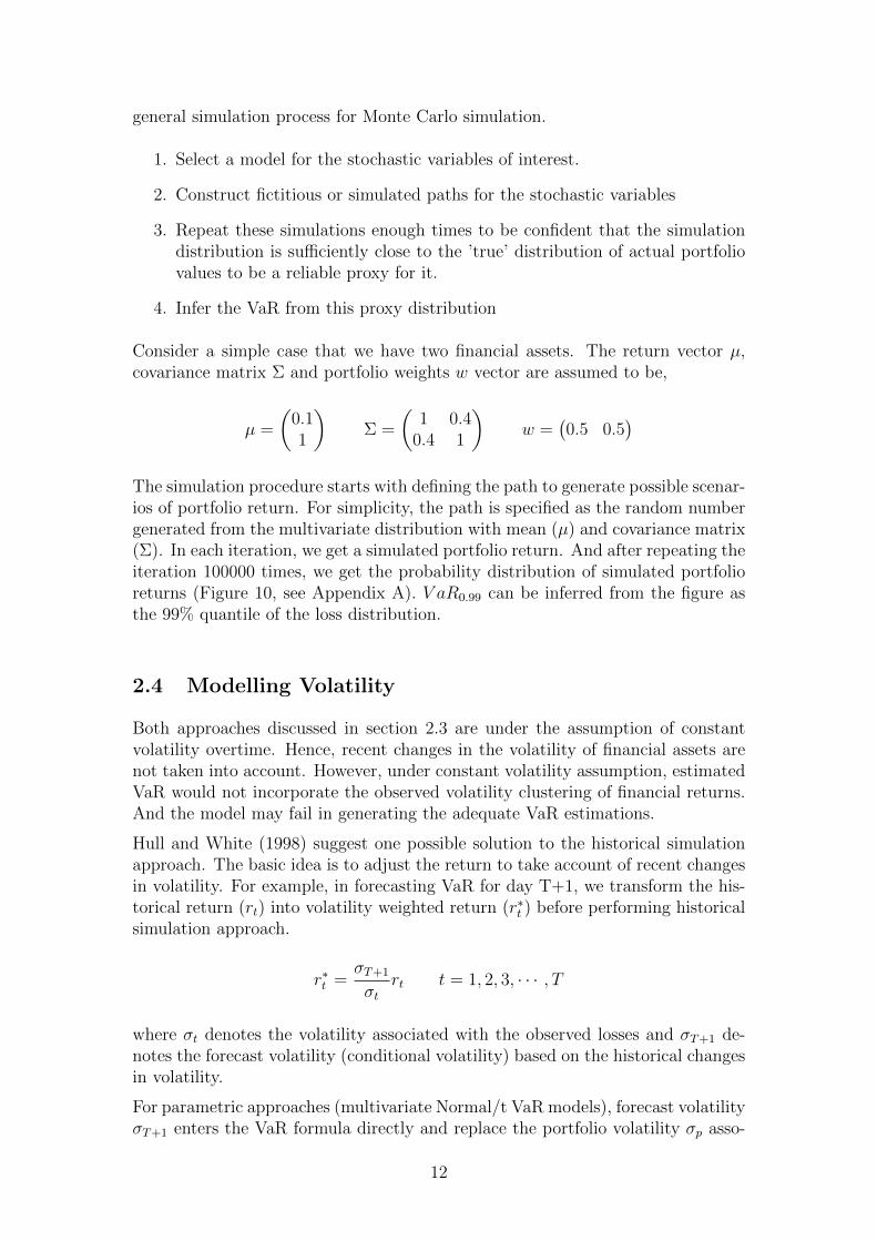
The theories presented in last section are applied to a portfolio composed by S&P500 index and Hang Seng Index (HSI). The dataset contains 2974 daily closingprices from January 3rd, 2000 to March 29th, 2012. The daily closing prices arepresented in Figure 11 (see Appendix A). In order to apply the multivariate VaRmodels, the original indexes are transformed into log-returns. We denote the log-returns of S&P 500 index as variable 1, the log-returns of Hang Seng Index (HSI)as variable 2. Figure 4 presents the daily log-returns of both series. In the figure,we can observe the evidence of stylized fact known as volatility clustering. Largereturns follow with large returns, and similar for small returns.

Log−Returns − Hang Seng Index

20042000 2008 2012

Log−Returns − S&P 500 Index

20042000 2008 2012

Figure 4: Daily log-returns of HSI and S&P 500 Index

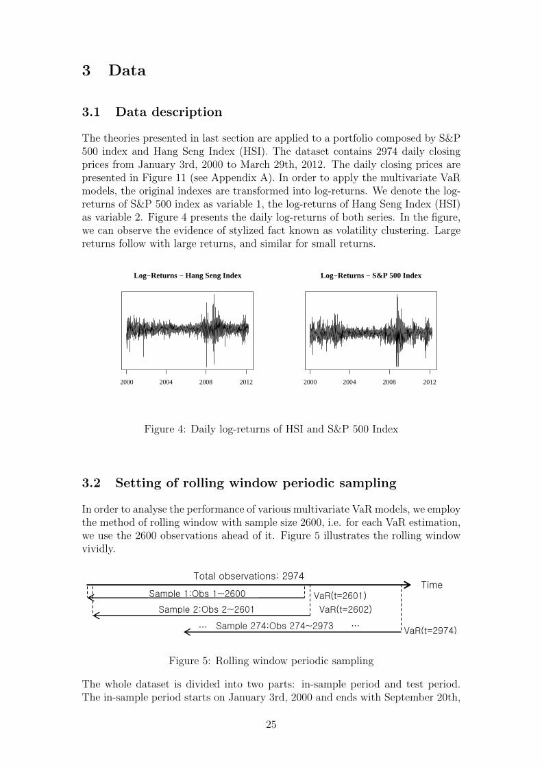
3.2 Setting of rolling window periodic sampling

In order to analyse the performance of various multivariate VaR models, we employthe method of rolling window with sample size 2600, i.e. for each VaR estimation,we use the 2600 observations ahead of it. Figure 5 illustrates the rolling windowvividly.

Total observations: 2974 Time

Sample 1:Obs 1~2600

Sample 2:Obs 2~2601

VaR(t=2601)

VaR(t=2602)

… … VaR(t=2974)

Sample 274:Obs 274~2973

Figure 5: Rolling window periodic sampling

The whole dataset is divided into two parts: in-sample period and test period.The in-sample period starts on January 3rd, 2000 and ends with September 20th,

25

2010. It consists of 2600 daily return of each stock index and offers the historicalinformation needed for estimating VaR. The test-period starts on September 21th,2010 and ends on March 29th, 2012. It is used for testing the performance of VaRmodels. The size of the test period is 374. VaR is estimated for each day in thetest period, with the information offered by the 2600 observations ahead of it. Theaccuracy of different VaR model can be assessed by comparing the estimated VaRand the actual loss. Table 1 summaries the sample division.

Table 1: In-sample period and test period

Period In-sample period test period Total

Date 3/1/2000-20/9/2010 21/9/2010-29/3/2012Number of observations N1 = 2600 N2 = 374 N=2974

3.3 Static and dynamic analysis on probability distribu-

tions

In this part, we discuss the static and dynamic statistical features of both indexes’log-returns. The study begins with a descriptive statistics on the log-return series,which is shown in Table 2.

Table 2: Descriptive statistics of daily log-return of HSI and S&P 500 indexes

Statistics Hang Seng Index S&P 500 Index

Mean 5.753× 10−5 −1.222× 10−5

Min -0.147 -0.095Max 0.134 0.110

Kurtosis 11.749 9.981Skewness -0.253 -0.150

Jarque-Bera Test 9513.012 6048.956

The table shows that Hang Seng Index has a positive average daily return, whileS&P 500 Index has a negative average daily return. Both series are nearly sym-metric, but fat-tailed (kurtosis > 3). In addition, the Jarque-Bera normalitytest rejects its normality null hypothesis (critical value for Jargue-Bera test is5.991, at 95% significance level), i.e. the returns of both indexes are not normallydistributed.

Furthermore, a comparison of descriptive statistics is made between the sampleperiod and test period (Table 3). The results indicate that the distributions ofboth index returns have large differences between sample-period and test-period.Estimating their VaR with multivariate normal distribution or multivariate t dis-tribution assumptions can be problematic and result in inadequate VaR estima-tions.

26

Table 3: Descriptive statistics of daily log-return of HSI and S&P 500 indexes

StatisticsHang Seng Index S&P 500 Index

In-sample period Test period In-sample period Test period

Mean 9.053× 10−5 −1.718× 10−4 −9.302× 10−5 5.492× 10−4

Min -0.147 -0.058 -0.095 -0.069Max 0.134 0.055 0.110 0.046

Kurtosis 12.116 5.158 10.211 7.216Skewness -0.251 -0.285 -0.105 -0.544

By employing multivariate kernel smoothing and kernel density estimation (KDE)techniques (Duong, 2007), we present the estimated density of the joint probabilitydistribution (Figure 6). The figure on the right shows the shape of empiricalprobability distribution is asymmetry and very sharp. It indicates no evidence ofmultivariate normality, but shows evidence of excess kurtosis.

HSI S&P 500

Joint density

Kernel density of Joint distribution level curve

200

400

600

800

100

0

−0.04 −0.02 0.00 0.02 0.04

−0.

040.

000.

020.

04

Figure 6: Joint kernel density and level curve of HSI and S&P 500 index

Afterwards, we analyse the dynamics of the sample distribution, by observingthe rolling samples of both index. The results are illustrated in Figure 12 andFigure 13 (see Appendix A). Figure 12 indicates the sample distribution of HangSeng index is unstable and varies with time. The volatility of Hang Seng index isdecreasing along the test period, and the probability distribution tends to be moreand more fat-tailed. Different with Hang Seng index, the continuously increasingaverage return in Figure 13 indicates the strong performance of S&P 500 index.Furthermore, the dynamics of sample volatility and kurtosis show no significantpattern. To conclude with, distributions of both index returns are unstable andthe research based on them should pay more attention to their time-varying sampleprobability distribution.

27

4 Methodology: VaR models and notations

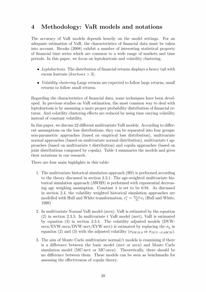
The accuracy of VaR models depends heavily on the model settings. For anadequate estimation of VaR, the characteristics of financial data must be takeninto account. Brooks (2008) exhibit a number of interesting statistical propertyof financial time series which are common to a wide range of markets and timeperiods. In this paper, we focus on leptokurtosis and volatility clustering.

• Leptokurtosis. The distribution of financial returns displays a heavy tail withexcess kurtosis (kurtosis > 3).

• Volatility clustering Large returns are expected to follow large returns, smallreturns to follow small returns.

Regarding the characteristics of financial data, some techniques have been devel-oped. In previous studies on VaR estimation, the most common way to deal withleptokurtosis is by assuming a more proper probability distribution of financial re-turns. And volatility clustering effects are reduced by using time varying volatilityinstead of constant volatility.

In this paper, we discuss 22 different multivariate VaR models. According to differ-ent assumptions on the loss distributions, they can be separated into four groups:non-parametric approaches (based on empirical loss distribution), multivariatenormal approaches (based on multivariate normal distribution), multivariate t ap-proaches (based on multivariate t distribution) and copula approaches (based onjoint distributions composed by copula). Table 4 summaries the models and givestheir notations in our research.

There are four main highlights in this table:

1. The multivariate historical simulation approach (HS) is performed accordingto the theory discussed in section 2.3.1. The age-weighted multivariate his-torical simulation approach (AWHS) is performed with exponential decreas-ing age weighing assumption. Constant λ is set to be 0.94. As discussedin section 2.4, the volatility weighted historical simulation approaches aremodelled with Hull and White transformation, r∗t = σT+1

σtrt (Hull and White,

1998)

2. In multivariate Normal VaR model (mvn), VaR is estimated by the equation(2) in section 2.3.3. In multivariate t VaR model (mvt), VaR is estimatedby equation (3) in section 2.3.4. The volatility adjusted models (DVW-mvn/EVW-mvn/DVW-mvt/EVW-mvt) is estimated by replacing the σp inequation (2) and (3) with the adjusted volatility (σEWMA or σDCC−GARCH).

3. The aim of Monte Carlo multivariate normal/t models is examining if thereis a difference between the basic model (mvt or mvn) and Monte Carlosimulation model (MC-mvt or MC-mvn). Theoretically, there should beno difference between them. These models can be seen as benchmarks forassessing the effectiveness of copula theory.

28

Table 4: VaR models and notation

Model Notation

Historical Simulation HSAge weighted Historical Simulation AWHSVolatility weighted (DCC-GARCH) Historical Simulation DVWHSVolatility weighted (EWMA) Historical Simulation EVWHS

Multivariate Normal approach mvnMonte Carlo-multivariate normal MC-mvnVolatility adjusted (DCC-GARCH) Multivariate Normal DVW-mvnVolatility adjusted (EWMA) Multivariate Normal EVW-mvn

Multivariate t approach mvtMonte Carlo-multivariate t MC-mvtVolatility adjusted (DCC-GARCH) Multivariate t DVW-mvtVolatility adjusted (EWMA) Multivariate t EVW-mvt

Monte Carlo-Gaussian Copula(pseudo) MC-GCpMonte Carlo-Gaussian Copula(normal) MC-GCnMonte Carlo-Student’s t-Copula(pseudo) MC-tCpMonte Carlo-Student’s t-Copula(normal) MC-tCnMonte Carlo-Gumbel Copula(pseudo) MC-GuCpMonte Carlo-Gumbel Copula(normal) MC-GuCnMonte Carlo-Clayton Copula(pseudo) MC-ClCpMonte Carlo-Clayton Copula(normal) MC-ClCnMonte Carlo-Frank Copula(pseudo) MC-FrCpMonte Carlo-Frank Copula(normal) MC-FrCn

4. Monte Carlo-Gaussian/t/Gumbel/Clayton/Frank copula represents the copula-based multivariate VaR model. The models are performed following the pro-cedures proposed in section 2.5.6. Pseudo/normal in the parentheses showsthe assumption of marginal distribution. ’Pseudo’ denotes the copula is con-structed on the pseudo observations and without specifying the marginaldistribution. ’Normal’ denotes the normal distribution is specified as themarginal distribution of copula function.

29

5 Modelling Volatility

The section starts with a focus on the time series properties of the S&P 500Index and Hang Seng Index. Next, multivariate DCC-GARCH model and EWMAmodel are employed as an estimation of time-varying volatility. A discussion onthe results of multivariate volatility model is presented. This section ends with astudy on the dependence structure between S&P 500 Index and Hang Seng Index.

5.1 Time series properties

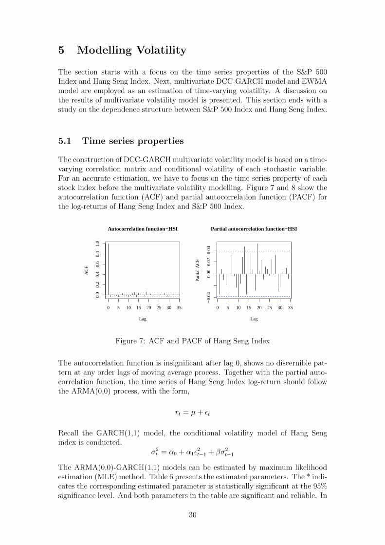
The construction of DCC-GARCH multivariate volatility model is based on a time-varying correlation matrix and conditional volatility of each stochastic variable.For an accurate estimation, we have to focus on the time series property of eachstock index before the multivariate volatility modelling. Figure 7 and 8 show theautocorrelation function (ACF) and partial autocorrelation function (PACF) forthe log-returns of Hang Seng Index and S&P 500 Index.

0 5 10 15 20 25 30 35

0.0

0.2

0.4

0.6

0.8

1.0

Lag

AC

F

Autocorrelation function−HSI

0 5 10 15 20 25 30 35

−0.

040.

000.

020.

04

Lag

Par

tial A

CF

Partial autocorrelation function−HSI

Figure 7: ACF and PACF of Hang Seng Index

The autocorrelation function is insignificant after lag 0, shows no discernible pat-tern at any order lags of moving average process. Together with the partial auto-correlation function, the time series of Hang Seng Index log-return should followthe ARMA(0,0) process, with the form,

rt = µ+ εt

Recall the GARCH(1,1) model, the conditional volatility model of Hang Sengindex is conducted.

σ2t = α0 + α1ε

2t−1 + βσ2

t−1

The ARMA(0,0)-GARCH(1,1) models can be estimated by maximum likelihoodestimation (MLE) method. Table 6 presents the estimated parameters. The * indi-cates the corresponding estimated parameter is statistically significant at the 95%significance level. And both parameters in the table are significant and reliable. In

30

addition, the results of LM ARCH test show ’ARCH-effects’ presents in residualsof the ARMA(0,0) model and it makes sense to employ an ARCH/GARCH model.

Table 5: ARMA-GARCH model estimation results, Hang Seng Index

Parameters Estimates Standard Error p-value

µ 5.597× 10−4 2.312× 10−4 0.01547*α0 1.292× 10−6 4.438× 10−7 0.00359*α1 6.870× 10−2 8.559× 10−3 0.00000*β1 9.279× 10−1 8.488× 10−3 0.00000*

Loglikelihood 7412.912AIC -5.699BIC -5.690

LM Arch Test p=0.07535

0 5 10 15 20 25 30 35

0.0

0.2

0.4

0.6

0.8

1.0

Lag

AC

F

Autocorrelation function−S&P 500

0 5 10 15 20 25 30 35

−0.

050.

000.

05

Lag

Par

tial A

CF

Partial autocorrelation function−S&P 500

Figure 8: ACF and PACF of S&P 500 Index

The autocorrelation function of S&P 500 log-return shows a different pattern. Thecorrelations at lag 1 and 2 are significant and negative. We can identify this seriesas it follows ARMA(0,2) process. Similar with Hang Seng Index, we construct theARMA(0,2)-GARCH(1,1) model for S&P 500 index,

rt = µ+ εt + θ1εt−1 + θ2εt−2

σ2t = α0 + α1ε

2t−1 + βσ2

t−1

The results of ARMA(0,2)-GARCH(1,1) are presented in Table 6. In a similarmanner, the results show the estimated parameters are significant (significance lev-el, 95%) and reliable. The results of LM ARCH test show ’ARCH-effects’ presentsin residuals of the ARMA(0,2) model and it makes sense to use an ARCH/GARCHmodel.

31

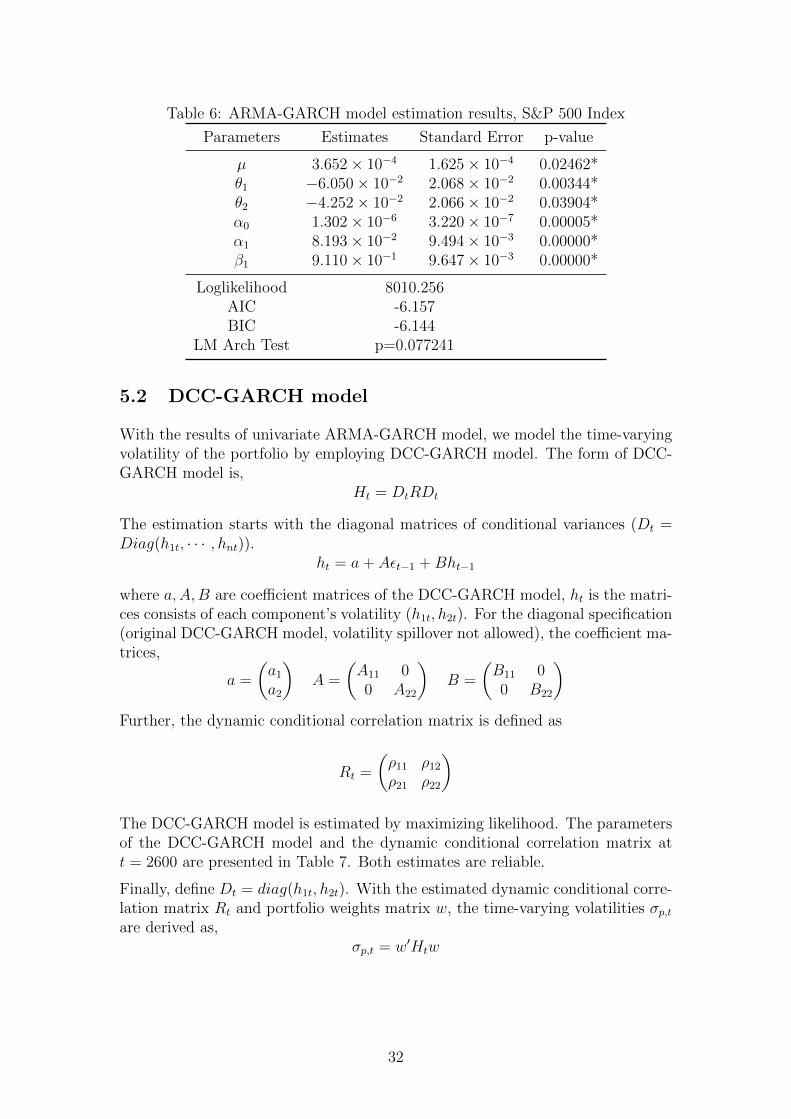
Table 6: ARMA-GARCH model estimation results, S&P 500 Index

Parameters Estimates Standard Error p-value

µ 3.652× 10−4 1.625× 10−4 0.02462*θ1 −6.050× 10−2 2.068× 10−2 0.00344*θ2 −4.252× 10−2 2.066× 10−2 0.03904*α0 1.302× 10−6 3.220× 10−7 0.00005*α1 8.193× 10−2 9.494× 10−3 0.00000*β1 9.110× 10−1 9.647× 10−3 0.00000*

Loglikelihood 8010.256AIC -6.157BIC -6.144

LM Arch Test p=0.077241

5.2 DCC-GARCH model

With the results of univariate ARMA-GARCH model, we model the time-varyingvolatility of the portfolio by employing DCC-GARCH model. The form of DCC-GARCH model is,

Ht = DtRDt

The estimation starts with the diagonal matrices of conditional variances (Dt =Diag(h1t, · · · , hnt)).

ht = a+ Aεt−1 +Bht−1

where a,A,B are coefficient matrices of the DCC-GARCH model, ht is the matri-ces consists of each component’s volatility (h1t, h2t). For the diagonal specification(original DCC-GARCH model, volatility spillover not allowed), the coefficient ma-trices,

a =

(a1

a2

)A =

(A11 00 A22

)B =

(B11 00 B22

)Further, the dynamic conditional correlation matrix is defined as

Rt =

(ρ11 ρ12

ρ21 ρ22

)The DCC-GARCH model is estimated by maximizing likelihood. The parametersof the DCC-GARCH model and the dynamic conditional correlation matrix att = 2600 are presented in Table 7. Both estimates are reliable.

Finally, define Dt = diag(h1t, h2t). With the estimated dynamic conditional corre-lation matrix Rt and portfolio weights matrix w, the time-varying volatilities σp,tare derived as,

σp,t = w′Htw

32

Table 7: DCC-GARCH estimation results

Parameters Estimates Standard Error

a1 1.292× 10−6 4.910× 10−7

a2 1.302× 10−6 1.378× 10−2

A11 6.870× 10−2 1.111× 10−2

A22 8.193× 10−2 5.960× 10−7

B11 9.279× 10−1 1.251× 10−2

B22 9.110× 10−1 1.149× 10−2

Dynamic conditional correlation matrix at t = 2600

ρ11 = ρ22 1.000ρ12 = ρ21 0.187

Loglikelihood 38242.61

5.3 Multivariate EWMA

Compared with modelling volatility with DCC-GARCH model, multivariate EW-MA approach is easier to be realized. This approach starts with the unconditionalcovariance matrix of the first 2600 observations (In-sample period).

Σ0(rHSI , rS&P500) =

(0.01713 0.007360.00736 0.01409

)

Then, the covariance matrix at time t = 2601 (denote as Σ1),

Σ1 = λΣ0(rHSI , rS&P500) + (1− λ)ε0ε′0

Where ε0 = r0 − µ. And in this paper, we assume λ = 0.94. Then the covariancematrix for any time in the test period (Σt) can be derived by the following equation.

Σt = λΣt−1 + (1− λ)εt−1ε′t−1

With the calculated time-varying covariance matrix (Σ0,Σ1, · · · ,Σn), the time-varying portfolio volatility σp,t is derived by,

σp,t = w′Σtw

5.4 Dependence structure

In this part, we discuss the dependence structures between the portfolio compo-nents. It is an important concept to the estimation of portfolio VaR. It determinesthe covariance matrix and defines the risk level of the portfolio.

33

The discussion starts with the static measurement of the dependence structures.Dependence structure between Hang Seng Index and S&P 500 index is measuredin terms of Pearson’s ρ (linear dependence), Kendall’s τ and Spearman’s ρ (rankcorrelation coefficient). The result is shown in Table 8. Both the results show thetwo indexes are positive correlated, but their correlation is not strong. They arefacing with different risk factors. It is worth consisting a portfolio that diversifythe unsystematic risks.

Table 8: Static dependence structure measurement

Measurement of dependence structure Value

Pearson’s ρ 0.2247Kendall’s τ 0.1111

Spearman’s ρ 0.1610

Afterwards, we focus on the dynamic conditional correlation matrices estimatedby DCC-GARCH model. It gives the measurement of time-varying dependencestructures between Hang Seng Index and S&P 500 Index (Figure 9).

0.12

0.16

0.20

0.24

dyna

mic

con

ditio

nal c

orre

latio

n

20042000 2008

Figure 9: Dynamic of conditional correlation between HSI and S&P 500

The figure shows the dynamic correlations of HSI and S&P 500 are time-varyingand volatiles at the range between 0.11 and 0.2455. In addition, by observing theprobability distribution of the dependence structures, more than 70% observationsof correlation lying in range between 0.15 and 0.2. It is highly concentrated andtends to continue fluctuating in the interval 0.15-0.2, which can be treated asrelatively stable in a short period of time.

Thus, the correlation matrix of the HSI and S&P indexes could be assumed tobe constant overtime in the test period. With the assumption, there is no needto estimate DCC-GARCH model for each day in the test period. The correlationbetween Hang Seng index and S&P 500 index is assumed to be consistent withthe estimated correlation matrix of DCC-GARCH model (Table 6) at the end ofthe sample period (t = 2600), in the matrix form:

ρ =

(1 0.187

0.187 1

)34

6 Empirical Results

This section presents the empirical results of various multivariate VaR modelsthat defined in methodology section. Both models are calculated on the 99%confidence level (α = 0.99) and the holding period (H) is one-day. For each MonteCarlo simulations process, 10000 iterations are performed. The results for eachmodel are presented (Table 9) in terms of three evaluation criteria: Christoffersentest, quadratic probability score (QPS) and root mean squared error (RMSE).Significant LR statistics are highlighted in bold, which indicate the VaR modelsfail to pass the corresponding test.

Table 9: Model evaluation, V aRα : 1− α = 1%

Christoffersen Test Relative PerformanceVaR Model Violations LRuc LRind LRcc QPS RMSE

HS 1 2.862 2.666 5.528 0.005441 353.656AWHS 13 14.106 2.666 16.772 0.068328 299.312

DVWHS 7 2.284 2.666 4.950 0.036884 277.616EVWHS 4 0.018 2.666 2.684 0.021163 278.234

mvn 11 9.357 2.666 12.023 0.057847 314.098MC-mvn 10 7.256 2.666 9.922 0.052606 313.526

DVW-mvn 4 0.018 2.666 2.684 0.021163 282.902EVW-mvn 4 0.018 2.666 2.684 0.021163 281.837

mvt 11 9.357 2.666 12.023 0.057847 314.157MC-mvt 11 9.357 2.666 12.023 0.057847 313.981

DVW-mvt 4 0.018 2.666 2.684 0.021163 282.951EVW-mvt 4 0.018 2.666 2.684 0.021163 281.886

MC-GCp 4 0.018 2.666 2.684 0.021163 341.869MC-GCn 1 2.862 2.666 5.528 0.005441 374.886MC-tCp 3 0.159 2.666 2.825 0.015922 351.993MC-tCn 1 2.862 2.666 5.528 0.005441 375.996

MC-GuCp 6 1.166 2.666 3.832 0.031643 337.798MC-GuCn 2 0.984 2.666 3.650 0.010681 376.275MC-ClCp 2 0.984 2.666 3.650 0.010681 362.967MC-ClCn 1 2.862 2.666 5.528 0.005441 375.681MC-FrCp 7 2.284 2.666 4.950 0.036884 333.797MC-FrCn 1 2.862 2.666 5.528 0.005441 376.747

LRcritic, α∗ = 95% 3.841 3.841 5.991

Confidence Interval, violations (Obs=374, α∗ = 99%) 0-9Confidence Interval, violations (Obs=374, α∗ = 95%) 1-8

The results can be summarized as follows:

1. Basic multivariate VaR models (mvn/mvt/HS/AWHS) do not perform wellin predicting future losses. As indicated by the christoffersen test (LRuc)

35

(Table 9), three of them (mvn/mvt/AWHS) fail to generate adequate esti-mation of future losses. As a results, their QPS is larger than other models.In addition, the number of violations during the test period is relativelylarge, which indicates their underestimation of future losses.

However, one of them - the historical simulation VaR model (HS) passesthe christoffersen test and have few violation during the test period. Conse-quently, its QPS is low which indicates its good performance in the violationdays. The historical simulation VaR model could have a lower probability ofoccurring violations. Despite its good performance in violation days, someevidences of overestimating the future losses are found. Compared with theother VaR models, the RMSE of historical simulation VaR model is larg-er. It shows its relatively poor performance in non-violation days: usershave to hold a higher level of capital reserves, which is costly. Figure 14(see Appendix A) also shows some evidences of overestimating future loss-es. The estimated VaR is slightly higher than the other basic VaR models.Less violations are at the expense of higher reserves in non-violation days.For a regulatory purposes, the model is acceptable and conservative enough.However, from the users’ perspective, it is costly to accept the historicalsimulation model.

2. Volatility adjusted multivariate VaR models (DVWHS/EVWHS/DVW-mvn/EVW-mvn/DVW-mvt/EVW-mvt) shows notable improvements in the per-formance of predicting future losses, compared with the basic multivariateVaR models. Both volatility adjusted multivariate VaR models pass thechristoffersen test (Table 9, LRuc, LRind, LRcc). The relatively low QPS andthe relatively low RMSE shows its good performance in the violation daysas well as the non-violation days. Compared with the other VaR models,they have less probability of violations and at the same time, do not requirea high-level capital reserve.

The DCC-GARCH model and the multivariate EWMA model have similarperformances in estimating the future volatilities. However, their featuresare slightly different. Among volatility adjusted parametric VaR model-s (DVW-mvn/EVW-mvn/DVW-mvt/EVW-mvt), the RMSE statistics inTable 9 indicate VaR models with multivariate EWMA volatility performslightly better in non-violation days. In addition, figure 15 and 16 (see Ap-pendix A) show DCC-GARCH model overestimates the volatility’s suddenchange in August, 2011. On other days of the test period, it is hard tofigure out any difference between multivariate EWMA volatility model andmultivariate DCC-GARCH volatility model. In non-parametric VaR models(DVWHS/EVWHS), the RMSE statistics indicate VaR models with DCC-GARCH have better performance in non-violation days. While the QPSstatistics indicate VaR models with multivariate EWMA have lower viola-tions in the test period. VaR models with multivariate EWMA are moreconservative, compared with VaR models with multivariate DCC-GARCH.

3. Monte Carlo approaches of multivariate VaR (MC-mvn/MC-mvt) show con-sistent results with basic multivariate VaR models. Theoretically, MonteCarlo approach and its corresponding basic VaR model are under the same

36

assumptions and they should have the same results. The differences betweenQPS and RMSE statistics come from the standard errors of estimation. Thebias can be decreased by increasing the simulation iterations.

4. Compared with basic multivariate VaR models, copula-based multivariateVaR models have better predictive power on future losses. Both copula-basedmultivariate VaR models pass the christoffersen test (Table 9), which indicatetheir adequate estimation of future losses. Their number of violations in thetest period is low. Consequently, the QPS statistics is lower than the basicmodels (mvn/mvt/AWHS). From the regulatory perspective, copula-basedmultivariate VaR models performs well.

In basic multivariate VaR models, we assume the probability distribution ofloss as a specific statistical probability distribution. However, in practice,the actual losses do not always follow a certain probability distribution thatcan be specified by a simple equation. Sometimes, the probability distribu-tion can be complex. In that case, the VaR estimation based on a specificprobability distribution could be inadequate. By contrast, the copula theo-ry shows its brilliant ability of describing complex multivariate probabilitydistributions. The selection of probability distribution is not limited on theexisting probability distribution. With the copula theory, we can constructan unknown distribution that fits the data best. It is the reason behind thebetter performance of copula-based multivariate VaR models.

Despite its advantages over the basic models, they face the same problemwith non-volatility adjusted VaR models: in order to lower the probabilityof violations, the estimated VaR values have to be more conservative thanthe volatility adjusted models. As a results, their RMSE statistics can berelatively high. From the users’ perspective, it is costly to have a high levelcapital reserves.

However, the problem can be solved by introducing volatility models into thecopula theory, namely, conditional copula models. Due to the limited timeframe, we do not employ the conditional copula models. But it is availablefor future study. We believe it can generate a VaR estimation with lessviolations and demanding less capital reserves.

In the paper, five families of copula functions and two different assump-tions on marginal distributions are employed. As indicated by the results,they have shown different features in estimating multivariate VaR. As indi-cated by the RMSE statistics and the figures (Figure 17-21, see Appendix),copula-based copula VaR models with normal marginal distribution are moreconservative (RMSE is higher) than the copula-based copula VaR modelsbased on pseudo observations. As a results, they have lower probability ofviolations.

Among different copula functions (Gaussian/t/Gumbel/Clayton/Frank), Clay-ton copula and student’s t copula perform the best in lowering violations.Gaussian copula performs on the average level and is less conservative thanClayton/student’s t copula. Gumbel copula ranks at the fourth and Frankcopula performs the least conservative. The results are consistent with some

37

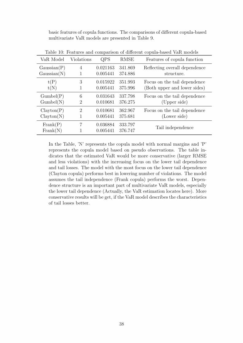
basic features of copula functions. The comparisons of different copula-basedmultivariate VaR models are presented in Table 9.

Table 10: Features and comparison of different copula-based VaR models

VaR Model Violations QPS RMSE Features of copula function

Gaussian(P) 4 0.021163 341.869 Reflecting overall dependencestructure.Gaussian(N) 1 0.005441 374.886

t(P) 3 0.015922 351.993 Focus on the tail dependence(Both upper and lower sides)t(N) 1 0.005441 375.996

Gumbel(P) 6 0.031643 337.798 Focus on the tail dependence(Upper side)Gumbel(N) 2 0.010681 376.275

Clayton(P) 2 0.010681 362.967 Focus on the tail dependence(Lower side)Clayton(N) 1 0.005441 375.681

Frank(P) 7 0.036884 333.797Tail independence

Frank(N) 1 0.005441 376.747

In the Table, ’N’ represents the copula model with normal margins and ’P’represents the copula model based on pseudo observations. The table in-dicates that the estimated VaR would be more conservative (larger RMSEand less violations) with the increasing focus on the lower tail dependenceand tail losses. The model with the most focus on the lower tail dependence(Clayton copula) performs best in lowering number of violations. The modelassumes the tail independence (Frank copula) performs the worst. Depen-dence structure is an important part of multivariate VaR models, especiallythe lower tail dependence (Actually, the VaR estimation locates here). Moreconservative results will be get, if the VaR model describes the characteristicsof tail losses better.

38

7 Conclusion

The aim of this paper has been to examine the one-day predictive power of sever-al multivariate VaR models, including basic multivariate VaR models, volatility-adjusted multivariate VaR models and copula-based multivariate VaR models.The comparison is made on a portfolio consisting of S&P 500 index and HangSeng Index. Christoffersen test, quadratic probability score and root mean squareerror are used as standard tools to evaluate the performance. Following the re-search questions in the introduction section, the empirical results can be concludedas follows:

1. Based on the results of quadratic probability score and the root mean squarederror, basic multivariate VaR models (mvn/mvt/HS/AWHS) show poor per-formances in estimating future losses. Additionally, three basic multivariateVaR models (mvn/mvt/AWHS) fail to pass the christoffersen test. TheirVaR estimation can be treated as inadequate.

2. Multivariate EWMA and DCC-GARCH model are employed as the multi-variate volatility model. Both models are easy to implement (section 5) andthe results indicate the accurate estimation of the time-varying multivariatevolatility.

3. Both volatility adjusted multivariate VaR models pass the christoffersentest. Compared with the basic multivariate VaR models, they have high-er quadratic probability scores and lower root mean squared errors. Theresults indicate that volatility adjusted multivariate VaR models have bet-ter predictive performances than the basic VaR models.

4. Compared with basic multivariate VaR models, copula-based multivariateVaR models show notable improvements in lowering probability of violations.The copula theory constructs multivariate distributions with attentions onthe tail losses and tail dependence. As a result, the copula-based multivariateVaR models have a better predictive power on the tail losses and show similarcharacters with extreme value theory (EVT) VaR models. All the copula-based multivariate VaR models pass the christoffersen test and have a lowerquadratic probability score.

As a final point, the main implication of this research for practitioners is it offers apractical guidance for estimating portfolio VaR by multivariate VaR models. Thecomparison between different multivariate VaR models gives an overview of theirperformances and features. This paper can be effective as a reference when facingportfolio risk measurement problems or facing the problem of selecting adequatemultivariate VaR models.

39

References

Aeschliman, C., Park, J. and Kak, A.C., (2010). A novel parameter estima-tion algorithm for the multivariate t-distribution and its application to computervision. 11th European conference on computer vision (ECCV), Berlin Heidelberg.Springer, 594-607.

Basel Committee on Banking Supervision, (1996). Amendment to thecapital accord to incorporate market risks. Basel Committee Publications, 24.

Belzunee, F., Castano, A., Olvera-Cervantes, A. and Suarez-Lorens,A., (2007). Quantile curves and dependence structure for bivariate distribution.Computational statistics and data analysis, 45(3), 5112-5129.

Blanco, C. and Ihle, G., (1999). How good is your VaR? Using back-testingto assess system performance. Financial Engineering News, 11(8), 1-2.

Bollerslev, T., (1990). Modelling the coherence in short-run nominal exchangerates: a multivariate generalized ARCH model. Review of Economics and Statis-tics, 72, 498-505.

Bollerslev, T., Engle, R.F. and Wooldridge, J.M., (1988). A capitalasset pricing model with time varying covariances. Journal of political economy,96(1), 116-131.

Boudoukh, J., Richardson, M. and Whitelaw R., (1998). The best of bothworlds: a hybrid approach to calculating value at risk. Risk, 11, 64-47.

Bouye, E., Durrleman, V., Nikeghbali, A., Riboulet, G. and RoncalliT., (2000). Copulas for finance-a reading guide and some applications. WorkingPaper, Group de Recherche Operationelle, Credit Lyonnais.

Brooks, C., (2008). Introductory econometrics for finance. 2nd ed. Cambridge:Cambridge University Press.

Byrd, R.H., Lu, P. and Nocedal, J., (1995). A Limited Memory Algorithmfor Bound Constrained Optimization. SIAM Journal on Scientific and StatisticalComputing, 16(5), 1190-1208.

Cherubini, U., Luciano, E. and Vecchinato, W., (2004). Copula methodsin finance. Chichester: John Wiley and Sons, Ltd.

Christodoulakis, G.A. and Satchell, S.E., (2002). Correlated ARCH: mod-elling the time-varying correlation between financial asset returns. European jour-nal of operations research, 139, 351-370.

Christoffersen, P.F., (1998). Evaluating interval forecasts. International e-conomic review, 39, 841-862.

Clayton, D.G., (1978). A model for association in bivariate life tables andits application in epidemiological studies of familial tendency in chronic diseaseincidence. Biometrika, 65, 141-151.

40

Cousin, A. and Di Bernardino, E., (2011). A multivariate extension of Value-at-Risk and Conditional-Tail-Expectation. ArXiv e-prints, 1111.1349.

Dowd, K., (1999). Backtesting Market Risk Models. ICBI conference, Geneva.

Dowd, K., (2005). Mesuring market risk. 2nd ed. Chichester: Wiley.

Duong, T., (2007). ks: Kernel density estimation and kernel discriminant anal-ysis for multivariate data in R. Journal of statistical software, 21(7).

Einhoen, D. and Brown, A., (2008). Private profits and socialized risk. Globalassociation of risk professionals, 42, 10-26.

Embrechts, P. and Puccetti, G., (2006). Bounds for functions of multivariaterisks. Journal of multivariate analysis, 97(2), 526-547.

Engel, R.F., (2002). Dynamic conditional correlation-a simple class of multi-variate GARCH models. Journal of business and economic statistics, 20, 339-350.

Engel, R.F., Kroner, K. and Kraft, D., (1995). Multivariate simultaneousgeneralized ARCH. Econometric theory, 11, 122-150.

Engel, R.F. and Sheppard, K., (2001). Theoretical and empirical propertiesof dynamic conditional correlation multivariate GARCH. NBER Working Paper8554, National Bureau of Economic Research.

Engelbrecht, R. and West, G., (2003). A comparison of value-at-risk meth-ods for portfolios consisting of interest rate swap and FRAs. Economic SeriesWorking Papers, University of Oxford.

Fernandez-Ponce, J.M. and Suarez-Llorens, A., (2002). Central regionsfor bivariate distributions. Austrian journal of statistic, 31(2-3), 141-156.

Frank, M.J., (1979). On the simultaneous associativity of F (x, y) and x+ y −F (x, y). Aequationes math, 19, 194-226.

Guermat, C. and Harris, R., (2002). Robust conditional variance estimationand value-at-risk. Journal of Risk, 4, 25-41.

Gumbel, E.J., (1960). Bivariate exponential distributions. J. Amer. Statist.Assoc., 55, 698-707.

Hull, J. and White, A., (1988). Value at risk when daily changes in marketvariables are not normally distributed. Journal of derivatives, 5(Spring), 9-19.

Ivanov, S., Jordan, R., Panajotova, B., and Schoess, S., (2003). DynamicValue-at-Risk with heavy tailed distribution. 9th Annual IFCI Risk ManagementRound Table.

Joe, H., (1997). Multivariate models and dependence concepts. London: Chap-man & Hall Ltd.

41

Joe, H. and Xu, J., (1996). The estimation method of inference functions formargins for multivariate models. Technical Report 166, Department of Statistics,University of British Columbia.

Laubsch, A.J., (1999). Risk management:a practical guide. 1st ed. United S-tates: MSCI.

Lehmann, E., (1966). Some concepts of dependence. Ann. Math. Statist., 37,1137-1153.

Lopez, J.A., (1998). Regulatory evaluation of Value-at-Risk models. FederalReserve Bank of New York Economic Policy Review, 4(3), 119-124.

McNeil, A., Frey, R. and Embrechts, P., (2005). Quantitative risk man-agement: concepts, techniques, and tools. United Kingdom: Princeton UniversityPress.

Morgan Guaranty Trust Company, (1996). RiskMetrics-Technical docu-ment. 4th ed. New York: Morgan Guaranty Trust Company.

Nappo, G. and Spizzichino, F., (2009). Kendall distributions and level sets inbivariate exchangale survival models. Information sciences, 179, 2878-2890.

Nelsen, R.B., (1999). An introduction to copulas. Springer-Verlag Inc.

Palaro, H.P. and Hotta, L.K., (2006). Using conditional copula to estimatevalue at risk. Journal of data science, 4, 93-115.

Sheikh, A.Z. and Qiao, H.T., (2010). Non-normality of market returns: aframework for asset allocation decision making. The journal of alternative in-vestments, 12(3), 8.

Sklar, A., (1959). Fonctions de repartition a n dimensions et leurs marges. Pub.Inst. Statist. Univ. Paris, 8, 229-231.

Taleb, N.N., (1997). Dynamic hedging: managing vanilla and exotic options.New York: Wiley.

Tibiletti, L., (1993). On a new notion of multidimensional quantile. Interna-tional Journal of statistics, 51(3-4), 77-83.

Tse, Y.K. and Tsui, A.K.C, (2002). A multivariate GARCH model with time-varying correlations. Journal of business and economic statistics, 20, 351-362.

Yan, J., (2007). Enjoy the joy of copulas: with a package copula. Journal ofstatistical software, 21(4).

Zhu, C., Byrd, R.H., Lu, P. and Nocedal, J., (1994). L-BFGS-B: For-tran subroutines for large-scale bound constrained optimization. Report NAM-11,EECS Department, Northwest university.

42

Appendix A

0.0

0.1

0.2

0.3

0.4

0.5

loss(+)/profit(−)

Pro

babi

lity

Den

sity

99% VaRSample Mean

Figure 10: A simple illustration of Monte Carlo approach

This figure graphs a realization of 100000 simulated portfolio returns. The port-folio is consist of two assets with equal weights. The assets follow a multivariate

normal distribution, with µ = (0.1, 1) and Σ =

(1 0.4

0.4 1

). Additionally, the 99%

VaR can be point out as the 99% quantile of the loss distribution.

Hang Seng Index

20042000 2008 2012

3163

884

0920

000

S&P 500 Index

20042000 2008 2012

1565

676

1000

Figure 11: Daily closing price of Hang Seng Index and S&P 500 Index

43

0 50 100 200 300

0.00

000

0.00

010

0.00

020

Dynamic − Sample Mean

0 50 100 200 300

0.01

640.

0168

Dynamic − Standard Deviation

0 50 100 200 300

12.5

13.0

13.5

Dynamic − Kurtosis

Figure 12: Dynamic of log-return distributions (Hang Seng Index)

The figure on the left shows the time-varying sample mean of Hang Seng Index.The average return seems to have a gap in t = 240 ∼ 260. The figure in themiddle shows the time-varying sample standard deviation of Hang Seng Index. Itshows a trend that the volatility of the index returns is decreasing. The figureon the right shows the time-varying kurtosis of Hang Seng Index. It seems theprobability distribution tends to be more and more fat-tailed overtime. It can beimproper to assume the loss distributions follow normal distribution.

0 50 100 200 300

−8e

−05

−2e

−05

4e−

05

Dynamic − Sample Mean

0 50 100 200 300

0.01

370.

0139

0.01

41

Dynamic − Standard Deviation

0 50 100 200 300

10.2

10.4

10.6

10.8

11.0

Dynamic − Kurtosis

Figure 13: Dynamic of log-return distributions (S&P 500 Index)

The figure on the left shows the time-varying sample mean of S&P 500 Index. Theaverage return is increasing overtime, and the performance of the index is strong.The figure in the middle shows the time-varying sample standard deviation of S&P500 Index. The figure on the right shows the time-varying kurtosis of S&P 500Index.

44

−20

00

200

400

HS,AWHS,DVWHS,EVWHS

Date

Loss

2010/12 2011/03 2011/06 2011/09 2011/12 2012/03

Figure 14: Estimated VaR: Multivariate historical simulation approach

The black fold line represents the actual losses of the portfolio. The blue line represents theestimated VaR by multivariate historical simulation VaR model (HS). The red line denotes theestimated VaR by multivariate age-weighted historical simulation VaR model (AWHS). The greenline denotes the estimated VaR by volatility weighted (EWMA) historical simulation VaR model(EVWHS). The pink line represents the estimated VaR by volatility weighted (DCC-GARCH)historical simulation VaR model (DVWHS).

−20

00

200

400

mvn,MC−mvn,DVW−mvn,EVW−mvn

Date

Loss

2010/12 2011/03 2011/06 2011/09 2011/12 2012/03

Figure 15: Estimated VaR: Multivariate normal approach

The black fold line represents the actual losses of the portfolio. The blue and pink line representsthe estimated VaR by multivariate normal VaR model (mvn) and Monte Carlo multivariatenormal VaR model (MC-mvn). The red line denotes the estimated VaR by volatility weighted(EWMA) multivariate normal VaR model (EVW-mvn). The green line denotes the estimatedVaR by volatility weighted (DCC-GARCH) multivariate normal VaR model (DVW-mvn).

45

−20

00

200

400

mvt,MC−mvt,DVW−mvt,EVW−mvt

Date

Loss

2010/12 2011/03 2011/06 2011/09 2011/12 2012/03

Figure 16: Estimated VaR: Multivariate t approach

The black fold line represents the actual losses of the portfolio. The blue and pink line representsthe estimated VaR by multivariate t VaR model (mvt) and Monte Carlo multivariate t VaRmodel (MC-mvt). The red line denotes the estimated VaR by volatility weighted (EWMA)multivariate t VaR model (EVW-mvt). The green line denotes the estimated VaR by volatilityweighted (DCC-GARCH) multivariate t VaR model (DVW-mvt).

−20

00

200

400

Gussian Copula−pseudo/normal margin

Date

Loss

2010/12 2011/03 2011/06 2011/09 2011/12 2012/03

Figure 17: Estimated VaR: Gaussian Copula Monte Carlo approach

The black fold line represents the actual losses of the portfolio. The red line denotes the estimatedVaR by Gaussian Copula (normal margin) multivariate VaR model (MC-GCn). The blue linedenotes the estimated VaR by Gaussian Copula (pseudo observations) multivariate VaR model(MC-GCp).

46

−20

00

200

400

Student's t Copula−pseudo/normal margin

Date

Loss

2010/12 2011/03 2011/06 2011/09 2011/12 2012/03

Figure 18: Estimated VaR: Student’s t Copula Monte Carlo approach

The black fold line represents the actual losses of the portfolio. The red line denotes the estimatedVaR by student’s t Copula (normal margin) multivariate VaR model (MC-tCn). The blue linedenotes the estimated VaR by student’s t Copula (pseudo observations) multivariate VaR model(MC-tCp).

−20

00

200

400

Gumbel Copula−pseudo/normal margin

Date

Loss

2010/12 2011/03 2011/06 2011/09 2011/12 2012/03

Figure 19: Estimated VaR: Gumbel Copula Monte Carlo approach

The black fold line represents the actual losses of the portfolio. The red line denotes the estimatedVaR by Gumbel Copula (normal margin) multivariate VaR model (MC-GuCn). The blue linedenotes the estimated VaR by Gumbel Copula (pseudo observations) multivariate VaR model(MC-GuCp).

47

−20

00

200

400

Clayton Copula−pseudo/normal margin

Date

Loss

2010/12 2011/03 2011/06 2011/09 2011/12 2012/03

Figure 20: Estimated VaR: Clayton Copula Monte Carlo approach

The black fold line represents the actual losses of the portfolio. The red line denotes the estimatedVaR by Clayton Copula (normal margin) multivariate VaR model (MC-ClCn). The blue linedenotes the estimated VaR by Clayton Copula (pseudo observations) multivariate VaR model(MC-ClCp).

−20

00

200

400

Frank Copula−pseudo/normal margin

Date

Loss

2010/12 2011/03 2011/06 2011/09 2011/12 2012/03

Figure 21: Estimated VaR: Frank Copula Monte Carlo approach

The black fold line represents the actual losses of the portfolio. The red line denotes the estimatedVaR by Frank Copula (normal margin) multivariate VaR model (MC-FrCn). The blue linedenotes the estimated VaR by Frank Copula (pseudo observations) multivariate VaR model(MC-FrCp).

48

Appendix B

R codes for this paper(304 lines)

R: A Language and Environment for Statistical Computing, Version 2.15.0 (2012-3-30). R De-velopment Core Team. http://www.R-project.org

1 #Define Portfolio weights , sample size and alpha level

2 w=c(0.5 ,0.5)

3 tP=374

4 si=0.01

5

6 #Multivariate EWMA volatility

7 xdata=cbind(hsreturn ,spreturn)

8 res=xdata -apply(xdata ,2,mean)

9 s=var(sdata)

10 lambda =0.94

11 s=lambda*s

12 sigma=sqrt(t(w)%*%s%*%w)

13 EWMAsigma=rep(0,T+1)

14 EWMAsigma [1]= sigma

15 T=length(hsreturn)

16 for(i in 2:(T+1)){

17 s=lambda*s+(1- lambda)*res[(i-1) ,]%*%t(res[(i-1) ,])

18 sigma=sqrt(t(w)%*%s%*%w)

19 EWMAsigma[i]= sigma

20 }

21

22 #Dynamic conditional correlation GARCH volatility

23 library(ccgarch)

24 library(fGarch)

25 f1=garchFit(~garch (1,1),sdata[,1],trace=FALSE)

26 f1=f1@fit$coef

27 f2=garchFit(~arma (0,2)+garch (1,1),sdata[,2],trace=FALSE)

28 #f2=garchFit(~garch (1,1),sdata[,2],trace=FALSE)

29 f2=f2@fit$coef

30 inia=c(f1[2],f2[4])

31 iniA=diag(c(f1[3],f2[5]))

32 iniB=diag(c(f1[4],f2[6]))

33 dcc.para=c(0.01 ,0.97) #intial Value

34 dcc.results=dcc.estimation(inia ,iniA ,iniB ,dcc.para ,sdata ,model="diagonal")

35 #dcc.results=dcc.estimation(inia ,iniA ,iniB ,dcc.para ,sdata ,model=" extended ")

36 DCCGarchsigma=rep(0,( length(hsreturn)+1))

37 for(i in 1:2600){

38 D=diag(sqrt(dcc.results$h[i,]))

39 R=matrix(dcc.results$DCC[i,],2,2)

40 H=D%*%R%*%D

41 DCCGarchsigma[i]=sqrt(t(w)%*%H%*%w)

42 }

43 T=length(sdata [,1])

49

44 h=matrix (0,(tP+1) ,2)

45 h[1,]=dcc.results$h[T,]

46 for(i in 2:(tP+1)){

47 h[i,]=c(dcc.results$out[1,1],dcc.results$out[1,2])+diag(c(dcc.results$out[1,3],

dcc.results$out[1,4]))%*%c(res[(i+2598) ,1]^2,res[(i+2598) ,2]^2)+diag(c(dcc.

results$out[1,5],dcc.results$out [1 ,6]))%*%h[i-1,]

48 }

49 R=matrix(dcc.results$DCC[T,],2,2)

50 for(i in 2601:2974){

51 D=diag(sqrt(h[(i -2599) ,]))

52 H=D%*%R%*%D

53 DCCGarchsigma[i]=sqrt(t(w)%*%H%*%w)}

54

55 #Multivariate t VaR model

56 VaRmt=rep(0,tP)

57 VaRmtEWMA=rep(0,tP)

58 VaRmtDCCG=rep(0,tP)

59 mupts=rep(0,tP)

60 sigmapts=rep(0,tP)

61 for(i in 1:tP){

62 data1=NULL

63 data1=cbind(hsi[i,],sp[i,])

64 kurt1=kurtosis(data1[,1],method="moment")

65 #kurt1=kurtosis(data1 [,1])

66 kurt2=kurtosis(data1[,2],method="moment")

67 #kurt1=kurtosis(data1 [,2])

68 kavg=( kurt1+kurt2)/2

69 df=(4*kavg -6)/(kavg -3)

70 mu=apply(data1 ,2,mean)

71 T=length(sdata [,1])

72 sigmat =(T-1)*var(data1)/T

73 cort=cor(data1)

74 params=c(mu,df)

75 out <-nlm(mlogl ,params ,cort ,data1)

76 mue=c(out$estimate [1],out$estimate [2])

77 df=out$estimate [3]

78 mupts[i]=w%*%mue

79 sigmapts[i]=sqrt(t(w)%*%sigmat%*%w)

80 VaRmt[i]= cpprice[i]*(-mupts[i]-sigmapts[i]*sqrt((df -2)/df)*qt(si,df))

81 VaRmtEWMA[i]= cpprice[i]*(-mupts[i]-EWMAsigma[i+2600]*sqrt((df -2)/df)*qt(si,df))

82 VaRmtDCCG[i]= cpprice[i]*(-mupts[i]-DCCGarchsigma[i+2600]*sqrt((df -2)/df)*qt(si,df

))

83 }

84

85 #Multivariate normal VaR models

86 VaRmn=rep(0,tP)

87 VaRmnEWMA=rep(0,tP)

88 VaRmnDCCG=rep(0,tP)

89 mupns=rep(0,tP)

50

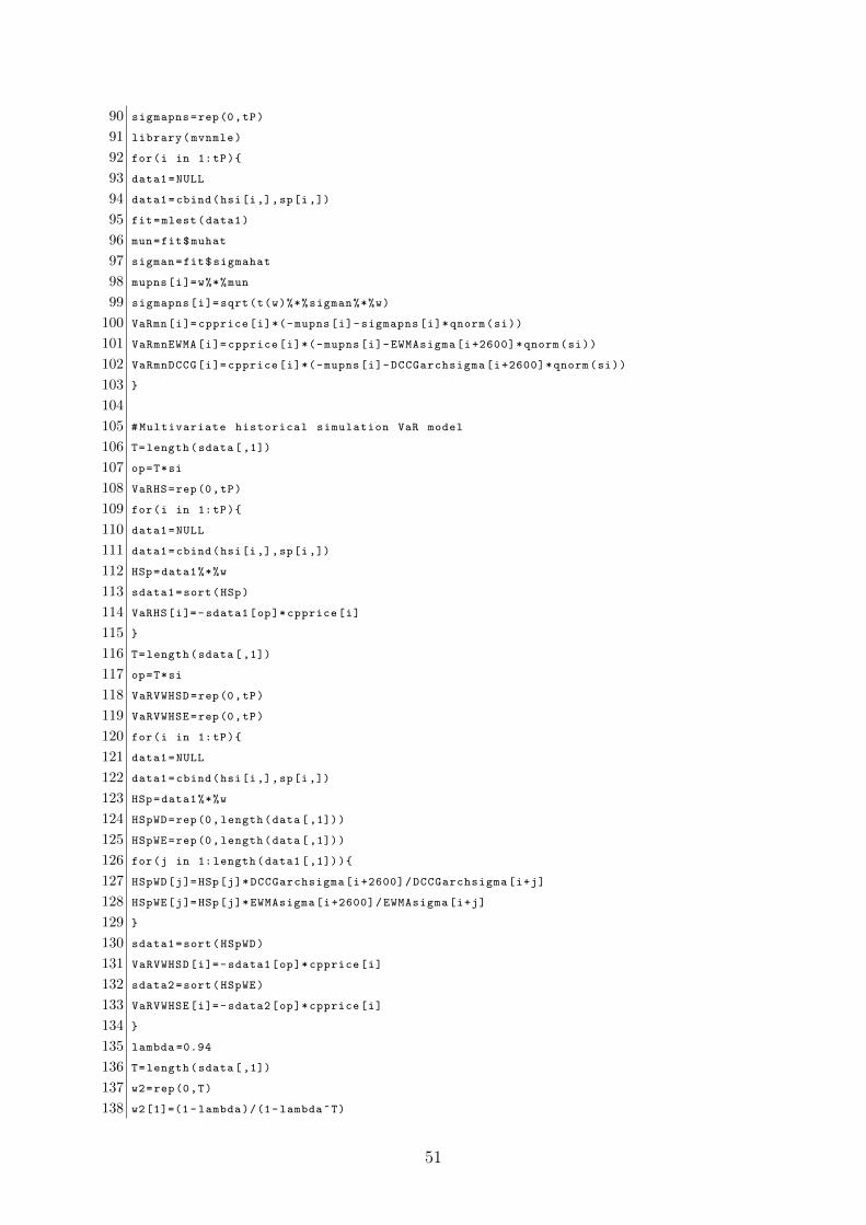
90 sigmapns=rep(0,tP)

91 library(mvnmle)

92 for(i in 1:tP){

93 data1=NULL

94 data1=cbind(hsi[i,],sp[i,])

95 fit=mlest(data1)

96 mun=fit$muhat

97 sigman=fit$sigmahat

98 mupns[i]=w%*%mun

99 sigmapns[i]=sqrt(t(w)%*%sigman%*%w)

100 VaRmn[i]= cpprice[i]*(-mupns[i]-sigmapns[i]*qnorm(si))

101 VaRmnEWMA[i]= cpprice[i]*(-mupns[i]-EWMAsigma[i+2600]*qnorm(si))

102 VaRmnDCCG[i]= cpprice[i]*(-mupns[i]-DCCGarchsigma[i+2600]*qnorm(si))

103 }

104

105 #Multivariate historical simulation VaR model

106 T=length(sdata [,1])

107 op=T*si

108 VaRHS=rep(0,tP)

109 for(i in 1:tP){

110 data1=NULL

111 data1=cbind(hsi[i,],sp[i,])

112 HSp=data1%*%w

113 sdata1=sort(HSp)

114 VaRHS[i]=-sdata1[op]*cpprice[i]

115 }

116 T=length(sdata [,1])

117 op=T*si

118 VaRVWHSD=rep(0,tP)

119 VaRVWHSE=rep(0,tP)

120 for(i in 1:tP){

121 data1=NULL

122 data1=cbind(hsi[i,],sp[i,])

123 HSp=data1%*%w

124 HSpWD=rep(0,length(data [,1]))

125 HSpWE=rep(0,length(data [,1]))

126 for(j in 1: length(data1 [,1])){

127 HSpWD[j]=HSp[j]*DCCGarchsigma[i+2600]/DCCGarchsigma[i+j]

128 HSpWE[j]=HSp[j]*EWMAsigma[i+2600]/EWMAsigma[i+j]

129 }

130 sdata1=sort(HSpWD)

131 VaRVWHSD[i]=-sdata1[op]*cpprice[i]

132 sdata2=sort(HSpWE)

133 VaRVWHSE[i]=-sdata2[op]*cpprice[i]

134 }

135 lambda =0.94

136 T=length(sdata [,1])

137 w2=rep(0,T)

138 w2[1]=(1 - lambda)/(1-lambda^T)

51

139 VaRAWHS=rep(0,tP)

140 for(i in 2:T){w2[i]=w2[i-1]*lambda}

141 for(i in 1:tP){

142 data1=NULL

143 data1=cbind(hsi[i,],sp[i,])

144 HSp=data1%*%w

145 AWHS=cbind(HSp ,w2)

146 sAWHS=AWHS[order(AWHS [,1]) ,]

147 prob=0

148 j=1

149 while(prob <=si){

150 prob=prob+sAWHS[j,2]

151 j=j+1

152 }

153 op=j

154 VaRAWHS[i]=-sAWHS[op ,1]*cpprice[i]

155 }

156

157 #Monte Carlo Method - mvt & mvn

158 library(MASS)

159 MCVaRn=rep(0,tP)

160 for(i in 1:tP){

161 data1=NULL

162 data1=cbind(hsi[i,],sp[i,])

163 fit=mlest(data1)

164 mun=fit$muhat

165 sigman=fit$sigmahat

166 MC=mvrnorm (10000 ,mun ,sigman)

167 MCportfolio=MC%*%w

168 MCVaRn[i]=-cpprice[i]*quantile(MCportfolio ,p=si)

169 }

170 library(mvtnorm)

171 MCVaRt=rep(0,tP)

172 for(i in 1:tP){

173 data1=NULL

174 data1=cbind(hsi[i,],sp[i,])

175 kurt1=kurtosis(data1[,1],method="moment")

176 kurt2=kurtosis(data1[,2],method="moment")

177 kavg=( kurt1+kurt2)/2

178 df=(4*kavg -6)/(kavg -3)

179 mu=apply(data1 ,2,mean)

180 T=length(sdata [,1])

181 cort=cor(data1)

182 params=c(mu,df)

183 sigmat =(T-1)*var(data1)/T

184 out <-nlm(mlogl ,params ,cort ,data1)

185 mue=c(out$estimate [1],out$estimate [2])

186 df=out$estimate [3]

187 MC=rmvt (10000 , sigmat ,df,mue)

52

188 MCportfolio=MC%*%w

189 MCVaRt[i]=-cpprice[i]*quantile(MCportfolio ,p=si)

190 }

191

192 #Copula -based multivariate VaR models

193 library(copula)

194 VaRGaussianC=rep(0,tP)

195 VaRGaussianC2=rep(0,tP)

196 VaRtC=rep(0,tP)

197 VaRtC2=rep(0,tP)

198 VaRGC=rep(0,tP)

199 VaRGC2=rep(0,tP)

200 VaRCC=rep(0,tP)

201 VaRCC2=rep(0,tP)

202 VaRFC=rep(0,tP)

203 VaRFC2=rep(0,tP)

204 for(i in 1:tP){

205 v=4

206 data1=NULL

207 data1=cbind(hsi[i,],sp[i,])

208 fit1=fitdistr(data1[,1],"normal")

209 fit2=fitdistr(data1[,2],"normal")

210 u1=pnorm(data1[,1],fit1$estimate [1],fit1$estimate [2])

211 u2=pnorm(data1[,2],fit2$estimate [1],fit2$estimate [2])

212 Un=cbind(u1 ,u2)

213 T=length(data1 [,1])

214 Up=apply(data1 ,2,rank)/(T+1) #pseudo -observations

215 fitGp=fitCopula(normalCopula (0.6,dim=2,dispstr="ex"),Up,method="mpl")

216 fitGn=fitCopula(normalCopula (0.6,dim=2,dispstr="ex"),Un,method="mpl")

217 fitTp=fitCopula(tCopula (0.6,dim=2,dispstr="ex",df=v,df.fixed=TRUE),Up,method="mpl

")

218 fitTn=fitCopula(tCopula (0.6,dim=2,dispstr="ex",df=v,df.fixed=TRUE),Un,method="mpl

")

219 fitGUp=fitCopula(gumbelCopula (2,dim=2),Up,method="mpl")

220 fitGUn=fitCopula(gumbelCopula (2,dim=2),Un,method="mpl")

221 fitCp=fitCopula(claytonCopula (2,dim =2),Up,method="mpl")

222 fitCn=fitCopula(claytonCopula (2,dim =2),Un,method="mpl")

223 fitFp=fitCopula(frankCopula (2,dim=2),Up,method="mpl")

224 fitFn=fitCopula(frankCopula (2,dim=2),Un,method="mpl")

225 xGp=rcopula(normalCopula(fitGp@estimate ,dim=2,dispstr="ex") ,10000)

226 xGn=rcopula(normalCopula(fitGn@estimate ,dim=2,dispstr="ex") ,10000)

227 xTp=rcopula(tCopula(fitTp@estimate ,dim=2,dispstr="ex",df=v,df.fixed=TRUE) ,10000)

228 xTn=rcopula(tCopula(fitTn@estimate ,dim=2,dispstr="ex",df=v,df.fixed=TRUE) ,10000)

229 xGUp=rcopula(gumbelCopula(fitGUp@estimate ,dim=2) ,10000)

230 xGUn=rcopula(gumbelCopula(fitGUn@estimate ,dim=2) ,10000)

231 xCp=rcopula(claytonCopula(fitCp@estimate ,dim=2) ,10000)

232 xCn=rcopula(claytonCopula(fitCn@estimate ,dim=2) ,10000)

233 xFp=rcopula(frankCopula(fitFp@estimate ,dim=2) ,10000)

234 xFn=rcopula(frankCopula(fitFn@estimate ,dim=2) ,10000)

53

235 yGp=w[1]*quantile(data1[,1],xGp[,1])+w[2]*quantile(data1[,2],xGp[,2])

236 yGn=w[1]*qnorm(xGn[,1],fit1$estimate [1],fit1$estimate [2])+w[2]*qnorm(xGn[,1],fit2

$estimate [1],fit2$estimate [2])

237 yTp=w[1]*quantile(data1[,1],xTp[,1])+w[2]*quantile(data1[,2],xTp[,2])

238 yTn=w[1]*qnorm(xTn[,1],fit1$estimate [1],fit1$estimate [2])+w[2]*qnorm(xTn[,1],fit2

$estimate [1],fit2$estimate [2])

239 yGUp=w[1]*quantile(data1[,1],xGUp [,1])+w[2]*quantile(data1[,2],xGUp [,2])

240 yGUn=w[1]*qnorm(xGUn[,1],fit1$estimate [1],fit1$estimate [2])+w[2]*qnorm(xGUn[,1],

fit2$estimate [1],fit2$estimate [2])

241 yCp=w[1]*quantile(data1[,1],xCp[,1])+w[2]*quantile(data1[,2],xCp[,2])

242 yCn=w[1]*qnorm(xCn[,1],fit1$estimate [1],fit1$estimate [2])+w[2]*qnorm(xCn[,1],fit2

$estimate [1],fit2$estimate [2])

243 yFp=w[1]*quantile(data1[,1],xFp[,1])+w[2]*quantile(data1[,2],xFp[,2])

244 yFn=w[1]*qnorm(xFn[,1],fit1$estimate [1],fit1$estimate [2])+w[2]*qnorm(xFn[,1],fit2

$estimate [1],fit2$estimate [2])

245 VaRGaussianC[i]=-quantile(yGp ,si)*cpprice[i]

246 VaRGaussianC2[i]=-quantile(yGn ,si)*cpprice[i]

247 VaRtC[i]=-quantile(yTp ,si)*cpprice[i]

248 VaRtC2[i]=-quantile(yTn ,si)*cpprice[i]

249 VaRGC[i]=-quantile(yGUp ,si)*cpprice[i]

250 VaRGC2[i]=-quantile(yGUn ,si)*cpprice[i]

251 VaRCC[i]=-quantile(yCp ,si)*cpprice[i]

252 VaRCC2[i]=-quantile(yCn ,si)*cpprice[i]

253 VaRFC[i]=-quantile(yFp ,si)*cpprice[i]

254 VaRFC2[i]=-quantile(yFn ,si)*cpprice[i]

255 }

256

257 #Backtesting methdology

258 #Christoffersen Test

259 CC<-function(ploss ,VaR ,p){

260 n=length(VaR)

261 v=sum(ploss >VaR)

262 LRuc=0

263 LRuc=2*(log((v/n)^v*(1-v/n)^(n-v))-log(p^v*(1-p)^(n-v)))

264 LRind=0

265 I=rep(0,n)

266 n0=n1=n00=n01=n10=n11=0

267 pi0=pi1=pi00=pi01=pi10=pi11=0

268 for(i in 1:n){if(ploss[i]>VaRmt[i]){I[i]=1}}

269 for(i in 2:n){

270 if(I[i -1]==0 & I[i]==0){n00=n00+1}

271 if(I[i -1]==1 & I[i]==1){n11=n11+1}

272 if(I[i -1]==0 & I[i]==1){n01=n01+1}

273 if(I[i -1]==1 & I[i]==0){n10=n10+1}

274 }

275 n0=n00+n10

276 n1=n01+n11

277 pi0=n0/n

278 pi1=n1/n

54

279 pi00=n00/(n00+n01)

280 pi01=n01/(n00+n01)

281 pi10=n10/(n10+n11)

282 pi11=n11/(n10+n11)

283 LRind=2*(log(pi00^n00*pi01^n01*pi10^n10*pi11^n11)-log(pi0^n0*pi1^n1))

284 LRcc=LRuc+LRind

285 return(list(LRuc=LRuc ,LRind=LRind ,LRcc=LRcc ,chisq1=qchisq (0.95 ,df=1),chisq2=

qchisq (0.95,df=2)))

286 }

287 #QPS statistic

288 QPS <-function(ploss ,VaR ,p){

289 n=length(VaR)

290 QPS=0

291 C=rep(0,n)

292 for(i in 1:n){if(ploss[i]>VaR[i]){C[i]=1}}

293 QPS=2*sum((C-p)^2)/n

294 return(QPS)

295 }

296 #RMSE statistic

297 RMSE <-function(ploss ,VaR){

298 temp1=ploss[ploss <=VaR]

299 temp2=VaR[ploss <=VaR]

300 n=length(temp1)

301 RMSE=0

302 RMSE=sqrt((sum((temp1 -temp2)^2))/(n-1))

303 return(RMSE)

304 }

55