Multivariate calibration model from overlapping voltammetric signals employing wavelet neural...

ry Systems 83 (2006) 169–179www.elsevier.com/locate/chemolab

Chemometrics and Intelligent Laborato

Multivariate calibration model from overlapping voltammetricsignals employing wavelet neural networks

A. Gutés a, F. Céspedes a, R. Cartas a, S. Alegret a, M. del Valle a,⁎,J.M. Gutierrez b, R. Muñoz b

a Grup de Sensors i Biosensors, Departament de Química, Universitat Autònoma de Barcelona, 08193 Bellaterra, Catalunya, Spainb Sección de Bioelectrónica, Departamento de Ingeniería Eléctrica, CINVESTAV, Ciudad de México, México

Received 26 July 2005; received in revised form 3 March 2006; accepted 9 March 2006Available online 19 April 2006

Abstract

This work presents the use of a Wavelet Neural Network (WNN) to build the model for multianalyte quantification in an overlapped-signalvoltammetric application. The Wavelet Neural Network is implemented with a feedforward multilayer perceptron architecture, in which theactivation function in hidden layer neurons is substituted for the first derivative of a Gaussian function, used as a mother wavelet. The neural networkis trained using a backpropagation algorithm, and the connection weights along with the network parameters are adjusted during this process. Theprinciple is applied to the simultaneous quantification of three oxidizable compounds namely ascorbic acid, 4-aminophenol and paracetamol, thatpresent overlapping voltammograms. The theory supporting this tool is presented and the results are compared to the more classical tool that uses thewavelet transform for feature extraction and an artificial neural network for modeling; results are of special interest in the work with voltammetricelectronic tongues.© 2006 Elsevier B.V. All rights reserved.

Keywords: Wavelet Neural Network; Wavelet transform; Voltammetric analysis; Oxidizable compounds

1. Introduction

There is no doubt of the use of multivariate signals as aconsolidated trend in analytical chemistry. To work with thesesignals, the application of appropriate chemometrical tools ismandatory. In the field of electrochemical sensors for liquids,there is the recent approach known as electronic tongue [1].These systems use both a non-specific sensor array that respondsnon-selectively to a series of chemical species [2] and some ofthe existent signal processing techniques. These systems havemade possible to discriminate different types of drinks [3,4], tomonitor milk quality by measuring microorganisms' growth [5],the classification of clinical samples and food [6,7] and thequantification of ionic concentrations in aqueous solutions [8,9],among other applications. Two main variants exist, which are

⁎ Corresponding author. Tel.: +34 93 5811017; fax: +34 93 5812379.E-mail address: [email protected] (M. del Valle).

0169-7439/$ - see front matter © 2006 Elsevier B.V. All rights reserved.doi:10.1016/j.chemolab.2006.03.002

those using arrays of potentiometric sensors [6–9], and thoseusing voltammetric electrodes [3–5]. Among the latter, authorshave proposed the use of a number of different metallic elec-trodes, or a number of modified electrodes. Conceptually, a vol-tammetric system with a single electrode brings a first level ofcomplexity, as there is measured information of high order datafed to the chemometric tool.

In this way, the proposed approach entails the contribution oftwo parts, being the first one the sensor array, or the electro-chemical technique itself; this, as in the application presented inthis work, provides a complete multidimensional signal for eachexperiment [3], in our case a voltammogram. In a multicompo-nent environment, the sensor array produces complex signals,which contain information about different compounds plus otherfeatures; hence, the second part needed in the electronic tongueis the multivariate signal processing tool. Commonly, signalscoming from voltammetric procedures are serious overlappingrecords having non-stationary characteristics. Additionally, vol-tammograms contain hundreds of measures related with the

mailto:[email protected]

http://dx.doi.org/10.1016/j.chemolab.2006.03.002

170 A. Gutés et al. / Chemometrics and Intelligent Laboratory Systems 83 (2006) 169–179

sample that demands a preprocessing stage intended for the fea-ture extraction prior to the use of chemometric tools. A tool thathas already demonstrated its power and versatility in voltam-metry, is the Artificial Neural Network (ANN), specially usefulfor the modeling and calibration of complex analytical signals[10].

The processing of raw voltammograms by ANNs has beenreported in the literature. Bessant and Saini [11] used ANNs forcalibration with voltammograms acquired from aqueous solu-tions having mixtures of different organic compounds. In thatwork, no data reduction was performed, so one input neuron wasrequired for each point of the voltammogram. Gutés et al. [12]developed a bio-electronic tongue based on voltammetry andANNs for quantifying phenolic compounds. As in Saini's work,no data reduction was performed to process the voltammograms.Even though the results reported by Saini or Gutés for ANNscalibrated with voltammetric data were good, it is often nec-essary to reduce the length of input data to an ANN in order togain advantages such as the reduction in training time andavoiding of repetition and redundancy of input data. This canpotentially yield more accurate networks, since successful datacompression may improve the generalization ability of theANN, may enhance the robustness and may simplify the modelrepresentation [13].

The most popular method for data compression in chemo-metrics is principal component analysis (PCA). When voltam-mograms are compressed by PCA, one must be aware of sometheoretical limitations. PCA is a linear projection method thatfails to preserve the structure of a non-linear data set. If there issome non-linearity in voltammograms, this non-linearity canappear as a small perturbation on a linear solution and will not bedescribed by the first PCs as in a linear case [10]. Alternatively, itis possible to use Wavelet analysis to pre-process voltammetricsignals before ANN modeling.

For non-stationary signals, the Wavelet Transform (WT) hasbecome an interesting method in the chemical field [14,15]because of its ability to compress, filter and smooth signals. Thecoefficients obtained fromwavelet decomposition, which are thevoltammograms' extracted features, were fed to an ANN toattain successful calibration models for voltammetric analysis[16,17]. The preprocessing byWTreduces the size of the data setbeing input to an ANN and also its noise content. However, todevelop this strategy, a huge effort is required in order to get aproper wavelet-ANN combination that yields acceptable results.Part of this effort consists on determining the mother waveletfunction and the maximum decomposition level that best repre-sents the original signal without significant loss of information.To compact electrochemical signals, Palacios-Santander et al.[18] tested 110 possible combinations made with 22 motherwavelets and five consecutive decomposition levels. The finalcombination was chosen considering the reconstruction error ofthe signals as well as the number of approximation coefficientsobtained. Other criteria to select these parameters have beenused [19–21], such as the analysis of wavelet coefficients byPLS, variance or correlation.

In order to reduce the tasks described above for getting theappropriate wavelet-ANN set, a new class of neural network

that makes use of wavelets as activation functions has beendeveloped [22]. These state-of-the-art networks, known asWavelet Neural Networks (WNN), have demonstrated remark-able results in the prediction, classification and modeling ofdifferent non-linear signals [23–25]. Among the few reports ofWNN applied in the chemical area, the modeling and predictionof chemical properties is the main theme, gathering the com-plexation equilibria of organic compounds with α-cyclodextrins[26], the chromatographic retention times of naphtas [27] or theQSPR relationships for critical micelle concentration of surfac-tants [28]. The application of WNN in chemical process control[29] is also mentioned. A single application was found in ana-lytical chemistry, the oscillographic chronopotentiometric de-termination of mixtures of Pb2+, In3+ and Zn2+ [30], where adiscrete WNN was used to build the calibration model.

In this work, a WNN is used as a signal processing tool in avoltammetric calibration model devised for multideterminationpurposes. Specifically, a three-component study case is select-ed, the simultaneous determination of the oxidizable compoundsAscorbic acid (AA), 4-Aminophenol (4-Aph) and Paracetamol(Pct) that present overlapped responses. The information en-tered to the WNN is a set of raw voltammograms obtained witha carbon-based electrode and an automated Sequential InjectionAnalysis (SIA) system. The previously described system [31]generates effortlessly the set of experimental points needed fortraining the network. The WNN was built departing from theMultilayer Perceptron Network architecture, with wavelets asactivation functions in its hidden layer neurons. The set of para-meters to be adjusted during training now include the translationand scaling parameters of the Wavelet, as well as the weightsbetween neurons. The performance of the WNN in our cali-bration model for voltammetry was compared to the alreadyvalidated WT-ANN coupling [17].

2. Theory

2.1. Artificial neural networks

Artificial Neural Networks are computing systems made upwith a large number of simple, highly interconnected processingelements (called nodes or artificial neurons) that abstractlyemulate the structure and operation of the biological nervoussystem. There are many different types and architectures ofneural networks that vary fundamentally in the way they learn.The architecture of the WNN implemented in this work is basedon a Multilayer Perceptron (MLP) network.

The basic MLP network has an input, a hidden and an outputlayer. The input layer has neurons with no activation functionand is only used to distribute the input data. The hidden layer(which can be more that one) has neurons with continuouslydifferentiable non-linear activation function; finally, the outputlayer has neurons with either linear or non-linear activationfunctions. The data entered to the network move through ittowards the output layer where the results are obtained. Theseoutputs are compared with expected values, and if a differenceexists, then the connection weights between neurons arechanged according to the rules of some learning error algorithm.

Fig. 1. Architecture of the WNN proposed as a processing tool in the voltam-metric e-tongue. xj

i denotes the j-th intensity value of the i-th voltammogramm,and yi the sought information in it, viz. one component's concentration value.

171A. Gutés et al. / Chemometrics and Intelligent Laboratory Systems 83 (2006) 169–179

2.2. Wavelet Transform (WT)

TheWT is an important tool for the analysis and processing ofnon-stationary signals (whose spectral components vary in time)because it provides an alternative to the classical analysis madewith the Short Time Fourier Transform (STFT) [32]. The advan-tage of WT over STFT is the good localization properties ob-tained in both time and frequency domains. The main idea ofwavelet theory consists on representing an arbitrary signal f (x)by means of a family of functions that are scaled and translatedversions of a single main function known as the mother wavelet.The relationship between these functions is represented byEq. (1):

Ws;tðxÞ ¼ 1ffiffiffiffiffijsjp Wx−ts

� �s; taR ð1Þ

Where W(x) is the mother wavelet, Ws,t(x) is the derivedwavelet family known as the daughter wavelets, s is the scaleparameter and t is the translation parameter. The factor s−1/2

normalizes the family of wavelets in order to keep the unityenergy. For a detailed analysis the reader can consult Ref. [33].

The Wavelet Transform of f (x) is given by Eq. (2):

Wf ðs; tÞ ¼Z l

−lf ðxÞ―Ws;tðxÞdx ð2Þ

where―Ws;tðxÞ is the complex conjugate of Ws,t(x).

The inversion formula of WT is given by Eq. (3)

f ðxÞ ¼ 1CW

Z l

−l

Z l

−lWf ðs; tÞ 1ffiffiffiffiffijsjp W

x−ts

� � dsdts2

ð3Þ

where CW is a constant that depends only onW(x) and is definedas follows:

CW ¼Z l

−l

jWwðxÞj2x

dxbl ð4Þ

This last equation is known as the admissibility condition anddepends only on the mother wavelet. The termW

wðxÞ in Eq. (4) isthe Fourier transform of W(x). For CWb∞, W(x) must be suchthat:

jWwðxÞjbl; for any x ð5Þand W

wð0Þ ¼ 0, implying thatZWðxÞdx ¼ 0 ð6Þ

meaning that W(x) cannot have offset values [34].

2.3. Wavelet neural network

ANNs can use different non-linear activation functions aswell as diverse training algorithms, being the most popular thesigmoidal functions and the backpropagation algorithm, respec-tively. The WNN is a relatively new class of network that useswavelets with adjusted position and scale parameters as ac-

tivation functions. This first approach to a WNN model makessense if the inversion formula for theWT is seen like a sum of theproducts between the wavelet coefficients and the family ofdaughter wavelets [35]. The WNN is based on the similarityfound between the inverse WT Strömberg's equation and ahidden layerMLP network [36]. Combiningwavelets and neuro-nal networks can hopefully remedy the weakness of each other,resulting in networks with efficient constructive methods andcapable of handling problems of moderately large dimension[37].

2.4. WNN model

For developing a WNN, frames are less complex to use thanorthogonal wavelet functions. The family of wavelets generatedfrom a mother wavelet W can be represented as a continuousframe Mc by Refs. [35,38]:

Mc ¼ 1ffiffiffiffiffiffijsijp W

x−tisi

� �; ti; siaZ; siN0

( )ð7Þ

that must fulfill the next requirement

Ajjf ðxÞjj2VXs;t

jhf ðxÞ;WiðxÞij2V Bjjf ðxÞjj2

with AN0; Bbþlð8Þ

The family of frames described by Eqs. (7), (8) belongs to theHilbert space L2ðRÞ and has been successfully used as the baseapproach tool in the design of WNNs [39].

The WNN model proposed is shown in Fig. 1. The modelcorresponds to a feedforward MLP architecture with a singleoutput. The output yn (where n is an index, not a power)depends on the connection weights ci between the output ofeach neuron and the output of the network, the connectionweights wj between the input data and the output, an offset valueb0 useful when adjusting functions that have a mean value other

020

4060 0 0.167 0.333 0.501 0.668 0.835 1

-10

0

10

20

30

40

50

60

Potential (V)

Sample index

Inte

nsity

val

ues

(mA

)

Fig. 3. Measured signals obtained with the generated standards.


than zero, the n-th input vector xn and the wavelet functionWi ofeach neuron. The model depicted in Fig. 1 can be represented byEq. (9).

yn ¼XKi¼1

ciWiðxnÞ þ bo þXPj¼1

wjxnj fi; j;K;PgaZ ð9Þ

where subindexes i and j stand for the i-th neuron in the hiddenlayer and the j-th element in the input vector xn, respectively, Kis the number of wavelet neurons and P is the number ofelements in input vector xn. With the model just described, a P-dimensional space can be mapped to a monodimensional space(RP→R), letting it to predict the value of the output yn when then-th voltammogram xn is input to the trained network.

The basic neuron in this architecture is a multidimensionalwavelet, Wi, which is built with the product of P monodimen-sional wavelets, W(aij), of the form:

WiðxnÞ ¼ jP

j¼1WðaijÞ where aij ¼

xnj −tijsij

ð10Þ

whose scaling (sij) and translation (tij) coefficients are the ad-justable parameters of the i-th wavelet neuron. With this math-ematical model for the wavelet neuron the network's outputbecomes a linear combination of several multidimensionalwavelets [22,40–42].

Here, we use the first derivative of a Gaussian function de-fined by W(x)=xe−0.5x

2

as a mother wavelet, which has demon-strated to be an effective function for the implementation ofWNN [22].

2.5. Training algorithm

The error backpropagation method proposed by Rumelhart[43] is widely used as a training rule in multilayer perceptronnetworks. This process is based on the derivation of the deltarule, which allows the weights of the network to be updated

00.1

0.20.3

0.40.5

00.2

0.4

0.60.80

0.1

0.2

0.3

0.4

[Ascorbic acid] (mM)

[4-Aminophenol] (mM)

[Par

acet

amol

] (m

M)

Fig. 2. Three dimensional space of the automatically generated training stan-dards. Each point corresponds to the triad of concentrations of the three oxi-dizable components.

whenever a training vector is input to the network. Avariation ofthis rule is called the least minimum square rule; in this variationthe weights of the network are updated when all the trainingvectors have been input to the network. The training algorithm isaimed to diminish the difference between the outputs of thenetwork and the expected values. This difference is evaluatedaccording to the Mean Squared Error (MSE) function definedby Eq. (11):

JðXÞ ¼ 1=2XNn¼1

ðynexp−ynÞ2 ¼ 1=2XNn¼1

ðenÞ2 ð11Þ

where yn is the output of the network and yexpn is the expected

output value related to the input vector xn.Since the proposed model is of multi-variable character, we

define:

X ¼ fb0;wj; ci; tij; sijg ð12Þ

as the set of parameters that will be adjusted during training.These parameters must change in the direction determined

by the negative of the output error function's gradient.

−AJAX

¼XNn¼1

enAyn

AXwhere

Ayn

AX¼ Ay

AX jx¼xnð13Þ

In addition, we propose to average these changes with thenumber, N, of input vectors, in order to obtain a weighted error.

−AJAX

¼ 1N

XNn¼1

enAyn

AXð14Þ

The partial derivatives of yn for the set of parameters in Ω areindicated in Eqs. (15)–(19)

Ayn

Ab0¼ 1 ð15Þ

Ayn

Awj¼ xnj ð16Þ


Ayn

Aci¼ WiðxnÞ ð17Þ

Ayn

Atij¼ −

cisij

AWi

Aaijjx¼xn

ð18Þ

Ayn

Asij¼ −

cisijaij

AWi

Aaijjx¼xn

ð19Þ

in Eqs. (18) and (19), AWiAaij jx¼xn

¼Wðani1ÞWðani2Þ:::W VðanijÞ:::WðaniPÞwhere W′(ai

jn) is the value taken by the derivative of the motherwavelet at point aij

n.The changes in network parameters are calculated at each

iteration according to DX ¼ lAJAX

, where μ is a positive real

value known as the learning rate. With these changes the

variables contained in Ω are updated using:

Xnew ¼ Xold þ DX ð20Þ

where Ωold represents the current values, ΔΩ represents thechanges and Ωnew corresponds to the new values after eachiteration.

The algorithm has two conditions that stop the training pro-cess when any of them is accomplished. These conditions are thenumber of training epochs and the convergence error.

2.6. Initialization of network parameters

An important point in the training process is the proper ini-tialization of the network parameters, because the convergenceof the error depends on it. In particular, for our networkmodel, the initialization reported by Oussar [39] is appropri-ate. Considering a range in input vectors defined by the do-main [xj,min, xj,max], then the initial values of the i-th neuronfor translation and scaling parameters are set to tij=0.5(xj,min+

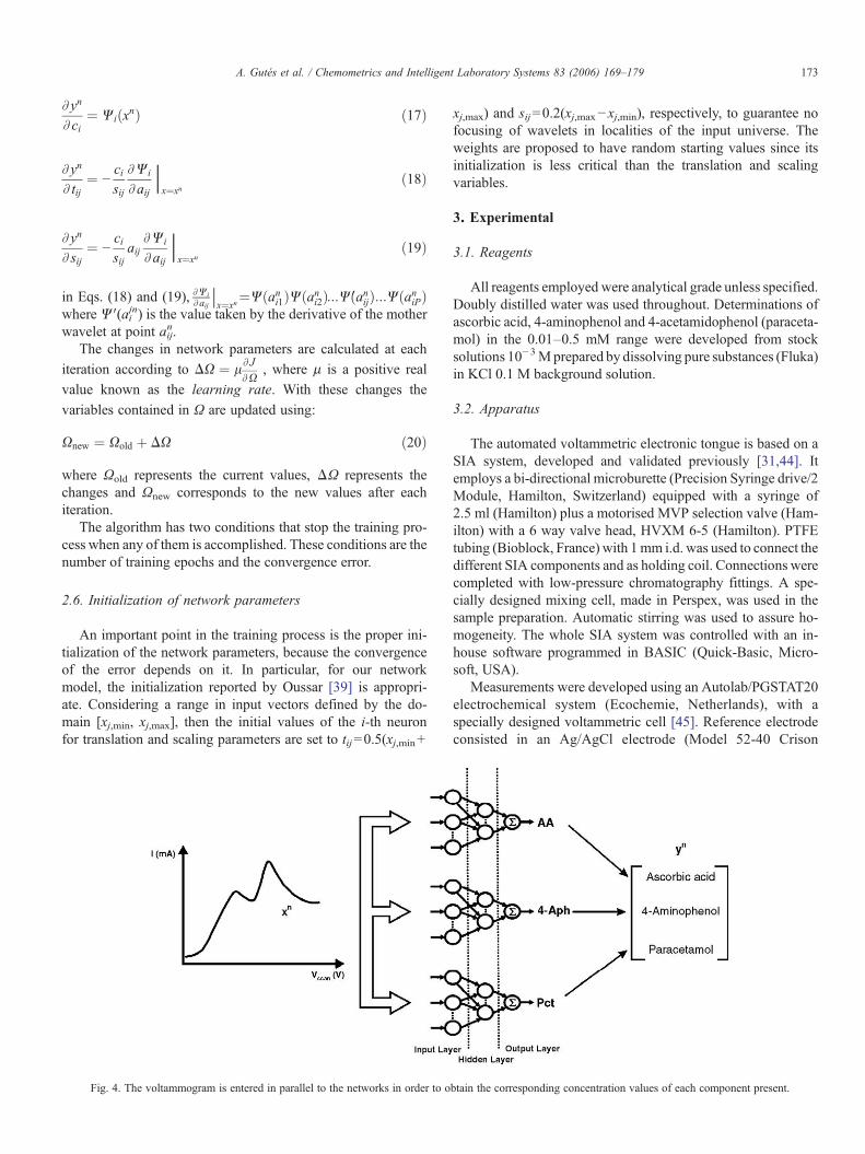
Fig. 4. The voltammogram is entered in parallel to the networks in order to o

xj,max) and sij=0.2(xj,max−xj,min), respectively, to guarantee nofocusing of wavelets in localities of the input universe. Theweights are proposed to have random starting values since itsinitialization is less critical than the translation and scalingvariables.

3. Experimental

3.1. Reagents

All reagents employed were analytical grade unless specified.Doubly distilled water was used throughout. Determinations ofascorbic acid, 4-aminophenol and 4-acetamidophenol (paraceta-mol) in the 0.01–0.5 mM range were developed from stocksolutions 10−3Mprepared by dissolving pure substances (Fluka)in KCl 0.1 M background solution.

3.2. Apparatus

The automated voltammetric electronic tongue is based on aSIA system, developed and validated previously [31,44]. Itemploys a bi-directional microburette (Precision Syringe drive/2Module, Hamilton, Switzerland) equipped with a syringe of2.5 ml (Hamilton) plus a motorised MVP selection valve (Ham-ilton) with a 6 way valve head, HVXM 6-5 (Hamilton). PTFEtubing (Bioblock, France) with 1mm i.d. was used to connect thedifferent SIA components and as holding coil. Connections werecompleted with low-pressure chromatography fittings. A spe-cially designed mixing cell, made in Perspex, was used in thesample preparation. Automatic stirring was used to assure ho-mogeneity. The whole SIA system was controlled with an in-house software programmed in BASIC (Quick-Basic, Micro-soft, USA).

Measurements were developed using an Autolab/PGSTAT20electrochemical system (Ecochemie, Netherlands), with aspecially designed voltammetric cell [45]. Reference electrodeconsisted in an Ag/AgCl electrode (Model 52-40 Crison

btain the corresponding concentration values of each component present.


Instruments, Spain). Stainless steel used as a constitutional partof themeasuring cell was used as counter electrode. Theworkingelectrode consisted in a home-made epoxy–graphite transducer,of general use in our laboratories [46]. Voltammograms wereobtained with the linear sweep voltammetric technique, withscan potentials from 0 to 1.0 V at 0.1 V/s in steps of 10 mV.

0

0.05

0.1

0.15

0.2

0.25

0.3

0.35

0.4

0.45

Expected [Ascorbic acid] (mM)

Obt

aine

d [A

scor

bic

acid

] (m

M)

R = 0.983

0 0.1 0.2 0.3 0.4 0.5 0.6 0.70

0.1

0.2

0.3

0.4

0.5

0.6

0.7

Expected [4-Aminophenol] (mM)

Obt

aine

d [4

-Am

inop

heno

l] (m

M)

R = 0.985

0 0.05 0.1 0.15 0.2 0.25 0.3 0.35 0.4-0.05

0

0.05

0.1

0.15

0.2

0.25

0.3

0.35

0.4

Expected [Paracetamol] (mM)

Obt

aine

d [P

arac

etam

ol] (

mM

)

R = 0.985

0 0.1 0.2 0.3 0.4 0.5

Fig. 5. Comparison between the expected results and those obtained with theWNNwiline corresponds to ideality (y=x) and the solid line is the regression of the compar

3.3. Data generation

Three oxidizable components are analyzed by the proposedvoltammetric e-tongue: Ascorbic Acid (AA), 4-Aminophenol(4-Aph) and Paracetamol (Pct). The sensitivity of the method isgenerally high; nevertheless, the selected case presents a

-0.1

0

0.1

0.2

0.3

0.4

0.5

0.6

Obt

aine

d [A

scor

bic

acid

] (m

M)

R = 0.947

0.05

0.1

0.15

0.2

0.25

0.3

0.35

0.4

0.45

0.5

0.55

Obt

aine

d [4

-Am

inop

heno

l] (m

M)

R = 0.956

00

0.05

0.1

0.15

0.2

0.25

0.3

0.35

0.4

0.45

Obt

aine

d [P

arac

etam

ol] (

mM

)

R = 0.979

0.1 0.2 0.3 0.4 0.5


0 0.1 0.2 0.3 0.4 0.5



0 0.05 0.1 0.15 0.2 0.25 0.3 0.35 0.4

th 3 neurons. The graphs correspond to the three species under study. The dashedison data. Plots at left correspond to training and plots at right to testing.

0

0.05

0.1

0.15

0.2

0.25

0.3

0.35

0.4

0.45


Obt

aine

d [A

scor

bic

acid

] (m

M)

R = 0.983

-0.1

0

0.1

0.2

0.3

0.4

0.5

0.6

Obt

aine

d [A

scor

bic

acid

] (m

M)

R = 0.947

0 0.1 0.2 0.3 0.4 0.5 0.6 0.70

0.1

0.2

0.3

0.4

0.5

0.6

0.7


Obt

aine

d [4

-Am

inop

heno

l] (m

M)

R = 0.985

0.05

0.1

0.15

0.2

0.25

0.3

0.35

0.4

0.45

0.5

0.55

Obt

aine

d [4

-Am

inop

heno

l] (m

M)

R = 0.954

0 0.05 0.1 0.15 0.2 0.25 0.3 0.35 0.40

0.05

0.1

0.15

0.2

0.25

0.3

0.35

0.4


Obt

aine

d [P

arac

etam

ol] (

mM

)

R = 0.985

00

0.05

0.1

0.15

0.2

0.25

0.3

0.35

0.4

0.45

Obt

aine

d [P

arac

etam

ol] (

mM

)

R = 0.979

0.1 0.2 0.3 0.4 0.5


0 0.1 0.2 0.3 0.4 0.5


0 0.1 0.2 0.3 0.4 0.5


0 0.05 0.1 0.15 0.2 0.25 0.3 0.35 0.4

Fig. 6. Comparison between the expected results and those obtained with the WNNwith 5 neurons. The graphs correspond to the three species under study. The dashedline corresponds to ideality (y=x) and the solid line is the regression of the comparison data. Plots at left correspond to training and plots at right to testing.


voltammetric signal with a high degree of overlapped response,making difficult the determination of each component.

The SIA system was used to prepare individual standards bymixing, diluting and homogenizing prefixed volumes of thestock solutions. Next, the prepared standard was pumped intothe mixing cell and the scanning measurement performed. The

prepared standards ranged their concentrations in the intervals(mM) [0.012,0.373] for AA, [0.017,0.529] for 4-Aph and[0.010,0.424] for Pct. Fig. 2 plots the distribution of standards ina three-dimensional space, where each point in the plot repre-sents a triad of concentrations under study. A set of 60 standardswas prepared, and for each one a voltammogram of 101 intensity

Table 1Linear regression parameters corresponding to the comparison lines of obtained versus expected concentration values using the WNNs

3 neurons 5 neurons

m b m b

AA train 0.951±0.056 0.010±0.013 0.952±0.056 0.010±0.013test 1.076±0.200 0.008±0.042 1.067±0.200 0.012±0.042

4-Aph train 0.956±0.053 0.012±0.016 0.956±0.053 0.012±0.016test 1.002±0.170 0.011±0.047 1.005±0.048 0.006±0.174

Pct train 0.964±0.053 0.008±0.013 0.963±0.053 0.078±0.013test 0.906±0.105 0.019±0.024 0.913±0.105 0.020±0.024

Train and test correspond to the training and testing processes, respectively. Confidence intervals calculated at the 95% confidence level.


values was obtained. The set of voltammograms is plotted inFig. 3, each voltammogram corresponds to one point in thethree-dimensional space of concentrations (Fig. 2). Measuredintensities were in the interval [−1.4, 52.4] mA.

3.4. Programming

As the voltammetric matrix contains information related tothe concentrations of the oxidizable components under study, itconstitutes the input data for training and testing the WNN,whereas the concentrations of AA, 4-Aph and Pct constitute thetargets to be modeled. The WNN will map a voltammogramrepresented by xn to a point of the three-dimensional space ofconcentrations identified by yn. To accomplish this, three WNNwith 3 or 5 neurons in its hidden layer were programmed andtrained for modeling each compound (Fig. 4). Structures ofgreater dimension were not tested because the training processbecame very slow due to the network and input data sizes andbecause the results obtained with the mentioned dimensionalitywere satisfactory.

3.5. Information preprocessing

Being 60 the number of generated standards, the input data isa voltammetric matrix of dimension [101, 60], and the target isthe concentration matrix of dimension [3, 60] (AA, 4-Aph andPct). For training convenience, the input data and targets werenormalized to an interval of [−1, 1] and randomly split into twogroups, 70% of the total information was taken for training andthe rest for testing.

3.6. Discrete Wavelet Transform (DWT) coupled with ANN

In order to evaluate the WNN, results were compared toANNs trained with approximation coefficients obtained by pre-

Table 2Recovery percentages obtained for the three trainings of the WNN with 3 hidden ne

Oxidizablecompound

Training

Case 1 Case 2 Case 3 Mean RSD (

AA 101.94 101.94 102.72 102.20 0.444-Aph 103.67 103.43 104.03 103.71 0.29Pct 96.82 97.32 97.70 97.28 0.45

Along with the recovery percentages are the mean and Relative Standard Deviation

vious discrete wavelet transformation of the signal. The behaviorof DWT—ANN combination has already been tested by theauthors and the details are given in Ref. [17].

3.7. Software

The functions listed in the algorithm that describes the WNNstructure and the gradients for each variable were written inMatlab 7 (Math Works, Natick, MA) using an Intel Pentium IIIprocessor desktop computer at 1.1 GHz with 512 Mbytes ofRAM.

4. Results and discussion

4.1. Training

The networks were programmed to reach an error of 0.01,evaluated by 2

NJðXÞ, where J(Ω) is the MSE defined in Eq. (11);

we denote this error as the Mean Squared Training Error. Theinitialization of weights, translation and scaling parameters wereaccording to the description given above in the trainingalgorithm. The learning rate and the maximum number of train-ing epochs were set to 0.001 and 20,000, respectively. In allcases, the training error was reached in a number of iterationsless than this maximum. Greater values of learning rate causedthe network output to oscillate and not to converge; on the otherhand, smaller values yielded a slow convergence.

4.2. Testing

Figs. 5 and 6 show the comparative graphs between theexpected and predicted concentrations for the three oxidizablecompounds when using networks with 3 and 5 neurons. Table 1summarizes this information for both variants. The slope (m) andintercept (b) that defines the comparison line y=mx+b that best

urons

Testing

%) Case 1 Case 2 Case 3 Mean RSD (%)

103.82 103.82 103.56 103.73 0.14106.33 104.74 105.93 105.67 0.78105.83 103.59 102.88 104.10 1.48

(RSD%) for the three cases.

Table 3Recovery percentages obtained for the three trainings of the WNN with 5 hidden neurons

Oxidizablecompound

Training Testing

Case 1 Case 2 Case 3 Mean RSD (%) Case 1 Case 2 Case 3 Mean RSD (%)

AA 102.09 102.43 102.50 102.34 0.21 109.56 103.38 104.83 105.92 3.054-Aph 103.42 103.43 103.74 103.53 0.18 102.91 104.74 103.55 103.73 0.90Pct 101.52 97.32 97.67 98.84 2.36 103.12 103.59 103.79 103.50 0.33

Along with the recovery percentages are the mean and Relative Standard Deviation (RSD%) for the three cases.


fits the data altogether with the uncertainty interval for a 95% ofconfidence interval are shown for each one of the networks. Theideal case implies lines with m=1 and b=0, which is fulfilled inall cases at the 95% confidence level, except a slight bias in the5-neurons training case for Pct.

Two more trainings for each WNN structure were made withrandom initialization of weights to check if the final model isconsistent. To compare the accuracy of the predicted informa-tion, a Recovery Percentage (RP) was calculated for each trainedWNN. The RP is defined by Eq. (21).

RP ¼

XNi¼1

100d 1þ yi−yexpiyexpi

� �N

ð21Þ

where yi is the i-th obtained value, yexpi is the i-th expected valueand N is the number of targets. The results are contained inTables 2 and 3 along with the mean and variance for each studiedsubstance.

From Tables 2 and 3, it is evident that for the WNN with 3neurons, the majority of the recovered information is within±5% of the ideal recovery percentage. Nevertheless, althoughsome recovered information exceeds the expected values, thedistribution of these values around an average fall into theexpected recovery interval. This situation is different for the caseof the WNN with 5 neurons, where the dispersion of the data isout of the 95% interval. From these results we can conclude thatan increase in the number of neurons in the hidden layer does notimprove the performance of the network. This can be explainedif we consider that for each neuron added to the network a total of101 monodimensional wavelets are added too, increasing thepossibility of having redundant wavelets in the model. Thisredundancy affects negatively the performance of the networkand hence the recovery percentage.

Finally, for a further validation of the presented results, 10replicate training processes were performed on the selected3-neuron architecture, with a 17-fold cross validation, selectingthe test set each time at random from the total set of experiments.The different results were recorded, and the comparison lines

Table 4Linear regression parameters obtained with the training and testing data sets using t

Threeoutputsnetwork

Training

m b R

AA 0.994±0.008 2.07e−4±0.016 0.94-Aph 0.995±0.007 −2.75e−4±0.011 0.9Pct 0.994±0.012 −5.38e−5±0.021 0.9

constructed for each case. Stating y and x for the obtained andexpected values, for the training case, the average compari-son lines were y=(0.9513±0.0015)·x+(0.0098±0.0002), y=(0.9548 ± 0.0001)·x+ (0.0119 ± 0.0001) and y= (0.9643 ±0.0004)·x+(0.0075±0.0001) for AA, 4-Aph and Pct, respec-tively. For the testing case, the comparison lines were y=(1.0789±0.0398)·x+(0.0068±0.0052), y=(0.9803±0.0192)·x+ (0.0133±0.0037) and y=(0.9052±0.0027)·x+ (0.0207±0.0011) in the same order as before. Uncertainties indicatedfor each parameter correspond to the 95% confidence interval ofthe 10-replicate distribution. Analogously, average correlationcoefficients (corresponding to the 10 replicate training cases)were 0.983, 0.985 and 0.985 for AA, 4-Aph and Pct. For the testcomparison lines, average correlation coefficients were 0.937,0.947 and 0.971, in the same order as above. From these values,it is deducted that the case presented before in graphic details isan average situation from the infinite training possibilities.

4.3. DWT coupled with ANN

Several mother wavelets (daubechies, coiflets, symlets andbiorthogonal) and four successive decomposition levels weretested. At each level, only the approximation coefficients wereretained and used to reconstruct the voltammograms. In order tochoose the combination of mother wavelet, order and decom-position level that yielded a good recovery with the less possiblenumber of approximation coefficients, the original and recov-ered voltammograms were compared by correlation analysis.The combination that fulfilled our purpose was obtained with theDaubechies wavelet of eighth order and decomposition levelnumber three. The number of approximation coefficients finallyused was 16, getting a compression of 84% and a correlationfactor of 0.987 between the original and reconstructed signals.

The matrices of the approximation coefficients and concen-tration values were used as inputs and targets for training andtesting an ANN with three outputs, and a set of 3 parallel singleoutput ANNs. Network's topologywas feedforward trained withBayesian regularization algorithm. The ANN with three outputshad two hidden layers with 10 and 5 neurons, respectively; each

he ANN with three outputs trained with the wavelet coefficients

Testing

m b R

99 0.817±0.274 0.0294±0.154 0.78599 0.843±0.246 −0.0587±0.135 0.84398 0.886±0.29 0.00259±0 0.929

Table 5Linear regression parameters obtained with the training and testing data sets using three ANNs with one output trained with the wavelet coefficients

Parallelnetworks

Training Testing

m b R m b R

AA 0.992±0.01 −6.20e−4±0.019 0.998 0.644±0.147 −0.033±0.262 0.7724-Aph 0.937±0.038 −6.7e−3±0.064 0.978 0.732±0.113 −0.030±0.206 0.869Pct 0.997±0.005 6.20e−4±0.009 0.999 0.954±0.109 0.012±0.173 0.938


parallel network had two hidden layers with 6 and 24 neurons,and a single neuron in output layer. Both structures had non-linear functions in the hidden layers and linear function in theoutput layer.

The set of input and output matrices were normalized to[−1,1] and split into training and testing subsets (two third partswere taken for training). The error goal for training was set to0.01, to be reached in 300 epochs of training or less and wastracked by using the sum of squared errors (SSE).

Trained networks were evaluated with training and testinginput data, and a linear regression analysis between the outputsof the networks and the expected values for each component wasdone. The correlation factors obtained, along with the para-meters of the straight line that best fits the corresponding set ofdata are contained in Tables 4 and 5.

4.4. Comparison between WNN and DWT—ANN

In this work, wavelet analysis and neural network have beencombined in two manners, DWT—ANN and WNN. In the firstone, the wavelet theory is decoupled from the neural networks.The voltammograms are decomposed with the help of wavelettransform and the approximation coefficients obtained are, in asecond stage, furnished to a neural network for modeling pur-poses. In the second one, wavelet theory and neural networks arecombined into a single method. In this methodology, the trans-lation and the scaling parameters, along with the weights ofneuron's connections are adjusted during training. As it isobserved by the results, the outputs of the DWT—ANN com-bination produces a correlation factor greater than 0.9 when thetraining data is applied to the input, however, this correlationdiminishes when the testing data is used, particularly in therecovery of ascorbic acid (AA) where Rb0.8.

The performance of the proposed WNN architecture wasbetter than that of the DWT—ANN combination. In WNN, Rwas greater than 0.94 for training and testing when determiningthe three chemical species. To explain the good performance ofthe WNN the following factors can be considered:

– Whereas in the DWT—ANN method each voltammogram isrepresented by 16 approximation coefficients that retain thespectral information contained at low frequencies, in theWNN the complete data set is fed into the network. In thiscase a quasi-continuous transformation takes place due to theway in which the wavelets parameters are adjusted; on theother hand, when DWT is applied, the approximation coef-ficients are obtained by digital filtering and subsampling,which is interpreted as a more discrete process.

– In the WNN there is one weight wi for each i-th data pointcontained in the set of voltammograms xi

n. After the networkwas trained, the set {wi} establishes which points in a vol-tammogram contribute more to the quantification of thechemical species.

A network with high modeling performance, as it is neededto solve complex learning related problems is correctly builtwith the proposed WNN architecture. This network is expectedto be especially valuable when the input data is irregularlyspaced and/or overlapped, being the latter the usual case withmulticomponent voltammetric signals.

The proper choice of the number of hidden neurons and theuse of continuous multidimensional frames for decomposingthe input data, allow the network to map the voltammogramswith their respective concentration values by simply adjustingthe scale and translation parameters.

5. Conclusions

An innovative neural network which intrinsically uses wave-let functions has been developed. The design merges the arti-ficial neural networks and wavelet theory to give rise to anew class of network known as the Wavelet Neural Network(WNN). We have described here an application aimed to quan-titatively determine the concentration of chemical species basedon information obtained from voltammetric sensors. The WNNresults in a proper multivariate modeling tool for voltam-metry that performs better than the sequential WT—ANNcombination.

As the wavelet transform has proven its ability for capturingessential features in the time-frequency behavior of a signal, itseems reasonable to represent a non-stationary signal by thesefunctions. The strategy for training the WNN lets us define theappropriate parameters for a family of wavelet functions thatbest fits the voltammetric signals solved in this work. Multi-resolution analysis offers to the WNN a unique characteristic inprediction tasks doing an appropriate selection of a motherwavelet and the number of hidden units, with which the over-fitting problem can be effectively avoided. The accuracy andstability of the WNN can be further improved by the imple-mentation of other wavelet functions and increasing the numberof network outputs.

Acknowledgments

Financial support for this work was provided by the MCyT(Madrid, Spain) through the project CTQ2004-08134, by


CONACYT (Mexico) through the project 43553 and by theDepartment of Universities and the Information Society(DURSI) from the Generalitat de Catalunya.

References

[1] Y. Vlasov, A. Legin, Fresenius J. Anal. Chem. 361 (1998) 255–260.[2] Y. Vlasov, L. Andrey, A. Rudnistkaya, Sens. Actuators, B 44 (1997)

532–537.[3] F. Winquist, P. Wide, I. Lundström, Anal. Chim. Acta 357 (1997) 21–31.[4] A. Legin, A. Rudnitskaya, Y.G. Vlasov, C. Di Natale, E. Mazzane, A.

D'Amico, Sens. Actuators, B 44 (1997) 291–296.[5] F. Winquist, C. Krantz-Rülcker, P. Wide, I. Lundström, Meas. Sci.

Technol. 9 (1998) 1937–1946.[6] A. Legin, A. Smirnova, A. Rudnitskaya, L. Lvova, E. Suglobova, Y.

Vlasov, Anal. Chim. Acta 385 (1999) 131–135.[7] C. Di Natale, R. Paolesse, A. Macagnano, A. Mantini, A. D'Amico, A.

Legin, L. Lvova, A. Rudnitskaya, Y. Vlasov, Sens. Actuators, B 64 (2000)15–21.

[8] J. Gallardo, S. Alegret, R. Muñoz, M. De-Roman, L. Leija, P.R.Hernández, M. del Valle, Anal. Bioanal. Chem. 377 (2003) 248–256.

[9] J. Gallardo, S. Alegret, M.A. de Roman, R. Muñoz, P.R. Hernández, L.Leija, M. del Valle, Anal. Lett. 36 (2003) 2893–2908.

[10] F. Despagne, D.L. Massart, Analyst 123 (1998) 157R–178R.[11] C. Bessant, S. Saini, Anal. Chem. 71 (1999) 2806–2813.[12] A. Gutés, F. Céspedes, S. Alegret, M. del Valle, Biosens. Bioelectron. 20

(2005) 1668–1673.[13] E. Richards, C. Bessant, S. Saini, Chemometr. Intell. Lab. Syst. 61 (2002)

35–49.[14] A.K.-M. Leung, F. Chau, J. Gao, Chemometr. Intell. Lab. Syst. 43 (1998)

165–184.[15] S. Xue-Guang, A. Kai-Man, C. Foo-Tim, Acc. Chem. Res. 36 (2003)

276–283.[16] M. Cocchi, J.L. Hidalgo-Hidalgo-de-Cisneros, I. Naranjo-Rodriguez, J.M.

Palacios-Santander, R. Seeber, A. Ulrici, Talanta 59 (2003) 735–749.[17] L. Moreno-Barón, R. Cartas, A. Merkoçi, S. Alegret, M. del Valle, L. Leija,

P.R. Hernández, R. Muñoz, Sens. Actuators, B 113 (2006) 487–499.[18] J.M. Palacios-Santander, A. Jiménez-Jiménez, L.M. Cubillana-Aguilera, I.

Naranjo-Rodríguez, J.L. Hidalgo-Hidalgo-de-Cisneros, Microchim. Acta142 (2003) 27–36.

[19] D.J. Rimbaud, B. Walczak, R.J. Poppi, O.E. De Noord, D.L. Massart,Anal. Chem. 69 (1997) 4317–4323.

[20] L. Eriksson, J. Trygg, E. Johansson, R. Bro, S. Wold, Anal. Chim. Acta420 (2000) 181–195.

[21] B.K. Alsberg, A.M. Woodward, M.K. Winson, J.J. Rowland, D.B. Kell,Anal. Chim. Acta 368 (1998) 29–44.

[22] Q. Zhang, A. Benveniste, IEEE Trans. Neural Netw. 3 (1992) 889–898.[23] B.R. Bhakshi, G. Stephanopoulos, AIChE J. 39 (1993) 57–81.[24] L. Cao, Y. Hong, H. Fang, G. He, Physica, D 85 (1995) 225–238.[25] H. Szu, B. Telfer, J. Garcia, Neuronal Netw. 9 (1996) 695–708.[26] Q.-X. Guo, L. Liu, W.-S. Cai, Y. Jiang, Y.-C. Liu, Chem. Phys. Lett. 290

(1998) 514–518.[27] X. Zhang, J. Qi, R. Zhang, M. Liu, Z. Hu, H. Xue, B. Fan, Comput. Chem.

25 (2001) 125–133.[28] Z. Kardanpour, B. Hemmateenejad, T. Khayamian, Anal. Chim. Acta 531

(2005) 285–291.[29] J. Zhao, B. Chen, J. Shen, Comput. Chem. Eng. 23 (1998) 83–92.[30] H. Zhong, J. Zhang, M. Gao, J. Zheng, G. Li, L. Chen, Chemometr. Intell.

Lab. Syst. 59 (2001) 67–74.[31] A. Gutés, F. Céspedes, S. Alegret, M. del Valle, Talanta 66 (2005)

1187–1196.[32] O. Rioul, M. Vetterli, IEEE Signal Process. 8 (1991) 14–38.[33] G. Kaiser, A Friendly Guide to Wavelets. Ed. Birkhäuser, Boston MA,

1994, p. 300.[34] Y.T. Chan, Wavelet Basics, Kluwer Publishers, Boston MA, 1995, p. 134.[35] M. Akay (Ed.), Time Frecuency and wavelets in Biomedical Signal

Processing. IEEE Press Series on Biomedical Engineering, Wiley—IEEEPress, Piscataway NJ, 1997, p. 739.

[36] Y. Meyer, Wavelets: Algorithms and Applications, Society for Industrialand Applied Mathematics, SIAM, Philadelphia, PA, 1993, p. 133.

[37] Q. Zhang, IEEE Trans. Neural Netw. 8 (1997) 227–236.[38] C.E. Heil, D.F. Walnut, SIAM Rev. 31 (1989) 628–666.[39] Y. Oussar, I. Rivals, L. Personnaz, G. Dreyfus, Neurocomputing 20 (1998)

173–188.[40] M. Cannon, J.E. Slotine, Neurocomputing 9 (1995) 293–342.[41] S.G. Mallat, IEEE Trans. Pattern Anal. Mach. Intell. 11 (1989) 674–693.[42] J. Zhang, G.G. Walter, Y. Miao, W.N.W. Lee, IEEE Trans. Signal Process.

43 (1995) 1485–1497.[43] D.E. Rumelhart, G.E. Hilton, R.J. Williams, Learning internal represen-

tation by error propagation, Parallel Distributed Processing: Explorationsin the Microstructures of Cognition, vol. 1, MIT Press, Cambridge MA,1986, Chapter 8.

[44] A. Gutés, F. Céspedes, S. Alegret, M. del Valle, Anal. Bioanal. Chem. 382(2005) 471–476.

[45] X. Llopis, A. Merkoçi, M. del Valle, S. Alegret, Sens. Actuators, B 107(2005) 742–748.

[46] F. Céspedes, S. Alegret, Trends Anal. Chem. 19 (2000) 276–285.

Multivariate calibration model from overlapping voltammetric signals employing wavelet neural...

Documents

Transcript of Multivariate calibration model from overlapping voltammetric signals employing wavelet neural...