Multisensitive polyurethane/polyurea nanocapsules for smart ...

Multisensitive polyurethane/polyurea nanocapsules for smart drug delivery

Cristina Cuscó Marigó

ADVERTIMENT. La consulta d’aquesta tesi queda condicionada a l’acceptació de les següents condicions d'ús: La difusió d’aquesta tesi per mitjà del servei TDX (www.tdx.cat) i a través del Dipòsit Digital de la UB (diposit.ub.edu) ha estat autoritzada pels titulars dels drets de propietat intel·lectual únicament per a usos privats emmarcats en activitats d’investigació i docència. No s’autoritza la seva reproducció amb finalitats de lucre ni la seva difusió i posada a disposició des d’un lloc aliè al servei TDX ni al Dipòsit Digital de la UB. No s’autoritza la presentació del seu contingut en una finestra o marc aliè a TDX o al Dipòsit Digital de la UB (framing). Aquesta reserva de drets afecta tant al resum de presentació de la tesi com als seus continguts. En la utilització o cita de parts de la tesi és obligat indicar el nom de la persona autora. ADVERTENCIA. La consulta de esta tesis queda condicionada a la aceptación de las siguientes condiciones de uso: La difusión de esta tesis por medio del servicio TDR (www.tdx.cat) y a través del Repositorio Digital de la UB (diposit.ub.edu) ha sido autorizada por los titulares de los derechos de propiedad intelectual únicamente para usos privados enmarcados en actividades de investigación y docencia. No se autoriza su reproducción con finalidades de lucro ni su difusión y puesta a disposición desde un sitio ajeno al servicio TDR o al Repositorio Digital de la UB. No se autoriza la presentación de su contenido en una ventana o marco ajeno a TDR o al Repositorio Digital de la UB (framing). Esta reserva de derechos afecta tanto al resumen de presentación de la tesis como a sus contenidos. En la utilización o cita de partes de la tesis es obligado indicar el nombre de la persona autora. WARNING. On having consulted this thesis you’re accepting the following use conditions: Spreading this thesis by the TDX (www.tdx.cat) service and by the UB Digital Repository (diposit.ub.edu) has been authorized by the titular of the intellectual property rights only for private uses placed in investigation and teaching activities. Reproduction with lucrative aims is not authorized nor its spreading and availability from a site foreign to the TDX service or to the UB Digital Repository. Introducing its content in a window or frame foreign to the TDX service or to the UB Digital Repository is not authorized (framing). Those rights affect to the presentation summary of the thesis as well as to its contents. In the using or citation of parts of the thesis it’s obliged to indicate the name of the author.



Barcelona, February 2018

Programa de Doctorat en Química Orgànica


Doctoral Thesis submitted by:


Supervised by:

Dr. Ernesto Nicolás Galindo Departament de Química

Inorgànica i Orgànica Secció de Química Orgànica

Universitat de Barcelona

Dr. José Rocas Sorolla Ecopol Tech, S. L.

Barcelona, February 2018

Agraïments

Primer de tot m’agradaria agrair-li al Josep l’oportunitat que em va brindar per

fer una tesi industrial a Ecopol Tech sobre un tema tant apassionant com són els

sistemes d’alliberació controlats aplicats a càncer. Ha estat una etapa intensa en la

qual he viscut un procés maduratiu brutal, com a persona i com a professional.

M’agradaria agrair especialment l’oportunitat que vaig tenir per conèixer

l’ecosistema científic i d’empreses de Boston, així com també tota la llibertat que

sempre m’has donat per innovar a l’investigar, per tots els reptes que m’has

plantejat i totes les hores que hem passat al teu despatx discutint sobre resultats. He

après molt de tu i del teu entusiasme.

En segon lloc, m’agradaria agrair-li a l’Ernesto haver-me tutoritzat la tesi i

haver-me acompanyat en aquest camí, així com també al Jordi, qui va guiar-me en

les primeres etapes de la tesi.

Voldria continuar agraint a la meva mare i al meu pare el suport incondicional

amb que sempre he comptat i per haver-me ensenyat a guanyar-me les coses; també

a la Laura i al Patit per haver estat a costat meu sempre, tant en les èpoques més

complicades com en aquelles en què tot anava sobre rodes. Gràcies a vosaltres sóc

qui sóc avui. I també m’agradaria seguir dedicant aquests agraïments a tots aquells

que formen part de la família que es tria, és a dir, als amics. No els puc escriure tots,

però voldria destacar la meva Marina, els Ramallets, les Divas, els amics d’Ecopol,

companys de la uni i les titis, la meva parella preferida (la Lídia i el Roc) i els meus

satèl·lits que formen part de mi, la Rosinha i la Beltzane. Vull fer una especial menció

a l’Arnald, que com ja sap, ha esdevingut un pilar fonamental a la meva vida i no m’ha

deixat sola ni un segon des d’aquell juliol del 2012. No podré mai tornar-te tot el que

has fet per mi, ets un sol. I al Joan també li vull agrair que hagi cregut en mi sempre,

des del primer dia que ens vam conèixer. I que hagi estat a costat meu en tots els

moments, per ajudar-me a aixecar i per celebrar les victòries. Ja saps que aquesta

tesi va, en part, dedicada a tu.

Per últim, vull acabar aquests agraïments dedicant-li unes paraules a la Mar, la

meva celestina, qui va portar-me aquell 9 de juliol a una de les persones més

importants de la meva vida. Carles, ja saps què penso de tu. Sobren les paraules.

A la meva família i amics, és un plaer créixer amb vosaltres

El més important en ciència no és obtenir nous resultats, sinó descobrir noves formes de pensar en ells

William Lawrence Bragg

Abbreviations and acronyms

AABA -Aminobutyric acid

AFM Atomic force microscopy

AQC 6-Aminoquinolyl-N-hydroxysuccinimidyl carbamate

BAPMA N,N-bis(3-aminopropyl)-N-methylamine

BC Breast cancer

BSA Bovine serum albumin

CSC Cancer stem cell

CU Curcumin

DDS Drug delivery system

DEDS 2,2'-Dihydroxyethyl disulfide

DETA Diethylenetriamine

DiI 1,1'-Dioctadecyl-3,3,3',3'-tetramethylindocarbocyanine

perchlorate

DiO 3,3'-Dioctadecyloxacarbocyanine perchlorate

DiR 1,1-Dioctadecyl-3,3,3,3-tetramethylindotricarbocyanine

iodide

DL Drug loading

DLS Dynamic light scattering

DMEM Dulbecco’s modified eagle medium

DMPA 2,2-Dihydroxymethylpropanoic acid

DMSO Dimethyl sulfoxide

DOX Doxorubicin

DPPC Dipalmitoylphosphaditylcholine

DSPC Distearoylphosphatidylcholine

ECM Extracellular matrix

EDC N-(3-dimethylaminopropyl)-N′-ethylcarbodiimide

EE Encapsulation efficiency

EMA European medicines agency

EPR Enhanced permeation and retention

ER Estrogen receptor

FBS Fetal bovine serum

FDA Food and drug administration

FLI Fluorescence imaging

FRET Förster resonance energy transfer

Genamin TAP 100D 1,3-Diamino-N-octadecylpropane

GSH Glutathione

GTCC Capric/caprylic trigliceride

HEPES 4-(2-Hydroxyethyl)-1-piperazineethanesulfonic acid

HER2 Human epidermal growth factor receptor type 2

HLB Hydrophilic lipophilic balance

HPLC High performance liquid cromatography

HPLC-MS High performance liquid cromatography-mass spectrometry

HSA Human serum albumin

IPDI Isophorone diisocyanate

IR Infrared spectroscopy

IS Internal standard

Jeffamine ED2003 Water-soluble aliphatic diamine derived from a propylene

oxide capped polyethylene glycol

Jeffcat DPA N-(3-Dimethylaminopropyl)-N,N-diisopropanolamine

KDa Kilodalton

LC Lung cancer

MAb Monoclonal antibody

MaI Maleimide

MALDI-TOF Matrix-assisted laser desorption/ionization time of flight

MDI Methylene diphenyl diisocyanate

MFI Mean fluorescence intensity

Mowiol 4-88 Poly(vinyl)alcohol with a 4 mPa·s viscosity (4% wt aqueous

solution at 20 °C) and 88% degree of hydrolysis.

MTT 3-(4,5-Dimethylthiazol-2-yl)-2,5-diphenyltetrazolium

bromide

MWCO Molecular weight cutoff

NALA Sodium laurate

NAST Sodium stearate

NB Neuroblastoma

NC Nanocapsule

NEAA Non-essential aminoacids

NHS N-hydroxysuccinimide

NLE Norleucine

NMR Nuclear magnetic resonance

NP Nanoparticle

NSCLC Non-small cell lung cancer

O/W Oil in water

PBS Phosphate buffered saline

PCL Poly(caprolactone)

PECA Poly(ethyl cyanoacrylate)

PEG Poly(ethylene glycol)

PPG Poly(propylene glycol)

PFA Paraformaldehyde

PGA Poly(glycolic acid)

pHe Extracellular pH

pHi Intracellular pH

PLA Poly(lactic acid)

PLGA Poly(lactic-co-glycolic acid)

PMMA Poly(methyl methacrylate)

PNIPAAM Poly(N-isopropyl acrylamide)

PR Progesterone receptor

PS Polystyrene

PTX Paclitaxel

PVA Poly(vinyl alcohol)

PVP Poly(vinyl pyrrolidone)

RES Rethiculoendothelial system

RPMI Roswell park memorial institute

RP-HPLC Reverse-phase HPLC

rt Room temperature

SCLC Small cell lung cancer

T17 Tambjamine 17

T18 Tambjamine 18

TDI Toluene diisocyanate

TEA Triethylamine

TEM Transmission electron microscopy

TFA Trifluoroacetic acid

THF Tetrahydrofurane

TMXDI Tetramethyl-1,3-xylylene diisocyanate

TNBC Triple-negative breast cancer

UV/Vis Ultraviolate/Visible

VEGF Vascular endothelial growth factor

VEGFR Vascular endothelial growth factor receptor

Vm Membrane potential

W/O/W Water-in-oil-in-water

Wt Weight

YMER N-120 Non-ionic hydrophilic polymer with two primary hydroxyl

groups and a long capped ethoyxylated side chain

pot Zeta potential

Table of Contents CHAPTER 1

1. Drug delivery systems for biomedical applications ........................................ 1

2. Preparation of polymer nanoparticles ................................................................. 6

2.1. NPs obtained from dispersion of preformed polymers ....................................... 7

2.1.1. Emulsification/solvent evaporation ......................................................................... 7

2.1.2. Salting-out ........................................................................................................................... 8

2.1.3. Dialysis ...............................................................................................................................10

2.1.4. Supercritical fluid technology ...................................................................................10

2.2. NPs obtained from polymerization of monomers ................................................11

2.2.1. Emulsion polymerization ............................................................................................12

2.2.2. Interfacial polymerization ..........................................................................................13

2.2.3. Controlled/living radical polymerization .............................................................13

3. Most relevant polyurethane and polyurea DDS ............................................. 14

3.1. Polyurethane NPs .............................................................................................................14

3.2. Polyurethane nanomicelles ...........................................................................................15

3.3. Polyurethane hydrogel NPs ..........................................................................................15

3.4. Polyurethane-polysaccharide hybrid NPs ...............................................................16

4. Biological considerations ....................................................................................... 16

4.1. Tumor targeting ................................................................................................................17

4.1.1. Tumor microenvironment ..........................................................................................17

4.1.2. Passive targeting by the EPR effect .........................................................................19

4.1.3. Active targeting ...............................................................................................................19

4.2. Intracellular delivery .......................................................................................................20

4.2.1. Endocytosis ......................................................................................................................21

4.2.2. Intracellular trafficking, endosomal escape and degradation ......................22

4.3. Drug release ........................................................................................................................23

4.3.1. Exogenous .........................................................................................................................24

4.3.1.1. Thermoresponsive systems ...............................................................................24

4.3.1.2. Magnetically responsive systems ....................................................................25

4.3.1.3. Photoresponsive systems ...................................................................................26

4.3.1.4. Ultrasound and electric responsive systems ...............................................27

4.3.2. Endogenous ......................................................................................................................29

4.3.2.1. pH-responsive systems ........................................................................................29

4.3.2.2. Glutathione-responsive systems ......................................................................30

4.3.2.3. Enzymatically responsive systems ..................................................................31

5. Clinically approved NP therapies and diagnostics ........................................ 32

6. Bibliography ............................................................................................................... 35

General Objectives ..................................................................................................... 47

CHAPTER 2

1. Introduction ................................................................................................................ 51

1.1. Polyurethane and polyurea DDS .................................................................................51

1.2. Chemistry of polyurethanes and polyureas ............................................................51

1.2.1. Chemistry of isocyanates ............................................................................................51

1.2.2. Main reactions derived from isocyanates ............................................................54

1.2.3. Side-reactions derived from isocyanates .............................................................56

1.2.4. Polymer functionality ...................................................................................................58

1.3. Important considerations in DDS design .................................................................59

1.3.1. Biocompatibility .............................................................................................................60

1.3.2. Shell tunability ................................................................................................................60

1.3.3. Stratified nanostructured shell .................................................................................62

1.3.3.1. The hydrophobic effect and micelle formation ..........................................62

1.3.3.2. Self-ordered and compact structures .............................................................64

1.3.4. Interactions with the biological medium ..............................................................65

1.3.5. Encapsulation efficiency and stability ...................................................................66

1.3.5.1. Preformed amphiphilic shell .............................................................................66

1.3.5.2. Tailor-made polymer shell .................................................................................67

1.3.6. Particle size ......................................................................................................................68

1.3.7. Smart targeting ...............................................................................................................69

1.3.8. Biodegradability .............................................................................................................71

2. Objectives ..................................................................................................................... 72

3. Results and discussion ............................................................................................ 73

3.1. General experimental design........................................................................................73

3.2. Preparation of the polymers .........................................................................................75

3.2.1. Monomers considered .................................................................................................75

3.2.2. Polymers syntheses and characterization ............................................................80

3.3. Nanoencapsulation ...........................................................................................................89

3.3.1. Preparation of the NCs .................................................................................................89

3.3.2. Characterization of the NCs .......................................................................................95

3.3.2.1. Morphology and size .............................................................................................96

3.3.2.2. Surface properties .................................................................................................98

3.3.2.3. Encapsulation efficiency and drug loading ............................................... 103

3.3.2.4. NC degradation and release ............................................................................ 105

4. Conclusions .............................................................................................................. 113

5. Bibliography ............................................................................................................ 115

CHAPTER 3

1. Introduction ............................................................................................................. 127

1.1. Lung cancer ...................................................................................................................... 127

1.1.1. Epidemiology and risk factors ............................................................................... 127

1.1.2. Histology ......................................................................................................................... 128

1.1.2.1. Small cell lung cancer (SCLC) ......................................................................... 129

1.1.2.2. Non-small cell lung cancer (NSCLC) ............................................................ 129

1.1.3. Treatments .................................................................................................................... 129

1.1.3.1. Conventional treatments.................................................................................. 130

1.1.3.2. Experimental treatments: ionophores........................................................ 133

1.1.3.3. Tambjamines ........................................................................................................ 137

1.1.3.4. FDA-approved nanosystems applied to LC ............................................... 140

1.2. Neuroblastoma ............................................................................................................... 141

1.2.1. Origin ............................................................................................................................... 141

1.2.2. Epidemiology and prognostics .............................................................................. 142

1.2.3. Treatments .................................................................................................................... 143

1.2.3.1. Conventional therapies ..................................................................................... 143

1.2.3.2. Targeted treatments .......................................................................................... 144

2. Objectives .................................................................................................................. 145

3. Results and discussion ......................................................................................... 145

3.1. Application of Chapter 2 methodology .................................................................. 147

3.1.1. Preparation of the NCs .............................................................................................. 147

3.1.2. Characterization of the NCs .................................................................................... 149

3.2. Optimization .................................................................................................................... 155



3.3. In vitro studies in LC and NB cell lines ................................................................... 163

3.3.1. Cell viability ................................................................................................................... 163

3.3.1.1. LC cell lines ............................................................................................................ 163

3.3.1.2. NB cell lines ........................................................................................................... 167

3.3.2. Cell uptake ..................................................................................................................... 168

3.3.2.1. Physiological conditions ................................................................................... 169

3.3.2.2. Slightly acidic conditions ................................................................................. 170

3.3.3. Cell internalization ..................................................................................................... 172

3.4. In vivo biodistribution in a NB mouse model ...................................................... 175


3.4.2. Characterization .......................................................................................................... 180

3.4.2.1. Morphology and size .......................................................................................... 180

3.4.2.2. Surface properties .............................................................................................. 182

3.4.2.3. Antibody conjugation efficiency .................................................................... 183

3.5. In vivo and ex vivo data................................................................................................. 185

3.5.1. Incidences ...................................................................................................................... 186

3.5.2. Body weight change during treatment ............................................................... 187

3.5.3. In vivo whole-body biodistribution kinetics ..................................................... 188

3.5.4. Ex vivo tumor and whole-body tissue-accumulation kinetics ................... 189

3.5.5. Percentage of ex vivo tissue-accumulation per tissue weight .................... 201

4. Conclusions .............................................................................................................. 202

5. Bibliography ............................................................................................................ 204

CHAPTER 4

1. Introduction ............................................................................................................. 211

1.1. Breast cancer ................................................................................................................... 211

1.1.1. Epidemiology and risk factors ............................................................................... 211

1.1.2. Subtypes ......................................................................................................................... 212

1.1.3. Treatments .................................................................................................................... 214

1.1.3.1. Conventional treatments.................................................................................. 214

1.1.3.2. Targeted therapies ............................................................................................. 217

1.1.3.3. FDA-approved nanosystems applied to BC ............................................... 219

2. Objectives .................................................................................................................. 220

3. Results and discussion ......................................................................................... 221

3.1. Amphoteric NCs .............................................................................................................. 221



3.1.3. Cell viability ................................................................................................................... 226

3.2. Use of peptides to target BC cells ............................................................................. 227

3.3. Functionalization considerations ............................................................................ 228

3.4. Functionalization with A5 .......................................................................................... 231

3.4.1. Preparation of hydrophilic linkers and conjugates ....................................... 231

3.4.2. Preparation of A5-functionalized NCs ................................................................ 236




3.4.3.3. A5 conjugation efficiency ................................................................................. 243

3.4.4. Cell uptake ..................................................................................................................... 245

3.5. Functionalization with IPEP ...................................................................................... 247

3.5.1. Preparation of the hydrophilic linker and the conjugate ............................ 247

3.5.2. Preparation of IPEP-functionalized NCs ............................................................ 251




3.5.3.3. Peptide conjugation efficiency ....................................................................... 256

3.5.4. Cell uptake ..................................................................................................................... 256

4. Conclusions .............................................................................................................. 258

5. Bibliography ............................................................................................................ 259

CHAPTER 5

1. Materials ................................................................................................................... 265

1.1. Building blocks and crosslinkers ............................................................................. 265

1.2. Targeting molecules ...................................................................................................... 265

1.3. Encapsulated molecules .............................................................................................. 265

1.4. Solvents and auxiliary solutions .............................................................................. 266

1.5. Materials for biological studies ................................................................................ 266

1.5.1. In vitro studies .............................................................................................................. 266

1.5.2. In vivo studies ............................................................................................................... 266

2. Analytical techniques ........................................................................................... 267

2.1. Infrared spectroscopy (IR) ......................................................................................... 267

2.2. pH measurements .......................................................................................................... 267

2.3. Automatic isocyanate titration ................................................................................. 268

2.4. Nuclear magnetic resonance (NMR)....................................................................... 268

2.5. High Pressure Liquid Cromatography (HPLC) ................................................... 268

2.6. Amino acid analysis....................................................................................................... 269

2.7. Dynamic light scattering (DLS) ................................................................................. 271

2.8. Zeta potential ( -pot) .................................................................................................. 271

2.9. Transmission electron microscopy (TEM)........................................................... 271

2.10. Atomic force microscopy (AFM) .............................................................................. 271

2.11. Ultraviolet/visible spectroscopy (UV/Vis) .......................................................... 272

2.12. Fluorescence spectroscopy ........................................................................................ 272

2.13. Lyophilization and reconstitution ........................................................................... 274

2.14. Solids concentration ..................................................................................................... 274

2.15. Centrifugal separation ................................................................................................. 274

2.16. Dialysis purification ...................................................................................................... 275

3. In vitro assays .......................................................................................................... 275

3.1. Lung cancer ...................................................................................................................... 275

3.2. Neuroblastoma ............................................................................................................... 280

3.3. Breast cancer ................................................................................................................... 280

4. In vivo biodistribution .......................................................................................... 282

5. Synthetic procedures of Chapter 2 ................................................................... 286



General Conclusions .............................................................................................. 321

1. Methodology ............................................................................................................ 321

2. Properties of the NCs ............................................................................................ 321

3. Biological studies ................................................................................................... 322

Future Prospects ...................................................................................................... 323

ANNEXES

1. Reactive molecules .................................................................................................. 327

1.1. Building blocks and crosslinkers............................................................................. 327

1.2. Targeting molecules ..................................................................................................... 328

2. Encapsulated molecules ......................................................................................... 329

2.1. Drugs .................................................................................................................................. 329

2.2. Superhydrophobic agents .......................................................................................... 331

2.3. Fluorophores ................................................................................................................... 332

3. NMR spectra of the monomers ............................................................................. 333

4. Z-potential measurements .................................................................................... 339

5. Cytometry raw data ................................................................................................. 340

6. Chromatograms ........................................................................................................ 341

7. In vivo data (organs weight) ................................................................................. 352

CHAPTER 1

General Introduction

Chapter 1

1

1. Drug delivery systems for biomedical applications

One of the most important long-term goals of pharmaceutical industry is to

develop therapeutic agents that can specifically reach a target site and be delivered

at the right time, leaving the rest of the body unaffected. The therapeutic system

should be concentrated at the tissue or organ of interest, providing sufficient drug

concentration to effectively perform its cytotoxic effect at the desired site. This

would lead to a maximization of the therapeutic index of the drug and a decrease of

potential side-effects, along with an improvement of the quality of life of the

patient.1-4

Drugs are the perfect candidates to destroy cancer cells, but their inherent

toxicity also damages normal tissues, causing undesired life-threatening

consequences.5,6 To overcome these hurdles, different disciplines have been

combining forces to design alternative therapies, but unfortunately most of the

times these efforts do not translate into tangible clinical applications.2,7 This is due

to low solubility at physiological pH,8 poor oral absorption,9,10 reduced

bioavailability, low biodistribution profiles,11,12 limited cellular uptake,6,13-15

premature inactivation or rapid elimination.16

Given these limitations, a wide range of DDS with improved efficacy and

negligible toxicity has emerged, especially in the field of nanotechnology.4,6,17-19

Nanoparticle-based drugs have unique properties due to their small size, large

surface-to-volume ratios and the possibility to functionalize their surface, resulting

in better pharmacokinetic and pharmacodynamic profiles compared to the

corresponding free drugs.11,12,20 The first generation of DDS was developed to

address single challenges, such as the in vivo drug stability, the half-life in

bloodstream, the delivery of the drug across the membrane or its targeted delivery

to the desired site.19,21 From then, the systems have evolved to multifunctional and

multisensitive entities able to carry out different roles simultaneously, improving

their in vivo residence times and enhancing the delivery of the drug at the target site.

However, despite of the current progress made in this field, most of the advances

have not been materialized into commercial products22 due to different reasons.

Firstly, the developed nanosystems are not sufficiently robust and compact,

Chapter 1

2

therefore, they can eventually leak the encapsulated cargo before reaching the

target tissue,23 causing local toxicities and a decrease of drug concentration.

Secondly, the encapsulation efficiency and drug entrapment are low,24,25 forcing the

use of higher amounts of encapsulating material, which increases the toxicity and

makes the whole process less efficient. Thirdly, common diblock and triblock

copolymers present invariable surface properties,5,25-28 with the consequent lack of

reactive sites for modification or functionalization, and the inability to respond to

changing external conditions. Finally, the complexity of scaling-up multistep

processes requiring several synthetic steps and purification cycles also limits the

industrial development of multifunctional systems.7,15 Overall, these disadvantages

make the manufacturing process unfeasible and non-affordable for the consumer.

In this scenario, the intensive research activity has focused on resolving some

of the drawbacks presented above and have prioritized the development of scalable

DDS. These goals have been considered from different nanotechnological

approaches that have led to a wide range of novel DDS. The most important ones are

reviewed in the following paragraphs.

Quantum dots constitute the first example and are nanometric semiconductor

crystals acting as inorganic fluorophores that have become emerging materials due

to their photophysical properties29,30 (Figure 1).

Core

Shell

Amphiphihliccoating

Cd

Se/S Se/S

Zn/Cd

Figure 1. Example of the structure of a quantum dot. Adapted from reference 31

Depending on the specific functionalization of quantum dots, they can be used

in the monitoring of protein interactions or conformational changes, given the

possibility to use them in Förster Resonance Energy Transfer (FRET) technologies.

Chapter 1

3

Other applications involve the fluorescent labelling of cellular proteins, the

determination of toxins and pathogens and the in vivo imaging or tumor biology

investigation.30,32-34

Secondly, dendritic structures have also played an important role in the

biomedical area, and particularly, dendrimers, which are tree-like macromolecules

with layered architectures that start from the central core and grow to the terminal

sites (Figure 2).

Dendrimers

Dendritic structures

Hyperbranchedpolymers

DendrigraftsDendronized

polymers

Figure 2. Schematic presentation of dendritic structures. Reproduced from reference 35

Dendrimers are synthesized in a step-by-step fashion starting either from the

core (divergent process) or from the outer shell (convergent sequence).36-38 The

control over branching achieved by a step-by-step synthesis makes dendrimers

unique compared to other randomly crosslinked polymers and have been applied to

drug and gene delivery, imaging, tissue repair39 and photodynamic therapy.37

Nevertheless, dendrimers generally show low entrapment efficiencies and rapid

renal excretion rates due to their small sizes.35

Chapter 1

4

Thirdly, hydrogels are three-dimensional networks composed of hydrophilic

polymer chains that can absorb a high amount of water (Figure 3).

Assembly

Hydrophilic polymers Hydrogel

Figure 3. Schematic presentation of the formation of a hydrogel. Adapted from reference 40

In medicine, dozens of hydrogel products are being currently used, such as

contact lenses, biological adhesives or wound dressings.40 Since they are highly

biocompatible due to their similarities to biological systems, they have been

extended to other biomedical purposes. Some of them involve stem cell and cancer

research, cell therapy, tissue engineering, immunomodulation and in vitro

diagnostics.37,41,42

In fourth place, liposomes are nanovesicles made of phospholipids disposed in

a unilamellar o multilamellar construction.43,44 Bilayer structures are called

liposomes, whereas monolayer structures are named micelles (Figure 4).

Liposome

Micelle

Lipid bilayer

Figure 4. Schematic structure of liposomes and micelles from lipid bilayers. Adapted from

reference 45

Chapter 1

5

Liposomes are advantageous to other DDS, since they can load both hydrophilic

and hydrophobic drugs, which are entrapped in the aqueous core and in the lipid

phase, respectively. In fact, these benefits, along with their enhanced

biocompatibility, have situated both liposomes and micelles in a number of clinical

trials and clinically-approved nanomedicines.46,47 Despite their clear advantages in

terms of biocompatibility and wide applicability,48 the manufacturing cost is high,

they frequently suffer cargo leakage, are rapidly cleared from blood and they can

undergo phospholipid oxidation in vivo.23,49,50

Other well-known DDS are metal nanoparticles (NPs) and, as their name

suggests, they are NPs made of materials like iron, iron oxides, zinc oxides, gold and

silver.51 Owing to the inherent properties of metal NPs, they have been explored for

diagnostic, imaging and therapeutic purposes. For instance, the superparamagnetic

properties are useful for imaging, whereas their ability to produce reactive oxygen

species can be used to kill cancer cells, which is especially attractive to avoid their

conjugation to drugs52 (Figure 5).

MetalNP

Figure 5. Example of a multifunctionalized metal NP. Adapted from reference 53

Metal NPs offer the possibility to link drugs, polymer coatings, targeting ligands,

fluorescent dyes, radioisotopes, gene sequences and imaging agents and have

become multipurpose tools for diagnosis, therapy and monitoring all within one

formulation.53,54 However, despite these advantages, some toxicological issues have

been reported frequently, due to excessive oxidative stress that can trigger

Chapter 1

6

irreversible damage to proteins, lipids, and DNA, and can eventually lead to necrosis

and/or apoptosis.

Finally, polymer NPs are defined as solid and colloidal particles composed of

polymer materials that can be classified into nanocapsules (NCs) and

nanospheres2,3,55-57 (Figure 6).

Figure 6. The structure of nanocapsules and nanospheres. Reproduced from reference 57

NCs are composed of vesicles that offer a physical cavity (core) where the

molecules are entrapped, surrounded by a polymer shell; nanospheres are

composed of a solid matrix where the molecules are adsorbed at the surface or

encapsulated in the particle.26,55,56,58-60

Polymer NPs can be synthesized easily, they present more biocompatibility

compared to existing metal NPs and can be tuned for the desired applications.

Among the most common ones, polymer NPs stand out as DDS to encapsulate both

hydrophilic and hydrophobic molecules and as bioimaging and biosensing tools.56,60

2. Preparation of polymer nanoparticles

A wide range of methods have been developed to prepare polymer NPs

depending on different parameters, such as the type and area of application, desired

size, physicochemical properties of the core, desired surface properties, stability

requirements, method feasibility and the scaling-up associated cost, among

others.55,61,62 In this regard, the polymer NPs can be divided into two main categories

regarding the preparation techniques: NPs obtained from preformed polymers and

NPs synthesized from direct polymerization of monomers.56,63-66

Chapter 1

7

2.1. NPs obtained from dispersion of preformed polymers

The nanoparticulate systems obtained from the dispersion of preformed

polymers can be synthesized by using different methods, which are listed below.

2.1.1. Emulsification/solvent evaporation

Solvent evaporation was the first method developed to prepare polymer NPs

from preformed polymers and it is still the most widely used technique in this

category.56,59,65,67 The NPs are formed from a two-step synthesis that involves the

emulsification of an organic polymer solution containing the drug into an aqueous

phase, followed by the evaporation of the solvent, which induces polymer

precipitation into nanospheres56,59,66 (Figure 7).

Drug + polymer inorganic solvent

Continuous phase(aqueous)

O/W emulsion Solvent evaporation Recovery of NPs

Figure 7. Schematic process of mulsion/evaporation method. Adapted from reference 66

In this process, the drug, which is mixed with a polymer in an organic solvent,

is introduced into the aqueous phase using surfactants and high-energy

homogenization/ultrasonication, which contribute to the micelle stabilization. The

word surfactant is a contraction of the descriptive words surface-active agent. These

molecules present amphiphilic structures and tend to concentrate at interfacial

regions, such as air-water, oil-water and solid-liquid.68 Once the polymer

precipitates, the solvents are removed by increasing the temperature, under

reduced pressure or by continuous stirring. Afterwards, the solidified NPs are

usually collected by ultracentrifugation and washed several times to remove the

dispersing agents.65,67

Chapter 1

8

This method allows the preparation of both single and double emulsions,

depending on the physicochemical properties of the encapsulated drug. In the first

case, the molecules in the core are hydrophobic and yield oil in water (o/w)

emulsions. In the second group, the hydrophilic bioactive molecules are dispersed

in an oily phase, which is subsequently emulsified into an aqueous medium, leading

to (water-in-oil)-in-water (w/o/w) emulsions.56,65,67

The limitations of this method are imposed by the scale-up of the high energy

homogenization processes that are necessary to adjust the desired size. The most

frequently used polymers to prepare these NPs are poly(lactic acid) (PLA),

poly(lactic-co-glycolic acid) (PLGA), ethylcellulose, poly(caprolactone) (PCL) and

poly(vinyl alcohol) (PVA)56,59,65,67 (Figure 8).

O

O

n

O O

O

OEt

OEt

EtO

EtO

EtO

O

OEt

OEt

Et

n

O

O

nOH

n

PLA Ethylcellulose PLGA PVA

HO

O

O

O

OH

n m

PLGA

Figure 8. Chemical structures of the polymers used in emulsification/evaporation method

The polymers used in the preparation of NPs through this method are usually

hydrophilic, since they help with the dispersion and stabilization of the oily droplets

in the aqueous phase.

2.1.2. Salting-out

Bindschaedler et al.69 reported a modified version of the previous technique in

order to avoid the use of hazardous solvents and surfactants. In the salting-out

process, the polymer and the drug are initially dissolved in a solvent, such as

acetone, which is emulsified into an aqueous gel containing a salting-out agent

(electrolytes and non-electrolytic molecules as sucrose) and a colloidal stabilizer,

like poly(vinyl pyrrolidone) (PVP) or hydroxyethylcellulose66 (Figure 9).

Chapter 1

9

Organic phase(drug + polymer + solvent)

Aqueous phase(electrolyte + stabilizer)

Emulsification

O/W emulsion

Dilution

Raw NPs

OO

O

OR

OR

RO

RO

OR

OR

Hydroxyethyl cellulose

O R

RO n

R = OH

x

HH

N O

n

Aqueous stabilizers

PVP

Figure 9. Schematic process of the salting-out method. Adapted from reference 66

The o/w emulsion is diluted with a sufficient volume of aqueous solution to

enhance the diffusion of acetone into the aqueous phase, inducing the formation of

nanospheres. The selection of the salting-out agent is important to guarantee the

encapsulation efficiency of the drug. Both the solvent and the salting-out molecules

are removed at the end of the process by cross-flow filtration.65

The main advantage of this technique is that proteins can be encapsulated, since

harsh conditions such as high temperature, high-intensity stirring or shearing are

avoided. However, the greatest drawbacks are the exclusive application of

hydrophobic molecules and the extensive NP washing steps.56

Chapter 1

10

2.1.3. Dialysis

Dialysis is a simple and effective method to prepare small and narrow-

distributed NPs56,65 (Figure 10).

Aqueousmedium

Polymer solution

Dialysis

Stirring bar

Figure 10. Schematic process of the dialysis method. Adapted from reference 56

The polymer is dissolved in an organic solvent and placed inside a dialysis tube

with the desired molecular weight cutoff (MWCO). The dialysis is performed against

an aqueous medium that is not miscible with the solvent containing the polymer.

Then, the displacement of the solvent from the interior of the membrane results in

a progressive aggregation of polymer due to a loss of solubility.56,63

The mechanism of formation of NPs through this method is not fully

understood, but it is thought that it may be based on a sort of nanoprecipitation of

the polymer on the organic phase.70 A wide range of NPs have been developed by

using solvents such as DMF, DMA and DMSO, and dialysis periods between 12 and

96 h.56,65

2.1.4. Supercritical fluid technology

Some of the techniques described above are complex and the products derived

thereof are usually characterized by a high content of residual solvents, low drug

loading, drug denaturation or undesired physicochemical properties.59 In this

scenario, the techniques based on compressed or supercritical fluids, such as

Chapter 1

11

supercritical CO2, can be an interesting alternative to prepare nanoparticulate

products (Figure 11).

Synringe pump

Polymer in supercritical CO2

Pre-expansion unit

Nozzle

Polymer NPs

Figure 11. Schematic process to prepare NPs through supercritical fluid technology. Adapted from

reference 56

This process consists of dissolving the polymer and the drug into a supercritical

fluid, which passes through an expansion unit to finally reach a nozzle. Then, the

fluid is evaporated in the spraying process where solute particles precipitate.56,71,72

The main advantages of this technique are the elimination of solvents and the

possibility to prepare the products in high quality, including protein DDS.

Nevertheless, the equipment requires a considerable capital investment and

elevated pressures that are associated with high energy costs.65

2.2. NPs obtained from polymerization of monomers

This section describes the process that allows the preparation of polymer NPs

from the polymerization of monomers followed by the emulsion of the polymers. In

this category, the polymerization techniques can be further divided into: emulsion

polymerization, interfacial polymerization and controlled/living radical

polymerization.56,65

Chapter 1

12

2.2.1. Emulsion polymerization

Emulsion polymerization is the most common technique to manufacture a wide

variety of specialty polymers, since water is used as the dispersion medium,

providing environmentally friendly properties and excellent heat dissipation during

polymerization. This technique is further classified as conventional and surfactant-

free emulsion polymerization, depending on the presence of surfactants in the

process.56

On one hand, the conventional emulsion polymerization involves emulsification

of a relatively hydrophobic monomer in water with an emulsifier, followed by the

initiation reaction. The polymerization process can be initiated either when the

monomer, dissolved in the continuous phase, collides with the initiator or when it is

converted into an initiating radical by applying high-energy radiation. Then, the

chain growth occurs when the initiated monomer collides with other monomers,

extending the length of the polymer in water. An extremely large oil–water

interfacial area is generated as the particle nuclei form and grow in size with the

progress of the polymerization. Thus, an effective stabilizer is incorporated onto the

particle surface, preventing coagulation.

Typical monomers used in emulsion polymerization include polystyrene (PS),

poly(methyl methacrylate) (PMMA) or poly(ethyl cyanoacrylate) (PECA)56,63,65

(Figure 12).

Figure 12. Some of the polymers that are used in emulsion polymerization

On the other hand, surfactant-free emulsion polymerization avoids the addition

and subsequent removal of surfactants once the products are synthesized.

Therefore, the main components of this technique are water, an aqueous-soluble

initiator and a monomer, such as vinyl or acryl derivatives. In this particular case,

the stabilization of the NPs occurs through the use of ionizable initiators or ionic co-

Chapter 1

13

monomers and their formation is done via micellar or homogeneous

nucleation.56,63,65

Although surfactant-free emulsion polymerization emerged as a simple and

green process for the preparation of NPs without stabilizers, several challenges are

still unresolved and hinder their manufacturing. Among them, the preparation of

monodisperse emulsions and the controlled particle size systems.56

2.2.2. Interfacial polymerization

Interfacial polymerization involves two reactive monomers dissolved in two

different phases (continuous and disperse phase), which polymerize at the interface

of the two liquids to form the shell of the NPs.56,73-76 This technique has been widely

used in many fields, ranging from the encapsulation of pharmaceutical products to

the preparation of conducting polymers.

Oil-containing NPs can be obtained by the polymerization of the monomers at

the o/w interface of very fine emulsions. In this case, a water-soluble solvent is used

as a vehicle and the polymerization takes place at the surface of the oil droplets

formed during emulsification. Alternatively, water-containing NPs can be obtained

from w/o emulsions and the polymer formed at the interface precipitates to form

the NP shell.

Interfacial polymerization combined with spontaneous emulsification in a

single stage is a new technique used for the preparation of NPs. More specifically,

polyurethane NPs with different physicochemical properties have been prepared

using polyols and isocyanates, as reported by different groups.76-81 In this case, a fast

dispersion of the droplets is produced by spontaneous emulsification and

subsequent polycondensation reactions take place at the oil surface to yield the

polyurethane shell.

2.2.3. Controlled/living radical polymerization

Radical polymerization is a method by which a polymer is formed by successive

addition of free-radical building blocks82-84 but, despite of its frequent presence in

different applications, it presents important limitations. The primary drawbacks

include the lack of control over the molar mass, molar mass distribution, end-

functionalities and the macromolecular architecture due to the unavoidable fast

Chapter 1

14

radical-radical termination reactions.65,85 In this scenario, by using controlled/living

radical polymerization, most of these issues are addressed, besides the

improvement of the processes from the environmental point of view.

There are three main approaches for controlled/living radical polymerization:

nitroxide-mediated polymerization, atom transfer radical polymerization and

reversible addition and fragmentation transfer chain polymerization. Despite of the

progress achieved in this particular type of polymerization, there are still some

issues to be solved. For instance, the process complexity or the presence of residual

control agents in the final product that lead to color, odor and stability problems.56,65

3. Most relevant polyurethane and polyurea DDS

First conceived in 1950s, polymer NPs have evolved from very simple

nanostructures to clinically accepted smart nanosystems for multiple

purposes.2,3,55,56 Although there is still modest research activity to develop

nanocarriers based on polyurethane and polyurea chemistry, some of them have

either entered the market or are in different phases of clinical trials.86 Given the

chemical versatility of this chemistry, nanomedicines based on these materials are

currently one of the most promising systems for drug delivery. In this section some

of the most common types of polyurethane and polyurea all-in-one nanosystems are

reviewed.

3.1. Polyurethane NPs

Polyurethane NPs can be prepared from environmentally friendly processes by

different techniques, being emulsification the most common one.76,87. They can

present different functionalities due to their chemical versatility and they can load

both hydrophobic and hydrophilic molecules.88 Hydrophobic drugs can be

incorporated inside the NP by means of an amphipilic polymer, while hydrophilic

drugs can be loaded by w/o/w double emulsions or incorporated onto the NP

surface after manufacturing.56,65

Given that polyurethane NPs are still novel DDS, deeper studies have to be

performed to determine their biodegradation rates to allow the prediction of their

release profiles. In this regard, Uscátegui et al.89 studied the effects of the type of

Chapter 1

15

polyol and concentration of PCL in polyurethanes on microbial degradability,

cytotoxicity, biological properties and antibacterial activity. Another example is

based on the work of Ou et al.,90 who demonstrated that one type of biodegradable

polyurethane NPs was a smart tool to deliver drugs close to body temperature. This

effect was achieved by the modulation of hard and soft segments of the polymer,

which led to different degree of crystallinity around 37 °C.

3.2. Polyurethane nanomicelles

Polyurethane nanomicelles aim to combine the advantages of shell flexibility of

liposomes and the chemical tunability of polymers. To prepare this kind of

nanosystems, the polymers forming the shell self-assemble only by physical

interactions and lead most of the times to non-controlled molecular weight,

polydispersed polymers and in vivo unpredicted release profiles.23

However, some groups have reported benefits upon the use of polyurethane

nanomicelles, in terms of controlled intracellular drug release and cell

internalization.91,92 For instance, Jabbarzadegan et al.93 prepared arteether-loaded

polyurethane nanomicelles with a rapid delivery at acidic pH, along with an

inhibitory effect of the growth of a specific breast cancer cell line. In another study,

Ajorlou et al.94 demonstrated that polyurethane nanomicelles loaded with paclitaxel

(PTX) caused a significant tumor shrinking in an in vivo mouse model, compared to

the free drug.

3.3. Polyurethane hydrogel NPs

Hydrogel NPs are three-dimensional highly crosslinked networks of

hydrophilic polymers with high capacity for water and physiological fluids,

promoting ordered gelification into nanometric systems.95 In the last decade,

polyurethane hydrogels have gained importance, since they exhibit high chemical

tunability and outstanding biocompatibility.96-98 In addition, polyurethane

hydrogels can easily incorporate specific moieties to make them responsive to

temperature or enzymatic environments or the drug loading can be tuned by

controlling the porosity of the material. In this line, thermoresponsive polyurethane

Chapter 1

16

dispersions were prepared by Hsieh et al.99,100 and showed outstanding

performance in restoring the brain function of injured adult zebrafish.

3.4. Polyurethane-polysaccharide hybrid NPs

A common issue encountered when nanosystems are tested in vivo is the

formation of a physisorbed protein corona on their surfaces. This causes the

modification of the size, targeting abilities and surface properties of the NPs, which

jeopardizes their biodistribution, circulation rates and clearance.

In this scenario, polysaccharides, conjugated to the NP surface, have been

reported to reduce protein-particle interactions and lower sequestration by the

reticuloendothelial system (RES) when conjugated to the NP surface. For instance,

several groups101,102 developed hybrid hydroxyethyl starch-polyurethane NPs and

succeeded in minimizing plasma protein interactions and achieving an efficient and

stealth targeting. Likewise, Xu et al.103 reported a series of core-shell NPs containing

anionic polyurethane moieties and functionalized with chitosan. They were tested

in cell culture experiments and exhibited very low protein absorption, along with

very low cytotoxicity.

4. Biological considerations

A DDS should be designed considering not only the desired physicochemical

properties but also the biological interactions it will face from its administration to

its degradation in the target tissue. This process entails four important phases,

which are depicted in Figure 13.

Blood circulation Tumor targetingEndocytosis

DDS degradation Drug release

Figure 13. Different stages that a DDS faces. Adapted from reference 104

Chapter 1

17

In line with the figure, there are some requirements that the DDS should fulfill

in order to ensure its expected performance. Firstly, it is crucial that the DDS does

not release the drug prematurely upon contact with macromolecules, when it is in

circulation. Secondly, it should be able to target the tumor site as efficiently as

possible to avoid its accumulation in undesired tissues and organs. Once in the

target site, it should be able to penetrate the cancer cells in a controlled manner to

prevent cell saturation, and finally, it should degrade under a specific stimulus

occurring in the target tissue. Once the DDS is disassembled, it should release the

drug that will lead to the therapeutic effect. Each one of these aspects will be

explained in more detail in the following sections.

4.1. Tumor targeting

Tumor targeting is the ability of a given nanosystem to specifically reach the

diseased site, the tumor environment in the case of cancer, leaving the rest of the

organism unaffected. Tumor targeting is key to ensure that the administered drug is

sufficiently concentrated at the desired site and thus can lead to a therapeutic effect.

In addition, an appropriate tumor targeting also avoids the use of higher and

unnecessary drug doses that are harmful to healthy tissues and organs and promote

the appearance of side-effects. In this regard, there are two main mechanisms to

achieve tumor targeting, the so-called passive and active targeting. However, before

going in depth with these two pathways, the biological features of the target site, the

tumor microenvironment, will be firstly discussed.

4.1.1. Tumor microenvironment

In cancer therapy, the tumor microenvironment is the physical scaffold

composed of proliferating tumor cells, tumor stroma, blood vessels, fibroblasts,

immune cells, non-cancerous cells and the extracellular matrix (ECM).105,106 This

network is altered due to cancer progression and thus presents numerous

differences compared to normal tissues, including vascular abnormalities, acidity,

oxygenation, perfusion and abnormal metabolic state. Among them, the first two

will be particularly described as they influence the tumor-targeted DDS.105

Chapter 1

18

On one hand, angiogenesis is the formation of new blood vessels from existing

ones. For small tumors having 1–2 mm3, the oxygen and nutrients can be supplied

by simple diffusion from the microenvironment, but once tumors grow to larger

sizes, a state of cellular hypoxia starts and angiogenic processes are activated.

Different complex steps take place in the construction of new vessels, but the result

is an immature vasculature with a heterogeneous dilated shape. This process is

crucial for cancer progression and dissemination and is directly related to the

enhanced permeability and retention (EPR) effect,107-109 which will be discussed

later.

On the other hand, pH is also deregulated in the tumor microenvironment due

to an increased glucose metabolism that has to respond to highly proliferating

cells.110,111 (Figure 14).

Figure 14. Differential features between normal and cancer tissues

This effect is combined with a poor perfusion and results into a more acidic

extracellular pH (pHe) in malignant tumors (pHe = 6.5–6.9), compared to a normal

tissue under physiologic conditions (pHe = 7.2–7.4). This reversed pH gradient (pHe

< pHi) is responsible for the proton migration from the tumor into adjacent normal

tissues and the alteration of healthy cells at the tumor-stroma interface.

Chapter 1

19

4.1.2. Passive targeting by the EPR effect

Passive targeting consists on the transport of nanocarriers through leaky tumor

capillaries into the tumor interstitium by convection and diffusion.112 Such

spontaneous accumulation works specially well in these conditions, since the high

permeability of the tumor vasculature allows NPs to enter the tumor interstitial

space, while the compromised lymphatic filtration avoids their excretion. This

combination of events is called the EPR effect and is the basis of tumor accumulation

for all nanocarriers around 10–100 nm (Figure 15). Indeed, the EPR effect is

observed in most of the human cancers, but there is variability regarding the tumor

types and the anatomical sites.105

Figure 15. Passive tumor targeting. Adapted from reference 113

The EPR effect is optimal if nanocarriers can evade immune sequestration and

are long-circulating, since they will have a greater chance to reach the tumor

tissues.114,115 Therefore, stealth nanocarriers will predominantly accumulate in

tumors than in healthy cells and will release their cargo and generate an anticancer

effect.107 However, there are two key parameters that the nanomedicines should

fulfill. The ideal size should be larger than 10 nm to avoid renal accumulation and

smaller than 100 nm to prevent liver sequestration. Moreover, the charge should be

neutral to anionic to evade renal elimination and capture by the RES.105

4.1.3. Active targeting

In this approach, targeting ligands are attached on the surface of the

nanocarrier to interact with the receptors specifically overexpressed at the tumor

cell membrane or at the tumor vasculature. Targeting entities can be monoclonal

Chapter 1

20

antibodies (mAb), antibody fragments, peptides, carbohydrates or nucleic acid

sequences105,112,116,117 (Figure 16).

Figure 16. Active tumor targeting. Adapted from reference 113

MAbs target specific receptors and interfere to different signal-transduction

pathways, regulating certain oncogenes involved in cancer proliferation and thus

they can function as targeting ligands or as drugs (i.e. trastuzumab, bevacizumab).

For the rest of the cases, the targeting ligand only addresses the nanocarrier to the

tumor without displaying any anticancer effect.105,118

Regardless the type of functionalization, targeted nanomedicines should also

avoid clearance by RES, show prolonged blood circulation, specific interaction with

the cell receptor and degrade at the target site. Likewise, other parameters such as

the size, density and type of ligand should also be considered to ensure an enhanced

therapeutic effect.

4.2. Intracellular delivery

After a given nanosystem has reached the tumor site, either by passive or active

targeting mechanisms, it is internalized by endocytosis and transferred to different

organelles, such as endosomes, lysosomes, mitochondria, endoplasmic reticulum or

the nucleus.119,120 In this section, the most important endosomal mechanisms and

intracellular delivery are presented.

Chapter 1

21

4.2.1. Endocytosis

Endocytosis is a common mechanism found in all cells in the body in which

macromolecules are internalized and retained in transport vesicles which traffic

along the endolysosomal scaffold.121 This process can be achieved selectively,

whereby a cell-interacting moiety is presented on the nanocarrier surface, or non-

selectively, which occurs by hydrophobic and electrostatic interactions.122-124

Different internalization pathways have been described depending mainly on

the nature and size of the nanosystems.120,125-127 (Figure 17).

Figure 17. Different endocytic pathways. Adapted from reference 127

Phagocytosis has been frequently associated to large particles (> 1 µm),

although some examples of nanosized medicines have been reported to internalize

through this mechanism.121,128 Similarly, macropinocytosis is exploited for the

uptake of large particles having up to 1 mm of diameter and it operates in synchrony

with other entry mechanisms because a wide range of cargo sizes can be

accommodated. Moreover, eukaryotic cells can use clathrin-mediated entry to

internalize particles ranging from 10 to 300 nm and calveolin-mediated endocytosis

for 50 to 80 nm.120 In addition, pinocytosis, also known as cell drinking, is a process

that starts with the formation of a pocket through the erosion of the cell membrane

Chapter 1

22

and then the pocket is subsequently englobed into the cell, generating a vesicle

containing the particles and extracellular fluid.129

Both pinocytosis and phagocytosis involve the uptake of much larger areas of

cell compared to clathrin-and caveolin-mediated pathways. In addition, while

pinocytosis can occur in all types of cells, phagocytosis only can be performed by a

specialized set of mammalian cells, such as macrophages, monocytes and

neutrophils.

4.2.2. Intracellular trafficking, endosomal escape and degradation

Endocytosis transports NPs into cells within vesicles and, depending on the

mechanism of internalization, they can be either recycled, driven out of the cell or

trafficked to organelles.123 (Figure 18).

Figure 18. Intracellular trafficking, endosomal escape and degradation. From reference 113

During endosomal trafficking, vesicles are sorted, fused or dissociated, as well

as matured into endosomes and lysosomes. For those nanosystems intended to

target the endolysosomal network, the endocytic uptake is the best option, since it

allows accessibility to their targets. Nevertheless, for the rest of the nanosystems,

this fate is undesired, since the maturation of the vesicles into late endosomes and

lysosomes implies a pH decrease from 6 to 4 and their digestion by

Chapter 1

23

enzymes.122,123,129 Several strategies have been developed to overcome the

endosomal barrier. For instance, coating with virus-like envelopes or pH-sensitive

peptides that can disrupt the vesicle membrane. Another strategy is the

functionalization the nanosystems with polymers showing buffer capacities that

mediate their escape through the “proton-sponge effect”.113,122,130

Once the nanosystems are released from endosomal vesicles, they have to move

across the cytoplasm to bind their targets. During this process, they bind to

intracellular components that modify their mobility. For instance, there are motor

proteins that typically transport vesicular cargoes or propel the particle in and out

of the cell.113,122,130 Exocytosis mechanisms have been superficially explored and

thus have led to important unanswered questions regarding toxicity issues and

accumulation of NPs in filtration organs. Overall, more investigation in these aspects

should be performed in order to achieve more reliable results and to move more

confidently from in vitro preclinical phases to clinical trials.131,132

4.3. Drug release

Recent chronopharmacology studies indicate that some diseases, such as tumor

stages and progression of cancer, present a strong circadian influence.133 Therefore,

the treatment of these diseases requires an accurate and predictable control of the

release of drugs in response to a single or multiple stimuli.134 This effect can be

achieved by inserting specific chemical moieties along the polymer shell that can be

activated or cleaved under certain conditions. In this regard, two different types of

drug release can be differentiated depending on the source of the stimulus:

exogeneous and endogenous release.135,136 The former is related to those DDS that

take advantage of externally applied stimuli, while the latter is based on those

nanosystems that respond to internal stimuli.130,135,136

Chapter 1

24

4.3.1. Exogenous

4.3.1.1. Thermoresponsive systems

A thermoresponsive system is based on conformational and structural changes

that experience the components of the nanocarrier when local heat is applied and

results in some variations on the shell permeability. Ideally, thermoresponsive

carriers should retain their cargo at body temperature and rapidly deliver the drug

within a locally heated tumor (∼40–42 °C)137 (Figure 19).

T = 40-42 ºC

Figure 19. Example of thermoresponsive DDS. Adapted from reference 137

The prime thermoresponsive polymer is poly(N-isopropyl acrylamide)

(PNIPAAM) (Figure 20), which becomes water soluble or insoluble when

temperature is above or below a certain value, respectively. This value, though, can

be raised by copolymerization or conjugation with other hydrophilic polymers and

vice versa.135

Chapter 1

25

NHO

n

OO

O PO

OO

N

OO

OO

O PO

OO

N

OO

PNIPAAM DPPC DSPC

Figure 20. Examples of thermoresponsive polymers

Another well-known example of thermoresponsiveness is found in liposomes.

In this case, temperature causes the phase transition of the constituent lipids that

induce conformational variations in the lipid bilayers. For instance,

dipalmitoylphosphatidylcholine (DPPC) and distearoylphosphatidylcholine (DSPC)

(Figure 20), evolve from gel to a liquid crystalline state and result in passive

permeability when heat is applied. When the ratio of DPPC and DSPC is modulated,

the phase transition temperature can be varied. For instance, a higher content of

DPPC results in a lower transition temperature and more diffuse liposomes.

Thermoresponsiveness can also occur on a brief temperature decrease, also

known as cold shock or cryotherapy. In this case, a thermally reversible swelling or

de-swelling of the nanocarrier leads to free diffusion of the encapsulated drugs as a

consequence of increased porosity.130,134-136

4.3.1.2. Magnetically responsive systems

Although a temperature change is normally achieved by applying heat at the

diseased site, it is also possible to trigger the drug release by providing a magnetic

field.135 The main advantage of that is the possibility to generate different responses

that can be used for magnetic guidance, a temperature increase that could result into

drug release, or both. Therefore, magnetic responsive systems are very potent tools,

since they can act both as diagnosis and therapeutic agents (theranostics)135-137

(Figure 21).

Chapter 1

26

Figure 21. Example of a magnetically responsive DDS. Adapted from reference 138

Magnetic guidance is typically achieved by focusing an external magnetic field

on the biological target during the infection of a magnetically responsive

nanocarrier. Commonly known candidates are core-shell NPs, where the core is

made of magnetite (Fe3O4) coated with silica; magnetoliposomes, which are

liposomes that contain magnetite or maghemite (Fe2O3) and porous metal NPs.

The use of magnetically responsive NPs, either for magnetic guidance or local

hyperthermia, is generally applicable to accessible tumors and not to metastasis.

They are especially suitable in those cases that tumors are not removable by surgery

or when they are very hemorrhagic. Moreover, magnetic guidance is nowadays

hampered by the complexity of the set-up of the magnetic fields, which need

adequate focusing and deep penetration into the tissues.137

4.3.1.3. Photoresponsive systems

The use of light as a stimulus to trigger drug release has been actively explored

owing to its non-invasiveness and the possibility of remote spatiotemporal control.

In this regard, a large variety of photosensitive systems has been engineered to

achieve an on-demand drug delivery in response to illumination in the UV, Vis or

Near IR regions18,137,139 (Figure 22).

Chapter 1

27

UV lightVis lightNIR light

Figure 22. Example of photoresponsive DDS. Adapted from reference 137

Photosensitiveness is achieved by introducing certain functional groups that

can change their conformations or other properties upon irradiation at a certain

wavelength. For instance, the UV/Vis reversible photoisomerization of azobenzene

derivatives from trans to cis on irradiation at 300–380 nm, and from cis to trans by

shining light in the Vis region, enables a photoregulated control of drug release.137

Other groups, such as o-nitrobenzyl and its derivatives, have been used for the same

purpose, by attaching these moieties to Au NPs or as crosslinkers incorporated to

the backbone of polymers.137

Regarding polyurethane-based DDS, Rosenbauer et al.140 prepared multivalent

polyurethane NPs from a diisocyanate and an azo-containing diol that triggered the

release of sulforhodamine via UV light. In another study, Lv et al.141 developed 2-

nitrophenylethylene glycol-containing micelles and observed selective cell death as

a consequence of UV light irradiation.

4.3.1.4. Ultrasound and electric responsive systems

Ultrasounds represent an effective method to regulate drug release with a

spatiotemporal control. Moreover, they provide non-invasiveness, the absence of

ionizing radiations and the selection of the degree of penetration depth by tuning

frequency, number of cycles and time of exposure. Ultrasound waves can trigger the

release of drugs through thermal and/or mechanical effects generated by cavitation

or radiation forces. In fact, these forces have been proved to induce nanocarrier

destabilization and an increase in vessel permeability137 (Figure 23).

Chapter 1

28

Ultrasound

Polymershell

PEG

Liquidperfluorocarbon

Drug

Microbubble

Cancer cells

Droplet

Figure 23. Example of an ultrasound-sensitive DDS. Adapted from reference 137

It is believed that the mechanism of delivery involves a droplet-to-bubble

transition under the action of ultrasound. The microbubbles generated promote

cellular uptake and the release of the drugs in the tumor site.

Another approach for stimuli responsiveness is based on weak electric fields to

achieve a pulsed or sustained drug release. For instance, polypyrrole-based NPs, a

conductive polymer, exhibited a tailored-drug release, and multiwalled carbon

nanotubes have been sometimes added as a conductive additive to increase

electrical sensitivity of certain DDS. Similarly, supramolecular polymersomes

formed through host-guest complexation between β-cyclodextrin, ferrocene and a

pair of homopolymers underwent vesicle splitting after a specific voltage was

provided.

Despite the promising properties of electroresponsive systems, low tissue

penetration and the need to avoid undesired tissue damage restrict their application

in therapy.137

Chapter 1

29

4.3.2. Endogenous

4.3.2.1. pH-responsive systems

pH variations have been widely explored to control delivery of drugs in specific

organs, such as the gastrointestinal tract or the vagina, the intracellular

compartments (endosomes and lysosomes) and pathological sites, such as cancer or

inflammation. In this regard, pH sensitiveness can be achieved with polymers that

experience conformational or solubility changes upon pH variations or with

polymers containing acid-cleavable bonds.

Countless nanosystems have been developed to respond to the difference

existing between the ECM of tumor (pHe = 6.5–6.9) and healthy cells (pHe = 7.2–7.4),

as a consequence of the tumor microenvironment. Some of the most common

nanocarriers that benefit from this differential feature are imine-, hydrazone-,

hydrazide-, oxime-, ketal- and acetal-based polymers142-144 (Figure 24).

Figure 24. Some of the acid clevable bonds commonly used in polymers

For instance, Wu et al.145 prepared micelles based on hydrophobic segments

that were conjugated to doxorubicin through hydrazone bonds. A selective release

of the drug at endosomal pH was able to suppress tumor growth in mice, with a

better therapeutic effect compared to free doxorubicin. In another study, Huang et

al.146 introduced acetal moieties into the urethane backbone and proved a pH-

dependent release of PTX, as well as an enhanced performance in vivo.

Another strategy to achieve pH responsiveness is by conjugating “titrable”

groups in the copolymers, such as amines or carboxylic acids. Some examples of

these polymers are shown in Figure 25.147

Chapter 1

30

Figure 25. Chemical structure of pH-sensitive polymers

In this case, the pH-sensitive polymers forming the hydrophobic core are

protonated under acidic conditions and undergo conformational changes that result

in the drug release.

4.3.2.2. Glutathione-responsive systems

Glutathione (GSH) is a tripeptide composed of L-γ-glutamyl-L-cysteinyl-glycine

and is found in high concentration in intracellular compartments of cells, along with

its oxidized form (GSSG),148 configuring one of the most representative redox couple.149

GSH plays a critical role in many different functions, such as cellular, gene

expression, immune responses, cell cycle regulation and activation of cell death, among

others. In fact, the GSH level is related to some human diseases and in the case of cancer,

an abnormal GSH concentration protects the cells against the anticancer drugs and free

radicals generated during radiotherapy, which leads to resistance to drugs and

radiation.135

GSH is found at millimolar concentrations (2–10 mM) in intracellular

compartments, while its concentration is much smaller in extracellular milieu (<10

M). Moreover, the GSH concentration in tumor cells has been described to be

higher than in normal cells, which has been exploited in the design of nanocarriers

with sensitiveness to redox environments. One of the most frequent approaches to

achieve this effect is by inserting disulfide bonds in the polymer shell of the

nanocarriers135,150,151 (Figure 26).

Chapter 1

31

Figure 26. Redox-responsive DDS. Adapted from reference 135

Redox responsiveness is mainly achieved by inserting disulfide bonds in

amphiphilic copolymers that self-assemble to form degradable micelles or by

connecting two different polymer blocks by this redox-cleavable bond.152 Other

approaches are based on the use of crosslinking agents incorporated on the shell or the

core of micelles, allowing rapid nanostructure disassembly under reductive conditions,

followed by intracellular release of hydrophobic drugs.

4.3.2.3. Enzymatically responsive systems

The altered expression of proteases, phospholipases or glycosidases observed

in cancer or inflammation events can be exploited to achieve an enzyme-triggered

release.135,137 For instance, in a study conducted by Law et al.153 a polymer matrix

developed and assembled with two different peptide sequences was destabilized

and disassembled to release the drug in the presence of these enzymes. However,

when the sensitive sequence was scrambled, the degradation did not occur.

Another example is cathepsin, which is an enzyme that can degrade proteins

and is also upregulated in cancer.135 In a study carried out by Vicent et al.154

cathepsin-sensitive N-(2-hydroxypropyl)methacrylamide copolymers were

conjugated with doxorubicin and the release of this drug was demonstrated under

the presence of this enzyme.

Multisensitive nanocarriers have also been developed combining pH and

enzymatic degradable moieties for different applications.155 For instance, Naeem et

al. 156 reported an efficient drug release achieved at pH > 7.4 in the presence of azo-

Chapter 1

32

reductase enzymes. Under these conditions, burst release was demonstrated in vitro

and in vivo, enhancing the accumulation of the drug in the inflamed colon of rats.

5. Clinically approved NP therapies and diagnostics

There is currently a number of NPs intended for therapeutic use that have been

approved by the Food and Drug Administration (FDA) in the United States or the

European Medicines Agency (EMA). The NPs that have been approved to date are

listed in Table 1.47

Table 1. Clinically approved intravenous nanoparticle therapies. From reference 47

Chapter 1

33

Doxil is a PEG-functionalized liposomal doxorubicin that constituted the first

FDA-approved nanomedicine. Afterwards, liposomal daunorubicin (DaunoXome),

liposomal vincristine (Marqibo) and liposomal irinotecan (Onivyde) were approved

by the FDA, whereas non-PEGylated liposomal doxorubicin (Myocet) and liposomal

mifamurtide (MEPACT) were approved by EMA. The only non-liposomal NP system

currently approved is Abraxane, which is based on albumin-bound NPs loading PTX.

Surprisingly, the majority of these formulations are not PEGylated, except for Foxil

and Onivyde, given the known advantages of PEG that have shown to confer to

delivery systems. Moreover, all these formulations are passively targeted, meaning

that none of them exhibit any chemical-based targeting ligand. Finally, it is possible

that their reduced toxicity is due to their preferential accumulation at tumor sites

via the EPR effect, resulting in an increased efficacy of these formulations over the

free drugs.

Iron-replacement NP therapies have also made an impact in the treatment of

anemia. The goal of these formulations is to increase the Fe concentration in the

body and reduce toxicity issues that arise from the injection of free Fe. By using

colloidal Fe coated with polysaccharides these drawbacks can be overcome.46,47,157

Micro- and nanoparticles developed for diagnosis and approved by the FDA and

EMA are listed below (Table 2).47

Chapter 1

34

Table 2. Clinically approved intravenous nanoparticle diagnostics. From reference 47

Some iron oxide NPs have been approved as contrast agents for imaging

applications, given their inherent magnetic properties. The combination of these

characteristics along with small size, provides a preferential uptake in tumors and a

precise imaging of the cancer tissues. In addition, other particles such as Definity,

SonoVue and Optison have been also used as intravenous ultrasound enhancing

agents. Basically, they are formulations of lipid shells or albumin containing

fluorocarbons or SF6.46,47,157

Chapter 1

35

6. Bibliography

1 M. Ferrari, Nat. Rev. Cancer, 2005, 5, 161-171.

2 J. D. Kingsley, H. Dou, J. Morehead, B. Rabinow, H. E. Gendelman and C. J.

Destache, J. Neuroimmune Pharmacol., 2006, 1, 340-350.

3 W. Li, Y. Yang, C. Wang, Z. Liu, X. Zhang, F. An, X. Diao, X. Hao and X. Zhang,

Chem. Commun., 2012, 48, 8120-8122.

4 S. Singh, A. Sharma and G. P. Robertson, Cancer Res., 2012, 72, 5663-5668.

5 Z. Cao, Q. Yu, H. Xue, G. Cheng and S. Jiang, Angew. Chem., Int. Ed., 2010, 49,

3771-3776.

6 A. De, R. Bose, A. Kumar and S. Mozumdar, Targeted Delivery of Pesticides

Using Biodegradable Polymeric Nanoparticles, Springer India, New Delhi,

2014.

7 C. Cusco, J. Garcia, E. Nicolas, P. Rocas and J. Rocas, Polym. Chem., 2016, 7,

6457-6466.

8 E. M. Persson, A. S. Gustafsson, A. S. Carlsson, R. G. Nilsson, L. Knutson, P.

Forsell, G. Hanisch, H. Lennernäs and B. Abrahamsson, Pharm. Res., 2005, 22,

2141-2151.

9 D. F. Veber, S. R. Johnson, H. Y. Cheng, B. R. Smith, K. W. Ward and K. D. Kopple,

J. Med. Chem., 2002, 45, 2615-2623.

10 T. Vasconcelos, B. Sarmento and P. Costa, Drug Discovery Today, 2007, 12,

1068-1075.

11 A. G. Cuenca, H. Jiang, S. N. Hochwald, M. Delano, W. G. Cance and S. R.

Grobmyer, Cancer, 2006, 107, 459-466.

12 P. Boisseau and B. Loubaton, C. R. Phys., 2011, 12, 620-636.

13 P. A. Wender, D. J. Mitchell, K. Pattabiraman, E. T. Pelkey, L. Steinman and J. B.

Rothbard, Proc. Natl. Acad. Sci., 2000, 97, 13003-13008.

14 S. E. McNeil, Characterization of Nanoparticles Intended for Drug Delivery,

Humana Press, Totowa, 2011.

15 M. Ding, N. Song, X. He, J. Li, L. Zhou, H. Tan, Q. Fu and Q. Gu, ACS Nano, 2013,

7, 1918-1928.

16 V. P. Torchilin and A. N. Lukyanov, Drug Discovery Today, 2003, 8, 259-266.

Chapter 1

36

17 L. Brannon-Peppas and J. O. Blanchette, Adv. Drug Delivery Rev., 2004, 56,

1649-1659.

18 J. Kost and R. Langer, Adv. Drug Delivery Rev., 2012, 64, Supplement, 327-

341.

19 H. Wei, R. X. Zhuo and X. Z. Zhang, Prog. Polym. Sci., 2013, 38, 503-535.

20 Z. Zuo, V. H. L. Lee and T. P. Begley, Wiley Encyclopedia of Chemical Biology,

John Wiley & Sons, 2007.

21 L. Zhu and V. P. Torchilin, Integr. Biol., 2013, 5, 96-107.

22 P. Workman and S. B. Kaye, Trends Mol. Med., 2002, 8, S1-S9.

23 A. Sharma and U. S. Sharma, Int. J. Pharm., 1997, 154, 123-140.

24 R. Gref, A. Domb, P. Quellec, T. Blunk, R. H. Müller, J. M. Verbavatz and R.

Langer, Adv. Drug Delivery Rev., 2012, 64, Supplement, 316-326.

25 N. Mody, R. K. Tekade, N. K. Mehra, P. Chopdey and N. K. Jain, AAPS

PharmSciTech, 2014, 15, 388-399.

26 D. K. Sahana, G. Mittal, V. Bhardwaj and M. N. V. R. Kumar, J. Pharm. Sci., 2008,

97, 1530-1542.

27 A. Zanotto-Filho, K. Coradini, E. Braganhol, R. Schröder, C. M. de Oliveira, A.

Simões-Pires, A. M. O. Battastini, A. R. Pohlmann, S. S. Guterres, C. M. Forcelini,

R. C. R. Beck and J. C. F. Moreira, Eur. J. Pharm. Biopharm., 2013, 83, 156-167.

28 J. H. Fang, Y. H. Lai, T. L. Chiu, Y. Y. Chen, S. H. Hu and S. Y. Chen, Adv. Healthcare

Mater., 2014, 3, 1250-1260.

29 J. M. Klostranec and W. C. W. Chan, Adv. Mater., 2006, 18, 1953-1964.

30 T. Jamieson, R. Bakhshi, D. Petrova, R. Pocock, M. Imani and A. M. Seifalian,

Biomaterials, 2007, 28, 4717-4732.

31 TAO Patch Human Upgrade Device, Quantum dots entangled with single

photons, http://www.taopatch.com/blog/quantum-dots-entangled-with-

single-photons/, (accessed 20th January 2017).

32 H. S. Choi, W. Liu, P. Misra, E. Tanaka, J. P. Zimmer, B. I. Ipe, M. G. Bawendi and

J. V. Frangioni, Nat. Biotechnol., 2007, 25, 1165-1170.

33 X. Meshik, S. Farid, M. Choi, Y. Lan, S. Mukherjee, D. Datta, M. Dutta and M. A.

Stroscio, CRC Crit. Rev. Bioeng., 2015, 43, 277-296.

34 J. Zhou, Y. Yang and C. y. Zhang, Chem. Rev., 2015, 115, 11669-11717.

35 S. Svenson, Chem. Soc. Rev., 2015, 44, 4131-4144.

Chapter 1

37

36 W. J. Feast, S. P. Rannard and A. Stoddart, Macromolecules, 2003, 36, 9704-

9706.

37 E. R. Gillies and J. M. J. Frechet, Drug Discovery Today, 2005, 10, 35-43.

38 A. M. Caminade, D. Yan and D. K. Smith, Chem. Soc. Rev., 2015, 44, 3870-3873.

39 C. C. Lee, J. A. MacKay, J. M. J. Fréchet and F. C. Szoka, Nat. Biotechnol., 2005,

23, 1517-1526.

40 E. Caló and V. V. Khutoryanskiy, Eur. Polym. J., 2015, 65, 252-267.

41 N. A. Peppas, J. Z. Hilt, A. Khademhosseini and R. Langer, Adv. Mater., 2006,

18, 1345-1360.

42 D. Seliktar, Science, 2012, 336, 1124-1128.

43 A. Samad, Y. Sultana and M. Aqil, Curr. Drug Delivery, 2007, 4, 297-305.

44 T. M. Allen and P. R. Cullis, Adv. Drug Delivery Rev., 2013, 65, 36-48.

45 Institute of longlife learning, University of New Dehli, Lipid aggregates:

micelles, bilayers and liposones,

http://vle.du.ac.in/mod/book/view.php?id=13513&chapterid=30151,

(accessed 20th January 2018).

46 D. Bobo, K. J. Robinson, J. Islam, K. J. Thurecht and S. R. Corrie, Pharm. Res.,

2016, 33, 2373-2387.

47 A. C. Anselmo and S. Mitragotri, Bioeng. Transl. Med., 2016, 1, 10-29.

48 H. Daraee, A. Etemadi, M. Kouhi, S. Alimirzalu and A. Akbarzadeh, Artif. Cells,

Nanomed., Biotechnol., 2016, 44, 381-391.

49 J. O. Eloy, M. Claro de Souza, R. Petrilli, J. P. A. Barcellos, R. J. Lee and J. M.

Marchetti, Colloids Surf., B, 2014, 123, 345-363.

50 T. Garg and A. K. Goyal, Drug Delivery Lett., 2014, 10, 62-71.

51 J. Conde, G. Doria and P. Baptista, J. Drug Delivery, 2012, 2012, 1-12.

52 M. Rai, A. P. Ingle, I. Gupta and A. Brandelli, Int. J. Pharm., 2015, 496, 159-172.

53 J. Conde, J. T. Dias, V. Grazú, M. Moros, P. V. Baptista and J. M. de la Fuente,

Front. Chem., 2014, 2, 1-27.

54 H. Sharma, P. K. Mishra, S. Talegaonkar and B. Vaidya, Drug Discovery Today,

2015, 20, 1143-1151.

55 C. E. Mora-Huertas, H. Fessi and A. Elaissari, Int. J. Pharm., 2010, 385, 113-

142.

56 J. P. Rao and K. E. Geckeler, Prog. Polym. Sci., 2011, 36, 887-913.

Chapter 1

38

57 G. Suffredini, J. E. East and L. M. Levy, Am. J. Neuroradiol., 2014, 35, 1246-

1253.

58 S. Cammas, K. Suzuki, C. Sone, Y. Sakurai, K. Kataoka and T. Okano, J.

Controlled Release, 1997, 48, 157-164.

59 C. Pinto Reis, R. J. Neufeld, A. J. Ribeiro and F. Veiga, Nanomed. Nanotech. Biol.

Med., 2006, 2, 8-21.

60 I. Brigger, C. Dubernet and P. Couvreur, Adv. Drug Delivery Rev., 2012, 64,

Supplement, 24-36.

61 P. N. Ezhilarasi, P. Karthik, N. Chhanwal and C. Anandharamakrishnan, Food

Bioprocess Technol., 2013, 6, 628-647.

62 S. Ortelli and A. L. Costa, Nano-Struct. Nano-Objects, 2016, DOI:

10.1016/j.nanoso.2016.03.006

63 C. Vauthier and K. Bouchemal, Pharm. Res., 2009, 26, 1025-1058.

64 D. Tuncel and H. V. Demir, Nanoscale, 2010, 2, 484-494.

65 B. N. V. Nagavarma, K. S. H. Yadav, A. Ayaz, L. S. Vasudha and H. G. Shivakumar,

Asian J. Pharm. Clin. Res., 2012, 5, Suppl 3, 16-23.

66 Y. Wang, P. Li, T. Truong-Dinh Tran, J. Zhang and L. Kong, Nanomaterials,

2016, 6, 1-18.

67 I. Katouzian and S. M. Jafari, Trends Food Sci. Technol., 2016, 53, 34-48.

68 C. C. West and J. H. Harwell, Environ. Sci. Technol., 1992, 26, 2324-2330.

69 C. Bindschaedler, R. Gurny and E. Doelker, US Pat US4968350, 1990.

70 H. Fessi, F. Puisieux, J. P. Devissaguet, N. Ammoury and S. Benita, Int. J. Pharm.,

1989, 55, R1-R4.

71 P. Pathak, M. J. Meziani, T. Desai and Y. P. Sun, J. Supercrit. Fluid., 2006, 37,

279-286.

72 V. J. Mohanraj and Y. Chen, Trop. J. Pharm. Res., 2006, 5, 561-573.

73 V. Freger, Langmuir, 2003, 19, 4791-4797.

74 H. Gao, T. Jiang, B. Han, Y. Wang, J. Du, Z. Liu and J. Zhang, Polymer, 2004, 45,

3017-3019.

75 B. H. Jeong, E. M. V. Hoek, Y. Yan, A. Subramani, X. Huang, G. Hurwitz, A. K.

Ghosh and A. Jawor, J. Membr. Sci., 2007, 294, 1-7.

76 K. Landfester, Angew. Chem., Int. Ed., 2009, 48, 4488-4507.

Chapter 1

39

77 F. Tiarks, K. Landfester and M. Antonietti, J. Polym. Sci., Part A: Polym. Chem.,

2001, 39, 2520-2524.

78 K. Bouchemal, S. Briançon, E. Perrier, H. Fessi, I. Bonnet and N. Zydowicz, Int.

J. Pharm., 2004, 269, 89-100.

79 L. Torini, J. F. Argillier and N. Zydowicz, Macromolecules, 2005, 38, 3225-

3236.

80 G. Morral-Ruíz, P. Melgar-Lesmes, M. L. García, C. Solans and M. J. García-

Celma, Polymer, 2012, 53, 6072-6080.

81 N. Song, M. Ding, Z. Pan, J. Li, L. Zhou, H. Tan and Q. Fu, Biomacromolecules,

2013, 14, 4407-4419.

82 J. S. Wang and K. Matyjaszewski, J. Am. Chem. Soc., 1995, 117, 5614-5615.

83 W. A. Braunecker and K. Matyjaszewski, Prog. Mater. Sci., 2007, 32, 93-146.

84 C. E. Wang, P. S. Stayton, S. H. Pun and A. J. Convertine, J. Controlled Release,

2015, 219, 345-354.

85 P. B. Zetterlund, S. C. Thickett, S. b. Perrier, E. Bourgeat-Lami and M. Lansalot,

Chem. Rev., 2015, 115, 9745-9800.

86 P. Rocas, C. Cuscó, J. Rocas and F. Albericio, Curr. Drug Delivery, 2017, 15, 37-

43.

87 K. Landfester, A. Musyanovych and V. Mailänder, J. Polym. Sci., Part A: Polym.

Chem., 2010, 48, 493-515.

88 R. A. Jain, Biomaterials, 2000, 21, 2475-2490.

89 Y. L. Uscátegui, F. R. Arévalo, L. E. Díaz, M. I. Cobo and M. F. Valero, J. Biomater.

Sci., Polym. Ed., 2016, 27, 1860-1879.

90 C. W. Ou, C. H. Su, U. S. Jeng and S. h. Hsu, ACS Appl. Mater. Interfaces, 2014, 6,

5685-5694.

91 S. Yu, J. Ding, C. He, Y. Cao, W. Xu and X. Chen, Adv. Healthcare Mater., 2014, 3,

752-760.

92 M. Ding, X. Zeng, X. He, J. Li, H. Tan and Q. Fu, Biomacromolecules, 2014, 15,

2896-2906.

93 M. Jabbarzadegan, H. Rajayi, M. A. Mofazzal Jahromi, H. Yeganeh, M. Yousefi,

Z. Muhammad Hassan and J. Majidi, Artif. Cells, Nanomed., Biotechnol., 2017,

45, 808-816.

Chapter 1

40

94 E. Ajorlou, A. Y. Khosroushahi and H. Yeganeh, Pharm. Res., 2016, 33, 1426-

1439.

95 N. M. Matsumoto, D. C. González-Toro, R. T. Chacko, H. D. Maynard and S.

Thayumanavan, Polym. Chem., 2013, 4, 2464-2469.

96 M. Goldberg, R. Langer and X. Jia, J. Biomater. Sci., Polym. Ed., 2007, 18, 241-

268.

97 P. P. Shah, P. R. Desai, A. R. Patel and M. S. Singh, Biomaterials, 2012, 33, 1607-

1617.

98 S. Mavuso, T. Marimuthu, E. Y. Choonara, P. Kumar, L. C. du Toit and V. Pillay,

Curr. Pharm. Des., 2015, 21, 2801-2813.

99 F. Y. Hsieh, H. H. Lin and S. h. Hsu, Biomaterials, 2015, 71, 48-57.

100 H. H. Lin, F. Y. Hsieh, C. S. Tseng and S. h. Hsu, J. Mater. Chem. B, 2016, 4, 6694-

6705.

101 H. Freichels, M. Wagner, P. Okwieka, R. G. Meyer, V. Mailänder, K. Landfester

and A. Musyanovych, J. Mater. Chem. B, 2013, 1, 4338-4348.

102 B. Kang, P. Okwieka, S. Schöttler, S. Winzen, J. Langhanki, K. Mohr, T. Opatz, V.

Mailänder, K. Landfester and F. R. Wurm, Angew. Chem., Int. Ed., 2015, 54,

7436-7440.

103 D. Xu, K. Wu, Q. Zhang, H. Hu, K. Xi, Q. Chen, X. Yu, J. Chen and X. Jia, Polymer,

2010, 51, 1926-1933.

104 E. Blanco, H. Shen and M. Ferrari, Nat. Biotechnol., 2015, 33, 941-951.

105 F. Danhier, O. Feron and V. Préat, J. Controlled Release, 2010, 148, 135-146.

106 A. Giakoustidis, S. Mudan and T. Hagemann, Cancer Microenviron., 2015, 8,

177-186.

107 J. Fang, H. Nakamura and H. Maeda, Adv. Drug Delivery Rev., 2011, 63, 136-

151.

108 V. Torchilin, Adv. Drug Delivery Rev., 2011, 63, 131-135.

109 H. Maeda, H. Nakamura and J. Fang, Adv. Drug Delivery Rev., 2013, 65, 71-79.

110 B. A. Webb, M. Chimenti, M. P. Jacobson and D. L. Barber, Nat Rev Cancer,

2011, 11, 671-677.

111 I. Böhme and A. K. Bosserhoff, Pigm. Cell Melanoma Res., 2016, 29, 508-523.

112 V. P. Torchilin, Drug Delivery, Springer, Berlin, 2010.

113 S. Biswas and V. P. Torchilin, Adv. Drug Delivery Rev., 2014, 66, 26-41.

Chapter 1

41

114 N. Bertrand, J. Wu, X. Xu, N. Kamaly and O. C. Farokhzad, Adv. Drug Delivery

Rev., 2014, 66, 2-25.

115 X. Xu, W. Ho, X. Zhang, N. Bertrand and O. Farokhzad, Trends Mol. Med., 2015,

21, 223-232.

116 Z. Ghotbi, A. Haddadi, S. Hamdy, R. W. Hung, J. Samuel and A. Lavasanifar, J.

Drug Targeting, 2011, 19, 281-292.

117 B. S. Brown, T. Patanam, K. Mobli, C. Celia, P. E. Zage, A. J. Bean and E. Tasciotti,

Cancer Biol. Ther., 2014, 15, 851-861.

118 K. Maruyama, O. Tomoko and T. Kunikazu Moribe, Adv. Drug Delivery Rev.,

1999, 40, 89-102.

119 B. R. Liu, S. Y. Lo, C. C. Liu, C. L. Chyan, Y. W. Huang, R. S. Aronstam and H. J.

Lee, PLoS ONE, 2013, 8, 1-12.

120 A. Akinc and G. Battaglia, Cold Spring Harbor Perspect. Biol., 2013, 5, 1-24.

121 L. M. Bareford and P. W. Swaan, Adv. Drug Delivery Rev., 2007, 59, 748-758.

122 F. Zhao, Y. Zhao, Y. Liu, X. Chang, C. Chen and Y. Zhao, Small, 2011, 7, 1322-

1337.

123 L. Y. T. Chou, K. Ming and W. C. W. Chan, Chem. Soc. Rev., 2011, 40, 233-245.

124 H. Gao, Z. Yang, S. Zhang, S. Cao, S. Shen, Z. Pang and X. Jiang, Sci. Rep., 2013,

3, 1-8.

125 L. Kou, J. Sun, Y. Zhai and Z. He, Asian J. Pharm. Sci., 2013, 8, 1-10.

126 N. Oh and J. H. Park, Int. J. Nanomed., 2014, 9, 51-63.

127 M. S. H. Akash, K. Rehman and S. Chen, Pharm. Dev. Technol., 2016, 21, 367-

378.

128 Ž. Krpetić, F. Porta, E. Caneva, V. Dal Santo and G. Scarì, Langmuir, 2010, 26,

14799-14805.

129 I. Canton and G. Battaglia, Chem. Soc. Rev., 2012, 41, 2718-2739.

130 S. Ganta, H. Devalapally, A. Shahiwala and M. Amiji, J. Controlled Release, 2008,

126, 187-204.

131 S. E. Paramonov, E. M. Bachelder, T. T. Beaudette, S. M. Standley, C. C. Lee, J.

Dashe and J. M. J. Fréchet, Bioconjugate Chem., 2008, 19, 911-919.

132 E. M. Bachelder, T. T. Beaudette, K. E. Broaders, S. E. Paramonov, J. Dashe and

J. M. J. Fréchet, Mol. Pharmaceutics, 2008, 5, 876-884.

Chapter 1

42

133 P. F. Innominato, V. P. Roche, O. G. Palesh, A. Ulusakarya, D. Spiegel and F. A.

Lévi, Ann. Med., 2014, 46, 191-207.

134 Y. Li, K. Xiao, W. Zhu, W. Deng and K. S. Lam, Adv. Drug Delivery Rev., 2014, 66,

58-73.

135 W. Cheng, L. Gu, W. Ren and Y. Liu, Mater. Sci. Eng. C, 2014, 45, 600-608.

136 A. P. Blum, J. K. Kammeyer, A. M. Rush, C. E. Callmann, M. E. Hahn and N. C.

Gianneschi, J. Am. Chem. Soc., 2015, 137, 2140-2154.

137 S. Mura, J. Nicolas and P. Couvreur, Nat. Mater., 2013, 12, 991-1003.

138 S. Louguet, B. Rousseau, R. Epherre, N. Guidolin, G. Goglio, S. Mornet, E.

Duguet, S. Lecommandoux and C. Schatz, Polym. Chem., 2012, 3, 1408-1417.

139 B. Priya, P. Viness, E. C. Yahya and C. d. T. Lisa, Biomed. Mater., 2009, 4, 1-15.

140 E. M. Rosenbauer, M. Wagner, A. Musyanovych and K. Landfester,

Macromolecules, 2010, 43, 5083-5093.

141 C. Lv, Z. Wang, P. Wang and X. Tang, Langmuir, 2012, 28, 9387-9394.

142 D. Schmaljohann, Adv. Drug Delivery Rev., 2006, 58, 1655-1670.

143 K. E. Broaders, S. J. Pastine, S. Grandhe and J. M. J. Frechet, Chem. Commun.,

2011, 47, 665-667.

144 K. M. Huh, H. C. Kang, Y. J. Lee and Y. H. Bae, Macromol. Res., 2012, 20, 224-

233.

145 H. Wu, L. Zhu and V. P. Torchilin, Biomaterials, 2013, 34, 1213-1222.

146 F. Huang, R. Cheng, F. Meng, C. Deng and Z. Zhong, Biomacromolecules, 2015,

16, 2228-2236.

147 Y. Liu, W. Wang, J. Yang, C. Zhou and J. Sun, Asian J. Pharm. Sci., 2013, 8, 159-

167.

148 A. Pompella, A. Visvikis, A. Paolicchi, V. D. Tata and A. F. Casini, Biochem.

Pharmacol., 2003, 66, 1499-1503.

149 B. Ketterer, B. Coles and D. J. Meyer, Environ. Health Perspect., 1983, 49, 59-

69.

150 N. Ma, Y. Li, H. Xu, Z. Wang and X. Zhang, J. Am. Chem. Soc., 2010, 132, 442-

443.

151 A. Latorre and A. Somoza, Curr. Top. Med. Chem., 2014, 14, 2662-2671.

152 N. R. Ko and J. K. Oh, Biomacromolecules, 2014, 15, 3180-3189.

153 B. Law, R. Weissleder and C. H. Tung, Biomacromolecules, 2006, 7, 1261-1265.

Chapter 1

43

154 M. J. Vicent, F. Greco, R. I. Nicholson, A. Paul, P. C. Griffiths and R. Duncan,

Angew. Chem., 2005, 117, 4129-4134.

155 W. Chen, P. Zhong, F. Meng, R. Cheng, C. Deng, J. Feijen and Z. Zhong, J.

Controlled Release, 2013, 169, 171-179.

156 M. Naeem, W. Kim, J. Cao, Y. Jung and J. W. Yoo, Colloids Surf., B, 2014, 123,

271-278.

157 G. Pillai, SOJ Pharmacy & Pharmaceutical Sciences, 2014, 2, 1-13.

General Objectives

General objectives

47

General objectives

The main objective for this Thesis is the development of a synthetic

methodology that allows the preparation of multifunctional and multisensitive

polyurethane/polyurea NCs for smart drug delivery. In this regard, the general

objectives can be further split into four main goals:

• The development of a potentially scalable synthetic method to prepare

the NCs that is based on a one-pot process and that proceeds under mild

conditions.

• The thorough study of the physicochemical properties of the NCs in

terms of morphology, size, surface charge, entrapment efficiency, drug

loading and stability under different conditions.

• The biological characterization of the NCs in different cancer cell lines to

determine their cytotoxicity, internalization mechanism and cell uptake

efficiency.

• The study of the in vivo biodistribution of the NCs in a mice model to

evaluate the accumulation of the NCs in tumor, organs and plasma.

CHAPTER 2

Multisensitive and smart nanocapsules for tumor-targeted drug delivery

Chapter 2

51

1. Introduction

1.1. Polyurethane and polyurea DDS

Introduced for the first time in 1967 as implantable materials,1 polyurethanes

have been well established as one of the most versatile materials used for different

biomedical purposes, such as heart valves, catheters and wound dressings.2,3 The

straightforward synthetic methodologies,4-6 the facile preparation and the highly

variable chemistries that can be achieved through polyurethanes7 have allowed the

incorporation of different functionalities into the nanoparticulate material.

Moreover, polyureas have been described to provide chemical resistance, high

stability and biocompatibility to materials destined to biomedical purposes. Overall,

the combination of polyurethane and polyurea chemistries offer countless

possibilities to develop high performance DDS in terms of selective stimuli

responsiveness, targeting capacities, high biocompatibility, specific

biodegradability and stability in physiological conditions. Therefore, polyurethane-

and polyurea-based nanoassemblies exhibiting diverse physicochemical properties

have become appealing candidates in the clinical exploration of next generation of

nanotherapeutics for smart drug delivery.2

1.2. Chemistry of polyurethanes and polyureas

1.2.1. Chemistry of isocyanates

Isocyanates are ideal precursors of polyurethanes and polyureas due to their

fast kinetics and quantitative reactions, which proceed with complete atom

economy7-12 (Scheme 1).

Scheme 1. Example of a reaction involving an isocyanate

Chapter 2

52

According to the figure, all the atoms involved in the reaction take part in the

final product. This quality allows the introduction of different kind of functionalities

into a polymer in very high efficiency. The reactivity of NCO group is governed by

the electrophilic character of the carbon atom (Scheme 2), which is susceptible to

nucleophilic attack.4,10,11

Scheme 2. Resonance structures of isocyanate group

Generally, if steric factors are neglected, any electron-withdrawing group

attached on the NCO increases the positive charge of the carbon atom and therefore

enhances the reactivity. According to this effect, the relative reactivity of different

types of isocyanates can be listed as in Figure 1.

Figure 1. Reactivity of different types of isocyanates

According to the list, aromatic isocyanates are generally more reactive than

aliphatic or cycloaliphatic analogues.13,14 In fact, Sato et al.15 showed that phenyl

isocyanate was fifty times more reactive than ethyl isocyanate with respect to

methanol. Such effect can be explained by the delocalization of the negative charge

in the aromatic ring4 (Scheme 3).

Scheme 3. Delocalization of the negative charge in aromatic isocyanates

Chapter 2

53

As expected, the type and position of the substituents on the aromatic ring affect

the reactivity. It is observed that electron withdrawing groups in ortho or para

positions increase the reactivity whereas the opposite holds for electron donating

groups.16 In the case of aromatic diisocyanates, the electron withdrawing nature of

this group, increases the reactivity of the other one.4

A similar effect occurs in aliphatic isocyanates such as isophorone diisocyanate

(IPDI), with the peculiarity that the difference between the two NCO groups

becomes more accentuated due to the steric hindrance of the primary

isocyanate.17,18 The structure of IPDI and other common isocyanates is shown in

Figure 2.

Figure 2. Chemical structure of some of the most common isocyanates

As seen in the figure, the molecules on the top are aromatic diisocyanates,

whereas the ones on the bottom are aliphatic. These are some of the most widely

used diisocyanates for the production of polyurethanes and polyureas. However,

aromatic isocyanates have been reported to be substantially more reactive and toxic

than their aliphatic counterparts7 and their use has been limited. Both types can

easily bind proteins such as albumin at physiological conditions, especially in

mucous membranes and in the respiratory tract. In fact, a wide variety of

toxicological studies have demonstrated that occupational exposure to toluene

diisocyanate induces bronchial asthma, non-obstructive bronchitis and rhinitis19-21

In addition, the type of exposure to these chemicals (vapor or liquid) does play an

important role in their toxicity, since volatile isocyanates such as hexamethylene

diisocyanate having a high vapor pressure (∼5·10–2 mmHg, 20 °C) cause a stronger

immune response than IPDI, which has a vapor pressure two orders of magnitude

lower (∼3·10–4 mmHg, 20 °C).20,21 This suggests that volatile isocyanates induce

Chapter 2

54

higher toxicity when they are in vapor phase, rather than in the liquid form. In fact,

while a large number of workers in contact with these chemicals develop severe

occupational health issues, few cases of allergic contact dermatitis have been

reported.22

In order to overcome volatility problems, MDI, with a vapor pressure of 5·10–6

mmHg (20 °C), has become an alternative for the manufacturing of flexible and rigid

foams, coatings, adhesives, elastomers, sealants, lacquers and resins.23-26 However,

despite of its lower volatility, MDI, which is presented as a mixture of 4,4’, 2,4’ and

2,2’ isomers, is highly reactive and leads to a toxic aminated form when in contact

with moisture. The generated aromatic amines are the indirect responsible for the

MDI biological toxicity, as it has been reported to cause several dermatological

allergies.25,26

1.2.2. Main reactions derived from isocyanates

The reactions with isocyanates are quite simple, leading to a wide variety of

addition products, along with the migration of the active hydrogen atom to the

nitrogen atom of the isocyanate (Scheme 4).4,7,8,10,11,23,27-29

Scheme 4. Most common reactions involving isocyanates and a nucleophile

Chapter 2

55

Among these reaction products, ureas and urethanes, which are prepared from

amines and alcohols, respectively, are the most commonly found in coatings,

sealants, adhesives.7 Thiocarbamates, and specially S-alkyl thiocarbamates, are

widely used as herbicides and pesticides.30,31 Finally, the reaction of isocyanates

with water generates a unstable carbamic acid, which decomposes into gaseous CO2

and a primary amine, a common way to produce a wide range of materials with

different densities such as foams.4,7,11

The reactivity of some nucleophiles is listed in Table 1.

Table 1. Relative reactivity of isocyanates with compounds containing an active hydrogen atom7

Hydrogen compound Simplified structure

Relative reaction rate (uncatalyzed, 25 °C)

Primary aliphatic amine R-NH2 1000

Secondary aliphatic amine R2-NH 200–500

Primary aromatic amine Ar-NH2 2–3

Primary alcohol R-CH2-OH 1

Water H2O 1

Secondary alcohol R2-CH-OH 0.3

Urea R-NH-CO-NH-R 0.15

Tertiary alcohol R3-C-OH 0.005

Phenolic alcohol Ar-OH 0.001–0.005

Urethane R-NH-COOR 0.001

The reactivity increases with the nucleophilicity of the molecule having the

active hydrogen.4,7,9,12,28,32 Thus, primary and secondary amines react readily with

isocyanates without the need of adding catalysts due to their inherent

nucleophilicity. Among them, primary amines are generally more reactive than

secondary ones because of the steric hindrance. Aromatic amines react slower than

aliphatic ones due to electron delocalization and in contrast to isocyanates, electron-

withdrawing groups in ortho or para reduce nucleophilicity. Regarding alcohols,

primary, secondary and tertiary alcohols exhibit decreasing reactivity due to

increasing steric hindrance, as expected. In fact, tertiary alcohols can be several

orders of magnitude less reactive than primary ones but are barely used in synthetic

Chapter 2

56

processes. Catalysts and/or high temperatures are usually required for reaction

completion between isocyanates and alcohols.10,28,33

1.2.3. Side-reactions derived from isocyanates

Besides the most common reactions detailed in the previous section, a number

of side-reactions can be given depending on the conditions, especially if catalysts

and/or high temperatures are used.7,12,29 Indeed, these secondary reactions occur

because the products of isocyanates and nucleophiles still have active hydrogen

atoms than can further react with a second equivalent of NCO groups, leading mainly

to allophanates and biurets27-29 (Scheme 5).

Scheme 5. Most common side-reactions involving isocyanates

Under mild conditions and without catalysts, the formation of allophanates and

biurets is limited due to the electron withdrawing effect of the carbonyl group

attached to the nitrogen atom.34 Therefore, the use of special reaction conditions

(temperature, catalysts, high NCO:nucleophile ratio) are required.7,29 In this line,

according to Spirkova et al.,35 allophanates are formed at very slow rates under

temperatures below 60 °C without catalysts. Similarly, Schwetlick et al.36

demonstrated that the reaction between isocyanates and alcohols did not lead to

allophanate-based products at 50 °C, using equimolar NCO:OH ratios and regardless

the presence of catalysts.29

The formation of biurets from isocyanates and water should not be neglected,

since traces of water are frequently present in commercial starting materials, such

as polyols. In fact, since the molecular weight of water is very low compared to the

polyol precursors, the presence of traces become important on molar scale.

According to Dusek et al.,37 the formation of biuret is much faster than generation of

Chapter 2

57

allophanate in organotin-catalyzed reactions but the contribution of these side-

products is very low at temperatures below 60 °C.35

There are other well-known types of isocyanate by-products that are formed

from self-condensation reactions. Depending on the conditions used, different

products can be obtained, such as carbodiimides, isocyanurates (cyclotrimer),

uretdiones (cyclodimer) and polyisocyanates7,10,11,27,28,34,38 (Scheme 6).

Scheme 6. Isocyanate self-addition reactions

Although most of the times side-reactions are undesired, the generation of these

by-products can also be intentional. In fact, isocyanurates, uretdiones and

carbodiimides are frequently used to modify the physicochemical properties of

certain isocyanates, such as increasing their functionality, lowering their melting

point or decreasing their volatility.28,36

Carbodiimides can be obtained from isocyanates by prolonged heating

(temperatures around 200 °C) with elimination of carbon dioxide. Aromatic

uretdiones are easily prepared at high temperatures with the presence of catalysts

such as trialkylphosphines, substituted pyridines or trialkylamines. Timerization of

alkyl or aryl isocyanates is catalyzed mainly by alkali metal alkoxydes, although

tertiary amines or tin-based compounds also promote the reaction but at slower

Chapter 2

58

rates.7,12,28 Finally, polyisocyanates are synthesized at low to intermediate

temperatures (from –40 °C to 100 ° C) by anionic chain polymerization.7,39.

1.2.4. Polymer functionality

The concept of functionality is one of the main properties of monomers used in

polycondensation reactions and was established for the first time by Wallace H.

Carothers.40 He related this notion to the structure of the resulting polymers, as

shown in Table 2.

Table 2. Relationship between the functionality and possible polymer configurations

F Spatial disposition (PS = polymerization site)

Configuration

1

End-capped polymer

2

Linear polymer

2

Branched polymer

> 2

Crosslinked polymer

With his study concluded that linear polymers are formed from difunctional

monomers whereas highly-functionalized polymers yield to crosslinked gels.

Nevertheless, the experimental conditions and the differences on the reactivity of

the groups involved allow to control the final polymer structure.41 For instance, IPDI

Chapter 2

59

presents two NCO groups with different reactivity, since one of them is primary and

the other is a secondary group and both present different steric hindrances (Figure

2). Therefore, their reaction rates are not the same, providing a higher reaction

control and favoring linear configurations rather than crosslinked ones.17,18 In this

line, hexamethylene diisocyanate (Figure 2) is more prone to lead to uncontrolled

reactions due to the presence of two equal NCO groups with the same reactivity.

1.3. Important considerations in DDS design

In order to develop a DDS with an improved performance, there are several

properties that have to be thoroughly considered (Figure 3).

1

2

3

4

3

2

1 Size, surface charge

Presence and ligand density

Presence and density of targeting ligands

4 Cell internalization mechanisms

Figure 3. Some of the parameters influencing DDS performance

The generated nanosystems have to be designed according to the

biocompatibility of the material of choice, the tunability of the polymers that will

allow the incorporation of different functionalities and the hydrophobic effects that

will take place with the lipophilic drug and will stabilize a micellar form.42,43 Other

parameters involve the interactions that will occur with the external aqueous

medium,44,45 and the presence of ligands or chemical moieties that will display a

targeting effect and promote the DDS accumulation at the desired site.46,47 Finally,

the control of the nanoencapsulation efficiency and stability,48 the optimal size to

Chapter 2

60

promote tumor permeation49,50 and the biodegradation of the system at the site of

action are also important.51 All of these features will be explained in detail in the

following sections.

1.3.1. Biocompatibility

The development of nanomaterials in scientific and technologic fields has

grown significantly during the past decades and has brought significant concerns

about their safety, biocompatibility and toxicity. The biocompatibility is defined as

the ability of a substance to present an appropriate host response in a particular

application, according to a consensus conference of the European Society for

biomaterials in 1986.52

The toxicity of nanomaterials has been described to depend mainly on their

size, surface area, shape, functional groups, dosage, physicochemical stability and

agglomeration state53,54. However, the chemical composition of the carrier is, at

least, equally important as the former parameters because it is in direct contact with

the biological medium and therefore plays an important role in the activation of the

complement, coagulation and immune system alteration.55

In this regard, polyurethanes have been established as very versatile carriers

and polyurea have been described as biocompatible materials56-59 applied in

micelles, dendrimers and nanoparticles.59-61 Therefore, a merge of both

functionalities is an interesting approach to develop high-performance

biomaterials, since the excellent chemical resistance offered by polyureas would be

combined to the synthetic versatility that can be achieved via polyurethanes.4-7

1.3.2. Shell tunability

The possibility of a polymer to convey multiple functions, tunability, is directly

related to its intrinsic reactivity. In the ideal case, the polymer should present high

reactivity in intermediate stages to allow its convenient functionalization to

introduce different moieties, such as fluorescent tags, targeting ligands, charged

groups, cleavable bonds, etc (Figure 4).46,62-66

Chapter 2

61

Figure 4. Possible chemical functionalities that a nanosystem can exhibit

Besides the possibility of adding multiple functions, the polymer should be able

to adopt different morphologies and structures, depending on the final purpose. The

existing chemical approaches to generate multifunctional nanoparticles are not able

to functionalize them in a straightforward and reproducible manner,67-69 yet they

are based on the subsequent addition of functional monomers that do not

participate in the overall nanostructuration. Moreover, most of the times the

multiple decoration of the polymer backbone is accompanied by repeated

purification cycles that imply a waste of energy and chemical resources.68,70 This

makes it almost impossible for pharmaceutical industry to consider their

manufacturing, especially in large amounts, while not making them overly

expensive.

The idea of creating architecturally controlled species arises from the need to

develop tailored structures with high control at the nanometric level. In this regard,

the chemistry of polyurethanes and polyureas offers an attractive approach to

achieve such sophisticated nanostructures, due to their well-known chemical

versatility and their vast presence in industrial applications.

Chapter 2

62

1.3.3. Stratified nanostructured shell

Although stratification in macromolecular structures has been accepted for a

long time,71-73 its importance was not totally recognized until it was proved that the

analysis of o/w interfaces allowed the prediction of structure-property

relationships.43,74 The progress in this field has provided the sufficient

understanding on interfacial molecule-molecule interactions to bring a new

generation of colloidal nanomaterials with specific interfacial properties. In this

regard, both electrostatic and hydrophobic interactions were found to be

fundamental in the stratifying capacities of biological systems and nowadays are

commonly applied in technological applications.75,76 In this section, the importance

of hydrophobic effects and the control of interfacial nanostructuration will be

analyzed in detail.

1.3.3.1. The hydrophobic effect and micelle formation

The hydrophobic effect, which is the driving force of the nonpolar groups to

adhere in aqueous environments to minimize their contact with water,72,77,78 has

been widely studied because of its central role in chemistry and biology.42

Hydrophobic forces lead to structures that are compact but flexible enough to allow

fluidity in the organization of living matter. Cells have to be capable of deformation

as part of locomotive activities, when squeezed by neighboring cells or when they

have to allow free mobility of metabolites, among others. These essential properties

of membranes would be impossible to achieve if the permeability barriers found in

biological compartments were only based on attractive forces that normally lead to

rigid inflexible structures.78

Chapter 2

63

This kind of interactions are manifested in many ways, but the tendency of

hydrophobic moieties to aggregate or cluster is observed in all of them (Figure 5).

Figure 5. Different manifestations of the hydrophobic effect

For instance, hydrophobic interactions are responsible for the low solubility or

nonpolar solutes in water79,80, self-assembly events, such as micelle formation81 and

protein folding82,83, among others.

In the particular case of micelle formation, the opposing thermodynamic

preferences of the two ends of an amphiphilic molecule (polar head and

hydrophobic tail) are satisfied by self-association to form an aggregate with the

carbon chains pointing to the center and the hydrophilic groups on the surface. This

kind of entity is named micelle and it typically contains on the order of 100

molecules per particle. Micelle formation strongly depends on monomers

concentration, meaning that there is a critical concentration below which no

micelles can exist and above which virtually all added amphiphile enters the

micellar state.

The size and morphology of micelles is determined by both geometric and

thermodynamic factors. One of the geometric factors is the surface/volume ratio,

which tends to decrease as the number of hydrophobic tails core becomes larger.

Hence, by using less hydrophobic chains but increasing their length in an

amphiphile, the size of the resulting nanostructure should decrease. Among the

thermodynamic parameters, surface area calculations suggest that very small

spherical micelles are thermodynamically unstable due to their large

surface/volume ratio. Therefore, a very efficient manner that small micelles have to

achieve stability is by varying their shape in one or two dimensions, leading to

cylindrical, rod-like or disk-like morphologies. Among them, a disk-like

configuration is described as the best way to regain a thermodynamically favored

state.

Chapter 2

64

1.3.3.2. Self-ordered and compact structures

The formation of self-ordered and self-stratified structures brings a high degree

of compaction and the achievement of a more thermodynamically stable state. 77

This concept is crucial in a DDS, since the hydrophobic drug needs to be highly

stabilized in the core of the nanoparticle to avoid its premature release. To create

self-stratification in polymer nanosystems by hydrophobic effects, both lipophilic

and hydrophilic segments of an amphiphile need to be thoroughly designed in order

to maximize the favorable interactions and achieve thermodynamic and geometric

stability.77 In this regard, as seen in Figure 6, the length and nature of both

hydrophobic and hydrophilic chains and their relative position in the polymer

backbone (in the main chain or sideways) are relevant parameters that have to be

considered.42,83

Figure 6. Representation of an interface, containing hydrophobic and hydrophilic side chains

As mentioned previously, the critical micelle concentration decreases as the

length of the hydrophobic tail increases. This means that the generation of the

vesicle is more favored and forms at lower amphiphile concentrations when the

hydrocarbon chain is longer. Likewise, the presence of more extended polar groups

Chapter 2

65

instead of short ones also contributes to the overall thermodynamic stability.

Finally, relatively long pendant chains anchored to the main polymer backbone also

favors more compact and self-stratified structures than shorter ones, since the

hydrophobic/hydrophilic gradient created is more accentuated.

1.3.4. Interactions with the biological medium

The presence of hydrophilic segments has been proved to be relevant in micelle

formation, however, its importance goes much further than a favorable interfacial

nanostructuration. Hydrophilic chains also participate in the interactions

established with the external medium, given their inherent tendency to orient

outwards. The interactions between biological macromolecules and the surface

occur from the initial contact with blood and are, as a last resort, the responsible for

the DDS fate.

Among all the possible interactions between the NPs and the biological

environment, their association with blood proteins is considered one of the most

critical steps in reaching and releasing the cargo at the target site, determining to a

major extent the nanocarrier biodistribution, efficacy and toxicity.84-86 One of the

most common events that occur as a consequence of these inteactions is

opsonization, defined as the process by which a foreign particle, particularly a

microbe, is coated with plasma proteins (opsonins) so as to facilitate the attachment

and internalization of that particle by a phagocytic cell.87

In general, the process refers to covering the microbe with immunoglobulin

molecules (antibodies) that are specific for antigenic determinants on that

organism, or with complement proteins deposited on the surface of the organism

via either the classical or alternative activation pathways.87

The formation of an opsonin corona immediately alerts the phagocyte system

thereby promoting rapid clearance of the nanocarrier-opsonin complex from the

bloodstream.88,89 Therefore, macrophage recognition can dramatically reduce the

effectiveness of such treatments. Furthermore, the uptake of the nanocarriers by the

cells of the phagocytic system can damage the immune system cells due to both drug

and nanomaterial.84

Chapter 2

66

An effective manner to avoid opsonization and prolong blood circulation is by

decorating the surface of the nanocarriers with repelling hydrophilic polymers

(Figure 7).89-91

Figure 7. Some of the polymer coatings used in nanomedicine

The most common example is long chain PEG,44,92,93 although other polymers

such as PEG-PPG block-copolymers, PVA, dextran and PVP can be used to achieve

hydrophilicity and emulsionability.

1.3.5. Encapsulation efficiency and stability

1.3.5.1. Preformed amphiphilic shell

Common and commercially available polymers based on PLA,45,91 PLGA,92,94,95

PGA,96,97 PEG-lipid, cholesterol and DPPC, among others.98,99 All of them are

biocompatible and biodegradable materials suitable for different kinds of drugs and,

most of them, FDA-approved. Nevertheless, since these structures cannot be easily

tuned, some properties such as encapsulation ability, particle size and in vivo

stability can be compromised.100

Nanocarriers generated by self-assembly of amphiphilic polymers have the

limitation that they usually present a diffuse and labile compaction. This is a direct

consequence of the low nanostructure control at the moment of emulsification that

lead to irregularly aggregated and randomly packed walls. This kind of amphiphilic

polymers facilitate superficial entrapment of hydrophobic cargos instead of robust

encapsulation properties. This causes a rapid burst of cargo release upon interaction

with naturally existing biomolecules due to their extracting properties.101,102

Chapter 2

67

Alternatively, the loss of shell stability over time can be due to coalescence,

aggregation or Ostwald ripening events (Figure 8). This effect describes the

tendency of small and unstable particles to redeposit their material onto larger

droplets to reach higher thermodynamic stability103-105

Figure 8. Different mechanisms for emulsion destabilization

An common way to increase the solubility of the oil into the aqueous phase is

by adding surfactants into the system.106 However, their presence in the

encapsulation matrix create diffusion channels at the polymerization interface,

compromising the encapsulation efficiency and stability and lowering the drug

entrapped in the shell. Finally, besides altering the o/w interface, the use of

emulsifiers also causes toxicity, hypersensitivities and allergies.107-110

1.3.5.2. Tailor-made polymer shell

In order to avoid such undesired effects, the polymers forming the shell should

be tailor-made. This way, a highly packed and nanostructured wall could be

achieved and would efficiently retain the encapsulated cargo until the moment of

delivery. The formation of a compact shell is mainly due to the hydrophobic

forces,111 as described in the previous section. However, the presence of other

amphiphilic and hydrophobic moieties in the external phase can affect negatively

the nanostructure integrity, since they can disrupt hydrophobic stratifications in

vitro and in vivo.101,102 For this reason, chemical crosslinking of the former

nanostructures is an interesting approach to avoid destabilization by other

Chapter 2

68

amphiphilic molecules that would jeopardize the specific delivery of the

encapsulated cargo (Figure 9).

Figure 9. Micelle before (left) and after (right) a crosslinking step

The crosslinking can be achieved by covalent bonding, hydrogen bonding or -

stacking.112-114 Regardless the approach, the crosslinked nanosystems have

generally shown better pharmacokinetic profiles due to a better drug retention

compared to their non-crosslinked analogs. This improvement has led to the

development of novel nanosystems following this direction, with more promising in

vivo performances and with higher chances to enter clinical trials.115

1.3.6. Particle size

The structural properties, and especially the size of the nanosystems, have a

dramatic effect on its performance, since it dictates the potential accumulation and

retention at target sites.

As explained in Chapter 1, tumors possess large fenestrations between

endothelial cells of blood vessels as a consequence of angiogenesis events and hence

can retain particulates circulating in blood.116-119 This effect, termed the EPR, allows

the nanoparticulate systems to accumulate inside the tumor cells provided that they

are not cleared by the liver or spleen or excreted through the kidney.

Throughout the era of the nanotechnology, different size ranges have been

studied in order to determine the optimal diameter to allow the nanoparticle

navigation between the tumor interstitium after extravasation. In this regard, it was

found that liposomal and particulate systems with diameters around 100 nm

improved distribution and tumor accumulation only in highly permeable tumors.120

In addition, they could not extravasate far beyond the blood vessels because they

Chapter 2

69

remained trapped in the extracellular matrix between cells.121 Moreover, 100 nm

micelles showed higher liver accumulation compared to smaller analogs, which

caused toxicity in this organ.120

In this line, results from intratumoral microdistribution also indicate that sub-

30 nm nanomedicines have superior properties in terms of extravasation and tumor

penetration among the sub-100 nm nanosystems.120 Considering that the threshold

of renal clearance is 5.5 nm,122 tumor accumulation and intratumoral distribution of

nanomedicines ranging from 6 to 30 nm are theoretically the most promising

ones.120,121 In fact, Cabral et al.120 proved that nanoparticles made of the same carrier

material of 30, 50, 70 and 100 nm had an important accumulation in highly

permeable tumors but only the 30 nm version could successfully penetrate poorly

permeable pancreatic tumors and achieve an antitumor effect.

Another study, conducted by Wang et al.,50 demonstrated indeed that micelle

size strongly affected blood clearance rate, tumor accumulation and therapeutic

effect. On one hand, 100 nm micelles showed slow blood clearance rates while larger

nanocarriers caused a more rapid elimination. Moreover, analyzing organ

accumulation, small micelles (35 nm) were mainly cleared by the liver, while large

ones (150 nm) were sequestered by spleen. The 100 nm micelles presented 10 to

20 times more accumulation in BCap37 xenografted tumors than the 30 nm analogs,

but the latter caused a relatively higher anticancer activity due to their higher ability

to penetrate tumors.50

1.3.7. Smart targeting

Translational research seeking cutting-edge effective clinical treatments have

increasingly turned to targeted nanoparticle platforms. The ideal nanoparticulate

nanosystems should exhibit a specific effect to pathologic tissues, minimizing or

avoiding off-target events of the active therapeutic agents on healthy tissues.123,124

Targeting can be achieved via conjugation or physisorption of different kinds of

ligands, such as small molecules, polypeptides, protein domains, antibodies and

nucleic acid-based aptamers.125

Among the aforementioned targeted nanosystems, antibody therapy is

currently the most promising option but owing to their inherent large molecular size

and tendency to resist internalization, antibodies have a limited use in NP-based

Chapter 2

70

therapies. Peptides, glycopeptides or protein moieties, given their lower molecular

weight, are more suitable for a receptor-mediated endocytosis and therefore have

emerged as elegant alternatives for targeted delivery.123-125

Although numerous publications highlight the importance of a targeting ligand

bound on a nanocarrier in vitro,47,65,66,126-130 the in vivo data and the clinical outcome

reflect a less encouraging scenario. For instance, the study conducted by Kirpotin et

al.131 confirms that the presence of a mAb fragment on the liposomes shell did not

affect the biodistribution or long-circulating properties. Moreover, the antibody-

conjugated liposomes were not localized in higher concentrations in the tumor,

since both targeted and non-targeted versions achieved similar levels in HER2-

overexpressing breast cancer xenografts. Another example can be illustrated with

the study of Bartlett et al.,132 who concluded that both non-targeted and transferrin-

targeted nanoparticles loading siRNA exhibited similar biodistribution patterns by

positron emission tomography. In this case, the only advantage that presented the

targeted nanoparticles is associated with processes involved in cellular uptake

rather than tumor localization.132

According to the previous examples, the reality of current targeted

nanosystems is that they do not have the ability to lead themselves to the target, yet

they reach it as a consequence of blood circulation and extravasation followed by

intratumoral retention and distribution.131,133,134 This explains why an increase of

the blood circulation by, for instance, PEGylation can have a deeper effect on the

delivery than the presence of a very active ligand. Overall, this may suggest that an

active targeting does not automatically translate into an effective delivery,125 yet it

is a consequence of the combination of other multiple and more complex effects.

In this scenario, the development of a next generation of nanosystems with real

smart properties is becoming urgent. In this line, the concept ‘smart’ would not

uniquely mean that the nanocarrier possesses certain properties related to

triggered self- or dis-assembly, stimuli-responsiveness, magnetic guidance or

photo-activation.67 Yet it would be referred to an ideal nanoconstruct that it would

also display variable properties as a direct consequence of their ability to adapt and

respond to the external conditions. More specifically, really smart nanobiomaterials

should present a tailor-made shell with the ability to turn on and turn off the

targeting moiety on demand. On one hand, it should display certain physicochemical

Chapter 2

71

properties to evade RES sequestration and ensure target latency (suppression) in

circulation, where it should not cause any effect. On the other hand, after

approaching the diseased site, enhanced by the long residence in blood, the latent

target would then be activated by the external conditions and be efficiently

internalized in the target cells (Figure 10).

Figure 10. The evolution of the different nanomedicine generations

Such a sophisticated behavior is not possible with standard targeting moieties

(carbohydrates, peptides, proteins, antibodies…) due to their inherent invariable

properties. Therefore, a thorough engineering of the nanoparticle and a very deep

control of the encapsulating chemistry is required in this new generation of

nanobiomaterials. From this perspective, the selectivity of a DDS would evolve from

mere ligand-bearing nanocarriers with unchanging behaviors to more complex and

elaborated systems that finely tune their properties as a consequence of their

targeting abilities.

1.3.8. Biodegradability

Once in the targeted tissue, the nanocarrier should be able to degrade and

release its cargo in order to perform its therapeutic effect. In other words, the

nanosystem should be sensitive to the external conditions of the targeting site and

not to the rest of the organism to ensure a specific drug delivery.

The high reducing potential of the intracellular environment has been

extensively applied as a stimulus for the degradation of polyurethane-based NPs for

controlled release in cancer cells. For instance, Yu et al.114 developed polyurethane

core-crosslinked NPs containing disulfide bonds and they proved the selective

Chapter 2

72

degradation and subsequent release of doxorubicin in vitro and in vivo. Another

example is reported by Ma et al.,135 who developed polyurethane micelles with

diselenide bonds in its structure as an approach to achieve a dual effect in both

reductive and oxidative environments.

2. Objectives

The specific objectives for this Chapter are grouped into two main categories,

depending whether they refer to the methodology or to the properties of the NCS:

Methodology

The development of an industrially scalable synthetic methodology to

produce polyurethane/polyurea NCs. In this regard, the process should

involve the least number of steps and should proceed through the maximum

atom economy. Moreover, the monomers used should be obtained from

industrial sources to ensure manufacturing feasibility.

The development of an environmentally friendly process that leads to

waterborne products that do not contain external emulsifiers and organic

solvents.

The development of a robust process able to compensate batch-to-batch

differences. In addition, it should be applicable to different kinds of bioactive

ingredients to become more industrially attractive.

The development of a chemically versatile method that allows the

insertion of different functionalities on the NCs in a straightforward manner.

Properties of the NCs:

The synthesis of biocompatible NCs that are composed of materials that do

not induce systemic toxicities.

The generation of biodegradable NCs that can be selectively cleaved by

GSH and that are stable in physiological conditions.

The preparation of NCs that can load different types of molecules in high

concentrations to avoid the unnecessary use of encapsulating material.

Chapter 2

73

The synthesis of NCs with a monomodal particle size below 30 nm to

achieve long blood-circulation rates and avoid opsonization in vivo.

The generation of NCs that can change their surface charge depending

on the pH conditions as a tool to specifically target the tumor

microenvironment.

3. Results and discussion

3.1. General experimental design

This Chapter is devoted to describing a versatile and potentially scalable

synthetic method to produce polyurethane/polyurea NCs conceived to respond to

narrow pH changes and be cleaved in reductive environments. The NCs developed

were designed to fulfill the requirements described in the objectives, in terms of

shell tunability, biocompatibility, redox-triggered release, loading versatility,

entrapment efficiency, controlled particle size and smart targeting. To this aim, the

polymer forming the NC shell was decorated with the appropriate functional groups

that provided the desired properties to the nanosystem. Figure 11 shows a model

nanoparticulate system that includes the necessary functionalities to fulfill the

requirements described in the objectives.

Figure 11. Nanosystem of interest exhibiting the desired properties

Chapter 2

74

According to the figure, the polymer forming the shell should contain

biodegradable bonds to allow the release of the cargo under reductive conditions.

In addition, the polymer shell should be functionalized with specific chemical groups

to achieve an on-demand targeting to the tumor microenvironment. Moreover, it

should also contain hydrophilic PEG-based side chains to provide stealth properties

and contribute to a controlled particle size. Finally, the nanosystem should present

a crosslinked shell to prevent premature drug leakage and hydrophobic tails to

provide cargo stability.

Given the complexity of the systems to be prepared, the present Chapter is

divided into two different parts. The first one describes the synthesis of the

polymers that will subsequently be used for the preparation of the NCs, while the

second one discusses the nanoencapsulation process and the NCs characterization.

The whole process is schematized in Scheme 7, in which the Lego pieces

represent the different monomers used and the purple dots account for the

nanoencapsulated molecules.

Scheme 7. Overview of the nanoencapsulation process

Chapter 2

75

As described in the scheme, the first part involved the polymer synthesis (part 1).

Accordingly, the method started with the polymerization of the monomers

(difunctional nucleophiles in red, green and blue) with a certain diisocyanate

(yellow), in THF, under N2 atmosphere at rt (steps A, B). The reaction led to an

intermediate polymer, which was added into another precooled reactor containing

the last monomer (brown pieces, step C). The polymerization reaction resulted into

an amine-terminated polymer (step D) that was further used in the

nanoencapsulation part. This process (part 2) started with the dissolution of the

hydrophobic molecule in the former amine-terminated polymer. This mixture was

transferred into a reactor containing an excess of the diisocyanate, at 4 °C and under

N2, and the amines of the polymer reacted with an excess of NCO groups, yielding to

a NCO-reactive prepolymer (steps E, F). At that point, L-lysine sodium salt was added

as an ionomer and reacted with the NCO-reactive polymer, resulting into an

amphiphilic and amphoteric intermediate. Then, the organic phase (drug/dye in the

polymer mixture) was emulsified in water, and finally, DETA was added at rt to

covalently crosslink the remaining NCO groups and form the final NCs (step G).

3.2. Preparation of the polymers

3.2.1. Monomers considered

3.2.1.1. Isophorone diisocyanate (IPDI)

The polymers and NCs described were synthesized considering thoroughly the

chemistry of isocyanates outlined before. In this regard, isophorone diisocyanate

(IPDI) (Figure 12) was the isocyanate of choice for two different reasons.

Figure 12. Chemical structure of IPDI

Chapter 2

76

Firstly, its reduced toxicity due to the aliphatic structure and relatively high

vapor pressure, compared to other isocyanates and, secondly, the presence of two

NCO groups with different reactivity that contribute to an improved polyaddition

control.7,22,136,137 Moreover, the polymerization conditions chosen involved low

temperatures, generally between 4 °C and rt, no need for catalysts, pre-dried

monomers and solvents and the use of NCO:nucleophile ratios below 2, most of the

times. These reaction parameters, along with the fact that IPDI presents an exact

functionality of 2, make the polymers very likely to show a linear structure with a

negligible presence of allophanates, biurets, isocyanurates or uretdione by-

products.7,27,29

3.2.1.2. Genamin TAP100D

Genamin TAP100D (Figure 13) was selected due to its aliphatic chain that

contributes to the micellar morphology42,111 and the stabilization of the

encapsulated molecules, which are hydrophobic, through hydrophobic interactions.

Figure 13. Chemical structure of Genamin TAP100D

Moreover, the length of the alkyl side chain (C18) is relevant according to the

geometric factors of the theory of the hydrophobic effect.72,77 Accordingly, by

reducing the amount of hydrophobic chains and increasing their length in an

amphiphile, the resulting nanostructures become smaller. Therefore, since one of

the objectives was to develop very small NCs, the length of the hydrophobic chain

could not be shorter, for instance, than C10 because it would result into a non-

thermodynamically stabilized system. In addition, the side chain should not be much

longer, since larger tails would lead to a higher hydrophobic cargo and would

increase the NC diameter.

Chapter 2

77

Another important feature of the chemical structure of Genamin TAP100D is

that once this monomer is polymerized, the hydrocarbon tail is likely to be disposed

as a side chain and not in the polymer backbone. This favors the hydrophobic

interactions between the tails and the drug and promotes a highly packed

structuration at the interface. These effects, along with the fact that it can be easily

obtained from industrial sources and in bulk volumes, made Genamin TAP 100D the

monomer of choice to achieve these properties.

3.2.1.3. YMER N-120

YMER N-120 (Figure 14) was also present in the polymer backbone and was

selected for two main reasons. Firstly, because of its hydrophilic properties as a

PEG-based monomer and, secondly, because the multiple ethylene oxide units are

organized as side branches and not as a main chain.

HO OH

OO

21

Figure 14. Chemical structure of YMER N-120

The incorporation of YMER N-120, along with the hydrophobic side chains of

Genamin TAP100D, turned the polymer into an amphiphile. Both monomers

gathered in the o/w interface preventing emulsion destabilization, driven by

coalescence, flocculation or aggregation.

The self-emulsifying properties of the polymer, in turn, avoid the addition of

external surfactants and the need of high speed stirring during emulsification. Self-

emulsionability is considered a crucial feature in a nanosystem, because some

additives, such as surfactants, are generally difficult to remove from the final

product. When the product is either food, cosmetics or pharmaceuticals, this issue

becomes more serious, since the remaining emulsifiers can induce contact allergies

or hypersensitivities in the consumers.138-141 Moreover, when the system is not self-

emulsifiable, it requires high speed stirring and intensive shearing to be able to

emulsify an oily phase in an aqueous medium. Generally, these requirements are

difficult to achieve in large-scale productions due to technical limitations.

Chapter 2

78

Besides playing an important role in emulsification, YMER N-120 also provides

stealthiness to the NCs to prevent macrophage sequestration and rapid blood

clearance. In fact, PEG has been shown to create a brush border around the NCs and

provide an impermeable barrier that sterically prevents access to proteins.89 It is

described that every ethylene glycol unit is tightly associated with two or three

water molecules, generating the hydrophilic shield.90 Interestingly, branched PEG

coatings are better in cloaking the attached nanocarrier from the immune system

and proteolytic enzymes than their lineal analogs.84,90 Other studies point out that

branched PEG also shows increased stability towards denaturant conditions,

prolonged body residence times and a reduced antibody recognition.49,91,142-146

Thanks to YMER N-120, the synthesized polymers present a sided PEG chain

while the two hydroxyl groups are used for the polymerization and remain in the

main backbone (Figure 15).

O

O

O

O

O

O

O

O

O

O

O

O

O O

O

O

O O

O

O

O

O

O

O

O

O

O

O

O

O

O

O

O

O

OO

O

OO

OO

OO

BACKBONE

YMER N-120 LINEAR PEG-1000OH-PEG21-OH

H2O

H2O

H2O

H2OH2O

H2OH2O

H2OH2O

H2O

H2O

H2O

H2O

H2OH2O

H2O H2O

H2O

H2O

H2O

H2O

H2O

H2O

H2OH2O

H2O

H2O

H2O

H2O

BACKBONEBACKBONE

BACKBONE

Figure 15. Side-chained PEG and lineal PEG of equivalent molecular weight

Chapter 2

79

As it can be seen in the figure, YMER N-120 is more prone of establishing water-

PEG interactions due to its free mobility and flexibility compared to its linear PEG-

1000 analog, which has a more restricted mobility along with a shorter pendant

chain.

3.2.1.4. Jeffcat DPA

Jeffcat DPA (Figure 16) was also considered as a monomer for the polymer

synthesis because it provides two tertiary amines that participate in the smart

targeting properties of the system.

Figure 16. Chemical structure of Jeffcat DPA (left) and L-lysine sodium salt (right)

This monomer was selected because one of the tertiary amines presents a

specific pKa value that allows the NC cationization at the desired pH range to achieve

an on-demand targeting. According to our approach, the cooperation between this

monomer and L-lysine sodium salt, which is polymerized through the 2 amines

during nanoencapsulation, gives the nanosystem the possibility to modulate the

surface charge and become be long-circulating in blood and highly permeating in

tumor. These aspects will be analyzed in more detail in section 3.3.2.2.

3.2.1.5. 2,2'-Dihydroxyethyl disulfide (DEDS)

Finally, the polymer was decorated with disulfide bonds, introduced through

DEDS (Figure 17), in order to provide specific biodegradability under reductive

conditions.

Figure 17. Chemical structure of DEDS

Chapter 2

80

Disulfide bonds are prone to rapid cleavage by GSH and thus can be used to

confer redox sensitivity. The cytosolic release of cargos can be triggered by the

overexpressed GSH concentration found in the intracellular compartments (∼2–10

mM) of tumor cells.97,147-149 DEDS was selected among other candidates because as

a small molecule, it would not significantly affect the amphiphilic properties

achieved via Genamin TAP100D/YMER N-120 combination.

3.2.2. Polymers syntheses and characterization

The polymers synthesized in the present Chapter are named P1, P2 and P3 and

are shown below without revealing the exact structure (Figure 18).

Chapter 2

81

New urea bonds

New urethane bonds

IPDI

DEDS

YMER N-120

Jeffcat DPA

Genamin TAP100D

1,6-Hexanediol

NH

HN O

OS

SO N

H

O HN O

O

O

O

OO

O

O

O

O

O

O

O

O

OO

O

O

O

O

OO

O

O

OHN

ONH

O

ON

O

N

NH

O HN

NH

O HN

OHN

NH

s t u

NH

HN O

OS

SO N

H

OHN O

O

O

O

OO

O

O

O

O

O

O

O

O

OO

O

O

O

O

OO

O

O

OHN

ONH

O

HN

v w

NH

O

NH

NH

NH

HN O

OO N

H

OHN O

O

O

O

OO

O

O

O

O

O

O

O

O

OO

O

O

O

O

OO

O

O

OHN

O

NH

O

ON

O

N

NH

O HN

NH

O HN

OHN

NH

x y z

P1 polymer

P2 polymer

P3 polymer

Figure 18. Schematic structure of polymers P1, P2 and P3

Chapter 2

82

Most of the nanoencapsulation reactions were performed using P1, since P2

and P3 were prepared as control polymers that lack one of the starting monomers

and were only used in sections 3.3.2.2 and 3.3.2.4, respectively. Therefore, the

results presented in the present section will be based on P1.

These polymers were designed as amine-terminated polymers, since NCO-

reactive polymers, and especially those that contain hydrophilic groups such as PEG

(in green), are sensitive to hydrolysis and tend to lose NCO content over time.7 For

this reason, P1–P3 were prepared as amine-reactive polymers susceptible to be

reactivated in situ during the nanoencapsulation step. The preparation of the

polymer is split into two different steps, as shown in Scheme 8.

Scheme 8. Steps involved in the preparation of the polymer

The first part of the polyaddition reaction (1.1 in the scheme) involved the

polymerization between IPDI (yellow), DEDS (red), YMER N-120 (green) and Jeffcat

DPA (blue), resulting into a NCO-reactive linear polymer containing new urethane

bonds. In the next step (1.2 in the scheme), the polymer was end-capped by Genamin

TAP 100D (brown), leaving free amine residues to allow reactivation in the

nanoencapsulation step. During the second part, new urea bonds were formed

between the polymer and the free IPDI. These two synthetic steps are described in

Scheme 9, where each part of the polymer is colored according to the corresponding

monomer.

Chapter 2

83

OCN

HN O

OS

SO N

H

OHN O

O

O

O

OO

O

O

O

O

O

O

O

O

OO

O

O

O

O

OO

O

O

OHN

O

NH

O

ON

O

N

NH

O

NCO

s t u

OCNNCO

HOS

SOH HO OH

OO

21 HON

OH

N

+ + +

THF rt, N2

New urea bonds

New urethane bonds

IPDI

DEDS

YMER N-120

Jeffcat DPA

Genamin TAP100D

NH

HN O

OS

SO N

H

O HN O

O

O

O

OO

O

O

O

O

O

O

O

O

OO

O

O

O

O

OO

O

O

OHN

ONH

O

ON

O

N

NH

O HN

NH

O HN

OHN

NH

s t u

P1 polymer

H2N NHTHF

4 ºC

N2

Scheme 9. The two steps involved in the P1 synthesis

The monitorization of the polymer synthesis was carried out by IR

spectroscopy, since automatic NCO titrations led to erroneous results. These

titrations are based on the reaction detailed in Scheme 10.150-152

Chapter 2

84

Scheme 10. Isocyanate titration with N,N-dibutylamine

According to the scheme, the NCO-reactive polymer, dissolved in

cyclohexanone, reacts with a known excess of N,N-dibutylamine (titrant) in dry

toluene and methanol, leading to an urea derivate and a non-reacted fraction of the

amine. This excess is back-titrated against hydrochloric acid and this reaction is

controlled by pH measurements. Given that P1 contains tertiary amines (from

Jeffcat DPA), the total excess of amines is a sum of the non-consumed N,N-

dibutylamine and the tertiary amines from the polymer. Consequently, the final

amine equivalents that were titrated against the acid were so high that exceeded the

initial number of equivalents of titrant. Therefore, the calculations performed in

basis of this reaction led to a negative NCO content.

Fortunately, the reaction could easily be controlled by IR spectroscopy given

that NCO has a very clear and characteristic stretching band at 2280–2230 cm–1.7

Figure 19 contains the IR spectra during the monitoring of the first step of the

reaction, while Figure 20 corresponds to the second step. The IR spectra of P2 and

P3 were very similar to P1, since the amount and nature of the monomers were

almost the same, and thus are not enclosed herein.

Chapter 2

85

Figure 19. IR spectra of the first step of P1 synthesis

IR spectra of polymer P1 indicated a successful polyaddition reaction between

the diols DEDS, YMER N-120, Jeffcat DPA and the diisocyanate IPDI. The orange line

corresponds to the first sample recorded, at the start of the reaction. At that time,

the NCO asymmetric stretching band at 2252 cm–1 was very sharp and intense. After

1 h (dark green line), the intensity of the NCO stretching band decreased

significantly while the intensities of the CO stretching band at 1716 cm–1, the CN

stretching band at 1533 cm–1, the NCOO/COC asymmetric stretching band at 1239

cm–1 and the NH stretching band at 3335 cm–1 increased.7,153,154

The following samples (red and purple, respectively) were measured after 2

and 3 h of the start of the reaction and the obtained spectra showed a continuous

decrease of the intensity of the NCO stretching band, along with a slight increase of

the previously mentioned bands. Finally, the two last spectra (light green and blue)

were measured after 4 and 5 h and confirmed that the reaction was complete since

there were no noticeable changes in the most characteristic bands. Overall, the IR

spectra performed during the first step of the synthesis confirmed polyurethane

bond formation along with NCO consumption.

123

9

153

3

171

6

225

2

287

0

333

5

50

55

60

65

70

75

80

85

90

95

100%

T

500 1000 1500 2000 2500 3000 3500 4000

cm-1

22

52

48

50

52

54

56

58

60

62

64

66

68

70

72

74

76

%T

2160 2180 2200 2220 2240 2260 2280 2300 2320 2340

cm-1

* *

Chapter 2

86

The second step was also monitored by IR spectroscopy and Figure 20 shows

the overlapped spectra.

Figure 20. IR spectra of the second polyaddition reaction for P1 preparation

During the second step of the synthesis, two different samples were recorded,

just before (red) and after (blue) the addition of Genamin TAP100D. According to

the IR spectra, the NCO stretching band at 2253 cm–1 disappeared instantaneously,

which was explained by the high reactivity of the amines.4,7,9,28 Simultaneously,

other characteristic bands appeared or changed, such as a new stretching band at

1636 cm–1, which was associated to the carbonyl of urea bonds, a new wagging band

at 909 cm–1 corresponding to the free secondary amine and an increase of the CN

stretching band at 1533 cm–1, which also confirmed polyurea formation.7,153,154

Polymer P1 was further characterized by 1H NMR and 13C{1H} NMR

spectroscopy. In order to assign the spectra of the polymer, 1H NMR and 13C{1H} of

the monomers had been previously recorded (section 3 of the Annexes). Figure 21

shows the 1H NMR spectrum while Figure 22 shows the 13C{1H} NMR spectrum of

P1. The multiplicities are not specified because the peaks are broad and ill-defined.

123

9

153

3

171

6

225

3

90

9

163

6

284

6 2

926

333

5

50

55

60

65

70

75

80

85

90

95

%T

500 1000 1500 2000 2500 3000 3500 4000

cm-1

76

78

80

82

84

86

88

90

92

94

96

98

%T

2150 2200 2250 2300 2350 2400

cm-1

*

*

Chapter 2

87

H (ppm) Monomer Moiety

5.35

Genamin TAP100D *

-NH-

1.29 -CH2-

0.89 -CH3

3.36

YMER N-120 *

-O-CH2-CH2-O-

3.47 -CH2-OH

0.87 -CH3

3.29 DEDS * -CH2-OH

1.08 Jeffcat DPA * -CH3

3.64

IPDI *

-CH-NCO

3.58 -CH-NCO

0.94 -CH3

Figure 21. The most characteristic 1H NMR peaks of P1

There are characteristic regions in the 1H NMR spectrum where the presence of

the monomers could be identified. Regarding 13C{1H} NMR spectroscopy, the

identified shifts were also compared to the peaks assigned to the monomers.

Chapter 2

88

C (ppm) Monomer Moiety

30.23 Genamin TAP100D *

-CH2-

14.22 -CH3

72.44

YMER N-120 *

-O-CH2-CH2-O-

71.55 -O-CH2-CH2-O-

71.42 -O-CH2-CH2-O-

71.02 -O-CH2-CH2-O-

70.84 -O-CH2-CH2-O-

58.61 -O-CH2-CH2-O-

67.84 Jeffcat DPA * HO-CH-

32.32 IPDI * -CH3

Figure 22. The most characteristic 13C{1H} NMR peaks of P1

13C{1H} NMR spectrum also showed characteristic regions that corresponded to

the monomers used, marked with an asterisk.

Chapter 2

89

3.3. Nanoencapsulation

3.3.1. Preparation of the NCs

Different types of NCs were synthesized in this Chapter, depending on the cargo,

the surface properties and the biodegradability of the shell. In this regard, Table 3

summarizes the obtained NCs, where the ticks indicate that a certain property is

actually found in the NC whereas the crosses denote the opposite.

Table 3. Different versions of NCs and the differences between them

Code Core Amphoteric Cationic Anionic Redox-labile

PTX-AMP NCs Paclitaxel

CU-AMP NCs Curcumin

HP-AMP NCs HP

HQ-AMP NCs HQ

Unloaded-AMP NCs Unloaded

DiO-AMP NCs DiO

DiI-AMP NCs DiI

PTX-CAT NCs Paclitaxel

PTX-AN NCs Paclitaxel

NL-PTX-AMP NCs Paclitaxel

NL-DiO-AMP NCs DiO

NL-DiI-AMP NCs DiI

The table highlights some interesting differences among NCs. Regarding the

encapsulated material, they loaded either drugs (PTX, CU, HP or HQ), fluorophores

(DiO and DiI) or were empty (unloaded). In addition, their surface properties were

also modulated depending on the type of NC, leading to products with either

amphoteric (AMP), cationic (CAT) or anionic (AN) properties. Finally, some of the

Chapter 2

90

NCs contained a specific moiety (DEDS), which provided redox-triggered

biodegradability. Therefore, redox-labile and non-redox labile (NL) versions were

also prepared. The general nanoencapsulation process is detailed in Scheme 11.

Scheme 11. Graphic representation of the nanoencapsulation process

The process started with the mixture of the hydrophobic molecule (drug, dye,

oil…) in the polymer (P1, P2 or P3) and the addition of the organic phase into a

round-bottom flask containing IPDI (A, B), under N2 atmosphere and cold

temperature. Once the polymer reacted with NCO groups, it was reactivated, and L-

lysine sodium salt was introduced as an ionomer. Finally, water was added dropwise

to turn the organic phase into an o/w nanoemulsion and the process finalized with

the addition of, DETA at rt, which rapidly crosslinked the NCO-reactive polymers

gathered in the interface to generate the desired NCs (C). The reactions taking place

from the start of the nanoencapsulation to the generation of the NCs are given in

more detail in Scheme 12.

Chapter 2

91

Scheme 12. Reactions taking place during nanoencapsulation

Chapter 2

92

As seen in the scheme, an excess of IPDI was mixed with the polymer (P1, P2 or

P3), along with the hydrophobic molecule to be encapsulated. Since the polymer

was amine-terminated, it reacted with the IPDI and led to an NCO-reactive

intermediate (P1-NCO). Afterwards, when L-lysine sodium salt was added, P1-NCO

was extended by incorporating this amino acid residue into the polymer main chain,

affording P1-LYS-NCO. The addition of water did not imply any reaction, since it was

incorporated at low temperature. Finally, DETA reacted in aqueous medium with

three different P1-LYS-NCO intermediates and led to a crosslinked network,

CROSSLINKED P1-LYS. Moreover, since IPDI was loaded in excess, part of DETA

also reacted with the remaining IPDI to give a crosslinked polymer (CROSSLINKED

IPDI-DETA) that formed a second, more internal shell. This double wall was

intended to better retain the hydrophobic drug and prevent premature drug

leakage.

During the nanoencapsulation process, and before the final crosslinking, the

components that formed the shell self-assembled and self-organized according to

the hydrophobic gradient created from the center of the sphere to the exterior. Thus,

the hydrophobic drugs (purple dots) and the hydrocarbon side chains of Genamin

TAP 100D (brown bonds) spontaneously pointed to the interior whereas the

hydrophilic and potentially charged groups derived from YMER N-120 (green

groups), Jeffcat DPA (blue groups) and L-lysine sodium salt (pink groups) oriented

outwards. Figure 23 schematically shows the relative position of these moieties in

the core/shell.

Chapter 2

93

Figure 23. Nanocapsule morphology

The nanoencapsulation process was monitored by IR spectroscopy (Figure 24)

and the final crosslinking step was also tracked by pH measurements (Figure 25).

Figure 24. IR spectra of three steps of the nanoencapsulation process

15

33

16

36

33

38

171

3

225

4

28

52

292

0

62

64

66

68

70

72

74

76

78

80

82

84

86

88

90

92

94

96

98

100

%T

500 1000 1500 2000 2500 3000 3500 4000

cm-1

82

83

84

85

86

87

88

89

90

91

92

93

94

95

96

97

98

99

100

%T

2180 2200 2220 2240 2260 2280 2300 2320 2340 2360 2380

cm-1

*

*

Chapter 2

94

The light green line in the IR spectra represents the sample when P1, together

with the drug, was mixed with IPDI and the red line shows the reaction after 30 min.

In this step, the intensity of the NCO stretching band at 2254 cm–1 decreased slightly

while the band at 1636 cm–1 and 1533 cm–1 increased, confirming the formation of

urea bonds caused by the reactivation of aminic P1 with IPDI. Afterwards, L-lysine

sodium salt was added (purple line) and reacted with the activated P1. The sample

was analyzed after 45 min and another decrease on the intensity of the NCO

stretching band was observed, concomitantly with an increase of the carbonyl and

CN stretching bands, confirming urea formation (1636 cm–1 and 1533 cm–1

respectively). Finally, DETA was added (blue line) and another sample was recorded

after 5 min. The NCO stretching band instantaneously disappeared and the urea-

associated bands increased their intensity as a result of the rapid reaction between

remaining NCO groups and this polyamine.

The monitoring of DETA reaction was performed by periodically measuring the

pH of the emulsion, as shown in Figure 25.

Figure 25. Monitorization of the pH of the emulsion after DETA addition

A high pH value was observed upon the addition of the polyamine but steadily

decreased as it was consumed to reach a plateau. Once the reaction had finished, the

solvent was evaporated under vacuum and the excess of amine was neutralized with

HCl to pH 7. When the reaction was finished, it was dialyzed against Milli-Q water

for 24 h for further physicochemical characterization.

Chapter 2

95

Noteworthy, the dialysis is the process by which small solutes diffuse from a

high concentration solution to a low concentration solution across a semipermeable

membrane until the osmotic gradient is in equilibrium (Figure 26)155.

Figure 26. Dialysis process using a semipermeable membrane. Adapted from reference 155.

According to the figure, at the initial conditions, the porous membrane contains

the product, which consists of large (NCs) and small particles (salts, non-reacted

monomers, drugs…). It is stirred for a given period of time in the desired medium

(buffer, water…) and during this process the smaller solutes are allowed to migrate

to the external medium while the larger species are retained. Therefore, the dialysis

can be considered as a separation method based on size rejection. The size is

selected depending on the molecular weight of the nanosystems to be purified.

3.3.2. Characterization of the NCs

The techniques used to evaluate the properties of the NCs were Transmission

Electron Microscopy (TEM), Atomic Force Microscopy (AFM), Dynamic Light

Scattering (DLSL, -potential (-pot), UV/Vis spectroscopy and FRET. Both TEM and

AFM provided information about the morphology of the NCs and DLS allowed the

study of the particle size distribution. -pot measurements were performed to

analyze the surface charge of the NCs under different pH conditions. UV/Vis

spectroscopy gave information about the encapsulation efficiency and drug loading

and finally, FRET studies revealed the release kinetics of the NCs under different

environments.

Chapter 2

96

3.3.2.1. Morphology and size

The NCs were firstly characterized by TEM (Figure 27) and AFM (Figure 28)

to study their morphology.

Figure 27. TEM micrographs of PTX-AMP NCs. Scale bars: left = 200 nm; right = 100 nm

TEM micrographs showed the presence of roughly round NCs and a

homogeneous size distribution.

Figure 28. AFM microgrphs of PTX-AMP NCs in 2D and 3D modes. Scale bar (left) = 750 nm

The AFM analyses corroborated that the NCs presented a roughly round shape.

The other versions of NCs exhibited similar morphological properties because they

share almost the same composition in terms of hydrophilicity/hydrophobicity.

175

175

350

350 525

525

700

700

Chapter 2

97

According to the hydrophobic effect explained previously, the droplet size is

dictated by the surfactant type and concentration in the emulsion. Since P1, P2 and

P3 have almost the same amphiphilic properties and are added in approximately

the same amount in the emulsion, the resulting NCs present very similar particle

sizes and roughly spherical morphologies.

The NCs were analyzed by DLS to determine the influence of the polymer type

and the shell decoration on the average particle size distribution. Figure 29 shows

the size distributions for the NCs prepared in this Chapter, the average diameter (Ø),

the standard deviation (SD) and the polydispersity index (PDI).

Sample code Mean Ø (nm) SD (nm) PDI

PTX-AMP NCs 23.25 4.96 0.04

CU-AMP NCs 20.08 5.03 0.05

HP-AMP NCs 20.08 4.15 0.05

HQ-AMP NCs 17.33 4.07 0.05

Unloaded-AMP NCs 12.92 2.56 0.03

DiO-AMP NCs 12.65 3.21 0.04

DiI-AMP NCs 13.54 1.71 0.01

PTX-CAT NCs 21.18 3.97 0.04

PTX-AN NCs 17.39 5.50 0.06

NL-PTX-AMP NCs 24.36 3.72 0.02

Chapter 2

98

NL-DiO-AMP NCs 16.62 2.67 0.02

NL-DiI-AMP NCs 13.31 3.66 0.05

Figure 29. Particle size distributions and statistical analysis of different types of NCs

DLS measurements of the NCs show monodispersity with an average size

between 12.65 nm and 23.35 nm, with low SD and PDI values. The lowest diameters

measured refer to those nanosystems containing no core molecule (unloaded-AMP

NCs) or a small hydrophobic cargo concentration, below 2 % wt (DiO-AMP NCs, DiI-

AMP NCs, NL-DiO-AMP NCs and NL-DiO-AMP NCs), which can be also related to

the hydrophobic effect. For those systems having approximately the same

amphiphile amount but low concentration of encapsulating molecules, the droplet

size decreases because the system is more emulsified. Therefore, the NCs containing

no core or fluorophores, have slightly lower diameters. In addition, the obtained SD

and PDI values can be associated with a small variation between the measurements

and can indicate monodispersity with a narrow size distribution, respectively.

3.3.2.2. Surface properties

One of the aims of the present Chapter was to develop a nanocarrier with

microenvironment-targeting abilities independent from ligands (peptides, protein

fractions, antibodies…), which present invariable properties. In this regard, the ideal

targeting molecule should be able to adapt to external conditions, being stealth in

blood and highly permeating in the tumor microenvironment. One of the possible

approaches to achieve an on-demand targeting without ligands is the response of

the surface charge to the external conditions. According to previous

reports,44,88,91,156 neutral to slightly anionic NCs have longer blood life-times and a

lower mononuclear phagocyte system uptake than their positively charged analogs.

In contrast, cationic NCs have been described to bind the negatively charged groups

on the cell surface (sialic acid, phospholipids…) via electrostatic interactions,

causing translocation across the cell membrane and high levels of cell

penetration.157-160 Therefore, the nanosystems were designed to have dynamic

amphoteric properties, being anionic or neutral at physiological conditions (pH =

7.4) and cationic at the typical tumor pH (pH = 5.8–6.9).161 The tumor

Chapter 2

99

microenvironment presents differential pH characteristics as a result of a high

glycolysis rate under both aerobic and anaerobic conditions, poor lymphatic

drainage, high interstitial pressure and inadequate blood supply near the tumor

tissues.51,161 Therefore, this pH shift between physiological conditions and the

tumor microenvironment can be the basis for the design of the amphoteric

properties of the nanosystem.

According to this approach, the requirements for the shell cationization in such

a narrow pH range are highly dependent on the acid/base properties of the

monomers involved. To achieve this behavior, the shell should be amphiprotic,

which means that it should act either as an acid or a base depending on the medium.

On one hand, in physiological conditions, the NCs should behave as an acid, since

they should donate all their protons to become globally neutral or anionic. On the

other hand, in more acidic conditions (the tumor microenvironment) the NCs should

accept protons to turn into cationic entities. To this end, a thorough research was

performed to select potential monomers prone to accept and donate protons in a pH

range between 6.5 (an intermediate value between 5.8 and 6.9) and 7.4. Besides the

presence of acid and basic moieties, the monomer should also present nucleophilic

groups (alcohols or amines) to be able to polymerize with IPDI. Two building blocks

considered are shown in Figure 30.

Figure 30. Chemical structures of two candidates

The monomers shown in the figure contain amine groups (marked in red) that

can protonate/deprotonate in the pH range of interest162 and all of them present

nucleophilic groups (marked in blue) to allow polymerization with isocyanates.

BAPMA and Jeffcat DPA present only two reactive sites and therefore are suitable

for their incorporation into the polymer chain through lineal polymerization. The

NCs having BAPMA in the shell were evaluated by -pot measurements in a pH range

Chapter 2

100

of 5.5–8.0 and the results showed that the NCs were invariably anionic in the pH

range studied and that the expected change on the surface charge did not occur

(section 4 of the Annexes). This could be explained by the fact that BAPMA could not

accept any proton at these specific conditions and the anionicity observed was due

to the carboxylate group of L-lysine sodium salt present on the polymer shell.

Another trial was performed by using Jeffcat DPA in the synthesis of P1 and

their -pot was also studied at the same pH conditions. The results are shown in

Figure 31.

Figure 31. -pot of four types of amphoteric NCs at different pH conditions

According to the -pot analyses, the four types of the NCs tended to become

cationic when the pH of the medium decreased while they presented neutral to

anionic properties at physiological conditions. From the chemical point of view,

these observations could be explained by the selective protonation of Jeffcat DPA

and its synchronized effect with L-lysine sodium salt (Figure 32).

Figure 32. Chemical structures of Jeffcat DPA and L-lysine sodium salt

Chapter 2

101

On one hand, Jeffcat DPA contains a tertiary amine with a pKa value of 7.2162 (in

orange), which modulates the surface charge at the pH range studied. The other

amino group (marked in green), presents a pKa value of 9.7162 and thus is protonated

at the pH interval of interest (5.5–8.0). On the other hand, L-lysine, which is added

as a sodium salt to stabilize the emulsion during the nanoencapsulation process,

provides anionicity due to its carboxylate group. On the overall, this negative charge

can form a zwitterion with the most basic tertiary amine of Jeffcat DPA, which is

protonated (green), and become a neutral internal salt. Then, the second amine

(orange) would modulate the global surface charge because it would selectively

accept and donate a proton at a pH ∼ 7.2. This Jeffcat DPA/L-lysine synchronized

effect is described in Figure 33.

O

O

O

OO

O OO O

O

O

O

OOO

O

OO

OO

OO

O

OOO

O

O

OO O

O O

OO

O

O

O

7.2 pH 8.05.5 pH 7.2

NN

COO

HN

N

OOC

NH

N

OOC

O

O

O

OO

O OO O

O

O

O

OOO

O

OO

OO

OO

O

OOO

O

O

OO O

O O

OO

O

O

O

N

HN

COO

HN

HN

OOC

NH

HN

OOC

Figure 33. Representation of the protonation state of the NC under each condition

According to this figure, when the pH of the medium is between 7.2 and 8, the

predominant species is neutral, since one of the tertiary amines is neutralized with

the carboxylate group, while the other one is uncharged. However, when the pH

becomes more acidic, with values between 5.5 and 7.2, the main species is cationic,

given that the second amine accepts a proton, promoting a switch from neutral to

positively charged nanosystems.

Chapter 2

102

In order to further confirm that a synchronized effect existed between Jeffcat

DPA and L-lysine sodium salt, control NCs were prepared by using only one of the

amphoteric pair and their -pot was evaluated again. In this regard, PTX-CAT NCs

were generated by skipping the chain extension step (addition of L-lysine sodium

salt) and PTX-AN NCs were prepared by removing Jeffcat DPA from the

polymerization reaction (P2). The NCs were loaded with PTX as a reference drug,

were dialyzed and characterized. The results of the -pot measurements are shown

in Figure 34.

Figure 34. -pot of PTX-AN NCs and PTX-CAT NCs at different pH conditions

In this case, regardless the pH, PTX-AN NCs presented an invariable anionic

surface, while PTX-CAT NCs exhibited cationic properties in the entire pH interval

studied. In the latter case, an abrupt change on the -pot state of the NC could be

observed probably due to the protonation of the second amine. The acid/base

equilibrium of these NCs in the pH range established is described in Figure 35.

Chapter 2

103

Figure 35. Protonation state of PTX-AN NCs and PTX-CAT NCs in the pH conditions studied

According to the figure, the predominant species in PTX-AN NCs is anionic in

the pH range 5.5–8, since the carboxylate groups usually protonate at lower pH

values. In contrast, the main species of PTX-CAT NCs is cationic, since one of the

amines is protonated at the whole pH range, but when the medium reaches pH

values between 5.5 and 7.2, the second amine accepts a proton and the whole system

becomes doubly cationic.

Finally, the rest of the NCs shown in Table 3 were also characterized by -pot

measurements and led to similar protonation patterns as in Figure 31 and thus are

not included here.

3.3.2.3. Encapsulation efficiency and drug loading

As it has been seen throughout this Chapter, the design of the polymer dictates

the properties of the resulting nanocarriers, also in terms of encapsulation ability.

In this regard, an amphiphilic polymer with a well-balanced composition is

advantageous because the cargo can be incorporated inside the NC without any

emulsifier that would decrease the drug concentration and could induce toxicity. In

this sense, a well-known example of a surfactant causing serious health issues is

Cremphor EL (Figure 36), which has been commonly used in the formulation of

hydrophobic drugs such as PTX.

Chapter 2

104

Figure 36. Chemical structure of Cremophor EL

This molecule helps the solubilization of poorly soluble drugs, but has been

reported to cause severe anaphylactoid hypersensitivity reactions, hyperlipidaemia,

abnormal lipoprotein patterns, aggregation of erythrocytes and peripheral

neuropathy, among other effects.109,163,164

As a consequence, if surfactants are avoided, the derived toxicological issues

can be prevented and the encapsulation efficiency (EE) and the drug loading (DL)

can be enhanced.

In the present case, the parameters EE and DL, shown in Table 4, were

determined for the 4 nanoencapsulated hydrophobic drugs using the formulae

described in section 2.11 of Chapter 5.

Table 4. EE and DL values (and their standard deviations) for drug-loaded amphoteric NCs

Sample code EE (% wt) DL (% wt)

PTX-AMP NCs 87.84 ± 4.20 13.19 ± 0.63

CU-AMP NCs 79.12 ± 4.00 11.88 ± 0.06

HP-AMP NCs 96.97 ± 0.83 9.71 ± 0.05

HQ-AMP NCs 85.21 ± 5.47 11.76 ± 0.05

The EE and the DL were higher for all the cases analyzed than other common

amphiphilic nanosystems. For instance, Song et al.48 reported PLGA NPs loading

vincristine sulfate and quercetin with DL values of only 0.0037% and 1.36%,

respectively. Another example was described by Hu et al.,165 who developed

multifunctional NCs made of poly(styrene allyl alcohol) encapsulating doxorubicin,

leading to an EE of 20–53%. Finally, Graf et al.92 reported PLGA-PEG NPs loading

cisplatin and showing a DL of 1% and an EE of 3%.

Chapter 2

105

In all the cases of the present study, the EE was higher than 75%, which directly

meant that most of the drug was incorporated inside the NC and a very low amount

was discarded. This turned out to be advantageous in the scale-up of nanosystems

because when the drug is not efficiently introduced into the nanocarrier, part of the

cargo is wasted, more purification steps are required and the whole process

becomes costlier and less environmentally friendly. In fact, this issue is also found

in liposomal formulations, because even though they are considered as one of the

most biocompatible materials, their leaky walls result into low entrapments and

systemic toxicities due to premature drug migrations in vivo.100,156,166

Likewise, a high DL is equally important since it reduces the excessive use of

carrier material and the risk to induce systemic toxicity. This is particularly

important for those carriers that regardless being biocompatible, their

accumulation in excretion organs is a serious issue.55

3.3.2.4. NC degradation and release

Besides size, morphology, surface properties, encapsulation efficiency and drug

loading, shell biodegradability and specific cargo release are other essential aspects

of a DDS. To this aim, the polymer forming the NC wall was decorated with disulfide

bonds introduced via the monomer DEDS. This kind of bonds can be selectively

cleaved by reductive enzymes and peptides overexpressed in the cytosolic

environment of tumor cells, such as reduced GSH. This reduced tripeptide was

chosen as a reference molecule in the degradation experiments.

The in vitro degradation of the NCs was assessed by TEM, DLS and FRET in a

time-course mode. The first two techniques were useful to provide information

about changes on the morphology, the size and aggregation state of the NCs, while

the last one was used to elucidate the release dynamics of the cargo under different

conditions. TEM and DLS measurements were carried out in parallel. The first

sample was performed as a control of a prefiltered (0.22 m) untreated emulsion of

NCs and subsequent aliquots were withdrawn after 24, 48, 72 and 96 h of incubation

with 10 mM of GSH at 37 °C. In order to prove that the size alterations were

exclusively due to the presence of the enzyme, an extra study was carried out by

Chapter 2

106

incubating another sample of NCs under the same conditions but in the absence of

GSH and the size was measured at the same time periods (Figure 37).

Figure 37. Study of the biodegradation of the NCs by TEM and DLS. Scale bars = 200 nm

TEM micrographs showed that after 24 h of the addition of the enzyme the NCs

started losing their homogeneity and began to form larger entities. At 48 h, the

sample became more heterogeneous and the NCs lost their initial roughly round

shape, leading to a non-structured polymer material. At 72 h, the unstructured shells

started self-organizing into aggregates, some of them exhibiting holes that indicated

extensive degradation. The last sample studied showed more accentuated physical

alterations and the aggregates evolved to a larger size.

In addition, a parallel study was carried out by DLS by incubating at 37 °C the

NCs under a reductive environment (GSH 10mM) and under control conditions (PBS

pH 7.4) and the average particle size was monitored at the start of the assay and

after 24, 48, 72 and 96 h. Figure 38 shows the evolution of the NCs size over time.

C 24 h 48 h

72 h 96 h

Chapter 2

107

Figure 38. Average particle size of the NCs incubated with GSH 10 mM and in PBS (control)

According to the image, the assay confirmed that the aggregation of the sample

was a direct consequence of the action of GSH, since the same nanoemulsion

incubated in physiological conditions did not show significant size variations.

In order to confirm these results and study the release dynamics of hydrophobic

molecules from the NCs, time-course FRET experiments were carried out. FRET is a

technique of particular interest due to its intrinsic sensitivity to small variations in

molecular distance and orientation between two fluorescent molecules, a donor and

an acceptor.167,168 To this end, two different lipophilic fluorescent tags, DiO and DiI,

shown in Figure 39 were nanoencapsulated to yield DiO-AMP NCs and DiI-AMP

NCs.

Chapter 2

108

ClO4

N

ON

O

DiO

ClO4

N

N

DiI

Figure 39. Chemical structures of DiO and DiI fluorophores

After their physicochemical characterization, the leakage of these dyes from the

NCs was analyzed under four different conditions: PBS (control), BSA- and HSA-rich

environments and a reductive medium containing 10 mM of GSH.

DiO-AMP NCs and DiI-AMP NCs were mixed in the cuvette and the fluorescence

was recorded at 37 °C under constant stirring by exciting the sample at 484 nm and

measuring the emission from 498 nm to 650 nm. The FRET ratio was calculated as

Ia/(Ia+Id), Ia being the maximum intensity of the acceptor (DiI) and Id the maximum

intensity of the donor (DiO). The first measurements were performed in PBS as a

control experiment and then two other assays were carried out using BSA and HSA,

respectively, to mimic blood plasma conditions. These two proteins were selected

due to their high abundance in plasma and their exceptional binding capabilities.

They can bind steroid hormones, thyroxine, tryptophan, several vitamins, metal ions

and drugs, among others, facilitating their transportation around the body or

delivery to disposal sites.169 In fact, it has been reported that amphiphilic molecules,

such as proteins like albumins, can negatively affect the nanostructuration of a

system, by disrupting hydrophobic stratifications and compromising the

nanocarrier integrity in vitro and in vivo.101,102 It was deemed interesting to study

the potential release of the dyes out of the NCs as a possible consequence of the

interaction between these kind of proteins and the nanocarriers. Under these

Chapter 2

109

conditions (PBS, BSA and HSA), the measurements were continuously performed

every 30 min for the first 2 h, then every hour until 10 h of experiment and finally

the recordings were carried out once a day to the end of the assay. In order to prove

that any fluorescence change occurring would be due to the tripeptide, a few spectra

were carried out before its addition (up to 2 h). After this time, the measurements

were performed every hour with a longer delay between two consecutive days. The

fluorescence profiles are shown in Figure 40.

Figure 40. Fluorescence spectra of DiO-AMP NCs and DiI-AMP NCs in PBS, BSA, HSA and GSH

According to the first, second and third graphic of the figure, the fluorescence of the

sample did not significantly change over the time. Small variations were observed

in the emission band at 506 nm (associated with DiO) but they were not

accompanied by any increase at 572 nm (corresponding to DiI), ruling out FRET

effects. However, in the last graphic, the DiO emission band decreased dramatically

whereas the DiI emission band increased, which was a direct consequence of FRET

events between the donor fluorophore and the acceptor.

PBS BSA

HSA GSH

Chapter 2

110

After recording the fluorescence spectra for all the conditions tested, the FRET

ratio was calculated over time and resulted into Figure 41.

Figure 41. FRET ratio of the NCs over time for different conditions

According to the figure, two different profiles could be observed. For the

experiments carried out in PBS, BSA and HSA, the FRET ratio was low and almost

constant. However, FRET ratio increased following three different tendencies for the

reductive medium. These results are analyzed deeper in Figure 42.

(1)

(2)

(3)

Chapter 2

111

Figure 42. FRET ratios under different conditions: PBS, BSA, HAS and GSH

The slopes calculated for control conditions (PBS) and BSA- and HSA-rich

solutions were very low (2.95·10–4 h–1, 3.42·10–4 h–1 and 2.30·10–4 h–1, respectively)

and almost invariable during the whole experiment. This meant that no significant

release of the tracers occurred under these conditions. However, for the reductive

medium, three different profiles could be identified. The release kinetics started

PBS

y = 2.95·10–4x + 0.23

BSA

y = 3.42·10–4x + 0.23

HSA

y = 2.30·10–4x + 0.25

GSH (1)

y = 3.80·10–3x + 0.22

GSH (2)

y = 1.15·10–2x + 0.17

GSH (3)

y = 2.12·10–3x + 0.71

Chapter 2

112

with a slope of 3.80·10–3 h–1 and became more accentuated after GSH addition,

reaching a value of 1.15·10–2 h–1. Finally, the degradation profile reached a plateau

with a slope of 2.12·10–3 h–1, indicating that the cargo had been virtually released.

With these results, it can be stated that the NCs specifically releases their content in

a reductive medium based on GSH 10 mM and that their crosslinked shell was robust

enough to remain stable and retain the encapsulated molecules in buffered or

protein-rich environments. These results were expected, since it is known that

polyurethane and polyurea bonds are very stable against degradation,4,7,34

especially if they are forming a crosslinked network.

Another FRET experiment was carried out to support that GSH was only

cleaving disulfide bridges and not urethane or urea bonds. In this case, the non-

labile cationic amphiphilic polymer (P3) was synthesized and was used to

nanoencapsulate the lipophilic dyes yielding non-labile versions of the NCs (NL-

DiO-AMP NCs and NL-DiI-AMP NCs). The difference between P3 and P1 was

basically the replacement of DEDS for an equivalent molecule lacking disulfide

bonds: 1,6-hexanediol. The assay was repeated following the same procedure as for

the reductive medium and the results are shown in Figure 43.

Figure 43. Fluorescence spectra of NL-DiO-AMP NCs and NL-DiI-AMP NCs under GSH conditions

GSH (non-labile NCs)

Chapter 2

113

The fluorescence spectra showed only a differentiated change on the intensity

in both emission bands after 4 days of assay, as depicted by the pink line. The rest of

the profiles were very similar and ruled out any important release of the

hydrophobic tracers out of the NCs. Moreover, the FRET ratios were calculated and

compared with the ones obtained with the labile NCs under reductive conditions

(Figure 44).

Figure 44. FRET ratio over time with redox-labile and non-redox-labile under GSH

The FRET ratio observed with non-labile NCs (purple marker) was almost flat

and had a slope of 5.62·10–4 h–1. The profile only increased slightly after 4 days of

the start of the assay and was clearly different from pattern marked in pink (redox-

labile NCs). In fact, the difference between the two FRET ratios after 24 h is already

considerably different, since the value obtained for labile NCs almost doubles the

one derived from non-labile analogs. This means that although the complete release

is not achieved until 3–4 days, the degradation of the nanosystems starts right when

a reductive medium is applied.

4. Conclusions

According to the results obtained, the methodology developed in this Chapter

allowed the preparation of multifunctional NCs in almost a straightforward manner.

The syntheses of the NCs proceeded with the minimum use of organic solvents and

involved few steps. No purification cycles were needed, except for the final dialysis

GSH GSH (non-labile NCs)

y = 5.62·10–4x + 0.26

Chapter 2

114

to remove non-encapsulated drugs, non-reacted monomers or salts generated in the

nanoencapsulation step.

The NCs were synthesized from biocompatible polymers, polyurethanes and

polyureas. In this scenario, the versatility and reactivity offered by the isocyanate

chemistry allowed the successful introduction of multiple functionalities. In this

regard, hydrophilic pendant chains, hydrophobic side tails, potentially protonable

functional groups, anionic moieties and redox-labile bonds were almost

simultaneously incorporated into the polymer chain. All these functionalities were

introduced during the polymer synthesis, except for the anionic groups, that were

conjugated during the nanoencapsulation step via L-lysine sodium salt.

In addition, the NCs presented a roughly round shape, confirmed by TEM and

AFM, and a controlled size below 30 nm, studied by DLS. These properties were

observed in all the versions of NCs prepared, regardless the encapsulated cargo and

the surface charge. Moreover, the samples showed monomodal particle size

distributions, confirming the stability of o/w emulsions.

Regarding the -pot measurements, the NCs responded to pH changes as

expected, given the Jeffcat DPA/L-lysine sodium salt synchronized effect.

Accordingly, the surface charge was neutral at physiological pH and became cationic

as the medium became more acidic. These results confirmed the selective

protonation of the shell in the range between physiologic and tumor

microenvironment pH. Other versions of NCs, lacking one of the amphoteric pairs,

presented invariable anionic or cationic properties, depending on the case. This

modulation of the surface charge was intended for a smart targeted delivery without

targeting ligands.

Finally, as proven by TEM, DLS and FRET, the NCs were selectively degraded

under reductive conditions (GSH) and did not show any significant release in

aqueous and albumin-rich solutions. This suggests that the nanosystems were stable

under physiological conditions and that they only released their content when a

reductive molecule such as GSH was present. With these assays, the chemical

hydrolytic resistance of polyurethanes and polyureas forming crosslinked systems

was confirmed. Moreover, the NCs did not aggregate or coalesce when incubated for

a few days, proving their chemical stability and suggesting long shelf-lives.

Chapter 2

115

5. Bibliography

1 J. W. Boretos and W. S. Pierce, Science, 1967, 158, 1481-1482.

2 M. Ding, J. Li, H. Tan and Q. Fu, Soft Matter, 2012, 8, 5414-5428.

3 J. L. A. Perales-Alcacio, J. Santa-Olalla Tapia, C. Mojica-Cardoso, R. F. Vargas-

Coronado, L. H. Chan-Chan, D. M. Headen, A. J. García, J. M. Cervantes-Uc and

J. V. Cauich-Rodríguez, J. Biomater. Sci., Polym. Ed., 2013, 24, 1601-1617.

4 E. Sharmin and F. Zafar, Polyurethanes, InTech, 2012.

5 B. Fernández-d’Arlas, J. A. Ramos, A. Saralegi, M. Corcuera, I. Mondragon and

A. Eceiza, Macromolecules, 2012, 45, 3436-3443.

6 G. Morral-Ruíz, P. Melgar-Lesmes, M. L. García, C. Solans and M. J. García-

Celma, Polymer, 2012, 53, 6072-6080.

7 E. Delebecq, J. P. Pascault, B. Boutevin and F. Ganachaud, Chem. Rev., 2013,

113, 80-118.

8 J. H. Saunders and R. J. Slocombe, Chem. Rev., 1948, 43, 203-218.

9 R. G. Arnold, J. A. Nelson and J. J. Verbanc, Chem. Rev., 1957, 57, 47-76.

10 A. Lowe, Proc. R. Soc. Med., 1970, 63, 367-368.

11 S. Ozaki, Chem. Rev., 1972, 72, 457-496.

12 A. A. Caraculacu and S. Coseri, Prog. Polym. Sci., 2001, 26, 799-851.

13 I. C. Kogon, J. Am. Chem. Soc., 1956, 78, 4911-4914.

14 I. Kogon, J. Org. Chem, 1958, 23, 1594-1594.

15 M. Sato, J. Org. Chem., 1962, 27, 819–825.

16 I. Kogon, J. Org. Chem, 1961, 26, 3004-3005.

17 H. K. Ono, F. N. Jones and S. P. Pappas, J. Polym. Sci., Polym. Lett. Ed., 1985, 23,

509-515.

18 N. Bialas, H. Höcker, M. Marschner and W. Ritter, Makromol. Chem., 1990, 191,

1843-1852.

19 J. M. Peters, Proc. roy. Soc. Med., 1970, 63, 372-375.

20 C. B. McKerrow, H. J. Davies and A. P. Jones, Proc. roy. Soc. Med., 1970, 63, 376-

378.

21 Y. M. Ye, C. W. Kim, H. R. Kim, H. M. Kim, C. H. Suh, D. H. Nahm, H. S. Park, C. A.

Redlich and A. V. Wisnewski, J. Allergy Clin. Immunol., 2006, 118, 885-891.

22 A. Goossens, T. Detienne and M. Bruze, Contact Dermatitis, 2002, 47, 304-308.

Chapter 2

116

23 M. Szycher, Szycher's Handbook of Polyurethanes, CRC Press, Florida, 1999.

24 A. N. Papadopoulos, C. A. S. Hill, E. Traboulay and J. R. B. Hague, Holz Roh-

Werkst., 2002, 60, 81-83.

25 H. Hamada, Doctoral Thesis, Lund University, 2017.

26 N. C. Schaal, W. J. Brazile, K. L. Finnie and J. P. Tiger, Ann Work Expo Health,

2017, 61, 872-882.

27 J. H. Saunders, Rubber Chem. Technol., 1959, 32, 337-345.

28 M. E. Rogers and T. E. Long, Synthetic methods in step-growth polymers, John

Wiley & Sons, New Jersey, 2003.

29 A. Lapprand, F. Boisson, F. Delolme, F. Méchin and J. P. Pascault, Polym.

Degrad. Stab., 2005, 90, 363-373.

30 E. P. Fuerst, Weed Technol., 1987, 1, 270-277.

31 P. Bolton and J. L. Harwood, Phytochemistry, 1976, 15, 1507-1509.

32 E. Dyer, J. F. Glenn and E. G. Lendrat, J. Org. Chem, 1961, 26, 2919-2925.

33 D. Kincal and S. Özkar, J. Appl. Polym. Sci., 1997, 66, 1979-1983.

34 M. Ionescu, Chemistry and Technology of Polyols and Polyurethanes, Smithers

Rapra Press, UK, 2005.

35 M. Špírková and K. Dušek, Polym. Bull., 1989, 22, 191-198.

36 K. Schwetlick and R. Noack, J. Chem. Soc., Perkin Trans. 2, 1995, 0, 395-402.

37 K. Dusek, M. Spirkova and I. Havlicek, Macromolecules, 1990, 23, 1774-1781.

38 G. Kabas and H. C. Rutz, Tetrahedron, 1966, 22, 1219-1226.

39 A. J. Bur and L. J. Fetters, Chem. Rev., 1976, 76, 727-746.

40 W. H. Carothers, Trans. Faraday Soc., 1936, 32, 39-49.

41 V. V. Korshak, Polym. Sci. U.S.S.R., 1982, 24, 1783-1797.

42 N. T. Southall, K. A. Dill and A. D. J. Haymet, J. Phys. Chem. B, 2002, 106, 521-

533.

43 D. Chandler, Nature, 2005, 437, 640-647.

44 R. Pignatello, A. Leonardi, R. Pellitteri, C. Carbone, S. Caggia, A. C. E. Graziano

and V. Cardile, Colloids Surf., A, 2013, 434, 136-144.

45 J. M. Rabanel, J. Faivre, S. F. Tehrani, A. Lalloz, P. Hildgen and X. Banquy, ACS

Appl. Mater. Interfaces, 2015, 7, 10374-10385.

46 E. S. Lee, Z. Gao and Y. H. Bae, J. Controlled Release, 2008, 132, 164-170.

47 M. Martin, H. Wei and T. Lu, Oncotarget, 2016, 7, 52575-52583.

Chapter 2

117

48 X. Song, Y. Zhao, S. Hou, F. Xu, R. Zhao, J. He, Z. Cai, Y. Li and Q. Chen, Eur. J.

Pharm. Biopharm., 2008, 69, 445-453.

49 C. J. Fee, Biotechnol. Bioeng., 2007, 98, 725-731.

50 J. Wang, W. Mao, L. L. Lock, J. Tang, M. Sui, W. Sun, H. Cui, D. Xu and Y. Shen,

ACS Nano, 2015, 9, 7195-7206.

51 K. T. Oh, H. Yin, E. S. Lee and Y. H. Bae, J. Mater. Chem., 2007, 17, 3987-4001.

52 M. Adabi, M. Naghibzadeh, M. Adabi, M. A. Zarrinfard, S. S. Esnaashari, A. M.

Seifalian, R. Faridi-Majidi, H. Tanimowo Aiyelabegan and H. Ghanbari, Artif.

Cells, Nanomed., Biotechnol., 2017, 45, 833-842.

53 M. Foldvari and M. Bagonluri, Nanomedicine: Nanotechnology, Biology and

Medicine, 2008, 4, 183-200.

54 Y. Yoshioka, K. Higashisaka and Y. Tsutsumi, Nanomaterials in Pharmacology,

Springer, New York, 2016.

55 A. Kunzmann, B. Andersson, T. Thurnherr, H. Krug, A. Scheynius and B.

Fadeel, Biochim. Biophys. Acta, Gen. Subj., 2011, 1810, 361-373.

56 W. Yin, S. M. Venkitachalam, E. Jarrett, S. Staggs, N. Leventis, H. Lu and D. A.

Rubenstein, J. Biomed. Mater. Res., Part A, 2010, 92A, 1431-1439.

57 F. Sabri, J. D. Boughter Jr, D. Gerth, O. Skalli, T. C. N. Phung, G. R. M. Tamula

and N. Leventis, PLoS One, 2012, 7, 1-7.

58 R. B. Restani, P. I. Morgado, M. P. Ribeiro, I. J. Correia, A. Aguiar-Ricardo and

V. D. B. Bonifácio, Angew. Chem., Int. Ed., 2012, 51, 5162-5165.

59 F. Xiang, M. Stuart, J. Vorenkamp, S. Roest, H. Timmer-Bosscha, M. C. Stuart,

R. Fokkink and T. Loontjens, Macromolecules, 2013, 46, 4418-4425.

60 K. Laumann, U. Boas, H. M. Larsen, P. M. H. Heegaard and A. L. Bergström,

Biomacromolecules, 2015, 16, 116-124.

61 T. Berthold, C. R. Castro, M. Winter, G. Hoerpel, M. Kurttepeli, S. Bals, M.

Antonietti and N. Fechler, ChemNanoMat, 2017, 3, 311-318.

62 V. A. Sethuraman and Y. H. Bae, J. Controlled Release, 2007, 118, 216-224.

63 V. Fievez, L. Plapied, A. des Rieux, V. Pourcelle, H. Freichels, V. Wascotte, M. L.

Vanderhaeghen, C. Jerôme, A. Vanderplasschen, J. Marchand-Brynaert, Y. J.

Schneider and V. Préat, Eur. J. Pharm. Biopharm., 2009, 73, 16-24.

64 N. M. Sakhrani and H. Padh, Drug Des., Dev. Ther., 2013, 7, 585-599.

Chapter 2

118


Cancer Biol. Ther., 2014, 15, 851-861.

66 B. Kang, P. Okwieka, S. Schöttler, S. Winzen, J. Langhanki, K. Mohr, T. Opatz, V.

Mailänder, K. Landfester and F. R. Wurm, Angew. Chem., Int. Ed., 2015, 54,

7436-7440.

67 T. Lammers, Int. J. Pharm., 2013, 454, 527-529.

68 R. Paliwal, R. J. Babu and S. Palakurthi, AAPS PharmSciTech, 2014, 15, 1527-

1534.

69 C. Cusco, J. Garcia, E. Nicolas, P. Rocas and J. Rocas, Polym. Chem., 2016, 7,

6457-6466.

70 J. M. Asua, Prog. Polym. Sci., 2014, 39, 1797-1826.

71 H. J. Hamilton, Zygon, 1977, 12, 289-335.

72 C. Tanford, Science, 1978, 200, 1012-1018.

73 N. Muller, Acc. Chem. Res., 1990, 23, 23-28.

74 O. Félix, Z. Zheng, F. Cousin and G. Decher, C. R. Chim., 2009, 12, 225-234.

75 M. W. Urban, Prog. Polym. Sci., 2009, 34, 679-687.

76 M. W. Urban, Curr. Opin. Colloid Interface Sci., 2014, 19, 66-75.

77 L. R. Pratt and D. Chandler, J. Chem. Phys., 1977, 67, 3683-3704.

78 R. S. Spolar, J. H. Ha and M. T. Record, Proc. Natl. Acad. Sci., 1989, 86, 8382-

8385.

79 K. Lum, D. Chandler and J. D. Weeks, J. Phys. Chem. B, 1999, 103, 4570-4577.

80 A. Wallqvist and B. J. Berne, J. Phys. Chem., 1995, 99, 2885-2892.

81 E. E. Meyer, K. J. Rosenberg and J. Israelachvili, Proc. Natl. Acad. Sci., 2006,

103, 15739-15746.

82 S. H. White and W. C. Wimley, Biochim. Biophys. Acta, 1998, 1376, 339-352.

83 A. Ben-Naim. Hydrophobic Interactions, Plenum Press: New York, 1980; 1-24.

84 P. P. Karmali and D. Simberg, Expert Opin. Drug Delivery, 2011, 8, 343-357.

85 C. Sacchetti, K. Motamedchaboki, A. Magrini, G. Palmieri, M. Mattei, S.

Bernardini, N. Rosato, N. Bottini and M. Bottini, ACS Nano, 2013, 7, 1974-

1989.

86 B. Pelaz, P. del Pino, P. Maffre, R. Hartmann, M. Gallego, S. Rivera-Fernández,

J. M. de la Fuente, G. U. Nienhaus and W. J. Parak, ACS Nano, 2015, 9, 6996-

7008.

Chapter 2

119

87 C. J. Czuprynski, Encyclopedic Reference of Immunotoxicology, Springer,

Berlin, Heidelberg, 2005.

88 V. C. F. Mosqueira, P. Legrand, J. L. Morgat, M. Vert, E. Mysiakine, R. Gref, J. P.

Devissaguet and G. Barratt, Pharm. Res., 2001, 18, 1411-1419.

89 R. Michel, S. Pasche, M. Textor and D. G. Castner, Langmuir, 2005, 21, 12327-

12332.

90 J. M. Harris and R. B. Chess, Nat. Rev. Drug Discovery, 2003, 2, 214-221.

91 Y. Sheng, Y. Yuan, C. Liu, X. Tao, X. Shan and F. Xu, J. Mater. Sci.: Mater. Med.,

2009, 20, 1881-1891.

92 N. Graf, D. R. Bielenberg, N. Kolishetti, C. Muus, J. Banyard, O. C. Farokhzad

and S. J. Lippard, ACS Nano, 2012, 6, 4530-4539.

93 R. Gref, A. Domb, P. Quellec, T. Blunk, R. H. Müller, J. M. Verbavatz and R.

Langer, Adv. Drug Delivery Rev., 2012, 64, Supplement, 316-326.

94 D. K. Sahana, G. Mittal, V. Bhardwaj and M. N. V. R. Kumar, J. Pharm. Sci., 2008,

97, 1530-1542.

95 Z. Ghotbi, A. Haddadi, S. Hamdy, R. W. Hung, J. Samuel and A. Lavasanifar, J.

Drug Targeting, 2011, 19, 281-292.

96 R. Zhang, S. Xu, J. Luo and X. Liu, Microchim. Acta, 2015, 182, 175-183.

97 S. Pillarisetti, S. Maya, S. Sathianarayanan and R. Jayakumar, Colloids Surf., B,

2017, 159, 809-819.

98 C. Wan, T. M. Allen and P. R. Cullis, Drug Delivery Transl. Res., 2014, 4, 74-83.

99 J. C. Kraft, J. P. Freeling, Z. Wang and R. J. Y. Ho, J. Pharm. Sci., 2014, 103, 29-

52.

100 A. Sharma and U. S. Sharma, Int. J. Pharm., 1997, 154, 123-140.

101 H. Chen, S. Kim, L. Li, S. Wang, K. Park and J. X. Cheng, Proc. Natl. Acad. Sci.,

2008, 105, 6596-6601.

102 P. Zou, H. Chen, H. J. Paholak and D. Sun, Mol. Pharmaceutics, 2013, 10, 4185-

4194.

103 P. W. Voorhees, J. Stat. Phys., 1985, 38, 231-252.

104 J. Weiss, N. Herrmann and D. J. McClements, Langmuir, 1999, 15, 6652-6657.

105 L. V. Ratke, P.W., Growth and Coarsening Ostwald Ripening in Material

Processing, Springer, Berlin, 2002.

106 P. Taylor, Adv. Colloid Interface Sci., 1998, 75, 107-163.

Chapter 2

120

107 D. Dye and J. Watkins, Br. Med. J., 1980, 280, 1353-1353.

108 J. Szebeni, C. R. Alving and F. M. Muggia, J. Natl. Cancer Inst., 1998, 90, 300-

306.

109 K. Iwase, Y. Oyama, T. Tatsuishi, J. y. Yamaguchi, Y. Nishimura, A. Kanada, M.

Kobayashi, Y. Maemura, S. Ishida and Y. Okano, Toxicol. Lett., 2004, 154, 143-

148.

110 S. T. Kim, K. Saha, C. Kim and V. M. Rotello, Acc. Chem. Res., 2013, 46, 681-691.

111 L. Maibaum, A. R. Dinner and D. Chandler, J. Phys. Chem. B, 2004, 108, 6778-

6781.

112 C. K. Simi and T. Emilia Abraham, Bioprocess Biosyst. Eng., 2007, 30, 173-180.

113 S. Shu, X. Zhang, Z. Wu, Z. Wang and C. Li, Biomaterials, 2010, 31, 6039-6049.

114 S. Yu, J. Ding, C. He, Y. Cao, W. Xu and X. Chen, Adv. Healthcare Mater., 2014, 3,

752-760.

115 M. Talelli, M. Barz, C. J. F. Rijcken, F. Kiessling, W. E. Hennink and T. Lammers,

Nano Today, 2015, 10, 93-117.

116 P. Carmeliet and R. K. Jain, Nature, 2000, 407, 249-257.

117 J. L. Yu, L. May, P. Klement, J. I. Weitz and J. Rak, Semin. Thromb. Hemostasis,

2004, 30, 21-30.

118 N. Ferrara and R. S. Kerbel, Nature, 2005, 438, 967-974.

119 N. Nishida, H. Yano, T. Nishida, T. Kamura and M. Kojiro, Vasc. Health Risk

Manage., 2006, 2, 213-219.

120 H. Cabral, Y. Matsumoto, K. Mizuno, Q. Chen, M. Murakami, M. Kimura, Y.

Terada, M. R. Kano, K. Miyazono, M. Uesaka, N. Nishiyama and K. Kataoka, Nat

Nano, 2011, 6, 815-823.

121 A. Albanese, P. S. Tang and W. C. W. Chan, Annu. Rev. Biomed. Eng., 2012, 14,

1-16.



123 S. Franzen and S. A. Lommel, Nanomedicine, 2009, 4, 575-588.

124 A. D. Friedman, S. E. Claypool and R. Liu, Curr. Pharm. Des., 2013, 19, 6315-

6329.

125 Y. H. Bae and K. Park, J. Controlled Release, 2011, 153, 198-205.

Chapter 2

121

126 J. M. Irache, H. H. Salman, C. Gamazo and S. Espuelas, Expert Opin. Drug

Delivery, 2008, 5, 703-724.

127 W. Chung-Hao, H. Yao-Jhang, C. Chia-Wei, H. Wen-Ming and P. Ching-An,

Nanotechnology, 2009, 20, 1-7.

128 A. Tivnan, W. S. Orr, V. Gubala, R. Nooney, D. E. Williams, C. McDonagh, S.

Prenter, H. Harvey, R. Domingo-Fernández, I. M. Bray, O. Piskareva, C. Y. Ng,

H. N. Lode, A. M. Davidoff and R. L. Stallings, PLoS ONE, 2012, 7, 1-12.

129 K. Landfester and V. Mailänder, Expert Opin. Drug Delivery, 2013, 10, 593-

609.

130 H. Freichels, M. Wagner, P. Okwieka, R. G. Meyer, V. Mailänder, K. Landfester

and A. Musyanovych, J. Mater. Chem. B, 2013, 1, 4338-4348.

131 D. B. Kirpotin, D. C. Drummond, Y. Shao, M. R. Shalaby, K. Hong, U. B. Nielsen,

J. D. Marks, C. C. Benz and J. W. Park, Cancer Res., 2006, 66, 6732-6740.

132 D. W. Bartlett, H. Su, I. J. Hildebrandt, W. A. Weber and M. E. Davis, Proc. Natl.

Acad. Sci., 2007, 104, 15549-15554.

133 K. F. Pirollo and E. H. Chang, Trends Biotechnol., 2008, 26, 552-558.

134 A. S. Mikhail and C. Allen, J. Controlled Release, 2009, 138, 214-223.

135 N. Ma, Y. Li, H. Xu, Z. Wang and X. Zhang, J. Am. Chem. Soc., 2010, 132, 442-

443.

136 H. Sardon, L. Irusta and M. J. Fernández-Berridi, Prog. Org. Coat., 2009, 66,

291-295.

137 K. Aalto-Korte, K. Suuronen, O. Kuuliala, M. L. Henriks-Eckerman and R.

Jolanki, Contact Dermatitis, 2012, 67, 78-88.

138 D. Roux, C. Degert and R. Laversanne, WO Pat. WO/1997/000623, 1999.

139 C. Fruijtier-Pölloth, Toxicology, 2005, 214, 1-38.

140 I. Kralova and J. Sjöblom, J. Dispersion Sci. Technol., 2009, 30, 1363-1383.

141 A. Goossens, J. Allergy, 2011, 2011, 1-6.

142 F. M. Veronese, C. Monfardini, P. Caliceti, O. Schiavon, M. D. Scrawen and D.

Beer, J. Controlled Release, 1996, 40, 199-209.

143 F. M. Veronese, P. Caliceti and O. Schiavon, J. Bioact. Compat. Polym., 1997, 12,

196-207.

144 L. Zhang, F. X. Gu, J. M. Chan, A. Z. Wang, R. S. Langer and O. C. Farokhzad, Clin.

Pharmacol. Ther., 2008, 83, 761-769.

Chapter 2

122

145 C. Pinholt, J. T. Bukrinsky, S. Hostrup, S. Frokjaer, W. Norde and L. Jorgensen,

Eur. J. Pharm. Biopharm., 2011, 77, 139-147.

146 G. Morral-Ruíz, C. Solans, M. L. García and M. J. García-Celma, Langmuir, 2012,

28, 6256-6264.

147 Y. Tang, Z. Gu and M. Zhao, WO Pat. WO2012/142410A2, 2012.

148 J. Wang, X. Sun, W. Mao, W. Sun, J. Tang, M. Sui, Y. Shen and Z. Gu, Adv. Mater.,

2013, 25, 3670-3676.

149 S. Mura, J. Nicolas and P. Couvreur, Nat. Mater., 2013, 12, 991-1003.

150 S. Siggia and J. G. Hanna, Anal. Chem., 1948, 20, 1084-1084.

151 J. E. Dumas, K. Zienkiewicz, S. A. Tanner, E. M. Prieto, S. Bhattacharyya and S.

A. Guelcher, Tissue Eng., Part A, 2010, 16, 2505-2518.

152 ASTM Standard D2572, 2010, Standard Test Method for Isocyanate Groups in

Urethane Materials or Prepolymers, West Conshohocken, PA.

153 A. K. Mishra, D. K. Chattopadhyay, B. Sreedhar and K. V. S. N. Raju, Prog. Org.

Coat., 2006, 55, 231-243.

154 K. K. Jena, D. K. Chattopadhyay and K. V. S. N. Raju, Eur. Polym. J., 2007, 43,

1825-1837.

155 Spectrum Labs, Fundamentals of Membrane Dialysis,

http://spectrumlabs.com/dialysis/Fund.html, (accessed 14th October,

2017).

156 M. L. Immordino, F. Dosio and L. Cattel, Int. J. Nanomed., 2006, 1, 297-315.

157 A. Verma and F. Stellacci, Small, 2010, 6, 12-21.

158 M. Wang, A. D. Miller and M. Thanou, J. Drug Targeting, 2013, 21, 684-692.

159 P. R. Leroueil, S. A. Berry, K. Duthie, G. Han, V. M. Rotello, D. Q. McNerny, J. R.

Baker, B. G. Orr and M. M. Banaszak Holl, Nano Lett., 2008, 8, 420-424.

160 N. Oh and J. H. Park, Int. J. Nanomed., 2014, 9, 51-63.

161 V. Estrella, T. Chen, M. Lloyd, J. Wojtkowiak, H. H. Cornnell, A. Ibrahim-

Hashim, K. Bailey, Y. Balagurunathan, J. M. Rothberg, B. F. Sloane, J. Johnson,

R. A. Gatenby and R. J. Gillies, Cancer Res., 2013, 73, 1524-1535.

162 ChemAxon, https://chemicalize.com/ (accessed 15th November, 2015).

163 H. Gelderblom, J. Verweij, K. Nooter and A. Sparreboom, Eur. J. Cancer, 2001,

37, 1590-1598.

Chapter 2

123

164 J. y. Yamaguchi, Y. Nishimura, A. Kanada, M. Kobayashi, K. Mishima, T.

Tatsuishi, K. Iwase and Y. Oyama, Toxicology, 2005, 211, 179-186.

165 S. H. Hu, S. Y. Chen and X. Gao, ACS Nano, 2012, 6, 2558-2565.

166 A. A. Date, M. D. Joshi and V. B. Patravale, Adv. Drug Delivery Rev., 2007, 59,

505-521.

167 R. M. Clegg, Curr. Opin. Biotechnol., 1995, 6, 103-110.

168 T. Ha, T. Enderle, D. F. Ogletree, D. S. Chemla, P. R. Selvin and S. Weiss, Proc.

Natl. Acad. Sci., 1996, 93, 6264-6268.

169 S. Curry, Vox Sang., 2002, 83, 315-319.

CHAPTER 3

Application of ionophore-loaded nanocapsules to lung cancer and

neuroblastoma

Chapter 3

127

1. Introduction

1.1. Lung cancer

1.1.1. Epidemiology and risk factors

Cancer is nowadays the second major cause of death in developed countries,

following coronary diseases and stroke. According to the World Health

Organization, more than 14 million new cases were diagnosed and more than 8

million deaths occurred in 2012. Moreover, the prognostics suggest an ever-

increasing cancer burden in low and middle-income countries, reaching 20 million

of new cases by 2030, due to a higher incidence of the risk factors and a longer life

expectancy.1-5

The risk factors associated with cancer can come from external causes, such as

smoking, atmospheric pollution, sedentarism, unbalanced food habits, alcohol

consumption, sun exposure, stress, obesity… or internal factors, such as inherited

genetic mutations or personal immunologic state.6,7

Lung, breast and colorectal cancers are the most frequenctly diagnosed, while

lung, stomach and kidney cancers cause the major number of deaths.3 In fact, lung

cancer (LC) has emerged as the most common cause of cancer-related death

worldwide, affecting millions of individuals. In 2012, LC was diagnosed in

approximately 1.8 million of new cases and led to 1.6 million of deaths, accounting

to approximately 19% of total deceases. In the male population, LC is the first cause

of cancer death worldwide, while in females, it is the leading cause of cancer death

only in less developed countries.8-10

Epidemiological studies have identified different risk factors from

environmental, behavioral or lifestyle causes and have associated them to patterns

of cancer occurrence (Figure 1).

128

Chapter 3

Figure 1. Relevant risk factors for lung cancer

The most important risk factor attributed to lung carcinogenesis is smoking,

both active and passive.11 Tobacco smoke contains more than 5,000 identified

constituents that contribute to carcinogenesis through multiple pathways,12-14

including DNA binding, inflammation, oxidative stress, mutations and other changes

in crucial genes such as tumor protein 53 (p53).15,11

Other risk factors involve the exposure to air pollution from unventilated coal-

fueled stoves and cooking fumes, exposure to occupational and environmental

carcinogens such as asbestos, arsenic, radon and polycyclic hydrocarbons.8 Outdoor

pollution and alcohol consumption play also an important role, while sedentarism

and unbalanced diets increase the risks to contract this disease.16 Finally, intrinsic

host factors, such as genetic heredity, susceptibility and instability are also relevant

mechanisms in LC development.17

1.1.2. Histology

LC is classified by its histologic appearance into small cell lung cancer (SCLC) or

non-small cell lung cancer (NSCLC), the latter being further divided into

adenocarcinoma, squamous cell carcinoma and large-cell carcinoma.14 About 80–

85% of LC cases belong to NSCLC type,18 for which the predicted 5-year survival rate

is around 16%19 and the rest are associated to SCLC.

Chapter 3

129

1.1.2.1. Small cell lung cancer (SCLC)

SCLC is a carcinoma of neuroendocrine origin and is one of the most distinctive

malignancies in the field of oncology, due to its high proliferative rates.20 This type

of cancer usually starts in the bronchial tubes and tend to spread quickly to other

parts of the body. In fact, most of the patients present hematogenous metastasis

while only one third of them present limited-stage disease confined to the chest.

SCLC is highly sensitive to initial chemotherapy and radiotherapy but most of the

patients eventually die of recurrent disease.21 The main cause for this type of

carcinomas is tobacco smoking.

1.1.2.2. Non-small cell lung cancer (NSCLC)

The major part of NSCLC are adenocarcinomas, squamous cell carcinomas or

large-cell carcinomas (90–95%), while the rest are classified as mixed tumors.

Adenocarcinomas are present in about 40% of the cases and occur in both current

and former smokers and in non-smokers. It typically appears as small peripheral

lesions that have a high propensity to metastasize to regional lymph nodes and

distant sites.22 Squamous cell carcinomas account for 25–30% of the cases and are

associated to active smokers. This type of cancer arises from bronchial epithelium

and spreads to regional lymph nodes. Finally, large-cell carcinomas occur in 10–

15% of LC cases and can be found in any part of the lung. They tend to grow and

spread rapidly, worsening its diagnosis and treatment.23

1.1.3. Treatments

Several types of therapies are currently available to treat LC. The most suitable

treatment is selected by considering the histological type of cancer, molecular

characteristics of the tumor, general health of the patient and level of fitness.18

Another important parameter is the tumor stage at the moment of diagnosis. There

are four main phases in cancer development, I to IV. In phase I, the cancer is still

small and has not grown deeply into nearby tissues. In stages II and III, the tumor

has invaded adjacent tissues or lymph nodes. Finally, in phase IV, the cancer has

metastasized to other parts of the body.24

130

Chapter 3

1.1.3.1. Conventional treatments

Therapies for NSCLC, which cover the main part of LC cases, strongly depend on

the stage of the disease. For patients with stage I to III, the goal is the cure, whereas

those facing a IV phase disease, the aim is palliation of the symptoms and life

prolongation.18 With patients with NSCLC in stage I or II, with or without metastases,

the primary curative modality is surgical resection. When the LC is in a more

advanced phase but presents no invasion to other organs, a preoperative

radiotherapy or chemotherapy are used. By doing this, the spread of cancer cells

during surgery can be reduced or prevented.25 When the tumor is unresectable or

after surgical practice, the patients start a treatment care plan with the combination

of radiotherapy and/or drug therapy (chemotherapy, targeted therapy or

immunotherapy).

Pt-based compounds, and more specifically cisplatin (Figure 2), have been long

administered as primary cytotoxic chemotherapeutics for LC, since they have been

associated to acceptable response and survival rates.26

Pt

ClH3N

H3N Cl

Pt

H2N

NH2

O

OO

O

Cisplatin Carboplatin Oxaliplatin

O

O

O

Pt

Nedaplatin

O

Pt

O

O

O

H3N

H3N NH3

NH3

Figure 2. The most commonly used Pt-based drugs in LC

After the synthesis of cisplatin in 1978, more than 3,000 Pt analogs were

developed and tested in cancer cells, but less than 15 succeeded in reaching clinical

trials and only a few of them were accepted for clinical use. Among them, cisplatin

and carboplatin are used worldwide, oxaliplatin is available in few countries and

nedaplatin is only accepted in Japan.27 They are all Pt(II) complexes bound to two

amino groups with different hydrophobicities and reactivity.27-29

Chapter 3

131

The mechanism of action of Pt-based complexes is shown in Scheme 1 and

proceeds through different steps.

Scheme 1. Mechanism of action of cisplatin

There is overwhelming evidence that cisplatin becomes activated after an

aquation step, in which the two chloride leaving groups are replaced by two

hydroxides.27,30 This intermediate can subsequently react with DNA bases,

preferentially with the N7 position of guanine or adenine, leading to crosslinked

adducts between the same and opposite strands. This activates DNA-damage

recognition and repair pathways, cell-cycle arrest and programmed cell death or

apoptosis.31,32 Thus, the efficacy of the Pt-based complexes is related to the cellular

saturation to repair Pt adducts of DNA. Trans-adducts are more easily repaired than

cis-analogs, and therefore the cis configuration of the diaquo- intermediates are

reported to be more toxic than the trans isomer.27

Besides Pt-based drugs, there is a broad range of therapeutic modalities,

depending on the subtype of LC. Given the wide variety of parameters to be

considered, the selection of drug therapy strategy, dosing and administration can be

a complex endeavor. To facilitate this process, the National Comprehensive Cancer

Network has generated some guidelines with the currently accepted approaches for

NSCLC and SCLC treatment (Figure 3).

132

Chapter 3

Figure 3. Guidelines for NSCLC and SCLC treatment. Adapted from reference 33

For patients diagnosed with LC, chemotherapy is the mainstay therapy and can

be applied as a neoadjuvant/adjuvant therapy or as a first/second line-systemic

treatment. The most common chemotherapeutic agents are Pt-based compounds,

etoposide, vinblastine, paclitaxel, docetaxel, pemetrexed and irinotecan. The

application of chemotherapy and radiotherapy, however, is limited because of drug

resistance and serious adverse effects, such as renal problems, hair loss, deafness,

neurotoxicity and decrease of the immunity towards infections.32,34 Therefore, new

research lines have involved the use of novel therapies that can overcome side

effects and offer a better life quality. This is the case of targeted therapeutic agents,

Chapter 3

133

which are based on discovering genetic variations and the signaling pathways

altered in cancer as an inhibition tool. The firstly approved molecularly-targeted

drug was trastuzumab and was followed by gefitinib, erlotinib and bevacizumab.35

Systemic treatment with targeted therapies, however, present some disadvantages

related to drug resistance developed by most patents after 1 year of treatment and

also the variability obtained in the clinical response.36

For those patients with inoperable locally advanced NSCLC, thoracic

radiotherapy in combination with chemotherapy is considered the best option.37

Nevertheless, the target tumor motion limits the efficacy of this treatment because

geometrical errors in dose delivery easily lead to high exposure of healthy tissues to

high doses.

Altogether, despite the advances achieved, the prognosis and clinical outcome

are not satisfactory for LC patients. Therefore, the research on the development of

new drugs and alternative therapies should address the current limitations and

particularly the acquired drug resistance in patients.

1.1.3.2. Experimental treatments: ionophores

Marine-derived compounds have gained a considerable degree of attention in

the last decades due to their promising properties in the healthcare area.38 In fact,

oceans, which cover two third parts of the planet, offer a huge opportunity to

discover and isolate new molecules. Among all the described products of marine

origin, almost 20% present active properties and around 600 are included in the

pipeline of drug discovery programs and in clinical trials.39 In line with this

potential, prodiginines, red pigments produced by the aquatic bacterium Serratia

marcescens, have shown interesting biological activities, such as

immunosuppressive, antiviral, antibiotic and anticancer effects both in vitro and in

vivo.40-43

Prodiginines are characterized by a common pyrrolyl dipyrromethene skeleton.

There are two main structural types of prodiginines, depending whether the

substituent is linear (i.e. prodigiosin) or cyclic (i.e. streptorubin B)40,42(Figure 4).

134

Chapter 3

Figure 4. Chemical structure of two prodiginines

Prodiginines show promising anticancer activities, for instance, prodigiosin has

an average IC50 (half inhibitory concentration) of 2.1 M, tested in more than 60

cancer cell lines. They are classified as proapoptotic drugs that induce cellular stress

through different mechanisms and have proven to be unaltered by multidrug

resistance pumps.40,44,45 Such an outstanding biological activity is related to their

capacity to change the pHi, which is an essential parameter to guarantee cell

homeostatic maintenance and correct functioning, including endocytosis,

exocytosis, intracellular trafficking as well as cell differentiation, cell growth and cell

death. There is considerable evidence that prodiginines can disrupt this pH gradient

and induce an increase in pHi by rapidly and reversibly importing and exporting H+

and Cl– ions across the lipid bilayer.46,47 Such behavior is typically found in

ionophores, which are molecules that reversibly bind to cations or anions to

facilitate their passage across hydrophobic membranes (Figure 5).

Figure 5. Graphic representation of the activity of a ionophore

Chapter 3

135

There are two main types of ionophores: cationophores and anionophores. The

first group comprises all those molecules that bind cationic entities, including

protons and different types of metal ions to assist their transport across the

membranes. These cationic species are essential for living organisms and their local

concentration must be accurately controlled. For instance, proton concentration

must be different depending on the cell compartment, since in lysosomes hydrolytic

enzymes work at acidic pH while in cytosol the environment has to be closer to

neutrality. Therefore, the proton efflux should be maintained within specific levels

to guarantee the correct functioning of the cell. Besides regulation of the

concentration of specific positively charged species, cationophores stand out for

their antibiotic properties due to their high affinity for ions like Na+ or K+.47

Structurally speaking, cationophores usually consist of an array of oxygen

atoms or other heteroatoms with a suitable binding pocket surrounded by a

hydrophobic envelope (Figure 6).

Figure 6. Some examples of cationophores

For instance, imidazole derivatives are well-known for their ability to dissipate

pH gradients. Moreover, macrocyclic peptides or depsipeptides, such as

valinomicyn, selectively form an inner polar binding site with K+, transporting it

across the membrane thanks to an external hydrophobic shell. Other examples are

crown ethers, which specifically bind alkali and earth alkali metal cations, or certain

amino-derived cyclodextrins, which have the ability to solubilize K+ in their polar

pocket.47

136

Chapter 3

The second group of ionophores are the less commonly studied anionophores,

which as their name suggests, act as anion transporters.48 Among them, there are

specific short peptides that have shown efficient insertion into membranes and self-

association to generate Cl–channels (Figure 7).47

Figure 7. Small peptides that self-assemble into ion channels. Adapted from reference 47

Some isophatalamide-based derivatives have demonstrated the same effect,45

while other examples have been inspired in aminosterol squalamine, anion

receptors derived from bile acids (cholapods) and the previously described

prodiginines (Figure 8).

Figure 8. Some examples of anionophores

Squalamine has been described to form a positively charged pathway across the

membrane as a tool to selectively bind SO3– groups. Cholapods are able to allow the

Cl–/NO3– exchange and prodiginines have been described to successfully promote

HCl co-transport and Cl–/HCO3–exchange in model liposomes.45

Recently, the synthetic hydrophobic prodiginine obatoclax (Figure 9) has

generated particular interest due to its promising results in preclinical and phase II

clinical trials in different types of cancer and has shown encouraging outcomes in

combination with carboplatin, etoposide in front-line extensive-stage SCLC.42,45,49

Chapter 3

137

Figure 9. Chemical structure of obatoclax

This molecule is described to efficiently promote Cl–, HCO3–and NO3– transport

and such a potent anion binding ability correlates well with its outstanding

anticancer activity. In fact, other analogs of obatoclax were synthesized by

modifying the number of hydrogen bond donors and resulted into poorer anion-

carrier abilities and therefore non-cytotoxic properties.49

1.1.3.3. Tambjamines

Synthetic prodigiosin analogues have shown potential anticancer effects but

their non-straightforward preparation and the difficulties to improve their

bioactivity have limited their development. Therefore, other prodiginine-based

molecules have emerged, such as tambjamines.40,42,44,48,49 Similarly to prodiginines,

tambjamines have shown interesting antimicrobial and anticancer activity that have

been related to their role as anion transporters. The first tambjamine molecules that

Quesada’s group studied48 are shown in Figure 10.

Figure 10. Some examples of tambjamine analogs

138

Chapter 3

Tambjamines 1–4 are secondary naturally occurring analogs, while

tambjamines 5 and 6 are synthetic molecules with aromatic groups as amine

substituents.

Solid state structures of hydrochloride salts of tambjamines 2 and 6 were

determined by X-ray diffraction studies and revealed a flat bipyrrolenamine core

with the chloride anion interacting with the tambjamine.48

The anion transport properties of these molecules were tested in model

liposomes by loading them with NaCl and measuring the chloride release promoted

by tambjamines 1–6 with a Cl–-selective electrode. The results pointed out that

tambjamines were very potent NO3– and HCO3–/Cl– exchangers, with 6 being the best

candidate and 2 the worst one, due to its low hydrophobicity. In addition, their in

vitro ionophoric activity was studied in a SCLC cell line using vital staining with

acridine orange. This fluorophore shows orange fluorescence in acidic

compartments (lysosomes) and green fluorescence at sites with higher pH (Figure

11).

Figure 11. (a) Control; (b) exposure to tambjamine 4; (c) tambjamine 6; (d) tambjamine 2.

Reproduced from reference 48

On one hand, those analogs with better ionophoric properties (4 and 6) led to a

general green fluorescence in the entire cell, indicating a deacidification of the

lysosomes, probably promoted by a hydrogencarbonate influx. On the other hand,

the molecules showing low exchange abilities did not alter the lysosomal pH and

therefore this compartment remained orange.

Other studies carried out with tambjamines bearing different aromatic enamine

substituents (Figure 12) also supported outstanding anion exchange properties,

deacidification of acidic organelles and cytotoxicity values in the lower micromolar

range in different cancer cell lines.50

Chapter 3

139

Figure 12. Tambjamines bearing aromatic substituents

Finally, Soto-Cerrato et al., characterized the effect of two other types of

tambjamines (Figure 13) in cancer stem cells (CSCs).51

Figure 13. Chemical structures of T17 and T18

As mentioned previously, cancer cells present a reversed pH gradient compared

to normal differentiated cells, with a pHi higher than pHe. This feature is regulated

by ion channels and pumps and is directly related to the acquisition of sustained

proliferative signaling or resistance to cell death. Likewise, membrane potential

(Vm) is another parameter that is altered in cancer cells compared to healthy ones.

Vm is depolarized in rapidly proliferating cells and hyperpolarized in non-

proliferating terminally differentiated cells. In this regard, CSC, a tumor cell

subpopulation that shows tumor initiating capacities and contributes to its acquired

chemotherapy resistance, shows a depolarized Vm as a tool to maintain their

stemness capacities. Therefore, pH modulation and alteration of Vm can be viewed

as two interesting therapeutic approaches for cancer treatment.

In Soto-Cerrato’s study,51 tambjamine analogs 17 and 18 (T17 and T18) were

developed by carefully calculating their relative hydrophobicity as a key parameter

to enhance their performance as anion transporters. The experimental data fully

supported that hydrophobicity favorably contributed to a high transport activity,

140

Chapter 3

since a more hydrophilic version caused insignificant anion transportation. They

exhibited a remarkable exchange of Cl- and HCO3- in model liposomes that correlated

with their high cytotoxicity. Cell viability was tested in differentiated and CSC and

the results showed that the most active anion transporters were able to significantly

reduce CSC viability. In addition, these two molecules induced cytoplasmic pH

acidification after 1 h of treatment, being a sufficient change to trigger apoptotic

processes in cells. Finally, these tambjamines also proved to induce plasma

membrane hyperpolarization, leading to suppression of stemness properties, which

caused cell differentiation and effective elimination of this cell population.

1.1.3.4. FDA-approved nanosystems applied to LC

Among the targeted therapies, there are also nanosystems in the market,

approved by the FDA, to treat different types of LC. However, despite of the intensive

research specifically focused on this disease, there are only two of them that have

reached the market to date, Genexol-PM and Abraxane (Figure 14).

Figure 14. Graphic representations of Genexol-PM and Abraxane

On one hand, Genexol-PM is based on 20–50 nm PTX-loaded micelles formed by

self-assembly of PEG and polylactide polymers for the treatment of SCLC. This

copolymer increases the water-solubility of the drug and allows the delivery of a

higher doses than the drug alone.52,53

Chapter 3

141

On the other hand, Abraxane is based on albumin-bound paclitaxel nanospheres

of around 130 nm, developed for the treatment of NSCLC. Albumin serves as a

carrier and is highly appropriate due to its preferential uptake in tumors and

inflamed tissues. In previous reports, the benefits of Abraxane have been associated

with fewer acute adverse reactions and a significant reduction in healthcare

resources rather than a successful performance in improving survival.52,53

1.2. Neuroblastoma

1.2.1. Origin

Neuroblastoma (NB) is the most common malignancy found in childhood. It is

diagnosed at the average age of 17 months and affects 10.2 cases per million

children under the age of 15.54,55 NB is an embryonal solid tumor of the autonomic

nervous system, which is originated in the neural crest tissues. The neural crest is a

critically important structure that is present only during embryogenesis and gives

rise to diverse cell types, including peripheral neurons, enteric neurons and glia,

melanocytes, Schwann cells, and cells of the craniofacial skeleton and adrenal

medulla.55

The tumors typically arise in the adrenal medulla (70% of the cases) or

paraspinal ganglia, and can be presented as mass lesions in the chest (20%), neck

(5%), abdomen or pelvis (5%) (Figure 15).56

Figure 15. Different clinical presentations of NB. Adapted from reference 56

142

Chapter 3

Primary tumors in the neck or upper chest can cause the Horner’s syndrome

and those along the spinal column can lead to cord compression, resulting in

paralysis. Although several cases of lower-stage NB are encapsulated and can be

surgically excised, higher-stage tumors often infiltrate local organs like the liver,

surround critical nerves, such as the celiac axis and are largely unresectable at the

time of diagnosis. NB typically metastasizes to regional lymph nodes and to the bone

marrow and these tumor cells can infiltrate cortical bone.55,56

The clinical presentation is highly variable, ranging from a mass that causes no

symptoms to a primary tumor that leads to a critical illness as a result of local

invasion, widely disseminated disease or both.56

Four categories are established in terms of 5-year event-free survival rates:

very low risk (>85%), low risk (75–85%), intermediate (50–75%) and high risk

(<50%). These groups are based on the age, tumor stage, histologic category, grade

of tumor differentiation and DNA-ploidy, among others.

1.2.2. Epidemiology and prognostics

The prevalence of NB is about one case in 7,000 live births and there are about

700 new cases per year in the US, although this incidence is relatively uniform

throughout the developed countries.54

On one hand, NB accounts for very high morbidity and mortality among the

cancers of childhood and, on the other hand, it is associated with one of the highest

proportions of spontaneous and complete regression of all human cancers. The

outcomes in patients with NB have improved in the last years, with 5-year survival

rates increasing from 52% to 74% in approximately 10 years. However, such an

improvement has not been observed with children suffering from high-risk NB,

despite receiving dramatic escalations in the intensity of the therapy provided.

Most children experience complete regression of the disease by minimal

therapy, even with metastatic disease. However, older patients frequently have a

metastatic disease that grows relentlessly, despite of the most invasive

multimodality therapy. Whether a patient will evolve to one or the other direction

primarily depends on age, the stage of the disease at diagnosis and the molecular,

cellular and genetic features of the tumor.

Chapter 3

143

1.2.3. Treatments


The treatment applied in each case is based on the stage and risk group of the

patient. For instance, surgery is often applied in low-risk NB when the tumor is

localized, not located near vital structures and not wrapped around large blood

vessels. In this case, as much of the tumor as possible is removed and usually,

chemotherapy or radiotherapy are applied afterwards in order to eliminate the

remaining cancer cells.57

In contrast, current treatments for intermediate- to high-risk NB depend mainly

on medium to high-dose chemotherapy and can be divided into three different

phases: induction of remission, consolidation of the remission and a maintenance

phase to eradicate residual disease.56,58 Chemotherapy for NB usually includes dose-

invasive cycles of cisplatin or carboplatin (Figure 2) and etoposide alternating with

vincristine, doxorubicin and cyclophosphamide. Recently, topotecan was also added

due to its anti-NB activity in cases of relapse54,56,57 (Figure 16).

Figure 16. The most common chemotherapeutic agents for NB treatment

144

Chapter 3

In addition, external-beam radiotherapy is most of the times applied in high-

risk patients in order to shrink the tumor before surgery or to destroy remaining NB

cells.

Giving higher doses of chemotherapeutics (and sometimes radiation) might be

more effective in treating high-risk NB, but unfortunately, such an invasive

treatment often causes severe damage to the bone marrow, leading to life-

threatening shortages of blood cells. The only solution is to replace the patient’s

bone marrow cells by new ones through the so-called stem cell transplant.57

Most of the high-risk NB initially respond to chemotherapy, but ultimately

relapse. Therefore, there is a growing interest in developing agents that can attack

residual NB cells. Well-known examples are retinoic compounds, which induce NB

cell lines terminal differentiation into normal cells upon their exposure. In fact, 13-

cis-retinoic acid (isotretinoin) (Figure 16) decreases NB cells proliferation54,59 and

when applied after high-dose chemotherapy and stem cell transplant, the risk of

relapse is significantly reduced.56,58

1.2.3.2. Targeted therapies

Among the targeted therapies, the treatment with the antiGD2 mAb to prevent

NB relapse after a cytotoxic therapy is maybe the most extended one.56,58,60

GD2 is a disialoganglioside antigen that is expressed in tumors of

neuroectodermal origin, including NB and melanoma, with relatively little

heterogeneity between cells. Moreover, GD2 expression in normal tissues is

restricted to skin melanocytes, peripheral pain fibers and the brain, which is

inaccessible to circulating antibodies.58,61

AntiGD2 mAbs, such as chimeric 14.18 (Ch14.18) and 3F8, have been tested in

clinical trials for NB for over the past two decades and have shown antitumor

activity via antibody-directed cellular cytotoxicity and complement-mediated

cytotoxicity.58,62 However, antiGD2 mAb requires the co-administration of other

agents, such as interleukin-2 and granulocyte-macrophage colony-stimulating

factor, in order to result in a therapeutic effect. In addition, other disadvantages that

limit the use of the antiGD2 are the acute pain associated with GD2 expression on

peripheral nerves and the inability of antibodies to treat bulky tumors.56,60 Despite

Chapter 3

145

these hurdles, antiGD2 mAb has still been exploited as a potential targeting agent to

specifically detect and deliver chemotherapeutics in NB cell lines.60,62,63

Other examples of targeted therapies are related to the presence of

norepinephrine on the cell surface of NB. Scientists have taken advantage of this

molecular target to deliver high levels of radiation to NB cells. Finally, the discovery

of NB-predisposition genes, such as ALK, has allowed the exploration of their

inhibition of a targeted therapeutic approach. In fact, preclinical data has shown

high effectivity in cell models that harbor ALK mutations or amplifications and are

providing the basis for an early-phase clinical trial.56,64

2. Objectives

The objectives of the present Chapter are:

The nanoencapsulation of tambjamines T17 and T18 through the

methodology presented in Chapter 2 and its optimization.

The physicochemical characterization of the resulting NCs, in terms of

morphology, average particle size, surface charge modulation in different pH

conditions, EE and DL.

The biological characterization of the most promising NCs in terms of cell

viability (LC cell lines, NB cell lines and a normal cell line), cell uptake and cell

internalization in physiological conditions and slightly acidic conditions that

mimic the tumor microenvironment.

The study of the in vivo biodistribution of two types of NCs, amphoteric and

antiGD2-functionalized NCs, in a mouse NB model. Determination of the relative

accumulation of the nanosystems in tumor, organs and plasma.


T17 and T18 were selected due to their outstanding biological activity in

different types of LC and NB cell lines and CSC. In addition, they were preferred

among other analogs because of their increased hydrophobicity, a feature that

should made amenable to nanoencapsulation though the methodology described in

146

Chapter 3

Chapter 2. The strategy followed to study the nanoencapsulation of T17 and T18 is

depicted in Figure 17.

Figure 17. Nanoencapsulation and biological studies of T17 and T18

The approach started with the nanoencapsulation of both tambjamines, firstly

by just applying the methodology presented in the previous Chapter and, secondly,

by modifying the process, regarding the NC shell and the NC core. Some changes had

to be introduced into the design because tambjamines are not purely hydrophobic

entities, but amphiphilic. It should be recalled that ionophores change their

hydrophobicity when coordinating ions or penetrating membranes. Thus, this

dynamic behavior can hamper their encapsulation by the process presented

previously.

Once the NCs were synthesized, they were analyzed according to their

morphology, size, surface characteristics, DL and EE through different analytical

techniques. The best nanoencapsulated candidates were further studied in vitro

with LC and NB cell lines, determining their cytotoxicity, cell uptake and

internalization mechanisms. Finally, in vivo biodistribution studies were carried out

in a NB mice model with amphoteric and antiGD2-functionalized NCs.

It should be noted that part of the work shown in the present Chapter is the

result of a collaboration with the Department of Chemistry of the University of

Burgos (UBU), who kindly provided T17 and T18 for their nanoencapsulation. In

addition, the in vitro studies performed in both LC and NB resulted from another

well-established collaboration with the Department of Pathology and Experimental

Therapeutics of the University of Barcelona (UB). Finally, the in vivo biodistribution

studies were performed at the Functional Validation and Preclinical Research

laboratory of Vall d’Hebron Research Institute (VHIR).

Chapter 3

147

3.1. Application of Chapter 2 methodology


The first set of nanocapsules were prepared in three different loading

capacities, in terms of % wt: low (5 < DL < 7), medium (7 ≤ DL < 9) and high (DL >

9), as shown in Table 1.

Table 1. Summary of the first trials using the developed methodology

Sample code Tambjamine Drug concentration

T17-AMP-L NCs 17 Low (L)

T18-AMP-L NCs 18 Low (L)

T17-AMP-M NCs 17 Medium (M)

T18-AMP-M NCs 18 Medium (M)

T17-AMP-H NCs 17 High (H)

T18-AMP-H NCs 18 High (H)

The first two trials, T17-AMP-L NCs and T18-AMP-L NCs, were performed as

preliminary tests to study the ability of P1 polymer to nanoencapsulate these

amphiphilic compounds in low concentration and the drug content was increased in

the rest of the trials.

The preparation of these NCs was performed according to the process

described in Scheme 11 of Chapter 2. Briefly, polymer P1 was used to dissolve T17

or T18 and the resulting mixture was transferred into a reactor containing IPDI.

Since P1 is an amine-reactive polymer, it instantaneously reacted with an excess of

IPDI, becoming an NCO-reactive polymer (P1 reactivation). Then, L-lysine sodium

salt was added and the organic phase was emulsified with water to yield an o/w

nanoemulsion. Finally, DETA ended the process by crosslinking the NCO-reactive

sites along the polymer micelles and forming polyurethane/polyurea NCs. The

nanoencapsulation reaction was monitored by IR spectroscopy (Figure 18) as

reported in the experiments of Chapter 2.

148

Chapter 3

Figure 18. IR spectra showing the different steps of the nanoencapsulation process

The red line in the IR spectra corresponds to the sample when P1, along with

the drug, was mixed with IPDI and the dark green line represents this reaction after

30 min. In this step, the intensity of the NCO stretching band at 2254 cm–1 decreased

slightly, confirming the isocyanate consumption. Afterwards, L-lysine sodium salt

was added and reacted with the previously activated P1 polymer. The sample was

analyzed after 45 min (light green line) and another decrease on the intensity of the

NCO stretching band was observed, concomitantly with the increase of the carbonyl

and CN stretching bands, confirming urea formation (1633 cm–1 and 1527 cm–1

respectively). Finally, DETA was added and the sample was recorded after 5 min

(pink line). The NCO stretching band instantaneously disappeared and the urea-

associated bands increased their intensity as a result of the rapid reaction between

remaining NCO groups and this polyamine.

15

27

16

33

171

0

22

54 3

323

60

65

70

75

80

85

90

95

100%

T

500 1000 1500 2000 2500 3000 3500 4000

cm-1

*

*

89

90

91

92

93

94

95

96

97

98

99

100

101

102

%T

2150 2200 2250 2300 2350 2400 2450

cm-1

Chapter 3

149

The last stage of the nanoencapsulation, the crosslinking step, was also

monitored by measuring the pH changes in the nanoemulsion (Figure 19).

Figure 19. pH of the nanoemulsion after the addition of DETA

The pH of the medium was high at the moment DETA was added but it rapidly

decreased indicating the reaction between the amines from DETA and the remaining

NCO groups from the NCs. After crosslinking the NCs, they were dialyzed in order to

remove the non-reacted monomers, salts and other small molecules present in the

nanoemulsion.



After confirming that the nanoencapsulation proceeded as expected, the

morphology and the size of this set of NCs was studied by TEM and DLS, respectively.

T17-AMP-L NCs and T18-AMP-L NCs were not characterized in detail because they

uniquely served as preliminary tests to validate these tambjamines could be

nanoencapsulated. The morphology of T17-AMP-M NCs, which was taken as a

reference, was studied by TEM (Figure 20).

150

Chapter 3

Figure 20. TEM micrographs of T17-AMP-M NCs. Scale bars: left = 200 nm; right = 100 nm

The image on the left showed a panoramic view of the sample while the one on

the right was the zoom of a random zone. The results indicated a heterogeneous

sample consisting of two differentiated particle populations. Both particle sizes

presented irregular shapes, with the larger ones being roughly double in diameter

than the smaller ones. Moreover, some of the large NCs seemed to be composed of

the aggregation of the small particles, as highlighted in the red square. These

observations could be the result of Ostwald ripening effects,65-67 where the small

drops dissolve and redeposit their material onto larger entities to reach a higher

thermodynamic stability. The results obtained by TEM analyses were further

confirmed with the study of the particle size distribution of the NCs by DLS (Figure

21).

Chapter 3

151


T17-AMP-M NCs 15.69 3.95 0.06

T18-AMP-M NCs 13.55 3.12 0.05

T17-AMP-H NCs 21.03 6.29 0.09

T18-AMP-H NCs 18.17 3.30 0.03

Figure 21. Particle size distribution of four different versions of NCs containing T17 and T18

The particle size distributions of the samples were not as homogeneous as the

ones obtained with purely hydrophobic cargos (Chapter 2). Figure 21 shows the

appearance of a larger subpopulation of NCs in the T17-AMP-M NCs sample,

highlighted with the arrow.

The average particle sizes were comprised between 13.55 nm and 21.03 nm. It

can be observed that the higher the drug loading (T17-AMP-H NCs and T18-AMP-

H NCs), the larger the diameter of the NCs. SDs and PDIs values were acceptable,

although the distributions were fairly broad, probably because of the coexistence of

two different particle populations.

152

Chapter 3


The surface charge was studied in the four versions of NCs and a control sample

(BLANK-AMP-2 NCs) that consisted on unloaded NCs. The study was performed by

measuring the -pot of diluted samples at two different pH values, 6.50 and 7.50

(Figure 22). These two values were selected because the shell cationization due to

Jeffcat DPA monomer was expected to occur between this pH range.

Figure 22. -pot of some of the NCs including the blank NCs

As seen in this figure, the -pot of the tambjamine-loaded NCs was much higher

than the unloaded NCs, regardless the pH conditions. These results suggest that the

nanosystems were invariably cationic and did not respond to the selective shell

protonation observed in Chapter 2. Furthermore, the error bars associated to these

results were considerable, indicating unhomogeneous NCs surface.

In contrast, blank NCs showed very different patterns of cationization, which

were very similar to those observed with NCs loading purely hydrophobic drugs

(Chapter 2). In this case, the surface showed almost neutral properties at

physiological conditions, while it cationized when the pH of the medium decreased,

reaching values in the +15 to +20 mV range.

Chapter 3

153

Overall, it can be confirmed that the cationization pattern observed with

tambjamine-loaded NCs was due to the physicochemical properties of the drug and

its presence close to the NC surface. These conclusions are in line with the

nanostructuration of the polymer wall explained in the previous Chapter. According

to the hydrophobic/hydrophilic gradient created in the micelles, the hydrophobic

elements are placed in the interior in order to avoid their contact with the external

aqueous medium. In contrast, hydrophilic molecules tend to orient outwards so that

they can establish favorable interactions with water molecules. Therefore,

tambjamines, that are composed of a polar protonable moiety and a hydrophobic

substituent, do not have a clear location in the NC and they prefer to accommodate

close to the interface. Figure 23 tries to provide a feasible hypothesis of the way

tambjamine-loaded NCs are nanostructured.

Figure 23. NC zoom showing the position of T17 inside the core

As it can be seen in this figure, the more polar groups marked in black tend to

approximate the surface, whereas the hydrophobic tails highlighted in grey behave

the opposite way and point inwards.

154

Chapter 3


Besides the morphology, size and surface properties of tambjamine-loaded NCs,

the DL and EE were also analyzed (Table 2).

Table 2. EE and DL values and their respective SD for tambjamine-loaded NCs


T17-AMP-M NCs 37.39 ± 3.57 3.26 ± 0.31

T18-AMP-M NCs 36.59 ± 1.45 2.87 ± 0.11

T17-AMP-H NCs 38.67 ± 0.98 3.43 ± 0.90

T18-AMP-H NCs 25.87 ± 3.26 2.29 ± 0.29

The EE values were relatively low in all cases, meaning that more than half of

tambjamine added did not incorporate into the NC. The most feasible explanation is

that tambjamines are initially entrapped into the polymer matrix but once the NCs

are crosslinked and dialyzed, they eventually migrate outside the shell. Figure 24

shows a picture of real example of tambjamine-loaded NCs purification.

Figure 24. Dialysis medium after 24 h of purification of tambjamine-loaded NCs

As shown in this image, the dialysis medium becomes yellow after the

purification step. This provides a clear evidence of the presence of these drugs,

which have a yellow/green color, in the external phase. Therefore, such low EE and

Chapter 3

155

DL values can be the result of the tambjamine migration outside the NC during

dialysis.

The physicochemical characterization of tambjamine-loaded NCs in terms of

morphology, size, surface properties, EE and DL provided strong evidence that the

methodology presented in Chapter 2 was not completely suitable to

nanoencapsulate amphiphilic drugs. Therefore, changes on the synthetic procedure

were required to better stabilize the tambjamines inside the NCs and prevent the

alteration of the NC amphoteric properties and their premature leakage.

3.2. Optimization


In order to overcome the issues described in the previous section, some changes

were applied to optimize the procedure to nanoencapsulate amphiphilic molecules.

The optimization work was divided into two different strategies (Figure 25).

Figure 25. Organization of the optimization work

In both approaches, the general methodology developed previously was

preserved and minor variations were applied. Firstly, the composition of the shell

was modified by replacing the excess of IPDI by tetramethyl-1,3-xylylene

diisocyanate (TMXDI). Secondly, the shell was slightly tuned by adding

hydrophobizing oils or fatty acid-derived salts.

156

Chapter 3

The first modification was intended to improve the stabilization of the

encapsulated cargo by - stacking interactions between the diisocyanate and the

tambjamines. Through the establishment of these new interactions, the drug could

be more prone to stay in the NC shell rather than diffuse across the polymer wall.

The second strategy was designed to increase the cargo hydrophobicity in order

to be more encapsulable. Different agents were considered, such as medium-chain

triglycerides (GTCC) or fatty-acid derived salts (sodium stearate, NAST, and sodium

laurate, NALA). GTCC was added at a concentration of 1% wt. of solids and both

NAST and NALA were incorporated according to the necessary equivalents to

neutralize the positive charges of tambjamines.

Table 3 classifies the different NCs developed in the optimization part

according to the changes applied in the shell and the addition of hydrophobizing

agents in the core.

Table 3. Shell and core change as part of the optimization work

Code Tambjamine Shell change Core change

T18-TMXDI-AMP NCs T18 TMXDI

T18-GTCC-AMP NCs T18 GTCC

T18-TMXDI-GTCC-AMP NCs T18 TMXDI GTCC

T18-NAST-AMP NCs T18 NAST

T17-NAST-AMP NCs T17 NAST

T18-NALA-AMP NCs T18 NALA

The first trial was performed by replacing IPDI used in the reactivation of P1 by

TMXDI, an aliphatic diisocyanate containing an aromatic moiety. In this case, the NCs

only contained T18 as a hydrophobic core. Secondly, a change on the core

composition was applied by adding GTCC as a hydrophobizing agent, along with

T18. After that, both GTCC and TMXDI were included in the nanoencapsulation and

finally the salts derived from fatty acids, NAST and NALA, were tested in the core.

Overall, the nanoencapsulation of T17 and T18 was performed by considering these

Chapter 3

157

slight modifications and the resulting nanosystems were characterized by the

typical analytical techniques after 24 h of dialysis.



The morphology and size were again studied for two types of optimized NCs,

T18-TMXDI-GTCC-AMP NCs (Figure 26) and T18-NAST-AMP NCs (Figure 27).

These two versions were selected because the first one contained modifications

both in the shell and in the core and therefore it was assumed they would lead to

more morphological changes than those NCs bearing only one modification. The

other sample was considered because it was also interesting to evaluate the effect

of salts derived from fatty acids in the core of the NC. Among NAST and NALA, the

former was selected because it was more prone to induce size and shape changes

due to its longer hydrocarbon chain compared to the latter.

Figure 26. TEM micrographs of T18-TMXDI-GTCC-AMP NCs. Scale bars: left = 200 nm; right = 100 nm

According to Figure 26, the size distribution was not homogeneous, since two

clear particle populations could be observed. The appearance of this sample was

very similar to the previous one with the NCs without any modification (Figure 20).

In addition, the large particles appeared as an aggregation of the small ones,

suggesting Ostwald ripening events as a consequence of micelle destabilization

during emulsion. The red square highlights large particles that have absorbed small

158

Chapter 3

ones in their structure. This contrasts with the morphology of the sample containing

NAST, shown in Figure 27.

Figure 27. TEM micrographs of T18- NAST-AMP NCs. Scale bars: left = 200 nm; right = 100 nm

In this case, the micrographs showed more homogeneous particle sizes, since

only one differentiated particle size population could be observed. Moreover, the

size was similar to the NCs containing hydrophobic drugs (Chapter 2). Therefore,

according to the morphological studies performed, NAST seemed to have a more

positive effect in stabilizing the o/w interface than GTCC or TMXDI.

Chapter 3

159

The particle size distributions were evaluated for all the optimized samples and

a statistical analysis was also performed (Figure 28).


T18-TMXDI-AMP NCs 15.08 2.74 0.04

T18-GTCC-AMP NCs 16.63 4.09 0.05

T18-TMXDI-GTCC-AMP NCs 15.18 3.11 0.04

T18-NAST-AMP NCs 20.08 3.31 0.02

T17-NAST-AMP NCs 17.47 3.92 0.06

T18-NALA-AMP NCs 17.47 2.72 0.03

Figure 28. Particle size distribution of the different samples and statistical analysis

The average particle sizes were comprised between 15.08 nm and 20.02 nm.

The samples having the smallest diameters corresponded to the NCs whose shell

was composed of TMXDI, regardless the presence of GTCC (T18-TMXDI-AMP NCs,

T18-GTCC-AMP NCs and T18-TMXDI-GTCC-AMP NCs). The samples showing

larger sizes corresponded to the NCs loading a certain amount of fatty acid-derived

salts along with the tambjamines (T18-NAST-AMP NCs, T17-NAST-AMP NCs and

T18-NALA-AMP NCs). These results are coherent with previous analyses (Chapter

2), where the nanosystems containing a higher concentration of hydrophobic cargo

160

Chapter 3

led to structures with larger diameters. Regarding the SD and PDI values, they were

approximately in the range of the other versions of NCs.


The surface charge of the NCs bearing a modified shell and/or loading GTCC was

evaluated by following the same procedures as described previously. In order to

analyze the results more accurately, a sample of blank NCs (BLANK-TMXDI-GTCC

NCs) was prepared containing both modifications. This was intended to evaluate

whether the -pot obtained was due to the optimization made on the polymer wall

or was attributed to the NC core. Therefore, the surface charge of the nanosystems

was analyzed at the two significant pH values, 6.5 and 7.5 (Figure 29).

Figure 29. -pot of the optimized samples containing TMXDI/GTCC with the corresponding blank

According to this analysis, the surface charge of the NCs loading T18 (black, red

and blue symbols) was clearly cationic in both pH conditions (-pot > +37 mV at pH

= 6.5 and -pot > +19 mV at pH = 7.5). Such a highly positive charge could be

attributed to the effect of T18 in the core of the NCs, since BLANK-TMXDI-GTCC

NCs (light green symbol) showed the expected amphoteric behavior, with a neutral

surface charge at pH 7.5 and slightly cationic properties under acidic conditions.

These results suggest that the first attempt to optimize the NCs by introducing

Chapter 3

161

TMXDI and/or GTCC did not lead to any improvement, since T18 was still not

stabilized inside the NC core yet. This could be due to the presence of T18, which

could be the responsible for the loss of nanostructuration at the o/w interface

during emulsification, resulting in a diffuse shell. The higher SD obtained for T18-

loaded NCs compared to their blank analogs also supported that the interface was

not appropriately stabilized in the emulsion.

The same study was repeated with those NCs containing NAST or NALA, along

with T17 or T18. In this particular case, given that the -pot values suggested an

amphoteric pattern, the results were extended to the whole pH range from 5.5 to 8.0

(Figure 30).

Figure 30. -pot of the optimized samples containing NAST/NALA with their corresponding blank

On one hand, the NCs containing T17/T18 and NAST/NALA (pink, orange and

grey symbols) showed a more evident shell cationization in the pH range studied. At

physiological conditions the surface charge was almost neutral (–3.5 mV < -pot <

+3.5 mV) while it became cationic under slightly acidic pH (-pot > 7.5 mV). On the

other hand, the blank NCs loading NAST (BLANK-NAST NCs) presented the

expected anionic properties in almost the whole pH range, due to the presence of

the carboxylate moieties (from NAST) close to the NC surface. In this case, the SD

associated to the values were narrower than in the previous studies, suggesting a

more stabilized interface.

162

Chapter 3

From the -pot studies, it can be concluded that the replacement of IPDI for

TMXDI or the addition of GTCC did not lead into an enhanced stabilization of T18

inside the NC core. This resulted in the alteration of the shell nanostructuration by

the presence of protonated moieties of the drug and the loss of the specific pH-

cationization effect. However, by adding fatty acid-derived salts inside the core, the

surface charge was neutralized and followed the amphoteric pattern that they were

designed for. From these results, the presence of NAST and NALA could have two

roles: firstly, it could serve merely as an anionic counterpart to neutralize the

protonated amines of T17 or T18, and secondly, it could also stabilize them into the

NC. This question was solved by analyzing the EE and the DL of the NCs.


Whether NAST and NALA behaved as anionic counterparts of tambjamines

and/or stabilized them into the NCs, was evaluated by measuring the DL and EE,

since an appropriate stabilization of the core would translate into an improvement

of these parameters (Table 4).

Table 4. EE and DL values and their respective SD for optimized NCs


T18-TMXDI-AMP NCs 37.79 ± 1.40 4.11 ± 0.15

T18-GTCC-AMP NCs 37.15 ± 3.83 4.00 ± 0.41

T18-TMXDI-GTCC-AMP NCs 34.47 ± 1.53 3.75 ± 0.17

T18-NAST-AMP NCs 43.89 ± 0.29 4.32 ± 0.03

T17-NAST-AMP NCs 48.43 ± 2.44 4.90 ± 0.25

T18-NALA-AMP NCs 68.28 ± 0.71 6.90 ± 0.07

The EE for the first three samples analyzed was relatively low and in the same

range as the non-optimized NCs. The values were approximately 35% wt, which

meant that 65% of the total amount of drug was discarded during

nanoencapsulation and/or the dialysis purification. This resulted into a small

concentration of drug entrapped inside the NC and therefore a low DL content.

Chapter 3

163

However, those versions containing NAST and NALA afforded fairly improved

values for these parameters. The NCs loading NAST showed an EE > 40% wt, while

this value was enhanced until almost 70% wt in those having NALA in the core. The

DL of these NCs were accordingly improved, being almost 7% wt the concentration

of T18 in the NC after 24 h of dialysis.

3.3. In vitro studies in LC and NB cell lines

The best tambjamine-loaded NCs in terms of size, surface properties, EE and DL

were also evaluated in vitro in terms of cell viability, cell uptake and cell

internalization. The first one aims to study the concentration of NCs that induces

50% of inhibition of a specific biological of biochemical function, the IC50 value. The

second assay allows the determination of the efficiency by which the NCs permeate

the cells after different incubation periods. Finally, the cell internalization aims to

determine which penetration mechanism is preferred by the NCs.

The best candidates to be tested in vitro were T18-NAST-AMP NCs, T17-NAST-

AMP NCs and T18-NALA-AMP NCs, since they showed an amphoteric behavior and

they presented improved DL and EE values, compared to the previous versions. In

this Chapter, though, the results are based on T18-NAST-AMP NCs, since the studies

with T18-NALA-AMP NCs are still underway and T18 was a more potent cytotoxic

molecule than T17.

3.3.1. Cell viability

3.3.1.1. LC cell lines

Both A549 and H520 cancer cell lines belong to the NSCLC histological subtype,

which accounts for 80–85% total LC cases. More specifically, A549 cells are

adenocarcinomic human alveolar epithelial cells, while H520 are squamous

carcinoma cells. DMS53 cell line was also selected because it represents one type of

SCLC, which is responsible for the remaining 15–20% of the cases, is the most

aggressive, the fastest growing and the most prone to induce metastasis. The cell

viability was also studied in a non-cancerous LC cell line, HFL-1, in order to assess

164

Chapter 3

whether the cytotoxicity of the T18-NAST-AMP NCs had different responses in

cancer cells and in normal cells.

Cell viability in the A549 and H520 cell lines was calculated after 48 and 72 h of

treatment with the NCs. These time periods were selected because the cytotoxic

effect of the NCs was not expected to be immediate, given their intended controlled

release. Therefore, the assays were planned waiting long enough for the cells to

internalize the NCs, degrade the polymer shell and finally release the drug. The

experiments included the free drug T18 and blank NCs (BLANK-NAST NCs) in order

to take into account the effect of the polymer wall in the cytotoxicity observed in

T18-NAST-AMP NCs. The cell viability curves for adenocarcinoma A549 and

squamous cell carcinoma H520 cell lines are shown in Figure 31.

A B

C D

Chapter 3

165

Figure 31. Cell viability curves in different cell lines and incubation periods. A) A549, 48 h; B) A549,

72 h; C) H520, 48 h; D)H520, 72 h; E)DMS53, 48 h; F) DMS53, 72 h; G)HFL-1, 48 h; H) HFL-1, 72 h

It can be observed that for T18-NAST-AMP NCs and T18, the cell viability

decreased when the concentration of these substances increased. In contrast,

BLANK-AMP NCs did not induce any significant cytotoxic effect in the concentration

range assayed. The exact IC50 values were calculated for each case from the cell

viability curves (Table 5).

Table 5. IC50 values in the LC and normal cell lines after 48 and 72 h of treatment

TYPE OF SUBSTANCE MEAN ± SD (g T18/mL) A549 (48 h) A549 (72 h)

T18-NAST-AMP NCs 7.03 ± 0.18 5.19 ± 0.07 BLANK-NAST NCs > 320 > 320

T18 2.61 ± 0.57 1.52 ± 0.04 H520 (48 h) H520 (48 h)

T18-NAST-AMP NCs 7.85 ± 0.22 7.47 ± 0.14 BLANK-NAST NCs > 320 > 320

T18 2.04 ± 0.57 2.45 ± 0.58

E F

G H

166

Chapter 3

DMS53 (48 h) DMS53 (72 h) T18-NAST-AMP NCs 9.62 ± 2.11 7.76 ± 0.57

BLANK-NAST NCs > 320 > 320 T18 1.59 ± 0.61 1.73 ± 0.71

HFL-1 (48 h) HFL-1 (72 h) T18-NAST-AMP NCs 11.00 ± 0.78 10.75 ± 0.28

BLANK-NAST NCs > 320 > 320 T18 2.10 ± 0.75 1.66 ± 0.05

On one hand, the cell viability in A549 cell line showed that IC50 values of T18-

NAST-AMP NCs were barely different between the two incubation times

considered. In the case of H520 cell line, these differences were even less significant.

However, in all cases studied, T18 showed a lower cytotoxicity when

nanoencapsulated, since the IC50 values were higher than those associated to the

free drug. This observation agrees with the fact that the cytotoxic effect of

nanoencapsulated T18 is not immediate and is a consequence of a process that

involves cell internalization, polymer degradation and drug release. It is also likely

that a certain fraction of the drug remains stabilized inside the NC shell and

therefore does not induce a cytotoxic effect. Nevertheless, it is very important to

emphasize that the therapeutic window with T18-NAST-AMP NCs is considerably

broad since the BLANK-NAST NCs did not induce any important decrease on the cell

viability at the concentration range studied.

Cell viabilities in DMS53 cell line showed that IC50 values of T18-NAST-AMP

NCs presented slight differences between the two time periods considered. In the

case of HFL-1 cell line, these differences were less significant. Nevertheless, in the

case of DMS53, T18 resulted into a slightly lower cytotoxicity than the previous

cases, since the nanoencapsulated drug is approximately four times less cytotoxic

than the free drug. Regarding the non-cancerous cell line, T18 seemed to induce a

similar cytotoxic effect than cancerous cell lines but, surprisingly, T18-NAST-AMP

NCs were less toxic to this normal cell line than in A549, H520 and DMS53. This

result could suggest a slight selectivity of the NCs for the cancer cell lines. In all the

cases studied, the therapeutic window was also wide, since the BLANK-NAST NCs

did not induce any important decrease on the cell viability at the concentration

range studied.

Chapter 3

167

3.3.1.2. NB cell lines

Cell viability of T18-NAST-AMP NCs was studied in two different NB cell lines,

CHLA90 and SKNBE2. The results were compared to the blank NCs, BLANK-NAST

NCs, and the free drug T18. The results of the cell viability curves are shown in the

following graphs (Figure 32).

Figure 32. Cell viability curves in different cell lines and incubation periods. A) CHLA90, 48 h; B)

CHLA90, 72 h; C) SKNBE2, 48 h; D)SKNBE2, 72 h

As seen in the previous figure, the cell viability for T18-NAST-AMP NCs and

T18 induced cytotoxicity when the concentration increased. However, in the case of

BLANK-NAST NCs, the cell viability was almost invariable in the whole

concentration range assayed, indicating that the polymer shell is biocompatible. The

exact IC50 values derived from these curves are detailed in Table 6.

A B

C D

168

Chapter 3

Table 6. IC50 values in CHLA90 and SKNBE2after 48 and 72 h of treatment

TYPE OF SUBSTANCE MEAN ± SD (g T18/mL) CHLA90 (48 h) CHLA90 (72 h)

T18-NAST-AMP NCs > 15.30 11.49 ± 0.97 BLANK-NAST NCs > 320 > 320

T18 2.10 ± 0.74 1.73 ± 0.08 SKNBE2 (48 h) SKNBE2 (72 h)

T18-NAST-AMP NCs > 15.30 > 15.30 BLANK-NAST NCs > 320 > 320

T18 2.48 ± 0.16 2.52 ± 0.63

In this case, the cytotoxicity of the T18-NAST-AMP NCs could not be exactly

determined in CHL90 cell line (48 h) and SKNBE2 cell line (48 and 72 h), due to a

technical limitation of the method. However, by analyzing these results, it can be

concluded that, in general, NB cell lines were less sensitive to the tambjamine-

loaded NCs than LC cell lines, since the IC50 values obtained were higher. Finally, as

observed in the previous in vitro cell viability tests, the control NCs (BLANK-NAST

NCs) did not induce any significant cytotoxic effect.

3.3.2. Cell uptake

The second in vitro assay performed was the study of the NCs cellular uptake,

which is the efficiency of the nanosystems to penetrate cells. In this case, the

experiments were carried out with A549 cells, because LC is more common than NB

and this specific LC subtype has a high incidence.

To perform the assay, the NCs were loaded with a fluorescent molecule, DiO,

DiO-AMP-2 NCs, and were incubated with the cells for different periods of time,

including unloaded NCs (BLANK-AMP-3 NCs) as a control. After each incubation

time, they were washed several times to remove non-internalized NCs and were

finally fixed with PFA. Therefore, those cells that had uptaken the NCs, the

fluorescent-positive cells, could be detected by a specific laser of the flow cytometer.

The cell uptake assay was divided into three different conditions regarding the pH

used to perform the experiments. In this regard, besides performing the analyses at

physiological conditions (pH = 7.4), the experiments were repeated with more acidic

pH values (pH = 6.8 and 7.1). These extra measurements were included in order to

evaluate whether the NCs were internalized more efficiently in slightly acidic

Chapter 3

169

conditions (mimicking the tumor microenvironment) due to shell cationization as a

result of the amphoteric effect.

3.3.2.1. Physiological conditions

The first assays were performed following the standard protocols at pH 7.4 in

order to determine how efficiently NCs were internalized under normal conditions.

Six different time periods were selected (1, 4, 8, 16, 24 and 48 h) and a control

condition (non-fluorescent NCs) was included in the assay and applied at the longest

time. The initial objective was to monitor the NCs cellular uptake using the same

incubation times than cell viability assays (after 48 and 72 h of treatment), but due

to technical difficulties, the incubation time had to be shortened, being 48 h the

longest time studied.

The fluorescence detected by the cytometer was plotted against the incubation

time and the results are shown in Figure 33.

Figure 33. NCs cell uptake under physiological conditions

According to the graphic, the internalization of NCs depends on the incubation

time, being the fluorescence low after 1 h of treatment and increasing 200-fold after

48 h. Interestingly, this experiment confirmed that the cells were not saturated after

the 48 h-treatment, since the fluorescence continued increasing.

170

Chapter 3

Although the fluorescence intensity at the shortest incubation time was low, the

entire cell population was DiO-positive, according to the cytometer raw data (graphs

shown in section 5 of the Annexes). Accordingly, all the cells had uptaken the NCs

after 1 h of treatment, but after 48 h they continued internalizing them without

reaching a saturation state or undergoing any toxic effect. Therefore, the

physicochemical properties of the NCs are adequate for a long-term treatment.

3.3.2.2. Slightly acidic conditions

Some modifications of the protocol were applied in order to perform the assay

in slightly acidic conditions. In this case, instead of using the standard growing

medium, a HEPES buffer (at 15 mM) was prepared in order to keep the pH

conditions at the initially stablished values. Three different volumes were separated

and the pH was adjusted to 6.8, 7.1 and 7.4. The cells were seeded in the standard

buffer and were let grow in these conditions until the next day, when the medium

was removed and replaced by the new one having the desired pH. The cells were

allowed to grow and adapt into the new pH conditions for another day and after that

the treatment with DiO-AMP-2 NCs started. The time course selected was 1, 4, 8 and

24 h and the pH of each well was measured before washing and fixing the cells. By

doing this, it could be assessed whether the pH conditions stablished at the

beginning of the experiment were preserved along the treatment or were varied due

to cell metabolism.

Chapter 3

171

The results obtained from the cytometer are expressed in fluorescence mean

for every incubation time at the three pH values studied (Figure 34).

Figure 34. NCs cell uptake using media at different pH containing HEPES at 15 mM

The results of NCs cell uptake obtained in this assay were quite similar to those

shown in Figure 33. The fluorescence mean increased over time and the values

obtained in each time period were in the range of the previous studies. However,

these results also point out that there was no statistically significant difference

between the NCs uptake at each pH. These findings could be explained by analyzing

the final pH measurements after each treatment (Figure 35).

Figure 35. pH variation measurements after each treatment

172

Chapter 3

The general trend observed was that the cell culture tended to increase the pH

of the medium to reach physiological conditions. For instance, the cells that were set

at pH 6.8 raised the pH to approximately pH 7.3 after only 1 h of treatment (orange

bar on the left). The same behavior was observed with the other conditions,

although the global pH was slightly higher. The fact that the pH was not maintained

along the experiment could be due to the cell metabolism and to the incubator

working conditions, which include temperature, gas tension (CO2/O2/N2) and

humidity. These three parameters work in synchrony to provide the optimum cell

growth and mimic an in vivo state. The CO2 gas present in the incubator is combined

with NaHCO3 of the growth medium to control pH to 7.4 to achieve bloodstream

conditions.

Therefore, due to this technical limitation, the acidic pH could not be preserved

along the treatments and hence all the results obtained actually correspond to

physiological conditions. This explains why there was no statistically significant

difference between each type of treatment.

3.3.3. Cell internalization

The internalization mechanism was also studied with DiO-loaded NCs (DiO-

AMP-2 NCs) in A549 cells. The NCs were incubated for different time periods (1, 8,

16, 24 and 48 h), including a control condition with unloaded NCs (BLANK-AMP-3

NCs). One h before finishing each treatment, Lysotracker red, a fluorescent dye that

tags acidic organelles such as lysosomes, was added. Cells were washed several

times, fixed with PFA and visualized in a confocal microscope. The images are shown

in Figure 36.

Chapter 3

173

Figure 36. Cell internalization in A549 cells during different incubation times

1 h

8

h

16 h

24

h

48 h

C

ON

TR

OL

LYSOTRACKER DIO-LOADED NCs PHASE CONTRAST MERGE

174

Chapter 3

According to Figure 36, four different types of images were collected in this

assay, depending on the cytometer channel used. In this regard, the pictures on the

left column show the acidic organelles, which are stained in red due to the effect of

Lysotracker red. The second column highlights the NCs that have been internalized

by the cells and they are colored in green because of the DiO fluorophore. The

control phase images show the relief of the cells and provide a confirmation that

their morphologies do not present significant alterations due to the treatments.

Finally, the right column corresponds to the overlaid images showing the

Lysotracker red and the NCs in order to determine possible colocalizations.

In general terms, it has been demonstrated that the longer the exposure, the

more NCs that are internalized inside the cells. Therefore, the images recorded after

48 h of treatment show a very intense green fluorescence due to the high

concentration of NCs that have been able to permeate the cells. Accordingly, shorter

incubation times led to a lower fluorescence signals. However, it should be noted

that the lack of fluorescence observed in 1 h- and 8 h-treatments is due to the

microscope settings. Before starting the visualization of the samples, the parameters

were adjusted by using the image having the highest signal and the rest were

normalized accordingly. As a result, the green fluorescence observed at 1 h and 8 h

was much lower than the one obtained for the longest time.

The samples incubated for 16 and 24 h with the NCs show a large number of

green spots inside the cells. When these images are overlaid to study the

colocalization with Lysotracker red, a mixture of yellow, orange and red colors

appear simultaneously (Figure 37).

Chapter 3

175

Figure 37. Merge image corresponding to 16 h (left) and 24 h (right) of incubation

This figure shows different degrees of colocalization. Regions labeled as A

highlight the acidic organelles in red and almost no green dots can be distinguished.

However, in regions B, the merge leads to an orange color, which indicates that more

NCs colocalize with the Lysotracker and therefore the red color is not so intense.

Finally, areas labeled in C clearly show a yellow color that indicates there is a high

concentration of green NCs which are localized in the acidic organelles.

After 48 h of exposure, the main part of the NCs are colocalizing with the

Lysotracker, since a general yellow color can be observed. Overall, these results

suggest that the NCs were internalized through endocytosis and their localization

was mainly in acidic organelles, such as the lysosomes.

3.4. In vivo biodistribution in a NB mouse model

After performing the previous physicochemical and biological characterization,

the next step considered was the biodistribution of the NCs in an in vivo NB mouse

model. This study aimed to elucidate the relative accumulation of the amphoteric

NCs (DiR-AMP NCs) into the tumor, plasma and organs. In order to evaluate their

targeting abilities, a version of antibody-functionalized NCs (DiR-antiGD2 NCs)

directed to GD2 ganglioside was included in the assay. To perform the experiment,

the NCs were loaded with the DiR fluorophore (Figure 38), since it allowed their

detection using a non-invasive near IR visualization system.

B

C

A

A

B

B

176

Chapter 3

Figure 38. Chemical structure of DiR

The in vivo biodistribution could only be performed in a NB mouse model

because a national funding was given specifically for this disease. Thus, DiR-AMP

NCs and DiR-antiGD2 NCs were prepared, characterized and injected in NB-bearing

mice. It should be reminded that GD2 disialoganglioside has been reported to be

overexpressed in NB cells and not in normal tissues, except the skin melanocytes,

peripheral nerves and the brain, where the antibody does not have access.62,63,68,69


Plain amphoteric NCs, DiR-AMP NCs, were prepared as explained previously in

Chapter 2 but the NCs bearing the antiGD2 mAb (amino acid sequence shown in

Figure 39) were synthesized by modifying the encapsulation procedure in order to

properly conjugate the antibody.

Amino acid heavy chain (variable and constant domains)

EVQLLQSGPE LEKPGASVMI SCKASGSSFT GYNMNWVRQN IGKSLEWIGA IDPYYGGTSY NQKFKGRATL TVDKSSSTAY MHLKSLTSED SAVYYCVSGM

EYWGQGTSVT VSSASTKGPS VFPLAPSSKS TSGGTAALGC LVKDYFPEPV

TVSWNSGALT SGVHTFPAVL QSSGLYSLSS VVTVPSSSLG TQTYICNVNH KPSNTKVDKR VEPKSCDKTH TCPPCPAPEL LGGPSVFLFP PKPKDTLMIS

RTPEVTCVVV DVSHEDPEVK FNWYVDGVEV HNAKTKPREE QYNSTYRVVS

VLTVLHQDWL NGKEYKCKVS NKALPAPIEK TISKAKGQPR EPQVYTLPPS REEMTKNQVS LTCLVKGFYP SDIAVEWESN GQPENNYKTT PPVLDSDGSF

FLYSKLTVDK SRWQQGNVFS CSVMHEALHN HYTQKSLSLS PGK

Chapter 3

177

Amino acid light chain (variable and constant domains)

EIVMTQSPAT LSVSPGERAT LSCRSSQSLV HRNGNTYLHW YLQKPGQSPK LLIHKVSNRF SGVPDRFSGS GSGTDFTLKI SRVEAEDLGV YFCSQSTHVP

PLTFGAGTKL ELKRTVAAPS VFIFPPSDEQ LKSGTASVVC LLNNFYPREA

KVQWKVDNAL QSGNSQESVT EQDSKDSTYS LSSTLTLSKA DYEKHKVYAC EVTHQGLSSP VTKSFNRGEC

Figure 39. AntiGD2 antibody amino acid sequence. Both chains are duplicated.

There is an array of crosslinkers for protein conjugation on nanocapsules,70 but

the most common ones are N-hydroxysuccinimide (NHS)/N-(3-

dimethylaminopropyl)-N′-ethylcarbodiimide (EDC, commercially available as

hydrochloride) and maleimide (MaI) (Figure 40). These reagents can be used in

physiological conditions in order to prevent tertiary and quaternary structure

alteration that would cause the loss of the antibody targeting abilities.71

Figure 40. Chemical structures of common crosslinkers

Carbodiimides are smooth dehydrating agents that are usually used in peptide

synthesis.72 The crosslinking reaction involving NHS/EDC is shown in Scheme

2.73,74

Scheme 2. EDC/NHS crosslinking reaction scheme between a NC and an antibody

178

Chapter 3

The NCs functionalized with carboxylic moieties react with NHS, after being

dehydrated by EDC, yielding a NHS-active ester. This intermediate reacts with the

amines of the antibody to form the NC-mAb conjugate via a stable amide bond.

However, although the NHS/EDC combination is biologically compatible, the

reactions taking place are difficult to control in antibodies due to the high number

of amines.75 To solve this issue, more specific crosslinkers such as MaI are used.

MaI chemistry involves a specific reaction with thiol groups. Since thiols are

generally unavailable in proteins due to the tendency of cysteine to form disulfide

bonds, prior reduction of this bond has to be performed. In this sense, there are two

very common approaches to achieve that. The first one consists of reducing solvent-

exposed disulfide bonds with reducing agents, such as dithiothreitol, tris(2-

carboxyethyl)phosphine and 2-mercaptoethanol (Figure 41).

Figure 41. Chemical structures of some reducing agents

The second approach is based on the thiolation of primary amine residues with

agents such as 2-iminothiolane hydrochloride (Traut’s reagent), N-succinimidyl S-

acetylthioacetate or N-succinimidyl S-acetylthiopropionate (Figure 42).

Figure 42. Chemical structures of thiolating agents

Chapter 3

179

Once the thiol is formed, the reaction with a MaI-functionalized NC proceeds as

Scheme 3 shows.71

Scheme 3. Conjugation reaction between a mAb and a NC via MaI chemistry

In this case, MaI groups react with thiols to lead to a stable thioether bond,

which links the antibody to the NC.76

Taking into account that the aforementioned conjugation methods involve

various steps and the addition of large excesses of crosslinkers, in our case the

conjugation was done via the direct coupling between amines (from lysines of the

mAb) and the remaining NCO groups (from the NC). This new approach allowed the

preparation of the conjugates more directly, in quantitative yields and avoided the

excesses of reagents, given the very high reactivity of NCO groups with amines

(Scheme 4).77-80 As a consequence, besides obtaining the conjugates in only one

step, there was no need purify the products.

Scheme 4. Conjugation reaction via isocyanate chemistry

The coupling reaction was performed at pH 7.4 and rt and the aim was to modify

the least number of lysine residues and preserve protein function. At neural pH

conditions, most of the lysine side chains were protonated, according to their

theoretical pKa value of 8.95,81 leading to a more controlled reaction with IPDI and

avoiding the generation of highly crosslinked conjugates. In addition, Traut’s

reagent also involves the lysine primary amines, but requires an extra step with MaI-

180

Chapter 3

derivatives to complete the conjugation reaction. Therefore, the antibody coupling

using isocyanate chemistry can be as quantitative and more direct.

3.4.2. Characterization

DiR-AMP NCs and DiR-antiGD2 NCs were fully characterized in terms of

morphology, size and surface charge at different pH conditions by the typical

analytical techniques. In addition, the antibody conjugation efficiency was

determined by amino acid analysis using the AccQ·Tag pre-column derivatization

method.82,83


The morphology of both types of NCs was studied by TEM and the results are

shown in Figure 43.

Figure 43. TEM micrographs of DiR-AMP NCs (top) and DiR-antiGD2 NCs (bottom). Scale bars

images on the left = 200 nm; images on the right = 100 nm.

Chapter 3

181

The two micrographs on the top correspond to the amphoteric NCs (DiR-AMP

NCs), while the other two represent the antibody-functionalized NCs (DiR-antiGD2

NCs). On one hand, the morphology of DiR-AMP NCs was homogeneous and with a

roughly round shape. In this sample, only one particle size population could be

observed, having an average diameter of around 20 nm. On the other hand, DiR-

antiGD2 NCs showed a slightly less homogeneous morphology. Despite observing

only one particle size population, the diameters observed in the sample presented

more variability than the previous case. This could be explained by the presence of

the antibody on the surface of the NCs, which would enlarge the size of the particles,

due to its high molecular weight (around 150 KDa). According to the micrographs,

the approximate size for this sample was also around 20 nm, although more

variability could be observed. However, although the sample was not entirely

homogeneous, no Ostwald ripening effects could be detected as in the case of

tambjamine-loaded NCs.

The size of the NCs was further characterized by DLS, as in the previous cases.

Figure 44 shows the particle size distributions and the statistical analyses derived

thereof.


DiR-AMP NCs 17.34 2.04 0.01

DiR-antiGD2 NCs 19.65 8.62 0.13

Figure 44. Particle size distributions of the samples and statistical analyses

182

Chapter 3

The particle size distribution of DiR-AMP NCs sample was narrower than the

DiR-antiGD2 NCs, probably because of the presence of the antibody in the interface

of the NCs. AntiGD2 antibody is a large protein that contains a wide variety of amino

acids of different nature (Figure 39), both hydrophobic and hydrophilic. Therefore,

by considering the hydrophobic/hydrophilic gradient created from the interior of

the NC to the exterior, hydrophobic side chains of antiGD2 can cause o/w

destabilization because of its inherent tendency to self-allocate inside, with the rest

of hydrophobic groups. This could be a reasonable explanation why the particle size

distribution of this sample is slightly higher and presents a four-times larger SD than

that without the antibody. However, the average sizes of both samples are around

20 nm, in accordance with the TEM observations.


The study of the surface properties provided in this case a solid confirmation of

the different nature of both types of NCs due to the presence of antiGD2. In this

regard, in DiR-AMP NCs, the amphoteric properties were expected with an increase

of a -pot with a pH decrease, while in DiR-antiGD2 NCs, a different cationization

patter was expected. The measurements were performed as in the previous cases,

using the diluted solutions of the samples at different pH conditions, ranging from

5.5 to 8.0. The results are shown in Figure 45.

Figure 45. -pot of DiR-AMP NCs and DiR-antiGD2 NCs at different pH conditions

Chapter 3

183

According to the figure, the black symbols are referred to the amphoteric NCs,

while the red ones correspond to the antibody-functionalized NCs. The former

showed the typical cationization pattern, which is characterized by an increase of

the -pot along with the acidification of the medium. On the other hand, DiR-

antiGD2 NCs followed a different -pot profile, since the surface charge of the NCs

was invariably anionic regardless the pH conditions. Nevertheless, the charge

became slightly more negative when the medium was more alkaline. Taking into

account the number of positively-charged amino acid residues present in antiGD2

antibody (arginine and lysine, 132 in total) and those exhibiting negative charges

(aspartic acid and glutamic acid, 120 in total), the global -pot expected should be

slightly positive. A feasible explanation for that could be that part of the lysine

residues from antiGD2 reacted with the IPDI during the conjugation process,

resulting into less cationic side chains exposed and a decrease of the overall -pot.

3.4.2.3. Antibody conjugation efficiency

The antiGD2 mAb conjugation efficiency was determined by amino acid

analysis, after hydrolyzing the samples under strong acidic conditions. The

chromatograms of the control sample (DiR-AMP NCs) and the antiGD2-

functionalized NCs (DiR-antiGD2 NCs) are shown in section 6 of the Annexes.

As seen in the chromatogram from DiR-AMP NCs, some of the peaks

correspond to the derivatized amino acids, while the others can be attributed to

certain molecules coming from the NC shell, including the monomers and the

crosslinker DETA. As expected, the area of the amino acid peaks is almost negligible

in some cases and therefore leads to very low amount numbers, except for the IS

compounds (-aminoburytic acid, AABA, and norleucine, NLE). Interestingly, the

amount of lysine is relatively high compared to the rest of the amino acids, due to its

presence in the NC shell.

In the case of DiR-antiGD2 NCs, most of the peaks are attributed to the amino

acid residues and, moreover, the amounts derived from the areas are higher than

the previous chromatogram. These results are in line with the nature of the sample,

since it contains the protein and therefore the concentration of amino acids is higher

184

Chapter 3

than in the control assay. In addition, and as observed before, the amount of lysine

exceeds the expected value because of its presence in the NC shell.

Regarding the quantification of the antibody, three different amino acids were

considered to make the calculations: Arg, Thr and Ile. They were selected because

they were not present into the control sample and therefore their concentrations

could unequivocally be derived from the antiGD2 mAb. Additionally, they are among

the amino acids that do not undergo degradation events and thus they are more

reliable for quantification. In order to determine the conjugation yield (%), the

amount per residue was firstly calculated (Table 7).

Table 7. Previous calculations for the antibody conjugation yield

Amino acid Number of residues Amount Amount/residue

Arg 36 0.031 8.61·10–4

Thr 102 0.091 8.92·10–4

Ile 26 0.022 8.46·10–4

As seen in the previous table, the amount/residue was very similar between the

three amino acid residues considered. Therefore, the average value (8.66·10–4) was

fixed as a reference to calculate the total amount of antiGD2 that corresponded to

the analyzed sample of lyophilized NCs. The calculations took into account the

volume injected to the HPLC, the total volume of derivatized sample, the aliquot that

was used for the derivatization reaction, the volume of medium used to resuspend

the hydrolyzed amino acids, the molecular weight of the antibody (around 150 KDa)

and the amount of AABA added into the initial sample. After the necessary

calculations, the average the conjugation yield was:

% 𝑐𝑜𝑛𝑗𝑢𝑔𝑎𝑡𝑖𝑜𝑛 𝑦𝑖𝑒𝑙𝑑 =𝑚𝑔 𝑎𝑛𝑡𝑖𝐺𝐷2 (𝑒𝑥𝑝𝑒𝑟𝑖𝑚𝑒𝑛𝑡𝑎𝑙)

𝑚𝑔 𝑎𝑛𝑡𝑖𝐺𝐷2 (𝑡ℎ𝑒𝑜𝑟𝑒𝑡𝑖𝑐𝑎𝑙)∗ 100 = 𝟗𝟖. 𝟓 %

Given this high value, it can be confirmed that the antibody was successfully

conjugated to the NCs via direct IPDI/lysine coupling under physiological conditions

and rt.

Chapter 3

185

3.5. In vivo and ex vivo data

This in vivo assay aimed the study of the accumulation of amphoteric DiR-AMP

NCs and antibody-functionalized DiR-antiGD2 NCs into NB-bearing mice. To do so,

tumor-accumulation and whole-body biodistribution of the NCs in mice with

subcutaneous CHLA90 human NB cancer tumors was measured by means of in vivo

and ex vivo fluorescence imaging (FLI) with an optical system using a near IR dye,

DiR (Figure 38), as a probe.

In vivo FLI was performed at 24 and 48 h post administration. Plasma, tumor,

liver, spleen, kidney and lung samples were collected at 24 and 48 h end time points.

Tumors were weighted, measured ex vivo, imaged and processed. The plasma and

the other tissues were also weighted, imaged and processed. The experimental

groups were organized as follows (Figure 46).

Figure 46. Organization of experimental conditions for the in vivo biodistribution

According to the experimental design shown in the figure, mice were

randomized in two different groups once the tumor reached acceptable volumes

(range 90.54 mm3 to 409.46 mm3). The treatments were based on a unique injection

at a DiR concentration of 0.8 mg DiR/kg. The first group, which was treated with

186

Chapter 3

DiR-AMP NCs for 24 h, consisted of 5 mice that were divided into 1 tumor-bearing

mouse non-treated as a control to set the tissue autofluorescence (G0), 1 non-tumor-

bearing mouse with the corresponding treatment and three tumor-bearing mice

injected with the NCs (G1a). The next group was identical but with the exception

that the end time was 48 h instead of 24 h (G0, G1b). The other two groups were

treated with DiR-antiGD2 NCs for 24 and 48 h, respectively, and were based on the

same organization. Therefore, in this case the groups were named G0

(autofluorescence control at 24 and 48 h), G2a (treatment for 24 h for both tumor-

bearing and non-tumor bearing mice) and G2b (treatment for 48 h for both tumor-

bearing and non-tumor bearing mice).

At 24 and 48 h post administration, tumor-accumulation and whole-body

biodistribution were measured non-invasively by DiR FLI monitoring from the

dorsal and ventral mouse views. Moreover, at 24 and 48 h post administration end

time point, plasma, tumor, liver, spleen, kidneys and lung samples were collected,

and the NC plasma and tissue accumulations were determined by ex vivo DIR FLI

monitoring.

3.5.1. Incidences

In the course of the study, some deviations from the study plan occurred. The

cell inoculation had to be postponed for weeks because the tumors did not grow

sufficiently, therefore, more cells were implanted later without any other incidence.

After 49 days post cell implantation, the animals did not develop subcutaneous

tumors. This was corrected by implanting again the cells in the left flank with

Matrigel, which is a gelatinous protein mixture secreted by Engelbreth-Holm-

Swarm mouse sarcoma cells that resembles the complex extracellular environment

found in many tissues. Fortunately, the tumors grew correctly and 3 of the whole

group of animals also developed tumors at the right flank, corresponding to the cells

implanted without Matrigel.

Chapter 3

187

3.5.2. Body weight change during treatment

Mice were weighted twice a week in order to detect any important change after

cell implantation and once a day during the treatment (Figure 47).

Figure 47. Monitoring of body weight change during the treatment

According to the body weight change, a unique intravenous administration dose

of DiR-AMP NCs and DiR-antiGD2 NCs at 0.8 mg DiR/kg was well tolerated and

adverse side effects were not observed up to 48 h post administration.

188

Chapter 3

3.5.3. In vivo whole-body biodistribution kinetics

In vivo FLI tissue accumulation of both versions of NCs was monitored after 24

and 48 h post injections. Representative ventral images of mice are shown in Figure

48.

Figure 48. Non-invasive monitoring of whole-body tissue-accumulations over time

Control mice on the left of every group did not show any fluorescence signal and

therefore all the color observed in the rest of the images was due to DiR

accumulation in the tissues. At a first glance, and comparing the fluorescence

intensities with the pseudocolor scale bars, the highest accumulation was generally

observed in the liver. Undetectable changes could be noticed between the two time

points and between untargeted DiR-AMP NCs and DiR-antiGD2 NCs. Nevertheless,

these preliminary observations were further confirmed by ex vivo tumor and whole-

body tissue analyses.

Chapter 3

189

3.5.4. Ex vivo tumor and whole-body tissue-accumulation kinetics

After 24 and 48 h post administration, animals were euthanized by cervical

dislocation while still anaesthetized, following the euthanasia standard operating

procedure. Then, plasma, tumor, liver, spleen, kidneys and lung samples were

collected, and plasma and tissue accumulations were determined by ex vivo DiR FLI

monitoring. Mean values ± SEM (standard error of the mean) and individual values

were displayed at each corresponding end point.

3.5.4.1. Tumor accumulation

The accumulation of both types of NCs in tumor was measured qualitatively by

fluorescence intensity. It was found that some of the mice developed more than one

tumor as a consequence of different cell implantations (see section 3.5.1). The

results are shown in Figure 49.

Figure 49. Qualitative data of ex vivo tumor accumulation of both types of NCs after 24 and 48 h

190

Chapter 3

Ex vivo accumulation measurements showed a moderate fluorescence intensity

in the tumors, being slightly higher for those treated with DiR-AMP NCs than their

antibody-targeted analog DiR-antiGD2 NCs. Particularly, among the 24 h-treated

mice with DiR-AMP NCs there were four tumors with a relevant fluorescence

intensity, while in those injected with DiR-antiGD2 NCs, there were two cases of

remarkable fluorescence (highlighted with a square). In contrast to these results, in

the 48 h-post injection mice, no NCs showed any significant accumulation

enhancement. Quantitative DiR tumor accumulation was measured by taking into

account fluorescence intensity and the tumor weight. The results are shown in

Figure 50.

Figure 50. Quantitative ex vivo tumor accumulation of both types of NCs after 24 and 48 h

In contrast to the previous observations regarding the qualitative data, the DiR

tumor accumulation showed higher accumulation rates after 48 h post injection

than after only 24 h, proving the slow permeating abilities of the synthesized

nanosystems. This result was in line with the nature of the NCs, which were designed

to be long circulating and to approach and permeate the tumor in a controlled

manner by changing their surface charge. Therefore, a higher accumulation after

Chapter 3

191

longer circulation times was expected and proved that both versions of NCs

continued circulating and increasing their accumulation in the tumors. Between the

NCs tested, a slightly higher accumulation was observed with DiR-AMP NCs (around

3·1010 radiant efficiency/g) than with DiR-antiGD2 NCs (around 2·1010 radiant

efficiency/g).

3.5.4.2. Liver accumulation

As in the previous case, the liver accumulation was measured qualitatively by

fluorescence intensity (Figure 51).

Figure 51. Qualitative data of ex vivo liver accumulation of both types of NCs after 24 and 48 h

Liver showed an important DiR accumulation, according to the general orange

and yellow coloration of this organ in both types of NCs and both end time points.

At a first glance, though, amphoteric DiR-AMP NCs seemed to have experimented

lower liver penetration than DiR-antiGD2 NCs, as highlighted by the squares. The

192

Chapter 3

quantitative data obtained from the fluorescence intensities and the weights of

these organs is shown in Figure 52.

Figure 52. Quantitative ex vivo liver accumulation of both types of NCs after 24 and 48 h

By analyzing the quantitative data, the accumulation of DiR-AMP NCs in the

liver (2–2.5·1011 radiant efficiency/g) slightly decreased over time, both in control

mice and NB-bearing mice. In the case of DiR-antiGD2 NCs injected to control mice,

their permeation was in the range of the previous ones, and the accumulation

slightly increased from 24 to 48 h. However, the DiR accumulation was a little bit

higher (2.5–3·1011 radiant efficiency/g) in mice with tumors, and this tendency

slightly decreased after 48 h post injection.

Chapter 3

193

3.5.4.3. Spleen accumulation

As with the previous cases, the spleen accumulation was measured qualitatively

by fluorescence intensity (Figure 53).

Figure 53. Qualitative data of ex vivo spleen accumulation of both types of NCs after 24 and 48 h

The fluorescence intensity in the spleens analyzed seemed to be higher for DiR-

antiGD2 NCs than for DiR-AMP NCs, regardless the duration of the treatment. As

marked by the squares, the spleens treated with the antibody-functionalized NCs

have orange to yellow colorations, while the ones treated with amphoteric NCs are

generally red. The quantitative data of these results is shown in Figure 54.

194

Chapter 3

Figure 54. Quantitative ex vivo spleen accumulation of both types of NCs after 24 and 48 h

According to the quantitative data, spleen accumulation was clearly lower than

the values found in liver. Particularly, DiR-AMP NCs led to a constant accumulation

around 7·1010 radiant efficiency/g, which was clearly lower than those presented by

DiR-antiGD2 NCs in NB-bearing mice. However, the second type of NCs had almost

the same accumulation than the first one, but it increased after 48 h of treatment.

Overall, DiR-AMP NCs resulted into low accumulation rates in this organ and,

interestingly, they were not uptaken more intensively at longer circulation times.

Chapter 3

195

3.5.4.4. Kidneys accumulation

As with the previous cases, the kidneys accumulation was measured

qualitatively by fluorescence intensity (Figure 55).

Figure 55. Qualitative data of ex vivo kidneys accumulation of both types of NCs after 24 and 48 h

The general tendency of the qualitative results indicated that DiR-AMP NCs

have been more efficiently uptaken by the kidneys than DiR-antiGD2 NCs,

especially after 24 h. However, the amphoteric NCs were less accumulated after 48

h in this organ, while these differences were not observed in antibody-

functionalized NCs. Quantitative results from the fluorescence intensities and the

weight of the organs are detailed in Figure 56.

196

Chapter 3

Figure 56. Quantitative ex vivo kidneys accumulation of both types of NCs after 24 and 48 h

Quantitative data showed that DiR-AMP NCs led to a relatively high

accumulation in kidneys after 24 h (3–4·1010 radiant efficiency/g), which clearly

decreased after 48 h post injection (around 2·1010 radiant efficiency/g). In contrast,

DiR-antiGD2 NCs showed a lower and invariable accumulation in kidneys, which

was independent on time. These observations could be relate to the size of the

nanosystems, since larger particles have been reported to undergo renal clearance

less likely than smaller analogs.84-86 Although both types of NCs have very similar

average diameters (Figure 44), the particle size distribution of DiR-antiGD2 NCs is

broader, meaning that there is a higher number of larger particles. Therefore, the

probability of renal elimination of antibody-functionalized NCs is lower than for the

other kind of NCs.

Chapter 3

197

3.5.4.5. Lungs accumulation

As with the previous cases, the kidneys accumulation was measured

qualitatively by fluorescence intensity (Figure 57).

Figure 57. Qualitative data of ex vivo lungs accumulation of both types of NCs after 24 and 48 h

The qualitative analyses regarding the NCs accumulation in the lungs showed

higher permeation by DiR-AMP NCs after 24 h post injection than by DiR-antiGD2

NCs at any of the two time intervals. The quantitative data is shown in Figure 58.

198

Chapter 3

Figure 58. Quantitative ex vivo lungs accumulation of both types of NCs after 24 and 48 h

Quantitative data showed that DiR-AMP NCs presented a higher accumulation

in lungs (5–7·1010 radiant efficiency/g) after 24 h post injection, compared to DiR-

antiGD2 NCs (2–4·1010 radiant efficiency/g). The amphoteric NCs that were

injected to control mice increased their accumulation significantly after 48 h, while

the inverted behavior was observed in tumor-bearing mice. Among the antibody-

targeted NCs, the accumulation increased for both control and NB-bearing mice,

although for the control mice, the differences were more accentuated.

Chapter 3

199

3.5.4.6. Plasma accumulation

As with the organs, the plasma accumulation was measured qualitatively by

fluorescence intensity (Figure 59).

Figure 59. Qualitative data of ex vivo plasma accumulation of both types of NCs after 24 and 48 h

In this case, a more intense fluorescence was observed in DiR-AMP NCs after

24 h post injection than in DiR-antiGD2 NCs. However, this trend changed after 48

h, since the fluorescence intensities were lower and at the range of the rest of the

samples analyzed. These observations were further confirmed with the quantitative

analyses (Figure 60).

200

Chapter 3

Figure 60. Quantitative ex vivo plasma accumulation of both types of NCs after 24 and 48 h

Plasma accumulations were generally lower than those found in tumor and in

the rest of the organs. The data regarding DiR-AMP NCs showed a clear decrease of

plasma accumulation from 24 (9·109 radiant efficiency/g) to 48 h post injection

(2·109 radiant efficiency/g). In the case of DiR-antiGD2 NCs the plasma

accumulation was clearly lower and constant in the two time points analyzed.

Chapter 3

201

3.5.5. Percentage of ex vivo tissue-accumulation per tissue weight

The percentage of ex vivo DiR-AMP NCs and antiGD2-AMP NCs FLI tissue-

accumulations per tissue weight is represented in Figure 61.

Figure 61. Ex vivo tumor, liver, spleen, kidney, lung and plasma FLI per tissue weight

The ex vivo accumulations were further compared and normalized to the weight

of the tissue analyzed. Accordingly, the highest accumulation achieved was found in

the liver and was followed by the spleen, which are the two major detoxification

organs. In both cases, a higher accumulation in these organs was observed for DiR-

antiGD2 NCs than DiR-AMP NCs. The lungs had a similar uptake of amphoteric NCs

than the spleen, but in the case of antibody-functionalized NCs, the accumulation

was significantly lower. The tumor targeting abilities of DiR-AMP NCs were higher

than those of DiR-antiGD2 NCs, since the accumulation of the former NCs was

almost twice the latter. The kidneys presented low NCs uptake for both types of

nanosystems and the plasma did not have any significant accumulation of the NCs.

One observation raising from these results was that the injected dose was

probably too high taking into account the low size and weight of the tumors.

Therefore, such small tumors could only accept a small fraction of the entire dose

and hence the excess was destined to the detoxification organs (liver, spleen).

Moreover, the heterogeneity of the tumors also affected the expected performance

of the NCs. Since there were different implantation periods (section 3.5.1), the

202

Chapter 3

tumors developed were more heterogeneous and thus the resulting tumor

microenvironment was not totally defined. Overall, the non-ideal conditions by

which this in vivo biodistribution study was carried out should be taken into account

to draw conclusions about the real performance of the NCs.

4. Conclusions

Two different tambjamine molecules, T17 and T18, were nanoencapsulated

through the methodology described in Chapter 2. Firstly, the process was applied

with no modifications and the resulting NCs were characterized by the typical

analytical techniques. The morphology of the nanosystems was roughly round but

two different particle size populations could be observed and confirmed by DLS.

These results indicated that the possible destabilization of the o/w interface could

have occurred during nanoemulsion and crosslinking. Additionally, the surface

charge analyses supported that both T17 and T18 were interfering the interface,

since the -pot values were very high regardless the pH conditions. Finally, the

calculated EE and DL were relatively low and such discouraging results could be

explained by the migration of the drugs from the NC core during the dialysis, as

confirmed by the color of the external medium.

Minor changes were applied in the encapsulation reaction to improve the

results. TMXDI, GTCC, a combination of both and fatty acid-derived salts, NAST and

NALA, were added along with T17 and T18 in order to increase the hydrophobic

cargo and make the core more encapsulable. The best results were obtained by

including NAST and NALA in the core, as confirmed by the characterization data. In

this regard, much more homogeneous samples were obtained, narrower particle

size distributions, selective shell-cationization dependent on pH conditions and

higher EE and DL values. With these results, it can be confirmed that the

nanoencapsulation methodology presented in Chapter 2 could also be extended to

amphiphilic molecules, such as tambjamines, preserving the desired properties

(size, -pot, EE and DL).

The best candidates were further characterized in biological studies. Cell

viability of T18-NAST AMP NCs was tested in three different LC cell lines, a normal

cell fibroblast cell line and two different NB cell lines. The experiments showed that

Chapter 3

203

the NCs were properly degraded, releasing T18 into the cell culture, which

performed a controlled cytotoxic effect that was maximum after 72 h of incubation.

A slightly lower cytotoxicity was observed with the normal cell fibroblasts,

indicating that they were not as sensitive as the cancerous cell lines. Irrespective of

the cell line considered, the unloaded NCs did not cause any significant cell

inhibition in all the concentration range assayed. Regarding the cell viabilities in the

NB cell lines, the results showed that T18-NAST-AMP NCs were not as cytotoxic

than in LC cell lines, since the obtained IC50 values were higher. However, the control

NCs (unloaded) did not cause any cell viability decrease, confirming the safety and

biocompatibility of the polymers used.

Moreover, the NCs uptake was evaluated at short (1 h) and long incubation

times (up to 48 h) and the results showed that the NCs were rapidly uptaken, since

all the cells were DiO-positive after the shortest time assayed. Expectedly, more NCs

were internalized after longer treatments and no saturation was observed after 48

h. Regarding the internalization mechanism, DiO-AMP-2 NCs penetrated A549 cells

by endosomal entry and colocalized into the lysosomes and acidic compartments of

the cells.

Finally, the amphoteric NCs (DiR-AMP NCs) were evaluated through in vivo

biodistribution studies and compared to antiGD2-functionalized NCs (DiR-antiGD2

NCs). The results showed that both types of NCs were accumulated in liver and

spleen, being the accumulation of antibody-targeted NCs higher than amphoteric

NCs. DiR-antiGD2 NCs were less accumulated into the lungs than DiR-AMP NCs,

but this trend was inverted in the tumor. The tumor targeting abilities of the

amphoteric NCs were almost twice than those observed for antibody-functioanlized

NCs. The kidneys presented low NCs uptake of both types of nanosystems and

plasma did not show any significant presence of NCs. As mentioned before, the high

accumulation of NCs found in liver and spleen could indicate that the dose used in

these in vivo studies was excessive, especially considering the small size and

heterogeneity of the tumors.

Despite these experimental drawbacks, the amphoteric NCs led to good tumor

accumulation rates. Such encouraging results could give way to other studies.

Firstly, another in vivo biodistribution study using a lower dose of NCs (preserving

the necessary DiR concentration) in order to assess whether the tumor targeting

204

Chapter 3

abilities could be improved while minimizing the liver and spleen affectation.

Secondly, in vivo efficacy studies to determine the therapeutic dose of the

nanosystems and compare it to the free drug. These studies could be performed in

various cancer cell lines, providing that the tumors generated are larger, have more

microenvironment and are more homogeneous.

5. Bibliography

1 F. Bray, A. Jemal, N. Grey, J. Ferlay and D. Forman, Lancet Oncol., 2012, 13,

790-801.

2 R. L. Siegel, K. D. Miller and A. Jemal, CA Cancer J. Clin., 2015, 65, 5-29.

3 J. Ferlay, I. Soerjomataram, R. Dikshit, S. Eser, C. Mathers, M. Rebelo, D. M.

Parkin, D. Forman and F. Bray, Int. J. Cancer, 2015, 136, E359-E386.

4 D. Farmakis, P. Stafylas, G. Giamouzis, N. Maniadakis and J. Parissis, Int. J.

Cardiol., 2016, 203, 279-281.

5 F. Bray, Cancer Epidemiol., Biomarkers Prev., 2016, 25, 3-5.

6 A. Jemal, F. Bray, M. M. Center, J. Ferlay, E. Ward and D. Forman, CA Cancer J.

Clin., 2011, 61, 69-90.

7 American Cancer Society, What is cancer?,

https://www.cancer.org/cancer/cancer-basics/what-is-cancer.html,

(accessed 21st September, 2017).

8 L. A. Torre, F. Bray, R. L. Siegel, J. Ferlay, J. Lortet-Tieulent and A. Jemal, CA

Cancer J. Clin., 2015, 65, 87-108.

9 L. A. Torre, R. L. Siegel, E. M. Ward and A. Jemal, Cancer Epidemiol. Biomarkers

Prev., 2016, 25, 16-27.

10 K. D. Miller, R. L. Siegel, C. C. Lin, A. B. Mariotto, J. L. Kramer, J. H. Rowland, K.

D. Stein, R. Alteri and A. Jemal, CA Cancer J. Clin., 2016, 66, 271-289.

11 S. S. Hecht, Nat. Rev. Cancer, 2003, 3, 733-744.

12 S. S. Hecht, J. Natl. Cancer. Inst., 1999, 91, 1194-1210.

13 S. S. Hecht, Int. J. Cancer, 2012, 131, 2724-2732.

14 K. Latimer and T. Mott, Am. Fam. Physician, 2015 4, 250-256.

15 G. Pfeifer, M. Denissenko, M. Olivier, N. Tretyakova, S. Hecht and P. Hainaut,

Oncogene, 2002, 21, 7435-7451.

Chapter 3

205

16 J. R. Molina, P. Yang, S. D. Cassivi, S. E. Schild and A. A. Adjei, Mayo Clin. Proc.,

2008, 83, 584-594.

17 K. Ohtsuka, H. Ohnishi, D. Kurai, S. Matsushima, Y. Morishita, M. Shinonaga, H.

Goto and T. Watanabe, J. Clin. Oncol., 2011, 29, e191-e192.

18 S. M. Gadgeel, S. S. Ramalingam and G. P. Kalemkerian, Radiol. Clin. North Am,

2012, 50, 961-974.

19 Z. Chen, C. M. Fillmore, P. S. Hammerman, C. F. Kim and K. k. Wong, Nat. Rev.

Cancer, 2014, 14, 535-546.

20 W. D. Travis, Mod. Pathol., 2012, 25, S18-30.

21 G. P. Kalemkerian, W. Akerley, P. Bogner, H. Borghaei, L. Q. M. Chow, R. J.

Downey, L. Gandhi, A. K. P. Ganti, R. Govindan, J. C. Grecula, J. Hayman, R. S.

Heist, L. Horn, T. Jahan, M. Koczywas, B. W. Loo, R. E. Merritt, C. A. Moran, H.

B. Niell, J. O’Malley, J. D. Patel, N. Ready, C. M. Rudin, C. C. Williams, K. Gregory

and M. Hughes, J. Natl. Compr. Cancer Network, 2013, 11, 78-98.

22 A. C. Society, What is non-small cell lung cancer? ,

https://www.cancer.org/cancer/non-small-cell-lung-cancer/about/what-

is-non-small-cell-lung-cancer.html, (accessed 27th September, 2017).

23 M. Reck, D. F. Heigener, T. Mok, J. C. Soria and K. F. Rabe, The Lancet, 2013,

382, 709-719.

24 A. S. o. C. Oncology, Stages of Cancer, https://www.cancer.net/navigating-

cancer-care/diagnosing-cancer/stages-cancer, (accessed 3rd January, 2018).

25 N. Horita, T. Woo, N. Miyazawa and T. Kaneko, Transl. Lung Cancer Res., 2014,

4, 1561-1571.

26 V. Georgoulias, E. Papadakis, A. Alexopoulos, X. Tsiafaki, A. Rapti, M.

Veslemes, P. Palamidas and I. Vlachonikolis, The Lancet, 2001, 357, 1478-

1484.

27 B. Desoize and C. Madoulet, Crit. Rev. Oncol. Hematol., 2002, 42, 317-325.

28 J. T. Hartmann and H. P. Lipp, Expert Opin. Pharmacother., 2003, 4, 889-901.

29 M. Shimada, H. Itamochi and J. Kigawa, Cancer Manage. Res., 2013, 5, 67-76.

30 L. Kelland, Nat. Rev. Cancer, 2007, 7, 573-584.

31 O. Rixe, W. Ortuzar, M. Alvarez, R. Parker, E. Reed, K. Paull and T. Fojo,

Biochem. Pharmacol., 1996, 52, 1855-1865.

32 S. Dasari and P. Bernard Tchounwou, Eur. J. Pharmacol., 2014, 740, 364-378.

206

Chapter 3

33 National Comprehensive Cancer Network, NCCN Guidelines,

https://www.nccn.org/professionals/physician_gls/default.asp, (accessed

2nd February, 2018).

34 D. Screnci, M. J. McKeage, P. Galettis, T. W. Hambley, B. D. Palmer and B. C.

Baguley, Br. J. Cancer, 2000, 82, 966-972.

35 L. R. Chirieac and S. Dacic, Surg Pathol Clin, 2010, 3, 71-82.

36 P. Maione, P. C. Sacco, A. Sgambato, F. Casaluce, A. Rossi and C. Gridelli, Ther.

Adv. Med. Oncol., 2015, 7, 263-273.

37 A. R. Filippi, C. Mantovani and U. Ricardi, Transl. Lung Cancer Res., 2012, 1.

38 A. M. S. Mayer, A. D. Rodríguez, R. G. S. Berlinck and N. Fusetani, Comp.

Biochem. Physiol., Part C: Toxicol. Pharmacol., 2011, 153, 191-222.

39 H. Malve, J. Pharm. BioAllied Sci., 2016, 8, 83-91.

40 R. Perez-Tomas and M. Vinas, Curr. Med. Chem., 2010, 17, 2222-2231.

41 K. Papireddy, M. Smilkstein, J. X. Kelly, Shweta, S. M. Salem, M. Alhamadsheh,

S. W. Haynes, G. L. Challis and K. A. Reynolds, J. Med. Chem., 2011, 54, 5296-

5306.

42 N. Darshan and H. K. Manonmani, J. Food Sci. Technol., 2015, 52, 5393-5407.

43 S. Afra, A. Makhdoumi, M. M. Matin and J. Feizy, J. Appl. Microbiol., 2017, 123,

1228-1236.

44 V. Soto-Cerrato, E. Llagostera, B. Montaner, G. L. Scheffer and R. Perez-Tomas,

Biochem. Pharmacol., 2004, 68, 1345-1352.

45 J. T. Davis, P. A. Gale, O. A. Okunola, P. Prados, J. C. Iglesias-Sánchez, T. Torroba

and R. Quesada, Nat. Chem., 2009, 1, 138-144.

46 A. Huczyński, Bioorg. Med. Chem. Lett., 2012, 22, 7002-7010.

47 I. Alfonso and R. Quesada, Chem. Sci., 2013, 4, 3009-3019.

48 P. I. Hernandez, D. Moreno, A. A. Javier, T. Torroba, R. Perez-Tomas and R.

Quesada, Chem. Commun., 2012, 48, 1556-1558.

49 P. A. Gale, N. Busschaert, C. J. E. Haynes, L. E. Karagiannidis and I. L. Kirby,

Chem. Soc. Rev., 2014, 43, 205-241.

50 E. Hernando, V. Soto-Cerrato, S. Cortes-Arroyo, R. Perez-Tomas and R.

Quesada, Org. Biomol. Chem., 2014, 12, 1771-1778.

Chapter 3

207

51 V. Soto-Cerrato, P. Manuel-Manresa, E. Hernando, S. Calabuig-Fariñas, A.

Martínez-Romero, V. Fernández-Dueñas, K. Sahlholm, T. Knöpfel, M. García-

Valverde, A. M. Rodilla, E. Jantus-Lewintre, R. Farràs, F. Ciruela, R. Pérez-

Tomás and R. Quesada, J. Am. Chem. Soc., 2015, 137, 15892-15898.



2016, 33, 2373-2387.

54 G. M. Brodeur, Nat Rev Cancer, 2003, 3, 203-216.

55 N. K. V. Cheung and M. A. Dyer, Nat. Rev. Cancer 2013, 13, 397-411.

56 J. M. Maris, N. Engl. J. Med., 2010, 362, 2202-2211.

57 American Cancer Society, Neuroblastoma Surgery,

https://www.cancer.org/cancer/neuroblastoma/treating/surgery.html,

(accessed 15th November, 2017).

58 R. K. Yang and P. M. Sondel, Drugs Future, 2010, 35, 665-278.

59 K. K. Matthay, J. G. Villablanca, R. C. Seeger, D. O. Stram, R. E. Harris, N. K.

Ramsay, P. Swift, H. Shimada, C. T. Black, G. M. Brodeur, R. B. Gerbing and C.

P. Reynolds, N. Engl. J. Med., 1999, 341, 1165-1173.

60 J. E. Adrian, A. Wolf, A. Steinbach, J. Rössler and R. Süss, Pharm. Res., 2011, 28,

2261-2272.

61 M. Ahmed and N. K. V. Cheung, FEBS Lett., 2014, 588, 288-297.


Cancer Biol. Ther., 2014, 15, 851-861.

63 A. A. Zubareva, A. A. Boyko, I. V. Kholodenko, F. N. Rozov, M. V. Larina, T. K.

Aliev, I. I. Doronin, P. A. Vishnyakova, I. M. Molotkovskaya and R. V.

Kholodenko, Russ. J. Bioorg. Chem., 2016, 42, 532-545.

64 D. Di Paolo, C. Brignole, F. Pastorino, R. Carosio, A. Zorzoli, M. Rossi, M. Loi, G.

Pagnan, L. Emionite, M. Cilli, S. Bruno, R. Chiarle, T. M. Allen, M. Ponzoni and

P. Perri, Mol. Ther., 2011, 19, 1131-1140.

65 P. W. Voorhees, J. Stat. Phys., 1985, 38, 231-252.

66 P. Taylor, Adv. Colloid Interface Sci., 1998, 75, 107-163.

67 J. Weiss, N. Herrmann and D. J. McClements, Langmuir, 1999, 15, 6652-6657.

68 W. Chung-Hao, H. Yao-Jhang, C. Chia-Wei, H. Wen-Ming and P. Ching-An,

Nanotechnology, 2009, 20, 1-7.

208

Chapter 3

69 C. A. Peng and C. H. Wang, Cancers, 2011, 3, 227-240.

70 G. T. Hermanson, Bioconjugate Techniques, Academic Press, Boston, 2013.

71 B. S. Brown, PhD, University of Texas, 2014.

72 M. Bodanszky, Principles of peptide synthesis, Springer Science & Business

Media, Berlin, 2012.

73 D. Sehgal and I. K. Vijay, Anal. Biochem., 1994, 218, 87-91.

74 M. J. E. Fischer, Surface Plasmon Resonance: Methods and Protocols, Humana

Press: Totowa, 2010.

75 A. J. van der Vlies, C. P. O’Neil, U. Hasegawa, N. Hammond and J. A. Hubbell,

Bioconjugate Chem., 2010, 21, 653-662.

76 C. P. Ryan, M. E. B. Smith, F. F. Schumacher, D. Grohmann, D. Papaioannou, G.

Waksman, F. W. b, J. R. Baker and S. Caddick, Chem. Commun., 2011, 47, 5452-

5454.

77 J. H. Saunders and R. J. Slocombe, Chem. Rev., 1948, 43, 203-218.

78 R. G. Arnold, J. A. Nelson and J. J. Verbanc, Chem. Rev., 1957, 57, 47-76.

79 S. Ozaki, Chem. Rev., 1972, 72, 457-496.


113, 80-118.

81 J. R. Rumble, Handbook of Chemistry and Physics, 98th Edition, CRC Press, Boca

Raton, 2017.

82 S. A. Cohen and D. P. Michaud, Anal. Biochem., 1993, 211, 279-287.

83 S. A. Cohen and K. M. De Antonis, J. Chromatogr. A, 1994, 661, 25-34.



85 A. A. Burns, J. Vider, H. Ow, E. Herz, O. Penate-Medina, M. Baumgart, S. M.

Larson, U. Wiesner and M. Bradbury, Nano Lett., 2008, 9, 442-448.

86 J. H. Park, L. Gu, G. Von Maltzahn, E. Ruoslahti, S. N. Bhatia and M. J. Sailor, Nat.

Mater., 2009, 8, 331-336.

CHAPTER 4

Application of peptide-functionalized nanocapsules to breast cancer

Chapter 4

211

1. Introduction

1.1. Breast cancer

1.1.1. Epidemiology and risk factors

Breast cancer (BC) is the most frequently occurring cancer in women1,2 and

represents a major public health problem, being responsible for approximately half

a million deaths per year.3-8 The World Health Organization shows that nearly 1.7

million women were diagnosed with BC in 2012, leading to 522,000 related deaths,

which represented an increase in BC incidence and mortality of approximately 18%

from 2008. Moreover, such an alarming increase is expected to be even more

accentuated in upcoming years, since 3.2 million new cases are predicted to occur

in 2050.2,5,9

BC is one of the most heterogeneous cancers and therefore it cannot be

considered as a single disease, but a group of malignancies developing from a single

organ. In fact, the different BC types show important biological and pathological

disparities that encompass from slow growing tumors with excellent prognosis, to

very aggressive untreatable tumors.2,6,10,11

There are several risk factors and lifestyle habits that have been attributed to

BC development (Figure 1).

Figure 1. Risk factors for BC

Chapter 4

212

Regarding the risk factors related to the woman’s biology and parity, early age

at menarche, late age at first birth, nulliparity, no breastfeeding, late age at

menopause and use of combined estrogen and progestin postmenopausal hormone

therapy have been commonly reported. About the lifestyle habits, alcohol and

tobacco consumption, exposure to ionizing radiation, leanness in early life, obesity

in later life and sedentarism have been identified.3,4,10,12-15

These risk factors may promote the development of specific types of BC and it

is possible that, besides influencing the course of the disease, they have an effect on

survival. For instance, some studies point out that nulliparous women have a better

prognosis and an early age at first full-term pregnancy results in an adverse

prognostic factor.2,5,12,16 Likewise, smoking has been associated with a less favorable

prognosis and this fact becomes more accentuated with increasing number of

cigarettes per day.17 Alcohol consumption also goes in that direction, since different

studies have demonstrated a dose-response relationship between ethanol intake

and risk to contract this disease.12,18 Moreover, a statistically significant association

has been found between sedentarism and obesity and survival from BC. However,

some uncertainty surrounds the link between exogenous estrogen use and survival.

Several investigations show no association, whereas other point out adverse

prognostics or an improved survival among users of the oral contraceptive pill.6,19

1.1.2. Subtypes

There are different strategies for classifying BC, focusing on tumor

morphological characteristics, histological grade and the expression of specific

receptors, such as the estrogen receptor (ER), progesterone receptor (PR) and

human epidermal growth factor receptor type 2 (HER2).2 Among these classification

criteria, the last one is most interesting, since it gives an idea about the clinical

options for each of them.

Using RNA expression arrays, different molecular types of BC could be

identified by Perou et al.20 in 2000: two ER/PR-positive subgroups and three ER-

negative subtypes2-4,10,15,16,21-23 (Figure 2).

Chapter 4

213

Figure 2. BC subtypes depending on the expression of specific receptors

ER+ and PR+ tumors can be further classified into luminal A and the less

endocrine-responsive luminal B. Among the ER– tumors, normal-like BC are usually

enriched for genes expressed in adipose tissue24 and basal-like tumors present high

expression of genes normally identified in myoepithelial or basal cells.4,15,22,25

Finally, the HER2+ subtype presents an elevated expression of HER2 and related

genes.26 Overall, ER+ tumors are more common than ER– cancers whereas HER2+ and

basal-like subtypes exhibit clinically a poorer outcome than luminal and normal-like

groups. Moreover, it has been observed that the prognosis is worse in a stage-

independent manner for both HER2+ and basal-like subtypes of ER–. HER2+ and

basal-like groups were also found to contain a larger percentage of stem cell-like

cells, which contribute to their aggressive clinical behavior.2

Breast tumors that do not express either ER, PR or HER2 are called triple-

negative breast cancers (TNBC) and fall into the basal-like subgroup, representing

approximately 80% of the cases and 15% of the overall BC.4,15,22,25 TNBC is a

phenotype with very poor clinical outcome and occur more frequently in African-

American or Hispanic women than in other racial or ethnic groups.15,21-23

Importantly, there is another form of BC, which is called inflammatory breast

cancer. Its main characteristic is that it is presented as a tumor embolus in dermal

lymphatic channels, with a generalized breast tenderness and is frequently

diagnosed at an advanced stage. Almost half of the IBC have elevated levels of HER2,

highly angiogenic nature and tend to metastasize.2

BC

ER+/PR+

Luminal A

Luminal B

ER-

Normal-like

Basal-like

HER2+

Chapter 4

214

1.1.3. Treatments


In clinical practice, three major subsets of BC can be readily recognized:

hormone-receptor positive BC, HER2-overexpressing BC and the so-called TNBC,

which lack ER, PR and HER211,27,28 (Figure 3).

Figure 3. BC types according to clinical criteria

In general, in developed countries offering routine mammography programs,

hormone receptor-positive BC constitute the large majority of all tumors and are

very common in postmenopausal and older women. HER2+ BC account for around

20% of all tumors and approximately half of them also express ER or PR, although

in lower levels.29 TNBC represent approximately 20% of all cases and, as the rest of

basal-like BC, show a highly proliferative nature and serious invasive capacities.22,30

Therefore, due to the lack of ER, PR and HER2 receptors and the fact that they are

less likely to be detected by mammographies,15 the prognosis of TNBC remain poor

and difficult to treat.10,14,22,25 Both HER2+ and TNBC subtypes are found more

commonly in young women.3,4,10,14,15

ER+

and/or PR+

• ∼60%

HER2+ • ∼10% HER2+

• ∼10% ER+ or PR+

TNBC • ∼20%

Chapter 4

215

Different treatment paradigms are emerging for each of the major clinical

subsets of BC. For women having a hormone receptor-positive BC, endocrine

therapy remains the mainstay alternative for early and advanced stages and

frequently leads to good survival rates.4,31 Additionally, these patients may also

undergo chemotherapy on a selective basis in the adjuvant setting, or simply as

treatment in case they become endocrine therapy-resistant. Those women with

overexpressed HER2 receptor will typically be candidates for antiHER2 therapy

with trastuzumab, the antiHER2-targeted mAb. However, this drug is commonly

administered in combination with chemotherapy.

Finally, those patients with TNBC cannot benefit from targeted approaches,

providing their lack of hormonal or HER2 receptors and therefore chemotherapy is

currently their sole option.22,30,32 The clinical outcome has shown a discouraging

scenario for this BC subtype, since early relapse occurs very often and the chances

of developing visceral and brain metastases are higher than for other BC subset.3,4

In this case, chemotherapeutic agents include anthracyclines (i.e. doxorubicin and

epirubicin) and microtubule pathway-inhibitors, such as taxanes (i.e. PTX and

docetaxel) (Figure 4).4,14,33

Figure 4. Chemical structure of some chemotherapeutic agents used to treat BC

Chapter 4

216

Drug resistance to anthracyclines and taxanes, along with the fact that the time

to progression is under 12 months, led to the development of more advanced

chemotherapeutic agents. Among them, the most common ones are ixabepilone,

eribulin mesylate, cyclophosphamide, methotrexate and fluorouracil (Figure 5).

O

HN

O

O

OH

HO S

N

Ixabepilone Eribulin mesylate

N

N

NN

NH2N

NH2

O

NH O

OH

O OH

NP

O

NHO

Cl

Cl ONH

O

HNF

MethotrexateCyclophosphamide Fluorouracil

OO

O

O O

H

H

H

H

OO

MeO

O

Me

O

H2N

HO

MsOH

Figure 5. Chemical structure of some chemotherapeutic agents used to treat BC

The semi-synthetic epothilone B analog, ixabepilone, has shown similar

cytotoxicity compared to taxanes and an increased aqueous solubility. Eribulin

mesylate was developed for women with metastatic BC who had already received

anthracycline and taxane-based chemotherapy. Its administration led to a response

rate of 9% and a survival advantage compared to other treatment options. Finally,

the combination of cyclophosphamide, methotrexate and fluorouracil is currently

the option for patients with low to intermediate-risk of relapse or for those who

cannot tolerate the aforementioned therapies. Oral administration of these drugs

led to a 34% improvement in disease-free survival and overall survival.4,14,34

Finally, there are some types of BC in which the genes associated with the DNA

repair are dysfunctional. In these cases, the use of Pt derivatives has been also

proposed, since the efficacy of this kind of drugs is related to the cellular saturation

to repair Pt adducts of DNA. In fact, it was demonstrated that the progression-free

survival in TNBC patients receiving cisplatin- and carboplatin-based

chemotherapies was significantly prolonged.4,14

Chapter 4

217

1.1.3.2. Targeted therapies

Antiestrogen therapies

Approximately 75% of invasive breast tumors are ER+ or PR+. Therefore, the

use of antiestrogen drugs has been a well-known paradigm for decades now. There

are two main groups or antiestrogen therapies: selective ER modulators or ER

downregulators and aromatase inhibitors.

On one hand, selective ER modulators’ action is based on the competition to

bind the ER with estrogen and the most frequent drugs are tamoxifen and

toremifene, which were approved for metastatic and adjuvant BC treatments.

Raloxifene is also administered but only to reduce the risk of invasive BC in high-

risk postmenopausal women. On the other hand, ER downregulators reduce the

levels of ER protein in cells, by potentiating its degradation. Fulvestrant has been

proved to induce relatively good outcomes, with long periods of tumor control and

no increased toxicity.

Finally, aromatase inhibitors base their mechanism of action on the inhibition

of aromatase enzymes, which are crucial for the conversion of androgen to estrogen.

The new generation of aromatase inhibitors have shown a significant disease-free

survival benefit over tamoxifen and have replaced it as a standard of care for ER+ BC

in adjuvant and neoadjuvant settings. Among them, exemestane, anastrozole and

letrozole are some of the common examples of aromatase inhibitors.

HER2-directed therapies

Among HER2+ BC treatment options, trastuzumab is the most common one. It

is a humanized mAb directed against the extracellular domain of the HER2 protein.

In randomized clinical trials, the addition of this antibody to standard chemotherapy

regimens improved the response rate, time to progression and overall survival.26,35

Trastuzumab is very well tolerated but can induce heart failure in those cases is

administered with anthracyclines.

Lapatinib is another drug, approved by the FDA, for the treatment of HER2+ BC

with who previously received anthracyclines, taxanes and trastuzumab-based

therapies. Clinical results have shown that adding lapatinib to a chemotherapeutic

Chapter 4

218

agent named capecitabine improved response rates and time to progression. In line

with these findings, lapatinib has led to small but better responses in those patients

suffering from HER2-overexpressing tumors that have spread to brain and liver.

Therefore, this drug, in combination with other agents, has opened new

opportunities for larger and more successful trials of this challenging patient

population.

Novel antibody therapies have emerged after realizing the potential of

antibody-mediated therapies. In this regard, pertuzumab and traztuzumab-DM1,

are two examples of next-generation mAb and has shown the capacity to potentiate

the effects of trastuzumab in inhibiting the HER2+ BC cells in vivo.36

Angiogenesis inhibitors

The central hypothesis that underlies the development of this modality of

therapy is that the formation of new blood vessels, angiogenesis, is a critical event

in the maintenance and dissemination of clinically significant cancers. The most

important mediators of angiogenesis include the epidermal growth factor receptor

(EGFR) and the vascular endothelial growth factor receptor (VEGFR).31,36

EGFR is a membrane-bound tyrosine kinase receptor that is believed to play a

central role in cancer growth and expression. Since this receptor has been observed

in 60–70% of TNBC cases,15,22 a great deal of investigations focused their efforts on

exploiting such a promising research line. There are mainly two types of EGFR-

targeted therapies: EGFR-directed antibodies, such as cetuximab, and inhibitors of

receptor phosphorylation, like gefitinib and erlotinib. In a Phase II study, cetuximab

was investigated in combination with irinotecan and carboplatin and the presence

of the antibody led to a higher response rate, but with a higher incidence of grade 3

and 4 toxicities.15,28,37-39

Likewise, the vascular endothelial growth factor (VEGF) has been reported to

show increased levels among women with TNBC. VEGF has been implicated in

pathological angiogenesis associated with tumors, intraocular neovascular

disorders and other conditions.40,41 In this regard, bevacizumab has been

prospectively investigated in combination with paclitaxel in women showing HER2–

metastatic BC. The results indicated a significant improvement in progression-free

Chapter 4

219

survival with the addition of the antibody, an effect that was also observed in women

with TNBC.15

1.1.3.3. FDA-approved nanosystems applied to BC

In the last decades, the general tendency has evolved to small molecules or

antibodies with the capacity to specifically target BC cells. In this scenario, a great

deal of nanosystems have also been developed and tested in a variety of preclinical

and clinical trials. However, despite of the intensive activity in the nanotechnology

field, only some of them have reached the market or are being studied in very

advanced phases.

Among them, the first one approved by the FDA was the liposomal doxorubicin

Doxil (also known as Caelyx, Evacet and Lipodox), which was formulated to improve

the balance between the efficacy and toxicity of the drug. Basically, Doxil is prepared

from unilamellar liposomes of 80–90 nm of size, coated with PEG, and accumulates

to the tumor passively due to the increased blood circulation times (Figure 6). This

formulation generates lower heart-related side effects but high skin reactions,

hypersensitivity and inflammation of the mucus lining. Moreover, despite of the

expected targeting abilities of these systems, the increase in patients’ survival has

not been yet demonstrated.

Figure 6. FDA-approved nanosystems to treat different modalities of BC

Chapter 4

220

Abraxane, as described in Chapter 3, is based on albumin-bound PTX

nanospheres of around 130 nm. Besides being applied for a specific type of LC, it

was also approved for the treatment of metastatic BC.42,43

Finally, Myocet, approved in Europe and Canada, is another doxorubicin-loaded

DDS, which is based on non-pegylated liposomes and is indicated for the first-line

treatment of metastatic BC in combination with cyclophosphamide. It is currently

being studied in combination with trastuzumab and paclitaxel for metastatic HER2+

BC. In this case, the diameter of Myocet is around 180 nm and it has shown a

significantly longer half-life compared to the free drug.42,43 Moreover, in patients

with metastatic BC, this product has proven to be as effective as free doxorubicin

and less cardiotoxic, allowing longer treatment periods.44

2. Objectives

The particular goals for this Chapter are:

The preparation of amphoteric NCs loaded with a high concentration of

PTX by using the methodology presented in Chapter 2.

The study of the physicochemical properties of highly concentrated

amphoteric NCs and their in vitro cytotoxicity.

The synthesis of highly concentrated PTX-loaded NCs decorated with a

peptide targeting TNBC and luminal-A BC cells.

The study of the physicochemical properties and the in vitro cell uptake of

the NCs targeting TNBC and luminal-A BC cells.

The preparation of highly concentrated PTX-loaded NCs decorated with a

peptide targeting endothelial cells.

The study of the physicochemical properties and the in vitro cell uptake of

the NCs targeting endothelial cells.

Chapter 4

221


The results obtained in this Chapter are based on a collaboration project

between Ecopol Tech, SL, Vall d’Hebron Research Institute (VHIR) and the

Combinatorial Chemistry Unit from Parc Científic de Barcelona (UQC-PCB).

Considering the objectives mentioned above, this section is divided into three main

parts. The first one contains all the results regarding the synthesis and

characterization of highly drug-concentrated amphoteric NCs. The second one

presents the work carried out on the synthesis and characterization of NCs

decorated with a specific peptide that targets luminal-A and TNBC cells. Finally, the

last part is similar to the previous one, but with using another peptide to target

endothelial cells.

A common feature that the tree types of NCs share is that they contain PTX

(Figure 4), since it is widely used as a chemotherapeutic agent against BC and it is

an encapsulable drug, according to its hydrophobicity. However, for the in vitro

studies, a fluorophore (DiO) was used instead of PTX. As part of the collaboration,

the peptides were developed in the Combinatorial Chemistry Unit from Parc

Científic de Barcelona (UQC-PCB) and the biological studies were performed in the

Functional Validation and Preclinical Research laboratory (VHIR).

3.1. Amphoteric NCs


The NCs were synthesized following the typical nanoencapsulation process

described in Scheme 11 of Chapter 2, with the exception that a higher amount of

drug was added in order to make the NCs highly concentrated. The target DL was

around 17–18% wt, because that should guarantee the desired concentration of PTX

in the aqueous solution.

Chapter 4

222

As it was shown in the previous experiments, Figure 7 displays the

monitorization of the nanoencapsulation reaction by IR spectroscopy.

Figure 7. IR spectra showing the different steps of the nanoencapsulation process

The red line of the IR spectra corresponds to the sample when P1, along with

PTX, was mixed with IPDI and the black line represents the sample after 30 min. In

this step, the intensity of the NCO stretching band at 2252 cm–1 decreased slightly,

confirming the isocyanate consumption due to the reaction between the amines of

P1 and NCO groups of IPDI. In this step, an increase of the intensity of the bands at

1642 cm–1 and 1527 cm–1 was also observed, confirming the formation of new urea

bonds. Afterwards, L-lysine sodium salt was added and reacted with the previously

activated P1 polymer. The sample was analyzed after 45 min (light green line) and

another decrease of the NCO stretching band and an increase of the urea bands were

noticed. Finally, DETA was added and the IR spectrum of the sample was recorded

after 5 min (blue line). The NCO stretching band instantaneously disappeared

because of the rapid reaction between remaining NCO groups and this polyamine.

33

32

15

27

164

2 1

71

3

22

52

60

62

64

66

68

70

72

74

76

78

80

82

84

86

88

90

92

94

96

98

100

%T

500 1000 1500 2000 2500 3000 3500 4000

cm-1

93,5

94,0

94,5

95,0

95,5

96,0

96,5

97,0

97,5

98,0

98,5

99,0

99,5

100,0

100,5

101,0

%T

2200 2220 2240 2260 2280 2300 2320 2340 2360

cm-1

*

*

Chapter 4

223

The crosslinking reaction was also monitored measuring the pH of the

nanoemulsion over time. The result is shown in Figure 8.

Figure 8. pH of the nanoemulsion after the addition of DETA

The pH of the medium became high (∼ pH = 11) when DETA was added, but it

decreased over time, suggesting that the amine residues and the remaining NCO groups

from the NCs reacted to form new urea bonds, therefore the pH of the emulsion

decreased accordingly. After the crosslinking, the NCs were dialyzed prior to

physicochemical characterization.


The PTX-AMP-2 NCs were characterized in terms of size, surface charge, EE

and DL by the typical analytical methods used previously. However, the morphology

of these NCs was not evaluated because it had been studied for analogous NCs

loading a lower concentration of PTX (PTX-AMP NCs), as described in Chapter 2.

Therefore, it was not considered necessary to repeat this study, since no significant

morphological changes were expected.

Chapter 4

224

3.1.2.1. Size

The particle size distribution of PTX-AMP-2 NCs was measured and compared

to its corresponding blank, BLANK-AMP-4 NCs, to evaluate the effect of a high cargo

concentration inside the NC (Figure 9).


PTX-AMP-2 NCs 20.08 5.74 0.08

BLANK-AMP-4 NCs 14.26 1.835 0.02

Figure 9. Particle size distribution of the samples and statistical analysis

The average particle size of the sample was approximately 20 nm, while the

blank particles were slightly smaller, with around 15 nm. This result is coherent

with the fact that the higher the hydrophobic cargo, the larger the diameter.

However, by comparing these results with the ones obtained for PTX-AMP NCs,

described in Chapter 2 (Figure 29 of Chapter 2), it can be concluded that an increase

of the PTX cargo from around 13% wt to 17% wt did not have any significant effect

on the NC size.

Chapter 4

225


The surface charge was studied by -pot measurements at different pH values,

ranging from 5.5 to 8.0 (Figure 10).

Figure 10. -Pot of PTX-AMP-2 NCs and BLANK-AMP-4 NCs

Both types of NCs showed a shell cationization that depended on the acidity of

the medium, confirming the amphoteric properties of the NCs. The difference

between the -pot of both samples analyzed was very low, suggesting that the

presence of PTX inside the NC core did not have any effect in the surface properties

of the system. These results are in line with the ones obtained for the previous

sample loading PTX (PTX-AMP NCs), described in Chapter 2 (Figure 31 of Chapter

2).

Chapter 4

226


The EE and DL were also determined in order to evaluate the effect of a higher

payload inside the NC. The results are shown in Table 1.

Table 1. EE and DL values for the PTX-AMP-2 NCs


PTX-AMP-2 NCs 98.80 ± 0.67 17.35 ± 0.12

The EE value was almost 100%, which indicates that the PTX added in the

nanoencapsulation process was successfully incorporated into the NC core.

Therefore, the DL was also high and it nearly reached the theoretical value. Finally,

these results are coherent with the conclusions of the work described in Chapter 3,

which confirm that the more hydrophobic the drug, the greater the entrapment

efficiency.


The cytotoxicity of the PTX-loaded NCs was evaluated in vitro in two well-

established BC cell lines, MDA-MB-231 and MCF-7. The former belongs to the TNBC

subtype, while the latter falls into the luminal-A subset. The cell viability was studied

using the MTT assay by incubating the PTX-AMP-2 NCs, BLANK-AMP-4 NCs and

free PTX for 72 h with each type of cells. The results are presented in Figure 11.

Figure 11. Cell viability curves in MDA-MB-231 cell line (left) and MCF-7 cell line (right)

Chapter 4

227

On one hand, the cell viability of BLANK-AMP-4 NCs was almost 100% in the

whole concentration range assayed for both cell lines, indicating that the unloaded

NCs did not have any effect on the cell survival. On the other hand, the decrease on

the cell viability in both cell lines caused by PTX-AMP-2 NCs followed a similar

trend than free PTX, although there is a noticeable difference between their IC50

values (intersection with the dotted line). Finally, the MCF-7 cells seemed more

sensitive to PTX than the MDA-MB-231 cells, since the PTX concentration needed to

induce 50% of cell death is lower. The exact values for the IC50 are given in Table 2.

Table 2. IC50 values obtained for MDA-MB-231 and MCF-7 after 72 h of treatment with the NCs

TYPE OF SUBSTANCE MEAN ± SD () MDA-MB-231 (72 h) MCF-7 (72 h)

PTX-AMP-2 NCs 0.0416 ± 0.01 0.1194 ± 0.04 BLANK-AMP-4 NCs > 10 > 10

PTX 2.011·10–4 ± 1·10–4 4.074·10–3 ± 1·10–3

As observed previously in the cell viability curves, the BLANK-AMP-4 NCs did

not induce cell death at the concentration range used, therefore, their exact IC50

could not be calculated. On the other hand, PTX-AMP-2 NCs led to an IC50 value that

was one order of magnitude higher than the free PTX, suggesting that part of the

drug remained entrapped in the shell and thus a larger concentration of NCs was

needed to produce the same cytotoxic effect. Finally, according to the IC50 values

obtained, MCF-7 cells were more sensitive to PTX than MDA-MB-231 cells. This fact

is explained by the difference in the nature of the cytoskeleton of both cell types, as

reported in several publications.45-48

3.2. Use of peptides to target BC cells

Besides the studies performed with amphoteric NCs, this Chapter is also

devoted to exploring the functionalization of the NCs with peptides that can target

specific receptors in BC cells. In this regard, two different targets were considered.

Firstly, the transmembrane glycoprotein CD44, which is a cell surface adhesion

receptor that promotes migration and invasion processes involved in metastasis

once it interacts with the appropriate extracellular matrix ligands.49-51 Secondly, the

transmembrane protein P-selectin, which is highly expressed in some types of

Chapter 4

228

endothelial cells and plays an important role in metastatic processes, since they

facilitate cancer cells to invade into the bloodstream.52-54

Considering these two membrane receptors, an array of peptides was

developed and their targeting abilities were tested in vitro. The most promising ones

were N-acetyl-A5 (from now on, A5) and IPEP, which developed to target CD44 and

P-selectin, respectively (Figure 12).

Figure 12. Chemical structures of the targeting peptides

A5 presented a good activity in MDA-MB-231 and MCF-7 BC cell lines (TNBC

and luminal-A subtypes, respectively), while IPEP was a good candidate targeting

HMEC-1 and Eahy-926 endothelial cells.

3.3. Functionalization considerations

Once these two targeting peptides were developed and tested in vitro, they were

evaluated from the physicochemical point of view. In this regard, there were two

important conditions that they had to fulfill. Firstly, they had to be relatively

hydrophilic in order to ensure their correct exposition towards the aqueous phase

and allow the receptor-peptide interaction. This concept is depicted in Figure 13.

Chapter 4

229

Figure 13. Peptide exposition depending on their nature

According to the image, the NCs are structured from a hydrophobic core to the

hydrophilic surface. Therefore, if the targeting peptide is hydrophilic, it will have a

tendency to establish interactions with water molecules and thus will be exposed

outwards. On the contrary, hydrophobic peptides will present a different behavior,

since they will have a certain tendency to become entrapped in order to avoid

contact with water and gain thermodynamic stability. In this case, their targeting

abilities will be reduced or completely lost.

The second requirement is based on the number of nucleophilic groups

(primary or secondary amines and primary alcohols) found in the peptide. Ideally,

the peptide should contain only one terminal nucleophilic group so that it can react

with NCO groups present in the NC to allow functionalization. This is concept is

depicted in Figure 14.

Chapter 4

230

Figure 14. NC functionalization depending on the peptide reactivity

It can be seen in the figure that it is crucial that the targeting molecule presents

only one terminal nucleophilic group for reaction with the isocyanate. On the

contrary, multiple conjugation sites would lead to crosslinked structures along with

a loss of biological activity.

The first requirement was assessed by calculating the partition coefficient value

(logP) of each peptide. By definition, this physical parameter expresses the

equilibrium concentration ratio of an organic compound partitioned between an

organic liquid (n-octanol) and water. Therefore, positive logP values will be

associated to relatively hydrophobic molecules whereas negative ones will be

related to hydrophilic compounds. The logP was calculated for both peptides

through three different calculation softwares55-57(Table 3).

Table 3. LogP values for A5 and IPEP peptides

Peptide logP 155 logP 256 logP 357 Mean logP ±

SD

A5 –1.67 –0.23 –3.26 –1.72 ± 1.52

IPEP –4.55 –1.72 –6.29 –4.19 ± 2.31

Chapter 4

231

According to the calculations shown in the previous table, both peptides are

hydrophilic, although IPEP is clearly more hydrophilic than A5.

The second condition, the presence of only one nucleophilic group, was also

confirmed by observing their chemical structure. In fact, both A5 and IPEP have a

terminal amino group available for NC conjugation, as highlighted in red in Figure

12. In the case of A5, the nucleophilic group available for conjugation to the NC was

the amino group from a lysine side chain in the carboxy-terminal end. For IPEP, the

nucleophilic group was the amino-terminal end itself.

Although both peptides fulfilled the two requirements, they were not bound

directly to the NCs, but specific linkers were used. These linkers provided two

important properties to the conjugates. First of all, they acted as physical spacers

between the NC and the peptide in order to reduce the interference of the polymer

shell during the peptide-receptor recognition and secondly, they provided

hydrophilicity in order to guide the peptides to the external phase and avoid their

entrapment in the shell.

3.4. Functionalization with A5

3.4.1. Preparation of hydrophilic linkers and conjugates

Different types of linkers were prepared for A5. All of them were hydrophilic

and/or contained ionic moieties to enhance the hydrophilicity of the linker-A5

conjugate. The monomers considered to synthesize the linkers, including IPDI, are

shown in Figure 15.

Chapter 4

232

Figure 15. Chemical structure of the monomers considered for peptide conjugation.

As seen in the previous figure, all the monomers contained two nucleophilic

groups (highlighted in red), either alcohols or amines, besides IPDI, that was the

isocyanate of choice. Therefore, the hydrophilic linkers were prepared by reacting

the amine- or alcohol-terminated molecules with IPDI, yielding to difunctional NCO-

reactive polymers (Figure 16).

Figure 16. Chemical structures of the hydrophilic linkers and their conjugation sites

Chapter 4

233

As seen in the figure, one side of the linker serves to bind to the NC and the other

one is the conjugation site to the peptide. Among the linkers prepared in this

Chapter, HL1 is the simplest one because it is synthesized only from IPDI and

Jeffamine ED2003. The rest are prepared from a combination of Jeffamine ED2003

and different ionomers with IPDI. For instance, HL2 contain L-lysine as an ionomer

and HL3, HL4 and HL5 contain diaminopimelic acid, Jeffcat DPA and DMPA,

respectively. Therefore, the most hydrophilic linkers are H2–H5, since, besides

Jeffamine ED2003, they also contain anionic or cationic fragments that provide more

aqueous solubility. As an example, the preparation of HL5 proceeded as Scheme 1

shows.

Scheme 1. Preparation of HL5

The first reaction was carried out between DMPA and IPDI, yielding a NCO-

reactive prepolymer with new urethane bonds. After the first step, Jeffamine

ED2003 was added and new urea bonds were generated almost instantaneously,

leading to a larger prepolymer. Thus, HL5 is an NCO-reactive prepolymer composed

of two DMPA molecules, one Jeffamine ED2003 and 4 linking IPDI molecules. The

monitorization of these reactions was carried out by IR spectroscopy and the

spectra are shown in Figure 17.

Chapter 4

234

Figure 17. IR spectra of the preparation of HL5

The blue line corresponds to the first sample recorded, at the start of the

reaction between IPDI and DMPA. At that time, the NCO asymmetric stretching band

at 2252 cm–1 was sharp and intense. After 1.5 h (grey line), the intensity of the NCO

stretching band decreased significantly, while the CO stretching band at 1713 cm–1

and the CN stretching band at 1536 cm–1 increased.58-60 After 3 h, the sample (light

green line) was practically the same as the previous one, confirming that the first

step was complete.

The second step started with the addition of Jeffamine ED2003. The first sample

was analyzed after 30 min (purple line) and an important decrease of the intensity

of the NCO asymmetric stretching band was noticed. The final sample was analyzed

1.5 h after the amine addition (red line) and the spectrum was found to be practically

identical as the previous one, suggesting that the second step had finalized.

The conjugation reaction between HL5 and A5 (Scheme 2) was also monitored

by IR spectroscopy, but the changes in the intensity of the bands were undetectable,

since a large excess of linker was used compared to the equivalents of A5.

15

36

17

13

225

2

332

0

40

45

50

55

60

65

70

75

80

85

90

95

100

%T

500 1000 1500 2000 2500 3000 3500 4000

cm-1

40

45

50

55

60

65

70

75

80

85

90

95

100

%T

2150 2200 2250 2300 2350 2400 2450

cm-1

* *

Chapter 4

235

Scheme 2. Conjugation reaction between HL5 and A5

The conjugation reaction involved an excess of HL5 and the TEA-preneutralized

peptide. In this reaction, the decrease of the intensity of the NCO stretching band

and the consequent increase of the urea-associated bands were insufficient to be

detected by IR spectroscopy. Therefore, considering the high reactivity of amines

and taking into account other experimental procedures dealing with peptides and

NCO-reactive polymers,61-63 the reaction time was set to 4 h in order to ensure the

complete conjugation. The percentage of conjugation was determined by amino acid

analysis once the NCs were synthesized (section 3.4.3.3).

Chapter 4

236

3.4.2. Preparation of A5-functionalized NCs

The NCs prepared in this section are summarized in Table 4.

Table 4. Summary of the NCs synthesized in this section

Code Core Linker A5 (%)

PTX-HL1-A5 NCs PTX HL1 ∼ 5





DiO-HL5-A5-5 NCs DiO HL5 ∼ 5

DiO-HL5-A5-2 NCs DiO HL5 ∼ 2

DiO-AMP-3 NCs DiO - 0

According to the table, the first versions of NCs were loaded with PTX (PTX-

HL1-A5 NCs to PTX-HL5-A5 NCs) and were functionalized with A5 at a

concentration of around 5% wt, since this peptide content was able to induce a

biological effect in vitro. Once the NCs were optimized, new NCs were prepared with

DiO instead of PTX (DiO-HL5-A5-5 NCs) to be able to monitor the NCs

internalization in vitro and study their targeting abilities. As a comparison, another

concentration of A5 was tested, yielding to NCs functionalized with around 2% wt

of the peptide (DiO-HL5-A5-2 NCs). A control sample was used to determine the

cell internalization of untargeted NCs (DiO-AMP-3 NCs). Once the NCs were

obtained, they were dialyzed and characterized using the typical analytical

techniques.

The nanoencapsulation reaction to prepare A5-functionalized NCs proceeded

with some differences compared to the procedures described in Chapter 2. Firstly,

the conjugates were synthesized and kept under N2 atmosphere until utilization.

Secondly, the crosslinker (DETA) was added in two different fractions, separated by

the addition of the A5 conjugate. The whole process, from the synthesis of P1 to the

Chapter 4

237

final nanoencapsulation including the aforementioned changes, is described in

Scheme 3.

Scheme 3. Synthetic process for the preparation of A5-functionalized NCs

As seen in the scheme, polymer P1 was synthesized as previously described in

Chapter 2, with no modifications (1.1 and 1.2 from the scheme). Then, the

hydrophilic linker was prepared at rt and under N2 atmosphere (2.1). Once finished,

an aliquot of this polymer was placed in a vial, also purged with N2, and A5 peptide,

premixed with DMSO and TEA, was added and was left to react with the linker (2.2).

Finally, the nanoencapsulation reaction started with the dissolution of the lipophilic

core molecule (drug/dye) in P1. Then, this mixture was transferred into a purged

and precooled flask containing IPDI and L-lysine sodium salt was added after a

certain time. Then, the organic phase was nanoemulsified with water and the first

fraction of DETA was added to precrosslink the nanodroplets. Finally, the A5

conjugate was added, followed by the last fraction of DETA, which completed the

shell crosslinking (3).

Chapter 4

238

DETA was split into two different fractions because it was important to add A5

conjugate after the nanodroplets had been slightly crosslinked. This procedure was

carried out this way to avoid a possible encapsulation of the peptide, since it was not

water-soluble, despite the logP calculations (Figure 18).

Figure 18. NC configuration during the last steps of the nanoencapsulation

According to the figure, the first addition of DETA led to a more hindered

nanodroplet surface, hampering the entrapment of the conjugate. In the last step,

the second fraction of DETA completed the crosslinking, making the NC robust and

properly sealed.

The monitorization of the nanoencapsulation reaction was done by IR

spectroscopy and by measuring the pH changes during the final crosslinking. The

graphs are not shown, though, because they are very similar to those of Figure 7.


All the synthesized NCs were studied by DLS, but only four of them were found

to be sufficiently stable to be further characterized by -pot: PTX-HL5-A5 NCs, DiO-

HL5-A5-2 NCs, DiO-HL5-A5-5 NCs and DiO-AMP-3 NCs. Moreover, the last two

were also analyzed by TEM.

Chapter 4

239


The TEM micrographs of samples DiO-HL5-A5-5 NCs and DiO-AMP-3 NCs are

shown in Figure 19.

Figure 19. TEM micrographs of DiO-HL5-A5-5 NCs. Scale bars: left = 200 nm; right = 100 nm

The samples presented a quite homogeneous particle size distribution, but the

morphology was unexpectedly different than the ones described in Chapters 2 and

3. In this case, roughly-round shaped NCs could be observed along with some long

and narrow polymer segments. The NCs had the regular morphology, being very

similar to the nanosystems loading PTX developed in Chapter 2 (Figure 27).

However, the presence of worm-like entities had not been observed before. The

formation of these structures could be driven by the hydrophobic domains of the

NCs surface (basically A5 peptide), considering that A5 was not sufficiently

hydrophilic despite the logP calculations. These hydrophobic segments tended to

establish hydrophobic interactions between them, inducing aggregation and

coalescence. The hydrophobic fractions of the NCs shell could lead to a certain

physical approach in order to regain the thermodynamic stability that had been lost

when A5 was forced to accommodate in the aqueous phase. Alternatively, this

surprising morphology could be the result of the drying process during sample

preparation. According to Rabani et al.,64 there are basically four regimes of NP self-

assembly mediated by the type of drying. Disk-like or ribbon-like domains form at

early stages when solvent is evaporated homogeneously, but when these aggregates

remain fluxional, they continue to evolve by diffusion and coalescence.

Chapter 4

240

The particle size distributions of the eight samples were recorded and are

shown, along with the statistical analyses in Figure 20. The first measurements

correspond to the NCs loading a high concentration of PTX (nearly 18% wt) and A5

at 5% wt (PTX-HL1-A5 NCs to PTX-HL5-A5 NCs) and the last ones are associated

to the samples containing DiO and A5 at 5, 2 and 0% wt (DiO-HL5-A5-5 NCs, DiO-

HL5-A5-2 NCs and DiO-AMP-3 NCs).


PTX-HL1-A5 NCs 962.28 220.9 0.568

PTX-HL2-A5 NCs 105.70 155.0 0.445

PTX-HL3-A5 NCs 91.28 127.7 0.568

PTX-HL4-A5 NCs 68.06 26.02 0.323

PTX-HL5-A5 NCs 21.04 4.05 0.253

DiO-HL5-A5-5-NCs 18.30 2.05 0.013

DiO-HL5-A5-2-NCs 15.69 2.98 0.033

DiO-AMP-3 NCs 12.70 2.88 0.055

Figure 20. Particle size distribution of the different samples and their statistical analysis

The particle sizes of the NCs were significantly different depending on the

hydrophilic linker used for the peptide conjugation. PTX-HL1-A5 NCs were the

largest ones, with an average diameter around a micron, along with a high SD and

Chapter 4

241

PDI. In this case, the emulsion was white and numerous aggregates could be clearly

observed at the bottom of the flask. This could indicate that HL1 was not sufficiently

hydrophilic to guarantee a global aqueous corona around the shell and therefore the

effect of the hydrophobic peptide on the surface triggered aggregation and

precipitation. However, the incorporation of ionomers along the linker caused a

positive effect on the overall particle size, since this parameter decreased

significantly to below 200 nm. When L-lysine was used in HL2, the corresponding

NCs (PTX-HL2-A5 NCs) presented an average size around 100 nm and were

associated to broad distributions and multiple particle populations. By using

diaminopimelic acid in the preparation of the HL3, the resulting NCs (PTX-HL3-A5

NCs) were improved in terms of particle size, but they still had high SD. When Jeffcat

DPA was introduced as an ionomer in the synthesis of HL4, the resulting NCs (PTX-

HL4-A5 NCs) showed an acceptable average diameter around 70 nm, but the

particle size distribution was broad, and the emulsion eventually precipitated.

Finally, the best combination was achieved by using DMPA in the preparation of HL5

linker, since the resulting nanosystems (PTX-HL5-A5 NCs) had the lowest particle

size (approximately 20 nm) and the minimum SD value.

The same observation arose from DiO-HL5-A5-5 NCs and DiO-HL5-A5-2 NCs,

which presented even lower diameters (due to a lower concentration of

hydrophobic core) and also narrow particle size distributions. Finally, the

amphoteric version of NCs, DiO-AMP-3 NCs, showed the typical size properties,

with an average diameter below 20 nm and low SD. Therefore, HL5 was the only

hydrophilic linker that mediated the incorporation of a hydrophobic peptide on the

NC surface without altering the desired size.

The main conclusion arising from this study was that the hydrophilic nature of

Jeffamine ED2003, with almost 40 repeating units or PEG, was not sufficient to

stabilize the peptide at the NC surface, but the introduction of ionomers was clearly

needed. The use of L-lysine, diaminopimelic acid and Jeffcat DPA caused similar

effects on the resulting NCs but the associated conjugates did not generate long

enough stable emulsions. Finally, DMPA was the only ionomeric candidate that,

when incorporated in form of conjugate, caused a clear decrease on the NCs size and

an increase on the overall stabilization of the micelles.

Chapter 4

242


As with the samples of the previous chapters, the surface charge of the stable

NCs was evaluated in a pH range from 5.5 to 8.0. For the rest of the nanosystems, the

precipitation observed hampered the preparation of the samples for -pot

measurements. The results are presented in the same graph (Figure 21).

Figure 21. -Pot of some of some of the samples bearing A5 peptide

The amphoteric NCs, DiO-AMP-3 NCs, showed the typical surface charge profile

that changed depending on pH, caused by the synchronized DPA/L-lysine effect. In

this case, -pot shifted from nearly neutral values to clearly positive when the acidity

of the medium increased, as expected. However, the patterns for the other samples

were slightly different. Thus, PTX-HL5-A5 NCs and DiO-HL5-A5-5 NCs exhibited

very similar variations, but they were not so accentuated compared to the

amphoteric NCs. In these two cases, a slight increase of the surface charge was

observed when the conditions became more acidic, but the profile was flatter. This

result could be explained by the presence of the negatively charged DMPA monomer

in HL5 (Scheme 1), which produced a decrease on the overall surface charge. For

DiO-HL5-A5-2 NCs, the -pot was slightly higher than the analogs bearing A5 at 5%

wt, but it followed the same cationization pattern that depended on pH. This fact

Chapter 4

243

could be related to the lower concentration of the HL5-A5 conjugate on the NC

surface.

3.4.3.3. A5 conjugation efficiency

The first attempt to determine the A5 conjugation efficiency was performed by

analyzing the presence of peptide in the filtrates of precentrifuged NCs by HPLC.

However, the characteristics of A5, especially its hydrophobicity and tendency to

aggregate, did not allow a correct analysis by this technique. Therefore, other

attempts were tried by measuring the content of arginine, but the experiments did

not led to coherent results. Finally, the characterization method that allowed the

determination of the peptide conjugation efficiency was the amino acid analysis

(AccQ·Tag pre-column derivatization method65,66) after hydrolyzing the samples in

strong acidic conditions, high temperature and long hydrolysis time.

The chromatograms from DiO-AMP-3 NCs, DiO-HL5-A5-5 NCs and DiO-HL5-

A5-2 NCs are shown, in this order, in section 6 of the Annexes. Regarding the first

sample, there were only four identified peaks, corresponding to threonine, AABA,

lysine and NLE. These results could be expected, because in DiO-AMP-3 NCs there

is no functionalized peptide, and therefore AABA and NLE appear as IS, lysine as an

ionomer introduced during encapsulation, and threonine may appear as an

interference due to its low concentration.

The sample corresponding to the NCs bearing A5 at a concentration of around

5% (DiO-HL5-A5-5 NCs) led to significantly different results, since most of the

expected amino acids were present in the chromatogram. For the quantification of

the conjugation efficiency, three different amino acids were considered: Val, Ile and

Leu. They were selected because they were not present into the control sample and

thus their concentration would unequivocally belong to the peptide. Moreover, they

are among those amino acids that do not undergo degradation during the hydrolysis

step and therefore should be more reliable for quantification. To this aim, the

amount per residue was firstly calculated, as shown in Table 5.

Chapter 4

244

Table 5. Previous calculations for the peptide conjugation yield


Val 1 0.020 0.020

Ile 2 0.044 0.022

Leu 2 0.048 0.024

Accordingly, the amount/residue was similar between the three amino acids

considered. Therefore, the average value (0.022) was set as a reference to calculate

the total amount A5 present in the sample of lyophilized NCs. The calculations took

into account the volume injected to the HPLC, the total volume of derivatized

sample, the aliquot that was used for the derivatization reaction, the volume of

medium used to resuspend the hydrolyzed amino acids, the A5 molecular weight

(1611.15 g/mol) and the amount of AABA added into the initial sample. After the

necessary calculations, the average conjugation yield was:

% 𝑐𝑜𝑛𝑗𝑢𝑔𝑎𝑡𝑖𝑜𝑛 𝑦𝑖𝑒𝑙𝑑 =𝑚𝑔 𝐴5 (𝑒𝑥𝑝𝑒𝑟𝑖𝑚𝑒𝑛𝑡𝑎𝑙)

𝑚𝑔 𝐴5 (𝑡ℎ𝑒𝑜𝑟𝑒𝑡𝑖𝑐𝑎𝑙)∗ 100 = 𝟕𝟓. 𝟎 %

The A5 conjugation yield was fairly good, meaning that most of the peptide was

successfully bound to the NC surface.

The same protocol was performed with DiO-HL5-A5-2 NCs, which were

different from the previous ones regarding the concentration of peptide

functionalized to the NC surface peptide (around 2% wt according to theoretical

calculations). In this case, most of the expected amino acid residues were also

detected in the chromatogram, and therefore the quantification of A5 on the NC

surface was determined following the procedure mentioned above.

The same amino acids (Val, Ile and Leu) were considered for the calculations

and the amount/residue obtained in this case is given in Table 6.

Chapter 4

245

Table 6. Previous calculations for the peptide conjugation yield


Val 1 0.044 0.044

Ile 2 0.090 0.045

Leu 2 0.097 0.049

After the necessary calculations, the average the conjugation yield was:

% 𝑐𝑜𝑛𝑗𝑢𝑔𝑎𝑡𝑖𝑜𝑛 𝑦𝑖𝑒𝑙𝑑 =𝑚𝑔 𝐴5 (𝑒𝑥𝑝𝑒𝑟𝑖𝑚𝑒𝑛𝑡𝑎𝑙)

𝑚𝑔 𝐴5 (𝑡ℎ𝑒𝑜𝑟𝑒𝑡𝑖𝑐𝑎𝑙)∗ 100 = 𝟔𝟐. 𝟓 %

In this case, the A5 conjugation yield was lower than those obtained for DiO-

HL5-A5-5 NCs, but it was still acceptable.

3.4.4. Cell uptake

Besides the physicochemical characterization, biological studies were also

performed with the three fluorescent versions of NCs: DiO-HL5-A5-5 NCs, DiO-

HL5-A5-2 NCs and DiO-AMP-3 NCs. In this regard, their cell internalization was

tested in vitro in MDA-MB-231 BC cells and in MCF-7 cells. As mentioned previously,

both cell lines overexpress the CD44 receptor, therefore the aim of this in vitro study

was the assessment of the targeting abilities of the NCs functionalized with A5 and

compare them with a control sample of amphoteric NCs.

To this aim, each cell line was treated with the NCs for different incubation

times (30, 60 and 120 min) at a DiO concentration of 15 M. All the results are

expressed in percentage of positive cells and in MFI. The first parameter indicates

which percentage of the entire cell population has incorporated the NCs and thus

has become fluorescent. On the other hand, MFI is related to the average

fluorescence intensity emitted by the cells as a consequence of the NC uptake.

Therefore, MFI can be understood as the concentration of NCs that have internalized

the cells. The results are shown in Figure 22.

Chapter 4

246

Figure 22. Cell internalization in MDA-MB-231 and MCF-7 cell lines. (A, C) Measurements in

percentage of positive cells; (B, D) measurements in MFI

This experiment shows that, in general, the cell uptake increased over time in

all the cases, indicating a clear time-effect relationship. More specifically, figure A

indicates that DiO-HL5-A5-5 NCs were slightly more internalized by MDA-MB-231

cells than the rest of the samples at the longest incubation time, although the

differences were not very significant. Analyzing these results in MFI (figure B)

confirm that the cell uptake was very similar for the three cases and the NCs

decorated with A5 had a slightly higher internalization only after 120 min of

incubation.

The results obtained for MCF-7 cells expressed in percentage positive cells

(figure C) show a clearly different trend, since the NCs functionalized with A5 were

internalized more efficiently than the amphoteric NCs after 30 and 60 min of

incubation. However, this observation was not valid for long treatments, since

almost 100% of the cells were fluorescent-positive after 120 min of incubation,

regardless the characteristics of the NCs. In contrast to these conclusions, cell uptake

expressed in MFI (figure D) suggested that there was no significant difference

between the fluorescence intensity measured in each case. This result suggests that

even though the NCs bearing A5 were internalized more rapidly, only a low

A B

C D

Chapter 4

247

concentration could penetrate the cells. In contrast, although amphoteric NCs were

uptaken less efficiently, a larger concentration of NCs could be internalized, leading

to similar MFI values.

Overall, it can be concluded that the presence of A5 on the NC surface did not

induce a clearly enhanced cell targeting effect, since amphoteric NCs achieved the

same level of cell uptake after 120 min of incubation in both cell lines. This could be

due to an inappropriate peptide exposition that hampered a correct interaction with

the CD44 receptor. This could be the result of the peptide folding and aggregation,

altering its binding site. Alternatively, it could also be explained by the loss of

targeting abilities of the peptide after the conjugation to the NC.

3.5. Functionalization with IPEP

3.5.1. Preparation of the hydrophilic linker and the conjugate

Given the higher hydrophilicity of IPEP, the linker used for conjugation was only

intended to provide a physical spacing between the peptide and the NC surface,

rather than more hydrophilicity. For this reason, the linker that was considered for

IPEP conjugation was HL1, which was the least hydrophilic one and the easiest to

prepare (Scheme 4).

Scheme 4. Synthesis of HL1

According to this scheme, HL1 was prepared in only one step by mixing IPDI

and Jeffamine ED2003. As usual, the reaction monitorization of the reaction was

performed by IR spectroscopy (Figure 23).

Chapter 4

248

Figure 23. IR spectra of the HL1 synthesis

The red line corresponds to the first sample, which was immediately recorded

after the addition of jeffamine ED2003. In this case, the NCO asymmetric stretching

band at 2252 cm–1 was sharp and intense. After 30 min, another sample was

analyzed (blue line) and a noticeable decrease on the intensity of the NCO

asymmetric stretching band was observed, along with an increase of the urea-

associated bands at 1719 cm–1 and 1533 cm–1. The last sample (green line) was

recorded after 1 h from the start of the reaction and was practically identical as the

previous one, indicating the finalization of the reaction.

14

54

153

3

17

19

22

52

34

55

40

45

50

55

60

65

70

75

80

85

90

95

100

%T

500 1000 1500 2000 2500 3000 3500 4000

cm-1

58

60

62

64

66

68

70

72

74

76

78

80

82

84

86

88

90

92

94

96

98 100

%T

2100 2150 2200 2250 2300 2350 2400 2450

cm-1

*

*

Chapter 4

249

Once HL1 was prepared, the synthesis of the conjugate with IPEP proceeded as

Scheme 5 shows.

Scheme 5. Preparation of HL1-IPEP conjugate

HL1-IPEP conjugate was obtained through a one-step reaction, involving an

excess of the linker and the TEA-preneutralized IPEP. The monitorization of this

reaction was done by HPLC (Figure 24), since the changes in the IR stretching bands

were undetectable. The peak corresponding to IPEP is marked with an arrow.

Chapter 4

250

Figure 24. HL1-IPEP reaction monitorization by HPLC

Different samples of the mixture were taken and injected in the HPLC. Firstly,

IPEP was dissolved in water and TEA was added in to deprotonate the free amine

from lysine and make it more nucleophilic. At that time, an aliquot of the sample was

taken and analyzed to establish a reference of IPEP in terms of retention time and

intensity. Then, the desired amount of HL1 was added and the reaction started.

Samples were retrieved and injected to the HPLC after 45 min, 2 and 4 h from the

start of the reaction. Accordingly, the reaction between the linker and the peptide

was complete after 4 h and this time was set as a standard in the subsequent

syntheses.

Chapter 4

251

3.5.2. Preparation of IPEP-functionalized NCs

The NCs prepared in this section are listed in Table 7.

Table 7. Summary of the NCs synthesized in this section

Code Core Linker A5 (%)

PTX-HL1-IPEP NCs PTX HL1 ∼ 5

DiO-HL1-IPEP-5 NCs DiO HL1 ∼ 5

DiO-HL1-IPEP-2 NCs DiO HL1 ∼ 2

DiO-AMP-4 NCs DiO - 0

As with the NCs functionalized with A5, the NCs bearing IPEP were decorated

with the same concentration of peptide (5% wt) and loaded with PTX (PTX-HL1-

IPEP NCs). In order to monitor their internalization in vitro, the core was replaced

by DiO fluorophore (DiO-HL1-IPEP-5 NCs). Moreover, another concentration of

peptide was included to compare the targeting abilities of the resulting NCs.

Therefore, another analog was prepared with approximately 2% wt, leading to DiO-

HL1-IPEP-2 NCs. A control sample of amphoteric NCs, DiO-AMP-4 NCs, was

included in the assay. As in the previous cases, once the NCs were obtained, they

were dialyzed and characterized using the typical analytical techniques.

The preparation of the NCs was similar to the one described for A5-

functionalized NCs, with some differences in the conditions used for the conjugation

reaction and in the nanoencapsulation process (Scheme 6).

Chapter 4

252

Scheme 6. Synthetic process for the preparation of IPEP-functionalized NCs

According to the scheme, the first difference is that IPEP was dissolved in water

instead of DMSO and that the IPEP conjugate was added after the reaction with L-

lysine sodium salt and before the emulsification. No precrosslinking step took place

in this case because of the hydrophilic nature of the peptide was sufficiently high to

guarantee its correct exposition outwards.

The monitorization of the nanoencapsulation was done by IR spectroscopy and

by measuring the pH changes during the crosslinking. The graphs are not shown,

though, because they are very similar to those of Figure 7.

Chapter 4

253


All the NCs were characterized by DLS and -pot but only DiO-HL1-IPEP-5 NCs

and DiO-AMP-4 NCs were studied by TEM.


The TEM micrographs of DiO-HL1-IPEP-5 NCs and DiO-AMP-4 NCs are

presented in Figure 25.

Figure 25. TEM micrographs of DiO-HL1-IPEP-5 NCs. Scale bars: left = 200 nm; right = 100 nm

The DiO-HL1-IPEP-5 NCs presented a considerably homogeneous particle size

distribution and the shape of the nanosystems was roughly round. In some parts of

the micrograph, however, worm-like structures could be noticed, but in a lower

extent than for the NCs bearing A5 peptide. This could be explained by the fact that

the HL1-IPEP conjugates were added before the emulsification step and therefore

they took place in the o/w interface creation. Given that IPEP was not a totally

hydrophilic peptide, but presented some hydrophobic moieties (one Ile and two

Leu), the structuration of the interface from hydrophobic parts (interior) to

hydrophilic sites (exterior) could not follow such an ordered gradient and therefore

led to these unexpected morphologies.

Chapter 4

254

The particle size distributions, along with the statistical analyses of the samples,

are shown below in Figure 26.


PTX-HL1-IPEP-5 NCs 18.83 3.96 0.044

DiO-HL1-IPEP-5 NCs 21.04 3.37 0.026

DiO-HL1-IPEP-2 NCs 17.25 3.58 0.043

DiO-AMP-4 NCs 21.04 4.09 0.037

Figure 26. Particle size distribution of the different samples and statistical analysis

The four samples prepared in this section had very similar mean particle sizes,

which ranged between 17 and 21 nm, approximately, with low SD and PDI values.

However, in the case of DiO-AMP-4 NCs, two different populations could be noticed,

having different contributions in the sample. The large particles were more

abundant than the small ones, of around 10 nm. This result is in accordance with the

TEM micrographs shown above, where the sample was more heterogeneous and

different types of particles could be distinguished.

By analyzing these results, it can be stated that the hydrophilic nature of the

peptide plays a crucial role with the size of the obtained nanosystems. In section

3.4.3.1, the NCs prepared with the conjugates HL1-A5 to HL4-A5 had too large

diameters and important SD values, indicating that the hydrophobicity of the

Chapter 4

255

peptide hampered the generation of very small nanosystems. Therefore, the nature

of the targeting molecule is highly relevant when designing the conjugates and the

NCs.


The surface charge was studied through -pot measurements at different pH

conditions, ranging from 5.5 to 8.0 (Figure 27).

Figure 27. -pot of the NCs functionalized with IPEP and the amphoteric NCs

The surface charge of the samples followed the typical amphoteric profile, being

clearly cationic at acidic environments and almost neutral at physiologic to alkaline

conditions. In this case, the presence of HL1-IPEP conjugates did not induce to any

significant charge shift because HL1, which was added in large excess, is neutral.

Chapter 4

256

3.5.3.3. Peptide conjugation efficiency

In this case, the peptide conjugation efficiency was determined by centrifuging

DiO-HL1-IPEP-5 NCs, DiO-HL1-IPEP-2 NCs and DiO-AMP-4 NCs and analyzing the

resulting filtrates by HPLC (Scheme 7). This procedure was used because IPEP

could be easily monitored by HPLC and the amino acid analysis was more time-

consuming.

Scheme 7. Process performed before peptide quantification

Each sample was loaded into an Eppendorf containing a filter of 30,000 Da (MW

of the peptide is 842.01 g/mol), to ensure that the NCs were retained while smaller

molecules passed through the filter. Thus, the samples were placed in the centrifuge

and the NCs were separated from the rest of the emulsion, which was filtered and

was collected on the bottom. This fraction contained small molecules resulting from

the nanoencapsulation reaction, such as non-reacted monomers, crosslinkers, salts

and unconjugated IPEP. The recovered filtrates were then injected in the HPLC after

a calibration curve was performed and the conjugation efficiency percentage was

calculated as shown in section 2.5.1 of Chapter 5.

As it can be seen in the chromatograms shown in section 6 of the Annexes, there

was no observable peak that could be attributed to IPEP. Therefore, it can be

concluded that the fraction of free IPEP is negligible and therefore, the conjugation

efficiency was nearly 100%.

3.5.4. Cell uptake

The targeting abilities of DiO-HL1-IPEP-5 NCs, DiO-HL1-IPEP-2 NCs and DiO-

AMP-4 NCs were tested in HMEC-1 and Eahy-926 endothelial cell lines. In this case,

Chapter 4

257

the DiO concentration was also set to 15 M and the incubation times assayed were

15, 30, 60 and 180 min. The results are shown in Figure 28.

Figure 28. Cell internalization in HMEC-1 and Eahy-926 cell lines. (A, C) Measurements in

percentage of positive cells; (B, D) measurements in MFI

As a general observation, the cell uptake increased over time in all the cases,

indicating a clear time-effect relationship, as expected. In particular, the

internalization of NCs in HMEC-1 cells, measured in percentage of positive cells

(figure A), showed that DiO-HL1-IPEP-2 NCs and DiO-HL1-IPEP-5 NCs penetrated

the cells more efficiently than the amphoteric NCs (DiO-AMP-4 NCs). However,

there was not a significant difference between the NCs having 2% wt or 5% wt IPEP.

By analyzing the results in MFI (figure B), DiO-HL1-IPEP-2 NCs presented the

highest internalization rates in each incubation time assayed, followed by DiO-HL1-

IPEP-5 and DiO-AMP-4 NCs.

The internalization results for Eahy-926 cells, either expressed in percentage of

positive cells or MFI (figures C, D), showed a similar trend to the previous cell line.

The NCs functionalized with IPEP displayed a more efficient cell uptake than the

amphoteric NCs, which confirmed the beneficial role of the peptide in the

internalization process.

A B

C D

Chapter 4

258

4. Conclusions

The amphoteric NCs (PTX-AMP-2 NCs) were prepared in a high drug loading,

approximately 17% wt, and were properly characterized by the typical analytical

methods. The results showed that the NCs preserved the desired size around 20 nm,

selective shell cationization that responded to pH conditions and high EE and DL

values. The in vitro cell viability of these NCs in MDA-MB-231 and MCF-7 BC cell lines

showed that they were cytotoxic after 72 h of treatment, while the unloaded NCs

(BLANK-AMP-4 NCs) were totally biocompatible at the concentration range

assayed. Finally, the IC50 values obtained for the NCs were higher than those

measured from the free drug, suggesting that a fraction of PTX was not totally

released. This finding could be potentially interesting to be used as a very slow-

release DDS, therefore, in vivo efficacy studies should be performed to confirm this

hypothesis.

Regarding the NCs functionalized with A5, an array of hydrophilic linkers was

prepared to compensate the inherent hydrophobicity of the peptide. Among them,

HL5 was the most promising one, since it allowed the preparation of the NCs (PTX-

HL5-A5 NCs) with a controlled size and amphoteric properties. The rest of the

linkers led to large and unstable nanosystems that were not valid for

characterization. The A5 conjugation efficiency was fairly good, with yields around

60–80%, according to the amino acid analyses. Finally, the cell uptake results of A5-

functionalized NCs (DiO-HL5-A5-5 NCs and DiO-HL5-A5-2 NCs) did not lead to

clear evidence of their targeting abilities, since the amphoteric NCs (DiO-AMP-3

NCs) were also very well internalized.

Finally, IPEP peptide was considered for NC functionalization and given its

hydrophilic nature, it could be more easily incorporated to the NC surface. In this

case, HL1 was used for the decoration and the resulting NCs (PTX-HL1-IPEP-5 NCs)

were characterized as usual. The results demonstrated a controlled particle size,

shell cationization depending on the pH conditions and almost quantitative

conjugation yields, assessed by HPLC. The cell uptake results showed a significant

difference between the IPEP-functionalized NCs (DiO-HL1-IPEP-5 NCs and DiO-

HL1-IPEP-2 NCs) and the amphoteric NCs (DiO-AMP-4 NCs), although the

concentration of the peptide did not correlate with the targeting efficiency.

Chapter 4

259

Considering the high conjugation yields obtained, this unexpected result has no

explanation so far, therefore, more experiments should be performed.

5. Bibliography

1 F. Bray, P. McCarron and D. M. Parkin, Breast Cancer Res., 2004, 6, 229-239.

2 Z. Tao, A. Shi, C. Lu, T. Song, Z. Zhang and J. Zhao, Cell Biochem. Biophys., 2015,

72, 333-338.

3 E. A. Rakha and I. O. Ellis, Pathology, 2009, 41, 40-47.

4 R. Bartsch, R. Ziebermayr, C. C. Zielinski and G. G. Steger, Wien. Med.

Wochenschr., 2010, 160, 174-181.

5 C. DeSantis, J. Ma, L. Bryan and A. Jemal, CA Cancer J. Clin., 2014, 64, 52-62.

6 G. A. Colditz, K. Bohlke and C. S. Berkey, Breast Cancer Res. Treat., 2014, 145,

567-579.

7 C. Xuan, J. M. Shamonki, A. Chung, M. L. DiNome, M. Chung, P. A. Sieling and D.

J. Lee, PLOS ONE, 2014, 9, 1-7.

8 G. Dong, D. Wang, X. Liang, H. Gao, L. Wang, X. Yu and J. Liu, Int J Clin Exp Med,

2014, 7, 3719-3724.

9 A. Pawar, Master Thesis, Indiana University, 2015.

10 J. S. Reis-Filho and A. N. J. Tutt, Histopathology, 2008, 52, 108-118.

11 M. S. U. Hassan, J. Ansari, D. Spooner and S. A. Hussain, Oncol. Rep., 2010, 24,

1121-1131.

12 G. C. Barnett, M. Shah, K. Redman, D. F. Easton, B. A. J. Ponder and P. D. P.

Pharoah, J. Clin. Oncol., 2008, 26, 3310-3316.

13 X. R. Yang, J. Chang-Claude, E. L. Goode, F. J. Couch, H. Nevanlinna, R. L. Milne,

M. Gaudet, M. K. Schmidt, A. Broeks and A. Cox, J. Natl. Cancer Inst., 2010, 103,

250-263.

14 W. D. Foulkes, I. E. Smith and J. S. Reis-Filho, N. Engl. J. Med., 2010, 363, 1938-

1948.

15 S. Dawood, Drugs, 2010, 70, 2247-2258.

16 J. Russo, The Pathobiology of Breast Cancer, Springer, Berlin, 2016.

17 L. Dossus, M. C. Boutron-Ruault, R. Kaaks, I. T. Gram, A. Vilier, B. Fervers, J.

Manjer, A. Tjonneland, A. Olsen, K. Overvad, J. Chang-Claude, H. Boeing, A.

Chapter 4

260

Steffen, A. Trichopoulou, P. Lagiou, M. Sarantopoulou, D. Palli, F. Berrino, R.

Tumino, P. Vineis, A. Mattiello, H. B. Bueno-de-Mesquita, F. J. B. van

Duijnhoven, M. F. Bakker, P. H. M. Peeters, E. Weiderpass, E. Bjerkaas, T.

Braaten, V. Menéndez, A. Agudo, M. J. Sanchez, P. Amiano, M. J. Tormo, A.

Barricarte, S. Butt, K. T. Khaw, N. Wareham, T. J. Key, R. C. Travis, S. Rinaldi, V.

McCormack, I. Romieu, D. G. Cox, T. Norat, E. Riboli and F. Clavel-Chapelon,

Int. J. Cancer, 2014, 134, 1871-1888.

18 R. Qamar, M. A. Syed and J. Y. A. R. Carmichael, Open Access Library Journal,

2014, 1, 1-10.

19 K. A. Ban and C. V. Godellas, Surg. Oncol. Clin. N. Am., 2014, 23, 409-422.

20 C. M. Perou, T. Sørlie, M. B. Eisen, M. van de Rijn, S. S. Jeffrey, C. A. Rees, J. R.

Pollack, D. T. Ross, H. Johnsen and L. A. Akslen, Nature, 2000, 406, 747-752.

21 R. Dent, M. Trudeau, K. I. Pritchard, W. M. Hanna, H. K. Kahn, C. A. Sawka, L. A.

Lickley, E. Rawlinson, P. Sun and S. A. Narod, Clin. Cancer Res., 2007, 13, 4429-

4434.

22 G. Stockmans, K. Deraedt, H. Wildiers, P. Moerman and R. Paridaens, Curr.

Opin. Oncol., 2008, 20, 614-620.

23 W. J. Irvin and L. A. Carey, Eur. J. Cancer, 2008, 44, 2799-2805.

24 B. Weigelt, F. C. Geyer and J. S. Reis-Filho, Mol. Oncol., 2010, 4, 192-208.

25 S. Cleator, W. Heller and R. C. Coombes, Lancet Oncol., 2007, 8, 235-244.

26 S. M. Swain, J. Baselga, S. B. Kim, J. Ro, V. Semiglazov, M. Campone, E. Ciruelos,

J. M. Ferrero, A. Schneeweiss, S. Heeson, E. Clark, G. Ross, M. C. Benyunes and

J. Cortés, N. Engl. J. Med., 2015, 372, 724-734.

27 E. Senkus, S. Kyriakides, F. Penault-Llorca, P. Poortmans, A. Thompson, S.

Zackrisson and F. Cardoso, Ann. Oncol, 2013, 24, vi7-vi23.

28 M. Kalimutho, K. Parsons, D. Mittal, J. A. López, S. Srihari and K. K. Khanna,

Trends Pharmacol. Sci., 2015, 36, 822-846.

29 H. J. Burstein, Targeted Therapies in Breast Cancer, Oxford University Press,

Oxford, New York, 2011.

30 C. Liedtke, C. Mazouni, K. R. Hess, F. André, A. Tordai, J. A. Mejia, W. F.

Symmans, A. M. Gonzalez-Angulo, B. Hennessy, M. Green, M. Cristofanilli, G.

N. Hortobagyi and L. Pusztai, J. Clin. Oncol., 2008, 26, 1275-1281.

31 M. J. Higgins and J. Baselga, J Clin Invest, 2011, 121, 3797-3803.

Chapter 4

261

32 C. Denkert, C. Liedtke, A. Tutt and G. von Minckwitz, The Lancet, 2017, 389,

2430-2442.

33 L. A. Carey, E. C. Dees, L. Sawyer, L. Gatti, D. T. Moore, F. Collichio, D. W. Ollila,

C. I. Sartor, M. L. Graham and C. M. Perou, Clin. Cancer Res., 2007, 13, 2329-

2334.

34 P. Drullinsky, S. M. Sugarman, M. N. Fornier, G. D’Andrea, T. Gilewski, D. Lake,

T. Traina, C. Wasserheit-Lieblich, N. Sklarin, D. Atieh-Graham, N. Mills, T.

Troso-Sandoval, A. D. Seidman, J. Yuan, H. Patel, S. Patil, L. Norton and C.

Hudis, Clin. Breast Cancer, 2010, 10, 440-444.

35 G. Bianchini and L. Gianni, Lancet Oncol., 2014, 15, e58-e68.

36 A. Mohamed, K. Krajewski, B. Cakar and C. X. Ma, Am. J. Pathol., 2013, 183,

1096-1112.

37 M. L. Burness, T. A. Grushko and O. I. Olopade, The Cancer Journal, 2010, 16,

23-32.

38 B. D. Lehmann, J. A. Bauer, X. Chen, M. E. Sanders, A. B. Chakravarthy, Y. Shyr

and J. A. Pietenpol, J Clin Invest, 2011, 121, 2750-2767.

39 F. Marmé and A. Schneeweiss, Breast Care, 2015, 10, 159-166.

40 N. Ferrara, H. P. Gerber and J. LeCouter, Nat Med, 2003, 9, 669-676.

41 O. Gluz, C. Liedtke, N. Gottschalk, L. Pusztai, U. Nitz and N. Harbeck, Ann. Oncol,

2009, 20, 1913-1927.



2016, 33, 2373-2387.

44 J. Lao, J. Madani, T. Puértolas, M. Álvarez, A. Hernández, R. Pazo-Cid, Á. Artal

and A. Antón Torres, J. Drug Delivery, 2013, 2013, 1-12.

45 N. M. Patel, S. Nozaki, N. H. Shortle, P. Bhat-Nakshatri, T. R. Newton, S. Rice, V.

Gelfanov, S. H. Boswell, R. J. Goulet, G. W. Sledge and H. Nakshatri, Oncogene,

2000, 19, 4159-4169.

46 R. Rouzier, R. Rajan, P. Wagner, K. R. Hess, D. L. Gold, J. Stec, M. Ayers, J. S.

Ross, P. Zhang and T. A. Buchholz, Proc. Natl. Acad. Sci. U. S. A., 2005, 102,

8315-8320.

Chapter 4

262

47 S. Tommasi, A. Mangia, R. Lacalamita, A. Bellizzi, V. Fedele, A. Chiriatti, C.

Thomssen, N. Kendzierski, A. Latorre and V. Lorusso, Int. J. Cancer, 2007, 120,

2078-2085.

48 A. L. Risinger, N. F. Dybdal-Hargreaves and S. L. Mooberry, Anticancer Res.,

2015, 35, 5845-5850.

49 E. Marangoni, N. Lecomte, L. Durand, G. de Pinieux, D. Decaudin, C.

Chomienne, F. Smadja-Joffe and M. F. Poupon, Br. J. Cancer, 2009, 100, 918-

922.

50 H. Wang, L. Wang, Y. Song, S. Wang, X. Huang, Q. Xuan, X. Kang and Q. Zhang,

Oncol. Lett. , 2017, 14, 5890-5898.

51 L. T. Senbanjo and M. A. Chellaiah, Front Cell Dev Biol, 2017, 5, 1-6.

52 J. A. Koedam, E. M. Cramer, E. Briend, B. Furie, B. C. Furie and D. D. Wagner,

The Journal of Cell Biology, 1992, 116, 617-625.

53 N. Nishida, H. Yano, T. Nishida, T. Kamura and M. Kojiro, Vasc. Health Risk

Manage., 2006, 2, 213-219.

54 M. Chen and J. G. Geng, Arch. Immunol. Ther. Exp., 2006, 54, 75-84.

55 Bratislava University, Molinspiration Cheminformatics,

http://www.molinspiration.com/cgi-bin/properties, (accessed 4th March,

2015).

56 ChemAxon, https://chemicalize.com/ (accessed 15th November, 2015).

57 ALOGPS 2.1, http://146.107.217.178/web/alogps/, (accessed 3rd March,

2015).

58 A. K. Mishra, D. K. Chattopadhyay, B. Sreedhar and K. V. S. N. Raju, Prog. Org.

Coat., 2006, 55, 231-243.

59 K. K. Jena, D. K. Chattopadhyay and K. V. S. N. Raju, Eur. Polym. J., 2007, 43,

1825-1837.


113, 80-118.

61 P. Rocas, Y. Fernandez, S. Schwartz, I. Abasolo, J. Rocas and F. Albericio, J.

Mater. Chem. B, 2015, 3, 8421-8421.

62 P. Rocas, M. Hoyos-Nogués, J. Rocas, J. M. Manero, J. Gil, F. Albericio and C.

Mas-Moruno, Adv. Healthcare Mater., 2015, 4, 1956-1960.

Chapter 4

263

63 P. Rocas, Y. Fernández, N. García-Aranda, L. Foradada, P. Calvo, P. Avilés, M. J.

Guillén, S. Schwartz, Jr., J. Rocas, F. Albericio and I. Abasolo, Nanomed.

Nanotech. Biol. Med., 2017, 14, 257-267.

64 E. Rabani, D. R. Reichman, P. L. Geissler and L. E. Brus, Nature, 2003, 426, 271-

274.

65 S. A. Cohen and D. P. Michaud, Anal. Biochem., 1993, 211, 279-287.

66 S. A. Cohen and K. M. De Antonis, J. Chromatogr. A, 1994, 661, 25-34.

CHAPTER 5

Experimental Section

Chapter 5

265

1. Materials

1.1. Building blocks and crosslinkers

IPDI was purchased from Quimidroga (Barcelona, Spain), TMXDI was

purchased from Cytec Solvay (Stamford, USA), YMER N-120 was supplied by

Perstorp (Perstorp, Sweden) and Genamin TAP 100D was provided by Clariant

(Barcelona, Spain). Jeffcat DPA, Jeffamine ED2003 and DMPA were purchased from

Huntsman Corporation (Barcelona, Spain), 1,6-hexanediol was provided by MERCK

(Barcelona, Spain), diaminopimelic acid was purchased from TCI Chemicals

(Zwijndrecht, Belgium) and DEDS, DETA and L-lysine hydrochloride were

purchased from Sigma Aldrich (St Louis, USA).

1.2. Targeting molecules

A5 and IPEP peptides were kindly provided by Dr. Royo’s group (UQC-PCB) and

Anti-GD2 MAb (Dinutuximab) was purchased from Creative Biolabs (Shirley, USA).

1.3. Encapsulated molecules

PTX was purchased from Fujian South Pharmaceutical (Xuefeng, China), CU was

obtained from TCI Chemicals (Zwijndrecht, Belgium), HP (originally named as HL3)

and HQ (originally named as HL4) were kindly provided by Prof. Patrick Gamez (UB)

and T17 and T18 were kindly provided by Dr. Quesada’s group (UBU). Crodamol

GTCC was provided by Croda (Barcelona, Spain), NALA and NAST were purchased

from Sigma Aldrich (St Louis, USA), and tributyrin was purchased from TCI

Chemicals (Zwijndrecht, Belgium). DiO, DiI and DiR were purchased from Thermo

Fisher Scientific (Barcelona, Spain), CB was obtained from Risk Reactor (Santa Ana,

USA).

Chapter 5

266

1.4. Solvents and auxiliary solutions

THF, HNO3 65% by wt, dry toluene, HCl 1 M, absolute EtOH, absolute MeOH and

N,N-dibutylamine were obtained by Panreac (Castellar del Vallès, Spain), Milli-Q

water was obtained from a Merck Millipore purification system (Madrid, Spain), PBS

was purchased from Merck (Madrid, Spain), HCl 37% by wt, NaOH in pellets, TEA,

CDCl3, DMSO-d6, (CD3)2CO, L-phenylalanine, AABA acid, reduced GSH and uranyl

acetate were purchased from Sigma-Aldrich (St Louis, USA) and DMSO was obtained

from Alfa Aesar (Karlsruhe, Germany). Acetonitrile (HPLC grade) and TFA were

purchased from Fischer (Madrid, Spain). AccQ·Fluor™ reagent was purchased from

Waters (Cerdanyola del Vallès, Spain).

1.5. Materials for biological studies

1.5.1. In vitro studies

HSA, BSA, FBS and LysoTracker Red were obtained from Life Technologies

(Madrid, Spain), DMEM, l-glutamine, penicillin, streptomycin, trypsin, RPMI

medium, HAM-F-12, NEAA were purchased from Biological Industries (Cromwell,

USA). MTT, DMSO, PFA, Mowiol 4-88 and DAPI were purchased from Sigma Aldrich

(St Louis, USA). Neomycin, DMEM-F12, MCDB-131 and HAT were obtained from

Invitrogen.

Human adenocarcinoma lung A549 cells, human small lung cancer DMS53 cells,

human squamous lung carcinoma H520 cells, normal human lung fibroblasts, HFL-1

cells, human neuroblastoma CHLA-90 and SK-N-BE2 cells, human mammary gland

adenocarcinoma MDA-MB-231 cells, human breast adenocarcinoma MCF-7 cells,

human microvascular endothelial HMEC-1 cells and human vascular endothelial

EA.hy926 cells were purchased from ATCC (Barcelona, Spain).

1.5.2. In vivo studies

Human CHLA-90 neuroblastoma cancer cells in exponential growth were

purchased from ATCC (Barcelona, Spain), iodine solution was obtained from Meda

Pharma (Madrid, Spain), Isoflurane was purchased from Abbott Laboratories

(Barcelona, Spain), Matrigel was obtained from BD Biosciences (Madrid, Spain), PBS

Chapter 5

267

1x in sterile water was purchased from Laboratorios Serra Pamies (Reus, Spain) and

trypan blue 0.4 % was purchased from Invitrogen (Barcelona, Spain). Athymic

Nude-Foxn1 mice (female, 5 weeks old) were purchased from ENVIGO (Santa

Perpètua de la Mogoda, Spain) and were weighted at the beginning of the

experimental phase.

2. Analytical techniques

The present work, including most of the characterization techniques, has been

developed between Ecopol Tech’s facilities and the Organic Chemistry section from

the Inorganic and Organic Department of University of Barcelona. TEM, AFM, HPLC

for the amino acid analysis and flow cytometers were used from Scientific and

Technological Centers of University of Barcelona.

2.1. Infrared spectroscopy (IR)

IR spectra were performed in a Smart ATR (Nicolet iS10, Thermo Scientific,

Raleigh, USA) using a transmittance mode (32 scans) and OMNIC software. For the

monitoring of solvent-based samples, one drop was deposited onto the diamond

crystal and the solvent was left to dry by evaporation. IR spectra were recorded from

a dry film of the sample for the reaction control after emulsification.

2.2. pH measurements

The pH of the emulsion was determined right after the crosslinker was added

and at different time intervals until the last polyaddition reaction was complete. All

the determinations were carried out in a pH-meter HI 2211 pH/ORP-Meter (HANNA

Instruments, Eibar, Spain) equipped with a pH electrode Crison 5029 (Crison

Instruments, Barcelona, Spain) and a temperature probe.

Chapter 5

268

2.3. Automatic isocyanate titration

Automatic isocyanate titrations were performed in a Titromatic (Crison,

Instruments, Barcelona, Spain). Isocyanate-reactive polymers were dissolved in 20

mL cyclohexanone and reacted with 10 mL of a N,N-dibutylamine standard at 0.4 M

(excess) in dry toluene. This mixture was stirred magnetically, methanol (20 mL)

was added through a pump and the mixture was stirred upon homogenization.

Residual N,N-dibutylamine was back-titrated with HCl 1 M to the endpoint. The

isocyanate content in the polymer was calculated from the consumed volume and

was expressed in percentage of NCO by weight.

2.4. Nuclear magnetic resonance (NMR)

1H NMR (400 MHz) and 13C NMR (101 MHz) spectra were recorded in a Varian

Mercury 400 (Varian, Yamton, UK), using CDCl3, DMSO-d6 or (CD3)2CO as solvents

and TMS as a reference.

2.5. High Pressure Liquid Cromatography (HPLC)

HPLC chromatograms were recorded in a SHIMADZU Instrument (Shimadzu,

Riverwood Drive, USA) equipped with a LC-20AD quaternary pump, DGU-20A5

degasser, SIL-10ADVP auto injector and a 2PD-20A dual UV-Vis detector. The

analyses were performed with a reverse phase column PROTONSIL 120-5-C18 (250

x 4.6 mm), AQ PLUS 5.0 m (Bischoff Chromatography, Atlanta, USA) using Milli-Q

water (0.045% v/v TFA) and acetonitrile (0.036% v/v TFA) as mobile phases A and

B respectively. All samples were prefiltered through a 0.45 m syringe filter.

2.5.1. IPEP determination

For IPEP peptide characterization, L-phenylalanine (2.18 mg/mL) was used as

an IS and the analyses were performed with a gradient of B from 15% to 20% in 17

min with UV detection at 220 nm.

In order to monitor the HL1-IPEP conjugation reaction, an initial sample was

taken to check the presence of the peptide and to establish its relative absorbance.

Then, HL1 polymer was added and different samples were taken until all the IPEP

Chapter 5

269

peptide was reacted. In all cases, 50 L of the reaction mixture were dissolved in a

2 mL-volumetric flask with Milli-Q water and a volume of 100 L of the resulting

solution were injected.

For the calibration curve, IPEP peptide was prepared at different

concentrations and a fixed volume of L-phenylalanine was added in each standard.

Linearity: 0.0545 mg IPEP/mL - 0.872 mg IPEP/mL.

For conjugated IPEP peptide quantification, the samples (DiO-HL1-IPEP-2,

DiO-HL1-IPEP-5 and DiO-AMP-4 NCs) were firstly centrifuged in order to collect

the filtrates that contained non-reacted (free) IPEP (see section 2.15). Then, the IS

was added and the solution was brought to a final volume of 2 mL with Milli-Q water.

Finally, 30 L of the sample were injected and the IPEP conjugation yield was

indirectly calculated by withdrawing the amount of free peptide (analyzed by HPLC)

from the known total amount of peptide.

% 𝑐𝑜𝑛𝑗𝑢𝑔𝑎𝑡𝑖𝑜𝑛 𝑦𝑖𝑒𝑙𝑑 =𝐼𝑃𝐸𝑃(𝑡𝑜𝑡𝑎𝑙) − 𝐼𝑃𝐸𝑃 (𝑓𝑟𝑒𝑒)

𝐼𝑃𝐸𝑃 (𝑡𝑜𝑡𝑎𝑙)∗ 100

2.6. Amino acid analysis

Amino acids were analyzed by HPLC using the AccQ·Tag pre-column

derivatization method. The reaction of the amino acids with

6-aminoquinolyl-N-hydroxysuccinimidyl carbamate yields specific derivatives that

are detected at 254 nm.

The HPLC system consists of a Waters Delta 600 chromatographic system with

a Waters 2487 Dual absorbance detector, a Water 717plus autosampler and a

Waters TCM II module temperature controller. The column was a Waters Nova-Pak

C18 4 m, 3.9 x 150 mm, the volume of injection was 20 L and the gradient

conditions were those described in the Waters AccQ·Tag method protocol.

The identification of the amino acids was carried out according to the retention

times of the corresponding standards and the quantification was calculated by the

IS method. A known amount of AABA and norleucine (NLE) were added to the

sample and the analyte amount was calculated using the areas of the analytes and

the IS. Working amino acid standard solutions were prepared by dilution of

commercial 2.5 mM standards (Thermo Scientific, Barcelona, Spain) and IS solutions

Chapter 5

270

at 2.5 mM were prepared using AABA or NLE (Sigma-Aldrich, St Louis, USA). Data

acquisition and treatment were performed using the Empower 2 software.

2.6.1. Hydrolysis

For conjugated A5 peptide quantification, 10–20 mg of lyophilized NCs

(DiO-HL6-A5-2, DiO-HL6-A5-5 and DiO-AMP-3 NCs) were dissolved in an

Eppendorf with 120 L of HCl 12 M, 60 L of AABA and 60 L of NLE. The samples

were vortexed and ultrasonicated until the solids were totally dissolved. Then, the

solution was transferred to a hydrolysis tube and the Eppendorf was washed three

times with 100 L of HCl 6 M containing 1% w/v of phenol. Then, the hydrolysis

tube was flame-sealed.

Once sealed, the hydrolysis tube was left for 24 h at 110 °C in a sand bath. After

that time, the tube was open and the hydrolyzed samples were brought to dryness

under reduced pressure at 80 °C for 2 h. Then, they were resuspended in 400 L of

Milli-Q water and ultrasonicated for 30 minutes. In those case the solutions were

not clear, the sample was centrifugated at 6000 rpm for 10 min to separate the solid

fraction from the supernatant amino acids. The supernatant fraction was filtered

through a 0.22 m filter and was used for the derivatization step.

For conjugated antiGD2 antibody quantification in DiR-antiGD2 NCs and

DiR-AMP NCs, the hydrolyzation procedure was followed as for the samples

containing A5 peptide, with some modifications. Firstly, the sample weight was

around 10 mg, the hydrolysis tube was left for 48 h at 110 °C instead of 24 h and the

hydrolyzed samples were resuspended in 150 L of Milli-Q water (DiR-AMP NCs)

and 250 L of Milli-Q water (DiR-antiGD2 NCs).

2.6.2. Derivatization

In a derivatization tube, 10 L of the hydrolyzed mixture were added to 70 L

borate buffer and vortexed for 10–20 s. Then, 20 L of AccQ·Fluor reagent was

added and the mixture was vortexed for additional 15–20 s. The tube was covered

with Parafilm and after 1 min, it was placed in an aluminum block at 55 °C for 10

min. After that time, it was cooled down to rt and 100 L of acetate/phosphate buffer

Chapter 5

271

(pH = 5.7) was added and vortexed for 15–20 s. The mixture was transferred to a

microvial for posterior analysis.

2.7. Dynamic light scattering (DLS)

The size distribution of the NCs was analyzed on a Zetasizer Nano-ZS90

(Malvern, Worcestershire, UK) in Milli-Q water at 25 °C at a concentration of 1

mg/mL.

2.8. Zeta potential ( -pot)

The -pot of the NCs was analyzed on a Zetasizer Nano-ZS90 (Malvern,

Worcestershire, UK) in Milli-Q water at 25 °C at a concentration of 5 mg/mL,

measured at different pH values.

2.9. Transmission electron microscopy (TEM)

The morphology of NCs and the in vitro degradation in presence of reduced GSH

were studied in a Jeol JEM 1010 (Jeol, Peabody, USA). A 200-mesh copper grid coated

with 0.75% FORMVAR was deposited on 6 L of an aqueous NCs suspension at 10

mg/mL for 1 min. The excess of sample was removed by contact with a drop of

Milli-Q water for 1 min and the grid was deposited on a drop of uranyl acetate 2%

by wt in Milli-Q water for 1 min. The excess of uranyl acetate was removed and the

grid was air-dried for at least 3 h prior to measurement.

For in vitro degradation experiments, 150 L of an aqueous NCs suspension at

20 mg/mL were filtered through a 0.22 m filter and added into a freshly prepared

solution of reduced GSH in PBS (final GSH concentration of 10 mM). The mixture

was incubated at 37 °C for 24, 48, 72 and 96 h.

2.10. Atomic force microscopy (AFM)

AFM analyses were performed in a Multimode 8 Atomic Force Microscope in

Quantitative nanoMechanical mode (QNM) and Nanoscope V electronics (Bruker,

Billerica, USA). The measurements were performed using a rectangular-shaped

silicon cantilever with a pyramidal tip curvature of 8 nm and a nominal spring

Chapter 5

272

constant of 200 N/m, TAP 525, (Bruker, Billerica, USA). Mica discs were made of

muscovite (Ted Pella, Redding, USA).

2.11. Ultraviolet/visible spectroscopy (UV/Vis)

The encapsulation efficiency (EE) and drug loading (DL) of the NCs were

determined by UV-Vis measurements performed in a Cary 500 Scan UV-Vis-NIR

spectrophotometer (Varian, Palo Alto, USA). Firstly, a calibration curve was

developed by preparing a range of standard solutions containing the drug at

different concentrations and analyzing their UV profile and maximum absorbance.

Then, EE (%) and DL (%) were calculated from the following equations:

% 𝐸𝐸 = 𝑎𝑚𝑜𝑢𝑛𝑡 𝑜𝑓 𝑑𝑟𝑢𝑔 𝑖𝑛𝑐𝑜𝑟𝑝𝑜𝑟𝑎𝑡𝑒𝑑 𝑖𝑛 𝑡ℎ𝑒 𝑛𝑎𝑛𝑜𝑐𝑎𝑝𝑠𝑢𝑙𝑒

𝑡𝑜𝑡𝑎𝑙 𝑎𝑚𝑜𝑢𝑛𝑡 𝑜𝑓 𝑑𝑟𝑢𝑔 𝑎𝑑𝑑𝑒𝑑 𝑖𝑛 𝑡ℎ𝑒 𝑎𝑞𝑢𝑒𝑜𝑢𝑠 𝑑𝑖𝑠𝑝𝑒𝑟𝑠𝑖𝑜𝑛∗ 100

% 𝐷𝐿 = 𝑎𝑚𝑜𝑢𝑛𝑡 𝑜𝑓 𝑑𝑟𝑢𝑔 𝑖𝑛𝑐𝑜𝑟𝑝𝑜𝑟𝑎𝑡𝑒𝑑 𝑖𝑛 𝑡ℎ𝑒 𝑛𝑎𝑛𝑜𝑐𝑎𝑝𝑠𝑢𝑙𝑒

𝑡𝑜𝑡𝑎𝑙 𝑎𝑚𝑜𝑢𝑛𝑡 𝑜𝑓 𝑙𝑦𝑜𝑝ℎ𝑖𝑙𝑖𝑧𝑒𝑑 𝑛𝑎𝑛𝑜𝑐𝑎𝑝𝑠𝑢𝑙𝑒𝑠∗ 100

To determine the amount of drug incorporated in the NCs, a desired amount of

lyophilized NCs was dissolved in an exact volume of solvent and the measurement

was calculated from the calibration curve. Unloaded NCs were used as the reference.

All measurements were recorded at the desired wavelength range depending on the

drug under study and assayed in triplicates.

2.12. Fluorescence spectroscopy

Fluorescence experiments were performed in a Photon Technology

International spectrofluorimeter (PTI, Birmingham, USA), equipped with a

Brytebox, MD-5020 motor driver and LPS-220B lamp power supply.

2.12.1. Förster Ressonance Energy Transfer (FRET)

FRET experiments were carried out by exciting the donor (DiO) at 484 nm and

recording the emission spectrum from 495 nm to 650 nm (em,DiO = 506 nm; exc,DiI =

550 nm, em,DiI = 572 nm). DiO and DiI stock solutions were prepared in PBS at 7.5

Chapter 5

273

g fluorophore/mL (pH = 7.4) from predialyzed and prelyophilized samples

(DiO-AMP NCs and DiI-AMP NCs). The experiments were carried out with a

slitwidth of 0.55 mm and at a fixed temperature of 37 °C under constant magnetic

stirring for 96 h.

To study the release kinetics of hydrophobic molecules in an aqueous buffer, a

control assay with PBS was performed by diluting 16 L of each stock solution in 3

mL of PBS. In order to have a complete profile of the kinetics release of the system

in this medium, the first measurements were performed every 30 min until 2 h.

Afterwards, the delay between measurements was extended.

To assess the influence of HSA-rich and BSA-rich solutions, the previous

experiment was repeated with a 40 mg/mL solution of HSA and BSA in PBS.

To evaluate the effect of reduced GSH, the experiment was carried out under the

same conditions that those used in the control experiment for the first 2 h and then,

the required amount of GSH was added to reach a concentration of 10 mM. In order

to have a complete profile of the kinetics release of the system in this reductive

medium, the first measurements were taken every 30 min for 2 h and then, the delay

between measurements was extended.

To evaluate the effect of reduced GSH in non-labile NCs (NL-DiO-AMP NCs and

NL-DiI-AMP NCs), the experiment was carried out following the same procedure

that was used for the labile NCs under GSH medium.

2.12.2. Fluorescence measurements to determine the content of arginine

The A5 peptide content of the samples (DiO-HL6-A5-2 NCs, DiO-HL6-A5-5 and

DiO-AMP-3 NCs) was indirectly determined by measuring the arginine content of

the filtrates. Firstly, the samples were centrifuged (see section 2.15) and the filtrates

were collected and used for the assay. Then, the adequate volumes of the filtrates

were introduced in a vial and mixed with 9,10-phenanthrenequinone reagent in

EtOH (161 M) and NaOH (2 N). The mixture was incubated for 3 h at 60 °C and HCl

1.2 N was added. Fluorescence of the reaction product was allowed to develop for 1

h in the dark at rt and the samples were excited at exc = 312 nm and recorded at

330–600 nm (em = 395 nm).

The calibration curve was built by running the same derivatization reaction

with 2.5 mL of A5 peptide solution at 0.402 mg/mL, 12.58 mL of

Chapter 5

274

9.10-phenanthrenequinone reagent in EtOH (161 M) and 6.75 mL of NaOH 2 N. The

resulting product was aliquoted at different concentrations and completed with

Milli-Q water. The linearity of the fluorescence signal was held in the range of 0–

63.11 g of A5 and 0–6.82 g of arginine.

2.13. Lyophilization and reconstitution

Lyophilization was carried out with purified aqueous samples in a Christ Alpha

2-4 LDplus freeze dryer (Martin Christ, Osterode am Harz, Germany). Previously

dialyzed samples were lyophilized and redispersed in the desired solvent depending

on the characterization method. For organic solvents, the dry samples were

immediately dissolved without stirring; in the case of aqueous buffers or Milli-Q

water, the dry samples were redispersed by vigorous magnetic stirring overnight

and ultrasonication.

2.14. Solids concentration

NCs concentration in the aqueous dispersion was determined by triplicate

using an OHAUS MB25 moisture analyzer (Ohaus, Greifensee, Switzerland), with a

temperature range from 23 °C to 160 °C in 5 °C increments.

2.15. Centrifugal separation

The separation between the NCs and the rest of the dispersion, including

non-reacted monomers, was performed in a Rotofix 32A (Hettich Zentrifugen,

Tuttlingen, Germany). The samples were centrifuged using Vivaspin 2 Hydrosart

30,000 MWCO concentrators (Sartorius AG, Göttingen, Germany), which consist of a

vertical membrane disposed as a thin channel filtration chamber attached to a

conical tube. The membrane retains all the compounds with a molecular cut off

equal or higher than 30,000 g/mol, while the tube collects the aqueous medium with

lighter analytes.

The samples were centrifuged for 3 h in cycles of 60 min at 6,000 rpm (25 °C)

to ensure that the NCs were well separated and that all the non-reacted monomers

were collected.

Chapter 5

275

2.16. Dialysis purification

The NCs were dialyzed against distilled water for 24 h for chemical

characterization and against Milli-Q water for 72 h for biological assays using a

Spectra/Por molecular porous membrane tubing with a 12–14 kDa molecular

MWCO (Spectrum Laboratories, Rancho Dominguez, USA). For the in vivo

experiments, the NCs (DiR-antiGD2 and DiR-AMP NCs) were dialyzed against PBS

0.01 M (0.138 M NaCl; 0.0027 M KCl; pH 7.4 at 25 °C) using Spectra/Por molecular

porous membrane tubing with a 300 kDa molecular MWCO.

3. In vitro assays

The biological characterization described in Chapter 3 was carried out in the

Department of Pathology and Experimental Therapeutics of the Faculty of Medicine

and Health Sciences of University of Barcelona. Biological assays reported in

Chapter 4 as well as the in vivo biodistribution studies were performed in the

Functional Validation and Preclinical Research lab, from Vall d’Hebron Research

Institute.

3.1. Lung cancer

3.1.1. Cell culturing

Human adenocarcinoma lung A549 cells were cultured in DMEM supplemented

with 10% FBS, 1% of a stock solution of L-glutamine 200 mM, 1% of 1,000U/mL

penicilin and 1% of 10 mg/mL streptomycin solution. The medium was renewed

twice or three times a week and trypsinized to a dilution of 1:3 to 1:8. The cell

concentration should be maintained between 6·103 and 6·104 cells/cm2. When cells

were at 80–90% of confluence, they were trypsinized by adding 1 mL of trypsin for

a p100 plate after washing it with PBS. Cells were incubated at 37 °C for 2–3 min

until they were detached, which was confirmed by optical microscopy. Then, 9 mL

of medium were added to inactivate trypsin and cells in suspension were collected.

Finally, they were distributed to new plates according to the desired density.

Chapter 5

276

Small lung cancer DMS53 cells were cultured in RPMI medium supplemented

with 10% FBS, 1% of a stock solution of L-glutamine 200 mM, 1% of 1,000U/mL

penicilin and 1% of 10 mg/mL streptomycin solution. The media was renewed twice

or three times a week and trypsinized to a dilution of 1:2 to 1:3. When cells were at

80–90% of confluence, they were trypsinized by adding 1 mL of trypsin for a p100

plate after washing it with PBS. Cells were incubated at 37 °C during 8–10 min until

they were detached, which was confirmed by optical microscopy. Then, 9 mL of

medium were added to inactivate trypsin and cells in suspension were collected.

Finally, they were distributed to new plates according to the desired density.

Lung squamous carcinoma H520 cells were cultured in RPMI medium

supplemented with 10% FBS, 1% of a stock solution of L-glutamine 200 mM, 1% of

1,000U/mL penicillin, 10 mg/mL streptomycin and 1.5% of HEPES. The media was

renewed twice or three times a week and trypsinized to a dilution of 1:3 to 1:6. Once

cells were at 80–90% of confluence, they were trypsinized by adding 1 mL of trypsin

for a p100 plate after washing it with PBS. Cells were incubated at 37 °C during 5–7

min until they were detached, which was confirmed by optical microscopy. Then, 9

mL of medium were added to inactivate trypsin and cells in suspension were

collected. Finally, they were distributed to new plates according to the desired

density.

Normal lung fibroblasts, HFL-1 cells, were cultured in HAM-F-12 medium

supplemented with 10% FBS, 1% of a stock solution of L-glutamine 200 mM, 1%

1,000U/mL penicillin, 1% 10 mg/mL of streptomycin solution and 1% NEAA. The

media was renewed twice or three times a week and trypsinized to a dilution of 1:4

to 1:6. When cells were at 80–90% of confluence, they were trypsinized by adding 1

mL of trypsin for a p100 plate after washing it with PBS. Cells were incubated at 37

°C during 20 s–1 min until they were detached, confirmed by optical microscopy.

Then, 9 mL of medium were added to inactivate trypsin and cells in suspension were

collected. Finally, they were distributed to new plates according to the desired

density.

When cells were in p60 plate, they were trypsinized by adding 0.5 mL of trypsin

whereas when they were in a p150 plate, they were trypsinized by adding 1.5 mL of

trypsin.

Chapter 5

277


Cell viability was measured by the MTT assay, which is a colorimetric method

to assess cell metabolic activity. Viable cells with active metabolism are capable of

converting MTT, a tetrazolium dye (yellow), into colored formazan (purple) with an

absorbance maximum near 570 nm (Scheme 1). The reduction to formazan is not

well understood, but it likely involves reaction with NADH or similar reducing

molecules.

Scheme 1. MTT transformation to formazan

Therefore, when cells die due to the effect of the compound under study, they

lose the ability for this transformation and thus the color serves as a clear marker of

only viable cells.

The experiments were performed in 96-well plates with a density of 204 cells

per well for H520 and DMS53 cell lines, whereas a density of 104 cells per well was

used for A549 and HFL-1 cell lines. Firstly, cells were counted, seeded with the

corresponding density and were incubated for 24 h. After that, cells were treated by

adding the unloaded and loaded NCs at different drug concentrations.

After 48 or 72 h of treatment, a MTT solution was added to achieve a final

concentration of 0.5 mg/mL. After 2 or 4 h of incubation, depending on the cell line,

the solution was removed and 100 L of DMSO were added to dissolve formazan

crystals. Finally, using a Thermo Multiskan microplate reader (Thermo Fisher

Scientific, Barcelona, Spain), the absorbance was read at 570 nm and the percentage

of cell viability in each well was calculated.

Chapter 5

278

3.1.3. Cell uptake

3.1.3.1. Physiological conditions

Cells were seeded in a 6-well plate with a cell density of 105 cells/mL per well

and were allowed to grow for 24 h, confirming that the confluence was 50–%

Afterwards, the medium was removed and cells were treated with DiO-loaded NCs

(DiO-AMP NCs) and diluted with the appropriate volume of medium to reach a DiO

concentration of 15 g/mL. The time course used was set to 1 h , 4 h, 8 h, 16 h, 24 h

and 48 h for the samples and 8 h and 48 h for the controls (BLANK AMP NCs). After

the corresponding treatment, cells were washed by adding 1 mL of PBS and then

and 200 L of trypsin were added and cells were incubated until complete

detachment. After that, 1 mL of medium was added and the solution was transferred

into a 50 mL Falcon tube. This solution was centrifuged at 800 rpm for 4 min at 20

°C. Afterwards, cells were washed with PBS and centrifuged using the same

conditions as mentioned above. This procedure was repeated twice.

Cell fixation was done under the fume hood by filling another Falcon tube with

4 mL of PFA 4% in PBS and adding the cell solution into the former solution

dropwise while vortexing. The addition of the cells was done slowly enough so that

they did not aggregate into the PFA solution. After 20 min at rt, the solution was

centrifuged and PFA was removed. Again, the solution was washed with PBS and

centrifuged. Finally, 300 L of PBS were added and the Falcon tube was sealed with

parafilm. The samples were kept in the fridge protected from light until they were

analyzed in a FACS Canto cytometer (Beckman Coulter, Indianapolis, USA).

One-way ANOVA was carried out with the Statgraphics centurion statistical

package and post hoc Tukey analyses were performed.

3.1.3.2. Slightly acidic conditions

Different cell growing media were prepared by adding HEPES at a

concentration of 15 mM and Bis-tris propane at 40 mM in the standard medium.

Both buffers were separated into three different volumes and each of them was

adjusted to pH 6.8, 7.1 and 7.4 by adding HCl 1 M (prefiltered with a 0.22 µm syringe

Chapter 5

279

filter, since they were not sterile). The growing media were kept in the fridge until

they were used in the assays.

Cells were seeded in a 6-well plate using the standard medium with a cell

density of 105 cells/ml per well and this medium was replaced by the new one

having the desired pH after 24 hours of growing. Cells were allowed to adapt to the

new conditions for 24 h and then were incubated with the DiO-loaded NCs (DiO-

AMP NCs) at a DiO concentration of 15 g/mL and unloaded NCs (BLANK-AMP

NCs) as a control. The time course selected for the assay with HEPES buffer was 1 h,

4 h, 8 h and 24 h. Regarding the assay containing Bis-tris propane, shorter time

points were chosen (1 h, 4 h and 8 h). After each treatment, the medium at the end

of the time point was measured in order to know the variation occurred during the

incubation time.

The rest of the procedure, including cell washing, tripsinization, centrifugation

and fixation was followed as in the previous section (3.1.3.1).

3.1.4. Cell internalization

The coverslips were carefully placed inside the 12-well plate using

alcohol-sterilized forceps. Afterwards, FBS was added on each well and was brought

to dryness for cell attachment. Every well was seeded with a density of 100,000

cells/mL (total volume 500 L). After 24 h, cells were treated with NCs at the desired

concentration of DiO (15 g/mL), confirming that cells were at 50–60% of

confluence just before treatment. 1 h before finishing the treatment, the medium

was removed and replaced by a new solution containing LysoTracker Red at a

concentration of 0.25 M in order to tag the acidic organelles. After 1 h of incubation,

cells were washed three times with 500 L of PBS for 2 min. Then, cells were fixed

under the fume hood by adding a few drops of PFA at 4% by wt in PBS at rt. After 20

min, the coverslips were washed three times with 500 L of PBS for 1 min and were

put upside down on a slide containing 15 L of Mowiol 4-88. The samples were kept

in the cooling chamber and were let to warm up to rt 30 min before the visualization

in a Leica TCS-SL filter-free spectral confocal microscope (Leica Microsystems,

Barcelona, Spain).

Chapter 5

280

3.2. Neuroblastoma


Neuroblastoma CHLA-90 and SKNB-E-2 cells were cultured in DMEM

supplemented with 20% FBS, 1% of a stock solution of L-glutamine 200 mM, 1% of

1,000U/mL penicillin, 10 mg/mL streptomycin and 5 g/mL insulin, 5 g/mL

transferrin, 5 ng/mL selenous acid.


In vitro activity of the NCs was tested using the MTT assay with both

neuroblastoma cell lines following the same procedure as for the cell viability in lung

cancer (see section 3.1.2).

3.3. Breast cancer


Human mammary gland adenocarcinoma MDA-MB-231.Fluc. cells were

cultured in DMEM-F12 medium with 500 g/mL of neomycin. The medium was

renewed twice or three times a week and once the cells were at 80–90 % of

confluence, the p100 plate was washed with PBS and 1 mL of trypsin was added.

They were incubated at 37 °C for 2–3 min until they were detached, confirmed by

optical microscopy. Then, 9 mL of medium were added to inactivate trypsin and cells

in suspension were collected. Finally, according to the desired density, they were

distributed to new plates.

Human breast adenocarcinoma MCF-7 cells were cultured in DMEM-F-12

medium. The medium was renewed twice or three times a week and once the cells

were at 80–90 % of confluence, the p100 plate was washed with PBS and 1 mL of

trypsin was added. They were incubated at 37 °C for 2–3 min until they were

detached, confirmed by optical microscopy. Then, 9 mL of medium were added to

inactivate trypsin and cells in suspension were collected. Finally, according to the

desired density, they were distributed to new plates.

Chapter 5

281

Human microvascular endothelial HMEC-1 cells were cultured in MCDB-131

medium supplemented with 10 mM of L-glutamine. The medium was renewed twice

or three times a week and once the cells were at 80–90 % of confluence, the p100

plate was washed with PBS and 1 mL of trypsin was added. They were incubated at

37 °C for 2–3 min until they were detached, confirmed it by optical microscopy.

Then, 9 mL of medium were added to inactivate trypsin and cells in suspension were

collected. Finally, according to the desired density, they were distributed to new

plates.

Human endothelial hybrid EA.hy926 cells were cultured in DMEM

supplemented with 1x HAT. The medium was renewed twice or three times a week

and once the cells were at 80–90 % of confluence, the p100 plate was washed with

PBS and 1 mL of trypsin was added. They were incubated at 37 °C for 2–3 min until

they were detached, confirmed it by optical microscopy. Then, 9 mL of medium were

added to inactivate trypsin and cells in suspension were collected. Finally, according

to the desired density, they were distributed to new plates.


In vitro activity of the NCs (PTX-AMP-2 NCs and BLANK-AMP-2 NCs) was

tested using the MTT assay in MCF-7 and MDA-MB-231. Cells were seeded in 96-well

plates and were allowed to attach overnight. Then, they were treated with the NCs

at different final doses for 72 h. At the end of the incubation period, a 5 mg/mL of

MTT solution was added to the wells and 4 h later formazan crystals were dissolved

and the resulting solution was spectrophotometrically measured at 590 nm with a

Biotek ELx800 Absorbance Microplate Reader (Winooski, USA). Finally, the

percentage of cell viability in each well was calculated.

3.3.3. Cell uptake

The time-dependent cell uptake of A5-targeted and non-targeted NCs

(DiO-HL6-A5-2 NCs, DiO-HL6-A5-5 NCs and DiO-AMP NCs) was studied by flow

cytometry (LRS Fortessa Becton Dickinson, Franklin Lakes, USA) in

MDA-MB-231.Fluc. and MCF-7 cell lines. Firstly, exponentially grown cultures were

detached using PBS-EDTA (5 mM), resuspended in Ca2+- and Mg2+-free PBS and

incubated at 37 °C with the NCs at three different DiO concentrations (0.53 g/mL,

Chapter 5

282

1.32 g/mL and 52.90 g/mL) for 60 min to assess the optimal DiO concentration.

Secondly, the experiment was repeated with a fixed DiO dose of 1.32 g/mL and the

cell uptake was tested after 15, 30, 60 and 120 min of incubation. After all incubation

times, cells were washed twice with PBS, analyzed in the cytometer and processed

with the Express 4 De Novo software (Los Angeles, USA).

The time-dependent cell uptake of IPEP-targeted and non-targeted NCs

(DiO-HL1-IPEP-2 NCs, DiO-HL1-IPEP-5 NCs and DiO-AMP NCs) was studied

following the same procedure, with the exception that the cell lines used, HMEC-1

and EA-hy926 instead of MDA-MB-231.Fluc. and MCF-7, and the most prolonged

incubation time, which was 180 min instead of 120 min.

4. In vivo biodistribution

4.1. Conditions

In vivo biodistribution was studied using 5 weeks old athymic female mice Hsd:

Athymic nude-Foxn1 nu/nu. Neuroblastoma CHLA-90 cell model was implanted

subcutaneously with 5·106 cells/animal.

4.2. Test facilities

Animals used in this study were housed, during the acclimatization period of 9

days, in the quarantine rooms. During the acclimatization period all observations

were registered. All the animals were inspected by a veterinary to ensure their

health. Once the acclimatization was carried out, the animals were moved to the

corresponding animal rooms to perform the experimental phase.

Chapter 5

283

4.3. Housing

The animals were randomly housed under specific pathogen free (SPF)

conditions in autoventilated racks.

4.3.1. Habitat

Animals were housed in groups of 6, in Innocage IVC mouse type II 523 cm2

cages. Two enrichment elements were included, a carboard tube and a square

nestlet for nesting and thermoregulation. Each cage was identified by a card stating:

the study code, the name of the TVPR responsible and the FVPR in vivo section

technician, number of animals housed, species, sex, date of arrival, group, name,

number of inoculated cells and the implantation route.

4.3.2. Cage litter

Sterile corn cob bedding was used. The provider guaranteed that the litter was

analyzed according to the regulations of the manufacturer for contaminants, such as

microbiologic and physicochemical (heavy metals, aflatoxins, pesticides and

organophosphorus) and the analytical results proved that the shaving was suitable

for animal use.

4.3.3. Feed

Maintenance 14% protein rodent irradiated diet, in cases of 10 kg vacuum

packs ad libitum. The provider guaranteed that the feed was analyzed according to

the regulations of the manufacturer for contaminants, microbiologic and

physicochemical (heavy metals, aflatoxins, pesticides, estrogenic activity and

organophosphorus). The analytical results proved that the feed was appropriate for

animal consumption.

4.3.4. Drink

Disposable water bottles decalcified and sterile ad libitum. The provider

guaranteed that the water was regularly analyzed microbiologically,

physicochemically and chemically. The analytical results proved that the limits set

Chapter 5

284

by the Spanish regulations for human drinking water have been observed (drinking:

Real Decreto 140/2003).

4.3.5. Temperature and relative humidity

Temperature and relative humidity was continuously recorded in the animal

housing. The temperature ranged from 21.5 °C to 25.5 °C. Relative humidity ranged

between 52% and 58%.

4.3.6. Lighting

Lighting was artificial, from an automatic controlled supply. The cycle gradually

simulated twilight and sunset from 7.30 h to 8.00 h and from 19.30 h to 20.00 h,

respectively, giving 12 h of light with an intensity of 300 Lux and 12 h of darkness

for each 24 h period.

4.3.7. Preparation and administration

Both test items, DiR-AMP NCs and DiR-antiGD2 NCs, were prepared and

maintained at 4 °C and protected from light until the administration day. Prior to

administration, the test items were sonicated in an ultrasound bath for 4 min and

vigorously vortexed. Additionally, DiR-antiGD2 NCs were filtered through a 0.7 µm

filterLD-antiGD2 test items was filter through a 0.7 μm filter. The NCs were

administered at 0.8 mg DiR/kg in a single dose per intravenous route into the tail

vein in a volume of 2.7 mL/kg and 4.1 mL/kg body weight for DiR-AMP NCs and

DiR-antiGD2 NCs, respectively.

4.4. Experimental design

Mice were divided into four experimental groups with

- 1 animal/group as an autofluorescence control

- 1 animal/group as a control with no tumor

- 3 animals/group with tumor and administered with DiR-AMP NCs

- 3 animals/group with tumor and administered with DiR-antiGD2 NCs

Chapter 5

285

The organization of these experimental groups is better detailed in Table 1.

Table 1. Experimental design of in vivo biodistribution

Group NCs Mouse Model Mice

Number End

Point

G0 Autofluorescence control

Tumor-bearing mice 1 24 h

1 48 h

G1a

DiR-AMP NCs

Non-tumor-bearing mice 1 24 h

Tumor-bearing mice 3

G1b Non-tumor-bearing mice 1

48 h Tumor-bearing mice 3

G2a DiR-antiGD2

NCs

Non-tumor-bearing mice 1 24 h

Tumor-bearing mice 3

G2b Non-tumor-bearing mice 1

48 h Tumor-bearing mice 3

4.5. Procedure

Mice received subcutaneous cell injection into the rear left flank. Body weight

and tumor was measured twice a week by caliper measurements. The tumor volume

was calculated according to the formula Dxd2/2, where D and d are the longest and

shortest diameters. Once the tumors reached a median volume of ∼ 275 mm3 (range

90.54 mm3 to 409.46 mm3), mice were randomized in the different groups according

to their tumor volume. Randomized mice were treated with a unique dose of the test

NCs at 0.8 mg DiR/kg by intravenous administration. For each group, a non-tumor-

bearing mouse with the corresponding conjugate was included as a control for

tumor accumulation, and a subcutaneous tumor-bearing mouse non-treated as a

control to set the tissue autofluorescence. At 24 h and 48 h post administration,

tumor-accumulation and whole-body biodistribution were measured non-

invasively by DiR FLI monitoring from the dorsal and ventral mouse views.

Moreover, at the same 24 h and 48 h post administration end time point, plasma,

tumor, liver, spleen, kidneys and lung samples were collected, and the NC plasma

and tissue accumulations were determined by ex vivo DIR FLI monitoring.

Thereafter, all tissues were divided in two fragments and processed. One fragment

Chapter 5

286

was snapped-frozen and stored at -80 °C, and the second one was fixed and further

paraffin-embedded.

The animals were euthanized by cervical dislocation while still anaesthetized

and following the euthanasia standard operating procedure (SOP).

4.6. Evaluation and statistics

FLI in vivo and ex vivo were performed with the IVIS Spectrum imaging system

and images and measurements of fluorescence signals were acquired and analyzed

using Living Image 4.5 software (PerkinElmer). The fluorescence signal was

qualitatively quantified in radiant efficiency units (fluorescence emission radiance

per incident excitation power). The mean FLI intensity and corresponding standard

errors were determined. All the analyses and graphs were performed using

GraphPad Prism 5 software.

5. Synthetic procedures of Chapter 2

5.1. Amphiphilic cationic polymer (P1)

DEDS (381.4 mg, 4.94 meq), YMER N-120 (4.54 g, 8.74 meq) and Jeffcat DPA

(381.1 mg, 3.49 meq) were added into a three-necked round-bottom flask equipped

with mechanical stirring at rt and purged with N2. When the mixture was

homogeneous, IPDI (3.24 g, 29.15 meq) was added into the reaction vessel under

gentle mechanical stirring. The polyaddition reaction was kept under these

conditions until the NCO stretching band intensity did not change, monitored by IR

and isocyanate titrations. At this point, dry THF (10 mL) was added into the reaction

mixture in order to fluidify the polymer. In parallel, Genamin TAP 100D (2.54 g,

15.03 meq) was dissolved with dry THF (10 mL) into another 100 mL three-necked

round-bottom flask, which had previously been purged with N2 and precooled to 4

°C. The former reaction mixture was added dropwise onto the latter under smooth

mechanical stirring. The reaction was monitored by IR until the NCO stretching band

intensity had completely disappeared.

Chapter 5

287

5.2. Amphiphilic polymer (P2)

The procedure was based on the amphiphilic cationic polymer (see section 5.1)

with slight variations, detailed in Table 2.

Table 2. Amounts of reagents used to prepare P2

Substance Weight Equivalents

DEDS 370.6 mg 4.81 meq

YMER N-120 4.42 g 8.51 meq

Jeffcat DPA 0 g 0 meq

IPDI 2.34 g 23.98 meq

Genamin TAP 100D 3.16 g 13.86 meq

5.3. Non-labile amphiphilic cationic polymer (P3)

The procedure was based on the amphiphilic cationic polymer (see section 5.1)

with slight variations, detailed in Table 3.

Table 3. Amounts of reagents used to prepare P3

Substance Weight Equivalents

1,6-hexanediol 302.9 mg 5.12 meq

YMER N-120 4.79 g 9.23 meq

Jeffcat DPA 394.5 mg 3.61 meq

IPDI 3.46 g 31.10 meq

Genamin TAP 100D 2.82 g 16.72 meq

Chapter 5

288

5.4. Paclitaxel-loaded amphoteric NCs (PTX-AMP NCs)

IPDI (30.9 mg, 0.28 meq) was added into a three-necked round-bottom flask

equipped with mechanical stirring, precooled at 4 °C and purged with N2. In parallel,

PTX (50.2 mg, 0.059 meq), the amphiphilic cationic polymer P1 (242.8 mg of P1,

0.069 meq) and dry THF (1 mL) were mixed in a vial, added into the flask and left to

homogenize for 30 min at 150 rpm. At this point, an alkaline aqueous solution of

L-lysine was prepared by dissolving 1.19 g in 9.33 g of Milli-Q water and adjusting

pH to 11.0 with alkaline NaOH solutions at 3 M and 1 M (total L-lysine concentration

8.2% by wt). This solution (6.2 mg of L-lysine, 0.073 meq) was added and the

polyaddition reaction was checked after 45 min by IR. Then, the organic phase was

emulsified at 300 rpm with cold Milli-Q water (9.46 g) and finally an aqueous

solution of DETA (4.2 mg of DETA, 0.12 meq) was added in order to generate

crosslinked NCs from the nanodroplets present in the emulsion. The stirring was

reduced to 100 rpm and the ice bath was removed to let the reaction reach rt. This

polyaddition reaction was monitored by IR and pH measurements. Once the NCs

were formed, THF was removed from the reactor at 40 °C under reduced pressure

and the pH was adjusted to 7.0 using diluted aqueous HCl.

5.5. Curcumin-loaded amphoteric NCs (CU-AMP NCs)

The procedure was based on the paclitaxel-loaded amphoteric NCs (see section

5.4) with slight variations, detailed in Table 4.

Table 4. Amounts of reagents used to prepare CU-AMP NCs

Substance Amount Equivalents

IPDI 30.6 mg 0.28 meq

Drug (CU) 50.7 mg 0.15 meq

Polymer (P1) 256.8 mg 0.074 meq

Dry THF 1.2 mL –

L-lysine 5.9 mg 0.070 meq

Milli-Q water 11.89 g –

DETA 3.9 mg 0.11 meq

Chapter 5

289

5.6. HP-loaded amphoteric NCs (HP-AMP NCs)



Table 5. Amounts of reagents used to prepare HP-AMP NCs



Drug (HP) 50.0 mg 0.13 meq


Dry THF 1.4 mL –




5.7. HQ-loaded amphoteric NCs (HQ-AMP NCs)



Table 6. Amounts of reagents used to prepare HQ-AMP NCs



Drug (HQ) 45.6 mg 0.093 meq


Dry THF 1 mL –




Chapter 5

290

5.8. Unloaded amphoteric NCs (BLANK-AMP NCs)



Table 7. Amounts of reagents used to prepare BLANK-AMP NCs



Drug 0 mg 0 meq


Dry THF 1 mL –




5.9. DiO-loaded amphoteric NCs (DiO-AMP NCs)


5.4) with slight variations, detailed in Table 8. In this case, the three-necked

round-bottom flask was protected from light.

Table 8. Amounts of reagents used to prepare DiO-AMP NCs



Fluorophore (DiO) 4.0 mg 4.5 eq


Dry THF 1.5 mL –




Chapter 5

291

5.10. DiI-loaded amphoteric NCs (DiI-AMP NCs)




Table 9. Amounts of reagents used to prepare DiI-AMP NCs



Fluorophore (DiI) 4.0 mg 4.3 eq


Dry THF 1.5 mL –




5.11. Paclitaxel-loaded cationic NCs (PTX-CAT NCs)



Table 10. Amounts of reagents used to prepare PTX-CAT NCs



Drug (PTX) 44.0 mg 0.051 meq


Dry THF 1 mL –

L-lysine 0 mg 0 meq



Chapter 5

292

5.12. Paclitaxel-loaded anionic NCs (PTX-AN NCs)



Table 11. Amounts of reagents used to prepare PTX-AN NCs





Dry THF 1.3 mL –




5.13. Non-labile paclitaxel-loaded amphoteric NCs (NL-PTX-AMP

NCs)



Table 12. Amounts of reagents used to prepare NL-PTX-AMP NCs





Dry THF 1.1 mL –




Chapter 5

293

5.14. Non-labile DiO-loaded amphoteric NCs (NL-DiO-AMP NCs)




Table 13. Amounts of reagents used to prepare NL-DiO-AMP NCs





Dry THF 1.5 mL –




5.15. Non-labile DiI-loaded amphoteric NCs (NL-DiI-AMP NCs)




Table 14. Amounts of reagents used to prepare NL-DiI-AMP NCs



Fluorophore (DiI) 4.0 mg 4.3 eq


Dry THF 1.5 mL –




Chapter 5

294


6.1. Tambjamine17-loaded amphoteric NCs at low concentration

(T17-AMP-L NCs)

IPDI (53.7 mg, 0.48 meq) was added into a three-necked round-bottom flask

equipped with mechanical stirring, precooled at 4 °C, purged with N2 and protected

from light. In parallel, a mixture of T17 (25.2 mg, 0.066meq), the amphiphilic

cationic polymer P1 (314.5 mg of P1, 0.13 meq) and dry THF (1 mL) were dissolved

in a vial and ultrasonicated for 15 min. Then, the organic mixture was added into the

flask and left to homogenize for 30 min at 150 rpm. At this point, an alkaline aqueous

solution of L-lysine prepared as in section 5.4 from this Chapter (8.3 mg of L-lysine,

0.098 meq) was added and the polyaddition reaction was checked after 45 min by

IR. Then, the organic phase was emulsified at 300 rpm with cold Milli-Q water (9.99

g) and finally an aqueous solution of DETA (7.6 mg of DETA, 0.22 meq) was added

in order to crosslink the nanodroplets of the nanoemulsion. The stirring was

reduced to 100 rpm and the ice bath was removed to let the reaction reach rt. This

polyaddition reaction was monitored by IR and pH measurements. Once the NCs

were formed, THF was removed from the reactor at 40 °C under reduced pressure

and the pH was adjusted to 7.0 using diluted aqueous HCl.

6.2. Tambjamine18-loaded amphoteric NCs at low concentration

(T18-AMP-L NCs)

The procedure was based on the tambjamine17-loaded amphoteric NCs at low

concentration (see section 6.1) with slight variations, listed in Table 15.

Chapter 5

295

Table 15. Amounts of reagents used to prepare T18-AMP-L NCs



Drug (T18) 25.1 mg 0.070 meq


Dry THF 1.4 mL –




6.3. Tambjamine17-loaded amphoteric NCs at medium

concentration (T17-AMP-M NCs)


concentration (see section 6.1) with slight variations, detailed in Table 16.

Table 16. Amounts of reagents used to prepare T17-AMP-M NCs



Drug (T17) 40.6 mg 0.11 meq


Dry THF 1.2 mL –




Chapter 5

296

6.4. Tambjamine18-loaded amphoteric NCs at medium

concentration (T18-AMP-M NCs)


concentration (see section 6.1) with slight variations, included in Table 17.

Table 17. Amounts of reagents used to prepare T18-AMP-M NCs



Drug (T21) 17.2 mg 0.045 meq


Dry THF 1.3 mL –




6.5. Tambjamine17-loaded amphoteric NCs at high concentration

(T17-AMP-H NCs)


concentration (see section 6.1) with slight variations, shown in Table 18.

Table 18. Amounts of reagents used to prepare T17-AMP-H NCs



Drug (T17) 31.9 mg 0.084 meq


Dry THF 1.2 mL –




Chapter 5

297

6.6. Tambjamine18-loaded amphoteric NCs at high concentration

(T18-AMP-H NCs)



Table 19. Amounts of reagents used to prepare T18-AMP-H NCs



Drug (T18) 14.9 mg 0.041 meq


Dry THF 1.2 mL –




6.7. Unloaded amphoteric NCs-2 (BLANK-AMP-2 NCs)



Table 20. Amounts of reagents used to prepare BLANK-AMP-2 NCs



Drug (T18) 0 mg 0 meq


Dry THF 1.1 mL –




Chapter 5

298

6.8. Tambjamine18-loaded amphoteric TMXDI NCs (T18-TMXDI-

AMP NCs)


concentration (see section 6.1) with slight variations, detailed in Table 21. In this

case, IPDI was replaced by TMXDI.

Table 21. Amounts of reagents used to prepare T18-TMXDI-AMP NCs


TMXDI 6.0 mg 0.049 meq

Drug (T18) 7.0 mg 0.019 meq


Dry THF 1.4 mL –




6.9. Tambjamine18-loaded amphoteric GTCC NCs (T18-GTCC-AMP

NCs)



case, Crodamol GTCC was added in the organic phase as a hydrophobizing agent.

Table 22. Amounts of reagents used to prepare T18-GTCC-AMP NCs



Drug (T18) 7.3 mg 0.020 meq

Crodamol GTCC 0.7 mg 1.23 eq


Dry THF 1.4 mL –

Chapter 5

299




6.10. Tambjamine18-loaded amphoteric TMXDI GTCC NCs

(T18-TMXDI-GTCC-AMP NCs)


concentration (see section 6.1) with slight variations, listed in Table 23. In this case,

Crodamol GTCC was added in the organic phase as a hydrophobizing agent and IPDI

isocyanate was replaced by TMXDI.

Table 23. Amounts of reagents used to prepare T18-TMXDI-GTCC-AMP NCs



Drug (T18) 7.2 mg 0.020 meq



Dry THF 1.4 mL –




Chapter 5

300

6.11. Unloaded amphoteric TMXDI GTCC NCs (BLANK TMXDI-GTCC

NCs)



Table 24. Amounts of reagents used to prepare BLANK-TMXDI-GTCC NCs






Dry THF 1.2 mL –




6.12. Tambjamine18-loaded amphoteric NAST NCs (T18-NAST-AMP

NCs)



case, sodium stearate was added with the organic phase.

Table 25. Amounts of reagents used to prepare T18-NAST-AMP NCs



Drug (T18) 17.5 mg 0.049 meq

Sodium stearate 14.8 mg 0.048 meq


Dry THF 1.4 mL –

Chapter 5

301




6.13. Tambjamine17-loaded amphoteric NAST NCs (T17-NAST-AMP

NCs)



case, sodium stearate was added with the organic phase.

Table 26. Amounts of reagents used to prepare T17-NAST-AMP NCs



Drug (T17) 18.0 mg 0.047 meq



Dry THF 1.4 mL –




6.14. Unloaded amphoteric NAST NCs (BLANK-NAST NCs)



Chapter 5

302

Table 27. Amounts of reagents used to prepare BLANK-NAST NCs






Dry THF 1.4 mL –


Milli-Q water 10 g –


6.15. Tambjamine18-loaded amphoteric NALA NCs (T18-NALA-AMP

NCs)



case, sodium stearate was replaced by a shorter fatty acid salt, sodium laurate.

Table 28. Amounts of reagents used to prepare T18-NALA-AMP NCs



Drug (T18) 12.2 mg 0.034 meq

Sodium laurate 7.3 mg 0.033 meq


Dry THF 1.2 mL –




Chapter 5

303

6.16. DiO-loaded amphoteric NCs-2 (DiO-AMP-2 NCs)




Table 29. Amounts of reagents used to prepare DiO-AMP-2 NCs





Dry THF 1.5 mL –











Fluorophore (DiO) 0 mg 0 eq


Dry THF 1.1 mL –




Chapter 5

304

6.18. DiR-loaded amphoteric NCs (DiR-AMP NCs)




Table 31. Amounts of reagents used to prepare DiR-AMP NCs



Fluorophore (DiR) 3.8 mg 3.7 eq

Tributyrin 38.8 mg 0.13 meq


Dry THF 1.2 mL –




6.19. DiR-loaded NCs functionalized with antiGD2 (DiR-antiGD2 NCs)

IPDI (42.4 mg, 0.38 meq) was added into a purged three-necked round-bottom

flask equipped with a mechanical stirrer, precooled at 4 °C and protected from light.

In parallel, DiR (3.8 mg, 3.7 eq), tributyrin (40.0 mg, 0.13 meq), the amphiphilic

cationic polymer P1 (331.9 mg of P1, 0.064 meq) and dry THF (1 mL) were mixed in

a vial, added into the flask and left to homogenize for 30 min at 150 rpm. At this

point, an alkaline aqueous solution of L-lysine (11.5 mg of L-lysine, 0.14 meq) was

added and the polyaddition reaction was checked after 45 min by IR. The organic

phase was emulsified at 300 rpm with cold Milli-Q water (10.02 g) and when the

nanoemulsion was formed, part of the solution (6.70 mL) was rapidly transferred

into another three-necked round-bottom flask. The rest of the volume was used for

the antibody conjugation. To this end, an extra IR spectrum was recorded in order

to confirm the presence of NCO in the sample and then an aqueous solution of DETA

(1.1 mg of DETA, 0.035 meq) was added to precrosslink the NCs. At this point, the

Chapter 5

305

stirring was reduced to 200 rpm and an aqueous solution of antiGD2 antibody (6.4

mg at 1 mg/mL in PBS pH 7.4) was added dropwise. The ice bath was removed to let

the reaction reach rt and the conjugation reaction was monitored by pH

measurements. The reaction was left overnight at rt and 40 rpm. The next day, THF

was removed from the reactor at rt under reduced pressure and the pH was adjusted

to 7.4 with diluted aqueous HCl. Finally, the excess of water was evaporated with a

continuous N2 flow at 37 °C.


7.1. Paclitaxel-loaded amphoteric NCs (PTX-AMP-2 NCs)


5.4) with slight variations, shown in Table 32.

Table 32. Amounts of reagents used to prepare PTX-AMP-2 NCs





Dry THF 1 mL –







Chapter 5

306




Drug 0 mg 0 meq


Dry THF 1 mL –




7.3. Hydrophilic linker 1 (HL1)

Jeffamine ED2003 was dried under vacuum at 100 °C for 30 min. Meanwhile,

IPDI (707.1 mg, 6.36 meq) and dry DMSO (6 mL) were added into a three-necked

round-bottom flask equipped with mechanical stirring and purged with N2. Then,

dry Jeffamine ED2003 (3.91 g, 3.71 meq) was added dropwise into the flask at 200

rpm and the reaction was monitored by IR until NCO stretching band intensity did

not change.


Jeffamine ED2003 was dried under vacuum at 100 °C for 30 min. Meanwhile,

IPDI (1.75 g, 15.8 meq) was added into a purged three-necked round-bottom flask

equipped with mechanical stirring. Then, a suspension of L-lysine preneutralized

with NaOH 3 M (665.2 mg, 7.92 meq) in dry DMSO (3.5 mL) was slowly added and

the reaction was monitored by IR until NCO stretching band intensity did not

change. Finally, dry Jeffamine ED2003 (4.14 g, 3.90 meq) in dry DMSO (4 mL) was

added dropwise at 200 rpm and the reaction was monitored by IR until the NCO

stretching band intensity did not change.

Chapter 5

307


This procedure was based on the synthesis of hydrophilic linker 2 (see section

7.4) with some variations, detailed in Table 34.

Table 34. Amounts of reagents used to prepare HL3



Diaminopimelic acid/NaOH 3M 157.9 mg 1.66 meq

Dry DMSO 1.2 mL –

Jeffamine ED2003 873.3 mg 0.83 meq

Dry DMSO 1 mL –



7.4) with some variations, given in Table 35.




Jeffcat DPA 351.1 mg 3.22 meq

Dry DMSO 1 mL –

Dry DMSO 2 mL –

Jeffamine ED2003 1.65 g 1.57 meq

Chapter 5

308



7.4) with some variations, shown in Table 36.



IPDI 1.28 g 11.53 meq

Dry THF 1 mL –

DMPA 382.3 mg 5.70 meq

TEA 500 L 3.58 meq

Dry THF 2 mL –

Jeffamine ED2003 2.97 g 2.82 meq

7.8. HL1-A5 to HL5-A5 conjugates

A stirring bar and the hydrophilic linker were placed in a vial. After purging the

system with N2, dry DMSO (250 L) was added and left to homogenize for 5 min. At

this point, the peptide, pre-mixed with TEA and dry DMSO (250 L), was added into

the vial in several fractions in order to prevent aggregation. The mixture was left to

react for 4 h at rt.

This procedure was followed for the synthesis of all A5 conjugates using the

required amounts of reagents, as shown in Table 37.

Table 37. Amounts of reagents used to prepare from HL1-A5 to HL5-A5

Code Linker

type Linker

amount NCO eq.

A5 amount

A5 eq.

TEA amount

HL1-A5 HL1 211.4 mg 0.050 meq 20.1 mg 12 eq 5 l

HL2-A5 HL2 92.1 mg 0.025 meq 10.0 mg 6.2 eq 3 l



HL5-A5 HL6 229.8 mg 0.043 meq 17.5 mg 0.01 meq 4 l

Chapter 5

309

HL5-A5-2 HL6 44.3 mg 0.015 meq 6.1 mg 3.8 eq 2 l

HL5-A5-5 HL6 119.4 mg 0.041 meq 16.5 mg 10 eq 4 l

7.9. HL1-IPEP conjugate (HL1-IPEP)

HL1 linker (255.6 mg, 0.079 meq) was placed in a vial, purged with N2 and

precooled at 4 °C. Separately, IPEP peptide (16.0 mg, 0.019 meq) was dissolved in

cold Milli-Q water (500 L) and TEA (8 L, 0.057 meq) was added. The peptide

solution was slowly added into the vial and the reaction was left stirring for 4 h.

7.10. HL1-IPEP-2 and HL1-IPEP-5 conjugates

This procedure was based on the synthesis of HL1-IPEP conjugate (see section


Table 38. Amounts of reagents used to prepare HL1-IPEP to HL1-IPEP-5

Code Linker

type Linker

amount NCO eq.

IPEP amount

IPEP eq.

TEA amount

HL1-IPEP-2 HL1 73.0 mg 0.032 meq 6.2 mg 7.4 eq 4 l

HL1-IPEP-5 HL1 194.9 mg 0.086 meq 16.0 mg 19 eq 10l

7.11. Paclitaxel-loaded NCs functionalized with HL1-A5 (PTX-HL1-A5

NCs)


5.4), with the modification that the order of addition was altered. In this case, after

the emulsification, a first fraction of DETA was added at rt and an IR spectrum was

recorded. Then, the HL1-A5 conjugate was added and the reaction finished with the

addition of the second fraction of DETA. The amounts used are shown in Table 39.

.

Chapter 5

310

Table 39. Amounts of reagents used to prepare PTX-HL1-A5 NCs





Dry THF 1 mL –



DETA 0.7 mg 0,019 meq



NCs)





addition of the second fraction of DETA. The amounts used are shown Table 40.






Dry THF 1.1 mL –



DETA 1 0.8 mg 0.024 meq

DETA 2 1.6 mg 0.048 meq

Chapter 5

311


NCs)











Dry THF 1.2 mL –



DETA 1 0.8 mg 0.022 meq

DETA 2 1.5 mg 0.045 meq


NCs)






Chapter 5

312






Dry THF 1 mL –



DETA 1 0.7 mg 0.021 meq

DETA 2 1.5 mg 0.043 meq


NCs)











Dry THF 1.1 mL –



DETA 1 0.7 mg 0.019 meq

DETA 2 1.5 mg 0.043 meq

Chapter 5

313

7.16. DiO-loaded NCs functionalized with HL5-A5-2 (DiO-HL5-A5-5

NCs)

The procedure was based on the paclitaxel-loaded NCs functionalized with

HL5-A5 (see section 7.15), with the modification that the HL5-A5-2 conjugate was

used instead, and that the reactor was protected from light. The amounts used are

shown in Table 44.

Table 44. Amounts of reagents used to prepare DiO-HL5-A5-2 NCs





Dry THF 1.3 mL –



DETA 1 0.9 mg 0.027 meq

DETA 2 1.2 mg 0.034 meq

7.17. DiO-loaded NCs functionalized with HL5-A5-5 (DiO-HL5-A5-5

NCs)

The procedure was based on the paclitaxel-loaded NCs functionalized with

HL5-A5 (see section 7.15), with the modification that the HL5-A5-5 conjugate was

used instead, and that the reactor was protected from light. The amounts used are

shown in Table 45.

Chapter 5

314

Table 45. Amounts of reagents used to prepare DiO-HL5-A5-5 NCs





Dry THF 1.3 mL –



DETA 1 0.85 mg 0.025 meq

DETA 2 1.85 mg 0.053 meq



5.4) with slight variations, listed in Table 46. In this case, the three-necked







Dry THF 1.4 mL –




Chapter 5

315

7.19. Paclitaxel-loaded NCs functionalized with HL1-IPEP

(PTX-HL1-IPEP NCs)


5.4), with the modification that the HL1-IPEP conjugate was added right before the

emulsification step and that was left to homogenize for 5 min. The amounts used are

shown in Table 47.

Table 47. Amounts of reagents used to prepare PTX-HL1-IPEP NCs





Dry THF 1.2 mL –




7.20. DiO-loaded NCs functionalized with HL1-IPEP-2

(DiO-HL1-IPEP-2 NCs)


5.4), with the modification that the reactor was protected from light and that the

HL1-IPEP-2 conjugate was added right before the emulsification step and that was

left to homogenize for 5 min. The amounts used are shown in Table 48.

Table 48. Amounts of reagents used to prepare DiO-HL1-IPEP-2 NCs





Chapter 5

316

Dry THF 1.2 mL –




7.21. DiO-loaded NCs functionalized with HL1-IPEP-5

(DiO-HL1-IPEP-5 NCs)


5.4), with the modification that the reactor was protected from light and that the

HL1-IPEP-5 conjugate was added right before the emulsification step and that was

left to homogenize for 5 min. The amounts employed are given in Table 49.

Table 49. Amounts of reagents used to prepare DiO-HL1-IPEP-5 NCs





Dry THF 1.1 mL –






5.4) with slight variations, shown in Table 50. In this case, the three-necked


Chapter 5

317






Dry THF 1.2 mL –




General Conclusions and Future Prospects

General conclusions and future prospects

321

General conclusions

The general conclusions derived from this Thesis are organized in three

different parts: the methodology developed, the properties of the NCs and the

results obtained from the biological studies.

1. Methodology

The NCs were prepared in almost a one-pot process under mild temperatures

(only high temperatures were used to dry some of the starting monomers)

and using very small volumes of organic solvents.

The methodology yielded water-based NCs and avoided the use of external

surfactants.

The process was reproducible for different types of drugs, hydrophobic and

amphiphilic, although some modifications had to be applied in the latter.

The polymers prepared were functionalized in a few steps with different

kinds of chemical groups and targeting moieties. In this regard, hydrophilic

and hydrophobic side chains were inserted (YMER N-120 and Genamin

TAP100D, respectively), as well as charged groups (L-lysine and Jeffcat DPA)

and redox-cleavable bonds (DEDS).

Targeting peptides (A5 and IPEP) were conjugated with moderate to good

efficiency to the NCs surface through hydrophilic linkers that were prepared

for this purpose.

A specific mAb (antiGD2) was successfully functionalized to the NCs surface

via direct coupling.

2. Properties of the NCs

The NCs loading hydrophobic molecules (PTX, CU, HP, HQ, DiO, DiI, DiR) were

monodisperse and presented particle sizes around 20 nm on average. The

same properties were observed for the NCs functionalized with antiGD2,

IPEP and A5.

The stability studies revealed that the NCs were only degraded under

reductive conditions (presence of GSH), while they were stable in

physiological medium and in protein-rich solutions.


322

The NCs loading amphiphilic molecules (T17 and T18) were monodisperse

with diameters around 20 nm after adding fatty-acid derived salts (NAST and

NALA) in the process. By using these agents, the surface charge of the NCs

and the entrapment efficiencies were also improved. However, the NCs were

not improved when hydrophobizing agents (GTCC) and/or an aliphatic

diisocyanate bearing an aromatic ring (TMXDI) was added.

The study of the surface charge revealed a shell cationization effect that

depended on the pH conditions: the NCs were neutral/anionic at

physiological pH and cationic at slightly acidic conditions. This behavior was

observed for NCs loading hydrophobic molecules, T17 and T18 once the

process was optimized.

3. Biological studies

The unloaded NCs were totally biocompatible with the cell lines studied.

In the case of LC and NB cell lines, the drug-loaded NCs showed a cytotoxic

effect that was maximum after 72 h of incubation, although the cells were

slightly less sensitive to the encapsulated drug than to the free drug. These

differences were more accentuated in NB cell lines than in LC cell lines. In

addition, the drug-loaded NCs were more cytotoxic to LC cell lines than to

normal cell fibroblasts (healthy cells), suggesting a slight selectivity to cancer

cells.

The NCs were internalized by endocytosis, were transported within the cells

as endosomes and late endosomes and finally colocalized into the lysosomes.

The cell uptake study revealed that the NCs were already internalized after 1

h of incubation and no saturation was observed after long treatments (48 h),

confirming a sustained uptake. No differences were observed by performing

the assays in slightly acidic pH values because of a technical limitation

regarding the cell metabolism and the incubation conditions.

The NCs conjugated to A5 did not lead to an enhanced internalization

efficiency compared to the amphoteric NCs. In contrast, IPEP-functionalized

NCs were more rapidly internalized after short incubation periods than their

untargeted counterparts. However, the concentration of the peptide did not

correlate with the targeting efficiency


323

In vivo biodistribution studies showed that antiGD2-functionalized NCs were

more accumulated in detoxification organs (liver and spleen) than the

amphoteric NCs did, although this trend was reversed in the lungs. The tumor

targeting abilities of amphoteric NCs were almost twice than those observed

for antiGD2-functionalized NCs. The kidneys presented low uptake of both

types of NCs and plasma analyses did not show any significant presence of

them.

Future prospects

The results obtained from this Thesis have led to future prospects that aim the

extension of the developed methodology to other applications. In this regard, the

future studies involve:

The performance of a biodistribution study with amphoteric NCs in well-

stablished mice models developing tumors with a reasonable size and

weight. In this regard, lower doses and more prolonged treatments could be

tested according to the sustained accumulation and release of the NC. Besides

carrying out the study with the cancer cell lines used in the Thesis (LC, BC

and NB), other types of cancers could be also considered, and especially those

of difficult access (pancreatic cancer, liver cancer).

The study of an in vivo efficacy study to determine the capacity of the NCs to

reduce the tumor volumes, compared to the free drug. This experiment could

also be performed in different mice models, as long as the tumors have been

well developed.

The synthesis of polymers with other isocyanates containing aromatic rings

in order to increase the barrier between the encapsulated molecule and the

external environment. These studies could involve volatile compounds or

highly sensitive molecules that are easily degraded by light, oxygen or

humidity.

The exploration of other hydrophilic targeting moieties, such as

carbohydrates or gene sequences, to target specific cells or organelles.


324

The preparation of polymers with another hydrophilic/lipophilic

composition so as to explore the encapsulation of hydrophilic drugs such as

peptides, proteins or DNA/RNA sequences.

The synthesis of polymers containing other building blocks that provide

responsiveness to other types of stimuli, such as temperature or light, to

evaluate the NCs for theranostic purposes.

ANNEXES

Annexes

327

1. Reactive molecules

Polyisocyanates, polyols and polyamines used to synthesize the polymers and

prepare the NCs.

1.1. Building blocks and crosslinkers

Abbreviated

name

Nomenclature Chemical structure

BAPMA N,N-bis(3-aminopropyl)-N-

methylamine

DEDS 2,2'-Dihydroxyethyl disulfide

Diaminopimelic

acid 2,6-Diaminoheptanedioic acid

DMPA 2,2-Dihydroxymethylpropanoic

acid

1,6-Hexanediol 1,6-Dihydroxyhexane

Genamin

TAP100D

1,3-Diamino-N-

octadecylpropane

IPDI

1,3,3-Trimethyl-1-

(isocyanatomethyl)-5-

isocyanatocyclohexane

Jeffamine ED2003

-

Annexes

328

Jeffcat DPA N-(3-Dimethylaminopropyl)-

N,N-diisopropanolamine

L-Lysine·HCl L-lysine hydrochloride

TMXDI

Tetramethyl-1,3-xylylene

diisocyanate

YMER N-120 -

DETA

2,2'-Diaminodiethylamine

1.2. Targeting molecules

Targeting molecules used to functionalize the NC shell.

Abbreviated name Chemical structure and amino acid sequence

N-acetyl A5 (A5)

(N-acetyl-RLVSYNIIFFLK)

Annexes

329

IPEP

(IELLQAK)

AntiGD2 antibody

Amino acid sequence shown in Chapter 3

2. Encapsulated molecules

2.1. Drugs

Bioactive molecules which have been introduced inside the nanocapsules.

Abbreviated name

Chemical structure

PTX

O

O

O

NH

O

HO OH OO

OO

O

OHO

O

CU

OOH

OHO

O O

Annexes

330

HP

HQ

T17

T18

HN

HN

O

HNCl

Annexes

331

2.2. Superhydrophobic agents

Oils or derivatives used to define better the o/w interface

Abbreviated

name

IUPAC nomenclature

Chemical structure

GTCC C8-C10 glycerides

NAST Octadecanoic sodium

salt

NALA Dodecanoic sodium salt

Tributyrin Glycerol tributanoate

Annexes

332

2.3. Fluorophores

Fluorescent molecules used to load the NCs.

Abbreviated

name Nomenclature Chemical structure

DiI 1,1′-Dioctadecyl-3,3,3′,3′-

tetramethylindocarbocyanine perchlorate

DiO 3,3′-

Dioctadecyloxacarbocyanine perchlorate

Annexes

333

DiR

1,1’-Dioctadecyl-3,3,3’,3’-

tetramethylindotricarbocyanine

iodide

IN

N

3. NMR spectra of the monomers

1H NMR DEDS

Annexes

334

21

1H NMR Jeffcat DPA

1H NMR YMER N-120

Annexes

335

1H NMR Genamin TAP100D

0.51.01.52.02.53.03.54.04.55.05.56.06.57.0f1 (ppm)

NH2 NH

CH3

1.51.61.71.81.92.02.12.22.32.42.52.62.72.8f1 (ppm)

1H NMR IPDI

0.60.81.01.21.41.61.82.02.22.42.62.83.03.23.43.63.84.04.24.44.64.85.05.25.45.65.86.06.26.46.66.87.07.27.4f1 (ppm)

3.153.203.253.303.353.403.453.503.553.603.653.703.753.80f1 (ppm)

1.51.61.71.81.92.0f1 (ppm)

Annexes

336

1H NMR 1,6-hexanediol

13C{1H} NMR DEDS

Annexes

337

21

13C{1H} NMR Jeffcat DPA

13C{1H} NMR YMER N-120

Annexes

338

13C{1H} NMR Genamin TAP100D

13C{1H} NMR IPDI

Annexes

339

13C{1H} NMR 1,6-hexanediol

4. Z-potential measurements

Sample prepared from BAPMA

Annexes

340

5. Cytometry raw data

DiO-AMP-2 NCs incubated for 1 h

DiO-AMP-2 NCs incubated for 48 h

Annexes

341

6. Chromatograms

DiR-AMP NCs (CHAPTER 3)

Peak Name RT Area % Area Height Amount

1 - 16.340 1103372 10.82 65925 -

2 - 18.357 15150 0.15 1282 -

3 - 18.704 9428 0.09 754 -

4 Asp 21.277 - - - -

5 Ser 22.919 22096 0.22 1984 0.011

6 - 23.174 20733 0.20 1735 -

7 Glu 23.717 18675 0.18 1062 0.010

8 - 24.303 120380 1.18 11066 -

9 Gly 24.828 32653 0.32 3065 0.018

10 His 25.281 9280 0.09 1086 0.005

11 NH4+ 26.061 505986 4.96 45843 -

12 Thr 26.061 - - - -

13 - 27.507 130518 1.28 18725 -

14 Arg 27.760 - - - -

15 - 27.760 34106 0.33 3199 -

16 Ala 28.099 6891 0.07 1255 0.004

Annexes

342

17 - 28.301 9132 0.09 1087 -

18 - 28.767 23002 0.23 2344 -

19 Pro 29.250 3266 0.03 675 0.002

20 - 29.782 12398 0.12 1570 -

21 AABA 30.522 96834 0.95 14945 0.052

22 - 30.730 4867 0.05 677 -

23 - 31.232 6287 0.06 1123 -

24 Cys 31.898 29658 0.29 3410 0.018

25 - 32.482 62023 0.61 3213 -

26 Tyr 32.482 - - - -

27 - 32.915 26571 0.26 3754 -

28 - 33.594 5142 0.05 683 -

29 Val 33.594 - - - -

30 Met 33.594 14675 0.14 1373 0.007

31 - 33.963 14073 0.14 2089 -

32 - 34.323 58695 0.58 8238 -

33 - 34.621 18554 0.18 1502 -

34 - 35.020 54930 0.54 2227 -

35 Lys 35.295 311535 3.05 35882 0.108

36 - 35.828 29578 0.29 1555 -

37 Ile 36.067 12867 - - -

38 - 36.844 - 0.13 670 -

39 - 37.483 18153 0.18 895 -

40 Leu 37.483 - - - -

41 NLE 38.486 74730 0.73 7344 0.041

42 Phe 39.382 9255 0.09 530 0.005

43 - 40.333 8113 0.08 535 -

44 - 41.991 3180997 31.19 169595 -

45 Trp 41.991 - - - -

46 - 43.513 1163946 11.41 132538 -

Annexes

343

47 - 43.678 1415711 13.88 204660 -

48 - 43.961 43455 0.43 8529 -

49 - 44.019 95690 0.94 15840 -

50 - 44.289 534451 5.24 105670 -

51 - 44.465 755534 7.41 183425 -

52 - 44.660 35744 0.35 6889 -

53 - 44.785 17601 0.17 4533 -

54 - 44.925 22763 0.22 5970 -

DiR-antiGD2 NCs (CHAPTER 3)


1 - 16.303 1821688 13.49 109304 -

2 - 19.217 18536 0.14 1060 -

3 Asp 21.276 80305 0.59 7535 0.045

4 Ser 22.924 76199 0.56 6703 0.039

5 - 23.188 6427 0.05 596 -

6 Glu 23.601 74470 0.55 6815 0.042

7 - 24.318 166338 1.23 15143 -

8 Gly 24.844 149685 1.11 13694 0.084

9 His 25.298 52617 0.39 5842 0.028

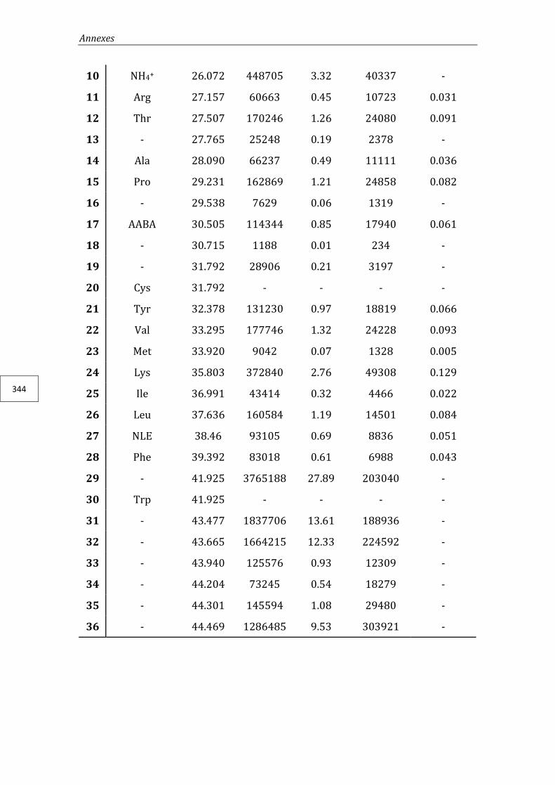
Annexes

344

10 NH4+ 26.072 448705 3.32 40337 -

11 Arg 27.157 60663 0.45 10723 0.031

12 Thr 27.507 170246 1.26 24080 0.091

13 - 27.765 25248 0.19 2378 -

14 Ala 28.090 66237 0.49 11111 0.036

15 Pro 29.231 162869 1.21 24858 0.082

16 - 29.538 7629 0.06 1319 -

17 AABA 30.505 114344 0.85 17940 0.061

18 - 30.715 1188 0.01 234 -

19 - 31.792 28906 0.21 3197 -

20 Cys 31.792 - - - -

21 Tyr 32.378 131230 0.97 18819 0.066

22 Val 33.295 177746 1.32 24228 0.093

23 Met 33.920 9042 0.07 1328 0.005

24 Lys 35.803 372840 2.76 49308 0.129

25 Ile 36.991 43414 0.32 4466 0.022

26 Leu 37.636 160584 1.19 14501 0.084

27 NLE 38.46 93105 0.69 8836 0.051

28 Phe 39.392 83018 0.61 6988 0.043

29 - 41.925 3765188 27.89 203040 -

30 Trp 41.925 - - - -

31 - 43.477 1837706 13.61 188936 -

32 - 43.665 1664215 12.33 224592 -

33 - 43.940 125576 0.93 12309 -

34 - 44.204 73245 0.54 18279 -

35 - 44.301 145594 1.08 29480 -

36 - 44.469 1286485 9.53 303921 -

Annexes

345

DiO-AMP-3 NCs (CHAPTER 4)


1 - 16.398 516782 13.31 30500 -

2 Asp 21.269 - - - -

3 Ser 22.912 - - - -

4 Glu 23.578 - - - -

5 - 24.315 17452 0.45 1608 -

6 Gly 24.817 - - - -

7 His 25.276 - - - -

8 NH4+ 26.082 64320 1.66 5865 -

9 Arg 27.138 - - - -

10 Thr 27.516 10048 0.26 1687 0.005

11 - 27.778 11105 0.29 1025 -

12 Ala 28.067 - - - -

13 Pro 29.213 - - - -

14 AABA 30.486 52271 1.35 8079 0.025

15 Cys 31.871 - - - -

16 Tyr 32.354 - - - -

17 Val 33.281 - - - -

18 Met 33.903 - - - -

Annexes

346

19 Lys 35.800 40280 1.04 5281 0.012

20 Ile 37.005 - - - -

21 Leu 37.655 - - - -

22 NLE 38.467 34333 0.88 3322 0.017

23 Phe 39.412 - - - -

24 Trp 41.868 - - - -

25 - 42.074 1167405 30.07 63248 -

26 - 43.502 695528 17.91 78129 -

27 - 43.662 514065 13.24 79885 -

28 - 43.914 26240 0.68 3094 -

29 - 44.258 153930 3.96 26378 -

30 - 44.431 496076 12.78 113476 -

31 - 44.632 28947 0.75 5076 -

32 - 44.780 10773 0.28 2001 -

33 - 44.886 43135 1.11 10174 -

DiO-HL5-A5-5 NCs (CHAPTER 4)


1 - 16.257 14677236 53.81 833610 -

2 Asp 21.337 16845 0.06 1600 0.008

Annexes

347

3 Ser 22.981 38327 0.14 3600 0.017

4 Glu 23.751 15549 0.06 1190 0.007

5 - 24.366 92229 0.34 7987 -

6 Gly 24.892 66206 0.24 6044 0.032

7 His 25.314 - - - -

8 NH4+ 26.137 101932 0.37 8289 -

9 Arg 27.172 102416 0.38 16869 0.046

10 Thr 27.546 22761 0.08 3765 0.011

11 - 27.820 70285 0.26 6431 -

12 Ala 28.097 - - - -

13 Pro 29.243 - - - -

14 AABA 30.501 21838 0.08 3117 0.010

15 - 30.720 10935 0.04 1417 -

16 - 31.189 23138 0.08 3038 -

17 - 31.533 32701 0.12 4397 -

18 Cys 31.533 - - - -

19 Tyr 32.374 192947 0.71 29044 0.086

20 Val 33.299 43555 0.16 6140 0.020

21 - 34.816 436974 1.60 12971 -

22 Met 34.816 - - - -

23 - 36.641 12998 0.05 944 -

24 Lys 36.641 - - - -

25 Ile 37.045 100033 0.37 10519 0.044

26 Leu 37.692 105937 0.39 9526 0.048

27 - 38.303 4080 0.01 430 -

28 NLE 38.529 23792 0.09 2269 0.011

29 - 38.650 10748 0.04 1010 -

30 Phe 39.464 434497 1.59 36341 0.199

31 - 41.964 5884651 21.57 312084 -

32 Trp 41.964 - - - -

Annexes

348

33 - 43.490 1860398 6.82 231140 -

34 - 43.652 2873078 10.53 418581 -

DiO-HL5-A5-2 NCs (CHAPTER 4)


1 - 16.348 3574552 32.19 833610 -

2 Asp 21.308 53810 0.48 1600 0.028

3 Ser 22.941 48239 0.43 3600 0.023

4 Glu 23.578 - - 1190 -

5 - 24.312 31765 0.29 7987 -

6 Gly 24.848 105088 0.95 6044 0.054

7 His 25.276 - - - -

8 NH4+ 26.101 270344 2.43 8289 -

9 Arg 27.158 80559 0.73 16869 0.038

10 Thr 27.528 17574 0.16 3765 0.009

11 - 27.814 23315 0.21 6431 -

12 Ala 28.067 - - - -

13 Pro 29.217 10324 0.09 - 0.005

14 AABA 30.503 124588 1.12 3117 0.06

15 - 30.954 18836 0.17 1417 -

Annexes

349

16 - 31.191 28263 0.25 3038 -

17 - 31.534 98211 0.88 4397 -

18 Cys 31.534 - - - -

19 Tyr 32.382 157698 1.42 29044 0.074

20 Val 33.278 92175 0.83 6140 0.044

21 Met 34.903 - - 12971 -

22 Lys 35.789 143307 1.29 - 0.044

23 Ile 37.003 195881 1.76 944 0.090

24 Leu 37.652 200469 1.81 - 0.097

25 NLE 38.482 110877 1.00 10519 0.056

26 Phe 39.439 224322 2.02 9526 0.108

27 - 42.041 2154877 19.41 430 -

28 Trp 42.041 - - 2269 -

29 - 43.493 982998 8.85 1010 -

30 - 43.660 960393 8.65 36341 -

31 - 43.948 38934 0.35 312084 -

32 - 44.069 32582 0.29 - -

33 - 44.252 471942 4.25 231140 -

34 - 44.431 773019 6.96 -

35 - 44.789 29429 0.27 -

36 - 44.892 49749 0.45 418581 -

Annexes

350

IPEP

DiO-HL1-IPEP-5 NCs

*

*

Annexes

351

DiO-HL1-IPEP-2 NCs

DiO-AMP-4 NCs

* *

*

Annexes

352

7. In vivo data (organs weight)

No

n-t

rea

ted

w/tu

mor

w/o

tum

or

G0-

1|-2

G1-

1|-5

G1-

2|-6

G1-

3|-7

G1-

4|-8

G1-

2RG

1-3R

24 h

0,21

230,

2550

0,08

770,

1085

0,11

100,

0812

48 h

0,19

200,

1598

0,03

790,

0548

24 h

0,15

200,

1495

0,09

820,

1149

0,13

4048

h0,

1623

0,11

350,

1361

0,12

750,

1099

24 h

1,41

371,

3780

1,40

561,

2556

1,17

2148

h1,

2912

1,43

621,

1647

1,36

591,

3859

24 h

0,29

090,

3272

0,34

150,

3582

0,33

8448

h0,

3538

0,33

860,

3778

0,28

780,

3486

24 h

0,12

600,

2035

0,17

490,

1655

0,16

5948

h0,

2089

0,16

960,

1632

0,17

940,

1646

24 h

0,04

500,

0509

0,05

110,

0492

0,05

2248

h0,

0457

0,05

290,

0488

0,05

130,

0526

No

n-t

rea

ted

w/tu

mor

w/o

tum

orG

0-3|

-4G

2-1|

-5G

2-2|

-6G

2-3|

-7G

2-4|

-8G

2-2R

G2-

8R

24 h

0,09

130,

1301

0,08

270,

1183

0,42

87

48 h

0,14

780,

0960

0,02

580,

1254

0,04

77

24 h

0,16

520,

1339

0,10

130,

1677

0,13

5248

h0,

1855

0,14

360,

1162

0,14

060,

1987

24 h

1,15

131,

2274

1,39

241,

4859

1,34

4548

h1,

4574

1,41

661,

1676

1,11

901,

3369

24 h

0,35

020,

2731

0,34

200,

3787

0,35

9848

h0,

3692

0,40

530,

3372

0,30

610,

3612

24 h

0,12

520,

1791

0,15

550,

1836

0,19

3348

h0,

1935

0,16

080,

1755

0,15

100,

1732

24 h

0,04

960,

0482

0,04

660,

0561

0,04

7348

h0,

0569

0,05

060,

0472

0,05

450,

0479

DiR

-AM

P N

Cs

w/tu

mor

Tu

mo

r

Sp

lee

n

Liv

er

Kid

ne

y

Lu

ng

Pla

sma

DiR

-an

tiG

D2

NC

sw

/tum

or

Tu

mo

r

Sp

lee

n

Liv

er

Kid

ne

y

Lu

ng

Pla

sma

Multisensitive polyurethane/polyurea nanocapsules for smart ...

Documents

Transcript of Multisensitive polyurethane/polyurea nanocapsules for smart ...