Multiple Fault Detection in a Four Stroke Engine Using Single Sensor System

Shankar N. Dandare et al, International Journal of Computer Science and Mobile Computing, Vol.3 Issue.5, May- 2014, pg. 648-658

© 2014, IJCSMC All Rights Reserved 648

Available Online at www.ijcsmc.com

International Journal of Computer Science and Mobile Computing

A Monthly Journal of Computer Science and Information Technology

ISSN 2320–088X

IJCSMC, Vol. 3, Issue. 5, May 2014, pg.648 – 658

RESEARCH ARTICLE

Multiple Fault Detection in a Four Stroke

Engine Using Single Sensor System Shankar N. Dandare

Associate Professor in Electronics & Tele. Engg.

Electronics Department,

College of Engineering, Pusad, Maharashtra-State, India

Email: [email protected]

S. V. Dudul

Professor & Head, Dept of Applied Electronics,

Sant Gadge Baba Amravati University, Amravati,

Maharashtra-State, India

Email: [email protected]

Abstract

The proposed system follows a model–based approach based on Digital Signal Processing and Artificial

Neural Network. Fault Detection and Isolation (FDI) of an Automobile Engine’ have been carried out using acoustic

signals which is captured from the engine. This method is based on parameter estimation, where a set of parameters

is used to check the status of an engine and a model based approach is employed to generate several symptoms

indicating the difference between faulty and non-faulty status.

In this work, experimentation is carried out on Hero Honda Passion Four Stroke (HHPFS) Engine. There

are many more types of faults which may be developed because of wear and tear or lack of maintenance but, the

database is generated only for five different types of faults and classification of the same is carried out. The signal

normalization, signal conditioning, signal decompositions, analog to digital conversion and feature extraction were

carried out by using the algorithm written in MATLAB R2010B. The paper describes the performance of statistical

and Artificial Neural Network (ANN) based classifiers for individual and multiple faults and finally the optimal

classifiers are proposed based on classification accuracy. It is observed from the experimental results that Artificial

Neural Network (ANN) based classifiers are more appropriate than statistical classifiers. It is also observed that the

magnitude of Mean Square Error (MSE) is under permissible limits and percentage Average Classification Accuracy

(%ACA) is also reasonable.

Keywords: Digital Signal Processing Statistical Classifiers, Four Stroke Engine and ANN Based Classifiers

1. Introduction

Today, transportation technology, especially car, grows fast, but many drivers do not know how to work for

their car. Fault Detection is not an easy for inexperienced mechanic or driver because it is needed a lot of knowledge

for finding the fault. Therefore, they extremely depend on expert mechanic. Looking into this the FDI system is

proposed to detect the fault in an incipient stage to avoid the inconvenience. The work carried out in this area is

discussed below.



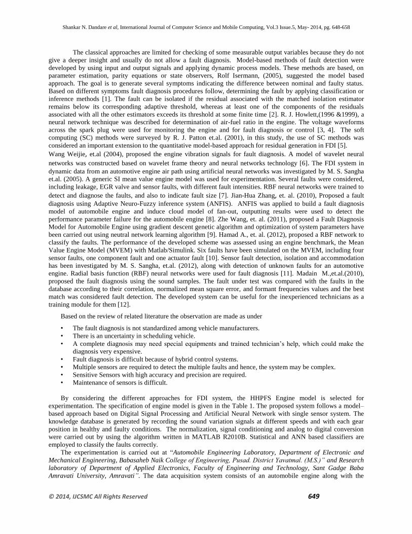
The classical approaches are limited for checking of some measurable output variables because they do not

give a deeper insight and usually do not allow a fault diagnosis. Model-based methods of fault detection were

developed by using input and output signals and applying dynamic process models. These methods are based, on

parameter estimation, parity equations or state observers, Rolf Isermann, (2005), suggested the model based

approach. The goal is to generate several symptoms indicating the difference between nominal and faulty status.

Based on different symptoms fault diagnosis procedures follow, determining the fault by applying classification or

inference methods [1]. The fault can be isolated if the residual associated with the matched isolation estimator

remains below its corresponding adaptive threshold, whereas at least one of the components of the residuals

associated with all the other estimators exceeds its threshold at some finite time [2]. R. J. Howlett,(1996 &1999), a

neural network technique was described for determination of air-fuel ratio in the engine. The voltage waveforms

across the spark plug were used for monitoring the engine and for fault diagnosis or control [3, 4]. The soft

computing (SC) methods were surveyed by R. J. Patton et.al. (2001), in this study, the use of SC methods was

considered an important extension to the quantitative model-based approach for residual generation in FDI [5].

Wang Weijie, et.al (2004), proposed the engine vibration signals for fault diagnosis. A model of wavelet neural

networks was constructed based on wavelet frame theory and neural networks technology [6]. The FDI system in

dynamic data from an automotive engine air path using artificial neural networks was investigated by M. S. Sangha

et.al. (2005). A generic SI mean value engine model was used for experimentation. Several faults were considered,

including leakage, EGR valve and sensor faults, with different fault intensities. RBF neural networks were trained to

detect and diagnose the faults, and also to indicate fault size [7]. Jian-Hua Zhang, et. al. (2010), Proposed a fault

diagnosis using Adaptive Neuro-Fuzzy inference system (ANFIS). ANFIS was applied to build a fault diagnosis

model of automobile engine and induce cloud model of fan-out, outputting results were used to detect the

performance parameter failure for the automobile engine [8]. Zhe Wang, et. al. (2011), proposed a Fault Diagnosis

Model for Automobile Engine using gradient descent genetic algorithm and optimization of system parameters have

been carried out using neutral network learning algorithm [9]. Hamad A., et. al. (2012), proposed a RBF network to

classify the faults. The performance of the developed scheme was assessed using an engine benchmark, the Mean

Value Engine Model (MVEM) with Matlab/Simulink. Six faults have been simulated on the MVEM, including four

sensor faults, one component fault and one actuator fault [10]. Sensor fault detection, isolation and accommodation

has been investigated by M. S. Sangha, et.al. (2012), along with detection of unknown faults for an automotive

engine. Radial basis function (RBF) neural networks were used for fault diagnosis [11]. Madain M.,et.al.(2010),

proposed the fault diagnosis using the sound samples. The fault under test was compared with the faults in the

database according to their correlation, normalized mean square error, and formant frequencies values and the best

match was considered fault detection. The developed system can be useful for the inexperienced technicians as a

training module for them [12].

Based on the review of related literature the observation are made as under

• The fault diagnosis is not standardized among vehicle manufacturers.

• There is an uncertainty in scheduling vehicle.

• A complete diagnosis may need special equipments and trained technician’s help, which could make the

diagnosis very expensive.

• Fault diagnosis is difficult because of hybrid control systems.

• Multiple sensors are required to detect the multiple faults and hence, the system may be complex.

• Sensitive Sensors with high accuracy and precision are required.

• Maintenance of sensors is difficult.

By considering the different approaches for FDI system, the HHPFS Engine model is selected for

experimentation. The specification of engine model is given in the Table 1. The proposed system follows a model–

based approach based on Digital Signal Processing and Artificial Neural Network with single sensor system. The

knowledge database is generated by recording the sound variation signals at different speeds and with each gear

position in healthy and faulty conditions. The normalization, signal conditioning and analog to digital conversion

were carried out by using the algorithm written in MATLAB R2010B. Statistical and ANN based classifiers are

employed to classify the faults correctly.

The experimentation is carried out at “Automobile Engineering Laboratory, Department of Electronic and

Mechanical Engineering, Babasaheb Naik College of Engineering, Pusad. District Yavatmal. (M.S.)” and Research

laboratory of Department of Applied Electronics, Faculty of Engineering and Technology, Sant Gadge Baba

Amravati University, Amravati”. The data acquisition system consists of an automobile engine along with the

http://ieeexplore.ieee.org/search/searchresult.jsp?searchWithin=p_Authors:.QT.Wang%20Weijie.QT.&searchWithin=p_Author_Ids:37269676700&newsearch=true

http://ieeexplore.ieee.org/search/searchresult.jsp?searchWithin=p_Authors:.QT.Jian-Hua%20Zhang.QT.&searchWithin=p_Author_Ids:37601218900&newsearch=true

http://ieeexplore.ieee.org/search/searchresult.jsp?searchWithin=p_Authors:.QT.Zhe%20Wang.QT.&searchWithin=p_Author_Ids:37898307400&newsearch=true

http://ieeexplore.ieee.org/search/searchresult.jsp?searchWithin=p_Authors:.QT.Madain,%20M..QT.&searchWithin=p_Author_Ids:37586529700&newsearch=true



microphone as a sensor to capture the acoustic signal, signal recording, signal conditioning and signal processing

system. There are many more types of faults which may be developed in the automobile engine but, the database is

generated for only five different types of faults that are Air Filter Fault (FF), Spark Plug Fault (SP), Rich Mixture

Fault (RM), Insufficient Lubricants Fault (ISL) and Piston Ring Fault (PR).

It is worthwhile to notice that the proposed system may be designed and attached to every newly produced

engine, so that the fault can be detected at an incipient level. It is also suggested that the proposed FDI system can

be extended to detect any number of faults. The proposed FDI system can be used as one type of tool to know the

status of the engine and will act as a guide for maintaining the vehicle in good condition that will save our time and

inconvenience. By considering the necessity of FDI system the broad objectives of proposed FDI system are listed

as under.

• It is possible to detect the faults at an incipient stage.

• To improve productivity & reliability of an automobile.

• To facilitate unskilled or less skilled automobile staff to work more efficiently.

• To reduce the maintenance cost and down-time of an automobile.

• To avoid vehicular accidents because of inadequate maintenance.

• To prevent the monetary loss of customer (in the event of a wrong diagnosis).

• As a tool for training inexperienced people.

• To improve knowledge of driver in diagnosing the fault.

• The proposed FDI system is simple, reliable and flexible.

• It is single sensor system based on acoustic signal.

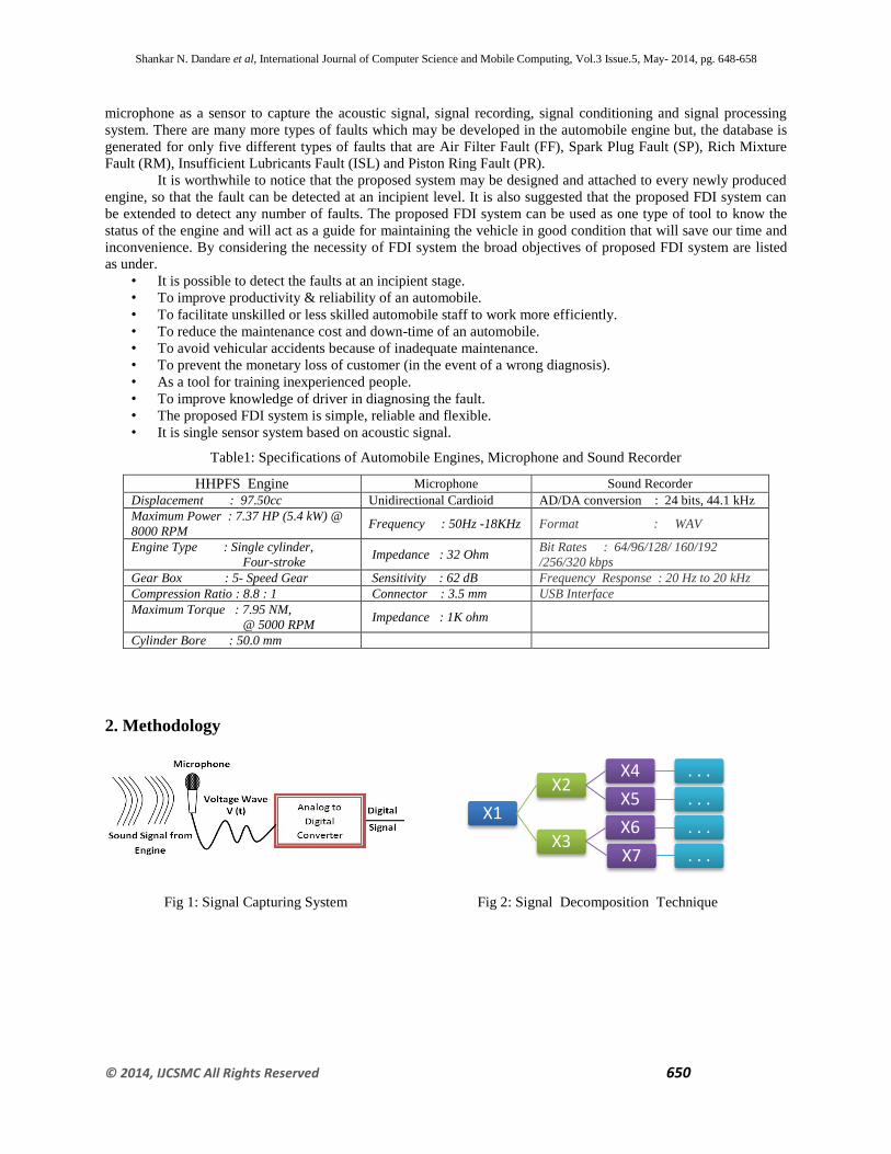
Table1: Specifications of Automobile Engines, Microphone and Sound Recorder

HHPFS Engine Microphone Sound Recorder

Displacement : 97.50cc Unidirectional Cardioid AD/DA conversion : 24 bits, 44.1 kHz

Maximum Power : 7.37 HP (5.4 kW) @

8000 RPM Frequency : 50Hz -18KHz Format : WAV

Engine Type : Single cylinder,

Four-stroke Impedance : 32 Ohm

Bit Rates : 64/96/128/ 160/192

/256/320 kbps

Gear Box : 5- Speed Gear Sensitivity : 62 dB Frequency Response : 20 Hz to 20 kHz

Compression Ratio : 8.8 : 1 Connector : 3.5 mm USB Interface

Maximum Torque : 7.95 NM,

@ 5000 RPM Impedance : 1K ohm

Cylinder Bore : 50.0 mm

2. Methodology

Fig 1: Signal Capturing System

Fig 2: Signal Decomposition Technique

X1

X2 X4 . . .

X5 . . .

X3 X6 . . .

X7 . . .



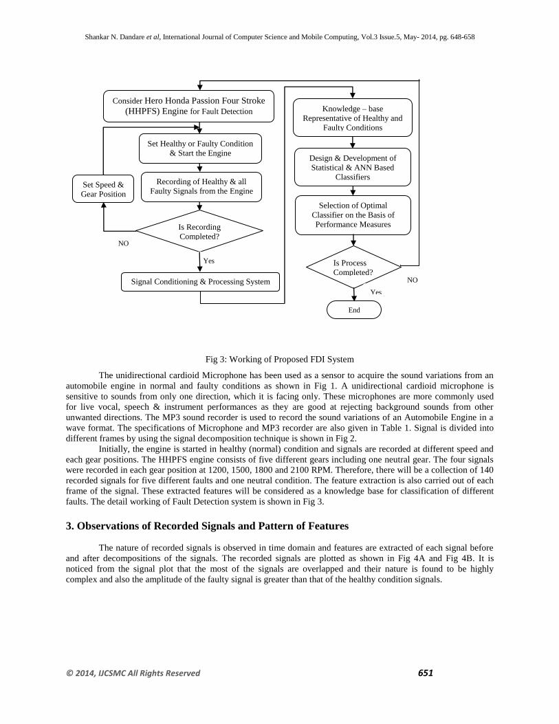
Fig 3: Working of Proposed FDI System

The unidirectional cardioid Microphone has been used as a sensor to acquire the sound variations from an

automobile engine in normal and faulty conditions as shown in Fig 1. A unidirectional cardioid microphone is

sensitive to sounds from only one direction, which it is facing only. These microphones are more commonly used

for live vocal, speech & instrument performances as they are good at rejecting background sounds from other

unwanted directions. The MP3 sound recorder is used to record the sound variations of an Automobile Engine in a

wave format. The specifications of Microphone and MP3 recorder are also given in Table 1. Signal is divided into

different frames by using the signal decomposition technique is shown in Fig 2.

Initially, the engine is started in healthy (normal) condition and signals are recorded at different speed and

each gear positions. The HHPFS engine consists of five different gears including one neutral gear. The four signals

were recorded in each gear position at 1200, 1500, 1800 and 2100 RPM. Therefore, there will be a collection of 140

recorded signals for five different faults and one neutral condition. The feature extraction is also carried out of each

frame of the signal. These extracted features will be considered as a knowledge base for classification of different

faults. The detail working of Fault Detection system is shown in Fig 3.

3. Observations of Recorded Signals and Pattern of Features

The nature of recorded signals is observed in time domain and features are extracted of each signal before

and after decompositions of the signals. The recorded signals are plotted as shown in Fig 4A and Fig 4B. It is

noticed from the signal plot that the most of the signals are overlapped and their nature is found to be highly

complex and also the amplitude of the faulty signal is greater than that of the healthy condition signals.

Consider Hero Honda Passion Four Stroke

(HHPFS) Engine for Fault Detection

Set Healthy or Faulty Condition

& Start the Engine

Set Speed &

Gear Position

Recording of Healthy & all

Faulty Signals from the Engine

Signal Conditioning & Processing System

Knowledge – base

Representative of Healthy and

Faulty Conditions

Design & Development of

Statistical & ANN Based

Classifiers

Selection of Optimal

Classifier on the Basis of

Performance Measures

Is Process

Completed?

Is Recording

Completed?

End

NO

Yes

Yes

NO



Fig 4A : Engine’ Signals for Normal and PR Fault Fig 4B: Engine’ Signals for Normal and ISL Fault

The knowledge base is generated by extracting the features of healthy and faulty conditions signals. The

extracted features are Mean, Energy, Maximum Value, Minimum Value, Standard Deviation, Variance and Mode

for five different types of faults and out of which Minimum vs. Energy and Mean vs. Energy features are plotted as

shown in Fig 5A & Fig 5B. After observing the overlapping nature of features and non separable decision

boundaries, the decision is taken to employ the soft computing approach to classify the faults. At the beginning the

statistical classifiers are employed to classify the faults which are explained in the subsequent section.

Fig 5A: Scatter Plot for Minimum Vs Energy Fig 5B: Scatter Plot for Mean Vs Energy

4. Classification of Faults Using Statistical Classifiers

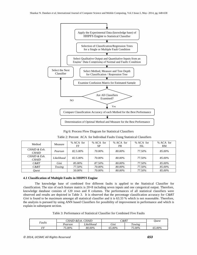
The statistical classification is carried out using XLSTAT and the Process Flow Diagram for Statistical

Classifiers is shown in Fig 7. In this the classification and regression trees have been employed to classify the faults.

The feature matrix comprising of 7 inputs and one categorical output has been applied to statistical classifiers. The

size of each feature matrix is 20×8 including seven inputs and one categorical output. Therefore, knowledge

database consists of 40 rows and 8 columns. The performance has been observed with respect to CHAID-Pearson,

CHAID-Likelihood, Exhaustive-CHAID-Pearson, Exhaustive-CHAID-Likelihood, C&RT Gini, C&RT-Towing and

Quest Methods and results are depicted in Table 2, for each fault, with the %ACA of each method. It is observed

that for FF condition and the maximum %ACA is found to be 85% for C&RT Gini method, for SP Fault condition

the maximum %ACA is found to be 87.50% for C&RT Gini method, for PR Fault condition the maximum %ACA is

found to be 80.00% for all types of statistical classifiers, for ISL Fault condition and the maximum %ACA is found

to be 77.50% for all types of statistical classifier, for Rich Mixture RM Fault condition and the maximum %ACA is

found to be 85.00% for all types of statistical classifiers.



Fig 6: Process Flow Diagram for Statistical Classifiers

Table 2: Percent ACA for Individual Faults Using Statistical Classifiers

Method Measure % ACA for

FF

% ACA for

SP

% ACA for

PR

% ACA for

ISL

% ACA for

RM

CHAID & Exh.

CHAID Pearson 82.5.00% 70.00% 80.00% 77.50% 85.00%

CHAID & Exh.

CHAID Likelihood 82.5.00% 70.00% 80.00% 77.50% 85.00%

C&RT Gini 85.00% 87.50% 80.00% 77.50% 85.00%

C&RT Towing 77.50% 70.00% 80.00% 77.50% 85.00%

Quest 50.00% 70.00% 80.00% 77.50% 85.00%

4.1 Classification of Multiple Faults in HHPFS Engine

The knowledge base of combined five different faults is applied to the Statistical Classifier for

classification. The size of each feature matrix is 20×8 including seven inputs and one categorical output. Therefore,

knowledge database consists of 120 rows and 8 columns. The performances of all statistical classifiers were

observed and results are depicted in Table 3. It is observed that the percentage classification accuracy for C&RT

Gini is found to be maximum amongst all statistical classifier and it is 63.33 % which is not reasonable. Therefore,

the analysis is pursued by using ANN based Classifiers for possibility of improvement in performance and which is

explain in subsequent section.

Table 3: Performance of Statistical Classifier for Combined Five Faults

Faults CHAID &Exh. CHAID C&RT Quest

Pearson Likelihood Gini Towing

FF 75.00% 80.00% 65.00% 75.00% 65.00%

Apply the Experimental Data (knowledge base) of

HHPFS Engine to Statistical Classifier

Selection of Classification/Regression Trees

for a Single or Multiple Fault Condition

Select Qualitative Output and Quantitative Inputs from an

Engine’ Data Comprising of Normal and Faulty Condition

Select Method, Measure and Tree Depth

for Classification / Regression Tree

Examine Confusion Matrix for Estimated Sample

Are All Classifiers

Examined?

Select the Next

Classifier

Compare Classification Accuracy of each Method for the Best Performance

Determination of Optimal Method and Measure for the Best Performance

NO

O Yes



ISL 50.00% 65.00% 75.00% 65.00% 65.00%

NOR 35.00% 35.00% 75.00% 20.00% 25.00%

PR 85.00% 85.00% 60.00% 20.00% 20.00%

RM 35.00% 35.00% 65.00% 45.00% 70.00%

SP 30.00% 40.00% 40.00% 20.00% 20.00%

Total % ACA 51.67% 56.67% 63.33% 40.83% 44.17%

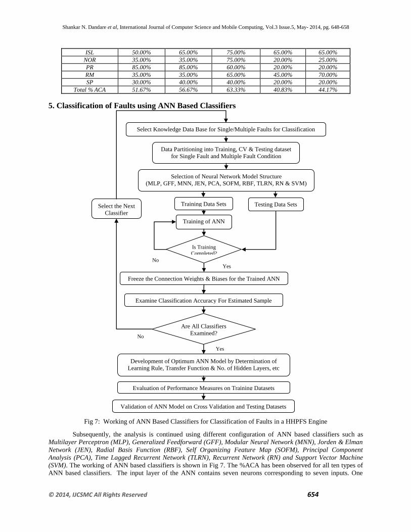
5. Classification of Faults using ANN Based Classifiers

Fig 7: Working of ANN Based Classifiers for Classification of Faults in a HHPFS Engine

Subsequently, the analysis is continued using different configuration of ANN based classifiers such as

Multilayer Perceptron (MLP), Generalized Feedforward (GFF), Modular Neural Network (MNN), Jorden & Elman

Network (JEN), Radial Basis Function (RBF), Self Organizing Feature Map (SOFM), Principal Component

Analysis (PCA), Time Lagged Recurrent Network (TLRN), Recurrent Network (RN) and Support Vector Machine

(SVM). The working of ANN based classifiers is shown in Fig 7. The %ACA has been observed for all ten types of

ANN based classifiers. The input layer of the ANN contains seven neurons corresponding to seven inputs. One

Select Knowledge Data Base for Single/Multiple Faults for Classification

Data Partitioning into Training, CV & Testing dataset

for Single Fault and Multiple Fault Condition

Selection of Neural Network Model Structure

(MLP, GFF, MNN, JEN, PCA, SOFM, RBF, TLRN, RN & SVM)

Training Data Sets

Testing Data Sets

Training of ANN

Is Training

Completed?

Freeze the Connection Weights & Biases for the Trained ANN

Examine Classification Accuracy For Estimated Sample

Are All Classifiers

Examined?

Development of Optimum ANN Model by Determination of

Learning Rule, Transfer Function & No. of Hidden Layers, etc

Evaluation of Performance Measures on Training Datasets

Validation of ANN Model on Cross Validation and Testing Datasets

Select the Next

Classifier

Yes No

Yes

No



categorical output denotes a type of fault or healthy condition of an engine. As there are five different types of faults

and one state indicating healthy condition, the number of neurons in the output layer must be six (five neurons

corresponding to five different faults and one neuron corresponding to healthy condition). Three data partitions,

namely, Training, Cross Validation (CV) and Testing were used with different tagging order. Every time, ANN is

retrained three times with different random initialization of connection weights and biases with a view to ensure true

learning and generalization.

5.1 Classification of Single Fault in a HHPFS Engine

Table 4: Performance of ANN Based Classifiers for Single Fault

ANN FF SP ISL RM PR

Testing CV Testing CV Testing CV Testing CV Testing CV

MLP 92.9 85.7 91.7 100.0 100.0 91.7 100.0 100.0 100.0 100.0

GFF 85.7 61.9 58.3 92.9 100.0 91.7 100.0 100.0 100.0 100.0

MNN 52.4 71.4 66.7 61.9 100.0 91.7 100.0 100.0 100.0 100.0

JEN 78.6 59.5 83.3 61.9 100.0 100.0 100.0 100.0 100.0 100.0

PCA 85.7 78.6 58.3 69.0 100.0 91.7 100.0 100.0 100.0 100.0

RBF 78.6 50.0 50.0 76.2 100.0 100.0 100.0 100.0 100.0 100.0

SOFM 52.4 71.4 87.5 85.7 100.0 100.0 91.7 62.5 100.0 100.0

TLRN 54.8 21.4 62.5 85.7 83.3 83.3 100.0 100.0 75.0 80.0

RN 38.1 69.0 45.8 66.7 100.0 100.0 100.0 100.0 100.0 100.0

SVM 59.5 57.1 83.3 76.2 100.0 100.0 100.0 100.0 100.0 100.0

The size of the feature matrix for a single fault with single frame is 40×8; i.e. 20×8 matrix for healthy

(normal) signal and 20×8 matrix for each Faulty Signal. The feature matrix was fragmented into three parts in the

ratio of 2:1:1 indicating training dataset: CV dataset: testing dataset. The classification accuracy of each faulty

condition for testing and CV data set has been depicted in the Table 4. It is observed that the classification accuracy

of MLP based classifier is better amongst all classifiers for FF and SP faults. Further it is also observed that

classification accuracy for all ANN based classifiers is reasonably good for single fault. Therefore, the analysis is

pursued by combining the multiple faults and it is explained in the subsequent sections.

5.2 Classification of Combined Three Faults (PR, FF & ISL) and (RM, SP & FF)

Table 5: Classification of Combined Three Faults (PR, FF & ISL) and (RM, SP & FF)

ANN PR, FF & ISL RM, SP & FF

Testing CV Training Testing CV Training

MLP 78.33333 91.66667 90 100 93.75 89.39394

GFF 70 67.91667 70 70.83333 83.33333 84.84848

MNN 57.5 61.11111 73.33333 77.08333 79.16667 82.57576

JEN 55.83333 70.83333 83.33333 79.16667 77.08333 91.28788

PCA 56.66667 70.83333 72.5 79.16667 75 80.30303

RBF 73.33333 69.16667 83.33333 75 79.16667 75

SOFM 62.5 66.66667 68.33333 90.75 87.5 89.39394

TLRN 55.83333 39.30556 67.5 75 75 75

RN 53.33333 67.91667 65.83333 75 79.16667 77.27273

SVM 78.33333 81.66667 100 93.75 88.75 100

Further, analysis is continued for considering the combined three faults togather in two groups. In one group

the faults considered are PR, FF & ISL and in another group the faults considered are RM, SP & FF. The extracted

features are combined for three faults along with the features of normal signal. The size of the feature matrix for

single frame is 80×8, i.e. 20×8 matrix for normal signal, 20×8 matrix for each faulty signals. The same types of data

partitioning is employed(2:1:1) as explained earlier. The performances of all ten types of ANN based classifiers are

depicted in Table 5. From the classification, it is observed that the performance of MLP and SVM based classifiers is

found to be impressive amongst all ten types of classifiers. It is observed that the classification accuracy of ANN

based classifiers for combined three faults is decreased as compared to single fault. The process of classification is

also continued for combined five faults together, which is explained in the subsequent sections.



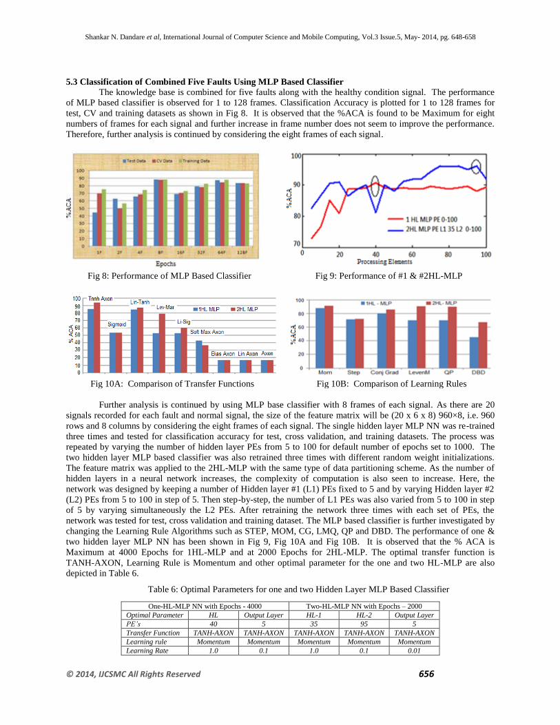
5.3 Classification of Combined Five Faults Using MLP Based Classifier

The knowledge base is combined for five faults along with the healthy condition signal. The performance

of MLP based classifier is observed for 1 to 128 frames. Classification Accuracy is plotted for 1 to 128 frames for

test, CV and training datasets as shown in Fig 8. It is observed that the %ACA is found to be Maximum for eight

numbers of frames for each signal and further increase in frame number does not seem to improve the performance.

Therefore, further analysis is continued by considering the eight frames of each signal.

Fig 8: Performance of MLP Based Classifier Fig 9: Performance of #1 & #2HL-MLP

Fig 10A: Comparison of Transfer Functions Fig 10B: Comparison of Learning Rules

Further analysis is continued by using MLP base classifier with 8 frames of each signal. As there are 20

signals recorded for each fault and normal signal, the size of the feature matrix will be (20 x 6 x 8) 960×8, i.e. 960

rows and 8 columns by considering the eight frames of each signal. The single hidden layer MLP NN was re-trained

three times and tested for classification accuracy for test, cross validation, and training datasets. The process was

repeated by varying the number of hidden layer PEs from 5 to 100 for default number of epochs set to 1000. The

two hidden layer MLP based classifier was also retrained three times with different random weight initializations.

The feature matrix was applied to the 2HL-MLP with the same type of data partitioning scheme. As the number of

hidden layers in a neural network increases, the complexity of computation is also seen to increase. Here, the

network was designed by keeping a number of Hidden layer #1 (L1) PEs fixed to 5 and by varying Hidden layer #2

(L2) PEs from 5 to 100 in step of 5. Then step-by-step, the number of L1 PEs was also varied from 5 to 100 in step

of 5 by varying simultaneously the L2 PEs. After retraining the network three times with each set of PEs, the

network was tested for test, cross validation and training dataset. The MLP based classifier is further investigated by

changing the Learning Rule Algorithms such as STEP, MOM, CG, LMQ, QP and DBD. The performance of one &

two hidden layer MLP NN has been shown in Fig 9, Fig 10A and Fig 10B. It is observed that the % ACA is

Maximum at 4000 Epochs for 1HL-MLP and at 2000 Epochs for 2HL-MLP. The optimal transfer function is

TANH-AXON, Learning Rule is Momentum and other optimal parameter for the one and two HL-MLP are also

depicted in Table 6.

Table 6: Optimal Parameters for one and two Hidden Layer MLP Based Classifier

One-HL-MLP NN with Epochs - 4000 Two-HL-MLP NN with Epochs – 2000 Optimal Parameter HL Output Layer HL-1 HL-2 Output Layer

PE’s 40 5 35 95 5

Transfer Function TANH-AXON TANH-AXON TANH-AXON TANH-AXON TANH-AXON

Learning rule Momentum Momentum Momentum Momentum Momentum

Learning Rate 1.0 0.1 1.0 0.1 0.01



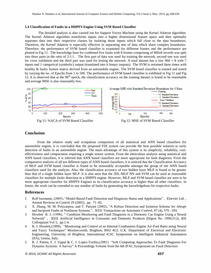
5.4 Classification of Faults in a HHPFS Engine Using SVM Based Classifier

The detailed analysis is also carried out for Support Vector Machine using the Kernel Adatron algorithm.

The Kernel Adatron algorithm transforms inputs into a higher dimensional feature space and then optimally

separates data into their respective classes by isolating those inputs which fall close to the data boundaries.

Therefore, the Kernel Adatron is especially effective in separating sets of data which share complex boundaries.

Therefore, the performance of SVM based classifier is examined for different frames and the performance are

plotted in Fig 11. The knowledge base for combined five faults with 8 frames comprising of 960x8 records was split

into three parts in the ratio of 2:1:1. The first part of data was used for training the network, second one was used

for cross validation and the third part was used for testing the network. A total dataset has a size 960 × 8 with 7

inputs and 1 categorical (symbolic) output (translated into 6 binary outputs). The SVM is retrained three times with

healthy & faulty feature matrix derived from an automobile engine. The SVM based classifier is trained and tested

by varying the no. of Epochs from 1 to 500. The performance of SVM based classifier is exhibited in Fig 11 and Fig

12. It is observed that at the 90th

epoch, the classification accuracy on the training dataset is found to be reasonable

and average MSE is also reasonably less.

Fig 11: %ACA of SVM Based Classifier Fig 12: MSE of SVM Based Classifier

Conclusion

From the relative study and scrupulous comparison of all statistical and ANN based classifiers for

automobile engine, it is concluded that the proposed FDI system can provide the best possible solution to early

detection of faults in an automobile engine. The main advantage of this system is its simplicity, reliability, cost-

effectiveness and compactness requiring a single sensor system. From the meticulous analysis using statistical and

ANN based classifiers, it is inferred that ANN based classifiers are more appropriate for fault diagnosis. From the

comparative analysis of all ten different types of ANN based classifiers, it is noticed that the Classification Accuracy

of MLP and SVM based classifier is found to be reasonably acceptable amongst the group of ten ANN based

classifiers used for the analysis. Also, the classification accuracy of two hidden layer MLP is found to be greater

than that of a single hidden layer MLP. It is also seen that the 2HL-MLP NN and SVM can be used as reasonable

classifiers for multiple faults detection in a HHPFS engine. However, MLP and SVM based classifier are seen to be

more appropriate classifier for HHPFS Engines as its classification accuracy is higher than all other classifiers. In

future, the work can be extended to any number of faults by generating the knowledgebase for respective faults.

References

1 Rolf Isermann, (2005), “Model-Based Fault Detection and Diagnosis Status and Applications” , Elsevier Ltd. ,

Annual Reviews in Control 29 (2005), pp. 71–85.

2 X. Zhang, M. M. Polycarpou, and T. Parisini (2002), “A Robust Detection and Isolation Scheme for Abrupt

and Incipient Faults in Nonlinear Systems.”, IEEE Transactions on Automatic Control, 47 (4), 576 –593.

3 Howlett R. J. (1996), “ Condition Monitoring and Fault Diagnosis in a Domestic Car Engine Using a Neural

Network” , IEEE Artificial Intelligence in Consumer and Domestic Products (Digest No. 1996/212), IEE

Colloquium Vol 5, pp.1-4.

4 R. J. Howlett,(1999), “Monitoring and Control of an Internal Combustion Engine Air-Fuel Ratio using Neural

and Fuzzy Techniques” Moulsecoomb, Brighton, BN2 4GJ, U.K. Department of Electrical and Electronic

Engineering, University of Brighton, International ICSC Symposium on Intelligent Industrial Automation

(IIA), Genoa, Italy.

5 R. J. Patton, F. J. Uppal & C. J. Lopez-Toribio,(2001) “Soft Computing Approaches To Fault Diagnosis For

Dynamic Systems: A Survey” A Proceedings Volume from the 6th IFAC Symposium on Fault Detection

http://ieeexplore.ieee.org/xpl/articleDetails.jsp?tp=&arnumber=603630&pageNumber%3D2%26queryText%3DFault+diagnosis+in+an+automobile+engine


http://ieeexplore.ieee.org/xpl/mostRecentIssue.jsp?punumber=4630




6 Wang Weijie, Kang Yuanfu, Zhao Xuezheng and Huang Wentao, (2004) “Study of Automobile Engine Fault

Diagnosis Based on Wavelet Neural Networks”, IEEE- Intelligent Control and Automation, Volume: 2, pp. :

1766 - 1770.

7 M. S. Sangha, J. B. Gomm, D. L. Yu, G. F. Page (2005), “Fault Detection and Identification of Automotive

Engines Using Neural Networks”, Proceedings of the 16th IFAC World Congress, pp. 1166-1166.

8 Jian-Hua Zhang, Li-Fang Kong, Zhang Tian and Wei Hao, ( 2010) , “The Performance Parameter Fault

Diagnosis for Automobile Engine Based on ANFIS”, Web Information Systems and Mining (WISM) -IEEE

International Conference on Volume 2, pp. 261 – 264.

9 Zhe Wang, Li Fang Kong, and Shi Song Zhu, ( 2011), “Fault Diagnosis Model for Automobile Engine Based

on Gradient Genetic Algorithm”, IEEE Artificial Intelligence, Management Science and Electronic Commerce

(AIMSEC), 2nd International Conference, pp. 1128 – 1131.

10 Hamad A., Dingli Yu, Gomm, J.B. and Sangha, M.S. (2012), “Fault Detection and Isolation for Engine

Under Closed-Loop Control”, IEEE Xplore, Control (CONTROL), UKACC- Proceedings of IEEE

International Conference, pp. 431 – 436.

11 M. S. Sangha, D. L. Yu and J. B. Gomm (2012), “Sensor Fault Detection, Isolation, Accommodation and

Unknown Fault Detection in Automotive Engine Using AI”, International Journal of Engineering, Science and

Technology, Vol. 4, No. 3, 2012, pp. 53-65.

12 Madain M., Al-Mosaiden A. & Al-khassaweneh M. (2010), “Fault Diagnosis in Vehicle Engines Using Sound

Recognition Techniques”, Electro/Information Technology (EIT), IEEE International Conference, pp. 1 – 4.

http://ieeexplore.ieee.org/search/searchresult.jsp?searchWithin=p_Authors:.QT.Wang%20Weijie.QT.&searchWithin=p_Author_Ids:37269676700&newsearch=true

http://ieeexplore.ieee.org/search/searchresult.jsp?searchWithin=p_Authors:.QT.Kang%20Yuanfu.QT.&searchWithin=p_Author_Ids:37269673000&newsearch=true

http://ieeexplore.ieee.org/search/searchresult.jsp?searchWithin=p_Authors:.QT.Zhao%20Xuezheng.QT.&searchWithin=p_Author_Ids:37269672900&newsearch=true

http://ieeexplore.ieee.org/search/searchresult.jsp?searchWithin=p_Authors:.QT.Huang%20Wentao.QT.&searchWithin=p_Author_Ids:37269671000&newsearch=true

http://ieeexplore.ieee.org/xpl/articleDetails.jsp?tp=&arnumber=1340976&queryText%3DFault+diagnosis+in+an+automobile+engine




http://ieeexplore.ieee.org/search/searchresult.jsp?searchWithin=p_Authors:.QT.Jian-Hua%20Zhang.QT.&searchWithin=p_Author_Ids:37601218900&newsearch=true

http://ieeexplore.ieee.org/search/searchresult.jsp?searchWithin=p_Authors:.QT.Li-Fang%20Kong.QT.&searchWithin=p_Author_Ids:37587746700&newsearch=true

http://ieeexplore.ieee.org/search/searchresult.jsp?searchWithin=p_Authors:.QT.Zhang%20Tian.QT.&searchWithin=p_Author_Ids:37597665700&newsearch=true

http://ieeexplore.ieee.org/search/searchresult.jsp?searchWithin=p_Authors:.QT.Wei%20Hao.QT.&searchWithin=p_Author_Ids:37591647800&newsearch=true





http://ieeexplore.ieee.org/search/searchresult.jsp?searchWithin=p_Authors:.QT.Zhe%20Wang.QT.&searchWithin=p_Author_Ids:37898307400&newsearch=true

http://ieeexplore.ieee.org/search/searchresult.jsp?searchWithin=p_Authors:.QT.Li%20Fang%20Kong.QT.&searchWithin=p_Author_Ids:37894441700&newsearch=true

http://ieeexplore.ieee.org/search/searchresult.jsp?searchWithin=p_Authors:.QT.Shi%20Song%20Zhu.QT.&searchWithin=p_Author_Ids:37859916700&newsearch=true



http://ieeexplore.ieee.org/search/searchresult.jsp?searchWithin=p_Authors:.QT.Hamad,%20A..QT.&newsearch=true

http://ieeexplore.ieee.org/search/searchresult.jsp?searchWithin=p_Authors:.QT.Dingli%20Yu.QT.&newsearch=true

http://ieeexplore.ieee.org/search/searchresult.jsp?searchWithin=p_Authors:.QT.Gomm,%20J.B..QT.&newsearch=true

http://ieeexplore.ieee.org/search/searchresult.jsp?searchWithin=p_Authors:.QT.Sangha,%20M.S..QT.&newsearch=true

http://ieeexplore.ieee.org/search/searchresult.jsp?searchWithin=p_Authors:.QT.Madain,%20M..QT.&searchWithin=p_Author_Ids:37586529700&newsearch=true

http://ieeexplore.ieee.org/search/searchresult.jsp?searchWithin=p_Authors:.QT.Al-Mosaiden,%20A..QT.&searchWithin=p_Author_Ids:37586532500&newsearch=true

http://ieeexplore.ieee.org/search/searchresult.jsp?searchWithin=p_Authors:.QT.Al-khassaweneh,%20M..QT.&searchWithin=p_Author_Ids:37586531900&newsearch=true



Multiple Fault Detection in a Four Stroke Engine Using Single Sensor System

Documents

Transcript of Multiple Fault Detection in a Four Stroke Engine Using Single Sensor System