Multiexposure laser speckle contrastimaging of the angiogenicmicroenvironment

Abhishek RegeKartikeya MurariAlan SeifertArvind P. PathakNitish V. Thakor

Journal of Biomedical Optics 16(5), 056006 (May 2011)

Multiexposure laser speckle contrast imaging of theangiogenic microenvironment

Abhishek Rege,a Kartikeya Murari,a Alan Seifert,a Arvind P. Pathak,b and Nitish V. ThakoraaJohns Hopkins University School of Medicine, Department of Biomedical Engineering, 720 Rutland Avenue,Baltimore, Maryland 21205bJohns Hopkins University School of Medicine, Russell H. Morgan Department of Radiology and Radiological Science,600 North Wolfe Street, Baltimore, Maryland 21287

Abstract. We report the novel use of laser speckle contrast imaging (LSCI) at multiple exposure times (meLSCI) forenhanced in vivo imaging of the microvascular changes that accompany angiogenesis. LSCI is an optical imagingtechnique that can monitor blood vessels and the flow therein at a high spatial resolution without requiring theadministration of an exogenous contrast agent. LSCI images are obtained under red (632 nm) laser illuminationat seven exposure times (1–7 ms) and combined using a curve-fitting approach to obtain high-resolution meLSCIimages of the rat brain vasculature. To evaluate enhancement in in vivo imaging performance, meLSCI images arestatistically compared to individual LSCI images obtained at a single exposure time. We find that meLSCI reducedthe observed variability in the LSCI-based blood-flow estimates by 30% and improved the contrast-to-noise ratioin regions with high microvessel density by 41%. The ability to better distinguish microvessels, makes meLSCIuniquely suited to longitudinal imaging of changes in the vascular microenvironment induced by pathologicalangiogenesis. We demonstrate this utility of meLSCI by sequentially monitoring, over days, the microvascularchanges that accompany wound healing in a mouse ear model. C©2011 Society of Photo-Optical Instrumentation Engineers (SPIE).[DOI: 10.1117/1.3582334]

Keywords: laser speckle contrast imaging; multiple exposure imaging; microvascular imaging; angiogenesis.

Paper 10413RR received Jul. 21, 2010; revised manuscript received Mar. 22, 2011; accepted for publication Mar. 24, 2011; publishedonline May 31, 2011.

1 IntroductionLaser speckle contrast (LSC) imaging (LSCI) is a wide fieldblood-flow imaging technique that is gaining popularity in neu-roscience research,1, 2 imaging skin tumors,3 and the retinalvasculature.4 LSCI has traditionally been used to study short-term (hours) blood-flow changes in animal models of cere-brovascular reactivity.5, 6 However, its use in long-term (days)assessment of vascular changes has been limited because of itssusceptibility to day-to-day variations in experimental condi-tions such as illumination and animal positioning. Although werecently developed a method to eliminate the effect of illumi-nation variations from LSCI using a model-based subtractionalgorithm,7 there remains a general need for a technique thatis insensitive to imaging variations arising from differences inexperimental preparation over multiple imaging sessions. Forexample, animal preparation for brain vessel imaging by LSCIinvolves thinning of the rat’s skull to make it transparent.8 Be-cause there is no objective way of ensuring the same skull thick-ness for every preparation, comparison of blood-flow estimatesacross animals is difficult. Additionally, positioning of the re-gion of interest (ROI) with respect to the illumination and imageacquisition setup over multiple imaging sessions is challenging.Thus, despite the advantages of LSCI, it has not been the methodof choice for long-term studies, such as those involving vascu-lar development or angiogenesis. Angiogenesis, which is the

Address all correspondence to: Nitish Thakor, Johns Hopkins University Schoolof Medicine, Department of Biomedical Engineering, 720 Rutland Avenue, Tray-lor 710, Baltimore, Maryland 21205. Tel: 410-955-7093; Fax: 410-955-3132;E-mail: nitish@jhu.edu.

sprouting of new vessels in response to biological cues, is aburgeoning research field because of its therapeutic potential toarrest tumor growth9, 10 and accelerate wound healing.11 Conse-quently, there exists a significant need for noninvasive in vivoimaging methods capable of sequentially assessing angiogen-esis over a period of days, in a variety of disease models.12

This would require a high contrast-to-noise ratio (CNR) tech-nique that is sensitive to both, low-flow neovasculature as wellas higher flow normal vasculature. Conventional LSCI, whichuses a spatial windowing scheme for contrast calculation, can-not distinguish microvessels due to its limited spatial resolution.Although LSCI with a temporal processing scheme for contrastcalculation can distinguish microvessels,13 the vessel contrastcan only be improved at the expense of sensitivity to blood flow.Although LSCI has previously been used to image angiogenicevents in tumors3 and wounds,14 no study has demonstrated orachieved robust flow measurements at a high spatial resolution,as may enable reliable longitudinal assessment of angiogene-sis using LSCI. We hypothesized that acquiring and combiningLSCI data at multiple exposure times will serve the dual pur-pose of making blood-flow estimates more robust, as well asimproving the CNR over a wide range of physiological bloodflows, thus enabling sequential monitoring of the angiogenicmicroenvironment.

The exposure time of the camera used for image acquisitionis one of the primary factors that determines flow-dependentcontrast in the LSCI image.15 Parthasarathy et al., initially sug-gested the use of LSCI at multiple exposure times to (i) producerobust flow estimates and demonstrated its usefulness in flow

1083-3668/2011/16(5)/056006/10/$25.00 C© 2011 SPIE

Journal of Biomedical Optics May 2011 � Vol. 16(5)056006-1

Rege et al.: Multiexposure laser speckle contrast imaging...

phantoms16 and (ii) to mitigate the effect of the thinned skullpreparation.17 They demonstrated that speckle data acquired atmultiple exposure times could be processed to reduce imag-ing noise, thereby producing blood-flow estimates that wereless variable with tissue depth and over multiple LSCI runs.We have expanded on their work to characterize the benefits ofusing speckle data at multiple exposure times for in vivo LSCIapplications. Yuan et al. analyzed the variation of spatial specklecontrast with exposure time and recommended a value of 5 msfor functional in vivo studies in the rodent brain.18 Although5 ms produces the highest sensitivity for relative blood-flowanalysis, it does not capture microvessel morphology with highCNR. Also, in a different pathological model, such as the mouseear wound model, in which blood-flow rates are significantlydifferent from the brain, one would have to determine a newoptimal exposure time. Therefore, there is a need for a tech-nique that can image blood vessels over a wide range of bloodflows, from functionally active macrovessels to low-flow angio-genic microvessels. For example, Parthasarathy et al. recentlydemonstrated the utility of multiple exposure LSCI for imaginga stroke event through the thinned skull of a rat.19

In this paper, we extensively characterize the advantages ofmultiexposure laser speckle contrast imaging (meLSCI) overconventional LSCI for in vivo imaging of the angiogenic mi-croenvironment. To do this, we employed two animal models.First, the widely employed rat brain vasculature model was usedto demonstrate that meLSCI yields estimates of blood flow thatare more stable across multiple trials compared to LSCI-basedestimates. Second, we used meLSCI on the mouse ear woundmodel to characterize the angiogenic changes that accompanywound healing over a period of days and show that it resolvedthe microvessels characteristic of the angiogenic microenviron-ment, better than conventional LSCI.

2 Theory and MethodsOur proposed technique for in vivo microvascular imaging,meLSCI, consists of repeating the LSCI procedure (describedby us previously in Ref. 13) at multiple exposure times of theimaging camera. We modeled the change in contrast with expo-sure time as an exponential function derived from the speckleequation [Eq. (1)]. The fit parameters yielded an estimate of invivo blood flow through the microvessels. An illustration of thismethodology is shown in Fig. 1.

2.1 TheoryLSCI is based on calculating the speckle contrast K, definedas the ratio of standard deviation of the pixel intensity to theaverage intensity of the pixel. K can be calculated using twodifferent schemes. The spatial scheme is the more widely usedscheme1, 20 and involves calculation of speckle contrast K ina (n×n)-pixel window that slides within the acquired speckleimage. The temporal scheme involves calculation of specklecontrast of every pixel calculated across a stack of m frames,sequentially in time. The temporal scheme is preferred whenspatial resolution is paramount, and is the scheme employed inthis study.13

The camera sensor integrates photons received over the ex-posure time for each image acquisition. Because LSCI captures

motion, each exposure time is sensitive to a finite range of ve-locities. For example, LSCI at an exposure time of 5 ms mightnot capture the low blood flows characteristic of small calibervessels, with an adequate CNR. Increasing the exposure timeto 10 ms will permit flow measurements in these microvessels.However, at such high exposure times, the intensity-velocitysensitivity of large caliber vessels will be compromised. It hasbeen previously shown that signal-to-noise ratio is maximum atan exposure time of 5 ms in rat brains.18 The relation of specklecontrast K to exposure time T is described in literature as21, 22

K 2 = τc

2T

{2 − τc

T

[1 − exp

(−2T

τc

)]}, (1)

where τ c is the correlation time of the intensity fluctuations.Note that Eq. (1) is an improvement over the classical speckle

equation proposed by Fercher and Briers.23 Equation (1) as-sumes that the speed model of the scatterers follows Lorentzianstatistics. As long at the speckle optics do not change,21 theblood velocity may be assumed to vary linearly with 1/τ c,24 andEq. (1) reduces to the form

K 2 = 1

2BvT

{2 − [1 − exp(−2BvT )]

BvT

}, (2)

where v is the velocity of blood flow and B is the proportionalityconstant that relates v to τ c.

Because recent work has suggested that the relationship be-tween 1/τ c and blood velocity may be nonlinear,25 v shouldbe considered as an indicator of blood velocity, rather than ameasure of absolute velocity itself.

2.2 Imaging Procedure: Equipment and SetupThe LSCI procedure has been described in detail in Ref. 13.Briefly, the animal to be imaged was immobilized on a rigidframe and illuminated with a red (632 nm) He–Ne gas laser(JDSU, California). A stack of 80 images at a fixed exposure timewas sequentially acquired using a 12-bit–cooled CCD camera(Cooke Corp., Mississippi) mounted with a 60-mm, f/2.8 macrolens. The magnification was set to 1:1, and the aperture was setto an f-number of 4.0, set such that the speckle diameter wasapproximately twice our pixel size of 6.7 μm, which is optimalfor photographing speckles.26 The 80 images were processedoff-line to calculate the temporal speckle contrast (K) using thefollowing equation:

K (x, y) = σ80(x, y)

μ80(x, y), (3)

where the standard deviation (σ 80) and mean (μ80) are calcu-lated for intensities at each pixel (x,y) over the 80 sequentiallyobtained images. The 2-D plot of K is what we call the laserspeckle contrast imaging image (LSCI image). This imagingprocedure was repeated for multiple exposure times of the cam-era, as shown in Fig. 1(a). meLSCI images were then generatedusing the processing scheme described in the ensuing section.

2.3 Multiexposure Laser Speckle Contrast ImagingProcessing Scheme

For each pixel (x, y), LSC values corresponding to seven differ-ent exposure times were obtained by imaging the rat brain and

Journal of Biomedical Optics May 2011 � Vol. 16(5)056006-2

Rege et al.: Multiexposure laser speckle contrast imaging...

Fig. 1 meLSCI methodology: The meLSCI technique involves the acquisition of multiple LSCI images at different exposure times and then simulta-neous processing of all the LSCI images to obtain refined estimates of blood flow. meLSCI processing is done using a curve-fitting approach, whereinsmooth curves of the form of Eq. (4) are fitted through the square of the laser speckle contrast values (K2) obtained at each exposure time. Thegraph illustrates the implementation of the meLSCI methodology at five example vessel pixels, which result in smooth curves with a characteristicsparameter Afit, one for each pixel. The value of Afit provides a refined estimate of velocity.

this acquired stack K (x, y, T ) of meLSCI data was fitted witha curve of the form

K 2fit = 1

2AfitT

{2 − [1 − exp(−2AfitT )]

AfitT

}. (4)

Note that Eq. (4) has the same form as Eq. (2). An optimizedvalue of Afit was obtained for every pixel by minimizing thesum of normalized square errors between the values of K2 andK 2

fit over the various exposures. Figure 1(b) illustrates the curve-fitting procedure. The value of Afit provides an estimate of theblood-flow velocity. This curve-fitting procedure was imple-mented for every pixel within the ROI, to obtain a matrix ofAfit values. Subsequently, velocity information was visualizedfrom Afit values instead of K values. Because this scheme com-bines information from all seven exposure times, it is useful forproviding velocity estimates that are insensitive to experimentalchanges but restricts the range over which these estimates aresensitive.

2.4 Experimental ProtocolWe acquired meLSCI data from two experimental models. Thebenefits of meLSCI for blood-flow estimation were demon-strated in vivo in the widely used rat brain vasculature model,and its utility for longitudinal in vivo imaging was shown in amouse ear wound healing model.

2.4.1 In vivo imaging of rat brain vasculature

Five adult female Fischer F344 rats were anesthetized and pre-pared as described previously.13 LSCI was done through thethinned skull of the rat under red laser illumination by serialacquisition of 80 frames of raw laser speckle images at sevendifferent exposure times ranging from 1 to 7 ms. Care was takento not disturb the preparation during image acquisition. Eachrat underwent meLSCI on five different days. On each day, thesame ROI was imaged, but the skull was rethinned to maintainoptical transparency.

Journal of Biomedical Optics May 2011 � Vol. 16(5)056006-3

Rege et al.: Multiexposure laser speckle contrast imaging...

2.4.2 In vivo imaging of mouse ear vasculature

We used eight immunocompetent, hairless SKH1 mice for thisstudy and imaged the external ear using meLSCI. The mouseear is ∼300 μm thick, and the planar microvasculature can beclearly visualized in the absence of fur; thus, this model hasbeen used in a number of wound healing studies.27, 28 The micewere anesthetized with an intraperitoneal injection of 0.15 mlof a stock solution containing a mixture of ketamine (50 mg/kg)and xylazine (5 mg/kg). The right ear of each mouse was injuredby creating a 2-mm-diam, full-thickness excision wound usinga biopsy punch. The wound was wiped using ethanol swabs toprevent infection. The wounded mouse ear was gently restrainedbetween a glass slide (bottom) and a cover slip (top) separatedby 300-μm spacers. A small fixed weight (50 mg) was addedto restrain the ears without occluding any vessels to maintaina constant pressure on the ear over several days of imaging.The mice were returned to the animal facility after imaging wascomplete and brought back at three and five days after woundingfor follow up meLSCI. The same procedure was followed on alldays of imaging (i.e., mice were reanesthetized and the earswere restrained for imaging).

3 ResultsThe meLSCI processing scheme was implemented on the rawlaser speckle images of both rat brain and mouse ear vascula-ture, and the resulting images were compared to LSCI imagesobtained at a single exposure time to compare their performance.

3.1 Refined Image of Rat Brain MicrovasculatureUsing meLSCI

Afit was extracted by curve fitting the meLSC values at everypixel within the field of view and plotted as a pseudocolor map.Figure 2(a) shows the resulting high-resolution meLSCI imageof rat brain vasculature. Because curve fitting is done on LSCIimages processed using temporal contrast calculation, spatialresolution and vessel distinguishability (i.e., conspicuity) washigh as compared to the image obtained using curve fitting onspatially processed LSCI images, as shown in Fig. 2(b). Asdescribed in the ensuing section, it was determined that Afit

calculated using meLSCI provided a refinement in velocity es-timation than when 1/τ c values were determined from LSCI ata single exposure time. Figure 2 demonstrates the need for suchrefinement in estimates by plotting the variability in the estimateof 1/τ c values across the seven exposure times. Figures 2(c)–2(e)show a qualitative comparison between independently obtainedLSCI images (1/τ c values) calculated using temporal contrastprocessing scheme at exposure times of 1, 2, and 5 ms. Fig-ure 2(f) shows the exposure time–dependent variability in theseimages. This variability was computed as follows: the standarddeviation of the 1/τ c value for each pixel across seven differentexposure times was calculated, normalized by the mean 1/τ c

value for that pixel, and plotted as a pseudocolor image. Ascan be seen in Fig. 2(f), this exposure time–dependent variabil-ity can be as high as 25% for vessel pixels. Images were alsosmoothed [Figs. 2(g)–2(i)] using a moving average window toremove the effect of stray pixels on the variability estimates. Al-though variability decreased with smoothing, as seen in Fig. 2(j),

it can still be as high as 17% for vessel pixels and higher forbackground tissue. Equivalent smoothed and unsmoothed LSCIimages with spatial contrast calculated at 1-, 2-, and 5-ms expo-sure times along with the associated variability maps are shownin Figs. 2(k)–2(r). These images suggest substantially inferiorperformance of the spatial technique compared to the temporalprocessing scheme.

3.2 Evaluation of Multiexposure Laser SpeckleContrast Imaging Technique for Imaging RatBrain Vasculature

Experiments were performed as described above, and meLSCIimages of brain surface were obtained from five rats over fiveimaging sessions (that is, over five days). These images wereanalyzed to obtain the following results.

3.2.1 Evaluation of curve fitting

Both spatial and temporal contrast values decrease with increas-ing exposure time and follow the exponential expression inEq. (1). To analyze the accuracy of the curve fit, a set of 100vessel pixels (x,y)1–100 were randomly chosen from the LSCIimages of these rats (five rats×20 vessel pixels per rat) for sta-tistical analysis. The coefficient of determination (R2 value) wascalculated for each pixel to determine the accuracy of the fit andfound to be 0.92 ± 0.02 (mean ± standard error). In someimages, our curve-fitting algorithm did not converge for somepixels. On investigation, these pixels were localized to imagediscrepancies such as intensity saturation from reflection fromthe occasional bubble in the sample preparation.

3.2.2 Multiexposure laser speckle contrast imagingproduces flow estimates that are robust acrossmultiple trials

meLSCI produces estimates of blood flow that are robust acrossmultiple trials compared to LSCI estimates of blood flow com-puted from a single exposure time. We showed that this im-provement was attributable to the use of multiple exposure timesrather than mere averaging of multiple images at a single ex-posure time. In each of 25 ROIs (five rats over five days), fourdifferent stacks of meLSC data were obtained and combined toobtain four meLSCI images. Each meLSCI image was gener-ated by curve-fitting images obtained at four different exposuretimes (1, 2, 4, and 8 ms). The standard deviation of meLSC val-ues across these four meLSCI images was calculated for everypixel and normalized to the mean meLSC value at the pixel.This normalized standard deviation (NSD) is an indicator of thevariability in velocity estimates between images obtained as partof different trials, and thus a measure of robustness of velocityestimation over multiple imaging sessions. For comparison, fourLSCI images were generated for each region and the 1/τ c val-ues averaged at exposure times of 1, 2, 4, and 8 ms. The NSDof 1/τ c values was calculated across the four LSCI images andindependently at each of the four exposure times. A compari-son of the NSD, as obtained from meLSCI and LSCI schemes,is summarized in Table 1. Note that the NSD in meLSCI im-ages is 0.238 ± 0.007 in vessel pixels and 0.247 ± 0.007 inbackground pixels, whereas the NSD in each of the averaged

Journal of Biomedical Optics May 2011 � Vol. 16(5)056006-4

Rege et al.: Multiexposure laser speckle contrast imaging...

Fig. 2 High-resolution image of rat brain vasculature using meLSCI technique: (a) A high-resolution plot of the parameter Afit obtained by curvefitting the temporal LSC values at multiple exposure times (T1–7 = 1, 2, 3, 4, 5, 6, and 7 ms) calculated using Eq. (4) for every pixel within the fieldof view. (b) A plot of parameter Afit similarly obtained by curve fitting the spatial LSC values at T. Note the ability of meLSCI in resolving microvesseldetails when it uses the temporal processing scheme. (c–e) Comparative plots of 1/τ c values calculated using Eq. (2) for every pixel within the boxin (a) at exposure times of 1, 2, and 5 ms, respectively. (f) The variation in LSC values at every pixel when acquired at T1–7 calculated as the ratio ofstandard deviation to mean of each pixel across T1–7. Note that error in most vessels is ∼20%. (g–j) These images are similar to (c–f), except thattemporal LSC images were smoothed (median filter with window size 5×5) to prevent any effect of minor motion on the error. The error shown in (j)reveals values smaller than in (f) but still significant (∼10%). (k–n) and (o–r) show images analogous to (c–f) and (g–j), generated from unsmoothedand smoothed spatial LSC images, respectively. Note that the errors in (n) and (r) are very high.

Journal of Biomedical Optics May 2011 � Vol. 16(5)056006-5

Rege et al.: Multiexposure laser speckle contrast imaging...

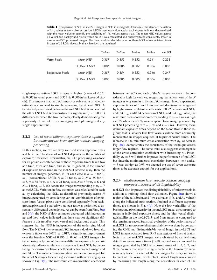
Table 1 Comparison of NSD in meLSCI images to NSD in averaged LSCI images. The standard deviationof 1/τ c values at every pixel across four LSCI images was calculated at each exposure time and normalizedwith the mean value to quantify the variability of 1/τ c values across trials. The mean NSD values acrossall vessel and background pixels within an ROI was calculated and observed to be consistently lower incase of meLSCI processed images. The mean and standard deviation of these NSD values obtained fromimages of 25 ROIs (five rat brains×five days) are tabulated.

T=1ms T=2ms T=4ms T=8ms meLSCI

Vessel Pixels Mean NSD 0.357 0.353 0.352 0.341 0.238

Std Dev of NSD 0.006 0.006 0.007 0.006 0.007

Background Pixels Mean NSD 0.357 0.354 0.353 0.346 0.247

Std Dev of NSD 0.005 0.005 0.005 0.006 0.007

single-exposure-time LSCI images is higher (mean of 0.351± 0.007 in vessel pixels and 0.353 ± 0.006 in background pix-els). This implies that meLSCI improves robustness of velocityestimation compared to simple averaging, by at least 30%. Atwo-tailed paired t-test between the meLSCI NSDs and each ofthe other LSCI NSDs demonstrated a significant (p < 0.0001)difference between the two methods, clearly demonstrating thesuperiority of meLSCI over averaging multiple images at anysingle exposure time.

3.2.3 Use of seven different exposure times is optimalfor multiexposure laser speckle contrast imagingprocessing

In this section, we explain why we used seven exposure timesand how the robustness of meLSCI depends on the number ofexposure times used. Toward this, meLSCI processing was donefor all possible combinations of these exposure times taken twoat a time, three at a time, and so on. In general, if the numberof exposure times used in the meLSCI scheme is nT, then thenumber of images generated, N, in each case is N = 7 for nT

= 1 (conventional LSCI), N = 21 for nT = 2, N = 35 for nT

= 3, N = 35 for nT = 4, N = 21 for nT = 5, N = 7 for nT = 6, andN = 1 for nT = 7. We denote the image corresponding to nT = 7as meLSCI7. Variation in flow estimates was calculated for eachnT by calculating the NSD, as described previously, across Nimages generated by considering various combinations of expo-sure times. Vessel pixels were considered separately from back-ground pixels, and a paired two-tailed t-test was performed to as-sess any differential dependence. As can be seen from Figs. 3(a)and 3(b), the NSD of flow estimates decreased with increasingnT, and the p values indicated that there was not significant dif-ference in this trend between vessel and background pixels. Thissuggests that the NSD is independent of the underlying bloodflow. The NSD of the seven meLSCI images calculated from sixexposure times was 0.075 ± 0.017, a significant improvementover the baseline NSD of 0.296 ± 0.067 in LSCI images ob-tained using only one of the seven different exposure times. Wealso analyzed how similar each image was to meLSCI7 by calcu-lating the cross-correlation coefficient between each image andmeLSCI7. The mean cross-correlation coefficient (averaged forthe set of N images for each nT) increased with increasing nT, asshown in Fig. 3(c). The maximum cross-correlation coefficient

between meLSCI7 and each of the N images was seen to be con-siderably high for each nT, suggesting that at least one of the Nimages is very similar to the meLSCI7 image. In our experiment,exposure times of 1 and 2 ms seemed dominant as suggestedby high cross-correlation coefficients of 0.92 between meLSCI7

and LSCI1ms and 0.84 between meLSCI7 and LSCI2ms. Also, themaximum cross-correlation corresponding to nT = 2 was as highas 0.99 when meLSCI7 was compared to an image generated bymeLSCI processing of T = 1 ms and T = 2 ms. However, thesedominant exposure times depend on the blood flow in those re-gions; that is, smaller low-flow vessels will be more accuratelyrepresented in images acquired at higher exposure times. Theincrease in the minimum cross-correlation with nT, as seen inFig. 3(c), demonstrates the robustness of the technique acrosslarger flow regimes. The same trend also suggests convergenceof the cross-correlation coefficient with increasing nT. Poten-tially, nT = 8 will further improve the performance of meLSCIbut since the minimum cross-correlation between nT = 6 and nT

= 7 was as high as 0.95, we deemed the use of seven exposuretimes to be accurate enough for our applications.

3.2.4 Multiexposure laser speckle contrast imagingimproves microvessel distinguishability

meLSCI also improves the distinguishability of microvessels inaddition to refining blood flow estimates. Figure 4(a) shows aregion of the rat’s brain, and flow estimates (1/τ c and Afit values)along the indicated cross section, obtained at different exposuretimes, are shown in Fig. 4(b). Note the low variability of thebackground pixel intensity in the meLSCI trace, as compared totraces at individual exposure times; and the high vessel distin-guishability in the meLSCI, 3- and 5-ms traces as compared tothe remaining traces. Statistical evaluation of the performance ofmeLSCI for microvessel distinguishability was done by compar-ing the CNR and distinguishable vessel length in meLSCI andLSCI images obtained from 3×3 mm regions of five rat brains.Note that the meLSCI images were obtained by curve-fittingdata from ten exposure times (1–10 ms) and were compared toimages generated by LSCI at exposure times of 1, 3, 5, 7, and9 ms. Vessels that were distinguishable to the human eye weremanually traced in each of the six images for every rat so asto paint all the vessel pixels black. Vessel length was countedby measuring the length along the centerlines in each of the

Journal of Biomedical Optics May 2011 � Vol. 16(5)056006-6

Rege et al.: Multiexposure laser speckle contrast imaging...

Fig. 3 Dependence of meLSCI images on the number of exposuretimes considered: (a,b) Dependence of the variation in flow estimateson the number of exposure times used in the meLSCI scheme. Themean and standard deviations have been calculated for data from fiverats on five imaging days (25 cases in all). For each case, variation wascalculated across all N images generated; that is, if number of exposuretimes used for meLSCI processing is denoted by nT, then for nT = 1,N = 7 (baseline LSCI); nT = 2, N = 21; nT = 3, N = 35; nT = 4, N= 35; nT = 5, N = 21; and for nT = 6, N = 7. Variation was calculatedas normalized standard deviation of Afit (1/τ c) values for every pixelacross the N images. Results are shown differently for (a) vessel pixelsand(b) background pixels though the variations in the two cases arevery similar (p values of paired two-tailed t-tests between vessel andbackground pixels are indicated in (b). (c) The graph shows the cross-correlation between meLSCI images obtained at various values of nTwith the image obtained at n(T) = 7. The cross-correlation was calcu-lated for each of the N images generated at each value of nT and mean,maximum, and minimum cross-correlation across the N images wasplotted for each nT. Note that while the maximum cross-correlation isvery close to 1 even with nT = 2, suggesting two dominant exposuretimes, the minimum cross-correlation improves significantly suggestingthat the robustness of meLSCI improves with increasing nT.

manual traces (obtained by a binary skeletonization operation inMATLAB) as a metric for vessel distinguishability. As shownin Fig. 4(c), we consistently observed an increase in distin-guishable vessel length with increasing exposure time. meLSCIwas often better at distinguishing vessels than single-exposure

Fig. 4 Distinguishability of microvessels using meLSCI technique:(a) An image of the rat brain brain vasculature obtained using meLSCItechnique (using 10 exposure times, 1–10 ms). Afit values, indicativeof blood velocity, are depicted in color. (b) Pixel intensities along thecross-section X-Y indicated in (a) as obtained by LSCI at various expo-sure times. Vessels are marked by numbers 1–9 and three significantbackground regions are marked by A, B, and C. Note the high back-ground variation in the traces of 1–9 ms, as compared to the meLSCItrace. (c) The total length of distinguishable blood vessels was esti-mated in single-exposure LSCI and meLSCI images of 3×3 mm regionsof five rat brains. The total vessel length is plotted relative to the vessellength extracted from the image at an exposure time of 1 ms. The dis-tinguishability of vessels increased with exposure time and was highestfor meLSCI images (plotted randomly at exposure time of 6 ms). (d,e)The CNRs of the images were analyzed and revealed that meLSCI re-sulted in a higher CNR than even the optimally recommended rangeof 3–5 ms for rat brain imaging. The increase in CNR can be primarilyattributed to the low variability in the background signal.

LSCI. Statistical analysis revealed that meLSCI resolved moremicrovessels, that is, more vessel length, than LSCI1ms by a fac-tor of 1.53 ± 0.18 and LSCI5ms by a factor of 1.12 ± 0.08. Asexpected, this difference was attributable to the identification ofmicrovessels, <20 μm diam (<3 pixels wide) as opposed to thelarger vessels. CNR was calculated as follows:

CNR = μvessel − μbackground

σbackground, (5)

where μvessel and μbackground are means of vessels and back-ground, respectively, and σ background is the variation in the back-ground tissue (noise). While it is the convention to consider thecontribution of noise in the vessel regions, for this analysis we

Journal of Biomedical Optics May 2011 � Vol. 16(5)056006-7

Rege et al.: Multiexposure laser speckle contrast imaging...

Fig. 5 Use of meLSCI for imaging the microvascular environment during wound healing in a mouse ear injury model: (a–c) The top panel showssequentially obtained meLSCI images of the mouse ear vasculature of the day of wounding, and three and five days after wounding. Note thatthe meLSCI scheme provides the contrast necessary to image the changes associated with neovascularization. (d–i) The middle panel shows highmagnification views of the boxed region in (c), obtained using LSCI at single-exposure times and using meLSCI. 1/τ c values have been depicted inpseudocolor. meLSCI can be clearly seen to have a higher contrast-to-noise ratio in proximal angiogenic regions by comparing (i) with (d–h). (j–n)The bottom panel shows equivalent high magnification views of the boxed region in (c), as they appear when the speckle contrast K is displayedin grayscale. Note that images (j–n) have been linearly and uniformly scaled for better print reproduction. Scale bar shown in (a) corresponds to0.5 mm.

were unable to do so because it was not possible to separatenoise from the vessel signal. Additionally, because the varianceof vessel pixel intensities is proportional to the blood flow, theCNRs reported in Figs. 4(d) and 4(e) were computed accordingto Eq. (5). It can be seen that CNR for meLSCI (4.63 ± 0.86)was higher than that for the recommended exposure time of 5 ms(4.06 ± 0.61).

3.3 Imaging of Vascular Microenvironment duringWound Healing in Mouse Ear UsingMultiexposure Laser Speckle Contrast Imaging

The advantage of meLSCI is that it can achieve better vesseldistinguishability at a high CNR, while providing more robustblood-flow measurements. To demonstrate the advantages ofmeLSCI, we employed it to image the microvascular changesthat accompany wound healing in an injured mouse ear model.Figure 5 shows sequential images of the region proximal tothe wound, obtained on the day of wounding, three days afterwounding, and five days after wounding. The wound causes aninterruption in blood supply from two major vessels, causing the

region downstream of the wound to receive limited blood flowthrough collateral circulation, as can be seen in the day 0 image.Extensive changes in vascularization and blood-flow redistribu-tion were witnessed on days 3 and 5, and could be resolvedwith high CNR using meLSCI. Figures 5(d)–5(i) illustrate high-magnification views of the neovascularized regions obtained atdifferent exposure times. Figures 5(j)–5(n) show comparativemonochrome images of the same vascular microenvironment,as resolved traditionally through plotting the speckle contrastK, calculated using Eq. (3). It is apparent that meLSCI is ableto resolve these microvessels with higher CNR than any of thecontributing single-exposure-time images. CNR was calculatedfor this region, as described previously, and was found to be2.28 as compared to a CNR of 1.80, which was best amongall the LSCI images generated using single exposure times. Forstatistical analysis, we identified angiogenic regions in eighthealing mice and compared the CNR values in these regions asimaged at single exposure times and using meLSCI. Table 2 liststhe obtained mean CNR values, along with standard deviation,clearly indicating that meLSCI provides a 41% improvement inCNR in the region proximal to the wound. A two-tailed paired

Journal of Biomedical Optics May 2011 � Vol. 16(5)056006-8

Rege et al.: Multiexposure laser speckle contrast imaging...

Table 2 CNR for angiogenic regions in mouse ear model of wound healing. Angiogenic regions wereidentified in the region proximal to the wound in eight mice, and the CNR was determined for each ofthese identified regions, obtained at single-exposure times and using meLSCI. A two-tailed paired t-testwas performed to determine whether the CNR values of meLSCI images were different from the CNRvalues of single-exposure-time LSCI images with statistical significance.

Exp 07ms 10ms 13ms 16ms 19ms 22ms 25ms meLSCI

Mean CNR 1.79 1.96 2.09 2.12 1.95 1.98 1.98 2.99

Std Dev 0.57 0.62 0.63 0.66 0.93 0.97 0.98 0.77

p value 0.0035 0.0107 0.0236 0.0288 0.0366 0.0366 0.0385

t-test demonstrated a significant difference (highest p = 0.0385)between the CNR values of meLSCI and every single-exposure-time LSCI image. This demonstrates the suitability of meLSCIfor longitudinal monitoring of angiogenesis induced changes inthe microvascular architecture and function.

4 Discussion and ConclusionsIn this paper, we report a novel processing scheme, meLSCI,and demonstrate its use in vivo. meLSCI combines the highsensitivity of LSCI at low exposure times with higher vesseldistinguishability possible with LSCI at high exposure times.In doing so, meLSCI produces blood-flow estimates that aremore robust than estimates obtained from LSCI by simple aver-aging. We used pixelwise curve fitting to generate high spatialresolution images of vasculature in animal models of normaland pathological vasculature. We evaluated the robustness ofthe meLSCI technique in vivo and demonstrated that the vari-ability in blood-flow estimates across multiple trials decreasedby at least 30%. Vessel distinguishability was also at least ashigh as in the largest exposure time used, but the higher CNRof meLSCI images, especially in regions with high microvesseldensity, makes a strong case for its use in vascular imaging.

Wound healing is accompanied by angiogenesis and is there-fore an excellent model of vasculature undergoing remodeling.Imaging these microvascular changes is not trivial, especiallydue to the small size and low flow through angiogenic vessels.However, meLSCI was successfully able to capture the changesassociated with this biological phenomenon. In the region prox-imal to the wound, meLSCI provided a 41% improvement inCNR over LSCI. This improvement in imaging specific regionswas not accurately represented in our overall CNR analysis inrat brain vasculature, and hence, CNR in meLSCI images of ratbrain seemed to improve only marginally. Thus, one could saythat while the CNR in meLSCI images is at least as good as thebest CNR of single-exposure LSCI images, meLSCI offered aclear advantage in imaging microvessels, <20 μm in diameter.

meLSCI is a processing scheme, wherein LSCI imagesobtained at multiple exposures are combined to generate aparametrized image. However, the choice of exposure times aswell as the number of exposure times that contribute to meLSCIis variable. It can be argued that meLSCI using only two expo-sure time (meLSCI2) with an accurate choice of both exposuretimes can produce fairly robust estimates that correlate well withmeLSCI at seven exposure times (meLSCI7). However, choice

of these two exposure times is not obvious and will dependheavily on the region of interest. For example, in the angiogenicregions where most of the vessels are small in size with low flow,meLSCI2 would be best at exposure times of 22 and 25 ms, butnot in a region that has higher flow vessels. We used seven ex-posure times in most of our meLSCI estimations because thecross-correlation coefficient between meLSCI6 and meLSCI7

was 0.99, but more importantly, a minimum as high as 0.95.In our implementation of the meLSCI technique, we have

assumed that the speed of scatterers contributing to the specklesignal follows Lorentzian statistics. As pointed out by Duncanand Kirkpatrick,21 a complete and precise treatment would re-quire that both Lorentzian statistics (for random motion) andGaussian statistics (for organized motion) be appropriately in-corporated into the speckle equation [Eq. (2)]. Our scheme,meLSCI, can be modified to use revised equations as well. Weexpect the results to be fairly model invariant, as suggestedby our observation that replacing Eq. (2) by the widely usedequation proposed by Fercher and Briers23 changed our resultsvery marginally without affecting our conclusions. Similarly,recent work has also pointed out anomalies in the classically ac-cepted linear relationship between blood velocity and parameter1/τ c. Ramirez-San-Juan et al. present a detailed understandingof relationship between blood velocity and speckle statistics.25

The equations used in the meLSCI technique can continuallybe refined with the advent of more precise models. We havedemonstrated that the combination of multiple images acquiredat different exposure times improves the robustness of flow es-timates and contrast-to-noise ratios in vivo.

The robustness offered by the meLSCI technique should en-able comparison of blood-flow estimates over multiple days ofimaging with reduced errors due to imaging and sample prepa-ration. However, it is not possible to demonstrate this in vivobecause the physiological state of the animal cannot be elimi-nated as a source of variability. Despite our best standardizationefforts, factors unrelated to imaging, such as degree of anesthe-sia or trauma, may cause the baseline blood flow to vary. Weimaged the same rats on multiple days and observed a slightdecrease in variability of the flow estimates across days usingmeLSCI. Although this difference was not statistically signifi-cant, ensuring an identical physiological state for each animalduring imaging is challenging.

A potential drawback of meLSCI is the additional time nec-essary for image acquisition. We used a processing scheme thatacquired 80 frames at seven exposure times, or 560 frames at

Journal of Biomedical Optics May 2011 � Vol. 16(5)056006-9

Rege et al.: Multiexposure laser speckle contrast imaging...

∼10 fps (as supported by our camera). Thus, acquiring datarequired for generation of each meLSCI image took ∼60 s.Therefore, although meLSCI is suitable for longitudinal mon-itoring, it lacks the temporal resolution necessary for imagingrapid changes in blood flow. Also, rapid changes/fluctuations inblood flow will adversely affect the flow estimated by meLSCIbecause it inherently assumes that blood flow is constant duringthe acquisition of multiple-exposure data. The temporal reso-lution could be improved by increasing the image acquisitionspeed by imaging smaller regions or considering the use of fewerimage frames for speckle contrast processing. However, in boththese cases, the temporal resolution would come at the expenseof spatial resolution.

LSCI enjoys inherent advantages for vascular imaging in thatblood flow can be imaged at a high spatial resolution withoutthe need for an exogenous contrast agent. The meLSCI ap-proach improves the contrast-to-noise ratio further and providesmore reliable flow estimates, enabling sequential longitudinalmonitoring of the vascular microenvironment. We foresee anapplication of meLSCI in understanding vascular reactivity atthe “micro” level and elucidating the physiology of angiogenesisin a variety of disease states such as tumors or retinopathies.

AcknowledgmentsThis work was supported jointly by National Institute of AgingGrant No. R01AG029681 and Department of Health and HumanServices Grant No 1R43CA139983-01. The authors also thankNicole Benoit, Peng Miao, and Dan Schlattman for their helpwith experimental preparation and Mohit Kumar Jolly for hishelp with preliminary in vitro experimentation.

References1. A. K. Dunn, H. Bolay, M. A. Moskowitz, and D. A. Boas, “Dynamic

imaging of cerebral blood flow using laser speckle,” J. Cereb. BloodFlow Metab. 21(3), 195–201 (2001).

2. J. S. Paul, A. R. Luft, E. Yew, and F.-S. Sheu, “Imaging the developmentof an ischemic core following photochemically induced cortical infarc-tion in rats using laser speckle contrast analysis (LASCA),” Neuroimage29(1), 38–45 (2006).

3. V. Kalchenko, D. Preise, M. Bayewitch, I. Fine, K. Burd, andA. Harmelin, “In vivo dynamic light scattering microscopy of tumourblood vessels,” J. Microsc. 228(2), 118–122 (2007).

4. D. A. Boas and A. K. Dunn, “Laser speckle contrast imaging in biomed-ical optics,” J. Biomed. Opt. 15(1), 011109 (2010).

5. P. B. Jones, H. K. Shin, D. A. Boas, B. T. Hyman, M. A. Moskowitz,C. Ayata, and A. K. Dunn, “Simultaneous multispectral reflectanceimaging and laser speckle flowmetry of cerebral blood flow and oxygenmetabolism in focal cerebral ischemia,” J. Biomed. Opt. 13(4), 044007(2008).

6. N. Li, X. Jia, K. Murari, R. Parlapalli, A. Rege, and N. V. Thakor,“High spatiotemporal resolution imaging of the neurovascular responseto electrical stimulation of rat peripheral trigeminal nerve as revealedby in vivo temporal laser speckle contrast,” J. Neurosci. Meth. 176(2),230–236 (2009).

7. P. Miao, N. Li, A. Rege, S. Tong and N. Thakor, “Model based recon-struction for simultaneously imaging cerebral blood flow and de-oxygenhemoglobin distribution,” in Proc. 31st Ann. Int. Conf. of IEEE Engr.Med. Biol. Soc. (EMBC), pp. 3236–3293 (2009).

8. M. Li, P. Miao, J. Yu, Y. Qiu, Y. Zhu, and S. Tong, “Influences ofhypothermia on the cortical blood supply by laser speckle imaging,”IEEE Trans. Neur. Sys. Rehab. Eng. 17(2), 128–134 (2009).

9. J. Folkman, “Tumor angiogenesis: therapeutic implications,” N. Eng. J.Med. 285(21), 1182–1186 (1971).

10. P. Carmeliet and R. K. Jain, “Angiogenesis in cancer and other diseases,”Nature 407(6801), 249–257 (2000).

11. N. N. Nissen, P. J. Polverini, A. E. Koch, M. V. Volin, R. L. Gamelli, andL. A. DiPietro, “Vascular endothelial growth factor mediates angiogenicactivity during the proliferative phase of wound healing,” Am. J. Pathol.152(6), 1445–1452 (1998).

12. A. P. Pathak, W. E. Hochfeld, S. L. Goodman, and M. S. Pepper, “Cir-culating and imaging markers for angiogenesis,” Angiogenesis 11(4),321–335 (2008).

13. K. Murari, N. Li, A. Rege, X. Jia, A. All, and N. V. Thakor, “Contrast-enhanced imaging of cerebral vasculature with laser speckle,” Appl.Opt. 46(22), 5340–5346 (2007)

14. C. J. Stewart, C. L. Gallant-Behm, K. Forrester, J. Tulip, D. A. Hart, andR. C. Bray, “Kinetics of blood flow during healing of excisional full-thickness skin wounds in pigs as monitored by laser speckle perfusionimaging,” Skin Res. Tech. 12(4), 247–253 (2006).

15. M. Le Thinh, J. S. Paul, H. Al-Nashash, A. Tan, A. R. Luft, F. S. Sheu,and S. H. Ong, “New insights into image processing of cortical bloodflow monitors using laser speckle imaging,” IEEE Trans. Med. Imag.26(6), 833–842 (2007).

16. A. B. Parthasarathy, W. J. Tom, A. Gopal, X. Zhang, and A. K. Dunn,“Robust flow measurement with multi-exposure speckle imaging,” Opt.Exp. 16(3), 1975–1989 (2008).

17. A. B. Parthasarathy, A. Ponticorvo, S. M. S. Kazmi, and A. K. Dunn,“Quantitative cerebral blood flow measurement through thinned skullwith multi exposure speckle imaging,” in Frontiers in Optics, p. FME2,Optical Society of America (2009).

18. S. Yuan, A. Devor, D. A. Boas, and A. K. Dunn, “Determination ofoptimal exposure time for imaging of blood flow changes with laserspeckle contrast imaging,” Appl. Opt. 44(10), 1823–1830 (2005).

19. A. B. Parthasarathy, S. M. S. Kazmi, and A. K. Dunn, “Quantitativeimaging of ischemic stroke through thinned skull in mice with multiex-posure speckle imaging,” Biomed. Opt. Exp. 1(1), 246–259 (2010).

20. C. Ayata, A. K. Dunn, O. Y. Gursoy, Z. Huang, D. A. Boas, and M. A.Moskowitz, “Laser speckle flowmetry for the study of cerebrovascularphysiology in normal and ischemic mouse cortex,” J. Cereb. Blood FlowMetab. 24(7), 744–755. (2004).

21. D. D. Duncan and S. J. Kirkpatrick, “Can laser speckle flowmetry bemade a quantitative tool?,” J. Opt. Soc. Am. A 25(8), 2088–2094 (2008).

22. R. Bandyopadhyay, A. Gittings, S. Suh, P. Dixon, and D. Durian,“Speckle-visibility spectroscopy: a tool to study time-varying dynam-ics,” Rev. Sci. Instrum. 76(9), 0931101–0931111 (2005).

23. A. R. Fercher and J. D. Briers, “Flow visualization by means of single-exposure speckle photography,” Opt. Commun. 37(5), 326–330 (1981).

24. M. Le Thinh, J. S. Paul, and S. H. Ong, “Laser speckle imaging forblood flow analysis,” Computational Biology, pp. 243–271 (2009).

25. J. C. Ramirez-San-Juan, R. Ramos-Garcı́a, I. Guizar-Iturbide,G. Martı́nez-Niconoff, and B. Choi, “Impact of velocity distributionassumption on simplified laser speckle imaging equation,” Opt. Exp.16(5), 3197–3203 (2008).

26. S. J. Kirkpatrick, D. D. Duncan, and E. M. Wells-Gray, “Detrimentaleffects of speckle-pixel size matching in laser speckle contrast imaging,”Opt. Lett. 33(24), 2886–2888 (2008).

27. H. Sorg, T. Schulz, C. Krueger, and B. Vollmar, “Consequences of sur-gical stress on the kinetics of skin wound healing: partial hepatectomydelays and functionally alters dermal repair,” Wound Repair Regen.17(3), 367–377 (2009).

28. J. H. Barker, D. Kjolseth, M. Kim, J. Frank, I. Bondar, E. Uhl,M. Kamler, K. Messmer, G. R. Tobin, and L. J. Weiner, “The hairlessmouse ear: an in vivo model for studying wound neovascularization,”Wound Repair Regen. 2(2), 138–143 (1994).

Journal of Biomedical Optics May 2011 � Vol. 16(5)056006-10