Proceedings of the 4th International Conference on

NOn-LInear Speech Processing

NOLISP 2007

Mai 22-25, 2007. Paris, France

Sponsored by:

• ISCA International Speech Communication Association

• EURASIP European Association for Signal Processing

• IEEE Institute of Electrical and Electronics Engineers

• HINDAWI Publishing corporation

Committees

Scientic Committee

Frédéric BIMBOT IRISA, Rennes (France)Mohamed CHETOUANI UPMC, Paris (France)Gérard CHOLLET ENST, Paris (France)Tariq DURRANI University of Strathclyde, Glasgow (UK)Marcos FAÚNDEZ-ZANUY EUPMt, Barcelona (Spain)Bruno GAS UPMC, Paris (France)Hynek HERMANSKY OGI, Portland (USA)Amir HUSSAIN University of Stirling, Scotland (UK)Eric KELLER University of Lausanne (Switzerland)Bastiaan KLEIJN KTH, Stockholm (Sweden)Gernot KUBIN TUG, Graz (Austria)Petros MARAGOS Nat. Tech. Univ. of Athens (Greece)Stephen Mc LAUGHLIN University of Edimburgh (UK)Kuldip PALIWAL University of Brisbane (Australia)Bojan PETEK University of Ljubljana (Slovenia)Jean ROUAT University of Sherbrooke (Canada)Jean SCHOENTGEN Univ. Libre Bruxelles (Belgium)Isabel TRANCOSO INESC (Portugal)

Organizing Committee

Mohamed CHETOUANI UPMC, Paris (FRANCE)Bruno GAS UPMC, Paris (FRANCE)Amir HUSSAIN University of Stirling, Scotland (UK)Maurice MILGRAM UPMC, Paris (FRANCE)Jean-Luc ZARADER UPMC, Paris (FRANCE)

2

Foreword

After the success of NOLISP'03, NOLISP'04 summer school and NOLISP'05, we are pleased to present NOLISP'07.The fourth event in a series of events related to Non-linear speech processing.

Many specics of the speech signal are not well addressed by conventional models currently used in the eld ofspeech processing. The purpose of NOLISP is to present and discuss novel ideas, work and results related to alter-native techniques for speech processing, which depart from mainstream approach.

With this intention in mind, we provide an open forum for discussion. ALternate approaches are appreciated,although the results achieved at present may not clearly surpass results based on stat-of-the-art methods.

Please, try to establish as many contacts with your colleagues and discussions as possible: these small-size work-shops make it feasible. Please, enjoy the workshop; enjoy the city, and the french meals and drinks.

We want to acknowledge our colleagues for their help and the reviewers for their very exhaustive reviews.

Best wishes for NOLISP

Mohamed ChetouaniBruno Gas

Jean-Luc zarader

3

Contents

Program committee 2

Foreword 3

HMM-based Spanish speech synthesis using CBR as F0 estimator,

Xavi Gonzalvo, Ignasi Iriondo, Joan Claudi Socoró, Francesc Alías, Carlos Monzo 6

A Wavelet-Based Technique Towards a More Natural Sounding Synthesized Speech,

Mehmet Atas, Suleyman Baykut, Tayfun Akgul 11

Objective and Subjective Evaluation of an Expressive Speech Corpus,

Ignasi Iriondo, Santiago Planet, Joan Claudi Socoró, Francesc Alías 15

On the Usefulness of Linear and Nonlinear Prediction Residual Signals for Speaker Recognition,

Marcos Faundez-Zanuy 19

Multi lter bank approach for speaker verication based on genetic algorithm,

Christophe Charbuillet, Bruno Gas, Mohamed Chetouani, Jean Luc Zarader 23

Speaker Recognition Via Nonlinear Discriminant Features,

Lara Stoll, Joe Frankel, Nikki Mirghafori 27

Bispectrum Mel-frequency Cepstrum Coecients for Robust Speaker Identication,

Ufuk Ulug, Tolga Esat Ozkurt, Tayfun Akgul 31

Perceptron-based Class Verication,

Michael Gerber, Tobias Kaufmann, Beat Pster 35

Manifold Learning-based Feature Transformation for Phone Classication,

Andrew Errity, John McKenna, Barry Kirkpatrick 39

Word Recognition with a Hierarchical Neural Network,

Xavier Domont, Martin Heckmann, Heiko Wersing, Frank Joublin, Stefan Menzel, BernhardSendho, Christian Goerick 43

Discriminative Keyword Spotting,

Joseph Keshet, David Grangier, Samy Bengio 47

Hybrid models for automatic speech recognition: a comparison of classical ANN and kernel based

methods,

Ana I. García-Moral, Rubén Solera-Ureña, Carmen Peláez-Moreno, Fernando Díaz-de-María 51

4

Towards phonetically-driven hidden Markov models: Can we incoporate phonetic landmarks in

HMM-based ASR?,

Guillaume Gravier, Daniel Moraru 55

A hybrid Genetic-Neural Front-End Extension for Robust Speech Recognition over Telephone

Lines,

Sid-Ahmed Selouani, Habib Hamam, Douglas O'Shaughnessy 59

Estimating the stability and dispersion of the biometric glottal ngerprint in continuous speech,

Pedro Gómez-Vilda, Agustín Álvarez-Marquina, Luis Miguel Mazaira-Fernández, RobertoFernández-Baillo, Victoria Rodellar-Biarge 63

Trajectory Mixture Density Networks with Multiple Mixtures for Acoustic-Articulatory Inver-

sion,

Korin Richmond 67

Application of Feature Subset Selection based on Evolutionary Algorithms for Automatic Emotion

Recognition in Speech,

Aitor Álvarez, Idoia Cearreta, Juan Miguel López, Andoni Arruti, Elena Lazkano, BasilioSierra, Nestor Garay 71

Non-stationary self-consistent acoustic objects as atoms of voiced speech,

Friedhelm R. Drepper 75

The Hartley Phase Cepstrum as a Tool for Signal Analysis,

I. Paraskevas, E. Chilton, M. Rangoussi 80

Quantitative perceptual separation of two kinds of degradation,

Anis Ben Aicha, Soa Ben Jebara 84

Threshold Reduction for Improving Sparse Coding Shrinkage Performance in Speech Enhance-

ment,

Neda Faraji, Seyed Mohammad Ahadi, Seyedeh Saloomeh Shariati 88

Ecient Viterbi algorithms for lexical tree based models,

Salvador España-Boquera, María José Castro-Bleda, Francisco Zamora-Martínez, Jorge Gorbe-Moya 92

Acoustic Units Selection in Chinese-English Bilingual Speech Recognition,

Lin Yang, Jianping Zhang, Yonghong Yan 96

Tone Recognition In Mandarin Spontaneous Speech,

Zhaojie Liu, Pengyuan Zhang, Jian Shao, Qingwei Zhao, Yonghong Yan, Ji Feng 100

Evaluation of a Feature Selection Scheme on ICA-based Filter- Bank for Speech Recognition,

Neda Faraji, Seyyed Mohammad Ahadi 104

A Robust Endpoint Detection Algorithm Based on Identication of the Noise Nature,

Denilson Silva 108

EMD Analysis of Speech Signal in Voiced Mode,

Aïcha Bouzid, Noureddine Ellouze 112

5

Estimation of Speech Features of Glottal Excitation by Nonlinear Prediction,

Karl Schnell, Arild Lacroix 116

An ecient VAD based on a Generalized Gaussian PDF,

Oscar Pernía, Juan M. Górriz, Javier Ramírez, Carlos Puntonet, Ignacio Turias 120

Index of authors 124

6

HMM-based Spanish speech synthesis using CBR as F0 estimator

Xavi Gonzalvo, Ignasi Iriondo, Joan Claudi Socoro, Francesc Alıas, Carlos Monzo

Department of Communications and Signal TheoryEnginyeria i Arquitectura La Salle, Ramon Llull University, Barcelona, Spain

gonzalvo,iriondo,jclaudi,falias,cmonzo@salle.url.edu

AbstractHidden Markov Models based text-to-speech (HMM-TTS) syn-thesis is a technique for generating speech from trained statisti-cal models where spectrum, pitch and durations of basic speechunits are modelled altogether. The aim of this work is to de-scribe a Spanish HMM-TTS system using CBR as a F0 esti-mator, analysing its performance objectively and subjectively.The experiments have been conducted on a reliable labelledspeech corpus, whose units have been clustered using contex-tual factors according to the Spanish language. The resultsshow that the CBR-based F0 estimation is capable of improvingthe HMM-based baseline performance when synthesizing non-declarative short sentences and reduced contextual informationis available.

1. IntroductionOne of the main interest in TTS synthesis is to improve qualityand naturalness in applications for general purposes. Concate-native speech synthesis for limited domain (e.g. Virtual Weatherman [1]) presents drawbacks when trying to use in a differentdomain. New recordings have the disadvantage of being timeconsuming and expensive (i.e. labelling, processing differentaudio levels, texts designs, etc.).

In contrast, the main benefit of HMM-TTS is the capabil-ity of modelling voices in order to synthesize different speakerfeatures, styles and emotions. Moreover, voice transforma-tion through concatenative speech synthesis still requires largedatabases in contrast to HMM which can obtain better resultswith smaller databases [2]. Some interesting voice transfor-mation approaches using HMM were presented using speakerinterpolation [3] or eigenvoices [4]. Furthermore, HMM forspeech synthesis could be used in new systems able to unifyboth approaches and to take advantage of their properties [5].

Language is another important topic when designing a TTSsystem. HMM-TTS scheme based on contextual factors forclustering can be used for any language (e.g. English [6] orPortuguese [7]). Phonemes (the basic synthesis units) and theircontext attributes-values pairs (e.g. number of syllables inword, stress and accents, utterance types, etc.) are the maininformation which changes from one language to another. Thiswork presents contextual factors adapted for Spanish.

The HMM-TTS system presented in this work is based ona source-filter model approach to generate speech directly fromHMM itself. It uses a decision tree based on context cluster-ing in order to improve models training and able to characterizephoneme units introducing a counterpart approach with respectto English [6]. As the HMM-TTS system is a complete tech-nique to generate speech, this work presents objective results tomeasure its performance as a prosody estimator and subjectivemeasures to test the synthesized speech. It is compared with a

tested Machine Learning strategy based on case based reason-ing (CBR) for prosody estimation [8].

This paper is organized as follows: Section 2 describesHMM system workflow and parameter training and synthesis.Section 3 concerns to CBR for prosody estimation. Section 4describes decision tree clustering based on contextual factors.Section 5 presents measures, section 6 discusses results and sec-tion 7 presents the concluding remarks and future work.

2. HMM-TTS system2.1. Training system workflow

As in any HMM-TTS system, two stages are distinguished:training and synthesis. Figure 1 depicts the classical trainingworkflow. Each HMM represents a contextual phoneme. First,HMM for isolated phonemes are estimated and each of thesemodels are used as a initialization of the contextual phonemes.Then, similar phonemes are clustered by means of a decisiontree using contextual information and designed questions (e.g.Is right an ’a’ vowel? Is left context an unvoiced consonant?Is phoneme in the 3rd position of the syllables? etc.). Thanksto this process, if a contextual phoneme does not have a HMMrepresentation (not present in the training data, but in the test),decision tree clusters will generate the unseen model.

Context Label

Parameter generation

HMMs

MLSA

Text to synthesize Excitation

generation CBR

Model

Synthetic speech

Parameter analysis

Speech corpus

HMM Training

HMMs Context

clustering

Figure 1: Training workflow

Each contextual phoneme HMM definition includes spec-trum, F0 and state durations. Topology used is a 5 states left-to-right with no-skips. Each state is represented with 2 inde-pendent streams, one for spectrum and another for pitch. Bothtypes of information are completed with their delta and delta-delta coefficients.

Spectrum is modelled by 13th order mel-cepstral coeffi-cients which can generate speech with MLSA filter [9]. Spec-trum model is a multivariate Gaussian distributions [2].

Spanish corpus has been pitch marked using the approachdescribed in [10]. This algorithm refines mark-up to get asmoothed F0 contour in order to reduce discontinuities in thegenerated curve for synthesis. The model is a multi-space prob-ability distribution [2] that may be used in order to store contin-uous logarithmic values of the F0 curve and a discrete indicatorfor voiced/unvoiced.

State durations of each HMM are modelled by a Multivari-ate Gaussian distribution [11]. Its dimensionality is equal to thenumber of states in the corresponding HMM.7

2.2. Synthesis process

Figure 2 shows synthesis workflow. Once the system has beentrained, it has a set of phonemes represented by contextual fac-tor (each contextual phoneme is a HMM). The first step in thesynthesis stage is devoted to produce a complete contextualizedlist of phonemes from a text to be synthesized. Chosen units areconverted into a sequence of HMM.

Context Label

Parameter generation

HMMs

MLSA

Text to synthesize Excitation

generation CBR

Model

Synthetic speech

Parameter analysis

Speech corpus

HMM Training

HMMs Context

clustering

Figure 2: Synthesis workflow

Using the algorithm proposed by Fukada in [9], spectrumand F0 parameters are generated from HMM models using dy-namic features. Duration is also estimated to maximize theprobability of state durations. Excitation signal is generatedfrom the F0 curve and the voiced and unvoiced information. Fi-nally, in order to reconstruct speech, the system uses spectrumparameters as the MLSA filter coefficients and excitation as thefiltered signal.

3. CBR system3.1. CBR and HMM-TTS system description

As shown in figure 2, CBR system for prosody estimator can beincluded as a module in any TTS system (i.e. excitation signalcan be created using either HMM or CBR). In a previous workit is demonstrated that using CBR approach is appropriate tocreate prosody even with expressive speech [8]. Despite CBRstrategy was originally designed for retrieving mean phonemeinformation related to F0, energy and duration, this work onlycompares the F0 results with the HMM based F0 estimator.

Figure 3 shows the diagram of this system. It is a corpus ori-ented method for the quantitative modelling of prosody. Anal-ysis of texts is carried out by SinLib library [12], an engine de-veloped to Spanish text analysis. Characteristics extracted fromthe text are used to build prosody cases.

density for each HMM is equal to the number of states in the corresponding HMM.

2.3. Synthesis process

Once the system has been trained, it has a set of units represented by contextual factors. During the synthesis process, first the input text must be labeled into contextual factors to choose the best synthesis units.

Chosen units in the sentence are converted in a sequence of HMM. Duration is estimated to maximize the probability of state durations. HMM parameters are spectrum and pitch with their delta and delta-delta coefficients. These parameters are extracted form HMM using the algorithm proposed by [11].

Figure 3: Time differences reproducing speech with and

without dynamic features.

Finally spectrum parameters are the filter coefficients of MLSA that will filter an excitation signal made by the estimated pitch. The standard excitation model with delta for voiced and white noise for unvoiced frames was used.

3. CBR system

3.1. System description

As shown in figures 2, CBR [15] system works as a prosody estimator which can be included as a new module in any TTS system. The retrieval objective is to map the solution from case memory to the new problem.

Figure 4: CBR Training workflow

Figure 3 shows how this system is based on the analysis of

labeled texts from which the system extracts prosodic attributes. Thus, it is a corpus oriented method for the quantitative modeling of prosody. It was originally designed for pitch, energy and duration but this work only uses the pitch estimation.

There exist various kinds of factors which can characterize each intonational unit. The system described here will basically use accent group (AG), related to speech rhythm and intonation group (IG). Some of the factors to consider are related with the kind of IG that belongs to the AG, position of IG in the phrase and the number of syllables of IG and AG. Curve intonation for each AG is modeled by polynomials.

3.2. Training and retrieval

CBR is a machine learning system which let an easy treatment of attributes from different kinds. The system training can be seen as a two stages flow: selection and adaptation. Case reduction is reaches thanks to grouping similar attributes. Once the case memory is created and a new set of attributes arrives, the system looks for the most similar stored example. Pitch curve is estimated by firstly estimating phoneme durations, normalizing temporal axis and associating each phoneme pitch depending on the retrieved polynomial.

4. Unit Selection This work presents a clustering based scheme [12] in order to choose the best unit model. As described next subsections, there are many contextual factors which can be used to characterize synthesis units. Therefore, the more contextual factors used, the more units extracted from the utterances. As the system is based on statistical models, parameters cannot be estimated with limited train data. As done in speech recognition systems, a decision tree technique is used to cluster similar state units. Unseen units’ model states will be clustered in the best estimated group. Spectrum, f0 or durations are clustered independently as they are affected by different factors.

Systems working with HMMs can be considered as multilingual as far as the contextual factors used are language dependent. Moreover, the system needs the design of a set of questions in order to choose the best clustering for each unit. These questions were extended to each Spanish unit and their specific characteristic. In table 1, units are classified in two groups: consonants and vowels.

Table 1: Spanish units.

Vowel frontal, back, Half open, Open, Closed a,ax,e,ex,i,ix,o,ox,u,ux

Consonant dental, velar, bilabial, alveolar, palatal, labio dental, Interdental, Prepalatal, plosive, nasal, fricative,lateral, Rhotic

zx,sx,rx,bx,k,gx, dx,s,n,r,j,l,m,t,tx,w,p,

f,x,lx,nx,cx,jx,b,d,mx,g

All languages have their own characteristics. This work

presents a performance comparison between standard utterance features and Spanish specific attributes extracted.

4.1. Festival Utterance features for Spanish

As used for other languages, these attributes affect phonemes, syllables, words, phrases and utterances (Table 2). Notice that most of them relates to units position in reference to over-units (e.g. phonemes over syllables or words over phrases). Features were extracted from a modified Spanish Festival voice [14].

Phonemes preceding, current, nextPhoneme Position of phoneme in syllable Syllables preceding, current, nextstressed preceding, current, next

Words preceding, current, nextPOS preceding, current, next Number of syllables Number of words in relation with phrase

Speech corpus

Parameters extraction CBR training CBR

Model

Texts Attribute-value extraction

Figure 3: CBR Training workflow

Each file of the corpus is analysed in order to convert it intonew cases (i.e. a set of attribute-value pairs). The goal is toobtain the solution from the memory of cases that best matchesthe new problem. When a new text is entered and converted in aset of attribute-value pairs, CBR will look for the best cases soas to retrieve prosody information from the most similar case ithas in memory.

3.2. Features

There are various suitable features to characterize each into-national unit. Features extracted will form a set of attribute-value pair that will be used by CBR system to build up a mem-ory of cases. These features (table 1) are based on accentual

group (AG) and intonational group (IG) parameters. AG in-corporates syllable influence and is related to speech rhythm.Structure at IG level is reached concatenating AGs. This systemdistinguishes IG for interrogative, declarative and exclamativephrases.

Table 1: Attribute-value pair for CBR system

Attributes

Position of AG in IG IG Position on phraseNumber of syllables IG type

Accent type Position of the stressed syllable

3.3. Training and retrieval

The system training can be seen as a two stages flow: selectionand adaptation. In order to optimize the system, case reduc-tion is carried out by grouping similar attributes. Once the casememory is created, the system looks for the most similar storedexample. Mean F0 curve per phoneme is retrieved by firstlyestimating phoneme durations, normalizing temporal axis andassociating each phoneme pitch in basis on the retrieved poly-nomial.

4. Context based clusteringEach HMM is a phoneme used to synthesize and it is identi-fied by contextual factors. During training stage, similar unitsare clustered using a decision tree [2]. Information referringto spectrum, F0 and state durations are treated independentlybecause they are affected by different contextual factors.

As the number of contextual factors increases, the numberof models will have less training data. To deal with this prob-lem, the clustering scheme will be used to provide the HMMswith enough samples as some states can be shared by similarunits.

Text analysis for HMM-TTS based decision tree clusteringwas carried out by Festival [13] updating an existing Spanishvoice. Spanish HMM-TTS required the design of specific ques-tions to use in the tree. Questions design concerns to unit fea-tures and contextual factors. Table 2 enumerates the main fea-tures taken into account and table 3 shows the main contextualfactors. These questions represent a yes/no decision in a node ofthe tree. Correct questions will determine clusters to reproducea fine F0 contour in relation to the original intonation.

Table 2: Spanish phonetic features.

Unit Features

Phoneme

Vowel Frontal, Back, Half open, Open, Closed

Consonant Dental, velar, bilabial, alveolarlateral, Rhotic, palatal, labio-dental,Interdental, Prepalatal, plosive, nasal,fricative

Syllable Stress, position in word, vowel

Word POS, #syllables

Phrase End Tone

5. ExperimentsExperiments are conducted on corpus and evaluate objectiveand subjective measures. On the one hand, objective measurespresent real F0 estimation results comparing HMM-TTS versus8

Table 3: Spanish phonetic contextual factors.

Unit Features

Phoneme Preceding, next Position in syllable

Syllable Preceding, next stress, #phonemes#stressed syllables

Word Preceding, next POS, #syllables

Phrase Preceding, next #syllables

CBR technique. On the other hand, subjective results validateSpanish synthesis 1. Results are presented for various phrasetypes (interrogative, declarative and exclamative) and lengths(number of phonemes). Phrase classification is referenced tothe corpus average length. Thus, a short (S) and a long (L) sen-tence are below and over the standard deviation while very short(VS) and very long (VL) exceed half the standard deviation overand below.

The Spanish female voice was created from a corpus devel-oped in conjunction with LAICOM [8]. Speech was recordedby a professional speaker in neutral emotion and segmented andrevised by speech processing researchers.

The system was trained with HTS [14] using 620 phrases ofa total of 833 (25% of the corpus is used for testing purposes).Contextual factors represent around 20000 units to be trainedand around 5000 are unseen units.

Firstly, texts were labelled using contextual factors de-scribed in table 3. Then, HMMs are trained and clustered.Next, decision trees for spectrum, F0 and state durations arebuilt. These trees are different among them because spectrum,F0 and states duration are affected by different contextual fac-tors (see figure 4). Spectrum states are basically clustered ac-cording to phoneme features while F0 questions show the in-fluence of syllables, word and phrase contextual factors. Du-rations work in a similar manner to F0 as reported in [2]. Inorder to analyse the effect of the number of nodes in the deci-sion trees, results are presented through two HMM configura-tions in basis of γ that controls the decision tree length (HMM1,γ(spectrum) = 1, γ(f0) = 1, γ(duration) = 1 and HMM2,γ(spectrum) = 0.3, γ(f0) = 0.1, γ(duration) = 1). Bothsystems present the best RMSE over other tested configurationsand a tree length below 30% of used units.

5.1. Objective measures

Fundamental frequency estimation is crucial in a source-filtermodel approach. Objectives measures evaluate F0 RMSE (i.e.estimated vs. real) of the mean F0 for each phoneme (figure 5)and for a full F0 contour (figures 6 and 7).

In order to analyse the effect of phrase length figure 5 showsCBR as the best system to estimate mean F0 per phoneme. Asthe phrase length increases HMM improves its RMSE. F0 con-tour RMSE in figure 6 also shows a better HMM RMSE forlong sentences than for short. However, CBR gets worse as thesentence is longer, although it presents the best results. Figure 7demonstrates a good HMM performance for declarative phrasesbut low for interrogative type. Pearson correlation factor forreal and estimated F0 contour is presented in table 4. WhileCBR presents a continuous correlation value independently ofthe phrase type and length, HMM presents good results whensentences are long and declarative.

1See http://www.salle.url.edu/∼gonzalvo/hmm, for some synthesis examples

Number of phonemes Position in current word Number of syllables in relation with phrase

Phrases preceding, current, next Number of words

Table 2: Festival based contextual factors.

4.2. CBR features

As specific for Spanish, table 3 represents the important information factors that could increase prosody reproduction. Main difference with section 4.1 is that the following attributes are based on AG and IG as used for CBR engine now applied to a phoneme based cluster scheme.

Table 3: CBR factors.

Attributes Previous phoneme Current phoneme Next phoneme C. phoneme stressed AG position in IG Ph. position in IG Ph. position in AG IG type Accent type Number of syllables

Ph. of the syllable Begin of word End of word Begin of AG End of AG Begin of IG End of IG Begin of syllable End of syllable

AG incorporates syllable influence. Structure at IG level is

reached concatenating AGs. In contrast to qualitative systems that use ToBi, this system distinguishes IG for interrogative, affirmative and exclamation phrases. This characteristics were extracted using SinLib [13], an engine develop to phrase analysis for Spanish.

5. Experiments Experiments are oriented to objective and subjective measures. Objectives measures try to present a real performance level comparing HMM system versus a CBR technique. Fundamental frequency estimation is crucial in a source-filter model approach. In the other hand, subjective user validation of test speech files has contributed to test HMM based speech synthesis as a full-blown system.

The Spanish voice was created from a corpus developed in conjunction with LAICOM [15]. Text were recorded in neutral emotion, segmented and revised by professional staff.

The systems were trained with HTS [16] using 620 utterances labeled with the above contextual factors using either Festival or SinLib. Full corpus has 833, so results are analyzed over the 25%. Some synthesis examples can be found here:

http://www.salle.url.edu/~gonzalvo/hmmdemos Decision tree based clustering presents interesting tree

reproduction different with spectrum and f0. Spectrum models are clustered using basically phoneme characteristics while pitch trees tends to cluster syllables, words and sentences features.

C‐Vowel

C‐Nasal_Consonant

C‐Consonant

C‐Fricative

C‐l

C‐Bilabial_Consonant

C‐Unvoiced_Consonant

C‐Alveolar_Consonant

C‐Unvoiced_Consonant

C‐Alveolar_Consonant

C‐Alveolar_Consonant

C‐Palatal_Consonant

mcep_s4_71

C‐Open_Vowel

C‐EVowel

C‐Front

C‐o1

C‐Half_Open_Vowel

C‐Voiced

C‐Inter_Dental_Consonant

C‐Palatal_Consonant

R‐Word_GPOS==0

L‐Voiced

L‐Consonant

C‐Front_Vowel

Pos_C‐Syl_in_C‐Word(Bw)==2

L‐Syl_Accent==1

C‐Nasal_Consonant

C‐Vowel

C‐Phrase_Num‐Words==12

C‐Word_GPOS==prep

L‐Nasal_Consonant

L‐Unvoiced_Consonant

C‐Nasal_Consonant

C‐Syl_Accent==1

Pos_C‐Syl_in_C‐Word(Bw)<=2

Num‐Words_in_Utterance<=15

logF0_s2_71

logF0_s2_72

Figure 5: Decision trees clustering 1) spectrum 2) f0.

5.1. Objective measures

Objectives measures evaluate RMSE of the mean pitch for each phoneme. This measurement differences between estimated and real f0. Figure 4 shows a comparison among some configurations. F stands for HMM with Festival features while C names HMM with CBR features. Configurations are presented basis on gamma factor to control tree building. As gamma varies, trees are larger. Figure 5, shows the mean percentage of units used. As noted from performance in figure 4 and tree depth in figure 5, larger trees does not strictly represent the best RMSE.

30333639424548

C B R HF S =1F =1 D=1

HFS =0,7F =0,4D=1,0

HFS =0,3F =0,1D=1

HFS =0,5F = 0,08D=0,7

HFS =0,5F =0,04D=0,5

HFS =0,5F =0,08D=1

HFS =0,3F = 0,08D=1

HCS =0,5F =0,5D=1

HCS =0,5F =0,08D=1

HCS =0,5F =0,04D=1

Figure 6: Mean f0 RMSE (Hz) for each phoneme.

Trained models present around 20000 units to train and around 25000 in total. Figure 5 shows the percentage of useful units depending on the gamma factor that controls the decision trees length.

0

20

40

60

80

100

1 0,5 0,3 0,1 0,08 0,04

f0 S pectrum

Figure 7: Gamma factor and decision trees length.

As noted in figure 4, CBR presents the best RMSE in comparison with any HMM configuration. CBR was originally designed for estimating phoneme’s mean pitch while HMM synthesis is designed to reproduce full f0 curves. As seen in

Figure 4: Decision trees clustering for: 1) spectrum 2) F0

HMM1 CBR0

20

40

60

80

100

Mea

n R

MS

E (

Hz)

VSHMM1 CBR

SHMM1 CBR

LHMM1 CBR

VL

Figure 5: Mean F0 RMSE for each phoneme and phrase length

5.2. Subjective evaluation

The aim of the subjective measures (see figure 8) is to test syn-thesized speech from HMM-TTS using either CBR or HMMbased F0 estimators. Figure 8(a) demonstrates that synthesisusing CBR or HMM as F0 estimators is equally preferred. How-ever, 8(b) presents CBR as the selected estimator for interroga-tive while HMM as the preferred for exclamative.

6. Discussion

In order to demonstrate objective results some real examplesare presented. For a long and declarative phrase (figure 9) bothHMM and CBR estimate a similar F0 contour. On the otherhand, in figure 10, CBR reproduces fast changes better whenestimating F0 in a short interrogative phrase (e.g. frames around200). AG and IG factors become a better approach in this case.

0

20

40

60

80

RM

SE

(Hz)

HMM1 52,87 50,01 45,81 44,87HMM2 53,75 50,10 46,07 46,27CBR 33,08 34,89 37,98 37,93

VS S L VL

Figure 6: RMSE for F0 contour and phrase length9

hmm1 16,57 11,07 16,70aff 46,241 23,791 31,708 28,72 38,423 48,948exc 33,64 17,622 35,838 27,391 38,301 34,48int 35,844 43,232 62,155 36,594 56,132 50,516

hmm2 15,99 8,97 16,70aff 43,801 21,132 52,245 24,038 40,45 48,569exc 30,067 22,422 32,225 32,713 34,955 33,148int 42,014 42,853 59,339 38,036 64,876 46,607

cbr 14,75 9,27 11,24aff 45,7 22,599 30,237 26,433 37,554 44,291exc 4,9805 15,541 33,208 25,723 25,205 32,344int 30,501 31,725 26,352 12,452 42,932 42,06

DEC EXC INTHMM1 37,04 35,34 51,83HMM2 38,18 34,70 51,51CBR 33,41 28,06 37,95

c_hmm1 0,47 0,34 0,35aff 0,48141 0,45434 0,76066 0,75085 0,67344 0,80646exc 0,75254 0,68159 0,36188 0,83774 0,51515 0,7798int 0,60099 0,41299 0,53028 0,16693 -0,024834 0,27747

0

10

20

30

40

50

60

70

RMSE

(Hz)

HMM1 37,04 35,34 51,83HMM2 38,18 34,70 51,51CBR 33,41 28,06 37,95

DEC EXC INT

Figure 7: F0 contour RMSE and phrase type

Table 4: Correlation for different length and types of phrase

VS S L VL ENU EXC INT

HMM1 0,28 0,40 0,42 0,55 0,52 0,59 0,37HMM2 0,21 0,37 0,37 0,46 0,47 0,55 0,36

CBR 0,55 0,61 0,55 0,57 0,59 0,69 0,61

7. Conclusions and future workThis work presented a Spanish HMM-TTS and compared itsperformance against CBR for F0 estimation. The HMM sys-tem performance has been analysed through objective and sub-jective measures. Objective measures demonstrated that HMMprosody reproduction has a few dependency on the tree lengthbut an important dependency on the type and length of thephrases. Interrogative sentences which have intense intona-tional variations are better reproduced by CBR approach. Sub-jective measures validated HMM-TTS synthesis results withHMM and CBR as F0 estimators. HMM estimates a plain F0contour which is more suitable for declarative phrases whileCBR estimation is selected for interrogatives sentences. Thiscan be explained as CBR approach uses AG and IG attributesto retrieve a changing F0 contour which are better in non-declarative phrases and low contextual information cases.

Moreover, CBR approach presents a computational costlower to HMM training process although modelling all param-eters together in a HMM takes advantage of voice analysis andtransformation. Therefore, future HMM-TTS system should in-clude AG and IG information in its features to improve F0 es-timation in cases where CBR has demonstrated a better perfor-mance.

8. AcknowledgementsThis work has been developed under SALERO (IST FP6-2004-027122). This document does not represent the opinion of theEuropean Community, and the European Community is not re-sponsible for any use that might be made of its content.

aff 1 4exc 2 8int 3 36HMMTTS1 1 1 2 2 2 2 3id mails darrerArxiu frase1 frase2 frase3 frase4 frase5 frase6 frase7

1 arxius 0 t0001 t0002 t0003 t0004 t0005 t0006 t00072 gonzalvo@sa 6 Primer Primer Iguals Iguals Segon Segon3 ebarquero25@ 48 Primer Primer Iguals Iguals Primer Primer Primer4 PEPE 05 ignasi@salle. 48 Segon Segon Primer Primer Segon Segon Segon6 falias@salle.u 48 Segon Segon Segon Segon Segon Segon Segon7 splanet@salle 48 Segon Segon Primer Primer Primer Primer Segon8 fpajares@sall 48 Primer Primer Iguals Iguals Segon Segon Segon9 jclaudi@salle 48 Primer Primer Segon Segon Primer Primer Primer

10 cmonzo@sall 48 Primer Primer Primer Primer Segon Segon Segon

0

20

40

60

80

100

% P

refe

renc

e

CBR 39,68 41,07HMM1 35,32 57,14

INT EXC05

10152025303540

HMM1 CBR EQUAL

% P

refe

renc

e

Figure 8: a) Preference among F0 estimators b) Preference forphrase type and length

0 100 200 300 400 500 600 7000

50

100

150

200

250

Frames

Hz

OriginalHMMCBR

Figure 9: Example of F0 estimation for HMM-TTS 2nd config-uration (“No encuentro la informacin que necesito.” translatedas “I don’t find the information I need.”)

0 100 200 300 400 500100

150

200

250

300

350

Frames

Hz

Original

HMM

CBR

Figure 10: Example of F0 estimation for HMM-TTS 2nd config-uration (“Aburrido de ver pequeneces?” translated as “Tiredof seeing littleness?”)

9. References[1] Alıas, F., Iriondo, I., Formiga, Ll., Gonzalvo, X., Monzo, C.,

Sevillano, X., ”High quality Spanish restricted-domain TTS ori-ented to a weather forecast application”, INTERSPEECH, 2005

[2] Yoshimura, T., Tokuda, K., Masuko, T., Kobayashi, T., Kitamura,T. ”Simultaneous modeling of spectrum, pitch and duration inhmm-based speech synthesis”, Eurospeech 1999

[3] Yoshimura, T., Tokuda, K., Masuko, T., Kobayashi, T., Kitamura,T., ”Speaker interpolation in HMM-based speech synthesis”, EU-ROSPEECH, 1997

[4] Shichiri, K., Sawabe, A., Yoshimura, T., Tokuda, K., Masuko,T., Kobayashi, T., Kitamura, T., ”Eigenvoices for HMM-basedspeech synthesis”, ICSLP, 2002

[5] Taylor, P. ”Unifying Unit Selection and Hidden Markov ModelSpeech Synthesis”, Interspeech - ICSLP, 2006

[6] Tokuda, K., Zen, H., Black, A.W., ”An HMM-based speech syn-thesis system applied to English”, IEEE SSW, 2002

[7] Maia, R., Zen, H., Tokuda, K., Kitamura, T., Resende Jr., F.G.,”Towards the development of a Brazilian Portuguese text-to-speech system based on HMM”, Eurospeech, 2003

[8] Iriondo, I., Socoro. J.C., Formiga, L., Gonzalvo X., Alıas F., Mi-ralles P., ”Modeling and estimating of prosody through CBR”,JTH 2006 (In Spanish)

[9] Fukada, Tokuda, K., Kobayashi, T., Imai, S., ”An adaptive algo-rithm for mel-cepstral analysis of speech”, ICASSP 1992

[10] Alıas, F., Monzo, C., Socoro, J.C. ”A Pitch Marks Filtering Algo-rithm based on Restricted Dynamic Programming” InterSpeech -ICSLP 2006

[11] Yoshimura, T., Tokuda, K., Masuko, T., Kobayashi, T., Kitamura,T., ”Duration modeling in HMM-based speech sytnhesis system”,ICSP 1998

[12] http://www.salle.url.edu/tsenyal/english/recerca/areaparla/tsenyal software.html

[13] Black, A. W., Taylor, P. Caley, R., ”The Festival Speech SynthesisSystem”, http://www.festvox.org/festival

[14] HTS, http://hts.ics.nitech.ac.jp10

A Wavelet-Based Technique Towards a More Natural Sounding Synthesized Speech

Mehmet Ataş, Süleyman Baykut, Tayfun Akgül

Department of Electronics and Communications Engineering Istanbul Technical University, Istanbul, Turkey

atasm@itu.edu.tr, baykut@itu.edu.tr, tayfun.akgul@itu.edu.tr

Abstract This paper presents a wavelet-based technique to increase

the quality and naturalness of LPC based synthesized speech signals. The proposed method is based on wavelet decomposition. We first obtain the wavelet coefficients, and then the variances of the wavelet coefficient at the last four scales (correspond the higher frequency region) of the synthetic speech are replaced by the original variances of the original speech. We apply the technique to synthetic speech. The results suggest that the wavelet-based technique increases the naturalness of the synthesized speech.

1. Introduction Speech coding based on Linear Predictive Coding (LPC)

is a successful and very commonly used method for years [1] and has found many application fields from mobile phones to voice mails [2, 3].

The common problem in the LPC based speech coding is to obtain more realistic speech synthesis at the receiver part. The synthesized speech segments may appear as metallic and buzz like due to the relatively smooth synthetic excitation signals and the use of insufficient number of filter coefficients. When we compare the metallic sounding speech with the natural sounding one, the richness and the naturalness are found to be detailed in the high frequency region of the voiced speech, i.e., the power of the high frequency component of natural speech is mostly higher than the metallic one.

In this study, we use wavelet decomposition to rearrange the energy of the high-frequency components to have more realistic synthesized speech.

First, as commonly used in speech coding, the LP coefficients, voiced/unvoiced decision, the gain and the pitch period (if voiced) is extracted and then they are used to synthesize the speech (at the receiver.) In our proposed method, additionally, variances of the wavelet coefficient at the last four scales (correspond to high frequency region) are extracted. These values are used for adjustment of the wavelet coefficients of the synthesized data yielding rich high frequency components. Experiments with real speech data show that the wavelet-based procedure increases the naturalness of the synthesized speech information.

This paper is organized as follows. In Section 2 we give brief background information on LPC analysis, plus wavelet-based analysis and synthesis. In Section 3, the proposed method is explained. The results are given in Section 4 before the conclusion.

2. Background In this section LPC analysis and the wavelet–based

analysis of speech are briefly explained.

2.1. LPC Analysis

The speech signals, s(n), are assumed to be generated by excitation of a linear filter by a residual source, r(n), as [1]:

s(n) = r(n) * h(n) (1)

Here h(n) is the impulse response of the linear filter that models the vocal tract, * denotes convolution. The filtering procedure in z-domain can be given as:

S(z) = R(z)H(z) (2) where H(z) is the vocal tract transfer function which is mostly an all-pole model:

)(1

)(zA

GzH+

= (3)

pp zazazazA −−− +++= ...)( 2

21

1 (4)

where G is the gain and ak are the LP coefficients. Then these coefficients are used for constructing the filter and the inverse filter that model the vocal tract.

2.2. Wavelet-based Analysis of Speech

Wavelet transform is an effective tool used in many signal processing applications. In this study we use the wavelet transform to obtain the variances of the wavelet coefficients which reveal the energy levels at different frequency regions. Orthonormal discrete dyadic wavelet transform (DWT) pair is given below [4]:

∑∑=m n

mn

mn )t(x)t(x ψ (5)

∫= dt)t()t(xx mn

mn ψ (6)

Here xnm are the wavelet coefficients, ψn

m(t) is the normalized dilations and translations of the mother wavelet function ψ(t), m and n are the dilation (scale) and translation indices, respectively. After obtaining wavelet coefficients along scales we calculate the variances of the wavelet coefficients which will be used in the wavelet-based high frequency adjustment technique.

3. Proposed Method The block diagram of the speech analysis/synthesis

method is shown in Fig. 1. The speech segments are coded and a code vector is formed in the analysis part and it is used by the synthesis part. After generating the synthesized speech, the richness of this speech is increased by changing the variances of the coefficients of the last four scales of the wavelet transform.

11

The analysis and the synthesis procedures are summarized below.

3.1. Analysis Part

The analysis part has the following steps:

3.1.1. Windowing and Pre-Emphasizing

The sampling frequency of the speech signals used in this study is 16 kHz. The speech signal is segmented into 32ms windows so that the windowed data is now assumed to be stationary.

3.1.2. LP Coefficients

LP analysis is applied to the speech segments and the LP coefficients are stored. In this study the order of the LP analysis is chosen as 16.

3.1.3. Wavelet-Based Analysis

The wavelet coefficients of the speech segments are obtained by equation (6) and the variances are calculated. Variances of the coefficients at the last four scales are stored for the use of the synthesis part.

In our labeling scheme, the higher scale coefficients correspond to the higher frequency regions. Therefore, we additionally store the variances of the last four scales which correspond the π/8 – π [radian] frequency band for the use of synthesis part.

3.1.4. Inverse Filtering

Inverse of the vocal tract filter is modeled by using the LP coefficients and the inverse filtering is performed to extract the residual signal. The variance of the residual also stored for the synthesis part.

3.1.5. Voiced/Unvoiced Detection

Speech signals can be classified in two basic characteristics: Voiced and unvoiced. Voiced speech signals show a pseudo-periodic structure whereas unvoiced speech signals are white noise-like. The other main difference between the voiced and unvoiced speech is the short-time energy. Voiced speech signals have higher energy than unvoiced speech signals. On the other hand, zero-crossing number of unvoiced speech signals is approximately 10 times higher than voiced speech signals [3]. In this study the voiced/unvoiced decision is made according to these criteria.

3.1.6. Pitch Period Estimation

If the corresponding speech segment is labeled as voiced, the pitch period of the speech is determined by cepstral pitch detection method [2].

3.1.7. Forming the Code Vector

The code vector contains the information to synthesize the speech. LP coefficients are the most important components of the code vector. Other components of the code vector are voiced/unvoiced decision, pitch period, the variance of the speech segment, and the variances of the wavelet coefficients at the last four scales. These values are then use to adjust the high frequency components in the synthesized speech.

3.2. Synthesis Section

The synthesis of speech signals are presented in this section.

3.2.1. Unvoiced Speech Synthesis

The vocal tract filter is modeled by using the LP coefficients. Then the filter is excited by white Gaussian noise with the same variance carried in the code vector. For voiced speech segment, the filter is excited by a periodic residual signal. This signal represents the glottal flow.

3.2.1.1 Glottal Pulse Model Glottal pulse shape selection is one of the most important

aspects of speech synthesis. There are many types of models used to model glottal flow. In this study, commonly used Liljencrants-Fant (LF) model is used to represent the voice source [5].

3.3. High Frequency Adjustment in the Wavelet Domain

The synthesized speech sounds as metallic and buzz like due to the relatively smooth synthetic excitation signals [6, 7]. The high frequency components of the synthesized speech have relatively low energy compared to the original speech. In this study we adjust the high frequency components by replacing the variances of the wavelet coefficients at the last four scales with the ones in the code vector. The procedure is shown in Fig. 2. The resulting speech now sounds more natural and rich.

4. Simulation on Real Speech Data We apply the wavelet-based technique to 32 ms long

synthesized voiced speech segment (/EE/) sampled at 16 kHz. The original, the synthesized and the adjusted high frequency components speech segments are given in Fig. 3- (a), (b) and (c), respectively. Even the visual inspection of Fig. 3-(b) and (c) show that Fig. 3-(c) has more detail (high frequency component) compared to Fig. 3-(b).

We apply the high frequency adjustment technique to longer speech signal. The signal is segmented into 32ms windows. After the voiced/unvoiced decision, and the pre-emphasizing filtering, the LP coefficients are calculated. If the segment is voiced, pitch period is estimated as well. The variances of the residual signals and the variances of the last four scales of the wavelet coefficients are also determined for every segment and the code vector is formed as explained in Section 3.1. In Fig. 4 - (a), the waveform of the Turkish sentence “Sayısal İşaret İşleme” which means “Digital Signal Processing” in English, is given. The sentence is articulated by an adult female speaker. The synthesized speech is given in Fig. 4 - (b) and the speech after our proposed method is applied is given in Fig. 4 - (c). These examples will be made available to listen for the audience during the presentation of this paper in the conference.

5. Conclusions LPC based speech synthesis makes speech communication possible at low bit rates. However, a problem of metallic and buzz like speech is faced due to the relatively smooth

12

synthetic excitation signals. In this study, the high frequency components of the synthesized speech is adjusted and enhanced by a wavelet-based technique to improve the naturalness of the synthesized speech. The results show that the technique gives promising results.

6. References [1] Atal B. S., Hanauer S., “Speech Analysis and Synthesis

by Linear Prediction of the Speech Wave,” The Journal of the Acoustical Society of America, vol.50, pp. 637-655, April 1971.

[2] Deller, J. R., Hansen, J. H. I., Proakis, J. G., “Discrete-Time Processing of Speech Signals,” IEEE Press, New York, NY, 2000

[3] Quateri, T., F., “Discrete–Time Speech Signal Processing Principles and Practice,” Prentice Hall Inc., 2002.

[4] G. W. Wornell, “Wavelet-Based Representations for the 1/f Family of Fractal Processes,” Proc. of IEEE, vol. 81, no. 10, pp. 1428-1450, Oct. 1993.

[5] Fant, G. and Lin, Q., “A Four Parameter Model of Glottal Flow,” STL-QPSR, 85(2), 1-13., 1988.

[6] Lee, Y., “Speech Quality Enhancement by Exploring 1/f Nature of Speech Residual,” MS Thesis, Drexel University, PA, 1998.

[7] Aoki, N., Ifukube, T., “Enhancing the Naturalness of Synthesized Speech by Using the Random Fractalness of Vowel Source Signals,” Electronics and Communications in Japan, vol. 84, no. 1, pp. 11-20., 2001.

7. Figures

Figure 1: Block Diagram of the Speech Analysis/Synthesis Procedure.

13

Figure 2: Wavelet-based high frequency component adjustment.

Figure 3: (a) A voiced speech segment /EE/ from the original speech data, (b) synthesized speech segment, (c) synthesized speech

segment with the adjusted high frequency components.

-0.2

0

0.2

(a)

-0.2

0

0.2

(b)

-0.2

0

0.2

(c)

Figure 4: (a) The original speech waveform of “Sayısal İşaret İşleme” (in Turkish), (b) the synthesized speech, (c) resulting speech

after the high frequency adjustment process.

14

Objective and Subjective Evaluation of an Expressive Speech Corpus

Ignasi Iriondo, Santiago Planet, Joan-Claudi Socoro, Francesc Alıas

Department of Communications and Signal TheoryEnginyeria i Arquitectura La Salle, Ramon Llull University,Barcelona, Spain

iriondo, splanet, jclaudi, falias@salle.url.edu

Abstract

This paper presents the validation of the expressive content ofan acted oral corpus produced to be used in speech synthesis.Firstly, objective validation has been conducted by means of au-tomatic emotion identification techniques using statistical fea-tures obtained from the prosodic parameters of speech. Sec-ondly, a listening test has been performed with a subset of utter-ances. The relationship between both objective and subjectiveevaluations is analysed and the obtained conclusions can be use-ful to improve the following steps related to expressive speechsynthesis.

1. IntroductionThere is a growing tendency towards the use of speech inhuman-machine interaction. Automatic speech recognition isused to consult information or to make managements. Speechsynthesis let machines to communicate orally with users (au-tomation of services or aid to disabled people). The incorpo-ration of the recognition of emotional states or the synthesisof emotional speech can improve the communication by do-ing it more natural [1]. Therefore, one of the most importantchallenges in the study of the expressive speech is the devel-opment of oral corpora with authentic emotional content thatenable robust analysis according to the task for which they havebeen developed. It is not the objective of the present work tocarry out an exhaustive summary of the available databases forthe study of emotional speech, since recently, complete studieshave appeared in the literature. In [2], a new compilation of48 databases is presented showing a notable increase of multi-modal databases. In [3], the databases used in 14 experimentsof automatic detection of the emotion are summarized. Finally,in [4] a revision of 64 databases of emotional speech is done,providing a basic description of each one and its application.

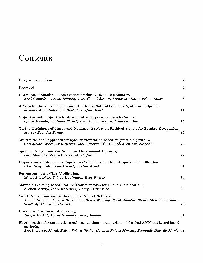
This paper describes the main aspects of the production ofan expressive speech corpus in Spanish faced to synthesis andthe objective and subjective evaluation of its emotional content.Section 2 introduces different aspects about the corpora of ex-pressive speech. Section 3 explains the production of our cor-pus. Section 4 details the process of objective validation carriedout through techniques of automatic identification of the emo-tion. The subjective evaluation by means of perception test isexplained in Section 5, and finally, the conclusions (Section 6).

2. Building emotional speech corporaAccording to [5], there are four main aspects to be consideredin the development of an emotional speech corpus:i) thescope

This work has been partially supported by the European Commis-sion, project SALERO FP6 IST-4-027122-IP.

that covers the database (number of speakers, the language, di-alects, genre of the speakers and types of emotional states);ii)the context in which a locution takes place (emotional signif-icance perceived across the semantics, the prosody, the facialexpression, gestures and posture);iii) the descriptors that al-low to represent the linguistic, emotional and acoustic contentof the speech; andiv) the naturalness of the locutions, whichwill depend on the strategy followed to obtain the emotionalspeech. With respect to the latter, the main debate is centredon the compromise between authenticity of the expressed emo-tion and the control on the recording. Campbell [1] and laterSchroder [6] propose 4 emotional speech sources:

Natural occurrences. Spontaneous human interactionpresents the most natural emotional speech although it has somedrawbacks due to the lack of control on its content, the qualityof sound, the difficulty of labelling, and finally, legal and ethicalaspects (e.g.The Reading-Leeds, The Belfast NaturalisticandThe CRESTdatabases described in [5]).

Elicitation. The provocation of authentic emotions in peo-ple in the laboratory is a way of compensating some of theproblems described previously, although the fullblown emo-tions would remain out of place [1]. In [6], five types of moodinduction procedures are described.

Stimulated emotional speech. This method consists of thereading of texts with a verbal content adapted for the emotion tobe expressed. The difficulty of comparing utterances with dif-ferent texts should be counteracted with an increase of the cor-pus size so that statistical methods allow to generalize models[1]. This technique was followed in the creation of theBelfastStructured Emotion Database[5].

Acted emotional speech. The great advantage of thismethod is the control of the verbal and phonetic content ofspeech since all the emotional states can be produced using thesame phrases. This allows direct comparisons of the phonetics,the prosody and the voice quality for the different emotions.The great objection that presents is the lack of authenticity ofthe expressed emotion [1].

Another important aspect to keep in mind is the purposeof the speech and emotion research. It is necessary to distin-guish between processes of perception (centred on the speaker)and expression (centred on the listener) [6]. The objective ofthe former is to establish the relation between the speaker emo-tional state and quantifiable parameters of speech. Usually, theydeal with the recognition of emotions from speech signal. Ac-cording to [3], one of the challenges is the identification of oralindicators (prosodic, spectral and vocal quality) attributable tothe emotional behavior and that are not simply own character-istics of conversational speech. The latter model the parametersof the speech with the goal to transmit a certain emotional state.The description of emotional states and the choice of speechparameters are key in the final result. There is a high consen-

15

sus in the scientific community for obtaining emotional speechby means of stimulated/acted speech for synthesis purposes [5][2], although other authors argue in favour of constructing anenormous corpus gathered from recordings of the daily life of anumber of voluntary speakers [7].

This work combines methods of both types of studies. Onthe one hand, the production of the corpus follows the guide-lines of the studiescentred on the listenersince it is orientedto speech synthesis. On the other hand, we apply techniques ofemotion recognition in order to validate its expressive content.

3. Our expressive speech corpus

We considered the development of a new expressive oral cor-pus for Spanish due to lack of availability of a corpus with thesuitable characteristics within the framework of our research inexpressive speech synthesis. This corpus had a double purpose:to learn the acoustic models of emotional speech and to be usedas the speech unit database for the synthesizer. This sectiondescribes the steps followed in the production of the corpus.

3.1. Stimulated emotion and text design

For the recording of the present corpus, a female professionalspeaker has been chosen due to her capability to use the suitableexpressive style to each text category (stimulted/acted speech).

For the design of texts semantically related to different ex-pressive styles, we have made use of an existing textual databaseof advertisements extracted from newspapers and magazines.Based on a study of the voice in the audio-visual publicity[8], five categories of the textual corpus have been chosen andthe most suitable emotion/style has been assigned to them:New technologies (neutral-mature), education (joy-elation),cosmetic (style sensual-sweet), automobiles (aggressive-hard)and trips (sad-melancholic).

A set of phrases has been selected from each category bymeans of agreedyalgorithm [9] that has allowed to obtain aphonetic balance in each subcorpus. This type of algorithmstake the locally optimum choice at each stage with the hope tofind an adequate global solution. Therefore, the application ofthis algorithm to the raised problem will obtain a valid solution,although may be not the optimum one. In addition to lookingfor a phonetic balance, phrases that contain exceptions (e.g. for-eign words, abbreviations) have been avoided due to they makedifficult the automatic processes of phonetic transcription andlabelling. Moreover, the selection of similar phrases to otherspreviously selected has been penalized by thegreedyalgorithm.

3.2. Recording

The recording of the oral corpus has been carried out in a profes-sional recording studio. Speech signals were sampled at 48 KHzand quantized using 24 bits per sample and stored in WAV files.Different recording sessions have been required and therefore apreestablished protocol has been followed in order to minimiz-ing errors that can cause deficiencies in the corpus labelling.For the corpus segmentation in phrases, a semiautomatic pro-cess has followed by means of a forced alignment using Hid-den Markov Models from the phonetic transcription and later amanual review and correction. This forced alignment also hasbeen used to segment the phrases in phonemes. The recordeddatabase has 4638 sentences and it is 5 h 12 min long.

4. Objective validationThe goal of the experiments described in this section was to val-idate the expressive content of the corpus by means of automaticemotion identification using different data mining techniquesapplied to statistical features computed over the prosodic pa-rameters of speech. An exhaustive subjective evaluation of thefull corpus (more than 5 hours of speech) would be a very te-dious task and practically impossible. However, the whole cor-pus can be validated by means of these automatic techniques.

4.1. Acoustic analysis

Prosodic features of speech (fundamental frequency, energy,duration of phones and frequency of pauses) are related to vocalexpression of emotion [10]. In this work, an automatic acousticanalysis of the sentences is performed using information of theprevious phonetic segmentation.

4.1.1. F0 related parameters

The analysis of the fundamental frequency (F0) parameters isbased on the result of the pitch marker described in [11]. Thissystem assigns marks over the whole signal. The unvoiced seg-ments and silences are marked using interpolated values fromthe neighboring voiced segments. For each phrase, three vec-tors of local F0 values are obtained (complete, excluding si-lences and unvoiced sounds, and only the stressed vowels). Theinformation about the boundaries of voiced/unvoiced (V/UV)segments and silences is obtained from the corpus labelling.Notice that if the phonetic segmentation was not available, anautomatic voice-activity detector (VAD) and a V/UV detectorwould be required [12]. Moreover, F0 has been calculated inboth lineal and logarithmic scales.

4.1.2. Energy related parameters

For energy, speech is processed with 20-ms rectangular win-dows and 50% of overlap, calculating the power (linear anddBs) every 10ms. Following the same idea that for F0, threevectors per utterance are generated (complete, excluding si-lences, and only in the stressed vowels).

4.1.3. Rhythm related parameters

The duration of phones is an important cue for vocal expressionof emotion. However, some studies omit this parameter by thedifficulty to obtain it automatically [12]. In the present work wehave incorporated this information (thanks to the labelling of thecorpus) to generate datasets with and without this information inorder to contrast its relevance. Z-scores have been employed forduration modeling in text-to-speech synthesis (TTS) to predictindividual segment durations and to control the lengthening orthe shortening of phones. As in [13], we take z-scores as ameans to analyze the temporal structure of speech:

z score =dur(ms)− µ

σ(1)

whereµ andσ are the mean and the standard desviation respec-tively of the corresponding phoneme. Therefore, the rhythmof an utterance is represented by a vector with the z-score ofeach phoneme. The version of this vector with only the stressedvowels is also computed.

Moreover, two pausing related parameters are added foreach utterance: the number of pauses per time unit and the per-centage of silence respect to the total time.

16

4.2. Statistical analysis and datasets

The prosody of an utterance is represented by some sequen-cies of values by phoneme such as F0 (lineal and logarithmic),energy (lineal and dB) and normalized durations (z-score). Foreach sequence, the first and the second derivative are calculated.For all these resulting sequences, the following statistics are ob-tained: mean, variance, maximum, minimum, range, skew, kur-tosis, quartiles, and interquartilic range. Finally, 464 parametersby utterance are calculated, considering both parameters relatedto the pausing.

This set of parameters has been divided into different sub-sets according to different strategies to reduce the dimensional-ity (see the diagram of the figure 1). A first criterion to reduceit has been to omit the second derivative (from Data1 to Data2)in order to valorate the significance of this function. Secondly,preliminary experiments have shown that the use of the loga-rithmic versions of F0 and energy obtain better results. For thisreason, two new datasets have been generated without the lin-ear versions of both F0 and energy. Each one of these datasets(Data1L and Data2L) has been divided in two new sets consid-ering all the phonemes or only the stressed vowels. Moreover,an automatic reduction of both initial datasets (with and withoutthe 2nd derivative) has been carried out by means of the simplegenetic algorithm (GA) implemeted in Weka [14] (Data1G andData2G). This reduction is independent of the later classifica-tion algorithm and therefore all the techniques have been tryedwith these datasets. Finally, two similar datasets toNavas etal. (2006)[12] have been generated to test the significance ofomiting the timing parameters (Data1N and DATA1NG).

DATA 1

(464)

GA

reduction

F0=Log

ENE=dB

(Navas et al., 2006)

DATA 1G

(214)

DATA 1L

(266)

DATA 1N(84)

Only

Stressed

Complete

DATA 1LS

(101)

DATA 1LC

(101)

Without 2nd

derivative

DATA 2

(310) GA

reduction

F0=Log

ENE=dB

DATA 2G

(127)

DATA 2L

(178)

Only

Stressed

Complete

DATA 2LS

(68)

DATA 2LC

(68)

GAreduction

DATA 1NG(39)

Figure 1: Generation of different datasets

4.3. Experiments and results

Numerous schemes of automatic learning can be used in a tasksuch as classifying the style/emotion from the acoustic analysisof the speech. The objective evaluation of expressivity in ourspeech corpus is based on [15], where a large-scale data min-ing experiment about the automatic recognition of basic emo-tions in short utterances was conducted. After different pre-liminary experiments, the set of machine learning algorithmsshowed in table 1 has been selected in order to be tested withthe different datasets. Some algorithms have been completedwith their boostedversions that achieve better results althoughthey present a greater computacional cost. All the experimentshave been carried out using Weka software [14] by means often-fold cross-validation. Both tryed versions of SMO (Sup-port Vector Machine of Weka) obtain the best results so muchon average as in maximum value (see table 1). SMO algorithmsachieve the highest results with Data1G, showing that the di-mensionality reduction based in GA helps to these systems, al-though differences with Data1L and Data1LC are minimum.However, other algorithms(i.e. J48, IB1 and IBk) work betterwith datasets genererated by two consecutive reductions (with-

Table 1: Learning Algorithms used for the automatic recogni-tion experiment

Name Description mean(95%CI) max(Data)J48 Decision tree based on C4.5 93.4± 2.0 96.4 (2G)B.J48 Adaboosted version of J48 96.4± 1.4 98.3 (1L)Part Decision Rules (PART) 94.2± 2.0 96.9 (2L)B.Part Adaboosted version of PART 96.7± 1.3 98.4 (1G)DT Decision Table 88.7± 2.6 92.3 (1L)B.T Adaboosted version of D. T. 93.4± 1.6 96.1 (1L)IB1 Instance-based (1 solution) 93.3± 2.8 97.5 (2G)IBk Instance-based (k solutions) 94.0± 2.3 97.9 (2G)NB Naive Bayes with discretization 94.6± 1.9 97.8 (1L)SMO1 SVM with 2nd degree pol. Kernel 97.3± 1.2 99.0 (1G)SMO2 SVM with 3rd degree pol. Kernel 97.1± 1.5 98.9 (1G)

80,00

82,00

84,00

86,00

88,00

90,00

92,00

94,00

96,00

98,00

100,00

J48 BoostJ48 PART BoostP DT BoostDT IB1 IBk NaiveBayes SMO1 SMO2

% I

de

nti

fic

ati

on

DATA1G DATA1L DATA1LC DATA1N DATA1NG DATA1LS

80,00

82,00

84,00

86,00

88,00

90,00

92,00

94,00

96,00

98,00

100,00

J48 BoostJ48 PART BoostP DT BoostDT IB1 IBk NaiveBayes SMO1 SMO2

% I

de

nti

fic

ati

on

DATA2G DATA2L DATA2LC DATA2LS

Figure 2: Identification percentage for the ten tested datasets

out 2nd derivative and latter GA reduction). And finally, wecan observe that there is a third group of algorithms that workbetter if the linear/logarithic redundance of F0 and energy is re-moved. Also we can observe that the boosted versions improvesignificantively the results respect to their corresponding algo-rithms. Figure 2 shows a comparison between different datasetsdepending on the algorithm. Notice that Data1LC obtains al-most the same results than Data1G and Data1L, but with lessthan the half of parameters. The same effect is presented inthe datasets without de 2nd derivative. Results experiment aslight loss when timing parameters are removed (Data1N andData 1NG). However, results worsen significantly when param-eters are calculated only in the stressed vowels (Data1LS andData2LS). Table 2 shows the confusion matrix with the averageresults for the eleven classifiers with Data2G, that has achievedthe best mean percentage of identification (97.02 %± 1.23).

5. Subjective evaluationA subjective evaluation is a tool that allows to validate the ex-pressivity of acted speech from a point of view of the users. Anexhaustive evaluation of corpus would be excessively tedious(the corpus has 4635 utterances). For each style, 96 utteranceshave been chosen, having done a total of 480. This test sethas been divided in 4 subsets, having 120 utterances each one.An ordered pair of subsets has been assigned to each subject.Therefore, 12 different tests have been generated. The alloca-tion of ordered pairs tries to compensate the fact that the secondtest could be easier to evaluate due to the previous training.

A forced answer test has been designed with the question¿What emotional state do you recognize from the voice of the

17

50%55%

60%65%

70%75%

80%85%

90%95%

100%

AGR HAP SAD NEU SEN

Ide

nti

fic

ati

on

Test1 Test2 Test3 Test4 Avg

Figure 3: Percentage of identification depending on the test

AGR1 AGR2 HAP1 HAP2 SAD1 SAD2 NEU1 NEU2 SEN1 SEN2 AVG1 AVG2

40

50

60

70

80

90

100

% Identification

Figure 4: Boxplots of sorted pairs first-second round dependingon the style and the average

speaker in this phrase?. The possible answers are the 5 styles ofthe corpus plus one more optionDon’t know / Another, with theobjective of avoid insecure or erroneous answers for the confus-ing cases. Adding this option has the risk that some evaluatorsuse excessively this answer to accelerate the end of the test [12].However, this effect has not been considerable in this test.

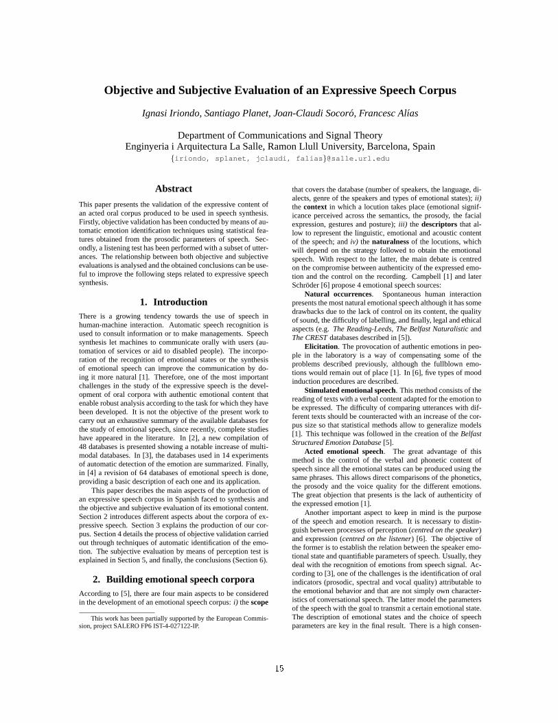
The process of evaluation has been carried out on a webplatform developed for this type of tests, that permits to leavethe test and to resume it subsequently. The evaluators belongmainly to the staff ofEnginyeria i Arquitectura La Sallewith aquite heterogeneous profile. Only the results of the 26 volun-teers who finished the two tests have been taken into account.The results of the subjective test show that all the styles achievea high percentage of identification. The figure 3 shows the per-centage of identification by style and test, being the sad stylethe best rated (98.8% of average), followed by sensual (86.8%)and neutral (86.4%) styles, and finally the aggressive (82.7%)and happy (81%) ones.

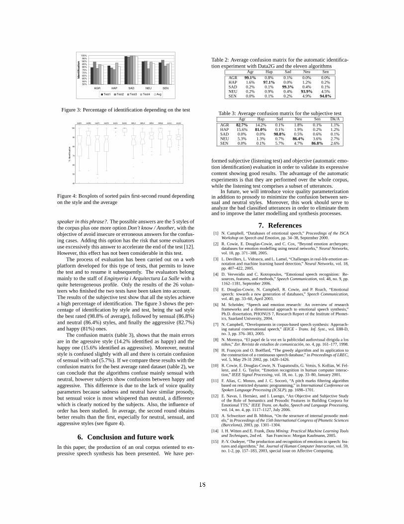
The confusion matrix (table 3), shows that the main errorsare in the agressive style (14.2% identified as happy) and thehappy one (15.6% identified as aggressive). Moreover, neutralstyle is confused slightly with all and there is certain confusionof sensual with sad (5.7%). If we compare these results with theconfusion matrix for the best average rated dataset (table 2), wecan conclude that the algorithms confuse mainly sensual withneutral, however subjects show confusions between happy andaggressive. This difference is due to the lack of voice qualityparameters because sadness and neutral have similar prosody,but sensual voice is most whispered than neutral, a differencewhich is clearly noticed by the subjects. Also, the influence oforder has been studied. In average, the second round obtainsbetter results than the first, especially for neutral, sensual, andaggressive styles (see figure 4).

6. Conclusion and future workIn this paper, the production of an oral corpus oriented to ex-pressive speech synthesis has been presented. We have per-

Table 2: Average confusion matrix for the automatic identifica-tion experiment with Data2G and the eleven algorithms

Agr Hap Sad Neu Sen

AGR 99.1% 0.8% 0.1% 0.0% 0.0%HAP 1.6% 97.1% 0.0% 1.2% 0.2%SAD 0.2% 0.1% 99.3% 0.4% 0.1%NEU 0.2% 0.9% 0.4% 93.9% 4.5%SEN 0.0% 0.1% 0.2% 4.9% 94.8%

Table 3: Average confusion matrix for the subjective testAgr Hap Sad Neu Sen Dk/A

AGR 82.7% 14.2% 0.1% 1.8% 0.1% 1.1%HAP 15.6% 81.0% 0.1% 1.9% 0.2% 1.2%SAD 0.0% 0.0% 98.8% 0.5% 0.6% 0.1%NEU 5.3% 1.3% 0.7% 86.4% 3.6% 2.7%SEN 0.0% 0.1% 5.7% 4.7% 86.8% 2.6%

formed subjective (listening test) and objective (automatic emo-tion identification) evaluation in order to validate its expressivecontent showing good results. The advantage of the automaticexperiments is that they are performed over the whole corpus,while the listening test comprises a subset of utterances.

In future, we will introduce voice quality parameterizationin addition to prosody to minimize the confusion between sen-sual and neutral styles. Moreover, this work should serve toanalyze the bad classified utterances in order to eliminate themand to improve the latter modelling and synthesis processes.

7. References[1] N. Campbell, “Databases of emotional speech,”Proceedings of the ISCA

Workshop on Speech and Emotion, pp. 34–38, September 2000.

[2] R. Cowie, E. Douglas-Cowie, and C. Cox, “Beyond emotion archetypes:databases for emotion modelling using neural networks,”Neural Networks,vol. 18, pp. 371–388, 2005.

[3] L. Devillers, L. Vidrascu, and L. Lamel, “Challenges in real-life emotion an-notation and machine learning based detection,”Neural Networks, vol. 18,pp. 407–422, 2005.

[4] D. Ververidis and C. Kotropoulos, “Emotional speech recognition: Re-sources, features, and methods,”Speech Communication, vol. 48, no. 9, pp.1162–1181, September 2006.

[5] E. Douglas-Cowie, N. Campbell, R. Cowie, and P. Roach, “Emotionalspeech: towards a new generation of databases,”Speech Communication,vol. 40, pp. 33–60, April 2003.

[6] M. Schroder, “Speech and emotion research: An overview of researchframeworks and a dimensional approach to emotional speech synthesis,”Ph.D. dissertation, PHONUS 7, Research Report of the Institute of Phonet-ics, Saarland University, 2004.

[7] N. Campbell, “Developments in corpus-based speech synthesis: Approach-ing natural conversational speech,”IEICE - Trans. Inf. Syst., vol. E88-D,no. 3, pp. 376–383, 2005.

[8] N. Montoya, “El papel de la voz en la publicidad audiovisual dirigida alosninos,”Zer. Revista de estudios de comunicacion, no. 4, pp. 161–177, 1998.

[9] H. Francois and O. Boeffard, “The greedy algorithm and its application tothe construction of a continuous speech database,” inProceedings of LREC,vol. 5, May 29-31 2002, pp. 1420–1426.

[10] R. Cowie, E. Douglas-Cowie, N. Tsapatsoulis, G. Votsis, S. Kollias, W. Fel-lenz, and J. G. Taylor, “Emotion recognition in human computer interac-tion,” IEEE Signal Processing, vol. 18, no. 1, pp. 33–80, January 2001.

[11] F. Alıas, C. Monzo, and J. C. Socoro, “A pitch marks filtering algorithmbased on restricted dynamic programming,” inInternational Conference onSpoken Language Processing (ICSLP), pp. 1698–1701.

[12] E. Navas, I. Hernaez, and I. Luengo, “An Objective and Subjective Studyof the Role of Semantics and Prosodic Features in Building Corpora forEmotional TTS,”IEEE Trans. on Audio, Speech and Language Processing,vol. 14, no. 4, pp. 1117–1127, July 2006.

[13] A. Schweitzer and B. Mobius, “On the structure of internal prosodic mod-els,” inProceedings of the 15th International Congress of Phonetic Sciences(Barcelona), 2003, pp. 1301–1304.

[14] I. H. Witten and E. Frank,Data Mining: Practical Machine Learning Toolsand Techniques, 2nd ed. San Francisco: Morgan Kaufmann, 2005.

[15] P.-Y. Oudeyer, “The production and recognition of emotions in speech: fea-tures and algorithms,”Int. Journal of Human Computer Interaction, vol. 59,no. 1-2, pp. 157–183, 2003, special issue on Affective Computing.

18

ON THE USEFULNESS OF LINEAR AND NONLINEAR PREDICTION RESIDUAL SIGNALS FOR SPEAKER RECOGNITION1

Marcos Faundez-Zanuy

Escola Universitaria Politécnica de Mataró, UPC Barcelona, SPAIN

1 This work has been supported by FEDER and MEC TIC-2003-08382-C05-02, TEC2006-13141-C03-02/TCM

ABSTRACT This paper compares the identification rates of a speaker recognition system using several parameterizations, with special emphasis on the residual signal obtained from linear and nonlinear predictive analysis. It is found that the residual signal is still useful even when using a high dimensional linear predictive analysis. On the other hand, it is shown that the residual signal of a nonlinear analysis contains less useful information, even for a prediction order of 10, than the linear residual signal. This shows the inability of the linear models to cope with nonlinear dependences present in speech signals, which are useful for recognition purposes.

Index Terms— Neural networks, speaker recognition, nonlinearities, prediction methods

1. INTRODUCTION Several parameterization techniques exist for speech [17] and speaker [15] recognition, cepstral analysis and its related parameterizations such as Delta-Cepstral features, Cepstral Mean Subtraction, etc. being the most popular. There are two main ways to compute the cepstral coefficients and one important drawback in both cases: relevant information is discarded, as follows. 1. LP-derived cepstral coefficients. The linear prediction

analysis produces two main components, the prediction coefficients (synthesis filter) and the residue of the predictive analysis. This latter signal is usually discarded. However, experiments exist [9] where it is shown that human beings are able to recognize the identity of the speaker listening to residual signals of LP analysis. Based on this fact several authors have evaluated the usefulness of the LPC-residue and have found that although the identification rates using this kind of information alone does not perform as well as the LP-derived cepstral coefficients, a combination of both can improve the results [20,12,14,22,11].

2. Fourier Transform derived cepstral coefficients. Instead of working out a set of Linear prediction coefficients, are based on the power spectrum information, where phase information has been discarded. [19] proposed the use of new acoustic features based on the short-term Fourier phase spectrum. The results are similar to the LP-derived cepstral coefficients. Although these (phase spectrum) features cannot outperform the classical cepstral parameterization, the results are improved using a combination of both features.

In this paper we will focus on the first kind of parameterization, because they are a clear alternative to the nonlinear predictive models, which have shown an improvement over the classical linear techniques in several fields (for a recent overview about these techniques [7]). In [4,6] we proposed a new set of features and models based on these types of nonlinear models and an improvement was also found when this information was combined with the traditional cepstral analysis, but so far, the relevance of the residual signals from linear and nonlinear predictive analysis has not been studied and compared. In this paper we will study if the relevance of the residual signal is due to an insufficient linear predictive analysis order or because of the incapability of the linear analysis to model nonlinearities present in speech and demonstrate is usefulness for speaker recognition purposes. This important question has not been solved in previous papers that focus on a typical 8 to 16 prediction order.

2. EXPERIMENT SET UP 2.1. Database For our experiments we have used the Gaudi database [16]. We have used one subcorpora of 49 speakers acquired with a simultaneous stereo recording with two different microphones. The speech is in wav format with a sampling frequency (fs) = 16 kHz, 16 bit/sample and the bandwidth is 8 kHz.

From this database we have generated narrow-band signals using the potsband routine that can be downloaded from [21]. This function meets the specifications of G.151 for any sampling frequency. Thus, our study has been performed on telephone bandwidth.

2.2. Identification algorithm In this study, we are only interested in the relative performance between linear and nonlinear analyses. Thus, we have chosen a simple algorithm for speaker recognition. In the training phase, we compute, for each speaker, empirical covariance matrices based on feature vectors extracted from overlapped short time segments of the speech signals. As features representing short time spectra we use both linear prediction cepstral coefficients (LPCC) and mel-frequency cepstral coefficients melceps [3]. In the speaker-recognition system, the trained covariance matrices for each speaker are compared with an estimate of the covariance matrix obtained from a test sequence from a speaker. An arithmetic-harmonic sphericity measure is used in order to compare the matrices [1]:

19

( ) ( )lCCCCd testjjtest log2)tr()tr(log 11 −= −− , where )tr(⋅ denotes

the trace operator, l is the dimension of the feature vector, Ctest and Cj is the covariance estimate from the test speaker and speaker model j, respectively.

2.3. Parameterizations We have used the following parameterizations 1. LP-derived cepstral coefficients (LPCC) 2. Fourier transform derived cepstral coefficients (melceps) 3. LP- residue coefficients The first two first parameterizations can be found, for instance, in [17,15,3], while the third is proposed in [11] and will be described in more detail next.

Inverse filtering

x[n] Channel 1

T ...

...

T

FFT | · |2

...

Channel 2

Channel M

V(1)

V(2)

V(M)

( )

( )

1

11

i i

i

i

i

H N

k LH

k Li

S k

S kN

=

=

⎛ ⎞⎜ ⎟⎜ ⎟⎝ ⎠−∏

∑

Linear predictor ...

a1 a2 aP

...

T Figure 1. LP residual signal parameterization Feature extraction from the LP-residual signal We will use the Power Difference of Spectrum in Subband (PDSS) obtained as follows [11]: 1. Calculate the LP-residual signal using the Pth-order linear

prediction coefficients. 2. Calculate the Fast Fourier Transform (fft) of the LP-residual

signal using zero padding in order to increase the frequency

resolution: ( ) 2S fft residue=

3. Group power spectrum into P subbands. 4. Calculate the ratio of the geometric to the arithmetic mean of

the power spectrum in the ith subband, and subtract it from 1:

( )

( )

1

( ) 11

i i

i

i

i

H N

k LH

k Li

S kPDSS i

S kN

=

=

⎛ ⎞⎜ ⎟⎜ ⎟⎝ ⎠= −∏

∑, where 1i i iN H L= − + is the

sample number of frequency points in the ith subband and Li, Hi is the lower and upper limit of frequency in ith subband respectively. We have used the same bandwidth for all the bands.

PDSS can be interpreted as the subband version of spectral flatness measure for quantifying the flatness of the signal spectrum. Figure 1 summarizes the procedure.

3. NEW POSSIBILITIES USING NON-LINEAR PREDICTIVE ANALYSIS

Although the relevance of residual NL-predictive analysis for speaker recognition has not been studied previously, nonlinear predictive analysis has been widely studied in the context of speech coding. For instance, [5] revealed that a forward ADPCM scheme with nonlinear prediction can achieve the same Segmental Signal to Noise Ratio (SEGSNR) as the equivalent linear

predictive system (same prediction order) with one less quantization bit. We propose an analogous scheme replacing the linear predictor with a nonlinear predictor. Figure 2 shows the scheme.

Inverse filtering

x[n] Channel 1

T ...

...

T

FFT | · |2

...

Channel 2

Channel M

V(1)

V(2)

V(M)

( )

( )

1

11

i i

i

i

i

H N

k LH

k Li

S k

S kN

=

=

⎛ ⎞⎜ ⎟⎜ ⎟⎝ ⎠−∏

∑

NNET predictor

...

T

Figure 2: Block diagram used to calculate PDSS parameters from NL-prediction residual signal. We have used a Multi-Layer Perceptron (MLP). The structure of the neural net has 10 inputs, 2 neurons in the hidden layer, and one output. The selected training algorithm was the Levenberg-Marquardt [10]. The number of epochs has been set up to 6. First layer and hidden layer transfer functions are tansig, while the output layer is linear.

4. EXPERIMENTAL RESULTS Obviously one important question when dealing with residual

LP signals is: Is the information contained in this residual signal coming from an insufficient predictive analysis order? That is, what happens when the prediction analysis order is so high that it is not possible to extract more relevant information using a linear analysis?

The experimental approach used to solve this question is to use a number of LP coefficients higher than usual. Two possible results can be obtained: 1. When the analysis order is increased, the discriminative

power of the residual signal is reduced to simple chance results. This means that there is potential for speaker recognition rate improvements through extraction of the LP coefficients in a more efficient manner, probably by increasing the number of coefficients.

2. When the analysis order is increased, the residual signal still contains useful information. This means that a linear analysis is unable to extract this information, and there is room for improvement combining parameterizations defined on the LP coefficients and the residual signal. In order to obtain the optimal results, both signals should be extracted and optimized jointly.

Figure 3 shows the results obtained with the following parameterizations: Melcepstrum, LPC –P residue, LPCC, LPC-80 residue, MLP 10x2x1 and several combinations between them. LPC-P residue is the parameterization obtained from the residual P-analysis order. It is interesting to observe the following: The residual signal of an LPC-80 analysis can produce a

recognition rate higher than 80% for a 15 dimensional vector extraction. Thus, it was found that the residual signal of a LP analysis contains relevant information, and this is due to the inability to extract this information using a linear analysis (80th order analysis is enough to model short term and long

20

term dependencies between samples, but if the analysis is linear, it is limited to linear dependencies).

The residual signal of a nonlinear predictive analysis, as expected, produces the lower recognition rates, because the relevant information has been retained in the predictor coefficients. However, a maximum of 70% recognition rate is possible.

5 10 15 20 25 30 35 4020 30 40 50 60 70 80 90

100

P= Vector dimension

Iden

tific

atio

n ra

te

opinion fusion MEL+ residue melcepstrumLPC-P residueLPCC opinion fusion LPCC+ residue LPC-80 residue MLP 10x2x1 residue

Figure 3: Identification for several parameterization algorithms. 4.1. Opinion fusion One way to improve the results is by means of a combination of different classifiers opinion [13,8]. In our case, we will use the same classifier scheme, but different parameterizations. In order to study the complementarity of the parameterizations studied, we have computed the correlation coefficient and scatter diagrams. Table 1 shows the correlation coefficients between distances of several parameterizations. The higher the correlation, the smaller the complementarity of both measures. Figure 2 shows a scatter diagram, which represents points on a two-dimensional space. The coordinates correspond to the obtained distance measures, which correspond to each parameterization (one in each axis). Looking at the diagram we observe that the points diverge from a strip. Thus, they have complementary information and can be combined in order to improve the results.

Table 1: Correlation coefficients between obtained distance values for P=20

LPCC Mel-ceps

LP-20 resid

LP-80 resid

MLP 10x2x1

LPCC 0,79 0,68 0,52 0,55 melceps 0,79 0,69 0,56 0,62 LP-20 resid 0,68 0,69 0,78 0,64 LP-80 resid 0,52 0,56 0,78 0,60 MLP 10x2x1 0,55 0,62 0,64 0,60

When combining different measures, special care must be taken for the range of the values. If they are not commensurate, some kind of normalization must be applied. We have tested the

following, based on a sigmoid function [18], 11 ii ko

e−′ =

+

where: ( )2

2i i i

ii

o mk

σσ

− −= , [ ]0,1io ′ ∈ , and oi is the initial

opinion of the ith classifier. ,i im σ are the mean and standard deviation of the opinions of the i classifier, obtained with data from the authentic speakers (intra-model distances).

We have limited the combinations to the outputs of two different classifiers, and the sum and product combination rules [13].

Table 2. Identification rates (combinations with sum rule)

P Param.

5 10 15 20 25 30 40

LPCC 46.9 90.6 93.5 97.1 98.0 98.8 94.7 Melceps 65.7 89.8 92.7 95.5 93.5 91.8 87.4 LP-P resid 44.1 75.9 84.1 78.4 82.0 78.8 77.1 LP-80 resid 32.7 72.2 78.0 78.0 73.5 68.6 68.6 MLP resid 20.0 65.3 70.2 66.1 65.3 62.9 53.5 LPCC+LP-P 64.9 89.8 94.7 97.6 97.1 97.1 95.1 LPCC+MLP 51.0 91.4 95.1 97.1 97.96 98.4 95.1 We have experimentally observed that slightly better results are obtained without normalization. Looking at figure 4 it can be seen that the distance values obtained with the residual signal parameterization have less amplitude (about 2 to 3 times). Thus, if the normalization is not done, it is equivalent to a weighted combination where the LPCC distances have more influence over the combined result than the residual signal. Figure 3 and table 2 summarize the identification rates for several vector dimensions (P) and different combined parameters.

5. CONCLUSIONS So far several papers have established that a combination between classical parameters (LPCC, melceps) with some kind of parameterization computed over the residual analysis signal can yield improvements in recognition rates. In our experiments we have found that this is only true when the analysis order ranges from 8 to 16. These values have been selected mainly because a spectral envelope can be sufficiently fitted with this amount of data, so there was no reason to increase the number of parameters. Although we consider that this is true for speech analysis, synthesis and coding, it is interesting to observe that the parameterization step for a speaker recognition system is twofold: 1. We make a dimensionality reduction, so it is easier to

compute models, distances between vectors, etc. 2. We make a transformation from one space to another one. In

this new domain, it can be easier to discriminate between speakers, and some parameterizations are better than others.

Thus, we are not looking for good quality representation of the speech signal (or a compromise between good representation with the smallest number of parameters). We are just looking for good discrimination capability. In our experiments we have found that for parameter vectors of high order, although the residual signal has a significant discriminative power among speakers, this signal seems to be redundant with LPCC or melceps, and it is not useful. If instead of using the residual signal of a linear analysis a nonlinear analysis is used, both combined signals are more uncorrelated and although the discriminative power of the NL residual signal is lower, the combined scheme outperforms the linear one for several analysis orders.

21

The results show that there is just a marginal improvement on the results when increasing the number of parameters (the identification rate plot saturates), but the residual signal is whiter when increasing the prediction order, especially for the nonlinear analysis. This is a promising result, because although a good

parameterization based on nonlinear analysis has not yet been established, this paper reveals that the NL analysis can extract more relevant information with the same prediction order as a linear analysis. Thus, it opens a new way for investigation that has started to provide successful results [2].

Figure 4: Scatter diagram of distances for observing the correlation between parameters.

6. REFERENCES

[1] F. Bimbot, L. Mathan "Text-free speaker recognition using an arithmetic-harmonic sphericity measure." pp.169-172, Eurospeech 1993. [2] M. Chetouani, M. Faundez, B. Gas, J. L. Zarader “A New Nonlinear speaker parameterization algorithm for speaker identification”. ISCA Speaker Odyssey Workshop·, 2004. [3] J. Deller et al. “Discrete-Time Processing of Speech Signals,” Prentice-Hall, 1993. [4] M. Faundez and D. Rodriguez "Speaker recognition using residual signal of linear and nonlinear prediction models". Vol.2 pp.121-124. ICSLP'98, Sidney. [5] M. Faundez, F. Vallverdú, E. Monte, "Nonlinear prediction with neural nets in adpcm" IEEE International Conference on Acoustics, Speech, and Signal Processing, ICASSP 1998, Vol I, pp.345-348.Seattle. [6] M. Faundez "Speaker recognition by means of a combination of linear and nonlinear predictive models" EUROSPEECH'99, Budapest. Vol. 2 pp. 763-766. [7] M. Faundez et al.. “nonlinear speech processing: overview and applications”. Control and intelligent systems, Vol. 30 Nº 1, pp.1-10, 2002, ACTA Press [8] M. Faundez “Data fusion in Biometrics”. IEEE Aerosp. Electron. Syst. Mag. Vol.20 nº 1, pp.34-38, January 2005 [9] T. C. Feustel & G. A. Velius “Human and machine performance on speaker identity verification”. Speech Tech 1989, pp.169-170. [10] F. D. Foresee and M. T. Hagan, “Gauss-Newton approximation to Bayesian regulariza-tion”, proceedings of the 1997 International Joint Conference on Neural Networks, pp.1930-1935, 1997

[11] S. Hayakawa, K. Takeda & F. Itakura “Speaker identification using harmonic structure of LP-Residual spectrum” Audio Video Biometric personal autentification 1997, pp. 253-260 LNCS-1206. [12] J. He, L. Liu & G. Palm “On the use of features from prediction residual signals in speaker identification”. EUROSPEECH’1995 pp.313-316. [13] J. Kittler, M. Hatef, R. P. W. Duin & J. Matas “On combining classifiers”. IEEE Trans. On PAMI, Vol. 20, Nº 3, pp. 226-239, 1998 [14] L. Liu et al. “Signal modelling for speaker identification”. Proceedings of the IEEE ICASSP 1996, Vol.2, pp. 665 - 668 [15] R. J. Mammone, X. Zhang & R. Ramachandran “Robust speaker recognition” IEEE Sig. Proc. magazine, 1996, pp.58-70. [16] J. Ortega et al. “Ahumada: a large speech corpus in Spanish for speaker identification and verification”. ICASSP 1998 Seattle, Vol. 2, pp. 773-776. [17] J. W. Picone “Signal Modeling techniques in speech recognition” Proceedings of the IEEE, Vol. 79, Nº 4, April 1991, pp.1215-1247 [18] C. Sanderson “Information fusion and person verification using speech & face information”. IDIAP Research Report 02-33, pp. 1-37. September 2002 [19] R. Schlüter, H. Ney “Using phase spectrum information for improved speech recognition performance” Proceedings of the IEEE ICASSP 2001, Vol.1, pp.133-136 [20] P. Thévenaz, H. Hügli “Usefulness of the LPC-residue in text-independent speaker verification” Speech Communication 17 (1995) pp. 145-157 [21] http://www.ee.ic.ac.uk/hp/staff/dmb/voicebox/voicebox.html [22] B. Yegnanarayana et al. “Source and system features for speaker recognition using AANN models” IEEE ICASSP 2001, Vol.1, pp.409-412

22

Multi filter bank approach for speaker verification based on genetic algorithm

Christophe Charbuillet, Bruno Gas, Mohamed Chetouani, Jean Luc Zarader

Universite Pierre et Marie Curie-Paris6, FRE2507Institut des Systemes Intelligents et Robotique (ISIR), Ivry sur Seine, F-94200 France

Christophe.Charbuillet@lis.jussieu.fr, Gas@ccr.jussieu.fr,

Mohamed.Chetouani@upmc.fr, jean-luc.zarader@upmc.fr

AbstractSpeech recognition systems usually need a feature extractionstage which aims at obtaining the best signal representation.State of the art speaker verification systems are based on cep-stral features like MFCC, LFCC or LPCC. In this article, wepropose a feature extraction system based on the combinationof three feature extractors adapted to the speaker verificationtask. A genetic algorithm is used to optimize the features com-plementarities. This optimization consists in designing a set ofthree non linear scaled filter banks. Experiments are carried outusing a state of the art speaker verification system. Results showthat the proposed method improves significantly the system per-formances on the 2005 Nist SRE Database. Furthermore, theobtained feature extractors show the importance of some spe-cific spectral information for speaker verification.

1. IntroductionSpeech feature extraction plays a major role in speaker verifica-tion systems. State of the art speaker verification systems frontend are based on the estimation of the spectral envelope of theshort term signal, e.g., Mel-scale Filterbank Cepstrum Coeffi-cients (MFCCs), Linear-scale Filterbank Cepstrum Coefficients(LFCCs), or Linear Predictive Cepstrum Coefficients (LPCCs).Even if these extraction methods achieve good performanceson speaker verification, they do not take into account specificinformation about the task to achieve. To avoid this draw back,several approaches have been proposed to optimize the featureextractor to a specific task. These methods consist to simulta-neously learn the parameters of both the feature extractor andthe classifier [1]. This procedure consists in the optimization ofa criterion, which can be the Maximization of the Mutual In-formation (MMI) [2] or the Minimization of the ClassificationError (MCE) [3]. In this paper we proposed to used a geneticalgorithm to design a feature extraction system adapted to thespeaker verification task.Genetic algorithms (GA) were first proposed by Holland in1975 [4] and became widely used in various disciplines as anew means of complex systems optimization. In recent yearstheir have been successfully applied to the speech processingdomain. Chin-Teng Lin and al. [5] proposed to apply a GA tothe feature transformation problem for speech recognition andM. Zamalloa and al. [6] worked on a GA based feature selectionfor speaker recognition. GAs most attractive quality is certainlytheir aptitude to avoid local minima. However, our study relieson another quality which is the fact that GAs are unsupervisedoptimization methods. So they can be used as an explorationtool, free to find the best solution without any constraint. In a

Figure 1: Feature extraction optimization

Figure 2: Linear scaled filter bank

previous work [7] we used this approach to show the importanceof specific spectral information for the speaker diarization task.State of the art speaker verification systems are based on a cep-stral feature extraction front end (LFCC, MFCC, LPCC) followby a GMM [8] or an hybrid GMM/SVM classifier [9]. Nowa-days, an alternative an increasingly used approach consists infusing different systems. This technique can be divided in twomain categories depending on the source of this difference. Thesystems based on a classifier’s variety [10] and the systemsbased on different features. Our study deals with the secondprinciple. We can quote the work of M. Zhiyou and al. [11]which consist of combining the LFCC and MFCC features, orthe study of Poh Hoon Thian & al. [12] who proposed to com-plete the LFCC’s with spectral centroids subands features.In this paper we proposed to fuse three systems based on differ-ent feature extractors. A genetic algorithm is used to optimizethe feature extractor’s complementarities. Figure 1 describesthis approach. In the second section, a description of the featureextraction method is given. Afterward, we describe the geneticalgorithm we used, followed by its application to complemen-tary feature extraction. Then, the experiments we made and theobtained results are presented.23

2. Filter bank based feature extractorsThe conventional MFCC and LFCC feature extractor processmainly consists of modifying the short-term spectrum by a filterbank. This process has four steps:

• Compute the power spectrum of the analyzed frame;

• Sum the power spectrum for each triangular filter of thebank;

• Apply the log operator to the obtained coefficients;

• Compute the Discrete Cosine Transform (DCT).

Figure 2 presents the linear scaled filter bank used for theLFCC’s computation. This feature extractor is known to be themost robust for the short band signals representation. The pur-pose of our study is to find a set of three cepstrum based featureextractors design for high level fusion. To this end, we proposeto use a genetic algorithm to optimize, the number of filters onthe bank, the scaled of the filter bank and the number of cepstraloutput coefficients.

3. Genetic algorithmA genetic algorithm is an optimization method. Its aim is to findthe best values of the system’s parameters in order to maximizeits performance. The basic idea is that of ”natural selection”, i.e.the principle of ”the survival of the fittest”. A GA operates ona population of systems. In our application, each individual ofthe population is a feature extractor defined by its genes. Genesconsists in a condensed an adapted representation of the featureextractor’s operational parameters.

3.1. Gene encoding

Parameter’s encoding plays a major role in a genetic algo-rithm. By an adapted parameter representation, this methodcan strongly increases the speed convergence of the algorithm.Moreover it reduces the over fitting effect by reducing the pa-rameters dimention. The parameters we chose to optimize are:

• Nf : Number of filters in the bank;

• Nc: Number of cepstral coefficients;

• Ci: Center frequency of the ith filter in the bank;

• Bi: Band width of the ith filter in the bank.

Parameters C and B are encoded with two polynomialfunctions described by the equations (1) and (2). This encod-ing method reduces the parameter’s dimention from 50 to 12(in the average case) and guaranties the filter bank’s regularity.The parameter Nf and Nc are not encoded and will be directlymuted.

Ci = gc0 +gc1 · i

Nf+gc2 ·( i

Nf)2 + ...+gcN ·( i

Nf)N (1)

Bi = gb0 +gb1 · i

Nf+gb2 ·( i

Nf)2 + ...+gbN ·( i

Nf)N (2)

Where gc0,...,gcN and gb0,...,gbN are the genesrelative to the parameters C0,...,CNf and B0,...,BNf; Nis the polynomial order; Nf represent the number of filter.

Figure 3: Genetic algorithm

3.2. Genetic algorithm description

The algorithm we used is made of four operators: Mutation,Decoding, Evaluation and Selection (M, D, E, S). These opera-tors are applied to the current population p(t) to produce a newgeneration p(t + 1) by the relation:

p(t + 1) = S E D M(p(t)) (3)

Figure 3 represent this algorithm. The first step consists ona random initialization of the feature extractor’s genes. Then,the operators are iteratively applied.The Mutation operator consists in a short random variation ofthe genes.The Decoding operator aim at decode the genes to obtain theoperational feature extractor’s parameters.The Evaluation operator’s goal is to evaluate each feature ex-tractor performances. The evaluation criterion we used is de-fined on the section 3.3.The Selection operator selects the Ns better feature extractorsof the current population. These individuals are then cloned ac-cording to the evaluation results to produce the new generationp(t + 1) of Np feature extractors. As a consequence of thisselection process, the average of the performance of the popu-lation tends to increase and in our application adapted featureextractors tend to emerge.

3.3. Application to complementary feature extraction

The objective is to obtain a set of three complementary featureextractors. The main idea is to evolve three isolated populationsof feature extractors and to select the best combination. At eachgeneration, the fusion is done for all combination of feature ex-tractors and the resulting Equal Error Rate (EER) is memorized.At the end of this process, the fitness of an individual is definedas the lower EER obtained (e.i. the EER corresponding to thebest combination including this feature extractor). As a conse-quence of this process, each population tends to specialize onspecific feature, complementary with the others.

4. Experiments and results4.1. Data bases

The databases used for the evolution phase and for the test areextracted from the 2005 Nist SRE corpus [13]. This corpusis composed of conversational telephone speech signals passedthrough different channels, (landline, cordless or cellular) andsampled to 8 kHz. We used 10 male and 10 female with oneutterance of 2 min 30s per speaker for the evolution phase. Thenumber of tests between model and test signal involved for each24

(a) Formant and fondamental frequency distributions

(b) Obtained filter banks for C1 (top) C2 (midle) and C3 (bottom)

Figure 4: Spectral analyse and obtained solutions

feature extractor evaluation was of 2052. For the test database,we used 50 males and 50 females whose not appear on the train-ing base. The number of tests involved was of 116942.

4.2. Speaker verification system

All experiments we made are based on a state of the art GMM-UBM speaker verification system. This system, called LIA Sp-kDet [14] was provided by the University of Avignon, France.We used a system with 16 gaussian per mixture, with diagonalcovariance matrix.

4.3. Genetic algorithm parameters

The genes gc0,...,gcN and gb0,...,gbN which code for thecentres frequencies and the band widths are initialized with aGaussian normalized random. The parameter Nf are initializedto 24, and Nc to 16.The parameter we used for the feature extractor’s evolution are:

• Population size Np : 20;

• Number of selected individuals Ns : 5;

• Polynomial order for the genes encoding N : 5;

• Mutation method for the polynomials coefficients: Gaus-sian random variation of ± 0.1;

• Mutation method for Nf : uniform random variation of± 5;

• Mutation method for Nc : uniform random variation of± 3;

4.4. Results

In this section, obtained feature extractors are presented andanalysed. Figure 4.b presents the obtained filter banks. In or-der to interpret the obtained solution, a statistical analysis of thefundamental frequency and formants was done on a databasecomposed of 20 male and 20 females. Figure 4.a presents theprobability distributions of these mesures.

Table 1: Comparative results

Feature extractor Nf Nc Fmin Fmax EER%LFCC 24 16 300 3400 14.44MFCC 24 16 300 3400 14.88

C1 23 15 360 1145 22.90C2 25 20 266 3372 14.79C3 19 19 156 3309 16.07

C1+C2+C3 - - - - - - - - 12.69

Table 2: Fusion analysis

Feature extractor Correlation EER obtained by fusionC1+C2 0.51 13.21%

C2 + C3 0.83 13.45%C1 + C3 0.64 15.39%

Table 1 details both the feature extractor’s characteristicsand the results obtained on the test base. The combinationmethod used is an arithmetic fusion, as illustrated by the fig-ure 1.

Table 2 presents the correlation coefficients between thecompared system and the EER obtained by fusion. The cor-relation is based on the log-likelihood outputs of the comparedsystems for the whole tests of the test database. A test consiststo measure the log-likehood between a speaker model and testsignal. The r correlation coefficient is defined by:

r =

∑Nti=1(S1i − S1) · (S2i − S2)√∑Nt

i=1 (S1i − S1)2 ·√∑Nt

i=1 (S2i − S2)2(4)

Where S1i represent the log-likelihood obtained by thesystem 1 on ith test; Nt is the number of test.

The correlation coefficient, which takes value in [-1;1],is a measure of the system’s decision similarity. In ourapplication, the classifiers are identical. As a consequence,this measure can be interpreted as the similarity between theinformation provied by the feature extractors. A correlation of1 means that the information supplied by the feature extractorsare equivalent (i.e. they lead to the same decision). A corre-lation of 0 means that the information supplied are independent.

Taking into account these different information, we can no-tice that:

• Information relative to the fundamental frequencies isnot used;

• C2 covers a large spectral zone and obtained results sim-ilar are to the LFCC or MFCC feature extractors;

• C1 seems to focus exclusively on the first formant;

• C3 presents a high filter density centred on the first for-mant, while keeping the whole spectre information;

• The de-correlation of the obtained systems are signifi-cant.

• The final combination of the three feature extractors im-prove the system performance of 12% compare to thebaseline system.25

These results show that the proposed method is reliable.The correlation between the diferent systems and the improve-ment supplied by the fusion show that the obtained feature ex-tractors are complementary. This improvement seems to be re-lated to the information provied by the first formant. In thefinal article, a more detailed analyse of these results will be pre-sented.

5. ConclusionIn this paper, we proposed to use a genetic algorithm to optimizea feature extraction system adapted to the speaker verificationtask. The proposed system is based on a combination of threecomplementary feature extractors. Obtained results show thatthe proposed method improves significantly the system perfor-mance. Furthermore, the obtained feature extractors reveal theimportance of specific spectral information relatives to the firstformant.Our future work will consist in study the robustness of the ob-tained solutions according to both the initial conditions and thebase used for the evolution phase.

6. References[1] B. G. Mohamed Chetouani, Marcos Faundez-Zanuy and

J.-L. Zarader, Nonlinear Speech Modeling and Applica-tions. Springer, 2005, ch. Non-linear Speech Feature Ex-traction for Phoneme Classification and Speaker Recogni-tion, pp. 344–350.

[2] K. Torkkola, “Feature extraction by non parametric mu-tual information maximization,” The Journal of MachineLearning Research, vol. 3, pp. 1415–1438, 2003.

[3] C. Miyajima, H. Watanabe, K. Tokuda, T. Kitamura, andS. Katagiri, “A new approach to designing a feature ex-tractor in speaker identification based on discriminativefeature extraction,” Speech Communication, vol. 35, no.3-4, pp. 203–218, Oct. 2001.

[4] J. H. Holland, “Adaptation in natural and artificial sys-tems,” University of Michigan Press, 1975.

[5] L. Chin-Teng, N. Hsi-Wen, and H. Jiing-Yuan, “Ga-based noisy speech recognition using two-dimensionalcepstrum,” in IEEE Transactions on Speech and AudioProcessing, vol. 8, 2000, pp. 664–675.

[6] M. Zamalloa, G. Bordel, J. L. Rodriguez, and M. Pena-garikano, “Feature selection based on genetic algorithmsfor speaker recognition,” in IEEE Odyssey, vol. 1, 2006,pp. 1–8.

[7] C. Charbuillet, B. Gas, M. Chetouani, and J. L. Zarader,“Filter bank design for speaker diarization based on ge-netic algorithms,” in Acoustics, Speech, and Signal Pro-cessing, 2006. Proceedings. (ICASSP ’06). IEEE Interna-tional Conference on, vol. 1, 2006, pp. 673–676.

[8] D. Reynolds and R. Rose, “Robust text-independentspeaker identification using gaussian mixture speakermodels,” Speech and Audio Processing, IEEE Transac-tions on, vol. 3, no. 1, pp. 72–83, 1995.

[9] S. Fine, J. Navratil, and R. Gopinath, “A hybrid gmm/svmapproach to speaker identification,” in Acoustics, Speech,and Signal Processing, 2001. Proceedings. (ICASSP ’01).2001 IEEE International Conference on, vol. 1, 2001, pp.417–420 vol.1.

[10] K. Farrell, R. Ramachandran, and R. Mammone, “Ananalysis of data fusion methods for speaker verifica-tion,” in Acoustics, Speech, and Signal Processing, 1998.ICASSP ’98. Proceedings of the 1998 IEEE InternationalConference on, vol. 2, 1998, pp. 1129–1132 vol.2.

[11] M. Zhiyou, Y. Yingchun, and W. Zhaohui, “Further fea-ture extraction for speaker recognition,” IEEE Interna-tional Conference on Systems, Man and Cybernetics,vol. 5, pp. 4153–4158, 2003.

[12] N. Poh Hoon Thian, C. Sanderson, S. Bengio, D. Zhang,and K. Jain Anil, “Spectral subband centroids as comple-mentary features for speaker authentication,” Lect. notescomput. sci., vol. 3072, pp. 631–639, 2004.

[13] “2005 nist speaker recognition evaluation site.” [Online].Available: http://www.nist.gov/speech/tests/spk/2005/

[14] “Lia spkdet web site.” [Online]. Available:http://www.lia.univ-avignon.fr/heberges/ALIZE/LIARAL

26

Speaker Recognition Via Nonlinear Discriminant Features

Lara Stoll1,2, Joe Frankel1,3, Nikki Mirghafori1

1International Computer Science Institute, Berkeley, CA, USA2University of California at Berkeley, USA

3Centre for Speech Technology Research, Edinburgh, UKlstoll,nikki @icsi.berkeley.edu, joe@cstr.ed.ac.uk

AbstractWe use a multi-layer perceptron (MLP) to transform cep-stral features into features better suited for speaker recogni-tion. Two types of MLP output targets are considered: phones(Tandem/HATS-MLP) and speakers (Speaker-MLP). In the for-mer case, output activations are used as features in a GMMspeaker recognition system, while for the latter, hidden activa-tions are used as features in an SVM system. Using a smallerset of MLP training speakers, chosen through clustering, yieldssystem performance similar to that of a Speaker-MLP trainedwith many more speakers. For the NIST Speaker RecognitionEvaluation 2004, both Tandem/HATS-GMM and Speaker-SVMsystems improve upon a basic GMM baseline, but are unable tocontribute in a score-level combination with a state-of-the-artGMM system. It may be that the application of normalizationsand channel compensation techniques to the current state-of-the-art GMM has reduced channel mismatch errors to the pointthat contributions of the MLP systems are no longer additive.

1. IntroductionThe speaker recognition task is that of deciding whether or nota (previously unseen) test utterance belongs to a given targetspeaker, for whom there is only a limited amount of train-ing data available. The traditionally successful approach tospeaker recognition uses low-level cepstral features extractedfrom speech in a Gaussian mixture model (GMM) system. Al-though cepstral features have proven to be the most successfulchoice of low-level features for speech processing, discrimina-tively trained features may be better suited to the speaker recog-nition problem. We utilize multi-layer perceptrons (MLPs),which are trained to distinguish between either phones or speak-ers, as a means of performing a feature transformation of cep-stral features.

There are two types of previous work that are directly re-lated to our research, both involving the development of dis-criminative features. In the phonetically discriminative case,the use of features generated by one or more MLPs trained todistinguish between phones has been shown to improve perfor-mance for automatic speech recognition (ASR). At ICSI, Zhuand Chen, et al. developed what they termed Tandem/HATS-MLP features, which incorporate longer term temporal infor-mation through the use of MLPs whose outputs are phone pos-teriors [1, 2].

In the area of speaker recognition, Heck and Konig, etal. focused on extracting speaker discriminative features fromMFCCs using an MLP [3, 4]. They used the outputs from themiddle layer of a 5-layer MLP, which was trained to discrimi-nate between speakers, as features in a GMM speaker recogni-tion system. The MLP features, when combined on the score-

level with a cepstral GMM system, yielded consistent improve-ment when the training data and testing data were collectedfrom mismatched telephone handsets [3]. A similar approachwas followed by Morris and Wu, et al.[5]. They found thatspeaker identification performance improved as more speakerswere used to train the MLP, up to a certain limit [6].

In the phonetic space, we use the Tandem/HATS-MLP fea-tures in a GMM speaker recognition system. The idea is that wecan use the phonetic information of a speaker in order to distin-guish that speaker from others.

In the speaker space, we train 3-layer Speaker-MLPs ofvarying sizes to discriminate between a set of speakers, and thenuse the hidden activations as features for a support vector ma-chine (SVM) speaker recognition system. The intuition behindthis method is that the hidden activations from the Speaker-MLP represent a nonlinear mapping of the input cepstral fea-tures into a general set of speaker patterns. Our Speaker-MLPsare on a larger scale than any previous work: we use more train-ing speakers, training data, and input frames of cepstral fea-tures, and larger networks.

To begin, Section 2 outlines the experimental setup. Theresults of our experiments are reported in Section 3. Finally, weend with discussion and conclusions in Section 4.

2. Experiments2.1. Overall Setup

The basic setups of the Tandem/HATS-GMM and Speaker-SVM systems are shown in Figures 1 and 2, respectively.Frames of perceptual linear prediction (PLP) coefficients, aswell as frames of critical band energies in the former case, arethe inputs to the MLPs. A log is applied to either the outputor hidden activations, and after either dimensionality reductionor calculation of mean, standard deviation, histograms, and per-centiles, the final features are used in a speaker recognition sys-tem (GMM or SVM).

2.2. Baseline GMM Systems

We make use of two types of GMM baselines for purposes ofcomparison. The first is a state-of-the-art GMM system, whichwas developed by our colleagues at SRI, and which we will referto as SRI-GMM [7]. It utilizes 2048 Gaussians, CMS, T-norm,H-norm, and channel mapping to improve its results. We usethis system for score-level combinations, in which the scoresfrom SRI’s GMM system are combined with the scores fromour MLP features systems. For more details, see Section 2.6.

The second system, on the other hand, is a very basic GMMsystem, with 256 Gaussians, and which includes only CMS,without any other normalizations. This system, which we will27

...

...

51 frames ofcritical band

energy

... ...

...

Phone−1

Phone−N

Tandem−MLP

... ...

...

... ...

...

... ...

...

Hiddenactivations

Hiddenactivations

...

Phone−1

Phone−N

HATS−MLP

Log

Dimensionalityreduction

GMMSystem

Outputactivations

Outputactivations

9 frames of PLP

Combination

Figure 1:Tandem/HATS-GMM System

...

... ...

...

Log

SystemSVM

SVM featurecalculations

Hiddenactivations

21 frames of PLP

Speaker−1

Speaker−N

Speaker−MLP

Figure 2:Speaker-SVM System

refer to as Basic-GMM, is useful for the purpose of feature-level combination (where we use MFCC features augmentedwith MLP features as features in the GMM system), as well asfor score-level combination.

2.3. Tandem/HATS-MLP Features

There are two components to the Tandem/HATS-MLP features,namely the Tandem-MLP and the HATS-MLP. The Tandem-MLP is a single 3-layer MLP, which takes as input 9 framesof PLPs (12th order plus energy) with deltas and double-deltas,contains 20,800 units in its hidden layer, and has 46 outputs,corresponding to phone posteriors. The hidden layer appliesthe sigmoid function, while the output uses softmax.

The HATS-MLP is actually two stages of MLPs that per-form phonetic classification with long-term (500-1000 ms) in-formation. The first stage MLPs take as input 51 frames of logcritical band energies (LCBE), with one MLP for each of the15 critical bands; each MLP has 60 hidden units (with sigmoidapplied), and the output layer has 46 units (with softmax) corre-sponding to phones. For the HATS (Hidden Activation TRAPS)features, the hidden layer outputs are taken from each first-stagecritical band MLP, and then input to the second-stage mergerMLP, which contains 750 hidden units, and 46 output units.

The Tandem-MLP and HATS-MLP features are then com-bined using a weighted sum, where the weights are a normalizedversion of inverse entropy. The log is applied to the output, anda Karhunen-Loeve Transform (KLT) dimensionality reductionis applied to reduce the output feature vector to an experimen-tally determined optimal length of 25. This process is illustratedin Figure 1.

The Tandem/HATS-MLP system is trained on roughly 1800

hours of conversational speech from the Fisher [8] and Switch-board [9] corpora.

2.4. Speaker-MLP Features

2.4.1. Speaker Target Selection Through Clustering

As a contrast to using all speakers with enough training dataavailable (with the idea that including more training speakerswill yield better results), we also implemented MLPs trained us-ing only subsets of specifically chosen speakers. These speak-ers were chosen through clustering in the following way. First, abackground GMM model was trained using 286 speakers fromthe Fisher corpus. Then, a GMM was adapted from the back-ground model with the data from each MLP-training speaker.These GMMs used 32 Gaussians, with input features of 12thorder MFCCs plus energy and their first order derivatives. Thelength-26 mean vectors of each Gaussian were concatenatedto form a length-832 feature vector for each speaker. Prin-cipal component analysis was performed, keeping the top 16dimensions of each feature vector (accounting for 68% of thetotal variance). In this reduced-dimensionality speaker space,k-means clustering was done, using the Euclidean distance be-tween speakers, fork = 64 andk = 128. Finally, the sets of 64and 128 speakers were chosen by selecting the speaker closestto each of the (64 or 128) cluster centroids.

2.4.2. MLP Training

A set of 64, 128, or 836 speakers was used to train each Speaker-MLP, with 6 conversation sides per speaker used for training,and 2 for cross-validation (CV). The training speaker data camefrom the Switchboard-2 corpus [9]. The set of 836 speakers in-cluded all speakers in the Switchboard2 corpus with at least 8conversations available. The smaller sets of speakers, selectedthrough clustering, used training and CV data that was balancedin terms of handsets.

ICSI’s QuickNet MLP training tool [10] was used to trainthe Speaker-MLPs. The input to each Speaker-MLP is 21frames of PLPs (12th order plus energy) with first and secondorder derivatives appended. The hidden layer applies a sigmoid,while the output uses softmax.

Table 2 shows the sizes of MLPs (varying in the number ofhidden units) trained for each set of speakers.

2.5. SVM Speaker Recognition System

The GMM system is well suited to modeling features with fewerthan 100 dimensions. However, problems of data sparsity andsingular covariance matrices soon arise in trying to estimatehigh dimensional Gaussians. Previous work in speech recog-nition (HATS) has shown that there is a great deal of infor-mation in the hidden structure of the MLP. Preliminary experi-ments also showed that reducing the dimensionality of the hid-den activations using principal component analysis (PCA) orlinear discriminant analysis (LDA), so that the features couldbe used in a GMM system, yielded poor results. In order to takeadvantage of the speaker discriminative information in the hid-den activations of the Speaker-MLPs, we use an SVM speakerrecognition system, which is better suited to handle the high di-mensional sparse features, is naturally discriminative in the wayit is posed, and has proven useful in other approaches to speakerverification.

Since the SVM speaker recognition system requires thesame length feature vector for each speaker (whether a target,an impostor, or a test speaker), we produce a set of statistics28

to summarize the information along each dimension of the hid-den activations. These statistics (mean, standard deviation, his-tograms of varying numbers of bins, and percentiles) are thenused as the SVM features for each speaker. For our experi-ments, the set of impostor speakers used in the SVM systemis a set of 286 speakers from the Fisher corpus designed to bebalanced in terms of gender, channel, and other conditions.

2.6. System Combinations Using LNKnet

In order to improve upon the baseline of the SRI-GMM system,we choose to combine our various systems on the score-levelwith the SRI-GMM, using LNKnet software [11]. We use aneural network with no hidden layer and sigmoid output non-linearity, which takes two or more sets of likelihood scores asinput. We use a round-robin approach and divide our test datainto two subsets for development and evaluation.

3. Results3.1. Testing Database

In order to compare the performance of our systems, we use thedatabase released by NIST for the 2004 Speaker RecognitionEvaluation (SRE) [12]. This database consists of conversationalspeech collected in the Mixer project, and includes various lan-guages and various channel types. We use only telephone data,containing a variety of handsets and microphones.

One conversation side (roughly 2.5 minutes) is used forboth the training of each target speaker model and the testing ofeach test speaker. As performance measures, we use the detec-tion cost function (DCF) of the NIST evaluation and the equalerror rate (EER). The DCF is defined to be a weighted sum ofthe miss and false alarm error probabilities, while the EER isthe rate at which these error probabilites are equal.

3.2. Tandem/HATS-GMM

For NIST’s SRE2004, the DCF and EER results are given inTable 1 for the Basic-GMM system, the Tandem/HATS-GMMsystem, and their score- and feature-level combinations, aswell as for the SRI-GMM system and its combination with theTandem/HATS-GMM. Changes relative to each baseline (wherea positive value indicates improvement) are shown in parenthe-ses.

Alone, the Tandem/HATS-GMM system performs slightlybetter than the Basic-GMM system. Feature-level combinationof MFCC and Tandem/HATS features in a GMM system, aswell as score-level combination of the Tandem/HATS-GMMsystem with the Basic-GMM, both yield significant improve-ments. When the Tandem/HATS-GMM system is combined onthe score-level with the SRI-GMM system, there is no gain inperformance over the SRI-GMM alone.

DCF×10 EER (%)

Basic-GMM 0.724 18.48Tandem/HATS-GMM 0.713 (2%) 18.48 (0%)

Score-level fusion 0.618 (15%) 16.26 (12%)Feature-level fusion 0.601 (17%) 16.35 (12%)

SRI-GMM 0.374 9.01Tandem-GMM 0.713 18.48

Score-level fusion 0.378 (-1%) 9.09 (-1%)

Table 1: Tandem/HATS-GMM system improves upon Basic-GMM system, especially in combination, but there is no im-provement for SRI-GMM system.

3.3. Speaker-SVM

Both the cross-validation and SRE2004 results for the Speaker-MLPs are shown in Table 2 for each size MLP. It is clear thatthe CV accuracy increases with respect to the number of hiddenunits, for each training speaker set. The accuracy increase onadding further hidden units does not appear to have reached aplateau at 2500 hidden units for the 836 speaker net, thoughfor the purposes of the current study the training times becameprohibitive. With the computation shared between 4 CPUs, ittook over 4 weeks to train the MLP with 2500 hidden units.

Similar to the CV accuracy, the speaker recognition resultsimprove with an increase in the size of the hidden layer whenconsidering a given number of training speakers.

# spkrs Hid. units CV acc. DCF×10 EER (%)

64 400 37.8% 0.753 21.0464 1000 47.8% 0.715 20.41128 1000 39.4% 0.702 20.45128 2000 44.5% 0.691 19.70836 400 20.5% 0.756 22.88836 800 25.5% 0.734 21.37836 1500 32.0% 0.711 20.45836 2500 35.5% 0.689 19.91

Table 2:Speaker-SVM results improve as the number of hiddenunits, as well as the CV accuracy, increase.

In Table 3, the results are given for the score-level combina-tion of the 64 speaker, 1000 hidden unit, Speaker-SVM systemwith the Basic-GMM and SRI-GMM systems. For the SRI-GMM, the best combination is yielded when the Speaker-MLPis trained with 64 speakers and 1000 hidden units (althoughthe 128 speakers with 2000 hidden units does somewhat bet-ter in combination with the Basic-GMM). There is a reason-able gain made when combining the Speaker-SVM system withthe Basic-GMM, but there is no significant improvement for thecombination of the Speaker-SVM and SRI-GMM systems.

DCF×10 EER (%)

Basic-GMM 0.724 18.48Speaker-SVM 0.715 20.41

Score-level fusion 0.671 (7%) 17.52 (5%)

SRI-GMM 0.374 9.01Speaker-SVM 0.715 20.41

Score-level fusion 0.373 (0%) 9.01 (0%)

Table 3:System combination with 64 speaker, 1000 hidden unit,Speaker-SVM improves Basic-GMM results, but not the SRI-GMM.

3.4. Mismatched Train and Test Conditions

We now consider matched (same gender and handset) and mis-matched (different gender or handset) conditions between thetraining and test data. Such a breakdown is given in Table 4 forboth the Tandem/HATS-GMM and Speaker-SVM systems andtheir score-level combinations with the Basic-GMM and SRI-GMM. For each combination, changes relative to the appropri-ate baseline system are given in parentheses.

When considering a score-level fusion with the Basic-GMM system, gains are made in the matched and especiallythe mismatched conditions for both the Tandem/HATS-GMMand Speaker-SVM. For the SRI-GMM baseline, combinationwith the Tandem/HATS-GMM and Speaker-SVM systems hasmarginal impact in either the matched or mismatched case.29

System Alone Fusion with Basic-GMM Fusion with SRI-GMMMatched Mismatched Matched Mismatched Matched MismatchedEER (%) EER (%) EER (%) EER (%) EER (%) EER (%)

Basic-GMM 9.13 22.65 – – – –SRI-GMM 5.74 10.71 – – – –

Tandem/HATS-GMM 12.53 21.54 8.67 (5%) 19.84 (12%) 5.74 (0%) 10.77 (-1%)Speaker-SVM (1000hu, 64ou) 13.93 23.56 8.78 (4%) 20.95 (7%) 5.74 (0%) 10.64 (1%)

Table 4:Breakdown of results for matched and mismatched conditions for the MLP-based systems and their score-level fusions withthe Basic-GMM and SRI-GMM.

4. Discussion and conclusions

For the first time, phonetic Tandem/HATS-MLP features weretested in a speaker recognition application. Although developedfor ASR, the Tandem/HATS-MLP features still yield good re-sults for a speaker recognition task, and in fact perform betterthan a basic cepstral GMM system; even more improvementcomes from score- and feature-level combinations of the two.

Prior related work used discriminative features from MLPstrained to distinguish between speakers. Motivated by havinga well-established infrastructure for neural network training atICSI, we felt that there was potential for making greater gainsby using more speakers, more hidden units, and a larger con-textual window of cepstral features at the input. Even thoughpreliminary experiments confirmed this, ultimately, however,a smaller subset of speakers chosen through clustering provedsimilar in performance and could be trained in less time.

Although the MLP-based systems do not improve upon theSRI-GMM baseline in combination, this result could be ex-plained by considering the difference in the performance be-tween the two types of systems: standalone, each MLP-basedsystem performs much more poorly than the SRI-GMM. Theaddition of channel compensating normalizations, like T-norm[13], to an MLP-based system should help reduce the perfor-mance gap between the MLP-based system and the SRI-GMM.It may then be possible for the MLP-based system to improveupon the state-of-the-art cepstral GMM system in combination,in the event that the performance gap is narrowed sufficiently.

Similar to results observed in prior work, the Speaker-SVMsystem improved speaker recognition performance for a cep-stral GMM system lacking sophisticated normalizations (suchas feature mapping [14], speaker model synthesis (SMS) [15],and T-norm); such a result was also true for the Tandem/HATS-GMM system. However, no gains were visible in addition withthe SRI-GMM, which is significantly improved from the Basic-GMM (as well as the GMM systems of Wu and Morris, et al.and Heck and Konig, et al.) by the addition of feature mapping,T-norm, as well as increasing the number of Gaussians to 2048.

As shown in Table 4, combinations of the Basic-GMM withthe phonetic- and speaker-discriminant MLP-based systems ofthis paper do yield larger improvements for the mismatchedcondition (which refers to the training data and test data beingdifferent genders or different handset types). However, such aresult does not hold for combinations of the MLP-based systemswith the SRI-GMM. The previous work of Heck and Konig, etal., completed prior to the year 2000, showed that the great-est strength of an MLP-based approach was for the case whenthere is a handset mismatch between the training and test data,however, the state-of-the-art has since advanced significantly innormalization and channel compensation techniques. As a re-sult, the contributions of the MLP-based systems, without anynormalizations applied, to a state-of-the-art cepstral GMM sys-tem are no longer significant for the mismatched condition.

5. AcknowledgementsThis material is based upon work supported under a NationalScience Foundation Graduate Research Fellowship and uponwork supported by the National Science Foundation under grantnumber 0329258. This work was also made possible by fundingfrom the EPSRC Grant GR/S21281/01 and the AMI TrainingProgramme. We would also like to thank our colleagues at ICSIand SRI.

6. References[1] B. Chen, Q. Zhu, and N. Morgan, “Learning long-term temporal

features in LVCSR using neural networks,” inICSLP, 2004.

[2] Q. Zhu, B. Chen, N. Morgan, and A. Stolcke, “On using MLPfeatures in LVCSR,” inICSLP, 2004.

[3] L. P. Heck, Y. Konig, M. K. Sonmez, and M. Weintraub, “Ro-bustness to telephone handset distortion in speaker recognition bydiscriminative feature design,”Speech Communications, vol. 31,no. 2-3, pp. 181–192, 2000.

[4] Y. Konig, L. Heck, M. Weintraub, and K. Sonmez, “Nonlinear dis-criminant feature extraction for robust text-independent speakerrecognition,” in Proceedings of RLA2C - Speaker Recognitionand Its Commercial and Forensic Applications, Avignon, France,1998.

[5] A. C. Morris, D. Wu, and J. Koreman, “MLP trained to separateproblem speakers provides improved features for speaker identi-fication,” in IEEE Int. Carnahan Conf. on Security Technology,2005.

[6] D. Wu, A. Morris, and J. Koreman, “MLP internal representationas discriminative features for improved speaker recognition,” inProc. NOLISP, 2005, pp. 25–33.

[7] S. Kajarekar, L. Ferrer, E. Shriberg, K. Sonmez, A. Stolcke,A. Venkataraman, and J. Zheng, “SRI’s 2004 NIST speaker recog-nition evaluation system,” inICASSP, vol. 1, 2005, pp. 173–176.

[8] C. Cieri, D. Miller, and K. Walker, “The Fisher corpus: a resourcefor the next generations of speech to text,” inLREC, 2004, pp.69–71.

[9] Linguistic Data Consortium, “Switchboard-2 corpora,”http://www.ldc.upenn.edu.

[10] D. Johnson, “QuickNet3,” http://www.icsi.berkeley.edu/Speech/qn.html,2004.

[11] MIT Lincoln Labs, “LNKNet,” http://www.ll.mit.edu/IST/lnknet,2005.

[12] National Institute of Standards and Technology, “TheNIST year 2004 speaker recognition evaluation plan,”http://www.nist.gov/speech/tests/spk/2004/SRE-04evalplan-v1a.pdf, 2004.

[13] R. Auckenthaler, M. Carey, and H. Lloyd-Thomas, “Score nor-malization for text-independent speaker verification systems,” inDigital Signal Processing, vol. 10, 2000, pp. 42–54.

[14] D. Reynolds, “Channel robust speaker verification via featuremapping,” inICASSP, 2003.

[15] R. Teunen, B. Shahshahani, and L. Heck, “A model-based trans-formational approach to robust speaker recognition,” inICSLP,2000.

30

Bispectrum Mel-frequency Cepstrum Coefficients for Robust Speaker Identification

Ufuk Ülüğ1, Tolga Esat Özkurt2, Tayfun Akgül1 1Department of Electronics and Communications Engineering, Istanbul Technical University, Istanbul, Turkey

2Department of Electrical and Computer Engineering, University of Pittsburgh, Pittsburgh, PA, USA

ulug@itu.edu.tr, tolga@neuronet.pitt.edu, tayfun.akgul@itu.edu.tr

Abstract In this paper, we introduce the use of bispectrum slice for mel-frequency cepstrum coefficients as robust text-independent speaker identification. The main advantage of using the bispectrum is to be able to suppress additive Gaussian noise while preserving the phase information of the signal. In order to obtain cepstral coefficients, features of the speech signal are extracted by mel-frequency filter banks, the cosine transform and the logarithm operator. Under various noisy test utterances, we compare and present the performances of the methods which use the bispectrum and the classical mel-frequency cepstrum coefficients.

1. Introduction Speech signals yield information about the identity of the speaker as well as the content of the speech. Speaker recognition methods have found various applications such as security, voiced internet applications and telephone banking. Such systems consist mainly two parts: Speaker identification and verification. While speaker identification determines the identity of the speaker among a group of people from text dependent or independent speech signal, speaker verification is utilized as a second step to ensure the validity of the resultant speaker obtained by the identification process. In speaker identification systems, speech signals are recorded and saved into a database. Training sets, which consist of the feature vectors of previously archived speech signals, are compared with the test sets. The conditions for obtaining the training set and the test set can be tremendously different. While the former can usually be obtained in noiseless environments, the test set may not. This may lead to an important decrease in the performance of a speaker identification system. Various methods have been proposed in literature in order to prevent this problem. They mainly include robust feature extraction, speech enhancement techniques and noise compensation [1]. The main advantage of using higher order statistics is to be able to suppress Gaussian noise unlike the classical

autocorrelation-based (power spectrum-based) methods. For example, in [2] a particular part of bispectrum is suggested for feature extraction for speaker identification which is shown to be robust to additive Gaussian noise compared to the classical cepstrum. In this study, we propose to use a bispectrum slice for the computation of mel-frequency cepstrum coefficients as robust features in a text-independent speaker identification system. The organization of the paper is as follows: Section 2 is for a brief explanation of feature extraction, bispectrum and sum-of-cumulants. In Section 3, the speaker identification systems and Gaussian mixture models are summarized. Simulation results are presented in Section 4. Conclusion is given in Section 5.

2. Feature Extraction Using Bispectrum Slice

Feature extraction of a speech signal is mostly based on the spectrum because any information about the characteristics of the vocal track can be obtained from the spectrum [3]. Although the spectrum of a speech signal can be defined by different models, using filter banks instead of linear prediction analysis provides more robust speech features. In this study, we extend to use bispectrum slice instead of the classical spectrum cepstrum coefficients obtained by the mel-frequency filter banks. The brief introduction of the bispectrum slice is given below.

2.1. Bispectrum Slice

If the autotripplecorrelation of any discrete signal x(n) is c(τ1, τ2) = E[x(n)x(n+ τ1)x(n+ τ2)] (1) then the bispectrum B(ω1, ω2) is defined as the 2-D Fourier transform of its autotripplecorrelation [4]: B(ω1,ω2) = Ғc(τ1,τ2) (2) where E[.] is the expected value and Ғ. is Fourier transform. 1-D inverse Fourier transform of the

31

bispectrum, q(n), on the ω1 = ω2 line is defined as the sum of cumulants [4]: q(n) = x(n)*x(n)*k(n) (3) where * denotes convolution operator and x(N-1-N/2) n odd k(n)= (4) 0 n even for the signal with n=0,1,…,N-1. The sequence, q(n), has 4N-3 samples with n=-2(N-1),…,-1,0,1,…,2(N-1). 2.2. Feature Extraction Before the analysis, speech signal is divided into segments of 16 ms length and 10 ms overlap. After the estimation of the sum of cumulants using (3) for these frames, Mel-Frequency Cepstrum Coefficients (MFCC) are obtained by utilizing mel-frequency filter banks. Figure 1 shows the block diagram of the steps for the extraction of features.

Figure 1: Feature Extraction Block Diagram 3. Speaker Identification System Gaussian Mixture Model (GMM) is used for speaker identification in this study. In text-independent speaker identification systems, the performance of GMM is known to be relatively high. Let M be the order, then GMM is expressed as:

1( | ) ( )

M

i ii

p w bλ=

=∑x x (5)

where 1

/ 2 1/ 2

1( ) exp( 0.5( ) ( ))(2 ) | |

Ti Db

π−= − − −i i i

i

x x μ C x μC

(6)

In that expression x is a D dimensional random vector, wi (i=1,…,M) are weight coefficients and bi(x) are component density functions. The mixture weight coefficients satisfy the below equation: ∑

=

=M

iiw

11 (7)

GMM is defined with λ = wi, μi, Ci, where μi is the mean value vectors and Ci is the covariance matrix. For speaker identification systems, λ can be represented to model the speaker. Then the model parameters are estimated by expectation maximization method, which maximizes the model likelihood iteratively [6]. 4. Simulation Results For the training and test sets we use TIMIT database. The training set contains 50 male speech excerpts with the same dialect for various lengths. Test data contains 5 different sentences from different speech segments for each training member. The order of GMM is chosen as M=40. The performance of the proposed bispectrum-based mel-frequency cepstrum coefficients are compared with the classical mel-frequency cepstrum coefficients. The evaluation is done by the normalized total score which is the logarithmic extraction of the actual speaker’s likelihood from the maximum likelihood of the other speakers apart from the actual speaker:

)),|(max(),|(log))(log( λλ cc SSXpSSXpXL ≠−== (9) Here, X is the features in the test set, S is the speakers in the training set and Sc is the actual speaker with λ model parameters. If the normalized score is positive, the speaker is estimated correctly. First, we simulated our speaker identification system with noiseless training sets and noise-free test sets and reached almost %100 correct identification with both spectral and bispectral methods. Then, in order to compare the robustness of bispectrum to spectrum, we add white Gaussian noise with SNR = 40, 20, 15, 10, 5 dBs to the speech signal. Speaker identification performances for both methods are given in Figure 2. Below 10 dB, the performance results of both the spectrum and the bispectrum slice is low but above 10 dB, the speaker identification rate is better when the bispectral method is used.

Digital Speech Signal

Sum of Cumulants q(n)

Windowing

|FFT(.)| Mel-frequency Filter Bank

Cosine Transform

32

Figure 2: Correct identification ratios vs. SNR for spectral (straight-line) and bispectral methods (dashed-line) are used when white Gaussian noise added. Various noises are also added to the speech signals in test set to show the effect of the proposed methods. Real noise samples, such as babble, car and factory noises, are collected from NOISEX database of NATO Speech Signal Workgroup [8]. We down sampled that noise samples from 19.98 kHz to 16 kHz and added them to speech signals with SNR = 30, 25, 15, 10, 5, 0 dBs. Although, the distributions of these noises may not be Gaussian, they are symmetric since their skewnesses are closer to zero. The histograms of the noises can be seen in Figure 3. Test results for real noise experiment are provided in Figures 4, 5, 6, which show that, at any SNR above 0 dB, the performance is higher when the bispectrum slice is utilized for feature extraction in our speaker identification system.

Figure 3: Noise histograms for babble, car and factory

Figure 4: Correct identification ratios vs. SNR for spectral (straight-line) and bispectral methods (dashed-line) are used when babble noise added.

Figure 5: Correct identification ratios vs. SNR for spectral (straight-line) and bispectral methods (dashed-line) are used when factory noise added.

Figure 6: Correct identification ratios vs. SNR for spectral (straight-line) and bispectral methods (dashed-line) are used when car noise added.

33

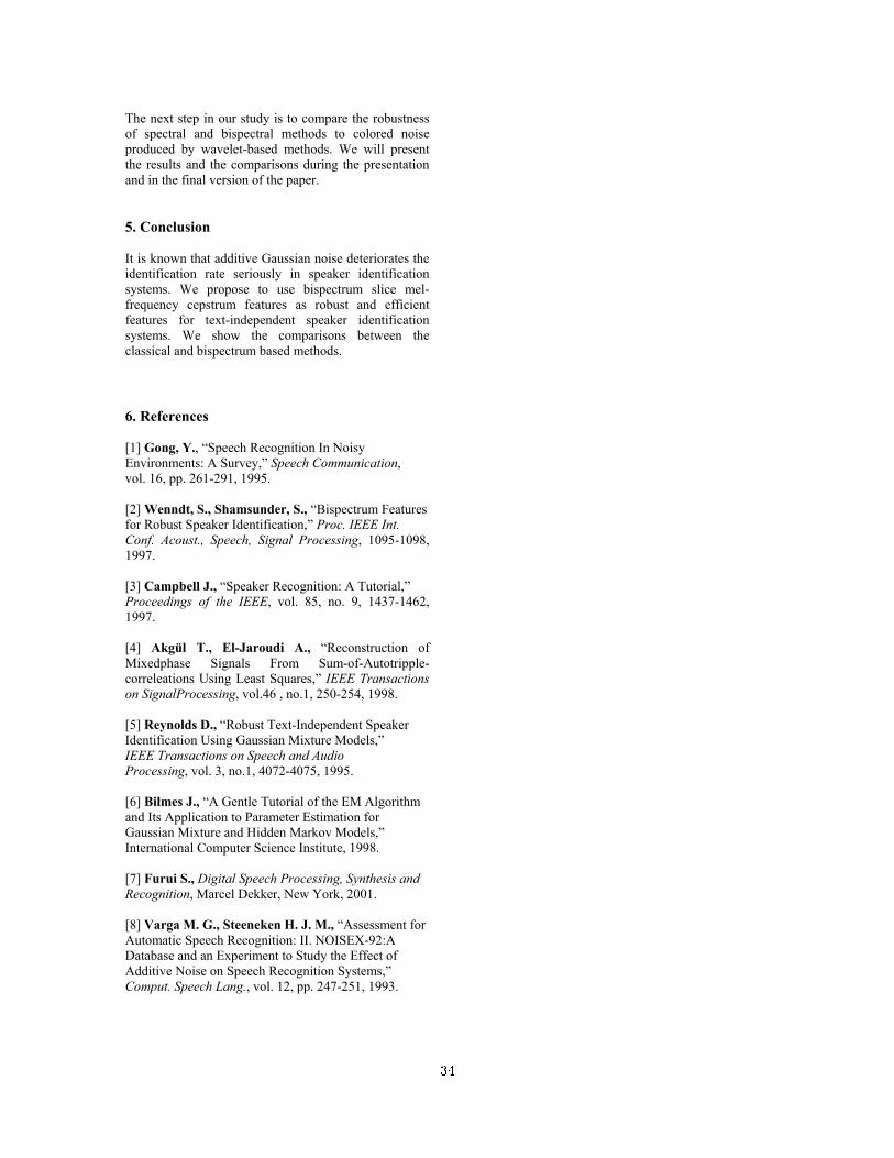
The next step in our study is to compare the robustness of spectral and bispectral methods to colored noise produced by wavelet-based methods. We will present the results and the comparisons during the presentation and in the final version of the paper. 5. Conclusion It is known that additive Gaussian noise deteriorates the identification rate seriously in speaker identification systems. We propose to use bispectrum slice mel-frequency cepstrum features as robust and efficient features for text-independent speaker identification systems. We show the comparisons between the classical and bispectrum based methods. 6. References [1] Gong, Y., “Speech Recognition In Noisy Environments: A Survey,” Speech Communication, vol. 16, pp. 261-291, 1995. [2] Wenndt, S., Shamsunder, S., “Bispectrum Features for Robust Speaker Identification,” Proc. IEEE Int. Conf. Acoust., Speech, Signal Processing, 1095-1098, 1997. [3] Campbell J., “Speaker Recognition: A Tutorial,” Proceedings of the IEEE, vol. 85, no. 9, 1437-1462, 1997. [4] Akgül T., El-Jaroudi A., “Reconstruction of Mixedphase Signals From Sum-of-Autotripple-correleations Using Least Squares,” IEEE Transactions on SignalProcessing, vol.46 , no.1, 250-254, 1998. [5] Reynolds D., “Robust Text-Independent Speaker Identification Using Gaussian Mixture Models,” IEEE Transactions on Speech and Audio Processing, vol. 3, no.1, 4072-4075, 1995. [6] Bilmes J., “A Gentle Tutorial of the EM Algorithm and Its Application to Parameter Estimation for Gaussian Mixture and Hidden Markov Models,” International Computer Science Institute, 1998. [7] Furui S., Digital Speech Processing, Synthesis and Recognition, Marcel Dekker, New York, 2001. [8] Varga M. G., Steeneken H. J. M., “Assessment for Automatic Speech Recognition: II. NOISEX-92:A Database and an Experiment to Study the Effect of Additive Noise on Speech Recognition Systems,” Comput. Speech Lang., vol. 12, pp. 247-251, 1993.

34

Perceptron-based Class Verification

Michael Gerber, Tobias Kaufmann and Beat Pfister

Speech Processing GroupComputer Engineering and Networks Laboratory

gerber,kaufmann,pfister@tik.ee.ethz.ch

Abstract

We present a method to use multilayer perceptrons (MLPs) fora verification task, i.e. to verify whether two vectors are fromthe same class or not. In tests with synthetic data we could showthat the verification MLPs are almost optimal from a Bayesianpoint of view. With speech data we have shown that verificationMLPs generalize well such that they can be deployed as wellfor classes which were not seen during the training.

1. Introduction

Multilayer perceptrons (MLPs) are successfully used in speechprocessing. For example they are used to calculate the phonemeposterior probabilities in hybrid MLP/HMM speech recognizers(see for example [1]). In this case their task is to output for everyphoneme the posterior probability that a given input feature vec-tor is from this phoneme. They are thus used to identify a featurevector with a given phoneme. Expressed in more general termsthe MLPs are used for the identification of input vectors with aclass from within a closed set of classes.

There are applications however, where the identification ofinput vectors is not necessary but it has to be verified whethertwo given input vectors x and y are from the same class or not.In Section 2 we present two verification tasks in the domain ofspeech processing. In this work we show that MLPs have the ca-pability to optimally solve verification problems. Furthermorewe have observed in a task with real-world data that the verifi-cation MLPs can even be used to discriminate between classeswhich were not present in the training set. This is an especiallyuseful property for two reasons:

• The verification MLP is usable for an open set of classes.

• Since we do not need training data from the classespresent in the application but can collect training datafrom other classes which have the same classificationobjective (e.g. classifying speakers). Therefore we canbuild a training set of a virtually unlimited size.

In Section 2 we present the motivation for our approach toclass verification and outline how MLPs can be used for thatpurpose. The structure and training of our verification MLPs isdescribed in Section 3. Our evaluation methods are describedin Section 4. In order to test whether verification MLPs arecapable of performing the verification task in an optimal wayfrom a Bayesian point of view we made experiments with syn-thetic data. These experiments and their results are describedin Section 5. The results of experiments with speech data areshown in Section 6. Finally, our conclusions are summarized inSection 7.

2. MotivationOur method to decide whether two speech signals are spokenby the same speaker or not includes the following 3 steps: Firstequally worded segments are sought in the two speech signals.This results in a series of frame pairs where both frames of a pairare from the same phoneme. In a second step for each frame pairthe probability that the two frames come from the same speakeris computed. Finally, the global indicator that the two speechsignals were spoken by the same speaker can be calculated fromthese frame-level probabilities. See e.g. [2] for a more detaileddescription of the speaker-verification approach. We used theverification MLPs for the following two tasks:

• In order to seek phonetically matching segments in twospeech signals with a method based on dynamic pro-gramming we need a phonetic probability matrix. Thismatrix is spanned by the two signals and every elementPij(x1i, x2j) gives the probability that frame i of sig-nal 1 given as feature vector x1i and frame j of signal 2given as feature vector x2j are from the same phoneme.The probabilities Pij(x1i, x2j) are calculated by an ap-propriately trained verification MLP.

• For every frame pair we use a verification MLP to calcu-late a score which stands for the probability that the twophonetically matching frames are from the same speaker.In this case we use a MLP which was trained with datafrom speakers which are not present in the test. There-fore we make use of the generalization property of theverification MLP.

3. Verification MLPSince the MLP has to decide whether two given input vectorsx and y are from the same class the MLP has to process vectorpairs rather than single vectors. The target output of the MLPis os if the two vectors of the pair are from the same class andod if they are from different classes. The vectors are decidedto belong to the same class if the output is closer to os and todifferent classes otherwise.

The sizes of the 3-layer perceptrons used for the experi-ments described in Sections 5 and 6 are as follows:

input 1st hidden 2nd hidden outputdatasetsize layer layer layer

syntheticdata

2 · 2...5 20 (tanh) 10 (tanh) 1 (tanh)

phonemeverification

2 · 26 80 (tanh) 35 (tanh) 1 (tanh)

speakerverification

2 · 16 70 (tanh) 18 (tanh) 1 (tanh)

35

The verification MLPs are trained by means of the backpropa-gation algorithm. For a hyperbolic tangent output neuron a goodchoice for the output targets is os = 0.75 and od = −0.75 suchthat the weights are not driven towards infinity (see for example[3]).

4. Performance evaluationIn order to evaluate a verification MLP, we measure its verifica-tion error rate for a given dataset and compare it to a referenceerror rate which is optimal in a certain sense. By formulatingour verification task as a classification problem, we can use theBayes error as a reference. The Bayes error is known to beoptimal for classification problems given the distribution of thedata.

To reformulate a verification task as a classification prob-lem, each pair of vectors is assigned one of the following twogroups:

GS group of all vector pairs where the two vectors are fromthe same class

GD group of all vector pairs where both vectors are from dif-ferent classes.

In the case of synthetic data it is possible to calculate the Bayesverification error since the data distributions are given in a para-metric form. For real-world problems the data distributions arenot given in a parametric form and hence the Bayes verificationerror can’t be computed directly. In this case we can use a knearest neighbor (KNN) classifier to asymptotically approachthe Bayes error as described below.

The KNN approach is a straightforward means of classifi-cation. The training set for the KNN algorithm consists of train-ing vectors with known classification (atr,i, btr,i) where atr,i isthe training vector and btr,i is its associated class. A test vectoratst,j is classified by seeking the k nearest training vectors atr,i

and it is assigned to the class which is most often present amongthe k nearest neighbors. The KNN classifier is known to reachthe Bayes error when an infinite number of training vectors isavailable (see e.g. [4]) and is therefore a means to approximatethe Bayes error if the data distributions are not known in a para-metric form.

5. Experiments with synthetic dataThe aim of the experiments with synthetic datasets, i.e. datasetswith known data distributions, was to test if the verificationMLP achieves the lowest possible verification error from aBayesian point of view. The data sets had 2 to 4 classes andwere 2- to 5-dimensional. We illustrate these investigations by

......

......

......

vect

or 2

vect

or 1

outp

ut v

alue

output targets:os same classod different classes

Figure 1: Structure of the verification MLPs.

−3 −2 −1 0 1 2−2

−1.5

−1

−0.5

0

0.5

1

1.5

c1

c 2

Figure 2: Synthetic data: 2 classes with 2-dimensional non-Gaussian distributions.

means of an experiment with a 2-dimensional dataset with 2classes that are distributed as shown in Figure 2.

The number of training epochs which were necessary totrain the verification MLP depended largely on the type of thedataset. We observed the following dependencies:

• If only a few features carried discriminating informationand all other features were just random values the verifi-cation MLP learned quickly which features were usefuland which ones could be neglected.

• The shape of the distributions strongly influenced thenumber of epochs that were necessary for the train-ing. For example, two classes distributed in two paral-lel stripes or classes that had a non-linear Bayes deci-sion boundary, such as those shown in Figure 2, requiredmany epochs.

Figure 3 shows the error rates of different verification methodsfor data distributed as shown in Figure 2. It can be seen thatthe error of the verification MLP is almost as low as the Bayeserror. Note that the MLP was trained with a fixed number of20’000 vector pairs. We are only interested in the best possi-ble verification error for a given task and not in the verificationerror in function of the number of training vectors (see Section1). Therefore the MLP training set was chosen as large as nec-essary.

For all investigated datasets the verification error achievedwith the verification MLP was not significantly higher than theBayes verification error.

6. Experiments with speech data6.1. Data description and feature extraction

For a speaker verification task with single speech frames weused speech signals from 48 male speakers recorded from dif-ferent telephones. From short speech segments (32 ms frames)the 13 first Mel frequency cepstral coefficients (MFCCs) wereextracted and used as feature vectors for our experiments. For

36

102

103

104

105

0

0.05

0.1

0.15

0.2

0.25

0.3

0.35

Number of KNN training vectors

Rat

e of

wro

ng v

erifi

catio

n

Verification with KNNVerification with ANNBayes verification error

Figure 3: Class verification error for the test set as shown inFigure 2: the KNN verification error is shown in function of thetraining set size. As expected, with increasing size it approxi-mates the Bayes limit which is indicated by the dotted line. Theerror rate of the verification MLP is close to the Bayes error.

the phoneme verification task the first derivatives of the MFCCswere used in addition to the static MFCCs. The data from allspeakers was divided into 3 disjoint sets (i.e. no speaker waspresent in more than one set). The MLP and KNN training vec-tor pairs were extracted from the training set (26 speakers). Thevalidation set (10 speakers) was used to stop the MLP trainingat the optimal point and to find the optimal k of the KNN classi-fier. The test vector pairs were taken from the test set (12 speak-ers). Within all sets vector pairs were formed in a way that thetwo vectors of a pair were always from the same phoneme. Inevery set the number of pairs with vectors of the same speakerand the number of pairs with vectors from different speakerswere equal.

6.2. Phoneme Verification

In this task the objective was to decide whether two speech fea-ture vectors originate from the same phoneme. In this task thesame classes (phonemes) are present in all 3 datasets since allsignals have similar phonetic content. Yet all sets are extractedfrom different speakers as is described in Section 6.1.

Because of the slow convergence of the KNN for this ver-ification problem we used two types of input, namely pairs ofconcatenated vectors pin = (x, y) as mentioned above andcoded vector pairs pin = (|x − y|, x + y) (see [5] for detailsabout the input coding). This input coding sped up the trainingof the MLPs and led to a faster convergence of the KNN.

The verification error of an MLP trained with 580000 vectorpairs is shown in Figure 4. For comparison also the KNN errorrate in function of the training set size is drawn. It can be seenthat with this data the verification KNN converges much slowerthan with synthetic data. This was expected because of the morecomplex nature of the problem. It can only be guessed where

102

104

106

0

0.05

0.1

0.15

0.2

0.25

0.3

0.35

0.4

0.45

0.5

Number of KNN training vectors

Rat

e of

wro

ng v

erifi

catio

n

Verification with KNN (input coding)Verification with KNN (no input coding)Verification with ANN (input coding)Verification with ANN (no input coding)

Figure 4: Phoneme verification task: The KNN error rates de-crease with increasing number of KNN training vectors. Theerror rates of the verification MLPs are shown as dots. The errorrates for both, KNN and MLP are given for coded and uncodedinput vectors.

the asymptote and therefore the Bayes error will be. It seemsthat the verification error of the MLP is close to the Bayes ver-ification error however. Since we did not have enough trainingdata we could not prove this assumption. Furthermore it doesnot seem that the input coding had a big effect on the optimalverification result - the verification MLP which used coded in-put vectors was even a bit better.

6.3. Speaker Verification

In this task the objective was to decide whether two speechframes are from speech signals of the same speaker or not. Inthis case all 3 sets of classes (speakers) were disjoint. Thereforea good generalization of the verification MLP is required.

The experiment results are shown in Figure 5. It can beseen that the KNN verification error in function of the trainingset size decreases much slower than in the experiments donewith synthetic data and does not even reach the verification errorof the MLP. This is possible since the training and test set havesome mismatch because the speaker sets are disjoint. Here it canbe seen very well that the KNN which is based on coded vectorpairs converged much quicker. In this case the verification ANNwhich used coded vector pairs was a bit worse however.

The MLP has a quite low verification error if it is consid-ered that the feature vectors x and y were extracted from singlespeech frames only. If all phonetically matching frame pairs oftwo equally worded speech segments of about 1 s length are fedseparately into the MLP and the output values of the MLP areaveraged, the verification error rate is about 6 %.

37

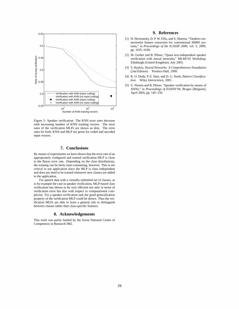
102

104

106

0.25

0.3

0.35

0.4

0.45

0.5

0.55

Number of KNN training vectors

Rat

e of

wro

ng v

erifi

catio

n

Verification with KNN (input coding)Verification with KNN (no input coding)Verification with ANN (input coding)Verification with ANN (no input coding)

Figure 5: Speaker verification: The KNN error rates decreasewith increasing number of KNN training vectors. The errorrates of the verification MLPs are shown as dots. The errorrates for both, KNN and MLP are given for coded and uncodedinput vectors.

7. ConclusionsBy means of experiments we have shown that the error rate of anappropriately configured and trained verification MLP is closeto the Bayes error rate. Depending on the class distributions,the training can be fairly time-consuming, however. This is notcritical in our application since the MLP is class independentand does not need to be trained whenever new classes are addedto the application.

For speech data with a virtually unlimited set of classes, asis for example the case in speaker verification, MLP-based classverification has shown to be very efficient not only in terms ofverification error but also with respect to computational com-plexity. For a speaker-verification task the good generalizationproperty of the verification MLP could be shown. Thus the ver-ification MLPs are able to learn a general rule to distinguishbetween classes rather than class-specific features.

8. AcknowledgementsThis work was partly funded by the Swiss National Center ofCompetence in Research IM2.

9. References[1] H. Hermansky, D. P. W. Ellis, and S. Sharma, “Tandem con-

nectionist feature extraction for conventional HMM sys-tems,” in Proceedings of the ICASSP 2000, vol. 3, 2000,pp. 1635–1638.

[2] M. Gerber and B. Pfister, “Quasi text-independent speakerverification with neural networks,” MLMI’05 Workshop,Edinburgh (United Kingdom), July 2005.

[3] S. Haykin, Neural Networks: A Comprehensive Foundation(2nd Edition). Prentice-Hall, 1999.

[4] R. O. Duda, P. E. Hart, and D. G. Stork, Pattern Classifica-tion. Wiley Interscience, 2001.

[5] U. Niesen and B. Pfister, “Speaker verification by means ofANNs,” in Proceedings of ESANN’04, Bruges (Belgium),April 2004, pp. 145–150.

38

Manifold Learning-based Feature Transformation for Phone Classification

Andrew Errity, John McKenna and Barry Kirkpatrick

School of ComputingDublin City University, Dublin 9, Ireland

andrew.errity, john.mckenna, barry.kirkpatrick@computing.dcu.ie

AbstractThis paper investigates approaches for low dimensional speechfeature transformation using manifold learning. It has recentlybeen shown that speech sounds may exist on a low dimensionalmanifold nonlinearly embedded in high dimensional space. Anumber of techniques have been developed in recent years thatattempt to discover the geometric structure of the underlyinglow dimensional manifold. The manifold learning techniqueslocally linear embedding and Isomap are considered in thisstudy. The low dimensional feature representations producedby these techniques are applied to several phone classificationtasks on the TIMIT corpus. Classification accuracy is analysedand compared to conventional MFCC features and PCA, a lin-ear dimensionality reduction method, transformed features. Itis shown that features resulting from manifold learning are ca-pable of yielding higher classification accuracy than these base-line features. The best phone classification accuracy in generalis demonstrated by feature transformation with Isomap.

1. IntroductionFeature transformation is an important part of the speech recog-nition process and can be viewed as a two step procedure.Firstly, relevant information is extracted from short time seg-ments of the acoustic speech signal using a procedure suchas Fourier analysis, cepstral analysis or some other perceptu-ally motivated analysis. The resultingD-dimensional param-eter vectors are then transformed to a feature vector of lowerdimensionalityd (d ≤ D). The aim of dimensionality reduc-tion is to produce features which are concise low dimensionalrepresentations that retain the most discriminating informationfor the intended application and are thus more suitable for pat-tern classification. Dimensionality reduction also decreases thecomputational cost associated with subsequent processing.

Physiological constraints on the articulators limit the de-grees of freedom of the speech production apparatus. As a resulthumans are only capable of producing sounds occupying a sub-space of the acoustic space. Thus, speech data can be viewedas lying on or near a low dimensional manifold embedded inthe original acoustic space. The underlying dimensionality ofspeech has been the subject of much previous research includ-ing classical dimensionality reduction analysis [1, 2], nonlineardynamical analysis [3] and manifold learning [4]. The consen-sus of this work is that some speech sounds, particularly voicedspeech, are inherently low dimensional.

Dimensionality reduction methods aim to discover this un-derlying low dimensional structure. These methods can be cat-egorised as linear or nonlinear. Linear methods are limited todiscovering the structure of data lying on or near a linear sub-space of the high dimensional input space. The most widelyused linear dimensionality reduction methods include principal

component analysis (PCA) [5] and linear discriminant analysis(LDA) [6]. These methods have been successfully applied tofeature transformation in speech processing applications [7, 8]in the past.

However if speech data occupies a low dimensional sub-manifold nonlinearly embedded in the original space, as pro-posed previously [2, 4], linear methods will fail to discoverthe low dimensional structure. A number of manifold learn-ing, also referred to as nonlinear dimensionality reduction, al-gorithms have been developed [9–11] which overcome the lim-itations of linear methods. Manifold learning algorithms haverecently been shown to be useful in a number of speech pro-cessing applications including low dimensional visualization ofspeech [4,11–14] and limited phone classification tasks [14,15].

In this paper, we build upon previous work and apply twomanifold learning algorithms, locally linear embedding (LLE)[9] and isometric feature mapping (Isomap) [10], to extractfeatures from speech data. These features are evaluated inphone classification experiments using a support vector ma-chine (SVM) [16] classifier. The classification performance ofthese features is compared to baseline Mel-frequency cepstralcoefficients (MFCC) and those resulting from the classical lin-ear method, PCA.

The remainder of this paper is structured as follows. In Sec-tion 2, the manifold learning algorithms LLE and Isomap arebriefly described. Section 3 details the experimental procedure,data set, parameter extraction, feature transformation and clas-sification technique used. Results are examined and discussedin Section 4, with conclusions presented in Section 5. Finally,possibilities for future work are outlined in Section 6.

2. Manifold learning algorithms2.1. Locally linear embedding

LLE [9] is an unsupervised learning algorithm that computeslow dimensional embeddings of high dimensional data. Theprinciple of LLE is to compute a low dimensional embeddingwith the property that nearby points in the high dimensionalspace remain nearby and similarly co-located with respect toone another in the low dimensional space. In other words, theembedding is optimised to preserve local neighbourhoods.

The LLE algorithm can be summarised in three steps:

1. For each data pointXi, compute itsk nearest neighbours(based on Euclidean distance or some other appropriatedefinition of ‘nearness’).

2. Compute weightsWij that best reconstruct each datapointXi from its neighbours, minimising the reconstruc-tion errorE:

E(W ) =∑

i

∣∣∣Xi −∑

j

WijXj

∣∣∣2 (1)

39

3. Compute the low dimensional embeddingsYi, best re-constructed by the weightsWij , minimising the costfunctionΩ:

Ω(W ) =∑

i

∣∣∣Yi −∑

j

WijYj

∣∣∣2 (2)

In step 2, the reconstruction error is minimised subject to twoconstraints: first, that each input is reconstructed only from itsnearest neighbours, orWij = 0 if Xi is not a neighbour ofXj ; second, that the reconstruction weights for each data pointsum to one, or

∑j Wij = 1 ∀i. The optimum weights for each

input can be computed efficiently by solving a constrained leastsquares problem.

The cost function in step 3 is also based on locally linearreconstruction errors, but here the weightsWij are kept fixedwhile optimising the outputsYi. The embedding cost functionin Equation (2) is a quadratic function inYi. The minimisationis performed subject to constraints that the outputs are centeredand have unit covariance. The cost function has a unique globalminimum solution for the outputsYi. This is the result returnedby LLE as the low dimensional embedding of the high dimen-sional data pointsXi.

2.2. Isomap

The Isomap algorithm [10] offers a differently motivated ap-proach to manifold learning. Isomap is a nonlinear generalisa-tion of multidimensional scaling (MDS) [6] that seeks a map-ping from high dimensional spaceX to low dimensional featurespaceY that preserves geodesic distances between pairs of datapoints—that is, distances on the manifold from which the datais sampled.

While Isomap and LLE have similar aims, Isomap is basedon a different principle than LLE. In particular, Isomap attemptsto preserve the global geometric properties of the manifoldwhile LLE attempts to preserve the local geometric propertiesof the manifold.

As with LLE, the Isomap algorithm consists of three steps:

1. Construct a neighbourhood graph - Determine whichpoints are neighbours on the manifold based on distancesl(i, j) between pairs of pointsi, j in the input space(as in step 1 of LLE). These neighbourhood relationsare then represented as a weighted graph over the datapoints with edges of weightl(i, j) between neighbour-ing points.

2. Compute the shortest path between all pairs of pointsamong only those paths that connect nearest neighboursusing a technique such as Dijkstra’s algorithm.

3. Use classical MDS to embed the data in ad-dimensionalEuclidean space so as to preserve these geodesic dis-tances.

3. Experiments3.1. Classification tasks

The objective of these experiments is to perform phone clas-sification using four different feature types: baseline MFCCvectors and features produced by applying PCA, Isomap andLLE to MFCC vectors. Each feature type was evaluated inthree phone classification experiments. The first experiment in-volves distinguishing between a set of five vowels (‘aa’, ‘iy’,

‘uw’, ‘eh’, and ‘ae’). Phones are labeled using TIMIT sym-bols [17]. In the second test, a further five vowels (‘ah’, ‘ay’,‘oy’, ‘ih’ and ‘ow’) were added to the previous vowel set, form-ing a more complex ten class vowel classification problem. Thefinal test involves classifying a set of 19 phones into their asso-ciated phone classes. The phone classes and phones used were:vowels (listed above), fricatives (‘s’, ‘sh’), stops (‘p’, ‘t’, ‘k’),nasals (‘m’, ‘n’) and, semivowels and glides (‘l’, ‘y’).

3.2. Data

The speech data used in this study was taken from the TIMITcorpus [17]. This corpus contains 6300 utterances, 10 spokenby each of 630 American English speakers. The speech record-ings are provided at a sampling frequency of 16 kHz.

3.3. Parameter extraction

Based on the phonetic transcriptions and associated phoneboundaries provided in TIMIT all units of a subset of phones,listed in Section 3.1, were extracted from the corpus. One 40 msframe was extracted from the middle of each phone unit (unitsof duration less than 100 ms were discarded). The raw speechframes were amplitude normalised, preemphasized with the fil-ter H(z) = 1− 0.98z−1 and Hamming windowed. Followingthis preprocessing, 19-dimensional MFCC vectors were com-puted for each frame. These MFCC vectors serve as both abaseline feature and high dimensional input for PCA, Isomapand LLE methods.

3.4. Feature transformation

For each of the three phone classification experiments, 250 unitsrepresenting each of the required phones were chosen at ran-dom from those extracted above to make up the data set. PCA,Isomap and LLE were applied to the equivalent set of MFCCvectors.

In order to examine the ability of the feature transformationmethods to compute concise representations of the input vec-tors retaining discriminating information, the dimensionality ofthe resulting feature vectors was varied from 1 to 19. A sepa-rate classifier was subsequently trained and tested using featurevectors with each of the 19 different dimensionalities. Thus theability of these feature transformation methods to produce use-ful low dimensional features could be evaluated and changes inperformance with varying dimension analysed. As a baselinethe original MFCC vectors were used, also varying in dimen-sionality from 1 to 19.

The number of nearest neighbours,k, used in Isomap andLLE was set equal to 14 and 6 respectively. These values werechosen empirically by varyingk and examining classificationperformance. The performance of both methods was found tobe sensitive to the choice ofk.

3.5. Support vector machine classification

SVM [16], a powerful classification tool, was used in these ex-periments. SVM is a binary pattern classification algorithm.For our experiments it is necessary to construct a multiclassclassifier. This was achieved using a one-against-one trainingscheme, training one classifier for every possible pair of classes.The final classification result was determined by majority vot-ing.

It is also necessary to choose an appropriate kernel func-tion to be used in the SVM. In order to select an effective

40

0 2 4 6 8 10 12 14 16 18 2035

45

55

65

75

85

95Training Data

Cla

ssifi

catio

n R

ate

(%)

0 2 4 6 8 10 12 14 16 18 2030

40

50

60

70

8085

Feature Dimension

Cla

ssifi

catio

n R

ate

(%)

Testing Data

PCAMFCCIsomapLLE

Figure 1:Five vowel classification results for baseline MFCC,PCA, Isomap and LLE features on the TIMIT database.

kernel, different SVM models using linear, polynomial and ra-dial basis function (RBF) kernels were evaluated in a numberof phone classification tasks. SVM with RBF kernel demon-strated the best classification accuracy and is used for classi-fication throughout this work. The RBF kernel used is givenin Equation (3) below, withx andx′ feature vectors andd thefeature vector dimensionality.

K(x, x′) = exp(−1

d

∥∥x− x′∥∥2

) (3)

In all classification experiments 80% of the data was as-signed as training data with the remaining 20% withheld andused as unseen testing data.

4. ResultsIn each experiment the classifier was evaluated on each of thefour feature types. The dimensionality of the feature vectorsused in the experiment vary from 1 to 19—the original, full di-mension. Results are presented for evaluation on both the train-ing data and testing data.

Fig. 1 shows the results of the five vowel classification taskusing the baseline MFCC, PCA, Isomap and LLE features. Thepercentage of phones correctly classified is given on the verti-cal axis. The horizontal axis represents the dimensionality ofthe feature vector. The results in Fig. 1 can be summarized asfollows:

• The performance of the baseline MFCC vectors im-proves with increasing dimensionality, plateauing at adimensionality of approximately 8.

• PCA features offer improvements over baseline MFCCfor low dimensions, 1 to 7.

• For the training data, maximum classification accuracyin all dimensions is demonstrated with Isomap features,outperforming all other features including the originalfull 19-dimensional MFCC vectors.

• Isomap features also offer performance comparable to,and in some dimensions better than, other features onthe testing data.

• Accuracy with LLE features is better than both MFCCand PCA in low dimensions, (d < 3). However in higher

0 2 4 6 8 10 12 14 16 18 2020

30

40

50

60

7075

Training Data

Cla

ssifi

catio

n R

ate

(%)

0 2 4 6 8 10 12 14 16 18 2015

25

35

45

50

Feature Dimension

Cla

ssifi

catio

n R

ate

(%)

Testing Data

PCAMFCCIsomapLLE

Figure 2: Ten vowel classification results for baseline MFCC,PCA, Isomap and LLE features on the TIMIT database.

dimensions LLE features do not offer a performance in-crease over other methods.

Results for ten vowel classification are given in Fig. 2. Theresults are similar to those of the task above, with reduced clas-sification accuracy due to increased complexity and increasedpossibility of phone confusion. The important findings are asfollows:

• Again, Isomap performs best for the training data, andalso for testing data in low dimensions (d < 8).

• Isomap, PCA and MFCC performance reach a flat per-formance level from approximately 10 dimensions.

• A classification accuracy of 48.2% is achieved on thetesting data with 5-dimensional Isomap features. Thisperformance is only exceeded by much higher dimen-sional, (d > 12), MFCC and PCA features.

The mean classification accuracy results for each feature type inthe ten vowel classification task are presented in Table 1. Themean accuracy scores were computed for the testing data eval-uation. Averages are computed for three dimensionality ranges.It can be seen that Isomap gives the highest average accuracyin all ranges. LLE is shown to perform better than PCA andMFCC in low dimensions.

Dimensions MFCC PCA Isomap LLE

1–5 32.2000 38.3200 43.5600 38.60006–19 47.0000 47.0143 47.5286 44.62861–19 43.1053 44.7263 46.4842 43.0421

Table 1: Mean classification accuracy in the ten vowel classifi-cation task for MFCC, PCA, Isomap and LLE features.

Phone class classification results are presented in Fig. 3.The following is evident:

• Best accuracy is achieved in all dimensions with Isomapfeatures.

• PCA and MFCC features yield similar performance,with PCA features offering improved accuracy for lowdimensional features.

41

0 2 4 6 8 10 12 14 16 18 2035

45

55

65

75

85Training Data

Cla

ssifi

catio

n R

ate

(%)

0 2 4 6 8 10 12 14 16 18 2040

50

60

70

80

Feature Dimension

Cla

ssifi

catio

n R

ate

(%)

Testing Data

PCAMFCCIsomapLLE

Figure 3:Phone class classification results for baseline MFCC,PCA, Isomap and LLE features on the TIMIT database.

• LLE features give the lowest classification rates, exceptfor 2 and 3 dimensional features where they are secondonly to Isomap.

5. Conclusions

In this paper a phone classification system based on nonlinearmanifold learning was proposed and evaluated against a base-line linear dimensionality reduction method, PCA, and con-ventional MFCC features. All of the dimensionality reductionmethods presented outperform the baseline MFCC features forlow dimensions. This illustrates the capability of these meth-ods to extract discriminating information from the original 19-dimensional MFCC features.

Higher classification accuracy is shown for manifold learn-ing derived features compared to baseline MFCC and PCA fea-tures for low dimensions. Also, in general Isomap yields su-perior performance to both MFCC and PCA features. This in-dicates that nonlinear manifold learning algorithms are morecapable of retaining information required for discriminating be-tween phones, especially in low dimensional space.

Comparing the manifold learning methods, Isomap demon-strates better classification accuracy than LLE. This indicatesthat preserving global structure rather than local relationshipsmay be more important for speech feature transformation.

6. Future Work

Possible future work includes the application of the mani-fold learning feature transformation procedure presented hereto continuous ASR. The manifold learning methods describedabove are batch processing algorithms. A number of out-of-sample extensions have been proposed to overcome this limi-tation. In the future these out-of-sample approaches could bedeveloped for use with speech data.

7. Acknowledgments

Andrew Errity would like to acknowledge the support of theIrish Research Council for Science, Engineering and Technol-ogy; grant number RS/2003/114.

8. References[1] W. Klein, R. Plomp, and L. C. W. Pols, “Vowel spectra,

vowel spaces, and vowel identification,”J. Acoust. Soc.Amer., vol. 48, no. 4, pp. 999–1009, 1970.

[2] R. Togneri, M. Alder, and J. Attikiouzel, “Dimension andstructure of the speech space,”IEE Proceedings-I, vol.139, no. 2, pp. 123–127, 1992.

[3] M. Banbrook, S. McLaughlin, and I. Mann, “Speech char-acterization and synthesis by nonlinear methods,”IEEETransactions on Speech and Audio Processing, vol. 7,no. 1, pp. 1–17, January 1999.

[4] A. Jansen and P. Niyogi, “Intrinsic Fourier analysis onthe manifold of speech sounds,” inProc. of the IEEEInt. Conf. on Acoustics, Speech and Signal Processing(ICASSP), 2006.

[5] I. Jolliffe, Principal Component Analysis, ser. SpringerSeries in Statistics. New York: Springer-Verlag, 1986.

[6] R. O. Duda and P. E. Hart,Pattern Classification andScene Analysis. New York: Wiley, 1973.

[7] X. Wang and K. Paliwal, “Feature extraction and dimen-sionality reduction algorithms and their applications invowel recognition,”Pattern Recognition, vol. 36, no. 10,pp. 2429–2439, October 2003.

[8] P. Somervuo, “Experiments with linear and nonlinear fea-ture transformations in HMM based phone recognitionbased phone recognition,” inProc. of the IEEE Int. Conf.on Acoustics, Speech and Signal Processing (ICASSP),vol. 1, April 2003, pp. 52–55.

[9] S. T. Roweis and L. K. Saul, “Nonlinear dimensionalityreduction by locally linear embedding,”Science, vol. 290,no. 5500, pp. 2323–2326, December 2000.

[10] J. B. Tenenbaum, V. de Silva, and J. C. Langford, “Aglobal geometric framework for nonlinear dimensionalityreduction,”Science, vol. 290, pp. 2319–2323, 2000.

[11] M. Belkin and P. Niyogi, “Laplacian eigenmaps and spec-tral techniques for embedding and clustering,” inAd-vances in Neural Information Processing Systems, T. G.Dietterich, S. Becker, and Z. Ghahramani, Eds., vol. 14.Cambridge, MA: MIT Press, 2002, pp. 585–591.

[12] R. M. Hegde and H. A. Murthy, “Cluster and intrinsic di-mensionality analysis of the modified group delay featurefor speaker classification,”Lecture Notes in Computer Sci-ence, vol. 3316, pp. 1172–1178, January 2004.

[13] V. Jain and L. Saul, “Exploratory analysis and visualiza-tion of speech and music by locally linear embedding,”in Proc. of the IEEE Int. Conf. on Acoustics, Speech andSignal Processing (ICASSP), vol. 3, 2004, pp. 984–987.

[14] A. Errity and J. McKenna, “An investigation of manifoldlearning for speech analysis,” inProc. of the Int. Conf.on Spoken Language Processing (ICSLP), Pittsburgh PA,USA, September 2006, pp. 2506–2509.

[15] M. Belkin and P. Niyogi, “Semi-supervised learning onRiemannian manifolds,”Machine Learning, vol. 56, no. 1- 3, pp. 209–239, July 2004.

[16] V. Vapnik, The Nature of Statistical Learning Theory.Springer, N.Y., 1995.

[17] J. S. Garofalo, L. F. Lamel, W. M. Fisher, J. G. Fiscus,D. S. Pallett, and N. L. Dahlgren,The DARPA TIMITAcoustic-Phonetic Continuous Speech Corpus CDROM,NIST, 1990.

42

Word Recognition with a Hierarchical Neural Network

Xavier Domont1,2, Martin Heckmann1, Heiko Wersing1,Frank Joublin1, Stefan Menzel1, Bernhard Sendhoff 1, Christian Goerick1

1Honda Research Institute Europe, 63073 Offenbach/Main, Germanyfirstname.lastname@honda-ri.de

2Technische Universitat Darmstadt, 64283 Darmstadt, Germanyxavier.domont@rtr.tu-darmstadt.de

Abstract

In this paper we propose a feedforward neural network for syl-lable recognition. The core of the recognition system is basedon a hierarchical architecture initially developed for visual ob-ject recognition. We show that, given the similarities betweenthe primary auditory and visual cortexes, such a system can suc-cessfully be used for speech recognition. Syllables are used asbasic units for the recognition. Their spectrograms, computedusing a Gammatone filterbank, are interpreted as images andsubsequently feed into the neural network after a preprocessingstep that enhances the formant frequencies and normalizes thelength of the syllables. The performance of our system has beenanalyzed on the recognition of 25 different monosyllabic words.The parameters of the architecture have been optimized using anevolutionary strategy. Compared to the Sphinx-4 speech recog-nition system, our system achieves better robustness and gener-alization capabilities in noisy conditions.

1. IntroductionThe aim of the proposed speech recognition architecture is toovercome the limitations of conventional, HMM-based, sys-tems which substantially lack robustness against noise.

It has recently been shown that the time-frequency recep-tive fields in the primary auditory cortex of ferrets have strongsimilarities to those of the visual cortex [1]. They are selectiveto modulations in the time-frequency domain and have Gabor-like shapes. A mathematical model of these receptive fields wasgiven in [2] and has already been used for source separation [3]and speech detection [4]. As Gabor-like filters are extensivelyused in object recognition systems [5, 6], we decided to developa system for speech recognition by adapting the feedforwardneural network initially developed by Wersing and Korner forobject recognition [6].

Syllables are the basic units for speech production andshow less co-articulatory effects across their boundaries. There-fore, we believe that they are the adequate speech units for ourbiologically-inspired system. Moreover, the syllable segmenta-tion required for the training of the system seems biologicallyplausible for speech acquisition.

The building blocks of the system (Fig. 1) are detailed in thefollowing sections. After explaining how we optimized the pa-rameters of the architecture using an evolutionary strategy, wewill compare our results to a state of the art speech recognitionsystem and conclude with a discussion of the obtained results.

2. Preprocessing of the spectrogramThe preprocessing mainly aims at transforming a previouslysegmented speech signal, corresponding to one syllable, intoan ”image” that is fed into the hierarchical recognition architec-ture. A two-dimensional representation of a signal is obtainedby computing its spectrogram. In addition to the phonetic in-formation, the speech signal also contains many speaker andrecording specific information. As the phonetic information ischiefly conveyed by the formant trajectories, we enhance themin the spectrograms prior to recognition.

We used a Gammatone filterbank to compute the spectro-gram of the signal. It models the response of the basilar mem-brane in the human inner ear and is, therefore, adapted to abiology-inspired system. The signal’s sampling frequency is16 kHz. The filterbank has 128 channels ranging from 80 Hz to8 kHz. The left part of Fig. 2 shows the response of the Gam-matone filterbank after rectification and low-pass filtering. Tocompensate for the influence of the speech excitation signal, thehigh frequencies are emphasized by +6 dB per octave resultingin a flattened spectrogram (Fig. 2 center). Next, the formantfrequencies are enhanced by filtering along the channel axis us-ing mexican-hat filters (Fig. 2 right), only the positive valuesare kept. For the filtering the size of the kernel is channel-dependent, varying from 90Hz for low frequencies to 120Hzfor high frequencies. This takes the logarithmic arrangementof the center frequencies in the Gammatone filterbank into ac-count.

Finally, the length of the spectrogram is scaled using linearinterpolation so that all the spectrograms feeding the recogni-tion hierarchy have the same size. The sampling rate is thenreduced to 100Hz. By doing so syllables of different lengthsare scaled to the same length. This relies on the assumption thata linear scaling can handle variations in the length of the samesyllable uttered at different speaking rates. However, these areknown to be non-linear. In particular, some parts of the signal,like vowels, are more affected by variation in the speech ratethan other parts, e.g. plosives. The generalization over thesevariations is a main challenge in the recognition task. In orderto also assess the performance of the recognition hierarchy in-dependent of this non-linear scaling, we applied the DynamicTime Warping (DTW) method to the spectrograms. For eachsyllable, we selected one single repetition as reference templateand aligned the other by DTW.

Afterwards the syllables were again scaled to the samelength and downsampled. At the output of the preprocessingstage the spectrograms feeding the recognition hierarchy have

43

Hierarchical Architecture

PreprocessingFeature-Selective

Layer

Combination Layer

Syllable-Tuned Units

Speech Signal

Recognized Syllable

Figure 1: Overview of the system.

Time [ms]

Cha

nnel

No.

0 100 200 300 400

20406080

100120

Time [ms]C

hann

el N

o.

0 100 200 300 400

20406080

100120

Time [ms]

Cha

nnel

No.

0 100 200 300 400

20406080

100120

Figure 2: Overview of the preprocessing step for the word ”list” spoken by a female American speaker. The 128 channels logarithmi-cally span the frequency range from 80Hz to 8 kHz. Left: Response of the basilar membrane. Center: After a low-pass filtering overtime and a preemphasis has been applied. Right: The harmonic structure has been removed using a filtering along the frequency axis.

all the size of 128 × 128, i.e. 128 time frames over 128 fre-quency channels. Note, however, that the application of DTWrequires that a hypothesis for the syllable is available. Thus, itcannot easily be applied to a real recognition test.

3. The recognition hierarchyThe preprocessed two-dimensional spectrogram is from now onconsidered to be an image and feeds into a feedforward archi-tecture initially aimed at visual object recognition. However,the structure of spectrograms differs from the structure of im-ages taken from objects and, while keeping the overall layoutof the network described in [6], the receptive fields and the pa-rameters of the neurons were retrained for the task of syllablerecognition. The recognition hierarchy is illustrated in Fig. 3.

3.1. Feature-Selective Layer

The first feature-matching stage consists of a linear receptivefield summation, a Winner-Take-Most (WTM) and a poolingmechanism. The preprocessed spectrogram is first filtered byeight different Gabor-like filters. The purpose of these filters isto extract local features from the spectrogram. In [6] the recep-tive fields were chosen as four first-order even Gabor filters. Forsyllable recognition, 8 receptive fields were learned using inde-pendent component analysis on 3500 randomly selected localpatches of preprocessed spectrograms.

The WTM competition mechanism between features at thesame position introduces nonlinearity into the system. Thevalue rl(t, f) of the spectrogram in the lth neuron of thefeature-selective layer after the WTM competition is given atthe position (t, f) by the following equation:

rl(t, f) =

(0, if ql(t,f)

M(t,f)< γ1 or M(t, f) = 0

ql(t,f)−γ1M(t,f)1−γ1

, else(1)

where ql(t, f) is the value of the spectrogram before the WTMcompetition, M(t, f) = maxk qk(t, f) the maximal value atposition (t, f) over the eight neurons and 0 ≤ γ1 ≤ 1 is a pa-rameter controlling the strength of the competition. A thresholdθ1 is applied to the activity rl(t, f). This threshold is commonfor all the neurons in the layer. The pooling performs a down-

sampling of the spectrogram by four in both time and frequencydirection. It is done by a Gaussian receptive field with widthσ1. The feature-selective layer transforms the 128× 128 origi-nal spectrogram to eight 32× 32 spectrogram feature maps.

3.2. Combination Layer

The goal of the combination layer is to detect relevant local fea-ture combinations in the first layer. Similar to the previous layerit consists of a linear receptive field summation, a Winner-Take-Most and a pooling mechanism. These combination cells arelearned using the non-negative sparse coding method (NNSC)as in [6], however no invariance transformations have been im-plemented at this stage. Similarly to Non-Negative Matrix Fac-torization (NMF), the NNSC method decomposes data vectorsIp into linear combinations (with non-negative weights sp

i )of non-negative features wi by minimizing the following costfunction:

E =X

p

‖Ip −X

i

spi wi‖2 + β

Xp

Xi

|spi |.

NNSC differs from NMF by the presence of a sparsity en-forcing term in the cost function, controlled by the parameter β,which aims at limiting the number of non-zero coefficients re-quired for the reconstruction. Consequently, if a feature appearsoften in the data, it will be learned, even if it can be obtained bya combination of two or more other features. Therefore, theNNSC is expected to learn complex and global features appear-ing in the data. An comprehensive description of this methodcan be found in [7].

For the proposed syllable recognition system 50 complexfeatures wi have been learned from image patches extractedfrom the output of the feature-selective layer. At last, a WTMcompetition (γ2, θ2) and pooling (σ2) are applied to the 50 neu-rons and their size is reduced to 16× 16.

3.3. Syllable-Tuned Units

In the last stage of the architecture, linear discriminant classi-fiers are learned based on the output of the combination layer.A classical gradient descent is used for this supervised learn-ing including an early stopping mechanism to avoid overfitting.The obtained classifiers are called Syllable-Tuned Units (STUs)in reference to the View-Tuned Units used in [5] and [6].

44

"HOW"

"HAVE"

"LIST"

"SHIPS"

"CHART"

Feature-SelectiveLayer

CombinationLayer

Syllable-TunedUnits

Figure 3: The system is based on a feedforward architecture with weight-sharing and a succession of feature sensitive matching andpooling stages. It comprises three stages arranged in a processing hierarchy.

4. Optimization of the architectureThe performance of the recognition highly depends on thechoice of the non-linearities present in the hidden layers of thearchitecture, i.e. the coefficients and the thresholds of the WTMcompetitions (Eq. 1) and the width of the poolings. The six pa-rameters (γ1,2, θ1,2 and σ1,2) have to be tuned simultaneouslyand the receptive field of the combination layer as well as theSyllable-Tuned Units have to be learned at each iteration, simi-larly to the method used in [8].

Practically, this tuning of the model parameter set has beenrealized within an evolutionary optimization aiming at maxi-mizing the recognition performance in a clean speech scenario.Due to the stochastic components and the use of a populationof solutions evolutionary algorithms need more quality evalu-ations than other algorithms, but on the other hand they allowfor a global search and are able to overcome local optima. Inthe present context, an evolutionary strategy with global stepsize adaptation (GSA-ES) has been applied relying on similarranges of the object variables. Initially, standard values, see[9, 10], have been used and then tuned in some test experimentsto this specific task. Based on these experiments we have cho-sen a population size of 32 individuals. Each generation, thetwo individuals with the best performance have been chosenas parents for the next generation. The optimization parame-ters have been scaled and the initial global step size was set to0.003.

Although the evolutionary optimization used a clean sce-nario for the performance evaluation of each individual we willshow that the optimized parameters are robust with respect tonoisy signals.

5. Recognition performanceIn order to evaluate the performance of the system, a databasewas built using 25 very frequent monosyllabic words extractedfrom the DARPA Resource Management (RM) database. Iso-lated monosyllabic words have been chosen in lack of a syllablesegmented database with sufficient size. The words were seg-mented using forced-alignment. For each of the monosyllabicwords we selected 140 occurrences from 12 different speakers(6 males and 6 females) from the speaker dependent part of the

0 5 10 15 20 clean0

20

40

60

80

SNR [dB]

Wor

d Er

ror R

ates

[%]

Step by step tuningEvolutionary Optimization

Figure 4: Improvement of the recognition performance usingan evolutionary algorithm to tune the parameters, compared tomanual tuning one layer after the other. The spectrograms arescaled using a linear interpolation.

database. 70 repetitions of each word were used for training,20 for the early stopping validation of the Syllable-Tuned Unitsand 50 for testing.

The performance of our system has been compared to theSphinx-4 speech recognition system, an open source speechrecognition system that performs well on the whole RM corpus[11]. The Hidden Markov Models for Sphinx were trained onlyon the segmented monosyllabic words. The robustness towardsnoise has been investigated by adding babble noise to the testdatabase at different signal to noise ratios (SNR) while trainingwas still performed on clean data.

Figure 4 illustrates the gain in performance obtained us-ing the evolutionary algorithm, compared to a manual tuningof the parameters one layer after the other. Following the no-tation introduced in [6], the optimal parameters given by theevolution strategy are γ1 = 0.82, θ1 = 2.66, σ1 = 3.16 forthe first layer and γ2 = 0.84, θ2 = 2.78, σ2 = 1.87 for thesecond layer, when linear interpolation is used to scale the sig-nals. Using a DTW, the optimal set of parameters is γ1 = 0.99,θ1 = 0.32, σ1 = 4 for the first layer and γ2 = 0.89, θ2 = 0.99,σ2 = 1.93. As can be seen, the performance increased due tothe optimization at all SNR levels. With clean speech we ob-

45

0 5 10 15 20 clean0

20

40

60

80

100

SNR [dB]

Wor

d Er

ror R

ates

[%]

SPHINXNN on InputAuditory Hierarchy

0 5 10 15 20 clean0

20

40

60

80

100

SNR [dB]

Wor

d Er

ror R

ates

[%]

SPHINXAuditory HierarchyAuditory Hierarchy (DTW)

Figure 5: Comparison of the Word Error Rates (WER) between the proposed system and Sphinx-4 in the presence of babble noise.Left: The spectrograms are scaled using a linear interpolation. Comparison between Sphinx-4, a nearest neighbor classifier on thepreprocessed spectrograms and the proposed hierarchy. Right: Improvement of the performance when a Dynamic Time Warpingmethod is used to scale the signals.

serve an improvement from 6.72% to 5.44% (19% relative).The largest improvement was achieved at 15 dB SNR from30.72% to 17.04% (44.5% relative).

Fig. 5 summarizes the performance of both Sphinx-4 andthe proposed system. To measure the baseline similarities ofthe image ensemble, we also give the performance of a nearestneighbor classifier (NN) that matches the test data against allavailable training ”views”. An exhaustive storage of examplesis, however, not a viable model for auditory classification. Withclean signals, the STUs show better generalization capabilitiesand perform better than a nearest neighbor on the input layer(Fig. 5 left). For noisy signals, the STUs are slightly worse,however, at a strong reduction of representational complexity.

With a simple linear time scaling our system only outper-forms Sphinx-4 in noisy conditions but shows inferior perfor-mance on clean data. When Dynamic Time Warping is used toproperly scale the signals, the STUs improve the already goodperformance obtained directly after the preprocessing in all thecases and our system outperforms Sphinx-4 even for clean sig-nals (Fig. 5 right). With clean data Sphinx obtains a 3.1% WordError Rate (WER), our system achieves 0.9% WER with theDTW and 5.4% without the DTW.

6. DiscussionIn this paper, we presented a novel approach to speech recog-nition interpreting spectrograms as images and deploying a hi-erarchical object recognition system. To optimize the main freeparameters of the system, we used an evolutionary algorithmwhich allows us to quickly change the system without the needfor manual parameter tuning.

We could show that our system performs better than a stateof the art system in noisy conditions even when we applied asimplistic linear scaling of the input for time alignment. Whenwe aligned the current utterance with the DTW to a known rep-resentation in an optimal non-linear way, we obtained betterthan state of the art results for all cases tested. However, in itscurrent form the DTW makes use of information not availablein real situations.

From this we conclude that our architecture and the under-lying features are more robust against noise than the commonlyused mel frequency cepstral coefficients (MFCCs). This robust-ness against noise is very important for real world scenarioswhich are usually characterized by significant background noiseand variations in the recording conditions. A similar robustness

was also observed for visual recognition in clutter scenes [6].Our comparison between the linear scaling and the DTW

shows that the performance of the model could be significantlyimproved by better temporal alignment. We therefore considermethods for improving this alignment as interesting future re-search directions.

7. References[1] S. Shamma, “On the role of space and time in auditory

processing,” Trends Cogn. Sci., vol. 5, no. 8, pp. 340–348,2001.

[2] T. Chih, P. Ru, and S. Shamma, “Multiresolution spec-trotemporal analysis of complex sounds,” J. Acoust. Soc.Am., vol. 118, pp. 887–906, 2005.

[3] M. Elhilali and S. Shamma, “A biologically-inspired ap-proach to the cocktail party problem,” in Proc. ICASSPConf., vol. 5, 2006, pp. V–637–640.

[4] N. Mesgarani, M. Slaney, and S. Shamma, “Discrimi-nation of speech from non-speech based on multiscalespectro-temporal modulations,” IEEE Trans. Speech andAudio Process., pp. 920–930, 2006.

[5] M. Riesenhuber and T. Poggio, “Hierachical models ofobject recognition in cortex,” Nature Neuroscience, vol. 2,pp. 1019–1025, 1999.

[6] H. Wersing and E. Korner, “Learning optimized featuresfor hierarchical models of invariant recognition,” NeuralComputation, vol. 15, no. 7, pp. 1559–1588, 2003.

[7] P. O. Hoyer, “Non-negative matrix factorization withsparseness constraints,” J. Machine Learning Research,vol. 5, pp. 1457–1469, 2004.

[8] G. Schneider, H. Wersing, B. Sendhoff, and E. Korner,“Evolutionary optimization of a hierarchical object recog-nition model,” IEEE Trans. Syst., Man and Cybern. B, Cy-bern., vol. 35, no. 3, pp. 426–437, 2005.

[9] H.-P. Schwefel, Evolution and Optimum Seeking. JohnWiley and sons, New York, 1995.

[10] T. Back, Evolutionary Algorithms in Theory and Practice.Oxford University Press, 1996.

[11] W. Walker, P. Lamere, and P. Kwok, “Sphinx-4: A flex-ible open source framework for speech recognition,” SunMicrosystems Inc., Tech. Rep., 2004.

46

Discriminative Keyword Spotting

Joseph Keshet1, David Grangier2 and Samy Bengio2

1 School of Computer Science & Engineering, The Hebrew University, Jerusalem, Israeljkeshet@cs.huji.ac.il

2 IDIAP Research Institute, Martigny, Switzerlandgrangier,bengio@idiap.ch

AbstractThis paper proposes a new approach for keyword spotting,which is not based on HMMs. The proposed method employsa new discriminative learning procedure, in which the learn-ing phase aims at maximizing the area under the ROC curve,as this quantity is the most common measure to evaluate key-word spotters. The keyword spotter we devise is based on non-linearly mapping the input acoustic representation of the speechutterance along with the target keyword into an abstract vectorspace. Building on techniques used for large margin methodsfor predicting whole sequences, our keyword spotter distills toa classifier in the abstract vector-space which separates speechutterances in which the keyword was uttered from speech ut-terances in which the keyword was not uttered. We describe asimple iterative algorithm for learning the keyword spotter anddiscuss its formal properties. Experiments with the TIMIT cor-pus show that our method outperforms the conventional HMM-based approach.

1. IntroductionKeyword (or word) spotting refers to a proper detecting of anyoccurrence of a given word in a speech signal. Most previouswork on keyword spotting has been based on hidden Markovmodels (HMMs). See for example [1, 2, 3] and the referencestherein. Despite their popularity, HMM-based approaches haveseveral known drawbacks such as convergence of the trainingalgorithm (EM) to a local maxima, conditional independenceof observations given the state sequence and the fact that thelikelihood is dominated by the observation probabilities, oftenleaving the transition probabilities unused. However, the mostacute weakness of HMMs for keyword spotting is that they donot aim at maximizing the detection rate of the keywords.

In this paper we propose an alternative approach for key-word spotting that builds upon recent work on discriminativesupervised learning and overcomes some of the inherent prob-lems of the HMM-based approaches. The advantage of discrim-inative learning algorithms stems from the fact that the objectivefunction used during the learning phase is tightly coupled withthe decision task one needs to perform. In addition, there is boththeoretical and empirical evidence that discriminative learningalgorithms are likely to outperform generative models for thesame task (see for instance [4, 5]). One of the main goals ofthis work is to extend the notion of discriminative learning tothe task of keyword spotting.

Our proposed method is based on recent advances in ker-nel machines and large margin classifiers for sequences [6, 7],which in turn build on the pioneering work of Vapnik and col-leagues [4, 5]. The keyword spotter we devise is based on non-

linear mapping the speech signal along with the target keywordinto a vector-space endowed with an inner-product. Our learn-ing procedure distills to a classifier in this vector-space which isaimed at separating the utterances in which the keyword was ut-tered from those in which the keyword was not uttered. On thisaspect, our approach is hence related to support vector machine(SVM), which has already been successfully applied in speechapplications [8, 9]. However, the model proposed in this paperis different from a classical SVM since we are not addressing asimple decision task such as binary classification or regression.Our algorithm is in fact closer to recent work on kernel machinemethods for sequence prediction, such as [10, 6, 11], with themain difference that we avoid the costly optimization problemsintroduced by such models. Instead, we propose an efficient it-erative algorithm for learning a discriminative keyword spotterby traversing the training set a single time.

This paper is organized as follows. In Sec. 2 we formallyintroduce the keyword spotting problem. We then present aniterative algorithm for keyword spotting in Sec. 3. The imple-mentation details of our learning approach and the non-linearset of feature functions we use are presented in Sec. 4. Next,we present experimental results in Sec. 5. Finally, concludingremarks and future directions are discussed in Sec. 6.

2. Problem SettingAny keyword (or word) is naturally composed of a sequenceof phonemes. In the keyword spotting task, we are providedwith a speech utterance and a keyword and the goal is to de-cide whether the keyword is uttered or not, namely, whether thesequence of phonemes was articulated in the given utterance.

Formally, we represent a speech signal as a sequence ofacoustic feature vectors x = (x1, . . . ,xT ), where xt ∈ X ⊂Rd for all 1 ≤ t ≤ T . We denote a keyword by k ∈ K, whereK is a lexicon of words. Each keyword k is composed of asequence of phonemes pk = (p1, . . . , pL), where pl ∈ P forall 1 ≤ l ≤ L and P is the domain of the phoneme symbols.We denote by P∗ the set of all finite length sequences over P .Our goal is to learn a keyword spotter, denoted f , which takesas input the pair (x, pk) and returns a real value expressing theconfidence that the targeted keyword k is uttered in x. That is, fis a function from X ∗ × P∗ to the set R. The confidence scoreoutputted by f for a given pair (x, pk) can then be comparedto a threshold b to actually determine whether pk was utteredin x. Let us further define the alignment between a keywordphoneme sequence and a speech signal. We denote by sl ∈ Nthe start time of phoneme pl (in frame units), and by el ∈ Nthe end time of phoneme pl. We assume that the start time ofphoneme pl+1 is equal to the end time of phoneme pl, that is,47

el = sl+1 for all 1 ≤ l ≤ L − 1. The alignment sequencesk corresponding to the phonemes sequence pk is a sequence ofstart-times and an end-time, sk = (s1, . . . , sL, eL), where sl isthe start-time of phoneme pl and eL is the end-time of the lastphoneme pL.

Our construction is based on a set of predefined non-linearfeature functions φjnj=1. Each feature function is of the formφj : X ∗ × P∗ × N∗ → R . That is, each feature functiontakes as input an acoustic representation of a speech utterancex ∈ X ∗, together with a keyword phoneme sequence pk ∈ P∗,and a candidate alignment sequence sk ∈ N∗, and returns ascalar in R which represents the confidence in the suggestedalignment sequence given the keyword pk. For example, oneelement of the feature function can sum the number of timesphoneme p comes after phoneme p′, while other elements of thefeature function may extract properties of each acoustic featurevector xt provided that phoneme p was pronounced at time t.The complete set of the non-linear feature functions we use isdescribed in Sec. 4.

As mentioned above, our goal is to learn a keyword spotterf , which takes as input a sequence of acoustic features x, akeyword pk, and returns a confidence value in R. The form ofthe function f we use is

f(x, pk) = maxs

w · φ(x, pk, s) , (1)

where w ∈ Rn is a vector of importance weights that should belearned and φ ∈ Rn is a vector function composed out of thefeature functions φj . In other words, f returns a confidence pre-diction about the existence of the keyword in the utterance bymaximizing a weighted sum of the scores returned by the fea-ture function elements over all possible alignment sequences.The maximization defined by Eq. (1) is over an exponentiallylarge number of all possible alignment sequences. Neverthe-less, as in HMMs, if the feature functions φ are decomposable,the maximization in Eq. (1) can be efficiently calculated usinga dynamic programming procedure.

The performance of a keyword spotting system is oftenmeasured by the Receiver Operating Characteristics (ROC)curve, that is, a plot of the true positive (spotting a keywordcorrectly) rate as a function of the false positive (mis-spottinga keyword) rate (see for example [1, 3, 2] and the referencestherein). The points on the curve are obtained by sweeping thedecision threshold b from the most positive confidence valueoutputted by the system to the most negative one. Hence,the choice of b represents a trade-off between different opera-tional settings, corresponding to different cost functions weigh-ing false positive and false negative errors. Assuming a flatprior over all these cost functions, a criterion to identify a goodkeyword spotting system that would be good on average for allthese settings could be to select the one maximizing the areaunder the ROC curve (AUC). In the following we propose analgorithm which directly aims at maximizing the AUC.

Recall that we would like to obtain an algorithm that max-imizes the AUC on unseen data. In order to do so, we willmaximize the AUC over a large set of training examples. Let usconsider two sets of examples. Denote by X+

k a set of speechutterances in which the the keyword k was uttered. Similarly,denote by X−

k a set of speech utterances in which the keywordk was not uttered. The AUC for the keyword k can be writtenin the form of the Wilcoxon-Mann-Whitney statistics [12] as

Ak =1

|X+k ||X−

k |X

x+∈X+k

x−∈X−k

1f(x+,pk)>f(x−,pk),

where 1· refers to the indicator function and pk refers to thephoneme sequence corresponding to keyword k. Thus, Ak es-timates the probability that the score assigned to an utterancein which the keyword was uttered is greater than the score as-signed to an utterance in which the keyword was not uttered.The average AUC over the set of keywords K can be written asA = 1

|K|P

k∈K Ak. In the next section we describe an itera-tive algorithm for learning the weight vector w, which aims atmaximizing the average AUC.

3. An Iterative AlgorithmWe now describe a simple iterative algorithm for learning theweight vector w based on a training set of examples. Each ex-ample in the training set S is composed of a keyword phonemesequence pk, an utterance in which the keyword k was utteredx+ ∈ X+

k , an utterance in which the keyword k was not utteredx− ∈ X−

k , and an alignment sequence sk that corresponds tothe location of the keyword in x+. The algorithm receives asinput a set of training examples S = (pki , x+

i , x−i , skii )mi=1.

and examines each of them sequentially. Initially, we set w =0. At each iteration i, the algorithm updates w according to thecurrent example (pki , x+

i , x−i , skii ) as we now describe. Denote

by wi−1 the value of the weight vector before the ith iteration.Let s′ be the predicted alignment for the negative utterance, x−i ,according to wi−1,

s′ = arg maxs

wi−1 · φ(x−i , pki , s) . (2)

Let us define the difference between the feature functions ofthe acoustic sequence in which the keyword was uttered and thefeature functions of the acoustic sequence in which the keywordwas not uttered as ∆φi, that is,

∆φi =1

|X+ki||X−

ki|“φ(x+

i , pki , ski)− φ(x−i , pki , s′)”

.

We set the next weight vector wi to be the minimizer of thefollowing optimization problem,

minw∈Rn,ξ≥0

1

2‖w −wi−1‖2 + C ξ (3)

s.t. w ·∆φi ≥ 1−ξ ,

where C serves as a complexity-accuracy trade-off parameter(see [13]) and ξ is a non-negative slack variable, which indi-cates the loss of the ith example. Intuitively, we would like tominimize the loss of the current example, i.e., the slack variableξ, while keeping the weight vector w as close as possible to ourprevious weight vector wi−1. The constraint makes the projec-tion of the utterance in which the keyword was uttered onto whigher than the projection of the utterance in which the keywordwas not uttered onto w by at least 1. It can be shown (see [13])that the solution to the above optimization problem is

wi = wi−1 + αi∆φi . (4)

The value of the scalar αi is based on the different scores thatx+ and x− received according to wi−1, and a parameter C.Formally,

αi = min

C,

[1−wi−1 ·∆φi]+‖∆φi‖2

ff. (5)

The optimization problem given in Eq. (3) is based on on-going work on online learning algorithms appearing in [13].48

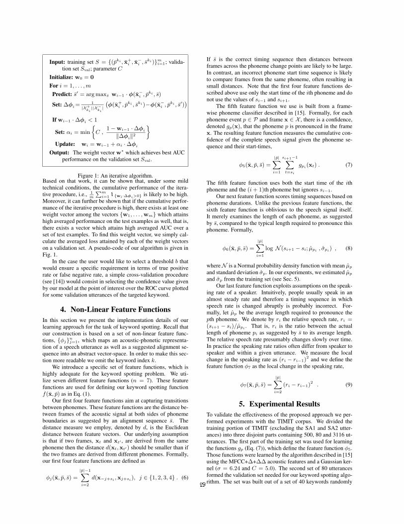
Input: training set S = (pki , x+i , x−i , ski)mi=1; valida-

tion set Sval; parameter C

Initialize: w0 = 0

For i = 1, . . . , m

Predict: s′ = arg maxs wi−1 · φ(x−i , pki , s)

Set: ∆φi =1

|X+ki||X−

ki|`φ(x+

i , pki , ski)−φ(x−i , pki , s′)´

If wi−1 ·∆φi < 1

Set: αi = min

C ,

1−wi−1 ·∆φi

‖∆φi‖2ff

Update: wi = wi−1 + αi ·∆φi

Output: The weight vector w∗ which achieves best AUCperformance on the validation set Sval.

Figure 1: An iterative algorithm.Based on that work, it can be shown that, under some mildtechnical conditions, the cumulative performance of the itera-tive procedure, i.e., 1

m

Pmi=1 1wi·∆φi>0 is likely to be high.

Moreover, it can further be shown that if the cumulative perfor-mance of the iterative procedure is high, there exists at least oneweight vector among the vectors w1, . . . ,wm which attainshigh averaged performance on the test examples as well, that is,there exists a vector which attains high averaged AUC over aset of test examples. To find this weight vector, we simply cal-culate the averaged loss attained by each of the weight vectorson a validation set. A pseudo-code of our algorithm is given inFig. 1.

In the case the user would like to select a threshold b thatwould ensure a specific requirement in terms of true positiverate or false negative rate, a simple cross-validation procedure(see [14]) would consist in selecting the confidence value givenby our model at the point of interest over the ROC curve plottedfor some validation utterances of the targeted keyword.

4. Non-Linear Feature FunctionsIn this section we present the implementation details of ourlearning approach for the task of keyword spotting. Recall thatour construction is based on a set of non-linear feature func-tions, φjnj=1, which maps an acoustic-phonetic representa-tion of a speech utterance as well as a suggested alignment se-quence into an abstract vector-space. In order to make this sec-tion more readable we omit the keyword index k.

We introduce a specific set of feature functions, which ishighly adequate for the keyword spotting problem. We uti-lize seven different feature functions (n = 7). These featurefunctions are used for defining our keyword spotting functionf(x, p) as in Eq. (1).

Our first four feature functions aim at capturing transitionsbetween phonemes. These feature functions are the distance be-tween frames of the acoustic signal at both sides of phonemeboundaries as suggested by an alignment sequence s. Thedistance measure we employ, denoted by d, is the Euclideandistance between feature vectors. Our underlying assumptionis that if two frames, xt and xt′ , are derived from the samephoneme then the distance d(xt,xt′) should be smaller than ifthe two frames are derived from different phonemes. Formally,our first four feature functions are defined as

φj(x, p, s) =

|p|−1Xi=2

d(x−j+si ,xj+si), j ∈ 1, 2, 3, 4 . (6)

If s is the correct timing sequence then distances betweenframes across the phoneme change points are likely to be large.In contrast, an incorrect phoneme start time sequence is likelyto compare frames from the same phoneme, often resulting insmall distances. Note that the first four feature functions de-scribed above use only the start time of the ith phoneme and donot use the values of si−1 and si+1.

The fifth feature function we use is built from a frame-wise phoneme classifier described in [15]. Formally, for eachphoneme event p ∈ P and frame x ∈ X , there is a confidence,denoted gp(x), that the phoneme p is pronounced in the framex. The resulting feature function measures the cumulative con-fidence of the complete speech signal given the phoneme se-quence and their start-times,

φ5(x, p, s) =

|p|Xi=1

si+1−1Xt=si

gpi(xt) . (7)

The fifth feature function uses both the start time of the ithphoneme and the (i + 1)th phoneme but ignores si−1.

Our next feature function scores timing sequences based onphoneme durations. Unlike the previous feature functions, thesixth feature function is oblivious to the speech signal itself.It merely examines the length of each phoneme, as suggestedby s, compared to the typical length required to pronounce thisphoneme. Formally,

φ6(x, p, s) =

|p|Xi=1

log N (si+1 − si; µpi , σpi) , (8)

whereN is a Normal probability density function with mean µp

and standard deviation σp. In our experiments, we estimated µp

and σp from the training set (see Sec. 5).Our last feature function exploits assumptions on the speak-

ing rate of a speaker. Intuitively, people usually speak in analmost steady rate and therefore a timing sequence in whichspeech rate is changed abruptly is probably incorrect. For-mally, let µp be the average length required to pronounce thepth phoneme. We denote by ri the relative speech rate, ri =(si+1 − si)/µpi . That is, ri is the ratio between the actuallength of phoneme pi as suggested by s to its average length.The relative speech rate presumably changes slowly over time.In practice the speaking rate ratios often differ from speaker tospeaker and within a given utterance. We measure the localchange in the speaking rate as (ri − ri−1)

2 and we define thefeature function φ7 as the local change in the speaking rate,

φ7(x, p, s) =

|p|Xi=2

(ri − ri−1)2 . (9)

5. Experimental ResultsTo validate the effectiveness of the proposed approach we per-formed experiments with the TIMIT corpus. We divided thetraining portion of TIMIT (excluding the SA1 and SA2 utter-ances) into three disjoint parts containing 500, 80 and 3116 ut-terances. The first part of the training set was used for learningthe functions gp (Eq. (7)), which define the feature function φ5.Those functions were learned by the algorithm described in [15]using the MFCC+∆+∆∆ acoustic features and a Gaussian ker-nel (σ = 6.24 and C = 5.0). The second set of 80 utterancesformed the validation set needed for our keyword spotting algo-rithm. The set was built out of a set of 40 keywords randomly49

0 0.2 0.4 0.6 0.8 10

0.2

0.4

0.6

0.8

1

false positive rate

true

posit

ive ra

te

discriminativeHMM

Figure 2: ROC curves of the discriminative algorithm and theHMM approach. The AUC of the ROC curves is 0.99 and 0.96for the discriminative algorithm and the HMM algorithm, re-spectively.

chosen from the TIMIT lexicon. The 80 utterances were chosenby pairs: one utterance in which the keyword was uttered andanother utterance in which the keyword was not uttered. Fi-nally, we ran our iterative algorithm on the rest of the utterancesin the training set. The value of C was set to be 1.

We compared the results of our method to the HMM ap-proach, where each phoneme was represented by a simple left-to-right HMM of 5 emitting states with 40 diagonal Gaussians.These models were enrolled as follows: first the HMMs wereinitialized using K-means, and then enrolled independently us-ing EM. The second step, often called embedded training, re-enrolls all the models by relaxing the segmentation constraintsusing a forced alignment. Minimum values of the variancesfor each Gaussian were set to 20% of the global variance ofthe data. All HMM experiments were done using the Torchpackage [16]. All hyper-parameters including number of states,number of Gaussians per state, variance flooring factor, weretuned using the validation set.

Keyword detection is performed with a new HMM com-posed of two sub HMM models, the keyword model and thegarbage model. The keyword model is an HMM, which es-timates the likelihood of an acoustic sequence given that thissequence represents the keyword phoneme sequence. Thegarbage model is an HMM composed of phoneme HMMs fullyconnected with each others, which estimates the likelihood ofany acoustic sequence. The overall HMM fully connects thekeyword model and the garbage model and the best path foundby Viterbi decoding on this overall HMM either passes throughthe keyword model (in which case the keyword is said to be ut-tered) or not (in which case the keyword is not in the acousticsequence).

The test set was composed of 80 keywords, distinct fromthe keywords of the training and validation set. For each key-word, we randomly picked at most 20 utterances in which thekeyword was uttered and at most 20 utterances in which it wasnot uttered. The number of test utterances in which the keywordwas uttered was not always 20, since some keywords were ut-tered less than 20 times in the whole TIMIT test set. Both thediscriminative algorithm and the HMM based algorithm havebeen evaluated against this data and their results are reported asaveraged ROC curves in Fig. 2. The AUC of the ROC curvesis 0.99 and 0.96 for the discriminative algorithm and the HMMalgorithm, respectively. In order to check whether the advan-

tage over the averaged AUC could be due to a few keyword, weran the Wilcoxon test. At the 95% confidence level, the test re-jected this hypothesis, showing that our model indeed brings aconsistent improvement on the keyword set.

6. ConclusionsIn this work, we introduced a discriminative approach to key-word spotting. We adopted a large-margin formulation of theproblem and proposed a model relying on an objective functionrelated the area under the ROC curve, i.e., the most commonmeasure for keyword spotter evaluation. Compared to state-of-the-art approaches which mostly rely on generative HMMmodels, the proposed model has shown to yield an improve-ment over the TIMIT corpus.Acknowledgments: This research was partly conducted whileJoseph Keshet was visiting the IDIAP Research Institute. Thisresearch was supported by the PASCAL European Network ofExcellence and the DIRAC project.

7. References[1] M.-C. Silaghi and H. Bourlard, “Iterative posterior-based

keyword spotting without filler models,” in ASRU, 1999.

[2] Y. B. Ayed, D. Fohr, J.-P. Haton, and G. Chollet, “Confi-dence measure for keyword spotting using support vectormachines,” in ICASSP, 2004.

[3] H. Ketabdar, J. Vepa, S. Bengio, and H. Bourlard, “Pos-terior based keyword spotting with a priori thresholds,” inInterspeech, 2006.

[4] V. N. Vapnik, Statistical Learning Theory. Wiley, 1998.

[5] N. Cristianini and J. Shawe-Taylor, An Introduction toSupport Vector Machines. Cambridge Univ. Press, 2000.

[6] B. Taskar, C. Guestrin, and D. Koller, “Max-marginmarkov networks,” in NIPS, 2003.

[7] S. Shalev-Shwartz, J. Keshet, and Y. Singer, “Learning toalign polyphonic music,” in ISMIR, 2004.

[8] J. Keshet, D. Chazan, and B.-Z. Bobrovsky, “Plosive spot-ting with margin classifiers,” in Eurospeech, 2001.

[9] J. Salomon, S. King, and M. Osborne, “Framewise phoneclassification using support vector machines,” in Inter-speech, 2002.

[10] M. Collins, “Discriminative training methods for hiddenmarkov models: Theory and experiments with perceptronalgorithms,” in EMNLP, 2002.

[11] I. Tsochantaridis, T. Hofmann, T. Joachims, and Y. Altun,“Support vector machine learning for interdependent andstructured output spaces,” in ICML, 2004.

[12] C. Cortes and M. Mohri, “Confidence intervals for the areaunder the roc curve,” in NIPS, 2004.

[13] K. Crammer, O. Dekel, J. Keshet, S. Shalev-Shwartz, andY. Singer, “Online passive aggressive algorithms,” Journalof Machine Learning Research, vol. 7, Mar 2006.

[14] S. Bengio, J. Marethoz, and M. Keller, “The expected per-formance curve,” in ICML, 2005.

[15] O. Dekel, J. Keshet, and Y. Singer, “Online algorithm forhierarchical phoneme classification,” in MLMI, 2004.

[16] R. Collobert, S. Bengio, and J. Mariethoz, “Torch: amodular machine learning library,” IDIAP-RR 46, IDIAP,2002.

50

Hybrid models for automatic speech recognition: a comparison of classicalANN and kernel based methods

Ana I. Garcıa-Moral, Ruben Solera-Urena, Carmen Pelaez-Morenoand Fernando Dıaz-de-Marıa

Department of Signal Theory and CommunicationosUniversity Carlos III Madrid, Leganes (Madrid), Spain

rsolera@tsc.uc3m.es

AbstractSupport Vector Machines (SVM) are state-of-the-art methodsfor machine learning but share with more classical ArtificialNeural Networks (ANN) the difficulty of their application totemporally variable input patterns. This is the case in Auto-matic Speech Recognition (ASR). In this paper we have recalledthe solutions provided in the past for ANN and applied them toSVMs performing a comparison between them. Preliminary re-sults show a similar behaviour which results encouraging if wetake into account the novelty of the SVM systems in compari-son with classical ANNs. The envisioned ways of improvementare outlined in the paper.

1. IntroductionHidden Markov Models (HMMs) have become the most em-ployed core technique for Automatic Speech Recognition(ASR). After several decades of intense research work in thefield, it seems that the HMM ASR systems are very closeto reach their limit of performance. Some alternative ap-proaches, most of them based on Artificial Neural Networks(ANNs), were proposed during the late eighties and earlynineties. Among them, it is worth to draw out attention to hy-brid HMM/ANN systems (see [1] for an overview), since thereported results were comparable or even slightly superior tothose achieved by HMMs.

On the other hand, during the last decade, a new tool ap-peared in the field of machine learning that has proved to beable to cope with hard classification problems in several fieldsof application: the Support Vector Machines (SVMs) [2]. TheSVMs are effective discriminative classifiers with several out-standing characteristics, namely: their solution is that with max-imum margin; they are capable to deal with samples of a veryhigh dimensionality; and their convergence to the minimum ofthe associated cost function is guaranteed.

Nevertheless, it seems clear that the application of thesekernel-based machines to the ASR problem is not straightfor-ward. In our opinion, the main difficulties to be overcome arethree: 1) SVMs are originally static classifiers and have to beadapted to deal with the variability of duration of speech utter-ances; 2) the SVMs were originally formulated as a binary clas-sifier while the ASR problem is multiclass; and 3) current SVMtraining algorithms are not able to manage the huge databasestypically used in ASR. In order to cope with these difficulties,some researchers have suggested hybrid SVM/HMM systems[3, 4], that notably resemble the previous hybrid ANN/HMMsystems ([5]). In this paper we comparatively describe bothtypes of hybrid systems (SVM/ and ANN/HMM), highlighting

both their common fundamentals and their special character-istics with the aim of also conducting an experimental perfor-mance comparison for both clean and noisy speech recognitiontasks.

2. Hybrid systems for ASRAs a result of the difficulties found in the application of ANN tospeech recognition, mostly motivated by the temporal variabil-ity of the speech instances corresponding to the same class, avariety of different architectures and novel training algorithmsthat combined both HMM with ANNs were proposed in the late80’s and 90’s. For a comprehensive survey of these techniquessee [1]. In this paper, we have focused on those that employANNs (and SVMs) to estimate the HMM state posterior proba-bilities proposed by Bourlard and Morgan ([5, 6]).

The starting point for this approach is the well-know prop-erty of using feed-forward networks such as multi-layer percep-trons (MLPs) of estimating a posteriori probabilities given twoconditions:

1. There must be enough number of parameters to train agood approximation between the input and output layersand

2. A global error minimum criterion must be used to trainthe network (for example, mean square error or relativeentropy).

The fundamental advantage of this approach is that it in-troduces a discriminative technique (ANN) into HMM (genera-tive systems) while retaining their ability to handle the temporalvariability.

However, this original formulation had to be modified toestimate the true emission (likelihood) probabilities by apply-ing Bayes’ rule. Therefore, the a posteriori probabilities outputshould be normalized by the class priors to obtain what is calledscaled likelihoods. This fact was further reinforced by posteriortheoretical developments in the search of a global ANN opti-mization procedure (see [7]).

Thus, systems of this type keep being locally discriminantgiven that the ANN was trained to estimate a posteriori proba-bilities. However, it can also be shown that, in theory, HMMscan be trained using local posterior probabilities as emissionprobabilities, resulting in models that are both locally and glob-ally discriminant but the problem is that there are generallymismatches between the prior class probabilities implicit to thetraining data and the priors that are implicit to the lexical andsyntactic models that are used in recognition. In spite of this,51

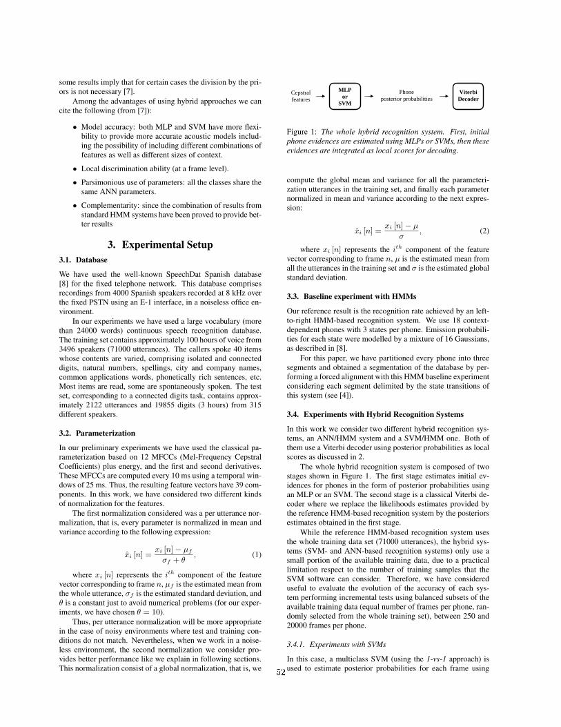
some results imply that for certain cases the division by the pri-ors is not necessary [7].

Among the advantages of using hybrid approaches we cancite the following (from [7]):

• Model accuracy: both MLP and SVM have more flexi-bility to provide more accurate acoustic models includ-ing the possibility of including different combinations offeatures as well as different sizes of context.

• Local discrimination ability (at a frame level).

• Parsimonious use of parameters: all the classes share thesame ANN parameters.

• Complementarity: since the combination of results fromstandard HMM systems have been proved to provide bet-ter results

3. Experimental Setup3.1. Database

We have used the well-known SpeechDat Spanish database[8] for the fixed telephone network. This database comprisesrecordings from 4000 Spanish speakers recorded at 8 kHz overthe fixed PSTN using an E-1 interface, in a noiseless office en-vironment.

In our experiments we have used a large vocabulary (morethan 24000 words) continuous speech recognition database.The training set contains approximately 100 hours of voice from3496 speakers (71000 utterances). The callers spoke 40 itemswhose contents are varied, comprising isolated and connecteddigits, natural numbers, spellings, city and company names,common applications words, phonetically rich sentences, etc.Most items are read, some are spontaneously spoken. The testset, corresponding to a connected digits task, contains approx-imately 2122 utterances and 19855 digits (3 hours) from 315different speakers.

3.2. Parameterization

In our preliminary experiments we have used the classical pa-rameterization based on 12 MFCCs (Mel-Frequency CepstralCoefficients) plus energy, and the first and second derivatives.These MFCCs are computed every 10 ms using a temporal win-dows of 25 ms. Thus, the resulting feature vectors have 39 com-ponents. In this work, we have considered two different kindsof normalization for the features.

The first normalization considered was a per utterance nor-malization, that is, every parameter is normalized in mean andvariance according to the following expression:

xi [n] =xi [n]− µf

σf + θ, (1)

where xi [n] represents the ith component of the featurevector corresponding to frame n, µf is the estimated mean fromthe whole utterance, σf is the estimated standard deviation, andθ is a constant just to avoid numerical problems (for our exper-iments, we have chosen θ = 10).

Thus, per utterance normalization will be more appropriatein the case of noisy environments where test and training con-ditions do not match. Nevertheless, when we work in a noise-less environment, the second normalization we consider pro-vides better performance like we explain in following sections.This normalization consist of a global normalization, that is, we

Phone posterior probabilities

MLP or

SVM

Cepstral features

Viterbi Decoder

Figure 1: The whole hybrid recognition system. First, initialphone evidences are estimated using MLPs or SVMs, then theseevidences are integrated as local scores for decoding.

compute the global mean and variance for all the parameteri-zation utterances in the training set, and finally each parameternormalized in mean and variance according to the next expres-sion:

xi [n] =xi [n]− µ

σ, (2)

where xi [n] represents the ith component of the featurevector corresponding to frame n, µ is the estimated mean fromall the utterances in the training set and σ is the estimated globalstandard deviation.

3.3. Baseline experiment with HMMs

Our reference result is the recognition rate achieved by an left-to-right HMM-based recognition system. We use 18 context-dependent phones with 3 states per phone. Emission probabili-ties for each state were modelled by a mixture of 16 Gaussians,as described in [8].

For this paper, we have partitioned every phone into threesegments and obtained a segmentation of the database by per-forming a forced alignment with this HMM baseline experimentconsidering each segment delimited by the state transitions ofthis system (see [4]).

3.4. Experiments with Hybrid Recognition Systems

In this work we consider two different hybrid recognition sys-tems, an ANN/HMM system and a SVM/HMM one. Both ofthem use a Viterbi decoder using posterior probabilities as localscores as discussed in 2.

The whole hybrid recognition system is composed of twostages shown in Figure 1. The first stage estimates initial ev-idences for phones in the form of posterior probabilities usingan MLP or an SVM. The second stage is a classical Viterbi de-coder where we replace the likelihoods estimates provided bythe reference HMM-based recognition system by the posteriorsestimates obtained in the first stage.

While the reference HMM-based recognition system usesthe whole training data set (71000 utterances), the hybrid sys-tems (SVM- and ANN-based recognition systems) only use asmall portion of the available training data, due to a practicallimitation respect to the number of training samples that theSVM software can consider. Therefore, we have considereduseful to evaluate the evolution of the accuracy of each sys-tem performing incremental tests using balanced subsets of theavailable training data (equal number of frames per phone, ran-domly selected from the whole training set), between 250 and20000 frames per phone.

3.4.1. Experiments with SVMs

In this case, a multiclass SVM (using the 1-vs-1 approach) isused to estimate posterior probabilities for each frame using52

0 2 4 6 8 10 12

x 105

44

46

48

50

52

54

56

58

60

62

64

# Training Frames

FR

R: F

ram

e R

econ

igtio

n R

ate(

%)

SVM FRRMLP FRR

Figure 2: Frame recognition rate of SVMs and ANNs.

Platt’s approximation ([9]). The SVM uses a RBF (Radial Ba-sis Function) kernel whose parameter, the standard deviationσ, must be tuned by means of a cross-validation process, aswell as a parameter C, which establishes a compromise betweenerror minimization and generalization capability in the SVM.The values we have used in our experiments are C = 256 andσ = 0.007812 [4].

3.4.2. Experiments with ANNs

Posterior probabilities used by the Viterbi decoder are now ob-tained using a MLP trained on a smaller version of the trainingset, as we mentioned before. The MLP has one hidden layerwith 1800 units. MFCC features jointly with energy, delta andacceleration features are used as inputs. There are 54 outputunits, each of them corresponding to a different part of phone,as we described in section 3.4. The MLP is trained using therelative entropy criterion and the back propagation factor µ wasexperimentally fixed at 0.14.

4. Preliminary Results and DiscussionThis section is devoted to the presentation and discussion ofthe results obtained by the systems described in the previoussection.

Preliminary experiments show a similar behaviour of bothSVMs and ANNs at a frame classification level. For the firstdata normalization method presented in section 3, we observelittle differences between SVMs and ANNs. Also, we can seein figure 2 that better results are achieved when more samplesare added to the training database, up to a final recognitionrate around 61% obtained for the maximum number of inputsamples our SVM-based system can handle (1080000, 20000frames per phone).

We have noticed that this first normalization methodpresents a problem: delta and acceleration coefficients do nothave unitary variance. This is due to the constant θ added tothe standard deviation in (1). The value used in the experiments(10) is not comparable with the standard deviation of the dataand it results in a excessive normalization. This is a problemfor the SVM and ANN-based systems. For the first case, theSVM employs a RBF kernel with the same variance for all di-mensions, while the training data present different variances foreach component (or, at least, for the static, delta and accelera-

tion coefficients). For the latter, this may cause to start in a pointfar from the solution and, as a consequence, to slow down theconvergence of the algorithm. This has led us to apply a sec-ond normalization stage to the database, in order to get a uni-tary variance for all the components of the training data. Someexperiments show an important improvement of the previousresults (around 4.5%).

Preliminary experiments at word and sentence levels showresults are comparable with respect to those of the standardHMM-based speech recognition system used as a baseline.These results are specially promising due to the fact that SVMand ANN-based systems are trained using a maximum of only3.04% of the available data samples, whereas HMMs are trainedusing the entire database. This limit is imposed by the SVMsoftware used in the experiments [10], which requieres to man-tain the kernel matrix in memory.

In addition, as we have stated in section 2, both SVMs andANNs provide posteriors to the Viterbi decoder, whereas whatwe really need and HMMs compute are likelihoods. We thinkthat the hybrid methods might benefit from the use of likeli-hoods instead of posteriors [5], just by dividing them by the apriori probabilities.

Finally, one of the major drawbacks of current HMM-basedautomatic speech recognition systems is its poor robustnessagainst noisy conditions. During the last years, several tech-niques aimed at increasing the performance of these systemshave been presented, most of them consisting in some pre-processing of the voice signal or modifications of the parame-terization stage. From previous experiments ([11]) we suspectthat SVM-based systems could provide inherent robust mod-els. Besides, as discussed in section 2, hybrid systems are moreamenable for its use with different types of parameterizationsthat do not comply with the restrictions of independence im-posed by HMM. This could result advantageous in the searchof robustness.

5. ConclusionsIn this paper we have performed a comparison of the accuracyof MLPs and SVMs at a frame level showing a similar perfor-mance. However, we still think there is room for improvementof the latter, specially in noisy environment conditions. Themaximum margin principle used for its training can make animportant difference under those conditions. There are also sev-eral issues that should be address as the possibility to incorpo-rate more training samples, the addition of a wider context inthe feature vectors, the selection of appropriate feature sets andthe computation of further results at a word level.

6. References[1] E. Trentin and M. Gori, “A survey of hybrid ANN/HMM

models for automatic speech recognition,” Neurocomput-ing, vol. 37, pp. 91–126, 2001.

[2] B. E. Boser, I. Guyon, and V. Vapnik, “A training algo-rithm for optimal margin classifiers,” in ComputationalLearning Theory, 1992, pp. 144–152. [Online]. Available:citeseer.ist.psu.edu/boser92training.html

[3] A. Ganapathiraju, J. Hamaker, and J. Picone, “HybridSVM/HMM architectures for speech recognition,” in Pro-ceedings of the 2000 Speech Transcription Workshop,vol. 4, Maryland (USA), May 2000, pp. 504–507.

[4] J. Padrell-Sendra, D. Martın-Iglesias, and F. Dıaz-de-53

Marıa, “Support vector machines for continuous speechrecognition,” in Proc. of the 14th European SignalProcessing Conference, 2006.

[5] H. Bourlard and N. Morgan, Connectionist speech recog-nition: a hybrid approach. Norwell, MA (USA): Boston:Kluwer Academic, 1994.

[6] N. Morgan and H. Bourlard, “Continuous speech recog-nition: An introduction to the hybrid hmm/connectionistapproach,” IEEE Signal Processing Magazine, pp. pp. 25–42, 1995.

[7] H. Bourlard, N. Morgan, C. L. Giles, and M. Gori, Adap-tive Processing of Sequences and Data Structures. Inter-national Summer School on Neural Networks ‘E.R. Ca-ianiello’. Tutorial Lectures. Germany; Berlin: Springer-Verlag, 1998, ch. Hybrid HMM/ANN systems for speechrecognition: overview and new research directions, pp.389–417.

[8] A. Moreno, “SpeechDat Spanish database for fixed tele-phone network,” Technical University of Catalonia, Tech.Rep., 1997.

[9] J. C. Platt, Advances in kernel methods: support vectorlearning. Cambridge, MA (USA): MIT Press, 1999, ch.Fast Training of Support Vector Machines Using Sequen-tial Minimal Optimization, pp. 185–208.

[10] C. C. Chang and C. J. Lin, LIBSVM: a library forsupport vector machines, 2001, software available athttp://www.csie.ntu.edu.tw/cjlin/∼libsvm.

[11] R. Solera-Urena, D. Martın-Iglesias, A. Gallardo-Antolın,C. Pelaez-Moreno, and F. Dıaz-de-Marıa, “Robust asr us-ing support vector machines,” Speech Communication (Inpress), 2007.

54

Towards phonetically-driven hidden Markov models: Can we incoporatephonetic landmarks in HMM-based ASR?

Guillaume Gravier, Daniel Moraru

Equipe MetissIrisa, Rennes, France.

http://www.irisa.fr/metiss

AbstractAutomatic speech recognition mainly relies on hidden Markovmodels (HMM) which make little use of phonetic knowledge.As an alternative, landmark based recognizers rely mainly onprecise phonetic knowledge and exploit distinctive features. Wepropose a theoretical framework to combine both approaches byintroducing phonetic knowledge in a non stationary HMM de-coder. To demonstrate the potential of the method, we investi-gate how broad phonetic landmarks could be used to improve aHMM decoder by focusing the best path search. We show that,assuming error free landmark detection, every broad phoneticclass brings a small improvement. The use of all the classesreduces the error rate from 22% to 14% on a broadcast newstranscription task. We also experimentally validate that land-marks boundaries does not need to be detected precisely andthat the algorithm is robust to non detection errors.

1. IntroductionIn hidden Markov models (HMM) based speech recognitionsystems, the decoding process consists in compiling a graphwhich includes all the available sources of knowledge (languagemodel, pronunciations, acoustic models) before finding out thebest path in the graph in order to obtain the best word sequence

w = arg maxw

p(y|w)p(w) . (1)

At the acoustic level, this approach relies on data-driven meth-ods that learn from examples. Therefore, integrating explicitphonetic knowledge in such systems is difficult.

Alternately, various studies aimed at explicitly relying onphonetic knowledge to represent the speech signal for automaticspeech recognition [1, 2, 3]. These approaches are most of thetime based on the extraction of a set phonetic features, a.k.a.landmarks, on top of which a model, either rule based or statisti-cal based, is build for the purpose of recognition. Phonetically-driven ASR relies on fine grain phonetic features such as onsetand offset times [2] and distinctive features [1, 3]. However, inpractice, automatically detecting such features might be diffi-cult and error prone, in particular in the case of noisy signals orspontaneous speech.

This work is a preliminary study which aims at bridgingthese two paradigms in order to make use of explicit phoneticknowledge in the framework of HMMs. While landmark-basedsystems use phonetic landmarks as a feature describing the sig-nal, the idea of our approach is to use landmarks in order toguide the search for the best path during Viterbi decoding in anHMM-based system. Hence, prior knowledge on the nature ofthe signal is used as anchor points during decoding. We will

use indistinctly the two terms landmark and anchor to designateconstraints on the search.

The aim of this study is twofold. The first aim is to definea theoretical framework to incorporate phonetic knowledge inHMM based systems using anchor points and to experimentallyvalidate this approach. This framework allows for uncertaintyin the landmark detection step, though this is not validated in thestudy as of now. The second aim is to study which landmarkseffectively complements the data-driven knowledge embeddedin HMM systems. We believe that detecting fine grain phoneticfeatures is a particularly challenging problem – in spite of recentpromising results on the detection of distinctive features, seee.g. [4, 5, 3] – while detecting broad phonetic features can beachieved with reasonably good performance [6, 7, 8]. Hence,to avoid problems related to the detection of fine grain features,we investigate if, and to what extent, broad phonetic landmarkscan help.

in this paper, we first extend the Viterbi algorithm in orderto incorporate prior knowledge carried out by landmarks. Wethen study the impact of broad phonetic landmarks in an idealsetting where landmarks are manually detected, with an em-phasis on the temporal precision of the landmarks. Finally, wediscuss some upcoming experiments whose results are expectedto be presented at the workshop.

2. Landmark-driven Viterbi decodingMost HMM-based systems rely on the Viterbi algorithm in or-der to solve Eq. (1), along with pruning techniques to keep thesearch tractable for large vocabularies. We briefly recall the ba-sics of the Viterbi algorithm before extending this algorithm forthe integration of phonetic anchors.

2.1. Beam-search Viterbi decoding

The Viterbi algorithm aims at finding out the best alignmentpath in a graph using dynamic programming (DP) on a trellis.The DP algorithm proceeds incrementally by searching for thebest hypothesis reaching the state (j, t) of the trellis accordingto

S(j, t) = maxi

S(i, t− 1) + ln(aij) + ln(p(yt|j)) , (2)

where j is the state in the decoding graph and t the frame in-dex in the observation sequence. In Eq. (2), ln(aij) denotes theweight for the transition from state i to j in the graph1 while

1Note that this weight actually combines the language model andthe acoustic model probabilities for cross-word transitions.

55

p(yt|j) denotes the likelihood of the feature vector yt condi-tional to state j. Hence, S(i, t) represents the score of the bestpartial path ending in state i at time t.

In practice, not all paths are explored in order to keep thealgorithm tractable on large decoding graphs. Unlikely partialhypotheses are pruned according to the score of the best pathending at time t.

2.2. Introducing anchors

Anchors can be considered as hints on what the best path is.For example, if a landmark indicates that a portion of an ut-terance corresponds to a vowel, then we can constrain the bestpath to be consistent with this piece of information since nodesin the decoding graph are linked to phonemes. One easy wayto do this is to penalize, or even prune, all the paths of the trel-lis which are inconsistent with the knowledge brought by thevowel landmark. Assuming confidence measures are associatedwith the landmarks, the penalty should be proportional to theconfidence.

Formally, the above principle can be expressed using non-stationary graphs, i.e. graphs whose transition probabilities aredependent on time. The idea is that if a transition leading tostate (i, t) of the trellis is inconsistent with the landmark knowl-edge, then the transition cost increases. In order to do this, wereplace in (2) the transition weights ln(aij) by

ln(aij(t)) = ln(aij)− λ(t)Ij(t) . (3)

Ij(t) is an indicator function whose value is 0 if node j is com-patible with the available anchor information and 1 otherwise.The penalization term λ(t) > 0 reflects the confidence in theanchor available at time t, if any. Hence, if no anchor is avail-able or if a node is consistent with the anchor, then no penal-ization is applied. In the opposite case, we apply a penaltywhere the higher the confidence in the landmark, the higherthe penalty. In the extreme case where landmark detection isperfect, setting λ(t) = ∞, enables to actually prune paths in-consistent with the landmarks.

In (3), one can notice that the penalty term only depends onthe target state j and hence the proposed scheme is equivalent tomodifying the state-conditional probability p(yt|j) to includea penalty. However, introducing the penalty at the transitionlevel might be useful in the future to introduce phonologicalconstraints or word-level constraints.

A by product of the proposed method is that decodingshould be much faster with landmarks as adding a penalty willmost likely result in inconsistent paths being pruned.

In this preliminary study, we use manually detected land-marks in order to investigate whether or not broad phoneticlandmarks can help and to what extent in an ideal case. We willtherefore set λ(t) = ∞, ∀t in all the experiments described insection 4.

3. Baseline systemBefore describing the experiments, we briefly present the dataand baseline system used.

3.1. Corpus

Experiments are carried out on a radio broadcast news corpusin the French language. The data used is a 4 hour subset of thedevelopment data for the ESTER broadcast news rich transcrip-tion evaluation campaign [9]. The corpus mostly contains high-

fidelity planned speech from professional radio speakers. In-terviews, however, contain more spontaneous speech from nonprofessional speakers, sometimes in degraded acoustic condi-tions.

The entire data set was labeled phonetically based on thereference orthographic transcription, using our ASR system toselect pronunciation variants.

3.2. ASR system

Two reference systems were used in this study. Both systemsare two-pass systems where a first pass aims at generating aword graph which is then rescored in a second pass with moresophisticated acoustic models. The two systems differ in thecomplexity of the acoustic models used for the word graphgeneration, the first system using context-independent modelswhile word-internal context-dependent ones are used for thesecond system. Clearly, using landmarks to guide the decod-ing is more interesting when generating the word graph as itshould enable better and smaller word graphs which alreadytake into account the landmark knowledge. Therefore, the rea-son for comparing two systems for word graph generation is todetermine to what extent phone models capture broad phoneticinformation.

Both transcription passes are carried out with a trigram lan-guage model. Monophone acoustic models have 114 states with128 Gaussians per state while the word-internal triphone modelshave 4,019 distinct states with 32 Gaussians each. Cross-wordtriphones models are used for word graph rescoring, with about6,000 distinct states and 32 Gaussians per state.

4. Broad phonetic landmarks

The experiments described in this section are performed usingmanually detected broad phonetic landmarks, the goal beingto measure the best expected gain from the use of such land-marks. The main motivation for using this type of landmarks,as opposed to distinctive features, is that we believe that reliableand robust automatic broad phonetic landmark detectors can bebuild. For example, in [6, 7, 8] (to cite a few), good results arereported on the detection of nasals and vowels. Fricatives alsoseems relatively easy to detect using energy and zero crossingrate information. Moreover, we observed that the heap of activehypotheses in our ASR system most of time contains hypothe-ses corresponding to different broad phonetic classes. Thoughthis is normal since hypotheses correspond to complete partialpaths rather than to local decisions, this observation indicatesthat a better selection of the active hypotheses based on (locallydetected) landmarks is bound to improve the results.

4.1. Landmark generation

Five broad phonetic classes are considered in this study, namelyvowels, fricatives, plosives, nasal consonants and glides. Land-marks are generated from the available phonetic alignments ob-tained from the orthographic transcription. For each phone, alandmark corresponding to the broad phonetic class to whichthe phone belongs is generated, centered on the phone segment.The landmark duration is proportional to the phone segmentlength. In the first set of experiments, the landmark length is setto 50% of the phone segment length. We study in section 4.3the impact of the landmark duration.

56

4.2. Which landmarks?

The first question to answer is what is the optimal improvementthat can be obtained using each broad phonetic class separately.Results are given in table 1 for the monophone and triphonesystems after the first and second pass, with each landmark typetaken separately. Results using all the landmarks or a combina-tion of vowel, plosive and fricative landmarks are also reported.

Results show a small improvement for each type of land-marks, thus clearly indicating that the transcription system isnot misled by phones from a particular broad phonetic class.The best improvement is obtained with landmarks for glides,that correspond to highly transitory phones which are difficultto model, in particular because of co-articulation effects. Moresurprisingly, vowel landmarks yield a small but significant im-provement, in spite of the fact that the phone models used inthe ASR system do little confusions between vowels and otherphones. This result is due to the fact that the DP maximizationnot only depends on the local state-conditional probabilities butalso on the score of the entire path resulting in an hypothesis.In other words, even if the local probabilities p(yt|i) are muchbetter for states corresponding to a vowel than for states corre-sponding to some other class, some paths, incompatible with theknowledge of a vowel landmark, might get a good cumulatedscore and are therefore kept in the heap of active hypotheses.Using the landmark-driven version of the Viterbi algorithm ac-tually remove such paths from the search space, thus explainingthe gain obtained with vowel landmarks.

Clearly, using all the available landmarks strongly improvesthe WER for both systems, the improvement being unsurpris-ingly better for the monophone-based system. One interestingpoint to note is that, when using all the landmarks, the two sys-tems exhibit comparable levels of performance, with a slightadvantage for the monophone system. This advantage is dueto the fact that the word graph generated with the monophonesystem contains more sentence hypotheses than the one gener-ated with the triphone system, though both graphs have roughlythe same density. A last point worth noting is the rather goodperformance obtained after the first pass using the monophonesystem. This result suggest that combining landmark-drivendecoding with fairly simple acoustic models can provide goodtranscriptions with a limited amount of computation. Indeed,the average number of active hypotheses, and hence the decod-ing time, is divided by a factor of four when using landmarks.

In a practical setting, the reliable detection and segmenta-tion of a signal into broad phonetic classes is somewhat unre-alistic, the detection of nasals and glides being a rather difficultproblem. However, detecting vowels, plosives and fricativesseems feasible with a great accuracy. We therefore report resultsusing only landmarks from those three classes (VPF results intable 1). Using such landmarks, a nice performance gain canstill be expected, in particular with a monophone-based wordgraph generation.

These results show the optimal gain that can be obtained us-ing broad phonetic landmarks as anchors in a Viterbi decoding,thus justifying further work on landmark detection.

4.3. Landmark precision

Two questions arise regarding the precision of the landmark de-tection step. The first question is to determine whether a precisedetection of the landmark boundaries is necessary or not. Thesecond question concerns the robustness to detection errors ofthe proposed algorithm.

13

14

15

16

17

18

19

20

21

22

23

0 10 20 30 40 50 60 70

Wor

d E

rror

Rat

e

landmark extent

31346

12985

51730

22421

35000

8370

monophonestriphones

Figure 1: WER (in %) as a function of the landmarks length,using all landmarks. The landmark length is defined as a frac-tion of the length of the phone which generated the landmark.Figures reported on the graph correspond to the average size ofthe active hypotheses heap during word graph generation.

4.3.1. Temporal precision

Figure 1 shows the word error rate for the two systems as afunction of the landmark extent, where the extent is defined asthe relative duration with respect to the phone used to generatethe landmark. An extent of 10 therefore means that the dura-tion of a landmark is 0.1 times that of the corresponding phone.All the landmarks are considered in these experiments. Unsur-prisingly, the longer the landmarks, the better the transcription.It was also observed that longer landmarks reduce the searchspace and yield smaller, yet better, word graphs. In spite of this,most of the improvement comes from the fact that landmarksare introduced, no matter their extent. Indeed, with a landmarkextent of only 5%, the word error rate decreases from 22.3% to14.3% with the monophone system. When increasing the land-mark extent to 50%, the gain is marginal, with a word error rateof 13.9%. Note that with an extent of 5%, the total durationof landmarks corresponds to 4.4% of the total duration of thesignal, and therefore landmark-based pruning of the hypothe-ses heap happens only for 4.4% of the frames. Similar conclu-sions were obtained using only the vowel landmarks. This is aparticularly interesting result as it demonstrates that landmarkboundaries do not need to be detected precisely. Reliably de-tecting landmarks on some very short portion of the signal (oneor two frames) is sufficient to drive a Viterbi decoder with thoselandmarks.

4.3.2. Robustness to non-detection errors

In the absence of confidence measures, landmark-driven Viterbiis highly sensitive to detection errors. Clearly, false alarms,i.e. insertion and confusion errors, have detrimental effectson the system. However, miss detection errors are less disas-trous. Therefore, automatic broad phonetic landmark detectionsystems should be designed to have as low as possible a falsealarm rate. However, lower false alarm rates unfortunately im-ply higher miss detection rates. We tested the robustness of ourlandmark-driven decoder by simulating miss detection errorsat various rates, assuming a uniform distribution of the errorsacross the five broad phonetic classes. Results show that theword error rate is a linear function of the miss detection rate.

57

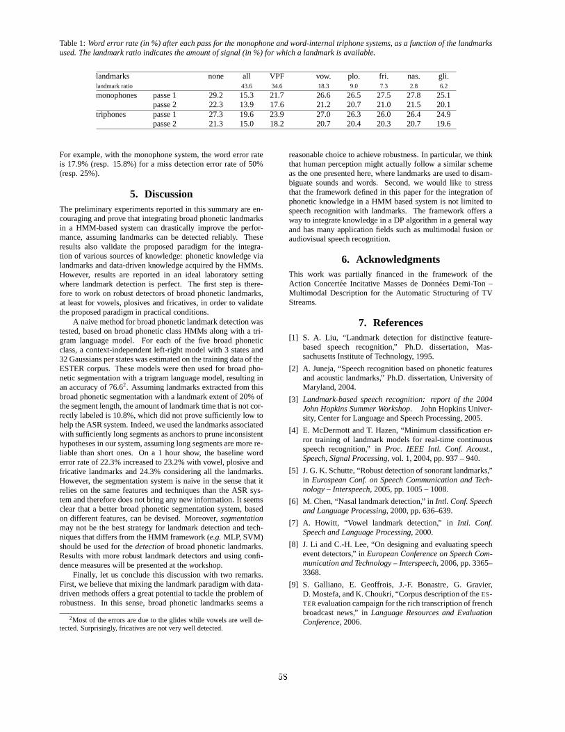
Table 1: Word error rate (in %) after each pass for the monophone and word-internal triphone systems, as a function of the landmarksused. The landmark ratio indicates the amount of signal (in %) for which a landmark is available.

landmarks none all VPF vow. plo. fri. nas. gli.landmark ratio 43.6 34.6 18.3 9.0 7.3 2.8 6.2

monophones passe 1 29.2 15.3 21.7 26.6 26.5 27.5 27.8 25.1passe 2 22.3 13.9 17.6 21.2 20.7 21.0 21.5 20.1

triphones passe 1 27.3 19.6 23.9 27.0 26.3 26.0 26.4 24.9passe 2 21.3 15.0 18.2 20.7 20.4 20.3 20.7 19.6

For example, with the monophone system, the word error rateis 17.9% (resp. 15.8%) for a miss detection error rate of 50%(resp. 25%).

5. DiscussionThe preliminary experiments reported in this summary are en-couraging and prove that integrating broad phonetic landmarksin a HMM-based system can drastically improve the perfor-mance, assuming landmarks can be detected reliably. Theseresults also validate the proposed paradigm for the integra-tion of various sources of knowledge: phonetic knowledge vialandmarks and data-driven knowledge acquired by the HMMs.However, results are reported in an ideal laboratory settingwhere landmark detection is perfect. The first step is there-fore to work on robust detectors of broad phonetic landmarks,at least for vowels, plosives and fricatives, in order to validatethe proposed paradigm in practical conditions.

A naive method for broad phonetic landmark detection wastested, based on broad phonetic class HMMs along with a tri-gram language model. For each of the five broad phoneticclass, a context-independent left-right model with 3 states and32 Gaussians per states was estimated on the training data of theESTER corpus. These models were then used for broad pho-netic segmentation with a trigram language model, resulting inan accuracy of 76.62. Assuming landmarks extracted from thisbroad phonetic segmentation with a landmark extent of 20% ofthe segment length, the amount of landmark time that is not cor-rectly labeled is 10.8%, which did not prove sufficiently low tohelp the ASR system. Indeed, we used the landmarks associatedwith sufficiently long segments as anchors to prune inconsistenthypotheses in our system, assuming long segments are more re-liable than short ones. On a 1 hour show, the baseline worderror rate of 22.3% increased to 23.2% with vowel, plosive andfricative landmarks and 24.3% considering all the landmarks.However, the segmentation system is naive in the sense that itrelies on the same features and techniques than the ASR sys-tem and therefore does not bring any new information. It seemsclear that a better broad phonetic segmentation system, basedon different features, can be devised. Moreover, segmentationmay not be the best strategy for landmark detection and tech-niques that differs from the HMM framework (e.g. MLP, SVM)should be used for the detection of broad phonetic landmarks.Results with more robust landmark detectors and using confi-dence measures will be presented at the workshop.

Finally, let us conclude this discussion with two remarks.First, we believe that mixing the landmark paradigm with data-driven methods offers a great potential to tackle the problem ofrobustness. In this sense, broad phonetic landmarks seems a

2Most of the errors are due to the glides while vowels are well de-tected. Surprisingly, fricatives are not very well detected.

reasonable choice to achieve robustness. In particular, we thinkthat human perception might actually follow a similar schemeas the one presented here, where landmarks are used to disam-biguate sounds and words. Second, we would like to stressthat the framework defined in this paper for the integration ofphonetic knowledge in a HMM based system is not limited tospeech recognition with landmarks. The framework offers away to integrate knowledge in a DP algorithm in a general wayand has many application fields such as multimodal fusion oraudiovisual speech recognition.

6. AcknowledgmentsThis work was partially financed in the framework of theAction Concertee Incitative Masses de Donnees Demi-Ton –Multimodal Description for the Automatic Structuring of TVStreams.

7. References[1] S. A. Liu, “Landmark detection for distinctive feature-

based speech recognition,” Ph.D. dissertation, Mas-sachusetts Institute of Technology, 1995.

[2] A. Juneja, “Speech recognition based on phonetic featuresand acoustic landmarks,” Ph.D. dissertation, University ofMaryland, 2004.

[3] Landmark-based speech recognition: report of the 2004John Hopkins Summer Workshop. John Hopkins Univer-sity, Center for Language and Speech Processing, 2005.

[4] E. McDermott and T. Hazen, “Minimum classification er-ror training of landmark models for real-time continuousspeech recognition,” in Proc. IEEE Intl. Conf. Acoust.,Speech, Signal Processing, vol. 1, 2004, pp. 937 – 940.

[5] J. G. K. Schutte, “Robust detection of sonorant landmarks,”in Eurospean Conf. on Speech Communication and Tech-nology – Interspeech, 2005, pp. 1005 – 1008.

[6] M. Chen, “Nasal landmark detection,” in Intl. Conf. Speechand Language Processing, 2000, pp. 636–639.

[7] A. Howitt, “Vowel landmark detection,” in Intl. Conf.Speech and Language Processing, 2000.

[8] J. Li and C.-H. Lee, “On designing and evaluating speechevent detectors,” in European Conference on Speech Com-munication and Technology – Interspeech, 2006, pp. 3365–3368.

[9] S. Galliano, E. Geoffrois, J.-F. Bonastre, G. Gravier,D. Mostefa, and K. Choukri, “Corpus description of the ES-TER evaluation campaign for the rich transcription of frenchbroadcast news,” in Language Resources and EvaluationConference, 2006.

58

A HYBRID GENETIC-NEURAL FRONT-END EXTENSION FOR ROBUSTSPEECH RECOGNITION OVER TELEPHONE LINES

Sid-Ahmed Selouani*, Habib Hamam**, Douglas O’Shaughnessy***

*Universite de Moncton, Campus de Shippagan, Canada**Universite de Moncton, Campus de Moncton, Canada

***INRS-Energie-Materiaux-Telecommunications, Canadaselouani@umcs.ca, hamamh@umoncton.ca, dougo@emt.inrs.ca

Abstract

This paper presents a hybrid technique combining theKarhonen-Loeve Transform (KLT), the Multilayer Perceptron(MLP) and Genetic Algorithms (GAs) to obtain less-variantMel-frequency parameters. The advantages of such an approachare that the robustness can be reached without modifying therecognition system, and that neither assumption nor estima-tion of the noise are required. To evaluate the effectiveness ofthe proposed approach, an extensive set of continuous speechrecognition experiments are carried out by using the NTIMITtelephone speech database. The results show that the proposedapproach outperforms the baseline and conventional systems.

1. IntroductionAdaptation to the environment changes and artifacts remainsone of the most challenging problems for the ContinuousSpeech Recognition (CSR) systems. The principle of CSRmethods consists of building speech sound models based onlarge speech corpora that attempt to include common sourcesof variability that may occur in practice. Nevertheless, not allsituations and contexts can be exhaustively covered. As speechand language technologies are being transferred to real applica-tions, the need for greater robustness in recognition technologybecomes more apparent when speech is transmitted over tele-phone lines, when the signal-to-noise ratio (SNR) is extremelylow, and more generally, when adverse conditions and/or un-seen situations are encountered. To cope with these adverseconditions and to achieve noise robustness, different approacheshave been studied. Two major approaches have emerged. Thefirst approach consists of preprocessing the corrupted speechinput signal prior to the pattern matching in an attempt to en-hance the SNR. The second approach attempts to establish acompensation method that modifies the pattern matching itselfto account for the effects of noise. Methods in this approachinclude noise masking, the use of robust distance measures, andHMM decomposition. For more details see [5].

As an alternative approach, we propose a new enhancementscheme based on the combination of subspace filtering, theMultilayer Perceptron (MLP) and Genetic Algorithms (GAs) toobtain less-variant Mel-frequency parameters. The enhancedparameters are expected to be insensitive to the degradation ofspeech signals due to telephone-channel degradation. The mainadvantages of such an approach over the compensation methodare that the robustness can be reached without modifying therecognition system, and without requiring assumption or esti-mation of the noise.

This paper is organized as follows. In section 2, we de-scribe the basis of the signal subspace approach, namely theKarhonen-Loeve Transform (KLT) and the extension we pro-posed to enable the use of the technique in the Mel-frequencyspace. In section 3, we briefly describe the principle of MLP-based enhacement method. Then, we proceed in section 4 withthe description of the evolutionary-based paradigm that we in-troduced to perform noise reduction. In section 5, we evaluatethe hybrid MLP-KLT-GA-based front-end technique in the con-text of telephone speech. Finally, in section 6, we conclude anddiscuss our results.

2. Signal and Mel-frequency subspacefiltering

The principle of the signal subspace techniques is based on theconstruction of an orthonormal set of axes. These axes point inthe directions of maximum variance, thus forming a represen-tational basis that projects on the direction of maximum vari-ability. Applied in the context of noise reduction, these axesenable decomposing the space of the noisy signal into a signal-plus-noise subspace and a noise subspace. The enhancement isperformed by removing the noise subspace and estimating theclean signal from the remaining signal space. The decomposi-tion of the space into two subspaces can be performed by usingKLT (eigendecomposition). Let x = [x1,x2, ..., xN]T be anN -dimensional noisy observation vector which can be writtenas the sum of an additive noise distortion vector w and the vec-tor of clean speech samples s. The noise is assumed to be un-correlated with the clean speech. Further, let Rx, Rs, and Rw

be the covariance matrices from x, s, and w respectively. Theeigendecomposition of Rs is given by Rs = QΛsQ

T whereΛs= diag(λs1, λs2, ...., λsN ) is the diagonal matrix of eigen-values given in a decreasing order. The eigenvector matrix Qof the clean speech covariance matrix is identical to that of thenoise. Major signal subspace techniques assume the noise tobe white with Rw = σ2

wI where σ2w is the noise variance and

I the identity matrix. Thus, the eigendecomposition of Rx isgiven by: Rs = Q(Λs + σ2

wI)QT. The enhancement is per-formed by assuming that the clean speech is concentrated inan r < N dimensional subspace, the so-called signal subspace,whereas the noise occupies the N − r dimensional observa-tion space. Then the noise reduction is obtained by consider-ing only the signal subspace in the reconstruction of the en-hanced signal. Mathematically it consists of finding a linearestimate of s given by s = Fx = Fs + Fw where F is the en-hancement filter. This filter matrix F can be written as follows:

59

F = QrGrQTr in which the diagonal matrix Gr contains the

weighting factors gi with i = 1 , ..., r , for the eigenvalues ofthe noisy speech. Perceptually meaningful weighting functionsexist to generate gi . These functions are empirically guided inorder to constitute an alternative choice for gi, which resultsin a more or less aggressive noise suppression, depending onthe SNR. In [1], the linear estimation of the clean vector is per-formed using two perceptually meaningful weighting functions.The first function is given by :

gi =[ λxi

λxi + σ2w

]γ

, i = 1, ..., r, (1)

where γ ≥ 1.

The second function constitutes an alternative choice for gi

which results in a more aggressive noise suppression:

gi = exp−νσ2

w

λxi

. i = 1, ..., r, (2)

The value of the parameter ν is to be fixed experimentally.

Instead of dealing with the speech signal, we chose to usethe noisy Mel-Frequency Cepstral Coefficients (MFCC) vectorC

′as well. The reason is that these parameters are suited to

speech recognition due to the advantage that one can derivefrom them a set of parameters which are invariant to any fixedfrequency-response distortion introduced by either the adverseenvironments or the transmission channels [6]. The main ad-vantage of the approach proposed here is that we do not need todefine weighting functions. In this approach, the filter matrix Fcan be written as follows: Fgen = QGgenQ

T in which the di-agonal matrix Ggen contains now weighting factors optimizedusing genetic operators. Optimization is reached when the Eu-clidian distance between the noisy and clean MFCCs is mini-mized. To improve the enhancement of noisy MFFCs, we in-troduce a preprocessing level which uses the MLP. As depictedin Figure 1, the noisy (MFCC) vectors C

′are first enhanced

by MLP. Then, a KLT is performed on the output of MLP, de-noted by C. Finally, the space of feature representation is re-constructed by using the eigenvectors weighted by the optimalfactors of the Ggen matrix.

3. MLP-based enhancement preprocessingof the KLT

Numerous approaches were proposed in the literature to in-corporate acoustic features estimated by the MLP under noisyconditions [6] [12]. The connectionist approaches offer inher-ent nonlinear capabilities as well as easy training from pairsof corresponding noisy and noise-free signal frames. Becausethe front end is very modular, the MLP estimator can be intro-duced at different stages in the feature processing stream. Forinstance, the MLP can estimate robust filterbank log-energiesthat will then be processed with the traditional Distrete CosineTransform to get the unnormalized cepstral coefficients. Al-ternatively, we can estimate the cepstral features directly withan MLP. Yet another possibility is to estimate filterbank log-energies but to measure the feature distortion at the cepstrumlevel and optimize the filterbank log-energy estimator accord-ingly [12]. The fact that the noise and the speech signal arecombined in a nonlinear way in the cepstral domain led us to

Figure 1: The proposed MLP-KLT-GA-based CSR system.

choose the second alternative described above. MLP can ap-proximate the required nonlinear function to some extent [6].Hence, the input of the MLP is the noisy MFCC vector C

′,

while the actual response of the network C is computed duringa training phase by using a convergence algorithm to update theweight vector in a manner to minimize the error between theoutput C and the desired clean cepstrum value C. The weightsof this network are calculated during a training phase with aback-propagation training algorithm using a mean square errorcriterion.

The noisy 13-dimensional vector (12 MFCCs + energy) isfed to an MLP network in order to reduce the noise effectson this vector. This first-level pre-processing does not requireany knowledge about the nature of the corrupting noisy signal,which permits dealing with any kind of noise. Moreover, usingthis enhancement technique we avoid the noise estimation pro-cess that requires a speech/non-speech pre-classification, whichmay be not accurate enough for low SNRs. It is worth notingthat this technique is less complex than many other enhance-ment techniques that requires either modeling or compensatingfor the noise.

Once the enhanced vector is obtained, it is fed to the KLT-GA module, which represents the second enhancement level.This module refines the enhanced vector by projecting its com-ponents in the subspace generated by a genetically weightedversion of the eigenvectors of the clean signal. The motivationbehind the use of a second level of enhancement after usingthe MLP network is to compensate for the limited power of theMLP network for enhancement outside the training space [6].

4. Hybrid MLP-KLT-GA speech front-endThe KLT processing on the MLP-enhanced noisy vectors

C gives the diagonal matrix Gr containing the weighting fac-tors gi with i = 1 , ..., r . In the classical subspace filteringapproaches, a key issue is to determine the rank r from whichthe high order components (those who are supposed to containthe noise are removed). In the evolutionary-based method wepropose, all components are used in the optimization process.Only the performance criterion will determine the final compo-nents that are retained to perform the reconstruction of the spaceof enhanced features.

The evolution process starts with the creation of a popula-tion of the weight factors, gi with i = 1 , ..., N , which rep-resent the individuals. The individuals evolve through manygenerations in a pool where genetic operators are applied [4].

60

Some of these individuals are selected to reproduce accordingto their performance. The individuals’ evaluation is performedthrough the use of an objective function. When the fittest indi-vidual (best set of weights) is obtained, it is then use in the testphase to project the noisy data. Genetically modified MFCCs,their first and second derivatives, are finally used as enhancedfeatures for the recognition process. As mentioned earlier, theproblem of determining optimal r is not needed, since the GAconsiders the complete space dimension N.

4.1. Initialization, termination and solution representation

A solution representation is needed to describe each individualin the population. For our application, the useful representa-tion of an individual for function optimization involves genes orvariables from an alphabet of floating point numbers with val-ues within the variables’ upper and lower bounds, noted (ai , bi )respectively. Concerning the initialization of the pool, the idealzero-knowledge assumption is to start with a population of com-pletely random values of weights. These values follow an uni-form distribution within the upper and lower boundaries. Theevolution process is terminated when a certain number of max-imum generations is reached. This number corresponds to aconvergence of the objective function.

4.2. Selection function

A common selection method assigns a probability of selection,Pj , to each individual, j, based on its objective function value.Various methods exist to assign probabilities to individuals. Inour application, the normalized geometric ranking is used [7].This method defines Pj for each individual by:

Pj =q(1− q)s−1

1− (1− q)P, (3)

where q is the probability of selecting the best individual, s isthe rank of the individual (1 is the rank of the best), and P is thepopulation size.

4.3. Crossover

In order to avoid the extension of the exploration domain of thebest solution, a simple crossover operator can be used [7]. Itgenerates a random number l from a uniform distribution anddoes an exchange of the genes of the parents (X and Y) on theoffspring genes (X’ and Y’). It can be expressed by the followingequations:

X ′ = lX + (1− l)YY ′ = (1− l)X + lY.

(4)

4.4. Mutation

The principle of the non-uniform mutation consists of randomlyselecting one component, xk , of an individual X , and setting itequal to a non-uniform random number, x′k :

x′k =

xk + (bk − xk)f(Gen) if u1 < 0.5xk − (ak + xk)f(Gen) if u1 ≥ 0.5,

(5)

where the function f(Gen) is given by:

f(Gen) = (u2(1− Gen

Genmax))

t

, (6)

where u1 ,u2 are uniform random numbers in the range (0,1), tis a shape parameter, Gen is the current generation and Genmax

is the maximum number of generations. The multi-non-uniformmutation generalizes the application of the non-uniform muta-tion operator to all the components of the parent X.

4.5. Objective function

The GA must search all the axes generated by the KLT of theMEL-frequency space to find the closest to the clean MFCCs.Thus, evolution is driven by a fitness function defined in termsof a distance measure between noisy MFCCs pre-processed byMLP and projected on a given individual (axis), and the cleanMFCCs. The fittest individual is the axis which corresponds tothe minimum of that distance. The distance function applied tocepstral (or other voice representations) refers to spectral dis-tortion measures and represents the cost in a classification sys-tem of speech frames. For two vectors C and C representingtwo frames, each with N components, the geometric distance isdefined as:

d(C, C) = (

N∑k=1

(Ck − Ck)l)

1/l

. (7)

For simplicity, the Euclidian distance is considered (l = 2 ),which turned out to be a valuable measure for both clean andnoisy speech. Note that −d(C,C) is used as a distance mea-sure because the evaluation function must be maximized.

5. Experiments and ResultsExtensive experimental studies were carried out to character-ize the impairment induced by telephone networks [3]. Whenspeech is recorded through telephone lines, a reduction in theanalysis bandwidth yields a higher recognition error, particu-larly when the system is trained with high-quality speech andtested using simulated telephone speech [9].

In our experiments, the training set composed of the dr1and dr2 subdirectories of the TIMIT database, described in [2],was used to train a set of clean speech models. The speechrecognition system used the dr1 subdirectory of NTIMIT astest set [2]. HTK the HMM-based speech recognition systemdescribed in [11] has been used throughout all experiments. Wecompared three systems: the KLT-based system as detailed in[10], the new MLP-KLT-GA-based CSR system and the base-line HMM-based system which uses a MFCC+first and secondderivatives front-end denoted: MFCC D A. The architecture ofthe MLP network consists of three layers. The input layer con-sists of 13 neurons, while the hidden layer and the output layerconsists of 26 and 13 neurons, respectively. The input to thenetwork is the noisy 12-dimensional MFCC vector in additionto the energy. The weights of this network are calculated dur-ing a training phase with a back-propagation algorithm with alearning rate equal to 0.25 and a momentum coefficient equalto 0.09. The obtained weight values are then used during therecognition process to reduce the noise in the enhanced obtainedvector that is incorporated into the KLT-GA module. To controlthe run behaviour of a genetic algorithm, a number of parame-ter values must be defined. The initial population is composedof 250 individuals and was created by duplicating the elementsof the weighting matrix. The genetic algorithm was halted after500 generations. The percentages of crossover rate and muta-tion rate are fixed respectively at 28% and 4%. The number of

61

%εSub %εDel %εIns %CWrd

MFCC D A (1) 82.71 4.27 33.44 13.02KLT-(1) 77.05 5.11 30.04 17.84MLP-KLT-GA-(1) 52.15 5.07 21.36 43.22

[a] %CWrd using 1-mixture triphone models.

%εSub %εDel %εIns %CWrd

MFCC D A (1) 81.25 3.44 38.44 15.31KLT-(1) 78.11 3.81 48.89 18.08MLP-KLT-GA-(1) 49.78 3.68 49.40 46.48

[b] %CWrd using 2-mixture triphone models.

%εSub %εDel %εIns %CWrd

MFCC D A (1) 78.85 3.75 38.23 17.40KLT-(1) 76.27 4.88 39.54 18.85MLP-KLT-GA-(1) 50.95 3.58 22.98 49.10

[c] %CWrd using 4-mixture triphone models.

%εSub %εDel %εIns %CWrd

MFCC D A (1) 78.02 3.96 40.83 18.02KLT-(1) 77.36 5.37 34.62 17.32MLP-KLT-GA-(1) 47.85 5.86 25.39 50.48

[d] %CWrd using 8-mixture triphone models.

Table 1: Percentages of word recognition rate (%CWrd), in-sertion rate (%εIns), deletion rate (%εDel), and substitu-tion rate (%εSub) of the MFCC D A (denoted (1)), KLT-MFCC D A, and MLP-KLT-GA-MFCC D A CSR systems us-ing (a) 1-mixture, (b) 2-mixture, (c) 4-mixture and (d) 8-mixturetri-phone models. (Best rates are highlighted in boldface.)

total runs was fixed at 70. After the GA processing, the MFCCsstatic vectors are then expanded to produce a 39-dimensional(static+dynamic) vector upon which the hidden Markov models(HMMs), that model the speech subword units, were trained.

We found through experiments that using the MLP-KLT-GA as a pre-processing approach to enhance the MFCCs thatwere used for recognition with N -mixture Gaussian HMMsfor N=1, 2, 4 and 8, using tri-phone models, leads to an im-portant improvement in the accuracy of the word recognitionrate. A correct rate of 50.48% is reached by the MLP-KLT-GA-MFCC D A-based CSR system when the baseline and the KLT-baseline systems achieve 18.02% and 17.32% respectively. Thisrepresents an improvement of more than 32% comparativelyto the baseline system when the 8-mixture tri-phone model isused. Expanding to more than 8 mixtures did not improve theperformance. The results in Table 1 show also that substitutionand insertion errors are considerably reduced when the hybridneural-evolutionary approach is included, leading to more ef-fectiveness to the CSR system.

6. ConclusionIn this paper, a hybrid genetic-neural front-end was proposed toimprove speech recognition over telephone lines. It is based onan MLP-KLT-GA hybrid enhancement scheme which aims toobtain less-variant MFCC parameters under telephone-channel

degradation. Experiments show that the use of the proposed ro-bust front-end processing increases the recognition rate by 32%when dr1 and dr2 TIMIT directories are used for the trainingand dr1 directory of NTIMIT for the test. This indicates thatboth subspace filtering and GA-based optimization gained fromthe use of MLP as pre-processing. It is worthy of noting that theneural-evolutionary-based technique is less complex than manyother enhancement techniques, which need to either model orcompensate for the noise. For further work, many other direc-tions remain open. Present goals include the improvement ofthe objective function in order to perform the online adaptationof the HMM-based CSR system when it faces new and unseencontexts and environments.

7. References[1] Ephraim Y., and Van Trees H. L., “A signal subspace ap-

proach for Speech Enhancement”, IEEE Transactions onSpeech and Audio Processing, 3(4), pp. 251–266, 1995.

[2] Fisher W. M., Dodington G. R., and Goudie-Marshall K.M., “The DARPA Speech Recognition Research Database:Specification and Status”, Proc. DARPA Workshop onSpeech Recognition, pp. 93–99, 1986.

[3] Gaylor W. D., “Telephone voice transmission. standardsand measurements”, Prentice Hall, Englewood Clifs, N.J.1989.

[4] Goldberg D. E., “Genetic algorithms in search, optimiza-tion and machine learning”, Addison-Wesley Publishing,1989.

[5] Gong Y., “Speech Recognition in Noisy Environments: Asurvey”, Speech Communication, 16, pp. 261-291, 1995.

[6] Haverinen H., Salmela P., Hakkinen J., Lehtokangas M.,and Saarinen J., “MLP Network for Enhancement of NoisyMFCC Vectors”, Proc. Eurospeech, pp. 2371-2374, 1999.

[7] Houk C. R., Joines J. A. and Kay M. G., “A Genetic Algo-rithm for function optimization: a matlab implementation”,North Carolina University-NCSU-IE, TR 95-09, 1995.

[8] Jankowski C., Kalyanswamy A., Basson S. and SpitzJ., “NTIMIT: A phonetically balanced continuous speech,telephone bandwidth speech database”, Proc. IEEE-ICASSP, Vol.1, pp.109–112, 1990.

[9] Moreno P. J., and Stern R., “Sources of degradation ofspeech recognition in the telephone network”, Proc. IEEE-ICASSP, Vol.1, pp. 109-112, 1994.

[10] Selouani S.-A., and O’Shaughnessy D., “Robustness ofspeech recognition using genetic algorithms and a Mel-cepstral subspace approach”, Proc. IEEE-ICASSP, Vol.I,pp. 201–204, 2004.

[11] Speech Group, Cambridge University , “The HTK Book(Version 3.4)”, Cambridge University Group, 2006.

[12] Weintraub M., and Beaufays F., “Increased Robustnessof Noisy Speech Features Using Neural Networks”, Work-shop on Robust Methods for Speech Recognition in Ad-verse Conditions, Tampere, Finland, May 1999.

62

Estimating the Stability and Dispersion of the Biometric Glottal Fingerprint in Continuous Speech

P. Gómez, A. Álvarez, L. M. Mazaira, R. Fernández, V. Rodellar

Grupo de Informática Aplicada al Procesado de Señal e Imagen Universidad Politécnica de Madrid, Campus de Montegancedo, s/n, Boadilla del Monte

E-28660 Madrid, Spain pedro@pino.datsi.fi.upm.es

Abstract The speaker’s biometric voice fingerprint may be derived

from voice as a whole, or from the vocal tract and glottal signals, after separation by inverse filtering. This last approach has been used by the authors in early work, where it has been shown that the biometric fingerprint obtained from the glottal source or related speech residuals gives a good description of the speaker’s identity and meta-information, as gender or age. In the present work a new technique is proposed based on the accurate estimation of the glottal residual by adaptive removal of the vocal tract, and the detection of the glottal spectral singularities in continuous speech. Results on a reduced database of speakers demonstrate that the biometric fingerprint estimation is robust, and shows low intra-speaker variability, which makes it a useful tool for speaker identification as well as for pathology detection, and other fields related with speech characterization.

1. Introduction In previous work it has been shown that the biometric

fingerprint obtained from the glottal source or related speech residuals after careful removal of the vocal tract function by inverse filtering [1][2] gives a good description of the speaker’s identity and meta-information, as gender. The main inconvenience in using this technique was the requirement of using phonation cycles for the estimation of the fingerprint parameters, and its frame-based stationary nature. Besides, the variability of the estimates was strongly conditioned by the glottal gesture (tension, pitch extent and radiation – chest, mouth or head). To solve these problems a new technique is proposed, based on the accurate estimation of the glottal residual by adaptive removal of the vocal tract, and the detection of the glottal spectral singularities using lateral inhibition. The paper is organized as follows: an overview of the adaptive estimation of the glottal source and the vocal tract is briefly summarized. The glottal residual (glottal pulse, or first derivative of the glottal source) and the glottal source power spectral densities obtained by FFT in succesive sliding windows are scanned to detect their spectral singularities (maxima and minima) as these may be shown to be strongly related to vocal fold biomechanics [5]. Estimates from male and female voice show that these singularities are gender-specific. Based on the estimations from a wide data base of 100 subjects, it may be shown that specific parameters present in the glottal fingerprint may be used for gender classification [7]. The extension of the present results for age

and gender characterization following well established research based on formant estimates [11] is foreseen.

2. Glottal Source adaptive estimation The key for the accurate estimation of the glottal source is

to obtain a good estimation of the vocal tract transfer function, and vice-versa. Traditionally it has been considered that the glottal source has a power spectral density of 1/f. This assumption, being acceptable as far as its spectral envelope is concerned, hiddens the fact that the glottal signals have spectral signatures of their own, on which the fingerprint of vocal fold biomechanics can be found and used for specific applications, as is the biometrical description of the speaker or pathology detection [4].

Inverse Radiation

Model H(z)

Glottal Pulse Inverse Model

Hg(z)

Vocal Tract Model Fv(z)

Vocal Tract Inverse Model

Hv(z)

Glottal Pulse Model Fg(z)

Radiation-Compensated Voice sl(n)

Input voice s(n)

De-glottalized voice sv(n)

a) Glottal

pulse sg(n)

Figure 1. a) Iterative estimation of the vocal tract transfer

function Fv(z) and the glottal pulse residual sg(n). b) Paired adaptive-fixed lattice section to implement parallel

function estimation and removal.

z-1

1−knf

1kng −

knf

kng

z-1

1−knp

1knq −

knp

knq

Adaptive LMS

Estimation of ck

b)

63

The iteration is based on the successive application of the following loop as shown in Figure 1.a: • Estimate the inverse glottal pulse model Fg(z) from input

voice using an order-2 adaptive lattice (upper lattice in Figure 1.b).

• Remove the glottal pulse from input voice using a paired fixed lattice (lower lattice in Figure 1.b) fed with the reflection coefficients obtained by the adaptive lattice for the glottal function. The resulting trace sv(n) will keep the vocal tract information but the glottal information will be diminished.

• Estimate the vocal tract transfer function Fv(z) from this last trace using another adaptive lattice (typically of order 20-30), similar to Figure 1.b.

• Remove the vocal tract transfer function from input voice using a fixed lattice (lower lattice in Figure 1.b) fed with the reflection coefficients obtained by the adaptive lattice for the vocal tract function. The resulting trace sg(n) will keep the glottal information but the vocal tract influence will be small.

This iteration is repeated several times till successive estimations of the vocal tract transfer function is almost free from glottal source information, and vice-versa. The results produced for the present paper were obtained after an initialization lap and two more iterations. The details for the adaptive lattice implemented may be found in [8]. An example of the traces obtained from the utterance of vowel /a/ by a typical male speaker is shown in Figure 2.

3. Estimating the biometric fingerprint The fingerprint is estimated from the FFT power spectral

density of the glottal residual, after normalization to obtain the positions of envelope singularities as follows: • The glottal residual and glottal source are windowed in

512 sample frames sliding 2 msec and the power spectral density of each window is estimated by FFT in logarithmic (dB) scale as shown in (full line) for two examples of typical male and female speakers.

Figure 3

• The envelopes of the power spectral densities of these short-time power spectra are estimated (dot line).

• The maxima (*) and minima (◊) found on the respective envelopes are detected and their amplitudes and frequencies collected as two lists of ordered pairs: T , f and T , f , with k the ordering index.

Mk

Mk mk mk• The largest of all maxima (T , f ) is used as a

normalization reference both in amplitude and in frequency as given by:

Mm Mm

Kk1TTTT

Mmmkmk

MmMkMk ≤≤⎭⎬⎫

−=

−=;

ττ

(1)

Kk1

ffff

Mm

mkmk

Mm

MkMk

≤≤

⎪⎪⎭

⎪⎪⎬

⎫

=

=

;ϕ

ϕ (2)

An important parameter derived from the ordered minima and maxima pairs is the slenderness factor, defined on each “V” trough formed by each minimum and the two neighbor maxima, which may be defined as:

( )( ) Kk1

ff2TTT2f

Mk1Mk

Mk1MkmkMmmk ≤≤

−−−

=+

+ ;σ (3)

The results of estimating the normalized singularity parameters for the cases under study may be seen in Figure 4.

Figure 3. Short-term Power Spectral Density of Glottal

Signals. Two top plots: Glottal Source(showing superimposed the singularities) and Glottal Residual for a typical male speaker (vowel /a/). Two bottom plots: idem

for a typical female speaker (vowel /a/).

Figure 2. A typical male speaker utterance of vowel /a/ and derived glottal traces. From top to bottom: input

voice, glottal residual after adaptive inverse removal of e vocal tract, glottal source, and glottal flowth

64

4. Materials and methods To establish the validity of the proposed biometric fingerpring data recorded on a population set of 100 normal speakers equally distributed by gender were used. Subject ages ranged from 19 to 39, with an average of 26.77 years and a standard deviation of 5.75 years. The normal phonation condition of speakers was determined by electroglottographic, video-endoscopic and GRBAS [9] evaluations. The recordings at a sampling rate of 44,100 Hz consisted in three utterances of the vowel /a/ produced in different sessions of about 3 sec per record, a 0.2 sec segment derived from the central part being used in the experiments. For presentation purposes the traces were re-sampled at 11,025 Hz. This database was fully parameterized to obtain the singularity biometric fingerprint described in section 3. The normalized biometric fingerprints for the speakers presented are given in Figure 4.

Figure 4. Normalized singularity profiles for the male (top

and female (bottom) typical utterances of vowel /a/

A first inspection of the fingerprints shows that the one from the male speaker exhibits deeper “V” troughs at lower relative frequencies than the female case. This is consistent with the biomechanical explanation of the nature of peaks and troughs, as these are based on the mechanical resonances and anti-resonances of the systems of masses and springs describing vocal fold vibration. In general, female vocal folds show more stiff links among body and cover masses, and this

would explain the lower amount of less sharp anti-resonances (see [3] and [5] for a wider explanation).

Important considerations are robustness and intra-speaker variability of estimates. The processing of the 0.2 sec segments in 512 sample windows sliding in 2 msec steps produce around 76 estimates per segment. The positions of the 3 minima and maxima for the male and female speakers (plus the origin value) vs time are given in Figure 5.

Figure 5. Relative positions of the first 7 singularity points and the origin for a 0.2 sec segment of the reference male

and female traces

It may be observed that lower order are more stable than higher order estimates. This finding is consistent with the biomechanical explanation of the estimates. Lower frequency troughs and peaks are due to larger vocal fold masses, which for a given articulation and load do not change substantially during phonation, whereas higher order singularities are due to irregular small mass distributions on the cord, which may suffer important alterations during phonation and are more sensitive to vocal tract coupling effects. This is especially so when analyzing results from complete sentences including different voiced sounds, not shown here for the lack of extent.

5. Results and discussion The issue of intra-speaker variability may be better illustrated giving the statistical dispersion of the estimates for sustained vowels as the cases studied in normalized amplitude and frequency as given in Figure 5.

65

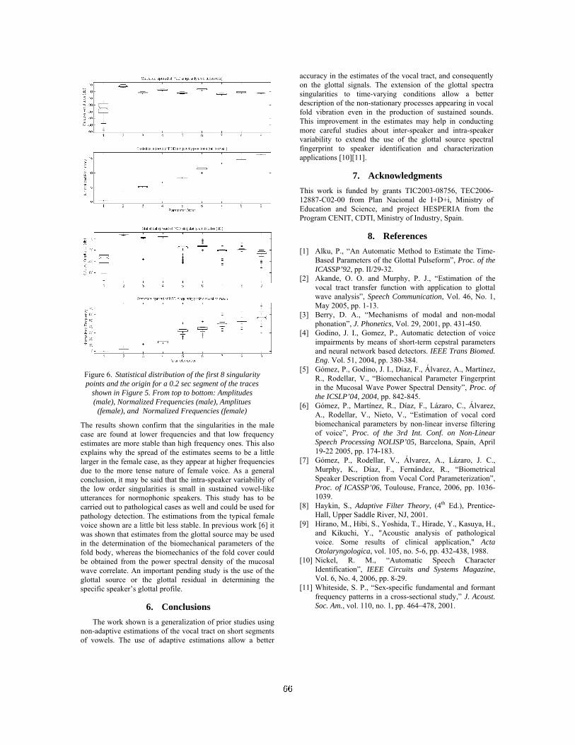
Figure 6. Statistical distribution of the first 8 singularity points and the origin for a 0.2 sec segment of the traces

shown in Figure 5. From top to bottom: Amplitudes (male), Normalized Frequencies (male), Amplitues

e), and Normalized Frequencies (female)(femal

of vowels. The use of adaptive estimations allow a better

7. Acknowledgments This work is fu 56, TEC2006-

8. References [1] Alku, P., “An Automatic Method to Estimate the Time-

[2] hy, P. J., “Estimation of the

[3] hanisms of modal and non-modal

[4] ce

[5] lvarez, A., Martínez,

[6]

[7] Álvarez, A., Lázaro, J. C.,

[8] , S., Adaptive Filter Theory, (4 Ed.), Prentice-

[9] ., Kasuya, H.,

[10] r

[11] fundamental and formant

The results shown confirm that the singularities in the male case are found at lower frequencies and that low frequency estimates are more stable than high frequency ones. This also explains why the spread of the estimates seems to be a little larger in the female case, as they appear at higher frequencies due to the more tense nature of female voice. As a general conclusion, it may be said that the intra-speaker variability of the low order singularities is small in sustained vowel-like utterances for normophonic speakers. This study has to be carried out to pathological cases as well and could be used for pathology detection. The estimations from the typical female voice shown are a little bit less stable. In previous work [6] it was shown that estimates from the glottal source may be used in the determination of the biomechanical parameters of the fold body, whereas the biomechanics of the fold cover could be obtained from the power spectral density of the mucosal wave correlate. An important pending study is the use of the glottal source or the glottal residual in determining the specific speaker’s glottal profile.

6. Conclusions The work shown is a generalization of prior studies using

non-adaptive estimations of the vocal tract on short segments

accuracy in the estimates of the vocal tract, and consequently on the glottal signals. The extension of the glottal spectra singularities to time-varying conditions allow a better description of the non-stationary processes appearing in vocal fold vibration even in the production of sustained sounds. This improvement in the estimates may help in conducting more careful studies about inter-speaker and intra-speaker variability to extend the use of the glottal source spectral fingerprint to speaker identification and characterization applications [10][11].

nded by grants TIC2003-08712887-C02-00 from Plan Nacional de I+D+i, Ministry of Education and Science, and project HESPERIA from the Program CENIT, CDTI, Ministry of Industry, Spain.

Based Parameters of the Glottal Pulseform”, Proc. of the ICASSP’92, pp. II/29-32. Akande, O. O. and Murpvocal tract transfer function with application to glottal wave analysis”, Speech Communication, Vol. 46, No. 1, May 2005, pp. 1-13. Berry, D. A., “Mecphonation”, J. Phonetics, Vol. 29, 2001, pp. 431-450. Godino, J. I., Gomez, P., Automatic detection of voiimpairments by means of short-term cepstral parameters and neural network based detectors. IEEE Trans Biomed. Eng. Vol. 51, 2004, pp. 380-384. Gómez, P., Godino, J. I., Díaz, F., ÁR., Rodellar, V., “Biomechanical Parameter Fingerprint in the Mucosal Wave Power Spectral Density”, Proc. of the ICSLP’04, 2004, pp. 842-845. Gómez, P., Martínez, R., Díaz, F., Lázaro, C., Álvarez, A., Rodellar, V., Nieto, V., “Estimation of vocal cord biomechanical parameters by non-linear inverse filtering of voice”, Proc. of the 3rd Int. Conf. on Non-Linear Speech Processing NOLISP’05, Barcelona, Spain, April 19-22 2005, pp. 174-183. Gómez, P., Rodellar, V.,Murphy, K., Díaz, F., Fernández, R., “Biometrical Speaker Description from Vocal Cord Parameterization”, Proc. of ICASSP’06, Toulouse, France, 2006, pp. 1036-1039. Haykin th

Hall, Upper Saddle River, NJ, 2001. Hirano, M., Hibi, S., Yoshida, T., Hirade, Yand Kikuchi, Y., "Acoustic analysis of pathological voice. Some results of clinical application," Acta Otolaryngologica, vol. 105, no. 5-6, pp. 432-438, 1988.

Nickel, R. M., “Automatic Speech CharacteIdentification”, IEEE Circuits and Systems Magazine, Vol. 6, No. 4, 2006, pp. 8-29.

Whiteside, S. P., “Sex-specificfrequency patterns in a cross-sectional study,” J. Acoust. Soc. Am., vol. 110, no. 1, pp. 464–478, 2001.

66

Trajectory Mixture Density Network with Multiple Mixtures forAcoustic-articulatory Inversion

Korin Richmond

Centre for Speech Technology ResearchEdinburgh University, Edinburgh, United Kingdom

korin@cstr.ed.ac.uk

Abstract

We have previously proposed a trajectory model which is basedon a mixture density network trained with target variables aug-mented with dynamic features together with an algorithm forestimating maximum likelihood trajectories which respects theconstraints between those features. In this paper, we have ex-tended that model to allow diagonal covariance matrices andmultiple mixture components. We have evaluated the model onan inversion mapping task and found the trajectory model workswell, outperforming smoothing of equivalent trajectories usinglow-pass filters. Increasing the number of mixture componentsin the TMDN improves results further.

1. IntroductionMainstream speech technology, such as automatic speechrecognition and concatenative speech synthesis, is strongly fo-cuses on the acoustic speech signal. This is natural, consid-ering the acoustic domain is where the speech signal exists intransmission between humans, and we can conveniently mea-sure and manipulate an acoustic representation of speech. How-ever, an articulatory representation of speech has certain prop-erties which are attractive and which may be exploited in mod-elling. Speech articulators move relatively slowly and smoothly,and their movements are continuous; the mouth cannot “jump”from one position to the next. Using knowledge of the speechproduction system could improve speech processing methodsby providing useful constraints. Accordingly, there is growinginterest in exploiting articulatory information and representa-tions in speech processing, with many suggested applications;for example, low bit-rate speech coding [1], speech analysis andsynthesis [2], automatic speech recognition [3, 4], animatingtalking heads and so on.

For an articulatory approach to be practical, we need conve-nient access to an articulatory representation. Recent work onincorporating articulation into speech technology has used dataprovided by X-ray microbeam cinematography and electromag-netic articulography (EMA). These methods, particularly thelatter, mean we are now able to gather reasonably large quanti-ties of articulatory data. However, they are still invasive tech-niques and require bulky and expensive experimental setups.Therefore, there is interest in developing a way to recover anarticulatory representation from the acoustic speech signal. Inother words, for a given acoustic speech signal we aim to es-timate the underlying sequence of articulatory configurationswhich produced it. This is termed acoustic-articulatory inver-sion, or the inversion mapping.

The inversion mapping problem has been the subject of re-search for several decades. One approach has been to attemptanalysis of acoustic signals based on mathematical models ofspeech production [5]. Another popular approach has been to

use articulatory synthesis models, either as part of an analysis-by-synthesis algorithm [6], or to generate acoustic-articulatorycorpora which may be used with a code-book mapping [7] or totrain other models [8]. Much of the more recent work reportedhas applied machine learning models to human measured artic-ulatory data, including artificial neural networks (ANNs) [9],codebook methods [10] and GMMs [11].

The inversion mapping is widely regarded as difficult be-cause it may be an ill-posed problem; multiple evidence existsto suggest the articulatory-to-acoustic mapping is many-to-one,which means that instantaneous inversion of this mapping re-sults in a one-to-many mapping. If which case, an inversionmapping method must take account of the alternative articula-tory configurations possible in response to an acoustic vector.

In previous work [12, 9], we have successfully employedthe mixture density network (MDN) [13] to address this prob-lem. The MDN provides a probability density function (pdf) ofarbitrary complexity over the target articulatory domain whichis conditioned on the acoustic input. In [14], we began to ex-tend this work to provide a statistical trajectory model, termedthe Trajectory MDN, along similar lines as the HMM-basedspeech production model of [15] and the GMM-based inver-sion mapping of [11]. This was achieved by augmenting thestatic articulatory target data with dynamic delta and deltadeltafeatures and incorporating the maximum likelihood parametergeneration (MLPG) algorithm [16]. This allows to calculate themaximum likelihood estimate of articulatory trajectories whichrespect the constraints between the static and derived dynamicfeatures.

This paper seeks to further the work in [14] with three spe-cific aims: 1) to evaluate an extension to the TMDNs in [14]which allows mixture models with diagonal covariance matri-ces. 2) to evaluate the new implementation of TMDN on the fullset of articulator channels, and in comparison with a low-passfiltering approach previously reported. 3) to evaluate TMDNswith multiple mixture components.

2. The Trajectory Mixture Density NetworkModel

We give here a very brief introduction to the MDN, and describehow it may be extended with the MLPG algorithm to give a tra-jectory model. For full details of the MDN and MLPG, thereader is referred to [13] and [16] respectively. We have at-tempted to retain the original notation as far as possible.

2.1. Mixture density networks

The MDN combines a mixture model with an ANN. Here,we will consider a multilayer perceptron and Gaussian mixturecomponents. The ANN maps from the input vectorx to thecontrol parameters of the mixture model (priorsα, meansµ and67

2 22

conditionalprobabilitydensity

mixturemodel

neuralnetwork

p(t|x)

xvectorinput

α σµ α σµα σµ

Figure 1: The mixture density network is the combination of amixture model and a neural network.

variancesσ2), which in turn gives a pdf over the target domain,conditioned on the input vectorp(t|x). The toy-example MDNin Figure 1 takes an input vectorx (dimensionality 5) and givesthe conditional probability density of a vectort (dimensionality1) in the target domain. This pdf takes the form of a GMM with3 components, so it is given as:

p(t|x) =

MXj=1

αj(x)φj(t|x) (1)

whereM is the number of mixture components (in this exam-ple, 3),φj(t|x) is the probability density given by thejth ker-nel, andαj(x) is the prior for thejth kernel.

In order to constrain the GMM priors to within the range0 ≤ αj(x) ≤ 1 and to sum to unity, thesoftmaxfunction isused

αj =exp(zαj )PMl=1 exp(zαl )

(2)

wherezαj is the output of the ANN corresponding to the priorfor thejth mixture component. The variances are similarly re-lated to the outputs of the ANN as

σj = exp(zσj ) (3)

wherezσj is the output of the ANN corresponding to the vari-ance for thejth mixture component. This avoids the variancebecoming≤ 0. Finally, the means are represented directly:

µjk = zµjk (4)

wherezµjk is the value of the output unit corresponding to thekth dimension of the mean vector for thejth mixture compo-nent.

Training the MDN aims to minimise the negative log like-lihood of the observed target data points

E = −Xn

ln

(MXj=1

αj(xn)φj(t

n|xn)

)(5)

given the mixture model parameters. Since the ANN part ofthe MDN provides the parameters for the mixture model, thiserror function must be minimised with respect to the networkweights. The derivatives of the error at the network output unitscorresponding separately to the priors, means and variances ofthe mixture model are calculated (see [13]) and then propagatedback through the network to find the derivatives of the errorwith respect to the network weights. Thus, standard non-linearoptimisation algorithms can be applied to MDN training.

VTDTBTT

ULLL

LI

Figure 2: Placement of EMA receiver coils in the MOCHAdatabase for speakerfsew0 . See Table 1 for the key to ab-breviations.

2.2. Maximum likelihood parameter generation

The first step to an MDN-based trajectory model is to train anMDN with target feature vectors augmented with dynamic fea-tures, derived from linear combinations of a window of staticfeatures. For the sake of simplicity and economy of space1,we will consider MDNs with a single Gaussian distribution anda single target static featurect at each time step. Next, giventhe output of this MDN in response to a sequence of inputvectors, in order to generate the maximum likelihood trajec-tory, we aim to maximizeP (O|Q) with respect toO, whereO = [oT1 ,o

T2 , ...,o

TT ]T , ot = [ct,∆ct,∆∆ct] andQ is the

sequence of Gaussians output by our MDN. The relationshipbetween the static features and those augmented with deriveddynamic features can be arranged in matrix form,

O = WC (6)

whereC is a sequence of static features andW is a transfor-mation matrix composed of the coefficients of the delta anddeltadelta calculation window and0. Under the condition ex-pressed in Eq. 6, maximisingP (O|Q) is equivalent to max-imisingP (WC|Q) with respect toC. By setting

∂ logP (WC|Q)

∂C= 0 (7)

a set of linear equations is obtained (see [16])

WTU−1WC = WTU−1MT (8)

where MT = [µq1 , µq2 , ..., µqT ] and U−1 =diag[U−1

q1 ,U−1q2 , ...,U

−1qT ] (µqT and U−1

qt are the 3 × 1mean vector and3 × 3 (diagonal) covariance matrix respec-tively). Solving Eq. 8 forC computes the maximum likelihoodtrajectory.

3. Inversion mapping experiment3.1. MOCHA articulatory data

The multichannel articulatory (MOCHA) dataset [17] used forthe experiments in this paper gives the acoustic waveformrecorded concurrently with electromagnetic articulograph (2DEMA) data. The sensors shown in Figure 2 provide x- andy-coordinates in the midsagittal plane at 500Hz sample rate.Speakers were recorded reading a set of 460 short, phonetically-balanced British-TIMIT sentences. Female speakerfsew0 wasused for the experiments here. This is the same data set as used

1the full version of this paper will require a description of MLPG inthe case of multiple mixture components68

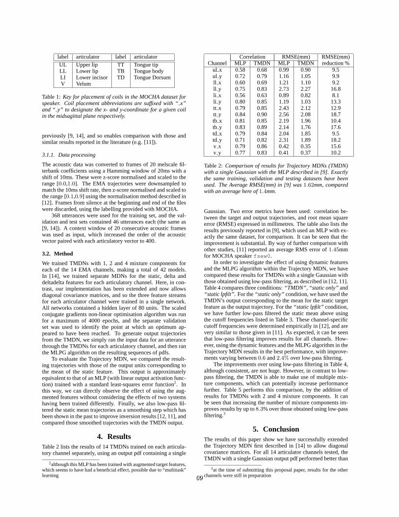
label articulator label articulatorUL Upper lip TT Tongue tipLL Lower lip TB Tongue bodyLI Lower incisor TD Tongue DorsumV Velum

Table 1:Key for placement of coils in the MOCHA dataset forspeaker. Coil placement abbreviations are suffixed with “x”and “ y” to designate the x- and y-coordinate for a given coilin the midsagittal plane respectively.

previously [9, 14], and so enables comparison with those andsimilar results reported in the literature (e.g. [11]).

3.1.1. Data processing

The acoustic data was converted to frames of 20 melscale fil-terbank coefficients using a Hamming window of 20ms with ashift of 10ms. These were z-score normalised and scaled to therange [0.0,1.0]. The EMA trajectories were downsampled tomatch the 10ms shift rate, then z-score normalised and scaled tothe range [0.1,0.9] using the normalisation method described in[12]. Frames from silence at the beginning and end of the fileswere discarded, using the labelling provided with MOCHA.

368 utterances were used for the training set, and the val-idation and test sets contained 46 utterances each (the same as[9, 14]). A context window of 20 consecutive acoustic frameswas used as input, which increased the order of the acousticvector paired with each articulatory vector to 400.

3.2. Method

We trained TMDNs with 1, 2 and 4 mixture components foreach of the 14 EMA channels, making a total of 42 models.In [14], we trained separate MDNs for the static, delta anddeltadelta features for each articulatory channel. Here, in con-trast, our implementation has been extended and now allowsdiagonal covariance matrices, and so the three feature streamsfor each articulator channel were trained in a single network.All networks contained a hidden layer of 80 units. The scaledconjugate gradients non-linear optimisation algorithm was runfor a maximum of 4000 epochs, and the separate validationset was used to identify the point at which an optimum ap-peared to have been reached. To generate output trajectoriesfrom the TMDN, we simply ran the input data for an utterancethrough the TMDNs for each articulatory channel, and then ranthe MLPG algorithm on the resulting sequences of pdfs.

To evaluate the Trajectory MDN, we compared the result-ing trajectories with those of the output units corresponding tothe mean of the static feature. This output is approximatelyequivalent to that of an MLP (with linear output activation func-tion) trained with a standard least-squares error function2. Inthis way, we can directly observe the effect of using the aug-mented features without considering the effects of two systemshaving been trained differently. Finally, we also low-pass fil-tered the static mean trajectories as a smoothing step which hasbeen shown in the past to improve inversion results [12, 11], andcompared those smoothed trajectories with the TMDN output.

4. ResultsTable 2 lists the results of 14 TMDNs trained on each articula-tory channel separately, using an output pdf containing a single

2although this MLP has been trained with augmented target features,which seems to have had a beneficial effect, possible due to “multitask”learning

Correlation RMSE(mm) RMSE(mm)Channel MLP TMDN MLP TMDN reduction %

ul x 0.58 0.68 0.99 0.90 9.5ul y 0.72 0.79 1.16 1.05 9.9ll x 0.60 0.69 1.21 1.10 9.2ll y 0.75 0.83 2.73 2.27 16.8li x 0.56 0.63 0.89 0.82 8.1li y 0.80 0.85 1.19 1.03 13.3tt x 0.79 0.85 2.43 2.12 12.9tt y 0.84 0.90 2.56 2.08 18.7tb x 0.81 0.85 2.19 1.96 10.4tb y 0.83 0.89 2.14 1.76 17.6td x 0.79 0.84 2.04 1.85 9.5td y 0.71 0.82 2.31 1.89 18.2v x 0.79 0.86 0.42 0.35 15.6v y 0.77 0.83 0.41 0.37 10.2

Table 2: Comparison of results for Trajectory MDNs (TMDN)with a single Gaussian with the MLP described in [9]. Exactlythe same training, validation and testing datasets have beenused. The Average RMSE(mm) in [9] was1.62mm, comparedwith an average here of1.4mm.

Gaussian. Two error metrics have been used: correlation be-tween the target and output trajectories, and root mean squareerror (RMSE) expressed in millimetres. The table also lists theresults previously reported in [9], which used an MLP with ex-actly the same dataset, for comparison. It can be seen that theimprovement is substantial. By way of further comparison withother studies, [11] reported an average RMS error of1.45mmfor MOCHA speakerfsew0 .

In order to investigate the effect of using dynamic featuresand the MLPG algorithm within the Trajectory MDN, we havecompared these results for TMDNs with a single Gaussian withthose obtained using low-pass filtering, as described in [12, 11].Table 4 compares three conditions:“TMDN” , “static only” and“static lpfilt” . For the“static only” condition, we have used theTMDN’s output corresponding to the mean for the static targetfeature as the output trajectory. For the“static lpfilt” condition,we have further low-pass filtered the static mean above usingthe cutoff frequencies listed in Table 3. These channel-specificcutoff frequencies were determined empirically in [12], and arevery similar to those given in [11]. As expected, it can be seenthat low-pass filtering improves results for all channels. How-ever, using the dynamic features and the MLPG algorithm in theTrajectory MDN results in the best performance, with improve-ments varying between0.6 and2.4% over low-pass filtering.

The improvements over using low-pass filtering in Table 4,although consistent, are not huge. However, in contrast to low-pass filtering, the TMDN is able to make use of multiple mix-ture components, which can potentially increase performancefurther. Table 5 performs this comparison, by the addition ofresults for TMDNs with 2 and 4 mixture components. It canbe seen that increasing the number of mixture components im-proves results by up to8.3% over those obtained using low-passfiltering.3

5. ConclusionThe results of this paper show we have successfully extendedthe Trajectory MDN first described in [14] to allow diagonalcovariance matrices. For all 14 articulator channels tested, theTMDN with a single Gaussian output pdf performed better than

3at the time of submitting this proposal paper, results for the otherchannels were still in preparation69

Correlation RMSE(mm) RMSE(mm)Channel static only static lpfilt TMDN static only static lpfilt TMDN reduction %

ul x 0.63 0.67 0.68 0.93 0.90 0.90 0.6ul y 0.74 0.77 0.79 1.13 1.06 1.05 1.5ll x 0.64 0.69 0.69 1.17 1.11 1.10 1.0ll y 0.81 0.83 0.83 2.40 2.31 2.27 1.6li x 0.57 0.62 0.63 0.88 0.84 0.82 2.4li y 0.83 0.84 0.85 1.07 1.05 1.03 1.5tt x 0.82 0.84 0.85 2.26 2.14 2.12 1.0tt y 0.88 0.89 0.90 2.19 2.12 2.08 1.8tb x 0.83 0.85 0.85 2.05 1.99 1.96 1.2tb y 0.87 0.89 0.89 1.88 1.80 1.76 1.8td x 0.81 0.83 0.84 1.95 1.88 1.85 2.1td y 0.78 0.81 0.82 2.04 1.92 1.89 1.7v x 0.84 0.85 0.86 0.37 0.36 0.35 1.2v y 0.80 0.82 0.83 0.39 0.37 0.37 1.6

Table 4:Comparison of correlation and RMS error (in millimetres) for Trajectory MDN model (“TMDN”) with the static mean MDNoutput only (“static only”) and low-pass filtered static mean (“static lpfilt”). Low-pass filtering the static feature output, using thecutoff frequencies in Table 3, improves results for all channels. However, using the delta and deltadelta features in the Trajectory MDNgives the best performance for all channels. The TMDN here has a single Gaussian as its output distribution. Compare these resultswith those in table 5.

ul ll li tt tb td vx 3Hz 3Hz 3Hz 6Hz 6Hz 7Hz 5Hzy 5Hz 8Hz 7Hz 9Hz 7Hz 6Hz 5Hz

Table 3:Channel-specific cutoff frequencies used for low passfiltering (empirically determined in [12]).

static TMDN % bestChannel lpfilt 1mix 2mix 4mix reduction

tt x 2.14 2.12 2.09 2.10 2.1tt y 2.12 2.08 1.98 1.94 8.3td x 1.88 1.85 1.81 1.83 4.1td y 1.92 1.89 1.85 1.88 3.6

Table 5: Comparison of RMS error (expressed in millimetres)between using the low-pass filtered static feature mean (“staticlpfilt”) and Trajectory MDNs with 1, 2 or 4 mixture compo-nents. Compared with the results in Table 4, using multiplemixture components improves the performance of the TMDNover low-pass filtering even further.

low-pass filter smoothing. Increasing the number of mixturecomponents improved results further. This is a unique advan-tage of the TMDN model over smoothing single trajectorieswith, for example, low-pass filters.

6. References[1] J. Schroeter and M. M. Sondhi, “Speech coding based on phys-

iological models of speech production,” inAdvances in SpeechSignal Processing, S. Furui and M. M. Sondhi, Eds. New York:Marcel Dekker Inc, 1992, ch. 8, pp. 231–268.

[2] T. Toda, A. Black, and K. Tokuda, “Mapping from articulatorymovements to vocal tract spectrum with Gaussian mixture modelfor articulatory speech synthesis,” inProc. 5th ISCA Workshop onSpeech Synthesis, 2004.

[3] S. King, J. Frankel, K. Livescu, E. McDermott, K. Richmond, andM. Wester, “Speech production knowledge in automatic speechrecognition,”Journal of the Acoustical Society of America, vol.121, no. 2, p. (pages TBA), February 2007.

[4] A. Wrench and K. Richmond, “Continuous speech recognition us-ing articulatory data,” inProc. ICSLP 2000, Beijing, China, 2000.

[5] H. Wakita, “Estimation of vocal-tract shapes from acoustical anal-ysis of the speech wave: The state of the art,”IEEE Trans. Acoust.Speech Signal Process., vol. ASSP-27, pp. 281–285, 1979.

[6] K. Shirai and T. Kobayashi, “Estimating articulatory motion fromspeech wave,”Speech Communication, vol. 5, pp. 159–170, 1986.

[7] B. S. Atal, J. J. Chang, M. V. Mathews, and J. W. Tukey, “Inver-sion of articulatory-to-acoustic transformation in the vocal tractby a computer sorting technique,”J. Acoust. Soc. Am., vol. 63, pp.1535–1555, 1978.

[8] M. G. Rahim, W. B. Kleijn, J. Schroeter, and C. C. Goodyear,“Acoustic-to-articulatory parameter mapping using an assemblyof neural networks,” inProceedings of the IEEE InternationalConference on Acoustics, Speech, and Signal Processing, 1991,pp. 485–488.

[9] K. Richmond, S. King, and P. Taylor, “Modelling the uncertaintyin recovering articulation from acoustics,”Computer Speech andLanguage, vol. 17, pp. 153–172, 2003.

[10] J. Hogden, A. Lofqvist, V. Gracco, I. Zlokarnik, P. Rubin, andE. Saltzman, “Accurate recovery of articulator positions fromacoustics: New conclusions based on human data,”J. Acoust. Soc.Am., vol. 100, no. 3, pp. 1819–1834, September 1996.

[11] T. Toda, A. Black, and K. Tokuda, “Acoustic-to-articulatory inver-sion mapping with Gaussian mixture model,” inProc. 8th Interna-tional Conference on Spoken Language Processing, Jeju, Korea,2004.

[12] K. Richmond, “Estimating articulatory parameters from theacoustic speech signal,” Ph.D. dissertation, The Centre for SpeechTechnology Research, Edinburgh University, 2002.

[13] C. Bishop,Neural Networks for Pattern Recognition. OxfordUniversity Press, 1995.

[14] K. Richmond, “A trajectory mixture density network for theacoustic-articulatory inversion mapping,” inProc. Interspeech,Pittsburgh, USA, September 2006.

[15] S. Hiroya and M. Honda, “Estimation of articulatory movementsfrom speech acoustics using an HMM-based speech productionmodel,” IEEE Transactions on Speech and Audio Processing,vol. 12, no. 2, pp. 175–185, mar 2004.

[16] K. Tokuda, T. Yoshimura, T. Masuko, T. Kobayashi, and T. Kita-mura, “Speech parameter generation algorithms for HMM-basedspeech synthesis,” inProc. ICASSP, Istanbul, Turkey, June 2000,pp. 1315–1318.

[17] A. Wrench, “The MOCHA-TIMIT articulatory database,”http://www.cstr.ed.ac.uk/artic/mocha.html, 1999.

70

Application of Feature Subset Selection based on Evolutionary Algorithms for Automatic Emotion Recognition in Speech

Aitor Álvarez, Idoia Cearreta, Juan Miguel López, Andoni Arruti, Elena Lazkano, Basilio Sierra, Nestor Garay

Computer Science Faculty (University of the Basque Country) Manuel Lardizabal 1, E-20018 Donostia (Gipuzkoa), Spain

aalvarez031@ikasle.ehu.es

Abstract The study of emotions in human-computer interaction is a growing research area. Focusing on automatic emotion recognition, work is being performed in order to achieve good results particularly in speech and facial gesture recognition. In this paper we present a study performed to analyze different machine learning techniques validity in automatic speech emotion recognition area. Using a bilingual affective database, different speech parameters have been calculated for each audio recording. Then, several machine learning techniques have been applied to evaluate their usefulness in speech emotion recognition. In this particular case, techniques based on evolutive algorithms (EDA) have been used to select speech feature subsets that optimize automatic emotion recognition success rate. Achieved experimental results show a representative increase in the abovementioned success rate.

1. Introduction Human beings are eminently emotional, as their social interaction is based on the ability to communicate their emotions and perceive the emotional states of others [1]. Affective computing, a discipline that develops devices for detecting and responding to users’ emotions [2], is a growing research area [3]. The main objective of affective computation is to capture and process affective information with the aim of enhancing the communication between the human and the computer.

Within the scope of affective computing, the development of affective applications is a challenge that involves analyzing different multimodal data sources. In order to develop such applications, a large amount of data is needed in order to include a wide range of emotionally significant material. Affective databases are a good chance for developing affective recognizers or affective synthesizers.

In this paper different speech paralinguistic parameters have been calculated for the analysis of the human emotional voice, using several audio recordings. These recordings are stored in a bilingual and multimodal affective database. Several works have already been done in which the use of Machine Learning paradigms takes a principal role.

2. Related work As previously mentioned affective databases provide a good opportunity for training affective applications. This type of databases usually record information such as images, sounds, psychophysiological values, etc. There are some references in the literature that present affective databases and their characteristics. In [4], the authors carried out a wide review of

affective databases. Other interesting reviews are the ones provided in [5] and [6].

Many studies have been focused on the different features used in human emotional speech analysis [7, 8]. The number of voice features analysed varies among the studies, but basically most of these are based in fundamental frequency, energy and timing parameters, such as speech rate or mean phone duration.

Works where the use of Machine Learning paradigms take a principal role can also be found in the literature. [9] presented a good reference paper. The Neural Networks Journal devoted a special issue to emotion treatment from a Neural Networks perspective [10]. The work by [4] is related with this paper in the sense of using a Feature Selection method in order to apply a Neural Network to emotion recognition in speech, although both, the methods to perform the FSS and the paradigms used, are different. In this line it has to be pointed out the work by [11] which uses a reduced number of emotions and a greedy approach to select the features.

3. Study of automatic emotion recognition relevant parameters using Machine Learning

paradigms

3.1. RekEmozio Database

The RekEmozio bilingual database was created with the aim of serving as an information repository for performing research on user emotion. The aim when building the RekEmozio resource was to add descriptive information about the performed recordings, so that processes such as extracting speech parameters and video features could be carried out on them. Members of different work groups involved in research projects related to RekEmozio have performed several processes for extracting speech and video features; this information was subsequently added to the database. The emotions used were chosen based on [12], and the neutral emotion was added. The characteristics of the RekEmozio database are described in [13]. The languages that are considered in RekEmozio database are Spanish and Basque.

3.2. Emotional feature extraction

For emotion recognition in speech, one of the most important questions is which features should be extracted from the voice signal. Previous studies show us that it is difficult to find

71

specific voice features that could be used as reliable indicators of the emotion present in the speech [14].

In this work, RekEmozio database audio recordings (stereo wave files, sampled at 44100 Hz) have been processed using standard signal processing techniques (windowing, Fast Fourier Transform, auto-correlation …) to extract a wide group of 32 features which are described below. Supposing that each recording in the database corresponds to one single emotion, only one global vector of features has been obtained for each recording by using some statistical operations. Parameters used are global parameters calculated over entire recordings. Selected features are detailed next (in italics):

• Fundamental Frequency (F0): It is the most common

feature analyzed in several studies [7, 8]. For F0 estimation we used Sun algorithm [15] and statistics are computed: Maximum, Minimum, Mean, Range, Variance, Standard deviation and Maximum positive slope in F0 contour.

• RMS Energy: The mean energy of speech quantified by calculating root mean square (RMS) value and 6 statistics Maximum, Minimum, Mean, Range, Variance and Standard Deviation.

• Loudness: Absolute loudness based on Zwicker’s model [16].

• Spectral distribution of energy: Each emotion requires a different effort in the speech and it is known that the spectral distribution of energy varies with speech effort [7]. We have computed energy in Low band, between 0 and 1300 Hz, Medium band, between 1300 and 2600 Hz and High band from 2600 to 4000 Hz [17].

• Mean Formants and Bandwidth: Energy from the sound source (vocal folds) is modified by the resonance characteristics of the vocal tract (formants). Acoustic variations dues to emotion are reflected in formants [18]. The first three mean Formants, and their corresponding mean Bandwidths.

• Jitter: Perturbation in vibration of vocal chords. It is estimated based on the model presented by [19].

• Shimmer: Perturbation cycle to cycle of the energy. Its estimation is based on the previously calculated absolute loudness.

• Speaking Rate: Rhythm is known to be an important aspect in recognition of emotion in speech. Progress has been made on a simple aspect of rhythm, the alternation between speech and silence [7]. The speaking rate estimation has been divided in 6 values based on their duration with respect to the whole elocution: Duration of voice part, Silence part, Maximum voice part, Minimum voice part, Maximum silence part and Minimum silence part.

3.3. Machine Learning standard paradigms used

In the supervised learning task, a classification problem has been defined where the main goal is to construct a model or a classifier able to manage the classification itself with acceptable accuracy. With this aim, some variables are to be

used in order to identify different elements, the so called predictor variables. For the current problem, each sample is composed by the set of 32 speech related values, while the label value is one of the seven emotions identified. The single paradigms used in our experiments that come from the family of Machine Learning (ML) are briefly introduced

3.3.1. Decision trees

A decision tree consists of nodes and branches to partition a set of samples into a set of covering decision rules. In each node, a single test or decision is made to obtain a partition. The starting node is usually referred as the root node. In each node, the goal is to select an attribute that makes the best partition between the classes of the samples in the training set [20], [21]. In our experiments, two well-known decision tree induction algorithms are used, ID3 [22] and C4.5 [23].

3.3.2. Instance-Based Learning

Instance-Based Learning (IBL) has its root in the study of nearest neighbor algorithm [24] in the field of machine learning. The simplest form of nearest neighbor (NN) or k-nearest neighbor (k-NN) algorithms simply stores the training instances and classifies a new instance by predicting the same class its nearest stored instance has or the majority class of its k nearest stored instances have, respectively, according to some distance measure as described in [25]. The core of this non-parametric paradigm is the form of the similarity function that computes the distances from the new instance to the training instances, to find the nearest or k-nearest training instances to the new case. In our experiments the IB paradigm is used, an inducer developed in the MLC++ project [26] and based on the works of [27] and [28].

3.3.3. Naive Bayes classifiers

The Naive-Bayes (NB) rule [29] uses the Bayes theorem to predict the class for each case, assuming that the predictive genes are independent given the category. To classify a new sample characterized by d genes X = (X1,X2, ...,Xd), the NB classifier applies the following rule:

cj)|p(xi c

d

1iB - N p(cj)max arg ∏

=∈

=Ccj

(1)

where CN-B denotes the class label predicted by the Naive-Bayes classifier and the possible classes of the problem are grouped in C = c1, . . . , cl. A normal distribution is assumed to estimate the class conditional densities for predictive genes. Despite its simplicity, the NB rule obtains better results than more complex algorithms in many domains.

3.3.4. Naive Bayesian Tree learner

The naive Bayesian tree learner, NBTree [30], combines naive Bayesian classification and decision tree learning. It uses a tree structure to split the instance space into sub-spaces defined by the paths of the tree, and generates one naive Bayesian classifier in each sub-space.

3.3.5. Feature Subset Selection by Estimation of Distribution Algorithms

The basic problem of ML is concerned with the induction of a model that classifies a given object into one of several known

72

classes. In order to induce the classification model, each object is described by a pattern of d features. Here, the ML community has formulated the following question: are all of these d descriptive features useful for learning the ‘classification rule’? On trying to respond to this question, we come up with the Feature Subset Selection (FSS) [31] approach which can be reformulated as follows: given a set of candidate features, select the ‘best’ subset in a classification problem. In our case, the ‘best’ subset will be the one with the best predictive accuracy.

Most of the supervised learning algorithms perform rather poorly when faced with many irrelevant or redundant (depending on the specific characteristics of the classifier) features. In this way, the FSS proposes additional methods to reduce the number of features so as to improve the performance of the supervised classification algorithm.

FSS can be viewed as a search problem [32], with each state in the search space specifying a subset of the possible features of the task. Exhaustive evaluation of possible feature subsets is usually unfeasible in practice due to the large amount of computational effort required. In this way, any feature selection method must determine the nature of the search process. In the experiments performed, an Estimation of Distribution Algorithm (EDA) has been used which has the model accuracy as fitness function.

To assess the goodness of each proposed gene subset for a specific classifier, a wrapper approach is applied. In the same way as supervised classifiers when no gene selection is applied, this wrapper approach estimates, by using the 10-fold crossvalidation [33] procedure, the goodness of the classifier using only the variable subset found by the search algorithm.

4. Experimental Results The above mentioned methods have been applied over the crossvalidated data sets using the MLC++ library [26]. Each dataset corresponds to a single actor. Experiments were carried out with and without FSS in order to extract the accuracy improvement introduced by the feature selection process. Tables 1 and 2 show the classification results obtained using the whole set of variables, for Basque and Spanish languages respectively. Each column represents a female (Fi) of male (Mi) actor, and mean values corresponding to each classifier/gender is also included. Last column presents the total average for each classifier.

Table 1: 10-fold crossvalidation accuracy for Basque Language using the whole variable set

Female Male Total F1 F2 F3 mean M1 M2 M3 M4 mean

IB 35.4 48.8 35.2 39.8 44.2 49.3 36.9 40.9 42.8 41.5 ID3 38.7 45.5 44.7 42.9 46.7 46.9 43.3 51.1 47.0 45.3 C4.5 41.5 52.2 35.0 42.9 60.4 53.3 45.1 49.5 52.0 48.1 NB 42.9 45.8 37.7 42.1 52.2 44.1 36.2 41.4 43.5 42.9

NBT 42.3 39.8 35.2 39.1 53.1 46.2 45.2 43.3 46.9 43.6

Table 2: 10-fold crossvalidation accuracy for Spanish Language using the whole variable set

Female Male Total F1 F2 F3 F4 F5 mean M1 M2 M3 M4 M5 mean

IB 34.6 43.6 54.6 54.6 38.2 45.1 25.5 33.6 51.8 47.7 33.6 38.4 41.8 ID3 36.4 52.7 49.1 47.3 42.7 45.6 20.9 30.9 40.9 47.3 40.0 36.0 40.8 C4.5 30.9 50.0 46.4 43.6 42.7 42.7 29.1 31.8 46.4 42.7 35.5 37.1 39.9 NB 38.2 42.7 49.1 40.0 42.7 42.5 24.6 30.9 49.1 45.5 34.6 36.9 39.7

NBT 42.7 43.6 49.1 50.0 39.1 44.9 18.2 27.3 40.9 48.2 42.7 35.5 40.2

Results don't seem very impressive; ID3 best classifies the emotions for female actresses, for both Basque and Spanish languages, while C4.5 outstands for Basque male actors and IB for Spanish male actors.

Results obtained after applying FSS are more appealing, as can be seen in Tables 3 and 4. There, classifier IB appears as the best paradigm for all the categories, female and male, and Basque and Spanish languages. Moreover, the accuracies outperform the previous ones in more than 15%. It must also be highlighted that FSS improves the well classified rate for all the ML paradigms, as it can be seen in Figure 1.

Table 3: 10-fold crossvalidation accuracy for Basque Language using FSS

Female Male Total F1 F2 F3 mean M1 M2 M3 M4 mean

IB 63.0 68.0 59.3 63.5 72.7 67.4 61.0 62.8 65.9 64.9 ID3 62.7 60.5 65.5 62.9 72.7 62.0 56.5 62.7 63.4 63.2 C4.5 60.2 66.0 60.0 62.1 71.8 62.8 60.1 63.6 64.6 63.5 NB 64.5 64.6 48.9 59.3 74.6 62.5 62.7 60.0 64.9 62.5 NBT 58.6 61.1 54.8 58.1 74.4 59.9 62.7 59.4 64.1 61.6

Table 4: 10-fold crossvalidation accuracy for Spanish Language using FSS

Female Male Total F1 F2 F3 F4 F5 mean M1 M2 M3 M4 M5 mean

IB 61.8 66.4 75.5 71.8 68.2 68.7 42.7 57.3 69.1 63.6 60.9 58.7 63.7 ID3 59.1 66.4 66.4 60.0 61.8 62.7 42.7 51.8 66.4 61.8 60.0 56.5 59.6 C4.5 57.3 62.7 64.6 65.5 63.6 62.7 43.6 56.4 65.5 64.6 56.4 57.3 60.0 NB 54.6 59.1 68.2 65.5 60.0 61.5 40.9 48.2 64.6 59.1 51.8 52.9 57.2

NBT 53.6 66.4 63.6 58.2 60.0 60.4 38.2 47.3 60.0 63.6 59.1 53.6 57.0

Figure 1: The improvement in Basque and Spanish languages using FSS in all the classifiers.

5. Conclusions and future work RekEmozio database has been used to training some automatic recognition systems. In this paper we have shown that applying FSS enhances classification rates for the ML paradigms that we have used (IB, ID3, C4.5, NB and NBTree).

An analysis of the selected features by FSS is required. Also, the speech data should be combined with visual information. This combination could be performed by means of a multiclassifier model [34].

6. References [1] Casacuberta, D., La mente humana: Diez Enigmas y 100

preguntas (The human mind: Ten Enigmas and 100 questions), Océano (Ed), Barcelona, Spain, ISBN: 84-7556-122-5, 2001.

[2] Picard, R. W., Affective Computing, MIT Press, Cambridge, MA, 1997.

0

10

20

30

40

50

60

70

IB ID3 C4.5 NB NBT

Emot

ion

reco

gniti

on ra

te

Basque no FSS Basque FSS

0 10 20 30 40 50 60 70

IB ID3 C4.5 NB NBTEm

otio

n re

cogn

ition

rate

Spanish no FSS Spanish FSS

73

[3] Tao, J., Tan, T., “Affective computing: A review”, In: J. Tao, T. Tan, R. W. Picard (eds.): Lecture Notes in Computer Science, Vol. 3784 - Proceedings of The First International Conference on Affective Computing & Intelligent Interaction (ACII’05), Beijing, China, 981-995, 2005.

[4] Cowie, R., Douglas-Cowie, E., Cox, C., “Beyond emotion archetypes: Databases for emotion modelling using neural networks”, Neural Networks, Vol. 18, 2005, p 371-388.

[5] Humaine, “Retrieved January 10, 2007”, from [http://emotion-research.net/wiki/Databases], (n.d.).

[6] López, J.M., Cearreta, I., Fajardo, I., Garay, N., “Validating a multimodal and multilingual affective database”, To be published in Proceedings of HCI International, 2007.

[7] Cowie, R., Douglas-Cowie, E., Tsapatsoulis, N., Votsis, G., Kollias, S., Fellenz, W., Taylor, J., “Emotion recognition in human-computer interaction”, IEEE Signal Processing Magazine, Vol. 18(1), 2001, p 32-80.

[8] Schröder, M., Speech and Emotion Research: An overview of research frameworks and a dimensional approach to emotional speech synthesis, Ph.D. thesis, PHONUS 7, Research Report of the Institute of Phonetics, Saarland University, 2004.

[9] Dellaert, F., Polzin, T., Waibel, A., “Recognizing Emotion in Speech”, In Proc. of ICSLP’96, 1996.

[10] Taylor, J. G., Scherer, K., Cowie, R., “Neural Networks, special issue on Emotion and Brain”, Vol. 18, Issue 4, 2005, p 313-455.

[11] Huber, R., Batliner, A., Buckow, J., Noth, E., Warnke, V., Niemann, H., “Recognition of emotion in a realistic dialogue scenario”, In Proc. ICSLP’00, p 665-668, 2000.

[12] Ekman, P., Friesen, W., Pictures of facial affect, Consulting Psychologist Press, Palo Alto, CA, 1976.

[13] López, J.M., Cearreta, I., Garay, N., López de Ipiña, K., Beristain, A., “Creación de una base de datos emocional bilingüe y multimodal”, In Redondo, M.A., Bravo C., Ortega M. (Eds). Proceeding of the 7th Spanish Human Computer Interaction Conference, Interacción-06, Puertollano, p 55-66, 2006.

[14] Laukka, P., Vocal Expression of Emotion. Discrete-emotions and Dimensional Accounts, Acta Universitatis Upsaliensis. Comprehensive Summaries of Uppsala Dissertations from the Faculty of Social Sciences, pp 141, 80, ISBN 91-554-6091-7, Uppsala, 2004.

[15] Sun, X., “Pitch determination and voice quality analysis using subharmonic-to-harmonic ratio”, To appear in the Proc. of IEEE International Conference on Acoustics, Speech, and Signal Processing, Orlando, Florida, 2002

[16] Fernandez, R., A Computational Model for the Automatic Recognition of Affect in Speech, Ph.D. thesis, Massachusetts Institute of Technology, 2004.

[17] Kazemzadeh, A., Lee, S., Narayanan, S., “Acoustic correlates of user response to errors in human-computer dialogues”, Proc. IEEE ASRU, (St. Thomas, U.S. Virgin Islands), 2003 (December).

[18] Bachorowski, J.A., Owren, M. J., “Vocal expression of emotion: Acoustic properties of speech are associated with emotional intensity and context” Psychological Science, Vol. 6,1995, p 219-224.

[19] Rothkrantz, L.J.M., Wiggers, P., van Wees, J.W.A., van Vark, R.J., “Voice stress analysis”, Proceedings of Text, Speech and Dialogues 2004, 2004.

[20] Martin, J.K., “An exact probability metric for Decision Tree splitting and stopping, Machine Learning”, 1997, p 28(2/3).

[21] Mingers, J., “A comparison of methods of pruning induced Rule Trees, Technical Report”, Coventry, England: University of Warwick, School of Indutrial and Business Studies, 1988.

[22] Quinlan, J.R., “Induction of Decision Trees”, Machine Learning, Vol 1, 1986, p 81-106.

[23] Quinlan, J.R., C4.5: Programs for Machine Learning, Morgan Kaufmann Publishers, Inc. Los Altos, California, 1993.

[24] Dasarathy, B.V., “Nearest Neighbor (NN) Norms: NN Pattern Recognition Classification Techniques”, IEEE Computer Society Press, 1991.

[25] Ting, K.M., Common issues in Instance-Based and Naive-Bayesian classifiers, Ph.D. Thesis, Basser Department of Computer Science, The University of Sidney, Australia, 1995.

[26] Kohavi, R., Sommerfield, D., Dougherty, J., “Data mining using MLC++, a Machine Learning Library in C++”, International Journal of Artificial Intelligence Tools, Vol. 6 (4), 1997, p 537-566, [http://www.sgi.com/Technology/mlc/].

[27] Aha, D., Kibler, D., Albert, M.K., “Instance-Based learning algorithms”, Machine Learning, Vol. 6, 37-66, 1991.

[28] Wettschereck, D., A study of distance-based Machine Learning Algorithms, Ph.D. Thesis, Oregon State University, 1994.

[29] Minsky, M. “Steps towards artificial intelligence”, Proceedings of the IRE, 49, 8–30, 1961.

[30] Kohavi, R., “Scaling up the Accuracy of Naive-Bayes Classifiers: A Decision-Tree Hybrid”, In: Simoudis, E., Han, J.-W., Fayyad, U. M. (eds.): Proceedings of the Second International Conference on Knowledge Discovery and Data Mining. Menlo Park, CA: AAAI Press, p 202-207, 1996.

[31] Liu, H., Motoda, H., Feature Selection for Knowledge Discovery and Data Mining, Kluwer Academic Publishers, 1998.

[32] Inza, I., Larrañaga, P., Etxeberria, R., Sierra, B., “Feature subsetselection by Bayesian network-based optimization”, Artificial Intelligence, Vol. 123, 2000, p 157-184.

[33] Stone, M., “Cross-validation choice and assessment of statistical procedures”, Journal Royal of Statistical Society, Vol. 36, 1974, p 111-147.

[34] Gunes, V., Menard, M., Loonis, P., Petit-Renaud, S., “Combination, cooperation and selection of classiers”, A state of the art. International Journal of Pattern Recognition, Vol. 17, 2003, p 1303-1324.

74

Non-stationary self-consistent acoustic objects as atoms of voiced speech

Friedhelm R. Drepper

Forschungszentrum Jülich GmbH, 52425 Jülich, Germany, f.drepper@fz-juelich.de

Voiced segments of speech are assumed to be composed of non-stationary voiced acoustic objects which are generated as stationary (secondary) response of a non-stationary drive oscillator and which are analysed by introducing a self-consistent part-tone decomposition. The self-consistency implies that the part-tones (of voiced continuants) are suited to reconstruct a topologically equivalent image of the hidden drive (glottal master oscillator). As receiver side image the fundamental drive (FD) is suited to describe the broadband voiced excitation as entrained (synchronized) and/or modulated primary response and to serve as low frequency part of the basic time-scale separation of auditive perception, which separates phone or timbre specific processes from intonation and prosody. The self-consistent time-scale separation avoids the conventional assumption of stationary excitation and represents the basic decoding step of the phase-modulation transmission-protocol of self-consistent (voiced) acoustic objects. The present study is focussed on the adaptation of the contours of the centre frequency of the part-tone filters to the chirp of the glottal master oscillator.

1. INTRODUCTION Many methods being conventionally used to analyze non-stationary (speech) signals like short time Fourier analysis or wavelet analysis [1, 2] are based on a complete and orthogonal decomposition of the signal into elementary components. The amplitudes of such components can be interpreted in terms of a time-frequency energy distribution. The elementary components are preferentially chosen as near optimal time-frequency atoms, which are each characterized by a reference time 0 and angular frequency 0 . As a characteristic feature of wavelet analysis, the time-frequency atoms are chosen on different time scales. Time-frequency atoms are wave packets which are optimized to describe simultaneously event (particle) and wave type properties of non-stationary wave processes [3]. Their most general form can be written as second order logarithmic expansion of a complex signal around the reference time resulting in a complex Gaussian of the form

t Ω

0t

)))(2/1()(2

)(exp()( 0002

20 ttcttitttSG −+−Ω+

−−≈

σ . (1a)

Contrary to the conventional one [3], this parametric set of time-frequency atoms is characterized by a quadratic trend phase or a linear trend phase velocity (angular frequency) ))(1( 00,0 ttct −+Ω=ω (1b)

with relative chirp rate c. Due to their neglect of the chirp parameter, the time-frequency atoms of short time Fourier analysis and wavelet analysis are preferentially aimed at linear time invariant (LTI) systems [1] (with a time periodic deterministic skeleton). In contrast to the latter approaches, the present one is aimed at non-stationary acoustic objects which represent a superposition of time-frequency atoms with chirped angular frequencies. The general aim, however, is not a complete and orthogonal decomposition of the speech signal, but a (potentially incomplete) decomposition into part-tones which can be interpreted as topologically equivalent images of plausible underlying acoustic modes [4-8]. The part-tones are generated by bandpass filters with impulse responses which represent optimal or near optimal time-frequency atoms. The preference of time-frequency atoms of the form (1a) results from the aim to generate part-tones with a maximal time reso-lution, which is compatible with a frequency resolution being necessary to isolate a sufficient number of topologically equivalent images of the underlying acoustic modes.

Like in auditory scene analysis, an a priori knowledge about the behaviour of the underlying acoustic modes can be used to remove a potential ambiguity of the unknown acoustic object parameters (in particular of the time course of the centre frequencies of the bandpass filters). In case of voiced speech it is “known” a priori that the common origin of the acoustic modes (the pulsed airflow through the glottis) and the nonlinearity of the aero-acoustic dynamics in the vocal tract lead to a characteristic phase locking of the acoustic modes [5-8].

In the situation of signal analysis the detection of a strict ( ) synchronization of the phases of a priori independent part-tone pairs (with non-overlapping spectral bands) repre-sents a phenomenon, which has a low probability to happen by chance, in particular, when the higher harmonic order n has a large value. For such part-tone pairs it can therefore be assumed that there exists an uninterrupted causal link between those part-tones, including the only plausible case of two uninterrupted causal links to a common drive, which can be identified as a glottal master oscillator [4-8]. Since the ( ) phase-locking with

': nn

': nn'nn ≠ is generated by the nonlinear

coupling of the acoustic modes to the glottal oscillator, a stable synchronization of a priori independent part-tone phases can be taken as a confirmation of topological equiva-lence between these part-tones and respective acoustic modes in the vocal tract of the transmitter.

Based on the a priori knowledge about the phase locking

of the acoustic modes, the phase velocity contours of the part-tones can be assumed to be centered around harmonic mul-

75

tiples ( hπ2 with integer h) of the frequency contour of the glottal oscillator. A cluster analysis of harmonically norma-lized part-tone phase velocity contours can thus be used to identify a consistent set of part-tone phases, which is suited to reconstruct a unique phase velocity of the fundamental drive [6-8]. The present study is focussed on the construction of centre frequency contours of the bandpass filters which are consistent with the corresponding part-tone phase velocity contours. Self-consistently reconstructed part-tone phases are proven to be suited for a phase-modulation transmission protocol of voiced speech.

2. VOICE ADAPTED PART-TONES In case of the characteristic isolated pulse type events of stop consonants, single time-frequency atoms are potentially suited to describe such events. For real time analysis of voiced conti-nuants it is unavoidable to generate part-tones which result from causal bandpass filters. The present study uses an all pole approximation of complex -tone bandpass filters with approximately gamma-distribution like amplitudes of the impulse response [10]. For sufficiently high autoregressive order, the -function like amplitude distribution guarantees a near optimal time-frequency atom property of the impulse responses. (That is why an autoregressive order (

Γ

Γ

Γ -order) will be used in the example instead of the more common

choice [11, 10].) 5=Γ

4=Γ

The choice of (roughly) audiological bandwidths for the part-tone decomposition has the effect that we can distinguish a lower range of part-tone indices characterized by guaranteed single harmonic (resolved) part-tones and a range of potential-ly multiple harmonic (unresolved) part-tones. In the resolved part-tone range the harmonic order is identical to the part-tone index j. To avoid a substantial over-completeness (and a priori correlation between neighbouring part-tones) in the unresolved range , the set of harmonic part-tones is pruned according to the respective equivalent rectangular bandwidths (ERB). A typical set of part-tones may have the harmonic orders

61 ≤≤ j jh

Nj ≤<6

...,15,12,10,8,6...,,2,1=jh . (Diplophonic voice types may lead to rational winding numbers mnh jj /= with a common subharmonic period number [5-8].) In particular for speech segments, which correspond to nasals or vowels it is typical that some of the part-tones in the (a priori) unresolved range are also dominated by a single harmonic acoustic mode. The under-completeness of the part-tones in the (a priori) resolved range has a welcome noise suppression effect.

1>m

The all pole approximation of the gammatone filters has

the advantage of a fast autoregressive algorithmic implementation [10]. For theoretical reasons we prefer its description in terms of a matrix recursion with a lower triangular matrix L of dimension which plays the role of the cascade depth of the cascaded first order autoregressive filter,

Γ

tStit eXXL t 11)exp( +−= ωλ (2a)

with input signal being sampled at discrete times t , tS Γ -dimensional vectors , ',,, ttt zwvtX L= '0,,0,11 L=e ,

and matrix 00 =X

⎟⎟⎟⎟

⎠

⎞

⎜⎜⎜⎜

⎝

⎛

=

−−

−−

1100011

1011

001

L

OM

MOO

MO

LL

L . (2b)

The scalar λ represents the damping factor of every first order autoregressive filter and is directly related to the ERB of the Γ -tone filter, )exp( ERBaΓ−=λ , the Γ -order dependent factor

being given e.g. in [10]. The complex phase factor Γa)exp( tiω defines the instantaneous centre filter frequency

being simply related to the instantaneous angular velocity . The unusual feature is the time dependence of the angular velocity

πω 2/ttF =

tω

tω which will be specified later. The inverse of matrix L is the lower triangular matrix with ones on and below the diagonal. It can be used to obtain

as a power series of matrix tX 1−L ,

'1)'1(

0' 1')exp( '

tSttt

t

t

tkkit eLX tt

−+−∑=

∏+=

= −λω . (3)

The filter output is represented by the last component of vector t . Therefore we are interested in the matrix element in the lower left corner of any power of matrix

tzX

1−L . For the (n+1)th power this element can easily be obtained by complete induction as the ratio of three factorials !)!1/()!1( nn −Γ−Γ+ . Taking into account the additional dependence on the part-tone index j, the output of the (non-normalized) bandpass filter of part-tone j is thus obtained as

')!'()!1()!1'(

0'

'

1',exp, )( tS

ttttt

t

ttj

t

tkkjitjz

−−Γ−Γ+−

∑=

−∑+=

= λω . (4)

For the set of (normalized) part-tones can be interpreted as a highly over-sampled time-frequency decom-position of the speech signal 't where the over-sampling is restricted to the time axis. The non-normalized part-tones (4) can be used to generate the part-tone phases (carrier phases)

Nj ...,,1=

S

))(/)(arctan( ,,, tjtjtj zrezim=ϕ (5) as well as the (harmonically) normalized part-tone phases

jtj h/,ϕ in the frequency range of the pitch. If the trajectory (contour) of the centre filter frequency πω 2/, kj is chosen as identical to the one of the instantaneous frequency of a constant amplitude input signal

= 0k, the

application of bandpass filter (4) generates the output

πω 2/'k

∑=' '

' )exp(t

kt iAS ω

)!'()!1()!1'(

0'

')exp(, 0

'

ttttt

t

ttjiAtj

t

kkz

−−Γ−Γ+−

∑=

−∑==

λω . (6)

This filter output has the remarkable property that its instanta-neous phase velocity is identical to the one of the input signal. For a given filter frequency contour, other input signals experience a damping due to interference of the phase factors. For a given input frequency contour, other filter frequency contours generate a phase distortion of the output. In the limit

∞→t , the sum in equation (6) represents an asymptotic gain 76

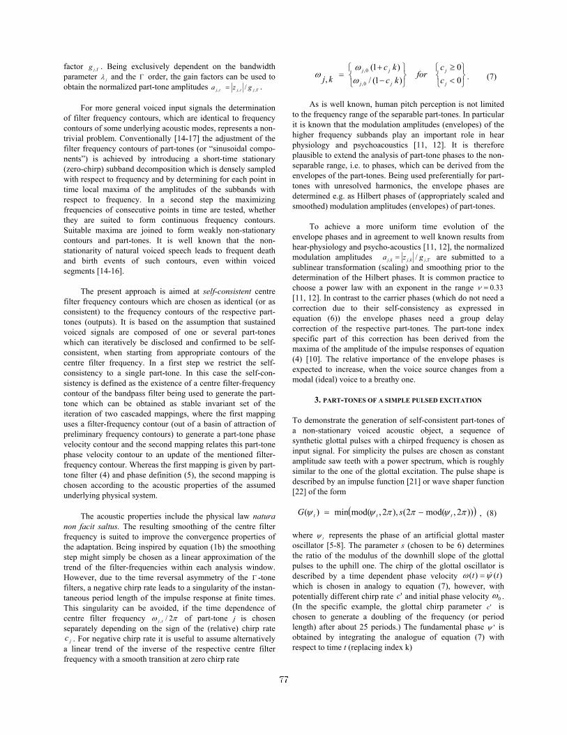
factor . Being exclusively dependent on the bandwidth parameter j

Γ,jgλ and the Γ order, the gain factors can be used to

obtain the normalized part-tone amplitudes Γ= ,,, / jtjtj gza .

For more general voiced input signals the determination of filter frequency contours, which are identical to frequency contours of some underlying acoustic modes, represents a non-trivial problem. Conventionally [14-17] the adjustment of the filter frequency contours of part-tones (or “sinusoidal compo-nents”) is achieved by introducing a short-time stationary (zero-chirp) subband decomposition which is densely sampled with respect to frequency and by determining for each point in time local maxima of the amplitudes of the subbands with respect to frequency. In a second step the maximizing frequencies of consecutive points in time are tested, whether they are suited to form continuous frequency contours. Suitable maxima are joined to form weakly non-stationary contours and part-tones. It is well known that the non-stationarity of natural voiced speech leads to frequent death and birth events of such contours, even within voiced segments [14-16].

The present approach is aimed at self-consistent centre

filter frequency contours which are chosen as identical (or as consistent) to the frequency contours of the respective part-tones (outputs). It is based on the assumption that sustained voiced signals are composed of one or several part-tones which can iteratively be disclosed and confirmed to be self-consistent, when starting from appropriate contours of the centre filter frequency. In a first step we restrict the self-consistency to a single part-tone. In this case the self-con-sistency is defined as the existence of a centre filter-frequency contour of the bandpass filter being used to generate the part-tone which can be obtained as stable invariant set of the iteration of two cascaded mappings, where the first mapping uses a filter-frequency contour (out of a basin of attraction of preliminary frequency contours) to generate a part-tone phase velocity contour and the second mapping relates this part-tone phase velocity contour to an update of the mentioned filter-frequency contour. Whereas the first mapping is given by part-tone filter (4) and phase definition (5), the second mapping is chosen according to the acoustic properties of the assumed underlying physical system.

The acoustic properties include the physical law natura

non facit saltus. The resulting smoothing of the centre filter frequency is suited to improve the convergence properties of the adaptation. Being inspired by equation (1b) the smoothing step might simply be chosen as a linear approximation of the trend of the filter-frequencies within each analysis window. However, due to the time reversal asymmetry of the Γ -tone filters, a negative chirp rate leads to a singularity of the instan-taneous period length of the impulse response at finite times. This singularity can be avoided, if the time dependence of centre filter frequency of part-tone j is chosen separately depending on the sign of the (relative) chirp rate

. For negative chirp rate it is useful to assume alternatively a linear trend of the inverse of the respective centre filter frequency with a smooth transition at zero chirp rate

πω 2/, tj

jc

. (7)

⎭⎬⎫

⎩⎨⎧

<≥

⎭⎬⎫

⎩⎨⎧

−+

=00

)1(/)1(

, 0,

0,

j

j

jj

jj

cc

forkckc

kj ωω

ω

As is well known, human pitch perception is not limited to the frequency range of the separable part-tones. In particular it is known that the modulation amplitudes (envelopes) of the higher frequency subbands play an important role in hear physiology and psychoacoustics [11, 12]. It is therefore plausible to extend the analysis of part-tone phases to the non-separable range, i.e. to phases, which can be derived from the envelopes of the part-tones. Being used preferentially for part-tones with unresolved harmonics, the envelope phases are determined e.g. as Hilbert phases of (appropriately scaled and smoothed) modulation amplitudes (envelopes) of part-tones.

To achieve a more uniform time evolution of the

envelope phases and in agreement to well known results from hear-physiology and psycho-acoustics [11, 12], the normalized modulation amplitudes Γ= ,,, / jkjkj gza are submitted to a sublinear transformation (scaling) and smoothing prior to the determination of the Hilbert phases. It is common practice to choose a power law with an exponent in the range 33.0=ν [11, 12]. In contrast to the carrier phases (which do not need a correction due to their self-consistency as expressed in equation (6)) the envelope phases need a group delay correction of the respective part-tones. The part-tone index specific part of this correction has been derived from the maxima of the amplitude of the impulse responses of equation (4) [10]. The relative importance of the envelope phases is expected to increase, when the voice source changes from a modal (ideal) voice to a breathy one.

3. PART-TONES OF A SIMPLE PULSED EXCITATION

To demonstrate the generation of self-consistent part-tones of a non-stationary voiced acoustic object, a sequence of synthetic glottal pulses with a chirped frequency is chosen as input signal. For simplicity the pulses are chosen as constant amplitude saw teeth with a power spectrum, which is roughly similar to the one of the glottal excitation. The pulse shape is described by an impulse function [21] or wave shaper function [22] of the form

( )))2,mod(2(),2,mod(min)( πψππψψ ttt sG −= , (8)

where tψ represents the phase of an artificial glottal master oscillator [5-8]. The parameter s (chosen to be 6) determines the ratio of the modulus of the downhill slope of the glottal pulses to the uphill one. The chirp of the glottal oscillator is described by a time dependent phase velocity )()( tt ψω &= which is chosen in analogy to equation (7), however, with potentially different chirp rate and initial phase velocity . (In the specific example, the glottal chirp parameter is chosen to generate a doubling of the frequency (or period length) after about 25 periods.) The fundamental phase

'c '0ω

'c

'ψ is obtained by integrating the analogue of equation (7) with respect to time t (replacing index k)

77

⎭⎬⎫

⎩⎨⎧

<≥

⎭⎬⎫

⎩⎨⎧

−−+

=0'0'

)'1ln('/)2/'(

)( '0

2'0

cc

fortcc

tctt

ωω

ψ . (9)

In the situation of signal analysis, appropriate contours of

the centre filter frequency of the part-tone specific bandpass filters have to be obtained iteratively from the observed signal. As part of the time scale separation step of the second mapping of the last section, we assume that these contours can be described (within the current rectangular window of analysis) by a simple smooth function of time chosen as indicated in equation (7). The part-tone adaptation of the filter-frequency contour of the bandpass filter of part-tone j can thus be achieved by estimating the parameters of equation (7). To reduce the dependence of the estimate on the size and position of the window of analysis (and/or to avoid the adaptation of the window length to the instantaneous period length), time scale separation ansatz (7) is extended by a π2 periodic function )/( , jtjj hP ϕ of the respective normalized part-tone phase )/(/ ,, jtjjjjtj hPth ϕαϕ +=& (10a) )/(/ ,, jtjjjtjj hPth ϕαϕ +−=& . (10b) The π2 periodic function )(ϕjP accounts for the periodic oscillations of the phase velocity around the long term trend being generated by the characteristic auto phase-locking and is approximated by an appropriate finite order Fourier series. The Fourier coefficients as well as the trend parameter jα are obtained by multiple linear regression.

Within a voiced segment of speech the adaptation of the parameters is performed sequentially for successive analysis windows. The initial value of the centre filter frequency of the current window is therefore typically given as result of the adaptation of the filter chirp of the preceding analysis window. Thus we treat the latter parameter as given ( ) and concentrate on the convergence properties of the chirp parameter of a filter-frequency contour. The adaptation of a single parameter can be represented graphically. To explain the approach to self-consistency we use a graph, which shows the trend parameter of equations (10a or 10b) for several part-tone indices j as function of the common filter chirp rate c. To make figure 1 suited for the graphical analysis it gives the estimates of the relative trend for the indices j = 2, 4, 6, 9 (corresponding to the sequence of the fixed points from bottom to top) as function of the relative filter chirp rate

.

'00, ωω jj h=

jα

)''/( 0 cj ωα

'/ ccThe iterative adaptation of the chirp parameter of each

filter-frequency contour can be read off from figure 1 by an iteration of two geometric steps: Project horizontally from one of the described curves to the diagonal of the first quadrant (which indicates the line where the fixed points of the iteration are situated) and project vertically down (or up) to the curve again. As can be seen from figure 1, the chirp parameters of all four part-tones have a stable fixed point (equilibrium) within a well extended basin of attraction of the chirp parameter which exceeds the shown interval of the abscissa. The fixed points (corresponding to the more general invariant sets of the preceding section) indicate the final error of the filter chirp

which depends not only on the part-tone index but also on the size of the analysis window (which was chosen to have a length of about five periods of the glottal process). Due to the simple least squares regression of equations (10a,b), the modulus of the trend jα is systematically underestimated.

0.8 0.9 1 1.1 1.2 1.3 1.4 1.50.8

0.85

0.9

0.95

1

1.05

1.1

rel. filter chirp

rel.

part

−to

ne c

hirp

Figure 1: Estimated relative part-tone chirp rates as function of the relative chirp rate of the respective centre filter fre-quency, given for the envelope phase of part-tone 9 (circles, top) and the three carrier phases of part-tones 2, 4, and 6 (lines crossing the diagonal from bottom to top). All chirp rates are given relative to the chirp rate of the input sawtooth process defined in equations (8-9). The arrows and the diagonal of the first quadrant explain the algorithm, to determine the self-consistent centre filter frequencies.

4. MULTI PART-TONE STABLE ACOUSTIC OBJECTS

It is well known that human pitch perception can be trained to switch between analytic listening to a spectral pitch and synthetic listening to a virtual pitch [12, 16]. It is thus plausible to correlate the described single part-tone stable acoustic objects (with a macroscopic basin of attraction of the filter frequency contour or contour parameters) to outstanding part-tones, which are potentially perceived as spectral pitches by analytic listening [16, 27]. The number of stable invariant sets (fixed points) with a macroscopic basin of attraction depends in particular on the width of the power spectrum of the voiced signal. In the example of the last section a strong asymmetry of the sawteeth ( in equation 10) favors the stability of higher order fixed points.

1>>s

From psychoacoustic experiments it is also known that

virtual pitch is a more universal and robust percept than spectral pitch [4, 16]. Based on the a priori assumption that the signal is generated by a voice production system, which generates several phase locked higher frequency acoustic modes, the observed (carrier or envelope) phase velocity of one part-tone might be used to adjust the centre filter frequency of other part-tones. This opens the possibility to use a more robust multi part-tone adaptation strategy which can be expected to converge even in cases with no single part-tone stability.

In analogy to the single part-tone stability of the last sec-tions we relate multipart-tone stability of an acoustic object to

78

the existence of a fundamental phase velocity contour which can be obtained as stable invariant set of the iteration of three cascaded mappings, where the first mapping relates a prelimi-nary fundamental phase velocity contour (out of a macros-copic basin of attraction) to a set of filter-frequency contours, the second mapping uses the set of filter-frequency contours to generate a corresponding set of part-tone phase velocity contours and the third mapping relates a subset of the part-tone phase velocity contours to update the fundamental phase velocity contour. The first mapping makes use of the charac-teristic auto-phase-locking of the voiced excitation ( ). The second mapping is given by filter (4) and phase (5) and the third mapping uses cluster analysis to identify invertible phase relations which are suited to re-construct the phase velocity of the fundamental drive [4-8].

kjkj h ,0, ωω =

This way the contradiction between Rameau’s concept of

a son fundamentale or fundamental bass [20] and Seebeck’s observation, that pitch perception does not rely on a funda-mental acoustic mode as part of the heard signal [21], can be reconciled by replacing Rameau’s son fundamentale by the described FD. Being an abstract order parameter and in need of a confirmation of its existence, the FD of a multi-part-tone voiced acoustic object cannot be reconstructed from a single part-tone alone. This qualifies the instantaneous fundamental phase velocity as acoustic correlate of virtual pitch perception. When reconstructed coherently for uninterrupted voiced speech segments, the fundamental phase becomes the central ingredient of a phase modulation decoder of voiced speech.

Contrary to the conventional psycho-acoustic theory [12,

16] (originating from Ohm and Helmholtz) which interprets the amplitudes of part-tones (with psycho-acoustically cali-brated bandwidths) as primary acoustic cues, it is expected that the deviations of the phases of self-consistently determined part-tones from the synchronization manifold of the unperturbed ideally pulsed excitation have a comparable or higher relevance for acoustic perception than the corres-ponding amplitudes [17]. At the present state of analysis this hypothesis is mainly based on deductive arguments, which favor phase modulation features as more differentiated and robust cues for the distinction of the voiced phones of human speech as well as for the distinction of their speakers.

5. CONCLUSION

A transmission protocol of non-stationary self-consistent

(voiced) acoustic objects is outlined, which are generated as stationary response of a non-stationary fundamental drive (FD) and which can self-consistently be decomposed into non-stationary part-tones. Self-consistent part-tones are charac-terized by phase velocities which are consistent with the centre filter frequencies being used to generate the part-tones. The second property of the self-consistent acoustic objects qualifies them as most elementary symbols of a voice transmission protocol which is centred on a time scale separation with a precise and robust decoding option. It is hypothesized that the self-consistent decomposition of speech segments, which are suited to transmit voiced continuants, leads to a subset of part-tones which shows generalized

synchronization of their phases. The iterative identification of multi part-tone stable voiced acoustic objects relies on and enables a high precision reconstruction of a fundamental phase which can be confirmed as phase of a topologically equivalent image of a glottal master oscillator on the transmitter side. As topologically equivalent image on the receiver side, the self-consistent FD represents the long time scale part of the basic time scale separation known from human acoustic perception. The self-consistent reconstruction of the FD avoids the assumption of a frequency gap being necessary to justify the conventional assumption of a stationary or periodic voice source.

Acknowledgements: The author would like to thank M. Kob, B. Kröger, C. Neuschaefer-Rube and R. Schlüter, Aachen, J. Schoentgen, Brussels, A. Lacroix and K. Schnell, Frankfurt, and J. Rouat, Québec for helpful discussions.

6. REFERENCES

[1] Rabiner L.R. and R.W. Schafer, “Digital Processing of Speech Signals”,.Englewood Cliffs, NJ: Prentice-Hall (1978) [2] Daubechies I., “Ten Lectures on Wavelets”, SIAM, Philadelphia (1992) [3] Gabor D, „Acoustic quanta and the theory of hearing“, Nature 159, 591-594 (1947) [4] Drepper F.R., ”Topologically equivalent reconstruction of instationary voiced speech”, in C. Manfredi (editor), MAVEBA 2003, Firenze University Press (2004) [5] Drepper F.R., „Selfconsistent time scale separation of non-stationary speech“, Fortschritte der Akustik-DAGA’05 (2005) [6] Drepper F.R., ”A two-level drive-response model of non-stationary speech signals”, in M. Faundez-Zanuy et al. (Eds), NOLISP 2005, LNAI 3817, 125-138, Springer (2005) [7] Drepper F.R., “Voiced excitation as entrained primary response of a reconstructed glottal master oscillator”, Interspeech 2005, Lisboa (2005) [8] Drepper F.R., „Stimmhafte Sprache als sekundäre Antwort eines selbst-konsistenten Treiberprozesses“, DAGA’06 (2006) [10] Hohmann V., “Frequency analysis and synthesis using a Gammatone filterbank”, Acta Acustica 10, 433-442 (2002) [11] Patterson R.D., “Auditory images: How complex sounds are represented”, J. Acoust. Soc. Jpn. (E) 21, 4 (2000) [12] Moore B.C.J., “An introduction to the psychology of hearing”, Academic Press (1989) [14] McAulay R. and T. Quatieri, “Speech analysis/synthesis based on a sinusoidal representation”, IEEE Trans. Acoust., Speech a. Signal Proc. ASSP-34(4), 744-754 (1986) [15] Heinbach W., “Aurally adequate signal representation: The part-tone-time-pattern”, Acustica 67, 113-121 (1988) [16] Terhardt E. „Akustische Kommunikation“, Springer, Berlin (1998) [17] Paliwal K.K. and B.S. Atal, “Frequency-related represen-tation of speech”, Eurospeech 2003, Genf (2003) [20] Jean-Philippe Rameau, “Generation harmonique” (1737) reprinted in E. Jacobi (ed.), Complete Theoretical Writings Vol. 3, American Institute of Musicology (1967) [21] August Seebeck, “Über die Definition des Tones”, Poggendorf’s Annalen der Physik und Chemie Vol. LXIII, pp 353-368 (1844) [22] Schoentgen J., “Non-linear signal representation and its application to the modelling of the glottal waveform”, Speech Communication 9, pp. 189–201 (1990)

79

THE HARTLEY PHASE CEPSTRUM AS A TOOL FOR SIGNAL ANALYSIS

I. Paraskevas, E. Chilton, M. Rangoussi Centre for Vision Speech and Signal Processing (CVSSP) Department of Electronics

School of Electronics and Physical Sciences, University of Surrey

Technological Education Institute of Piraeus

Guildford, GU2 7XH, Surrey, UK 250, Thivon str., Aigaleo-Athens, GR-12244, GREECE

e-mail: paraskevas@env.aegean.gr, E.Chilton@ee.surrey.ac.uk

Phone/Fax: +302105381222,6 e-mail: mariar@teipir.gr

1. Introduction This paper proposes the use of the Hartley Phase Cepstrum as a tool for signal analysis. The phase of a signal conveys critical information, which is exploited in a variety of applications. The role of phase is particularly important for the case of speech or audio signals. Accurate phase information extraction is a prerequisite for speech applications such as coding, synchronization, synthesis or recognition. However, signal phase extraction is not a straightforward procedure, mainly due to the discontinuities appearing in it (‘wrapping’ effect). A variety of phase ‘unwrapping’ algorithms have been proposed to overcome this point, when the extraction of the accurate phase values is required. In order to extract the phase content of a signal for subsequent utilization, it is necessary to choose a function that can encapsulate it. In this paper we propose the use of the Hartley Phase Cepstrum (HPC). 2. The Hatrley Phase Cepstrum In general, computation of the cepstrum of a signal belongs to a class of methods known as homomorphic deconvolution processes, [1]. A homomorphic process describes the invertible procedure in which a signal is transformed into another domain via an orthogonal transform Ξ , a non-linear process is applied to the transformed signal in the new domain, and the result is transformed back to the original domain, via the inverse transform, : 1−Ξ

non-linear

process 1−ΞΞ x(n) x*(n)

Figure 1: Summary of the homomorphic deconvolution process

In the special case where and represent the DTFT (Discrete-Time Fourier Transform) and the IDTFT (Inverse Discrete-Time Fourier Transform), respectively, while the non-linear process is the evaluation of the Fourier phase spectrum,

Ξ 1−Ξ

⎟⎟⎠

⎞⎜⎜⎝

⎛ℜℑ

=))(())((arctan)(

ωωωϕ

SS

(1)

where ))(( ωSℜ and ))(( ωSℑ are the real and imaginary components of the Fourier transform )(ωS of the signal , respectively, we obtain the so-called Fourier Phase Cepstrum, )(ts )(τFc :

))(()( ωϕτ IDTFTcF = (2)

80

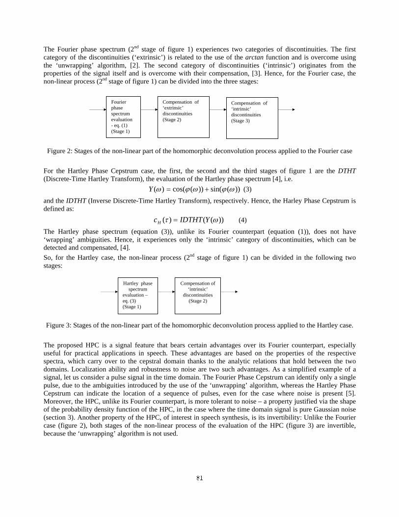
The Fourier phase spectrum (2nd stage of figure 1) experiences two categories of discontinuities. The first category of the discontinuities (‘extrinsic’) is related to the use of the arctan function and is overcome using the ‘unwrapping’ algorithm, [2]. The second category of discontinuities (‘intrinsic’) originates from the properties of the signal itself and is overcome with their compensation, [3]. Hence, for the Fourier case, the non-linear process (2nd stage of figure 1) can be divided into the three stages:

Compensation of

‘extrinsic’ discontinuities (Stage 2)

Fourier phase spectrum evaluation - eq. (1) (Stage 1)

Compensation of ‘intrinsic’ discontinuities (Stage 3)

Figure 2: Stages of the non-linear part of the homomorphic deconvolution process applied to the Fourier case For the Hartley Phase Cepstrum case, the first, the second and the third stages of figure 1 are the DTHT (Discrete-Time Hartley Transform), the evaluation of the Hartley phase spectrum [4], i.e.

)(ωY ))(sin())(cos( ωϕωϕ += (3)

and the IDTHT (Inverse Discrete-Time Hartley Transform), respectively. Hence, the Harley Phase Cepstrum is defined as:

))(()( ωτ YIDTHTcH = (4)

The Hartley phase spectrum (equation (3)), unlike its Fourier counterpart (equation (1)), does not have ‘wrapping’ ambiguities. Hence, it experiences only the ‘intrinsic’ category of discontinuities, which can be detected and compensated, [4]. So, for the Hartley case, the non-linear process (2nd stage of figure 1) can be divided in the following two stages:

Hartley phase

spectrum evaluation – eq. (3) (Stage 1)

Compensation of ‘intrinsic’

discontinuities (Stage 2)

Figure 3: Stages of the non-linear part of the homomorphic deconvolution process applied to the Hartley case. The proposed HPC is a signal feature that bears certain advantages over its Fourier counterpart, especially useful for practical applications in speech. These advantages are based on the properties of the respective spectra, which carry over to the cepstral domain thanks to the analytic relations that hold between the two domains. Localization ability and robustness to noise are two such advantages. As a simplified example of a signal, let us consider a pulse signal in the time domain. The Fourier Phase Cepstrum can identify only a single pulse, due to the ambiguities introduced by the use of the ‘unwrapping’ algorithm, whereas the Hartley Phase Cepstrum can indicate the location of a sequence of pulses, even for the case where noise is present [5]. Moreover, the HPC, unlike its Fourier counterpart, is more tolerant to noise – a property justified via the shape of the probability density function of the HPC, in the case where the time domain signal is pure Gaussian noise (section 3). Another property of the HPC, of interest in speech synthesis, is its invertibility: Unlike the Fourier case (figure 2), both stages of the non-linear process of the evaluation of the HPC (figure 3) are invertible, because the ‘unwrapping’ algorithm is not used.

81

3. Noise robustness of the HPC The aim of this section is to show why the Hartley phase spectrum is more immune to noise as compared to the Fourier phase spectrum. To this end are employed the Probability Density Functions (PDFs) of the Hartley and of the Fourier phase spectra, in the special case of a pure Gaussian noise signal. The PDF of the Hartley phase spectrum is given by:

2

212

1)(

⎟⎠

⎞⎜⎝

⎛−

=βπ

βHp, 22 <<− β , (5)

where β denotes the Hartley phase function values, )(ωY . (See [5] for the proof of eq. (5) – proof not shown here because of lack of space).

The shape of )(βHp is shown in figure 4 (left). It can be observed from figure 4 (left) that the peaks of this PDF are in its upper and lower range of the horizontal axis (i.e. 2 and 2− ). However, the information content of the signal, in the Hartley phase spectrum, is encapsulated in the zero crossings with respect to the frequency axis rather than in the minimum / maximum values of the cosinusoidal signal (i.e. 2± ), [5]. Consequently, noise mainly affects the higher and the lower domain of the Hartley phase spectrum values and hence, its information content (encapsulated in the zero-crossings, middle part of its domain) is less affected. For the Fourier phase spectrum case though, assuming again a Gaussian noise signal, and if the arctan function is omitted from eq. (1), then the )(βFp is a Cauchy distribution, assuming that the real and the imaginary parts of the Fourier spectrum are independent, [6]. In this case:

211)(βπ

β+

=Fp , ∞<<∞− β (6)

where now β denotes the Fourier phase spectrum, )(ωϕ . The Cauchy distribution )(βFp (shown for 5)(5 <<− ωϕ in figure 4 (right)), similarly to the Gaussian distribution, is symmetrical about 0=β with its

maximum value at 0=β . However, the Cauchy distribution falls more rapidly as β increases and also its tails are heavier, compared to the Gaussian. Audio signals (e.g. speech, mechanical sounds etc.), convey a heavy noise additive component and hence, the PDFs of their phase spectra are similar to the Cauchy distribution for the Fourier case and to the distribution in eq. (5) for the Hartley case, respectively.

Figure 4: PDFs (a) of the Hartley phase spectrum, )(ωY , (left) and (b) of the Fourier phase spectrum, )(ωϕ ,

(right) for a pure Gaussian noise signal.

82

It should be noted here that, if the definition of the conventional Fourier phase spectrum is used (i.e. if the arctan function is not omitted in eq. (1) ) then the PDF of the phase spectrum is no more a Cauchy, (see, eg., [6], chapter V.5); rather, it becomes uniform in πωϕπ <<− )( . Nevertheless, in either of the above two choices for the definition of the Fourier phase spectrum (i.e., either including the arctan function or not), the information content is distributed across the whole range of )(ωϕ values and hence there does not exist a specific region of the PDF horizontal axis where the information content is mainly encapsulated. This constitutes a major difference to the case of the Hartley phase spectrum, where, as pointed out earlier, information lies mainly towards the two endpoints of the PDF range. This difference in the shapes of the respective PDFs justifies the relative noise immunity of the proposed HPC.

4. Conclusions

The phase of a signal as a function of frequency conveys meaningful information that is particularly useful for speech or audio signals. Accurate phase extraction is crucial in various speech processing applications, such as localization, synchronization, coding, etc. The major disadvantage of the computation of the phase spectrum via the Fourier transform is the heuristics employed of the compensation of the ‘extrinsic’ discontinuities (‘wrapping’ ambiguities). The effect of the ‘wrapping’ ambiguities is more severe in the case where noise is present. The Hartley phase spectrum, on the other hand, is advantageous as (a) it does not convey ‘extrinsic’ discontinuities and (b) due to its structure, it is less affected by the presence of noise, as justified through comparison of the shapes of the respective PDFs. As signal localization applications show, the phase content of a signal is encapsulated in a more efficient and easy to identify manner in the Hartley Phase rather than in the Fourier Phase Cepstral function. Hence, the Hartley Phase Cepstrum is proposed here as a promising and viable substitute to its Fourier counterpart.

References [1] ‘Theory and Applications of Digital Signal Processing’, Rabiner, L.R., Gold, B., ch. 12, Prentice-Hall,

Englewood Cliffs, New Jersey, 1975. [2] ‘A new phase unwrapping algorithm’, Tribolet, J., Acoustics, Speech, and Signal Processing [see also IEEE

Transactions on Signal Processing], IEEE Transactions on, vol. 25, no. 2, Apr 1977, pp. 170 – 177. [3] ‘Combination of Magnitude and Phase Statistical Features for Audio Classification’, Paraskevas, I.,

Chilton, E., Acoustics Research Letters Online (ARLO), Acoustical Society of America, July 2004. [4] ‘Audio Classification Using Features Derived From The Hartley Transform’, Paraskevas, I., Chilton, E.,

Rangoussi, M., 13th Int. Conference on Systems, Signals and Image Processing (IWSSIP’2006), Budapest, Hungary, September 2006.

[5] ‘Phase as a Feature Extraction Tool for Audio Classification and Signal Localisation’, Paraskevas I., Ph.D. thesis, University of Surrey, 2005.

[6] ‘Introduction to the theory of statistics’, Mood, A.M., Graybill F.A. and Boes, D.C., MacGraw-Hill International, 1974.

Acknowledgement

Authors gratefully acknowledge Dr. Alex Kadyrov of the CVSSP, University of Surrey, for his contribution in the derivation of eq. (5).

83

Quantitative perceptual separation of two kinds of degradationin speech denoising applications

Anis Ben Aicha and Sofia Ben Jebara

Unite de recherche TECHTRAEcole Superieure des Communications de Tunis, 2083 Cite El-Ghazala/Ariana, TUNISIE

anis ben aicha@yahoo.fr,sofia.benjebara@supcom.rnu.tn

Abstract

Classical objective criteria evaluate speech quality using onequantity which embed all possible kind of degradation. Forspeech denoising applications, there is a great need to deter-mine with accuracy the kind of the degradation (residual back-ground noise, speech distortion or both). In this work, we pro-pose two perceptual bounds UBPE and LBPE defining regionswhere original and denoised signals are perceptually equivalentor different. Next, two quantitative criteria PSANR and PSADRare developed to quantify separately the two kinds of degrada-tion. Some simulation results for speech denoising using differ-ent approaches show the usefulness of proposed criteria.

1. IntroductionEvaluation of denoised speech quality can be done using sub-jective criteria such as MOS (Mean Opinion Score) or DMOS(Degradation MOS) [1]. However, such evaluation is expen-sive and time consuming so that, there is an increasing interestin the development of robust quantitative speech quality mea-sures that correlate well with subjective tests. Objective criteriacan be classified according to the domain in which they operate.We relate for example the Signal to Noise Ratio (SNR) and seg-mental SNR operating in time domain [2], the Cepstral Distance(CD) and Weighted Slope Spectral distance (WSS) operating infrequency domain [2] and Modified Bark Spectral Distortion(MBSD) operating in perceptual domain [3]. Perceptual mea-sures are shown to have the best chance of predicting subjectivequality of speech and other audio signals since they are basedon human auditory perception models.

The common point of all objective criteria is their ability ofevaluating speech quality using a single parameter which embedall kind of degradations after any processing. Indeed, speechquality measures are basing their evaluation on both originaland degraded speeches according to the following applicationC:

C : E2 −→ R(x, y) 7−→ c

(1)

where E denotes the time, frequency or perceptual domain. x(resp. y) denotes original speech (resp. observed speech alteredby noise or denoised speech after processing) and c is the scoreof the objective measure.

Mathematically, C is not a bijection from E2 to R. It meansthat it is possible to find a signal y′ which is perceptually dif-ferent from y but has the same score than the one obtained withy (c(x, y) = c(x, y′)). We relate for example the case of anoriginal signal x which is corrupted by an additive noise to con-struct the signal y. Then, x is coded and decoded using a CELP

coder to obtain the signal y′. It is obviously that the degrada-tion noticed in both y and y′ are not the same. Degradation ofy is heard as a background noise and the degradation of y′ isperceptually heard as distortion of original signal. However, ina previous work, we show that they have the same SNR [4].

In this paper, we aim improving speech quality evaluationby separating two kinds of degradation which are the additiveresidual noise and the speech distortion. Each degradation willbe evaluated using its adequate criterion so that the non bijectionC will be avoided and replaced by a bijection one characterizedby a couple of outputs instead of a single output. Moreover,thanks to the advantage of perceptual tools in the evaluationof speech quality, the new couple of criteria will be based onauditor properties of human ear.

2. Study context: speech denoisingBefore defining novel criteria of speech quality evaluation, let’sdefine the different kinds of degradation altering speech. With-out loss of generality, we consider the speech denoising applica-tion and we use spectral denoising approaches. They are viewedas a multiplication of noisy speech spectrum Y (m, k) by a realpositive coefficient filter H(m, k) (see for example [5]). Theestimated spectrum of clean speech is written

S(m, k) = H(m, k)Y (m, k), (2)

where m (resp. k) denotes frame index (resp. frequency index).The estimation error spectrum ξ(m, k) is given by

ξ(m, k) = S(m, k)− S(m, k). (3)

We assume that speech and noise are uncorrelated. Thus,the estimated error power spectrum is given by

E|ξ(m, k)|2 = [H(m, f)− 1]2E|S(m, k)|2+H(m, k)2E|N(m, k)|2, (4)

where |N(m, k)|2 denotes the noise power spectrum.Since 0 < H(m, k) < 1, the first term of Eq. 4 expresses

the ‘attenuation’ of clean speech frequency components. Suchdegradation is perceptually heard as a distortion of clean speech.However, the second term expresses the residual noise which isperceptually heard as a background noise. Since, it is additive,it is possible to formulate it as an ‘accentuation’ of clean speechfrequency components.

3. Proposed perceptual characterization ofaudible degradation

We aim to perceptually characterize the degradation altering de-noised speech. Hence, auditory properties of human ear are84

considered. More precisely, the masking concept is used: amasked signal is made inaudible by a masker if the masked sig-nal magnitude is below the perceptual masking threshold MT. Inour case, both degradation can be audible or inaudible accordingto their position regarding the masking threshold. We proposeto find decision rules to decide on the audibility of residual noiseand speech distortion by using the masking threshold concept.If they are audible, the audibility rate will be quantified accord-ing to the proposed criterion. There are many techniques tocompute masking threshold MT, we use in this paper Johnstonmodel well known for its simplicity and well used in codingcontext [6].

3.1. Perceptual characterization of audible noise

According to MT definition, it is possible to add to the cleanspeech power spectrum, the MT curve (considered as a ‘certainsignal’) so that the resulting signal (obtained by inverse FFT)has the same audible quality than the clean one. The result-ing spectrum is called Upper Bound of Perceptual Equivalence“UBPE” and is defined as follows

UBPE(m, k) = Γs(m, k) + MT (m, k), (5)

where Γs(m, k) is the clean speech power spectrum.When some frequency components of the denoised speech

are above UBPE, the resulting additive noise is heard.

3.2. Perceptual characterization of audible distortion

By duality, some attenuations of frequency components can beheard as speech distortion. Thus, by analogy to UBPE, wepropose to calculate a second curve which expresses the lowerbound under which any attenuation of frequency componentsis heard as a distortion. We call it Lower Bound of PerceptualEquivalence “LBPE”. To compute LBPE, we used the au-dible spectrum introduced by Tsoukalas and al for audio signalenhancement [7]. In such case, audible spectrum is calculatedby considering the maximum between clean speech spectrumand masking threshold.

When speech components are under MT, they are not heardand we can replace them by a chosen threshold σ(m, k).The proposed LBPE is defined as follows

LBPE(m, k) =

(Γs(m, k) if Γs(m, k) ≥MT (m, k)

σ(m, k) otherwise .

(6)The choice of σ(m, k) obeys only one condition σ(m, k) <

MT (m, k). During this work, we choose it equal 0 dB.

3.3. Usefulness of UBPE and LBPE

Using UBPE and LBPE, we can define three regions char-acterizing the perceptual quantity of denoised speech: fre-quency components between UBPE and LBPE are percep-tually equivalent to the original speech components, frequencycomponents above UBPE contain a background noise and fre-quency components under LBPE are characterized by speechdistortion. This characterization constitutes our idea to iden-tify and detect audible additive noise and audible distortion. Asillustration, we present in Fig. 1 an example of speech framepower spectrum and its related curves UBPE (upper curve inbold line) and LBPE (bottom curve in dash line). The cleanspeech power spectrum is, for all frequencies index, betweenthe two curves UBPE and LBPE. We remark that the two

curves are the same for most peaks. It means that for these fre-quency intervals, any kind of degradation altering speech willbe audible. If it quite over UBPE, it will be heard as back-ground noise. In the opposite case, it will be heard as speechdistortion.

Figure 1: An example of UBPE and LBPE in dB of cleanspeech frame.

4. Audible degradation estimation4.1. Audible additive noise PSD estimation

Once UBPE calculated, the superposition of denoised signalpower spectrum and UBPE leads to separate two cases.The First one corresponds to the regions of denoised speechpower spectrum which are under UBPE. In such case,there is no audible residual noise. In the second case, somedenoised speech frequency components are above UBPE,the amount above UBPE constitutes the audible residualnoise. As illustration, we represent in Fig.2 an example ofdenoised speech power spectrum and its related UBPE curvecalculated from clean speech. The used denoising approach isspectral subtraction [5]. From Fig.2, we notice that frequencyregions between 1 kHz and 2 kHz are above UBPE, theyhence contain residual audible noise. In term of listening tests,such residual noise is annoying and constitutes in some casesthe musical noise. Such musical noise is well popular andconstitutes the main drawback of spectral subtraction.

Once the UBPE is calculated, it is possible to estimate theaudible power spectrum density of residual noise using a sim-ple subtraction when it exists. Hence, the residual noise powerspectrum density PSD is written

Γpn(m, k) =

8><>:Γs(m, k)− UBPE(m, k)

if Γs(m, k) > UBPE(m, k)

0 otherwise

(7)

where Γs(m, k) denotes the PSD of denoised speech and thesuffix p designs the perceptually sense of the PSD.

4.2. Audible speech distortion PSD estimation

We use the same methodology as the one used for residual back-ground noise. We represent in Fig.3 an example of denoisedspeech power spectrum and its related curve LBPE calculatedfrom the clean speech. We notice that some regions are underLBPE (for example regions between 1.5 kHz and 2 kHz), they85

Figure 2: Superposition of a denoised speech power spectrumand its related clean speech UBPE.

hence constitute the audible distortion of the clean speech. Interm of listening tests, they are completely different from resid-ual background noise. They are heard as a loss of speech tonal-ity.It is possible to estimate the audible distortion PSD Γp

d as fol-lows

Γpd(m, k) =

8><>:LBPE(m, k)− Γs(m, k)

if Γs(m, k) < LBPE(m, k)

0 otherwise .

(8)

Figure 3: Superposition of a denoised speech frame and its re-lated clean speech LBPE.

5. Audible degradation evaluationIn this section, we detail the proposed approach to quantify sep-arately the two kinds of degradation. The assessment of thedenoised speech quality by means of two parameters permitsto overcome the problem of non bijection of classic objectiveevaluation and to better characterize each kind of speech degra-dation. Hence, instead of the application defined in Eq. 1, wedevelop a novel application from perceptual domain to R2

C : E2 −→ R2

(x, y) 7−→ (PSANR, PSADR)(9)

where PSANR and PSADR are two parameters related re-spectively to the residual noise and the distortion.

The definition of PSANR and PSADR is inspired fromthe SNR definition which is the ratio between signal energyand noise energy. Thanks to Parseval theorem it can be calcu-lated in frequency domain. Moreover, since the UBPE andLBPE are perceptually equivalent to the original signal, theproposed definition uses the energy of UBPE and LBPE in-stead of the energy of the clean speech. The time domain signalrelated to UBPE is called “upper effective signal” whereas thetime domain signal related to LBPE is called “lower effectivesignal”. In the following subsection, we define the proposedcriteria.

5.1. Perceptual noise criterion PSANR

The perceptual residual noise criterion is defined as the ratiobetween the upper effective signal which is the UBPE and theaudible residual noise. The Perceptual Signal to Audible NoiseRatio PSANR(m) of frame m is calculated in frequency do-main (due to the Parseval theorem) and it is formulated as fol-lows

PSANR(m) =

PNk=1 UBPE(m, k)PN

k=1 Γpn(m, k)

. (10)

5.2. Perceptual distortion criterion PSADR

By the same manner, we define the Perceptual Signal to AudibleDistortion Ratio PSADR(m) of frame m as a ratio betweenthe lower effective signal which is LBPE and the audible dis-tortion. The PSADR(m) is given by:

PSADR(m) =

PNk=1 LBPE(m, k)PN

k=1 Γpd(m, k)

. (11)

5.3. PSANDR criteria

to compute the global PSANR and PSADR of the to-tal speech sequence, we are referred to the segmental SNRSNRseg thanks to its better correlation with subjective testswhen compared to the traditional SNR. The principle of seg-mental SNR consists on determining the SNR for each frameSNR(m) and then calculating their geometric mean over the

total number of frames SNRseg = N

qQNm SNR(m) [2].

Moreover, since the SNR and SNRseg are usually expressedin dB. The geometric mean is equivalent to the arithmetic meanin log domain.Using this approach, we compute the global PSANR andPSADR for a given sequence of speech. Next, the couple(PSANR,PSADR) defines the new criterion to evaluate bothkinds of degradation. We call it Perceptual Signal to AudibleNoise and Distortion Ratio “PSANDR”.

6. experimental results6.1. Test signals

To show the ability of PSANDR to take into account the per-ceptual effect of an additive noise, we add artificial noise, con-structed from the masking threshold by multiplying it with afactor α ≥ 0 (y(n) = s(n) + αMT (n)). In Fig.4, we repre-sent the evolution of SNRseg , PSANR and PSADR versusα. For the range of α between 0 and 1, SNRseg decreaseswhich means that there is a degradation of speech. This fact istrue in term of signal to noise ratio but not true in term of per-ceptual sense, because the power of added artificial noise don’tovertake MT. With PSANR, the amount of audible noise is86

null (see Eq. 7) and the PSANR is infinity which is truncatedto 35 dB in our simulations. For α > 1, the background noisebecomes audible and the PSANR decreases as α increases butremains above SNRseg . This is explained by the ability of theclean speech to mask a certain portion of the added noise.

We notice that for any value of α, the second term PSADRis still constant and is equal to 35 dB. In fact, there is no distor-tion of the clean speech and the only audible degradation is thebackground noise.

Figure 4: Evolution of SNRseg , PSANR and PSADR ver-sus α in case of additive noise.

6.2. real signals

Let’s now compare some denoising techniques by means of thenew objective criteria. We propose to denoise a corrupted sig-nal, by gaussian noise with SNR = 0 dB, using the followingtechniques:• Classical wiener filtering [5].• Perceptual filtering proposed by Gustafsson and al in [8]

which consists in masking the residual noise and allow-ing a variable speech distortion.

• Modified wiener technique [9]. In this technique, theshape of the tones is used as a selective parameter to de-tect and eliminate musical tones.

Evaluation of denoising quality is done using classic objec-tive criteria (segmental SNR, WSS, MBSD) and the proposedPSANDR. Results are resumed in Tab.1. In term of SNRseg ,the used techniques are comparable even if there is a little im-provement noticed with perceptual technique. But, subjectivetests show that the denoised signals are completely different.Using WSS criterion, the best score is obtained with percep-tual technique and it is nearly equal to the noisy speech score.Although, subjective tests show that the two signals are percep-tually different. Indeed, the denoised speech using perceptualtechnique is heard as distorted version of clean speech and notas clean speech with background noise. In term of MBSD, theperceptual technique is also the best. However, this techniqueis characterized by a loss of the speech tonality comparing towiener technique. Thus, we can see that classic evaluation toolsdon’t give any idea of the kind and nature of the degradation ofthe signals. PSANR, giving idea about residual noise, showsthat perceptual technique is the best one regarding noise atten-uation. PSADR, determining the distortion of the denoisedsignals, shows that the important distortion is obtained usingperceptual technique. These observations are confirmed by sub-jective tests.

Table 1: Evaluation of denoised signals.

SNRseg

dB WSS MBSDPSANR

dBPSADR

dBnoisy

speech -4.30 46.07 2.32 -3.90 17.27wiener

technique 1.05 74.25 0.28 5.04 7.53modifiedwiener 1.13 69.63 0.19 5.54 7.01

perceptualtechnique 1.62 45.41 0.15 12.71 6.93

7. ConclusionThe spectral and perceptual analysis of the degradation, in thecase of denoised speech, imposes to separate between residualnoise and signal distortion. We first propose two curves UBPEand LBPE to calculate the audible residual noise and audibledistortion. Next, two parameters PSANR and PSADR char-acterizing the two kinds of degradation are developed. Sim-ulation results comparing different denoising approaches andclassical objective measures, show a better characterization ofdegradation nature of denoised signal. The calculation of thedegree of correlation of the proposed criteria with MOS crite-rion constitutes the perspectives of our work.

8. References[1] Recommandation UIT-T P.800. Mthodes d’valuation sub-

jective de la qualite de transmission, 1996.[2] J.H.L. Hansen and B.L. Pellom “An effective quality eval-

uation protocol for speech enhancement algorithms ” Int.Conf. on Spoken Language Processing ICSLP, Austria1998.

[3] W. Yang, M. Benbouchta and R. Yantorno, “Performanceof the modified bark spectral distortion as an objectivespeech measure,” Proc. Int. Conf. on Acoustics, Speechand Signal Processing ICASSP, vol 1, pp. 541-544, 1988.

[4] A. Ben aicha et S. Ben Jebara, “Caracterisation per-ceptuelle de la degradation apportee par les techniques dedebruitage de la parole,” submited in Traitement et Anal-yse de l’Information Methodes et Applications TAIMA,Tunisia 2007.

[5] J.S Lim and A.V Oppenheim, Enhancement and Band-width Compression of Noisy Speech, in Proc. IEEE, vol.67, pp. 1586-1604, 1979.

[6] J. D. Johnston, “Transform coding of audio signal usingperceptual noise criteria,” IEEE J. Select. Areas Commun,vol 6, pp. 314-323, 1988.

[7] D. E. Tsoukalas, J. Mourjopoulos and G. Kokkinakis,“Speech enhancement based on audible noise suppres-sion,” IEEE Trans. Speech and Audio Processing, vol. 5,no. 6, pp. 497- 514, November 1997.

[8] S. Gustafsson, P. Jax and P. Vary, “A novel psychoacous-tically motivated audio enhancement algorithm preserv-ing backround noise characteristics,” in Proc. Int. Conf.Acoustics, Speech, and Signal Processing, Seattle, WA,pp. 397-400, May 1998

[9] A. Ben Aicha, S. Ben Jebara and D. Pastor “Speech de-noising improvement by musical tones shape modifica-tion,” International Symposium on Communication, Con-trol and Signal Processing ISCCSP, Morocco 2006.87

Threshold Reduction for Improving Sparse Coding Shrinkage Performance in Speech Enhancement

Neda Faraji*, S. M. Ahadi*, S. Saloomeh Shariati**

Department of Electrical Engineering * Amirkabir University of Technology, **Iran University of Science and Technology,

Tehran, Iran nfaraji@cic.aut.ac.ir , sma@aut.ac.ir, ssaloomeh_shariati@ee.iust.ac.ir

Abstract In this paper, we modify the Sparse Coding Shrinkage (SCS) method with an appropriate optimal linear filter (Wiener filter) in order to improve its efficiency as a speech enhancement algorithm. SCS transform is only applicable for sparse data and speech features do not have this property in either time or frequency domains. Therefore we have used Linear Independent Component Analysis (LICA) to transfer the corrupted speech frames to the sparse code space in which noise and speech components are separated by means of a shrinkage function. Before employing SCS, Wiener filtering was applied on the ICA components to reduce noise energy and consequently the SCS shrinkage threshold. Experimental results have been obtained using connected digit database TIDIGIT contaminated with NATO RSG-10 noise data.

1. Introduction The primary purpose of noise compensation methods applied in the context of speech processing is to reduce the effect of any signal which is alien to and disruptive of the message and to extract original speech as pure as possible. Depending on the application, speech enhancement methods aim at speech quality improvement and or speech or speaker recognition. Some common noise compensation methods are a) Spectral Subtraction, b) least mean square (LMS), adaptive filtering, c) filter-based parametric approaches , d) Hidden Markov Model (HMM)-based speech enhancement techniques. Wavelet transform has also been employed in speech enhancement systems during recent years [1]. In this paper we focus on modifying a relatively new method that is Sparse Coding Shrinkage. It has been used in [2, 3] for image denoising and in [4] for speech enhancement. The advantages of this method with respect to other popular methods can be summarized as: 1) Most algorithms apply Fourier transform, discrete Fourier transform or Karhunen-Loeve transform which facilitate the estimation of the clean speech model parameters. However, SCS is based on a data-driven transformation that is highly conformed to the structure of clean speech data. 2) Most methods just amend the distorted amplitude of the speech signal leaving the phase unprocessed. On the other hand, experimental results have shown that phase parameter plays a relatively important role in speech quality [5]. In the SCS method, the speech frame is uniformly processed without need to separating the amplitude and phase data. Independent Component Analysis is a basic method for blind source separation. In Linear Independent Component Analysis (LICA), the goal is to transfer the

observed data to the independent source space. Assuming that all independent sources are supergaussian, ICA technique will be equivalent to sparse coding method [2]. Denoising process includes an offline training stage in which clean speech frames are employed for estimating the ICA transform matrix and required parameters of the shrinkage function. These estimated functions can then be used to extract the clean components from the noisy ones. The organization of the paper is as follows: First we explain in detail each of the methods used for speech enhancement in section 2. Section 3 demonstrates the noise reduction capability of the proposed algorithm through the computer simulations. Finally, conclusions are given in the last section.

2. Algorithms used in the proposed enhancement method

Sparse Coding Shrinkage is carried out in 2 stages: 1) Transferring data to the sparse coding space that is

performed using ICA in this paper. 2) Computing Shrinkage function for each sparse code that

can be achieved through Maximum Likelihood Estimation. In this section we have provided details about the employed algorithms.

2.1. Independent Component Analysis

Linear Independent component analysis mixing model can be formulated as [6]:

=x As (1)

We can rewrite the Eq. (1) as:

i ii

s=∑x a (2)

where ,ia x and is are basis functions , observed vector and independent components respectively. This ICA model is a generative model, i.e. it describes how the observed data are generated by a process of mixing the components is . After estimating the matrix A, we can compute its inverse, say W, and obtain the independent components simply by:

1, −s = Wx W = A (3)

In mixing model, A and s are both unknown and should be solely estimated using observed data x. One estimation method is to use probabilistic characteristics of components that are assumed independent in ICA method. It has been shown that component independency in ICA mixing model is

88

directly related to maximum nongaussianity of the components. One robust criterion for nongaussianity testing is negetropy that can be expressed as:

gaussJ(y) H(y ) H(y)= − (4)

In which H is entropy function and J(y) represents the entropy difference between random value y and Gaussian variable gaussy , which has the same covariance matrix as y.

J(y) will be zero if and only if y is Gaussian, otherwise it has positive non-zero value. Using a robust estimation of negentropy and ascent gradient method, we can rewrite W matrix rows as following:

T TE g( ) E g ( ) + −′= −w x w x w x w (5)

where x is the observed vector and w- and w+ represent the W matrix row before update and after update respectively. Here g(u)=tanh(au) and a is selected so that 1<a<2. In order to increase the convergence speed, data is whitened in the first step. Hence, the searching space is limited to the space perpendicular to the previous vectors (rows).

2.1.1. Parametric estimation of the probabilistic density function of the independent components

Probability density of independent components is defined as a generalized exponential function as follows [7]:

2 1 βω(β) x µp(x|µ,σ,β) exp c(β)σ σ

+ −= −

[ ][ ]

[ ][ ]

113

2

12

13 22

31 22

(1 )c( ) ,

(1 )

(1 ) ( ) 0

(1 ) (1 )

βΓ ββ

Γ β

Γ βω β σ

β Γ β

++=

+

+= >

+ +

(6)

where µ is the mean parameter, σ represents standard

deviation and Γ is Gamma function. iβ is the parameter that controls the deviation of probability density function from normal distribution. The higher β gets ( 1>>β ), the more the super-Gaussian of the independent components PDF is. Assuming si components with zero mean )0( =µ and unit

variance )( 1σ 2 = , we can estimate β by Maximum A Posterior (MAP) method as follows:

i

i

i β i i

β i i i

β max p(β |s )

max p(s |β )p(β )

= ∝ (7)

Assuming )p(βi is uniform for 1βi > and making the

derivative with respect to iβ equal to zero, we can estimate

iβ by means of iteration methods.

2.2. Shrinkage function extraction

SCS uses Maximum A Posterior for estimating the non-Gaussian variable contaminated with Gaussian noise. Suppose s is the random non-Gaussian variable and ν is the Gaussian noise with zero mean and unit variance and y is the observed variable, so that:

y s ν= + (8)

We want to extract s from the observed vector y. If the probability density function of s is shown by p, then we can estimate s by:

2u 2

1s argmin (y u) f(u)2σ = − +

(9)

where logpf −= and 2σ is the noise variance. Minimizing the left side of (9) and making its derivative with respect to u equal to zero is equivalent to the following equation:

2

1 ˆ ˆ(s y) f (s) 02σ

′− + = (10)

For the Laplace function in the form of

|)s|λexp(2λ)sp( ˆˆ −= , we have )ssign()s(f ˆˆ =′ . After

substitution of (s)f ′ in (10), we find 2λσys −=ˆ for 2λσy > and the equation has no answer for 2λσy < .

Assuming that the clean signal components are sparse, we can

conclude that, for 2λσy < the observed component y is

only resulted from noise and therefore 0s =ˆ . In general, nonlinear relationship between s and y components can be stated:

2s g(y) sign(y) max(0, y λσ )= = × − (11)

where g represents the shrinkage function. In ICA space, the probability density of the clean speech, p(s) , can be obtained as explained in section 2-1-1. Assuming generalized exponential distribution for s, it is unlikely to find s with respect to y from (10) in the closed form. The shrinkage function of a high sparse variable ( 1>>β ) can be approximated as [1]:

2 2

s sign(y)

y bd y bdmax(0, ( ) 4σ (a 3) )

2 2

= ×

− ++ − +

(12)

where d is the standard deviation of the independent

components and 2σ is the noise components variance in ICA

space and 1)|s|1/d/(Ea 2 −= , 21)a(ab += . Two examples of shrinkage function are illustrated in Fig.1. Since independent components extracted from speech have high sparsity, we can use the shrinkage function stated in (12).

89

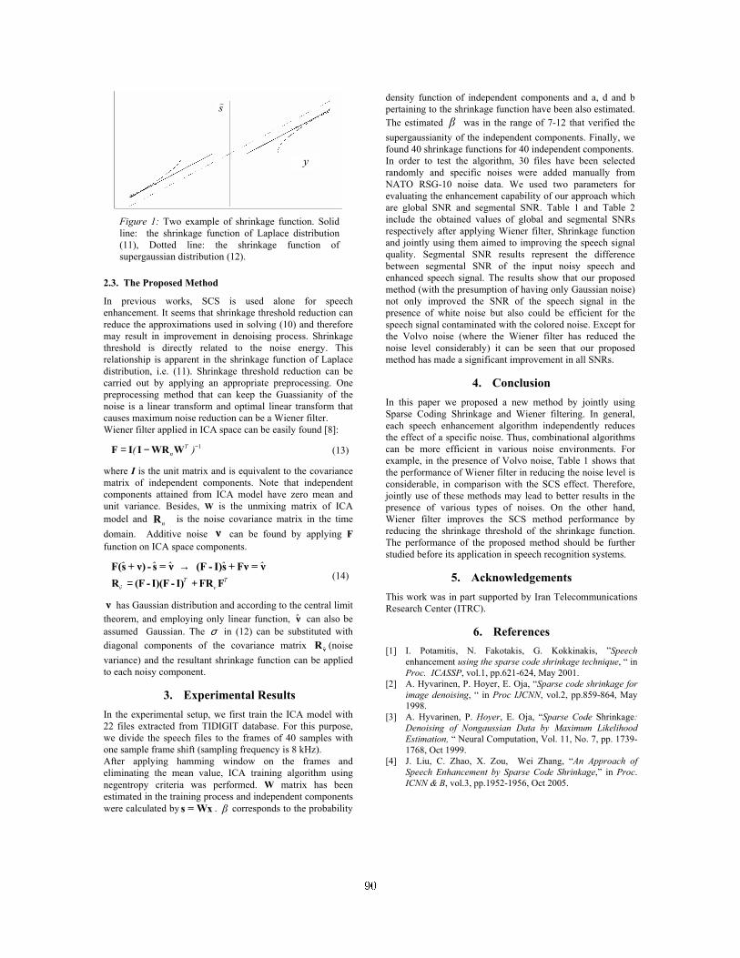
Figure 1: Two example of shrinkage function. Solid line: the shrinkage function of Laplace distribution (11), Dotted line: the shrinkage function of supergaussian distribution (12).

2.3. The Proposed Method

In previous works, SCS is used alone for speech enhancement. It seems that shrinkage threshold reduction can reduce the approximations used in solving (10) and therefore may result in improvement in denoising process. Shrinkage threshold is directly related to the noise energy. This relationship is apparent in the shrinkage function of Laplace distribution, i.e. (11). Shrinkage threshold reduction can be carried out by applying an appropriate preprocessing. One preprocessing method that can keep the Guassianity of the noise is a linear transform and optimal linear transform that causes maximum noise reduction can be a Wiener filter. Wiener filter applied in ICA space can be easily found [8]:

1Tn( )−= −F I I WR W (13)

where I is the unit matrix and is equivalent to the covariance matrix of independent components. Note that independent components attained from ICA model have zero mean and unit variance. Besides, W is the unmixing matrix of ICA model and nR is the noise covariance matrix in the time domain. Additive noise ν can be found by applying F function on ICA space components.

ˆ ˆ ˆ ˆ ˆ→F(s + ν) - s = ν (F - I)s + Fν = ν T T

ν ν= +R (F - I)(F - I) FR F (14)

ν has Gaussian distribution and according to the central limit theorem, and employing only linear function, ν can also be assumed Gaussian. The σ in (12) can be substituted with diagonal components of the covariance matrix νR (noise variance) and the resultant shrinkage function can be applied to each noisy component.

3. Experimental Results In the experimental setup, we first train the ICA model with 22 files extracted from TIDIGIT database. For this purpose, we divide the speech files to the frames of 40 samples with one sample frame shift (sampling frequency is 8 kHz). After applying hamming window on the frames and eliminating the mean value, ICA training algorithm using negentropy criteria was performed. W matrix has been estimated in the training process and independent components were calculated by s = Wx . β corresponds to the probability

density function of independent components and a, d and b pertaining to the shrinkage function have been also estimated. The estimated β was in the range of 7-12 that verified the supergaussianity of the independent components. Finally, we found 40 shrinkage functions for 40 independent components. In order to test the algorithm, 30 files have been selected randomly and specific noises were added manually from NATO RSG-10 noise data. We used two parameters for evaluating the enhancement capability of our approach which are global SNR and segmental SNR. Table 1 and Table 2 include the obtained values of global and segmental SNRs respectively after applying Wiener filter, Shrinkage function and jointly using them aimed to improving the speech signal quality. Segmental SNR results represent the difference between segmental SNR of the input noisy speech and enhanced speech signal. The results show that our proposed method (with the presumption of having only Gaussian noise) not only improved the SNR of the speech signal in the presence of white noise but also could be efficient for the speech signal contaminated with the colored noise. Except for the Volvo noise (where the Wiener filter has reduced the noise level considerably) it can be seen that our proposed method has made a significant improvement in all SNRs.

4. Conclusion In this paper we proposed a new method by jointly using Sparse Coding Shrinkage and Wiener filtering. In general, each speech enhancement algorithm independently reduces the effect of a specific noise. Thus, combinational algorithms can be more efficient in various noise environments. For example, in the presence of Volvo noise, Table 1 shows that the performance of Wiener filter in reducing the noise level is considerable, in comparison with the SCS effect. Therefore, jointly use of these methods may lead to better results in the presence of various types of noises. On the other hand, Wiener filter improves the SCS method performance by reducing the shrinkage threshold of the shrinkage function. The performance of the proposed method should be further studied before its application in speech recognition systems.

5. Acknowledgements This work was in part supported by Iran Telecommunications Research Center (ITRC).

6. References [1] I. Potamitis, N. Fakotakis, G. Kokkinakis, ”Speech

enhancement using the sparse code shrinkage technique, “ in Proc. ICASSP, vol.1, pp.621-624, May 2001.

[2] A. Hyvarinen, P. Hoyer, E. Oja, “Sparse code shrinkage for image denoising, “ in Proc IJCNN, vol.2, pp.859-864, May 1998.

[3] A. Hyvarinen, P. Hoyer, E. Oja, “Sparse Code Shrinkage: Denoising of Nongaussian Data by Maximum Likelihood Estimation, “ Neural Computation, Vol. 11, No. 7, pp. 1739-1768, Oct 1999.

[4] J. Liu, C. Zhao, X. Zou, Wei Zhang, “An Approach of Speech Enhancement by Sparse Code Shrinkage,” in Proc. ICNN & B, vol.3, pp.1952-1956, Oct 2005.

y

s

90

Table 1: Global SNRs of enhanced signals in different enhancement algorithms.

SNR(dB) noise

20 15 10 5 0 -5 Ave.

SCS 20.92 16.39 11.98 7.74 3.73 -.26 10.08 Wiener 20.2 15.47 10.9 6.7 3.17 .78 9.54 Babble

SCS+Wiener 20.9 16.4 12 7.8 4.1 1.59 10.47 SCS 21 16.59 12.24 7.95 3.8 -.3 10.21

Wiener 20.68 16.2 11.8 7.6 4 1.3 10.26 Factory SCS+Wiener 21.2 17.1 13.1 8.9 4.9 2 11.20

SCS 21.22 16.79 12.42 8.11 3.99 -.8 10.29 Wiener 20.2 16.5 12.2 8.2 4.53 1.7 10.56 F16

SCS+Wiener 21.5 17.5 13.6 9.6 5.6 2.49 11.72 SCS 22.37 18 13.55 9 4.65 .2 11.30

Wiener 20.7 16.14 12 8.25 5 2.38 10.75 White SCS+Wiener 22.4 18 13.8 9.9 6.2 3.2 12.25

SCS 21.28 17.22 12.95 8.68 4.46 .16 10.79 Wiener 25.8 24.7 23.4 20.95 17.8 16.4 21.51 Volvo

SCS+Wiener 24 22.9 21.4 18.8 15.8 13 19.42 SCS 22.51 18.24 13.8 9.3 4.86 .4 11.52

Wiener 20.32 15.9 11.94 8.36 5.03 2.2 10.63 Destroyer Engine

SCS+Wiener 22 18 13.9 10 6.3 2.2 12.07 SCS 21.55 17.21 12.82 8.46 4.25 -0.10 10.70

Wiener 21.32 17.49 13.71 10.01 6.59 4.13 12.21 Ave. SCS+Wiener 22.00 18.32 14.63 9.24 7.15 4.08 12.85

Table 2: Segmental SNR improvemnet for different enhancement algorithms (the results are differential SNR between input

signal and enhanced signal).

SNR(dB) noise

20 15 10 5 0 -5 Ave.

SCS 1.19 2.10 3.5 4.8 5.6 5.9 3.85 Wiener .17 .46 .99 1.93 3.77 7.1 2.40 Babble

SCS+Wiener 1.18 2.32 4.46 7.46 10.63 14.43 6.75 SCS 1.18 2.14 3.32 4.37 5.1 5.6 3.62

Wiener .56 1 1.8 2.8 4.56 7.6 3.05 Factory SCS+Wiener 1.42 2.9 5.2 8.1 11 14.9 7.25

SCS 1.4 2.27 3.33 4.33 5.1 5.6 3.67 Wiener .7 1.34 2.19 3.31 5 7.9 3.41 F16

SCS+Wiener 1.77 3.3 5.6 8.4 11.4 15 7.58 SCS 2.54 3.33 4.01 4.58 5.06 5.45 4.16

Wiener .8 1.4 2.43 3.97 6.12 9 3.95 White SCS+Wiener 3.12 4.47 6.25 8.65 11.79 15.8 8.35

SCS .16 1.13 1.82 2.61 3.6 4.56 2.31 Wiener 5 8.2 11 13 15 17 11.53 Volvo

SCS+Wiener 3.5 7 10.3 13.3 16.5 19.8 11.73 SCS 2.97 3.9 4.56 5.05 5.43 5.74 4.61

Wiener .4 1.13 2.34 4 6 8.8 3.78 Destroyer Engine

SCS+Wiener 3.12 4.5 6.3 8.9 12 15.8 8.44 SCS 1.57 2.48 3.42 4.29 4.98 5.48 3.70

Wiener 1.27 2.26 3.46 4.84 6.74 9.57 4.69 Ave. SCS+Wiener 2.35 4.08 6.35 9.14 12.22 15.96 8.35

[5] P. Vary, “Noise suppression by spectral magnitude

estimation," Signal Processing, Vol. 8, pp. 387-00, 1985. [6] A. Hyvarinen, J. Karhunen, E. Oja, Independent Component

Analysis, John Wiley & Sons, New Yourk etc. 2001.

[7] T.-W. Lee, M.-S. Lewicki" The Generalized Gaussian Mixture Model Using ICA," in Proc. Int Workshop. on Independent Component Analysis, pp.239-244, 2000.

[8] T.-W. Lee, M.-S. Lewicki" The Generalized Gaussian Mixture Model Using ICA," in Proc. Int Workshop. on Independent Component Analysis, pp.239-244, 2000.

91

Efficient Viterbi algorithms for lexical tree based models

S. Espana-Boquera, M.J. Castro-Bleda, F. Zamora-Martınez, J. Gorbe-Moya

Departamento de Sistemas Informaticos y ComputacionUniversidad Politecnica de Valencia

sespana@dsic.upv.es

AbstractIn this paper we propose a family of Viterbi algorithms spe-cialized for lexical tree based FSA and HMM acoustic mod-els. Two algorithms to decode a tree lexicon with left-to-rightmodels with or without skips and other algorithm which takesa directed acyclic graph as input and performs error correctingdecoding are presented. They store the set of active states topo-logically sorted in contiguous memory queues. The number ofbasic operations needed to update each hypothesis is reducedand also more locality in memory is obtained reducing the ex-pected number of cache misses and achieving a speed-up overother implementations.

1. IntroductionMost of large vocabulary Viterbi based recognizers (for speech,handwritten or other recognition tasks, although speech termi-nology is used in this work with no loss of generality) makeuse of a lexicon tree organization which has many advantagesover a linear lexicon representation [1, 2]. As it is shown in theliterature, more compact representations are possible (using alexicon network [3], which is a minimized Finite State Automa-ton –FSA–) but the gain in space is accompanied with a morecomplex Viterbi decoder. Therefore, lexical tree organization isa very good tradeoff between compact space representation andadequacy for decoding.

The search space in a recognizer can be huge and the keyto achieve practical performance is to consider only the set ofactive hypothesis (those with non trivial zero probability) andto apply pruning techniques such as beam search which onlymaintain active the best hypothesis.

Large vocabulary one-step decoders [4] usually keep a setof lexical tree based Viterbi parsers in parallel. Two commonapproaches are the time-start copies and language model historycopies [5, 6]. In the time-start approach, all hypothesis com-peting in a tree parsing share the same word start time. Whena trigram language model is used, the language model historycopies approach maintains a tree parsing for every bigram his-tory (w1, w2). This second approach has a loss of optimalitywhich is known as word-pair approximation [6]. In both cases,it is straightforward to use a specialized Viterbi algorithm forthe lexical tree model and, as the core of an automatic speechrecognizer lies in the search process, every little improvementin performing specialized decoding of lexical tree models hasa great impact in the overall performance. Therefore, it is notstrange to find specialized algorithms which take advantage ofthe properties of tree based HMM models which integrate thetree lexicon and the acoustic HMM models.

This work has been partially supported by the Spanish Government(TIN2006-12767) and by the Generalitat Valenciana (GVA06/302).

When the acoustic models are strict left-to-right withoutskips, the resulting expanded HMM model is acyclic if loops areignored, and every node has only zero or one preceding state totake into account in the dynamic programming equation. Left-to-right units with skips are known as Bakis topology and have awidespread use as acoustic models in most recognizers. Whenthose models are used in conjunction with a tree lexicon, thenumber of predecessors given an active state can be zero, oneor two.

Not expanding the acoustic models in the tree lexicon andmaintaining a pure tree structure which matches a phone-graphis another possibility. In this case, the input is no longer a se-quence of acoustic frames but a phone-graph (a directed acyclicgraph –DAG– labelled with phones and acoustic scores). Be-sides the capability of using a directed acyclic input, the pos-sibility of insertions, deletions and substitutions of phones isneeded to tolerate the errors in the phone-graph generation.

In this work, three specialized Viterbi algorithms basedon contiguous memory queues (FIFO data structures) are pro-posed. When performing a Viterbi step, a new result queue iscreated with the help of one or several auxiliary queues.

The basic algorithm uses left-to-right HMM acoustic mod-els with no skips. This algorithm can be applied wheneveracoustic left-to-right models without skips are used: it can beused for isolated word or continuous speech recognition, eitherwith a one-step or a two-step approach, with time-start or lan-guage model history copies, and also within-word or across-word context dependent units (triphones, quinphones, etc.). Asimple extension is presented to show how to use it with across-word context dependent models [7].

A second version of the algorithm extends the first one toallow the use of skips in the acoustic units with a negligibleadditional cost.

The last proposed algorithm performs an error correctingViterbi decoding and is capable of analyzing a DAG instead ofa sequence. This algorithm can be used, for instance, to obtaina word-graph from a phone-graph.

2. Left-to-right without skips algorithmIf a lexicon tree is expanded with left-to-right acoustic HMMmodels without skips, the following observations about the ex-panded tree models are straightforward:

• Every state has at most two predecessors: itself and pos-sibly his parent.

• If we ignore the loops, the expanded model is acyclic.Therefore, a topological order is possible in general.

• A level traversal of the tree provides a topological orderwith some additional features:92

– The children of a given node occupy contiguouspositions. The grandchildren also occupy contigu-ous positions.

– If a subset of states is stored in topological orderand we generate the children of every active statefollowing that order, the resulting list also is or-dered with respect to the topological order.

2.1. Model representation

A tree model T of n states is represented with three vectors ofsize n and one of size n + 1 as follows:

• loop prob stores the loop transition probabilities.

• from prob stores the parent incoming transition proba-bilities.

• e index stores the index of the associated emissionprobability class associated to the acoustic frame to beobserved. The vector of emission probabilities can beobtained with a multilayer perceptron in a hybrid model[8] or with a set of mixture of Gaussian distributions in aconventional continuous density HMM.

• first child stores the index of the first child. The lastchild is deduced by looking the first child of the nextstate thanks to the topological sorting. This representa-tion allows specifying an empty set of children. A sen-tinel in position n + 1 is needed for the last state.

2.2. Viterbi-Merge algorithm

The Viterbi-M algorithm takes a sequence of acoustic framesas input and updates a set of active states after observing everyframe (a Viterbi step). An active state is composed by an indexstate and a score (i, s). A queue α(t) (a FIFO data structure) isused to store the set of active states at time t. The purpose of aViterbi step consists of creating another queue α(t + 1) giventhe model T , the current queue α(t) and the vector of emis-sion probabilities emission associated to the observed acousticframe.

An auxiliary queue aux child is used to store temporallythe scores of states produced by the transitions from parent tochild. The algorithm proceeds as follows (see Figure 1):

1. best prob← 0.

2. For every active state (i, s) of the queue α(t) whosescore s is above the beam threshold:

(a) s next← s · loop prob[i].

(b) While the first active state (i′, s′) of the queueaux child satisfies i′ < i, extract it and place(i′, s′ · emission[e index [i′]]) in α(t + 1).

(c) If the first active state (i′, s′) of the queueaux child satisfies i′ = i, drop it and update thescore s next← max(s next, s′).

(d) s next ← s next · emission[e index [i]], insert(i, s next) in the queue α(t + 1) and updatebest prob← max(best prob, s next).

(e) For every state j from first child [i] tofirst child [i + 1] − 1, add (j, s · from prob[j])to the queue aux child.

3. For every active state (i′, s′) of the queue aux child, ex-tract it and place (i′, s′ · emission[e index [i′]) in thequeue α(t + 1).

α (t)

α

merge

(t+1)

generate children

generate grandchildren

>= beam threshold?

*loop probability

*emission probabilityupdate best probability

aux_child

aux_gchild

Figure 1: Viterbi-M and Viterbi-MS algorithms. The queueaux gchild (dotted part) is only used in Viterbi-MS.

phonetic contextsDifferent

Gen

eral

to

po

log

y H

MM

mo

del

Coar

ticu

late

d w

ord

tra

nsi

tio

n

Tree lexicon HMM models

Figure 2: HMM model for across-word context dependent units.The general topology HMM model represents only the first con-text dependent phones of the words.

The active states of α(t) whose score is below the beamthreshold are discarded. Whenever an active state is placed inthe queue α(t + 1), the emission probability associated to it isapplied, and the best probability is updated. This value is usedto obtain the beam threshold for the following Viterbi step.

This algorithm is linear with the number of active statesand the number of children of active states which is an upperbound to the number of active states in the resulting queue. Intotal, the global cost is linear with the number of active states,which is the same as any reasonable implementation of a con-ventional Viterbi implementation. The main advantage of thisalgorithm is the use of contiguous memory FIFO queues to storethe active states. Therefore, a better cache performance and aninternal loop with less overhead is obtained compared to otheralgorithms that use linked lists or use hash tables to store andlook up the set of active states. Therefore, the asymptotic costis the same but a practical speed-up is obtained.

2.3. Extension to across-word context dependent units

Since this algorithm is used on lexical tree models with ex-panded acoustic HMM models, the use of context dependentunits is straightforward for within-word context modeling.

Across-word models consider a different context dependentunit at the beginning of a word to take into account the lastphones of the preceding word during continuous speech recog-nition. It would be very inefficient to use a different tree modelfor every possible context since they only differ in the first con-text dependent acoustic models. Therefore, a model which re-sembles a tree lexicon excepting the root is used. This modelcan be composed of two models: a general HMM connecting aset of tree lexicon models (see Figure 2).93

A set of trees can be traversed by levels as if they were justone tree and the resulting model can be used with the same al-gorithm with no modification. Therefore, a conventional Viterbialgorithm can be used to update the scores of the states of thegeneral topology HMM part of the model, and the rest of themodel (a forest) can be computed with the Viterbi-M algorithm.

3. Left-to-right with skips algorithmThis algorithm generalizes the previous one by allowing the useof Bakis HMM acoustic models.

3.1. Model representation

The model representation is similar to the previous section.The only difference is another vector skip prob which stores,for every state, the incoming skip transition probabilities.In order to iterate over the set of grandchildren of a givenstate i, the algorithm loops from first child [first child [i]] tofirst child [first child [i + 1]]− 1.

3.2. Viterbi-Merge algorithm with skips

The Viterbi-MS algorithm is the same of previous section butanother auxiliary queue aux gchild is used to store the activestates with scores computed by means of the skip transitions.Every time an active state is extracted from α(t), the set ofgrandchildren is used to add items to the queue aux gchild justas the set of children is used to add items to the other auxiliaryqueue. Now, the resulting queue α(t + 1) is obtained by merg-ing the loop transition score of the processed active state withthe states from the two auxiliary queues (see Figure 1).

This algorithm is linear with the number of active states andthe number of children and grandchildren of active states. Theresulting cost is thus linear with the number of active states.

3.3. Extension to across-word context dependent units

The same observations of previous algorithm are also applicablehere.

4. Error-Correcting Viterbi for DAGsThe last proposed algorithm performs an error correctingViterbi decoding and is capable of analyzing a DAG instead ofa sequence.

4.1. Model representation

A tree model T of n states where symbols are placed at thetransitions is represented with two vectors of size n and otherof size n + 1 as follows:

• symbol stores the incoming transition label.

• from prob stores the incoming transition probability.

• first child stores the index of the first child as in theprevious algorithms.

A table with the costs of insertions, deletions and substitutionof every symbol is also required.

4.2. Error-Correcting Viterbi-Merge algorithm for DAGs

The Viterbi-MEC-DAG algorithm takes a DAG as input. Con-sider the phone-graph of Figure 3. A set of active states isassociated to every vertex of the input DAG. The algorithmapplies two different procedures associated to the input DAG,

2 51

3

4

b

a

b

a

a

a,b

Figure 3: Phone-graph example.

origin

aux

destination

merge

generate children with

substitution operation

deletion operation

>= beam threshold?

updated destination

update best probability

Figure 4: Viterbi-MEC-DAG edge-step procedure.

which must be applied following the DAG topological order:the vertex-step procedure must be applied to every vertex beforeusing this set of active states as the origin of an edge edge-stepprocedure.

4.2.1. Edge-step

For every edge, a Viterbi step takes the set of active states ofthe origin vertex and use them to update the active states of thedestination vertex. This procedure only considers the cost ofdeletions and substitutions. As can be observed in Figure 4,this algorithm is similar to the Viterbi-M algorithm where loopprobability updating is replaced by the deletion operation, thegeneration of children states corresponds to the substitution op-eration (including a symbol by itself or a correct transition).Another difference, which can be also used in Viterbi-M andViterbi-MS to process a DAG as input data, is the presence ofsecond input queue which stores the active states already up-dated at the destination vertex by means of other edges of theDAG. These values are simply merged and this queue is notneeded when the input data is a sequence. The cost of this pro-cedure is linear with the number of active states in both inputqueues because the number of generated successor states growslinearly with the number of active states.

4.2.2. Vertex-step

Once all edges arriving at a given vertex have been processed,the insertion operation is considered. This operation updates aset of active states without consuming any symbol. As can beobserved in Figure 5, the output of the auxiliary queue is used toinsert more active states in the same queue to take into accountthe possibility of several insertion operations. The cost is notlinear with the number of active states: a sole active state atthe root could, in principle, activate all the states of the model,but most of them are expected to be pruned by the beam searchdepending on the cost of insertions and the beam width. Thecost of this operation is linear with the number of active statesbefore applying the procedure plus the number of active statesafter the procedure, which is bounded by the number of statesin the model.94

merge

aux

vertex active states

updated vertex active states

(compare with beam threshold at this point)

generate children with insertion operation

Figure 5: Viterbi-MEC-DAG vertex-step procedure.

Num. states Hash swap A. Envelope Viterbi-M9 571 3.001 16.082 29.350

76 189 2.761 12.924 28.036310 888 1.922 6.442 24.534

Table 1: Experimental results. The results are shown in millionsof active states or hypothesis updated per second.

5. Experimental resultsA previous work related to lexical tree Viterbi decoding we wereaware of after our algorithms were developed is the active enve-lope algorithm [9]. This algorithm also uses a total order whichsubsumes the partial order of the states of the model and placessiblings contiguously. This algorithm is specified for left-to-right models without skips, so it is only comparable to our firstalgorithm Viterbi-M. The active envelope algorithm uses a sin-gle linked list to perform a Viterbi step, which is an advantagein memory usage. Since this algorithm modifies the originalset of active states, it is restricted to sequential input data andcannot be used when the input data is a DAG. In order to useonly a list, the active hypothesis in active envelope algorithmare traversed in reverse topological order. The “price to pay”for this advantage is the need of linked lists instead of contigu-ous memory arrays. Since the use of linked lists cannot assurememory locality and the cost of traversing them is greater thantraversing memory arrays, it is expected to perform worse thanViterbi-M algorithm. The memory occupied by an active hy-pothesis is an index state and a score; if linked lists are used,a pointer is also needed: so a linked list needs approximately50% or 100% more memory per active state depending on thecomputer architecture. On the other hand, the use of memoryarrays needs an estimation of the number of active states.

In order to compare the performance of our Viterbi-M al-gorithm, two more algorithms have been implemented: a con-ventional Viterbi algorithm based on hash tables with chainingto store and to look up the active states and the active envelopealgorithm. All algorithms have been implemented in C++ anduse the same data structures to represent the tree based HMMmodels as described in section 2.1.

The experiments were done on a Pentium D machine at3GHz with 2 Gbytes of RAM using a Linux with kernel2.6.18 and the gcc compiler version 4.1.2 with -O3 op-timization. The lexical trees used in the experiments were ob-tained by expanding 3-state left-to-right without skips hybridneural/HMM acoustic models in the tree lexicon. The size ofthese trees varies from 9 571 to 310 888 states. Only the Viterbidecoding time has been measured (the emission scores calcula-tion and other preprocessing steps were not taken into account).The result is shown in Table 1. The speed is measured in mil-lions of active states updated per second.

6. ConclusionsIn this paper, three Viterbi algorithms specialized for lexi-cal tree based FSA and HMM acoustic models have been de-scribed. Two of these algorithms are useful to decode a set ofwords given a sequence of acoustic frames and the third oneis useful to parse a phone-graph with error-correcting editionoperations. These algorithms are based on contiguous mem-ory queues which contain the set of active states topologicallysorted.

Although the asymptotic cost of these algorithms is thesame as any reasonable implementation of the Viterbi algo-rithm, the experimental comparison between the Viterbi-M al-gorithm, a conventional Hash-table swapping algorithm and theactive envelope algorithm, shows that our algorithm is approxi-mately 10 times faster than the hash-table swapping implemen-tation and from 2 to 4 times faster than the active envelope al-gorithm. A decrease in speed with the size of the models isobserved in the three algorithms, which is possibly related withthe main memory and the cache relative speeds. For this reason,more experimentation is needed in order to better understandthis behaviour and also to study the effect of other parameterssuch as the beam width of the pruning during the search.

7. References[1] J. Klovstad and L. Mondshein, “The CASPERS linguistic

analysis system,” IEEE Transactions on Acoustic, Speechand Signal Processing, vol. 23, no. 1, pp. 118–123, Feb.1975.

[2] D. Klatt, Trends in Speech Recognition. Prentice-Hall,1980, ch. Scriber and Lafs: Two New Approaches toSpeech Analysis, pp. 529–525.

[3] K. Demuynck, J. Duchateau, and D. V. Compernolle, “AStatic Lexicon Network Representation for Cross-wordContext Dependent Phones,” in Proc. European Conferenceon Speech Communication and Technology, vol. I, Rhodes,Greece, September 1997, pp. 143–146.

[4] X. L. Aubert, “An overview of decoding techniques forlarge vocabulary continuous speech recognition,” in Com-puter Speech and Language, vol. 16, 2002, pp. 89–114.

[5] S. Ortmanns, H. Ney, F. Seide, and I. Lindam, “A compari-son of time conditioned and word conditioned search tech-niques for large vocabulary speech recognition,” in Proc.ICSLP ’96, vol. 4, Philadelphia, PA, 1996, pp. 2091–2094.

[6] H. Ney and S. Ortmanns, “Dynamic programming searchfor continuous speech recognition,” IEEE Signal Process-ing Magazine, vol. 16, no. 5, pp. 64–83, 1999.

[7] S. Kanthak, A. Sixtus, S. Molau, and H. Ney, “Within-wordvs. across-word decoding for online speech recognition,”2000.

[8] Y. Konig, H. Bourlard, and N. Morgan, “REMAP: Recur-sive estimation and maximization of A posteriori probabili-ties — application to transition-based connectionist speechrecognition,” in Advances in Neural Information Process-ing Systems, D. S. Touretzky, M. C. Mozer, and M. E. Has-selmo, Eds., vol. 8. The MIT Press, 1996, pp. 388–394.

[9] P. Nguyen, L. Rigazio, and J.-C. Junqua, “EWAVES: Anefficient decoding algorithm for lexical tree based speechrecognition,” in ICSLP-2000, vol. 4, 2000, pp. 286–289.

95

Acoustic Units Selection in Chinese-English Bilingual Speech Recognition

Lin Yang. Jianping Zhang. Yonghong Yan

ThinkIT Speech Lab Chinese Academy of Sciences, Beijing, China

yanglin@h

Abstract We present an effective method to merge the acoustic units between Chinese and English to develop a language-independent speech recognition system. Chinese as a tonal language has large differences from English. An optimal Chinese phoneme inventory is set up in order to keep consistent with the representation of English acoustic units. Two different approaches for Chinese-English bilingual phoneme modeling are illustrated and compared. One is to combine the Chinese and English phonemes together based on International Phonetic Association (IPA). The other is a data-driven method on the basis of the confusion matrix. Experimental results show that all these methods are feasible and the data-driven method reduced the WER by 0.73% in Chinese and 3.76% in English relatively compared to the IPA-based method. As a by-product, the idea of data sharing across languages can obtain relative 8.7% error reduction under noise condition.

1. Introduction With the increasing internationalization, research in multilingual speech recognition (MSR) has gained more and more interest in the last few years. But Chinese as one of the most important languages in the world was not considered as much as western languages in some present MSR systems [1][2][3] because of its own peculiarity. So a thorough research on the Chinese-English bilingual recognition is potentially needed, especially the groundwork of a MSR system: the selection of language-independent acoustic units.

So far, there are two main frameworks when solving the MSR problem. One is using a language identification (LID) module to identify the speech as a specific language. Then the specific monolingual utterance can be recognized by language-dependant speech recognizers. The other is using a universal framework including multi-lingual acoustic model, language model and decoder. In the first framework an apparent weak is that the upper bound of performance is limited by the accuracy of LID module. Thus we use the second framework to study how to construct a consistent Chinese-English phoneme inventory and acoustic model.

Linguistically speaking, there are many differences between Chinese and English since they come from two different language families [4]. Firstly, Chinese is a kind of tonal language, including 5 tones; Secondly it is monosyllabic mainly in CV structure where C is consonant and V is vowel, whereas English is a kind of atonal language whose structure is more complex than Chinese. As a result in most cases the basic acoustic units are different largely between the two languages. For example, the Chinese mono phoneme is often represented by initials and tonal finals rather than more subtle units as English. So it is essential to make the acoustic

units of the two languages uniform. This paper gives some experiments about how to split the phonemes of Chinese to make it keep consistent with English representations.

Some phonemes across the two languages may be similar enough to be equated. Those resemblances must be merged together for decreasing the number of parameters in the acoustic model. At present there are two main methods of phoneme cluster. One is based on phonetic knowledge; the other is data-driven. Both of the methods are studied to find the most suitable universal phoneme inventory and build a language-independent acoustic model which keeps balance between the number of parameters and system performance in a real MSR framework.

The remainder of this paper is organized as follows. In section 2, an approach of Chinese phone splitting to subtle units and two methods of bilingual phoneme clustering are illustrated in detail. Some experimental results on language independent speech recognizer with different cluster technologies are compared in section 3. Conclusion is given in section 4.

2. Building Language-Independent Acoustic Model and MSR System

In order to define a universal phoneme sets for the two languages, we firstly split original Chinese initials and tonal finals into subtle units consistent with the representation of English. If the phonemes of the two languages are put together directly, the final number of acoustical model parameters would be much large and be a burden for decoder. The cluster of phonemes can be performed either manually or automatically. A kind of most common used method of data-driven cluster is based on the direct distance of mono phoneme models. However this method does not consider the context of the phonemes. In order to utilize the information of triphones a new data-driven method based on the concept of confusion matrix is given.

2.1. Setup of Chinese phoneme inventory

In our original system the acoustic units are initials and tonal finals, a total number of 213, which is a characteristic of Chinese. In order to be compatible with English atonal phonemes, we discard the tones at first, as a result with the total number of 69. There still exist some compound vowels in the atonal Chinese phoneme inventory although they have resembled to an extent with English units. So splitting according to IPA [5] at various levels is attempted with a number of comparative experiments. Detailed results are shown in table 1. Finally the best Chinese inventory is given with a total number of 49 (including silence and short pause),

96

balanced in size with English phoneme set with the number of 42 (including silence and short pause).

Table 1. Results of recognition in various phoneme sets of Chinese

213 tonal set

69 atonal set

57 atonal set

49 atonal set

43 atonal set

Accuracy(%) 94.9 94.1 94.2 94.4 94.0

In this group of comparative experiments, the training set includes 70 hours data and the test set is 863test set including 9042 read utterances. From the results we could conclude that the set of 49 phonemes provides the best performance comparative with other atonal sets, although there still exists a disparity from the original tonal phone set.

2.2. Experience-based phoneme cluster

After the subtle split of Chinese phonemes, we get two sets of similar phoneme inventories representing the two languages. Then the language-dependent phonemes should be combined into one set in order to realize the language-independent phoneme modeling. A manual and direct way of building bilingual inventory is according to the phonetic knowledge. Some language-dependent phonemes which are represented by the same IPA symbols can be merged into one unit. Table 2 is a list of IPA-based Chinese-English universal phoneme set consisting of 67 units (excluding silence, short pause and garbage model). In this table 19 pairs of phonemes sharing the same IPA symbols are merged, thus the total number of parameters is reduced by more than 21% comparative to the total number of the two sets, which is 89.

Table 2. Phoneme cluster based on IPA

Lang. Phonemes number

Chinese

p_ch t_ch nn_ch k_ch z_ch c_ch sh_ch r_ch zh_ch ch_ch j_ch q_ch x_ch h_ch a_ch

au_ch at_ch e_ch err_ch ix_ch iy_ch v_ch iaa_ch ioo_ch iee_ch iii_ch iuu_ch ivv_ch

28

English b_en ch_en d_en dh_en g_en hh_en jh_en

r_en sh_en th_en v_en w_en y_en z_en zh_en ah_en ao_en aw_en ay_en oy_en

20

Merged

b_ch/p_en f_ch/f_en n_ch/n_en g_ch/k_en ng_ch/ng_en d_ch/t_en m_ch/m_en

l_ch/l_en s_ch/s_en aa_ch/aa_en ee_ch/eh_en ak_ch/ae_en o_ch/ow_en uu_ch/uh_en u_ch/uw_en ea_ch/ey_en

ii_ch/ih_en er_ch/er_en i_ch/iy_en

19

2.3. Data-driven phoneme cluster

The data-driven method of cluster is based on the statistical similarity or distance measurement rather than phonetic knowledge. So far the clustering algorithm is mostly applied Bhattacharyya distance [6] as a theoretical similar measure between two Gaussian distributions. However this approach considers only the mono phoneme’s distance without any information of context. A novel method of distance measurement with the information of triphones, which is similar to [7][8], is used in this study. The phonemes’ distances are calculated according to confusion matrix between English and Chinese phonemes. The confusion is

measured by finding the best path for test data of one language on the other’s triphone model. The optimization is realized by simple Viterbi decoding and a large number of training utterances are required.

Detailed steps are as follows: (1) Based on the English triphone HMM model, find the most possible phoneme series for every Chinese utterance using Viterbi decoding. That is

),|(maxarg

),|(maxarg

trienench

trienchenen

MOP

MOP

en

en

Λ=

Λ=Λ

Λ

Λ

)

(1)

where enΛ means the best possible English phoneme series,

engtriM means the English triphone model, and

chO represents the Chinese training utterance. Then based on

the time information to align enΛ and the real phoneme

array chΛ by DTW. (2) A confusion matrix is build by a large number of training data. The degree of confusion is calculated by

)(/)|( chichienjenjchi NNC λλλ=→ (2)

where enjchiC → means the distance of Chinese phoneme i

from English phoneme j , and )( chiN λ and )( enjN λ

represent the number of Chinese phoneme i and the number of English phoneme j respectively. Thus a matrix denotes the distance of Chinese phonemes from English phonemes is achieved.

(3) Vice verse. Change the places of English and Chinese and repeat the step 1 and 2 to calculate the distance of English phonemes from Chinese phonemes.

(4) Since the measure is asymmetrical, the average distance is given as follows:

2/)( chienjenjchi CCC →→ += (3)

In order to compare with IPA-based method, we limited the size of data-driven cluster to 67 mono phonemes. The English training data come from TIMIT corpora including 6300 utterance, and transcriptions with the time information are available. The Chinese data come from 863test sets, including 9042 sentences with the time information transcriptions. Experimental results show that when the training data exceeds 2000 utterances the distance of phonemes in the confusion matrix is stable. Thus the size of our training data can gain the reliable statistical measurement. Table 3 shows the result of bilingual phoneme inventory using data-driven method.

97

Table 3. Phoneme cluster based on Confusion Matrix Data-Driven

Lang. Phonemes number

Chinese

ng_ch l_ch t_ch nn_ch z_ch c_ch r_chj_ch q_ch x_ch h_ch aa_ch ee_ch ak_cho_ch ii_ch er_ch at_ch e_ch err_chix_ch iy_ch v_ch iaa_ch ioo_ch iee_chiuu_ch ivv_ch

28

English

ng_en t_en l_en dh_en hh_en r_en th_env_en z_en zh_en eh_en ae_en uh_enuw_en ih_en er_en ah_en ao_en aw_enoy_en

20

Merged

a_ch/aa_en au_ch/ay_en b_ch/b_en ch_ch/ch_en d_ch/d_en ea_ch/ey_en

f_ch/f_en g_ch/g_en i_ch/iy_en iii_ch/y_en k_ch/k_en m_ch/m_en

n_ch/n_en p_ch/p_en s_ch/s_en sh_ch/sh_en u_ch/u_en uu_ch/ow_en

zh_ch/jh_en

19

3. Experiments and Discussion The goal of the experiment is to evaluate the performance of our language-independent LVCSR system and compare the cluster method based on IPA with our proposed approach based on confusion matrix data-driven.

3.1. Corpora and experiment setup

The training data has about 340 hours Chinese speech data (including various dialects) and 160 hours English data (including TIMIT, WSJ). These data are recorded under relatively clean acoustic conditions. The recognizer makes use of continuous density HMM with Gaussian mixture for acoustic model. Each triphone model is a 3-state left-to-right with Gaussian mixture observation densities (typically 32 components). The acoustic feature of speech is MFCC with 39 dimensions.

The size of vocabulary is 43K for Chinese and 50K for English. The bilingual dictionary is composed of the pooled monolingual dictionaries and consists of 93K entries. The training corpora of bilingual language model (BILM) are the combination of Chinese and English data. In order to test the performance of language-independent acoustic model we also build monolingual LM, labeled as MONOLM.

We selected two sets of Chinese testing data in order to evaluate the performance under various situations. One is recorded under clean acoustic condition, including 341 Chinese sentences labeled as TestCH1, while the other is recorded under noise condition consisting of 200 sentences labeled as TestCH2. The English testing data is standard WSJ0 testing set labeled as TestEN, including 330 English utterances.

3.2. Experiments and discussion

For the purpose of comparing the language-independent system with the language-dependent system, we conducted the experiments on the monolingual LVCSR system. Table 4 shows the word error rates of the baseline on different testing sets.

Table 4. The monolingual results on different testing sets

TestCH1 TestCH2 TestEN WER (%) 25.8 36.8 9.7

In order to compare the two methods of cluster we trained the acoustic model on the two bilingual phoneme sets, labeled as IPA and CMDD. They are combined with different language models MONOLM and BILM. The comparative results are shown in Table 5.

Table 5. The comparative results of language-independent models

TestCH1 (%)

TestCH2 (%)

TestEN (%)

IPA-MONOLM 27.1 36.0 10.8 CMDD-MONOLM 26.8 36.0 11.1

IPA-BILM 27.4 36.4 13.3 CMDD-BILM 27.2 36.2 12.8

From the table 4 and table 5, we can see that the bilingual system can achieve comparable performance to the monolingual system whether in English or Chinese testing sets. In the worst cases the WER increased 1.6% in Chinese and 3.6% in English respectively. This may be due to the dramatic increase of the size of bilingual dictionary, with nearly 10K entries.

By comparing the IPA cluster method with CMDD method in table 5, we can see that the CMDD method accepts moderate improvements in various testing conditions except combined with the monolingual language model in TestEN set. This loss may result both from the unmatchable acoustic and language model and from the asymmetric size of training data between English and Chinese. But on English testing set, using bilingual LM a significant improvement can be observed, with WER relative reduction by 3.76% than IPA-based method. Although the improvement is not dramatic as a whole, the advantage of CMDD is evident whether for adjusting the size of phoneme inventory or from the theoretical foundations. As a result, the method of confusion matrix data-driven gives us a promising belief that a great improvement can be achieved by conditioning the size of universal phoneme inventory and bilingual dictionary.

It is interesting that in the universal system the performance is improved greatly under noise conditions TestCH2, which WER is from 36.8% to 36%. For confirming the contribution of bilingual acoustic models which share data across languages we put them into monolingual systems, avoiding the influences of merged dictionary and language model. The results are listed in Table 6. These results demonstrated that the shared data across language can deduce the WER by %8.7 relatively, making the recognizer more robust under noise condition.

98

Table 6: Acoustic model performance comparison under noise conditions

Monolingual baseline

IPA bilingual model

CMDD bilingual model

WER(%) 36.8 33.6 34.2

4. Summary and Future Work In this paper, we presented the work of setting up Chinese phoneme inventory and two methods of building language-independent MSR system. By comparing the two cluster sets on different testing data and language models, the CMDD cluster method outperforms the IPA-based approach as a whole. As a by-product, the sharing data across languages provides us a new idea to improve the performance of recognizer under noise condition. In future experiments, we will try various methods to build bilingual language model and select the optimal size of universal phoneme inventory. It is also a challenging task about how to combine the experience-based method and data-driven method. This approach proposed in this paper could be generalized to other languages.

5. Acknowledgements This work is supported by Chinese 973 program (2004CB318106), National Natural Science Foundation of China (10574140, 60535030)

6. References [1] Zhirong Wang, Umut Tokpara, Tanja Schultz, Alex

Waibel: Towards Universal Speech Recognition, Proceedings of the Fourth International Conference on Multimodal Interface (ICMI), IEEE Computer Society, (2002), 247-252

[2] F. Weng, H. Bratt, L. Neumeyer, A Stolcke: A Study of Multilingual speech recognition. In Proc. Eurospeech’97, Rhodos, Greece (1997)

[3] Ulla Uebler: Multilingual speech recognition in seven languages. Speech Communication. 35(2001), 53-69

[4] D. Lyu, R.Lyu, Y.Chiang, C.Hsu: Speech Recognition on Code-switching Among Chinese Dialects, ICASSP, I(1105-1108), (2006)

[5] IPA: The International Phonetic Association (revised to 1993) IPA Chart. Journal of the International Phonetic Association 23, (1993).

[6] M. Brian, B.Etienne: Phone Clustering Using the Bhattacharyya Distance, In Proc. ICSLP, 2005-2008, (1996)

[7] R.Bayeh, S. Lin, G. Chollet, C. Mokbel: Towards Multilingual Speech Recognition Using Data Driven Source/Target Acoustical Units Association, ICASSP’04, 521-524, (2004)

[8] E. Wong, T. Martin, T. Svendsen, S. Sridharan: Multilingual Phone Clustering for Recognition of Spontaneous Indonesian Speech Utilising Pronunciation Modeling Techniques, EUROSPEECH’03, Geneva, 3133-3136, (2003)

99

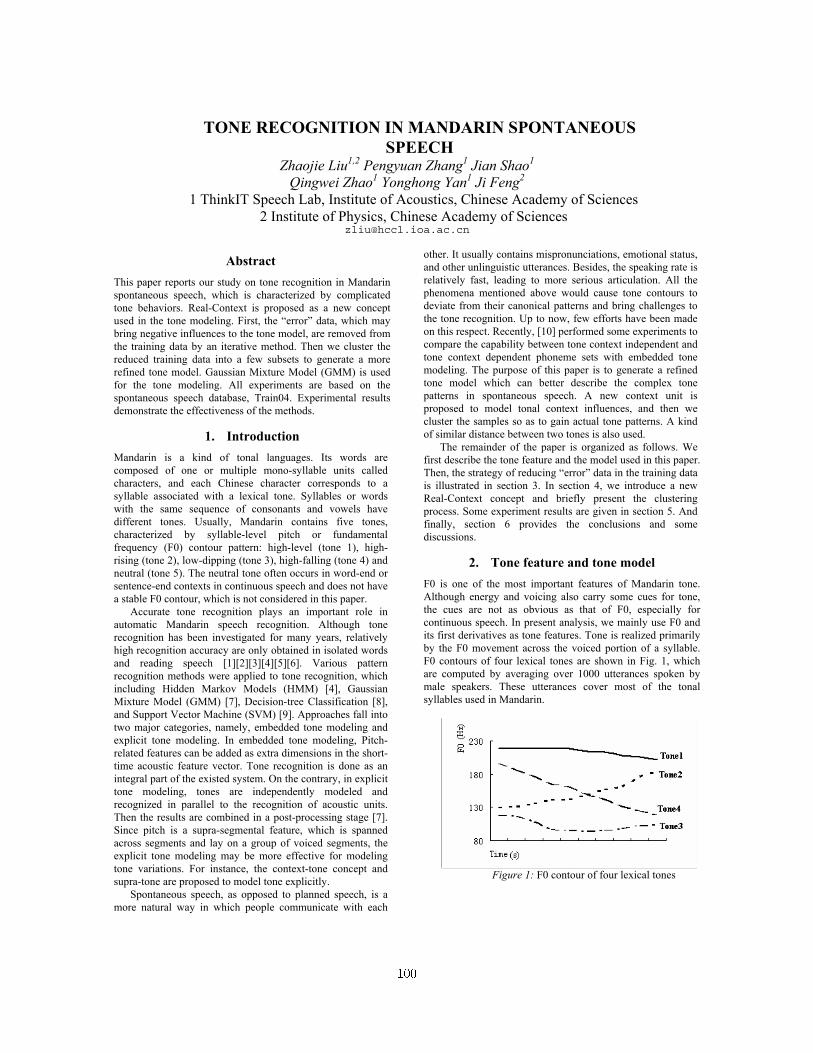
TONE RECOGNITION IN MANDARIN SPONTANEOUS SPEECH

Zhaojie Liu1,2 Pengyuan Zhang1 Jian Shao1 Qingwei Zhao1 Yonghong Yan1 Ji Feng2

1 ThinkIT Speech Lab, Institute of Acoustics, Chinese Academy of Sciences 2 Institute of Physics, Chinese Academy of Sciences

zliu@hccl.ioa.ac.cn

Abstract This paper reports our study on tone recognition in Mandarin spontaneous speech, which is characterized by complicated tone behaviors. Real-Context is proposed as a new concept used in the tone modeling. First, the “error” data, which may bring negative influences to the tone model, are removed from the training data by an iterative method. Then we cluster the reduced training data into a few subsets to generate a more refined tone model. Gaussian Mixture Model (GMM) is used for the tone modeling. All experiments are based on the spontaneous speech database, Train04. Experimental results demonstrate the effectiveness of the methods.

1. Introduction Mandarin is a kind of tonal languages. Its words are composed of one or multiple mono-syllable units called characters, and each Chinese character corresponds to a syllable associated with a lexical tone. Syllables or words with the same sequence of consonants and vowels have different tones. Usually, Mandarin contains five tones, characterized by syllable-level pitch or fundamental frequency (F0) contour pattern: high-level (tone 1), high-rising (tone 2), low-dipping (tone 3), high-falling (tone 4) and neutral (tone 5). The neutral tone often occurs in word-end or sentence-end contexts in continuous speech and does not have a stable F0 contour, which is not considered in this paper.

Accurate tone recognition plays an important role in automatic Mandarin speech recognition. Although tone recognition has been investigated for many years, relatively high recognition accuracy are only obtained in isolated words and reading speech [1][2][3][4][5][6]. Various pattern recognition methods were applied to tone recognition, which including Hidden Markov Models (HMM) [4], Gaussian Mixture Model (GMM) [7], Decision-tree Classification [8], and Support Vector Machine (SVM) [9]. Approaches fall into two major categories, namely, embedded tone modeling and explicit tone modeling. In embedded tone modeling, Pitch-related features can be added as extra dimensions in the short-time acoustic feature vector. Tone recognition is done as an integral part of the existed system. On the contrary, in explicit tone modeling, tones are independently modeled and recognized in parallel to the recognition of acoustic units. Then the results are combined in a post-processing stage [7]. Since pitch is a supra-segmental feature, which is spanned across segments and lay on a group of voiced segments, the explicit tone modeling may be more effective for modeling tone variations. For instance, the context-tone concept and supra-tone are proposed to model tone explicitly.

Spontaneous speech, as opposed to planned speech, is a more natural way in which people communicate with each

other. It usually contains mispronunciations, emotional status, and other unlinguistic utterances. Besides, the speaking rate is relatively fast, leading to more serious articulation. All the phenomena mentioned above would cause tone contours to deviate from their canonical patterns and bring challenges to the tone recognition. Up to now, few efforts have been made on this respect. Recently, [10] performed some experiments to compare the capability between tone context independent and tone context dependent phoneme sets with embedded tone modeling. The purpose of this paper is to generate a refined tone model which can better describe the complex tone patterns in spontaneous speech. A new context unit is proposed to model tonal context influences, and then we cluster the samples so as to gain actual tone patterns. A kind of similar distance between two tones is also used.

The remainder of the paper is organized as follows. We first describe the tone feature and the model used in this paper. Then, the strategy of reducing “error” data in the training data is illustrated in section 3. In section 4, we introduce a new Real-Context concept and briefly present the clustering process. Some experiment results are given in section 5. And finally, section 6 provides the conclusions and some discussions.

2. Tone feature and tone model F0 is one of the most important features of Mandarin tone. Although energy and voicing also carry some cues for tone, the cues are not as obvious as that of F0, especially for continuous speech. In present analysis, we mainly use F0 and its first derivatives as tone features. Tone is realized primarily by the F0 movement across the voiced portion of a syllable. F0 contours of four lexical tones are shown in Fig. 1, which are computed by averaging over 1000 utterances spoken by male speakers. These utterances cover most of the tonal syllables used in Mandarin.

Figure 1: F0 contour of four lexical tones

100

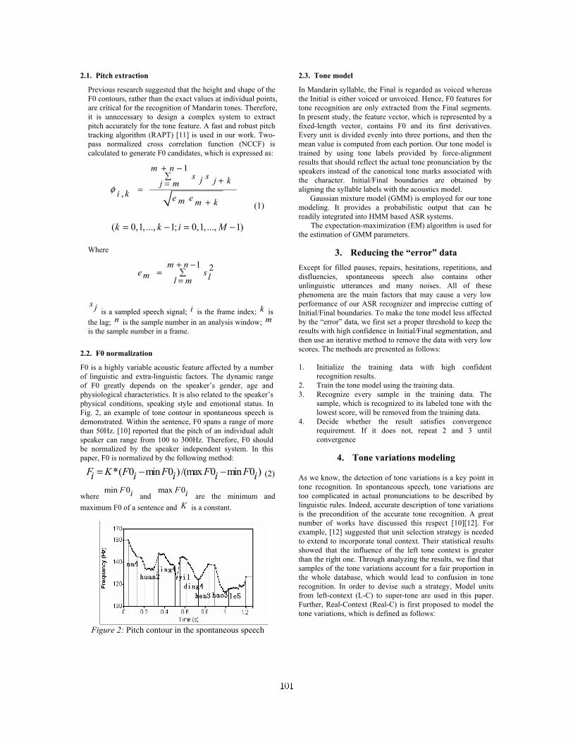
2.1. Pitch extraction

Previous research suggested that the height and shape of the F0 contours, rather than the exact values at individual points, are critical for the recognition of Mandarin tones. Therefore, it is unnecessary to design a complex system to extract pitch accurately for the tone feature. A fast and robust pitch tracking algorithm (RAPT) [11] is used in our work. Two-pass normalized cross correlation function (NCCF) is calculated to generate F0 candidates, which is expressed as:

1

,

m ns sj j kj m

i k e em m kφ

+ −∑ +==

+ (1)

( 0,1, ..., 1; 0,1, ..., 1)k k i M= − = −

Where

1 2m ne sm ll m

+ −= ∑

=

s j is a sampled speech signal; i is the frame index; k is the lag; n is the sample number in an analysis window; m is the sample number in a frame.

2.2. F0 normalization

F0 is a highly variable acoustic feature affected by a number of linguistic and extra-linguistic factors. The dynamic range of F0 greatly depends on the speaker’s gender, age and physiological characteristics. It is also related to the speaker’s physical conditions, speaking style and emotional status. In Fig. 2, an example of tone contour in spontaneous speech is demonstrated. Within the sentence, F0 spans a range of more than 50Hz. [10] reported that the pitch of an individual adult speaker can range from 100 to 300Hz. Therefore, F0 should be normalized by the speaker independent system. In this paper, F0 is normalized by the following method:

*( 0 min 0 ) /(max 0 min 0 )F K F F F Fi i i i i= − − (2)

wheremin 0F i and

max 0F i are the minimum and maximum F0 of a sentence and K is a constant.

Figure 2: Pitch contour in the spontaneous speech

2.3. Tone model

In Mandarin syllable, the Final is regarded as voiced whereas the Initial is either voiced or unvoiced. Hence, F0 features for tone recognition are only extracted from the Final segments. In present study, the feature vector, which is represented by a fixed-length vector, contains F0 and its first derivatives. Every unit is divided evenly into three portions, and then the mean value is computed from each portion. Our tone model is trained by using tone labels provided by force-alignment results that should reflect the actual tone pronunciation by the speakers instead of the canonical tone marks associated with the character. Initial/Final boundaries are obtained by aligning the syllable labels with the acoustics model.

Gaussian mixture model (GMM) is employed for our tone modeling. It provides a probabilistic output that can be readily integrated into HMM based ASR systems.

The expectation-maximization (EM) algorithm is used for the estimation of GMM parameters.

3. Reducing the “error” data Except for filled pauses, repairs, hesitations, repetitions, and disfluencies, spontaneous speech also contains other unlinguistic utterances and many noises. All of these phenomena are the main factors that may cause a very low performance of our ASR recognizer and imprecise cutting of Initial/Final boundaries. To make the tone model less affected by the “error” data, we first set a proper threshold to keep the results with high confidence in Initial/Final segmentation, and then use an iterative method to remove the data with very low scores. The methods are presented as follows: 1. Initialize the training data with high confident

recognition results. 2. Train the tone model using the training data. 3. Recognize every sample in the training data. The

sample, which is recognized to its labeled tone with the lowest score, will be removed from the training data.

4. Decide whether the result satisfies convergence requirement. If it does not, repeat 2 and 3 until convergence

4. Tone variations modeling

As we know, the detection of tone variations is a key point in tone recognition. In spontaneous speech, tone variations are too complicated in actual pronunciations to be described by linguistic rules. Indeed, accurate description of tone variations is the precondition of the accurate tone recognition. A great number of works have discussed this respect [10][12]. For example, [12] suggested that unit selection strategy is needed to extend to incorporate tonal context. Their statistical results showed that the influence of the left tone context is greater than the right one. Through analyzing the results, we find that samples of the tone variations account for a fair proportion in the whole database, which would lead to confusion in tone recognition. In order to devise such a strategy, Model units from left-context (L-C) to super-tone are used in this paper. Further, Real-Context (Real-C) is first proposed to model the tone variations, which is defined as follows:

101

0,0,

,

preF context is defined HpreF context is defined L

other defined M

βα

− >− <

⎧⎪⎨⎪⎩

(3)

where α and β are set in advance, preF is the real pitch position of pre-tone last dimension vector. The context will become H-*, M-*, L-*, each of which is a real context. * indicates the current tone. Real-Context, which is opposite to the tonal context, will reflect the context influence of the pre-tone pitch position in reality. And Real-Context has fewer feature vectors than supra-tone. Fig. 3 shows the difference among them. 1 denotes context tone model, 2 is supra-tone model and 3 is Real-Context model.

Figure 3: Tone Units

In current study, the method based on clustering is presented to model tone explicitly. Before that, we employ a kind of similarity measurements to compute the distance between two tones, which should reveal the similarity of their pitch contour shapes, and also include their different pitch height. The distance is defined:

2( , ) (( ) ( ) )0

nD is X Y x x y y x yi ii

= − − − + −∑=

1( , , ..., ),0 1 0

nX x x x x xn iin

= = ∑= (4)

1( , , .. . , ) ,0 1 0

nY y y y y yn iin

= = ∑=

In the clustering process, we first classify the tone data

into four groups based on their labels. Second, the hierarchical clustering technique is used to find pitch contour patterns of each tone group. Initially, all samples in the group are assigned to their own clusters. Then the algorithm proceeds iteratively, joining two most similar clusters at one stage, and continuing until the condition is satisfied. The advantage of this method is that the number of clusters does not have to be fixed in advance.

5. Experiments For all the experiments report in this paper, we use the

Mandarin CTS data collected by Hong Kong University of

Science and Technology in 2004, made within China and Hong Kong by mostly college students. The training set, a part of the train04, contains phonetically rich training utterances spoken by male and female speakers. The testing set comprises about utterances which are unseen from the training set. The contents are given in table 1.

Table1: Speech database used in this paper

Num of speakers Num of sentences male female

training 13046 50 50

testing 2729 10 10

Our recognition system is HMM-based. The acoustic

models are Initial/Final models with both left and right context dependency. The acoustic feature vector is composed of 12 MFCC plus energy, and their first and second order derivatives. The recognition accuracy for base syllable is 58.9% for all the train utterances.

We perform experiments with different tone units. Table 2 shows the tone recognition results of different models. The baseline (L-C) overall accuracy is 40.8%. The best performance, 43.0%, has been attained for tone 4(T4), which has the highest percentage of distribution among all tones. Tone 3(T3) gets the lowest accuracy of 36.7%. Experiments have also been done with right-context, and the results become a little worse. It is also revealed that the Real-C outperforms L-C with 2.3% absolutely and is slightly better than supra-tone models (di-tone).

Table 2: Tone recognition accuracy with different models

Unit T1(%) T2(%) T3(%) T4(%) total(%) gain

L-C 42.4 39.6 36.7 43.0 40.8 ref

di-tone 45.6 40.3 38.4 45.5 42.9 2.1

Real-C 46.2 40.5 38.1 45.8 43.1 2.3

The experimental results of reducing the “error” data and

clustering are given in Table 3. Improvement of 3.3% by reducing the “error” data can be attained, but clustering does not exhibit noticeable performance improvement.

Table 3: Reducing the “error” data and clustering

Unit Reducing the “error” data(gain)

Clustering (gain)

di-tone 45.4 (2.5%) 46.1 (0.7%)

Real-C 46.4 (3.3%) 46.7 (0.3%)

6. Conclusion and discussion In this paper, we have explored tone recognition in Mandarin spontaneous speech. The proposed new Real-Context concept

α β

3

12

102

would be more helpful in modeling the tonal context influence, as shown by more than 2% improvement absolutely. Meanwhile, a refined tone model is generated by reducing the “error” data from the original data, improving the tone recognition accuracy of 3.3%. Furthermore, through clustering the training data to subsets, which may accurately describe the tone variations, we can achieve a tone recognition accuracy of 46.7%. Nevertheless, there are still aspects of modification for the proposed methods in our study. Although tone recognition accuracy with 5.9% has been absolutely improved, it is still much lower than that of base syllable. Therefore, refining the tone modeling still requires intensive analyses, for example, tone variation rules may be added into the clustering process. Further, additional experiments are needed by other different database.

7. Acknowledgements This work is partially supported by Chinese 973 program (2004CB318106), National Natural Science Foundation of China (10574140, 60535030), and Beijing Municipal Science & Technology Commission (Z0005189040391).

8. References [1] C. J. Chen, R. A. Gopinath, M. D. Monkowski, M. A. Picheny and K. Shen, “New methods in continuous Mandarin speech recognition”, 5th European Conference on Speech and Communication and Technology, Vol. 3, 1543-1546, 1997. [2] H. Huang, and F. Seide, “Pitch Tracking and Tone Features for Mandarin Speech Recognition”, Proc. ICASSP 2000, vol.3, 1523-1526, 2000. [3] C.J. Chen, H.P. Li, L.Q. Shen, G.K. Fu, “Recognize Tone Languages Using Pitch Information on the Main Vowel of Each Syllable”, Proc. ICASSP 2001, Vol. 1, 61-64, 2001. [4] W. J. Yang, J. C. Lee, Y. C Chang, and H. C. Wang, “Hidden Markov Model for Mandarin Lexical Tone Recognition,” IEEE Trans. ASSP, Vol. 36, 988-992, 1988. [5] G. P. Kong, S. N. Lu, “A VQ study on pitch models of disyllable in Mandarin”. ACTA ACUSTICA, 25(2), 2000. [6] E. Chang, J. L. Zhou, C. Huang, S. Di, K. F. Lee, “Large vocabulary mandarin speech recognition with different approaches in modeling tones”, Proc. ICSLP 2000, 983-986 2000. [7] Y. Qian, “Use of tone information in Cantonese LVCSR based on Generalized Character Posterior Probability Decoding,” Ph. D Dissertation, The Chinese University of Hong Kong, 2005 [8] Cao Yang et al. Decision-tree based Mandarin tone model and its application to speech recognition. Proc. ICASSP 2000, 1759-1762. [9] S. D. Dinoj et al. “Tone Recognition in Mandarin using Focus”, INTERSPEECH, 2005, 3301-3304, 2005. [10] J. L. Zhou, Y. Tian, Y. Shi, C. Huang, E. Chang, “Tone Articulation Modeling for Mandarin Spontaneous Speech Recognition”, Proc. ICASSP 2004, 997-1000, ICASSP 2004.

[11] A.D. Talkin, Speech Coding and Synthesis, Elsevier Science B.V., Amsterdam, chapter A robust algorithm for pitch tracking (RAPT), 495-518, 1995 [12] Y. Xu, Q.E. Wang, “Pitch target and their realization: Evidence from Mandarin Chinese”, Speech communication, Vol.33, 319-337, 2001.

103

Evaluation of a Feature Selection Scheme on ICA-based Filter- Bank for Speech Recognition

Neda Faraji & S.M. Ahadi

Department of Electrical Engineering, Amirkabir University of Technology, Tehran, Iran

nfaraji@cic.aut.ac.ir sma@aut.ac.ir

Abstract In this paper, we propose a new feature selection scheme that can contribute to an ICA-based feature extraction block for speech recognition. The initial set of speech basis functions obtained in independent component analysis training phase, has some redundancies. Thus, finding a minimal-size optimal subset of these basis functions is rather vital. On the contrary to the previous works that used reordering methods on all the frequency bands, we have introduced an algorithm that finds optimal basis functions in each discriminative frequency band. This leads to an appropriate coverage of various frequency components and easy extension to other data is also provided. Our experiments show that the proposed method is very useful, specifically in larger vocabulary size tasks, where the selected basis functions trained using a limited dataset, may get localized in certain frequency bands and not appropriately generalized to residual dataset. The proposed algorithm surmounts this problem by a local reordering method in which contribution of a basis function is specified with three factors: class separability power, energy and central frequency. The experiments on a Persian continuous speech corpus indicated that the proposed method has led to 17% improvement in noisy condition recognition rate in comparison to a conventional MFCC-based system.

1. Introduction A fundamental problem in applied digital signal processing is to find suitable representations for image, audio or other kind of data for applications such as recognition and denoising. Data representations are often based on linear transformations. Standard linear transformations widely used in signal processing are the Fourier, Haar, cosine transform, etc. It would be most useful to estimate the linear transformation from the data itself, in which case the transform could be ideally adapted to the kind of data that is being processed [1]. Independent Component Analysis (ICA) is a data-driven method that can capture the higher order statistics from the signal. ICA can separate independent components from the signals which are mixtures of the unknown sources and it can be applied to image, speech and medical signal processing [2]. In [3], ICA was used for feature extraction of speech signal. The extracted ICA-based features were then applied to an Isolated-word recognition task. Since the ICA algorithm finds the independent components corresponding to the dimensionality of the input, it may result in redundant components. However, the extracted independent components of speech correspond to the sources of speech production. Some of these sources are irrelevant sources. In reality, these

may not be useful for speech recognition and should be removed. Identifying the irrelevant and redundant sources and their removal could be carried out by a feature selection method. In [3], two measures have been used for reordering and selecting of basis vectors:

1) The energy of the basis vector. 2) The variance of the basis vector coefficient.

Although the basis vectors selected with these two simple methods outperformed mel-scale filter-bank in capturing the higher order structures of speech, our experiments have shown that two mentioned methods lead to high degradations of recognition rate in some conditions. In reality, the overall ICA-based feature extraction performance is very sensitive to applied feature selection method. We should, therefore, use an effective feature selection method that considers all aspects of a given problem, here speech recognition. We propose a new feature selection algorithm that minimizes the available problems in two aforementioned methods by obtaining a nearly optimal subset of the initial ICA-based filters with respect to adaptation and generalization issues. The considerable effect of proposed method in improving recognition rate has been approved by our experiments on a Persian continuous speech corpus. Also, the recognition results obtained on both Aurora 2 and Persian tasks show that the ICA-based features are robust in noisy conditions. It should be noted that in the case of Aurora 2 task, the global reordering method was adequate and only the effect of initial number of filters is evaluated. The paper is organized as follows. In section 2 we briefly review the use of ICA technique in feature extraction of speech. The proposed feature selection method is presented in section 3. Experimental results are discussed in section 4 and conclusions are drawn in section 5.

2. Extracting speech features using ICA

2.1. Extracting basis vectors of speech

The linear model of independent component analysis assumes that the observation is a linear mixture of the independent components and is represented as:

1

,N

i ii

s=

= = =∑x As a s Wx (1)

In this model, ia is a basis vector that contributes to the generation of the observed data with source coefficient is . The estimation of sources and basis functions could be done by maximization of negentropy ( )iJ s [1]:

104

2

( ) ( ) ( ) ( )T Ti i imax J s J E G E G ν = = − w x w x (2)

where iw is the ith row of mixing matrix W , G is a contrast function and ν is a standardized Gaussian variable. In this work, we take the exponential function as the contrast function:

21( ) exp( )2

G u u= − − (3)

To find basis vectors of speech, short-time segments from speech signals are constructed and using an iterative algorithm, negentropy is maximized. We take a fixed point version of the algorithm and an iterative symmetric decorrelation scheme. Finally, the columns of A matrix are obtained from the inverse of the estimated W. These columns are considered as the initial set of ICA-derived filter-bank.

2.2. Selection of dominant basis vectors

The dimension of the extracted basis vectors is equal to the dimension of the short-time segments [3]. It is desirable to select dominant basis vectors from the initial set so that the feature extraction method is computationally comparable with the conventional one. Also, irrelevant and redundant basis functions are eliminated. We could decide based on the L2-norm of the basis vector or the variance of the basis vector coefficient [3]. The block diagram of ICA-based speech recognition system has been shown in Fig. 1.

3. Proposed feature selection algorithm The feature selection methods utilized in [3], may omit filters in some frequency bands. We face this effect in certain conditions. For example, most of high energy basis vectors are localized in low frequency bands. Thus, the feature selection method may suppress the high frequency basis vectors. However, when the dimensionality of the training speech frames in ICA algorithm is increased, global reordering methods may result in almost low frequency dominant basis functions. Also, the ICA-derived filters are highly adapted to its normally limited training dataset. It emphasizes on some frequency bands available in ICA training dataset. Thus, the feature selection algorithm may remove less significant filters. These removed filters may have very important role in extracting information from the non-training data. In practice, there should be a trade-off between adaptation and generalization. The flow diagram of the algorithm has been demonstrated in Fig. 2.

3.1. Measure of comparing basis vectors

It is preferable to choose a measure that considers the classification problem more strongly. Thus, we have introduced a weighted version of L2-norm in which L2-norm of a basis vector is weighted with its Proportion of Variance (PoV).

( ) ( ) ( )measure = PoV L2-normj j j× (4)

where j indicates jth filter. PoV [4] is calculated using the ratio of between-class variance to within-class variance. The PoV measure of a given basis vector, shows its capability in

Figure 1: Block Diagram of ICA-based speech recognition system

Figure 2 : Proposed Feature Selection Block.

separating different classes, and along with L2-norm directs us to choose those high energy basis vectors that also have high discrimination power. We assume that the number of classes is L. Then, the between-class and within-class variances for a given variable x, are defined as follows [5]:

1 1

( )( )L L

T

W i i i i i ii i

S PE x x w Pµ µ= =

= − − = ∑ ∑ ∑ (5)

1 1

( )( ) ,L L

T

B i i i i ii i

S P Pµ µ µ µ µ µ= =

= − − = ∑ ∑ (6)

where ,i iµ ∑ and iP are the mean, variance and the a priori probability of the ith class respectively. Then we write:

PoV= B

W

S

S. (7)

The aforementioned measure in Eq. 4 is very useful when we want to select dominant basis vectors from a set of basis vectors with the same central frequencies. It is probable that a low-power high-frequency basis vector has more capability to discriminate classes than a high-power low-frequency one. In other words, comparing two basis vectors without considering their central frequencies is not correct and finally may result in giving more weight to a certain band in comparison to the others. This has been the main motivation behind our work on providing an algorithm to select dominant basis vectors automatically. In reality, the problem may be solved with local decisions instead of global ones. The proposed algorithm includes three parts:

1) Total pruning 2) Identifying the cut-point filters 3) Filling gap spaces.

105

3.2. Total pruning

In this step, each filter competes with the filters whose central frequencies are near its. The competition is local and the difference between central frequencies should be below a threshold value. These filters constitute a group and one or more filters from this group with the largest PoV-weighted L2-norm are selected. It should be noted that a very small threshold value may lead to no filter pruning. Meanwhile, a very large threshold value destroys the locality assumption. We have selected a threshold value equal to 80 Hz. This value is about half of the minimum bandwidth in a conventional mel-scale filter-bank.

3.3. Identifying cut-point filters

The aim of this part of algorithm is identifying the critical filters. The critical filters have more distinct characteristics in comparison to the others and would be kept to improve generalization and classification. The central frequency of a filter is an index that can separate it from the others. A hierarchical clustering algorithm is applied to the central frequency values to reach a certain number of central frequency clusters. The number of clusters is increased by one, if no cluster is found to have a single member. Single member clusters include the filters that have more distinct central frequencies than the other filters. These filters have an important role in generalization. Concurrently, another clustering is performed on PoV-weighted L2-norm values to reach 3 clusters corresponding to low, medium and high values. In this case, the single member clusters have more distinct PoV-weighted L2-norm values. We are interested in keeping the filters with high PoV-weighted L2-norms. These filters can improve the classification. The filters found from two aforementioned clustering approaches are cut-point filters and can divide the whole frequency band into sub-bands. After finding the initial cut-point filters, the two explained clusterings are performed on each sub-band filters. Sub-band clustering is performed from low to high frequency sub-bands. For the algorithm to be well conditioned, we have applied constraints on it. The constraints were put on:

1) The initial number of central frequency clusters in the beginning of the algorithm.

2) The maximum number of clusters in each sub-band. The large number of clusters in the beginning of the algorithm lead to fast but not accurate converging. We begin the algorithm with the minimum number of central frequency clusters, so that it can find cut-points (single-member clusters) gradually. In sub-band clustering, the low frequency sub-bands are prior to the high frequency sub-bands. If we do not limit the number of clusters in each sub-band, the algorithm finds the cut-points only in low frequency bands. However, the maximum number of clusters in each sub-band specifies the final number of cut-point filters found.

3.4. Filling gap space

According to the values of constraints, there would remain some gaps between the cut-point filters found. We heuristically fill these gap spaces.

Table 1: The recognition results in single Gaussian HMM and Persian corpus. The number of filters in

each sub-band has been selected heuristically.

Recognition Rate

MFCC 43.57 Global reordering 32.22 4 sub-band 33.92

8 sub-band 39.11 13 sub-band 40.08 18 sub-band 43.68

ICA

Proposed method 44.52

Table 2: The recognition rate in different noisy conditions and 15-Gaussian mixture HMM.

Recognition Rate ICA MFCC Clean 72.83 76.43 Babble 27.54 20.01 Car 70.96 50.32 F16 28.72 19.6 Average 42.4 29.97

Table 3: The recognition rate of ICA-based features in AURORA 2 task (12 Ceps.coeff+C0 in ICA features,

12 Ceps.coeff+log Energy in baseline system)

Recognition Rate

35 50 baseline Set A 65.44 63.94 61.13 Set B 64.85 64.1 55.57 Set C 60.28 65.57 66.68 Average 63.52 64.53 61.12

4. Experiments and results

4.1. Experiments on Farsi continuous speech corpus

The Farsi continuous speech corpus, FARSDAT was used in this work [6]. This corpus is the only continuous speech corpus of Farsi, which is available to public. It consists of 6000 sentences from 300 speakers, each uttering 20 sentences selected from a set of 392 available sentences. We have used 1819 sentences from 91 speakers for building a 3-state phoneme-based HMM system. Also, the test set includes 888 sentences from 46 speakers. Training and test have been carried out using HTK [7] and with different number of Gaussian mixtures in each state. The noise was then added to the speech in different SNRs. The noise data was extracted from the NATO RSG-10 corpus [8]. We have considered babble, car and F16 noises and added them to the clean signal at 20, 15, 10, 5 and 0 dB SNRs. Our experiments were carried out using MFCC (for comparison purposes) and ICA features. The features in two cases were computed using 25 msec. frames with 10 msec. of frame shifts. Pre-emphasis coefficient was set to 0.97 and a Hamming window was applied. The feature vectors for the two methods were composed of 12 cepstral and a log-energy parameter. For extracting MFCC features, a 24-channel mel-scale filter-bank was used. Also, for training the initial set of ICA-based filter-bank, the 100 sample short-time segments with frame shifts of 30 samples were used. These segments were

106

constructed using 110 sentences from 11 speakers. After training, the proposed feature selection block selected 24 dominant filters from a total of 100 filters. The selected filters were then replaced mel-scale filters in feature extraction block. In step 1 of feature selection algorithm, threshold value was set to 80Hz and 50 filters were pruned. From the 50 remaining filters, 20 cut-point filters were selected in step 2. This final number of cut-point filters was obtained with these parameters:

• The initial number of central frequency clusters was set to 4 at the beginning of the algorithm.

• The maximum number of clusters in each sub-band was set to the number of sub-band members minus one.

• The initial number of clusters in each sub-band clustering was set to the minimum value between 4 and half of the sub-band members.

Finally, 4 filters filled gap spaces to get 24 filters. In all steps, the comparison of filters was carried out by PoV-weighted L2-norm measure. Also, the PoV values of 100 initial filters were calculated using 119 phoneme-labeled sentences. Table 1 lists the recognition results of ICA-based features using sub-band reordering methods, in which the whole frequency band was divided into some sub-bands and in each sub-band, the L2-norm measure was used for selecting dominant filters. The number of filters in each sub-band is selected according to the number of mel-scaled filters in that sub-band. The results have been brought from clean condition and 1-mixture phoneme-based HMM recognizer. Also, the recognition result of MFCC features is given for comparison. The indicated results show the considerable effect of used feature selection method in overall result. As seen in Table. 1, proposed feature selection algorithm has increased the recognition rate about 1.6% in comparison to MFCC. Table 2 lists the recognition results obtained in clean and noisy conditions, on a 15-component HMM-based system using the proposed feature selection method. As indicated in this table, the performance of ICA-based features is worse than MFCC in clean condition when we used 15-Gaussian HMM system. This effect is the natural result of lower-variance ICA features. The results also show the robustness of ICA features in noisy conditions. The average values mentioned in this table are calculated over the results obtained from 0 dB to 20 dB SNRs , omitting the clean ones. The results obtained can be listed as follows:

1) The feature selection method is very important in ICA-based feature extraction.

2) The ICA-based features improve the robustness of speech recognition system.

3) When the number of Gaussian components is increased, the recognition rate of ICA-based features is degraded in comparison to MFCC features.

4.2. Experiments on AURORA 2 speech task

In this section, we briefly review the result of experiments on AURORA 2 task [9], adopting global reordering method and various initial number of ICA-based filters. It should be noted that ICA training phase was carried out using 22 files from 22 selected speakers in this task. The results are reported in Table 3 and the following conclusions can be listed:

1) The global reordering is adequate in this smaller size task.

2) The ICA-based features are more robust than MFCC features.

3) The initial number of ICA-derived filters is effective in obtained recognition rate.

5. Conclusions In this paper, we tried to emphasize on the significant role of the feature selection algorithm on the overall performance of ICA-based speech recognition systems. The ICA-derived filters are adapted to processing data, specifically with data used in training ICA basis functions. Therefore, they are able to extract maximum higher-order information from data. The insufficient feature selection algorithm can remove some of the essential filters and lead to degradation of recognition rate. However, if an appropriate algorithm is used for selecting dominant filters in ICA feature extraction block, the recognition rate in noisy conditions shows great improvements in comparison to the baseline. This effect also originates from adapting of ICA filters with data. It seems that the ICA-based features contain the maximum amount of data information, while extract minimum information of noise data. The initial number of filters is also an important parameter in obtaining filters with appropriate frequency resolutions and then better recognition rate.

6. Acknowledgement This work was in part supported by a grant from the Iran Telecommunications Research Center (ITRC).

7. References [1] A. Hyvarinen, J. Karhunen, E. Oja, Independent Component

Analysis. John Wiley & Sons, New York: 2001. [2] M. Kotani, Y. Shirata, S. Maekawa, S. Ozawa, K. Akazawa,

“Application of independent component analysis to feature extraction of speech,“ in Proc. IJCNN, Vol. 5, pp. 2981-2985, 1999.

[3] J.H Lee, H.Y Jung, T.W Lee, S.Y Lee “Speech feature extraction using independent component analysis,” in Proc. ICASSP .Vol. 3, pp. 1631-1634, 2000.

[4] E.K. Ekenel, N.Sankur, “Feature selection in the independent component subspace for face recognition,” in Pattern Recognition Letters, Vol. 25, pp. 1377-1388, June 2004.

[5] N. Malayath, H. Hermansky, “Data-driven spectral basis functions for automatic speech recognition,” in Speech Communication, Vol. 40, Issue 4, pp. 449-466, June 2003.

[6] D.Gharavian, S.M.Ahadi, “ Evaluation of the effect of stress on formants in Farsi vowels,” in Proc. ICASSP, vol. 1, pp. 661-664, Montreal, May 2004.

[7] The hidden Markov model toolkit available from http://htk.eng.cam.ac.uk.

[8] Available from http://spib.rice.edu/spib/select_noise.html [9] H.G. Hirsch, D. Pearce, “The AURORA experimental

framework for the performance evaluation of speech recognition systems under noisy conditions,“ in Proc. ASRU, pp. 181-188, September 2000.

107

A Robust Endpoint Detection Algorithm Based onIdentification of the Noise Nature

Denilson C. Silva

Program of Electrical Engineering - COPPESignal Processing Laboratory

Federal University of Rio de Janeiro, Rio de Janeiro, Brazildenilson@lps.ufrj.br

AbstractThe endpoint detection of speech is still a big problem in situa-tions of speech recognition in noisy environments. While tradi-tional methods concentrate on finding speech in noise, the pro-posed technique is based on noise identification throughHMMs, associated with bothSNRand euclidean distance of thelog-energy calculated on a frame-by-frame basis. Computer ex-periments confirm that the proposed algorithm gives rise to aconsiderable improvement on the precision of endpoint detec-tion, specially in severely adverse conditions where theSNRisvery low.

1. IntroductionIn many applications of speech signal processing, determina-tion of the endpoints of utterances is necessary. The traditionalmethods of endpoints detection based on both energy and zerocrossing rate work very well with clean speech [1]. When wehave utterances with fricatives, for instance, the endpoint de-tection might become complicated if the delimitation processhappens in a noisy environment.

Several works have been seeking to solve the subject ofthe endpoint detection in noisy environments [2, 3], but the ob-tained results are extremely sensitive to the signal-to-noise ratio(SNR).

In this article a method is proposed for endpoint detectionin utterance for speech recognition based on the principle ofidentification of the noise nature that contaminates the signal,through a classification on each frame using hidden Markovmodels (HMMs), delimiting the intervals with speech startingfrom the identification of frames with noise only. TheSNRandthe euclidean distance of the log-energy of each frame are alsoused to accomplish a refinement in the detection. The proposedmethod results in a significant precision improvement, partic-ularly for very adverse conditions, as computer experimentsshow.

This article is organized as follows. In Section 2, the pro-posed endpoint detection algorithm is introduced. In Section 3,the database is described. In Section 4, results of the accom-plished tests as well as comparisons with the traditional methodbased on both energy and zero crossing rate are shown. Finally,in Section 5, we present the conclusions.

2. Proposed methodThe proposed endpoints detection method is accomplishedthrough three processes of decision beginning with a frame-by-frame analysis: the identification of the noise nature [4] [5],

ENDPOINTS

K−1

0

SEGMENTATION

BUFF

ER

OF THE EUCLIDEANDISTANCE

DETERMINATION

IDENTIFICATIONOF THE NOISE

NATURE

DETERMINATIONOF THE SNR

DECISIONGLOBAL DETERMINATION

OF THE

x(i) = s(i) + d(i)

x(k,i)

[...+1+1+1−1−1+1...]

FRAM

ES

ϕSNR

ϕED

HMMϕ ϕ

global

Figure 1:Proposed method.

SNRand the euclidean distance of the log-energy (Figure 1). Wedefine that a frame with positive flag (+1) contains noise only,while a frame with negative flag (−1) contains both speech andnoise.

2.1. Identification of the noise nature

Consider the noisy signalx(i) a composition of the cleanspeechs(i) with the additive noised(i), that is,x(i) = s(i) +d(i).

The signalx(i) is segmented intoK frames withN sizeand overlap ofL samples:

x(k, i) = x(k(N − L) + i) (1)

where0 ≤ k ≤ K − 1 and0 ≤ i ≤ N − 1.The process of identification of the noise nature is accom-

plished through a classification of the frames of the noisy sig-nal (x(k, i)), using HMMs, among the types of noise involvedin the training. The settings used on tests were 18 parametersper subframes of 23 ms, 50% of overlap, Hamming window-ing, left-right HMM with skip allowed, four states, four modelsand 128 centroids. The stages of the identification are explainedbelow.

2.1.1. Extraction of parameters

The extracted parameters on each subframe were: one of spec-tral entropy (as described in [3]), one of zero crossing rate and16 of log-energy, described in Table 1.

The pth log-energy parameter,LogE(k, p), is defined asthe energy contained in thepth subband for framek.

2.1.2. Criterion of decision

The noisy utterances are segmented in frames of 46 ms andoverlap of 80%. The frames are identified by HMM, in agree-ment with trained noise models. The results are registered as108

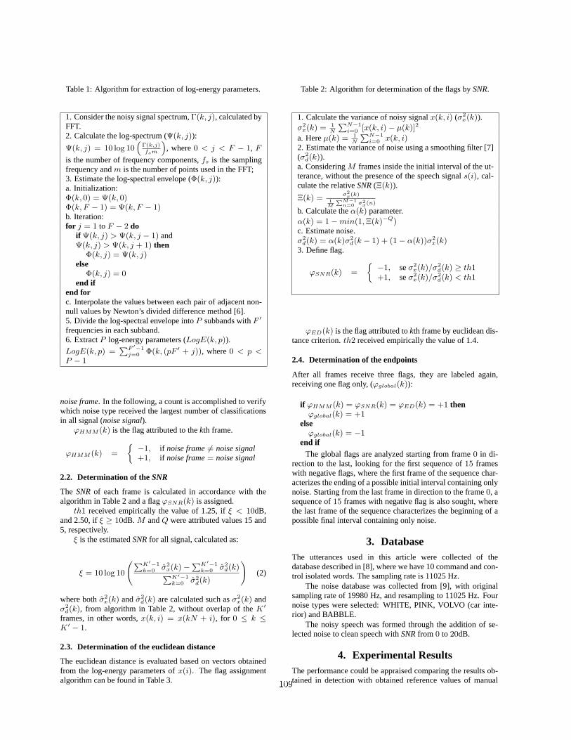
Table 1: Algorithm for extraction of log-energy parameters.

1. Consider the noisy signal spectrum,Γ(k, j), calculated byFFT.2. Calculate the log-spectrum (Ψ(k, j)):

Ψ(k, j) = 10 log 10“

Γ(k,j)fsm

”, where0 < j < F − 1, F

is the number of frequency components,fs is the samplingfrequency andm is the number of points used in the FFT;3. Estimate the log-spectral envelope (Φ(k, j)):a. Initialization:Φ(k, 0) = Ψ(k, 0)Φ(k, F − 1) = Ψ(k, F − 1)b. Iteration:for j = 1 toF − 2 do

if Ψ(k, j) > Ψ(k, j − 1) andΨ(k, j) > Ψ(k, j + 1) then

Φ(k, j) = Ψ(k, j)else

Φ(k, j) = 0end if

end forc. Interpolate the values between each pair of adjacent non-null values by Newton’s divided difference method [6].5. Divide the log-spectral envelope intoP subbands withF ′

frequencies in each subband.6. ExtractP log-energy parameters (LogE(k, p)).

LogE(k, p) =PF ′−1j=0 Φ(k, (pF ′ + j)), where0 < p <

P − 1

noise frame. In the following, a count is accomplished to verifywhich noise type received the largest number of classificationsin all signal (noise signal).

ϕHMM (k) is the flag attributed to thekth frame.

ϕHMM (k) =

−1, if noise frame6= noise signal+1, if noise frame= noise signal

2.2. Determination of theSNR

The SNRof each frame is calculated in accordance with thealgorithm in Table 2 and a flagϕSNR(k) is assigned.

th1 received empirically the value of 1.25, ifξ < 10dB,and 2.50, ifξ ≥ 10dB.M andQ were attributed values 15 and5, respectively.

ξ is the estimatedSNRfor all signal, calculated as:

ξ = 10 log 10

PK′−1k=0 σ2

x(k)−PK′−1k=0 σ2

d(k)PK′−1k=0 σ2

d(k)

!(2)

where bothσ2x(k) andσ2

d(k) are calculated such asσ2x(k) and

σ2d(k), from algorithm in Table 2, without overlap of theK′

frames, in other words,x(k, i) = x(kN + i), for 0 ≤ k ≤K′ − 1.

2.3. Determination of the euclidean distance

The euclidean distance is evaluated based on vectors obtainedfrom the log-energy parameters ofx(i). The flag assignmentalgorithm can be found in Table 3.

Table 2: Algorithm for determination of the flags bySNR.

1. Calculate the variance of noisy signalx(k, i) (σ2x(k)).

σ2x(k) = 1

N

PN−1i=0 [x(k, i)− µ(k)]2

a. Hereµ(k) = 1N

PN−1i=0 x(k, i)

2. Estimate the variance of noise using a smoothing filter [7](σ2d(k)).

a. ConsideringM frames inside the initial interval of the ut-terance, without the presence of the speech signals(i), cal-culate the relativeSNR(Ξ(k)).

Ξ(k) =σ2x(k)

1M

PM−1n=0 σ2

x(n)

b. Calculate theα(k) parameter.α(k) = 1−min(1,Ξ(k)−Q)c. Estimate noise.σ2d(k) = α(k)σ2

d(k − 1) + (1− α(k))σ2x(k)

3. Define flag.

ϕSNR(k) =

−1, seσ2x(k)/σ2

d(k) ≥ th1+1, seσ2

x(k)/σ2d(k) < th1

ϕED(k) is the flag attributed tokth frame by euclidean dis-tance criterion.th2 received empirically the value of 1.4.

2.4. Determination of the endpoints

After all frames receive three flags, they are labeled again,receiving one flag only, (ϕglobal(k)):

if ϕHMM (k) = ϕSNR(k) = ϕED(k) = +1 thenϕglobal(k) = +1

elseϕglobal(k) = −1

end ifThe global flags are analyzed starting from frame0 in di-

rection to the last, looking for the first sequence of15 frameswith negative flags, where the first frame of the sequence char-acterizes the ending of a possible initial interval containing onlynoise. Starting from the last frame in direction to the frame0, asequence of15 frames with negative flag is also sought, wherethe last frame of the sequence characterizes the beginning of apossible final interval containing only noise.

3. DatabaseThe utterances used in this article were collected of thedatabase described in [8], where we have 10 command and con-trol isolated words. The sampling rate is 11025 Hz.

The noise database was collected from [9], with originalsampling rate of 19980 Hz, and resampling to 11025 Hz. Fournoise types were selected: WHITE, PINK, VOLVO (car inte-rior) and BABBLE.

The noisy speech was formed through the addition of se-lected noise to clean speech withSNRfrom 0 to 20dB.

4. Experimental ResultsThe performance could be appraised comparing the results ob-tained in detection with obtained reference values of manual109

Table 3: Algorithm for determination of the flags by euclideandistance.

1. Calculate the euclidean distanceEDx(k), on each frame,between the log-energy vectors of signalx(i) and a referencevector.a. Calculate the reference vector,LogEref (p)

LogEref (p) = 1M

PM−1k=0 LogE(k, p)

b. Calculate the distance.

EDx(k) =qPP−1

p=0 (LogE(k, p)− LogEref (p))2

2. EstimateEDd.EDd = max0≤k≤M−1EDx(k)3. Define flag.

ϕED(k) =

−1, if EDx(k)/EDd ≥ th2+1, if EDx(k)/EDd < th2

Table 4: Table containing average percents of error reductionrate

BABBLE PINK VOLVO WHITEBeginning 6.82% 12.23% −2.65% 12.05%

Ending 20.81% 26.24% 0.70% 24.88%

clipping.Initially it was made a training of discrete HMMs of [8],

with 500 segments of 100 ms for each of the four types of noiseand 50% of overlap. An experiment was undertaken with 121corrupted utterances, setting both theSNRand the noise, ob-serving the percent of mistake in detection along the several val-ues ofSNRboth at beginning (εb) and at ending (εe), whereBandE are, respectively, the beginning and the ending by man-ual clipping,Eb andEe are, respectively, the detected points bythe proposed system.

εb =|B − Eb|E −B × 100% (3)

εe =|E − Ee|E −B × 100% (4)

The average reduction of the error rate in detection, com-paratively to the method described in [1], is shown in Table4. We can see that there was a considerable error reduction inevery case, except for the car interior noise, where no significantchange was observed.

The results for each type of noise of the traditional [1] andproposed technique can be found in Tables 5, 6, 7 and 8. It isalso noticed that the best performance of the introduced detectorhappens in low-SNRzone.

Figure 2 exemplifies the endpoint detection on low-energysounds. We can see that the proposed method kept all usefulinformation signal.

5. ConclusionsIn this paper a robust endpoint detection method was pro-posed based on identification of the noise nature using

Table 5: Percentual error of the endpoint detection in babblenoise environment

SNRTraditional Proposed

beginning ending beginning ending

0dB 40.0% 80.67% 11.96% 20.55%5dB 15.83% 39.41% 9.38% 10.78%10dB 8.95% 19.11% 7.28% 8.66%15dB 6.54% 10.85% 6.87% 6.33%20dB 5.34% 6.04% 7.04% 5.71%

Table 6: Percentual error of the endpoint detection in pink noiseenvironment

SNRTraditional Proposed

beginning ending beginning ending

0dB 68.52% 114.26% 15.20% 36.55%5dB 19.07% 53.69% 11.87% 20.35%10dB 14.04% 34.13% 11.18% 17.32%15dB 9.79% 14.66% 10.08% 9.95%20dB 7.10% 6.63% 9.03% 8.04%

0 200 400 600 800 1000 1200 1400 1600 1800−1

0

1

2

3

4

5

6

7

8

x 104

(a)

(b)

(c)

Time (ms)

Figure 2: Endpoint detection based on identification of the noisenature. (a) Endpoint detection by the proposed method. (b)Corrupted signal by babble noise at5dB SNRand (c) Cleanspeech referring to “baixo” (which means “down”) utterance.

HMMs, associated toSNRand to euclidean distance of log-energy parameters, that were used to adjust the detection in seg-ments with low-energy sounds. With this method we try to de-tect the frames that contain only noise and to separate them fromthe useful information of the signal. Computer experimentswith 121 utterances corrupted by four different noise types andwith varying levels ofSNRfrom 0 to 20dB were presented. Itcan be seen from the results that in severe adverse conditions,when theSNRis very low, that the proposed method offers aconsiderably more precise detection of endpoints as comparedto the traditional technique. The proposal of an algorithm that,based on the estimation ofSNRand type of noise, can decide110

Table 7: Percentual error of the endpoint detection inside car

SNRTraditional Proposed

beginning ending beginning ending

0dB 9.67% 15.02% 7.52% 5.64%5dB 7.43% 10.86% 8.22% 6.08%10dB 7.55% 6.71% 9.38% 6.16%15dB 8.40% 5.04% 12.66% 8.24%20dB 7.09% 4.53% 15.61% 12.53%

Table 8: Percentual error of the endpoint detection in whitenoise environment

SNRTraditional Proposed

beginning ending beginning ending

0dB 62.44% 105.94% 13.04% 29.29%5dB 18.31% 50.79% 11.49% 21.94%10dB 13.68% 33.22% 9.87% 16.44%15dB 9.61% 15.19% 8.05% 9.25%20dB 6.93% 6.57% 8.29% 10.37%

which is the most suitable technique for end point detection andrecognition in adverse conditions is subject of ongoing research.

6. References[1] Teruszkin, R., Consort, T. A. and Resende Jr., F. G. V.,

“Endpoint detection analysis for an implementation of aspeech recognition system applied to robot control”, InProc. SAWCAS, November, 2001.

[2] Bou-Ghazale, S. E. and Assaleh, K., “A robust endpointdetection of speech for noisy environment with applica-tion to automatic speech recognition”, In IEEE Interna-tional Conference on Acoustics, Speech, and Signal Pro-cessing, vol.4, pp. 3808-3811, May, 2002.

[3] Jia-Lin Shen, Jeih-Weih Hung and Lin-Shan Lee, “Robustentropy-based endpoint detection for speech recognitionin noisy environments”, In International Conference onSpoken Language Processing, Sydney, November, 1998.

[4] Silva, D. C. and Resende Jr., F. G. V., “Identificationof the Noise Nature based on HMMs” (in Portuguese),In Simposio Brasileiro de Telecomunicacoes, September,2004.

[5] Silva, D. C., “Identification of the Noise Nature with Ap-plication in Robust Speech Recognition” (in Portuguese),Masters Thesis, Federal University of Rio de Janeiro,February, 2005.

[6] Hildebrand, F. B., Introduction to Numerical Analysis,McGraw-Hill, New York, Second Edition, 1974.

[7] Lin, L., Holmes, W. H. and Ambikairajah, E., “Sub-band noise estimation for enhancement using a percep-tual Wiener filter”, In IEEE International Conference onAcoustics, Speech, and Signal Processing, vol.1, pp.80-83, April, 2003.

[8] Teruszkin, R., Resende Jr., F. G. V., Villas-Boas, S. B. andLizarralde, F., “Object-oriented speech recognition libraryapplied to robot control” (in Portuguese), In CongressoBrasileiro de Automatica, September, 2002.

[9] http://spib.rice.edu/pib/selectnoise.html, “Signal Pro-cessing Information Base (SPIB)”,September, 2002.

111

EMD Analysis of Speech Signal in Voiced Mode

Aïcha Bouzid1, Noureddine Ellouze2

1Institute of Electronic and Communication of Sfax, Sfax, Tunisie 2National School of Engineers of Tunis, Tunis, Tunisie

N.Ellouze@enit.rnu.tn, bouzidacha@yahoo.fr

Abstract

Like almost all natural phenomena, speech is the result of many nonlinearly interacting processes; therefore any linear analysis has the potential risk of underestimating, or even missing, a great amount of information content. Recently the technique of Empirical Mode Decomposition (EMD) has been proposed as a new tool for the analysis for nonlinear and nonstationary data. We applied EMD analysis to decompose speech signal into intrinsic oscillatory modes. Besides, the LPC analysis of each mode provides an estimation of formants.

1. Introduction

Speech signal, as with many real-world signals, are nonstationary, making Fourier analysis unsatisfying since the frequency contents changes across the time. In time-frequency analysis, we analyse the frequency content across a small span of time and then move to another time position [1] and [2]. The major drawback of most time- frequency transforms is that the rectangular tiling of the time frequency plane does not match the shape of many signals.

On the other hand, basis decomposition techniques such as Fourier decomposition or the wavelet decomposition have also been used to analyse real world signals [3]. The main drawback of these approaches is that the basis functions are fixed, and do not necessarily match varying nature of signals.

In this paper, we use the empirical mode decomposition (EMD), first introduced by N. E. Huang and al. in 1998 [4]. This technique adaptively decomposes a signal into oscillating components. The different components match the signal itself very well. Because the approach is algorithmic, it does not allow expressing the different components in closed form. The EMD is in fact type of adaptive wavelet decomposition whose sub bands are built as needed to separate the different components of the signal.

EMD was applied to a number of real situations [5], [6] and [7], motivating us to consider work on naturally speech decomposition in order to delimit EMD limitations and possibilities. The out line of the present paper is as follows. Firstly we introduce the new non linear decomposition technique known as empirical mode decomposition. Then we apply this technique to decompose a simple

signal consisting of a sum of three pure frequencies. The second section presents results of this approach applied to speech signal decomposition. Computing the LPC analysis of different intrinsic mode functions provides measure of formant speaker. Last section concludes this work.

2. Empirical mode decomposition The empirical mode decomposition is a signal processing technique proposed to extract all the oscillatory modes embedded in a signal without any requirement of stationarity or linearity of the data. The goal of this procedure is to decompose a time series into components with well defined instantaneous frequency by empirically identifying the physical time scales intrinsic to the data that is the time lapse between successive extrema [8].

Each characteristic oscillatory mode extracted, named Intrinsic Mode Function (IMF), and satisfies the following properties: an IMF is symmetric, has unique local frequency, and different IMFs do not exihibit the same frequency at the same time. In other words the IMFs are characterized by having the number of extrema and the number of zero crossings equal (or different at most by one), and the mean value between the upper and lower envelope equal to zero at any point.

The algorithm operates through six steps [4]:

1) Identification of all the extrema (maxima and minima) of the series x(t).

2) Generation of the upper and lower envelope via cubic spline interpolation among all the maxima and minima, respectively.

3) Point by point averaging of the two envelopes to compute a local mean series m(t).

4) Subtraction of m(t) from the data to obtain a IMF candidate d(t)=x(t)-m(t).

5) Check the properties of d(t): • If d is not a IMF (i.e it does not satisfy the

previously defined properties), replace x(t) with d(t) and repeat the procedure from step 1

• If d is a IMF, evaluate the residue m(t)=x(t)-d(t)

Repeat the procedure from step 1 to step 5 by sifting the residual signal.

112

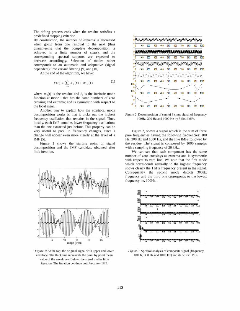
The sifting process ends when the residue satisfies a predefined stopping criterion. By construction, the number of extrema is decreased when going from one residual to the next (thus guaranteeing that the complete decomposition is achieved in a finite number of steps), and the corresponding spectral supports are expected to decrease accordingly. Selection of modes rather corresponds to an automatic and adaptative (signal dependent) time variant filtering [9] and [10].

At the end of the algorithm, we have:

)()()(1

tmtdtx n

n

ii += ∑

=

(1) where mn(t) is the residue and di is the intrinsic mode function at mode i that has the same numbers of zero crossing and extrema; and is symmetric with respect to the local mean.

Another way to explain how the empirical mode decomposition works is that it picks out the highest frequency oscillation that remains in the signal. Thus, locally, each IMF contains lower frequency oscillations than the one extracted just before. This property can be very useful to pick up frequency changes, since a change will appear even more clearly at the level of a IMF [5].

Figure 1 shows the starting point of signal decomposition and the IMF candidate obtained after little iteration.

Figure 1: At the top: the original signal with upper and lower envelope. The thick line represents the point by point mean

value of the envelopes. Below: the signal d after little iteration. The iteration continue until becomes IMF.

Figure 2: Decomposition of sum of 3 sinus signal of frequency

100Hz, 300 Hz and 1000 Hz by 5 first IMFs.

Figure 2, shows a signal which is the sum of three pure frequencies having the following frequencies: 100 Hz, 300 Hz and 1000 Hz, and the five IMFs followed by the residue. The signal is composed by 1000 samples with a sampling frequency of 20 kHz.

We can see that each component has the same number of zero crossings as extrema and is symmetric with respect to zero line. We note that the first mode which corresponds naturally to the highest frequency shows clearly the 1 kHz frequency present in the signal. Consequently the second mode depicts 300Hz frequency and the third one corresponds to the lowest frequency i.e. 100Hz.

Figure 3: Spectral analysis of composite signal (frequency 100Hz, 300 Hz and 1000 Hz) and its 5 first IMFs.

113

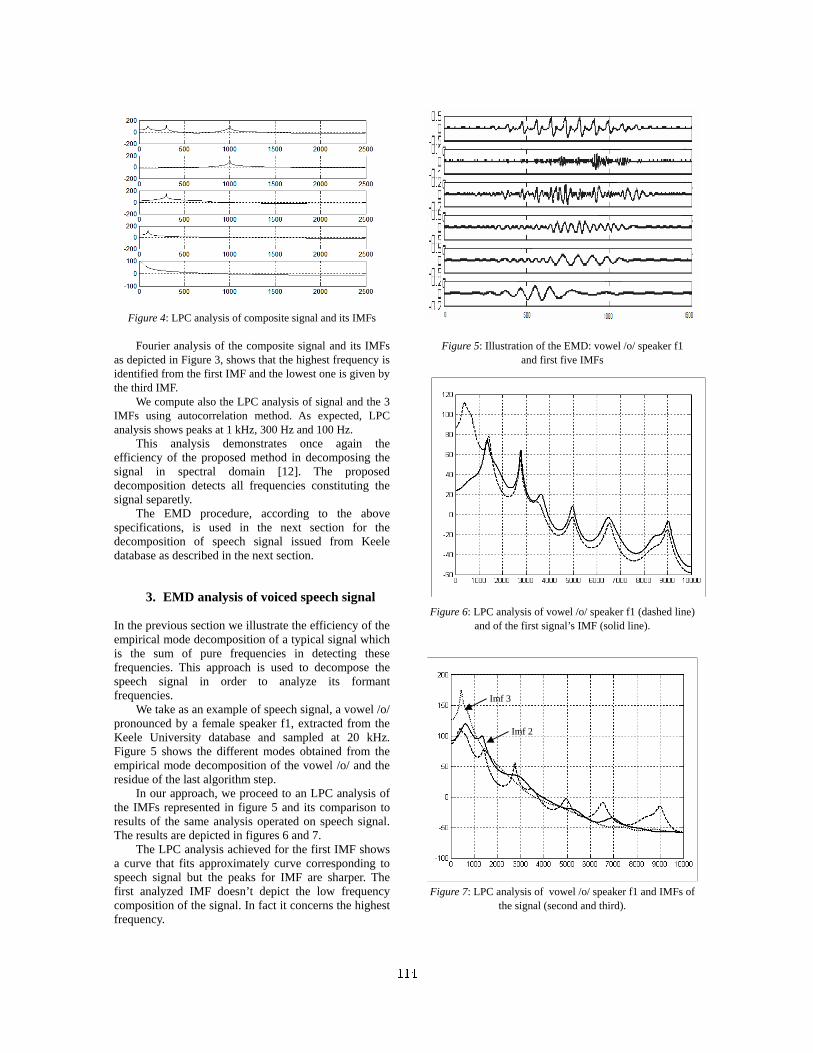
Figure 4: LPC analysis of composite signal and its IMFs

Fourier analysis of the composite signal and its IMFs

as depicted in Figure 3, shows that the highest frequency is identified from the first IMF and the lowest one is given by the third IMF.

We compute also the LPC analysis of signal and the 3 IMFs using autocorrelation method. As expected, LPC analysis shows peaks at 1 kHz, 300 Hz and 100 Hz.

This analysis demonstrates once again the efficiency of the proposed method in decomposing the signal in spectral domain [12]. The proposed decomposition detects all frequencies constituting the signal separetly.

The EMD procedure, according to the above specifications, is used in the next section for the decomposition of speech signal issued from Keele database as described in the next section.

3. EMD analysis of voiced speech signal In the previous section we illustrate the efficiency of the empirical mode decomposition of a typical signal which is the sum of pure frequencies in detecting these frequencies. This approach is used to decompose the speech signal in order to analyze its formant frequencies.

We take as an example of speech signal, a vowel /o/ pronounced by a female speaker f1, extracted from the Keele University database and sampled at 20 kHz. Figure 5 shows the different modes obtained from the empirical mode decomposition of the vowel /o/ and the residue of the last algorithm step.

In our approach, we proceed to an LPC analysis of the IMFs represented in figure 5 and its comparison to results of the same analysis operated on speech signal. The results are depicted in figures 6 and 7.

The LPC analysis achieved for the first IMF shows a curve that fits approximately curve corresponding to speech signal but the peaks for IMF are sharper. The first analyzed IMF doesn’t depict the low frequency composition of the signal. In fact it concerns the highest frequency.

Figure 5: Illustration of the EMD: vowel /o/ speaker f1 and first five IMFs

Figure 6: LPC analysis of vowel /o/ speaker f1 (dashed line) and of the first signal’s IMF (solid line).

Figure 7: LPC analysis of vowel /o/ speaker f1 and IMFs of

the signal (second and third).

Imf 2

Imf 3

114

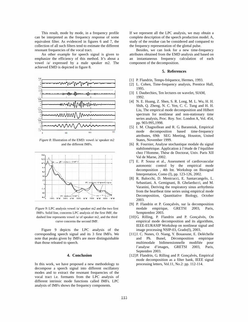
This result, mode by mode, in a frequency profile can be interpreted as the frequency response of some equivalent filter. As evidenced in figures 6 and 7, the collection of all such filters tend to estimate the different resonant frequencies of the vocal tract.

An other example for speech signal is given to emphasize the efficiency of this method. It’s about a vowel /a/ expressed by a male speaker m2. The achieved EMD is depicted in figure 8.

Figure 8: Illustration of the EMD: vowel /a/ speaker m2

and the different IMFs.

Figure 9: LPC analysis vowel /a/ speaker m2 and the two first IMFs. Solid line, concerns LPC analysis of the first IMF, the dashed line represents vowel /a/ of speaker m2, and the third

curve concerns the second IMF.

Figure 9 depicts the LPC analysis of the corresponding speech signal and its 3 first IMFs. We note that peaks given by IMFs are more distinguishable than those releated to speech.

4. Conclusion In this work, we have proposed a new methodology to decompose a speech signal into different oscillatory modes and to extract the resonant frequencies of the vocal tract i.e. formants from the LPC analysis of different intrinsic mode functions called IMFs. LPC analysis of IMFs shows the frequency components.

If we represent all the LPC analysis, we may obtain a complete description of the speech production model. A, study of the residue can be considered and compared to the frequency representation of the glottal pulse. Besides, we can look for a new time-frequency attributes obtained from the EMD analysis and based on an instantaneous frequency calculation of each component of the decomposition.

5. References [1] P. Flandrin, Temps-fréquence, Hermes, 1993. [2] L. Cohen, Time-frequency analysis, Prentice Hall,

1995. [3] I. Daubechies, Ten lectures on wavelet, SIAM, 1992. [4] N. E. Huang, Z. Shen, S. R. Long, M. L. Wu, H. H.

Shih, Q. Zheng, N. C. Yen, C. C. Tung and H. H. Liu, The empirical mode decomposition and Hilbert spectrum for nonlinear and non-stationary time series analysis, Proc. Roy. Soc. London A, Vol. 454, pp. 903-995,1998.

[5] I. M. Chagnollean and R. G. Baranniuk, Empirical mode decomposition based time-frequency attributes, 69th SEG Meeting, Houston, United States, November 1999.

[6] R. Fournier, Analyse stochastique modale du signal stabilométrique. Application à l’étude de l’équilibre chez l’Homme, Thèse de Doctorat, Univ. Paris XII Val de Marne, 2002.

[7] E. P. Sousa et al., Assessment of cardiovascular autonomic control by the empirical mode decomposition , 4th Int. Workshop on Biosignal Interpretation, Como (I), pp. 123-126, 2002.

[8] R. Balocchi, D. Menicucci, E. Santarcangelo, L. Sebastiani, A. Gemignani, B. Ghelarducci, and M. Varanini, Deriving the respiratory sinus arrhythmia from the heartbeat time series using empirical mode Decomposition, Qauntitative Biology, October 2003.

[9] P. Flandrin et P. Gonçalvès, sur la decomposition modale empirique, GRETSI 2003, Paris, Semptembre 2003.

[10] G. Rilling, P. Flandrin and P. Gonçalvès, On empirical mode decomposition and its algorithms, IEEE-EURASIP Workshop on nonlinear signal and image processing NSIP-03, Grado(I), 2003.

[11] J. C. Nunes, O. Niang, Y. Bouaoune, E. Deléchelle and Ph. Bunel, Décomposition empirique multimodale bidimensionnelle modifiée pour l’analyse d’images, GRETSI 2003, Paris, Septembre 2003.

[12] P. Flandrin, G. Rilling and P. Gonçalvès, Empirical mode decomposition as a filter bank, IEEE signal processing letters, Vol.11, No.2: pp. 112-114.

115

Estimation of Speech Features of Glottal Excitation by

Nonlinear Prediction

Karl Schnell, Arild Lacroix

Institute of Applied Physics, Goethe-University Frankfurt

Max-von-Laue-Str. 1, D-60438 Frankfurt am Main, Germany schnell@iap.uni-frankfurt.de

Abstract

Analysis of speech signals can be performed with the aid of

linear or nonlinear statistics using appropriate prediction

algorithms. In this contribution, speech features are treated

using the results of a nonlinear prediction based on Volterra

series. Features are investigated representing the prediction

gain by nonlinear statistics and representing individual

coefficients of the nonlinear components. The features are

estimated quasi continuously resulting in a feature signal.

Additionally, to obtain features which are highly sensitive to

segmentation shifting, an asymmetric window function is

integrated into the prediction algorithm. The analyses of

speech signals show that the estimated features correlate with

the glottal pulses. Furthermore, the investigations show that

using the first individual nonlinear coefficient as a feature is

advantageous over using the prediction gain.

1. Introduction

Speech analysis is usually performed using linear models and

statistics. However, nonlinear components are also contained

in the speech signal [1]. The voiced excitation is caused by

vibrations of the vocal folds which can be described by a

nonlinear oscillator; additionally nonlinear fluid dynamics are

effective. Nonlinear systems and operators, like the energy

operator, can be used for speech analysis [2],[3]. In this

contribution nonlinear components of the speech signal are

estimated by nonlinear prediction. The nonlinear system of a

Volterra series is used for the prediction. The estimation can

be achieved by an adaptive algorithm like LMS or RLS [4].

Another approach for the estimation is to minimize the

prediction error of individual signal segments, which can be

applied to coding [5] or speech generation [6]. For speech

analysis the integration of an appropriate window function can

be relevant [7]. In [7] speech features based on the prediction

gain are discussed. In this contribution, features of nonlinear

coefficients of the predictor are proposed delivering feature

signals advantageously for analysis. Additionally, a post-

processing of the feature signal is carried out accentuating the

regions of glottal closures.

2. Nonlinear Prediction

The nonlinear predictor based on Volterra systems estimates a

signal value ( )x n by a linear combination of last signal

values ( )x n k− and, additionally, by a linear combination

of products of last signal values. Here, without loss of

generality systems are treated with the first and second order

Volterra kernels only, leading to the prediction error

11

21 1

ˆ( ) ( ) :

( ) ( ) ( )

( , ) ( ) ( ) .

N

k

M i

i k

e x n x n

x n h k x n k

h i k x n i x n k

=

= =

= −

= − ⋅ −

′− ⋅ − −

∑

∑∑

(1)

e is the prediction error and ˆ( )x n is the estimation of ( )x n .

The coefficients 1h represent the linear components whereas

2h′ represent the nonlinear components; 2h′ are coefficients

of the second-order kernel 2h , which can be assumed

symmetrically 2 2( , ) ( , )h i k h i k′ = for i k= and

2 2( , ) 2 ( , )h i k h i k′ = ⋅ for i k≠ . For speech analysis the

speech signal is segmented in frames. Due to the

segmentation a window function ( )w n is integrated into the

estimation of the nonlinear prediction. If the window function

is applied directly to the signal ( )x n the prediction error

results in

11

21 1

( ) ( ) ( ) ( ) ( )

( , ) ( ) ( ) ( ) ( )

N

k

M i

i k

e w n x n h k w n k x n k

h i k w n i w n k x n i x n k

=

= =

= − ⋅ − −

′− ⋅ − − − −

∑

∑∑

leading to different weights of the components, especially

between the linear and nonlinear components. For this reason

the window function has to be applied to the error ( )e n

yielding the weighted error ( ) ( ) ( )we n w n e n= ⋅ . Applying to

eq. (1) results in

11

21 1

( ) ( ) ( ) ( ) ( ) ( )

( , ) ( ) ( ) ( ) .

N

w

k

M i

i k

e n w n x n h k w n x n k

h i k w n x n i x n k

=

= =

= ⋅ − ⋅ ⋅ −

′− ⋅ ⋅ − −

∑

∑∑ (2)

The predictor coefficients are determined by minimizing the

weighted error

2( ) minwne n →∑ , (3)

which is explained in the following section.

2.1. Vector based nonlinear prediction

The prediction is applied to a segment of the speech signal, so

that it is convenient to describe the signals by vectors. For

116

that purpose the analyzed weighted signal ( ) ( ) ( )u n w n x n= ⋅

is described by the vector

( )T(0) (0), (1) (1), , ( ) ( )w x w x w K x K= ⋅ ⋅ ⋅u …

of length 1L K= + . Since the prediction error ( )we n

contains last values ( )x n k− , additionally the vectors iu and

,i ku containing the shifted signals with fixed weights are

defined by

( )

T

T,

( (0) ( ), (1) (1 ), , ( ) ( ))

(0) ( ) ( ), (1) (1 ) (1 ), .

i

i k

w x i w x i w K x K i

w x i x k w x i x k

= ⋅ − ⋅ − ⋅ −

= − − − −

u

u

…

…

(4)

The estimation of the weighted signal values ( )u n can be

described by the vector u with

1 2 ,

1 1 1

ˆ ( ) ( , )N M i

i i k

i i k

h i h i k

= = =

′= ⋅ + ⋅∑ ∑∑u u u . (5)

By these definitions the prediction problem can be described

by the vector equation ˆw = −e u u . Since the error depends on

the order N of linear coefficients and order M of nonlinear

coefficients, the error ,N Mw w→e e is extended by the

superscripts N and M:

,1 2 ,

1 1 1

( ) ( , )N M i

N Mw i i k

i i k

h i h i k

= = =

′= − ⋅ − ⋅∑ ∑∑e u u u , (6)

respectively

,

,

,

1

,

2

2

2 2

2

(0) (0) (0) ( 1)(0)

(1) (1) (1) (0)(1)(1)

( ) ( ) ( ) ( 1)( )

(0(0) ( 1)

(1) (0)(1,1) (1,2)

( ) ( 1)

N M

w

N M

N M w

w

N M

w

w x w xe

w x w xeh

w K x K w K x Ke K

ww x

w xh h

w K x K

− = = − −

− ′ ′− − −

e ⋯⋮ ⋮⋮

⋮

) ( 1) ( 2)

(1) (0) ( 1).

( ) ( 1) ( 2)

x x

w x x

w K x K x K

− − − − −

⋯⋮

Equation (6) represents a vector based description of eq. (2).

From the equations (5) and (6) it can be seen that the optimal

prediction u is an expansion of u by the vectors iu and

,i ku . For this expansion the vectors iu and ,i ku are

transformed into an orthogonal basis mv with the dot

products , 0m k =v v . This is performed by the Gram-

Schmidt orthogonalization. Since the vectors of the basis

mv are orthogonal, the optimal coefficients mb in

description of the basis mv can easily be obtained by

2, | |m m mb = u v v ,

yielding an expansion with the vectors mv . Finally the

coefficients mb of basis mv are converted back into the

original basis of ,,i i ku u . The resulting coefficients

minimize the Euclidean norm | ,N Mwe | representing a least

square estimation.

Since in eqs. (2), (6) signal values outside of the frame

appear, represented by negative arguments of n k− , the

vector lengths are truncated in such a way that only values

inside of the analyzed segment appear in the vectors.

3. Speech Features

The results of the nonlinear prediction can be utilized to

define speech features. One approach is to consider the

prediction gain by the nonlinear components. The gain can be

described by the ratio between the prediction errors with and

without nonlinear components, which is used in [7]. The

logarithmic error ratio leads to the feature definition:

,0

,gain ,

log

NwN M

N Mw

F

=

e

e

.

Nonlinear coefficients 2( , )h i k′ are considered for the

prediction error of the denominator, which can be seen from

the superscript M. Since the nonlinear coefficients contribute

only to a decrease of the prediction error, the feature ,gainN MF

has positive values.

Another approach for defining features is to consider

individual values of the estimated predictor coefficients,

especially these of the nonlinear components. Here the value

of the nonlinear coefficients 2( , )h i k′ of the prediction of

orders N and M are used leading to the feature

,2, ( , )N M

i kF h i k′= .

3.1. Feature signals

The feature F is obtained from the results of the nonlinear

prediction. To consider the time-dependence of the feature,

the speech signal is segmented into overlapping frames

analyzed individually. Applying the nonlinear prediction to

each segment yields the corresponding values of the speech

feature F. To measure the features quasi continuously in time,

the displacement of the segments is chosen to one sample.

Hence, the sequence of the feature values which are estimated

from the segments represents a feature signal ( )F n . Each

value ( )F n is obtained from the nonlinear prediction of a

segment. The estimation is influenced by the type of the

window function w of the prediction algorithm. If a Hann-

window is used, the feature F can be estimated smoothly in

time, however, the time resolution of the feature estimation is

blurred. This behaviour is caused by the shape of the window;

the Hann window is insensitive to small changes of the

segmentation since its values tend continuously towards zero

to the left and right side. In contrast to that, an asymmetric

window with a value greater one at one side is sensitive to

small changes of the segmentation and can deliver a more

precise time resolution. The window aw defined by

( )( )2

( / 4)

/ 4 4

( ) 1 for 0 / 4 1

( ) 0.5 1 cos for

a

k K Ka K K

w k k K

w k k Kπ −

−

= = −

= + =

…

…

117

delivering a strong discontinuity between the left-side values

and values outside of the window, which can be assumed as

zero. The asymmetric window is shown in fig. 1.

Figure 1: Asymmetric window function aw .

4. Analysis of Speech

For the analysis of individual sounds and speech utterances,

speech signals with a sampling rate of 16 kHz are

investigated. The speech signals are segmented and analyzed

as described in the previous section. Fig. 2 shows the

estimated feature signals 16,1gain ( )F n and 16,1

1,1 ( )F n from the

analysis of the vowel /a/; additionally, the original speech

waveform and the LPC-residual is shown. The main impulses

of the residual of fig. 2(b) indicate the abrupt glottal closures,

which are denoted as the glottal closure instances (CGI). It

can be seen that the feature signal has peaks correlating with

those of the residual. Hence, the peaks of the feature signals

indicate the CGI. The high time resolution of the feature

signal results from the asymmetric window. In the case of

voiced fricatives often many impulses occur in the residual,

which can be seen from fig. 3 showing the analysis of the

voiced fricative /z/. The LPC-residual shows a more or less

unperiodic structure and especially the high incidence of

pulses makes it hard to detect the impulses corresponding to

the glottal closures. In contrast to that, the feature signals are

more periodic and have fewer pulses. The analyses show that

the feature signal 16,11,1 ( )F n shows even mostly only one

dominant positive pulse per period corresponding to the

glottal closure; therefore the feature 16,11,1 ( )F n is advantageous

in comparison to the prediction gain delivering often more

potential pulses per period. One reason for that is given in the

following: For the prediction with order 1M = only the

nonlinear coefficient 2(1,1)h′ is effective. The prediction gain

depends on the absolute value of the coefficient, whereas the

feature 16,11,1 ( )F n preserves the information about the sign of

the coefficient 2(1,1)h′ . Analysis results show that the glottal

closures cause impulses with positive sign. Other regions of

the feature signal show also impulses or bulges, however, for 16,1

1,1 ( )F n they have usually negative sign. Hence, by the

feature signal 16,11,1 ( )F n the impulses of glottal closure can be

separated from the other regions with the aid of the sign of

2(1,1)h′ . In comparison to that the feature 16,1gain ( )F n cannot

distinguish since the information of the sign is lost in the

prediction gain.

Figure 2: Analysis of the vowel /a/: (a) analyzed speech

signal, (b) corresponding LPC-residual, (c) feature signal

of prediction gain 16,1gain ( )F n , (d) feature signal 16,1

1,1 ( )F n .

Figure 3: Analysis of the voiced fricative /z/: (a) analyzed

speech, (b) corresponding LPC-residual, (c) feature signal

of prediction gain 16,1gain ( )F n , (d) feature signal 16,1

1,1 ( )F n .

Overall, the analyses show that especially the feature signal 16,1

1,1 ( )F n is suitable for detection of regions of glottal closures

not only for stationary speech signals, but also for speech

utterances. A post-processing of the feature signal is useful to

mark the regions of glottal closures. At first, fluctuations of

the mean value differing from zero should be compensated;

additionally, the power of the feature signal should be

balanced achieving a constant envelope of the amplitude.

Therefor a short-time estimation of the mean of the feature

signal is subtracted to each feature value. After that, each

feature value is divided by a short-time estimation of the

power of the feature signal resulting in the modified feature

signal 16,11,1 ( )F nɶ .

Figure 4 shows the analysis of the German word [nUl]. The

curves 4(c) and (d) show the initial feature and the modified

feature signal 16,11,1 ( )F nɶ ; variations of the mean and the power

of the feature signal are balanced. After that the modified

118

Figure 4: Analysis of word [nUl]: (a) analyzed speech

signal, (b) feature signal of prediction gain 16,1gain ( )F n , (c)

feature signal 16,11,1 ( )F n , (d) processed feature 16,1

1,1 ( )F nɶ ,

(e) derived feature signal ( )f n′ .

feature signal is convolved by a finite pattern-signal g

depicted in fig. 5 which has a pointed shape resulting in the

signal

16,11,1( ) ( ) ( )f n F n g n= ∗ɶ ;

the mean value of the signal g is zero. The convolution

implies dot products with time-shifted segments. If the

segment is similar to the pointed shape, a high value results.

Figure 5: Pattern-signal g.

Since only positive correlations with the pointed shape are of

interest, negative values of f are set to zero by

'( ) ( ( ) sgn( ( )) ( )) / 2f n f n f n f n= + ⋅ .

The curve 4(e) shows the derived feature signal '( )f n

representing the positive values of the convolution results of

the modified feature signal of the utterance [nUl]. The peaks

indicate regions of glottal pulses.

In figure 6 the analysis result for the utterance [vaIma] of the

German word “Weimar” is shown. It can be seen that the

corresponding feature signal ( )f n′ represents a sequence of

pulses, which is disturbed only occasionally by artifacts.

Figure 6: Analysis of word [vaIma]: (a) analyzed speech

signal, (b) derived feature signal ( )f n′ .

5. Conclusions

Speech features based on nonlinear prediction are proposed

and discussed for the analysis of speech. The features are

correlated with the voiced excitation and especially with the

glottal pulses. For analysis of real speech, one important

feature of estimation algorithms is their robustness.

Concerning this, features based on the first nonlinear

prediction coefficient have been proven advantageously in

comparison to the prediction gain. The deciding reason for

this fact is that the informational content of the sign of the

coefficient is useful. By the use of that feature signal with an

additional post-processing the algorithm is applicable to

analyse real speech.

6. References

[1] M. Faundez et al., "Nonlinear Speech Processing: Over-

view and Applications", in Int. J. Control Intelligent Syst.,

vol. 30, no. 1, pp. 1–10, 2002.

[2] P. Maragos, T. Quatieri, and J. Kaiser, "Speech Nonlin-

earities, Modulations, and Energy Operators", in Proc.

ICASSP’91, 1991, pp. 421-424.

[3] L. Atlas and J. Fang, "Quadratic Detectors for General

Nonlinear Analysis of Speech", in Proc. ICASSP’92, vol. II,

1992, pp. 9–12.

[4] E. Mumolu, A. Carini, and D. Francescato, "ADPCM

With Non Linear Predictors", in Proc. EUSIPCO’94, 1994,

pp. 387–390.

[5] J. Thyssen, H. Nielsen, and S. D. Hansen, "Non-linear

Short-term Prediction in Speech Coding", in Proc.

ICASSP’94, vol. I, 1994 pp. 185–188.

[6] K. Schnell and A. Lacroix, "Modeling Fluctuations of

Voiced Excitation for Speech Generation Based on Recur-

sive Volterra Systems", contribution in Nonlinear Analyses

and Algorithms for Speech Processing – NOLISP’05, LNAI

Vol. 3817, pp. 338-347, Springer 2005.

[7] K. Schnell and A. Lacroix, "Weighted Nonlinear

Prediction Based on Volterra Series for Speech Analysis'', in

Proc. EUSIPCO’06, Florence 2006.

119

An efficient VAD based on a Generalized Gaussian PDF

O. Pernıa, J.M. Gorriz, J. Ramırez and C.G. Puntonet and I. Turias

Department of Signal TheoryUniversity of Granada, Granada, Spain

gorriz@ugr.es

AbstractThe emerging applications of wireless speech communicationare demanding increasing levels of performance in noise ad-verse environments together with the design of high responserate speech processing systems. This is a serious obstacle tomeet the demands of modern applications and therefore thesesystems often needs a noise reduction algorithm working incombination with a precise voice activity detector (VAD). Thispaper presents a new voice activity detector (VAD) for improv-ing speech detection robustness in noisy environments and theperformance of speech recognition systems. The algorithm de-fines an optimum likelihood ratio test (LRT) involving Multipleand correlated Observations (MCO). An analysis of the method-ology for N = 2, 3 shows the robustness of the proposed ap-proach by means of a clear reduction of the classification erroras the number of observations is increased. The algorithm isalso compared to different VAD methods including the G.729,AMR and AFE standards, as well as recently reported algo-rithms showing a sustained advantage in speech/non-speech de-tection accuracy and speech recognition performance.

1. IntroductionThe emerging applications of speech communication are de-manding increasing levels of performance in noise adverse envi-ronments. Examples of such systems are the new voice servicesincluding discontinuous speech transmission [1, 2, 3] or distrib-uted speech recognition (DSR) over wireless and IP networks[4]. These systems often require a noise reduction schemeworking in combination with a precise voice activity detector(VAD) [5] for estimating the noise spectrum during non-speechperiods in order to compensate its harmful effect on the speechsignal.

During the last decade numerous researchers have studieddifferent strategies for detecting speech in noise and the influ-ence of the VAD on the performance of speech processing sys-tems [5]. Sohn et al. [6] proposed a robust VAD algorithmbased on a statistical likelihood ratio test (LRT) involving a sin-gle observation vector. Later, Cho et al [7] suggested an im-provement based on a smoothed LRT. Most VADs in use to-day normally consider hangover algorithms based on empiricalmodels to smooth the VAD decision. It has been shown re-cently [8, 9] that incorporating long-term speech informationto the decision rule reports benefits for speech/pause discrim-ination in high noise environments, however an important as-sumption made on these previous works has to be revised: theindependence of overlapped observations. In this work we pro-pose a more realistic one: the observations are jointly gaussiandistributed with non-zero correlations. In addition, importantissues that need to be addressed are: i) the increased computa-tional complexity mainly due to the definition of the decision

rule over large data sets, and ii) the optimum criterion of thedecision rule. This work advances in the field by defining adecision rule based on an optimum statistical LRT which in-volves multiple and correlated observations. The paper is orga-nized as follows. Section 2 reviews the theoretical backgroundon the LRT statistical decision theory. Section 4 considers itsapplication to the problem of detecting speech in a noisy sig-nal. Finally in Section 4.1 we discuss the suitability of the pro-posed approach for pair-wise correlated observations using theexperimental data set AURORA 3 subset of the original SpanishSpeechDat-Car (SDC) database [10] and state some conclusionsin section 6.

2. Multiple Observation Probability RatioTest

Under a two hypothesis test, the optimal decision rule that min-imizes the error probability is the Bayes classifier. Given anobservation vector y to be classified, the problem is reduced toselecting the hypothesis (H0 or H1) with the largest posteriorprobability P(Hi|y). From the Bayes rule:

L(y) =py|H1(y|H1)

py|H0(y|H0)

><

P [H0]

P [H1]⇒ y↔H1

y↔H0(1)

In the LRT, it is assumed that the number of observationsis fixed and represented by a vector y. The performance ofthe decision procedure can be improved by incorporating moreobservations to the statistical test. When N measurements y1,y2, . . . , yN are available in a two-class classification problem,a multiple observation likelihood ratio test (MO-LRT) can bedefined by:

LN (y1, y2, ..., yN ) =py1,y2,...,yN |H1(y1, y2, ..., yN |H1)

py1,y2,...,yN |H0(y1, y2, ..., yN |H0)(2)

This test involves the evaluation of an N-th order LRTwhich enables a computationally efficient evaluation when theindividual measurements yk are independent. However, theyare not since the windows used in the computation of the obser-vation vectors yk are usually overlapped. In order to evaluatethe proposed MCO-LRT VAD on an incoming signal, an ade-quate statistical model for the feature vectors in presence andabsence of speech needs to be selected. The joint probabilitydistributions under both hypotheses are assumed to be jointlygaussian independently distributed in frequency and in each part(real and imaginary) of vector with correlation components be-tween each pair of frequency observations:

LN (y1, y2, ..., yN ) =Q

p∈R,IQω

pyω1 ,yω

2 ,...,yωN|H1

(yω1 ,yω

2 ,...,yωN |H1)

pyω1 ,yω

2 ,...,yωN|H0

(yω1 ,yω

2 ,...,yωN|H0)p (3)

120

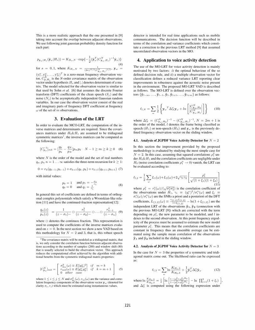
This is a more realistic approach that the one presented in [9]taking into account the overlap between adjacent observations.We use following joint gaussian probability density function foreach part:

pyω|Hs(yω|Hs)) = KHs,N · exp−1

2(yT

ω (CNyω,Hs

)−1yω)(4)

for s = 0, 1, where KHs,N = 1

(2π)N/2|CNyω,Hs

|1/2 , yω =

(yω1 , yω

2 , . . . , yωN )T is a zero-mean frequency observation vec-

tor, CNy,Hs

is the N-order covariance matrix of the observationvector under hypothesis Hs and |.| denotes determinant of a ma-trix. The model selected for the observation vector is similar tothat used by Sohn et al. [6] that assumes the discrete Fouriertransform (DFT) coefficients of the clean speech (Sj) and thenoise (Nj) to be asymptotically independent Gaussian randomvariables. In our case the observation vector consist of the realand imaginary parts of frequency DFT coefficient at frequencyω of the set of m observations.

3. Evaluation of the LRTIn order to evaluate the MCO-LRT, the computation of the in-verse matrices and determinants are required. Since the covari-ances matrices under H0&H1 are assumed to be tridiagonalsymmetric matrices1, the inverses matrices can be computed asthe following:

[C−1yω

]mk = [qk

pk− qN

pN]pmpk N − 1 ≥ m ≥ k ≥ 0 (6)

where N is the order of the model and the set of real numbersqn, pn n = 1 . . .∞ satisfies the three-term recursion for k ≥ 1:

0 = rk(qk−1, pk−1)+σk+1(qk, pk)+ rk+1(qk+1, pk+1) (7)

with initial values:

p0 = 1q0 = 0

and p1 = −σ1r1

and q1 = 1r1

(8)

In general this set of coefficients are defined in terms of orthog-onal complex polynomials which satisfy a Wronskian-like rela-tion [11] and have the continued-fraction representation[12]:

qn(z)

pn(z)

=

1

(z − σ1)− ªr21

(z − σ2)− ª . . .ª r2n−1

(z − σn)(9)

where ª denotes the continuos fraction. This representation isused to compute the coefficients of the inverse matrices evalu-ated on z = 0. In the next section we show a new VAD based onthis methodology for N = 2 and 3, that is, this robust speech

1The covariance matrix will be modeled as a tridiagonal matrix, thatis, we only consider the correlation function between adjacent observa-tions according to the number of samples (200) and window shift (80)that is usually selected to build the observation vector. This approachreduces the computational effort achieved by the algorithm with addi-tional benefits from the symmetric tridiagonal matrix properties:

[CNyω

]mk =

24

σ2ym

(ω) ≡ E[|yωm|2] if m = k

rmk(ω) ≡ E[yωmyω

k ] if k = m + 10 other case

35 (5)

where 1 ≤ i ≤ j ≤ N and σ2yi

(ω), rij(ω) are the variance and corre-lation frequency components of the observation vector yω (denoted forclarity σi, ri) which must be estimated using instantaneous values.

detector is intended for real time applications such us mobilecommunications. The decision function will be described interms of the correlation and variance coefficients which consti-tute a correction to the previous LRT method [9] that assumeduncorrelated observation vectors in the MO.

4. Application to voice activity detectionThe use of the MO-LRT for voice activity detection is mainlymotivated by two factors: i) the optimal behaviour of the sodefined decision rule, and ii) a multiple observation vector forclassification defines a reduced variance LRT reporting clearimprovements in robustness against the acoustic noise presentin the environment. The proposed MO-LRT VAD is describedas follows. The MO-LRT is defined over the observation vec-tors yl−m, . . . , yl−1, yl, yl+1, . . . , yl+m as follows:

`l,N =X

ω

1

2

(yω

T ∆ωNyω + ln

"|CN

yω,H0 ||CN

yω,H1|

#)(10)

where ∆ωN = (CN

yω,H0)−1 − (CN

yω,H1)−1, N = 2m + 1 is

the order of the model, l denotes the frame being classified asspeech (H1) or non-speech (H0) and yω is the previously de-fined frequency observation vector on the sliding window.

4.1. Analysis of JGPDF Voice Activity Detector for N = 2

In this section the improvement provided by the proposedmethodology is evaluated by studying the most simple case forN = 2. In this case, assuming that squared correlations ρ2

1 un-der H0&H1 and the correlation coefficients are negligible underH0 (noise correlation coefficients ρn

1 → 0) vanish, the LRT canbe evaluated according to:

`l,2 =1

2

Xω

L1(ω)+L2(ω)+2√

γ1γ2

"ρs1p

(1 + ξ1)(1 + ξ2)

#

(11)where ρs

1 = rs1(ω)/(

√σs

1σs2) is the correlation coefficient of

the observations under H1, γi ≡ (yωi )2/σn

i (ω) and ξi ≡σs

i (ω)/σni (ω) are the SNRs a priori and a posteriori of the DFT

coefficients, L1,2(ω) ≡ γ1,2ξ1,21+ξ1,2

− ln(1 + ξ1,2) are theindependent LRT of the observations y1, y2 (connection withthe previous MO-LRT [9]) which are corrected with the termdepending on ρs

1, the new parameter to be modeled, and l in-dexes to the second observation. At this point frequency ergod-icity of the process must be assumed to estimate the new modelparameter ρs

1. This means that the correlation coefficients areconstant in frequency thus an ensemble average can be esti-mated using the sample mean correlation of the observationsy1 and y2 included in the sliding window.

4.2. Analysis of JGPDF Voice Activity Detector for N = 3

In the case for N = 3 the properties of a symmetric and tridi-agonal matrix come out. The likelihood ratio can be expressedas:

`l,3 =X

ω

lnKH1,3

KH0,3+

1

2yT

ω ∆ω3 yω (12)

where lnKH1,3KH0,3

= 12

hlnh

1−(ρ21+ρ2

2)H0

1−(ρ21+ρ2

2)H1

i− ln

Q3i=1(1 + ξi)

i,

and ∆ω3 is computed using the following expression under

121

7.5 8 8.5 9 9.5

x 104

−2

−1

0

1

2

3x 10

4

7.5 8 8.5 9 9.5

x 104

−50

−40

−30

−20

−10

0

10

Noisy SpeechjGpdf VAD decision N=3

jGpdf−LRT N=3jGpdf−LRT N=2MO−LRT

(a)

0

20

40

60

80

100

0 5 10 15 20 25 30FALSE ALARM RATE (FAR0)

PAUSE HIT RATE (HR0)

Sohn's VAD

jGpdf VAD N=2

(b)

Figure 1: a) JGPDF-VAD vs. MO-LRT decision for N = 2 and3. b) ROC curve for JGPDF VAD with lh = 8 and Sohn’s VAD[6] using a similar hang-over mechanism.

hypotheses H0&H1:

yTω (C3

yω,Hs)−1yω = 1

1−(ρ21+ρ2

2)

h1−ρ2

2σ1

(yω1 )2 +

(yω2 )2

σ2. . .i

h+

1−ρ21

σ3(yω

3 )2 − 2ρ1yω1 yω

2√σ1σ2

− 2ρ2yω2 yω

3√σ2σ3

+ 2ρ1ρ2yω1 yω

3√σ1σ3

i

(13)Assuming that squared correlations under H0&H1 and the

correlations under H0 vanish, the log-LRT can be evaluated asthe following:

`l,3 = 12

Pω

P3i=1 Li(ω) +

2√

γ1γ2ρs1√

(1+ξ1)(1+ξ2)

+2√

γ2γ3ρs2√

(1+ξ2)(1+ξ3)− 2

√γ1γ3ρs

1ρs2√

(1+ξ1)(1+ξ2)2(1+ξ3)

(14)

5. Experimental FrameworkThe ROC curves are frequently used to completely describe theVAD error rate. The AURORA 3 subset of the original Span-ish SpeechDat-Car (SDC) database [10] was used in this analy-sis. The files are categorized into three noisy conditions: quiet,low noisy and highly noisy conditions, which represent differ-ent driving conditions with average SNR values between 25dB,and 5dB. The non-speech hit rate (HR0) and the false alarm rate(FAR0= 100-HR1) were determined in each noise condition.

Using the proposed decision functions (equations 14 and11) we obtain an almost binary decision rule as it is shown infigure 1(a) which accurately detects the beginnings of the voice

0

20

40

60

80

100

0 5 10 15 20 25 30 35FALSE ALARM RATE (FAR0)

PAUSE HIT RATE (HR0)

jGpdf LRT VAD N=3, ho=0, m=1

jGpdf LRT VAD N=3, ho=4, m=1

jGpdf LRT VAD N=3, ho=6, m=1

jGpdf LRT VAD N=3, ho=8, m=1

jGpdf LRT VAD N=3, ho=10, m=1

(a)

0

20

40

60

80

100

0 5 10 15 20 25 30 35 40FALSE ALARM RATE (FAR0)

PAUSE HIT RATE (HR0)

G.729

AMR1

AMR2

AFE (Noise Est.)

AFE (frame-dropping)

Li

Li (TU=3 db, TL= -3dB)

Marzinzik

Sohn

Woo

jGpdf VAD ho=8, N=2, m=8

jGpdf VAD ho=8, N=2, m=1

jGpdf VAD ho=8, N=3, m=1

(b)

Figure 2: a) ROC curve analysis of the jGpdf-VAD (N = 3)for the selection of the hang-over parameter lh. b) ROC curvesof the jGpdf-VAD using contextual information (eight MO win-dows for N = 2) and standards and recently reported VADs.

periods. In this figure we have used the same level of informa-tion in both methods (m = 1). The detection of voice endingsis improved using a hang-over scheme based on the decision ofprevious frames. Observe how this strategy cannot be appliedto the independent LRT [6] because of its hard decision rule andchanging bias as it is shown in the same figure. We implementa very simple hang-over mechanism based on contextual infor-mation of the previous frames, thus no delay obstacle is addedto the algorithm:

`hl,N = `l,N + `l−lh,N (15)

where the parameter lh is selected experimentally. The ROCcurve analysis for this hang-over parameter is shown in figure2(a) for N = 3 where the influence of hang-over in the zerohit rate is studied with variable detection threshold. Finally, thebenefits of contextual information [9] can be incorporated justaveraging the decision rule over a set of multiple observationswindows (two observations for each window). A typical valuefor m = 8 produces increasing levels of detection accuracy asit is shown in the ROC curve in figure 2(b). Of course, these re-sults are not the optimum ones since only pair-wise dependenceis considered here. However for a small number of observationsthe proposed VAD presents the best trade-off between detectionaccuracy and delay.

122

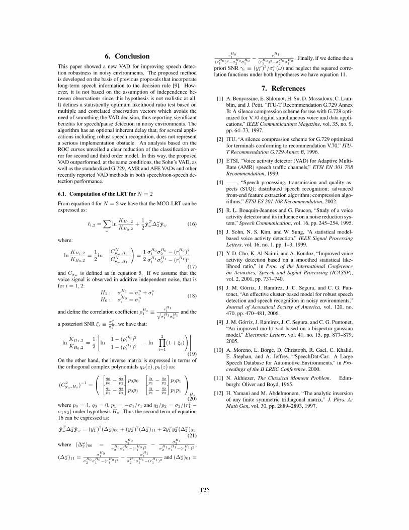
6. ConclusionThis paper showed a new VAD for improving speech detec-tion robustness in noisy environments. The proposed methodis developed on the basis of previous proposals that incorporatelong-term speech information to the decision rule [9]. How-ever, it is not based on the assumption of independence be-tween observations since this hypothesis is not realistic at all.It defines a statistically optimum likelihood ratio test based onmultiple and correlated observation vectors which avoids theneed of smoothing the VAD decision, thus reporting significantbenefits for speech/pause detection in noisy environments. Thealgorithm has an optional inherent delay that, for several appli-cations including robust speech recognition, does not representa serious implementation obstacle. An analysis based on theROC curves unveiled a clear reduction of the classification er-ror for second and third order model. In this way, the proposedVAD outperformed, at the same conditions, the Sohn’s VAD, aswell as the standardized G.729, AMR and AFE VADs and otherrecently reported VAD methods in both speech/non-speech de-tection performance.

6.1. Computation of the LRT for N = 2

From equation 4 for N = 2 we have that the MCO-LRT can beexpressed as:

`l,2 =X

ω

lnKH1,2

KH0,2+

1

2yT

ω ∆ω2 yω (16)

where:

lnKH1,2

KH0,2=

1

2ln

|CN

yω,H0 ||CN

yω,H1|

!=

1

2

σH01 σH0

2 − (rH01 )2

σH11 σH1

2 − (rH11 )2

(17)and Cyω is defined as in equation 5. If we assume that thevoice signal is observed in additive independent noise, that isfor i = 1, 2:

H1 : σH1i = σn

i + σsi

H0 : σH0i = σn

i

(18)

and define the correlation coefficient ρHs1 ≡ r

H11q

σH11 σ

H12

and the

a posteriori SNR ξi ≡ σsi

σni

, we have that:

lnKH1,2

KH0,2=

1

2

"ln

1− (ρH0

1 )2

1− (ρH11 )2

− ln

2Y

i=1

(1 + ξi)

!#

(19)On the other hand, the inverse matrix is expressed in terms ofthe orthogonal complex polynomials qk(z), pk(z) as:

(C2yω,Hs

)−1 =

0@h

q0p0− q2

p2

ip0p0

hq1p1− q2

p2

ip0p1h

q1p1− q2

p2

ip0p1

hq1p1− q2

p2

ip1p1

1A

Hs

(20)where p0 = 1, q0 = 0, p1 = −σ1/r1 and q2/p2 = σ2/(r2

1 −σ1σ2) under hypothesis Hs. Thus the second term of equation16 can be expressed as:

yTω ∆ω

2 yω = (yω1 )2(∆ω

2 )00 + (yω2 )2(∆ω

2 )11 + 2yω1 yω

2 (∆ω2 )01(21)

where (∆ω2 )00 =

σH02

σH02 σ

H01 −(r

H01 )2

− σH12

σH12 σ

H11 −(r

H11 )2

,

(∆ω2 )11 =

σH01

σH02 σ

H01 −(r

H01 )2

− σH11

σH12 σ

H11 −(r

H11 )2

and (∆ω2 )01 =

rH01

(rH01 )2−σ

H02 σ

H01

− rH11

(rH01 )2−σ

H02 σ

H01

. Finally, if we define the a

priori SNR γi ≡ (yωi )2/σn

i (ω) and neglect the squared corre-lation functions under both hypotheses we have equation 11.

7. References[1] A. Benyassine, E. Shlomot, H. Su, D. Massaloux, C. Lam-

blin, and J. Petit, “ITU-T Recommendation G.729 AnnexB: A silence compression scheme for use with G.729 opti-mized for V.70 digital simultaneous voice and data appli-cations,” IEEE Communications Magazine, vol. 35, no. 9,pp. 64–73, 1997.

[2] ITU, “A silence compression scheme for G.729 optimizedfor terminals conforming to recommendation V.70,” ITU-T Recommendation G.729-Annex B, 1996.

[3] ETSI, “Voice activity detector (VAD) for Adaptive Multi-Rate (AMR) speech traffic channels,” ETSI EN 301 708Recommendation, 1999.

[4] ——, “Speech processing, transmission and quality as-pects (STQ); distributed speech recognition; advancedfront-end feature extraction algorithm; compression algo-rithms,” ETSI ES 201 108 Recommendation, 2002.

[5] R. L. Bouquin-Jeannes and G. Faucon, “Study of a voiceactivity detector and its influence on a noise reduction sys-tem,” Speech Communication, vol. 16, pp. 245–254, 1995.

[6] J. Sohn, N. S. Kim, and W. Sung, “A statistical model-based voice activity detection,” IEEE Signal ProcessingLetters, vol. 16, no. 1, pp. 1–3, 1999.

[7] Y. D. Cho, K. Al-Naimi, and A. Kondoz, “Improved voiceactivity detection based on a smoothed statistical like-lihood ratio,” in Proc. of the International Conferenceon Acoustics, Speech and Signal Processing (ICASSP),vol. 2, 2001, pp. 737–740.

[8] J. M. Gorriz, J. Ramırez, J. C. Segura, and C. G. Pun-tonet, “An effective cluster-based model for robust speechdetection and speech recognition in noisy environments,”Journal of Acoustical Society of America, vol. 120, no.470, pp. 470–481, 2006.

[9] J. M. Gorriz, J. Ramirez, J. C. Segura, and C. G. Puntonet,“An improved mo-lrt vad based on a bispectra gaussianmodel,” Electronic Letters, vol. 41, no. 15, pp. 877–879,2005.

[10] A. Moreno, L. Borge, D. Christoph, R. Gael, C. Khalid,E. Stephan, and A. Jeffrey, “SpeechDat-Car: A LargeSpeech Database for Automotive Environments,” in Pro-ceedings of the II LREC Conference, 2000.

[11] N. Akhiezer, The Classical Moment Problem. Edim-burgh: Oliver and Boyd, 1965.

[12] H. Yamani and M. Abdelmonem, “The analytic inversionof any finite symmetric tridiagonal matrix,” J. Phys. A:Math Gen, vol. 30, pp. 2889–2893, 1997.

123

Index of authors

Ahadi, Seyed Mohammad, 88Ahadi, Seyyed Mohammad, 104Akgul, Tayfun, 11, 31Alías, Francesc, 6, 15Arruti, Andoni, 71Atas, Mehmet, 11

Baykut, Suleyman, 11Ben Aicha, Anis, 84Ben Jebara, Soa, 84Bengio, Samy, 47Bouzid, Aïcha, 112

Castro-Bleda, María José, 92Cearreta, Idoia, 71Charbuillet, Christophe, 23Chetouani, Mohamed, 23Chilton, E., 80

Domont, Xavier, 43Drepper, Friedhelm R., 75Díaz-de-María, Fernando, 51

Ellouze, Noureddine, 112Errity, Andrew, 39España-Boquera, Salvador, 92

Faraji, Neda, 88, 104Faundez-Zanuy, Marcos, 19Feng, Ji, 100Fernández-Baillo, Roberto, 63Frankel, Joe, 27

Garay, Nestor, 71García-Moral, Ana I., 51Gas, Bruno, 23Gerber, Michael, 35Goerick, Christian, 43Gonzalvo, Xavi, 6Gorbe-Moya, Jorge, 92Grangier, David, 47Gravier, Guillaume, 55

Gómez-Vilda, Pedro, 63Górriz, Juan M., 120

Hamam, Habib, 59Heckmann, Martin, 43

Iriondo, Ignasi, 6, 15

Joublin, Frank, 43

Kaufmann, Tobias, 35Keshet, Joseph, 47Kirkpatrick, Barry, 39

Lacroix, Arild, 116Lazkano, Elena, 71Liu, Zhaojie, 100López, Juan Miguel, 71

Mazaira-Fernández, Luis Miguel, 63McKenna, John, 39Menzel, Stefan, 43Mirghafori, Nikki, 27Monzo, Carlos, 6Moraru, Daniel, 55

O'Shaughnessy, Douglas, 59Ozkurt, Tolga Esat, 31

Paraskevas, I., 80Peláez-Moreno, Carmen, 51Pernía, Oscar, 120Pster, Beat, 35Planet, Santiago, 15Puntonet, Carlos, 120

Ramírez, Javier, 120Rangoussi, M., 80Richmond, Korin, 67Rodellar-Biarge, Victoria, 63

Schnell, Karl, 116Selouani, Sid-Ahmed, 59

124

Sendho, Bernhard, 43Shao, Jian, 100Shariati, Seyedeh Saloomeh, 88Sierra, Basilio, 71Silva, Denilson, 108Socoró, Joan Claudi, 6, 15Solera-Ureña, Rubén, 51Stoll, Lara, 27

Turias, Ignacio, 120

Ulug, Ufuk, 31

Wersing, Heiko, 43

Yan, Yonghong, 96, 100Yang, Lin, 96

Zamora-Martínez, Francisco, 92Zarader, Jean Luc, 23Zhang, Jianping, 96Zhang, Pengyuan, 100Zhao, Qingwei, 100

Álvarez, Aitor, 71Álvarez-Marquina, Agustín, 63

125