Research summer 2010-summer 2011

By Arna Friend under the direction of Dr. Mark Fowler

Table of ContentsTable of Figures.....................................................21. Abstract..........................................................2

2. DSP background knowledge..........................................32.1.1 Relationship Between Analog and Digital....................3

2.1.2 Poly-phase Filter and Decimate.............................32.1.3 Polyphase Filter and Interpolate...........................5

3. FDOA/TDOA.........................................................64. Boxcar Versus Equiripple Filters..................................6

4.1 General Characteristics of Rectangular Windows used in Stein’s Algorithm...........................................................6

4.2 Performance of Rectangular Filters in terms of Computational Efficiency and Aliasing Error.......................................7

4.3 Performance of Equiripple FIR filters in terms of Computational Efficiency and Aliasing Error.......................................7

5. Effects of Decimation............................................106. Graphical Results................................................12

6.1 Doppler Sweep.................................................126.2 Delay Sweep...................................................13

7. Error Reduction..................................................138. Error Sources....................................................14

8.1 Aliasing of Higher Frequencies to Lower Frequencies...........148.2 Decimation Factor Order.......................................16

8.3 Artificial Low Frequency Content..............................16

1

9. Efficiency.......................................................1710. Optimization...................................................17

10.1 Discussion of Optimization Strategy...........................1710.2 Gradient Descent Optimization.................................19

11. Time Compression Modeled as Sampling Rate Change...............2012. Appendix A: Tabulated Data, Doppler Sweep......................20

13. Appendix B: Tabulated Results, Delay Sweep.....................2514. References.....................................................29

1. Table of FiguresFigure 1: First Remez Impulse Response, M = 5, Fs = 1e6..............8Figure 2: First Remez Filter in the Frequency Domain.................9Figure 3: Second Remez Impulse Response, M = 5, Fs = 200000..........9Figure 4: Second Filter in The Frequency Domain......................9Figure 5: Third Remez Filter Impulse Response, M = 2, Fs = 40000....10Figure 6: Third Filter in the Frequency Domain......................10Figure 7: Low Pass Equivalent Signal in The Frequency Domain........11Figure 8: Doppler Range of Lag Product Signal Before Decimation.....11Figure 9: Doppler range of lag Product Signal After Decimation......11Figure 10: Doppler Range of LP signal in the Frequency Domain Prior toDecimation As Calculated by my polyphase, polystage filter and decimate routine....................................................12Figure 11: Doppler Range of LP signal after Decimation using my algorithm...........................................................12Figure 12: Percent Error Over Doppler Sweep.........................13Figure 13: Percent Error over Delay Sweep...........................13Figure 14: Aliasing.................................................14Figure 15: Folding Frequency........................................15Figure 16: Spectral Replicas........................................15Figure 17: Spectral Replicas and Aliasing...........................16Figure 18: Efficiency considerations................................19Figure 3: Design Curves [2].........................................19Figure 19: Time Compression/Expansion...............................20

2

2. Abstract

The Following documentation is for a project completed under the direction of Professor Mark Fowler, beginning with revision of Stein’salgorithm for emitter location to use FIR digital filters designed using the Remez exchange algorithm for FIR filter design rather than the moving average, or “boxcar” filters used in Stein’s algorithm; which save computational efficiency at the expense of accuracy. Movingaverage filters require only addition in their convolution with the signal to be processed and hence require less computing power than more sophisticated filters using non-one co-efficients. The algorithm is then refined by replacing the double stage filter and decimate process used on the lag product signal with a polyphase, single stage filter/decimate routine. Sources of error in the filter design and order and magnitude of decimation factors are examined, followed by a discussion of optimal decimation. For the sake of context, general discussions of aliasing, as well as polystage, polyphase decimation are included.

The second phase of this project is the completion of an algorithm to model the signal to be processed as time compressed upon arrival at the sensor, as opposed to having exactly the same characteristics as when it was emitted. The signal is currently modeled as Doppler shifted when it arrives at the sensor. We cannot fully assess the accuracy of this model without modeling the signal as time compressed since in real life the signal will arrive at the sensor in that condition. At this point, the algorithm for time compression exists only in abstraction.

3. DSP background knowledgeI have included these sections primarily to show you that I understandthis, and I know it should be edited out if I ever do anything with this.

3

3.1.1 Relationship Between Analog and DigitalThe sampling rate and the frequency range are related by the followingequation:

± Fs2

=±π

It follows from this equation that as the sampling rate increases, therange shown in the frequency domain increases; at the expense of resolution in the frequency domain. Different sampling rates can be implemented digitally through interpolation or decimation.

3.1.2 Poly-phase Filter and DecimateThe polyphase approach to filtering and decimation is efficient in twoways. First, it accomplishes both tasks (filtering and decimating) in one operation, and second, it does no computation on the samples that are to be disposed of in the decimation. This is accomplished by splitting up the filter and signal as shown below. The reason for the zeros, and also the name polyphase is that the indexing is arranged insuch a way that the samples to be decimated are never computed in the convolution of the filter with the signal and the interaction of the polyphase filters and the signal mimic the interaction of the signal and the filter from which the polyphase filters are derived were they to interact in a linear fashion. The stream of numbers resulting from the convolution of the two matrices, when interpreted with the proper sampling rate is equivalent to the signal that would be obtained by first convolving the full filter with the full signal and then decimating by M. [1]

A hypothetical filter is shown below, the purpose of the zeros will become apparent:

h [0 ] h [1] h [2 ] h [3 ] h [4 ] h [5 ] h [6 ] h [7 ] h [8] h [9 ] 0 0 0 0 0 0 0 0

To achieve the polyphase form, the filter is broken up into M sub-filters. In this case, M is equal to three. The division of the signalinto these filters is illustrated with color coding below:

4

h [0] h[1] h [2] h[3] h[4 ] h[5] h [6] h [7 ] h[8] h[9 ] 0 0 0 0 0 0 0 0

h [0] h[1] h [2] h[3] h[4 ] h[5] h [6] h [7 ] h[8] h[9 ] 0 0 0 0 0 0 0 0

Each color corresponds to a sub-filter. The zeros are only there for the sake of filling a matrix if the programmer chooses to store the sub-filters in a matrix.

The signal is split in a similar way as shown below:

0 0 s[0 ] s [1] s[2 ] s [3 ] s[4] s [5 ] s [6] s[7] s [8 ] s[9] s[10] s[11] s[12] s[13]

s[−2 ] s[−1 ] s [0 ] s [1] s [2 ] s [3] s[4 ] s [5] s [6] s [7] s[8] s[9 ] s[10] s[11] s [12]

The filter and signal are then split into matrices as shown below:

h[0] h[3] h[6 ] h[9]h[1] h[4] h[7 ] 0h[2] h[5] h[8 ] 0

s[0 ] s [−1 ] s[−2]s[1 ] s[2 ] s [1]s[6 ] s[5 ] s [4]s[9 ] s[8 ] s [7]s [12] s [11 ] s[10]

Each sub-filter is convolved with each sub-signal, and the output for any given instant in time is the sum of the three (in this case, in the general case, M) convolutions. This results in a division of the number of input samples by M as shown below: [1]

The convolution of any sub-filter with any sub-signal (or any two signals) results in a sequence with:

NTOTAL=NSIGNAL+NFILTER−1

The operation discussed above yields M sequences

M¿) =NSIGNAL+NFILTER−M

5

The right hand side of the above equation is the total number of values calculated in all M convolutions. However, each output sample is the sum of M values, resulting in a total number of samples as shown below:

NSIGNAL+NFILTER−MM

=NSIGNAL+NFILTER−1

Therefore, the total number of samples is the same as if the convolution were to be done in the regular fashion and followed by decimation. The sampling rate of the output signal can be correctly interpreted as the sampling rate of the decimated signal.[1]

3.1.3 Polyphase Filter and Interpolate This discussion is included because of the importance of interpolationin time compression, the next stage of this project. Interpolation using polyphase filtering rests on extremely similar ideas and is illustrated below. The sub-filters (of which there are L, the decimation factor in the case below L = 3) are broken up as shown below:

h [−3 ] h[−2 ] h [−1] h[0] h [1 ] h [2] h [3 ] h[4] h[5] h [6 ] h [7] h[8 ] h [9] 0 0 0 0 0

h [−2 ] h[−1 ] h [−0] h[0] h [1 ] h [2] h [3 ] h[4] h[5] h [6 ] h [7] h[8 ] h [9] 0 0 0 0 0

The initial conditions of h[n], are assumed to be zero, they are shownas h[-n] for the sake of illustrating the polyphase concept. The sub-filters are arranged in a matrix exactly as shown for the decimation case. The sub-signals are interpolated, as shown below:

s [0 ] 0 0 0 s[1 ] 0 0 0 s [3 ] 0 0 0 s[4 ] 0 0 0 s [5] 0

0 0 0 s[0 ] 0 0 0 s [1 ] 0 0 0 s [3 ] 0 0 0 s[4 ] 0 0 0 s [5 ] 0

The sub-signals are then arranged in a matrix, as are the sub-filters,after being interpolated by L as shown below:

6

h [−1 ] 0 0 0 h [0 ] 0 0 0 h [3 ] 0 0 0 h [6 ] 0 0 0 h [9 ] 0 0 0h [−2 ] 0 0 0 h [1 ] 0 0 0 h [4 ] 0 0 0 h [7 ] 0 0 0 0 0 0 0h [−3 ] 0 0 0 h [2 ] 0 0 0 h [5 ] 0 0 0 h [8 ] 0 0 0 0 0 0 0

0 0 0s [0] 0 00 s[1] 00 0 s[3 ]0 0 0

s [4] 0 00 s[5] 0

A similar illustration of interpolation to that for decimation in terms of samples is shown below:

The operation discussed above yields L sequences. The length of each sub-sequence has been interpolated by a factor L already and the filters have each been delayed.

L¿) =L∗(N¿¿SIGNAL+NFILTER−1)¿

The right hand side of the above equation is the total number of values calculated in all L convolutions, which is the correct number of overall samples. In order to reconstruct the output we simply need to interpret the results as alternating between the output of each filter. Similarly to decimation, the above math shows that the polyphase approach yields the expected number of samples.[1]

4. FDOA/TDOAFDOA/TDOA stands for time difference of arrival and frequency difference of arrival. This algorithm I have been refining will be implemented in real time. From the delay and Doppler shift, the distanceof a moving sensor from a stationary emitter can be ascertained but not the location of the emitter. When the data from one sensor is combined with the data from at least two more, the location can be

7

calculated. Each set of data constrains one coordinate essentially, ifthree are used to describe the emitter’s location. Steins algorithm, as well as my code, use a correlation function to find the time and frequency difference of arrival. This function is shown below

CAF=∫0

T

ss¿e−jωtdt wheres¿istheconjugateofs

The integration is performed over whichever time interval is measured,and that interval is taken to be the fundamental period, T. The quantity ss¿ is called the lag product. It is clear that CAF (complex ambiguity function) represents the Fourier transform of the product, delayed by some amount t (in the digital world, delayed by some numberof samples) as defined by the distance of the emitter from the sensor.In the algorithm the lag product is calculated across several delays and advances. The lag product is a function of frequency, and when computed at several different time shifts and stored in a matrix, it forms a three dimensional surface. The integral above amounts to the Fourier transform of the Lag Product. The peak of the FFT has for frequency and time coordinates the correct delay and Doppler shift. This makes sense when considered in light of Euler’s seminal formulas.The conjugated signal has the opposite sign on its imaginary component. So if s and s¿ are of the same magnitude, they will have themaximum amount of real content and hence the largest possible absolutevalue. In the algorithm, several versions of s¿, manifested as various delays in samples, are tested.

5. Boxcar Versus Equiripple FiltersThe maximum Doppler, as compared to the maximum frequency is very small, so it makes sense to decimate before performing the Fourier transform on the signal as we are interested in low frequency content,hence the previous discussions of filtration and decimation. Error Using Equiripple Filters vs. Error Using Boxcar Filters.

5.1 General Characteristics of Rectangular Windows used in Stein’s Algorithm

The filters used in Stein’s algorithm, in the time domain simply appear as rectangles. In the frequency domain, they act as relatively

8

imprecise low pass filters. As will be demonstrated in figured to follow, such filters appear as sinc functions (to be more precise, as the absolute values of sinc functions) in the frequency domain. The main-lobe width is simply /N where N is the order of the filter. The simplicity of structure, and the necessity to filter signals in the frequency domain prior to decimation in order to reduce frequency content above /M where M is the decimation factor. The following discussion will compare the performance of rectangular filters of appropriate order to those produced by the equiripple filters. A comparison of the amount of aliasing error introduced, in the form of a calculation of the disparity between the magnitude of the lag product signal in the Doppler range before and after the filter and decimate operation using each of the two types of FIR filters. The twofiltering methods will also be compared on the grounds of computational efficiency. Finally, there will be discussion of possible refinements to the algorithm to reduce aliasing error by precisely modifying the magnitude of the output signal according to the characteristics of the filter, specifically the stop-band ripple. The discussion will focus on decimation by a factor of 50.

5.2 Performance of Rectangular Filters in terms of Computational Efficiency and Aliasing Error

Since the rectangular windows used in Stein’s algorithm have such easily discernable characteristics, the selection of filter order is simple. The equiripple filters are able to conform to much more specific characteristics. This means that if the filtering and decimation is to be performed in stages, the final filter would be exceedingly small being of only order 2. The rectangular filters are limited in their ability to perform satisfactorily when precision is aconcern, especially when used in low sampling rate contexts. The widthof the filter in the continuous time domain is not fundamental to its width in the digital frequency domain. The digital domain is entirely relative to the sampling rate. The width in the time domain, in the digital world, is described in radians per sample. This means that thewidth is described in samples, and the sampling rate serves to interpret the samples correctly. Each additional sample makes the pass-band narrower, and reduces the aliasing by sharpening the difference in magnitude between the pass and stop bands. The reason

9

0 0.5

1 1.5

2 2.5

3x 10

-5

-0.1

-0.05

0

0.05

0.1

0.15

0.2

0.25

0.3

for this is that rectangular filters contain an abrupt drop from zero to one; a discontinuity. The more space the signal occupies in the time domain, the more zero frequency components (due to continuous unitary magnitude) the signal contains, and the less the distortion ofhigh frequencies resulting from an attempt to resolve an infinite transition into high frequency components. This problem is exacerbatedwhen the sampling rate is reduced, as during the decimation process. This is because although the signal is occupying a wide range of time,the low sampling rate renders it digitally narrow, adding to aliasing error. These characteristics suggest that a poly-stage and poly-phase approach is most efficient as it avoids computation of samples destined for decimation, compensating somewhat for the efficiency lostin abandoning boxcar filters.

5.3 Performance of Equiripple FIR filters in terms of Computational Efficiency and Aliasing Error

Below are the impulse responses of the equiripple FIR filters used in the multi-stage decimation of the signal. The impulse responses, and frequency responses of filters, used in a three-stage decimation, are shown below. The total decimation factor (M) is 50. The three stages are M1 = 5, M2 =5, and M3 = 2. The filters are shown in their entirety, rather than as their poly-phase components since the poly-phase approach is primarily an indexing trick and does not affect the aliasing error caused by the filtering process.

Figure 1: First Remez Impulse Response, M = 5, Fs = 1e6

10

0 0.5

1 1.5x

10

-4

-0.1

-0.05

0

0.05

0.1

0.15

0.2

0.25

0.3

-4 -3 -2 -1 0 1 2 3 40

0.2

0.4

0.6

0.8

1

1.2

1.4First Filter in the Frequency Dom ain

Digital Frequency

Magnitude

Figure 2: First Remez Filter in the Frequency Domain

Figure 3: Second Remez Impulse Response, M = 5, Fs = 200000

-4 -3 -2 -1 0 1 2 3 40

0.2

0.4

0.6

0.8

1

1.2

1.4Second Filter in the Frequency Dom ain

Digital Frequency

Magnitude

Figure 4: Second Filter in The Frequency Domain

11

0 0.2

0.4

0.6

0.8

1 1.2

1.4x

10

-3

-0.06

-0.04

-0.02

0

0.02

0.04

0.06

0.08

Figure 5: Third Remez Filter Impulse Response, M = 2, Fs = 40000

-4 -3 -2 -1 0 1 2 3 40

0.2

0.4

0.6

0.8

1

1.2

1.4Third Filter in the Frequency Dom ain

Digital Frequency

Magnitude

Figure 6: Third Filter in the Frequency Domain

The end result of this polyphase filter and decimate routine, being a decrease of the range in the signal in the frequency domain, is illustrated in the section.

6. Effects of DecimationBelow are graphs from the development of the initial CAF subroutine tofilter and decimate the signal, illustrating the effect of decimation on the frequency domain resolution, as well as graphs of the low-pass equivalent signal model of an FM signal; as generated by Dr. Mark

12

Fowler’s script. This signal is the basis for the rest of the results presented. The signal does not look like an FM signal because it is a low pass equivalent signal. Before processing by the CAF function, thesignal is subjected to a Hilbert transform, demolishing negative frequencies (odd components) and shifting the positive frequencies to be centered on DC.

-5 -4 -3 -2 -1 0 1 2 3 4 5x 105

0

200

400

600

800

1000

1200

1400

Figure 7: Low Pass Equivalent Signal in The Frequency Domain

The signal in the graphs following is the lag product, discussed previously, before and after decimation.

-0.06 -0.04 -0.02 0 0.02 0.04 0.060

1000

2000

3000

4000

5000

Signal in the frequency dom ain prior to Decim ation

Digital Frequency

Magnitude

Figure 8: Doppler Range of Lag Product Signal Before Decimation

13

-4 -3 -2 -1 0 1 2 3 40

20

40

60

80

100

120

140Sam e LP Signal Post Decim ation

Digital Frequency

Magnitude

Figure 9: Doppler range of lag Product Signal After Decimation

The initial modification of Stein’s algorithm used a filter and decimate routine built into matlab’s function library called upfirdn. The upfirdn routine performs the decimation in several steps, which are factors of the overall decimation rate. I wrote my own algorithm to do the same thing. Later in this discussion I will present my solution to the problem of optimizing the choice of how many stages todecimate in, and in what order. The two graphs below illustrate the efficacy of this routine.

-0.06 -0.04 -0.02 0 0.02 0.04 0.060

1000

2000

3000

4000

5000

Signal in the frequency dom ain prior to Decim ation W ith M y Algorithm

Digital Frequency

Magnitude

Figure 10: Doppler Range of LP signal in the Frequency Domain Prior toDecimation As Calculated by my polyphase, polystage filter and

decimate routine

14

-4 -3 -2 -1 0 1 2 3 40

20

40

60

80

100

120Sam e LP Signal Post Decim ation W ith M y Algorithm

Digital Frequency

Magnitude

Figure 11: Doppler Range of LP signal after Decimation using myalgorithm

7. Graphical Results

7.1 Doppler SweepThe following graph, whose data is contained in the accompanying excelfile, was generated by setting test code in a loop across several induced Doppler shifts and sending the results to excel.

0 2 4 6 8 10 12024681012

Imparted Doppler in kHz% Error Doppler

Figure 12: Percent Error Over Doppler Sweep

15

The chart above shows an increase in error when the Doppler shift is very small. This is not entirely surprising as the aliasing errors incurred during the low pass filtering of the lag product signal wouldlikely cause more distortion at lower Doppler shifts.

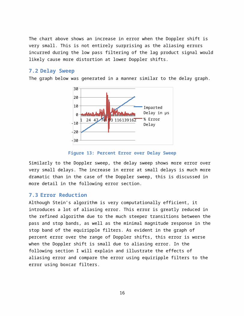
7.2 Delay SweepThe graph below was generated in a manner similar to the delay graph.

1 24 47 70 93 116139162

-30

-20

-10

0

10

20

30

Imparted Delay in µs% Error Delay

Figure 13: Percent Error over Delay Sweep

Similarly to the Doppler sweep, the delay sweep shows more error over very small delays. The increase in error at small delays is much more dramatic than in the case of the Doppler sweep, this is discussed in more detail in the following error section.

7.3 Error ReductionAlthough Stein’s algorithm is very computationally efficient, it introduces a lot of aliasing error. This error is greatly reduced in the refined algorithm due to the much steeper transitions between the pass and stop bands, as well as the minimal magnitude response in the stop band of the equiripple filters. As evident in the graph of percent error over the range of Doppler shifts, this error is worse when the Doppler shift is small due to aliasing error. In the following section I will explain and illustrate the effects of aliasing error and compare the error using equiripple filters to the error using boxcar filters.

16

8. Error Sources

8.1 Aliasing of Higher Frequencies to Lower Frequencies

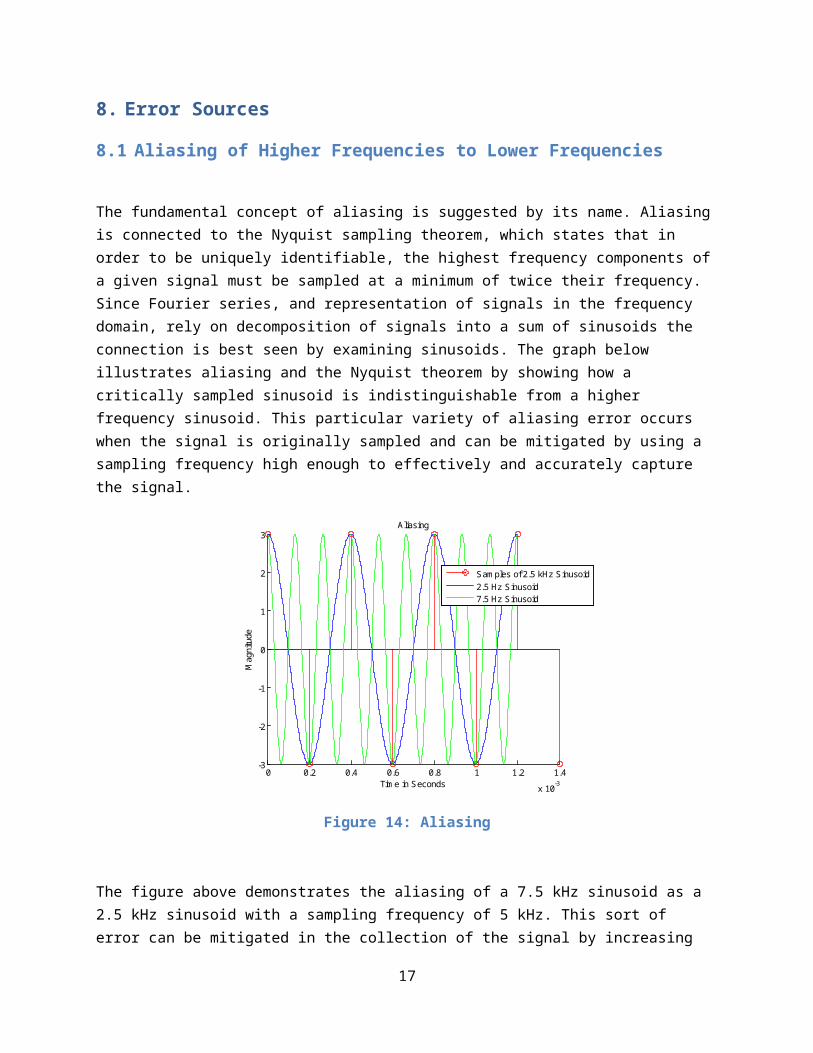
The fundamental concept of aliasing is suggested by its name. Aliasingis connected to the Nyquist sampling theorem, which states that in order to be uniquely identifiable, the highest frequency components ofa given signal must be sampled at a minimum of twice their frequency. Since Fourier series, and representation of signals in the frequency domain, rely on decomposition of signals into a sum of sinusoids the connection is best seen by examining sinusoids. The graph below illustrates aliasing and the Nyquist theorem by showing how a critically sampled sinusoid is indistinguishable from a higher frequency sinusoid. This particular variety of aliasing error occurs when the signal is originally sampled and can be mitigated by using a sampling frequency high enough to effectively and accurately capture the signal.

0 0.2 0.4 0.6 0.8 1 1.2 1.4x 10-3

-3

-2

-1

0

1

2

3Aliasing

Magnitude

Tim e in Seconds

Sam ples of 2.5 kHz Sinusoid2.5 Hz Sinusoid7.5 Hz Sinusoid

Figure 14: Aliasing

The figure above demonstrates the aliasing of a 7.5 kHz sinusoid as a 2.5 kHz sinusoid with a sampling frequency of 5 kHz. This sort of error can be mitigated in the collection of the signal by increasing

17

the sampling rate to a rate at least twice that of the highest frequency components of the signal. Such error also arises after the signal has been digitized, during the process of filtering and decimation. This is the type of aliasing error minimized by the use ofequiripple as opposed to boxcar filters. Below are a series of illustrations of aliasing due to filtering and decimation, beginning with a figure explaining the folding frequency and a method for determining which frequencies will alias to which lower frequencies.

18

Figure 15: Folding Frequency

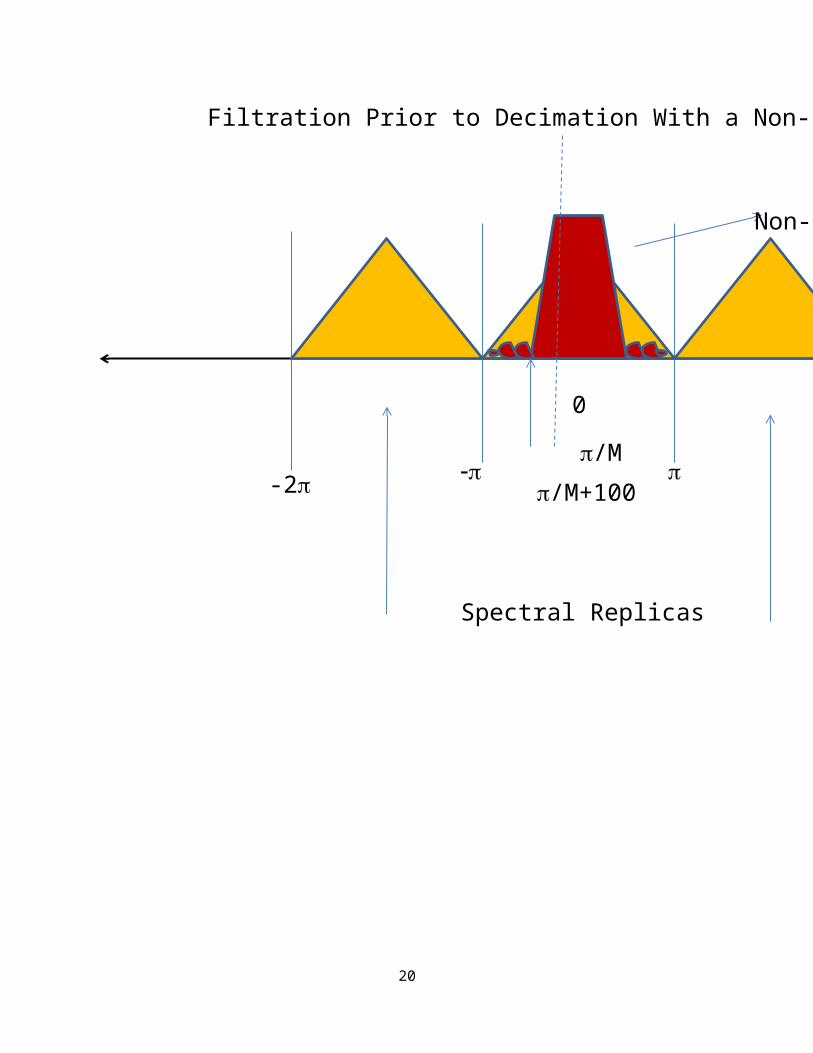
The figure above shows the way in which frequencies alias as well as the connection between the digital and analog domain. The aliasing error involved in filtration and decimation are subtly different as illustrated by the figures below.

19

0

Fs/2 or “folding frequency”

Digital Frequency Domain: extends

infinitely in either direction

3/4 3/4

1/8Fs

7/8Fs

/4

Higher frequency sinusoids alias to frequencies lower by factors of 2in the digital domain, and by multiples of Fs in the analog domain.

20

0

-2

Spectral Replicas

Non-Ideal LPF

Filtration Prior to Decimation With a Non-Ideal LPF

/M+100/M

Figure 16: Spectral Replicas

Figure 17: Spectral Replicas and Aliasing

8.2 Decimation Factor OrderThe limitation on the degree to which aliasing can affect the signal after it has been filtered and decimated is due to the limitation of the spectrum prior to decimation. This consideration is one reason to decimate the signal in stages rather than all at once. Decimating in stages ensures that in any given stage, aliasing error is largely

21

0

-2

Higher Frequencies Aliased to Lower Frequencies

After Decimation and Filtering

In this case, the aliasing is caused by non-idealities in the filter and limited to frequencies whose frequencies fall below roughly M in the digital domain

limited to remnants of frequencies whose pre-decimation digital frequency was above π/M in the digital domain prior to decimation and below πΜ after decimation.These remnants exist due to non-idealities in the filter. Minimizationof the decimation factor at each stage also serves to reduce the orderof the equiripple filter used in the decimation process by relaxing requirements on the width of the passband. A very high order filter would be required to decimate in one stage. This is intuitive when considered in terms of the relationships between the time and frequency domains. Since the width of signal in the time domain, or inthis case the impulse response of a filter, is inversely proportional to its width in the frequency domain, a narrow passband necessitates higher order filter. It also makes sense to decimate in small factors in descending order because as the decimation proceeds, and Fs/2 shrinks, the passband becomes narrower and narrower, necessitating a higher order filter and more computational complexity. Since smaller decimation factors allow for wider passbands, it makes sense to decimate the lag product signal with factors in descending order. The optimization of these factors is discussed in the optimization section.

8.3 Artificial Low Frequency ContentI was puzzled at first by the pronounced spike error at low delays. I have an idea of how to fix it, which I will explain after I explain the error itself. I wanted to implement it but an improbable double hard drive failure set me back considerably. Anyhow, I believe the reason for the spike is that the conjugated signal is padded on both sides by zeros, always a total of the sum of delays and advances in integer sample delays spaced in time according to the sampling rate. When the delay is one for instance, and 60 each of delays and advancesare tested, there is one zero in the front of the signal and 119 at the end. Even though the signals are long, the presence of the 119 zeros adds a considerable amount of artificial low frequency content in the lag product signal. Since the Doppler tends to be very near DC,the additional low frequency content can easily obscure the true Doppler. In order to ameliorate this problem, I believe I merely need to eliminate the excess zeros. This would necessitate another loop, but it is worth a try as error spikes near 20% at very low delays.

22

9. Efficiency

9.1 Qualitative Measurement of ComplexityA good qualitative measure of the computational complexity necessary to perform a decimation is f, which is defined as follows, where Fs is the continuous time transition-band edge frequency and Fp is the continuous time pass-band edge frequency. The transition-band and pass-band together comprise the base-band. To minimize aliasing, the filters are designed such that Fs = FI-Fp, where FI is the original sampling frequency divided by the product of all decimation factors, including the factor about to be performed. This ensures that no aliasing occurs between zero and Fp. In this application, the value of Fp is defined as the maximum expected Doppler shift plus one hundred hertz. This value remains the same, although its position in the digital domain moves progressively towards . [2]

∆f=FS−FPFS

The value of this measure varies between zero and one, the larger f, the narrower the pass-band, the larger the decimation rate, and the more complex the required filter. Because Fp is constant, and small, and Fs depends on FP and FI, it is clear that f at each stage can be reduced considerably by reduction of FI, which can only be accomplishedby a decrease in the decimation rate at any given stage.f is inversely proportional to the width of the pass-band, therefore complexity is minimized when f is minimized. [2] In the following discussion of optimization, f is defined as f at the final stage of decimation.

10. Optimization

10.1 Discussion of Optimization Strategy For this application, the single stage decimation rate is the floor

of: Fs2/maximumexpecteddoppler. This value is rarely decomposable

23

into more than three prime factors. The computational complexity of a decimation (or interpolation) system is measured by computation of number of adds and multiplies involved in the process. [2] Large gainsin efficiency are generally made in the change from single stage to two-stage decimation, but additional factors beyond that do not generally add as much to the efficiency of the process. [2] The equations below begin with several definitions, culminating in an expression forRT

¿, the total number of multiplications involved in the decimation process, not accounting for gains made through poly-stage implementation. [2]

δp,δs:Pass and Stop band ripple for Total Decimation processδp=δs

Pass Band Ripple For Each Stage (subsequent references to δs refer tothis definition)

δs=δs

stages

FP,FS:Normalized Pass and Stop Band Frequencies

FS=ωs

2π

FP=ωp

2π

∆F : Normalized Transition Width (A Measure of Frequency DomainResolution)

∆F=FS−FP=ωs−ωp2π

f (δs,δp) For ¿δs∨≤∨δp∨¿

f (δs,δp)=11.012+.512(log (δp)−log (δs ))

24

D∞=f (δs,δp )∆F2

S=2

∆F ∏i=1

stages−1Mi

+ ∑i=1

stages−1 Mi

∏j=1

iMj ¿¿

¿

Total Multiplications, where FO=originalFs

RT¿=D∞( δp

stages ,δs)FOS

The Above Equation is to be optimized. It is clear that such optimization relies on the minimization of the function S, in which all factors of M are independent variables. This can be accomplished for the two-stage case by taking the derivative of the expression for S, with respect toM1, and setting it equal to zero. This yields an equation with two solutions, only one of which is viable, and is in the form below. [2]

M1opt= 2M

(2−∆f )+√2M∆f−M∆f2

M2opt can then be found by simply dividing the total M by M1op t. The designprocedure for more stages requires the use of a pattern search algorithm, such as the Hooke and Jeeves algorithm. [2] There exist design curves for minimum values of S for various numbers of stages given the decimation rate and∆f. The current procedure defines FP as the maximum expected Doppler shift minus 100 hertz, and FS as the maximum expected Doppler plus 100 hertz, meaning that regardless of the maximum expected Doppler; the width of the transition band is always 200 Hz. Since ∆f is a ratio of the width of the transition bandto the width of the transition band plus that of the base band (the transition band plus the pass band), the value of ∆f becomes smaller as the expected Doppler becomes larger. Given the limited advantages of adding more decimation factors, the decision to undergo a more complex optimization procedure, using a pattern search algorithm, can be made based on the calculation of ∆f and the characteristics of the design curves for that value and for M. Since creating the design curves is a computationally extensive process, cutoff values of M,

25

above which it is practical to add a third or fourth decimation factor, are defined. The design curve below is for ∆f=.01. [2]

Figure 18: Efficiency considerations

Figure 2: Design Curves [2]

10.2 Gradient Descent OptimizationThe ranges of ∆f values in this routine are on the order of .01. It is only practical to decimate in more than two stages only when the decimation rate is fairly high. So I set up a routine to decide, basedon the value of M, when to perform the optimization for three factors rather than the simpler optimization for two discussed earlier. If M is greater than ten, the three stage optimization routine is performed. Based on the Hookes-Jeeves search algorithm, the optimization routine finds a local minimum in the S function by probing in each direction and calculating S. The routine is initialized with a factorization of the total decimation factor. Assuming the numbers are not prime, the routine does have the defect that it may sometimes be performed in vain. The routine takes the

26

decimation factor, a step size, and a minimum step as its arguments. The step size is initiated as .5, and the first factor is incremented and decremented by .5, and the S is calculated using that value and the fixed values of M from the initial vector. The routine keeps the Mthat yielded the lower S, and decrements the step to its minimum, .25.Since it is essential that decimation factors be integers, imprecise values must be accepted. The routine then repeats the increase and reduction of the first factor, keeping the factor that yields a smaller S. The routine repeats on the other two factors and all are rounded to the nearest integer. The three are then multiplied togetherto obtain the decimation rate, which may be slightly different than that intended.

10.3 Time Compression Modeled as Sampling Rate ChangeThe source is always considered to be absolutely stationary so the relative motion of the sensor always results in time compression or expansion, depending on the direction of motion, but both can be handled in the same way. This relativistic effect means that when the signal is considered in continuous time, the analog to digital converter on the sensor is sampling at slightly different instants than those of the simulated signal. To correct for this, the incoming signal must be interpolated by a large amount because the effect of the time compression is very small and the desired sample is very close in time to the more crudely modeled sample. Because the relativistic effects are extremely small the rate of interpolation to achieve a sampling period the size of the sample offset is enormous, adirect interpolation approach is extremely computationally intensive. The algorithm I am will define the distance from the sample instant asa function of time over the course of the sampling period, solve it for a given time and interpolate only a very small region, essentiallygrabbing only the sample needed. The figure below demonstrates the effect graphically.

27

Figure 19: Time Compression/Expansion

11. Appendix A: Tabulated Data, Doppler SweepImparted Delay

ImpartedDoppler in

CalculatedDelay in µs

Calculated Dopplerin kHz

% ErrorDelay

% ErrorDoppler

28

The smaller section is the sampling period from the point of view of the emitter, the total section is the sampling period from the point of view of the sensor

Non-compressed sampling instant

Correct Sampling Instant

sensor travels more distance in the same time relative to the emitter but experiences the same passage of time

in µs kHz2.3 9 2.175892986 8.99568328 -5.395957132 0.04796355

82.3 8.9 2.439442697 8.904868193 6.062725958 -

0.054698801

2.3 8.8 2.262150329 8.814382276 -1.645637855 -0.16343495

2.3 8.7 2.537799759 8.724048879 10.33911997 -0.276423892

2.3 8.6 2.153734812 8.633849244 -6.359356018 -0.393595857

2.3 8.5 2.583917755 8.460404223 12.34425022 0.465832668

2.3 8.4 2.322722376 8.370745767 0.987929402 0.348264673

2.3 8.3 2.113236522 8.281146083 -8.1201512 0.227155632.3 8.2 2.21223094 8.19165088 -3.816046072 0.10181853

12.3 8.1 2.485062918 8.102310971 8.046213813 -

0.028530509

2.3 8 2.33428679 8.012942106 1.490730015 -0.16177633

2.3 7.9 2.435025022 7.923590869 5.870653116 -0.298618593

2.3 7.8 2.54979844 7.834283637 10.86080174 -0.43953381

2.3 7.7 2.064549062 7.663723877 -10.23699732 0.471118475

2.3 7.6 2.222982941 7.574649857 -3.348567784 0.333554513

2.3 7.5 2.163238952 7.485555155 -5.946132508 0.192597935

2.3 7.4 2.078074569 7.396597034 -9.648931798 0.045986032.3 7.3 2.269146243 7.307576824 -1.341467708 -

0.103792115

2.3 7.2 2.472204585 7.218582824 7.487155867 -0.258094776

2.3 7.1 2.260956496 7.12949895 -1.697543647 -0.415478167

2.3 7 2.099635057 6.96082273 -8.711519281 0.559675286

2.3 6.9 2.32107149 6.871897887 0.916151727 0.407277005

29

2.3 6.8 2.359988967 6.782919805 2.608215976 0.251179342

2.3 6.7 2.121284413 6.694093939 -7.770242933 0.088150162

2.3 6.6 2.208965211 6.605165771 -3.958034321 -0.07826926

2.3 6.5 1.686889455 6.516289521 -26.65698022 -0.25060801

2.3 6.4 2.341318535 6.427323656 1.796458032 -0.426932131

2.3 6.3 2.068078654 6.338168926 -10.08353676 -0.605855975

2.3 6.2 2.181198826 6.171312558 -5.165268417 0.462700676

2.3 6.1 2.37858488 6.082357507 3.416733914 0.289221194

2.3 6 2.326337065 5.993506369 1.145089791 0.108227182

2.3 5.9 2.128772377 5.904632235 -7.444679268 -0.078512452

2.3 5.8 2.457153127 5.815648114 6.832744641 -0.269795066

2.3 5.7 2.126006781 5.726620145 -7.564922578 -0.467020093

2.3 5.6 2.475427239 5.637385273 7.627271241 -0.667594159

2.3 5.5 2.797828122 5.472100499 21.64470096 0.507263658

2.3 5.4 2.031155393 5.383110084 -11.68889595 0.312776221

2.3 5.3 2.147879577 5.294110604 -6.613931431 0.111120682

2.3 5.2 2.135834946 5.205129007 -7.137611055 -0.098634749

2.3 5.1 2.376694656 5.116075791 3.334550272 -0.315211591

2.3 5 2.286779616 5.026840604 -0.574799323 -0.536812088

2.3 4.9 2.698580716 4.863167754 17.32959636 0.751678487

2.3 4.8 2.393868137 4.773871516 4.081223348 0.544343414

30

2.3 4.7 2.146911224 4.684739595 -6.656033751 0.324689475

2.3 -0.6 2.178496163 4.595563221 -5.282775501 -665.9272036

2.3 4.5 2.185529646 4.506383393 -4.976971922 -0.141853176

2.3 4.4 1.781550787 4.417069873 -22.54127013 -0.387951663

2.3 4.3 2.172499829 4.327613339 -5.543485714 -0.642170684

2.3 4.2 2.396040454 4.165862675 4.175671893 0.812793462.3 4.1 2.30354116 4.076372574 0.153963459 0.576278682.3 4 2.326496414 3.986950693 1.152018017 0.32623267

52.3 3.9 2.253927012 3.897519448 -2.00317338 0.06360389

92.3 3.8 2.252523801 3.808053047 -2.064182573 -

0.211922296

2.3 3.7 2.08751877 3.718411876 -9.238314335 -0.497618267

2.3 3.6 2.602409309 3.628501107 13.14823083 -0.791697411

2.3 3.5 2.508651655 3.469204558 9.071811108 0.879869764

2.3 3.4 2.369488501 3.379313735 3.021239179 0.608419551

2.3 3.3 2.243548798 3.289531289 -2.454400089 0.317233677

2.3 3.2 2.205509564 3.199823663 -4.108279841 0.005510542.3 3.1 2.292080374 3.109893534 -0.344331563 -

0.319146252

2.3 3 2.386077182 3.019732918 3.742486178 -0.65776394

2.3 2.9 2.013189611 2.929176764 -12.4700169 -1.006095315

2.3 2.8 2.27452489 2.773043153 -1.107613494 0.962744529

2.3 2.7 2.19577615 2.682701139 -4.531471734 0.640698569

2.3 2.6 2.177627603 2.592418274 -5.320538998 0.291604831

2.3 2.5 2.224491782 2.502114181 -3.282965994 -

31

0.084567243

2.3 2.4 2.304675842 2.411605932 0.203297493 -0.483580498

2.3 2.3 2.103550794 2.320658546 -8.541269824 -0.898197671

2.3 2.2 1.974734339 2.228794092 -14.14198525 -1.308822374

2.3 2.1 2.513209001 2.077468016 9.26995655 1.072951601

2.3 2 2.055102033 1.986288896 -10.64773768 0.685555219

2.3 1.9 2.114931641 1.895345593 -8.046450411 0.244968794

2.3 1.8 2.153152495 1.80421509 -6.384674144 -0.234171661

2.3 1.7 2.34877444 1.712664525 2.120627826 -0.744972061

2.3 1.6 2.251600708 1.620179882 -2.104317054 -1.261242632

2.3 1.5 2.271436132 1.475950529 -1.241907319 1.603298064

2.3 1.4 2.347367005 1.382718244 2.059435016 1.234411142.3 1.3 2.130368657 1.290332993 -7.37527579 0.74361593

82.3 1.2 2.201903319 1.198148875 -4.265073079 0.15426039

92.3 1.1 2.206338196 1.1055314 -4.072252347 -

0.502854548

2.3 1 2.179620901 1.011921981 -5.233873862 -1.19219806

2.3 0.9 2.081932282 0.915297345 -9.481205134 -1.699705027

2.3 0.8 2.40025895 0.786745091 4.35908477 1.656863569

2.3 0.7 2.037138173 0.689614591 -11.42877509 1.483629854

2.3 0.6 2.230305081 0.594981147 -3.030213884 0.836475572

2.3 0.5 2.191889079 0.500270533 -4.700474818 -0.054106642

2.3 0.4 2.192791195 0.404288194 -4.661252403 -

32

1.072048462

2.3 0.3 2.156804358 0.305149978 -6.225897476 -1.716659243

2.3 0.2 2.110137093 0.201015404 -8.254908984 -0.507702215

2.3 0.1 2.129749896 0.09870235 -7.402178453 1.297650261

2.3 0 2.179458746 1.51208E-05 -5.24092409 #DIV/0!2.3 -0.1 2.161160625 -0.098669659 -6.036494571 1.33034090

52.3 -0.2 2.230178267 -0.201039354 -3.035727535 -

0.519677103

2.3 -0.3 2.112160791 -0.305123052 -8.166922112 -1.707684074

2.3 -0.4 2.195679854 -0.404291134 -4.535658525 -1.072783397

2.3 -0.5 2.24431951 -0.500261372 -2.420890877 -0.052274489

2.3 -0.6 2.205199519 -0.594981109 -4.121760048 0.836481832

2.3 -0.7 2.034939044 -0.689612626 -11.52438941 1.483910615

2.3 -0.8 2.43013063 -0.786749431 5.657853495 1.656321161

2.3 -0.9 2.304000855 -0.915267599 0.173950213 -1.696399894

2.3 -1 2.260966104 -1.011917043 -1.697125901 -1.191704328

2.3 -1.1 2.189649131 -1.105532961 -4.797863854 -0.502996428

2.3 -1.2 2.161872984 -1.198138735 -6.00552243 0.155105404

2.3 -1.3 2.170657373 -1.290338458 -5.623592488 0.743195506

2.3 -1.4 2.431592616 -1.38272081 5.721418088 1.234227843

2.3 -1.5 2.059882862 -1.475942757 -10.43987555 1.603816176

2.3 -1.6 2.301666747 -1.6201777 0.072467263 -1.261106257

33

2.3 -1.7 2.027845637 -1.712679508 -11.83279838 -0.74585342

2.3 -1.8 2.124944498 -1.80422178 -7.611108762 -0.23454335

2.3 -1.9 2.215732002 -1.895350332 -3.663825993 0.244719372

2.3 -2 2.031411408 -1.986296433 -11.67776486 0.685178339

2.3 -2.1 2.009232004 -2.0774561 -12.64208678 1.073519034

2.3 -2.2 2.434831956 -2.228785327 5.862258951 -1.308423937

2.3 -2.3 2.279073599 -2.320654461 -0.909843535 -0.89802006

2.3 -2.4 2.288043586 -2.411606181 -0.51984407 -0.483590861

2.3 -2.5 2.22349852 -2.502113274 -3.326151313 -0.084530977

2.3 -2.6 2.170151637 -2.592422274 -5.645580985 0.291451014

2.3 -2.7 2.252300122 -2.68270266 -2.073907722 0.640642205

2.3 -2.8 2.369903761 -2.773045297 3.039293935 0.962667975

2.3 -2.9 2.163358694 -2.929175704 -5.940926348 -1.006058756

2.3 -3 1.555304764 -3.019745154 -32.37805373 -0.658171787

2.3 -3.1 2.122867542 -3.109900501 -7.701411232 -0.319371005

2.3 -3.2 2.236478582 -3.19981991 -2.761800761 0.005627809

2.3 -3.3 2.257815045 -3.289530503 -1.834128483 0.317257487

2.3 -3.4 2.628822053 -3.379300838 14.29661101 0.608798882.3 -3.5 2.594862043 -3.469190545 12.82008884 0.88027013

52.3 -3.6 2.225023667 -3.62848254 -3.259840545 -

0.791181672

2.3 -3.7 2.090994195 -3.718411361 -9.087208934 -0.497604343

2.3 -3.8 2.106949479 -3.808057736 -8.393500914 -0.21204568

34

12.3 -3.9 2.171750356 -3.897516278 -5.576071462 0.063685182.3 -4 2.253398463 -3.986948727 -2.02615377 0.32628182

42.3 -4.1 2.160924325 -4.076370525 -6.046768478 0.57632865

92.3 -4.2 1.934542866 -4.165858201 -15.88944061 0.81289998

52.3 -4.3 1.574225557 -4.327615962 -31.55541055 -

0.642231671

2.3 -4.4 2.021332816 -4.417069153 -12.1159645 -0.387935303

2.3 -4.5 2.189947721 -4.506382706 -4.784881698 -0.141837914

2.3 -4.6 2.220486178 -4.595565403 -3.457122714 0.096404279

2.3 -4.7 1.982094779 -4.684739375 -13.82196611 0.324694157

2.3 -4.8 2.295772076 -4.773870314 -0.183822773 0.544368453

2.3 -4.9 2.967166621 -4.863169651 29.00724438 0.751639777

2.3 -5 2.251890178 -5.026841142 -2.091731378 -0.536822833

2.3 -5.1 2.310642324 -5.116075879 0.462709728 -0.315213322

2.3 -5.2 1.991274061 -5.205127335 -13.4228669 -0.098602593

2.3 -5.3 2.166389463 -5.294111764 -5.809153783 0.111098793

2.3 -5.4 2.379914765 -5.383113437 3.474555017 0.312714132.3 -5.5 2.729791844 -5.472102661 18.6866019 0.50722434

92.3 -5.6 2.510650767 -5.637385721 9.158728998 -

0.667602163

2.3 -5.7 2.618776677 -5.72662274 13.85985551 -0.467065608

2.3 -5.8 2.089114929 -5.815649721 -9.16891614 -0.26982277

2.3 -5.9 2.261496223 -5.904629048 -1.674077246 -0.078458436

2.3 -6 2.241650287 -5.993503105 -2.53694405 0.10828159

35

2.3 -6.1 2.1730364 -6.082356271 -5.5201565 0.289241454

2.3 -6.2 2.088390675 -6.171314358 -9.20040543 0.462671652

2.3 -6.3 2.121434094 -6.338170265 -7.763735047 -0.605877227

2.3 -6.4 2.65343342 -6.427331041 15.36667043 -0.427047522

2.3 -6.5 1.988479951 -6.516288024 -13.54434994 -0.250584988

2.3 -6.6 2.150692519 -6.605166175 -6.491629627 -0.07827538

2.3 -6.7 2.203440119 -6.694094073 -4.198255711 0.088148171

2.3 -6.8 2.531393515 -6.782916493 10.06058761 0.251228041

2.3 -6.9 1.867815135 -6.871897472 -18.79064632 0.407283018

2.3 -7 1.985066994 -6.960822874 -13.6927394 0.559673225

2.3 7.1 2.269255569 -7.12949932 -1.336714406 -0.415483387

2.3 -7.2 2.250485564 -7.218584484 -2.152801579 -0.258117831

2.3 -7.3 2.272573257 -7.307577264 -1.192467084 -0.103798136

2.3 -7.4 2.353514163 -7.396597366 2.32670274 0.045981542.3 -7.5 2.269638866 -7.485555556 -1.320049289 0.19259258

22.3 -7.6 2.131595693 -7.574650353 -7.321926385 0.33354798

22.3 -7.7 2.280441399 -7.663724922 -0.850373973 0.47110490

92.3 -7.8 2.974219312 -7.834290843 29.31388313 -

0.439626192.3 -7.9 2.319300755 -7.923587798 0.839163271 -

0.298579715

2.3 -8 2.556687189 -8.012944087 11.16031256 -0.161801089

2.3 -8.1 2.23124314 -8.102309251 -2.989428679 -0.028509271

2.3 -8.2 2.145284959 -8.191651055 -6.72674091 0.10181640

36

42.3 -8.3 2.243950178 -8.281146544 -2.436948778 0.22715006

62.3 -8.4 1.759056477 -8.370745178 -23.51928362 0.34827169

52.3 -8.5 2.195281702 -8.460405357 -4.552969471 0.46581932

82.3 -8.6 2.310260708 -8.63385053 0.446117744 -

0.393610811

2.3 -8.7 2.221311137 -8.724049707 -3.421254907 -0.27643341

2.3 -8.8 2.643895323 -8.814382917 14.95197057 -0.163442236

2.3 -8.9 2.367310753 -8.904867682 2.926554496 -0.054693055

2.3 -9 2.14008412 -8.995684177 -6.952864362 0.047953593

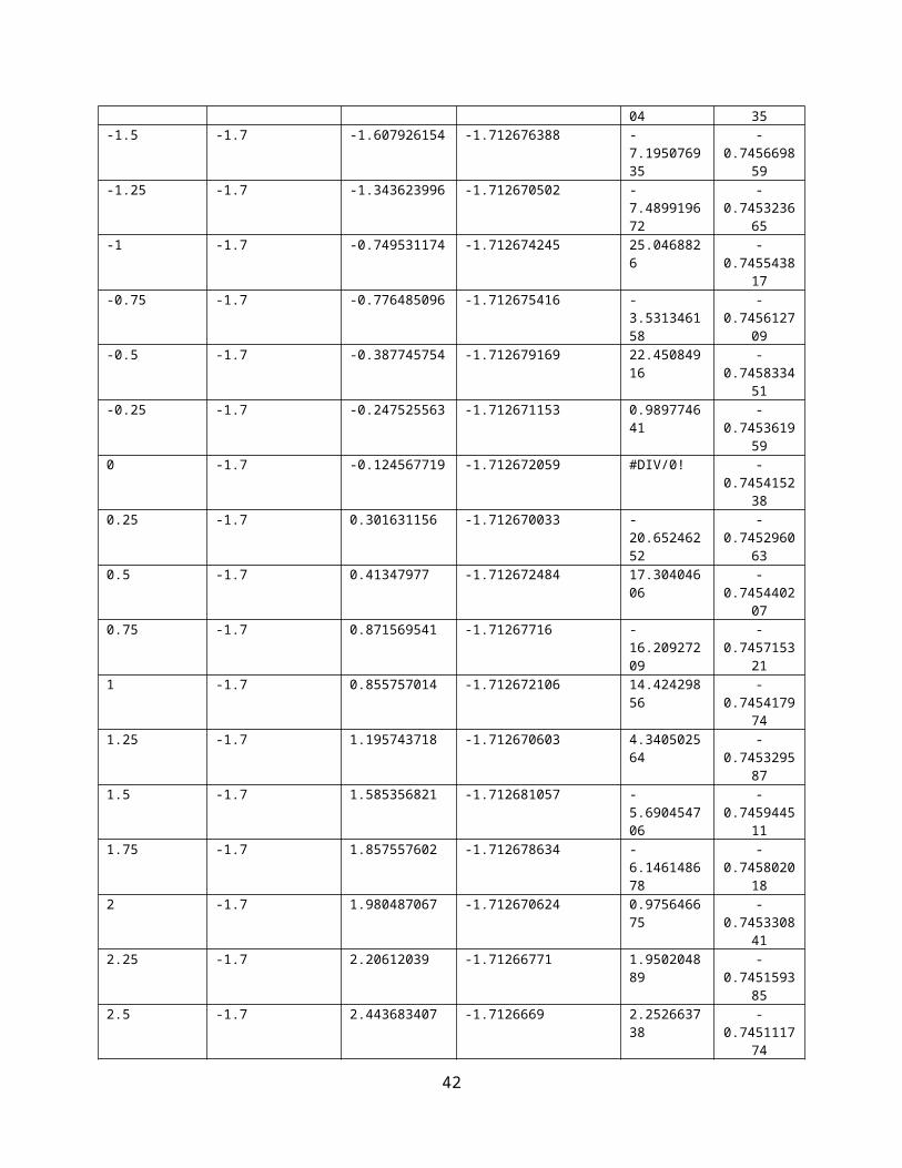
12. Appendix B: Tabulated Results, Delay SweepImparted Delay in µs

Imparted Doppler in kHz

Calculated Delay in µs

Calculated Dopplerin kHz

% Error Delay

% Error Doppler

-21 -1.7 -20.83909407 -1.712706105 0.766218702

-0.7474179

14-20.75 -1.7 -20.82421793 -1.712707162 -

0.357676771

-0.7474801

25-20.5 -1.7 -20.42972253 -1.712708188 0.3428169

06-

0.747540469

-20.25 -1.7 -20.15451105 -1.712702838 0.471550361

-0.7472257

73-20 -1.7 -20.0594797 -1.712703366 -

0.297398517

-0.7472568

51-19.75 -1.7 -19.56953572 -1.712700887 0.9137432

07-

0.747111012

-19.5 -1.7 -19.55163237 -1.712709509 -0.264781395

-0.7476181

99-19.25 -1.7 -19.24046768 -1.712700551 0.0495185

32-

0.74709123

37

-19 -1.7 -19.09446533 -1.712701228 -0.49718597

-0.7471310

44-18.75 -1.7 -18.78015461 -1.712705593 -

0.160824612

-0.7473878

44-18.5 -1.7 -18.49329867 -1.71269973 0.0362233

8-

0.747042961

-18.25 -1.7 -18.19190871 -1.712698398 0.318308451

-0.7469645

72-18 -1.7 -17.8875686 -1.712699151 0.6246189

09-

0.747008863

-17.75 -1.7 -17.795569 -1.712705083 -0.256726782

-0.7473578

14-17.5 -1.7 -17.68692387 -1.712714779 -

1.068136392

-0.7479282

04-17.25 -1.7 -17.03972715 -1.712699324 1.2189730

63-

0.747019033

-17 -1.7 -16.91422776 -1.712696883 0.5045426 -0.7468754

45-16.75 -1.7 -16.33211361 -1.712724673 2.4948441

18-

0.748510173

-16.5 -1.7 -16.47383628 -1.712690251 0.158568015

-0.7464853

58-16.25 -1.7 -16.34862606 -1.71269012 -

0.606929598

-0.7464776

28-16 -1.7 -16.12272972 -1.712694133 -

0.767060739

-0.7467136

9-15.75 -1.7 -15.69522539 -1.712694958 0.3477753

05-

0.746762258

-15.5 -1.7 -15.43805285 -1.712690274 0.399659024

-0.7464866

83-15.25 -1.7 -14.97640435 -1.712693656 1.7940698

12-

0.746685638

-15 -1.7 -14.72361987 -1.712690674 1.842534205

-0.7465102

17-14.75 -1.7 -14.84062712 -1.712693315 - -

38

0.614421123

0.746665589

-14.5 -1.7 -14.45334686 -1.712693084 0.321745825

-0.7466520

25-14.25 -1.7 -14.3461916 -1.71268604 -

0.675028788

-0.7462376

57-14 -1.7 -13.97525125 -1.712687994 0.1767767

69-

0.746352597

-13.75 -1.7 -13.7553021 -1.712691803 -0.038560704

-0.7465766

73-13.5 -1.7 -13.2896335 -1.712695334 1.5582704

02-

0.746784351

-13.25 -1.7 -13.25498165 -1.712686037 -0.037597331

-0.7462374

61-13 -1.7 -13.11843302 -1.712685221 -

0.911023238

-0.7461894

87-12.75 -1.7 -12.78738652 -1.712687949 -

0.293227611

-0.7463499

48-12.5 -1.7 -12.67817245 -1.712694153 -

1.425379579

-0.7467148

9-12.25 -1.7 -12.42743181 -1.712678704 -

1.448422936

-0.7458061

38-12 -1.7 -11.73039533 -1.71268324 2.2467055

63-

0.746072957

-11.75 -1.7 -11.49260046 -1.712711496 2.190634411

-0.7477350

34-11.5 -1.7 -11.36450041 -1.71268097 1.1782573

38-

0.745939421

-11.25 -1.7 -11.44570672 -1.712676374 -1.739615263

-0.7456690

7-11 -1.7 -11.15163475 -1.712680215 -

1.378497721

-0.7458950

14-10.75 -1.7 -10.76695745 -1.712684903 -

0.157743683

-0.7461707

54-10.5 -1.7 -10.56649306 -1.712683797 -

0.6332672-

0.7461057

39

14 28-10.25 -1.7 -10.31159312 -1.712677045 -

0.600908534

-0.7457085

51-10 -1.7 -10.02299142 -1.712680377 -

0.229914187

-0.7459045

15-9.75 -1.7 -9.682674952 -1.712680139 0.6905133

13-

0.745890555

-9.5 -1.7 -9.532304838 -1.712679235 -0.340050926

-0.7458373

56-9.25 -1.7 -8.991626548 -1.712679349 2.7932265

08-

0.745844041

-9 -1.7 -8.970819567 -1.712678024 0.324227039

-0.7457661

26-8.75 -1.7 -8.796389981 -1.71267746 -

0.530171217

-0.7457329

56-8.5 -1.7 -8.524767009 -1.71267589 -

0.291376576

-0.7456406

16-8.25 -1.7 -8.165616224 -1.712675878 1.0228336

52-

0.7456399-8 -1.7 -7.918043503 -1.712673306 1.0244562

15-

0.745488615

-7.75 -1.7 -7.826758667 -1.712674237 -0.990434407

-0.7455433

24-7.5 -1.7 -7.609253812 -1.712679188 -

1.456717497

-0.7458345

85-7.25 -1.7 -7.222315046 -1.712669921 0.3818614

38-

0.745289488

-7 -1.7 -6.893207089 -1.712668473 1.52561302

-0.7452042

83-6.75 -1.7 -6.832391912 -1.712674121 -

1.220620926

-0.7455365

41-6.5 -1.7 -6.514781634 -1.71266991 -

0.227409757

-0.7452888

05-6.25 -1.7 -5.867429911 -1.712673481 6.1211214

18-

0.745498893

-6 -1.7 -5.853978059 -1.712664709 2.4336990 -

40

12 0.74498287

-5.75 -1.7 -5.578974771 -1.712659504 2.974351809

-0.7446767

31-5.5 -1.7 -5.532605274 -1.712663819 -

0.592823158

-0.7449305

41-5.25 -1.7 -5.127682485 -1.712667201 2.3298574

23-

0.745129446

-5 -1.7 -5.215946513 -1.712664744 -4.31893025

-0.7449849

4-4.75 -1.7 -4.504385406 -1.712681877 5.1708335

67-

0.745992767

-4.5 -1.7 -4.340213246 -1.712684699 3.550816745

-0.7461587

64-4.25 -1.7 -4.281184793 -1.712662018 -

0.73375984

-0.7448245

79-4 -1.7 -4.027455434 -1.712665922 -

0.68638586

-0.7450542

14-3.75 -1.7 -3.650902964 -1.712664765 2.6425876

39-

0.744986187

-3.5 -1.7 -3.278505661 -1.712682187 6.328409674

-0.7460110

24-3.25 -1.7 -3.099574945 -1.7126693 4.6284632

2-

0.745252936

-3 -1.7 -2.964817455 -1.712667864 1.172751486

-0.7451684

81-2.75 -1.7 -2.718565046 -1.71266541 1.1430892

42-

0.745024096

-2.5 -1.7 -2.69978797 -1.712677593 -7.991518819

-0.7457407

74-2.25 -1.7 -2.277505361 -1.71266726 -

1.222460494

-0.7451329

35-2 -1.7 -2.054972276 -1.712671448 -

2.748613776

-0.7453793

07-1.75 -1.7 -1.792639182 -1.712673383 -

2.4365247-

0.7454931

41

04 35-1.5 -1.7 -1.607926154 -1.712676388 -

7.195076935

-0.7456698

59-1.25 -1.7 -1.343623996 -1.712670502 -

7.489919672

-0.7453236

65-1 -1.7 -0.749531174 -1.712674245 25.046882

6-

0.745543817

-0.75 -1.7 -0.776485096 -1.712675416 -3.531346158

-0.7456127

09-0.5 -1.7 -0.387745754 -1.712679169 22.450849

16-

0.745833451

-0.25 -1.7 -0.247525563 -1.712671153 0.989774641

-0.7453619

590 -1.7 -0.124567719 -1.712672059 #DIV/0! -

0.745415238

0.25 -1.7 0.301631156 -1.712670033 -20.65246252

-0.7452960

630.5 -1.7 0.41347977 -1.712672484 17.304046

06-

0.745440207

0.75 -1.7 0.871569541 -1.71267716 -16.20927209

-0.7457153

211 -1.7 0.855757014 -1.712672106 14.424298

56-

0.745417974

1.25 -1.7 1.195743718 -1.712670603 4.340502564

-0.7453295

871.5 -1.7 1.585356821 -1.712681057 -

5.690454706

-0.7459445

111.75 -1.7 1.857557602 -1.712678634 -

6.146148678

-0.7458020

182 -1.7 1.980487067 -1.712670624 0.9756466

75-

0.745330841

2.25 -1.7 2.20612039 -1.71266771 1.950204889

-0.7451593

852.5 -1.7 2.443683407 -1.7126669 2.2526637

38-

0.745111774

42

2.75 -1.7 2.677593088 -1.712671238 2.632978609

-0.7453669

263 -1.7 2.91361161 -1.712669837 2.8796130

1-

0.74528453

3.25 -1.7 3.013932343 -1.71267122 7.263620219

-0.7453658

773.5 -1.7 3.382730289 -1.712667368 3.3505631

85-

0.745139281

3.75 -1.7 3.600137673 -1.712669335 3.996328716

-0.7452549

974 -1.7 4.059459457 -1.712669116 -

1.48648642

-0.7452421

324.25 -1.7 4.205997498 -1.712666348 1.0353529

85-

0.745079281

4.5 -1.7 4.198010382 -1.712677069 6.710880396

-0.7457099

434.75 -1.7 4.705029527 -1.712672118 0.9467467

98-

0.745418693

5 -1.7 4.879344238 -1.712668923 2.413115246

-0.7452307

455.25 -1.7 5.218856555 -1.71266598 0.5932084

83-

0.745057637

5.5 -1.7 5.25147556 -1.712676438 4.518626177

-0.7456728

065.75 -1.7 5.756034772 -1.712673425 -

0.104952551

-0.7454956

166 -1.7 5.888586955 -1.712669096 1.8568840

81-

0.745240924

6.25 -1.7 6.135218197 -1.71266966 1.836508849

-0.7452741

186.5 -1.7 6.220992192 -1.712675013 4.2924278

1-

0.745589014

6.75 -1.7 6.578392388 -1.712669085 2.542334987

-0.7452402

747 -1.7 6.600528489 -1.712669446 5.7067358 -

43

71 0.745261538

7.25 -1.7 7.211245706 -1.71266733 0.534541985

-0.7451370

327.5 -1.7 7.422506064 -1.712664974 1.0332524

86-

0.744998474

7.75 -1.7 7.824944755 -1.712676233 -0.967029094

-0.7456607

848 -1.7 7.934720888 -1.712669483 0.8159888

99-

0.74526371

8.25 -1.7 8.001049726 -1.712672623 3.017579079

-0.7454483

848.5 -1.7 8.316890683 -1.712674396 2.1542272

64-

0.745552701

8.75 -1.7 8.562410356 -1.712669028 2.143881641

-0.7452369

519 -1.7 8.797429111 -1.71267047 2.2507876

54-

0.745321788

9.25 -1.7 9.188601227 -1.71266936 0.663770518

-0.7452564

819.5 -1.7 9.562368489 -1.712681092 -

0.656510409

-0.7459465

639.75 -1.7 9.617641035 -1.712667796 1.3575278

45-

0.745164455

10 -1.7 10.00863119 -1.712670125 -0.086311931

-0.7453014

4810.25 -1.7 10.18351671 -1.712670262 0.6486174

19-

0.74530951

10.5 -1.7 10.19636002 -1.712683787 2.891809317

-0.7461051

1610.75 -1.7 10.7948387 -1.712673346 -

0.417104185

-0.7454909

5911 -1.7 10.97890942 -1.712668818 0.1917325

89-

0.745224581

11.25 -1.7 10.99951624 -1.712670415 2.226522303

-0.7453185

44

0611.5 -1.7 11.4831726 -1.712663063 0.1463252

4-

0.744886043

11.75 -1.7 11.86783006 -1.712671967 -1.002809028

-0.7454097

9612 -1.7 11.93560823 -1.712666997 0.5365980

46-

0.745117469

12.25 -1.7 12.28144431 -1.712661755 -0.256688235

-0.7448091

3212.5 -1.7 12.63298407 -1.712687519 -

1.063872525

-0.7463246

4412.75 -1.7 12.65957792 -1.712667525 0.7091927

83-

0.745148526

13 -1.7 13.1224015 -1.712666023 -0.941549962

-0.7450601

9613.25 -1.7 12.90701061 -1.712668283 2.5885991

85-

0.745193116

13.5 -1.7 13.0796576 -1.712681461 3.113647405

-0.7459682

8313.75 -1.7 13.7696985 -1.712671098 -

0.143261845

-0.7453587

2314 -1.7 13.84599579 -1.712667754 1.1000300

78-

0.745162019

14.25 -1.7 14.33019109 -1.712662761 -0.562744483

-0.7448683

1314.5 -1.7 14.30052437 -1.712673636 1.3756939

86-

0.745507999

14.75 -1.7 14.71607197 -1.712669906 0.230020563

-0.7452885

9215 -1.7 14.99719554 -1.712669334 0.0186964

13-

0.74525495

15.25 -1.7 15.31231271 -1.712664017 -0.408607965

-0.7449421

9315.5 -1.7 15.27903379 -1.712684407 1.4255884

64-

0.746141579

45

15.75 -1.7 15.775299 -1.712674511 -0.160628545

-0.7455594

8116 -1.7 15.88999218 -1.712671029 0.6875489

06-

0.745354637

16.25 -1.7 16.18890727 -1.712671287 0.375955276

-0.7453698

1916.5 -1.7 16.46165701 -1.712674811 0.2323817

83-

0.745577126

16.75 -1.7 16.85123334 -1.71267925 -0.604378132

-0.7458382

1817 -1.7 17.02287294 -1.712673081 -

0.134546693

-0.7454753

3817.25 -1.7 17.22327966 -1.712671788 0.1549005

25-

0.74539929

17.5 -1.7 17.37295992 -1.712676945 0.725943308

-0.7457026

2917.75 -1.7 17.73899346 -1.712678562 0.0620086

92-

0.745797774

18 -1.7 17.87074203 -1.712675439 0.718099818

-0.7456140

4918.25 -1.7 18.18680611 -1.712674079 0.3462678

93-

0.745534055

18.5 -1.7 18.39172279 -1.712674811 0.585282226

-0.7455771

2218.75 -1.7 18.32912056 -1.712699888 2.2446903

33-

0.747052225

19 -1.7 18.95612964 -1.712675779 0.23089661

-0.7456340

6319.25 -1.7 18.94468803 -1.712683026 1.5860361

83-

0.746060343

19.5 -1.7 19.48017734 -1.712669702 0.101654691

-0.7452766

1319.75 -1.7 19.46462478 -1.712691471 1.4449378

16-

0.746557147

20 -1.7 19.72844508 -1.712677343 1.3577746 -

46

02 0.745726058

20.25 -1.7 20.37903293 -1.712669142 -0.637199653

-0.7452436

7620.5 -1.7 20.31227462 -1.712682204 0.9157335

4-

0.746011986

20.75 -1.7 20.83698551 -1.712688292 -0.419207264

-0.7463701

2421 -1.7 20.68471594 -1.712680218 1.5013526

47-

0.745895177

13. References[1] http://www.ws.binghamton.edu/fowler/fowler%20personal%20page/EE521_files/IV-05%20Polyphase%20FIlters_2007.pdf

[2] Book in black binder, entire book on multirate DSP. Need to find out title.

47