ES

EA

RC

HR

EP

RO

RT

ID

IA

P

Rue du Simplon 4

IDIAP Research Institute1920 Martigny − Switzerland

www.idiap.ch

Tel: +41 27 721 77 11 Email: info@idiap.chP.O. Box 592Fax: +41 27 721 77 12

MOTION LIKELIHOOD AND

PROPOSAL MODELING

IN MODEL-BASED STOCHASTIC

TRACKING

Jean-Marc Odobez * Daniel Gatica-Perez *

IDIAP–RR 04-61

DECEMBER 10, 2004

SUBMITTED FOR PUBLICATION

* IDIAP Research Institute, Martigny, Switzerland

IDIAP Research Report 04-61

MOTION LIKELIHOOD AND PROPOSAL MODELING

IN MODEL-BASED STOCHASTIC TRACKING

Jean-Marc Odobez Daniel Gatica-Perez

DECEMBER 10, 2004

SUBMITTED FOR PUBLICATION

Abstract. Particle filtering is now established as one of the most popular methods forvisual tracking. Within this framework, there are two important considerations. The firstone refers to the generic assumption that the observations are temporally independentgiven the sequence of object states. The second consideration, often made in the liter-ature, uses the transition prior as proposal distribution. Thus, the current observationsare not taken into account, requesting the noise process of this prior to be large enoughto handle abrupt trajectory changes. As a result, many particles are either wasted in lowlikelihood regions of the state space, resulting in low sampling efficiency, or more im-portantly, propagated to distractor regions of the image, resulting in tracking failures. Inthis paper, we propose to handle both considerations using motion. We first argue that ingeneral observations are conditionally correlated, and propose a new model to accountfor this correlation allowing for the natural introduction of implicit and/or explicit mo-tion measurements in the likelihood term. Secondly, explicit motion measurements areused to drive the sampling process towards the most likely regions of the state space.Overall, the proposed model allows to handle abrupt motion changes and to filter outvisual distractors when tracking objects with generic models based on shape or colordistribution. Experimental results obtained on head tracking, using several sequenceswith moving camera involving large dynamics, and compared against the CONDEN-SATION algorithm, have demonstrated superior tracking performance of our approach.

IDIAP–RR 04-61 1

1 Introduction

Visual tracking is an important problem in computer vision, with applications in telecon-ferencing, visual surveillance, gesture recognition, and vision based interfaces [BI98]. Al-though tracking has been intensively studied in the literature, it still represents a challengingtask in adverse situations, due to the presence of ambiguities (e.g. when tracking an objectin a cluttered scene or when tracking multiple instances of the same object class), the noisein image measurements (e.g. lighting chnages), and the variability of the object class (e.g.pose variations).

In the pursuit of robust tracking, Sequential Monte Carlo methods [AMGC01, DdFG01,BI98] have shown to be a successful approach. In this temporal Bayesian framework, theprobability of an object configuration given the observations is represented by a set ofweighted random samples, called particles. This representation allows in principle to simul-taneously maintain multiple hypotheses in the presence of ambiguities, unlike algorithms thatkeep only one configuration state [CRM00], which are therefore sensitive to single failuresin the presence of ambiguities or fast or erratic motion.

In this paper, we address two important issues related to tracking with a particle filter.The first issue refers to the specific form of the observation likelihood, that relies on theconditional independence of observations given the state sequence. The second one refers tothe choice of an appropriate proposal distribution, which, tunlike the prior dynamical model,should take into account the new observations. To handle these issues, we propose a newparticle filter tracking method based on visual motion. Our method relies on a new graphicalmodel allowing for the natural introduction of implicit or explicit motion information in thelikelihood term, and on the exploitation of explicit motion measurements in the proposaldistribution. A longer description of the above issues, our approach, and their benefits, isgiven in the following paragraphs.

The definition of the observation likelihood distribution is perhaps the most importantelement in visual tracking with a particle filter. This distribution allows for the evalua-tion of the likelihood of the current observation given the current object state, and relieson the specific object representation. The object representation corresponds to all the in-formation that characterizes the object like the target position, geometry, appearance, color,etc. Parametrized shapes like splines [BI98] or ellipses [WH01], and color distributions[RMG98, CRM00, PHVG02, WH01], are often used as target representation. One draw-back of these generic representations is that they can be quite unspecific, which augmentsthe chances of ambiguities. One way to improve the robustness of a tracker consists ofcombining low-level measurements such as shape and color [WH01].

The generic conditional form of the likelihood term relies on a standard hypothesis inprobabilistic visual tracking, namely the independence of observations given the state se-quence [AMF04, BJ98a, BI98, IB89, RC01, TB01, WH01]. In this paper, we argue that thisassumption can be inaccurate in the case of visual tracking. As a remedy, we propose a newmodel that assumes that the current observation depends on the current and previous objectconfigurations as well as on the past observation. We show that under this more generalassumption, the obtained particle filtering algorithm has similar equations than the algorithm

IDIAP–RR 04-61 2

based on the standard hypothesis. To our knowledge, this has not been shown before, andso it represents the first contribution of this article. The new assumption can thus be usedto naturally introduce implicit or explicit motion information in the observation likelihoodterm. The introduction of such data correlation between successive images will turn generictrackers like shape or color histogram trackers into more specific ones.

Another important distribution to define when designing a particle filter is the proposaldistribution, that is, the function that predicts the new state hypotheses where the observa-tion likelihood will be evaluated. In general, an optimal choice [AMGC01, DGA00] consistsof drawing samples from the more likely regions taking into account both the dynamicalmodel, which characterizes the prior on the state sequence, and the new observations. How-ever, simulating from the optimal law is often difficult when using standard likelihood terms.Thus, a common assumption in particle filtering consists in using the dynamics as proposaldistribution. With this assumption, the variance of the noise process in the dynamical modelimplicitly defines a search range for the new hypotheses. This assumption raises difficultiesin modeling dynamics since this term should fulfill two contradictory objectives. On onehand, as prior distribution, dynamics should be tight to avoid the tracker being confused bydistractors in the vicinity of the true object configuration, a situation that is likely to happenfor unspecific object representations such as generic shapes or color distributions. On theother hand, as proposal distribution, dynamics should be broad enough to cope with abruptmotion changes. Furthermore, this proposal distribution does not take into account the mostrecent observations. Many particles drawn from it will probably have a low likelihood, whichresults in low sampling efficiency. Overall, such a particle filter is likely to be distracted bybackground clutter. To address these issues, we propose to use explicit motion measures inthe proposal function. One benefit of this approach will be to increase the sampling efficiencyby handling unexpected motion, allowing for a reduced noise variance in the prediction pro-cess. Combined with the new observation likelihood term, using our proposal distributionwill reduce the sensitivity of the particle filter algorithm to the different noise variances set-ting in the proposal and prior since, when using larger values, potential distractors shouldbe filtered out by the introduced correlation and visual motion measurements. Finally, ourproposal allows to implement the intuitive idea according to which the likely configurationswith respect to an object model are evolving in conformity with the visual motion.

The rest of the paper is organized as follows. In the next Section, we discuss the state-of-the-art and relate it to our work. For sake of completeness, in Section 3, we describe thestandard particle filter algorithm. Our approach is motivated in Section 4, while Section 5describes the specific parts of our model in details. Experiments and results are reported inSection 6. Section 7 concludes the article with some discussion and future work.

2 Related work

In this article, the first contribution refers to the introduction of a new graphical model forparticle filtering. This model allows for the modeling of temporal dependencies betweenobservations. In practice, it lead us to naturally introduce motion observation within the data

IDIAP–RR 04-61 3

likelihood.The use of motion for tracking is not a new idea. Motion-based trackers, essentially de-

terministic, integrate two-frame motion estimates over time. However, without any objectmodel, it is almost impossible to avoid some drift after a few seconds of tracking. For longterm tracking, the use of appearence-based models such as templates [AMF04, SJ01, TSK01]lead to more robust results. However, a template representation do not allow for largechanges of appearence over time.To handle appearance changes, an often difficult template adaptation step is needed [JFEM03,NWvdB01], or more complex global appearence models are used (e.g. eigen-spaces [BJ98b]or examplars [RMD01, TB01]), which poses the problem of learning these models, eitheroff-line [BJ98a, TB01] or on-line [RMD01]. For instance, in [JFEM03], a generative modelrelying on the past frame template, a long term template, and a non-Gaussian noise com-ponent is proposed. Adaptation is performed through the estimation of the optimal stateparameters -comprising the spatial 2D localization and the long-term template-, via an EMalgorithm that identifies the stable regions of the template as a byproduct. A similar ap-proach is taken in [NWvdB01], where the gray level of each template pixel is updated usinga Kalman filter, and the adaptation is blocked whenever the innovation is too large. In thesetwo cases, although partial and total occlusion can be handled, nothing prevents the trackerfrom long term drifts. This drift happens when the 2D visual motion does not match perfectlythe real state evolution. This corresponds to the problematic case, reported in [JFEM03], ofa turning head remaining at the same place in the image; in [NWvdB01], tracked objects(mainly high resolution faces and people) undergo very little pose changes. Another in-teresting approach towards adaptation using motion is proposed in [VPGB02] where, in aparticle filter framework, a color model is adapted on-line. Assuming a static camera, a mo-tion detection module is employed to select the instants more suitable for adaptation, whichleads to good results.

In the present article, however, the method we propose is not template-based, i.e. no ref-erence appearence template is employed or adapted (see discussion at the end of subsection5.3.2). The implementation of our model aims at evaluating, either explicitly or implicitly,the similarity between the visual motion estimated from low-level information and the mo-tion field induced by the state change. Our approach is thus different from the above ones,and more similar to the methods proposed in [SB01, SBF00]. In particular, the work in[SB01] addresses the difficult problem of people tracking using articulated models, and theiruse of the motion measures implicitly corresponds to the graphical model we propose here.

In the introduction, we raised the problems linked to the choice of the dynamical modelas proposal. In the literature, several approaches have been proposed to address these issues.For instance, when available, auxiliary information generated from color [IB89, VPGB02,PVB04], motion detection [PVB04], or audio in the case of speaker tracking [GPLMO03,PVB04], can be used to draw samples from. The proposal distribution is then expressed as amixture of the prior and components of the likelihood distribution. An important advantageof this approach is to allow for automatic (re)initialization. However, one drawback of thisapproach is that, since these additional samples are not related to the previous samples, theevaluation of the transition prior term for one new sample involves all past samples, which

IDIAP–RR 04-61 4

can become very costly [IB89, GPLMO03]. [PVB04] avoids this problem by defining theprior as a mixture of distributions that includes a uniform law component, and by relying ondistinctive and discriminative likelihoods, allowing for reinitialization using the standard par-ticle filter equations. Another auxiliary particle filter proposed in [PS99] avoids this problem.The idea is to use the likelihood of a first set of predicted samples at time k + 1 to resamplethe seed samples at time k, and to then apply the standard prediction and evaluation stepson these seed samples. The feedback from the new data acts by increasing or decreasing thenumber of descendents of a sample according to its “predicted” likelihood. Such a scheme,however, works well only if the variance of the transition prior is small, which is usually notthe case in visual tracking.As an alternative, the work in [RC01] proposed to use the unscented particle filter to generateimportance densities. Although attractive, it is still likely to fail in the presence of abrupt mo-tion changes, and the method needs to convert likelihood evaluations (e.g. of shape) into statespace measurements (e.g. translation, scale). This would be difficult with color distributionlikelihoods and for some state parameters. In [RC01], only a translation state is considered.In [AMF04, AM04], all the equations of the filter are conditioned with respect to the images.This allows for the use of the inter-frame motion estimates as dynamical model instead of anauto-regressive model to improve the state prediction. Moreover, in their application (pointtracking), thanks to the use of a linear observation model, the optimal proposal function canbe employed. However, as in [RC01], measures in state space are needed, and only transla-tions are thus considered. Although their utilization of explicit motion measures is similarto what we propose here, it was introduced in a different way (through the dynamics ratherthan the likelihood), and was in practice restricted to translation.

3 Particle filtering

There exist at least two ways of introducing particle filters. The first one is through Sequen-tial Importance Sampling (SIS) [AMGC01, DdFG01], and the second one is based on fac-tored sampling [GCK91] applied to the filtering distribution [BI98]. While both approacheslead to the same algorithm with the standard assumptions, it is interesting to notice that thetwo methods do not lend themselves to the same extensions. In this paper, we follow the SISapproach, as it allows for the proposed extension.

Particle filtering is a technique for implementing a recursive Bayesian filter by MonteCarlo simulations. The key idea is to represent the required posterior probability densityfunction (pdf) p(c0:k|z1:k) of the state sequence c0:k = {cl, l = 0, . . . , k} up to time k condi-tionally to the observation sequence z1:k = {zl, l = 1, . . . , k}, by a set of weighted samples{ci

0:k, wik}

Ns

i=1. Each sample (or particle) ci0:k represents a potential trajectory of the state se-

quence, and wik denotes its likelihood estimated from the sequence of observations up to time

k. The weights are normalized (∑

i wik = 1) in order to obtain a discrete approximation of

the true posterior :

p(c0:k|z1:k) ≈Ns∑

i=1

wikδ(c0:k − ci

0:k) . (1)

IDIAP–RR 04-61 5

Such a representation then allows to compute the expectation of any function f with respectto this distribution using a weighted sum :

∫f(c0:k)p(c0:k|z1:k)dc0:k ≈

Ns∑

i=1

wikf(ci

0:k) (2)

In particular, the mean of the hidden state sequence can be computed from the first ordermoment (i.e. by using f(x) = x). Since sampling directly form the posterior is usuallyimpossible, the weights are chosen using the principle of Importance Sampling (IS). Thisconsists in simulating the samples from an importance (a.k.a proposal) function, and thenintroducing a correction factor (the weight) to account for the discrepancy between the pro-posal and the true posterior. More precisely, denoting by q(c0:k|z1:k) the importance density,the proper weights in (1) are given by :

wik ∝

p(ci0:k|z1:k)

q(ci0:k|z1:k)

. (3)

The goal of the particle filtering algorithm is the recursive propagation of the samples andestimation of the associated weights as each measurement is received sequentially. ApplyingBayes’ rule, we obtain the following recursive equation for the posterior :

p(c0:k|z1:k) =p(zk|c0:k, z1:k−1)p(ck|c0:k−1, z1:k−1)

p(zk|z1:k−1)× p(c0:k−1|z1:k−1) (4)

Assuming a factorized form for the proposal (i.e. q(c0:k|z1:k) = q(ck|c0:k−1, z1:k)q(c0:k−1|z1:k−1))we obtain the following recursive update equation [AMGC01, DdFG01]:

wik ∝ wi

k−1

p(zk|ci0:k, z1:k−1)p(ci

k|ci0:k−1, z1:k−1)

q(cik|c

i0:k−1, z1:k)

. (5)

In order to simplify this general expression, conditional dependencies between variables areusually modeled according to the graphical model of Figure 1a, which corresponds to thefollowing assumptions :

H1 : The observations {zk}, given the sequence of states, are independent. This leadsto p(z1:k|c0:k) =

∏ki=1 p(zk|ck), which requires the definition of the data-likelihood

p(zk|ck). In Eq. 5, this assumption translates in p(zk|c0:k, z1:k−1) = p(zk|ck).

H2 : The state sequence c0:k follows a first-order Markov chain model. In Eq. 5, this meansthat p(ck|c0:k−1, z1:k−1) = p(ck|ck−1).

We then obtain the simplified weight update equation :

wik ∝ wi

k−1

p(zk|cik)p(ci

k|cik−1)

q(cik|c

i0:k−1, z1:k)

( and∑

i

wik = 1 ) . (6)

IDIAP–RR 04-61 6

(a)

kk-1 k+1

observations

states

(b)

k+1kk-1

states

observations

Figure 1: Graphical models for tracking. (a) standard model (b) proposed model.

1. Initialization- for i = 1, . . . , Ns, sample ci

0 ∼p(c0) and set k = 1.

2. Diffusion/propagation :- for i = 1, . . . , Ns, sample ci

k ∼q(ci

k|ci0:k−1, z1:k).

3. Weight updating- for i = 1, . . . , Ns, evaluate theweight wi

k with Equation (5)

4. Selection resample with replacementNs particles- {cj

k,1

Ns} ← resample({ci

k, wik})

- set k = k + 1 and goto step 2.

Figure 2: The generic particle filter algorithm.

The set {ci0:k, w

ik}

Ns

i=1 is then approximately distributed according to p(c0:k|z0:k).It is known that importance sampling is inefficient in high-dimensional spaces [DGA00],

which is the case of the state space c0:k as k increases. In practice, this leads to the continuousincrease of the weight variance, concentrating the mass of the weights onto a few particlesonly. To solve this problem, it is necessary to apply an additional resampling step, whose ef-fect is to eliminate the particles with low importance weights and to multiply particles havinghigh weights. Several resampling schemes exist [DGA00]. In our implementation, we usedthe one described in [AMGC01], and perform a systematic resampling. We finally obtain theparticle filter displayed in Fig. 2.

The efficiency of a particle filter algorithm relies on the definition of a good proposaldistribution. A temporally local strategy consists of choosing the importance function that

IDIAP–RR 04-61 7

minimizes the weight variance of the new samples at time k conditionally to trajectoriesci1:k−1 and observations z1:k. It can be shown [DGA00] that this optimal function is given by

q(cik|c

i0:k−1, z1:k) = q(ck|c

ik−1, zk) = p(ck|c

ik−1, zk) ∝ p(zk|ck)p(ck|c

ik−1) , (7)

which leads to the following weight update equation :

wik ∝ wi

k−1 p(zk|cik−1) . (8)

In practice, sampling from p(ck|cik−1, zk) and evaluating p(zk|ci

k−1) are only achievablein particular cases, involving for instance Gaussian noise and linear observation models[AMGC01, DGA00, AM04]. As an alternative, a choice often made consists of selectingthe prior as importance function. In that case, we have :

wik ∝ wi

k−1 p(zk|cik) . (9)

Although this model is intuitive and simple to implement, this choice, which does nottake into account the current observations, has several drawbacks, especially with high-dimensional vector spaces or narrow likelihood models.Finally, notice that while the weighted set {ci

0:k, wik}

Ns

i=1 allows for the representation of theposterior pdf p(c0:k|z0:k), the set {ci

k, wik}

Ns

i=1, that can be obtained from it, is also a represen-tative sample of the filtering distribution p(ck|z0:k), thanks to simple marginalization.

4 Our approach

In this Section, we propose a new method that embeds motion in the particle filter. This isfirst obtained by incorporating motion information into the measurement process. This canbe achieved by modifying the traditional graphical model represented in Fig. 1a, by makingthe current observation dependent not only on the current object configuration but also onthe object configuration and observation at the previous instant (see Fig. 1b). Secondly, wepropose to use explicit motion measurements in order to obtain a better proposal distribution.In the following Subsections, we motivate our approach by pointing out the limitations ofthe basic particle filter.

4.1 Revisiting the hypotheses in particle filtering

The filter described in Fig. 2 is based on the standard probabilistic model for tracking dis-played in Fig. 1a and corresponding to hypotheses H1 and H2 of the previous section.

In visual tracking, hypothesis H1 of conditional independence of temporal measurementsgiven the states may not be very accurate. Keeping only two time instants for simplicity, theassumption implies that for all state sequences ck−1:k and data sequences zk−1:k,

p(zk, zk−1|ck, ck−1) = p(zk|ck, ck−1)p(zk−1|ck, ck−1) .

IDIAP–RR 04-61 8

This is a very strong assumption: in practice, there exist some state sequences ck−1:k of in-terest (e.g. the "true" or "target" state sequences, or state sequences close to the mean statesequence) for which the data are correlated, and hence, for which the standard assumptiondoes not hold. This can be illustrated as follows.In most tracking algorithms, the state space includes the parameters of a geometric transfor-mation T . Then, the measurements consist of implicitly or explicitly extracting some part ofthe image by :

zck(r) = zk(Tck

r) ∀r ∈ R , (10)

where zck= zk|ck, r denotes a pixel position, R denotes a fixed reference region, and Tck

rrepresents the application of the transform T parameterized by ck to the pixel r. The datalikelihood is then usually computed from this local patch : p(zk|ck) = p(zck

). However, ifck−1 and ck correspond to two consecutive states of a given object, it is reasonable to assumethat :

zck(r) = zck−1

(r) + η(r) ∀r ∈ R . (11)

where η(r) are prediction noise random variables, assumed to be symmetric with zero mean.This point is illustrated in Figure 3. Equation (11) is at the core of all motion estimationand compensation algorithms like MPEG and is indeed a valid hypothesis [Tek95]. Moreformally, if we consider the patch z• as a vector of i.i.d components, we can compute thenormalized cross-correlation (NCC) between two data vectors zck−1

and zck, for state couples

ck−1:k of interest, to study their dependencies. The NCC of two patches z1 and z2 is givenby :

NCC(z1, z2) =

∑r∈R (z1(r)− ¯z1) · (z2(r)− ¯z2)√

Var(z1)√

Var(z2), (12)

where ¯z1 represents the mean of z1.To perform experiments, we defined, as ground truth (GT) object sequences, ellipses manu-ally fitted to the head of persons in two sequences of 300 images each. Next, we consideredthe state couple (ck−1, ck) = (cgt

k−1, cgtk + ~δ), where cgt denotes a GT object image position,

and ~δ corresponds to an offset around the GT state. Furthermore, the dimensions of the el-lipse at time k − 1 are used to define the ellipse at time k.The dependency between measurements is illustrated in Fig. 4a and 4b, where the averageNCC is ploted against the amplitude of ~δ, measured either in number of pixels, or in per-centage of object size, where object size is defined as the average between the two ellipse’saxis lengths. In the training data, object size ranges between 30 and 80 pixels, and there arebetween 600 and 12000 measurements per δ value. As can be seen, when the offset displace-ment reaches 50% of object size, correlation becomes close to 0. When the displacement isgreater than 100%, the NCC should be 0 in average, as there is no more overlap between thetwo measurement vectors. Fig. 4c and 4d illustrates this further by displaying the histogramof the NCC for different values of δ. Again, while the histograms are peaked around 1 forsmall values for δ, it gradually moves towards a symmetric histogram centered at 0 with theincrease of δ.

This issue bears similarities with the work on Bayesian correlation [SBIM99]. In suchwork, the dependence/independence of measurements (in this case, the output of a set of

IDIAP–RR 04-61 9

Figure 3: Images at time t and t + 3. The two local patches corresponding to the head andextracted from the two images are strongly correlated.

filters) at different spatial positions, given the object state, was studied. It was shown that in-dependence was achieved as long as the supports of the filters were distant enough. For fore-ground object modeling, however, the obtained measurement distributions were not specificenough. The work in [SBR00] further showed that the independence still holds conditionedon the availability of some form of object template to predict the filter output. In trackingterms, the patch extracted in the previous frame from the state at time k − 1 plays the roleof the conditioning template, as shown by Eq. (11), and the independence result of [SBR00]states that the noise variables η(r) and η(r′) are independent when |r− r′| is large enough.

The above analysis illustrates that the independence of the data given the sequence ofstates is not a true assumption in general. More precisely :

p(zk|z1:k−1, c1:k) 6= p(zk|ck) , (13)

which means that we can not reduce the left hand side to the right one as usually done withthe standard derivation of the particle filter equations. A more accurate model for visualtracking is thus represented by the graphical model of Fig. 1b.

The new model can be easily incorporated in the particle filter framework. First, note thatall computation leading to Eq. 5 in Section 3 are general and do not depend on assumptionsH1 and H2. Starting from there, replacing H1 by the new model gives :

p(zk|z1:k−1, c1:k) = p(zk|zk−1, ck, cik−1) . (14)

If we keep H2, it is easy to see that the new weight update equation is given by :

wik ∝ wi

k−1

p(zk|zk−1, cik, c

ik−1)p(ci

k|cik−1)

q(cik|c

i0:k−1, z1:k)

(15)

in replacement of equation (6).

4.2 Proposal distribution and dynamical model

According to our new graphical model, and following the same arguments as in [AMGC01,DGA00], we can show that the optimal proposal distribution and the corresponding update

IDIAP–RR 04-61 10

a) 0 10 20 30 40 50 60 70−0.4

−0.2

0

0.2

0.4

0.6

0.8

1

1.2

distance offset (in pixel)

norm

aliz

ed c

ross

−co

rrel

atio

n

Normalized cross−correlation : mean and mean+/−std

b) 0 50 100 150 200−0.5

0

0.5

1

distance offset (in proportion of object size)

norm

aliz

ed c

ross

−co

rrel

atio

n

Normalized cross−correlation : mean and mean+/−std

c) −1 −0.5 0 0.5 10

0.1

0.2

0.3

0.4

0.5

0.6

0.7

0.8

0.9

normalized cross−correlation

prob

abili

ty

0 4102250

d) −1 −0.5 0 0.5 10

0.1

0.2

0.3

0.4

0.5

0.6

0.7

0.8

0.9

normalized cross−correlationpr

obab

ility

0 % 10 % 25 %62.5 % 125 %

Figure 4: (a) and (b) Average of the NCC coefficient for state couples at varying distancefrom the ground truth state values. In (a), the distance is measured in pixels, while in (b)it is measured in proportion of object size. (c) and (d) Empirical distribution of the NCCcoefficients for different displacement distance, measured either in pixel (c), or in proportionof object size (d).

rule are given by :

q(ck|cik−1, z1:k) = p(ck|zk, zk−1, c

ik−1) ∝ p(zk|ck, zk−1, c

ik−1)p(ck|c

ik−1) and

wik ∝ wi

k−1p(zk|cik−1, zk−1) .

As their homologous Equations (7) and (8), these equations are difficult to be used in prac-tice.

A possibility then consists of using the dynamical model (i.e. the prior) as the proposal.This suffers from the generic drawbacks mentioned in the introduction, and in visual track-ing, from the unspecificity of some state changes, which often plays in favor of the use ofsimple dynamical models (e.g. constant speed models). Also, the low temporal sampling rateand the presence of fast and unexpected motions, due either to camera or object movements,render the noise parameter estimation problem difficult.

An alternative, that we adopt in this paper, consists of using as proposal a mixture modelbuilt from the prior and observation likelihood distributions [PVB04]. In our case, the like-lihood term p(zk|ck, zk−1, c

ik−1) comprises an object-related term and one motion term (see

paragraph 5.3). In this article, we will construct a proposal distribution from the latter. More-

IDIAP–RR 04-61 11

over, as motivated by the rest of this section, this term happens to be more adapted to modelstate changes than dynamics relying only on state values.

The relevance of using a visual motion-based proposal rather than the dynamics is il-lustrated by the following experiments. Consider as state c the horizontal position of thehead of the foreground person in the sequence displayed in Fig. 6, which has been hand heldrecorded and features a person moving around in an office, and denote by cgt the GT valueobtained from a manual annotation of the head position in 200 images. Furthermore, let usdenote by ξk the state prediction error, whose expression is given by

ξk = cgtk − ck , (16)

where ck denotes the state prediction, computed by two methods. The first one uses a simpleAR model :

ck = cgtk−1 + ck−1 with ck−1 = cgt

k−1 − cgtk−2 , (17)

where c denotes the state derivative and models the evolution of the state. In the secondmethod, ck is computed by exploiting the inter-frame motion to predict the new state value :

ck = cgtk−1 + cmotion

k−1 (18)

where cmotionk−1 is computed using the coefficients of an affine motion model robustly estimated

on the region defined by cgtk−1 (see Section 5.2).

Fig. 5a reports the prediction error obtained with the AR model. As can be seen, thisprediction is noisy. The standard deviation of the prediction error, σξ, is equal to 2.7. Fur-thermore, there are large peak errors (up to 30% of the head width)1. To cope with thesepeaks, the noise variance in the dynamics has to be overestimated to avoid particles nearthe ground truth to be too disfavored. Otherwise, only particles lying near the -erroneous-predicted states may survive the resampling step. However, a large noise variance has the ef-fect of wasting many particles in low likelihood areas or spreading them on local distractors,which can ultimately lead to tracking failures. On the other hand, exploiting the inter-framemotion leads to a reduction of both the noise variance (σξ=0.83) and the error peaks (Fig. 5b).There is another advantage of using image-based motion estimates. Let us first note that theprevious state values (here ck−1, ck−2) used to predict the new state value ck are affectedby noise, due to measurement errors and uncertainty. Thus, in the standard AR approach,both the state ck−1 and state derivative ck−1 in Eq. 17 are affected by this noise, resulting inlarge errors (Fig. 5c). When using the inter-frame motion estimates, the estimation cmotion

k−1

is almost not affected by noise (whose effect is to slightly modify the support region used toestimate the motion), as illustrated in Fig. 6, resulting again in a lower noise variance process(Fig. 5d).

Thus, despite needing more computation resources, inter-frame motion estimates are usu-ally more precise than auto-regressive models to predict new state values; as a consequence,they are a better choice when designing a proposal function. This observation is supported

1Higher order models were also tested. Although they usually led to a variance reduction of the predictionerror, they also increased the amplitude and duration of the error peaks.

IDIAP–RR 04-61 12

a) 0 50 100 150 200−15

−10

−5

0

5

10

15prediction error (using AR model)

time

x po

sitio

n

b) 0 50 100 150 200−15

−10

−5

0

5

10

15prediction error (using image−based motion)

time

x po

sitio

n

c) 0 50 100 150 200−15

−10

−5

0

5

10

15prediction error (using AR model)

time

x po

sitio

n

d) 0 50 100 150 200−15

−10

−5

0

5

10

15prediction error (using image−based motion)

time

x po

sitio

n

Figure 5: (a) Prediction error of the x position, when using an AR2 model . (b) Predictionerror, but exploiting the inter-frame motion estimation. (c) resp. (d), same as (a) resp. (b)but now adding a random Gaussian noise (std=2 pixels) on the GT measurements used forprediction. With the AR model (Fig. c) both the previous state and state derivative estimatesare affected by noise (σξ=5.6), while with visual-motion (Fig. d) the noise mainly affects theprevious measurement (σξ=2.3).

by experiments on other state parameters -vertical position, scale-, and on other sequences.Finally, this observation can also be applied to a set of particles. If these are localized onmodes of a distribution related to visual measurements, their prediction according to the vi-sual motion will generally place them around the new modes associated with the currentimage.

5 The implemented model

The graphical model of Fig. 1b is generic. In this paper, our specific implementation will bebased on the graphical model of Fig. 7, whose elements are described more precisely in therest of this section.

5.1 Object representation and state space

We follow an image-based standard approach, where the object is represented by a regionR subject to some valid geometric transformation, and is characterized either by a shape orby a color distribution. For geometric transformations, we have chosen a subspace of the

IDIAP–RR 04-61 13

50 100 150 200 250 300 350

50

100

150

200

250

50 100 150 200 250 300 350

50

100

150

200

250

Figure 6: Example of motion estimates between two images from noisy states. The 3 ellipsescorrespond to different state values. Although the estimation support regions only cover partof the head and enclose textured background, the head motion estimate is still good.

ck−1

zok−1

zg

k−1

ck

zok

zg

k

ck+1

zok+1

zg

k+1

Figure 7: Specific graphical model for our implementation.

affine transformations comprising a translation T, a scaling factor s, and an aspect ratio e :

Tαr =

(Tx + xsx

Ty + ysy

), (19)

where r = (x, y) denotes a point position in the reference frame, α = (T, s, e), and :

s =sx + sy

2, e =

sx

sy, sx =

2es

1 + eand sy =

2s

1 + e(20)

A state is then defined as ck = (αk, αk−1).

5.2 Motion estimation

As mentioned in the previous Section, we use inter-frame motion estimates both as observa-tions and to sample the new state values. More precisely, an affine displacement model ~dΘ

parameterized by Θ = (ai), i = 1..6 is computed using a gradient-based robust estimationmethod described in [OB95]2. ~dΘ is defined by:

~dΘr =

(a1 + a2x + a3ya4 + a5x + a6y

). (21)

2We use the code available at http://www.irisa.fr/vista

IDIAP–RR 04-61 14

This method takes advantage of a multiresolution framework and an incremental schemebased on the Gauss-Newton method. It minimizes an M-estimator criterion to ensure thegoal of robustness, as follows :

Θ(ck−1) = argminΘ

∑

r∈R(ck−1)

ρ (DFDΘ(r))

with DFDΘ(r) = zk(r + ~dΘr)− zk−1(r) , (22)

where zk−1 and zk are the images, and ρ(·) is a robust estimator (bounded for high valuesof its argument). Owing to the robustness of the estimator, an imprecise region definitionR(ck−1) due to a noisy state value does not sensibly affect the estimation (see Fig. 6). Fromthese estimates, we can construct an estimate αk−1 of the variation of the coefficients betweenthe two instants. Assuming that the coordinates in Eq. 21 are expressed with respect to theobject center (located at T in the image), we propose the following derivative estimates :

{Tx = a1

Ty = a4,

{sx = a2sx

sy = a6syand

{s = s

1+e(a2e + a6)

e = e(a2 − a6)(23)

The estimated predicted value is then given by αk = αk−1 + αk−1. Although not usedin the reported experiments, the covariance matrix of the estimated parameters can also becomputed. With model-based approaches involving more state parameters, this would beuseful to account for uncertainty and underconstrained optimization.

5.3 Data likelihood modeling

To implement the new particle filter, we assume that the measurements zk are of two types:object measurements zo

k (i.e. edges or color), and patch gray level measurements zgk. Then,

we consider the following data likelihood :

p(zk|zk−1, ck, ck−1) = p(zok, z

gk|z

ok−1, z

gk−1, ck, ck−1) (24)

= p(zok|z

gk, z

ok−1, z

gk−1, ck, ck−1)p(zg

k|zok−1, z

gk−1, ck, ck−1) (25)

= p(zok|ck)p(zg

k|zgk−1, ck, ck−1) (26)

where the last derivations exploit the properties of the graphical model of Fig. 7. Two as-sumptions were made to derive this model. The first one assumed that object observations areindependent of patch observations given the state sequence measurements. This choice de-couples the model of the dependency existing between two images, whose implicit goal is toensure that the object trajectory follows the optical flow field implied by the sequence of im-ages, from the shape or appearence object model. When the object is modeled by a shape, ourassumption is valid since shape observations will mainly involve measurements on the bor-der of the object, while the correlation term will apply to the regions inside the object. Whena color representation is employed, the assumption is valid as well, as color measurementscan usually be considered as being independent of gray-scale measurements. The second

IDIAP–RR 04-61 15

assumption we made is that object measurements are uncorrelated over time. When con-sidering shape measurements, the assumption is quite valid as the temporal auto-correlationfunction of contours is peaked. However, with the color representation [CRM00, PHVG02],the temporal independence assumption might not hold. Better models need to be searchedfor to handle this case.We describe the specific observations models as follows.

5.3.1 Visual object measurement

For the experiments, we considered both contour models or color models.Shape model :The observation model assumes that objects are embedded in clutter. Edge-based measure-ments are computed along L normal lines to a hypothesized contour, resulting for each linel in a vector of candidate positions {ν l

m} relative to a point lying on the contour ν l0. With

some usual assumptions [BI98], the shape likelihood can be expressed as

p(zok|ck) ∝

L∏

l=1

max

(K, exp(−

‖νlm − νl

0‖2

2σ2s

)

), (27)

where ν lm is the nearest edge on l, and K is a constant used when no edges are detected. In

all experiments, we used L = 16 search lines, the search range along each line was 10 pixelsinside and outside the contour, σs was set to half the search range (i.e. 5), and K = exp−2

(value we obtain for the farthest edge detection).

Color model :As color models we used color distributions represented by normalized histograms in theHSV space and gathered inside the candidate region R(ck) associated with the state ck. Tobe robust to illumination effects, we only considered the HS values. Then, a normalized mul-tidimensional histogram was computed, resulting in a vector b(ck) = (bj(ck))j=1..N , whereN = Nh×Ns with Nh and Ns representing the number of bins along the hue and saturationdimensions respectively (Nh = Ns = 8), and where the index j corresponds to a couple(h, s) with h and s denoting hue and saturation bin numbers. At time k, the candidate colormodel b(ck) is compared to a reference color model bref . We use the histogram computed inthe first frame as reference model. As a distance measure, we employed the Bhattacharyyadistance measure [CRM00, PHVG02]:

Dbhat(b(ck), bref) =

(1−

N∑

j=1

√bj(ck)b

jref

)1/2

(28)

and assumed that the probability distribution of the square of this distance for a given objectfollows an exponential law,

p(zok|ck) ∝ exp{−λbhat D2

bhat(bk(ck), bref)} . (29)

We used a value of λbhat = 20 in all experiments.

IDIAP–RR 04-61 16

5.3.2 Image correlation measurement

To model this term, we used two possibilities :

• The first one consists of extracting measures in the parameter space. Usually, thisis achieved by thresholding and/or extracting local maxima of some interest function[AM04, PVB04]. In our case, this corresponds to the extraction of peaks of a correla-tion map, as done in [AM04] for translations. One advantage of such a method is toprovide a well-behaved likelihood (i.e. involving only a few well identified modes).One drawback is that the extraction process can be time consumming.

• In the second approach, gray-level patches are directly compared after having warpedthem according to the state values (see Eq.(10)). The advantages of this method are tosupply more “detailed” likelihoods that can be computed directly from the data.

In this paper, we employ both options, by assuming that observations are made of the mea-sured parameters αk obtained using the estimated motion, and of the local patches zg

ck. We

model the correlation term in the following way :

p(zgk|z

gk−1, ck, ck−1) ∝ pc1(αk, αk)pc2(z

gck

, zgck−1

) (30)

with :

pc1(αk, αk) = N (αk; αk, Λξp) (31)

pc2(zgck

, zgck−1

) = Z−1 exp−λcDc2(zg

ck,zg

ck−1) (32)

Z =

∫

z′,z′′exp−λcDc

2(z′,z′′) dz′dz′′ (33)

where N (.; µ, Λ) represents a Gaussian distribution with mean µ and covariance matrix Λ,Dc denotes a distance between two image patches, Λξp = diag(σξ

2p,j) is the covariance of

the measurements, Z is a normalization constant whose value can be computed from (33),where the integral runs over pairs of consecutive patches corresponding to the same trackedobject extracted in training sequences [TB01]. In practice, however, we did not computethis value and assumed it to be constant for all object patches. The first probability term inEq. 30 compares the measured parameters with the sampled values, and assumes a Gaussiannoise process in parameter space. The second term introduces a non-Gaussian model, bycomparing directly the patches defined by ck and ck−1 using the similarity distance Dc. Ithas been derived by assuming that all patches are equally probable. Although the use of thosetwo terms is somewhat redundant, it proved to be a good choice in practice and its purposecan be illustrated using Fig. 6. While all the three predicted configurations will be weightedequally according to pc1, the second term pc2 will downweight the two predictions (greenand white ellipses) whose corresponding support region is covering part of the background,which is undergoing a different motion than the head.

The definition of pc2 requires the specification of a patch distance. Many such distanceshave been defined and used in the literature [SJ01, TB01, SB01]. The choice of the distanceshould take into account the followings considerations :

IDIAP–RR 04-61 17

1. the distance should still model the underlying motion content, i.e. the distance shouldincrease as the error in the predicted configuration grows;

2. the random nature of the prediction process in the SMC filtering will rarely produceconfigurations corresponding to exact matches. This is particularly true when using asmall number of samples;

3. particles covering both background and object, each undergoing different motions,should have a low likelihood.

For these purposes, we found out in practice that it was preferable not to use robust normssuch as L1 saturated distance or a Haussdorf distance [TB01]. Additionally, we needed toavoid distances which might a priori favor patches with specific content. This is the caseof the L2 distance, which corresponds to an additive Gaussian noise model in Eq.(11) andgenerally provides lower scores for tracked patches with large uniform areas3. Instead, weused a distance based on the normalized-cross correlation coefficient (Eq. (12)) defined as :

Dc(z1, z2) = 1− NCC(z1, z2) (34)

Regarding the above equation, it is important to emphasize again that the method is notperforming template matching, as in [SJ01]. No object template is learned off-line or de-fined at the begining of the sequence, and the tracker does not maintain a single templateobject representation at each instant of the sequence. Thus, the correlation term is not objectspecific (except through the definition of the reference region R). A particle placed on thebackground would thus receive a high weight if the predicted motion is in adequation withthe background motion. Nevertheless, the methodology can be extended to be more objectdependent, by using more object specific regions R and by allowing the region R to varyover time, as is done in articulated object tracking [SB01].

5.4 Dynamics definition

To model the prior, we use a standard second order AR model (Eq. 17) for each of thecomponents of α. However, to account for outliers (i.e. unexpected and abrupt changes)and reduce the sensitivity of the prior in the tail, we model the noise process with a Cauchydistribution, ρc(x, σ2) = σ

π(x2+σ2). This leads to

p(ck|ck−1) =

4∏

j=1

ρc

(αk,j − (2αk−1,j − αk−2,j), σξ

2d,j))

. (35)

where σξ2d,j denotes the dynamics noise variance of the j th component. Moreover, as the

correlation likelihood term is indeed more reliable than the prior to constraint trajectories,we set σξd,j to three times the σξp,j value.

3This issue is related to our assumption of equally probable patches. Given our likelihood model for jointtracked patches, Eq. (32), this assumption is only approximate.

IDIAP–RR 04-61 18

5.5 Proposal distribution

As motivated in Section 4.2, the proposal distribution function relies on the estimated motion.More precisely, we define it as :

q(ck|c0:k−1, z1:k) ∝ N (αk; αk, Λξp) (36)

which means that we sample new positions around the predicted state value.

6 Results

To illustrate the method, we considered three sequences involving head tracking. Resultsshould be appreciated by looking directly at typical video results that can be found on ourwebsite 4. To differentiate the different elements of the model, we considered three kinds oftrackers :

• condensation tracker M1 : this tracker corresponds to the standard CONDENSATIONalgorithm [BI98], with the object likelihood po (Eq. 27 or 29) combined with the sameAR model with Gaussian noise for the proposal and the prior.

• implicit correlation tracker M2 : it corresponds to CONDENSATION, with the addi-tion of the implicit motion likelihood term in the likelihood evaluation (i.e now equalto po.pc2). This method does not use explicit motion measurements.

• motion proposal tracker M3 : it is the full model. The samples are drawn from themotion proposal, Eq. 36, and the weight update is performed using Eq. 5. After sim-plification, the update equation becomes :

wik = wi

k−1 po(zok|c

ik)pc2(z

g

cik

, zg

cik−1

)p(cik|c

ik−1) (37)

For this model, the motion estimation is not performed for all particles since it isrobust to variations of the support region. At each time, the particles are clustered intoK clusters. The motion is estimated using the mean of each cluster and exploited forall the particles of the cluster. We use K = max(20, Ns/10) clusters.

For 200 particles, the shape-based M1 tracker runs in real time (on a 2.5GHz P IV machine),M2 at around 20 image/s, and M3 around 8 image/s. In experiments, all the common pa-rameters are kept identical. Only the number of samples Ns, and the noise variance in theproposal distribution (and consequently in the dynamics) will be changed. The noise stan-dard deviations will be denoted σT for the translation components (i.e. σξp,1 = σξp,2 = σT)and σs for the scale (i.e. σξp,3 = σs). The aspect ratio component noise is kept fixed, withσξp,4 = 0.01.

The first sequence (Fig. 8 and 9), containing 64 images of size 240×320, illustratesqualitatively the benefit of the method in the presence of strong ambiguities. The sequence

4www.idiap.ch/∼odobez/IPpaper/EmbeddingMotion.html

IDIAP–RR 04-61 19

(a) t9 (b) t10 (c) t11 (d) t13

(e) t10 (f) t18 (g) t25 (h) t40

(i) t1 (j) t10 (k) t35 (l) t63

Figure 8: Head tracking 1 : first row : shape-based tracker M1. Second row : shape-basedtracker M2. Third row : shape-based tracker M3. In red, mean state; in green, mode state; inyellow, likely particles.

features a highly textured background producing very noisy shape measurements, cameraand head motion, change of appearence of the head, and partial occlusion. Whatever thenumber of particles or the noise variance in the dynamical model, the shape-based tracker M1alone is unable to perform a correct tracking after time t12. In contrast, tracker M2 is able todo the tracking correctly on a large majority of runs when using small dynamics ((σT, σs) =(1, 0.005)). However, with an increase of the noise variance, it fails (see second row ofFig. 8) : the observations are clearly multimodal, and the head motion is only occasionalydifferent from the background, which makes it especially hard for the correlation term tokeep configurations enclosing only the head. Using tracker M3, however, leads to correcttracking, even with large noise values. There might be two reasons for this. The first oneconsists of the use of the correlation likelihood measure in parameter space. The second oneis due to its ability to better maintain multimodality5. Consider a mode that is momentarilyrepresented by only a few particles. With a “blind” proposal, these particles are spreadwith few chances to hit the object likelihood mode, decreasing their probability of survivalin the next selection step. On the other hand, with the motion proposal, these chances areincreased. Finally, for small dynamics, the color-based tracker M1 usually succeeds, but itfails with standard dynamics (e.g. dynamics used in [PVB04]), as shown in the first rowof Fig. 9). This is due to the presence of the brick color and more importantly, the face ofthe boy. Exploiting correlation leads to successful tracking, but with a lower precision whenusing M2 (see images 9(e) to 9(h)), than with M3 (images 9(i) to 9(l)).

5In [VDP03], it has been shown on simulated experiments that even when the true density is a two Gaussianmixture model with the same mixture weight for each Gaussian, and with the appropriate likelihood model, the

IDIAP–RR 04-61 20

(a) t5 (b) t10 (c) t14 (d) t20

(e) t12 (f) t24 (g) t36 (h) t48

(i) t12 (j) t24 (k) t36 (l) t48

Figure 9: Head tracking sequence 1 : color-based model. First row : M1, second row :M2, last row : M3. All experiments (including those of Fig. 8) with Ns=250 and (σT, σs) =(5, 0.01). In red, mean state; in green, mode state; in yellow, likely particles.

The second sequence is a 330 frame sequence (Fig. 10) extracted from a hand-held homevideo. Figure 11 reports the tracking performance of the three trackers for different dynamicsand number of particle. At each frame, the resulting tracked region Rt (obtained from themean state value) is considered as successful if the recall and precision are both higher than25%, where these rates are defined by :

R∩,t = Rgt,t ∩ Rt , rprec =|R∩,t|

|Rt|, rrec =

|R∩,t|

|Rgt,t|(38)

where Rgt,t is the ground truth region, and | · | denotes the set cardinality operator.A tracking failure is considered As can be seen, while the shape-based tracker M1 per-

forms quite well for tuned dynamics (parameter set D1), it breaks down rapidly, even forslight increases of dynamics variances (parameters D2 to D4). Fig. 10 illustrates a typicalfailure due to the small size of the head at the begining of the sequence, the low contrast atthe left of the head, and the clutter. On the other hand, the shape-based tracker M2 performswell under almost all circumstances, showing its robustness against clutter, partial measure-ments (around time t250) and partial occlusion (end of the sequence). Only when the numberof samples is low (see Fig. 11(g)) does the tracker fail. These failures are occuring at differ-ent parts of the sequence. Finally, in all experiments, the shape-based tracker M3 producesa correct tracking rate. When looking at the color-based tracker M1, we can see that it per-forms much better than its shape equivalent (compare Fig. 11(d) and 11(a)). However, dueto the presence of a person in the background, it fails around 25% of the time with standardnoise values. Incorporating the motion leads to perfect tracking, though with a very small

standard particle filter loses rapidly one of the modes.

IDIAP–RR 04-61 21

(a) t1 (b) t8 (c) t15

(d) t20 (e) t60 (f) t165

(g) t250 (h) t295 (i) t305

(j) t180 (k) t185 (l) t190

Figure 10: Head tracking sequence 2 (Ns=500) : top row : shape-based tracker M1. Secondand third rows : shape-based tracker M2. Last row : color-based tracker M1. In red, meanstate. In green, mode state. In yellow, highly likely particles.

number of samples (Ns=50, see 11(f)), the M2 tracker sometimes fails while the full modelis always successful.

The last sequence (Fig. 12) better illustrates the benefit of using the motion proposalapproach. This 72s sequence acquired at 12 frame/s is specially difficult because of theoccurence of several head turns6(which prevents us from using the color trackers), and abruptmotion changes (translations, zooms in and out), and importantly, due to the absence of headcontours as the head moves near (frames 160 to 200) or in front of the bookshelves (frames620 to the end). Because of these factors, the shape-based tracker M1 fails due to a localambiguity with the whiteboard frame (around frame 65), or because of camera jitter (frame246) (cf Fig.13(a)). The M2 tracker works better, handling correctly the jitter situation when

6Head turns are difficult cases for the new method, as in the extreme case, the motion inside the head regionindicates a right (or left) movement while the head outline remains static.

IDIAP–RR 04-61 22

0 50 100 150 200 250 300 3500

20

40

60

80

100

Condensation tracker M1 − shape

Frame number

Tra

ckin

g ra

te

D1D2D3D4

(a) M1 - Shape

0 50 100 150 200 250 300 3500

20

40

60

80

100

Frame number

Tra

ckin

g ra

te

Implicit tracker M2 − shape

D1D2D3D4

(b) M2 - Shape

0 50 100 150 200 250 300 3500

20

40

60

80

100

Frame number

Tra

ckin

g ra

te

Proposal tracker M3 − shape

D1D2D3D4

(c) M3 - Shape

0 50 100 150 200 250 300 3500

20

40

60

80

100

Frame number

Tra

ckin

g ra

te

Condensation tracker M1 − color

D1D2D3D4

(d) M1 - Color

0 50 100 150 200 250 300 3500

20

40

60

80

100

Frame number

Tra

ckin

g ra

te

Implicit tracker M2 − color

D1D2D3D4

(e) M2 - Color

0 50 100 150 200 250 300 3500

20

40

60

80

100

Frame number

Tra

ckin

g ra

te

Implicit tracker M2 − color

50025010050

(f) M2 - Color

0 50 100 150 200 250 300 3500

20

40

60

80

100

Frame number

Tra

ckin

g ra

te

Implicit tracker M2 − shape

50025010050

(g) M2 - Shape

0 50 100 150 200 250 300 3500

20

40

60

80

100

Frame number

Tra

ckin

g ra

te

Proposal tracker M3 − shape

50025010050

(h) M3 - Shape

Figure 11: Head tracking sequence 2 : successful tracking rate (in %, computed over 50 trialswith different random seeds). Experiments (a) to (e) : parameter sets D1 to D4 correspondto Ns=500, with dynamics (σT, σs) : D1 (2,0.01), D2 (3,0.01), D3 (5,0.01) D4 (8,0.02).Experiments (f) to (h), different number of particles are tested (500/250/100/50) using theD3 (5,0.01) noise values.

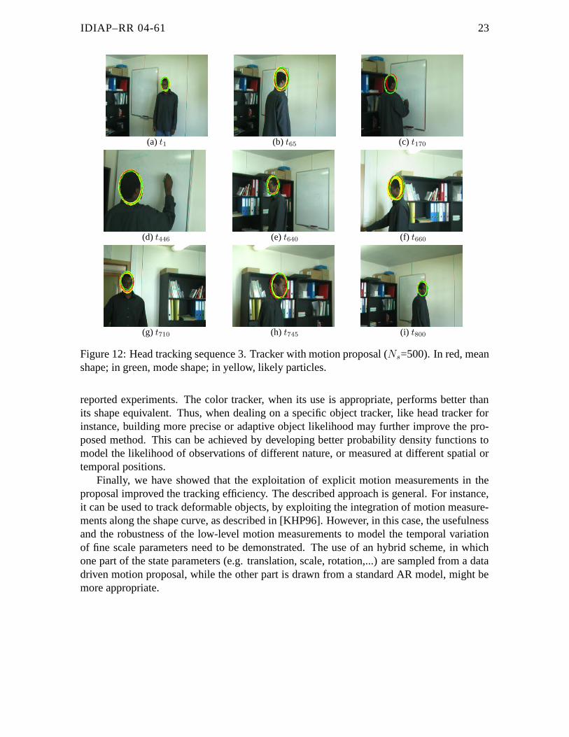
the dynamic noise is large enough, but fails when the head moves in front of the bookshelves,due to the temporally lack of head contours, combined with background clutter. In contrast,all these issues are resolved by the M3 tracker, which better capture the state variations, andallows a successful track of the head until the end of the sequence under almost all conditions(Fig. 13(c) and 13(d)).

7 Conclusion

We presented a methodology to embed data-driven motion measurements into particle filters.This was first achieved by proposing a new graphical model that accounts for the temporalcorrelation existing between successive images of the same object. We show that this newmodel can be easily handled by the particle filter framework. The new introduced obser-vation likelihood term can be exploited to model the visual motion using either implicit orexplicit measurements. Secondly, explicit motion estimates were exploited to predict moreprecisely the new state values. This data-driven approach allows for designing better propos-als that take into account the new image. Altogether, the algorithm allows to better handleunexpected and fast motion changes, to remove tracking ambiguities that arise when usinggeneric shape-based or color-based object models, and to reduce the sensitivity to the differ-ent parameters of the prior model.

The conducted experiments have demonstrated the benefit of exploiting the proposedscheme. However, this should not obliterate the fact that the tracking performance de-pends on the choice of a good and robust object model. This was also illustrated in the

IDIAP–RR 04-61 23

(a) t1 (b) t65 (c) t170

(d) t446 (e) t640 (f) t660

(g) t710 (h) t745 (i) t800

Figure 12: Head tracking sequence 3. Tracker with motion proposal (Ns=500). In red, meanshape; in green, mode shape; in yellow, likely particles.

reported experiments. The color tracker, when its use is appropriate, performs better thanits shape equivalent. Thus, when dealing on a specific object tracker, like head tracker forinstance, building more precise or adaptive object likelihood may further improve the pro-posed method. This can be achieved by developing better probability density functions tomodel the likelihood of observations of different nature, or measured at different spatial ortemporal positions.

Finally, we have showed that the exploitation of explicit motion measurements in theproposal improved the tracking efficiency. The described approach is general. For instance,it can be used to track deformable objects, by exploiting the integration of motion measure-ments along the shape curve, as described in [KHP96]. However, in this case, the usefulnessand the robustness of the low-level motion measurements to model the temporal variationof fine scale parameters need to be demonstrated. The use of an hybrid scheme, in whichone part of the state parameters (e.g. translation, scale, rotation,...) are sampled from a datadriven motion proposal, while the other part is drawn from a standard AR model, might bemore appropriate.

IDIAP–RR 04-61 24

0 200 400 600 800 10000

20

40

60

80

100

Frame number

Tra

ckin

g ra

te

Condensation tracker M1 − shape

D1D2D3D4

(a) M1 - Shape

0 200 400 600 800 10000

20

40

60

80

100

Implicit tracker M2 − shape

Frame number

Tra

ckin

g ra

te

D1D2D3D4

(b) M2 - Shape

0 200 400 600 800 10000

20

40

60

80

100

Frame number

Tra

ckin

g ra

te

Proposal tracker M3 − shape

D1D2D3D4

(c) M3 - Shape

0 200 400 600 800 10000

20

40

60

80

100

Frame number

Tra

ckin

g ra

te

Proposal tracker M3 − shape

501002505001000

(d) M3 - Shape

Figure 13: Head tracking sequence 3 : successful tracking rate (in %, computed over 50trials with different random seeds). Experiments 13(a) to 13(c) : parameter sets D1 to D4correspond to Ns=1000, with dynamics (σT, σs) : D1 (2,0.01), D2 (3,0.01), D3 (5,0.01) D4(8,0.02). In experiments 13(d), different number of particles are tested using the D3 (5,0.01)noise values.

Acknowledgment

The authors would like to thank the Swiss National Fund for Scientific Research that sup-ported this work through the IM2 MUCATAR project.

References

[AM04] E. Arnaud and E. Mémin. Optimal importance sampling for tracking in im-age sequences:application to point tracking. In Proc. of 8th European Conf.Computer Vision, Prague, Czech Republic, May 2004.

[AMF04] E. Arnaud, E. Mémin, and B. Cernushi Frias. Filtrage conditionnel pour latrajectographie dans des séquences d’images - application au suivi de points.In 14ème Congrès Francophone AFRIF-AFIA de Reconnaissance des Formeset Intelligence Artificielle, Toulouse, France, January 2004.

[AMGC01] S. Arulampalam, S. Maskell, N. Gordon, and T. Clapp. A tutorial on particlefilters for on-line non-linear/non-gaussian. IEEE Trans. Image Process., pages100–107, 2001.

[BI98] Andrew Blake and Michael Isard. Active Contours. Springer, 1998.

[BJ98a] M. J. Black and A. D. Jepson. A probabilistic framework for matching tempo-ral trajectories: Condensation-based recognition of gestures and expressions.In H. Burkhardt and B. Neumann, editors, Proc. of 5th European Conf. Com-puter Vision, Lecture Notes in Compter Science, vol. 1406, pages 909–924,Freiburg, Germany, 1998. Springer-Verlag.

[BJ98b] M.J. Black and A.D. Jepson. Eigentracking : robust matching and tracking ofarticulated objects using a view based representation. Int. J. Computer Vision,26(1):63–84, 1998.

IDIAP–RR 04-61 25

[CRM00] D. Comaniciu, V. Ramesh, and P. Meer. Real-time tracking of non-rigid ob-jects using mean shift. In Proc. IEEE Conf. Computer Vision Pattern Recog-nition, pages 142–151, 2000.

[DdFG01] A. Doucet, N. de Freitas, and N. Gordon. Sequential Monte Carlo Methods inPractice. Springer-Verlag, 2001.

[DGA00] A. Doucet, S. Godsill, and C. Andrieu. On sequential monte carlo samplingmethods for bayesian filtering. Statistics and Computing, 10(3):197–208,2000.

[GCK91] U. Grenander, Y. Chow, and D.M. Keenan. HANDS. A Pattern TheoreticalStudy of Biological Shapes. Springer-Verlag, New-York, 1991.

[GPLMO03] Daniel Gatica-Perez, Guillaume Lathoud, Iain McCowan, and Jean-MarcOdobez. A Mixed-State I-Particle Filter for Multi-Camera Speaker Tracking.In IEEE Int. Conf. on Computer Vision Workshop on Multimedia Technologiesfor E-Learning and Collaboration (ICCV-WOMTEC), 2003.

[IB89] M. Isard and A. Blake. Icondensation : Unifying low-level and high-leveltracking in a stochastic framework. In Proc. of 5th European Conf. ComputerVision, Lecture Notes in Compter Science, vol. 1406, pages 893–908, 1889.

[JFEM03] A.D. Jepson, D. J. Fleet, and T. F. El-Maraghi. Robust on-line appear-ance models for visual tracking. IEEE Trans. Pattern Anal. Machine Intell.,25(10):661–673, October 2003.

[KHP96] C. Kervrann, F. Heitz, and P. Pérez. Statistical model-based estimation andtracking of non-rigid motion. In Proc. 13th Int. Conf. Pattern Recognition,pages 244–248, Vienna, Austria, August 1996.

[NWvdB01] H. T. Nguyen, M. Worring, and R. van den Boomgaard. Occlusion robustadaptive template tracking. In Proc. 8th IEEE Int. Conf. Computer Vision,pages 678–683, Vancouver, July 2001.

[OB95] J.-M. Odobez and P. Bouthemy. Robust multiresolution estimation of para-metric motion models. Journal of Visual Communication and Image Repre-sentation, 6(4):348–365, December 1995.

[PHVG02] P. Pérez, C. Hue, J. Vermaak, and M. Gangnet. Color-based probabilistictracking. In Proc. of 7th European Conf. Computer Vision, Lecture Notesin Compter Science, vol. 2350, pages 661–675, Copenhaguen„ June 2002.

[PS99] Michael K. Pitt and Neil Shephard. Filtering via simulation: Auxiliary particlefilters. Jl of the American Statistical Association, 94(446):590–599, 1999.

IDIAP–RR 04-61 26

[PVB04] P. Pérez, J. Vermaak, and A. Blake. Data fusion for visual tracking with parti-cles. Proc. IEEE, 92(3):495–513, 2004.

[RC01] Y. Rui and Y. Chen. Better proposal distribution: object tracking using un-scented particle filter. In Proc. IEEE Conf. Computer Vision Pattern Recogni-tion, pages 786–793, December 2001.

[RMD01] A. Rahimi, L.P. Morency, and T. Darrell. Reducing drift in parametric mo-tion tracking. In Proc. 8th IEEE Int. Conf. Computer Vision, pages 315–322,Vancouver, July 2001.

[RMG98] Y. Raja, S. McKenna, and S. Gong. Colour model selection and adaptationin dynamic scenes. In Proc. of 5th European Conf. Computer Vision, LectureNotes in Compter Science, vol. 1406, pages 460–474, 1998.

[SB01] H. Sidenbladh and M.J. Black. Learning image statistics for bayesian track-ing. In Proc. 8th IEEE Int. Conf. Computer Vision, volume 2, pages 709–716,Vancouver, Canada, July 2001.

[SBF00] H. Sidenbladh, M.J. Black, and D.J. Fleet. Stochastic tracking of 3d humanfigures using 2d image motion. In Proc. European Conf. Computer Vision,volume 2, pages 702–718, Dublin, Ireland, June 2000.

[SBIM99] J. Sullivan, A. Blake, M. Isard, and J. MacCormick. Object localization bybayesian correlation. In Proc. 7th IEEE Int. Conf. Computer Vision, pages1068–1075, 1999.

[SBR00] J. Sullivan, A. Blake, and J. Rittscher. Statistical foreground modeling forobject localisation. In Proc. European Conf. Computer Vision, pages 307–323, 2000.

[SJ01] J. Sullivan and Rittscher J. Guiding random particles by deterministic search.In Proc. 8th IEEE Int. Conf. Computer Vision, pages 323–330, Vancouver, July2001.

[TB01] K. Toyama and A. Blake. Probabilistic tracking in a metric space. In Proc. 8th

IEEE Int. Conf. Computer Vision, Vancouver, July 2001.

[Tek95] A.M. Tekalp. Digital video processing. Signal Processing series. PrenticeHall, 1995.

[TSK01] Hai Tao, Harpreet S. Sawhney, and Rakesh Kumar. Object tracking withbayesian estimation of dynamic layer representations. IEEE Trans. PatternAnal. Machine Intell., 24(1):75–89, 2001.

[VDP03] J. Vermaak, A. Doucet, and P. Pérez. Maintaining multi-modality throughmixture tracking. In Proc. 9th IEEE Int. Conf. Computer Vision, Nice, France,June 2003.

IDIAP–RR 04-61 27

[VPGB02] J. Vermaak, P. Pérez, M. Gangnet, and A. Blake. Towards improved observa-tion models for visual tracking: Selective adaptation. In Proc. of 7th EuropeanConf. Computer Vision, Lecture Notes in Compter Science, vol. 2350, pages645–660, Copenhague, Danemark, 2002.

[WH01] Y. Wu and T. Huang. A co-inference approach for robust visual tracking. InProc. 8th IEEE Int. Conf. Computer Vision, Vancouver, July 2001.