MORTGAGE VALUATION AND

THE TERM STRUCTURE OF INTEREST RATES

3HT

MORTGAGE VALUATION AND

THE TERM STRUCTURE OF INTEREST RATES

I'HOKFSCHMFT

ter verkrijgiiig van de graad van doctor aaii de Universitelt Maastricht

op gezag van de Rector Magnificus. Prof. mr. G.P.M.F. Mols,

volgens het besluit van het College van Dccanen, in het openbaar te verdedigen

op woensdag 8 december 2004 orn 12.00 mir

door

Bart Henricus Matthijs Kuijpers

I'romotorea:

Prof. dr. ir. A.W..J. Kolen

Prof. dr. P.C. Schotman

BaourdcliugHcommiiMtic:

Prof. dr. ir. C.P.M. van Hoescl (voorzitter)

Dr. W.F.M. Bmiut (Univcraitcit MaaHtricht) l [ { i

Prof, dr. A.A.I. POIHWT (Krawmiw Univermteit Rotterdam)

• ? • : > * * # M - ? - ' I K J H

Valuation and the Term Structure of Interest Rates

©2004, Bart H.M. Kuijprrs

ISBN 90-9018761-8

a*i!;

Preface

The origin of this dissertation lies in the early spring of 1999, when Antoon K<>l' n .•!!< -ml

mo a Ph.D. fxxsition on mortgage valuation at the University of Maastricht. Tin* petition,

bring a joint project of the Department of Quantitative Fx-onomics and the Depart mrnl of

Finance, gave me the |M«ssil>ility to combine division theory and linance The combination

interested me. and still dors, and I started after finishing my Htud\ <• metrics later thut

year. Although the last year of my Ph.D. has IMVII difficult, I am still convinced that the

choice I made five years ago was the right one at that time. Ultimately, it hax remitted in

this Ph.D. dissertation I look hack on a challenging ami enjoyable period

Several people contributed to this thesis. Many thanks go to my supervisors Antoon

Kolen and Peter Schotman. Together, we analyzed many research problems from different

perspectives. I am grateful to Antoon for sharing his knowledge and experience of oper-

ations research and his desire to solve mathematical problems. I thank Peter for passing

on his financial and econometric knowledge and intuition. Also. I have very much appre-

ciated the opportunity he gave me to work together in Stotkhohn on several parts of this

dissertation, which led to a fruitful cooperation and a very enjoyable time.

Of the other places I had the privilege to visit during my Ph.D. period, Barcelona has

made the most unforgettable impression. I am grateful to Bart, Carl and Roger for the

great days in which we explored this beautiful city and the 'nearby' Pyrenees.

Of course I am thankful to my colleagues at the departments of Finance and Quantitative

Economics for the pleasant atmosphere, inside and outside university. I have enjoyed our

activities such as going to the movies and playing unihockey and soccer matches, even

though I can hardly remember a won soccer game. Special thanks go to Frank for his

inspiration, both during our study and the subsequent Ph.D. period.

Veruit mijn grootste dank gaat uit naar mijn ouders en broer. die er altijd zijn Is ik

z<' nodig li«'l>. HorwH jullk* vaak niet precies wistcn waar ik mee l>ezig was. toondenullk*

altijd lM>lang.stolling vfKjr inijn vordoringon (en tegenslagen). Bij jullie vond. en vind inog

dc lUMligt- tiflciding. Zonder jullie ttteun zou dit proefschrift er niet zijn gewe*.

Bart

Si'plrinlxT 2(K)I

•• ••!«'. m ; . ;

Contents

Preface I

1 Introduction |

1.1 MortKftgc valuation 1

1.2 Term structure of intent MII-S g

1.3 Optimal exercinc of prepayment options 12

1.4 Outline 13

1 Interest Rate Tree Calibration 17

2 Term Structure Models and Data 18

2.1 Introduction 18

2.2 Overview of term structure models 20

2.3 Notation for swap and swaption valuation 26

2.4 Term structure fitting using swaps 28

2.4.1 Swap data 28

2.4.2 Pricing of swaps 29

2.4.3 Term structure derivation 32

2.4.4 Results 34

2.5 Swaption pricing 37

2.5.1 Swaption data 38

2.5.2 Black and Scholes method for swaption pricing 38

iii

ir COJVTEVTS

2.6 Performance of term structure models . . . 43

2.7 BDT and binomial trees 45

2.8 Concluding remarks . 46

3 Interest Rate Lattice Calibration , 48

3.1 Introduction 48

.'1.2 Lattice construction 50

.'J.2.1 framework 50

3.2.2 Parameterization 56

3.3 Calibration 63

3.3.1 One-factor model 63

3.3.2 Two-factor model 66

3.3.3 Goodness of fit 66

3.3.4 Optimizing parameter values 68

3.4 Data 70

3.r> ItcMiltK 71

3..V1 One factor model 71

3..V2 Two-factor model 87

3.6 Conclusion 94

II Mortgage Valuation 97

4 Introduction to Mortgage Valuation 98

11 Introduction 98

•1.2 Mortgage characteristics 100

4.2.1 Amortization schedule 100

4.2.2 Call options 104

4.2.3 Contract rate adjustment 105

4.3 Valuation 107

4.3.1 Fixed rate mortgage valuation 108

CONTENTS v

4.3.2 Adjustable rate mortgage valuation 112

4 4 Concluding remarks 116

5 Optimal Prepayment of Dutch Mortgages 118

5.1 Introduction IIS

5.2 Formulation 119

5.3 Results 127

5.4 Concluding remarks 132

6 Mortgage Valuation with Partial Prepayment* 134

G.I Introduction I'M

6.2 Mathematical framework I .'Hi

6.3 Tin- IIKMIOI 138

6.4 Dual formulation 141

6.5 Implication* for fully callable mortgage* 11.1

6.6 Rounding the fair ra te I l<>

6 . 7 Results 151

6.8 Concluding remarks 152

7 A Comparison of Fair Mortgage Rates 154

7.1 Introduction 154

7.2 Results 155

7.3 Concluding remarks 107

8 Summary and Concluding Remarks 170

Bibliography 173

Samenvatting / Summary in Dutch 178

Curriculum Vitae 181

i 4,:>

IChapter 1

Introduction

This thesis deals with mortgage valuation and interest rnto tn-c calihnition. Optimization

and computation play a prominent rule in l>oth fields. Optimization is important fur the

derivation ofa rational excreta'polk-y of implicit mortgAgr prepayment options. Section I I

provides an overview of the Dutch mortga^' market and describes typical Dutch niortKi'K''

features such as limite<l prepayment and tax issues. Sinn- the term structure <>f interest

rates is the main driver behind mortgage valuation and mortgage prepayment, interest rate

modelling, interest rate tree calibration and interest rate derivative pricing are introduced

in section 1.2. After discussing the modelling structures used throughout this dissertation,

optimization aspects of mortgage valuation are introduced separately in section 1..'{. Section

1.4 includes an outline of this thesis.

1.1 Mortgage valuation

A mortgage loan is a long term loan secured by a collateral, usually real estate. The

mortgagor borrows money from the mortgagee and pays back the loan according to an

agreed upon amortization schedule. In case the mortgagor fails to make the required

payments, the mortgagee has the right to use the proceeds of the collateral to offset the

loan, for example by selling the house.

The Dutch mortgage market has developed extremely fast from the early nineties on.

An overview of the mortgage market in the Netherlands is provided by Alink [1], Charlier

and Van Bussel [19] and Hayre [32]. Based on Charlicr and Van Bussel and on data from

CBS. the Dutch Central Bureau for Statistics, figure 1.1 shows that the total amount (in

1

CHAPTER i. /.VTRODl/CT/OiV

480

400

f 350

• 300

250i200

150

100

50

FIGURE 1.1: Dutch mortgage market development. Sourre: CBS

I Outstanding '

I Newly issued and refinanced

- Average mortgage rate

1

1993 1UU4 IUU5 1UUG 1997 1998 1999 2000 2001 2002 2003

Y*ar

euros) of mortgage loans outstanding has more than tripled between 1993 and 2003. The

proportion of newly issued and refinanced mortgages in the mortgage pool has increased,

as the corresponding market share has more than quadrupled in the same period. This

latter increase is mainly due to the rise of newly issued and refinanced mortgages in the

years 15)95 to 1999, a period in which the average mortgage rate dropped from 7.1% to

5.1%.

Annual mortgage transactions can lie divided in issuing new mortgages and refinancing

existing mortgage contracts. The amount of newly issued mortgages has hardly changed

over the past ten years, according to figure 1.2. The increase in market share of newly

issued and refinanced mortgage loans is completely due to refinancing existing loans, mainly

driven by the significant mortgage rate decrease. Consequently, the importance of optimal

interest rate driven prepayment and refinancing has increased. This dissertation covers

both the derivation of optimal prepayment and refinancing strategies and the valuation of

implicit prepayment and refinancing options.

Figure 1.3 shows the importance of mortgages on the combined balance sheet of Dutch

banks. Mortgages make up for almost one quarter of the total bank's assets, which is more

Li. A/ORTGAGE VALIMT7ON

FIGURE 1.2: Amount of newly iiwuvd aud refinanced uiurtgagm. Sown*; CAS

700• Newlyesued

600 • Refinanced

500

400

'300

200

100

1995 1996 1997 1990 1909 2000 2001 2002 2003

than bonds or short term loans and slightly less than long term loans.

Many types of mortgage contracts exist. A complete overview of Dutch mortgages

in 2003 is available in the 'Hypothekengids 2003', the guide of the Dutch homeowners

association 'Vereniging Eigen Huis'. A mortgage loan consists of several components.

Loans may differ with respect to amortization schedule, contract rate adjustments and

prepayment, refinancing or default options. Besides these basic ingredients of a mortgage

contract, a variety of options is possibly included. Many contracts have insurance or

investment opportunities. Also, tax regulations play an important role concerning the

popularity of mortgage types.

Most commonly known amortization schedules include annuity mortgages and linear

mortgages. Annuities are constant periodical payments including both redemption and

interest. Initial payments are split into large interest payments and small redemption

amounts. Later, when the remaining loan decreases, interest payments decline whereas

redemption increases. Linear mortgages have constant amortization payments, but initially

large total cash flows due to large interest payments.

A popular amortization schedule in the Netherlands is adopted by savings, investment or

interest-only mortgages. With these mortgage types only interest payments occur during

the lifetime of the contract. A savings mortgage is repaid at maturity, using a fund to

Deposits

Bonds

Equity

S*°" ' • " * loans

4

* ' " ' " ' ' H h a w . K

on ,

returns T ?

hy 2

during

'""'"» An i

^ t r a c t s is

,.

• new ioa

i- client » e fi

house.

up the

U A/ORTG.AGE V:4LU/IT/OiV

FIGURE 1.4: Market shares development of utortgiw rrtlfitiption

60%

40%

30%

20%

10%

0%

iino'• 1W4• 1008Q2000

MOTM-onty Savings Lite innnance Annuity luisai MlicaNanaoua

majority of the total mortgage pool. Nowadays the popularity of traditional redemption

types (both annuity and linear mortgages) has decreased, in favor of interest-only mort-

gages and savings and investment mortgages, the latter type making up the largest part

of the 'miscellaneous' category.

Mortgage contracts also differ with respect to fixed rate periods and contract rate ad-

justments. Longer fixed rate periods do not expose the borrower to future interest rate

changes, but usually require a higher contract rate. A variable contract rate is attractive

initially when the term structure is upward sloping, but implies a large borrower risk since

any interest rate change is reflected in the contract rate. For longer maturity contracts, at

the end of a fixed rate period the contract rate will be adjusted to match future interest

rate conditions. With some contracts this adjustment is unrestricted. Others may have

cap or floor restrictions to limit a contract rate increase or decrease respectively. In the

Netherlands a typical mortgage contract has a fixed rate period of 5, 7 or 10 years, after

which the contract rate is reset. The lifetime of a mortgage contract is usually 30 years.

Thirty years is also the maximum period for tax deductions of interest payments.

6 CHAPTER i. /ATKODUC77OJV

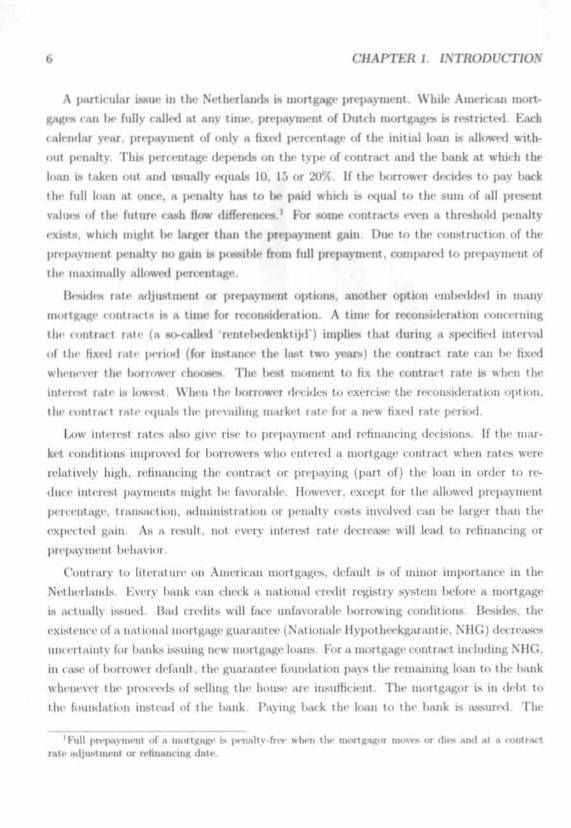
A particular issue in the Netherlands is mortgage prepayment. While American mort-

gages can be fully called at any time, prepayment of Dutch mortgages Ls restricted. Each

calendar year, prepayment of only a fixed percentage of the initial loan is allowed with-

out |M-nalty. This percentage depends on the type of contract and the bank at which the

loan is taken out and usually equals 10, 15 or 20%. If the borrower decides to pay backthe full loan at once, a penalty has to be paid which is equal to the sum of all present

values of the future cash flow differences.' For some contracts even a threshold penalty

exists, which might be larger than the prepayment gain. Due to the construction of the

prepayment penalty no gain is |>ossible from full prepayment, compared to prepayment of

the maximally allowed percentage.

Besides rate adjustment or prepayment options, another option embedded in many

mortgage contracts is a time for reconsideration. A time for reconsideration concerning

the contract rate (a so-called 'rentebedenktijd') implies that during a specified interval

ol the fixed rate period (for instance the last two years) the contract rate can be fixed

whenever the borrower chooses. The bent moment to fix the contract rate is when the

interest rate is lowest. When the borrower decides to exercise the reconsideration option,

tin- coiitnu t rate <-<|iials the prevailing market rate for a new fixed rate period.

Low interest rates also give rise to prepayment and refinancing decisions. If the mar-

ket conditions improved for borrowers who entered a mortgage contract when rates were

relatively high, refinancing the contract or prepaying (part of) the loan in order to re-

duce interest payments might be favorable. However, except for the allowed prepayment

percentage, transaction, administration or penalty costs involved can be larger than the

expected gain. As a result, not every interest rate decrease will lead to refinancing or

prepayment behavior.

Contrary to literature on American mortgages, default is of minor importance in the

Netherlands. Every bank can clunk a national credit registry system before a mortgage

is actually issued. Bad credits will face unfavorable lx>rrowing conditions. Besides, the

existence of a national mortgage guarantee (Nationale Hypotheekgarantie. NHG) decreases

uncertainty for banks issuing new mortgage loans. For a mortgage contract including NHG.

in case of borrower default, the guarantee foundation pays the remaining loan to the bank

whenever the proceeds of selling the house are insufficient. The mortgagor is in debt to

the foundation instead of the bank. Paying Iwck the loan to the bank is assured. The

'FNill prepayment of « mortgage is penalty-fnv when tin- mortgagor moves or dies and at a contractrat(> mljustmnit or rohimiu IIIR dale

J.I. A/ORTGAGE VALl/AT/ON

FIGURE 1.5: Mortgage rat* vs interest n»tw. 5ourrr: C/W and />A'/?

-Mortgage6 yaa> Warwt r»H

••••••1 yaw iniaraM rait

01966 1990 1994 1996

Yaar

2002

bank's risk therefore decreases and the contract rate will be lower compared to a mortgage

contract without NHG.

We focus on the optimal prepayment strategy for mortgage loans, thereby dealing with

mortgage valuation from a client's perspective. The role of a bank issuing mortgage con-

tracts is to set the contract rate based on, among other aspects, prepayment behavior. The

main contribution of this thesis to the existing mortgage valuation literature includes the

valuation of the partial prepayment option and the derivation of the corresponding optimal

prepayment strategy. We present various optimization algorithms, baser! on dynamic pro-

gramming and linear programming, to obtain optimal mortgage values. An introduction

to optimization issues will be provided in section 1.3.

For the valuation of mortgages, the development of interest rates is a key factor. The

mortgage rate is highly correlated with (long term) interest rates, as can be concluded

from figure 1.5. based on data from CBS and 'De Nederlandsche Bank' (DNB). Besides the

interest rate level, interest rate volatility is important for the pricing of embedded options.

Volatility is usually not observable, but implied by derivatives. Both the term structure; of

interest rates and volatilities implied by interest rate derivatives will be introduced in the

next section.

8 CHAPTER 1. fiVTRODUCTJON

1.2 Term structure of interest rates

The term structure of interest rates is the main driver behind mortgage prices and pre-

payment decisions. In mortgage valuation, prepayment can be accounted for in two ways.

Kit her empirically olwerved prepayment or optimal, interest rate based prepayment is mod-

elled. Empirically olwerved prepayments on Dutch mortgage contracts, for instance due

to moving, have been analyzed by Alink [1] and Havre [32].

Although borrowers might have different reasons to prepay a mortgage loan, our focus

is (in optimal, interest rate based prepayment. Optimal prepayment is interesting for both

clients, minimizing the present value of all cash flows to amortize the mortgage loan, and

for bunks, to infer the impart on contract rates when mortgages are optimally prepaid.

Optimal prepayment provides a worst case for mortgage issuers.

In this dissertation we will view mortgage loans as fixed income derivatives No cash

restrictions apply as soon as prepayment is optimal. If the cash position is insufficient

In prepay (part of) the loan, we assume that the required amount can be borrowed at

prevailing (lower) interest rates. Consequently, frictionless trading is assumed.

A term structure of interest rates represents current spot rates or prices of discount

bonds (zero-coupon bonds) for varying maturities. Basic mortgage contracts, without

prepayment or rate adjustment options, can be valued by the term .structure only. Future

cash flows arc discounted using the spot rate with corresponding maturity in order to

obtain the present value.

Prices of options on interest rate dependent assets, such as bond options, caps, floors,

swap options (so called swaptions) and also mortgages including prepayment options, de-

pend on interest rate volatility. To capture volatility the distribution of future interest rates

must be known. Future interest rates are uncertain ami can be modelled using different

approaches and interest rate models.

In this thesis we will model uncertainty in future interest rates by using a discrete state

space. A state space is a directed tree (of which a recombining and a non-recombining

version are shown in figure 1.6). A node is also referred to as a state. The set of all states

is partitioned into layers, each layer corresponds to one of the time points f = 0 7* and

contains all the states that may occur at that time point. A state is represented by its

layer f and index » as (», r). Node (0.0) is called the root node. An arc connects two states

in subsequent layers. Consider node A\ indexed by (i.f). and node /. indexed by (j. f + 1).

If an arc (A\/) exists, then node A- is called the predecessor of node / and / is called the

1.2. TERA/ STRUCTURE OF INTEREST RATES

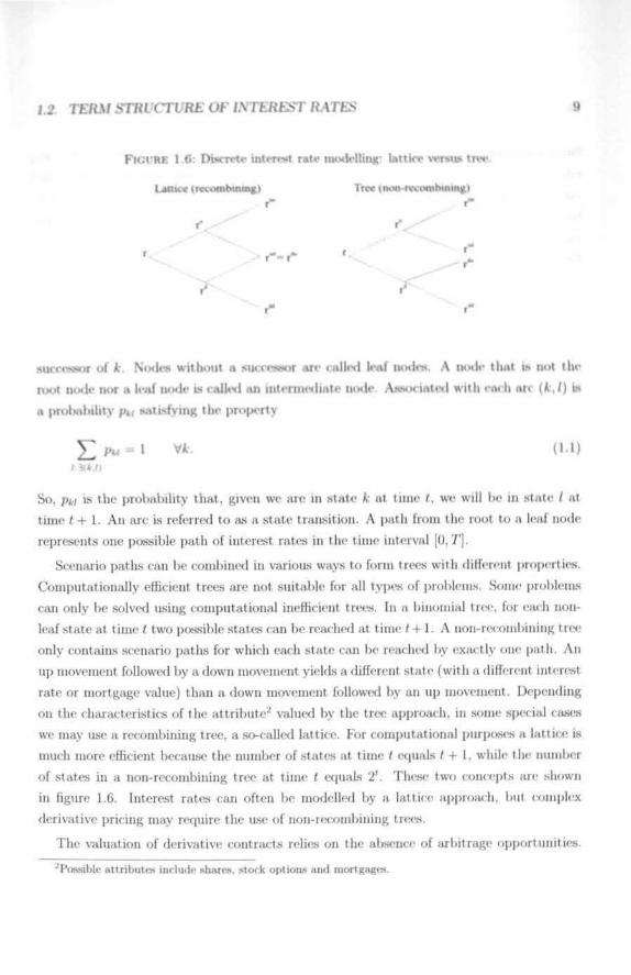
FIGURE 1.6: Dwrrrte interest rate modelling: lattice versus tree.

Lattice (recombining) Tree (non-rveomhinmg)

r

s u c c e m o r of it. N o d e s w i t h o u t n s u c c e s s o r a r e cal l i -d l<\-if in>des. A IMM|I- t li . i t is no t t h e

root n o d e n o r a leaf n o d e is c a l l e d a n i n t e r m e d i a t e IHKII- . A N M K m t e d w i t l i >m II m> ( A \ / ) W

a protmhility pu satisfying the property

£ f » M = l VX-. (1.1)

So, pw is the probability that, given we are in state A: at time f. we will be in state / at

time < + 1. An arc is referred to as a state transition. A path from the root to a leaf node

represents one possible path of interest rates in the time interval [0, T],

Scenario paths can be combined in various ways to form trees with different properties.

Computationally efficient trees are not suitable for all types of problems. Sonic problems

can only be solved using computational inefficient trees. In a binomial tree, for each non-

leaf state at time f two possible states can be reached at time r + 1. A non-rceombining tree

only contains scenario paths for which each state can be reached by exactly one path. An

up movement followed by a down movement yields a different state (with a different interest

rate or mortgage value) than a down movement followed by an up movement. Depending

on the characteristics of the attribute'^ valued by the tree approach, in some special cases

we may use a recombining tree, a so-called lattice. For computational purposes a lattice is

much more efficient because the number of states at time < equals < + 1, while the number

of states in a non-recombining tree at time < equals 2'. These two concepts are shown

in figure 1.6. Interest rates can often be modelled by a lattice approach, but complex

derivative pricing may require the use of non-recombining trees.

The valuation of derivative contracts relies on the absence of arbitrage opportunities.

-Possible attributes include shares, stock options and mortgages.

10 CHAPTER 1 LVTRODl/CTJON

Since a mortgage ia in essence a portfolio of elementary interest rate dependent contracts,

taking out a mortgage is equivalent to investing in a (possibly complicate*!) bond portfolio.

An invoNt iiK'iit strategy defines a portfolio for each non-leaf state consisting of zero-coupon

bonds (that is, we sell and buy available zero-coupon bonds). To liquidate a portfolio we

sell the assets that we own and buy l>ack the assets we sold. For a non-recoinbining tree,

the state contribution of an investment strategy is defined as the revenue of a portfolio

if the state is the root state, is defined as the revenue of liquidating the portfolio of the

unique predecessor state if the state is a leaf state (at the leaf node prices), and is defined

as liquidating tin; portfolio of the unique predecessor state minus the cost of constructing

the portfolio of the state itself if the state is an intermediate state.

An arbitrage opportunity is defined as an investment strategy for which every state

contribution is non-negative and the sum of all state contributions is positive. If the

contribution of the root node is positive, then we make a sure profit now without having

any future costs. This is a sure way of making money. If the contribution of the root node

is zero, then at least one price path exists for which the total contribution is positive. This

situation is comparable with a free ticket in a lottery.

The existence of arbitrage run be fnrmaliwwl »« folio*™ -1-n* 1' «tn»o«u» AKr »a»l«rjni/v-wmr

of an asset (or n portfolio of assets). Now V(i.t) represents the value of the asset at time

f in state /. An arbitrage opportunity, having root node contribution equal to 0, is then

defined as a trading strategy such that

• 1(0 ,0) - 0

• V'(i.f) > 0 V/.f

Stated differently, an arbitrage opportunity is a possibility of making money, starting with

nothing, without any risk of losing money.

A version of Parkas' Lemma shows that there are no arbitrage opportunities if and only

if (hero exists a positive weight for each state transition such that the vector of prices at

a state is the weighted sum over all successor states of the vector of prices at these states

(for textbook references, sec Dutfio [27] and Pliska [73]). In a non-recombing tree, the state

price of a state is defined as the product of all arc weight* over all arcs on the unique path

from the root to that state. By Farkas' lemma, the absence of arbitrage opportunities is

equivalent to the existence of a vector of non-negative state prices. For a lattice, the state

1.2 TEKA/STR^CT^RE OF/\T£REST R.4TES 11

price of a particular state is the sum o m all jwths leading to that state of all state price*

belonging to the same patlis in the non-recouibiniug tree.

One frequently used way to construct mi interest rate model is to define in each node

(i,() the so-called short rate r,,. that is the interest rate for the time interval runnuiK liom

I to f + 1 . The positive art- weight of an arc rooted in (i.f) is defined as ^ j , ^- We assume

equal up and down prolmbilities: p,^ = 1 for l>oth sncc«»or nodes. Dividing by I f r,,.

prices at time f + 1 are discounted towards prices at time /. Once interest rates are defined

for all states, a complete term structure can l>c derived in each node

Given all arc weights it Is easy to calculate all zero-coupon bond price* and show thai

the no-arbitrage conditions are satisfied. To see this, note that a zero-cou|>on bond has

value 1 at its maturity. Using the arc weights we can calculate its value at the previous

time point. Continuing this way. for each state the zero-coupon IMHKI value at that state

can IK- determined by multiplying the value at the mumMor node by the arc weigh! and

summing the result over all successors.

A claim defines for each state a claim value. The interest rate model is complete if for

even' claim an invest merit strategy exists for which the contribution in each state is equalto the claim value. A necessary and sufficient condition for completeness is that for every

non-leaf state the matrix with rows equal to the price vectors of all successor states has

full row rank (see Duffie [27]). The interest rate model defined above is complete. One

can view a cliiim as a financial product- that pays the claim value if positive, and receives

minus the claim if the claim value is negative. If the interest rate model is complete, then

the price of the claim can be shown to be equal to the sum over all states of the product

of the state price and the claim value.

A contingent claim is defined as a security having payoffs dependent (contingent) on

the outcome of some underlying process (for instance, a price process of an underlying

asset). As an example, consider an option paying out when expired in-the-money and not

paying out when expired out-of-the-money. An Arrow-Debreu or state-contingent claim

is a security paying 1 in one state at maturity, and zero in all other states. Denote the

present value of a state-contingent claim paying 1 in state i at time < as G'on(i, i)- Many

traded assets can be viewed as a portfolio of state-contingent claims. A bond maturing at

time f pays 1 in every lattice state z = 0, < at <. Hence this bond is an equally weighted

portfolio of the state-contingent claims having present value C"oo(M)- The present bond

12 C7MPTEK 1 /.VTRODl/CT/O.

price Poo(') follows as > ? ;

Interest rate trees are calibrated using an underlying term structure model. Thes

models differ with nwpect to the miiiilx-r of factors and to the extent they capture futur

drift, volatility and mean reversion of interest rates. For a given model an interest rat

tree r-un !>«• calibrated, such that model prices of interest rate dependent assets are as clo»

i | >• i-al>le to ol)«erved prices. Performance of a term structure model is measured as th<

difference between model prices and observed prices.

Both the future interest rate level and the future volatility or uncertainty are rcflectei

by observed market prices of interest rate dependent instruments. Bonds and swajxs can I*

used to extract information about the level, whereas volatility Ls included in option data

Implied volatilities are generally available from caps, floors or swaptions.

We will calibrate interest iat<,-, in order to match swap and swaption prices as closelj

an possible. A swap is a financial instrument to exchange a series of floating payments inU

fixed payments (or vice vena). The main use of a swap is to hedge financial risk, present

in future float inn payments or revenues, for instance due to uncertain exchange rates in

case of purchasing or selling goods in a foreign country. A swaption is the right, but not

the obligation, to enter a swap contract at a certain date (the option expiration or exercise

date) and a certain price (the strike or exercise price). Uncertain future interest rates

determine the price development of swaps and swaptions. The current price must equal

the sum of all discounted expected cash flows, both floating and fixed.

Optimal exercise of prepayment options in mortgage contracts is based on the volatility

structure observed from swaptions. The next section introduces some of the optimization

issues concerning prepayment decisions, related literature and an overview of optimization

algorithms for the valuation of prepayment options applied in this thesis.

1.3 Optimal exercise of prepayment options

Exorcise of prepayment options is based on the term structures of interest rates and interest

rate volatilities. Much literature on Dutch mortgages, for instance Alink [1] and Charlier

and Van Bussel [19], has focussod on empirical prepayment, which Ls not directly affected

by interest rate driven prepayment divisions. In this dissertation, mortgage prepayment Ls

1.4. OUTLJATE IS

triggered by the interest rate level. This approach provide i w. .i-t , ,i>, tor banks and an

O|>tinial prepayment strategy* for • li<nt>

Given a scenario troe of intereM iai«-s. optimal valuation of fullv or |uirtiallv callable

mortgages can be modelled. The majority of literature on opt mini exercise of prepayment

options focuneB on American mortgage contracts for which full and unre«tricted pre|wy-

ment is allowed without penalty. Optimal exercise policies for American mortgage loans

haw been derived by Kau. Keenan. Mnller and Kp|>erson (48]-(51). A default option in

typically included as well. Fully callable adjustable rate mortgages are also <lis< nssiil

Hilliard. Kau and Slaw-son [37] apply a two-factor mortgage valuation model, the socuud

factor being house price development.

Dutch mortgages, allowing only a limited prepayment amount, are more ditliailt to

value, since partial pre|>ayments imply path dcpcndeucieN in the scenario tree. First, the

remaining loan depends on earlier prepayments Partially callable mortgage* can have

various remaining loan amounts Second, the price of the (remaining) mortgage loan de-

pends on the future prepayment strategy. Third, tin- calendar year restriction, const Miming

prc|>ayment to a limited amount per year, impomw a restriction on the allowance of pre-

payments along parts of scenario paths belonging to the same calendar year.

Because of these path dependencies a mortgage value (and adopted prepayment strategy)

can be different when reaching the same state, but having followed different paths. In gen-

eral, valuation of partially callable mortgages requires the use of non-rccombiniug trees.

Since these are inefficient due to the exponential growth of the number of states, this thesis

focusses on deriving lattice based algorithms to value partially callable mortgage loans.

Fortunately, some partially callable mortgages can be priced optimally by applying an

efficient lattice approach, decomposing a mortgage contract into a portfolio of callable

bonds. This approach is valid for mortgage loans that can be decomposed a priori, with-

out knowledge of the optimal prepayment strategy. These mortgage contracts can be

valued according to dynamic programming. Other mortgage types cannot be valued both

optimally and efficient. For these contracts we derive a linear programming formulation.

1.4 Outline

The ordering of chapters in this dissertation describes the logical process, starting with

observing interest rate derivative data, which are used for interest rate lattice calibration.

14 CHAPTER 1. JNTRODl/CTJON

The resulting lattices, describing interest rate scenarios, are applied for mortgage valuation.

The first part of this thesis deals with the calibration of interest rate trees from observed

data. For calibrating we require a term structure of interest rates, swaption prices and a

term structure model. Chapter 2 provides an overview of several widely used term structure

models. Characteristics. ;idvautagc» and disadvantages of the models are discussed, while

keeping in mind our purpose: to value long term mortgage contracts with typical embedded

options. . '

Our data set include)) swap rates, short term EURIBORs and implied swaption volatilities.

Chapter 2 describe how to construct a term structure based on a spline method, for given

swup ratc-s mid short interest rates. The valuation of ln>th payer's and receiver's swaps

is explained, given cash How patterns and common quoting conventions. Black's option

formula for (at-the-money) swap)ions transforms swaption volatilities into swaption prices.

Put-call |>arity shows that for at-t he-money swaptions the prices for newly issued payer's

swuptions and receiver's swaptions are equal.

In chapter .'< the data (term structure and swaption prices) and models of chapter 2

are used to calibrate a binomial interest rate lattice. A detailed technical analysis of

the Hlack. Herman and Tov (•). HDT] HUM lei. as well as the Ho .MKJ L«- /as. HL/ model,

is provided. One of the most important characteristics of these models is the relation

between volatility and menu reversion. These can not be matched independently, unless

variable period lengths are allowed. The second part of chapter 3 is an extensive analysis

of the calibration results. We consider input data on several dates and provide results on

swaption pricing errors, term structure fitting, volatilities and mean reversion of interest

rates.

Part II deals with mortgage valuation, based on the calibrated interest rate lattice

resulting from part I. The typical Dutch prepayment feature of allowing a fixed percentage

of the initial loan per calendar year introduces path dependencies in the binomial mortgage

valuation tree. We focus on optimal prepayment behavior from a client's perspective.

Chapter I introduces distinctive features of mortgage contracts, including amortization

schedules, call options and contract rate adjustments. We discuss mortgage valuation based

on binomial lattice methods. Our focus is on deriving fair contract rates of common Dutch

mortgage types. The fair rate is the contract rate for which the mortgage price is equal

to the nominal loan value. For a mortgage quoted at the fair rate, neither bank nor client

can make a profit. Fair rates are particularly useful when deriving option premiums as the

difference between the fair rate of a mortgage including pre|>ayment option and the fair

1.4. OiVTLIJVE 15

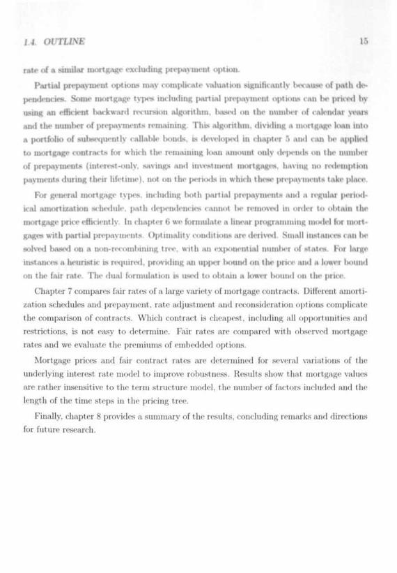
ofa similar mortgage excluding prepayment option.

Partial prepayment options may complicate \-aluation significantly txvause of path de-

pendencies. Some mortgage ty|>es including partial prepayment options can l>e price*I by

using an efficient Imckward recursion algorithm. luiscd on the number of calendar years

and the number of prepayments remaining. Tills algorithm, dividing a mortgage loan into

n |M>rtfolio of sulisc<|tiently callable ttonds. is developed in chapter 5 and can l>c applied

to mortgage contracts for which the remaining l".m mioiint only depends on the number

of prepayments (interest-milv. savings and inu-M nxiit mortgages. havuiK n<> re<lcmption

payments <luring their lifetime), not on the |MTKM1S in which tlicw pn-payiuciits tak«- place

For general mortgage types, including Imth partial prepayments and a regular period-

ical amortization schedule, path dependencies cannot IM> removed in order to obtain the

mortgage price efficiently In chapter 6 we formulate a linear programming model for mort-

gages with partial prepayments. Optimally conditions are derived. Small instance* can l>e

.solved K.iM-d on a iioii-nvomtiining tree, with an exponential numlxt of states, l-'or large

in.si.in. >> ,i liciiristu is re<|uire<l, providing IUI up|M>r lioiuul on the pricr and a lower bound

on the fair rate. The dual formulation is ased to obtain a lower IMXIIKI on the price.

Chapter 7 compares fair rates of a large variety of mortgage contracts. Different amorti-

zation schedules and prepayment, rate adjustment and reconsideration options complicate

the comparison of contracts. Which contract is cheapest, including all opportunities and

restrictions, is not easy to determine. Fair rates are compared with observed mortgage

rates and we evaluate the premiums of embedded options.

Mortgage prices and fair contract rates are determined for several variations of the

underlying interest rate model to improve robustness. Results show that mortgage values

are rather insensitive to the term structure model, the number of factors included anil the

length of the time steps in the pricing tree.

Finally, chapter 8 provides a summary of the results, concluding remarks and directions

for future research.

Part I

Interest Rate Tree Calibration

Chapter 2

Term Structure Models and Data

2.1 Introduction

\Ji>/K'JJ«^''.lA"\»vrw\.»;twct«m/r'im^t«c'iatt!s i.4 important'l6r the valuation ot interest rate

dependent instruments such as bonds, swaps, liond and swap options, or mortgages. The

purpose of this chapter is to introduce the ingredients from term structure models and data

that arc necessary for the calibration of interest rate trees in chapter 3 and, ultimately, for

the valuation of mortgage loans in the second part of this dissertation.

The first important choice concerns the type of term structure model. Traditional

models derive the term structure endogenously from assumptions on the dynamics of macro

economic variables using equilibrium theory. These models derive a dynamic process for

short term interest rates. Important aspects of the dynamics are drift, volatility and mean

reversion. All other fixed income claims follow from no-arbitrage conditions. The best

known of these models has been introduced by Cox, Ingersoll and Ross [23. CIR].

The main drawback of endogenous models is that they do not provide an exact fit for

ohserved yield curves. As a result, the valuation of derivative securities is not accurate,

since derivative prices are conditional on olwerved prices of plain bonds. To overcome this

problem many term structure models haw been extended. A dynamic process for the spot

rate is constructed such that the implied yield curve is exactly equal to the ohserved yield

curve. The extension involves time varying parameters that haw to l>e re-calibrated ewry

period. Since the okscrved yield curve is given, the extended models are called exogenous

term structure models. We will review some of the well known models in section 2.2.

In order to model volatilities, one could construct a dynamic process for the spot rate

18

21. JNTftODl/CT/O.Y 10

that not only fits the olwerved yield run*, but also a art of liquid traded opt ions Other

options will then be priced relative to the observed yield curve and the calibrated sol of

options. This will be the approach taken in this dissertation. We view a mortgage loan art

a roinpk*x derivative security, which is priced relative to an olwerved yield curve and a set

of observed option prices.

Since mortgage levins an- modelled its fixed income securities, possibly involving compli-

cated cml>edded options, valuation requires option pricing technique* One of the powerful

methods in no-arbitrage theory in rink neutral valuation 1'nder rink neutral valuation,

expected future cash flows .H.• discounted at the risk free short term interest rate. TVi

justify the risk free rate as discount rate, the expectation is defined on a transformation

of the original probability measure* that governs the behavior of the spot rate. This new

proltahility measure is called the risk neutral measure. In section 2 2 we will review the

mechanics of the method. A detailed treatment and explanation is available in all major

textltooks on option pricing.'

The second choice concerns the instruments on which the term structure model is cali-

brated. We use swap data to represent the term structure of interest rates, because opt ions

on swaps (so-called swaptions) are available to describe the volatility structure, the swap

market is liquid for all maturities considered and the default risk of swaps is very lim-

ited (comparable to mortgages). Swaption data are used to model the term structure of

interest rate volatilities. In sections 2.3 to 2.5 we discuss swaps and swaptions in detail

and present the data. A method to transform raw swap data to a smooth yield curve of

discount bonds is described. Observed swaption volatilities are transformed to swaption

prices using Black's model. The yield curve and swaption prices obtained are used to

evaluate the calibrated models.

Even with a preference for an exogenous term structure model and calibration to swaps

and swaptions, there is still a wide range of candidate models. From a brief overview of

recent empirical literature on swaption pricing in section 2.6 we conclude that a model that,

significantly outperforms all other models does not exist. All models have specific problems

in fitting both the swap rate curve and a large set of swaptions. Combining different criteria

(calibration, tractability, ease of implementation, possibility for generalization) we motivate

our choice for a variation of the Black, Derman and Toy [9, BDT] model.

Although term structure models are presented in a continuous time setting, models

are often discretized in applications with derivatives for which no closed form valuation

'See for example Hull [39]. Duffie [27]. Luenberger [59]. Lyiro (60] and Rebonato [75].

20 CHAPTER 2. TERM STRUCTURE AfODELS AND DATA

formula* arc known The discretization we will use is a binomial tree or lattice, based on

discrete time periods and discrete states. A tree is a set of scenario paths for which each

state of the world can be readied by exactly one path. When pricing instruments in «

dis<Kt'' vtting. optimally decisions (such as exercising an option) can be easily traced.

I'm "•tin•H'licy reasons wr prefer to work with a lattice (a set of scenario paths for which

different patlw can lead to the same state), if possible. The basics of trees and lattice*

have been introduced in section 1.2. This chapter will be closed with a discussion of the

implementation of the BDT model on a binomial lattice.

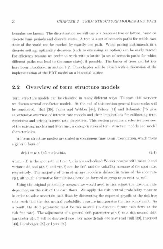
2.2 Overview of term structure models

Term structure models can be classified in many different ways. To start this overview

we discuss several one-factor models. At the end of this section general frameworks will

be considered. Hull [39], James and Webber [44]. Pelsser [71) and Relwnato [75] give

an extensive overview of interest rate models and their implications for calibrating term

structures and pricing interest rate derivatives. This section provides a selective overview

of the existing models and literature, a categorization of term structure models and model

characteristics.

All term struct lire models are stated in continuous time as an Ito-equation, which takes

a general form of

rfr(/) = /i(r, /)</< + <r(r, f )<fc. (2.1)

where r(f) is the spot rate at time f. c is a standardized Wiener process with mean 0 and

variance dr. and //(/\ /) and ir(r, /) are the drift and the volatility measure of the spot rate,

respectively. The majority of term structure models is defined in terms of the spot rate

r(f). although alternative formulations based on forward or swap rates exist as well.

Using the original probability measure we would need to risk adjust the discount rate

depending on the risk of the cash flows. We apply the risk neutral probability measure

in order to value uncertain cash flows by discounting the expected payoffs at the risk free

rate, such that the risk neutral probability measure incorporates the risk adjustment. As

a result, the drift parameter must be risk neutral (to discount future cash flows at the

risk free rate). The adjustment of a general drift parameter /«(r. f) to a risk neutral drift

parameter <7>(r, r) will be discussed now. For more details one may read Hull [39]. Ingersoll

[43]. Luenbergvr [59] or Lyuu [60).

2.2. OVEflVJEM' OF TERAf STRUCTURE .MODELS SI

Suppose that the aero-coupon IKMMI price /*(r. I, T) follow* -

where f is the issuing date of the bond and T Is the maturity date. To obtain a risk free

position we eoasider a short position in one bond maturing at 7', and a long position in n

bonds maturing at 7Y The jwrameter a will be chosen such that the bond |>ortfolio is risk

free at time f. The return on the portfolio equals

-rfP(r, f. Ti) + f» • rfP(r.«. 7,)

= [-P{r,«J,).Mr.lTi)+«»-P(r,»J,)-MMJ,)|* (2.3)

+ (-P(r.f,T,) • ff|»(r,t,Ti) + o • P ( r , l , r j )dHMT, ) | r f j .

The bond portfolio stays risk free only if the weight o is updated continuously. For an

instantaneously risk free portfolio, the vulutility term must equal zero, hence

^ P(r ,f , r , )-g, .(r , t , r i)P ( r « r ) 7 ( r t r ) " * • '

As an implication of no-arbitrage a risk free portfolio must earn the risk free rate r. There-

fore the portfolio return must satisfy

stating that the absolute return (the drift term in equation 2.3) divided by the initial

investment must be equal to the risk-free rate. Substituting for « and simplifying 2.5 leads

to

, t, T|) - r /<p(r, f, fg) - r _

where A. called the market price of risk, is independent of the bond maturity since T[ and

Ti have been arbitrarily chosen. The instantaneous return on any asset depends on the

asset's risk according to r + A(r. f) • <r,.(r. ?. T). A risk neutral process for the short rate is

now represented as

rfr(f) = <&(r, /!)rft + «7(r. t)^2, (2.7)

where 0(r. f.) = /i(r. r) - A(r. f.) • <r(r, f) is the risk free drift parameter. Using this drift

allows us to discount future cash flows at the risk neutral probability measure. In the

22 CHAPTER/ TERAf STRUCTURE A/ODELS A,VD DATA

models discussed IM'IOW, the effect of the short rate r on drifts and volatilities is included

separately. Therefore we suppress the index r ami write 0(0 for the model specific- risk

free drift and T ( 0 for volatility. Some models use a constant drift 0. a constant volatility

S7, or both.

A scl<-ctivc overview of one-factor term structure models and their characteristics will be

pnwnteri here. The main difference* between the one-factor term structure models concern

lime i|i'|wndency of the drift And volatility parameters, the degree of moan reversion and

the impact of the interest rate level on the volatility term. We present the continuous time

representation, although all models have an equivalent discrete version.

I Morton model

The Merton |0r>| model is specified by a constant drift parameter 0 and a constant

volatility parameter ff. yielding

rfr = M/ + mi*. (2.8)

A significant drawback of this model is its inflexibility, due to the fact that both

drift and volatility are independent of time. Also. r(f) may become negative in

some periods /. The Merton model implies negative long rates, because the short

rate follows a random walk process with a constant drift and lacks mean reversion.

Ingersoll [43] examines this effect in more detail.

2. Ho and Lee model

The Ho and Lev [:W. ML] model is the no-arbitrage version of the Merton model,

allowing the drift parameter 0 to be time dependent:

rfr = 0(0 '" + "</-. (2.9)

Still r(f) can become negative. The drift parameter 0(0 is chosen to match the

current term structure P(f.T). Ho and Lee assume normally distributed short rates.

;i. Black, Derman and Toy model

Originally, the Black, Dennan and Toy [9. BDT] model was introduced on a discrete

state space. Suksequently. the continuous time limit has been derived. Following

Hull [;W], the model can be stated as follows:

(flu r = [0(0 + ^ J r l n ']<" + ff(0<*-- (210)<r(r)

. OVER\7EUOF TERA/ STRl/CTl'R£ A/ODKLS 23

The BDT model is a noarbitrage model similar to HI.. A significant advantage of

" BDT over HL is the model definition on the natural logarithm of tin- short title

i instead of the short ratr itself, preventing interest rates from lie«tiining negative.

This model definition implies that short rate volatilities are high when intent! ri»ten

are high. Another strength of the BDT model is the inclusion of mean leversion.

For dre-PMMii'.', volatility functions, interest i i i . - m the HOT model exhiliit meiui

reversion 1 lie (logarithm of the) short i.Ui IIIVUMMS towards the long run average

for large interest rates and increases for small rates Blai k, Dermun and Toy assume

that short rates are lognormaJIv distributed.

4. Black and Karasinski model

The Black and Karasinski [10] model is similar to the BDT model, assuming a log-

normal distribution of short rates, hut allows for independent moan reversion and

volatility:

rfln r = K.[0(t) - In r]<ft + <7(<)rf2. (2.11)

To capture mean reversion as well as drift and volatility, an additional degree of

freedom is required, which is obtained by either using a trinomial lattice method

or a binomial lattice with varying period lengths. To model three unknowns -drift,

volatility and mean reversion- a binomial lattice (with constant period lengths) is

not sufficient.

5. Vasicek model

The Vasicek [79] model is an equilibrium model including mean reversion:

rfr = /v[0-r]rff+ <rrfz. (2,12)

Here K[0—r] represents the drift parameter. Both K and 0 are constant over time. The

interest rate tends to move back to its natural average 0 with rate K. Volatility and

mean reversion are modelled independently. Short rates are normally distributed.

6. Hull and White model

The Hull and White [41] model can be seen as the exogenous version of the Vasicek

model, including a time dependent drift parameter. The model is also similar to the

Ho and Lee model, but including a mean reversion term:

(2.13)

24 CHAPTER 2. TERAf STRl/CTl/RE AfODELS AND

7. Cox, Ingersoll, and Ross model

Some models include a positive correlation between the short rate and its volatility.

The volatility of the short rate w large whenever the short rate itself is large. Also,

the short rate volatility is small for low interest rates, implying that negative rates

are unlikely. The Cox, Ingersoll, and ROBS [23, CIR] model, an equilibrium model in-

chiding mean reversion, developed in 1985. captures the positive correlation between

interest rate level and volatility:

rfr = «(fl - r]rff + ffv/^rfz (2.14)

CIR include the link lietwwn volatility and interest rate level explicitly, whereat

the HDP model incorporates a similar effect due to the model definition on the

nut unil logarithm of the short rate. Chan. Karolyi. LongstaHand Sanders [18. CKLS|

concluded in l!)!)2 that for a volatility term equal to i r r \ -> = 3/2 provides the best

fit.

No-arhitrage models are not exposed to arbitrage opportunities by construction, being

set up from u martingale approach (using risk neutral probabilities, see Rebonato [75]).

Models 1-7, defined on the short rate, contain the Markov property, stating that only the

current state (and not the path to reach the state) affects the future conditional interest

rate distribution. This justifies the use of interest rate lattices.

A general framework for many of the previously discussed term structure models (for

instance Vasicck [79] and Ho and Lee [38]) has been introduced by Heath. Jarrow and

Morton [31, H.IMj. H.1M allow for the inclusion of multiple factors, such that not all bonds

of different maturities need to be perfectly correlated. Unlike the models discussed so far,

H.IM initially define a stochastic process for forward rates, instead of spot rates. The

forward rate process is given by

4W. r) = ji(/. «)* + £ " . ( r - 0 • /(*• *>fc» (215)I - I

where <T, denote the volatility processes. The forward rate process in the H.IM framework

is non-Markovian. Current forward rates depend on the complete history- of forward rates.

Therefore, modelling forward rates requires a non-recombining tree, severely slowing down

computations and limiting the IIUIHIHT of periods that can be included.'

*Fbr the HJM model. a lattice r*u only bo used in owe the volatility function bolonjp to a special classof volatility structure (so- Li. Ritrhken aiul Sankwasubranianian (55)).

2.2. OVERVIEW OF TERM STRt/CTl/RE MODELS 25

For the definition of the original HJM forward rate procsm glvm by equation 2.15,

forward rates are normally distributed, or equivalently. pri<< - >i • lo-cuiipon bonds are

lognormallv distributed. This allows for negative forward and spot rate*, and hence arbi-

trage opportunities when money ran be stored without rusts mid risks. In rase forward

rates are assumed to 1H- loginiruial. negative rates arc excluded, rnfortuuatcrv. interest

rates might explode if these are continuously compounded, lending to zero prut* fur bonds

and arbitrage opportunities.

Miltersen. Sand maim and Sondermann [6C. MSS] introduced a framework in which

simple interest rates over a fixed finite period are lognormally distributed. This framework,

which became known as the I.limn Market Model (I.MM), was simultaneously developed bv

Brace, Gatarck and Musiela .!.<. IU,\|, and .lamshidian [45]. The lognmmally distributed

rates in LMM are consistent with the HJM framework fur a specific choice of volatility,

discussed by MSS. The forward rate process is given by

(2.16)

where a, denote the volatility processes and / faces simple compounding. For calibration

purposes LMM has the same disadvantage as HJM: calibration to a binomial lattice is

difficult because forward rates and swap rates are non-Markovian.

Until recently, LMM could be applied only for pricing European options, based on Monte

Carlo simulation (see Rebonato [75]). At that time we did not. consider LMM as a candidate

term structure model for the valuation of mortgages with (American type) prepayment,

options. Recently, methods have been developed to suit LMM for pricing American options.

For the first extensions of LMM, see for instance Andersen and Andreasen [3] and Longstaff

and Schwartz [58]. Nowadays, market models are a serious alternative for pricing complex

options. Many large investment banks currently use market models to value interest rate

derivatives. Although we do not consider market models to price mortgage, the impact of

a term structure model on mortgage valuation is analyzed in the second part of this thesis

for robustness of the results.

The HJM framework and the LIBOR market model can naturally deal with multiple

factors. Other multi-factor models have been introduced by Brennan and Schwartz [14]

and Longstaff and Schwartz [57]. Brennan and Schwartz include a long term interest rate

process as a second factor. They consider a stochastic process for the long rate and a

process for the short rate oscillating around the long rate according to a mean reversion

26 CHAPTER 2. TERM STRUCTURE AfODELS AND DATA

parameter. Longstaff and Schwartz [57] include a stochastic volatility process. Brigo and

Mereurio [15] show that this model is equivalent to a two-factor extension of the CIR

model.

The Black. Dennan and Toy model can also be extended to a two-factor model, as will

be done in chapter 3. Both factors are assumed to have all BDT properties, that is. they

are lognormally distributed, face mean reversion, have non-negative interest rates and can

be easily calibrated to a lattice-. In the final sections of this chapter we will motivate our

choice for the BDT model, based on model {lerformance with respect to swap and swaption

pricing. Before evaluating term structure models, we discuss the valuation of swaps and

swaptions.

2.3 Notation for swap and swaption valuation

A swap is a financial instrument to exchange a floating leg and a fixed leg of payments,

without exchanging the principal. The floating log might be determined by floating interest

rates, such as Kl'kllioit or MliOK. The fixed rate determining the fixed leg of payments is

called the swap rate. Note that in a swap contract usually only the net payments occur.

Swajw are mainly used to hedge against uncertain payments or revenues in the future. The

owner of a payer's swap pays a series of fixed amounts, while receiving floating cash flows.

It can therefore be used when floating cash flows have to paid, to transfer these into a

series of fixed payments, running less risk. Similarly, a receiver's swap can be used when

facing positive floating cash flows, paying floating amounts in exchange for receiving fixed.

A swaption is an option to enter a swap at a certain time (the expiration date) and at a

certain rate (the forward swap rate agreed upon when entering the swaption). Swaptions

can be used for several purposes and are mainly an alternative to forward swaps. With a

swaption, one might still profit from favorable interest rate movements, while being hedged

against unfavorable movements. Contrary to forward swaps, swaptions will therefore have

a positive price when settled, called the swaption premium.

In this section we introduce some notation for both swap and swaption valuation. The

terms mid concepts defined here will be explained in detail in the following sections. Con-

cerning time issues we will adopt the following notation. The time unit is considered to

be in wars. A swap is entered at f = 7",). which can l>e either the current or any future

period. A swap matures at its final period T. A swaption starts at f«i and expires at t,

2.3. NOT-AT/ON FOR SWAP AND SW.4PT/ON VALUATION 27

when i -ua|> can be entered hy exorcising tho option The conditions for this future swap

t o U- c u u i c d arc agret-d ii|«»ii at f,i. For th is ivtisoti we will refer t o f,, IUS the i i^n i i i i cn t

date of the swap. In < i- > -v\i|> is actually entered at f,,. then f,, = f. A naming indox

over time is usually rrpn -• nt<-d hy a. All time indi< r- .m- annual -

During the lifetime of a swap, there are \ |>ayment daten: r,,i « 1.....N, The laMt

payment date equals the maturity of the swap, hence • >.-

<o < ' = Tb < r, < 7-, < . . . < TJV = T.

The time .« \-alue of a swap entered into at f and maturing at T is rlPtinted l>y \"(.«*). .•» ^

fo T. its swap rate agn>ed upon at /,) by A". This swap rate is constant during the

lifetime of the swap, although the future swap rate might change due to an evolving term

structure of interest rates.

The principal of a l»ond with the same maturity an the swap is represented by /?. The

price of a zero-coupon IHHKI with a lifetime from / to T equals P(f.7"). Zero-coupon bond

prices will also be used to discount future cash flows and for defining the term structure

of interest rates. Trivially, P(f, <) = 1. The term structure will also be represented as

a yield curve, where the yield ?/(i,T') is the (T — <)-period interest rate per annum. A

third representation is a forward rate curve, with the one-period forward rates stated by

/(s , s + 1) = r(.s), ,s = f,.... T — I""*. Hence r(s) is the forward rate over a period from .s to

s + 1. The relation between the three representations is given in section 2.4.4, where the

resulting term structures arc discussed.

The frequency or tenor of a swap is denoted by m and defined by the reciprocal of 1 lie

number of cash flows per year. Typical tenors are 0.5 for semi-annual payments or 0.25

for quarterly payments. Payment frequencies for the floating leg and the fixed leg may

be different. Common swap contracts in euros have semi-annual floating payments and

annual fixed payments.

Because swaptions can be viewed as call or put options, their values are denoted by c

and p. The implied volatility of the underlying swap is represented by <r, the underlying

swap rate is again A", whereas the strike price is A'. All swaptions considered are at-the-

money when entered, therefore A' = X at initialization. The notation discussed here will

appear frequently in the remainder of this chapter, together with less frequently occurring

variables to be explained later.

that in continuous time r denoted the instantaneous spot rate. In discrete time r denotes theone-period forward rate.

28 CHAPTER 2. TERAf STR[7CT17RE AfODELS AND DATA

2.4 Term structure fitting using swaps

In this section we will construct term structures on selected days based on swap rates and

short term EURIBORs. First, the availability of swap data is discussed.

2.4.1 Swap data

TABLE 2.1: EURIBOIU and bid-ask averages of swap rates.

Tin- table provides annualizcd Kt'KlHOK data (in percentages) forFebruary "29, 2000, February 1">. 2001 and July 2, 2001. These shortterm interest rates have maturities for each month up to 1 year. Also,swap rutf-N (in percent ages) are included for the same dates as the aver-age between !>i<l and ask rate. Swap maturities range from 1 to 10 years.

1 1 KIIUIK

1 m i ml li

2 months3 months4 months5 months(i months7 monthsS months<J months

10 months11 months12 months

Swap rates1 year

2 years3 wars4 years5 yearsC wars7 years8 years9 years

10 years

| i l , J ' l . J I M M l

.( I:>N

3.5463.6343.6843.7503.8233.8733.9333.9994.0584.0994.156

Fob 29, 20004.2354.6804.9905.2005.3805.5405.6805.7905.8705.930

hi. 1 j . 20014.8004.7694.7474.7144.6924.6664.6494.6314.6194.6134.6104.608

Feb 15. 20014.7154.7354.8254.9155.0055.0955.1855.2555.3155.365

Jul 2, 20014.5174.4674.4354.3954.3744.3614.3424.3314.3214.3114.3064.305

Jul 2. 20014.3554.4454.6154.7654.9255.0755.2155.3455.4355.515

2.4. T£«A/ STRl/CTl/RE FJTT/NG l/SLVG SU'APS 29

An example of i - I K - • •! >wap data at thrve arbitrary days (here February 25). 2

February 15. 2001 and July 2. 2001) in provide*I in table 2.1. All listed swap rat.- u>

quoted against El'RIBOR on :i <o Mil' b.»i- Floating pa\ imms occur twice a yvar. except

for the ! war swap which h<t.» a liti|in-iit \ of four pa\iii<iit* per year. Fixed payments

are annual. The swap rate is determined such tliat the initial value of a swap is /.ero. For

example, a fair exchange I tetwen a float ing leg tuid a Hxe<l leg of |mvincnt* o<-curs if a swap

contract is settled to exchange El RIUOH t«> a fixixl rato of 4.235% during one war , Ht art ing

at February 29, 2000. At this swap rate, lx>th |>arties in the swap agrn-inrnt rxp<>i't to

break even.

In order to match the term structure in the first year, we use monthly Kt'Kllioit.s, which

arc quoted on an at't/360 lm.sis and with the convention of traiixforiniiig yield* to price* by

* ' • " - • + ,.'»•-.)• »">

Fabozzi [30] states similar conventions for US interest rates. The period 7' - / (in years)

is measured in actual days divided by 360. In case the payment day is a Saturday or a

Sunday, the next Monday is considered to be the actual payment date, unless this Monday

falls in the next month. In that case the Friday before is considered to be the actual

payment date. The EURIBOR data for the three dates considered are provided in table 2.1.

For deriving a term structure of interest rates consisting of monthly periods the prices

corresponding to swap rates and EURIBORs must be interpolated. To achieve this we

will apply a spline method. A continuous, time-dependent function is fitted through the

observed data, minimizing the sum of squared pricing errors. In the next subsection we

first formalize the idea of the swap rate following from the fact that a swap contract is

worthless when entered, thereby linking the swap rates to the term structure of interest

rates. Then interpolation methods will be discussed to obtain a continuous zero-coupon

bond price curve.

2.4.2 Pricing of swaps

For the valuation of swaps at the spot market, the swap starts as soon as the swap agree-

ment is made (that is, £ = <„). As a first step in swap valuation we will price the cash

^An interest rate quoted on a 30/360 basis implies that each month is assumed to have 30 days and eachyear has 360 days. Other common quoting conventions include act/360 and act/art, where act indicatesthe actual days of a month or year.

30 CHAPTER 2 TERA/ STRl/CTl/RE MODELS AND DATA

FIGURE 2.1: The value and the payoffs of a floating rate bond.

The figure HIIOWM the payment date* of a floating-rate bond. Each paymentdate r, a ra»h flow of r(r, j )/i is tran.sferre<l. This amount etjualh the interestearned from i - 1 to i on a bond with notational principal fl. Consequently,the value of the bond in 0 jiutt after each payment date.

r(f})) • B r(T|) • /i Floating rate payments

/ / /f,, = T,, r , T2 . . . Tjy = T

** 11 Floating bond value0 fl

HOWH corresponding to the fixed and the floating leg separately. Fixed and floating legs can

include the payment of a notational principal at maturity. This payment is equal for both

legs and does not affect the swap value. Including principal, the fixed and floating legs are

comparable to the cash How patterns of a fixed-rate and floating-rate bond respectively.

The float ing-rate bond is worth /? at initialization. At each payment date the interest

earned in the previous period is paid, and the bond is again worth /? immediately after

each payment date (see figure 2.1). ThLs can easily be derived from discounting the cash

flows of an /V-period floating-rate bond:

= B.

The fix»nl-rate bond is worth the present value of all payments (which can be seen as

zero-coupon bonds) plus the principal payment at maturity:

0 , , , = * • »• • H • }T P(«. r.) + B • P(f. T). (2.18)

24. HERA/ STRUCTURE FITTING USING SWAPS 51

where A' is the annual swap rate agreed U|M>II at /,, foi .1 --nip --laiinir. .\i / and maturing

at the last payment date 7" = T \ . HI is the frr«|ueii(-y (e.g. (I.*) t«u srini-unmial |myment«)'\

and r,,i = 1,2 A' are the (Mtyment dates. The hrst term represents the periodical

payments, the second term is the linal prim i|ml pnvinmt The time f value of n swap with

a lifetime from < to 7 \ V(t) . » the different l.rtwivn the fixwl leg mid the Moating leg of

payments:

N

V(0 = 0/,, - B/i - X • in • fl • J ] P(f. r.) + /? • P«, T) - B, (2.19)• • '

where the floating leg is worth /? initially by definition. The principal amount /? ran he

scaled, resulting in an equivalent scaling of the swap value. We consider a receiver's swap

here, that is the buyer of the swap receive* the fixed leg of payments and pays the floating

leg. A payer's swap has opposite value At creation the swap has no value, so the swap

rate (the fixed rate of the swap) A' is set at a level at which the swap is worthless. The

swap rate follows when setting V(t) to zero:

(2.20)

After initialization the swap value may vary depending on the development of the float-

ing rate. If this interest rate is lower (higher) than accounted for in the current term

structure, then the payer of the floating rate gains (loses) and a receiver's swap has a posi-

tive (negative) value. The receiver of the floating rate loses (gains) and a payer's swap will

have negative (positive) value. When calculating the one year swap rate from the EURI-

BOR data listed in table 2.1, these will not exactly match the observed swap rate. Reason

for this is the day count convention. Swap rates are quoted at a 30/300 basis, whereas

EURlBORs arc listed at an act/360 basis. In case EURIBOR data are used to derive swap

rates, the latter will also be on an act/360 basis. To obtain swap rates on a 30/360 basis,

EURlBORs at a 30/360 basis are required. EURlBORs based on a 30/360 quotation will not

be exactly the same as the rates used, resulting in a slightly different swap rate. In the

sequel we allow for this small difference and use the 30/360 convention for the resulting

monthly term structure of zero-coupon bond prices.

^Analogous to EURIBOR data, the payment frequency for swap rat<!S mast be adapted in rase thepayment date is a weekend dav.

32 CWAPTER2. TERM STRUCTURE MODELS AND DATA

Pricing forward swaps

Up to this point only swajw traded in the spot market have been priced. The agreement to

exchange fixed and floating legs was made at date / and the actual exchange occurred from

date < on. Now the valuation of forward swaps will l>e discussed. Suppose that at time

to < < we make HI .i! i.•< inent to exchange fixed and floating legs, hut the actual exchange

only Htiirts lit time / The fix<-d rate of the contract is determined at f,,. Riven the current

term structure. Hence the swap Ls worthless at <o, but might have a value when entered at

time /.

Consider the current |>criod to be <„, the agreement date of a forward swap. Actual

payments only start at time <. Given swap rate data we might infer the current term

structure, that in, P(t«, a) for all a = to. • • •. T. The value at time f of a forward swap with

lifetime (/.'/') can be directly inferred from equation 2.19. To obtain the current (time /,))

.swap value we simply discount the swap value from < to ?»:

V(<«) = A' • in /> • ] T /»(«„,n) + fl • P(«o,T) - 0 • P(/o,')• (221)i-i

Solving for the swap rate by setting the swap value to zero yields

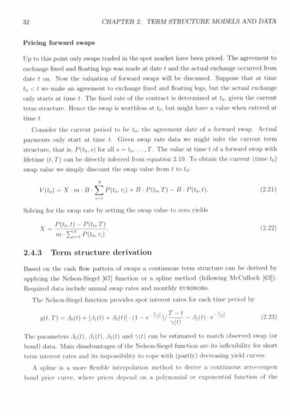
2.4.3 Term structure derivation

Based on the cash How pattern of swaps a continuous term structure can lie derived by

applying the Nelson-Siegel [07] function or a spline method (following McCulloch [63]).

Required data include annual swap rates and monthly EURIBORs.The Nelson-Siegel function provides spot interest rates for each time period by

^ ^ « " ^ (2-23)

The parameters 4>(0- Ji( ' ) . i*i(') and ^(r) can be estimated to match observed swap (orbond) data. Main disadvantages of the Nelson-Siegel function are its inflexibility for short

term interest rates and its impossibility to cope with (partly) decreasing yield curves.

A spline is a more flexible interpolation method to derive a continuous zero-coupon

bond price curve, where prices depend on a polynomial or exponential function of the

2.4. TERM STRUCTURE F/TT/JVG (/S/NG SWAPS 91

bond maturity Spline methods are widely used, see fur example Uams ((>], Matins and

Bierwag [61] tuid Bali and Karagozoglu [5]. In order to obtain a continuous price curw of

Bero-coupon bonds we use a spline function on these prices, such that the sum of squared

errors between the resulting swap prices (from 2.20 and 2.1!)) together with the short term

bond prices (following from 2.17) and the observed data are minimized. Such a spline

function might lx> polynomial (e.g. cubic) or exponential.

Exponential spline met lux Is have the advantage that out of sample observation* do not

diverge when time approaches infinity. However, wr consider a finite 10 year horizon of

monthly periods. Cubic splines are more flexible l>ecause more parameter- n< u-.i-d. Using

a cubic spline method a number of breakpoints is chosen, dividing the time to maturity

into M\II , I ! intervals. MKII that on each interval a cubic function with different coeflicients

can l» u--'il MoiitA'ci, .t cubic spline method involves performing a linear regression. For

th<>< ;• ..-.us the cubic spline method is chosen to match the swap prices

The genera] form of a cubic spline function to derive a price curve of wro-cou|M)ii bonds

P(t, T), with r = T - Ms given by

/.P(«,T) = 1 + a, • r + aa • r* + «:) • r" + £":«+/ • [r - /*] + (2.24)

where $ , / = 1,...,L are the breakpoints and [•], = niax[.,()J. P(M) trivially has unit

value. The time index r varies continuously from r. to f. + 10 years. The number of

breakpoints L is determined by a rule of thumb,

L = | V A 7 J , (2.25)

where M is the cardinality of the data set, that is, the total number of swap rates and

EURIBOR data. According to our data set we are allowed to include four breakpoints, but

we have used only three as we could not, find a significant improvement witli an extra

breakpoint and we want to avoid overfitting.

To obtain the final regression we substitute the cubic spline equation 2.24 in equations

2.19 and 2.17 to obtain an expression for swap values and short term zero-coupon bond

prices. Since the swap values are zero, the following joint regression must be performed:

7 ^ 77

(2.26)

(2.27)

34 CHAPTER 2. TERAf STRUCTURE .MODELS AND DATA

where u, and H* arc the error terms, J is the number of swap rates and A' the numl>er of

El'KIBOK*. Thin implies performing a regression on the following set of equations: i

t - i

• - I

"=• •' • ( ] [ > , • X, • jr., - t - A]* + [T, - i - Aji) (2.28)

( - 1

BreiikpointH are inserted after 1, 3 and 5 years, that is, J, = 1, & = 3 and Jn = 5. The

sum of squared deviations to be minimized equals

Having deti'iiniiH-<l the zero-coupon bond price curve out of yearly swap rates and

monthly interest rates according to EURIBOK. we will show the term structure of interest

rates in the next section, in terms of prices, yields and forward rates.

2.4.4 Results

The spline coefficients and the resulting sum of squared errors to the regression stated in

equations 2.28 and 2.29 are provided in table 2.2. The resulting term structures of interest

rates Iwusod ..n the swap and interest data of table 2.1 are depicted in figures 2.2 to 2.4.

Results are provided for February 29. 2(XK). February 15. 2(K)1 and July 2. 2001." For each

figure, tho top left diagram displays the zero-coupon l*>nd price curve P(f.7"). We used

"A fourth insttuico. Juno 1. 2001. is routidrml ax well. Results are similar to those of July 2, 2001 andwv therefore not iiu-luded in this chapter. In the second part of this thesis, results for June 1. 2001 areIIMHI for inortRi\ge valuation.

2.4. TERM 5TRUrTl/R£ F/7T/.VG l/S/NC SIMPS 38

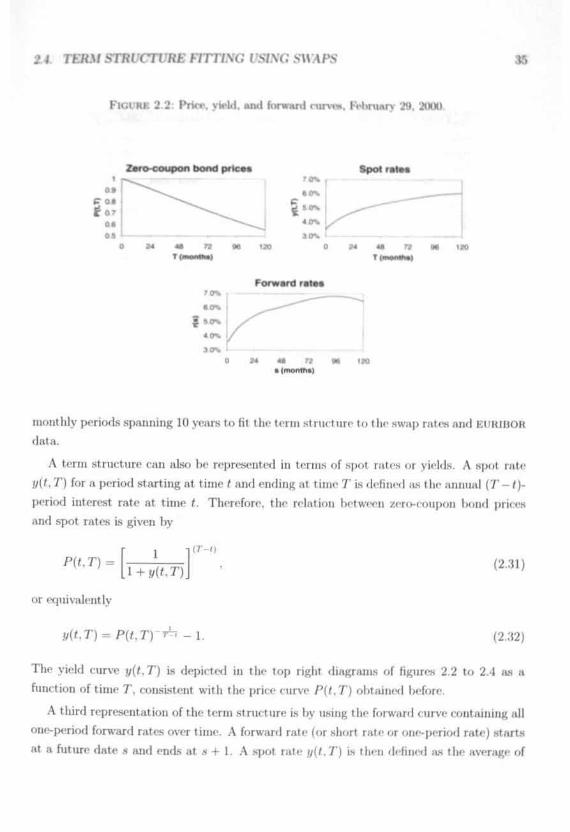
FIGURE 2.2: Pric*. yield, and f»>rwnrd rurvm. FWwuarv 29. 21XX).

Zwo-coupon bood prte*«

monthly periods spanning 10 years to fit the term structure to the swap rates and EUKIBOR

data.

A term structure can also be represented in terms of spot rates or yields. A spot rate

j/(t, T) for a period starting at time * and ending at time T is defined as the animal ('/' - /)-

period interest rate at time f. Therefore, the relation between zero-coupon bond prices

and spot rates is given by

or equivalently

- 1 .

(2.31)

(2.32)

The yield curve j/(f.T) is depicted in the top right fliagrams of figures 2.2 to 2.4 as a

function of time T, consistent with the price curve P(<,T) obtained before.

A third representation of the term structure is by using the forward curve containing all

one-period forward rates over time. A forward rate (or short rate or one-period rate) starts

at a future date s and ends at .s + 1. A spot rate y(<. T) Ls then defined as the average of

36 CHAPTER 2. TERA/ STRUCTl/RE MODELS AND DATA

FIGURE 2.3: Price, yield, and forward curves, February 15, 2001.

Zaro-coupon bond prtcaa Spot rate*

5"f 0.7

0*08 0 24 48 72 «e 120 0 24 48 72

T(moMlw)120

Forward rataa70%

s.o%

44%

3.0%0 24 4B 72 96 I2O

• (montfm)

FIGURE 2.4: Price, yield, and forward curves, July 2, 2001.

109

go.r 0.7

06OS

<

Zaro-coupon bond prices

) 24 48 72 96T (months)

7.0%

60%

$ S.0%

4.0%

S.0%

P

120

Forward

.*-

60%

55%

50%

45%

40%0

rataa

^ -

Spot rates

^ ^

24 48 72 96 12T(mon«»)

0 24 46 72 96 120t (months)

2.5. SM'APT/O.V PRJCfNG S?

TABLE 2 2 Splint- estinmtioiis timl i<->nlt>-

The table provides tin- result IIIK K'UK-V-IUM mctlu nnis o| th«' j<>miregression stated in equations 2.28 and 2.29. for all throe datesconsidered. The sum of squared pricing errors. including both swapsand short term zero-coupon bonds, IS also report til The principalof the swaps equals I. Breakpoints are inserted after 1, 3 and 5 yean*.

Coefficient*

Q j

<*s

OS

Q «

- - ' I

Feb 29. 2000-3 45 E-2-7.97 E-31.85 E-3

-1.38 E-3-4.79 E-41.18 E-4

.! 7", I-:-:

Feb 15. 2001-4 74 E-23.96 E-3

-1.37 E-31 43 E-3

-4 61 E-5i in i: '>

" . ' 1 V

Jul 2, 2(MH-4.68 E-28.35 E-3

-3.33 E-33.57 E-3

-2.18 E-41.04 E-4

: - ' 1 '"

the short rates r(s) for all future periods (s, s + 1), s = £,. . . , T — 1:

+r(.s)]. (2.33)

Short rates are derived from the spot rates by forward recursion. The resulting one-period

forward rates are depicted in the bottom diagram of each figure.

The swap prices implied by the yield curve are presented in table 2.3 for February 29,

2000. Note that these swap values should be (close to) zero. To calculate the values, the

observed swap rates of table 2.1 have been used. Besides, the .swap rates are stated that,

imply a swap value of 0. The calculated swap rates differ between 0 and 0.G basis points

from the observed swap rates. A typical bid-ask spread for swap rates equals 3 basis points.

2.5 Swaption pricing

Besides the term structure to determine the interest rate drift, a volatility measure is

required for interest rate tree construction. Interest rate volatilities are observed from

options on interest rate swaps, so called swaptions. In this section we will outline the

basics of swaption pricing using a Black and Scholes [11] approach/ In order to compare

' Longstaff. Santa-Clara and Schwartz [56] provide an accurate overview of the valuation of Hwaptiorwapplying implied Black (8) volatilities.

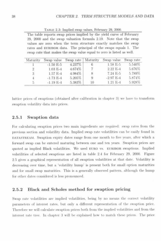
38 C7MPTER 2. TERM STRl/CTl/RE MODELS AND DATA

TABLE 2.3: Implied swap values. February 29, 2000.The fable reports swap prices implied by the yield curve of February29. 2(XM) and the swap valuation formula 2.19. Note that the swapvalues are zero when the term structure exactly matches the swaprates ami KURIHOR data. The principal of the swaps equals 1. Theswap rate that makes the swap value equal to zero is listed as well.

Maturity1234

Swap value-1.50 E-5

1 03 E-41.57 K-4

-1.73 K-4-11!) K-l

Swap rate4.237%4.674%4.984%5.205%.'.:w:M

Maturity678910

Swap value1.58 E-52.22 E-47.24 E-5

-2.97 E-41.21 E-4

Swap rate5.540%5.676%5.789%5.874%5.928%

lattice price* of swaptions (obtained after calibration in chapter 3) we have to transform

Nwaption volatility data into prices.

2.5.1 Swaption data

For calculating swnption prices two main ingredients are required: swap rates from the

previous section and volatility data. Implied swap rate volatilities can be easily found in

DATASTKKAM. Swaption expiry dates range from one month to five years, after which a

forward swap can be entered maturing between one and ten years. Swaption prices are

quoted as implied Black volatilities. We used EURO vs. EUR1BOR swaptions. Implied

volatilities of selected swaptions are listed in table 2.4 for February 29. 2000. Figure

2.5 gives a graphical representation of all swaption volatilities at that date. Volatility is

decreasing over time, but a 'volatility hump" is present both for small option maturities

and for small swap maturities. This is a generally ohserved pattern, although the hump

for other dates considered is less pronounced.

2.5.2 Black and Scholes method for swaption pricing

Swap rate volatilities are implied volatilities, being by no means the correct volatility

parameters of interest rates, but only a different representation of the swaption price.

Therefore we will calculate swaption prices both from the implied volatilities and from the

interest rate tree. In chapter 3 will l>e explained how to match these prices. The price

2.5. SttaPTJOJV PRK7XG

' T A B L K 2 . 4 : l a a p l i x l > w . i i > t i < > n \ < > 1 . I M I I I H • - I . U w u v . " >

The table shows implx-d swuption vulatilitu-> (', ' l"i i M-livtiou ofswaption expirations mid swap maturities on Kebru.in ."• 2000. Thedata are retrieved from DATASTRKAM A typical bid-ask spread is 1

swaption maturity1 month3 months6 months1 year5 years

1 year16.0516.3517.0517.701 *. on

- U . 11 • 111

17.0016.7016.4516.90I .i sn

aturitles5 years15.7015.3514.7513.90in r.

Id VI'

l I inl.iW)13.0012.25

••> i n

of a Hwaption depends on the current and on the expected future yield curve, itN option

maturity, swap maturity, strike rate and the interest rate volatility.

Here we discuss the payoff structure of a swaption and show how to obtain swaption

prices out of implied volatilities. Consider a swaption on a swap where we have the right

to pay A'| and receive a floating rate starting at the option maturity / and lasting, iV = £jp

periods of length m years. Such option on a payer's swap is called a payer's swaption. The

principal is scaled to 1. Suppose that the (fair) swap rate at option maturity has changed

to A'_>. The payer's swaption is exercised if X2 > X| resulting in a series of cash (lows at

Ti, . . . , r.\-, each equal to

m • max(A2 — Xi.0).

Hence the cash flows from this payer's swaption can be seen as payoffs from a call option

on a forward swap with fair swap rate X2 at option maturity and strike X| *. Analogously,

the payoffs from a receiver's swaption equal

m • max(Xi - X2.O).

Therefore a receiver's swaption can be viewed as a put option on the same swap with

terminal value A'j and strike A',.

"Note that financial literature often refers to a payer's swaption as a put swaption. This can !><• explainedby the fact that a payer's swaption is a put on a fixed-rate instrument We follow Hull's notation [39] inthe sequel, as payer's swaptions pay out for high future swap ratre*. and thereby resemble a call option ona swap rate.

40

from HATA«TRF*M

Feb 29, 2000

onereceiver's swaption

one payer's swap and

in portfolio payoffs equal to

j - - ^>" ' • ith the s

• -

215. SW'4P77O.V PR/C/.VG 41

denote tin- initial value of t h e swap (at f,i) by V'(fo). and tin- vnhn>s of I lie call and put

option.-, on t h r >aine >w.ip l>v c and ;». wv I I H W p + V'(f,,) = r . After all, if t he pavolK lioin

a payer ' s s w a p a n d a i< <. i\. i - >u. tpt iun ( a put option) equa l tl><^< <.| .1 |>>\. 1 •. -.u.iption

( • c a l l op t i on ) , t h e n b o t h s t ra teg ies must h a w equal IO.M» to i\< lu<l< .u l . in . i | ; . . msc

V(<o) = 0 (by dct in i t ion a t in i t ia l iza t ion) , wt> h a w r = p a t t he Mart of t he upturn < o n i i m t.

If the call a n d put prices a re not equal wi> ( a n make ,m a rb i t r age |>r<>(it Suppose

C > p . By ttclliiiK t h e cull a n d buy ing the put and the p.i\< 1 - swap <>m num-i l i ite profit

is c — p > 0. At op t ion m a t u r i t y t h e value of our |>ortfolio .<pi.il- .•• i<> In n< • VM make a

tota l profit. 1(< 1 .iiise t he denuuid for t h e pu t increases, i ts p r i o ' I I M S MHO, UN I he citll is

excessively suppl ied t h e price decreases , unti l r = p . Similar arnuinentw hold for tli< < i <

when r < p t o show tha t th i s s i tua t ion cannot last e i ther . As t he call a n d put prices o | IUI

a t - the- inonev swapt iou a re equal , we may in terpre t t h e oltserved impl in l volat ihtv a* t he

price of lujth op t ion typ«"s.

To concliKle th i s sect ion we present t he Black-S<holes formula for t h e value r of n payer ' s

swapt ion, giving t h e holder t he r ight t o receive a floating r a t e a n d to pay a fixed ra te :

c = m-/4-[X-7V(rf,)- A'

where

£y(M, . r , ) ]"" ' - '"> (2.34)

'

Here j/(ro. r,) is the annual interest yield for the period (/„. r,) for discounting future swap

payments to <o (time of entering the swaption), the swaption expiration or starting date of

the swap Ls given by f, 4 is the total discounted payment during the lifetime of the swap,

A" is the underlying swap rate at <o, A' the exercise rate, m the tenor or frequency, and

<r the underlying swap rate volatility. The principal is scaled to 1. Finally, /V(-) is tin-

standard normal distribution.

Formula 2.34 can be simplified a bit as all swaptions are issued at-t he-money. When

entering a swap now; the swap rate is determined such that the initial swap value is equal

to zero, according to equations 2.19 and 2.20. Also, when making a swap agreement now

42 C/MPTE/?2. TERAf STRUCTURE AfODELS AND DATA

to enter a swap in /fcf /wturp. the initial swap value at the agreement date <» is zero and

the swap rate is determined l>y c<|imtion 2.22.

Because both the nwap rate ami the exercise rate are determined such that the initial

swap value is worthiest, these rates are equal when making a swap agreement, whether

payments start now or in the future. At swaption expiration however, the swap rate has

changed due to ti changing term structure over time and does not equal the exercise rate

anymore. Hence, at option maturity the swap has some value on which the exercise decision

is bawd. At the agreement date, by setting A' = X when entering a swaption and X given

by 2.22, equation 2.34 simplifies to

c - » r » A A ' ( A r ( r f , ) ]where

£ + V«o, *)]-<"-«> (2.35)

The value of an at-the-money put (receiver's swaption) is

p = m-i4-.Y-(A'(-rf; ,)-tf(-di)l , (2.36)

with .1. </, and </.. as before. Trivially this results in c = p for at-the-money swaptions.

Substituting for the swap rate given by equation 2.22, we observe that the market price

of an at-the-money swaption does not depend on the tenor of the underlying swap:

c = [P(f,,.rj)-P(h.7')]-[N(d,)-A'(rf2)]- (2.37)

Having transformed observed swap and swaption data into prices, the next section

discusses recent literature on the jierforinance of term structure models, in particular with

respect to pricing swajvs and swaptions. The swap and swaption prices obtained in the

previous sections serve as a benchmark to evaluate model performance. A term structure

model is accurate if model prices of swaps and swaptions are close to the benchmark.

2.6. PERFORAIAJVCE OF TERM STHl/CTl'R£ AIODKL5 43

2.6 Performance of term structure models

After observing or constructing a price rurvr of zero-coupon bonds, swaps ran ho rxnrtly

priced bv the inajoritv of term structure models. Volatility structures can usimllv nut be

modelled exactly. An extensive amount of literature exists on the performance of term

•tincture models, interest rates being calibrated to both swaptious and ca|>s and floor*.

We will focus on the calibration to swaption prices. Comment* in Rebouato (75] are

closely related to interest rate tree calibration on ~.\vaption prices observed at one particular

date. Relx>nato argues that prices of swaptious with the same maturity can be nuil< lull

accurately using a one-factor model. but a <>ne-fnctor model is considered unsuitable for

pricing swaptions of various maturitii.- l.<<.uisc forward rate correlations implied by the

•waption prices are not equal to 1 for different maturities.

Opposed to Relwnato. recent empirical rrwults on historical estimation of swaption

prices show that one-factor mix Iris perform quite well for several volatility structures,

even compared to multi-factor models. Biihler. Uhrig-Homburg. Walter and Weber [16,

BUWW] estimate the term structure on interest rate derivatives, especially warrants. They

analyze the performance of seven one- and two-factor models, classified as either spot rate

or forward rate models. BUWW conclude that a one-factor forward rate model with linear

proportional volatility outperforms the other models, in terms of predictability. As a result,

no clear evidence is found for the inclusion of multiple factors.

Driessen. Klaassen and Melenberg [26. DKM] and Fan. Gupta and Ritchkcn [:}1, FGRj

apply several term structure models to price and hedge caps, floors and swaptions. They

empirically investigate the term structure models to describe the behavior of these financial

instruments over a period of several years, and predict future (in sample and out of sample)

prices.

DKM apply option-based and interest-based estimation to model volatility. Option-

based estimation takes derivative data into account, interest-based estimation models

(co)variances of interest rates. Results indicate that for swaptions option-based models

outperform interest-based models. DKM report best possible prediction errors for swaption

pricing to be 8.5%, obtained by a Hull and White [41] based one-factor model. Increasing

the number of factors does not improve accuracy: a three-factor model does not perform

significantly better than a one-factor model. The swaps accurately fit the term structure,

but all models considered tend to overprice swaptions with a short swap maturity.

The paper by FGR is closely related to DKM, but the results for swaptions in terms

44 CHAPTERS. TERA/STRUCTURE AJODELS AND DATA

of pricing errors are somewhat more promising: average pricing errors are between 2.36%

and 3.03% of the option price. As in DKM there is no need to include many factors to

capture interest rate dynamics and price swaptions. since one- and two-factor parametric

models perform at leant equally well. FGR find, contrary to Hel>onato, a better calibration

performance on the pricing of swaptions, compared to cap and floor pricing. Swaption

pricing errors are relatively small, but contrary to DKM, FGR observe an undcrpricing of

Mwaptions with a lower swap maturity.

LougHtarT. Santa-Clara and Schwartz [56] solve for the correlation matrix of forward

rates implied l>v market prices of traded swaptions. Results indicate an overpricing of long

maturity options and an uuderpricing of short maturity options. Average pricing errors

are smaller than the assumed bid-ask spread of 6% for swaptions. Equivalently. pricing

errors quoted in terms of implied volatility are below the bid-ask spread of 1 percentage

point.

Peterson, Stapleton and Suhrahmanyam [72] consider a multi-factor extension of the

Ulack and Kantsinski model, including factors describing forward rate behavior. Volatilities

and mean reversion are assumed to be constant. Swaptions with a long option lifetime are

underpriced, options expiring in the near future are overpriced, contrary to Longstaff,

Santa-Clara and Schwartz [56]. Notice the striking inconsistencies between the papers

discussed here with respect to pricing error patterns.

Note that our calibration of interest rate lattices, to be discussed in chapter 3. does

not depend on underlying correlation structures or on historical option prices. All current

option prices are only ahVetcxl by the current interest rate lattice, not by past interest rate

developments. This largely differs from the majority of the previously discussed literature,

where calculated option prices (and thereby model performance) are based on model param-

eters estimated on past option prices. Besides a volatility function, these articles include

historical price information for the valuation of current options.

Considering recent literature, including multiple factors to calibrate the term structure

of interest rates on swap, swaption. bond, bond option, cap and floor prices does not

significantly improve model performance. More factors might also lead to overtiming on

one type of financial instrument, while out-of-sample assets are priced worse. Especially the

results of Fan. Gupta and Ritchken [31] imply that for the accurate pricing of swaptions,

correlations of forward rates do not necessarily have to match historical correlations. Given

this empirical evidence, the next chapter analyzes calibration l>ased on one- and two-factor

variations of the Ho and Lee [38. HL] model and the Black. Derman and Toy [9. BDT]

2.7. BDT /\.VD B/JVOMM/. TRKfS 48

model, denned on a discrete-MI. >|>ACP. i4M

The term structure modeLs by BDT and HL can he captured in the saino framework,

but we will analyze the BDT model in more detail. BDT include empirically observed

interest rate characteristics such as lognormally distributed and non-ncgative short rat**

and mean reversion. Mean reversion is obtained when volatilities an* decreasing, which is

possible but not enforced for our volatility sjM-cilicat ion in chapter H."

From the model definition 2.10 follows that the short rate volatilities underlying the

BDT model are independent of (the logarithm of) the interest rate level. The one |>eriod

volatility of the logarithms of the interest rates in two successor state* doe* not depend on

In r (which i> > n>-< .•»>..,rv condition for trees to recombine) Consequently, the volatility

of the short tali itM-lt i.-. larger for high interest rates and smaller for low interest rates.

This feature is also incor|K>rated in the Cox, Ingersoll ami Ron* [2.'i| model and empirically

olwerved by Chan. Karolyi. Longstaff and Sanders [18). The Ho and !>ee model assumes

volatilities inde|>endeiit of the interest rate level. This partly explains the mxleiperfor-

mance of the HL model compared to the BDT model, as found by Matins and Bierwag

[61].

2.7 BDT and binomial trees

This section introduces some properties of the Black, Derman and Toy [9] model on a

discrete state space, thereby providing a preface to chapter 3, where a detailed specification

is discussed. In a binomial tree or lattice, BDT assume that interest rate volatility only

depends on time, and hence is constant for all states of the world in each period. Consider a

one-period tree. The future one-period interest rate is either r,, or r,j, both with probability

one half. The average (logarithm of the) short rate equals

_ In r,, + In r^

and the variance of In r is

, ^ (In r,, - ;i)2 (In r , -2 2 4 V r,,/

"In section 2.2 we have evaluated L1BOR market models. Both the performance and applicability ofthese models are promising. Only recently, market models are extended in order to deal with complexAmerican type options. See Hull [39] for an overview.

46 C7MPTER 2. TERAf STRl/CTl/RE MODELS AND DATA

Hence the one-period volatility equals 0.5 • In ^». For multi-period trees the short rate

average and volatility can be derived similarly by considering the two possible multi-period

yields after one period. i

A BDT based interest rate lattice must satisfy the no-arbitrage property. Section 1.2

ha* introduced the concept of arbitrage as a possibility of gaining money, without risk of

losing money. My construction of a binomial tree or lattice, arbitrage is not possible when

luting risk neutral probabilities for upward and downward movements (see PILska [73]).

Without loss of generality, these risk neutral probabilities are assumed to be one half for

each transition or arc in the tree. Every period, three parameters (drift and volatility of

the BDT model and the risk neutral probability) have to be estimated, matching only two

observation* (term structure and volatility). Hence we choose to fix the probabilities to

one half for all periods and states of the world, and calibrate the model to the observed

yield curve and the volatility measure implied by swaption prices. Note that for trees

to be recomluning one degree of freedom is given up, as volatility parameters cannot be

state dependent. The BDT model, to be calibrated on a binomial lattice, incorporates a

volatility parameter which is only time dependent.

Some term structure models do not have the possibility of equating all probabilities to

one half without loss of generality, but require more complicated lattices. An important

difference between the BDT model and other mean reverting models is that BDT is defined

on a random walk process, whereas for example the Hull and White model assumes a

stationary state variable. For this reason, the HW model requires a more complicated

lattice. A HW lattice reaches a maximum width; therefore the dynamics at the boundaries

of the lattice must be different from the dynamics in the center. At some point the grid

does not extend and at the edge there are sure upward or downward movements.

The BDT model is easily calibrated to a lattice. In the next chapter we calibrate swap

and swaption prices and construct a lattice of short rates based on a variation of BDT.

Additionally, we propose a two-factor extension of the BDT model, for which a trinomial

lattice of interest rates is built.

2.8 Concluding remarks

This chapter has provided an overview of interest rate models and the valuation of interest

rate derivatives. Several term structure models have l>oen discussed in section 2.2. To

2.8. CONCLl/D/.VG REA/.4RKS 47

calibrate IUI interest rate lattice to observed market |ui<>'> <>t s\\.i|» .m.l w.iptions. the

Black. Dennan and Toy model will lx> applied in the next chapter. Its main charactii M i. s

include lognormally distributed and positive interest rates, positively correlated volatilities

and interot i.ite*. .mil nn-.m reversion, although linked l«> volatility.

Einpim .ill\ "iie-l<i< im iu< •< !••!> prilium well compared to mult i-fact or models Including

more factor-, does often not improve calibration results significantly, while it may lead to

ovcrfitting of the in-sample assets. For instance, when the model is fitted to match caps,

Kwaption-s can still be prirrd poorly.

Within the class of one-factor models, the BDT model provides gt>od calibration result*.

Interest rates are often assumed to t>e loKiiormallv distribute!, to have larger volatility

when inter«>st rate levels an' higher and to be mean reverting. Thes«> features are covered!

by the BDT model Also, mean reversion is suHiciently small to have an expanding tree

in the distant future. Volatility decreases very slowly to 0. This ap|wars to l>e no problem

for our lattices with a 10 year horizon. For distant future time |>eriodH, when the number

of states is sufficiently large to closely approximate a continuous distribution, a stable

lognormal interest rate distribution is attained. In the next chapter we will analyze one-

and two-factor variations of the BDT model for the calibration of interest rate lattices.

To evaluate model performance a term structure and swaption prices are required.

Observed yearly swap rates and short term EURlBORs are transformed into a price curve

for zero-coupon bonds by a cubic spline method. Besides a price curve, the term structure

of interest rates can also be represented as a yield curve or a forward curve.

Swaption prices have been determined by transforming observed implied volatilities of

at-the-money swaptions. applying the Black and Seholes [11] option model. This model

can be rewritten in a format that allows the valuation of (at-the-money) swaptions. Payer's

swaptions (call options on the swap rate) and receiver's swaptions (put options on the swap

rate) are shown to have equal value, as long as both are at-the-money. Volatility data and

calibration issues therefore hold for both payer's and receiver's swaptions.

The resulting yield curve and swaption prices generated in this chapter are used to

evaluate the accuracy of the applied interest rate model when turning to calibration in

chapter 3. Term structures of the three dates considered closely match swap rat(« and

EURlBORs. as can be concluded from tables 2.2 and 2.3.

Chapter 3

Interest Rate Lattice Calibration*

3.1 Introduction

Binomial t r«* arc widely iwed for pricing American and Bcrmudan type derivatives. In

i'iw of lixcd iiiciiiiic securities the nodes arc related to spot interest rates. For practical

use the tree is calibrated to the current term structure and usually the prices of a number

ill highly liquid Kuropean options, such as caps or swaptions. When the tree is calibrated

it can be used to price American options by backward induction.

In constructing the tree there is a tradeoff between complicated trees that are calibrated

on many instruments and simple trees that allow efficient computation of American options.

Simple models have only one or two factors and use a recoinbining tree (lattice). In this

chapter we are concerned with calibration of a lattice for subsequent use in pricing long

term contracts with American options.

The literature contains a large number of one factor models that all have specific

strengths and weaknesses.-' We concentrate on extensions of some of the more popular

models: Ho and Lee (38, HL| and Black, Derman and Toy [9, BDT]. Both are one-factor

models that have a straightforward binomial lattice representation and can easily be cali-

brated to an initial term structure. In addition volatility parameters can be specified for

both models such that they also exactly fit a series of caps or a subset of swaptions.

'This chapter is hiwrd on joint work with P Schotman.''The literature is MI large that individual coatrilmtions would make up an excessively long list. Instead

we refer ID H mmilx'i of textbook.* that provide an extensive discussion of the theoretical and empiricalproperties, of the many ditferenl one- ami two-factor term structure models: Hull [39]. James and WPMHT|44|. Jarrow (lb] and Kclxmato |75|.

48

3.1. /ATRODl/CT/ON 49

In this chapter we consider the calibration to swaption volati l i ty in more detail \V«>

March for the lattice that best fits a matrix of swaption prices with a range of option

expiration dates and swap maturities In calibrating a hinominl tree one has a huge number

of degrees of freedom, since in principle everv s|>ot rate at everv nude of the lattice can In*

chosen freely. In practice, to make calibration manageable sunn- struct tire is rt<t|uired. iw

in the BDT and HL models. Within either the HL or BDT motlel. w --|» < ih .1 tliAihlc

volatility function to provide the Ix-st possible fit for the swaption prices. AM is well known

from the literature this is not enough to price .ill vw.iptiniis ••\;u-tly. Neither the HOT nor

the HL model will deliver a |>crfect fit.' Swapliou.s an- in<|ex<-<l by both the inatiintv of the

underlying swap contract and the expiration of the option. This two-dimensional array of

volatilities can not in general l>e fitted by a volatility function with a single time index.

The problem is due to the lack of control within the model over the correlation ami

relative volatilities of swap rates of various maturities. The literature suggests two ways to

improve the model fit for the whole matrix of swaptions at a given time.' One solution In

to add more factors, also with a flexible volatility S|H-< iti< at ion The other, partial, solution

is to specify the degree of mean reversion of spot rates independent of the volatility like*

in the Black and Karasinski [10] and Hull and White [42] models. In the BDT and ML

models the mean reversion properties of the spot rate are directly related to the volatility

specification. Within a lattice we can change the mean reversion by making the time steps

in the model time-varying. Like the extension to a two-factor model this complicates the

subsequent application of the model for the valuation of other instruments. In the sequel

we pursue both possibilities.

A recent alternative parameterization of the lattice is proposed by Peterson, Stapleton

and Subrahmanyam [72]. They specify a two-factor dynamic model for the logarithm of

spot rates with constant mean reversion and volatility parameters. Mercurio and Moraleda

[64] construct a trinomial tree with a hump shaped volatility function.

We emphasize that this chapter is not meant to provide a test of term structure models

or to obtain the best possible model for swaptions. Other models, like the LIBOR market

model, are specifically designed for swaps and swaptions, and might very well fit swaption

prices better than the lattices we construct in this chapter. Not being a lattice method,

''Backus, Foresi and Zin [4] provide an insightful analytical analysis of the pricing errorx of calibratedHL and BDT models when the true process is a Vasirek [79] model.

^See Rebonato [75. chapter 3] for a textbook treatment and references.

50 CHAPTER 3. INTEREST RATE LATT/CE CAL/BRAT/ON

the LIBOR market model, when accurately fitted to swap and swaption prices, is not im-

mediately applicable to price a different class of financial instruments, especially American

derivatives. Despite the advances in Monte Carlo techniques, a lattice remains the preferred

tool for the valuation of complex derivatives where early exercise is important. Still, in

evaluating the lattice models we will compare the patterns in the pricing errors with other

models in tin' literature. Hecent empirical studies investigating swaption pricing errors are

Longstaff, Santa-Clara and Schwartz [5C] and De Jong, Driessen and Pelsscr [24].

The remainder of this chapter is organized as follows. Section 3.2 describes the con-

struction of an interest rate lattice for a model with a flexible volatility structure and

the extensions to general mean reversion or a second factor. The calibration method is

discussed in section .'{..'{. Section 3.4 introduces input data for testing the specifications.

Results are presented in section 3.5. Section 3.G concludes.

3.2 Lattice construction

Thin section first explains flic general framework. The next subsection takes up parame-

terization issues.

3.2.1 Framework

Our setup is related to Schmidt [78], but formulated in discrete time. Starting point for the

const ruction of the lattice is n binomial random walk process for the state variable £(*„),

where f,, is the time at the ri"' step of the process. The state variable evolves according to

5(f«) = 0

&U.) = S(f,, • ) + (/,„ «>0. (3.1)

where the shock {'„ can take two values,

= l] = Pr[t/,, = - l ] = ^, (3.2)

corresponding to either an up or a down movement. The initial time is fo = 0. Time steps

haw length A,, = f,, — f,,.-i > 0. Time f,, is reached in n steps of length /u- (fc = 1 »i),

so that r,, = JZ*.- ''*• Changes in the state, S(f,,) - S(/,, i). are uncorrelated over time,

haw zero mean and unit variance. The marginal distribution of the discrete process 5(/,,)

3.2 MTT7CE CONSTRUCTION $1

is binomial with mean zero and variance n. At step n the state prix-ess >'(f») can take

n + 1 integer values between — n and >i with intervals of 2. Molding f lixed tuul increasing

the numlter of steps n to reach f = <„. the central limit theorem implies that n '•*6*(0

converges to a standard normal distribution. ; •..-:

Associated with the state procesw is a binomial lattice If the process is at state £((„) " 4*

we are at node (i .n) in the tree. FYom node (I . II ) the tree branch)* out to either nodes

(i - l .n + 1) or (i + I.n + 1). At step n the lattice has n -t 1 nodes. indexed l>\ t The

nodes run from i = —n to t = n with increments of 2.'' TIH> pnilmlulii> to i«.«. h .state

(i.n) is giwn by

At each node of the lattice we define the spot rate* r,». These are the spot ratew at t ime

f,, to discount values at f , , . i . the next s tep in the tree. The spot rate r,,, is exprewted on

an annualixtxl l>asis with discrete discounting o\-er an horizon of length / I , , , I This given

the spot rates maturity h,, + i. The value at node (»,n) of one unit at nodes (> + l,»i + 1)

and (i — 1, n + 1) is defined as

<">

We assume that the risk neutral dynamic process for the spot rates is related to the stateprocess through the functional form

G(r(t,,)) = fl(f,,) + 6(f,,)-yU, (3.5)

where G(r) is a monotone increasing function. The spot rates in the tree are then

i = - n , . . . , n . (3.6)

The function G(r) determines the shape of the distribution of the spot rates. Popularchoices for G(r) are the identity G(r) = r or the logarithmic G(r) = Inr. The first leadsto a generalization of the Ho and Lee [38] model, the second is a variation of the Black,Dennan and Toy [9] or Black and Karasinski [10] model.

•'FYom here on we will suppress the qualifier 'with increments of 2' when there can be no conftution.This makes notation lighter than the use of i = 2j - n (ji = 0 n).

52 CHAPTER 3. INTEREST RATE LATTICE CALIBRATION

The constants «(f,J arc used to calibrate the tree to the current yield curve. From

equations 3.5 and 3.6 we immediately find that the distribution of spot rates at time £„

haw a median equal to G~'(a(t,,)). The function a(t) therefore controls the /orahon of spot

rates (conditional on the current spot rate r(0)). If interest rates are mean reverting we

expect thin function to converge to a constant.

Since the normalized state process S(f,,)/v/n has unit variance at all steps in the tree,

the function />(/) determines the standard deviation or scair of the spot rate levels. For a

mean reverting process we must have ••• • •> •

Inn /HO - 1». (3.7)/ • «

On the nther hand, if spot rates follow a random walk, we expect 6(r) proportional to \/t

for large f. Information about b(f) is obtained from option volatilities.

Taking first differences with respect to both sides of equation 3.5 gives

This is a first order autoregrcssive process with parameters that are deterministically time

varying.'' With appropriate choices for <>U,,) and /i,, we can control various aspects of the

spot rate process.

To further analyze the dynamic properties of the process we normalize the drift by /in

and the shock by v//»n- Also, let y = 6'(r) - a, and rewrite the dynamic process as

</('„) - .«(',. l) = - K ( O J/CM l)('« - ',.-•) + ff(<n) «(<n) (3-9)

where

' ' H r t i r i \ u i n > t i i i i i r . i n - i l i . n 11n- r n i n r s . ' . i u r i i o i ' s a ( f , , ) , 6 ( t n ) " » d ' • n a r c f u n c t i o n s o f d a t a a s o f t i m e

3.2. LATT7CE CONSTRUCT/ON

The weWa/iMy of the ]>• n In- <r((,,). Tlie volatility of <(*„) has beento v^»n. which Ls sinul.u ..-•,.. > , itilttv of a Brownian motion. A/rrin rn rmon i.s defined

by the coefficient *(*„). M«\m rrvri>n>n occurs if *(/„) > 0. For a random walk with iijuai

time steps, having constant <?((„), *(<•) = 0.

Both K(f,,) and <r(fn) are intimately related to &((„). Morr insight in I lie n*latioii Itotwtvn

*(f) and <r(<) is obtained in the .special raw that time steps are equal. With /i,, - A = Af,

we haw that fn = n/i and the process simplifies to

<r(f)((O (3.11)

with

(3.12)

Tlie mean reversion K ( 0 W •» function of the volatility The continuouii time limit (/i —» 0)

of the process is"

rfy = — yrf/+ arfz. (.114)(7

where a' = d<r(<)/cft. The derivative rfz is defined its a random variable with mean zero

and variance eft.

Mean reversion implies that 6(() is a non-increasing (but positive) function of time for

large f. Hence 6(7) approaches a constant, <r(<) —» 0 and the dynamics of tin- process

become deterministic for large <. Despite all the flexibility of the tree, this is a theoretical

drawback of this construction method. The property i.s well known in the literature, see for

example Rebonato [75. chapter 12] in the context of the BDT model. It is an implication of

attempting to convert the random walk state process 5(<«) into a mean reverting process

for interest rates.

Returning to the general specification, the length of the time steps //„ provides an

additional degree of freedom by which we can gain independent control over mean reversion

and volatility. The time interval /i,, appears in the denominator of the volatility parameter

<r(fn) in equation 3.9. By taking shorter time steps for large n we can have a convergence

to a stationary distribution (6(<) —• 6) and non-zero volatility at the same time.

'See for example Hull [39. chapter 23] for a textbook reference to this result.

54 CHAPTER 3. INTEREST RATE LATTICE CAL/BRATiCW

The relation l>etween /»„ and «((„) becomes more explicit by rewriting *(/„) in 3.10d i r e c t l y i n t e r m s o f ff(in) a n d A , , , - . w < w i « ••• / •••«-> s«v ••

AN in Black and Karasinski [10]. Note the difference with the original Black and Karasinski

model, where mean reversion at <„ depends on the length of the subsequent time period,

bc<ausc the first difference in equation 3.8 is taken with respect to f,,.,|. To obtain the

desired mean reversion at step n of the tree, we need to choose a time step that satisfies

equation 3.15. Models with varying time intervals involve a relatively large number of

Mte|jH at distant future periods making them less efficient (or requiring more heavy use of

pruning low probability segments of the lattice to prevent highly inefficient oversanipling

of the tails). To value short term options, smaller time steps in the beginning of the tree

would be preferred, but this does not satisfy equation 3.15.

Two-factor model

i'iir rue generalization to a two-factor model we first define a bivariate lattice analogous to

the construction in .larrow [4C, chapter 12]. The two state variables 5i(<) and 5i(<) have

initial conditions S|(<o) = Sa(fo) ~ " *"*' '^'•''^'* **** random walks.

,) + t/2,, (3.16)

The innovations (7|,, and J7j,, have a joint distribution with three passible outcomes.

, = 0] = ^

= -1 ] = J (3.17)

Mean, \tuiance and c-o\*ariajice of the state variables follow as

) = 0. E[S.(/,,)] = 0.V(i',(f«)) = r». VlSa(f..)l = n/2. (3.18)

] = 0.

J.2. LATT/CE COATSTRUC77ON SI

The two state processes are uncomlated. If n —« oo for constant f,, - f. the procmm

n"'^Si(f) and rr "*>/2Si(0 b<*h haw a limiting A"(0.1) distribution. The advantage of

this construction method is that only three nodes ran ho an <>snl from any Riven node.

Among the various methods to construct a two factor lattice, thin structure has a ininimtU

expansion of the number of nodes.

Spot interest rates in the two-factor lattice are defined as

(3.19)

for deterministic functions o(f). MO and fr..(f). Each period three successor nodes JUT

required to solve for these three unknown pariunrtcni. A trinomial luttice is Hulticieut

to describe interest rate dynamics for l>oth fat-tore. An extension towards two binomial

latticeti (one for each factor) w not required as that would lead to four equation* and still

three unknowns In general, this approach leatis to an (n + l)-nomial tree for an >i-fnc.tor

model.

Nodes in the two-factor lattice arc defined as triplets ( i . j . n), where at stej) » the index

i can take values between —JI and ;i (with increments of 2) and the index j takes vuliies

between —(n — i)/2 and (n — i)/2 (also with increments of 2). The total number of nodes

at step n is j(n + 1)(» + 2). The root of the lattice is (0,0,0). The possible transitions

from node (t, j , n) at step /i -I- 1 are

/* (J + 1. j . n + 1) with probability ^

(i,j,»i) -» ( i - l . j + l . n + 1 ) with probability j (3.20)

\ (i — 1, j — 1, ?i + 1) with probability i

The probability to reach state (t. j . n) is given by"

*> -" - 0 (0 Gn>

((n + i)/2)! • ((n - i + 2j)/4)! • ((n - i - 2j)/4)!

"The state probabilitits hold for all reachable states (j.j, n). Not attainable states trivially havePr[i.j.n]=0.

56 CHAPTER 3. INTEREST RATE LATTICE CALIBRATION

These state probabilities cau be rewritten into a simpler format with A: = (n + i)/2 and

Interest rate* at each node of the lattice at Htep n are given by

7. (3-2

The lirst three steps of the two-factor lattice are shown in figure 3.1. The tree is trinomial

witli nonstandard branching. Possible tnuisitions are depicted in an (i.j(-surface in figure

3.2, whore the node labels represent the time period n.

For cane of parameterization we define the scaled processes

A',(U MUS.C.Vv^ (3 22)

Dynamics of the two sealed processes ore

A:,(«„)- *.( ' . . ,) = -«,(*„)*,(*„ ,)('.. - ' . . . ) + ff.(t») fi(«»), (3.23)

where rr,(f,,) and N,(^,,) me similar to the expressions in 3.10 and the innovations «,(<„)

have variance equal to /i,,, i = 1,2.

3.2.2 Parameterization

The lattice will be calibrated to an observed yield curve. This will determine the function

«(/). Assuming we have a complete smooth curve of zero-discount yields, determining <i(f)

conditional on all other parameters will be easy and we do not need to put any further

structure on the function <i(r). A smooth discount curve is available from fitting a spline

function for discount bond prices based on okserved coupon bond prices or swap yields.

For given volatility parameters 6(0. «(i) is determined by matching the term structure

exactly applying a forward recursion.

The tit her input data for the calibration is a matrix of swaption volatilities for various

combinations of option expiration dates and swap maturities. Providing a perfect fit to

this entire matrix will in general not be feasible within a one-fact or model, no matter

3.2 LAT77CE CONSTRUCT/ON

FIGURE 3.1: Two-factor lattice M • trinomial

The figure shows the Brut thnv turn stc|w of tho bivarinte random wnlk(5i(U).5j(U)) in (3.16). Tr«ui>ax.ii> «.ith thick Uoe* have probaluhty j , lliiiiiH-rbncs have probability J.

(1.0)

(2.0)

(-2,-2

(1.-1)

-1.2)

(-1.0)

(-1,-2)

(-3.3)

(-3.1)

(-3,-1)

(-3,-3)

58 CHAPTER 3. /NTEREST RATE LATT/CE CAL/BRATJON

FIC:IJRK 3.2: Two-factor lattice in (ij) space

The figure; NIIIIWH the first four lime steps of the bivariate random walk process(S I .SJ ) '" (3.16). The process stfirts at the origin (©). The number below a nodeIN the time Mtep at which the nodr is reached. The process Si/y/n evolves along thehorizontal axi* and ^j/>/n/2 along the vertical axis.

3.2. LATTICE CONSTRUCT/ON 60

bow flexible we are with rmpert to 6(f). /i and (7(r) SiiniUrlv. leaving .*>(/„) and A,, as free

parametm for all n leads to a huge IIUIIIIMT of parameters irlntivr (u tin- limited IUIIMIM r of

additional instruments Such a large IIIIIIIIHT of |Mi,mi. t. I - will. i. .»t»• numerical dithVulti<<tt

in finding the optimal fit and will also lead to «.•n--i.i. 1 .il>l< .>\<itittin^. For tin < n r,,.ns

we need to impose conditions on the parameters."

The analysis is , ss. ntially the same for any function (»(r). Since the input data are

prices of KIIII'|M .in .it-the-money options, the <lata will not IH< wry informative about the

distribution.d ih.u.uteristics The advantage of using d'(r) - l»(r) is that nil inteti-si i ,,(.•*

are positive by construction The empirical ml vantage is that th< ,i. tu.il <iiipiii.il .|...i

rate distribution is closer to a lognonnal distribution than a normal. Allothn empirical

advantage is that the volatility of r Ixwomes proportional t>> ilie |e\i>| n| the spot t.ite. Cliun,

Karolvi. Longstaffand Sanders (18] and a large IMMIV of sul>Mi|iient nx-uirli provide* ample

evidence of the relation Iwtween volatility and the level of mleieM rate*. AN a robiiistiieiw

check all models are run with C7(r) either equal to r or Itir. '" In the remainder of the

paper we will refer to models with G(r) = r as Ho-Lee (HL) specifications and use HDT

to denote the specification G(r) = In r.

The choice for /i,, and <r(<) are interrelated, since both jointly affect the volatility and

the mean reversion of the process. Models with equal time steps /»„ = // are preferable from

a computational point of view. Models with varying time intervals involve a relatively large

number of steps towards the end of the tree. Time varying step sizes also need greater care

in preparing the input data, since it must be possible to evaluate the yield curve at every

maturity if. In the calibration stage every change in the parameters will lead to different

points at which the yield curve is fitted. Time varying step lengths also do not guarantee,

that an option expires exactly at a node, a feature that is more important for subsequent

uses of the lattice to price American options.

Unequal time steps are only required to correct for implausible mean reversion features

of the calibrated process. Empirically, however, the restriction of equal period lengths does

not create severe problems. We observe very little mean reversion in the actual time series

behavior of short term interest rates. Time series models of interest rate dynamics usually

''Instead of restricting the model parameters, we could also interpolate the implied xwaption volatilitiesin order to fill the entire surface <T(T. 7"), with 7" being the swap maturity and T the option expiration date.We have chosen to work with the fixed amount of hard data in order to reduce th<; numerical burden ofhaving to search within a very high dimensional parameter space.

'"Although the distributional assumptions may be less critical for fitting swaption volatilities, they areimportant for other instruments like out-of-the-money options.

60 CHAPTER 3. /NTEREST JL4TE M7T/CE G4L/BRA77OJV

do not provide precise estimates of mean reversion. Evidence for the risk neutral process

comes from principal component analysis of yields, in which the first factor invariably has

equal factor loadings at each maturity. Such a pattern of factor loadings is typically implied

by a Hpot rate process that is close to a random walk." Neither do we find much mean

reversion implied by the relative volatility of long and short term interest rates. Both

under the actual probability measure as under the risk neutral measure, mean reversion is

likely to be positive but close to zero.

From equation 3.13 we know that mean reversion equals (minus) the rate of change of

the volatility function. When the volatility <r(t) is flat or slowly falling for large (, mean

reversion «(f) will automatically remain close to zero. A small decrease in volatility is

required to create enough mean reversion to make long term yields somewhat less volatile

than short term interest rates. Under the same circumstances the implication that the

spot rate process IMT<IIIM-S deterministic for large f will not be a serious problem.

A special case with unequal time steps is the first order autoregression with constant

volatility and constant mean reversion. With G(r) = r, this is the Hull and White [40]

extension of the Viwicek model. For G(r) = Inr. it is a restricted version of Black and

Kaiasinski [If)]. Setting rr(f,,) = <?(<„-i) in equation 3.15, requiring K(/,,) = K, and solving

for

+ -»«-i/r^- 1 (3-24)

as the implied time steps. The sequence /»„ is strictly decreasing for K > 0. Similarly, the

limit as K —» 0 leads back to the equally spaced lattice for a random walk with constant

volatility. D«xTeasing step si/.es as time evolves are unattractive, since the density of the

lattice increases towards the end, whereas we would like to have finer step sizes early in

the tree.

For models with lime varying volatility there is an implicit dependence of <r(<n) =

<T((,,_I + /»„) on the step size. Using a first order approximation of a(fn) in equation 3.15,

we lind the relation

(3-25)7— 1 » / r -r»M)V'n--W»n /j- I •**« V V " " I V"" 1/

" Analytically this is aeon inont clearly in single affino nKxIrls. whorv the limit as mean reversion goesto jtrro implint tlirtt yield etirw niowinents will ho parallol

3.2. MTTJCE CONSTRl/CTJOAf 61

«h««Ko(t.-i) » -<r'(t«-i)/<r(t._|) is tho implie<l mean n \> IM n trom tlw- rate of change

in the volatility. Rearranging gives

-7, (J.26)

which has an approximate solution

* " " i + 2(Mn-'*,,(< .))' **'"*As long as the implied mean reversion *,,('„ i) does not deviate too t li fi..m the de-

sired mean reversion K(I) or from implaiLsilile large or small valu«>. si< j • in remain

constant.

Our main einphiLM- i- .i> in mont of the literature, on the specification of the vola-

tility function <r(0 We conclude that the iu*e<l for modelling *(0 w Utw than the need

for UKMlelling the volatility. We therefore explore in more detail models with a llexiMe

functional form for rr(O with coast ant time ste|>s /i. Our I'cnchmurk model is the random

walk with constant volatility and equal time steps /i,, = /i,

ff(0 = <T. (3.28)

The resulting specification for 6(0 is

6(0 = (T\/7. (3.29)

We consider two more general types of functional forms for the volatility. The first is a

function with exponential decay,

>=o

where p is the degree of a polynomial (equal to 1 in our applications). The implied functions

for mean reversion and scale are

6(0 = vfo(0 (3.32)

The result for N(0 is the continuous time approximation K ( 0 = — <^'(0/"(0- ' ' " ' limitsfor K(<) ast—• oo or t = 0 are K and K — ^i /0n respectively. To avoid weird implications

62 CHAPTER! INTEREST RATE LATTICE CAL/BR.4T7ON

for tin' dynamics we assume that the polynomial 53J^J '^ does not have roots for positive

f. Kcstri< ting 0j > 0 for all j is an easy way to impose this.

An important special case is p = 1,

<7(<) = (0,, + <M)e "'• (3.33)

With equal time steps, volatility can IK- hump-shaped. For positive 0o and 0| the volatility

reaches a peak at

? = - - £ • (334)

Due to tlie exponential decline of <r(f), also the scale function 6(f) goes to zero. For large

< the process converges to a single point.

The implausible long run implications of the exponential volatility model motivate the

second functional form. We would like to allow for a rate of decline in the volatility function

that is less than exponential. One functional .specification that can have this property is

4 (3-35)

where the weighting function

^ (3-36)

When W • 0 the weight function approaches 1 for large f mid f'(0) = 0. If 0 > 1 the

volatility goes to zero for large f. For smaller values of ft the process exhibits explosive

behavior. For values 1 < 0 < 3/2. the volatility goes to zero, but the scale fe(r) = <r(f)V?

still diverges. For the existence of a limiting variance of the spot rate we need the stronger

condition fl > 3/2. The convergence to the constant /'(x;) = J» is at the rate f-''2-", and

thus extremely slow if W is only slightly above the threshold. The initial volatility. a(0). is

well defined if 0 > j . For 0 > 5, volatility starts at J | .

Two-factor model

Parameterization of the two-factor model is similar to the single factor model. The function

a(f) is used to tit the current yield curve, while the functions <T<(<) will be calibrated to

implied swaption volatilities. The functional forms for both volatility functions are identical

JJL CAL/B/LA7/ON

to equations 3.30 and 3.35 in tin- single factor case. Analogous to 3.35, the ivolatilities of both factors are given by

(3.37)

where the weighting functions F,(() are

Time steps in the two factor model are the same for both factors As for the single

factor model we will initially u><- < ••n^taiil time stops /•„ = /i, so that the moan rovention

of both A',(f) processes is equal to the rate of change in the volatility.

3.3 Calibration

This section discusses the determination of the parameters <r(f) and /»„. We start with tin;

single factor model, than generalize to the two-factor model.

3.3.1 One-factor model

The short term interest rates at step ;i are

G(r,,,) = a(f,,) + - ^ i . i! = - n » (:*..'*<>)v "

with parameters <!(<„) and 6(<n)? " = 0 , . . . . AT, to bo calibrated. For the calibration we s ta r t

with a forward recursion to construct the Arrow-Debreu s ta te prices <j , (i = — n , . . . , n ) .

The s ta te prices <?,„ are the prices at < = 0 of elementary securities with payoff 1 at node

(i. JI) and zero at all other nodes. Star t with f/m, = 1. Given a tree up to s tep M. the s ta te

prices a t s tep n + 1 in a binomial tree with transit ion probabilities ^ can be derived as '^

12

9i.n+l = r (9i+l.nd|+l.n +9i-l.nd|-l.n) - 71 < I < U (3.40)

-S«> for example Duffic [27. chapter 3] or Hull [39. chapter 23]

64 CHAPTERS. INTEREST fL4T£ LATTJCE CALIBRATION

where </<„ = (1 + r^)"*"*' is the discount factor at node (i,n). The price at f = 0 of a

security with payoffs C,,, at step n of the tree is

(3.41)

The first input to which the tree i.s calibrated is a yield curve of discount bonds. The yield

curve in used to determine the function «(f) conditional on &(<) and G'(r). Discount bonds

have payoffs C,,, = 1 at all nodes at their maturity date. For maturity r = f,,+ i the price

is

(r.H)

* " - (3.42)

The bond price is monotone decreasing in n(f,,). Numerically solving for a(<n). given 6(<n)

and G(r), is iv simple univariate problem. The entire sequence a(<n) >s found recursively

by moving forwards through the tree.

After calibrating to the yield curve, the resulting tree is used to price a set of swaptions.

Let r = f,, be a swaption exercise date and let T be the maturity date of the underlying

swap. For a call option on the swap rate, called a payer's swaption, the payoffs at nodes

(*, M) at the exercise date r are

A ;

a,(r,T) = PUT) - .Yo(r, T)]' in £ P,»(T,), (3.43)

where

3.3. C.4L/BR.477ON 6S

X,,(T) : swap rate at node (i.n) for a swap maturing at timeT, * v.?-

Jfo(r.T) : forward swap rate at time f = 0 for a -w <|' -tart ing at r and

maturing at 7\(x]* : maxiiiuiin of J-and 0. '

m : tenor of the swap, denned as tho reciprocal of the nuintM>r of

cash flows per year.

A/ : total IIUIIIIMT <>f rash Hows of the swap,

7^ : cash flow d.ti<-> .>l tin >w«ip. 7", - r + m • j ,

f*m('") : price at node (i,«) of a discount liond with maturity date r.

The forward swap rate Xo(r, T) is a function of the initial yield curve.

The actual swap rates at node (i.n) are

The future actual swap rates require the entire term structure at node (j,»), which is only

available after the function «(f) has been calibrated up to time T. For the valuation of the

swaption the tree has to be constructed up to time T and then rolled back to time r. Once

the payoffs C,,,(r, T) have been computed, the value of the swaption is given according to

equation 3.41:

(3.46)

A put option on the swap rate, called a receiver's swaption, has payoffs for which [X,,, (r, T) —

Xo(T)r •« Placed by [Xo(T) - A',«(r. T)] + . The difference between the two is X,,,(r. T) -

A'o(T) at all nodes (i.n). The difference in value between the put and the call is exactly

equal to the value of the forward swap with rate A'i,(r). By construction the value of

this swap Ls equal to zero, and therefore the payer's and receiver's swaption have the same

value.

00 CHAPTER 3. INTEREST RATE LATTJCE CALJBRAT/ON

3.3.2 Two-factor model ;

Most of the analysis for the single factor model carries over to the two-factor case. The

definition of the spot rates is different and, instead of 3.39, becomes

G ( r ^ ) = a ( O + ^ - i + ^ ^ - J , » = " " "• (347)

The state prices in the two-factor model satisfy the forward recursion

</0."+l = «9i IJII'A IJII + Tfll+IJ-l,ndi+l.j-l,n + T<ft +1 J+l.n^i + l j+l.m (3.48)«9i IJII'A IJII + Tfll+IJ-l,ndi+l.j-l,n + T

when- we define f/,,,, = r/,j,, = 0 for nodes (*, j.r») that do not exist. Existing nodes are

defined in section 3.2 as » = - n , . . . , » and j = - ( n - i ) /2 , . . . , (n - »)/2, l>oth with

increments of 2.

The function «(<„) is calibrated in forward recursion to the yield curve similar to equa-

tion 3.42. Calibration to swuptions is completely analogous to 3.43 with future swap rates

-^0»('"' ^ ) ' <li*™ii»t prices /',_,„(r) mid option payoffs C',j,,(r, T) all having the additional

j Hiilwcript.

The two-factor model is obviously more general than u single factor model but also

computationally much more demanding. For the same number of time steps the 2-factor

model has j(i» + 2) times as many states as the single factor model. It will converge more

quickly to the limiting continuous distribution.

3.3.3 Goodness of fit

Swaptions are valued conditional on the parameters that determine the functions 6(f)

and G(r). Best fitting parameters are found by minimizing the relative pricing errors

between the computed swuptiou prices and okserved swaption prices using least absolute

deviations"'.

EL . (3.49)

where

\V also »i>rki-rl with squarre iiixtnul of ah«otiitr \7ihn^. hut did not find important differences in

3.3. CALJBR477CW 87

t) : expiration date of swaptiou, '•• (fft

7J : swap maturity. • " • • » * *

Q(r,T) : observed swaptiou price using Black's formula aud the olwerved ^

implied volatility.

QO(T. 7") : computed swaption price from the lattice model.:..£

Swaption volatilities are ohHcrvcd for A' different expiration dates mid /. different OWIp

maturity's. Since a single factor model will not l>e able to price all >u.i|'ti<>ns |>i ifectly, the

minimized value for s will not t>e zero. The least stmanw criterion in formulated on relntivn

pricing errors, since all swaption prices will generally increase with the time to expirntion

and the time to maturity. A measure of fit for absolute pricing errors would give a large

weight t<> long term options on long term swajm. Relative pricing error* distribute the

weights more evenly.

Implicit in the goodness of tit criterion is that the yield curve is always calibrated

exactly using the drift adjustment parameters a((,,). We experimented with relaxing this

constraint by making it part of the objective function. Let X(T,) be the observed swap

yields. The augmented objective function adds an additional term

A/

to the original objective 3.49, where * is the weight attached to fitting the swap curve

relative to fitting swaptions. In that case we also need to parameterize a(<n), for example

using a cubic spline. We found that the relaxation of the yield curve constraint did not lend

to much improvement for the swaption prices, because the weight ty must be very large.

If * is too small the swap curve differs significantly from the observed term structure,

implying that forward swaps with rate Xo(T) have non-zero value. As a result, payer's

and receiver's swaptions have different values. Because option values are small compared

to swap values, relative pricing errors of receiver's swaptioas are huge if the interest rate

lattice is calibrated on the yield curve and payer's swaptions, even if pricing errors for the

latter options are small.

In table 2.3 pricing errors are listed for swaps traded at February 29, 2000 for different

maturities, given discount factors resulting from the cubic spline on zero coupon bond

prices. As these errors do not significantly differ from zero we use the yield curve from

chapter 2 for swap valuation. Note that this pricing error is equal to the difference between

68 CHAPTER 3. INTEREST RATE LATTICE CALIBRATION

an at-the-moncy payer'8 swaption and an at-the-nioney receiver's swaption with the same

strike rate and maturity. As by construction payer's swaptions and receiver's swaptions

must be equally priced, the yield curve must be exactly matched. We therefore only report

results with exact calibration of the yield curve.

3.3.4 Optimizing parameter values

For given parameters &(<„) and function G(r), the sequence a(t,,) is numerically found

by forward recursion, exactly fitting the term structure. Given previous interest rates,

the current, drift «(/„) is mulched to the corresponding zero-coupon bond price Pn('n+i)

according to 3.42. The resulting interest rate lattice is used to value swaptions. Swaption

pricoH are compared to observed prices to obtain the goodness of fit measure s. The optimal

values of the parameters 6(r), minimizing .s. are found numerically using the Broyden,

Fletcher, (Joldfarb and Sluinno (I3FGS) method, a quasi-Newton search method.

An outline of the HF(IS method is presentefl here, based on the NEOS Guide [69]. We

consider the optimization problem

min

where the parameter vector ^ consists of the five coefficients of the smoothed volatility

function 3.35, including <> and 0. Alternatively, the exponentially decaying function 3.30

might lie used its well. The function V(/7) determines the sum of swaption pricing errors s.

Since no closed form expression for V(tf) exists, the function value can only be evaluated

numerically. For given .'i. the goal function .s = V(tf) is computed as described in the

previous section. Our goal is to minimize ,s by updating d.

For updating tf first and second order derivative information is required. The gradient

is not calculated exactly (since no closed form for V'(J) is available), but approximated

by considering discrete deviations from the current J variables. The _/"" element of the

gradient of V(J) (that is, the derivative of V(J) with respect to J,) is obtained by the

approximation

^ + *V<*-*'> v;-owhore c, is the unit vector with the /"" element equal to 1. <5 is a small positive number

mul J is the number of coefficients.

3.3. CALJB/L477OJV «

Second order derivative infnrniatioii is raptured by the Hessian matrix, which is approx-imated by using gradient inform.it K>M tr..m p.iM iterations Wo initialize the Hessian at the

identity matrix. Tlie Hessian improve* Kiiuliiitllv towards the Inn- sentnd ordrr derivative.

Given .f*. the coefficient vet-tor J in iteration fc, the <oiii>pon<liM£ gradient V \ ' ^* ) and

the approxnnato Hoi«iaii //*, the linear system ••

W*rf* = -VV(J*) (3.50)

is solwd to generate the improving direction </*. The next iterate w found by mating ;

^ ' = ^ * + o * d * (3.51)

and denning

where o* is si't to the first element of the series* 2 ',/ 0,1.2 that mitinfiif( the

curvature condition ( j / ) ' s* > 0. Now the improved approximation of the Hessian matrix

is obtained by the BFGS update

satisfying the quasi-Newton condition

#*+'** = y*.

Because it takes a lot of computation time to solve a system such as given in equation

3.50, due to inverting Hessian matrices, we can achieve the same result by updating the

inverse of the Hessian matrix

Now a BFGS update of //* is equivalent to the following update of

The improving direction can now be directly found by

70 CHAPTER .3. /JVTEREST RATE LATTJCE CAL/BRAT/ON

'•'•'••• FIGURE 3.3: Yield curves for all input dates. '• . . , < ' • i : . - I f

The figure shows the input yield curves for February 29, 2000, February 15, . < • < ;2001, June 1, 2001 and July 2, 2001, respectively. The time axis displays ,tiionlliH. where T = 0 is the corresponding date. The yields y(0,T) on thevertical ax in are stated in percentages per month.

0.55%

0J0%

048%

0 40%

0.8i% •

I o » t = Feb 29.2000

I * * t-Feb 15.2001° * * * j • t » June 1. 2001

! x I = July 2. 20010.25%

0 12 24 36 48 60 72 84 96 108 120T (maturity In months)

The updated and improved 0*+' follows from equation 3.51. Every iteration, V(d) is

calculated until 11 (local) minimum is attained. Notice that each iteration requires many

calculations to obtain the model prices of all swaptions and a univariate optimization phase

to optimize nil drift parameters fitting the term structure. An accurate starting solution,

formed by the initial vector J, might accelerate convergence towards a minimum pricing

error.

3.4 Data

We use data on Euro swap curves for four randomly chosen dates in 2000 and 2001 (Febru-

ary 29, 2000, February 15. 2001. June 1. 2001 and July 2. 2001). The swap data are

15. RESULTS 71

augmented with EURlBORs having inonthlv mat writ kti up to I war Doth sets of data we

pooled to construct a term struct in. ,.| .li^ ..nut yk'kls using culm splines. Input term

structures for all dates are depicted in figure 3.3. All yield curvrs are upward doping. The

first one IIKMI.>t<mi« .illy: the otlier three with a slight initial inverse hump. Such a negative

hump will IM .At i. mi'ly difficult to capture for standard e<|uihl>riutn term structure models

like CIR or V.iMick

For the same dates we also haw otwervations for a matrix of implied volatilities of

swaptions with various maturities for the underlying swap and various expiration dates of

the option Wec<.n-i.|. i options with expiration- .ill. i I month. 3 montli*. (i months and I

to 5 years on forward swaps with maturities Itetween 1 and 10 yearn. We calibrate a lattice

for a ten year horizon. Swaptions for wliicli tin- sum of the expiration date and maturity of

the swap exceed ton years are discarded. This l< .i\<> t>2 swaptions for calibration Swnpl ion

data are available as volatilities implied by Black's model. They are transformed to prices

using Blacks formula, ^

^ ^ i ] ( (3.52)

Swaption volatilities for the dates considered are shown in figure 3.4. The volatility surfaces

show a more or less pronounced hump. Volatilities are highest up to the middle of the option

expiration range. The hump is strongest for options with the shortest swap maturity. The

pattern is typical for implied volatilities.'^

3.5 Results

We first present calibration results and implied interest rate dynamics for the one-factor

model. After that we discuss the two-factor model.

3.5.1 One factor model

Table 3.1 presents an overview of the fit, measured by the average relative swaption pricing

errors, for three volatility specifications (constant, exponential and square root) and two

specifications for the distribution of spot rates (HL and BDT). The volatility specifications

are formalized in equations 3.28, 3.33 and 3.35, respectively.

'''The example in table 22.3 in Hull (2003) exhibits the xame pattern for iratance.

72

tin

F«b 29. 2000

Feb15,2O01

July 2.2001

June V2001

3.5. RESULTS 73

Txni.F 3 1: AwrMf swuplion pricing error-.

1 i n - l . i i i l . •• . - • • • . - . :. i | H > | - l i j ( 1 1 1 p e l l f i l l . n ; . .. . > . p l . l t l u l l

3.49) ovw all 62 swaptions with joint time to expiration and maturity ofthe underlying swap I<-N> than <>i equ.il ti> 10 wars .V is the number ofequally spaced turn -t. |»> m ih. i.n \ . .n l.iiu.. The "Normal" modeluses G(r ) = r. the "Lognonnal" s|Hvihc-atioii has d'(r) -- In r Volatility iseither constant (R\V) or exponential (EXP) or square root (SQHT). Kxmtspecifications for the volatility functions an* in 3.28. 3.33 and 3 35. respe<tive!v

DateFeb 29. 2000

Feb 15. 2001

June 1. 2001

July 2. 2001

N120240480120240480120240480120240480

RW10 8413.5012.6011.119.829.55

10.9711.6010.9510.5811.1010.53

LognormnSQRT

5.876.265.659.925.976.317.063.443.447.274.034.42

1

fcXf>6.615.925.19

10.026.106.487.613.733.717.424.294.34

"ffiv9.618.357.60

11.067.277.198.276.115.G18.485.164.85

V 'i m.tlsi ) |; |

U.216.715.73

10 556.957.187,183.773.737.774.8!)4.74

1 \ ! 'ti<.KI

5.7(i5.16

10.266.246.607.663.633.617.(if>1 1(14.19

The lattice horizon equals 10 years. The number of periods in the lattice varies. Com-

putationally it proved very efficient to start by calibrating parameters for monthly periods,

that is, N = 120. Due to the small number of states and time steps, numerical calibration

works fast in such a small lattice. The optimal parameters for ,/V = 120 are used as input

to redo the calibration with ./V = 240 (or semi-monthly time steps). Since the parameters

in the volatility function remain fairly stable with respect to the number of time steps,

iterations for finding the optimal parameters for A' = 240 converge in a few steps when we

use the results from AT = 120 as starting values in the numerical optimization. The same

applies a fortiori for the refinement to ,/V = 480 ('weekly' time steps) with the solution for

AT = 240 as starting values.

In general pricing errors are smaller the more steps we take. As a crude measure, moving

from A' = 120 to A' = 240 reduces the average error by about 2%. Further doubling the

number of steps to A' = 480 leads to an additional reduction of only 0.2%. Most of the

74 CHAPTER 3. INTEREST IMTE LATTICE CALIBRATION

improvement for the overall fit comes from the short term swaption.s. With a single time

step per month there would only be two states at the first expiration date. Here the

increase from A' = 120 to JV = 480 is most important. Since results hardly change after 4

steps a month, we further report tin; results for weekly time steps only.

The BDT model with constant volatility Is the worst performing model. Surprisingly,

the results for the HL model with constant volatility are often very close to the models with

a more flexible volatility specification. Normal and lognormal models have a similar tit. The

DDT model is slightly better in combination with a square root decaying volatility function,

whereas the HI, model performs a little better when volatilities decrease exponentially. In

general, the BUT model with square root decaying volatilities performs best.

Figure 3.5 provide** more details on the residuals. We focus on the BDT model for which

volatilities decrease according to the square root function. Other model types (excluding

the random wulk process for volatilities) show similar patterns. Errors are denned as

model prices minus olwcrvcd prices as a percentage of the observed swaption price. For the

systematic elfect of expiration and maturity on the pricing errors we consider the regression

model,

v< = r,,(date) + r,T, + rir, + »/,, (3.53)

where r, is tlic pricing error for expiration r, and swap maturity T,, and Co(date) an in-

tercept that varies over the four dates considered. Pooling over all model specifications

(excluding the random walk models) the coefficients are r, =0.11 and f\> = -0.22. For

each option expiration date the longer maturity swaps are overpriced more (or underpriced

less), contrary to the results of Driessen, Klaassen and Melenberg [26], but supporting

the findings of Fan, Gupta and Ritchkcn [31]. Short maturity options are usually over-

priced, while long maturity options are underpriced by the model, contrary to the results of

Longstaff, Santa-Clara and Schwartz [5G]. The intercept is negative for all four instances,

meaning that short term options on short maturity swaps are underpriced by the model.''''

Repeating the regression with the aksolute errors |t\| and including the quadratic terms

7? and 7-* we find

|i\ | = Mdatc) - 0.13r, + 0.003r; - 0.30T, + 0.0037?. (3.54)

The model tits best for options on five year swaps. Best fitting options are those with

maturity around J years.

' Mi..ii SM.I|>IMII> li.iw low prirm and are very sensitive to small interest rate changes.

45. RESULTS

FIGURE 3.5: Swaption pricing error*.

The figure shows relative swaption pricing error* un four differentmodel price minus observed prior divided by obncrvrd price. Pricing entmresult (rum thr BDT IIKKICI WIH-M' volntility parametom decay «l rnti< >/7-Short term upturn* on lonj; tnm >w<i|» art' mostly overpriced, whilf luimtenn uptiutui on ohort term swaptt an- underpriced. The underlying latticehax -1H0 periods.

••**.•»

• ! ' >

g £ S •" «• * e s f?

»

A

.1

1C 8

76 CHAPTER 3. LVTEREST RATE LA7T/CE CALJBRA77OJV

To understand how volatility parameters should change to overcome this pricing error

pattern, the following division of nodes could be made. First, divide the time periods in two

categories: before option maturity and Iwtween option maturity and swap maturity. After

swap maturity, volatilities do not affect the swaption price. Second, consider the upper half

(representing the higher interest rates, for which payer's swaptions have positive values)

and the lower half (for which receiver's swaptions have positive values) of the lattice. This

divides the nodes of the lattice in four groups. As a consequence, four channels exist that

may influence swaption prices via volatility changes. The first two affect the value of a

payer's swaption. This value decreases if the volatility after option maturity decreases or if

the volatility before option maturity increases. The first channel states that the resulting

decrease in interest rates in the upper half of the lattice implies increasing discount factors

mid hence the fixed payments at option maturity increase. With higher payments, the

present option value decreases. The second channel can be explained by an interest rate

iiirroa.se before option maturity, decreasing discount factors, and therefore payoffs at option

maturity are discounted more. As a result the present option value decreases.

Channels three and four affect the receiver's swaption price. The value of a receiver's

swaption decreases if the volatility after option maturity decreases or if the volatility before

option maturity decreases. Interest rates in the lower part of the lattice are higher (less

extreme, closer to the menu short rate) when volatility is small. Higher interest rates after

option maturity decrease discount factors, the value of fixed revenues at option maturity

decreases. Therefore the current option value decreases. Finally, increasing interest rates

before option maturity lead to decreasing discount factors and a lower option value.

Payer's and receiver's swaptions are priced equally. Both payer's and receiver's swap-

tions with a short option maturity and a long swap maturity are overpriced. Their value

can only be reduced simultaneously by decreasing the volatility after option maturity. Af-

ter all, decreasing volatility fo/on option maturity would decrease the receiver's swaption

value, but also raise the payer's swaption value. But a reduction in the short rate volatility

in later periods would decrease the value of longer maturity options with payments in these

periods (for example a 5 year option on a 5 year forward swap) as well. These swaptions

are already uuderprieed. Heine, a tradeoff is found between iinderpricing and overpricing

options. The UDT model, with only one factor to explain the volatility behavior, is not

able to improw on this.

An important question might be why this tradeoff in pricing errors exists as described

3.5. RESULTS 77

FIGURE 3.6: Swaption fit February 29. 2000: iinplkd vulatilit) .lill. i. n.. -

The figure shows atwolutc implkxi volatility tliffrmutf. for February 29. 2W10,AN tiuxicl volatility minus <>IW«T\T<I volatility Tin III.MI.1 volatility is the

implied volatility of the UKMII-I swnptum prirtv I-!it.«i- i• —nil from tin- MOT

model with square root smoothing on volatility |MU.HII< t> I - \ \ . . .1.-.m ilir

same em>r putiiTii as in U>nii8 of prior ditf< i< m • - 11,, ,,i,.l. IIVHIK Inl ine

baa 480 p«Tiod.v

12 24 36Option aspiration (months)

90

before (and shown by all calibration results) and not opposite (underpriciiig of short matu-

rity swaptions, especially on long maturity swaps, and overpricing of long maturity swap-

tions). To overcome this particular pattern of underpriciiig short maturity swaptions. the

volatility after option maturity should increase, also raising the value of already overpriced

long maturity swaptions. This effect may be prevented flue to the imposed restrictions.

The current smoothing function for volatility parameters (decreasing at rate v/<) implies

lower instantaneous short rate volatilities in the future. Consequently, the olraerved pricing

error pattern is more consistent with the volatility specification. However, other .smooth-

ing functions (such as exponential decay or even a constant volatility parameter) have the

same limitations, perform worse and are theoretically incorrect in this framework.

For the calibration, we minimized relative option pricing errors. A more interpretable

(though computationally more cumbersome) measure are implied volatilities. However,

the pricing error patterns formed by implied volatilities and relative option prices (as

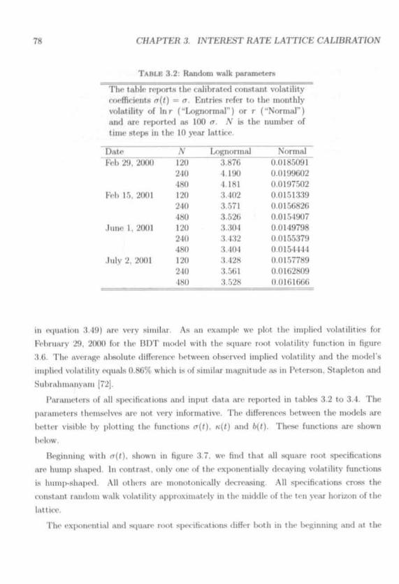
78 CHAPTER 3. /NTEREST RATE MTT/CE CAUBRAT/ON

TABLE 3.2: Random walk parameters

The table reports the calibrated constant volatilitycoefficients (7(0 = <r. Entries refer to the monthlyvolatility of lnr ("Lognormal") or r ("Normal")and are reported as 100 rr. A' is the number oftime steps in the 10 year lattice.

DateFeb29,

F.-b 15.

June 1,

July 2,

2000

2001

2001

2001

120240480120240180120240480120240480

Lognormal3.8764.1904.1813.4023.5713.5263.3043.4323.4043.4283.5613.528

Normal0.01850910.01996020.01975020.01513390.01568260.01549070.01497980.01553790.01544440.01577890.01628090.0161666

in equation 3.49) arc very similar. As an example we plot the implied volatilities for

February 29, 2000 for the BDT model with the square root volatility function in figure

:U>. The average absolute difference between observed implied volatility and the model's

implied volatility equals 0.86% which is of similar magnitude as in Peterson, Stapleton and

Subriihmanvam [72],

Parameters of all specifications and input data arc reported in tables 3.2 to 3.4. The

parameters themselves are not very informative. The differences between the models are

better visible by plotting the functions <r(f), K(<) and 6(<)- These functions are shown

below.

neginning with <r(/). shown in figure 3.7. we find that all square root specifications

are hump shaped. In contrast, only one of the exponentially decaying volatility functions

is humiKshapcd. All others are monotonically decreasing. All specifications cross the

constant random walk volatility approximately in the middle of the ten year horizon of the

lattice.

The exponential and square root s|>ecifications differ both in the beginning and at the

A5. RESULTS 79

T A H 1 - K 3 . 1 P i i r n i i i r t r r s M | i m n - r o o t v o l n t i l i t v

1 i i r l . i l i l c r < ' | x > l t > < a l i l x . i l t i l < c » ' t h < i r u t . s l e u t i n - v o l a t i l i t y l i l l u ' l i o n

^ + (l - F(0)• (A0 01

a/*

for IM)|1I llio "LognoniMr an<l "NunmU" dirt rilttit ion* for spot ruti* r.A' is the imintx-r of time st«-|»s in the 10 war Inltiov

AFeh 29.120240480

Feh 15.120240480

Juno 1.120240480

July 2.120240480

200012.5814.5012.48

200120.7416.3413.29

200119.3514.5611.49

200114.379.4214.50

Lognormal

3.

1.0123.3652.267

0.1592.1612.854

0.0002.6492.929

0.0002.6390.804

A0.3900.2750.394

0.1170.1620.180

0.1860.2960.360

0.3430.5650.430

1.591.471.54

1.040.960.98

1.281.211.21

1.281.261.28

a

0.0170.0240.021

0.0730.1310.112

0.0620.0950.089

0.0590.0890.081

0.02010.02020.0189

0.03450.03460.0346

0.01690.00000.0(K)0

0.01130.01110.0109

\

1.9803.2575.286

6.3717.3857.385

7.361lfi.8%32.270

9.26810.61611.633

• >i m i l

••

2.0292.5992.090

0.9791.1621.137

1.1310.8791.658

0.9431.2971.115

1.501.491.47

1.271.271.27

1.301.211.19

1.261.271.26

0.0150.0200.017

0.0250.0300.030

0.0230.0270.026

0.0200.0280.026

80 CHAPTER 3. INTEREST RATE LATTICE C A L / B R A T / O J V

TABLE 3.4: Parameters exponential volatility

The table reports calibrated coefficients for the exponential volatilityfunction

<r(t) =0.01(0,, + 0,0 *>-"',

for both the "Lognormar and the "Normal" distributions for the spotrates r. jV is the number of time steps in the 10 year lattice.

DateFeb 29,

Feb 15,

. l l l l K ' 1 .

July 2,

2000

2001

2001

2001

4)120 3.086924018012024048012(1

210480120 :210ISO 1

.7123

.703!)(.2763,r,2r>o.3944.1710<)!)<Mi

.8844

.1185

.9299

.7496

Lognormal0.

0.19070.13320.12230.05570.02640.01900.00720.01580.M770.08980.04520.0459

K

0.02230.02000.01940.01070.00930.00780.00580.01020.00850.01540.01330.0129

0o0.012320.016930.015760.011910.017180.016590.013590.017940.017560.012950.017470.01722

Normal0, .,»•7.8136.8407.0313.3091.3681.0772.4180.6500.1382.8061.1491.024

0.01860.01820.01820.01170.00800.00660.01000.00620.00330.01000.00680.0063

end of the time horizon. The first few months the square root function is increasing steeply.

This is offset at the end. where it is much flatter than the exponential.

The differences are more pronounced for the scale function fc(f). The scale functions

fr(f) = rr(/)y*7 are shown in figure 3.8. For a mean reverting process the scale must approach

a constant level for large r. By construction the exponentially decaying volatility functions

show a decreasing variance of interest rate levels. Whether the theoretical problem is

empirically relevant depends on the parameters K and 0o/0i- For the calibrated parameters

in a ten year lattice the difference with the random walk model is clearly visible after a

five years horizon. From that point on the random walk still increases at rate v^ while

the exponential function quickly Hat tens. For three out of four instances it is already

decreasing well before the end of the ten year period. This is the main drawback of the

exponential decay of the volatility function.

The square root function implies higher standard deviations for the level of interest

3.5. RESULTS 81

FlCl'RE 3.7: Instiuitaneoui Aort rate voUtilitieo.

The figure display* iiistantaneouN volatility curvw <r(<) for nil four date* con-atdered. Each panel shows three different amoothiiift funrtiuiut fur the vuhv-tihty parameters: ronstaiit (rw). square root (aqrt) ami ox|»>in"iilml (rxp).For the square root functions the hump in inure pronounce*:! mul tli<- fiiluredecline is more IIHMUTHIC than for ex|x>iiiiiti.il ilt-rnv fund ions Thr coiiKtnnlvolatility provides au average volatility k \ i 1. 1 he uuderlyuig lattirc has 480period*.

Feb29. 2000 F*>b 15.2001

M1 | —sqrti,—«Pi

o0 12 24 36 48 60 72 84 96 106 120

t (months)

12 24 36 48 60 72 64 96 106 120

t (months)

June 1,2001 July 2, 2001

004

§OJ»

aoe

0 01 —sqn 001 —iqrt

0 12 24 36 48 60 72 64 96 108 120

t (months)

0 12 24 36 46 60 72 64 96 106 120

I (months)

82 CHAPTER 3. INTEREST RATE LATT/CE CAL/BRATJON

: , FtGURE 3.8: Scale parameters.

The figure displays Hcale curves b(<) = <r(t)\/< for all four dates considered.Each panel shows three different smoothing functions for the scale param-eters: constant (rw). square root (sqrt) and exponential (exp). The squareroot functions approach a constant for large f, while the exponential decayfunctions imply a decreasing future scale. The underlying lattice has 480periods.

Feb 29, 2000

o oo*

• rw

coon 1 ' ' M|rt _»••*•

coat • *^

0.001$ t . ^ g ^ * " « . ^ _ — »

oooi y j *

OOOOA ^ ^

00 12 24 M 48 80 72 M M 108 120

t (month*)

Feb 15,2001oow

00018 * "" ' v ^ "

0 0018 ^ . ^ - - \ ^ ^ _

0 0014 ^ ^ ^ j I M " ' ••••

00012 ^ ^ ^

§ oooi jrf**^00000 J ^ ^

00008 j j r

00004 ^ ^

00 12 24 36 48 60 72 84 96 108 120

t (month*)

June 1,2001 July 2, 2001

O.O0H

am i ; _

S» 4» 60 7? M M 10S t »I (month*)

0 12 24 » 4« «0 72 M 98 KM 120

3.5. RESULTS M

rates 6(0 than the exponential model The increase in variance is at a slower rate than for

the random walk. It bi remarkahle that lx>lh the exponential and the square root functions

are steeper than \/t in the fir>i n. i •- first two wars) This means that initially

interest rales display explosive Ulmviui (negative mean reversion). A letter description in

that within the lattice there is positive aut<» i>rr<l.iti<<n for . li.un;i> in tin s|,,.i i,it.-> This

feature corresponds with the actual tune .-<m\> piiipntw ••- M| IMICII-M into

Interestingly the crucial parameter 0 is mostly l«-twin - and 1 J The weight function

F(0 converges to one at such a slow rate that the scale function 6(f) doew not converge to

a constant, even though <r(f) vanishes in the limit. The square root function is const meted

such that it satisfies the implications with rcs|>ect to volatility and •-< ilc approaching a

constant level for all data sets.

The mean reversion functions *(<) = —<r'(f )/ff(r) are depicted in figure 3.9. According

to volatility functions decaying at rate \/?, interest rate* dilfiiM* dining the lintt .year, after

which mean revri--i"ii M.irta.

Figure 3.10 plots the drift parameters a(f) for all instance* for the MI) I model. Only

the curves for the square root volatility function are shown. The results for the constant

volatility and exponentially decaying volatility are indistinguishable from the curves shown.

The shape of the drift curve is comparable to the shape of the corresponding yield curve.

Differences occur because the drift parameters refer to short rates and are median interest

rates. This implies that the yield curve is mostly determined by the drift correction and

hardly by the dynamic properties of the spot rate process. The dynamics, modelled through

the volatility function <T(0I only serve to fit the swaption prices.

To gain some insight in the yield curve dynamics, figure 3.11 shows the five future term

structures belonging to the states after 1 month (n = 4) for the first date (February 29,

2000). The initial yield curve is shown in figure 3.3. Contrary to the implications of most

term structure models, the curves are closer together at short maturities than at long

maturities. The explanation is that dynamics are not mean reverting initially and mean

reversion, if any. is only limited afterwards. The other models and other dates show a

similar term structure behavior.

Figure 3.12 shows the final period distributions according to the BDT and the HL

model for the square root model on February 29. 2000. Since 0 > 1.5 in this instance

the distribution converges to a limiting stationary distribution. Both HL and BDT have

84 CHAPTER 3. JiVTEREST RATE LATTICE CAL7BRATJOJV

FIGURE 3.9: Mean reversion

The figure shows mean reversion rates K(<) = ^W for BDT for the fourdates considered. Volatility is smoothed by exponential and square rootfunctions. Mean reversion only starts after the first year. The amount ofmean reversion is very small for large /, while initially a diffusion of interestrates occurs. The underlying lattice has 480 periods.

Fab 29, 2000 Fob 15. 2001

§ • 0 01

12 24 36 46 SO 72 M 96 106 120

t (months)

Ott i

•CM

June 1,2001

« 36 48 «0 72 84 M 106 120t (month*)

July 2, 2001

2 24 36 48 60 72 S4 96 106 120t (months)

3.5. RESULTS

F I G U R E 3.10: Drift panuueteni.

The BRUIT show* the resulting drift |Mr<uiiet«nt a(() for tin- four dt»t«t con-sidered. Drift* (t>rr«»|MiiiiliiiR to the constant mid i'X|xm<ntml smoothingfunrtiuiis fur the BDT IIMHM nr«' MIMIIHX to (he squitrr riKil function Thrunderlying lattice- IIJO. IMI |M-II.«U

0.60%

0.50% . • « - ; . • • •

. . • • • , : • " *

f 045% . * | » * . » * *

0.40% ^ ° » » I * *

* * « * * • * • I = Feb 29. 2000

035% V ; * * *l = Febi5.2001• t = June 1.2001«t = July 2, 2001

0.30%0 12 24 36 48 60 72 84 96 108 120

t (months)

converged after 10 years."* Although both models fit the at-the-money swaptioiw equally

well, the difference between the normal and log-normal distributions will he import ant for

the valuation of out-of-the-money options.

""Note that all modek converge to a stable distribution in the final period*, even Feb 15, 2001 for which0 < 1. Models having 0 < 1.5 imply a non-stationary (listrilmtion of thr short rat«. Thitt noti-Hlatioiiarityis not observed in the final periods, but becomes evident when comparing (lixtributi»n» after five and Urnyears.

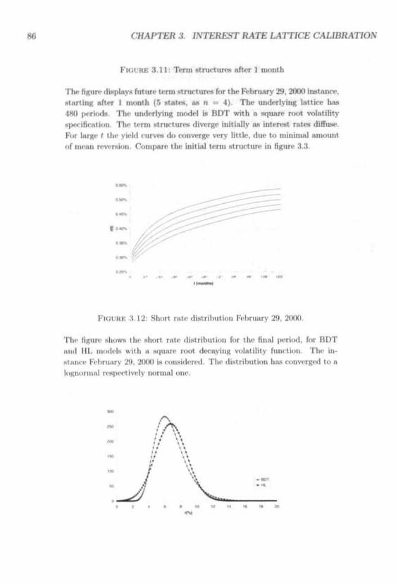
86 CHAPTER 3. INTEREST RATE LATT/CE CALIBRATION

FIGURE 3.11: Term structures after 1 month

The figure displays future term structures for the February 29, 2000 instance,starting after 1 month (."i states, an n = 4). The underlying lattice has480 IMTHMIH. The underlying model is BDT with a square root volatilityspecification. The term structures diverge initially as interest rates diffuse.For large f the yield curves do converge very little, due to minimal amountof menu reversion. Compare the initial term structure in figure 3.3.

H03»N

FlUUUK 3.12: Short rate distribution February 29, 201)0.

Tin- figure shows the short rate distribution for the final period, for BDTanil III. models with a square root decaying volatility function. The in-stance February 29. 2(MK) is considered. The distribution has converged to alognormal respectively normal one.

3.5. RESULTS 87

TABLE 3.5: Averagr swnrrtion {wiring erntm twtvfnrtor nwxM

The table reports th< i\'I.IL;. pii. mu rn. ' i - t.J m r,|u.»ti<>u3.49 (in percentages) i w r all ti'2 swaptions with joint tuneto expiration mid maturity of the underlying swap lessthan or equal to 10 yearn. A' is the iiumlx>r of equallyspao-d time steps in the ton-year lattice Kntiii-> ««-!«-« U>the "Lognormal" model (»(r) - Inr with the Mmmspecification for lx>th volatility functions in (3.37).

DateFeb 29.Feb 15.June I.l u l v _•

200020012001

J l M 11

A T - 120

4.276.594.99

'. U

\

4 l'»

5.903.24t 7.'

3.5.2 Two-factor model

For monthly periods (A = 120). calibration results improve significantly when considering

a two-factor model. The improvement over a one-factor model is at least 25% in terms of

average swaption pricing errors. Table 3.5 shows the average pricing errors for the four

dates in 2000 and 2001. We only consider the BDT model with square root volatility

function as in equation 3.37.

Despite the large improvement due to the second factor, larger improvements have been

achieved for the one-factor model when increasing the number of periods from 120 to 210

for three out of four instances. Only for the February 29, 2000 instance an improvement

over the best one-factor model solution is obtained with the two-factor mode) with monthly

periods. This observation gives rise to doubling the number of periods of the two-factor

model. Table 3.5 also presents the average pricing errors for 240 semi-monthly periods.

Computationally. 240 periods in a two-factor model proved to be the maximum

To enhance convergence to an optimal calibration of the two-factor model with 210 pe-

riods, an appropriate initial solution is chosen from known coefficients. Either, the optimal

coefficients of the two-factor model with 120 periods or those of the one-factor model with

240 periods are used. Our initial coefficient set is the one that given lowest average pricing

errors. That is. for February 29. 2000 we start with the two-factor model coefficients for

monthly periods. For all other instances, the optimization process is initialized by the one-

factor model coefficients for semi-monthly periods. The coefficients for the second factor

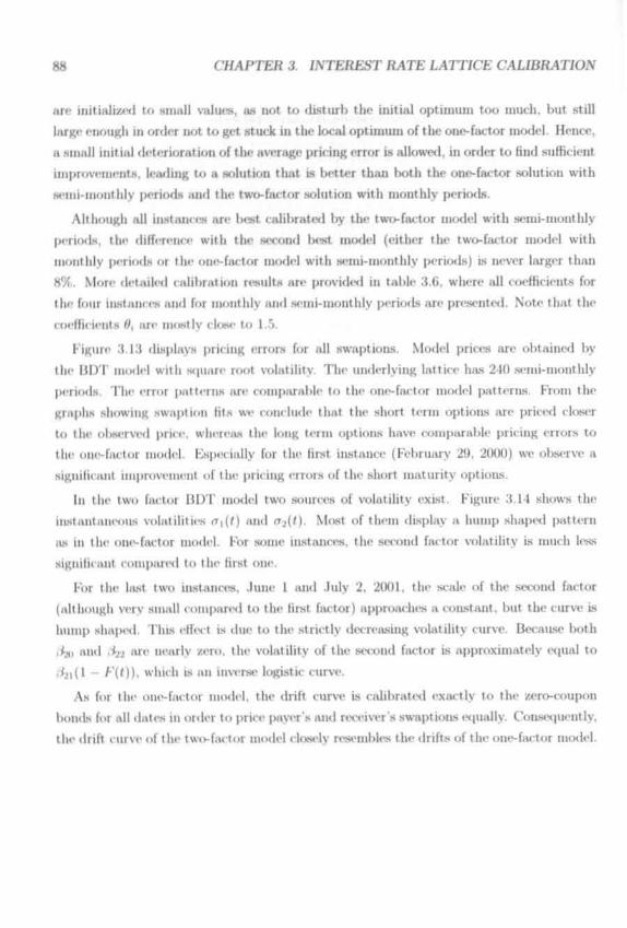
88 C7MPTEK 3. INTEREST JL4TE LATT/CE CALJBRAT/ON

are initialized to small values, as not to disturb the initial optimum too much, but still

large enough in order not to get stuck in the local optimum of the one-factor model. Hence,

ii .small initial deterioration of the average pricing error is allowed, in order to find sufficient

improvements, leading to a solution that is better than both the one-factor solution with

semi-monthly periods and the two-factor solution with monthly periods.

Although all instances are best calibrated by the two-factor model with semi-monthly

periods, the difference with the second best model (either the two-factor model with

monthly periods or the one-fact or model with semi-monthly periods) is never larger than

8%. More detailed calibration results are provided in table 3.6, where all coefficients for

the four instances and for monthly and semi-monthly periods are presented. Note that the

coefficients 0, are mostly close to 1.5.

Figure 3.13 displays pricing errors for all swaptions. Model prices are obtained by

the BDT model with square root volatility. The underlying lattice has 240 semi-monthly

periods. The error patterns are comparable to the one-factor model patterns. From the

graphs showing swaptiou tits we conclude that the short term options are priced closer

to the ol>served price, whereas the long term options have comparable pricing errors to

the one-factor model. Especially for the first instance (February 29. 2000) we observe a

significant improvement of the pricing errors of the short maturity options.

In the two factor BDT model two sources of volatility exist. Figure 3.14 shows the

instantaneous volatilities >r,(/) and T.>(')- Most of them display a hump shaped pattern

as in the one-factor model. For some instances, the second factor volatility is much less

significant compared to the first one.

For the la.st two instances, June 1 and July 2. 2001, the scale of the second factor

(although very small compared to the first factor) approaches a constant, but the curve is

hump shaped. This effort is due to the strictly decreasing volatility curve. Because l>oth

/tjii and .^j are nearly zero, the volatility of the second factor is approximately equal to

#»(1 - EC)), which is an inverse logistic curve.

As for the one-fact or model, the drift curve is calibrated exactly to the zero-coupon

bonds for all dates in order to price payer's and receiver's swaptions equally. Consequently,

the drift curve of the two-factor model closely resembles the drifts of the one-factor model.

15. RESULTS

T A B I I : t t • r . i i . i i u i ' t i ' i v , i f t i n i u o f . i i i . i l ^ , | u . i n I . M . I \ , . ! . i i i l i t \ i i i m

T h f t t b k l r i " | " M i i l i l I i l - I • t i l • i - n i - t i t i n \ . . | . i t i h t \ h i m I i t M i - -

*,(<) = O.Ol^F.(f) ^ + ( l - F ,

with

for tho "LngnoniiHr model (7(r) = Inr. W is th<' IIUIHIM-I nf timein the 10 war lattice.

Feb 29. 20()0120 9.00 1.443 0.375 1.49 0.023 2.11 0.758 0.585 1.50 0.039240 9.00 1.443 0.391 1.49 0.023 2.11 0.703 0.583 1.50 0.039

Feb 15. 2001120 5.62 0.705 0.G16 1.62 0.034 0.00 0.000 0.200 1.40 0.007240 16.14 2.183 0.1C4 0.96 0.129 0.11 0.033 0.002 1.00 0.049

June 1, 2001120 4.33 0.520 0.000 1.48 0.027 9.63 1.533 0.744 1.51 0.027240 13.95 2.563 0.317 1.23 0.089 0.00 1.110 0.002 1.55 0.034

July 2, 2001120 5.43 0.283 0.558 1.49 0.035 15.22 0.000 0.187 1.48 0.024240 9.98 2.523 0.464 1.24 0.082 0.00 1.942 0.000 1.51 0.032

CHAPTER 3. INTEREST RATE LATTICE CALIBRATION

FIGURE 3.13: Swaption fit two-factor model.

The figure shows relative swaption pricing errors for four dates, as modelprice minus observed price divided by observed price. Pricing errors resultfrom the BDT model with square root smoothing on volatility parameters.The pricing error pattern is similar to the one-factor model, pricing errorsare slightly smaller, especially for short term swaptions. The underlyinglattice has 240 periods.

i

e * •» ? S 8 19

ft

i

!

— !— i

S

' 1i_ r

s s a « s

3.5. RESULTS OVV

FIGURE 3.14: Instantaneous volatility two-factor model.

The figure displays instantaneous volatility ciirvw tf,(f) for IM>I1I Cm tors ofthe two-fartor model, for all four date* considered. Result* for the HOTlinxlcl with square root volatilities an- shown. The underlying lattice hiui240 periods.

Mi

0049

004

OOM

on i

I— /0 0> 1

001J

001 /

0005 '

00

F«to29, 2000

— _

12 24 36 48 60 72 84

t (months)

• MOM—laoofZ

•

96 108 120

oos

OOM

004

ooa

oos

f.«oot

F«to15. 2001

• Moi 1 ^/ *N_ —t»elo« I (anas 100)

/ ^

001*

001

0 006

00 12 24 36 48 60 7? 84 90 106 120

t (months)

June 1,2001 July 2, 2001

0.06

006

004

§003

on

• lactor i— Isclof2

0 12 24 36 48 60 72 84 96 KM 120

I (months)

0 12 24 36 48 60 72 84 96 108 120

I (months)

92 CHAPTER 3. INTEREST RATE LATT/CE CAL/BRAT/CW

FIGURE 3.15: Scale two-factor model.

Tin- figure displays the wale 6;(<) = rj,(<)\/< for both factors of the two-factormodel, for nil four date* considered. Results for the BDT model with squareroot volatilities are shown. The underlying lattice has 24U periods.

ooota

00014

00012

0001

§00008

DOOM

00004

00002 //i

0 '0

Fab 29,

• lactor i

/

/

/ ^

12 24 M 48 SO

I (moo

2000

^ ^

•^ -

72 M 98 106 120

ttw)

Feb15, 2001

• factor 10 0018 —factor 2 I t r a i 100)

Jun« 1,2001

• factor 1ooou —factor?

0 tj M 38 4« 80 7J 84 98 10» <M

t (month*)

00 12 24 38 48 60 77 84 98 108 120

t (month*)

3L5. RESULTS 9S

FIGURE 3.16: Mean reversion two-factor

Tbc figure display* the IIK-HII n-\rr>i<>n K , ( 0 for t>oth fat-tore of the two Curloi

model. fur all foui <l.ii< - • ..UM.II i.»1 Ki-MtltK for tlu- BUT IIHMICI wiilr ^.|u,u.

root volntilitio HIT showti. The uiuicrlvinR lattirr HAH 240

F«b29.2000 F»b 15.2001 . : E

« <

factor 1-lacto>2

• N II « • 10) IM

—IMor2

June 1,2001 July 2, 2001

• factor 1— factor 2

• (actor 1— lactorZ

94 CHAPTERS. INTEREST RATE LATTICE CALIBRATION

3.6 Conclusion

The calibration performance of a term structure model depends on many interest rate

characteristics, most importantly volatility and mean reversion. Applying a one- or two-

factor model, based on Ho and Lee [38] or Black. Dcrman and Toy [9], limits the freedom of

parameter choice to describe these characteristics. As shown in equation 3.15. variable time

periods are one way to model volatility and mean reversion independently. To have positive

menu reversion of interest rates, we show that the length of time steps must be decreasing.

However, as long as the implied mean reversion, defined by /c<>(f) = -ff'(<)/W')- does not

deviate too much from the desired menu reversion, step sizes can remain constant.

Both theoretically and empirically, the volatility parameters <r(t) are best smoothed by

a function decaying at rate y// I" order to have a stationary distribution of the short rate,

the smoothing parameter 0 must be larger than l.Ji. Calibration results suggest that 0 is

very close to l.!>, an are both coefficients 0, in the two-factor model. This implies that the

wale parameter (7(f)v^ approaches a constant.

The term structure model is calibrated to match observed swap prices and at-tho-inoney

swaptiou prices. To value short term options, one is tempted to consider many small periods

initially and increasing the step length for distant future periods. This leads to decreasing

mean reversion (or own diffusion) according to equation 3.27, an increase of the short

rate volatility T ( 0 mid an explosion of the yield volatility. To price short term options we

therefore considered small, but constant, period lengths.

We Apply variations of the one-factor models introduced by HL and BDT for calibration.

Interest rates are modelled by means of a recombining binomial scenario tree. Volatility

parameters are smoothed according to square root decline, exponential decline, or a con-

stant volatility implying a random walk interest rate process. Our analysis is extended by

introducing a two-factor model, based on a trinomial rccombining tree, where both factors

have independent volatility processes. All models use the drift parameter to fit the yield

curve of zero-coupon bonds exactly. If the yield curve is not exactly matched, at-the-money

payer's and nveiver's swnption prices will be different, while these are quoted equally.

The best performing models when considering four periods per month. BDT with square

root volatility and HL with exponential volatility, have average swaption pricing errors of

approximately .VX over all instances. When including monthly and semi-monthly periwls,

the HDT model with square root volatility performs best in nine out of twelve instances.

All instances show a similar pattern of swaption pricing errors. Long term options are

3 6 CONCLUS/ON 95

underprkrd by the model • - | » < i.illy on short term swaps Short maturity option* on long

swaps arc typically overpriced An analogous pattern is I'l-riM-d when quoting pricing

errors in terms of implied volatilities

After optimizing the model p.ti .mirtci s l>\- a quasi-Newton approach, we trie<l to impHWt

the resulting local opt imum using l<>< .il s< ,n< h I / x al search inrludes more |>aiami'tirs (drift

and non-smoothed volatility for each |MIIIMI), but calibration sp»fd is s lower However, no

improvement could IM> found. When starting with i« l<«.il v , u i h method to optimize the

volatility parameters (using all drift parameters to exactly match the yield curve), we ilid

also not obtain a better fit and the error |>attern remained.

Volatility wcording to the square root volatility functions is usually hump shaped,

although i iiinrii;ciii «• Ls rather slow. As a result, the wa le p,u.nuclei i> m u r . w n r < \ i u

after 11) w.u.v Me.in reversion only starts after one w a r and KIU.UII- m ill ill. l u . m U .

The short rate distribution after a sufficient IIIIIIIIHT of (MTKNIS I.-- -I.II.I. .m.I > !•••. to a

logiionnal (normal) distribution for the B D T (HL) nuxlel.

The two-factor model slightly improves calibration results, but the error pattern r ^

mains. Short maturity options are priced more accurately because short term flexibility

increases with the number of states. Although for monthly periods the implied short

rate distribution after one month cannot be modelled accurately, and pricing errors can

be larger than for the one-factor model with smaller periods, the two-factor model with

semi-monthly periods performs best for all instances considered.

Our purpose is to use the calibrated interest rate lattices for mortgage valuation. Mort-

gages are particularly long term contracts. As pricing errors for long term assets appear to

be small and less subject to discretization issues, the interest rate lattices arc applicable,

for mortgage valuation.

Part II

Mortgage Valuation

Chapter 4

Introduction to Mortgage Valuation

4.1 Introduction

Mortgage contracts have developed from simple bank loans to fixed income securities with

various embedded options. A Dutch mortgage contract can have a mix of fixed and ad-

justable contract rates, can be partially prepaid, may offer borrowers the opportunity to

change the fixed rate period of the loan, can have the possibility to lock in minimum rates

over a certain time span, or includes a combination of these and additional features. Com-

puting the oilers from various lenders (often intermediaries) and distinguishing between

the products on the market is a difficult task in the intransparent mortgage loan market.'

The objective of the second part, of this thesis is to provide a meaningful comparison of the

basic contracts offered on the Dutch market. The main complicating factor is the valuation

of partially callable mortgage contracts, which will be the topic of the two core chapters

of this part.

The best offer would be the contract which has the lowest present value of future cash

flows. Since for many mortgage loans the future cash flows depend on future mortgage

rates offered by banks and on prepayment decisions made by borrowers, a comparison of

different loans requires assumpt ions about interest rate dynamics and prepayment behavior.

In a competitive market one could assume that all loans are priced correctly and that the

contract rates reflect the embedded options. The interest to be paid is such that the

present value of the future cash flows is equal to the nominal value of the loan. In that

'For nil overview of the range of mortgage loans on offer in the first half of 2003. we refer to the'Hypothekennids', H publication (in Dutch) of the 'Vereniging Eigen Huts', an association supporting theinterests of homeowners in the Netherlands.

98

4.1. INTRODI/C77ON 9t

case, the various mortgage- contracts will not differ in value, but onlv in their sensitivity

to Chandra in the term structure. Throughout the second |>art of this thesis we invest uuitt'

what magnitude of spreads we can expect for popular cmlx-ddcd options

Our methodology » based on fair rate computations. Given the current yield curve

and infonnation about interest rate volatilitx- u. .l.titu- the fair rate as ttw contract rate

that makes the present value of the sum of all cash Hows equal to the nominal value, Tliis

is the interest rate at which it lender cannot expect to make IUI abnormal ptulit >>n tIx-

loan If the contract rate is higher (lower) than the fair rate, implying a nioitn.iK< value

higher (lower) than the nominal loan value, the Itank makes a profit (IONS) on the emit nut

equal to the difference in value. The nominal loan value or principal is sealed to I lor all

mortgage contracts. Fair rate differences betwi < n ...utracts are an indication of the value

of embe<l<led options. For each rontnu t m . I•!.1111 the fair rate that is consislenl with the

current term structure and volatilities rtlli 11 < -. 1 in liquid derivatives such as swuptinii.s

For some contracts we also observe the contract rate quoted by a lender. The difference

compared to the fair rate is an indication of the profitability of the market plus n rink

premium for default. Default risk is limited for Dutch mortgages. Full information on the

credit status of borrowers is maintained in a central database which is accessible to all

major lenders in the market. In addition, many contracts are subject to the 'Nationals

Hypotheekgarantic' (N'HG) which compensates banks for default losses. Banks quote dif-

ferent rates according to default risk. The lowest rate is for loans secured by NHCJ, tho

highest for loan values higher than 75% of the value of the house. In our computations we

ignore default risk.

Another important assumption underlying our fair rate calculations is the absence of taxeffects. In this chapter we do not consider any client specific aspects affecting the choice

for a certain mortgage contract or the mortgage value. Tax effects influence mortgage

choice in the Netherlands. Mortgage interest payments are fully tax deductible. AH a

result mortgage loans are cheap credit. Perpetual mortgages are popular because interest

payments remain high. One major effect of tax deducibility is the discouragement of

prepayment, since the net contract rate paid is typically lower than the fair rate. When

prepaying the mortgage loan while this is not allowed, a prepayment penalty mast be paid.

This penalty is also tax deductible. The decision to move from a contract with a high

interest rate to one with a lower contract rate Ls not affected by tax effects, as long as both

contracts are equally taxed.

A second reason for differences between fair and quoted contract rates could be the

100 CHAPTER 4. /NTRODl/CT/ON TO A/ORTGAGE VALUATION

interest rate model. For the valuation of embedded options we mast assume a dynamic

process for spot rates. Although the process is calibrated to the current term structure

and to volatilities, many degrees of freedom about distributional characteristics and implied

dynamics remain. For robustness of the results we will therefore compute fair rates based

on several interest rate models.

We focus on optimal prepayment decisions, driven by interest rate behavior. We only

deal with mortgage contracts exposed to interest rate risk and exclude combinations of

mortgages with insurances or investments, for which other types of risk play a role. Optimal

prepayment of Dutch mortgages is limited to a percentage of the initial loan per calendar

year, complicating mortgage valuation significantly. Chapters 5 and 6 introduce valuation

procedures for Dutch partially callable mortgages. Chapter 5 deals with interest-only

mortgages with partial prepayment options, which can be valued by a lattice approach

by keeping track of the number of prepayment options and the number of calendar years

remaining. Chapter (i introduces a linear programming model for general Dutch mortgages.

This chapter provides an introduction to the second part of this thesis. Characteris-

tics of popular contracts will be discussed in the next section. Section 4.3 outlines the

valuation methodology for fixed rate mortgages, non-callable and fully callable, which is

based on a calibrated binomial lattice. The full prepayment boundary is determined. We

provide a valuation method for adjustable rate mortgages based on a dynamic program-

ming approach to create and solve subprobleins of the original (path dependent) valuation

problem. Section 4.4 identifies valuation problems for Dutch mortgages including partial

prepayment options.

4.2 Mortgage characteristics

In this section several mortgage characteristics and options are described concerning the

amortization schedule of the mortgage, options to call the mortgage before maturity, and

options to adjust the contract rate during the lifetime.

4.2.1 Amortization schedule

The periodical payment of a mortgage is denoted by A/, and depends on the principal

fo (tl>«' nominal loan value, which can be scaled to 1). the lifetime of the mortgage T

and the contract rate ;/ With monthly periods. T is stated in months, y is the monthly

4.2. A/ORTCACE CrMJLACTERJSTJCS 101

contract rate and A/, is a monthly payment. The |x<riodical cash Hows tin- determined

a s if t h e c o n t r a c t r a t e w o u l d IM- v a l i d u n t i l m a t u r i t y . M o s t c o n t r a c t * , l u m v v . i h , i \ . t.«i«>

a d j u s t m e n t s a f t e r 5 . 7 o r 1 0 y e a r s . •

The unpakl Imlance {/, at a future date f can he expressed in terms of the unpaid luUonrtt

at time r — 1:

I/. = (1 + V) t / , - i -A / , . (4.1)

The periodical payment consists of ait interest |wyment and an ainntti/atinit |>art /4,:

A/, = y • £ / , . , + M,.

Boundary conditions imply that ('„ bi given (waled to 1) and f'/ • 0. xurh that tlio

inortKHK*' loan is repaid at maturity Prepayments are defined as additional amorti/.iitioit

ca*h Hows L», If additional pre|Mtyineutti are allowed, then the periodic ill puviiicllt <<t|llnli*

Af, = y t / , _ , + i 4 , +O, . (4.3)

An additional prepayment affects the future amortization schedule. All contractN consid-

ered in this thesis have the restriction O< > 0. Some modern contracts allow for negative

O, a.s long as (/, < (/() for all periods <.

Annuity mortgages

An annuity mortgage is characterized by a constant periodical payment A/, such that

t/r = 0. The periodical payment of a non-callable annuity is given by*

(4-4)

This follows easily from the fact that the principal equals the sum of all future payments

discounted at the contract rate:

on the ncmaimnj loan valur f, i the next periodical payment can be ot)taine<l l<y(_i | / |^ )*ir-i»iii being equal to A/ for all ( for ronxtant y.

102 CHAPTER J. /NTRODl/CTIOJV TO A/ORTGAGE VALl/AT/ON

Tlif periodical payment consists of redemption and interest payments. When time evolves

intercut payments decrease ami the perio<lical redemption amount increases. At date £ the

interest payment can be shown to be

(4.6)

whereas the redemption amount equals

The unpaid balance of an annuity mortgage is given by

tf, = ( l + » ) • * / , . , - A / . (4.8)

Linear mortgages

A linear mortgage is characterized by a constant redemption amount. The interest pay-

ments, and hence the total periodical payments, decrease over time. The periodical re-

demption A, = A is given by

-4 - ^ , (4.9)

where f',i and 7' arc again the principal and the lifetime of the mortgage. Now the total

periodical payment at date t, A/,, of a non-callable linear mortgage is given by the sum of

redemption and interest:

A/, = /» + !/•( ' , ,, (4.10)

with }/ representing the contract rate as before. Finally, the unpaid balance at date /, {/,,

is given by (he principal minus all redemption payments up to and including period f:

I/, = [(/„ - A • (f - I)] • (1 + v) - A/, = l/o - A • r (4.11)

Interest-only mortgages

Interest-only mortgages are free of regular redemption (A, = 0) during the lifetime of the

contract. Only interest has to IK* paid, amortization takes place at the end (Ar = l/o)-

4.2. MORTGAGE CHARACTERiSTJCS 101

The final redemption could U> done by taking out a now loan, selling the hou.se or usingprivate savings. Without pre|w»yment.s the unpaid IwUamv remains nt (lie initial level:

t/, =t / ,_, = . . . » l / o . (4.12)

Each period f. int.iot is paid equal to y • f/«_i. This » also the |>eriodical |myment

A/( became of the al«s.m. , ,f regular redemption amounts. Concerning the contractual

payments, an interest-only mortgage is a long term cou|>on bond for which the print i|>al

i.s riilo-tiK-d at maturity.

Since in the Netherlands interest (lavineuts on a IIIOIIIM - 1. • m ire fullv tax deductible,

interest-only mortgage* arc popular The unpaid IM1.HU • . noi decline IMHIUIW no

retlemption takes place. Therefore interest paynxm> .ui.l (ax dediutions remain high.

Savings and investment mortgages

During the lifetime of a savings or investment mortgage only interest payments occur.

Redemption does not take place before the end of the mortgage contract. Without prepay-

ments the unpaid balance remains unchanged until maturity. To repay the loan an account

is opened at the beginning of the contract. Such an account usually takes the form of a

savings or investment fund. At the end of the contract the mortgage is repaid using the

account balance.

If we assume that payments to the account are made according to an annuity schedule,

a savings or investment mortgage is a combination of an annuity and an interest-only mort-

gage. Tax deductible interest payments remain high, while periodic redemption payments

are used to increase the account and not for amortization purposes. The savings account

earns the same interest as must be paid on the mortgage loan. Consolidating the loan and

the savings account, the pre-tax cash flows are identical to an annuity mortgage. On an

after-tax basis they are different to the client.

Similar to an interest-only mortgage, excluding additional prepayments the unpaid bal-

ance remains at the initial level (/,). The savings account B, increases by the interest earned

and by the monthly redemption, redemption being equal to the total monthly payment

minus interest:

Bi = (1 + y) • £ , . , + A / - y - ( / o - (4.13)

104 G7MPTE/? 4 /JVTRODl/CTJOiV TO MORTGAGE VALl/AT/ON

The net outstanding loan, denoted by ty = t/« - B/, can easily be shown to be :

AT, = ( l + y ) A T , . , - M , (4.14)

which is similar to the unpaid balance of an amortizing mortgage.

An invtwtment mortgage is similar to a savings mortgage, but Ls exposed to higher

risk since it is uncertain whether the return on the investment fund Ls sufficient to repay

the loan at maturity. Comparable to an interest-only mortgage, savings and investment

mortgagiw are long term coupon bonds for which the principal is redeemed at maturity.

4.2.2 Call options

When entering a non-callable mortgage contract, prepayment of (any part of) the loan is

not allowed. Only regular redemption and interest payments occur. Valuation of a non-

callable, fixed rate mortgage boils down to a simple present value calculation using the

current term .structure. It does not require an interest rate model. Non-callable mortgages

are hardly issued by banks. A typical mortgage contract includes some form of prepayment

opportunity.

A fully callable mortgage can be completely prepaid in a single period. This is a typical

feature for US mortgage contracts. Besides the regular periodical payment the mortgagor

muHt decide whether to prepay or not in each period. Interest rate driven prepayment

takes place when interest rates are low. Calling the total mortgage loan can be financed

by taking out a new mortgage loan at the prevailing lower contract rate.

In the Netherlands, only prepayment of a percentage (10% to 20%, depending on con-

tract and lender) of the principal mortgage loan is allowed every calendar year. If the

mortgagor wants to prepay more than this percentage a penalty must be paid equal to

the present value of the difference bet wren the future monthly payments of the new con-

tract and the existing mortgage. Because of this prepayment penalty a larger than allowed

prepayment is never optimal. A penalty is not paid in case of moving or death of the

mortgagor or at a contract rat* adjustment date.

For Dutch mortgage contracts, as an alternative to full prepayment, many loans include

a 'time for reconsideration' option. A 'time for reconsideration* option allows a borrower

to fix the contract rate achieved during the reconsideration period for the next fixed rate

period For many contracts the specified period equals the last war or two wars of the

4.2. .\fORTC.4GE CHARACTERiST/CS 105

current fixed rate period. Clients can choose when to fix the contract rate during I hit*

pcrkMl and will do so when it is observed to be low

A mortgage with an etnlieddexl 'time for rcvi>iiM<l<!ation' option Is equivalent to n time

court rained fully callable mortgage. The option allow* |..i i< luuuicing the mortgage loan

during the sj>ecified period, at a future (lower) contract rate, i<quivalent to calling the

complete loan and initiating a new contract at the future rate, (.'outrider a mortgage

contract with an option to fix the contract rate to the future mortgage rate in any desirable

month / during the last year of the fixed rate |MTKM1 This is e<|Uivulent to calling the

mortgage (without penalty costs) in month f and initializing a new contract at the mortgage

rate valid at (. Calling is restricted to the hist year of the Kxed rate |x*riod and the new

loan must t>e initiated at the same bank.

Sometimes the lowest mtrn-st rate during the first year (or two yearn) ran be fixed M

contra«t rate. This rate is called IUI entering rate. During an entering period, the mortgage

loan LS equivalent to a variable rate mortgage. The contract is fair priced since each period

the contract rate is adjusted to the one-period fair rate. After the contract rate IM fixed,

the mortgage loan is comparable to a fixed rate mortgage. For this reason, in the sequel a

mortgage including an entering rate option is not considered as a separate mortgage type.

4.2.3 Contract rate adjustment

With a fixed rate mortgage (FRM) an adjustment of the contract rate during the lifetime

of the mortgage is not possible, neither for the bank nor for the client. A single contract

rate is faced during the total lifetime. Fixed rate mortgages are rare in the Netherlands.

An adjustable rate mortgage (ARM) is defined as a mortgage which contract rate is reset

periodically. Usually the time between reset dates is constant. During a period between

two reset dates, called a fixed rate period, the contract rate is fixed. Typical fixed rate

periods span 5 or 10 years, whereas a common mortgage lifetime equals 30 years. After

each fixed rate period the contract rate is reset, based on the future term structure. At

every adjustment date full prepayment is allowed without penalty. However, as long as

fair rate valuation is considered, the adjusted contract rate Ls fair and prepayment is not

profitable at a reset date. Valuation of AflM's Ls the topic of section 4..'{.2. For a detailed

discussion on ARM valuation, see Kau, Keenan, Muller and Epperson [48) and Van Busscl

[17].

The contract rate adjustments can be unrestricted or restricted. In case of unrestricted

106 CHAPTER 4. iNTRODl/CTJOJV TO A/ORTGAGE VALUATION

adjustments the future contract rates are solely based on the future term structure and are

independent of the initial contract rate. Restricted adjustments might impose caps, floors

or l>oth on the future contract rate. A cap (limiting a contract rate increase compared

to the current rate) protects the client from extremely increasing mortgage rates, while a

floor (limiting a contract rate; decrease) protects the bank from decreasing rates. Typical

Dutch mortgages do not have adjustment caps or floors.

In the Netherlands many variations on contract rate adjustments exist, two of which

arc diMCUHHod in more detail: n bandwidth mortgage (a variable contract rate which is

not adjusted if the contract rate remains within a bandwidth) and an interest rate limit

mortgage (combining a fixed rate and a variable rate mortgage by the use of a contract

rate limit).

A fcam/u'wi</t mortgage is a variable rate mortgage for which every period a contract rate

iidjust merit, may occur. If an adjustment takes place, the new rate is set to the contract rate

for a mortgage with the same maturity date (that is, a shorter lifetime). The contract rate

is only adjusted if the new rate lies outside a bandwidth. Let us consider a bandwidth on

an increase of the contract rate. If the new contract rate is lower than the initial rate, the

contract rate is adapted. But if the new contract rate is larger, adjustment only happens

when the difference between the two contract rates exceeds the bandwidth. In that case,

the new contract rate is set to the higher contract rate minus the bandwidth.

As an example of a bandwidth mortgage, suppose the initial contract rate equals 6%,

and the bandwidth, usually depending on the length of the fixed rate period, is 1.25%.

11 in the next period the newly determined contract rate is 5%. then the contract rate is

adjusted to 5%. But if the future contract rate rises to 7% no adjustment takes place. Only

if the contract rate rises above 7.25% the rate is changed. For example, if the new rate

becomes 8% only 6.75% is paid as the bandwidth is deducted. Many mortgage contracts

exhibit an equally sized bandwidth for decreasing contract rates. In that case contract rate

decreases are passed on only if they exceed the bandwidth.

A bandwidth mortgage can be interpreted as an adjustable rate mortgage with every

period being an adjustment date. Adjustments are restricted and depend on the original

rate since the contract rate is only adjusted if the contract rate difference exceeds the

bandwidth.

The inrVTwf nifp /imif mortgage combines a variable interest rate with a fixed interest

rate. Initially the client chooses a fixed rate period and an interest rate limit to be paid

at most. First, the variable rate is paid until the contract rate for the chosen fixed rate

4.3. VALUATION 107

period exceeds the interest rate limit. FVom that date on the fixed rat«> pern>.l M.IM

the fixed interest rate corresponding to the chosen fixed rate penod Ls pnid, until this fixed

rate period ends.

When |>ayii)g variable interest rates, the |>eriodical payment* of tut intenwt rate limit

mortgage rail Ix- determined directIv Kate adjustments occur every IMTHHI and unre-

stricted, which is comparable to i \.u tattle rate mortgage. After fixing the i n t e n d rate,

the mortgage price can be determined similar to a fixed rate m<>ii r..u-.«v The fair rate in

equal to the interest rate limit by construction. Consequently. the valuation of interettt

rate limit mortgages does not re»mire scjuirate treatment.

4.3 Valuation

Binomial tree methods for American mortgage valuation are developed by among other*

Kau. Keenan. Muller and F.p|>erson [48. .10]. Viut BiiNsel [17]. and. for multiple state vari-

ables. Hilliard. Kau and Slawson [37]. Also (exotic) option literature (see Hull [.<!)] for an

overview) is valuable for mortgages with prepayment options.

The underlying process of mortgage valuation problems is captured by an interest rate

model. We calibrated a binomial scenario tree of interest rates on market prices of swaps

and swaptions to reflect the term structure of interest rates and volatilities. For calibration

purposes the scenario tree is allowed to be recombining. and is therefore called a Milennial

lattice. When valuing mortgages however, we cannot always rely on a lattice approach.

For many contracts (for instance ARM's and mortgages with partial prepayments) we

must apply a non-recombining tree approach, because the history of prepayment decisions

or adjustments Ls relevant for the current mortgage value, thereby introducing path de-

pendencies. Hence a unique path is required to lead to each node, which in typical for a

non-recoinbiuing tree.

Non-recombining trees are computationally inefficient compared to lattices, as the num-

ber of states increases exponentially. To avoid working with non-recomhining trees, algo-

rithms can be developed for decomposing the original mortgage valuation problem* into

smaller problems, each of which can be solved using a lattice. After all, we prefer to use

multiple lattices instead of a single tree. In chapter 5 we will analyze the decomposition of

a mortgage contract into several coupon bonds. In chapter C we discuss a decomposition

method based on the past prepayment strategy. An ARM can be decomposed in line with

108 CHAPTER 4. INTRODUCTION TO MORTGAGE VALl/AT/ON

this last approach, based on past adjustments. This will be the topic of section 4.3.2. First,

we analyze the valuation of fixed rate mortgages.

4.3.1 Fixed rate mortgage valuation

In thi« section we describe valuation methods for both non-callable and callable fixed rate

mortgages. These mortgage types are path independent, that is, mortgage prices do not

depend on past prepayment decisions, and can be based on a binomial lattice approach.

The perioils in a binomial lattice are denoted by t = 0, . . . ,T. For a period £the number of

states equals i + 1, labelled i = 0 , . . . , r. Transitions are defined by two possible successors,

(i + 1,< + 1) and (i,/ + 1), of each node (i.r)/' Both successor nodes are reached with

probability one half. Node (0,0) is called the root node.

As analyzed in chapter 3, the state process can be extended to a two-factor binomial

lattice (», j , 0- I"'' ••»«> costs in terms of computation increase rapidly. To study the ro-

bustness of the underlying term structure model with respect to the number of factors

included, we will consider both one- and two-fact or models for pricing mortgage contracts.

Non-callable m o r t a g e valuation

For the valuation of noii-cullable fixed rate mortgages an interest rate model is not required.

We can use a simple pricing method haml on separating a mortgage into zero-coupon bonds

with different maturities. The price of a non-callable fixed-rate mortgage can be obtained

by discounting the periodical payments using the current term structure:

where .(/((),f) is the current f-period spot rate. For aii annuity the periodical payment

is constant: A/, = A/. Mortgage's with different amortization schedules have varying

periodical payments A/,.

Although a lattice approach is not required for pricing non-callable mortgages, we in-

troduce the valuation procedure based on a binomial lattice for a non-callable mortgage,

before proceeding to fully callable mortgages. During a fixed rate |>eriod the contract rate

is constant. For a particular rate y the monthly payment A/, is calculated by equation 4.4

' Although the t w structure Ls similar a.* in the previous chapter, nodes arc labelled •' = 0 , f.Previously, we used imlirtw j = -f f with im-reiuents of 2 and > = 2i - f.

4.3. VAtl//4T/O\ 109

if we consider an annuity or by 4.10 in < i- "I i Imonr mortgage. The unpaid balance at

the end of the fixed rate period is found recursively l>y equation 4.8 or 4 11, n-sqxvtively.

At the end of a fixed rate [MTKMI (time r) either the mortgage is fully amortized or it

can l>e pre|Niid or refinanced cowtlessly. Full amorti/ntion ocetirs if r equals the lifetime

7* of the mortgage, in rase the final unpaid Iwilancc (', = 0 . If the fixed rate period in

shorter than the mortgage lifetime (r < T), a positive unpaid balance remain* at time r,

which can he prepaid without penalty. Consequently this remaining unpniil balance can

t>e valued at the current maturity r discount rate.

Since full prepayment is allowed, the price of a mortgage loan at r in all state!* of the

world Ls equal to the uii|>aid Itahwce: P(i , r) = t>, I = 0 r. After determining the

final mortgage values, the intermediate values P(M) of the mortgage are found l>y working

backwards, starting at ( = r — 1, until the current value /'(().()) is obtained:

^ ^ ^ , ^ ^

1 + r,,

The mortgage price equals the discounted sum of next period's expected price and the

periodical payment.

The fair contract rate, that is, the contract rate that results in a mortgage price equal

to the principal of 1, can be solved for numerically by increasing (decreasing) the initial

contract rate when P(0,0) is smaller (larger) than 1. The fair rate is iteratively determined

by a straightforward bisection method. The monotouicity of the morlKHgc price with

respect to the contract rate follows from the fact that a higher contract rate implies an

increase in interest payments. Consequently, the price, being the sum of all (discounted)

cash flows, rises.

Up to this point the effect of commission costs is excluded. Commission costs, typically

1% of the mortgage loan, can be easily accounted for in fair rate calculations. Including a

1% commission the contract rate is fair if the resulting mortgage price equals 0.99 instead

of 1.

A (binomial) lattice approach for non-callable fixed rate contracts provides information

about the contract rate risk. The two possible fair rates at < = 1, !/„ and {/,/, are a measure

of the current fair rate volatility according to

<r, = 0.5 • ( » „ - » , ) . (4.17)

Note that different measures of contract rate risk can be applied, for instance based on the

change in the mortgage price.

110 CHAPTER 4. /JVTRODl/CTJON TO MORTGAGE VALl/AT/OJV

Fully callable mortgage valuation

Basic non-callable mortgages can he valued by a term structure of interest rates. When

pricing fully callable mortgage* a lattice approach is required, since the mortgage value

does not only depend on time but also on the state of the world. Prepayment typically

occura at low interest rates, while for high interest rates the mortgage loan is continued.

Full prepayment options are included in all American type mortgages. Compared to non-

callable mortgages, the lattice based valuation procedure for fully callable loans differs

in just one aspect. In every period and state of the world, the mortgagor must decide

whether to prepay or not. If no prepayment takes place, valuation continues exactly as

described by the backward recursion 4.16. If the loan is prepaid, the true mortgage value

must equal the value of the remaining unpaid balance. We refer to Kau. Keenan. Muller

and Kppcrson [19] for a detailed discussion on fully callable mortgages and to Hull [39] for

American option valuation in general.

In the mortgage valuation lattice, full prepayment will occur if interest rates are low.

Following a scenario path, prepayment is triggered as soon as the interest rate drops below

a certain level. This level is indicated by the /«// prrpflj/rnrnf fcounrfar-y. We define the

full prepayment boundary as the distinction between nodes for which full prepayment is

optimal (nodes with the lower interest rates) and nodes for which full prepayment is not

optimal (at the higher interest rates).

The regular periodical payment A/, of a fully callable mortgage is obtained by equation

4.4 for an annuity and by 4.10 for a linear mortgage. Unpaid balances are determined

according to equation 4.8 or 4.11. as if no prepayment is allowed.

To determine the optimal prepayment strategy, the profitability of calling the mortgage

must be evaluated in every nodi- of the mortgage valuation lattice. The value of a fully

callable mortgage in node (i. 0 without calling is given by

^ ^ ^ , ^1 + r,,

For each node, the mortgage is called if and only if L', < P*(i,f) during the Imckward

recursion process. The mortgage value in node (i,r) after the prepayment decision is taken

equals

The division whether to pre|xty in state (».f) is based on the optimal prepayment strategy

4.3. VylLlMTJCWV 111

FlGl'RE 4.1: Full prepayment txmmUry

after time f. since the future mortgage price has been adapted if prepayment were optimal

in a successor node of (».f). Now. P(i./) = (/< if (/, < P'(i./) (that i.s. prepayment

is optimal) and (i.f) is marked before the recursion continues. When the recursion is

completed the marked nodes are separated from the unmarked nodes by the full prepayment,

boundary. The current price P(0,0) of a full prepayment mortgage is lower then the price of

a similar non-prepayment mortgage, because full prepayment reduces the mortgage value.

Equivalently. the fair rate is larger to compensate for prepayment advantages.

Calling penalties can easily be accounted for by either multiplying £/, with (1 + r)

where c is a relative penalty, or by adding C to (/, where C is an absolute penalty. Then

prepayment takes place if and only if (/, • (1 + c) < f ( i , f) or £/, + C < P*(i, *). Taking the

relative prepayment penalty as an example, the mortgage price in node (i,r) ol»scrved by

the borrower equals

) (4.20)

For positive prepayment penalties the current price of such contract will be larger than for a

penalty-free fully callable mortgage, but smaller (or equal) than the price of a non-callable

mortgage.

Figure 4.1 shows a small lattice example with a possible full prepayment l>oundary (the

112 CHAPTER 4. JJVTRODl/CTJON TO AfORTGAGE VALUATION

line labelled /p6). Note that in general the boundary does not have to be horizontal.

Also, II larger interest rate decrease might be required to trigger full prepayment behavior,

especially when penalty or commission costs are involved. In the nodes below the boundary

(labelled P), interest rates are low and full prepayment is optimal, whereas in nodes above

the boundary (labelled /V), interest rates arc high and no full prepayment is optimal.

We conclude this section with a description of the mortgage valuation algorithm for

fully callable mortgages:

• Fix the initial contract rate. Calculate the periodical payment according to equation

4.4 or 1.10. For interest-only mortgages, the periodical payment equals y • f/o-

• Calculate the unpaid balance (/,. at the end of the fixed rate period according to

equation 4.8. 4.11 or 4.12.

• For all states at the end of the fixed rate period, set the mortgage value equal to the

unpaid balance: P (» ,T ) = (/(r).

• Perform a backward recursion to obtain the continuation value of the mortgage ac-

cording to equation 4.18. A prepayment decision must be taken in each node. The

mortgage price including prepayment decision is given by equation 4.19.

• In case we nun to lind t lie fair rate, increase (decrease) the contract rate if the current

mortgage value is smaller (larger) than the nominal loan value (scaled to 1). Repeat

the process until the mortgage price equals 1.

4.3.2 Adjustable rate mortgage valuation

After analyzing the valuation of mortgages with a single fixetl rate period, we will now deal

with adjustable rate mortgages (ARM's). having multiple fixed rate periods. Each fixed

rate period has a (fair) contract rate. The current mortgage price can be determined solely

based on the contract rate of the first fixed rate period, if and only if the future contract

rates are not restricted to the first.

Adjustable rate mortgages haw boon discussed by Kan, Keenan. Muller and Epperson

[48] and Van Bussel [17]. An ARM is a relatiwly simple mortgage, but one that cannot be

valued by a single lattice approach in case the future contract rates are related to the initial

contract rate. An ARM is a path dependent instrument (the contract rate in a certain

4.3. VALIM77OJV 113

FKJUHB 4.2: Decomposition fur ARM

, I i: -

state depends on which adjustment node has been passed). Path dependent contracts are

basically valued by a non-recombining tree approach. For efficiency reason* we prefer to

decompose the original ARM valuation problem into smaller subproblems. in order to use

binomial lattices.

An ARM may be considered as a combination of several mortgages, each spanning

a single fixed rate period. Mortgages spanning a single fixed rat*' period can be priced

similar to an FRM. The main idea of the decomposition method is to split up the original

ARM valuation problem into several fixed rate periods. In this section we discuss ARM'H

with possibly several adjustment dates. At each adjustment date the new contract rate

becomes the fair rate for the next fixed rate period, if the adaptation to any future fair rate

is allowed. Adjustment restrictions such as caps and floors, limiting the allowed increase

and decrease of the contract rate respectively, raise the complexity of the valuation of an

ARM.

114 CHAPTER 4. INTRODUCTION TO MORTGAGE VALUATION

To show the decomposition process, consider a four period lattice as in the upper di-

agram of figure 4.2. Suppose the first fixed rate period lasts two time steps. After two

steps the contract rate in adjusted to the future fair rate, which can have three different

values. Assume that the mortgage is fully amortized after four steps, at the end of the

lattice. To determine all fair rates during the contract lifetime, we consider the fixed rate

periods separately. See figure 4.2 for the decomposition at < = 2. The future fixed rate

periods can he viewed as fixed rate mortgages with a two-period lifetime. For the root

node* of all sublattices, the unpaid balance is scaled to 1. The periodical payment can be

calculated bawd <ni ii two-period lifetime. Analogous to a usual FRM. the mortgage price

is calculated by backward recursion through each sublattice from f = 4 to < = 2. To obtain

the fair contract rates for all future sublattices the process is run iteratively.

When determining the fair rate of the original ARM (for the initial fixed rate period

in the original lattice), the same procedure can be used. For a given contract rate, the

periodical payment is calculated for a four-period mortgage. Then the unpaid balance at

the end of the fixed rate period (/ = 2) is derived. The possible mortgage prices at f = 2

are based on this unpaid balance. If all future contract rates are fair, the mortgage prices

P(t, 2) = t/a, t = 0,1,2. Given P(«, 2), backward recursion 4.18 is applied to determine the

current price P(0.0). In case of a fully callable mortgage, intermediate prices are compared

tn the remaining loan (V

Without caps or floors the mortgage value in points A. B and C equals the remaining

loan value. Therefore it is sufficient to consider only the first fixed rate period to obtain

the initial fair contract rate or the mortgage price. Adjustable rate mortgages including

cajw and floors may not have feasible fair contract rates for all fixed rate periods. When

adjustments are restricted, the initial contract rate affects the range of future rates. For

fairly pricing an ARM including caps or floors we must therefore consider all fixed rate

periods.

Cap and floor restrictions might imply that fair future contract rates are not feasible,

although a fair initial contract rate can still be achieved. Returning to our small example

in figure 4.2. let tV,(O) and P,(0,0), » = 0,1,2. be the unpaid balances and prices of an

FRM starting at f = 2 in the roots of the three sublattices. The initial unpaid balance

of each sublattice T,(0) has hem scaled to 1. the corresponding price P,(0.0) is therefore

bused on an initial loan of 1. However, the unpaid balance (of the original four-period

mortgage) after 2 periods equals T(2). The correct price in the original lattice is given by

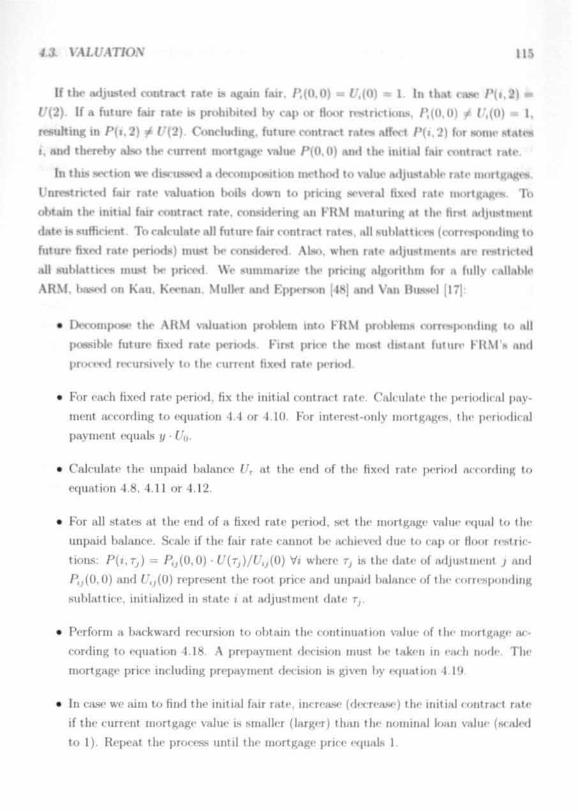
4.3L VALIMTJON 115

If the adjusted contract rate is again fair. P,(0,0) = (/,(()) = 1. In that case P(i,2) •

t/(2). If a future fair rate is prohibited by cap or floor restrictions. /',(().()) / (',(0) = 1,

resulting in P(i.2) ^ 1^(2). Concluding, future contract rates alfect P(i,2) for Nome Ntate*

i, and thereby also the current mortgage value P(0.0) and the initial fair contract rate.

In this section we discussed a decomposition method to value adjustable rate mortgages.Unrestricted fair rate valuation boils down to pricing several fixed rate mortgaged, To

obtain the initial fair contract rate, considering an FRM maturing at die first adjustment

date te sufficient. To calculate all future fair contract rate;), all sublattices (corK-spmiding to

future fixed rate periods) must lie considered. Abo. when rate adjustments are restricted

all sublattices must be priced. We summarize the pricing algorithm for a fully callable

ARM. based on Kau. Keenan. Muller and Epperson (48] and Van Bunscl [17):

• Decompose the ARM valuation problem into FRM problems corre»<|>ondiiig to all

possible future fixc<d rate periods. First price the most distant future FRM'N and

proceed recursively to the current fixed rate period.

• For each fixed rate period, fix the initial contract rate. Calculate the periodical pay-

ment according to equation 4.4 or 4.10. For interest-only mortgages, the periodical

payment equals t/ • (/(>.

• Calculate the unpaid balance (/, at the end of the fixed rate period according to

equation 4.8, 4.11 or 4.12.

• For all states at the end of a fixed rate period, set the mortgage value equal to the

unpaid balance. Scale if the fair rate cannot be achieved due to cap or floor restric-

tions: P(i,r,) = P,j(0,0) • (/(r,)/(/,,(0) VJ where r, is the date of adjustment j and

P,j(0,0) and (/,j(0) represent the root price and unpaid balance of the corresponding

sublattice. initialized in state i at adjustment date r,.

• Perform a backward recursion to obtain the continuation value of the mortgage ac-

cording to equation 4.18. A prepayment decision must be taken in each node. The

mortgage price including prepayment decision Is given by equation 4.19.

• In case we aim to find the initial fair rate, increase (decrease) the initial contract rate

if the current mortgage value is smaller (larger) than the nominal loan value (scaled

to 1). Repeat the process until the mortgage price equals 1.

i

116 CHAPTER 4. JJVTRODITC77OJV TO MORTGAGE VALUATION

4.4 Concluding remarks *! :

In this chapter we analyzed the main concepts of mortgage valuation using binomial lat- \

ticea. Non-callable and fully callable mortgages have been covered, as well as fixed and ;

adjustable rate mortgages. Resulting fair rates will be provided and analyzed in chapter •.

7, in which also fair rates of partially callable mortgages are included.

Because all mortgage! contracts issued in the Netherlands are partially callable, the fol-

lowing two chapters deal with the valuation of such contracts. Valuation of mortgages

including partial prepayment options is more complicated than the valuation issues dis-

cussed in this chapter. Partial prepayments introduce path dependencies. The mortgage

price in node (i.f) does not only depend on the prepayment decision in node (i. f)> but

also on past prepayment decisions, that is, the scenario path towards (i.f)- Moreover,

prepayment is limited per calendar year, introducing dependencies between prepayment

decisions in the same calendar year. A trivial lattice approach is therefore not applicable

for the valuation of partially callable mortgages.

In chapter 5 we introduce a valuation approach to circumvent the use of inefficient

non-recomblnlng trees. A lattice bused backward recursion approach, storing at each node

the number of remaining prepayment opportunities and the number of calendar years left

proves sufficient to value partially callable interest-only mortgages.

Chapter 6 introduces a linear programming model for the valuation of general partially

callable mortgage contracts. This model is based on a non-recombining tree, but LP duality

enables us to bound the fair contract rate efficiently and accurately.

Chapter 7 combines fair rates for all mortgage contracts to determine the values of full

and partial prepayment options for various mortgage types. Also, the effect of commission

costs is analyzed. Several model specifications are applied to improve robustness.

Chapter 5

Optimal Prepayment of Dutch

Partial Prepayment Mortgages*

5.1 Introduction

The Dutch mortgage market is one of the largest in Europe. Charlier and Van Bussel

[19] show that the Netherlands is ranked second among the countries of the European

Union in terms of both the outstanding mortgage debt us a percentage of GDP and the

outstanding mortgage debt per capita. The size of the total mortgage pool is huge, taking

into account the limited number of inhabitants. Increasingly popular are interest-only and

savings mortgages. These mortgages are not amortized during the contract lifetime, such

that interest payments remain high. They are popular because the Netherlands is the only

(European) country where interest payments are fully tax deductible.

An important difference between Dutch mortgage contracts and US mortgages are the

prepayment restrictions. Whereas in the US the mortgage can be fully prepaid at the dis-

cretion of the borrower, a Dutch contract has limits imposed on the maximum prepayment

per year. Only 10 to 20 percent of the initial loan can be prepaid per calendar year.

Empirical prepayment behavior for Dutch mortgages has been documented extensively

in studies by Charlier and Van Bussel [19], Havre [32], Van Bussel [17] and Alink [1].

Optimal exercise of the Dutch prepayment option has not been considered so far, contrary

to the large literature on optimal prepayment for US mortgages.''

'This ilmploi is Imsrd on joint work with P. Schotman.•*Sw IVR. MtCoiiiicll tuul SinRh |fi-J). K«u rt ill. [4**J-|51] and textbook reference* such as Hull [39].

118

5.2. FORAtt/LylT/CXV 119

The technical problom in pricing a mortgage under the optimal prepayment policy in

the path <lepen<k»nce. Prepayment is IUI American style option that is usuallv valued

by backward induction. With |>artin] prejmvmcnts. backward induction is not directly

applicable since at the terminal node* of the lattice it is not known how often pre|>avment

has I liken pl.i. i n. • ulier years. This chapter derivw* the optimal prepayment strategy of

Dutch interest-only mortgages within a binomial lattice

Mortgage prices are compared t>ascd on fair rates. The fair rate in denned as the contract

rate at which the mortgage price is equal to the nominal loan value, losing the optimal

prepayment policv. we < al< ulate the tvpical fair rate spread* betwii-n the mortgage rates tor

a non-callable mortgage and a mortgage with |»uiial |>i< pi \ nnni> This spicad |>in\idc->

the value of the partial prepayment option and will be i<>in|i.n< d with the American option

value of full pre|mvment. provided by the contract rate -pi<-ad K< tu<. n .< ii<>n-callable and

a fully callable mortgage.

5.2 Formulation

We consider the following contract specifications. The contract has a maturity of /„ years.

The contract interest rate ("mortgage rate") is V percent per year. Contractual payment*)

have the form of a coupon bond. Each period a fraction j / = V/A' of the outstanding loan

is paid, with A' the number of periods per year. No regular amortization takes place. The

remaining principal, if any. is repaid at maturity. Before maturity, the principal can be

repaid according to the following two conditions:

• The mortgage rate is fixed for A/ < L years, after which it is adjusted to prevail-

ing market rates. No caps or floors apply to the interest rate adjustment. At the

adjustment date the borrower has the right of full prepayment.

• In each calendar year a fraction 1/./V of the principal can lx> prepaid. The total loan

can be prepaid over a period of A' years.

Full prepayment is also allowed when the borrower dies or when the house is sold. We

will not include the latter effects. We consider optimal call policies that minimize the

present value of the cash flows pair) by the borrower and received by the lender. The

optimal call policy provides a lower bound on the loan value to the lender. For several

reasons borrowers might not all follow the optimal prepayment policy. Foremost is the

120 CHAPTER 5. OPT/AML PREPAYMENT OF DUTCH A/ORTGAGES

tax incentive. Interest rate payments on a mortgage on a main residence are fully tax

deductible, whereas earned interest is not taxed in many cases (for example when household

wealth is below a threshold). Another reason is the link between a mortgage loan and a

life insurance contract, present in part of the outstanding mortgage contracts.

Since the interest rate is adjusted at the end of year A/ to the new market rate, and

full prepayment is allowed at that moment, the value of the contract at the end of year A/

will be (MJIIHI to the principal. Hence, for valuation we do not need to look beyond year

A/. The contract is in effect a coupon bond with maturity A/ that is callable in JV steps.

The valuation problem is complicated by the path dependence of the partial prepayment

option. AH an example, consider a 3-year bond that allows prepayment of 50% of the

principal each calendar year. For an American option we would like to apply backward

induction within an interest rate lattice. But at any node of the lattice in year 3 the value

of the contract i.s path dependent. Its value will differ depending on whether prepayment

has taken place in years 1 and 2. or not. The terminal conditions of year 3 will depend on

the number of prepayments in previous years.

I'nth dependence can often be solved by introducing an additional state variable, which

keeps truck of all possible values of a function of the state variable at each node. This is the

tcrlmi(|iic applied to price American lookhack options presented in Hull [39]. The present

problem is different. The path dependence is not through a function of the state variable

but through endogenous decisions of the borrower. In that sense the partial prepayment

problem is related to shout options (see Cheuk and Vorst [21]).

l'atli dependence does not occur for all partial prepayment mortgages. When A/ < N,

the loan cannot be fully prepaid until maturity. We can decompose this loan as a portfolio

of a MOIK allahle coupon bond, with interest payments being coupons, and a bond with

maturity A/ that is callable in exactly A/ annual steps. In symbols.

V(A/.A') = ^ \ ( . U , .U) + * ~ ^ / ' ( A / ) . A/<AT. (5.1)

when- V'(A/, N) is the value of a mortgage contract with maturity A/ years that can be

called in .V annual steps and /'(A/) is the value of a non-callable coupon bond with the

same maturity. If the total principal equals 1. a fraction of 1 — A//A' is invested in the

coupon bond. This jwut of the loan cannot be prepaid l>efore maturity. A fraction A//A

is invested in a bond of which a fraction I'A/ can be called in each calendar year. To

keep the notation as light as possible, we suppress the dependence on the contract rate K.

Valuation of n non-callable coupon Iximl is trivial. The callable bond, with value V(A/. A/)

5.2 PORAfl/M77O.V 121

can be further decomposed as a portfolio of A/ simple callable lx>n<ls,

l f (5.2)

where C(0 is the value of a i-oupon bond with maturity A/ that is only callable in year f

and not in any other year.

The possibility of partially railing a coupon bond can IK- excluded, since optimally

each callable bond is either prepaid fully or not at all. After jwirtiallv culling a coupon

bond a portfolio remains, which Is a linear combination of the continuation value of the

coupon bond and the call value. Therefore, partial prepayment i.s dominated bv either no

prepayment or full prepayment. If any prepayment i.s prohtahle. then full prepayment in

most profitable, clue no prepayment is optimal. Partial pre|>ayment may only IM* cousideml

if an investor is indifferent between calling the coii|>on bom I or not, but in that cam< one

of the extreme calling options is just as profitable.

We conclude that options having A/ < A are simple American style options, without

path dependence, that can be easily valued by a lattice method. The more complicated

contracts are the ones with A/ > A'. These are contracts that can be fully prepaid before

the contract rate adjustment date. We thus concentrate on pricing mortgage contracts

with A/ > TV.

The idea for the valuation of a partially callable mortgage is the construction of two

lattices. The first lattice has annual time steps and describes the evolution of the prepay-

ments. Figure 5.1 depicts the lattice for a mortgage with a fixed rate period of 7 years and

an annual prepayment of 20% of the principal. The original mortgage contract is indicated

as the root node (7.5) in the figure. If the borrower has not exercised the prepayment

option in the first year, the contract will become a mortgage with maturity of six years of

which 20% can l>e prepaid annually. In the lattice this Is node (6,5). The alternative is

that the borrower will have exercised the first prepayment option, in which case a mortgage

with maturity A/ = 6 remains that can be prepaid in A' = 4 steps; this i.s node (0,4).

If we would know the values of the two contracts at the end of year 1, we would 1M; able

to price the mortgage contract. For this we can use a regular binomial interest rate lattice

with nodes (». f) with associated discount factors rf,, = (1 + r,,) ' (r = 0, . . . ,T|, i = 0, . . . f).

The end of year f occurs at time r = 7). Each node (i. r) has two successors, (t + 1, t + 1)

and (i.r + 1). Both successor nodes are reached with probability one half.

122 CHAPTER 5. OPT7A/AL PREP4VA/EJVT OF Dt/TCH AfORTGAGES

FIGURE 5.1: Prepayment conversion lattice

The figure shows thn evolution over time (in ^'endar years) with respect to thennriilxT of years m and the number of prepayment options n remaining. Nodes arelabelled (m,n). Leave* have either the possibility of prepayment in each calendaryear, or a single prepayment possibility.

(3,1);

(7,5)

(6.4)

5.2. ro/tA/UMr/otf ia

Suppose V,.r,(6,5) and V,.r,(6,4) arr the values of the (6,5) and (6.4) contracts at (lieend of year 1 in state i. If the borrower does not prepay in war 1, he obtain- .« >ivtirity

with value V.j-, (6.5). The altemat ive is paving itW of t he principal and convert ing to 80%

of a contract V,,r, (6,4). Therefore at the end of year I. the original mortgage has value

i - O T,. (5.3)

Knowing the terminal values, discounting tutrk to f » 0. taking into arrount earh «-vnwe,

is done in the recursion

V,,(7.5) = min(v,;(7.5).l + gV,,(6.4)J. (5.4)

with

V.,(6.4) « rf

V/,(7,5) = rf

where y is the periodic coupon. The prepayment condition compares the routiiumt ion value

Vrt(7,5) with the conversion value (1 + 4V,/(6,4))/5, and sets V,i(7,5) t<> the minimum of

the two.

The problem with this recursion is that the values of the (6,5) and (6,4) contracts are

still unknown. We need to expand the annual lattice until we reach nodes with contracts

that we can value without path dependence. If, starting at node (0,5). the borrower iiguin

does not prepay in year 2, we arrive at node (5,5). This is a contract for which equation

5.2 provides the value. We can compute that value in the lattice by starting at the end

of year 7. and discounting back to the end of year 2 each of the five constituent callable

bonds. An efficient way to organize all computations will be discussed l>elow.

Nodes in the prepayment conversion lattice recombine: node (5,4) is reached by pre-

paying in year 1 and not in year 2 and also by prepaying in year 2 and not in year 1.

Terminal nodes can be reached in two ways. First, whenever we are at a node (m, m) we

have a contract without path dependence which can be priced using equation 5.2. Second,

if we reach a node (m. 1) we have a fully callable bond, which can be callr*l in one step.

Such a contract can also l>e easily priced in a spot rate lattice. Formally, the node* of the

124 CHAPTER 5. OPT/A/AL PREPAYA/ENT OF Dl/TCH A/ORTGAGES

prepayment lattice have transitions

/ " ( m - l . n - 1) ifn > 1

(m,».) (5.5)

\ (m — l,n) if n < m.

Once we have obtained values for all the path independent contracts, we can work

backwards to price the original mortgage. The procedure is identical to equation 5.4

above.

For the intermediate periods in a particular calendar year specified by the periods f S((A/—/;i)^f, (A/— in + 1)'A^)> <»ur aim is to find V,,(WJ,H) for all attainable >i, giventhe prepayment conversion lattice as in figure 5.1. Using general notation, the recursion,including partial prepayment decision, is given by

/„ U

K,,(m,ri) = mill (V/,(m,ri), ^ + ^-^V,,(m - l,r. - 1)) (5.6)

with

-K./

j K . , t i ( f n - l , n - l ) + iv,+ ,.,

I'W each period a prepayment decision must be made. Before arrival in such a pe-

riod the contract is characterized by »i calendar years and n prepayments to go. No

prepayment means continuation of the same contract (m.n). The value is obtained by

discounting the expected contract value plus interest payment. Prepayment implies that

the remaining contract has J»I — 1 calendar years and » — 1 opportunities to prepay, with

value I',, (HI — 1. n — 1). The fraction £ of the contract is repaid (at the nominal price of 1)

and the remaining fraction ^ p is obtained in the contract (m - 1. n — 1). The value of this

contract is also determined by backward recursion. The mortgage value V,,(m.n) is the

minimum of the continuation value and the portfolio of prepayment value and remaining

contract value.

The end-of-vear early exercise conditions are very different from the early prepaymentboundary of a mortgage with full prepayment. At the end of the year a node (m.n) inthe prepayment conversion lattice leads to either (m — l.n) or (m — l,n — 1), whereas inother periods (m. n) either remains (m. n) or changes to (rn — 1. n — 1). The recursion for

5.2 FOR.WL.4TJO.V 135

end-of-year nodes (for which / = (A/ - m + 1 ) ^ ) is given by

v,,(m - l.n). - + ^_liv',,(m - l,n - 1)) (5.7)

with

V , , ( m - l , n ) = rf,i ( y + j V , . i + i ( m - l . n ) + - V K U H I B I - l , n ) J

K i ( m - l . n - l ) = d ( ^

In any end-of-yrar node, prepayment takes place if 1 + ^ V,,r,(w> - 1, n — 1) is smaller

than the continuation value \', ,,(»» - 1") This latter \-nlue depends on the bonds still

to IH- called with values ( ' ( 0 Prejmyment Ls likely if the continuation value is IUKII.

which happens for high C(f)< >*> At low interest rates. Low interest rate* might give

rise to 'December' prepayments to decrease the future unpaid l)alance. and hence interest

|>avment.s A partial pre|wynieiit ran Ix* optimal e\-en if an inniiisliate low in faced, aw long

as the smaller future interest payments offset this loss. 'December' prepayments mi^ht he

optimal, because a prepayment option expires if not exercised in December. We stress the

important result that a partial prepayment can be optimal in nodes where full prepayment

is not.

Calendar year ends

Until now we have assumed that calendar years end between two layers of nodes. In that,

case each node belongs to a single calendar year. From this definition it is clear to which

year each prepayment decision belongs. The left panel of figure 5.2 shows calendar years

ending between nodes.

Calendar year ends might also fall exactly at interest rate nodes, which is represented

by the middle panel of figure 5.2. In these nodes two partial prepayments are allowed, one

for the previous year (at December 31 of year f) and one for the coming year (at January

1 of year f + 1). As a result complexity increases in two ways. First, two prepayment

opportunities mast be considered at the terminal nodes of each calendar year. Second,

even for annual periods a choice must be made in which period to prepay.

One possibility to cope with nodes being part of two successive calendar years is toconsider both prepayment opportunities separately. In period < = (A/ - w + l)^f we aim

196 CHAPTER 5. OP77MAL PREP4YAfENT OF Dl/TCH .MORTGAGES

FIGURE 5.2: Calendar year ends

The figure shows calendar year ends in a small lattice example. In the left panelcalendar years end between nodes. In the middle panel calendar years end at nodes.The problem of having two prepayment opportunities in these nodes can be circum-vented by splitting the nodes and assigning one prepayment opportunity to bothadjacent calendar years, as is shown in the right panel.

to find V,i("'.») f<>r nil attainable n and for all states i. The states in the prepayment

conversion lattice reachable from (;n,»i) are (;» - l .n ) and (HI - l .n - 1). For year

f + I, in case of continuation we haw m - 1 calendar years for H prepayments, whereas

after prepayment we have m - 1 calendar years for »i — 1 prepayments. Of course the

transitions only hold for »i > n and JI > 1. otherwise terminal nodes (HI .HI) or (HI. 1)

are reached, for which mortna^e values are known. For both possibilities we must then

consider prepayment in year f. The recursion for these end-of-year nodes, including two

prepayment opportunities, is givcu by

V,i(rn.n) = mill [ V,i(m - l . n ) , -n n

(5.8)

wit h

l . n ) mill I I',',(HI - l .n) .— H 1.in (\;',( -,,)

V',,(ni l . n — 1) = m i n i V / , ( r n - l . n - 1 ) , ^ — — + ^ —

a n d

- 2. n -

1;,(III-2.H-1) = 4 h + ^ ' " ( ' " -2 '» - ' )+2^" '

\ ; ' , ( H . i . n - i ) = , / , , r « + ^ v . . , . , ( H i - i . n - i ) + i v ; . , , , - l . n -

5.3. RESULTS 127

- 2.r> - 2) = <*,, (y + ^'...•i(m - 2,n - 2) + £tt+i.m(m - 2,n -

Now, the values V*(m — l ,n) and V,i(m— l,n— 1) an* not >t«t<-i tuiiutl only by Ixu'kwtutl

recursion. A second prepayment is allowed, belonging to the start of the next calendar

year. If the contract (HI - l.ri) is partially pre|mid. the new contract is (m - 2. M I) iw

pre|wyment is not allowed in tin irm.umiin "f'he next calendar year, and one prepayment

opportunity is given up. If not, the continuation value w V,,(m — 1, ft) and prepayment is

still allowed in the remaining of the next yen \ • innliir Argument holds for the contract

(m — 1, n — 1). Note that in case of a second prepayment, the prepayment fraction equals

;jfj and the fraction in the new contract (m - 2. n -M cpials " •

If calendar war ends occur exactly at nodes, two pn p.i\ mint d<-< IMOIIS must be taken

in these nodes. If valuation problems with the calendar year split through the node* CIUI be

solved, problems with calendar years ending Itetween IKMI<-> . msving edge* of the lattice,

can IK> solved as well l>ecaase the prc|wtymcnt conditions prove to be easier. In the latter

case only one prepayment option |MT time period ban to be considered.

In the siHjiicl we will assume calender year ends between layers. This assumption is not,

restrictive because each tree can be redesigned such that only one prepayment is allowed

in each node, even when a node is part of two successive years, as is shown in the right

panel of figure 5.2.

5.3 Results

Mortgages with different fixed rate periods and prepayment options are compared on a fair

rate basis. The fair rate of a mortgage is the contract rate at which the present value of

all payments equals the nominal value. If a mortgage rate is fair, neither the bank nor the

client can make a profit, based on the currently observed term structure of interest rates

and volatilities.

Fair rates for interest-only mortgage contracts with a varying number of prepayment

opportunities A>' and a varying fixed rate period of A/ years are presented in tables 5.1 to

5.3. All mortgages have a lifetime of 30 years. Tables differ with respect to tlie number

of periods in the underlying interest rate lattice. We consider monthly, semi-monthly and

weekly periods respectively. A' takes on the values 1 (corresponding to a fully callable

128 CHAPTER 5. OPT/A/AL PREPAYA/ENT OF D[/TCtf AfORTGAGES

TABLE 5.1: Fair rates for monthly periods

The table reports fair rates (in annualized percentages) for interest-onlymortgages with A/ = 5 or A/ = 10 and A' = 1, A' = 5, Af = 10 orJV —» oo. All mortgages mature after 30 years. Underlying term structureson four different dates are considered, with short rates transformed tomonthly rates. Depending on A/ the interest rate lattice requires 60and 120 periods respectively. The interest payments are based on anannual contract rate following y = Y/A' with A' = 12. The case Af —» oocorresponds to a non-callable mortgage, a mortgage is fully callable if A/ = 1.

DateFcb 29,Fel> 15,June 1,July 2,

JV:2000200120012001

oo5.8565.3055.4235.451

A/10

6.0265.5095.5725.609

= 105

6.1835.6985.7155.758

16.5686.1436.1346.189

oo5.3234.9554.9234.874

A/10

5.4005.0424.9964.949

= 55

5.5045.1675.0985.054

5555

1.869.612.544.504

TABLE 5.2: Fair rates for semi-monthly periods

The lablr icporis fair rates (in annualized percentages) for interest-onlymortgages with A/ = 5 or A/ = 10 and A' = 1. Af = 5. Af = 10 or A' —» oo.All mortgages mature after 30 years. Underlying term structures on fourdilferent dates are considered, with short rates transformed to semi-monthlyrates. Depending on A/ the interest rate lattice requires 120 and 240periods respectively. The interest payments are based on an annual contractrate following iy = Y/A with A = 24. The case A/ —> oo correspondsto a non-callable mortgage, a mortgage is fully callable if A' = 1. Fullprepayment is allowed at the end of each month.

DateFeb29,Feb 1.1.June 1.July J.

AT:2000200120012001

5.8495.299'. 117•. i n

M10

6.0215.5035.5655.599

= 105

6.1855.6985.7115.750

16.5776.1566.1406.192

oo5.3174.9504.9184.869

M10

5.3965.0394.9924.946

= 55

5.5035.1685.0965.053

15.8925.6645.5865.556

5.3. RESULTS 129

Tvnir 1 :?

I l ie lal>lf I C | H > I I > l a i r r a l o i, in . u i u u . i n / i u J M H i n; i. i - . ' fur i n t e r e s t - o n l y

m o r t g a g e with A/ - 5 or A/ - 10 luid .V 1, .V '.. \ 10 or V - • oo.All inortg.nv* in.iturc after iU) years. I'lulerlying (<tin MI\I< tuic.x on fourdifferent cl.it.--. .ue considered, with short rates tranMinincd to \\<vklv rates.Depending "it A/ the interest rate lattice r<t|iiircs 210 and IMI periodsrespectively. The interest payments arc l i .»e. | .in ,m .tniiual contract ratefollowing y = V//v with A' i s The < .»«• .\ ^ j y unr f sponds to anon-callable mortgage, a m< >i t ;;.!).;.• i- tulK > .<IUI>le if N » 1. Full pn'|m\ intiilis allowed at the end of each month.

DateFeb29,Feb 15.June 1,Julv 2.

AT:2000200120012001

0 0

5.8455.2965.4145.442

M =10

6.0155.5005.5665 594

= 105

6.1795.6965.7155746

16.5606.1546.1446180

5.314i !»is•1 !M".•1 M.7

Uin

'. I'M

5.0351 <»S«1

1 • ' ! 1

".

'.

• .00

5.UW5.092.'•.051

I

5.«»525.57255,-Mi

mortgage), 5. 10 or infinity (non-eaiiable mortgage). The lixtvl rate ]>eri»d A/ ecpiaLs 5 or

10 years. Calendar year ends fall between nodes, such that each node belongs to a .single

calendar year. In case a calendar year end falls at a node (implying that two prepayments

are allowed in end-of-year nodes, because these nodes are part, of two calendar years), only

the fair rates for contracts with A/ = 10 and Af = 5 are affected, but these only increase

(prepayment is less restricted) by 0.6 basis point at most.

Increasing the number of layers by decreasing the period length has only a minor effect

on the fair rates. Fully callable mortgages exhibit a fair rate difference that can increase to

5 basis points for five year fixed rate periods. Non-callable and partially callable mortgages

show differences not larger than 1 basis point when increasing the number of periods.

Tables 5.4 to 5.6 show that a partial prepayment option has significant value, alt hough

a prepayment of only a small loan amount is allowed once JMT calendar year. The fair rate

spread of a mortgage is defined as the difference Ijetween the fair rate of I he mortgage!

itself and the fair rate of a non-callable mortgage with otherwise the same conditions. For

an interest-only mortgage with a ten year fixed rate period, the average full prepayment

spread {in terms of fair rates) equals 0.75 percentage [joint and hardly changes for a finer

grid. Hence, the average full prepayment option is worth 75 basis points.

A partial prepayment option, embedded in an interest-only mortgage with a ten year

130 CHAPTER 5. OPTJAJAL PREPAYAfENT OF Dl/TCH AfORTGAGES

TABLE 5.4: Fair rate spreads for monthly periods

The table reports fair rate spreads (in annualized percentages) forinterest-only mortgages with A/ = 5 or A/ = 10 and Af = 1. A' = 5 or/V = 10, using the non-callable mortgage as benchmark. Underlyingterm structures on four different dates are considered, with short ratestransformed to monthly rates. Depending on A/ the interest ratelattice requires 00 mid 120 periods respectively. The interest paymentsare based on an annual contract rate following y = V/A' with A' = 12.

DateFeb 29,Feb 15,June 1.July 2,

average

JV:2000200120012001

100.1700.2040.1490.158

0.170

A/ = 105

0.3270.3930.2920.307

0.330

10.7120.8380.7110.738

0.750

100.0770.0870.0730.075

0.078

A/ = 55

0.1810.2120.1750.180

0.187

1

0.5460.6570.5890.630

0.606

TABLE 5.5: Fair rate spreads for semi-monthly periods

The table reports fair rate spreads (in annualizod percentages) forinterest-only mortgages with AA = 5 or A/ = 10 and ;V = 1. A' = 5 orN = 10, using the non-cullable mortgage as benchmark. Underlyingterm structures on lour ditferent dates arc considered, with short ratestransformed to semi-monthly rates. Depending on A/ the interestrate lattice requires 120 and 240 periods respectively. The interestpayments are based on an annual contract rate following j / = V'/A'with A' = 24.

D . l t r

Feb 29,Feb 15.June 1,July 2.

averagi

AT:2000200120012001

100.1720.2040.1480.154

0.169

A/=105

0.3360.3990.2940.305

0.334

10.7280.8570.7230.747

0.764

100.0790.0890.0740.077

0.080

A/= 55

0.1860.2180.1780.184

0.192

1

0.5750.7140.6680.687

0.661

5.3. RESULTS 131

TABLS 5.6: FWir rate 8prrad« fnr ww>kly pwkxl*

l l i - I . I M ' I . | I . . I I - t . u i M I . - | n . . i . l - i n . u i i m . i l i . ' i i l | » • - i • i n i . i . i ' , t - > ' | . . |

interest-only m o r t g a ^ o with A/ "> .•! \ / Id .m<l \ 1 \ "i or

•V = 10. using the non-callablr n io i t j ; .^ ' .i> I><-iu luiiiuk. I iiilrilvmR

term structures on four different dates are «-i>u-i<l<iiil. with short rates

traiisfuniiiil »«• \voklv md-- 0' |>'ndi l i^ oil A/ the interest late hit I ire

r e q u i t o Jill .mil INI peiiml- n-|>«vtivelv The interest jMiyiuents IUV

based on an annual contract rate following y = V/A' with A' = 48.

A/ = 10 A / - 5Dat<« AT: 10 5 1 10Feb29. 2000 0.170 0.334 (J.71J 0.07U DIM, u.'.t,.!Feb 15. 2001 0 204 0 400 0.858 0.087 0.215 0.704June 1. 2001 0.152 0.301 0.730 0.074 0.177 0.657July 2. 21X11 0.152 0.304 0.738 0.077 0.184 O.fiGU

average 0.170 0.335 0.760 0.079 n I'll m i l *

fixed rate period and AT = 5. implying a 20% penalty free prepayment each calendar year,

has an average premium of 33 basis points. Therefore, a 20% prepayment option is worth

44% of a full prepayment option. The premium for a 10% prepayment option (JV = 10) iH

half the premium of a 20% prepayment option: on average 17 basis points or 22% of a full

prepayment option.

For shorter fixed rate periods, the effects of prepayment are smaller. When considering

a fixed rate period of 5 years, a full prepayment option is worth Iwtween Gl and 6G basis

points. The premium of a 20% (10%) prepayment option is about 30%, (12%) of the

premium of a full prepayment option, corresponding to 19 (8) basis points.

Figure 5.3 shows the effect of changing the number of prepayment opportunities on

the mortgage price. The underlying interest rate lattice has semi-monthly periods and is

calibrated at February 29. 2000. The fixed rate period equals 10 years (A/ = 10). The

contract rate is either 6% or 6.5%. For a large contract rate the mortgage value is more

sensitive to prepayment options, as the price difference between a fully callable and a non-

callable mortgage is larger. Prices increase faster for increasing prepayment opportunities

if A' is low. For A' approaching infinity, the price asymptotically approximate the non-

callable mortgage value. The mortgage principal has been scaled to 1.

132 C7MPT£7?.5. OPT/AMIOF D£/TCH

FIGURE 5.3: Mortgage price for varying AT

ncnninal loan value e q u l i

5.4 Concluding remarks

•* "

5.4 CONCLl/D/NG RfcWMRA'S 133

Prepayment of a partially callable mortgage may occur earlier than it full prc|>aymcnt,

because at the end of n calendar war a pre|mymcnt option expires. A |KU(I»1 prepayment

in !)«•«<inl»i, ju>i IH-IOII' option expiration, tan he optimal, even if a full prepayment in

not. thereby decreasing the remaining loan and future int< n >i p.i\ incuts.

The main empirical ramlt of this chapter comprises the importance of a partial pro-

l>avinent option. In terms of fair rat> - i -'" ; |>i< p.ivment option u* worth 3H Iwcsis |>oint«

on average, when considering a 10 year hxed rate period This is almost half the value of

an unrestricted prepayment option. Including 1'.' commission costs a partial prepayment

option even proves to IH> worth (iO'X of a full pic|mvinciit option. Chaptci 7 will provide

an extensive overview and comparison of fair rates of all types of mortgages and eml>od-

ded options. The effect of coniiiiiv>ion n-sts on the value of prepayment options will he

analyzed as well.

An efficient valuation of interest-onlv inoituaiics i> ;>O.SMI>IC when the number of pre-

payments A' is integer. The majority of Dutili imiiin.i^c tonlincts includes a prepayment

option of 10'X or 20'/i of the principal. Mortgages including Mich option can be valued by

tin .ippio.u h pro[M)8ed in this chapter. However, a small proportion of mortgage contracts

includes a 15% prepayment option. The valuation procedure, discussed in this chapter can

be used to find accurate bounds on the fair rate by solving for N = G and N = 7. Moreover,

the bond portfolio algorithm can still be used if the number of prepayment opportunities

(i.e. calendar years A/) is less than or equal to (_7VJ. Then the mortgage loan can never be

fully amortized in any of the final nodes and all prepayment amounts are maximal.

A complicating factor for the valuation of general mortgages with partial prepayments is

the introduction of regular amortization during the contract lifetime. Periodical payments

depend on the remaining loan, whereas the prepayment amounts are independent of the

loan value. Because not only the number of prepayments determines the remaining loan

value, but also the prepayment and redemption amounts, a decomposition into callable

bonds is not possible. Redemption amounts are uncertain at the moment of decomposition

and depend on the timing of prepayments. Consequently, due to a regular amortization

schedule at least one prepayment will be less than the maximally allowed amount. Both

the timing and size of this prepayment are uncertain and depend on the underlying term

structure. In the next chapter a linear programming model is formulated, which can be

used to price general mortgage types and prepayment options. The approach in this chapter

is efficient but specific, in the next chapter a general and therefore less efficient approach

will be developed.

Chapter 6

Mortgage Valuation with Partial

Prepayments

6.1 Introduction

I'llllv callable innrffrwrox I'HJI )K\»ri«*<vl.}p*.4>>Jb»tt*c<jr'"tecc'imJtififi& ttee. lAoilgtt&es Wllll'

partial prepayment, options arc more difficult to price due to path dependencies. Both

past and future prepayment decisions affect the current prepayment decision and the cur-

rent mortgage value. Valuation of partially callable mortgages without regular periodical

amorti/ation IWLS been analyzed in the previous chapter, based on a lattice method. For

the valuation of partially callable mortgages including regular amortization we must rely

on noii-recomhining tree methods, because lattices are not able to capture path dependen-

cies.-' Nielsen and Poulsen [70], for example, apply a combination of a lattice and a tree

approach to price mortgage contracts with delivery options, introducing path dependen-

cies, where optimally decisions arc only taken in a small subset of time periods. Between

decision dates the unique scenario path for both mortgage price and interest rate is given.

At decision dates the state space behaves as a tree, branching out and not recombining.

The number of states increases exponentially with the number of decision dates.

Although the popularity of interest-only and savings mortgages is increasing, traditional

mortgage loans, mainly annuities, still make up a significant part of the Dutch mortgage

pool. The previous chapter covered the valuation of interest-only mortgages with partial

'This chapter is based on joint work with A. Kolon"Aiiother alternative. Montr Carlo .simulation ha* difficulties (o value American option types.

134

6 1 . /iVTRODUCT/ON 135

prepayments. Now we will focus on the valuation of annuity m<>i tv;.ige>. Ktuit month a

part of the loan is redeemed to the mortgagee. An annuity ha.- .. >n-t .tut |M<ho<li(- payments,

with increasing itxlemption aimiunt.s IUUI decreasing interest payments

Dutch mortgage contracts allow a prepayment of le the principal p<>r eal-

endar vear. Due to the regular |>eri«»li< payments i.pnmai pit-payment Iwhavior differs

from prepayment of interest-only nu>rlK<iK<'* Altci .1 pre|»ivme>ut the lunorti/ntion sched-

ule changes, which can he a reason to postpone this pre|tayment. Part of an optimal

prepayment strategy can be to reduce the future unpaid Italancv. A later prepayment

reduces this unpaid Iwlance more than an early pre|>avnieiit, as the regular amortisation

schedule n-duces the un|mid Imlance more before an additional prepayment This create*

an incentive to postpone prepayment relative to a mortgage without prepayment restrle-

lions. Interest-only mortgage* are not subject to this effect, as the un|mid Italance of tln*te

contracts does not decrease by means of a regular amortization schedule.

Another difference between the valuation of fully and (mrtially callable mortgages is the

existence of 'December' prepayments for partial pre|>ayinent options We have e-onclueled in

the previous chapter that a part ml prepayment might occur earlier than a full prepayment

since otherwise a prepayment option expires with the ending of a calendar year. Thin cliect

holds for all partially callable mortgages, independent of the amorti/.ation schedule.

In this chapter we formulate a linear programming model for the valuation of partially

callable annuity mortgages. The LP formulation can also capture linear ami interest-only

mortgages. All time periods in our model allow for prepayment of a part of the mortgage

loan, involving the use of a complete* non-recombining tree. Linear programming is ap-

plied both to obtain an exact mortgage value and prepayment strategy and. using duality

theory, to derive bounds on the optimal mortgage value. The next section introduce*s the

mathematical framework, section 6.3 builds the LP model. The dual problem is formulated

in section 6.4. The implications of the LP formulation for fully callable mortgages are pro-

vided in section 6.5. based on finality theory. Section 6.6 solve* an accurate heuristic for

the original LP model, obtaining upper bounds on the mortgage priee- and lower bounds

on the fair rate. We also narrow the gap between upper and lower bound on the mortgage

pric«, in order to derive an accurate approximation. Results are provided in section 6.7.

136 CHAPTER 6. AfORTGACE VALUATION M7TH R4RTML PREPAVAfENTS

6.2 Mathematical framework :

The prepayment strategy of any mortgage with partial prepayment opportunities is path

dependent because the optimally of a current prepayment decision depends on past and

future prepayment decisions. Periodical payments depend on the adopted strategy. More-

over, the allowance of a prepayment decision depends on whether a prepayment occurred

in the same calendar year. The prepayment decision itself depends on the profitability of

postponing a prepayment to a later month in the same calendar year.

The problem is formulated on a non-recombining tree. The states in a non-recombining

tn-c are labelled as in figure 6.1. The root node has label 0. the two nodes at time 1 are

labelled 1 and 2. Generally, the transitions are given by

/" 2< + 1

i (G.I)

\ 2i + 2.

The time period /(?) corresponding to state J is

+ D J - (6-2)

The final period r(t) = T. The final node is labelled m = 2'''+' - 2. Note that the unique

predecessor of state i, if not the root node, is labelled [(t - 1)/2J. A state i, for which

<(t) = T, is calle<l a leaf node. All nodes that are neither the root node nor a leaf node are

called intermediate nodes.

We will focus on mortgage contracts with a regular redemption schedule, of which an

annuity mortgage is most popular and well-known. An annuity contract is characterized

by a principal amount / ' . a periodic contract rate y and a maturity L. A constant regular

payment occurs at all r(i') = 1 L. The size of this payment A/, in state t depends on

the unpaid balance in the previous period, which in turn depends on the past prepayment

behavior, and on the contract rate and remaining lifetime ;), = £ , - r(i). The unpaid

balance (•', in state i is defined its the amount of money still owed to the mortgagee at this

state. By definition (f« = P. The periodic payment is now given by

A/, = % n/aj'/tsMi. + l)

wit h

! • ' < $ * • U7

14 3(J

138 C/MPTEK 6. A/OKTGAGE VALIM77ON WITH PART/.4L PREPAYMENTS

In case of no prepayments other than the periodic payments, the periodic payment is

constant over all states, that is M, = M. Linear and interest-only mortgages are easily

modelled by only adapting /(y, n<) according to the mortgage specifications in chapter 4.

An annuity mortgage with partial prepayments Ls defined by the principal amount P,

ft periodic contract rate j / , a maturity L and A' consecutive subintorvals /n. of [/o f,,],

containing all distinct <(J) in increasing order. The endpoints of all subintervals belong to

the not {<(,, • • •,'«} such that each point in the set is in exactly one interval. The first set

starts at /,,. the last set ends with <„• We consider a single fixed rate period, ending at

/„. In each interval /* the total amount that can be repaid in thus interval is restricted

to be low than or equal to F*. In most cases all intervals have equal length (for example

ii calendar year) and the prepayment is restricted to at most a fixed percentage a of the

principal amount: .Y = F* = a • P for all fc.

The actual prepayment in state i is denoted by i j . At the end of each fixed rate

period, the remaining loan balance can be fully repaid without penalty. The mortgage

price in leaf nodes is therefore equal to the remaining unpaid balance. Consequently, in

the optimization model the prepayment amount J-, can be set to zero in all leaf nodes. In

fact, in leaf nodes the mortgagor is indifferent to prepay.

The interest rate process is given by a one-period interest rate on all nodes in the state

space, denoted by r,. An interest rate scenario is represented by a path from the root node

to a leaf. A state price A, is the root price of a security that pays out 1 in state i and zero

in all other states. The state price is recursively defined by

and Ao -- 1. State prices are used for discounting cash flows along a scenario path. The

present value of an asset, paving a cash flow of r, in state t and zero in all other states, is

equal to A,c,.

6.3 The model

The model formulation is based on Kolen [53]. We assume that no prepayment takes place

at f = 0 (this could be accounted for in the initial loan amount). Formally,

I/,, = P. (6.3)

6.3. THEA/ODEL 139

Every period the unpaid balance increases at rate y A regular lunount A/,. including

intorest JUKI redemption amounts, is paid in stale i. Additionally. the mortgagor must

deride whether to prepay an amount up to the alkiwnd A' = r* • {/«, with o the maximally

allowed prepayment percentage. The firM < 1.I>N ,,I , ,,n-.n.imi- models the unpaid l>.il.uu«

in an interuic<liate state i:

I/, = t/t(.-i»/2] • (1 + y) - t/i(,-n/2j • / ( y . n , + 1) - x., i - 1 m/2 - 1. (6.4)

Because no prepayment occurs in a final state, the un)>ni<l Italanre in such state ii|uabt

t/, = £/i,,_i,/2j - ( l + yJ - t /u . -D/ j j / ( y . « . + 1). i » m / 2 m.

The next cla«8 of constraints models the upper hound on the total prepayments within

a given time interval. Let us denote by Q* the set of all |mths for which the first state on

the path l>elonRs to the layer mrresponding to the lie-in point of interval /* and the last

state on the path lx>lougs to the layer corn>spoinlinK to the end point of the interval /*,

Jt = 1 A'. Then the additional prepayment nine unit r, is restricted hy

(fi.fi)

We consider a constant prepayment amount X = Ft- and all siihintervals make up exactly

one calendar year.

An optimal prepayment strategy for the mortgagor is the strategy that minimizes the

present value of all payments. These payments include regular payments A-/,, additional

payments j , and. if any. redemption of the remaining contract value at the leaf nodes.

These latter values equal the unpaid balances at the penultimate states, increased by the

contract interest rate (recall that no prepayment occurs at leaf nodes). Payments are

discounted by means of the state prices A,. The mortgage value is now repnwonted by

m/2-l in

£ y). (6.G)

Now, the linear programming objective for pricing annuity mortgages with partial pre-

payments is to

140 CHAPTER 6. A/ORTGACE VALl/AT/ON U7TH PART/AL PREPAYA/EJVTS

(m-2)/2minimize jT Ai[t/^i_,,/2j •/(y,n, + 1) + x,]-I-

i - l i=m/2

subject to

£/„ = P

i, > 0, V,

The last two restrictions state tliat tlie borrower can never prepay more than the unpaid

balance and that prepaid amounts cannot be taken out again.''

An upper bound on the mortgage value can be obtained by constructing a feasible

solution to the general (primal) problem. No prepayment, equating all x variables to zero,

is a trivial feasible solution for which the objective boils down to discounting future regular

periodical payments. Consequently, the value of a non-callable mortgage is a trivial upper

bound on the value of a partial prepayment mortgage with the same contract rate and time

to maturity. In order to find the mortgage value with partial prepayments, the variables

x, (ami the resulting (/,) of this LP model must be optimized.

As an example, consider a problem instance defined on the state space given in figure 6.1.

We assume that we have two time intervals. / | = [fo,t|] and /-2 = ['2.'3]' Furthermore,

we face a constant maximum prepayment percentage A' and a contract lifetime of four

periods, that is. the final tree period marks the end of the contract. The model is given

below in standard format/'

'Sonir mortgage contracts allow taking out curlier prepaid loan amounts. In that case r, ran herestricted to IM> larger than minus the sum of nil previous prepayments, or larger than some contractspceilication restricting the maximal amount to take back

'Time intervals with I he year split through nixies, such that one time |>erio<l Mongx to both theprevious ami the upcoming year, requires two prepayment variables for each end-of-calenilar year node.This can he achievitl hy assigning one of the prepayments to each of the edges incident to the end-of-calendar year node. For the pur|x»se of the example, this would complicate the formulations and increasethe nmnher of variables unnecessarily.

'Note that for this small scale example the contract is fully amortized at the end of the tixed rateperiod (that is. at f|). In cost- the mortgage lifetime is longer than the fixed rate period, an analogousformulation can be applied, only clmuging 11,.

6 4 . DUAL PORAU L.A77ON 141

minimize A,[t'o /(y. 4) + X|] + . . . + Au[(/« • /(y. 2) + Xul

subject to

Uo - P

r, = 0

iu = 0

J-i > - A '

x, > - X

Xj > - A

14 > -A'

t/, > 0. Vi

x, > 0, Vi

6.4 Dual formulation

In order to make statements about the optimality of a solution, we applv duality theory.

Before deriving the general dual problem formulation, we provide the dual of the example at

the end of the previous section. Dual variables r, and z, are introduced, the first correspond

to the constraint set 6.4. the second to the restrictions 6.5. For each state of the tree there

exists one t»,, while a 2, is required only for periods concluding a calendar year as th«»e

determine the number of calendar year restrictions 6.5. Denote the set of nodes concluding

the calendar years by C. Both r, and c, have labels equal to the corresponding state, such

that the 2, labels are not continuous. For instance, in the state space example £, floes

not exist because state 3 does not mark a calendar year end. The dual formulation of the

142 CHAPTER 6. MORTGAGE VALUAT/ON WITH PARTIAL PREPAYMENTS

four-period example is given by

maximize - X y % , +

subject to

.3) + A</(y,3)

y) + «i.i/(y, 2) - vu(l + y) + v,4/(y, 2) < A,a/(y, 2) + A,.,/(y, 2)

"7 < (Air, + A,«)(1 +?/)

-«a + t'2 < Aj

-27 - 2H + t»;| < A;t

- J » - 2 i n + tM < A.,

- 2 7 + 1-7 < A7

— 2|.| + I'u ^ A14

2, > 0. Vi € C

Let O C C denote the set containing all states marking the end of the calendar year to

which state i belongs that are attainable from state i. For instance, considering interme-

diate state 3. Ca = {7,8}. Also, define the function <?(») to bo

6.4. DUAL FORM rrLATTCW - < 143

Final per iodstatesi = ( n i - 2 ) / 2 m huve »•. = ,\,. whichcan 1H>observed when including

the balance constraints I/, > 0 for tin.». -i.it.•> i-xplicitly in tho problem formulation and

rewriting the objective to include- tho remaining iui|wi<l Mal ice {', ftw lenf node* *>|mratelv,

discounted by A,. For penultun it' -t.itcs, 9(1) can th< 1. t. 1 < l>o simplilieii to

= A,+ 1",

Now, the complete definition of the function .9(1) is

V-/(V.".))

Vi - 0 (m - 6)/4 (gj)

+ A*o)(l + y). Vi - (m - 2)/4 (m - 2)/2.

The general formulation of the dual problem to value annuity mortgages with partial

prepayments is the following:

maximize - . Y J T ^ , . r, + JVP

subject to

", < </(«)• V » = 0 ( m - 2 ) / 2 (G.8)

- £ / e r . * + «'. ^ ^ - V' = l ( m - 2 ) / 2

r, > 0. Vf e C

Complementary slackness conditions can be used to find dual variables based mi the

primal solution. If a primal inequality contains slack, then the corresponding dual variable

equals zero. For the restrictions in our mortgage valuation problem, this implies:

z, < A' => 2, = 0, (6.9)

where f is the last node, at the time interval end. of path Q. Typically, prepayment is

restricted per calendar year, such that path ^ covers one year. Node f is then the last,

node of the year. Condition 6.9 states that if prepayment during scenario path interval Q

is less than maximal, the dual variable Z; can be fixed to 0.

When the dual solution is known, complementary slackness can be used to obtain a

partial solution to the primal LP problem:

r, = X. (0.10)

144 CHAPTER 6. MORTGAGE VALt/ATION U7TH PARTIAL PREPAYMENTS

This complementary slackness condition states that if the dual variable :,. belonging to

state; £, is positive;, then prepayment is maximal along path Q. which ends in node f and

covers exactly one year.

Complementary slackness conditioas with respect to the inequalities of the dual formu-

lation can be derived similarly. These conditions, Vi = 1 (m - 2)/2, read

, + ,;, <A, => i . = 0 (6.11)

i, >0 =» - J 3 « # + w, = Aj (6.12)fef,

and

i>, < <?(i) =• I/, = 0 (6.13)

«7, > 0 =*• v, = »(i) (614)

Prom I lie diuil formulation 6.8 follows that the dual variables t>, must be both less

than or c(|iial l<> (/(') '»><1 A, + £ , ^ . ^ . As r,, (the dual variable to be maximized) is

determined by a backward recursion approach depending on all future r,, we may state that

D, = min((/(0. A, + £ , ^ *')> ^ = 1 ("> ~ 2)/2. Hence for given J. the complete dual

solution and the corresponding mortgage value can bo obtained by backward recursion.

The optimal prepayment strategy in state i can be partly derived from this minimum

evaluation to obtain r,. as will be shown by the next two theorems.

Theorem 6.1 // A, + £ , e r , *' < »(')• ""'» « /•»"' P'Tppfli/mfn* "/ ^ rpmaintn^ /oan ta

in .i<a/e t.

Proof Sui>pos«< that A, + ^ , . _ ;, < .9(1). Then i-, = A, + £ , ^ . z < <?(i). and £/, = 0

because of complementary slackness condition 6.13. A full prepayment of the remaining

loan is optimal. Similarly, if full prepayment is not optimal in state i, then I/, > 0.

By complementary slackness condition G.14. r, = #(i). which can only be true if g(i) <

Theorem 6.2 //</(i) < A, + £fer , * . """n no po.«ittw prppaympnt o/a ^partta//y^ ca//o6/e

»«or/(/ri(;«' iv optima/ m .v(a(r 1.

Proof Suppose that </(i) < A, + £ , < ^ ;/. Then r, = g(i) < A, + ^ c , -'• »"*' •*"> = 0IKH-IUUSP of complementary slackness rondition 6.11. No prepayment is optimal. Similarly.

6.5. / A i P L / C . 4 r / O \ S R ) R FULLY'CALL.4BLK .MORTGAGES 145

if a positive prepayment is optimal in state t. then ?, > 0. By complementiirv slacknew

condition 6.12. r, = A, + $^<- *'• *"">•'« can only l>e tnie if A, + £,,:<• c* S

As a direct result from complementary >U ku< NS. the theorems imply that for a non-linal

partial prepayment.

must hold. The theorems on optimal prepayment an- difficult to use for |>artiallv callable

mortgage's, since all non-final |mrtinl pre|myment decisions cannot be determined by either

A, + 53/gf- if < fl(») or A, + ]C/«r, *' -* ?(•)• Both theor<-tns ii. • .IM. I .i|>|ilii<d to fully

callable mortgages.

6.5 Implications for fully callable mortgages

Mortgage valuation including, full prepayment is a relaxation of the original piolilcni for-

mulated in section G.3. omitting the limited prepayment restriction. Stated dilleientlv, the

maximum prepayment amount A' is infinite for fully callable mortgages. /tr<M<i/ prepay-

ments must still satisfy the conditions

1, > 0. Vi

£/, > 0, V;.

As a result, XI.ey*-' ^ '^- ^ ? •" * valid constraint for fully callable mortgages n« well,assuming A' to be infinitely large. By complementary slackness condition 6.9,

2, = 0, W e C , , Vi. (6.15)

The equations with respect to the dual variables »>, follow directly from the dual program-

ming formulation and the fact that ;:, = 0 . Vi € C. Therefore, the value of a fully callable

mortgage is equal to the dual objective t;,,P. where t>,> is given by

t'n = 9(0), (G.16)

t;, = min(</(i).A,). Vi = 1 (m - 2)/2. (617)

146 CHAPTER 6. MORTGAGE VALUAT/OA' U7TH PART/AL PREPAYMENTS

Terminal values to the backward recursion of w, are provided at the penultimate states, at

which i/, only depends on state prices and the contract rate, according to the definition of

0(i) in 6.7. This approach is comparable to the standard backward recursion (recursively

solving the primal LP) applied for the valuation of American options.

Optimal prepayment conditions for a fully callable mortgage are based on complemen-

tary slackness and can be easily derivwl from the theorems on optimal prepayment in the

previous section. The optimal prepayment strategy of a fully callable mortgage depends

solely on #(») and the state prices A,, according to 6.17. Theorem 6.1 implies that full

prepayment of a fully callable mortgage is optimal in state a if A, < #(»)." No positive

prepayment of 11 fully callable mortgage is optimal in state i if g(?) < A,, according to

theorem 6.2.

Any dual feasible solution provides a lower bound on the mortgage value. Consequently,

the value of a mortgage contract with partial prepayments is bounded from below by the

full prepayment value of a mortgage with the same contract rate and time to maturity.

The lower bound can be improved by increasing 2, for some 1. Although this decreases the

lower bound directly. i\ (and by backward recursion 6.17. i'(,) can increase due to constraint

relaxation. If the increase in i'nP is larger than the rise of X 5Z,tr *<• raising some c, can

improve the dual solution and hence the lower bound on the mortgage price.

Since the problem formulation is based on a non-reconibining tree only small problem

instances can be solved to optimality. For long term, partially callable mortgage contracts

the optimal prepayment strategy cannot be determined efficiently. The next section intro-

duces a heuristic to derive the optimal prepayment strategy based on a lattice approach.

This approximative strategy is used to obtain a bound on the mortgage price and on the

fair rate.

6.6 Bounding the fair rate

Small problem instances can be solved exactly by either primal or dual formulation, based

on a non-rocombining tree approach. For large instances (our typical problem size equals

120 periods, resulting in 2'*' final states), such formulation is not efficiently solvable.

"Note that if full prepayment is optimal in state 1, the short rate r, must IM- smaller than the contractrate j/. Hence, we haw also shown that if A, < 9(1). then r, < y (which also follows from the definition ofJ/(I). the recursive defining of the state prices and the restrictions of the dual problem). The converse, ifr, «. y. then full prepayment is optimal, din's not necessarily hold.

6.6. BOIWD/JVC THE F4/R RATE 147

IWrafcre. we focus on obtaining upper and k*»vr bounds on the m o r t i c e value bv eon-

ftracting primal or dual feasible s<>lution> n-sjuvtively. Any primal U.IMIIU .solution (that

is, an allowed prepayment sii.it. L;\ ) miplio an iip|x>r IHIIIIUI on the optimal value of a

partially callable mortgage, or by an iterative procedure, a lower Ixiund on tin- fair rate.

This section constructs a primal feasible .solution, based on a lattice approach to retain

computational efficiency.

The size of the original lattice equals the length of the first fixed rate period. During

this period a large IIIIIIIIMT of prepayment decision* must l><- taken Kach piepnymeiit

originates a new mortgage loan with a smaller unpaid lml.ni.. |n 11. .lic*il |>nymcut tuid

time to maturity. These new mortgage l.-.ui- .u. \.ilue<l by a suhlnttire of the original

lattice, using the corresponding interest raUw

Figure 6.2 shows the decotn|xisition pn» ••! "M the full prepayment boundary.

This )M>undarv is derived according to tin- <i|>< im.u |wi|iayiiicnt strategy of a fullv callable

mortgage. Valuation of fully callable nim!>;.i^rs and the derivation of the full prepayment

boundary has been dis< uss<il in chapter 4. All nodes Ix-low the full prepayment ItoimdAry

are considered as states in which full prep.ix in>nt (if allowe«l) w optimal. Hill prepayment

is not optimal in nodes above the full prepayment boundary. Postponing (a part of) a full

prepayment is never optimal. As sewn <is calling a fully callable mortgage is profit able, the

mortgage Ls fully prepaid. Postponing prepayment leads to higher total interest payments.

Optimal prepayment of a partially callable mortgage can l>e both earlier and later than

an optimal full prepayment. It might be optimal to postpone a partial prepayment if only

limited prepayment is allowed. The reason is that higher interest payments are compen-

sated by a lower future unpaid balance, because regular redemption is larger before than

after an Julditional prepayment. A lower unpaid balance leads to lower future periodical

payments. If these lower payments (more than) offset the disadvantageous higher interest

payments due to postponing prepayment, a later prepayment might be optimal. Conse-

quently, for a partially callable mortgage 'no prepayment' can be the optimal decision in a

node below the full prepayment boundary. For fully callable mortgages the unpaid balance

after full prepayment is zero, the resulting periodical payments are zero as well, and thejte

payments can therefore not be used as compensation for higher interest payments.

An optimal prepayment strategy might also involve a partial prepayment in a node

above the full prepayment lwundary. Such an early prepayment can l>e optimal in De-

cember to exercise a prepayment option just before the end of a calendar year, the option

expiration date. An extra prepayment reduces the future unpaid balance and periodical

148 GWAPTER 6. A/ORTGAGE VALUATION VV7TH PARTIAL PREPAYMENTS

FIGURE 6.2: Decomposition based on full prepayment boundary

The figure shows the main lattice and one of the first level sublattices aftera decomposition based on the full prepayment boundary (the horizontaldashed line). All encircled nodes are candidate prepayment nodes. All solidencircled nodex are nodes in which a first prepayment is considered andfrom which n new sublatticc is constructed. Vertical dashed lines representcalendar years. The effective prepayment boundary (longer dashes) is acombination of the full prepayment boundary and one of the calendar yearrestrictions. Prepayment in the first candidate prepayment node (that is,the root node of the sublattice) implies that the next prepayment cannot bein the same calendar year.

6.C. BOl'<VDfJVC THE FA/K R.ATE 149

payments. If the resulting lower payments more than offset tin- disadvantageous prepay

iiH'iit in Decemt>or. an early partial prepayment can lie optimal. i>ecvinber' prepayments

have Int'ii discussed in chapter ">.

Since an optimal partial ptvp.i\ incut can lx> lx>th earlier and lator titan an optimal full

prepayment, the full prepayment boundary provide* a feasible pro|tnvment strategy, l>ut

not IK-I i—..nily the optimal strategy-. To construct a primal fe.i>iMe solution we assume

thai no prepayment o<rurs in nodes al>ove the full prepayment boundary and a pnilial

prepayment occurs in nodes below the full pre|Niyment Ixmndarv Additionally, we assume

that a [Mirtial prep.i\ in. m .uuount is always e<|iial to the maximally allowed amount, IIUNXN

the remaining loan is smaller than the maximal pro|>avmeut. In the latter case we immune

a final prc-pnvinont of the rtMiiainiug loan."

Our approximation to the optimal pre|>aympnt 8tratoR\' in\-ol\T« no prepayment in nodes

aliove the full prepayment txmndarv. This |>art of the valuation process can be performed

by a single lattice approach. Furthermore, a maximally allowed prepayment (J , A')

b» included whenever the full prepayment !>ouudarv is crossed downwards. After each

prepayment a new sublattu . i- .. 'iistructed lww<| on the remaining mortgage lifetime and

unpaid balance. The prepayment boundary in each sublattice is similar to the boundary

in the original tree, except for prepayment to start at the first month of a new calendar

year. The prepayment node in the parent lattice is the root node of the sublattice.

One of the first level sublattices (after the first partial prepayment), including lull

prepayment boundaries adapted for calendar year restrictions, is depicted in figure 4.1.

The number of levels of sublattices is equal to the maximum number of prepayments. In

case of prepayments limited to 20%. the number of levels is bounded by five. The number of

sublattices increases with rate T per level. Denote the number of levels by A'. A recursion

through each sublattice to determine the mortgage price requires a computation time of

O(T*), implying a total computational effort of 0(7*'+*).

Although computation time is of a polynomial order (compared to exponential for a

non-recombining tree), the polynomial degree is still large. Efficiency can be improved

by performing a recursion only once for all .sublattices rooted in the same node. Suppose

'In some stales the optimal prepayment can be letw than maximal A lei* than maximal prepaymentLs optimal if a fully amortizing loan cannot !«• repaid by |wri(Mliial pavmrnlh plux 1111 niliyi niunUr ofadditional prepayments. At least one of the additional prepayment* i» nmaller than the maximally ulliwdamount. This prepayment optimally takiw place whenever intercM rale* are favorable, but l<iw favorablethan in the caw of a maximally allowed prepayment (which can be in any period, depending on interuttrate behavior).

150 CHAPTER 6. MORTGAGE VALl/ATJON M7TH PARTIAL PREPAYMENTS

node (t, f.) can be reached by two different paths. For the first path a recursion is required

to determine the price Pi corresponding to unpaid balance f/i in node (M)- The unpaid

balance according to the second path reaching node (i, t) equals 6/2- Now the price can

be scaled to be P^ = t^ • Pi/^i- This pricing strategy is similar to the valuation of an

adjustable rate mortgage discussed in section 4.3.2, based on Kau. Keenan. Muller and

Epperson [18|. However, additional prepayments are not scalable since these depend on

the initial loan and not on the remaining loan. These cash flows are excluded from the

traditional valuation procedure, but added separately and discounted at the appropriate

discount factors. The scaling approach is more efficient than the standard approach as long

as the decrease in the number of recursions is not outweighed by the preprocessing phase

of calculating discount factors. This is typically the case for large instances with many

prepayment opportunities. Computation time for the scalable decomposition method is of

(-*('/''). since at most one recursion of O(T^) is required for each node."

Partially callable mortgages with a fixed rate period of five years can be valued by the

(scalable) decomposition method based on the full prepayment boundary, providing an

upper bound on the mortgage price or a lower hound on the fair rate. Since many lattices

must be stored in memory simultaneously for large instances, loans with ten year fixed

rate periods can only be valued when lowering the prepayment boundary significantly. As

11 result, fewer sublattices have to be constructed. The lower bound on the fair rate will

deviate more from the optimal fair rate, as the prepayment strategy differs significantly

from the optimal prepayment strategy-."

The next section provides lower hounds on the optimal fair rate based on the lattice

decomposition method. We are interested in the difference between the optimal fair rate

and the calculated lower bound. For this reason, we use the fair rate of an interest-only

mortgage (derived in chapter 5) as an upper bound on the fair rate of a partially callable

annuity. Since all term structures are upward sloping, an interest-only mortgage faces an

unattractive redemption schedule. The fair rate of an interest-only mortgage is therefore

higher than the fair rate of an annuity or linear mortgage with similar characteristics.

"Fair ratrw following from tho scalable decomposition method slightly differ from fair rates accordingto llii' standard ilit ompoxition method Prepayment in nixlr (i.f) according to the stiindiird decomposi-tion method is based on the unpaid Imlancc and price in node (i.f) of the parent lattice The scalablemethod, having no recursion in most (sub)lattices and then-fore no truly optimal strategy of consecntiveprepayments, can only coin|mre unpaid Imlance mid price at the root of the child lattice. The standarddiHomposition method is more accurate, although fair rate ditferences are negligible.

'We have restricted prc|iaymcnt op|>ortunities in various ways to improve efficiency One could choosefor allowing prepayment only once or twice |>cr calendar year. However, shifting the prepayment boundarydownwards provide*I the best lower bound on the fair rate.

6.7. RESULTS 151

T A B I . K fi 1 F a i r r u t i ' * f o r a fiw \ v » r fi\<>«l r n t r } M - I I < M )

T h i s l . i M i ' i > i . i \ i i l < ~ - It >\\ • ; !.. . m i l l " , " i i I . i l l i . i t i - N " I p . u t l . i l U i a l l i i l > l « -

annuity And linear m- I'pper bounds cnrros|>ond In fair ratraof partially callable intcicM-onlv mortgages The underlying intenstrate lattice consists of monthly |>chods. The term structure model isbased on a one-factor BDT model. Mortgage contracts haw a fiwyear fixed rate |>eriod and exclude commission, resptvt ivclv include a1% commission

TypeAnnuity

Linear

DateFeb 29. 2000Fob 15, 2001June 1. 2001July 2. 2001

Feb 29. 2000Feb 15. 2001June 1. 2001liilv 2. 2<MH

no con

TIT5.485.145.105.05

5465.135.08

I l l l l N M , , h

l i t5.505.175.105.05

5.505.175.10f, or,

r ; ...i

i it

5.174,824.774.72

5.144.794.741 w>

IIIUI- . I ,

i it

5.214.854.804.75

5.214.854.80.i 7f,

6.7 Results

Lower bounds on the fair rates are calculated for both 5 and 10 year fixed rate periods. We

consider partially callable mortgages excluding commission and including a l'X commission

on four dates. Annuity and linear mortgages are included. A practical upper bound on

the fair annuity and linear mortgage rates is obtained by the fair rate of a corresponding

interest-only mortgage, since the underlying term structures are upward sloping. The

bounds define a range for the optimal fair rate of partially callable annuity and linear

mortgages.

For five year fixed rate periods no computational problems arise. When prepaying

the maximally allowed amount in any node below the full prepayment boundary and not

prepaying anything in any node above, a tight lower bound on the fair rate is obtained. As

can be concluded from table 6.1. the lower Injund differs between zero and 7 basis points

from the upper bound, defined by the fair rate of an interest-only mortgage with similar

conditions. Therefore, the lower bound is a very accurate approximation of the optimal

fair contract rate. Also, the optimal prepayment strategy will not differ largely from the

152 CHAPTER 6. MORTGAGE VALUATION WITH PARTIAL PREPAYMENTS

TABLE 6.2: Fair rates for a ten year fixed rate period.

This table provides lower bounds on fair rates of partially callableannuity and linear mortgages. Upper bounds correspond to fair ratesof partially callable interest-only mortgages. The underlying interestrate lattice consists of monthly periods. The term structure model isbased on a one-factor BDT model. Mortgage contracts have a ten yearfixed rate period and exclude commission, respectively include a 1%commission.

TypeAnnuity

Linear

DateFeb 29, 2000Feb 15, 2001June 1, 2001July 2, 2001

Feb 29, 2000Feb 15, 2001June 1, 2001July 2, 2001

no commissionLB6.075.565.615.65

6.015.535.575.60

UB6.185.705.725.76

6.185.705.725.76

1% commissionLB5.855.355.405.43

5.785.305.345.36

UB5.985.475.515.55

5.985.475.515.55

full prepayment, boundary.

Table 6.2 provides fair rate results for ten year fixed rate periods. Prepayment is re-

stricted to the bottom 22 nodes (per period) of the original lattice and the corresponding

nodes in all sublattices. us long as these are located below the full prepayment bound-

ary. This prepayment strategy restricts the number of sublattices. The difference between

lower and upper bound can rise up to 20 basis points, although the lower bound is consid-

erably improved compared to the initial lower bound, that is. the fair rate of a non-callable

mortgage.

6.8 Concluding remarks

In this chapter a linear programming formulation has been introduced for the valuation

and optimal prepayment of (partially) callable mortgages. We have also derived optimal

prepayment conditions for fully callable mortgage contracts based on state prices and

following from duality theory.

6.8. CONCU/D/.YG R B M R K S 153

A fully callable mortgage ran l>e modelled by a lattiee approach Partially callable annu-

ity and linear mortgages ran only 1M- priced to optimalitv by an ineHicient non-rrcombining

tree approach. To enhance efficiency, we |>i.«(>.»<• a lattiit* IMVMHI melluMl to obtain a clone

lower bound on the fair rate of these mortgage types.

Since, for upward sloping term structures, the fair rate of a partially callable intortxt-

only mortgage (priced to optimally in the chapter 5) provides a practical up|>er Imtinii

on the fair rate of a partially callable annuity, a narrow range for the optimal fair rate

is derived. This indicates that the lower bound heuristic is accurate. The comparison

of fair rates of non-callable. |mrt tally callable and fully callable mortgage* u* performed

• •\ti-iiMvely in the next chapter.

Related to the LP formulation provided in ttils chapter, we pro|>osc two dlrectioiiM for

future research on the optimal valuation of partially callable annuities. First, a theoretical

upper lx)iind on the fair rate can IM- derived by improving the basic dual feasible solution,

represented bv th«- full prepayment strategy. The upper Itoimd can be unproved by in< read-

ing i-variablo > i.in >|>oudiug to low interest rate states. For these states, an Increase in

2 implies an increase in I\I by Imckward recursion, surh that the dual objective (mortgage

price) increases and the fair rate decreases. The number of z-variables is exponential and

therefore many c-variables must be increased from zero to an (a priori unknown) positive

value to achieve a significant improvement.

A second direction for further research is based on approximating the fair rate of a

partially callable annuity. Since not all states in a non-recombining tree can be included,

we might consider a tree defined on a subset of scenario paths. Valuation base*I on this

subtree generates approximative mortgage prices. Approximations are more accurate for

finer subtrees. However, approximations ran lead to both higher and lower fair rates than

the optimal. As a consequence, measuring the accuracy of the approximative fair rate is

not possible without the use of fair rate boundaries derived in this chapter.

Chapter 7

A Comparison of Fair Mortgage

Rates *

7.1 Introduction

Previous chapters have analyzed the valuation of various mortgage contracts. In this

chapter we combine results in terms of fair rates. The fair rate is the contract rate at

which the mortgage value equals the nominal loan value. If a mortgage is quoted at

the fair rate neither bank nor client can make a profit. Fair rate differences between

mortgage contracts indicate the value of embedded options. We distinguish annuity, linear

and interest-only mortgages. Valuation of savings and investment mortgages is similar

to interest-only mortgages, since these mortgage types have a similar cash flow pattern.

Various fixed rate periods are considered. Fair rates of mortgages excluding commission

casts are stated and we study the effect of including a 1% commission on the fair rate.

Fair rates of non-callable, partially callable and fully callable mortgages are compared.

Prepayment is profitable when interest rates are low. However, we have concluded that

an optimal prepayment strategy for partially callable mortgages might differ substantially

from a full prepayment strategy. Partial prepayment can occur both sooner and later than

full prepayment. An early prepayment may occur in December to decrease the unpaid

balance before expiration of a prepayment option. A prepayment can be postponed (only

for contracts with periodic amortization) to decrease the unpaid balance, since regular

redemption payments are much larger before than after an additional prepayment.

'This chapter is lut-siil on joint work with P. Srhotman.

154

7.2. RESULTS 155

We examine the influence of the underlying term structure model on fair rates, by ana-

lyzing mortgage rates ttased on a one- and two-factor HI)T model. itpplyuiK a square n>ot

smoothing function for int. n M i.»te \-olatilities. The underlying interest rate India* «rt>

calibrated on a yield curve ba>«il i«n >wap rates and swaption prices, obtained lining ob-

served implied Black volatility- I h. exact specification and calibration of term structure

models has l>eon discussed in thapti-i 3. Additionally, a 111. Iwised model is npplit<d to

obtain fair mortgage rates, but a different term structure model did not ultei the Ian rnt«N

significantly. Fair rate results Itascd on tlie HL model are therefore not reported separately.

All mortgages have a lifetime of 30 years. Intern* rate lattices with monthly |>erioda

are considered for fair rate calculations. For some IIM.IIH •••> and mortgage types semi-

monthly periods have lx<en applied as well, but fair contract rates never iliffensl by more

than 2 lw.su* points compared to the fair rates corrcs|>ondmK to un interest rate lattice with

monthly periods. In the remaining of tins chapter, fair rates based on monthly periods ore

reported.

7.2 Results

Fair contract rates for several mortgage types and underlying interest rate models lire

provided in tables 7.1-7.5, both excluding commission and including a 1% cominiNsion. All

the examined mortgages have a lifetime of 30 years and a reset date after 5 <ir 10 years,

which can be viewed as a fixed rate period or the first period of an unrestricted ARM.

Both non-callable, partially callable and fully callable mortgages arc considered. Also, a

reconsideration option is included, which is equivalent to a full prepayment option during

the last two years of the fixed rate period. All contract rates are quoted as annual rates.

Monthly contract rates equal the listen! fair rates divided by 12.

Fair rates on variable rate mortgages equal the 1-month short rate and arc adapted

to the future 1-month rate each period. The difference between the observed variable

mortgage rate and the fair rate can be viewed as a premium to cover administration costs

plus the significant risk of a variable rate contract. Both client and bank arc exposed to

the risk of contract rate fluctuations. A change in mortgage rate is immediately reflected,

such that each mortgage rate increase is favorable for the bank and each mortgage rate

decrease is favorable for the client.

As in the previous chapters we consider fair rate results on four dates. AH instance*

156 CHAPTER 7. A COAfPARJSOiV OF FA/R MORTGAGE RATES

face an upward sloping term structure. A direct result from an increasing term structure

in a decreasing contract rate when the fixed rate period shortens. In the extreme case of a

variable contract rate the fair rate is lowest. The decrease is largest for the term structure

of February 29, 2000, for which the upward slope of the yield curve is steepest.

Tables 7.1-7.3 state fair rate results based on a one-factor BDT interest rate model.

Table 7.1 reports fair rates for annuity, linear and interest-only mortgages with a fixed rate

period of 10 years, both excluding commission and including a 1% commission. Excluding

commission, a full prepayment option is worth 70 to 80 basis points, as the fair rates for

fully callable mortgages exceed the fair rates for non-callable mortgages by this amount. A

reconsideration option, having the possibility to start a new fixed rate period at the lowest

mortgage rate in tin- last two years of the current fixed rate period, has only a value of 5

basis points. Hence, restricting full prepayment to the final two years decreases the option

value dramatically.

A full prepayment option restricted to the initial year(s) is much more valuable. The

fair rate of a loan for which full prepayment is restricted to the first two years is on average

only 1) basis points less than the fair rate of a fully callable mortgage, whereas a mortgage

incliuliiiR u prepayment option for the first ynir is 16 basis points less.* The explanation

for this is that the gain <>f '*» early prepayment is earned over a longer horizon, whereas

ii late prepayment is only profitable in a distant future and during a short time span.

The value of an early prepayment is not related to the choice of the term structure model

or the specification of the volatility function. One may argue that decreasing volatility

functions (because of mean reversion) lead to insignificant prepayment decisions due to a

non-expanding interest rate lattice for large f, a topic which has been discussed in chapters

2 and 3. This cllect would also lead to an early prepayment being much more valuable

than ii distant future prepayment. However, when using a stationary term structure model

(in this case the BDT specification with constant volatility, that is, no mean reversion),

the values of full and partial prepayment options do not differ significantly.

As can be concluded from the results, the (regular) amortization schedule which repays

the loan as soon as possible gives lowest fair rates. Fair rates are largest for the interest-

only mortgages, having the total redemption amount at the end of the contract, middle

for the annuities, having increasing redemption amounts over time, and smallest for the

linear mortgages, having constant redemption payments. This is consistent with the data,

the difference with an entering rate option, which fair rate is equal to the one-period interestrate and is ndjust<<d each period until the fixed-rate period starts.

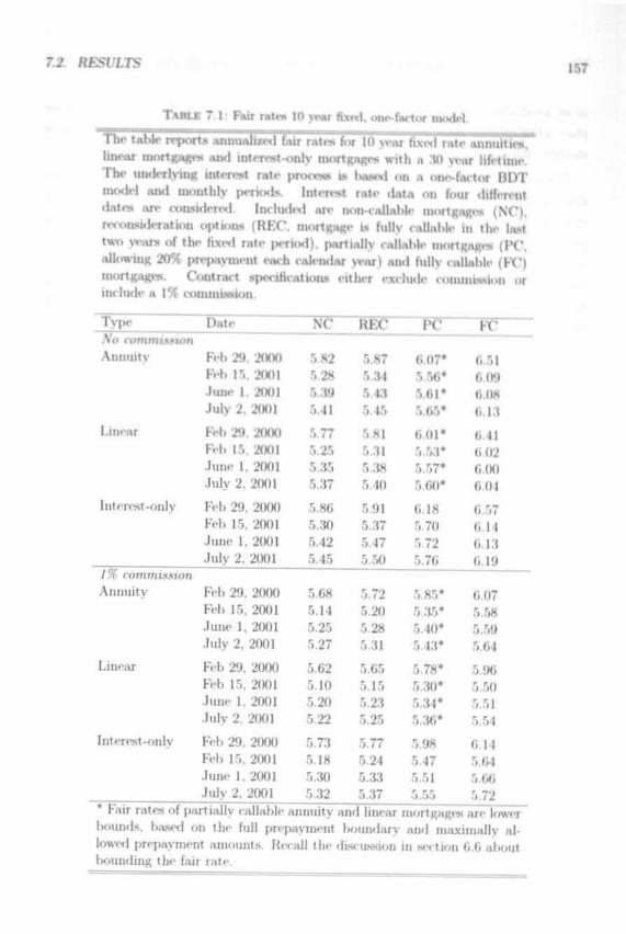
7.2. RESl/LTS ,57

TABLE 7.1: Fur rat« 10 year fixed, one-factor IIUKW. * *

The Uble reports anminfawi fair rates for 10 year fixed *nnui55rlinear mortgages and interest-only m<>rti'..u-.es with a 30 year lifetime.The underlying interest rate process i- |..,>.,| ,,n a one-factor DDTmo«lt>l and monthly IHTMXIS. lni.t,-.! i.,t,. data on four differentdates are considered. Included are non-callable mortgages (N(').r«t iiM.l-i.ition options (RKC. mortgage is fully callable in the lasttwo wars of the fixed rate JHTMKI), |mrtiallv raJlahle inortRanes (PC,allowing 2O9( prr|mynient each <aJcn<lar war) and fnllv eallaltle (FX")mortgages. Contrnrt spwUitatioas eitlur e.\ilu<le <oinnu>Mion orinclude a 1% commission.

TypeA o rommtsnonAnnuity

Linear

Interest-only

7% rommw.sionAnnuity

Linear

Interest-only

Dat<

Feh 29. 2000Feb 15. 2001June 1. 2001July 2, 2001

Feb 29. 2000Feb 15, 2001June 1, 2001July 2, 2001

Feb 29, 2000Feb 15, 2001June 1, 2001July 2, 2001

Feb 29. 2000Feb 15, 2001June 1, 2001July 2, 2001

Feb 29, 2000Feb 15, 2001June 1. 2001July 2. 2001

Feb 29. 2000Feb 15. 2001June 1, 2001July 2, 2001

\ ( '

5.825.285.395.41

5.775.255.355.37

5.865.305.425.45

5.685.145.255.27

5.625.105.205.22

5.735.185.305.32

H"K( •

5.875.345.435.45

5.815.315.385.40

5.915.375.475.50

5.725.205.285.31

5.655.155.235.25

5.775.245.335.37

IV

6.07*5.56*5.61*5.65*

6.01*5.53*5.57*5.60*

6.185.705.725.76

5.85*5.35*5.40*5.43*

5.78*5.30*5.34*5.36*

5.985.475.515.55

1 ('

6.516.096.086.13

6.416.026.006.04

6.576.146.136.19

6.075.585.595.64

5.965.505.515.54

6.145.645.665.72

bounds, based on the full prepayment boundary and maximally al-lowed prepayment amounts. Retail the discussion in section 6.6 aboutbounding the fair rate.

158 CHAPTER 7. A COMPARISON OF FA/R .MORTGAGE RATES

as we are dealing with an increasing term structure and redemption should preferably take

place when interest rates are low, implying that the duration of linear mortgage types is

shortest, followed by the duration of annuities.

The importance of a 20% partial prepayment option embedded in an interest-only mort-

gage haw been discussed in chapter 5. The values of partial prepayment options in annuity

or linear mortgages are similar. This can be concluded from the lower bounds on the fair

rate, obtained by the heuristic method described in chapter 6. Note that an upper bound

on the fair rate of a traditional mortgage is provided by the fair rate of the interest-only

loan, since all term structures are upward sloping. The lower bound is therefore very close

to the optimal fair rate, even for a ten year lifetime, for which the heuristic prepayment

strategy differs most from the optimal.

Fair rates have also been determined for mortgage loans including a 1% commission.

Concerning the ten year lixed rate period, the full prepayment premium is around 10 basis

points. The value of a partial prepayment option has significantly increased. An option

to prepay 20% per calendar year is worth around 25 basis points or more than 60% of the

value of a full prepayment option.

The value of a reconsideration option is still 5 basis points. Also, the value of a full

prepayment option restricted to the first years of the fixed rate period has not changed

much. If prepayment is restricted to the first two years the option is worth 8 basis points less

t hitii a full prepayment option, if prepayment is restricted to the first year the option is still

worth 16 basis points less. When comparing results to the case without commission, the

compensation for a 1% commission ranges from 15 basis points for non-callable mortgages

to 50 basis points for fully callable mortgages.

Table 7.2 shows fair rates for mortgage contracts with a five year fixed rate period, or

equivalontly, an unrestricted adjustable rate mortgage with an adjustment date after five

years. All mortgage rates are lower than the corresponding rates of mortgages with a ten

year fixed rate period, since all term structures are upward sloping. In the case without

commission costs, the full prepayment premium is about 60 basis points. A reconsideration

option valid in the last two wars of the fixed rate period (such that the reconsideration pe-

riod starts after three years) is worth 11 basis points on average. A 20% prepayment option

on a five year fixed rate period is worth 19 basis points on average. Partial prepayment

options can be priced very accurately, since the lower bound on the fair rate differs not

more than 3 basis points from the upper bound, being the fair rate of the corresponding

interest-only mortgage.

7.2. RESULTS 188

1 i n i . i i m - o | ' • •; i - i : . : i . i . . • • .

l i n e a r n i o r t ^ . n ; i > . m i l m i - i i - t -

T h e u n d e r l y i n g • • • ( • - • • -»t i . i t r

i i i i " l ' ! H I ' ! m o n t h l y | » I K » I >

.>i'i<- ,1.1

. I I I i i ! i - l i > l i \ i - . u i i \ < < i H i l t ' H l l l l U l t l f S ,

onl\ nu>iti;.im-s with a ;U) year lifetime.

pi •><>•<.> i- IM>I-. | on a one-factor H O T

I m . u M i.it< d a t a on four ditforeiit

d a t . - ui i..n-.idered Included a rc non-cal lable mortgagi 'S (NO) ,

n i i.n-nl< l.ilioii op t ions ( R K C . mor tgage is fully callable in th<- last

two \ c i i > of t h e fixed ra te JMTJIMH pnrtjiillv cal lable mor tgages ( I ' C ,

allowing 2O'/i p repayment . . i< 11 . .iliii.l.n \>.n • u n l tully callnlile ( P C )

mortgages. C o n t r a i l >|>n iii> .ii i> >u> <itli<i i \ ( l \ i d e commission or

include a 1% commiss ion

Type DateNo commiMionAnnuity

Linear

Interest-only

Feh 29. 2(K)0Feh 15. 2001June 1. 2001July 2. 2001

Feh 29. 2(KK)Feb 15, 2(K)1June 1, 2001July 2. 2001

Feh 29. 2000Feb 15, 2001June 1. 2001July 2, 2001

/% rommissionAnnuity

Linear

Interest-only

* Fair rates ofhounds, hasod

Feh 29. 2000Feb 15, 2001June 1. 2001July 2. 2001

Feb 29. 2000Feb 15, 2001June 1. 2001July 2. 2(K)1

Feb 29. 2000Feb 15. 2001June 1. 2001July 2. 2001

NC

5.314 954 914.86

.I 291944.904.85

5.324.%4.924.87

5.074.714.684.63

5.044.704.Of)4.G1

5.104.734.704.65

RKC

5425.085.014 96

5 395.074.994.95

5.445.095.024.98

5.154.814.744.70

5.114.784.714.67

5.184.834.774.72

partially callable annuity and linear

re

5.48*5.14*5.10*5.05*

546*r, 13*5.08*5.03*

5.505.175.105.05

5.17*4.82*4.77*4.72*

5.14*4.79*4.74*4.69*

5.214.854.801 75

in

on the full prepayment boundary and iiiiixiin;prepayment amounts.

IV

5.845.595525.48

5.805 575.505.45

5.875.615.54550

5.304.954.884.84

5.254.924.854.80

5.334.984.914.87l< lower

illy allowed

160 CHAPTER 7. A COA/R4RJSCW OF E4/R MORTGAGE RATES

When including 1% commission costs, the average full prepayment premium equals 22

basis points. A 20% partial prepayment option has an average value of 10 basis points.

The reconsideration option is worth only 7 basis points on average. For a shorter fixed rate

period, the compensation for a 1% commission increases to 25 basis points for non-callable

mortgagee and 60 basis points for fully callable loans.

Consider now a one-sided bandwidth mortgage, for which an interest rate decrease is

immediately reflected in the mortgage rate. In that sense, the bandwidth mortgage is an

ARM for which every period is an adjustment date. However, an interest rate increase

is reflected only if the increase exceeds a bandwidth, which is 1.25% on the annualized

contract rate. If the increase is larger the bandwidth is subtracted from the new mortgage

rate. A bandwidth mortgage protects the client from large contract rate increases. Any

prepayment option on a bandwidth mortgage is worthless since every interest rate decrease

lowers the mortgage rate to its fair rate. The fair rates for non-callable, partially callable

and fully callable mortgages are equal. Fair rates for the four instances are 3.94%, 4.85%,

4.71% and 4.66% respectively, which is only slightly higher than the variable mortgage

rates (3.49%, 4.71%, 4.64% and 4.64%,).

While in the no-commission case a mortgage is called at any interest rate decrease, this

is not. the case when a commission has to be paid. Then calling takes place only after

the commission costs are compensated for by the decrease of the interest rate. The initial

contract rate is decreasing faster for mortgage contracts with commission (compared to

contracts without commission) when shortening the length of the first fixed rate period.

For shorter fixed rate periods commission costs must be compensated for in a shorter time

span, by means of a lower fair rate. After the first period we assume that the contract

rate can be adjusted without commission or penalty. As a consequence, for very small first

fixed rate periods it might not even be possible to find a fair positive contract rate, because

the 1% commission costs cannot be compensated by a lower (and still positive) contract

rate. For this reason no fair rate for a bandwidth mortgage including commission can be

computed, unless the bandwidth is extremely large. In that case the mortgage behaves

like a fixed rate mortgage. Calculating fair rates for variable rate mortgages including

commission is impossible for the same reason.

Concerning the prepayment option in a mortgage contract, we conclude that this option

becomes less valuable when adjustment opportunities increase. Calling a mortgage is less

likely when the contract rate is adjusted to the fair rate more often. As an extreme

situation, note that the bandwidth mortgage (including only a bandwidth on contract rate

7.2. RESl/LIS

T A B L E 7 . 3 : F a i r r a t r s t w t v s i i i c d r m m t w k l t h . o n e - C u r t o r m o d e l . tn> . . • I M I M I - . M . .n

I I n l . i l ' l t n | » > i t > . m i i i i . i l i / o l I . > n i . i l < > ! " i . i n i i u i l n > l u x . u i i i '

and interest-only mortgages with a 3U year lifetime and IUI acijustmentdate after 10 \vars. including a two-sided bandwidth of 1.2.VX-. Theunderlying interest rate pmorew is basod on a duo-factor BDT modeland monthly |M»rio<ls. Interest rate data on four different dates art'considered. Included are non-callable mortgages (NC). reconsiderationoptions (REC. niortgnK*' '* fully cnllnl>le in the Inst two \-i'ars of thefixed rate perio«l) mid fully callable (FT) inortRaRes All i-outrmtspecifications exclude couuuisKiun.

TypeAnnuity

Linear

Interest-only

DateFtt>29, 2000Feb 15, 2001June 1, 2001July 2. 2001

Fcb 29. 2000Feb 15, 2001June 1, 2001July 2, 2001

Feb 29, 2000Feb 15, 2001June 1, 2001July 2. 2001

NC3.914.644.464.40

3.911 i . l

1 It.

4.40

3.924.644.464.40

meI'D

4.U41461 10

3.91Kit•Ufi1 1(1

3.924.644.464.40

IV.I'M

•».*:>

4714.66

3.941.851.714(>6

3.944.854.714 . ( i< i

increases) will never be called, as the contract rate is adjusted to the fair contract rule iw

soon as this fair rate is lower. Hence, there is no reason to prepay the loan Iwfore maturity.

Results for two-sided bandwidth mortgages are provided in table 7.3. Tin- bandwidth

equals 1.25% on both an interest rate increase and a decrease, protecting both client find

bank from (small) interest rate movements. Now the full prepayment premium is positive

and can be as large as 25 basis points. The fair rate of a fully callable mortgage with a

two-sided bandwidth equals the fair rate of a one-sided bandwidth mortgage, since with a

two-sided bandwidth an interest rate decrease does not lead to a contract rate adjustment;

instead the mortgage Ls called, affecting the fair rate similarly.

Comparing tables 7.4 and 7.5 to 7.1 and 7.2. results for the two-factor interest rate

model are verv close to the fair rates obtained with the one-factor model. Non-callable

CHAPTER 7. A COMPARISON OF FAJR A/ORTGAGE RATES

TABLE 7.4: Fair rates 10 year fixed, two-factor model.

The table reports annualizcd fair rates for 10 year fixed rateannuities, linear mortgages and interest-only mortgages with a 30year lifetime. The underlying interest rate process Is based on atwo-factor BDT model and monthly periods. Interest rate dataon four different dates are considered. Included are non-callablemortgages (NC), reconsideration options (REC, mortgage is fullycallable in the last two years of the fixed rate period) and fullycallable (FC) mortgages. Contract specifications either excludecommission or include a 1% commission.

TypeMJ commissionAnnuity

Linear

Interest-only

i% commissionAnnuity

Linear

Interest-only

Date

Feb 29, 2000Feb 15, 2001June 1, 2001July 2, 2001

Feb 29, 2000Feb 15, 2001June 1, 2001July 2, 2001

Feb 29, 2000Feb 15, 2001June 1. 2001July 2, 2001

Feb 29, 2000Feb 15, 2001June 1, 2001July 2. 2001

Feb 29. 2000Feb 15, 2001June 1, 2001July 2. 2001

Feb 29. 2000Feb 15, 2001June 1, 2001July 2. 2001

NC

5.825.285.395.41

5.775.255.355.37

5.805.305.425.45

5.685.145.255.27

5.625.105.205.22

5.735.185.305.32

REC

5.875.345.425.45

5.815.315.385.40

5.915.375.465.49

5.725.195.285.30

5.655.155.225.24

5.775.245.335.36

FC

6.496.076.076.10

6.396.016.006.02

6.556.136.136.16

6.055.555.575.60

5.955.475.495.51

6.125.625.645.67

7.2. RESULTS 163

TABLB 7.5: FWr rates 5 year fixed, two-factor model.

I ' I K ' t . i M i - n p i ' i t - . . n u m . i h / . i l t . u i i . i i . - N i",ii '• v i - . u t i x e d rate

a n n u i t i e s , l i n e a r m o i l ^ a ^ e s a m i i n t e r e s t - o n l y i n < » i I f . . i t - . « - w i t h . i ' 1 0

y e a r l i f t ' t I I I K V I I n - u n d e r l y i n g m t c r e s t r a t e p i n , . v . i - ! > . , > • . I , . i , . i

two-fwtor UDT model IUKI monthly |>eriods. Interest rate dataon four different ilntes are considered. Include! are non-< allaMemortgages (NC). r»-< • >u i. !• 'i.it ion options (HKC. inortK»K<' i" fullycallable in the l.»t t»<. \. .us of the lixed rate period) and fullycallnhle (FC) inoitnano Cotitriu't S|MH ihi atioiis either exehulr

ioii or include a 1' i ciitnini.s.sion.

Type Date NC Hl.c IfAfo commtMtonAnnui ty Feb 29. 2000 ."»;J1 ."» U ,iW

Fob 1.1. 2001 -1.95 5.08 5.60June 1. 2001 4 91 5.01 5.55July 2. 21X11 4.86 4.96 5.50

Linear Fob 29. 2000 529 5.39 5.78Feb 15. 2001 4.94 5.07 5.58June 1. 2001 1.90 4.99 5.52July 2, 2(K)1 4.85 4.94 5.47

Interest-only Feb 29. 2000 5.32 5.43 5.85Feb 15. 2001 4.96 5.09 5.62June 1. 2001 4.92 5.02 5.57Julv 2. 2001 4.87 4.98 5.52

/% commissionAnnuity

Linear

Interest-only

Feb 29. 2000Feb 15. 2001June 1. 2001July 2. 2001

Feb 29, 2(KK)Feb 15. 2001June 1. 2001July 2, 2001

Feb 29. 2000Feb 15. 2001June 1. 2(X)1July 2. 2001

5.074.714.084.63

5.044.704.664.(il

5.104.734.704.65

5.154.804.744.69

5.114.784.714.67

5.184.824.774.72

5.284.944.894.84

5.234.914.854.80

5.324.974.924.87

164 CHAPTER 7. A COMPAR/SON OF FAJR A/ORTGAGE RATES

fixed rate contracts arc; model independent by definition, as only the yield curve (which

is matched exactly) affects prices of mortgages without embedded options. Fair rates of

fully callable mortgages based on the two-factor model differ from one-factor results 5

basis points incidentally, although the majority of fair rate differences is limited by 2 basis

points. Since many fair rates for partially callable mortgages arc approximative and a 2

basis point difference is smaller than the approximation range, we have not included results

for partially callable mortgages based on an underlying two-factor interest rate model.

A similar robustness holds for the choice of the term structure model. Non-callable

fixed rate mortgages only depend on the term structure and are therefore not affected by

the underlying term structure model. Fully callable mortgages are only slightly affected.

For a ten year fixed rate period, the fair mortgage rate based on the Ho and Lee model

is approximately 5 basis points less than the fair rate based on BDT. For shorter fixed

rate periods, fair rates are even less sensitive with respect to the underlying term structure

model.

Table 7.6 reports both observed* mortgage rates and fair rates and provides an indication

of a bank's premium to cover costs and risk. The premium on a variable rate mortgage

ranges from 0.9 to 1.2 percentage point. Surprisingly, the premium on a five year fixed

rate period is larger, at least 1.2 percentage point. A ten year fixed rate period faces an

average premium of 1 percentage point. The bandwidth mortgages are very unattractive,

since the average premium on a one-sided bandwidth mortgage, with a bandwidth equal

to 1.25%, is huge: almost 2 percentage points.

Concerning observed mortgage rates, a contract rate is typically reduced by 30 basis

points when 'Nationale Hypotheek Garantie' is included, so even including NHG premiums

are large. Also, savings and investment mortgages are usually quoted at a contract rate

that is up to 20 basis points higher than annuity, linear or interest-only mortgages. Finally,

note that the fair rates for variable rate and bandwidth mortgages are calculated excluding

commission, while the olxserved rates include 1% commission costs in addition.

For the three instances of 2001 the bandwidth mortgage is far less attractive than a

fixed rate mortgage. The fair rate is lower than the fair rate of a comparable FRM. while

the observed contract rate is higher. For February 29. 2000 the bandwidth mortgage

can be attractive as both the real contract rate and the fair rate are significantly lower

than the corresponding contract rates of an FRM. although the premium on a bandwidth

mortgage is much higher. For clients, the risk of a bandwidth mortgage is high compared

''Mortgage ml"* are oliserveil from Bouwfoiuls, a Dutch mortgage provider.

7.2 RESULTS

TABLE 7.6: Ob*rv«d rate*.

Tbe tal)le provides a eompariaon between observe<l tin I tan lunti .utrates. Mortgage rates charged by Itanlcs are o l . s , n , , | during thesame month in which the term structure of interest i.iies i> unitedObserve! rates exclude 'Nationale Hvpotluvk Garantie ami aie basedon a mortgage loan of 100'X of the house value Annuity, linear andinterest-only mortgages have similar olwervttl rates All ob-eivedmortgage contracts include 1'X commission costs and an alloui-dprepayment of 20% per calendar year The convs|H>ndiiig fair rated,stated in brackets, are ti/»;x r honfxis IxLsetl on a cme factor interest ratemodel, indicating the luniks premium on ni"it^.i^i loans Variablerate (VAR), 5 year fixed rate (5Y), 10 year hxed rate (10Y) and10 year bandwidth (B\V) mortgages are mnsiderefl. Fair rates arcexcluiling commission for variable rate and lutndwidth u

Date1 . 1 . - " i

Feb 15.

June 1.

July 2,

•.INN)

2001

2001

2001

VAR1 7(1

5.80(471)5.50

(4.64)

5.50(4.64)

-.Yi. Id

6.10(4.85)

G.00(4.80)

6.20(4.75)

loYt , ' M 1

650(5.47)

(i.40(5.51)

6.60(5.55)

ItW'. Ml

6N0(4.K5)

6.60(471)

(i.7()(4.66)

to a fixed rate mortgage, especially because the yield curve of February 29. 2000 is very

steeply upward sloping. The future contract rate is adjusted continuously, which implies

mostly a rate increase (although corrected for the bandwidth). To illustrate the risk of

rate adjusting mortgage contracts, figure 7.1 plots the distribution of future contract ratCH

when considering a rate adjustment after 5 years. A contract rate adjustment towards

10% or more has a probability of almost 5%. A contract rate increase is almost inevitable

(82%). Note that the initial fair rate equals 5.3%.

Table 7.7 shows the annualized one-month fair rate volatility, given !>y

ff» = 0.5 • (»« -» , ) . (7.1)

where y>, and i/ are the annualized fair rates after one up movement or one down movement,

166 CHAPTER 7. A COA/PAR/SON OF FA/R A/ORTCAGE RATES

FIGURE 7.1: Distribution of fair future ARM rates.

The figure shows the distribution of fair contract rates of a non-callableadjustable rate annuity (excluding commission) after the adjustment dateat 5 yearn (< = 60). The instance considered is of February 29, 2000. Theunderlying term structure model is a oruvfactor based BDT model. Thevertical dashed line represents the initial contract rate.

30

28

20

16

10

6

0% 4% 6% 8% 10% 12% 14% 16% 18% 20%

respectively. The maturity date of the fixed rate period remains unchanged. We consider

fair rate volatilities of annuity mortgages. Volatilities of linear and interest-only mortgages

are similar. The tixed rate period is either five or ten years. Non-callable and fully callable

mortgages are included, both excluding commission and including a 1% commission. Fair

rate volatilities differ mostly between non-callable and fully callable mortgages. The length

of the fixed rate period and the commission do not alter volatilities significantly.

CONCLl/DINC ROMRKS " 107

TABLE 7.7: FMr ratr volatilitUw.

T l l > t . l l ' l i ~ } | i -\\ - . l l l t l l l . l l l / o l o l l l ' I l l n l l l l l t i l l I . I l l ' M > l . l l i l l t l l " . I l l | H | | i l l l . l l ' . l V

according to equation 7 1 Non-callable (M") and tullv callable (IV) annuitiesare considered All mortgages haw a 30 year lifetime. The tixt<«l rat«' pcnodequ-its ' ..I in \i .ii-. ('nmmisMon <t«sts are «*itIUT O'X or 1%. Tin* underlyingl h.i> iiiniiii i lv p e r i o d s

Fixed rati- periodCommission ('X)Call option

Feb 29. 2000Feb 15, 2001June 1. 2001Julv J Jill 11

Illy0

NC

0.2070.1750.172I I I M I

10y0

FC

0.2330 1940 190II 1')',

lUy1

NCO - J I H .

0.17»0 172II I7 ' i

10>1

FCII J J ' i

ii I'l.t

0 I8«lI I I ' H .

iy0

NC

U 17.".

0.179

I I I M I

5y0

FCn .' ! 1

tl 17.s

0 182(I I 7 ! l

5.v1

NCii . ' . ' i i

( I 1 7 1

0 178II I 7 ' i

5yi

FCn ' t !

II IM0 189I I l V I

7.3 Concluding remarks

This chapter provides an overview of fair mortgage rate* baned on term Ntrucliin* of

interest rates on four different dates. The contract rates are robust with renp<K-t l<i the

underlying model and the fineness of the grid. Applying a two-fartor interest rate model

does not change the fair contract rates significantly. Considering 2-10 semi-monthly periods

compared to 120 monthly periods also hardly affects fair rat<*. Obviously, valuation bawd

on monthly periods is more efficient.

Fair rates for a large variety of mortgage types, including partially callable mortgages

analyzed in the previous chapters, are compared. The main results include the value

of prepayment options. A full prepayment option is worth 70 to 80 basis points for 10

year fixed rate mortgage contracts excluding commission and 40 basis points for contracts

including a 1% commission. The value of a partial prepayment option to prepay 20%

per calendar year equals on average 34 basis points excluding commission and 25 basis

points including a 1% commission. Consequently, the value of a partial prepayment option

embedded in a ten year mortgage contract including commission is more than W)% of a full

prepayment option value, although prepayment according to the former option is severely

limited.

A reconsideration option, with the possibility to start a new fixed rate period at the

lowest contract rat* during the last two years of the current period, is only worth -I to 7

168 CHAPTER 7. A COMPARISON OF E4/R MORTGAGE RT\TES

basis points more than a non-callable mortgage. Options restricting prepayment to the

first two years of the fixed rate period, fixing the lowest contract rate of the first two years

for the remaining lifetime, do have significant value. . . >. -.

Shorter fixed rate periods imply lower fair contract rates, because all term structures

considered are upward sloping. Premiums of prepayment options are lower compared to a

ten year fixed rate period. An adjustable rate mortgage implies resetting the contract rate

to the prevailing future mortgage rate after five years. The lower initial contract rate is

offset by an increasing uncertainty about the future contract rate. The future rate is very

likely to be higher due to the upward sloping yield curve.

Fair rates have been compared to observed contract rates. For traditional variable and

fixed rate mortgage contracts the observed contract rate is roughly 1 percentage point

larger than the fitir rate. The more complex bandwidth mortgages are expensive, since the

premium (between observed and fair rate) on a bandwidth mortgage is almost 2 percentage

points.

To complete the discussion on Dutch mortgage contracts, we briefly consider tax regula-

tions in the Netherlands. Interest payments and prepayment penalties are tax deductible,

implying that each client will base prepayment decisions on personal (tax and income)

circumstances. In a tax free environment, the penalty for full prepayment (more than)

offsets the gain of full prepayment over the maximally allowed prepayment. Optimally,

clients will not. prepay more than allowed. Including tax effects, full prepayment is still not

optimal. Although a client is partly compensated for the prepayment penalty, future tax

deductions decrease because all future interest, payments decrease. These partly offsetting

arguments introduce a topic for further research on the effect of tax policies on optimal

prepayment. As long as prepayment gains and interest payments are equally taxed (by a

tax percentage r), the optimal prepayment strategy will not change and the new fair rate

becomes the 'tax free' fair rate multiplied by -pj-p.

.•*«?

Chapter 8

Summary and Concluding Remarks

Thin dinnertation contributes to two main research fields, mortgage valuation and term

structure calibration. Concerning mortgage valuation, computational methods are intro-

duced and analyzed to value restricted prepayment options, present in all Dutch mortgage

contracts. For both financial institutions and clients, the importance of mortgage valuation

lias increased due to the large growth of the Dutch mortgage market in the last decade. For

mortgage issuers, one of the largest, uncertainties in mortgage contracts concerns prepay-

ment risk. American mortgage loans allow for unrestricted and penalty-free prepayment

at any time. Dutch mortgage loans bear less prepayment risk, since only a limited prepay-

ment is allowed penalty-free per calendar year. This so-called partial prepayment option

complicates mortgage valuation significantly. Part II of this thesis deals with the valuation

of Dutch mortgages.

The second main theme concerns the contribution to the literature on term structure

calibration. For pricing interest rate derivatives, including mortgage contracts with em-

bedded options, a term structure of interest rates and a volatility structure are essential.

Calibrating a term structure model to a recombining scenario tree (a lattice), in order to

match market prices of interest rate derivatives, is discussed in the first part of this thesis.

Performance of term structure models is measured by the ability to price interest rate

derivatives accurately. Derivatives we consider include swaps and swaptions. Swap data

are available as annual swap rates, which are used to derive a yield curve. Implied swaption

volatilities are okserved and transformed into prices by Black's formula. Both cash flow

patterns and quoting conventions of swajxs and swaptions are examined in chapter 2 to

obtain a term structure of interest rates and swaption prices.

170

¥•-•• 1 7 1

Chapter 2 also provides an overview of commonly used term structure models ,i> u< II

as a comparison with respect to swap and swapt ion pricing based on both model p i i |« me s

and empirical performance. Model prices are compared to price- ..l.t.nned from observe*!

swap rates and implicit swapt ion volatilities. For our purpose of pin inn mortgage contracts

and embedded option*, a term structure model is si-Uvted tlwtt is easily calibrated to an

interest rate lattice. Empirically desirable pinpi nn>- <•! 1. nu structure nuxlcls include

lognoruialitv and mean reversion of one-period int. HM i.it.-- Since we consider monthly

periods, a model with a limited IIUIIIIMT of factors is preferred for efficiency reasons.

Calibration of interest rate lattio - is kised on the Black. Herman and Toy [U, BDT)

model. The BDT model, originally dclmed 111 discrete time. i> , .>M1Y «aliluat<-d In a lattice

and captures mean reversion and IOKIKIIUI.IIIV distributed mtt n M i.iics. The original BDT

model is a one-factor model. To in< i< .i>. Il< \ibility we also <-onsider a two-fm toi \-erNuiu.

Besides a detailed analysis of BDT model propi m< s . li.i|.i«r :i alwi provides exteimivc

calibration results. Zero-coupon bond pi 1 • •- IP >\.utly matched by H|Mvifving all drift

p.ii.iiin-ti-is Sumption pricing <'in>is sh..u .1 p.uiK 11I.11 patt<>ru. l^ong term option* 011

-li ' ii N nu »v\a|«s arc- umlcrprn «tl l>\ tin tin >• i<l slioii term options on long term swupn

in ••Mrpriced. Average pricing ernns .ur iypuall\ Miialler than the lud-a.sk spicud lor

swaptions. Volatih'ties are hump-shaped. Mean reversion usually starts during the second

year, while interest rates are diffusing in the first year. Results are robust, since one- and

two-factor models with varying specifications are used for four different dates. KmpiricaJly,

including multiple factors does not improve calibration results significantly.

Mortgage valuation is the topic of part II of this thesis. The mortgage value equals the

present value of all cash flows (redemption, interest payments and additional prepayments).

We particularly focus on the valuation of the partial prepayment opium Clients are

assumed to exercise prepayment options optimally, based on the development of interest,

rates. Interest rate scenarios derived in part I serve as input for mortgage valuation.

American mortgage types, allowing full prepayment, can be priced using lattices. Val-

uation of these mortgage contracts is described in chapter 4. The straightforward pricing

method for partially callable mortgages is based on a non-recombining tree approach. Due

to the inefficiency of non-recombining trees, we solve mortgage valuation problems includ-

ing partial prepayment options by applying extended lattice methods.

Some partially callable mortgages can be priced efficiently to optiinalitv. Interest-only

mortgages, having no regular periodical amortization, can be viewed as a portfolio of

callable bonds. Valuation is based on successively exorcising callable bonds, when; only

172 CHAPTERS. SUAfMARY AiVD CO.VCLl/D/NG REMARKS

one bond can bo exorcised each calendar year. The portfolio of callable bonds can be

valued optimally by an efficient lattice approach, according to chapter 5.

A bond portfolio cannot be used to price partially callable mortgages including a reg-

ular amortization schedule (for instance annuities). For this reason, optimal valuation of

partially callable annuity mortgages Is not possible using a lattice approach. If a non-

roeombining trw method is applied, optimal prepayment strategies can be derived, but

MIICII mot hod is only possible for very small instances. In chapter 6 wo formulate a linear

programming formulation based on a non-recombining tree. Duality theory and comple-

mentary slackness conditions can l>e applied to derive the optimal prepayment strategy.

A 'no prepayment' strategy is a feasible solution of the primal LP. formulating the

valuation of a partially callable mortgage. A 'full prepayment' strategy is a feasible solution

of the dual LP. Every feasible solution of the primal LP provides an upper bound on the

price of a partially callable mortgage. Similarly, every dual feasible solution provides a

lower bound on the price. To obtain a dose approximation of the optimal mortgage price

(that is, the mortgage price corresponding to an optimal and allowed prepayment strategy),

both feasible solutions must be improved in order to narrow the range for the optimal price.

To find a close upper bound on the mortgage price (or equivalently, a lower bound on

the fair rate), we propose a heuristic for a prepayment strategy that is close to optimal.

An upper bound on the fair rate is obtained by the fair rate of an interest-only mortgage,

in case term structures are upward sloping. Combining all results, close to optimal fair

ratiw can be computed efficiently. Directions for further research include the derivation of a

theoretical upper bound on the fair rate and the approximation of fair rates by considering

a subset of scenario paths.

Chapter 7 concludes the mortgage valuation part. Fair rate results are compared, indi-

cating the values of prepayment options. As an example, for a ten year fixed rate period,

a 20% prepayment option is worth more than half the value of a full prepayment option.

Addit ionallv. the effect of the yield curve and the fixed rate period on fair rates is discussed,

as well as values of contract rate adjustment options and the duration effect of cash flows

on the contract rate. Fair rates are robust with respect to the underlying term structure

model and the step size of the underlying grid.

An important direction for future research is the effect of the Dutch tax regime on

mortgage valuation. Both interest payments and prepayment penalty are tax deductive.

Although including tax effects requires a client specific approach, optimal prepayment will

not change if a tax-adjusted fair rate is considered.

Bibliography

[1] B. Alink. A/ortjoyf prr/xiymrrUj in Mr /VriArWan<£<<. Phi) thesis, UniwmiU'it Twt'iita,2002.

[2| K. Ainin. On the romputation of continuous time option primi using discrete approx-imations. ,/ournai <»/ Financial anrf (^tianftfafit*' .-hia/ysi.i. 2(>(-t). HWI.

[3] L Andersen and .1 Andreasen. Volatility skews and extensions of I lie I.IIIOH marketmodel, /tppfarf A/al/umoiu-oi Finance, 7, 2000.

[4] D. Backus. S. Foresi. and S Zin. Arhitrago opportnnitios in arliitriw-fni' tnodelH ofIK)IHI pricing. 7«HJTUI/ <»/ /iiwinos <ifif/ £,V<>rim;m .S7<i/i.<ifi< >. 1(>(I). I!K)H

[5] T. Bali and A. Karagozoglu. Pricing eurodollar futures o]>tion.s usinn the BUT termstructure model: the effect of yield curve smoothing. ./w»irmi/ fj/ /•ii/wir.s A/rirlriii,20(3). 2000.

[6] W. Bams. T/ir rrm s/nirf «rr' o/ intrrrof rn<p.t. n p«nW rfarn ana/yxix. I'll I) thesm,University of Maastricht. 1999.

[7j S. Benninga and Z. Wiener. Binomial term structure models. A/af/irm«/u« inand m'rmr/i, 7(3), 1998.

[8] F. Black. The pricing of commodity contracts. 7ouf7ia/ o/ Fmanriai franomtr*, 3,1976.

[9] F. Black, E. Derman, and W. Toy. A one-factor model of interest rates and itsapplication in treasury bond options, f'tnanrta/ .Anali/«k) 7»urna/, 40(1). 1990.

[10] F. Black and P. Karasinski. Bond and option pricing when short rates are lognormal.f'inanrio/ .4na/y.sts 7ournai, 47(4), 1991.

[11] F. Black and M. Scholes. The pricing of options and corporate liabilities, .//VMTT/U/ O/Po/i/«rn7 Economy. 81. 1973.

[12] P. Boyle, K. Tan, and W. Tian. Calibrating the Black-Dennan-Toy model: sometheoretical results. .4pp/i«i A/aJhrmadroi finance, 8(1). 2001.

173

174 B/BL/OGR.4PHY

[13] A. Brace, D. Gatarok, and M. Musiela. The market model of interest rate dynamics.A/u//*ematica/ Finance, 7(2), 1997.

[14] M. Brennan and E. Schwartz. An equilibrium model of bond pricing and a test ofmarket efficiency. JOUTTIH/ »/Financial and" ^uan<tia<ivp /lna/j/sts, 17(3). 1982.

(15) I). Brigo and F. Mercurio. /n/enest rate modeis: tneory and practice. Springer Finance,2001. • • • s

[16] W. Biihler, M. Uhrig-Honiburg. U. Walter, and T. Weber. An empirical comparisonof forward-rate and spot-rate models for valuing interest rate options. Journal o/Finance, 5-1(1), 1999.

[17] A. van Bussel. VVi/uatton and interest rate risifc o/mortgages in tne Netherlands. PhDthesis, University of Maastricht, 1998.

[18] K. Chan, G. Karolyi, F. Longstaff, and A. Sanders. An empirical comparison ofalternative models of the short-term interest rate. Journal o/ Finance, 47(3), 1992.

[19] K. C'lmrlicr and A. Van Bussel. Prepayment behavior of Dutch mortgagors: An em-pirical analysis. //«•«/ /v.s/rt/r A,'c«««wic.s, 31(2), 2(M)3.

[20] I,. Chen, /nterest m<e dynamics, dcriuatities pricino and risifc management. Springer,1996.

[21] T. Cheuk and T. Vorst. Shout floors. yVetF,iposunc - fi'/ectronic Journal o/ Finanrta//<*.•»*.-. 2, 1997.

[22] V. Chviital. Ainrar programming. W.H. Freeman and Company, 1983.

[23] J. Cox, .1. Ingersoll, and S. Ross. A theory of the term structure of interest rates.Fconcnnctrica, 53, 1985.

[24] F. I)e Jong, ,1. Driessen. and A. Pelsser. On the information in the interest rate termstructure and option prices. flrWrw o/DrncntM'cs /?r.srorr/i. 7(2), 2004.

[25] K. Dorinan and I. K.mi. Hiding on a smile. /?/SA\ 7(2). 1994.

[26] J. Driessen, P. Klnnssen. and B. Melenberg. The performance of multi-factor termstructure models for pricing and hedging caps and swaptions. 7o«rna/ o/ Finanria/and (^tianrira/ii'c .4m»/j/.si.s. 38(3). 2(M)3.

[27] D. DuHie. Dj/'i"»««c asset pricing tncor j/. Princeton University Press, 2'"* edition. 1996.

[28] D. Diifh'e and K. Singleton. An econometric model of the term structure of interest-rate swap yields, ./oiinui/ <>/ Finance 52(4). 1997.

[29] 15. Dumius. .1. Fleming, and H. Whalev. Implied volatility functions: Empirical tests.Journal o/Finance. 53(6), 1998.

B/BLJOGJUPHV 175

[30} F. Fabozzi. /nmirmrnt marutyrmrni. Prentice HJUI College. 2"* edition. 1999.

[31] R. Fan. A. Gupta, and P. Ritchken. On the |>erfonnaiict> of inulti-fai tor term struc-ture models for pricing caps and swaptions. Horibng /wiprr. C«wr WVairrn

y. 2001.

[32] L. Havre. Prepayment modeling and valuation of Dutch mortgage*. ,/ourW «/ Firerf/nrornr. 12(4). 2003.

[33] D. Heath. R. Jarrow, and A Morton llond prii ing and tin- Irnn structure of intercutrates: a discrete time approximation. . /ouiW •>/ Firi<uiri<i/ urid (^uariri/iifirr .-tnci/y.iM,25(4), 1990.

(34) D. Heath. R. Jarmw. and A. Morton. Bond pricing nnd the term structure of intercutrates: a new methodology. £ron<rnirtnra. 00(1). 1!)*.)2

[35] P. Hendershott and R. Viui Order. Pricing mortgages: An interpret at ton of the model*and results. Jouma/ »/ /-'murx IOV iVnnrr'.«i Ar.irnrr/i. 1(1), 1!)H7

[36] .1. Hilliard, J. Kau. D. Kecnan. and \V. Mullcr III. Pricing a clarw of American andEuropean path dependent securities. A/nna<;rmrnf jrirnrr, 41(12). 19Ur>.

[37] J. Hilliard, J. Kau. and V. Slawson .Ir. Valuing prepayment and default in a fixed-ratemortgage: a hivariatc binomial options pricing t<i lmi<|iie /fm/ /-.'••/(i/r /•'IIIIIMIIIK.I,2C(3). 1998.

[38] T. Ho and S. Lee. Term structure movements and pricing interest rate contingent,claims, ,/ournai o/Fmanrp, 41(5), 198G.

[39] J. Hull. Options, /ufurps. and ot/ier derit>a<tws. Pearson E<lucation. 5"' edition, 2002.

[40] J. Hull and A. White. The pricing of options on assets with stochastic volatility.JourTja/ o/ Fmanrr, 42(2), 1987.

[41] .1. Hull and A. White. Pricing interest rate derivative securities, ffcwn/i «/ A'manrifj/.SVurfir.s. 3(4). 19'X).

[42] J. Hull and A. White. One-factor interest rate models and the valuation of interestrate derivative securities. 7ourna/ o/ Finanria/ nnd QunnttYntitw /lnn/j/«w. 28(2), 1993.

[43] J. Ingersoll Jr. 77ieory o/yinanc»o/ aVcision moiktn . Rowman iuid Littlefiel<l. 1987.

[44] J. James and N. Webber, /n/rfr.st rntf modW/in^. John Wiley & Sons. 2000.

[45] F. Jamshidian. LIBOR and swap market models and measures, f'innnrr arid ,S7IICS, 1(4), 1997.

[46] R. Jarrow. A/odp/Zin^/irfd iwomf apruri/iM and «n<prr-.»< ni<p op/ion.i. McGraw-Hill,1996.

176 BIBLIOGRAPHY

[47] J. Kau ami D. Keenan. An overview of the option-theoretic pricing of mortgages,o/ //ouain^ /?e«eare/i, 6(2), 1995.

[48] .J. Kau, D. Keenan, W. Muller III, and J. Epperson. The valuation and analysis ofadjustable rate mortgages. A/anapemenf 5c»enre, 36(12). 1990.

[49] .1. Kau, D. Keenan. W. Muller III. and J. Epperson. A general valuation model forfixed-rale residential mortgages, ./ouma/ «/A/oney. Criprfi/ nnrf Bnn^mj. 24(3). 1992.

[50] J. Kau, D. Keenan. W. Muller III, and .1. Epperson. Option theory and floating-rate securities with a comparison of adjustable- and fixed-rate mortgages. Journa/ o/

s, 66(4), 1993.

[51] J. Kau, I). Keenan. W. Muller III. and .1. Epperson. The valuation at origination offixed rate mortgages with default and prepayment. Journa/ o/ flea/ £siate financeand fc'rwiomira, 11(1), 1998.

[52] .1, Kau and V. Slawson Jr. Frictions, heterogeneity and optimality in mortgagemodelling, ./OUTTW/ O/ flea/ £.v(alc Finance and Economics, 24(3), 2002.

[53] A. Kolen. Determining the fair value of a mortgage with partial prepayment: A math-ematical proKiammiiiK approach, /ie.sean/j mfrnorrindurit £/ftti;t'rsity o/ A/aasiricAl,2003.

[54| W. Leung and (.'. Simians. A lattice approach to pricing fixed-rate mortgages withdefault and prepayment options. VonrTia/ o/ Mr /Immran /fen/ £s<a<e and (/r6anF<COH<J//I/C.S- .I.SMK/ri//mi. 21 (.'{). 1990.

[55] A. Li. 1'. Kitchken, and L Saiikiinusuhiiimanian. Lattice models for pricing Americaninterest rate claims, ,/omwi/ o/ Finance. 50(2), 1995.

[56] F. Longstaff. P. Santa-Clara, and E. Schwartz. The relative valuation of caps andswaptions: Theory and empirical evidence. ./o«f7»«/ o/ Finance, 56(6), 2001.

[57] F. Longstuff and E. Schwartz. Interest rate volatility and the term structure: A twofactor general equilibrium model, ./{iiintn/ «/Fmance. 47(4). 1992.

[58] F. Loiigstaff and E. Schwartz. Valuing American options by simulation: a simple leastsquares approach, /fct'icio «/Financirt/ S/iidic.s. 14(1). 2001.

[59] I). Lucnberger. /nw.sfmpnt science. Oxford University Press, 1998.

[60] \'. Lyuu. Fmancia/ cn^triprfing and compu<aiion: pnncip/es, matAemahc*. a/50-u. Cambridge University Press, 2002.

[<il] H. Matins III and G. Bierwag. Pricing eurodollar futures options with the Ho andLeo and Black. Dermaii. Toy models: an empirical comparison, ,/owrna/ o/ Futures

rHrfc. 19(3). 1999.

BJBLJOGR.4PHV 177

[62] J. McConnell and M. Singh. Rational prepayments und the valuation of collateraliMtdmortgage oMigatkms. Joumai o/ Finance 49(3), 1994.

[63] J. McCulloch. The tax adjusted yield curve. Joumai o/ Fmoncr, 30(3), 1975.

[64] F. Mercurio and J. Moraleda. A family of humped volatility models. F.nm/>r<m Journalo/Finance. 7(2). 2001

[65] R. Merton. Theory of rational option pricing iJW/ Journal O/ EronofiiK.t ami A/«i»-Sinrnrr. 4. 1973.

[66] K. Miltersen. K. Sandmann. and D Sondernmun Closed form solutions for termstructure derivatives with log-normal intercut ran*. 7»uf»ioy o/Finance. 52(1), 1997.

[67] C. Nelson and A. Siegel ParsimonioiLs modelling of yield curves Journal o//JuAitirM.60(4). 1987.

[68] D Nelson and K. Rnmaswamy. Simple binomial pi• •« <•->..-s as division approximationsin financial models. fleiietc o/ Finanria/ £/!«/•«.«. 3(;i). 1U90.

[69] NEOS-Guide wwu--fp.mcs.anl.gov/ote/Kiiide/index.html, 1996.

[70] S. Nielsen and R. Poulsen. A two-factor. stcM-haslic progrnuimiiiK model of Danishmortgage-lmcked tMH'uritieM. Jouniai o/ Economic Dynamir.o onrf O»n/i»>/. 2M(7). 2004.

[71] A. Pelsser. E^icirnt t*a/ua(ion o/ inrrrrj< rn/r «frni*afit>ra. Springer, 2000.

[72] S. Peterson, R. Stapleton, and M. Subrahinaiiyiun. A multi-factor spot-rate modelfor the pricing of interest-rate derivatives. Juunta/ «/ A'in»nr(a/ ««(/ ^i/ri»///»(iur.4na/y.sw, 38(4). 2003.

[73] S. Pliska. /nirtN/urrton /o ma<Apma<ica/^nanrr: dwcrWr iimr rnorfrit. Blmkwell, 1997.

[74] J. Prendergast. The complexities of mortgage options. Journa/a/f'trfv//r/r«//ir, 12(4),2003.

[75] R. Rebonato. /n<eres/ rote option modeis. John Wiley & Sons, 2'"' edition. I!)!)M

[76] R. Rebonato. On the simultaneous calibration of multi-factor log-normal interest ratemodels to Black volatilities and to the correlation matrix, ./o/inju/ «/ (Finance, 2(4), 1999.

[77] P. Ritchken and I. Chuang. Interest rate option pricing with volatility huui|>s.o/ Dfnuo/iw WrswirrA, 3(3), 2000.

[78] W. Schmidt. On a general class of one-factor models for the term structure of interestrates. Finance anrf 5<oc/i«s<irs. 1(1). 199C.

[79] O. Vasicek. An equilibrium characterization of the term structure, ,/ciurna/ «/ finan-cia/ fconomics, 5. 1977.

Samenvatting / Summary in Dutch

Hypotheekwaardering on rentemodollen vormen de twee hoofdthema's in deze dissertatie.

De belangrijksto bijdrage aim de bostaande literatuur over het prijzen van hypotlieken is de

waardebopaling van m i optic tot godooltolijk aflossen. die in alle Ncderlandse hypotheken

aanwczig is. We vcronderstollcn dat (oen gedeelte van) con hypotheokloniiig wordt afgelost

op hct moment dat. rentes laag zijn. Oin die reden worden reiiteinodellcn gcanalyseerd in

het eerHte deel van dit proefschrift, voorafgaand aan hypotheekwaardering.

Ecn hypotheek is een lening, verstrckt door een hank of andere financiele instelling,

met onroerend good als ondcrpand. De bank vervult de rol van hypotheeknemer, de klant

Ht-elt. hot ondcrpand hosohikbaar <MI is daarmeo hypothookgever. Het onderpand dient als

garantic voor de bank als de klant de overeengekomen periodieke betalingen niet nakoint.

Hot belang van het waarderen van hypotheken voor alle financiele instellingen neenit de

laatsto jaren stork toe. Zowol bankon als institutionele beleggers geven nieuwe hypotheek-

leningen nit <>l helcggcn in besttvande leningen. Hot totale bedrag aan nitstaandc hypo-

theken in Nederland is verdrievondigd in do afgelopen tien jaar. In Enropa bezet de

Noderlandso hypotliokentnarkt do tweodo ]>laats op basis van hot bedrag aan uitstaande

leningen, ondanks ecu rclatiof klein jmntal inwoners. De belangrijkste oorzaak hicrvoor

is het gunstige Nwlerlandse belastingklimaat. dat hvpotheekgevers netto een goedkope

inogelijkheid hknlt om hoge hypot.heeklaston aan to honden.

Vervroegd aflexssen van hypotheken vormt een groot risico voor financiele instellingen.

Aincrikaanse hypotheken laten ongelimiteerde en boetevrije aflossingen toe op elk moment.

Nedorlandse hypotlieken zijn aan minder aflassingsrisioo onderlievig. oindat slechts een

beperkt ge<loelte van do lening boetovrij mag worden afgelost per kalenderjaar. Dcze

godooltolijko aHossingsoptie iM'moeilijkt hypotheekwaardering in grote mate.

Voor hot waardoron van hypotheekcontracten en bijbehorendc (aflossings)opties zijn

eon rontetermijnstnictinir tMi do volatilitoiten van do rentes essentieel. Beide worden

178

179

gemodelleerd met behulp van scenario's, die gwombineenl worden lot een ront<-l....mi.

Een rentcboom is een discrete weergave van de continue verdeling van mogolijke mi t t* in

de toekontst. V'oor net ealibreren van eon lenteboom maken wo i;cbttiiK \.m i'<-ol>s<t\<vide

swapreutes en swaptionprijzon K<u t>nt<'l><«>m is getahbrtvi.l iU -<\\.i|>.s tit ,N\\.I|>UOIIH

correct geprijsd worden. dat wil « y ; i i i ,il> do modclprijzeu >>w u< nkoinon mot ile geob-

aerveerde data.

Hoofdstuk 2 geeft een overzioht van populain i• ntim.><!• lion on him konmorkon. ()ok

wordt de waardenng van *w.ip-> '-n >waptious uitgebreid Ixwrhrewn, gel>a.soonl op do

kasstrotnen vnn do/o niii . -.|. •nviiion. Ion slotto no»-ft dil hoofd.siuk i rn litt-nii iiiu< <\ < i. -i. lit

watirm <!«• p r o i t t i o \.m \ 11 M Inlleiido mudollen met botn-kkiitK •»• »et piij/cii van .swaps

en swaptions worden uiteeiiKezet.

Calibratie ge»chiedt op l>a.sis %•«! wruchillonde variation op liet IJIa«k. Dormaii on Toy [9]

renteinodel. Hoofdstuk 3 analywert de kenmerken van dit model, wiuirondor 'mean rever-

sion' en loRiiorm ail \.ic|.^|.lc rentes. Do goniodolloordo rciitotorinijnstnirtinii komt exnrt

oven-en met do >;i-<il»«i \c»i,lc tcriiujnstriK tnur Ki'luLsoord op swuprontiw Do Rrmulilililo

afwijkiiiK tusson goolit«-rvo<-rdo prijzcn on m<Hlelprij/.on van switptioiiF« is kliimi dun do Iml-

ask »pi< i-l ^Aiption.s mot «<en lange optielooptijd en o<>n korto nwapliMiptijd WOK Ion door

net model ondergeprijsd, swaptiona met een korte optielooptijtl on con UUIKO »wa|)looptijd

worden overgeprijsd. De volatiliteit van de korte rente hceft een karakterwtioko 'hump'.

Rentt« zijn beperkt 'mean reverting", in het eerste jaar w er wlfN sprtiko van divergence.

De gecalibnvrde rentebomen worden gobruikt voor hot wiuirdoron vim hypothokeu en

voor het bepalen van de optimale arlos.singsstrHtegio. We vergelijkon hvpot lu-krn op I>HNJH

van eerlijke" contract rentes (fair rates). De hypot heekrente is fair als de HOIII van alle

verdisconteerde rentebetalingen en aflossingen exact gelijk is aan de noniinalo wtuudo vim

de lening. Bij deze rente maken zowel klant als bank goon winst. gegeven do verwadite

ontwikkeling van rente en volatiliteit. Fair rates worden vooral gebmikt om arloHsiugsoptir>N

te waarderen. Zo geeft het verschil tussen do fair rate van con ongor«*t riot cord allosliare

hypotheek en die van een niet aflosbare de waardc van een ongercstricteorde aflottisiiigMoptic.

In hoofdstuk 4 onderscheiden we hypotheekrontracten op bawiH van afloHNingNfM'h(rma,

optics tot vervroegd aflossen en opties tot het aanpassen van de contractrente. Hier worden

de nicest gangbare hypotheekvonnon Ixwchreven die (met bohulp van r-cn rotoinbinorr-nde

scenarioboom) efficient gewajirdeerd kunnen worden. D«' optimalo aflossingHHtrHtogio van

een onbeperkt aflosbare hypotheeklening komt aan do orde.

Hypotheken met gedeeltelijke aflossingen vereLsen complexere waardcringHteohnieken.

180 SAA/EJWttTT/JVG / Sl/AfMARY 7JV Dl/TCff

In hoofdstuk 5 ontwikkelen we een efficient algoritme voor het prijzen van beperkt aflos-

bare 'interest-only' hypotheken. Deze methode is gebaseerd op het opsplitsen van een

hypotheek in een aantal volledig aflosbare obligaties. De in Nederland populaire 'interest-

only' hypotheken kunnen met dit algoritme gewaardeerd worden omdat deze contracten

gecn regulierc maandelijkse aflossing kennen.

Hypotheken met reguliere aflosNingen ktmncn niet zonder moor opgesplitst worden in

obligation. Waardering is ingowikkclder omdat vcrvroegde aflossingen ook hot reguliorc

afloHHingspatroon bei'nvloeden. In hoofdstuk 6 formuleren we een lineair programmerings-

model (LP), waarin de Born van alle verdisconteerde betalingen wordt geminimaliseerd. Op

basin van LP dualitoit kan een optimalc aflossingsstrategie voor onbeperkt aflosbare hypo-

tlii'kcn worden afgoleid. Prijzen van niet en onbeperkt aflosbare hypotheken begrenzen de

waarde van con beperkt aflosbare hypotlieck. 'Niet afiossen' vomit een tocgclaten oplos-

Hing van het primale LP en geeft een bovengrens voor de prijs van een beperkt aflosbare

hypotheek. 'Onbeperkt afiossen' is een toegelaten oplossing van het duale LP en geeft een

oiidorgrens voor de prijs.

Door hot interval tnssen bovengrens en oiidorgrens to vorkleinen, wordt een nauwkourige

srhatting van do prijs (of van do fair rate) verkregen. Omdat aan het LP een niet-

recoinbinerende boom ten grondslag ligt, met eon oxponentieie toename van het aantal

seenario's, kunnen grote instanties niet. tegelijk efficient en optimaal worden opgelost. Om

die redon loidon wo een suboptimale aflossingsstrategic af, die een goede bovengrens op de

prijs oplevert.

Hoofdstuk 7 sluit het tweode deel af met een uitgebroid overzicht van fair rates van de

meost voorkomeiide hypothekon. gecategorisoord naar aflossingspatroon. renteaanpassingen

en toegostano aflossiugsmogolijkhe<leii. Hiernit volgen onder andere do waardes van aHos-

singsoptios. Km])irisch blijkt dat, voor een aantal typische hypotheken, een optie om 20%

van do oorspronkelijke lening per kalendorjaar af te lossen ten niinste de helft waard is van

een onbeperkt toegestane aflossing.

Ook komen het effect van de rentoN-astperiode en de termijnstructtiur op de fair rate en

do invlood van do duratie \iin kitsstronieu op de contractrente aan de orde. Waargenomon

contract rent «<s worden vorgelokon met fair rates oin wn indicatie te krijgon van do pre-

mie voor banken. Deze ligt \t>or bjisishypotheken rond 1 procentpunt, hypotheken met

geoomplieeerde opties kennen eon hogere premie.

Curriculum Vitae

Bart Kuijper* wits tx>rii <>n April 21. 1978 in K<lit. The Netherlands In 1 *»»»r> |n> grudu-

ated rum laude from the Hi.sschoppclijk C o l l i e Echt. From iwr> to 1999 he has studied

econometrics at the University of Maastricht, from which IK n•> • m >l cum Inude the degm-

Master of Science in ()|M>ration> K<•-.< .m li in S<-ptemlM>r 199U. He wrote his muster'N thralN

during an internship at KPN Heseartii in Lcidsrhendam.

From Octoln-r 199!) till March 2(MM. Bart Kuijp<i> W.L-. a Ph.D. candidate at I he Depart-

ments of Fimince and Quantitative Economics, at the l.tciilty of Economics and HusiuesM

Administration of the University of Maastricht. His research on mortKaKc valuation and

term structure models was SUJMIVi-<<l l>v Prof. dr. ir. Antoon Kolen mid Prof, dr Peter

Schotman.

In January 2002. Bart Kuijpers received the certificate of the Dutch Network of Math-

ematical Operations Research (LNMB). He was involved in executive teaching for Asset

Liability Management at the University of Maastricht and was active in graduate teaching

for the Departments of Finance and Quantitative Economics.

From April 1. 2004. Bart Kuijpers works for Optas Management BV in Rotterdam.

181