MONETARY POLICY SHIFTS AND THE FORWARD DISCOUNT PUZZLE

Michael Jetter

Alex Nikolsko-Rzhevskyy 

 

 

No. 13‐09 

2013 

Monetary Policy Shifts and the Forward Discount Puzzle∗

Michael Jetter†

Universidad EAFIT

Alex Nikolsko-Rzhevskyy‡

Lehigh University

April 14, 2013

Abstract

This paper argues that considerable switches in monetary policy are able to explain a majorpart of the forward discount puzzle. We build a theoretical model suggesting that violationsof the uncovered interest rate parity are owed to shifts in monetary policy from a destabilizing(when the Taylor principle is violated) to a stabilizing regime (when a central bank follows aTaylor-type rule). Following the switch is an “adjustment period” during which forecastersgradually update their expectations, eventually restoring the parity. It is in this adjustmentperiod, when the forward discount puzzle arises. In the second part of the paper we testthe model on the Canadian dollar, German mark, and British pound, all against the USdollar. Results indicate that the forward discount puzzle loses significance after allowingfor an adjustment period of about 1 – 2 years. Our results are robust to various differentspecifications, such as the use of different maturities or base currencies. Further, it seemsunlikely that our results coincide with contemporaneous events.

JEL Classification: E52, F31, G14Keywords: expectations errors, excess returns, forward discount puzzle, Taylor rule, mone-tary policy

∗We thank Ulrike Rondorf and the Commerzbank Germany for providing us with data for exchange and forwardrates. Also, we are grateful to participants of our sessions at the 2012 Midwest Economics Association Conference,the 2011 Southern Economics Association Conference, and the seminar participants from the University of MiamiFinance and Economics Departments for valuable comments and suggestions.†Department of Economics, Universidad EAFIT, Medellin, Colombia; email: mjetter@eafit.edu.co; web:

www.michaeljetter.com‡Department of Economics, Lehigh University, 621 Taylor Street, Rauch Business Center, Bethlehem, PA

18015. Tel: +1 (832) 858-2187. Email: alex.rzhevskyy@gmail.com; web: www.nikolsko-rzhevskyy.com

“Just how far Mr. Volcker will go in wielding the monetary sledgehammer is open to question.”

Lakeland Ledger (newspaper) on August 19, 1979.

1 Introduction

Although heavily researched, the forward discount puzzle (FDP from here on) still requires pieces

to be solved. Forward exchange rates are supposed to be an unbiased predictor of future spot

rates, but numerous studies have shown that they are not.1 The search for possible explanations

has been going on for a while, but it appears as if there is not one major cause for the significant

deviation from uncovered interest rate parity (UIRP), but rather a combination of reasons is

more likely to be the solution, as pointed out by Sarantis (2006) for example. To date, three

major explanations of the puzzle exist: (1) a risk premium, (2) infrequent portfolio decisions,

and (3) expectations errors.

Considering the first alternative, Froot and Frankel (1989) use survey data to decompose

the bias into portions attributed to a risk premium and to expectations errors. Their findings

indicate that a risk premium can at best explain a small portion of the puzzle. Subsequently,

Engel (1996) provides a good summary of the literature focusing on the risk premium. Although

the risk premium explanation has not received much support for a while, more recent papers

are reviving its validity, such as Lustig and Verdelhan (2007), Verdelhan (2010) or Alvarez et al.

(2009).

The second possible explanation focuses on the frequency of market participants’ portfo-

lio decisions. Bacchetta and Wincoop (2005) and Bacchetta and Van Wincoop (2007, 2010)

demonstrate that it could be optimal for rational decision makers to manage their portfolio

only on occasion, as corresponding fees may be higher than gains from trading more frequently,

leading to violations of the UIRP. But if this were the entire solution, a few powerful traders

could take advantage of forward excess returns in the long run. Plus, the puzzle would have to

exist throughout large sample periods if we assume that the structure of fees remained mostly

unchanged. However, several analyses suggest that the FDP is only a temporary phenomenon,

as we discuss in more depth below.

1See Froot and Thaler (1990), Lewis (1995), Engel (1996), or more recently Chinn (2006) for summaries. In thefollowing, we use the FDP and violations of the UIRP as synonimous statements, as is common in the literature.

1

Finally, a third explanation of the FDP focuses on expectations errors. If forecasters calculate

the forward exchange rate on the basis of their expectations, those expectations rely on a given

set of information. Consequently, if forecasters have an incomplete set of information regarding

the determination of the future spot rate, their predictions could be biased. Various studies

underline the importance of expectations errors, including Froot and Frankel (1989), Mark and

Wu (1998), MacDonald (2002), Gourinchas and Tornell (2004), or Lothian and Wu (2011).

Moon and Velasco (2011) and Sakoulis et al. (2010) are more specific in naming a reason for

potential expectations errors. Moon and Velasco (2011) attribute the strong predictability of

foreign excess returns in the 1980s to changes in forecasting techniques from fundamentalists to

chartists in the United States, as discussed in Frankel and Froot (1990). Several other studies

also show that the FDP is particularly prevalent in the 1980s, such as Choi and Zivot (2007),

Sakoulis et al. (2010), or Lothian and Wu (2011). In particular, Sakoulis et al. (2010) considers

shocks to US monetary policy in the early 1980s as a main driver of the violation of UIRP.

Our contribution is twofold. First, we provide evidence that the FDP is a temporary phe-

nomenon that persisted for less than two years in the 1970s and 1980s, narrowing down both

the time frame, which was previously suggested (the 1980s), and the amount of break points

in the data (see Sakoulis et al., 2010 for instance). Second, we provide a precise explanation of

why the UIRP is violated over that short time period: In the 1970s/1980s each major central

bank drastically revised their conduct of monetary policy by implementing – either explicitly or

implicitly – inflation targeting through adhering to a Taylor-type rule (for details see Clarida

et al., 1998). Since these one-time changes were (1) unexpected, (2) potentially non-credible

for the public, and/or (3) lead to uncertainty on how to calculate future exchange rates, their

forecasting models resulted in expectations errors. In the time following the monetary policy

shift, the forward discount bias arises and is slowly closed after forecasters gradually adjust to

the new system. Thus, our argument further strengthens the expectations errors hypothesis and

also provides evidence for the existence of specific break points, which may be responsible for

the resulting expectations errors.

We test this hypothesis by examining four major central banks – the Federal Reserve Bank,

the Bundesbank, the Bank of Canada, and the Bank of England – with their corresponding

currencies: the U.S. dollar, German mark, Canadian dollar, and British pound. All four central

2

banks have undertaken a drastic switch in monetary policy towards targeting inflation (by

applying a Taylor-type rule), albeit at different times, as discussed in Nikolsko-Rzhevskyy (2011).

We find that the UIRP is significantly violated for only about 1.5 years following each central

bank’s policy shift, out of the 33-year observation period in the entire sample. Our results remain

consistent for different base countries, several forecast horizons, and a test for an alternative

explanation, which might coincide with our theory.

The following section develops an intuitive theoretical framework, describing how forecasters

make their decision in determining the forward exchange rate. Section 3 starts with a description

of our methodology and data and then proceeds with the empirical part of the paper. Finally,

section 4 concludes.

2 The Model

A standard approach to testing the forward discount puzzle (FDP) is to regress foreign excess

returns on the “forward discount”:2

st+k − ft|k = α+ β · (ft|k − st) + εt+k, (1)

where st+k represents the spot bilateral nominal exchange rate in period t+k, ft|k is the forward

rate k periods ahead as predicted at time t, st stands for the spot rate at time t, and εt+k is a zero-

mean error term. Under uncovered interest rate parity – assuming no arbitrage, risk neutrality,

and rational expectations – both α and β should be insignificantly different from zero, making

ft|k an unbiased predictor of st+k. A typical result, however, is that β is statistically different

from zero, with its point estimate being negative.

How is the forward rate ft|k determined? As an example, consider the CAD/USD exchange

rate. At time t the Fed (or the Bank of Canada) announces the implementation of stabilizing

monetary policy with the aim to control inflation and to promote growth. In the literature, this

is often viewed as adhering to some form of the Taylor rule, which assumes that a central bank

adjusts the nominal interest rate in response to deviations of inflation from a constant target

2This formulation of the FDP follows Froot and Frankel (1989, p. 142, equation (2)) and Moon and Velasco(2011).

3

and output from the trend. Taylor (1993) stresses that in order to run stable monetary policy,

a central bank should respond more than one-for-one to inflation, which became known as the

Taylor principle. Now what happens after the Fed’s announcement? If forecasters determine ft|k

in the market, there are two possibilities: (1) the Fed does follow an inflation-stabilizing Taylor-

type rule, making the forward rate ft|k = EsTt+k or (2) the Fed does not follow a Taylor-type

rule and ft|k = EsNt+k.

Why would a forecaster consider EsNt+k, even though the announcement has been made? One

could think of several reasons. For example, forecasters may (a) question the Fed’s willingness

or capabilities in applying a Taylor-type rule, (b) underestimate the effect of applying a Taylor-

type rule or (c) simply be unsure on how to calculate EsTt+k, since the exact implementation of

the novel inflation-targeting policy regime has never been explicitly announced. Normalizing the

number of forecasters to one, we can write the forward rate as a function of the representative

agent’s expectation of the future spot rate as

ft|k = p · (EsTt+k) + (1− p) · (EsNt+k), (2)

where p (0 ≤ p ≤ 1) stands for the estimated probability of the central bank using a Taylor-type

rule. Now assume that our agent updates her forecasts based on her beliefs, which are formed

by previous experience (among other things) using Bayesian learning, i.e. past estimates of the

interest rate rule. In general, imagine that our agent considers x previous periods when making

her prediction of the spot rate in period t+ k. Let us say that, for instance, the Fed has made a

switch to stabilizing monetary policy and has used a Taylor-type rule in i of the past x periods.

We can then write p = p(i), where we assume pi > 0, p(0) = 0, and p(x) = 1. Any other factors

affecting the which makes equation 2 more detailed:

ft|k = p ·(EsTt+k

)+ (1− p) ·

(EsNt+k

). (3)

One can think of various scenarios as to how past periods are weighted (e.g. more weight on

more recent periods), so in the following we sketch the simplest version of valuing all past x

periods equally. Although in reality the decision process among forecasters might have been

different, this should suffice to illustrate the general idea. In the case of equal value to all x past

4

periods, we can then distinguish between 3 possibilities:

1. i = 0: In none of the x previous periods was a Taylor-type rule applied by either of the 2

participating central banks. In this case, ft|k = EsNt+k.

2. 0 < i < x: i of the past x periods have been marked by the Fed and/or the Bank

of Canada applying a Taylor-type rule. This is the diversified forward rate of ft|k =

( ix) · EsTt+k + (x−ix ) · EsNt+k.

3. i = x: All x previous periods were marked by the application of a Taylor-type rule, which

means ft|k = EsTt+k.

In retrospect we know that all major central banks switched once and never looked back. Thus,

only in the second point above would there be confusion as to how the future spot rate will

be determined. As long as both participating central banks run consistent monetary policy for

at least x + 1 periods (either following or not following a Taylor-type rule) the UIRP should

hold. It is during the x periods after a policy regime change by either of the banks, in which

forecasting models will be mixed, resulting in the FDP. In the following section we proceed to

testing this hypothesis.

3 Empirics

3.1 Methodology

We modify equation (1) to allow for 2 separate regimes: the “adjustment” regime following a

change in monetary policy, lasting x periods for each central bank involved, and the “normal”

regime of constant monetary policy.3 In particular, we allow β to take on 2 values, specific for

each x: β1,x during the adjustment period following the break in policy and β2,x during normal

times of constant monetary policy.

In order to estimate these coefficients, we define a dummy variableDt which equals 1 following

3Hence, we restrict the adjustment period to be of the same duration for both foreign and domestic centralbanks. The dates, however, are allowed to differ.

5

a change in monetary policy:

Dt =

1, tB < t ≤ tB + x

1, t∗B < t ≤ t∗B + x

0, otherwise

(4)

(5)

(6)

with tB and t∗B being the monetary regime shift dates for the home and foreign central bank.

For example, if tB = 10, t∗B = 20 and x = 18 months, then D = 1 for t ranging from 11 to 38.

If instead t∗B = 40, then D would be 1 for t = {11, ..., 28} and t = {41, ..., 58}, but 0 otherwise.

For a given adjustment period length x, this results in the following estimable equation:

st+k − ft|k = αx + β1,x(ft|k − st) ·Dt + β2,x(ft|k − st) · (1−Dt) + εt+k. (7)

We hypothesize that there exist some x’s for which β1,x is significantly different from zero and,

based on previous research, likely negative, while β2,x is insignificant, meaning the FDP does

not exist outside the adjustment time of x periods. The lowest value of x∗ = min{x} for which

these properties hold will have the meaning of the adjustment period length.

3.2 Data

We use monthly foreign exchange rates for the Canadian dollar, the German mark, and the

British pound, with the U.S. dollar being the base currency. Or data ranges from January

1978 to November 2011 and comes from “Global Insight”.4 Table 1 shows descriptive statistics

for the case of maturity k = 3 months. We are using these four currencies because they have

been pointed out to be examples of major independent central banks undergoing a monetary

regime change to applying a Taylor-type rule, as described in Clarida et al. (1998) and Nikolsko-

Rzhevskyy (2011). In particular, the following break point dates have been identified:

• Canada: January 1988

This is when John Crow, governor of the Bank of Canada, explicitly set price stability as

the Bank’s primary goal in his Hanson Memorial Lecture at the University of Alberta. As

Gordon Thiessen, another former Bank of Canada governor, noted in 2000, “The Hanson

4German data stops in December 1998 due to the introduction of the Euro on January 1, 1999. Exchange andforward rates are midpoint averages.

6

lecture contained probably the strongest commitment to price stability that had ever come

from the Bank of Canada.” (Nikolsko-Rzhevskyy, 2011, page 887).

• Germany: March 1979

Germany entered the European Monetary System (EMS) at the beginning of 1979, which is

normally considered as a start of a new monetary regime (Clarida et al., 1998, page 1044).

The same date is used in Molodtsova et al. (2008, page S67) and Nikolsko-Rzhevskyy

(2011, page 889).

• U.K.: June 1979

This is when Margaret Thatcher came to power and announced the Medium Term Finan-

cial Strategy (MTFS) with its main goal to control inflation, as suggested by Clarida et al.

(1998, page 1054) and Nikolsko-Rzhevskyy (2011, page 891).

• U.S.: August 1979

That month Paul Volcker was appointed as the new Federal Reserve Board Chairman,

who then managed to end the Great Inflation and stabilize prices (see Nikolsko-Rzhevskyy,

2011, page 883). The same breakpoint (the 3rd quarter of 1979) is also used in Orphanides

(2004, page 161).5

With these break points in mind, we now turn to testing our theory using regression analysis.

3.3 Results

Table 2 presents full sample estimates of equation (1) for maturity k = 3 as a representative case

for the FDP. Two out of three currencies, the Canadian dollar (CAD) and the German mark

(DM), show a violation of the UIRP with a negative and significant β. For the British pound

(GBP), the coefficient is not statistically significant, albeit also negative. We complement this

regression output with the variance ratio test, rejecting the random walk null of no predictability

at all conventional levels of significance.

Table 3 displays our main results from estimating equation (7), where we distinguish between

β1 (the coefficient of the forward discount during the adjustment period) and β2 (the coefficient of

5Using October 1979 as an alternative break point as suggested in Clarida et al. (1998, page 1042) does notchange the significance of our results.

7

the forward discount outside the adjustment period). We estimate two representative regressions

for each currency: one allowing forecasters x = 18 months to correct their expectations (columns

1 – 3) and another one giving them x = 36 months (columns 4 – 6). In addition, figures (1a)

– (1c) show both coefficients with the two-sided 5% confidence bands for possible adjustment

periods between x = 6 and x = 60 months to illustrate the process of getting used to the new

monetary policy regime.

Columns (1) and (4) in table 3 consider the CAD/USD exchange rate, showing that for both

adjustment periods β1 is highly significant, whereas no forward discount puzzle exists outside

this period. Figure (1a) displays different lengths of adaptation in months, measured on the

x-axis, and the corresponding values for β1 and β2 (with 5% two-sided confidence intervals)

along the y-axis for the Canadian dollar. β2, displayed by the dotted line, is insignificant and

remains so after increasing x up to 60 months. Further, the forward discount β1, displayed by

the solid line, is consistently significant for adjustment periods between 15 and 56 months.

Columns (2) and (5) display regressions for the DM/USD rate. Our expectations are con-

firmed on both the 18 and 36 month horizon: the forward discount during the adaptation period

is significant, whereas there is no significance outside this period. Along with these results, figure

(1b) displays different lengths of adjustment for the German mark. The forward discount is not

significant outside the adjustment period (β2) when allowing forecasters at least 13 months to

adjust. The lowest x for which β1 is consistently significant is about 32 months.

Finally, columns (3) and (6) display results for the GBP/USD exchange rate. Recall that

we do not find a significant forward discount for the full sample from 1978 – 2011 (table 2),

suggesting that the puzzle may not exist for the British currency. However, when recognizing

the break points in monetary policy for the Bank of England and the Fed, we do find that the

puzzle exists in the months after. For adjustment periods of 18 and 36 months, β1 is highly

significant but β2 is not. Figure (1c) confirms our theory: the forward discount is strongly

significant after central banks (in this case the Fed and the Bank of England) changed their

monetary policy – a result that is robust for adjustment periods in between 15 and 60 months.

Outside this adaptation period there is no puzzle, as displayed by β2.

In summary, the main results confirm our theory for all three currencies: the forward discount

disappears once we allow for an adjustment period of about 1 – 2 years after central banks switch

8

to following an application of the Taylor rule. The following section performs several robustness

checks.

3.4 Robustness Checks

The following sections display various robustness checks of our main results. Specifically, we

consider whether our results are driven by (1) the maturity of the forward rate, (2) the base

currency, or (3) an alternative hypothesis in which U.S. forecasters switch from analyzing fun-

damentals to charts (as suggested by Moon and Velasco, 2011).

3.4.1 Using different maturities

So far, we have looked at the forward rate with a k = 3 month maturity rate, but do these

results hold when using different maturities? Figures 2 – 4 display our main results for k = 1,

6, and 12 month maturities for adjustment period lengths up to x = 60 months.

Figures (2a) – (2c) look at the 1 month maturity for the CAD/USD, DM/USD, and GBP/USD

exchange rates. In all cases, we observe that there exists no forward discount after only allowing

forecasters an adjustment period of a few months. β1 on the other hand is significant for most

possible adjustment periods up to 60 months for the CAD and the GBP. Only for the DM do

we observe a bumpier process of adjustment as shown by figure (2b). This suggests that the

adjustment was not always smooth everywhere and potentially that other reasons might have

contributed to the FDP in this instance. Figures (2d) – (2f) and (2g) – (2i) depict graphs for the

6 and 12 month forward rate. Throughout all three currencies (with GBP/USD results being

somewhat weaker), there exists no FDP when allowing forecasters about 18 – 48 months to get

used to the new regime. The only result which is somewhat off with the rest is the British pound

in figure (2i) that suggests a significantly longer adjustment period of almost 5 years.

3.4.2 Using different base currencies

To test whether our results are in any way driven by the fact that all our exchange rates are

measured against the USD, we now look at what happens if we express all exchange and forward

rates in terms of the CAD or the GBP.

9

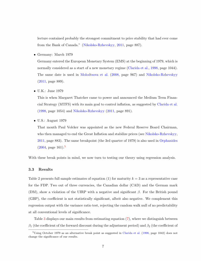
Figures (3a) and (3b) display 3 month forward rates of the DM and the GBP, both against

the CAD.6 Figure (3a) confirms our theory: β1 is significantly different from zero after allowing

for x = 11 months to adjust and β2 is insignificant outside the adjustment period. The British

pound in figure (3b) takes a little longer to react, since only after allowing for 23 months do our

results hold up. After that β2 becomes and stays insignificant.

Figure (3c) shows results for the DM when using the British pound as a base currency.7 While

β1 is highly significant as expected, β2 is only on the verge of insignificance. One explanation

why the DM/GBP rate may behave somewhat differently from other exchange rates could be

the special relationship between the Bundesbank and the Bank of England: between October

1990 and September 1992, the Bank of England was a part of the European Exchange Rate

Mechanism, thus not being independent from the Bundesbank.

Overall, violations of the UIRP do not seem to be driven by the Fed only, but rather by

changes in monetary policy of all central banks in question.

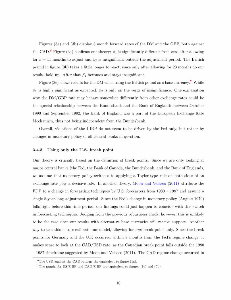
3.4.3 Using only the U.S. break point

Our theory is crucially based on the definition of break points. Since we are only looking at

major central banks (the Fed, the Bank of Canada, the Bundesbank, and the Bank of England),

we assume that monetary policy switches to applying a Taylor-type rule on both sides of an

exchange rate play a decisive role. In another theory, Moon and Velasco (2011) attribute the

FDP to a change in forecasting techniques by U.S. forecasters from 1980 – 1987 and assume a

single 8-year-long adjustment period. Since the Fed’s change in monetary policy (August 1979)

falls right before this time period, our findings could just happen to coincide with this switch

in forecasting techniques. Judging from the previous robustness check, however, this is unlikely

to be the case since our results with alternative base currencies still receive support. Another

way to test this is to reestimate our model, allowing for one break point only. Since the break

points for Germany and the U.K occurred within 8 months from the Fed’s regime change, it

makes sense to look at the CAD/USD rate, as the Canadian break point falls outside the 1980

– 1987 timeframe suggested by Moon and Velasco (2011). The CAD regime change occurred in

6The USD against the CAD returns the equivalent to figure (1a).7The graphs for US/GBP and CAD/GBP are equivalent to figures (1c) and (5b).

10

January 1988. Figure (3d) shows β1 and β2 when only allowing for the Fed’s break point in the

CAD/USD exchange rate. Notice that we extend the time frame displayed up to 120 months

here, mimicking Moon and Velasco (2011). There is no difference in terms of significance if we

look at the time during or outside the adjustment period: both β1 and β2 are insignificant for

up to 89 months.

In summary, our results do not seem to be driven by the maturity of the forward rate or the

base currency. Further, it seems unlikely that our results coincide with another explanation as

regime changes by both participating central banks seem to play a role in creating the FDP.

4 Conclusion

This paper argues that a major cause of the forward discount puzzle (FDP) – the violation of

the uncovered interest rate parity (UIRP) – are switches by central banks from a destabilizing

regime (not using a Taylor-type rule) to a stabilizing regime (following a Taylor-type rule). First,

we develop a model relating these regime changes to the forward discount puzzle. After a central

bank switches to using a Taylor-type rule, forecasters fail in predicting the exchange rate and

need time to adjust to the new regime. This period of adaptation is when the forward discount

puzzle emerges. Our empirical part confirms this theory examining the Canadian dollar, the

German mark, and the British pound, all against the U.S. dollar. Indeed, the UIRP is only

significantly violated during the adjustment periods of about 1 – 2 years following the regime

changes by both respective central banks. The forward discount puzzle is not significant outside

the adjustment periods. Our results are robust to using different maturities and base currencies.

Further, using only one break point for an exchange rate and neglecting the regime change by

the opposite central bank does not seem sufficient. This substantially weakens the possibility of

our explanation coinciding with any other contemporary events.

Our results provide additional evidence for the expectations errors hypothesis, one of the

most prominent potential explanations for the forward discount puzzle. By naming and testing

a specific reason for why expectations are biased – major regime switches to applying a Taylor-

type rule – this result adds another piece to solving the forward discount puzzle.

11

References

Alvarez, F., Atkeson, A., and Kehoe, P. (2009). Time-varying risk, interest rates, and exchange

rates in general equilibrium. Review of Economic Studies, 76(3):851–878.

Bacchetta, P. and Van Wincoop, E. (2007). Random walk expectations and the forward discount

puzzle. The American Economic Review, 97(2):346–350.

Bacchetta, P. and Van Wincoop, E. (2010). Infrequent portfolio decisions: A solution to the

forward discount puzzle. The American Economic Review, 100(3):870–904.

Bacchetta, P. and Wincoop, E. V. (2005). Rational inattention: A solution to the forward

discount puzzle. Working Paper 11633, National Bureau of Economic Research.

Chinn, M. (2006). The (partial) rehabilitation of interest rate parity in the floating rate era:

Longer horizons, alternative expectations, and emerging markets. Journal of International

Money and Finance, 25(1):7–21.

Choi, K. and Zivot, E. (2007). Long memory and structural changes in the forward discount:

An empirical investigation. Journal of International Money and Finance, 26(3):342–363.

Clarida, R., Gali, J., and Gertler, M. (1998). Monetary policy rules in practice:: Some interna-

tional evidence. European Economic Review, 42(6):1033–1067.

Engel, C. (1996). The forward discount anomaly and the risk premium: A survey of recent

evidence. Journal of empirical finance, 3(2):123–192.

Frankel, J. and Froot, K. (1990). Chartists, fundamentalists, and trading in the foreign exchange

market. The American Economic Review, pages 181–185.

Froot, K. and Frankel, J. (1989). Forward discount bias: Is it an exchange risk premium? The

Quarterly Journal of Economics, 104(1):139–161.

Froot, K. and Thaler, R. (1990). Anomalies: foreign exchange. The Journal of Economic

Perspectives, 4(3):179–192.

Gourinchas, P. and Tornell, A. (2004). Exchange rate puzzles and distorted beliefs. Journal of

International Economics, 64(2):303–333.

12

Lewis, K. K. (1995). Chapter 37 puzzles in international financial markets. volume 3 of Handbook

of International Economics, pages 1913 – 1971. Elsevier.

Lothian, J. and Wu, L. (2011). Uncovered interest-rate parity over the past two centuries.

Journal of International Money and Finance, 30(3):448–473.

Lustig, H. and Verdelhan, A. (2007). The cross section of foreign currency risk premia and

consumption growth risk. The American Economic Review, 97(1):89–117.

MacDonald, R. (2002). Expectations formation and risk in three financial markets: Surveying

what the surveys say. Journal of Economic Surveys, 14(1):69–100.

Mark, N. and Wu, Y. (1998). Rethinking deviations from uncovered interest parity: the role of

covariance risk and noise. The Economic Journal, 108(451):1686–1706.

Molodtsova, T., Nikolsko-Rzhevskyy, A., and Papell, D. (2008). Taylor rules with real-time data:

A tale of two countries and one exchange rate. Journal of Monetary Economics, 55:S63–S79.

Moon, S. and Velasco, C. (2011). The forward discount puzzle: Identi cation of economic

assumptions. Research Institute for Market Economy, Sogang University Working Papers.

Nikolsko-Rzhevskyy, A. (2011). Monetary policy estimation in real time: Forward-looking taylor

rules without forward-looking data. Journal of Money, Credit and Banking, 43(5):871–897.

Orphanides, A. (2004). Monetary policy rules, macroeconomic stability, and inflation: A view

from the trenches. Journal of Money, Credit, and Banking, 36(2):151–175.

Sakoulis, G., Zivot, E., and Choi, K. (2010). Structural change in the forward discount: Implica-

tions for the forward rate unbiasedness hypothesis. Journal of Empirical Finance, 17(5):957–

966.

Sarantis, N. (2006). Testing the uncovered interest parity using traded volatility, a time-varying

risk premium and heterogeneous expectations. Journal of International Money and Finance,

25(7):1168–1186.

Taylor, J. (1993). Discretion versus policy rules in practice. In Carnegie-Rochester conference

series on public policy, volume 39, pages 195–214. Elsevier.

13

Verdelhan, A. (2010). A habit-based explanation of the exchange rate risk premium. The Journal

of Finance, 65(1):123–146.

14

-6

-5

-4

-3

-2

-1

0

1

2

6 8 10 12 14 16 18 20 22 24 26 28 30 32 34 36 38 40 42 44 46 48 50 52 54 56 58 60

Adjustment Period, x

a) CAD/USD, k = 3 Month Maturity

-7

-6

-5

-4

-3

-2

-1

0

1

2

3

6 8 10 12 14 16 18 20 22 24 26 28 30 32 34 36 38 40 42 44 46 48 50 52 54 56 58 60

Adjustment Period, x

b) DM/USD, k = 3 Month Maturity

-10

-8

-6

-4

-2

0

2

4

6

8

6 8 10 12 14 16 18 20 22 24 26 28 30 32 34 36 38 40 42 44 46 48 50 52 54 56 58 60

Adjustment Period, x

c) BP/USD, k = 3 Month Maturity

Figure 1: Using Different Base Currencies or Only the U.S. Break Point

15

-8

-7

-6

-5

-4

-3

-2

-1

0

1

2

6

8

10

12

14

16

18

20

22

24

26

28

30

32

34

36

38

40

42

44

46

48

50

52

54

56

58

60

Adju

stm

ent

Per

iod, x

a)

CA

D/

USD

, k =

1 M

on

th M

aturi

ty

-6

-5

-4

-3

-2

-1

0

1

2

3

6

8

10

12

14

16

18

20

22

24

26

28

30

32

34

36

38

40

42

44

46

48

50

52

54

56

58

60

Ad

just

men

t P

erio

d, x

b)

D

M/U

SD

, k

= 1

Mo

nth

Mat

uri

ty

-10

-8

-6

-4

-2

0

2

4

6

8

6

8

10

12

14

16

18

20

22

24

26

28

30

32

34

36

38

40

42

44

46

48

50

52

54

56

58

60

Ad

just

men

t P

erio

d, x

c)

BP

/U

SD

, k

= 1

Mo

nth

Mat

uri

ty

-5

-4

-3

-2

-1

0

1

2

6

8

10

12

14

16

18

20

22

24

26

28

30

32

34

36

38

40

42

44

46

48

50

52

54

56

58

60

Ad

just

men

t P

erio

d, x

d)

CA

D/U

SD

, k

= 6

Mo

nth

Mat

uri

ty

-7

-6

-5

-4

-3

-2

-1

0

1

2

6

8

10

12

14

16

18

20

22

24

26

28

30

32

34

36

38

40

42

44

46

48

50

52

54

56

58

60

Ad

just

men

t P

erio

d, x

e)

DM

/U

SD

, k

= 6

Mo

nth

Mat

uri

ty

-12

-10

-8

-6

-4

-2

0

2

6

8

10

12

14

16

18

20

22

24

26

28

30

32

34

36

38

40

42

44

46

48

50

52

54

56

58

60

Ad

just

men

t P

erio

d, x

f)

BP

/U

SD

, k

= 6

Mo

nth

Mat

uri

ty

-5

-4

-3

-2

-1

0

1

6

8

10

12

14

16

18

20

22

24

26

28

30

32

34

36

38

40

42

44

46

48

50

52

54

56

58

60

Ad

just

men

t P

erio

d, x

g)

CA

D/

USD

, k =

12 M

on

th M

aturi

ty

-7

-6

-5

-4

-3

-2

-1

0

1

2

6

8

10

12

14

16

18

20

22

24

26

28

30

32

34

36

38

40

42

44

46

48

50

52

54

56

58

60

Ad

just

men

t P

erio

d, x

h)

D

M/U

SD

, k

= 1

2 M

on

th M

aturi

ty

-10

-8

-6

-4

-2

0

2

4

6

8

6

8

10

12

14

16

18

20

22

24

26

28

30

32

34

36

38

40

42

44

46

48

50

52

54

56

58

60

Ad

just

men

t P

erio

d, x

i)

BP

/U

SD

, k

= 1

2 M

on

th M

aturi

ty

Fig

ure

2:

Usi

ng

Diff

eren

tM

atu

riti

es

16

-10

-8

-6

-4

-2

0

2

4

6 8 10 12 14 16 18 20 22 24 26 28 30 32 34 36 38 40 42 44 46 48 50 52 54 56 58 60

Adjustment Period, x

a) DM/CAD, k = 3 Month Maturity

-14

-12

-10

-8

-6

-4

-2

0

2

4

6

6 8 10 12 14 16 18 20 22 24 26 28 30 32 34 36 38 40 42 44 46 48 50 52 54 56 58 60

Adjustment Period, x

b) BP/CAD, k = 3 Month Maturity

-6

-5

-4

-3

-2

-1

0

1

6 8 10 12 14 16 18 20 22 24 26 28 30 32 34 36 38 40 42 44 46 48 50 52 54 56 58 60

Adjustment Period, x

c) DM/BP, k = 3 Month Maturity

-4

-3

-2

-1

0

1

2

3

4

7

10

13

16

19

22

25

28

31

34

37

40

43

46

49

52

55

58

61

64

67

70

73

76

79

82

85

88

91

94

97

100

103

106

109

112

115

118

Adjustment Period, x

d) CAD/USD, k = 3 Month Maturity, only U.S. Break Point

Figure 3: Using Different Base Currencies or Only the U.S. Break Point

17

Table 1: Summary Statistics (k = 3-month maturity)

Mean Sample Period Observations Break Point(Std. Dev.)

Canadian dollar January 1988

Foreign excess -0.0023 January 1978 – 404Returns (0.0307)) November 2011s(t+ k)− f(t|k)

Forward discount 0.0017 January 1978 – 404f(t|k)− s(t) (0.0040) November 2011

German mark January 1979

Foreign excess 0.0026 January 1978 – 248Returns (0.0587) December 1998s(t+ k)− f(t|k)

Forward discount -0.0051 January 1978 – 248f(t|k)− s(t) (0.0082) December 1998

British pound June 1979

Foreign excess -0.0027 January 1978 – 404Returns (0.0543) November 2011s(t+ k)− f(t|k)

Forward discount 0.0041 January 1978 – 404f(t|k)− s(t) (0.0060) November 2011

US dollar August 1979

Notes: Break points indicate the respective central bank’s switch in monetary policy (please see section 3.2for details). The source of data is “Global Insight.” Data for Germany stops in December, 1998 due to theintroduction of the Euro on January 1, 1999.

18

Table 2: Full Sample Results, k = 3 month maturity

(1) (2) (3)

Canadian German Britishdollar mark pound

Dependent variable :foreign excess returns, s(t+ 3)− f(t|3)

Constant -0.000 -0.005 0.005(0.003) (-0.007) (0.005)

Forward discount -1.111* -1.429* -1.854f(t|3)− s(t) (0.620) (0.742) (1.225)

Variance ratio test 3.106 4.664 5.033P-value 0.006** 0.000** 0.000**

R2 0.021 0.040 0.042

Observations 404 248 404

Notes: * and ** indicate significance at the 10 and 5 percent level. Newey-West corrected standard errors arein parentheses. All exchange rates are measured against the U.S. dollar. p-value for the variance ratio test forforeign excess returns are obtained using the wild bootstrap method as recommended by Kim (2006).

19

Tab

le3:

Res

ult

sfo

rx

=18

andx

=36

mon

ths

ofad

just

men

t

(1)

(2)

(3)

(4)

(5)

(6)

Can

adia

nG

erm

an

Bri

tish

Can

ad

ian

Ger

man

Bri

tish

dol

lar

mark

pou

nd

doll

ar

mark

pou

nd

(18

mon

ths)

(18

month

s)(1

8m

onth

s)(3

6m

onth

s)(3

6m

onth

s)(3

6m

onth

s)

Dependentvariable

:foreignexcessreturns,s(t

+3)−f

(t|3

)

Con

stan

t-0

.001

-0.0

05

0.0

05

-0.0

00

-0.0

06

0.0

03

(0.0

03)

(0.0

07)

(0.0

07)

(0.0

03)

(0.0

07)

(0.0

05)

For

war

dd

isco

unt

du

rin

g-2

.065

**-2

.322*

-2.7

79**

-1.4

31**

-2.4

92**

-3.9

12**

adju

stm

ent

per

iod

,β1

(0.7

98)

(1.2

03)

(0.9

31)

(0.4

12)

(1.0

52)

(1.6

32)

For

war

dd

isco

unt

outs

ide

-0.9

99-1

.179

-1.7

76

-0.9

01

-0.8

99

-1.3

59

adju

stm

ent

per

iod

,β2

(0.6

71)

(0.8

02)

(1.2

87)

(0.8

65)

(0.8

85)

(1.3

49)

R2

0.02

30.0

46

0.0

43

0.0

23

0.0

56

0.0

54

Ob

serv

atio

ns

404

248

404

404

248

404

Notes:

*and

**

show

signifi

cance

at

the

10

and

5p

erce

nt

level

.See

als

onote

sto

Table

2.

20