The Exchange Rate Response Puzzle

The Exchange Rate Response Puzzle1

Viktoria Hnatkovska

University of British Columbia

[email protected]

Amartya Lahiri

University of British Columbia

[email protected]

Carlos A.Vegh

University of Maryland and NBER

[email protected]

Draft: February 2012

1We would like to thank Paul Beaudry, Barbara Rossi and seminar participants at various universities andinstitutions for comments. Hnatkovska and Lahiri would like to thank SSHRC for research support.

Abstract

Standard models in open economy macroeconomics predict that an expansionary (contractionary)

monetary policy will lead to a currency depreciation (appreciation). The data, however, reveals an

interesting twist to this prediction. In a sample of 25 industrial and 47 developing countries, we find

that while the nominal exchange rate does indeed tend to appreciate in response to interest rate

increases in developed countries, in 75 percent of the developing countries, the nominal exchange

rate depreciates in response to an increase in the interest rate. These findings represent a puzzle for

standard models. To rationalize these empirical facts, we develop a monetary model where interest

rate changes have a money demand effect, a fiscal effect, and an output effect. We show that a

calibrated version of the model rationalizes the opposing responses in developed and developing

countries as the outcome of differing intensities of these opposing effects in the two groups.

JEL Classification: F3, F4

Keywords: Monetary policy, interest rates, exchange rates

1 Introduction

Standard models in open economy macroeconomics predict that an expansionary (contractionary)

monetary policy will lead to a currency depreciation (appreciation). In Dornbusch (1976) celebrated

overshooting model, for example, an increase in the money supply results in a lower nominal interest

rate and a more-than-proportional increase in the nominal exchange rate.1 The mechanism is simple

enough: due to sticky prices, an increase in the nominal money supply is tantamount to an increase

in the real money supply. Since output is taken as exogenous, this incipient excess supply of real

money balances requires a fall in the nominal interest rate to equilibrate the money market. Given

the interest parity condition, the nominal interest rate can only fall if the public expects an increase

in the rate of appreciation of the domestic currency. This is only possible if the nominal exchange

rate jumps above its long-run level and then falls over time.2

While the Dornbush-Obstfeld-Rogoff paradigm (or Mundell-Fleming in modern clothes) is, by

far, the most widely used in monetary models of the open economy, four other types of models yield

exactly the same prediction: (i) flexible prices model; (ii) liquidity-type models, (iii) models based

on the fiscal theory of the price level, and (iv) models with more than one liquid asset.

(i) Flexible price models: While not always recognized, frictions are not needed to rationalize the

idea of a negative relationship between nominal interest rates and the level of the exchange rate.

Consider the simplest possible monetary model with flexible prices and monetary neutrality. A

temporary increase in the level of the nominal money supply will lead, on impact, to a fall in

the nominal interest rate and an increase in the nominal exchange rate (i.e., a depreciation of the

currency).3 Intuitively, because the increase in the nominal money supply will be reversed in the

future, the nominal exchange rises less than proportionately. A fall in the nominal interest rate is

thus needed to equilibrate the money market.

(ii) Liquidity-type models: In liquidity-type models, an increase in the money supply also leads to a

fall in the nominal interest rate because the increased money supply affects disproportionately some

particular agents (say, financial firms).4 The nominal interest rate must fall for such agents to absorb

the excess liquidity. In an open economy, the fall in the nominal interest rate will be associated with

a currency depreciation.

1Dornbusch (1976) model is, of course, the traditional Mundell-Fleming model with rational expectations. Withadded microfoundations and other refinements —as reflected in Obstfeld and Rogoff (1995) highly influential version —this model continues to be the workhorse of international finance well into the 21st century.

2 It is important to note that we are characterizing the stance of monetary policy by looking at changes in the levelof the money supply, as opposed to changes in the rate of change of the money supply. In the latter case, inflationaryexpectations will be affected and an expansionary monetary policy will be associated with a higher nominal interestrate.

3This result is easy to show using, for instance, the continuous-time version presented in Vegh (2010). Of course,a permanent change in the nominal money supply would have no effects on the nominal interest rate.

4See, for example, Christiano and Eichenbaum (1992) and Grilli and Roubini (1996).

1

(iii) Fiscal-theory models: In open-economy models based on the fiscal theory of the price level

(see, for example, Auernheimer (2008)), we can think of the nominal interest rate as the policy

instrument. As long as the interest-rate elasticity of money demand is less than one (as is typically

the case in practice), an increase in the nominal interest rate raises inflation tax revenues. These

higher revenues imply that the government can afford to service a higher real stock of government

debt, which requires a fall in the price level (i.e., the nominal exchange rate). Conversely, a reduction

in the policy interest rate will lead to a currency depreciation.

(iv) Imperfect asset substitution models: In models with imperfect substitution between two liquid

assets, we can also think of the nominal interest rate on an interest-bearing liquid asset as a policy

instrument.5 An increase in this policy interest rate leads to an increased demand for the liquid

asset, which requires a fall in the nominal exchange rate.

There is thus overwhelming theoretical support for the proposition that expansionary monetary

policy (i.e., a lower nominal interest rate) should lead to a currency depreciation and vice versa.

But what does the empirical evidence say? Most of the empirical studies have looked at industrial

countries and conclude that, indeed, this theoretical proposition holds true. The best-known study

for the United States is Eichenbaum and Evans (1995) who conclude, using a vector autoregression

(VAR) analysis, that a contractionary monetary policy in the United States leads to an appreciation

of the dollar relative to all major currencies. In turn, Kim and Roubini (2000) use a structural VAR

approach, which takes care of some identification problems that had plagued this literature up to

this point, to look at non-US G-7 countries and reach the same conclusion.

Case closed? Not in our view. In fact, we will argue in this paper that, contrary to the case of

industrial countries, in developing countries the currency depreciates in response to an increase in

interest rates. We establish this stylized fact based on a sample of 25 industrial and 47 developing

countries.6 We first run individual VARs and conclude that, for industrial countries, the domestic

currency appreciates in response to an increase in interest rates in 84 percent of the cases. In sharp

contrast, for developing countries we show that the nominal exchange rate increases (i.e., the domestic

currency depreciates) in response to higher interest rates in 75 percent of the cases. We also illustrate

this finding by running panel VARs for industrial and developing countries separately and showing

how, in response to an increase in the interest rate, the currency appreciates in industrial countries

but depreciates in developing countries. Finally, we subject the data to a battery of alternative

specifications and methods and find that the results are robust to them. We will refer to these

contrasting findings in industrial versus developing countries as the “exchange rate response puzzle.”

5See Calvo and Vegh (1995) and Lahiri and Vegh (2003).6For several developing countries we have multiple episodes giving us a total of 55 developing country-episode pairs

in our sample.

2

In order to provide an explanation for the puzzling data fact, we choose to focus on three key

margins along which developed and developing countries are often viewed to be different. These

differences arise mostly due to institutional reasons but also may be due to them being in different

stages of the developmental process. The first is the fact that developed economies tend to have a

larger money base possibly due to a more stable monetary history. This tends to primarily show up

in a larger demand deposits to output ratio in developed countries. Second, developing economies

tend to have weaker public finances which raises their dependence on the inflation tax for financing

public expenditures. Third, developed countries tend to have more developed financial markets which

lowers the dependence of firms on bank finance relative to firms in developing countries. We provide

evidence on these patterns later in the paper. Crucially, we believe that these three features introduce

differences in the monetary transmission channel between developed and developing countries.

We formalize these three features by presenting a model with two liquid assets (cash and demand-

deposits) in which the central bank controls the interest rate on the liquid asset. The government

finances its budget deficit with inflationary finance and firms must rely on bank credit to finance

their working capital. In this set-up, an increase in the policy-controlled interest rate has three

key effects. First, the higher interest rate increases the interest rate on deposits, which raises the

demand for deposits. This money demand effect tends to appreciate the currency and thus captures

the traditional channel in our set-up. Second, by increasing the government’s debt service costs,

the higher interest rate raises the required seigniorage revenue to finance government spending and,

ceteris paribus, increases the inflation rate. The rise in inflation increases the opportunity cost of

holding liquid assets and tends to depreciate the currency. We will refer to this channel as the fiscal

effect. Third, the higher domestic interest rate raises the lending rate to firms and thereby reduces

employment and output. The output contraction reduces net revenues for the government and hence,

increases the required seigniorage revenue to finance the government budget. This output effect also

tends to depreciate the currency.

The net effect of a higher policy-controlled interest rate on the nominal exchange rate will thus

depend on the relative strength of the money demand, fiscal, and output effects. If the money

demand effect dominates the other two, then higher interest rates will lead to an appreciation of

the currency. Conversely, if the money demand effect is dominated by the other two, the currency

will depreciate. Our way of solving the exchange rate response puzzle is to argue —and then show

quantitatively —that the fiscal effect and the output effects will typically be larger in developing than

in industrial countries. The fiscal effect is larger because, traditionally, developing countries have

ran larger fiscal deficits and relied more on inflationary finance (see, for instance, Fischer, Sahay, and

Vegh (2002)). The output effect is larger because firms in developing countries need to rely more on

3

bank credit as they are mostly unable to raise funds by issuing commercial paper.

As a final step, we recalibrate our model to developing and developed countries. We show that

the model-generated impulse responses of exchange rates reproduce the patterns estimated in the

data.

We should note at the outset that our paper is not concerned with the relationship between the

nominal market interest rate and the rate of currency depreciation. There is a voluminous literature

which attempts to document and/or explain this relationship. This literature is concerned with the

failure of the uncovered interest parity (UIP) condition (the “forward premium anomaly”). In our

model interest parity holds for internationally traded bonds. Hence, we do not shed any new light on

the observed deviations from UIP. Instead, our main focus is on the effects of policy-induced changes

in nominal interest rates on the level of the exchange rate.

The rest of the paper is organized as follows. The next section presents some empirical evidence

from a number of developing and developed countries detailing the mixed results on the relation-

ship between interest rates and the exchange rate. Section 3 presents the model while Section 4

discusses how the model is calibrated and solved. Section 5 presents our quantitative results using

the calibrated model. The last section concludes.

2 Empirical facts

We start off by empirically documenting our motivating issue through a look at the data. We use

a large sample of countries during 1974:1-2010:12 period for which monthly data on exchange rates

and interest rates was available. Most of the data is from International Financial Statistics (IFS)

compiled by the International Monetary Fund (IMF). We use period average offi cial exchange rates

whenever available to measure exchange rates. If offi cial rates are not available, we turn to period

average market rates, otherwise we use the period average principal exchange rates. Exchange rates

are in domestic currency units per U.S. dollar, so that an increase is a depreciation of local currency

relative to the US dollar. Our focus is on policy-controlled interest rates, which we measured in the

data as the period average T-bill rate. If T-bill rate was not available, we used the discount rate, or

the money market rate for that country. We note that for majority of countries in our sample we

used the T-bill rate. This rate is the closest to the overnight interbank lending rates, which would

be our preferred policy rate, but is not available for most of our countries.7 In our analysis we focus

on the interest rate differential between home and abroad computed as domestic interest rate minus

7 In what follows we show that our results are robust to using only countries for which the T-bill rate is available.We also verify that our results are not driven by the fact that our measures of interest rates may potentially containinformation other than the monetary policy change, i.e. changes in expected inflation or in the perceived sovereignrisk.

4

U.S. Federal Funds rate.

We focus only on those countries and time periods that are characterized by a flexible exchange

rate regime. To perform the selection, we rely on the Reinhart and Rogoff (2004) classification of

historical exchange rate regimes. We classify a country as having a flexible exchange rate regime

if, in a given year, its exchange rate was either (i) within a moving band that is narrower than or

equal to +/-2% (i.e., allows for both appreciation and depreciation over time); or (ii) was classified

as managed floating; or (iii) was classified as freely floating; or (iv) was classified as freely falling

according to Reinhart and Rogoff (2004).8 These correspond to their fine classification indices of 11,

12, 13, and 14, respectively.9 We only focus on the post-Bretton Woods period for all countries. High

income OECD countries are included in our sample, irrespective of their exchange rate classification.

For the Eurozone countries, we used their national exchange rates before the introduction of the

Euro as separate episodes. Since 1999:1 we included a separate episode for the Euro area, for which

we used the Euro-dollar exchange rate and the ECB marginal lending facility rate as the policy rate.

According to Reinhart and Rogoff (2004) regime classification, some countries had multiple episodes

of flexible exchange rates. We considered each such episode separately. To be included in our sample

we also require that an episode has at least 24 months of data in the flexible regime for each country.

This selection gives us a sample of 25 industrial country-episode pairs and 55 developing country-

episode pairs, for a total of 80 country-episode pairs. All country-episode pairs are listed in the

Appendix A.1.10

To illustrate the relationship between interest rate and the exchange rate, we first report some

simple time-series correlations between them. Panel A of Table 1 summarizes our results. We com-

pute correlations on a country-by-country basis for both levels and first-differences of (log) exchange

rate and interest rate variables, which are shown in the first column.11 Column “full sample”reports

the mean of all the time-series correlations obtained for the countries in our sample. Columns la-

8These categories are generally used in the literature to represent floating exchange rate regimes (see Reinhart andRogoff (2004)). In what follows we also check for robustness of our results with respect to the regime classification (seeSection 2.1.1).

9We also considered the coarse exchange rate classification of Reinhart and Rogoff (2004) to select countries andepisodes into the sample. We found the results to be robust with respect to the classification. The coarse classificationincluded countries that were on (i) pre announced crawling band that is wider than or equal to +/-2%; (ii) de factocrawling band that is narrower than or equal to +/-5%; (iii) moving band that is narrower than or equal to +/-2%;(iv) managed floating; (v) freely floating; (vi) freely falling. These correspond to indices 3, 4, and 5 in Reinhart andRogoff (2004).

10 It is probably not surprising that the majority of flexible exchange rate episodes in developing countries includedin our sample occur in the 1990s —the “globalization”decade.

11Using interest rates and exchange rate series in levels has been a conventional practice in the literature (see, forinstance, Kim and Roubini (2000), Faust and Rogers (2003) among others). Such approach implicitly assumes thatthe two variables are integrated of the same order. We confirm this result in our sample of countries. We test for thepresence of a unit root in the country exchange rate and interest rate differential series using augmented Dickey-Fullertest and Phillips-Perron test. We can not reject the presence of a unit root in the levels of both interest rate and (log)exchange rate for 90 percent of all country-episode pairs in our sample. Unit root it rejected in all country-episodepairs at 10 percent significance level when both variables are in first-differences.

5

belled “developed”and “developing”computes the corresponding correlations for the two groups of

countries separately. The results show that the correlation between exchange rates and interest rates

is low, on average. However, when the sample is broken into developed and developing countries,

the correlation is consistently negative in developed countries and consistently positive in developing

economies. Recall that negative correlation occurs when an increase in interest rate is accompanied

by an appreciation of the exchange rate, as in developed economies. In developing countries, higher

interest rates come together with currency depreciation, resulting in positive correlation between

them.

To confirm the significance of these correlations we also estimate simple regression of the log

exchange rate (or its first-difference) on a constant and domestic minus US interest rate differential

(or its first-difference) on a country-by-country basis. We then report the average of the slope

coeffi cients from these regressions and its 95% confidence interval for the full sample and separately

for developed and developing countries in the Panel B of Table 1. These regressions confirm our

findings from correlations: exchange rates and interest rates are negatively correlated in industrial

countries; and they are positively correlated in developing countries. These results hold in both levels

and first-differences and are highly statistically significant. Importantly, the confidence intervals for

the slope coeffi cients in developed and developing countries do not overlap, indicating significant

differences between them.

Table 1: Correlation between exchange rate and interest rate

Full sample Developed DevelopingPanel A

corr(lnEt, it − iust )mean 0.13 -0.09 0.24median 0.10 -0.08 0.36

corr(∆t lnE,∆t (i− ius))mean 0.06 -0.10 0.13median 0.03 -0.11 0.13

Panel BlnEt = β0 + β1(it − iust ) + εtmean(β1) 1.27 -0.74 2.1995% c.i.(β1) [1.13; 1.42] [-0.94; -0.54] [1.99; 2.39]

∆t lnEt = α0 + α1∆t(it − iust ) + utmean(α1) 0.02 -0.44 0.2495% c.i.(α1) [-0.08; 0.13] [-0.57; -0.31] [0.09; 0.38]

Note: Panel A of the Table reports the mean and median of the cross-sectional distribution of the correlationcoeffi cient between (log) exchange rate and interest rate (and their first-differences) for our sample of countries.Panel B presents the mean of the estimated slope coeffi cients from the regression lnEt = β0+β1(it− iust )+εtin levels and first-differences. 95% confidence intervals are in parenthesis.

6

We next turn to an analysis of the exchange rate-interest rate relationship using vector autore-

gressions (VARs). We estimate VAR on a country-by-country basis for our sample using log exchange

rate and interest rate differential between home and the U.S..12 Our VAR specification also includes

a constant term.13 We use the estimated VARs to calculate the impulse response of the exchange

rate to an orthogonalized one standard deviation innovation in the interest rate differential for each

country.14 Following Eichenbaum and Evans (1995) we compute the impulse responses using the

ordering: interest rate differential, exchange rate.15

Figure 1: Country VARs: Impulse responses of exchange rate to interest rate shock

.015

.01

.005

0.0

05.0

1

0 2 4 6 8 1 0m o n th s

90 % C I o r tho gona liz ed IR

re s pon s e o f le ra te to ir a te _d iff s h oc k s

Fra n c e

.015

.01

.005

0.0

05.0

1

0 2 4 6 8 1 0m o n th s

9 0 % C I o r th o g o n a liz e d IR

r e s p o n s e o f le r a te to ir a te _ d iff s h o c k s

S w e d e n

.01

5.

01.

005

0.0

05.0

1

0 2 4 6 8 1 0m o n th s



U n i te d _ K i n g d o m

.01

.01

.03

.05

0 2 4 6 8 1 0m o n th s



B ra zi l

.01

.01

.03

.05

0 2 4 6 8 1 0m o n th s



P h i l i p p i n e s

.01

.01

.03

.05

.07

.09

0 2 4 6 8 1 0m o n th s



M e xi c o , 1 9 8 2 m 2 1 9 8 8 m 1 1

Note: These figures present impulse responses of exchange rate to a positive interest rate innovationfrom individual country VARs estimated on (log) exchange rate and interest rate differential betweenhome and abroad. The following ordering is used: i− iUS , E.

We start by presenting the impulse responses of the nominal exchange rate to interest rate shocks

12 In our benchmark VAR specification we focus on interest rate differential and exchange rate variables only. Thisallows us to use and draw inference from the largest possible sample of countries. In section 2.1.2 we extend ourbenchmark VAR specification to include a broad set of other macroeconomic variables, such as output, prices, inflation,risk-premium, etc. Due to data limitations such analysis can only be conducted for a much smaller sample of countries.Nevertheless it allows us to provide robustness checks for the results in this section.

13We also tried a VAR specification with a trend and have found that the results remained largely unchanged.14 In each individual VAR we used the Akaike criterion to choose the lag length. The results remain unchanged when

Schwarz’s Bayesian information criterion (BIC) is used for selecting the lag length as the two criteria choose the samelag length in 97 percent of all cases.

15We conduct robustness checks with respect to the ordering of the variables in Section 2.1.3.

7

in several selected countries in our sample to illustrate the more general data fact. Figure 1 presents

the impulse responses in three developed and three developing countries. The picture reveals some

systematic patterns. For the developed countries —France, Sweden and the UK —there is a significant

appreciation of the currency in response to an increase in the interest rate differential. This is the

well-known result of Eichenbaum and Evans (1995). For the developing group the effect is the

opposite. In Brazil, Mexico and Philippines, a positive innovation in the interest rate differential

between home and the United States induces a significant depreciation of the currency.16

To check the generality of this differing relationship between interest rates and the exchange rate

in developed and developing countries, we ran individual country level VARs for all countries in our

sample.17 We adopted several approaches to classifying a country as exhibiting appreciation: (i) if

the response of its exchange rate after an interest rate shock is negative on impact; (ii) if the response

of its exchange rate to an interest rate shock is negative at the end of the 1st month; and (iii) if

the response of its exchange rate to an interest rate shock is negative at the end of the 1st quarter

(3rd month). Depreciation is defined similarly. Table 2 summarizes the results from the individual

country VARs, where we estimated a bivariate specification with variables ordered as i − iUS , lnE.Panel (a) reports the share of developed countries that have experienced appreciations and the share

of developing countries that experienced depreciations of their exchange rates following a positive

shock to the interest rate differential between home and abroad, based on level VARs.

Table 2: Individual country VARs: Summary

(a). Levels (b). First-differencesimpact 1 month 3 months impact 1 month 3 months

Bivariate VAR: i− iUS , lnEIndustrial countries: appreciation 84% 88% 84% 84% 88% 52%Developing countries: depreciation 75% 75% 75% 70% 62% 60%

Note: The table reports the fraction of developed (developing) countries that experience an appre-ciation (depreciation) of their exchange rate following a positive shock to the interest rate differen-tial. Appreciations and depreciations are defined based on the impact, 1st month and 1st quarter (3months) impulse responses from a country-by-country VAR analysis. The ordering used to obtain theorthogonalized impulse responses to interest rate shocks is i− iUS , E.

The results clearly indicate that an overwhelming majority of industrial economies see their

16Notice that some of these impulse responses have a hump-shaped pattern, which came to be known as the “delayedovershooting” result (see, for instance, Sims (1992), Eichenbaum and Evans (1995), among others). While there isongoing debate as for the reasons for such “delayed overshooting” pattern in exchange rate responses to monetarypolicy shocks (Faust and Rogers (2003), Bacchetta and van Wincoop (2010), Engel (2011)), our interest is on theimmediate response of the exchange rate. Thus when presenting results, we focus on the immediate responses.

17One may be concerned that the use of a linear VAR specification is not warranted in countries that experiencedlarge jumps in the level of the exchange rate or crisis episodes. We check the robustness of our results with respect tocrisis episodes and periods of high inflation in Section 2.1.1.

8

exchange rate appreciating after a positive interest rate shock both on impact (84 percent of all

industrial countries), as well as one month (88 percent of all industrial countries) and three months

after (84 percent of all industrial countries). For developing countries on the other hand, 75 percent

of countries show a depreciation following a positive interest rate shock on impact, after 1 month,

and the proportion remains at 75 percent if the cutoff is raised to the end of the 3rd month. If we

restrict our sample of countries to only those with T-bill data available, we find that our results

for developing countries become even stronger. In particular, in that subsample 83 percent of all

developing countries experienced an impact depreciation after an interest rate shock, and 80 percent

saw their currency depreciate one month later.

To check the robustness of our findings, we also re-estimate the individual VARs with the first

difference of the (log) exchange rate and the interest rate differential. The results from this estimation

and associated impulse responses are summarized in panel (b) of Table 2. Our earlier results remain

robust. In particular, we find that among industrial economies, 84 percent have experienced exchange

rate appreciation after an interest rate shock on impact, 88 percent still saw their currency appreciate

after the 1st month and 52 percent did so by the end of the first quarter. For the developing countries,

the corresponding numbers were 70 percent, 62 percent and 60 percent, respectively.18

We further confirm our empirical findings by running unrestricted, bivariate panel VARs for

industrial and developing countries separately. We start with a simple specification in which both

the (log) exchange rate and interest rate variables are included in levels. In the panel VAR analysis

country heterogeneity is likely to be important which suggests the presence of unobservable individual

country fixed effects. We eliminate country-specific fixed effects and common deterministic trends

by de-meaning and linearly de-trending both variables for each country. This within-transformation

wipes out fixed effects, but does not eliminate the fact that the lagged dependent variable and the

error term are correlated. This could lead the within-estimators to be inconsistent, unless T —the

time-series dimension of the data — is large. In our sample, the average number of periods across

countries is quite high, equal to 106 months in developing countries and 324 months in developed

economies. While this does not eliminate the bias in the estimates, it lends credibility to our level-

based results.19 An alternative transformation that eliminates the fixed effects is the first-difference

transformation. We present the results from the panel VARs on the first-differenced data below.

18We should note that when the model is estimated in first-differences, the exchange rate in the third month is thedifference between the exchange rate levels in months three and four. Hence, it is not surprising that the differencesin the responses of the groups to temporary shocks in the third month appear to be much smaller in first-differencesthan in levels since the first-difference observation reflects an additional period.

19We are interested in obtaining the results from the panel VAR in levels to retain comparability with the individualVAR results we presented earlier. An alternative transformation that preserves the VAR estimation in levels, but doesnot induce serial correlation, is based on the forward mean differencing (the Helmert procedure) as in Holtz-Eakin,Newey, and Rosen (1988) and Love and Zicchino (2006). We find our results to be robust to this transformation. Theseresults are available from the authors upon request.

9

Under either transformation of the data, the correlation between the lagged dependent variable

and the remainder error term remains. The standard approach of addressing this correlation is to

estimate the model coeffi cients by an instrumental variable (IV) method. We follow this practice

and apply the system generalized method of moments (GMM) of Arellano and Bond (1991) that

uses lagged regressors as instruments.

Figure 2 presents the impulse response of exchange rate to a positive interest rate innovation

together with the 90 percent confidence bands separately for our sample of industrial countries and

developing economies. It is easy to see that in response to an increase in the interest rate, the

currency appreciates in industrial countries but depreciates in developing countries.

Figure 2: Panel VAR: Impulse responses of exchange rate to interest rate shock (levels)

.006

.004

.002

0.0

02.0

04.0

06

0 2 4 6m o n th s

9 0 % C I o rth o g o n a l i ze d IR

re s p o n s e o f l e ra te to i ra te _ d i ff s h o c ks

D ev e lo p ed e c o no m ie s

.02

.01

0.0

1.0

2

0 2 4 6m o n th s

9 0 % C I o rth o g o n a l i ze d IR

re s p o n s e o f l e ra te to i ra te _ d i ff s h o c ks

D ev e lo p in g c ou n t rie s

Note: Figures present the impulse responses of the exchange rate to a positive interestrate differential shock from panel VARs estimated for developed and developing countries.Estimation uses (log) exchange rates and interest rates in levels. Both series are de-meanedand linearly de-trended.

Figure 3 presents the resulting impulse responses from the model estimated in first-differences.

As before, the exchange rate appreciates in our sample of developed countries; and depreciates for

developing countries, with the key difference being that these responses are more short-lived.

2.1 Robustness of empirical results

In this section we present a battery of additional robustness checks of our key empirical result:

interest rates and exchange rates are negatively related in industrial countries, but are positively

10

Figure 3: Panel VAR: Impulse responses of exchange rate to interest rate shock (1st differences)

.03

.02

.01

0.0

1.0

2.0

3

0 2 4 6m o n th s

9 0 % C I o rtho g o n a l i zed IR

re s p o n s e o f d l e ra te to d i ra te _ d i ff s h oc ks

D ev e loped ec onom ies

.02

.01

0.0

1.0

2

0 2 4 6m o n th s

9 0 % C I o rtho g o n a l i zed IR

re s p o n s e o f d l e ra te to d i ra te _ d i ff s h oc ks

D ev e lo p ing c oun t ries

Note: Figures present the impulse responses of the exchange rate to a positive interestrate differential shock from panel VARs estimated for developed and developing countries.Estimation uses (log) exchange rates and interest rates in first differences.

related in developing countries.

2.1.1 Exchange rate classification and crisis episodes

We begin by checking the robustness of our results with respect to the exchange rate classification.

As we noted above, we used the definition of the floating exchange rate regime following Reinhart

and Rogoff (2004) and the existing literature. This classification included the following categories:

exchange rate in a given year was (i) within a moving band that is narrower than or equal to +/-

2% (i.e., allows for both appreciation and depreciation over time); or (ii) was classified as managed

floating; or (iii) was classified as freely floating; or (iv) was classified as freely falling. The latter

“freely falling”category included countries in the following circumstances. First, it included countries

that have experienced inflation rates above 40 percent over the 12 month period. Second, it included

periods during the six months immediately following a currency crisis and accompanied by a regime

switch from a fixed or quasi fixed regime to a managed or independently floating regime.

To verify that our results are not driven by the high-inflation countries or crisis episodes, we

exclude these “freely falling” country-episodes from our benchmark sample. This leaves us with a

selection of 58 country-episode pairs in total, of which 25 are developed country-episode pairs and

33 are developing country-episode pairs. Table 3 reports correlation and regression results for this

modified sample. As is easy to see, all results remain practically unchanged and highly significant.

We also verify our individual country VARs and panel VARs for this restricted sample of countries

11

Table 3: Correlation between exchange rate and interest rate: No crisis or high inflation episodes

Full sample Developed DevelopingPanel A

corr(lnEt, it − iust )mean 0.15 -0.09 0.33median 0.11 -0.08 0.42

corr(∆t lnE,∆t (i− ius))mean 0.00 -0.10 0.08median -0.03 -0.11 0.05

Panel BlnEt = β0 + β1(it − iust ) + εtmean(β1) 1.21 -0.74 2.6995% c.i.(β1) [1.05; 1.37] [-0.94; -0.54] [2.45; 2.93]

∆t lnEt = α0 + α1∆t(it − iust ) + utmean(α1) -0.06 -0.44 0.2295% c.i.(α1) [-0.16; 0.04] [-0.57; -0.31] [0.08; 0.37]

Note: Panel A of the Table reports the mean and median of the cross-sectional distribution of thecorrelation coeffi cient between (log) exchange rate and interest rate (and their first-differences) for oursample of countries. Panel B presents the mean of the estimated slope coeffi cients from the regressionlnEt = β0+β1(it− iust ) + εt in levels and first-differences. 95% confidence intervals are in parenthesis.

and episodes. Our results change only marginally for developing countries. For instance, in bivariate

VARs estimated on the levels of (log) exchange rate and interest rate differential we find that 71

percent of developing countries experienced depreciation after a positive shock to the interest rate

differential on impact, 74 percent saw their currency depreciating 1 month after the shock, and ex-

change rate continued to depreciate 3 months after the shock in 76 percent of developing countries.20

The panel VAR results also go through unchanged.

2.1.2 VAR specification

One concern that may arise in the bivariate VAR specification we estimated above is related to

inflation. In particular, developing countries often experience higher inflation rates and may be more

susceptible to inflationary shocks. Hence, their interest rate innovations might be endogenous policy

responses to inflationary shocks which also tend to depreciate the currency. To account for this

possibility we amend our VAR specification to include monthly CPI. There are two specifications

that are popular in the literature. We examine both.

Specification (1): Price level shocks. First, following Eichenbaum and Evans (1995), for every country

we estimate a three-variable VAR that includes its (log) consumer price index (CPI), its interest

20Note that no industrial country is classified as “freely falling” in Reinhart and Rogoff (2004).

12

rate differential with the U.S., and its (log) exchange rate. This is the same as our benchmark

specification except that we have now also included the domestic price level. To obtain orthogonalized

impulse responses we use the same ordering as in Eichenbaum and Evans (1995): Price level, interest

rate differential, exchange rate. The data on all three variables, however, is available only for a

subsample of our countries. Thus, our subsample with CPI consists of 59 country-episode pairs, of

which 17 are for developed economies and 42 are for developing countries. We find that our results

remain robust under this extended model specification. As shown in panel (1) of Table 4, among

developed countries, 82 percent exhibit a currency appreciation on impact after a positive interest

rate innovation. In contrast, 76 percent of developing countries saw their currency depreciating on

impact after a positive interest rate shock. By the end of the first month, 82 percent of developed

countries saw an appreciation of their currency, while 67 percent of developing countries experienced

depreciations. By the end of the third month, the corresponding numbers were 82 percent and

74 percent. When estimated in growth rates, our VAR analysis suggests an impact exchange rate

appreciation following a positive shock to the interest rate differential in 82 percent of developed

countries and an exchange rate depreciation in 73 percent of all developing countries.

Specification (2): Inflation shocks. Second, we try another specification that is common in the

literature which uses the inflation rate rather than the price level (see, for instance, Grilli and

Roubini (1995, 1996)). Hence, we estimate a three-variable VAR that includes the domestic CPI

inflation rate differential over the U.S. CPI inflation rate, the interest rate differential between home

and the US, and the (log) exchange rate. We obtain orthogonalized impulse responses using the

ordering: Inflation rate differential, interest rate differential, exchange rate. As can been seen in

panel (2) of Table 4, under this specification, an orthogonalized interest rate shock led to an impact

appreciation of the exchange rate in 82 percent of all developed countries but a depreciation in 67

percent of developing countries. At the end of the first and third month, the corresponding numbers

were 82 percent for developed countries and 69 percent for developing economies.21

Specification (3): Expected inflation shocks. Inflation may matter for interest rate-exchange rate

relationship in another important way. It may be the case that interest changes reflect endogenous

policy responses to expected inflationary shocks. To account for this possibility, we estimate another

modified VAR in which we include one month ahead inflation differential between home and the U.S.

We order variables as follows: Forward CPI inflation differential, interest rate differential, exchange

rate. The results are presented in Panel (3) and confirm that our earlier findings remain unchanged

for developed countries and in fact become stronger for developing countries.

Specification (4): Risk premium shocks. Another potential concern is that the joint dynamics of

21Note that we do not run this specification in first-differences since CPI inflation is already the first-difference ofthe log price level.

13

Table 4: Individual country VARs: Robustness

(a). Levels (b). First-differencesimpact 1 month 3 months impact 1 month 3 months

(1) With CPI level: lnP, i− iUS , lnEIndustrial countries: appreciation 82% 82% 82% 82% 82% 52%Developing countries: depreciation 76% 67% 74% 73% 65% 68%

(2) With inflation differential: π − πUS , i− iUS , lnEIndustrial countries: appreciation 82% 82% 82% — —Developing countries: depreciation 67% 69% 69% — —

(3) With forward inflation differential: πt+1 − πUSt+1, it − iUSt , lnEtIndustrial countries: appreciation 82% 82% 82% — —Developing countries: depreciation 71% 69% 71% — —

(4) With risk-premium: rp, i− iUS , lnEIndustrial countries: appreciation 72% 84% 84% — —Developing countries: depreciation 72% 72% 69% — —

(5) With output: ln y, i− iUS , lnEIndustrial countries: appreciation 84% 89% 84% — —Developing countries: depreciation 64% 73% 64% — —

(6) With output, CPI and risk-premium: rp, ln y, lnP, i− iUS , lnEIndustrial countries: appreciation 83% 92% 92% — —Developing countries: depreciation 70% 60% 70% — —

Note: The table reports the fraction of developed (developing) countries that experience an appreci-ation (depreciation) of their exchange rate following a positive shock to the interest rate differential.Appreciations and depreciations are defined based on the impact, 1st month and 1st quarter (3 months)impulse responses from a country-by-country VAR analysis.

exchange rates and interest rates are driven by the changes in country risk-premiums. For instance,

if the country risk-premium rises, its currency may depreciate. At the same time, its Central Bank

may be compelled to raise domestic interest rates to counterweight the effect of the rising risk-

premium. To account for such a possibility, we control for the risk-premium in the country VARs.

Unfortunately, country-specific measures of risk-premium are available only for a very small group

of developing countries. Instead we proxy developing country risk premia with junk bond spreads

that are known to be highly correlated with the sovereign bond spreads —a standard measure of the

country risk-premium (see Uribe and Yue (2006)). More precisely, we use Moody’s Seasoned Baa

Corporate Bond Yield spread over the U.S. T-bill rate as a measure of risk-premium.22 We re-run

22Blanchard (2004) also uses Baa spread and shows that it is a good instrument for risk-premium in Brazil.

14

our VARs and obtain orthogonalized impulse responses using the ordering: Risk-premium, interest

rate differential, exchange rate. The proportions of appreciating developed countries and depreciating

developing countries are reported in panel (4) of Table 4. As is easy to see, an overwhelming majority

of all industrial countries in our sample still see their exchange rate appreciating following shocks to

the interest rate, even after controlling for changes in the risk-premium. In contrast, in the majority

of developing countries in our sample, exchange rates depreciate in response to interest rate shocks.

We also use the Merryl Lynch High Yield Master II bond yield spreads to measure the risk-premium

and find that the results remain robust.23 Both series are available from the Board of Governors of

the Federal Reserve System.

Specification (5): Talor rules. Our policy-controlled interest rates may also be driven by endogenous

policy responses to changes in domestic business cycles due to a Taylor rule. To account for this

possibility we include industrial production (index, 2000 base year) in our baseline VAR specification.

This would be our preferred VAR specification, but industrial production data is only available for less

than a half (30 country-pairs to be precise, of which 19 belong to developed countries and 11 belong

to developing countries) of all country-episode pairs in our sample.24 The results for this subsample

are reported in Panel (5) of Table 4. Importantly, our results are confirmed again: on impact, 84

percent of developed countries showed appreciation after an orthogonalized shock to interest rate,

while developing countries showed depreciation in 64 percent of all cases. One month later 89 percent

industrial countries currencies continued to appreciate, while 73 percent of developing countries saw

depreciation. Three months later the proportions were 84 percent and 64 percent, respectively.

Specification (6): All shocks. Finally, we estimate an extended VAR specification, were we include

CPI level, industrial production and risk-premium into the benchmark specification. We assume the

following ordering for the variables: risk-premium, industrial production, price level, interest rate

differential, exchange rate. This identification strategy implies that innovations to interest rates have

effects on domestic real activity, the price level and the risk-premium with a one-period lag, but,

as before, can affect exchange rates contemporaneously. This identification scheme also implies that

shocks to output, prices and the risk-premium can affect domestic interest rates contemporaneously.

This ordering reflects the standard assumption in the literature that macroeconomic variables react

to monetary policy shocks with a lag, while monetary policy can respond to macroeconomic shocks

immediately. A similar structure is assumed for the relationship between the exchange rate and

macroeconomic variables: exchange rate can respond immediately to all shocks, but its effect on

23We prefer to report the results for the BAA spread because it is available for a longer period thus allowing us toestimate VARs for a larger sample of countries (79 country-episode pairs, as opposed to 44 country-episode pairs if weuse high-yield spread instead).

24The ordering follows Eichenbaum and Evans (1995), where industrial production appears first, followed by interestrate differential and (log) exchange rate.

15

macroeconomic variables percolates only with a lag. The ordering of the first three variables assumes

that risk-premium shocks are the most exogenous.25 The assumption that output shocks affect prices

immediately is standard in the literature (see, for instance, Bernanke and Blinder (1992)).

Due to limited data availability, this extended VAR can only be estimated for 22 country-pairs,

of which 12 are industrial country-pairs and 10 are developing country-pairs. The results for this

VAR specification are presented in Panel (6). A shock to interest rate that is orthogonal to domestic

output, the price level, and risk-premium, leads to currency appreciation on impact in 83 percent

of developed countries, the share increases to 92 percent of all developed countries after one month,

and 92 percent see their currency appreciating three months following the shock. The corresponding

numbers for developing countries are 70 percent, on impact, 60 percent after 1 month and 70 percent

after 3 months.

2.1.3 Structural VAR

In our VAR analysis so far we obtained identification of interest rate shocks by placing zero con-

temporaneous restrictions on the interaction between interest rates and the exchange rate. This

assumption, while standard in the literature, rules out potential simultaneity effects between interest

rates and exchange rates in identifying interest rate shocks. However, contemporaneous feedback

between interest rates and exchange rates may be important in developing countries, as emphasized

in the “fear of floating” literature (see Calvo and Reinhart (2002)). This literature documents the

tendency of monetary authorities, especially in developing countries, to respond to fluctuations in

the exchange rate. Furthermore, since the exchange rate is a forward looking variable, it may contain

information about the future prospects of the economy to which the monetary authority may want

to react. Both these concerns raise the question of whether our results are sensitive to the identifying

restrictions we used?

To address this question we estimate a structural VAR (SVAR) in which we allow for a con-

temporaneous correlation between interest rate and the exchange rate. Identification is obtained by

imposing a long-run restriction that interest rates have no long-run effects on the real exchange rate.

This is a standard neutrality assumption that holds in a number of theoretical monetary models

(see Clarida and Gali (1994)) and has been recently used in several empirical studies (see Bjørnland

(2009)).26 Thus, we estimate a structural VAR containing interest rate differential, i− iUS , and thefirst difference of the log real exchange rate ∆tlrer, imposing long-run neutrality restriction described

above.27 We find that our results remain largely unchanged. Based on structural impulse responses,

25We also try an alternative ordering where risk-premium variable is placed after output and price level, and findthat results remain unchanged.

26This restriction is also satisfied by the model we develop in this paper.27We estimate the SVAR on the first differenced (log) real exchange rate so that, in the spirit of Blanchard and

16

we find that 73 percent of all developing countries in our sample experienced impact depreciations

following an interest rate shock, 69 percent depreciated 1 month after the shock while 55 percent

experienced depreciations 3 months after the shock. We interpret these results as not necessarily

suggesting that the contemporaneous feedback between interest rates and exchange rate is not im-

portant. Instead we think that the exchange rate classification scheme of Reinhart and Rogoff (2004)

that we used to identify flexible exchange rate countries, by being based on the de-facto exchange

rate regime, allowed us to focus on the countries and episodes for which “fear of floating”was less

of a concern.

Overall, based on the variety of samples and the battery of approaches, the evidence suggests

that interest rates and exchange rates are negatively related in industrial countries, consistent with

the existing theories. However, the relationship between the two variables is reversed for developing

countries, thus challenging the existing theory. We will refer to these contrasting findings in industrial

versus developing countries as the “exchange rate response puzzle”. In the next section we show that

a simple modification of the existing theoretical frameworks can rationalize the puzzle.

3 The model

Consider a model of a small open economy that is perfectly integrated with the rest of the world in

both goods and capital markets. It is populated by four types of agents: households, firms, banks

and the government. The infinitely-lived representative household receives utility from consuming

a (non-storable) good and disutility from supplying labor. The world price of the good in terms of

foreign currency is fixed and normalized to unity. Free goods mobility across borders implies that

the law of one price applies. The representative firm combines capital and labor to produce final

goods, and is subject to a working capital requirement. As a result, it must borrow from the banks.

The representative bank acts as an intermediary between households and firms, but also lends to the

government. The latter is comprised of a fiscal and monetary authority. We describe the problem of

each agent in details next.

3.1 Households

Household’s lifetime welfare is given by

V = E0∞∑t=0

βtU (ct, xt) , (1)

Quah (1989), the effects of the interest rate shock on the level of the exchange rate add up to zero. See Appendix A.2for econometric details.

17

where c denotes consumption, x denotes labor supply, and β(> 0) is the exogenous and constant

rate of time preference. E denotes expectations. We assume that the period utility function of the

representative household is given by

U(c, x) =1

1− σ (c− ζxν)1−σ , ζ > 0, ν > 1.

Here σ is the intertemporal elasticity of substitution, ν − 1 is the inverse of the elasticity of labor

supply with respect to the real wage. These preferences are well-known from the work of Greenwood,

Hercowitz, and Huffman (1988), which we will refer to as GHH.28

Households use cash, H, and nominal demand deposits, D, for reducing transactions costs. Specif-

ically, the transactions costs technology is given by

st = v

(Ht

Pt

)+ ψ

(Dt

Pt

), (2)

where P is the nominal price of goods in the economy, and s denotes the non-negative transactions

costs incurred by the consumer. Let h (= H/P ) denote cash and let d (= D/P ) denote interest-

bearing demand deposits in real terms. We assume that the transactions technology is strictly convex.

In particular, the functions v(h) and ψ(d), defined for h ∈ [0, h], h > 0, and d ∈ [0, d], d > 0,

respectively, satisfy the following properties:

v ≥ 0, v′ ≤ 0, v′′ > 0, v′(h) = v(h) = 0,

ψ ≥ 0, ψ′ ≤ 0, ψ′′ > 0, ψ′(d) = ψ(d) = 0.

Thus, additional cash and demand deposits lower transactions costs but at a decreasing rate. The

assumption that v′(h) = ψ′(d) = 0 ensures that the consumer can be satiated with real money

balances.

In addition to the two liquid assets, households also hold a real internationally-traded bond, b,

and physical capital, k, which they can rent out to firms. The households flow budget constraint in

nominal terms is

Ptbt+1 +Dt +Ht + Pt (ct + It + st + κt)

= Pt

(Rbt + wtxt + ρtkt−1 + τ t + Ωf

t + Ωbt

)+(

1 + idt

)Dt−1 +Ht−1.

28These preferences have been widely used in the real business cycle literature as they provide a better description ofconsumption and the trade balance for small open economies than alternative specifications (see, for instance, Correia,Neves, and Rebelo (1995)). The key analytical simplification introduced by GHH preferences is that there is no wealtheffect on labor supply.

18

Foreign bonds are denominated in terms of the good and pay the gross interest factor R(= 1 + r),

which is constant over time. idt denotes the deposit rate contracted in period t − 1 and paid in

period t. w and ρ denote the wage and rental rates. τ denotes lump-sum transfers received from

the government. Ωf and Ωb represent dividends from firms and banks respectively. κ denotes

capital adjustment costs

κt = κ (It, kt−1) , κI > 0, κII > 0, (3)

i.e., adjustment costs are convex in investment. Lastly,

It = kt − (1− δ) kt−1. (4)

In real terms the flow budget constraint facing the representative household is thus given by

bt+1 + ht + dt + ct + It + st + κt (5)

= Rbt + wtxt + ρtkt−1 +ht−1

1 + πt+

(1 + idt1 + πt

)dt−1 + Ωf

t + Ωbt ,

where Ωf and Ωb denote dividends received by households from firms and banks, respectively. 1+πt =

PtPt−1

denotes the gross rate of inflation between periods t− 1 and t. We define the nominal interest

rate as

1 + it+1 = REt (1 + πt+1) . (6)

Households maximize their lifetime welfare equation (1) subject to equations (2), (3), (4) and

(5).

3.2 Firms

The representative firm in this economy produces the perishable good using a constant returns to

scale technology over capital and labor

yt = F (kt−1, Atlt) = Atkαt−1l

1−αt , (7)

with α > 0, and At denoting the current state of productivity which is stochastic. l is labor demand.

At the beginning of the period, firms observe shocks for the period and then make production plans.

They rent capital and labor. However, a fraction φ of the total wage bill needs to be paid upfront to

workers. Since output is only realized at the end of the period, firms finance this payment through

loans from banks. The loan amount along with the interest is paid back to banks next period.29

29Alternatively, we could assume that bank credit is an input in the production function, in which case the deriveddemand for credit would be interest rate elastic. This would considerably complicate the model without adding any

19

Formally, this constraint is given by

Nt = φPtwtlt, φ > 0, (8)

where N denotes the nominal value of bank loans. The assumption that firms must use bank credit

to pay the wage bill is needed to generate a demand for bank loans.

The firm’s flow constraint in nominal terms is given by

Ptbft+1 −Nt = Pt

(Rbft + yt − wtlt − ρtkt−1 − Ωf

t

)−(

1 + ilt

)Nt−1,

where il is the lending rate charged by bank for their loans and Ωf denotes dividends paid out by

the firms to their shareholders. bf denotes foreign bonds held by firms which pay the going world

interest factor R. In real terms the flow constraint reduces to

bft+1 − nt = Rbft −(

1 + ilt1 + πt

)nt−1 + yt − wtlt − ρtkt−1 − Ωf

t .

Define

aft+1 ≡ bft+1 −

(1 + ilt+1

)R (1 + πt+1)

nt.

Substituting this expression together with the credit-in-advance constraint into the firm’s flow con-

straint in real terms gives

aft+1 + Ωft = Raft + yt − ρtkt−1 − wtlt

[1 + φ

1 + ilt+1 −R (1 + πt+1)

R (1 + πt+1)

]. (9)

Note that φ1+ilt+1−R(1+πt+1)

R(1+πt+1)

wtlt =

1+ilt+1−R(1+πt+1)

R(1+πt+1)

nt is the additional resource cost that is

incurred by firms due to the credit-in-advance constraint.30

The firm chooses a path of l and k to maximize the present discounted value of dividends subject

to equations (7), (8) and (9). Given that households own the firms, this formulation is equivalent

to the firm using the household’s stochastic discount factor to optimize. The first order conditions

for this problem are given by two usual conditions and an Euler equation which is identical to the

household’s Euler equation. The two usual conditions are standard —the firm equates the marginal

product of the factor to its marginal cost. In the case of labor the cost includes the cost of credit.

This is proportional to the difference between the nominal lending rate and the nominal interest rate.

additional insights.30We should note that the credit-in-advance constraint given by equation (8) holds as an equality only along paths

where the lending spread 1 + il − R (1 + π) is strictly positive. We will assume that if the lending spread is zero, thisconstraint also holds with equality.

20

3.3 Banks

The banking sector is assumed to be perfectly competitive. The representative bank holds foreign

real debt, db, accepts deposits from consumers and lends to both firms, N , and the government in

the form of domestic government bonds, Z.31 It also holds required cash reserves, θD, where θ > 0 is

the reserve-requirement ratio imposed on the representative bank by the central bank. Banks face a

cost q (in real terms) of managing their portfolio of foreign assets. Moreover, we assume that banks

also face a constant proportional cost φn per unit of loans to firms. This is intended to capture the

fact that domestic loans to private firms are potentially special as banks need to spend additional

resources in monitoring loans to private firms.32 The nominal flow constraint for the bank is

Nt + Zt − (1− θ)Dt + Ptqt − Ptdbt+1 =(

1 + ilt − φn)Nt−1 + (1 + igt )Zt−1

−(

1 + idt

)Dt−1 + θDt−1 − PtRdbt − PtΩb

t , (10)

where ig is the interest rate on government bonds. We assume that banking costs are a convex

function of the foreign debt held by the bank:

qt = q(dbt+1

), q′ > 0, q′′ > 0.

The costly banking assumption is needed to break the interest parity condition between domestic

and foreign bonds. Throughout the paper we assume that the banking cost technology is given by

the quadratic function:

qt =γ

2

(dbt+1 − db

)2, (11)

where γ > 0 and db are constant parameters.33

Deflating the nominal flow constraint by the price level gives the bank’s flow constraint in real

terms:

Ωbt =

[R(1 + πt)− 1

1 + πt

][(1− θ) dt−1 − nt−1 − zt−1]+

ilt − φn

1 + πtnt−1+

igt1 + πt

zt−1−idt

1 + πtdt−1−qt, (12)

31Commercial bank lending to governments is particularly common in developing countries. Government debt isheld not only as compulsory (and remunerated) reserve requirements but also voluntarily due to the lack of profitableinvestment opportunities in crisis-prone countries. This phenomenon was so pervasive in some Latin American countriesduring the 1980’s that Rodriguez (1991) aptly refers to such governments as “borrowers of first resort”. For evidence,see Rodriguez (1991) and Druck and Garibaldi (2000).

32We should note that this cost φn is needed solely for numerical reasons since, as will become clear below, it givesus a bigger range of policy-controlled interest rates to experiment with. Qualitatively, all our results would go throughwith φn = 0.

33Similar treatment of banking costs of managing assets and liabilities can be found in Diaz-Gimenez, Prescott,Fitzgerald, and Alvarez (1992) and Edwards and Vegh (1997). This approach to breaking the interest parity conditionis similar in spirit to Calvo and Vegh (1995).

21

where we have used the bank’s balance sheet identity: Ptdbt+1 = Nt +Zt− (1− θ)Dt. Note that this

is equivalent to setting the bank’s net worth to zero at all times. Also, the quadratic specification for

banking costs along with the zero net worth assumption implies that these banking costs can also be

reinterpreted as a cost of managing the portfolio of net domestic assets since dbt+1 = Nt+Zt−(1−θ)DtPt

.

The representative bank chooses sequences of N, Z, and D to maximize the present discounted

value of profits subject to equations (10) taking as given the paths for interest rates il, id, ig, i, and

the value of θ and φn. We assume that the bank uses the household’s stochastic discount factor to

value its profits. Note that igt+1, ilt+1 and i

dt+1 are all part of the information set of the household at

time t.

The bank optimality conditions imply that we must have

ilt+1 = igt+1 + φn, (13)

idt+1 = (1− θ) igt+1. (14)

These conditions are intuitive. Loans to firms and loans to the government are perfect substitutes

from the perspective of commercial banks up to the constant extra marginal cost φn of monitoring

loans to private firms. Hence, equation (13) says that the interest rate charged by banks on private

loans should equal the rate on loans to the government plus φn. For every unit of deposits held

the representative bank has to pay id as interest. The bank can earn ig by lending out the deposit.

However, it has to retain a fraction θ of deposits as required reserves. Hence, equation (14) shows

that at an optimum the deposit rate must equal the interest on government bonds net of the resource

cost of holding required reserves.

It is instructive to note that as the marginal banking costs becomes larger the bank will choose

to keep its holdings of foreign assets closer to db. This can be checked from the bank first order

conditions; all of them imply that limγ→∞ dbt+1 = db. Hence, in the limit as banking costs becomes

prohibitively large, the bank will choose to maintain a constant portfolio of external assets or liabil-

ities.

3.4 Government

The government issues high powered money, M , and domestic bonds, Z, makes lump-sum transfers,

τ , to the public, and sets the reserve requirement ratio, θ, on deposits. Domestic bonds are interest

bearing and pay ig per unit. Since we are focusing on flexible exchange rates, we assume with no

loss of generality that the central bank’s holdings of international reserves are zero. We assume

that the government’s transfers to the private sector are fixed exogenously at τ for all t. Hence, the

22

consolidated government’s nominal flow constraint is

Ptτ + (1 + igt )Zt−1 = Mt −Mt−1 + Zt.

As indicated by the left-hand-side of this expression, total expenditures consist of lump-sum transfers,

debt redemption and debt service. These expenditures may be financed by issuing either high

powered money or bonds. In real terms the government’s flow constraint reduces to

τ +1 + igt1 + πt

zt−1 = mt + zt −1

1 + πtmt−1. (15)

Lastly, the rate of growth of the nominal money supply is given by:

Mt+1

Mt= 1 + µt+1, M0 given. (16)

It is worth noting that from the central bank’s balance sheet the money base in the economy is

given by

Mt = Ht + θDt.

Hence, M can also be interpreted as the level of nominal domestic credit in the economy.

The consolidated government (both the fiscal and monetary authorities) has three policy instru-

ments: (a) monetary policy which entails setting the rate of growth of nominal money supply; (b)

interest rate policy which involves setting ig (or alternatively, setting the composition of m and z

and letting ig be market determined); and (c) the level of lump sum transfers to the private sector τ .

Given that lump-sum transfers are exogenously-given, only one of the other two instruments can be

chosen freely while the second gets determined through the government’s flow constraint (equation

(15)). Since the focus of this paper is on the effects of interest rate policy, we shall assume through-

out that ig is an actively chosen policy instrument. This implies that the rate of money growth µ

adjusts endogenously so that equation (15) is satisfied.

3.5 Resource constraint

By combining the flow constraints for the consumer, the firm, the bank, and the government (equa-

tions (5), (9), (12) and (15)) and using equations (7) and (8), we get the economy’s flow resource

constraint:

at+1 = Rat + yt − ct − It − κt − st − qt, (17)

where a = b+ bf − db. Note that the right hand side of equation (17) is simply the current account.

23

3.6 Equilibrium relations

We start by defining an equilibrium for this model economy. The three exogenous variables in the

economy are the productivity process A and the two policy variables τ and ig. We denote the entire

state history of the economy till date t by st = (s0, s1, s2, ..., st). An equilibrium for this economy is

defined as:

Given a sequence of realizations A(st), ig(st), r and τ , an equilibrium is a sequence of state con-

tingent allocationsc(st), x(st), l(st), h(st), d(st), k(st), b(st), bf(st), db(st), n(st), z(st)and

pricesP(st), π(st), i(st), id(st), il(st), w(st), ρ(st)such that (a) at the prices the allocations

solve the problems faced by households, firms and banks; (b) factor markets clear; and (c) the gov-

ernment budget constraint (equation (15)) is satisfied.

Combining the government flow constraint with the central and commercial bank balance sheets

yields the combined government flow constraint:

τ = ht −(

1

1 + πt

)ht−1 + θ

(dt −

dt−11 + πt

)+ zt −

(1 + igt1 + πt

)zt−1. (18)

It is useful at this stage to clarify the process of nominal exchange rate determination in this

model. Let m = M/E be real money while nominal money is denoted by M = H + θD. Since h and

d are functions of i and i− id respectively, the money market equilibrium condition can be written

implicitly as h+ θd = L (i, ig) where L denotes the implicit aggregate demand for cash and deposits.

Note that in writing the implicit L function we have used the fact that id is linked one-for-one with

ig. At any date t, Mt is known while its growth rate µt+1 is endogenous. Money market equilibrium

then dictates that at date t the nominal exchange rate is given by

Et =Mt

L (it, igt ). (19)

For any given policy rate igt , the inflation rate πt (and hence the nominal interest rate it) is determined

from the government budget constraint (18). From equation (19), knowledge of igt and it are suffi cient

to determine the nominal exchange rate Et at that date for a givenMt. Note that the rate of nominal

money growth µ between dates t and t+ 1 also gets determined at date from equation (15). Hence,

Mt+1 gets determined at date t.34

34 It is important to note that there is no nominal indeterminacy in this model despite the policy rate being chosenexogenously. Essentially, the real money demand L is a function of both i and ig. While ig is exogenous, i is determinedendogenously within the model from the government budget constraint through the inflation tax that is required tofinance the exogenous level of public spending τ .

24

3.7 The tradeoffs

The model laid out above has the three key margins that we set out to include. To see this note that

a rise in the policy controlled interest rate ig has two direct effects. First, it raises both the lending

rate rate il and the deposit rate id. Ceteris paribus, this raises the lending spread il − i and reducesthe deposit spread i− id. The effect on the lending spread reduces the demand for loans and therebyalso reduces output. This is the “output” effect wherein higher interest rates have a recessionary

effect by raising the cost of financing working capital requirements. The lower deposit spread, on

the other hand, raises the demand for deposits. This increases the demand for money —the “money

demand”effect.

The fiscal effect is more complicated. Notice that an increase in ig directly increases the cost of

servicing government bonds Z which increases the fiscal burden. However, there are two other indirect

ways in which changes in the policy controlled rate impacts the fiscal balance of the government.

First, since a higher ig lowers the amount of private loans N , for a given level of demand deposits

commercial banks make more loans to the public sector, i.e., Z rises. This reduces the reliance on

inflationary finance today but raises the future fiscal burden through a higher base level of debt.

This effect arises as a consequence of the “output” effect. On the other side, a higher id raises

demand deposits with commercial banks. For a given level of private loans, this reduces the reliance

on inflationary finance today to finance government spending. This effect arises due to the “money

demand”effect.

The effect of an interest rate increase on the equilibrium nominal exchange rate then depends

on the net effect of these often offsetting effects. Notice that the exchange rate depends not just on

monetary conditions but also on the real side of the economy as well as the state of public finances.

They are all fundamental determinants of the exchange rate. Interest rate changes impact these

fundamentals in often opposing ways. This is likely to make its end effect on the exchange rate

non-linear and possibly non-monotonic. We explore these possibilities quantitatively below.

4 Calibration

Our next point of interest is whether this model can generate the difference in exchange rate behavior

between developed and developing countries that we saw in the data. In order to examine this, we

conduct policy experiments on a calibrated version of the model developed above. We proceed

by choosing two different sets of parameterizations for the calibrated model — one for developed

and another for developing countries. We then examine whether the response of the exchange rate

to domestic interest rate shocks can reproduce the documented differences between developed and

25

developing countries.

Our basic approach is to keep the majority of the parameters of the model common to both sets

of countries. The parameters that we calibrate separately for developed and developing countries are

those that control the three key features that we have introduced in the model: the money demand

effect, the fiscal effect and the output effect. By restricting the differences between the two groups

of countries, we feel that this approach allows us to better ascertain the quantitative power of the

margins we have introduced in the model. Clearly, the more parameters we calibrate separately for

the two groups the greater our ability to explain differences in the data patterns since developed and

developing countries differ along many more margins than the three that we have chosen to focus on

here.

We calibrate the model to match the properties of the two groups of countries. The bench-

mark parameterization for the developed countries group utilizes data for 6 industrial economies —

Australia, Canada, Netherlands, New Zealand, Sweden and UK —during the period 1974-2010. For

developing countries we use the data for Argentina, Brazil, Korea, Mexico, Philippines, and Thailand

for the same 1974-2010 period. When focusing on nominal variables, i.e. nominal interest rates, we

restrict the sample to the 1998-2010 period to eliminate the periods of high interest rate volatility

and high inflation in developing countries before and during the East Asian crisis. Detailed data

description and data sources are discussed in the Appendix A.3. The model calibration is such that

one period in the model corresponds to one quarter.

4.1 Functional forms and parameters

We assume that the capital adjustment cost technology is given by

κ(It, kt−1) =ξ

2kt−1

(It − δkt−1kt−1

)2, ξ > 0,

with ξ being the level parameter.

As in Rebelo and Vegh (1995), we assume that the transactions costs functions υ(.) and ψ(.)

have quadratic forms given by

sκ

(κ2 − λκκ +

(λκ2

)2),

where κ represents cash or demand deposits, κ = h, d, while sκ and λκ are the level parameters.This formulation implies that the demand for money components are finite and that transaction

costs are zero when the nominal interest rate is zero.

26

The transaction technology for the banks is given by a quadratic function

qt =γ

2

(dbt+1 − db

)2,

where dbt+1 = Nt+Zt−(1−θ)DtPt

. Here γ is a constant and db is a steady state level of banks’debt to

GDP ratio.

We begin by discussing parameters that are set to be common to both developed and develop-

ing countries. Most of these parameter values are borrowed from Neumeyer and Perri (2005) and

Mendoza (1991).35 In particular, we set the coeffi cient of relative risk aversion, σ, to 5, while the

curvature of the labor, υ, is set to 1.6. This value is within the range of values used in the literature.36

This implies the elasticity of labor demand with respect to real wage, 1υ−1 , equal to 1.67, consistent

with the estimates for the U.S. Labor weight parameter ζ in the utility function is chosen to match

the average working time of 1/5 of total time and is set to 2.48. Subjective discount factor, β, is

set to 0.97, as in Uribe and Yue (2006). Capital income share, α, is chosen to be equal to 0.38,

while a depreciation rate for capital, δ, of 4.4% per quarter. Capital adjustment costs parameter ξ is

calibrated to replicate the volatility of investment relative to the volatility of output in our sample.

The remaining parameters are calibrated to developed and developing countries separately using

the sample of 6 developed and 6 developing countries discussed above. Parameter θ determines the

reserve requirement ratio in the model and is calibrated to match the observed reserve requirements

in each group of countries. We measure reserve requirements in the data following Brock (1989),

who computes reserve requirements as the ratio of monetary base less currency outside banks to

M2 less currency outside banks. This gives us θ equal to 0.03 in developed countries and 0.10 in

developing economies over our sample period. Reserve requirement ratio θ, together with sκ and

λκ,κ = h, d parameters in the transactions costs technology for banks, jointly determine the levelof money demand in the model. We calibrate them to match several targets. First, we match the

average ratios of M1 to GDP in the data equal to 20% in developed countries and 10% in developing

economies. Second, we match the relative size of deposits to currency in circulation in the data

equal to 1 in developing countries and 4 in industrial economies. Finally, since the estimates for the

interest elasticities of deposits and cash are not readily available, we discipline our calibration by

picking parameters such that these elasticities are equalized within each group of countries in the

steady state. The lump-sum transfers paid by the government to the private sector, τ , are measured

as the net lending/borrowing by the general government as a share of GDP. Over our sample period,

35Note that all of these common parameters are almost the same in the two papers —Neumeyer and Perri (2005)who focus on Argentina and in Mendoza (1991) who calibrates to Canada.

36For example, Mendoza (1991) uses υ equal to 1.455 for Canada, while Correia, Neves, and Rebelo (1995) set υ to1.7 for Portugal.

27

this ratio is equal to -1.3% in developed economies, and -2.1% in developing countries.

It is important to note that the differences in the moments between developed and developing

countries that we relied on so far to calibrate our key parameters are systematic. For instance, all

developing countries in our calibration sample have higher reserve requirement ratios, significantly

lower ratio of M1 to GDP and ratio of deposits to cash, as well as larger negative fiscal imbalances.37

Based on these evidence, we believe that our key parameters are correlated with the level of income

and can be used to distinguish developed and developing countries.

The share of wage bill paid in advance, φ, is a diffi cult parameter to calibrate. Most of the existing

studies that incorporate such working capital constraints focus on industrial economies, and typically

assume that firms must borrow the entire wage bill in advance (see Christiano, Eichenbaum, and

Evans (2005), Altig, Christiano, Eichenbaum, and Linde (2011)). Schmitt-Grohé and Uribe (2006)

deviate from this practice and calibrate the share of the wage bill paid in advance to match the

average money-to-output ratio in the post-war US data. Their calibration implies that only 51% of

wage payments must be held in money. Rabanal (2007), whose main goal is to assess the importance

of the cost channel in monetary policy, estimates the wage-in-advance parameter in the U.S. equal to

0.15. For developing countries, Neumeyer and Perri (2005) assume φ equal to 1, while Uribe and Yue

(2006), find that a value of φ greater than 1 is needed to match the empirical impulse responses of

several macroeconomic aggregates with their counterparts in their model. Given the great uncertainty

in the literature associated with this parameter, we proceed as follows. We use the value for φ equal

to 0.15, as estimated by Rabanal (2007), and we fix this value to be the same for both developed and

developing countries. We then investigate the sensitivity of our quantitative results with respect to

this parameter. As we will argue later, this parameter determines the strength of the “output”effect

in the model, which works to depreciate the exchange rate following rises in ig. By requiring φ to be

the same in developed and developing countries under our benchmark parameterization, we eliminate

the differential contribution of this effect to the exchange rate dynamics in the two sets of countries.

If the working capital requirements are more pronounced in developing countries, so that the output

effect is stronger for them, by setting φ to be the same in developed and developing countries, we

give up an important degree of freedom in generating depreciation in developing countries in our

quantitative exercises.

We calibrate parameters γ and db to match the average net foreign asset position to GDP ratios

equal to -0.26% in developed economies and -0.33% in developing countries over our sample period.38

The proportional cost parameter φn in the banking sector’problem is chosen to match the average

37The only exception is Korea, whose fiscal balance to GDP ratio is positive, on average.38 In fact, we restrict γ to be the same in the two groups of countries to reduce the number of the free parameters.

The resulting banking costs, q, in the steady state are very small, equal to less than 0.00086% of GDP.

28

spread of nominal lending rate over money market rate equal 9% in developing countries and 5%

in developed economies over our sample period. Table 5 summarizes parameter values under our

benchmark parametrization.39

Table 5: Benchmark parameter values

preferences developed developingdiscount factor β 0.971 0.971risk-aversion σ 5 5labor curvature υ 1.6 1.6labor weight ζ 2.48 2.48technologycapital income share α 0.38 0.38depreciation rate δ 0.044 0.044share of wage-in-advance φ 0.15 0.15capital adjustment costs ξ 4.5 4.5moneyreserve requirement θ 0.03 0.10transaction cost technology λκ,κ = h, d λh =0.24, λd =0.98 λh =0.125, λd =0.138banks cost technology γ 100 100per unit loans costs φn 0.05 0.09lump-sum transfers τ 1.3% of GDP 2.1% of GDP

4.2 Calibration of the shock processes

There are two sources of uncertainty in our benchmark model: exogenous productivity realizations,

A, and the policy-controlled interest rate realizations, ig.We now describe how we calibrate the total

factor productivity (TFP) and the process for interest rates. We will use a “hat”over a variable to

denote the deviation of that variable from its balanced growth path.

We assume that productivity, At, in both developed and developing countries is an independent

AR(1) process with autoregressive coeffi cient, ρa, equal to 0.95. The innovations, εa, to this process

are assumed to be independent and identically normally distributed with the standard deviation,

σ(εa), equal to 0.0195. This process is commonly used to describe total factor productivity in the

U.S. In the absence of quarterly data on employment for our sample of countries, we rely on it to

calibrate the dynamics of At, as in Neumeyer and Perri (2005).

We estimate the process for the policy-controlled interest rate ig separately for developed and

developing countries. To proxy the policy-controlled interest rates in the data we use the period

average T-bill rate. For Netherlands we used a 3-month interbank rate in the Euro area. For

Argentina, Australia, Brazil, Korea, Philippines and Thailand the T-bill rate was either not available39For all the experiments reported below we checked to ensure that the implied inflation tax revenues are on the

upward sloping portion of the Laffer-curve.

29

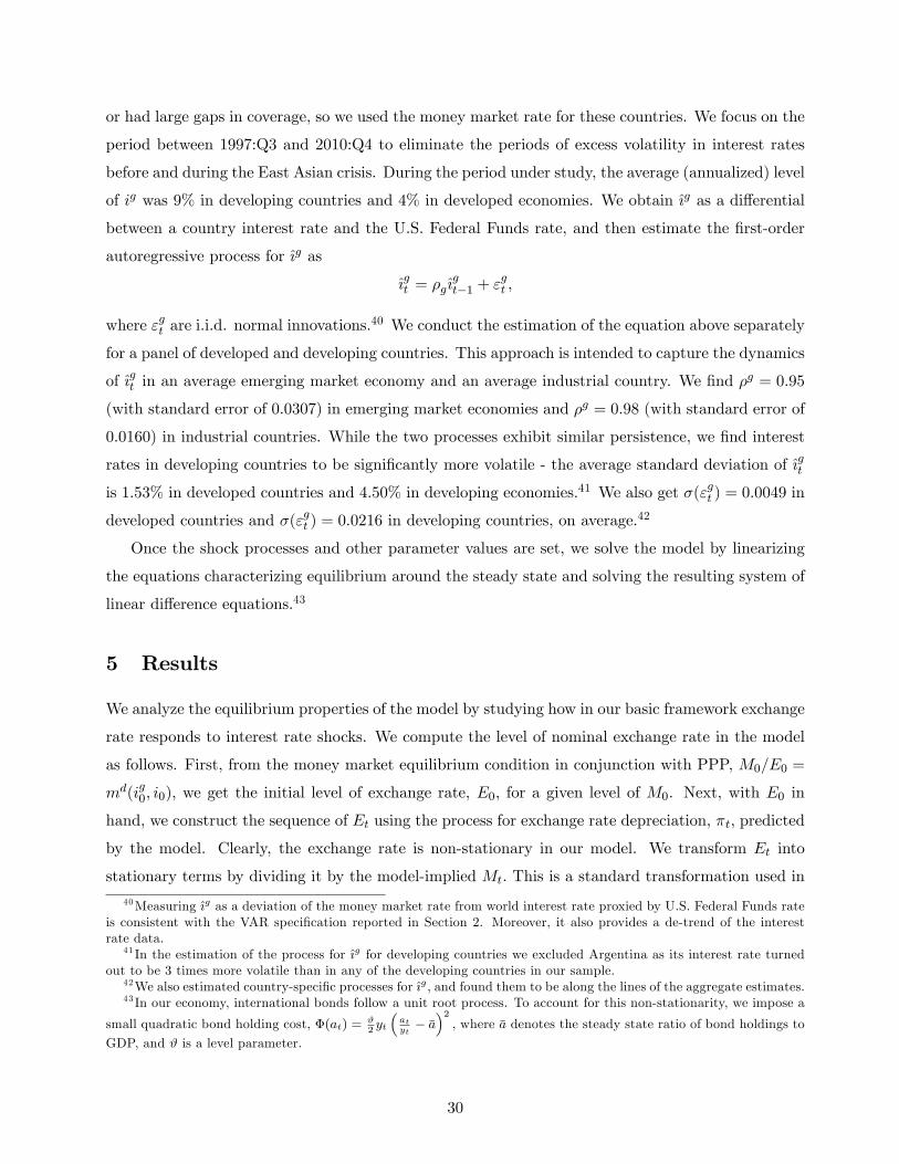
or had large gaps in coverage, so we used the money market rate for these countries. We focus on the

period between 1997:Q3 and 2010:Q4 to eliminate the periods of excess volatility in interest rates

before and during the East Asian crisis. During the period under study, the average (annualized) level

of ig was 9% in developing countries and 4% in developed economies. We obtain ıg as a differential

between a country interest rate and the U.S. Federal Funds rate, and then estimate the first-order

autoregressive process for ıg as

ıgt = ρg ıgt−1 + εgt ,

where εgt are i.i.d. normal innovations.40 We conduct the estimation of the equation above separately

for a panel of developed and developing countries. This approach is intended to capture the dynamics

of ıgt in an average emerging market economy and an average industrial country. We find ρg = 0.95

(with standard error of 0.0307) in emerging market economies and ρg = 0.98 (with standard error of

0.0160) in industrial countries. While the two processes exhibit similar persistence, we find interest

rates in developing countries to be significantly more volatile - the average standard deviation of ıgt

is 1.53% in developed countries and 4.50% in developing economies.41 We also get σ(εgt ) = 0.0049 in

developed countries and σ(εgt ) = 0.0216 in developing countries, on average.42

Once the shock processes and other parameter values are set, we solve the model by linearizing

the equations characterizing equilibrium around the steady state and solving the resulting system of

linear difference equations.43

5 Results

We analyze the equilibrium properties of the model by studying how in our basic framework exchange

rate responds to interest rate shocks. We compute the level of nominal exchange rate in the model

as follows. First, from the money market equilibrium condition in conjunction with PPP, M0/E0 =

md(ig0, i0), we get the initial level of exchange rate, E0, for a given level of M0. Next, with E0 in

hand, we construct the sequence of Et using the process for exchange rate depreciation, πt, predicted

by the model. Clearly, the exchange rate is non-stationary in our model. We transform Et into

stationary terms by dividing it by the model-implied Mt. This is a standard transformation used in

40Measuring ıg as a deviation of the money market rate from world interest rate proxied by U.S. Federal Funds rateis consistent with the VAR specification reported in Section 2. Moreover, it also provides a de-trend of the interestrate data.

41 In the estimation of the process for ıg for developing countries we excluded Argentina as its interest rate turnedout to be 3 times more volatile than in any of the developing countries in our sample.

42We also estimated country-specific processes for ıg, and found them to be along the lines of the aggregate estimates.43 In our economy, international bonds follow a unit root process. To account for this non-stationarity, we impose a

small quadratic bond holding cost, Φ(at) = ϑ2yt(atyt− a

)2, where a denotes the steady state ratio of bond holdings to

GDP, and ϑ is a level parameter.

30

the literature to normalize nominal non-stationary variables in monetary models. Before proceeding,

it is important to note that only nominal variables are non-stationary in the model. All real variables,

including real money demand, in our model are stationary in that temporary shocks leave their long

run levels unchanged.

Figure 4 presents impulse responses of the exchange rate to a temporary positive one standard

deviation shock to the policy-controlled interest rate ig in the model. Panel (a) is based on the model

parameterized for a developed country, while panel (b) is for the model calibrated to a developing

country. We also report the impulse responses of the market interest rate, i, to the same ig shock in

developed and developing countries on Figure 4.

Figure 4: Impulse responses following 1 std dev shock to ig

Panel (a). Developed countries

.004

.003

.002

.001

0%

dev

from

s.s

.

1 3 5 7 9 11quarters

exchange rate, E

7.6

7.7

7.8

7.9

8%


interest rate, i

Panel (b). Developing countries

0.0

2.0

4.0

6%

dev

from

s.s

.


exchange rate, E

15.5

1616

.517

17.5

%


interest rate, i

Note: The left panels present the responses of nominal exchange rate to a 1 std.dev. positive shock to policy-controlled interest rate, ig. The right panels showthe response of the market interest rate, i, to the same shock. Panel (a) presentsimpulse responses from the model calibrated to developed countries, while panel (b)does the same for developing countries.

For developed countries, the model predicts an impact appreciation of the exchange rate. In

particular, a one standard deviation increase in ig is associated with a 0.0034% appreciation of the

exchange rate in developed countries. On the other hand, a corresponding positive shock to ig in

31

an emerging market economy leads to a 0.06% depreciation of its exchange rate on impact. Note

that these responses not only match the signs of the empirical impulse responses, but are also in line

with the quantitative estimates of those responses in Figures 1 and 2. The market interest rate, i,

increases after the shock to ig in both countries.

The impulse responses in Panels (a) and (b) of Figure 4 highlight the inherent non-monotonicities

in the relationship between interest rates and the exchange rate present in our model. One might

argue that the interest rates measured in the data and used in our empirical analysis might not

be fully controlled by the policymakers. Our theoretical impulse responses above highlight the fact

that the differing relationship between exchange rate and interest rate for developed and developing

countries also holds more generally for market interest rates, not just policy-controlled interest rate.

There is a positive comovements between the market interest rate and exchange rate in developing

countries but negative comovement in developed countries rather than a systematic relationship for

all.44

5.1 Under the hood

So what is behind these contrasting dynamics in interest rates and the exchange rate in developed

and developing countries? As we discussed earlier, the interaction between the two variables in

the model is built around three key effects: the “money demand”effect, the “fiscal”effect and the

“output”effect. While the money demand effect tends to strengthen the currency after an increase

in ig, the fiscal and output effects tend to weaken the currency. The net effect on the exchange rate

is determined by the relative strength of each of these effects.

To build intuition for the results, consider a perfect foresight version of the model. In addition,

assume that γ ≈ ∞ so that banking costs are infinitely large. In this case the banking sector will

hold a constant amount of foreign assets, i.e., db = db. From expression (19), the exchange rate at

any date t is given by Et = Mtht+θdt

where Mt is given. Log differentiating this relationship gives

Et = Mt −h

mht −

θd

mdt (20)

where hats over a variable indicate its percentage change and m = M/E. Suppose M = 0 , i.e.,

nominal supply is unchanged at date t. If both cash holdings, h, and interest-bearing demand44Note that following the shock, market interest rates remains above their steady state value for a prolonged period

of time in both developed and developing country calibrations. Since uncovered interest parity holds in our model, thisimplies a depreciating path for the exchange rate in both countries immediately following the differing impact response.This is indeed in the case in our model. However, while panel (a) in Figure 4 is consistent with this pattern in that theexchange rate exhibits a depreciating path after the impact appreciation, the response of developing countries shown inpanel (b) appears to contradict it. The exchange rate in developing countries seem to be appreciating after an impactdepreciation. This pattern is an artefact of the normalization by M that we used. Because M is also increasing afterthe shock, but does so at a faster rate than the exchange rate for developing countries, the ratio of E/M is falling.

32

deposits, d, rise in response to a shock then the exchange rate, E, appreciates; while if both decline

then E depreciates. Our interest is in the effect of changes in ig on E. The preceding relation then

makes it clear that this depends on the effect that changes in ig have on h and d.

The optimality conditions for cash and deposits holdings along with the definition for the nominal

interest rate under perfect foresight, 1 + it+1 = R (1 + πt+1) , yield the equilibrium cash and deposit

demands in the model as ht = h(

it+11+it+1

)and dt = d

(it+1−(1−θ)igt+1

1+it+1

)where both functions are

decreasing in their arguments. Clearly, a rise in ig positively affects E by increasing the demand for

deposits d. However, ig also affects E indirectly through its effect on i since the market interest rate

i affects the demand for both cash and deposits. The effect of ig on i in turn is determined from the

government flow budget constraint

τ +1 + igt1 + πt

zt−1 = ht −ht−1

1 + πt+ θdt −

θdt−11 + πt

+ zt (21)

where z = (1− θ) d − n + db (assuming γ ≈ ∞). The left hand side of equation (21) gives totalexpenditures while the right hand side gives net revenues. For a given τ and ig, equations (21) and

(20) along with the equilibrium conditions for cash and demand deposits pin down both πt and it+1.

Note that it and igt are given at any date t while πt and Pt are determined within the period. Since

Pt−1 is given, pinning down πt (= PtPt−1

) and is equivalent to determining Pt.45

In light of these linkages, how does one understand the differences in the calibrated responses of

developed and developing countries? The discussion above makes clear that the opposing responses of

the exchange rate in these two groups of countries to interest rate shocks must be due to differences

in the responses of cash and demand deposits. But what factors explain the differences in the

response of these two variables? We illustrate the key factors at play by using impulse responses

of various variables to a positive shock to ig. To facilitate the comparison across developed and

developing countries calibrations we use the same size of the shock (equal to developed country

standard deviation of ig) in both calibrations. Also, since the steady states are different in the two

calibrations, we present all impulse responses as deviations from the steady state (multiplied by 100).

Results are in Figure 5.

An increase in ig leads to a fall in the demand for loans, and therefore output, due to a working

capital constraint. Since parameter φ, which governs the tightness of this constraint, is calibrated to

be the same across developed and developing countries, the impact response of output is symmetric for

45 It is important to note that pinning down it+1 is not equivalent to determining Pt+1. To see this, note that

1 + it+1 = REt (1 + πt+1) = REt(

1 +Pt+1Pt

). Clearly, this is not equivalent to determining Pt+1 which is free to

deviate from Et (Pt+1) in response to shocks that hit the economy after the formation of expectations about periodt+ 1.

33

the two groups.46 The response is more long-lived in developed countries due to a higher persistence

of the process for ig in that group of countries. All else equal, a smaller loan portfolio of banks

raises the amount of government bonds that banks buy, i.e., z rises. In combination with the higher

interest rate on these bonds, the interest burden on the government rises. Financing this higher level

of fiscal spending thus requires a higher inflation rate, π. This, in turn, leads to a higher interest rate

i following the shock to ig.

How do money demand and its components respond to a rise in ig and i? Not surprisingly,

demand for cash declines in both groups, since a rise in i unambiguously leads to a rise in the

opportunity cost of holding cash, it+11+it+1

. This effect is larger for developing country calibration,

leading to a larger drop in cash holdings. On the other hand, demand for deposits rises in both

calibrations. This is because the opportunity cost of holding deposits,it+1−(1−θ)igt+1

1+it+1, declines. On

the one hand, higher ig lowers this opportunity cost while on the other, an increase in i works in

the opposite direction. Quantitatively, the first effect dominates under both calibrations, leading to

higher deposit demand in both groups of countries. Turning to aggregate money demand, m = h+θd,

we see opposing responses in the two calibrations: money demand increases in the developed country

calibration, but declines in the developing country. This reflects the fact that, following the shock,

the increase in deposits is larger than the fall in cash holdings in developed countries but not so in

developing countries. Why is this the case? The key reason for the difference is that the steady state

level of deposits to cash is four-times higher in developed economies than in developing countries in

our calibration, reflecting the same difference in the data. This implies that deposits constitute a

significantly larger fraction of total money demand in developed countries.47 Hence, money demand

in developed countries is more sensitive to changes in deposits than in developing countries (where

cash holdings occupy a larger weight in money demand). As a result, after a positive shock to ig,

money demand increases in developed countries leading to an appreciation in E as shown in equation

(20). However, the same shock leads to a fall in money demand in developing countries and to a

currency depreciation for them.

Next, we evaluate the sensitivity of our results with respect to several key parameters that

distinguish developed and developing countries in our calibration. These parameters also affect the

strength of the three effects —fiscal, output, and money demand effects —that we focused on in the

model.46Note that the loan to output ratio is φwl

y. Under the Cobb-Douglas specification for technology, wl

y= 1−α is the

same for both groups. Hence, under our maintained parameterization of a common φ, the loan-output ratio is the sameacross countries. This is the reason for the symmetric output effect on impact for developed and developing countriesin 5.

47Note, however, that the parameter θ is higher in the developing country calibration, thus increasing the weight ofdeposits in total money demand in this group. This effect, however, is not too strong under our benchmark calibration.We investigate the robustness of our results with respect to parameter θ in the next sub-section.

34

Figure 5: Impulse responses following 1 std dev shock to ig

.006

.004

.002

0de

v fro

m s

.s. x

100


developed developing

output, y

0.0

1.0

2.0

3.0

4de

v fro

m s

.s. x

100



government bonds, z

0.1

.2.3

.4de

v fro

m s

.s. x

100



inflation, pai

.001

5.0

01.0

005

0de

v fro

m s

.s. x

100



cash, h

0.0

1.0

2.0

3.0

4de

v fro

m s

.s. x

100



deposits, d

.001

.000

50

.000

5de

v fro

m s

.s. x

100



money demand, m

Note: The figures present the responses of various variables to a 1 std. dev. positiveshock to policy-controlled interest rate, ig, in the versions of the model calibratedto developed and developing countries. The shock is set to be the same in the twogroups of countries equal to the std. dev. of ig in developed economies. All responsesare presented in deviation from the steady state multiplied by 100.

5.2 Varying key parameters

The first of our three effects is the fiscal effect. The size of the fiscal burden in the model is captured

by τ and ig. An increase in τ , ceteris paribus, raises the financing burden on the government.

Equation (21) makes clear that the financing can be done by some combination of a rise in πt (or

35

equivalently, Pt) and it+1.48 Consider equation (21) in a perfect foresight steady state:

τ =

(i− r1 + i

)(hss + θdss) +

(1 + i−R (1 + ig)

1 + i

)zss (22)

where we have used the steady state relation 1 + i = R (1 + π). Keeping everything else constant,

a higher τ necessitates a higher steady state i. Since 1 + i = R (1 + π) and 1 + πt = EtEt−1

, a higher

i implies an immediate depreciation of the currency. Thus, the model predicts that the higher is τ

the more depreciated the country’s currency.

Figure 6 shows the fiscal effect in play for both developed countries (left panel) and emerging

economies (right panel). In each panel, the figures have two lines —a solid line and a dashed line.

Both lines are derived for the baseline calibration for the country in question. The solid line plots

the initial level of the exchange rate as a function of τ for a given and constant initial level of money

supply M0. The initial level of the exchange rate is measured on the left axis. The dashed lines

in the two panels of the Figure 6 depict the impact effect of an increase in ig on the exchange rate

(expressed as percent deviation from the steady state). This is measured on the right axis.

The solid lines in the Figure show that the initial E rises with τ for both developed and emerging

economies, exactly as the model suggests. The dashed lines reveal an important difference between

the two groups. For developed countries, a higher ig induces an impact currency appreciation for

the entire range of τ’s plotted. For developing economies however, a higher ig induces a depreciation

of the currency on impact, i.e., a rise in E. Note though that the size of the impact depreciation

declines as τ becomes larger, reflecting partly the fact that the exchange rate changes are in percent

deviations from the steady state and the higher τ raises the steady state level of E itself for both

groups.

We draw two main conclusions from these results. First, for any given level of nominal money

supply, a higher τ , which is partially responsible for the strength of the fiscal effect, always leads

to a more depreciated currency in the steady state. Second, the difference between developed and

emerging economies that we found in Figure 4 is robust to changes in the level of τ since changes in

τ do not appear to qualitatively change the impact effect of ig on the exchange rate.

The second effect in the model is the money demand effect. One of the key parameters that

controls the strength of this effect is θ which is the share of deposits that comprises the money base

(bank reserves). In the model, the higher is θ the greater is the base money in the economy. The

greater money base implies that the same τ can now be financed with a lower initial level of E (or

48Note equation (21) can be rewritten as a first order difference equation in it+1 and it. The standard condition fora unique flexible price monetary equilibrium is that the difference equation in i be unstable. We impose it through out.It can be verified that this stability condition also implies government revenues are increasing in the nominal interestrate i.

36

Figure 6: Comparative statics for parameter τ

(a). Developed countries (b). Developing countries

.003

7.0

036

.003

5.0

034

.003

3%

dev

from

s.s

.

.998

11.

002

1.00

4le

vel

0 .01 .02 .03 .04 .05tau

steady state impact response

Exchange rate

.054

.056

.058

.06

.062

.064

% d

ev fr

om s

.s

.99

.995

11.

005

1.01

1.01

5le

vel

0 .01 .02 .03 .04 .05tau


Exchange rate

Note: The figure presents the responses of nominal exchange rate to changes in τ . Thedeveloped country calibration is shown in the left panel while the right panel shows thedeveloping country calibration. Dotted vertical line indicates the level of τ under ourbenchmark calibration in each country group.

equivalently a lower π) as well as a lower steady state rate of currency depreciation. It is easy to

check that the right hand side of equation 22 is increasing in both π and i. However, for a given ig

a higher θ also reduces the deposit rate since id = (1− θ) ig. This tends to reduce the demand fordeposits. The resultant fall in overall real money demand tends to depreciate the currency. Which

of these two effects dominates depends on the specific parameters governing the relationship.

Figure 7 shows the effect of the parameter θ on the exchange rate. The figure is symmetric to

the one for the fiscal spending parameter τ above. The solid lines depict the effect of θ on the initial

level of the exchange rate for a constant initial nominal money supply. The dashed lines show the

impact effect of a temporary increase in ig on the exchange rate (the initial response on impact) for

different values of θ. The initial levels are measured on the left axis while the impact responses in

percent deviations from steady state are measured on the right axis.

The downward sloping solid lines in Figure 7 show that the initial value of the exchange rate is a

decreasing function of θ, i.e., as the reserve requirement ratio rises the initial level of E declines due

to a strengthening of the money demand effect. Importantly, this effect is the same in both groups

of countries. In terms of the impact effect of ig on the exchange rate however, there are differences

between the two sets of countries. In emerging economies, a higher domestic interest rate ig induces

an initial depreciation of the currency (positive numbers in the right axis of the right panel). As the

dashed lines indicate, this is true for the broad range of relevant θ’s ranging from 0.01 to 0.2. For

developed countries on the other hand, the impact effect is a depreciation if the reserve requirement

ratio is low enough (below 0.015), but an appreciation for higher values of θ. More generally, for

37

developed countries a higher domestic interest rate would depreciate the currency for very low levels

of θ but begin to appreciate it for higher θ’s.

The switch in the impact response of E to ig shock in developed countries from depreciation to

appreciation as one changes θ suggests that the differences in the impulse responses of the two groups

to interest rate shocks that we found in 4 depend crucially on the reserve requirement parameter θ.

Figure 7: Comparative statics for parameter θ


.008

.006

.004

.002

0.0

02%

dev

from

s.s

.

.9.9

51

1.05

1.1

leve

l

.01 .02 .03 .04 .05theta


Exchange rate

.05

.06

.07

.08

.09

.1%

dev

from

s.s

.9.9

51

1.05

1.1

leve

l0 .05 .1 .15 .2

theta


Exchange rate

Note: The top panel presents the responses of nominal exchange rate to changes in θ.The developed country calibration is shown in the left panel while the right panel showsthe developing country calibration. Dotted vertical line indicates the level of θ under ourbenchmark calibration in each country group.

Our third effect is the output effect. The size of this effect is captured by the wage-in-advance

parameter φ. The higher is φ the greater is the wage-in-advance requirement and hence the demand

for loans. All else equal, a higher loan portfolio of banks reduces the amount of government bonds

that banks buy, i.e., z falls. From equation (22) it is easy to see that a lower z reduces government

revenues. Financing of a given fiscal spending τ then requires a combination of a higher π (a more

depreciated initial exchange rate) along with a higher steady state depreciation rate.

As we noted earlier, there are complications in calibrating this parameter with precision. However,

this makes it all the more important to examine the sensitivity of the results to variations in φ. Figure

8 shows the effects of varying φ in our model. The figure is symmetric to the ones for τ and θ. The

upward sloping solid lines in the two panels of Figure 8 demonstrate that the higher is φ the more

depreciated is the exchange rate in the initial steady state for a constant level of initial nominal

money supply M0. In terms of the impact effect of a temporary increase in ig on the exchange rate,

in developed countries the response is an appreciation while in emerging economies it is a depreciation

for a broad range of values for φ.

Given that Figure 8 consistently reveals a depreciation for developing countries and an apprecia-

38

tion for developed economies for a broad range of values for φ leads us to conclude that the differences

in the impulse responses for the two groups to interest rate shocks highlighted in Figure 4 are robust

to variations in the wage-in-advance parameter φ.

Figure 8: Comparative statics for parameter φ


.004

.003

5.0

03.0

025

% d

ev fr

om s

.s.

.999

96.9

9998

11.

0000

2 1.0

0004

leve

l

0 .05 .1 .15 .2 .25fi


Exchange rate

.04

.05

.06

.07

.08

% d

ev fr

om s

.s

.999

.999

51

1.00

051.

001 1

.001

5le

vel

0 .05 .1 .15 .2 .25fi


Exchange rate

Note: The top panel presents the responses of nominal exchange rate to changes in φ.The developed country calibration is shown in the left panel while the right panel showsthe developing country calibration. Dotted vertical line indicates the level of φ under ourbenchmark calibration in each country group.

How does this help us understand the different impulse responses for developed and developing

countries? As we showed above, the strength of the effects considered in the model are different in

developed and developing countries. In developing countries, both τ and ig are about twice as high

relative to developed economies. This leads to a much higher interest burden on the government in

developing countries. As a result, the fiscal effect is larger which contributes to the tendency for

exchange rates to depreciate in response to interest rate increases in developing countries.

Concurrently, the bank reserves as a share of deposits is about three times higher in developing

countries relative to developed countries in our sample. This would suggest a stronger money demand

effect in developing countries. However, there are two other important ratios that also influence the

size of the money demand effect. These are the ratio of base money to output and the ratio of

deposits to cash. The higher these ratios, the stronger the money demand effect of higher interest

rates. The base money to output ratio in developing countries is half of that in developed countries

while the ratio of deposits to cash is four times smaller in developing countries relative to developed

economies. These two effects tend to swamp the effect of a higher θ and make the money demand

effect substantially weaker in developing countries relative to developed economies. As panel (a)

of Figure 7 shows, if bank reserves in developed economies were lowered from the benchmark level

of 0.03 to about 0.015, then the impact appreciation of E in developed countries in response to an

39

increase in ig would switch to an impact depreciation of the currency.

Finally, in our benchmark calibration we assumed that the wage-in-advance parameter φ was the

same in developed and developing countries. This calibration implied that the strength of the output

effect is the same across the two groups of countries, and thus does not contribute to their differing

exchange rate dynamics. Arguably, the working capital requirements tend to be more important in

developing countries, which would suggest a larger parameter φ for these economies. In this case,

our model would imply a stronger output effect in developing countries and even more pronounced

tendency for their exchange rate to depreciate following rises in ig.

We should also point out that the size of the shocks to interest rates in developing countries is

four-times larger than the size of interest rate shocks in developed countries. The impulse responses

reported for the two sets of countries in Figure 4 reflect the tradeoffs amongst these offsetting effects.

6 Conclusions

The effect of monetary policy on the exchange rate has long been one of the fundamental concerns of

academics and practitioners alike. A large preponderance of existing models predict that monetary

policy tightening should induce an exchange rate appreciation. What does the evidence suggest

though? In this paper we have used a panel dataset comprising of 72 countries between 1974 and

2010 to show that while most developed countries indeed exhibit exchange rate appreciations in

response to interest rate increases, in developing countries the effect is the opposite: most of them

exhibit depreciating currencies in response to interest rate increases. We call this puzzling new data

fact the “exchange rate response puzzle”.

We have provided an explanation for this puzzle using a simple open economy monetary model.

Our explanation rests on the contrasts in the interplay between three key effects between developed

and developing countries. Our model formalized three important effects of raising interest rates —a

larger fiscal burden, a negative output effect and a positive effect on real money demand. While the

first two effects tend to depreciate the currency, the last tends to appreciate it. Using a calibrated

version of the model, we have shown that the differences in the relative importance of these three

effects between the two groups of countries can account for the contrasting responses in the two

groups.

References

Altig, D., L. Christiano, M. Eichenbaum, and J. Linde (2011): “Firm-Specific Capital, Nom-

inal Rigidities and the Business Cycle,”Review of Economic Dynamics, 14(2), 225—247.

40

Arellano, M., and S. Bond (1991): “Some Tests of Specification for Panel Data: Monte Carlo

Evidence and an Application to Employment Equations,” Review of Economic Studies, 58(2),

277—97.

Auernheimer, L. (2008): “Monetary Policy Rules, the Fiscal Theory of the Price Level, and

(Almost) All that Jazz,” in Money, Crises, and Transition: Essays in Honor of Guillermo A.

Calvo, pp. 41—67. MIT Press.

Bacchetta, P., and E. van Wincoop (2010): “Infrequent Portfolio Decisions: A Solution to the

Forward Discount Puzzle,”American Economic Review, 100(3), 870—904.

Bernanke, B. S., and A. S. Blinder (1992): “The Federal Funds Rate and the Channels of

Monetary Transmission,”American Economic Review, 82(4), 901—21.

Bjørnland, H. C. (2009): “Monetary policy and exchange rate overshooting: Dornbusch was right

after all,”Journal of International Economics, 79(1), 64—77.

Blanchard, O. (2004): “Fiscal Dominance and Inflation Targeting: Lessons from Brazil,”Working

Paper 10389, National Bureau of Economic Research.

Blanchard, O. J., and D. Quah (1989): “The Dynamic Effects of Aggregate De-

mand and Supply Disturbances,” American Economic Review, 79(4), 655—73, available at

http://ideas.repec.org/a/aea/aecrev/v79y1989i4p655-73.html.

Brock, P. L. (1989): “Reserve Requirements and the Inflation Tax,”Journal of Money, Credit and

Banking, 21(1), 106—21.

Calvo, G. A., and C. M. Reinhart (2002): “Fear Of Floating,”The Quarterly Journal of Eco-

nomics, 117(2), 379—408.

Calvo, G. A., and C. A. Vegh (1995): “Fighting Inflation with High Interest Rates: The Small

Open Economy Case under Flexible Prices,”Journal of Money, Credit and Banking, 27(1), 49—66.

Christiano, L. J., andM. Eichenbaum (1992): “Liquidity Effects and the Monetary Transmission

Mechanism,”American Economic Review, 82(2), 346—53.

Christiano, L. J., M. Eichenbaum, and C. L. Evans (2005): “Nominal Rigidities and the

Dynamic Effects of a Shock to Monetary Policy,”Journal of Political Economy, 113(1), 1—45.

Clarida, R., and J. Gali (1994): “Sources of real exchange-rate fluctuations: How important are

nominal shocks?,”Carnegie-Rochester Conference Series on Public Policy, 41(1), 1—56.

41

Correia, I., J. C. Neves, and S. Rebelo (1995): “Business cycles in a small open economy,”

European Economic Review, 39(6), 1089—1113.

Diaz-Gimenez, J., E. C. Prescott, T. Fitzgerald, and F. Alvarez (1992): “Banking in

Computable General Equilibrium Economies,”Journal of Economic Dynamics and Control, 16(3-

4), 533—559.

Dornbusch, R. (1976): “Expectations and Exchange Rate Dynamics,”Journal of Political Econ-

omy, 84(6), 1161—76.

Druck, P., and P. Garibaldi (2000): “Inflation Risk and Portfolio Allocation in the Banking

System,”CEMA Working Papers: Serie Documentos de Trabajo. 181, Universidad del CEMA.

Edwards, S., and C. A. Vegh (1997): “Banks and Macroeconomic Disturbances under Predeter-

mined Exchange Rates,”Journal of Monetary Economics, 40(2), 239—278.

Eichenbaum, M., and C. L. Evans (1995): “Some Empirical Evidence on the Effects of Shocks

to Monetary Policy on Exchange Rates,”The Quarterly Journal of Economics, 110(4), 975—1009.

Engel, C. (2011): “The Real Exchange Rate, Real Interest Rates, and the Risk Premium,”Working

papers, University of Wisconsin.

Faust, J., and J. H. Rogers (2003): “Monetary policy’s role in exchange rate behavior,”Journal

of Monetary Economics, 50(7), 1403—1424.

Fischer, S., R. Sahay, and C. A. Vegh (2002): “Modern Hyper- and High Inflations,”Journal

of Economic Literature, 40(3), 837—880.

Greenwood, J., Z. Hercowitz, and G. W. Huffman (1988): “Investment, Capacity Utilization,

and the Real Business Cycle,”American Economic Review, 78(3), 402—17.

Grilli, V., and N. Roubini (1995): “Liquidity and Exchange Rates: Puzzling Evidence from the

G-7 Countries,”Working Papers 95-17, New York University, Leonard N. Stern School of Business,

Department of Economics.

(1996): “Liquidity models in open economies: Theory and empirical evidence,”European

Economic Review, 40(3-5), 847—859.

Holtz-Eakin, D., W. Newey, and H. S. Rosen (1988): “Estimating Vector Autoregressions with

Panel Data,”Econometrica, 56(6), 1371—95.

42

Kim, S., and N. Roubini (2000): “Exchange Rate Anomalies in the Industrial Countries: A Solution

with a Structural VAR Approach,”Journal of Monetary Economics, 45(3), 561—586.

Lahiri, A., and C. A. Vegh (2003): “Delaying the Inevitable: Interest Rate Defense and Balance

of Payments Crises,”Journal of Political Economy, 111(2), 404—424.

Lane, P. R., and G. M. Milesi-Ferretti (2007): “The external wealth of nations mark II: Re-

vised and extended estimates of foreign assets and liabilities, 1970-2004,”Journal of International

Economics, 73(2), 223—250.

Love, I., and L. Zicchino (2006): “Financial development and dynamic investment behavior:

Evidence from panel VAR,”The Quarterly Review of Economics and Finance, 46(2), 190—210.

Mendoza, E. G. (1991): “Real Business Cycles in a Small Open Economy,”American Economic

Review, 81(4), 797—818.

Neumeyer, P. A., and F. Perri (2005): “Business Cycles in Emerging Economies: The Role of

Interest Rates,”Journal of Monetary Economics, 52(2), 345—380.

Obstfeld, M., and K. Rogoff (1995): “Exchange Rate Dynamics Redux,” Journal of Political

Economy, 103(3), 624—60.

Rabanal, P. (2007): “Does inflation increase after a monetary policy tightening? Answers based

on an estimated DSGE model,”Journal of Economic Dynamics and Control, 31(3), 906—937.

Rebelo, S., and C. A. Vegh (1995): “Real Effects of Exchange-Rate-Based Stabilization: An

Analysis of Competing Theories,” in NBER Macroeconomics Annual 1995, Volume 10, NBER

Chapters, pp. 125—188. National Bureau of Economic Research, Inc.

Reinhart, C. M., and K. S. Rogoff (2004): “The Modern History of Exchange Rate Arrange-

ments: A Reinterpretation,”The Quarterly Journal of Economics, 119(1), 1—48.

Rodriguez, C. A. (1991): “Financial Reform and Macroeconomic Developments in Argentina,

Chile and Uruguay During the Decade of the 1980s,”Cema working papers: Serie documentos de

trabajo., Universidad del CEMA.

Schmitt-Grohé, S., and M. Uribe (2006): “Optimal Fiscal and Monetary Policy in a Medium-

Scale Macroeconomic Model,”in NBER Macroeconomics Annual 2005, Volume 20, NBER Chap-

ters, pp. 383—462. National Bureau of Economic Research, Inc.

Sims, C. A. (1992): “Interpreting the Macroeconomic Time Series Facts: The Effects of Monetary

Policy,”European Economic Review, 36, 975—1011.

43

Uribe, M., and V. Z. Yue (2006): “Country Spreads and Emerging Countries: Who Drives

Whom?,”Journal of International Economics, 69(1), 6—36.

Vegh, C. (2010): Open Economy Macroeconomics in Developing Countrieschap. 5. Manuscript.

44

A Appendix

A.1 Empirical evidence

In this Appendix we describe our data sources used in the empirical sections of the paper. Our

primary data sources are the International Financial Statistics (IFS) compiled by the International

Monetary Fund (IMF) and the World Development Indicators (WDI) compiled by the World Bank.

In our analysis we considered all countries in the IFS and WDI datasets for which monthly data on

exchange rates and interest rates was available for any fraction of the 1974-2010 period.

Data description and sources are summarized in Table A1.

Table A1: Data description and sources

Variable Definition SourceExchange rate offi cial exchange rate, period average IFS by IMF

market exchange rate, period average IFS by IMFprincipal exchange rate, period average IFS by IMFcommercial exchange rate, period average IFS by IMF

Interest rate T-bill rate, period average IFS by IMFdiscount rate, period average IFS by IMFmoney market rate, period average IFS by IMF

Output Industrial production index IFS by IMF2000 base year

CPI Consumer price index IFS by IMFRisk premium BofA Merrill Lynch US High Yield Master II Option-Adjusted Spread BofA Merrill Lynch

Moody’s Seasoned Baa Corporate Bond Yield Board of Governorsof the Federal Reserve System

As we mentioned in the main text, in our empirical analysis we restrict the sample to only those

countries and time periods that are characterized by a flexible exchange rate regime. To perform the

selection, we rely on the Reinhart and Rogoff (2004) classification of historical exchange rate regimes.

In particular, we classify a country as having a flexible exchange rate regime if, in a given year, its

exchange rate was either (i) within a moving band that is narrower than or equal to +/-2% (i.e.,

allows for both appreciation and depreciation over time); or (ii) was classified as managed floating; or

(iii) was classified as freely floating; or (iv) was classified as freely falling according to Reinhart and

Rogoff (2004). These correspond to their fine classification indices of 11, 12, 13, and 14, respectively.

We only focus on the post-Bretton Woods period for all countries. High income OECD countries are

included in our sample, irrespective of their exchange rate classification. Table A2 contains the list

of country-episode pairs that are included in our sample.

A1

Table A2: Sample used in the empirical work

No from to country No from to country1 1994m7 2001m12 Albania 41 1990m1 1998m12 Luxembourg2 1988m1 1995m1 Algeria 42 2002m10 2007m12 Madagascar3 2002m1 2005m5 Angola 43 1983m1 1994m12 Malawi4 1974m1 2010m11 Australia 44 1997m8 2003m8 Malawi5 1974m1 1998m12 Austria 45 1987m11 2000m12 Malta6 1994m1 2002m10 Belarus 46 1982m2 1988m11 Mexico7 1974m1 1998m12 Belgium 47 1995m1 2007m12 Mexico8 1999m2 2007m12 Brazil 48 1991m1 1994m1 Myanmar9 1992m1 1996m12 Bulgaria 49 1996m8 1999m1 Myanmar10 1974m1 2010m11 Canada 50 1974m1 1990m8 Netherlands11 1999m9 2001m12 Chile 51 1978m1 2010m11 New Zealand12 1990m3 1992m7 China, P.R. (Mainland) 52 1991m7 2007m12 Nigeria13 1994m7 2004m2 Congo, Dem. Rep. of 53 1974m1 2009m5 Norway14 1980m10 1983m10 Costa Rica 54 1990m1 1993m10 Peru15 1997m6 2001m12 Czech Republic 55 1997m7 1999m11 Philippines16 1981m5 1988m12 Denmark 56 1982m4 1998m5 Portugal17 2003m11 2007m12 Dominican Republic 57 1994m3 2001m3 Romania18 1999m1 2010m11 Euro Area 58 2003m4 2007m12 Serbia, Rep. of19 1974m1 1998m12 Finland 59 2002m1 2005m6 Sierra Leone20 1974m1 1998m12 France 60 1974m1 2007m12 Singapore21 1986m1 1991m9 Gambia, The 61 1974m1 1985m8 South Africa22 1975m7 1998m12 Germany 62 1995m3 2007m12 South Africa23 1985m4 2001m3 Ghana 63 1979m1 1998m12 Spain24 1983m1 2000m12 Greece 64 1974m1 2010m11 Sweden25 2000m5 2002m6 Guinea 65 1980m1 2010m11 Switzerland26 1988m1 1991m12 Guyana 66 1982m6 1987m12 Syrian Arab Rep.27 1994m10 2007m12 Haiti 67 1998m10 2002m10 Tajikistan28 1987m6 2010m11 Iceland 68 2001m2 2007m12 Thailand29 1997m8 2007m12 Indonesia 69 1991m12 1996m5 Turkey30 1977m1 1979m10 Iran, I.R. of 70 2001m2 2007m12 Turkey31 1974m1 1998m12 Ireland 71 1980m1 1986m8 Uganda32 1977m3 1998m12 Italy 72 1989m10 1992m12 Uganda33 1990m10 1992m12 Jamaica 73 1992m12 1996m9 Ukraine34 1974m1 2010m11 Japan 74 1974m1 2010m10 United Kingdom35 1994m4 1996m5 Kazakhstan 75 1991m12 1995m9 Uruguay36 1987m1 1995m12 Kenya 76 2002m5 2005m5 Uruguay37 1997m12 2007m12 Korea, Republic of 77 1984m3 1996m6 Venezuela, Rep. Bol.38 1994m1 1999m11 Kyrgyz Republic 78 1978m1 1983m7 Zambia39 1997m9 2000m3 Lao People S Dem.Rep 79 1985m11 2007m12 Zambia40 1984m3 1991m7 Lebanon 80 1991m10 1999m3 Zimbabwe

A.2 Structural VAR: Details

Let yt be a (2x1) vector consisting of interest rate differential and (log) exchange rate: yt =[it − iUSt , lnEt

]. The VAR can be written as:

yt = (I −A1L− ...−ApLp)−1 ut,

where ut is a (2x1) vector of reduced-form residuals, assumed to be i.i.d., with zero mean and

Eutu′t = Σ. L is a lag operator, while A1, ...Ap are (2x2) matrices. Following the literature we

assume that orthogonal structural shocks, εt, are linear combinations of ut: ut = Bεt, where εt are

i.i.d. with mean zero and the variance-covariance matrix equal to the identity matrix. The VAR can

A2

then be written in terms of structural shocks as

yt = (I −A1L− ...−ApLp)−1Bεt. (A1)

Parameters in A1, ...Ap and Σ can be estimated from the data. Thus, to obtain structural interpre-

tation from the reduced form VAR we need to identify matrix B. Matrix B satisfies Σ = BB′. To

obtain identification in our structural VAR we impose a long-run neutrality restriction as discussed

in the text. Specifically, we assume that interest rate shocks cannot have long-run effects on the real

exchange rate. This is achieved by setting the values of the relevant lag coeffi cients in equation (A1)

to zero. For instance, if we redefine

(I −A1L− ...−ApLp)−1B = C(L)

and write the long-run expression of C(L) as C∗ =∑∞

j=0Cj , then our long-run neutrality restriction

reduces to C∗21 = 0. As we discussed in the text, this identification scheme allows for contemporaneous

link between interest rates and exchange rate, while maintaining comparability with the Cholesky

ordering results.

A.3 Calibration: Data sources

In this Appendix we describe data and sources used in model calibration. We focused on a sample

of 6 industrial economies —Australia, Canada, Netherlands, New Zealand, Sweden and UK and 6

developing countries —Argentina, Brazil, Korea, Mexico, Philippines, and Thailand —during 1974-

2010 period. When focusing on nominal variables, i.e. nominal interest rates, we restrict the sample

to 1998-2010 period to eliminate the periods of high interest rate volatility and high inflation in

developing countries before and during the East Asian crisis.

Monetary variables: M1 (in local currency) for all countries comes from World Development

Indicators (WDI) and Global Development Finance (GDF) datasets compiled by the World Bank.

GDP (in local currency) was obtained from the same dataset. Reserve ratio was computed for each

country following Brock (1989) as the ratio of monetary base less currency outside banks to M2 less

currency outside banks. All series used in the computation were obtained from the International

Financial Statistics (IFS) by the International Monetary Fund (IMF). To obtain the ratio of deposits

to cash holdings we computed the level of deposits in each country as M1 minus currency outside

banks. Cash holdings were measured by the currency outside banks. Consumer price (CPI) data is

from the IFS database.

Fiscal variables: We used general government net lending/borrowing as a share of GDP to

A3

calibrate parameter τ . This data is from the World Economic Outlook (WEO) dataset of the IMF.

Other: We obtained average net foreign asset position (NFA) from Lane and Milesi-Ferretti

(2007) dataset. To proxy the policy-controlled interest rates in the data we use the period average

T-bill rate. For Netherlands we used a 3-month interbank rate in the Euro area. For Argentina,

Australia, Brazil, Korea, Philippines and Thailand the T-bill rate was either not available or had

large gaps in coverage, so we used the money market rate for these countries. This data is from the

IFS database.

A4

The Exchange Rate Response Puzzle

Documents

Transcript of The Exchange Rate Response Puzzle