Int Econ Econ Policy (2010) 7:371–390DOI 10.1007/s10368-010-0147-y

ORIGINAL PAPER

Sources of time-varying exchange rate exposure

Christian Pierdzioch · Renatas Kizys

Published online: 9 March 2010© Springer-Verlag 2010

Abstract We report evidence of a time-varying link between returns onnational stock market indexes and exchange rate returns (exchange rateexposure). We use this evidence to analyze the sources of changes over time inexchange rate exposure. Using monthly data for 14 industrialized countriesfor the period 1975–2006, we report evidence of a cointegration relationbetween exchange rate exposure and the industry composition of a country’simports, and weaker evidence of a cointegration relation between exchangerate exposure and openness to trade.

Keywords Stock market returns · Exchange rate exposure ·Time-varying parameter model · Cointegration analysis

JEL Classifications F31 · F37 · G15

1 Introduction

Exchange rate exposure, defined as the link between stock market returnsand exchange rate movements, summarizes how exchange rate movements

C. Pierdzioch (B)Department of Economics, Saarland University, P.O. Box 15 11 50, 66041,Saarbruecken, Germanye-mail: c.pierdzioch@mx.uni-saarland.de

R. KizysDepartamento de Economia,Instituto Tecnologico y de Estudios Superiores de Monterrey (ITESM),C.P. 64849, Monterrey, Nuevo Leon, Mexicoe-mail: renatas.kizys@itesm.mx

372 C. Pierdzioch, R. Kizys

affect the value of firms and the competitiveness of industries. Beginning withAdler and Dumas (1984), much substantial theoretical and empirical researchhas been done to trace out potential sources of exchange rate exposure. Ourresearch contributes to the literature that examines the sources of exchangerate exposure of national stock market indexes (Friberg and Nydahl 1999;Holmes and Magrebi 2002; Kizys and Pierdzioch 2007, to name just a few).

Our first contribution is that we estimated a time-varying parameter modelto trace out how exchange rate exposure has changed over time. Our empiricalmodel measures the link between national stock market returns, the returnson a world stock market index, and exchange rate movements. Keeping withthe standard in the asset pricing literature, we studied monthly data. Ourestimation results, derived using data for 14 industrialized countries for theperiod 1970–2006, indicate that exchange rate exposure substantially changedover time. While exchange rate exposure also showed substantial variationacross countries, when averaged over our cross-section of countries, recurrentupward drifts in exchange rate exposure become visible that lasted untilaround 1995. Thereafter, exchange rate exposure stabilized.

Our second contribution is that we studied the sources of time-varyingexchange rate exposure. First, tests for cointegration revealed that exchangerate exposure, in many of the countries in our sample, shares a commonstochastic trend with the industry composition of imports. We measured theindustry composition of imports in terms of the ratio of the value of importsfrom non-oil exporting countries to imports from oil exporting countries. Wefound that an increase in this ratio brought about a long-run increase inexchange rate exposure. Second, confirming results reported by Friberg andNydahl (1999), we found that exchange rate exposure and a country’s opennessto international trade are correlated. Tests for cointegration, however, do notprovide strong support for a cointegration relation between exchange rateexposure and a country’s openness to trade.

Our third contribution is that we studied the temporal stability of thecointegration relations between exchange rate exposure and its sources. Giventhat our sample period covers the period of time since the introduction ofthe euro in 1999 and, thereby, extends the sample period studied in earlierresearch by Friberg and Nydahl (1999), a detailed analysis of the temporalstability of the cointegration relations is warranted. Because the exact timingof potential changes in the cointegration relations is unknown as marketparticipants may have anticipated the effects of the introduction of the eurolong before 1999, we used a rolling-window-estimation approach to analyzechanges over time in the cointegration relations. We found evidence that thesignificance of the cointegration relations indeed changed over time, whereevidence of cointegration between exchange rate exposure and the industrycomposition of imports is stronger than evidence of cointegration betweenexchange rate exposure and openness to trade.

Exchange rate exposure of national stock markets could be linked toexchange rate pass-through (Friberg and Nydahl 1999; Bodnar et al. 2002).A large body of empirical literature has emerged in which the prevalence, the

Sources of time-varying exchange rate exposure 373

variation over time and the determinants of exchange rate pass-through havebeen analyzed (Yang 1997; Campa and Goldberg 2005; Marazzi and Sheets2007; Sekine 2006). Exchange rate pass-through defines the degree to whichexchange rate movements transmit into goods prices. Limited exchange ratepass-through implies limited price responses in importing countries in the wakeof exchange rate movements. Friberg and Nydahl (1999) have pointed out thatlimited exchange rate pass-through should give rise to a positive correlationbetween exchange rate exposure and a country’s openness to trade. We set upa stylized model based on Floden et al. (2008) to illustrate this argument. Themodel also illustrates the link between the industry composition of imports,exchange rate exposure, and exchange rate pass-through. The model furtherillustrates that the industry composition of imports is likely to be an importantdeterminant of the broad shift towards a larger exchange rate exposure thatwe document for our cross-section of countries.

We organize our analysis as follows. In Section 2, we lay out the time-varyingparameter model we used to analyze the variation over time in exchange rateexposure, we describe our stock market and exchange rate data, and we reportour estimation results. In Section 3, we analyze the sources of exchange rateexposure by means of cointegration tests estimated on the full sample of data.In Section 4, we analyze the sources of exchange rate exposure by means ofrolling-window tests for cointegration. In Section 5, we lay out a stylized modelthat helps to explain why the industry composition of imports can explain time-variation in exchange rate exposure. In Section 6, we offer some concludingremarks.

2 Time-varying exchange rate exposure

We describe, in a first step, the time-varying parameter (TVP) model we usedto measure variation over time in exchange rate exposure. In a second step,we describe the data we used to estimate our TVP model. In a third step, wesummarize our estimation results.

2.1 A time-varying parameter model

We opted for a TVP model to analyze exchange rate exposure becauseempirical evidence suggests that exchange rate exposure has not been stableover time (Allayannis and Ihrig 2001; Williamson 2001). Our TVP model linksnational stock market returns, Ri,t, in country i, to the returns on a world stockmarket index, RW,t, and to exchange rate movements, �Si,t. Our TVP modelis given by the following two equations:

Ri,t = β0,i,t + β1,i,t RW,t + β2,i,t�Si,t + εi,t, (1)

β j,i,t = β j,i,t−1 + u j,i,t, (2)

374 C. Pierdzioch, R. Kizys

where j = 0, 1, 2 and t denotes a time index. The parameter β2,i,t measurestime-varying exchange rate exposure. The disturbance terms, εi,t and u j,i,t, aremutually uncorrelated and independently normally distributed.

The parameters, β j,i,t, have a time index and, thus, can change over time.The time-varying parameters follow a random walk without drift. The randomwalk provides a simple empirical model of the dynamic behavior of regressioncoefficients, is robust to misspecification, and contains constant coefficientsas a special case (Garbade 1977; Engle and Watson 1987). The random walkmodel has been applied in many recent studies to analyze the implications oftime-varying parameters for empirical research in finance (Kim et al. 2001;Kizys and Pierdzioch 2007).

The time-paths of the time-varying parameters can be estimated along withthe variances of the disturbance terms using the Kalman filter (Kim and Nelson2000). To this end, we transformed our TVP model into a state-space form andestimated the model using the maximum likelihood technique. For the sakeof brevity, technical details concerning the Kalman filter and the state-spaceform of the model are not reported, but are available from the authors uponrequest.

When using the Kalman filter to estimate exchange rate exposure, onecan either use filtered or smoothed estimates of the coefficients in orderto estimate exchange rate exposure. The difference between filtered andsmoothed estimates lies in the information set one uses to compute theseestimates. Filtered estimates refer to an estimate of the coefficients based oninformation available up to time t. In contrast, smoothed estimates refer toan estimate of the coefficients based on all available information in the entiresample. The results we report in this paper are based on the filtered estimates,which approximate the information set available to stock market investors inreal time. The results for the smoothed estimates are similar and are availableupon request.

In the context of our TVP model, the time-varying parameter, β2,i,t, mea-sures marginal exchange rate exposure. Marginal exchange rate exposurereflects the link between stock returns and exchange rate movements afterconditioning on movements of “the market” as defined in terms of the returnson the world stock market index. Thus, marginal exposure should reflectchanges in the present value of firms’ and industries’ cash flows causedby exchange rate movements after removing “macroeconomic effects” thattrigger correlated movements in both the world stock market index and theexchange rate.

We did not include potential sources of exchange rate exposure in our TVPmodel. Rather, we opted for a two-stage approach. The first stage consistsof estimation of our TVP model to trace out the variation of exchange rateexposure over time. The second stage consists of a cointegration analysisto trace out the sources of variation over time in exchange rate exposure(Sections 3 and 4). A two-stage approach yields the flexibility necessary toshed light on the economic determinants of exchange rate exposure fromdifferent angles. For example, the two-stage approach makes it easy to run a

Sources of time-varying exchange rate exposure 375

horserace between openness to trade and the industry composition of imports(Table 2). In addition, a two-step approach renders it possible to implementin a straightforward way rolling-window cointegration tests that shed light onpotential changes in cointegration relations over time.

2.2 Stock market and exchange rate data

In order to study time-variation in exchange rate exposure, we collected datafor the period from January 1970 to August 2006 for the following 14 industri-alized countries: Austria, Belgium, Denmark, Finland, France, Germany, Italy,Japan, the Netherlands, Norway, Sweden, Switzerland, the United Kingdom,and the United States. Our sample of countries is the same as the one studiedby Friberg and Nydahl (1999), making it easy to compare our results with theirresults.

In order to measure returns on a national stock market index, we down-loaded monthly MSCI stock market indexes from Thompson Financial Datas-tream and computed continuously compounded monthly returns. We usedthe MSCI index for the U.S. stock market as our proxy of the returns onthe world stock market index. In the case of the United States, we usedthe MSCI world market index excluding the U.S. to measure the returnson the world stock market index. We used national consumer-price indexes,retrieved from the IFS CD-ROM published by the IMF, to transform nominalreturns into real returns. Finally, we used the real effective exchange rateindex constructed and disseminated by the BIS (2006) to measure exchangerate movements. We transformed the BIS data such that an increase in theindex implies a depreciation of the exchange rate, whereas a decrease impliesan appreciation of the exchange rate. Results for nominal returns and nominaleffective exchange rates are similar to the results for real ones and are availablefrom the authors upon request.

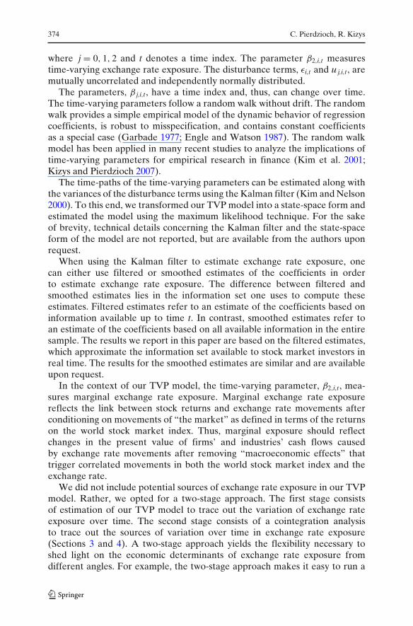
Table 1 summarizes descriptive statistics of monthly stock market returnsand exchange rate movements. Mean returns during our sample period werehighest in Finland and lowest in Italy (Panel A). Stock market returns showedthe highest standard deviation (Stdev) in Finland. As one would have ex-pected, investments in the world stock market portfolio were the least risky.The mean change in the real effective exchange rate (Panel B) was largest(smallest) in Sweden (Japan). Exchange rate movements showed the highest(lowest) standard deviation in the case of Japan (Austria).

2.3 Estimation results

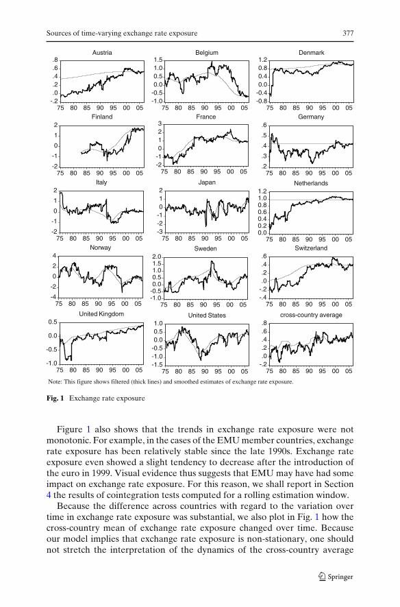
Figure 1 shows how exchange rate exposure changed over time. The resultthat exchange rate exposure changed over time is consistent with evidenceof time-variation in exchange rate exposure reported in the earlier literature(for example, Williamson 2001). Dominguez and Tesar (2006), however, haveargued, for a sample consisting of both OECD and developing countries, thatexchange rate exposure tends to be constant at the country level, and is varying

376 C. Pierdzioch, R. Kizys

Table 1 Descriptive statistics

Mean Median Maximum Minimum Stdev

Panel A: Monthly stock market returnsAustria 0.2458 −0.1121 24.3014 −27.2909 5.4712Belgium 0.2231 0.1294 23.9347 −25.6877 4.9779Denmark 0.3469 0.3362 16.0821 −18.4452 5.1751Finland 1.0513 0.9657 31.6886 −35.0230 9.0570France 0.2179 0.6018 19.6511 −27.2126 6.0427Germany 0.1754 0.3751 17.2050 −28.8447 5.6335Italy −0.0438 −0.1828 26.2075 −21.1786 6.7641Japan 0.2555 0.3488 16.8415 −23.6716 5.4428Netherlands 0.2207 0.5478 19.4335 −28.6970 5.4659Norway 0.3037 0.7421 22.9010 −34.1726 7.4273Sweden 0.5281 0.4229 27.7957 −25.29527 6.5925Switzerland 0.2870 0.6493 19.7844 −27.4507 4.9892United Kingdom 0.1037 0.8533 41.2787 −32.6530 5.7767United States 0.1816 0.4686 15.1184 −24.5130 4.3418World 0.1419 0.4630 13.4620 −18.8391 4.2441

Panel B: Monthly exchange rate returnsAustria −0.0409 −0.0228 2.0300 −4.4047 0.7549Belgium 0.0134 0.0307 6.7548 −2.2461 0.7816Denmark −0.0207 −0.0206 4.4773 −4.7651 0.9020Finland 0.0239 −0.0669 9.6288 −4.3044 1.1754France 0.0218 −0.0364 4.3705 −3.2081 0.9838Germany 0.0081 0.0969 2.6478 −6.7029 1.0769Italy 0.0277 −0.0577 8.0600 −5.4213 1.3183Japan −0.0888 0.1329 7.3000 −9.4725 2.3129Netherlands −0.0236 0.0095 3.6479 −3.3625 0.8843Norway −0.0071 −0.0177 5.59449 −3.7302 1.1080Sweden 0.0998 0.0134 11.9428 −3.6785 1.4388Switzerland −0.0620 0.0100 5.5516 −5.1522 1.4061United Kingdom −0.0302 −0.0654 8.5253 −7.8723 1.7672United States 0.0784 0.0231 4.7413 −4.7259 1.4567

over time at the firm level. We present results for the period 1975–2006 inorder to minimize the influence of the initial conditions we used to start theestimation of our TVP model.

As indicated by the smoothed estimates, only for Germany and the Nether-lands exchange rate exposure potentially was stable over time. When inter-preting the smoothed estimates, however, one should take into account thatthe maximum likelihood estimator of the variance of a coefficient in a TVPmodel has a large point mass at zero when coefficient variation is small (Stockand Watson 1998). Thus, the variance may be readily mistaken for zero. Inaddition, evidence reported in earlier empirical studies implies that, in the caseof Germany, exchange rate exposure was not constant over time (Entorf andJamin 2007). We focus in the remainder of this paper on the filtered estimates.

When interpreting the time-paths of exchange rate exposure, one shouldtake into account that both large positive and large negative values implya large absolute exchange rate exposure. Small positive and small negativevalues, in contrast, imply a small absolute exchange rate exposure. For themajority of the countries in our sample, exchange rate exposure has shown atendency to grow and to become positive over time.

Sources of time-varying exchange rate exposure 377

-.2.0.2.4.6.8

75 80 85 90 95 00 05

Austria

-1.0-0.50.00.51.01.5

75 80 85 90 95 00 05

Belgium

-0.8-0.40.00.40.81.2

75 80 85 90 95 00 05

Denmark

-2

-1

0

1

2

75 80 85 90 95 00 05

Finland

-2-10123

75 80 85 90 95 00 05

France

.2

.3

.4

.5

.6

75 80 85 90 95 00 05

Germany

-2

-1

0

1

2

75 80 85 90 95 00 05

Italy

-3-2-1012

75 80 85 90 95 00 05

Japan

0.00.20.40.60.81.01.2

75 80 85 90 95 00 05

Netherlands

-4

-2

0

2

4

75 80 85 90 95 00 05

Norway

-1.0-0.50.00.51.01.52.0

75 80 85 90 95 00 05

Sweden

-.4-.2.0.2.4.6

75 80 85 90 95 00 05

Switzerland

-1.0

-0.5

0.0

0.5

75 80 85 90 95 00 05

United Kingdom

-1.5-1.0-0.50.00.51.0

75 80 85 90 95 00 05

United States

-.2.0.2.4.6.8

75 80 85 90 95 00 05

cross-country average

Note: This figure shows filtered (thick lines) and smoothed estimates of exchange rate exposure.

Fig. 1 Exchange rate exposure

Figure 1 also shows that the trends in exchange rate exposure were notmonotonic. For example, in the cases of the EMU member countries, exchangerate exposure has been relatively stable since the late 1990s. Exchange rateexposure even showed a slight tendency to decrease after the introduction ofthe euro in 1999. Visual evidence thus suggests that EMU may have had someimpact on exchange rate exposure. For this reason, we shall report in Section4 the results of cointegration tests computed for a rolling estimation window.

Because the difference across countries with regard to the variation overtime in exchange rate exposure was substantial, we also plot in Fig. 1 how thecross-country mean of exchange rate exposure changed over time. Becauseour model implies that exchange rate exposure is non-stationary, one shouldnot stretch the interpretation of the dynamics of the cross-country average

378 C. Pierdzioch, R. Kizys

too far. Notwithstanding, the dynamics of the cross-country average shouldgive a broad picture of the general trends in exchange rate exposure. Forthe countries in our sample, the cross-country mean of exchange rate expo-sure fluctuated between −0.2 and +0.4 until around 1995, then temporarilyincreased to a level of +0.6, and slightly decreased again to fluctuate around alevel of +0.4 at the end of the sample period.

3 Full-sample cointegration tests

We now analyze the links between exchange rate exposure, an economy’sopenness to trade, and the industry composition of imports. To this end, wepresent results of cointegration tests estimated on the full sample of data.

In order to construct our measure of openness to trade, we collectedmonthly data on imports and exports from the database maintained by theOECD, and we downloaded quarterly data on GDP from Thompson FinancialDatastream. The data for Denmark, Belgium, and Sweden start in 1977, 1993,and 1980, respectively. We computed our measure of openness to trade as thesum of a country’s monthly exports and imports divided by GDP. To this end,we transformed the quarterly GDP data to monthly data by using a simplemethod of constant frequency conversion. This method divides the quarterlyGDP data by a factor of three and assigns the same monthly value to everymonth in a quarter.

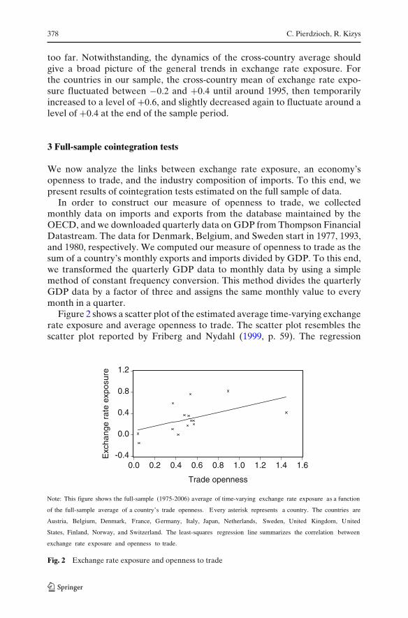
Figure 2 shows a scatter plot of the estimated average time-varying exchangerate exposure and average openness to trade. The scatter plot resembles thescatter plot reported by Friberg and Nydahl (1999, p. 59). The regression

-0.4

0.0

0.4

0.8

1.2

0.0 0.2 0.4 0.6 0.8 1.0 1.2 1.4 1.6

Trade openness

Exc

hang

e ra

te e

xpos

ure

Note: This figure shows the full-sample (1975-2006) average of time-varying exchange rate exposure as a function

of the full-sample average of a country’s trade openness. Every asterisk represents a country. The countries are

Austria, Belgium, Denmark, France, Germany, Italy, Japan, Netherlands, Sweden, United Kingdom, United

States, Finland, Norway, and Switzerland. The least-squares regression line summarizes the correlation between

exchange rate exposure and openness to trade.

Fig. 2 Exchange rate exposure and openness to trade

Sources of time-varying exchange rate exposure 379

line also shown in the scatter plot captures the positive correlation betweenexchange rate exposure and openness to trade. In the context of our empiricalmodel, however, a comparison of the full-sample averages of exchange rateexposure and openness to trade could be problematic. Our TVP model impliesthat exchange rate exposure follows a random walk and, by construction,has a stochastic trend. Similarly, because international trade has substantiallyincreased over time, it is not surprising that the results of unit root tests shownin panel A of Fig. 3 indicate that openness to trade also may feature a stochastictrend.

Imported inputs and the industry composition of imports may matter forexchange rate exposure (see, for example, Allayannis and Ihrig 2001). In orderto measure the industry composition of a country’s imports, we computed theratio of imports from non-oil exporting countries to imports from oil exportingcountries. The data on imports are from Thompson Financial Datastream.The data for Belgium start in 1997. The results of unit root tests suggest that,with few exceptions, the industry composition of imports may be integrated oforder one (panel B of Fig. 3). Because the industry composition of importsmay be integrated and thus may feature a stochastic trend, it is interestingto analyze whether time-varying exchange rate exposure shared the samestochastic trend.

In order to test for a common stochastic trend, we implemented Johansen’s(1988) approach to test for cointegration. For the sake of brevity, we report the

Panel A: Openness to trade

0.0

0.2

0.4

0.6

0.8

1.0

1 2 3 4 5 6 7 8 9 10 11 12 13 14

Panel A: Industry composition of imports

.0

.2

.4

.6

.8

1 2 3 4 5 6 7 8 9 10 11 12 13 14

Note: Panel A shows p-values of Augmented Dickey-Fuller (ADF) tests for a unit root in trade openness. Panel

B shows p-values of ADF tests for a unit root in the industry composition of imports. The numbers shown at the

horizontal axis represent the countries in our sample, where 1 = Austria, 2 = Belgium, 3 = Denmark, 4 = France,

5 = Germany, 6 = Italy, 7 = Japan, 8 = Netherlands, 9 = Sweden, 10 = United Kingdom, 11 = United States, 12 =

Finland, 13 = Norway, and 14 = Switzerland. We used data for the period 1975-2006 to implement the tests. The

solid (dashed) horizontal line denotes the 5 (10) percent level of significance.

Fig. 3 Unit-root tests

380 C. Pierdzioch, R. Kizys

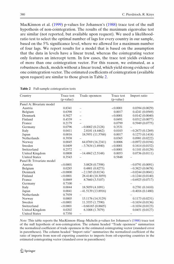
MacKinnon et al. (1999) p-values for Johansen’s (1988) trace test of the nullhypothesis of non-cointegration. The results of the maximum eigenvalue testare similar (not reported, but available upon request). We used a likelihood-ratio test to select the optimal number of lags for every country in our sample,based on the 5% significance level, where we allowed for a maximum numberof four lags. We report results for a model that is based on the assumptionthat the data in levels have a linear trend, whereas the cointegrating vectoronly features an intercept term. In few cases, the trace test yields evidenceof more than one cointegration vector. For this reason, we estimated, as arobustness check, models without a linear trend, which yield strong evidence ofone cointegration vector. The estimated coefficients of cointegration (availableupon request) are similar to those given in Table 2.

Table 2 Full-sample cointegration tests

Country Trace test Trade openness Trace test Import ratio(p-value) (p-value)

Panel A: Bivariate modelAustria 0.8341 – <0.0001 0.0394 (0.0029)Belgium 0.6398 – 0.0017 0.4241 (0.0569)Denmark 0.5827 – <0.0001 0.0142 (0.0040)Finland 0.4539 – 0.0491 0.0312 (0.0077)France 0.2179 – 0.0799 0.5949 (0.0775)Germany 0.0796 −0.0002 (0.2128) 0.3531 –Italy 0.0411 2.8181 (4.4462) 0.0103 −0.2673 (0.1269)Japan 0.0016 18.5951 (11.5768) 0.0017 0.1273 (0.1418)Netherlands 0.3938 – 0.0365 0.0981 (0.0222)Norway 0.0045 64.0769 (16.2341) 0.0006 −0.0972 (0.0194)Sweden 0.0409 −3.7634 (1.6940) <0.0001 0.1614 (0.0152)Switzerland 0.2572 – <0.0001 0.1101 (0.0129)United Kingdom 0.0008 −14.4862 (2.5148) 0.0053 0.0736 (0.0111)United States 0.3543 – 0.5848 –

Panel B: Trivariate modelAustria <0.0001 3.0828 (0.7398) −0.0791 (0.0091)Belgium 0.0285 0.4801 (0.8273) −0.3823 (0.0678)Denmark <0.0000 −2.1385 (0.8134) −0.0244 (0.0041)Finland <0.0001 28.4140 (10.3059) −0.1244 (0.0140)France 0.0069 8.7660 (3.5107) −0.6925 (0.0717)Germany 0.7100 – –Italy 0.0044 18.5059 (4.1091) 0.2781 (0.1610)Japan 0.0041 −41.5139 (13.8916) −0.4016 (0.1480)Netherlands 0.7939 – –Norway 0.0005 15.1176 (14.5129) 0.1173 (0.0231)Sweden <0.0001 11.3355 (1.7590) −0.1654 (0.0136)Switzerland <0.0001 −0.66165 (0.8605) −0.1034 (0.0123)United Kingdom 0.0202 6.1008 (1.7079) 0.0451 (0.0127)United States 0.7350 – –

Note: This table reports the MacKinnon–Haug–Michelis p-values for Johansen’s (1988) trace testof the null hypothesis of non-cointegration. The column headed “Trade openness” summarizesthe normalized coefficient of trade openness in the estimated cointegrating vector (standard errorin parentheses). The column headed “Import ratio” summarizes the normalized coeffcient of theratio of imports from non-oil exporting countries to imports from oil-exporting countries in theestimated cointegrating vector (standard error in parentheses)

Sources of time-varying exchange rate exposure 381

The results summarized in Table 2 indicate that, in a bivariate model,there is strong evidence of cointegration between exchange rate exposure andthe industry composition of imports. In contrast, evidence of cointegrationbetween exchange rate exposure and openness to trade is weak. The resultsfor a trivariate model indicate that, for the majority of countries, there is acommon stochastic trend among exchange rate exposure, openness to trade,and the industry composition of imports. Germany, the Netherlands, andthe United States are exceptions. For some countries, Johansen’s trace testindicates cointegration between trade openness and the industry compositionof imports (results not reported).

The coefficient that captures the effect of the industry composition ofimports on exchange rate exposure is positive in the majority of countries. Itfollows that an increase in the ratio of imports from non-oil exporting countriesto imports from oil-exporting countries led to a long-run increase in exchangerate exposure. Given the positive correlation between average time-varyingexchange rate exposure and openness to trade reported in Fig. 2, it is somewhatunexpected in economic terms that the coefficient of openness to trade often isnegative in the trivariate model. A negative coefficient implies that an increasein a country’s openness to trade in many cases led to a decrease in long-runexchange rate exposure. A negative coefficient, however, is consistent with theview that exchange rate exposure is linked to imported input factors and, morespecifically, the industry structure of imports rather than to openness to tradeper se.

4 Rolling-window cointegration tests

Because the cointegration relations between exchange rate exposure and itssources may have changed over time, we implemented rolling-window tests forcointegration. We used bivariate models to estimate the cointegration relationbetween exchange rate exposure and openness to trade and between exchangerate exposure and the industry composition of imports. We excluded Belgiumand Finland from the analysis because data start relatively late in the sampleperiod.

We used a rolling estimation window of length 10 years to compute Jo-hansen’s trace eigenvalue test for cointegration. Concerning the number oflags in the error correction model, we varied the number of lags between oneand four and selected, in every estimation, the lag length based on a likelihoodratio test. In order to assess the statistical significance of our results, we formedthe ratio of the trace eigenvalue statistic to the respective 95% critical value. Ifthe ratio exceeds one, the null hypothesis of non-cointegration can be rejected.

The cointegration analysis in Section 3 yielded the result that in the longrun the industry composition of imports may be a more important source ofchanges over time in exchange rate exposure than a country’s openness totrade. The results of the rolling-window cointegration tests summarized inFigs. 4 and 5 corroborate this result. In the case of the industry composition

382 C. Pierdzioch, R. Kizys

0.0

0.4

0.8

1.2

1.6

1985 1990 1995 2000 2005

Austria

0.0

0.5

1.0

1.5

2.0

2.5

1985 1990 1995 2000 2005

Denmark

0.0

0.5

1.0

1.5

2.0

2.5

1985 1990 1995 2000 2005

France

0.4

0.8

1.2

1.6

2.0

2.4

1985 1990 1995 2000 2005

Germany

0

1

2

3

4

1985 1990 1995 2000 2005

Italy

0.0

0.5

1.0

1.5

2.0

2.5

1985 1990 1995 2000 2005

Japan

0.0

0.5

1.0

1.5

2.0

2.5

1985 1990 1995 2000 2005

Netherlands

0.0

0.5

1.0

1.5

2.0

2.5

1985 1990 1995 2000 2005

Norway

0

1

2

3

4

5

1985 1990 1995 2000 2005

Sweden

0.0

0.4

0.8

1.2

1.6

2.0

1985 1990 1995 2000 2005

Switzerland

0

1

2

3

4

5

1985 1990 1995 2000 2005

United Kingdom

0.0

0.4

0.8

1.2

1.6

2.0

1985 1990 1995 2000 2005

United States

Note: The tests for cointegration are based on models that feature exchange rate exposure and openness to

trade. The rolling estimation window has a length of ten years. This figure summarizes results for Johansen’s

trace eigenvalue statistic scaled by its critical value (thick line). Whenever the scaled statistic exceeds unity, the

null hypothesis of non-cointegration is rejected.

Fig. 4 Rolling-window cointegration tests (openness to trade)

of imports, the trace eigenvalue test clearly exceeds its critical value in themajority of cases. The only clear-cut exception is Germany. In contrast, thetrace eigenvalue test is often smaller than its critical value in the case ofopenness to trade. The evidence of cointegration between exchange rateexposure and openness to trade is strongest for Denmark, Norway, Sweden,and the United Kingdom. In the cases of the other countries in our sample, thetrace eigenvalue test only becomes significant occasionally.

It is interesting to note that the introduction of the euro in 1999 did not leadto a discernible change in the cointegration relation between exchange rateexposure of EMU member countries and the industry composition of imports.In contrast, cointegration between exchange rate exposure and opennessto trade temporarily peaked after the introduction of the euro, but lost insignificance again at the very end of the sample period.

5 An illustrative model

In order to illustrate why openness to trade and the industry compositionof imports may matter for exchange rate exposure, we consider a stylized

Sources of time-varying exchange rate exposure 383

0

5

10

15

20

1985 1990 1995 2000 2005

Austria

0

2

4

6

8

1985 1990 1995 2000 2005

Denmark

0.0

0.5

1.0

1.5

2.0

1985 1990 1995 2000 2005

France

0.0

0.4

0.8

1.2

1.6

1985 1990 1995 2000 2005

Germany

0

1

2

3

4

1985 1990 1995 2000 2005

Italy

0.0

0.5

1.0

1.5

2.0

1985 1990 1995 2000 2005

Japan

0

1

2

3

4

1985 1990 1995 2000 2005

Netherlands

0

1

2

3

4

1985 1990 1995 2000 2005

Norway

0

2

4

6

8

10

1985 1990 1995 2000 2005

Sweden

0.5

1.0

1.5

2.0

2.5

3.0

1985 1990 1995 2000 2005

Switzerland

0

1

2

3

4

5

1985 1990 1995 2000 2005

United Kingdom

0.0

0.4

0.8

1.2

1.6

1985 1990 1995 2000 2005

United States

Note: The tests for cointegration are based on models that feature exchange rate exposure and the industry

composition of imports. The rolling estimation window has a length of ten years. This figure summarizes results

for Johansen’s trace eigenvalue statistic scaled by its critical value (thick line). Whenever the scaled statistic

exceeds unity, the null hypothesis of non-cointegration is rejected.

Fig. 5 Rolling-window cointegration tests (industry composition of imports)

monopolistic-competition model based on Floden et al. (2008). For a oligopolyversion of the model, see Bodnar et al. (2002). We consider a model thatdeliberately leaves many aspects important for the study of exchange rateexposure unexplored, but it illustrates the theoretical foundation of our mainresults. We then move on to study the effect of large multinational firms onexchange rate exposure. Finally, we consider the effect of the introduction ofthe euro on exchange rate exposure.

5.1 The model

The model features a firm that sells a good at home and abroad at prices pand p∗, where foreign sales account for a proportion 0 ≤ α ≤ 1 of total sales.The firm combines domestic and imported raw materials for producing thegood, where the proportion of domestic raw materials used in production isgiven by 0 ≤ μ ≤ 1. The price of foreign raw materials is denominated in termsof foreign currency. We assume that both the price of domestic inputs andthe foreign currency price of foreign raw materials are constant and scaled toassume the value unity. When q (q∗) denotes the quantity of the good sold at

384 C. Pierdzioch, R. Kizys

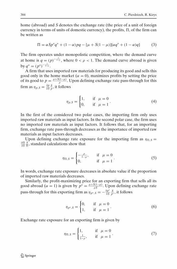
home (abroad) and S denotes the exchange rate (the price of a unit of foreigncurrency in terms of units of domestic currency), the profits, �, of the firm canbe written as

� = αSp∗q∗ + (1 − α)pq − [μ + S(1 − μ)][αq∗ + (1 − α)q] (3)

The firm operates under monopolistic competition, where the demand curveat home is q = (p)

− 11−ρ , where 0 < ρ < 1. The demand curve abroad is given

by q∗ = (p∗)−1

1−ρ .A firm that uses imported raw materials for producing its good and sells this

good only in the home market (α = 0), maximizes profits by setting the priceof its good to p = μ+S(1−μ)

ρ. Upon defining exchange rate pass-through for this

firm as ηp,S = ∂p∂S

Sp , it follows

ηp,S ={

1, if μ = 00, if μ = 1

. (4)

In the first of the considered two polar cases, the importing firm only usesimported raw materials as input factors. In the second polar case, the firm usesno imported raw materials as input factors. It follows that, for an importingfirm, exchange rate pass-through decreases as the importance of imported rawmaterials as input factors decreases.

Upon defining exchange rate exposure for the importing firm as η�,S =∂�∂S

S�

, standard calculations show that

η�,S ={

− ρ

1−ρ, if μ = 0

0, if μ = 1. (5)

In words, exchange rate exposure decreases in absolute value if the proportionof imported raw materials decreases.

Similarly, the profit-maximizing price for an exporting firm that sells all itsgood abroad (α = 1) is given by p∗ = μ+S(1−μ)

ρS . Upon defining exchange rate

pass-through for this exporting firm as ηp∗,S = − ∂p∗∂S

Sp∗ , it follows

ηp∗,S ={

0, if μ = 01, if μ = 1

. (6)

Exchange rate exposure for an exporting firm is given by

η�,S ={

1, if μ = 01

1−ρ, if μ = 1

. (7)

Sources of time-varying exchange rate exposure 385

In the case of an exporting firm acting under monopolistic competition,exchange rate pass-through and exchange rate exposure increase as the pro-portion of imported raw materials decreases.

Because a national stock market index comprises both importing andexporting firms, the model shows that, when one neglects imported rawmaterials, a country’s trade openness should have a positive effect on exchangerate exposure (Friberg and Nydahl 1999). As μ approaches unity, the exchangerate exposure of the exporting firm clearly is larger than the exchange rateexposure of the importing firm.

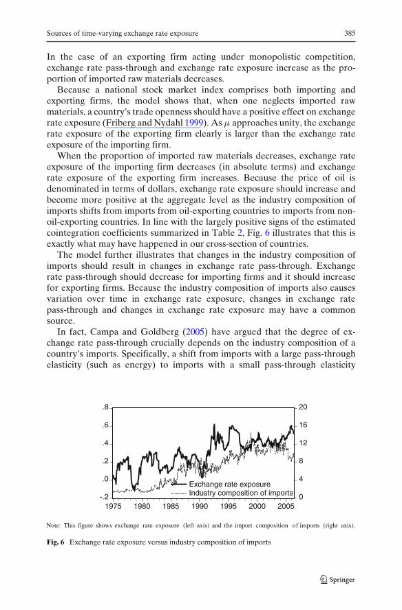
When the proportion of imported raw materials decreases, exchange rateexposure of the importing firm decreases (in absolute terms) and exchangerate exposure of the exporting firm increases. Because the price of oil isdenominated in terms of dollars, exchange rate exposure should increase andbecome more positive at the aggregate level as the industry composition ofimports shifts from imports from oil-exporting countries to imports from non-oil-exporting countries. In line with the largely positive signs of the estimatedcointegration coefficients summarized in Table 2, Fig. 6 illustrates that this isexactly what may have happened in our cross-section of countries.

The model further illustrates that changes in the industry composition ofimports should result in changes in exchange rate pass-through. Exchangerate pass-through should decrease for importing firms and it should increasefor exporting firms. Because the industry composition of imports also causesvariation over time in exchange rate exposure, changes in exchange ratepass-through and changes in exchange rate exposure may have a commonsource.

In fact, Campa and Goldberg (2005) have argued that the degree of ex-change rate pass-through crucially depends on the industry composition of acountry’s imports. Specifically, a shift from imports with a large pass-throughelasticity (such as energy) to imports with a small pass-through elasticity

-.2

.0

.2

.4

.6

.8

0

4

8

12

16

20

1975 1980 1985 1990 1995 2000 2005

Exchange rate exposureIndustry composition of imports

Note: This figure shows exchange rate exposure (left axis) and the import composition of imports (right axis).

Fig. 6 Exchange rate exposure versus industry composition of imports

386 C. Pierdzioch, R. Kizys

(such as manufacturing) should result in a decrease of exchange rate pass-through into import prices. Using data for 25 OECD countries, Campa andGoldberg (2005) have found that an increase in the ratio of imports from non-oil exporting countries to imports from oil exporting countries indeed loweredthe degree of exchange rate pass-through into import prices.

Our stock-market-based evidence of a cointegration relation between theindustry composition of imports and exchange rate exposure, thus, lendssupport to the result reported by Campa and Goldberg (2005) that the industrycomposition of a country’s imports is an important determinant of exchangerate pass-through. Moreover, because changes in exchange rate pass-throughand changes in exchange rate exposure may have a common source, thenon-monotonic variation over time in exchange rate exposure documented inSection 2.3 may explain why some authors have reported that exchange ratepass-through has declined in the past decade (Marazzi and Sheets 2007), whileother authors have reported mixed evidence of such a decline (Campa andGoldberg 2005).

Finally, we only mention very briefly that evidence of time-varying ex-change rate pass-through is important for macroeconomic modeling. Recentresearch on micro-founded dynamic general equilibrium modeling showsthat the welfare effects of, for example, monetary policy in open economiescrucially depend on the degree of exchange rate pass-through (Betts andDevereux 2000). The fact that our stock-market-based evidence of time-varying exchange rate exposure can be linked to time-varying exchange ratepass-through, thus, may provide insights useful for macroeconomic modelingof open economies.

5.2 Large multinational firms

Yet another aspect that is worth mentioning is that large multinational firmsaccount for a considerable weight in MSCI stock market indexes, which weused to calculate stock returns for our sample of countries. Multinational firmsmay account for a substantial proportion of total stock market capitalizationin small countries. The model shows that large multinational firms withproduction facilities abroad may have a substantial effect on exchange rateexposure. In terms of the model, multinational firms with production facilitiesabroad may fall into the category of a firm with revenues and costs mainlydenominated in terms of foreign currency (α = 1, μ = 0).

The growing importance of multinational firms may, thus, account for thestabilization of average exchange rate exposure in the second half of the 1990s.On the one hand side, an ongoing shift away from imported raw materialsmay have caused exchange rate exposure to increase. On the other hand,the growing importance of multinational firms may have countered the effectof this shift on exchange rate exposure because, when cast in terms of themodel, the exchange rate exposure of multinational firms with production

Sources of time-varying exchange rate exposure 387

facilities abroad may be more appropriately described by the case α = 1, μ = 0,η�,S = 1 than by the case α = 1, μ = 1, η�,S = 1

1−ρ.

As regards empirical evidence concerning exchange rate exposure of multi-national firms, the results of recent research by Williamson (2001) suggestthat exchange rate exposure of automotive firms from the United Statesand Japan changed over time, and that exchange rate exposure is positivelylinked to the ratio of foreign sales to total sales. Gao (2000) has found thata depreciation of the dollar has a significant positive effect on the returnsof stocks of U.S. multinational firms through foreign sales, and a significantnegative effect through foreign production. Crabb (2002) has documentedevidence that some previous findings of insignificant exchange rate exposure ofU.S. multinational firms may be due in part to hedging activities undertaken bythese firms. As for Japan, He and Ng (1998) have argued that highly leveragedJapanese multinational firms tend to have smaller exchange rate exposure, buta firm’s foreign involvement is positively linked to the degree of exchangeexposure.

5.3 The introduction of the euro

The model can be used to illustrate the implications of the introduction of theeuro for exchange rate exposure. As concerns the eurozone, the introductionof the euro should have reduced exchange rate exposure stemming from intra-eurozone trade. In terms of the model, firms that are involved mainly in intra-eurozone trade may be described in terms of an importing firm that sells itsgood in the euro area, but that still imports raw materials. A comparison ofEqs. 5 and 7 then shows that, for a given openness to trade and a given industrycomposition of imports, the introduction of the euro should have led to areduction in exchange rate exposure. It follows that the introduction of theeuro in 1999 may also help to explain, at least with respect to EMU membercountries, why average exchange rate exposure stabilized in the second half ofthe 1990s.

The introduction of the euro also may explain in part why we found onlyweak evidence of a common stochastic trend of exchange rate exposure andopenness to trade. Only an extra-eurozone measure of openness to tradeshould matter for exchange rate exposure of the eurozone countries (Hutsonand O’Driscoll 2009). However, the introduction of the euro does not explainwhy our rolling-window cointegration tests often yield insignificant results inthe case of openness to trade even before the introduction of the euro. In anycase, the introduction of the euro reinforces our main result that the industrycomposition of imports should be a more important source of exchange rateexposure than openness to trade.

Available empirical evidence suggests that the introduction of the euro hashad a significant effect on exchange rate exposure in EMU member countries.For example, Bartram and Karolyi (2006) have reported that the introductionof the euro led to a reduction in exchange rate exposure of euro-area firms and

388 C. Pierdzioch, R. Kizys

of non-euro firms with a high proportion of foreign sales or assets in Europe.Furthermore, they have found that exchange rate exposure of firms withpositive (negative) exchange rate exposure decreased (increased) after theintroduction of the euro. In another empirical study, Hutson and O’Driscoll(2009) have found that the introduction of the euro was followed by an increasein firm-specific exchange-rate exposure. Hutson and O’Driscoll (2009) havealso reported that the introduction of the euro was followed by a reduction inmarket-level exchange rate exposure.

6 Concluding remarks

We have reported evidence of time-varying exchange rate exposure sharing acommon stochastic trend with the industry composition of a country’s imports.Evidence of a common stochastic trend of exchange rate exposure with acountry’s openness to trade, in contrast, is weaker than in the case of theindustry composition of imports. We have also implemented rolling-windowcointegration tests to account for changes in cointegration relations over timethat were caused, for example, by the introduction of the euro. While tradeopenness has received considerable attention as a potential source of exchangerate exposure in the earlier empirical literature (Friberg and Nydahl 1999;Hutson and O’Driscoll 2009), the role played by the industry composition ofimports has received less attention in the empirical literature (see, for example,Allayannis and Ihrig 2001 for the US). Our evidence sheds some light on thevariation over time in exchange rate exposure, and on the sources of thisvariation, but more research needs to be done to better understand time-variation of exchange rate exposure.

First, the evidence we have reported mainly describes the sources of long-run trends in exchange rate exposure. A natural challenge is to identifyfactors that help to explain the variation in exchange rate exposure over shorthorizons. Second, we have assumed that the link between stock market returnsand exchange rate movements is linear. Because some authors have studiednonlinearities in exchange rate exposure (Holmes and Magrebi 2002; Kizys andPierdzioch 2007), it is interesting to complement our analysis in future researchby taking into account such nonlinearities. Third, we have been concernedwith the variation over time in the exchange rate exposure of national stockmarket indexes. In future research, one could extend our analysis to the levelof individual industries or individual firms. Such an analysis may have thepotential to link the research on exchange rate exposure with the micro-oriented research on the determinants of exchange rate pass-through. Fourth,apart from the industry composition of imports, another potentially importanteconomic determinant of exchange rate exposure is the well-known “balance-sheet effect”. In case of a depreciation, firms balance-sheets deteriorate incase firms debt is denominated in terms of foreign currency. While beyondthe scope of this paper, it would be interesting to study in future research thebalance-sheet effect in more detail.

Sources of time-varying exchange rate exposure 389

Acknowledgements Part of this paper was written during a visit of Renatas Kizys at SaarlandUniversity. The hospitality of Saarland University is gratefully acknowledged. We thank threeanonymous referees for helpful comments. We also thank participants of a seminar at theFraunhofer-Institut für Techno- und Wirtschaftsmathematik, Kaiserslautern, for helpful com-ments. The usual disclaimer applies.

References

Adler M, Dumas B (1984) Exposure to currency risk: definition and measurement. Financ Manage3:41–50

Allayannis G, Ihrig J (2001) Exposure and markups. Rev Financ Stud 14(3):805–835Bartram SM, Karolyi GA (2006) The impact of the introduction of the Euro on foreign exchange

rate risk exposures. J Empir Finance 13:519–549Betts C, Devereux MB (2000) Exchange rate dynamics in a model of pricing-to-market. J Int Econ

50:215–244BIS (2006) BIS effective exchange rate indices. Data available from the internet page of the BIS

at http://www.bis.org/statistics/eer/index.htmBodnar GM, Dumas B, Marston RC (2002) Pass-through and exposure. J Finance 57:199–231Campa J, Goldberg L (2005) Exchange rate pass-through into import prices. Rev Econ Stat

87:679–690Crabb, PC (2002) Multinational corporations and hedging exchange rate exposure. Int Rev Econ

Finance 11:299–314Dominguez KME, Tesar LL (2006) Exchange rate exposure. J Int Econ 68:188–218Engle RF, Watson M (1987) Kalman filter: applications to forecasting and rational-expectation

models. In: Bewley T (ed) Advances in econometrics, fifth world congress. Cambridge Uni-versity Press, Cambridge

Entorf H, Jamin G (2007) German exchange rate exposure at DAT and aggregate levels, interna-tional trade and the role of exchange rate adjustment costs. Ger Econ Rev 8:344–374

Floden M, Simbanegavi W, Wilander, W (2008) When Is a lower exchange Rate pass-throughassociated with greater exchange rate exposure? J Int Money Finance 27:124–139

Friberg R, Nydahl S (1999) Openness and the exchange rate exposure of national stock markets.Int J Financ Econ 4:55–62

Gao, T (2000) Exchange rate movements and the profitability of U.S. multinationals. J Int MoneyFinance 19:117–134

Garbade K (1977) Two methods for examining the stability of regression coefficients. J Am StatAssoc 72:54–63

He J, Ng LK (1998) The foreign exchange exposure of Japanese multinational corporations. JFinance 53:733–753

Holmes MJ, Magrebi N (2002) Non-linearities, regime switching, and the relationship betweenAsian equity and foreign exchange markets. Int Econ J 16:121–139

Hutson E, O’Driscoll A (2009) Firm-level exchange rate exposure in the Eurozone. Int Bus Rev(in press)

Johansen S (1988) Statistical analysis of cointegration vectors. J Econ Dyn Control 12:231–254Kim CJ, Nelson CR (2000) State-space models with regime switching. MIT, CambridgeKim CJ, Morley MC, Nelson CR (2001) Does an intertemporal tradeoff between risk and return

explain mean reversion in stock prices? J Empir Finance 8:403–426Kizys R, Pierdzioch C (2007) Time-varying nonlinear exchange rate exposure. Applied Financial

Economics Letters 3:385–389Marazzi M, Sheets N (2007) Declining exchange rate pass-through to U.S. import prices: the

potential role of global factors. J Int Money Finance 26:924–947MacKinnon JG, Haug AA, Michelis L (1999) Numerical distribution functions of likelihood ratio

tests for cointegration. J Appl Econ 14:563–577Sekine T (2006) Time-varying exchange rate pass-through: experiences of some industrialized

countries. BIS working papers 202. Bank for International Settlements, Basel

390 C. Pierdzioch, R. Kizys

Stock JH, Watson MW (1998) Median unbiased estimation of coefficient variance in a time-varying parameter model. J Am Stat Assoc 93:349–358

Williamson R (2001) Exchange rate exposure and competition: evidence from the automotiveindustry. J Financ Econ 59:441–475

Yang J (1997) Exchange rate pass-through into U.S. manufacturing industries. Rev Econ Stat79:95–104

Int Econ Econ Policy (2010) 7:391–409DOI 10.1007/s10368-010-0146-z

ORIGINAL PAPER

Capital mobility and labor market volatility

M. Alper Çenesiz · Christian Pierdzioch

Published online: 12 February 2010© Springer-Verlag 2010

Abstract We used a dynamic two-country optimizing model featuringefficiency wages to analyze the implications of capital mobility for labor mar-ket volatility. Capital mobility magnifies the short-run effects of productivityshocks and monetary shocks on employment and the real wage, but dampensthe medium-run effects. The overall effects of capital mobility on the volatilityand the cyclical properties of employment and the real wage are moderate.

Keywords Capital mobility · Efficiency wages · Labor market volatility

JEL Classification E44 · F36 · F41

1 Introduction

A question widely discussed among academics and politicians is whether theincrease in capital mobility that has taken place since the mid-1980s has givenrise to more labor market volatility and job uncertainty (Scheve and Slaughter2004). This question is of central importance because the burden of adjustmentthat labor has to bear in the wake of macroeconomic fluctuations shouldincrease when capital is internationally highly mobile while labor is not. Inconsequence, the recent increases in capital mobility may have resulted in an

M. A. Çenesiz (B)FEP, CEF.UP, University of Porto, R. Roberto Frias, 4200-464 Porto, Portugale-mail: acenesiz@fep.up.pt

C. PierdziochDepartment of Economics, Saarland University, P.O. Box 15 11 50,66041, Saarbruecken, Germanye-mail: c.pierdzioch@mx.uni-saarland.de

392 M.A. Çenesiz, C. Pierdzioch

asymmetric distribution of the benefits and losses from globalization amongmobile capital and immobile labor. Inflexibilities and frictions in labor marketsthat are beleaguered by structural unemployment have the power to reinforcethis asymmetric distribution of the benefits and losses from globalization. Inconsequence, the potentially complex interaction of capital mobility and labormarket frictions is likely to be one key determinant of the extent to whichpeople are willing to accept the economic and social changes brought about bythe globalization of the world’s economy.

We used a dynamic general equilibrium model to analyze whether and, if so,to which extent capital mobility increases labor market volatility. Our dynamicgeneral equilibrium model builds on the two-country general equilibriummodels developed by Obstfeld and Rogoff (1995) and Betts and Devereux(2000, 2001), which have become the prototype models for analyzing macro-economic dynamics in open economies. Their models feature a Walrasianlabor market in which wages adjust rapidly, households are always on theirlabor supply schedule, and structural unemployment is absent. To accountfor the stylized facts of real-world labor markets, we developed an extendedmodel that features a non-Walrasian labor market. Our extended model canexplain important stylized facts of labor markets like the existence of structuralunemployment, the moderate procyclical dynamics of real wages, the lowcorrelation between real wages and employment, and the high volatility ofemployment relative to that of real wages.

In order to model a non-Walrasian labor market, we extended our dynamicgeneral equilibrium model to incorporate efficiency wages. The analysis ofthe implications of efficiency wages for the properties of dynamic generalequilibrium models has a long tradition in macroeconomic research (Danthineand Donaldson 1990). Our approach to introduce efficiency wages into ourdynamic general equilibrium model builds on the recent contributions ofCollard and de la Croix (2000) and Danthine and Kurmann (2004). Theyextend dynamic general equilibrium models to incorporate the so-called “giftexchange” efficiency-wage theory that traces back to the work of Akerlof(1982). The “gift exchange” efficiency-wage theory stipulates that workersdislike effort. Workers are willing to provide effort beyond some referencelevel of effort (the gift of workers) if they feel that their firm treats them well.Firms, in turn, seek to motivate workers by offering a wage above the market-clearing wage (the gift of the firm). The optimizing behavior of workers andfirms results in structural unemployment.

We found that, in a model featuring efficiency wages, capital mobilitymagnifies the response of employment and the real wage in the immediate af-termath of productivity shocks and monetary shocks. At the same time capitalmobility dampens the medium run effects of productivity shocks and monetaryshocks on employment and the real wage. As a result, the overall effect ofcapital mobility on the volatility of employment and the real wage, and on theircyclical properties, is moderate. Our results regarding the effects of capital

Capital mobility and labor market volatility 393

mobility on the volatilities of key macroeconomic variables is reminiscent of afamous result derived by Cole and Obstfeld (1991), who show that allocationsin an endowment economy may be identical under complete markets andfinancial autarky.

Much significant research has been done in recent years to explore the linkbetween financial openness and macroeconomic volatility. Razin and Rose(1994), who study common and country-specific shocks as well as transitoryand persistent shocks in a large panel of countries, find no clear linkagebetween measures of goods and capital mobility and volatility (Page 71). Theyattribute their result to the prevalence of shocks that are common acrosscountries (Page 73). Using a search-theoretic model, Aziarides and Pissarides(2007) report that capital mobility may result in a substantial increase in labormarket volatility. Buch and Pierdzioch (2005) and Buch et al. (2005) reportthat the link between capital mobility and macroeconomic volatility in OECDcountries has changed over time and may depend on the nature of shockshitting an economy. Similarly, Kose et al. (2003) find that capital mobility maybe associated with an increase in the ratio of consumption volatility to incomevolatility, but that this effect turns negative if the volume of gross capitalflows crosses a particular threshold. Recent empirical evidence, thus, showsthat capital mobility need not necessarily increase macroeconomic volatility.This result is consistent with the observation that in the United States andother Western countries business-cycle volatility and employment volatilityhave tended to decrease since the mid 1980s (Stock and Watson 2002; Carlinoet al. 2003).

We organize the remainder of this paper as follows. In Section 2, we layout the dynamic general equilibrium model we used to derive our results. Thebasic structure of our model resembles the structures of the models developedby Obstfeld and Rogoff (1995) and Betts and Devereux (2000, 2001), so thatour discussion can be relatively brief. In Section 3, we report the results ofnumerical simulations of our model. In Section 4, we offer some concludingremarks.

2 The model

The world consists of two countries. Both countries are populated by a con-tinuum of infinitely lived households. Households form rational expectations.Domestic and foreign households have identical preferences. Households areinternationally immobile. Households own the firms of the country in whichthey reside. Firms sell the differentiated goods they produce in a monopolisti-cally competitive goods market. Some firms set the prices of their goods in thecurrency of the country in which they reside. Other firms set the prices of theirgoods in the currency of their customers. We call the latter a pricing-to-market

394 M.A. Çenesiz, C. Pierdzioch

(PTM) firms (Betts and Devereux 2000, 2001). In addition to households andfirms, every country is populated by a government.

2.1 Households’ preferences

Each household consists of a large number of household members of totalmeasure unity. Some members of households are unemployed, while the oth-ers are employed. Following Alexopoulos (2004) and Danthine and Kurmann(2004), employment is randomly allocated across workers. The proportion ofunemployed household members is the same across households. Householdsmake all intertemporal decisions, and redistribute consumption equally amongtheir members. Each household inelastically supplies one unit of time for work.At the household level, fluctuations in employment can, thus, be interpretedas fluctuations in hours worked. Each household has preferences definedover consumption, real balances, and effort. The expected discounted lifetimeutility of a representative household is given by

E0

∞∑

t=0

β t

⎡

⎣log(C jt − X j

t ) + χ

1 − σ

(M j

t

Pt

)1−σ

− N jt G(e j

t )

⎤

⎦ , (1)

with j being a household index and 0 < β < 1, χ > 0, and σ > 0. Et denotesthe conditional expectations operator, Nt denotes the proportion of householdmembers working, G(et) denotes the disutility of effort, Mt/Pt denotes realmoney holdings, and Ct denotes a real consumption index. This consumption

index, Ct =[∫ 1

0 ct(z)θ−1θ dz

] θθ−1

, is defined as a constant elasticity of substitutionindex of differentiated goods, ct(z), z ∈ [0, 1], where the elasticity of substi-tution is given by θ > 1 . The consumer price index, Pt, is defined as theminimum expenditure required to buy one unit of Ct. The consumer priceindex is defined as

Pt =[∫ n

0pt(z)1−θdz +

∫ n+(1−n)ξ

nqt(z∗)1−θdz +

∫ 1

n+(1−n)ξ

(St p∗(z∗)1−θdz] 1

1−θ

,

(2)

where n ∈ (0, 1) denotes the size of the domestic country, pt(z) denotes thedomestic currency price of a domestically produced good, qt(z∗) denotes thedomestic currency price of a foreign PTM good, St denotes the nominalexchange rate, and p∗

t (z∗) denotes the foreign currency price of a foreign non-

PTM good. The parameter ξ denotes the proportion of PTM firms.Households do not only derive utility from consuming the consumption

index, C jt , but also derive disutility from the variable X j

t . This variable capturesa “catching-up with the Joneses” effect in households’ preferences and isdefined as

X jt = hCA

t−1, (3)

Capital mobility and labor market volatility 395

where 0 < h < 1, and CAt = denotes aggregate (per capita) consumption. An

increase in the level of aggregate consumption results in a decrease in thelevel of utility a household attains, and in an increase in the marginal utilitya household derives from consumption, implying that households try to “catchup with the Joneses”.

The disutility a household derives from effort is determined by an effortfunction, G(e j

t ). Four considerations matter for the specification of the effortfunction (Collard and de la Croix 2000; Danthine and Kurmann 2004). First,if a firm pays a higher real wage, households are motivated and work harder.For this reason, their reference level of effort is an increasing function of theindividual households’ current real wage, w

jt . Second, if the aggregate level

of employment is high, households realize that they can easily find a newemployment opportunity in case they lose their job. Hence, the reference levelof effort is a decreasing function of the aggregate level of employment, Nt.Third, if the real wage received by a household does not change when theaggregate real wage increases, individual households’ relative compensationdecreases. Because households perceive this to be unfair, they decrease thelevel of effort they provide. This implies that the reference level of effort isa decreasing function of the aggregate real wage, wt. Fourth, if householdsobserve changes in real wages from one period to the next, they adjust theirreference level of effort. This captures the empirical finding reported byBewley (1998) that changes in wages rather than wage levels are an importantdeterminant of effort. Accordingly, the reference level of effort is a decreasingfunction of an individual households’ past wage, w

jt−1. Assuming that the

past wage affects effort resolves the problem documented by Danthine andDonaldson (1990) that effort functions which only feature contemporaneousvariables do not give rise to rigid and sluggish equilibrium wage dynamics (seealso Danthine and Kurmann 2004). Taken together, these four considerationsimply that the effort function is of the format

G(e jt ) =

[e j

t −(φ0 + φ1 log w

jt + φ2 ln Nt + φ3 log wt + φ4 log w

jt−1

)]2, (4)

where φ1 > 1, φ2 < 0, φ3 < 0, and φ4 < 0.

2.2 Budget constraint and first-order conditions

Households maximize their expected discounted lifetime utility subject totheir budget constraint. According to households’ budget constraint, the totalincome received by households consists of the yield on their holdings inbonds, the profit income yielded by their ownership of domestic firms, theirlabor income, and their income from renting capital to domestic firms. Giventheir total income, households determine their optimal consumption, effort,investment, and next period’s capital stock. Households also decide on their

396 M.A. Çenesiz, C. Pierdzioch

preferred holdings in domestic money and bonds. The individual households’budget constraint is given by

D jt = Rt−1 D j

t−1 + M jt−1 + w

jt N j

t Pt + Rkt k j

t Pt

−PtCjt − Pt I

jt − Pt AC j

t + �t + PtTt, (5)

where Dt denotes the quantity of domestic nominal riskless one-period bonds,Rt denotes the gross nominal interest rate on bonds, Rk

t denotes the realrental rate of capital, Tt denotes real lump-sum transfers received from thegovernment, It denotes real investment, ACt is the real adjustment costhouseholds incur when adjusting their capital stock, and �t denotes the profitincome the household receives from domestic firms. The law of motion ofhouseholds’ capital stock, k j

t , is given by

I jt = k j

t+1 − (1 − δ)k jt , (6)

where 0 < δ < 1 denotes the depreciation rate. The investment good, I jt , is

constructed in the same way as the consumption index, C jt . The adjustment

cost households incur when adjusting their capital stock are given by

AC jt = ψ

2(k j

t+1 − k jt )

2

k jt

, (7)

where ψ ≥ 0.The first-order conditions that describe the solution to an individual house-

holds’ utility-maximization problem are given by

C jt − X j

t = λt Pt, (8)

χ

(M j

t

Pt

)−σ

= λt Pt − β Pt Etλt+1, (9)

λt = β Rt Etλt+1, (10)

e jt = φ0 + φ1 log w

jt + φ2 ln Nt + φ3 log wt + φ4 log w

jt−1, (11)

λt Pt + β(1 − δ)Etλt+1 Pt+1 + βEt Rkt+1λt+1 Pt+1 − ψλt Pt

k jt+1 − k j

t

k jt

+ ψ

2βEtλt+1 Pt+1

(k jt+2)

2 − (k jt+1)

2

(k jt+1)

2= 0 (12)

where λt denotes the Lagrange multiplier on the households’ budget con-straint.

Capital mobility and labor market volatility 397

2.3 Financial markets

As regards the structure of international financial markets, we consideredtwo polar cases. First, we considered the case of a world economy in whichagents can trade in integrated financial markets for riskless one-period nom-inal bonds. For simplicity, we assume that domestic households invest ina home-currency denominated nominal bond, and that foreign householdsinvest in a foreign-currency denominated nominal bond and a home-currencydenominated nominal bond. This assumption implies that, in the case of anintegrated international bond market, the condition of uncovered interest-rate parity holds. Second, we considered the case of a world economy inwhich markets for trade in international assets do not exist (Cole and Obstfeld1991; Heathcote and Perri 2002). In this case, home households invest in ahome-currency denominated nominal bond, and foreign households invest ina foreign-currency denominated nominal bond. The market-clearing conditionfor the home-currency denominated nominal bond in the case of an integratedinternational bond market is given by

∫

jD j

t d j +∫

jD j∗

t d j = 0 (13)

and the market-clearing conditions in the case of financial autarky are givenby

∫

jD j

t d j = 0 (14)

and∫

jF j∗

t d j = 0 (15)

where F j∗t denotes the foreign-currency denominated bond.

2.4 Firms

Each firm consists of a production and a price-setting unit. The production unitproduces the good, z, according to the production function

yt(z) = Atkt(z)α[et(z)Nt(z)]1−α, (16)

where At denotes an aggregate productivity shock. Given the level of effortprovided by households, the production unit determines the real wage andchooses the level of capital and employment in order to minimize totalproduction costs. Following Danthine and Kurmann (2004), we assume thatthe production unit replaces the individual households’ past wage, w

jt−1, with

the aggregate past wage wt−1 in the effort function when minimizing totalproduction costs. Because firms treat wt−1 as exogenous when minimizing

398 M.A. Çenesiz, C. Pierdzioch

total production costs, they do not account for the consequences of offeringa higher wage today for the future effort of households. In technical terms,this assumption implies that the production unit solves a static wage-settingproblem. Hence, the production unit does not have to store informationon the distribution of past wages of its employees. In economic terms, thisassumption implies that, in a symmetric equilibrium, all firms will pay identicalwages. Using wt−1 in the effort function, the first-order conditions for the cost-minimization problem are given by

wt(z) = (1 − α)mct(z)yt(z)

nt(z), (17)

nt(z) = (1 − α)mct(z)φ1 yt(z)

et(z)wt(z), (18)

Rkt (z) = αmct(z)

yt(z)

kt(z), (19)

where mct(z) denotes real marginal costs. The first-order conditions implyet(z) = φ1, a condition known as the Solow (1979) condition.

Because of monopolistic competition in the goods market, the price-settingunit can set the price of the good produced by the production unit in order tomaximize profits. We let q∗

t (z) denote the foreign-currency price of a domesticPTM good, and yD

t (z) and yFt (z) denote the demand at home and abroad. The

demand functions are given by

yDt (z) = (pt(z)/Pt)

−θ Qt, (20)

yFt (z) = (

q∗t (z)/P∗

t

)−θQ∗

t , (21)

Qt = n(Ct + It + ACt) and Q∗t = (1 − n)(C∗

t + I∗t + AC∗

t ). The price-settingunit sets the price of the good subject to a discrete time version of the price-setting mechanism developed by Calvo (1983). With probability 0 < γ < 1, theprice-setting unit cannot revise the price of its good in any given period oftime. Therefore, the price-setting unit of a PTM firm sets the current domestic-currency and foreign-currency prices of the product, pt(z) and q∗

t (z), so as tomaximize the expected discounted present value of profits. The solutions tothis maximization problem are

pt(z) = θ

θ − 1Et

∑∞s=t γ

s−t Rt,s(Qs/P−θs )mcs

Et∑∞

s=t γs−t Rt,s(Qs/P1−θ

s ), (22)

q∗t (z) = θ

θ − 1Et

∑∞s=t γ

s−t Rt,s(Q∗s /P∗−θ

s )mcs

Et∑∞

s=t γs−t Rt,s(Q∗

s /P∗−θs )Ss/Ps

, (23)

Capital mobility and labor market volatility 399

where Rt,s ≡ ∏tj=s R−1

t is the market discount factor. Similar expressions canbe derived for the profit-maximizing prices, qt(z∗) and p∗

t (z∗), set by the price-

setting unit of a foreign PTM firm, and for the profit-maximizing price setby the price-setting unit of a non-PTM firm. The latter set a single domesticcurrency denominated price for both the domestic and the foreign goodsmarket.

2.5 The government sector

The government sector consists of a single central bank and a fiscal authority.The central bank controls the money supply. The budget constraint of the fiscalauthority is given by

PtTt = Mt − Mt−1. (24)

2.6 Solution and calibration of the model

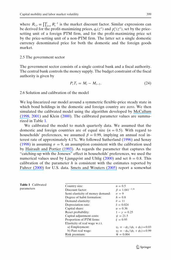
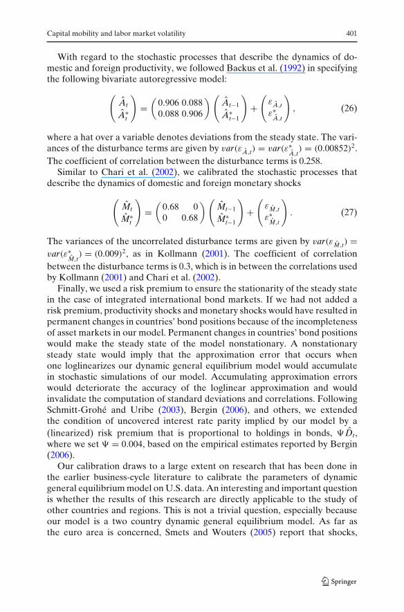
We log-linearized our model around a symmetric flexible-price steady state inwhich bond holdings in the domestic and foreign country are zero. We thensimulated the calibrated model using the algorithm developed by McCallum(1998, 2001) and Klein (2000). The calibrated parameter values are summa-rized in Table 1.

We calibrated the model to match quarterly data. We assumed that thedomestic and foreign countries are of equal size (n = 0.5). With regard tohouseholds’ preferences, we assumed β = 0.99, implying an annual real in-terest rate of approximately 4.1%. We followed Sutherland (1996) and Senay(1998) in assuming σ = 9, an assumption consistent with the calibration usedby Hairault and Portier (1993). As regards the parameter that captures the“catching-up with the Joneses” effect in households’ preferences, we used thenumerical values used by Ljungqvist and Uhlig (2000) and set h = 0.8. Thiscalibration of the parameter h is consistent with the estimates reported byFuhrer (2000) for U.S. data. Smets and Wouters (2005) report a somewhat

Table 1 Calibratedparameters

Country size: n = 0.5Discount factor: β = 1.041−1/4

Semi elasticity of money demand: σ = 9Degree of habit formation: h = 0.8Demand elasticity: θ = 11Depreciation rate: δ = 0.024Capital share: α = 0.36Reset probability: 1 − γ = 0.25Capital adjustment costs: ψ = 21.5Proportion of PTM firms: ξ = 0.95Elasticity of real wage w.r.t.

a) Employment: η1 ≡ −φ2/(φ1 + φ3)=0.03b) Past real wage: η2 ≡ −φ4/(φ1 + φ3)=0.99

Risk premium: � = 0.004

400 M.A. Çenesiz, C. Pierdzioch

lower parameter of h = 0.59 for the euro area and h = 0.69 for U.S. data.In Section 3.2 we, therefore, shall report results for alternative calibrationsof the parameter that captures the “catching-up with the Joneses” effect inhouseholds’ preferences.

With regard to the elasticity of substitution between differentiated goods,we assumed θ = 11, which is common in the literature. The value we chosefor θ implies a steady-state markup of prices over marginal costs of 10%. Asregards the depreciation rate, we assumed δ = 0.024, implying an annual de-preciation rate of 10%. The capital share parameter in the production functionassumes the value α = 0.36. We calibrated the Calvo-pricing parameter suchthat the average delay between price adjustments is four periods (γ = 0.75),a value roughly the same as the one in Danthine and Kurmann (2004). Weresorted to the empirical estimates that have recently been reported by Bergin(2006) to calibrate the adjustment costs households’ incur when adjustingtheir capital stock. Accordingly, we assumed ψ = 21.5. Following again Bergin(2006), we assumed that the proportion of firms that follow a PTM price-setting strategy is relatively large. We set ξ = 0.95.

In order to calibrate the parameters of the effort function, we first derivedthe efficiency-wage function. The efficiency-wage function obtains when theSolow condition, et = φ1, is used in the effort function. Apart from a constant,the efficiency-wage function, in a symmetric equilibrium, is given by

log wt = η1 log Nt + η2 log wt−1, (25)

where η1 = −φ2/(φ1 + φ3) and η2 = −φ4/(φ1 + φ3). Danthine and Kurmann(2004) report the estimates η1 = 0.0348 and η2 = 0.9912 for the United States.Given significant cross-country differences with regard to labor-market in-stitutions and labor-market rigidities, it is interesting to ask whether thiscalibration is also valid when one studies, for example, a European or Asiancountry. In order to explore this question, we collected quarterly data fromthe International Financial Statistics CD-ROM published by the IMF onemployment, wages, and the GDP deflator for Germany and Japan. Using datafor the sample period 1991:1−2004:4 and applying the two-stage least squaresestimation technique described in detail by Danthine and Kurmann (2004),we estimated the parameters, η1 and η2, of the efficiency-wage function. ForGermany, we found η1 = 0.05 and η2 = 0.75. For Japan, we estimated η2 =0.02 and η2 = 0.90. As one would have expected, the estimation results suggestthat, with regard to labor-market related variables, there are in fact interestingdifferences between Germany and Japan, on the one hand side, and the UnitedStates, on the other hand side. Because the parameters of the efficiency-wage function are key parameters of our model, we shall present in Section 3simulation results that we obtained when we used alternative numerical valuesfor the parameters of the efficiency-wage function to calibrate our model.

Capital mobility and labor market volatility 401

With regard to the stochastic processes that describe the dynamics of do-mestic and foreign productivity, we followed Backus et al. (1992) in specifyingthe following bivariate autoregressive model:

(At

A∗t

)=

(0.906 0.0880.088 0.906

) (At−1

A∗t−1

)+

(εA,tε∗

A,t

), (26)

where a hat over a variable denotes deviations from the steady state. The vari-ances of the disturbance terms are given by var(εA,t) = var(ε∗

A,t) = (0.00852)2.

The coefficient of correlation between the disturbance terms is 0.258.Similar to Chari et al. (2002), we calibrated the stochastic processes that

describe the dynamics of domestic and foreign monetary shocks

(Mt

M∗t

)=

(0.68 00 0.68

) (Mt−1

M∗t−1

)+

(εM,tε∗

M,t

). (27)

The variances of the uncorrelated disturbance terms are given by var(εM,t) =var(ε∗

M,t) = (0.009)2, as in Kollmann (2001). The coefficient of correlation

between the disturbance terms is 0.3, which is in between the correlations usedby Kollmann (2001) and Chari et al. (2002).

Finally, we used a risk premium to ensure the stationarity of the steady statein the case of integrated international bond markets. If we had not added arisk premium, productivity shocks and monetary shocks would have resulted inpermanent changes in countries’ bond positions because of the incompletenessof asset markets in our model. Permanent changes in countries’ bond positionswould make the steady state of the model nonstationary. A nonstationarysteady state would imply that the approximation error that occurs whenone loglinearizes our dynamic general equilibrium model would accumulatein stochastic simulations of our model. Accumulating approximation errorswould deteriorate the accuracy of the loglinear approximation and wouldinvalidate the computation of standard deviations and correlations. FollowingSchmitt-Grohé and Uribe (2003), Bergin (2006), and others, we extendedthe condition of uncovered interest rate parity implied by our model by a(linearized) risk premium that is proportional to holdings in bonds, � Dt,where we set � = 0.004, based on the empirical estimates reported by Bergin(2006).

Our calibration draws to a large extent on research that has been done inthe earlier business-cycle literature to calibrate the parameters of dynamicgeneral equilibrium model on U.S. data. An interesting and important questionis whether the results of this research are directly applicable to the study ofother countries and regions. This is not a trivial question, especially becauseour model is a two country dynamic general equilibrium model. As far asthe euro area is concerned, Smets and Wouters (2005) report that shocks,

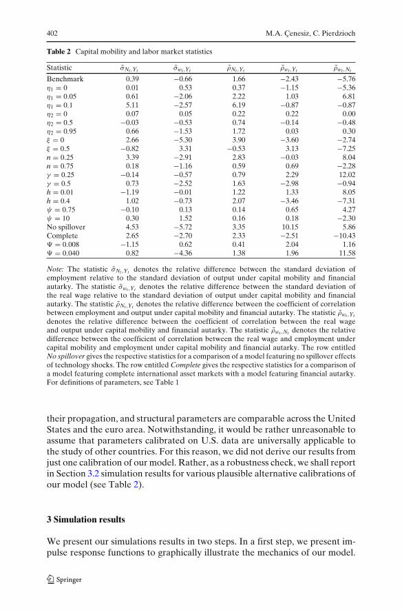
402 M.A. Çenesiz, C. Pierdzioch

Table 2 Capital mobility and labor market statistics

Statistic σNt,Yt σwt,Yt ρNt,Yt ρwt,Yt ρwt,Nt

Benchmark 0.39 −0.66 1.66 −2.43 −5.76η1 = 0 0.01 0.53 0.37 −1.15 −5.36η1 = 0.05 0.61 −2.06 2.22 1.03 6.81η1 = 0.1 5.11 −2.57 6.19 −0.87 −0.87η2 = 0 0.07 0.05 0.22 0.22 0.00η2 = 0.5 −0.03 −0.53 0.74 −0.14 −0.48η2 = 0.95 0.66 −1.53 1.72 0.03 0.30ξ = 0 2.66 −5.30 3.90 −3.60 −2.74ξ = 0.5 −0.82 3.31 −0.53 3.13 −7.25n = 0.25 3.39 −2.91 2.83 −0.03 8.04n = 0.75 0.18 −1.16 0.59 0.69 −2.28γ = 0.25 −0.14 −0.57 0.79 2.29 12.02γ = 0.5 0.73 −2.52 1.63 −2.98 −0.94h = 0.01 −1.19 −0.01 1.22 1.33 8.05h = 0.4 1.02 −0.73 2.07 −3.46 −7.31ψ = 0.75 −0.10 0.13 0.14 0.65 4.27ψ = 10 0.30 1.52 0.16 0.18 −2.30No spillover 4.53 −5.72 3.35 10.15 5.86Complete 2.65 −2.70 2.33 −2.51 −10.43� = 0.008 −1.15 0.62 0.41 2.04 1.16� = 0.040 0.82 −4.36 1.38 1.96 11.58

Note: The statistic σNt,Yt denotes the relative difference between the standard deviation ofemployment relative to the standard deviation of output under capital mobility and financialautarky. The statistic σwt,Yt denotes the relative difference between the standard deviation ofthe real wage relative to the standard deviation of output under capital mobility and financialautarky. The statistic ρNt,Yt denotes the relative difference between the coefficient of correlationbetween employment and output under capital mobility and financial autarky. The statistic ρwt,Yt

denotes the relative difference between the coefficient of correlation between the real wageand output under capital mobility and financial autarky. The statistic ρwt,Nt denotes the relativedifference between the coefficient of correlation between the real wage and employment undercapital mobility and employment under capital mobility and financial autarky. The row entitledNo spillover gives the respective statistics for a comparison of a model featuring no spillover effectsof technology shocks. The row entitled Complete gives the respective statistics for a comparison ofa model featuring complete international asset markets with a model featuring financial autarky.For definitions of parameters, see Table 1

their propagation, and structural parameters are comparable across the UnitedStates and the euro area. Notwithstanding, it would be rather unreasonable toassume that parameters calibrated on U.S. data are universally applicable tothe study of other countries. For this reason, we did not derive our results fromjust one calibration of our model. Rather, as a robustness check, we shall reportin Section 3.2 simulation results for various plausible alternative calibrations ofour model (see Table 2).

3 Simulation results

We present our simulations results in two steps. In a first step, we present im-pulse response functions to graphically illustrate the mechanics of our model.

Capital mobility and labor market volatility 403

In a second step, we report results of stochastic simulations that show how keylabor market statistics change in the wake of financial market integration.

3.1 Impulse response functions

In order to illustrate the mechanics of the model in the wake of productivityshocks and monetary shocks, we computed impulse response functions. Theimpulse response functions we shall report describe the dynamics of keymacroeconomic variables in the aftermath of a shock in terms of percentagedeviations form the steady state. Figure 1 presents impulse response functionsfor a domestic productivity shock, and Fig. 2 presents impulse responsefunctions for a domestic monetary shock.

A productivity shock increases the marginal product of capital and labor.Accordingly, firms’ demand for capital and labor increases, giving rise tohigher investment and a higher real interest rate. Firms are also willing to paya higher real wage but, given households’ effort function, the real wage adjusts

0 5 10 150.8

1

1.2

1.4

1.6 Output

0 5 10 150

0.5

1

1.5 Consumption

0 5 10 15–0.5

0

0.5

1

1.5 Employment

0 5 10 15–0.2

0

0.2

0.4

0.6 Real Wage

0 5 10 15–0.8

–0.6

–0.4

–0.2

0Nominal Exchange Rate

0 5 10 15–0.6

–0.4

–0.2

0

0.2 Real Exchange Rate

0 5 10 151

1.5

2

2.5 Investment

0 5 10 15–0.1

0

0.1

0.2

0.3 Real Interest Rate

0 5 10 150

0.5

1

1.5 Productivity

Capital MobilityAutarky

Note: The figure plots the responses of domestic variables to a unit domestic productivity shock.

All variables are measured as percentage deviations from the steady state.

Fig. 1 Productivity shock and capital mobility

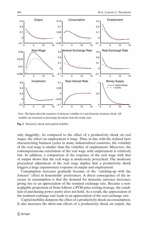
404 M.A. Çenesiz, C. Pierdzioch

0 5 10 15–0.1

0

0.1

0.2

0.3 Output

0 5 10 15–0.05

0

0.05

0.1

0.15 Consumption

0 5 10 15–0.1

0

0.1

0.2

0.3 Employment

0 5 10 150.005

0.01

0.015

0.02 Real Wage

0 5 10 15–0.1

0

0.1

0.2

0.3Nominal Exchange Rate

0 5 10 15–0.1

0

0.1

0.2

0.3 Real Exchange Rate

0 5 10 15–0.2

0

0.2

0.4

0.6 Investment

0 5 10 15–0.1

–0.05

0

0.05

0.1 Real Interest Rate

0 5 10 150

0.5

1 Money Supply

Capital MobilityAutarky

Note: The figure plots the responses of domestic variables to a unit domestic monetary shock. All

variables are measured as percentage deviations from the steady state.

Fig. 2 Monetary shock and capital mobility

only sluggishly. As compared to the effect of a productivity shock on realwages, the effect on employment is large. Thus, in line with the stylized factscharacterizing business cycles in many industrialized countries, the volatilityof the real wage is smaller than the volatility of employment. Moreover, thecontemporaneous correlation of the real wage with employment is relativelylow. In addition, a comparison of the response of the real wage with thatof output shows that the real wage is moderately procyclical. The moderateprocyclical adjustment of the real wage implies that a productivity shocktriggers a large expansionary response of output and employment.

Consumption increases gradually because of the “catching-up with theJoneses” effect in households’ preferences. A direct consequence of the in-crease in consumption is that the demand for domestic currency increases,giving rise to an appreciation of the nominal exchange rate. Because a non-negligible proportion of firms follows a PTM price-setting strategy, the condi-tion of purchasing power parity does not hold. As a result, the appreciation ofthe nominal exchange rate leads to an appreciation of the real exchange rate.

Capital mobility dampens the effect of a productivity shock on consumption.It also increases the short-run effects of a productivity shock on output, the

Capital mobility and labor market volatility 405

nominal and real exchange rates, and employment. At the same time, capitalmobility dampens the medium-run effects of such a shock on output andemployment. Thus, in order to trace out the overall effects of changes inthe degree of capital mobility on macroeconomic volatility, one should usestochastic simulations of the model. We shall present the results of stochasticsimulations in Section 3.2.

Figure 2 presents impulse response functions for a monetary shock. Theliquidity effect of a monetary shock results in a decrease in the real interestrate and an increase in investment. Consumption also increases, but onlygradually because of the “catching-up with the Joneses” effect in households’preferences. The increase in the demand for goods implies that a monetarypolicy shock results in an increase in output and employment. Firms are willingto pay higher wages, but the assumption of efficiency wages implies that amonetary policy shock exerts only a small effect on real wages. As in the caseof a productivity shock, the assumption of efficiency wages implies that thevolatility of the real wage is smaller than the volatility of employment, andthat the real wage is weakly procyclical.

With regard to international capital mobility, the impulse response functionsfor a monetary shock confirm the insights we derived from the impulseresponse functions for a productivity shock. The effects of a monetary shock onoutput and employment increase in the short run, but capital mobility dampensthe effects in the medium run. Calculation of the overall effects of changes inthe degree of capital mobility on macroeconomic volatility requires runningstochastic simulations of the model.

3.2 The effect of capital mobility on labor market volatility

We used stochastic simulation to quantitatively analyze the effects of capitalmobility on the following labor market statistics: the volatilities (i.e., standarddeviations) of employment and the real wage, their correlation, and theircorrelations with output. To this end, we computed the relative difference (inpercentage terms) between these labor market statistics under capital mobilityand under financial autarky. We simulated the model 1,000 times, where eachsimulation had a length of 25 years. As a robustness check, we performed thesimulation for various alternative calibrations of the model.

To this end, we first computed labor market statistics for our benchmarkcalibration described in Section 2.6. We then varied the parameter η1 between0 and 0.1, and the parameter η2 between 0 and 0.95 to account for our evidenceof cross-country heterogeneity with regards to the parameters of the effortfunction. In order to study the robustness of our results with respect to changesin firms’ price-setting strategies, we reduced the proportion of PTM firms, ξ ,from 0.95 to 0.5 and even to 0. In order to capture whether our results alsoapply in the case of a small (large) country, we assumed that the parameterthat captures country size, n, assumes a value of 0.25 (0.75).

We also experimented with alternative numerical values for the probabilityof not adjusting goods prices, γ . Relative to the benchmark calibration we

406 M.A. Çenesiz, C. Pierdzioch

reduced the parameter γ to 0.25 and 0.5. As an additional robustness check,we reduced the strength of the “catching up with the Joneses” effect inhouseholds’ preferences, h, from 0.8 in our benchmark calibration to 0.4 and,in yet another alternative (but empirically rather implausible) scenario, to0.01. As yet another robustness check, we set ψ = 0.75, implying that theratio of the volatility of investment to the volatility of output assumes a valueapproximately equal to the value equal to the ratio implied by U.S. data. Butwe also tried the calibration ψ = 10 to assess the sensitivity of our results withrespect to the magnitude of the capital adjustment costs.

In order to analyze the sensitivity of our simulation results to thespecification of the processes for productivity, we set the off-diagonal elementsof the bivariate autoregressive model that describes the dynamics of domesticand productivity equal to zero. In this case, the shock processes are uncorre-lated and do not feature a common cross-country component, but are purelyidiosyncratic. Razin and Rose (1994) account in their empirical study of thelink between capital mobility and macroeconomic volatility for idiosyncraticshocks and shocks that are common across countries.

Furthermore, we compared the simulation results for a model featuringcomplete international asset markets with the simulations results for a modelfeaturing financial autarky. As a final robustness check, we analyzed therobustness of our results with respect to changes in the sensitivity of the riskpremium to bond holdings. To this end, we increased the parameter � from� = 0.004 in our benchmark calibration to � = 0.008 and to � = 0.040.

Table 2 summarizes the simulation results. The relative differences betweenthe labor market statistics under capital mobility and under financial autarkyare fairly small. In many cases, the relative differences are smaller than 1%.Only the contemporaneous correlation of the real wage with employmentincreases, in the case where the average frequency of price changes is onequarter, about 12%. This correlation also increases about 12% in case ofa large risk premium (� = 0.040). Many of the relative differences have anegative sign. Moreover, the simulation results do not change much when weassume complete international asset markets rather than trade in riskless one-period nominal bond. Only the contemporaneous correlation of the real wagewith employment substantially decreases when one studies a model featuringcomplete international asset markets. Taken together, our simulation resultsindicate that our model implies that capital mobility affects the propagationof shocks, but capital mobility per se is unlikely to be a major source of labormarket volatility.

4 Conclusions

We have extended a two-country dynamic general equilibrium model to incor-porate efficiency wages. We have used our model to analyze the implicationsof capital mobility for labor market volatility. Our results suggest that capitalmobility, in the form of international trade in financial assets, is unlikely to give

Capital mobility and labor market volatility 407

rise to a significant increase in labor market volatility. Before general policy-relevant conclusions can be drawn from the kind of research we have laid outin this paper, however, more research needs to be done.

For example, in future research, our analysis could be extended to explorethe implications of other efficiency-wage theories (Danthine and Donaldson1990) or other labor market frictions like, for example, labor market search(Hairault 2002) for the link between capital mobility and labor market per-formance in open-economy dynamic general equilibrium models. In addition,it would be interesting to analyze the implications for the link betweencapital mobility and labor market volatility of other structures of internationalfinancial markets than the ones we have considered in this paper. For example,Kehoe and Perri (2002) study a model with endogenous incomplete interna-tional financial markets. In their model, international loans are imperfectlyenforceable because countries can renege on their debt and suffer the conse-quences for future borrowing.

It is also important to note that we have not considered in our analysis thatcapital mobility may affect unskilled workers in a different way than skilledworkers. Mukoyama and Sahin (2006) argue that, under incomplete markets,the costs of business cycles may be higher for unskilled workers than forskilled workers. Krusell and Smith (1999) point out that the cost of businesscycles may be high for unemployed agents with no wealth and no opportunityto insure against unemployment risk. In a similar vein, Buch and Pierdzioch(2009) argue that low-skilled workers often have more limited access tointernational financial markets than high-skilled workers. As a result, it maybe more difficult for low-skilled workers to smooth income and consumptionacross states of nature. A reasonable hypothesis for future research, therefore,is that differences in wealth and financial market participation across skilledand unskilled workers give rise to differences with regard to their abilityto benefit from international risk sharing. In other words, while our resultssuggest that, at the macro level, financial market integration does not amplifylabor market volatility to a significant extent, capital mobility may still havea significant effect on labor market volatility and job uncertainty at the microlevel.

Finally, it is important to note that we have studied the implications ofthe integration of more or less frictionless financial markets for labor marketvolatility. In the case of integrated financial markets, the only financial marketfriction that we have studied is a risk premium that is proportional to holdingsin bonds. Given the significant and disrupting financial market turmoil of2007/2008, it would be interesting, in future research, to add other financialmarket frictions and even shocks originating in financial markets to ourmodel. If financial market integration gives rise to such shocks or amplifiestheir propagation, it might well be the case that capital mobility has a largereffect on labor market volatility than implied by our stylized dynamic generalequilibrium model. In this respect, it might be worthwhile to reconsider theeffects of financial-accelerator effects in an open economy or to draw on thelarge and growing literature that studies the implications of asset price bubbles

408 M.A. Çenesiz, C. Pierdzioch

for monetary policy. Because much of this research has been framed in terms ofdynamic general equilibrium models, this research may give important insightsas to how our dynamic general equilibrium can be extended to capture in amore realistic way the potentially complex interplay between financial marketturmoil and labor market volatility.

Acknowledgements We thank two anonymous referees for their very helpful comments. Theusual disclaimer applies.

References

Akerlof GA (1982) Labor contracts as partial gift exchange. Q J Econ 97:543–569Alexopoulos M (2004) Unemployment and the business cycle. J Monet Econ 51:277–298Aziarides C, Pissarides CA (2007) Unemployment dynamics with international capital mobility.

Eur Econ Rev 51:27–48Backus DK, Kehoe PJ, Kydland FE (1992) International real business cycles. J Polit Econ 100:

745–775Bergin PR (2006) How well can the new open economy macroeconomics explain the exchange

rate and current account? J Int Money Financ 25:675–701Betts C, Devereux MB (2000) Exchange rate dynamics in a model of pricing-to-market. J Int Econ

50:215–244Betts C, Devereux MB (2001) The international effects of monetary and fiscal policy in a two-

country model. In: Calvo GA, Dornbusch R, Obstfeld M (eds) Money, capital mobility, andtrade: essays in honor of Robert A. Mundell. MIT, Cambridge, pp 9–52

Bewley TF (1998) Why not cut pay? Eur Econ Rev 42:459–490Buch CM, Döpke J, Pierdzioch C (2005) Financial openness and business cycle volatility. J Int

Money Financ 24:744–765Buch CM, Pierdzioch C (2005) The integration of imperfect financial markets: implications for

business cycle volatility. J Policy Model 27:789–804Buch CM, Pierdzioch C (2009) Low skills but high volatility? CESifo Working Paper 2665Calvo G (1983) Staggered prices in a utility-maximizing framework. J Monet Econ 12:383–398Carlino G, DeFina R, Sill K (2003) Postwar period changes in employment volatility: new evidence

from state/industry panel data. Federal Reserve Bank of Philadelphia Working Paper 03-18Chari VV, Kehoe PJ, McGrattan ER (2002) Can sticky price models generate volatile and persis-

tent real exchange rates? Rev Econ Stud 69:533–563Cole HL, Obstfeld M (1991) Commodity trade and international risk sharing: how much do

financial markets matter? J Monet Econ 28:3–24Collard F, de la Croix D (2000) Gift exchange and the business cycle: the fair wage strikes back.

Rev Econ Dyn 3:166–193Danthine JP, Donaldson JB (1990) Efficiency wages and the business cycle puzzle. Eur Econ Rev

34:1275–1301Danthine JP, Kurmann A (2004) Fair wages in a new Keynesian model of the business cycle. Rev

Econ Dyn 7:107–142Fuhrer J (2000) Habit formation in consumption and its implications for monetary-policy models.

Am Econ Rev 90:367–390Hairault JO (2002) Labor-market search and international business cycles. Rev Econ Dyn 5:

535–558Hairault JO, Portier F (1993) Money, new-Keynesian macroeconomics, and the business cycle.

Eur Econ Rev 37:1533–1568Heathcote J, Perri F (2002) Financial autarky and international business cycles. J Monet Econ 49:

601–627Kehoe PJ, Perri F (2002) International business cycles with endogenous incomplete markets.

Econometrica 70:907–928

Capital mobility and labor market volatility 409

Klein P (2000) Using the generalized Schur form to solve a multivariate linear rational expecta-tions model. J Econ Dyn Control 24:1405–1423

Kollmann R (2001) Explaining international comovements of output and asset returns: the role ofmoney and nominal rigidities. J Econ Dyn Control 25:1547–1583

Kose MA, Prasad ES, Terrones ME (2003) Financial integration and macroeconomic volatility.IMF Staff Pap 50:119–142

Krusell P, Smith AA Jr (1999) On the welfare effects of eliminating business cycles. Rev EconDyn 2:245–272

Ljungqvist L, Uhlig H (2000) Tax policy and aggregate demand management under catching upwith the Joneses. Am Econ Rev 90:356–366

McCallum B (1998) Solutions to linear rational expectations models: a compact exposition. EconLett 61:143–147

McCallum B (2001) Software for RE analysis. Computer software available at: http://wpweb2.tepper.cmu.edu/faculty/mccallum/research.html. Accessed 20 Jan 2010

Mukoyama T, Sahin A (2006) Costs of business cycles for unskilled workers. J Monet Econ53:2179–2193

Obstfeld M, Rogoff K (1995) Exchange rate dynamics redux. J Polit Econ 103:624–660Razin A, Rose AK (1994) Business-cycle volatility and openness: an exploratory cross-sectional

analysis. In: Leiderman L, Razin A (eds.) Capital mobility: the impact on consumption,investment, and growth. Cambridge University Press, Cambridge, pp 48–75

Scheve K, Slaughter MJ (2004) Economic insecurity and the globalization of production. Am JPolit Sci 48:662–674

Schmitt-Grohé S, Uribe M (2003) Closing small open economy models. J Int Econ 61:163–185Senay Ö (1998) The effects of goods and financial market integration on macroeconomic volatility.

Manch Sch Suppl 66:39–61Smets F, Wouters R (2005) Comparing shocks and frictions in the US and Euro area business

cycles: a Bayesian DSGE approach. J Appl Econ 20:161–183Solow RM (1979) Another possible source of wage stickiness. J Macroecon 1:79–82Stock JH, Watson MW (2002) Has the business cycle changed and why? NBER Macroeconomics

Annual 2002, pp 159–218Sutherland A (1996) Financial market integration and macroeconomic volatility. Scand J Econ

98:521–539

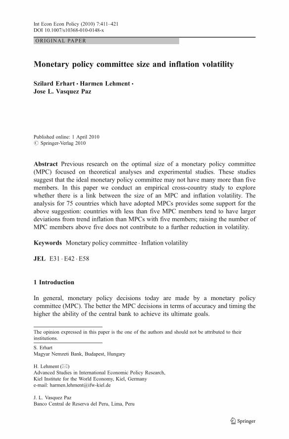
ORIGINAL PAPER

Monetary policy committee size and inflation volatility

Szilard Erhart & Harmen Lehment &Jose L. Vasquez Paz

Published online: 1 April 2010# Springer-Verlag 2010

Abstract Previous research on the optimal size of a monetary policy committee(MPC) focused on theoretical analyses and experimental studies. These studiessuggest that the ideal monetary policy committee may not have many more than fivemembers. In this paper we conduct an empirical cross-country study to explorewhether there is a link between the size of an MPC and inflation volatility. Theanalysis for 75 countries which have adopted MPCs provides some support for theabove suggestion: countries with less than five MPC members tend to have largerdeviations from trend inflation than MPCs with five members; raising the number ofMPC members above five does not contribute to a further reduction in volatility.

Keywords Monetary policy committee . Inflation volatility

JEL E31 . E42 . E58

1 Introduction

In general, monetary policy decisions today are made by a monetary policycommittee (MPC). The better the MPC decisions in terms of accuracy and timing thehigher the ability of the central bank to achieve its ultimate goals.

Int Econ Econ Policy (2010) 7:411–421DOI 10.1007/s10368-010-0148-x

The opinion expressed in this paper is the one of the authors and should not be attributed to theirinstitutions.

S. ErhartMagyar Nemzeti Bank, Budapest, Hungary

H. Lehment (*)Advanced Studies in International Economic Policy Research,Kiel Institute for the World Economy, Kiel, Germanye-mail: harmen.lehment@ifw-kiel.de

J. L. Vasquez PazBanco Central de Reserva del Peru, Lima, Peru

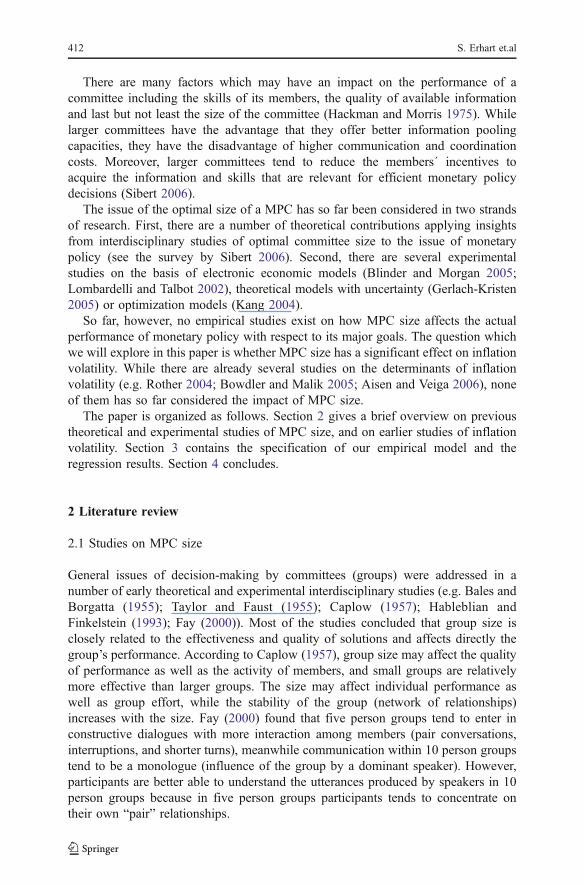
There are many factors which may have an impact on the performance of acommittee including the skills of its members, the quality of available informationand last but not least the size of the committee (Hackman and Morris 1975). Whilelarger committees have the advantage that they offer better information poolingcapacities, they have the disadvantage of higher communication and coordinationcosts. Moreover, larger committees tend to reduce the members´ incentives toacquire the information and skills that are relevant for efficient monetary policydecisions (Sibert 2006).

The issue of the optimal size of a MPC has so far been considered in two strandsof research. First, there are a number of theoretical contributions applying insightsfrom interdisciplinary studies of optimal committee size to the issue of monetarypolicy (see the survey by Sibert 2006). Second, there are several experimentalstudies on the basis of electronic economic models (Blinder and Morgan 2005;Lombardelli and Talbot 2002), theoretical models with uncertainty (Gerlach-Kristen2005) or optimization models (Kang 2004).

So far, however, no empirical studies exist on how MPC size affects the actualperformance of monetary policy with respect to its major goals. The question whichwe will explore in this paper is whether MPC size has a significant effect on inflationvolatility. While there are already several studies on the determinants of inflationvolatility (e.g. Rother 2004; Bowdler and Malik 2005; Aisen and Veiga 2006), noneof them has so far considered the impact of MPC size.

The paper is organized as follows. Section 2 gives a brief overview on previoustheoretical and experimental studies of MPC size, and on earlier studies of inflationvolatility. Section 3 contains the specification of our empirical model and theregression results. Section 4 concludes.

2 Literature review

2.1 Studies on MPC size

General issues of decision-making by committees (groups) were addressed in anumber of early theoretical and experimental interdisciplinary studies (e.g. Bales andBorgatta (1955); Taylor and Faust (1955); Caplow (1957); Hableblian andFinkelstein (1993); Fay (2000)). Most of the studies concluded that group size isclosely related to the effectiveness and quality of solutions and affects directly thegroup’s performance. According to Caplow (1957), group size may affect the qualityof performance as well as the activity of members, and small groups are relativelymore effective than larger groups. The size may affect individual performance aswell as group effort, while the stability of the group (network of relationships)increases with the size. Fay (2000) found that five person groups tend to enter inconstructive dialogues with more interaction among members (pair conversations,interruptions, and shorter turns), meanwhile communication within 10 person groupstend to be a monologue (influence of the group by a dominant speaker). However,participants are better able to understand the utterances produced by speakers in 10person groups because in five person groups participants tends to concentrate ontheir own “pair” relationships.

412 S. Erhart et.al

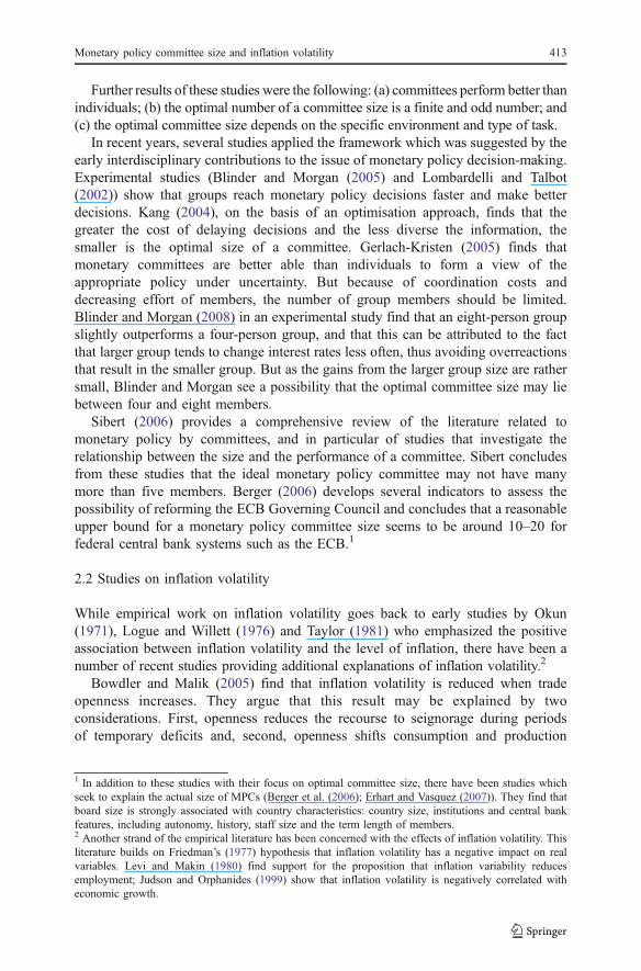
Further results of these studies were the following: (a) committees perform better thanindividuals; (b) the optimal number of a committee size is a finite and odd number; and(c) the optimal committee size depends on the specific environment and type of task.

In recent years, several studies applied the framework which was suggested by theearly interdisciplinary contributions to the issue of monetary policy decision-making.Experimental studies (Blinder and Morgan (2005) and Lombardelli and Talbot(2002)) show that groups reach monetary policy decisions faster and make betterdecisions. Kang (2004), on the basis of an optimisation approach, finds that thegreater the cost of delaying decisions and the less diverse the information, thesmaller is the optimal size of a committee. Gerlach-Kristen (2005) finds thatmonetary committees are better able than individuals to form a view of theappropriate policy under uncertainty. But because of coordination costs anddecreasing effort of members, the number of group members should be limited.Blinder and Morgan (2008) in an experimental study find that an eight-person groupslightly outperforms a four-person group, and that this can be attributed to the factthat larger group tends to change interest rates less often, thus avoiding overreactionsthat result in the smaller group. But as the gains from the larger group size are rathersmall, Blinder and Morgan see a possibility that the optimal committee size may liebetween four and eight members.

Sibert (2006) provides a comprehensive review of the literature related tomonetary policy by committees, and in particular of studies that investigate therelationship between the size and the performance of a committee. Sibert concludesfrom these studies that the ideal monetary policy committee may not have manymore than five members. Berger (2006) develops several indicators to assess thepossibility of reforming the ECB Governing Council and concludes that a reasonableupper bound for a monetary policy committee size seems to be around 10–20 forfederal central bank systems such as the ECB.1

2.2 Studies on inflation volatility

While empirical work on inflation volatility goes back to early studies by Okun(1971), Logue and Willett (1976) and Taylor (1981) who emphasized the positiveassociation between inflation volatility and the level of inflation, there have been anumber of recent studies providing additional explanations of inflation volatility.2

Bowdler and Malik (2005) find that inflation volatility is reduced when tradeopenness increases. They argue that this result may be explained by twoconsiderations. First, openness reduces the recourse to seignorage during periodsof temporary deficits and, second, openness shifts consumption and production

1 In addition to these studies with their focus on optimal committee size, there have been studies whichseek to explain the actual size of MPCs (Berger et al. (2006); Erhart and Vasquez (2007)). They find thatboard size is strongly associated with country characteristics: country size, institutions and central bankfeatures, including autonomy, history, staff size and the term length of members.2 Another strand of the empirical literature has been concerned with the effects of inflation volatility. Thisliterature builds on Friedman’s (1977) hypothesis that inflation volatility has a negative impact on realvariables. Levi and Makin (1980) find support for the proposition that inflation variability reducesemployment; Judson and Orphanides (1999) show that inflation volatility is negatively correlated witheconomic growth.

Monetary policy committee size and inflation volatility 413

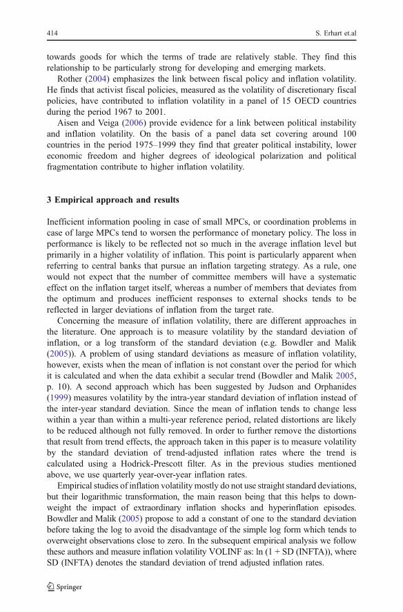
towards goods for which the terms of trade are relatively stable. They find thisrelationship to be particularly strong for developing and emerging markets.

Rother (2004) emphasizes the link between fiscal policy and inflation volatility.He finds that activist fiscal policies, measured as the volatility of discretionary fiscalpolicies, have contributed to inflation volatility in a panel of 15 OECD countriesduring the period 1967 to 2001.

Aisen and Veiga (2006) provide evidence for a link between political instabilityand inflation volatility. On the basis of a panel data set covering around 100countries in the period 1975–1999 they find that greater political instability, lowereconomic freedom and higher degrees of ideological polarization and politicalfragmentation contribute to higher inflation volatility.

3 Empirical approach and results

Inefficient information pooling in case of small MPCs, or coordination problems incase of large MPCs tend to worsen the performance of monetary policy. The loss inperformance is likely to be reflected not so much in the average inflation level butprimarily in a higher volatility of inflation. This point is particularly apparent whenreferring to central banks that pursue an inflation targeting strategy. As a rule, onewould not expect that the number of committee members will have a systematiceffect on the inflation target itself, whereas a number of members that deviates fromthe optimum and produces inefficient responses to external shocks tends to bereflected in larger deviations of inflation from the target rate.

Concerning the measure of inflation volatility, there are different approaches inthe literature. One approach is to measure volatility by the standard deviation ofinflation, or a log transform of the standard deviation (e.g. Bowdler and Malik(2005)). A problem of using standard deviations as measure of inflation volatility,however, exists when the mean of inflation is not constant over the period for whichit is calculated and when the data exhibit a secular trend (Bowdler and Malik 2005,p. 10). A second approach which has been suggested by Judson and Orphanides(1999) measures volatility by the intra-year standard deviation of inflation instead ofthe inter-year standard deviation. Since the mean of inflation tends to change lesswithin a year than within a multi-year reference period, related distortions are likelyto be reduced although not fully removed. In order to further remove the distortionsthat result from trend effects, the approach taken in this paper is to measure volatilityby the standard deviation of trend-adjusted inflation rates where the trend iscalculated using a Hodrick-Prescott filter. As in the previous studies mentionedabove, we use quarterly year-over-year inflation rates.

Empirical studies of inflation volatility mostly do not use straight standard deviations,but their logarithmic transformation, the main reason being that this helps to down-weight the impact of extraordinary inflation shocks and hyperinflation episodes.Bowdler and Malik (2005) propose to add a constant of one to the standard deviationbefore taking the log to avoid the disadvantage of the simple log form which tends tooverweight observations close to zero. In the subsequent empirical analysis we followthese authors and measure inflation volatility VOLINF as: ln (1 + SD (INFTA)), whereSD (INFTA) denotes the standard deviation of trend adjusted inflation rates.

414 S. Erhart et.al

Table 1 shows the volatility of consumer price inflation in the period 2000–2005for 75 countries with a monetary policy committee. As can be seen, volatility islowest for the Euro Area, followed by Japan and Switzerland, while the highestlevels are obtained for Lesotho, Ecuador and Belarus.

To assess the impact of MPC size on inflation volatility in the period 2000:1 to2005:4 we specify a equation for a cross-section regression analysis that links thevolatility of inflation to a basic set of control variables (X) and a vector of variablesrelated to the size of the monetary policy committee (MPC)

VOLINF ¼ a þ bX þ lMPC þ " ð1Þ

Table 1 Volatility of inflation (standard deviation of quarterly year-over-year inflation rates, trendadjusted) 2000–2005

Low volatility Medium volatility High volatility

Country Standarddeviation

Country Standarddeviation

Country Standarddeviation

Euro Area 0.22 Latvia 0.76 Israel 1.21

Japan 0.27 Trinidad and 0.77 Seychelles 1.26

Switzerland 0.31 Malta 0.79 Egypt 1.26

Denmark 0.35 Croatia 0.83 Armenia 1.30

Saudi Arabia 0.39 Czech Republic 0.84 Slovak Republic 1.33

Malaysia 0.41 Lithuania 0.85 South Africa 1.34

Slovenia 0.45 Peru 0.85 Brazil 1.36

Colombia 0.45 Hungary 0.88 Romania 1.38

Belize 0.49 Tonga 0.90 Uganda 1.45

United Kingdom 0.49 Estonia 0.91 Solomon Islands 1.45

New Zealand 0.50 Tanzania 0.91 Indonesia 1.56

United States 0.50 Guyana 0.92 Sri Lanka 1.59

Sweden 0.54 Nepal 0.93 Malawi 1.63

Bhutan 0.55 Pakistan 0.95 Papua New Guinea 1.73

Aruba 0.57 Macedonia 0.95 Kyrgyz Republic 1.86

Singapore 0.58 Albania 0.96 Sierra Leone 1.87

Canada 0.59 Barbados 0.99 Venezuela 1.94

Mexico 0.62 Iceland 1.01 Nigeria 1.97

Honduras 0.66 Poland 1.06 Moldova 2.07

Chile 0.68 Botswana 1.09 Madagascar 2.27

Cyprus 0.69 Russian Federation 1.09 Turkey 2.40

Australia 0.69 Mauritius 1.11 Argentina 2.51

Norway 0.72 Kazakhstan 1.15 Lesotho 2.62

Vanuatu 0.74 Philippines 1.15 Ecuador 2.80

Kuwait 0.74 Bulgaria 1.16 Belarus 3.35

Monetary policy committee size and inflation volatility 415

With respect to the control variables we follow the previous literature and use a setof macroeconomic variables as well as variables for the exchange rate regime. Theset of macroeconomic variables includes

– the level of the CPI inflation rate, which has been found to be a significantexplanatory variable in previous studies (Bowdler and Malik 2005; Rother2004),3

– the degree of openness, measured as the ratio of imports plus exports over GDP,which had a significant impact in the study by Bowdler and Malik (2005), and

– per capita GDP to cover effects related to the level of development; to excludefeedback effects of volatility on per capita GDP in the observation period 2000–2005, we used per capita GDP levels of 1999. Developing countries may besubject to higher inflation volatility due to less developed fiscal systems (Rother2004);4 another reason may be the relatively high share of (particularly volatile)food prices in the consumer price index of low-income countries.

With respect to the effect of MPC size we start from Sibert’s (2006) review ofprevious theoretical and experimental studies which suggests that the ideal monetarypolicy committee may not have many more than five members. In the regression weuse two dummy variables to assess the effect of a downward or upward deviationfrom this benchmark (FIVEMINUS and FIVEPLUS, taking respectively a value of 1if the number of members is below 5 or above 5). Moreover, we consider a dummyvariable ODD which takes a value of 1 if the committee size is an odd number, and 0otherwise, to test whether the higher decision efficiency of committees with an oddnumber of members—which is found in theoretical and experimental studies (e.g.Bales and Borgatta 1955)—is reflected in lower inflation volatility. Data on MPCsize are obtained from Erhart and Vasquez (2007) and are shown in (Table 4 inAppendix).

Estimation results are reported in Table 2, column (1).5 Turning first to the controlvariables, we find that the level of inflation (INF) has a significant positive effect oninflation volatility, thus confirming the result of previous studies. The effect of GDPper head is also significant and in line with the hypothesis that inflation volatilitytends to be lower in more developed countries. The effect of openness is notsignificant, in contrast to the findings by Bowdler and Malik (2005) for the period upto 2000.6 This observation can be related to a study by Bleaney (1999) according towhich the robust negative correlation between openness and the level of inflationwhich was found in cross-country data for the 1970s and 1980s has disappeared inthe 1990s. Our results suggest that the formerly robust correlation between opennessand inflation volatility which was found by Bowdler and Malik, has disappeared aswell in the recent years.

3 For a discussion of the theoretical link between inflation levels and inflation volatility see Taylor (1981)and Devereux (1989).4 We considered also fiscal indicators, but found that variables used by Rother (2004) for OECD countrieswere not available for a large number of developing countries which appear in our sample.5 Honduras is excluded here since there are no IMF data on openness provided for this country.6 This result was also obtained when measuring inflation volatility on the basis of standard deviations ofinflation rates (as in their study) rather than of trend adjusted inflation rates.

416 S. Erhart et.al

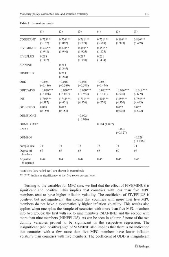
Turning to the variables for MPC size, we find that the effect of FIVEMINUS issignificant and positive. This implies that countries with less than five MPCmembers tend to have higher inflation volatility. The coefficient of FIVEPLUS ispositive, but not significant; this means that countries with more than five MPCmembers do not have a systematically higher inflation volatility. This results alsoapplies when one splits the sample of countries with more than five MPC membersinto two groups: the first with six to nine members (SIXNINE) and the second withmore than nine members (NINEPLUS). As can be seen in column 2 none of the twodummy variables proved to be significant in the respective regression. Theinsignificant (and positive) sign of SIXNINE also implies that there is no indicationthat countries with a few more than five MPC members have lower inflationvolatility than countries with five members. The coefficient of ODD is insignificant

Table 2 Estimation results

(1) (2) (3) (4) (5) (6)

CONSTANT 0.733***(3.152)

0.726***(3.062)

0.761***(3.789)

0.721***(3.568)

0.896***(1.973)

0.866***(5.469)

FIVEMINUS 0.376**(1.948)

0.378**(1.940)

0.360**(1.905)

0.351**(1.875)

FIVEPLUS 0.218(1.392)

0.217(1.388)

0.221(1.434)

SIXNINE 0.214(1.349)

NINEPLUS 0.235(1.204)

ODD −0.054(−0.486)

−0.046(−0.380)

−0.065(−0.598)

−0.051(−0.474)

GDPCAP99 −0.020***(−3.086)

−0.020***(−3.067)

−0.020***(−2.962)

−0.022***(−3.411)

−0.016***(2.596)

−0.016***(2.609)

INF 5.760***(4.517)

5.742***(4.451)

5.701***(4.576)

5.402***(4.270)

5.889***(4.520)

5.784***(4.493)

OPENNESS 0.018(0.159)

0.017(0.155)

0.057(0.505)

0.062(0.572)

DUMFLOAT1 −0.002(−0.016)

DUMFLOAT2 0.104 (1.087)

LNPOP −0.003(−0.127)

DUMPOP −0.129(−1.006)

Sample size 74 74 75 75 74 74

Degree offreedom

67 66 68 68 69 69

AdjustedR-squared

0.44 0.43 0.44 0.45 0.45 0.45

t-statistics (two-tailed test) are shown in parenthesis

** (***) indicates significance at the five (one) percent level

Monetary policy committee size and inflation volatility 417

in all regressions. Thus, while theory suggests an odd size for committees, we do notfind that committees with an even number of members perform worse in respect tostabilizing the inflation rate.

In columns (3) and (4) we control additionally for the effects of the exchange rateregime on volatility. We introduce dummies for countries whose exchange ratesystem is classified as Floating (DUMFLOAT1), or as either Floating or ManagedFloating (DUMFLOAT2). Theoretically, the effect of floating on the volatility ofinflation is ambiguous: on the one hand, floating permits an autonomous monetarypolicy which tends to be conducive for the task of stabilizing inflation; on the otherhand, floating tends to result in larger real exchange-rate fluctuations and thereby, toraise inflation volatility (Mussa 1983). As can be seen in columns (3) and (4), thetwo dummies for floating have no significant impact on inflation volatility,suggesting that both effects approximately offset each other.

As countries with less than five MPC members include some very small states(see Table 4 in Appendix), this may raise the question, whether the positive effect ofthe variable FIVEMINUS represents the effect of small country size on inflationvolatility, rather than small MPC size. To account for this consideration, we ranadditional regressions in which we replaced the MPC size variables by variables forpopulation size, using two measures (a) the log of population LNPOP, and (b) adummy DUMPOP for very small countries (less than 1 million inhabitants). Theresults are shown in columns (5) and (6). As can be seen, neither of the variables issignificant, suggesting that country size does not affect inflation volatility.7

4 Conclusion

In this paper we went beyond the standard theoretical and experimental approachesto the determination of optimal monetary policy committee (MPC) size and analysedthe empirical link between MPC size and inflation volatility. We find some supportfor the hypothesis that an MPC should not have less than five members: ourregressions showed that countries with less than five MPC members tend to havelarger deviations of inflation rates from their trend than MPCs with five members.There is also some support for the earlier suggestion (Sibert 2006) that the idealmonetary policy committee may not have more than five members, since our resultsshow that raising the number of MPC members above five does not contribute to afurther reduction in inflation volatility.

7 We also conducted a number of further robustness tests. In order to check for the possibility thatcommittee size matters only because it captures better institutions, we replaced the MPC dummies bydummies for democratic quality (dummy 1 for countries with democratic constitution and 0 otherwise) andmonetary independence (dummy 1 for countries with inflation targeting and 0 otherwise). Neither of thesetwo dummies was significant. In a further robustness test we replaced the MPC dummies by a dummy forthe federal political structure (federal countries tend to have larger monetary committees, so that the effectof committee size on economic performance may capture the effect of having a federal structure), but thisdummy also turned out to be insignificant. We also checked whether inflation volatility is affected bywhether or not MPC decisions are made by vote or by consensus (using a dummy 1 for consensusdecision-making and 0 otherwise); the dummy variable did not show a significant effect. Finally, wechecked for a single-central banker dummy which also was not significant. Results are provided by theauthors on request.

418 S. Erhart et.al

Considering actual MPC size across countries, one finds that it is mostly abovethe number of five, and in some cases substantially above this number. Reducing thenumber towards five could bring benefits in form of reduced administrative costs,but one cannot expect that it would also provide more inflation stability. Theempirical analysis in this paper suggests that central banks with more than fivemembers do not show systematically different inflation volatility if compared tocentral banks with a five member committee.

This also suggests that in the range of MPC size which we see today, costs ofcoordinating decisions within an committee have not reached a level where they leadto an actual worsening of inflation performance. The most notable case is theEuropean Central Bank which has the highest number of board members but alsothe lowest inflation volatility of the countries under consideration. The results of thepresent study, however, suggest that large MPCs could be reduced in size withoutnegative consequences for the task of keeping inflation volatility low.

Appendix

Table 3 Data source

Variable Name Source

GDP per capita GDPCAP99 IFS

Inflation INF IFS

Openness OPENNESS IFS, OECD (2002)

Exchange rate regime DUMFLOAT1 IFS

DUMFLOAT2

MPC measures FIVEMINUS Erhart and Vasquez (2007)

FIVEPLUS

ODD

Population POP IFS

Table 4 MPC size

Size “de jure” Size “de jure” Size “de jure”

Albania 9 Hungary 13 Pakistan 9

Argentina 10 Iceland 3 Papua New Guinea 1

Armenia 7 Indonesia 9 Peru 7

Aruba 1 Israel 1 Philippines 7

Australia 9 Japan 9 Poland 10

Barbados 7 Kazakhstan 9 Romania 9

Belarus 9 Kuwait 8 Russian Federation 13

Monetary policy committee size and inflation volatility 419

References

Aisen A, Veiga FJ (2006) Political instability and inflation volatility. IMF Working Paper WP/06/212.International Monetary Fund, Washington, DC

Bales R, Borgatta E (1955) Size of group as a factor in the interaction profile. In: Hare P, Borgatta E, BalesR (eds) Handbook of small group research. Alfred A. Knopf, New York, pp 396–414

Berger H (2006) Optimal Central Bank design: benchmarks for the ECB, CESIFO Working Paper 1697,March 2006

Berger H, Nitsch V, Lybeck T (2006) Central Bank Boards around the world: why does membership sizediffer? Mimeo

Bleaney M (1999) The disappearing openness-inflation relationship: a cross-country analysis of inflationrates. IMF Working Paper WP/99/161. International Monetary Fund, Washington, DC

Blinder A, Morgan J (2005) Are two hands better than one?: monetary policy by committee. J MoneyCredit Bank 37(5):789–812

Blinder A, Morgan J (2008) Leadership in groups: a monetary policy experiment. Int J Cent Bank 4(4):117–150

Bowdler C, Malik A (2005) Openness and inflation volatility. CSAE Working Papers 2005–08. Center forthe Study of African Economies, Oxford University

Caplow T (1957) Organizational size. Admin Q 1(2):350–369Devereux M (1989) A positive theory of inflation and inflation variance. Econ Inq 27(1):105–116Erhart, S, Vasquez J (2007) Optimal monetary policy committee size: theory and cross country evidence.

Kiel Advanced Studies Working Papers 439. Kiel Institute for the World EconomyFay N (2000) The effect of group size upon influence and process in group communication. Submitted for

the Degree of Ph.D. to The Higher Degree Committee of The Faculty of Social Sciences, Universityof Glasgow

Table 4 (continued)

Size “de jure” Size “de jure” Size “de jure”

Belize 7 Kyrgyz Republic 9 Saudi Arabia 5

Bhutan 5 Latvia 8 Seychelles 6

Botswana 9 Lesotho 8 Sierra Leone 7

Brazil 9 Libya 7 Slovak Republic 11

Bulgaria 7 Lithuania 5 Slovenia 9

Canada 6 Macedonia 9 Solomon Islands 9

Chile 5 Madagascar 1 Sri Lanka 5

Colombia 7 Malawi 7 Sweden 6

Croatia 14 Malaysia 12 Switzerland 3

Cyprus 7 Malta 1 Tanzania 10

Czech Republic 7 Mauritius 10 Tonga 7

Denmark 3 Mexico 5 Trinidad and Tobago 9

EuroArea 18 Moldova 5 Turkey 7

Ecuador 5 Nepal 7 United Kingdom 9

Egypt 15 New Zealand 1 United States 12

Estonia 10 Nigeria 11 Vanuatu 4

Guyana 6 Norway 7 Venezuela 7

Honduras 5 Oman 7

Erhart and Vasquez (2007)

420 S. Erhart et.al

Friedman M (1977) Nobel lecture: inflation and unemployment. J Polit Econ 85(3):451–472Gerlach-Kristen P (2005) Monetary policy committees and interest rate setting. Eur Econ Rev 50(2):487–

507Hableblian J, Finkelstein S (1993) Top management team size, CEO dominance, and firm performance:

the moderating roles of environmental turbulence and discretion. Acad Manage J 36(4):844–863Hackman R, Morris C (1975) Group task, group interaction process, and group performance effectiveness:

a review and proposed integration. In: Berkowitz L (ed) Advances in experimental social psychology,vol 8. Academic, New York

Judson R, Orphanides A (1999) Inflation volatility and growth. Int Financ 2(1):117–138Kang S (2004) The optimal size of committee. J Econ Res 9:217–238Levi MD, Makin JH (1980) Inflation uncertainty and the Phillips curve: some empirical evidence. Am

Econ Rev 70(5):1022–1027Logue DE, Willett TD (1976) A note on the relationship between the rate and the variability of inflation.

Economica 43:151–158Lombardelli C, Talbot J (2002) Committees versus Individuals: an experimental analysis of monetary

policy decision-making. Bank Engl Q Bull 42(3):262–273Mussa M (1983) Empirical regularities in the behaviour of exchange rates and theories of the foreign

exchange market. In: Brunner K, Meltzer A (eds) Theory, policy and institutions: papers fromCarnegie-Rochester Conference on Public Policy, pp 165–213

OECD (2002) Statistics brief, FebruaryOkun A (1971) The mirage of steady anticipated inflation. Brookings Pap Econ Act 2:485–498Rother PC (2004) Fiscal policy and inflation volatility. ECB Working Papers 317. European Central Bank,

FrankfurtSibert A (2006) Central banking by committee. Int Financ 9(2):145–168Taylor D, Faust W (1955) Twenty questions: efficiency in problem solving as a function of size of group.

In: Hare P, Bogatta E, Bales R (eds) Handbook of small group research. Alfred A. Knopf, New York,pp 208–220

Taylor J (1981) On the relation between the variability of inflation and the average inflation rate.Carnegie-Rochester Conference Series on Public Policy, Spring, pp 57–86

Monetary policy committee size and inflation volatility 421

Int Econ Econ Policy (2010) 7:423–436DOI 10.1007/s10368-010-0150-3

ORIGINAL PAPER

Exchange rate volatility, international tradeand labour demand

Udo Broll · Sabine Hansen-Averlant

Published online: 13 March 2010© Springer-Verlag 2010

Abstract The purpose of this study is to assess under what conditions exchangerate volatility generates a positive effect on an exporting firm’s labour demand.As the exchange rate volatility increases, so does the value of the export op-tion, provided that firms are flexible with respect to international trade. Highervolatility increases the potential gains from trade and can increase the demandfor labour. The firm’s trade flexibility can be interpreted as a real hedgingstrategy when financial markets are incomplete. In many newly industrializingcountries and emerging economies financial markets are imperfect or risksharing markets are just starting to develop at a rather slow pace.

Keywords Exchange rate volatility · Trade · Labour demand · Flexibility ·Risk aversion · Real option · Real hedge

JEL Classification F16 · F23 · F31 · F41

1 Introduction

In the last decades international firms were exposed to high foreign exchangerate risk since major currencies showed substantial volatility (Doehring 2008).The volatility of prices and foreign exchange rates may affect employmentand the wage process in two ways, first through international trade in goodsand services and second through foreign direct investment.1 The intensified

1See for example, Krugman (1989), Franke (1991), Schmidt and Broll (2009).

U. Broll (B) · S. Hansen-AverlantFakultät für Wirtschaftswissenschaften, Technische Universität Dresden,01062 Dresden, Germanye-mail: udo.broll@tu-dresden.de

424 U. Broll, S. Hansen-Averlant

interest in the various effects of exchange rate volatility arose with theabolition of the Bretton-Woods agreement. The outcome of the research onthis topic is far from unique, and the debate on the effects of exchange ratevolatility keeps going on.

Many of the first studies concentrated on the impact of a regime of freelyfloating exchange rates on international trade flows. A common belief by someof the early critics of freely floating exchange rates was that they would makeinternational trade and hence welfare decrease and not increase as predictedby its supporters. The reasoning behind this rejection is that international firmsare commonly risk averse: they would not be willing to incur revenue lossesthat would arise from uncertain export or import activity.2 This is the overalleffect which is found when uncertainty is introduced to a formerly certainsituation. One might think that a great part of the associated riskiness hasdisappeared with the realization of the euro currency area.3 However, thisstatement is overly generalized. Within the EU-27, differences with regardto internal terms-of-trade continue to matter. As regards international traderelationships with extra-EU countries, exchange rate volatility has the samebearing for each member country as it had before the single currency wasintroduced.

Another branch of literature deals with the impact of exchange rate volatil-ity on international trade flows, i.e. with an increase in uncertainty whichrepresents the marginal effect of uncertainty (Dellas and Zilberfarb 1993).A priori, the firm’s reaction is not clear. A risk averse firm may well reactadversely, which means it may rather expand than reduce its export activity inresponse to an increase in exchange rate volatility, i.e. the risk averse firm willintend to offset probable revenue losses by an increase in its export volume. Apositive effect of exchange rate volatility could thus be observed, but possiblyfor reasons different from those put forward by the supporters of freely floatingexchange rates.

McKenzie (1999) provides a survey of theoretical and empirical studieson the impact of exchange rate volatility on international trade flows. Hesummarizes that both positive and negative findings of exchange rate volatilitywere found in both theoretical and empirical studies and that some of the latterwere significant and others were not. Despite the use of different estimationtechniques, McKenzie (1999) deduces some general findings from the empiri-cal studies. First, whether nominal or real exchange rates are modeled does notseem to influence the result. Second, it seems that disaggregated sectoral datayield more reliable outcomes than aggregate or bilateral trade data (Funke andKoske 2008; Schmidt and Broll 2009).

2See for example Battermann et al. (2008).3De Grauwe (2007) argues that within the EU the elimination of transaction costs is anothersource of gains in economic efficiency arising from a single currency, and it is certainly the mostvisible gain from the monetary union.

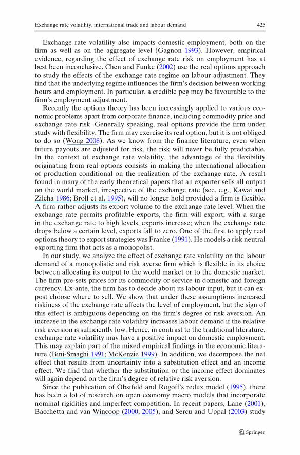
Exchange rate volatility, international trade and labour demand 425

Exchange rate volatility also impacts domestic employment, both on thefirm as well as on the aggregate level (Gagnon 1993). However, empiricalevidence, regarding the effect of exchange rate risk on employment has atbest been inconclusive. Chen and Funke (2002) use the real options approachto study the effects of the exchange rate regime on labour adjustment. Theyfind that the underlying regime influences the firm’s decision between workinghours and employment. In particular, a credible peg may be favourable to thefirm’s employment adjustment.

Recently the options theory has been increasingly applied to various eco-nomic problems apart from corporate finance, including commodity price andexchange rate risk. Generally speaking, real options provide the firm understudy with flexibility. The firm may exercise its real option, but it is not obligedto do so (Wong 2008). As we know from the finance literature, even whenfuture payouts are adjusted for risk, the risk will never be fully predictable.In the context of exchange rate volatility, the advantage of the flexibilityoriginating from real options consists in making the international allocationof production conditional on the realization of the exchange rate. A resultfound in many of the early theoretical papers that an exporter sells all outputon the world market, irrespective of the exchange rate (see, e.g., Kawai andZilcha 1986; Broll et al. 1995), will no longer hold provided a firm is flexible.A firm rather adjusts its export volume to the exchange rate level. When theexchange rate permits profitable exports, the firm will export; with a surgein the exchange rate to high levels, exports increase; when the exchange ratedrops below a certain level, exports fall to zero. One of the first to apply realoptions theory to export strategies was Franke (1991). He models a risk neutralexporting firm that acts as a monopolist.

In our study, we analyze the effect of exchange rate volatility on the labourdemand of a monopolistic and risk averse firm which is flexible in its choicebetween allocating its output to the world market or to the domestic market.The firm pre-sets prices for its commodity or service in domestic and foreigncurrency. Ex-ante, the firm has to decide about its labour input, but it can ex-post choose where to sell. We show that under these assumptions increasedriskiness of the exchange rate affects the level of employment, but the sign ofthis effect is ambiguous depending on the firm’s degree of risk aversion. Anincrease in the exchange rate volatility increases labour demand if the relativerisk aversion is sufficiently low. Hence, in contrast to the traditional literature,exchange rate volatility may have a positive impact on domestic employment.This may explain part of the mixed empirical findings in the economic litera-ture (Bini-Smaghi 1991; McKenzie 1999). In addition, we decompose the neteffect that results from uncertainty into a substitution effect and an incomeeffect. We find that whether the substitution or the income effect dominateswill again depend on the firm’s degree of relative risk aversion.

Since the publication of Obstfeld and Rogoff’s redux model (1995), therehas been a lot of research on open economy macro models that incorporatenominal rigidities and imperfect competition. In recent papers, Lane (2001),Bacchetta and van Wincoop (2000, 2005), and Sercu and Uppal (2003) study

426 U. Broll, S. Hansen-Averlant

the effects of the exchange rate volatility on the volume of internationaltrade and welfare in a stochastic general equilibrium analysis with imperfectlyintegrated international commodity markets. One of their findings is that ingeneral, a fixed exchange rate regime is not necessarily associated with highertrade levels than a floating exchange rate regime. Furthermore the sign of therelation depends on the source for the change in volatility. For instance, morevolatility of the endowments and higher costs to international trade both boostexchange risk; but the first increases the expected volume of trade, while thesecond decreases trade.

In other contributions it is shown that currency invoicing and hedgingallow internationally active firms to reduce their exposure to exchange ratevariations. It is argued that currency invoicing and hedging with exchange ratederivatives allow for a fairly straightforward management of transaction andtranslation risk (Broll and Eckwert 2006; Wong 2007). Economic risk is byits very nature harder to manage, but (Doehring 2008) argues that naturalhedging provides possibilities to reduce risk. In Friberg (1998), Friberg andWilander (2008) and Bacchetta and van Wincoop (2005) it is shown thatcurrency denomination of international trade has significant macroeconomicand policy implications. They find that the less competition firms face in globalmarkets, as reflected in product differentiation and market share, the morelikely they will price in their own currency. Furthermore, they demonstratethat when a set of countries forms a monetary union, the new currency islikely to be used more extensively in international trade than the sum of thecurrencies it replaces.

Furthermore there is a relationship between exchange rate volatility, inter-national trade, competition, invoicing and exchange rate pass-through. Theliterature on exchange rate pass-through examines how much import priceschange when exchange rates change. The dominating empirical finding in thisliterature is that import prices change less than the exchange rate. All thesefindings have been one of the messages from the recent new open economymacroeconomics literature.

While our goal is to present a model to examine the role of global flexibilityof firms under imperfect competition and the impact on labour demand, themodel is kept simple in order to obtain results that are transparent and can beeasily analytically derived. An important feature of the model is deviation fromlaw of one price, caused by rigid price setting in buyers’ or sellers’ currency.Consistent with most empirical studies trade is affected by the exchange ratesystem. Both trade and welfare in terms of expected utility can be higher undereither exchange rate system, depending on preferences and flexibility.

We proceed as follows. In Section 2 we present the relationship betweenimperfect competition, risk and global flexibility. In Section 3, we set up themodel of a risk averse monopolistic firm under exchange rate risk endowedwith some firm specific degree of regional flexibility of trade. We deriveemployment effects of an increase in the exchange rate volatility includingthe analysis of the substitution and the income effect. We discuss some policyimplications. In Section 4 we present our conclusions.

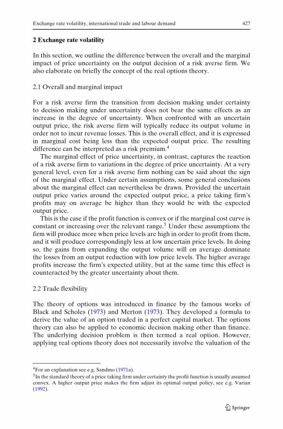
Exchange rate volatility, international trade and labour demand 427

2 Exchange rate volatility

In this section, we outline the difference between the overall and the marginalimpact of price uncertainty on the output decision of a risk averse firm. Wealso elaborate on briefly the concept of the real options theory.

2.1 Overall and marginal impact

For a risk averse firm the transition from decision making under certaintyto decision making under uncertainty does not bear the same effects as anincrease in the degree of uncertainty. When confronted with an uncertainoutput price, the risk averse firm will typically reduce its output volume inorder not to incur revenue losses. This is the overall effect, and it is expressedin marginal cost being less than the expected output price. The resultingdifference can be interpreted as a risk premium.4

The marginal effect of price uncertainty, in contrast, captures the reactionof a risk averse firm to variations in the degree of price uncertainty. At a verygeneral level, even for a risk averse firm nothing can be said about the signof the marginal effect. Under certain assumptions, some general conclusionsabout the marginal effect can nevertheless be drawn. Provided the uncertainoutput price varies around the expected output price, a price taking firm’sprofits may on average be higher than they would be with the expectedoutput price.

This is the case if the profit function is convex or if the marginal cost curve isconstant or increasing over the relevant range.5 Under these assumptions thefirm will produce more when price levels are high in order to profit from them,and it will produce correspondingly less at low uncertain price levels. In doingso, the gains from expanding the output volume will on average dominatethe losses from an output reduction with low price levels. The higher averageprofits increase the firm’s expected utility, but at the same time this effect iscounteracted by the greater uncertainty about them.

2.2 Trade flexibility

The theory of options was introduced in finance by the famous works ofBlack and Scholes (1973) and Merton (1973). They developed a formula toderive the value of an option traded in a perfect capital market. The optionstheory can also be applied to economic decision making other than finance.The underlying decision problem is then termed a real option. However,applying real options theory does not necessarily involve the valuation of the

4For an explanation see e.g. Sandmo (1971a).5In the standard theory of a price taking firm under certainty the profit function is usually assumedconvex. A higher output price makes the firm adjust its optimal output policy, see e.g. Varian(1992).

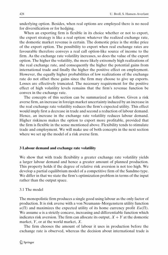
428 U. Broll, S. Hansen-Averlant

underlying option. Besides, when real options are employed there is no needfor diversification or for hedging.

When an exporting firm is flexible in its choice whether or not to export,the export strategy is like a real option: whatever the realized exchange rate,the domestic market revenue is certain. The domestic price is the strike priceof the export option. The possibility to export when real exchange rates arefavourable therefore conveys a real call option-like source of income to thefirm. As the exchange rate volatility increases, so does the value of the exportoption. The higher the volatility, the more likely extremely high realizations ofthe real exchange rate, and consequently the higher the potential gains frominternational trade and finally the higher the positive effect on employment.However, the equally higher probabilities of low realizations of the exchangerate do not offset these gains since the firm may choose to give up exports.Losses are effectively truncated. The necessary requirement for the positiveeffect of high volatility levels remains that the firm’s revenue function beconvex in the exchange rate.

The concepts of this section can be summarized as follows. Given a riskaverse firm, an increase in foreign market uncertainty induced by an increase inthe real exchange rate volatility reduces the firm’s expected utility. This effectwould imply first a decrease in trade and second a reduction of labour demand.Hence, an increase in the exchange rate volatility reduces labour demand.Higher riskiness makes the option to export more profitable, provided thatthe firm is flexible in the sense mentioned above. Flexibility tends to stimulatetrade and employment. We will make use of both concepts in the next sectionwhere we set up the model of a risk averse firm.

3 Labour demand and exchange rate volatility

We show that with trade flexibility a greater exchange rate volatility yieldsa larger labour demand and hence a greater amount of planned production.This property holds if the degree of relative risk aversion is not too high. Wedevelop a partial equilibrium model of a competitive firm of the Sandmo type.We differ in that we state the firm’s optimization problem in terms of the inputrather than the output space.

3.1 The model

The monopolistic firm produces a single good using labour as the only factor ofproduction. It is risk averse with a von Neumann–Morgenstern utility functionu(�) and maximizes the expected utility of its home currency profit Eu(�).We assume u is a strictly concave, increasing and differentiable function whichindicates risk aversion. The firm can allocate its output, X + Y at the domesticmarket, Y, or at the world market, X.

The firm chooses the amount of labour it uses in production before theexchange rate is observed, whereas the decision about international trade is

Exchange rate volatility, international trade and labour demand 429

not made until the exchange rate is observed. Product prices are pre-set. Ourmodel differs from the Sandmo approach in that the firm’s decision is not onan adjustment of the output volume or the export volume, respectively, buton whether or not to export. This captures the notion of flexibility throughuse of real options (see Krugman 1989; Franke 1991; Gagnon 1993; Broll andEckwert 1999).

We specify the time structure of the model as follows: in the current period(period 0) the firm decides on labour input L which gives rise to labour costsWL, where W denotes the real wage rate. At date 1, the random real exchangerate e realizes and the firm decides about the output allocation between thehome and the foreign goods markets.

The real exchange rate e is a random variable and is defined as e = SP/Qwhere S denotes the spot exchange rate, defined as units of domestic to unitsof foreign currency, and P and Q denote the foreign and domestic goodsprices, respectively. The latter are assumed to be pre-set and fixed. We modelmonetary shocks as a mean-preserving spread in the exchange rate volatility.6

Assumption 1 The real exchange rate f luctuates around the purchasing powerparity, i.e., e = 1 + αε, where E(ε) = 0, and σ 2

ε = 1, α > 0. The parameter α

is the standard deviation. The parity exchange rate for the traded goods ise = SP/Q = 1.

The production process adopted by the firm is given by a strictly concaveproduction function F(L). The allocation decision, X + Y = F(L), is condi-tional on the realization of the real exchange rate. Hence, the firm’s randomrevenues in domestic currency are

arg max {e[F(L) − Y]; Y}. (1)

Y denotes domestic supply and X = F(L) − Y is the export volume. There-fore the firm’s profit at date 1, for a given first-stage labour demand L0, isdefined by

max {e[F(L0) − Y]; Y} − WL0.

The optimal decision rule at date 1 is found by maximizing profit with respectto the optimal allocation of production for given e and labour input L0.

6The exchange rate process can be interpreted as a mean reverting stochastic process. The bulkof literature dealing with forward pricing and optimal hedge decisions focusses on evolutionsexpressed by standard geometric Brownian motion (GBM). The problem with GBM is that inmany cases price changes are not independent and prices tend to return to an average level. For adiscussion, see Broll et al. (2010).

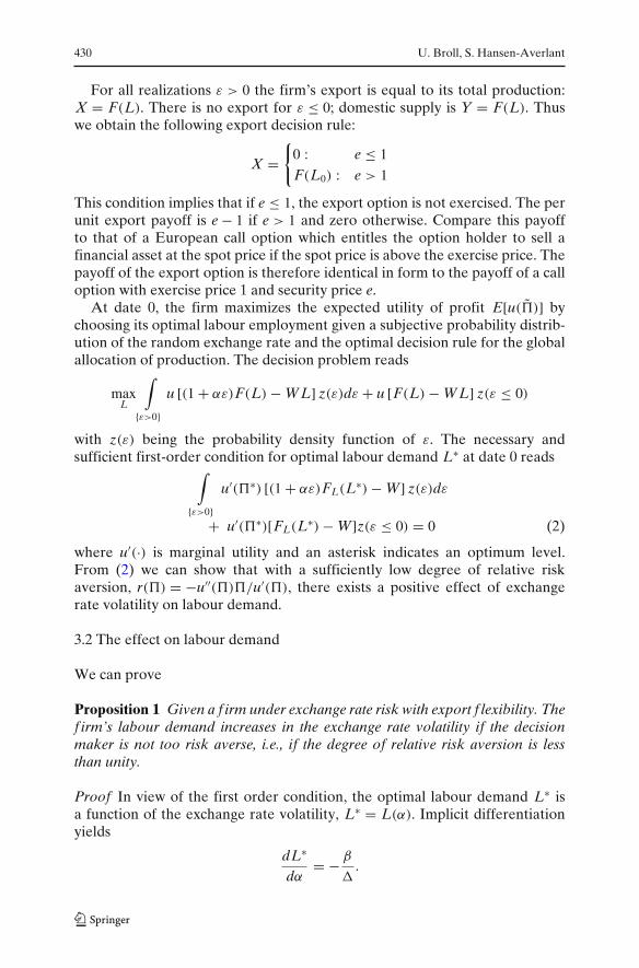
430 U. Broll, S. Hansen-Averlant

For all realizations ε > 0 the firm’s export is equal to its total production:X = F(L). There is no export for ε ≤ 0; domestic supply is Y = F(L). Thuswe obtain the following export decision rule:

X ={

0 : e ≤ 1F(L0) : e > 1

This condition implies that if e ≤ 1, the export option is not exercised. The perunit export payoff is e − 1 if e > 1 and zero otherwise. Compare this payoffto that of a European call option which entitles the option holder to sell afinancial asset at the spot price if the spot price is above the exercise price. Thepayoff of the export option is therefore identical in form to the payoff of a calloption with exercise price 1 and security price e.

At date 0, the firm maximizes the expected utility of profit E[u(�)] bychoosing its optimal labour employment given a subjective probability distrib-ution of the random exchange rate and the optimal decision rule for the globalallocation of production. The decision problem reads

maxL

∫{ε>0}

u [(1 + αε)F(L) − WL] z(ε)dε + u [F(L) − WL] z(ε ≤ 0)

with z(ε) being the probability density function of ε. The necessary andsufficient first-order condition for optimal labour demand L∗ at date 0 reads∫

{ε>0}u′(�∗) [(1 + αε)FL(L∗) − W] z(ε)dε

+ u′(�∗)[FL(L∗) − W]z(ε ≤ 0) = 0 (2)

where u′(·) is marginal utility and an asterisk indicates an optimum level.From (2) we can show that with a sufficiently low degree of relative riskaversion, r(�) = −u′′(�)�/u′(�), there exists a positive effect of exchangerate volatility on labour demand.

3.2 The effect on labour demand

We can prove

Proposition 1 Given a f irm under exchange rate risk with export f lexibility. Thef irm’s labour demand increases in the exchange rate volatility if the decisionmaker is not too risk averse, i.e., if the degree of relative risk aversion is lessthan unity.

Proof In view of the first order condition, the optimal labour demand L∗ isa function of the exchange rate volatility, L∗ = L(α). Implicit differentiationyields

dL∗

dα= − β

�.

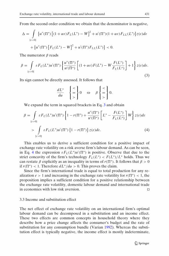
Exchange rate volatility, international trade and labour demand 431

From the second order condition we obtain that the denominator is negative,

� =∫

{ε>0}

{u′′(�∗)

[(1 + αε)FL(L∗) − W

]2 + u′(�∗)(1 + αε)FLL(L∗)}z(ε)dε

+ {u′′(�∗)

[FL(L∗) − W

]2 + u′(�∗)FLL(L∗)}

< 0.

The numerator β reads

β =∫

{ε>0}εFL(L∗)u′(�∗)

{u′′(�∗)u′(�∗)

[(1 + αε)F(L∗) − W

F(L∗)FL(L∗)

]+ 1

}z(ε)dε.

(3)Its sign cannot be directly assessed. It follows that

dL∗

dα

⎧⎨⎩

<

=>

⎫⎬⎭ 0 ⇔ β

⎧⎨⎩

<

=>

⎫⎬⎭ 0.

We expand the term in squared brackets in Eq. 3 and obtain

β =∫

{ε>0}εFL(L∗)u′(�∗)

{1 − r(�∗) + u′′(�∗)

u′(�∗)

[L∗ − F(L∗)

FL(L∗)

]W

}z(ε)dε

>

∫{ε>0}

εFL(L∗)u′(�∗){1 − r(�∗)

}z(ε)dε. (4)

This enables us to derive a sufficient condition for a positive impact ofexchange rate volatility on a risk averse firm’s labour demand. As can be seen,in Eq. 4 the expression εFL(L∗)u′(�∗) is positive. Observe that due to thestrict concavity of the firm’s technology FL(L∗) < F(L∗)/L∗ holds. Thus wecan restate β explicitly as an inequality in terms of r(�∗). It follows that β > 0if r(�∗) < 1. Therefore dL∗/dα > 0. This proves the claim.

Since the firm’s international trade is equal to total production for any re-alization e > 1 and increasing in the exchange rate volatility for r(�∗) < 1, theproposition implies a sufficient condition for a positive relationship betweenthe exchange rate volatility, domestic labour demand and international tradein economies with low risk aversion. ��

3.3 Income and substitution effect

The net effect of exchange rate volatility on an international firm’s optimallabour demand can be decomposed in a substitution and an income effect.These two effects are common concepts in household theory where theydescribe how a price change affects the consumer’s budget and the rate ofsubstitution for any consumption bundle (Varian 1992). Whereas the substi-tution effect is typically negative, the income effect is mostly indeterminate,

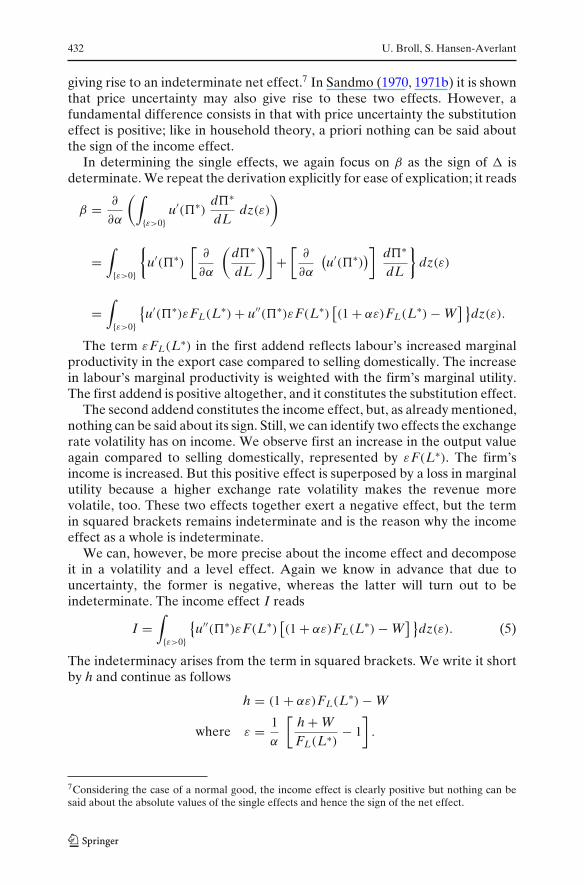
432 U. Broll, S. Hansen-Averlant

giving rise to an indeterminate net effect.7 In Sandmo (1970, 1971b) it is shownthat price uncertainty may also give rise to these two effects. However, afundamental difference consists in that with price uncertainty the substitutioneffect is positive; like in household theory, a priori nothing can be said aboutthe sign of the income effect.

In determining the single effects, we again focus on β as the sign of � isdeterminate. We repeat the derivation explicitly for ease of explication; it reads

β = ∂

∂α

(∫{ε>0}

u′(�∗)d�∗

dLdz(ε)

)

=∫

{ε>0}

{u′(�∗)

[∂

∂α

(d�∗

dL

)]+

[∂

∂α

(u′(�∗)

)] d�∗

dL

}dz(ε)

=∫

{ε>0}

{u′(�∗)εFL(L∗) + u′′(�∗)εF(L∗)

[(1 + αε)FL(L∗) − W

] }dz(ε).

The term εFL(L∗) in the first addend reflects labour’s increased marginalproductivity in the export case compared to selling domestically. The increasein labour’s marginal productivity is weighted with the firm’s marginal utility.The first addend is positive altogether, and it constitutes the substitution effect.

The second addend constitutes the income effect, but, as already mentioned,nothing can be said about its sign. Still, we can identify two effects the exchangerate volatility has on income. We observe first an increase in the output valueagain compared to selling domestically, represented by εF(L∗). The firm’sincome is increased. But this positive effect is superposed by a loss in marginalutility because a higher exchange rate volatility makes the revenue morevolatile, too. These two effects together exert a negative effect, but the termin squared brackets remains indeterminate and is the reason why the incomeeffect as a whole is indeterminate.

We can, however, be more precise about the income effect and decomposeit in a volatility and a level effect. Again we know in advance that due touncertainty, the former is negative, whereas the latter will turn out to beindeterminate. The income effect I reads

I =∫

{ε>0}

{u′′(�∗)εF(L∗)

[(1 + αε)FL(L∗) − W

] }dz(ε). (5)

The indeterminacy arises from the term in squared brackets. We write it shortby h and continue as follows

h = (1 + αε)FL(L∗) − W

where ε = 1α

[h + WFL(L∗)

− 1]

.

7Considering the case of a normal good, the income effect is clearly positive but nothing can besaid about the absolute values of the single effects and hence the sign of the net effect.

Exchange rate volatility, international trade and labour demand 433

We substitute for ε in Eq. 5 to get

I =∫

{ε>0}

{u′′(�∗)

αF(L∗)

[h + WFL(L∗)

− 1]

h}

dz(ε)

=∫

{ε>0}

{u′′(�∗)

α

F(L∗)FL(L∗)

h2

+ h F(L∗)u′′(�∗)

α

[w

FL(L∗)− 1

]}dz(ε).

The first addend constitutes the negative volatility effect. The second addendrepresents the level effect which is still indeterminate. Thus, I cannot be fullydetermined.

Finally we can conclude that the net effect of the real exchange rate volatilityon labour demand is positive when the income effect is greater than thesubstitution effect in absolute value.

3.4 Economic policy implications

The feature of the new open economy macroeconomics (NOEM) is theintroduction of nominal rigidities in prices, wages and market imperfectionsinto a general equilibrium model with well-specified microfoundations. TheNOEM offers several advantages. Considering profit and utility maximizationproblems provide analytical rigor. Allowing for nominal rigidities and marketimperfections such as financial market incompleteness alters the transmissionmechanisms for real and monetary shocks and provides a more prominent rolefor fiscal and monetary policies.

Two attractions of the NOEM, which are related to our study, are marketsegmentation and pricing to the market on the one hand and financial structureof the economy on the other hand. International market segmentation meansthat at least some firms have the ability to charge different prices for the samegood in home and foreign markets. Provided that prices are sticky in eachcountry in terms of the local currency, it can be shown that the real exchangerate fluctuates and delinks home and foreign price levels. In the event of ashock, exchange rate movements cause deviations from the law of one price.

In our model prices in foreign currency, in home currency and the domesticwage rate are assumed to be set one period in advance, introducing a nominalrigidity into the model. To study the effects of a monetary shock, a meanpreserving spread (MPS) is taken around the mean of the exchange rate. Weshow the conditions under which exchange rate volatility generates a positiveeffect on an exporting firm’s labour demand. As the exchange rate volatilityincreases, so does the value of the export option provided the exportingfirm is flexible with respect to international trade. Multinational enterprises,especially, can be regarded as firms with trade flexibility because of their useof worldwide distribution facilities (Caves 2007). The firm’s trade flexibilitycan be interpreted as a real hedging strategy when financial markets are

434 U. Broll, S. Hansen-Averlant

incomplete. In many newly industrializing countries and emerging economiesfinancial markets are imperfect or risk sharing markets are just starting todevelop at a rather slow pace.

One of the fundamental issues in new open economy macroeconomics is theoptimal choice of the exchange rate regime (Lane 2001) under different marketconditions. Several contributions have look at the optimality of the exchangerate system in general equilibrium optimizing models. Exchange rate stabilityis often viewed as favourable to international trade in goods and services andtherefore welfare enhancing. In our partial equilibrium model we establishsufficient conditions for a positive interaction between trade and welfare underpre-set prices under a exchange rate uncertainty, i.e. exchange rate system witha stochastic exchange rate. While our goal is to present a microeconomic modelto examine the role of global flexibility of monopolistic firms and the impacton labour demand, the model is kept simple in order to obtain results that aretransparent and can be easily analytically derived.

An important feature of the model is deviation from law of one price,caused by rigid price setting in buyers’ or sellers’ currency. Trade is affectedby the exchange rate system, consistent with most empirical studies. Bothinternational trade and welfare in terms of expected utility can be higherunter either exchange rate system, depending on preferences and flexibility.Traditionally in the study of exchange rate regime, the source of shocks playsa significant role.

4 Concluding remarks

This paper develops a framework to study the effect of the exchange ratevolatility on labour demand, international trade and welfare in terms ofexpected utility of a firm. The aim of this study is to provide a theoretical foun-dation of a positive effect of exchange rate volatility on domestic productionand labour demand given that a risk averse firm can react to exchange ratevolatility, i.e. the firm can export or sell in the domestic market.

With a strictly concave production technology, the sufficient condition fora positive link between real exchange rate volatility and the firm’s labourdemand is a degree of relative risk aversion less than unity. The economicintuition for this result is the following: as the real exchange rate volatilityincreases, so does the value of the option to export to the world market.A more volatile exchange rate volatility increases the potential gains frominternational trade what makes exports more profitable and consequentlyincreases the firm’s labour demand.

We decompose the net effect of exchange rate volatility on labour demandin a substitution and an income effect in order to identify those terms whichmay be responsible for the general indeterminacy of exchange rate volatilityon labour demand. We confirm that the substitution effect is positive and thatthe income effect is indeterminate. The decomposition of the income effectreveals that its indeterminacy stems from an indeterminate level effect whereas

Exchange rate volatility, international trade and labour demand 435

the volatility effect is identified to be clearly negative. We eventually concludethat with a degree of relative risk aversion less than one, the substitution effectdominates the income effect, i.e. the former is larger in absolute value thanthe latter.

In our partial equilibrium model we discuss the interaction between theeffect of exchange rate system on international trade and welfare. While ourgoal is to present a model to examine the role of global flexibility of firmsand the impact on labour demand, the model is kept simple in order to obtainresults that are transparent and can be easily analytically derived. An impor-tant feature of the model is deviation from law of one price, caused by rigidprice setting in buyers’ or sellers’ currency. Trade is affected by the exchangerate system, consistent with most empirical studies. Both international tradeand welfare in terms of expected utility can be higher unter either exchangerate system, depending on preferences and flexibility. Our benchmark decisionmaking model can be extended to include other sources of uncertainty, such asproductivity shocks and unpredictable changes in costs of production.

Acknowledgements We would like to thank our anonymous referee for very constructive andhelpful comments. Furthermore we thank the editor of this Journal (P.J.J. Welfens) and CarstenEckel for helpful discussions.

References

Bacchetta P, van Wincoop E (2000) Does exchange rate stability increase trade and welfare? AmEcon Rev 90:1093–1109

Bacchetta P, van Wincoop E (2005) A theory of the currency denomination of international trade.J Int Econ 67: 295–319

Battermann HL, Broll U, Wahl JE (2008) Utility functions of equivalent form and the effect ofparameter changes on optimum decision making. Econ Theory 34:401–414

Bini-Smaghi L (1991) Exchange rate variability and trade: why is it so difficult to find any empiricalrelationship? Appl Econ 23:927–936

Black F, Scholes M (1973) The pricing of options and corporate liabilities. J Polit Econ 81:637–654Broll U, Clark, E, Lukas, E (2010) Hedging mean-reverting commodities. J Manag Math

21(1):19–26Broll U, Eckwert B (1999) Exchange rate volatility and international trade. South Econ J

66:178–185Broll U, Eckwert B (2006) Transparency in the foreign exchange market and the volume of

international trade. Rev Int Econ 14:571–581Broll U, Wahl JE, Zilcha I (1995) Indirect hedging of exchange rate risk. J Int Money Financ

14:667–678Caves RE (2007) Multinational enterprise and economic analysis. Cambridge University Press,

CambridgeChen Y, Funke M (2002) Exchange rate uncertainty and labour market adjustment under fixed

exchange rates, working paper 779. CESifo, MünchenDe Grauwe P (2007) Economics of monetary union, 7th edn. Oxford University Press, OxfordDellas H, Zilberfarb BZ (1993) Real exchange rate volatility and international trade: a re-

examination of the theory. South Econ J 59:641–649Doehring B (2008) Hedging and invoicing strategies to reduce exchange rate exposure: a euro-area

perspective. Economic papers 299. European Commission, Economic and Financial AffairsFranke G (1991) Exchange rate volatility and international trading strategy. J Int Money Financ

10:292–307

436 U. Broll, S. Hansen-Averlant

Friberg R (1998) In which currency should exporters set their prices? J Int Econ 45:59–76Friberg R, Wilander F (2008) The currency denomination of exports—a questionnaire study. J Int

Econ 75:54–69Funke K, Koske I (2008) Does the law of one price hold within the EU? A panel analysis. Int Adv

Econ Res 14:11–24Gagnon JE (1993) Exchange rate variability and the level of international trade. J Int Econ 34:

269–287Kawai M, Zilcha I (1986) International trade with forward-futures markets under exchange rate

and price uncertainty. J Int Econ 20:83–98Krugman PR (1989) Exchange rate instability. MIT, CambridgeLane PR (2001) The new open economy macroeconomics: a survey. J Int Econ 54:235–266McKenzie M (1999) The impact of exchange rate volatility on international trade flows. J Econ

Surv 13:71–106Merton R (1973) Theory of rational option pricing. Bell J Econ 4:141–183Obstfeld M, Rogoff K (1995) Exchange rate dynamics redux. J Polit Econ 103:624–660Sandmo A (1970) The effect of uncertainty on saving decisions. Rev Econ Stud 37:353–360Sandmo A (1971a) On the theory of competitive firm under price uncertainty. Am Econ Rev

61:65–73Sandmo A (1971b) Portfolio theory, asset demand and taxation: comparative statics with many

assets. Rev Econ Stud 44:369–379Schmidt CW, Broll U (2009) Real exchange rate uncertainty and U.S. foreign direct investment:

an empirical analysis. Rev World Econ 145:513–530Sercu P, Uppal R (2003) Exchange rate volatility and international trade: a general equilibrium

analysis. Eur Econ Rev 47:429–441Varian HR (1992) Microeconomic analyses, 3RD edn. Norton, New YorkWong KP (2007) Optimal export and hedging decisions when forward markets are incomplete.

Bull Econ Res 59:67–81Wong KP (2008) Does market demand volatility facilitate collusion? Econ Model 25:696–703

ORIGINAL PAPER

Is there an Anglo-American corporategovernance model?

Andrew Mullineux &

For the Jean Monnet Project (Financial Integration, Structural Change,Foreign Direct Investment and Economic Growth in EU-25)

Published online: 30 March 2010# Springer-Verlag 2010

Abstract This paper questions the existence of an Anglo-American model ofcorporate governance and capitalism. Significant differences between the UK andUS models of corporate governance are identified. The UK is a principles orientatedsystem based more on voluntary codes operated on a ‘comply or explain’ basis,whilst the US system is more rules based and litigious. The UK focuses more on exante protection of ‘outside’ shareholders, whilst the US focuses on ex post protectionof share traders. Institutional investors are expected to play a more prominent andwide ranging role in corporate governance in the UK than the US, though theevidence on their voting behaviour and wider ‘engagement’ activity is not readilyavailable. The explosion of private equity led leveraged buy-out activity in the mid2000s challenges the efficiency of both models and could be a harbinger of a ‘newcapitalism’; relying more on incentive compatible remuneration packages and lesson public disclosure and market discipline. Alternatively, it could simply be drivenby the tax advantages currently enjoyed by debt over equity, the special deferredcapital gains (‘carried interest’) tax treatment enjoyed by private equity, low (long aswell as short term) real interest rates (‘cheap money’), and rising equity prices.

Keywords Corporate governance . Institutional investors . Private equity

1 The influence of legal type

Masulis (2006, p.1), sees corporate governance as a problem of preventing investor(‘outside’ shareholder) expropriation by managers and/or controlling (‘inside’)

Int Econ Econ Policy (2010) 7:437–448DOI 10.1007/s10368-010-0151-2

A. MullineuxDepartment of Accounting and Finance, University of Birmingham, Birmingham, UK

A. Mullineux (*)The Business School, University of Birmingham, University House, Birmingham B15 2TT, UKe-mail: a.w.mullineux@bham.ac.uk

shareholders through self dealing. Following the pioneering work of La Porta et al.(1998), Masulis contrasts protection against the self dealing under Civil and CommonLaw systems and considers ‘French Origin’, ‘German Origin’ and ‘ScandinavianOrigin’ variants of the Civil Law system. Masulis and La Porta et al. find systematicdifferences among these legal types in the protection of both minority (or ‘outside’)shareholders and creditors through corporate and bankruptcy laws.

Masulis concentrates on ‘outside’ shareholder protection, as we do here. However,the situation with regard to bankruptcy is not as clear cut as the work of La Porta and itsfollowers suggest. There are significant differences between the US and the UK. TheUK traditionally favours creditors more than the US, which offers fairly strongprotection to debitors; including ‘Chapter 11’ protection. Recent law changes in bothcountries have redressed the imbalances to some extent, but full convergence has by nomeans been achieved. Further, France has enhanced the protection of large debtors byintroducing additional protection against creditors modelled on ‘Chapter 11’ in the US.

Masulis’ paper attempts to develop a (regulation of) Self-Dealing Index (SDI). The UKis taken as typical of Common Law countries, indeed the model. Directors in the UK haveclear fiduciary duties to shareholders, as apposed to a wider group of stakeholders, as inGermany for example. In the case of a ‘deal’ involving a potential conflict interestbetween the directors and ‘outside’ shareholders, shareholders approval is required in theUK. In contrast to the US, the UK favours ex ante scrutiny over ex post litigation byminority shareholders. Disclosure requirements are generally lower in the US than in theUK and the average of Civil Law countries. It should also be noted that ex post privatecontrol is relatively high in France, and so is Masulis’ Public Enforcement Index.

The US is in fact not typical of the Common Law group. It does not requireshareholder approval for related party transactions, relying instead on litigation toprotect against ‘self dealing’. Under US Delaware (State) Law, transactions can beapproved by boards of directors without shareholder approval. In contrast, in Francethe requirement to seek shareholder approval for related party transactions is in laweasily avoided, but in practice approval is almost always sought.

The Masulis paper also considers another theme explored by La Porta et al. namelythe relationship between regulation of self dealing and stock (equity, not bond) marketdevelopment. It is found that there are wide differences in stock market developmentacross the legal families, most strikingly between Common Law and French Civil Lawcountries. Common Law countries have larger stock market value to GDP ratios andless concentrated ownership. It should be noted that the inclusion of the US in theCommon Law group strongly biases this result given that it has the most highlydeveloped stock markets and is in fact atypical. In addition, there are some strongeconometric issues in the La Porta inspired methodology—endogeneity issues are notdealt with properly, for example (Masulis 2006, p.27).

The work of La Porta et al. focused on ‘anti-director rights’ and constructed anAnti Self Dealing Index (ASDI). It has been criticised (Masulis 2006, p.30) for its adhoc nature and coding mistakes, and its conceptual ambiguity. Masulis reconstructsthe ‘La Porta’ indices, which aim to summarise the protection of minorityshareholders in the corporate decision process, particularly relating to voting rightsand the ease of exercising them. In his index, the US is an outlier amongst theCommon Law countries, with shareholder protection falling well behind the UK, butalso France! Interestingly, ‘disclosure in the prospectus’ is highly correlated with the

438 A. Mullineux

ASDI and when both are used to explain stock market development, it is disclosurethat is significant, not the ASDI.

In sum, to the extent that self dealing is the central problem of corporategovernance, the law seems to play a big part in shareholder protection and the levelof protection varies across countries, seemingly in relation to legal family.

However, the US is exceptional, given its non-Common Law emphasis on ex postlitigation, rather than ex ante disclosure and approval. Ex ante transparency in selfdealing transactions is taken by Masulis to be the central difference betweenCommon and Civil Law, and so, the US is more akin to a Civil Law country andindeed behind France in providing ex ante protection!

Masulis concludes that the role of ‘the public sector’ is to provide the ‘rules of thegame’. These are then enforced by private action with relatively little reliance on fines orcriminal action (pace Section 404 of the 2002 Sarbanes-Oxley Act in the US). Morespecifically, his findings suggest that ‘an effective strategy for regulating large self-dealingtransactions is to combine full public disclosure of such transactions (including potentialconflicts) with the requirement of approval by interested shareholders and strong privateenforcement’. The UK seems closer to this ideal than the US, which is weak on ex anteapproval, but strong on ex post litigation.

2 An Anglo-American system of corporate governance?

The Enron, WorldCom and other debacles in the US brought forth the 2002Sarbanes-Oxley Act (‘Sarbox’), whose infamous Section 404 threatens Chief ExecutiveOfficers (CEOs) and Chief Finance Officers (CFOs) with fines and even imprisonmentif a corporation’s ‘internal controls’ are found to be inadequate. Because privatesolutions were found wanting, a public solution had to be put into practice.

In contrast, the UK’s ‘Combined Code on Corporate Governance’ is a set ofprinciples to which major corporations adhere on a voluntary, ‘comply or explain’basis. Further, shareholders have considerable power under the code to appointdirectors, and indeed replace CEOs and Chairmen and to influence their remuneration.Increasingly this power is exercised through institutional shareholders, particularly inthe UK; where share-ownership is much more concentrated in the hands ofinstitutional investors than in the US (despite recent diversification of UK pensionsand other funds away from equity into bonds and ‘alternative’ investments).

Bush (2005, p.41) contrasts the Turnbull Guidance on Internal Controls1 withSection 404 of the Sarbanes-Oxley Act and notes that the Guidance has beenapproved, by the US Securities Exchange Commission, to be Section 404 compliant.He regards the so called Anglo-American corporate governance model to be a mythand argues that in Britain, as well as ‘Continental Europe’ and ‘The Common-wealth’, the purpose and focus of presenting and auditing financial accounts is toserve the interests of the shareholders, which is not the case in the US.

The US ‘deviation’ is traced back to the 1933 Securities Act. The original aimwas to adopt the British Company Law model, but this could not be imposed at

1 See “Consultation on draft revised Turnbull Guidance”, June 2005, Financial Reporting Council (www.frc.org.uk).

Is there an Anglo-American corporate governance model? 439

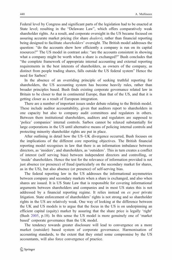
Federal level by Congress and significant parts of the legislation had to be enacted atState level; resulting in the “Delaware Law”, which offers comparatively weakshareholder rights. As a result, and corporate oversight in the US became focused onassuring accurate market pricing (for share dealers), rather than financial reportingbeing designed to facilitate shareholders’ oversight. The British model addresses thequestion: “do the accounts show how efficiently a company is run on its capitalresources?” The US model in contrast asks: “are the accounts consistent in showingwhat a company might be worth when a share is exchanged?” Bush concludes that“the complete framework of appropriate internal accounting and external reportingrequirements in the best interests of shareholders, as owners of the company, asdistinct from people trading shares, falls outside the US federal system” Hence theneed for Sarbox!

In the absence of an overriding principle of seeking truthful reporting forshareholders, the US accounting system has become heavily rules, rather thanbroader principles based. Bush finds existing corporate governance related law inBritain to be closer to that in continental Europe, than that of the US, and that it isgetting closer as a result of European integration.

There are a number of important issues under debate relating to the British model.These include auditor accountability, given that auditors report to shareholders inone capacity but also to company audit committees and regulators in others.Between them institutional shareholders, auditors and regulators are supposed to‘police’ companies’ internal controls. Sarbox cannot be relaxed substantially forlarge corporations in the US until alternative means of policing internal controls andprotecting minority shareholder rights are put in place.

After outlining in detail how the US–UK divergence occurred, Bush focuses onthe implications of the different core reporting objectives. The British financialreporting model recognises in law that there is an information imbalance betweendirectors, as ‘insiders’, and shareholders, as ‘outsiders’. This in turn creates a conflictof interest (self serving bias) between independent directors and controlling, or‘inside’ shareholders. Hence the test for the relevance of information provided is notjust absence (or presence) of fraud (particularly on the secondary market for shares,as in the US), but also absence (or presence) of self-serving bias.

The federal reporting law in the US addresses the informational asymmetriesbetween company and secondary markets when a share is exchanged, and also whenshares are issued. It is US State Law that is responsible for covering informationalarguments between shareholders and companies and in most US states this is notaddressed by a financial reporting regime. It relies instead on ex post privatelitigation. State enforcement of shareholders’ rights is not strong and so shareholderrights in the US are relatively weak. One way of looking at the difference betweenthe UK and US models is to argue that the focus in the US is on underpinning anefficient capital (equity) market by assuring that the share price is legally ‘right’(Bush 2005, p.18). In this sense the US model is more genuinely one of ‘marketbased’ corporate governance than the UK model.

The tendency towards greater disclosure will lead to convergence on a moremarket (outsider) based system of corporate governance. Harmonisation ofaccounting standards, to the extent that they entail some compromise by the USaccountants, will also force convergence of practice.

440 A. Mullineux

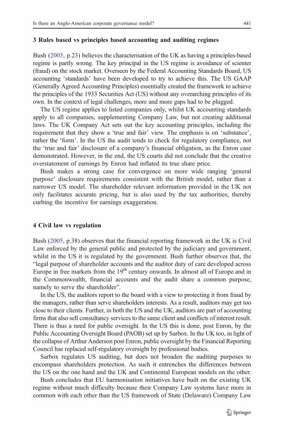
3 Rules based vs principles based accounting and auditing regimes

Bush (2005, p.23) believes the characterisation of the UK as having a principles-basedregime is partly wrong. The key principal in the US regime is avoidance of scienter(fraud) on the stock market. Overseen by the Federal Accounting Standards Board, USaccounting ‘standards’ have been developed to try to achieve this. The US GAAP(Generally Agreed Accounting Principles) essentially created the framework to achievethe principles of the 1933 Securities Act (US) without any overarching principles of itsown. In the context of legal challenges, more and more gaps had to be plugged.

The US regime applies to listed companies only, whilst UK accounting standardsapply to all companies, supplementing Company Law, but not creating additionallaws. The UK Company Act sets out the key accounting principles, including therequirement that they show a ‘true and fair’ view. The emphasis is on ‘substance’,rather the ‘form’. In the US the audit tends to check for regulatory compliance, notthe ‘true and fair’ disclosure of a company’s financial obligation, as the Enron casedemonstrated. However, in the end, the US courts did not conclude that the creativeoverstatement of earnings by Enron had inflated its true share price.

Bush makes a strong case for convergence on more wide ranging ‘generalpurpose’ disclosure requirements consistent with the British model, rather than anarrower US model. The shareholder relevant information provided in the UK notonly facilitates accurate pricing, but is also used by the tax authorities; therebycurbing the incentive for earnings exaggeration.

4 Civil law vs regulation

Bush (2005, p.38) observes that the financial reporting framework in the UK is CivilLaw enforced by the general public and protected by the judiciary and government,whilst in the US it is regulated by the government. Bush further observes that, the“legal purpose of shareholder accounts and the auditor duty of care developed acrossEurope in free markets from the 19th century onwards. In almost all of Europe and inthe Commonwealth, financial accounts and the audit share a common purpose,namely to serve the shareholder”.

In the US, the auditors report to the board with a view to protecting it from fraud bythe managers, rather than serve shareholders interests. As a result, auditors may get tooclose to their clients. Further, in both the US and the UK, auditors are part of accountingfirms that also sell consultancy services to the same client and conflicts of interest result.There is thus a need for public oversight. In the US this is done, post Enron, by thePublic Accounting Oversight Board (PAOB) set up by Sarbox. In the UK too, in light ofthe collapse of Arthur Anderson post Enron, public oversight by the Financial ReportingCouncil has replaced self-regulatory oversight by professional bodies.

Sarbox regulates US auditing, but does not broaden the auditing purposes toencompass shareholders protection. As such it entrenches the differences betweenthe US on the one hand and the UK and Continental European models on the other.

Bush concludes that EU harmonisation initiatives have built on the existing UKregime without much difficulty because their Company Law systems have more incommon with each other than the US framework of State (Delaware) Company Law

Is there an Anglo-American corporate governance model? 441

interacting with Federal regulations. He sees the harmonisation of accounting andauditing standards as a potential threat and feels that the importation of US standardsis not necessary to support capital market development in Europe, as the success ofthe London markets and the rapid blooming of the euro denominated corporate bondmarkets demonstrates.

5 Capital market competition: London vs New York

Post Sarbox, the London capital markets have attracted an increasing share of newlistings by foreign companies relative to the New York capital markets. This hasraised concerned in the US that London, with its principles based (‘litigation lite’)regulation under the Financial Services Authority and ‘comply or explain’(voluntary) corporate governance system, might be proving attractive to foreigncompanies seeking listings (initial public offering or ‘IPOs’) which are put off NewYork by Sarbox’s more rule based litigious system overseen by the Securities andExchange Commission (SEC). An alternative view is that London’s geographical(and hence time zone) position and international focus makes it attractive as aninternational market serving Europe, Africa and Asia. New York is not onlynaturally more inward looking, given that it serves the worlds largest economy andthere is a well known home-bias to stock market investment (Kho et al. 2006, P.19),but also tainted by attitudes towards the US intervention in Iraq. As a result of itsColonial past, membership of the EU and the small size of its domestic economy,London has no choice but to compete for international business. This is illustrated byits recent success in becoming a centre for Islamic bond, Sukuk issuance. The UShas a number of committees looking into the issue, but already some attempt hasbeen made to water down Sarbox as applied to smaller companies and seems to beleaning towards adopting a more ‘principles based’ approach.

Further, the former head of the NYSE (John Thain) alleged that the success ofLondon’s Alternative Investment Market (AIM), which competes more directly withNASDAQ, than the NYSE, derives from its dangerously lax regulatory regime andthe weak corporate governance requirements on its members. To be fair, there hasbeen some concern about this issue in the UK. The LSE (London Stock Exchange),which overseas AIM, has proposed some measures aimed at encouraging the‘nomads’ (‘nominated advisors’) of AIM quoted firms to perform their ‘duediligence’ roles more assiduously and has increased disclosure requirements. Tosome extent, however, such allegations from New York are seen as ‘sour grapes’.Sarbox cannot, or should not, be significantly weakened until alternative means ofpolicing internal controls are in place. As noted earlier, the policing or monitoring isdone in the UK by auditors and institutional shareholders (pension funds, insurancecompanies, investment trusts and other collective investment vehicles).

6 Institutional shareholders and ‘engagement’ in the US and the UK

Institutional shareholders (ISs) hold a significant majority of shares in the UK andtheir responsibilities are outlined in a statement of principles updated in September

442 A. Mullineux

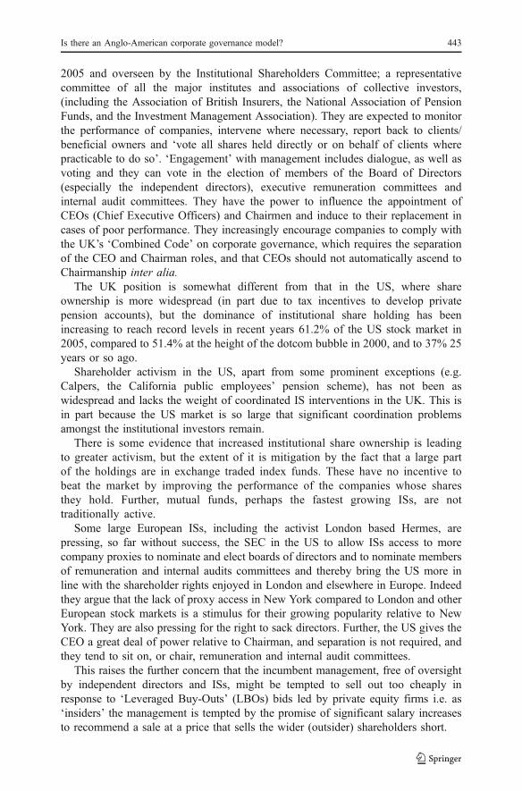
2005 and overseen by the Institutional Shareholders Committee; a representativecommittee of all the major institutes and associations of collective investors,(including the Association of British Insurers, the National Association of PensionFunds, and the Investment Management Association). They are expected to monitorthe performance of companies, intervene where necessary, report back to clients/beneficial owners and ‘vote all shares held directly or on behalf of clients wherepracticable to do so’. ‘Engagement’ with management includes dialogue, as well asvoting and they can vote in the election of members of the Board of Directors(especially the independent directors), executive remuneration committees andinternal audit committees. They have the power to influence the appointment ofCEOs (Chief Executive Officers) and Chairmen and induce to their replacement incases of poor performance. They increasingly encourage companies to comply withthe UK’s ‘Combined Code’ on corporate governance, which requires the separationof the CEO and Chairman roles, and that CEOs should not automatically ascend toChairmanship inter alia.

The UK position is somewhat different from that in the US, where shareownership is more widespread (in part due to tax incentives to develop privatepension accounts), but the dominance of institutional share holding has beenincreasing to reach record levels in recent years 61.2% of the US stock market in2005, compared to 51.4% at the height of the dotcom bubble in 2000, and to 37% 25years or so ago.

Shareholder activism in the US, apart from some prominent exceptions (e.g.Calpers, the California public employees’ pension scheme), has not been aswidespread and lacks the weight of coordinated IS interventions in the UK. This isin part because the US market is so large that significant coordination problemsamongst the institutional investors remain.

There is some evidence that increased institutional share ownership is leadingto greater activism, but the extent of it is mitigation by the fact that a large partof the holdings are in exchange traded index funds. These have no incentive tobeat the market by improving the performance of the companies whose sharesthey hold. Further, mutual funds, perhaps the fastest growing ISs, are nottraditionally active.

Some large European ISs, including the activist London based Hermes, arepressing, so far without success, the SEC in the US to allow ISs access to morecompany proxies to nominate and elect boards of directors and to nominate membersof remuneration and internal audits committees and thereby bring the US more inline with the shareholder rights enjoyed in London and elsewhere in Europe. Indeedthey argue that the lack of proxy access in New York compared to London and otherEuropean stock markets is a stimulus for their growing popularity relative to NewYork. They are also pressing for the right to sack directors. Further, the US gives theCEO a great deal of power relative to Chairman, and separation is not required, andthey tend to sit on, or chair, remuneration and internal audit committees.

This raises the further concern that the incumbent management, free of oversightby independent directors and ISs, might be tempted to sell out too cheaply inresponse to ‘Leveraged Buy-Outs’ (LBOs) bids led by private equity firms i.e. as‘insiders’ the management is tempted by the promise of significant salary increasesto recommend a sale at a price that sells the wider (outsider) shareholders short.

Is there an Anglo-American corporate governance model? 443

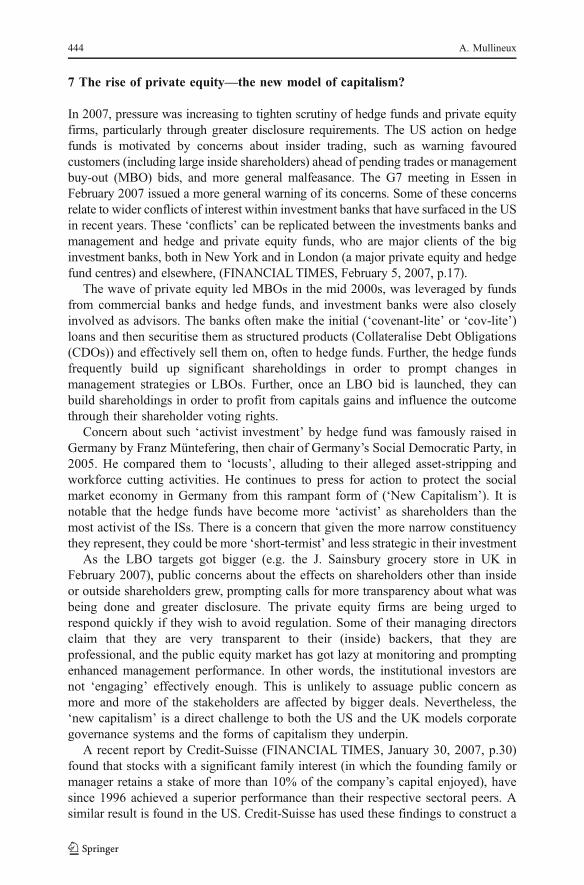
7 The rise of private equity—the new model of capitalism?

In 2007, pressure was increasing to tighten scrutiny of hedge funds and private equityfirms, particularly through greater disclosure requirements. The US action on hedgefunds is motivated by concerns about insider trading, such as warning favouredcustomers (including large inside shareholders) ahead of pending trades or managementbuy-out (MBO) bids, and more general malfeasance. The G7 meeting in Essen inFebruary 2007 issued a more general warning of its concerns. Some of these concernsrelate to wider conflicts of interest within investment banks that have surfaced in the USin recent years. These ‘conflicts’ can be replicated between the investments banks andmanagement and hedge and private equity funds, who are major clients of the biginvestment banks, both in New York and in London (a major private equity and hedgefund centres) and elsewhere, (FINANCIALTIMES, February 5, 2007, p.17).

The wave of private equity led MBOs in the mid 2000s, was leveraged by fundsfrom commercial banks and hedge funds, and investment banks were also closelyinvolved as advisors. The banks often make the initial (‘covenant-lite’ or ‘cov-lite’)loans and then securitise them as structured products (Collateralise Debt Obligations(CDOs)) and effectively sell them on, often to hedge funds. Further, the hedge fundsfrequently build up significant shareholdings in order to prompt changes inmanagement strategies or LBOs. Further, once an LBO bid is launched, they canbuild shareholdings in order to profit from capitals gains and influence the outcomethrough their shareholder voting rights.

Concern about such ‘activist investment’ by hedge fund was famously raised inGermany by Franz Müntefering, then chair of Germany’s Social Democratic Party, in2005. He compared them to ‘locusts’, alluding to their alleged asset-stripping andworkforce cutting activities. He continues to press for action to protect the socialmarket economy in Germany from this rampant form of (‘New Capitalism’). It isnotable that the hedge funds have become more ‘activist’ as shareholders than themost activist of the ISs. There is a concern that given the more narrow constituencythey represent, they could be more ‘short-termist’ and less strategic in their investment

As the LBO targets got bigger (e.g. the J. Sainsbury grocery store in UK inFebruary 2007), public concerns about the effects on shareholders other than insideor outside shareholders grew, prompting calls for more transparency about what wasbeing done and greater disclosure. The private equity firms are being urged torespond quickly if they wish to avoid regulation. Some of their managing directorsclaim that they are very transparent to their (inside) backers, that they areprofessional, and the public equity market has got lazy at monitoring and promptingenhanced management performance. In other words, the institutional investors arenot ‘engaging’ effectively enough. This is unlikely to assuage public concern asmore and more of the stakeholders are affected by bigger deals. Nevertheless, the‘new capitalism’ is a direct challenge to both the US and the UK models corporategovernance systems and the forms of capitalism they underpin.

A recent report by Credit-Suisse (FINANCIAL TIMES, January 30, 2007, p.30)found that stocks with a significant family interest (in which the founding family ormanager retains a stake of more than 10% of the company’s capital enjoyed), havesince 1996 achieved a superior performance than their respective sectoral peers. Asimilar result is found in the US. Credit-Suisse has used these findings to construct a

444 A. Mullineux

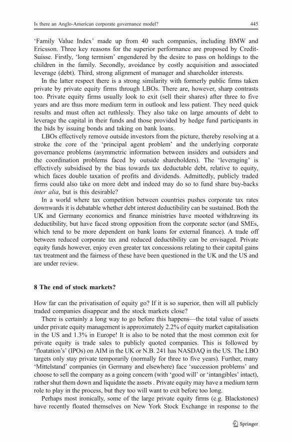
‘Family Value Index’ made up from 40 such companies, including BMW andEricsson. Three key reasons for the superior performance are proposed by Credit-Suisse. Firstly, ‘long termism’ engendered by the desire to pass on holdings to thechildren in the family. Secondly, avoidance by costly acquisition and associatedleverage (debt). Third, strong alignment of manager and shareholder interests.

In the latter respect there is a strong similarity with formerly public firms takenprivate by private equity firms through LBOs. There are, however, sharp contraststoo. Private equity firms usually look to exit (sell their shares) after three to fiveyears and are thus more medium term in outlook and less patient. They need quickresults and must often act ruthlessly. They also take on large amounts of debt toleverage the capital in their funds and those provided by hedge fund participants inthe bids by issuing bonds and taking on bank loans.

LBOs effectively remove outside investors from the picture, thereby resolving at astroke the core of the ‘principal agent problem’ and the underlying corporategovernance problems (asymmetric information between insiders and outsiders andthe coordination problems faced by outside shareholders). The ‘leveraging’ iseffectively subsidised by the bias towards tax deductable debt, relative to equity,which faces double taxation of profits and dividends. Admittedly, publicly tradedfirms could also take on more debt and indeed may do so to fund share buy-backsinter alia, but is this desirable?

In a world where tax competition between countries pushes corporate tax ratesdownwards it is debatable whether debt interest deductibility can be sustained. Both theUK and Germany economics and finance ministries have mooted withdrawing itsdeductibility, but have faced strong opposition from the corporate sector (and SMEs,which tend to be more dependent on bank loans for external finance). A trade offbetween reduced corporate tax and reduced deductibility can be envisaged. Privateequity funds however, enjoy even greater tax concessions relating to their capital gainstax treatment and the fairness of these have been questioned in the UK and the US andare under review.

8 The end of stock markets?

How far can the privatisation of equity go? If it is so superior, then will all publiclytraded companies disappear and the stock markets close?

There is certainly a long way to go before this happens—the total value of assetsunder private equity management is approximately 2.2% of equity market capitalisationin the US and 1.3% in Europe! It is also to be noted that the most common exit forprivate equity is trade sales to publicly quoted companies. This is followed by‘floatation’s’ (IPOs) on AIM in the UK or N.B. 241 has NASDAQ in the US. The LBOtargets only stay private temporarily (normally for three to five years). Further, many‘Mittelstand’ companies (in Germany and elsewhere) face ‘succession problems’ andchoose to sell the company as a going concern (with ‘good will’ or ‘intangibles’ intact),rather shut them down and liquidate the assets . Private equity may have a medium termrole to play in the process, but they too will want to exit before too long.

Perhaps most ironically, some of the large private equity firms (e.g. Blackstones)have recently floated themselves on New York Stock Exchange in response to the

Is there an Anglo-American corporate governance model? 445

pressure for more disclosure and to enable the founding managers to ‘exit’; rather thanpass the ‘goodwill’ they have built up onto their successors. This would perhaps nothave been the choice they would have made if the management was likely to be kept inthe family, as in the pre-Big Bang days of the merchant and private banking associationsin London and New York. Such family run banks still trade successfully in continentalEurope; but increasingly they describe what they do, as ‘private banking’ or ‘wealthmanagement’ and private equity and venture capital, or more generally, ‘alternativeinvestment’. This, of course, not very different from what they have always done.

Kho et al. (2006, p.10) find that, notwithstanding home bias, US investment fundsare more attracted to markets that offer (outside) investor protection, than to marketsperceived to be insider driven. The globalisation of finance is thus likely in the end toencourage more disclosure (by private equity funds) and to favour markets that offergreater (outside) investor protection. To the extent that London is doing so, New Yorkshould take note. But the Sarbox rules may in the end (perhaps following a scandalinvolving in an AIM. or an LSE quoted company) prove superior to London’sprinciples based, voluntary ‘comply or explain’ regime. Further, New York could helpitself by enhancing the proxy voting rights of institutional investors, whose role asoutside monitors should be enhanced as a means of reducing dependence on auditorsand rules backed by law; thereby requiring less resort to costly litigation.

The private equity model dramatically raises risk compared to the public equitymodel, which is why the returns are on average higher. The higher risk is a result of thehigher debt levels and much more concentrated share ownership. There is more risk ofilliquidity and a lack transparency. Liquidity and transparency are the underpinningsof the public stock markets. Lack of transparency can lead to cost escalation throughfees paid to advisors and generous management remuneration packages. Finally, themodel works against widespread share ownership and makes informed portfoliodiversification more difficult for pension and other fund managers. If it progresses toofar, it could undermine confidence in the public markets, especially if the firms withthe most upside potential have been taken private.

The backlash against private equity is also linked to concerns about foreignownership of formerly domestically owned firms. There is a suspicion that the newforeign owners, whether private equity or public equity funded, may asset strip orruthlessly cut costs (and jobs) and that the boards sell out too easily due toaforementioned conflicts of interest between them and outside shareholders,

Under US securities laws, companies that are taken private must file reports onexactly how executives and investment banks come to be involved in bids for thecompanies they manage or advise subsequent to the introduction of the managers tothe private equity firms. In the interest of greater transparency, such reports would beuseful in the UK and so too would similar reports for other mergers and acquisitionsinvolving domestic or foreign public equity backed companies.

9 Conclusions

This paper questions the existence of an Anglo-American model of corporategovernance and capitalism The UK model relies heavily on institutional shareholder‘engagement’ and regulatory principles, the US much more on regulatory rules and

446 A. Mullineux

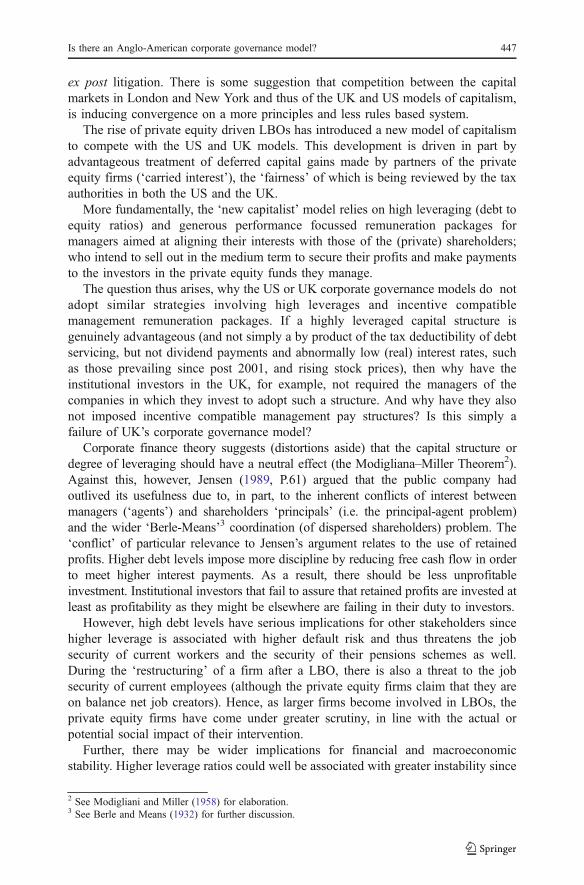
ex post litigation. There is some suggestion that competition between the capitalmarkets in London and New York and thus of the UK and US models of capitalism,is inducing convergence on a more principles and less rules based system.

The rise of private equity driven LBOs has introduced a new model of capitalismto compete with the US and UK models. This development is driven in part byadvantageous treatment of deferred capital gains made by partners of the privateequity firms (‘carried interest’), the ‘fairness’ of which is being reviewed by the taxauthorities in both the US and the UK.

More fundamentally, the ‘new capitalist’ model relies on high leveraging (debt toequity ratios) and generous performance focussed remuneration packages formanagers aimed at aligning their interests with those of the (private) shareholders;who intend to sell out in the medium term to secure their profits and make paymentsto the investors in the private equity funds they manage.

The question thus arises, why the US or UK corporate governance models do notadopt similar strategies involving high leverages and incentive compatiblemanagement remuneration packages. If a highly leveraged capital structure isgenuinely advantageous (and not simply a by product of the tax deductibility of debtservicing, but not dividend payments and abnormally low (real) interest rates, suchas those prevailing since post 2001, and rising stock prices), then why have theinstitutional investors in the UK, for example, not required the managers of thecompanies in which they invest to adopt such a structure. And why have they alsonot imposed incentive compatible management pay structures? Is this simply afailure of UK’s corporate governance model?

Corporate finance theory suggests (distortions aside) that the capital structure ordegree of leveraging should have a neutral effect (the Modigliana–Miller Theorem2).Against this, however, Jensen (1989, P.61) argued that the public company hadoutlived its usefulness due to, in part, to the inherent conflicts of interest betweenmanagers (‘agents’) and shareholders ‘principals’ (i.e. the principal-agent problem)and the wider ‘Berle-Means’3 coordination (of dispersed shareholders) problem. The‘conflict’ of particular relevance to Jensen’s argument relates to the use of retainedprofits. Higher debt levels impose more discipline by reducing free cash flow in orderto meet higher interest payments. As a result, there should be less unprofitableinvestment. Institutional investors that fail to assure that retained profits are invested atleast as profitability as they might be elsewhere are failing in their duty to investors.

However, high debt levels have serious implications for other stakeholders sincehigher leverage is associated with higher default risk and thus threatens the jobsecurity of current workers and the security of their pensions schemes as well.During the ‘restructuring’ of a firm after a LBO, there is also a threat to the jobsecurity of current employees (although the private equity firms claim that they areon balance net job creators). Hence, as larger firms become involved in LBOs, theprivate equity firms have come under greater scrutiny, in line with the actual orpotential social impact of their intervention.

Further, there may be wider implications for financial and macroeconomicstability. Higher leverage ratios could well be associated with greater instability since

2 See Modigliani and Miller (1958) for elaboration.3 See Berle and Means (1932) for further discussion.

Is there an Anglo-American corporate governance model? 447

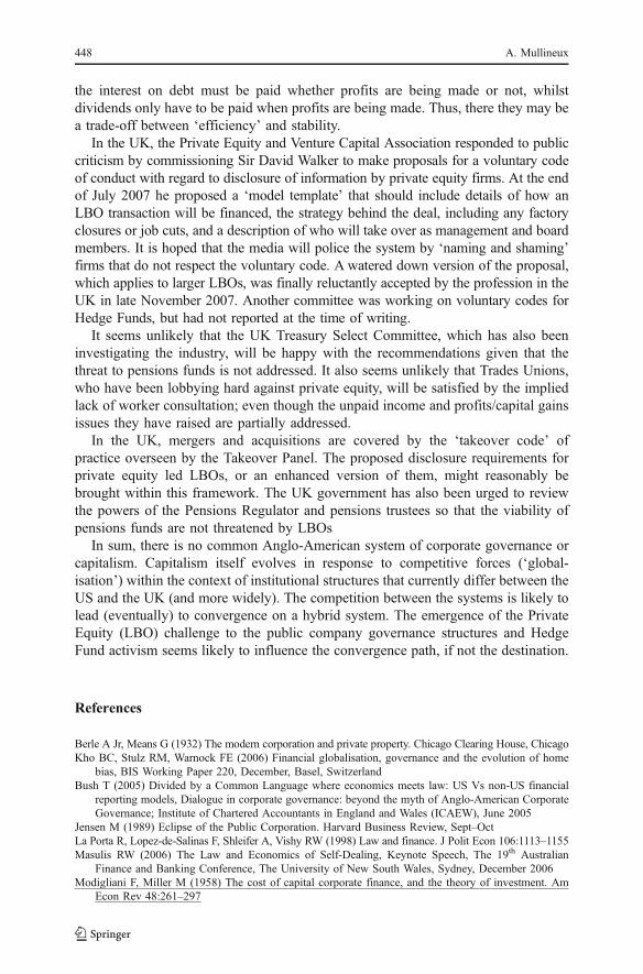
the interest on debt must be paid whether profits are being made or not, whilstdividends only have to be paid when profits are being made. Thus, there they may bea trade-off between ‘efficiency’ and stability.

In the UK, the Private Equity and Venture Capital Association responded to publiccriticism by commissioning Sir David Walker to make proposals for a voluntary codeof conduct with regard to disclosure of information by private equity firms. At the endof July 2007 he proposed a ‘model template’ that should include details of how anLBO transaction will be financed, the strategy behind the deal, including any factoryclosures or job cuts, and a description of who will take over as management and boardmembers. It is hoped that the media will police the system by ‘naming and shaming’firms that do not respect the voluntary code. A watered down version of the proposal,which applies to larger LBOs, was finally reluctantly accepted by the profession in theUK in late November 2007. Another committee was working on voluntary codes forHedge Funds, but had not reported at the time of writing.

It seems unlikely that the UK Treasury Select Committee, which has also beeninvestigating the industry, will be happy with the recommendations given that thethreat to pensions funds is not addressed. It also seems unlikely that Trades Unions,who have been lobbying hard against private equity, will be satisfied by the impliedlack of worker consultation; even though the unpaid income and profits/capital gainsissues they have raised are partially addressed.

In the UK, mergers and acquisitions are covered by the ‘takeover code’ ofpractice overseen by the Takeover Panel. The proposed disclosure requirements forprivate equity led LBOs, or an enhanced version of them, might reasonably bebrought within this framework. The UK government has also been urged to reviewthe powers of the Pensions Regulator and pensions trustees so that the viability ofpensions funds are not threatened by LBOs

In sum, there is no common Anglo-American system of corporate governance orcapitalism. Capitalism itself evolves in response to competitive forces (‘global-isation’) within the context of institutional structures that currently differ between theUS and the UK (and more widely). The competition between the systems is likely tolead (eventually) to convergence on a hybrid system. The emergence of the PrivateEquity (LBO) challenge to the public company governance structures and HedgeFund activism seems likely to influence the convergence path, if not the destination.

References

Berle A Jr, Means G (1932) The modern corporation and private property. Chicago Clearing House, ChicagoKho BC, Stulz RM, Warnock FE (2006) Financial globalisation, governance and the evolution of home

bias, BIS Working Paper 220, December, Basel, SwitzerlandBush T (2005) Divided by a Common Language where economics meets law: US Vs non-US financial

reporting models, Dialogue in corporate governance: beyond the myth of Anglo-American CorporateGovernance; Institute of Chartered Accountants in England and Wales (ICAEW), June 2005

Jensen M (1989) Eclipse of the Public Corporation. Harvard Business Review, Sept–OctLa Porta R, Lopez-de-Salinas F, Shleifer A, Vishy RW (1998) Law and finance. J Polit Econ 106:1113–1155Masulis RW (2006) The Law and Economics of Self-Dealing, Keynote Speech, The 19th Australian

Finance and Banking Conference, The University of New South Wales, Sydney, December 2006Modigliani F, Miller M (1958) The cost of capital corporate finance, and the theory of investment. Am

Econ Rev 48:261–297

448 A. Mullineux