ESTIMATING EXCHANGE RATE PASS-THROUGH IN SOUTH AFRICA

PRELIMINARY DRAFT APRIL 2014

ESTIMATING EXCHANGE RATE PASS-THROUGH

IN SOUTH AFRICA

By Dr. Mark Ellyne and

Ms. Nikol Hearn1

AbstractThis paper focuses on the exchange rate transmission mechanismon inflation in South Africa in the post-2000 period. Itmakes use of a recursive Vector Auto Regression (VAR) analysisto examine the pass-through of a change in the nominalexchange rate into domestic prices at each stage of the supplychain. We find that the impulse responses of the nominal effectiveexchange rate leads to incomplete pass-through in the consumerprice index, despite the larger pass-through into importprices. The exchange rate pass-through into consumer pricestook place over eight quarters and is slightly lower than theaverage for a wide cross section of developing countries. Thisimplies are that South Africa has is largely subject tocompetitive market pricing pressures and that monetary policyis cushioned by the low pass-through.

JEL classification: F31, E31 …

1 Dr. Mark Ellyne is Adjunct Associate Professor at University of Cape Townand Ms. Nikol Hearn is a post-graduate student at the School of Economics,UCT.

1


Keywords: South Africa, exchange rate pass-through,inflation

Authors’ e-mails: [email protected] and [email protected]

2


Introduction

The exchange rate pass-through (ERPT) is typically measured bythe percentage change in domestic prices (either import pricesor consumer prices) compared to the percentage change in thenominal exchange rate, and can vary between 0 for no pass-through and 1 for full pass-through. This sensitivity can tellus about firms’ pricing behaviour: to what degree they canpass on exchange rate related price increases (high ERPT)versus having to absorb them out of their profit margin(incomplete or low ERPT) in order to maintain sales volume. Wealso note that the pass-through may be different at differentlevels of the supply chain.

The ERPT can thus give us some indication about marketstructure and competitiveness. High ERPT indicates strongproducer pricing which may mean weak competitive domesticforces. This may also indicate that nominal exchange rateadjustment is being motivated by domestic factors, likedomestic inflation. On the other hand, low ERPT indicates theability of ability of domestic firms to absorb pricefluctuations out of profits, productivity changes, orsubstitution of alternative goods. The ERPT may be reflectiveof the source of causality of exchange rate changes as well asdomestic economic conditions and the structure of the localeconomy.

In addition we are interested in the ERPT since monetarypolicy is largely focused on the control of inflation andwould therefore have an impact on optimal monetary policy. Ithas been observed that the rate of inflation affects economicgrowth, income distribution, and domestic economic policy. Inresponse to the disruptive effects of inflation, SouthAfrica’s monetary policy has evolved to focus on maintaininginflation within a target range. Modelling the degree to whichexchange rate fluctuations cause changes in the price levelprovides guidance for monetary policy makers, who would seekto offset higher inflation resulting from exchange rate

3


depreciation with increased interest rates (Krugman, 1987;McCarthy, 1999; Taylor, 2000; Campa & Goldberg, 2002;Choudhri & Hakura, 2006; Devereux & Yetman, 2010; Ocran,2010).

We are interested in the ERPT in South Africa to understandmore about both the structure of the economy and the monetaryauthorities’ scope for management of inflation. A quickobservation of annual changes in the nominal effectiveexchange rate (in foreign/domestic currency) and the annualinflation rate, illustrates the inverse relationship.

Figure 1: South Africa – Annual change in NEER and CPI

Source: Data from IMF and SARB; year-over-year percentage change.

Background

The exchange rate pass-through to import prices, particularlyof raw materials and goods, constitutes the “direct channel”(Mohsin et al, 2012). If a depreciation of the currencyresults in local firms increasing their final prices by thefull amount of the depreciation so as to maintain their profitmargins (Jabara, 2009), then complete or full pass-through(ERPT≈1) occurs and signals ‘producer currency pricing’ (Campa &Goldberg, 2002; Brun et al, 2012:819). This generallyindicates that markets are not very competitive, there are few

4

CPI % Chg

NEER % changeNEER

CPI


domestic substitutes, or there is little opportunity foroffsetting price increases with productivity gains.

Producer currency pricing or full pass-through of exchange movementstends to reduce the impact of having a domestic currency anddemands more of domestic monetary policy to control inflation.A post-conflict country that is highly dependent on importsand has weak domestic capacity would likely have producercurrency pricing or a high pass-through. For exporters, whomay have to absorb the increased costs of imports, exchangerate depreciation would only affect the domestic value-addedof the production process.

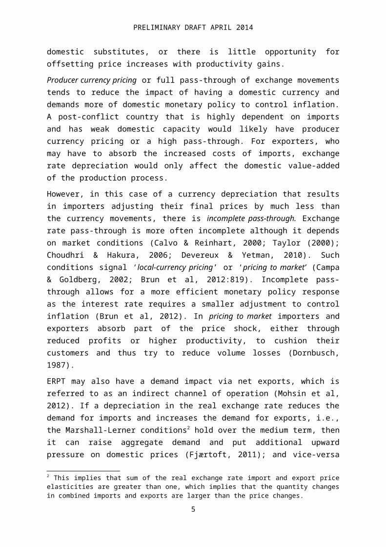
However, in this case of a currency depreciation that resultsin importers adjusting their final prices by much less thanthe currency movements, there is incomplete pass-through. Exchangerate pass-through is more often incomplete although it dependson market conditions (Calvo & Reinhart, 2000; Taylor (2000);Choudhri & Hakura, 2006; Devereux & Yetman, 2010). Suchconditions signal ‘local-currency pricing’ or ‘pricing to market’ (Campa& Goldberg, 2002; Brun et al, 2012:819). Incomplete pass-through allows for a more efficient monetary policy responseas the interest rate requires a smaller adjustment to controlinflation (Brun et al, 2012). In pricing to market importers andexporters absorb part of the price shock, either throughreduced profits or higher productivity, to cushion theircustomers and thus try to reduce volume losses (Dornbusch,1987).

ERPT may also have a demand impact via net exports, which isreferred to as an indirect channel of operation (Mohsin et al,2012). If a depreciation in the real exchange rate reduces thedemand for imports and increases the demand for exports, i.e.,the Marshall-Lerner conditions2 hold over the medium term, thenit can raise aggregate demand and put additional upwardpressure on domestic prices (Fjærtoft, 2011); and vice-versa

2 This implies that sum of the real exchange rate import and export priceelasticities are greater than one, which implies that the quantity changesin combined imports and exports are larger than the price changes.

5


for an appreciation. Our view is that this is a valid but muchless important impact for South Africa.

ERPT first became of popular interest in the 1990’s when theindustrialized countries were faced with strong demand butwith corresponding low levels of inflation, which seemedcontrary to the short-run Phillips curve. It appeared thatsome traditional inflation relationships were no longerholding. The literature of the time viewed the degree of pass-through as a microeconomic concern related to the firm andindustry structure (Bergen and Feenstra, 1998; Dornbusch,1987; Knetter, 1994). McCarthy (1999) first focused on themacroeconomic degree of pass-through (Taylor, 2000; Campa &Goldberg, 2002).

ERPT Observed in Earlier Studies

McCarthy (1999) used a recursive vector auto regression (VAR)to model the exchange rate pass-through into domestic pricesat various stages of the supply chain. He argued that exchangerate shocks first hit import prices, then wholesale orproducer prices, and only lastly consumer or retail prices.The findings indicated that in developed economies exchangerate shocks had a fairly small impact on domestic inflation,although they had larger impacts on producer prices. Thedegree of ERPT is affected by various country specificfactors; for example, the more volatile the domestic demand,the lower the pass-through as it changes the earnings margins.The size of the country matters for pass-through as well:pass-through tends to be lower if the country is large.Moreover, some argued that more regular exchange rate shocksproduced a greater the degree of pass-through (McCarthy, 1999;Taylor, 2000). Thus it appeared that the lower inflationenvironments in developed countries during the 90’s werebrought about by other factors, which were more likelyattributable to monetary policy (Taylor, 2000).

Following McCarthy’s work, Choudhri and Hakura (2006) foundthat with a 10% increase in the mean inflation rate increased

6


the elasticity of pass-through by 5% in the short run and by6% in the long run. In a high inflation regime, shocks becomemore constant and have larger effects through the exchangerate; whereas the price pass-through in low inflation regimeswill be lower (Choudhri & Hakura, 2006). Thus the averageinflation rate of a country is an important factor determiningits pass-through.

Choudhri and Hakura (2006) classified South Africa as amoderate inflation regime in the period prior to 2000, i.e.where inflation is between 10% and 30%.3 Thus, it would havehigher pass-through than today, when it is considered to be alow inflation regime (under 10% inflation). They estimated thelong-term ERPT for South Africa over the period of 1979 to2000 at 14%, whilst the pass-through was only 7% one quarterafter the shock (Choudhri and Hakura, 2006). They attributedthe low pass-through to the well-known stickiness of pricesand “menu cost” theory promoted by New Keynesians (Knetter,1994; Bhundia, 2002).

Mwase (2006) studied the exchange rate pass-through intoconsumer prices in Tanzania using a Vector Error CorrectionModel (VECM) and Granger Causality Tests. He found that thepass-through was modest and incomplete for the period 1990 to2005. Ahmed and Hossain (2009) employed cointegration and VECMtechniques to determine the long run pass through ofinternational prices in Bangladesh, which he found to becomplete [??] during the period 2000 to 2008.

Devereux and Yetman (2010) specifically tested whether theERPT is dependent on sticky prices. They found that the ERPTcoefficient to consumer price inflation was approximately 0.18in a wide cross-section of countries. In situations where theprices of consumer goods could more freely fluctuate, thecoefficient of pass-through increased to 0.8 (Devereux &Yetman, 2010). This indicated that varying levels of nominalrigidities across countries could account for differences in

3 A low inflation environment refers to under-10 percent inflation and highinflation refers to over 30 percent inflation (Choudhri and Hakura, 2006).

7


pass-through. In the same cross section of countries they alsoestablished that if shocks were persistent, despite stickyprices, then pass-through was high , (Devereux & Yetman,2010).

Bhundia (2002) evaluated the degree of pass-through into theCPIX4 in South Africa. The channel of effects was modelledusing a vector auto regression, following McCarthy (1999). Hefound that a 1% shock to the exchange rate resulted in a0.132% increase in the level of the CPIX index over tenquarters. A study by Karoro et al (2009) on the ERPT intoimport prices in South Africa for the period 1980- 2005 foundthat import prices increased faster when the nominal effectiveexchange rate depreciated, whereas import prices decreased ata slower rate when the exchange rate appreciated. A pass-through elasticity into import prices of 0.79 was established.

More recently, Ocran (2010) studied the South African ERPTusing monthly data from 2000 to mid-2009 in an unrestrictedVAR, also following McCarthy’s supply chain approach. Heidentified the ERPT into consumer prices over two years was13%, into producer prices was 18%, and into import prices was20%. He found that the ERPT peaked at 27% into producer pricesafter 7 months, whilst it peaked at 40% into import pricesafter 7 months.

Certain similarities were found across the range of studies.Fluctuations in the exchange rate had a mild impact onconsumer prices in the short run, which appears tosubstantiate some degree of nominal rigidities or stickyprices. The full impact seems to take at least 4 quarters,which seems longer than expected. Calvo & Reinhart (2000)observed that the ERPT is lower in developed countries than inemerging economies. The higher pass-through typicallyexperienced by developing economies may be linked to thepersistence of exchange rate shocks, the dependence onimports, or to their lack of market power. Recent studies

4 CPIX is the consumer price index excluding interest on mortgage bonds(South African Reserve Bank, 2013).

8


suggest that the pass-through for developed economies isdeclining (Campa and Goldberg, 2002; Bouakez and Rebei, 2008).Devereux & Yetman (2010) ascribe the differences in pass-through among countries as a result of the ongoing level ofinflation: the higher the average inflation, the greater thepass-through, regardless of whether the country is developingor developed.

InvestigationThis paper investigates the exchange rate pass-through intodomestic prices for South Africa taking into account the datafollowing the international financial crisis of 2008. Itfollows the general McCarthy stage of processing approach butuses a recursive structural vector auto regression model(Section 2) to separate the impact on the import price index,the producer price index, and finally the consumer price index(Section 3). The approach used the resulting impulse responsefunction to examine the response path of a one standarddeviation exchange rate shock on the import price index (IPI),producer price index (PPI) and consumer price index (CPI). Thelong run pass-through into consumer prices is low at 10%, butcomparable to that found in previous studies (Section 4).These results not only provide some indications about thevibrancy and competitiveness of the South African economy, butalso have implications for a more restrained monetary policy(Section 5).

Model

We create a model to examine the impact of a shock to thenominal exchange rate on three levels of prices: importprices, producer prices and consumer prices, while controllingfor overall supply and demand conditions. The model followsthe work of McCarthy (1999), who used a recursive Vector AutoRegression (VAR) model employing the Cholesky decomposition.

9


That approach implies that the variance decompositions andimpulse response functions may be greatly dependent upon thesequencing of the variables in the VAR, where the firstvariable is the most exogenous and the last variable is themost endogenous (Enders, 2004). This study following thegeneral strategy of exploring the ERPT with a VAR, and extendsthe data to the post financial crisis period.

Data

The model is tested using quarterly data over the period 2000to 2013. South Africa formally introduced inflation targetingthe first quarter of February 2000; thus the period representsa fairly homogenous period for monetary policy. A dynamicmodel is used, where all endogenous variables are expressed asquarter-to-quarter changes measured as the first difference ofthe log of the level data.

The nominal effective exchange rate (NEER) comes from theSouth African Reserve Bank and is measured in foreign currencyper unit of local currency, so that depreciation results inthe index decreasing.5

Figure 2. South Africa – Quarterly Change in NEER(in logs)

-.20

-.15

-.10

-.05

.00

.05

.10

.15

00 01 02 03 04 05 06 07 08 09 10 11 12 13

DLNEER

Source:

5 The NEER is a weighted average of the currencies of South Africa’s 15 maintrading partners (KBP5376).

10


The import price index (IPI) comes from Statistics SouthAfrica and is the quarterly average of the monthly importindices for all imported commodities. The producer price index6

(PPI) is the quarterly average of the monthly producer priceindex for domestic output of South African industry groups,and the consumer price index (CPI) is taken from the IMFInternational Financial Statistics and is the general CPI forall items.

Figure 3. South Africa – Quarterly Change in CPI(in logs)

-.02

-.01

.00

.01

.02

.03

.04

00 01 02 03 04 05 06 07 08 09 10 11 12 13

DLCPI DLCPI_A

Figure 4. South Africa – Quarterly Change in PPI(in logs)

6 The three price index series used are not seasonally adjusted. The

seasonally adjusted series produced non-stationarity. Additionally, a

smoothed series may produce autocorrelations amongst the residuals, which

may flaw interpretations (Cogley & Nason, 1995: 265).

11


-.06

-.04

-.02

.00

.02

.04

.06

.08

.10

00 01 02 03 04 05 06 07 08 09 10 11 12 13

DLPPI DLPPI_A

Figure 5. South Africa – Quarterly Change in IPI(in logs)

-.12

-.08

-.04

.00

.04

.08

.12

00 01 02 03 04 05 06 07 08 09 10 11 12 13

DLIPI DLIPI_A

The quarterly inflation rates for all of the variables-- π¿m ;

π¿p,; π¿

c –are significantly correlated (Figure 6).

Figure 6. South Africa: Correlation Between VariablesCorrelation/(Probability

)dlNEER dlIPI dlPPI dlCPI

dlNEER 1.00

dlIPI= π¿m -0.2169

(0.115) 1.00

12


dlPPI=π¿p, -0.1761

(0.203)0.7114(0.0) 1.00

dlCPI=π¿c -0.1222

(0.379)0.3958(.003)

0.585(0.000) 1.00

Source: Calculations by authors

Two exogenous variables are used to control for demand andsupply effects. The output gap (Ygap) captures demand pressureand is calculated as the difference between the log of GDP inconstant 2000 prices and the log of the GDP trend, which wascalculated using the Hodrick-Prescott Filter. The quarterlypercentage change in the Brent crude oil price,7 measured asthe first difference of the log of the variable, is used tocontrol for supply shocks.

SVAR modelling

The SVAR approach lends itself to studying the transmission ofshocks through the economy by providing the impulse-responsefunctions among variables and the variance decomposition ofshocks to each variable. The SVAR approach is based on a setof structural relationships (E1), defined by the parametercoefficients in matrices A and B, where yt is a vector ofendogenous current variables (Lutkepohl, Chapter 9). Ayt=A1

¿ yt−1+…+Ap¿yt−p+Bϵt (1)

Aμt=Bϵt (2)

The so-called AB model (E2) is commonly used for the SVAR(Lutkepohl Chapter 9), where ϵt are the observed LutkepohlChapter 9 residuals or forecast errors and the μt are theunobserved structural innovations.

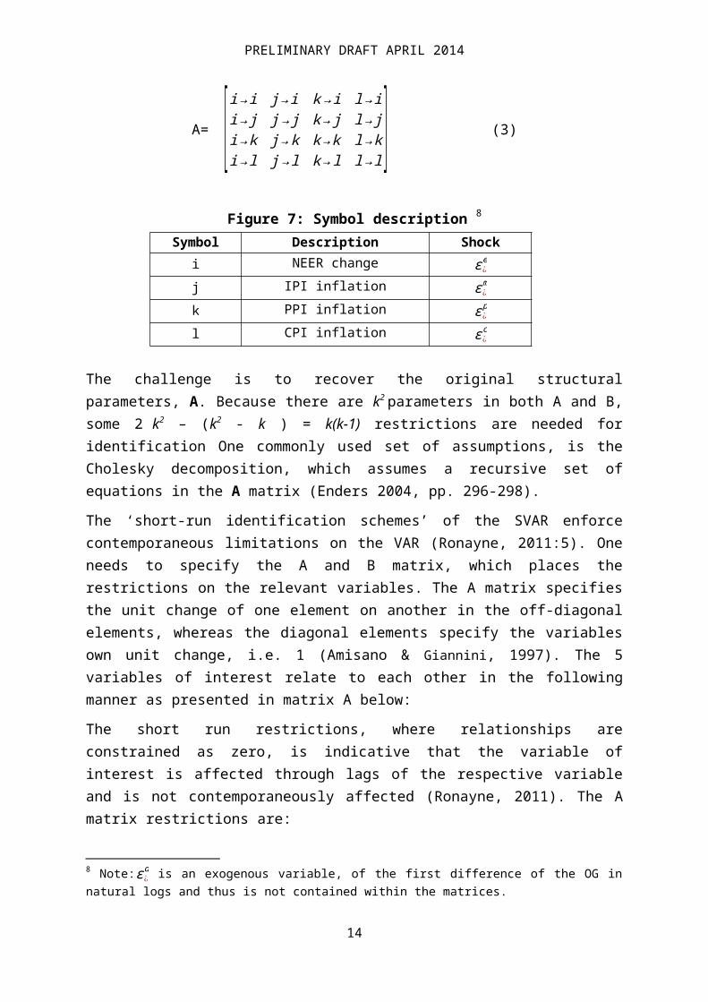
The A matrix captures the structural relations amongvariables, which have been identified in Table 1 below.

7 This series is the quarterly average of monthly Brent Crude prices in USdollars, reported by the South African Reserve Bank (series KBP5344M).

13


A= [i→i j→i k→i l→ii→ji→ki→l

j→jj→kj→l

k→jk→kk→l

l→jl→kl→l ] (3)

Figure 7: Symbol description 8

Symbol Description Shocki NEER change ϵ¿

e

j IPI inflation ϵ¿m

k PPI inflation ϵ¿p

l CPI inflation ϵ¿c

The challenge is to recover the original structuralparameters, A. Because there are k2 parameters in both A and B,some 2 k2 – (k2 - k ) = k(k-1) restrictions are needed foridentification One commonly used set of assumptions, is theCholesky decomposition, which assumes a recursive set ofequations in the A matrix (Enders 2004, pp. 296-298).

The ‘short-run identification schemes’ of the SVAR enforcecontemporaneous limitations on the VAR (Ronayne, 2011:5). Oneneeds to specify the A and B matrix, which places therestrictions on the relevant variables. The A matrix specifiesthe unit change of one element on another in the off-diagonalelements, whereas the diagonal elements specify the variablesown unit change, i.e. 1 (Amisano & Giannini, 1997). The 5variables of interest relate to each other in the followingmanner as presented in matrix A below:

The short run restrictions, where relationships areconstrained as zero, is indicative that the variable ofinterest is affected through lags of the respective variableand is not contemporaneously affected (Ronayne, 2011). The Amatrix restrictions are:

8 Note:ϵ¿d is an exogenous variable, of the first difference of the OG in

natural logs and thus is not contained within the matrices.

14


A=[ 1 0 0 0a21a31a41

1a32

a42

01a43

001] (4)

The B matrix places restrictions on the error structure of thesystem and requires the assumption that the covariance betweentwo variables is unrelated (Amisano & Giannini, 1997).Specifying the B matrix as follows:

B =[b11 0 0 0000

b22

00

0b33

0

00b44

] (5)

In order to retrieve the short run coefficients, one shouldmake use of the variance covariance matrix of the VAR in itserror correction structure (Lütkepohl, 1993). The εtcolumnvector signifies the disturbances whilst theet column vectorindicates the innovations. Both follow a normal distributionwith a mean of zero (StataCorp, 2011). A shock to the elementsin theεt vector allows us to trace the path of effects overtime. The final short run model to be estimated is as follows:

[ 1 0 0 0a21a31a41

1a32

a42

01a43

001]¿ (6)

The SVAR places limitations on the way in which the variablesrelate to each other based on the underlying VAR (StataCorp,2011). Thus the underlying VAR models of the three steps ofpricing in the distribution stage are depicted below, withequations for import prices as π¿

m (2), producer prices π¿p (3),

and consumer prices asπ¿c (4).

Equation 7: Recursive Model

15π¿m=Et−1 (π¿

m )+α1iϵ¿s+α2iϵ¿

d+α3iϵ¿e+ϵ¿

m

π¿p=Et−1 (π¿

p )+β1iϵ¿s+β2iϵ¿

d+β3iϵ¿e+β4iϵ¿

m+ϵ¿p

π¿c=Et−1 (π¿

c )+γ1iϵ¿s+γ2iϵ¿

d+γ3iϵ¿e+γ4iϵ¿

m+γ5iϵ¿p+ϵ¿

c


Data Properties and Tests

We undertake the standard array of tests to ensure thestability of the variables and model. First, we test forstationarity of the variables with the Augmented Dickey-Fuller(ADF) test and find all of the variables to be I(1), orstationary in the first difference (Table 2).

The optimal lag length for the SVAR was determined from theVAR model for NEER, IPI, PPI and CPI. The optimal lagselection was identified as one for all variables, whichseemed reasonable for quarterly (Appendix Tables 3-5).

The control variables for the output gap (demand variable) andgrowth rate of oil price (supply variable) were stipulated asexogenous variables, as they are outside the endogenouspricing system that we are examining, accordance withBhundia’s (2002) VAR model for South Africa.

16


Figure 8: ADF results

Variable Test Statistic z(t) MacKinnon approximatep-value for z(t)

ϵ¿c -4.255 0.0005

ϵ¿s -5.630 0.0000

ϵ¿d -6.776 0.0000

ϵ¿e -5.820 0.0000

ϵ¿m -4.296 0.0005

ϵ¿p -5.588 0.0000

Notes: The p-values are significant at the 1% level (i.e., less than -3.580) for the first differenced log of each variable and thus one canreject the null hypothesis that the first difference of each variablefollows a unit root process and conclude that the process is integrated oforder 1 (I (1)).

Secondly, the SVAR model must be stable, which is indicativeof covariance stationarity and no significant autocorrelations(Lütkepohl, 1993). If the VAR can be portrayed as an infinite-order vector moving-average portrayal as well as beinginvertible, then it is stable (Lütkepohl, 1993; and Hamilton,1994). We find that the modulus of each eigenvalue is strictlyless than one for the VAR, indicative of SVAR stability(Hamilton, 1994). The Lagrange-Multiplier tests forautocorrelation in the disturbances suggest that noautocorrelation is present in the models (Appendix Tables 6-8). Finally, the vector of residuals appears to meet therequirement of being white noise and normally distributed(Appendix Table 9).

As an alternative to the SVAR model, we also checked for thepossibility of using the vector error correction model (VECM).Although the Johansen test found the presence of one co-integrating equation, the stability condition was rejected asit had an eigenvalue greater than one (Johansen, 1995). Thusthe SVAR model was used as it better met all the stipulatedcriteria as the model for analysis.

17


Empirical Results

Because the variables are already in growth rate form, thecumulative impulse-response function (IRF) identifies theexchange rate pass-through elasticity at time t (equation 9).

Passthroughelasticityattimet=cumulative%∆∈priceleveltquartersaftershock

initial %∆∈exchangerateatt=0(8)

The shock to the exchange rate is a 1% appreciation of theNEER that is a one standard error on the variable itself attime 0.9 Table 9 presents the cumulative pass-throughelasticity to the IPI, PPI and CPI over 16 quarters followingthe initial shock. The appreciation of the NEER invokes adecrease in the price levels as theory suggests.

We found that 90 to 95 percent of the total pass-through ofthe exchange rate shock into prices takes place within 4 or 5quarters and most of that takes place within the first 2quarters (Table 9).

Figure 9: Accumulated Exchange Rate Pass-Through

Exchange Rate Pass Through Elasticity on:

After shockat T=0 IPI PPI CPI

T=1 -0.289 -0.15 -0.048T=4 -0.439 -0.24 -0.092T=6 -0.45 -0.243 -0.097T=10 -0.457 -0.244 -0.098T=16 -0.457 -0.244 -0.10

Source: Authors results from Stata.

By comparison, Bhundia (2002) found the peak pass-through intoimport prices was 40% occurring in the third quarter, whilstthe peak pass-through into producer prices was 23% in thetenth quarter. Ocran (2010) found an ERPT into import pricespeaking of 40% after 8 months, an ERPT into producer prices

9 This is normalized to 1 standard deviation = 1%.

18


peaking at 27% after 7 months. These figures comparefavourably to that found in this study.

As would be expected, the exchange rate pass-through islargest for import prices and smallest for the consumerprices. This ordering is consistent with McCarthy’s (1999)results, where the long run pass-through into import priceswas 41%, a long run pass-through of 20% into producer prices,and a 15% long run pass-through into consumer prices.

Interestingly, Kororo et al (2009) established the long runpass-through into South African import prices at 79% for theperiod 1980 to 2005. This finding differs greatly to thatfound in this study of 46%, as well as to the long run pass-through of 24 months found by Ocran (2010) of 18% and thepass-through into import prices found by Bhundia (2002) of40%. The large variation in long-run findings may be due tothe estimation algorithms that are used. Faust and Leeper(1997) ascertain that when the data is finite, one cannotprecisely estimate the long-run outcome of shocks.

Compared to these other recent studies on South Africa ERPT,cited above, the pass-through finding in this study are verycomparable (Figure 10).

Figure 10. South Africa-Comparison of ERPT Results With OtherStudies

Source: Authors’ calculations.

Devereux & Yetman (2010) establish an ERPT into consumerprices of 18% for a vast array of countries and thus can betaken as some type of average magnitude. Choudhri and Hakura(2006) indicated that a low inflation regime should maintain a

19


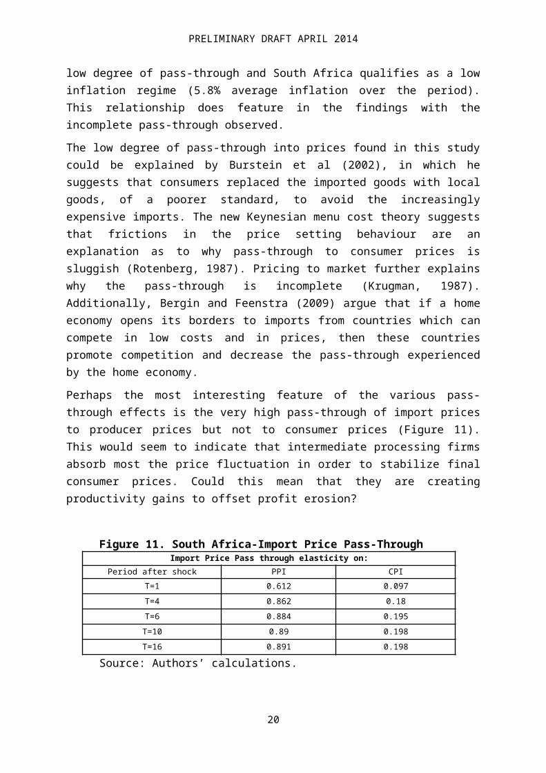
low degree of pass-through and South Africa qualifies as a lowinflation regime (5.8% average inflation over the period).This relationship does feature in the findings with theincomplete pass-through observed.

The low degree of pass-through into prices found in this studycould be explained by Burstein et al (2002), in which hesuggests that consumers replaced the imported goods with localgoods, of a poorer standard, to avoid the increasinglyexpensive imports. The new Keynesian menu cost theory suggeststhat frictions in the price setting behaviour are anexplanation as to why pass-through to consumer prices issluggish (Rotenberg, 1987). Pricing to market further explainswhy the pass-through is incomplete (Krugman, 1987).Additionally, Bergin and Feenstra (2009) argue that if a homeeconomy opens its borders to imports from countries which cancompete in low costs and in prices, then these countriespromote competition and decrease the pass-through experiencedby the home economy.

Perhaps the most interesting feature of the various pass-through effects is the very high pass-through of import pricesto producer prices but not to consumer prices (Figure 11).This would seem to indicate that intermediate processing firmsabsorb most the price fluctuation in order to stabilize finalconsumer prices. Could this mean that they are creatingproductivity gains to offset profit erosion?

Figure 11. South Africa-Import Price Pass-ThroughImport Price Pass through elasticity on:

Period after shock PPI CPIT=1 0.612 0.097T=4 0.862 0.18T=6 0.884 0.195T=10 0.89 0.198T=16 0.891 0.198


20


Similarly, the low pass-through from producer prices to theCPI (Figure 12) indicates fairly strong market pricing inSouth Africa.

Figure 12: Accumulated Producer price shocksProducer Price Pass through elasticity on:After shock CPI

T=1 0.185T=4 0.185T=6 0.185T=10 0.185T=16 0.185


Next we examine the variance decomposition, which indicatesthe portion of the response variable’s forecast variance thatcan be attributed to shocks of the impulse variable. We see inFigure 13 that NEER growth ultimately explains about 20% ofthe forecast variance of CPI growth, about double the amountof the IPI or PPI; but all three variables explain about 38%of the CPI error variance. The high variance contributed byCPI growth itself, 62.4%, indicates that other factors outsideof this system are responsible for most of the variance,possibly including money supply, wages, and demand factors.

Figure 13: Variance Decomposition of CPI Variance Decomposition of CPI owing to:

After shock dlNEER dlIPI dlPPI dlCPIT=1 .0110 .0177 .1306 .8405T=4 .1919 .0893 .0895 .6291T=8 .1953 .0918 .0888 .6240T=12 .1953 .0918 .0888 .6240T=16 .1953 .0918 .0888 .6240


21


Figure 14: Variance Decomposition of PPIVariance Decomposition of PPI owing to:

After shock dlNEER dlIPI dlPPIT=1 .0535 .1755 .7710T=4 .2212 .2581 .5084T=8 .223 .260 .5062T=12 .223 .260 .5062T=16 .223 .260 .5062


Conclusion and Policy Implications

This study has used an SVAR analysis to examine the impact ofthe quarterly change in the nominal effective exchange rate onquarterly changes in import prices, producer prices andconsumer prices in the South African supply chain, over theperiod 2000 to 2013. The Cholesky decomposition was used,which restricts the system of equations to a recursive SVARand lends itself ideally to this analysis. In this model, thenominal effective rate was taken as the most exogenousvariable and the CPI was most endogenous. This was realisticas we are trying to understand the transmission of exogenousexchange rate shocks, as opposed to exchange rate shocksemanating from domestic inflation.

The model results indicated that just 10% of exchange rateshocks passed through to the CPI, whereas some 46% passed intothe growth of import prices. Furthermore, 89% of the change inimport prices passed into producer prices, but only 18% ofproducer price inflation passed into consumer price inflation.These results are comparable to those obtained by McCarthy(1999), Choudhri & Hakura (2001), Bhundia (2002), and Ocran(2010).

This chain of processing approach indicates that theintermediate processing firms absorb the bulk of exchange ratefluctuations but are unable to pass them on to finalconsumers. This pricing to market or Keynesian price stickiness at

22


the producer level means that intermediate processing firmshave had to absorb exchange rate-related cost increaseswithout fully passing them on. This ability to absorb costsseems to indicate that South African firms have a considerabledegree of flexibility. One can speculate whether this abilityto absorb costs is due to the ability to find substitutes forexpensive imported goods, the ability to absorb temporary costincreases out of profits, or the ability to raise productivityto offset costs, possibly through higher capital/labourratios. Separate evidence (Holland) does indicate that SouthAfrican firms have relatively high rates of return on assets.

As the exchange rate is a critical variable for exportcompetitiveness, and a real depreciation can improve thecurrent account and stimulate growth, the low ERPT providessome confidence that a nominal exchange rate shock will not besimply offset by movements in the price level that return thereal exchange rate to its previous position. Then the low ERPTfor South Africa may be reflective of the high variability ofthe real exchange rate of the rand.

Our model estimation may also have important implications formonetary policy in 2014. The low ERPT would mean that exchangerate shocks have less impact on inflation, so the monetaryauthorities have less need to raise interest rates. However,the nominal rand depreciated by 9% between September 2012 andJanuary 2014 (and by almost double that amount over the prior12 months to January 2014). A long-run pass-through into CPIinflation of 10% implies that this shock would add 0.9% moreto the quarterly inflation rate or an additional 3.6% perannum over the next year. This has been sufficient to worrythe central bank, which raised the policy interest rate by0.5% in February 2014. The important point here is that ahigher ERPT might have led to an even higher expectedinflation and hence higher rise in the policy interest rate.

However, because inflation has risen considerably less thanthe nominal exchange rate depreciation since January 2013,most of that nominal depreciation has translated into a real

23


depreciation of almost 15% by January 2014. That realdepreciation should stimulate GDP by reducing the currentaccount deficit. Such a positive result will depend on SouthAfrican firms living up to their inferred ability to maintaina low ERPT by raising productivity and finding less expensiveimport substitutes.

The test between the effects of a real depreciation of theexchange rate and the impact of an interest rate increase willbe seen during 2014.

24


REFERENCES

ADOLFSON, M. (2007). Incomplete exchange rate pass-through andsimple monetary policy rules. Journal of International Money and Finance, 26:468-494.

AHMED, M and HOSSAIN, M. (2009). Exchange rate management underfloating regime in Bangladesh, paper no. 20487. Available athttp://mpra.ub.uni-muenchen.de/20487/MPRA [Accessed 21 May 2013].

AMISANO, G. and GIANNINI,C. (1997). Topics in Structural VAREconometrics. 2nd edition. Heidelberg: Springer.

BERGIN, P.R. and FEENSTRA, R.C. (2009). Pass-through of exchangerates and competition between floaters and fixers. Journal of Money,Credit and Banking, 41 (1): 35–70.

BERNANKE, B. (1986). Alternative explorations of the money-incomecorrelation. Carnegie-Rochester Series on Public Policy, 25 (1): 49–99.

BHUNDIA, A. (2002). An Empirical Investigation of Exchange RatePass-Through in South Africa. IMF Working Paper, 2(165):1-28.

BLANCHARD, OLIVIER J. (1983). Price Asynchronization and Price LevelInertia, in Rudiger Dornbusch and Mario Henrique Simsonen, eds.,Inflation, Debt, and Indexation, Cambridge, MA: MIT Press, 3–24.

BOUAKEZ, H and REBEI, N. (2008). Has exchange rate pass-through really declined? Evidence from Canada. Journal of International Economics, 75: 249–267.

BURSTEIN, A., EICHENBAUM, M. and REBELO, S. (2002). Why are Rates ofInflation so Low after Large Devaluations? Unpublished. Availableat http://www.kellog.nwu.edu/faculty/rebelo/htm/research.html[Accessed 10 July 2013].

CALVO, G. and REINHART, C. (2000). Fixing for your life. NBERworking paper 8006.CAMPA, M. J. and GOLDBERG, L. S. (2002). Exchange Rate Pass-Through into Import Prices: A Macro or Micro Phenomenon? NBERWorking Papers No 34.

25


CHOUDHRI, E. U. and HAKURA, D. (2006). Exchange Rate Pass -Throughto Domestic Prices: Does the Inflationary Environemt Matter? Journal ofInternational Money and Finance, 25 (4): 614-639 .

COGLEY, T. and NASON, J.M. (1995) .Effects of the Hodrick-Prescottfilter on trend and difference stationary time series. Implicationsfor business cycle research. Journal of Economic Dynamics and Control, 19:253-278.

DEVEREUX, M. B. and YETMAN, J. (2010). Price adjustment and Exchangerate pass-through. Journal of International Money and Finance, 29: 181-200.

26


DORNBUSCH, R. (1987). Exchange Rates and Prices. American EconomicReview, 77 (1): 93-106.

ENDERS, W. (2004). Applied Econometric Time Series, 2nd ed. John Wiley& Sons, NewYork, NY.

FAUST, J. and LEEPER, E. M. (1997). When Do Long-Run IdentifyingRestrictions Give Reliable Results? Journal of Business & Economic Statistics,15 (3):345-353.FJÆRTOFT, D. (2011). Monetary Policy in Russia and Effects of theFinancial Crisis. Econ-Working Paper no. 2008-011, project no. 27100.

FULLER, W. (1996). Introduction to Statistical Time Series. 2nd ed.New York: Wiley.

GUTTENTAG, J. (1966). The strategy of open market operations. TheQuarterly Journal of Economics, 80(1):1-30.

HAMILTON, J. D. (1994). Time Series Analysis. Princeton: PrincetonUniversity Press.

INTERNATIONAL MONETARY FUND. (2013). IMF Data and Statistics . Availableat: http://www.imf.org/external/data.htm [Accessed 9 April 2013].

JABARA, C.L. (2009). How Do Exchange Rates Affect Import Prices?Recent Economic Literature and Data Analysis. U.S. International TradeCommission, Washington, DC. No. ID 21.

JOHANSEN, S. (1995). Likelihood-Based Inference in CointegratedVector Autoregressive Models. Oxford: Oxford University Press.

KARORO, T.D., AZIAKPONO, M.J., and CATTANEO, N. (2009). Exchangerate pass-through to import prices in South Africa: Is thereasymmetry? South African Journal of Economics, 77(3).

KNETTER, M. M. (1994). Is export price adjustment asymmetric?Evaluating the market share and marketing bottlenecks hypotheses.Journal of International Money and Finance, 13(1): 55-70.

KRUGMAN, PAUL R. (1987). Pricing to Market When the Exchange RateChanges,in Sven W. Arndt and J. David Richardson, eds., Real-Financial Linkages Among Open Economies, Cambridge, MA and London: MITPress, 49–70.

27

http://www.imf.org/external/data.htm


LÜTKEPOHL, H. (1993). Introduction to Multiple Time Series Analysis.2nd ed. New York: Springer.

LÜTKEPOHL, H. (2005). New Introduction to Multiple Time SeriesAnalysis. New York: Springer.

MANN, C.L. (1986). Prices, Profits Margins, and Exchange Rates,Federal Reserve Bulletin, 72: 366–79.

MCCARTHY, J. (1999). Pass-Through of Exchange Rates and ImportPrices to Domestic Inflation in Some Indutrialized Countries. Bankfor International Settlements.Working Paper, 79:1-52.

MOHSIN, A., NAZ, F. and ZAMAN, K. (2012). Exchange rate pass Throughinto inflation: New insights into the cointegration relationshipfrom Pakistan. Economic Modelling, 29:2205-2221.

MWASE, N. (2006). An Empirical Investigation of the Exchange RatePass-Through to Inflation in Tanzania. International Monetary Fund WorkingPaper Series WP/06/150.

NIELSEN, B. (2001). Order determination in general vectorautoregressions. Department of Economic, University of Oxford andNuffield College. Working paper.

OCRAN, M. (2010). Exchange rate pass-through to domestic prices: Thecase of South Africa. Prague Economic Papers, 4:291-306.

RONAYNE, D. 2011. Which Impulse Response Fuction? Warwick economicresearch papers, no 971. University of Warwick, Department of Economics.

ROTEMBERG, J. (1987). The New Keynesian Microfoundations. NBERMacroeconomics Annual, 2:69-104.

SANUSI, A. (2010). Exchange rate pass-through to consumer prices inGhana: evidencefrom structural vector auto-regression. The West African Journal of Monetaryand Economic Integration, 10 (1):25–54.

SOUTH AFRICAN RESERVE BANK. (2013). Inflation Targeting Framework.Available at:http://www.resbank.co.za/MonetaryPolicy/DecisionMaking/Pages/default.aspx [Accessed 12 April 2013].

SOUTH AFRICAN RESERVE BANK. (2013). Statistics. Available at:http://www.resbank.co.za/Research/Statistics/Pages/Statistics-

28


Home.aspx [Accessed 9 April 2013].

STATACORP. (2011). Stata: Release 12. Stata Time-Series ReferenceManual. College Station, TX: StataCorp LP.

STATISTICS SOUTH AFRICA. (2013). Time series data. Available at:http://www.statssa.gov.za/timeseriesdata/excel_format.asp [Accessed10 April 2013].

TAYLOR, J. B. (2000). Low inflation, pass-through, and the pricingpower of firms. European Economic Review, 44(7):1389-1408.

TAYLOR, M. P. (2004). Estimating Structural Macroeconomic ShocksThrough Long-Run Recursive Restrictions on Vector AutoregressiveModels: The Problem of Identification. International Journal of Finance andEconomics, 9:229-244.ZORZI, M.C., HAHN, E and SÁNCHEZ, M. (2007). Exchange Rate Pass-Through in emerging markets. European Central Bank (ECB) Working Paper SeriesNo 739.

LARSEN, T and HOLLAND,D.(2008). Beyond earnings: A user’s guide toexcess return models and the HOLT CFROI 1 framework. Equity Valuation:Models from Leading Investment Banks, ed. Jan Viebig, Thorsten Poddig, and Armin Varmaz.West Sussex, England: John Wiley & Sons.

29


APPENDIXIdentification of lag length

The AIC, SIC, HQ, LR, FPE criteria were used to select theappropriate lag length (Nielsen, 2001). The output reports the finalprediction error (FPE), Akaike's information criterion (AIC),Schwarz's Bayesian information criterion (SBIC), and the Hannan andQuinn information criterion (HQIC) (Nielsen, 2001).

Table 3: Import Price Index model in first differences Lag LL LR Df P FPE AIC HQIC SBIC0 204.628 6.00E-08 -8.10727 -8.01938 -7.87562

1 229.324 49.392 90.000 3.20E-08 -8.74791

-8.52819*

-8.16879*

2 240.697 22.745* 90.007 2.9e-08*

-8.84476* -8.49321 -7.91815

Table 4: Producer Price Index model in first differences Lag LL LR Df P FPE AIC HQIC SBIC0 320.788 1.90E-11 -13.3101 -13.1916 -12.9952

1 353.448 65.321 16 0.000 9.60E-12 -14.0191 -13.6636*

-13.0743*

2 371.945 36.993 16 0.002 8.90E-12 -14.1253 -13.5328 -12.55073 385.879 27.867 16 0.033 1.00E-11 -14.0374 -13.2078 -11.833

4 409.73 47.702* 16 0.000 7.9e-12* -14.3715* -13.3049 -11.5372

Table 5: Consumer Price Index model in first differences Lag LL LR Df P FPE AIC HQIC SBIC0 475.149 1.10E-15 -20.2239 -20.0750 -19.8264*

1 515.973 81.647 25 0.000 5.80E-16 -20.9119 -

20.3906* -19.5205

2 544.073 56.201 25 0.000 5.30E-16 -21.4073 -20.1532 -18.6615

3 577.368 66.590 25 0.000 4.2e-16* -21.5199 -20.1415 -18.0283

4 604.957 55.178 25 0.000 4.70E-16 -21.5199 -19.8818 -17.1470

5 636.615 63.316* 25 0.000 5.50E-16 -21.8093* -19.7990 -16. 4427

30


Tests for autocorrelation

The Johansen test (1995) for autocorrelation has a nullhypothesis that “no autocorrelation at lag order stipulated ispresent.” Tables 6-8, illustrate that rejection of the nullhypothesis is not possible for any of the three models.

Table 6: Import Price Index model Lag Chi2 Df Prob>Chi21 3.8953 9 0.918162 3.7380 9 0.92780

Table 7: Producer Price Index modelLag Chi2 Df Prob>Chi21 8.0046 16 0.948732 13.4544 16 0.639293 7.9325 16 0.950854 20.3393 16 0.20532

Table 8: Consumer Price Index model Lag Chi2 Df Prob>Chi21 37.3527 25 0.053432 23.3804 25 0.555363 25.0271 25 0.460854 26.5433 25 0.379085 20.5393 25 0.71800

Test for normality of disturbancesThe normality of the disturbances are confirmed by the Jarque-Bera test for normality, a test for skewness and kurtosis(Lütkepohl, 2005). displays the results in which the nullhypothesis of normality cannot be rejected and thus the whitenoise property holds. Using the qnorm and pnorm tests inStata, normality cannot be rejected.

Table 9:

TestVariable

ϵ¿c ϵ¿

s ϵ¿e ϵ¿

m ϵ¿w

31


Normality(JB) 0.79436 0.40455 0.98729 0.91773 0.47312

Skewness 0.49799 0.25906 0.98424 0.89935 0.32078

Kurtosis 0.97219 0.46402 0.87390 0.69315 0.47469

Note: Values indicate Prob > chi2, the p- value for each variable interms of normality, skewness and kurtosis is highly insignificant.

32

ESTIMATING EXCHANGE RATE PASS-THROUGH IN SOUTH AFRICA

Documents

Transcript of ESTIMATING EXCHANGE RATE PASS-THROUGH IN SOUTH AFRICA