Exchange Rate Pass-Through Effects: A Disaggregate Analysis of Colombian Imports of Manufactured...

1

Exchange Rate Pass-Through Effects: A Disaggregate Analysis of Colombian Imports of Manufactured Goods∗

Hernan Rincon Edgar Caicedo

Norberto Rodríguez∗∗

March 2005

Abstract Colombian monthly data covering the period from 1995:01 to 2002:11 and ECM, fixed and time-varying parameters and Kalman filter techniques are used in this paper to quantify the exchange rate pass-through effects on import prices within a sample of manufactured imports. Also, whether the foreign exchange and inflation regimes affect the degree of pass-through is evaluated. The analytical framework used was a mark-up model. The main finding is that the long-run pass-through elasticities for the industries in the sample are stable and go from 0.1 to 0.8 and the short-run ones are unstable and go from 0.1 to 0.7, supporting mark-up hypotheses, in contrast to the hypotheses of perfect market competition and complete pass-through. The findings also show evidence of the variability and different degrees of pass-trough among manufacturing sectors, which confirm the importance of using dynamic models and disaggregate data for an analysis of the pass-through. Both, the hypothesis that under a floating regime there is a low degree of pass-through and the hypothesis that a low inflation environment has the same result are not supported. JEL Classification: F31; F41; E31; E52; C32; C51; C52 Keywords: Pass-through effects; PPP; Imperfect competition; Floating regime; Low inflation environment; Fixed parameter model; Time-varying parameter model; Kalman filtering.

∗ We are grateful to Hernando Vargas, Leonardo Villar, and Munir Jalil for their comments. Aaron Garavito, Carlos Patiño, and Camilo Rodriguez provided research assistance. The views expressed in this paper are those of the authors and do not represent those of the Banco de la República or the Board of Directors. We are solely responsible for any errors of omission or commission. Corresponding author’s e-mail address: [email protected]. ∗∗ In the order in which they are listed, the first author belongs to the Research Unit, the second one to the Inflation Office, and the last one to the Econometric Unit, of the Economic Studies Department of the central bank of Colombia (Banco de la República).

2

1. Introduction

The Colombian central bank has been formally targeting inflation since the end of the

nineties. Setting, meeting, or forecasting the target depends, among other things, on the

effects that changes in the exchange rate will have on the import prices, and through this

cost channel, on the consumer price variation.1 Therefore, it is essential to know how those

variables relate. Moreover, this knowledge is important because it allows authorities to

measure their ability to affect macroeconomic aggregates such as trade and current account

balances through foreign exchange policies.

The objective in this paper is to analyze the response of import prices to exchange rate

changes using monthly disaggregated data on Colombian imports of manufactured products

covering the period from 1995:1 to 2002:11. The techniques to be used are cointegration,

fixed and time-varying-parameters, and Kalman filtering. Specifically, the study estimates

the magnitude of the pass-through and tests two hypotheses derived from perfect and non-

perfect competition. It also tests for structural changes in the pass-through coefficient due

to changes in the foreign exchange rate regime: if exchange rate changes are perceived to

be transitory, as should happen under a floating regime, the pass-through will be more

variable and smaller than in other cases (Krugman, 1986; Froot and Klemperer, 1989).

Finally, it evaluates Taylor’s (2000) hypothesis, which states that there will be a decline in

pass-through or in the pricing power that firms have in low inflation environments.

It is worth noting that as in the case of New Zealand which was analyzed by Steel and King

(2004), Colombia also offers a natural experiment for evaluating the hypotheses developed

by Krugman and Froot and Klemperer, and Taylor, because the currency of the country has

been floating since 1999, after a long period of a crawling-peg regime and an exchange rate

band just before October 1999. Also, because the Colombian inflation rate has been in the

single digits since June 1999, after having had an endemic average inflation rate above 20%

1 The import component of the Colombian CPI amounts around 25%.

3

for three decades.2 The Colombian central bank has been following an inflation targeting

regime since the end of the nineties.

The response of the prices of traded goods to exchange rate changes is known in the

literature as the exchange rate pass-through effect (PTE). Strictly speaking, the PTE refers

to the extent to which the prices of traded goods in the currency of the destination country

respond to exchange rate changes. According to the law of one price, the price of a certain

good should be the same measured in terms of a common currency, independently of the

place where it is produced or sold (perfect arbitrage and mobility of goods and services

should guarantee that the law will hold). As a result, it is expected that in any country,

which does not have important differences in its tradable goods with respect to the rest of

the world in terms of homogeneity and substitutability, the law of one price holds

permanently. This means that, in the case of a “small” economy, there will be a full

transmission of the change in the exchange rate into domestic prices and the PTE over such

prices will be completed (Dornbusch, 1973; Bruno, 1978).

The hypothesis of the law of one price, or the Purchasing Power Parity (PPP) hypothesis

as a generalization of it, has been extensively tested in the international literature.3 In most

of the cases, it has been rejected (Isard, 1977; Richardson, 1978; Frenkel, 1981; De Grauwe

et al., 1985; Kasa, 1992; Froot et al., 1995; Feenstra and Kendall, 1997). In the case of

Colombia, the authors are not aware of any direct empirical work having been done on the

hypothesis of the law of one price. It has simply been assumed that it holds permanently.4

What happens if there is imperfect competition, lack of spatial arbitrage, imperfect

substitutability of traded goods, heterogeneity of goods, or policy decisions that affect

trade, foreign exchange markets or inflation? What happens if there are different

2 The inflation rate of the countries that export to Colombia in the sample period (USA, Germany, and Japan) declined from levels that averaged above 2.6% in the period 1970-1998 to levels between -0.7 to 2.5 in the period 1999-2002. 3 Notice that the law of one price has to do with prices of individual goods while the PPP hypothesis refers to price aggregates. Of course, if the law of one price is met for every good and the PPP hypothesis refers to the same basket of goods for each country, then testing either of the two hypotheses should be equivalent. 4 Rincón (1999, 2000) tests (indirectly) the relative and absolute PPP hypotheses for the Colombian case. He found no empirical evidence to support them.

4

perceptions by producers on the nature (temporary or permanent) of the exchange rate

change? Or what if there are different inflation environments or exchange rate regimes? In

these cases, the PTE could be lower than that which is predicted by the law of one price. In

other words, there exists deviations from the law and the PTE may be incomplete.

The degree of pass-through will then depend on i) the market structure and degree of

concentration (Krugman, 1986; Dornbusch, 1987); ii) the perception of the variability and

duration of the exchange rate change (Krugman, 1986; Froot and Klemperer, 1989); iii) the

degree of homogeneity and substitutability of traded goods and the market share of foreign

firms with respect to domestic competitors (Dornbusch, 1987; Froot and Klemperer, 1989;

Kardaz et al., 2001; Burstein et al., 2001); iv) the degree of asymmetry (hysteresis) of the

entry or exit decision processes of firms when the exchange rate changes (Krugman and

Baldwin, 1987; Baldwin, 1988; Dixit, 1989); v) the degree of intra-firm trade (Holmes,

1978; Goldstein and Khan, 1985; Mirus and Yeung, 1987; Menon, 1993); vi) the trade

policies (Bhagwati, 1988; Branson, 1989; Froot and Klemperer, 1989; Steel and King,

2004); vii) the foreign exchange policies affecting the market prices of traded-goods

(Hooper and Mann, 1989); viii) or the different inflationary environments (Taylor, 2000).

The empirical literature on pass-through effects based on most of these models grew

rapidly during the eighties and nineties.5 Many of the results, using primarily data for

developed countries, have found empirical support for them. A partial list includes

Dornbusch (1987), Krugman and Baldwin (1987), Hooper and Mann (1989), Kim (1990),

Menon (1993, 1996), Murgasova (1996), Gross and Schmitt (1999), Takagi and Yoshida

(1999), Kardaz et al. (2001), Burstein et al. (2001), and Steel and King (2004).

The PTE for Colombia was studied by Meza et al. (1988), Rincón (2000), and Rowland

(2003) using aggregate import price data. While Meza et al. found long-run pass-through

elasticities close to one for the import prices, Rincón and Rowland found elasticities of

about 0.8. As is currently well documented in the literature, empirical work based on

5 Menon (1995) and Goldberg and Knetter (1997) are two complete and good reviews of the theoretical and empirical literature on pass-through.

5

aggregate data may suffer problems from aggregation bias, as will be shown below. Rosas

(2004) made a first attempt to use disaggregated data from the Colombian wholesale and

consumer price indexes to evaluate the degree of pass-through. He found coefficients

ranging from 0.5 to above 1, the latter being an explained result.

Contributions to the literature will be made in this paper in four ways. First, the issue of

tradable-goods price determination for a small open economy is dealt with. Second, light is

shed on the import market structure in the Colombian import market. Third, high frequency

data are used. Fourth, dynamic coefficients are introduced and structural changes in the

way import prices have adjusted to changes in the inflation environment and foreign

exchange rate regime are tested for. Finally, since disaggregated data are used; the results

do not face the problems of aggregation bias that are so well known.

The remainder of the paper is organized as follows. The analytical framework underlying

the relationship between exchange rate changes and import prices is discussed in Section 2

and the equations used in making estimations are derived. The data are described, their

time-series properties are evaluated, and the econometrics is developed in Section 3. The

estimations are presented and the results are discussed in Section 4. Finally, the conclusions

are summarized and some of the policy implications are outlined in Section 5.

2. Analytical framework

First of all, a static model is set up in a partial equilibrium framework to analyze the

exchange rate effects on import prices (no quantity effects are analyzed in this paper).6 The

model provides the simplest framework for analyzing the price effects of changes in the

exchange rate, under features of the market structure that make price responses deviate

from complete pass-through. Secondly, the hypotheses of Krugman, Froot and Klemperer,

Kim, and Taylor are outlined. Finally, the analytical equations used in making the

6 See, for example, Dornbusch (1987) and Venables (1990) for extensions of the model. Notice that this is a partial equilibrium analysis because it refers to a single industry (producing one good) and takes as exogenous the nominal exchange rate, income, and the factor prices.

6

estimations are derived.

2.1 An imperfect competition model

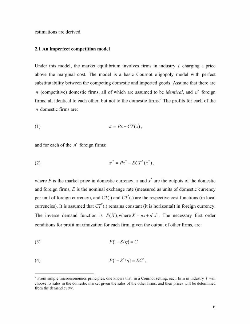
Under this model, the market equilibrium involves firms in industry i charging a price

above the marginal cost. The model is a basic Cournot oligopoly model with perfect

substitutability between the competing domestic and imported goods. Assume that there are

n (competitive) domestic firms, all of which are assumed to be identical, and n∗ foreign

firms, all identical to each other, but not to the domestic firms.7 The profits for each of the

n domestic firms are:

(1) )(xCTPx −=π ,

and for each of the n∗ foreign firms:

(2) )( **** xECTPx −=π ,

where P is the market price in domestic currency, x and x* are the outputs of the domestic

and foreign firms, E is the nominal exchange rate (measured as units of domestic currency

per unit of foreign currency), and CT(.) and CT*(.) are the respective cost functions (in local

currencies). It is assumed that CT*(.) remains constant (it is horizontal) in foreign currency.

The inverse demand function is ( )P X ,where X nx n x∗ ∗= + . The necessary first order

conditions for profit maximization for each firm, given the output of other firms, are:

(3) 1 P S Cη− / =

(4) 1 P S ECη∗ ∗− / = ,

7 From simple microeconomics principles, one knows that, in a Cournot setting, each firm in industry i will choose its sales in the domestic market given the sales of the other firms, and then prices will be determined from the demand curve.

7

where S and S ∗ are the respective market shares of a single domestic and a single foreign

firm and C and C∗ are the respective marginal costs. Notice that a firm’s markup is an

increasing function of its market share. If 1S → , then the solution to the maximization

problem is monopoly. If 0S → , then the solution is that of perfect competition. When the

estimable equation is derived, the markup will be modeled as a function of competitive

pressures in the domestic market and demand pressures in the foreign markets.

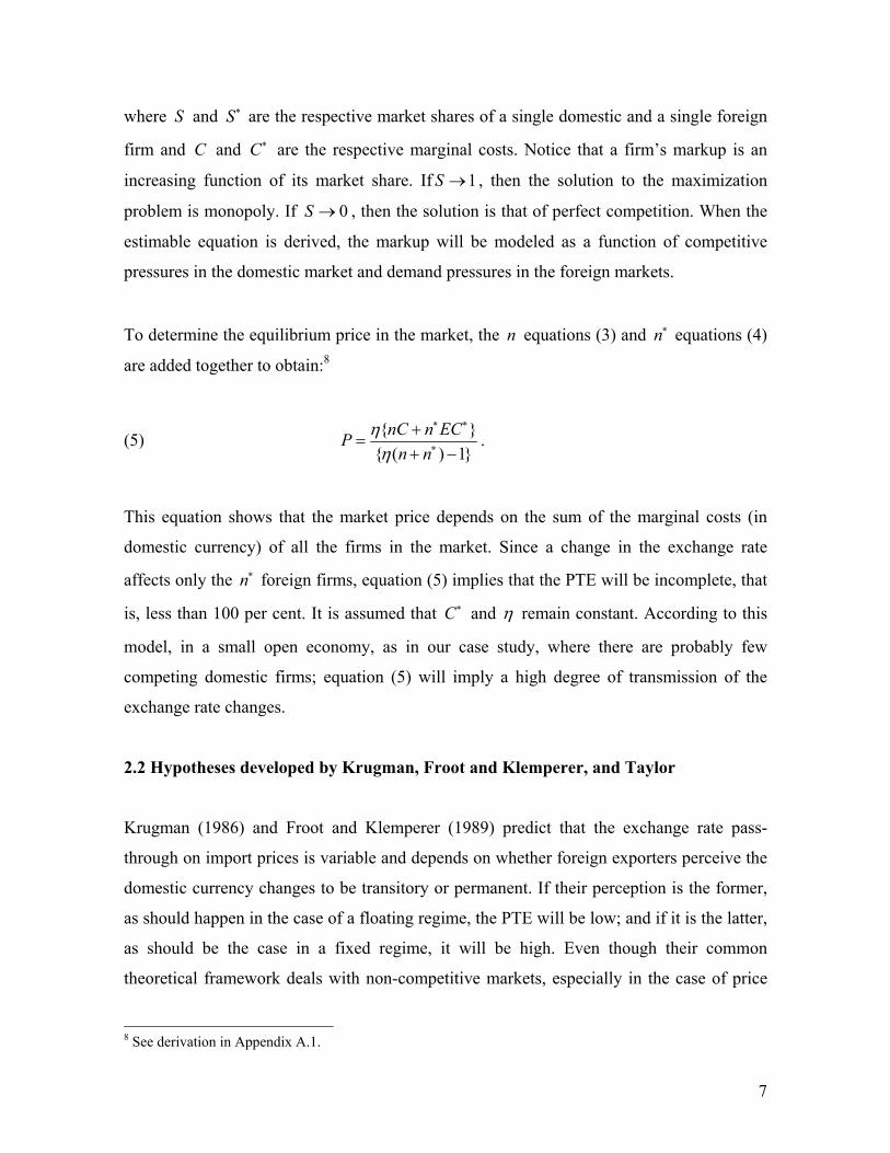
To determine the equilibrium price in the market, the n equations (3) and n∗ equations (4)

are added together to obtain:8

(5) ( ) 1

nC n ECPn n

ηη

∗ ∗

∗

+=

+ −.

This equation shows that the market price depends on the sum of the marginal costs (in

domestic currency) of all the firms in the market. Since a change in the exchange rate

affects only the n∗ foreign firms, equation (5) implies that the PTE will be incomplete, that

is, less than 100 per cent. It is assumed that C∗ and η remain constant. According to this

model, in a small open economy, as in our case study, where there are probably few

competing domestic firms; equation (5) will imply a high degree of transmission of the

exchange rate changes.

2.2 Hypotheses developed by Krugman, Froot and Klemperer, and Taylor

Krugman (1986) and Froot and Klemperer (1989) predict that the exchange rate pass-

through on import prices is variable and depends on whether foreign exporters perceive the

domestic currency changes to be transitory or permanent. If their perception is the former,

as should happen in the case of a floating regime, the PTE will be low; and if it is the latter,

as should be the case in a fixed regime, it will be high. Even though their common

theoretical framework deals with non-competitive markets, especially in the case of price

8 See derivation in Appendix A.1.

8

discrimination behavior, the arguments that support these predictions are however, different

in the case of each author.

Krugman argues that in order to keep (take) the market share from domestic competitors,

the foreign firms selling to the local market absorb (through changes in their markup)

exchange rate depreciations (appreciations), so they are not (are) fully passed-through to

local import prices. Moreover, the more transitory the change in exchange rates is

perceived to be, the smaller and slower the pass-through.

Froot and Klemperer point out that because foreign firms’ future demands will depend on

the exchange rate changes, specifically, on whether exchange rate changes are perceived to

be temporary or permanent, then their current “pricing strategies” will also depend on them.

For example, in the face of a temporary appreciation of the domestic currency, foreign

exporters will reduce their foreign exporter price less in domestic currency than in the

opposite case. The explanation is that the appreciation intertemporally increases the value

of the current profits measured in domestic currency (it shifts profits from tomorrow to

today), so the exporter uses this opportunity to raise markups instead of lowering their

prices fully. If the appreciation is perceived as permanent, such incentives do not appear, so

the pass-through (the reduction in their prices) is higher.

Based on the evidence reported by Cunningham and Haldane (1999), McCarthy (1999), and

Reserve Bank of Australia Bulletin (1999), of a reduction in the pricing-power that firms

have had in many countries, Taylor (2000) postulates that “lower and more stable inflation

is a factor behind the reduction in the degree to which firms ‘pass through’… both price

increases at competing firms and cost increases due to exchange rate movements or other

factors” (Ibid., p. 1390). His point is that, since lower inflation is associated with lower

persistence of inflation, ceteris paribus, firms expect a change in costs and/or prices to be

less persistent making them to set prices for several periods in advance. This will result in a

lower matching of prices and cost increases, and therefore, for our purposes, in a smaller

pass-through to import prices (in domestic currency).

9

2.3 The estimable equation

Studies of the PTE for manufacturing sectors which have been reported in the literature

generally use the mark-up model of price determination we developed in section 2.1.

Certainly, since most modern industries seem to act under that type of market condition, we

use that type of model to set up our estimable equation. Moreover, this type of model may

be particularly suitable for analyzing small open economies, as was discussed above.

We assume i th− industry sets the price of its exports to Colombia ( XP∗ ) at a markup (κ)

over its marginal cost of production (C∗ ):

(6) ** CPX κ= .

The import price in domestic currency ( MP ) is thus given by:

(7) )( ** CEEPP XM κ== .

As in Hooper and Mann (1989), the markup is assumed to be variable and to respond,

among others, to both competitive pressures in the Colombian market and demand

pressures in Colombia and in the foreign markets. Also, as specified by Hooper and Mann,

competitive and demand pressures on the i th− industry in the Colombian market are

captured by the gap between the price (in Colombian currency) of the Colombian industry

that is competing with imports ( CP ) and foreign production costs in domestic currency,

while demand pressure on foreign output is measured by capacity utilization of the foreign

firm ( CU ∗ ). Thus, the markup κ is defined as:

(8) γφκ )/ ** CUECPC= 9.

9 Galí and López-Salido (2000) and Kardasz and Stollery (2001) built microfounded models where a condition like this can be derived.

10

Substituting equation (8) in (7) and then, taking logs and rearranging yields (lowercase

letters denote natural logarithmic values):

(9) **)1()1( cucpep cm γφφφ +−++−= .

The pass-through coefficient is )1( φ− , )10 ≤≤ φ . If 1=φ , the PTE is zero, which means

that the foreign industry sets a domestic import price which is equal to the price of the

Colombian industry that is competing with imports (pricing to the Colombian market) and

changes in exchange rates and foreign costs, keeping cu* unchanged, are absorbed by their

markup and are not passed through. If 0=φ , changes in exchange rates, as well as in

foreign costs, are passed through completely to import prices so that the markup is left

unmodified.

As argued by Hooper and Mann (1989, p. 301-303), models that have the form specified by

equation (9) have some limitations. Fist, they do not consider possible effects of exchange

rates on other determinants of import prices such as c* and cu*. Second, they are static and

the pass-through may change over time because firms may adjust their profits margins in

response to exchange rate changes. Third, they impose the same rate of pass-through on e

and c*, and implicitly, a restriction on the coefficient of pc. Other limitations are: (i.) They

are partial equilibrium models; consequently, they ignore possible endogenous responses of

pc when exchange rate changes. (ii) The pass-through coefficient may be different from one

industry to another, and it may also change over time, for example, because of certain

market asymmetries or changes in the exchange rate regime, or in the commercial, financial

or monetary policy. As was said before, the case of Colombia is critical in this aspect since

it drastically changed its monetary and exchange rate regime during the sample period,

making the exchange rates less predictable, and yielding a low inflation environment.

The first limitation need not be an important one given the fact that data for a small open

economy were used. With respect to the second limitation, a dynamic model that takes into

account the adjustments will be estimated. As for the third one, a version of equation (9)

that relaxes those restrictions is estimated. Concerning the other limitations, a partial error

11

correction model is estimated, where pm and pc are endogenous and e, c*, and cu* are

weakly exogenous variables.10 Then, monthly disaggregated data and a time-varying

parameter estimation technique will be used. These will allow us not only to estimate the

possible changes in the coefficient of pass-trough for different sectors of the manufacturing

industry but also to tests the hypotheses proposed by Krugman (1986), Froot and

Klemperer (1989), and Taylor (2000).

3. The data, their time-series properties, and the econometrics

The data11

Monthly data for the period 1995:01 through 2002:11 (T = 95) were used. Due to

limitations on the availability of data for foreign countries, only data up to 2002:11 and for

the United States, Germany, and Japan (j = 1, 2 3) were used. On average, these countries

represented 50% of the total imports to Colombia during the period (the United States alone

represented 40%).

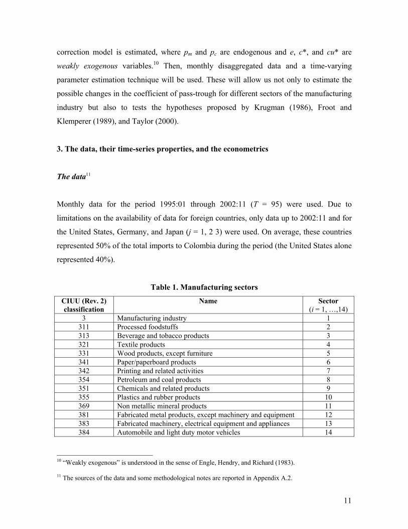
Table 1. Manufacturing sectors

CIUU (Rev. 2) classification

Name Sector (i = 1, …,14)

3 Manufacturing industry 1 311 Processed foodstuffs 2 313 Beverage and tobacco products 3 321 Textile products 4 331 Wood products, except furniture 5 341 Paper/paperboard products 6 342 Printing and related activities 7 354 Petroleum and coal products 8 351 Chemicals and related products 9 355 Plastics and rubber products 10 369 Non metallic mineral products 11 381 Fabricated metal products, except machinery and equipment 12 383 Fabricated machinery, electrical equipment and appliances 13 384 Automobile and light duty motor vehicles 14

10 “Weakly exogenous” is understood in the sense of Engle, Hendry, and Richard (1983). 11 The sources of the data and some methodological notes are reported in Appendix A.2.

12

Table 1 describes the manufacturing sectors which were analyzed. On average these sectors

represented 60% of the total Colombian manufacturing imports for the period.

For sectors i = 2, …, 14, pm represents the respective average wholesale price index for

import products and pc is the respective average wholesale price index for domestic

products. The other variables in equation (9) were built up at each period t as average

indexes weighted by trade as follows:

∑=

=3

1jjj Etwe

where twj is the trade weight corresponding to country j (∑=

=3

11

jjtw ) and Ej is an index of

the average nominal exchange rate between Colombia and country j (domestic

currency/foreign currency);

∑=

=3

1

**

jjj cutwcu ;

∑=

=3

1

**

jjj ctwc

where cj* is the average wholesale price index for exports of country j, which is used as a

proxy for the foreign sector’s marginal costs.

For the manufacturing industry (sector i = 1), all variables, except c*, where re-weighted at

each period t by the re-scaled import weight (mw) for each of the sectors of the Colombian

imports of manufacturer products.

∑=

=14

2imiim pmwp

13

∑=

=14

2iciic pmwp

where ∑=

=14

2

1i

imw . Concerning c*, first, we obtain a weighted average of unit labor costs,

and the cost indexes for raw materials and energy inputs into the manufacturing industry for

all j.12 The average weights used were 0.63 for labor and 0.37 for the other costs (0.70 for

raw materials and 0.30, as in Hooper and Mann, 1989). Second, the weighted average costs

are re-weighted by the respective twj to obtain c*.

The econometrics

With regard to the econometric technique, a partial (or conditional) error correction model

was firstly used, following Johansen (1992) and Harbo et al. (1998), in order to distinguish

the short-run from the long-run effects of the exchange rate changes for each of the i-th

sectors. The model estimated was:

(10) tht

k

hhlt

k

llttt uYZZXY +∆Ψ+∆Γ+∆Γ+Β=∆ −

−

=−

−

=− ∑∑

1

1

1

101'α ,

where Y is a (2x1) vector of the endogenous variables pm and pc; α is a (2xr) vector of the

speed-of error correction parameters; В is a (5xr) vector of the long-run elasticities of

variables pm, pc, e, c*, and cu*, which are included in the cointegration space;13 r is the

cointegrating rank; X is a (5x1) vector of variables, which is decomposed into Y of

dimension 2 and Z of dimension 3: X’ = (Y’, Z’);14 Г0 is a (2x3) matrix of the

contemporaneous short-run elasticities; Гl is a (2x3) matrix of the lagged short-run

elasticities; Ψh is a (2x2) matrix of the lagged short-run elasticities of the endogenous

variables; u is the error term, which is assumed u ~ i.i.d. N2(0,Ω); k is the lag length; and, ∆

12 This seeks to face criticisms on the c* proxies used by the literature, as argued by Goldberg and Knetter (1997). 13 According to the data, the dimension of this space will be enlarged if any constant or trend is present in it. 14 Notice that Z is a vector of the weakly endogenous variables e, c*, and cu*.

14

is the difference operator.

Equation (10) can explicitly keep the lung-run relationship given by (9) without the

imposition of any restriction on the elasticities of the import prices with respect to the any

of the variables in the right-hand side in the long and short run. Call this model a fixed

parameter model (FPM).

Time-series properties of the data

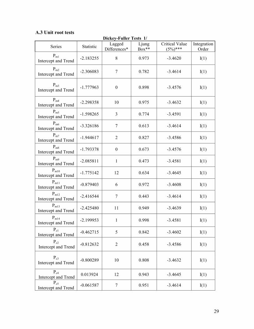
First of all, the statistical properties of the time series are explored. Regarding the

integration order, all series, except one, are I(1) as shown in Appendix A.3. Then,

cointegration a la Johansen on the model (10) was tested for each of the sectors in the

sample.15 As shown in Table 2, in all cases only one cointegration vector was found. Notice

that the coefficients for all vectors are normalized by the coefficient of pm and that all of

them are in the same side of the long.-run equation; thus, they have to be read with the

inverse sign to that expected. In all sectors, most of the estimated long-run elasticities

present the expected (positive) sign. It is worth to say that, a positive (negative) coefficient

for the price of the domestic competing production pc would indicate that imports substitute

(complement) domestic production.

The table also shows that the long-run PTE (elasticity) goes from 0.1 in sector 10 to 0.9 in

sector 8. The hypotheses of cero ( 1=φ ) and complete ( 0=φ ) PTE were carried out. As

reported, no cointegration vector support such hypotheses, which implies that neither

perfect marker behavior nor perfect market competing hypotheses are supported by the

data. What the estimates indicate is that markups are not zero.

15 E-Views 5.0 and CATS were used for the unit root and cointegration tests, respectively. The outputs of specification and misspecification tests, as well as the stability tests and the TVPM estimates are available upon request.

15

Table 2. Cointegration estimates

Sector

Deterministic

component

K

r 1/

Vector 'B 2/ (Order: pm, pc, e, c*, cu*)

1α 3/

Ho: 1=φ

4/

Ho: 0=φ

4/

1 CIMEAN 5 1 (1, -0.5, -0.4, -0.4,0.2) -0.46 (-4.2)

15.2 (0.00)

11.2 (0.02)

2 CIMEAN 6 1 (1,-0.6,-0.6,-1.5,-4.4) -0.25 (-4.4)

15.9 (0.00)

11.6 (0.02)

3 CIMEAN 10 1 (1,-0.4,-0.5,-1.9,-0.1) -0.73 (-5.7)

50.0 (0.00)

66.5 (0.00)

4 CIMEAN 9 1 (1,-0.9,-0.4,-0.5,-0.3) -0.64

(-5.73)46.7

(0.00) 32.9

(0.00)

5 CIMEAN 3 1 (1,-0.5,-0.7,0.2,-0.3) -0.15

(-3.61)15.2

(0.00) 11.1

(0.00)

6 CIDRIFT 1 1 (1,3.8,-0.3,-2.5,-5.6) -0.05

(-5.08)24.0

(0.00) 21.2

(0.00)

7 CIDRIFT 5 1 (1,1.9,-0.6,2.7,0.7) -0.02 (-2.0)

18.6 (0.00)

21.6 (0.00)

8 CIDRIFT 1 1 (1,6.4,-0.9,-3.0,1.5) -0.08 (-5.6)

38.3 (0.00)

37.3 (0.00)

9 DRITF 2 1 (1,-0.3,-0.5,-1.2,-0.3) -0.10 (-4.3)

16.4 (0.00)

17.1 (0.00)

10 CIMEAN 4 1 (1,-0.7,-0.1,-1.7,-0.2) -0.14 (-3.8)

11.5 (0.02)

14.3 (0.01)

11 DRIFT 2 1 (1,-0.4,-0.4,0.01,-1.1) -0.11 (-3.6)

11.3 (0.01)

11.8 (0.01)

12 CIMEAN 6 1 (1,-0.3,-0.6,-0.2,-0.01) -0.20 (-4.6)

16.0 (0.00)

16.1 (0.00)

13 DRIFT 5 1 (1,-0.2,-0.3,1.3,-1.1) -0.11 (-3.4)

13.9 (0.00)

18.1 (0.00)

14 DRIFT 3 1 (1,-0.6,-0.6,2.4,0.3) -0.24 (-4.0)

14.1 (0.00)

9.1 (0.03)

1/ The critical values for the cointegrating rank tests were taken from Harbo, Johansen, Nielsen and Rahbek (1998). 2/ The estimates of the deterministic components are not reported. 3/ Speed of adjustment estimate for the equation of ∆pm (t-test). Centered seasonal dummy variables were included in the VEC system. 4/ LR test, 2

cχ statistics (p-value), where c is the number of constraints.

16

Preliminary results on stability tests in a recursive analysis (Hansen y Johansen, 1993;

Hansen and Juselius, 1995; Hansen and Johansen, 1999) indicated that the long-run

cointegrating relationship in equation (10) was stable for all sectors but the short-run

elasticities were unstable for all of them. This seemed to indicate a structural change, which

had only short-run effects, probably related to the changes in the Colombian foreign

exchange and monetary regimes.

A time varying-parameter procedure

Given the results of the stability tests, a Time Varying-Parameter Model (TVPM) is used to

estimate the short-run pass-trough coefficients for each of the i-th sectors. The equation

estimated is:

(11) +∆+∆+∆+∆+−+=∆ ∑−

=−−−

1

1,1,

*,3,0

*,2,0,1,011,1,0 )~'ˆ(

k

llttltttttttmtttmt ecuceXBpp γγγγαα

t

k

hhctth

k

hhmtth

k

lttl

k

lttl ppcuc υψψγγ +∆+∆+∆+∆ ∑∑∑∑

−

=−

−

=−

−

=

−

=

1

1,2,

1

1,1,

1

1

*,3,

1

1

*,2, ,

where B = (β2, β3, β4, β5)’ and 1~

−tX = (pc, e, c*, cu*)’t-1, and the error term

tυ ~ ),0( 2σNID .16 The numerical subscripts denote an element in the corresponding vector

or matrix. The way the parameters change in time can be expressed compactly as a

multivariate random walk:

(12) ttt v+Θ=Θ −1 , with tv ~ ),0( 2QNID σ ,

where tkkkkkt )...,...,...,...,...,,,,,( 2,12,11,11,13,13,12,12,11,11,13,02,01,010'

−−−−−=Θ ψψψψγγγγγγγγγαα

16 According to the results shown in Table 1, equation (11) is augmented by the respective constant term in the cointegration space or in the data. They are included to capture possible non-observable effects, which change through time and are not capture by the error term.

17

and tv is a [5+5(k-1)] by 1 vector of innovations, which are mutually and serially

uncorrelated with tυ , with a mean of zero and a stationary variance-covariance matrix of

the innovations Q2σ .

Notice that equations (11) and (12) stand for each and every one of the 13 sectors by

individually as well as for the whole manufacturing sector (sector 1).

The process in (12) allows constant and varying parameters, even in a non-stationary

environment. Other structures could be tried, but as usual, the random walk is a useful

initial starting point. Under another framework, such as the multivariate AR(1) with drift,

the number of parameters to be estimated would increase enormously, which is costly in

terms of degrees of freedom.

Equations in (11) and (12) are already in the state-space form with equation (11) being the

state equation and (12) the transition one. This allows us to use the Kalman-filter algorithm

for estimating the state-vector as well as the hyper-parameters (Harvey, 1989) and,

depending on the software (numerical method), for estimating their standard errors.17

4. The estimations of the short-run PTE

The estimation procedure stars allowing Q matrix elements in the equation (12) being

estimated freely, that is, as well as Kim (1990), it is not assumed a diagonal matrix. Thus,

the estimation procedure imposes no restrictions over variances and co-variances into

matrixQ . To initialize the algorithm, 0Θ in equation (12) should be specified, along with

its variance-covariance matrix, which might affect the results since equation (12) is a non-

stationary representation. Here, the OLS estimates from equation (10) on the sample

1995:01 through 1998:01 were used for that purpose. The idea was to use an initial sample

which was neither too small nor too large and a number of complete years. The results

reported below, however, do not change notoriously when one year is added or excluded

17 E-Views 5.0 was used for all the calculations.

18

from the initial sample. This finding is used as support to argue that that non-stationarity

does not affect the results.

The variance-covariance matrix of 0Θ was taken as proportional to V ( VVar µ=Θ )( 0 ),

where V is the variance-covariance matrix of the OLS estimates of Θ using the same

sample. Then, a likelihood maximization procedure (grid search) on µ was followed.

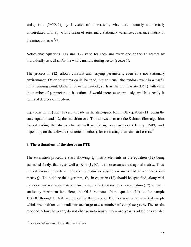
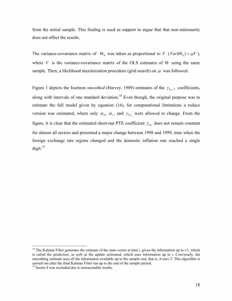
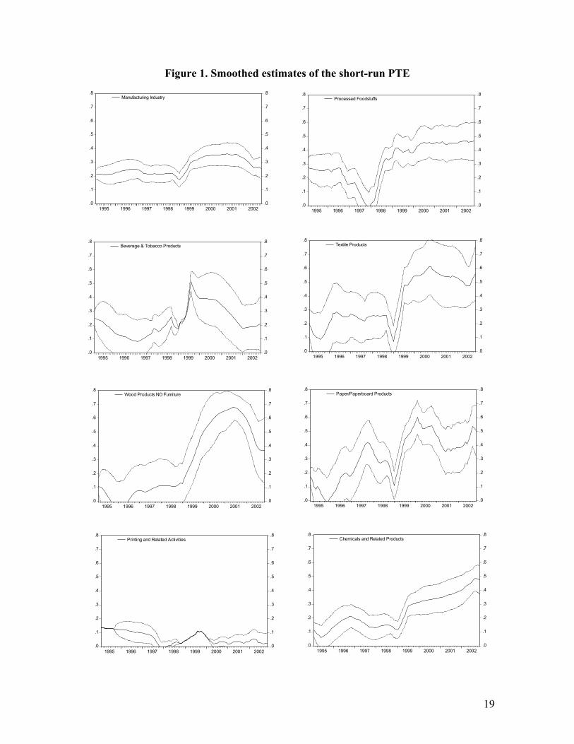
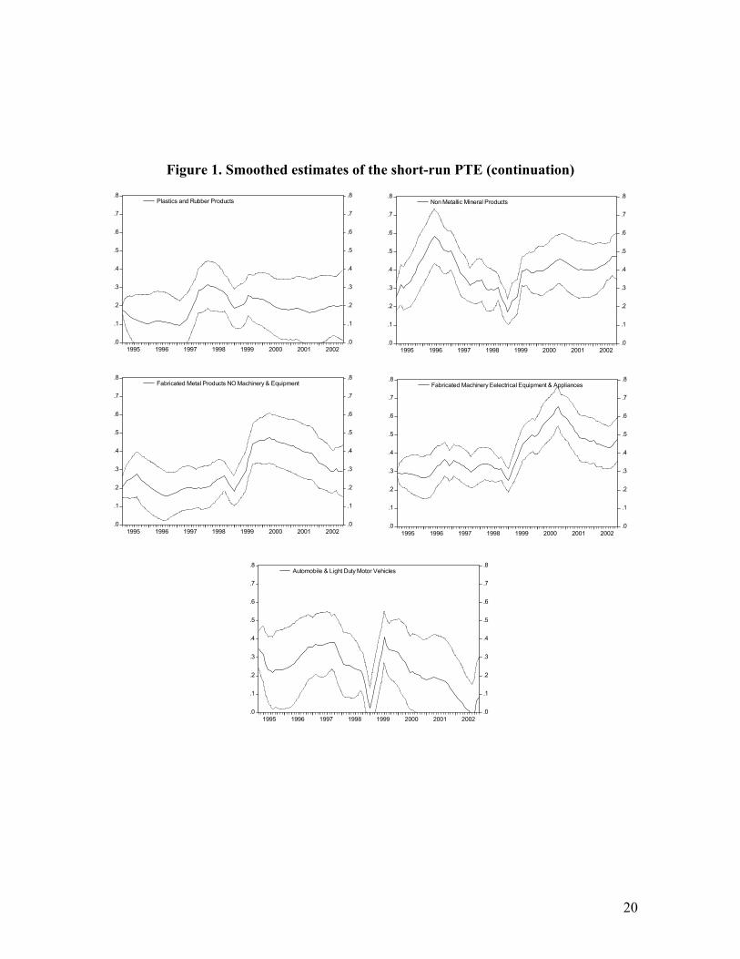
Figure 1 depicts the fourteen smoothed (Harvey, 1989) estimates of the Tt /,0γ coefficients,

along with intervals of one standard deviation.18 Even though, the original purpose was to

estimate the full model given by equation (16), for computational limitations a reduce

version was estimated, where only 0α , 1α , and 1,0γ were allowed to change. From the

figure, it is clear that the estimated short-run PTE coefficient t,0γ does not remain constant

for almost all sectors and presented a major change between 1998 and 1999, time when the

foreign exchange rate regime changed and the domestic inflation rate reached a single

digit.19

18 The Kalman Filter generates the estimate of the state vector at time t, given the information up to t-1, which is called the prediction, as well as the update estimated, which uses information up to t. Conversely, the smoothing estimate uses all the information available up to the sample end, that is, it uses T. This algorithm is carried out after the final Kalman Filter run up to the end of the sample period. 19 Sector 8 was excluded due to unreasonable results.

19

Figure 1. Smoothed estimates of the short-run PTE

.0

.1

.2

.3

.4

.5

.6

.7

.8

.0

.1

.2

.3

.4

.5

.6

.7

.8

1995 1996 1997 1998 1999 2000 2001 2002

Manufacturing Industry

.0

.1

.2

.3

.4

.5

.6

.7

.8

.0

.1

.2

.3

.4

.5

.6

.7

.8

1995 1996 1997 1998 1999 2000 2001 2002

Processed Foodstuffs

.0

.1

.2

.3

.4

.5

.6

.7

.8

.0

.1

.2

.3

.4

.5

.6

.7

.8

1995 1996 1997 1998 1999 2000 2001 2002

Beverage & Tobacco Products

.0

.1

.2

.3

.4

.5

.6

.7

.8

.0

.1

.2

.3

.4

.5

.6

.7

.8

1995 1996 1997 1998 1999 2000 2001 2002

Textile Products

.0

.1

.2

.3

.4

.5

.6

.7

.8

.0

.1

.2

.3

.4

.5

.6

.7

.8

1995 1996 1997 1998 1999 2000 2001 2002

Wood Products NO Furniture

.0

.1

.2

.3

.4

.5

.6

.7

.8

.0

.1

.2

.3

.4

.5

.6

.7

.8

1995 1996 1997 1998 1999 2000 2001 2002

Paper/Paperboard Products

.0

.1

.2

.3

.4

.5

.6

.7

.8

.0

.1

.2

.3

.4

.5

.6

.7

.8

1995 1996 1997 1998 1999 2000 2001 2002

Printing and Related Activities

.0

.1

.2

.3

.4

.5

.6

.7

.8

.0

.1

.2

.3

.4

.5

.6

.7

.8

1995 1996 1997 1998 1999 2000 2001 2002

Chemicals and Related Products

20

Figure 1. Smoothed estimates of the short-run PTE (continuation)

.0

.1

.2

.3

.4

.5

.6

.7

.8

.0

.1

.2

.3

.4

.5

.6

.7

.8

1995 1996 1997 1998 1999 2000 2001 2002

Plastics and Rubber Products

.0

.1

.2

.3

.4

.5

.6

.7

.8

.0

.1

.2

.3

.4

.5

.6

.7

.8

1995 1996 1997 1998 1999 2000 2001 2002

Non Metallic Mineral Products

.0

.1

.2

.3

.4

.5

.6

.7

.8

.0

.1

.2

.3

.4

.5

.6

.7

.8

1995 1996 1997 1998 1999 2000 2001 2002

Fabricated Metal Products NO Machinery & Equipment

.0

.1

.2

.3

.4

.5

.6

.7

.8

.0

.1

.2

.3

.4

.5

.6

.7

.8

1995 1996 1997 1998 1999 2000 2001 2002

Fabricated Machinery Eelectrical Equipment & Appliances

.0

.1

.2

.3

.4

.5

.6

.7

.8

.0

.1

.2

.3

.4

.5

.6

.7

.8

1995 1996 1997 1998 1999 2000 2001 2002

Automobile & Light Duty Motor Vehicles

21

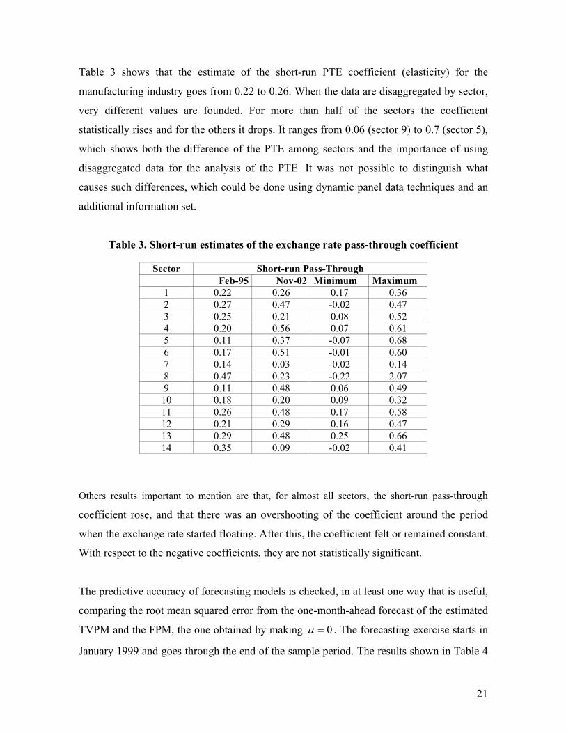
Table 3 shows that the estimate of the short-run PTE coefficient (elasticity) for the

manufacturing industry goes from 0.22 to 0.26. When the data are disaggregated by sector,

very different values are founded. For more than half of the sectors the coefficient

statistically rises and for the others it drops. It ranges from 0.06 (sector 9) to 0.7 (sector 5),

which shows both the difference of the PTE among sectors and the importance of using

disaggregated data for the analysis of the PTE. It was not possible to distinguish what

causes such differences, which could be done using dynamic panel data techniques and an

additional information set.

Table 3. Short-run estimates of the exchange rate pass-through coefficient

Sector Short-run Pass-Through Feb-95 Nov-02 Minimum Maximum

1 0.22 0.26 0.17 0.36 2 0.27 0.47 -0.02 0.47 3 0.25 0.21 0.08 0.52 4 0.20 0.56 0.07 0.61 5 0.11 0.37 -0.07 0.68 6 0.17 0.51 -0.01 0.60 7 0.14 0.03 -0.02 0.14 8 0.47 0.23 -0.22 2.07 9 0.11 0.48 0.06 0.49

10 0.18 0.20 0.09 0.32 11 0.26 0.48 0.17 0.58 12 0.21 0.29 0.16 0.47 13 0.29 0.48 0.25 0.66 14 0.35 0.09 -0.02 0.41

Others results important to mention are that, for almost all sectors, the short-run pass-through

coefficient rose, and that there was an overshooting of the coefficient around the period

when the exchange rate started floating. After this, the coefficient felt or remained constant.

With respect to the negative coefficients, they are not statistically significant.

The predictive accuracy of forecasting models is checked, in at least one way that is useful,

comparing the root mean squared error from the one-month-ahead forecast of the estimated

TVPM and the FPM, the one obtained by making 0=µ . The forecasting exercise starts in

January 1999 and goes through the end of the sample period. The results shown in Table 4

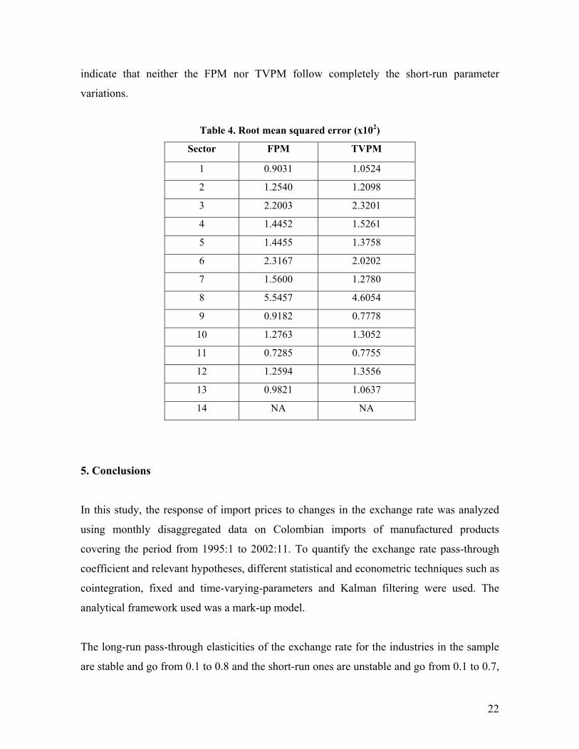
22

indicate that neither the FPM nor TVPM follow completely the short-run parameter

variations.

Table 4. Root mean squared error (x102)

Sector FPM TVPM

1 0.9031 1.0524

2 1.2540 1.2098

3 2.2003 2.3201

4 1.4452 1.5261

5 1.4455 1.3758

6 2.3167 2.0202

7 1.5600 1.2780

8 5.5457 4.6054

9 0.9182 0.7778

10 1.2763 1.3052

11 0.7285 0.7755

12 1.2594 1.3556

13 0.9821 1.0637

14 NA NA

5. Conclusions

In this study, the response of import prices to changes in the exchange rate was analyzed

using monthly disaggregated data on Colombian imports of manufactured products

covering the period from 1995:1 to 2002:11. To quantify the exchange rate pass-through

coefficient and relevant hypotheses, different statistical and econometric techniques such as

cointegration, fixed and time-varying-parameters and Kalman filtering were used. The

analytical framework used was a mark-up model.

The long-run pass-through elasticities of the exchange rate for the industries in the sample

are stable and go from 0.1 to 0.8 and the short-run ones are unstable and go from 0.1 to 0.7,

23

which supports mark-up hypotheses, in contrast to the hypotheses of perfect market

competition and complete pass-through. Both the hypothesis that under a floating regime

there is a low degree of pass-through and the hypothesis that a low inflation environment

has the same result are not supported.

The findings also show evidence of the variability and the different degrees of the pass-

trough among manufacturing sectors, which indicates the importance of using dynamic

models and disaggregated data for the analysis of the pass-through, and, implicitly, the

different nature of the price setting behavior of the different manufacturing sectors. This

paper did not perform a deeper analysis to find an explanation for this.

An additional finding from the short-run estimates is that, under the exchange rate floating

regime, the pass-through coefficient is higher than during the exchange rate bands (a semi-

fixed regime), which go against hypotheses developed and tested by Froot and Klemperer

and Kim. That also does not support the Taylor’s hypothesis, in the sense that, in a low

inflation environment, the pass-through is lower than in other cases.

Some of the main policy implications of our findings for the monetary and exchange rate

policy are: (i) the floating regime, instead of lowering the PTE, appeared to increase it; (ii)

during the floating and inflation targeting regimes there was a structural change on the

short-run pass-trough coefficient and an unexpected pass-though increase; (iii) a time-

varying parameter model is a good alternative for forecasting PTE.

This paper can be extended in several ways. First, explain better the different degrees of the

PTE among industries can be done. Second, study possible asymmetries when exchange

rate is appreciating/depreciating. Third, quantify the different responses of the coefficients

of pass-through in the face of different levels or duration of the appreciation/depreciation of

the importer’s currency.

24

References Baldwin, R. E. (1988). “Hysteresis in Import Prices: The Beachhead Effect,” American

Economic Review, 78, 773-85. Bhagwati, J. (1988). “The Pass-Through Puzzle: The Missing Prince from Hamlet,”

mimeo, Columbia University. Branson, W. (1988). “Comment”, on Exchange rate Pass-Through in the 1980s: The Case of U.S. Imports of Manufacturers’ by P. Hooper and C. Mann, Brookings Papers on Economic Activity, 1, 330-33. Bruno, M. (1978). “Exchange Rates, Import Costs, and Wage-Price Dynamics,” Journal of

Political Economy, 86, 379-403. Burstein, A., M. Echenbaum, and S. Rebelo (2001). “Why are rates of inflation so low after

large contractionary devaluations,” IMF. Cunningham, A., and A. G. Haldane (1999). “The monetary transmission mechanism in the

United Kingdom: Pass-through and policy rules.” Prepared for the Third Annual Conference of the Central Bank of Chile, September.

De Grauwe, P., M. Janssens, and H. Leliaert (1985). “Real-Exchange-Rate Variability from 1920 to 1982,” Princeton Studies in International Finance, 56. Dixit, A. (1989). “Hysteresis, Import Penetration, and Exchange Rate Pass- Through,” Quarterly Journal of Economics, 104, 205-28. Dornbusch, R. (1973). “Devaluation, Money, and Nontraded Goods,” American Economic Review, 5, 871-80. ——————– (1987), “Exchange Rates and Prices,” American Economic Review, 77, 93-105. Engle, R. F., D. Hendry, and J-F. Richard (1983). “Exogeneity,” Econometrica, 51, 277-

304. Feenstra, R. C., and J. D. Kendall (1997). “Pass-Through of Exchange Rates and Purchasing Power Parity,” Journal of International Economics, 43, 237-61. Frenkel, J. A. (1981). “The Collapse of Purchasing Power Parities during the 1970s,” European Economic Review, 16, 145-65. Froot, K., and P. Klemperer (1989). “Exchange Rate Pass-Through when Market Share Matters,” American Economic Review, 79, 637-54. Froot, K., M. Kim, and K. Rogoff (1995). “The Law of One Price over 700 Years,” NBER Working Paper, No. 5132. Galí, J., and D. López-Salido (2001). “A New Phillips Curve for Spain,” BIS Papers, No. 3,

174-203. Goldberg, P., and M. Knetter (1997). “Goods Prices and Exchange Rates: What Have We Learned?,” Journal of Economic Literature, Vol. XXXV, 1243-72. Goldstein, M., and M. Khan (1985). “Income and Price Effects in Foreign Trade,” in R. Jones y P. Kenen (eds.), Handbook of International Economics, Vol. II, 1040- 1105. Gross, D. M. and N. Schmitt (1999). “Exchange Rate Pass-Through and Dynamic

Oligopoly: An Empirical Investigation,” IMF Working Paper, WP/99/47. Hansen, H. y S. Johansen (1993). “Recursive Estimation in Cointegrated Var-models,”

Preprint, No. 1, Institute of Mathematical Statistics, University of Copenhagen. Hansen, H., and K. Juselius (1995). Cats in RATS: Cointegration Analysis of Time Series,

Estima.

25

Hansen, H., and S. Johansen (1999). “Some tests for parameter constancy in cointegrated VAR-models,” Econometrics Journal, Vol. 2, 306-333.

Harbo, I., S. Johansen, B. Nielsen, and A. Rahbek (1998). “Asymptotic Inference on Cointegrating Rank in Partial Systems,” Journal of Business and Economic Statistics, 16, 4, 388-399.

Harvey, Andrew (1989). Forecasting, Structural Time Series and the Kalman Filter, Cambridge Univ. Press.

Holmes, P. M. (1978), Industrial Pricing Behavior and Devaluation, Macmillan, London. Hooper, P. and C. Mann (1989). “Exchange Rate Pass-Through in the 1980s: The case of U.S. Imports of Manufactures,” Brookings Papers on Economic Activity, 1, 297-329. Isard, P. (1977). “How Far Can We Push the Law of One Price?,” American Economic Review, 67, 942-48. ———— (1995). Exchange Rate Economics, Cambridge Surveys of Economic Literature. Johansen, Soren (1992). “Cointegration in partial systems and efficiency of single-equation

analysis,” Journal of Econometrics, 52, 389-402. Kardasz, S., and K. Stollery (2001). “Exchange rate pass-through and its determinants in

Canadian manufacturing industries,” Canadian Journal of Economics, Vol. 34, 719-738.

Kasa, K. (1992). “Adjustment Costs and Pricing to Market: Theory and Evidence,” Journal of International Economics, 32, 1-30. Kim, Y. (1990). “Exchange Rates and Import Prices in the United States: A Varying- Parameter Estimation of Exchange-Rate Pass-Through,” Journal of Business and Statistics, 8, 3, 305-315. Krugman, P. (1986). “Pricing to Market When the Exchange Rate Changes,” NBER Working Paper, 1926. Krugman, P. y R. Baldwin (1987). “The Persistence pf the U.S. Trade Deficit”, Brookings Papers on Economic Activity, 1, 1-43. MacDonald, R. y M. P. Taylor (1992). “Exchange Rate Economics: A Survey”, IMF Staff Papers, 39, 1-57. McCarthy, J. (1999). “Pass-Through of Exchange Rates and Import Prices to Domestic

Inflation in Some Industrialized Countries,” Federal Reserve Bank of New York. Menon, J. (1993). “Exchange Rate Pass-Through Elasticities for the MONASH Model: A

Disaggregate Analysis of Australian Manufactured Imports,” Working Paper No. OP-76, CPSIP.

————– (1995). “Exchange Rate Pass-Through”, Journal of Economic Surveys, 9, 197-231. ————– (1996). “The Degree and Determinants of Exchange Rate Pass-Through: Market Structure, Non-Tariff Barriers and Multinational Corporations,” The Economic Journal, 106, 434-44. Mesa, F., L. Salguero and F. Sánchez (1998). “Efectos de la Tasa de Cambio Real sobre la

Inversión Industrial en un Modelo de Transferencia de Precios (Pass Through),” Revista de Economía del Rosario, 1, 111-43.

Mirus, R. and B. Yeung (1987). “The Relevance of the Invoicing Currency in Intra-firm Trade Transactions,” Journal of International Money and Finance, 6, 449-64. Richardson, D. (1978). “Some Empirical Evidence on Commodity Arbitrage and the

26

Law of one Price,” Journal of International Economics, 8, 341-51. Rincón, H. (1999). “Testing the Short-and-Long-Run Exchange Rate Effects on Trade Balance: The Case of Colombia,” Ensayos Sobre Política Económica, 35, Banco de la República, Colombia. —————— (2000). “Devaluación y Precios Agregados en Colombia, 1980-1998,” Desarrollo y Sociedad, 46, CEDE, Unversidad de los Andes, Colombia. Rosas, Efraín (2004). “El pass-through del tipo de cambio en Colombia: un análisis

sectorial,” tesis de maestría en economía de la Universidad de los Andes, enero. Rowland, Peter (2003). “Exchange Rate Pass-Trhoug to Domestic Prices: The Case of

Colombia,” Borradores de Economía, 254, Banco de la República. Steel, Douglas and Alan King (2004). “Exchange Rate Pass-through: The Role of Regime

Changes,” International Review of Applied Economics, Vol. 18, No. 3, 301-322. Takagi, S. and Y. Yoshida (1999). “Exchange Rate Movements and Tradable Goods Prices in East Asia: An Analysis Based on Japanese Customs Data, 1988-98,” IMF Working Paper, WP/99/31. Taylor, John B. (2000). “Low inflation, pass-through, and the pricing power of firms,”

European Economic Review, 44, 1389-1408. Venables, A. J. (1990). “Microeconomic Implications of Exchange Rate Variations,”

Oxford Review of Economic Policy, 6, 18-27.

27

Appendixes A.1 Derivation of equation (5): To determine the market equilibrium price, the n equations (3) and n∗ equations (4) are added up: nCSnP =− /1 η and

**** /1 ECnSPn =− η , then 0/1/1 **** =−−+−− ECnSPnnCSnP ηη . Solving for P, using the fact 1nS n S∗ ∗+ = , yields equation (5). A.2 Sources of the data and methodological notes Colombia: Import prices (“import whole price index”) and domestic competing prices (“produced and consumed whole price index”): Subgerencia de Estudios Económicos, Banco de la República; imports: customs data from the Dirección de Impuestos y Aduanas Nacionales (DIAN); exchange rates: CD Rom of the IFS, FMI (time series “233..RF.ZF…”). Germany: Capacity utilization (“Capacity utilization of manufactured (quartely)”): Federal Statistic Office Germany (www.destatis.de). The monthly data were obtained letting constant two months and then, using an MA(4) filter; export prices (“export price index”): Deutsche Bundesbank (www.bundesbak.de) and University of Munich’s Center for Economic Studies (CES) and the Ifo Institute for Economic Research (www.cesifo.de); exchange rates: CD Rom of the IFS, FMI (time series “134..RF.ZF…” for data from 1995 to 19989 and “163..RF.ZF…” from 1999 to 2002); and, costs and their weights: Input-Output Accounts 2000, Federal Statistic Office Germany (www.destatis.de). Since the unit labor cost index was not available in a monthly frequency, we calculate it as the ratio of the manufacturing wage index (“Wages and Salaries per Employee”) and the manufacturing labor productivity index. This is estimated as the ratio of the manufacturing production index (“Output Industry”) and the manufacturing employment (“Persons in employment (Mining and MFG sectors)”). The source for these series is Bundesbank-Time Series Database. The estimated unit labor cost series was seasonally adjusted using a filter from RATS. Japon: Capacity utilization: Ministry of Economy, Trade and Industry (www.meti.go.jp/English/statistics/data); export and whole price indexes (“export price index” and “domestic whole price index”): Bank of Japon (www2.boj.jp); exchange rates: CD Rom of the IFS, FMI (time series “158..RF.ZF…”). Data of capacity utilization were not found for the homologous Japanese industries 311, 313, 331, and 342. Then, 311 and 331 were replaced by “Other manufacturing”; 313 by “Manufacturing (exc. machinery industry)”; and 342 by “pulp, paper and paper products.” Also, the export price index for industries 321, 331, and 354 were not available. They were replaced by the respective whole price indexes; and, costs and their weights: Input-Output Accounts 2000, Ministry of International Affairs and Communications (Statistics Bureau). Since the unit labor cost index was not available in a monthly frequency, we calculate it as explained above. The names of the series used are, respectively, “Wages MFG”, “Production index”, “Employment (MFG)”. The sources for these series are Statistics Bureau-Labor Force Survey and Ministry of Economy, Trade and Industry. All the cost series, except raw materials, were seasonally adjusted.

28

United States: Capacity utilization: Economic Time Series Page (www.economagic.com); export and whole price indexes (“export price index” and “domestic whole price index”): Bureau of Labor Statistics (www.bls.gov); exchange rates: CD Rom of the IFS, FMI (time series “111..RF.ZF…”); and, costs and their weights: Input-Output Accounts 2003, Bureau of Economic Analysis. Since the unit labor cost index was not available in a monthly frequency, we calculate it as explained above. The names of the series used are, respectively, “Average Weekly Earnings of Production Workers”, “Industrial Production Index”, and “Employment”. The sources for these series are BLS-Employment Statistics Survey and Federal Reserve-Statistical Release. All the cost series, except raw materials, were seasonally adjusted.

29

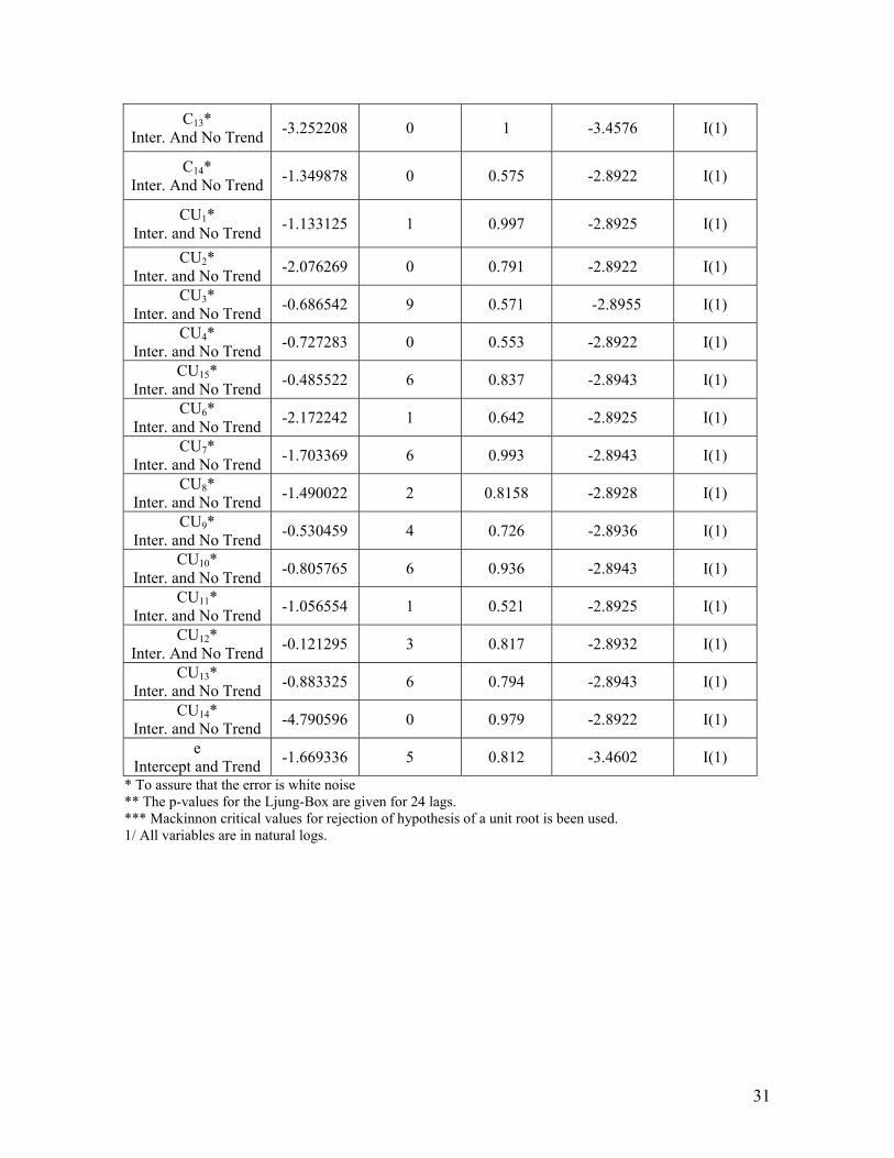
A.3 Unit root tests Dickey-Fuller Tests 1/

Series Statistic Lagged Differences*

Ljung Box**

Critical Value (5%)***

Integration Order

Pm1 Intercept and Trend -2.183255 8 0.973 -3.4620 I(1)














Pc1 Intercept and Trend -0.462715 5 0.842 -3.4602 I(1)



Pc4 Intercept and Trend 0.013924 12 0.943 -3.4645 I(1)


30










C1* Inter. and No Trend -2.293296 6 0.418 -2.8943 I(1)


C3* Inter. And No Trend -2.618568 2 0.988 -2.8928 I(1)









C12* Inter. And Trend -3.447928 0 0.997 -3.4576 I(1)

31

C13* Inter. And No Trend -3.252208 0 1 -3.4576 I(1)


CU1* Inter. and No Trend -1.133125 1 0.997 -2.8925 I(1)











CU12* Inter. And No Trend -0.121295 3 0.817 -2.8932 I(1)



e Intercept and Trend -1.669336 5 0.812 -3.4602 I(1)

* To assure that the error is white noise ** The p-values for the Ljung-Box are given for 24 lags. *** Mackinnon critical values for rejection of hypothesis of a unit root is been used. 1/ All variables are in natural logs.

Exchange Rate Pass-Through Effects: A Disaggregate Analysis of Colombian Imports of Manufactured...

Documents

Transcript of Exchange Rate Pass-Through Effects: A Disaggregate Analysis of Colombian Imports of Manufactured...