Economic Impact of Port Activity: A Disaggregate Analysis - The Case of Antwerp

© The Pakistan Development Review
52:4 Part I (Winter 2013) pp. 493–516
Disaggregate Energy Consumption,
Agricultural Output and Economic
Growth in Pakistan
MUHAMMAD ZAHIR FARIDI and GHULAM MURTAZA*
1. INTRODUCTION
The performance of an economy is generally measured by sustained rise in GDP
growth over the period of time. The economic growth is the major goal of
macroeconomics. According to neo-classical growth theory, the core factors of growth
are labour and capital. In addition to these factors; technological progress, human capital
development etc. are the most efficient factors of production. Development of technology
and use of mechanisation in production process require energy at massive scale. So,
energy has become a crucial factor of economic growth indirectly.
Energy is widely regarded as a propelling force behind any economic activity and
indeed plays a vital role in enhancing production. Therefore, highly important resources
of energy will enhance the technology impact manifold. Quality energy resources can act
as facilitator of technology while less worthy resources can dampen the power of new
technology. Ojinnaka (1998) argued that the consumption of energy tracks with the
national product. Hence, the scale of energy consumption per capita is an important
indicator of economic modernisation. In general countries that have higher per capita
energy consumption are more developed than those with low level of consumption.
The importance of energy lies in other aspect of development—increase in foreign
earnings when energy products are exported, transfer of technology in the process of
exploration, production and marketing; increase in employment in energy industries;
improvement of workers welfare through increase in worker’s salary and wages,
improvement in infrastructure and socio-economic activities in the process of energy
resource exploitation. Thus in the quest for optimal development and efficient
management of available energy resources, equitable allocation and efficient utilisation
can put the economy on the part of sustainable growth and development. Arising from
this argument, adequate supply of energy thus becomes central to the radical
transformation of the nation’s economy.
Muhammad Zahir Faridi, PhD <[email protected]> is Assistant Professor at Bahauddin Zakariya
University, Multan, Pakistan. Ghulam Murtaza <[email protected], [email protected]> is
Visiting Lecturer at Bahauddin Zakariya University, Multan, Pakistan.
Authors’ Note: The authors gratefully acknowledge the comments and suggestions received from
Mahmood Khalid, PIDE at the 29th AGM and Conference, PSDE.

494 Faridi and Murtaza
The main objective of the study is to investigate the effect of disaggregate energy
consumption on agricultural output and generally overall growth in Pakistan. Because
agriculture is the mainstay of Pakistan economy and is basic production sector. The
manufacturing sector, services sector and even communication sector have secondary
position albeit their growth rates are higher in absolute terms. The growth rate of
agricultural sector is very low. When structural changes have occurred, the process of
mechanisation has taken place in the agricultural sector. The use of energy has increased
for running the machinery like tubewells, tractors, threshers etc. Due to shortfall of
energy, the output of agricultural sector has dropped.
One of the interesting features of the study is that it differentiates short run and the
long run effect because it has been observed that impact of energy consumption varies
from short to long run for the same country. For this purpose, we have employed ARDL
modelling to co-integration to find out long run and short run effect. Unit root problem of
the data is handled by ADF test. The rest of the article is structured as follows. Trends
and structure of energy variables are given in Section 2. Section 3 provides literature
review in detail while data and methodology are given in Section 4. Empirical results and
their discussion are presented in Section 5. At the end, some policy implications for
energy consumption are suggested on the basis of empirical results.
2. TRENDS AND SIZE OF PAKISTAN ANNUAL ENERGY CONSUMPTION
Total energy consumption measured in oil consumption is 38.8 million tonnes in
the year of 2010-11. Currently gas consumption is the leading one in total energy
consumptions that is 43.2 percent of total energy consumption. Since 2005-06, Gas,
electricity and coal consumption are equally utilised. Oil consumption stood at second
position regarding usage as its usage is 29 percent of total energy consumption.
We present the trends of energy consumption at disaggregate level in Pakistan
over the last decade. The Figure 1 explains the trends of annual gas consumption. While,
Figure 2 and Figure 3 provide the trends of annual electricity consumption and annual oil
consumption respectively.
Fig. 1. Annual Gas Consumption in Pakistan
0
200,000
400,000
600,000
800,000
1,000,000
1,200,000
1,400,000
2001 2002 2003 2004 2005 2006 2007 2008 2009 2010 2011
Gas (mmcft)
Gas…

Disaggregate Energy Consumption, Agricultural Output and Economic Growth 495
Gas consumption share is equal to four percent of total energy consumption
during 2005-06 to 20010-11. This is because of the substitution of gas for expensive
energy sources. The consumption of oil in Pakistan decreased by three percent during
the period 2001-2011 because of high prices of oil in the international market. Since the
year 2001-02, a decreasing trend is observed in the consumption of petroleum products.
Fig. 2. Annual Electricity Consumption in Pakistan
Source: Pakistan Economic Survey (Various Issues).
Yet it is observed that there has been an increase in oil consumption from 2004-
10, the overall average increase for last ten years stood at 11 percent per annum. Trends
indicate that due to high volatility in the oil prices consumption intensity is shifting from
oil consumption to some others sources of energy consumption. Figure 2 indicates that
the trend of annual electricity consumption (in Giga Watt Hour) over the last ten years
i.e., 2001-2011. Trends show that electricity consumption increased continuously till
2007 and then fell. But after the year 2010, there is sharp decline in electricity
consumption. Thus, Gas, electricity and oil consumption trends indicate an annual
increase at an average rate of 5.1 percent, 4.8 percent and 7.7 percent respectively.
Fig. 3. Annual Oil Consumption in Pakistan
Source: Pakistan Economic Survey (Various Issues).
0
20,000
40,000
60,000
80,000
100,000
2001 2002 2003 2004 2005 2006 2007 2008 2009 2010 2011
Electricity (Gwh)
Electricity…
0
2,000
4,000
6,000
8,000
10,000
12,000
2001 2002 2003 2004 2005 2006 2007 2008 2009 2010 2011
OIL Tonnes(Millions)
OIL…

496 Faridi and Murtaza
3. LITERATURE REVIEW
Theoretically, neo-classical and endogenous theories both suggest that energy use
and efficiency are drivers of economic growth. Though there are many studies that find a
direct relationship between productivity and energy consumption in the industrialised
world [see Worrell, et al. (2001)], evidence from the developing world remains
inconclusive. Few disaggregated studies have been conducted on this issue and the
studies using data aggregated at the national or economic level indicate mixed findings.
Further complicating the relationship is the extent to which economic growth and energy
consumption can theoretically be decoupled, a question raised by ecological economists
who argue thermodynamic laws limit such division. Below is a brief review of the
various theories on the relationship between energy consumption, energy efficiency and
economic growth, followed by a summary of a select list of empirical studies.
By incorporating energy end-use efficiency gains into a Cobb-Douglas production
function, Wei (2007) theorizes about short-term and long-term effects of increased
energy efficiency beginning with the production function specification as output is a
function of labour, capital and some measures of energy consumption. In the short term,
energy use efficiency is found to lower the cost of non-energy goods and increase the
output of non-energy goods. A 100 percent rebound effect is evident such that in the short
term, energy efficiency gains have no effect on absolute energy use. In the long term, the
impact on non-energy output of energy end use efficiency is positive. The long term
impact of energy use efficiency on total energy use is lower than the short-term impact.
Wei also finds that energy use efficiency will increase real energy price in the long term.
Van Zon and Yetkiner (2003) modify the Romer model to include energy consumption of
intermediates and to make them heterogeneous due to endogenous energy-saving
technical change. They found out that energy-saving technical transformation can
enhance economic growth. On the other hand, it may dampen economic growth with the
increase in energy prices that imply that rising real energy prices consistently will cause
to harm economic growth.
Embodied technical change includes improvements in energy efficiency, thus
positively linking improvements in energy efficiency to economic growth. They conclude
that in an environment of rising energy prices, recycling energy tax proceeds in the form
of R&D is necessary for both energy efficiency growth and output growth. Sorrell (2009)
pointed out that conventional and ecological economists have conflict on the issue of
energy effects on economic growth. The growth models presented by Neo-classical and
new Endogenous growth theories give little importance to energy consumption as a
major factor of production by giving argument that it has a small share in total cost of
production. Ecological economist contests their point of view by replying that over the
last two centuries, energy inputs are accelerating economic growth at valuable rate.
For a steady economic growth the role of technological change is of great
importance as earlier growth models have integrated technological change as an
important factor for growth [Solow (1956)]. Energy and raw material besides labour and
capital cause to decrease the statistical residual. Onakoya, et al. (2013) studied the
relationship between energy consumption and Nigerian economic growth during the
period of 1975 to 2010 to find out energy consumption as an important variable for
production. Co-integration results provided evidence of a long run relationship between
Disaggregate Energy Consumption, Agricultural Output and Economic Growth 497
energy consumption and economic growth which was positive. Same results were also
found by Paul and Bhattacharya (2004) who employed Engle–Granger technique to
investigate the direction of relationship between economic growth and energy
consumption for India for the period of 1950-1996. Results revealed that energy
consumption has causality for energy consumption. Hondroyiannis, et al. (2002)
followed the same results in case of Greece by using vector error-correction estimation
on the data from 1960-1996. The findings of the study indicate the existence of long run
relationship.
Oh and Lee (2004) did not find the significant and positive effect of energy
consumption on growth in case of Korea. For Bangladesh, Mozumder and Marathe
(2007) examined a positive relationship between per capita income and per capita energy
consumption. The relationship between gas consumption and growth was analysed by
Apergis and Payne (2010) to reveal the co-integration among labour, capital, gas
consumption and economic growth. ECM model was employed to find the bidirectional
causality between gas consumption and economic growth but Yang (2000) opposed this
relationship as his study show the absence of long run relationship between natural gas
consumption and real GDP. Same results of no relationship are also found out by Aqeel
and Butt (2001).
Shahbaz and Feridun (2011) investigated the impact of electricity consumption on
economic growth in Pakistan between 1971 and 2008 by using ARDL technique to
identify the long run relationship between electricity consumption and economic growth.
Study gives the evidence of long run relationship between electricity consumption and
economic growth but inverse is not true. Alam and Butt (2001) investigation provided the
evidence that structural changes also cause to change the share of various energy
consumption variables. And increase in energy is because of increase in economic
activity as well as structural changes.
Javid, et al. (2013) argued that shocks to electricity supply will have a negative
impact on economic growth. Nwosa and Akinbobola (2012) and Dantama, et al. (2011)
come to a conclusion that govt. should adopt sector specific energy policies rather the one
fit-for-all policy by observing positive aggregate energy consumption and sectoral output.
For Pakistan, Kakar and Khilji (2011) explored the nature of relationship between
economic growth and total energy consumption for the period 1980-2009 by using
Johansen Co- integration and confirmed that energy consumption is essential for
economic growth and any energy shock may affect the long-run economic development
of Pakistan. Ahmad, et al. (2013) analysed the impact of energy consumption and
economic growth in case of Pakistan employing data from 1975 to 2009. The results of
ordinary least squares test show positive relation between GDP and energy consumption
in Pakistan.
A number of reviews of prior work compel us to make a healthy endeavour on the
concerned issues because a little attention has been given to agricultural sector regarding
energy consumption relationship. We have observed in the literature review most of the
studies are emphasising on the relationship between overall growth and energy,
manufacturing sector growth and energy. A few studies discuss the agricultural sector
growth and energy. But the present study removes a number of imperfections of previous
studies such as use of energy consumption and its relationship with overall economic

498 Faridi and Murtaza
growth instead of growth in agricultural sector at the disaggregate level. We have used
fresh data on certain variables. An appropriate technique for co-integration, model
specification and proper estimation technique is employed.
4. DATA AND METHODOLOGY
The present segment consists of data and methodology used to estimate effects of
disaggregates energy consumption on economic growth and Agricultural output in
Pakistan. To order to analyse relationships, secondary data from year 1972-2011 are
employed and Auto Regressive Distributed Lags (ARDL) technique has been used.
(a) Data Source
The data generated from Pakistan Economic Survey (various issues), Handbook of
Statistics of Pakistan Economy. While, data on variables of energy consumption, have
been obtained from HDIP, Ministry of Petroleum and Natural Resources. The variables
about which data are collected, are RGDP (Gross Domestic Product) that is used as
dependent variable while RGFCF (Real Gross Fixed Capital Formation), TELF (Total
Employed Labour Force), IR (Inflation Rate), TOC (Total Oil Consumption), TGC (Total
Gas Consumption), TEC (Total Electricity Consumption), AGRI (Agricultural Output),
TELF (Total Employed Labour Force), RAGFCF (Real Agricultural Gross Fixed Capital
Formation), TOC (Total Oil Consumption), TGC (Total Gas Consumption), TEC (Total
Electricity Consumption), ACRDT (Agricultural Credit).
(b) Methodological Issues
The study is based on time series data. In order to examine the properties of the
time series data, we first examine the stationarity of data and then decide about the
appropriate technique.
(i) Stationarity of Data
In practice, ADF test is used to check the stationary of variables to see if all
the variables are integrated of degree one. In this case, the variables can be estimated
by employing error correction model because of co-integrated series. However, if all
the variables are not integrated of same degree i.e. some variables are integrated at I
(1) or some are at I (0) or both I(1) and I(0) then ARDL modeling approach will be
employed to identify the existence of long run and short run relationships among the
variables.
(ii) Auto Regressive Distributed Lag Approach to Co-integration
ARDL approach will be applied only on single equation. It will estimate the long
run and short run parameters of model simultaneously. The estimated model obtained
from the ARDL technique will be unbiased and efficient. ARDL approach to co-
integration is useful for small sample Narayan (2004). Engel-Granger and Johensan
technique are not reliable for small samples. ARDL gives better results in sample rather
than Johesan co-integration approach. ARDL approach has a drawback because it is not
necessary that all variables are of same order. The variables can be at I(0) or I(1) or

Disaggregate Energy Consumption, Agricultural Output and Economic Growth 499
combination of both, the ARDL approach can be applied. If the variables are stationary at
higher order of I(1) then ARDL is not applicable. ARDL approach consists of two stages.
First, the long run relationship between variables is tested using F-statistics to determine
the significance of the lagged levels variables. Second, the coefficient of the long run and
short run relationship will be examined.
(iii) Bound Testing Procedure
The bound test is based on three basic assumptions that are; first, use ARDL model
after identifying the order of integration of series Pesaran, et al. (2001). Second, series
are not bound to possess the same order of integration i.e., the regressors can be at I(0) or
I(1). Third, this technique estimates better results in case of small sample size. The vector
auto regression (VAR) of order p, for the economic growth function can be narrated as
Pesaran, et al. (2001);
1
p
t i t i t
i
Z z
... ... ... ... ... ... (1)
Where xt and yt are included in vector zt. Economic growth (RGDP) and agricultural
output (AGRI) are indicated by yt and xt is the vector matrix which represents a set of
explanatory variables such as [Xt = RGFCF, TELF, TOC, TEC, TGC, IR] and [Xt =
TELF, RGFCF, TOC, TGC, TEC, ACRDT] for Model-1 and Model-2 and t denotes time
indicator. Vector error correction model (VECM) is given as below:
1
1
1 1
p i p
t t t t i t t i t
i i
z t z y x
... ... ... (2)
where is the first-difference operator. The long-run multiplier matrix as:
YY YX
XY XX
The diagonal elements of the matrix are unrestricted, so the selected series can be
either I(0) or I(1). If 0,YY then Y is I(1). In contrast, if 0,YY then Y is I(0).
The VECM procedures described above are imperative in the testing of at most
one co-integrating vector between dependent variable yt and a set of regressors xt. To
build up the model, study uses Pesaran, et al. (2001) postulation of Case V, that is,
unrestricted intercepts and trends.
(c) Description of the Variables
In the present analysis, we have used the variables like employed labour force and
real gross fixed capital formation as theoretical variables for growth and there are three
core variables relating to energy. Two variables are used as control factors. The
explanation and hypothetical relation of these variables are given below.
500 Faridi and Murtaza
Real Gross Domestic Product (RGDP)
Real gross domestic product at factor cost is used as proxy for economic growth. It
is assumed as GDP expands over the period of time, the economy will grow. RGDP is
measured in millions rupees.
Agricultural Output (AGRI)
In order to measure the performance of agricultural sector, we have used
agricultural output measured at current market prices in million rupees.
Real Gross Fixed Capital Formation (RGFCF)
We have considered real gross fixed capital formation as a proxy for capital in the
present study. It is measured at market prices in million rupees.
Total Employed Labour Force (TELF)
Labour is used as a core variable in economic growth model. It is expected that
labour contributes positively to economic growth. The present study uses total employed
labour force as a proxy for labour. Total employed labour force is measured in millions
peoples.
Total Oil Consumption (TOC)
Total oil consumption is measured in thousands of tonnes per year. It is expected
that oil consumption has positive relationship with growth.
Total Gas Consumption (TGC)
It is expected that the utilisation of gas consumption cause to increase the GDP
growth positively. We have used total gas consumption in million cubic feet (mmcft).
Total Electricity Consumption (TEC)
Use of electricity in production process is an important factor. Due to shortage of
electricity it is expected that total electricity consumption is contributing negatively to
GDP growth as well as to agriculture output. The total electricity consumption per
Annam is measured in Giga Watt hour (GWh) or (106 Kilo Watt hour).
Agricultural Credit (ACRDT)
Agricultural credit is used as a central variable in the present analysis. The
expected impact of agricultural credit on output is positive. Agricultural credit is
measured in million rupees.
Inflation Rate (IR)
In order to examine the effect of general price level on economic growth, we have
used consumer price index as a proxy for inflation rate. The inflation rate has negative
impact on economic growth because cost of the production increases, output falls and
growth is retarded.
Disaggregate Energy Consumption, Agricultural Output and Economic Growth 501
(d) Model Specification
The current study is based on general Neo-classical Production Function;
Y = A f (L, K) ... ... ... ... ... ... ... (3)
Where, Y = Total output, L = Total employed labour force, K= Total stock of capital,
A= Total productivity factor.
We have employed extended neo-classical growth model by incorporating energy
as a productivity factor as an endogenous variable.
A = f (TOC, TGC, TEC) ... ... ... ... ... ... (4)
Substituting A in Equation (i), we obtained extended growth model.
Y = f (L , K , TOC , TGC , TEC ) ... ... ... ... ... (5)
Based on the suggested economic techniques, we have two specified model. These
specified models are given below.
Model-1. Impact of Disaggregate Energy Consumption on Economic Growth
0 1 - 2 - 3 - 4 -
0 0 0 0
5 - 7 - 8 -1 9 -1 6 -
0 0 1
( ) ( ) ( ) ( ) ( )
( ) ( ) ( ) ( ) ( )
a b c d
t i t i i t i i t i i t i
i i i i
g fe
i t i i t i t t i t i
i i i
RGDP RGFCF TELF TOC TGC
TEC IR RGDP RGFCF RGDP
10 -1 11 -1 12 -1 13 -1 14 -1( ) ( ) ( ) ( ) ( ) tt t t t tTELF TOC TGC TGC IR u … (6)
Where, is the first-difference operator while Ut is a white-noise disturbance term. This
model would estimate the impact of disaggregate energy consumption on economic
growth in which real GDP is used as dependant variable while real gross fixed capital
formation (proxy for capital), total employed labour force, total oil consumption, total
gas consumption an total electricity consumption are used as independent variables.
Equation (6) also can be viewed as an ARDL of order (a, b, c, d, e, f, g). Equation
(6) indicates that economic growth tends to be influenced and explained by its past
values. The structural lags are established by using minimum Schwarz Information
Criteria (SIC). In our model, we will use the lagged value of first difference dependent
variable and independent variables for short run and first lagged values of dependent and
independent variables for long run. So, this model is consisted of both long run and short
run coefficients of variables as well. Where β1, β2, β3, β4, β5 and β6, β7 are the short
run coefficients of variables and β8, β9, β10, β11, β12 and β13, β14 are the long run
coefficients of variables and β0 is the intercept term.
Model-2. Impact of Disaggregate Energy Consumption on Agricultural Output
The second model would capture the effect of energy consumption on agricultural
output in Pakistan with the help of some explanatory variables like TELF (Total
Employed Labour Force), RGFCF (Real Gross Fixed Capital Formation), TOC (Total Oil
Consumption), TGC (Total Gas Consumption), TEC (Total Electricity Consumption),
ACRDT (Agricultural Credit); the unrestricted ECM model for Agricultural output is as
under;
502 Faridi and Murtaza
0 1 - 2 - 3 - 4 -
1 0 0 0
5 - 6 - 7 - 1 -1 2 -1
0 0 1
( ) ( ) ( ) ( )
( ) ( ) ( ) ( ) ( )
p q r s
t i t i i t i i t i i t i
i i i i
t u v
i t i i t i i t i t t
i i i
AGRI TELF RGFCF TEC TGC
TOC ACRDT AGRI AGRI TELF
3 -1 4 -1 5 -1 6 -1 7 -1 ( ) ( ) ( ) ( ) ( ) t t t t t tRGFCF TEC TGC TOC ACRDT … (7)
Where Δ shows the first difference operator and Ut is the residual of the model.
Equation (7) also can be viewed as an ARDL of order (p, q, r, s, t, u, v). Where li,
2i, 3i and 4i, 5i, 6i, 7i are the short run coefficients of variables and γ1, γ2, γ3, γ4, γ5, γ6
and γ7 are the long run coefficients of variables and 0 is the intercept term.
The Wald Test (F-statistics)
After regression of Equation (6) and Equation (7), the Wald test (F-statistic) is
computed to differentiate the long-run relationship between the concerned variables. The
Wald test can be carried out by imposing restrictions on the estimated long-run
coefficients of real GDP, total employed labour force, real gross fixed capital formation,
total oil consumption, total gas consumption, total electricity consumption and inflation
rate for the Model-1 as under:
The null hypothesis is as follows;
0 8 9 10 11 12 13 14: 0H (No long-run relationship exists)
Against the alternative hypothesis,
1 8 9 10 11 12 13 14: 0H (A long-run relationship exists)
If the calculated F-statistics does not exceed lower bound value, we do not reject
Null Hypothesis and it is concluded that there is no existence of long run relationship
between RGDP and independent variables. On the other hand, if the calculated F-
statistics exceeds the value of upper bound, the co-integration exists between RGDP and
independent variables. We will apply the Wald coefficient test on all lagged explanatory
and dependant variables in the model Equations (7). Our null hypothesis will be that
lagged coefficient of explanatory variables are equal to zero or absent from the model. If
we do not reject the null hypothesis it means long run relationships among variables do
not exist.
Null and alternative hypothesis for Model-2 to apply Wald test is as follows.
H0: 1 = 2 = 3 = 4 = 5 = 6 = 7 = 0 (No Cointegration Exists)
H1: 1 2 3 4 5 6 7 0 (Cointegration Exists)
(d) The Time Horizons
To see the effects of explanatory variables on economic growth in case of Pakistan
both in the short run and long run, we have to estimate the model which are given
Equations (6) and (7) with OLS (Bound test approach to co-integration) technique and
then normalise the resulting values. The ARDL model for the long run coefficient of

Disaggregate Energy Consumption, Agricultural Output and Economic Growth 503
Model-1Equation (6) is to determine the long run effect of energy consumption on
economic growth in Pakistan.
31 2
0 1 - 2 - 3 -
1 0 0
( ) ( ) ( ) kk k
t i t i i t i i t i
i i i
RGDP RGDP RGFCF TELF
5 64
4 - 5 - 6 -
0 0 0
( ) ( ) ( ) k kk
i t i i t i i t i
i i i
TEC TOC TGC
7
7 -
0
( ) k
i t i t
i
IR
… … … … … (8)
The ARDL model for the long run coefficients of Model-2 Equation (7) is to
capture the long run energy consumption effects on agricultural output in Pakistan.
1 2 3
0 1 - 2 - 31 0 0
( ) ( ) ( )z z z
t i t i i t i ii i i
AGRI TELF RGFCF TOC
4 5 6
4 - 5 - 6 -0 0 0
( ) ( ) ( ) z z z
i t i i t i i t ii i i
TEC TGC ACRDT
… (9)
Now we will find the short coefficient of the model with error correction term. We
will use the short run error correction estimates of ARDL model. The difference between
actual and estimated values is considered as error correction term. Error correction term
is defined as adjustment term showing the time required in the short run to move toward
equilibrium value in the long run. The coefficient of error term has to be negative and
significant. The short run error correction (ECM) model of Model-1 Equation (6) to find
out impact of energy consumption on economic growth in time adjusting frame work to
attain long run equilibrium is as follows;
31 2 4
t 0 1i t-i 2i t-i 3i t-i 4i t-i
i=1 i=0 i=0 i=0
= + (RGDP) + (RGFCF) + (TELF) + (TOC) kk k k
RGDP
5 6 7
5 - 6 - 7 - -1
0 0 0
( ) ( ) ( ) ( ) k k k
i t i i t i i t i t t
i i i
TGC TEC IR ECM
… (10)
ECMt–1 is lagged error correction term of the model and λ is the coefficient value
of ECM which is the speed of adjustment.
The short run (ECM) model of Model-2 Equation (7) to find out impact of energy
consumption on Agricultural output in Pakistan in time adjusting frame work to attain
long run equilibrium is as follows.
31 2
0 1 - 2 - 3 -
1 0 0
( ) ( ) ( ) kk k
t i t i i t i i t i
i i i
AGRI RGFCF TELF TOC
4 4
4 - 4 - -1
0 0
( ) ( ) ( ) k k
i t i i t i t t
i i
TGC TEC ECM
… (11)
ECMt–1 is lagged error correction term of the model and ω is the coefficient value
of ECM which is the speed of adjustment.
The Error Correction Term (ECt–1)
The error correction term (ECt–1), which instrument the adjustment speed in the
dynamic model for restoring equilibrium. Banerjee, et al. (1998) grasped that a highly
504 Faridi and Murtaza
significant error correction term is further proof of the existence of stable long run
relationship. The negative sign of error correction term also give uni-directional effect of
variables.
4. RESULTS AND DISCUSSIONS
After discussing the data sources, we analyse the impact of disaggregate energy
consumption on economic growth and Agricultural output on empirical grounds. To
analyse these issues, we will provide an insight to draw some conclusions on the basis of
empirical results of this research. The results are discussed as follows.
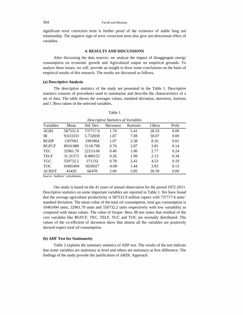
(a) Descriptive Analysis
The descriptive statistics of the study are presented in the Table 1. Descriptive
statistics consists of procedures used to summarise and describe the characteristics of a
set of data. The table shows the averages values, standard deviation, skewness, kurtosis
and J. Bera values of the selected variables.
Table 1
Descriptive Statistics of Variables
Variables Mean Std. Dev. Skewness Kurtosis J.Bera Prob.
AGRI 587531.9 737717.6 1.70 5.41 28.33 0.00
IR 9.633333 5.732839 1.87 7.08 50.07 0.00
RGDP 1507061 1991864 1.07 2.38 8.16 0.01
RGFCF 8910.988 5118.798 0.76 2.87 3.81 0.14
TEC 32961.79 22153.06 0.40 1.96 2.77 0.24
TELF 31.31373 8.480152 0.26 1.98 2.13 0.34
TGC 550732.2 371132 0.78 2.41 4.53 0.10
TOC 10465494 5656927 -0.00 1.44 3.93 0.13
ACRDT 43420 66478 2.00 5.85 39.39 0.00
Source: Authors’ calculations.
Our study is based on the 41 years of annual observation for the period 1972-2011.
Descriptive statistics on some important variables are reported in Table 1. We have found
that the average agriculture productivity is 587531.9 million rupees with 737717.6 units’
standard deviation. The mean value of the total oil consumption, total gas consumption is
10465494 units, 32961.79 units and 550732.2 units respectively with low variability as
compared with mean values. The value of Jarque- Bera JB test states that residual of the
core variables like RGFCF, TEC, TELF, TGC and TOC are normally distributed. The
values of the co-efficient of skewness show that almost all the variables are positively
skewed expect total oil consumption.
(b) ADF Test for Stationarity
Table 2 explains the summary statistics of ADF test. The results of the test indicate
that some variables are stationary at level and others are stationary at first difference. The
findings of the study provide the justification of ARDL Approach.
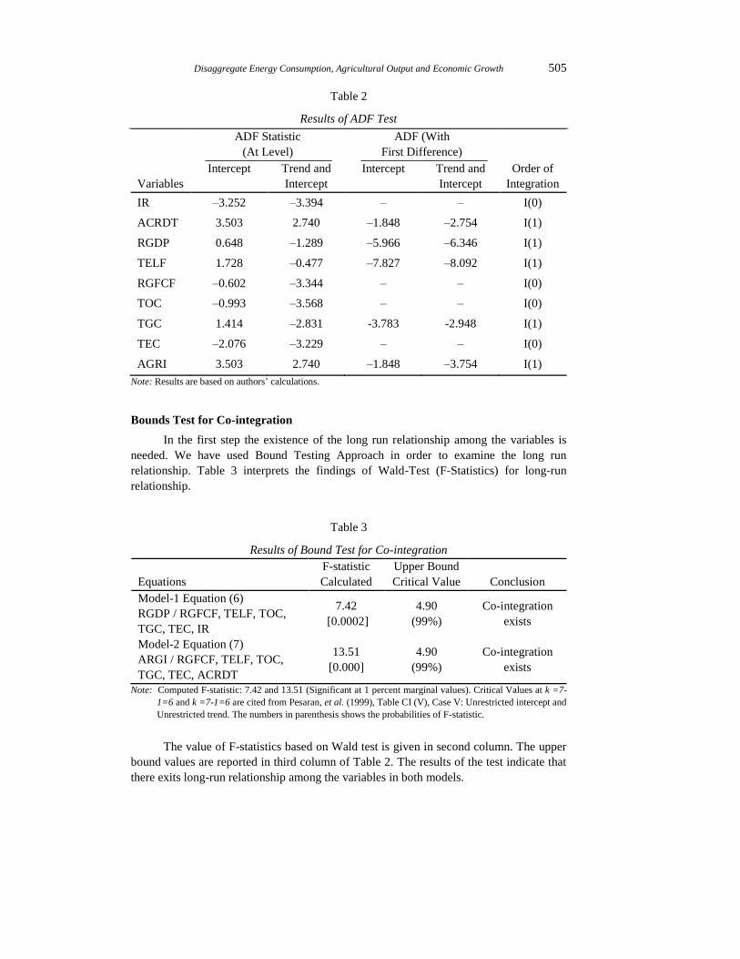
Disaggregate Energy Consumption, Agricultural Output and Economic Growth 505
Table 2
Results of ADF Test
Variables
ADF Statistic
(At Level)
ADF (With
First Difference)
Order of
Integration
Intercept Trend and
Intercept
Intercept Trend and
Intercept
IR –3.252 –3.394 – – I(0)
ACRDT 3.503 2.740 –1.848 –2.754 I(1)
RGDP 0.648 –1.289 –5.966 –6.346 I(1)
TELF 1.728 –0.477 –7.827 –8.092 I(1)
RGFCF –0.602 –3.344 – – I(0)
TOC –0.993 –3.568 – – I(0)
TGC 1.414 –2.831 -3.783 -2.948 I(1)
TEC –2.076 –3.229 – – I(0)
AGRI 3.503 2.740 –1.848 –3.754 I(1)
Note: Results are based on authors’ calculations.
Bounds Test for Co-integration
In the first step the existence of the long run relationship among the variables is
needed. We have used Bound Testing Approach in order to examine the long run
relationship. Table 3 interprets the findings of Wald-Test (F-Statistics) for long-run
relationship.
Table 3
Results of Bound Test for Co-integration
Equations
F-statistic
Calculated
Upper Bound
Critical Value Conclusion
Model-1 Equation (6)
RGDP / RGFCF, TELF, TOC,
TGC, TEC, IR
7.42
[0.0002]
4.90
(99%)
Co-integration
exists
Model-2 Equation (7)
ARGI / RGFCF, TELF, TOC,
TGC, TEC, ACRDT
13.51
[0.000]
4.90
(99%)
Co-integration
exists
Note: Computed F-statistic: 7.42 and 13.51 (Significant at 1 percent marginal values). Critical Values at k =7-
1=6 and k =7-1=6 are cited from Pesaran, et al. (1999), Table CI (V), Case V: Unrestricted intercept and
Unrestricted trend. The numbers in parenthesis shows the probabilities of F-statistic.
The value of F-statistics based on Wald test is given in second column. The upper
bound values are reported in third column of Table 2. The results of the test indicate that
there exits long-run relationship among the variables in both models.

506 Faridi and Murtaza
Estimates of Energy Consumption and Economic Growth
The long-run estimates of the model-1 are reported in Table 4. The dependant
variable is economic growth which is proxied as real GDP whereas RGFCF, TELF, TOC,
TEC and TGC, IR are independent variables.
Table 4
Long- run Results of Disaggregate Energy Consumption and Economic Growth
Estimated Long Run Coefficients using the ARDL Approach
ARDL(1,0,2,0,1,2,1) selected based on Schwarz Bayesian Criterion
Dependent Variable is RGDP
Regressor Coefficient Standard Error T-Ratio [Prob]
RGFCF 604.54 332.51 1.81 [.083]
TELF 588561 523156 1.12 [.273]
TOC .90 .29 3.00 [.007]
TGC 15.63 6.30 2.47 [.021]
TEC –346.85 157.78 –2.19[.039]
IR –69002 60625.9 –1.13 [.267]
C –1.17 9592168 –1.22 [.235]
T –779741 351826.6 –2.21 [.037]
Note: Results are based on Authors’ calculations using Microfit 4.1.
We have observed that the value of regression coefficient of Real Gross Fixed
Capital Formation (RGFCF) that is 604.54 which means that the one unit increase in Real
Gross Fixed Capital Formation increases the economic growth (RGDP) by 604.54 units
and this effect is strong and statistically significant. The expansion of infrastructure
directly stimulates productive activities. The other channel may be that investment
spending in various projects raises overall productivity and economic growth. Our results
stay in line with Khan and Reinhart (1990); Blomstrom, et al. (1994) who find positive
relationship between investment and growth.
Table 5
Short Run Estimates of Disaggregate Energy Consumption on Economic Growth
ARDL (1,0,2,0,1,2,1) selected based on Schwarz Bayesian Criterion
Dependent variable is dRGDP
Regressor Coefficient Standard Error T-Ratio[Prob]
dRGFCF 229.9852 87.6733 2.6232[.014]
dTELF 153071.4 101752.5 1.5044[.145]
dTELF1 –205340.1 101328.0 –2.0265[.053]
dTOC .34272 .077428 4.4263[.000]
dTGC 10.8104 2.3522 4.5958[.000]
dTEC –92.0338 52.6229 –1.7489[.092]
dTEC1 –152.8186 54.7032 –2.7936[.010]
dIR 2370.6 16643.9 –14243[.888]
dC –4460483 3357701 –1.3284[.196]
dT –296635.0 113131.6 –2.6220[.014]
ecm(–1) –.38043 .11781 –3.2290[.003]
ecm = RGDP –604.54*RGFCF –588561.3*TELF –.90*TOC –15.63*TGC + 346.8594*TEC + 69002.1*IR + 1.17E*C + 779741.9*T
R-Squared .76189 R-Bar-Squared .61036
DW-statistic 2.3488 F-stat. F( 10, 26) 7.0393[.000]
Note: Results are based on Authors’ calculations using Microfit 4.1.

Disaggregate Energy Consumption, Agricultural Output and Economic Growth 507
The coefficient of the employed labour force is although positive but insignificant.
Our findings are matched with conventional neo-classical theories of growth [see Barrow
and Sala-i-Martin (1995)].
The core variables of the study are energy variables i.e., total energy consumption,
total gas consumption and total electricity consumption. We have noted in the present
study that total oil consumption directly influence the economic growth. The value of the
coefficient of oil consumption is 0.90 which means that an increase of one unit in total oil
consumption raises real GDP about 0.90 units. The same results are found in the short
run. The findings support the theoretical results. The reason may be that the wheel of the
economic life cannot be run without oil now-a-days because of mechanisation and
technological progress.
We have observed that the coefficient of total gas consumption is positive
and highly significant. The real GDP increases almost 15.6 units due to one unit
increase in total gas consumption. It is noted that the third variable of the energy
turns out to be negative. The coefficient of the total electricity consumption is
(–346.85) and statistically significant. The short run findings also indicate negative
impact on growth. The analysis concludes that electricity is considered as limiting
factor to economic growth in Pakistan. The reason may be that the continuous short
fall of the electricity and electricity supply shock are the main causes of growth
deterioration. Our results support the [Javaid, et al. (2013); Kakar and Khilji
(2011); Shahbaz, et al. (2013); Onakoya, et al. (2013) and Yuan, et al. (2007)]
findings.
The inflation rate is used as control variable in the growth model. The analysis
concludes that the effect of inflation rate on economic growth is negative and
statistically insignificant. Theoretically, it is sound because rising prices cause an
increase in the cost of production. As a result production decreases and ultimately
economic growth declines.
Interpretation of Error Correction Term (ECt-1)
The coefficient of ecmt-1 for Model-1 is equal to (–0.38) for the short-run model
and implies that deviation from the long-term economic growth is corrected by 38
percent over each year at 1 percent level of significance.
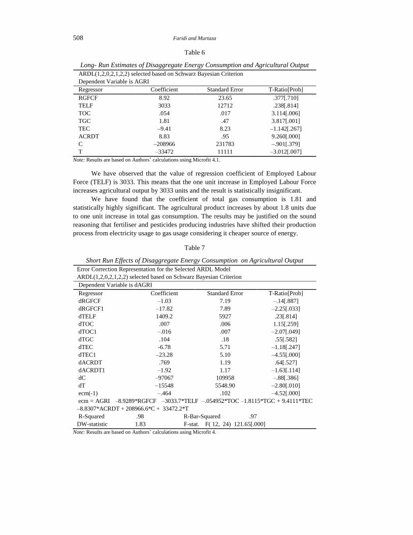
Estimates of Disaggregate Energy Consumption and Agricultural Output
The value of regression coefficient of real Gross Fixed Capital Formation
(RGFCF) is 8.92 which means that the one unit increase in real Gross Fixed Capital
formation raises the Agricultural output by 8.92 units. The reason may be that
investments in agriculture input industry like tractors, thrashers, tube wells and pesticides
increase along with an increase in the income of the farmer. Therefore, per capita saving
rate increases and ultimately growth per capita increases [Barro (1991)].
508 Faridi and Murtaza
Table 6
Long- Run Estimates of Disaggregate Energy Consumption and Agricultural Output
ARDL(1,2,0,2,1,2,2) selected based on Schwarz Bayesian Criterion
Dependent Variable is AGRI
Regressor Coefficient Standard Error T-Ratio[Prob]
RGFCF 8.92 23.65 .377[.710]
TELF 3033 12712 .238[.814]
TOC .054 .017 3.114[.006]
TGC 1.81 .47 3.817[.001]
TEC –9.41 8.23 –1.142[.267]
ACRDT 8.83 .95 9.260[.000]
C –208966 231783 –.901[.379]
T –33472 11111 –3.012[.007]
Note: Results are based on Authors’ calculations using Microfit 4.1.
We have observed that the value of regression coefficient of Employed Labour
Force (TELF) is 3033. This means that the one unit increase in Employed Labour Force
increases agricultural output by 3033 units and the result is statistically insignificant.
We have found that the coefficient of total gas consumption is 1.81 and
statistically highly significant. The agricultural product increases by about 1.8 units due
to one unit increase in total gas consumption. The results may be justified on the sound
reasoning that fertiliser and pesticides producing industries have shifted their production
process from electricity usage to gas usage considering it cheaper source of energy.
Table 7
Short Run Effects of Disaggregate Energy Consumption on Agricultural Output
Error Correction Representation for the Selected ARDL Model
ARDL(1,2,0,2,1,2,2) selected based on Schwarz Bayesian Criterion
Dependent Variable is dAGRI
Regressor Coefficient Standard Error T-Ratio[Prob]
dRGFCF –1.03 7.19 –.14[.887]
dRGFCF1 –17.82 7.89 –2.25[.033]
dTELF 1409.2 5927 .23[.814]
dTOC .007 .006 1.15[.259]
dTOC1 –.016 .007 –2.07[.049]
dTGC .104 .18 .55[.582]
dTEC -6.78 5.71 –1.18[.247]
dTEC1 –23.28 5.10 –4.55[.000]
dACRDT .769 1.19 .64[.527]
dACRDT1 –1.92 1.17 –1.63[.114]
dC –97067 109958 –.88[.386]
dT –15548 5548.90 –2.80[.010]
ecm(-1) –.464 .102 –4.52[.000]
ecm = AGRI –8.9289*RGFCF –3033.7*TELF –.054952*TOC –1.8115*TGC + 9.4111*TEC
–8.8307*ACRDT + 208966.6*C + 33472.2*T
R-Squared .98 R-Bar-Squared .97
DW-statistic 1.83 F-stat. F( 12, 24) 121.65[.000]
Note: Results are based on Authors’ calculations using Microfit 4.
Disaggregate Energy Consumption, Agricultural Output and Economic Growth 509
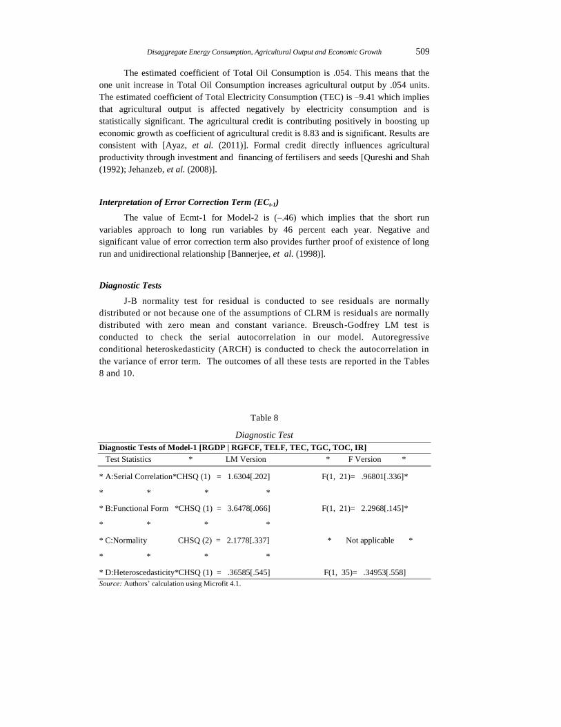
The estimated coefficient of Total Oil Consumption is .054. This means that the
one unit increase in Total Oil Consumption increases agricultural output by .054 units.
The estimated coefficient of Total Electricity Consumption (TEC) is –9.41 which implies
that agricultural output is affected negatively by electricity consumption and is
statistically significant. The agricultural credit is contributing positively in boosting up
economic growth as coefficient of agricultural credit is 8.83 and is significant. Results are
consistent with [Ayaz, et al. (2011)]. Formal credit directly influences agricultural
productivity through investment and financing of fertilisers and seeds [Qureshi and Shah
(1992); Jehanzeb, et al. (2008)].
Interpretation of Error Correction Term (ECt-1)
The value of Ecmt-1 for Model-2 is (–.46) which implies that the short run
variables approach to long run variables by 46 percent each year. Negative and
significant value of error correction term also provides further proof of existence of long
run and unidirectional relationship [Bannerjee, et al. (1998)].
Diagnostic Tests
J-B normality test for residual is conducted to see residuals are normally
distributed or not because one of the assumptions of CLRM is residuals are normally
distributed with zero mean and constant variance. Breusch-Godfrey LM test is
conducted to check the serial autocorrelation in our model. Autoregressive
conditional heteroskedasticity (ARCH) is conducted to check the autocorrelation in
the variance of error term. The outcomes of all these tests are reported in the Tables
8 and 10.
Table 8
Diagnostic Test
Diagnostic Tests of Model-1 [RGDP | RGFCF, TELF, TEC, TGC, TOC, IR]
Test Statistics * LM Version * F Version *
* A:Serial Correlation*CHSQ (1) = 1.6304[.202] F(1, 21)= .96801[.336]*
* * * *
* B:Functional Form *CHSQ (1) = 3.6478[.066] F(1, 21)= 2.2968[.145]*
* * * *
* C:Normality CHSQ (2) = 2.1778[.337] * Not applicable *
* * * *
* D:Heteroscedasticity*CHSQ (1) = .36585[.545] F(1, 35)= .34953[.558]
Source: Authors’ calculation using Microfit 4.1.
510 Faridi and Murtaza
Table 9
Diagnostic Test
Diagnostic Tests of Model-2 [AGRI | RGFCF, TELF, TEC, TGC, TOC, ACRDT]
Test Statistics * LM Version * F Version *
* A:Serial Correlation*CHSQ (1) = .53399[.465]* F(1, 18)= .26358[.614]*
* * * *
* B:Functional Form *CHSQ (1) = 2.5889[.118]* F(1, 18)= 1.3542[.260]*
* * * *
* C:Normality *CHSQ (2) = 2.4167[.299] * Not applicable *
* * * *
* D:Heteroscedasticity*CHSQ (1) = .46974[.493]* F(1, 35)= .45007[.507]*
Source: Authors’ calculation using Microfit 4.1.
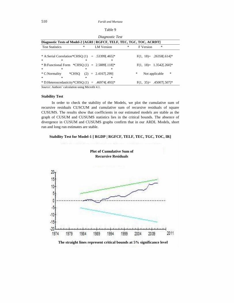
Stability Test
In order to check the stability of the Models, we plot the cumulative sum of
recursive residuals CUSCUM and cumulative sum of recursive residuals of square
CUSUMS. The results show that coefficients in our estimated models are stable as the
graph of CUSUM and CUSUMS statistics lies in the critical bounds. The absence of
divergence in CUSUM and CUSUMS graphs confirm that in our ARDL Models, short
run and long run estimates are stable.
Stability Test for Model-1 [ RGDP | RGFCF, TELF, TEC, TGC, TOC, IR]
Plot of Cumulative Sum of
Recursive Residuals
The straight lines represent critical bounds at 5% significance level
Disaggregate Energy Consumption, Agricultural Output and Economic Growth 511
Stability Test for Model-2 [AGRI | RGFCF, TELF, TOC, TEC, TGC, ACRDT]
Plot of Cumulative Sum of
Recursive Residuals
The straight lines represent critical bounds at 5% significance level
Plot of Cumulative Sum of
Recursive Residuals
The straight lines represent critical bounds at 5% significance level
The straight lines represent critical bounds at 5% significance level
Plot of Cumulative Sum of
Recursive Residuals

512 Faridi and Murtaza
5. CONCLUSIONS
In this study, we have analysed the impact of disaggregate energy consumption on
economic growth and Agricultural output on empirical grounds with respect to Pakistan.
Study has used ADF test which indicates mixed results with different order of integration.
Existence of long run relationship among variables is examined for both models. Long
run estimation and error correction representation of both models have been discussed
and their interpretations are made. Findings of the study conclude that disaggregate
energy consumption, economic growth and agricultural output are interlinked with each
other in short as well as in long run.
The empirical analysis of disaggregate consumption on economic growth and on
agricultural output leads to a number of conclusions for policy formulation. Electricity
consumption and economic growth puts some essential policy implications on the
economy of Pakistan. The unidirectional relationship of electricity consumption to
economic growth and agricultural output leads us to draw a conclusion that shortage of
electricity supply at the prevailing level can harm Pakistan’s economic growth and
agricultural output. As, consumption of electricity can influence national and agricultural
output as it is the main source of energy, that is why it is significant to maintain the
supply of electricity according to its demand. And since in cyclical sense economic
fluctuations are also caused due to changes in electricity consumption which implies
that electricity may be a leading indicator for business cycle. Another important
implication is that as oil consumption and gas consumption are contributing positively to
economic growth and agricultural growth. therefore, Pakistan energy sources (i.e., oil,
coal and gas) other than electricity should be enhanced for sustainable economic growth
because Pakistan production sectors like agricultural sector also rely on electricity
consumption mainly and increasing demand of electricity as compared to its supply and
insufficient installed capacity reduce agricultural as well as national output.
REFERENCES
Ahmed, W., K. Zaman, S. Taj, R. Rustam, M. Waseem, and M. Shabir (2013) Economic
Growth and Energy Consumption Nexus in Pakistan. South Asian Journal of Global
Business Research 2:2, 251–275.
Alam, S. and M. S. Butt (2001) Assessing Energy Consumption and Energy Intensity
Changes in Pakistan: An Application of Complete Decomposition Model. The
Pakistan Development Review 40:2, 135–147.
Apergis, N. and E. Payne (2010) Natural Gas Consumption and Economic Growth: A
Panel Investigation of 67 Countries. Applied Energy 87, 2759–2763.
Aqeel, A. and M. S. Butt (2001) The Relationship between Energy Consumption and
Economic Growth in Pakistan. Asia- Pac. Dev. J. 8, 101–110.
Ayaz, S., S. Anwar, M. H. Sial and Z. Hussain (2011) Role of Agricultural Credit on
Production Efficiency of Farming Sector in Pakistan – A Data Envelopment Analysis.
Pak. J. Life Soc. Sci. 9:1, 38–44.
Banerjee, A., J. J. Dolado, and R. Mestre (1998) Error-Correction Mechanism Tests for
Cointegration in a Single-Equation Framework. Journal of Time Series Analysis 19,
267–283.
Disaggregate Energy Consumption, Agricultural Output and Economic Growth 513
Barro, R. (1991) Economic Growth in a Cross-section of Countries. Quarterly Journal of
Economics 106, 407–443.
Barro, R. J. and X. Sala-i-Martin (1995) Economic Growth. New York: McGraw-Hill.
Blomstrom, M., R. Lipsey, and M. Zejan (1994) What Explains Growth in Developing
Countries? In W. Baumol, R. Nelson and E. Wolff (eds.) Convergence of
Productivity: Cross-National Studies and Historical Evidence. Oxford and New York:
Oxford University Press. 243–59.
Dantama, Y. U., Y. Z. Abdullahi, and N. Inuwa (2011) Energy Consumption—
Economic Growth Nexus in Nigeria: An Empirical Assessment Based on ARDL
Bound Test Approach. European Scientific Journal 8:12.
Hondroyiannis, G., S. Lolos, and E. Papapetrou (2002) Energy Consumption and
Economic Growth: Assessing the Evidence from Greece. Energy Economics 24, 319–
336.
Javid, A. Y., M. Javid, and Z. A. Awan (2013) Electricity Consumption and Economic
Growth: Evidence from Pakistan. Economics and Business Letters 2, 21–32.
Kakar, Z. K. and B. A. Khilji (2011) Energy Consumption and Economic Growth in
Pakistan. Journal of International Academic Research 11:1.
Khan, M. S. and C. M. Reinhart (1990) Private Investment and Economic Growth in the
Developing Countries. World Development (January).
Mozumder, P. and A. Marathe (2007) Causality Relationship between Electricity
Consumption and GDP in Bangladesh. Energy Policy 35, 395–402.
Nwosa, P. I. and T. O. Akinbobola (2012) Aggregate Energy Consumption and Sectoral
Output in Nigeria. African Research Review 6:4, 206–215.
Oh, Wankeun and Kihoon Lee (2004) Energy Consumption and Economic Growth in
Korea: Testing the Causality Relation. Journal of Policy Modeling 26: 973–981.
Ojinnaka, I. P. (1998) Energy Crisis in Nigeria: The Role of Natural Gas. CBN Bulletin
22:4, 8–12.
Onakoya, A. O., O. A. Jimi – Salami, and B. O. Odedairo (2013) Energy Consumption
and Nigerian Economic Growth: An Empirical Analysis. European Scientific Journal
9:4, 25–40.
Paul, S. and R. N. Bhattacharya (2004) Causality between Energy Consumption and
Economic Growth in India: A Note on Conflicting Results. Energy Economics 26,
977– 983.
Pesaran, M. H. and Y. Shin (1999) An Autoregressive Distributed Lag Modelling
Approach to Cointegration Analysis. In S. Strom, A. Holly and P. Diamond (eds.)
Econometrics and Economic Theory in the 20th Century: The Ragner Frisch
Centennial Symposium. Cambridge: Cambridge University Press.
Pesaran, M. H., Y. Shin, and R. J. Smith (2001) Bounds Testing Approaches to the
Analysis of Level Relationships. Journal of Applied Econometrics 16:3, 289–326.
Pew Centre on Global Climate Change and the National Commission on Energy Policy.
Qureshi, S. K. and A. H. Shah (1992) A Critical Review of Rural Credit Policy in
Pakistan. The Pakistan Development Review 31:4 871801.
Shah, M., K. Khan, H. Jehanzeb and Z. Khan (2008) Impact Of Agricultural Credit On
Farm Productivity And Income Of Farmers In Mountainous Agriculture In Northern
Pakistan: A Case Study of Selected Villages in District Chitral. Sarhad. J. Agri 24:4.

514 Faridi and Murtaza
Shahbaz, M. and M. Feridun (2011) Electricity Consumption and Economic Growth
Empirical Evidence from Pakistan. Qual Quant.
Shahbaz, M., H. H. Lean, and A. Farooq (2013) Natural Gas Consumption and
Economic Growth in Pakistan. Renewable and Sustainable Energy Reviews 18, 87–
94.
Solow, R. M. (1956) A Contribution to the Theory of Economic Growth. The Quarterly
Journal of Economics, 65–94.
Sorrell, S. (2009) Jevons’ Paradox revisited: The Evidence for Backfire from Improved
Energy Efficiency. Energy Policy 37, 2310–2317.
Van Zon and Yetkiner (2003) An Endogenous Growth Model with Embodied Energy-
saving Technical Change. Resource and Energy Economics 25, 81–103.
Wei, T. (2007) Impact of Energy Efficiency Gains on Output and Energy Use with
Cobb-Douglas Production Function. Energy Policy 35, 2023–2030.
Worrell, E., L. Price, and LBNL (2001) Pew Centre/NCEP 10-50. Improving Industrial
Energy Efficiency in the U.S.: Technologies and Policies for 2010 to 2050. Workshop
proceedings. “The 10-50 Solution: Technologies and Policies for a Low-Carbon
Future.”
Yang, H. Y. (2000) A Note on the Causal Relationship Between Energy and GDP in
Taiwan. Energy Economics 22:3, 309–317.
Yuan, J., C. Zhao, S. Yu, and Z. Hu (2007) Electricity Consumption and Economic
Growth in China: Cointegration and Co-feature Analysis. Energy Economics 29:6,
1179–1191.
Copyright © 2022 FDOKUMEN