The Macroeconomic Effects of Large Exchange Rate Appreciations

econstor www.econstor.eu

Der Open-Access-Publikationsserver der ZBW – Leibniz-Informationszentrum WirtschaftThe Open Access Publication Server of the ZBW – Leibniz Information Centre for Economics

Nutzungsbedingungen:Die ZBW räumt Ihnen als Nutzerin/Nutzer das unentgeltliche,räumlich unbeschränkte und zeitlich auf die Dauer des Schutzrechtsbeschränkte einfache Recht ein, das ausgewählte Werk im Rahmender unter→ http://www.econstor.eu/dspace/Nutzungsbedingungennachzulesenden vollständigen Nutzungsbedingungen zuvervielfältigen, mit denen die Nutzerin/der Nutzer sich durch dieerste Nutzung einverstanden erklärt.

Terms of use:The ZBW grants you, the user, the non-exclusive right to usethe selected work free of charge, territorially unrestricted andwithin the time limit of the term of the property rights accordingto the terms specified at→ http://www.econstor.eu/dspace/NutzungsbedingungenBy the first use of the selected work the user agrees anddeclares to comply with these terms of use.

zbw Leibniz-Informationszentrum WirtschaftLeibniz Information Centre for Economics

Kappler, Marcus; Reisen, Helmut; Schularick, Moritz; Turkisch, Edouard

Working Paper

The macroeconomic effects of large exchange rateappreciations

ZEW Discussion Papers, No. 11-016

Provided in Cooperation with:ZEW - Zentrum für Europäische Wirtschaftsforschung / Center forEuropean Economic Research

Suggested Citation: Kappler, Marcus; Reisen, Helmut; Schularick, Moritz; Turkisch, Edouard(2011) : The macroeconomic effects of large exchange rate appreciations, ZEW DiscussionPapers, No. 11-016, http://nbn-resolving.de/urn:nbn:de:bsz:180-madoc-31440

This Version is available at:http://hdl.handle.net/10419/44467

Dis cus si on Paper No. 11-016

The Macroeconomic Effects of Large Exchange Rate Appreciations

Marcus Kappler, Helmut Reisen, Moritz Schularick, and Edouard Turkisch

Dis cus si on Paper No. 11-016

The Macroeconomic Effects of Large Exchange Rate Appreciations

Marcus Kappler, Helmut Reisen, Moritz Schularick, and Edouard Turkisch

Die Dis cus si on Pape rs die nen einer mög lichst schnel len Ver brei tung von neue ren For schungs arbei ten des ZEW. Die Bei trä ge lie gen in allei ni ger Ver ant wor tung

der Auto ren und stel len nicht not wen di ger wei se die Mei nung des ZEW dar.

Dis cus si on Papers are inten ded to make results of ZEW research prompt ly avai la ble to other eco no mists in order to encou ra ge dis cus si on and sug gesti ons for revi si ons. The aut hors are sole ly

respon si ble for the con tents which do not neces sa ri ly repre sent the opi ni on of the ZEW.

Download this ZEW Discussion Paper from our ftp server:

ftp://ftp.zew.de/pub/zew-docs/dp/dp11016.pdf

Non-technical summary

The aim of this paper is to provide an empirical backbone to the debate about the

macroeconomic effects of large upward exchange rate adjustments of tightly managed or

pegged exchange rate regimes. Using a large cross-country dataset covering almost 50

years of international economic history between 1960 and 2008, we study the empirical

record of large exchange rate appreciation and revaluation shocks. Our goal is to provide

systematic evidence on the macroeconomic lessons that can be learned from these

episodes. Our approach is the following: in a first step, we identify large exchange rate

appreciations and revaluations. Our definition of a large exchange rate event comprises a

10 percent (or larger) appreciation of the nominal effective exchange rate over a two-year

window (or less), leading to sustained real effective appreciation. We hence limit

ourselves to studying such nominal exchange rate appreciations that have led to large

movements in real exchange rates. We require the appreciation to be sustained in real

terms over at least five years. From 1960, we identify 25 episodes of large nominal and

real appreciations in a sample of 128 countries of developing and advanced economies.

Having identified these events, we ask in a second step how these affected the current

account balance and output using a dummy variable augmented autoregressive panel

model. We also split our sample and look at differences between advanced and

developing countries in response to nominal and real appreciation shocks.

We establish four central empirical regularities. First, the current account balance

typically deteriorates strongly in response to appreciation and revaluation shocks. Three

years after the strengthening of the exchange rate, the current account balance falls by

about three percentage points of GDP as a function of decreased savings with stable

investment rates. Second, the effects on output are limited. The negative effect on the

level of output amounts to a modest 1 percent after six years. The confidence intervals are

wide and the results are statistically insignificant. Third, while aggregate output is not

strongly affected, export growth falls significantly after appreciation and revaluation

shocks. Finally, most of these effects seem to be more pronounced in developing

countries.

Das Wichtigste in Kürze

Die globalen Ungleichgewichte in den Leistungsbilanzen werden häufig als Bedrohung

für die weltwirtschaftliche Stabilität angesehen. Ausgehend davon wird argumentiert,

dass die Überschussländer wie China deshalb ihre Währung aufwerten sollen, um diese

stabilitätsgefährdenden Ungleichgewichte abzubauen. Die Studie trägt zu dieser Debatte

bei, indem sie untersucht, welche Auswirkungen ausgeprägte und dauerhafte nominale

und reale Wechselkursaufwertungen auf die Leistungsbilanz und weitere

makroökonomische Schlüsselgrößen wie Wirtschaftswachstum, Investitionen und

Ersparnisse sowie den Außenhandel haben.

Das Vorgehen ist wie folgt. In einem ersten Schritt werden historische Episoden

starker Aufwertungen in einem 128 Länder umfassenden Querschnitt mit Beobachtungen

über die Jahre 1960 bis 2008 anhand folgender Kriterien definiert: Sowohl der nominale

als auch reale effektive Wechselkurs eines Landes werten um mindestens 10 Prozent auf

und die reale Aufwertung hatte mindestens fünf Jahre Bestand. Entsprechend dieser

Kriterien können insgesamt 25 Episoden in dem vorliegenden Datensatz identifiziert

werden. In einem nächsten Schritt wird untersucht, welche Auswirkungen der Eintritt in

eine Episode ausgeprägter Wechselkursänderungen auf die Leistungsbilanz, das BIP-

Wachstum, die Ersparnisse, die Investitionen, die Exporte und die Importe ausübt. Zu

diesem Zweck schätzt die Studie ein dynamisches Panel-Modell, das um Impulsdummies

erweitert wird.

Die Ergebnisse zeigen, dass signifikante makroökonomische Reaktionen mit

starken Währungsaufwertungen verbunden sind. Die Leistungsbilanz fällt signifikant und

der negative Effekt der Währungsaufwertung entfaltet nach drei Jahren seine stärkste

Wirkung. Die Ersparnisse geben deutlich und lang anhaltend nach, während die

Investitionen zunächst steigen, der Währungseffekt aber schnell ausläuft. Die

Outputreaktion ist zunächst positiv und verläuft anschließend insignifikant. Die Exporte

reagieren mit ihrem Einbruch wie zu erwarten und die Importe insignifikant. Eine

Trennung der Beobachtungen nach dem Status des Pro-Kopf-Einkommens zeigt, dass die

Effekte in Entwicklungsländern stärker und signifikanter sind als in entwickelten

Ländern.

The Macroeconomic Effects of Large

Exchange Rate Appreciations

Marcus Kappler† ZEW Mannheim

Helmut Reisen‡ OECD Paris

Moritz Schularick Free University Berlin

Edouard Turkisch OECD Paris

February 2011

– Abstract –

In this paper we study the macroeconomic effects of large exchange rate appreciations.

Using a sample of 128 countries from 1960-2008, we identify large nominal and real

appreciations shocks and study their macroeconomic effects in a dummy-augmented

panel autoregressive model. Our results show that an exchange rate appreciation can have

strong effects on current account balances. Within three years after the appreciation

event, the current account balance on average deteriorates by three percentage points of

GDP. This effect occurs through a reduction of savings without a meaningful reduction in

investment. Real export growth slows down substantially, while imports remain by and

large unaffected. The output costs of appreciation are small and not statistically

significant, indicating a shift towards domestic sources of growth. All these effects

appear somewhat more pronounced in developing countries.

Keywords: current account adjustment; global imbalances; exchange rate changes

JEL codes: F4; F31; F32; N10; O16.

We wish to thank Menzie Chinn, Christian Daude, Luiz de Mello and Helen Qiao for helpful comments on an earlier draft. † Email: [email protected] ‡ Email: [email protected] Corresponding author. Email: moritz.schularick @fu-berlin.de Email: [email protected]

1

The aim of this paper is to provide an empirical backbone to the debate about the

macroeconomic effects of large upward exchange rate adjustments of tightly managed or

pegged exchange rate regimes. Using a large cross-country dataset covering almost 50

years of international economic history between 1960 and 2008, we study the empirical

record of large exchange rate appreciation and revaluation shocks. Some of these

episodes are regularly referred to in the debate about global rebalancing in the wake of

the recent financial crisis, e.g. in Germany and in Japan. Our goal is to provide systematic

evidence on the macroeconomic lessons that can be learned from these episodes.

Global imbalances have become a household word. In particular, the large trade

imbalance between China and the United States has gained prominence in academic and

political debates. Despite considerable disagreement about the causes, many economists

think that the international imbalances that have developed in the past decade are

problematic and should be reduced (e.g., Obstfeld and Rogoff 2005; Cline and

Williamson 2007; Feldstein 2008). However the appropriate policy treatment remains

debated.1 One group of economists thinks that large exchange rate adjustments –

basically a dollar depreciation and an appreciation of the Chinese renminbi and of other

Asian currencies – will eventually play a role in rebalancing the world economy

(Obstfeld and Rogoff 2005; Goldstein, 2006; Wolf 2009; Subramanian 2010; Ferguson

and Schularick 2011).

Yet other scholars argue that currency adjustment is not an effective policy tool as

elasticities could be relatively low and underlying savings and investment remain

unaffected by exchange rate changes (Devereux and Genberg 2007; McKinnon 2007;

Qiao 2007). A third group of development economists, by contrast, fears that exchange

rate adjustment might be all too effective – but mainly in reducing the growth rate of the

Chinese and other developing economies as China has become a locomotive for

developing country growth in the 2000s (Rodrik 2008; Berg and Miao 2010; Garroway et

al. 2010).2

1 There is also an emerging consensus that the imbalances were closely linked to the financial crisis of 2008-09 (Bini Smaghi 2008; Caballero and Krishnamurthy 2009; Blanchard and Milesi-Ferretti 2009; Obstfeld and Rogoff 2009). However, some authors maintain that the financial crisis of 2008-09 was by and large unrelated to global imbalances (e.g. Dooley et al. 2009). 2 The key argument is that revaluation might put a successful export-led growth model at risk that was centred on a competitive real exchange rate and positive externalities from investment in the tradable goods

2

The main points of disagreement about the effects of exchange rate changes on

the macroeconomy relate to two central issues. First, how effective would currency

revaluation be in reducing current account surpluses in Asia and deficits in the United

States? Second, is there reason to believe that appreciation would come with the negative

side effect of reducing growth in developing countries? The first question relates to the

role of exchange rates in international adjustment and the second to the role of real

exchange valuation in the development process. While these questions open up two very

different theoretical boxes, they are to some degree open to a joint empirical treatment,

which is what we aim to do in this paper.

Despite the large literature dealing with exchange rates and trade elasticities, the

number of studies that have specifically analyzed the economic effects of appreciation

episodes is relatively small3. Goldfajn and Valdés (1999) have studied large real effective

appreciation episodes from 1960 to 1994 for a broad country sample, but with a focus on

the dynamics of appreciation and overvaluation. Eichengreen and Hatase (2007) have

analyzed the Japanese revaluation experience with an eye on the policy lessons for China

today. A recent study by Eichengreen and Rose (2010) has broadened this approach and

is similar to our study in its research objective, but not in the empirical approach.

Our approach is the following: in a first step, we identify large exchange rate

appreciations and revaluations. Our definition of a large exchange rate event comprises a

10 percent (or larger) appreciation of the nominal effective exchange rate over a two-year

window (or less), leading to sustained real effective appreciation. We hence limit

ourselves to studying such nominal exchange rate appreciations that have led to large

movements in real exchange rates. We require the appreciation to be sustained in real

terms over at least five years.

From 1960, we identify 25 episodes of large nominal and real appreciations in a

sample of 128 countries of developing and advanced economies. Having identified these

events, we ask in a second step how these affected the current account balance and output

using a dummy variable augmented autoregressive panel model following the

sector. For a formal model see Korinek and Servén (2010). Similar causes have been named as an explanation for the widespread phenomenon of “fear of floating” among emerging market countries (Calvo and Reinhart, 2002). 3 At least outside the narrower context of appreciation pressures in resource rich economies. The seminal contribution on the so-called Dutch disease is Corden and Neary (1982).

3

methodology pioneered in Cerra and Saxena (2008). We also split our sample and look at

differences between advanced and developing countries in response to nominal and real

appreciation shocks.

We establish four central empirical regularities. First, the current account balance

typically deteriorates strongly in response to appreciation and revaluation shocks. Three

years after the strengthening of the exchange rate, the current account balance falls by

about three percentage points of GDP as a function of decreased savings with stable

investment rates. Second, the effects on output are limited. The negative effect on the

level of output amounts to a modest 1 percent after six years. The confidence intervals are

wide and the results are statistically insignificant. Third, while aggregate output is not

strongly affected, export growth falls significantly after appreciation and revaluation

shocks. Finally, most of these effects seem to be more pronounced in developing

countries.

Difficulties in disentangling the effects of exchange rate changes from the factors

that lead to the change of the exchange rate have been a typical problem for empirical

analysis in this field (Engel 2009). In this paper, we deal with the exogeneity issue

through detailed narrative documentation of the individual appreciation episodes4 and

explicit exogeneity tests. This allows us to differentiate between appreciation episodes

that occurred for largely exogenous reasons, and those that might have been partly

endogenous to economic development. We identify 14 episodes when a country's real and

nominal effective exchange rate appreciated by 10 percent or more without discretionary

adjustments of the parity by the country's government. Typically, such appreciations were

the indirect consequence of the appreciation of the anchor currency of the peg against

important other currencies.5 We use the estimated effects of these events to evaluate the

robustness of estimations using a broader definition of appreciation episodes.

4 Not dissimilar to the approach taken by Romer and Romer (2010) to identify the effect of tax changes. 5 To give an example, the Malaysian ringgit was managed relative to the Singapore Dollar in the late 1970s. When the Singapore Dollar strengthened against the US dollar in the early 1980s, the Malaysian ringit appreciated strongly on a trade weighted basis (both in nominal and real terms) for reasons that were by and large unrelated to Malaysia's economic position. We consider this an exogenous appreciation event. By contrast, when the German government decided to revalue the Deutschmark in 1970, it is likely that the decision partly reflected the strength of the German economy and the strength of the external position. We consequently treat such an event as at least partly endogenous.

4

The structure of the paper is as follows. Section 1 provides a theoretical and

empirical introduction. In section 2, we define and describe the appreciation events we

are studying. Section 3 introduces our econometric methodology; section 4 presents the

key results and a number of robustness tests. Section 5 summarises the key results of this

study – strong effects on current account balances, a small and insignificant negative

impact on output but pronounced effects on export growth, and somewhat stronger

overall responses in developing countries – and discusses their implication for economic

policy.

1. Real Effects of Large Exchange Rate Adjustments

In the debate about the real effects of large exchange rate adjustments, two

different strands of international economics meet. First, the debate opens up old fault

lines in international economics about the effects of exchange rate adjustments on current

account balances. Some scholars are more pessimistic about elasticities, pass-through or

effects on savings and investment, while others are more optimistic. Second, these long-

standing disagreements are amplified by concerns coming mainly of development

economics with regard to the positive growth effects of undervaluation (and the potential

costs of undoing it). We shall discuss both in turn.

In its simplest form, the idea that large exchange rate movements affect trade and

current account balances and could help the global rebalancing process goes back to

traditional elasticity models. In this framework, changes in real exchange rates will affect

the current account if the Marshall-Lerner condition is fulfilled, i.e. if the sum of export

and import elasticities exceeds one.6 However, "elasticity pessimism" has a long tradition

in international economics.7 Many empirical studies found relatively low elasticities, at

least at short-time horizons (Rose and Yellen 1989; Hooper et al. 2000; Chinn 2004;

Chinn and Lee 2009). Also the literature in the field of new open economy models has

often pointed to limited short-run responsiveness of the current account to exchange rate

6 Initially, there might be a J-Curve effect due to counteracting valuation effects, but eventually the current account would deteriorate as price elasticities rise over time. 7 See the discussion in Obstfeld (2002).

5

changes (Goldberg and Knetter 1997; Devereux and Engel 2003).8 All in all, skepticism

with regard to the role of exchange rates in generating adjustment is widespread and no

consensus has been reached to date (Engel 2009).9 Models incorporating low elasticities,

limited pass-through, and imports of intermediate goods yield only small adjustment

effects (Devereux and Genberg 2007).

It does not come as a surprise that the same lack of consensus can be found in the

literature debating the Chinese case. Devereux and Genberg (2007) develop a general

equilibrium model to analyze the impact of an exchange rate appreciation on the current

account that generates only small effects. Also Kwack et al. (2007), Marquez and

Schindler (2007), Cheung et al. (2010), Thorbecke and Smith (2010) have studied

Chinese trade elasticities. However, while this literature has generally arrived at

relatively small effects from possible Renminbi revaluation, other recent contributions by

Ahmed (2009) and Cline (2010) have found export price elasticities closer to unity and

see greater potential for exchange rate adjustment.

As a country’s current account balance equals the gap between national saving

and investment, real exchange rate movements ultimately have to impact savings and

investment patterns to be effective in changing the current account. Yet to what extent

changes in real exchange rates affect savings and investment remains an open issue.

Other factors such as income, growth expectations and demographic trends are likely to

play an important role for savings and investment decisions, but exchange rates might

also matter. Economic historians have often seen real exchange rate undervaluation as

important factors in explaining growth performance. Eichengreen (2008) as well as

Ferguson and Schularick (2011) argue that real exchange rate undervaluation has often

been a cornerstone of successful catching-up, partly through the effect on corporate

profitability and investment.

Levy-Yeyati and Sturzenegger (2007) argue that a more depreciated exchange

rate leads to lower real wages, inducing firms to increase saving, thereby rising overall

8 Chinn and Wei (2008) demonstrate that flexible exchange rate regimes are no more effective in facilitating current account adjustment than fixed regimes. 9 However, some authors take the opposite position and argue that the "elasticity pessimism" might have gone too far (Obstfeld 2002). In the Asian context, models that show only small adjustment effects (at best) due to sticky prices are also at odds with the rich literature on particularly high pass-through in emerging markets leading to the "fear of floating" phenomenon (Calvo and Reinhart 2002).

6

saving. Gala (2008) explores the link between depreciated exchange rate changes,

depressed real wages and high corporate savings in Asian economies. Similar channels

have been analysed by Montiel (2000) and Montiel and Servén (2008). Qiao (2007), by

contrast, studies the effect of appreciation on investment. Her model predicts that

investment will be dampened by appreciation and thereby possibly causing the current

account to improve as appreciation exerts a negative wealth effect. But related empirical

evidence remains relatively scarce.10 These disagreements clearly call for a targeted

research strategy. If we want to understand how exchange rate changes affect investments

and savings determinants, we need to study the impact of exchange rate changes not only

on the current account balance, but on savings and investment separately.

The impact of exchange rate changes on economic growth is another field that has

attracted considerable attention in the literature. A large empirical literature deals with

the growth effects of depreciation events (Edward 1986; Hong and Tornell 2005; Gupta

et al. 2007). Bussière et al. (2010) have recently provided new evidence on the output

effects of currency collapses that is methodologically similar to ours. However, the role

of exchange rate policy and its effects on growth has also been the subject of a more

fundamental debate among development economists. At the core of the debate is the

question whether the view needs modification that any departures of the real exchange

rate from its equilibrium level would harm growth by distorting a key relative price in the

economy.11 A key implication of this traditional "misalignment view" was that

undervaluation is equally harmful as overvaluation.

Recent contributions argue that a depreciated real exchange rate can be

economically beneficial as it promotes economic growth through technology transfers

and learning-by-doing externalities (Eichengreen 2008; Aizenman and Lee 2008). The

literature on export-led growth has repeatedly stressed that such ideas are influential for

development strategies in large parts of Asia (Dooley et al. 2003). Korinek and Serven

(2010) present a model in which real exchange rate valuation improves welfare via 10 Campa and Goldberg (1995, 1999) study the linkage between exchange rate and investment in industry in the US, Canada, UK and Japan. They find that during the 1970s appreciation generated a reduction in capital goods orders, but that the opposite pattern prevailed during the 1980s. Over a sample of Italian manufacturing firms, Nucci and Pozzolo (2001) show that a depreciation of the exchange rate can have positive effects on investment through higher revenues and a negative effect through the cost channel, but the magnitude of these effects varying significantly over time. 11 For a useful survey see Eichengreen (2008).

7

positive externalities stemming from investment in the tradables sector. Through real

exchange rate undervaluation, the government effectively subsidizes investment in the

tradables sector. But by using the exchange rate as a tool, the government outsources the

targeting of the subsidy to foreign consumers avoiding domestic rent-seeking and other

political economy complications. On the empirical side, Rodrik (2008) presents panel

regressions that show a correlation of growth rates in developing countries with a

measure of real exchange rate undervaluation. A recent study by Berg and Miao (2010)

essentially confirmed Rodrik’s analysis. The authors find empirical evidence that

currency overvaluations are negative for growth while undervaluations are positively

correlated with growth in developing-countries. Undoing real undervaluation could then

be expected to be harmful to economic growth.

Summing up, there is considerable uncertainty about the real economic effects of

exchange rate changes. In the remainder of the paper, we want to subject these various

positions to an empirical test: we first identify large appreciation shocks in the 1960-2008

period for a broad country sample. We will then move on to estimate the macroeconomic

effects on the current account balance, saving, investment and on overall economic

growth.

2. Identifying appreciation episodes

Our sample consists of annual data for 128 advanced and developing countries for

the period 1960-2008. We code an appreciation event for country (i) in year (t) when the

following conditions are met. First, we define an appreciation event if the nominal

effective exchange rate is revalued by at least 10 percent or more relative to the average

level two years before. The two-year horizon allows us to capture not only one-time step

revaluations, but also a number of smaller appreciation steps that happen within a short

time window. We restrict our analysis to countries that operate fixed exchange rate

regimes, i.e. pegs and managed floats, according to the Reinhart and Rogoff (2004)

classification (with a few minor modifications detailed in the appendix) as we expect

appreciation episodes under floating regimes to be endogenous to economic

8

fundamentals. We define an appreciation event when the nominal effective exchange rate

appreciates by 10 percent, so that

(1) , , 2ln( ) ln( ) 0.1i t i tNEER NEER .

Second, the nominal appreciation must lead to sustained real appreciation. We

therefore require that the real effective exchange rate remains stronger by 10 percent (or

more) on average for three years relative to the beginning of the appreciation process,

(2) , 1 , 2 , 3 , 2ln(( ) / 3) ln( ) 0.1i t i t i t i tREER REER REER REER .

We also ensure that the appreciation was not preceded by devaluation of similar

magnitude, so that

(3) , 2 , 5 , 4 , 3ln( ) ln(( ) / 3) 0.1i t i t i t i tNEER NEER NEER NEER .

Table 1 lists the resulting appreciation events. In total, we identify 25 large

appreciation episodes. Moreover, we found this list of large appreciations to be

surprisingly robust to variations in the event definition – such as expanding or shortening

the time frame of the appreciation episode from two years to one or three years, relaxing

or strengthening the criteria for previous devaluations.

In a next step, we collected detailed historical information on each of these

appreciation events. This allowed us to classify the events into two different groups. The

first group consists of appreciation events that occurred without an active policy decision

to alter the parity on part of the authorities in the concerned country. Typically, such

cases relate to the appreciation of the anchor currency in a peg against key trading

partners leading to nominal and real appreciation of a country's currency on a trade-

weighted basis. In other cases, the countries actively adjusted their nominal exchange

rates, so that the appreciation is potentially endogenous to economic fundamentals as

discussed below. An example here would be the Bundesbank's consent to a revaluation of

9

the Deutschmark in the late 1960s and early 1970s in response to fears about imported

inflationary pressures.

Table 1: Appreciation Events

Country Period NEER REER Description

Australia* 1971 1973 10.20% 10.30% After the breakdown of the Bretton Woods system, the depreciation of the US dollar led to the appreciation of the Australian dollar which was pegged to the British pound.

Sweden* 1977 1979 10.80% 11.30% From 1977 to 1991, the Krona was pegged to a trade-weighted basket of foreign currencies. The appreciation of European currencies indirectly triggered the appreciation of the Krona on a nominal and real effective basis.

Ireland* 1978 1980 12.90% 22.00% Ireland joined the European Exchange Rate Mechanism (ERM) in 1979. The appreciation of European currencies in the late 1970s triggered appreciation on a trade-weighted basis.

Malaysia* 1978 1980 20.30% 16.50% From September 1976 to the end of 1984, the Malaysian National Bank stabilized the exchange rate against the Singapore dollar. The rise in the Singapore dollar triggered the appreciation of the currency.

Algeria* 1980 1982 17.20% 28.00% The exchange rate of the Algerian dinar was pegged to abasket of currencies with a large U.S. dollar weight. Dollar strength during the early 1980s led to a strong appreciation of the dinar on a trade-weighted basis.

Singapore* 1980 1982 12.90% 12.40% From 1973 to 1985, Singapore pegged the value of Singapore Dollar against a basket of currencies with a large US dollar weight. The trade-weighted appreciation resulted from dollar strength.

Belize* 1981 1983 13.70% 16.00% The Belizean currency was pegged to the US dollar. The appreciation was triggered by dollar strength at the beginning of the 1980s.

Algeria* 1982 1984 16.60% 11.70% The appreciation of the U.S. dollar during the first half of the 1980s led to a strong rise in the real value of the Algerian dinar on a trade-weighted basis relative to European trading partners.

Ivory Coast* 1983 1985 16.60% 26.40% The currency appreciated on a trade-weighted basis as a consequence of the appreciation of the anchor currency (French Franc) against the US Dollar.

Cameroon* 1984 1986 11.80% 21.20% The currency appreciated on a trade-weighted basis as a consequence of the appreciation of the anchor currency (French Franc) against the US Dollar.

Ivory Coast* 1985 1987 30.20% 27.00% The currency appreciated on a trade-weighted basis as a consequence of the appreciation of the anchor currency (French Franc) against the US Dollar.

Spain* 1986 1988 10.40% 19.00% The peseta was managed vis-à-vis to other ERM

10

currencies whose appreciation against the dollar, triggered appreciation on a trade-weighted basis.

Singapore* 1988 1990 12.00% 17.00% Trade-weighted appreciation as a function of strength of the main anchor currency.

Spain* 1988 1990 13.40% 11.20% Appreciation was triggered by the appreciation of European currencies against the dollar in the late 1980s.

Germany 1968 1970 10.70% 12.90% Under the Bretton Woods system, the rate of the DM was amended in October 1969. The DM was revalued.

Japan 1970 1972 14.40% 24.00% The exchange rate of the yen was maintained at Yen 360 per USD from 1949 to 1971. After the United States devalued, the Yen was revalued to 308 per USD.

Switzerland 1971 1973 10.20% 20.60% After the demise of the Bretton Woods system, the Swiss franc was revalued twice in 1971.

Switzerland 1974 1976 22.40% 13.00% The Swiss National Bank de facto managed a sustained exchange rate appreciation against dollar and DM,

Japan 1975 1977 14.70% 20.90% The Bank of Japan managed the appreciation of the yen against the dollar.

Romania 1980 1982 47.50% 35.40% At the beginning of the 1980s, several step appreciations of the commercial exchange rate were taken.

Taiwan 1986 1988 13.90% 11.40% In 1987, the exchange rate regime was changed towards amore market determined rate, leading to an appreciation on a trade-weighted basis.

Chile 1992 1994 29.80% 15.00% The central bank revalued the “central parity” of the currency. It was also decided to widen the bands from ±5% to ±10%.

Colombia 1993 1995 11.20% 30.60% The central bank revalued the “central parity” of the currency.

Czech Republic

2001 2003 11.20% 16.40% The appreciation was linked to the introduction of a newexchange rate regime framework (with a crawling band and Central Bank interventions).

Colombia 2004 2006 10.00% 23.00% The central bank revalued the “central parity” of the currency.

* denotes indirect appreciation events as detailed in the text. All other cases involve active parity adjustments by national authorities. Sources: see appendix.

A crucial problem for students of the economic effects is that decision to adjust

the parity and revalue is typically not random. The economic variables whose post-

appreciation behaviour is of interest – such as the current account balance – can be

11

expected to play an important role for the decision to change the exchange rate. Clearly,

our analysis also needs to address this problem. We propose two ways to deal with the

issue. First, on the basis of our detailed narrative of the appreciation events we are able to

identify 14 cases of indirect appreciations, i.e. cases where the nominal and real

appreciation were "mechanistic" consequences of the appreciation of the anchor currency.

We argue that such instances of appreciation by the (typically larger) anchor currency are

by and large exogenous. Put differently, the appreciation of the French franc against the

dollar in the mid-1980s was not driven by economic developments in Cameroon. But the

result was an effective appreciation of the trade-weighted exchange rate of Cameroon

whose macroeconomic effects we can then estimate.

Second, we run a number of statistical tests to gauge the potential endogeneity

problems. In table 2 we show the results of panel logit regressions relating the probability

of appreciation episodes to lagged growth and current accounts. We run separate analysis

both for the small sample of indirect appreciation episodes (where no active policy

decision was taken) and the large sample of all appreciations, including active

revaluations. We test whether strong growth or high current account surpluses increase

the probability of an appreciation event in a significant way. We also interact the two

using rolling 3-year moving averages that exclude the initial year when appreciation

started. While there are reasons to believe that active policy steps to revalue the currency

become more likely with good economic fundamentals, it is equally conceivable that

countries with good fundamentals resist exchange rate adjustment for many years and

that countries with bad fundamentals can also be affected by exogenous appreciation

shocks linked to movements in their anchor currency.

The results presented in table 2 gives us an idea about the potential endogeneity

problems of the two samples. For our small sample of indirect appreciations there is no

evidence that appreciation is linked to economic fundamentals in the preceding years. All

individual lags are insignificant. Looking at them jointly, we cannot reject hypothesis that

all lags are equal to zero. We obtain similar results for the current account. In regression

(3) we interact growth and current account balance, but we fail to find evidence for

significant effects. Also for the large sample (which includes episodes with active policy

adjustments), the lags remain individually and jointly insignificant, but the coefficient

12

estimates increase somewhat. We interpret this as an indication that caution is needed in

the causal interpretation of our results, in particular in the case of the larger sample. But

all in all we come away confident that the exogeneity assumptions behind our analysis

hold up relatively well. In any case, we cannot reject the hypothesis that appreciation and

revaluation events are unrelated to previous trends in growth and external balances in

both the restricted and the larger sample.

Table 2: Exogeneity testsPanel-Logit Regression (1) (2) (3) (4) (5) (6)Sample small small small large large large

Real growthL.dy 0.948 1.787

(7.197) (5.094)L2.dy 6.385 5.932

(8.108) (4.501)L3.dy 5.993 2.795

(7.303) (4.33) 3-year mov. av. 1.275 3.011

(3.491) (2.461)Current account/GDP

L.cagdp 0.0401 -0.0106(0.073) (0.051)

L2.cagdp 0.0298 0.0527(0.095) (0.057)

L3.cagdp -0.0255 -0.000791(0.076) (0.037)

3-year mov. av. -0.0105 -0.00925(0.0182) (0.0144)

Growth*Current account/GDP 0.0834 0.183 3-year mov. av. (0.279) (0.197)

Constant 1.266* 1.433* -3.303*** 0.620 0.497 -2.830***(0.725) (0.767) (0.383) (0.657) (0.745) (0.214)

Test for all lags =0 ,x2 2.028 1.189 4.966 2.217p-value 0.567 0.756 0.174 0.529Sum of lag coefficients 13.33 0.0444 10.51 0.0413se 10.04 0.0533 5.409 0.0316Time-effects Yes Yes Yes Yes Yes YesObservations 5,392 3,450 3,628 5,392 3,450 3,628Number of Countries 127 128 123 127 128 123Standard errors in parentheses; *** denotes significance at 99% level, ** at 95% level, * at 90% level.

Dependent variable: revaluation event (0/1)

13

3. Econometric Analysis

In the following, we estimate the macroeconomic impact of appreciation episodes.

We broadly follow the methodology introduced by Cerra and Saxena (2008) and

extended by Bussière et al. (2010) in their study of the macroeconomic effects of

devaluations12. Revisiting the literature on the contractionary effects of devaluations is

beyond of the scope of this paper.13 Yet we think that of the channels and methods

pioneered in this literature can be studied symmetrically in the appreciation case.

Bussière et al. (2010) use both static and dynamic panel analysis. In the static model,

growth is regressed on a number of variables in a first attempt to determine the average

behaviour of output following a currency crash. The dynamic model builds on univariate

autoregressive fixed-effects estimation. From this one can derive impulse-responses that

display an estimate of the total effect of a currency change over time. The dummy

augmented panel autoregressive model we use takes the following form,

(4) 1 0

p q

it i t i it j s it s itj s

x x E

.

The dependent variable xi,t is the macroeconomic variable of interest. Period and

time effects capture cross-sectional and time-specific heterogeneity in the evolution of

xi,t. They are given by i and t, respectively. Inertia, i.e. serial correlation, is modelled

through the inclusion of lagged variables of xi,t . Large appreciation events enter the

equation through current and lagged values of the dummy variable Eit. Finally, εit denotes

unsystematic error in the evolution of the left hand side variable. The model is estimated

for each of the variables of interest by OLS. White standard errors that are robust to

observation specific heteroskedasticity in the disturbances are used for inference. The lag

length of the endogenous variable and the dummy variable is set to four for all model

12 More generally, there is a large literature on the contractionary effects of devaluation, mostly in a developing-country context, which we will not recall here (see for instance Krugman and Taylor (1978), Shi (2006), etc.). Some of the channels emphasised in that specific literature (beyond those discussed below for elasticity’s and real balance effects) have been symmetrically used in this paper for the analysis of appreciations. 13 Important references are Krugman and Taylor (1978) as well as Shi (2006).

14

specifications. First, a common lag length facilitates comparison of impulse response

functions across different estimation setups by assuring that lagged influences from the

endogenous variables and the event dummies are captured equally across models.

Second, four lags of both the endogenous variable and the event dummy turned out to be

sufficient for capturing the relevant dynamics. Shorter lag lengths typically did not

capture all relevant dynamics.

For robustness purposes, we work with the two different appreciation event

definitions that we discussed above. Our small sample consists of 14 instances of large

appreciations that occurred without active policy changes on the part of the country. In

our large sample, we additionally include a roughly equal number of large appreciations

that reflect active policy decision by the countries' authorities. Our strategy therefore

builds on two pillars. First, we took great care to study the history of each individual

appreciation episode. In our sample of indirect appreciation events we included only

appreciation shocks that were linked to changes in the value of the anchor currency and

appeared exogenous to economic trends in the country that operated the peg. Second, our

statistical tests above returned no major hints of serious violations of the exogeneity

assumption also for the larger sample, although careful interpretation of the results is

needed.

However, in light of the importance of the question, we need to be aware of the

potential biases introduced to our analysis, which will help to guide the interpretation. A

simultaneity bias could arise when the contemporaneous exchange rate event Eit is

determined simultaneously along with the left hand side variable xit. For instance, if

revaluation becomes more likely with strong growth or with an increasing current

account surplus, then Eit and the error term of equation (5) are correlated and OLS-based

estimates of δ0 will be biased. The size and direction of the bias generally depend on the

covariance between xit and the error term that governs the law of motion of Eit. At least

for the direction of the bias we can give an intuition for the potential effect.

Consider the finding that a strong and sustained exchange rate appreciation

deteriorates the current account (detailed results are presented below). By assuming that

the exchange rate event is exogenous, we attribute the adjustment of the current account

to the impact of the event. However, if the occurrence of a period of currency

15

appreciation is a result, rather than a cause, of the deteriorating current account, then the

impact of the exchange rate event would be due only to the lagged effects of Eit in

equation (5). In this case, the estimated downward adjustments of the current account as

shown in the figures below may be too strong. Yet from an economic point of view, it

seems rather unlikely that appreciation is a function of a deteriorating current account. If

anything, the opposite would be expected.

We present our estimation results as responses of the current account and output

growth to contemporaneous and lagged impulses from of the appreciation event. As

discussed above, we also model the effect on aggregate saving and investment separately.

These impulse responses are shown with 68 percent confidence intervals based on

stochastic simulations of the estimated coefficient uncertainty. For the purpose of

simplicity, in the figures below we present the mean response together with bands that

show the mean response ± one standard deviation. We will refer to responses as

significant in statistical terms if the 68 percent confidence intervals do not encompass the

zero line. Our main conclusions do not change if we use 90 percent confidence intervals.

Impulse response functions using 90 percent intervals are reported in the appendix. The

data appendix also shows the individual panel regression results underlying the impulse

responses. In the following discussion of the results, we focus on the effect of the

appreciation shock on the post-event trend of the macroeconomic variables under study,

but also refer to the resulting level effects for clarification.

4. The Macroeconomic Effects of Large Appreciations

We start with the large sample of appreciation events, which we corroborate later

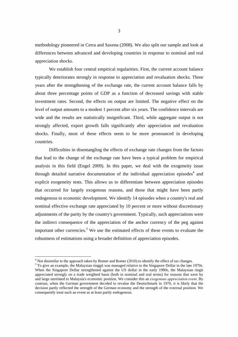
with the smaller set of indirect appreciation shocks. Figure 1 shows the impulse response

functions for all 25 appreciation events that we identified across all countries. A number

of interesting insights emerge from the estimated impulse responses.

16

Figure 1. Impulse responses: all countries, all events

Output

-1 0 1 2 3 4 5 6 7 8 9 10-0.05

-0.04

-0.03

-0.02

-0.01

0

0.01

0.02

0.03

Current account

-1 0 1 2 3 4 5 6 7 8 9 10-4

-3.5

-3

-2.5

-2

-1.5

-1

-0.5

0

Savings

-1 0 1 2 3 4 5 6 7 8 9 10-3.5

-3

-2.5

-2

-1.5

-1

-0.5

0

Investment

-1 0 1 2 3 4 5 6 7 8 9 10-1.5

-1

-0.5

0

0.5

1

1.5

2

Exports

-1 0 1 2 3 4 5 6 7 8 9 10-0.35

-0.3

-0.25

-0.2

-0.15

-0.1

-0.05

0

Imports

-1 0 1 2 3 4 5 6 7 8 9 10-0.25

-0.2

-0.15

-0.1

-0.05

0

0.05

0.1

First, the immediate output responses seem positive, i.e. output growth

accelerates, but they turn negative after about three years. After six years, the reduction in

output growth accumulates to an output loss of about one percent in levels. However,

wide confidence intervals imply that these losses are insignificant in statistical terms. In

17

light of the time span and possible margins of error, these results provide only weak

support for the idea that large appreciation shocks lead to pronounced output losses. By

contrast, the impact of appreciation events on the current account is much stronger. The

current account balance deteriorates persistently after an appreciation event. The biggest

effect materialises after three years when the current account balance (as ratio of GDP) is

almost three percentage points lower than before.

Does the deterioration of the current account balance reflect a fall in savings or an

increase in investment? The impulse response of the current account is a reflection of the

savings and investment responses which are shown in the lower part of figure 1. The

estimation yields an interesting picture. The sharp decline in the current account balance

after appreciation is a function of falling saving and increasing investment (at least in the

first years after the appreciation impulse). It is clear from the data that the impulse

response of savings dies out only slowly. Even after ten years aggregate saving remains

significantly below its pre-appreciation level. Investment first jumps after appreciation,

but turns negative after three years, thus compensating part of the longer-term savings

effect on the current account. From an econometric perspective, it is worth to mention

that the estimated responses of the current account, saving and investment are

considerably more precise than the estimated responses for output. They are also

statistically significant as the error bands are narrow and do not breach the zero line.

The reaction of (real) exports and imports diverges strongly post-appreciation. As

can be seen from the lowest panel in figure 1, imports are by and large unaffected by

appreciation, but export growth falls sharply in the first three years. The losses

accumulate to about 15% (relative to trend) in the first three years, but stabilise

afterwards. Correct interpretation of these level effects is crucial. They do not imply an

outright decline in the level of real exports, but a significant reduction relative to the pre-

event trend which results in a roughly 15% lower level after three years. Yet the strong

slowdown in export growth does not leave a strong imprint on overall output. Domestic

demand becomes the beacon of growth.

To summarise figure 1, the results provide evidence of a negative and significant

impact of appreciation events on the current account. This effect is due to the negative

reaction of domestic savings. Looking at this through the lenses of foreign trade

18

transactions, it becomes clear that export growth decelerates sharply while imports

remain by and large unaffected. However, these dynamics leave a lesser imprint on

overall output. The mean output response is negative for horizons above three years but

insignificant from a statistical point of view. Proponents of appreciation as a remedy for

global imbalances will take these results as supportive for their position. Large

appreciation shocks do not meaningfully reduce domestic investment or affect economic

growth but help rebalance the economy. Domestic absorption rises as a result of lower

savings. Whether the decline in savings reflects mainly a decline in corporate or

household savings, will be an interesting topic for further research.

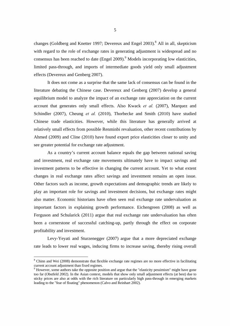
In Figure 2, we show the estimated impulse responses from our small sample of

indirect appreciations, i.e. nominal and real effective appreciations that resulted from an

appreciation of the anchor currency in the peg. Reassuringly, the results are very similar

so that our key finding seem robust to endogeneity concerns. Appreciation shocks lead to

a visible deterioration of the current balance, driven by a strong effect on savings. Export

growth decelerates sharply while imports perform relatively better. With regard to output,

the estimated effects are similar to those reported above for the broader sample of

appreciation events. The mean response of output shows a cumulative loss of about two

percent. While this effect seems permanent, it appears relatively small and statistically

not different from zero.

`

19

Figure 2. Impulse responses: all countries, indirect events only

Output

-1 0 1 2 3 4 5 6 7 8 9 10-0.08

-0.06

-0.04

-0.02

0

0.02

0.04

Current account

-1 0 1 2 3 4 5 6 7 8 9 10-4.5

-4

-3.5

-3

-2.5

-2

-1.5

-1

-0.5

0

Savings

-1 0 1 2 3 4 5 6 7 8 9 10-4.5

-4

-3.5

-3

-2.5

-2

-1.5

-1

-0.5

0

Investment

-1 0 1 2 3 4 5 6 7 8 9 10-1.5

-1

-0.5

0

0.5

1

1.5

2

2.5

3

Exports

-1 0 1 2 3 4 5 6 7 8 9 10-0.45

-0.4

-0.35

-0.3

-0.25

-0.2

-0.15

-0.1

-0.05

0

Imports

-1 0 1 2 3 4 5 6 7 8 9 10-0.3

-0.25

-0.2

-0.15

-0.1

-0.05

0

0.05

0.1

Table 3 summarizes the key results of our analysis showing the estimated mean

level effects in the first five years after appreciation and revaluation shocks for all

countries. Output levels are initially rising, but after five years the cumulated effect is

marginally negative (output levels are less than 1 percent lower relative to trend).

However, the current account deteriorates meaningfully (by about 2-3 pp. relative to

GDP), and export losses accumulate to close to 15% over 5 years. Investment is only

20

marginally affected, while savings fall by about 2.5 pp relative to GDP. If we restrict our

analysis to the smaller sample of indirect appreciation shocks, the results are very similar,

albeit the current account deterioration and the slowdown in export growth appear

somewhat more pronounced.

Table 3: Mean level effects after appreciation (all countries)Years after appreciation 1 2 3 4 5

Large sampleOutput 0.011** 0.014 0.004 -0.005 -0.009Current account/GDP -1.721** -2.284*** -2.929*** -2.548*** -1.876**Investment/GDP 0.618 1.373** 0.584 -0.175 -0.792Savings/GDP -1.050* -1.058 -2.222** -2.159** -2.512**Real exports -0.044*** -0.122*** -0.160** -0.145 -0.145Real imports -0.016 -0.033 -0.053 -0.078 -0.077

Small sampleOutput 0.019*** 0.022 0.007 -0.009 -0.015Current account/GDP -1.849 -2.947** -3.102** -2.771** -2.787**Investment/GDP 0.923 1.948*** 0.91 -0.041 -0.577Savings/GDP -1.101 -1.307 -2.832** -2.358* -2.912*Real exports -0.041 -0.162** -0.224* -0.204 -0.242Real imports -0.005 -0.023 -0.068 -0.119 -0.110

Note: cumulative log-level change for output, exports and imports. Percentage point change over GDP for current account, investment and savings,*,**,*** denotessignificance to the 90%, 95%, and 99% level.

5. Effects in Developing and Advanced Economies

In the next step of our empirical analysis, we split our sample in an attempt to

potentially uncover different dynamics for developing and developed countries.14 As

discussed above, a growing literature argues that the real exchange rate plays a central

role for the economic development of poor countries, e.g.. through positive externalities

from exports of manufactured goods. This sets developing countries apart from advanced

economies and calls for a disaggregated analysis. As above, we start with the broad event

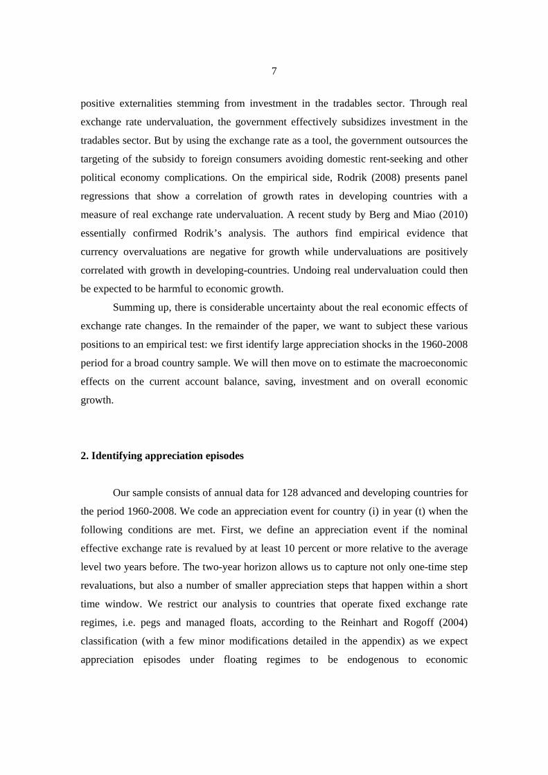
definition, but corroborate our results with the purely indirect appreciation episodes. For

developing countries (figure 3), the estimated event responses of the key variables are

qualitatively the same as for the entire sample: strong and significant current account

responses and an indeterminate impact on economic growth. What differs somewhat is

14 We classify all those countries as developing that had a PPP adjusted income of less than one third of the US level in the year 1980.

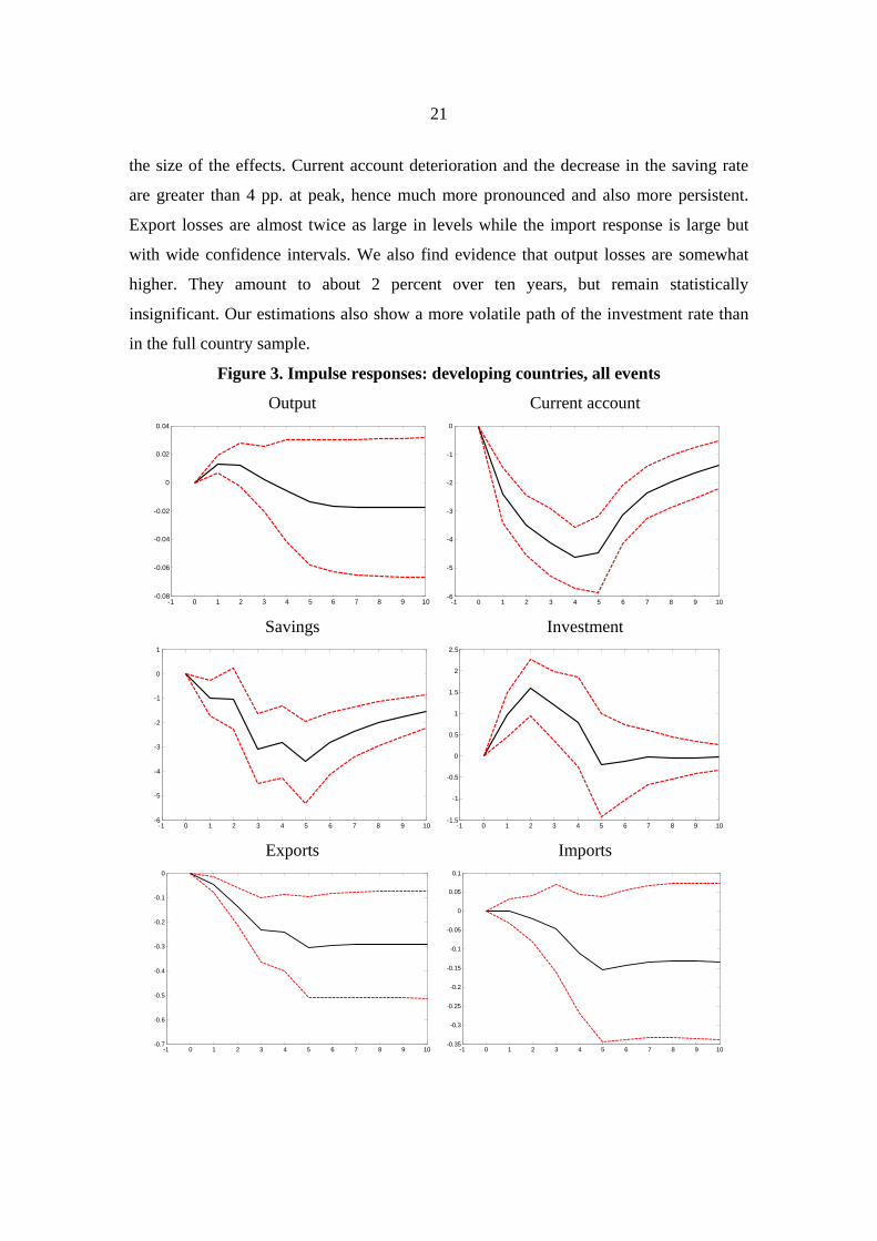
21

the size of the effects. Current account deterioration and the decrease in the saving rate

are greater than 4 pp. at peak, hence much more pronounced and also more persistent.

Export losses are almost twice as large in levels while the import response is large but

with wide confidence intervals. We also find evidence that output losses are somewhat

higher. They amount to about 2 percent over ten years, but remain statistically

insignificant. Our estimations also show a more volatile path of the investment rate than

in the full country sample.

Figure 3. Impulse responses: developing countries, all events

Output

-1 0 1 2 3 4 5 6 7 8 9 10-0.08

-0.06

-0.04

-0.02

0

0.02

0.04

Current account

-1 0 1 2 3 4 5 6 7 8 9 10-6

-5

-4

-3

-2

-1

0

Savings

-1 0 1 2 3 4 5 6 7 8 9 10-6

-5

-4

-3

-2

-1

0

1

Investment

-1 0 1 2 3 4 5 6 7 8 9 10-1.5

-1

-0.5

0

0.5

1

1.5

2

2.5

Exports

-1 0 1 2 3 4 5 6 7 8 9 10-0.7

-0.6

-0.5

-0.4

-0.3

-0.2

-0.1

0

Imports

-1 0 1 2 3 4 5 6 7 8 9 10-0.35

-0.3

-0.25

-0.2

-0.15

-0.1

-0.05

0

0.05

0.1

22

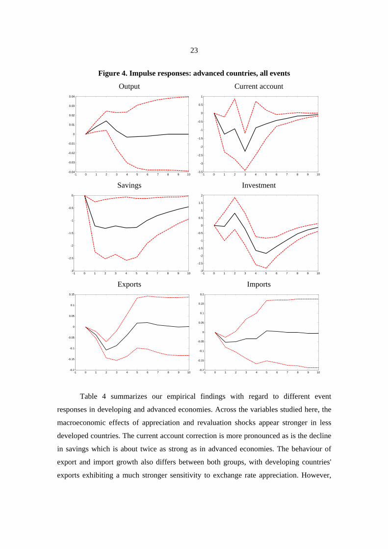
For advanced economies (figure 4), output effects of appreciation shocks are also

not significantly different from zero and the current account response is considerably

milder owing to a more short-lived impact on export growth. Large exchange rate

appreciations have only short (if any) effects on the external balance. Our estimations

show a significant response only at the three-year horizon. We find an interesting

difference here as the savings decline is actually more abrupt than in the developing

country sub-sample. But it goes hand in hand with a decline in investment so that the

overall savings-investment balance is not strongly affected. However, a smaller number

of observations in the advanced country sample lowers the precision of the estimated

coefficients and renders most impulse response functions insignificant.

All in all, we think that the evidence we find is sufficiently strong to justify the

idea that the macroeconomic effects of appreciation shocks differ between developed and

developing countries. The differential effects appear particularly pronounced with regard

to the external balance that deteriorates more persistently in developing countries. Export

growth takes a stronger hit in developing countries, but is counterbalanced by stronger

domestic growth. Also the growth response is different. While not statistically significant,

the point estimates suggest a stronger impact of appreciation on economic growth in

developing countries. The growth path of a typical advanced country is hardly affected by

appreciation. In developing countries, appreciation episodes lead to output losses more

often.

23

Figure 4. Impulse responses: advanced countries, all events

Output

-1 0 1 2 3 4 5 6 7 8 9 10-0.04

-0.03

-0.02

-0.01

0

0.01

0.02

0.03

0.04

Current account

-1 0 1 2 3 4 5 6 7 8 9 10-3.5

-3

-2.5

-2

-1.5

-1

-0.5

0

0.5

1

Savings

-1 0 1 2 3 4 5 6 7 8 9 10-3

-2.5

-2

-1.5

-1

-0.5

0

Investment

-1 0 1 2 3 4 5 6 7 8 9 10-3

-2.5

-2

-1.5

-1

-0.5

0

0.5

1

1.5

2

Exports

-1 0 1 2 3 4 5 6 7 8 9 10-0.2

-0.15

-0.1

-0.05

0

0.05

0.1

0.15

Imports

-1 0 1 2 3 4 5 6 7 8 9 10-0.2

-0.15

-0.1

-0.05

0

0.05

0.1

0.15

0.2

Table 4 summarizes our empirical findings with regard to different event

responses in developing and advanced economies. Across the variables studied here, the

macroeconomic effects of appreciation and revaluation shocks appear stronger in less

developed countries. The current account correction is more pronounced as is the decline

in savings which is about twice as strong as in advanced economies. The behaviour of

export and import growth also differs between both groups, with developing countries'

exports exhibiting a much stronger sensitivity to exchange rate appreciation. However,

24

according to our estimates here the investment dynamic remains by and large unaffected

and the output effects in developing countries remain small and statistically insignificant.

Overall, the previous conclusion that the economic effects of appreciation shocks are

somewhat stronger in developing countries is clearly confirmed.

Table 4: Mean level effects in developing and advanced economiesYears after appreciation 1 2 3 4 5

Advanced economiesOutput 0.007 0.014 0.003 -0.004 -0.003Current account/GDP -1.165 -0.939 -2.309* -0.827 -0.595Investment/GDP -0.094 0.787 -0.258 -1.712* -1.886**Savings/GDP -1.171 -1.255 -1.176 -1.228 -1.246Real exports -0.038*** -0.108*** -0.088 -0.042 0.016Real imports -0.052** -0.049 -0.031 -0.031 0.009

Developing economiesOutput 0.013* 0.012 0.002 -0.006 -0.014Current account/GDP -2.402** -3.398*** -4.045*** -4.56*** -4.422***Investment/GDP 0.965* 1.603** 1.272 0.769 -0.205Savings/GDP -0.999 -1.138 -3.161** -2.893* -3.668**Real exports -0.049 -0.137* -0.231* -0.247 -0.306Real imports -0.001 -0.020 -0.047 -0.113 -0.153

Note: cumulative log-level change for output, exports and imports. Percentage point change over GDP for current account, investment and savings,*,**,*** denotes significance to the 90%, 95%, and 99% level.

In a final step, we will again test the robustness of these results to a change in the

event definition. By limiting our analysis to events that did not involve discretionary

action by the authorities, we aim to get an idea about potential biases introduced by

endogeneity of the appreciation event. In brief, this robustness check does not lead to

materially different conclusions. In figures 5 and 6, we maintain the split of the sample

between developing and developed countries, but study the responses of growth and

external balances using the more parsimonious indirect event definition. The external

adjustment in response to large exchange rate appreciations appears again stronger in

developing countries where savings fall but investment remains by and large unaffected.

In advanced countries, the fall in savings is not only less pronounced, it is also

compensated by a parallel fall in investment which leaves the external balance

unaffected. As noted above, a similar difference between developing and advanced

countries can also be seen in the graph showing the output response. The confidence

25

bands remain wide so that these results have to be taken with caution, but our estimates

point to limited output losses in developing countries while appreciation has virtually no

impact on growth in advanced economies. All in all, these results confirm our previous

findings with regard to the macroeconomic effects of large appreciation shocks.

Figure 5. Impulse responses: developing countries, indirect events only

Output

-1 0 1 2 3 4 5 6 7 8 9 10-0.1

-0.08

-0.06

-0.04

-0.02

0

0.02

0.04

0.06

Current account

-1 0 1 2 3 4 5 6 7 8 9 10-8

-7

-6

-5

-4

-3

-2

-1

0

Savings

-1 0 1 2 3 4 5 6 7 8 9 10-7

-6

-5

-4

-3

-2

-1

0

1

Investment

-1 0 1 2 3 4 5 6 7 8 9 10-2

-1

0

1

2

3

4

Exports

-1 0 1 2 3 4 5 6 7 8 9 10-0.8

-0.7

-0.6

-0.5

-0.4

-0.3

-0.2

-0.1

0

0.1

Imports

-1 0 1 2 3 4 5 6 7 8 9 10-0.5

-0.4

-0.3

-0.2

-0.1

0

0.1

0.2

26

Figure 6. Impulse responses: advanced countries, indirect events only

Output

-1 0 1 2 3 4 5 6 7 8 9 10-0.05

-0.04

-0.03

-0.02

-0.01

0

0.01

0.02

0.03

0.04

Current account

-1 0 1 2 3 4 5 6 7 8 9 10-6

-4

-2

0

2

4

6

Savings

-1 0 1 2 3 4 5 6 7 8 9 10-4

-3

-2

-1

0

1

2

Investment

-1 0 1 2 3 4 5 6 7 8 9 10-3

-2.5

-2

-1.5

-1

-0.5

0

0.5

1

1.5

2

Exports

-1 0 1 2 3 4 5 6 7 8 9 10-0.2

-0.15

-0.1

-0.05

0

0.05

0.1

0.15

0.2

Imports

-1 0 1 2 3 4 5 6 7 8 9 10-0.25

-0.2

-0.15

-0.1

-0.05

0

0.05

0.1

0.15

0.2

5. Conclusion

The macroeconomic effects of exchange rate changes are likely to remain a

contentious issue in international economics. While the debate about global rebalancing

has gained traction after the financial crisis of 2008-09, the wisdom of using exchange

27

rates as an adjustment tool remains debated. This partly reflects long-standing

disagreement in the profession about the determinants of current account balances. Until

recently, scepticism with regard to the effects of (even large) exchange rate adjustment on

global current account balances has been widespread. Other recent contributions by

Ahmed (2009), and Cline (2010), however, have struck a little more optimistic tune

towards the effects of exchange rate changes.

In this paper, we have studied the empirical record of almost 50 years of

international economic history. Using data for 128 countries between 1960 and 2008, we

have found 25 episodes of large sustained exchange rate revaluations, which we define as

both nominal and real effective exchange rate appreciations of 10 percent (and more)

within a two year window (or less). Studying the institutional context of each individual

episode in detail, we identified 14 cases of appreciation shocks that occurred not as a

result of discretionary policy action, but were passively linked to the appreciation of the

anchor currency in the context of an exchange rate peg. We argue that these cases

represent instances of exogenous appreciation shocks that we can use to estimate the

macroeconomic impact of large appreciations and assess the robustness of estimates

based on a wider definition of appreciation and revaluation events. Using a dummy-

augmented autoregressive panel model we could indeed show that such large

appreciations episodes have strong macroeconomic effects. Most importantly, we

established four key stylized facts that can prove useful in the ongoing debate about the

role of exchange rate adjustment for global rebalancing.

First, the current account balance typically falls strongly in response to large

exchange rate revaluations. Three years after the revaluation, the current account balance

deteriorates by about 3 pp. relative to GDP. This is due to a reduction in aggregate

savings without a concomitant fall in investment. The effect on the current account

balance is statistically significant and robust to variation in the country sample and the

definition of appreciation events.

Second, the effects on output seem limited. Our point estimates suggest a negative

effect of output growth, albeit of relatively small magnitude: on average, the aggregate

level effect on output amounts to about 1 percent after six years. The confidence intervals

28

are also considerably wider than for the current account. The output effects are

statistically not significant.

Third, while aggregate output is not strongly affected, export growth falls

significantly after appreciation shocks. Import growth remains by and large unchanged

resulting in the observed deterioration in external balances. As aggregate economic

growth is much less affected, our results point to a positive domestic demand response

following appreciation episodes.

Fourth, these effects seem to be more pronounced in developing countries. The

sensitivity of the current account balance to revaluation shocks is higher. The effect

reaches almost 4 percentage points of GDP after three years and is statistically

significant. But also the potentially negative effects on output are larger. Our point

estimates point to a loss in output of 2 percent over ten years. But confidence intervals

remain wide, so that these results miss statistically significant levels. Why these effects

are stronger in developing countries will be an important question that we aim to address

in future research.

In sum, the historical record of large exchange rate revaluations that we have

studied in this paper lends some support to the idea that large exchange rate appreciations

and revaluations have an impact on the current account as they lead to marked changes of

savings and investment within countries. Appreciation shocks impact external balances,

but this effect potentially comes at the cost of a reduction of dynamism in exports. While

the domestic economy seems to pick up some of the external slack, leaving overall

growth relatively unaffected, the prospect of sharp decelerations in export growth will

remain a concern for policy-makers and bears watching especially in the context of

developing countries.

29

Appendix A: Impulse Responses with 90% Confidence Intervals

Figure 1a. Impulse responses: all countries, all events

Output

-1 0 1 2 3 4 5 6 7 8 9 10-0.08

-0.06

-0.04

-0.02

0

0.02

0.04

0.06

Current account

-1 0 1 2 3 4 5 6 7 8 9 10-4.5

-4

-3.5

-3

-2.5

-2

-1.5

-1

-0.5

0

Savings

-1 0 1 2 3 4 5 6 7 8 9 10-4.5

-4

-3.5

-3

-2.5

-2

-1.5

-1

-0.5

0

0.5

Investment

-1 0 1 2 3 4 5 6 7 8 9 10-2

-1.5

-1

-0.5

0

0.5

1

1.5

2

2.5

30

Figure 2a. Impulse responses: all countries, indirect events only

Output

-1 0 1 2 3 4 5 6 7 8 9 10-0.1

-0.08

-0.06

-0.04

-0.02

0

0.02

0.04

0.06

Current account

-1 0 1 2 3 4 5 6 7 8 9 10-6

-5

-4

-3

-2

-1

0

1

Savings

-1 0 1 2 3 4 5 6 7 8 9 10-6

-5

-4

-3

-2

-1

0

1

Investment

-1 0 1 2 3 4 5 6 7 8 9 10-3

-2

-1

0

1

2

3

31

Figure 3a. Impulse responses: developing countries, all events

Output

-1 0 1 2 3 4 5 6 7 8 9 10-0.1

-0.08

-0.06

-0.04

-0.02

0

0.02

0.04

0.06

0.08

Current account

-1 0 1 2 3 4 5 6 7 8 9 10-7

-6

-5

-4

-3

-2

-1

0

Savings

-1 0 1 2 3 4 5 6 7 8 9 10-7

-6

-5

-4

-3

-2

-1

0

1

2

Investment

-1 0 1 2 3 4 5 6 7 8 9 10-3

-2

-1

0

1

2

3

32

Figure 4a. Impulse responses: advanced countries, all events

Output

-1 0 1 2 3 4 5 6 7 8 9 10-0.08

-0.06

-0.04

-0.02

0

0.02

0.04

0.06

0.08

Current account

-1 0 1 2 3 4 5 6 7 8 9 10-5

-4

-3

-2

-1

0

1

2

Savings

-1 0 1 2 3 4 5 6 7 8 9 10-3.5

-3

-2.5

-2

-1.5

-1

-0.5

0

0.5

1

1.5

Investment

-1 0 1 2 3 4 5 6 7 8 9 10-4

-3

-2

-1

0

1

2

3

33

Figure 5a. Impulse responses: developing countries, indirect events only

Output

-1 0 1 2 3 4 5 6 7 8 9 10-0.15

-0.1

-0.05

0

0.05

0.1

Current account

-1 0 1 2 3 4 5 6 7 8 9 10-10

-8

-6

-4

-2

0

2

Savings

-1 0 1 2 3 4 5 6 7 8 9 10-8

-7

-6

-5

-4

-3

-2

-1

0

1

2

Investment

-1 0 1 2 3 4 5 6 7 8 9 10-3

-2

-1

0

1

2

3

4

34

Figure 6a. Impulse responses: advanced countries, indirect events only

Output

-1 0 1 2 3 4 5 6 7 8 9 10-0.08

-0.06

-0.04

-0.02

0

0.02

0.04

0.06

0.08

Current account

-1 0 1 2 3 4 5 6 7 8 9 10-8

-6

-4

-2

0

2

4

6

8

Savings

-1 0 1 2 3 4 5 6 7 8 9 10-5

-4

-3

-2

-1

0

1

2

3

Investment

-1 0 1 2 3 4 5 6 7 8 9 10-3

-2

-1

0

1

2

3

35

Appendix B: Regression Results

Table 1b. All countries, all events

CAGDP Coefficient Std. Error t-Statistic Prob.

C -1.018 0.245 -4.163 0.00 CAGDP(-1) 0.396 0.152 2.609 0.01 CAGDP(-2) 0.037 0.072 0.512 0.61 CAGDP(-3) 0.077 0.047 1.634 0.10 CAGDP(-4) 0.048 0.039 1.223 0.22

REVAL -1.740 0.755 -2.305 0.02 REVAL (-1) -1.567 0.778 -2.015 0.04 REVAL (-2) -1.945 0.760 -2.558 0.01 REVAL (-3) -1.202 0.696 -1.728 0.08 REVAL (-4) -0.546 0.683 -0.800 0.42

DY Coefficient Std. Error t-Statistic Prob.

C 0.013 0.001 11.973 0.00 DY(-1) 0.204 0.042 4.871 0.00 DY(-2) 0.062 0.022 2.856 0.00 DY(-3) 0.030 0.024 1.247 0.21 DY(-4) -0.049 0.023 -2.131 0.03

REVHAL 0.011 0.004 2.614 0.01 REVAL (-1) 0.001 0.005 0.092 0.93 REVAL (-2) -0.012 0.006 -1.983 0.05 REVAL (-3) -0.007 0.008 -0.931 0.35 REVAL (-4) -0.002 0.005 -0.332 0.74

INVGDP Coefficient Std. Error t-Statistic Prob.

C 5.719 0.548 10.428 0.00 INVGDP(-1) 0.734 0.052 14.020 0.00 INVGDP(-2) -0.022 0.065 -0.340 0.73 INVGDP(-3) 0.029 0.062 0.473 0.64 INVGDP(-4) 0.003 0.034 0.075 0.94

REVAL 0.629 0.438 1.436 0.15 REVAL(-1) 0.922 0.374 2.463 0.01 REVAL(-2) -0.435 0.549 -0.794 0.43 REVAL(-3) -0.569 0.578 -0.986 0.32 REVAL(-4) -0.704 0.525 -1.342 0.18

SAVGDP Coefficient Std. Error t-Statistic Prob.

C 3.255 0.575 5.660 0.00 SAVGDP(-1) 0.737 0.067 11.002 0.00 SAVGDP(-2) 0.043 0.056 0.770 0.44 SAVGDP(-3) 0.017 0.052 0.327 0.74 SAVGDP(-4) 0.029 0.036 0.807 0.42

REVAL -1.043 0.543 -1.919 0.06 REVAL (-1) -0.277 0.672 -0.413 0.68 REVAL (-2) -1.404 0.674 -2.083 0.04 REVAL (-3) -0.451 0.600 -0.751 0.45 REVAL (-4) -0.791 0.615 -1.286 0.20

36

Table 2b. All countries, indirect events only


C -1.034 0.246 -4.195 0.00 CAGDP(-1) 0.397 0.152 2.610 0.01 CAGDP(-2) 0.037 0.072 0.511 0.61 CAGDP(-3) 0.077 0.047 1.633 0.10 CAGDP(-4) 0.048 0.039 1.216 0.22

REVAL1 -1.802 1.288 -1.399 0.16 REVAL1(-1) -2.266 1.215 -1.865 0.06 REVAL1 (-2) -1.806 1.194 -1.513 0.13 REVAL1 (-3) -1.291 1.024 -1.261 0.21 REVAL1 (-4) -1.281 0.988 -1.297 0.19

EQ_DY Dep. Var: DY Variable Coefficient Std. Error t-Statistic Prob.

C 0.013 0.001 11.974 0.00 DY(-1) 0.204 0.042 4.869 0.00 DY(-2) 0.062 0.022 2.862 0.00 DY(-3) 0.030 0.024 1.249 0.21 DY(-4) -0.049 0.023 -2.134 0.03

REVAL1 0.020 0.006 3.499 0.00 REVAL1 (-1) -0.002 0.009 -0.201 0.84 REVAL1 (-2) -0.016 0.007 -2.270 0.02 REVAL1 (-3) -0.014 0.012 -1.161 0.25 REVAL1 (-4) -0.001 0.006 -0.174 0.86

EQ_INVGDP Dep. Var: INVGDP Variable Coefficient Std. Error t-Statistic Prob.

C 5.717 0.548 10.432 0.00 INVGDP(-1) 0.734 0.052 14.019 0.00 INVGDP(-2) -0.022 0.065 -0.338 0.74 INVGDP(-3) 0.029 0.062 0.473 0.64 INVGDP(-4) 0.002 0.034 0.070 0.94

REVAL1 0.896 0.596 1.504 0.13 REVAL1 (-1) 1.277 0.478 2.674 0.01 REVAL1 (-2) -0.503 0.705 -0.713 0.48 REVAL1 (-3) -0.742 0.820 -0.904 0.37 REVAL1 (-4) -0.571 0.617 -0.926 0.35

EQ_SAVGDP Dep. Var: SAVGDP Variable Coefficient Std. Error t-Statistic Prob.


REVAL1 -1.075 0.816 -1.316 0.19 REVAL1 (-1) -0.484 1.035 -0.468 0.64 REVAL1 (-2) -1.807 1.005 -1.798 0.07 REVAL1 (-3) -0.224 0.884 -0.254 0.80 REVAL1 (-4) -1.018 0.859 -1.185 0.24

37

Table 3b. Developing countries, all events


C -0.983 0.319 -3.079 0.00 CAGDP(-1) 0.634 0.060 10.555 0.00 CAGDP(-2) -0.041 0.059 -0.687 0.49 CAGDP(-3) 0.063 0.054 1.166 0.24 CAGDP(-4) 0.060 0.054 1.108 0.27

REVAL -2.426 1.002 -2.420 0.02 REVAL(-1) -1.907 0.800 -2.385 0.02 REVAL(-2) -2.000 0.913 -2.191 0.03 REVAL(-3) -1.998 0.724 -2.760 0.01 REVAL(-4) -1.305 1.104 -1.182 0.24


C 0.013 0.001 10.269 0.00 DY(-1) 0.173 0.044 3.959 0.00 DY(-2) 0.080 0.022 3.672 0.00 DY(-3) 0.045 0.026 1.754 0.08 DY(-4) -0.047 0.025 -1.835 0.07 REVAL 0.013 0.006 2.021 0.04

REVAL(-1) -0.003 0.009 -0.307 0.76 REVAL(-2) -0.011 0.008 -1.471 0.14 REVAL(-3) -0.007 0.012 -0.597 0.55 REVAL(-4) -0.005 0.008 -0.600 0.55


C 5.635 0.499 11.289 0.00 INVGDP(-1) 0.753 0.061 12.356 0.00 INVGDP(-2) -0.082 0.078 -1.053 0.29 INVGDP(-3) 0.081 0.071 1.136 0.26 INVGDP(-4) -0.009 0.037 -0.252 0.80

REVAL 0.969 0.517 1.875 0.06 REVAL(-1) 0.859 0.523 1.642 0.10 REVAL(-2) 0.117 0.705 0.167 0.87 REVAL(-3) -0.137 0.898 -0.153 0.88 REVAL(-4) -0.830 0.857 -0.968 0.33




38

Table 4b. Advanced countries, all events


C 0.378 0.315 1.201 0.23 CAGDP(-1) 0.247 0.127 1.942 0.05 CAGDP(-2) 0.027 0.068 0.402 0.69 CAGDP(-3) 0.074 0.054 1.364 0.17 CAGDP(-4) 0.051 0.051 1.007 0.31



C 0.016 0.002 6.825 0.00 DY(-1) 0.339 0.099 3.441 0.00 DY(-2) -0.046 0.070 -0.660 0.51 DY(-3) -0.040 0.066 -0.605 0.55 DY(-4) -0.064 0.053 -1.201 0.23 REVAL 0.007 0.005 1.385 0.17

REVAL(-1) 0.004 0.005 0.842 0.40 REVAL(-2) -0.013 0.008 -1.499 0.13 REVAL(-3) -0.003 0.007 -0.460 0.65 REVAL(-4) 0.003 0.006 0.527 0.60


C 8.717 2.278 3.826 0.00 INVGDP(-1) 0.640 0.108 5.934 0.00 INVGDP(-2) 0.132 0.093 1.423 0.15 INVGDP(-3) -0.116 0.087 -1.332 0.18 INVGDP(-4) -0.026 0.076 -0.348 0.73

REVAL -0.111 0.934 -0.119 0.91 REVAL(-1) 0.845 0.787 1.075 0.28 REVAL(-2) -0.755 0.761 -0.992 0.32 REVAL(-3) -1.636 0.643 -2.542 0.01 REVAL(-4) -0.672 0.749 -0.897 0.37


C 5.080 1.797 2.826 0.00 SAVGDP(-1) 0.712 0.184 3.871 0.00 SAVGDP(-2) 0.065 0.120 0.544 0.59 SAVGDP(-3) 0.032 0.088 0.367 0.71 SAVGDP(-4) -0.010 0.061 -0.160 0.87


39

Table 5b. Developing countries, indirect events only


C -0.998 0.319 -3.126 0.00 CAGDP(-1) 0.634 0.060 10.555 0.00 CAGDP(-2) -0.041 0.059 -0.693 0.49 CAGDP(-3) 0.064 0.054 1.170 0.24 CAGDP(-4) 0.059 0.054 1.094 0.27

REVAL1 -2.314 1.525 -1.518 0.13 REVAL1(-1) -2.538 1.193 -2.129 0.03 REVAL1(-2) -2.900 1.368 -2.119 0.03 REVAL1(-3) -2.558 1.014 -2.523 0.01 REVAL1(-4) -1.973 1.556 -1.268 0.21


C 0.013 0.001 10.258 0.00 DY(-1) 0.173 0.044 3.957 0.00 DY(-2) 0.080 0.022 3.683 0.00 DY(-3) 0.046 0.026 1.757 0.08 DY(-4) -0.047 0.025 -1.844 0.07

REVAL1 0.026 0.007 3.674 0.00 REVAL1(-1) -0.004 0.014 -0.247 0.81 REVAL1(-2) -0.027 0.010 -2.683 0.01 REVAL1(-3) -0.016 0.019 -0.852 0.39 REVAL1(-4) 0.002 0.009 0.186 0.85


C 5.637 0.499 11.292 0.00 INVGDP(-1) 0.753 0.061 12.355 0.00 INVGDP(-2) -0.082 0.078 -1.050 0.29 INVGDP(-3) 0.081 0.071 1.136 0.26 INVGDP(-4) -0.010 0.037 -0.262 0.79

REVAL1 1.338 0.671 1.993 0.05 REVAL1(-1) 1.284 0.715 1.796 0.07 REVAL1(-2) 0.021 1.040 0.021 0.98 REVAL1(-3) -0.538 1.287 -0.418 0.68 REVAL1(-4) -0.705 1.005 -0.702 0.48



REVAL1 -0.975 1.040 -0.938 0.35 REVAL1(-1) -0.750 1.595 -0.470 0.64 REVAL1(-2) -3.174 1.372 -2.313 0.02 REVAL1(-3) -0.419 1.313 -0.319 0.75 REVAL1(-4) -1.622 1.259 -1.289 0.20

40

Table 6b. Advanced countries, indirect events only


C 0.332 0.315 1.055 0.29 CAGDP(-1) 0.247 0.127 1.941 0.05 CAGDP(-2) 0.028 0.068 0.409 0.68 CAGDP(-3) 0.075 0.055 1.362 0.17 CAGDP(-4) 0.051 0.051 1.009 0.31

REVAL1 -1.092 1.681 -0.650 0.52 REVAL1(-1) -1.470 2.703 -0.544 0.59 REVAL1(-2) -0.569 1.190 -0.479 0.63 REVAL1(-3) 2.833 2.359 1.201 0.23 REVAL1(-4) 0.423 0.673 0.628 0.53


C 0.016 0.002 6.866 0.00 DY(-1) 0.339 0.098 3.445 0.00 DY(-2) -0.047 0.070 -0.670 0.50 DY(-3) -0.039 0.066 -0.586 0.56 DY(-4) -0.065 0.053 -1.211 0.23

REVAL1 0.008 0.005 1.618 0.11 REVAL1(-1) 0.001 0.007 0.104 0.92 REVAL1(-2) 0.003 0.007 0.477 0.63 REVAL1(-3) -0.011 0.010 -1.051 0.29 REVAL1(-4) -0.006 0.006 -0.909 0.36


C 8.687 2.279 3.813 0.00 INVGDP(-1) 0.640 0.108 5.939 0.00 INVGDP(-2) 0.132 0.093 1.418 0.16 INVGDP(-3) -0.116 0.087 -1.326 0.18 INVGDP(-4) -0.026 0.076 -0.347 0.73

REVAL1 -0.067 1.039 -0.064 0.95 REVAL1(-1) 0.986 0.702 1.405 0.16 REVAL1(-2) -0.506 0.618 -0.818 0.41 REVAL1(-3) -1.970 0.460 -4.285 0.00 REVAL1(-4) -0.358 0.572 -0.626 0.53


C 5.056 1.797 2.814 0.00 SAVGDP(-1) 0.712 0.184 3.870 0.00 SAVGDP(-2) 0.066 0.120 0.546 0.59 SAVGDP(-3) 0.033 0.088 0.370 0.71 SAVGDP(-4) -0.010 0.061 -0.165 0.87

REVAL1 -1.513 1.314 -1.151 0.25 REVAL1(-1) -0.736 1.112 -0.661 0.51 REVAL1(-2) 0.430 1.123 0.383 0.70 REVAL1(-3) 0.571 1.016 0.562 0.57 REVAL1(-4) -0.163 0.988 -0.165 0.87

41

Appendix C: Data Sources

1. Real GDP per capita in constant prices

Angus Maddison, The World Economy: Historical Statistics, OECD, Paris 2003. The

data can be found online at http://www.ggdc.net/maddison/

2. Current account balance (% of GDP)

Data are from the World Bank, World Development Indicators 2006, Washington DC.

Taiwanese data were obtained from the Key Indicators of Developing Asian and Pacific

Countries, published by the Asian Development Bank.

3. Gross national savings (% of GDP)

Calculated as current price gross national savings as a proportion of current price GDP.

Data are from International Monetary Fund (2009), World Economic Outlook Database,

Washington DC. For Taiwan, see above

4. Investment (% of GDP)

Calculated as current price investment as a proportion of current price GDP.

Data are from the International Monetary Fund, World Economic Outlook Database

(2009), Washington DC. Data are based on individual countries' national accounts

statistics. For Taiwan, see above

5. Nominal Effective Exchange Rate (NEER)

Data are from the International Monetary Fund, International Financial Statistics (2009),

Washington DC. We also used Bank for International Settlements estimates to extend the

sample from 1963, when data are available.

6. Real Effective Exchange Rate (REER)

Real effective exchange rate are based on relative consumer prices.

42

Data are from the International Monetary Fund, International Financial Statistics (2009),

Washington DC. We also used Bank for International Settlements estimates to extend the

sample from 1963, when data are available.

7. Exchange rate regime

We used the Reinhart-Rogoff (RR) classification of exchange rate regimes, updated by

Ilzetzki, Reinhart and Rogoff (2008). We used the fine RR classification, ranging de facto

exchange rate regimes from 1 to 15. For an index from 1 to 8, we classified the exchange

rate regime as pegged, and from 9 to 15, we classified it as floating. For each case, we

then described in greater details the appreciations, to identify episodes corresponding to

our definition. We also included a small number of episodes in the broad sample when

countries' managed their exchange rates tightly in a narrow band corresponding to

classification 9-11 on the RR scale.

The classification codes are the following:

1 No separate legal tender 2 Pre announced peg or currency board arrangement 3 Pre announced horizontal band that is narrower than or equal to +/-2% 4 De facto peg 5 Pre announced crawling peg 6 Pre announced crawling band that is narrower than or equal to +/-2% 7 De factor crawling peg 8 De facto crawling band that is narrower than or equal to +/-2% 9 Pre announced crawling band that is wider than or equal to +/-2%

10 De facto crawling band that is narrower than or equal to +/-5% 11 Moving band that is narrower than or equal to +/-2% 12 Managed floating 13 Freely floating 14 Freely falling 15 Dual market in which parallel market data is missing.

Source: Ilzetzki, Ethan O., Reinhart, Carmen, and Kenneth S. Rogoff (2008) “Exchange Rate Arrangements Entering the 21st Century: Which Anchor Will Hold?” available at: http://terpconnect.umd.edu/~creinhar/Papers.html

8. Real exports and imports

Data are from the World Bank, World Development Indicators 2006, Washington DC.

43

Taiwanese data were obtained from the Key Indicators of Developing Asian and Pacific

Countries, published by the Asian Development Bank.

44

References

Aizenman, Joshua and Jaewoo Lee (2008), “The Real Exchange Rate, Mercantilism and

the Learning by Doing Externality”, NBER Working Papers 13853, National Bureau of

Economic Research, Inc., Cambridge, MA.

Ahmed, Shaghil (2009), “Are Chinese Exports Sensitive to Changes in the Exchange

Rate?”, International Finance Discussion Paper No. 987 (December).

Berg, Andrew and Yanlang Miao (2010)‚ “The Real Exchange Rate and Growth

Revisited: The Washington Consensus Strikes Back?”, IMF Working Paper WP/10/58,

International Monetary Fund, Washington DC, March.

Bini Smaghi, Lorenzo (2008), “The financial crisis and global imbalances – two sides of

the same coin”, Speech by Mr Lorenzo Bini Smaghi, Member of the Executive Board of

the European Central Bank, at the Asia Europe Economic Forum conference “The Global

Financial Crisis: Policy choices in Asia and Europe”, Beijing, 9 December 2008.

Blanchard, Olivier and Gian M. Milesi-Ferretti (2009), “Global Imbalances: In

Midstream?”, IMF Staff Position Note, December 22, SPN/09/29, International Monetary

Fund, Washington D.C.

Bussière, Matthieu, Sweta C. Saxena and Camilo Tovar (2010), “Chronicle of currency

collapses: re-examining the effects on output”, BIS Working Papers 314, Bank for

International Settlements.

Caballero, Ricardo J. and Arvind Krishnamurthy (2009), “Global Imbalances and

Financial Fragility”, American Economic Review, American Economic Association, vol.

99(2), pages 584-88, May.

45

Calvo, Guillermo A., and Carmen M. Reinhart (2002), “Fear of Floating”, Quarterly

Journal of Economics, 117, 2002, pp. 379–408.

Campa, Jose M. and Linda S. Goldberg (1995), “Investment in manufacturing, exchange

rates and external exposure”, Journal of International Economics, Elsevier, vol. 38(3-4),

pages 297-320, May.

Campa, Jose M. and Linda S. Goldberg (1999), “Investment, Pass-Through, and

Exchange Rates: A Cross-Country Comparison”, International Economic Review,

Department of Economics, University of Pennsylvania and Osaka University Institute of

Social and Economic Research Association, vol. 40(2), pages 287-314, May. Available

at: http://www.nber.org/papers/w5139.pdf

Cerra, Valerie and Sweta C. Saxena (2008), “Growth Dynamics: The Myth of Economic

Recovery”, American Economic Review, American Economic Association, vol. 98(1),

pages 439-57, March.

Cheung Yin-Wong, Menzie D. Chinn and Eiji Fujii (2010), “China's Current and

Account and Exchange Rate”, in China's Growing Role in World Trade, co-edited by

Robert Feenstra and Shang-Jin Wei, pages 231-271, National Bureau of Economic

Research, Inc.

Chinn, Menzie D. (2004), “Incomes, Exchange Rates and the U.S. Trade Deficit, Once

Again”, International Finance 7 (3): 451–69.

Chinn, Menzie D. and Jaewoo Lee (2009), “Three Current Account Balances: A ‘Semi-

Structuralist’ Interpretation”, Japan and the World Economy 21 (2):202–12.

Chinn, Menzie D. and Shang-Jin Wei (2008), “A faith-based Initiative: Does a Flexible

Exchange Rate Regime Really Facilitate Current Account Adjustment?”, NBER Working

Paper 14420, National Bureau of Economic Research, Inc., Cambridge, MA.

46

Cline, William R. (2010), “Renminbi Undervaluation, China’s Surplus, and the US Trade

Deficit”, Policy Brief 10-20, Peterson Institute, Washington DC.

Cline, William R. and John Williamson (2007), “Estimates of the Equilibrium Exchange

Rate of the Renminbi: Is There a Consensus and, If Not, Why Not?”, Paper presented at

the Conference on China's Exchange Rate Policy (October 12, 2007), Peterson Institute,

Washington DC.

Corden, Warner M. and James P. Neary (1982), “Booming Sector and De-

industrialisation in a Small Open Economy”, The Economic Journal, Vol. 92 (December):

825–848.

Devereux, Michael B., and Charles Engel (2003), “Monetary Policy in the Open

Economy Revisited: Price Setting and Exchange-Rate Flexibility”, Review of Economic

Studies 70 (4): 765–83.

Devereux, Michael B., and Hans Genberg (2007), “Currency Appreciation and Current

Account Adjustment”, Journal of International Money and Finance 26 (4): 570–86.

Dooley, Michael P., David Folkerts-Landau and Peter Garber (2003), “An Essay on the

Revived Bretton-Woods System”, NBER Working Paper No. 9971, September. , National

Bureau of Economic Research, Inc., Cambridge, MA.

Dooley, Michael P., David Folkerts-Landau and Peter Garber (2009), “Bretton Woods II

Still Defines The International Monetary System”, Pacific Economic Review, Blackwell

Publishing, vol. 14(3), pages 297-311, 08.

Edward, Sebastian (1986), “Are Devaluations Contractionary?”, The Review of

Economics and Statistics, MIT Press, vol. 68(3), pages 501-08, August.

47

Eichengreen, Barry (2008), “The Real Exchange Rate and Economic Growth”,

Commission on Growth and Development Working Paper No.4.

Eichengreen, Barry and Mariko Hatase (2007), “Can a Rapidly-Growing Export-Oriented

Economy Smoothly Exit a Peg? Lessons for China from Japan's High Growth Era”,

Explorations in Economic History 44 (3), pp. 501-521.

Eichengreen, Barry and Andrew K. Rose (2010), “How will the new exchange rate

regime affect the Chinese economy”, VoxEu.org, June 21.

Engel, Charles (2009), “Exchange rate policies”, Staff Papers, Federal Reserve Bank of

Dallas, issue Nov. Published as: “Exchange rate policies”, BIS Papers chapters, in: Bank

for International Settlements (ed.), The international financial crisis and policy

challenges in Asia and the Pacific, volume 52, pages 229-250 Bank for International

Settlements.

Feldstein, Martin (2008), “Resolving the Global Imbalances: The Dollar and the US

Savings Rate”, Journal of Economic Perspectives, 22/3, 113-125.

Ferguson, Niall and Moritz Schularick (2011), “The End of Chimerica”, International

Finance, Vol. 14(1).

Gala, Paulo (2008), “Real Exchange Rate Levels and Economic Development”,

Cambridge Journal of Economics, 2008 32(2): 273-288.

Garroway, Chris, Burcu Hacibedel Helmut Reisen and Edouard Turkisch (2010), “The

Renminbi and Poor Country Growth”, OECD Development Centre Working Paper,

No.292, forthcoming, The World Economy 2011.

48

Goldberg, Pinelopi K. and Michael M. Knetter (1997), “Goods Prices and Exchange

Rates: What Have We Learned?”, Journal of Economic Literature, American Economic

Association, vol. 35(3), pages 1243-1272, September.

Goldfajn, Ilan and Rodrigo Valdés (1999), “The Aftermath of Appreciations”, Quarterly

Journal of Economics.

Goldstein, Morris (2006), “Renminbi Controversies”, Cato Journal, Vol. 26, No.2, 251-

265.

Gupta, Poonam, Deepak Mishra and Ratna Sahay (2007), “Behavior of output during

currency crises”, Journal of International Economics, Vol. 72, pp. 428-450.

Hong, Kiseok and Aaron Tornell (2005), “Recovery from a currency crisis: some stylized

facts”, Journal of Development Economics, Vol. 76, pp. 71-96.

Hooper, Peter, Karen Johnson, and Jaime Marquez (2000), “Trade Elasticities for G-7

Countries”, Princeton Studies in International Economics, no. 87 (Princeton, N.J.:

International Economics Section, Department of Economics, Princeton University,

August).

Korinek, Anton and Luis Serven (2010), “Undervaluation through foreign reserve

accumulation: static losses, dynamic gains”, Policy Research Working Paper Series 5250,

The World Bank.

Krugman, Paul R. and Lance Taylor (1978), “Contractionary effects of devaluation”,

Journal of International Economics, Elsevier, vol. 8(3), pages 445-456, August.

Kwack, Sung Y., Choong Y. Ahn, Young S. Lee and Doo Y. Yang (2007), “Consistent

Estimates of World Trade Elasticities and an Application to the Effects of Chinese Yuan

(RMB) Appreciation”, Journal of Asian Economics 18: 314–330.

49

Levy-Yeyati, Eduardo and Federico Sturzenegger (2007), “Fear of Appreciation”, World

Bank Policy Research Working Paper 4387.

Marquez, Jaime and John W. Schindler (2007), “Exchange-Rate Effects on China’s

Trade”, Review of International Economics 15(5), 837–853.

McKinnon, Ronald (2007), “Why China Should Keep Its Exchange Rate Pegged to the

Dollar: A Historical Perspective from Japan”, International Finance, March.

Montiel, Peter J. (2000), “What Drives Consumption Booms?”, The World Bank

Economic Review, Vol. 14, No. 3: 457-80.

Montiel, Peter J. and Luis Servén (2009), “Real Exchange Rates, Saving, and Growth: Is

There a Link?”, Commission on growth and development, Working Paper No.46.

Nucci, Francesco and Alberto F. Pozzolo (2001), “Investment and the Exchange Rate: an

Analysis with Firm-Level Panel Data”, European Economic Review, Volume 45,

February, 259-283.

Obstfeld, Maurice (2002), “Exchange Rates and Adjustment: Perspectives from the New

Open- Economy Macroeconomics”, Monetary and Economic Studies, Institute for

Monetary and Economic Studies, Bank of Japan, vol. 20(S1), pages 23-46, December.

Obstfeld, Maurice (2004), “The Unsustainable US Current Account Position Revisited”,

NBER Working Paper 10869, November, National Bureau of Economic Research, Inc.,

Cambridge, MA.

Obstfeld, Maurice and Kenneth S. Rogoff (2005), “Global Current Account Imbalances

and Exchange Rate Adjustments”, Brookings Papers on Economic Activity 1, pp. 67–146.

50

Obstfeld, Maurice and Kenneth S. Rogoff (2009), “Global Imbalances and the Financial

Crisis: Products of Common Causes”, CEPR Discussion Papers 7606, C.E.P.R.

Discussion Papers.

Qiao, Hong H. (2007), “Exchange Rates and Trade Balances Under the Dollar Standard”,

Journal of Policy Modeling, 29, pp. 765-82.

Reinhart, Carmen and Kenneth S. Rogoff (2004), “The Modern History of Exchange

Rate Arrangements: A Reinterpretation”, Quarterly Journal of Economics, 119(1):1-48.

Rodrik, Dani (2008), “The Real Exchange Rate and Economic Growth”, Working Paper,

October 2008.

Romer, David and Christina D. Romer (2010), “The Macroeconomic Effects of Tax

Changes: Estimates Based on a New Measure of Fiscal Shocks”, American Economic

Review, June.

Rose, Andrew K. and Janet Yellen (1989), “Is There a J-curve?”, Journal of Monetary

Economics 24 (1): 53–68.

Shi, Jianhuai (2006), “Are Currency Appreciations Contractionary in China?”, NBER

Working Papers 12551, National Bureau of Economic Research, Inc., Cambridge, MA.

Subramanian, Arvind (2010), “New PPP-Based Estimates of Renminbi Undervaluation

and Policy Implications”, Peterson Institute for International Economics, Policy Brief,

PB10-08.

Thorbecke, Willem and Gordon Smith (2010), “How Would an Appreciation of the

Renminbi and Other East Asian Currencies Affect China's Exports?”, Review of

International Economics, Blackwell Publishing, vol. 18(1), pages 95-108, 02.

51

Wolf, Martin (2009), Fixing Global Finance, New Haven, Yale University Press.

The Macroeconomic Effects of Large Exchange Rate Appreciations

Documents

Transcript of The Macroeconomic Effects of Large Exchange Rate Appreciations