Modeling Exchange Rate and Nigerian Deposit Money Market ...

Modeling Exchange Rate and Nigerian Deposit Money Market Dynamics Using Trivariate

Form of Multivariate GARCH Model

Abstract

The risks associated with exchange rate and money markets rate have drawn the attentions of econometricians, researchers, statisticians, and even investors in deposit money banks in Nigeria. The study targeted modeling exchange rate and Nigerian deposit banks money market dynamics using trivariate form of multivariate GARCH model. Data for the period spanning from 1991 to 2017on exchange rate (Naira/Dollar) and money market indicators (Maximum and prime lending rate) were sourced from the central bank of Nigeria (CBN) online statistical database. The study specifically investigated; the dynamics of the variance and covariance of volatility returns between exchange rate and money market indicators in Nigeria, examine whether there was a linkage in terms of returns and volatility transmission between exchange rate and money market indicators in Nigeria and compared the difference between Multivariate BEKK GARCH with restrictive indefinite under the assumption of normality and that of student’s –t error distribution. Preliminary time series checks were done on the data and the results revealed the present of volatility clustering. Results reveal the estimate of the maximum lag for exchange rate and money market indicators were 4 respectively. Also, the results confirmed that there wre two cointegrating equations in the relationship between the returns on exchange rate and money market indicators. The results of the diagonal MGARCH –BEKK estimation confirmed that diagonal MGARCH –BEKK in students’-t was the best fitted and an appropriate model for modeling exchange rate and Nigerian deposit money market dynamics using trivariate form of multivariate GARCH model. Also, the presence of two directional volatility spillovers between the two sets of variables was confirmed. Key words: Exchange Rate, Money, Market, Dynamics, Trivariate, GARCH , Model

INTRODUCTION

1.1 Background to the Study

In Nigerian and the world at large Exchange rate is consider as one of the strongest indicator and

instrument used in evaluating economic performance of a nation. Jhingan,(2005), once refers to

exchange rate as the amount at which a country’s currency exchange for another. In another

separate view, tt is also referred to as the price of one country’s currency with respect to another

country’s currency (Da-wariboko and Essi, 2018). They further opined that a very strong exchange

rate is an indication of a viable and strong economy. On the contrary, a very weak currency is an

evidence of a very weak economy. Although, it depreciates in measure when the amount of money

required to purchase a foreign currency increases, on the other hand, it will appreciate if the amount

of local currency required to purchase a foreign currency reduces.

Also, when we talk about money market it appears to our mind that we are referring to shops,

outlets, stalls, hawkers and other newly developed markets refers to as malls. Although, all these

are crucial parts of what constitutes market but when we talk about Money Market, we are referring

to financial markets (deposit money banks) that provide quick liquidity for short term financial need

that is helpful in meeting the urgent and immediate obligations in the economy. It is a type of

markets that aids all form of business transactions such as purchase and sales of funds on short term

bases and it is controlled by central banks. According to Anayaele(2012), Some of the examples of

institutions in money markets and their respective indicators include; commercial Banks, central

banks, discount houses, insurance companies, acceptance and financial houses and some of the

indicators used in this markets are treasury bills, call money funds, Bill of exchange interest rate,

Saving rate, maximum lending and prime lending rate etc (Anayaele,2012).

According to Anayaele(2012), the greatest advantage of this markets is that it enables investors to

meet up with their short-term financial need and funds invested in the markets can be recalled at

short notice for purposes. According to Lyndon and peter (2017), the money market plays an

important role in the mobilization of financial resources for long term investment through financial

intermediation. Meanwhile , Mohammed (2009) observed that the existence of money markets

facilitate trading in short-term debt instruments to meet short-term needs of large users of funds

such as government, banks and similar institutions.

Also, Oghenekaro (2013) revealed that the money market is mainly for the easily distribution of

liquidity in the financial system, allocation of capital as well as the hedging of short-term risks. It is

essentially an intermediary, where short-term financial assets that are near substitute for money are

usually traded (Lyndon & peter, 2017). According to Lyndon and peter(2017), the money market

in Nigeria is not yet vibrant and developed. They further opined that the reason why the market is

not yet vibrant and developed could be attributed to liquidity problems currently facing the

institution. In another development, they observed that the market is largely dominated by

government instruments such as treasury bills and bonds that has created wide gap for deposit and

lending rates that leads to very high cost of borrowing when observed.

However, the exchange rate and money market are two different markets both in terms liquidity and

transactional stability among others. Although, both markets are critical to the development of the

economy and there is need to examine the relationship that exist between them. Also, there is need

to examine the interdependencies of these markets, the shocks spillover and co-movement and their

cross-market linkages. Although, several studies have attempt to examine the relationship between

these markets, for example Lyndon and peter(2017) examined the relationship between money

market and economic growth in Nigeria. Ogunbiyi, samuel1, Ihejirika, and Peters (2014), examine

interest rates and deposit money banks’ profitability nexus: the Nigerian experience with the target

of knowing how interest rates affect the profitability of deposit money banks in Nigeria. Similarly,

Agbada and Odejimi (2015) investigated the developments in money market operations and

economic viability in Nigeria for the period 1981 – 2011, using multiple regression techniques for

data analysis. Also, Tasi’u,Yakubu , and Gulumbe (2014), exchange rate volatility of Nigerian naira

against some major currencies in the world: an application of multivariate GARCH models. In

another development, Afees, Salisu and Kazeem (2015),developed spillovers model between stock

market and money market in Nigeria using VARMA-AMGARCH1 models by McAleer et al.

(2009). However, A wealth of literature existing in this area focus on the relationship between the

two markets , while the only one that considered shocks spillover did not account for the underlying

Multivariate GARCH error distribution assumptions. Also, basically most of the literature existing

in this area deals with bivarate Multivariate GARCH modeling. Therefore, the research study seeks

to fill this gap in literature by adopting trivariate Bekk form of multivariate GARCH with specific

error distribution assumption. This study will serve as yardstick for market control, determination

and established an idea s in terms of Value at risks determination.

1.2 Statement of the problem

The risk associated with exchange rate market is one of the major challenges facing developing

countries in the world. One central aspect of it, is its volatility and its associated effects on other

micro and macroeconomic indicators. According to Deebom and Essi (2017), the difficulties

encountered in major international markets are shocks caused by the interplay of demand and

supply while the external demand shocks arise from the economic difficulties encountered by the

marketers and countries major trading partners.

In order to measure this behavior and other volatility conditions, the GARCH family models were

introduced (Deebom & Essi, 2017). However, there are still existing problems and one of the major

weaknesses was the inability of the Univariate GARCH to capture the dynamics process for time-

varying variance-covariance matrix of times series data as well as jointly modeling of the first and

second order conditional moment of time series data. This led to the introduction and use of the

multivariate GARCH Model in modeling such condition. One of the advantages of this is that it

helps in measuring covariance and correlation between two markets directly. Yet, it has its own

weaknesses like in the case of VEC-GARCH model, there is no guarantee of a positive semi-

definite covariance matrix (De Goeij et al,2004). It is against this background that this study used

Multivariate BEKK GARCH with restrictive indefinite under the assumption of normality and

student’s –t error distribution. This will in away provide for positive definiteness and measure

dynamic dependence between the volatility series.

1.3 Aim and objectives of the study

This study model exchange rate and Nigerian deposit money market indicators dynamics using

trivariate form of multivariate GARCH model, while the specific objectives were to :

1. Investigate the dynamics of the variance and covariance of volatility returns between

exchange rate and money market indicators in Nigeria

2. Examine whether there is a linkage in terms of returns and volatility transmission between

exchange rate and money market indicators in Nigeria

3. Compare the difference between Multivariate BEKK GARCH with restrictive indefinite

under the assumption of normality and that of student’s –t error distribution

2.0 Literature Review

The following studies were review; Shamiri and Isa (2009) examine the multivariate GARCH

model with BEKK representation to test the transfer of volatility in the financial crisis of 2007 to

the stock markets of Southeast Asia. They found a spillover effect of the volatility from US to

Asian countries.

Similarly, Bensafta and Semodo (2011) introduce breaks in variance in a multivariate GARCH to

analyze contagion during crises. Authors emphasize that the bias correction of heteroscedasticity

conditional correlation allows saying that crises are not always contagious for confirming results

found by Forbes and Rigobon (2002).

Serpil and Mesut (2013), examines BEKK-MGARCH model approach to generate the conditional

variances of monthly stock exchange prices, exchange rates and interest rates for Turkey. The

study used a sample period 2002:M1-2009:M1, and was done before the effects of global economic

crisis knock Turkey and the result obtained indicates a significant transmission of shocks and

volatility among the three financial sectors.

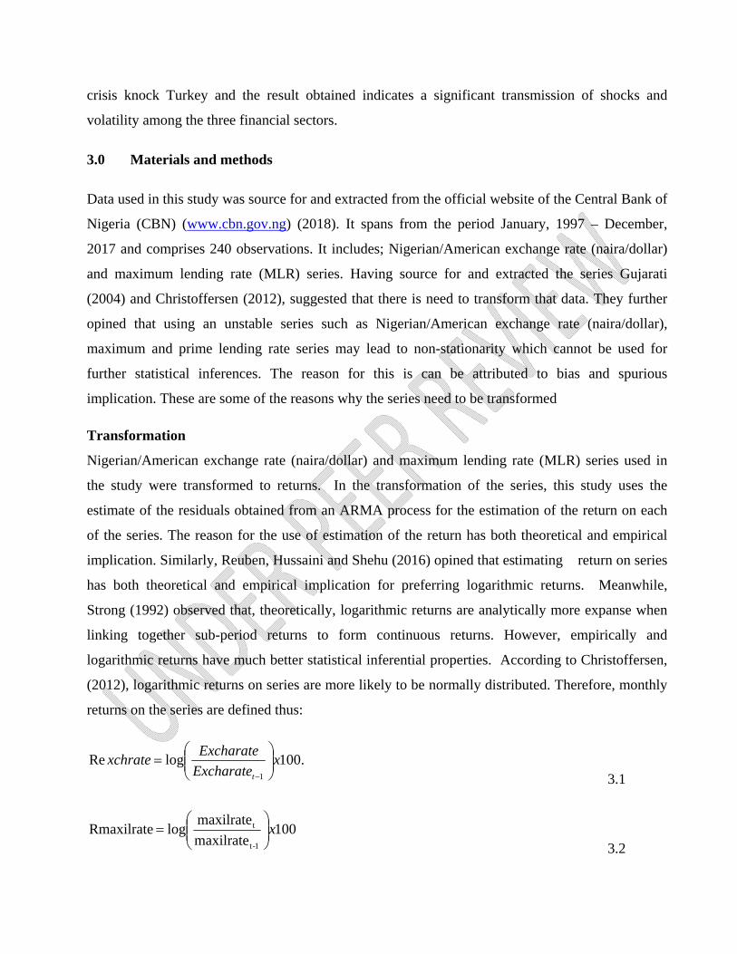
3.0 Materials and methods

Data used in this study was source for and extracted from the official website of the Central Bank of

Nigeria (CBN) (www.cbn.gov.ng) (2018). It spans from the period January, 1997 – December,

2017 and comprises 240 observations. It includes; Nigerian/American exchange rate (naira/dollar)

and maximum lending rate (MLR) series. Having source for and extracted the series Gujarati

(2004) and Christoffersen (2012), suggested that there is need to transform that data. They further

opined that using an unstable series such as Nigerian/American exchange rate (naira/dollar),

maximum and prime lending rate series may lead to non-stationarity which cannot be used for

further statistical inferences. The reason for this is can be attributed to bias and spurious

implication. These are some of the reasons why the series need to be transformed

Transformation

Nigerian/American exchange rate (naira/dollar) and maximum lending rate (MLR) series used in

the study were transformed to returns. In the transformation of the series, this study uses the

estimate of the residuals obtained from an ARMA process for the estimation of the return on each

of the series. The reason for the use of estimation of the return has both theoretical and empirical

implication. Similarly, Reuben, Hussaini and Shehu (2016) opined that estimating return on series

has both theoretical and empirical implication for preferring logarithmic returns. Meanwhile,

Strong (1992) observed that, theoretically, logarithmic returns are analytically more expanse when

linking together sub-period returns to form continuous returns. However, empirically and

logarithmic returns have much better statistical inferential properties. According to Christoffersen,

(2012), logarithmic returns on series are more likely to be normally distributed. Therefore, monthly

returns on the series are defined thus:

.100logRe1

xExcharate

Excharatexchrate

t

3.1

100maxilrate

maxilratelogRmaxilrate

1-t

t x

3.2

100Plrate

PlratelogRPrlrate

1-t

t x

3.3

For t = 1, 2, ….t-j where RExcharatet is exchange rate return at time t, R tmaxilrate is Return on

Maximum lending rate at time t and RPLrate is return on Prime lending rate at “t” . Similarly,

Excharatet-1 represents exchange rate at time “t-1’’ , 1-tMaxilrate represents maximum lending

rate at time “t-1’’ and RPLratet-1 represents return on Prime lending rate at time “t-1’’. The

transformation of above is the monthly returns on the variables used in the study, It helps us to

ensure that variable are well differenced (D) to get rid of outlier and it is also useful in obtaining

stationarity of the data.

3.1 Model Specification

Multivariate BEKK-GARCH(1,1) model specification, the BEKK – GARCH Model is simply an

acronym BEKK representing Baba, Engle, Kraft and Kroner, which was a preliminary version of

Engle and Kroner (1995) and was stated that for a single series, the volatility pattern follow

univariate specification of GARCH model of the form:

qtqtptptt hbhbaach ............. 1122

110 (3.4)

Where and q are order of the GARCH Model. This can be generalized in the form

Ht = 01CCo +

k

k 1

q

iikctH

1

1ik (3.5)

Where C, Aik and ik are (NxN) matrix, 01CCo is the intercept of the matrix in a dew posed form,

where C is a lower triangular matrix and it is positive semi definite.

For BEKK (1, 1), it is represented as thus:

tH = 11111111

111110

1 BHBAACC ttto (3.6)

Where, Ai and B1 are nxn parameter matrix and Co is nxn upper triangular matrix. Then, the

Bivariate BEKK (1,1) model can be written as;

Ht= 01CCo

+

2221

1211

a

a

a

a

2121112

12112

1

ttt

ttit

1

2221

1211

a

a

a

a+

2221

1211

b

b

b

b

221- t21

11211

h

h

h

h t

1

2221

1211

b

b

b

b (3.7)

The off diagonal parameter in matrix B, B12 and B21 respectively estimated as the independence of

conditional volatility of the returns on exchange rate and money market rate series. The b11 and b22

represents persistence in one set of variable of the returns on exchange rate and money market rate

series. Similarly, the parameter a12 or a21 represents the cross variable effects. Conversely, a11 and

a22 represents the returns own effects. This specification is applied in several bivariate GARCH

empirical studies. it ensures that the variance-covariance matrix is positive. However, the number of

parameters to estimate for the variance-covariance matrix is very high. It is of the order of

222

)1(N

NN

: 164 parameters to be estimated for 3variables.

Most studies using a multivariate GARCH specification to limit the number of studied assets and /

or impose restrictions on the process generating Ht. Bollerslev (1990) and Ng (1991) assume that

correlations are constant. Bollerslev, Engle and Wooldridge (1988) require diagonality condition

matrices A and B. This implies that the variances of Ht depend only on the square past residuals

and an autoregressive term. Covariances depend on the cross product past residuals and an

autoregressive term. This specification also seems very restrictive because does not take into

account the dependence of conditional volatilities between markets evidenced particularly by

Hamao Masulis and Ng (1990) and Chan, Karolyi and Stulez (1992) on data with high frequencies.

Engle and Ng (1993), Glosten, Jagannathan and Runkle (1993) and Kroner and Ng (1998) found

that, in most cases, the effect of a negative shock to the conditional variance is greater than that of a

positive shock. This adopted an extension to MGARCH BEKK model specification in order to

capture the asymmetric responses of conditional variances and covariance of the return series as

it is recommended in Samar and Khoufi (2016) and it was stated as thus:

: TTSXBHBAACCH tttttttt1

1111

111

111

1111

3.8

Where S and T are two size matrices (N×N) such as:

ititit I where itI = 1 if it < 0 and 0 otherwise

ititit I where itI = 1 if it > iith and 0 otherwise

For the reasons already mentioned, we impose the condition of diagonality for S and T matrices.

However, the the transformed trivariate Diagonal BEKK–GARCH Specification (Eviews)

Estimation Command for restrictive indefinite in specific error distributional assumption could

stated as thus : ARCH(TDIST) @DIAGVECH C(INDEF)ARCH(1,INDEF) GARCH(1,INDEF)

Estimated Equations:

REXCHRATE = C(1) 3.9

RMLRATE = C(2) 3.10

RPLRATE = C(3) 3.11

The transformed Variance-Covariance Representation:

GARCH = M + A1.*RESID(-1)*RESID(-1)' + B1.*GARCH(-1) 3.12

Variance and Covariance Equations:

GARCH1 = M(1,1) + A1(1,1)*RESID1(-1)^2 + B1(1,1)*GARCH1(-1) 3.13



COV1_2 = M(1,2) + A1(1,2)*RESID1(-1)*RESID2(-1) + B1(1,2)*COV1_2(-1) 3.16



Similarly, for simple analysis, understanding and representation the restricted indefinite trivariate

GARCH BEKK model in specific error distribution assumption above can be represented in

generic form as thus :

Mean component

REXCHRATE = C(1) 3.19

RMLRATE = C(2) 3.20

RPLRATE = C(3) 3.21

The transformed Variance-Covariance Representation

3.21

1,32

1,32

1,2,23

1,32

1,32

1,1,13

1,22

1,22

1,1,12

1,2222

1,22

,33

1,2222

1,22

,22

1,1122

1,12

,11

ˆ)3,3(1*)2,2(1*)3,3(1*)2,2(1)3,2(ˆ

ˆ)3,3(1*)1,1(1*)3,3(1*)1,1(1)3,1(ˆ

ˆ)2,2(1*)1,1(1*)2,2(1*)1,1(1)2,1(ˆ

)3,3(1)3,3(1)3,3(ˆ

)2,2(1)2,2(1)2,2(ˆ

)1,1(1)1,1(1)1,1(ˆ

tttt

tttt

tttt

ttt

ttt

ttt

BBAAM

BBAAM

BBAAM

BAM

BAM

BAM

Model Estimation Procedure

i. Time plot for the raw data

ii. Time plot on the transformation of the return series

iii. Descriptive Test Statistic for Normality Test on the estimated return series

The normality test is carried out using the Jarque-Bera test statistics. According to (Chinyere,

Dickko & Isah, 2015) Jargue-Bera is defined as joint test of skewness and kurtosis that examine

whether data series exhibit normal distribution or not; and this test statistic was developed by

Jargue and Bera (1980). It is defined as;

4

3

6

222

~

KS

NX (3.23)

Where S represents Skewness, K represents Kurtosis and N represents the size of the

macroeconomic variables used. The test statistic under the Null hypothesis of a normal distribution

has a degree of freedom 2. When a distribution does not obey the normality test, Abdulkarem et al,

(2017) suggested that the alternative inferential statistic was to use GARCH with its error

distribution assumptions with fixed degree of freedom.

(iii) Test for Co-integration

There is need to identify the co-integrating relationship between the two variables series and the

two likelihood ratio tests to be used are the Trace and Max respectively.

i

n

1r t Trace - 1 T - In

(3.24)

For i = 0, 1……………….n -1

1)r - (1In TMax (3.25)

Where n is the number of usable observations and i are the estimated eigen values otherwise

refers to as characteristics roots, the trace test statistic ( Trace ) test the null hypothesis of r co-

integrating relationship Vs the alternative hypothesis of less than or equal to r co-integrating

relationship. Similarly, Max test statistic examines the null hypothesis of r co- integrating relation

against r +1 co-integrating relations. However, the rank of estimate can be determined using

Trace or Max test statistic. This is done on the condition that if rank of = 1, then there is single

co-integrating vector and the estimator can be factorized as = a, where and are x 1,

vectors representing error correction co-efficient examining the speed of convergence and

integrating parameters respectively.

iv. Vector Error Correction Model: The vector Error correction model (VECM) is used to

investigate the causal relationship between the return on exchange rates and crude oil prices after

identifying the appropriate order of integration of each variable. This is done by first identifying

the significant lag length of the VAR model using suitable information criteria. If the returns on

Nigerian/American exchange rate and money market indicator are co-integrated we can estimate the

VAR model including a variable representing the deviations from the long- run equilibrium. The

VECM model for variables including; constant, the error correction term and lagged form;

D(REXCHRATE) = A(1,1)*(B(1,1)*REXCHRATEt-1 + B(1,2)*RMLRATE t-1 +

B(1,3)*RPLRATE t-1 + B(1,4)) + A(1,2)*(B(2,1)*REXCHRATE t-1 + B(2,2)*RMLRATE t-1 +

B(2,3)*RPLRATE t-1 + B(2,4)) + C(1,1)*D(REXCHRATE t-1) + C(1,2)*D(RMLRATE t-1 ) +

C(1,3)*D(RPLRATE t-1)) + C(1,4) 3.26

D(RMLRATE) = A(2,1)*(B(1,1)*REXCHRATE t-1 + B(1,2)*RMLRATE t-1 + B(1,3)*RPLRATE t-1

+ B(1,4)) + A(2,2)*(B(2,1)*REXCHRATE t-1 + B(2,2)*RMLRATE t-1 + B(2,3)*RPLRATE t-1 +

B(2,4)) + C(2,1)*D(REXCHRATE t-1) + C(2,2)*D(RMLRATE t-1) + C(2,3)*D(RPLRATE t-1) +

C(2,4) 3.27

D(RPLRATE) = A(3,1)*(B(1,1)*REXCHRATE t-1 + B(1,2)*RMLRATE t-1 + B(1,3)*RPLRATE t-1

+ B(1,4)) + A(3,2)*(B(2,1)*REXCHRATE t-1 + B(2,2)*RMLRATE t-1 + B(2,3)*RPLRATE t-1 +

B(2,4)) + C(3,1)*D(REXCHRATE t-1) + C(3,2)*D(RMLRATE t-1) + C(3,3)*D(RPLRATE t-1) +

C(3,4) 3.28

REXCHRATE represents returns on exchange rate , RMLRATE represent the returns on

Maximum lending rate series and RPLRATE represent the returns on prime lending Rate . The

VECM estimation as a preliminary stage to model estimation is particularly necessary and

interesting as it allows for estimation of how the variables adjust deviations towards the long- run

equilibrium. The error correction co-efficient (ai) reflects the speed of Adjustment.

Estimation of Multivariate GARCH Models

The estimation of the BEKK-model could be liken to the univariate case where the parameters of

the multivariate GARCH model are estimated by maximum likelihood (ml) optimizing

arithmetically the GAUSSIAN log-likelihood function. We say let f should denote the multivariate

normal density, the contribution of a single observation; lt to the log-likelihood of a sample is given

as:

)/( 1 ttt FfInl =

1

2

1)(

2

1)2(

2 t tTttInIn

N 3.29

According to Berndt et al.(1974), maximizing the log-likelihood T

t tlL may likely requires

nonlinear maximization methods and this can be done easily by the use of first order derivatives the

algorithm developed by Berndt et al.(1974). This is easily implemented and particularly useful for

the estimation of multivariate GARCH processes.

Student’s –t Distribution Assumption.

The conditional student’s-t distribution could be stated as thus:

21)(

2

1)det(

2

1

22

2),(

1'

22

2

ttttnn

ZZInnIn

n

Inl

n

3.30

In case the case of the student’s-t distribution, V> 2 is the number of degrees of freedom.

Normal Error Distribution assumption

Also, the conditional normality distribution assumption could be stated as thus:

tttt ZZInnInl )(2

1))(det(

2

1)2(

2

1)( 11

3.31

4.0 RESULTS

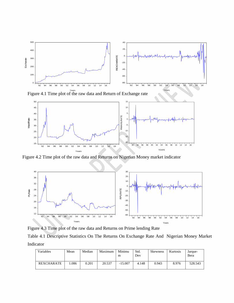
Figure 4.1 Time plot of the raw data and Return of Exchange rate

Figure 4.2 Time plot of the raw data and Returns on Nigerian Money market indicator

Figure 4.3 Time plot of the raw data and Returns on Prime lending Rate

Table 4.1 Descriptive Statistics On The Returns On Exchange Rate And Nigerian Money Market

Indicator

Variables Mean Median Maximum Minimum

Std. Dev

Skewness Kurtosis Jarque-Bera

REXCHARATE 1.086 0.201 20.537 -15.007 4.148 0.943 8.976 528.543

0

100

200

300

400

500

92 94 96 98 00 02 04 06 08 10 12 14 16

Exc

hara

te

Years

-80

-60

-40

-20

0

20

40

92 94 96 98 00 02 04 06 08 10 12 14 16

RE

XC

HAR

ATE

Years

15

20

25

30

35

40

45

50

92 94 96 98 00 02 04 06 08 10 12 14 16

Max

ilRat

e

Years

-20

-15

-10

-5

0

5

10

15

92 94 96 98 00 02 04 06 08 10 12 14 16

RM

AX

ILR

AT

E

YEARS

12

16

20

24

28

32

36

40

92 94 96 98 00 02 04 06 08 10 12 14 16

PLR

ate

Years

-60

-50

-40

-30

-20

-10

0

10

20

30

92 94 96 98 00 02 04 06 08 10 12 14 16

RP

LRA

TE

Years

RMAXILRATE 0.1204 0.091 31.135 -58.778 4.750 -5.049 80.584 82384.12

RPLRATE -0.037 0.000 25.472 -54.654 4.562 -4.921 69.106 60117.18

Source: Researcher’s computations, 2019 using Eview software version10

Table 4.2. Correlation between Return on exchange rate and money market indicators

Prices Series EXCHRATE RMAXILRATE RPLRATE

REXCHARATE 1 0.0301 0.1004

RMAXILRATE 0.0301 1 0.7996

RPLRATE 0.1004 0.7996 1


Table 4.3: VAR Lag Order Selection Criteria

Lag AIC SC HQ

0 16.50697 16.54238 16.52111

1 16.38635 16.52799* 16.44292*

2 16.40395 16.65182 16.50294

3 16.42359 16.77768 16.56500

4 16.36802* 16.82835 16.55186

* indicates lag order selected by the criterion


Table 4.4 Test for Cointegration using the Johansen co-integration test

Hypothesized Unrestricted Cointegration Rank Test (Trace) Unrestricted Cointegration Rank Test

(Maximum Eigenvalue)

Eigenvalue Trace

statistic

0.05

Critical

value

Prob

Hypoth

esized

Eigenvalue Max-

Eigen

statistic

0.05

Critica

l value

Prob

None * 0.255386 197.1144 29.79707 0.0001 0.255 93.77459 21.13162 0.000 0.255

At most 1 * 0.169764 103.3398 15.49471 0.0001 0.169 59.16235 14.26460 0.000 0.169

At most 2 * 0.129705 44.17747 3.841466 0.0000 0.129 44.17747 3.841466 0.000 0.129


Estimated VEC Model:

D(REXCHRATE) = 0.0044*REXCHRATEt-1 - 5.1073*RPLRATE t-1 - 1.2590 + 0.1017*

RMLRATE t-1 - 0.6200*RPLRATE t-1 - 0.1497 - 0.2703*D(REXCHRATE t-1) -

0.0342*D(RMLRATE t-1) - 0.0088*D(RPLRATE t-1) - 0.0116 4.1

D(RMLRATE) = 0.1377*( REXCHRATE t-1 - 5.1073*RPLRATE t-1) - 1.2590 ) - 0.8328*(

RMLRATE t-1- 0.6199*RPLRATE t-1 - 0.1497 ) - 0.0623*D(REXCHRATE t-1) -

0.2112*D(RMLRATE t-1) + 0.1663*D(RPLRATE t-1) + 0.00154 4.2

D(RPLRATE) = 0.2331*( REXCHRATE t-1 - 5.1073*RPLRATE t-1) - 1.2590 ) + 0.3360*(

RMLRATE t-1) - 0.6200*RPLRATE t-1 - 0.1497) - 0.0564*D(REXCHRATE t-1) -

0.2767*D(RMLRATE t-1) + 0.2196*D(RPLRATE t-1) + 0.0005 4.3

Table 4. 5 VEC Residual Heteroskedasticity Tests (Levels and Squares)

Dependent R-squared F(10,310) Prob. Chi-sq(10) Prob.

res1*res1 0.040836 1.319799 0.2187 13.10824 0.2177 res2*res2 0.051008 1.666226 0.0878 16.37345 0.0894 res3*res3 0.049175 1.603254 0.1045 15.78507 0.1060 res2*res1 0.103963 3.596774 0.0002 33.37203 0.0002 res3*res1 0.094600 3.238999 0.0005 30.36650 0.0007 res3*res2 0.049842 1.626160 0.0981 15.99935 0.0997

The trivariate Diagonal BEKK–GARCH for restrictive indefinite in normal error distributional

assumption estimate could be stated as thus

Mean component

REXCHRATE = 0.1974 4.4 (0.2691) RMLRATE = 0.0650 4.5 (0.6567) RPLRATE = -0.1410 4.6 (0.3861) The estimated transformed Variance-Covariance Representation

1,112

1,1,11 0.56593967.01.5090ˆ ttt

4.7

(0.0000) (0.0000) (0.0000)

1,222

1,2,22 0.64560.36381.1819ˆ ttt 4.8

(0.0000) (0.0000) (0.0000)

1,222

1,2,33 0.68440.33171.1099ˆ ttt 4.9

(0.0000) (0.0000) (0.0000)

1,22

1,22

1,1,12 ˆ0.6044*0.3799 0.0352ˆ tttt 4.10

(0.8633) (0.0000) (0.0000)

1,32

1,32

1,1,13 ˆ6223.0*3627.00.0426ˆ tttt 4.11

(0.7378) (0.0000) (0.0000)

1,32

1,32

1,2,23 ˆ6647.0*3474.05611.0ˆ tttt 4.12

(0.0000) (0.0000) (0.0000)

The trivariate Diagonal BEKK–GARCH for restrictive indefinite in student’s-t error distributional

assumption estimate could be stated as thus

Mean component

REXCHRATE = 0.1208 4.13

(0.1570)

RMLRATE = 0.1339 4.14

(0.0646)

RPLRATE = -0.0518 4.15

(0.4837)

The estimated transformed Variance-Covariance Representation

1,112

1,1,11 0.47831.1659 1.4029ˆ ttt

4.16

(0.0323) (0.0421) (0.0000)

1,222

1,2,22 0.49340.66191.4426ˆ ttt 4.17

(0.0179) (0.0282) (0.0000)

1,222

1,2,33 *0.58010.7329 0.864ˆ ttt 4.18

(0.0420) (0.0293) (0.000)

1,22

1,22

1,1,12 ˆ0.0145*0.2246 -0.2689ˆ tttt 4.19

(0.6478) (0.04067) (0.9875)

1,32

1,32

1,1,13 ˆ0897.0*0415.00.0683ˆ tttt 4.20

(0.9037) (0.8644) (0.9828)

1,32

1,32

1,2,23 ˆ5545.0*5833.05289.0ˆ tttt 4.21

(0.0535) (0.0225) (0.9875)

Table 4. 6 Information Criteria Selection Technique

Information Criteria

Selection Technique

Diagonal MGARCH -

BEKK In Normal Error

Distribution

Diagonal MGARCH-

BEKK In Students’-T

Error Distribution

Least Akaike

Information

Criteria(AIC)

Schwarz criterion 15.00652 13.51352

Hannan-Quinn criter. 14.90112 13.35893

Akaike info criterion 14.83109 13.25622 13.25622

Source: Researcher’s computations, 2019using Eview software version10

5.0 Discussions of Results

Figure 4.1 – 4.3 is the time plot of the raw data variables used in the study. It reveals that all the

variables showed fluctuations within the period of the study. No variables followed a particular

steady trend. Similarly, Figure 4.4 – 4.6 revealed the volatility clustering of the variables after

estimating returns on each of the series under investigation.

Table 4.1 present the summary descriptive statistics of the set of returns (returns on exchange rate

and money markets indicators). The sample mean of all the returns with an exception of returns on

prime lending rate(RPlrate) are positive and small compare to their standard deviations. The simply

mean that returns on exchange rate and maximum lending rate exhibit the characteristic of mean

reverting. Also, the higher the standard deviation leads to an increasing volatility as acclaimed in

Deebom and Essi(2017) and this means that the interaction between these indicators is risky. The

return distributions of maximum and prime lending rate are negatively skewed to the left.

According to Bala and Takinoto(2017), this simply implies that negative returns are more common

than positive returns in the two indicators. The kurtosis are all greater than three (3) and since this

measures the magnitude of extremes , and it is higher than it mean. This simply means all the

variables exhibit leptokurtic behavior. Also, the Jarque –Bera(JB) statistics indicate that the

returns are not normally distributed.

Similarly, table 4.3 shows the corresponding correlation between exchange rates and indicators of

money market. The result shows positive strong relationship between these variables. This simply

means there is significant relationship revealing higher co-movement and greater integration

between these variables.

In another development, Johansen test of co-integration for lag of endogenous variables were

considered for selection using three information criteria and lag two(2) was choose as it is

represented in table (4.4) above.

Table 4.4 presents the results for the test for co-integration using the Johansen co-integration test. In

this case, the trace test statistic, the result indicates evidence of long run relationship among the

returns on exchange rate and money markets indicators used in the study. The evidence of this

claim is clearly shown as the trace and maximum eigenvalue statistics with their corresponding

probabilities values (P-values) as estimated in the test are less than 5%. This indicates that long run

relationship exist among exchange rate and variables money markets. This results corroborates

Ogunbiyi and Ihejirika’s (2014) findings.

Ogunbiyi and Ihejirika’s(2014), investigated how interest rates affects deposit money Bank’s

profitability in Nigeria and it was found that long run equilibrium relationship exist among

variables used in their study.

Table 4. 5 VEC residual heteroskedasticity tests (Levels and Squares) shows no present of arch

effect in the model as their probability values are not all greater than the standard probability of

0.05.

Also, the results of the Diagonal MGARCH–BEKK model estimated in students’-t and normal error

distribution as shown in equation 4.7 -4.21 reveals that there exists strong GARCH (1, 1) process

influencing the conditional variances of the variables under investigation. The results obtain here

corroborates Malik and Ewing’s(2014) assertion. In Malik and Ewing’s(2014) study, it was asserted

that in parameterized multivariate GARCH model when the diagonal quadratic function are

positively significant this means there exist a very strong GARCH(1,1) and this is evident as the

values of the sum of the ARCH and GARCH co-efficients are 0.9826,1.0094 and 1.0161

respectively for Diagonal MGARCH –BEKK in Normal error distribution while in student’s-t

error, we have 0.64442,1.1553 and 1.313 respectively. This also prove that the covariance matrix

are positive semi-definite. This is synonymous to Tasi’u et al (2014) assertion. Tasi’u et al (2014)

examine exchange rate volatility of Nigerian naira against some major currencies in the world: an

application of multivariate GARCH models and it was found that the covariance matrixes are

positive semi-definite.

In another development, the result also confirmed there is linkage in terms of returns and volatility

transmission between returns of exchange rate and money market rate. In both model all the

estimates of all the diagonal parameters are significant at 5% level of significance. This indicate

that the own past shocks have effect on the current volatility of the Nigerian money market

indicator. Similarly, all the off-diagonal estimates are all statistically significant at 1% and 5% level

of significance levels, revealing that own past volatility does affect the current volatility of

exchange rate and money market rate in Nigeria.

In the same vein, the two models in equation 4.7-4.21 also revealed evidence of bi-direction shock

transmission between these variables. This confirmed Afees and Isah’s (2016) findings. In Afees

and Isah (2016), examine the modeling of return and shock spillovers between stock market and

money market in Nigeria and it was found that shocks to stock returns tend to persist when they

occur while shocks to money market returns tend to die out over time.

Finally, the result shows that these models allow for dynamic dependence between the two set of

volatility series. However, selection of the two models were also considered and the result revealed

that the model with the least Akaike Information Criteria(AIC) should be choose since its’

maximizes the lost of degree of freedom (Deebom &Essi,2017). Therefore, the Diagonal

MGARCH BEKK in student’s-t was considered the best fitted and appropriate model for modeling

exchange rate and Nigerian deposit money market dynamics in trivariate form.

Conclusion

This shows that there is a serious interdependence of measure of deposit Bank s money market rate

on the exchange rate (dollar/Naira) and the dynamics of the variance and covariance of volatility

returns between exchange rate and money market indicators in Nigeria was also confirmed.

Evidence shows there is a linkage in terms of returns and volatility transmission between exchange

rate and money market indicators in Nigeria. Also , on the bases of Comparison the difference

between Multivariate BEKK GARCH with restrictive indefinite under the assumption of normality

and that of student’s –t error distribution, the Multivariate BEKK GARCH with restrictive

indefinite in students’-t error distribution was considered best fitted and appropriate in modeling

exchange rate and Nigerian deposit money market dynamics using trivariate form of multivariate

GARCH model

5.1 RECOMMENDATIONS:

The result of the analysis reveal that diagonal BEKK model in student’s-t error distribution

assumption was recommended to be the best model. This is because most of their

variances/covariance are statistically significant and they have maximum likelihood, lower Akaike

information criteria (AIC) and lower Schwarz information criteria (SIC). There are some

implications of these findings:

(i) The findings of this study imply that exchange rate returns exhibit a behavior that tends

to change over time while that of the money market indicator appears to be fairly stable.

(ii) This follows that investors need to consider risks involved in exchange rate markets before

making investment decisions in terms of deposit money market transaction.

(iii) Thirdly, we find significant cross-variables returns and shock spillovers between exchange

rate and money market indicators.

(iv) In addition, the exchange rate and money market rate are more susceptible to external

shocks as there exist the present of strong GARCH(1,1).

References

Serpil , T. and Mesut, B. (2013), The relationships among interest rate, exchange rate and stock price: A BEKK MGARCH approach. International Journal of Economics, Finance and Management Sciences 1(3):166-174

Samar , Z. A and Khoufi, W. (2016), To what extent crude oil, International Stock Markets and Exchange rates are interdependent in Emerging and developed countries? Research 1ournal of Finance and Accounting, 7(15)

Oghenekaro, O. A. (2013) The Nigeria money market, Central Bank of Nigeria (CBN) nderstanding Monetary Policy Series 27.

Mohamed, J. (2009) The Role of financial markets in economic growth, DG/CEO, Sierra Leone Stock Exchange and Bank of Sierra Leone

Berndt, E. K., Bronwyn H. H, Robert E. H, and Jerry A. H (1974),Estimation and Inference in Non- linear Structural Models, Annals of Economic and Social Measurement (4)653-665.

Glosten, L., Jagannathan, R., & Runkle, D. (1992),On the relation between the expected value and volatility of nominal excess returns on stocks. Journal of Finance, 46, 17791801https://doi.org/10.2307/2329067

Bollerslev, T. (1990), Modeling the Coherence in Short-Run Nominal Exchange Rates: A Multivariate Generalized ARCH Approach, Review of Economics and Statistics, 72, 498-505.

Kroner, K.F., and Ng, V.K. (1998) Modeling asymmetric co-movements of asset returns, Review of Financial Studies, 11 (winter): 817-844

De Goeij, P., Marquering, W.( 2004,),Modeling the Conditional Covariance Between Stock and Bond Returns: A Multivariate GARCH Approach, Journal of Financial Econometrics, 2,(4). 531-564

Afees A. S, and Kazeem O. I (2016).Modeling return and shock spillovers between stock market and money market in Nigeria. Centre for Econometric and Allied Research (CEAR), University of Ibadan, Nigeria.

Ogunbiyi, S. S and , Ihejirika, P. O. (2014). Interest Rates And Deposit Money Banks’ Profitability Nexus: The Nigerian Experience. Arabian Journal of Business and Management Review (OMAN Chapter) 3,(11)

Engle, R.F. and K.F. Kroner (1995) Multivariate simultaneous generalized ARCH. Econometric Theory, 11, 122-150.

Engle, R. and Ng, V. (1993) Measuring and testing the impact of news on volatility, Journal of Finance, 48, 1749-1777.

Da-WaribokoAsikiye Y and Isaac D. E (2019), Modeling of Determinants of Exchange Rate in Nigeria (1991-2017) ARDL/Long –Run form of Bound Test Methodology. International Journal Of Applied Science And Mathematical Theory (IJASMT) 2489-009.

Bollerslev, T., Engle, R. F and Wooldridge, J. M. (1998), A capital asset pricing model with time-varying covariance. The Journal of Political Economy, 116–131.

Abduikareem, A. & Abdulhakeem, K. A. (2016). Analyzing Oil Price – Macroeconomic Volatility in Nigeria. Central Bank of Nigeria Journal of Applied Statistics, 2, 234 – 240.

Jarque, C.M. & Bera, A.K. (1980). An Efficient Large Sample Test for Normality of Observations and Regression Residuals. Journal of American Statistical Association, 16(2), 40-50.

Tasi’u M , Yakubu. M , and Gulumbe S. U (2014). Exchange rate volatility of Nigerian Naira against some major currencies in the world: An application of multivariate GARCH models. International Journal of Mathematics and Statistics Invention (IJMSI) 2(6)52-65

McAleer, M., Hoti and F. Chan (2009). Structure and asymptotic theory for multivariate asymmetric conditional volatility. Econometric Reviews, 28, 422-440.

Hamao, Y. R., Masulis R. W. and Ng V. K. (1990), Correlations in price changes and volatility across international stock markets, Review of Financial Studies, 32,81–307

Appendix

Lag LogL LR FPE AIC SC HQ

0 -2629.861 NA 2961.162 16.50697 16.54238 16.52111 1 -2601.623 55.76880 2624.704 16.38635 16.52799* 16.44292* 2 -2595.431 12.11255 2671.364 16.40395 16.65182 16.50294 3 -2589.562 11.36888 2724.442 16.42359 16.77768 16.56500 4 -2571.700 34.26900* 2577.381* 16.36802* 16.82835 16.55186

Multivariate Diagonal BEKK –GARCH with Normal error Distribution System: UNTITLED Estimation Method: ARCH Maximum Likelihood (BFGS / Marquardt steps) Covariance specification: Diagonal BEKK Date: 02/14/19 Time: 02:07

Sample: 1991M02 2017M12 Included observations: 323 Total system (balanced) observations 969 Presample covariance: backcast (parameter =0.7) Convergence achieved after 48 iterations Coefficient covariance computed using outer product of gradients

Coefficient Std. Error z-Statistic Prob.

C(1) 0.197353 0.178564 1.105226 0.2691C(2) 0.065018 0.146291 0.444438 0.6567C(3) -0.141009 0.162682 -0.866780 0.3861

Variance Equation Coefficients

C(4) 1.508953 0.228832 6.594155 0.0000C(5) 0.035180 0.204263 0.172226 0.8633C(6) 0.042607 0.127279 0.334752 0.7378C(7) 1.181901 0.141258 8.366969 0.0000C(8) 0.561101 0.087547 6.409138 0.0000C(9) 1.109899 0.197285 5.625878 0.0000C(10) 0.629765 0.064869 9.708257 0.0000C(11) 0.603192 0.036497 16.52727 0.0000C(12) 0.575942 0.046810 12.30388 0.0000C(13) 0.752293 0.037937 19.83013 0.0000C(14) 0.803493 0.018094 44.40560 0.0000C(15) 0.827289 0.018935 43.69189 0.0000

Log likelihood -2380.221 Schwarz criterion 15.00652Avg. log likelihood -2.456369 Hannan-Quinn criter. 14.90112Akaike info criterion 14.83109

Equation: REXCHRATE = C(1) R-squared -0.046031 Mean dependent var 1.086046Adjusted R-squared -0.046031 S.D. dependent var 4.148597S.E. of regression 4.243004 Sum squared resid 5796.994Durbin-Watson stat 1.249847

Equation: RMLRATE = C(2) R-squared -0.000137 Mean dependent var 0.120477Adjusted R-squared -0.000137 S.D. dependent var 4.750449S.E. of regression 4.750774 Sum squared resid 7267.493Durbin-Watson stat 2.127896

Equation: RPLRATE = C(3) R-squared -0.000518 Mean dependent var -0.037338Adjusted R-squared -0.000518 S.D. dependent var 4.562551S.E. of regression 4.563733 Sum squared resid 6706.506Durbin-Watson stat 2.222938

Covariance specification: Diagonal BEKK GARCH = M + A1*RESID(-1)*RESID(-1)'*A1 + B1*GARCH(-1)*B1 M is an indefinite matrix A1 is a diagonal matrix B1 is a diagonal matrix

Transformed Variance Coefficients


M(1,1) 1.508953 0.228832 6.594155 0.0000M(1,2) 0.035180 0.204263 0.172226 0.8633M(1,3) 0.042607 0.127279 0.334752 0.7378M(2,2) 1.181901 0.141258 8.366969 0.0000M(2,3) 0.561101 0.087547 6.409138 0.0000M(3,3) 1.109899 0.197285 5.625878 0.0000A1(1,1) 0.629765 0.064869 9.708257 0.0000A1(2,2) 0.603192 0.036497 16.52727 0.0000A1(3,3) 0.575942 0.046810 12.30388 0.0000B1(1,1) 0.752293 0.037937 19.83013 0.0000B1(2,2) 0.803493 0.018094 44.40560 0.0000B1(3,3) 0.827289 0.018935 43.69189 0.0000

Multivariate Diagonal BEKK –GARCH with student’s-t error Distribution System: UNTITLED Estimation Method: ARCH Maximum Likelihood (BFGS / Marquardt steps) Covariance specification: Diagonal VECH Date: 02/14/19 Time: 02:10 Sample: 1991M02 2017M12 Included observations: 323 Total system (balanced) observations 969 Disturbance assumption: Student's t distribution Presample covariance: backcast (parameter =0.7) Failure to improve likelihood (non-zero gradients) after 68 iterations Coefficient covariance computed using outer product of gradients


C(1) 0.120778 0.085341 1.415241 0.1570C(2) 0.133885 0.072444 1.848123 0.0646

C(3) -0.051773 0.073925 -0.700339 0.4837

Variance Equation Coefficients

C(4) 1.402945 0.655267 2.141029 0.0323C(5) -0.268061 0.586815 -0.456806 0.6478C(6) 0.068292 0.564171 0.121049 0.9037C(7) 1.442653 0.609104 2.368484 0.0179C(8) 0.528961 0.273939 1.930942 0.0535C(9) 0.864398 0.425089 2.033450 0.0420C(10) 1.165930 0.573647 2.032487 0.0421C(11) 0.224585 0.270667 0.829749 0.4067C(12) 0.041464 0.242881 0.170719 0.8644C(13) 0.661891 0.301644 2.194279 0.0282C(14) 0.583276 0.255598 2.282003 0.0225C(15) 0.732855 0.336332 2.178963 0.0293C(16) 0.478384 0.056306 8.496131 0.0000C(17) 0.014523 0.923752 0.015722 0.9875C(18) 0.089714 4.162533 0.021553 0.9828C(19) 0.493361 0.040417 12.20666 0.0000C(20) 0.554548 0.023259 23.84220 0.0000C(21) 0.580139 0.042820 13.54840 0.0000

t-Distribution (Degree of Freedom)

C(22) 2.513800 0.281295 8.936533 0.0000

Log likelihood -2118.880 Schwarz criterion 13.51352Avg. log likelihood -2.186666 Hannan-Quinn criter. 13.35893Akaike info criterion 13.25622

Equation: REXCHRATE = C(1) R-squared -0.054305 Mean dependent var 1.086046Adjusted R-squared -0.054305 S.D. dependent var 4.148597S.E. of regression 4.259753 Sum squared resid 5842.850Durbin-Watson stat 1.240038

Equation: RMLRATE = C(2) R-squared -0.000008 Mean dependent var 0.120477Adjusted R-squared -0.000008 S.D. dependent var 4.750449S.E. of regression 4.750468 Sum squared resid 7266.557Durbin-Watson stat 2.128170

Equation: RPLRATE = C(3) R-squared -0.000010 Mean dependent var -0.037338Adjusted R-squared -0.000010 S.D. dependent var 4.562551S.E. of regression 4.562574 Sum squared resid 6703.102Durbin-Watson stat 2.224067

Covariance specification: Diagonal VECH GARCH = M + A1.*RESID(-1)*RESID(-1)' + B1.*GARCH(-1) M is an indefinite matrix A1 is an indefinite matrix B1 is an indefinite matrix*

Transformed Variance Coefficients


M(1,1) 1.402945 0.655267 2.141029 0.0323M(1,2) -0.268061 0.586815 -0.456806 0.6478M(1,3) 0.068292 0.564171 0.121049 0.9037M(2,2) 1.442653 0.609104 2.368484 0.0179M(2,3) 0.528961 0.273939 1.930942 0.0535M(3,3) 0.864398 0.425089 2.033450 0.0420A1(1,1) 1.165930 0.573647 2.032487 0.0421A1(1,2) 0.224585 0.270667 0.829749 0.4067A1(1,3) 0.041464 0.242881 0.170719 0.8644A1(2,2) 0.661891 0.301644 2.194279 0.0282A1(2,3) 0.583276 0.255598 2.282003 0.0225A1(3,3) 0.732855 0.336332 2.178963 0.0293B1(1,1) 0.478384 0.056306 8.496131 0.0000B1(1,2) 0.014523 0.923752 0.015722 0.9875B1(1,3) 0.089714 4.162533 0.021553 0.9828B1(2,2) 0.493361 0.040417 12.20666 0.0000B1(2,3) 0.554548 0.023259 23.84220 0.0000B1(3,3) 0.580139 0.042820 13.54840 0.0000

* Coefficient matrix is not PSD.

System Residual Portmanteau Tests for Autocorrelations Null Hypothesis: no residual autocorrelations up to lag h Date: 02/16/19 Time: 10:26 Sample: 1991M02 2017M12 Included observations: 323

Lags Q-Stat Prob. Adj Q-Stat Prob. Df

1 52.55832 0.0000 52.72155 0.0000 9 2 63.48067 0.0000 63.71195 0.0000 18 3 72.02376 0.0000 72.33513 0.0000 27 4 99.64742 0.0000 100.3052 0.0000 36 5 120.8047 0.0000 121.7951 0.0000 45 6 134.9654 0.0000 136.2238 0.0000 54 7 152.7274 0.0000 154.3793 0.0000 63 8 190.3441 0.0000 192.9514 0.0000 72 9 208.1538 0.0000 211.2715 0.0000 81

10 223.7651 0.0000 227.3816 0.0000 90

11 248.0447 0.0000 252.5171 0.0000 99 12 269.9683 0.0000 275.2867 0.0000 108

*The test is valid only for lags larger than the System lag order. df is degrees of freedom for (approximate) chi-square distribution

Modeling Exchange Rate and Nigerian Deposit Money Market ...

Documents

Transcript of Modeling Exchange Rate and Nigerian Deposit Money Market ...