Modular Games for Coalgebraic Fixed Point Logics

CMCS 2008

Modular Games for Coalgebraic Fixed PointLogics

Corina Cırstea1,2

School of Electronics and Computer ScienceUniversity of Southampton

Mehrnoosh Sadrzadeh1,3

Laboratoire PPSUniversite Paris Diderot - Paris 7

Abstract

We build on existing work on finitary modular coalgebraic logics [3,4], which we extend with general fixedpoints, including CTL- and PDL-like fixed points, and modular evaluation games. These results are gener-alisations of their correspondents in the modal µ-calculus, as described e.g. in [19]. Inspired by recent workof Venema [21], we provide our logics with evaluation games that come equipped with a modular way ofbuilding the game boards. We also study a specific class of modular coalgebraic logics that allow for theintroduction of an implicit negation operator.

Keywords: coalgebra, modal logic, fixed point logic, parity games

1 Introduction

Modular coalgebraic logics were introduced in [3,4], where it was shown that thesyntax and semantics of logics for T-coalgebras, with T an ω-accessible Set functor,can be defined modularly by exploiting the structure of T, and moreover, thatexpressiveness of the resulting logics w.r.t. behavioural equivalence, as well as soundand complete proof systems for these logics, can also be derived modularly. In termsof expressivity, these logics are more expressive than logics induced by monadicpredicate liftings, as considered in [16], but are as expressive as logics induced byfinitary polyadic predicate liftings, as defined in [17].

Coalgebraic fixed point logics were first considered in the work of Venema [21],where a finitary version of the coalgebraic logic of Moss [14] was used as the underly-ing modal language. Our motivation for considering fixed point logics over different

1 Research supported by the EPSRC grant EP/D000033/1.2 Email: [email protected] Email: [email protected]

This paper is electronically published inElectronic Notes in Theoretical Computer Science

URL: www.elsevier.nl/locate/entcs

mailto:[email protected]

mailto:[email protected]

Cırstea and Sadrzadeh

modal languages is rooted in our interest in verification techniques for systemsmodelled as coalgebras. In this setting, the logics obtained through the modulartechniques described in [3] appear to be better suited as specification logics.

The syntax of modular coalgebraic logics is based on the notion of syntax con-structor [3], while their semantics uses a notion of one-step semantics for a syntaxconstructor [3], which generalises the predicate liftings of [16]. The logics obtainedfrom syntax constructors are originally boolean, but in order to ensure that fixedpoints have a well-defined semantics, we leave out negation from these languages.However, for the specific class of syntax constructors which are closed under duals(that is, for each modality they specify, a semantically dual modality is also speci-fied), a safe negation becomes definable in the language, and thus the expressivityof the logic stays as before. For this class of syntax constructors, we also introduce ageneral way of defining CTL- and PDL-like fixed points, and illustrate their applica-bility via examples. For instance, we obtain the fixed points of Dynamic EpistemicLogic [2] via the coalgebraic semantics for this logic described in [5]. In standardmodel checking terminology, these fixed points are referred to as ‘alternation-free’,and enjoy a linear-time model checking algorithm based on parity games [8].

The results concerning the implicit negation and the alternation-free fragmentsof our logics make use of the notion of an S-modality (of some finite arity), with Sa syntax constructor with an associated one-step semantics. This notion also allowsus to relate logics induced by sets of polyadic predicate liftings, as considered in[17], with logics induced by syntax constructors. As a result, we obtain a way toadd fixed points to logics of the former type.

In [21], deciding about the satisfaction of formulae by states of a coalgebra isachieved through deciding the winner of so-called evaluation games. These areparity games that generalize those for the modal µ-calculus [15,7,10,19,20,22], byreplacing the usual single moves of either the verifier or the refuter in positions thatcorrespond to modal formulae by two consecutive moves: a move of the verifier, whohas to exhibit a relation between sub-formulae of the original formula and states ofthe coalgebra, that witnesses the satisfaction of the given modal formula by a stateof the coalgebra, and a move of the refuter, who has to choose an element of thisrelation. These two consecutive moves are, in turn, inspired by similar moves in thebisimulation game of Baltag [1].

We introduce a variant of the evaluation games of [21] tailored to our fixedpoint logics, and prove their adequacy w.r.t. the standard coalgebraic semantics.The only difference w.r.t. [21] is in the moves corresponding to modal positions,where the one-step semantics for the syntax constructor defining the underlyingmodal language is used to define the valid moves. The distinctive feature of ourgames, however, is that they come equipped with one-step games. These adequatelyreplace the two consecutive moves, of the verifier followed by the refuter, in modalpositions, by an equivalent sub-game played between the verifier and the refuter.The use of one-step games has some advantages: on the one hand, it provides a wayto construct the board of the evaluation games by induction on the structure of thesignature functor ; on the other hand, only witnessing relations that are relevant todeciding the winner of an evaluation game are accounted for in the one-step games,thus significantly reducing the size of the resulting parity games.

2


2 Preliminaries

Existing work [3] shows how to modularly derive coalgebraic modal logics forinductively-defined classes of endofunctors, including the class of so-called poly-nomial functors (that is, functors defined inductively on the identity, constant,powerset and discrete probability distribution functors, using products, coproducts,exponentiation and functor composition). A modal language with finitary modali-ties can be defined using a syntax constructor [3], that is, an inclusion-preserving,ω-accessible set endofunctor S : Set → Set. Given a syntax constructor S, the(negation-free) modal language LS it induces is the least set of formulae which isclosed under finite (including empty) conjunctions and disjunctions and under theapplication of S. Equivalently (using the ω-accessibility of S), LS is defined induc-tively by:

LS 3 φ := ff | tt | φ ∨ φ | φ ∧ ψ | Ψwhere Ψ ∈ S(F ) with F ⊆ LS finite.

Simple syntax constructors can be used to define modal languages for (coalgebrasof) the constant, identity, powerset and discrete probability distribution functors,as follows:

SA(L) = a,¬a | a ∈ ASId(L) = ©φ | φ ∈ LSP(L) = 2φ, 3φ | φ ∈ LSD(L) = Lpφ, Gpφ | φ ∈ L, p ∈ [0, 1] ∩Q

In the definition of SD, Lpφ is to be read as “φ holds in the next state with probabilityat least p”, whereas Gpφ is to be read as “φ holds in the next state with probabilitygreater than p”.

Syntax constructors can be combined to obtain modal languages for (coalgebrasof) functors structured using products, coproducts, exponentiation with constantexponent E and functor composition, as follows:

(S1 ⊗ S2)(L) = [πi]φ | φ ∈ Si(L), i = 1, 2(S1 ⊕ S2)(L) = [κi]φ, 〈κi〉φ | φ ∈ Si(L), i = 1, 2

(S E)(L) = [e]φ | e ∈ E, φ ∈ S(L)(S1 S2)(L) = S1(S2(L))

where · denotes closure under finite (including empty) conjunctions and disjunc-tions. For a polynomial functor, the resulting syntax can be expressed using a BNFwith multiple levels, one for each ingredient of the functor [3,4].

Example 2.1 An alternative way of associating a syntax constructor with eachω-accessible, weak pullback preserving endofunctor T : Set→ Set is to take S = T.This is the approach followed in [14] 4 .

We note that all of the above definitions are negation-free variants of the defini-tions in [3]. The restriction to negation-free fragments is a common way to ensure

4 The restriction regarding the ω-accessibility of T is not present in [14]. Here it is required since we areconcerned with languages with finitary modalities.

3


that fixed point logical operators defined on top of these languages have a well-defined (fixed point) semantics, see e.g. [19].

Given a functor T and a syntax constructor S, a semantics for the modal lan-guage LS w.r.t. T-coalgebras can be obtained from a one-step semantics for Sw.r.t. T [3]. Given a set L (of formulae) and a set X (of points), a one-step seman-tics [[S]] for S w.r.t. T maps interpretations of the formulae in L over the elementsof X (given by functions d : L → PX, or equivalently, by relations |=⊆ X × L)to interpretations of the formulae in SL over the elements of TX (given by func-tions d′ : SL → PTX, or by relations |=′⊆ TX × SL), see [3] for details. (Here,P : Set → Set also denotes the powerset functor, but a different notation is em-ployed when this functor is not used as a signature functor.) The interpretation offormulae in LS over the states of a T-coalgebra (C, γ) is then defined inductivelyon the structure of formulae, by

c |= Ψ iff γ(c) ([[S]] |=Base(Ψ)) Ψ

and the usual definitions for finite conjunctions and disjunctions, where forΨ ∈ S(F ) with F ⊆ LS , Base(Ψ) is the smallest F with this property, while|=Base(Ψ) is the restriction of the relation |= ⊆ C × LS to C × Base(Ψ) (and thus([[S]] |=Base(Ψ)) ⊆ TC × S(Base(Ψ))).

One-step semantics for the syntax constructors SA, SId, SP and SD can be definedin a natural way. Specifically, they map a relation |=⊆ X×L to the relations [[SA]] |=,[[SId]] |=, [[SP]] |=, [[SD]] |= defined as follows:

b ([[SA]] |=) a iff b = a

b ([[SA]] |=)¬a iff b 6= a

x ([[SId]] |=) © φ iff x |= φ

Y ([[SP]] |=) 2φ iff x |= φ for all x ∈ YY ([[SP]] |=) 3φ iff x |= φ for some x ∈ Yµ ([[SD]] |=)Lpφ iff

∑x|=φ

µ(x) ≥ p

µ ([[SD]] |=)Gpφ iff∑x|=φ

µ(x) > p

Also, one-step semantics for syntax constructors built using ⊗ , ⊕ , E and , w.r.t. functors built using products, coproducts, exponentiation with constant

exponent E and respectively functor composition, can be modularly derived fromone-step semantics for the ingredient syntax constructors [3]. Concretely, if [[Si]]is a one-step semantics for Si w.r.t. Ti, with i = 1, 2, then the one-step semantics[[S1 ⊗ S2]] for S1 ⊗ S2 w.r.t. T1 × T2, [[S1 ⊕ S2]] for S1 ⊕ S2 w.r.t. T1 + T2, [[S1 E]]for S1 E w.r.t. T1

E and [[S1 S2]] for S1 S2 w.r.t. T1 T2 are defined by:

(t1, t2) ([[S1 ⊗ S2]] |=) [πi]φi iff ti([[Si]] |=)φit ([[S1 ⊕ S2]] |=) [κi]φi iff t = ιi(z) ∈ ιi(TiX) implies z ([[Si]] |=)φit ([[S1 ⊕ S2]] |=) 〈κi〉φi iff t = ιi(z) ∈ ιi(TiX) and z ([[Si]] |=)φif ([[S1 E]] |=) [e]φ1 iff f(e) ([[S1]] |=)φ1

where ιi : TiX → T1X + T2X are the coproduct injections, and

4


([[S1 S2]] |=) = ([[S1]][[S2]] |=)

for each |=⊆ X × L, where [[S2]] |= ⊆ T2X × S2L denotes the natural extension ofthe relation ([[S2]] |=) ⊆ T2X × S2L to formulae containing finite conjunctions anddisjunctions. (See [3] for further details.)

Example 2.2 Given an ω-accessible endofunctor T, a one-step semantics for thesyntax constructor S = T w.r.t. the functor T can be defined by mapping eachrelation |=⊆ X×L to the relation |=T⊆ TX×TL defined by t |=T Φ iff there existsw ∈ (T |=) such that Tπ1(w) = t and Tπ2(w) = Φ. (Here, π1 : X × L → X andπ2 : X × L→ L denote the canonical projections.)

Example 2.3 Transition systems with spatial structure were proposed in [13] as ageneral model for spatial logic. They are defined as coalgebras of the functor T =P×(1+P(Id×Id)), where 1 denotes the constant functor induced by a one-elementset. Thus, T-coalgebras incorporate non-deterministic structure, through the firstcomponent of T, as well as spatial structure, through the second component of T. Asfar as the spatial structure is concerned, a one-step observation of 0 ∈ 1 correspondsto inactive states, whereas a one-step observation in P(Id×Id) describes the spatialstructure of active states; for the latter, the empty set describes states which arelocal, i.e. have no spatial structure. By applying the modular techniques describedin [?] to this functor, one arrives at a modal language with the following (multi-sorted) syntax, where the formula sort of interest is L1 and the remaining sorts aremerely used to define this sort:

L1 3 φ ::= ff | tt | φ1 ∨ φ2 | φ1 ∧ φ2 | [π1]ψ | [π2]χ (ψ ∈ L2, χ ∈ L3)L2 3 ψ ::= ff | tt | ψ1 ∨ ψ2 | ψ1 ∧ ψ2 | 2φ | 3φ (φ ∈ L1)L3 3 χ ::= ff | tt | χ1 ∨ χ2 | χ1 ∧ χ2 | [κ1]ξ | [κ2]ζ | 〈κ1〉ξ | 〈κ2〉ζ (ξ ∈ L4, ζ ∈ L5)L4 3 ξ ::= ff | tt | ξ1 ∨ ξ2 | ξ1 ∧ ξ2 | 0 | ¬0L5 3 ζ ::= ff | tt | ζ1 ∨ ζ2 | ζ1 ∧ ζ2 | [π1]φ | [π2]φ (φ ∈ L1)

Both the temporal and the spatial modalities defined in [13] can now be recovered,namely by defining: 2φ := [π1]2φ, 3φ := [π1]3φ, 0 := [π2]〈κ1〉0, φ1 |φ2 :=[π2]〈κ2〉3([π1]© φ1 ∧ [π2]© φ2) (where the notation for the 2, 3 and 0 modalitieshas been overloaded in order to maintain the notation of [13]). We note that theabove language is a negation-free version of the language of [13], but, as we will seein Section 3.3, this does not lead to a loss in expressivity.

Example 2.4 Simple Segala systems [18] can be modelled as coalgebras of thefunctor (P D)E . The one-step observations one can make about the states of suchsystems consist of non-deterministic transitions into discrete probability distribu-tions over states. This mirrors the original definition of simple Segala systems,which divides the states into non-deterministic and probabilistic ones, the formerbeing observed through non-deterministic transitions into the latter, and the latterbeing observed through probabilistic transitions back to the former. The languageinduced by (SP SD) E is a negation-free variant of the language considered in[11], and contains modalities of the form [e]2Lp and [e]2Gp with e ∈ E.

5


3 Modular Coalgebraic Fixed Point Logics

From now on we restrict our attention to syntax constructors with an associatedone-step semantics that is monotonic in the following sense.

Definition 3.1 (Monotonic one-step semantics) Given interpretations d, d′ :L→ PX, we write d ⊆ d′ if d(φ) ⊆ d′(φ) for each φ ∈ L. A one-step semantics [[S]]for a syntax constructor S is said to be monotonic if, for each d, d′ : L → PX, wehave that d ⊆ d′ implies [[S]](d) ⊆ [[S]](d′).

It is easy to check that all syntax constructors considered in Section 2 are monotonic:

Proposition 3.2 SA, SId, SP and SD are monotonic. Moreover, if S1 and S2 aremonotonic, so are S1 ⊗ S2, S1 ⊕ S2, S1 E and S1 S2.

3.1 Syntax

By adding fixed point formulae to the language LS , we obtain the following lan-guage:

µLS(V) 3 φ := ff | tt | φ ∨ φ | φ ∧ ψ | Ψ | x | µx.φ | νx.φwhere V is a set of variables, x ∈ V, and Ψ ∈ S(F ) with F ⊆ µLS(V) finite.

Example 3.3 The fixed point languages of SP and SP E are the mono- andmulti-modal propositional µ-calculi (of e.g. [19]), respectively.

3.2 Semantics

The interpretation of formulae in µLS(V) over the states of a T-coalgebra (C, γ) isdefined w.r.t. a valuation V : V → P(C), as follows:

c |=V Ψ ∈ S(F ) iff γ(c) ([[S]]|=V,Base(Ψ)) Ψc |=V x iff c ∈ V (x)

c |=V µx.φ iff c ∈⋂

B ⊆ C | [[φ]]V [B/x] ⊆ B

c |=V νx.φ iff c ∈⋃

B ⊆ C | B ⊆ [[φ]]V [B/x]

where

[[φ]]V =c ∈ C | c |=V φ

V [B/x](y) =

B y = x

V (y) o.w.

and the relation |=V,Base(Ψ) ⊆ C ×Base(Ψ) gives the interpretation of formulae inBase(Ψ) over the states of (C, γ).

The absence of negation in the language and the monotonicity of the one-stepsemantics [[S]] ensure that the semantics for fixed point formulae is well-defined:

Lemma 3.4 (Monotonicity) Let (C, γ) be a T-coalgebra, φ ∈ µLS(V), and V, V ′ :V → P(C) two valuations such that V (x) ⊆ V ′(x) for all x ∈ V. Then, for c ∈ C,we have: c |=V φ implies c |=V ′ φ.

Proof (Sketch) The statement is proved by structural induction on φ. The casewhere φ ∈ SF with F ⊆ µLS(V) finite uses the monotonicity of [[S]]. 2

6


The previous lemma ensures that, for a T-coalgebra (C, γ), a valuation V : V →P(C) and a formula φ ∈ µLS(V), the map X ∈ P(C) 7−→ [[φ]]V [X/x] ∈ P(C) is amonotone map on the complete lattice P(C), and therefore by the Knaster-Tarskitheorem, this map has a least and a greatest fixed point; these fixed points can becomputed as the intersection of all pre-fixed points and the union of all post-fixedpoints, respectively.

Example 3.5 [[SP]] and [[SP E]] provide semantics for the languages of mono-and multi-modal propositional µ-calculus (of e.g. [19]), interpreted over transitionsystems and labelled transition systems, respectively.

3.3 Simulating Negation

It is worth noting that, for languages where the semantic dual of each modal operatoris also in the language, we do not lose any expressivity by leaving out the negationoperator. We will show that, in this case, negation can be implicitly defined. Tothis end, we introduce the notions of an S-modality, and of a dual modality.

Definition 3.6 (S-modality) For a syntax constructor S and n ∈ ω, an S-modality of arity n is an element of S(n) which does not belong to any ofS(1), . . . ,S(n− 1) 5 .

Thus, an S-modality a of arity n is a modal operator which takes n arguments;the set n = 0, . . . , n− 1 is used to define the placeholders for the arguments of a.

Next, we define what it means to apply an S-modality of arity n to a set of nformulae.

Definition 3.7 If a is an S-modality of arity n and φ1, . . . , φn ∈ µLS(V), we definea(φ1, . . . , φn) as S([φ1, . . . , φn])(a) ∈ µLS(V), where [φ1, . . . , φn] : n→ φ1, . . . , φnmaps i to φi+1 for i = 0, . . . , n− 1.

We also note that a one-step semantics [[S]] for S w.r.t. T automatically providesa (coalgebraic) semantics for each S-modality.

Example 3.8 The 2 and 3 operators specified by the syntax constructor SP areunary SP-modalities, when identified with the two elements of SP(1).

Example 3.9 For the spatial transition systems of Example 2.3, the modal oper-ator 0 is an S-modality of arity 0, the temporal operators 2 and 3 are unaryS-modalities, while the spatial operator | is a binary S-modality.

Incidentally, the notion of S-modality allows us to relate languages inducedby finitary polyadic predicate liftings, as considered in [17], on the one hand, andlanguages induced by syntax constructors with associated one-step semantics on theother. To this end, we write P : Set → Set for the contravariant powerset functor.Given a set Λ of finitary polyadic predicate liftings for a functor T (that is, naturaltransformations λ : Pn → PT with n ∈ ω), a syntax constructor SΛ : Set→ Set canbe defined by

SΛ(L) = λ(φ1, . . . , φn) | λ ∈ Λ has arity n, φi ∈ L for i = 1, . . . , n

5 Recall that S is inclusion-preserving.

7


while a one-step semantics [[SΛ]] for S w.r.t. T can be defined by mapping an inter-pretation d : L→ PX to the interpretation d′ : SΛL→ PTX given by

d′(λ(φ1, . . . , φn)) = λX(d(φ1), . . . , d(φn)) for φ1, . . . , φn ∈ L

Thus, SΛ-modalities of arity n are exactly the n-ary predicate liftings of Λ and,as expected, the semantics of these modal operators agree with each other. Nowmonotonicity of the one-step semantics [[SΛ]] amounts to the predicate liftings λ :(P)n → PT being monotonic in all arguments. Consequently, our approach can beused to add fixed points to logics induced by sets of monotonic predicate liftings.

We now return to the issue of simulating negation in the language µLS(V). Fora given set of formulae L, we introduce a syntactic negation for the formulae of Lvia the set Lc := φc | φ ∈ L. Now for a given set of points X, an interpretationrelation |=⊆ X × L is extended to negated formulae in Lc via the relation |=c⊆X × Lc given by

x |=c φc iff x 6|= φ for x ∈ X and φ ∈ L

Definition 3.10 (Closure under duals) A syntax constructor S with a one-stepsemantics [[S]] is said to be closed under duals if, for each S-modality a, thereexists an S-modality a of arity n, called the dual of a, such that for each relation|=⊆ X × L, the relation |=′= [[S]](|= ∪ |=c) ⊆ TX × S(L ∪ Lc) satisfies

t |=′ a(φ1, . . . , φn) iff t 6|=′ a(φc1, . . . , φcn)

Thus, S is closed under duals if, whenever it specifies a modality, then it alsospecifies its semantic dual.

Example 3.11 The syntax constructors SA, SId, SP and SD with their associatedone-step semantics are closed under duals. In particular, we have a = ¬a, © =©,2 = 3 and Lp = G1−p for 0 ≤ p ≤ 1.

Proposition 3.12 If the syntax constructors for all the ingredients of a polynomialfunctor T (with their respective one-step semantics) are closed under duals, thenso is the combined syntax constructor for T (with the one-step semantics definedmodularly from the one-step semantics w.r.t. its ingredients).

Proof (Sketch) The statement follows from the definitions of S1 ⊗ S2, S1 ⊕ S2,S1 E and S1 S2 and of the associated one-step semantics, together with theobservations that, if ai is an Si-modality, for i = 1, 2, then [πi]ai = [πi]ai, [κi]ai =〈κi〉ai and [e]ai = [e]ai, and that the dual of an S1 S2-modality can be defined interms of the duals of S1- and S2-modalities; for example, if ai is a unary Si-modality,with i = 1, 2, then a1a2 = a1 a2. 2

As a consequence of Proposition 3.12, the modal language for spatial transitionsystems described in Example 2.3 is closed under duals.

We now observe that any Ψ ∈ S(F ) with F finite is of the form a(φ1, . . . , φn),with a an S-modality. If Base(Ψ) = φ1, . . . , φn, then since S(Base(Ψ)) is iso-morphic to S(n) (via S([φ1, . . . , φn])), there must exist an a ∈ S(n) such that

8


Ψ = S([φ1, . . . , φn])(a), that is, Ψ = a(φ1, . . . , φn). Moreover, by the minimality ofBase(Ψ), it follows that a can not come from any of S(1), . . . ,S(n− 1). Thus, a isan S-modality of arity n.

We note in passing that the above argument also applies to the case S = T,that is, to the finitary version of Moss’ coalgebraic logic [14]. Thus, when T is ω-accessible, the finitary version of the ∇ modality, considered in [21], can be regardedas a shorthand for an infinite number of modalities, each with a specific finite arity.

The previous observation is used in the following definition.

Definition 3.13 (Negation) For a syntax constructor S which is closed underduals, the negations of formulae in µLS(V) are defined inductively as follows:

ffc := tt ttc := ff

(φ ∨ ψ)c := φc ∧ ψc (φ ∧ ψ)c := φc ∨ ψc

(a(φ1, . . . , φn))c := a(φc1, . . . , φcn) xc := x

(µx.φ)c := νx.φc (νx.φ)c := µx.φc

Proposition 3.14 For a state c of a T-coalgebra (C, γ), a valuation V : V → P(C),and a formula φ ∈ µLS(V) we have

c |=V φ iff c 6|=V c φc

where V c : V → P(C) is given by V c(x) = C \ V (x) for x ∈ V.

Proof. The statement follows from Definitions 3.10 and 3.13 and the definition of|=V . 2

In order to account for some interesting examples, we now introduce the notionof a derived S-modality. Intuitively, a derived modality involves applications of S-modalities as well as of boolean operators, with nested applications of S-modalitiesnot being allowed.

Definition 3.15 (Derived S-modality) For a syntax constructor S and n ∈ ω,a derived S-modality of arity n is an element of S(n), which does not belong to anyof S(1), . . . ,S(n− 1).

It follows easily that, when S is closed under duals, for each derived S-modalityone can also define a semantic dual, again as a derived S-modality.

Example 3.16 In the case of spatial transition systems, that is, coalgebras of thefunctor T = P × (1 + P (Id × Id)), | tt, tt | ∈ ST(1) ⊆ ST(1) are derived ST-modalities of arity 1 (where the binary modality | was defined in Example 2.3).Their duals are (semantically equivalent to) [π2][κ2]2[π1]© and [π2][κ2]2[π2]© ,respectively.

We conclude this section by looking at conjunction-preserving modalities. Thesewill play a role when defining until- and dynamic-like fixed points in the next section.

Proposition 3.17 For a syntax constructor S with an associated one-step seman-tics [[S]], a (derived) S-modality of arity n preserves conjunctions if and only if its

9


dual preserves disjunctions.

Proof. Follows from Definitions 3.10 and 3.13 and Proposition 3.14. 2

Example 3.18 © is both conjunction- and disjunction-preserving, whereas 2 isconjunction-preserving. The SD-modalities are neither conjunction- nor disjunction-preserving, with the exception of L1 ≡ G0, defined as

c |=V L1φ iff ∀c′ ∈ C s.t. γ(c)(c′) 6= 0, c′ |=V φ

c |=V G0φ iff ∃c′ ∈ C s.t. γ(c)(c′) 6= 0 and c′ |=V φ

where L1 is conjunction-preserving and its dual G0 is disjunction-preserving.

Example 3.19 The modalities | tt, tt | of Example 3.16 are disjunction-preserving, whereas their duals are conjunction-preserving.

Conjunction-preserving S1 ⊗ S2-, S1 ⊕ S2-, S1 E- and S1 S2-modalities canbe derived from conjunction-preserving S1- and S2-modalities, as shown next.

Proposition 3.20 Let Si be a syntax constructor with one-step semantics [[Si]], fori = 1, 2. If ai is a conjunction-preserving (derived) Si-modality, for i = 1, 2, thenso are [πi]ai (as an S1 ⊗ S2-modality), [κi]ai (as an S1 ⊕ S2-modality), [e]a1 (asan S1 E-modality) and, in the case of modalities of arity 1, also a1a2 (as anS1 S2-modality).

Proof (Sketch) The conclusion follows by noting that [πi], [κi] and [e] areconjunction-preserving (by the definitions of [[S1 ⊗ S2]], [[S1 ⊕ S2]] and [[S1 E]]),and that the successive application of conjunction-preserving modalities is itselfconjunction-preserving. 2

3.4 Macros

As in the propositional µ-calculus, one can distinguish fragments of our coalgebraicfixed point logics that have desirable properties, for example the independent fixedpoint fragment IµLS(V) and the alternation-free fragment AµLS(V). For σ1, σ2 ∈µ, ν and writing Subf(φ) for the set of sub-formulae of a formula φ ∈ µLS(V),these fragments are defined as follows:

• φ ∈ IµLS(V) iff σ1 x.φ1 ∈ Subf(φ) and σ2 y.φ2 ∈ Subf(φ) implies that x is notfree in φ2 and y is not free in φ1;

• φ ∈ AµLS(V) iff µx.φ1 ∈ Subf(φ) and ν y.φ2 ∈ Subf(φ) implies that x is notfree in φ2 and y is not free in φ1.

While the IµLS(V)-fragment does not allow any dependency among the fixed pointsub-formulae of a formula, the AµLS(V)-fragment allows dependency as long as thefixed points are of the same type. These fragments relate to each other as follows:

IµLS(V) ⊆ AµLS(V) ⊆ µLS(V)

The two well-known independent fixed point fragments of the propositional µ-calculus are CTL with its until fixed points, and PDL with its dynamic fixed points,see [19] for details. The definitions of these special fixed point formulae can be ex-tended to our general coalgebraic fixed point logic µLS(V).

10


Definition 3.21 Given a functor T, a syntax constructor S with a one-step seman-tics [[S]] w.r.t. T such that S is closed under duals, and a finite set α of conjunction-preserving, unary S-modalities 6 , until and dynamic fixed point formulae are definedas follows:

A(φUα ψ) := µx.(ψ ∨ (φ ∧∨a∈α

a tt ∧∧a∈α

a x))

E(φUα ψ) := µx.(ψ ∨ (φ ∧∨a∈α

a x))

[ ]∗α φ := νx.(φ ∧∧a∈α

a x)

〈〉∗αφ := µx.(φ ∨∨a∈α

a x)

where x ∈ V, φ, ψ ∈ µLS(V), x does not occur free in φ, ψ, and for a ∈ α, a is thedual of a.

We motivate our conjunction-preservation condition on the set α of S-modalitiesin Definition 3.21 by noting that, under this condition, the S-modality defined by2αx :=

∧a∈α a x is itself conjunction-preserving, and thus can be regarded as a

generalisation of the 2-modality used in the standard definitions of the until anddynamic modalities.

Proposition 3.22 The until and dynamic fixed point formulae defined above belongto the IµLS(V)-fragment of µLS(V).

Proof. Since x does not occur free in φ and ψ, neither will it occur free in anyfixed point formulae that might occur in Subf(φ) or Subf(ψ). 2

Intuitively, the formula E(φUα ψ) is read as “there exists a route described bymodalities in α along which φ holds until ψ holds”, whereas the formula A(φUα ψ)is read as “along all routes described by modalities in α, φ holds until ψ holds”.Particular choices for the set α can be obtained using Example 3.18 and Proposi-tion 3.20. Below we mention some choices for α which give us known fixed points.

Example 3.23 In the case of labelled transition systems, that is, coalgebras of thefunctor PE , the until operators of CTL (as defined e.g. in [19]) are recovered asA(φUα ψ) and E(φUα ψ) with α = [e]2 | e ∈ E.

Example 3.24 In the case of spatial transition systems, taking α to consist of theduals of the two derived modalities of Example 3.16 yields the somewhere modalityof spatial logic (as used e.g. in [6]):

♦φ = E(ttUα φ) := µx. (φ ∨ (tt |x) ∨ (x | tt))

Also, by taking α = 3, where 3 was defined in Example 2.3, one recovers thesometime modality of spatial logic:

φ = E(ttUα φ) := µx. (φ ∨3x)

6 Derived S-modalities can also be considered here.

11


The duals of the above two modalities, defined using Definition 3.13 as (E(ttUα φc))c

for the respective choices of α, are the everywhere and respectively every timemodalities of [6].

Example 3.25 As shown in previous work [5], coalgebras of the functor T = PE ×(1+Id)E

′×C (subject to additional axioms) provide semantics for epistemic update.The language LS induced by S = (SP E) ⊗ ((1 ⊕ SId) E′) ⊗ SC gives rise toa modular coalgebraic logic for T, which is shown in [5] to be equivalent to theDynamic Epistemic Logic (DEL) of [2]. By extending this language to µLS(V) andtaking α = [π1][e]2 | e ∈ E, one obtains a dynamic fixed point [ ]∗αφ, whichis equivalent to the common knowledge fixed point of DEL. At the same time,taking α′ = [π2][e′][κ2] | e′ ∈ E′ provides us with the update fixed point of DEL.Moreover, taking α ∪ α′ provides us with a new dynamic modality that quantifiesover both knowledge and update transitions.

Example 3.26 In the case of simple Segala systems, by taking α = [e]2L1 | e ∈E, the resulting until operator A(φUα ψ) requires that along every path (alternat-ing between non-deterministic and probabilistic transitions), φ holds until ψ holds(in the non-deterministic states reached along the path). In contrast, E(φUα ψ)requires the existence of a path along which φ holds until ψ holds.

4 Games

In this section we present a game-theoretic approach to deciding satisfaction betweenstates of coalgebras and formulae of our fixed point logics.

4.1 Evaluation Games

We first recall the main definitions from the theory of two-player infinite games (seee.g. [8]). A graph game played between two players, here referred to as ∃ and ∀, isdefined by:

• a set Pos of positions, with each position belonging to exactly one player,• for each position of the game, a set of possible moves from that position,• an initial position.

A play in a graph game is a (finite or infinite) sequence of positions, such thatthe first position is the initial position, and each subsequent position is obtainedby a valid move from the position immediately preceding it. A full play is eitheran infinite play or a finite play where there are no possible moves from the lastposition. A winning condition for a graph game associates, to each infinite play, awinner and a loser. (Finite plays are always lost by the player who can not move.)The winner of an infinite play can be defined e.g. via a parity winning condition –this involves defining a parity map Ω : Pos → ω with finite range, and letting ∃win exactly those infinite plays for which the maximum of those values Ω(p) thatoccur infinitely often in that play is even. A strategy for a player in a graph gamemaps partial plays ending in positions associated to that player to next moves forthat player. A strategy is history-free if it only depends on the current position. A

12


player is said to use a strategy in a play if all of his moves in that play obey therules in the strategy. A strategy is winning for a player P from a position p ∈ Posif P wins all plays starting in p by using the strategy.

Following [21], we now define a (parity) graph game for evaluating a formula ofµLS(V) in a state of a T-coalgebra.

Definition 4.1 (Evaluation game) Given a pointed T-coalgebra C = (C, γ, c0),a valuation V : V → P(C) and a clean 7 formula φ0 ∈ µLS(V), the evaluationgame EC,Vφ0

is an infinite two-player game, played between ∃ (who aims to verify thestatement c0 |=V φ) and ∀ (who aims to refute this statement) as follows:

• The positions of the game are elements of the set Pos = (C×Subf(φ0))t (TC×Subf(φ0)) t P(C × Subf(φ0)). We use the superscript ( )o (for “observations”)for positions in TC × Subf(φ0), whenever we need to distinguish such positionsfrom positions in C × Subf(φ0) 8 .

• The possible moves are as follows 9 :

Position Player Moves

(c,ff) ∃ ∅

(c, tt) ∀ ∅

(c, φ ∨ ψ) ∃ (c, φ), (c, ψ)

(c, φ ∧ ψ) ∀ (c, φ), (c, ψ)

(c, σx.φx) – (c, φx)

(c, x), x ∈ BV ar(φ0) – (c, φx)

(c, x), x /∈ BV ar(φ0), c ∈ V (x) ∀ ∅

(c, x), x /∈ BV ar(φ0), c /∈ V (x) ∃ ∅

(c, ψ) ∈ C × S(µLS(V)) – (γ(c), ψ)o

(t, ψ)o ∈ TC × S(µLS(V)) ∃ Z ⊆ C × Subf(φ0) | (t, ψ) ∈ [[S]](Z)

Z ⊆ C × µLS(V) ∀ Z

where σ ∈ µ, ν and for a variable x, µx.φx or νx.φx is the subformula of φwhich binds x.

• The winning conditions of the game are as follows:· finite plays are lost by the player who can not move,· infinite plays are won by ∃ (respectively ∀) if the outermost variable that is

unfolded infinitely often in that play 10 is a ν-variable (µ-variable).

7 A formula φ is called clean if no variable occurs both free and bound in φ, and if different occurrences offixed point operators do not bind the same variable.8 As noted by one of our referees, this distinction is needed in the case when T = Id, to prevent severalunfoldings of the coalgebra map in consecutive moves.9 Whenever no player is associated to a position, this is because there is only one possible move from thatposition, and thus it does not matter which player moves in such a position.10Since φ is clean, this variable is uniquely defined; see e.g. [21] for the proof of a similar result.

13


In what follows, we will write Ec0φ0for EC,Vφ0

whenever C and V are clear from thecontext.

The only difference w.r.t. the evaluation games of [21] is the set of moves of ∃in positions of type (t, ψ) ∈ TC × S(µLS(V)) – here, the one-step semantics of Sw.r.t. T is used to determine when a relation Z ⊆ C × Subf(φ0) can be regardedas a witness for (t, ψ). Indeed, the evaluation game of [21] can be obtained as aparticular case, namely by taking S = T and [[S]] as in Example 2.2.

We note that the winning condition of Ec0φ0for infinite plays can be reformulated

as a parity condition. This is done by first defining a map Ω : Subf(φ0)→ ω subjectto the following constraints:

• Ω(φ) = 0 unless φ = x with x ∈ BV ar(φ0),• for x ∈ BV ar(φ0), Ω(x) is odd if x is a µ-variable, and even if x is a ν-variable,• Ω(x) ≤ Ω(y) whenever the formula binding x is a subformula of the formula

binding y.

A map Ω′ : Pos→ ω can then be defined by letting Ω′(c, φ) = Ω(φ). It can easily beseen that the winning condition of Ec0φ0

for infinite plays is equivalent to the paritywinning condition induced by Ω′; that is, the outermost variable that is unfoldedinfinitely often in a play is a ν-variable iff the maximum of the values Ω′(c, x) whichoccur infinitely often in that play is even.

According to general results, see e.g. [7,15,19], and since the above evaluationgames are parity games, they enjoy the history-free determinacy property, that is,in each position of the game, either ∃ or ∀ has a history-free winning strategy.

We now prove an adequacy result (of the evaluation game w.r.t. the semanticsof fixed point formulae), which generalises a similar result in [21].

Theorem 4.2 (Adequacy of evaluation game) For a pointed T-coalgebra(C, γ, c), a valuation V : V → P(C), and a clean formula φ ∈ µLS(V) we have

(i) c |=V φ iff ∃ has a history-free winning strategy in Ecφ from position (c, φ),

(ii) c 6|=V φ iff ∀ has a history-free winning strategy in Ecφ from position (c, φ).

Proof. The proof of the “only if” direction of the first statement is done by con-structing history-free winning strategies for ∃ by induction on the structure of φ.The construction for non-modal formulae is as for the modal µ-calculus, and fol-lows the same line as the proof of the adequacy result in [21]. For formulae inS(µLS(V)), assume we are at position (c,Ψ) with Ψ ∈ SF and F ⊆ µLS(V) finite.Since c |=V Ψ, we have t ([[S]] |=V,Base(Ψ)) Ψ, where t = γ(c). A strategy for ∃ inthe game starting at position (t,Ψ) is obtained by extending the strategy comingfrom the induction hypothesis with the rule ‘at (t,Ψ) choose |=V,Base(Ψ) as Z’. Thisis a legitimate move, since t ([[S]] |=V,Base(Ψ)) Ψ and therefore (t,Ψ) ∈ [[S]](Z). Toshow that the resulting strategy is a winning strategy for ∃ in the game starting at(c,Ψ), we show that it is impossible for ∀ to win if ∃ follows this strategy. Assumethat, at position Z, ∀ chooses (c′, ψ) ∈ Z as the next position. (If Z is empty, then∀ loses immediately.) By the choice of Z, we have c′ |=V ψ. Now by the inductionhypothesis, ∃ has a winning strategy starting from (c′, ψ). We have thus provedthat ∃ wins in the game starting at (c,Ψ).

14


The proof of the “if” direction is also done by induction. For the modal case,assume we are at position (c,Ψ) with Ψ ∈ S(µLS(V)) and ∃ has a winning strategyin the game starting at (c,Ψ). This strategy provides a certain Z ⊆ C × Subf(φ0)such that (t,Ψ) ∈ [[S]]Z, where t = γ(c). By the induction hypothesis, c′ |=V ψ forall (c′, ψ) ∈ Z, and thus Z ⊆ |=V . Now by the monotonicity of [[S]] we have [[S]]Z ⊆[[S]] |=V , and hence (t,Ψ) ∈ [[S]] |=V . We have thus proved that t ([[S]] |=V ) Ψ, andtherefore c |=V Ψ.

The second statement follows easily, since if c 6|= φ, then by the first statement∃ does not have a (history-free) winning strategy in (c, φ), and by the determinacyproperty of parity games, ∀ has a history-free winning strategy in (c, φ). 2

As a consequence of Theorem 4.2, we obtain a result about the implicit negationof a fixed point formula. Before stating this result, we define the complement of anevaluation game.

Definition 4.3 (Complement game) For a T-coalgebra C = (C, γ, c0), a val-uation V : V → P(C) and a clean formula φ0 ∈ µLS(V), the complement of theevaluation game EC,Vφ0

is the evaluation game EC,Vc

φc0

, where φc0 is as in Definition 3.13and V c is as in Proposition 3.14.

Analysing the definition of the complement of EC,Vφ0, we see that this game is ob-

tained from EC,Vφ0by complementing the formulae defining the positions of EC,Vφ0

,complementing the valuation V , and reversing the roles of ∃ and ∀.

Corollary 4.4 For a syntax constructor S with a one-step semantics [[S]] such thatS is closed under duals, a pointed T-coalgebra (C, γ, c0), a valuation V : V → P(C)and a clean formula φ0 ∈ µLS(V), a player does not have a history-free winningstrategy in EC,Vφ0

iff he has a history-free winning strategy in its complement EC,Vc

φc0

.

Proof. From Proposition 3.14 it follows that c0 |=V φ0 iff c0 6|=V c φc0. Then, byTheorem 4.2 and respectively the determinacy property, ∃ has a history-free winningstrategy at (c0, φ0) in EC,Vφ0

iff ∀ has a history-free winning strategy at (c0, φc0) in

EC,Vc

φc0

iff ∃ does not have a history-free wining strategy at (c0, φc0) in EC,Vφc

0. The case

for ∀ is proved similarly. 2

4.2 One-Step Games

The evaluation game Ec0φ0has the drawback that in a position of type (t, ψ) ∈

TC × S(µLS(V)), some of the possible moves of ∃ are not relevant when it comesto deciding the winner of the game. Indeed, only relations Z which are minimalamong those with the property that (t, ψ) ∈ [[S]](Z) are relevant, as shown next.

Definition 4.5 Given a position (t, ψ) ∈ TC×SµLS(V) in the game Ec0φ0, a relation

Z ⊆ C×µLS(V) with the property that (t, ψ) ∈ [[S]](Z) is said to be minimal relativeto (t, ψ) if there is no Z ′ ⊆ C × µLS(V) such that Z ′ ( Z and (t, ψ) ∈ [[S]](Z ′).

Lemma 4.6 Let Ec0φ0be the game obtained from Ec0φ0

by only allowing relations Zwhich are minimal relative to (t, ψ) as possible moves of ∃ in positions of type(t, ψ) ∈ TC × SµLS(V). Then ∃ has a winning strategy in Ec0φ0

iff he has a winningstrategy in Ec0φ0

.

15


Proof. Assume first that ∃ has a winning strategy in Ec0φ0. This strategy provides,

for each position of type (t, ψ) ∈ TC×SµLS(V), a relation Z ⊆ C×µLS(V). Then,there exists Z ′ ⊆ Z (not necessarily unique) such that (t, ψ) ∈ [[S]](Z ′) and Z ′ isminimal relative to (t, ψ). Thus, Z ′ is a legitimate move in the game Ec0φ0

. Since∀’s choices in Z ′ are a subset of his choices in the position Z of the game Ec0φ0

, andsince ∃ had a winning strategy from each z ∈ Z in Ec0φ0

, it follows that ∃ also hasa winning strategy from each z ∈ Z ′ in Ec0φ0

. We have thus proved that ∃ has awinning strategy from (t, ψ) in Ec0φ0

. Now assume that ∃ has a winning strategy inEc0φ0

. Since by always using this strategy when playing in Ec0φ0, the game stays inside

Ec0φ0, it follows that ∃ can also win in Ec0φ0

with this strategy. 2

However, even if ∃’s moves are limited to the minimal Zs, it is not straight-forward to identify these relations in the case of a complex functor T with anassociated syntax constructor S and a one-step semantics [[S]] for S w.r.t. T. Toovercome this, we replace the two moves (of ∃ followed by ∀) from a position of type(t, ψ) ∈ TC × S(µLS(V)) to a position of type (c, φ) ∈ C × µLS(V), by a sequenceof moves in a “sub-game” played by ∃ and ∀. This sequence of moves essentiallyconstructs the minimal relations Z by induction on the structure of the functor T.Moreover, ∃ has a winning strategy in the modified game if and only if he has awinning strategy in the original one. The concept of a one-step game is used todefine the above-mentioned sequence of moves.

Definition 4.7 (One-step game) A one-step game w.r.t. a functor T and a syn-tax constructor S is a graph game between ∃ and ∀, whose positions include positionsof type (t, ψ) ∈ TX ×SL and of type (x, φ) ∈ X ×L, with X and L being arbitrarysets, and such that positions of type (x, φ) ∈ X × L are terminal, that is, they arenot associated with either ∃ or ∀ and there are no moves defined for these positions.

For each simple polynomial functor with corresponding syntax constructor andone-step semantics, we associate a one-step game which, when played instead ofthe two moves, of ∃ followed by ∀, in positions of type (t, ψ) ∈ TX × SL of thegame Ec0φ0

, has the same effect as these two moves in terms of the positions beingreached. Moreover, we show how to obtain one-step games for functors built usingproducts, coproducts, exponentiation and functor composition by combining one-step games for the ingredient functors, and that these combinations preserve theadequacy property w.r.t. the original evaluation games.

Example 4.8 (i) A one-step game GA w.r.t. A and SA is given by:


(a, a) ∈ A× SAL ∀ ∅

(b, a) ∈ A× SAL with b 6= a ∃ ∅

(a,¬a) ∈ A× SAL ∃ ∅

(b,¬a) ∈ A× SAL with b 6= a ∀ ∅

(ii) A one-step game GId w.r.t. Id and SId is given by:

16



(x,©φ) ∈ X × SIdL – (x, φ)

(iii) A one-step game GP w.r.t. P and SP is given by:


(t,2φ) ∈ PX × SPL ∀ (x, φ) | x ∈ t

(t,3φ) ∈ PX × SPL ∃ (x, φ) | x ∈ t

(iv) A one-step game GD w.r.t. D and SD is given by:


(µ,Lpφ) ∈ DX × SDL ∃ (x1, φ), . . . , (xn, φ) | µ(xi) 6= 0,n∑i=1

µ(xi) ≥ p ,n∑i=1

µ(xi)− µ(xj) < p for each j ∈ 1, . . . , n

(µ,Gpφ) ∈ DX × SDL ∃ (x1, φ), . . . , (xn, φ) | µ(xi) 6= 0,n∑i=1

µ(xi) > p ,

n∑i=1

µ(xi)− µ(xj) ≤ p for each j ∈ 1, . . . , n

Z ⊆ X × L ∀ Z

The above one-step games have been obtained by unfolding the definitions of[[SA]], [[SId]], [[SP]] and [[SD]], requiring minimality of the Zs in ∃’s moves, and sim-plifying the resulting one-step games by making implicit those steps where the setsof possible moves are singletons. For example, at position (t,2φ) in GP, the onlyplayer that can move is ∀, since in the original game ∃ has no choice of a minimalrelation but to move to (t, φ) | φ ∈ Φ. Similarly, at position (t,3φ), only ∃ canmove, since all the minimal relations he can choose are singletons and thus ∀ is leftwith no choice. It is also worth noting that, for T = P, the moves of the one-stepgame are similar to the moves corresponding to modal positions in the games forthe modal µ-calculus, see e.g. [19]. Finally, the game GD still requires two moves,one of ∃ and one of ∀, to go from positions of type (µ, ψ) ∈ DX ×SDL to positionsof type (x, φ) ∈ X × L. The underlying reason for this is that the modalities Lpand Gp are neither conjunction- nor disjunction-preserving, and thus both ∃ and ∀have a real choice to make.

We now show how to obtain one-step games for complex endofunctors, by com-bining the one-step games for their ingredients.

Definition 4.9 (Combining one-step games) For i = 1, 2, let Gi be a one-stepgame w.r.t. Ti and Si.

(i) A one-step game G1 ⊗ G2 w.r.t. T1 × T2 and S1 ⊗S2 is obtained by adding thefollowing moves to the union of the moves of G1 and G2:

17



((t1, t2), [πi]φ) ∈ (T1 × T2)X × (S1 ⊗ S2)L – (ti, φ)

(t,∨

Φ) ∈ TiX × SiL ∃ (t, φ) | φ ∈ Φ

(t,∧

Φ) ∈ TiX × SiL ∀ (t, φ) | φ ∈ Φ

(ii) A one-step game G1 ⊕ G2 w.r.t. T1 + T2 and S1 ⊕S2 is obtained by adding thefollowing moves to the union of the moves of G1 and G2:


(ιi(ti), [κj ]φ) ∈ (T1 + T2)X × (S1 ⊕ S2)L with i 6= j ∀ ∅

(ιi(ti), [κi]φ) ∈ (T1 + T2)X × (S1 ⊕ S2)L – (ti, φ)

(ιi(ti), 〈κj〉φ) ∈ (T1 + T2)X × (S1 ⊕ S2)L with i 6= j ∃ ∅

(ιi(ti), 〈κi〉φ) ∈ (T1 + T2)X × (S1 ⊕ S2)L – (ti, φ)

(t,∨

Φ) ∈ TiX × SiL ∃ (t, φ) | φ ∈ Φ

(t,∧

Φ) ∈ TiX × SiL ∀ (t, φ) | φ ∈ Φ

(iii) A one-step game GE w.r.t. TE and SE is obtained by adding the followingmoves to the moves of G:


(f, [e]φ) ∈ (TX)E × (S E)(L) – (f(e), φ)

(t,∨

Φ) ∈ TX × SL ∃ (t, φ) | φ ∈ Φ

(t,∧

Φ) ∈ TX × SL ∀ (t, φ) | φ ∈ Φ

(iv) A one-step game G1 G2 w.r.t. T1 T2 and S1 S2 is given by the union ofthe moves of G1 and G2 and the following moves:


(t,∨

Φ) ∈ T2X × S2L ∃ (t, φ) | φ ∈ Φ

(t,∧

Φ) ∈ T2X × S2L ∀ (t, φ) | φ ∈ Φ

The moves corresponding to finite conjunctions and disjunctions in the defini-tions of G1⊗G2, G1⊕G2, G1E and G1G2 have the role of dealing with conjunctionsand disjunctions occurring at inner levels in the structure of formulae in L(S). Forexample, if T = P× (1 + P (Id× Id)), (and thus T-coalgebras are spatial transitionsystems), the language induced by SP⊗ (S1 +SP (SId⊗SId)) contains formulae ofform [π2]〈κ2〉3([π1]© φ1 ∧ [π2]© φ2). The binary conjunction in this formula willbe dealt with in a move from a position of type P(X ×X) × SIdL⊗ SIdL. This isaccounted for by the additional moves of ∀ in the game GId ⊗ GId.

In what follows, we make formal the relationship between one-step games andminimal relations relative to specific positions in the game Ec0φ0

.

18


Definition 4.10 (Play tree) Let G be a one-step game w.r.t. T and S. A playtree in G is a tree labelled by nodes of G with the following properties:

(i) the root of the tree is some (t, ψ) ∈ TX × SL, and the leaves of the tree are(terminal) nodes of type (x, φ) ∈ X × L;

(ii) each ∃ node has only one successor, taken from the set of G-moves of ∃ in thatnode;

(iii) the successors of a ∀ node are all G-successors of that node.

The notion of adequacy of a one-step game now captures the necessary conditionsfor the recovery of minimal relations via one-step games.

Definition 4.11 (Adequacy of one-step game) Given a one-step semantics[[S]] for S w.r.t. T, a one-step game G w.r.t. T and S is called adequate for [[S]]if for any t ∈ TX and ψ ∈ SL, minimal relations Z ⊆ X × L relative to (t, ψ) arein one-to-one correspondence with sets of leaves of play trees in G.

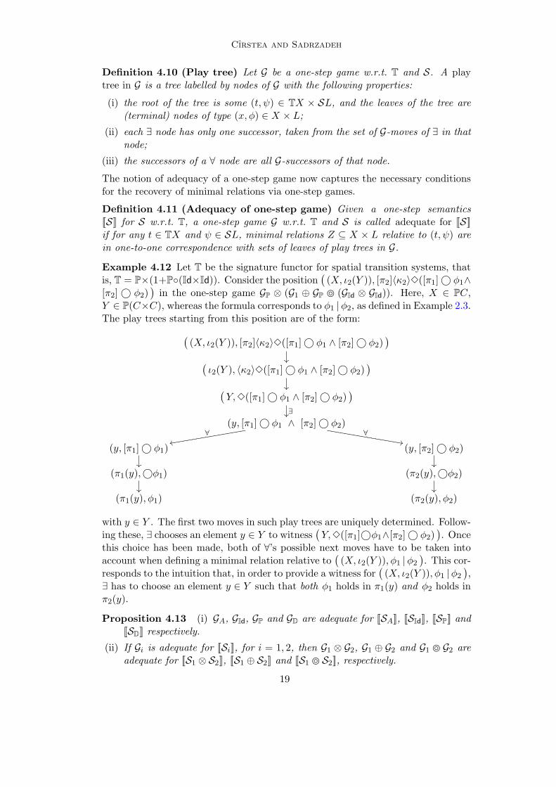
Example 4.12 Let T be the signature functor for spatial transition systems, thatis, T = P×(1+P(Id×Id)). Consider the position

((X, ι2(Y )), [π2]〈κ2〉3([π1]© φ1∧

[π2]© φ2))

in the one-step game GP ⊗ (G1 ⊕ GP (GId ⊗ GId)). Here, X ∈ PC,Y ∈ P(C×C), whereas the formula corresponds to φ1 |φ2, as defined in Example 2.3.The play trees starting from this position are of the form:(

(X, ι2(Y )), [π2]〈κ2〉3([π1]© φ1 ∧ [π2]© φ2))

(ι2(Y ), 〈κ2〉3([π1]© φ1 ∧ [π2]© φ2)

)(

Y,3([π1]© φ1 ∧ [π2]© φ2))

∃(y, [π1]© φ1 ∧ [π2]© φ2)

∀rrddddddddddddddddd ∀

,,ZZZZZZZZZZZZZZZZZ

(y, [π1]© φ1)

(y, [π2]© φ2)

(π1(y),©φ1)

(π2(y),©φ2)

(π1(y), φ1) (π2(y), φ2)

with y ∈ Y . The first two moves in such play trees are uniquely determined. Follow-ing these, ∃ chooses an element y ∈ Y to witness

(Y,3([π1]©φ1∧[π2]© φ2)

). Once

this choice has been made, both of ∀’s possible next moves have to be taken intoaccount when defining a minimal relation relative to

((X, ι2(Y )), φ1 |φ2

). This cor-

responds to the intuition that, in order to provide a witness for(

(X, ι2(Y )), φ1 |φ2

),

∃ has to choose an element y ∈ Y such that both φ1 holds in π1(y) and φ2 holds inπ2(y).

Proposition 4.13 (i) GA, GId, GP and GD are adequate for [[SA]], [[SId]], [[SP]] and[[SD]] respectively.

(ii) If Gi is adequate for [[Si]], for i = 1, 2, then G1 ⊗ G2, G1 ⊕ G2 and G1 G2 areadequate for [[S1 ⊗ S2]], [[S1 ⊕ S2]] and [[S1 S2]], respectively.

19


Proof (Sketch) Follows directly from the definitions of the corresponding one-stepsemantics. 2

Theorem 4.14 (One-step adequacy) If G is adequate for [[S]], then ∃ has a win-ning strategy in Ec0φ0

if and only if he has a winning strategy in the game obtainedfrom Ec0φ0

by replacing the last two moves in Definition 4.1 by the moves of G.

Proof (Sketch) Assume first that ∃ has a winning strategy in the original game.This strategy provides, for each position of type (t, ψ) ∈ TC × SL, a relation Z ⊆C×L s.t. (t, ψ) ∈ [[S]](Z). By Lemma 4.6, we can assume that Z is minimal relativeto (t, ψ). We construct a winning strategy for ∃ in the modified game by replacing∃’s move given by the winning strategy in a position of type (t, ψ) ∈ TC ×SL withmoves in the modified game. By adequacy of G for [[S]], for each minimal Z ⊆ C×Lrelative to (t, ψ) ∈ [[S]](Z), there exists a corresponding play tree starting in (t, ψ).The moves of ∃ in the modified game are obtained directly from this play tree.Specifically, in each ∃ position that belongs to the play tree, ∃ chooses the onlymove that keeps the play inside the play tree. Now since the play tree contains allpossible ∀ moves in the modified game, a move of ∀ will itself keep the play insidethe play tree. Since the Z move of ∃ in the original game was part of a winningstrategy, so is the newly built strategy in the modified game.

Now assume that ∃ has a winning strategy in the modified game. This strategycan be used to define, for each position of type (t, ψ) ∈ TC × SL, a play tree inG – this is done by using ∃’s strategy in each ∃ position, and collecting all of ∀’sG-moves in each ∀ position, repeatedly until a terminal position in G is reached. Byadequacy of G for [[S]], to each such play tree in G there corresponds a minimal Zrelative to (t, ψ). The resulting relations Z and the winning strategy of ∃ in themodified game can now be used to define a winning strategy for ∃ in the originalgame – this is done by replacing ∃’s moves in positions of type (t, ψ) ∈ TC ×SL bythe moves resulting from the play trees. 2

5 Summary and Future Work

We have extended the modular coalgebraic logics of [?,?] with general fixed points,of which until- and dynamic-like fixed points are an instance. Following [21], wehave provided the resulting fixed point logics with a game semantics (by definingevaluation games for formulae and states of coalgebras), and have shown the ade-quacy of this semantics w.r.t. the standard fixed point semantics. Furthermore, wehave shown that the moves corresponding to modal positions in these evaluationgames can be replaced by so-called one-step games, whose boards can be built in-ductively on the structure of the underlying signature functors, and whose movessimulate exactly those moves of the evaluation games which are relevant to decidingthe existence of winning strategies for ∃ (and thus the satisfaction of formulae bystates of coalgebras).

Existing temporal logics for probabilistic systems (as described e.g. in [9]) allowthe formalisation of properties of the kind “with probability at least p, φ holds untilψ holds”. Such languages, interpreted over Markov chains (which are exactly theD-coalgebras), are not recovered as fragments of our fixed point logic for the functor

20


D. We believe that this is due to our choice of modalities Lp and Gp and of theirsemantics. Ongoing work aims to address this by changing the underlying modallanguage.

Developing proof systems for coalgebraic fixed point logics is a natural androutine extension of this paper, but proving completeness of these proof systemsrequires more work. Proof systems are obtained in two steps: (1) the proof systemconstructors of [?] are used to derive a complete set of axioms and rules for theunderlying modal language, and (2) a generalization of Kozen’s induction rule forfixed points [12] is added to the proof system. The subtlety of the first step is thatproof system constructors are functors operating on a category of boolean theories,which for the purpose of well-definedness of our fixed points have to be restrictedto theories closed under conjunction and disjunction.

Our adequacy theorem shows that deciding about the satisfaction of a formulaby a pointed coalgebra is equivalent to deciding whether ∃ has a history-free winningstrategy in the evaluation game. The time complexity of the latter is exponential inthe size of the game board [19]. However, it is well known that if one restricts thefixed points to the alternation-free fragment, the complexity reduces to polynomialtime [19]. Our game boards are generalizations of those for the propositional µ-calculus, and the exact impact this has on complexity deserves further study. How-ever, we conjecture that by only using minimal relations (Definition 4.5) as possiblemoves of ∃, similar complexity results to those for the propositional µ-calculus canbe obtained.

Acknowledgement

Thanks are due to James Worrell for useful discussions on games for the modalµ-calculus, and to the anonymous referees for several suggestions on improving thepaper.

References

[1] A. Baltag. A logic for coalgebraic simulation. In H. Reichel, editor, Coalgebraic Methods in ComputerScience, volume 33 of Electronic Notes in Theoretical Computer Science, pages 41–60, 2000.

[2] A. Baltag and L.S. Moss. Logics for epistemic programs. Synthese, 139, 2004.

[3] C. Cırstea. A compositional approach to defining logics for coalgebras. Theoretical Computer Science,327:45–69, 2004.

[4] C. Cırstea and D. Pattinson. Modular construction of complete coalgebraic logics. TheoreticalComputer Science, 388:83–108, 2007.

[5] C. Cırstea and M. Sadrzadeh. Coalgebraic epistemic update without change of model. In Proceedingsof the 2nd Conference on Algebra and Coalgebra in Computer Science, volume 4624 of Lecture Notesin Computer Science, pages 158–172. 2007.

[6] L. Cardelli and A.D. Gordon. Anytime, anywhere: modal logics for mobile ambients. In POPL ’00:Proceedings of the 27th ACM SIGPLAN-SIGACT symposium on Principles of programming languages,pages 365–377. ACM, 2000.

[7] E.A. Emerson and C.S. Jutla. Tree automata, mu-calculus and determinacy. In Proceedings of the32nd IEEE Symposium on Foundations of Computer Science, pages 368–377. IEEE Computer SocietyPress, 1991.

[8] E. Graedel, W. Thomas, and T. Wilke, editors. Automata, Logic, and Infinite Games, volume 2500 ofLecture Notes in Computer Science. 2002.

21


[9] H. Hansson and B. Jonsson. A logic for reasoning about time and reliability. Formal Aspects ofComputing, 6(5):512–535, 1994.

[10] D. Janin and I. Walukiewicz. Automata for the modal µ-calculus and related results. In Proceedingsof the 20th International Symposium on Mathematical Structures in Computer Science, volume 969 ofLecture Notes in Computer Science, pages 552–562. 1995.

[11] B. Jonsson, K.G. Larsen, and W. Yi. Probabilistic extensions of process algebras. In J.A. Bergstraet al, editor, Handbook of Process Algebra, pages 685–710. Elsevier, 2001.

[12] D. Kozen. Results on the propositional mu-calculus. Theoretical Computer Science, 27:333–354, 1983.

[13] L. Monteiro. A noninterleaving model of concurrency based on transition systems with spatial structure.In Proceedings of the Workshop on Coalgebraic Methods in Computer Science, volume 106 of ElectronicNotes in Theoretical Computer Science, pages 261–277. Elsevier, 2004.

[14] L.S. Moss. Coalgebraic logic. Annals of Pure and Applied Logic, 96:241–259, 1999.

[15] D. Niwinski. Fixed point characterization of infinite behavior of finite-state systems. TheoreticalComputer Science, 189, 1997.

[16] D. Pattinson. Coalgebraic modal logic: soundness, completeness and decidability of local consequence.Theoretical Computer Science, 309:177–193, 2003.

[17] L. Schroder. Expressivity of coalgebraic modal logic: The limits and beyond. In V. Sassone, editor,Foundations of Software Science and Computation Structures, volume 3441 of Lecture Notes inComputer Science, pages 440–454, 2005.

[18] R. Segala. Modelling and Verification of Randomized Distributed Real-Time Systems. PhD thesis,Massachusetts Institute of Technology, 1995.

[19] C. Stirling. Modal and Temporal Properties of Processes. Springer, 2001.

[20] M. Vardi. Alternating automata: Checking truth and validity for temporal logics. In Proceedings ofthe 14th International Conference on Automated Deduction. 1997.

[21] Y. Venema. Automata and fixed point logic: a coalgebraic perspective. Information and Computation,204:637–678, 2006.

[22] T. Wilke. Alternating tree automata, parity games, and modal µ-calculus. Bulletin of BelgianMathematical Society, 8:359–391, 2002.

22

Modular Games for Coalgebraic Fixed Point Logics

Documents

Transcript of Modular Games for Coalgebraic Fixed Point Logics