arX

iv:1

407.

1386

v1 [

cs.L

O]

5 J

ul 2

014

Undecidable propositional bimodal logics and

one-variable first-order linear temporal logics with counting

C. Hampson and A. Kurucz

Department of Informatics, King’s College London

July 8, 2014

Abstract

First-order temporal logics are notorious for their bad computational behaviour. It isknown that even the two-variable monadic fragment is highly undecidable over various lin-ear timelines, and over branching time even one-variable fragments might be undecidable.However, there have been several attempts on finding well-behaved fragments of first-ordertemporal logics and related temporal description logics, mostly either by restricting the avail-able quantifier patterns, or considering sub-Boolean languages. Here we analyse seemingly‘mild’ extensions of decidable one-variable fragments with counting capabilities, interpretedin models with constant, decreasing, and expanding first-order domains. We show that overmost classes of linear orders these logics are (sometimes highly) undecidable, even withoutconstant and function symbols, and with the sole temporal operator ‘eventually’.

We establish connections with bimodal logics over 2D product structures having linear and‘difference’ (inequality) component relations, and prove our results in this bimodal setting.We show a general result saying that satisfiability over many classes of bimodal models withcommuting ‘unbounded’ linear and difference relations is undecidable. As a by-product, wealso obtain new examples of finitely axiomatisable but Kripke incomplete bimodal logics. Ourresults generalise similar lower bounds on bimodal logics over products of two linear relations,and our proof methods are quite different from the proofs of these results. Unlike previousproofs that first ‘diagonally encode’ an infinite grid, and then use reductions of tiling or Turingmachine problems, here we make direct use the grid-like structure of product frames and obtainundecidability by reductions of counter (Minsky) machine problems. Representing countermachine runs apparently requires less control over neighbouring grid-points than tilings orTuring machine runs, and so this technique is possibly more versatile, even if one componentof the underlying product structures is ‘close to’ being an equivalence relation.

1 Introduction

1.1 First-order linear temporal logic with counting.

Though first-order temporal logics are natural and expressive languages for querying and con-straining temporal databases [7, 8] and reasoning about knowledge that changes in time [25],their practical use has been discouraged by their high computational complexity. It is well-knownthat even the two-variable monadic fragment is undecidable over various linear timelines, and itssatisfiability problem is Σ1

1-hard over the natural numbers [47, 48, 35, 12, 13]. Also, even the one-variable fragment of first-order branching time logic CTL∗ is undecidable [26]. Still, similarly toclassical first-order logic where the decision problems of its fragments were studied in great detail[5], there have been several attempts on finding well-behaved decidable fragments of first-ordertemporal logics and related temporal description logics, mostly either by restricting the availablequantifier patterns [8, 24, 25, 3, 9, 21, 22, 31], or considering sub-Boolean languages [30, 2].

In this paper we contribute to this research line by considering seemingly ‘mild’ extensions ofdecidable one-variable fragments. We study the one-variable ‘future’ fragment of linear temporal

1

logic with counting to two, interpreted in models over various timelines, and having constant,decreasing, or expanding first-order domains. Our language FOLTL 6= keeps all Boolean connec-tives, it has no restriction on formula-generation, and it is strong enough to express uniqueness ofa property of domain elements (∃=1x ), and the ‘elsewhere’ quantifier (∀6=x ). However, FOLTL 6=-formulas use only a single variable (and so contain only monadic predicate symbols), FOLTL 6=

has no equality, no constant or function symbols, and its only temporal operators are ‘eventually’and ‘always in the future’. FOLTL 6= is weaker than the two-variable monadic monodic fragmentwith equality, where temporal operators can be applied only to subformulas with at most one freevariable. (This fragment with the ‘next time’ operator is known to be Σ1

1-hard over the naturalnumbers [50, 10].) FOLTL 6= is connected to bimodal product logics [14, 13] (see also below), andto the temporalisation of the expressive description logic CQ with one global universal role [49].Here are some examples of FOLTL 6=-formulas:

• “An order can only be submitted once:” ∀x✷F(Subm(x) → ✷F¬Subm(x)

).

• The Barcan formula: ∃x✸FP ↔ ✸F∃xP.

• “Every day has its unique dog:” ✷F∃=1x(Dog(x) ∧ ✷F¬Dog(x)

).

• “It’s only me who is always unlucky:” ∀6=x✸FLucky(x).

Note that FOLTL 6= can also be considered as a fragment of three-variable classical first-orderlogic with only binary predicate symbols, but it is not within the guarded fragment.

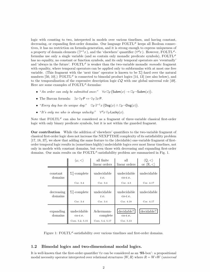
Our contribution While the addition of ‘elsewhere’ quantifiers to the two-variable fragment ofclassical first-order logic does not increase the NEXPTIME complexity of its satisfiability problem[17, 18, 37], we show that adding the same feature to the (decidable) one-variable fragment of first-order temporal logic results in (sometimes highly) undecidable logics over most linear timelines, notonly in models with constant domains, but even those with decreasing and expanding first-orderdomains. Our main results on the FOLTL 6=-satisfiability problem are summarised in Fig. 1.

〈ω,<〉 all finite all 〈Q, <〉linear orders linear orders or 〈R, <〉

constant Σ11-complete undecidable undecidable undecidable

domains r.e. co-r.e.

Cor. 3.4 Cor. 3.4 Cor. 4.3 Cor. 4.17

decreasing Σ11-complete undecidable undecidable undecidable

domains r.e. co-r.e.

Cor. 3.4 Cor. 3.4 Cor. 4.18 Cor. 4.17

expanding undecidable Ackermann- decidable? decidable?domains co-r.e. complete co-r.e.

Cors. 5.2, 5.15 Cors. 5.4, 5.17 Cor. 5.13

Figure 1: FOLTL 6=-satisfiability over various timelines and first-order domains.

1.2 Bimodal logics and two-dimensional modal logics.

It is well-known that the first-order quantifier ∀x can be considered as an ‘S5-box’: a propositionalmodal necessity operator interpreted over relational structures 〈W,R〉 where R = W×W (universal

2

frames , in modal logic parlance). Therefore, the two-variable fragment of classical first-orderlogic is related to propositional bimodal logic over two-dimensional (2D) product frames [33].Similarly, the ‘elsewhere’ quantifier ∀6=x can be regarded as a ‘Diff -box’: a propositional modalnecessity operator interpreted over difference frames 〈W, 6=〉 where 6= is the inequality relationon W . Looking at FOLTL 6= this way, it turns out that it is just a notational variant of thepropositional bimodal logic over 2D products of linear orders and difference frames (Prop. 2.3).

Propositional multimodal languages interpreted in various product-like structures show up inmany other contexts, and connected to several other multi-dimensional logical formalisms, suchas modal and temporal description logics, and spatio-temporal logics (see [13, 28] for surveysand references). The product construction as a general combination method on modal logics wasintroduced in [43, 45, 14], and has been extensively studied ever since.

Our contribution We study the satisfiability problem of our logics in the propositional bi-modal setting. We show that satisfiability over many classes of bimodal frames with commutinglinear and difference relations are undecidable (Theorems 3.2, 4.1), sometimes not even recursivelyenumerable (Theorems 3.1, 4.11). As a by-product, we also obtain new examples of finitely ax-iomatisable but Kripke incomplete bimodal logics (Cor. 4.13). It is easy to see (Prop. 2.2) thatsatisfiability over decreasing or expanding subframes of product frames is always reducible to ‘fullrectangular’ product frame-satisfiability. We show cases when expanding frame-satisfiability isgenuinely simpler than product-satisfiability (Theorems 5.14, 5.16), while it is still very complex(Theorems 5.3, 5.1).

Our results are in sharp contrast with the much lower complexity of bimodal logics over prod-ucts of linear and universal frames: Satisfiability over these is usually decidable with complexitybetween EXPSPACE and 2EXPTIME [23, 38]. On the other hand, our findings are quite parallelto the results about products where both components are linear [32, 39, 16, 15, 27]. So the ques-tion arises whether there is a ‘direct’ reduction from these product logics into ‘linear×difference’type products. The more so that satisfiability over linear and difference frames is of the same(NP-complete) complexity, and so there is a reduction from ‘linear-satisfiability’ to ‘difference-satisfiability’. However, we cannot hope that such a reduction can be ‘lifted’ somehow to the2D level: satisfiability over ‘difference×difference’ type products is decidable (being a fragmentof two-variable classical first-order logic with counting), while ‘linear×linear’-satisfiability is un-decidable [39]. So our lower bound results seem to be proper generalisations of the lower boundresults in the papers listed above.

Our undecidability proofs are quite different from most known undecidability proofs about2D product logics with transitive components [32, 39, 15]. Even if frames with two commutingrelations (and so product frames) always have grid-like substructures, there are two issues oneneeds to deal with in order to encode grid-based complex problems into them:

• to generate infinity, and

• somehow to ‘access’ or ‘refer to’ neighbouring-grid points, even when there might be furthernon-grid points around, there is no ‘next-time’ operator in the language, and the relationsare transitive and/or dense and/or even ‘close to’ universal.

Unlike previous proofs that first ‘diagonally encode’ the ω × ω-grid, and then use reductionsof tiling or Turing machine problems, here we make direct use the grid-like substructures incommutative frames and obtain lower bounds by reductions of counter (Minsky) machine problems.Representing counter machine runs apparently requires less control over neighbouring grid-pointsthan tilings or Turing machine runs, and so this technique is possibly more versatile (see Section 2.5for more details).

Structure Section 2 provides all the necessary definitions, and establishes connections betweenthe two different formalisms. All results are then proved in the propositional bimodal setting. Inparticular, Section 3 deals with the constant and decreasing domain cases over 〈ω,<〉 and finitelinear orders. More general results on bimodal logics with ‘linear’ and ‘difference’ components are

3

in Section 4. The expanding domain cases are treated in Section 5. Finally, in Section 6 we discusssome related open problems.

Some of the results appeared in the extended abstract [19].

2 Preliminaries

2.1 Propositional bimodal logics

We define bimodal formulas by the following grammar:

φ :: P | ¬φ | φ ∧ ψ | ✸0φ | ✸1φ

where P ranges over an infinite set of propositional variables. We use the usual abbreviations ∨,→, ↔, ⊥ := P ∧ ¬P, ⊤ := ¬⊥, ✷i := ¬✸i¬, and also

✸+i φ :: φ ∨✸iφ, ✷

+i φ :: φ ∧ ✷iφ,

for i = 0, 1. For any bimodal formula φ, we denote by subφ the set of its subformulas.A 2-frame is a tuple F = 〈W,R0, R1〉 where Ri are binary relations on the non-empty set W .

A model based on F is a pair M = (F, ν), where ν is a function mapping propositional variablesto subsets of W . The truth relation M, w |= ϕ is defined, for all w ∈ W , by induction on φ asfollows:

• M, w |= P iff w ∈ ν(P),

• M, w |= ¬φ iff M, w 6|= φ, M, w |= φ ∧ ψ iff M, w |= φ and M, w |= ψ,

• M, w |= ✸iφ iff there exists v ∈W such that wRv and M, v |= φ.

We say that φ is satisfied in M, if there is w ∈ W with M, w |= φ. Given a set Σ of bimodalformulas, we write M |= Σ if we have M, w |= φ, for every φ ∈ Σ and every w ∈ W . We say thatφ is valid in F, if M, w |= φ, for every model M based on F and for every w ∈W . If every formulain a set Σ is valid in F, then we say that F is a frame for Σ. We let FrΣ denote the class of allframes for Σ.

A set L of bimodal formulas is called a (normal) bimodal logic (or logic, for short) if it containsall propositional tautologies and the formulas ✷i(p → q) → (✷ip → ✷iq), for i < 2, and is closedunder the rules of Substitution, Modus Ponens and Necessitation ϕ/✷iϕ, for i < 2. Given abimodal logic L, we will consider the following problem:

L-satisfiability: Given a bimodal formula φ, is there a model M such that M |= L andφ is satisfied in M?

For any class C of 2-frames, we always obtain a logic by taking

Log C = {ϕ : ϕ is a bimodal formula valid in every member of C}.

We say that Log C is determined by C, and call such a logic Kripke complete. (We write just LogF

for Log {F}.) Clearly, if L = Log C, then there might exist frames for L that are not in C, butL-satisfiability is the same as

C-satisfiability: Given a bimodal formula φ, is there a 2-frame F ∈ C such that φ issatisfied in a model based on F?

Commutators and products We might consider bimodal logics as ‘combinations’ of theirunimodal1 ‘components’. Let L0 and L1 be two unimodal logics formulated using the same propo-sitional variables and Booleans, but having different modal operators (✸0 for L0 and ✸1 for L1).

1Syntax and semantics of unimodal logics are defined similarly to bimodal ones, using only one of the two modaloperators. Throughout, 1-frames will be called simply frames.

4

Their fusion L0⊕L1 is the smallest bimodal logic that contains both L0 and L1. The commutator

[L0, L1] of L0 and L1 is the smallest bimodal logic that contains L0 ⊕ L1 and the formulas

✷1✷0P → ✷0✷1P, ✷0✷1P → ✷1✷0P, ✸0✷1P → ✷1✸0P. (1)

It is well-known that a 2-frame 〈W,R0, R1〉 validates these formulas iff

• R0 and R1 commute: ∀x, y, z(xR0yR1z → ∃u (xR1uR0z)

), and

• R0 and R1 are confluent : ∀x, y, z(xR0y ∧ xR1z → ∃u (yR1u ∧ zR0u)

).

Note that if at least one of R0 or R1 is symmetric, then confluence follows from commutativity.Next, we introduce some special ‘two-dimensional’ 2-frames for commutators. Given frames

F0 = 〈W0, R0〉 and F1 = 〈W1, R1〉, their product is defined to be the 2-frame

F0×F1 = 〈W0×W1, R0, R1〉,

where W0×W1 is the Cartesian product of W0 and W1 and, for all u, u′ ∈W0, v, v′ ∈ W1,

〈u, v〉R0〈u′, v′〉 iff uR0u

′ and v = v′,

〈u, v〉R1〈u′, v′〉 iff vR1v

′ and u = u′.

2-frames of this form will be called product frames throughout. For classes C0 and C1 of unimodalframes, we define

C0×C1 = {F0×F1 : Fi ∈ Ci, for i = 0, 1}.

Now, for i < 2, let Li be a Kripke complete unimodal logic in the language with ✸i. The product

of L0 and L1 is defined as the (Kripke complete) bimodal logic

L0 × L1 = Log (FrL0×FrL1).

Product frames always validate the formulas in (1), and so [L0, L1] ⊆ L0×L1 always holds. Ifboth L0 and L1 are Horn axiomatisable, then [L0, L1] = L0×L1 [14]. In general, [L0, L1] can notonly be properly contained in L0×L1, but there might even be infinitely many logics in between[29, 20].

The following result of Gabbay and Shehtman [14] is one of the few general ‘transfer’ resultson the satisfiability problem of 2D logics. It is an easy consequence of the recursive enumerabilityof the consequence relation of classical (many-sorted) first-order logic:

Theorem 2.1. If C0 and C1 are classes of frames such that both are recursively first-order definable

in the language having a binary predicate symbol, then C0×C1-satisfiability is co-r.e., that is, its

complement is recursively enumerable.

Expanding and decreasing 2-frames Product frames are special cases of the following con-struction for getting 2D frames. Take a (‘horizontal’) frame F = 〈W,R〉 and a sequence G =⟨Gu = 〈Wu, Ru〉 : u ∈W

⟩of (‘vertical’) frames. We can define a 2-frame by taking

HF,G =

⟨{〈u, v〉 : u ∈ W, v ∈Wu}, R0, R1

⟩,

where

〈u, v〉R0〈u′, v′〉 iff uRu′ and v = v′,

〈u, v〉R1〈u′, v′〉 iff vRuv

′ and u = u′.

Clearly, if Gx = Gy = G for all x, y in F, then HF,G = F×G. However, we can put slightly milder

assumptions on the Gx. We call a 2-frame of the form HF,G

5

• an expanding 2-frame if Gx is a subframe2 of Gy whenever xRy, and

• a decreasing 2-frame if Gy is a subframe of Gx whenever xRy.

So product frames are both expanding and decreasing 2-frames. Expanding 2-frames alwaysvalidate ✷0✷1P → ✷1✷0P and ✸0✷1P → ✷1✸0P (but not necessarily ✷1✷0P → ✷0✷1P), anddecreasing 2-frames validate ✷1✷0P → ✷0✷1P (but not necessarily the other two formulas in (1)).

For classes C0 and C1 of frames, we define

C0×eC1 = {expanding 2-frame H

F,G : F ∈ C0, Gx ∈ C1 for all x in F},

C0×dC1 = {decreasing 2-frame H

F,G : F ∈ C0, Gx ∈ C1 for all x in F}.

It is not hard to see that for all classes C0, C1 of frames, both C0×dC1-satisfiability and C0×eC1-satisfiability is reducible to C0×C1-satisfiability. Indeed, take a fresh propositional variable D, andfor every bimodal formula φ, define φD by relativising each occurrence of ✸0 and ✸1 in φ to D.Let n be the nesting depth of the modal operators in φ, any for any formula ψ and i = 0, 1, let

✷≤ni ψ :=

∧

k≤n

k︷ ︸︸ ︷

✷i . . .✷i ψ.

Then we have (cf. [13, Thm.9.12]):

Proposition 2.2.

• φ is C0×dC1-satisfiable iff D ∧ ✷

≤n0 ✷

≤n1

(✸0D → D

)∧ φD is C0×C1-satisfiable.

• φ is C0×eC1-satisfiable iff D ∧ ✷≤n0 ✷

≤n1

(D → ✷0D

)∧ φD is C0×C1-satisfiable.

‘Linear’ and ‘difference’ logics Throughout, a frame 〈W,R〉 is called rooted with root r ∈Wif every w ∈ W can be reached from r by taking finitely many R-steps. By a linear order wemean an irreflexive3, transitive and trichotomous relation. Let Clin and Cfin

lin denote the classes ofall linear orders and all finite linear orders, respectively. We let K4.3 := Log Cdiff, that is, theunimodal logic determined by all linear orders. K4.3 is well-studied as a temporal logic, and it iswell-known that frames for K4.3 are weak orders.4 A linear order 〈W,R〉 is a called a well-order

if every non-empty subset of W has an R-least element.We denote by Cdiff (Cfin

diff) the class of all (finite) difference frames, that is, frames of the form〈W, 6=〉 where 6= is the inequality relation on W . We let Diff = Log Cdiff, that is, the unimodallogic determined by all difference frames. From the axiomatisation of Diff by Segerberg [44] itfollows that frames for Diff are pseudo-equivalence5 relations. If M is a model based on a rootedpseudo-equivalence frame, then we can express the uniqueness of a modally definable property inM. For any formula φ,

✸=1φ :: ✸

+(φ ∧✷¬φ).

Then, ✸=1φ is satisfied in M iff there is a unique w with M, w |= φ.As all the axioms of K4.3 and Diff , and the formulas in (1) are Sahlqvist formulas, the

commutator [K4.3,Diff ] is Sahlqvist axiomatisable, and so Kripke complete:

[K4.3,Diff ] = Log{〈W,R0, R1〉 : R0 is a weak order,

R1 is a pseudo-equivalence, R0 and R1 commute} (2)

(for more information on Sahlqvist formulas and canonicity, consult e.g. [4, 6]).

2〈W,R〉 is called a subframe of 〈U,S〉, if W ⊆ U and R = S ∩ (W×W ).3This is just for simplifying the overall presentation. Reflexive cases are covered in Section 4.3.4A relation R is called a weak order if it is transitive and weakly connected : ∀x, y, z

(

xRy ∧ xRz → (y = z ∨

yRz ∨ zRy))

. In other words, a rooted weak order is a linear chain of clusters of universally connected points.5A relation R is called a pseudo-equivalence if it is symmetric and pseudo-transitive: ∀x, y, z

(

xRyRz → (x = z∨

xRz))

. So a pseudo-equivalence is almost an equivalence relation, just it might have both reflexive and irreflexivepoints.

6

2.2 One-variable first-order linear temporal logic with counting to two

We define FOLTL 6=-formulas by the following grammar:

φ :: P(x) | ¬φ | φ ∧ ψ | ✸Fφ | ∃6=x φ

where (with a slight abuse of notation) P ranges over an infinite set P of monadic predicatesymbols.

A FOLTL-model is a tuple M =⟨〈T,<〉, Dt, I

⟩

t∈T, where 〈T,<〉 is a linear order, representing

the timeline, Dt is a non-empty set, the domain at moment t, for each t ∈ T , and I is a functionassociating with every t ∈ T a first-order structure I(t) = 〈Dt,P

I(t)〉P∈P . We say that M isbased on the linear order 〈T,<〉. M is a constant (resp. decreasing, expanding) domain model , ifDt = Dt′ , (resp. Dt ⊇ Dt′ , Dt ⊆ Dt′) whenever t, t′ ∈ T and t < t′. A constant domain model isclearly both a decreasing and expanding domain model as well, and can be represented as a triple⟨〈T,<〉, D, I

⟩.

The truth-relation (M, t) |=a φ (or simply t |=a φ if M is understood) is defined, for all t ∈ Tand a ∈ Dt, by induction on φ as follows:

• t |=a P(x) iff a ∈ PI(t), t |=a ¬φ iff t 6|=a φ, t |=a φ ∧ ψ iff t |=a φ and t |=a ψ,

• t |=a ∃6=xφ iff there exists b ∈ Dt such that b 6= a and t |=b φ,

• t |=a✸Fφ iff there is t′ ∈ T such that t′ > t, a ∈ Dt′ and t′ |=a φ.

We say that φ is satisfiable in M, if t |=a φ holds for some t ∈ T and a ∈ Dt. Given a class Cof linear orders, we say that φ is FOLTL 6=-satisfiable in constant (decreasing, expanding) domain

models over C, if φ is satisfiable in some constant (decreasing, expanding) domain FOLTL-modelbased on some linear order from C.

We introduce the following abbreviations:

∃xφ :: φ ∨ ∃6=xφ, ∃≥2xφ :: ∃x (φ ∧ ∃6=xφ).

It is straightforward to see that they have the intended semantics:

• t |=a ∃xφ iff there exists b ∈ Dt with t |=b φ,

• t |=a ∃≥2xφ iff there exist b, b′ ∈ Dt with b 6= b′, t |=b φ and t |=b′ φ.

Also, we could have chosen ∃x and ∃≥2x as our primary connectives instead of ∃6=x , as

∃6=xφ ↔ (¬φ ∧ ∃xφ) ∨ ∃≥2xφ.

2.3 Connections between propositional bimodal logic and FOLTL6=

Clearly, one can define a bijection ⋆ from FOLTL 6=-formulas to bimodal formulas, mapping eachP(x) to P, ✸Fφ to ✸0φ

⋆, ∃6=xφ to ✸1φ⋆, and commuting with the Booleans. Also, there is

a bijection † between constant domain FOLTL-models M =⟨〈T,<〉, D, I

⟩and modal models

M† = 〈F, ν〉 where F = 〈T,<〉× 〈D, 6=〉 and ν(P) = {〈t, a〉 : M, t |=a P(x)}. Similarly, there isa one-to-one connection between expanding (decreasing) 2-frames with linear ‘horizontal’ anddifference ‘vertical’ components, and expanding (decreasing) domain FOLTL-models. So it isstraightforward to see the following:

Proposition 2.3. For any class C of linear orders, and any FOLTL 6=-formula φ,

• φ is FOLTL6=-satisfiable in constant domain models over C iff φ⋆ is C×Cdiff-satisfiable;

• φ is FOLTL 6=-satisfiable in expanding domain models over C iff φ⋆ is C×eCdiff-satisfiable;

• φ is FOLTL 6=-satisfiable in decreasing domain models over C iff φ⋆ is C×dCdiff-satisfiable.

7

2.4 Counter machines

A Minsky or counter machine M is described by a finite set Q of states, a set H ⊆ Q of terminalstates, a finite set C = {c0, . . . , cN−1} of counters with N > 1, a finite nonempty set Iq ⊆ OpC×Qof instructions, for each q ∈ Q −H , where each operation in OpC is one of the following forms,for some i < N :

• c++i (increment counter ci by one),

• c−−i (decrement counter ci by one),

• c??i (test whether counter ci is empty).

A configuration of M is a tuple 〈q, c〉 with q ∈ Q representing the current state, and an N -tuplec = 〈c0, . . . , cN−1〉 of natural numbers representing the current contents of the counters. For eachι ∈ OpC , we say that there is a (reliable) ι-step between configurations σ = 〈q, c〉 and σ′ = 〈q′, c′〉(written σ→ι σ′) iff there is 〈ι, q′〉 ∈ Iq such that

• either ι = c++i and c′i = ci + 1, c′j = cj for j 6= i, j < N ,

• or ι = c−−i and c′i = ci − 1, c′j = cj for j 6= i, j < N ,

• or ι = c??i and c′i = ci = 0, c′j = cj for j < N .

We write σ→σ′ iff σ→ι σ′ for some ι ∈ OpC . For each ι ∈ OpC , we write σ→ιlossy σ

′ if there

are configurations σ1 = 〈q, c1〉 and σ2 = 〈q′, c2〉 such that σ1 →ι σ2, ci ≥ c1i and c2i ≥ c′i forevery i < N . We write σ→lossy σ

′ iff σ→ιlossy σ

′ for some ι ∈ OpC . A sequence 〈σn : n <B〉 of configurations, with 0 < B ≤ ω, is called a run (resp. lossy run), if σn−1 →σn (resp.σn−1 →lossy σn) holds for every 0 < n < B.

Below we list the counter machine problems we will use in our lower bound proofs.

CM non-termination: (Π01-hard [36])

Given a counter machine M and a state q0, does M have an infiniterun starting with 〈q0,0〉?

CM reachability: (Σ01-hard [36])

Given a counter machine M, a configuration σ0 = 〈q0,0〉 and a state qr,does M have a run starting with σ0 and reaching qr?

CM recurrence: (Σ11-hard [1])

Given a counter machine M and two states q0, qr, does M have a run startingwith 〈q0,0〉 and visiting qr infinitely often?

LCM reachability: (Ackermann-hard [41])

Given a counter machine M, a configuration σ0 = 〈q0,0〉 and a state qr,does M have a lossy run starting with σ0 and reaching qr?

The Ackermann-hardness of this problem is shown by Schnoebelen [41] without the restrictionthat σ0 has all-0 counters. It is not hard to see that this restriction does not matter: For every Mand σ0 one can define a machine Mσ0 that first performs incrementation steps filling the countersup to their ‘σ0-level’, and then performs M’s actions. Then M has a lossy run starting with σ0and reaching qr iff Mσ0 has a lossy run starting with all-0 counters and reaching qr.

LCM ω-reachability: (Π01-hard [27, 34, 40])

Given a counter machine M , a configuration σ0 = 〈q0,0〉 and a state qr,is it the case that for every n < ω M has a lossy run starting with σ0and visiting qr at least n times?

8

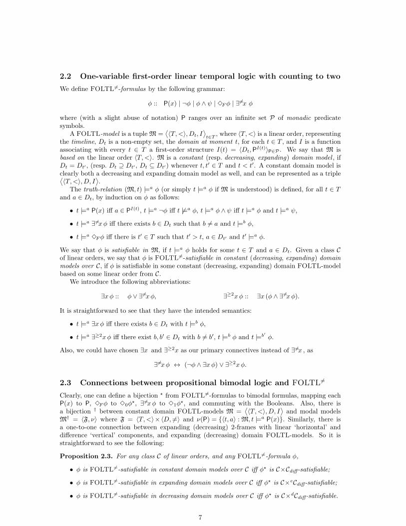
2.5 Representing counter machine runs in our logics

Before stating and proving our results, here we give a short informal guide on how we intend touse counter machines in the various lower bound proofs of the paper. To begin with, using twodifferent propositional variables S (for state) and N (for next), we force a ‘diagonal staircase’ withthe following properties:

(i) every S-point R1-sees a unique N-point, and

(ii) every N-point has an S-point as its ‘immediate R0-successor’.

This way we not only force infinity, but also get a ‘horizontal’ next-time operator:

Xφ :: ✷1

(N → ✷0(S → φ)

)

(see Fig. 2). In the simplest case of product frames of the form 〈ω,<〉×〈W, 6=〉, a grid-like structurewith subsequent columns comes by definition, so everything is ready for encoding counter machineruns in them: Subsequent states of a run will be represented by subsequently generated S-points,and the content of each counter ci at step n of a run will be represented by the number of Ci-points at the nth column of the grid, for some formula Ci (see Fig. 2). As in difference framesuniqueness of a property is modally expressible, we can faithfully express the subsequent changesof the counters (see Section 3).

✲ ✲ ✲ ✲ ✲ ✲ ✲ ✲

ci(n)=3

✲

✲

✲

✲

✲

✲

✲

s

s

s

s

s

s

s

s

s

s

s

s

s

s

s

s✲

✈ ✈

✈

✈

✈

✈ ✈

✈

✈

✈

✈

✈

✈

✈

✈

N

N

N

N

N

N

N

N

SS

S

S

S

S

S

q0

q1

q2

qn

♣ ♣ ♣

♣ ♣ ♣

〈ω,<〉

〈D, 6=〉

♣♣♣

♣♣♣

♣♣♣

♣♣♣

♣♣♣

♣♣♣

♣♣♣

♣♣♣

Figure 2: Representing counter machine runs in product frames 〈ω,<〉×〈D, 6=〉 ‘going forward’.

When generalising this technique to ‘timelines’ other than 〈ω,<〉, there can be additionaldifficulties, as (ii) above is clearly not doable over dense linear orders. Instead of working withR0-connected points, we work with ‘R0-intervals’ and have the ‘interval-analogue’ of (ii): EveryN-interval has an S-interval as its ‘immediate R0-successor’ (see Section 4.3).

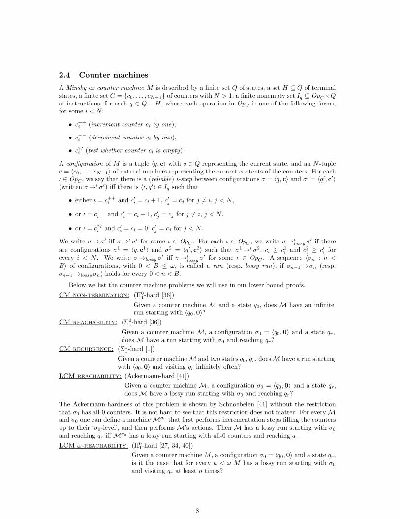
We also generalise our results not only to decreasing 2-frames but for more ‘abstract’ 2-frameshaving commuting weak order and pseudo-equivance relations (see (2)). In the abstract case, weface an additional difficulty: While commutativity does force the presence of grid-points once adiagonal staircase is present, there might be many other non-grid points in the corresponding‘vertical columns’, so the control over runs becomes more complicated. In these cases, both thediagonal staircase and counter machine runs are forced going ‘backward’ (see Fig. 3), as this wayseemingly gives us greater control over the ‘intended’ grid-points (see Section 4.1).

9

✲ ✲ ✲ ✲ ✲ ✲ ✲

✲ ✲ ✲ ✲ ✲ ✲ ✲

✲ ✲ ✲ ✲ ✲ ✲ ✲

✲ ✲ ✲ ✲ ✲ ✲ ✲

✲ ✲ ✲ ✲ ✲ ✲ ✲

✲ ✲ ✲ ✲ ✲ ✲ ✲

✲ ✲ ✲ ✲ ✲ ✲ ✲

✲ ✲ ✲ ✲ ✲ ✲ ✲

✲

✲

✲

✲

✲

✲

✲

✲

✲

✲

✲

✲

✲

✲

✲

♣ ♣ ♣

♣ ♣ ♣

♣ ♣ ♣

♣ ♣ ♣

♣ ♣ ♣

♣ ♣ ♣

♣ ♣ ♣

♣ ♣ ♣

❅❅

��

ci(n)=3

✲

✲

✲

✲

✲

✲

✲

s

s

s

s

s

s

s

s

s

s

s

s

s

s

s

✲

〈W1,R1〉

♣♣♣

♣♣♣

♣♣♣

♣♣♣

♣♣♣

♣♣♣

♣♣♣

♣♣♣

♣♣♣

✈✈

✈

✈

✈

✈

✈

✈

✈

✈

✈

✈

✈

✈

✈

S

S

S

S

S

S

S

S

N

N

N

N

N

N

N

q0

q1

q2

qn

〈W0,R0〉

Figure 3: Representing counter machine runs in commutative 2-frames ‘going backward’.

The backward technique also helps us to represent lossy counter machine runs in expanding2-frames. When going backward horizontally in expanding 2-frames, the vertical columns mightbecome smaller and smaller, so some of the points carrying the information on the content of thecounters might disappear as the runs progress (see Section 5.1).

3 〈ω,<〉 or finite linear orders as ‘timelines’

In this section we show the constant and decreasing domain results in the first two columns ofFig. 1.

Theorem 3.1. {〈ω,<〉}×Cdiff-satisfiability is Σ11-complete.

Theorem 3.2. Cfinlin×Cdiff-satisfiability is recursively enumerable, but undecidable.

By Prop. 2.2, C×dCdiff-satisfiability is always reducible to C×Cdiff-satisfiability. It is not hard

to see that, whenever C = {〈ω,<〉} or C = Cfinlin , then we also have this the other way round:

C×Cdiff-satisfiability is reducible to C×dCdiff-satisfiability.

Proposition 3.3. If C = {〈ω,<〉} or C = Cfinlin , then for any formula φ,

φ is C×Cdiff-satisfiable iff ✷+1 ✷

+0 (✸0⊤ → ✷1✸0⊤) ∧ φ is C×dCdiff-satisfiable.

So by Theorems 3.1, 3.2 and Props. 2.3, 3.3 we obtain:

Corollary 3.4. FOLTL 6=-satisfiability recursively enumerable but undecidable in both constant

decreasing domain models over the class of all finite linear orders, and Σ11-complete in both constant

and decreasing domain models over 〈ω,<〉.

We prove the lower bound of Theorem 3.1 by reducing the ‘CM recurrence’ problem to {〈ω,<〉}×Cdiff-satisfiability. Let M be a model based on the the product of 〈ω,<〉 and some differenceframe 〈W, 6=〉. First, we generate a forward going infinite diagonal staircase in M. Let grid be theconjunction of the formulas

S ∧✷+0 ✷

+1

(S → ✸1(N ∧ ✷1¬N)

), (3)

✷+0 ✷1

(N → (✸0S ∧ ✷0✷0¬S)

). (4)

10

The following claim can be proved by a straightforward induction on m:

Claim 3.5. Suppose that M, 〈0, r〉 |= grid. Then there exist ym ∈W , for m < ω, such that for all

m < ω,

(i) y0 = r and for all n < m, ym 6= yn,

(ii) for all n < ω, M, 〈n, ym〉 |= S iff n = m,

. (iii) for all w ∈W , M, 〈m,w〉 |= N iff w = ym+1.

Given a counter machine M , we will encode runs that start with all-0 counters by going forwardalong the created diagonal staircase. For each counter i < N , we take two fresh propositionalvariables C+

i and C−i . At each moment n of time, these will be used to mark those pairs 〈n, . . .〉in M where M increments and decrements counter ci at step n. The actual content of counter ciis represented by those pairs 〈n, . . .〉 where C+

i ∧ ¬C−i holds. The following formula ensures thateach ‘vertical coordinate’ in M is used only once, and only previously incremented points can bedecremented:

counter ::∧

i<N

✷+0 ✷

+1

((C+i → ✷0C

+i ) ∧ (C−i → ✷0C

−i ) ∧ (C−i → C+

i )).

For each i < N , the following formulas simulate the possible changes in the counters:

Fixi :: ✷+1 (✷0C

+i → C+

i ) ∧✷+1 (✷0C

−i → C−i ),

Inci :: ✸=1

1 (¬C+i ∧ ✷0C

+i ) ∧ ✷

+1 (✷0C

−i → C−i ),

Deci :: ✸=1

1 (C+i ∧ ¬C−i ∧✷0C

−i ) ∧✷1(✷0C

+i → C+

i ).

It is straightforward to prove the following:

Claim 3.6. Suppose that M, 〈0, r〉 |= grid ∧ counter and let, for all m < ω and i < n, ci(m) :=|{w ∈ W : M, 〈m,w〉 |= C+

i ∧ ¬C−i }|. Then

ci(m+ 1) =

ci(m), if M, 〈m, ym〉 |= Fixi,

ci(m) + 1, if M, 〈m, ym〉 |= Inci,

ci(m) − 1, if M, 〈m, ym〉 |= Deci.

Using the above machinery, we can encode the various counter machine instructions. For eachι ∈ OpC , we define the formula Doι by taking

Doι ::

Inci ∧∧

i6=j<N

Fixj , if ι = c++i ,

Deci ∧∧

i6=j<N

Fixj , if ι = c−−i ,

✷+1 (C+

i → C−i ) ∧∧

j<N

Fixj , if ι = c??i .

Now we can encode runs that start with all-0 counters. For each q ∈ Q, we take a fresh predicatesymbol Sq, and define ϕM to be the conjunction of counter and the following formulas:

∧

i<N

✷+1 (¬C+

i ∧ ¬C−i ), (5)

✷+1 ✷

+0

(S ↔

∨

q∈Q−H

(Sq ∧∧

q 6=q′∈Q

¬Sq′ )), (6)

✷+1 ✷

+0

∧

q∈Q−H

[

Sq →∨

〈ι,q′〉∈Iq

(

Doι ∧ ✷1

(N → ✷0(S → Sq′)

))]

. (7)

The following lemma says that going forward along the diagonal staircase generated in Claim 3.5,we can force infinite recurrent runs of M :

11

Lemma 3.7. Suppose that M, 〈0, r〉 |= grid ∧ ϕM ∧ ✷0✸0✸1Sqr . For all m < ω and i < N , let

qm := q, if M, 〈m, ym〉 |= Sq, ci(m) := |{w ∈W : M, 〈m,w〉 |= C+i ∧ ¬C−i }|.

Then⟨〈qm, c(m)〉 : m < ω

⟩is a well-defined infinite run of M starting with all-0 counters and

visiting qr infinitely often.

Proof. The sequence 〈qm : m < ω〉 is well-defined and contains qr infinitely often by Claim 3.5(iii),(6) and ✷0✸0✸1Sqr . We show by induction on m that for all m < ω,

⟨〈q0, c(0)〉, . . . , 〈qm, c(m)〉

⟩

is a run of M starting with all-0 counters. Indeed, ci(0) = 0 for i < N by (5). Now supposethe statement holds for some m < ω. By the IH, M, ym |= Sqm . So by (7), there is 〈ι, q′〉 ∈ Iqmsuch that M, ym |= Doι ∧ ✷

+1

(N → ✷0(S → Sq′)

). It follows from Claims 3.5 and 3.6 that

〈qm, c(m)〉→ι〈q′, c(m+ 1)〉 as required.

On the other hand, suppose M has an infinite run⟨〈qm, c(m)〉 : m < ω

⟩starting with all-0

counters and visiting qr infinitely often. We define a model Mrec =⟨〈ω,<〉×〈ω, 6=〉, ρ

⟩as follows.

For all q ∈ Q, we let

ρ(S) := {〈n, n〉 : n < ω},

ρ(Sq) := {〈n, n〉 : n < ω, qn = q},

ρ(N) := {〈n, n+ 1〉 : n < ω}.

Further, for all i < N , n < ω, we define inductively the sets ρn(C+i ) and ρn(C−i ). We let ρ0(C+

i ) =ρ0(C−i ) := ∅, and

ρn+1(C+i ) :=

{ρn(C+

i ) ∪ {n}, if ιn = c++i ,

ρn(C+i ), otherwise.

ρn+1(C−i ) :=

{ρn(C−i ) ∪ {min

(µn(C+

i ))}, if ιn = c−−i ,

ρn(C−i ), otherwise.

Finally, for each i < N , we let

ρ(C+i ) := {〈m,n〉 : n ∈ ρm(C+

i )}, ρ(C−i ) := {〈m,n〉 : n ∈ ρm(C−i )}.

It is straightforward to check that Mrec, 〈0, 0〉 |= grid ∧ ϕM ∧ ✷0✸0✸1Sqr , showing that CMrecurrence is reducible to 〈ω,<〉×Cdiff-satisfiability.

As concerns the Σ11 upper bound, it is not hard to see that 〈ω,<〉×Cdiff-satisfiability of a

bimodal formula φ is expressible by a Σ11-formula over ω in the first-order language having binary

predicate symbols < and P+, for each propositional variable P in φ. This completes the proof ofTheorem 3.1.

Next, we prove the lower bound of Theorem 3.2 by reducing the ‘CM reachability’ problem toCfinlin×Cdiff-satisfiability. Let M be a model based on the product of some finite linear order 〈T,<〉

and some difference frame 〈W, 6=〉. We may assume that T = |T | < ω. We encode counter machineruns in M like we did in the proof of Theorem 3.1, but of course this time only finite runs arepossible. We introduce a fresh propositional variable end, and let gridfin be the conjunction of (3)and the following version of (4):

✷+0 ✷

+1

(N ∧ ¬end → (✸0S ∧ ✷0✷0¬S)

).

The following claim can be proved similarly to Claim 3.5:

Claim 3.8. Suppose that M, 〈0, r〉 |= gridfin. Then there exist 0 < E ≤ T and ym ∈ W , for

m ≤ E, such that M, 〈E − 1, yE〉 |= end and M, 〈m, ym+1〉 |= ¬end whenever n < E − 1, and the

following hold for all m ≤ E:

12

(i) y0 = r and for all n < m, ym 6= yn,

(ii) for all n < E, M, 〈n, ym〉 |= S iff n = m,

(iii) if m < E then for all w ∈ W , M, 〈m,w〉 |= N iff w = ym+1.

Now let reach be the conjunction of the following formulas:

✷0(✸0✸1end → ✷+1 ¬end), (8)

✷+0

(✸1end → ✷1(S → Sqr )

).

The proof of the following lemma is similar to that of Lemma 3.7:

Lemma 3.9. Suppose that M, 〈0, r〉 |= gridfin ∧ ϕM ∧ reach, and for all m ≤ E and i < N , let

qm := q, if M, 〈m, ym〉 |= Sq, ci(m) := |{w ∈W : M, 〈m,w〉 |= C+i ∧ ¬C−i }|.

Then⟨〈qm, c(m)〉 : m ≤ E

⟩is a well-defined run of M starting with all-0 counters and reaching

qr.

On the other hand, suppose M has a run⟨〈qn, c(n)〉 : n < T

⟩for some T < ω such that it

starts with all-0 counters and qT = qr. Take the model Mrec defined in the proof of Theorem 3.1above. Let Mfin be its restriction to 〈T + 1, <〉×〈ω, 6=〉, and let

ρ(end) = {〈T, T + 1〉}.

Then it is straightforward to check that Mfin, 〈0, 0〉 |= gridfin ∧ ϕM ∧ reach, completing the proofof the lower bound in Theorem 3.2.

As concerns the upper bound, recursively enumerability follows from the fact that Cfinlin×Cdiff-

satisfiability has the ‘finite product model’ property:

Claim 3.10. For any formula φ, if φ is Cfinlin×Cdiff-satisfiable, then φ is Cfin

lin×Cfindiff-satisfiable.

Proof. Suppose M, 〈r0, r1〉 |= φ for some model M based on the product of a finite linear order〈T,<〉 and a (possibly infinite) difference frame 〈W, 6=〉. We may assume that T = |T | < ω andr0 = 0. For all n < T , X ⊆ W , we define cln(X) as the smallest set Y such that X ⊆ Y ⊆ Wand having the following property: If x ∈ Y and M, 〈n, x〉 |= ✸1ψ for some ψ ∈ subφ, then thereis y ∈ Y such that y 6= x and M, 〈n, y〉 |= ψ. It is not hard to see that if X is finite then cln(X)is finite as well. In fact, |cln(X)| ≤ |X | + 2|subφ|. Now let W0 := cl0({0}) and for 0 < n < Tlet Wn := cln(Wn−1). Let M′ be the restriction of M to the product frame 〈T,<〉×〈WT−1, 6=〉.An easy induction shows that for all ψ ∈ subφ, n < T , w ∈ WT−1, we have M, 〈n,w〉 |= ψ iffM′, 〈n,w〉 |= ψ.

4 Undecidable bimodal logics with a ‘linear’ component

In this section we show that further combinations of weak order and pseudo-equivalence relationsare undecidable. First, in Subsections 4.1 and 4.2 we show how to represent counter machineruns in ‘abstract’, not necessarily product frames for commutators. Then in Subsection 4.3 weextend our techniques to cover dense linear timelines. In order to obtain tighter control over thegrid-structure, in all these cases we generate both the diagonal staircase and counter machine runsgoing backward, so the used formulas force infinite rooted descending chains in linear orders.

It is not clear, however, whether this change is always necessary, in other words, where exactlythe limits of the ‘forward going’ technique are. In particular, it would be interesting to knowwhether the ‘infinite ascending chain’ analogues of the general Theorems 4.1 and 4.16 below hold.

13

4.1 Between commutators and products

In the following theorem we do not require the bimodal logic L to be Kripke complete:

Theorem 4.1. Let L be any bimodal logic such that

• L contains [K4.3,Diff ], and

• 〈ω + 1, >〉×〈ω, 6=〉 is a frame for L.

Then L-satisfiability is undecidable.

Corollary 4.2. Both [K4.3,Diff ] and K4.3×Diff are undecidable.

Note that Theorem 4.1 is much more general than Corollary 4.2, as not only [K4.3,Diff ] 6=K4.3×Diff , but there are infinitely many different logics between them [20].

As a consequence of Theorems 2.1, 4.1 and Prop. 2.3 we also obtain:

Corollary 4.3. FOLTL6=-satisfiability is undecidable but co-r.e. in constant domain models over

the class of all linear orders.

We prove Theorem 4.1 by reducing ‘CM non-termination’ to L-satisfiability. To this end, fixsome model M based on a 2-frame F = 〈W,R0, R1〉 for L. By (2) we may assume that R0 is atransitive and weakly connected, R1 is symmetric and pseudo-transitive, and R0, R1 commute.We begin with forcing an infinite diagonal staircase backward. Let gridbw be the conjunction ofthe following formulas:

✸0(S ∧✷0⊥), (9)

✷+1 ✸0N, (10)

✷+1 ✷0

(N → (✷1¬N ∧✸1S)

), (11)

✷+1 ✷0

(N → (✸0S ∧ ✷0✷0¬S)

), (12)

✷+1 ✷0

(S → (✷0¬S ∧ ✷1¬S)

). (13)

We will show, via a series of claims, that gridbw forces not only a unique diagonal staircase, butalso a unique ‘half-grid’ in M. To this end, for all x ∈ W , we define the horizontal rank of x bytaking

hr(x) :=

{m, if the length of the longest R0-path starting at x is m < ω,ω, otherwise.

Claim 4.4. Suppose that M, r |= gridbw. Then there exist points ym, um, vm, for m < ω, in Wsuch that, for every m < ω,

(i) ym = r or rR1ym, and ymR0vmR0um,

(ii) if m > 0 then vm−1R1um,

(iii) M, um |= S and hr(um) = m,

(iv) M, vm |= N and hr(vm) = m+ 1.

Proof. By induction on m. To begin with, let y0 = r. By (9), there is u0 such that y0R0u0,M, u0 |= S and hr(u0) = 0. By (10), there is v0 such that y0R0v0 and M, v0 |= N. By (12),(13) and the weak connectedness of R0, we have that v0R0u0, there is no x with v0R0xR0u0, andhr(v0) = 1.

Now suppose inductively that for some m < ω we have uk, vk, for all k ≤ m as required. By(11), there is um+1 such that vmR1um+1 and M, um+1 |= S. As hr(vm) = m + 1 by the IH, wehave hr(um+1) = m + 1 by the commutativity of R0 and R1. As ymR0vm by the IH, again by

14

commutativity there is ym+1 such that ymR1ym+1R0um+1. As either r = ym or rR1ym by the IHand R1 is pseudo-transitive, we have that either r = ym+1 or rR1ym+1. So by (10), there is vm+1

such that ym+1R0vm+1 and M, vm+1 |= N. By (12), (13) and the weak connectedness of R0, wehave that vm+1R0um+1, there is no x with vm+1R0xR0um+1, and hr(vm+1) = hr(um+1)+1 = m+2as required.

For each m < ω, let Columnm := {um} ∪ {x ∈ W : xR1um}. The following claim is astraightforward consequence of Claim 4.4(iii), and the commutativity of R0 and R1:

Claim 4.5. For all m < ω and all x ∈ Columnm, hr(x) = m.

Next, we define the half-grid points and prove some of their properties:

Claim 4.6. Suppose that M, r |= gridbw. Then for every pair 〈m,n〉 with n < m < ω, there exists

xm,n ∈ Columnm such that

(i) xm,m−1 = vm−1, and if n < m− 1 then xm,nR0xm−1,n,

(ii) if n < m− 1 then there is no x with xm,nR0xR0xm−1,n.

Moreover, the xm,n are such that

(iii) for all x ∈ Columnm, xR0un iff x = xm,n,

(iv) xm,n 6= xm,n′ whever n 6= n′.

Proof. First, by using Claim 4.4 throughout, we define some xm,n ∈ Columnm by induction on msatisfying (i) and (ii). To begin with, let x1,0 = v1. Now suppose that xm,n satisfying (i) and (ii)have been defined for all n < m for some 0 < m < ω. Take any n < m + 1. If n = m, then letxm+1,m = vm. If n < m then vmR0umR1xm,n by the IH. So by commutativity, there is xm+1,n

such that vmR1xm+1,nR0xm,n. As um+1R1vm, we have xm+1,n ∈ Columnm+1 by the pseudo-transitivity of R1. Further, it follows from Claim 4.5 that there is no x with xm+1,nR0xR0xm,n.

Next, we show that the xm,n defined above satisfy (iii) and (iv). As vnR0un by Claim 4.4(i),and xm,nR0vn by (i), we have xm,nR0un by the transitivity of R0. For (iii): Let x ∈ Columnm besuch that xR0un, and suppose that x 6= xm,n. Then xR1xm,n, and so by commutativity, there is zwith xm,nR0zR1un. As R0 is weakly connected and hr(un) = hr(z) by Claim 4.5, we have un = z,and so unR1un follows. As M, un |= S by Claim 4.4(iii), this contradicts (13), proving x = xm,n.For (iv): Suppose xm,n = xm,n′ for some n 6= n′. By Claim 4.4(iii), hr(un) = n 6= n′ = hr(un′),and so un 6= un′ . As xm,nR0un and xm,nR0un′ , by the weak connectedness of R0, either unR0un′

or un′R0un. As M, un |= S and M, un′ |= S by Claim 4.4(iii), this contradicts (13).

The following claim shows that we can in fact ‘single out’ the half-grid points in the columnsby formulas:

Claim 4.7. Suppose that M, r |= gridbw. Then for all m < ω and all x ∈ Columnm,

(i) if M, x |= N then m > 0 and x = vm−1 = xm,m−1,

(ii) if M, x |= ✸0N then m > 1 and x = xm,n for some 0 < n < m− 1.

Proof. Item (i) follows from Claim 4.4(iv) and (11). For (ii): Suppose that M, x |= ✸0N for somex ∈ Columnm. Then there is y such that xR0y and M, y |= N. By Claim 4.5, hr(x) = m, andso hr(y) = n for some n < m. First, we claim that x 6= xm,n. Indeed, suppose that x = xm,n,Then by Claim 4.6, either x = vn or xR0vn. If x = vn then M, x |= N by Claim 4.4, contradicting(12). As hr(vn) = n+ 1 > n = hr(y), vn 6= y, the weak connectedness ofR0 and xR0vn imply thatvnR0y, contradicting (12) again, and proving that x 6= xm,n.

So we have xR1xm,n. By Claim 4.6, xm,nR0un. So by commutativity there is z such thatxR0zR1un. Thus, z ∈ Columnn and so hr(z) = n by Claim 4.5. Then y = z follows by the weakconnectedness of R0, and so y ∈ Columnn. Thus, we have n > 0 and y = vn−1 by (i). Therefore,m > 1, and xR0vn−1R0un−1 by Claim 4.4. So x = xm,n−1 follows by Claim 4.6(iii).

15

Given a counter machine M , we now encode runs that start with all-0 counters by going back-ward along the created diagonal staircase. For each counter i < N , we take a fresh propositionalvariable Ci. At each moment n of time, the content of counter ci at step n of a run is representedby those points in Columnn where Ci holds. We also force these points only to be among thehalf-grid points xm,n. We can achieve these by the following formula:

counter bw :: ✷+1 ✷0

∧

i<N

(Ci → (N ∨ AllCi)

), where (14)

AllCi :: ✸0N ∧ ✷0(N ∨✸0N → Ci).

Claim 4.8. Suppose that M, r |= gridbw ∧ counter bw. Then for all m < ω, i < N ,

|{x ∈ Columnm+1 : M, x |= AllCi}| = |{x ∈ Columnm : M, x |= Ci}|.

Proof. As ✸0N is a conjunct of AllCi, by Claims 4.6(iv), 4.7 and counter bw, we have

|{x ∈ Columnm+1 : M, x |= AllCi}| = |{〈m+ 1, n〉 : n ≤ m and M, xm+1,n |= AllCi}|, and

|{x ∈ Columnm : M, x |= Ci}| = |{〈m,n〉 : n < m and M, xm,n |= Ci}|.

So it is enough to show that the two right hand sides are equal. To this end, suppose first thatM, xm+1,n |= AllCi for some n ≤ m. As xm+1,nR0xm,n by Claim 4.6(i), and M, xm,n |= N ∨✸0N

by Claims 4.4(iv) and 4.6(i), we obtain that M, xm,n |= Ci.Conversely, suppose that M, xm,n |= Ci for some n < m. By Claims 4.4(iv) and 4.6(i), we

have M, xm+1,n |= ✸0N. Now let x be such that xm+1,nR0x and M, x |= N ∨✸0N. By Claim 4.7and the weak connectedness of R0, either x = xm,n or xm,nR0x. In the former case, M, x |= Ciby assumption. If xm,nR0x then M, xm,n |= ¬N by (12), and so M, xm,n |= AllCi by (14). Thus,M, x |= Ci follows in this case as well, and so M, xm+1,n |= ✷0(N ∨✸0N → Ci) as required.

Now, for each i < N , the following formulas simulate the possible changes that may happen inthe counters when stepping backward, and also ensure that each ‘vertical coordinate’ is used onlyonce in the counting:

Fixbwi :: ✷+1 (Ci ↔ AllCi), (15)

Incbwi :: ✷+1

(Ci ↔ (N ∨ AllCi)

), (16)

Decbwi :: ✷+1 (Ci → AllCi) ∧✸

=1

1 (¬Ci ∧ AllCi). (17)

The following analogue of Claim 3.6 is a straightforward consequence of Claim 4.8:

Claim 4.9. Suppose that M, r |= gridbw∧ counter bw and let, for all m < ω, i < N , ci(m) := |{x ∈Columnm : M, x |= Ci}|. Then

ci(m+ 1) =

ci(m), if M, um+1 |= Fixbwi ,

ci(m) + 1, if M, um+1 |= Incbwi ,

ci(m) − 1, if M, um+1 |= Decbwi .

Next, we encode the various counter machine instructions, acting backward. For each ι ∈ OpC ,we define the formula Dobwι by taking

Dobwι ::

Incbwi ∧∧

i6=j<N

Fixbwj , if ι = c++i ,

Decbwi ∧∧

i6=j<N

Fixbwj , if ι = c−−i ,

✷+1 ¬Ci ∧

∧

j<N

Fixbwj , if ι = c??i .

16

Finally, we encode runs that start with all-0 counters. For each ι ∈ OpC , we introduce a proposi-tional variable Iι, and define ϕbw

M to be the conjunction of counter bw and the following formulas:

✷+1 ✷0

(S ↔

∨

q∈Q−H

(Sq ∧

∧

q 6=q′∈Q

¬Sq′ )), (18)

✷1✷0

∧

q∈Q−H

[(S ∧✸1(N ∧✸0Sq)

)→

∨

〈ι,q′〉∈Iq

(Iι ∧ Sq′)], (19)

✷1✷0

∧

ι∈OpC

(Iι → (Dobwι ∧

∧

ι 6=ι′∈OpC

¬Iι′)). (20)

The following analogue of Lemma 3.7 says that going backward along the diagonal staircasegenerated in Claim 4.4, we can force infinite runs of M :

Lemma 4.10. Suppose that M, r |= gridbw ∧ ϕbwM , and for all m < ω and i < N , let

qm := q, if M, um |= Sq, ci(m) := |{x ∈ Columnm : M, x |= Ci}|, σm := 〈qm, c(m)〉.

Then 〈σm : m < ω〉 is a well-defined infinite run of M starting with all-0 counters.

Proof. The sequence 〈qm : m < ω〉 is well-defined by Claim 4.4(iii) and (18). We show byinduction on m that for all m < ω, 〈σ0, . . . , σm〉 is a run of M starting with all-0 counters. Indeed,ci(0) = 0 for i < N by (14) and Claim 4.7. Now suppose the statement holds for some m < ω.By Claim 4.4, M, um+1 |= S ∧ ✸1(N ∧ ✸0Sqm). So by (19), there is 〈ι, qm+1〉 ∈ Iqm such that

M, um+1 |= Iι ∧ Sqm+1, and so M, um+1 |= Dobwι by (20). It follows from Claims 4.8 and 4.9 that

σm→ι σm+1 as required.

On the other hand, suppose that M has an infinite run 〈σn : n < ω〉 starting with all-0 counterssuch that σn = 〈qn, cn〉 and σn→ιn σn+1, for n < ω. We define a model M∞ =

⟨〈ω+ 1, >〉×〈ω, 6=

〉, µ⟩

as follows. For all q ∈ Q and ι ∈ OpC , we let

µ(S) := {〈n, n〉 : n < ω}, (21)

µ(Sq) := {〈n, n〉 : n < ω, qn = q}, (22)

µ(N) := {〈n+ 1, n〉 : n < ω}, (23)

µ(Iι) := {〈n, n〉 : n < ω, ι = ιn}. (24)

Further, for all i < N , n < ω, we define inductively the sets µn(Ci). We let µ0(Ci) := ∅, and

µn+1(Ci) :=

µn(Ci) ∪ {n}, if ιn = c++i ,

µn(Ci) − {min(µn(Ci)

)}, if ιn = c−−i ,

µn(Ci), otherwise.(25)

Finally, for each i < N , we let

µ(Ci) := {〈m,n〉 : m < ω, n ∈ µm(Ci)}. (26)

It is straightforward to check that M∞, 〈ω, 0〉 |= gridbw ∧ ϕbwM , showing that CM non-termination

can be reduced to L-satisfiability. This completes the proof of Theorem 4.1.

4.2 Modally discrete weak orders with infinite descending chains

In some cases, we can have stronger lower bounds than in Theorem 4.1. We call a frame〈W,R〉 modally discrete if it satisfies the following aspect of discreteness: there are no pointsx0, x1, . . . , xn, . . . , x∞ in W such that x0Rx1Rx2R . . . RxnR . . .Rx∞, xi 6= xi+1 and x∞¬Rxi, forall i < ω. We denote by DisK4.3 the logic of all modally discrete weak orders. Several well-known‘linear’ modal logics are extensions of DisK4.3, for example, Log〈ω,<〉 and GL.3 (the logic of

17

all Noetherian6 irreflexive linear orders). Unlike ‘real’ discreteness, modal discreteness can becaptured by modal formulas, and each of these logics is finitely axiomatisable [42, 11]. Also, notethat for L ∈ {DisK4.3, Log〈ω,<〉,GL.3}, either 〈ω+ 1, >〉 or 〈{∞}∪Z, >〉 is a frame for L (hereZ denotes the set of all integers).

Theorem 4.11. Let C be any class of frames for [DisK4.3,Diff ] such that either 〈ω+1, >〉×〈ω, 6=〉or 〈{∞} ∪ Z, >〉×〈ω, 6=〉 belongs to C. Then C-satisfiability is Σ1

1-hard.

Corollary 4.12. Let L1 be any logic from the list

Log〈ω,<〉, GL.3, DisK4.3.

Then, for any Kripke complete bimodal logic L in the interval

[L1,Diff ] ⊆ L ⊆ L1×Diff ,

L-satisfiability is Σ11-hard.

We also obtain the following interesting corollary. As [L0, L1]-satisfiability is clearly co-r.ewhenever both L0 and L1 are finitely axiomatisable, Corollary 4.12 yields new examples of Kripke

incomplete commutators of Kripke complete and finitely axiomatisable logics:

Corollary 4.13. Let L1 be like in Corollary 4.12. Then the commutator [L1,Diff ] is Kripke

incomplete.

Note that it is not known whether any of the commutators [L1,S5] is decidable or Kripkecomplete, whenever L1 is one of the logics in Corollary 4.12.

We prove Theorem 4.11 by reducing the ‘CM recurrence’ problem to C-satisfiability. Let M

be a model over some 2-frame F = 〈W,R0, R1〉 in C. As DisK4.3 ⊇ K4.3, F is a frame for[K4.3,Diff ]. So by (2) we may assume that R0 is a modally discrete weak order, R1 is symmetricand pseudo-transitive, and R0, R1 commute. We will encode counter machine runs in M ‘goingbackward’, like we did in the proof of Theorem 4.1, with the help of the formulas gridbw and ϕbw

M .This time we use some additional machinery ensuring recurrence. To this end, we introduce afresh propositional variable R, and define the formula recbw as the conjunction of the followingformulas:

✷+1 ✷0(S → ✸

+1 R), (27)

✷+1 ✷0(R → ✷0¬S), (28)

✷+1 ✷0(S ∧✸

+0 R → Sqr ), (29)

✷1✷0(S → ✷1N). (30)

In the following claim and its proof we use the notation introduced in Claims 4.4–4.6:

Claim 4.14. Suppose that M, r |= gridbw ∧ recbw. Then there are infinitely many m such that

M, um |= Sqr .

Proof. We show that for every m < ω there is km ≥ m with M, ukm |= Sqr . Fix any m < ω. ByClaim 4.4(iii) and (27), there is w∗ ∈ Columnm with M, w∗ |= R. We claim that

there is k < ω such that either w∗ = uk or ukR0w∗. (31)

Suppose (31) does not hold. We define by induction an, n < ω, such that for all n < ω,

an /∈ Columnk for any k < ω, (32)

M, an |= S, (33)

anR0vR1an+1 for some v. (34)

6〈W,R〉 is Noetherian if it contains no infinite ascending chains x0Rx1Rx2R . . . where xi 6= xi+1.

18

To begin with, by commutativity of R0 and R1, we have some y with rR1yR0w∗. So by (10),

there is v such that yR0v and M, v |= N. By (12), there is a0 such that vR0a0, there is no x withvR0xR0a0 and M, a0 |= S. By (28), either a0 = w∗ or a0R0w

∗, and so by our indirect assumption,a0 6= uk for any k < ω, and so by (13), a0 /∈ Columnk for any k < ω. Now suppose inductivelythat for some n < ω we have ai, i ≤ n, satisfying (32)–(34). By (30), there is v such that anR1vand M, v |= N. By (12), there is an+1 such that vR0an+1, there is no x with vR0xR0an+1 andM, an+1 |= S. We claim that

an+1 /∈ Columnk for any k < ω. (35)

Suppose not, that is, an+1 ∈ Columnk for some k < ω. Then by the weak connectedness of R0

and Claim 4.5, hr(v) = k+ 1. By commutativity, there is z with rR0zR1v. So again by Claim 4.5,hr(z) = k + 1. Take the grid-point xk,0 defined in Claim 4.4. As hr(xk,0) = k by Claim 4.5, wehave zR0xk,0 by the weak connectedness of R0. As by the IH, v /∈ Columnk for any k < ω, wehave z 6= xk+1,0. As by Claim 4.6, there is no x with xk+1,0R0xR0xk,0, we obtain that zR0xk+1,0,again by the weak connectedness of R0. But this is a contradiction, as hr(xk+1,0) = k + 1 as wellby Claim 4.5, proving (35).

So we have defined an, n > ω with (32)–(34). Then by commutativity, there exists b suchthat rR0bR1a0, and so hr(b) = hr(a0) = ω. As rR0u0 and hr(u0) = 0 by Claim 4.4, by the weakconnectedness of R0 we obtain that bR0u0, contradicting the modal discreteness of R0, and soproving (31).

Let km be such that either w∗ = ukm or ukmR0w∗. As w∗ ∈ Columnm, km ≥ m follows from

Claim 4.5. Now by (29), we have M, ukm |= Sqr as required.

Now the following lemma is a straightforward consequence of Lemma 4.10 and Claim 4.14:

Lemma 4.15. Suppose that M, r |= gridbw ∧ ϕbwM ∧ recbw, and for all m < ω, i < N , let

qm := q, if M, um |= Sq, ci(m) := |{x ∈ Columnm : M, x |= Ci}|, σm := 〈qm, c(m)〉.

Then 〈σm : m < ω〉 is a well-defined run of M starting with all-0 counters and visiting qr infinitelyoften.

On the other hand, suppose that M has run⟨〈qn, c(n)〉 : n < ω

⟩such that c(0) = 0 and

qkn = qr for an infinite sequence 〈kn : n < ω〉. Clearly, we may assume that kn ≥ n, for n < ω.By assumption, F ∈ C for either F = 〈ω + 1, >〉×〈ω, 6=〉 or F = 〈{∞} ∪ Z, >〉×〈ω, 6=〉. Then themodel M∞ defined in (21)–(26) can be regarded as a model based on F, and we may add

µ(R) := {〈n, kn〉 : n < ω}.

It is straightforward to check that M∞, 〈ω, 0〉 |= gridbw ∧ ϕbwM ∧ recbw. So by Lemma 4.15, CM

recurrence can be reduced to C-satisfiability, proving Theorem 4.11.

4.3 Decreasing 2-frames based on dense weak orders

A weak order 〈W,R〉 is called dense if ∀x, y (xRy → ∃z xRzRy). Well-known examples of denselinear orders are 〈Q, <〉 and 〈R, <〉 of the rationals and the reals, respectively. Neither Theorem 3.1nor Theorem 4.1 apply if the ‘horizontal component’ of a bimodal logic has only dense frames. Inthis section we cover some of these cases.

We say that a frame F = 〈W,R〉 contains an 〈ω + 1, >〉-type chain, if there are distinct pointsxn, for n ≤ ω, in W such that xnRxm iff n > m, for all n,m ≤ ω, n 6= m. Observe that this is lessthan saying that F has a subframe isomorphic to 〈ω+ 1, >〉, as for each n, xnRxn might or mightnot hold. So F can be reflexive and/or dense, and still have this property. We have the followinggeneralisation of Theorem 4.1 for classes of decreasing 2-frames:

Theorem 4.16. Let C be any class of weak orders such that F ∈ C for some F containing an

〈ω + 1, >〉-type chain. Then C×dCdiff-satisfiability is undecidable.

19

As a consequence of Theorem 4.16 and Props. 2.2, 2.3 we obtain:

Corollary 4.17. FOLTL 6=-satisfiability is undecidable both in decreasing and in constant domain

models over 〈Q, <〉 and over 〈R, <〉.

Also, as a consequence of Theorems 2.1, 4.16 and Props. 2.2, 2.3 we have:

Corollary 4.18. FOLTL6=-satisfiability is undecidable but co-r.e. in decreasing domain models

over the class of all linear orders.

We prove Theorem 4.16 by reducing the ‘CM non-termination’ problem to C×dCdiff-satisfiability.

We intend to use something like the formula gridbw∧ϕbwM defined in the proof of Theorem 4.1. The

problem is that if 〈W,R〉 is reflexive and/or dense, then a formula of the form ✸0S ∧ ✷0✷0¬S isclearly not satisfiable. In order to overcome this, we will apply a version of the well-known ‘ticktrick’ (see e.g. [46, 39, 15]).

So let M be a model based on a decreasing 2-frame HF,G where F = 〈W,R〉 is a weak order,

and for every x ∈ W , Gx = 〈Wx, 6=〉. We may assume that F is rooted with some r0 as its root.We take a fresh propositional variable Tick, and define a new modal operator by setting, for everyformula ψ,

�0ψ =[Tick → ✸0

(¬Tick ∧ (ψ ∨✸0ψ)

)]∧[¬Tick → ✸0

(Tick ∧ (ψ ∨✸0ψ)

)], and

�0φ = ¬�0¬ψ.

Now suppose that M, 〈r0, r1〉 |= (36), where

✷+1 ✷

+0

(Tick ∨✸1Tick → (Tick ∧ ✷1Tick)

). (36)

We define a new binary relation RM on W by taking, for all x, y ∈W ,

xRMy iff ∃ z ∈ W(xRz and (z = y or zRy) and

∀u ∈ Wz (M, 〈x, u〉 |= Tick ↔ M, 〈z, u〉 |= ¬Tick)).

Then it is not hard to check that RM is transitive, and �0 behaves like a ‘horizontal’ modaldiamond w.r.t. RM in M, that is, for all x ∈ W , u ∈Wx,

M, 〈x, u〉 |= �0ψ iff ∃y ∈W(xRMy, u ∈ Wy and M, 〈y, u〉 |= ψ

).

However, RM is not necessarily weakly connected. We only have:

∀x, y, z(xRMy ∧ xRMz → (y ∼ z ∨ yRMz ∨ zRMy)

), (37)

where

y ∼ z iff either y = z or(yR0z and y¬RMz

)or

(zR0y and z¬RMy

).

The relation ∼ can be genuinely larger than equality. It is not hard to check (using that 〈W,R〉is rooted) that ∼ is an equivalence relation, and ∼-related points have the following properties:

∀x, y, z (y ∼ z ∧ xRMy → xRMz), (38)

∀x, y, z (y ∼ z ∧ yRMx→ zRMx). (39)

We would like our propositional variables to behave ‘uniformly’ when interpreted at pairs with∼-related first components (that is, along ‘intervals’). To achieve this, for a propositional variableP, let IntervalP denote conjunction of the following formulas:

✷+1 ✷

+0

(P → �0¬P

), (40)

✷+1 ✷

+0

(✸0P ∧�0¬P → P

), (41)

✷+1 ✷

+0

(P ∧ ¬�0⊤ → ✷0P

), (42)

✷+1 ✷

+0

(P ∧ �0⊤ → �0P

′), (43)

✷+1 ✷

+0

(P → ✷0(�0P

′ → P)), (44)

20

where P′ is a fresh propositional variable. We also introduce the following notation, for all x ∈W ,y ∈Wx and all formulas φ:

M, 〈I(x), y〉 |= φ iff M, 〈z, y〉 |= φ for all z such that z ∼ x and y ∈Wz .

Claim 4.19. Suppose that M, 〈r0, r1〉 |= (36) ∧ IntervalP. For all x ∈ W , y ∈ Wx, if there is zsuch that z ∼ x, y ∈Wz and M, 〈z, y〉 |= P then M, 〈I(x), y〉 |= P.

Proof. Let z be such that z ∼ x, y ∈ Wz and M, 〈z, y〉 |= P. Take some u ∼ x with u 6= z andy ∈ Wu. Suppose first that uRz. As M, 〈z, y〉 |= �0¬P by (40), we have M, 〈u, y〉 |= �0¬P byy ∼ z and (39). Therefore, M, 〈u, y〉 |= P by (41).

Now suppose that zRu. There are two cases: If M, 〈z, y〉 |= ¬�0⊤ then M, 〈u, y〉 |= P followsby (42). If M, 〈z, y〉 |= �0⊤ then M, 〈z, y〉 |= �0P

′ by (43). Thus, M, 〈u, y〉 |= �0P′ by y ∼ z and

(39). So M, 〈u, y〉 |= P follows by (44).

Throughout, for any formula φ, we denote by φ• the formula obtained from φ by replacing eachoccurrence of ✸0 with �0. Now all the necessary tools are ready for forcing an infinite diagonalstaircase of intervals, going backward. In decreasing 2-frames this will also automatically give usan infinite half-grid. To this end, take the formula gridbw defined in the proof of Theorem 4.1. Wedefine a new formula grid∗ by modifying gridbw as follows. First, replace the conjunct (9) by

�0(S ∧ ✷+1 �0⊥), (45)

then replace each remaining conjunct φ in gridbw by φ•. Finally, add the conjuncts (36) andIntervalP, for P ∈ {N, S}. We then have the following analogue of Claims 4.4–4.6:

Claim 4.20. Suppose that M, 〈r0, r1〉 |= grid∗. Then there exist xm ∈ W , ym ∈Wxm, for m < ω,

such that for all m < ω,

(i) ym 6= yn, for all n < m,

(ii) there is no x with x0RMx, and if m > 0 then xmR

Mxm−1, and there is no x such that

xmRMxRMxm−1,

(iii) M, 〈I(xm), ym〉 |= S,

(iv) if m > 0 then M, 〈I(xm), ym−1〉 |= N.

Proof. By induction on m. To begin with, let y0 = r1. By (45), there is x0 such that r0RMx0,

y0 ∈Wx0, M, 〈x0, y0〉 |= S and

M, 〈x0, y0〉 |= ✷+1 �0⊥. (46)

By IntervalS, we have M, 〈I(x0), y0〉 |= S.Now suppose inductively that for some m < ω we have xk, yk, for all k ≤ m as required.

By the IH, ym ∈ Wxm⊆ Wr0 , so by (10)•, there is xm+1 such that r0R

Mxm+1, ym ∈ Wxm+1

and M, 〈xm+1, ym〉 |= N. By (12)•, (13)•, (37) and (39), we have that xm+1RMxm, and there

is no x with xm+1RMxRMxm+1. By IntervalN, we have M, 〈I(xm+1), ym〉 |= N. By (11)•, there

is ym+1 such that ym+1 6= ym, ym+1 ∈ Wxmand M, 〈xm+1, ym+1〉 |= S. By IntervalS, we have

M, 〈I(xm+1), ym+1〉 |= S. Finally, we have ym+1 6= yn for n < m by (13)•.

We have the following analogue of Claim 4.7:

Claim 4.21. Suppose that M, 〈r0, r1〉 |= grid∗. For all m < ω and all y ∈ Wxm,

(i) if there is z such that z ∼ xm, y ∈Wz and M, 〈z, y〉 |= N, then m > 0 and y = ym−1,

(ii) if there is z such that z ∼ xm, y ∈ Wz and M, 〈z, y〉 |= �0N, then m > 1 and y = yn for

some 0 < n < m− 1.

21

Proof. For (i): Take some z such that z ∼ xm, y ∈ Wz and M, 〈z, y〉 |= N. If m = 0, thenM, 〈z, y〉 |= �0⊥ by (39) and (46), and so M, 〈z, y〉 |= ¬N by (12)•. So we may assume thatm > 0. Then by (39) and Claim 4.20(ii), we have zRMxm−1, and so ym−1 ∈ Wz . Now (i) followsfrom Claim 4.20(iv) and (11)•.

For (ii): Take some z such that z ∼ xm, y ∈ Wz and M, 〈z, y〉 |= �0N. Then by (39), there isu such that xmR

Mu, y ∈ Wu and M, 〈u, y〉 |= N. By Claim 4.20(ii), u ∼ xn for some n < m, andso by (i), y = yn−1 as required.

Given a counter machine M , we intend to encode its runs going backward along the diagonalstaircase of intervals, using again a propositional variable Ci for each i < N to represent thechanging content of each counter. However, as (40) is not supposed to be true for P = Ci, wecannot use the formula IntervalCi

for forcing Ci to behave uniformly in intervals. Still, recall theformula counter bw defined in (14). It turns out that we do have the following analogue of Claim 4.8:

Claim 4.22. Suppose that M, 〈r0, r1〉 |= grid∗ ∧ counter•. Then for all m < ω, i < N ,

|{y ∈Wxm+1: M, 〈I(xm+1), y〉 |= AllC•i }| = |{y ∈Wxm

: M, 〈I(xm), y〉 |= Ci}|.

Proof. By Claims 4.6(iv), 4.7 and (14), we have

|{y ∈ Wxm+1: M, 〈I(xm+1), y〉 |= AllC•i }| = |{n : n ≤ m and M, 〈I(xm+1), yn〉 |= AllC•i }|,

|{y ∈Wxm: M, 〈I(xm), y〉 |= Ci}| = |{n : n < m and M, 〈I(xm), yn〉 |= Ci}|.

So it is enough to show that the two right hand sides are equal. To this end, suppose first thatM, 〈I(xm+1), yn〉 |= AllC•i for some n ≤ m, and so

M, 〈xm+1, yn〉 |= �0(N ∨ �0N → Ci).

Thus, it is enough to show that for all z such that z ∼ xm and yn ∈Wz , we have

xm+1R0z and M, 〈z, yn〉 |= N ∨ �0N. (47)

To this end, as xm+1RMz by Claim 4.20(ii), we have xm+1R0z by (38). If n = m − 1 then

M, 〈z, yn〉 |= N by Claim 4.20(iv). If n < m − 1 then xm+1RMxn+1 and M, 〈z, yn〉 |= N by

Claim 4.20(ii) and (iv), and so zRMxn+1 by (38), showing M, 〈z, yn〉 |= N ∨ �0N as required in(47).

Conversely, suppose that M, 〈I(xm), yn〉 |= Ci for some n < m. By Claims 4.20(ii),(iv) and(38), we have M, 〈I(xm+1), yn〉 |= �0N. It remains to show that

M, 〈I(xm+1), yn〉 |= �0(N ∨ �0N → Ci). (48)

To this end, let u, z be such that u ∼ xm+1, uRMz, yn ∈ Wz and M, 〈z, yn〉 |= N ∨ �0N. By(38), we have xm+1R

Mz, and so by (37) and Claims 4.20(ii), either z ∼ xm or xmRMz. In the

former case, M, 〈z, yn〉 |= Ci by assumption. If xmRMz then M, 〈xm, yn〉 |= ¬N by (12)•, and

so M, 〈xm, yn〉 |= AllC•i by counter•. Thus, M, 〈z, yn〉 |= Ci follows in this case as well, proving(48).

Now recall the formulas Fixbwi , Incbwi and Decbwi from (15)–(17), simulating the possible changesin the counters stepping backward, and ensuring that each ‘vertical coordinate’ is used only oncein the counting. Because of the latter, we can force that the changes happen uniformly in theintervals, even when the counter is decremented. To this end, for each i < N we introduce a freshpropositional variable C−i , and then postulate

∧

i<N

(

IntervalC−

i∧ ✷

+1 ✷0

(C−i ↔ (¬Ci ∧ AllC•i )

))

. (49)

Now the following analogue of Claim 4.9 is a straightforward consequence of Claims 4.19 and 4.22:

22

Claim 4.23. Suppose that M, 〈r0, r1〉 |= grid∗ ∧ counter• ∧ (49) and let, for all m < ω, i < n,ci(m) = |{y ∈Wxm

: M, 〈I(xm), y〉 |= Ci}|. Then

ci(m+ 1) =

ci(m), if M, 〈I(xm+1), ym+1〉 |= Fixbw•i ,

ci(m) + 1, if M, 〈I(xm+1), ym+1〉 |= Incbw•i ,

ci(m) − 1, if M, 〈I(xm+1), ym+1〉 |= Decbw•i .

Given a counter machine M , recall the formula ϕbwM defined in the proof of Theorem 4.1. Let

ϕ∗M be the conjunction of ϕbw•M , (49) and IntervalP, for P ∈ {Sq, Iι}q∈Q, ι∈OpC

. Then we have thefollowing analogue of Lemma 4.10:

Lemma 4.24. Suppose that M, 〈r0, r1〉 |= grid∗ ∧ ϕ∗M , and for all m < ω, i < N , let

qm := q, if M, 〈I(xm), ym〉 |= Sq, ci(m) := |{y ∈ Wxm: M, 〈I(xm), y〉 |= Ci}|.

Then⟨〈qm, c(m)〉 : m < ω

⟩is a well-defined infinite run of M starting with all-0 counters.

Proof. The sequence 〈qm : m < ω〉 is well-defined by Claims 4.20(iii), 4.19 and (18)•. We show byinduction on m that for all m < ω,

⟨〈q0, c(0)〉, . . . , 〈qm, c(m)〉

⟩is a run of M starting with all-0

counters. Indeed, ci(0) = 0 for i < N by counter• and Claim 4.21. Now suppose the statementholds for some m < ω. By Claim 4.20, M, 〈I(xm+1), ym+1〉 |= S ∧ ✸1(N ∧ �0Sqm). So by (19)•,there is 〈ι, qm+1〉 ∈ Iqm such that M, 〈xm+1, ym+1〉 |= Iι ∧ Sqm+1

, and so M, 〈I(xm+1), ym+1〉 |= Iι

by IntervalIι . Thus, M, 〈I(xm+1), ym+1〉 |= Dobw•ι by (20)•. It follows from Claim 4.23 thatσm→ι σm+1 as required.

For the other direction, suppose that M has an infinite run starting with all-0 counters. LetF = 〈W,R〉 be a weak order in C containing an 〈ω + 1, >〉-type chain xωR . . .RxmR . . . Rx0. Forevery m < ω, we let

[xm+1, xm) :=({w ∈ W : xm+1RwRxm} ∪ {xm+1}

)− {w : w = xm or xmRw}.

Take the model M∞ =⟨〈ω + 1, >〉×〈ω, 6=〉, µ

⟩defined in (21)–(26). We define a model N∞ =

⟨F×〈ω, 6=〉, ν

⟩as follows. We let

ν(Tick) := {〈w, n〉 : w ∈ [xm+1, xm), m, n < ω, m is odd},

for all P ∈ {N, S, Sq, Iι,Ci}q∈Q, ι∈OpC , i<N,

ν(P) := {〈w, n〉 : w ∈ [xm+1, xm), 〈m,n〉 ∈ µ(P) for some m < ω},

for all P ∈ {N, S, Sq, Iι}q∈Q, ι∈OpC,

ν(P′) := {〈w, n〉 : w ∈ [xm, xm−1), 〈m,n〉 ∈ µ(P) for some m > 0},

and for all i < N ,

ν(C−i ) := {〈w, n〉 : w ∈ [xm+1, xm), 〈m,n〉 /∈ µ(Ci), 〈m− 1, n〉 ∈ µ(Ci) for some m > 0},

ν(C−′

i ) := {〈w, n〉 : w ∈ [xm+1, xm), 〈m,n〉 ∈ µ(Ci), 〈m+ 1, n〉 /∈ µ(Ci) for some m < ω}.

It is not hard to check that N∞, 〈xω , 0〉 |= grid∗ ∧ ϕ∗M . So by Lemma 4.24, CM non-terminationis reducible to C×dCdiff-satisfiability. This completes the proof of Theorem 4.16.

5 Expanding 2-frames

In this section we show that satisfiability over classes of expanding 2-frames can be genuinelysimpler than satisfiability over the corresponding product frame classes, but it is still quite complex.

23

5.1 Lower bounds

Theorem 5.1. {〈ω,<〉}×eCdiff-satisfiability is undecidable.

Corollary 5.2. FOLTL 6=-satisfiability is undecidable in expanding domain models over 〈ω,<〉.

Theorem 5.3. Cfinlin×

eCdiff-satisfiability is Ackermann-hard.

Corollary 5.4. FOLTL 6=-satisfiability is Ackermann-hard in expanding domain models over the

class of all finite linear orders.

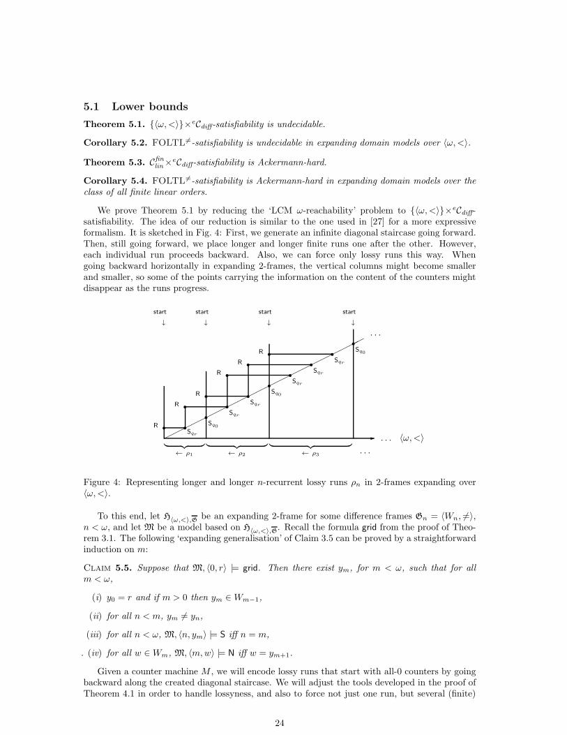
We prove Theorem 5.1 by reducing the ‘LCM ω-reachability’ problem to {〈ω,<〉}×eCdiff-satisfiability. The idea of our reduction is similar to the one used in [27] for a more expressiveformalism. It is sketched in Fig. 4: First, we generate an infinite diagonal staircase going forward.Then, still going forward, we place longer and longer finite runs one after the other. However,each individual run proceeds backward. Also, we can force only lossy runs this way. Whengoing backward horizontally in expanding 2-frames, the vertical columns might become smallerand smaller, so some of the points carrying the information on the content of the counters mightdisappear as the runs progress.

✲︸ ︷︷ ︸

← ρ1

start

↓

✟✟✟✟✟✟✟✟✟✟✟✟✟✟✟✟✟✟✟✟✟✟

r

r

r

r

r

r

r

r

r

︸ ︷︷ ︸

← ρ2

start

↓

︸ ︷︷ ︸

← ρ3

start

↓

start

↓

. . .

. . .

. . .

〈ω,<〉

rR

rR

rR

rR

rR

rR

Sqr

Sq0

Sqr

Sqr

Sq0

Sqr

Sqr

Sqr

Sq0

Figure 4: Representing longer and longer n-recurrent lossy runs ρn in 2-frames expanding over〈ω,<〉.

To this end, let H〈ω,<〉,G be an expanding 2-frame for some difference frames Gn = 〈Wn, 6=〉,n < ω, and let M be a model based on H〈ω,<〉,G. Recall the formula grid from the proof of Theo-rem 3.1. The following ‘expanding generalisation’ of Claim 3.5 can be proved by a straightforwardinduction on m:

Claim 5.5. Suppose that M, 〈0, r〉 |= grid. Then there exist ym, for m < ω, such that for all

m < ω,

(i) y0 = r and if m > 0 then ym ∈Wm−1,

(ii) for all n < m, ym 6= yn,

(iii) for all n < ω, M, 〈n, ym〉 |= S iff n = m,

. (iv) for all w ∈Wm, M, 〈m,w〉 |= N iff w = ym+1.

Given a counter machine M , we will encode lossy runs that start with all-0 counters by goingbackward along the created diagonal staircase. We will adjust the tools developed in the proof ofTheorem 4.1 in order to handle lossyness, and also to force not just one run, but several (finite)

24

runs, placed one after the other. To this end, we introduce a fresh propositional variable start,intended to mark the start of each run (see Fig. 4), and postulate

✷+0 ✷

+1

(start → ✷1start

). (50)

Also, for each i < N we let

TillStartAllCi :: ✸0N ∧ ✷0

(N ∨✸0N → (¬start ∧ Ci)

),

Then we have the following lossy analogue of Claim 4.8:

Claim 5.6. Suppose that M, 〈0, r〉 |= grid. Then for all m < ω, i < N ,

{w ∈ Wm : M, 〈m,w〉 |= TillStartAllCi} ⊆ {w ∈Wm+1 : M, 〈m+ 1, w〉 |= Ci}.

Proof. Suppose that M, 〈m,w〉 |= TillStartAllCi. Then M, 〈m,w〉 |= ✸0N and so by Claim 5.5(iv),w = yn for some n > m+ 1, and we have M, 〈n− 1, w〉 |= N. Thus, M, 〈m+ 1, w〉 |= N∨✸0N. AsM, 〈m,w〉 |= ✷0(N ∨✸0N → Ci), we obtain M, 〈m+ 1, w〉 |= Ci as required.

Now, for each i < N , we can simulate the possible lossy changes in the counters by the followingformulas:

Fixlossyi :: ✷

+1 (Ci → TillStartAllCi),

Inclossyi :: ✷

+1

(Ci → (N ∨ TillStartAllCi)

),

Declossyi :: ✷

+1 (Ci → TillStartAllCi) ∧✸

+1 (¬Ci ∧ TillStartAllCi).

Observe that the vertical counting capabilities are not used in simulating lossy steps. They areonly used in the formula grid, in order to force the uniqueness of the diagonal staircase in Claim 5.5.

The following lossy analogue of Claim 3.6 is a straightforward consequence of Claim 5.6:

Claim 5.7. Suppose that M, 〈0, r〉 |= grid ∧ (50) and let, for all m < ω, i < N , ci(m) := |{w ∈Wm : M, 〈m,w〉 |= Ci}|. If ci(n) = 0 whenever i < N and n < ω is such that M, 〈n, r〉 |= start,

then for all m < ω,

ci(m) ≤

ci(m+ 1), if M, 〈m, ym〉 |= Fixlossyi ,

ci(m+ 1) + 1, if M, 〈m, ym〉 |= Inclossyi ,

ci(m+ 1) − 1, if M, 〈m, ym〉 |= Declossyi .

Next, we encode the various counter machine instructions for lossy steps, acting backward. Foreach ι ∈ OpC , we define the formula Dolossyι by taking

Dolossyι ::

Inclossyi ∧

∧

i6=j<N

Fixlossyj , if ι = c++

i ,

Declossyi ∧

∧

i6=j<N

Fixlossyj , if ι = c−−i ,

✷+1 ¬Ci ∧

∧

j<N

Fixlossyj , if ι = c??i .

Finally, given a counter machine M , we encode lossy runs that start with all-0 counters at start-marks, and go backward until the next start-mark. We define ϕlossy

M to be the conjunction of (50)and the following formulas:

✷+0 ✷

+1

(S ↔

∨

q∈Q−H

(Sq ∧

∧

q 6=q′∈Q

¬Sq′ )), (51)

✷+0 ✷

+1

(S ∧ start → (Sq0 ∧

∧

i<N

✷+1 ¬Ci)

), (52)

✷0✷1

∧

q∈Q−H

[(S ∧ ¬start ∧✸1(N ∧✸0Sq)

)→

∨

〈ι,q′〉∈Iq

(Dolossyι ∧ Sq′)]. (53)

Then we have the following lossy analogue of Lemma 4.10:

25

Claim 5.8. Suppose that M, 〈0, r〉 |= grid ∧ ϕlossyM , and for all m < ω, i < N , let

qm := q, if M, 〈m, ym〉 |= Sq, ci(m) := |{w ∈Wm : M, 〈m,w〉 |= Ci}|, σm := 〈qm, c(m)〉.

Then 〈σn2, σn2−1, . . . , σn1

〉 is a well-defined lossy run of M starting with all-0 counters, whenever

n1 < n2 < ω is such that M, 〈n2, r〉 |= start, and M, 〈n, r〉 |= ¬start, for every n with n1 ≤ n < n2.

It remains to force that the nth run visits qr at least n times. To this end, we introduce twofresh propositional variables R and S∗, and define rec as the conjunction of (50) and the followingformulas:

start ∧✷+0 ✸0start, (54)

✷+0 ✷

+1

[start → ✸

+1

(R ∧✸0S ∧ ✷0(✸0S → ¬start)

)], (55)

✷+0 ✷

+1

(R → ✷0(S → S∗)

), (56)

✷0✷+1

[

S∗ → ✸1

[R ∧✸0(start ∧✸0S)∧

✷+0

(start ∧✸0S → ✷0(✸0S → ¬start)

)]]

, (57)

✷+0 ✷

+1 (S → ✷1¬S), (58)

✷+0 ✷

+1 (R → ✷0¬R). (59)

Claim 5.9. Suppose that M, 〈0, r〉 |= grid ∧ rec. Then there is an infinite sequence 〈kn : n < ω〉such that

(i) M, 〈kn, r〉 |= start for all n < ω, and

(ii) if n > 0 then |{k : kn−1 < k ≤ kn and M, 〈k, yk〉 |= S∗}| ≥ n.

Proof. By induction on n. To begin with, let k0 = 0. Now suppose inductively that we have〈kℓ : ℓ < n〉 as required, for some 0 < n < ω. Now let kn be the smallest k with k > kn−1 andM, 〈k, r〉 |= start (there is such by (54)). As by the IH we have M, 〈kn−1, r〉 |= start, by (55) thereis w ∈ Wkn−1

such that

M, 〈kn−1, w〉 |= R ∧✸0S ∧ ✷0(✸0S → ¬start).

By Claim 5.5(iii) and (58), w = yin for some kn−1 < in ≤ kn, and so M, 〈in, yin〉 |= S∗ follows by(56). In particular, M, 〈i1, yi1〉 |= S∗ and so

|{k : k0 < k ≤ k1 and M, 〈k, yk〉 |= S∗}| ≥ 1.

Now let n > 1 and take some k such that kn−2 < k ≤ kn−1 and M, 〈k, yk〉 |= S∗. By (57), there isv ∈ Wk such that

M, 〈k, v〉 |= R ∧ (start ∧✸0S) ∧ ✷0

(start ∧✸0S → ✷0(✸0S → ¬start)

).

By Claim 5.5(iii) and (58), there is k+ such that kn−1 < k < k+ ≤ kn, v = yk+ and M, 〈k+, yk+〉 |=S. So M, 〈k+, yk+〉 |= S∗ by (56). Moreover, by (59) we obtain that k+ 6= in, and k+ 6= ℓ+ wheneverk 6= ℓ. Therefore,

|{k : kn−1 < k ≤ kn and M, 〈k, yk〉 |= S∗}| ≥

|{k : kn−2 < k ≤ kn−1 and M, 〈k, yk〉 |= S∗}| + 1,

and so by the IH we obtain (ii) for n, as required.

Now the following lemma is a straightforward consequence of Claims 5.8 and 5.9:

Lemma 5.10. Suppose that M, 〈0, r〉 |= grid ∧ ϕlossyM ∧ rec ∧ ✷

+0 ✷

+1 (S∗ → Sqr ). Then, for every

n < ω, M has a lossy run starting with 〈q0,0〉 and visiting qr at least n times.

26

On the other hand, suppose that for every 0 < n < ω, M has a lossy run

ρn =⟨〈qn0 ,0〉, . . . , 〈q

nmn−1, c(mn − 1)〉

⟩

such that qn0 = q0 and ρn visits qr at least n times. Let M0 := 0 and for each 0 < n < ω, letMn :=

∑n

i=1mi, and let in1 , . . . , inn < mn be such that |{in1 , . . . , i

nn}| = n and qi = qr for every

i ∈ {in1 , . . . , inn}. We define a model N∞ =

⟨〈ω,<〉×〈ω, 6=〉, α

⟩as follows (cf. Fig. 4): For all q ∈ Q,

we let

α(Sq) := {〈n, n〉 : Mk ≤ n < Mk+1 and qk+1n−Mk

= q, for some k < ω},

α(S) := {〈n, n〉 : n < ω},

α(N) := {〈n, n+ 1〉 : n < ω},

α(start) := {〈n,m〉 : n = Mk for some k < ω, and m < ω}.

Further, for any finite subset X = {n1, . . . , nℓ} of ω with n1 < · · · < nℓ and any k ≤ |X |, we letmink(X) := {n1, . . . , nk}. Now for all i < N , 0 < n < ω and k < mn, we define the sets αnk (Ci)by induction on k: We let αn0 (Ci) := ∅, and for all k < mn − 1,

αnk+1(Ci) :=

{αnk (Ci) ∪ {Mn − k}, if cni (k + 1) = cni (k) + 1,αnk (Ci) −minℓ

(αnk (Ci)

), if |cni (k) − cni (k + 1)| = ℓ.

Then, for each i < N , we let

α(Ci) := {〈k,m〉 : Mn−1 ≤ k < Mn, m ∈ αnMn−k−1(Ci) for some 0 < n < ω}.

Also, we define the sequence 〈rn : n < ω〉 inductively as follows. Let r0 := i11 and let

rn+1 :=

{

Mk + ik+11 , if rn = Mk−1 + ikk for some k > 0,

Mk−1 + ikℓ+1, if rn = Mk−1 + ikℓ for some k > 0, ℓ < k.

Then let

α(S∗) := {〈rn, rn〉 : n < ω},

α(R) := {〈n, rn〉 : n < ω}.

It is not hard to check that N∞, 〈0, 0〉 |= grid∧ϕlossyM ∧rec∧✷+

0 ✷+1 (S∗ → Sqr ), and so by Lemma 5.10

LCM ω-reachability can be reduced to {〈ω,<〉}×eCdiff-satisfiability. This competes the proof ofTheorem 5.1.

Next, we prove Theorem 5.3 by reducing the ‘LCM-reachability’ problem to Cfinlin ×e Cdiff-

satisfiability. We will use the finitary versions of some of the formulas used in the previous proof.Let H〈T,<〉,G be an expanding 2-frame for some finite linear order 〈T,<〉 and for some difference

frames Gn = 〈Wn, 6=〉, n ∈ T , and let M be a model based on H〈T,<〉,G. We may assume that

T = |T | < ω. Take the formula gridfin defined in the proof of Theorem 3.2. The following finitaryversion of Claim 5.5 can be proved by a straightforward induction on m:

Claim 5.11. Suppose that M, 〈0, r〉 |= gridfin. Then there exist 0 < E ≤ T and ym, for m ≤ E,

such that M, 〈E − 1, yE〉 |= end and M, 〈m, ym+1〉 |= ¬end whenever n < E − 1, and the following

hold for all m ≤ E:

(i) y0 = r and if m > 0 then ym ∈Wm−1,

(ii) for all n < m, ym 6= yn,

(iii) for all n < E, M, 〈n, ym〉 |= S iff n = m,

27

. (iv) if m < E then for all w ∈ Wm, M, 〈m,w〉 |= N iff w = ym+1.

Now let reachbw be the conjunction of (8) and

Sqr ∧ ✷+0 ✷

+1 (end ↔ start).

The following lemma is a straightforward consequence of Claim 5.8:

Lemma 5.12. Suppose that M, 〈0, r〉 |= gridfin ∧ ϕlossyM ∧ reachbw, and for all m < E and i < N ,

let

qm := q, if M, 〈m, ym〉 |= Sq, ci(m) := |{w ∈W : M, 〈m,w〉 |= Ci}|, σm = 〈qm, c(m)〉.

Then 〈σE , σE−1, . . . , σ0〉 is a well-defined lossy run of M starting with all-0 counters and reaching

qr.

On the other hand, if M has a run⟨〈qm, c(m)〉 : m < T

⟩for some T < ω such that it starts

with all-0 counters and qT−1 = qr, then it is not hard to define a model based on 〈T,<〉×〈T +1, 6=〉

satisfying gridfin ∧ ϕlossyM ∧ reachbw (cf. how the finite runs in the model N∞ are defined in the

proof of Theorem 5.1). So by Lemma 5.12 the proof of Theorem 5.3 is completed.

5.2 Upper bounds

To begin with, as a consequence of Theorems 2.1 and Props. 2.2, 2.3 we obtain:

Corollary 5.13. FOLTL6=-satisfiability is co-r.e. in expanding domain models over the class of

all linear orders.

Unlike in the constant domain case, in the expanding domain case the same holds for 〈ω,<〉as timeline:

Theorem 5.14. {〈ω,<〉}×eCdiff-satisfiability is co-r.e.

Corollary 5.15. FOLTL 6=-satisfiability is co-r.e. in expanding domain models over 〈ω,<〉.

Theorem 5.16. Cfinlin×

eCdiff-satisfiability is decidable in Ackermann-time.

Corollary 5.17. FOLTL 6=-satisfiability is decidable in Ackermann-time, in expanding domain

models over the class of all finite linear orders.

In order to prove both Theorems 5.14 and 5.16, we begin with showing that there is a reductionfrom Cdiff-satisfiability to Clin-satisfiability that can be ‘lifted to the 2D level’. As we will use thisreduction to obtain upper bounds on satisfiability in expanding 2-frames, we formulate it in thissetting only. To this end, fix some bimodal formula φ. For every ψ ∈ subφ, we introduce a freshpropositional variable Pψ not occurring in φ, and define inductively a translation ψ† by taking

P† := P, for each propositional variable P ∈ subφ,

(¬ψ)† := ¬ψ†,

(ψ1 ∧ ψ2)† := ψ†1 ∧ ψ†2,

(✸0ψ)† := ✸0ψ†,

(✸1ψ)† := Pψ ∨✸1ψ†.

Further, we let

χφ :: ✷+0

∧

ψ∈subφ

¬Pψ ∧ ✷+1 (ψ† → ✷1Pψ) ∧

(✸1Pψ → ✸

+1 (¬Pψ ∧ ψ†)

).

Claim 5.18. For any formula φ, and any class C of transitive frames,

28

• φ is C×eCdiff-satisfiable iff χφ ∧ φ† is C×eClin-satisfiable.

• φ is C×eCfindiff-satisfiable iff χφ ∧ φ† is C×eCfin

lin -satisfiable.

Proof. ⇒: Suppose that M, 〈r0, r1〉 |= φ in some model M = 〈HF,G, µ〉 based on an expanding

2-frame HF,G where F = 〈W,R〉 is transitive and for every x ∈W , Gx = 〈Wx, 6=〉. Then Wx ⊆Wy

whenever xRy, x, y ∈ W . Also, we may assume that r0 is a root in F, and so r1 ∈ Wx for allx ∈ W . So for every x ∈ W we may take a well-order <x on Wx with least element r1 and suchthat <x⊆<y whenever xRy. Let Σ′x = 〈Wx, <x〉, for x ∈ W . Then clearly H

F,G′ ∈ C×eClin. We

define a model M′ = 〈HF,G

′ , µ′〉 by taking

µ′(P) := µ(P), for P ∈ subφ,

µ′(Pψ) = {〈x,w〉 : x ∈W and M, 〈x, u〉 |= ψ for some u ∈Wx with u <x w}.

First, we show by induction on ψ that for all ψ ∈ subφ, x ∈ W , u ∈Wx,

M, 〈x, u〉 |= ψ iff M′, 〈x, u〉 |= ψ†. (60)

Indeed, the only non-straightforward case is that of ✸1. So suppose first that M, 〈x, u〉 |= ✸1ψ.Then there is v ∈ Wx, v 6= u with M, 〈x, v〉 |= ψ. If u <x v then M′, 〈x, u〉 |= ✸1ψ

† by the IH. Ifv <x u, then M′, 〈x, u〉 |= Pψ by the definition of M′. So in both cases we have M′, 〈x, u〉 |= (✸1ψ)†.Conversely, suppose that M′, 〈x, u〉 |= (✸1ψ)†. If M′, 〈x, u〉 |= Pψ then there is v ∈Wx, v <x u withM, 〈x, v〉 |= ψ. Therefore, there is v ∈ Wx, v 6= u with M, 〈x, v〉 |= ψ. If M′, 〈x, u〉 |= ✸1ψ

† thenthere is v ∈ Wx, v <x u with M′, 〈x, v〉 |= ψ†, and so there is v ∈ Wx, v 6= u with M, 〈x, v〉 |= ψby the IH. So in both cases M, 〈x, u〉 |= ✸1ψ follows.

Second, we claim that M′, 〈r0, r1〉 |= χφ. Indeed, take any x ∈ W . As r1 is <x-least in Wx,we have M′, 〈x, r1〉 |= ¬Pψ. Now take any y ∈ Wx with M′, 〈x, y〉 |= ψ† and suppose that y <x zfor some z ∈ Wx. By (60), we have M, 〈x, y〉 |= ψ and so M′, 〈x, z〉 |= Pψ by the definition ofM′. Finally, suppose that M′, 〈x, r1〉 |= ✸1Pψ. Therefore, the set {w ∈ Wx : 〈x,w〉 ∈ µ′(Pψ)} isnon-empty. Let y be its <x-least element. So there is z ∈ Wx, z <x y such that M, 〈x, z〉 |= ψand 〈x, z〉 /∈ µ′(Pψ). Thus M′, 〈x, z〉 |= ¬Pψ ∧ ψ† by (60). As either r1 = y or r1 <x y, we haveM′, 〈x, r1〉 |= ✸

+1 (¬Pψ ∧ ψ†). as required.

⇐: Suppose that M, 〈r0, r1〉 |= χφ ∧ φ† in some model M = 〈HF,G, µ〉 based on an expanding

2-frame HF,G where F = 〈W,R〉 is transitive and for every x ∈ W , Gx = 〈Wx, <x〉 is a linear

order. Then Wx ⊆Wy and <x⊆<y whenever xRy, x, y ∈W . We may assume that r0 is a root inF, and so r1 ∈Wx for all x ∈W . Moreover, we may also assume that r1 is a root in 〈Wx, <x〉 forevery x ∈ W . Let Σ′x = 〈Wx, 6=〉, for x ∈ W . Then clearly H

F,G′ ∈ C×eCdiff. We define a model

M′ = 〈HF,G

′ , µ′〉 by taking µ′(P) := µ(P) for all P ∈ subφ.We show by induction on ψ that for all ψ ∈ subφ, x ∈W , u ∈ Wx,

M, 〈x, u〉 |= ψ† iff M′, 〈x, u〉 |= ψ. (61)

Again, the only interesting case is that of ✸1. Suppose first that M, 〈x, u〉 |= (✸1ψ)†. If

M, 〈x, u〉 |= Pψ, (62)

then r1 <x u by the first conjunct of χφ, and so M, 〈x, r1〉 |= ✸1Pψ. So M, 〈x, r1〉 |= ✸+1 (¬Pψ∧ψ†)

follows by the third conjunct of χφ. So there is v ∈ Wx with M, 〈x, v〉 |= ¬Pψ ∧ ψ†, and so v 6= uby (62). Also, by the IH, we have M′, 〈x, v〉 |= ψ, and so M′, 〈x, v〉 |= ✸1ψ follows as required.The other case when M, 〈x, u〉 |= ✸1ψ

† is straightforward.Conversely, suppose that M′, 〈x, u〉 |= ✸1ψ. Then there is v ∈ Wx, v 6= u with M′, 〈x, v〉 |= ψ,

and so by the IH, M, 〈x, v〉 |= ψ†. If u <x v then M, 〈x, u〉 |= ✸1ψ† follows. If v <x u then by the

second conjunct of χφ, we have M, 〈x, v〉 |= ✷1Pψ, and so M, 〈x, u〉 |= Pψ follows.

Next, we show that {〈ω,<〉}×eCdiff-satisfiability has the ‘finite expanding second componentsproperty’:

29

Claim 5.19. For any formula φ, if φ is {〈ω,<〉}×eCdiff-satisfiable, then φ is {〈ω,<〉}×eCfindiff-

satisfiable.

Proof. Suppose M, 〈0, r〉 |= φ for some model M based on an expanding 2-frame H〈ω,<〉,G where

Gn = 〈Wn, 6=〉 are difference frames, for n < ω. For all n < ω, X ⊆ Wn, we define cln(X) asthe smallest set Y such that X ⊆ Y ⊆ Wn and having the following property: If x ∈ Y andM, 〈n, x〉 |= ✸1ψ for some ψ ∈ subφ, then there is y ∈ Y such that y 6= x and M, 〈n, y〉 |= ψ. Itis not hard to see that if X is finite then |cln(X)| ≤ |X | + 2|subφ|. Now define G′n := 〈W ′n, 6=〉 bytaking W ′0 := cl0({r}) and W ′n+1 := cln+1(W ′n) for n < ω. Let M′ be the restriction of M to theexpanding 2-frame H〈ω,<〉,G′ . A straightforward induction shows that for all ψ ∈ subφ, n < ω,

w ∈W ′n, we have M, 〈n,w〉 |= ψ iff M′, 〈n,w〉 |= ψ.

Now Theorems 5.14 and 5.16, respectively, follow from Claims 5.18, 5.19 and the followingresults:

• [27, Thm.1] {〈ω,<〉}×eCfinlin -satisfiability is co-r.e.

• [16, Thm.1] Cfinlin×

e Clin-satisfiability is decidable in Ackermann-time.

6 Open problems

We have shown that FOLTL 6= is very complex over various classes of linear orders, whenever themodels have constant, decreasing, or expanding domains. By generalising our techniques to thepropositional bimodal setting, we have shown that the bimodal logic [K4.3,Diff ] of commutingweak order and pseudo-equivalence relations is undecidable. Here are some related unansweredquestions:

1. Is FOLTL 6=-satisfiability recursively enumerable in expanding domain models over the classof all linear orders? The bimodal reformulation of this question: Is Clin×eCdiff-satisfiabilityrecursively enumerable? By Cor. 5.13, a positive answer would imply decidability of these.Is FOLTL

6=-satisfiability decidable in expanding domain models over 〈Q, <〉 or 〈R, <〉?

2. In decreasing 2-frames only ‘half’ of commutativity (✷1✷0P → ✷0✷1P) is valid. While inTheorem 4.16 we generalised Theorem 4.1 to classes of decreasing 2-frames and showed thatClin×dCdiff-satisfiability is undecidable, it is not clear whether the same can be done in the‘abstract’ setting: Is satisfiability undecidable in the class of 2-frames having half-commutingweak order and pseudo-equivalence relations?

3. Is the bimodal logic [K4,Diff ] of commuting transitive and pseudo-equivalence relationsdecidable? Is the product logic K4×Diff decidable? As K4 can be seen as a notationalvariant of the fragment of branching time logic CTL that allows only two temporal operatorsE✸F and its dual A✷F , there is another reformulation of this question: Is the one-variablefragment of first-order CTL decidable when extended with counting and when only E✸F

and A✷F are allowed as temporal operators? Note that without counting this coincideswith K4×S5 = [K4,S5]-satisfiability, and that is shown to be decidable by Gabbay andShehtman [14].

In our lower bound proofs we used reductions of counter machine problems. Other lower boundresults about bimodal logics with grid-like models use reductions of tiling or Turing machineproblems [39, 13, 15]. On the one hand, it is not hard to re-prove the same results using countermachine reductions. On the other, it seems tiling and Turing machine techniques require morecontrol over the ω × ω-grid than the limited expressivity that FOLTL 6= provides. In order tounderstand the boundary of each technique, it would be interesting to find tiling or Turing machinereductions for the results of the present paper.

30

References

[1] R. Alur and T. Henzinger. A really temporal logic. J. ACM, 41:181–204, 1994.

[2] A. Artale, R. Kontchakov, V. Ryzhikov, and M. Zakharyaschev. A cookbook for temporalconceptual data modelling with description logics. ACM Trans. Comput. Log., to appear,2014.

[3] S. Bauer, I. Hodkinson, F. Wolter, and M. Zakharyaschev. On non-local propositional andweak monodic quantified CTL∗. J. Logic and Computation, 14:3–022, 2004.

[4] P. Blackburn, M. de Rijke, and Y. Venema. Modal Logic. Cambridge University Press, 2001.

[5] E. Borger, E. Gradel, and Yu. Gurevich. The Classical Decision Problem. Perspectives inMathematical Logic. Springer, 1997.

[6] A. Chagrov and M. Zakharyaschev. Modal Logic, volume 35 of Oxford Logic Guides. ClarendonPress, Oxford, 1997.

[7] J. Chomicki. Temporal query languages: a survey. In D. Gabbay and H.J. Ohlbach, editors,Procs. ICTL-1994, volume 827 of LNCS, pages 506–534. Springer, 1994.

[8] J. Chomicki and D. Niwinski. On the feasibility of checking temporal integrity constraints.J. Computer and Systems Sciences, 51:523–535, 1995.

[9] A. Degtyarev, M. Fisher, and B. Konev. Monodic temporal resolution. ACM Trans. Comput.

Log., 7:108–150, 2006.

[10] A. Degtyarev, M. Fisher, and A. Lisitsa. Equality and monodic first-order temporal logic.Studia Logica, 72:147–156, 2002.

[11] K. Fine. Logics containing K4, part II. J. Symbolic Logic, 50:619–651, 1985.

[12] D. Gabbay, I. Hodkinson, and M. Reynolds. Temporal Logic: Mathematical Foundations and

Computational Aspects, Volume 1. Oxford University Press, 1994.

[13] D. Gabbay, A. Kurucz, F. Wolter, and M. Zakharyaschev. Many-Dimensional Modal Logics:

Theory and Applications, volume 148 of Studies in Logic and the Foundations of Mathematics.Elsevier, 2003.

[14] D. Gabbay and V. Shehtman. Products of modal logics. Part I. Logic J. of the IGPL,6:73–146, 1998.

[15] D. Gabelaia, A. Kurucz, F. Wolter, and M. Zakharyaschev. Products of ‘transitive’ modallogics. J. Symbolic Logic, 70:993–1021, 2005.

[16] D. Gabelaia, A. Kurucz, F. Wolter, and M. Zakharyaschev. Non-primitive recursive decidabil-ity of products of modal logics with expanding domains. Ann. Pure Appl. Logic, 142:245–268,2006.

[17] E. Gradel, P. Kolaitis, and M. Vardi. On the decision problem for two-variable first orderlogic. Bulletin of Symbolic Logic, 3:53–69, 1997.

[18] E. Gradel, M. Otto, and E. Rosen. Two-variable logic with counting is decidable. In Procs.

LICS 1997, pages 306–317. IEEE, 1997.

[19] C. Hampson and A. Kurucz. One-variable first-order linear temporal logics with counting. InS. Ronchi Della Rocca, editor, Procs. CSL 2013, volume 23 of LIPIcs, pages 348–362. SchlossDagstuhl–Leibniz Zentrum fuer Informatik, 2013.

31

[20] C. Hampson and A. Kurucz. Axiomatisation problems of modal product logics with thedifference operator. Manuscript, 2014.

[21] I. Hodkinson. Monodic packed fragment with equality is decidable. Studia Logica, 72:185–197,2002.

[22] I. Hodkinson. Complexity of monodic guarded fragments over linear and real time. Ann.

Pure Appl. Logic, 138:94–125, 2006.

[23] I. Hodkinson, R. Kontchakov, A. Kurucz, F. Wolter, and M. Zakharyaschev. On the com-putational complexity of decidable fragments of first-order linear temporal logics. In Procs.

TIME-ICTL, pages 91–98. IEEE, 2003.

[24] I. Hodkinson, F. Wolter, and M. Zakharyaschev. Decidable fragments of first-order temporallogics. Ann. Pure Appl. Logic, 106:85–134, 2000.

[25] I. Hodkinson, F. Wolter, and M. Zakharyaschev. Monodic fragments of first-order temporallogics: 2000–2001 A.D. In Logic for Programming, Artificial Intelligence and Reasoning,number 2250 in LNAI, pages 1–23. Springer, 2001.

[26] I. Hodkinson, F. Wolter, and M. Zakharyaschev. Decidable and undecidable fragments offirst-order branching temporal logics. In Procs. LICS 2002, pages 393–402. IEEE, 2002.

[27] B. Konev, F. Wolter, and M. Zakharyaschev. Temporal logics over transitive states. InR. Nieuwenhuis, editor, Procs. CADE-20, volume 3632 of LNCS, pages 182–203. Springer,2005.

[28] A. Kurucz. Combining modal logics. In P. Blackburn, J. van Benthem, and F. Wolter,editors, Handbook of Modal Logic, volume 3 of Studies in Logic and Practical Reasoning,pages 869–924. Elsevier, 2007.

[29] A. Kurucz and S. Marcelino. Non-finitely axiomatisable two-dimensional modal logics. J.

Symbolic Logic, 77:970–986, 2012.

[30] C. Lutz, F. Wolter, and M. Zakharyaschev. Temporal description logics: a survey. In S. Demriand C.S. Jensen, editors, Procs. TIME 2008, pages 3–14. IEEE, 2008.

[31] K. Mamouras. First-order temporal logic with fixpoint operators over the natural numbers.Master’s thesis, Imperial College London, 2009.

[32] M. Marx and M. Reynolds. Undecidability of compass logic. J. Logic and Computation,9:897–914, 1999.

[33] M. Marx and Y. Venema. Multi-Dimensional Modal Logic. Kluwer Academic Publishers,1997.

[34] R. Mayr. Undecidable problems in unreliable computations. In G.H. Gonnet, D. Panario,and A. Viola, editors, Procs. LATIN-2000, volume 1776 of LNCS, pages 377–386. Springer,2000.

[35] S. Merz. Decidability and incompleteness results for first-order temporal logics of linear time.J. Applied Non-Classical Logics, 2:139–156, 1992.

[36] M. Minsky. Finite and infinite machines. Prentice-Hall, 1967.

[37] L. Pacholski, W. Szwast, and L. Tendera. Complexity results for first-order two-variable logicwith counting. SIAM J. Comput., 29:1083–1117, 2000.

[38] M. Reynolds. A decidable temporal logic of parallelism. Notre Dame J. Formal Logic, 38:419–436, 1997.

32

[39] M. Reynolds and M. Zakharyaschev. On the products of linear modal logics. J. Logic and

Computation, 11:909–931, 2001.

[40] P. Schnoebelen. Lossy counter machines decidability cheat sheet. In A. Kucera and I. Potapov,editors, Procs. RP-2010, volume 6227 of LNCS, pages 51–75. Springer, 2010.

[41] P. Schnoebelen. Revisiting Ackermann-hardness for lossy counter machines and reset Petrinets. In P. Hlineny and A. Kucera, editors, Procs. MFCS-2010, volume 6281 of LNCS, pages616–628. Springer, 2010.

[42] K. Segerberg. Modal logics with linear alternative relations. Theoria, 36:301–322, 1970.

[43] K. Segerberg. Two-dimensional modal logic. J. Philosophical Logic, 2:77–96, 1973.

[44] K. Segerberg. A note on the logic of elsewhere. Theoria, 46:183–187, 1980.

[45] V. Shehtman. Two-dimensional modal logics. Mathematical Notices of the USSR Academy

of Sciences, 23:417–424, 1978. (Translated from Russian).

[46] E. Spaan. Complexity of Modal Logics. PhD thesis, University of Amsterdam, 1993.

[47] A. Sza las. Concerning the semantic consequence relation in first-order temporal logic. Theor.Comput. Sci., 47(3):329–334, 1986.

[48] A. Sza las and L. Holenderski. Incompleteness of first-order temporal logic with until. Theor.

Comput. Sci., 57:317–325, 1988.

[49] F. Wolter and M. Zakharyaschev. Modal description logics: modalizing roles. Fundamenta

Informaticae, 39:411–438, 1999.

[50] F. Wolter and M. Zakharyaschev. Axiomatizing the monodic fragment of first-order temporallogic. Ann. Pure Appl. Logic, 118:133–145, 2002.

33