Modified Local Variance Based Method for Selecting the Optimal Spatial Resolution of Remote Sensing Image

Dongping Ming1,2*, Jiancheng Luo3, Longxiang Li1, Zhuoqin Song1 1School of Information Engineering,China University of Geosciences (Beijing), Beijing, China

2The State Key Laboratory of Remote Sensing Science, Beijing, China 3Institute of Remote Sensing Applications, CAS, Beijing, China

*Corresponding author: mingdpgis@163.com

Abstract—Facing with the prevalence of multi-spatial resolution satellite data sets, selecting data with appropriate resolution has become a new problem. This paper analyses the significance of scale selection of remote sensing images and discusses geo-statistics based method of quantitively selecting the optimal spatial resolution of remote sensing image. Breaking through the limitation of traditional average local variance, this paper proposes the modified average local variance method based on variable window size and variable resolution to quantitatively select the optimal spatial resolution of remote sensing image. In order to verify the validity of this method, this paper gives further image classification experiments at different spatial resolution. The experimental results show that the trend of classification accuracy along with spatial resolution is consistent with that of modified average local variance, which means that the image classification accuracy of the optimal resolution image is basically higher than those of other’s. Consequently, modified average local variance based method of quantitively selecting the optimal spatial resolution of remote sensing image has theoretical and instructive meaning to a certain extent.

Keywords- remote sensing image; scale; spatial resolution; modified local variance; image classification

I. INTRODUCTION The issue of scale is paid much attention in geographic

information system (GIS) and remote sensing and is regarded as one of the main challenges of earth observation. At present, a major concern in scale-and-resolution-related issues is to develop methods for determining the most appropriate scale and resolution for special study and assessing the effects of scale and resolution [1]. Selecting data in previous studies was generally limited by the availability of existing data of specific scales and resolutions. However, with the development and prevalence of multi-spectral and multi-spatial resolution data sets (such as remote sensing image), selecting data with appropriate scale has become a new problem. Davis gives a qualitative analysis about this [2], but it is significant to seek the quantitative relation between certain spatial pattern and spatial resolution to consequently select the optimal spatial resolution of remote sensing image according to the scale of geo-phenomena. The solution of this problem will be contributing for remote sensing and GIS and their geo-application. Several methods have been suggested to study the effects of scale and resolution, such as the methods based on local variance (LV), semivariogram, and fractal theory, etc.

However some unexpected results often conflict with the ideal theory when using them. This paper discusses the methods for selecting the optimal resolution of remote sensing image based on spatial statistics and proposes the modified LV method based on variable window size and variable resolution to quantitatively select the optimal spatial resolution..

II. MODIFIED LV METHOD BASED ON VARIABLE WINDOW SIZE AND VARIABLE RESOLUTION

A. TraditionalLV method for selecting the optimal spatial resolution Many geographers and ecologists quantitively discussed the

issue of optimal resolution of remote sensing image. Cao summarized the methods expressing relation between the research scale and spatial resolution, and they are geographic variance, local variance, texture analysis and the fractal method [1]. Of these methods (of course, local variance is a kind of texture analysis method and is also similar to geographic variance method), the first three are simple and useful, while he fractal method has a great potential in detecting the resolution effects and is used especially in landsacpe ecology researches. However, from the aspect of simplicity and performace of the method, local variance method proposed by Woodcock and Strahler [3] and semivariance method proposed by Markowitz [4] are used more widely for the panchromatic image data. The rationale that the two methods can be used in scale issues of remote sensing image is the theory of spatial dependence. That is the degree of similarity between the values at two points depends on the spatial distance between them. The longer the distance is, the higher the degree of similarity is, and the smaller the variance is.

Local variance is a scene texture statistic that has been shown to characterize the relationship between spatial resolution and objects in the scene [3]. In previous researches, local variance calculated the mean value of the standard deviation by passing a n pixel by n pixel moving window for each pixel, and then takes the mean of all local variance over the entire image as an indication of the local variability in an image. Woodcock and Strahler used a 3 x 3 window and degraded images to coarser levels to examine the change in local variance as pixel size [3]. Instead of changing pixel sizes, increasing window sizes could be used [5]. As shown in figure 1, pixel sizes were plotted on the x-axis and local variance on

Supported by the Fundamental Research Funds for the Central Universities (2010ZY20) and NSFC Project (40871203 & 40971228).

the y-axis, depicting the change in average local variance with pixel size. By examining a single image, several window sizes and orientations could be utilized to establish the scale and form of autocorrelation based on changes in variance levels. The main idea that local variance can be used to compute optimal spatial resolutions is: local variance is typically low when the spatial resolution of a scene (d1) is considerably less than the size of the objects in the scene; As these objects approximate the spatial resolution of the scene (d2), the likelihood of the neighborhood resembling the central pixel decreases and the local variance increases; When the resolution (d3) exceeds the object size and many objects are found within each pixel, the local variation again decreases [3]. Therefore, the spatial resolution d2 (on which the peak of maximal average local variance appears) is closely related to the dominant size of pattern elements in the image [6-10] and it is the optimal resolution of the image data for the research because it approaches the object size and can reflect the spatial features in the scene.

Figure 1. Relation between spatial resolution and local variance

The formulae of calculating mean value f and variance S2

are as follows,

ff i j

MNj

N

i

M

= =

−

=

−

∑∑ ( , )0

1

0

1

(1)

Sf i j f

MNj

N

i

M

2

2

0

1

0

1

=−

=

−

=

−

∑∑ [ ( , ) ]

(2) Where, M and N represent the width and the height of image, and f(i,j) is the gray scale value of pixel(i,j).

Local variance method is gradually executed on the degraded images and the maximal average LV of the whole image is used to select the optimal spatial resolution of the image. A serious limitation of this method is that it is dependent on the global variance in the image, so the values of local variance for one image can only be compared with those from the same images degraded to different resolutions. Coops and Catling propose an modified average local variance technique based on the extended window size (5×5, 7×7, 9×9,…), which results in a more general expression of the relationship between the local variance and scale [11].

B. Problems existing in traditional LV method Traditional LV method is used at first. As shown in figure 2

(shrinking the display), the primary experimental images with 1m spatial resolution are subset from a panchromatic IKONOS

image of a certain region, and their sizes are all 800×800. Then each image is gradually degraded at a gap of 1m (with standard deviation stretch), consequently the series of experimental images with different spatial resolution (from 1m to 15m) are prepared.

urban_a urban_b urban_c

farmland_a farmland_b farmland_c

woodland_a woodland_b woodland_c

Figure 2. Primary experimental images with 1m spatial resolution

According to formulae (1) and (2), the respective average LV of each primary image is shown in figure 4(a), (b) and (c).

0.0

10.0

20.0

30.0

40.0

50.0

60.0

1 3 5 7 9 11 13 15

Spatial resolution (meter)

Tradit

ional

aver

age LV

a

b

c

(a) urban

0.0

10.0

20.0

30.0

40.0

50.0

60.0

1 3 5 7 9 11 13 15

Spatial resolution (meter)

Traditional average LV

a

b

c

(b) farmland

0.0

10.0

20.0

30.0

40.0

50.0

60.0

1 2 3 4 5 6 7 8 9 10 11 12 13 14 15

Spatial resolution (meter)

Traditional average LV

a

b

c

(c) woodland

Figure 3. Average LV of experimental images by traditional method

Theoretically, there should be an obvious peak in the chart of average LV as is showed in figure 1, however, in practical calculation it is not as so. With the gradual degradation of spatial resolution, the average LV dose not evidently descend as expected, but arises smoothly and then maintains at a constant level in much the same way as a semivariogram [12]. This phenomenon is also conducted by other scholars [13]. The reasons are as follows:

(1) From the perspective of images and objects, images with higher spatial resolution tend to show more details of terrain, for example, single building and single tree, etc. When the spatial resolution declines, the neighborhood of a 3×3 window may shift to another object, so the average LV increases, but not decreases.

(2) From the view of computing method, traditional average LV is computed based on the variable ground area because it uses the same window size (for example 3×3) on images with variable spatial resolution. For instance, when the spatial resolution is 1m, the area of window 3×3 is (1×3)2＝9m2; when the spatial resolution is 2m, the area of window 3×3 is (2×3)2＝36m2; …; when the spatial resolution is 15m, the area of window 3×3 is (15×3)2＝2025m2. Average LV that is based on the far different ground area certainly differs greatly.

By the same token, for a certain image (with invariable spatial resolution), average LV increases obviously with the increase of window size (3×3,5×5,……). Figure 4 demonstrates the common modified average LV [12] of image urban_a. The same results can be conducted for other images.

Spatial resolution

15

20

25

30

35

40

45

50

3 5 7 9 11 13 15 17 19 21 23

Window size

Common modified ALV

1m

2m

3m

4m

5m

6m

7m

8m

9m

10m

11m

12m

13m

14m

15m

Figure 4. Average LV of urban_a by common modified method

C. Modified average LV based on variable window size and variable resolution In fact, the essences of the two methods mentioned above

are the same and both the two average LVs increase as the ground area of window increases, which leads the rationality of relationship between average LV and spatial resolution is deficient. And then this paper proposes the modified average LV method based on constant ground area. Its theoretical foundation is: average LVs based on constant ground area (different windows with different sizes on images with different spatial resolutions) have more comparability, so that they can reflect changes of variance with spatial resolution

more objectively. To keep the area consistent, windows in different sizes are utilized according to the spatial resolution of image. This paper denominates this method as modified average LV method based on variable window size and variable resolution, and that means high spatial resolution image with small window size and low spatial resolution image with large window size, so that the relevant ground area is kept consistent. Optimal spatial resolution can be conducted from the calculated average LVs.

Taking the data above as example and setting the window size of 45m×45m, table 1 shows ideal window size of modified average LV method on different spatial resolution image. However, in actual neighborhood window based computation, the size of the window is limited to integer. Otherwise, it is illogical for a fractional window size. As is showed in the experiments above, when the spatial resolution is constant, average LV increases logarithmically as the size of window gradually increases. However, under some local condition (when the size of the window is close to each other), average LV increases linearly, thus it can be fitted by interpolation method. This method can be viewed as an example of spatial statistics in spatial information analysis, that the similarity between closer sampling points is stronger than that between further sampling points and the similarity degree is only related to the spatial distance between the sampling points but not to their absolute position. Consequently, the values of non-observation points can be interpolated by weighted values of other observation points, which is famous Kring method [14-17].

In order to make the fitting closer to the fact, based on the theories that neighbor points are more similar than points far away and larger scale means increasing linear character and decreasing nonlinear character, this paper proposes the modified average LV method in which average LV of windows in integer size are used to predict those of windows in decimal size by interpolation. In the processing, weighted linearization method whose weight is determined by function relationship between windows in decimal size and those in approximate integer size (closer means more weight). Left or right bounding neighbor windows’ weight, in simple linear interpolation, can be calculated as below:

Wl =(rw*r-45) / [(45- lw*r)+( rw*r-45)] (3)

Wr=(45-lw*r) / [(45- lw*r)+( rw*r-45)] (4) Where, Wl and Wr respectively represent the weight of left and right bounding neighbor window, lw represents the size of left bounding window, while rw represents the size of right bounding window, r represents the spatial resolution. Table 1 shows the results.

TABLE I. IDEAL WINDOW SIZE OF MODIFIED AVERAGE LV

Spatial resolution (r, unit:

m)

Ideal window

size (area: 45m*45m)

Actually used window size Integral window

size

Fractional window sizes and weights

lw WL rw WR 1m 45 45 2m 22.5 21 0.2500 23 0.7500 3m 15 15 4m 11.25 11 0.8750 13 0.1250

5m 9 9 6m 7.5 7 0.7500 9 0.2500 7m 6.4286 5 0.2857 7 0.7143 8m 5.625 5 0.6875 7 0.3125 9m 5 5

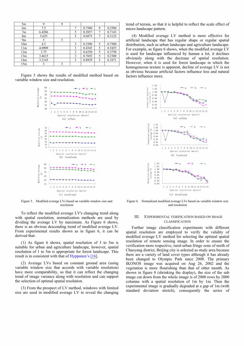
10m 4.5 3 0.2500 5 0.7500 11m 4.0909 3 0.4545 5 0.5455 12m 3.75 3 0.6250 5 0.3750 13m 3.4615 3 0.7692 5 0.2308 14m 3.2143 3 0.8929 5 0.1071 15m 3 3

Figure 5 shows the results of modified method based on variable window size and resolution.

(a) urban

30

35

40

45

50

55

60

1 2 3 4 5 6 7 8 9 10 11 12 13 14 15

Spatial resolution (meter)

Modified average

LV

a b c

(b) farmland

0

10

20

30

40

50

60

70

1 2 3 4 5 6 7 8 9 10 11 12 13 14 15

Spatial resolution (meter)

Modified average

LV

a b c

(c) woodland

15

25

35

45

55

65

1 2 3 4 5 6 7 8 9 10 11 12 13 14 15

Spatial resolution (meter)

Modified average

LV

a b c

Figure 5. Modified average LVs based on variable window size and

resolution

To reflect the modified average LV's changing trend along with spatial resolution, normalization methods are used by dividing the average LV by maximum. As Figure 6 shows, there is an obvious descending trend of modified average LV. From experimental results shown as in figure 6, it can be derived that:

(1) As figure 6 shows, spatial resolution of 3 to 5m is suitable for urban and agriculture landscape, however, spatial resolution of 1 to 5m is appropriate for forest landscape. This result is in consistent with that of Hyppanen’s [16].

(2) Average LVs based on constant ground area (using variable window size that accords with variable resolution) have more comparability, so that it can reflect the changing trend of image variance along with resolution and can support the selection of optimal spatial resolution.

(3) From the prospect of LV method, windows with limited size are used in modified average LV to reveal the changing

trend of terrain, so that it is helpful to reflect the scale effect of micro-landscape pattern.

(4) Modified average LV method is more effective for artificial landscape that has regular shape or regular spatial distribution, such as urban landscape and agriculture landscape. For example, as figure 6 shows, when the modified average LV is used for landscape influenced by human a lot, it declines obviously along with the decrease of spatial resolution. However, when it is used for forest landscape in which the homogeneous texture is apparent, decline of average LV is not as obvious because artificial factors influence less and natural factors influence more.

(a) urban

0.90

0.92

0.94

0.96

0.98

1.00

1.02

1.04

1 2 3 4 5 6 7 8 9 10 11 12 13 14 15

Spatial resolution (meter)

Normalized modified

average LV

a b c

(b) farmland

0.90

0.92

0.94

0.96

0.98

1.00

1.02

1.04

1 2 3 4 5 6 7 8 9 10 11 12 13 14 15

Spatial resolution (meter)Normalized modified

average LV

a b c

(c) woodland

0.90

0.92

0.94

0.96

0.98

1.00

1.02

1.04

1 2 3 4 5 6 7 8 9 10 11 12 13 14 15

Spatial resolution (meter)

Norm

aliz

ed m

odifi

edaverag

e LV

a b c

Figure 6. Normalized modified average LVs based on variable window size

and resolution

III. EXPERIMENTAL VERIFICATION BASED ON IMAGE CLASSIFICATION

Further image classification experiments with different spatial resolution are employed to verify the validity of modified average LV method for selecting the optimal spatial resolution of remote sensing image. In order to ensure the verification more respective, rural-urban fringe zone of north of Chaoyang district, Beijing city is selected as study area because there are a variety of land cover types although it has already been changed to Olympic Park since 2008. The primary IKONOS image was acquired on Aug 26, 2002 and the vegetation is more flourishing than that of other month. As shown in figure 8 (shrinking the display), the size of the sub image cut down from the whole image is of 2000 rows by 2000 columns with a spatial resolution of 1m by 1m. Then the experimental image is gradually degraded at a gap of 1m (with standard deviation stretch), consequently the series of

experimental images with different spatial resolution (from 1m to 10m) are prepared.

Figure 7. Primary experimental images with 1m spatial resolution and the

samples

It can be known by human vision that the study area is mainly covered with building, water, road, farmland, green land and barren. According to the coinstantaneous true color multi-spectral image of the same region, it can be interpreted that the farmland is uncultivated. Furthermore, considering the separability of high spatial resolution image and the reflectance diversity of building roof and road surface, six main types of land cover are identified as the reference for classification. They are: C1—bright artificial terrain; C2—dark artificial terrain; C3—water; C4—uncultivated farmland; C5— green land; and C6— barren. Maximum Likelihood method is used as the decision rule for supervised classifications.

In the series of maximum likelihood classification, samples are selected from the same region (as area of interest), so that the classification accuracies can be compared and assessed. In addition, the spectral difference between the same land use types should be taken into account when selecting the samples, so the samples should be representative and sufficient to different spectral feature and then can be combined into one class. In accuracy assessment, 256 samples (for classifications of images with 1m~6m spatial resolution) and 128 samples (for classifications of images with 7m~10m spatial resolution) are selected from the same regions for testing.

Figure 8(a) demonstrates the change of overall classification accuracy along with spatial resolution. Figure 8(b) demonstrates the trend of classification accuracy of different land use type along with spatial resolution. In figure 8(b), C1 and C2 are combined into one class (artificial terrain). Theoretically, the trend of classification accuracy should be consistent with that of modified average LV, because high LV means strong class separability. However, because of the

disturbance of random effect of natural landscape and the complexity of remote sensing image, it is not perfect as is expected. For example, image with 1m spatial resolution has high average LV but low classification accuracy. The analysis is as follows.

50%60%70%80%90%

100%

1 2 3 4 5 6 7 8 9 10Spatial resolution (meter)

Cla

ssifi

catio

n ac

cura

cy

(a)

0.00%

20.00%

40.00%

60.00%

80.00%

100.00%

1 2 3 4 5 6 7 8 9 10Spatial resolution (meter)

Cla

ssifi

catio

n ac

cura

cy

artificial terraingreen landuncultivated farmlandwater bodybarren

(b)

Figure 8. Classification accuracies of experimental images

(1) The reflectance rate of water from visible to infrared is very low and the gray value of water body is near to 0, which results in the average LV of the image in which large area of water exists is very high. Because the higher the spatial resolution is, the longer the border of water body is, the frequency that larger LV occurs is higher, which results in the higher the spatial resolution is, the larger the modified average LV is. However, the large average LV can not bring obvious improvement of classification accuracy because the pixel number of water body is limited.

(2) There is another important reason that image with 1m spatial resolution has high average LV but low classification accuracy is the complexity of high spatial resolution image, which contains several meanings. The first is the existence of different spectrum of the same objects and same spectrum of different objects, especially in high spatial resolution image. This phenomena is also proposed in [18, 19].The second is the existence of mixed pixel and shadow which makes many dark natural objects (especially their borders) and shadows be classified as dark artificial terrain.

(3) From figure 8(b), it can be seen that the trend of classification accuracy is basically consistent with that of figure (6), though there are random ditherings and deviations in the graphs. In addition, the classification accuracy of water body is almost 100% at different resolution, which is caused by the limited number of samples. Figure 8(b) shows that the modified average LV method for quantitively selecting the optimal spatial resolution has theoretical and instructional meaning to a certain extent.

IV. CONCLUSIONS Based on the analysis of scale characteristic of remote

sensing images, this paper not only emphasis the meanings of scale selection of remote sensing images but also discusses modified average LV method based on constant ground area to quantitively selecting the optimal spatial resolution of remote sensing image. The experimental results show that modified average LVs based on constant ground area (using variable window size that accords with variable resolution) can reflect the changing trend of image variance along with resolution and can support the selection of optimal spatial resolution. Further classification experiments also prove that the trend of classification accuracy along with spatial resolution is basically consistent with that of modified average LV, which means that the image classification accuracy of the optimal resolution image is basically higher than those of other’s. However, it is needed to specially note that:

(1) The value of this research is to try to theoretically interpret the relationship among spatial resolution, local variance and classification accuracy, but not to calculate the absolute optimal spatial resolution.

(2) Series of experiments show that the calculating results of different landscape or different subtypes are not absolutely same because of the random effect. Geoffrey indicates that the sole and absolute optimal scale that can correctly and comprehensively descript the shape and size of object does not exist [20]. For example, for the forest landscape on small scale, Hyppanen finds that the range of 5m suits for Scots pine, while 7m suits for Norway spruce [16].

However, though the primary research on selecting optimal spatial resolution of remote sensing image is theoretical and there are deviations between actual experimental results and ideal status, this geo-statistics based method is practically instructive and meaningful. In addition, from the view of object-oriented image processing, researches on the scale selection in segmentation based on geo-statistics and fractal theory are another meaningful direction of remote sensing scale research.

REFERENCES [1] C. Cao, N. S.-N. Lam. Understanding the scale and resolution effects in

remote sensing and GIS. D. A. Quattrochi and M. F. Goodchild, eds., Scale in Remote Sensing and GIS. 1997, pp.57-72.

[2] F. W. Davis, D. A. Quattrochi, M. K. Ridd, N. S.-N. Lam , S. J. Walsh, et al. “Environmental Analysis Using Integrated GIS and Remotely

Sensed Data: Some Research Needs and Priorities,” Photogrammetric Engineering and Remote Sensing, vol.37(6), pp.689-697, 1991.

[3] C. E. Woodcock, A H. Strahler. “The Factor of Scale in Remote Sensing,” Remote Sensing of Environment, vol.21, pp.311-332, 1987.

[4] H. Markowitz. Portfolio Selection - Efficient Diversification of Investments. Wiley,New York,1959.

[5] D. Chen. Multiresolution Models on Image Analysis and Classification. Paper submitted to UCGIS Summer Assembly and Retreat, 1998.

[6] N. Coops, D. Culvenor. “Utilizing Local Variance of Simulated High Spatial Resolution Imagery To Predict Spatial Pattern of Forest Stands. Remote Sensing of Environment,” Vol.71(3), pp.248-260, 2000.

[7] P. K. Bøcher, K. R. McCloy. “The fundamentals of average local variance — Part I: detecting regular patterns,” IEEE Transactions on Image Processing, 2006, vol.15, pp.300−310.

[8] P. K. Bøcher, K. R. McCloy. “The fundamentals of average local variance — Part II: sampling simple regular patterns with optical imagery,” IEEE Transactions on Image Processing, vol.15, pp.311−318, 2006.

[9] W. Nijland, E. A. Addink, S. M. D. Jong, F. D. Van der Meer. "Optimizing spatial image support for quantitative mapping of natural vegetation,” Remote Sensing of Environment, vol.113( 4), pp.771-780,2009.

[10] C. D. Lloyd, P. M. Atkinson. Scale and the spatial structure of landform: optimising sampling strategies with geostatistics. Proceedings of the 3rd International Conference on GeoComputation, 1998.

[11] N. C. Coops, P. C. Catling. “Predicting the complexity of habitat in forests from airborne videography for wildlife management,” International Journal of Remote Sensing, vol.18(12), pp.2677–2686, 1997.

[12] P. J. Curran. “The semi-variogram in remote sensing: an introduction,” Remote sensing of Environment, vol.24, pp.493-507, 1988.

[13] http://www.ffp.csiro.au/nfm/mdp/video/vidanal.htm. [14] G. Matheron. “Principles of geostatistics. Economic Geology,” vol.58,

pp.1246-1266, 1963. [15] A. Stein, F. D. Van der Meer, B. Gorte. Spatial Statistics for Remote

Sensing. Kluwer Academic Publishers, Dordrecht, 1999. [16] H. Hyppanen. “Spatial autocorrelation and optimal spatial resolution of

optical remote sensing data in boreal forest environment. International Journal of Remote Sensing,” vol.17(17), pp.3441-3452, 1996.

[17] M. A. Oliver, R. Webster. “Kriging: a Method of Interpolation for Geographical Information Systems,” International Journal of Geographic Information Systems, vol.4(3), pp.313-332, 1990.

[18] D. J. Marceau, G. J. Hay. “Remote sensing contributions to the scale issue,” Canadian Journal of Remote Sensing, vol.25(4), pp.357-366, 1999.

[19] B. Markham, J. R. G. Townshend. Land cover classification accuracy as a function of sensor spatial resolution. Proceedings of 15th Int. Symp. on Remote Sensing of Environment, Ann Arbor, MI, pp.1075-1090, 1981.

[20] G. J. Hay. Multiscale object-specific analysis: An integrated hierarchical approach for landscape ecology. Disseration of University of Montreal, 2002.