Mass Customization at Adidas: Three Strategic Capabilities to ...
Upload
khangminh22Category
view
2download
0
Models for Product Line Design with Customization - Considering Factors in Marketing and Operations
PhD Dissertation
Parisa Bagheri Tookanlou
Supervisor: Hartanto Wijaya Wong
Aarhus BSS, Aarhus University
Department of Economics and Business Economics
2018

Acknowledgements
This dissertation was conducted during my PhD study at Cluster for Operations Research and
Logistics (CORAL), Department of Economics and Business Economics, School of Business and
Social Sciences, Aarhus University in the period from January 2015 to January 2018.
First and foremost, my deep sincere gratitude goes to my supervisor Hartanto Wijaya Wong for his
tireless mentoring and patient supervision throughout my PhD study. This dissertation would not have
been possible without his continuous support and valuable guidance. He has broadened my
understanding of scientific work and I have learned a lot from his perspective on academic research.
I am indebted to him for all his time and efforts. Working under his supervision was a very fruitful
experience. Also, I am thankful to Professor Christian Larsen, my co-supervisor, for his advice and
insight during my PhD program.
I offer my respectable gratitude to all members of CORAL at Aarhus University for providing a very
great research environment and giving me the opportunity to pursue my higher education.
I also express my gratitude to the department of Operations Management and Information Systems at
Nottingham University, for their hospitality during my stay as visiting PhD student. I specially
appreciate Professor Bartholomew MacCarthy for his valuable suggestions for my research study.
I am also grateful to the assessment committee members Professor Anders Thorstenson, Professor
Linda Zhang, and Professor Mohamed Naim for their time and helpful suggestions and comments.
In addition, I would like to thank all my fellow PhD colleagues, both past and current, at CORAL. I
specially appreciate my officemate Maryam Ghoreishi and Ata Jalili Marand for their support. Also,
I would like to express my full thanks to Marjan Mohammadreza and Mohammad Sedigh Jasour for
their friendship and support during these three years.

I am also thankful to the following administrative staff Ingrid Lautrup, Karin Vinding, Thomas
Stephansen, Susanne Christensen, Birgitte Højklint Nielsen, and Christel Brajkovic Mortensen for
their support during my PhD program.
I would like to express my heartfelt gratitude to my fiancé, Meisam Karimkhani, for his
encouragement, patience, attention, and kindness and also my uncle and his wife, Mohammad Ali
Akbari and Sima Gholami, for their inspiration and encouragement during my PhD journey.
Last but not least, words have no power to express my deepest gratitude and regards to my beloved
Mother, Maryam Akbari, and my sister, Mahsa Bagheri Tookanlou, for their unconditional love,
kindness, and endless support they have throughout my life and my work.
Sincerely,
Parisa Bagheri Tookanlou
Aarhus, January 2018.

Summary
The central theme of this dissertation is product line design that involves customization. The theme
covers a range of strategic decisions for manufacturing firms that adopt mass customization. The
dissertation consists of three papers, each of which addresses different issues related to the product
line design problem where customized products are offered. The three papers all present stylized
models that take marketing and operations related factors into account.
In the first paper, we study a manufacturer’s product line design problem when consumers are
heterogeneous in their valuation of the product customization level and lead time. We extend the
standard quality-based segmentation problem by considering the degree of product customization and
lead time as the important attributes of product quality that affect a consumer’s purchase decision.
Contrary to the most existing studies that neglect inventories in the production system, this paper
explicitly considers the inventory positioning decision that is interdependent with the product line
decisions including pricing, product customization level, and lead time. We develop a model that
provides insights into the conditions under which the optimal decision for the manufacturer is to
implement the two-product strategy with two different customization levels or the one-product
strategy with a single customization level. The results of the numerical study show that the costs of
holding safety stock and pipeline inventory have an influence on the optimal choice of customization
levels. The optimal customization levels tend to be lower when the inventory costs are considered.
The focus in the second paper is on determining the optimal product line design in a market with
vertical and horizontal consumer heterogeneity. In particular, we are interested in examining the
effect of offering a customized product in the product line. We consider two comparison scenarios.
In the first scenario, we use the single-product strategy as the baseline strategy and examine the
conditions under which a horizontal product line extension through the offering of the customized
product is preferable to a vertical product line extension or quality-based segmentation strategy. In
the second scenario, we focus on examining the effect of offering the customized product to an
existing quality-based segmentation strategy. The main results show that the horizontal product line
extension may result in a higher increase in the channel profit as long as the investment to
accommodate flexibility is not too costly. Offering the customized product to an existing quality-
based segmentation strategy may also help increase the channel profit. The results show that the
channel structure is influential. The preference for the horizontal product line extension is stronger in
a decentralized channel than in a centralized channel.
In the third paper, the impact of demand uncertainty on product line design with customization is
studied. This paper considers horizontal product differentiation, and the product line studied consists
of a standard product offered in a make-to-stock fashion and a customized product offered in a make-
to-order fashion. Due to the demand uncertainty, the stocking level for the standard product must be
determined before the selling period starts, and consequently the problem is framed in a newsvendor
setting. The focus of the study is on examining the effects of demand uncertainty on the optimal
product line design and on how those effects are different when the products are sold in a centralized
channel or in a decentralized channel. In the centralized channel, the results show that the presence
of demand uncertainty drives the prices for the standard and customized products as well as the
customization level down. In the decentralized channel, the retail price for the standard product in the
case with demand uncertainty is lower than the price in the case with deterministic demand and the
numerical example shows that the optimal customization level decreases by increasing the uncertainty
in demand and also compared to when the demand is deterministic. This study also explores the
possibility of employing a buy-back contract as a way to improve the channel profit while providing
benefits for both the retailer and the manufacturer.
The dissertation advances the existing literature on product line design problem, especially the one
that considers customized products as an important offering in the product line. Furthermore, it
provides useful insights for practitioners regarding the effects of the different marketing and
operations factors and their interactions on the optimal product line decisions.

Resumé
Det centrale emne for denne afhandling er produktlinje-design, som involverer specifik
kundetilpasning. Emnet dækker en række strategiske beslutninger hos fremstillingsvirksomheder, der
masseproducerer kundetilpassede produkter. Afhandlingen består af tre selvstændige artikler. Disse
omhandler alle emner relateret til problemer i forbindelse med produktlinje-design i relation til
kundetilpassede produkter. Alle artiklerne præsenterer stiliserede modeller, der tager højde for
faktorer relateret til markedsføring og drift.
I den første artikel ser vi på en producents problemer ift. produktlinje-design, når kunderne er
heterogene i deres vurdering af produkttilpasning og leveringstid. Den normale model for
kvalitetsbaseret segmentering udvides ved at betragte graden af produkttilpasning og leveringstid som
væsentlige parametre for kundens købsbeslutning. I modsætning til de fleste nuværende studier, der
undlader at tage højde for lagerbeholdning i produktionssystemet, ser denne artikel eksplicit på
beslutninger vedrørende lagerbeholdning, der er gensidigt afhængig af beslutninger vedrørende
produktlinje, inklusiv prisfastsættelse, produkttilpasning og leveringstid. Vi udvikler en model, der
viser, hvilke forhold der danner baggrund for virksomhedens beslutning om at indføre henholdsvis
en to-produkt strategi med to forskellige tilpasningsniveauer og en et-produkt strategi med et enkelt
tilpasningsniveau. Resultaterne af den numeriske undersøgelse viser, at omkostningerne ved at have
et sikkerhedslager og et pipeline-lager har indflydelse på det optimale valg med hensyn til
tilpasningsniveauer. De optimale tilpasningsniveauer har en tendens til at være lavere, når
lageromkostninger tages i betragtning.
I afhandlingens anden artikel er fokus på at bestemme det optimale produktlinje-design i et marked
med vertikal og horisontal kunde-heterogenitet. Vi er specielt interesserede i at undersøge effekten af
at tilbyde et kundetilpasset produkt i produktlinjen. Vi sammenligner to scenarier. I det første scenarie
tager vi udgangspunkt i en ét-produkt strategi og undersøger, under hvilke forhold en horisontal
udvidelse af produktlinjen via tilbud om det kundetilpassede produkt er at foretrække fremfor en
vertikal udvidelse af produktlinjen eller en kvalitetsbaseret segmenteringsstrategi. I det andet scenarie
undersøger vi effekten af at tilbyde det kundetilpassede produkt til kunderne i en eksisterende
kvalitetsbaseret segmentstrategi. Resultaterne af undersøgelsen viser, at den horisontale produktlinje-
udvidelse kan resultere i en større stigning i overskuddet for den samlede forsyningskæde, så længe
der ikke er investeret for meget i at tilgodese fleksibilitet. At tilbyde det tilpassede produkt til
kunderne i en eksisterende kvalitetsbaseret segmentstrategi kan også medføre et øget overskud for
den samlede forsyningskæde. Resultaterne også viser, at forsyningskæde-strukturen har stor
betydning. Præferencen for den horisontale produktlinje-udvidelse er stærkere i en decentraliseret
kanal end i en centraliseret kanal.
I den sidste artikel undersøges betydningen af efterspørgselsusikkerhed for produktlinje-design med
kundetilpasning. Artiklen betragter horisontal produktdifferentiering og undersøger en produktlinje,
der består af et standardprodukt, der sælges som et fremstillet-til-lager (”make-to-stock”) produkt og
et kundetilpasset produkt, der sælges som et fremstillet-på-bestilling (”make-to-order”) produkt. På
grund af efterspørgselsusikkerheden skal lagerniveauet for standardproduktet være bestemt inden
salgsperioden starter, hvilket resulterer i et ”newsvendor” problem. Artiklen undersøger effekterne
af efterspørgselsusikkerhed på det optimale produktlinje-design, og hvordan disse effekter adskiller
sig, når produkterne sælges via en centraliseret kanal eller via en decentraliseret kanal. For den
centraliserede kanal viser resultaterne, at tilstedeværelsen af efterspørgselsusikkerhed får priserne på
standardprodukterne og de kundetilpassede produkter samt tilpasningsniveauet til at falde. For den
decentraliserede kanal er detailprisen for standardproduktet i tilfældet med efterspørgselsusikkerhed
lavere end prisen i tilfældet med deterministisk efterspørgsel, og tal-eksemplet viser, at det optimale
tilpasningsniveau falder, når usikkerheden i efterspørgslen stiger, og når der sammenlignes med det
tilfælde, hvor kundernes efterspørgsel er deterministisk. Artiklen undersøger også muligheden for at
anvende en tilbagekøbskontrakt for at forbedre overskuddet samtidig med, at det er til fordel for
detailvirksomheden og producenten.
Denne afhandling bidrager til den eksisterende litteratur om problemer ift. produktlinje-design,
specielt ift. de tilfælde hvor kundetilpassede produkter udgør en vigtig del af produktlinjen.
Derudover bidrager afhandlingen med vigtig viden til virksomhederne vedrørende effekterne af
forskellige markedsførings- og driftsfaktorer og deres betydning for beslutninger med henblik på at
opnå det optimale produktlinje design.
Table of Contents
1 Introduction. .......................................................................................................................... 1
1.1 Background and Motivation ..................................................................................................... 2
1.2 Focus of This Study ................................................................................................................. 3
1.3 Structure of Dissertation .......................................................................................................... 6
1.4 Highlights of Each Paper and Main Contributions .................................................................... 7
1.5 Managerial Implications .......................................................................................................... 9
2 Paper 1: Determining the optimal customization levels, lead times and inventory
positioning in vertical product differentiation ............................................................................. 8
2.1 Introduction ........................................................................................................................... 10
2.2 Literature Review .................................................................................................................. 12
2.3 Models ................................................................................................................................... 16
2.3.1 The Marketing Model ............................................................................................... 17 2.3.2 The Production-Inventory Model .............................................................................. 18 2.3.3 The Integrated Model ................................................................................................ 23
2.4 Numerical Results and Discussion ......................................................................................... 27
2.5 Conclusions ........................................................................................................................... 36
3 Paper 2: Product line design with vertical and horizontal consumer heterogeneity: the
effect of distribution channel structure on the optimal quality and customization levels ........ 45
3.1 Introduction ........................................................................................................................... 45
3.2 Literature Survey ................................................................................................................... 47
3.3 Models ................................................................................................................................... 50
3.3.1 Notation and Assumptions ........................................................................................ 50 3.3.2 Comparison of Product Line Strategies ..................................................................... 53
3.3.2.1 Comparison Scenario 1 – horizontal vs. vertical product line extension ............... 54
3.3.2.2 Comparison Scenario 2 – the role of offering the customized product in the quality-based segmentation strategy.................................................................................................................................... 66
3.4 Sensivity Analysis of Some Assumptions .............................................................................. 74
3.5 Conclusions ........................................................................................................................... 79
4 Paper 3: Product line design with customization: the effects of demand uncertainty and
distribution channel structure .................................................................................................... 89
4.1 Introduction ........................................................................................................................... 91
4.2 Literature Review .................................................................................................................. 92
4.3 Models ................................................................................................................................... 95
4.3.1 Centralized Channel .................................................................................................. 99 4.3.2 Decentralized Channel ............................................................................................ 102
4.4 Channel Coordination .......................................................................................................... 108
4.5 Conclusions ......................................................................................................................... 113
Bibliography .............................................................................................................................. 128

Chapter 1
1 Introduction

Introduction 2
1.1 Background and Motivation
This PhD dissertation considers product line design problems that involve the offering of customized
products. Designing a product line is a strategic decision for manufacturing firms and is the very
essence of every business. The firms, faced with a heterogeneous market in which consumers may
have their own ideal product, must decide on the number of products offered, product quality, and
price to maximize their profits. Customization is an important feature in the product line design
problems studied in this dissertation, and is concerned with offering tailored products to individual
consumers.
There is no doubt that designing a product line that involves customization will require a joint
perspective on marketing and operations decisions. The traditional view suggesting that marketing
and operations just focus on revenues and costs is outdated and will not give the best results (Tang
2010). In the context of product line design with customization, one important and relevant decision
that manufacturing firms need to make concerns the degree of customization offered to consumers.
This decision should be made based on careful consideration of marketing and operations related
factors regarding consumers’ preferences and manufacturing or operational capabilities, and it is also
important for the firms to enhance their understanding of the interaction among those factors.
As the offering of customized products represents an important part of the product line design
problems studied in this dissertation, the concept of mass customization (MC) is of relevance. Mass
customization refers to a manufacturing strategy aimed at providing sufficient product and service
variety so that nearly all consumers find exactly what they want without significantly compromising
cost efficiency. The concept of mass customization was first introduced by Davis (1987) and later
developed by Pine (1993), and remains perceived as a promising strategy that may help companies
gain competitive advantage (Gandhi et al. 2013). A study conducted by Bain and Company
(Spaulding and Perry 2013) shows the promising market opportunity for individualized
customization. According to their survey, 25 to 30% of online shoppers are interested in buying
customized products. To achieve mass customization, manufacturing firms will need to be equipped
with advanced manufacturing and information technologies and unique operational capabilities
(Salvador et al. 2009). Implementing MC remains a challenging issue for many manufacturing firms
due to increasing costs, uncertainty, and complexity of the manufacturing processes (Lai et al. 2012).
In an ideal world, firms implementing MC strategy should be able to provide customized products at
a comparable price and speed of equivalent standardized products. However, empirical evidence

Introduction 3
suggests that the customization is not ‘free’ and needs to be traded-off against factors such as lead
time and cost (Squire et al. 2006). This dissertation adopts this more pragmatic view. We are also in
agreement with Zipkin (2001) in that MC has its limits that depend on several factors such as the
availability of highly flexible technology and the existence of a potential mass market for customized
attributes. Different products (industries) may have different capabilities in meeting those
requirements. Clothing/apparel, footwear, computers, and furniture are some examples of products
that seem to have high capabilities in meeting the requirements (Zipkin 2001), for which this study is
quite relevant.
1.2 Focus of This Study
Product line design has been a key topic in the economics/marketing literature for decades, and more
recently, the integration of product line and operational decisions has become a central issue in the
literature. The literature on product line design can, in general, be classified into two categories.
Articles in the first category focus on the analytical results and the models presented are stylized and
rely on some restrictive assumptions. Nevertheless, they provide valuable managerial insights. Early
contributions in this category include e.g. Mussa and Rosen (1978) and Moorthy (1984). More recent
studies in this category that provide extensions to the earlier models include e.g. Kim and Chhajed
(2002), Netessine and Taylor (2007), Shi et al. (2013) and Jerath et al. (2017). Articles in the second
category present models in which the assumptions are less restrictive, but analytical and even
numerical solutions are difficult to obtain. The typical focus of those articles is on the development
of heuristic methods. With the help of data obtained through market surveys, the models developed
in the second category can be used for developing a decision support tool. Some earlier work is e.g.
Green and Krieger (1985), Dobson and Kalish (1988), and Kohli and Sukumar (1990). More recent
studies are presented in e.g. Belloni et al. (2008) and Wang and Curry (2012). The models developed
in this dissertation are more closely related to and contributes to extending the literature in the first
category.
One of the important aspects in product line design is concerning the market structure characterized
by consumers’ heterogeneity. Some studies in the literature (e.g. Mussa and Rosen 1978, Moorthy
1984 and Moorthy and Png 1992) consider the market where consumers are heterogeneous in their
valuation of product quality so that they focus on the quality-based segmentation or vertical product
differentiation strategies. The notion of quality adopted in this literature is represented by a set of
product attributes, on which consumers agree in their preference ordering, i.e., every consumer
prefers higher values on the attributes to lower values (or vice versa), ceteris paribus (Moorthy 1984;
Introduction 4
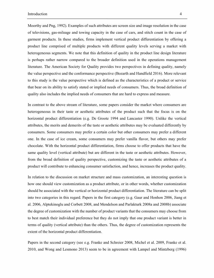
Moorthy and Png, 1992). Examples of such attributes are screen size and image resolution in the case
of televisions, gas-mileage and towing capacity in the case of cars, and stitch count in the case of
garment products. In these studies, firms implement vertical product differentiation by offering a
product line comprised of multiple products with different quality levels serving a market with
heterogeneous segments. We note that this definition of quality in the product line design literature
is perhaps rather narrow compared to the broader definition used in the operations management
literature. The American Society for Quality provides two perspectives in defining quality, namely
the value perspective and the conformance perspective (Bozarth and Handfield 2016). More relevant
to this study is the value perspective which is defined as the characteristics of a product or service
that bear on its ability to satisfy stated or implied needs of consumers. Thus, the broad definition of
quality also includes the implied needs of consumers that are hard to express and measure.
In contrast to the above stream of literature, some papers consider the market where consumers are
heterogeneous in their taste or aesthetic attributes of the product such that the focus is on the
horizontal product differentiation (e.g. De Groote 1994 and Lancaster 1990). Unlike the vertical
attributes, the merits and demerits of the taste or aesthetic attributes may be evaluated differently by
consumers. Some consumers may prefer a certain color but other consumers may prefer a different
one. In the case of ice cream, some consumers may prefer vanilla flavor, but others may prefer
chocolate. With the horizontal product differentiation, firms choose to offer products that have the
same quality level (vertical attribute) but are different in the taste or aesthetic attributes. However,
from the broad definition of quality perspective, customizing the taste or aesthetic attributes of a
product will contribute to enhancing consumer satisfaction, and hence, increases the product quality.
In relation to the discussion on market structure and mass customization, an interesting question is
how one should view customization as a product attribute, or in other words, whether customization
should be associated with the vertical or horizontal product differentiation. The literature can be split
into two categories in this regard. Papers in the first category (e.g. Gaur and Honhon 2006, Jiang et
al. 2006, Alptekinoglu and Corbett 2008, and Mendelson and Parlakturk 2008a and 2008b) associate
the degree of customization with the number of product variants that the consumers may choose from
to best match their individual preference but they do not imply that one product variant is better in
terms of quality (vertical attribute) than the others. Thus, the degree of customization represents the
extent of the horizontal product differentiation.
Papers in the second category (see e.g. Franke and Schreier 2008, Michel et al. 2009, Franke et al.
2010, and Wong and Lesmono 2013) seem to be in agreement with Lampel and Mintzberg (1996)
Introduction 5
and Duray et al. (2000) who suggest that the relative degree of product customization is determined
by the extent to which consumers are involved in the production cycle. Those papers take a different
view by arguing that increased customization may result in enhanced perceived values regarding
uniqueness, utility, self-expressiveness, etc., which will in turn increase the consumers’ willingness
to pay. When viewed from the value perspective of quality (Bozarth and Handfield 2016), this
suggests that increased customization contributes to the improvement in product quality. This view
on customization is particularly useful when considering a product line design that involves multiple
customization levels. This dissertation acknowledges the importance of these two different views and
the models developed in this dissertation are designed to be differentiated depending on which of the
two views is adopted.
In studying product line design strategies, it is also important to pay attention to distribution channel
structure used to sell the products. Channel structure can be differentiated by e.g. how many players
involved, and in the case of more than one players, who the focal player is. This dissertation focuses
on the setting where the manufacturer is the focal player and faced with the product line design
problem. We follow the mainstream literature on product line design that also focuses on such a
setting, and argue that the setting is commonly observed in practice, and hence of high relevance. In
a centralized channel, the manufacturer sells the products directly to the end consumers, i.e., the
manufacturer is the only player making all decisions. In contrast, in a decentralized channel, the
manufacturer depends on intermediate players such as retailers in selling the products to end
consumers. As the manufacturer’s interest is not always aligned with that of the retailers, it is expected
that the manufacturer’s optimal product line design will be influenced by the presence of channel
efficiency loss prevalent in a decentralized distribution channel. Of particular interest in this
dissertation is a dual channel that could be seen as a variant of decentralized channel. In a dual
channel, the manufacturer sells the standard products through the retailer, and sells the customized
products directly to end consumers via an online channel owned by the manufacturer (Chiang et al.
2003 and Dumrongsiri et al. 2008). The way in which the product line design decisions are affected
by the distribution channel structure represents an important line of inquiry examined in this
dissertation.
As a note, we are aware of the possible existence of other settings to which the results presented in
this dissertation may not be directly applicable. Consider, for example, a distribution channel where
other players, e.g. retailers, play a more dominant role in the channel. In some cases, retailers are the
players who make product line design decisions (see e.g. Dukes et al. 2014). There are also examples
Introduction 6
where both the manufacturer and retailer are involved in designing the product attributes (Kolay
2015).
Motivated by the fact that most articles in the literature on product line design focus heavily on the
marketing aspects and less so on the operations aspects, this dissertation examines enhancements by
developing models that incorporate some of the important issues that are widely studied in the
operations literature. By doing this, this dissertation contributes to developing more integrated models
in the interface of marketing and operations. One important simplification in the existing literature
on product line design is the assumption that demand is deterministic. This assumption certainly
facilitates neat analytical results, but those results are questionable when considering many real
settings in which demand uncertainty is actually prevalent. To cope with demand uncertainty, the
manufacturing firm will need to hold inventories, which will, in turn, influence the product line design
decisions.
Common to all the models developed in this study is the monopolistic setting assumption. That is, we
focus on product line design problems faced by a manufacturing firm without considering any
competition with other manufacturing firms. This allows us to focus on examining how a
manufacturing firm considering mass customization should design a product line when dealing with
the different issues explained above.
1.3 Structure of Dissertation
This dissertation consists of three self-contained papers prepared for publication in international
journals. As outlined above, these papers all address the product line design problems where the
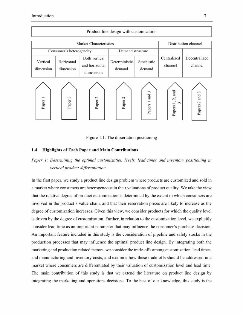
customized product is part of the offering. Figure 1.1 summarizes the main issues addressed in each
of the three papers and highlights how each paper differs from the other papers. The three papers can
be differentiated based on: (a) consumers’ heterogeneity – whether it is in the horizontal dimension
or vertical dimension or both; (b) demand – whether it is deterministic or stochastic; and (c) channel
structure – whether we deal with a centralized channel or decentralized channel.
Introduction 7
Product line design with customization
Market Characteristics Distribution channel
Consumer’s heterogeneity Demand structure
Centralized
channel
Decentralized
channel Vertical
dimension
Horizontal
dimension
Both vertical
and horizontal
dimensions
Deterministic
demand
Stochastic
demand
Figure 1.1: The dissertation positioning
1.4 Highlights of Each Paper and Main Contributions
Paper 1: Determining the optimal customization levels, lead times and inventory positioning in
vertical product differentiation
In the first paper, we study a product line design problem where products are customized and sold in
a market where consumers are heterogeneous in their valuations of product quality. We take the view
that the relative degree of product customization is determined by the extent to which consumers are
involved in the product’s value chain, and that their reservation prices are likely to increase as the
degree of customization increases. Given this view, we consider products for which the quality level
is driven by the degree of customization. Further, in relation to the customization level, we explicitly
consider lead time as an important parameter that may influence the consumer’s purchase decision.
An important feature included in this study is the consideration of pipeline and safety stocks in the
production processes that may influence the optimal product line design. By integrating both the
marketing and production related factors, we consider the trade-offs among customization, lead times,
and manufacturing and inventory costs, and examine how these trade-offs should be addressed in a
market where consumers are differentiated by their valuation of customization level and lead time.
The main contribution of this study is that we extend the literature on product line design by
integrating the marketing and operations decisions. To the best of our knowledge, this study is the

Introduction 8
first study to analyze the product line design problem that addresses the trade-offs between
customization, lead times, and manufacturing and inventory costs.
Paper 2: Product line design with vertical and horizontal consumer heterogeneity: the effect of
distribution channel structure on the optimal quality and customization levels
In this paper, we study a product line design problem where consumers are heterogeneous in both
quality and aesthetic component of the products. In this study, offering customization in the product
line is considered as a way of matching the product’s aesthetic component to the consumers’ ideal
preferences. The study focuses on examining the preference of different product line extension
strategies and how this preference is influenced by the type of distribution channel adopted. In
particular, we are interested in examining the effect of offering the customized product in the product
line. Using the single-product strategy as the baseline strategy, we first examine when a vertical
product line extension strategy or quality-based segmentation is preferable to a horizontal product
line extension strategy. In the vertical product line extension strategy, two products are offered with
different quality, and each product is targeted to each segment. In contrast, in the horizontal product
line extension strategy, a customized product is offered in addition to the standard product. We then
examine the effect of adding a customized product to the existing quality-based segmentation
strategy.
The main contribution of this chapter is as follows. We are the first to consider the product line design
problem in which quality and customization level are decision variables. To the best of our
knowledge, this is also the first time that two directions for the product line extension strategy are
compared. This contribution is enhanced further by the examination of how the type of distribution
channel may play a role in determining the best product line extension strategy.
Paper 3: Product line design with customization: the effects of demand uncertainty and distribution
channel structure
In this paper, the impact of demand uncertainty on the optimal product line design decisions is
investigated in a market where consumers are heterogeneous in the taste or preference of the products.
A stylized model is developed to analyze how the optimal product line design regarding price and
customization level is influenced by the risk of supply and demand mismatch, and how the influence
differs between the centralized and decentralized channels. An attempt is also made to improve the
channel profit in the decentralized channel by applying a supply chain contract. The work presented
in Chapter 4 adds to the existing literature in the following respects. First, it extends the relatively

Introduction 9
scant literature on product line design with customization in the presence of demand uncertainty. For
the setting where the product line consists of the standard and customized products that are sold
through a dual channel, this work is the first to examine the effect of demand uncertainty. Second,
this work also contributes to filling the void in the literature on supply chain coordination in the
context of product line design that especially involves marketing and operations decisions.
1.5 Managerial Implications
This PhD dissertation provides useful information for manufacturing firms interested in
implementing mass customization in (re)-designing their product line. The results clearly show the
importance of integrating operations and marketing related factors in product line design. Ignoring
factors that are pertinent in operations such as inventory costs and demand uncertainty may result in
sub-optimal product line design decisions. Furthermore, the impact of lead time cannot be ignored.
While lead time reduction initiatives are always welcome, the approach presented in this dissertation
provides helpful information for firms in determining the manufacturing processes where those lead
time reduction initiatives will be most beneficial.
The results show that offering the customized product in the product line may enhance profitability,
and manufacturing firms could consider offering customized products as an alternative to quality-
based segmentation or as a complement to the existing quality-based segmentation strategy. However,
this is not without conditions and depends on several factors. For example, in order to make the
offering of customized products appealing, there is a need for a manufacturing system with a
sufficiently high flexibility. In other words, the cost of enhancing flexibility that is driven by the
customization level cannot be too high. This finding can motivate the firms to consider the possible
adoption new advanced technologies (e.g. additive manufacturing), known for the high level of
flexibility without necessarily incurring significantly higher costs (Rylands et al. 2016; Durach et al
2017).
It is also important that manufacturing firms take into account the type of channel they are operating.
This study provides a better understanding of the limitations inherent in a decentralized channel and
provides guidelines for product line designers to determine the appropriate customization level in a
decentralized channel in contrast to a centralized channel. In this study, we show that the presence of
demand uncertainty has an influence on product line decisions. Hence, it highlights the importance
of coordination between marketing and operations in product line design. Furthermore, this study
should motivate the firms operating in a decentralized channel to be more proactive in designing
channel contracts since we show that such contracts may improve channel profitability. While the use

Introduction 10
of contracts is widespread in supply chain management practices, such contracts are less common
when it comes to product line design. Nevertheless, this study shows the importance of channel
coordination in product line design when the manufacturing firms rely on the retailer in selling their
product.

Chapter 2
2 Paper 1: Determining the optimal customization levels, lead
times and inventory positioning in vertical product
differentiation
History: This paper has been presented at: ISIR 2016-Conference of International Society for
Inventory Research, August 2016, Budapest, Hungary. The paper is currently under
revisions for possible future publication in International Journal of Production Economics.

Chapter 2: Paper 1 9
Determining the optimal customization levels, lead times and inventory positioning in vertical
product differentiation
Parisa Bagheri Tookanlou and Hartanto Wong
Department of Economics and Business Economics
School of Business and Social Sciences, Aarhus University
Fuglesangs Allé 4, 8210 Aarhus, Denmark
Abstract
In this paper we study a manufacturer’s product line decisions when selling customized products in
a market where consumers are heterogeneous with respect to their valuation of quality. The product
has two attributes based on which a consumer’s product valuation is determined. The first attribute is
customization level, defined by the extent to which consumers are involved in the value chain. The
second attribute is delivery lead time which is influenced by the customization level. The vertically
differentiated market is represented by two segments. Different from most existing work in the
product line design literature that neglects the operational aspects attached to production, in this paper
we consider the inventory positioning decision along the production processes which is
interdependent with the customization level and lead time decisions. The model developed provides
insights into the conditions under which the manufacturer should opt for the two-product strategy
with two different customization levels or the one-product strategy with a single customization level.
Our model can also be used to help determine which production process should be given the highest
priority when the manufacturer initiates a lead time reduction project.
Keywords: Product Line Design; Mass Customization; Safety Stock Positioning; Quality-based
Segmentation.
Chapter 2: Paper 1 10
2.1 Introduction
Since the concept was first coined by Davis (1987) and further popularized due to Pine (1993), Mass
Customization (MC) has been one of the central themes both practitioners and scholars focus on when
discussing future manufacturing strategies. MC has always been perceived as a promising strategy
that may help companies gain competitive advantage, increase revenue, and reduce waste through
on-demand production, see e.g., Gandhi et al. (2013). However, the successful implementation of MC
has proved hard to achieve; although there are successes, there are also many costly failures.
A study conducted by Bain and Company (Spaulding and Perry 2013) shows that the market
opportunity for individualized customization appears to be significant. The results of their survey
suggest that 25 to 30% of online shoppers are interested in trying the customization option. They also
discover that individualized customization can increase the consumer loyalty and engagement
because consumers who had experience in customizing a product online seem to be more willing to
engage more with the company and visit its website more frequently. This opportunity has been made
possible by the development of new technologies that not only allow firms to respond to consumers’
unique needs, but also to enhance the products’ affordability. Gandhi et al. (2013) states that some
key enabling technologies include online configuration technologies, 3-D digital modeling,
dynamically programmable robotic systems, etc.
Customized products can generally be categorized into two different groups. In the first group,
consumers are allowed, at one or more stages in the production processes, to configure the product
by choosing from an extensive set of choices. Examples of such products are many: bags (e.g.,
Timbuk), watches (e.g., Fossil), shoes (e.g., Nike and Adidas), and laptops (e.g., Dell). In recent years,
we have witnessed a growing list of products that belong to the second group in which manufacturing
firms offer individualized customization by letting consumers become involved in creating their own
unique product. For example, Brooks Brothers and Stitch Fix offer custom suits made to fit one’s
body shape and size. Regardless of the group to which a customized product belongs, firms must be
careful when deciding the right customization level to offer.
In this paper, we adopt the concept of customization presented in Lampel and Mintzberg (1996) and
Duray et al. (2000). That is, the relative degree of product customization is determined by the extent
to which consumers are involved in the product’s value chain. A product can be considered to have a
higher customization level when consumers are more deeply involved in the product’s value chain,
e.g., in the design phase, as opposed to the assembly phase. Consumers in the market certainly may
have different preferences for customization levels. Take, for example, customized furniture. Some

Chapter 2: Paper 1 11
consumers may be satisfied with a particular sofa design offered by a manufacturer but may want to
have customized fabric colors. Others might prefer a more unique sofa design instead. The differences
in customization level preference are, to a great extent, related to the preference for product delivery
lead time. Consumers who want a unique sofa design are willing to wait longer than those who only
want customized fabric colors. Ideally, as also widely discussed in the literature, mass customization
should allow consumers to buy a customized product at a price close to the price for the standard and
mass-produced product. In reality, however, many innovative customized products offered either by
start-ups or by established firms are still targeted at niche market segments. The reason is twofold.
First, the firms must still incur additional costs for manufacturing and delivering those customized
products. Second, the consumers in these niche segments, mostly conscious of product
innovativeness, are those who are willing to pay a price premium for such customized products.
Several studies (e.g. Tu et al. 2001, Franke and Schreier 2008, Michel et al. 2009, and Franke et al.
2010) support this notion as they show that when consumers perceive a product’s uniqueness as
enhanced due to their involvement in the production process, the consumers’ reservation prices are
likely to increase. Trentin et al. (2012) provides empirical support to the notion as they show that
increased customization achieved through the use of product configurators improves product quality.
The important role of product configurators in enhancing product quality is also highlighted in Zhang
(2014). Based on the above discussion, product quality in our model is primarily driven by the
customization level. We consider a product as a bundle of several attributes, but our focus is on two
interacting attributes: customization level for which higher is better, and product delivery lead time
for which shorter is better.
Given the differences in the consumers’ preferences as regards customization level and delivery lead
times, manufacturers are confronted with some choices: should they offer single or multiple
customization levels and which customization level(s) should they offer? When making those
decisions, the manufacturers must also consider the potential cannibalization of the product with high
customization level by the product with lower customization level. The manufacturers’ decisions on
customization levels also have some inter-dependence with their production/inventory system.
Depending on where the customization level is set, firms may still need to carry some product
materials or components inventories. When the customization level is higher, there are less materials
kept in the inventory compared to the situation where firms offer a lower customization level.
Furthermore, the work-in-process or pipeline inventories are also important and therefore cannot be
ignored.

Chapter 2: Paper 1 12
Our study is motivated by the fact that literature addressing the aforementioned problems is scarce.
In this paper, we frame the manufacturers’ product customization decisions as a product line design
problem in which the quality attributes are represented by the customization level and delivery lead
time. In contrast to most studies within product line design literature, we consider the interdependence
of the decisions on those two quality attributes and the decisions on inventory held in the production
system. More specifically, we aim to answer the following questions:
(i) Which customization level(s) should firms offer when taking into consideration the marketing
factors (consumers’ appreciation of customization level and lead time) as well as inventories
in the production system?
(ii) How the answer to the above question is affected by the changes in different marketing and
production related parameters?
While focusing on the questions above, this paper also offers a method that can be used to establish
priorities across all the main production processes such that firms can decide which process to focus
on when implementing lead time reduction initiatives. This issue is particularly important given the
fact that addressing the so-called customization-responsiveness squeeze is indeed crucial to the
success of mass customization strategies (McCutcheon et al. 1994 and Tu et al. 2001).
The rest of the paper is organized as follows: In the next section, we present a survey of the relevant
literature. Section 2.3 presents the model that integrates production-inventory and marketing
decisions. In Section 2.4, we present the numerical results and discuss the main managerial insights.
Finally, in Section 2.5 we wrap up the paper with a concluding discussion and some suggestions for
future research.
2.2 Literature Review
Our paper is primarily related to four streams of literature. The first one is the literature considering
product line design problems in a vertically differentiated market. Mussa and Rosen (1978) and
Moorthy (1984) are among the first authors to introduce quality differentiation into the marketing
literature. In an influential paper, Moorthy (1984) considers a monopolist serving multiple consumer
segments that are different in their valuations of quality. In that work, the monopolist offers a menu
of products with higher-quality products priced higher. The classical results from his study suggest
that the presence of cannibalization forces the monopolist to only offer consumers in the highest
valuation segment their optimal quality level, while all other segments receive products at the non-
optimal quality level. Unlike Moorthy (1984), who considered discrete consumer valuations, Mussa

Chapter 2: Paper 1 13
and Rosen (1978) present a model with a continuous distribution of consumer valuations. With
continuous distribution, the choice between full market coverage and partial market coverage
becomes relevant and has an impact on the optimal product prices and quality levels. Over the years
several authors have extended the above classical results. Moorthy and Png (1992) extend the above
classical results by considering the timing of product introductions. They show that under some
conditions the sequential product introductions can alleviate cannibalization. Kim and Chhajed
(2002) consider a product line design problem with multiple quality attributes. Choudhary et al.
(2005) use the product line design models to study the effect of personalized pricing on the firm’s
choices with regard to quality. Other papers examine the effect of channel structure in product line
design problems with quality differentiation (see e.g., Villas-Boas 1998, Liu and Cui 2010, and Chung
and Lee 2015), an issue we do not explore here.
What is common in all the literature above is that the authors do not consider relevant operational
costs beyond variable production costs. This has been the motivation for several studies included in
the second stream of literature related to our paper, a stream that integrates product line design and
operational decisions. Several authors, e.g., Karmarkar and Kekre (1987) and De Groote (1994),
examine the operational implications of product variety. In these papers, however, the authors
consider horizontal product differentiation. Below, we discuss several papers that consider vertical
product differentiation like we do in this paper. Netessine and Taylor (2007) study the impact of
production technology on the optimal product line design. They combine the standard product line
design problem with the classical EOQ (Economic Order Quantity) inventory model to capture the
problem faced by the manufacturer when balancing production setups with accumulation of
inventories in the presence of economies of scale. They show that the integration of the production-
inventory model and product line design leads to interesting results that challenge the established
results in the marketing literature. Their study reveals that more expensive production technology
characterized by higher inventory-related cost parameters leads to higher quality products and lower
product prices. Similar to their paper, we also integrate the production-inventory and product line
decisions. However, our model differs from theirs in many respects. First, they assume deterministic
demand such that the standard EOQ model is applicable whereas we consider demand uncertainty
such that safety stock is necessary. Second, they consider a simple production setting characterized
by a single stage production system, whereas we consider more complex production settings
characterized by multiple stages. And finally, as we consider customized products, the manufacturer
in our model is assumed to work in a make-to-order (MTO) or assemble-to-order (ATO) manner.
Hence, lead time is an important factor in our model. In Netessine and Taylor (2007), the authors
Chapter 2: Paper 1 14
consider make-to-stock production settings in which lead time is not relevant. Chayet et al. (2011)
study the problem of simultaneously optimizing the product line design and the capacity investment.
Our model is similar to theirs in that consumers make product choices to maximize a linear utility
function of price, quality level, and waiting cost. The focus of their analysis is on the choice between
dedicated or flexible production facilities for processing all product variants in the product line. They
use a simple M/M/1 queuing model to represent the production system. Our research differs from
their research as our primary focus is on the effect of inventory costs on the product line design
decisions, and we capture more realistic production settings in which inventory can be held at
different stages in the production processes.
The other stream of literature related to our paper includes papers that consider product line design
problems in the context of mass customization. Most of those papers consider horizontal product
differentiation, i.e., they compare the conventional strategy offering mass-produced standard products
and the mass customization strategy offering unlimited and customized products (see e.g. Jiang et al.
2006 and Alptekinoglu and Corbett 2008). None of the papers explicitly consider consumers’ waiting
costs incurred when buying customized products. Models considering the trade-off between
customization and lead times are presented in e.g. Xia and Rajagopalan (2009), Alptekinoglu and
Corbett (2010), and Mendelson and Parlakturk (2008a, 2008b). Xia and Rajagopalan (2009) study
the standardization and customization decisions of two firms in a competitive setting and consider
lead time along with product variety and price decisions. They show that product variety and lead
time may play strategic roles in the competition. Alptekinoglu and Corbett (2010) present a model to
optimize product line design while explicitly considering the trade-off between meeting individual
preferences and incurring the longer lead times associated with customized products. Mendelson and
Parlakturk (2008a, 2008b) consider competition between a mass customizer and a mass producer. In
their paper, only the mass producer carries inventories whereas the mass customizer does not. While
the main difference between our paper and theirs is that we consider vertical rather than horizontal
differentiation, our model also facilitates detailed analysis of a multi-stage production network
whereas they consider a simplified MTS system that produces standard products and a MTO system
that produces customized products. Wong and Lesmono (2013) consider customization vs. lead time
trade-off and vertical differentiation, and their paper is therefore the one that is most closely related
to our paper. Our paper is in line with their paper as we also consider the quality attributes as
customization level and lead time, but while they study the optimal conditions for offering a single
product or two products with different customization levels as we do in this paper, we extend their
work in two ways. Firstly, unlike their paper considering a simple queuing system to represent the

Chapter 2: Paper 1 15
production processes, we consider a more realistic production network that includes multiple stages
with interdependences among them. As a consequence of their modeling approach, the customization
level is assumed to be continuous in their model. Although such an approach provides useful
qualitative insights, it cannot be directly used by manufacturing firms for determining the optimal
customization level(s). Our model captures the fact that there is always a limited set of points in which
final customization can take place. Secondly, they do not include the question of inventories in their
study whereas we explicitly consider both safety and work in progress inventories. In a recent study,
Wong and Lesmono (2017) extends their previous work (Wong and Lesmono 2013) by examining
the effect of distribution channel structure on the product line decisions, but they do not consider the
operational aspects related to the production processes.
Finally, our work is also related to the literature studying assembly network operations that produce
customized products. Several authors, e.g., Lee and Tang (1997), Swaminathan and Tayur (1998), Su
et al. (2005) and Wong et al. (2009), present models to analyze the concept of postponement or
delayed product differentiation. When implementing postponement, manufacturing firms delay the
point at which the final customization of the product is to be configured. The concept has been
perceived as a cost-effective way to reduce the operating costs associated with managing proliferating
product variety (Van Hoek 2001 and Yang and Burns 2003). The literature on postponement is also
closely related to the literature on customer order decoupling point (CODP) (see e.g. Giesberts and
van den Tang 1992, Rudberg and Wikner 2004, van Donk and van Doorne 2016), defined as the point
in the value-adding material flow that separates decisions made under uncertainty from decisions
made under certainty concerning (customized) customer demand. Although we also investigate the
optimal point in the production processes for making the final customization of the product, there are
several important differences. None of the above papers associate the customization point with the
perceived quality level. In the literature on postponement and CODP, the final products are assumed
to have the same quality level, whereas we presume that customization level is related to perceived
quality and thereby influences the consumers’ willingness to pay. Another main difference is that all
the above mentioned papers focus solely on the operations aspect of customization whereas we
consider the integration of both the marketing and operations decisions.
Even though the above mentioned papers do not pay attention to the detailed operations of the
production processes, some authors do. Shao and Ji (2008) present a model for evaluating different
postponement strategies in mass customization with service guarantees. Shao and Dong (2012)
compare the order fulfilment performance in MTS and MTO systems taking into account an inventory
cost budget constraint. Lu et al. (2012) present a model to evaluate delayed differentiation strategies.
Chapter 2: Paper 1 16
They consider multiple points of product differentiation and develop a cost model that explicitly
includes the operational delay cost and the penalty cost. Our model is also related to these papers. For
example, we adopt service guarantees like in Shao and Ji (2008) although our inventory model differs.
In line with Lu et al. (2012), our model also allows more than one point of product differentiation.
Nevertheless, the main difference stems from the fact that, as we consider a product line design
problem, we use a profit maximization model whereas all these papers use a cost minimization model.
2.3 Models
In this section, we present our models. We first introduce the manufacturer’s decisions related to the
marketing factors. Then, we present the inventory model focusing on the safety stock placement
optimization for a given customization level. Finally, we present the integrated model. In Table 2.1
below, we summarize the model’s notation.
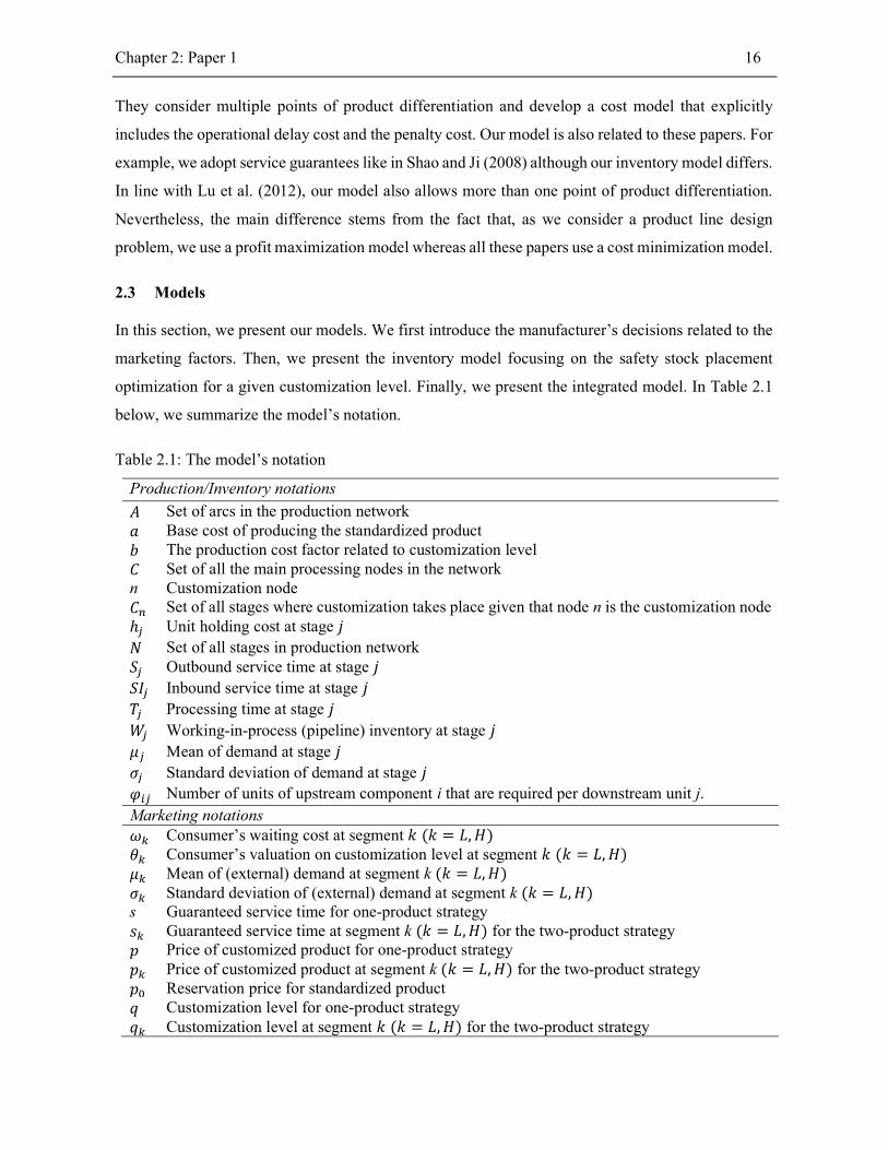
Table 2.1: The model’s notation
Production/Inventory notations
𝐴 Set of arcs in the production network 𝑎 Base cost of producing the standardized product 𝑏 The production cost factor related to customization level 𝐶 Set of all the main processing nodes in the network n Customization node 𝐶 Set of all stages where customization takes place given that node n is the customization node ℎ Unit holding cost at stage 𝑗 𝑁 Set of all stages in production network 𝑆 Outbound service time at stage 𝑗 𝑆𝐼 Inbound service time at stage 𝑗 𝑇 Processing time at stage 𝑗 𝑊 Working-in-process (pipeline) inventory at stage 𝑗 𝜇 Mean of demand at stage 𝑗 𝜎 Standard deviation of demand at stage 𝑗 𝜑 Number of units of upstream component i that are required per downstream unit j. Marketing notations 𝜔 Consumer’s waiting cost at segment 𝑘 (𝑘 = 𝐿, 𝐻) 𝜃 Consumer’s valuation on customization level at segment 𝑘 (𝑘 = 𝐿, 𝐻) 𝜇 Mean of (external) demand at segment k (𝑘 = 𝐿, 𝐻) 𝜎 Standard deviation of (external) demand at segment k (𝑘 = 𝐿, 𝐻) s Guaranteed service time for one-product strategy 𝑠 Guaranteed service time at segment k (𝑘 = 𝐿, 𝐻) for the two-product strategy 𝑝 Price of customized product for one-product strategy 𝑝 Price of customized product at segment k (𝑘 = 𝐿, 𝐻) for the two-product strategy 𝑝 Reservation price for standardized product 𝑞 Customization level for one-product strategy 𝑞 Customization level at segment 𝑘 (𝑘 = 𝐿, 𝐻) for the two-product strategy
Chapter 2: Paper 1 17
2.3.1 The Marketing Model
Here we present the marketing model that focuses on the product line design problem faced by the
manufacturer. The manufacturer produces and sells customized products in a market where
consumers are heterogeneous in their valuation of product quality. As stated earlier, the product
quality in our model is mainly represented by two quality attributes that are relevant in the
customization context: customization level and delivery lead time. The customization level is
determined by the extent to which consumers are involved in the production network. In the setting
we consider, the product delivery lead time is not independent of the customization level. Since the
final product is produced in a make-to-order or assemble-to-order fashion, there is a minimum lead
time incurred to make or to assemble the final products. This minimum delivery lead time is longer
when the customization level is higher.
The heterogeneity of consumer’s preferences is represented by two segments in the market denoted
by the high-valuation (H) segment and the low-valuation (L) segment. Consumers in each segment
are homogeneous in their valuation for attributes. Considering two segments in the market with
homogeneous valuation for attributes are common in the product line design literature (see e.g.
Moorthy and Png 1992, Netessine and Taylor (2007), and Kim et al. 2013). However, different from
the classical literature on product line design that assumes deterministic demand, in this paper, we
consider a different setting where the manufacturer faces demand uncertainty. Uncertain demand in
product line design is also considered in e.g. Chayet et al. (2011) and Wong and Lesmono (2013). In
our model, demand uncertainty is represented by the randomness in the size of each segment. Let 𝜇
and 𝜎 (𝑘 = 𝐻, 𝐿) denote the mean and standard deviation of demand in segment k, respectively. The
randomness in the size of each segment arising in our context can be due to the fact that the number
of potential consumers in each segment is uncertain at the time that decisions are made. We are aware
that the approach we use to model consumers’ heterogeneity and demand uncertainty may represent
one of the simplest approaches, but we believe it is sufficient for the purpose of our study.
In the context of mass customization, it is relevant to consider the scenario where a consumer who
highly values the customization level is less concerned about the product delivery lead time (Squire
et al. (2006); Wong and Lesmono (2013)). We assume that consumers who belong to the high-
valuation segment are more concerned with the product customization level than consumers in the
low-valuation segment. We denote 𝜃 (𝑘 = 𝐻, 𝐿) as the consumer’s valuation on customization level,
where 𝜃 > 𝜃 . Conversely, consumers who belong to the high-valuation segment are less concerned
with delivery lead time than consumers in the low-valuation segment. We define 𝜔 (𝑘 = 𝐻, 𝐿) as

Chapter 2: Paper 1 18
the cost per time unit incurred by every consumer in segment k waiting for the product to be delivered,
with 𝜔 < 𝜔 .
With the presence of two segments, the manufacturer aims to sell two different products, one for each
segment. We term this as the manufacturer’s two-product strategy. Depending on the production and
marketing related factors, it is also possible that the manufacturer adopts the one-product strategy in
which only one product is offered in the market. Under the two-product strategy, the manufacturer
offers a product with customization level, delivery lead time and price (𝑞 , 𝑠 , 𝑝 ) designed for the
high-valuation segment and product (𝑞 , 𝑠 , 𝑝 ) designed for the low-valuation segment. In the case
of single product strategy, one product (𝑞, 𝑠, 𝑝) is offered in the market.
For product (𝑞, 𝑠, 𝑝) offered in the market, a consumer from segment k has a utility function
𝑢 (𝑞, 𝑠, 𝑝) = 𝑝 +𝜃 𝑞 − 𝜔 𝑠 − 𝑝, (𝑘 = 𝐻, 𝐿). We define the constant 𝑝 as the reservation price for
a completely standardized product, and all consumers in the market are the potential buyers of the
customized product as long as their utility is nonnegative. Following Wong and Lesmono (2013), we
focus on the product line design problem where the customization level is the main attribute of
interest, and the completely standardized product, i.e., 𝑞 = 0, is therefore not included in our analysis.
2.3.2 The Production-Inventory Model
The value chain (production system) producing the customized products in our model can be
considered as a multi-stage network. Each stage in the network is a potential location for holding a
certain amount of safety stock to meet the uncertain demand of its consumers. In this paper, the
guaranteed-service model (Graves and Willems 2000) is adopted to determine the optimal amount
and placement of safety stocks in the network for a given customization level. The model allocates
and determines safety stocks across the supply chain to achieve a target service level at minimum
total safety stock costs. Although we acknowledge the possibility of applying other multi-stage
inventory models, we have chosen the guaranteed-service model for two reasons. Firstly, the model
is suitable for coping with complex multi-echelon inventory systems and it has been widely applied
in many real-world supply chains across different industries (Eruguz 2015). Secondly, the service
measure used in the model is the so-called guaranteed service time, which implies that the system
must guarantee (with 100% probability) that the service time promised to consumers will be met. We
believe that this service measure is appropriate for mass customization strategies given that there is
an increasing demand for manufacturing firms that offer customized products to be more responsive
and reliable at the same time (McCutcheon et al. 1994, Tu et al. 2001, and Rondeau et al. 2003).

Chapter 2: Paper 1 19
In the standard guaranteed-service model, all stages operate with a periodic-review base-stock policy.
External demands occur at the most downstream stages called the demand nodes in the network. Each
demand node 𝑗 faces the end-consumer’s demand that comes from a stationary process with mean 𝜇
and standard deviation 𝜎 . Depending on which segment is targeted, the demand node j may face
external demand with mean 𝜇 and standard deviation 𝜎 (𝑘 = 𝐻, 𝐿). Internal demands at internal
stages depend on the units ordered by its downstream nodes. The average demand rate at stage i is
represented by 𝜇 = ∑ 𝜇 𝜑( , )∈ , where 𝜑 is the number of units of the upstream component i that
are required per downstream unit j.
The production lead time at stage 𝑗 (𝑇 ) is deterministic and includes processing, waiting, and
transportation time to place the processed items for production at its downstream stages. Each stage
quotes a deterministic outbound service time (𝑆 ) to its consumers and guarantees that the demand
occurring at time 𝑡 is fulfilled at time 𝑆 + 𝑡, and each stage quotes the same service time to its
consumers. There is an inbound service time (𝑆𝐼 ) at stage 𝑗 that represents the time that should elapse
to get supplies from its direct upstream stages to start the production process. There is no stock-out
in the system and demand is bounded at each stage by an increasing concave function. The demand
bound function represents the amount of demand that should be satisfied by safety stocks over the
interval time (𝜏 = 𝑆𝐼 + 𝑇 − 𝑆 ) or net replenishment time, if it is positive. The demand bound is a
meaningful upper bound on demand, and the safety stock is set to cover all demand realizations that
fall within the upper bounds. Extra ordinary cases occur when demand surpasses the upper bounds,
and managers must use other approaches such as expediting, overtime, or subcontracting to meet the
excess demand. The expected inventory level at stage 𝑗 is defined by 𝐷 (𝜏) − (𝜏)𝜇 , where 𝐷 (𝜏)
represents the demand bound function in terms of net replenishment time.
In principle, the guaranteed service model does not require any assumptions about the distribution of
demand. In specifying the demand bounds, a manager indicates how demand variation should be
managed, i.e., what range is covered by safety stock and what range should be dealt with by other
actions or responses. For the purposes of positioning safety stock at demand node j, a manager might,
for example, specify the demand bound as 𝐷 (𝜏) = 𝜏𝜇 + 𝑧𝜎 √𝜏, which is derived based on the
assumption that the demand at demand node j is normally distributed with mean 𝜇 and standard
deviation 𝜎 . In this expression, z reflects the percentage of time that the safety stock covers the
demand variation. For each internal node 𝑖, demand bound can be determined from 𝐷 (𝜏) = 𝜏𝜇 +
∑ (φ𝒊𝒋(𝐷 (𝜏) − 𝜏𝜇 ))( , )∈ , where 𝑟 ≥ 1 is a given constant. Larger values of r correspond to
Chapter 2: Paper 1 20
more risk pooling. We refer the reader to Graves and Willems (2000) for the more detailed
explanation of the demand bound.
The expected inventory level represents the safety stock held at stage j, and depends on the net
replenishment time and the demand bound. In addition to safety stock, there is also pipeline inventory
at stage 𝑗 that depends on processing time 𝑇 , and the expected pipeline inventory level at stage j can
be written as 𝐸 𝑊 = 𝑇 𝜇 .
In the guaranteed-service model, the outbound and inbound service times are decision variables and
there are three main constraints in this optimization problem: (i) 𝑆𝐼 ≥ 𝑆 , to ensure that stage 𝑗 starts
its process after receiving all essential inputs from its upstream node 𝑖; (ii) 𝑆𝐼 + 𝑇 ≥ 𝑆 for all stages
𝑗, necessary for meeting the demand over the net replenishment time; and (iii) 𝑆 ≤ 𝑠 for all demand
nodes j, with 𝑠 representing the maximum service time promised to consumers.
Graves and Willems (2000 and 2003) develop a dynamic programming algorithm to determine the
optimal safety stock placement. Their algorithm is applied for a relabeled spanning-tree network. The
reader is referred to Graves and Willems (2000 and 2003) for a more detailed description of the
guaranteed-service model and the solution algorithm. In this paper, we need to slightly modify the
model because in our model, the service time promised to consumers depends on the customization
level. We explain the modified algorithm below.
The one-product strategy
Let 𝑁 denote the set of all the nodes in the production network, and 𝐴 denote the set of all the arcs in
the network. Let us also define 𝐶 as a subset of 𝑁 including all main processing nodes in the
production network where customization may take place. As customization at some nodes may be
impractical or even impossible, some nodes (production stages) in the network may not be
customization nodes. The production network is characterized by (𝑛; 𝑠) where 𝑛 ∈ 𝐶 is the
customization node and 𝑠 is the maximum service time promised to the end consumers.
Customization node n is defined as the most upstream stage in the production network where
customization takes place. In our model, we focus on the setting where all the main processing nodes
form a serial production line, but the whole production network is not restricted to a serial production
network. When the production network has customization node n, customization also takes place at
all the other nodes 𝑗 ∈ 𝐶 located downstream of node n. We define 𝐶 ⊆𝐶 as a set containing all the
stages in the production network where customization is carried out, including customization node n.
Chapter 2: Paper 1 21
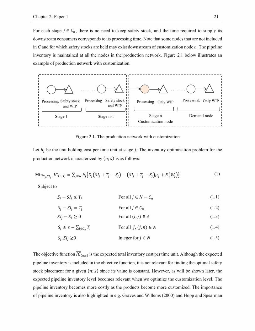
For each stage 𝑗 ∈ 𝐶 , there is no need to keep safety stock, and the time required to supply its
downstream consumers corresponds to its processing time. Note that some nodes that are not included
in C and for which safety stocks are held may exist downstream of customization node n. The pipeline
inventory is maintained at all the nodes in the production network. Figure 2.1 below illustrates an
example of production network with customization.
Figure 2.1. The production network with customization
Let ℎ be the unit holding cost per time unit at stage 𝑗. The inventory optimization problem for the
production network characterized by (𝑛; 𝑠) is as follows:
Min , 𝐼𝐶( ; ) = ∑ ℎ 𝐷 𝑆𝐼 + 𝑇 − 𝑆 − 𝑆𝐼 + 𝑇 − 𝑆 𝜇 + 𝐸 𝑊∈ (1)
Subject to
𝑆 − 𝑆𝐼 ≤ 𝑇 For all 𝑗 ∈ 𝑁 − 𝐶 (1.1)
𝑆 − 𝑆𝐼 = 𝑇 For all 𝑗 ∈ 𝐶 (1.2)
𝑆𝐼 − 𝑆 ≥ 0 For all (𝑖, 𝑗) ∈ 𝐴 (1.3)
𝑆 ≤ 𝑠 − ∑ 𝑇∈ For all 𝑗, (𝑗, 𝑛) ∈ 𝐴 (1.4)
𝑆 , 𝑆𝐼 ≥0 Integer for 𝑗 ∈ 𝑁 (1.5)
The objective function 𝐼𝐶( ; ) is the expected total inventory cost per time unit. Although the expected
pipeline inventory is included in the objective function, it is not relevant for finding the optimal safety
stock placement for a given (𝑛; 𝑠) since its value is constant. However, as will be shown later, the
expected pipeline inventory level becomes relevant when we optimize the customization level. The
pipeline inventory becomes more costly as the products become more customized. The importance
of pipeline inventory is also highlighted in e.g. Graves and Willems (2000) and Hopp and Spearman
Stage n Customization node
. . . . . . . . . . . . . .
Processing Safety stock and WIP
Processing Only WIP Processing Only WIP
Demand node Stage n-1
Processing Safety stock and WIP
Stage 1

Chapter 2: Paper 1 22
(2008). Constraint (1.1) indicates that the net replenishment times are nonnegative for all the nodes
not carrying out customization. Constraint (1.2) assures that the net replenishment times at the nodes
carrying out customization are zero so that no safety stocks are held, and this constraint represents
the first modification to the standard guaranteed-service model. Constraint (1.3) ensures that the
inbound service time at each stage is no less than the service times of its supplier stages. Constraint
(1.4), which is the second modification to the standard model, limits the service times at the nodes
directly supplying customization node n such that the guaranteed service time promised to consumers
is satisfied. The expected total inventory cost that corresponds to the optimal safety stock placement
is denoted by 𝐼𝐶∗( ; ). We use the dynamic programming algorithm of Graves and Willems (2000
and 2003) to determine the optimal safety stock placement in the production network. To apply the
algorithm for a production network with customization, some modifications are necessary. We
present a more detailed description of the dynamic programming algorithm in Appendix B.
The two-product strategy
In the two-product strategy, the manufacturer offers two customization levels, targeted at the low-
valuation segment and the high-valuation segment, respectively. We assume that there are two
parallel production networks, each with its customization level. We capture the scenario where,
despite the similarity of the production steps of the two products, the high quality product may require
more complex customizing operations than the low quality product, which can be achieved by
employing e.g. more skillful operators or more advanced machines. One could, alternatively, consider
a single production network that contains two customization levels. The main difference between the
two approaches stems from the omission of the pooling effect in the two parallel networks. We choose
to consider the first approach as the resulting model is simpler, and moreover, the resulting pooling
effect from two demand streams coming from the two segments seems to be limited.
The two independent parallel networks are characterized by (𝑛 ; 𝑠 ) and (𝑛 ; 𝑠 ) for the low and high
customization levels, respectively. For the first network producing the low-quality product, we define
𝐶 ⊆𝐶 as a set containing all the stages in the production network where customization is carried out,
including customization node 𝑛 . Similarly, we define 𝐶 ⊆𝐶 in the second network producing the
high-quality product. The total expected inventory cost that corresponds to the optimal safety stock
placements in the two parallel networks is denoted by 𝐼𝐶∗( ; ; ; ) = 𝐼𝐶∗
( ; ) + 𝐼𝐶∗( ; ).

Chapter 2: Paper 1 23
2.3.3 The Integrated Model
We now present the integrated model for the manufacturer’s product line design problem. In the
standard product line design problem with two market segments, the manufacturer must make
decisions on the optimal quality levels and prices for the high-quality and low-quality products taking
into account the potential cannibalization of the high-quality product by the low-quality product (see
Appendix A). In this paper, we extend the standard product line design problem in the following
respects. Firstly, the product quality in our paper is represented by two main attributes: customization
level and product delivery lead time, and the two attributes are interdependent of each other.
Secondly, we include the cost of holding safety stock and pipeline inventory in the manufacturer’s
profit function, and the cost of holding safety stock and pipeline inventory is influenced by the choice
of customization levels and product delivery lead times.
Given that there is a limited number of stages in the production network where customization can
take place, customization level is a discrete decision variable in our model. This also highlights
another difference of our model compared to the standard product line design model. The ratio of the
total customizing time to the total processing time is used as a proxy for the customization level. Let
us consider a production network with customization node n. Then, the customization level is defined
as 𝑞 =∑ ∈ (0 < 𝑞 ≤ 1) where 𝑇 is the sum of total processing times of the main production
stages. We assume that the higher the customization level, the higher the marginal production cost of
the customized product. This assumption is common in the product line design literature, and captures
the scenario where offering a higher quality product leads to a higher manufacturing complexity.
Following the literature (e.g. Syam and Kumar 2006; Wong and Lesmono 2013), we assume that the
unit production cost is an increasing and quadratic function in customization level and takes the form
of 𝑎 + 𝑏𝑞 , where 𝑎 represents the base cost of producing a standard product.
The Two-Product Strategy
Under the two-product strategy, the manufacturer offers two products with different customization
levels. The product with the low customization level is targeted at the low-valuation segment whereas
the product with the high customization level is targeted at the high-valuation segment. Like in the
standard product line design problem, the manufacturer must find a way to avoid the potential
cannibalization as consumers in the high-valuation segment may switch downward and purchase the
product with the low customization level whenever this product gives them a higher utility. This
potential cannibalization occurs because the manufacturer does not possess full information about

Chapter 2: Paper 1 24
individual consumers’ preferences (whether an individual belongs to the high or low valuation
segment), and it is difficult to deliver marketing programs to individual market segments without
‘leakage’ to other segments (Moorthy 1984; Netessine and Taylor 2007). In other words, it is almost
impossible for the manufacturer to directly address individual segments and achieve the perfect
market segmentation such that products do not cannibalize each other. Hence, the manufacturer must
design the product line such that consumers in each segment buy the product targeted at them.
The manufacturer’s product line design problem in the two-product strategy can be formulated as
follows:
Max , , , , ,
𝑍 ,
= 𝑝 − (𝑎 + 𝑏𝑞 ) 𝜇 + 𝑝 − (𝑎 + 𝑏𝑞 ) 𝜇 − 𝐼𝐶∗( ; ; ; )
(2)
Subject to
𝑝 + 𝜃 𝑞 − 𝜔 𝑠 − 𝑝 ≥ 0 (2.1)
𝑝 + 𝜃 𝑞 − 𝜔 𝑠 − 𝑝 ≥ 0 (2.2)
𝜃 𝑞 − 𝜔 𝑠 − 𝑝 ≥ 𝜃 𝑞 − 𝜔 𝑠 − 𝑝 (2.3)
𝜃 𝑞 − 𝜔 𝑠 − 𝑝 ≥ 𝜃 𝑞 − 𝜔 𝑠 − 𝑝 (2.4)
𝑠 ≥ ∑ 𝑇∈ (2.5)
𝑠 ≥ ∑ 𝑇∈ (2.6)
𝑠 , 𝑠 , 𝑞 , 𝑞 , 𝑝 , 𝑝 > 0 (2.7)
The objective function is the expected profit per time unit. Constraints (2.1) and (2.2) are the
participation constraints ensuring that consumers in each segment do not have negative utility by
buying the product offered to them. Constraints (2.3) and (2.4) are the self-selection constraints that
are needed because the manufacturer is unable to directly address individual segments as previously
explained. A consumer may find a product designed for another segment more attractive than the
product designed for her own segment, and so the firm faces a cannibalization problem. To prevent
this cannibalization, the two self-selection constraints must be included. If the manufacturer were
able to do perfect market segmentation, the self-selection constraints will not be required, and each
segment can be treated independently. Constraints (2.5) and (2.6) state that the guaranteed service
times that the manufacturer promise to consumers cannot be shorter than the sum of all the processing
times at the stages in the production network where customization is carried out, which depend on
the customization levels. Note that constraints (2.5) and (2.6) will actually be satisfied by constraint

Chapter 2: Paper 1 25
(1.4) in the inventory optimization problem. However, since 𝑠 and 𝑠 are decision variables in the
product line design problem while they are treated as given parameters in the inventory optimization
problem, we present the two constraints ((2.5) and (2.6)) above to explicitly show the feasible values
for 𝑠 and 𝑠 . For reference, we also present the standard product line design problem that exclude
the lead time and inventory in Appendix A.
The following propositions summarize how the manufacturer must set the prices and guaranteed
service times.
Proposition 1: In the two-product strategy, the manufacturer sets the prices for the two products
such that the participation constraint of the low-valuation segment (Constraint (2.1)) and the self-
selection constraint of the high-valuation segment (Constraint (2.4)) are binding. The prices are
equal to: 𝑝 = 𝑝 + 𝜃 𝑞 − 𝜔 𝑠 and 𝑝 = 𝜃 (𝑞 − 𝑞 ) − 𝜔 (𝑠 − 𝑠 ) + 𝑝 .
Proposition 2: In the two-product strategy, the guaranteed service times for the two products are
restricted by:
(i) ∑ 𝑇∈ ≤ 𝑠 < ;
(ii) ∑ 𝑇∈ ≤ 𝑠 <( ) ( )
Proofs of the two propositions are presented in Appendix C.
In Proposition 1, we show that the price setting method used in the standard product line design
problem is also valid for the product line design problem in which customization level and service
time are the two quality attributes. Given specific customization levels and service times, it is optimal
for the manufacturer to set the price of the low-quality product such that consumers in the low-
valuation segment are indifferent between buying the low-quality product and not buying. In order to
prevent cannibalization, the price of the high-quality product needs to be reduced such that consumers
in the high-valuation segment are indifferent between buying the high-quality product and buying the
low-quality product. The conditions in Proposition 2 show the ranges for the guaranteed service times
for the two products that lead to feasible solutions. These ranges help in reduce the search space in
the optimization algorithm.
The One-Product Strategy
Instead of selling two products with two different customization levels, the manufacturer may also be
interested in selling only one product. There are two possible options for the manufacturer to target

Chapter 2: Paper 1 26
the market under the one-product strategy. Firstly, the manufacturer may target both the high-
valuation and low-valuation segments. Secondly, the manufacturer may customize its product based
on the consumers’ preferences in the high-valuation segment. If he chooses the latter option, the
manufacturer extracts all surpluses of consumers in the high-valuation segment.
The problem under the one-product strategy targeting both segments can be formulated as follows:
Max , , 𝑍 , = 𝑝 − (𝑎 + 𝑏𝑞 ) (𝜇 + 𝜇 ) − 𝐼𝐶∗( ; ) (3)
Subject to
𝑝 + 𝜃 𝑞 − 𝜔 𝑠 − 𝑝 ≥ 0 (3.1)
𝑝 + 𝜃 𝑞 − 𝜔 𝑠 − 𝑝 ≥ 0 (3.2)
𝑠 ≥ ∑ 𝑇∈ (3.3)
𝑞, 𝑠, 𝑝 > 0 (3.4)
Notice that when both segments are targeted, the manufacturer sets the price such that the low-
valuation segment gets zero surpluses, i.e. by making (3.1) binding. This will make the participation
constraint for the high-valuation segment redundant.
The problem under the one-product strategy targeting only the high-valuation segment can be
formulated as follows:
Max , , 𝑍 = 𝑝 − (𝑎 + 𝑏𝑞 ) 𝜇 − 𝐼𝐶∗( ; ) (4)
Subject to
𝑝 + 𝜃 𝑞 − 𝜔 𝑠 − 𝑝 ≥ 0 (4.1)
𝑠 ≥ ∑ 𝑇∈ (4.2)
𝑞, 𝑠, 𝑝 > 0 (4.3)
Under the two-product strategy as well as under the one-product strategy the manufacturer’s product
line design problem is a nested optimization problem. Under the two-product strategy, the
manufacturer first decides on the customization levels 𝑞 and 𝑞 . Then, all the feasible values of 𝑠
and 𝑠 are determined. Next, for a given 𝑞 and 𝑞 (𝑞 < 𝑞 ) and 𝑠 and 𝑠 , we determine both the
optimal prices and safety stock placements. Next, we search over all the feasible values for 𝑠 and 𝑠
to find the optimal service times. And finally, we optimize the customization levels 𝑞 and 𝑞 . A
similar procedure is applied for the one-product strategy. In Appendix D we provide a more detailed
description of the optimization algorithm.
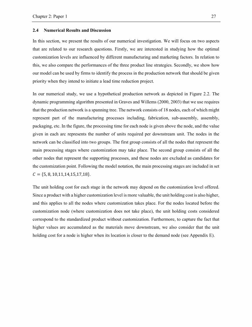
Chapter 2: Paper 1 27
2.4 Numerical Results and Discussion
In this section, we present the results of our numerical investigation. We will focus on two aspects
that are related to our research questions. Firstly, we are interested in studying how the optimal
customization levels are influenced by different manufacturing and marketing factors. In relation to
this, we also compare the performances of the three product line strategies. Secondly, we show how
our model can be used by firms to identify the process in the production network that should be given
priority when they intend to initiate a lead time reduction project.
In our numerical study, we use a hypothetical production network as depicted in Figure 2.2. The
dynamic programming algorithm presented in Graves and Willems (2000, 2003) that we use requires
that the production network is a spanning tree. The network consists of 18 nodes, each of which might
represent part of the manufacturing processes including, fabrication, sub-assembly, assembly,
packaging, etc. In the figure, the processing time for each node is given above the node, and the value
given in each arc represents the number of units required per downstream unit. The nodes in the
network can be classified into two groups. The first group consists of all the nodes that represent the
main processing stages where customization may take place. The second group consists of all the
other nodes that represent the supporting processes, and these nodes are excluded as candidates for
the customization point. Following the model notation, the main processing stages are included in set
𝐶 = {5, 8, 10,11,14,15,17,18}.
The unit holding cost for each stage in the network may depend on the customization level offered.
Since a product with a higher customization level is more valuable, the unit holding cost is also higher,
and this applies to all the nodes where customization takes place. For the nodes located before the
customization node (where customization does not take place), the unit holding costs considered
correspond to the standardized product without customization. Furthermore, to capture the fact that
higher values are accumulated as the materials move downstream, we also consider that the unit
holding cost for a node is higher when its location is closer to the demand node (see Appendix E).
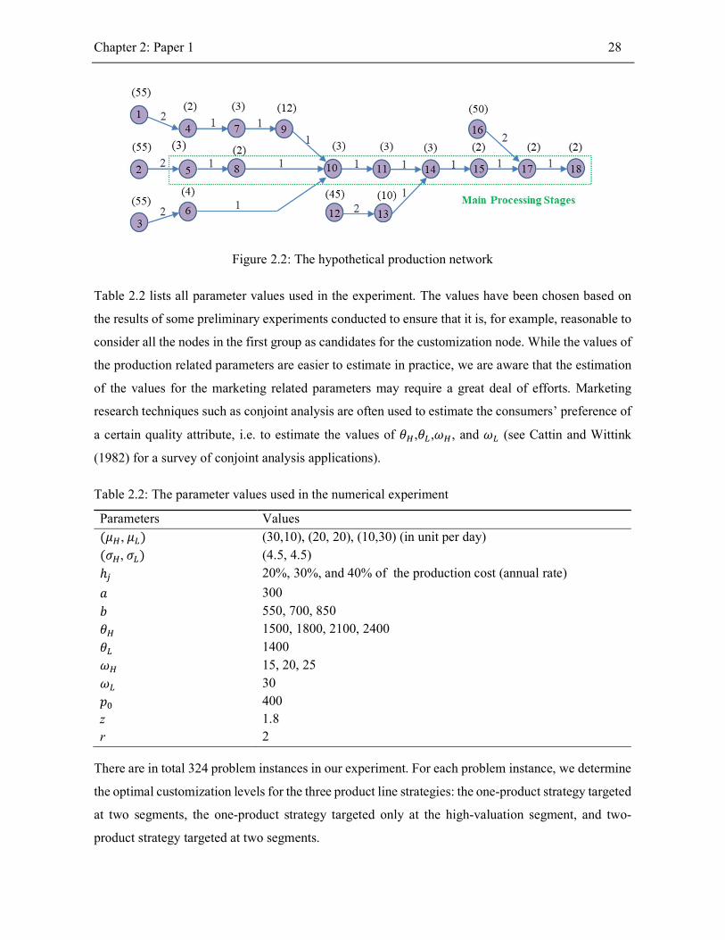
Chapter 2: Paper 1 28
Figure 2.2: The hypothetical production network
Table 2.2 lists all parameter values used in the experiment. The values have been chosen based on
the results of some preliminary experiments conducted to ensure that it is, for example, reasonable to
consider all the nodes in the first group as candidates for the customization node. While the values of
the production related parameters are easier to estimate in practice, we are aware that the estimation
of the values for the marketing related parameters may require a great deal of efforts. Marketing
research techniques such as conjoint analysis are often used to estimate the consumers’ preference of
a certain quality attribute, i.e. to estimate the values of 𝜃 ,𝜃 ,𝜔 , and 𝜔 (see Cattin and Wittink
(1982) for a survey of conjoint analysis applications).
Table 2.2: The parameter values used in the numerical experiment
Parameters Values (𝜇 , 𝜇 ) (30,10), (20, 20), (10,30) (in unit per day) (𝜎 , 𝜎 ) (4.5, 4.5)
ℎ 20%, 30%, and 40% of the production cost (annual rate)
𝑎 300
𝑏 550, 700, 850
𝜃 1500, 1800, 2100, 2400
𝜃 1400
𝜔 15, 20, 25
𝜔 30
𝑝 z r
400 1.8 2
There are in total 324 problem instances in our experiment. For each problem instance, we determine
the optimal customization levels for the three product line strategies: the one-product strategy targeted
at two segments, the one-product strategy targeted only at the high-valuation segment, and two-
product strategy targeted at two segments.
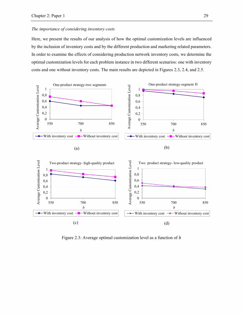
Chapter 2: Paper 1 29
The importance of considering inventory costs
Here, we present the results of our analysis of how the optimal customization levels are influenced
by the inclusion of inventory costs and by the different production and marketing related parameters.
In order to examine the effects of considering production network inventory costs, we determine the
optimal customization levels for each problem instance in two different scenarios: one with inventory
costs and one without inventory costs. The main results are depicted in Figures 2.3, 2.4, and 2.5.
(a)
(b)
(c) (d)
Figure 2.3: Average optimal customization level as a function of 𝑏
0
0,2
0,4
0,6
0,8
1
550 700 850
Ave
rage
Cus
tom
izat
ion
Lev
el
b
One-product strategy-two segments
With inventory cost Without inventory cost
0
0,2
0,4
0,6
0,8
1
550 700 850A
vera
ge C
usto
miz
atio
n L
evel
b
One-product strategy-segment H
With inventory cost Without inventory cost
0
0,2
0,4
0,6
0,8
1
550 700 850Ave
rage
Cus
tom
izat
ion
Lev
el
b
Two-product strategy- high-quality product
With inventory cost Without inventory cost
0
0,2
0,4
0,6
0,8
1
550 700 850Ave
rage
Cus
tom
izat
ion
Lev
el
b
Two product strategy- low-quality product
With inventory cost Without inventory cost

Chapter 2: Paper 1 30
(a)
(b)
(c) (d)
Figure 2.4: Average optimal customization level as a function of
0
0,2
0,4
0,6
0,8
1
1,071 1,29 1,5 1,714Ave
rage
Cus
tom
izat
ion
Lev
el One-product strategy-two segments
With inventory cost Without inventory cost
𝜃
𝜃
0
0,2
0,4
0,6
0,8
1
1,071 1,29 1,5 1,714
Ave
rage
Cus
tom
izat
ion
Lev
el One-product strategy-segment H
With inventory cost Without inventory cost
𝜃
𝜃
0
0,2
0,4
0,6
0,8
1
1,071 1,29 1,5 1,714
Ave
rage
Cus
tom
izat
ion
Lev
el
Two-product strategy- high-quality product
With inventory cost Without inventory cost
𝜃
𝜃
0
0,2
0,4
0,6
0,8
1
1,071 1,29 1,5 1,714
Ave
rage
Cus
tom
izat
ion
Lev
el Two product strategy-low-quality product
With inventory cost Without inventory cost
𝜃
𝜃
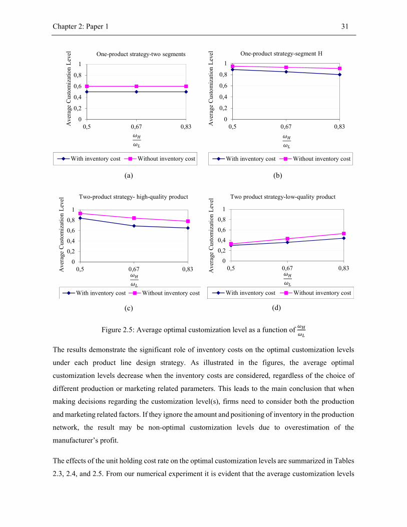
Chapter 2: Paper 1 31
(a) (b)
(c) (d)
Figure 2.5: Average optimal customization level as a function of
The results demonstrate the significant role of inventory costs on the optimal customization levels
under each product line design strategy. As illustrated in the figures, the average optimal
customization levels decrease when the inventory costs are considered, regardless of the choice of
different production or marketing related parameters. This leads to the main conclusion that when
making decisions regarding the customization level(s), firms need to consider both the production
and marketing related factors. If they ignore the amount and positioning of inventory in the production
network, the result may be non-optimal customization levels due to overestimation of the
manufacturer’s profit.
The effects of the unit holding cost rate on the optimal customization levels are summarized in Tables
2.3, 2.4, and 2.5. From our numerical experiment it is evident that the average customization levels
0
0,2
0,4
0,6
0,8
1
0,5 0,67 0,83Ave
rage
Cus
tom
izat
ion
Lev
el One-product strategy-two segments
With inventory cost Without inventory cost
𝜔
𝜔
0
0,2
0,4
0,6
0,8
1
0,5 0,67 0,83Ave
rage
Cus
tom
izat
ion
Lev
el One-product strategy-segment H
With inventory cost Without inventory cost
𝜔
𝜔
0
0,2
0,4
0,6
0,8
1
0,5 0,67 0,83Ave
rage
Cus
tom
izat
ion
Lev
el Two-product strategy- high-quality product
With inventory cost Without inventory cost
𝜔
𝜔
0
0,2
0,4
0,6
0,8
1
0,5 0,67 0,83Ave
rage
Cus
tom
izat
ion
Lev
el
Two product strategy-low-quality product
With inventory cost Without inventory cost
𝜔
𝜔
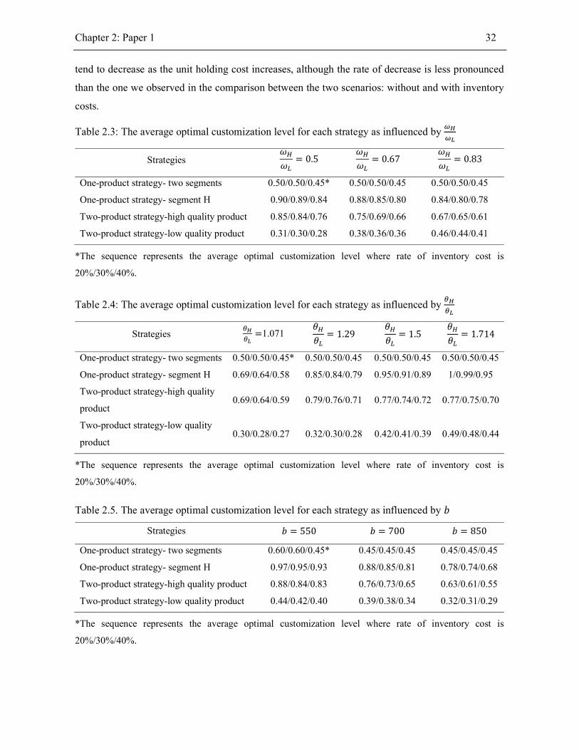
Chapter 2: Paper 1 32
tend to decrease as the unit holding cost increases, although the rate of decrease is less pronounced
than the one we observed in the comparison between the two scenarios: without and with inventory
costs.
Table 2.3: The average optimal customization level for each strategy as influenced by
Strategies 𝜔
𝜔= 0.5
𝜔
𝜔= 0.67
𝜔
𝜔= 0.83
One-product strategy- two segments 0.50/0.50/0.45* 0.50/0.50/0.45 0.50/0.50/0.45
One-product strategy- segment H 0.90/0.89/0.84 0.88/0.85/0.80 0.84/0.80/0.78
Two-product strategy-high quality product 0.85/0.84/0.76 0.75/0.69/0.66 0.67/0.65/0.61
Two-product strategy-low quality product 0.31/0.30/0.28 0.38/0.36/0.36 0.46/0.44/0.41
*The sequence represents the average optimal customization level where rate of inventory cost is
20%/30%/40%.
Table 2.4: The average optimal customization level for each strategy as influenced by
Strategies =1.071 𝜃
𝜃= 1.29
𝜃
𝜃= 1.5
𝜃
𝜃= 1.714
One-product strategy- two segments 0.50/0.50/0.45* 0.50/0.50/0.45 0.50/0.50/0.45 0.50/0.50/0.45
One-product strategy- segment H 0.69/0.64/0.58 0.85/0.84/0.79 0.95/0.91/0.89 1/0.99/0.95
Two-product strategy-high quality
product 0.69/0.64/0.59 0.79/0.76/0.71 0.77/0.74/0.72 0.77/0.75/0.70
Two-product strategy-low quality
product 0.30/0.28/0.27 0.32/0.30/0.28 0.42/0.41/0.39 0.49/0.48/0.44
*The sequence represents the average optimal customization level where rate of inventory cost is
20%/30%/40%.
Table 2.5. The average optimal customization level for each strategy as influenced by 𝑏
Strategies 𝑏 = 550 𝑏 = 700 𝑏 = 850
One-product strategy- two segments 0.60/0.60/0.45* 0.45/0.45/0.45 0.45/0.45/0.45
One-product strategy- segment H 0.97/0.95/0.93 0.88/0.85/0.81 0.78/0.74/0.68
Two-product strategy-high quality product 0.88/0.84/0.83 0.76/0.73/0.65 0.63/0.61/0.55
Two-product strategy-low quality product 0.44/0.42/0.40 0.39/0.38/0.34 0.32/0.31/0.29
*The sequence represents the average optimal customization level where rate of inventory cost is
20%/30%/40%.
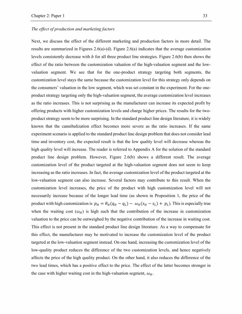
Chapter 2: Paper 1 33
The effect of production and marketing factors
Next, we discuss the effect of the different marketing and production factors in more detail. The
results are summarized in Figures 2.6(a)-(d). Figure 2.6(a) indicates that the average customization
levels consistently decrease with 𝑏 for all three product line strategies. Figure 2.6(b) then shows the
effect of the ratio between the customization valuation of the high-valuation segment and the low-
valuation segment. We see that for the one-product strategy targeting both segments, the
customization level stays the same because the customization level for this strategy only depends on
the consumers’ valuation in the low segment, which was set constant in the experiment. For the one-
product strategy targeting only the high-valuation segment, the average customization level increases
as the ratio increases. This is not surprising as the manufacturer can increase its expected profit by
offering products with higher customization levels and charge higher prices. The results for the two-
product strategy seem to be more surprising. In the standard product line design literature, it is widely
known that the cannibalization effect becomes more severe as the ratio increases. If the same
experiment scenario is applied to the standard product line design problem that does not consider lead
time and inventory cost, the expected result is that the low quality level will decrease whereas the
high quality level will increase. The reader is referred to Appendix A for the solution of the standard
product line design problem. However, Figure 2.6(b) shows a different result. The average
customization level of the product targeted at the high-valuation segment does not seem to keep
increasing as the ratio increases. In fact, the average customization level of the product targeted at the
low-valuation segment can also increase. Several factors may contribute to this result. When the
customization level increases, the price of the product with high customization level will not
necessarily increase because of the longer lead time (as shown in Proposition 1, the price of the
product with high customization is 𝑝 = 𝜃 (𝑞 − 𝑞 ) − 𝜔 (𝑠 − 𝑠 ) + 𝑝 ). This is especially true
when the waiting cost (𝜔 ) is high such that the contribution of the increase in customization
valuation to the price can be outweighed by the negative contribution of the increase in waiting cost.
This effect is not present in the standard product line design literature. As a way to compensate for
this effect, the manufacturer may be motivated to increase the customization level of the product
targeted at the low-valuation segment instead. On one hand, increasing the customization level of the
low-quality product reduces the difference of the two customization levels, and hence negatively
affects the price of the high quality product. On the other hand, it also reduces the difference of the
two lead times, which has a positive effect to the price. The effect of the latter becomes stronger in
the case with higher waiting cost in the high-valuation segment, 𝜔 .

Chapter 2: Paper 1 34
In Figure 2.6(c), we show the effect of the ratio between the waiting cost of the high-valuation
segment and the low-valuation segment. The results can be explained by the same arguments as were
used in relation to Figure 2.6(b). For the two-product strategy, in particular, increasing the ratio would
result in smaller differences between the two customization levels. We also study the effect of the
ratio of mean demand between the high-valuation segment and the low-valuation segment on the
customization levels, as depicted in Figure 2.6(d). As expected, the average customization levels are
not affected in the one-product strategies. Changing the relative sizes of the two segments in the one-
product strategies will affect the profit, but not the customization levels. For the two-product strategy,
we see a different result as the low customization level may also decrease.
(a) (b)
(c) (d)
Figure 2.6: Average optimal customization level as a function of 𝑏, , , and
0
0,2
0,4
0,6
0,8
1
550 700 850
Ave
rage
Cus
tom
izat
ion
Lev
el
b
0
0,2
0,4
0,6
0,8
1
1,071 1,29 1,5 1,714Ave
rage
Cus
tom
izat
ion
Lev
el
0
0,2
0,4
0,6
0,8
1
0,5 0,6 0,7 0,8Ave
rage
Cus
tom
izat
ion
Lev
el
00,10,20,30,40,50,60,70,80,9
0,25 0,5 0,75
Ave
rage
Cus
tom
izat
ion
Lev
el
𝜃
𝜃
𝜔
𝜔
𝜇
𝜇 + 𝜇
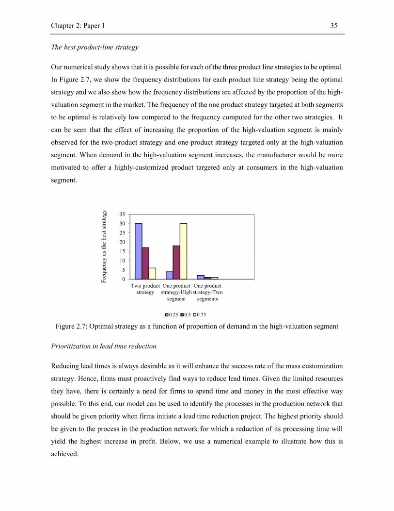
Chapter 2: Paper 1 35
The best product-line strategy
Our numerical study shows that it is possible for each of the three product line strategies to be optimal.
In Figure 2.7, we show the frequency distributions for each product line strategy being the optimal
strategy and we also show how the frequency distributions are affected by the proportion of the high-
valuation segment in the market. The frequency of the one product strategy targeted at both segments
to be optimal is relatively low compared to the frequency computed for the other two strategies. It
can be seen that the effect of increasing the proportion of the high-valuation segment is mainly
observed for the two-product strategy and one-product strategy targeted only at the high-valuation
segment. When demand in the high-valuation segment increases, the manufacturer would be more
motivated to offer a highly-customized product targeted only at consumers in the high-valuation
segment.
Figure 2.7: Optimal strategy as a function of proportion of demand in the high-valuation segment
Prioritization in lead time reduction
Reducing lead times is always desirable as it will enhance the success rate of the mass customization
strategy. Hence, firms must proactively find ways to reduce lead times. Given the limited resources
they have, there is certainly a need for firms to spend time and money in the most effective way
possible. To this end, our model can be used to identify the processes in the production network that
should be given priority when firms initiate a lead time reduction project. The highest priority should
be given to the process in the production network for which a reduction of its processing time will
yield the highest increase in profit. Below, we use a numerical example to illustrate how this is
achieved.
0
5
10
15
20
25
30
35
Two productstrategy
One productstrategy-High
segment
One productstrategy-Two
segments
Freq
uenc
y as
the
best
str
ateg
y
0.25 0.5 0.75

Chapter 2: Paper 1 36
Consider a setting with the following parameter values: 𝜇 = 20; 𝜇 = 20; 𝜃 = 1500; unit holding
cost rate = 30%; 𝜔 = 15; 𝜔 = 30; 𝑏 = 700. Under the one-product strategy (targeted at the high-
valuation segment), the optimal customization level is at node 10. Under the two-product strategy,
the optimal customization levels are at nodes 10 and 15. In Figure 2.8 below, we plot the profit
improvements for different nodes obtained when the manufacturer is able to shorten the processing
time of the corresponding node by one day. In this example, as shown in the figure, the manufacturer
should give priority at node 8 to maximize the benefits of the lead time reduction project. As also
shown in the figure, reducing the lead times of the nodes located upstream of the customization node
appears to yield higher profit improvements. A plausible explanation is that when lead times for those
nodes are reduced, the manufacturer may benefit both from offering a shorter delivery time to
consumers and from reducing the total inventory costs. This explanation can be directly related to
Constraint (1.4) in the inventory optimization problem. In the case where the constraint is binding,
we can clearly see the direct effect of reducing the lead time at node 8 located upstream the
customization node (node 10). Reducing the processing time at node 8 will result in a lower safety
stock level carried out by this node, and will allow the manufacturer to reduce the service time to the
customers. A similar, although smaller, effect can be observed in Figure 2.8 for the two-product
strategy at nodes 14 and 15, respectively. As for the nodes located downstream from the
customization node, the benefit is more limited since no safety stocks are held there.
Figure 2.8: Manufacturer’s profit improvement under budget constraints
2.5 Conclusions
In this paper, we examine how manufacturing firms can make optimal decisions regarding
customization levels in a vertically differentiated market. We extend the standard product line design
0,00E+00
3,00E+04
6,00E+04
9,00E+04
1,20E+05
1,50E+05
1,80E+05
2,10E+05
5 8 10 11 14 15 17 18
Δ A
nnua
l P
rofi
t
Customization Node
One product strategy-segment H Two product strategy

Chapter 2: Paper 1 37
problem by considering two interdependent product attributes, namely customization level and
product delivery lead time. In addition, we incorporate the importance of safety stock and pipeline
inventory costs in determining the optimal customization levels. We integrate the guaranteed service
model with the product line design model to determine the optimal customization levels, product
delivery lead times, prices, and safety stock placements in the production system.
Our numerical investigation reveals several interesting and important insights. We show that the cost
of holding safety stock and pipeline inventory influences the optimal choice of customization levels.
The optimal customization levels tend to be lower when the inventory costs are considered compared
to the case where the inventory costs are ignored. This finding highlights the importance of
considering operational factors other than the production cost when making product line design
decisions. Ignoring the amount and positioning of inventory in the production network may lead to
non-optimal customization levels due to the profit overestimation. Another interesting observation is
that the effect of consumer valuation difference between the two segments on the optimal
customization levels is affected by whether or not the lead time and inventory cost are included. In
the standard product line design problem in which the lead time and inventory cost are ignored, when
the quality valuation ratio of the high segment to the low segment increases, the low quality product
will be more distorted downward while the high quality level will increase. However, when the lead
time and inventory cost are included, the observation is different. Our numerical results show that the
high quality level does not always keep increasing, and the low quality level may also increase. Our
exploration on the two-product and one-product strategies shows that in most cases, the primary
choice for the manufacturer is either to offer only one customization level for the high-valuation
segment or to offer two customization levels, one for each segment. Offering one product (one
customization level) to the high-valuation segment will be attractive when the size of the high-
valuation segment is relatively larger than the size of the low-valuation segment.
We have also demonstrated how our model can be used for identifying the process in the production
system that should be given priority when firms intend to initiate a lead time reduction project. More
specifically, our model is able to identify the process for which a lead time reduction yields the highest
increase in profit. Not all processes should be given the same priority and we have proven that
marketing factors and inventory costs both have an impact on profits.
We acknowledge some limitations of this paper and would like to suggest several topics for future
research. First, our model assumes that consumers’ preferences are homogeneous within each market
segment such that each segment is represented by a single quality valuation value. The extent to which

Chapter 2: Paper 1 38
the optimal customization levels and service times in our results will change when consumers are also
heterogeneous within each segment is still unclear. Hence, a future research avenue could be to
consider a market where consumers’ preferences are continuously distributed such that market
segmentation is also part of the manufacturer’s decisions. In relation to this, one could also consider
a different approach in defining demand uncertainty. For example, one could model demand
uncertainty that is due to the probabilistic nature of the minimum and/or maximum values of the
consumers’ preferences.
Second, our model implicitly assumes that the manufacturer sells its customized products directly to
end consumers, i.e., no explicit consideration is given to the distribution channel. It would be
interesting to extend our study by considering the effect of channel structure. One interesting research
question could be, for example, what the manufacturer’s optimal customization strategy would be if
the manufacturer uses a dual channel by selling the products through a retailer as well as through an
online channel.

Chapter 2: Paper 1 39
Appendix A
Here, we introduce the standard product line design problem where a manufacturer sells two products
targeted to two segments. The manufacturer sells the low quality product with quality level 𝑞 and
price 𝑝 targeted at the low-valuation segment, and the high-quality product with quality level 𝑞 and
price 𝑝 targeted at the high-valuation segment. The size of the low-valuation and the high-valuation
segments are 𝜇 and 𝜇 , respectively. The manufacturer’s problem is as follows:
𝑚𝑎𝑥 , , , (𝑝 − 𝑏𝑞 )𝜇 + (𝑝 − 𝑏𝑞 ) 𝜇 (A)
Subject to
𝜃 𝑞 − 𝑝 ≥ 0 (A-1)
𝜃 𝑞 − 𝑝 ≥ 0 (A-2)
𝜃 𝑞 − 𝑝 ≥ 𝜃 𝑞 − 𝑝 (A-3)
𝜃 𝑞 − 𝑝 ≥ 𝜃 𝑞 − 𝑝 (A-4)
Constraints (A-1) and (A-2) denote the participation constraints for the two segments, and constraints
(A-3) and (A-4) are the self-selection constraints for the two segments.
It is optimal for the manufacturer to set the price for the low-quality product by making constraint
(A-1) binding, i.e. 𝑝 = 𝜃 𝑞 , and to set the price for the high-quality product by making constraint
(A-4) binding i.e. 𝑝 = 𝑝 + 𝜃 (𝑞 − 𝑞 ). The optimal quality levels of the two products are 𝑞∗ =
and 𝑞∗ = (1 − 𝑅), where 𝑅 = − 1 , is a measure of potential cannibalization and 𝑅 <
1 (Moorthy and Png 1992).
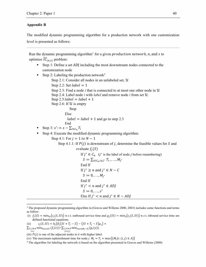
Chapter 2: Paper 1 40
Appendix B
The modified dynamic programming algorithm for a production network with one customization
level is presented as follows:
Run the dynamic programming algorithm1 for a given 𝑝𝑟𝑜𝑑𝑢𝑐𝑡𝑖𝑜𝑛 𝑛𝑒𝑡𝑤𝑜𝑟𝑘, 𝑛, and 𝑠 to
optimize 𝐼𝐶( ; ) problem:
Step 1: Define a set ADJ including the most downstream nodes connected to the customization node
Step 2: Labeling the production network2 Step 2.1: Consider all nodes in an unlabeled set, 𝒰 Step 2.2: Set 𝑙𝑎𝑏𝑒𝑙 = 1 Step 2.3: Find a node i that is connected to at most one other node in 𝒰 Step 2.4: Label node i with label and remove node i from set 𝒰. Step 2.5:𝑙𝑎𝑏𝑒𝑙 = 𝑙𝑎𝑏𝑒𝑙 + 1 Step 2.6: If 𝒰 is empty
Stop Else
𝑙𝑎𝑏𝑒𝑙 = 𝑙𝑎𝑏𝑒𝑙 + 1 and go to step 2.3 End
Step 3: 𝑠 : = 𝑠 − ∑ 𝑇∈
Step 4: Execute the modified dynamic programming algorithm: Step 4.1: For 𝑗 = 1 𝑡𝑜 𝑁 − 1
Step 4.1.1: If 𝑃(𝑗) is downstream of 𝑗, determine the feasible values for 𝑆 and evaluate 𝑓 (𝑆)
If 𝑗∗ ∈ 𝐶 (𝑗∗ is the label of node 𝑗 before renumbering) 𝑆 ≔ ∑ 𝑇∈ , ∗ , . . . , 𝑀 ∗
End If If 𝑗∗ ≥ 𝑛 and 𝑗∗ ∈ 𝑁 − 𝐶
𝑆 ≔ 0, . . . , 𝑀 ∗
End If If 𝑗∗ < 𝑛 and 𝑗∗ ∈ 𝐴𝐷𝐽
𝑆 ≔ 0, . . . , 𝑠 Else If 𝑗∗ < 𝑛 and 𝑗∗ ∈ 𝑁 − 𝐴𝐷𝐽
1 The proposed dynamic programming algorithm in (Graves and Willems 2000, 2003) includes some functions and terms as follow: (i) 𝑓 (𝑆) = 𝑚𝑖𝑛 𝑐 (𝑆, 𝑆𝐼) w.r.t. outbound service time and 𝑔 (𝑆𝐼) = 𝑚𝑖𝑛 𝑐 (𝑆, 𝑆𝐼) w.r.t. inbound service time are
defined functional equations. (ii) 𝑐 (𝑆, 𝑆𝐼) = ℎ 𝐷 𝑆𝐼 + 𝑇 − 𝑆 − 𝑆𝐼 + 𝑇 − 𝑆 𝜇 +
∑ 𝑚𝑖𝑛( , )∈ (𝑓 (𝑥))+∑ min (𝑔 (𝑦))( , )∈
( )
.
(iii) 𝑃(𝑗) is one of the adjacent nodes to k with higher label. (iv) The maximum replenishment time for node j: 𝑀 = 𝑇 + 𝑚𝑎𝑥 {𝑀 |𝑖: (𝑖, 𝑗) ∈ 𝐴} 2 The algorithm for labeling the network is based on the algorithm presented in Graves and Willems (2000)
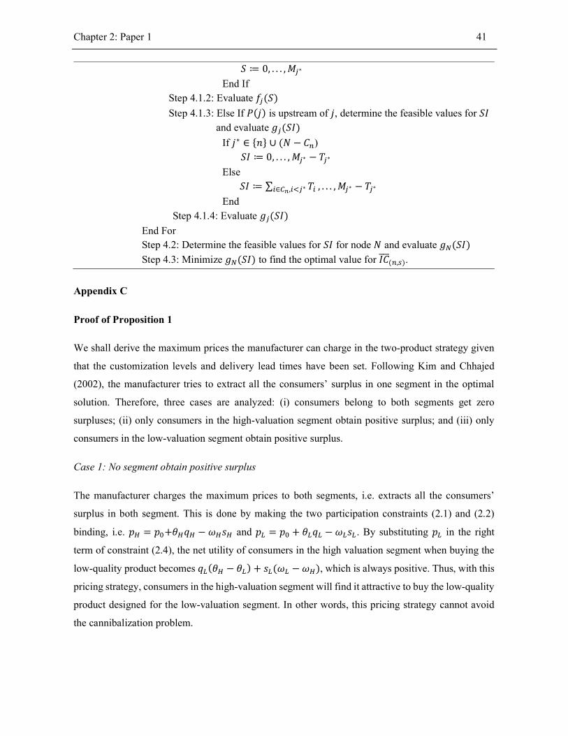
Chapter 2: Paper 1 41
𝑆 ≔ 0, . . . , 𝑀 ∗
End If Step 4.1.2: Evaluate 𝑓 (𝑆)
Step 4.1.3: Else If 𝑃(𝑗) is upstream of 𝑗, determine the feasible values for 𝑆𝐼 and evaluate 𝑔 (𝑆𝐼)
If 𝑗∗ ∈ {𝑛} ∪ (𝑁 − 𝐶 ) 𝑆𝐼 ≔ 0, . . . , 𝑀 ∗ − 𝑇 ∗
Else 𝑆𝐼 ≔ ∑ 𝑇∈ , ∗ , . . . , 𝑀 ∗ − 𝑇 ∗
End Step 4.1.4: Evaluate 𝑔 (𝑆𝐼)
End For Step 4.2: Determine the feasible values for 𝑆𝐼 for node 𝑁 and evaluate 𝑔 (𝑆𝐼)
Step 4.3: Minimize 𝑔 (𝑆𝐼) to find the optimal value for 𝐼𝐶( , ).
Appendix C
Proof of Proposition 1
We shall derive the maximum prices the manufacturer can charge in the two-product strategy given
that the customization levels and delivery lead times have been set. Following Kim and Chhajed
(2002), the manufacturer tries to extract all the consumers’ surplus in one segment in the optimal
solution. Therefore, three cases are analyzed: (i) consumers belong to both segments get zero
surpluses; (ii) only consumers in the high-valuation segment obtain positive surplus; and (iii) only
consumers in the low-valuation segment obtain positive surplus.
Case 1: No segment obtain positive surplus
The manufacturer charges the maximum prices to both segments, i.e. extracts all the consumers’
surplus in both segment. This is done by making the two participation constraints (2.1) and (2.2)
binding, i.e. 𝑝 = 𝑝 +𝜃 𝑞 − 𝜔 𝑠 and 𝑝 = 𝑝 + 𝜃 𝑞 − 𝜔 𝑠 . By substituting 𝑝 in the right
term of constraint (2.4), the net utility of consumers in the high valuation segment when buying the
low-quality product becomes 𝑞 (𝜃 − 𝜃 ) + 𝑠 (𝜔 − 𝜔 ), which is always positive. Thus, with this
pricing strategy, consumers in the high-valuation segment will find it attractive to buy the low-quality
product designed for the low-valuation segment. In other words, this pricing strategy cannot avoid
the cannibalization problem.

Chapter 2: Paper 1 42
Case 2: Only the low-valuation segment obtains positive surplus
In this case, the manufacturer extracts all the consumers’ surplus in the high-valuation segment by
making the participation constraint of the high-valuation segment (constraint (2.2)) binding. As a
result, the participation constraint (2.1) and self-selection constraint (2.3) provide two different upper
bounds for 𝑝 : 𝑝 ≤ 𝑝 + 𝜃 𝑞 − 𝜔 𝑠 and 𝑝 ≤ 𝑝 + 𝜃 𝑞 − 𝜔 𝑠 + 𝑞 (𝜃 − 𝜃 ) + 𝑠 (𝜔 +
𝜔 ). The first upper bound for 𝑝 is tighter than the second upper bound. However, if we set 𝑝 to
equal the first upper bound then the manufacturer faces the cannibalization problem.
Case 3: Only the high-valuation segment obtains positive surplus
In this case, the manufacturer only charges the maximum price to the low-valuation segment: 𝑝 =
𝑝 + 𝜃 𝑞 − 𝜔 𝑠 . Constraints (2.2) and (2.4) provide two different upper bounds for 𝑝 : 𝑝 ≤
𝑝 + 𝜃 𝑞 − 𝜔 𝑠 and 𝑝 ≤ 𝜃 (𝑞 − 𝑞 ) − 𝜔 (𝑠 − 𝑠 ) + 𝑝 . By substituting 𝑝 , the second
upper bound can be written as 𝜃 𝑞 − 𝜔 𝑠 − 𝑞 (𝜃 − 𝜃 ) − 𝑠 (𝜔 − 𝜔 ), which is tighter than
the first upper bound. Therefore, 𝑝 can be set as 𝜃 (𝑞 − 𝑞 ) − 𝜔 (𝑠 − 𝑠 ) + 𝑝 , and this is
sufficient to avoid the cannibalization problem. This case provides the pricing solutions to the
manufacturer’s product line design problem with customization.
Proof of Proposition 2
Since the manufacturer set 𝑝 = 𝑝 + 𝜃 𝑞 − 𝜔 𝑠 and 𝑝 = 𝜃 (𝑞 − 𝑞 ) − 𝜔 (𝑠 − 𝑠 ) + 𝑝 , 𝑠
should be less than and 𝑠 should be less than ( ) ( )
, to ensure that
the prices are positive. Additionally, both 𝑠 and 𝑠 are bounded from below by the total processing
time required to customize the products. Thus, we need the following condition: for segment k (𝑘 =
𝐿, 𝐻), 𝑠 ≥ ∑ 𝑇∈ .

Chapter 2: Paper 1 43
Appendix D
The optimization algorithm for two-product strategy is as follows:
Find all possible customization nodes (𝑛 , 𝑛 ) so that (𝑞 > 𝑞 ) and store in a set. 𝑐𝑜𝑢𝑛𝑡𝑒𝑟 ≔ 1 While 𝑐𝑜𝑢𝑛𝑡𝑒𝑟 ≤ (number of members of the set containing all (𝑛 , 𝑛 ) )
Create 𝐶 ⊆ 𝑁, and 𝐶 ⊆ 𝑁 for a given (𝑛 , 𝑛 )
Find the values of customization levels: 𝑞 =∑ ∈
and 𝑞 =∑ ∈
Evaluate the production costs for two product lines: (𝑎 + 𝑏𝑞 ) and (𝑎 + 𝑏𝑞 )
Determine the maximum and minimum values of the promised lead time at segment L:
𝑠 =∑ 𝑇∈ and 𝑠 =
Initialize 𝑙 ≔ 1 (The iteration counter) For 𝑠 =𝑠 to 𝑠
Set 𝑝 = 𝑝 + 𝜃 𝑞 − 𝜔 𝑠 Run the dynamic programming algorithm for given production network 𝑛 , and 𝑠 to
optimize 𝐼𝐶( ; ) Find the manufacturer’s profit in segment L for given 𝑞 , 𝑠 :
𝑍 , = (𝑝 − (𝑎 + 𝑏𝑞 ))𝜇 − 𝐼𝐶( ; )∗
Determine the maximum and minimum values of the promised lead time at segment H with a given 𝑠 and 𝑝 .
𝑠 = ∑ 𝑇∈ , 𝑠 =( ) ( )
𝑙 ≔ 1 (The iteration counter) For 𝑠 =𝑠 to 𝑠
Set 𝑝 = 𝜃 (𝑞 − 𝑞 ) − 𝜔 (𝑠 − 𝑠 ) + 𝑝 Run the dynamic programming algorithm to optimize 𝐼𝐶( ; ) problem. Find the maximum manufacturer’s profit at segment H for given 𝑞 , 𝑠 , 𝑞 , 𝑠
𝑍 , = (𝑝 − (𝑎 + 𝑏𝑞 ))𝜇 − 𝐼𝐶( ; )∗
𝑙 ≔ 𝑙 + 1 End For 𝑍 ≔ Find the maximum value of profit at segment H for a given 𝑞 𝑍 , , ≔ 𝑍 , + 𝑍 𝑙 ≔ 𝑙 + 1
End For 𝑍 , , ≔ Find the maximum value of profit at both segments for a given 𝑞 and 𝑞 𝑐𝑜𝑢𝑛𝑡𝑒𝑟 ≔ 𝑐𝑜𝑢𝑛𝑡𝑒𝑟 + 1 End While 𝑍 ,
∗ :=Find the maximum of 𝑍 , , (𝑞∗ , 𝑞∗) ≔The customization levels for the nodes in product lines where the total maximum profit occurs.
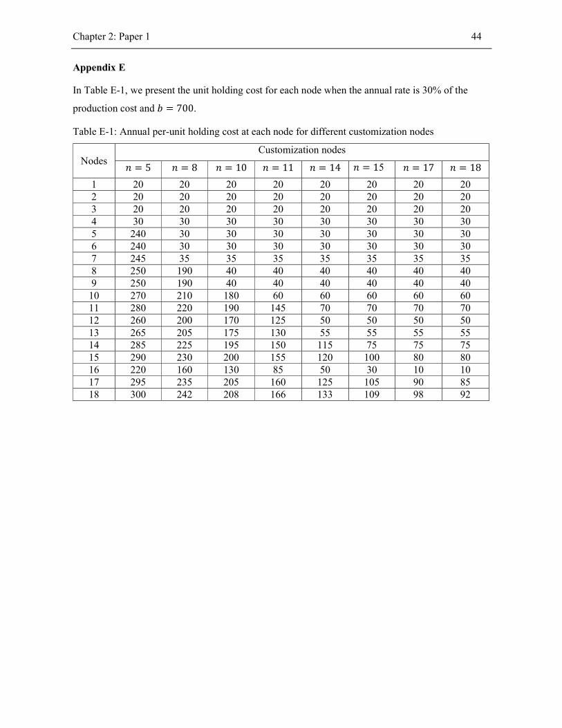
Chapter 2: Paper 1 44
Appendix E
In Table E-1, we present the unit holding cost for each node when the annual rate is 30% of the
production cost and 𝑏 = 700.
Table E-1: Annual per-unit holding cost at each node for different customization nodes
Nodes Customization nodes
𝑛 = 5 𝑛 = 8 𝑛 = 10 𝑛 = 11 𝑛 = 14 𝑛 = 15 𝑛 = 17 𝑛 = 18
1 20 20 20 20 20 20 20 20 2 20 20 20 20 20 20 20 20 3 20 20 20 20 20 20 20 20 4 30 30 30 30 30 30 30 30 5 240 30 30 30 30 30 30 30 6 240 30 30 30 30 30 30 30 7 245 35 35 35 35 35 35 35 8 250 190 40 40 40 40 40 40 9 250 190 40 40 40 40 40 40
10 270 210 180 60 60 60 60 60 11 280 220 190 145 70 70 70 70 12 260 200 170 125 50 50 50 50 13 265 205 175 130 55 55 55 55 14 285 225 195 150 115 75 75 75 15 290 230 200 155 120 100 80 80 16 220 160 130 85 50 30 10 10 17 295 235 205 160 125 105 90 85 18 300 242 208 166 133 109 98 92

Chapter 3
3 Paper 2: Product line design with vertical and horizontal
consumer heterogeneity: the effect of distribution channel
structure on the optimal quality and customization levels
History: This paper has been presented at: OR59 Annual Conference -Conference of OR Society,
September 2017, Loughborough, United Kingdom. The paper is submitted to IEEE
Transactions on Engineering Management.

Chapter 3: Paper 2 44
Product line design with vertical and horizontal consumer heterogeneity: the effect of
distribution channel structure on the optimal quality and customization levels
Parisa Bagheri Tookanlou and Hartanto Wong
Department of Economics and Business Economics
School of Business and Social Sciences, Aarhus University
Fuglesangs Allé 4, 8210 Aarhus, Denmark
Abstract
In this paper, we investigate a product line design problem for a manufacturer selling the products in
a market where consumers are heterogeneous in two aspects. First, consumers are vertically
heterogeneous with respect to their valuation of quality. Consumers in the high-valuation segment
value quality more than consumers in the low-valuation segment. Second, consumers are horizontally
heterogeneous with respect to their preference on the aesthetic component of the product. We
compare a number of product line strategies that can be chosen by the manufacturer. In particular, we
are interested in examining the effect of offering a customized product in the product line. Using the
single-product strategy as the baseline strategy, we examine when it is best for the manufacturer to
consider the product line extension in a vertical direction or in a horizontal direction. We also consider
the quality-based segmentation as the baseline strategy, and examine whether offering the customized
product will enhance the profitability, and whether the customized product should be offered with
low or high quality. Furthermore, we study how the choice of distribution channel in the supply chain
affects the optimal product line decision. First, we consider a centralized channel where the
manufacturer sells all the products directly to the end consumers. Second, we consider a dual channel
where the manufacturer sells the standard product through a retailer while the customized product is
sold through a direct (online) channel.
Keywords: product line design; customization; distribution channel; horizontal differentiation;
vertical differentiation.
Chapter 3: Paper 2 45
3.1 Introduction
It can be argued that one of the most important decisions within product line design is the length of
product line, which is defined as the number of product offerings in a product line. Offering a larger
product variety would allow firms to increase both demand and market share (Kotler 2000). Thus,
product line extension has always been an integral part of marketing managers’ strategies. Motivated
by the fact that consumers are heterogeneous in their valuation of product quality, firms often
differentiate their product lines vertically by offering a product line comprised of multiple products
with different quality levels. Quality-based segmentation is commonly practiced in marketing by
offering a product line comprised of multiple products with different quality levels, serving a market
comprised of heterogeneous segments. Consider, for example, garment products such as suits, pants,
sweaters, etc., that are offered in different materials based on which the prices are differentiated.
Apparel companies such as Land’s End and Levi Strauss offer a variety of jeans that are differentiated
by the quality of the fabric (organic or conventional; pure cotton or a synthetic mix), the treatment of
denim (washed or unwashed), and the quality of construction (high stitch count or low stitch count).
Alternatively, firms may choose to differentiate their product lines horizontally by offering products
that have the same quality level but different characteristics or aesthetic attributes such as taste, color
or flavor. Garment manufacturing firms usually offer products that are differentiated by color and
size but sold at the same price. In relation to the horizontal product line differentiation, we witness an
increasing number of firms offering the customized product to their consumers today. The two
examples above (Land’s End and Levi Strauss) offers customized shirts, jeans, and jackets by
allowing consumers to choose their preferred styles, colors, inseam, etc. There are abundant examples
of firms offering customized t-shirts where consumers have the possibility to choose the most
preferred color and /or pictures (Spreadshirt and Rush order Tees companies). Sisal Rugs Direct
(http://www.sisalrugsdirect.com) allows consumers to choose the shape, colors and pattern of their
rugs.
The motivation for firms to offer such customized products is that they may increase both their
consumer base and revenues. However, this motivation does not come without costs as some
investments are necessary to enhance flexibility in the production facility such that customization can
be accommodated. An interesting but less understood question related to the firms’ product line
extension decision is which extension direction is more desirable: vertical product line extension, or
horizontal product line extension with customization. Our literature review suggests that none of the
existing studies has ever compared the potential benefits offered by the horizontal product line

Chapter 3: Paper 2 46
extension strategy that accommodates customization to the benefits achieved from the vertical
product line extension strategy. Firms that are implementing quality-based segmentation may want
to make another interesting and related assessment on whether additional benefits can be obtained by
adding customized offerings to the product line, i.e., by combining both vertical and horizontal
product line extension strategies. In the case of firms offering the customized product, the question
of which customization level should be offered also becomes relevant.
Furthermore, manufacturing firms must also consider the type of distribution channel used to sell
their products when designing a product line. When the manufacturer sells directly to consumers i.e.
uses a centralized distribution channel, it has full control over the ultimate targeting of the products
to the different consumer segments through its pricing and quality level decisions. In a decentralized
channel, however, the manufacturer depends on intermediate parties, e.g. retailers, who may choose
a market coverage strategy that differs from what is intended by the manufacturer. For example, in
the case where the manufacturer intends to cover the whole market, the retailer may prefer to cover
the market only partially. This potential misalignment of the manufacturer’s and the retailer’s
strategies may create channel inefficiency that results in a reduction of channel profitability.
Inspired by observations in practice, in the case where the manufacturer chooses the horizontal
product line extension and sells the customized product, we also consider a dual channel which can
be seen as a variant of a decentralized channel. That is, the standard product is sold through the
retailer, and the customized product is sold online directly by the manufacturer. While the issue of
downward quality distortion in the decentralized channel has been studied previously, none of the
existing studies examines how the manufacturer’s adoption of dual channel strategy will affect the
extent of the quality distortion.
In this paper, we are interested in investigating the preference for different product line extension
strategies and how this preference is influenced by the type of distribution channel adopted.
More specifically, we aim to answer the following questions:
(1) When is the horizontal product line extension strategy preferable to the vertical product line
extension or quality-based segmentation strategy?
(2) What is the effect of adding a customized product to the product line that consists of products
with different quality? Which quality level should be chosen for the customized product?

Chapter 3: Paper 2 47
(3) How are the answers to the above questions influenced by the type of distribution channel and
by the operations and marketing factors?
In answering these research questions, we develop stylized models that extend and integrate the
existing models in the product line design literature. We limit the analysis to a monopolistic setting.
Though we consider competition between the retailer and the online channel in our model, we do not consider
competition between manufacturers as well as between retailers. The choice of this setting is conventional in
the literature studying channel structure in product line design (see e.g. Villas-Boas 1998, Liu and Cui 2010,
and Jerath et al. 2018), and allows us to isolate the impact of operations and marketing factors on the relative
performances of the different product line extension strategies without any interference from the market
competition. Our model should be seen as a building block for developing an extended model considering
market competition.
The remainder of this paper is structured as follows. Section 3.2 surveys the related literature. In
Section 3.3, we present two comparison scenarios for both the centralized and decentralized channels.
This section starts with the models and results for the first comparison scenario where the focus is on
contrasting the horizontal and vertical product line extension strategies. The section continues with
the second comparison scenario where the focus is on examining the effects of offering a customized
product to the existing quality-based segmentation strategy. In Section 3.4, we present the results of
our sensitivity analysis in relation to some of the assumptions used in our model. We conclude the
paper in Section 3.5.
3.2 Literature Survey
This paper is related to four streams of literature. The first stream of research that is related to our
paper is the stream considering quality-based segmentation or vertical product differentiation. Mussa
and Rosen (1978) and Moorthy (1984) are among the first introducing quality differentiation into the
marketing literature. The classical result from their studies is that due to potential cannibalization,
only consumers with the highest valuation for quality receive their optimal quality level, whereas
consumers in the other segments receive quality levels that are lower than their optimal quality levels.
Subsequent related-papers analyze the product line design problem with quality differentiation in
various settings. Netessine and Taylor (2007) study the impact of production technology on the
optimal quality and price decisions. Lauga and Ofek (2011) study a duopoly model in a market where
consumers are vertically heterogeneous with respect to the quality level of a product with two
attributes. They show that when the production cost for providing the quality is sufficiently low they
use only one attribute to differentiate the product. Several authors e.g. Kim and Chhajed (2000), Desai

Chapter 3: Paper 2 48
et al. (2001), and Heese and Swaminathan (2006) analyze quality-based segmentation with
commonality where it is possible to use common components in both the high and low quality
products.
The second stream of research considers product line design problems with horizontal product
differentiation. In this stream of research, quality is assumed to be given and therefore, the reservation
price of consumers is assumed to be constant. A common feature, as we also use in this paper, is that
consumers are assumed to be uniformly distributed over Hotelling’s line that is characterized by a
closed interval of product space [0, 1], (Hotelling, 1929). Each point on the line represents the
consumer’s preference (or location) for the aesthetic attribute(s) of the product. De Groote (1994)
studies the role of flexibility in accommodating product line extension in the horizontal direction.
Several papers in this stream particularly study the comparison between mass production offering a
limited set of standard products and mass customization offering unlimited and customized products
(see e.g. Gaur and Honhon 2006, Jiang et al. 2006, Alptekinoğlu and Corbett 2010, and Wong and
Eyers 2011). Several authors, e.g. Syam and Kumar (2006), Alptekinoğlu and Corbett (2008),
Mendelson and Parlaktürk (2008), and Xia and Rajagopalan (2009) examine the competition between
the standard and customized products in a duopoly market. Takagoshi and Matsubayashi (2013)
present a model considering a two-attribute space where one attribute indicates a characteristic in
relation to the function of the product and the other attribute indicates a taste or flavour of the product.
They define customization as a continuous extension of their product line from the core product only
along the function attribute, and study a competition between two firms. Some authors, e.g. Dewan
et al. (2003) and Xiao et al. (2014) model the product variety in a circular spatial market instead of
the traditional Hotelling model. Our paper differs from all the above papers in that they do not
consider product quality as a decision variable as we do in our paper.
Our literature review suggests that there are only a few papers in the literature on the third stream of
research studying product line design that considers vertical and horizontal consumer heterogeneity,
thereby lending support to the analysis presented in this paper. Desai (2001) considers a market where
consumers are two-dimensionally heterogeneous. They focus on the effect of cannibalization on
product line design and do not pay attention to product line extension. Lacourbe et al. (2009) study
the optimal product portfolio positioning in a market where consumers are two-dimensionally
heterogeneous. In our paper, we also consider vertical and horizontal consumer heterogeneity similar
to those two papers, but our paper is different in the two following respects. First, they consider
horizontal product differentiation on Hotelling’s line but does not relate them to the customization
level as we consider in our model. Second, the issue of distribution channel is not considered in their

Chapter 3: Paper 2 49
models whereas it is an important topic in our paper. Shi et al. (2013) consider a market where
consumers can be horizontally or vertically differentiated, but they do not look into the quality-based
segmentation problem.
The final stream of research considers product line design that takes into account the choice of
distribution channel structure. Villas-Boas (1998) considers a product line design problem in a
distribution channel that consists of a manufacturer selling a product line through a retailer. The paper
only considers a vertically differentiated market. They find that a manufacturer offers products that
are more differentiated in a decentralized channel than in a centralized channel. Chung and Lee (2014)
extend the work by Villas-Boas (1998) by considering consumer segments as clusters of somewhat
heterogeneous consumers. Hua et al. (2011) considers a problem similar to Villas-Boas (1998) in that
they only consider vertical product differentiation. Their focus, however, is on designing a contract
between the manufacturer and retailer in order to improve the performance of the channel. They find
that a revenue-sharing contract can perfectly coordinate the distribution channel on product design
decisions. Unlike Villas-Boas (1998), Hua et al. (2011) do not consider quality as part of the
manufacturer’s decision. In a recent study, Wong and Lesmono (2017) examine the effect of
distribution channel structure on product line decisions in settings where a product has a two-
conflicting attributes. While all the above four papers consider vertical product differentiation, we
consider both vertical and horizontal product differentiation. In contrast to the above four papers, Liu
and Cui (2010) study a product line design problem in a distribution channel where products are
differentiated horizontally. They focus on the optimal number of products in a product line. They
show that a decentralized channel can be an efficient structure of distribution by providing a product
line length that is optimal from a social welfare perspective. Their analysis, however, does not
consider quality-based segmentation and is only limited to the case of two different products without
paying attention to the choice of customization level. The paper most closely related to our work is
by Li et al. (2015). They consider competition between the manufacturer’s online customization
channel and the conventional retailer. Similar to their model, our modeling framework also includes
a dual channel in the case when both standard and customized products are offered in the market. In
their paper, however, as quality-based segmentation is not considered, there is only one product
quality level that is assumed to be given and constant. Hence, their main focus is on the effect of
extending the product line in the horizontal direction by offering a customized product in addition to
the existing standard product. We extend their model by considering quality-based segmentation as
an integral part of the manufacturer’s product line strategy. Such an extension allows us to compare
the horizontal product line extension to the vertical product line extension. In particular, our study is
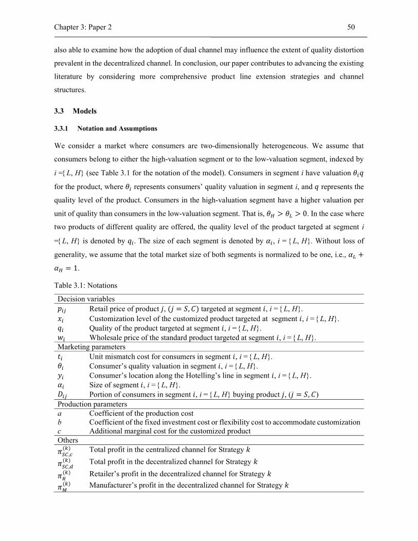
Chapter 3: Paper 2 50
also able to examine how the adoption of dual channel may influence the extent of quality distortion
prevalent in the decentralized channel. In conclusion, our paper contributes to advancing the existing
literature by considering more comprehensive product line extension strategies and channel
structures.
3.3 Models
3.3.1 Notation and Assumptions
We consider a market where consumers are two-dimensionally heterogeneous. We assume that
consumers belong to either the high-valuation segment or to the low-valuation segment, indexed by
i =L, H (see Table 3.1 for the notation of the model). Consumers in segment i have valuation 𝜃 𝑞
for the product, where 𝜃 represents consumers’ quality valuation in segment i, and 𝑞 represents the
quality level of the product. Consumers in the high-valuation segment have a higher valuation per
unit of quality than consumers in the low-valuation segment. That is, 𝜃 > 𝜃 > 0. In the case where
two products of different quality are offered, the quality level of the product targeted at segment i
=L, H is denoted by 𝑞 . The size of each segment is denoted by 𝛼 , i = L, H. Without loss of
generality, we assume that the total market size of both segments is normalized to be one, i.e., 𝛼 +
𝛼 = 1.
Table 3.1: Notations
Decision variables 𝑝 Retail price of product 𝑗, (𝑗 = 𝑆, 𝐶) targeted at segment 𝑖, i = L, H. 𝑥 Customization level of the customized product targeted at segment 𝑖, i = L, H. 𝑞 Quality of the product targeted at segment 𝑖, i = L, H. 𝑤 Wholesale price of the standard product targeted at segment 𝑖, i = L, H. Marketing parameters 𝑡 Unit mismatch cost for consumers in segment 𝑖, i = L, H. 𝜃 Consumer’s quality valuation in segment 𝑖, i = L, H. 𝑦 Consumer’s location along the Hotelling’s line in segment 𝑖, i = L, H. 𝛼 Size of segment 𝑖, i = L, H. 𝐷 Portion of consumers in segment 𝑖, i = L, H buying product 𝑗, (𝑗 = 𝑆, 𝐶) Production parameters a Coefficient of the production cost b Coefficient of the fixed investment cost or flexibility cost to accommodate customization c Additional marginal cost for the customized product Others
𝜋 ,( )
Total profit in the centralized channel for Strategy 𝑘
𝜋 ,( ) Total profit in the decentralized channel for Strategy 𝑘
𝜋( ) Retailer’s profit in the decentralized channel for Strategy 𝑘
𝜋( ) Manufacturer’s profit in the decentralized channel for Strategy 𝑘
Chapter 3: Paper 2 51
To model the horizontal consumer heterogeneity, we assume that consumers in each of the two
segments are uniformly located on Hotelling’s line that is characterized by a closed interval of product
space [0, 1] Each consumer in segment i = L, H is represented by his/her aesthetic preference of
the product, which is denoted as 𝑦 ∈ [0, 1]. Following Li et al. (2015), when the manufacturer
decides to offer a customized product, the customization level of the product is represented by 𝑥 ∈
(0,1), which measures the fraction of aesthetic attributes of the product that the manufacturer chooses
to customize. A standard product is represented by the left-end point, i.e., 𝑥 = 0, whereas a fully
customized product is represented at the right-end point, i.e., 𝑥 = 1. Suppose a standard product is
sold to consumers with price p and quality q. The utility derived by a consumer in segment i located
at 𝑦 ∈ [0, 1] is 𝑢 = 𝜃 𝑞 − 𝑡 𝑦 − 𝑝.
A customized product with customization level 𝑥 can satisfy the preference for consumers in segment
i located at 𝑦 ∈ [0, 𝑥]. However, consumers in segment i located at 𝑦 ∈ (𝑥, 1] incurs a mismatch
cost 𝑡 per unit deviation between their preference and that of the purchased product. We assume that
consumers in the high-valuation segment are more sensitive to this deviation than consumers in the
low-valuation segment, i.e. 𝑡 > 𝑡 > 0. This assumption is also used in Desai (2001). We are aware
that this assumption may not always reflect the true market characteristic. The situation where, for
example, consumers in the high-valuation segment are less sensitive to the deviation between their
preference and that of the purchased product than the low-valuation segment is also possible. In
Section 4, we provide a discussion of the effect of altering the assumption, and show that some of the
structural results of this study still hold under the assumption that 𝑡 > 𝑡 > 0.
In the product line extension strategies we consider, the manufacturer may offer a customized product
with low quality or high quality alongside the standard product. For notational convenience, we define
𝑥 , i = L, H, as the customization level targeted at segment i. Following the standard assumption in
the product line design literature (see e.g. Moorthy 1984; and Desai 2001), the manufacturer’s unit
production cost is a quadratic function of product quality, q, and equal to 𝑎𝑞 .
To capture the fact that offering a higher customization level will imply higher production complexity
and therefore require higher flexibility, we follow Li et al. (2015) and assume that the manufacturer
incurs a fixed flexibility cost 𝑏𝑥 when a customized product with customization level x is offered in
the product line. For example, a customized-rug manufacturer needs to invest in a new production
system or reconfigure the existing one that can produce the rugs with different patterns and/or color.
The quadratic form of the flexibility cost reflects the situation where it becomes increasingly difficult

Chapter 3: Paper 2 52
for a manufacturer to extend its customization ability, which may require a larger amount of machine
and labor resources.
We note several aspects of flexibility that deserve further elaboration. First, flexibility in the context
of this study should be interpreted more broadly as operations flexibility rather than manufacturing
flexibility. The reader is referred to e.g. Slack (1987, 2005) and Coronado and Lyons (2007), and the
references therein, for a comprehensive discussion of flexibility. This is especially true when
considering the customized product that is offered through an online channel where the fulfilment of
a customer order not only relies on manufacturing or production but also on order processing and
execution (pre-production) and distribution and transportation (post-production). Second, in relation
to manufacturing flexibility, the flexibility cost in our model is more closely related to the notion
product and mix flexibility. Product flexibility is defined as the ability to introduce new products or
modify the existing ones whereas mix flexibility is defined as the ability to change the range of
products (Slack 1987). Once the manufacturer decides to customize an aesthetic attribute of the
product, she must be able to produce a large number of product variants differentiated by this attribute.
The higher the customization level offered, the larger the number of product variants is.
We consider situations where the unit production cost is primarily driven by product quality, i.e.,
there is no difference in the unit production cost between the standard product and the customized
product with the same quality level. However, as the fulfilment of the customized product may require
additional order processing, we assume that there is an additional marginal cost c for the customized
product. Suppose a customized product is sold to consumers with price p, quality q, and customization
level x. The utility derived by a consumer in segment i located at 𝑦 ∈ [0, 𝑥] is 𝑢 = 𝜃 𝑞 − 𝑝. The
utility derived by a consumer in segment i located at 𝑦 ∈ (𝑥, 1] is 𝑢 = 𝜃 𝑞 − 𝑡 (𝑦 − 𝑥) − 𝑝. A
consumer will make a purchase as long as her utility is non-negative. We use index 𝑗 = 𝑆, 𝐶, to
differentiate the standard product(s) from the customized product.
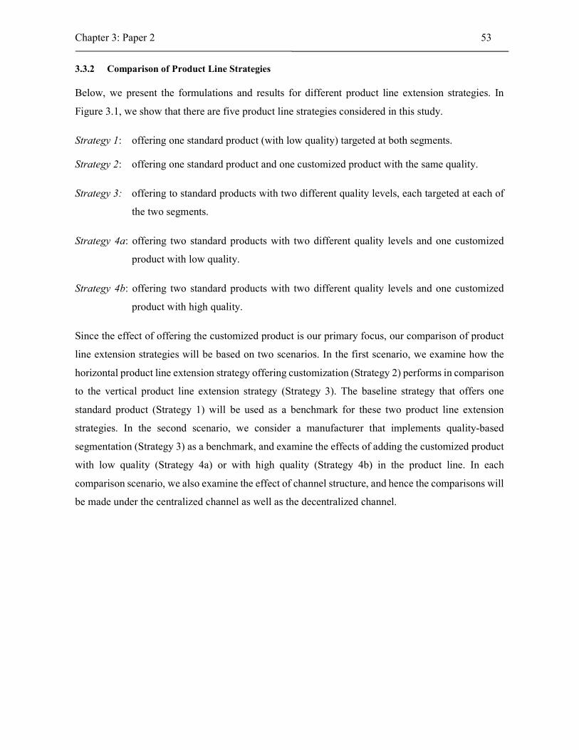
Chapter 3: Paper 2 53
3.3.2 Comparison of Product Line Strategies
Below, we present the formulations and results for different product line extension strategies. In
Figure 3.1, we show that there are five product line strategies considered in this study.
Strategy 1: offering one standard product (with low quality) targeted at both segments.
Strategy 2: offering one standard product and one customized product with the same quality.
Strategy 3: offering to standard products with two different quality levels, each targeted at each of
the two segments.
Strategy 4a: offering two standard products with two different quality levels and one customized
product with low quality.
Strategy 4b: offering two standard products with two different quality levels and one customized
product with high quality.
Since the effect of offering the customized product is our primary focus, our comparison of product
line extension strategies will be based on two scenarios. In the first scenario, we examine how the
horizontal product line extension strategy offering customization (Strategy 2) performs in comparison
to the vertical product line extension strategy (Strategy 3). The baseline strategy that offers one
standard product (Strategy 1) will be used as a benchmark for these two product line extension
strategies. In the second scenario, we consider a manufacturer that implements quality-based
segmentation (Strategy 3) as a benchmark, and examine the effects of adding the customized product
with low quality (Strategy 4a) or with high quality (Strategy 4b) in the product line. In each
comparison scenario, we also examine the effect of channel structure, and hence the comparisons will
be made under the centralized channel as well as the decentralized channel.
Chapter 3: Paper 2 54
Figure 3.1: Product line extension strategies based on two comparison scenarios
3.3.2.1 Comparison Scenario 1 – horizontal vs. vertical product line extension
We compare three product line strategies (Strategies 1, 2 and 3). We first investigate product line
strategies in a centralized channel, and then we continue with the analysis in a decentralized channel.
The centralized channel
Under a centralized distribution channel, the manufacturer is the only player involved. This could
also be seen as equivalent to the setting where the manufacturer sells its product directly to consumers
without any intermediaries.
Strategy 1: One standard product
Horizontal extension Vertical extension
Horizontal extension
Com
par
ison
sce
nari
o 1
Com
pari
son
sce
nari
o 2
Strategy 2: One standard product and one customized
product
Strategy 3: Two standard products
with two different quality levels
Strategy 4a: Two standard products
and one customized product with low quality
Strategy 4b: Two standard products
and one customized product with high quality

Chapter 3: Paper 2 55
Strategy 1 (one standard product)
As described in the standard literature on product line design (see e.g. Moorthy and Png 1992), the
manufacturer basically offers a low-quality product targeted at the two segments and sells a standard
product with quality level 𝑞 and price 𝑝 .We consequently use index L in this strategy. The
manufacturer thus solves the following optimization problem:
max ,
𝜋 ,( )
= (𝑝 − 𝑎𝑞 )(𝛼 𝐷 + 𝛼 𝐷 ) (1)
In (1), the term in the first parentheses on the right hand side denotes the manufacturer’s marginal
profit from selling the standard product with low-quality level. The term in the second parentheses
represents the total demand of the standard product in both the high-valuation and low-valuation
segments. Note that we use SC in the subscript of the profit since we are particularly interested in the
channel or supply chain profit in both the centralized and decentralized channels. Figure 3.2 below is
provided to illustrate the consumers’ utility in the two segments.
Figure 3.2: Consumer’s utility and demand in Strategy 1
Demands in the low-valuation and high-valuation segments can be expressed as 𝛼 𝐷 where 𝐷 =
𝑀𝑖𝑛 , 1 , and 𝛼 𝐷 where 𝐷 = 𝑀𝑖𝑛 , 1 , respectively. Note that in this paper,
we focus on the situation where the whole market is covered for all product line strategies, i.e., 𝐷 =
= 1 and 𝐷 = = 1. To impose the whole market coverage in this baseline
strategy, we need the following condition: 𝛽 −( )
( )≥ 1, i =L, H, where 𝛽 =
( ) (see Appendix A, for the derivation of this condition). The condition for the whole

Chapter 3: Paper 2 56
market coverage can be justified in settings where the mismatch cost, 𝑡 , is relatively small compared
to the quality valuation, 𝜃 . To limit the scope, we also focus on settings under the condition
−( )
( )≥ −
( )
( ), which implies that when it is optimal to cover
the whole market in the low-valuation segment, it is also optimal to cover the whole market in the
high-valuation segment. With the conditions above, the manufacturer sets the price such that
= 1 ⇔ 𝑝 = 𝜃 𝑞 − 𝑡 . The problem in (1) is solved by substituting 𝑝 with 𝜃 𝑞 − 𝑡
and by setting 𝐷 = 𝐷 = 1. The optimal results for strategy 1 are 𝑞∗ = , 𝑝∗ = − 𝑡 , and
𝜋 ,( ) ∗
= − 𝑡 . The reader is referred to Table 3.2 and Table 3.3 for the solutions to all the strategies
in the centralized and decentralized channels and to Appendix B for the complete derivation of the
solutions.
Table 3.2: The optimal solutions for all strategies in the centralized channel
Strategies Optimal solutions
Strategy 1 𝑞∗ = 𝜋 ,( ) ∗
= − 𝑡
Strategy 2
𝑞∗ = 𝑥∗ =
𝑝∗ = + − − 𝑡 𝜋 ,( ) ∗
= − 𝑐 − 𝑡 + + ( + )
Strategy 3
𝑞∗ = −( ) , where > 𝛼 𝑞∗ =
𝜋 ,( ) ∗
= − 𝑡 +( )
Strategy 4a
𝑞∗ = −( ) , where > 𝛼
𝑞∗ =
𝑥∗ = − , where > 𝛼 𝑝∗ = − − 𝑡 + −
𝜋 ,( )∗
= + 𝛼 + − 1 + 𝑡 − 𝛼 𝑐 + − + −
(( ) )
Strategy 4b
𝑞∗ = 𝑥∗ =( )
( )
𝑞∗ = −( )
, where > 𝛼
𝜋 ,( )∗
= + 𝛼( )
− 𝛼 1 +( )
− 𝑡 +( )
( )
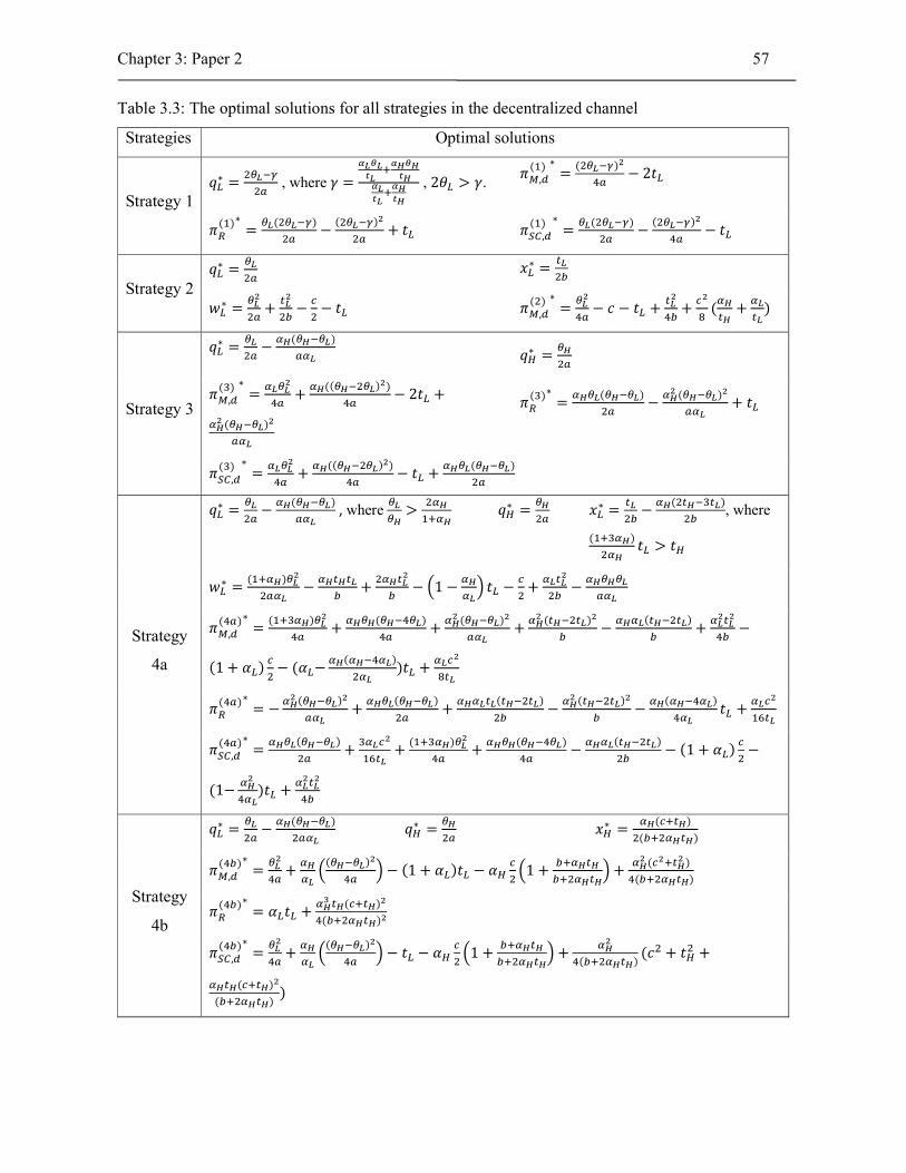
Chapter 3: Paper 2 57
Table 3.3: The optimal solutions for all strategies in the decentralized channel
Strategies Optimal solutions
Strategy 1 𝑞∗ = , where 𝛾 = , 2𝜃 > 𝛾.
𝜋 ,( ) ∗
=( )
− 2𝑡
𝜋( )∗
=( )
−( )
+ 𝑡 𝜋 ,( ) ∗
=( )
−( )
− 𝑡
Strategy 2 𝑞∗ = 𝑥∗ =
𝑤∗ = + − − 𝑡 𝜋 ,( ) ∗
= − 𝑐 − 𝑡 + + ( + )
Strategy 3
𝑞∗ = −( )
𝑞∗ =
𝜋 ,( ) ∗
= +(( ) )
− 2𝑡 +
( )
𝜋( )∗
=( )
−( )
+ 𝑡
𝜋 ,( ) ∗
= +(( ) )
− 𝑡 +( )
Strategy
4a
𝑞∗ = −( ) , where > 𝑞∗ = 𝑥∗ = −
( ), where
( )𝑡 > 𝑡
𝑤∗ =( )
− + − 1 − 𝑡 − + −
𝜋 ,( )∗
=( )
+( )
+( )
+( )
−( )
+ −
(1 + 𝛼 ) − (𝛼 −( )
)𝑡 +
𝜋( )∗
= −( )
+( )
+( )
−( )
−( )
𝑡 +
𝜋 ,( )∗
=( )
+ +( )
+( )
−( )
− (1 + 𝛼 ) −
(1− )𝑡 +
Strategy
4b
𝑞∗ = −( )
𝑞∗ = 𝑥∗ =( )
( )
𝜋 ,( )∗
= +( )
− (1 + 𝛼 )𝑡 − 𝛼 1 + +( )
( )
𝜋( )∗
= 𝛼 𝑡 +( )
( )
𝜋 ,( )∗
= +( )
− 𝑡 − 𝛼 1 + +( )
(𝑐 + 𝑡 +
( )
( ))
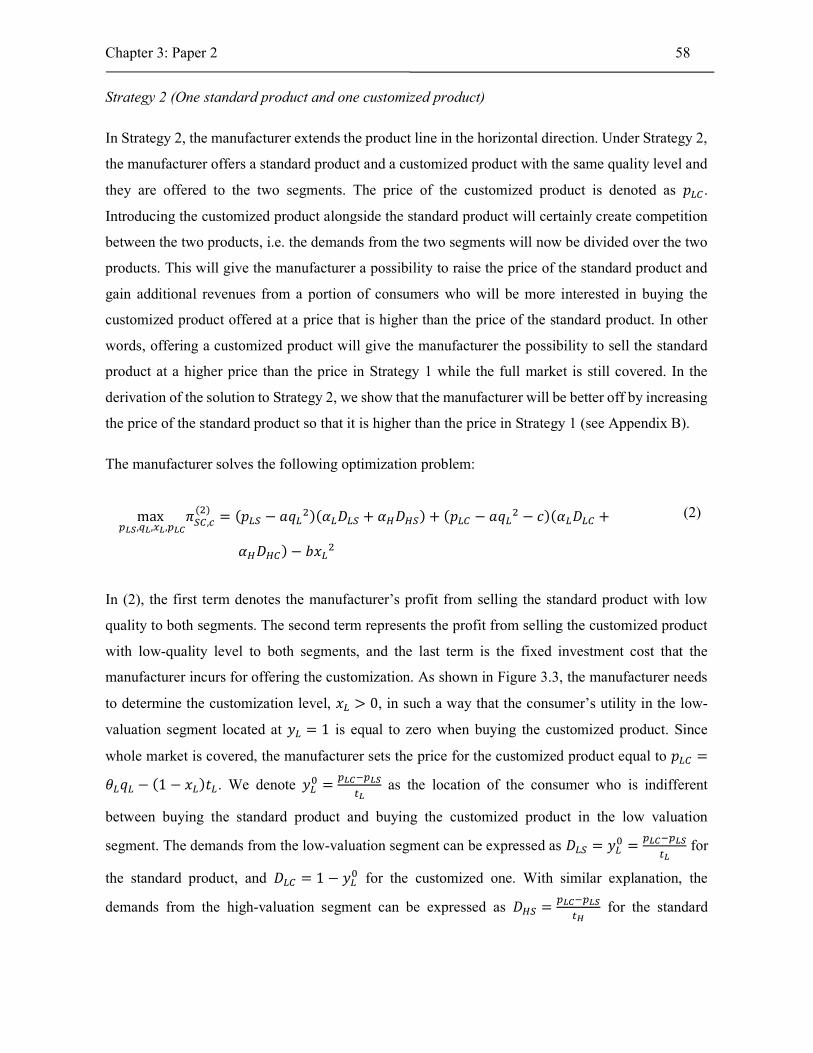
Chapter 3: Paper 2 58
Strategy 2 (One standard product and one customized product)
In Strategy 2, the manufacturer extends the product line in the horizontal direction. Under Strategy 2,
the manufacturer offers a standard product and a customized product with the same quality level and
they are offered to the two segments. The price of the customized product is denoted as 𝑝 .
Introducing the customized product alongside the standard product will certainly create competition
between the two products, i.e. the demands from the two segments will now be divided over the two
products. This will give the manufacturer a possibility to raise the price of the standard product and
gain additional revenues from a portion of consumers who will be more interested in buying the
customized product offered at a price that is higher than the price of the standard product. In other
words, offering a customized product will give the manufacturer the possibility to sell the standard
product at a higher price than the price in Strategy 1 while the full market is still covered. In the
derivation of the solution to Strategy 2, we show that the manufacturer will be better off by increasing
the price of the standard product so that it is higher than the price in Strategy 1 (see Appendix B).
The manufacturer solves the following optimization problem:
max , , ,
𝜋 ,( )
= (𝑝 − 𝑎𝑞 )(𝛼 𝐷 + 𝛼 𝐷 ) + (𝑝 − 𝑎𝑞 − 𝑐)(𝛼 𝐷 +
𝛼 𝐷 ) − 𝑏𝑥
(2)
In (2), the first term denotes the manufacturer’s profit from selling the standard product with low
quality to both segments. The second term represents the profit from selling the customized product
with low-quality level to both segments, and the last term is the fixed investment cost that the
manufacturer incurs for offering the customization. As shown in Figure 3.3, the manufacturer needs
to determine the customization level, 𝑥 > 0, in such a way that the consumer’s utility in the low-
valuation segment located at 𝑦 = 1 is equal to zero when buying the customized product. Since
whole market is covered, the manufacturer sets the price for the customized product equal to 𝑝 =
𝜃 𝑞 − (1 − 𝑥 )𝑡 . We denote 𝑦 = as the location of the consumer who is indifferent
between buying the standard product and buying the customized product in the low valuation
segment. The demands from the low-valuation segment can be expressed as 𝐷 = 𝑦 = for
the standard product, and 𝐷 = 1 − 𝑦 for the customized one. With similar explanation, the
demands from the high-valuation segment can be expressed as 𝐷 = for the standard
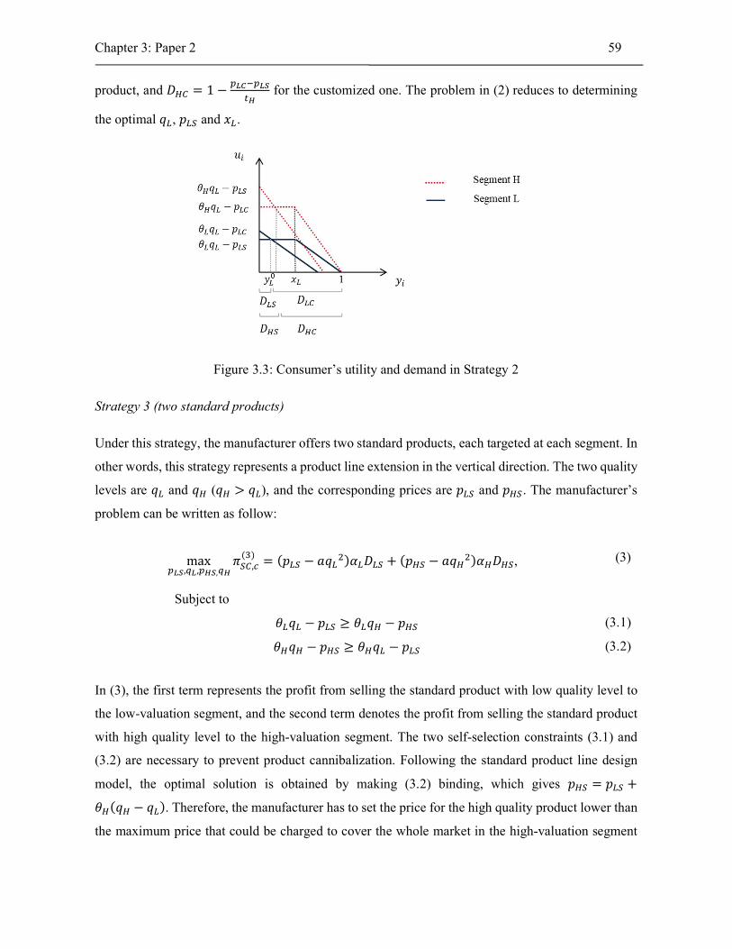
Chapter 3: Paper 2 59
product, and 𝐷 = 1 − for the customized one. The problem in (2) reduces to determining
the optimal 𝑞 , 𝑝 and 𝑥 .
Figure 3.3: Consumer’s utility and demand in Strategy 2
Strategy 3 (two standard products)
Under this strategy, the manufacturer offers two standard products, each targeted at each segment. In
other words, this strategy represents a product line extension in the vertical direction. The two quality
levels are 𝑞 and 𝑞 (𝑞 > 𝑞 ), and the corresponding prices are 𝑝 and 𝑝 . The manufacturer’s
problem can be written as follow:
max , , ,
𝜋 ,( )
= (𝑝 − 𝑎𝑞 )𝛼 𝐷 + (𝑝 − 𝑎𝑞 )𝛼 𝐷 , (3)
Subject to
𝜃 𝑞 − 𝑝 ≥ 𝜃 𝑞 − 𝑝 (3.1)
𝜃 𝑞 − 𝑝 ≥ 𝜃 𝑞 − 𝑝 (3.2)
In (3), the first term represents the profit from selling the standard product with low quality level to
the low-valuation segment, and the second term denotes the profit from selling the standard product
with high quality level to the high-valuation segment. The two self-selection constraints (3.1) and
(3.2) are necessary to prevent product cannibalization. Following the standard product line design
model, the optimal solution is obtained by making (3.2) binding, which gives 𝑝 = 𝑝 +
𝜃 (𝑞 − 𝑞 ). Therefore, the manufacturer has to set the price for the high quality product lower than
the maximum price that could be charged to cover the whole market in the high-valuation segment
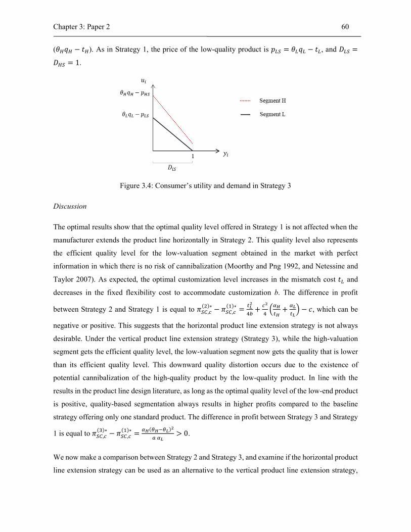
Chapter 3: Paper 2 60
(𝜃 𝑞 − 𝑡 ). As in Strategy 1, the price of the low-quality product is 𝑝 = 𝜃 𝑞 − 𝑡 , and 𝐷 =
𝐷 = 1.
Figure 3.4: Consumer’s utility and demand in Strategy 3
Discussion
The optimal results show that the optimal quality level offered in Strategy 1 is not affected when the
manufacturer extends the product line horizontally in Strategy 2. This quality level also represents
the efficient quality level for the low-valuation segment obtained in the market with perfect
information in which there is no risk of cannibalization (Moorthy and Png 1992, and Netessine and
Taylor 2007). As expected, the optimal customization level increases in the mismatch cost 𝑡 and
decreases in the fixed flexibility cost to accommodate customization b. The difference in profit
between Strategy 2 and Strategy 1 is equal to 𝜋 ,( )∗
− 𝜋 ,( )∗
= + + − 𝑐, which can be
negative or positive. This suggests that the horizontal product line extension strategy is not always
desirable. Under the vertical product line extension strategy (Strategy 3), while the high-valuation
segment gets the efficient quality level, the low-valuation segment now gets the quality that is lower
than its efficient quality level. This downward quality distortion occurs due to the existence of
potential cannibalization of the high-quality product by the low-quality product. In line with the
results in the product line design literature, as long as the optimal quality level of the low-end product
is positive, quality-based segmentation always results in higher profits compared to the baseline
strategy offering only one standard product. The difference in profit between Strategy 3 and Strategy
1 is equal to 𝜋 ,( )∗
− 𝜋 ,( )∗
=( )
> 0.
We now make a comparison between Strategy 2 and Strategy 3, and examine if the horizontal product
line extension strategy can be used as an alternative to the vertical product line extension strategy,
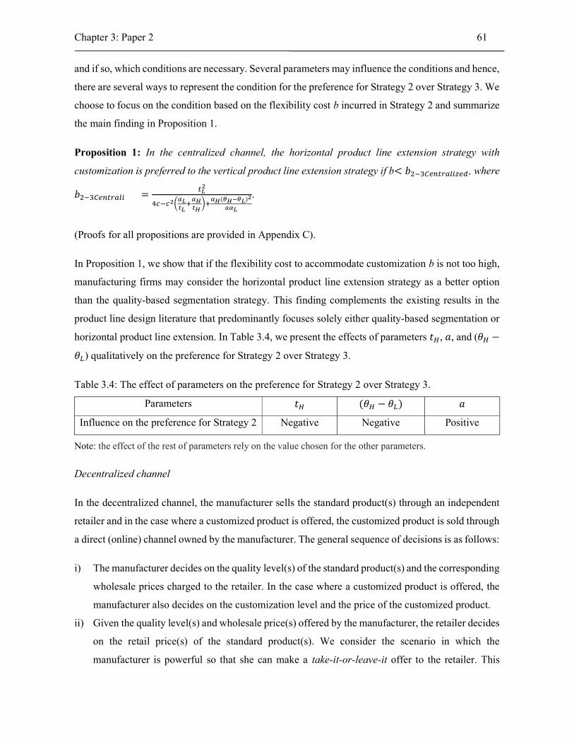
Chapter 3: Paper 2 61
and if so, which conditions are necessary. Several parameters may influence the conditions and hence,
there are several ways to represent the condition for the preference for Strategy 2 over Strategy 3. We
choose to focus on the condition based on the flexibility cost b incurred in Strategy 2 and summarize
the main finding in Proposition 1.
Proposition 1: In the centralized channel, the horizontal product line extension strategy with
customization is preferred to the vertical product line extension strategy if b< 𝑏 , where
𝑏 =( )
.
(Proofs for all propositions are provided in Appendix C).
In Proposition 1, we show that if the flexibility cost to accommodate customization b is not too high,
manufacturing firms may consider the horizontal product line extension strategy as a better option
than the quality-based segmentation strategy. This finding complements the existing results in the
product line design literature that predominantly focuses solely either quality-based segmentation or
horizontal product line extension. In Table 3.4, we present the effects of parameters 𝑡 , 𝑎, and (𝜃 −
𝜃 ) qualitatively on the preference for Strategy 2 over Strategy 3.
Table 3.4: The effect of parameters on the preference for Strategy 2 over Strategy 3.
Parameters 𝑡 (𝜃 − 𝜃 ) 𝑎
Influence on the preference for Strategy 2 Negative Negative Positive
Note: the effect of the rest of parameters rely on the value chosen for the other parameters.
Decentralized channel
In the decentralized channel, the manufacturer sells the standard product(s) through an independent
retailer and in the case where a customized product is offered, the customized product is sold through
a direct (online) channel owned by the manufacturer. The general sequence of decisions is as follows:
i) The manufacturer decides on the quality level(s) of the standard product(s) and the corresponding
wholesale prices charged to the retailer. In the case where a customized product is offered, the
manufacturer also decides on the customization level and the price of the customized product.
ii) Given the quality level(s) and wholesale price(s) offered by the manufacturer, the retailer decides
on the retail price(s) of the standard product(s). We consider the scenario in which the
manufacturer is powerful so that she can make a take-it-or-leave-it offer to the retailer. This
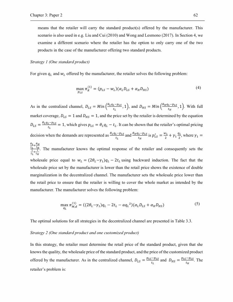
Chapter 3: Paper 2 62
means that the retailer will carry the standard product(s) offered by the manufacturer. This
scenario is also used in e.g. Liu and Cui (2010) and Wong and Lesmono (2017). In Section 4, we
examine a different scenario where the retailer has the option to only carry one of the two
products in the case of the manufacturer offering two standard products.
Strategy 1 (One standard product)
For given 𝑞 and 𝑤 offered by the manufacturer, the retailer solves the following problem:
max
𝜋( )
= (𝑝 − 𝑤 )(𝛼 𝐷 + 𝛼 𝐷 ) (4)
As in the centralized channel, 𝐷 = 𝑀𝑖𝑛 , 1 , and 𝐷 = 𝑀𝑖𝑛 , 1 . With full
market coverage, 𝐷 = 1 and 𝐷 = 1, and the price set by the retailer is determined by the equation
𝐷 = = 1, which gives 𝑝 = 𝜃 𝑞 − 𝑡 . It can be shown that the retailer’s optimal pricing
decision when the demands are represented as and is 𝑝∗ = + 𝛾 , where 𝛾 =
. The manufacturer knows the optimal response of the retailer and consequently sets the
wholesale price equal to 𝑤 = (2𝜃 −𝛾 )𝑞 − 2𝑡 using backward induction. The fact that the
wholesale price set by the manufacturer is lower than the retail price shows the existence of double
marginalization in the decentralized channel. The manufacturer sets the wholesale price lower than
the retail price to ensure that the retailer is willing to cover the whole market as intended by the
manufacturer. The manufacturer solves the following problem:
max 𝜋 ,( )
= ((2𝜃 −𝛾 )𝑞 − 2𝑡 − 𝑎𝑞 )(𝛼 𝐷 + 𝛼 𝐷 ) (5)
The optimal solutions for all strategies in the decentralized channel are presented in Table 3.3.
Strategy 2 (One standard product and one customized product)
In this strategy, the retailer must determine the retail price of the standard product, given that she
knows the quality, the wholesale price of the standard product, and the price of the customized product
offered by the manufacturer. As in the centralized channel, 𝐷 = and 𝐷 = . The
retailer’s problem is:
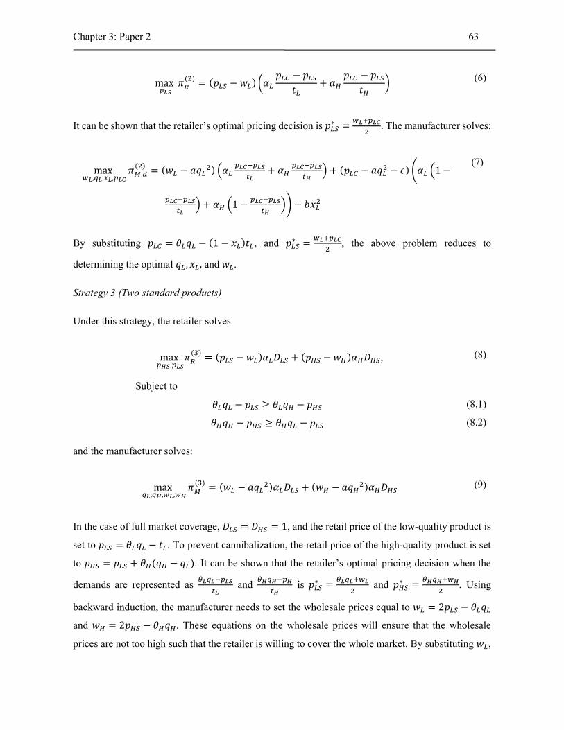
Chapter 3: Paper 2 63
max 𝜋( )
= (𝑝 − 𝑤 ) 𝛼𝑝 − 𝑝
𝑡+ 𝛼
𝑝 − 𝑝
𝑡 (6)
It can be shown that the retailer’s optimal pricing decision is 𝑝∗ = . The manufacturer solves:
max , , ,
𝜋 ,( )
= (𝑤 − 𝑎𝑞 ) 𝛼 + 𝛼 + (𝑝 − 𝑎𝑞 − 𝑐) 𝛼 1 −
+ 𝛼 1 − − 𝑏𝑥
(7)
By substituting 𝑝 = 𝜃 𝑞 − (1 − 𝑥 )𝑡 , and 𝑝∗ = , the above problem reduces to
determining the optimal 𝑞 , 𝑥 , and 𝑤 .
Strategy 3 (Two standard products)
Under this strategy, the retailer solves
max ,
𝜋( )
= (𝑝 − 𝑤 )𝛼 𝐷 + (𝑝 − 𝑤 )𝛼 𝐷 , (8)
Subject to
𝜃 𝑞 − 𝑝 ≥ 𝜃 𝑞 − 𝑝 (8.1)
𝜃 𝑞 − 𝑝 ≥ 𝜃 𝑞 − 𝑝 (8.2)
and the manufacturer solves:
max , , ,
𝜋( )
= (𝑤 − 𝑎𝑞 )𝛼 𝐷 + (𝑤 − 𝑎𝑞 )𝛼 𝐷 (9)
In the case of full market coverage, 𝐷 = 𝐷 = 1, and the retail price of the low-quality product is
set to 𝑝 = 𝜃 𝑞 − 𝑡 . To prevent cannibalization, the retail price of the high-quality product is set
to 𝑝 = 𝑝 + 𝜃 (𝑞 − 𝑞 ). It can be shown that the retailer’s optimal pricing decision when the
demands are represented as and is 𝑝∗ = and 𝑝∗ = . Using
backward induction, the manufacturer needs to set the wholesale prices equal to 𝑤 = 2𝑝 − 𝜃 𝑞
and 𝑤 = 2𝑝 − 𝜃 𝑞 . These equations on the wholesale prices will ensure that the wholesale
prices are not too high such that the retailer is willing to cover the whole market. By substituting 𝑤 ,

Chapter 3: Paper 2 64
𝑤 , 𝑝 , 𝑝 to the manufacturer’s objective function, the manufacturer’s problem reduces to
optimizing the quality levels 𝑞 and 𝑞 .
Discussion
In Strategy 1, the optimal quality in the decentralized channel is lower than the quality in the
centralized channel. It is interesting to see that downward quality distortion still occurs despite the
fact that we assume a take-it-or-leave-it offer from the manufacturer. This distortion is a consequence
of the potential misalignment of the manufacturer’s and the retailer’s market coverage decisions.
An interesting observation can be made about the results in Strategy 2 as the optimal quality and
customization levels are the same as those obtained in the centralized channel, which shows that the
quality distortion force is reduced when the manufacturer offers customization in the product line.
From the optimal results, we see that the wholesale price for the standard product in the decentralized
channel is as high as the retail price in the centralized channel, which explains why the quality level
remains the same as in the centralized channel. As a result, the product must be sold in the
decentralized channel at a higher retail price than the price in the centralized channel. The reduction
of quality distortion in Strategy 3 can be explained by the fact that even though the whole market is
covered by the two products, the offering of the customized product allows the retailer to increase the
retail price of the standard product and sell it only to a fraction of the market. The optimal results in
Strategy 3 show that the quality of the low-end product is lower than the quality level in Strategy 2,
and also lower compared to the quality level in the centralized channel under the same strategy. In
line with the standard results in product line design literature, the optimal quality of the high-end
product is not affected and the high-valuation segment always get the efficient quality level.
Similar to the case of centralized channel, we compare the channel profits of the three strategies and
examine the preference for Strategy 2 over Strategy 3, or vice versa. The following proposition
summarizes the condition for the preference for Strategy 2 over Strategy 3.
Proposition 2: In the decentralized channel, the horizontal product line extension strategy with
customization is preferred to the vertical product line extension strategy if 𝑏 < 𝑏 =
( ) .
In Proposition 2, we show that the horizontal product line extension may be preferable to the vertical
product line extension in the decentralized channel like in the centralized channel. It can be shown
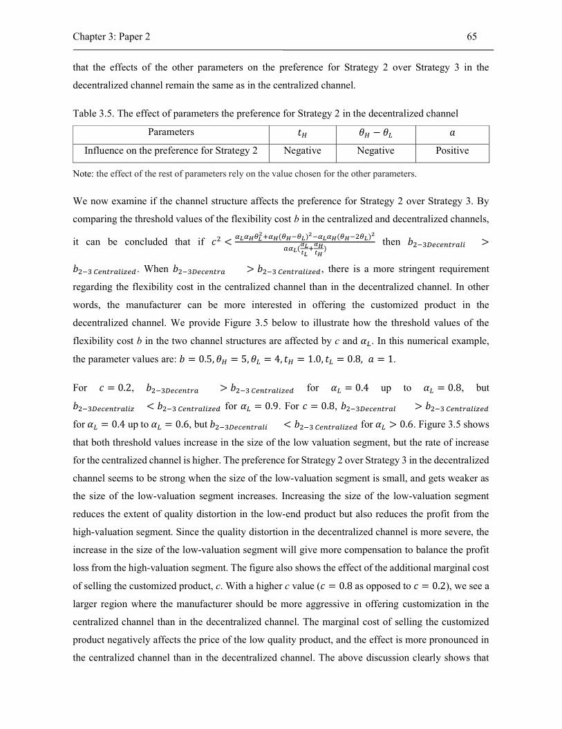
Chapter 3: Paper 2 65
that the effects of the other parameters on the preference for Strategy 2 over Strategy 3 in the
decentralized channel remain the same as in the centralized channel.
Table 3.5. The effect of parameters the preference for Strategy 2 in the decentralized channel
Parameters 𝑡 𝜃 − 𝜃 𝑎
Influence on the preference for Strategy 2 Negative Negative Positive
Note: the effect of the rest of parameters rely on the value chosen for the other parameters.
We now examine if the channel structure affects the preference for Strategy 2 over Strategy 3. By
comparing the threshold values of the flexibility cost b in the centralized and decentralized channels,
it can be concluded that if 𝑐 <( ) ( )
( ) then 𝑏 >
𝑏 . When 𝑏 > 𝑏 , there is a more stringent requirement
regarding the flexibility cost in the centralized channel than in the decentralized channel. In other
words, the manufacturer can be more interested in offering the customized product in the
decentralized channel. We provide Figure 3.5 below to illustrate how the threshold values of the
flexibility cost b in the two channel structures are affected by c and 𝛼 . In this numerical example,
the parameter values are: 𝑏 = 0.5, 𝜃 = 5, 𝜃 = 4, 𝑡 = 1.0, 𝑡 = 0.8, 𝑎 = 1.
For 𝑐 = 0.2, 𝑏 > 𝑏 for 𝛼 = 0.4 up to 𝛼 = 0.8, but
𝑏 < 𝑏 for 𝛼 = 0.9. For 𝑐 = 0.8, 𝑏 > 𝑏
for 𝛼 = 0.4 up to 𝛼 = 0.6, but 𝑏 < 𝑏 for 𝛼 > 0.6. Figure 3.5 shows
that both threshold values increase in the size of the low valuation segment, but the rate of increase
for the centralized channel is higher. The preference for Strategy 2 over Strategy 3 in the decentralized
channel seems to be strong when the size of the low-valuation segment is small, and gets weaker as
the size of the low-valuation segment increases. Increasing the size of the low-valuation segment
reduces the extent of quality distortion in the low-end product but also reduces the profit from the
high-valuation segment. Since the quality distortion in the decentralized channel is more severe, the
increase in the size of the low-valuation segment will give more compensation to balance the profit
loss from the high-valuation segment. The figure also shows the effect of the additional marginal cost
of selling the customized product, c. With a higher c value (𝑐 = 0.8 as opposed to 𝑐 = 0.2), we see a
larger region where the manufacturer should be more aggressive in offering customization in the
centralized channel than in the decentralized channel. The marginal cost of selling the customized
product negatively affects the price of the low quality product, and the effect is more pronounced in
the centralized channel than in the decentralized channel. The above discussion clearly shows that
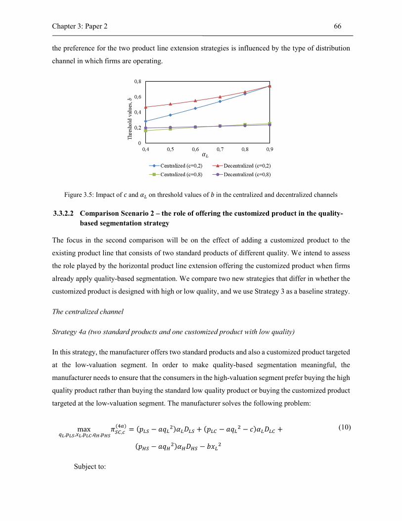
Chapter 3: Paper 2 66
the preference for the two product line extension strategies is influenced by the type of distribution
channel in which firms are operating.
Figure 3.5: Impact of 𝑐 and 𝛼 on threshold values of 𝑏 in the centralized and decentralized channels
3.3.2.2 Comparison Scenario 2 – the role of offering the customized product in the quality-based segmentation strategy
The focus in the second comparison will be on the effect of adding a customized product to the
existing product line that consists of two standard products of different quality. We intend to assess
the role played by the horizontal product line extension offering the customized product when firms
already apply quality-based segmentation. We compare two new strategies that differ in whether the
customized product is designed with high or low quality, and we use Strategy 3 as a baseline strategy.
The centralized channel
Strategy 4a (two standard products and one customized product with low quality)
In this strategy, the manufacturer offers two standard products and also a customized product targeted
at the low-valuation segment. In order to make quality-based segmentation meaningful, the
manufacturer needs to ensure that the consumers in the high-valuation segment prefer buying the high
quality product rather than buying the standard low quality product or buying the customized product
targeted at the low-valuation segment. The manufacturer solves the following problem:
max , , , , ,
𝜋 ,( )
= (𝑝 − 𝑎𝑞 )𝛼 𝐷 + (𝑝 − 𝑎𝑞 − 𝑐)𝛼 𝐷 +
(𝑝 − 𝑎𝑞 )𝛼 𝐷 − 𝑏𝑥
(10)
Subject to:

Chapter 3: Paper 2 67
𝜃 𝑞 − 𝑝 ≥ 𝜃 𝑞 − 𝑝 (10.1)
𝜃 𝑞 − 𝑝 ≥ 𝜃 𝑞 − 𝑝 (10.2)
𝜃 𝑞 − 𝑝 ≥ 𝜃 𝑞 + 𝑡 𝑥 − 𝑝 (10.3)
In (10), the first and second terms represent the manufacturer’s profit from selling the standard and
customized products, respectively, to the low-valuation segment. The third term is the profit from
selling the standard product with high quality to the high-valuation segment, and the last term denotes
the fixed investment cost for offering the customization. There are three self-selection constraints in
the above problem formulation. The first two constraints are necessary to prevent cannibalization
between the two standard products. The third self-selection constraint is required to prevent
consumers in the high-valuation segment from buying the customized product. Constraint (10.3) will
give the first upper bound on 𝑝 , �̅� = 𝑝 + 𝜃 (𝑞 − 𝑞 ) − 𝑡 𝑥 , and constraint (10.2) will give
the second upper bound �̅� = 𝑝 + 𝜃 (𝑞 − 𝑞 ). Since �̅� < �̅� , we make constraint (10.3)
binding. As in Strategy 2, the price of the customized product is 𝑝 = 𝜃 𝑞 − (1 − 𝑥 )𝑡 . Following
Strategy 2, with full market coverage, we have 𝐷 = , 𝐷 = 1 − , and 𝐷 = 1.
Figure 3.6: Consumer’s utility and demand in Strategy 4a
Strategy 4b (two standard products and one customized product with high quality)
This strategy is similar to Strategy 4a but the customized product is now offered with high quality
and targeted at the high-valuation segment. The customization level and price of the customized
product are denoted by 𝑥 and 𝑝 , respectively. As in Strategy 2, the manufacturer needs to
determine the customization level, 𝑥 , such that the utility of the consumer in the high-valuation
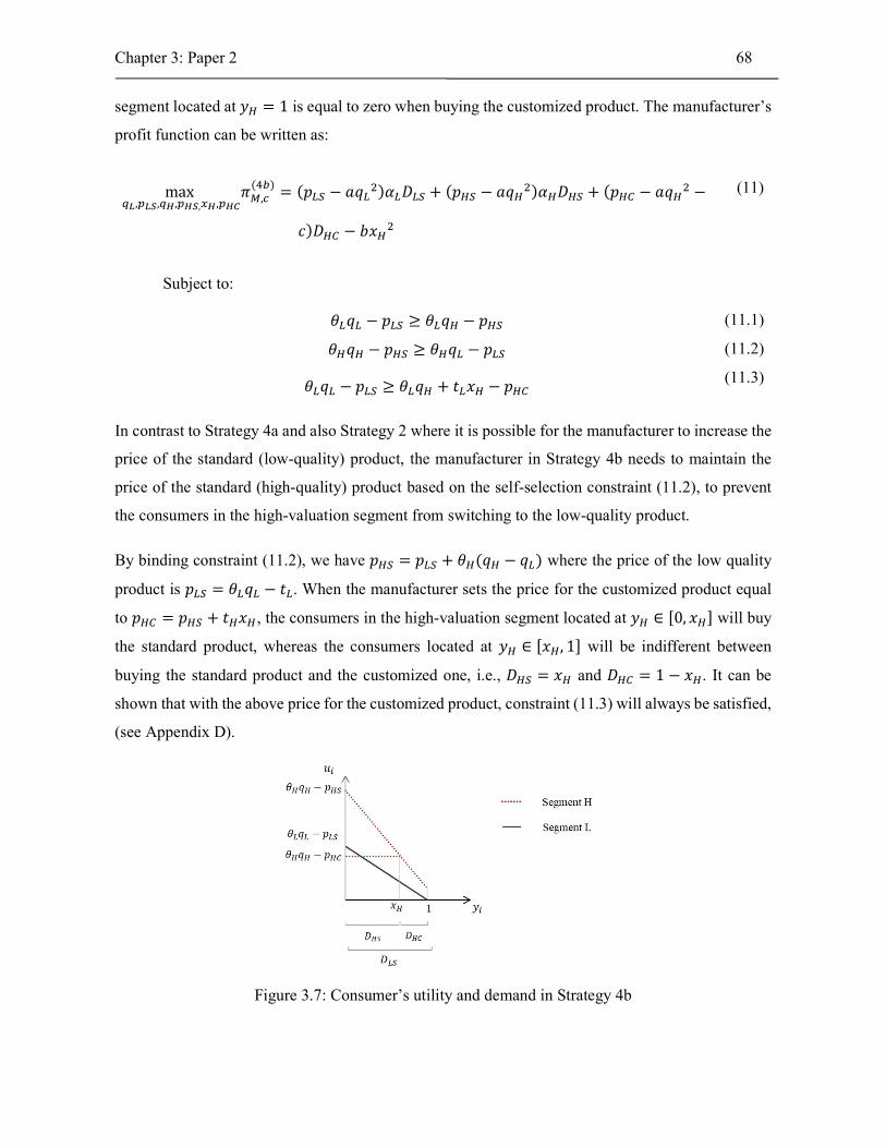
Chapter 3: Paper 2 68
segment located at 𝑦 = 1 is equal to zero when buying the customized product. The manufacturer’s
profit function can be written as:
max , , , , ,
𝜋 ,( )
= (𝑝 − 𝑎𝑞 )𝛼 𝐷 + (𝑝 − 𝑎𝑞 )𝛼 𝐷 + (𝑝 − 𝑎𝑞 −
𝑐)𝐷 − 𝑏𝑥
(11)
Subject to:
𝜃 𝑞 − 𝑝 ≥ 𝜃 𝑞 − 𝑝 (11.1)
𝜃 𝑞 − 𝑝 ≥ 𝜃 𝑞 − 𝑝 (11.2)
𝜃 𝑞 − 𝑝 ≥ 𝜃 𝑞 + 𝑡 𝑥 − 𝑝 (11.3)
In contrast to Strategy 4a and also Strategy 2 where it is possible for the manufacturer to increase the
price of the standard (low-quality) product, the manufacturer in Strategy 4b needs to maintain the
price of the standard (high-quality) product based on the self-selection constraint (11.2), to prevent
the consumers in the high-valuation segment from switching to the low-quality product.
By binding constraint (11.2), we have 𝑝 = 𝑝 + 𝜃 (𝑞 − 𝑞 ) where the price of the low quality
product is 𝑝 = 𝜃 𝑞 − 𝑡 . When the manufacturer sets the price for the customized product equal
to 𝑝 = 𝑝 + 𝑡 𝑥 , the consumers in the high-valuation segment located at 𝑦 ∈ [0, 𝑥 ] will buy
the standard product, whereas the consumers located at 𝑦 ∈ [𝑥 , 1] will be indifferent between
buying the standard product and the customized one, i.e., 𝐷 = 𝑥 and 𝐷 = 1 − 𝑥 . It can be
shown that with the above price for the customized product, constraint (11.3) will always be satisfied,
(see Appendix D).
Figure 3.7: Consumer’s utility and demand in Strategy 4b

Chapter 3: Paper 2 69
Discussion
By comparing the results in Strategy3 and Strategy 4a, we can see that offering the customized
product in Strategy 4a does not affect the optimal quality of the existing standard products. We also
note that the optimal customization level in Strategy 4a is lower than the customization level offered
in Strategy 2, which shows the existence of distortion in both quality and customization levels. The
additional distortion in the customization level occurs as a result of the manufacturer’s action to
prevent cannibalization of the high-quality standard product by the customized product. The extent
of distortion in customization level is increasing in the difference of the mismatch costs of consumers
in both segments. A notable advantage of moving from Strategy 3 to Strategy 4a can be drawn from
what we have observed when moving from Strategy 1 to Strategy 2. That is, the manufacturer has the
possibility to increase the profit from the low-valuation segment by introducing the customized
product with low quality, and this possibility can be justified when, for instance, the fixed flexibility
cost is not too high. However, there is also a detrimental effect due to the reduction in the price of the
high-quality product to prevent cannibalization by the customized product. Thus, there is no guarantee
that the manufacturer is better-off by offering the customized product to the existing quality-based
segmentation strategy. In the following proposition, we define the threshold value of the flexibility
cost.
Proposition 3: In the centralized channel, offering a customized product with low quality to the
existing quality-based segmentation strategy will increase the profit if 𝑏 <( )
( ).
When we compare Strategy 3 and Strategy 4b, we find no difference in the profit obtained from the
low-quality product offered to the low-valuation segment. Hence, the difference comes only from the
profit generated in the high-valuation segment. Since the prices of the standard products are the same
for the two strategies, the difference is then solely due to the profit generated from a fraction of
consumers who switch from buying the standard product in Strategy 3 to buying the customized
product in Strategy 4b. In contrast to Strategy 4a where the customization level is dependent on the
mismatch costs of consumers in both segments, 𝑡 and 𝑡 , the optimal customization level in Strategy
4b is only influenced by the mismatch cost in the high-valuation segment, 𝑡 . For a fixed 𝑡 , the
optimal customization level in Strategy 4a (Strategy 4b) is decreasing (increasing) in 𝑡 . As in
Strategy 4a, the preference for Strategy 4b over Strategy 3 cannot be guaranteed, and depends on
factors such as the flexibility cost associated with the customized product.
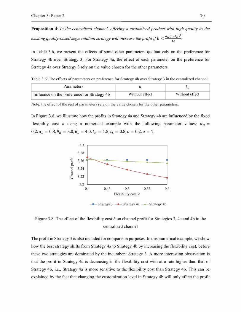
Chapter 3: Paper 2 70
Proposition 4: In the centralized channel, offering a customized product with high quality to the
existing quality-based segmentation strategy will increase the profit if 𝑏 <( )
.
In Table 3.6, we present the effects of some other parameters qualitatively on the preference for
Strategy 4b over Strategy 3. For Strategy 4a, the effect of each parameter on the preference for
Strategy 4a over Strategy 3 rely on the value chosen for the other parameters.
Table 3.6: The effects of parameters on preference for Strategy 4b over Strategy 3 in the centralized channel
Parameters 𝑎 𝑡
Influence on the preference for Strategy 4b Without effect Without effect
Note: the effect of the rest of parameters rely on the value chosen for the other parameters.
In Figure 3.8, we illustrate how the profits in Strategy 4a and Strategy 4b are influenced by the fixed
flexibility cost b using a numerical example with the following parameter values: 𝛼 =
0.2, 𝛼 = 0.8, 𝜃 = 5.0, 𝜃 = 4.0, 𝑡 = 1.5, 𝑡 = 0.8, 𝑐 = 0.2, 𝑎 = 1.
Figure 3.8: The effect of the flexibility cost b on channel profit for Strategies 3, 4a and 4b in the
centralized channel
The profit in Strategy 3 is also included for comparison purposes. In this numerical example, we show
how the best strategy shifts from Strategy 4a to Strategy 4b by increasing the flexibility cost, before
these two strategies are dominated by the incumbent Strategy 3. A more interesting observation is
that the profit in Strategy 4a is decreasing in the flexibility cost with at a rate higher than that of
Strategy 4b, i.e., Strategy 4a is more sensitive to the flexibility cost than Strategy 4b. This can be
explained by the fact that changing the customization level in Strategy 4b will only affect the profit
3,2
3,22
3,24
3,26
3,28
3,3
0,4 0,45 0,5 0,55 0,6
Cha
nnel
pro
fit
Flexibility cost, b
Strategy 3 Strategy 4a Strategy 4b

Chapter 3: Paper 2 71
generated from the high-valuation segment, as a consequence of changing the fraction of consumers
in this segment who buy the standard or customized products. Recall that the prices of the standard
products also remain the same in this strategy. But changing the customization level in Strategy 4a is
more impactful since it affects the profits in both segments and the prices of the three products.
The decentralized channel
Strategy 4a: Two standard products and one customized product with low quality
Based on the demands derived in the centralized channel, in this strategy, the retailer solves
max ,
𝜋( )
= (𝑝 − 𝑤 )𝛼 (𝐷 ) + (𝑝 − 𝑤 )𝛼 𝐷 (12)
Subject to:
𝜃 𝑞 − 𝑝 ≥ 𝜃 𝑞 − 𝑝 (12.1)
𝜃 𝑞 − 𝑝 ≥ 𝜃 𝑞 − 𝑝 (12.2)
𝜃 𝑞 − 𝑝 ≥ 𝜃 𝑞 + 𝑡 𝑥 − 𝑝 (12.3)
The retailer’s optimal prices are 𝑝∗ = and 𝑝∗ = (see Appendix E). As in the
centralized channel, we have 𝑝 = 𝜃 𝑞 − (1 − 𝑥 )𝑡 , and 𝑝 = 𝑝 + 𝜃 (𝑞 − 𝑞 ) − 𝑡 𝑥 ,
𝐷 = and 𝐷 = 1. The manufacturer’s objective function can be written as:
max , , , ,
𝜋( )
= (𝑤 − 𝑎𝑞 )𝛼 𝐷 + (𝑤 − 𝑎𝑞 )𝛼 𝐷 + (𝑝 − 𝑎𝑞 − 𝑐)𝛼 𝐷 −
𝑏𝑥
(13)
By substituting 𝑤 and 𝑝 , the above problem reduces to determining the optimal 𝑞 , 𝑞 , 𝑤 and
𝑥 .
Strategy 4b (two standard products and one customized product with high quality)
In this strategy, the retailer solves:
max ,
𝜋( )
= (𝑝 − 𝑤 )𝛼 𝐷 + (𝑝 − 𝑤 )𝛼 𝐷 , (14)
Subject to:
Chapter 3: Paper 2 72
𝜃 𝑞 − 𝑝 ≥ 𝜃 𝑞 − 𝑝 (14.1)
𝜃 𝑞 − 𝑝 ≥ 𝜃 𝑞 − 𝑝 (14.2)
𝜃 𝑞 − 𝑡 𝑥 − 𝑝 ≥ 𝜃 𝑞 − 𝑝 (14.3)
𝐷 = 1 and 𝐷 = . The retailer’s optimal responses to the manufacturer’s offer are 𝑝∗ =
and 𝑝∗ = . Like in the centralized channel, 𝑝 = 𝜃 𝑞 − 𝑡 , and by binding
constraint (14.2), we have 𝑝 = 𝑝 + 𝜃 (𝑞 − 𝑞 ). The manufacturer’s problem is:
max , , , , ,
𝜋( )
= (𝑤 − 𝑎𝑞 )𝛼 𝐷 + (𝑤 − 𝑎𝑞 )𝛼 𝐷 + (𝑝 − 𝑎𝑞 −
𝑐)𝛼 𝐷 − 𝑏𝑥
(15)
Like in the centralized channel, the manufacturer sets the price for the customized product equal to
𝑝 = 𝑝 + 𝑡 𝑥 . Knowing the retailer’s optimal responses, the manufacturer sets the wholesale
prices equal to 𝑤 = 2𝑝 − 𝑝 and 𝑤 = 2𝑝 − 𝜃 𝑞 (see Appendix E). By substitutions, 𝐷 =
𝑥 and 𝐷 = 1 − 𝑥 , and 𝑝 and 𝑝 the manufacturer’s problem reduces to determining the
optimal 𝑞 , 𝑞 , and 𝑥 .
Discussion
Like in the centralized channel, offering the customized product with low quality in Strategy 4a in
the decentralized channel does not affect the optimal quality of the existing standard products in
Strategy 3. However, it is interesting to see that offering the customized product with high quality in
Strategy 4b in the decentralized channel increases the optimal quality level of the low-quality product,
while there is no change in the centralized channel. In fact, the optimal quality level of the low-quality
product in Strategy 4b in the decentralized channel is the same as the optimal quality level in the
centralized channel. In other words, offering the customized product with high quality can alleviate
the quality distortion effect in the decentralized channel.
When the customized product is offered with low quality in the decentralized channel (Strategy 4a),
the optimal customization level can be higher or lower compared to the customization level offered
in the centralized channel. It can be shown that when < 3, the customization level in the
decentralized channel is higher. It would also be interesting to make a comparison with the
customization level offered in Strategy 2. The previous analysis has shown that the customization
level offered in Strategy 4a in the centralized channel is always lower than the customization level

Chapter 3: Paper 2 73
offered in Strategy 2. In the decentralized channel, however, under the condition < 1.5, it is
optimal for the manufacturer to offer a customization level that is higher than the optimal
customization level in Strategy 2. In all cases, when it is of the manufacturer’s interest to offer the
customized product with lower quality, the customization level offered should be higher when the
difference of the mismatch costs of the two segments becomes smaller.
In Strategy 4b, when the customized product is offered with high quality, the optimal customization
level offered in the decentralized channel is lower than that of the centralized channel. Different from
Strategy 4a, the customization level in Strategy 4b is only influenced by the mismatch cost of the
high-valuation segment rather than the mismatch costs of the two segments. This can be explained
by the fact that the self-selection constraint preventing the low-valuation segment from buying the
customized product is redundant in Strategy 4b.
Like in the centralized channel, offering the customized product to the existing quality-based
segmentation strategy provides the opportunity to increase the channel profit. However, there is no
guarantee that introducing the customized product in the product line will always increase the channel
profit. The preference for Strategy 4a or Strategy 4b over Strategy 3 depends on the flexibility cost
and other parameters. In the following propositions, we define the threshold values of the flexibility
cost.
Proposition 5: In the decentralized channel, offering customized product with low quality to the
existing quality-based segmentation strategy will not change the channel profit when
𝑏 =( )
( ) ( ).
Proposition 6: In the decentralized channel, offering customized product with high quality to the
existing quality-based segmentation strategy will not change the channel profit when
𝑏 =( ) ( ) ( )
( ( ) )− 𝛼 𝑡 .
In Tables 3.7 and 3.8, we present the effects of some other parameters qualitatively on the preference
for Strategy 4a and Strategy 4b over Strategy 3.
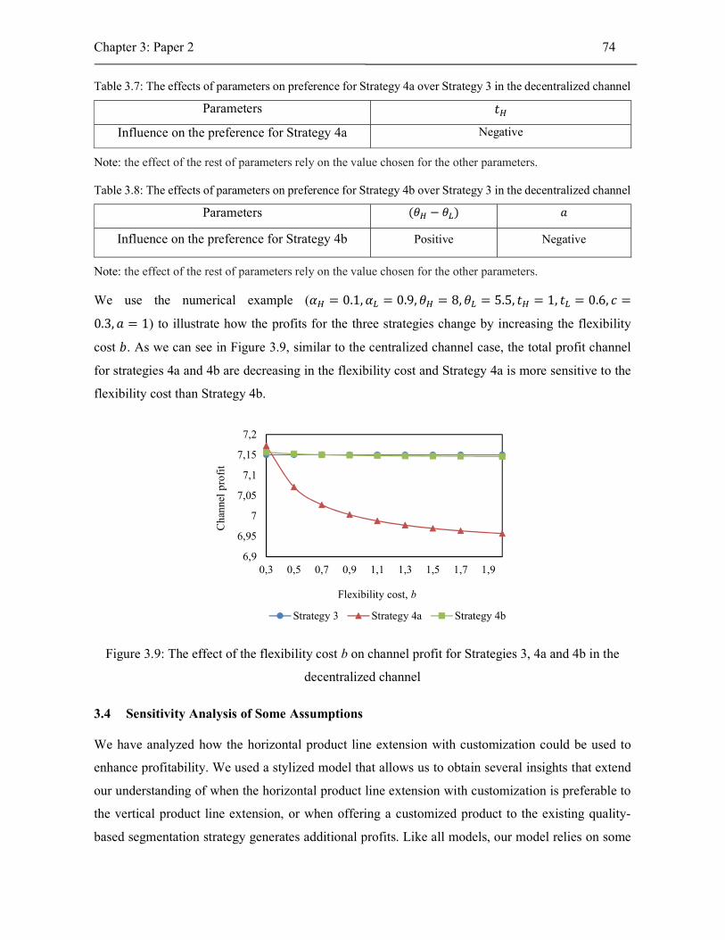
Chapter 3: Paper 2 74
Table 3.7: The effects of parameters on preference for Strategy 4a over Strategy 3 in the decentralized channel
Parameters 𝑡
Influence on the preference for Strategy 4a Negative
Note: the effect of the rest of parameters rely on the value chosen for the other parameters.
Table 3.8: The effects of parameters on preference for Strategy 4b over Strategy 3 in the decentralized channel
Parameters (𝜃 − 𝜃 ) 𝑎
Influence on the preference for Strategy 4b Positive Negative
Note: the effect of the rest of parameters rely on the value chosen for the other parameters.
We use the numerical example (𝛼 = 0.1, 𝛼 = 0.9, 𝜃 = 8, 𝜃 = 5.5, 𝑡 = 1, 𝑡 = 0.6, 𝑐 =
0.3, 𝑎 = 1) to illustrate how the profits for the three strategies change by increasing the flexibility
cost 𝑏. As we can see in Figure 3.9, similar to the centralized channel case, the total profit channel
for strategies 4a and 4b are decreasing in the flexibility cost and Strategy 4a is more sensitive to the
flexibility cost than Strategy 4b.
Figure 3.9: The effect of the flexibility cost b on channel profit for Strategies 3, 4a and 4b in the
decentralized channel
3.4 Sensitivity Analysis of Some Assumptions
We have analyzed how the horizontal product line extension with customization could be used to
enhance profitability. We used a stylized model that allows us to obtain several insights that extend
our understanding of when the horizontal product line extension with customization is preferable to
the vertical product line extension, or when offering a customized product to the existing quality-
based segmentation strategy generates additional profits. Like all models, our model relies on some
6,9
6,95
7
7,05
7,1
7,15
7,2
0,3 0,5 0,7 0,9 1,1 1,3 1,5 1,7 1,9
Cha
nnel
pro
fit
Flexibility cost, b
Strategy 3 Strategy 4a Strategy 4b
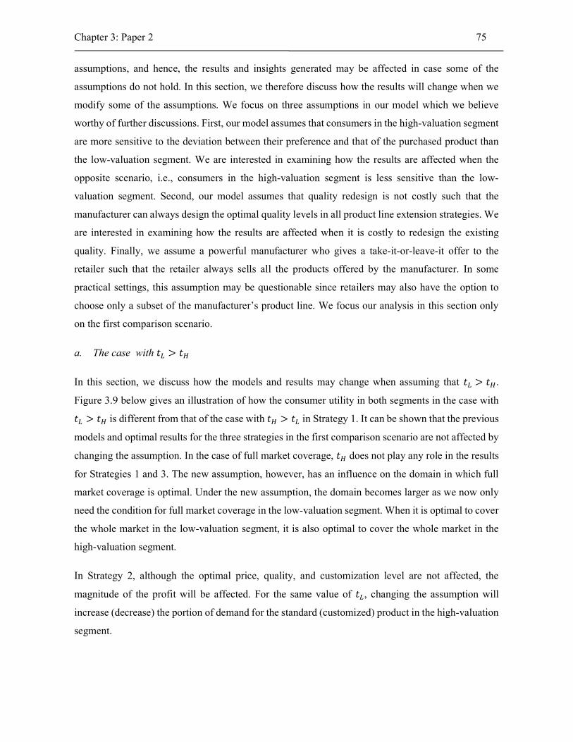
Chapter 3: Paper 2 75
assumptions, and hence, the results and insights generated may be affected in case some of the
assumptions do not hold. In this section, we therefore discuss how the results will change when we
modify some of the assumptions. We focus on three assumptions in our model which we believe
worthy of further discussions. First, our model assumes that consumers in the high-valuation segment
are more sensitive to the deviation between their preference and that of the purchased product than
the low-valuation segment. We are interested in examining how the results are affected when the
opposite scenario, i.e., consumers in the high-valuation segment is less sensitive than the low-
valuation segment. Second, our model assumes that quality redesign is not costly such that the
manufacturer can always design the optimal quality levels in all product line extension strategies. We
are interested in examining how the results are affected when it is costly to redesign the existing
quality. Finally, we assume a powerful manufacturer who gives a take-it-or-leave-it offer to the
retailer such that the retailer always sells all the products offered by the manufacturer. In some
practical settings, this assumption may be questionable since retailers may also have the option to
choose only a subset of the manufacturer’s product line. We focus our analysis in this section only
on the first comparison scenario.
a. The case with 𝑡 > 𝑡
In this section, we discuss how the models and results may change when assuming that 𝑡 > 𝑡 .
Figure 3.9 below gives an illustration of how the consumer utility in both segments in the case with
𝑡 > 𝑡 is different from that of the case with 𝑡 > 𝑡 in Strategy 1. It can be shown that the previous
models and optimal results for the three strategies in the first comparison scenario are not affected by
changing the assumption. In the case of full market coverage, 𝑡 does not play any role in the results
for Strategies 1 and 3. The new assumption, however, has an influence on the domain in which full
market coverage is optimal. Under the new assumption, the domain becomes larger as we now only
need the condition for full market coverage in the low-valuation segment. When it is optimal to cover
the whole market in the low-valuation segment, it is also optimal to cover the whole market in the
high-valuation segment.
In Strategy 2, although the optimal price, quality, and customization level are not affected, the
magnitude of the profit will be affected. For the same value of 𝑡 , changing the assumption will
increase (decrease) the portion of demand for the standard (customized) product in the high-valuation
segment.
Chapter 3: Paper 2 76
The preference for Strategy 2 over Strategy 3 certainly depends on both values of 𝑡 and 𝑡 . For the
same value of 𝑡 , as shown in Tables 3.4 and 3.5, the preference for the horizontal product line
extension (Strategy 2) over the vertical product line extension (Strategy 3) will become stronger when
consumers in the high-valuation segment has a lower mismatch cost than consumers in the low-
valuation segment.
Figure 3.10: Consumer’s utility in Strategy 1 under the assumptions 𝑡 > 𝑡 and 𝑡 < 𝑡
b. The case with costly quality redesign
We consider a new scenario in which the manufacturer is not interested in changing the quality offered
in Strategy 1 when considering horizontal product line extension (Strategy 2) or vertical product line
extension (Strategy 3). Recall that the optimal quality in Strategy 1 is 𝑞∗ = in the centralized
channel. The previous results in the centralized channel show that while there is no quality distortion
in Strategy 2, quality distortion does occur in Strategy 3 due to the potential cannibalization problem.
The optimal quality for the low-quality product in the case where it is not costly for the manufacturer
to redesign quality is 𝑞∗ = −( )
. Thus, if the manufacturer needs to maintain the existing
quality of the low-quality product in Strategy 1, i.e., 𝑞∗ = , the resulting profit in Strategy 3
becomes lower than the profit obtained in the case where it is not costly for the manufacturer to
redesign quality. The profit in Strategy 2, however, is not affected. Hence, the manufacturer will be
more motivated to extend the product line horizontally than to extend it vertically. In other words, the
manufacturer should be more motivated in offering a customized product in situations where quality
redesign is costly. It can be shown that the threshold value of the flexibility cost in the case where
Chapter 3: Paper 2 77
quality redesign is costly is equal to 𝑏 " =
( ), which is larger than
the threshold value in the case where quality redesign is not costly.
We now consider a similar scenario in the decentralized channel and maintain the quality level
obtained in Strategy 1 in the two product line extension strategies. Recall that the optimal quality in
Strategy 1 is 𝑞∗ = , where 𝛾 = . In contrast to the case of the centralized channel,
Strategy 2 is now disadvantaged by maintaining the optimal quality in Strategy 1 in the decentralized
channel. Recall that when quality is a free decision variable, offering the customized product in
Strategy 2 can actually increase the quality of the low-end product. The manufacturer can no longer
enjoy the same benefit when she has to maintain the quality obtained in Strategy 1. In Strategy 3, the
optimal quality of the low-end product in the case where quality design is not costly is equal to 𝑞∗ =
−( )
< is 𝑞∗ = . Thus, if the manufacturer needs to maintain the same quality as in
Strategy 1, the channel benefits from the reduction of quality distortion, but this will be
disadvantageous for the manufacturer who now earns a lower profit. Since we focus on channel profit
comparisons, the preference for Strategy 3 over Strategy 2 in the decentralized channel increases in
comparison to the case where quality design is not costly. This finding is interesting as we see the
opposite effects of the costly quality redesign on the preference for the horizontal or vertical product
line extension in the centralized and decentralized channels. It can be shown that the threshold value
of the flexibility cost in the case where quality redesign is costly is equal to 𝑏 " =
( ), which is smaller than the threshold value in the
case where quality redesign is not costly.
c. The case with the retailer having more options in a decentralized channel
We consider a different scenario where the retailer now has the option of not carrying the whole
product line offered by the manufacturer. This scenario is introduced in Villas-Boas (1998). Note that
under this scenario, modifications are only relevant for Strategy 3, i.e., the results for Strategy1 and
Strategy 2 will not be affected. Under Strategy 3, while the manufacturer intends to sell two products,
the retailer has three options: (a) to sell two products as intended by the manufacturer; (b) to sell only
the low-quality product targeted at both segments; or (c) to sell only the high-quality product targeted
at the high-valuation segment. This shows that in the decentralized channel, the manufacturer’s
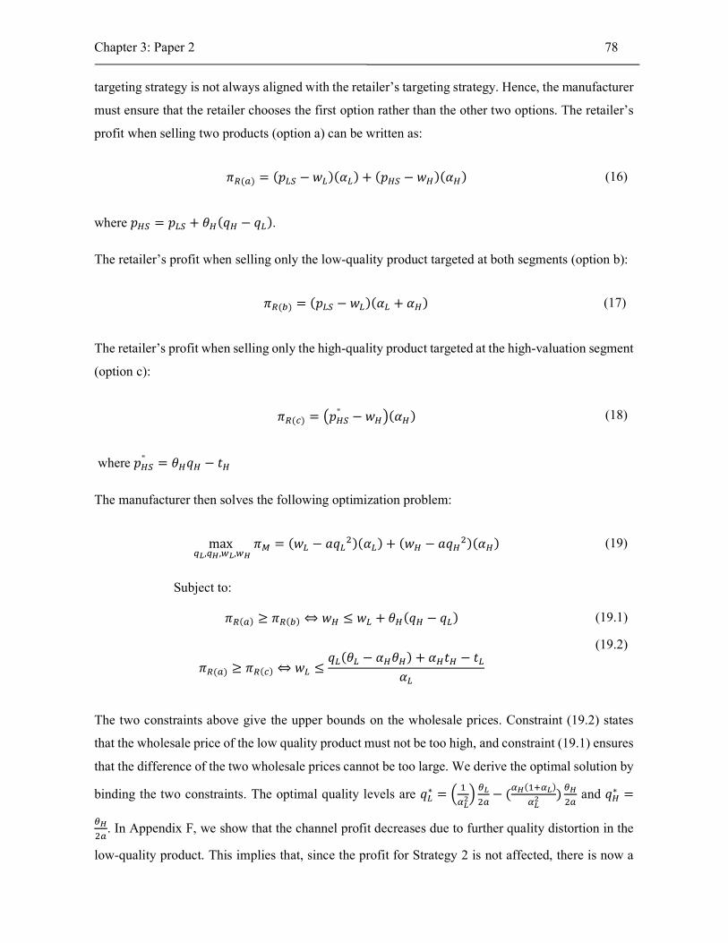
Chapter 3: Paper 2 78
targeting strategy is not always aligned with the retailer’s targeting strategy. Hence, the manufacturer
must ensure that the retailer chooses the first option rather than the other two options. The retailer’s
profit when selling two products (option a) can be written as:
𝜋 ( ) = (𝑝 − 𝑤 )(𝛼 ) + (𝑝 − 𝑤 )(𝛼 ) (16)
where 𝑝 = 𝑝 + 𝜃 (𝑞 − 𝑞 ).
The retailer’s profit when selling only the low-quality product targeted at both segments (option b):
𝜋 ( ) = (𝑝 − 𝑤 )(𝛼 + 𝛼 ) (17)
The retailer’s profit when selling only the high-quality product targeted at the high-valuation segment
(option c):
𝜋 ( ) = 𝑝" − 𝑤 (𝛼 ) (18)
where 𝑝" = 𝜃 𝑞 − 𝑡
The manufacturer then solves the following optimization problem:
max , , ,
𝜋 = (𝑤 − 𝑎𝑞 )(𝛼 ) + (𝑤 − 𝑎𝑞 )(𝛼 ) (19)
Subject to:
𝜋 ( ) ≥ 𝜋 ( ) ⇔ 𝑤 ≤ 𝑤 + 𝜃 (𝑞 − 𝑞 ) (19.1)
𝜋 ( ) ≥ 𝜋 ( ) ⇔ 𝑤 ≤𝑞 (𝜃 − 𝛼 𝜃 ) + 𝛼 𝑡 − 𝑡
𝛼
(19.2)
The two constraints above give the upper bounds on the wholesale prices. Constraint (19.2) states
that the wholesale price of the low quality product must not be too high, and constraint (19.1) ensures
that the difference of the two wholesale prices cannot be too large. We derive the optimal solution by
binding the two constraints. The optimal quality levels are 𝑞∗ = − (( )
) and 𝑞∗ =
. In Appendix F, we show that the channel profit decreases due to further quality distortion in the
low-quality product. This implies that, since the profit for Strategy 2 is not affected, there is now a

Chapter 3: Paper 2 79
higher motivation to consider the horizontal product line extension strategy. From this analysis, we
show how the power structure in the channel may play a role in determining the best product line
extension strategy.
3.5 Conclusions
In this article, we examine the role that offering the customized product may play in product line
design. We consider a market where consumers are heterogeneous with respect to their valuation of
quality and preference on the aesthetic component of the product. While the standard quality-based
segmentation is used for addressing the consumers’ heterogeneity in their valuation for quality,
offering the customized product is used for addressing the consumers’ heterogeneity in their
preference of the aesthetic component of the product. The effect of offering the customized product
in the product line is evaluated in two comparison scenarios. In the first scenario, we use a single
product strategy as a baseline strategy and examine the preference for the horizontal product line
extension strategy that offers the customized product of the same quality to the vertical product line
extension strategy that offers two products of different quality. In the second scenario, we use the
quality-based segmentation strategy as a baseline strategy and examine the effect of adding the
customized product to the existing product line. Furthermore, we examine if the channel structure
affects the results in those two comparison scenarios. For this purpose, we extend the standard models
in the literature on product line design by considering a joint decision on quality and customization
levels.
Some of the most important results are summarized as follows. When the single-product strategy is
used as the baseline strategy, adding a new product with a higher quality, i.e., applying the vertical
product line extension strategy, always increases the profit. The effect of adding the customized
product, i.e., applying the horizontal product line extension strategy, depends on several factors. One
notable factor is the fixed flexibility cost for accommodating the customization. The horizontal
product line extension strategy may increase the profit if this cost is not too high. Interestingly, our
study also shows that the horizontal product line extension strategy that offers the customized product
can be used as an alternative to the vertical product line extension strategy. Provided that the fixed
cost is not too high, offering the customized product with low quality may be preferred to the quality-
based segmentation strategy that offers two products of different quality. The main benefit of the
horizontal product line extension strategy comes from the increase in profit from the low-valuation
segment. Even though this result regarding the possible preference for the horizontal product line
extension strategy is observed in both the centralized and decentralized channels, we show that the
Chapter 3: Paper 2 80
channel structure is influential. That is, the preference for the horizontal product line extension
strategy is more pronounced in the decentralized channel than in the centralized channel. In the
decentralized channel, the vertical product line extension strategy suffers from the channel efficiency
loss because of the potential misalignment of the manufacturer’s and the retailer’s coverage strategies.
The manufacturer needs to keep the wholesale price sufficiently low such that the retailer is motivated
to apply full instead of partial market coverage, which results in downward quality distortion in the
low-quality product. This finding suggests that when manufacturing firms rely on retailers to sell their
products, the manufacturers have stronger incentives to offer the customized product in their product
lines.
The results in the second comparison scenario show that offering the customized product in addition
to an existing product line that consists of two products of different quality may increase the channel
profit. In line with the results in the first scenario, the fixed cost for accommodating customization
plays an important role. When the manufacturer offers the customized product targeted at the low-
valuation segment, we notice that the optimal customization level is lower compared to the
customization level offered in the single-product strategy in the first comparison scenario. The reason
is the need for preventing cannibalization of the high-quality product by the customized one. While
the optimal customization level offered to the low-valuation segment is influenced by both the
mismatch cost of the two segments, the optimal customization level offered to the high-valuation
segment is only influenced by the mismatch cost of the high-valuation segment. Another interesting
result is that offering the customized product targeted at the high-valuation segment may alleviate the
quality distortion effect, and hence, motivates the manufacturer to increase the quality level of the
low-quality product.
The results of our sensitivity analysis related to the first comparison scenario show that the market
characteristic regarding the mismatch costs of consumers in both segments do not affect the optimal
results. The cost of quality redesign has an influence on the optimal product line design. In the
centralized channel, there is a higher motivation to offer the customized product when the quality
redesign is costly, thereby increasing the preference for a horizontal product line extension over a
vertical product line extension. Interestingly, we see the opposite effect in the decentralized channel,
i.e., the preference for the horizontal product line extension over the vertical product line extension
is diminished. Furthermore, we show that the bargaining position of the retailer in the distribution
channel is also influential. When the retailer has the option of selling one of the two products offered
in the product line, the horizontal product line extension strategy could be considered as an appealing

Chapter 3: Paper 2 81
option for overcoming the potential misalignment of the manufacturer’s and the retailer’s targeting
strategies.
The present study has a number of limitations and we consequently suggest several topics for future
research. First, our study only considers the full market coverage, and hence, further research is
needed in order to see how the results presented in this paper can be generalized to the case with
partial market coverage. Additional results for the case with partial market coverage will give more
complete information on the benefits of offering the customized product in the product line.
Considering the case with partial market coverage, however, would require an extensive numerical
study since the analytical results are hard to obtain in most of the product line strategies studied in
this paper. Second, like most of the existing studies in the product line design literature, our model
setup does not capture the possible presence of demand uncertainty. In many realistic settings,
demand uncertainty cannot be neglected and may have an influence on the optimal product line
decisions. In the presence of demand uncertainty, the manufacturer must also determine an optimal
production or inventory level in addition to the product quality and customization levels, and there
might be interdependence between them. In the case of a decentralized channel, there is an even a
more interesting and complex problem because for instance the retailer’s order quantity decision may
influence the pricing decision, and vice versa. We further foresee a coordination issue between the
manufacturer and the retailer that must be investigated in order to maximize the channel profit.
Finally, as the main insights in this paper are generated from a stylized model, it would be useful to
conduct an empirical study that may reveal, for example, the heterogeneity of consumers’ valuation
for quality and their preference of the aesthetic component of the product. Such an empirical study
will be very valuable when considering the development of decision tools for product line managers.

Chapter 3: Paper 2 82
Appendix A
We show how to set the condition in Strategy 1 under which covering the whole market in the two
segments is optimal:
In the baseline strategy, we have:
max ,
𝜋 ,( )
= (𝑝 − 𝑎𝑞 )(𝛼𝜃 𝑞 − 𝑝
𝑡+ 𝛼
𝜃 𝑞 − 𝑝
𝑡)
(A1)
The first and second partial derivatives of the manufacturer’s profit function are as follows:
,( )
= −(𝑝 − 𝑎𝑞 ) + −( )
−( )
(A2)
,( )
= −2 − 2 < 0 (A3)
,( )
= (𝑝 − 𝑎𝑞 ) + + 2𝑎𝑞 (( )
+( )
) (A4)
,( )
= (𝑝 − 𝑎𝑞 ) + + 2𝑎𝑞 (( )
+( )
) (A5)
,( )
= −2𝑎( )
+( )
− 4𝑎𝑞 + (A6)
Since ( )
+( )
represents the total demand for the standard product in the
market, we can conclude that ,( )
< 0.
From the first-order conditions, there are two stationary points:
𝑝 , 𝑞 =( )
( ),
( ) (A7)
𝑝 , 𝑞 =( )
( ),
( ) (A8)
𝜋 ,( )
𝑝 , 𝑞 =
(( )
( )) (
( )( )
)
( )> 0 , where 𝜎 =
( )
( ).
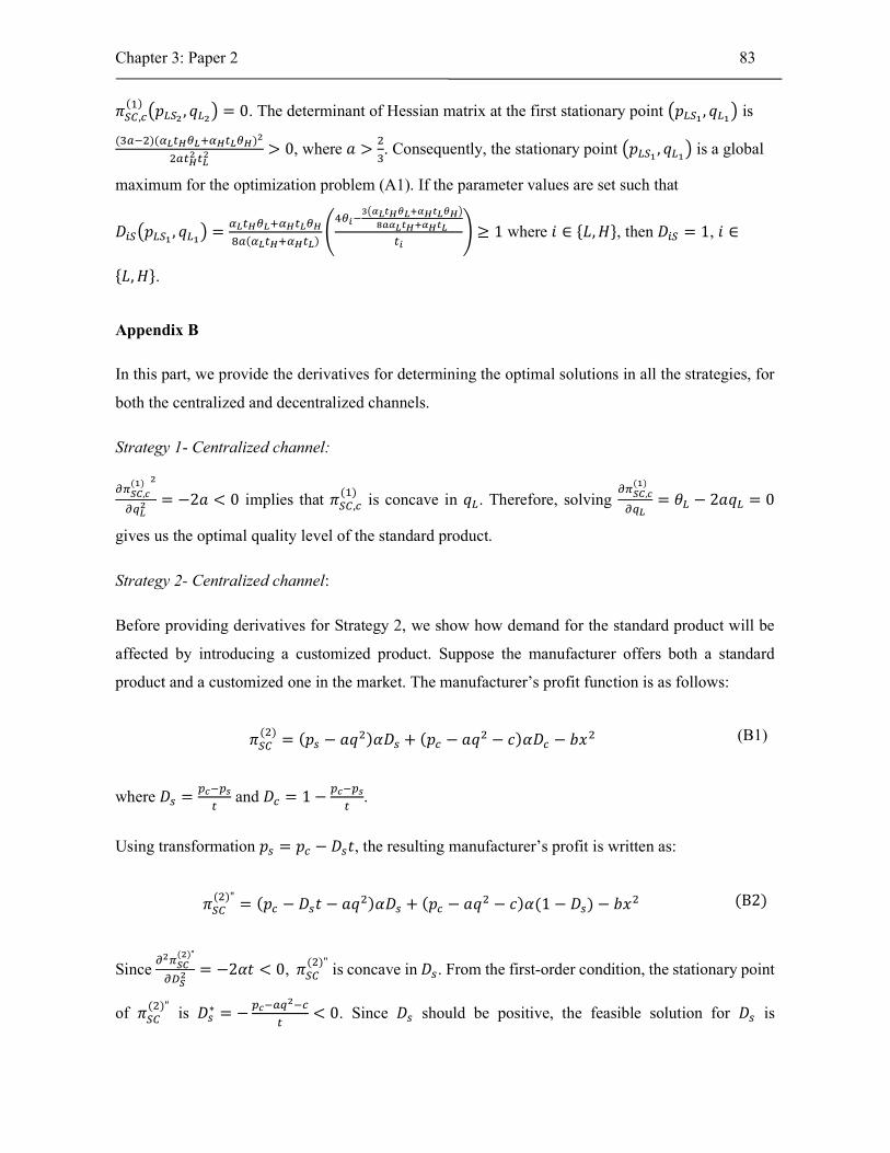
Chapter 3: Paper 2 83
𝜋 ,( )
𝑝 , 𝑞 = 0. The determinant of Hessian matrix at the first stationary point 𝑝 , 𝑞 is
( )( )> 0, where 𝑎 > . Consequently, the stationary point 𝑝 , 𝑞 is a global
maximum for the optimization problem (A1). If the parameter values are set such that
𝐷 𝑝 , 𝑞 =( )
≥ 1 where 𝑖 ∈ {𝐿, 𝐻}, then 𝐷 = 1, 𝑖 ∈
{𝐿, 𝐻}.
Appendix B
In this part, we provide the derivatives for determining the optimal solutions in all the strategies, for
both the centralized and decentralized channels.
Strategy 1- Centralized channel:
,( )
= −2𝑎 < 0 implies that 𝜋 ,( ) is concave in 𝑞 . Therefore, solving ,
( )
= 𝜃 − 2𝑎𝑞 = 0
gives us the optimal quality level of the standard product.
Strategy 2- Centralized channel:
Before providing derivatives for Strategy 2, we show how demand for the standard product will be
affected by introducing a customized product. Suppose the manufacturer offers both a standard
product and a customized one in the market. The manufacturer’s profit function is as follows:
𝜋( )
= (𝑝 − 𝑎𝑞 )𝛼𝐷 + (𝑝 − 𝑎𝑞 − 𝑐)𝛼𝐷 − 𝑏𝑥 (B1)
where 𝐷 = and 𝐷 = 1 − .
Using transformation 𝑝 = 𝑝 − 𝐷 𝑡, the resulting manufacturer’s profit is written as:
𝜋( )"
= (𝑝 − 𝐷 𝑡 − 𝑎𝑞 )𝛼𝐷 + (𝑝 − 𝑎𝑞 − 𝑐)𝛼(1 − 𝐷 ) − 𝑏𝑥 (B2)
Since ( )"
= −2𝛼𝑡 < 0, 𝜋( )" is concave in 𝐷 . From the first-order condition, the stationary point
of 𝜋( )" is 𝐷∗ = − < 0. Since 𝐷 should be positive, the feasible solution for 𝐷 is

Chapter 3: Paper 2 84
represented on interval (0, . 𝜋( )"is a decreasing function on this interval. Therefore, by decreasing
𝐷 , 𝜋( )"will increase. Under the full market coverage, 𝑝 will be set equal to 𝜃𝑞 − (1 − 𝑥)𝑡, and an
increase in 𝑝 leads to a decrease in 𝐷 which consequently increases 𝜋( )". Thus, the manufacturer
is better off by decreasing the demand for standard product. Figure B-1 shows the demand for the
standard product with and without accommodating a customized product.
Figure B-1: Changing demand by introducing a customized product
Following Wu et al. (2012), since ,( )
= −( )
< 0, 𝜋 ,( ) is a concave function
w.r.t. 𝑞 for given 𝑝 and 𝑥 . Therefore, by first solving for the optimal 𝑞 and substituting into the
original profit function, the problem can be reduced to solving for two variables, 𝑝 and 𝑥 . The
resulting profit function 𝜋 ,( , )
is jointly concave w.r.t. 𝑝 and 𝑥 . The sufficient conditions of the
resulting profit function are as follows: ,( , )
= − < 0 , ,( , )
= − < 0 , and
,( , )
,( , )
− ,( , )
= > 0 . Thus, from the first-order conditions of 𝜋 ,( , ) the optimal results
can be found.
Strategy 3- Centralized channel:
The conditions ,( )
= −2𝑎𝛼 < 0, ,( )
= −2𝑎𝛼 < 0, and ,( )
,( )
− ,( )
=
4𝑎 𝛼 𝛼 > 0 denote that 𝜋 ,( )
is jointly concave in 𝑞 and 𝑞 . Thus, the stationary point obtained
from the first-order conditions ,( )
= 𝛼 (𝜃 − 2𝑎𝑞 ) − 𝛼 (𝜃 − 𝜃 ) = 0 and ,( )
= 𝛼 (𝜃 −
2𝑎𝑞 ) = 0 give us the optimal result.

Chapter 3: Paper 2 85
Strategy 4a Centralized channel:
In this strategy, 𝑝 , 𝑞 , 𝑞 , 𝑥 are decision variables. The second partial derivatives of the profit
function w.r.t. the decision variables are as follows: ,( )
= − < 0, ,( )
= − <
0, ,( )
= −2𝑎𝛼 < 0, ,( )
= −2𝑏 − 2𝛼 𝑡 < 0. Also, the determinant of the Hessian matrix is
> 0. Therefore, the stationary point that comes from the first-order conditions is the
optimal solution.
Strategy 4b Centralized channel:
The manufacturer’s profit function 𝜋 ,( ) is not concave in 𝑞 , 𝑞 , and 𝑥 . However, ,
( )
=
−2𝑎𝛼 < 0 implies that, for given values of 𝑞 and 𝑥 , the manufacturer’s profit function is concave
in 𝑞 . Thus, we first solve for 𝑞 for given 𝑞 and 𝑥 then substitute the optimal 𝑞 into the profit
function. The resulting expected profit function 𝜋 ,( , ) is jointly concave in 𝑞 and 𝑥 , because we
have ,( , )
= −2𝑎𝛼 < 0 , ,( , )
= −2𝑏 − 2𝛼 𝑡 < 0, and ,( , )
,( , )
−
,( , )
= 4𝑎𝛼 (𝑏 + 𝛼 𝑡 ) > 0. From solving the first-order conditions of 𝜋 ,( , ), the optimal
solutions for 𝑞 and 𝑥 will be derived.
Strategy 1- Decentralized channel:
Since ,( )
= −2𝑎 < 0 , solving ,( )
= 2𝜃 − 𝜆 − 2𝑎𝑞 = 0 for 𝑞 results in the optimal quality
level.
Strategy 2- Decentralized channel:
Using a backward induction approach, we first maximize the retailer’s profit function. Since ( )
=
−2 − 2 < 0, the first-order condition gives us the retailer’s optimal pricing decision: 𝑝∗ =
+ +( )
for given values of 𝑤 , 𝑞 and 𝑥 . By knowing the retailer’s best response on
retail price for the standard product, the manufacturer’s profit function can be written as a function
of 𝑤 , 𝑞 , and 𝑥 . The determinant of the Hessian matrix of 𝜋 ,( )
(𝑤 , 𝑞 , 𝑥 ) is not negative definite.
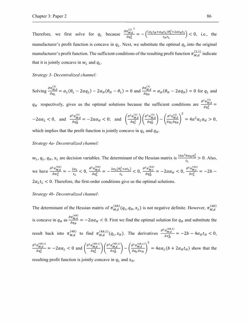
Chapter 3: Paper 2 86
Therefore, we first solve for 𝑞 because ,( )
= −( )
< 0, i.e., the
manufacturer’s profit function is concave in 𝑞 . Next, we substitute the optimal 𝑞 .into the original
manufacturer’s profit function. The sufficient conditions of the resulting profit function 𝜋 ,( , ) indicate
that it is jointly concave in 𝑤 and 𝑞 .
Strategy 3- Decentralized channel:
Solving ,( )
= 𝛼 (𝜃 − 2𝑎𝑞 ) − 2𝛼 (𝜃 − 𝜃 ) = 0 and ,( )
= 𝛼 (𝜃 − 2𝑎𝑞 ) = 0 for 𝑞 and
𝑞 respectively, gives us the optimal solutions because the sufficient conditions are ,( )
=
−2𝑎𝛼 < 0, and ,( )
= −2𝑎𝛼 < 0; and ,( )
,( )
− ,( )
= 4𝑎 𝛼 𝛼 > 0,
which implies that the profit function is jointly concave in 𝑞 and 𝑞 .
Strategy 4a- Decentralized channel:
𝑤 , 𝑞 , 𝑞 , 𝑥 are decision variables. The determinant of the Hessian matrix is > 0. Also,
we have ,( )
= − < 0, ,( )
= − < 0, ,( )
= −2𝑎𝛼 < 0, ,( )
= −2𝑏 −
2𝛼 𝑡 < 0. Therefore, the first-order conditions give us the optimal solutions.
Strategy 4b- Decentralized channel:
The determinant of the Hessian matrix of 𝜋 ,( )
(𝑞 , 𝑞 , 𝑥 ) is not negative definite. However, 𝜋 ,( )
is concave in 𝑞 as ,( )
= −2𝑎𝛼 < 0. First we find the optimal solution for 𝑞 and substitute the
result back into 𝜋 ,( ) to find 𝜋 ,
( , )(𝑞 , 𝑥 ). The derivatives ,
( , )
= −2𝑏 − 4𝛼 𝑡 < 0,
,( , )
= −2𝑎𝛼 < 0 and ,( , )
,( , )
− ,( , )
= 4𝑎𝛼 (𝑏 + 2𝛼 𝑡 ) show that the
resulting profit function is jointly concave in 𝑞 and 𝑥 .
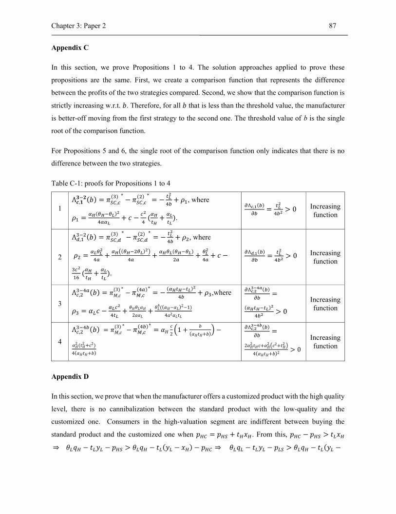
Chapter 3: Paper 2 87
Appendix C
In this section, we prove Propositions 1 to 4. The solution approaches applied to prove these
propositions are the same. First, we create a comparison function that represents the difference
between the profits of the two strategies compared. Second, we show that the comparison function is
strictly increasing w.r.t. 𝑏. Therefore, for all 𝑏 that is less than the threshold value, the manufacturer
is better-off moving from the first strategy to the second one. The threshold value of b is the single
root of the comparison function.
For Propositions 5 and 6, the single root of the comparison function only indicates that there is no
difference between the two strategies.
Table C-1: proofs for Propositions 1 to 4
1 Ʌ𝒄,𝟏
𝟑 𝟐(𝑏) = 𝜋 ,( ) ∗
− 𝜋 ,( ) ∗
= − + 𝜌 , where
𝜌 =( )
+ 𝑐 − ( + ).
Ʌ , ( )= > 0 Increasing
function
2
Ʌ , (𝑏) = 𝜋 ,( ) ∗
− 𝜋 ,( ) ∗
= − + 𝜌 , where
𝜌 = +( )
+( )
+ + 𝑐 −
( + ).
Ʌ , ( )= > 0 Increasing
function
3
Ʌ , (𝑏) = 𝜋𝑀,𝑐(3) ∗
− 𝜋 ,( )∗
= −( )
+ 𝜌 ,where
𝜌 = 𝛼 𝑐 − +𝜃𝐻𝜃𝐿𝛼𝐻
2𝑎𝛼𝐿+
𝜃𝐿4((𝛼𝐻−𝛼𝐿)2−1)
4𝑎2𝛼𝐿𝑡𝐿
Ʌ , ( )=
( )> 0
Increasing function
4
Ʌ , (𝑏) = 𝜋𝑀,𝑐(3) ∗
− 𝜋 ,( )∗
= 𝛼𝐻𝑐
21 +
𝑏
(𝛼𝐻𝑡𝐻+𝑏)−
𝛼𝐻2 (𝑡𝐻
2 +𝑐2)
4(𝛼𝐻𝑡𝐻+𝑏)
Ʌ , ( )=
2𝛼𝐻2 𝑡𝐻𝑐+𝛼𝐻
2 𝑐2+𝑡𝐻2
4(𝛼𝐻𝑡𝐻+𝑏)2> 0
Increasing function
Appendix D
In this section, we prove that when the manufacturer offers a customized product with the high quality
level, there is no cannibalization between the standard product with the low-quality and the
customized one. Consumers in the high-valuation segment are indifferent between buying the
standard product and the customized one when 𝑝 = 𝑝 + 𝑡 𝑥 . From this, 𝑝 − 𝑝 > 𝑡 𝑥
⇒ 𝜃 𝑞 − 𝑡 𝑦 − 𝑝 > 𝜃 𝑞 − 𝑡 (𝑦 − 𝑥 ) − 𝑝 ⇒ 𝜃 𝑞 − 𝑡 𝑦 − 𝑝 > 𝜃 𝑞 − 𝑡 (𝑦 −
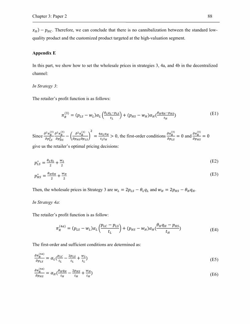
Chapter 3: Paper 2 88
𝑥 ) − 𝑝 . Therefore, we can conclude that there is no cannibalization between the standard low-
quality product and the customized product targeted at the high-valuation segment.
Appendix E
In this part, we show how to set the wholesale prices in strategies 3, 4a, and 4b in the decentralized
channel:
In Strategy 3:
The retailer’s profit function is as follows:
𝜋( )
= (𝑝 − 𝑤 )𝛼 + (𝑝 − 𝑤 )𝛼 ( ) (E1)
Since ( ) ( )
−( )
= > 0, the first-order conditions ( )
= 0 and ( )
= 0
give us the retailer’s optimal pricing decisions:
𝑝∗ = + (E2)
𝑝∗ = + (E3)
Then, the wholesale prices in Strategy 3 are 𝑤 = 2𝑝 − 𝜃 𝑞 and 𝑤 = 2𝑝 − 𝜃 𝑞 .
In Strategy 4a:
The retailer’s profit function is as follow:
𝜋( )
= (𝑝 − 𝑤 )𝛼𝑝 − 𝑝
𝑡+ (𝑝 − 𝑤 )𝛼 (
𝜃 𝑞 − 𝑝
𝑡) (E4)
The first-order and sufficient conditions are determined as:
( )
= 𝛼 ( − + ) (E5)
( )
= 𝛼 ( − + ) (E6)
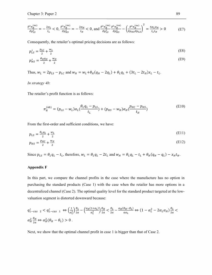
Chapter 3: Paper 2 89
( )
= − < 0, ( )
= − < 0, and ( ) ( )
−( )
= > 0 (E7)
Consequently, the retailer’s optimal pricing decisions are as follows:
𝑝∗ = + (E8)
𝑝∗ = + (E9)
Thus, 𝑤 = 2𝑝 − 𝑝 and 𝑤 = 𝑤 +𝜃 (𝑞 − 2𝑞 ) + 𝜃 𝑞 + (3𝑡 − 2𝑡 )𝑥 − 𝑡 .
In strategy 4b:
The retailer’s profit function is as follows:
𝜋( )
= (𝑝 − 𝑤 )𝛼 (𝜃 𝑞 − 𝑝
𝑡) + (𝑝 − 𝑤 )𝛼 (
𝑝 − 𝑝
𝑡)
(E10)
From the first-order and sufficient conditions, we have:
𝑝 = + (E11)
𝑝 = + (E12)
Since 𝑝 = 𝜃 𝑞 − 𝑡 , therefore, 𝑤 = 𝜃 𝑞 − 2𝑡 and 𝑤 = 𝜃 𝑞 − 𝑡 + 𝜃 (𝑞 − 𝑞 ) − 𝑥 𝑡 .
Appendix F
In this part, we compare the channel profits in the case where the manufacture has no option in
purchasing the standard products (Case 1) with the case when the retailer has more options in a
decentralized channel (Case 2). The optimal quality level for the standard product targeted at the low-
valuation segment is distorted downward because:
𝑞 ∗ < 𝑞
∗ ⇔ −( )
< −( )
⇔ (1 − 𝛼 − 2𝛼 𝛼 ) <
𝛼 ⇔ 𝛼 (𝜃 − 𝜃 ) > 0 .
Next, we show that the optimal channel profit in case 1 is bigger than that of Case 2.
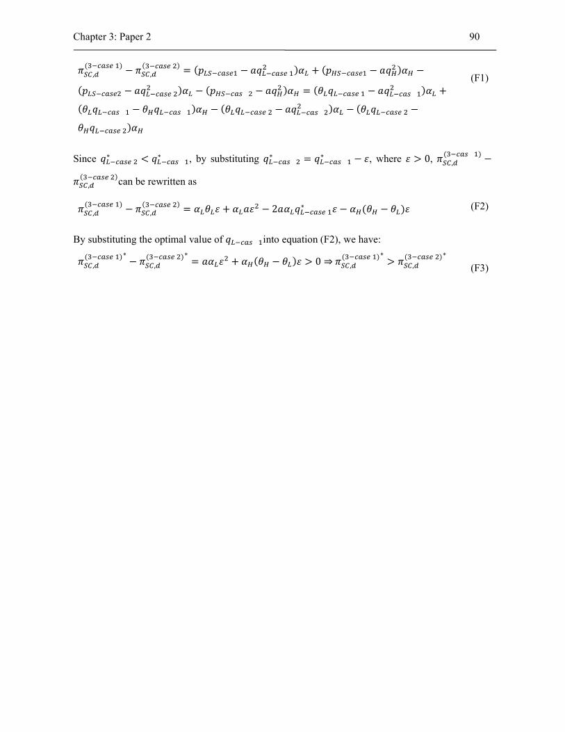
Chapter 3: Paper 2 90
𝜋 ,( )
− 𝜋 ,( )
= (𝑝 − 𝑎𝑞 )𝛼 + (𝑝 − 𝑎𝑞 )𝛼 −
(𝑝 − 𝑎𝑞 )𝛼 − (𝑝 − 𝑎𝑞 )𝛼 = (𝜃 𝑞 − 𝑎𝑞 )𝛼 +
(𝜃 𝑞 − 𝜃 𝑞 )𝛼 − (𝜃 𝑞 − 𝑎𝑞 )𝛼 − (𝜃 𝑞 −
𝜃 𝑞 )𝛼
(F1)
Since 𝑞 ∗ < 𝑞
∗ , by substituting 𝑞 ∗ = 𝑞
∗ − 𝜀, where 𝜀 > 0, 𝜋 ,( )
−
𝜋 ,( )can be rewritten as
𝜋 ,( )
− 𝜋 ,( )
= 𝛼 𝜃 𝜀 + 𝛼 𝑎𝜀 − 2𝑎𝛼 𝑞 ∗ 𝜀 − 𝛼 (𝜃 − 𝜃 )𝜀 (F2)
By substituting the optimal value of 𝑞 into equation (F2), we have:
𝜋 ,( )∗
− 𝜋 ,( )∗
= 𝑎𝛼 𝜀 + 𝛼 (𝜃 − 𝜃 )𝜀 > 0 ⇒ 𝜋 ,( )∗
> 𝜋 ,( )∗
(F3)

Chapter 4
4 Paper 3: Product line design with customization: the effects of
demand uncertainty and distribution channel structure
History: This paper was initiated during my stay abroad at the University of Nottingham in August
–September, 2017. This paper is expected to be submitted in May 2018.

Chapter 4: Paper 3 90
Product line design with customization in a horizontally differentiated market: the effects of
demand uncertainty and distribution channel structure
Parisa Bagheri Tookanlou
Department of Economics and Business Economics
School of Business and Social Sciences, Aarhus University
Fuglesangs Allé 4, 8210 Aarhus, Denmark
Abstract
In this paper, I analyze a product line design problem faced by a manufacturing firm where the product
line consists of a customized product in addition to a standard product, and is offered in a market in
which consumers are heterogeneous on the aesthetic attributes of the product. The product line
decisions include the prices of the two products and the customization level for the customized
product. The customization level of a product is defined by the fraction of aesthetic attributes of the
product that the manufacturer chooses to customize. In contrast to the existing literature on product
line design which predominantly assumes deterministic demand, I consider the presence of demand
uncertainty and frame the product line design problem in a single period (newsvendor) setting. With
the presence of demand uncertainty, the order or production quantity is also a relevant decision
variable. I examine the effect of demand uncertainty on product line decisions. Furthermore, I
examine how product line decisions are influenced by channel structure. While I use the centralized
channel as a benchmark, I consider the decentralized channel where the customized product is sold
through an online channel owned by the manufacturer and the standard product is sold through a
retailer. I introduce a supply contract between the manufacturer and the retailer with the purpose of
improving channel profitability and coordinating the distribution channel. The analytical results and
numerical examples provide interesting insights into the importance of taking into account demand
uncertainty in designing a product line. This study also demonstrates the potential of using a supply
contract in improving channel profitability, and hence, should motivate firms to implement such a
contract in the context of product line design.
Keywords: product line design, demand uncertainty, customization level, distribution channel.
Chapter 4: Paper 3 91
4.1 Introduction
In view of the rapid growth of e-commerce and mass customization technologies, manufacturing
firms, nowadays, cannot ignore the possibility of modifying their product line by offering customized
products alongside the standard or non-customized products. Such a product line extension may
require manufacturing firms to consider the adoption of a dual channel in selling their products. They
may often need to involve a channel partner, e.g. retailer, especially in selling the standard product.
However, selling customized products in a direct or online channel is obviously a viable option since
consumers may prefer to buy personalized goods online (Gandhi et al. 2013). Companies such as
Nike and Adidas implement the customization strategy where, in addition to selling the standard
trainers at their retail outlets, they also allow customers to personalize their trainers at their websites.
Timbuk2 offers customized bags online and also sells more standard bags through resellers. Dell and
Gateway also sells customized laptops in their online channel alongside the more standard laptops
sold at their retail stores. When employing such a product line design in a dual channel, a
manufacturer must make multiple decisions, including the customization level of the customized
products, the price to be charged to consumers, and the price to be charged to the retailer for the
standard product. The retailer must make decisions on the retail price for the standard product, and
on the quantity to order from the manufacturer. The latter decision made by the retailer is particularly
relevant in the case where demand uncertainty is present and the products are sold in a relatively short
selling season such that the retailer will only place one order prior to demand realization.
In this paper, I examine the product line design strategy that offers both the standard and customized
products, sold through a dual channel. This paper advances the existing literature primarily by
considering the presence of demand uncertainty. While product line design has long been a central
topic in the economics, marketing, and operations literature, most of the existing work considers
deterministic demand, thereby neglecting the possible supply-demand mismatch caused by the
demand uncertainty that is prevalent in many real settings. Hence, little light has been shed on how
demand uncertainty influences product line decisions. The deterministic demand assumption is
acceptable in situations where the firm operates in a make-to-order (MTO) or an assemble-to-order
(ATO) manner, i.e., the firm makes the ordering or production decision after the consumers make
their purchasing requests. However, the assumption is questionable in the situations where the number
of consumers is uncertain. For example, in the apparel industry, developing accurate forecasts
remains a major challenge, especially for any seasonal introduction (Fisher et al., 1994 and Kuksov
and Wang 2013). In such situations, production or ordering decision must be made prior to the selling
season, i.e., the firm operates in a make-to-stock (MTS) manner. As well illustrated by the classical

Chapter 4: Paper 3 92
newsvendor problem, the firm must pay the costs associated with the supply-demand mismatch
caused by the demand uncertainty.
Another basic problem analyzed in this paper is related to the adoption of a distribution channel where
the manufacturer must rely on the retailer to sell the standard product. As different parties along a
distribution channel may not share the same interest, the distribution channel is often not fully
coordinated. In the decentralized channel, the retailer who faces demand uncertainty must make a
joint decision on price and order quantity while taking into account the presence of the customized
product offered by the manufacturer via the online channel. This situation is different from the case
of a centralized channel where the manufacturer is the only channel member involved. In the light of
this, this paper also aims to uncover the extent to which the existence of a retailer in a distribution
channel and its strategic behavior influence the manufacturer’s product line decisions. As it is
expected that the channel’s performance in a decentralized distribution channel is inferior to that of a
centralized channel, this article also examines how channel coordination can be used to improve the
channel profitability. More specifically, I aim to answer the following questions:
(1) How does demand uncertainty affect product line design decisions when the product line
consists of a standard product and a customized product, and how are these decisions affected
by the type of distribution channel?
(2) How can channel profitability be improved to the benefit of the channel members by a supply
chain contract such as a buy-back contract?
The rest of this paper is organized as follows. In the next section, a review of the relevant literature
is presented. In Section 4.3, I present the models and results for the centralized and decentralized
channels. Section 4.4 focuses on the evaluation of a buy-back contract for improving the channel’s
profitability. In Section 4.5, I summarize the conclusions and suggest some directions for future
research.
4.2 Literature Review
This research contributes to the literature on product line design in a market where consumers are
horizontally differentiated. A common feature of the existing literature is that consumers are assumed
to be uniformly distributed over Hotelling’s line, and one of the main central questions is how many
products to be offered in the product line. De Groote (1994) studies the role of flexibility in
accommodating product line extension in the horizontal direction. Several authors analyze the
attractiveness of mass customization strategy relative to the standard mass production strategy (see

Chapter 4: Paper 3 93
e.g. Gaur and Honhon 2006, Jiang et al. 2006, Alptekinoğlu and Corbett 2010, and Wong and
Lesmono 2011). All these papers consider product line design from the manufacturer’s point of view,
so that competition and channel structure are not relevant. There are a number of papers that examine
the competition between the standard and customized products in a duopoly market. Dewan et al.
(2003) evaluate product customization and price discrimination in monopoly and duopoly markets.
They show that a manufacturer may obtain the highest profits by offering both standard and fully
customized products and that the manufacturer can increase prices for the standard and customized
products when customization and information technologies enhance. In their model, however, the
customization level is not a decision variable. Studies that consider customization level are presented
in e.g. Syam and Kumar (2006), Alptekinoğlu and Corbett (2008), Mendelson and Parlaktürk (2008a
and 2008b), and Xia and Rajagopalan (2009). Although these papers consider customization level,
they do not investigate the effect of the distribution channel structure. A study on the product line
design problem in a distribution channel where consumers are only horizontally differentiated is
presented in Liu and Cui (2010). They show that a decentralized channel can be an efficient structure
of distribution by providing a product line length that is optimal from a social welfare perspective.
Their analysis is, however, limited to the case of two different products and does not pay attention to
the choice of customization level, as is done in this paper. Furthermore, while they consider a standard
distribution channel that consists of a manufacturer and a retailer, I consider a dual channel where the
standard product is sold through a retailer and the customized products are sold in an online channel
owned by the manufacturer.
The product line design problem in a dual channel that involves customization is studied by Li et al.
(2015). They consider competition between the manufacturer’s online customization channel and the
conventional retailer, which is also adopted in this paper. In their paper, however, demand is assumed
to be deterministic. We extend their model by considering demand uncertainty and its effects on the
product line design decisions.
Most studies in the literature on product line design assume deterministic demand. Only few papers
consider product line design problems in the case with demand uncertainty, and they all consider a
market where consumers are vertically differentiated. Xiao and Xu (2014) focus on examining how
the risk aversion in the supply chain affects the product line decisions when information asymmetry
is not present. Rong et al. (2015) consider demand uncertainty in a product line design problem with
information asymmetry. They illustrate the interplay between two effects: risk pooling that mitigates
the supply-demand mismatch due to demand uncertainty and market segmentation that facilitates
consumer differentiation. While they consider product line design problems in a vertically
Chapter 4: Paper 3 94
differentiated market, this paper studies product line design in a horizontally differentiated market
where customized products are offered in addition to the standard product.
This paper is also related to the vast literature on dual channel supply chains (e.g. Chiang et al. 2003,
Tsay and Agrawal 2004, Chiang and Monahan 2005, Huang and Swaminathan 2009, and Hua et al.,
2010) that all considers a market without demand uncertainty. Few papers study dual channel supply
chains with demand uncertainty. Chiang (2010) investigates the impact of consumers’ stock-out based
substitution on the product availability and the channel efficiency of a dual-channel supply chain. In
his paper, there is only a single product sold through a direct channel and an independent retailer, and
the two channels apply a base stock inventory policy. This paper differs in that the products
distributed through the two channels are different, and the inventory or order quantity decision for
the standard product is modelled as a newsvendor problem. Dumrongsiri et al. (2008) investigate the
impact of demand variability on equilibrium prices. They consider a dual channel where the
manufacturer uses a traditional channel to sell its product and introduces a direct channel to sell the
product in a make-to-order fashion. They show that the dual channel is better than a single channel
when demand uncertainty, wholesale price, consumer valuation, and retailer’s marginal cost are low.
Although the dual channel setup considered in this paper is similar to that of Dumrongsiri et al.
(2008), there are some differences. First, they do not analyze a product line design problem in the
sense that none of product design decisions are considered, whereas in this paper, the manufacturer
must determine an optimal customization level. Second, this paper considers channel coordination
between the manufacturer and the retailer, an issue that is not considered in their paper.
Finally, this paper also contributes to the literature on channel coordination in product line design.
Although many studies analyze the effects of distribution channel structure on product line strategies,
literature focusing on channel performance improvements by means of channel coordination
mechanisms is sparse. Many authors study channel coordination in contexts other than product-line
design. Jeuland and Shugan (1983), Moorthy (1987), Ingene and Parry (1995), and Raju and Zhang
(2005) use quantity discounts or two-part tariffs as the coordination mechanism. Cachon and
Lariviere, (2005) examine revenue-sharing contracts as a mechanism to motivate supply chain
members to cooperate on ordering decisions. Some authors (e.g. Pasternack 1985, Song et al. 2008,
and Shao et al. 2013) examine the use of buy-back contracts to coordinate the supply chain. In this
paper, I also use the buy-back contract as a mechanism to improve the channel profitability. Channel
coordination mechanisms in the context of product line design are studied by Hua et al. (2011) and
Jerath et al. (2017). They both consider the product line design problem with vertical product
differentiation. Under the assumption of deterministic demand and exogenous quality, Hua et al.

Chapter 4: Paper 3 95
(2011) show that a revenue-sharing contract can perfectly coordinate the distribution channel on
product design decisions. The work of Jerath et al. (2017) is more related to this paper as it considers
demand uncertainty. They demonstrate that quality is decreasing in demand uncertainty, and that a
wholesale price contract cannot coordinate the channel. This paper, however, differs because I
consider the product line design problem in which consumers are horizontally differentiated and the
customization level is a key decision. Furthermore, while they consider a standard distribution
channel that involves a manufacturer and a retailer, this paper considers a dual channel in which the
retailer is also in competition with the manufacturer. To the best of the author’s knowledge, this paper
is the first studying channel coordination in the context of product line design in a horizontally
differentiated market where demand uncertainty is present.
4.3 Models
The product line considered in this paper consists of two products, a standard product and a
customized product, indexed by i = s, c. It is assumed that the two types of products have the same
quality level, which is determined exogenously. The product line decisions include the prices of the
two products and the customization level for the customized product. This study evaluates two
channel structures. In a centralized channel, the manufacturer directly sells both the standard and
customized products to the end consumers. In a decentralized channel, the standard product is sold
through a retailer, and the customized product is sold directly by the manufacturer. Consumers are
heterogeneous in their valuation of the aesthetic dimensions of the product, and their preferences are
represented on Hotelling’s line. Hotelling’s line is the interval [0,1] such that each point represents
customer’s preference (or location). In other words, each consumer is represented by his/her aesthetic
preference of the product, which is denoted by 𝑦 ∈ [0, 1]. The size of the market is normalized to
one. Note that since the focus of this paper is on horizontal differentiation, consumers’ heterogeneity
in their quality valuation is excluded. In other words, the product line design problem considered in
this paper does not include quality-based segmentation.
Each consumer incurs a per unit mismatch cost 𝑡 for any deviation between her best preference and
that of the purchased product. The manufacturer offers the customized product with customization
level 𝑥, which is defined as the fraction of aesthetic attributes of the product that she chooses to
customize. Following Li et al. (2015), a standard product (with 𝑥 = 0), is represented by the left-end
point of the Hotelling’s line, whereas a fully customized product (with 𝑥 = 1), is represented by the
right-end point of the Hotelling’s line. The utility of the consumer with preference y for the standard
product sold at price 𝑝 is 𝑢 = 𝑣 − 𝑡𝑦 − 𝑝 , where 𝑣 represents the consumer’s quality valuation of
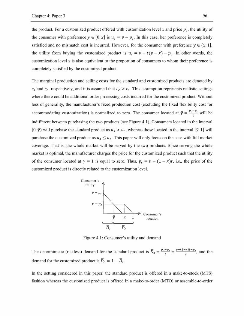
Chapter 4: Paper 3 96
the product. For a customized product offered with customization level x and price 𝑝 , the utility of
the consumer with preference y ∈ [0, 𝑥] is 𝑢 = 𝑣 − 𝑝 . In this case, her preference is completely
satisfied and no mismatch cost is incurred. However, for the consumer with preference 𝑦 ∈ (𝑥, 1],
the utility from buying the customized product is 𝑢 = 𝑣 − 𝑡(𝑦 − 𝑥) − 𝑝 . In other words, the
customization level x is also equivalent to the proportion of consumers to whom their preference is
completely satisfied by the customized product.
The marginal production and selling costs for the standard and customized products are denoted by
𝑐 and 𝑐 , respectively, and it is assumed that 𝑐 > 𝑐 . This assumption represents realistic settings
where there could be additional order processing costs incurred for the customized product. Without
loss of generality, the manufacturer’s fixed production cost (excluding the fixed flexibility cost for
accommodating customization) is normalized to zero. The consumer located at 𝑦 = will be
indifferent between purchasing the two products (see Figure 4.1). Consumers located in the interval
[0, 𝑦) will purchase the standard product as 𝑢 > 𝑢 , whereas those located in the interval [𝑦, 1] will
purchase the customized product as 𝑢 ≤ 𝑢 . This paper will only focus on the case with full market
coverage. That is, the whole market will be served by the two products. Since serving the whole
market is optimal, the manufacturer charges the price for the customized product such that the utility
of the consumer located at 𝑦 = 1 is equal to zero. Thus, 𝑝 = 𝑣 − (1 − 𝑥)𝑡, i.e., the price of the
customized product is directly related to the customization level.
Figure 4.1: Consumer’s utility and demand
The deterministic (riskless) demand for the standard product is 𝐷 = =( )
, and the
demand for the customized product is 𝐷 = 1 − 𝐷 .
In the setting considered in this paper, the standard product is offered in a make-to-stock (MTS)
fashion whereas the customized product is offered in a make-to-order (MTO) or assemble-to-order
1
⬚
𝑥 Consumer’s
location
Consumer’s utility
𝑦
𝑣 − 𝑝
𝑣 − 𝑝
𝐷 𝐷
Chapter 4: Paper 3 97
(ATO) fashion. The newsvendor problem is applied for the standard product so that the inventory for
the standard product must be determined before the selling period starts. Thus, in this problem, the
relevant decision variables include the prices of the standard and customized products, the
customization level for the customized product, and the inventory for the standard product.
Although demand uncertainty is present for both products, demand uncertainty for the customized
product will be excluded as it is assumed to be offered in a MTO or an ATO fashion. This assumption
is also adopted in Dumrongsiri et al. (2008). The model developed here is probably more suitable for
the ATO setting because the customization offered is mainly related to the aesthetic attributes of the
product while the basic components are the same as in the standard product. Furthermore, since the
consumer utility function in my model does not consider the waiting time consumers must incur, the
validity of the model is less questionable in the ATO setting since the lead time is shorter than the
MTO setting. However, the model could also be a good representation of the MTO setting as long as
the lead time is not so excessive or consumers are not so sensitive to lead time.
Note that in this paper, I focus on the effect of demand uncertainty on the optimal inventory of the
standard product that may have an influence on the product line design decisions, including prices
and customization level. The effect of demand uncertainty on the stocking of materials or
components, especially in the ATO setting, is excluded. This may represent one limitation of the
model, but it can, to a certain extent, be justified in real settings. Consider, for example, manufacturing
firms that offer standard and customized printed t-shirts. The supply of the basic material for the two
products, i.e., the blank t-shirts, is easier to manage because demand uncertainty is lower due to the
pooling effect and its life cycle may last much longer than the printing design.
To capture demand uncertainty for the standard product, randomness is included in addition to the
deterministic demand function explained above. Following Petruzzi and Dada (1999), randomness is
assumed to be price independent, and can be modelled either in an additive or a multiplicative fashion.
The additive fashion is considered in this paper because it makes the model more tractable as demand
variability becomes independent of the price charged. The choice of additive demand is also common
in the literature (e.g. Dumrongsiri et al. 2008). The stochastic demand function for the standard
product can be written as:
𝐷 = 𝐷 + 𝜗 , (1)

Chapter 4: Paper 3 98
where 𝜗 ∈ [𝐴, 𝐵] is a random variable with mean 𝜇 and standard deviation 𝜎 , and is independent
of the price charged to the consumers. The probability density function, cumulative distribution
function, and inverse cumulative distribution function of 𝜗 are denoted by 𝑓(·), 𝐹(·), and 𝐹 (·),
respectively.
The stochastic demand function for the customized product can be written as:
𝐷 = 𝐷 + 𝜗 , (2)
where 𝜗 is a random variable with mean 𝜇 and standard deviation 𝜎 . As previously explained, since
the customized product is offered in an MTO or ATO fashion, the manufacturer will always satisfy
the demand for the customized product without the risk of having the supply-demand mismatch, i.e.,
𝜎 does not play any role. Without loss of generality, it is assumed that both 𝜇 and 𝜇 are equal to
zero. This assumption implies that the randomness in demand does not have any influence on the
riskless demands for both products, i.e., the riskless demands are only influenced by the product line
decisions. Hence, the riskless demand for the customized product is equal to 𝐷 .
For the standard product, the number of units stocked at the beginning of the selling period, 𝑄, must
be determined prior to the selling period. If demand during the selling period does not exceed 𝑄, then
the revenue is 𝑝 𝐷 , and the per-unit inventory or disposal cost h is incurred for each of the 𝑄 − 𝐷
leftovers. Alternatively, if demand exceeds 𝑄, then the revenue is 𝑝 𝑄, and the per-unit penalty cost
𝑠 is incurred for each of the 𝐷 − 𝑄 shortages. Note that my model assumes that there is no
substitution between the two products. This implies that consumers who are willing to purchase the
standard product but face stock-out will not be interested in purchasing the customized product. This
assumption allows for an examination of the most severe impact of demand uncertainty on the channel
profitability.
Following Petruzzi and Dada (1999), the transformation of variables is applied by defining 𝑧 = 𝑄 −
𝐷 , as the stocking level to fulfill the stochastic portion of the demand. The order quantity is equal to
𝑄 = 𝑧 + 𝐷 . The notations regarding the parameters and decision variables are presented in Table
4.1.

Chapter 4: Paper 3 99
Table 4.1: Notations
Decision variables
𝑝 Price of product 𝑖, (𝑖 = 𝑠, 𝑐)
𝑥 Customization level offered by the manufacturer
𝑤 Wholesale price in the decentralized channel for the standard product
𝑤 Wholesale price for the standard product under the buy-back contract
𝑏 Buy-back price
Marketing parameters
𝐷 Demand for product 𝑖, (𝑖 = 𝑠, 𝑐)
𝑣 Consumer’s quality valuation of the product
𝑡 Unit mismatch cost for consumers
𝜇 Mean of the uncertain part of demand for product 𝑖, (𝑖 = 𝑠, 𝑐)
𝜎 Standard deviation of the uncertain part of demand for product 𝑖, (𝑖 = 𝑠, 𝑐)
𝜗 Uncertain part of demand for product 𝑖, (𝑖 = 𝑠, 𝑐)
𝑦 Consumer’s location along Hotelling’s line
Production parameters
a Cost coefficient of the production cost
b Coefficient of the fixed investment cost to accommodate customization
𝑐 Marginal production cost for the standard product
𝑐 Marginal production cost for the customized product
𝑧 Stocking level
𝑄 Total order quantity for the standard product
𝑠 Per-unit penalty cost for shortages
ℎ Per-unit holding/disposal cost for unsold products
Others
𝜋 Channel’s profit
𝜋 Retailer’s profit
𝜋 Manufacturer’s profit
4.3.1 Centralized Channel
I first consider the problem in the centralized channel where the manufacturer sells the two products
directly to the end consumers and makes decisions on the customization level 𝑥, the price for the

Chapter 4: Paper 3 100
standard product 𝑝 , the price for the customized one 𝑝 , and stocking level 𝑧 to maximize the
expected profit.
The manufacturer’s expected profit can be written as follows:
𝐸[𝜋 (z, 𝑝 , 𝑥)] = (𝑝 − 𝑐 )𝐷 + (𝑝 − 𝑐 )(1 − 𝐷 ) − (𝑐 + ℎ)O(z) − (𝑝 + 𝑠 −
𝑐 )S(𝑧) − 𝑏𝑥
(3)
where 𝑝 = 𝑣 − (1 − 𝑥)𝑡; O(𝑧) = ∫ (z − 𝓊) 𝑓(𝓊)𝑑𝓊 represents the expected overages at the end
of the selling period; and S(𝑧) = ∫ (𝓊 − 𝑧) 𝑓(𝓊)𝑑𝓊 represents the expected shortages at the end of
the selling period.
The first term at the right hand side of (3) represents the manufacturer’s expected profit from
producing and selling the standard product. The second term represents the expected profit from
producing and selling the customized product. The next two terms represent the expected overage
and underage costs for the standard product, and the last term is the fixed investment cost
corresponding to the customization level offered. Maximizing the manufacturer’s expected profit
function over the decision variables characterizes the manufacturer’s optimal customization level,
prices, and quantity ordered, that can be summarized in the following proposition.
(Proofs for all propositions in this section are provided in Appendix A).
Proposition 1: The manufacturer’s optimal decisions in the centralized channel: 𝑥∗, 𝑝∗, and 𝑧∗,
satisfy the following three equations simultaneously:
𝑝∗ = 𝑝 + 𝑥𝑡 − 𝑆(𝑧) , where 𝑝 = 𝑣 − 𝑡 − (𝑐 − 𝑐 ) (4)
𝐹(𝑧∗) = or 𝑧∗ = 𝐹 ( ) (5)
𝑥∗ =( )
(2𝑝 + 𝑥 ), where 𝑥 = 𝑐 − 𝑐 + 3𝑡 − 2𝑣 (6)
The optimal solutions for a newsvendor problem with price decision are uniquely determined if the
condition 2𝐻(𝑧) +( )
> 0 is fulfilled, where 𝐻(𝑧) =( )
( ) denotes the hazard rate function
Petruzzi and Dada (1999). This condition is satisfied by many distributions commonly used in the
literature on inventory modelling, such as the Normal and Uniform distributions (Dumrongsiri et al.

Chapter 4: Paper 3 101
2008). Equation (5) also represents what is called the critical ratio, i.e., the ratio of the unit underage
cost to the sum of the underage and overage costs. In Appendix A, I show that 𝑥∗, 𝑝∗, and 𝑧∗ are
uniquely determined if 𝐹(·) satisfies the condition 2𝐻(𝑧) +( )
> 0. The optimal selling price of
the customized product can be directly determined once the optimal customization level is obtained,
i.e., 𝑝 ∗ = 𝑣 − (1 − 𝑥∗)𝑡.
Before analyzing the effect of demand uncertainty on the product line decisions, it is useful to discuss
how the decision variables influence each other. Propositions 2(a) to 2(c) summarize the results.
Proposition 2: By assuming ceteris paribus:
(a) The optimal price for the standard product 𝑝∗ is increasing in the stocking level 𝑧.
(b) Under the following condition: 𝐻(𝑧∗) >( )
(1 − 𝐹(𝑧∗)) , the optimal stocking level 𝑧 is
increasing in the customization level 𝑥.
(c) The optimal stocking level 𝑧 is increasing in the price 𝑝 .
The following discussion will focus on the effect of demand uncertainty on the optimal product line
decisions. The main findings on the effect of demand uncertainty are summarized in the following
propositions.
Proposition 3: In the centralized channel, the optimal customization level for the customized product
and the price for the standard product in the case with demand uncertainty are lower than those in
the case with deterministic demand.
Proposition 4: In the centralized channel, the riskless demand for the standard product in the
presence of demand uncertainty is higher than that of the case with deterministic demand, and vice
versa for the customized product.
The two propositions above clearly show that the presence of demand uncertainty influences the
product line decisions. In the case with deterministic demand, there is no risk of overstocking or
understocking so that the optimal decisions on price and customization level are obtained by solving
the deterministic part of the manufacturer’s profit function. When demand is uncertain, there is the
risk of overstocking and understocking and hence, the optimal decisions obtained in the deterministic
setting need to be adjusted to reduce that risk. The manufacturer has the opportunity to reduce the
risk through her decision on the price for the standard product. As shown in Proposition 3, the price

Chapter 4: Paper 3 102
for the standard product in the stochastic setting is lower than the price in the deterministic setting.
This course of action will increase the riskless demand of the standard product. This result is in line
with Petruzzi and Dada (1999) in that the optimal pricing decision is such that the demand coefficient
of variation is reduced. In the additive case where a pricing decision cannot change demand variance,
a reduction in the price will increase the demand, which leads to the reduction in the coefficient of
variation. The price reduction for the standard product can also be seen as the manufacturer’s way of
reducing the unit underage cost associated with the risk of understocking. In fact, that is the only
possible way for the manufacturer to reduce the unit underage cost caused by demand uncertainty.
However, this course of action also has a downside as it reduces the revenue from the customized
product. The manufacturer has the opportunity to alleviate this downside by offering a lower
customization level, so that it may limit the reduction in the demand for the customized product. As
shown in Proposition 4, those two driving forces eventually result in the optimal solution with the
higher riskless demand for the standard product compared to the demand in the absence of
uncertainty.
4.3.2 Decentralized Channel
In this section, I study the case where the manufacturer sells the standard product to the end consumers
through a retailer who faces the uncertain demand. As in the centralized channel, the customized
product is sold in the direct channel owned by the manufacturer. The analysis is carried out under the
scenario in which the manufacturer first determines the customization level 𝑥, the selling price for
the customized product 𝑝 , and the wholesale price for the standard product 𝑤. The retailer then
determines the order quantity 𝑄 and the retail price 𝑝 . As in the centralized channel, the
transformation of variable is applied by defining 𝑧 = 𝑄 − 𝐷 (𝑝 , 𝑥), as the stocking level to fulfill
the stochastic portion of the demand. Since the manufacturer designs the customized product and full
market coverage is considered, the price of the customized product can be determined using the same
expression as in the centralized channel: 𝑝 = 𝑣 − (1 − 𝑥)𝑡. Note, however, that as will be shown
later, the optimal price of the customized product in the decentralized channel can be different from
that in the centralized channel due to the difference in the optimal customization level.
The retailer’s expected profit is as follows:
𝐸(𝜋 (𝑝 , z)) = (𝑝 − 𝑤)𝐷 − (𝑤 + ℎ)O(z) − (𝑝 + 𝑠 − 𝑤)S(z) (7)
where 𝐷 = , 𝑝 = 𝑣 − (1 − 𝑥)𝑡, O(𝑧) = ∫ (𝑧 − 𝓊) 𝑓(𝓊)𝑑𝓊, and S(𝑧) = ∫ (𝓊 − 𝑧) 𝑓(𝓊)𝑑𝓊.
Chapter 4: Paper 3 103
The following propositions characterize the retailer’s optimal decisions for the given values of the
manufacturer’s decisions on 𝑤, 𝑥, and 𝑝 .
Proposition 5: The retailer’s optimal decisions 𝑝∗ and 𝑧∗ satisfy the following two equations
simultaneously:
𝑝∗ = 𝑝 + 𝑥 + − 𝑆(𝑧) , where 𝑝 = (8)
𝐹(𝑧∗) = or 𝑧∗ = 𝐹 ( ) (9)
(Proofs for all propositions in this section are provided in Appendix B).
Similar to the centralized channel, the optimal solutions are uniquely determined if the condition
2𝐻(𝑧) +( )
> 0 is fulfilled (see Appendix B).
The following two propositions show how the retailer’s optimal order quantity is influenced by the
customization level and how the price for the standard product charged by the retailer in the stochastic
setting is different from the price offered in the deterministic setting. The results shown in the two
propositions are consistent with those in the centralized channel. Due to the risk of overstocking or
understocking, the retailer will have an incentive to increase the riskless demand for the standard
product by reducing the selling price in order to lower the demand coefficient of variation.
Proposition 6: In the decentralized channel, the retailer’s optimal stocking level 𝑧∗ is increasing in
the customization level 𝑥.
Proposition 7: In the decentralized channel, the price for the standard product in the case with
demand uncertainty is lower than the price in the case with deterministic demand.
The analysis of the manufacturer’s problem is presented below. The manufacturer’s expected profit
function can be written as follows:
𝐸(𝜋 (𝑤, 𝑥)) = (𝑤 − 𝑐 )(𝐷 + 𝑧) + (𝑝 − 𝑐 )(1 − 𝐷 ) − 𝑏𝑥 (10)
In principle, the problem for the manufacturer can be solved using backward induction approach.
That is, knowing the retailer’s optimal decisions for the given values of the manufacturer’s decisions,
the manufacturer optimizes her decisions. Due to the complexity of the manufacturer’s optimization

Chapter 4: Paper 3 104
problem in determining the optimal wholesale price, customization level, and the optimal selling price
for the customized product that needs to take into account the retailer’s decisions on the retail price
and order quantity under demand uncertainty, the numerical approach will be used to solve the
manufacturer’s optimization problem. The analytical result can only be obtained for the deterministic
setting. An algorithm for solving the manufacturer’s optimization problem, i.e., finding the optimal
solutions (𝑥∗, 𝑤∗, 𝑝∗), is presented below. By knowing the optimal customization level 𝑥∗, 𝑝∗ can be
directly determined from: 𝑝∗ = 𝑣 − (1 − 𝑥∗)𝑡. The derivation for the stopping criterion in the
algorithm is presented in Appendix C.
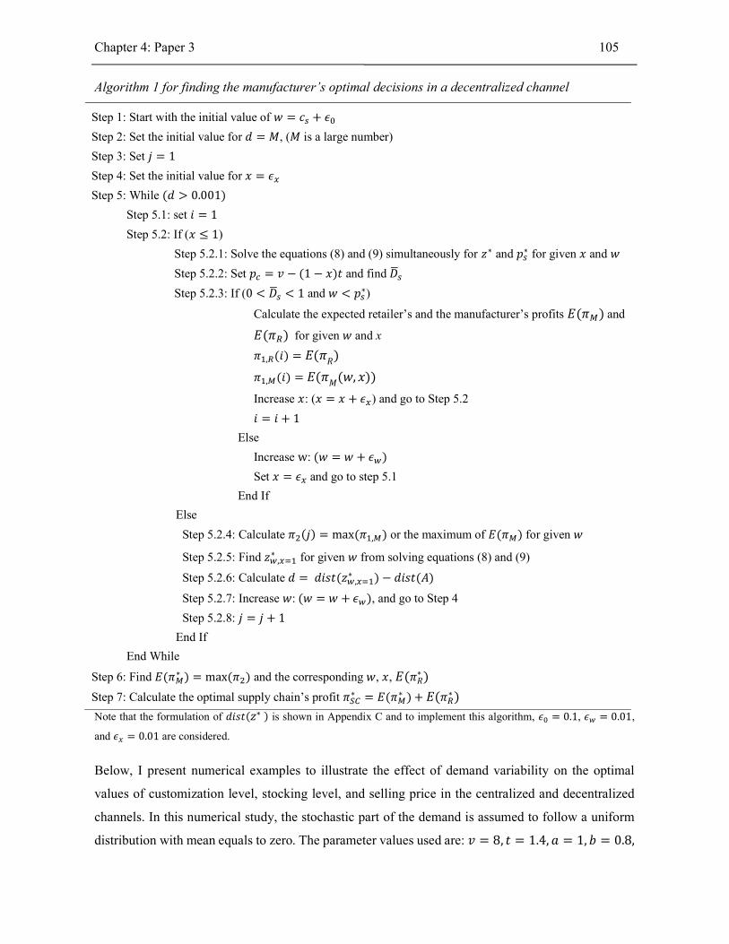
Chapter 4: Paper 3 105
Algorithm 1 for finding the manufacturer’s optimal decisions in a decentralized channel
Step 1: Start with the initial value of 𝑤 = 𝑐 + 𝜖
Step 2: Set the initial value for 𝑑 = 𝑀, (𝑀 is a large number)
Step 3: Set 𝑗 = 1
Step 4: Set the initial value for 𝑥 = 𝜖
Step 5: While (𝑑 > 0.001)
Step 5.1: set 𝑖 = 1
Step 5.2: If (𝑥 ≤ 1)
Step 5.2.1: Solve the equations (8) and (9) simultaneously for 𝑧∗ and 𝑝∗ for given 𝑥 and 𝑤
Step 5.2.2: Set 𝑝 = 𝑣 − (1 − 𝑥)𝑡 and find 𝐷
Step 5.2.3: If (0 < 𝐷 < 1 and 𝑤 < 𝑝∗)
Calculate the expected retailer’s and the manufacturer’s profits 𝐸(𝜋 ) and
𝐸(𝜋 ) for given 𝑤 and x
𝜋 , (𝑖) = 𝐸(𝜋𝑅)
𝜋 , (𝑖) = 𝐸(𝜋𝑀
(𝑤, 𝑥))
Increase 𝑥: (𝑥 = 𝑥 + 𝜖 ) and go to Step 5.2
𝑖 = 𝑖 + 1
Else
Increase w: (𝑤 = 𝑤 + 𝜖 )
Set 𝑥 = 𝜖 and go to step 5.1
End If
Else
Step 5.2.4: Calculate 𝜋 (𝑗) = max (𝜋 , ) or the maximum of 𝐸(𝜋 ) for given 𝑤
Step 5.2.5: Find 𝑧 ,∗ for given 𝑤 from solving equations (8) and (9)
Step 5.2.6: Calculate 𝑑 = 𝑑𝑖𝑠𝑡(𝑧 ,∗ ) − 𝑑𝑖𝑠𝑡(𝐴)
Step 5.2.7: Increase 𝑤: (𝑤 = 𝑤 + 𝜖 ), and go to Step 4
Step 5.2.8: 𝑗 = 𝑗 + 1
End If
End While
Step 6: Find 𝐸(𝜋∗ ) = max (𝜋 ) and the corresponding 𝑤, 𝑥, 𝐸(𝜋𝑅∗ )
Step 7: Calculate the optimal supply chain’s profit 𝜋∗ = 𝐸(𝜋∗ ) + 𝐸(𝜋∗ )
Note that the formulation of 𝑑𝑖𝑠𝑡(𝑧∗ ) is shown in Appendix C and to implement this algorithm, 𝜖 = 0.1, 𝜖 = 0.01,
and 𝜖 = 0.01 are considered.
Below, I present numerical examples to illustrate the effect of demand variability on the optimal
values of customization level, stocking level, and selling price in the centralized and decentralized
channels. In this numerical study, the stochastic part of the demand is assumed to follow a uniform
distribution with mean equals to zero. The parameter values used are: 𝑣 = 8, 𝑡 = 1.4, 𝑎 = 1, 𝑏 = 0.8,

Chapter 4: Paper 3 106
𝑐 = 4.2, 𝑐 = 3.5, ℎ = 0, 𝑠 = 0. The standard deviation of the uniform distribution is used to
represent the demand variability and the following five values are used: 0, 0.01, 0.02, 0.03 and 0.04,
0.05, 0.06, 0.07 where the zero value represents the deterministic setting. Note that although the
numerical study is based on this set of parameter values, most qualitative insights discussed here are
not parameter specific. The effects observed are, to a large extent, due to the relative differences
between parameters rather than the absolute differences. The choice of the parameter values is also
made by assuring that the feasibility conditions are met, i.e., 0 < 𝑥 < 1, and 0 < 𝐷 < 1.
(a) (b)
(c) (d)
Figure 4.2: Impact of demand variability in the centralized and decentralized channels
Figures 4.2(a) – 4.2(d) show the effect of demand variability on a number of measures in both the
centralized and decentralized channels. Figure 4.2(a) shows the difference in the optimal
7,28
7,36
7,44
7,52
7,6
7,68
0 0,01 0,02 0,03 0,04 0,05 0,06 0,07
Opt
imal
sel
ling
pri
ce
Standard deviation of demand, 𝜎
Centralized channel Decentralized channel
0,76
0,8
0,84
0,88
0,92
0 0,01 0,02 0,03 0,04 0,05 0,06 0,07
Opt
imal
cus
tom
izat
ion
leve
l
Standard deviation of demand, 𝜎
Centralized channel Decentralized channel
2,5
2,6
2,7
2,8
2,9
3
3,1
3,2
0 0,01 0,02 0,03 0,04 0,05 0,06 0,07
Opt
imal
cha
nnel
pro
fit
Standard deviation of demand, 𝜎
Centralized channel Decentralized channel
-0,15
-0,1
-0,05
0
0,05
0,1
0 0,01 0,02 0,03 0,04 0,05 0,06 0,07
Opt
imal
Sto
ckin
g le
vel
Standard deviation of demand, 𝜎
Centralized channel Decentralized channel

Chapter 4: Paper 3 107
customization level between the centralized and decentralized channels. From the analytical results
for the centralized channel, it is known that the customization level will decrease in the presence of
demand uncertainty. While the analytical results are not available for the decentralized channel,
Figure 4.2(a) indicates that the optimal customization level is also reduced in the decentralized
channel, and this reduction seems to be more pronounced than in the centralized channel. The double
marginalization of the standard product motivates the manufacturer to reduce the customization level
and thus increase the portion of demand for the customized product.
Figure 4.2(b) shows that the optimal selling price for the standard product in the stochastic setting is
lower than the price in the deterministic setting, and this is true for both types of channel (see
Propositions 2 and 7). The figure also shows that the selling price is lower as demand variability
increases in both the centralized and decentralized channels. As explained previously, reducing the
price for the standard product reduces the risk measured by the demand coefficient of variation. Thus,
it is reasonable that a larger price reduction is observed when demand variability increases. In the
absence of demand uncertainty, the selling price in the decentralized channel is always higher than
the centralized channel due to the double marginalization. However, as shown in Figure 4.2(b), the
selling price in the decentralized channel can also be lower than the selling price in the centralized
channel. Figure 4.2(c) depicts the optimal stocking levels in the two channels. For the parameter
values chosen in this study, the optimal stocking levels are positive in the centralized channel but
negative in the decentralized channel. The reason is that the values of the critical ratio in the
centralized channel are above 0.5, and since the uniform distribution has a mean of zero, the values
of z are positive. In contrast, due to the double marginalization, the values of the critical ratio in the
decentralized channel are below 0.5, resulting in the negative stocking levels. Note that a positive
(negative) value of z means that the order quantity is above (below) the riskless demand or the
deterministic part of the demand. Also note that the positive or negative values of z are parameter
specific, and hence, cannot be directly generalized to other settings. And finally, Figure 4.2(d) shows
the effect of demand variability on the channel profit. As expected, the channel profit in the
decentralized channel is lower than the channel profit in the centralized channel, and both channel
profits are decreasing in demand variability.
In view of the above results, manufacturing firms should be more conservative in offering
customization in the presence of demand uncertainty, i.e., there is a motivation to lower the
customization level compared to the case where the demand is deterministic. The channel structure
is also influential. The motivation to lower the customization level is higher when the manufacturing
firms have to rely on retailers in selling their standard products.
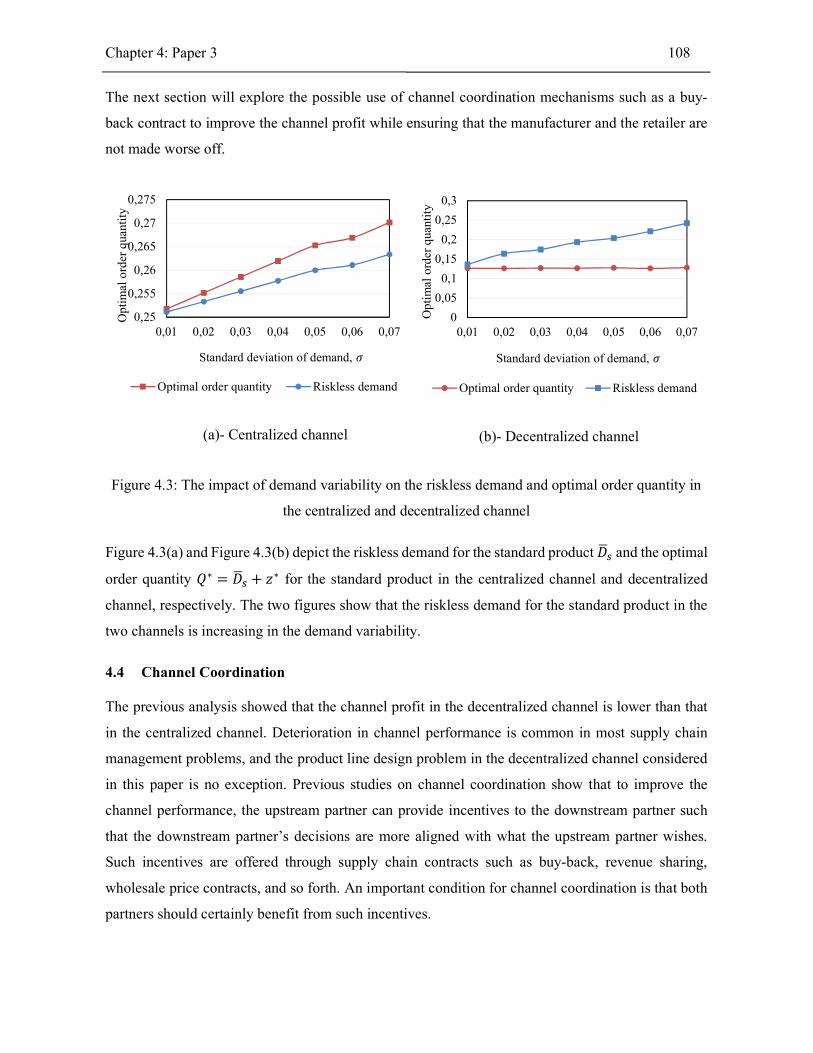
Chapter 4: Paper 3 108
The next section will explore the possible use of channel coordination mechanisms such as a buy-
back contract to improve the channel profit while ensuring that the manufacturer and the retailer are
not made worse off.
(a)- Centralized channel
(b)- Decentralized channel
Figure 4.3: The impact of demand variability on the riskless demand and optimal order quantity in
the centralized and decentralized channel
Figure 4.3(a) and Figure 4.3(b) depict the riskless demand for the standard product 𝐷 and the optimal
order quantity 𝑄∗ = 𝐷 + 𝑧∗ for the standard product in the centralized channel and decentralized
channel, respectively. The two figures show that the riskless demand for the standard product in the
two channels is increasing in the demand variability.
4.4 Channel Coordination
The previous analysis showed that the channel profit in the decentralized channel is lower than that
in the centralized channel. Deterioration in channel performance is common in most supply chain
management problems, and the product line design problem in the decentralized channel considered
in this paper is no exception. Previous studies on channel coordination show that to improve the
channel performance, the upstream partner can provide incentives to the downstream partner such
that the downstream partner’s decisions are more aligned with what the upstream partner wishes.
Such incentives are offered through supply chain contracts such as buy-back, revenue sharing,
wholesale price contracts, and so forth. An important condition for channel coordination is that both
partners should certainly benefit from such incentives.
0,25
0,255
0,26
0,265
0,27
0,275
0,01 0,02 0,03 0,04 0,05 0,06 0,07
Opt
imal
ord
er q
uant
ity
Standard deviation of demand, 𝜎
Optimal order quantity Riskless demand
0
0,05
0,1
0,15
0,2
0,25
0,3
0,01 0,02 0,03 0,04 0,05 0,06 0,07
Opt
imal
ord
er q
uant
ity
Standard deviation of demand, 𝜎
Optimal order quantity Riskless demand
Chapter 4: Paper 3 109
This section will therefore focus on exploring possibilities to improve the channel performance in the
product line design problem considered in this paper. I have chosen to focus on the buy-back contract
for two reasons. Firstly, it is one of the contracts widely studied in the literature (see e.g. Pasternack
1985, Wu 2013 and the references therein). Secondly, return contracts are commonly applied in some
industries such as cosmetics, fashion and apparel (Li et al. 2012). Padmanabhan and Png (1995) states
that return contracts play important roles for the sellers of seasonal or style goods to coordinate their
distribution channels. Buy-back contract is a simple return contract wherein suppliers specify a
wholesale price for the ordered items and a buyback price for the unsold items at the end of selling
season. The exploration of using the buy-back contract in this paper can serve as a building block or
departure point for future research that examines the use of other contracts in the context of product
line design with demand uncertainty.
Under the buy-back contract, the manufacturer charges the retailer a wholesale price 𝑤 for each unit
of the standard product ordered and offers a buy-back price 𝑏 , (𝑏 < 𝑤 ) for each unit of the
leftovers at the end of the selling period. The subscript B is added to denote the decentralized channel
with the buy-back contract. It is assumed that the retailer still needs to pay the holding cost h for each
unit of the leftovers at the end of the selling period. The expected profits for the manufacturer and the
retailer under the buy-back contract are as follows:
𝐸 𝜋 (𝑝 , 𝑧) = 𝑝 Γ(𝑝 , 𝑥, 𝑧) − 𝑤 (𝐷 + 𝑧) − (ℎ − 𝑏 ) 𝐷 + 𝑧 − Γ(𝑝 , 𝑥, 𝑧) − 𝑠 𝑆(𝑧) (11)
𝐸(𝜋 (𝑤 , 𝑥, 𝑏 )) = (𝑤 − 𝑐 )(𝐷 + 𝑧) + (𝑝 − 𝑐 )(1 − 𝐷 ) − 𝑏 𝐷 + 𝑧 −
Γ(𝑝 , 𝑥, 𝑧) − 𝑏𝑥 (12)
where Γ(𝑝 , 𝑥, 𝑧) = 𝐷 + 𝑧 − ∫ 𝐹(𝓊) 𝑑𝓊 denotes the retailer’s expected sales (see Appendix B).
The following propositions characterize the retailer’s optimal decisions for the given values of the
manufacturer’s decisions on 𝑤 , 𝑥, and 𝑏 .
Proposition 8: The retailer’s optimal decisions 𝑝∗ and 𝑧∗ with the buy-back contract can be
determined by solving the below equations simultaneously.
𝑝∗ = + + + (𝑧 − ∫ 𝐹(𝓊)𝑑𝓊) (13)
Chapter 4: Paper 3 110
𝐹(𝑧∗) =( )
(14)
The optimal solutions are uniquely determined if the condition 2𝐻(𝑧) +( )
> 0 is fulfilled (see
Appendix B). It is shown in Proposition 8 that the retailer’s problem can be solved analytically. From
(14), it is obvious that the buy-back price offered by the manufacturer will reduce the overage cost
incurred by the retailer, and hence, the retailer will be motivated to increase the stocking level. Given
this optimal response from the retailer, the manufacturer now solves her optimization problem that
maximizes her profit while ensuring that the retailer is not made worse-off compared to the case when
the contract is not implemented. Like in the case of the decentralized channel without contract, the
manufacturer’s optimal decisions on the wholesale price, customization level, and buy-back price
will be determined numerically. An algorithm for solving the manufacturer’s optimization problem,
i.e., finding the optimal solutions (𝑥∗, 𝑤∗ , 𝑏∗ , 𝑝∗) is presented below.

Chapter 4: Paper 3 111
Algorithm 2 for finding the manufacturer’s optimal decisions under the buy-back contract
Step 1: Run Algorithm 1 to find 𝐸(𝜋∗ ) and 𝐸(𝜋∗ ) Step 2: Set the initial value for 𝑤 = 𝑐 + 𝜖
Step 3: Set the initial value for 𝑑 = 𝑀, where 𝑀 is a very large number Step 4: Set 𝑗 = 1 Step 5: While (𝑑 > 0.001)
Step 5.1: Set the initial value for 𝑏 = 𝜖
Step 5.2: While (𝑏 < 𝑤 ) Step 5.2.1: set 𝑖 = 1 Step 5.2.2: Set the initial value for 𝑥 = 𝜖 Step 5.2.3: While (𝑥 ≤ 1)
Solve the equations (13) and (14) simultaneously for 𝑧∗ and 𝑝∗ for given 𝑥 , 𝑤 , and 𝑏
Set 𝑝 = 𝑣 − (1 − 𝑥)𝑡 and find 𝐷 If (0 < 𝐷 < 1 and 𝑤 < 𝑝∗)
Calculate the expected retailer’s and manufacturer’s profits for given 𝑤 , 𝑏 , and 𝑥 by using the equations (11) and (12)
𝜋 , (𝑖) = 𝐸 𝜋 (𝑝∗, 𝑧∗)
𝜋 , (𝑖) = 𝐸(𝜋 (𝑤 , 𝑥, 𝑏 ))
Increase 𝑥: (𝑥 = 𝑥 + 𝜖 ) and go to Step 5.2.3 𝑖 = 𝑖 + 1
Else Increase the buy-back price 𝑏 : (𝑏 = 𝑏 + 𝜖 ) and go to Step 5.2
End End While
Step 5.2.4: Calculate 𝜋 ,∗ = max (𝜋 , ) or the maximum of manufacturer’s profits for given the
𝑤 and 𝑏 and find corresponding index 𝑖 Step 5.2.5: Find the expected retailer’s profit 𝐸(𝜋 , ) = 𝜋 , (𝑖 )
Step 5.2.6: If (𝐸(𝜋 , ) > 𝐸(𝜋∗ ) and 𝐸(𝜋 ,∗ ) > 𝐸(𝜋∗ ))
𝜋 , (𝑗) = 𝐸(𝜋 , )
𝜋 , (𝑗) = 𝐸(𝜋 ,∗ )
𝑗 = 𝑗 + 1 End If
Step 5.2.7: Increase the buy-back price 𝑏 : (𝑏 = 𝑏 + 𝜖 ) and go to Step 5.2
End While Step 5.3: Find 𝑧 , ,
∗ for given 𝑤 from solving equations (13) and (14)
Step 5.4: Calculate 𝑑 = 𝑑𝑖𝑠𝑡 𝑧 , , ∗ − 𝑑𝑖𝑠𝑡 (𝐴)
Step 5.5: Increase 𝑤: (𝑤 = 𝑤 + 𝜖 ), and go to Step 5
End While Step 6: Calculate 𝜋∗ = max (𝜋 , ) and find the corresponding 𝑤 , 𝑏 , 𝑥, and index 𝑖
Step 7: Calculate the optimal supply chain’s profit: 𝜋∗ = 𝜋∗ + 𝜋 , (𝑖 )
Note that the formulation of 𝑑𝑖𝑠𝑡 (𝑧∗) is shown in Appendix C and to implement this algorithm, 𝜖 = 0.1, 𝜖 = 0.01,
𝜖 = 0.01 , and 𝜖 = 0.01 are considered.

Chapter 4: Paper 3 112
This algorithm is applied to the same numerical example that is used in the decentralized channel
without a contract. The discussions below focus on the effects of the buy-back contract. As shown in
Figures 4.4 and 4.5, the buy-back contract is able to increase the channel profit as well as the retailer’s
and the manufacturer’s profits. Under the buy-back contract, the retailer is motivated to place a larger
order quantity, as depicted in Figure 4.6. Also, increases in the channel profit and order quantity due
to the contract appears to be more pronounced when demand variability increases.
These results should give motivation to manufacturing firms, especially those operating a dual
channel and sell both the standard and customized products, to be more proactive in initiating a supply
contract with the retailers so that they achieve a win-win situation. This is especially true when they
face high demand uncertainty. Furthermore, they should also see that such a contract does not solely
affect the inventory or order quantity decision, but also the product line design decisions. This should
motivate the firms to enhance the integration of marketing (product line design) and operations
(inventory) decisions.
Figure 4.4: The impact of demand variability on the retailer and manufacturer’s profits with and without the
buy-back contract
0,018
0,02
0,022
0,024
0,026
0,028
0,01 0,02 0,03 0,04 0,05 0,06 0,07
Ret
aile
r's p
rofi
t
Standard deviation of demand, 𝜎
With BB contract Without BB contract
2,4
2,6
2,8
3
3,2
0,01 0,02 0,03 0,04 0,05 0,06 0,07
Man
ufac
ture
r's p
rofi
t
Standard deviation of demand, 𝜎
With BB contract Without BB contract
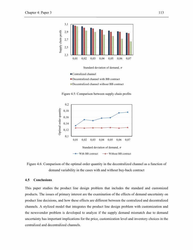
Chapter 4: Paper 3 113
Figure 4.5: Comparison between supply chain profits
Figure 4.6: Comparison of the optimal order quantity in the decentralized channel as a function of
demand variability in the cases with and without buy-back contract
4.5 Conclusions
This paper studies the product line design problem that includes the standard and customized
products. The issues of primary interest are the examination of the effects of demand uncertainty on
product line decisions, and how these effects are different between the centralized and decentralized
channels. A stylized model that integrates the product line design problem with customization and
the newsvendor problem is developed to analyze if the supply demand mismatch due to demand
uncertainty has important implications for the price, customization level and inventory choices in the
centralized and decentralized channels.
2,3
2,5
2,7
2,9
3,1
0,01 0,02 0,03 0,04 0,05 0,06 0,07S
uppl
y ch
ain
prof
it
Standard deviation of demand, 𝜎
Centralized channel
Decentralized channel with BB contract
Decentralized channel without BB contract
0,1
0,12
0,14
0,16
0,18
0,2
0,01 0,02 0,03 0,04 0,05 0,06 0,07
Opt
imal
ord
er q
uant
ity
Standard deviation of demand, 𝜎
With BB contract Without BB contract

Chapter 4: Paper 3 114
In a centralized channel, where the manufacturer makes all decisions, the presence of demand
uncertainty drives the prices for the standard and customized products as well as the customization
level down. These effects become more pronounced when the demand variability increases. Thus,
this paper shows that demand uncertainty can have a significant influence on the product line
decisions. The analytical results derived show the mutual dependence of the product line and order
quantity decisions. By lowering the price for the standard product, the manufacturer can reduce the
demand coefficient of variation and lessen the impact of demand uncertainty.
In a decentralized channel, where the manufacturer sells the standard product through a retailer, the
effect of demand uncertainty resembles what is observed in the centralized channel. One notable
difference is that due to double marginalization, the retailer tends to order the quantity that is lower
than that of the centralized channel. Consequently, the channel profitability deteriorates in the
decentralized channel, and even more when the demand variability is higher.
The existing literature on supply chain management points out the importance of coordination, which
has motivated us to examine the possibility of designing a coordination mechanism to improve
channel profitability in the decentralized channel. In this paper, the author has attempted to apply the
buy-back contract, which is one of the contracts widely studied in the literature. The results show
that, even though full coordination seems difficult to achieve, the buy-back contract is able to make
both the manufacturer and the retailer better off, and that the improvements seem more pronounced
when demand variability increases.
To address the limitations of this paper, I provide some suggestions for future research. First, the
number of numerical examples studied in this paper is rather limited. For some results that cannot be
derived analytically, more numerical examples are required to evaluate whether those results
presented in this paper can be more generalized. Second, this paper only considers consumers’
heterogeneity in product taste or preference, and hence, it excludes product quality from the product
line design problem. However, product quality is often an important consideration in product line
design. Further research can study a richer problem where consumers are heterogeneous in both
product taste and quality. Third, another interesting avenue for future research could be to carry out
a more comprehensive examination of the channel contracts that may result in a channel profit that is
closer to that achieved under a fully coordinated channel. This paper only explores the possibility of
a buy-back contract for improving the channel performance. Contracts that allow the retailer’s
initiatives to influence the manufacturer’s decisions could be an interesting topic to consider. Finally,
this paper analyzes a monopolistic setting where the manufacturer is not in competition with other

Chapter 4: Paper 3 115
manufacturers. Thus, the effects of competition are neglected. To consider a more realistic setting, it
would be interesting to consider the presence of more than one manufacturers (e.g. a duopoly setting).
In such a setting, the product line design decisions of each manufacturer, for example, regarding the
customization level, will depend on the other manufacturer’s decisions in addition to the response
from the retailer. Considering the competition at the retailer level is also a possible topic for future
research.
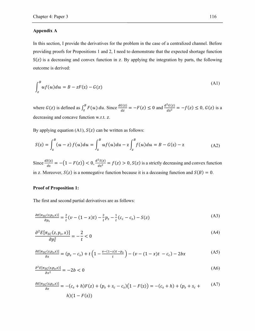
Chapter 4: Paper 3 116
Appendix A
In this section, I provide the derivatives for the problem in the case of a centralized channel. Before
providing proofs for Propositions 1 and 2, I need to demonstrate that the expected shortage function
S(𝑧) is a decreasing and convex function in 𝑧. By applying the integration by parts, the following
outcome is derived:
𝓊𝑓(𝓊)𝑑𝓊 = 𝐵 − 𝑧𝐹(z) − 𝐺(𝑧) (A1)
where 𝐺(𝑧) is defined as ∫ 𝐹(𝓊) 𝑑𝑢. Since ( )
= −𝐹(𝑧) ≤ 0 and ( )
= −𝑓(𝑧) ≤ 0, 𝐺(𝑧) is a
decreasing and concave function w.r.t. 𝑧.
By applying equation (A1), 𝑆(𝑧) can be written as follows:
𝑆(z) = (𝓊 − 𝑧) 𝑓(𝓊)𝑑𝓊 = 𝓊𝑓(𝓊)𝑑𝑢 − z 𝑓(𝓊)𝑑𝓊 = 𝐵 − 𝐺(z) − z (A2)
Since ( )
= − 1 − 𝐹(𝑧) < 0, ( )
= 𝑓(𝑧) > 0, 𝑆(𝑧) is a strictly decreasing and convex function
in 𝑧. Moreover, 𝑆(𝑧) is a nonnegative function because it is a deceasing function and 𝑆(𝐵) = 0.
Proof of Proposition 1:
The first and second partial derivatives are as follows:
[ ( , , )]= (𝑣 − (1 − 𝑥)𝑡) − 𝑝 − (𝑐 − 𝑐 ) − 𝑆(𝑧) (A3)
𝜕 𝐸[𝜋 (𝑧, 𝑝 , 𝑥)]
𝜕𝑝= −
2
𝑡< 0
(A4)
[ ( , , )]= (𝑝 − 𝑐 ) + 𝑡 1 −
( ) − (𝑣 − (1 − 𝑥)𝑡 − 𝑐 ) − 2𝑏𝑥 (A5)
[ ( , , )]= −2𝑏 < 0 (A6)
[ ( , , )]= −(𝑐 + ℎ)𝐹(𝑧) + (𝑝 + 𝑠 − 𝑐 ) 1 − 𝐹(z) = −(𝑐 + ℎ) + (𝑝 + 𝑠 +
ℎ)(1 − 𝐹(z))
(A7)

Chapter 4: Paper 3 117
[ ( , , )]= −(𝑝 + 𝑠 + ℎ)𝑓(𝑧) < 0 (A8)
By applying the first-order conditions, I obtain the three equations (4), (5), and (6). By substituting
𝑥∗ that comes from equation (6) into equation (4), 𝑝∗ can be written as in the below equation:
𝑝∗ = 𝑝 (z) = 𝑝 , −( )
𝑆(z) , where 𝑝 , = (𝑝 +( )
𝑥 ) (A9)
The first-order conditions reduce to equations (5) and (A9). Petruzzi and Dada (1999) states that 𝑝∗
and 𝑧∗ are uniquely determined if F(·) is a cumulative distribution satisfying the condition 2𝐻(𝑧) +
( )> 0 is fulfilled, where 𝐻(𝑧) =
( )
( ). Below, I show that this condition is valid for the
optimization problem in the centralized channel:
𝑅 (𝑧) is defined as [ ( , ( ), ( ))]
= −(𝑐 + ℎ) + 𝑝 , −( )
𝑆(z) + 𝑠 + ℎ (1 − 𝐹(z))
( )= −
( )𝑓(𝑧)(
( )𝑝 , + 𝑠 + ℎ − 𝑆(z) −
( )
( ))
( )( ) = −
( )𝑓(𝑧)
( )
( )(2𝐻 (𝑧) +
( ))
If 2𝐻(𝑧) +( )
> 0, 𝑅 (𝑧) is monotone or unimodal. Therefore, 𝑅 (𝑧) has at most two
roots. 𝑅 (𝐵) = −(𝑐 + ℎ) < 0. If 𝑅 (𝑧) has one root, it implies that the sign of 𝑅 (𝑧) changes from
positive to negative at the root. Thus, ( )
( )< 0 which means that the root is the local
maximum of 𝜋 (𝑧, 𝑝 (𝑧), 𝑥(𝑝 )). If there are two roots for 𝑅 (𝑧), it implies that two changes occur
for the sign of 𝑅 (𝑧), first from negative to positive at the smaller root and then from positive to
negative at the bigger root of 𝑅 (𝑧). Therefore, the bigger root is local maximum of
𝜋 (𝑧, 𝑝 (𝑧), 𝑥(𝑝 )). In addition, since ( )
< 0 and < 0, the stationary point for the
retailer’s profit function cannot be a minimum point and it can be concluded that 𝑅 (𝑧) has at most
one root. Consequently, (𝑝∗, 𝑧∗, 𝑥∗) from the first-order conditions maximizes the profit function.

Chapter 4: Paper 3 118
Proof of Proposition 2:
2(a):
As mentioned earlier, by substituting 𝑥∗ that comes from equation (6) into equation (4), 𝑝∗ can be
written as equation (A9). Since S(𝑧) is a decreasing function in the stocking level 𝑧, the optimal retail
price will increase.
2(b):
When I substitute 𝑝∗ from equation (4) into equation (5) the new equation below will be derived:
𝐹(𝑧∗) = 1 −( ∗)
(A10)
Equation (A10) can be written as Ʌ = 𝐹(𝑧∗) +( ∗)
− 1 = 0. I need to find Ʌ and
Ʌ∗
to use ∗
= −Ʌ
Ʌ∗
formulation, Ʌ
= −( ∗)
( ∗)< 0 and
Ʌ∗ = 𝑓(𝑧∗) −
( ( ∗))
( ( ∗) ). If 𝑓(𝑧∗) >
( ( ∗))
( ( ∗) )⇒ 𝐻(𝑧∗) >
( ( ∗))
( )⇒ 𝐻(𝑧∗) >
( )(1 − 𝐹(𝑧∗)) ,
Ʌ∗ will be positive and it can be concluded that
∗
> 0.
2(c):
The manufacturer’s decisions on 𝑧∗ and 𝑝∗ are the intersection point of equations (A9) and (5). To
prove this part of Proposition 2, ∗
should be calculated. From equation (5), ɣ = 𝐹(𝑧∗) + −
1 = 0. Accordingly, ɣ∗ = 𝑓(𝑧∗) > 0 and
ɣ= −
( ), therefore,
∗
= −
ɣ
ɣ∗
> 0.
Proof of Proposition 3:
Superscripts 𝑖 and 𝑗 are used in the optimal solutions to distinguish the case with deterministic demand
from the case with demand uncertainty. Without considering demand uncertainty, the manufacturer’s
profit function can be written as:
𝜋 𝑝 , 𝑥 = 𝑝 − 𝑐 𝐷 + 𝑝 − 𝑐 (1 − 𝐷 ) − 𝑏𝑥( ) (A11)
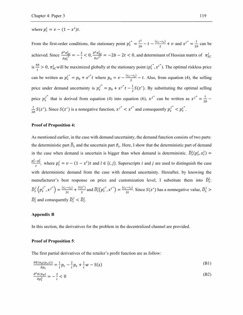
Chapter 4: Paper 3 119
where 𝑝 = 𝑣 − (1 − 𝑥 )𝑡.
From the first-order conditions, the stationary point 𝑝∗
= − 𝑡 −( )
+ 𝑣 and 𝑥∗
= can be
achieved. Since = − < 0, = −2𝑏 − 2𝑡 < 0, and determinant of Hessian matrix of 𝜋
is > 0, 𝜋 will be maximized globally at the stationary point (𝑝∗, 𝑥
∗). The optimal riskless price
can be written as 𝑝∗
= 𝑝 + 𝑥∗𝑡 where 𝑝 = 𝑣 −
( )− 𝑡. Also, from equation (4), the selling
price under demand uncertainty is 𝑝∗
= 𝑝 + 𝑥∗𝑡 − 𝑆(𝑧∗). By substituting the optimal selling
price 𝑝∗ that is derived from equation (4) into equation (6), 𝑥
∗ can be written as 𝑥
∗= −
𝑆(𝑧∗). Since 𝑆(𝑧∗) is a nonegative function, 𝑥∗
< 𝑥∗ and consequently 𝑝
∗< 𝑝
∗.
Proof of Proposition 4:
As mentioned earlier, in the case with demand uncertainty, the demand function consists of two parts:
the deterministic part 𝐷 and the uncertain part 𝜗 . Here, I show that the deterministic part of demand
in the case when demand is uncertain is bigger than when demand is deterministic. 𝐷 (𝑝 , 𝑥 ) =
, where 𝑝 = 𝑣 − (1 − 𝑥 )𝑡 and 𝑙 ∈ {𝑖, 𝑗}. Superscripts 𝑖 and 𝑗 are used to distinguish the case
with deterministic demand from the case with demand uncertainty. Hereafter, by knowing the
manufacturer’s best response on price and customization level, I substitute them into 𝐷 :
𝐷 𝑝∗, 𝑥
∗=
( )+
( ∗) and 𝐷 𝑝
∗, 𝑥
∗=
( ). Since 𝑆(𝑧∗) has a nonnegative value, 𝐷 >
𝐷 and consequently 𝐷 < 𝐷 .
Appendix B
In this section, the derivatives for the problem in the decentralized channel are provided.
Proof of Proposition 5:
The first partial derivatives of the retailer’s profit function are as follow:
( ( , ))= 𝑝 − 𝑝 + 𝑤 − S(z) (B1)
( )= − < 0 (B2)
Chapter 4: Paper 3 120
( ( , ))= −(𝑤 + ℎ)𝐹(𝑧) + (𝑝 + 𝑠 − 𝑤) 1 − 𝐹(𝑧) = −(𝑤 + ℎ) +
(𝑝 + 𝑠 + ℎ)(1 − 𝐹(𝑧))
(B3)
( )= −(𝑝 + 𝑠 + ℎ)𝑓(𝑧) < 0 (B4)
By applying the first-order conditions:
( ( , ))= 0 ⇒ 𝑝∗ = + − S(𝑧) (B5)
( ( , ))= 0 ⇒ 𝐹(𝑧∗) = (B6)
For the given 𝑤 and 𝑥, 𝑝∗ and 𝑧∗are uniquely determined because:
𝑅 (𝑧) =( ( , ∗( )))
= −(𝑤 + ℎ) + 𝑝 , − 𝑆(𝑧) + 𝑠 + ℎ 1 − 𝐹(z) (B7)
where 𝑝 , = + 𝑥 +
Next, I find zeros of 𝑅 (𝑧):
( )= − 𝑓(𝑧) (𝑝 + 𝑠 + ℎ) − 𝑆(𝑧) −
( )
( )) (B8)
( )( ) = − 𝑓(𝑧)
( )
( )(2𝐻 (𝑧) +
( ))
(B9)
If 2𝐻(𝑧) +( )
> 0, 𝑅 (𝑧) is monotone or unimodal. Therefore, 𝑅 (𝑧) has at most two
roots. 𝑅 (𝐵) = −(𝑤 + ℎ) < 0. If 𝑅 (𝑧) has one root, it implies that the sign of 𝑅 (𝑧) changes from
positive to negative at the root. Thus, ( )
( )< 0 which means that the root is local maximum
of 𝜋 (𝑧, 𝑝∗(𝑧)). If there are two roots for 𝑅 (𝑧), it implies that two changes occur for the sign of
𝑅 (𝑧), first from negative to positive at the smaller root and then from positive to negative at the
bigger root of 𝑅 (𝑧). Therefore, the bigger root is local maximum of 𝜋 (𝑧, 𝑝∗(𝑧)). Moreover, the
second-order necessary conditions ( )
< 0 and < 0 imply that the stationary point for the
retailer’s profit function cannot be a minimum point and it can be concluded that 𝑅 (𝑧) has at most
one root. Therefore, the retailer’s profit function is quasi-concave that has only one peak and the
stationary point represents the maximum point.
Chapter 4: Paper 3 121
Proof of Proposition 6:
I need to calculate the first partial derivative of 𝑧∗ w.r.t. 𝑥.
First, from equation (9), it can be obtained the below expression:
𝑝 =( ∗ )
− (𝑠 + ℎ) (B10)
Second, by equalizing the left-sides of equations (8) and (B10), there exists:
𝐾 = 𝑝 + 𝑥 + − 𝑆(𝑧∗ ) −( ∗)
= 0 , where 𝑝 = + 𝑠 + ℎ (B11)
By applying the implicit differentiation method, then:
∗
= −∗
=( ∗)
( ) ( ∗) ( ( ∗))
(B12)
The below condition for the retailer’s optimal decision on stocking level 𝑧 should be satisfied:
( )∗
= 1 − 𝐹(𝑧∗) − (𝑤 + ℎ)𝐻(𝑧∗) < 0 ⇒ (𝑤 + ℎ)𝐻(𝑧∗) − 1 −
𝐹(𝑧∗) > 0 ⇒ 2(𝑤 + ℎ)𝐻(𝑧∗) − 𝑡 1 − 𝐹(𝑧∗) > 0
(B13)
Therefore, ∗
> 0.
Proof of Proposition 7:
Without demand uncertainty, the retailer’s and manufacturer’s profit functions can be written as:
𝜋 = (𝑝 − 𝑤)𝐷 (B14)
𝜋 = (𝑤 − 𝑐 )𝐷 + (𝑝 − 𝑐 )𝐷 − 𝑏𝑥 (B15)
The first and second derivatives of the retailer’s profit function are as follows:
𝜕𝜋
𝜕𝑝=
𝑤
𝑡+
𝑝
𝑡−
2𝑝
𝑡
(B16)

Chapter 4: Paper 3 122
𝜕 𝜋
𝜕𝑝= −
2
𝑡< 0
(B17)
The retailer’s profit function is concave in 𝑝 . Therefore, the retailer’s optimal pricing decision can
be obtained from the first-order condition: 𝑝∗ = 𝑝 + + , where 𝑝 = . Since S(𝑧) is
nonnegative, a comparison of the optimal results for the selling price under demand certainty and
uncertainty demonstrates a reduction in the optimal selling price in the decentralized channel.
Buy-back contract
First, the expected sales function is provided. By defining 𝐷 (𝑝 , 𝑥, 𝜗 ) = 𝐷 (𝑝 , 𝑥) + 𝜗 and
applying the transformation 𝑧 = 𝑄 − 𝐷 (𝑝 , 𝑥), the retailer’s expected sales can be expressed as
follows:
Γ(𝑝 , 𝑥, 𝑄)=𝐷 (𝑝 , 𝑥, 𝜗 ), 𝑖𝑓 𝑄 > 𝐷(𝑝 , 𝑥, 𝜗 )
𝑄, 𝑖𝑓 𝑄 < 𝐷(𝑝 , 𝑥, 𝜗 ) ⇒
𝐷 (𝑝 , 𝑥) + 𝜗 , 𝑖𝑓 𝑧 > 𝜗
𝐷 (𝑝 , 𝑥) + 𝑧, 𝑖𝑓 𝑧 < 𝜗
(B18)
Thus, the retailer’s expected sales is defined as:
𝐸(Γ(𝑝 , 𝑥, 𝑄)) = 𝐸[min (𝑄, 𝐷 (𝑝 , 𝑥, 𝜗 ))] = ∫ (𝐷 (𝑝 , 𝑥) + 𝓊)𝑓(𝓊)𝑑𝓊 +
∫ (𝐷 (𝑝 , 𝑥) + 𝑧)𝑓(𝓊)𝑑𝓊 = 𝐷 (𝑝 , 𝑥) + 𝑧 − ∫ 𝐹(𝓊) 𝑑𝓊 = 𝑄 −
∫ 𝐹(𝓊) 𝑑𝓊
(B19)
Proof of Proposition 8:
( )= ( + 𝑧 − ∫ 𝐹(𝓊)𝑑𝓊) − +
(B20)
( )= − < 0
(B21)
𝜕𝐸(𝜋 )
𝜕𝑧= (𝑝 + (ℎ − 𝑏 ) + 𝑠 ) 1 − 𝐹(𝑧) − (𝑤 + (ℎ − 𝑏 ))
(B22)
( )= −𝑓(𝑧)(𝑝 + (ℎ − 𝑏 ) + 𝑠 ) < 0
(B23)
Chapter 4: Paper 3 123
First-order condition ( )
= 0 gives 𝑝∗(𝑧) = 𝑝 + (𝑧 − ∫ 𝐹(𝓊)𝑑𝓊), where 𝑝 = + +
. In what follows, I show that 𝑝∗ and 𝑧∗ are uniquely determined if 𝐹(·) as a cumulative distribution
function satisfies the condition 2𝐻(𝑧) +( )
> 0:
First, 𝑅 (𝑧) is defined as follows:
𝑅 (𝑧) =( , ∗( ) )
= 𝑝 + 𝑧 − ∫ 𝐹(𝓊)𝑑𝓊 + (ℎ − 𝑏 ) + 𝑠 1 − 𝐹(𝑧) −
(𝑤 + (ℎ − 𝑏 )),
(B24)
Next, I find zeros of 𝑅 (𝑧):
( ) )= − 𝑓(𝑧) 𝑝 + (ℎ − 𝑏 ) + 𝑠 + 𝑧 − ∫ 𝐹(𝓊)𝑑𝓊 −
( )
( ) (B25)
( ) ( ) = −
( ) ( )
( )(2𝐻(𝑧) +
( )) (B26)
If 2𝐻(𝑧) +( )
> 0, 𝑅 (𝑧) is monotone or unimodal. Therefore, 𝑅 (𝑧) has at most two roots. Let
𝑤 + ℎ > 𝑏 , therefore 𝑅 (𝐵) = − 𝑤 + (ℎ − 𝑏 ) < 0. If 𝑅 (𝑧) has one root, it implies that the
sign of 𝑅 (𝑧) changes from positive to negative at the root. Thus, ( )
( ) < 0 which it means
that the root is the local maximum of 𝜋 (𝑧, 𝑝 (𝑧)). If there are two roots for 𝑅 (𝑧), two changes
occur for sign of 𝑅 (𝑧), first from negative to positive at the smaller root, and then from positive to
negative at the bigger root of 𝑅 (𝑧). Therefore, the bigger root is the local maximum of 𝜋 (𝑧, 𝑝 (𝑧)).
Since ( )
< 0 and ( )
< 0, the second order necessary condition is satisfied. It implies that
the stationary point for the retailer’s profit function cannot be a minimum point and it can be
concluded that 𝑅 (𝑧) has at most one root. Therefore, the retailer’s profit function is quasi-concave
that has only one peak and the stationary point represents the maximum point.
Chapter 4: Paper 3 124
Appendix C
In this part, I derive the stopping criteria for both algorithms:
Algorithm 1:
By using the equations (B6) and (B8), there exists:
∗
= −∗
=( ∗)
( ) ( ∗) ( ∗)< 0
(B27)
The equation (B27) implies that for a given customization level 𝑥, increasing the wholesale price 𝑤
will decrease the optimal stocking level 𝑧∗. Equation (B13) states that for a given wholesale price 𝑤,
increasing the customization level 𝑥 will increase the optimal stocking level 𝑧∗. Also, since the
demand should be positive and the wholesale price 𝑤 should be less than the optimal retail price 𝑝∗,
the lower bound 𝐿(𝑧∗ ) and the upper bound 𝑈(𝑧∗ ) for given 𝑤 and x can be defined as follows:
𝐿(𝑧∗ ) = 2( + + 𝑆(𝑧∗ )) (B28)
𝑈 (𝑧∗ ) = 2( + − 𝑆(𝑧∗ )) (B29)
The upper bound and the lower bound are functions w.r.t. the optimal stocking level 𝑧∗. Furthermore,
the second upper bound can be defined. Because 𝑅 (𝐴) > 0 ⇒ 𝑝 − 𝑆(𝐴) + 𝑠 + ℎ −
(𝑤 + ℎ) > 0 ⇒ 𝑤 < 2 + 𝑥 − 𝑆(𝐴) + 𝑠 ⇒ 𝑈 = 2( + 𝑥 − 𝑆(𝐴) + 𝑠 ). Then, it
should be determined which one is tighter:
𝒰(𝑧) = 𝑈 − 𝑈 (𝑧∗ ) = 2 − 𝑆(𝐴) + 𝑠 + 2 𝑆(𝑧∗ ) = 𝑡 𝑆(𝑧∗ ) − 𝑆(𝐴) + 2𝑠 . (B30)
Since 𝑆(𝑧) is a decreasing function in 𝑧, I have 𝑆(𝑧∗ ) < 𝑆(𝐴). If 2𝑠 > 𝑡 𝑆(A ) − 𝑆(𝑧∗) , the first
upper bound is tighter than the second one.
Next, I define 𝑑𝑖𝑠𝑡(𝑧∗ ) as follows:
Chapter 4: Paper 3 125
𝑑𝑖𝑠𝑡(𝑧∗ ) = 𝑚𝑖𝑛{𝑈 , 𝑈 (𝑧∗ )} − 𝐿(𝑧∗ )
=2𝑡 − 2𝑡𝑆(𝑧∗ ); 𝑖𝑓 𝑈 (𝑧∗ ) < 𝑈
2𝑡 + 2𝑠 − 𝑡𝑆(𝐴) − 𝑡𝑆(𝑧∗ ); 𝑖𝑓 𝑈 (𝑧∗ ) > 𝑈
(B31)
Since ( ∗ )
∗ > 0, by decreasing the optimal stocking level 𝑧∗, 𝑑𝑖𝑠𝑡(𝑧∗ ) will decrease. According
to the equations (8) and (9), 𝑧∗ is a function w.r.t the wholesale price w and the customization level
x. For a given wholesale price w, the maximum of the optimal stocking level 𝑧 ,∗ occurs at 𝑥 = 1.
According to equation (B27), by increasing the wholesale price w, 𝑑𝑖𝑠𝑡(𝑧∗ ) will decrease.
𝐴 < 𝑧 ,∗ < 𝐵 ⇒ 𝑑𝑖𝑠𝑡(𝐴) < 𝑑𝑖𝑠𝑡 𝑧 ,
∗ < 𝑑𝑖𝑠𝑡(𝐵) ⇒ 0 < 𝑑𝑖𝑠𝑡 𝑧 ,∗ − 𝑑𝑖𝑠𝑡(𝐴) <
𝑑𝑖𝑠𝑡(𝐵) − 𝑑𝑖𝑠𝑡(𝐴). Thus, 𝑑(𝑧 ,∗ ) = 𝑑𝑖𝑠𝑡 𝑧 ,
∗ − 𝑑𝑖𝑠𝑡(𝐴) is a decreasing function w.r.t the
wholesale price w. In the algorithm, I increase the w value until the value of 𝑑(𝑧 ,∗ ) is sufficiently
small.
Algorithm 2:
As in Algorithm 1, the upper bound and the lower bound for the wholesale price under the buy-back
contract 𝑤 can be defined as:
𝐿 (𝑧∗) = 𝑣 − 𝑡 + 𝑥𝑡 − 𝑡 𝑧∗ − ∫ 𝐹(𝓊)𝑑𝓊∗
− 2𝑡 (B32)
𝑈 (𝑧∗) = 𝑣 − 𝑡 + 𝑥𝑡 + 𝑡(𝑧∗ − ∫ 𝐹(𝓊)𝑑𝓊∗
) (B33)
In addition, 𝑅 (𝐴) (see Appendix B) should be positive:
𝑅 (𝐴) > 0 ⇒ 𝑝 + + (ℎ − 𝑏 ) + 𝑠 − 𝑤 + (ℎ − 𝑏 ) > 0 ⇒ 𝑤 < 𝑝 + + 𝑠 . By
substituting 𝑝 , there exists the second upper bound for the wholesale price 𝑤 :
𝑤 < 𝑈 , where 𝑈 = 𝑣 − 𝑡 + 𝑥𝑡 + 𝐴𝑡 + 2𝑠 . (B34)
Next, it should be determined which upper bound is tighter:
𝒰 (𝑧∗) = 𝑈 − 𝑈 (𝑧∗) = 𝐴𝑡 + 2𝑠 − 𝑡(𝑧 − ∫ 𝐹(𝓊)𝑑𝓊∗
)

Chapter 4: Paper 3 126
𝒰 (𝐴) = 2𝑠 > 0 and 𝒰
= −𝑡 1 − 𝐹(𝑧∗) < 0 implies that 𝒰 (𝑧∗) is a decreasing function in 𝑧∗.
Therefore, there is a possibility that 𝒰(𝐵) has a negative value. Under the condition 𝑧∗ −
∫ 𝐹(𝓊)𝑑𝓊∗
> 𝐴 + , 𝑈 is tighter than 𝑈 , otherwise under the condition 𝑧∗ − ∫ 𝐹(𝓊)𝑑𝓊∗
<
𝐴 + , 𝑈 is tighter than 𝑈 .
The distance function 𝑑𝑖𝑠𝑡 (𝑧∗) is equal to:
𝑑𝑖𝑠𝑡 (𝑧∗) = 𝑚𝑖𝑛 𝑈 (𝑧∗), 𝑈 − 𝐿 (𝑧∗) =
𝑡 𝑧∗ − ∫ 𝐹(𝓊)𝑑𝓊∗
+ 2𝑡; 𝑖𝑓 𝑈 (𝑧∗) < 𝑈
𝑡 𝑧∗ − ∫ 𝐹(𝓊)𝑑𝓊∗
+ (𝐴 + 2)𝑡 + 2𝑠 ; 𝑖𝑓 𝑈 (𝑧∗) > 𝑈
Next, I show that 𝑑𝑖𝑠𝑡 will decrease by increasing the wholesale price.
(B35)
( ∗)
∗= 𝑡 1 − 𝐹(𝑧∗) > 0 implies that the distance function is an increasing function in 𝑧∗.
When I substitute 𝑝∗ from equation (13) into equation (14), I have 𝐾 = 0, where
𝐾 = + + + 𝑧∗ − ∫ 𝐹(𝓊)𝑑𝓊∗
−( )
( ∗)+ 𝑠 + (ℎ − 𝑏 ) (B36)
Then, by using the implicit differentiation formulation:
∗
= −∗
= −( ∗)
( ( )) ( ∗) ( ( ∗))
(B37)
∗
= −∗
=( ( ∗))
( ( )) ( ∗) ( ( ∗))
(B38)
∗
= −∗
=( ∗)
( ( ) ( ∗)) ( ( ∗))
(B39)
In what follows, I prove that 𝑤 + (ℎ − 𝑏 )𝐻(𝑧∗) − 𝑡 1 − 𝐹(𝑧∗) > 0. First, I substitute 𝑝∗ from
equation (13) into (B22) and take derivative w.r.t z:

Chapter 4: Paper 3 127
( , ∗( ))= −𝑓(𝑧)(𝑝∗(𝑧) + (ℎ − 𝑏 ) + 𝑠 ) + (1 − 𝐹(𝑧))
(B40)
Second, from equation (14), the optimal retail price can be written as:
𝑝∗(𝑧) =( )
( )− (𝑠 + (ℎ − 𝑏 )) (B41)
Third, by substituting 𝑝∗(𝑧) from equation (B41) into (B40), ( , ∗( ))
is equal to:
( , ∗( ))= −𝑓(𝑧)(
( )
( )) + (1 − 𝐹(𝑧))
(B42)
Since ( , ∗( ))
should be negative, 2 𝑤 + (ℎ − 𝑏 )𝐻(𝑧) − 𝑡 1 − 𝐹(𝑧) > 0. Therefore,
∗
< 0, ∗
> 0 and ∗
> 0. For a given wholesale price 𝑤 , the optimal stocking level occurs at
𝑏 =𝑤 − 𝜖𝑏𝐵 and 𝑥 = 1.
∗
< 0 implies that 𝑧∗decreases by increasing the wholesale price 𝑤 and
therefore 𝑑𝑖𝑠𝑡 (𝑧∗) will decrease by decreasing 𝑧∗. I also know that 𝐴 < 𝑧𝑤𝐵,𝑏𝐵=𝑤𝐵−𝜖𝑏𝐵,𝑥=1
∗ < 𝐵 ⇒
𝑑𝑖𝑠𝑡 (𝐴) < 𝑑𝑖𝑠𝑡 𝑧𝑤𝐵,𝑏𝐵=𝑤𝐵−𝜖𝑏𝐵,𝑥=1
∗ < 𝑑𝑖𝑠𝑡 (𝐵) ⇒ 0 < 𝑑𝑖𝑠𝑡 𝑧𝑤𝐵,𝑏𝐵=𝑤𝐵−𝜖𝑏𝐵,𝑥=1
∗ − 𝑑𝑖𝑠𝑡 (𝐴) <
𝑑𝑖𝑠𝑡 𝑧𝑤𝐵,𝑏𝐵=𝑤𝐵−𝜖𝑏𝐵,𝑥=1
∗ − 𝑑𝑖𝑠𝑡 (𝐴). Therefore, the stopping criterion is determined based on 𝑑 =
𝑑𝑖𝑠𝑡 𝑧𝑤𝐵,𝑏𝐵=𝑤𝐵−𝜖𝑏𝐵,𝑥=1
∗ − 𝑑𝑖𝑠𝑡 (𝐴).

Bibliography 128
Bibliography
Alptekinoğlu, A. & Corbett, C. J., 2010. Leadtime-variety trade-off in product differentiation.
Manufacturing & Service Operations Management, 12 (4), pp. 569-582.
Alptekinoğlu, A. & Corbett, C. J., 2008. Mass customization vs. mass productions: variety and price
competition. Manufacturing & Service Operations Management, 10 (2), pp. 204-217.
Belloni, A., Freund, R., Selove, M., Simester, D., 2008. Optimizing product line designs: efficient
methods and comparisons. Management Science, 54 (9), pp. 1544–1552.
Bozarth, C. C. & Handfield, R. B., 2016. Introduction to Operations and Supply Chain Management.
Fourth ed. New Jersey: Pearson Education.
Cachon, G. P. & Lariviere, M. A., 2005. Supply chain coordination with revenue-sharing contracts:
strengths and limitations. Management Science, 51 (1), pp. 30-44.
Cattin, . P. & Wittink, D. R., 1982. Commercial use of conjoint analysis: A survey. Journal of
Marketing, 46 (3), pp. 44-53.
Chayet, S., Kouvelis, P. & Yu, D. Z., 2011. Product variety and capacity investments in congested
production systems. Manufacturing and Service Operations Management, 13 (3), pp. 390-403.
Chiang, W. K., 2010. Product availability in competitive and cooperative dual-channel distribution
with stock-out based substitution. European Journal of Operational Research, 200 (1), pp. 111-126.
Chiang, W. K., Chhajed, D. & Hess, J. D., 2003. Direct marketing, indirect profits: A strategic
analysis of dual-channel supply-chain design. Management Science, 49 (1), pp. 1-20.
Chiang, W. K. & Monahan, G. E., 2005. Managing Inventories in a Two-echelon Dual-channel
Supply Chain. European Journal of Operational Research, 162 (2), p. 325–341.
Bibliography 129
Choudhary, V., Ghose, A., Mukhopadhyay, T. & Rajan, U., 2005. Personalized pricing and quality
differentiation. Management Science, 51 (7), pp. 1120-1130.
Chung, H. & Lee, E., 2014. Does channel decentralization lead to low quality product lines?.
European Journal of Marketing, 48 (9/10), pp. 1870-1891.
Coronado M., A. E. & Lyonz, A. C., 2007. Evaluating operations flexibility in industrial supply
chains to support build-to-order initiatives. Business Process Management Journal, 13 (4), pp.572-
587.
Davis, S. M., 1987. Future perfect. Addison-Wesley, Reading, MA.
De Groote, X., 1994. Flexibility and marketing/manufacturing coordination. International Journal of
Production Economics, 36 (2), p. 153–167.
Desai, P., Kekre, S., Radhakrishnan, S. & Srinivasan, K., 2001. Product differentiation and
commonality in design: balancing revenue and cost drivers. Management Science, 47 (1), pp. 37-51.
Desai, P. S., 2001. Quality segmentation in spatial markets: when does cannibalization affect product
line design?. Marketing Science, 20 (3), pp. 265-283.
Dewan, R., Jing, B. & Seidmann, A., 2003. Product customization and price competition on the
internet. Management Science, 49 (8), pp. 1055-1070.
Dobson, G. & Kalish, S., 1988. Positioning and pricing of a product-line: formulation and heuristics.
Marketing Science, 7 (2), pp. 107-125.
Dukes, A., Geylani, T., & Liu, Y., 2014, Dominant retailers’ incentives for product quality in
asymmetric distribution channels. Marketing Letters, 25, pp. 93–107.
Dumrongsiri, A., Fan, M., Jain, A. & Moinzadeh, K., 2008. A supply chain model with direct and
retail channels. European Journal of Operational Research, 187 (3), p. 691–718.
Durach, C. F., Kurpjuweit, S., & Wagner, S. M., 2017. The impact of additive manufacturing on
supply chains. International Journal of Physical Distribution & Logistics Management, 47 (10), pp.
954-971.
Duray, R., Ward, P. T., Milligan, G. W. & Berry, W. L., 2000. Approaches to mass customization:
configurations and empirical validation. Journal of Operations Management, 18 (6), p. 605–625.
Bibliography 130
Eruguz, A. S., Sahin, E., Jemai, Z. & Dallery, Y., 2016. A comprehensive survey of guaranteed-
service models for multi-echelon inventory optimization. International Journal of Production
Economics, 172, pp. 110-125.
Fisher, M., Hammond, J., Obermeyer, W. R. & Raman, A., 1994. Making supply meet demand in an
uncertain world. Harvard Business Review, pp. 83-93.
Franke, N. & Schreier, M., 2008. Product uniqueness as a driver of customer utility in mass
customization. Marketing Letters, 19 (2), pp. 93-107.
Franke, N., Schreier, M. & Kaiser, U., 2010. The " I designed it myself" effect in mass customization.
MAnagement Science, 56 (1), pp. 125-140.
Gandhi, A., Magar , C. & Roberts, R., 2013. How technology can drive the next shave of mass
customization. McKinsey on Business Technology, 32, pp. 2-9.
Gaur, V. & Honhon, D., 2006. Assortment planning and inventory decisions under a locational choice
model. Management Science, 52 (10), pp. 1528-1543.
Giesberts, P.M.J., van den Tang, L., 1992. Dynamics of the customer order decoupling point: impact
on information systems for production control. Production Planning and Control, 3 (3), pp. 300–313.
Graves, S. C. & Willems, S. P., 2000. Optimizing strategic safety stock placement in supply chains.
Manufacturing and Service Operations Management, 2 (1), pp. 68-83.
Graves, S. C. & Willems, S. P., 2003. Erratum: Optimizing strategic safety stock placement in supply
chains. Manufacturing and Service Operations Management, 5 (2), pp. 176-177.
Green, P. E. & Krieger, A. M., 1985. Models and heuristics for product line selection. Marketing
Science, 14 (1), pp. 1-19.
Heese, H. S. & Swaminathan, J. M., 2006. Product line design with component commonality and cost
reduction effort. Manufacturing and Service Operations Management, 8 (2), pp. 206-219.
Hopp, W. J. & Spearman , M. L., 2008. Factory Physics. 3rd ed. s.l.:Waveland Press Inc.
Hotelling, H., 1929. Stability in competition. The Economic Journal, 39, pp. 41-57.
Hua, Z., Zhang, X. & Xu, X., 2011. Product design strategies in a manufacturer-retailer distribution
channel. Omega, 39 (1), pp. 23-32.

Bibliography 131
Hua, G., Wang, S. & Cheng, T., 2010. Price and lead time decisions in dual-channel supply chains.
European Journal of Operation Research, 205 (1), pp. 113-126.
Huang, W. & Swaminathan, J. M., 2009. Introduction of a second channel: Implications for pricing
and profits. European Journal of Operation Research, 194 (1), pp. 258-279.
Ingene, C. A. & Parry, M. E., 1995. Channel coordination when retailers compete. Marketing Science,
14 (4), pp. 360-377.
Jerath, K., Kim, S. H. & Swinney, R., 2017. Product quality in a distribution channel with inventory
risk. Marketing Science, 36 (5), pp. 747-761.
Jeuland, A. P. & Shugan, S. M., 1983. Managing channel profits. Marketing Science, 27 (1), pp. 49-
51.
Jiang, K., Lee, H. L. & Seifert, R. W., 2006. Satisfying customer preferences via mass customization
and mass production. IIE Transactions, 38 (1), pp. 25-38.
Karmarkar, U. & Kekre, S., 1987. Manufacturing configuration, capacity and mix decisions
considering operational costs. Journal of Manufacturing Systems, 6 (4), pp. 315-324.
Kim, K. & Chhajed, D., 2000. Commonality in product design: cost saving, valuation change, and
cannibalization. European Journal of Operational Research, 125 (3), pp. 602-621.
Kim, K. & Chhajed, D., 2002. Product design with multiple quality-type attributes. Management
Science, 48 (11), pp. 1502 - 1511.
Kim, K., Chhajed, D. & Liu,Y. 2013. Can commonality relieve cannibalization in product line
design?. Marketing Science, 32 (3), pp. 510–521.
Kohli, R. & Sukumar, R., 1990. Heuristics for product-line selection using conjoint analysis.
Management Science, 36 (12), pp. 1464-1478.
Kolay, S., 2015. Manufacturer-provided services vs. Retailer-provided services: effect on product
quality, channel profits and consumer welfare. International Journal of Research in Marketing, 32,
pp. 124–54.
Kotler, P., 2000. Marketing Management. Boston, MA : Pearson Custom Publishing.

Bibliography 132
Kuksov, D. & Wang, K., 2013. A model of the ‘it’ products in fashion. Marketing Science, 32 (1),
pp. 51-69.
Lacourbe, P., Loch, C. H. & Kavadias, S., 2009. Product positioning in a two-dimensional market
space. Production and Operations Management, 18 (3), pp. 315-332.
Lai, F., Zhang, M., Lee, D. M. S. & Zhao, X., 2012. The impact of supply chain integration on mass
customization capability: an extended resource-based view. IEEE Transactions on Engineering
Management, 59 (3), pp. 443-456.
Lampel, J. & Mintzberg, H., 1996. Customizing customization. MIT Sloan Management Review, 38,
pp. 21-30.
Lancaster, K., 1990. The economics of product variety: a survey. Marketing Science, 9 (3), pp. 189-
206.
Lauga, D. O. & Ofek, E., 2011. Product positioning in a two-dimensional vertical differentiation
model: the role of quality costs. Marketing Science, 30 (5), pp. 903-923.
Lee, H. L. & Tang, C. S., 1997. Modelling the costs and benefits of delayed product differentiation.
Management Science, 43 (1), pp. 40-53.
Li, G., Huang, . F., Cheng, . T. C. E. & Ji, . P., 2015. Competition between manufacturer’s online
customization Channel and Conventional Retailer. IEEE Transactions on Engineering Management,
62 (2), pp. 150-157.
Li, Y., Wei, C., & Cai, X., 2012 .Optimal pricing and order policies with B2B product returns for
fashion products. International Journal of Production Economics, 135, pp. 637–646.
Liu, Y. & Cui, T. H., 2010. The Length of product line in distribution channels. Marketing Science,
29 (3), pp. 474-482.
Lu, C. C., Tsai, K. M. & Chen, J. H., 2012. Evaluation of manufacturing system redesign with
multiple points of product differentiation. International Journal of Production Research, 50 (24), pp.
7167-7180.
McCutcheon, D. M., Raturi, A. S. & Meredith, J. R., 1994. The customization-responsiveness
squeeze. MIT Sloan Management Review, 35 (2), pp. 89-99.
Bibliography 133
Mendelson, H. & Parlaktürk, A. K., 2008a. Competitive customization. Manufacturing & Service
Operations Management, 10 (3), pp. 377-390.
Mendelson, H. & Parlaktürk, A. K., 2008b. Product line competition: customization vs. proliferation.
Management Science, 54 (12), pp. 2039-2053.
Michel, S. et al., 2009. Mass-customized products: are re they bought for uniqueness or to overcome
problems with standard products?. Journal of Customer Behaviour, 8 (4), pp. 307-327.
Moorthy, K. S., 1984. Market Segmentation, Self-Selection, and Product Line Design. Marketing
Science, 3 (4), pp. 288-307.
Moorthy, K. S., 1987. Managing channel profits: Comment. Marketing Science, 6 (4), pp. 375-379.
Moorthy, K. S. & Png, I. P. L., 1992. Market Segmentation, Cannibalization, and the Timing of
Product Introductions. Management Sceince, 38 (3), pp. 345-359.
Mussa, M. & Rosen, S., 1978. Monopoly and product quality. Journal of Economic Theory, 18 (2),
pp. 301-317.
Netessine, S. & Taylor, T. A., 2007. Product line design and production technology. Marketing
Science, 26 (1), pp. 101-117.
Padmanabhan, V., & Png, I.P., 1995. Returns policies: make money by making good. MIT Sloan
Management Review, 37, pp. 65-65.
Pasternack, B. A., 1983. Optimal pricing and return policies for perishable commodities. Marketing
Science, 27 (1), pp. 133-140.
Petruzzi, N. C. & Dada, M., 1999. Pricing and the newsvendor problem: a review with extensions.
Operations Research, 47 (2), pp. 183-194.
Pine, B. J., 1993. Mass Customization: The New Frontier in Business Competition. Boston,
Massachusetts: Harvard Business School Press.
Raju, J. & Zhang, Z. J., 2005. Channel coordination in the presence of a dominant retailer. Marketing
Science, 24 (2), pp. 254-262.
Rondeau, P. J., Ragu-Nathan, T. & Vonderembse, M. A., 2003. The information systems environment
of time-based competitors. Omega, 31 (4), pp. 253–268.
Bibliography 134
Rong, Y., Chen, Y. J. & Max Shen, Z.-J., 2015. The impact of demand uncertainty on product line
design under endogenous substitution. Naval Research Logistics, 62 (2), pp. 143-157.
Rudberg, M. & Wikner, J., 2004. Mass customization in terms of the customer order decoupling point.
Production Planning and Control, 15 (4), pp. 445-458.
Rylands, B., Böhme T., Gorkin,R., Fan, J., & Birtchnel, T., 2016. The adoption process and impact
of additive manufacturing on manufacturing Systems. .Journal of Manufacturing Technology
Management, 27 (7), pp.969-989.
Salvador, F., Holan, P. M. d. & Piller, F., 2009. Cracking the code of mass customization. MIT Sloan
Management Review, 50 (3), pp. 71-78.
Shao, J., Krishnan, H. & McCormick, S. T., 2013. Distributing a product line in a decentralized supply
channel. Production and Operations Management, 22 (1), pp. 151-163.
Shao, X. F. & Dong, M., 2012. Comparison of order-fulfilment performance in MTO and MTS
systems with an inventory cost budget constraint. International Journal of Production Research, 50
(7), pp. 1917-1931.
Shao, X. F. & Ji, J. H., 2008. Evaluation of postponement strategies in mass customization with
service guarantees. International Journal of Production Research, 46 (1), pp. 153-171.
Shi, H., Liu, Y. & Petruzzi, N. C., 2013. Consumer heterogeneity, product quality, and distribution
channels. Management Science, 59 (5), pp. 1162-1176.
Slack, N., 1987. The flexibility of manufacturing systems, International Journal of Operations &
Production Management, 7 (4), pp.35-45.
Slack, N., 2005. The changing nature of operations flexibility. International Journal of Operations
& Production Management, 25 (12), pp. 1201-1210.
Song, Y., Ray, S. & Li, S., 2008. Structural properties of buy-back contracts for price-petting
newsvendors. Manufacturing and Service Operations Management, 10 (1), pp. 1-18.
Spaulding, E. & Perry , C., 2013. Making it personal: rules for success in product customization. Bain
& Company’s report (www.bain.com).
Squire, B., Brown, S., Readman, J. & Bessant, J., 2006. The impact of mass customization on
manufacturing trade-offs. Production and Operations Management, 15 (1), pp. 10-21.
Bibliography 135
Su, J. C., Chang, Y. L. & Ferguson, M., 2005. Evaluation of postponement structures to accommodate
mass customization. Journal of Operations Management, 23 (3-4), pp. 305-318.
Swaminathan, J. M. & Tayur, S. R., 1998. Managing broader product lines through delayed
differentiation using vanilla boxes source. Management Science, 44 (12), pp. 161-172.
Syam, N. B. & Kumar, N., 2006. On customized goods, standard goods, and competition. Marketing
Science, 25 (5), pp. 525-537.
Takagoshi, N. & Matsubayashi , N., 2013. Customization competition between branded firms:
Continuous extension of product line from core product. European Journal of Operational Reserach,
225, pp. 337–352.
Tang, C., 2010. A review of marketing-operations interface models: from coexistence to coordination
and collaboration. International Journal of Production Economics, 125 (1), pp. 22–40.
Trentin, A., Perin, E. & Forza, C., 2012. Product configurator impact on product quality. International
Journal of Production Economics, 135 (2), pp. 850-859.
Tsay, A. A. & Agrawal, N., 2004. Channel conflict and coordination in the e-commerce age.
Production and Operations Management, 13 (1), pp. 93-110.
Tu, Q., Vonderembse, M. A. & Ragu-Nathan, T., 2001. The impact of time-based manufacturing
practices on mass customization and value to customer. Journal of Operations Management, 19 (2),
pp. 201-217.
van Donk, D. P. & van Doorne, R., 2016. The impact of the customer order decoupling point on type
and level of supply chain integration. International Journal of Production Research, 54 (9), pp. 2572-
2584.
Van Hoek, R., 2001. The rediscovery of postponement: a literature review and directions for research.
Journal of Operations Management, 19 (2), pp. 161-184.
Villas-Boas, J. M., 1998. Product Line Design for a Distribution Channel. Marketing Science, 17 (2),
pp. 156-169.
Wang, X. & Curry, D. J., 2012. A robust approach to the share-of-choice product design problem. Omega, 40, pp. 818–826.
Bibliography 136
Wong, H. & Eyers, D., 2011. An analytical framework for evaluating the value of enhanced
customisation: an integrated operations-marketing perspective. International Journal of Production
research, 49 (19), pp. 5779-5800.
Wong, H. & Lesmono, D., 2013. On the evaluation of product customization strategies in a vertically
differentiated market. International Journal of Production Economics, 144 (1), pp. 105-117.
Wong, H. & Lesmono, D., 2017. Conflicting quality attributes, distribution channel structure and
product line length in quality-based segmentation. To appear IMA Journal of Management
Mathematics.
Wong, H., Wikner, J. & Naim, M., 2009. Analysis of form postponement based on optimal
positioning of the differentiation point and stocking decisions. International Journal of Production
Research, 47 (5), pp. 1201–1224.
Wu, D., 2013. Coordination of competing supply chains with news-vendor and buyback contract.
International Journal of Production Economics, 144 (1), pp. 1-13.
Wu, Z., Kazaz, B., Webster, S. & Yang, K. K., 2012. Ordering, pricing, and lead-time quotation under
lead-time and demand uncertainty. Production and Oprations Management, 21 (3), pp. 576–589.
Xia, N. & Rajagopalan, S., 2009. Standard vs. custom products: variety, lead time, and price
competition. Marketing Science, 28 (5), pp. 887-900.
Xiao, T. & Xu, T., 2014. Pricing and product line strategy in a supply chain with risk-averse players.
International Journal of Operation Economics, 156, pp. 305-315.
Yang, B. & Burns, N., 2010. Implications of postponement for the supply chain. International Journal
of Production Research, 41 (9), pp. 2075–2090.
Zipkin, P., 2001. The limits of mass customization, MIT Sloan Management Review, pp. 81-87.
Zhang, L. L., 2014. Product configuration: a review of the state-of-the-art and future research.
International Journal of Production Research, 52 (21), pp. 6381–6398.


Copyright © 2022 FDOKUMEN