New emerging trends in synthetic biodegradable polymers – Polylactide: A critique
Upload
khangminh22Category
view
4download
0
by
Kevser Sevim
Modelling of Drug Release from
Biodegradable Polymers
Department of Engineering
Leicester
U.K.
Thesis submitted for the degree of
Doctor of Philosophy
at the University of Leicester
April 2017

ABSTRACT
1 | P a g e
ABSTRACT
THESIS:
Modelling of drug release from biodegradable polymers
AUTHOR:
Kevser Sevim
Biodegradable polymers have highly desirable applications in the field of biomedical engineering, such as coronary stents, tissue engineering scaffolds and controlled release formulations. All these applications are primarily rely on the fact that the polymers ultimately disappear after providing a desired function. In this respect, the mechanism of their degradation and erosion in aqueous media has attracted great attention. There are several factors affecting the rate of degradation such as composition, molecular weight, crystallinity and sample size. Experimental investigations showed that the type of drug also plays a major role in determining the degradation rate of polymers. However, so far there is no theoretical understanding for the changes in degradation rate during the degradation in the presence of acidic and basic drugs. Moreover, there exists no model to couple the hydrolysis reaction equations with the erosion phenomena for a total understanding of drug release from biodegradable polymers. A solid mathematical framework describing the degradation of bioresorbable polymers has been established through several Ph.D. projects at Leicester. This Ph.D. thesis consists of three parts: the first part reviews the existing literature of biodegradable polymers and drug delivery systems. In the second part, the previous models are refined by considering the presence of acidic and basic drugs. Full interactions between the drug and polyesters are taken into account as well as the further catalyst effect of the species on polymer degradation and the release rates. The third part of this thesis develops a mathematical model combining hydrolytic degradation and erosion in order to fully understand the mechanical behaviour of the biodegradable polymers. The combined model is then applied to several case studies for blank polymers and a drug eluting stent. The study facilitates understanding the various mass loss and drug release trends from the literature and the underlying mechanisms of each study.

ACKNOWLEDGEMENTS
2 | P a g e
ACKNOWLEDGEMENTS
I would like to start by expressing my sincere gratitude to my supervisor, Prof.
Jingzhe Pan, for his continuous support and guidance during my Ph.D. studies.
His encouragements, vision and empathy, not only about my academic study but
also about academic life, enlightened me and gave me a great motivation for
keeping up for the times I stacked. He inspired me in great extent both
academically and personally. I could not imagined having a better mentor for my
Ph.D. studies. Hopefully, in the future, I would provide the same support and
approach to my own students.
I am thankful to my co-supervisor Dr. Csaba Sinka. I am also thankful to Prof.
Michel Vert and Prof. Jurgen Siepmann for their guidance in this work. And to Dr.
Mesut Erzurumluoglu for valuable advices on my thesis.
I have been continually motivated by my dear family, my parents Fatma and
Muzaffer as well as my siblings Esma and Furkan. I am so thankful for my mum’s
encouraging sentences and all the countless ways she contributed to my
emotional and physical wellbeing during this process.
I am extremely grateful for the loving support of my dear friends in Leicester,
especially my housemate Turkan Ozket, who suffered with all my mess and
cooked for me every single day during the write-up period of this thesis. My
wonderful friends Ramy Mesalam and Nawshin Dastagir accompanied me for
countless working hours and made my long days and nights full of adventure and
laughter. My dear friends Dhuha Abusalih and Amnani Binti Amujiddin supported
me emotionally and with their prayers. My officemates, Xinpu Chen, Mazin Al-
Isawi, Basam Al Bhadle, Peter Polak, Anas Alshammery and Christopher
Campbell made my everyday better. I also thank to Dr. Sivashangari
Gnanasambandam, Dr. Ali Tabatabaeian and Maurizio Foresta for their valuable
support during my Ph.D. Last but not least, I am grateful to my dear friends
Neslihan Suzen, Zahide Yildiz, Nurdan Cabukoglu, Hacer and Ali Yildirim,
Burhan Alveroglu, Fatma Altun, Ayse Ulku, Esra Kaya, Tuba Aksu, Asuman Unal,
Salih Cihangir, Resul Haser, my lovely aunty Ayse Sevim, and my uncles Dr.

ACKNOWLEDGEMENTS
3 | P a g e
Emin Sevim and Recep Sevim for their support and encouragement during the
process. I am truly blessed to have such as strong network of support.
I also acknowledge the financial support given by Republic of Turkey, Ministry of
Education (46814609/150.02/142744).
I would like to state that this research used the ALICE High Performance
Computing Facility at the University of Leicester.
Kevser SEVIM

TABLE OF CONTENTS
4 | P a g e
TABLE OF CONTENTS
Part 1 Background information and literature review ................................. 19
Chapter 1. Introduction to biodegradable-bioerodible polymers and controlled drug release ................................................................................. 20
1.1 Biodegradable-bioerodible polymers and their applications ............. 20
1.2 Controlled drug release ................................................................... 24
1.2.1 General concept of controlled drug release .............................. 24
1.2.2 Controlled drug release using PLA/GA ..................................... 26
1.3 Mechanisms for hydrolytic degradation, erosion and controlled drug release ....................................................................................................... 27
1.3.1 Mechanism for hydrolytic degradation ...................................... 27
1.3.2 Mechanism for erosion .............................................................. 33
1.3.3 Mechanism for drug release ..................................................... 35
1.4 The need for modeling ..................................................................... 37
Chapter 2. A review of existing mathematical models for polymer degradation and controlled drug release ..................................................... 39
2.1 Models for polymer degradation and erosion before the work by Pan and co-workers .......................................................................................... 39
2.1.1 Models for polymer hydrolysis kinetics ...................................... 39
2.1.2 Reaction – diffusion models ...................................................... 42
2.1.3 Models for surface erosion ........................................................ 43
2.1.4 Monte-Carlo Models .................................................................. 43
2.2 Previous work by Pan and co-workers ............................................. 48
2.3 Review of drug release models in the literature ............................... 56
2.4 Remaining challenges in the literature ............................................. 63
2.5 Research objectives ........................................................................ 63
2.6 Structure of the thesis ...................................................................... 64
Part 2 Mathematical models of drug release from PLA/GA polymers ...... 67
Chapter 3. A mechanistic model for acidic drug release using microspheres made of PLGA ........................................................................ 68
3.1 Introduction ...................................................................................... 68
3.2 The mathematical model.................................................................. 70
3.2.1 Extension of the autocatalytic term in polymer degradation model to account for acidic drugs ..................................................................... 71
3.2.2 Diffusion equations of short chains and drug molecules ........... 74
3.3 The numerical procedure ................................................................. 76

TABLE OF CONTENTS
5 | P a g e
3.4 Comparison between model prediction and experimental data obtained in the literature ............................................................................ 79
3.5 Design of microspheres to achieve desired profile of drug release .. 84
3.6 Conclusions ..................................................................................... 88
Chapter 4. A mechanistic model for basic drug release using microspheres made of PLGA ........................................................................ 90
4.1 Introduction ...................................................................................... 90
4.2 The mathematical model.................................................................. 91
4.2.1 Rate of polymer chain scission ................................................. 93
4.2.2 Interaction between drug molecules and carboxylic end groups ... .................................................................................................. 94
4.2.3 Diffusion equations of short chains and drug molecules ........... 96
4.3 The numerical procedure ................................................................. 98
4.4 Validation of the model .................................................................. 100
4.4.1 Case Study A .......................................................................... 100
4.4.2 Case Study B .......................................................................... 104
4.5 Conclusion ..................................................................................... 110
Part 3 A model by combination of hydrolytic degradation- erosion and its applications .................................................................................................. 112
Chapter 5. Combined hydrolytic degradation and erosion model for drug release .................................................................................................. 113
5.1 Introduction .................................................................................... 114
5.2 Hypothesis of the model and representation of the polymer matrix 115
5.3 Initializing the computational grid prior to erosion .......................... 117
5.4 A brief summary of the reaction-diffusion model ............................ 119
5.5 Surface erosion model ................................................................... 120
5.6 Interior erosion model .................................................................... 120
5.7 Combined hydrolytic degradation and erosion model .................... 121
5.7.1 Rule of interior erosion ............................................................ 121
5.7.2 Rule of surface erosion ........................................................... 122
5.7.3 Rate equation for oligomer and drug diffusion ........................ 122
5.8 The numerical procedure ............................................................... 123
5.9 Different behaviors of mass loss that can be obtained using the combined model ...................................................................................... 128
5.10 Conclusion ..................................................................................... 134
Chapter 6. Case studies of polymer degradation using combined hydrolytic degradation and erosion model ................................................ 136

TABLE OF CONTENTS
6 | P a g e
6.1 Summary of the experimental data by Grizzi et al. (1995) and Lyu et al. (2007) .................................................................................................. 136
6.2 Summary of the combined model .................................................. 137
6.3 Summary of the parameters used in the combined model ............. 138
6.4 Fittings of the combined model to experimental data ..................... 140
6.4.1 Case study A........................................................................... 140
6.4.2 Case study B........................................................................... 147
6.5 Conclusion ..................................................................................... 148
Chapter 7. Case studies of drug release from stents using the combined hydrolytic degradation and erosion model ................................................ 150
7.1 Introduction .................................................................................... 150
7.2 Summary of the experimental data by Wang et al. (2006) ............. 152
7.3 Modification of the combined degradation-erosion model to include drug term ................................................................................................. 153
7.4 Summary of the parameters used in case study ............................ 155
7.5 Fittings of the modified model with experimental data ................... 156
7.6 Conclusion ..................................................................................... 162
Chapter 8. Major conclusions and future work ....................................... 163
8.1 Major conclusions .......................................................................... 163
8.2 Future work .................................................................................... 165
References .................................................................................................. 166
Appendices .................................................................................................. 180
Appendix A .................................................................................................. 181
Appendix B .................................................................................................. 190
Appendix C .................................................................................................. 199

LIST OF FIGURES
7 | P a g e
LIST OF FIGURES
Fig. 1.1 Structure of PLA-PGA-PCL ................................................................. 23
Fig. 1.2 Drug concentration in plasma ranging from therapeutic level bounded by
minimum effective concentration (MEC) and maximum toxic concentration (MTC)
(modified from (Ward and Georgiou, 2011)) .................................................... 25
Fig. 1.3 Cumulative drug release for zero order and burst release .................. 26
Fig. 1.4 Schematic representation of hydrolytic degradation of polymer .......... 28
Fig. 1.5 Acid-catalysed hydrolysis of esters ..................................................... 32
Fig. 1.6 Base-catalysed hydrolysis of esters .................................................... 33
Fig. 1.7 Mechanisms of hydrolytic degradation, surface erosion and interior
erosion ............................................................................................................. 34
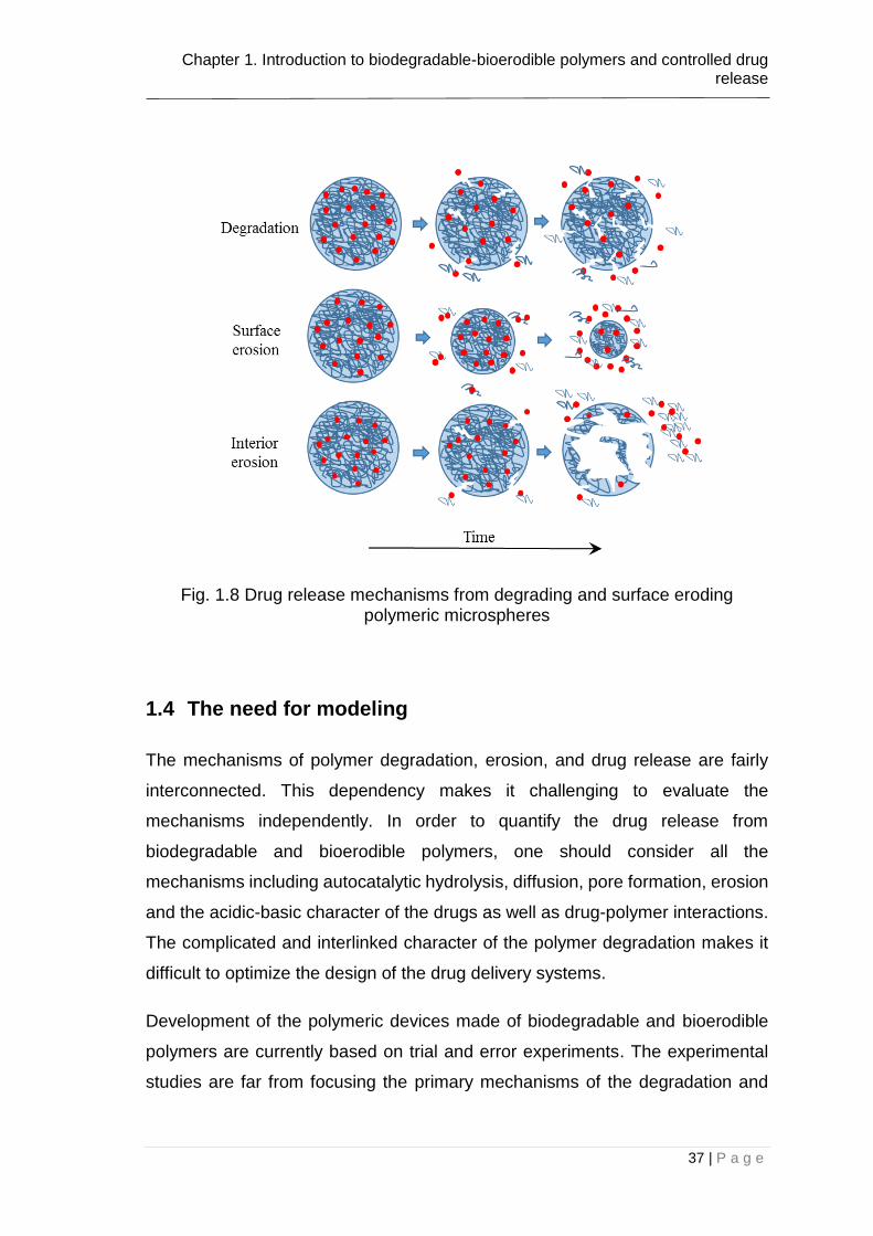
Fig. 1.8 Drug release mechanisms from degrading and surface eroding polymeric
microspheres .................................................................................................... 37
Fig. 2.1 Configuration of the polymer matrix grid through the device after Monte-
Carlo simulations are applied at (a) prior to erosion, (b) 25%, (c) 50% and (d)
75% drug is released. Reproduced from (Zygourakis, 1990) ........................... 45
Fig. 2.2 Monte-Carlo approach of Siepmann et al. (Siepmann et al., 2002); the
schematic structure of the matrix (a) prior to erosion (b) during the drug release.
......................................................................................................................... 47
Fig. 2.3 Biodegradation model for thin plate (Wang et al., 2008) ..................... 49
Fig. 2.4 Categorization of the mathematical models on drug delivery from
polymeric systems ............................................................................................ 57
Fig. 2.5 A literature map showing the state-of-the-art of the current research and
the research gap which is the matter of this thesis ........................................... 62
Fig. 3.1 Schematic illustration of drug and oligomer release from a drug-loaded
microsphere ..................................................................................................... 70
Fig. 3.2 Schematic representation of the possible proton sources ................... 72
Fig. 3.3 A schematic illustration of the grid size ............................................... 77
Fig. 3.4 Flow chart for the model in the presence of acidic drugs .................... 78
Fig. 3.5 Comparison between model prediction and experimental data for blank
particles with different sizes. The dashed and solid lines represent the model
predictions for microspheres of the average size of r = 7.9µm, and 55µm
LIST OF FIGURES
8 | P a g e
respectively. The discrete symbols represent the experimental data (Siepmann
et al., 2005). ..................................................................................................... 80
Fig. 3.6 Comparison between model prediction and experimental data for
degradation of blank and ibuprofen-loaded PLGA microspheres. The dashed and
solid lines represent model predictions for drug-free and drug-loaded particles
respectively. The discrete symbols represent the experimental data (Klose et al.,
2008, Siepmann et al., 2005). .......................................................................... 81
Fig. 3.7 Independent contributions of drug and oligomers to the proton
concentration throughout the degradation process. ......................................... 82
Fig. 3.8 Comparison between the model prediction (solid line) and experimental
data (Klose et al., 2008) (discrete symbols) for drug release. The dashed line is
model prediction using a constant drug diffusion coefficient. The size of the
microsphere is 52µm. ....................................................................................... 83
Fig. 3.9 Variable diffusivity of ibuprofen calculated using Eq. 18 for micro-particle
of r = 52µm. ...................................................................................................... 83
Fig. 3.10 Schematic representation of the microspheres resulting zero order
release profile in the mixture when mixed 1:2 (w/w) ratio of (a) over (b). (a) 75µm
in radius with drug loading of 400 mol/m3and a drug free outside layer of 0.2r
(15µm), (b) 150µm in radius with a drug loading of 400 mol/m3and a drug free
outside layer of 0.6r (90µm). ............................................................................ 85
Fig. 3.11 Calculated profiles of drug release using microspheres of (a) 75µm in
radius with drug loading of 400 mol/m3and a drug free outside layer of 0.2r, (b)
150µm in radius with a drug loading of 400 mol/m3and a drug free outside layer
of 0.6r and (c) mixture of (a) and (b) with 1:2 (w/w) ratio of (a) over (b). .......... 86
Fig. 3.12 Schematic representation of the microspheres resulting zero order
release profile in the mixture when mixed 1:2 (w/w) ratio of (a) over (b). (a) 75µm
in radius with a uniform drug loading of 400 mol/m3, (b) 150µm in radius with a
drug loading of 400 mol/m3and a drug free outside layer of 0.6r (90µm). ........ 87
Fig. 3.13 Calculated profiles of drug release using microspheres of (a) 75µm in
radius with a uniform drug loading of 400 mol/m3, (b) 150µm in radius with a drug
loading of 400 mol/m3and a drug free outside layer of 0.6r and (c) mixture of (a)
and (b) with 1:2 (w/w) ratio of (a) over (b). ....................................................... 88

LIST OF FIGURES
9 | P a g e
Fig. 4.1 Schematic representation of the interaction between basic drugs-
oligomers and catalyst effect of the free species.............................................. 93
Fig. 4.2 Flow chart for the model in the presence of basic drugs ................... 100
Fig. 4.3 Comparison between the model result and experimental data (Klose et
al., 2008, Siepmann et al., 2005): a) nM reduction and b) drug release. Lines
represent the model prediction for blank (dashed line) and loaded particles (solid
line); discrete symbols represent experimental data for blank (circle) and loaded
particles (square, triangle). ............................................................................. 103
Fig. 4.4 Comparison between the model result and experimental data (Dunne et
al., 2000) for blank PLGA microspheres. Lines represent the model prediction for
various sizes and discrete symbols represent corresponding experimental data
for r = 20µm (solid line, circles) and 50µm (dashed line, squares). ................ 107
Fig. 4.5 Comparison of Mn reduction between model results and experimental
data. Solid lines represent the model prediction for microspheres with various
levamisole loadings and discrete symbols represent corresponding experimental
data (Fitzgerald and Corrigan, 1996) (A) 2.4% w/w (solid line, square) (B) 14.3%
w/w (solid line, triangle) and (C) 19.7% w/w (solid line, circle). ...................... 108
Fig. 4.6 Comparison of drug release between model results and experimental
data. Solid lines represent the model prediction for microspheres with various
levamisole loadings and discrete symbols represent corresponding experimental
data (Fitzgerald and Corrigan, 1996) (A) 2.4% w/w (solid line, square) (B) 14.3%
w/w (solid line, triangle) and (C) 19.7% w/w (solid line, circle). ...................... 108
Fig. 4.7 The effect of partition parameter, Kp , on molecular weight ............... 110
Fig. 5.1 The coupling of hydrolytic degradation and erosion .......................... 117
Fig. 5.2 Schematic illustration of discretised polymer ..................................... 119
Fig. 5.4 Moving boundaries at different times and boundary conditions ......... 125
Fig. 5.5 Flow chart of the combined degradation-diffusion and erosion model
....................................................................................................................... 127
Fig. 5.6 Mass loss due to diffusion of short chains ......................................... 129
Fig. 5.7 Mass loss due to surface erosion ...................................................... 130
Fig. 5.8 Mass loss due to interior erosion ....................................................... 131
Fig. 5.9 Mass loss due to interior erosion with incubation period of 0.5 weeks
....................................................................................................................... 132

LIST OF FIGURES
10 | P a g e
Fig. 5.10 A summary of the mass loss profiles due to individual mechanisms133
Fig. 5.11 Combined effect of all the mechanisms on mass loss: degradation-
diffusion (5.9(a)), surface erosion (5.9(b)), interior erosion with incubation period
of 0.5 weeks (5.9(d)) ...................................................................................... 134
Fig. 6.1 Molecular weight distributions of plates at various times during the
degradation (a) t= 0 week; (b) t=1 week; (c) t=10 weeks and (d) t=13 weeks.141
Fig. 6.2 Molecular weight distributions of plates at various times during the
degradation (a) t= 0 week; (b) t=1 week; (c) t=10 weeks and (d) t=13 weeks.142
Fig. 6.3 Comparison of molecular weight change between model prediction and
experimental data for samples with thickness of 0.3 mm and 2 mm. The solid and
dashed lines represent the model predictions with the discrete symbols
representing the experimental data (Grizzi et al., 1995). ................................ 144
Fig. 6.4 Comparison of molecular mass loss between model prediction and
experimental data for samples with thickness of 0.3 mm and 2 mm. The solid and
dashed lines represent the model predictions with the discrete symbols
representing the experimental data (Grizzi et al., 1995) ................................. 144
Fig. 6.5 Hollow structure of PLA37.5GA25 specimen after 10 days of degradation
in distilled water (Li et al., 1990c) with permission via the Copyright Clearance
Centre. ........................................................................................................... 146
Fig. 6.6 Temporal evaluation of simulated the polymer matrix ....................... 146
Fig. 6.7 Comparison of molecular weight change between model prediction and
experimental data. The solid line represents the model prediction with the
discrete symbols representing the experimental data (Lyu et al., 2007) ........ 147
Fig. 6.8 Comparison of mass loss between model prediction and experimental
data. The solid line represents the model prediction with the discrete symbols
representing the experimental data (Lyu et al., 2007) .................................... 148
Fig. 7.1 Diagrams of the bi-layer and tri-layer polymer films of Wang et al. (Wang
et al., 2006) with the corresponding layer thicknesses (reproduced from relevant
study) ............................................................................................................. 153
Fig. 7.2 a) Cross section of an implanted stent in a coronary artery; b) schematic
of a single stent strut with drug-loaded polymer matrix; c) schematic of the drug
loaded polymer matrix which is modelled in the current chapter. ................... 154

LIST OF FIGURES
11 | P a g e
Fig. 7.3 Comparison of molecular weight decrease of PLGA between model
prediction and experimental data. The solid line represents the model predictions
with the discrete symbols representing the experimental data (Wang et al., 2006).
....................................................................................................................... 157
Fig. 7.4 Comparison of mass loss of PLGA between model prediction and
experimental data. The solid line represents the model predictions with the
discrete symbols representing the experimental data (Wang et al., 2006). .... 158
Fig. 7.5 Comparison of sirolimus release from PLGA between model prediction
and experimental data. The solid line represents the model predictions with the
discrete symbols representing the experimental data (Wang et al., 2006). .... 159
Fig. 7.6 Micrographs of the surface morphology of degrading PLGA 53/47 taken
from (Wang et al., 2006) (a) 0 days, (b) 7 days, (c) 14 days and (d) 21 days. 160
Fig. 7.7 Simulation results for drug loaded polymer matrix at t=21 days. ....... 161
LIST OF TABLES
12 | P a g e
LIST OF TABLES
Table 3.1 Model parameters used for the predictions ...................................... 80
Table 4.1 Parameters used in the model to fit with experimental data ........... 104
Table 4.2 Parameters used in the model to fit with experimental data ........... 106
Table 6.1 Parameters used in the fittings ....................................................... 139
Table 7.1 Values of the model parameters used in the fittings ....................... 155
LIST OF PUBLICATIONS AND CONFERENCE PRESENTATIONS
13 | P a g e
LIST OF PUBLICATIONS AND CONFERENCE PRESENTATIONS
Journal Publications
1. SEVIM, K. & PAN, J. 2016. A Mechanistic Model for Acidic Drug Release
Using Microspheres Made of PLGA 50: 50. Molecular Pharmaceutics, 13,
2729-2735.
2. SEVIM, K. & PAN, J. 2017. A model for hydrolytic degradation and erosion
of biodegradable polymers. Acta Biomaterialia, In press.
3. SEVIM, K. & PAN, J. 2017. A Mechanistic Model for Release of Basic
Drugs Using Microspheres Made of PLGA. Submitted for publication.
Conference Presentations
1. 2014, A Computer Model for Polymer Degradation in the Presence of
Acidic Drug. Poster presentation on 26th Annual Conference of the
European Society for Biomaterials (ESB), Liverpool, U.K.
2. 2015, A Mechanistic Model for Drug Release Using Spherical Particles
Made of PLGA. Poster presentation at 1st European Conference on
Pharmaceutics: Drug Delivery, Reims, France.
3. 2017, A Combined Degradation and Erosion Model for Drug Release from
Biodegradable Drug-eluting Stents. Oral presentation in 2nd MOM
Research Day, Leicester, U.K.
4. 2017, A Combined Degradation and Erosion Model for Biodegradable
Polymers. Oral presentation on 28th Annual Conference of the European
Society for Biomaterials (ESB), Athens, Greece.
5. 2017, A Mechanistic Model for Release of Basic Drugs Using
Microspheres made of PLGA. Oral presentation on 28th Annual
Conference of the European Society for Biomaterials (ESB), Athens,
Greece.
LIST OF SYMBOLS
14 | P a g e
LIST OF SYMBOLS
A : surface area of the samples
cd : permeability of the polymers
cd,0 : initial permeability of the polymers
Cdrug : mole concentration of drug
Cdrug,0 : initial mole concentration of drug
Cdrug_H+ : mole concentration of Drug_H+
Ce : mole concentration of ester bonds in the polymer
Ce,0 : initial mole concentration of ester bonds in the polymer
CH+ : mole concentration of H+
CH0+ : mole concentration of donated by the surrounding medium
Ci : mole concentration of species
CL : drug concentration in the liquid phase
COH- : mole concentration of OH-
Col : current mole concentration of ester bonds of oligomers
Col,0 : initial mole concentration of oligomers
CR1-COO- : mole concentration of R1-COO- in the polymer
CR1-COOH : molar concentration of carboxylic end groups in the polymer
CR1-COOH,0 : initial mole concentration of R1-COOH
CR2-COO- : mole concentration of R2-COO-
CR2-COOH : mole concentration of carboxylic acid drug
Csat : saturation concentration of drug in polymer
Cw : mole concentration of water in the polymer
Ddrug,poly : diffusion coefficient of drug in fresh bulk polymer

LIST OF SYMBOLS
15 | P a g e
Ddrug,pore : diffusion coefficient of drug in liquid filled pores
Ddrug: effective diffusion coefficient of drug in the polymer
Di : effective diffusion coefficient of species in the polymer
Di,poly : diffusion coefficient of species in fresh bulk polymer
Dol : effective diffusion coefficient of oligomer in polymer
Dol,poly : diffusion coefficient of oligomers in fresh bulk polymer
Dol,pore : diffusion coefficient of oligomers in liquid filled pores
Dw : diffusion coefficient of water in the polymer
Ek : activation energy for non-catalytic hydrolysis reaction
f : geometric and structural properties of the device
fdrug : the volume ratio of drug to the polymer phase
J : flux of the species
k : hydrolysis reaction rate constant
k1 : non-catalytic kinetic constant
k2 : acid-catalysed kinetic constant
k3 : base-catalysed kinetic constant
Ka : acid dissociation constant for oligomers
Ka,drug : acid dissociation constant for drug
Kb : base dissociation constant for oligomers
kdis : drug dissolution rate
Kp : drug-oligomers partition parameter
m : average degree of polymerization
Mb : drug release by bulk erosion
Md : drug release by diffusion

LIST OF SYMBOLS
16 | P a g e
Mn : number averaged molecular weight of the polymer
Mn,critical : critical molecular weight of the polymer
Mn,mean : mean value for molecular weight of the polymer
Mn,sr_dev : standart deviation for molecular weight of the polymer
Ms : drug release by surface erosion
Mt : cumulative absolute amount of drug release
Mt : total drug release
n : dissociation parameter
Ndp,0 : initial degree of polymerisation
r : radius of the polymer samples
Rdrug: mole concentration of dissolution of drug
Rol : mole concentration of ester bonds of oligomers produced by hydrolysis
Rs : mole concentration of chain scission
S : status of a pixel
Sm : current status of a pixel
t : the degradation time
Tg : glass transition temperature
Ts : reference temperature
V: rate of erosion
Vcell: volume of a single pixel
Vpore : porosity based on loss of short chains
Vpore,drug : porosity due to loss of drug
Vpore,ol : porosity due to loss of oligomers
Wb : weight loss of oligomer by bulk erosion

LIST OF SYMBOLS
17 | P a g e
Wd : weight loss of oligomer by diffusion
Ws : weight loss of oligomers by surface erosion
Wt : total weight loss of oligomers
xc : the degree of crystallinity
α : empirical constant reflecting probability of short chain production due to chain
scission
β : empirical constant reflecting probability of short chain production due to chain
scission
ε : porosity of the polymer matrix
ρ : polymer density
τ : tortuosity of polymer matrix
υ : the rate of synthesis of oligomers

LIST OF ABREVIATIONS
18 | P a g e
LIST OF ABREVIATIONS
ASA: acetyl Salicylic Acid (Aspirin)
DCM: Dichloromethane
DMSO: Dimethyl sulfoxide
FESEM: Field Emission Scanning Electron Microscopy
PBS: phosphate buffered saline
PCL: polycaprolactone acid
PDI: polydispersity index
PDLA: poly (D-lactide)
PDLLA: poly (DL-lactide)
PE: polyethylene
PGA: polyglycolic acid
PLA: poly-lactic acid
PLGA: poly(lactic-co-glycolic acid)
PLLA: poly (L-lactide)
PVA: poly(vinyl alcohol)
MARE: mean absolute relative error

Part 1 Background information and literature review
19 | P a g e
Part 1
Background information and literature review
Chapter 1. Introduction to biodegradable-bioerodible polymers and controlled drug release
20 | P a g e
Chapter 1. Introduction to biodegradable-bioerodible
polymers and controlled drug release
This chapter provides an overview of the current knowledge on biodegradable
polymers including their applications, degradation-erosion mechanisms and
principles of controlled drug release. More detailed information is provided at the
corresponding introductions of each chapter which is specific to the work
presented. Mathematical models describing the degradation is not covered here
as it is outside the scope of current chapter and is extensively addressed in
Chapter 2.
1.1 Biodegradable-bioerodible polymers and their applications
Biodegradable polymers are largely admitted as the materials that lose their
chemical and physical integrity progressively resulting natural by-products. The
literature generally uses the expressions bioresorbable, bioabsorbable and
bioerodible together with the biodegradable term with no clear distinction
between the terms (Vert, 2009). Vert (1992) proposed certain definitions to
prevent the confusion on the usage of the terms. From his definitions, first,
biodegradable refers to the polymeric systems that undergo the molecular
breakdown. Second, bioresorbable term is used for the systems which degrades
in biological conditions and further resorbed by the metabolism for a total
elimination. Third, bioabsorbable term is used for the devices that can be
dissolved in the body fluids without a chain cleavage. Finally, bioerodible term is
used for the polymeric systems which is degraded on its material surface
(Bosworth and Downes, 2010).
Following the definitions in the literature, degradation refer all the changes in
chemical structure and physical properties of the polymer (Pospıš́il et al., 1999).
According to that description, degradation term includes hydrolytic degradation,
enzymatic degradation, thermal degradation, surface erosion and bulk erosion.
On the other hand, erosion proceeds only through the morphological changes of
the polymer structure (Pillai and Panchagnula, 2001, Ratner et al., 2004). From
Chapter 1. Introduction to biodegradable-bioerodible polymers and controlled drug release
21 | P a g e
the definitions, degradation and erosion refers to different phenomena. However,
the difference between polymer degradation and erosion is not clear in many
cases in the literature.
Throughout the current thesis, we focus on hydrolytic degradation and erosion of
the polymers, and all models are established based on one or two of the
mechanisms. In the thesis, the term “hydrolytic degradation” or “hydrolysis” will
refer to the processes in which the polymer chains are cleavaged to form
monomers and oligomers. On the other hand, the term “erosion” will refer to the
physical processes through which polymer loses its integrity and eventually fall
apart. For an ideal erosion, the material is likely to collapse from the outer shell
or from the bulk in which erosion products are transported to the environment
through the cavities. The cavities interconnects the inner structure with the
surrounding medium. This phenomenon will be discussed in greater detail later
in Section 1.3. The definitions used in the current study is consistent with the
ones suggested by Gopferich (1996) and Tamada and Langer (1993).
Biodegradable polymers are the key members of the polymer family with the
improved mechanical and thermal properties and acceptable shelf life.
Furthermore, they are biocompatible, non-toxic and can be easily metabolized in
the body leaving no trace (Agrawal and Ray, 2001, Daniels et al., 1990, Middleton
and Tipton, 2000). Unlike their non-biodegradable counterparts, they can
naturally degrade and disappear from the body over the desired period of time;
this avoids the need for surgical treatments to remove the devices after they
performed their function (Domb and Kumar, 2011).
Much progress has been done in medical applications in recent years with the
exploration of alternative synthetic and naturally occurring polymers (Makadia
and Siegel, 2011). In general, synthetic polymers have greater benefits
compared to the naturally occurring ones as their required mechanical properties
can be easily tailored (Cascone et al., 1995, Domb and Kumar, 2011). Among all
biodegradable polymers, aliphatic polyester family in particular polylactic acids
(PLAs), polyglycolic acids (PGAs) and polycaprolactone acids (PCLs) (Fig. 1.1)
are more commonly used for medical applications. This is because of the
Chapter 1. Introduction to biodegradable-bioerodible polymers and controlled drug release
22 | P a g e
improved mechanical properties as well as the availability of these polymers
compared to the other biodegradable polymers (Klose et al., 2008, Saha et al.,
2016).
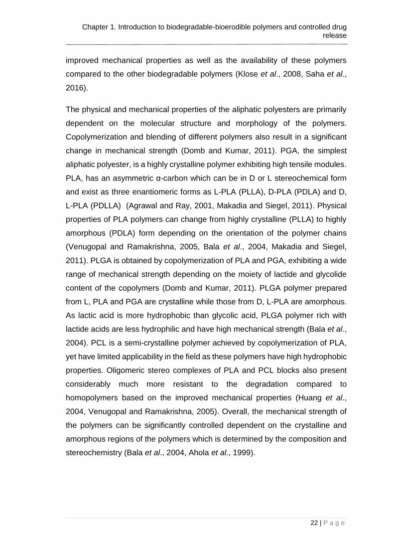
The physical and mechanical properties of the aliphatic polyesters are primarily
dependent on the molecular structure and morphology of the polymers.
Copolymerization and blending of different polymers also result in a significant
change in mechanical strength (Domb and Kumar, 2011). PGA, the simplest
aliphatic polyester, is a highly crystalline polymer exhibiting high tensile modules.
PLA, has an asymmetric α-carbon which can be in D or L stereochemical form
and exist as three enantiomeric forms as L-PLA (PLLA), D-PLA (PDLA) and D,
L-PLA (PDLLA) (Agrawal and Ray, 2001, Makadia and Siegel, 2011). Physical
properties of PLA polymers can change from highly crystalline (PLLA) to highly
amorphous (PDLA) form depending on the orientation of the polymer chains
(Venugopal and Ramakrishna, 2005, Bala et al., 2004, Makadia and Siegel,
2011). PLGA is obtained by copolymerization of PLA and PGA, exhibiting a wide
range of mechanical strength depending on the moiety of lactide and glycolide
content of the copolymers (Domb and Kumar, 2011). PLGA polymer prepared
from L, PLA and PGA are crystalline while those from D, L-PLA are amorphous.
As lactic acid is more hydrophobic than glycolic acid, PLGA polymer rich with
lactide acids are less hydrophilic and have high mechanical strength (Bala et al.,
2004). PCL is a semi-crystalline polymer achieved by copolymerization of PLA,
yet have limited applicability in the field as these polymers have high hydrophobic
properties. Oligomeric stereo complexes of PLA and PCL blocks also present
considerably much more resistant to the degradation compared to
homopolymers based on the improved mechanical properties (Huang et al.,
2004, Venugopal and Ramakrishna, 2005). Overall, the mechanical strength of
the polymers can be significantly controlled dependent on the crystalline and
amorphous regions of the polymers which is determined by the composition and
stereochemistry (Bala et al., 2004, Ahola et al., 1999).

Chapter 1. Introduction to biodegradable-bioerodible polymers and controlled drug release
23 | P a g e
Fig. 1.1 Structure of PLA-PGA-PCL
Several synthetic polyesters have been actively used in environmental,
agricultural and waste management applications. However, in last few decades,
there has been a growing trend towards the use of synthetic polymers in
biomedical engineering field including preventive medicine, surgical treatments,
and clinical inspections. This includes disposable products (e.g. syringe, blood
bag), supporting materials (e.g. sutures, bone plates and sealant), prosthesis for
tissue replacements (e.g. dental or breast implant), artificial tissue/organs (e.g.
artificial heart, kidney, eyes, teeth and etc.), and engineering products (e.g. tissue
engineering products) with an without targeting (Ikada and Tsuji, 2000, Domb
and Kumar, 2011, Bastioli, 2005, Rezaie et al., 2015). There are various reasons
for the favorable consideration of polyesters in biomedical applications over
biostable devices. The major driving force is that these devices would naturally
disappear from the tissue by time without the need for any clinical treatment.
Moreover, these materials function as long term implants while in contact with
the living tissue, without any risk of infection (Ikada and Tsuji, 2000, Rezaie et
al., 2015, Nair and Laurencin, 2007). The choice of material for a specific
application is primarily dependent on its physicochemical properties like
mechanical, chemical and biological functions.
Another common application of biodegradable polymers is as carriers for drugs
(e.g. injectable microspheres, drug eluting stents) (Rezaie et al., 2015) from
which drug is released at a predetermined rate to the possibly targeted sites.
Preferably, homo and copolymers of lactate and glycolide are used for that
specific purpose (Philip et al., 2007). The drug is either embedded in a membrane
or encapsulated in a matrix releasing the drug by time (Mark, 2004). More

Chapter 1. Introduction to biodegradable-bioerodible polymers and controlled drug release
24 | P a g e
detailed information about the controlled drug delivery systems will be discussed
throughout this thesis.
1.2 Controlled drug release
Controlled drug delivery systems are alternative to conventional delivery systems
that target to deliver drugs over an extended time or at a specific time in a
controlled manner. These systems are comprised of an active agent, drug, and
a polymer. Controlled release systems has many advantageous over other
release systems providing better management of the drug concentrations,
shielding drug to the desired location in action, minimizing side effects and
improving patient compliance (Langer, 1980, Mathiowitz et al., 1997, Ford et al.,
2011a, Siepmann et al., 2011).
1.2.1 General concept of controlled drug release
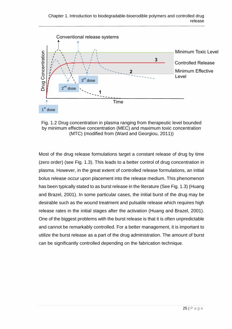
Controlled drug release systems are developed for a better administration of the
drug in the body enabling a stable concentration over time. Fig. 1.2 illustrates the
plasma concentration of drug in the blood. In conventional release systems,
single dose (1) leads to a sharp rise and fall in drug amount that might fall out of
the range of therapeutic level for certain time intervals. Moreover, the dose repeat
(2) might be necessary to extent the concentration of drug in plasma. On the
contrary, controlled systems (3) lead to a better regulation of drug concentration
by time. Such systems provide a stationary level for drug pharmacokinetics so
that drug concentration remains in the therapeutic level eliminating drug to reach
to the toxic concentrations (Siepmann et al., 2011).
Chapter 1. Introduction to biodegradable-bioerodible polymers and controlled drug release
25 | P a g e
Fig. 1.2 Drug concentration in plasma ranging from therapeutic level bounded by minimum effective concentration (MEC) and maximum toxic concentration
(MTC) (modified from (Ward and Georgiou, 2011))
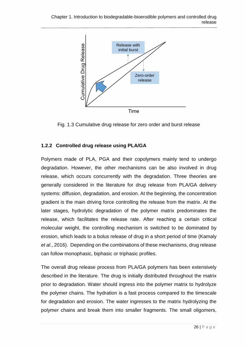
Most of the drug release formulations target a constant release of drug by time
(zero order) (see Fig. 1.3). This leads to a better control of drug concentration in
plasma. However, in the great extent of controlled release formulations, an initial
bolus release occur upon placement into the release medium. This phenomenon
has been typically stated to as burst release in the literature (See Fig. 1.3) (Huang
and Brazel, 2001). In some particular cases, the initial burst of the drug may be
desirable such as the wound treatment and pulsatile release which requires high
release rates in the initial stages after the activation (Huang and Brazel, 2001).
One of the biggest problems with the burst release is that it is often unpredictable
and cannot be remarkably controlled. For a better management, it is important to
utilize the burst release as a part of the drug administration. The amount of burst
can be significantly controlled depending on the fabrication technique.
Minimum Toxic Level
Conventional release systems
Time
Dru
g C
on
ce
ntr
ation
Minimum Effective Level
Controlled Release
1st dose
2nd
dose
3rd
dose
1
3
2
Chapter 1. Introduction to biodegradable-bioerodible polymers and controlled drug release
26 | P a g e
Fig. 1.3 Cumulative drug release for zero order and burst release
1.2.2 Controlled drug release using PLA/GA
Polymers made of PLA, PGA and their copolymers mainly tend to undergo
degradation. However, the other mechanisms can be also involved in drug
release, which occurs concurrently with the degradation. Three theories are
generally considered in the literature for drug release from PLA/GA delivery
systems: diffusion, degradation, and erosion. At the beginning, the concentration
gradient is the main driving force controlling the release from the matrix. At the
later stages, hydrolytic degradation of the polymer matrix predominates the
release, which facilitates the release rate. After reaching a certain critical
molecular weight, the controlling mechanism is switched to be dominated by
erosion, which leads to a bolus release of drug in a short period of time (Kamaly
et al., 2016). Depending on the combinations of these mechanisms, drug release
can follow monophasic, biphasic or triphasic profiles.
The overall drug release process from PLA/GA polymers has been extensively
described in the literature. The drug is initially distributed throughout the matrix
prior to degradation. Water should ingress into the polymer matrix to hydrolyze
the polymer chains. The hydration is a fast process compared to the timescale
for degradation and erosion. The water ingresses to the matrix hydrolyzing the
polymer chains and break them into smaller fragments. The small oligomers,
Time
Cum
ula
tive
Dru
g R
ele
ase
Zero-order release
Release with initial burst

Chapter 1. Introduction to biodegradable-bioerodible polymers and controlled drug release
27 | P a g e
which are produced by hydrolyses, are capable of diffusing out of the matrix as
a result of a concentration gradient. At the meantime, drug molecules are
dissolved and diffuse through the polymeric media (Uhrich et al., 1999, Ford
Versypt et al., 2013). Transport of the oligomers and drug take place via the bulk
polymer and the pores established during the degradation. Diffusion of the drug
can also contribute to the pore volume. Due to the dynamic structure of the
polymer matrix, the effective diffusivities of drug and oligomers enhances through
the degradation. Both degradation and drug release processes take place in
concert during the drug release process. In some cases, polymer matrix loses its
integrity after reaching a certain molecular weight which is followed by a sudden
erosion. This leads to a bolus release of oligomers and drug in short time. More
detail about the mechanism of drug release from PLA/GA polymers is given in
Section 1.3.3.
1.3 Mechanisms for hydrolytic degradation, erosion and
controlled drug release
The underlying mechanism of controlled release systems is diverse and complex,
and it is essential to comprehend the individual mechanisms involved in the
release process.
1.3.1 Mechanism for hydrolytic degradation
Polymers comprise of long chains made of many identical monomer units. Fig.
1.4 represent a schematic illustration of polymer chains. The blue spheres
represent the repeat units (monomers) of a long chain. In the aqueous
environment, long chains break into the smaller ester bonds (see Fig. 1.4). This
is known as hydrolysis reaction or hydrolytic degradation. Polymer hydrolysis
consist of four stages (Scott, 2002). Water uptake is the first stage of the chain
cleavage which triggers hydrolysis reaction (stage 1). Since diffusion of water is
a rapid process compared to the hydrolysis, one can assume the water molecules
to be abundant from the beginning of the reaction. The hydrolysis reaction
produces short chains which are known as oligomers. After the cleavage, two

Chapter 1. Introduction to biodegradable-bioerodible polymers and controlled drug release
28 | P a g e
loose ends terminate as alcohol end groups, R-OH and carboxylic acid end
groups, R-COOH (Pan, 2014) (stage 2).
Fig. 1.4 Schematic representation of hydrolytic degradation of polymer
The reaction is known to be autocatalytic which can be catalysed by acids and
bases. The acid catalyst can be from an external source such as the acidic
medium or an internal source such as carboxylic acids of the polymer chains
(Grizzi et al., 1995) (stage 3). The chemical mechanism of acid-catalysed
hydrolysis will be explained in detail in the following section.
As the number of chain cleavage increases, more and more carboxylic acid
groups are produced which are known to catalyze hydrolysis. The solubilized
oligomers are capable of moving out of the matrix leading to a mass loss (stage
4). Depending on the matrix size, monomers and oligomers can be trapped in the
device leading to an increase in local acidity. This effect is more predominant for
larger devices. Such an accumulation leads to acceleration in degradation rate
as well as leading to surface-interior differentiation (Siepmann et al., 2011). Over
Stage 1: Water ingress Stage 2: Production of R-COOH and R’-OH
COOH
COOH
OH
OH
Stage 3: Dissociation of short chains
COO-
COO-
OH
OH
H+
H+
Stage 4: Oligomer diffusion
OH
OH
COO-
COO-
H+
H+

Chapter 1. Introduction to biodegradable-bioerodible polymers and controlled drug release
29 | P a g e
time, the autocatalytic effect becomes more predominant, and microspheres
forms hollow interiors (Berkland et al., 2003). The experimental studies from the
literature have evidences of local acidity increase due to acidic byproducts of the
hydrolysis reaction. This provides very strong evidence that coupling between
autocatalytic reactions and diffusion of the acidic products is a necessity for the
systems made of PLA/GA polymers (Ford et al., 2011a).
It has been reported that there are two types of chain cleavage in a polymer bond:
random scission and end scission (Pan, 2014). In random scission, each polymer
chain is assumed to have equal chance to be cleaved, while end scission
assumes the cleave to happen only at the end of the chain (Gleadall et al., 2014).
While the concentration of carboxylic acid groups is low and the total number of
ester bonds is high, all ester bonds have same probability to cleavage with
random scission. As the concentration of end groups increases, and the
autocatalysis become the dominant mechanism, end scission becomes more
preferable (van Nostrum et al., 2004, Batycky et al., 1997). Degradation leads to
change in polymer microstructure by the formation of pores through which
monomers and oligomers are released. As oligomers are released, porosity
within the matrix becomes prominent (Gopferich, 1996). Finally, when the internal
material is totally transformed to water soluble material hollow structure can be
observed in the samples. Therefore, one can claim that the hydrolytic
degradation of polymers are heterogeneous depending on the size of the
degrading material (stage 4) (Scott, 2002). This leads to an increase in the
effective diffusivity of oligomers as microspheres diameter enlarges (Siepmann
et al., 2005).
Since the structure of the polymer matrix is dynamic, establishing diffusion-
reaction balance is rather difficult. The level of degradation can be monitored by
examining the change in molecular weight and mass loss (Gopferich, 1996). The
whole process of degradation mechanism is fairly complex and reasonable
assumptions should be proposed while developing a mathematical model.
The weaker intermolecular bonds increases the rate of hydrolytic degradation.
Several additional factors may also influence on the rate of degradation. In order

Chapter 1. Introduction to biodegradable-bioerodible polymers and controlled drug release
30 | P a g e
to sufficiently design drug delivery devices, it is important to comprehend all these
factors affecting the biodegradation of polyesters. As stated before, polymer
composition has a significant influence on the rate of degradation. Altering
number of units in a homopolymer (polymers with identical monomer units) or
proportion of glycolide and lactide units in a copolymer dramatically changes the
degradation rate (Park, 1995). Degradation rate is also a function of crystallinity.
Literature provides conflicting results about the relationship between degradation
rate and crystallinity (Bastioli, 2005). Few groups (Tsuji and Ikada, 2000) state
an acceleration of the degradation while others (Li et al., Montaudo and Rizzarelli,
2000, Cai et al., 1996, Li and McCarthy, 1999) propose a decrease in the
degradation trend with increasing crystallinity. Both of the results are expected
because crystalline regions prevent the water molecules from penetrating into
the polymer due to the packing of aligned chains. This causes to resistance to
hydrolytic degradation. On the other hand, with increasing crystalline fraction,
oligomers accumulate in the amorphous regions. This leads to an increase in
oligomer concentration inside the amorphous regions which accelerates the
chain scission. The relative influence of these theories determines the rate of
chain scission.
The molecular weight and its distribution have a dramatic effect on polymer
degradation. This is because of the fact that the physical properties of the
polymer such as Tg, crystallinity and Young’s modulus are directly related to the
polymer molecular weight. Basically, polymers having longer polymer chains
requires more time to be fully degraded. However, this can be opposite for some
cases such as for the case of PLLA due to the increase in crystallinity with
increasing chain size (Bastioli, 2005, Park, 1994).
Size and shape of the matrix also affect the biodegradation properties, since
higher surface area gives rise to accelerated degradation (Li, 1999). The acidity
of the microenvironment, pH, changes the degradation rate; both acidic and basic
media can accelerate degradation (Holy et al., 1999).
Drug type is another factor reported to have a significant influence on polymer
degradation. However, efforts to relate the drug chemistry to polymer degradation

Chapter 1. Introduction to biodegradable-bioerodible polymers and controlled drug release
31 | P a g e
is very limited and do not yield a strong relationship. Acidic drugs are reported to
enhance the polymer degradation rate; whereas there are conflicting results for
basic drugs (Siepmann et al., 2005, Makadia and Siegel, 2011, Cha and Pitt,
1989). The effect of drug chemistry on polymer degradation has been discussed
in detail through this thesis.
The evidences from the literature show that the factors influencing the
degradation rate are very complex and there can be many exceptions which put
obstacles to make correlations. Furthermore, a bunch of factors can overlap
causing challenges to make generalizations. However, it is still critical to
understand the factors affecting the degradation rate in different systems in order
to design optimum devices for drug delivery.
1.3.1.1 Hydrolysis of esters
As mentioned in the previous section, chemical hydrolysis of the polymer ester
bonds can be catalysed by acids and bases. In the current section, the catalytic
mechanisms of the esters will be explained in detail.
The term acid catalysis generally refers to proton catalysis in the literature. In this
sense, acid catalysed hydrolysis begins with protonation of the carbonyl O-atom
(stage 1). The main driving force behind the protonation is the susceptibility of
carbonyl C atom to nucleophilic attack. After the protonation, the electrophilicity
of the carbonyl increases. The first stage is followed by hydration of the
carbonium ion to produce a tetrahedral intermediate product (stage 2). In the
acidic medium, equilibrium will again be set up within this stage and the proton
will be shared by three oxygen atoms. The reaction continues with heterolytic
cleavage of the acyl-O bond (stage 3). This stage is followed by an acid-base
reaction: deprotonation of the oxygen that comes from the water molecules
(stage 4). In the next stage, the neutral methanol group is pushed out by use of
the electrons of the adjacent oxygen (stage 5). And finally, the oxonium ion is
deprotonated revealing the carbonyl in the carboxylic acid product. Thus, acid
catalyst is regenerated. Since the last step includes the loss of proton, the
reactions are considered as acid catalysed. All the steps of acid catalyst
hydrolysis is reversible. The stages of the acid catalysed hydrolysis is

Chapter 1. Introduction to biodegradable-bioerodible polymers and controlled drug release
32 | P a g e
schematized in Fig. 1.5. The symbol, R, refers to –CH3 group, whereas X stands
for -OCH3 group (Dewick, 2006, Testa and Mayer, 2003).
Fig. 1.5 Acid-catalysed hydrolysis of esters
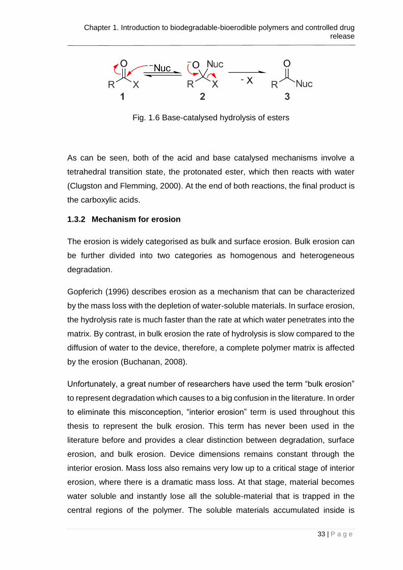
The term base catalysis is generally taken as OH- catalysis. In the base catalysed
hydrolysis of esters, the nucleophile which is hydroxide is able to attack to
carbonyl. This nucleophilic attack leads formation of a tetrahedral intermediate
(stage 1). In the latter stage, intermediate collapses with heterolytic cleavage of
the acyl- O bond, which leads to liberation of phenolate anion (represented as X
in the figure) (stage 2). This reaction is strongly driven to the right side. The final
step is the deprotonation of carboxylic acid (stage 3). The final proton transfer is
irreversible. This is why base catalyst hydrolysis is generally schematised with
irreversible arrows. The mechanism of base-catalysed ester hydrolysis is
presented in Fig. 1.6. The symbol, Nuc refers to the nucleophile which is
hydroxide (OH-) (Testa and Mayer, 2003).
protonation of carbonyl oxygen
nucleophilic attack on to protonated ester
acid catalyst regenerated
carboxylic acid
Chapter 1. Introduction to biodegradable-bioerodible polymers and controlled drug release
33 | P a g e
Fig. 1.6 Base-catalysed hydrolysis of esters
As can be seen, both of the acid and base catalysed mechanisms involve a
tetrahedral transition state, the protonated ester, which then reacts with water
(Clugston and Flemming, 2000). At the end of both reactions, the final product is
the carboxylic acids.
1.3.2 Mechanism for erosion
The erosion is widely categorised as bulk and surface erosion. Bulk erosion can
be further divided into two categories as homogenous and heterogeneous
degradation.
Gopferich (1996) describes erosion as a mechanism that can be characterized
by the mass loss with the depletion of water-soluble materials. In surface erosion,
the hydrolysis rate is much faster than the rate at which water penetrates into the
matrix. By contrast, in bulk erosion the rate of hydrolysis is slow compared to the
diffusion of water to the device, therefore, a complete polymer matrix is affected
by the erosion (Buchanan, 2008).
Unfortunately, a great number of researchers have used the term “bulk erosion”
to represent degradation which causes to a big confusion in the literature. In order
to eliminate this misconception, “interior erosion” term is used throughout this
thesis to represent the bulk erosion. This term has never been used in the
literature before and provides a clear distinction between degradation, surface
erosion, and bulk erosion. Device dimensions remains constant through the
interior erosion. Mass loss also remains very low up to a critical stage of interior
erosion, where there is a dramatic mass loss. At that stage, material becomes
water soluble and instantly lose all the soluble-material that is trapped in the
central regions of the polymer. The soluble materials accumulated inside is

Chapter 1. Introduction to biodegradable-bioerodible polymers and controlled drug release
34 | P a g e
released as soon as interior is connected with the surrounded medium (see Fig.
1.7).
In surface erosion, polymer falls apart with a constant speed starting from the
matrix surface, slowly decreasing the size and shrinking towards its interior as
illustrated in Fig. 1.7. For an ideal surface erosion, erosion rate is constant which
is proportional to the external surface area. Molecular weight does not change
significantly during the erosion process.
Fig. 1.7 Mechanisms of hydrolytic degradation, surface erosion and interior erosion
As a basic rule, the polymers having highly reactive groups tend to undergo
erosion, while the ones with less reactive groups undergo degradation.
Polyanhydrides, for example, preferably tend to be surface eroding; whereas
aliphatic polyesters such as PLA, PGA is more likely to degrade through
hydrolytic degradation and interior erosion (Buchanan, 2008). However, it should
be bare in mind that such kind of classification is not correct for all the cases

Chapter 1. Introduction to biodegradable-bioerodible polymers and controlled drug release
35 | P a g e
since degradable polymer can erode when the conditions are appropriate
(Burkersroda and Goepferich, 1998).
Mass loss profiles can be a simple and effective way to assess the undergoing
mechanism of polymers rather being controlled by degradation, surface erosion
or interior erosion. Degradation leads to a slow mass loss slightly increasing to
the end of the degradation. The observations show that only up to 5-10% mass
loss can be achieved with the degradation-diffusion mechanism. Surface erosion
leads to a linear mass loss profile through which greater amount of mass can be
lost (Engineer et al., 2011). For the case of interior erosion, polymers represent
a zero mass loss followed by a spontaneous mass loss after a critical degree
(von Burkersroda et al., 2002). Interior erosion leads to a great amount of
oligomer release. As can be seen from the definitions, the mechanisms of
degradation and erosion are fairly interconnected.
In most of the drug delivery applications, surface erosion is a preferable over the
degradation and interior erosion since it is more predictable and easy to control
compared to degradation and interior erosion (Kamaly et al., 2016).
1.3.3 Mechanism for drug release
For polymeric drug delivery systems, drug release mechanism generally refers
to how drug molecules have been transported from a starting point to the matrix’s
outer surface and finally released to the surrounding medium; and are classified
based on how the drug has been released from the system (Kamaly et al., 2016).
There can be one or more important phenomena controlling drug release from
the particles including diffusion, matrix degradation, erosion and swelling
(Siepmann et al., 2011, Arifin et al., 2006b). Generally, a combination of different
mechanisms is responsible for drug release which depends to the drug and
polymer type. In diffusion-controlled systems, drug release is predominantly
controlled by a non-degraded polymer, where drug molecules actions upon
exposure to a stimulation. Diffusion is caused by Brownian motion that is a
random walk of the drug molecules throughout the device. The prime modes of
degradation controlled systems are by the release of drugs throughout the

Chapter 1. Introduction to biodegradable-bioerodible polymers and controlled drug release
36 | P a g e
networks generated during the chain cleavage reactions (see Fig. 1.8). In an
erosion-controlled system, the drug has been released by the loss of matrix
starting from the surface or the interior (see Fig. 1.8). More detailed information
about the mechanisms of polymer degradation and erosion is the subject of
Section 1.3.1 and 1.3.2, therefore, will not be discussed in further detail in the
current section. In swelling controlled systems the drug is released from
hydrophilic polymers as swelling front moves into the matrix. In such systems,
the release rate is determined by the transport of the solvent into the matrix
(Siepmann and Siepmann, 2012, Ranga Rao and Padmalatha Devi, 1988, Heller,
1987).
Here, a brief introduction of the mechanisms for drug release is provided for
several drug delivery systems. However, it is a challenge to discuss these
processes independently. For an instance, in the case of swelling controlled
systems, the diffusion rate of water would be a key issue for the control. Likewise,
degradation and erosion mechanism are interlinked with each other as explained
in Section 1.3.
Chapter 1. Introduction to biodegradable-bioerodible polymers and controlled drug release
37 | P a g e
Fig. 1.8 Drug release mechanisms from degrading and surface eroding polymeric microspheres
1.4 The need for modeling
The mechanisms of polymer degradation, erosion, and drug release are fairly
interconnected. This dependency makes it challenging to evaluate the
mechanisms independently. In order to quantify the drug release from
biodegradable and bioerodible polymers, one should consider all the
mechanisms including autocatalytic hydrolysis, diffusion, pore formation, erosion
and the acidic-basic character of the drugs as well as drug-polymer interactions.
The complicated and interlinked character of the polymer degradation makes it
difficult to optimize the design of the drug delivery systems.
Development of the polymeric devices made of biodegradable and bioerodible
polymers are currently based on trial and error experiments. The experimental
studies are far from focusing the primary mechanisms of the degradation and
Chapter 1. Introduction to biodegradable-bioerodible polymers and controlled drug release
38 | P a g e
erosion processes. Moreover, the experimental approach has many limitations
including requirement of excess amount of time and money.
Modeling approaches help to understand the experimental data revealing
underlying mechanisms of drug release. This information in turn helps
optimization of release kinetics and tablet design. Mathematical models can
enlighten the effect of several parameters, including composition of polymers,
size, shape, drug content on polymer degradation and corresponding drug
release. Moreover, systemic use of the mathematical models in drug delivery field
significantly reduces the cost and the experimentation time. In terms of a better
design of biodegradable devices used in drug delivery field, mathematical models
have been proved to be effective and extend our knowledge of understanding the
biodegradable devices used for controlled drug delivery. Therefore, creating
advanced models would be able to meet the criteria needed for the market such
as being cost effective, applicable and efficient.
Many mathematical models have been developed to predict the polymer
degradation and erosion as well as the corresponding drug release from
biodegradable polymers. These models can be either empirical, semi empirical,
mechanistic or probabilistic. Mechanistic models are known to reflect real physics
behind the drug diffusion, degradation and erosion (Kamaly et al., 2016). In most
of the mechanistic models, the diffusivity of the species are reflected by Fick’s
laws of diffusion. A comprehensive review of the previous degradation and drug
release models are provided in Chapter 2.
The existing models form a solid baseline for the mathematical models developed
throughout the thesis. Taking these models as a basis, several mathematical
models will be developed to enlighten the underlying mechanism of drug release
from biodegradable polymers. This includes: i) the mechanistic models
presenting the effects of the acidic and basic drugs on the hydrolytic degradation
rate; ii) combined modelling of hydrolytic degradation and erosion; and iii) the
applications of proposed models on several case studies from the literature.
Chapter 2. A review of existing mathematical models for polymer degradation and controlled drug release
39 | P a g e
Chapter 2. A review of existing mathematical models
for polymer degradation and controlled drug release
In order to obtain the precise quantification of polymer degradation, erosion, and
drug release, modeling is extremely important. Mathematical/computational
models have some preferable properties over experimental studies such as
avoiding excessive experiments, allowing precise prediction of design
parameters (size, shape, geometry etc.) and accurately determination of
degradation and release profiles (Shaikh et al., 2015). Models for drug delivery
systems also helps to provide transfer mechanisms based on scientific
knowledge which facilitates the development of novel pharmaceutical products.
This chapter presents a brief review of the previous models in the literature for
the polymer degradation, erosion, and drug release. Degradation and erosion
models have been divided into the subsections such as the studies proposed
before Pan and co-workers (Section 2.1) and by Pan and co-workers (Section
2.2). Drug release models have been detailed in Section 2.3. This chapter also
gives details about the gaps in the literature as well as overall aims, objectives,
and structure of the thesis.
2.1 Models for polymer degradation and erosion before the
work by Pan and co-workers
2.1.1 Models for polymer hydrolysis kinetics
The simplest model for polymer hydrolysis has been proposed by Pitt and Gu
(1987) assuming that the rate of hydrolysis is only dependent on ester and water
concentrations
𝑑𝐶𝑅1−𝐶𝑂𝑂𝐻
𝑑𝑡= 𝑘𝐶𝑤𝐶𝑒 (2.1)
where 𝑘 is the rate constant, 𝐶𝑒, 𝐶𝑤 and 𝐶𝑅1−𝐶𝑂𝑂𝐻 are the mole concentrations of
the ester bonds, water and carboxylic end groups of oligomers, respectively and
Chapter 2. A review of existing mathematical models for polymer degradation and controlled drug release
40 | P a g e
t, the time. The model proposed lacks considering the catalyst effect of the acidic
groups. Pitt and Gu then correlated the reaction rate to include catalytic impact
of the carboxylic groups such as
𝑑𝐶𝑅1−𝐶𝑂𝑂𝐻
𝑑𝑡= 𝑘𝐶𝑤𝐶𝑒𝐶𝑅1−𝐶𝑂𝑂𝐻
(2.2)
Due to accounting the acid concentration, Eq. 2.2 has been referred as the
autocatalytic hydrolysis reaction. In their model, Pitt and Gu assumed that
reaction kinetics is proportional to the concentration of carboxylic acid end
groups. Siparsky et al. (1998) made a clear distinction between the acid catalyst
concentration, 𝐶𝐻+, and acid product concentration, 𝐶𝑅1−𝐶𝑂𝑂𝐻, and updated the
hydrolysis rate equation to include autocatalytic terms. They considered the
dissociation of carboxylic acids which leads to generation of 𝐻+and that has been
reckon as the main source of autocatalysis reaction. The equilibrium constant of
the oligomer dissociation reaction, 𝐾𝑎, is
𝐾𝑎 =
𝐶𝑅1−𝐶𝑂𝑂𝐻
(𝐶𝐻+𝐶𝑅1−𝐶𝑂𝑂−)
(2.3)
Since 𝐶𝐻+=𝐶𝑅1−𝐶𝑂𝑂−, Eq. 2.2 can be rearranged as 𝐶𝐻+ = [𝐾𝑎𝐶𝑅1−𝐶𝑂𝑂𝐻]1/2
which
is used to represent the acid catalyst concentration. Then the rate equation can
be updated as
𝑑𝐶𝑅1−𝐶𝑂𝑂𝐻
𝑑𝑡= 𝑘𝐶𝑤𝐶𝑒[𝐶𝑅1−𝐶𝑂𝑂𝐻 𝐾𝑎]
0.5
(2.4)
The reaction rate proposed by Siparsky et al. (1998) can be fitted with most of
the experimental data in the literature. The concentration of the chain ends is
usually very low to be measured. Therefore, instead of 𝐶𝑅1−𝐶𝑂𝑂𝐻, it is convenient
to characterize the polymer degradation with the number average molecular
weight, 𝑀𝑛. Basically, concentration of the carboxylic end groups are reciprocal
to the number average molecular weight of the polymers. Lyu and Untereker
(2009) proposed the following equation to link these two such as

Chapter 2. A review of existing mathematical models for polymer degradation and controlled drug release
41 | P a g e
𝑀𝑛 =𝜌
𝐶𝑅1−𝐶𝑂𝑂𝐻. (2.5)
Integrating Eq. 2.4 yields to
𝐶𝑅1−𝐶𝑂𝑂𝐻 − 𝐶𝑅1−𝐶𝑂𝑂𝐻,0 = 𝑘𝐶𝑤𝐶𝑒𝑡 (2.6)
where 𝐶𝑅1−𝐶𝑂𝑂𝐻,0 is the initial mole concentration of acid end groups. By using
Eqs. (2.5) and (2.6), we have
1
𝑀𝑛=
1
𝑀𝑛,0+
1
𝑀𝑢𝑛𝑖𝑡𝑘𝐶𝑤𝐶𝑒𝑡. (2.7)
Here, 𝑀𝑢𝑛𝑖𝑡 is the molecular weight of a polymer unit. Some published data uses
weight average molecular weight, 𝑀𝑤 or viscosity averaged molecular weight,
𝑀𝑣, to show reaction kinetics, which is not accurate. However, since these are
proportional to 𝑀𝑛 values, similar trend can be observed (Buchanan, 2008).
All the mentioned models above assume that the water concentration is a limiting
factor for the reaction kinetics, however, one can simply assume that water is
abundant during the physicochemical reactions. This assumption is acceptable
since the water ingress rate is much faster than hydrolysis reaction rate.
Arrhenius analyzed the effect of temperature on the reaction rate; proposed a
temperature dependent kinetic constant such as
𝑘 = 𝑘0𝑒−𝐸𝑘/𝑅𝑇 (2.8)
in which 𝐸𝑘 is the activation energy for the reaction; 𝑘0, a constant. Arrhenius
equation has some limitations above and below glass transition temperature, 𝑇𝑔.
Lyu et al. (2007) proposed an alternative equation to Arrhenius equation which
can be used below and under the 𝑇𝑔 such as
𝑘 = 𝑘0𝑒−(𝐸𝑘/𝑅(𝑇−𝑇𝑠). (2.9)
This equation is called as Vogel-Tammann-Fulcher equation. Here, 𝑇𝑠 is a
reference temperature. Eq. (2.9) can be effectively used below and under 𝑇𝑔.

Chapter 2. A review of existing mathematical models for polymer degradation and controlled drug release
42 | P a g e
2.1.2 Reaction – diffusion models
Thombre and Himmelstein (1985) and Joshi and Himmelstein (1991) developed
a comprehensive approach for drug release taking into account autocatalytic
effect of degradation products. In their model, water ingress into the matrix,
hydrolyzing the acid generator such as an acid anhydride, and the generated acid
is assumed to catalyze the chain cleavage. The chemical reactions then linked
with the diffusion controlled mass transfer equations. They used the following
equation to introduce diffusion component to the reaction equations such as
𝑑𝐶𝑖
𝑑𝑡=
𝜕
𝜕𝑥(𝐷𝑖(𝑥, 𝑡)
𝜕𝐶𝑖
𝜕𝑥) + 𝑣𝑖 (2.10)
in which 𝐶𝑖 and 𝐷𝑖 represents the concentration and effective diffusion coefficient
of the oligomers, respectively; x the position and 𝑣𝑖 , the rate of oligomer
production. Here, diffusion is assumed to be only in one direction. To introduce
the changing permeability of the system, 𝐶𝑑, they applied the following equation
𝐷𝑖 = 𝐷𝑖,𝑝𝑜𝑙𝑦 𝑒𝑥𝑝 [𝜇 (𝐶𝑑,0 − 𝐶𝑑)
𝐶𝑑,0]. (2.11)
Here, 𝐷𝑖,𝑝𝑜𝑙𝑦 is the diffusivity of the oligomers at fresh bulk polymer; 𝐶𝑑,0, the initial
permeability of the polymer and 𝜇, the constant.
Their model was solved numerically and tested over experimental data to prove
the effectiveness of the model. The model is fairly effective to predict the mass
loss and drug release behavior of the polymers loaded with drugs. The method
also effectively involves the dependency of the diffusion coefficients to the
dynamics of the matrix system. Zilberman and Malka (2009) has proposed an
alternative time-dependent diffusion coefficient, altering based on polymer’s
mass loss and degree of crystallinity such as
𝐷𝑖(𝑡) = 𝐷𝑖,𝑝𝑜𝑙𝑦 + (𝐷𝑤 − 𝐷𝑖,𝑝𝑜𝑙𝑦 ) ∗ 𝑊(t) ∗ (100% − 𝑥𝑐(t)) (2.12)
in which 𝐷𝑖 is the effective diffusion coefficient of the species, 𝐷𝑖,𝑝𝑜𝑙𝑦 , the diffusion
coefficient of the species at fresh bulk polymer, 𝐷𝑤, the diffusion coefficient of

Chapter 2. A review of existing mathematical models for polymer degradation and controlled drug release
43 | P a g e
particles in water, W is the mass loss (%), 𝑥𝑐 , the degree of crystallinity.
Compared to the polymer crystallinity, degradation rate of polymer was proved
to have a greater effect on the effective diffusivity of the species. Zhao et al.
(2010) considered the generation of pores during the chain scission reactions
and they linked the degradation kinetics to the pore radius which is a function of
time. The diffusion component of the models proposed in this thesis considers
Fick’s law of diffusion similar with the model proposed by Thombre and
Himmelstein (1985), Joshi and Himmelstein (1991).
2.1.3 Models for surface erosion
As stated at the beginning of Section 1.3, erosion refers to the physical processes
leading to a mass loss in the polymer. By virtue of this definition, surface erosion
models would be considered in the current section.
There is a large volume of published studies describing surface and interior
erosion behavior of polymers. Hopfenberg proposed a constant release of
incorporated agent for the case of the constant surface area (Paul and Harris,
1976). Similarly, Lee (2001) proposed moving boundaries for erodible devices
which consist of a moving diffusion front and a moving erosion front. Surface
erosion is characterized by a zero order rate constant. Thombre and Himmelstein
(1984) coupled the moving diffusion front with the moving erosion front to
represent the surface erosion. The speed of the moving boundary is given by
𝑑𝑉(𝑡)
𝑑𝑡= −𝐵. (2.13)
in which 𝑑𝑉(𝑡)
𝑑𝑡 represents the volume of material lost per unit surface area per unit
time, and B is a material constant. The rate equation proposed by Thombre and
Himmelstein is a simple way of representing the mathematics of surface erosion
and will be used in our model presented in Chapter 5.
2.1.4 Monte-Carlo Models
In the previous section, existing phenomenological models capturing surface
erosion behavior have been presented. In addition to the phenomenological
Chapter 2. A review of existing mathematical models for polymer degradation and controlled drug release
44 | P a g e
models, a considerable amount of literature has been published on Monte-Carlo
based models for the simulation of polymer degradation and drug release. From
our knowledge, one of the very first Monte-Carlo based model is proposed by
Zygourakis (1990), in order to simulate the polymer degradation and drug release
from surface eroding polymer samples. Cellular automata and discrete iterations
are used in the simulations. The method is based on the generation of regular
grids of cells. The status of each cell is defined by the status of current cell as
well as the states of the neighbouring cell. The rules are being applied to the
whole grid. The method has been applied to a surface eroding polymer by initially
representing the matrix consisting of 2-dimensional grids. Each pixel is assumed
to represent one of drug, polymer, filler and pore. A life expectancy was defined
for individual pixels. When the pixels are in contact with the aqueous medium,
their life expectancy starts to decrease. As soon as the life expectancy of the
pixels are expired, they assumed to dissolve instantaneously. The Fig. 2.1 shows
the initial configuration of their cellular array modelling as well as the grid after
25%, 50% and 75% drug is released.

Chapter 2. A review of existing mathematical models for polymer degradation and controlled drug release
45 | P a g e
Fig. 2.1 Configuration of the polymer matrix grid through the device after Monte-Carlo simulations are applied at (a) prior to erosion, (b) 25%, (c) 50% and (d)
75% drug is released. Reproduced from (Zygourakis, 1990)
Only the top boundary is assumed to be exposed to the aqueous medium. Fig.
2.1 represents the move of the erosion front from top to bottom. Model is shown
to be pioneering to apply the Cellular automata and discrete iterations for an
eroding polymer. However, the main weakness of the model is that the erosion
is not linked with the degradation of the polymer matrix. Moreover, diffusion of
the species such as drug and oligomers are not considered in the study.
Gopferich and Langer (1993) used a similar approach in their model, by
simplifying the design of the structural changes. Instead of describing the whole
matrix as a grid of pixels, Gopferich and Langer focused on the representative
part of the polymer matrix. The main target with their approach was to significantly
reduce the number of big calculations. The periodic boundary conditions are used
to account the new condition of the matrix. The life expectancies of each pixel is
randomly distributed according to first order Erlang distribution, which is a known
(d)
(b)
(c)
(a)

Chapter 2. A review of existing mathematical models for polymer degradation and controlled drug release
46 | P a g e
to be a specific Monte-Carlo method. The grids are initially categorised as
crystalline and amorphous phases. The matrix is assumed to be eroded only if it
contact with an eroded neighbour, at which the life expectation initiates to count
down. Another critical issue introduced with the study is that, Gopferich and
Langer assigned different life expectancy for crystalline and amorphous pixels.
This approach leads the simulations to converge to the real physics. The time
series of their representative polymer matrix was presented. The model becomes
a useful tool to understand the behaviour of surface erosion, however, the
simulations are restricted to surface erosion only.
Siepmann et al. (2002) took the application of Monte –Carlo studies on a
degrading polymer one step further. This has been accomplished by considering
the bulk erosion of the polymers as well the surface erosion. Likewise in the
previous Monte-Carlo models, a lifetime was individually assigned for all the
pixels. The lifetime of induvial pixels as a function of the random variable “Rran”
is shown as
𝑡𝑙𝑖𝑓𝑒𝑡𝑖𝑚𝑒 = 𝑡𝑎𝑣𝑒𝑟𝑎𝑔𝑒 +(−1)𝑅𝑟𝑎𝑛
𝜆 ln (1 −
𝑅𝑟𝑎𝑛
100). (2.14)
where 𝑡𝑎𝑣𝑒𝑟𝑎𝑔𝑒 is the average lifetime of the pixels and 𝜆 is a constant which is
characteristic for spesific polymer. This eqution is smilar with the one used by
Gopferich. The polymer pixel was counted as eroded as soon as the lifetime
expired. By knowing the status of each pixel at any time and location, the time
dependent porosities, 𝜀, in radial and axial directions was calculated
𝜀(𝑟, 𝑡) = 1 −1
𝑛𝑧 ∑ 𝑆(𝑖, 𝑗, 𝑡)
𝑗=𝑛𝑧
𝑗=1
. (2.15)
𝜀(𝑧, 𝑡) = 1 −1
𝑛𝑟 ∑ 𝑆(𝑖, 𝑗, 𝑡)
𝑗=𝑛𝑟
𝑗=1
.
(2.16)
The other main novelty with Siepmann’s model is to involve drug release by
considering drug dissolution and diffusion with effective diffusivities. The
diffusional mass transfer has been introduced by use of Fick’s second law for

Chapter 2. A review of existing mathematical models for polymer degradation and controlled drug release
47 | P a g e
spherical particles. Effective diffusivities, D, are dependent to the porosities for
axial and radial directions such that
𝐷(𝑟, 𝑡) = 𝐷𝑐𝑟𝑡 𝜀(𝑟, 𝑡). (2.17)
𝐷(𝑧, 𝑡) = 𝐷𝑐𝑟𝑡 𝜀(𝑧, 𝑡). (2.18)
in which 𝐷𝑐𝑟𝑡 represents a critical diffusion coefficient which is characteristic for
a specific drug-polymer combination. The principle of their Monte-Carlo approach
is represented in Fig. 2.2 prior to erosion and during the drug release. In the
figure, grey, dotted and white pixels show the non-degraded polymer, drug and
pores, respectively. The results obtained with the model proposed, showed a
good agreement with the experimental studies and provide further insight on the
underlying mechanisms of polymer erosion and drug release. In contrast with the
previous Monte-Carlo models, all phases of drug release including burst and zero
order release could be obtained. However, the one major limitation of their model
was to neglect the autocatalysis effects which is a product of polymer
degradation.
Fig. 2.2 Monte-Carlo approach of Siepmann et al. (Siepmann et al., 2002); the schematic structure of the matrix (a) prior to erosion (b) during the drug release.
(a) (b)

Chapter 2. A review of existing mathematical models for polymer degradation and controlled drug release
48 | P a g e
Collectively, the phenomenological and Monte-Carlo based models provide
important insights into the hydrolysis and erosion mechanisms of the polymer
devices. However, the studies reviewed here, remain insufficient to interlink the
all possible mechanisms such as autocatalytic hydrolysis, erosion, drug release
and far from calculating the effective diffusivities dependent on the
heterogeneous structure of the polymer matrix. However, the evidences from the
experimental studies give the hint of more than one mechanism is involved in the
process.
2.2 Previous work by Pan and co-workers
Ying Wang (2009): In his Ph.D thesis, Ying Wang developed a
phenomenological model for hydrolytic degradation of polymers using reaction-
diffusion equations. The equations include non-catalysed and acid-catalysed
terms. Monomers and oligomers were considered as the diffusing species and
their diffusivities are reflected by an effective diffusion coefficient. A concept of
biodegradation map is demonstrated to reveal the conditions leading to different
behaviours. The map has two limitations such as fast and slow diffusion limit of
oligomers. For the case of former, autocatalysis mechanism can be ignored in
the hydrolysis reaction since the reaction products quickly walk away from the
matrix. The thickness of the material becomes unimportant for this limit. For the
case of later, the short chains are caged in the matrix leading to domination of
autocatalysis on hydrolysis. This has been represented with four different zones
on the map on Fig. 2.3 marked as zones A, B, C and D. Zone B is the fast diffusion
zone, in which polymer is entirely controlled by non-catalysed hydrolysis. Zone C
represents the slow diffusion zone where degradation is entirely controlled by
autocatalysis. Zone D represents fast non-catalysed hydrolysis zone. In zone A,
all the kinetics are in the issue and has an effect on the degradation rate. The
degradation map provided is proved to be useful to tool for design of
biodegradable fixation devices.
Wang suggested the presence of a critical diffusion coefficient below which
degradation is independent of the material thickness. Taken together, these

Chapter 2. A review of existing mathematical models for polymer degradation and controlled drug release
49 | P a g e
theories are demonstrated in the biodegradation map for different degradation
mechanisms to provide a guide for the design of biodegradable devices.
Fig. 2.3 Biodegradation model for thin plate (Wang et al., 2008)
Wang also suggested to link Young’s modulus to the molecular weight in a Monte
Carlo simulation to investigate the polymer behavior. The linked model is based
on entropy spring theory that calculates Young’s modulus linearly dependent on
the number of polymer chains. The combined model allows the spatiotemporal
evaluation of Young’s modulus. For the crystalline polymers, the composite
theory is also included into the model to be able to predict Young’s modulus
(Wang, 2009).
Xiaoxiao Han (2011): In her Ph.D thesis, Xiaoxiao Han analyzed the interaction
between the polymer degradation and crystallization by drawing on the concept
of Wang. She modified Avrami’s theory which predicts the degree of crystallinity
and linked the theory with the mole concentrations in the amorphous phase.
Thus, chain scission equations were improved to involve crystallinity term. The
degradation model is then improved to predict the effect of elevated temperature

Chapter 2. A review of existing mathematical models for polymer degradation and controlled drug release
50 | P a g e
on degradation rate. This has been accomplished by integrating Arrhenius
Equation with chain scission equations. The model then compared with the
literature data to investigate whether models predict the experimental data. It is
concluded that the Arrhenius equation is only valid until a certain temperature. In
her thesis, Han also presented a model which couples chain scission equations
to the dissolution of tricalcium phosphate (TCP) and the related buffering
reactions. The biodegradation map provided by Ying Wang was modified to
incorporate the TCP which decelerates the degradation rate with the buffering
reactions. The updated map provides a deep understanding of the saturation
behavior of TCP, incorporated in the polyesters. TCP model is proved to be valid
for early stages of degradation before a certain critical molecular weight is
reached. The method used in the thesis provides a methodological approach for
the design of biomaterials and is applicable to other composites with a buffering
agent. In addition to focusing polymer degradation, a preliminary phase field
model capturing drug release from swellable polymers was presented. The
swelling of the tablet was separated into three phases: the thickness of gel phase,
drug dissolved phase, and drug dispersed phase. It was shown that drug release
is highly sensitive to the free volume of the matrix generated during the swelling
of polymer (Han, 2011).
Andrew Colin Gleadall (2015): In his Ph.D thesis, Andrew C. Gleadall
significantly simplified the chain scission equations proposed by Wang and Han
and provided a clear picture of in what extent the end scission and random
scission affect the polymer degradation. A significant analysis and discussion on
the effect of factors including autocatalytic and non-catalytic degradation; initial
molecular weight and residual monomer are presented. Gleadall also had an
attempt to develop a new atomic finite element analysis technique that translates
interatomic energy functions into linear functions. The technique uses the existing
MD coordinate input files and force fields. All atomic interactions were
represented in the linear elastic finite elements. This method has been applied to
further analyze the effect of mechanical properties on degradation rate.
Moreover, the atomic finite element analyses are combined with the degradation

Chapter 2. A review of existing mathematical models for polymer degradation and controlled drug release
51 | P a g e
model to present a complete set of the equations for molecular weight,
crystallinity and Young’s modulus (Gleadall, 2015).
Hassan Samami (2016): In his Ph.D thesis, Hassan Samami used the existing
mathematical models proposed by Pan and co-workers and analysed the effect
of size and geometry on the degradation of polymeric scaffolds. A great deal of
his studies was focused on presenting constitutive laws to determine the changes
in mechanical properties such as elastic modulus, tensile strength and Poisson’s
ratio for semi-crystalline and amorphous polymers. Furthermore, he applied the
damage detection method into coronary stents to detect the distribution of
degradation within the device. Both analytical and computational models were
used to detect the degradation in the degrading samples. His results showed that
the analytical displacement mode shapes lack to detect the degradation within
the beam since the method fails to identify the correct location of the damage.
On the other hand, analytical and FE curvature mode shapes were successful in
detecting the degradation during all the phases of polymer (Samami, 2016).
The hydrolytic degradation equations by Pan and co-workers (2014):
Pan and his co-workers provided a constitutive reaction-diffusion model for
hydrolytic degradation of polymers. This equations forms a solid basis for the
models developed during the current thesis. Therefore, it is convenient to clearly
and precisely describe their reaction-diffusion equations first.
As stated in the previous chapter, polyesters consist of long polymer chains. In
the presence of water, the long chains reduce their length and produce short
chain. The hydrolytic degradation of ester bonds leads the cleavage of the
polymer chains. After the cleavage two chain ends, one is with carboxylic group,
R1- COOH and one is with alcohol group, R’-OH are produced. The degradation
rate resorbable polymers is known to be accelerated by the acidic products. The
groups with carboxylic acids, indeed, have a high degree of acid dissociation,
which catalyse the reaction. Thus, the degradation of polyesters are
autocatalytic.

Chapter 2. A review of existing mathematical models for polymer degradation and controlled drug release
52 | P a g e
The hydrolysis reaction of most poly-α-hydroxy acids, such as PLA, PGA and
their co-polymers can be schematically written as
Ester bonds + H2O R1- COOH + R’-OH
The polymer degradation is known to be catalysed by the acid end groups. Since
the acid groups of polymer degradation Pan et al. used the following rate
equation for polymer chain scission:
𝑑𝑅𝑠
𝑑𝑡= 𝑘1𝐶𝑒 + 𝑘2𝐶𝑒𝐶𝐻+. (2.19)
Here, 𝑅𝑠, 𝐶𝑒 , and 𝐶𝐻+ represent the mole concentrations of chain scission, ester
bonds, and acid respectively. The first term on the right-hand side reflects the
non-catalytic part, whereas the second term reflects the autocatalytic part of the
hydrolysis reaction; 𝑘1 and 𝑘2 represent the kinetic rate constants for non-
catalytic and autocatalytic hydrolysis reactions, respectively. The hydration is
relatively fast compared to the time scale for polymer chain scission- on the order
of few hours compared to months. Since the hydration is a fast process, water
concentration is assumed to be abundant inside the polymer, therefore, it does
not appear in the rate equation.
As polymer chains are cleaved by the hydrolysis reaction, more and more short
chains (oligomers) are produced. According to few study in the literature (Kulkarni
et al., 2007, van Nostrum et al., 2004, Zhao et al., 2010), oligomers having less
than 10 monomer units are water soluble. Besides, Batycky et al. (1997) and
Zhao et al. (2010) reported that only the oligomers up to and including nonamers
(chains with 9 monomer units) are water soluble and they used that information
in their simulations. However, Pan et al. (2014) assumed that oligomers up to
and including 4 monomer units are water soluble. This assumption leaded to
good fittings with the experimental data. By considering this, Pan et al. (2014)
then separated the short chains from long chains in the sense that the short
chains can diffuse out of the polymer while long chains cannot. Following
Pan et al. the short chain production due to chain scission can be calculated as

Chapter 2. A review of existing mathematical models for polymer degradation and controlled drug release
53 | P a g e
𝑅𝑜𝑙 = 𝛼 𝐶𝑒,0 (𝑅𝑠
𝐶𝑒,0)
𝛽
(2.20)
in which 𝑅𝑜𝑙 represents the mole concentration of ester bonds of short chains
produced by hydrolysis. The ester bond concentration of the long chains, 𝐶𝑒, is
consumed by the production of short chains and can be expressed as
𝐶𝑒 = 𝐶𝑒,0 − 𝑅𝑜𝑙 = 𝐶𝑒,0 − 𝛼𝐶𝑒,0 (𝑅𝑠
𝐶𝑒,0)
𝛽
. (2.21)
Here, 𝐶𝑒,0 represents the initial concentration of ester bonds and 𝛼 and 𝛽 are
empirical constants reflecting the probability of short chain production due to
chain scissions.
Substituting (2.21) into (2.19) gives a final expression for chain scission rate
equation:
𝑑𝑅𝑠
𝑑𝑡= 𝐶𝑒,0 [1 − 𝛼 (
𝑅𝑠
𝐶𝑒,0)] (𝑘1 + 𝑘2𝐶𝐻+). (2.22)
Once an ester bond is broken, carboxylic and alcoholic end groups are formed.
The carboxylic groups have a high degree of acid dissociation; their equilibrium
reaction can be expressed as
R1-COOH R1-COO- + H+
in which R1-COOH represents short chains with carboxylic ends. The acid
dissociation constant for short chains, 𝐾𝑎, can be expressed by
𝐾𝑎 =𝐶𝐻+ 𝐶𝑅1−𝐶𝑂𝑂−
𝐶𝑅1−𝐶𝑂𝑂𝐻. (2.23)
Here, 𝐶𝑅1−𝐶𝑂𝑂𝐻 and 𝐶𝑅1−𝐶𝑂𝑂− represent the concentrations of R1-COOH and R1-
COO- respectively. The charge balance requires 𝐶𝐻+= 𝐶𝑅1−𝐶𝑂𝑂− and Eq. (2.23)
can be rearranged as
𝐶𝐻+ = [𝐾𝑎 𝐶𝑅1−𝐶𝑂𝑂𝐻]0.5
. (2.24)

Chapter 2. A review of existing mathematical models for polymer degradation and controlled drug release
54 | P a g e
Eq. (2.24) can be substituted into Eq. (2.21) which gives
𝑑𝑅𝑠
𝑑𝑡= 𝐶𝑒,0 [1 − 𝛼 (
𝑅𝑠
𝐶𝑒,0)] (𝑘1 + 𝑘2[𝐾𝑎𝐶𝑅1−𝐶𝑂𝑂𝐻]
0.5). (2.25)
Using 𝐶𝑜𝑙 to represent the current concentration of the short chains and m, the
average number of carboxylic end groups on the short chains is given by
𝐶𝑅1−𝐶𝑂𝑂𝐻 =𝐶𝑜𝑙
𝑚. (2.26)
Wang et al. (2008) and Han and Pan (2009) then introduced the diffusion
equations into the degradation model. They considered an extremely large plate;
only left and right surfaces are exposed to the aqueous environment. Because of
the symmetry, the diffusion occurs only in the x direction. As chains scission
proceeds, the short chains generated diffuse into the aqueous media. The molar
flux due to diffusion, J, is proportional to the concentration gradient per unit area
per time. Fick’s first law relates the diffusive flux to the concentration under the
assumption of steady state which is governed by
𝐽 = −𝐷𝑜𝑙
𝑑𝐶𝑜𝑙
𝑑𝑥. (2.27)
in which 𝐷𝑜𝑙 is the effective diffusion coefficient of oligomers. Fick’s law is the
simplistic way of describing the diffusion, and is capable of capturing the
experimental data.
The concentration of oligomers is contributed by two factors: (i) production of
short chains at that location, (ii) removal of the short chains by diffusion. First can
be calculated by differentiating (2.20) which leads to
𝑑𝑅𝑜𝑙
𝑑𝑡= 𝛼𝛽 (
𝑅𝑠
𝐶𝑒,0)
𝛽−1𝑑𝑅𝑠
𝑑𝑡. (2.28)
For a very small ∆𝑥, the matter conversation gives the changing rate of the
concentration such as

Chapter 2. A review of existing mathematical models for polymer degradation and controlled drug release
55 | P a g e
𝑑𝐶𝑜𝑙
𝑑𝑡= −
𝑑𝐽
𝑑𝑥. (2.29)
The change in concentration is given by the summation of these two factors such
as
𝑑𝐶𝑜𝑙
𝑑𝑡=
𝑑𝑅𝑜𝑙
𝑑𝑡−
𝑑𝐽
𝑑𝑥. (2.30)
Substituting Eqs. (2.27) and (2.28) into Eq. (2.29) gives a final expression for the
change in the concentration of the short chains by the time such as
𝑑𝐶𝑜𝑙
𝑑𝑡= 𝛼𝛽 (
𝑅𝑠
𝐶𝑒,0)
𝛽−1𝑑𝑅𝑠
𝑑𝑡+
𝑑
𝑑𝑥(𝐷𝑜𝑙
𝑑𝐶𝑜𝑙
𝑑𝑥). (2.31)
Eq. 2.31 is a general equation for plates in which diffusion route is in the x
direction. This equation can be expanded to represent other coordinates and
geometries.
The model proposed is referred as reaction-diffusion model in the literature. The
governing equations can be solved numerically by applying related initial and
boundary conditions.
Pan and co-workers, moreover, considered the degrading polymer consisting of
two phase: a polymer phase and a porous phase. They used a diffusion
coefficient based on the related porosity 𝑉𝑝𝑜𝑟𝑒 through (Jiang et al., 2008)
𝐷𝑜𝑙 = 𝐷𝑜𝑙,𝑝𝑜𝑙𝑦 + (1.3𝑉𝑝𝑜𝑟𝑒2 − 0.3𝑉𝑝𝑜𝑟𝑒
3)(𝐷𝑜𝑙,𝑝𝑜𝑟𝑒 − 𝐷𝑜𝑙,𝑝𝑜𝑙𝑦). (2.32)
Here, 𝐷𝑜𝑙,𝑝𝑜𝑙𝑦 is the diffusion coefficient of short chains in bulk polymer and
𝐷𝑜𝑙,𝑝𝑜𝑟𝑒, the diffusion coefficient of short chain in liquid filled pores. The porosity
based on the loss of short chains is
𝑉𝑝𝑜𝑟𝑒 =𝑅𝑜𝑙 − (𝐶𝑜𝑙 − 𝐶𝑜𝑙,0)
𝐶𝑒,0= 𝛼 (
𝑅𝑠
𝐶𝑒,0)
𝛽
−𝐶𝑜𝑙 − 𝐶𝑜𝑙,0
𝐶𝑒,0. (2.33)
The average molecular weight is calculated as a function of chain scission rate
as follows

Chapter 2. A review of existing mathematical models for polymer degradation and controlled drug release
56 | P a g e
𝑀𝑛 = 𝑀𝑛,0
1 − 𝛼 (𝑅𝑠
𝐶𝑒,0)
𝛽
1 + 𝑁𝑑𝑝,0 (𝑅𝑠
𝐶𝑒,0−
𝑎𝑚 (
𝑅𝑠
𝐶𝑒,0)
𝛽
)
. (2.34)
where 𝑀𝑛,0 is the initial molecular weight of the polymer and 𝑁𝑑𝑝,0, the initial
degree of polymerisation. 𝑁𝑑𝑝,0 can be defined as average number of ester units
per polymer chains.
The studies of the Pan and co-workers reviewed so far tends to fill gaps in the
literature by providing a clear picture of polymer degradation and considers the
autocatalytic effect arising from dissociation of carboxylic ends. Further, the
group used the established phenomenological model to explain the behavior of
various physical systems including beams, stents and scaffolds. However, use
of degradation equations to explain drug release from biodegradable polymers
are missing.
2.3 Review of drug release models in the literature
The mathematical models on polymeric drug delivery can be categorised based
on their release mechanisms i.e. diffusion controlled systems (diffusion from non-
degraded polymers), swelling controlled systems and degradation controlled
systems (release as a result of hydrolytic degradation, enzymatic degradation
and erosion) (Ford Versypt et al., 2013). These mechanisms are summarized in
Fig. 2.4 for the sake of clarity. However, for the case of biodegradable polyesters
such as PLA, PGA and their copolymers, drug release is mainly controlled by
hydrolytic degradation and erosion. Therefore, in the current section, we will be
only focusing on mathematical models from degradation-controlled systems.

Chapter 2. A review of existing mathematical models for polymer degradation and controlled drug release
57 | P a g e
Fig. 2.4 Categorization of the mathematical models on drug delivery from
polymeric systems
Degradation controlled systems can be further categorized as reaction-diffusion
models and the cellular automata models (Arifin et al., 2006a). The first category
considers the combination of chemical reactions and the transport through by
use of deterministic equations, whereas the second category treats degradation
(hydrolytic degradation and erosion) as random processes by use of Monte-Carlo
models. The cellular automata models can be applied to the systems degrading
with hydrolytic degradation as well as the surface erosion and interior-erosion.
The most well-known mathematical model describing the drug release is perhaps
the Higuchi equation (1961) which is first developed for planar systems and later
extended to other geometries (Frenning and Strømme, 2003). The equation
neglects the matrix swelling and degradation and assumes a constant diffusivity
for drug and water. Drug release is given by the equation
𝑀𝑡
𝑀∞= 𝑓𝑡0.5 (2.35)
in which f is representing the geometric and structural properties of the device,
𝑀𝑡 is the cumulative absolute amount of drug release and t, the time. This
equation assumes drug release is a process which is purely diffusion controlled.
A broader model has been adopted by Heller and Baker (1980) who argues that
Diffusion- controlled systems
(non-degraded polymer
Drug delivery from polymeric systems
Degradation- controlled systems
Swelling controlled systems
Interior erosion
Surface erosion
Hydrolytic degradation

Chapter 2. A review of existing mathematical models for polymer degradation and controlled drug release
58 | P a g e
permeability of the system enhances the drug release from non-degradable
polymers such that
𝑑𝑀𝑡
𝑑𝑡=
𝐴
2. √
2 𝑐𝑑 𝐶𝑑𝑟𝑢𝑔,0
𝑡. (2.36)
Here 𝑐𝑑 is the permeability of drug within the matrix, A is the surface area of the
samples and 𝐶𝑑𝑟𝑢𝑔,0, the initial drug concentration in the matrix. The drug
concentration is assumed to be below the solubility limit in the matrix. However,
one of the major drawback associated with the proposed equation is that,
permeability of the species in a biodegradable matrix is not a constant. Hellen
and Baker correlated the drug permeability as a function of time. 𝑐𝑑,0,
representing the initial drug permeability, the equation has been modified such
as
𝑐𝑑
𝑐𝑑,0=
𝐶𝑒,0
𝐶𝑒,0 − 𝑅𝑠. (2.37)
Here the nominator at the right-hand side of the equation represents the initial
number of ester bonds while denominator represents the remaining number of
ester bonds. They explained the rate of polymer cleavage with first order kinetics
such as
𝑑𝑅𝑠
𝑑𝑡= 𝑘(𝐶𝑒,0 − 𝑅𝑠) (2.38)
where k represents first-order reaction kinetics. The rearrangement of the model
leads to the following equation quantifying drug release from an eroding polymer
in which drug concentration is above the solubility limit in the matrix
𝑑𝑀𝑡
𝑑𝑡=
𝐴
2√
2 𝑐𝑑,0 𝑒𝑥𝑝(𝑘𝑡)𝐶𝑑𝑟𝑢𝑔,0
𝑡. (2.39)
Such modeling efforts, however, have failed to address the autocatalytic
character of the biodegradable devices. This is an important underestimation
since autocatalysis is one of the main mechanism controlling the degradation rate
Chapter 2. A review of existing mathematical models for polymer degradation and controlled drug release
59 | P a g e
of the polymers as stated before. Thombre and Himmelstein (1985), Joshi and
Himmelstein (1991) addressed these issues in their models and developed a
much comprehensive approach for drug release taking into account autocatalytic
effect. In their model, water ingress into the matrix, hydrolyzing the acid generator
such as an acid anhydride, and the generated acid is assumed to catalyze the
chain cleavage. The chemical reactions then linked with the mass transfer
equations. All the four species, water (A), the acid generator (B), acid (C) and
drug (D) are considered to diffuse throughout the matrix. They used one single
equation to explain diffusion of the four components such as
𝑑𝐶𝑖
𝑑𝑡=
𝜕
𝜕𝑥(𝐷𝑖(𝑥, 𝑡)
𝜕𝐶𝑖
𝜕𝑥) + 𝑣𝑖 𝑖 = 𝐴, 𝐵, 𝐶, 𝐷 (2.40)
in which 𝐶𝑖 and 𝐷𝑖 represents the concentration and diffusion coefficient of each
component, x the position and 𝑣𝑖, the rate of synthesis and degradation of
components. Here, diffusion of the species is assumed to be only in one direction.
To introduce the changing permeability of the system, they applied the following
equation
𝐷𝑖 = 𝐷𝑖,𝑝𝑜𝑙𝑦 𝑒𝑥𝑝 [𝜇 (𝐶𝑑0 − 𝐶𝑑)
𝐶𝑑0] 𝑖 = 𝐴, 𝐵, 𝐶, 𝐷. (2.41)
Here, 𝐷𝑖,𝑝𝑜𝑙𝑦 is the diffusivity of the species at fresh bulk polymer at t=0; and 𝜇 is
a constant.
Their model was solved numerically and tested over experimental data to prove
the effectiveness of the model. The model is fairly powerful to predict the mass
loss and drug release behavior of the polymers loaded with the drug. The method
also effectively involves the dependency of the diffusion coefficients to the
dynamic structure of the polymer matrix. Additionally, some other models have
been developed afterwards to link the diffusion coefficient of the species with the
degradation kinetics. Couarraze et al. (2000) proposed a first order chain
cleavage and assumed an exponential increase in the diffusion coefficient by
time.

Chapter 2. A review of existing mathematical models for polymer degradation and controlled drug release
60 | P a g e
Another study by Zhang et al. (2003), characterizes the drug release by
combining the drug dissolution, drug diffusion, and the hydrolytic chain cleavage.
Degradation kinetics were assumed to follow the linear mode. A recent study by
You et al. (2016) improved the model by Zhang et al. applying the power law and
root types model in order to explain the drug release from surface eroding
polymers. Their assumptions are: (1) the drug carrier is a microsphere, (2) drug
has been uniformly distributed initially and (3) effective diffusion coefficients
follows the percolation theory which assumes the effective diffusivity is only a
function of changing porosity and diffusivity of the polymer. The governing
equation is given by
𝜕𝐶𝐿
𝜕𝑡= 𝐷𝑑𝑟𝑢𝑔
1
𝑟2
𝜕
𝜕𝑟(𝑟2
𝜕𝐶𝐿
𝜕𝑟) + 𝑘𝑑𝑖𝑠(𝜀𝐶𝑠𝑎𝑡 − 𝐶𝐿) (2.42)
in which 𝐶𝐿 is the drug concentration in the liquid phase; 𝐶𝑠𝑎𝑡 is the saturation
concentration; r, the radius, 𝜀, the porosity of the polymer, 𝑘𝑑𝑖𝑠 , the drug
dissolution rate, 𝐷𝑑𝑟𝑢𝑔, the effective diffusivity of drug dependent on the porosity
and tortuosity of the matrix which is governed by
𝐷𝑑𝑟𝑢𝑔 = 𝐷𝑑𝑟𝑢𝑔,𝑝𝑜𝑙𝑦
𝜀𝜏. (2.43)
Here, 𝐷𝑑𝑟𝑢𝑔,𝑝𝑜𝑙𝑦 is the diffusion coefficient of drug in the fresh bulk polymer; and
𝜏, the tortuosity of the polymer. The model successfully links the power law mode
and root type mode for a better representation of the release behaviour of eroding
polymer microspheres. The model is fairly powerful to explain the drug release
from surface eroding polymers.
Modelling the hydrolytic degradation as interlinked with erosion is significantly
important for a better design of drug delivery devices, since, polyesters are
susceptible to erosion as well as the hydrolytic degradation. With such an effort,
Zhu and Braatz (2015) coupled degradation, erosion and drug release in a
mechanistic approach to describe the drug release from PLGA microspheres.
Polymer degradation is reflected as a first order model which is a straightforward
way of representing the hydrolytic degradation. Erosion was modelled based on
the method of moments, which is a statistical approach on estimation of the

Chapter 2. A review of existing mathematical models for polymer degradation and controlled drug release
61 | P a g e
parameters. The model was demonstrated for sirolimus release from stents,
which matches well with the experimental studies. Model seemed to be useful to
include effective diffusivities, drug hydrophobicity and porosity change
successfully, however, one major drawback of this approach is that, hydrolytic
degradation and erosion behaviours are represented with analytical equations,
which is far from covering the underlying physics.
So far, in the current section, we provided the drug release models considering
the real physicochemical phenomena. However, as mentioned at the beginning
of the section, the drug release can also be explained by probabilistic degradation
models. Monte-Carlo models are known to be most desirable probabilistic
approach to quantify the drug release. Most of the Monte-Carlo models
quantifying drug release are already discussed in Section 2.1.3. Therefore, they
will not be discussed further here. However, it is necessary to assess one of the
main limitation of the Monte-Carlo models to be used in drug release systems:
the autocatalysis mechanism cannot be accounted for in such models. As the
autocatalysis mechanism is significant for PLA/GA systems, this
oversimplification makes pure Monte-Carlo models non-justifiable. In order to
include this point, Monte-Carlo models are needed to be coupled with
autocatalytic reaction-diffusion equations.

Chapter 2. A review of existing mathematical models for polymer degradation and controlled drug release
62 | P a g e
Models of polymer hydrolysis & oligomer diffusion
Drug release models by diffusion
Models of polymer erosion
Higuchi (1961) Heller and Baker
(1980)
Zilberman and Malka (2009)
Zhao et al. (2010) Pan and co-
workers Ying Wang (2009)
Xiaoxiao Han (2011)
Andrew C. Gleadall (2015) Hassan Samami
(2016)
Gopferich and Langer (1993) Thombre and Himmelstein
(1984) Lee (2001)
Zygourakis (1990)
You et al. (2016)
Siepmann et al.
(2002) (2002)
Thombre and Himmelstein (1985);
Joshi and Himmelstein (1991)
Zhang et al. (2003)
There exist no model for the interplay between the physicochemical
properties of the drug and polymer
Coupling between hydrolytic degradation and erosion for quantifying drug release is
missing
Zhu and Braatz (2015)
Fig. 2.5 A literature map showing the state-of-the-art of the current research and the research gap which is the matter of this thesis

Chapter 2. A review of existing mathematical models for polymer degradation and controlled drug release
63 | P a g e
2.4 Remaining challenges in the literature
Mathematical models for polymer degradation have been established in the
previous works. However, a major gap is that drug release has not been
appropriately embedded into these models. The issues can be summarized as
follows:
The previous work by Pan and co-workers provides a solid foundation for
modelling hydrolytic degradation; however, the incorporation of a drug
release into the degradation mechanism is missing.
There exist no model for the interplay between the physicochemical
properties of the drug and polymer.
There is a lack of models and theories describing polymer erosion.
Coupling between hydrolytic degradation and erosion is missing.
Current Monte-Carlo models for polymer do not consider autocatalysis.
There exist no model linking reaction-diffusion equations with statistical
erosion models for drug release.
Current hydrolytic degradation models fail to predict the drug release from
drug eluting stents since the drug release follows biphasic or multiphasic
trend in these systems.
2.5 Research objectives
The overall objective of this thesis is to address the gap highlighted above. The
tasks required to achieve the overall objective lead to the formulation of the four
specific objectives:
To develop reaction-diffusion models for drug release considering
different type of drug-polymer interaction such as the interaction between
acidic drug-polymer and basic drug-polymer.
To further understand the link between hydrolytic degradation and erosion
mechanisms of polymers.
To develop a combined reaction-diffusion and erosion model and present
how each involved mechanism influences the mass loss profiles.

Chapter 2. A review of existing mathematical models for polymer degradation and controlled drug release
64 | P a g e
To modify the combined reaction-diffusion and erosion model to quantify
drug release from drug eluting stents.
2.6 Structure of the thesis
This thesis contains three main parts. In the first part (i.e. chapters 1 and 2),
background information is discussed and the existing literature is reviewed. In
the second part (i.e. chapters 3 and 4), mathematical models are developed
which quantifies drug release from PLA/GA polymers. These models are then
compared with the experimental data from the literature. In the third part (i.e.
chapters 5 to 8), a constitutive mathematical model is developed combining
hydrolytic degradation with erosion. The model is then further improved for the
case drug eluting stents.
Each chapter in this thesis covers different issues highlighted above. Since all
these issues cover a wide range of areas, a separate introduction and literature
review is also provided at the beginning of each chapter.
Thesis part one; background information and literature review:
Chapter 1 discusses the existing theory for biodegradable and bioerodible
polymers as well as controlled drug release systems. The mechanisms of
biodegradation, erosion and controlled drug release systems are also provided
in the chapter.
In Chapter 2, a review of the previous mathematical models related to the
kinetics of hydrolytic degradation, erosion and drug release is presented.
Degradation models are categorized as the models before Pan and co-workers
and by Pan and co-workers. All hydrolytic degradation equations which form a
basis of the models developed in this thesis are provided in Chapter 2.
Thesis part two; mathematical models of drug release from PLA/GA polymers:
Chapter 3 presents a reaction-diffusion model for polymer degradation which
considers the further catalyst influence of acidic drugs on the polymer. The
degradation models by Pan and co-workers are enhanced to include an acidic

Chapter 2. A review of existing mathematical models for polymer degradation and controlled drug release
65 | P a g e
drug term. The model results are compared with an experimental study from the
literature to check the validity of the model. The model is then used to design two
microsphere systems such that the drug release profiles follow zero order and
burst release.
Similarly, Chapter 4 provides a degradation model considering the complex
interaction between basic drug and polymer. The degradation equations by Pan
and co-workers are improved by considering the base catalyst term. The
shielding between drug and polymer and the catalyst effects of free acidic and
basic species are accounted in the model. Two independent case studies from
the literature are reviewed and compared with the model results.
Thesis part three; modelling of hydrolytic degradation–erosion and its
applications:
Many polymers undergo erosion after reaching a certain critical molecular weight.
However, so far no attempt has been done to link hydrolytic degradation and
erosion mechanisms of polymers. Chapter 5 presents a combined hydrolytic
degradation and erosion model to comprehend the two mechanisms together.
Both of the interior and surface erosion mechanism are linked with the hydrolytic
degradation model. Autocatalysis as a result of carboxylic chain ends of the
polymer is also involved successfully into a Monte-Carlo model. The simulations
results are further utilized to show the mass loss behaviour from independent
mechanisms such as hydrolysis-diffusion, surface erosion and interior erosion.
In Chapter 6, the model provided in Chapter 5 is compared with independent
case studies from the literature and the underlying mechanisms for each case
are determined. The simulation results allow presenting the time dependent
evaluation of polymer plates; which is also represented in the chapter.
In Chapter 7, the model provided in Chapter 5 is further developed to involve
drug term. The simulations are conducted to understand the mechanisms of
oligomer and drug release in a polymer. Model results are again compared with
a case study from the literature.
Chapter 2. A review of existing mathematical models for polymer degradation and controlled drug release
66 | P a g e
Chapter 8, discusses the overall achievements and conclusion of the thesis as
well as the recommended future work.
Part 2 Mathematical models of drug release from PLA/GA polymers
67 | P a g e
Part 2
Mathematical models of drug release from PLA/GA
polymers

Chapter 3. A mechanistic model for acidic drug release using microspheres made of PLGA
68 | P a g e
Chapter 3. A mechanistic model for acidic drug release
using microspheres made of PLGA
In this chapter, the mathematical model developed by Pan and co-workers (see
Section 2.2), is extended to include the acidic drugs incorporation. Polymer
degradation and drug release is simulated by use of the new model. The
autocatalytic term is a function of local acidity gained by oligomer and drug
dissociation. It is shown that the model is able to predict both polymer
degradation and drug release profile and fits with the experimental data well.
Finally, the model is used to design two systems of microspheres such that their
drug release follows either a zero order or a burst release profile. By mixing the
microspheres with different sizes, the desired release profiles can be achieved.
The result of the current chapter has been published in Molecular Pharmaceutics
(Sevim and Pan, 2016).
3.1 Introduction
Polylactic acids (PLAs), polyglycolic acid (PGAs) and their copolymers are widely
used for drug delivery applications because of their improved biocompatible
properties (Klose et al., 2008). For polymer-based delivery systems, there can
be one or more important phenomena controlling drug release from the particles
including drug diffusion, matrix degradation, swelling, polymer dissolution and
erosion (Arifin et al., 2006b). Generally, a combination of the mentioned
mechanisms is responsible for drug release depending on drug and polymer
type. For biodegradable devices made of PLA, PGA or PLGA, drug release is
mainly governed by degradation and diffusion simultaneously.
There are a series of published papers on the degradation rate of polyesters with
dispersed drug particles (Klose et al., 2008, Perale et al., 2009, Raman et al.,
2005, Siegel et al., 2006). Many of them observe that the acidic-basic character
of incorporated drugs can considerably alter the degradation rate. For basic
drugs incorporation, there can be two opposing effects: a basic drug can enhance
degradation, behaving as a catalyst (Cha and Pitt, 1989) or diminish degradation

Chapter 3. A mechanistic model for acidic drug release using microspheres made of PLGA
69 | P a g e
as a result of the drug-polymer interaction (Bodmeier and Chen, 1989). The
mathematical model for basic drug incorporation is presented in Chapter 4. In the
case of acidic drugs incorporation, experimental studies agree on the
accelerating influence of drugs on degradation rate. This influence has been
monitored either by examining the displays of polymer structure for blank or
loaded polymers (Tang and Singh, 2008), or comparing the molecular weight
changes between blank and loaded polymers (Klose et al., 2008). However, to
date, there has been no mathematical model that considers the catalyst impact
of acidic drugs on the rate of degradation. The existing models in the literature
are straightforward to capture drug release and changes in polymer properties.
However, they do not consider the effect of drug properties on the degradation
rate of polyester particles. Therefore, there is a need for a more detailed diffusion
reaction models to overcome the limitations of the literature work.
Pan and his coworkers (Han et al., 2010, Wang et al., 2008) proposed a
mathematical framework for modeling the degradation rate by considering the
effect of autocatalysis on degradation. In this chapter, the mathematical model
by Pan et al. is extended to the case of acidic drug incorporation to simulate
polymer degradation and drug release. Here, the autocatalytic term is a function
of local acidity gained by oligomer and drug dissociation. Microspheres were
chosen as dosage forms in this study. Such forms are generally used for
controlled drug delivery in either local applications such as injection of drugs into
some specific sites or oral drug delivery of easily degraded drugs (Ramteke et
al., 2012). Ibuprofen-loaded PLGA microspheres can be used in both ways. In
the current study, we focus on local applications such as intra-articular
administration. Nevertheless, in the case of oral uptake, most absorption occurs
in the small intestine because the gastric emptying time is very short in
comparison with the drug release time (Wilson and Crowley, 2011). The protons
absorbed by the particles in this short period is released quickly by diffusion once
they enter the intestine system. Consequently, the low pH in the stomach has
little effect on the particle degradation and drug release. It is shown that the model
is able to predict the in-vitro data in the literature.

Chapter 3. A mechanistic model for acidic drug release using microspheres made of PLGA
70 | P a g e
3.2 The mathematical model
Fig. 3.1 shows schematically a polyester microsphere loaded with drugs that are
considered in the current paper. The degradation behavior of polyester matrix is
modeled considering three mechanisms:
Fig. 3.1 Schematic illustration of drug and oligomer release from a drug-loaded microsphere
1) The hydrolysis reaction between ester bonds and penetrated water
molecules
2) The autocatalytic effect arising from the carboxylic acid end groups of the
oligomers
3) Further acid catalysis based on drug dissociation.
The hydrolysis reactions take place in the molecular scale whilst the transport
process takes place in the device scale. As long polymer chains are broken into
short chains, more and more carboxylic and alcoholic end groups are generated.
Meanwhile, water dissolves the drug particles. The dissociation reaction of acidic
drugs produce more proton, leading to a further increase in acidity. The
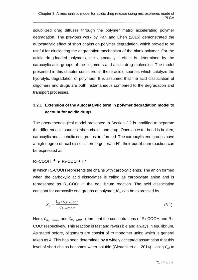
Chapter 3. A mechanistic model for acidic drug release using microspheres made of PLGA
71 | P a g e
solubilized drug diffuses through the polymer matrix accelerating polymer
degradation. The previous work by Pan and Chen (2015) demonstrated the
autocatalytic effect of short chains on polymer degradation, which proved to be
useful for elucidating the degradation mechanism of the blank polymer. For the
acidic drug-loaded polymers, the autocatalytic effect is determined by the
carboxylic acid groups of the oligomers and acidic drug molecules. The model
presented in this chapter considers all these acidic sources which catalyze the
hydrolytic degradation of polymers. It is assumed that the acid dissociation of
oligomers and drugs are both instantaneous compared to the degradation and
transport processes.
3.2.1 Extension of the autocatalytic term in polymer degradation model to
account for acidic drugs
The phenomenological model presented in Section 2.2 is modified to separate
the different acid sources: short chains and drug. Once an ester bond is broken,
carboxylic and alcoholic end groups are formed. The carboxylic end groups have
a high degree of acid dissociation to generate H+; their equilibrium reaction can
be expressed as
R1-COOH R1-COO- + H+
in which R1-COOH represents the chains with carboxylic ends. The anion formed
when the carboxylic acid dissociates is called as carboxylate anion and is
represented as R1-COO- in the equilibrium reaction. The acid dissociation
constant for carboxylic end groups of polymer, Ka, can be expressed by
𝐾𝑎 =𝐶𝐻+ 𝐶𝑅1−𝐶𝑂𝑂−
𝐶𝑅1−𝐶𝑂𝑂𝐻. (3.1)
Here, 𝐶𝑅1−𝐶𝑂𝑂𝐻 and 𝐶𝑅1−𝐶𝑂𝑂− represent the concentrations of R1-COOH and R1-
COO- respectively. This reaction is fast and reversible and always in equilibrium.
As stated before, oligomers are consist of m monomer units; which is general
taken as 4. This has been determined by a widely accepted assumption that this
level of short chains becomes water soluble (Gleadall et al., 2014). Using 𝐶𝑜𝑙 to
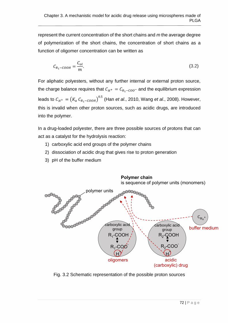
Chapter 3. A mechanistic model for acidic drug release using microspheres made of PLGA
72 | P a g e
represent the current concentration of the short chains and m the average degree
of polymerization of the short chains, the concentration of short chains as a
function of oligomer concentration can be written as
𝐶𝑅1−𝐶𝑂𝑂𝐻 =𝐶𝑜𝑙
𝑚. (3.2)
For aliphatic polyesters, without any further internal or external proton source,
the charge balance requires that 𝐶𝐻+ = 𝐶𝑅1−𝐶𝑂𝑂− and the equilibrium expression
leads to 𝐶𝐻+ = (𝐾𝑎 𝐶𝑅1−𝐶𝑂𝑂𝐻)0.5
(Han et al., 2010, Wang et al., 2008). However,
this is invalid when other proton sources, such as acidic drugs, are introduced
into the polymer.
In a drug-loaded polyester, there are three possible sources of protons that can
act as a catalyst for the hydrolysis reaction:
1) carboxylic acid end groups of the polymer chains
2) dissociation of acidic drug that gives rise to proton generation
3) pH of the buffer medium
Fig. 3.2 Schematic representation of the possible proton sources
polymer units
R1-COOH
R1-COO-
oligomers
carboxylic acid group
acidic (carboxylic) drug
R2-COOH
R2-COO-
carboxylic acid group
Polymer chain is sequence of polymer units (monomers)
CH0+
buffer medium
H+ H
+

Chapter 3. A mechanistic model for acidic drug release using microspheres made of PLGA
73 | P a g e
The equilibrium expression for the dissociation of short chains is given above.
While carboxylic groups of short chains dissociate, the solid drug particles
dissociate in the water concurrently to give an equilibrium solution containing a
mixture of unionised molecules: carboxylate ions and H+. To eliminate the
confusion with the carboxylate ions of short chains, we will call this as anionic
drug. The most common functional group conferring acidity to drugs is the
carboxylic group (Cairns, 2012). The dissociation reaction for carboxylic drugs
can be schematically written as
R2-COOH R2-COO- + H+
Here R2-COOH is a general representation for carboxylic acid drugs. R2 can be
any functional group including a benzene ring likewise in Ibuprofen or an ester
functional group such as in Acetyl Salicylic Acid (ASA, Aspirin). Some other
functional groups can also provide an acidic character to the drugs such as
phenol groups (Cairns, 2012) and dissociation reaction can be modified to
account for these different drugs. The H+ produced by drug dissociation is
available as a further catalyst for the hydrolysis reaction. The acid dissociation
constant for drug, 𝐾𝑎,𝑑𝑟𝑢𝑔 can be expressed as
𝐾𝑎,𝑑𝑟𝑢𝑔 =𝐶𝐻+ 𝐶𝑅2−𝐶𝑂𝑂−
𝐶𝑅2−𝐶𝑂𝑂𝐻. (3.3)
Here, 𝐶𝑅2−𝐶𝑂𝑂𝐻 and 𝐶𝑅2−𝐶𝑂𝑂− represent the concentrations of R2-COOH and R2-
COO- respectively.
The proton concentration donated by the surrounding medium is referred to as
𝐶𝐻0+ and the charge conservation requires that
𝐶𝐻+ = 𝐶𝑅1−𝐶𝑂𝑂− + 𝐶𝑅2−𝐶𝑂𝑂− + 𝐶𝐻0+ . (3.4)
In our calculations, 𝐶𝐻0+ is calculated assuming that the pH of the medium is 7.4.
Arrangement of Eq. 3.1, 3.3 and 3.4, gives a second order quadratic equation.
The only unknown of the equation is 𝐶𝐻+. To be able to solve the quadratic
equation, discriminant of the equation is calculated and checked whether it is

Chapter 3. A mechanistic model for acidic drug release using microspheres made of PLGA
74 | P a g e
zero, positive or negative. Depending on the condition, the root of the quadratic
equation was calculated. The root obtained is the local acidity, 𝐶𝐻+, which is the
input for Eq. 2.22. Thus, chains scission rate, 𝑅𝑠, can be calculated considering
the all proton sources affecting the local acidity.
3.2.2 Diffusion equations of short chains and drug molecules
Both the short polymer chains and the dissolved drug molecules are capable of
diffusion through the polymeric matrix. For the microspheres, these diffusions are
spherically symmetric and transportation occurs only in the radial direction r. It is
assumed that the diffusions follow the Fick’s law such that
𝑑𝐶𝑜𝑙
𝑑𝑡=
𝑑𝑅𝑜𝑙
𝑑𝑡+ 𝐷𝑜𝑙 (
1
𝑟2)
𝑑
𝑑𝑟(𝑟2
𝑑𝐶𝑜𝑙
𝑑𝑟). (3.5)
and
𝑑𝐶𝑑𝑟𝑢𝑔
𝑑𝑡=
𝑑𝑅𝑑𝑟𝑢𝑔
𝑑𝑡+ 𝐷𝑑𝑟𝑢𝑔 (
1
𝑟2)
𝑑
𝑑𝑟(𝑟2
𝑑𝐶𝑑𝑟𝑢𝑔
𝑑𝑟). (3.6)
Here, 𝐶𝑑𝑟𝑢𝑔(= 𝐶𝑅2−𝐶𝑂𝑂𝐻 in Eq. 3.3) represents the current drug concentration, t
the time, r the radius of the microspheres, and 𝐷𝑜𝑙 and 𝐷𝑑𝑟𝑢𝑔 the effective
diffusion coefficients for the oligomers and drug molecules. The first term on the
right-hand side of Eq. (3.5) represents the production rate of short polymer chains
due to chain scission, and that of Eq. (3.6), the rate of drug dissolution. It will be
seen in later part of this chapter that the drug release profile can be satisfactorily
predicted using Fickian diffusion law.
The loss of short chains and drug molecules generates porosity inside the matrix,
which leads to a significant increase in the diffusion coefficients. To reflect the
dynamic structure of the polymer matrix, effective diffusion coefficients are used.
In a previous study (Wang et al., 2008), this was determined by use of finite
element analysis of a representative 3-dimensional cubic material. A randomly
distributed second phase is introduced and effective diffusion coefficient of the
material was calculated. The details of their numerical approach can be found in
the reference study (Wang, 2009). A similar approach is applied when calculating
the effective diffusion coefficient of drug. Therefore, variable effective

Chapter 3. A mechanistic model for acidic drug release using microspheres made of PLGA
75 | P a g e
diffusivities, 𝐷𝑜𝑙 and 𝐷𝑑𝑟𝑢𝑔, are used in the equations based on the diffusion
coefficient of in the bulk polymer and the pores as discussed in the work by Pan
et al. (2014)
𝐷𝑜𝑙 = 𝐷𝑜𝑙,𝑝𝑜𝑙𝑦 + (1.3𝑉𝑝𝑜𝑟𝑒2 − 0.3𝑉𝑝𝑜𝑟𝑒
3)(𝐷𝑜𝑙,𝑝𝑜𝑟𝑒 − 𝐷𝑜𝑙,𝑝𝑜𝑙𝑦). (3.7)
and
𝐷𝑑𝑟𝑢𝑔 = 𝐷𝑑𝑟𝑢𝑔,𝑝𝑜𝑙𝑦
+ (1.3𝑉𝑝𝑜𝑟𝑒2 − 0.3𝑉𝑝𝑜𝑟𝑒
3)(𝐷𝑑𝑟𝑢𝑔,𝑝𝑜𝑟𝑒 − 𝐷𝑑𝑟𝑢𝑔,𝑝𝑜𝑙𝑦). (3.8)
in which 𝐷𝑜𝑙,𝑝𝑜𝑙𝑦 and 𝐷𝑑𝑟𝑢𝑔,𝑝𝑜𝑙𝑦 denote the diffusivities of oligomers and drug
molecules in the fresh bulk polymer, 𝑉𝑝𝑜𝑟𝑒, the total porosity, and 𝐷𝑜𝑙,𝑝𝑜𝑟𝑒 and
𝐷𝑑𝑟𝑢𝑔,𝑝𝑜𝑟𝑒 the diffusion coefficients of oligomers and drugs in liquid-filled pores
respectively. In this study 𝐷𝑜𝑙,𝑝𝑜𝑟𝑒 and 𝐷𝑑𝑟𝑢𝑔,𝑝𝑜𝑟𝑒 are simply taken as 1000 times
of their counter parts in the fresh bulk polymer as suggested by Wang et al.
(2008).
The porosity in the polymer is due to the loss of oligomers and drugs. The volume
fraction of pores due to loss of oligomers can be calculated as
𝑉𝑝𝑜𝑟𝑒,𝑜𝑙 =𝑅𝑜𝑙
𝐶𝑒,0−
𝐶𝑜𝑙
𝐶𝑒,0. (3.9)
The volume fraction of pores due to loss of drug can be calculated by the fraction
of drug released from the matrix, which is
𝑉𝑝𝑜𝑟𝑒,𝑑𝑟𝑢𝑔 = 1 −𝐶𝑑𝑟𝑢𝑔
𝐶𝑑𝑟𝑢𝑔,0. (3.10)
The total porosity, 𝑉𝑝𝑜𝑟𝑒, is contributed by the loss of oligomers and drug and can
be calculated using
𝑉𝑝𝑜𝑟𝑒 = 𝑉𝑝𝑜𝑟𝑒,𝑜𝑙 (1 − 𝑓𝑑𝑟𝑢𝑔) + 𝑉𝑝𝑜𝑟𝑒,𝑑𝑟𝑢𝑔 𝑓𝑑𝑟𝑢𝑔. (3.11)
where 𝑓𝑑𝑟𝑢𝑔 is volume ratio of drug to the polymer phase and (1-𝑓𝑑𝑟𝑢𝑔); the
volume ratio of oligomers to the polymer phase.

Chapter 3. A mechanistic model for acidic drug release using microspheres made of PLGA
76 | P a g e
Finally, the number averaged molecular weight of the polyester at any particular
location can be calculated as (Pan, 2014)
𝑀𝑛 = 𝑀𝑛,0
1 − 𝛼 (𝑅𝑠
𝐶𝑒0)
𝛽
1 + 𝑁𝑑𝑝0 (𝑅𝑠
𝐶𝑒,0−
𝑎𝑚 (
𝑅𝑠
𝐶𝑒,0)
𝛽
)
. (3.12)
where 𝑀𝑛,0 is the initial molecular weight of the polymer; 𝑁𝑑𝑝,0 is the average
degree of polymerization.
3.3 The numerical procedure
In the current section, boundary conditions and the details of the numerical
scheme is provided. The initial conditions of the microsphere are given by
𝑅𝑠(𝑟, 0) =0
𝐶𝑜𝑙(𝑟, 0) = 𝐶𝑜𝑙,0=0
𝐶𝑑𝑟𝑢𝑔(𝑟, 0) = 𝐶𝑑𝑟𝑢𝑔,0. (3.13)
and the boundary conditions (concentrations at particle surface) are assumed as:
𝐶𝑜𝑙 = 0.
𝐶𝑑𝑟𝑢𝑔 = 0. (3.14)
For initial drug concentration, two special cases are considered. In the first case,
the drug loading is below the solubility limit. An infinite dissolution rate for the
drug molecules is assumed and the initial drug concentration is simply taken as
the drug loading. This can be schematically represented as
𝐼𝑓 𝑉𝑑𝑟𝑢𝑔
𝑉𝑢𝑛𝑖𝑡< 𝐶𝑠 𝑡ℎ𝑒𝑛 𝐶𝑑𝑟𝑢𝑔,0 =
𝑉𝑑𝑟𝑢𝑔
𝑉𝑢𝑛𝑖𝑡. (3.15)
In the second case, the drug loading is above the solubility limit, the drug
dissociation rate becomes a limiting factor (Wise, 2000, Xiang and McHugh,

Chapter 3. A mechanistic model for acidic drug release using microspheres made of PLGA
77 | P a g e
2011). In this case, the initial drug concentration is taken as the solubility of the
drug which can be represented as
𝐼𝑓 𝑉𝑑𝑟𝑢𝑔
𝑉𝑢𝑛𝑖𝑡> 𝐶𝑠 𝑡ℎ𝑒𝑛 𝐶𝑑𝑟𝑢𝑔,0 = 𝐶𝑠. (3.16)
It is assumed that drug dissolution is instantaneous and the drug concentration
at any r remains at 𝐶𝑠 until all loaded drug at that location has dissolved.
Equations 2.19 and (3.1-3.16) form the complete mathematical model for polymer
degradation and drug release. Applying the initial and boundary conditions, these
equations are solved numerically using the central finite difference method
(Smith, 1965). The direct Euler scheme was used for the time integration. A
particle radius was discretized into 100 finite difference nodes. The grid size (Fig.
3.3) was found to be ∆r=0.000525mm. The time step length was found to be
∆t=2.7s, which ensures convergence both for blank and loaded microspheres.
Numerical convergence was ensured by increasing the number of finite
difference nodes and reducing the time step length such that no change in the
numerical solution can be found. Fig. 3.4 shows the algorithm flow chart for the
model developed in this chapter. The computer program is written in FORTRAN
90 (see Appendix A). The computational time for compete solution takes less
than 10min on the desktop PC by use of Microsoft Visual Studio 2010 as an
integrated development environment (IDE).
Fig. 3.3 A schematic illustration of the grid size
∆r
r R

Chapter 3. A mechanistic model for acidic drug release using microspheres made of PLGA
78 | P a g e
Fig. 3.4 Flow chart for the model in the presence of acidic drugs
Chapter 3. A mechanistic model for acidic drug release using microspheres made of PLGA
79 | P a g e
3.4 Comparison between model prediction and experimental
data obtained in the literature
Siepmann et al. (2005) and Klose et al. (2008) carried out a set of experiments
using microspheres made of PLGA 50:50 in phosphate buffer (pH 7.4) at 37 oC.
Here their experimental data are used to test the model presented in Section 3.2.
A common set of parameters in the model of polymer degradation is used for
both blank and drug-loaded samples. The following experimental data are taken
from their papers:
- average molecular weight as a function of time for blank microspheres
undergoing autocatalytic degradation (Siepmann et al., 2005)
- average molecular weight as a function of time for the acidic drug
(ibuprofen) loaded microspheres undergoing autocatalytic degradation
- ibuprofen release from microspheres (Klose et al., 2008)
Fig. 3.5 presents the comparison between the model prediction and experimental
data for average molecular weight changes of blank microspheres. Two different
sizes are used in the comparison. The kinetic parameters of the model used in
the model prediction are summarized in Table 3.1.
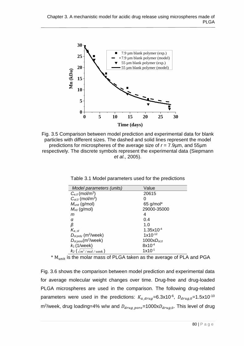
Chapter 3. A mechanistic model for acidic drug release using microspheres made of PLGA
80 | P a g e
Fig. 3.5 Comparison between model prediction and experimental data for blank particles with different sizes. The dashed and solid lines represent the model
predictions for microspheres of the average size of r = 7.9µm, and 55µm respectively. The discrete symbols represent the experimental data (Siepmann
et al., 2005).
Table 3.1 Model parameters used for the predictions
Model parameters (units) Value
Ce,0 (mol/m3) 20615
Col,0 (mol/m3) 0 Munit (g/mol) 65 g/mol* Mn0 (g/mol) 29000-35000 m 4 α 0.4 β 1.0 Ka_ol 1.35x10⁻⁴ Dol,poly (m2/week) 1x10-12 Dol,pore(m2/week) 1000xDol,0
k1 (1/week) 8x10⁻⁴ k2 ( week/mol/m3 ) 1x10⁻¹
* Munit is the molar mass of PLGA taken as the average of PLA and PGA
Fig. 3.6 shows the comparison between model prediction and experimental data
for average molecular weight changes over time. Drug-free and drug-loaded
PLGA microspheres are used in the comparison. The following drug-related
parameters were used in the predictions: 𝐾𝑎_𝑑𝑟𝑢𝑔=6.3x10⁻⁶, 𝐷𝑑𝑟𝑢𝑔,0=1.5x10⁻¹⁰
m2/week, drug loading=4% w/w and 𝐷𝑑𝑟𝑢𝑔_𝑝𝑜𝑟𝑒=1000x𝐷𝑑𝑟𝑢𝑔,0. This level of drug
0 5 10 15 20 25 300
5
10
15
20
25
30
Mn
(k
Da
)
Time (days)
7.9 µm blank polymer (exp.)
7.9 µm blank polymer (model)
55 µm blank polymer (exp.)
55 µm blank polymer (model)

Chapter 3. A mechanistic model for acidic drug release using microspheres made of PLGA
81 | P a g e
loading is below the solubility limit of the drug in the polymer. All the other
parameters are common for the blank and loaded microspheres (see Table 3.1).
Compared to the drug free microspheres, ibuprofen loaded PLGA microspheres
exhibit significantly faster degradation pattern. In a drug-loaded microsphere,
50% of the initial molecular weight has been reached at 4 days, while it is 7.5
days for drug free microspheres. The enhanced rate of degradation is attributed
to the decreased micro pH based on the acidic drug dissociation. The individual
contributions of drug and oligomers on the proton concentration are compared in
Fig. 3.7 through the degradation process. It can be seen that at the early stage
of degradation, most of the proton is dominated by the acidic drugs while the
contribution of the short chains are insignificant. As more and more drugs are
released and short chains are produced, the order is switched and short chains
start to dominate on the proton concentration. It is worth noting that the
calculations used the disassociation constants, Ka, drug and Ka, which are taken
from independent literature (Pan et al., 2011, Loftsson and Brewster, 1996).
Fig. 3.6 Comparison between model prediction and experimental data for degradation of blank and ibuprofen-loaded PLGA microspheres. The dashed
and solid lines represent model predictions for drug-free and drug-loaded particles respectively. The discrete symbols represent the experimental data
(Klose et al., 2008, Siepmann et al., 2005).
0 5 10 15 20 25 300
5
10
15
20
25
30
35
40
r
Mn
(k
Da
)
Time (days)
Exp. data for drug free particles
Exp. data for loaded particles
Model prediction for drug free particles
Model prediction for loaded particles
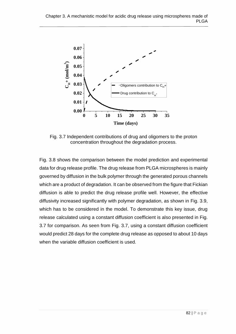
Chapter 3. A mechanistic model for acidic drug release using microspheres made of PLGA
82 | P a g e
Fig. 3.7 Independent contributions of drug and oligomers to the proton concentration throughout the degradation process.
Fig. 3.8 shows the comparison between the model prediction and experimental
data for drug release profile. The drug release from PLGA microspheres is mainly
governed by diffusion in the bulk polymer through the generated porous channels
which are a product of degradation. It can be observed from the figure that Fickian
diffusion is able to predict the drug release profile well. However, the effective
diffusivity increased significantly with polymer degradation, as shown in Fig. 3.9,
which has to be considered in the model. To demonstrate this key issue, drug
release calculated using a constant diffusion coefficient is also presented in Fig.
3.7 for comparison. As seen from Fig. 3.7, using a constant diffusion coefficient
would predict 28 days for the complete drug release as opposed to about 10 days
when the variable diffusion coefficient is used.
0 5 10 15 20 25 30 350.00
0.01
0.02
0.03
0.04
0.05
0.06
0.07
CH+
(m
ol/
m3)
Time (days)
Oligomers contribution to CH+
Drug contribution to CH
+

Chapter 3. A mechanistic model for acidic drug release using microspheres made of PLGA
83 | P a g e
Fig. 3.8 Comparison between the model prediction (solid line) and experimental data (Klose et al., 2008) (discrete symbols) for drug release. The dashed line is
model prediction using a constant drug diffusion coefficient. The size of the microsphere is 52µm.
Fig. 3.9 Variable diffusivity of ibuprofen calculated using Eq. 18 for micro-particle of r = 52µm.
0 5 10 15 20 25 300
20
40
60
80
100
Dru
g r
elea
se (
%)
Time (days)
Single diffusivity
Variable effective diffusivity
Experimental data
0 5 10 15 20 25 300
1
2
3
4
5
6
7
Dd
rug
(10-1
2 m
2/w
eek
)
Time (days)
Variable
effective diffusivity

Chapter 3. A mechanistic model for acidic drug release using microspheres made of PLGA
84 | P a g e
By observing Fig. 3.5, Fig. 3.6 and Fig. 3.8, it can be concluded that the
mathematical model presented in the current chapter is able to predict the
experimental data both for polymer degradation and drug release. In our
calculations, the model parameters were determined by varying them over a
range to obtain the best prediction. The hydrolysis rate constants, 𝑘1 and 𝑘2, in
Table 3.1 are determined using the blank polymer data as shown in Fig. 3.5. It is
worth highlighting that the model is able to predict the degradation behavior of
drug loaded polymers using the rate constants obtained by using the blank
polymers.
3.5 Design of microspheres to achieve desired profile of drug
release
Over the years, various release systems have been explored both experimentally
and computationally to obtain a stable release profile. In many of the controlled
release formulations, zero order release profile is desirable in order to maintain
a constant drug concentration over time. This is because, the burst effect in
ordinary drug delivery systems may result in toxicity and some other side effects
(Berkland et al., 2002, Huang and Brazel, 2001). Even if no harm is done during
the burst, an excess amount of drug is wasted and this can result in some
economic concerns. Drug release from polyester microspheres depends on
parameters such as the microsphere diameter and drug loading. Guided by a
simple analysis, Berkland et al. (2002) showed that a zero order release profile
can be achieved by mixing two different microspheres which have concave and
convex release profiles respectively. Taking inspiration from the study by
Berkland et al. (2002) and Narayani and Panduranga Roa (1996) we
demonstrate that the mathematical model presented in this chapter can be used
to design such systems.
Fig. 3.10 presents the schematic representation of the microspheres resulting
zero order release profile when mixed in appropriate portions. Fig. 3.11 shows
the drug release from induvial microspheres presented in Fig. 3.10, as well as
the release when two type pf microspheres mixed in 1:2 (w/w) ratio. A convex,
concave and nearly zero-order release profiles are obtained, all calculated using

Chapter 3. A mechanistic model for acidic drug release using microspheres made of PLGA
85 | P a g e
the mathematical model and the parameters that were used in the current
chapter. The convex release profile was obtained by using microspheres of 75µm
in radius with a drug loading of 400 mol/m3. The outer layer of the sphere with a
thickness of 0.2r was not loaded with any drug. This outer layer can be
considered as a drug-free coating that retards the initial drug release. The
concave release profile was obtained by using microspheres of 150µm in radius
with the same drug loading. The outer layer of the sphere with a thickness of 0.6r
was not loaded with any drug. Such a thick coating prevents drug release in the
initial stage and hence produced the convex release profile. The nearly zero
release profile was obtained by mixing the two types of spheres with 1:2 (w/w)
ratios of the thinly coated microspheres (concave profile) over the thickly coated
microspheres (convex profile).
Fig. 3.10 Schematic representation of the microspheres resulting zero order release profile in the mixture when mixed 1:2 (w/w) ratio of (a) over (b). (a)
75µm in radius with drug loading of 400 mol/m3and a drug free outside layer of 0.2r (15µm), (b) 150µm in radius with a drug loading of 400 mol/m3and a drug
free outside layer of 0.6r (90µm).
0.8r 0.2r
75µm
0.4r 0.6r
150µm (b) (a)

Chapter 3. A mechanistic model for acidic drug release using microspheres made of PLGA
86 | P a g e
Fig. 3.11 Calculated profiles of drug release using microspheres of (a) 75µm in radius with drug loading of 400 mol/m3and a drug free outside layer of 0.2r, (b) 150µm in radius with a drug loading of 400 mol/m3and a drug free outside layer
of 0.6r and (c) mixture of (a) and (b) with 1:2 (w/w) ratio of (a) over (b).
The long term linear release of drug from particles was crucial in most of the
applications. However, in some particular cases, an initial burst release followed
by a linear release may be required, likewise in wound treatment. Because of the
fact that burst happens in a quite short time compared to the all release process,
it cannot be well controlled, and it has been discounted in most of the
mathematical models in the literature (Huang and Brazel, 2001). In this study, we
proposed a mechanism to control the burst release.
Fig. 3.12 shows the schematic representation of the microspheres resulting a
burst release profile when mixed in appropriate portions. Fig. 3.13 presents the
drug release from induvial microspheres presented in Fig. 3.12, as well as the
release when two type of microspheres mixed in 1:2 (w/w) ratio. A convex,
concave and burst followed by zero order release profile were obtained, all
calculated using the mathematical model. The convex release profile was
obtained by using microspheres of 75µm in radius with a uniform drug loading of
400 mol/m3. The concave release profile was obtained by using microspheres of
0 5 10 15 20 25 300.00
0.04
0.08
0.12
0.16
0.20
1(a) + 2(b)
(b)
Zero order release
75 µm, 15 µm coating (a)
150 µm, 90 µm coating (b)
Mixture C
um
ula
tive
rele
ase
(µ
g)
Time (days)
(a)

Chapter 3. A mechanistic model for acidic drug release using microspheres made of PLGA
87 | P a g e
150µm in radius with the same drug loading. The outer layer of the sphere with
a thickness of 0.6r was not loaded with any drug. This is exactly the same as
case (b) in Fig. 3.11. The burst followed by nearly zero release profile was
obtained by mixing the two types of spheres with 1:2 (w/w) ratios of the uniformly
loaded microspheres (concave profile) over the thickly coated microspheres
(convex profile).
Fig. 3.12 Schematic representation of the microspheres resulting zero order release profile in the mixture when mixed 1:2 (w/w) ratio of (a) over (b). (a)
75µm in radius with a uniform drug loading of 400 mol/m3, (b) 150µm in radius with a drug loading of 400 mol/m3and a drug free outside layer of 0.6r (90µm).
75µm
0.4r 0.6r
150µm (b) (a)

Chapter 3. A mechanistic model for acidic drug release using microspheres made of PLGA
88 | P a g e
Fig. 3.13 Calculated profiles of drug release using microspheres of (a) 75µm in radius with a uniform drug loading of 400 mol/m3, (b) 150µm in radius with a
drug loading of 400 mol/m3and a drug free outside layer of 0.6r and (c) mixture of (a) and (b) with 1:2 (w/w) ratio of (a) over (b).
3.6 Conclusions
A mechanistic-based mathematical model is presented which can be used to
calculate the rate of hydrolytic degradation and drug release. The model is
generally valid for all the geometries, although, microspheres are used in the
chapter as a demonstrating example. The underlying assumptions in the
mathematical model were motivated by experimental studies in the literature
which demonstrated the influence of the acidic drug on autocatalysis of polyester
devices. It is shown that the model can predict polymer degradation and drug
release fairly well. Model results clearly indicated that, the presence of acidic
drugs significantly accelerates the rate of degradation. A key element of the
model is that the drug diffusion coefficient strongly depends on the polymer
degradation. This study shows that without considering this interaction between
acidic drug and polymer, it is unlikely to capture the observed profile of drug
release. It is worth noting that the model is able to predict the degradation
behavior of drug-loaded polymers using the kinetic constants for polymer
0 5 10 15 20 25 300.00
0.04
0.08
0.12
0.16
0.20
1(a) + 2(b)
(b)
(a)
Burst followed
by zero order release
75 µm, no coating (a)
150 µm, 90 µm coating (b)
Mixture C
um
ula
tive
rele
ase
(µ
g)
Time (days)
Chapter 3. A mechanistic model for acidic drug release using microspheres made of PLGA
89 | P a g e
degradation obtained using blank polymers. Moreover, the model results were
successfully implemented on the design of the microspheres to achieve desired
profile of drug release. This was achieved by use of appropriate mixtures of
uniform microspheres which have concave and convex release profiles. To
demonstrate potential applications of the mathematical model, it is shown that
the model can be used to design systems of microspheres of different sizes and
patterns of drug loading to achieve zero order release or burst followed by zero
order release. These systems will have significant practical implications for
various applications.

Chapter 4. A mechanistic model for basic drug release using microspheres made of PLGA
90 | P a g e
Chapter 4. A mechanistic model for basic drug release
using microspheres made of PLGA
This chapter presents a mathematical model predicting the release profiles of
basic drugs from biodegradable polyesters. The model calculates drug release
and molecular weight reduction as functions of time. The full interactions between
drug and polyester are taken into account as well as the effect of polymer
degradation on the release rate. These include the attractive ionic interaction
between basic drugs and polymer chain ends and the catalytic role played by the
free acidic and basic species on the hydrolysis reaction. The model predictions
satisfactorily match with different sets of experimental data from the literature,
indicating that the model is able to describe the key phenomena governing the
release of basic drugs embedded in degradable polymeric devices. The model
can be used in the design of microsphere systems for targeted release as well
as a tool to gain understanding in the underlying mechanisms responsible for the
release of basic drugs. This chapter has been submitted to European Journal of
Pharmaceutics and Biopharmaceutics.
4.1 Introduction
The model developed in Chapter 3, based on previous work of Pan and his co-
workers, allows investigating the effect of acidic drugs on the degradation rate. It
was shown that the protons gained by drug dissociation accelerate the hydrolysis
reaction. It is demonstrated that the model is able to fit with the experimental data
for the change in the molecular weight, mass loss, and drug release. In this
chapter, a mathematical model is presented which can explain the interaction
between basic drugs and polymers. The mathematical model is used to relate
the degradation behavior of polymers to the basic drug properties.
Unlike acidic drugs, there are contradicting reports in the literature for basic
drugs. Several groups (D’Souza et al., 2015, Klose et al., 2008, Fitzgerald and
Corrigan, 1996, Cha and Pitt, 1988, Cha and Pitt, 1989) have proposed that the
incorporation of basic drugs increases the degradation rate, while others
Chapter 4. A mechanistic model for basic drug release using microspheres made of PLGA
91 | P a g e
(Miyajima et al., 1998, Mauduit et al., 1993a) have found a reduction in
degradation rate with the incorporation. This divergence can be explained by the
fact that basic drugs can act as a catalyst for the hydrolysis reaction, accelerating
polymer degradation, and also shield carboxylic end groups, decelerating
degradation rate. The relative dominance of one of the two mechanisms
determines the observed behavior (Miyajima et al., 1998, Mauduit et al., 1993b,
Proikakis et al., 2006).
It has been also reported that, the interaction between the drug and polymer is
critical in controlling drug release (Li et al., 1996, Okada et al., 1994). This is
again because of the basic drugs ionically interacting with the polymer. Likewise
the effects seen in polymer degradation, two opposing results are reported for
how the properties of the basic drugs affect their own release rate (Miyajima et
al., 1999).
Literature provides a variety of mathematical models (Casalini et al., 2014, Ford
et al., 2011b, Siepmann et al., 2002, Thombre and Himmelstein, 1985) simulating
the release profiles from a biodegradable matrix. However, the interaction
between drugs and polymers has not been considered until our recent work, in
which a mathematical model taking into account of the interaction was presented
for polyesters loaded with acidic drugs (Sevim and Pan, 2016). In this chapter,
the model is further extended for polyesters loaded with basic drugs. The
shielding effect of basic drug molecules on the carboxylic end groups of the
polymer chains is considered. A partition parameter is introduced to reflect the
observed level of attachment of drug molecules to the carboxylic ends. The
validity of the model is tested using an experimental data obtained from the
literature. Microspheres are chosen as an example in this study but the model is
generally valid for any drug-loaded device.
4.2 The mathematical model
The microparticles are modelled as microspheres that are spherically symmetric
in which basic drug is uniformly distributed. It is assumed that the drug is
physically entrapped into the microsphere. Due to symmetry the model only
considers a radial coordinate, thus, matter transportation is assumed to occur in
Chapter 4. A mechanistic model for basic drug release using microspheres made of PLGA
92 | P a g e
the radial direction, r. All microspheres are assumed to have the same size. Once
the microspheres are placed in a liquid medium, water molecules diffuse into the
matrix and break the long polymer chains. Concurrently, water dissolves drug
molecules. Drug dissolution is assumed as instantaneous compared to the
degradation and the diffusion of oligomer and drugs. Chain scission reaction can
be catalysed by both acidic and basic species. A proportion of drug interacts with
the carboxyl ends of short chains and neutralizes their acidic effect, whilst the
rest stays in free form to catalyse the hydrolysis reaction. On the other side, free
short chains are also able to accelerate the hydrolysis reaction. To account for
these opposing effects, a partition parameter is introduced in the model such that
polymer degradation can either be accelerated or slowed down depending on the
partition of drug molecules in free or attached form. The representation of the
interaction between drug and polymer as well as the effect of free acidic and
basic species on degradation rate is schematised in Fig. 4.1. The model
considers transport of oligomers and drug through the polymeric matrix. Drug re-
lease is achieved by a combination of (i) diffusion of the drug molecules out of
the spheres and (ii) the diffusion of drug molecules that are attached to the ends
of the short chains. The water penetration into the polyester devices are rather
fast compared to the other kinetic processes such as degradation and drug
release. It is therefore assumed that water is always abundant in the polymer
particles.

Chapter 4. A mechanistic model for basic drug release using microspheres made of PLGA
93 | P a g e
Fig. 4.1 Schematic representation of the interaction between basic drugs-oligomers and catalyst effect of the free species
4.2.1 Rate of polymer chain scission
The phenomenological model by Leicester group, presented in Section 2.2, is
modified to include the base catalytic random scission, autocatalytic random
scission and non-catalytic scission. The polymer is assumed to consist of
amorphous chains, the formation of crystalline phase is again excluded during
the model development. It is assumed that water is abundant, therefore, its
concentration does not affect the chain scission rate. The rate equation for chain
scission in Pan’s study (Pan, 2014) is extended such that
𝑑𝑅𝑠
𝑑𝑡= 𝑘1𝐶𝑒 + 𝑘2𝐶𝑒𝐶𝐻+ + 𝑘3𝐶𝑒𝐶𝑂𝐻−. (4.1)
Here, 𝑅𝑠, 𝐶𝑒, 𝐶𝐻+ and 𝐶𝑂𝐻− represent the molar concentrations of chains
scissions, ester bonds, H+ and OH-; 𝑘1, 𝑘2 and 𝑘3, the non-catalytic, acid-
catalyzed and base-catalyzed kinetic constants respectively. The third term on
the right-hand side is newly introduced to take into account of catalyst effect of
the basic species. Each chain scission generates either a short or long chain.
The production rate of short chains and the concentration of ester bond are
polymer units
R1-COOH
R1-COO-
oligomers
carboxylic acid group
basic drug
Polymer chain
CH0+
Drug
Drug_H+
buffer medium
H+
OH-
ionic interaction (cluster)

Chapter 4. A mechanistic model for basic drug release using microspheres made of PLGA
94 | P a g e
provided in Eq. 2.20 and 2.21 in section 2.2, therefore, they will not be mentioned
here. By use of Eq. 2.20 and 2.21 in Eq. 4.1, we have
𝑑𝑅𝑠
𝑑𝑡= 𝐶𝑒,0 [1 − 𝛼 (
𝑅𝑠
𝐶𝑒,0)
𝛽
] (𝑘1 + 𝑘2𝐶𝐻+ + 𝑘3𝐶𝑂𝐻−). (4.2)
Breaking an ester bond results in the formation of a carboxylic and an alcoholic
end groups. The dissociation of carboxylic end groups produces H+ which acts
as a catalyst as presented in section 3.2.1. In their studies, Pan and his
coworkers (Pan, 2014, Wang et al., 2008) assumed that only the carboxylic end
groups of the short chains act as the catalyst for the hydrolysis reaction. They
showed that this assumption led to good fitting between the model prediction and
the experimental data (Pan, 2014). The mole concentration of acid generated by
dissociation of short chains is shown in Eq. 2.24. However, this is not valid in the
case of basic drug incorporation because some of the drug molecules can attach
to the carboxylic end groups neutralizing the chain ends.
4.2.2 Interaction between drug molecules and carboxylic end groups
As discussed in section 4.1, the following phenomena have to be considered in
a degradation model impregnated with basic drugs:
(i) Basic drug can behave as a catalyst accelerating the cleavage of the
polymer chains;
(ii) The basic drug can shield some of the carboxylic end groups of the
short chains diminishing their autocatalytic effect.
In view of the former, dissociation expression for basic drugs can be
schematically written as
Drug+H2O Drug_H++ OH-
As with any equilibrium constant for a reversible reaction, the equilibrium
expression for this reaction is defined through a base dissociation constant, Kb,
such that

Chapter 4. A mechanistic model for basic drug release using microspheres made of PLGA
95 | P a g e
𝐾𝑏 =𝐶𝑑𝑟𝑢𝑔_𝐻+ 𝐶𝑂𝐻−
𝐶𝑑𝑟𝑢𝑔. (4.3)
Here, 𝐶𝑑𝑟𝑢𝑔_𝐻+, 𝐶𝑑𝑟𝑢𝑔 and 𝐶𝑂𝐻− represent the mole concentrations of the cationic
drug, drug and OH- respectively. 𝐾𝑏 measures the strength of a base and is
directly related to the acid dissociation constant, 𝐾𝑎, by the relationship 𝑝𝐾𝑎 +
𝑝𝐾𝑏=14. Here, 𝑝𝐾𝑎 and 𝑝𝐾𝑏 are the negative logarithms of 𝐾𝑎 and 𝐾𝑏,
respectively. Therefore, for a known value of 𝐾𝑎, 𝐾𝑏 can be easily calculated.
Since the Drug_H+ and OH- come from the same drug molecules, we then have
𝐶𝑑𝑟𝑢𝑔_𝐻+=𝐶𝑂𝐻−, the equilibrium expression leads to
𝐶𝑂𝐻− = (𝐾𝑏𝐶𝑑𝑟𝑢𝑔)𝑛 (4.4)
in which n is generally taken as 0.5.
As stated in many studies (Miyajima et al., 1999, Engineer et al., 2011), the
products of the dissociation reaction of drug forms a cluster (shielding) with the
products of the dissociation reaction of short chains. The reason is that the
polarity increases largely after dissociation of the drug which is a driving force for
cationic drug and hydroxyl ions to pull the anionic carboxylic ends and protons
(for an example topological polar surface area, tPSA, is 15.6 for 𝐶𝑑𝑟𝑢𝑔 while it is
increasing to 18.84 for 𝐶𝑑𝑟𝑢𝑔_𝐻+ (Ultra, 2001)). The level of the shielding between
the drug and carboxylic ends is dependent on the structure and charge to mass
ratio of drug. In this sense, a portion of the drug would be interacted with the
carboxylic ends groups while rest would stay in free form. In order to reflect this
phenomena, we introduced a partition parameter, 𝐾𝑝, into the model to reflect the
number of drug molecules that are attached to the carboxylic end groups. 𝐾𝑝
varies between 0 and 1.0 with 𝐾𝑝=0 indicating no attachment and 𝐾𝑝 =1.0
indicating full attachment. Only the drug molecules free from the attachment are
available to act as a catalyst, therefore, Eq. (4.4) can be modified as
𝐶𝑂𝐻− = 𝐾𝑏(𝐾𝑏𝐶𝑑𝑟𝑢𝑔)0.5
(4.5)
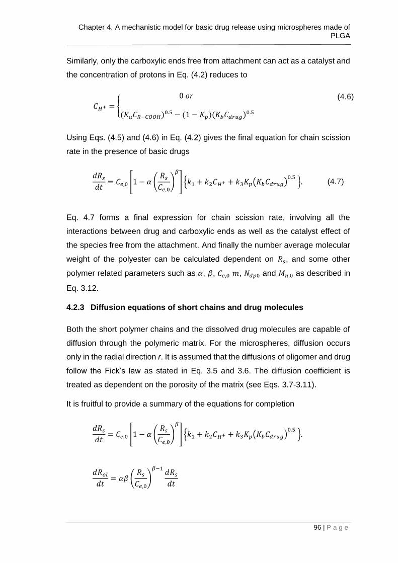
Chapter 4. A mechanistic model for basic drug release using microspheres made of PLGA
96 | P a g e
Similarly, only the carboxylic ends free from attachment can act as a catalyst and
the concentration of protons in Eq. (4.2) reduces to
𝐶𝐻+ = {
0 𝑜𝑟
(𝐾𝑎𝐶𝑅−𝐶𝑂𝑂𝐻)0.5 − (1 − 𝐾𝑝)(𝐾𝑏𝐶𝑑𝑟𝑢𝑔)0.5
(4.6)
Using Eqs. (4.5) and (4.6) in Eq. (4.2) gives the final equation for chain scission
rate in the presence of basic drugs
𝑑𝑅𝑠
𝑑𝑡= 𝐶𝑒,0 [1 − 𝛼 (
𝑅𝑠
𝐶𝑒,0)
𝛽
] {𝑘1 + 𝑘2𝐶𝐻+ + 𝑘3𝐾𝑝(𝐾𝑏𝐶𝑑𝑟𝑢𝑔)0.5
}. (4.7)
Eq. 4.7 forms a final expression for chain scission rate, involving all the
interactions between drug and carboxylic ends as well as the catalyst effect of
the species free from the attachment. And finally the number average molecular
weight of the polyester can be calculated dependent on 𝑅𝑠, and some other
polymer related parameters such as 𝛼, 𝛽, 𝐶𝑒,0 𝑚, 𝑁𝑑𝑝0 and 𝑀𝑛,0 as described in
Eq. 3.12.
4.2.3 Diffusion equations of short chains and drug molecules
Both the short polymer chains and the dissolved drug molecules are capable of
diffusion through the polymeric matrix. For the microspheres, diffusion occurs
only in the radial direction r. It is assumed that the diffusions of oligomer and drug
follow the Fick’s law as stated in Eq. 3.5 and 3.6. The diffusion coefficient is
treated as dependent on the porosity of the matrix (see Eqs. 3.7-3.11).
It is fruitful to provide a summary of the equations for completion
𝑑𝑅𝑠
𝑑𝑡= 𝐶𝑒,0 [1 − 𝛼 (
𝑅𝑠
𝐶𝑒,0)
𝛽
] {𝑘1 + 𝑘2𝐶𝐻+ + 𝑘3𝐾𝑝(𝐾𝑏𝐶𝑑𝑟𝑢𝑔)0.5
}.
𝑑𝑅𝑜𝑙
𝑑𝑡= 𝛼𝛽 (
𝑅𝑠
𝐶𝑒,0)
𝛽−1𝑑𝑅𝑠
𝑑𝑡

Chapter 4. A mechanistic model for basic drug release using microspheres made of PLGA
97 | P a g e
𝑑𝐶𝑜𝑙
𝑑𝑡=
𝑑𝑅𝑜𝑙
𝑑𝑡+ 𝐷𝑜𝑙 (
1
𝑟2)
𝑑
𝑑𝑟(𝑟2
𝑑𝐶𝑜𝑙
𝑑𝑟)
𝑑𝐶𝑑𝑟𝑢𝑔
𝑑𝑡=
𝑑𝑅𝑑𝑟𝑢𝑔
𝑑𝑡+ 𝐷𝑑𝑟𝑢𝑔 (
1
𝑟2)
𝑑
𝑑𝑟(𝑟2
𝑑𝐶𝑑𝑟𝑢𝑔
𝑑𝑟)
𝐷𝑜𝑙 = 𝐷𝑜𝑙,𝑝𝑜𝑙𝑦 + (1.3𝑉𝑝𝑜𝑟𝑒2 − 0.3𝑉𝑝𝑜𝑟𝑒
3)(𝐷𝑜𝑙,𝑝𝑜𝑟𝑒 − 𝐷𝑜𝑙,𝑝𝑜𝑙𝑦)
𝐷𝑑𝑟𝑢𝑔 = 𝐷𝑑𝑟𝑢𝑔,𝑝𝑜𝑙𝑦 + (1.3𝑉𝑝𝑜𝑟𝑒2 − 0.3𝑉𝑝𝑜𝑟𝑒
3)(𝐷𝑑𝑟𝑢𝑔,𝑝𝑜𝑟𝑒 − 𝐷𝑑𝑟𝑢𝑔,𝑝𝑜𝑙𝑦)
𝑉𝑝𝑜𝑟𝑒 =𝑅𝑜𝑙 − (𝐶𝑜𝑙 − 𝐶𝑜𝑙,0)
𝐶𝑒,0= 𝛼 (
𝑅𝑠
𝐶𝑒,0)
𝛽
−𝐶𝑜𝑙 − 𝐶𝑜𝑙,0
𝐶𝑒,0
𝑉𝑝𝑜𝑟𝑒,𝑑𝑟𝑢𝑔 = 1 −
𝐶𝑑𝑟𝑢𝑔
𝐶𝑑𝑟𝑢𝑔,0
𝑉𝑝𝑜𝑟𝑒 = 𝑉𝑝𝑜𝑟𝑒,𝑜𝑙 (1 − 𝑓𝑑𝑟𝑢𝑔) + 𝑉𝑝𝑜𝑟𝑒,𝑑𝑟𝑢𝑔 𝑓𝑑𝑟𝑢𝑔
𝑀𝑛 = 𝑀𝑛,0
1 − 𝛼 (𝑅𝑠
𝐶𝑒,0)
𝛽
1 + 𝑁𝑑𝑝,0 (𝑅𝑠
𝐶𝑒,0−
𝑎𝑚 (
𝑅𝑠
𝐶𝑒,0)
𝛽
)
The definitions of the symbols are provided in the List of Symbols. Here, the chain
scission equation reflects all the interactions and the catalyst of the free species.
Oligomer production is linked with the rate of chain scission. The effective
diffusion coefficients of drug, 𝐷𝑑𝑟𝑢𝑔 and oligomers, 𝐷𝑜𝑙 are calculated taking into
account the increasing porosity in the matrix. The porosity of the system is
calculated considering the oligomers and drug leaving the matrix.

Chapter 4. A mechanistic model for basic drug release using microspheres made of PLGA
98 | P a g e
4.3 The numerical procedure
The numerical procedure for computation of the model is presented in the current
section. The equation summarised forms a complete set of governing equations
for 𝑅𝑠, 𝐶𝑜𝑙 and 𝐶𝑑𝑟𝑢𝑔. It is assumed that initially there is no oligomer in the matrix,
therefore 𝐶𝑜𝑙(𝑟, 0) = 𝐶𝑜𝑙,0=0. Moreover, 𝐶𝑑𝑟𝑢𝑔(𝑟, 0) = 𝐶𝑑𝑟𝑢𝑔,0 and 𝑅𝑠(𝑟, 0) = 0 at
t=0. The perfect sink condition is used that requires 𝐶𝑜𝑙=0 and 𝐶𝑑𝑟𝑢𝑔=0 at the
particle surface. It is assumed that drug dissolution is instantaneous. For initial
drug concentration, we consider two different scenarios. If the drug loading is
below the solubility limit, the initial drug concentration is simply taken as the drug
loading. If the drug loading is above the solubility limit, the initial drug
concentration is taken as the solubility of the drug and the drug concentration at
any r remains at the solubility limit until all loaded drug at that location has
dissolved as presented in Section 3.3.
The equations form a complete model for degradation and drug release. Number
averaged molecular weight of the polymer can be calculated as Eq. 3.16. The
equations are solved numerically using a finite difference method, giving the time
evolution and spatial distribution of all the variables from which drug release
profile and average molecular weight of the polymers can be calculated. The
central finite difference method was used for spatial discretization (Smith, 1965)
and the direct Euler scheme was used for the time integration. A particle radius
was discretized into 100 finite difference nodes and a very small time step was
used. The grid size is set as ∆r=0.0017mm. The schematic illustration of the grid
size is represented in Fig. 3.4. The time step length was found to be ∆t=2.7s,
which guarantees convergence for all the cases including the blank and loaded
microparticles. Numerical convergence was ensured by gradually increasing the
number of finite difference nodes and reducing the time step length such that no
change in the numerical solution can be found.
The equations developed form the full mathematical model for polymer
degradation and drug release. FORTRAN 90 programming language is used for
performing the simulations (see Appendix B). The total computation time takes

Chapter 4. A mechanistic model for basic drug release using microspheres made of PLGA
99 | P a g e
less than 10min, on the desktop computer. The numerical details are presented
in a flow chart in Fig. 4.2.
Finally, the mean absolute relative error (MARE) is used to evaluate the
performance of the model which is calculated by the following equation (Malhotra,
2016)
𝑀𝐴𝑅𝐸 =
1
𝑁∑
|𝑃𝑖 − 𝐴𝑖|
𝐴𝑖
𝑁
1
(4.8)
in which N refers to the total number of instances in a data set, iP refers to the
model results for an instance i and iA refers to the experimental value of an
instance i.

Chapter 4. A mechanistic model for basic drug release using microspheres made of PLGA
100 | P a g e
Fig. 4.2 Flow chart for the model in the presence of basic drugs
4.4 Validation of the model
4.4.1 Case Study A
Siepmann et al. (2005) studied the degradation behaviour of drug loaded and
drug-free PLGA-based microparticles. Drug free and drug-loaded microparticles

Chapter 4. A mechanistic model for basic drug release using microspheres made of PLGA
101 | P a g e
with changing sizes were studied as 7.2µm, 24µm, 37µm and 53µm for lidocaine
loaded microparticles; and 7.9µm, 26µm, 38µm and 55µm for drug free particles.
Accumulation of the short chains resulted an enhanced level of degradation for
larger particles. However, varying particle diameter, had no significant effect on
the rate of drug release. This was explained with the following phenomena: as
diameter of the particle increases, degradation is accelerated, however, diffusion
pathways of the drug is increased. This combined effect leaded to same level of
drug release as particle diameter enlarged. A quantitative discussion was made
which provided new insights into the importance of the autocatalytic effects in
polyester-based microparticles.
Similarly, Klose et al. (2008) carried out a set of degradation and drug release
experiments using PLGA50:50 microspheres and thin, free films impregnated
with lidocaine (free base, apK 7.9) and ibuprofen. The initial drug concentrations
(4% w/w) were stated to be below the solubility limit in the study (Klose et al.,
2008). Molecular weight change for blank and loaded polymers and drug release
properties were physicochemically characterized in vitro in phosphate buffered
solution (pH 7.4) at 37oC. The initial molecular weight, 𝑀𝑛,0, is 29500Da for blank
samples and 31000Da for lidocaine loaded microspheres. Their results showed
that, the system size strongly affected the release kinetics for thin films. However,
for the case of spherical microparticles, the release was almost unaffected by the
system size. Ibuprofen release was reported to be much faster than the lidocaine
release for all systems geometries and sizes. This is attributed to attractive ionic
interaction between the carboxylic end groups of polymer and basic drug,
lidocaine.
In the current chapter, the experimental data by Siepmann et al. and Klose et al.
will be used for the fittings. The molecular weight change of blank polymer during
degradation is taken from Siepmann et al. study, whereas the molecular weight
change of the lidocaine loaded microparticles and drug release data is taken from
Klose et al. study. In order to eliminate the size dependence of degradation and
stick on analysing the impact of basic drug incorporation on the degradation rate,
Chapter 4. A mechanistic model for basic drug release using microspheres made of PLGA
102 | P a g e
we selected their data for similar particle sizes of 55µm for blank particles and
48µm for drug-loaded particles.
The model is first simulated for the case of blank polymer to collect the polymer
related parameters. Then the simulations are repeated for the case of loaded
microspheres, in order to collect the drug related parameters and the partition
parameter, 𝐾𝑝. Fig. 4.3 shows the comparison between the model results and
experimental data. The model results for molecular weight changes are shown in
Fig. 4.3a while the release profile is illustrated in Fig. 4.3b. Model parameters
used in the simulations are provided in Table 4.1. These parameters are
categorized into two groups: Group I consists parameters that were either
measured experimentally or cannot be varied artificially to fit a particular set of
experimental data. , and are initial average molecular weight of the polymer,
molecular weight of a representing unit and initial ester bond concentration, all of
which were taken from Siepmann et al. and Klose et al. m is the average number
of repeating unit of soluble and short polymer chains, which is taken as 4. α and
β represents the nature of polymer chain cleavage and were taken from Pan et
al. aK and bK are equilibrium constants for disassociation of oligomers and drug
molecules. 𝐷𝑜𝑙,𝑝𝑜𝑟𝑒 and 𝐷𝑑𝑟𝑢𝑔,𝑝𝑜𝑟𝑒 are the diffusion coefficients of oligomers and
drugs in liquid-filled pores which were just taken as a very large value. Group II
consist of parameters that were varied to fit with the experimental data. 𝑘1, 𝑘2
and 𝑘3 represent the non-catalytic, acid catalyzed and base catalyzed rate
constants for hydrolysis. 𝐷𝑜𝑙,0 and 𝐷𝑑𝑟𝑢𝑔,0 are the diffusion coefficients of
oligomers and drugs in non-degraded bulk polymer. pK is the partition constant
indicating percentage of drug molecules shielded by carboxylic ends, which was
set 0.75. The value of pK implifies that 75% of the drug molecules are attached
to the carboxylic end groups of the polyester chains whilst the rest remains in
free form.

Chapter 4. A mechanistic model for basic drug release using microspheres made of PLGA
103 | P a g e
Fig. 4.3 Comparison between the model result and experimental data (Klose et
al., 2008, Siepmann et al., 2005): a) nM reduction and b) drug release. Lines
represent the model prediction for blank (dashed line) and loaded particles (solid line); discrete symbols represent experimental data for blank (circle) and
loaded particles (square, triangle).

Chapter 4. A mechanistic model for basic drug release using microspheres made of PLGA
104 | P a g e
Table 4.1 Parameters used in the model to fit with experimental data
Model parameters
Units Values
0nM g mol-1 2.9-3.5x10⁴
unitM g mol-1 65
m no unit 4
no unit 0.4
Group I no unit 1
0eC mol m-3 20615
aK no unit 1.35x10⁻⁴
𝐷𝑜𝑙,𝑝𝑜𝑟𝑒 m2 week-1 1.0x10⁻⁵
𝐷𝑑𝑟𝑢𝑔,𝑝𝑜𝑟𝑒 m2 week-1 1.0x10⁻⁵
1k week-1 8x10⁻⁴
Group II 2k m3 mol-1 week-1 1x10⁻¹
3k m3 mol-1 week-1 8x101
𝐷𝑜𝑙,𝑝𝑜𝑙𝑦 m2 week-1 5.0x10⁻¹²
𝐷𝑑𝑟𝑢𝑔,𝑝𝑜𝑙𝑦 m2 week-1 6.0x10⁻¹⁰
Compared to the drug-free microspheres, loaded microspheres shows a more
rapid decrease in molecular weight, which is attributed to the free acidic and basic
species (Fig. 4.3). The increased rate of degradation can be attributed to the
dominant impact of basic drug that are free from the attachment. It is also worth
highlighting that the base-catalytic coefficient, 𝑘3, has a major impact on the
degradation rate relative to the non-catalytic and autocatalytic constants. The
results show that mean absolute relative error is 0.1 and 0.7 for molecular weight
reduction of loaded and blank microspheres respectively while is 0.08 for release
data.
4.4.2 Case Study B
Dunne et al. (2000) carried out a set of experiments to demonstrate the influence
of particle size on the molecular weight change of PLGA particles. Moreover, the
influence of processing conditions, particle characteristic and the temperature of
release media on the degradation of polymers was examined. It was found that
the larger particles degrades faster. Moreover, at lower incubation temperatures,
PLGA microparticles were reported to show an incubation period which is

Chapter 4. A mechanistic model for basic drug release using microspheres made of PLGA
105 | P a g e
followed by degradation. The increasing incubation temperature leaded to
increase in polymer degradation. The models result then fitted with Prout-
Tompkins equations, which is used in the kinetic analysis of solid-state reaction.
By use of the kinetic analysis the activation energy of the hydrolysis reaction was
determined.
In connection with the study by Dunne et al., Fitzgerald and Corrigan (1996)
examined the degradation behaviour of PLGA microspheres and co-evaporate
discs loaded with levamisole drug (free base, apK 8). In their study, various drug
loadings are compared to capture the impact of drug content on degradation rate.
No solid aggregate of the drug has been observed in their analysis; therefore, all
these levels of drug loading are assumed to be below the solubility limit
(Fitzgerald and Corrigan, 1996). The blank samples have an initial molecular
weight of 𝑀𝑛,0= 40000-45000Da, with the size range of <1µm (process A), <20µm
(process B) and <50µm (process C). Molecular weight varies between 10000-
13000Da for loaded particles. The sizes of microspheres are defined to be below
170µm in diameter; and constituted as 170µm in the simulations. In addition to
the change in molecular weight and mass loss, drug release was monitored from
microsphere and disc systems. The analysis showed that the drug content
significantly increase the rate of degradation.
Here, the experimental data obtained from Dunne et al. (2000) and Fitzgerald
and Corrigan (1996) is used for the comparison with the model results. The
molecular weight change of blank polymer is obtained from the study by Dunne
et al. (2000), while molecular weight change of levamisole loaded microspheres
is taken from the study by Fitzgerald and Corrigan (1996). Different drug loading
have been compared with the model result in order to comprehend the validity of
the model for changing drug loading. Only microspheres are compared with the
model results, although the model is valid for all the geometries.
The comparison between the calculated and the experimental results of
molecular weight as a function of time for blank microspheres are shown in Fig.
4.4. Model parameters used in the simulations are presented in Table 4.2. The
case of sub-micron particles was not considered in the model, hence, only

Chapter 4. A mechanistic model for basic drug release using microspheres made of PLGA
106 | P a g e
particles having 20µm and 50µm sizes are used for the validation. It can be
observed that the model is able to capture the size effect of microsphere
degradation (Fig. 4.4) Mean absolute relative error of molecular weight reduction
is 0.04 and 0.003 for blank samples with 20µm and 50µm, respectively.
Table 4.2 Parameters used in the model to fit with experimental data
Model parameters
Units Values
0nM g mol-1 1-3x10⁴
unitM g mol-1 65
0eC mol m-3 20615
m no unit 4
no unit 0.4
Group I no unit 1
aK no unit 1.35x10⁻⁴
bK no unit
𝐷𝑜𝑙,𝑝𝑜𝑟𝑒 m2 week-1 1.0x10⁻⁵
𝐷𝑑𝑟𝑢𝑔,𝑝𝑜𝑟𝑒 m2 week-1 1.0x10⁻⁵
1k week-1 5x10⁻⁴
Group II 2k m3 mol-1 week-1 1x10⁻¹
3k m3 mol-1 week-1 1x101
𝐷𝑜𝑙,0 m2 week-1 5.0x10⁻¹¹
𝐷𝑑𝑟𝑢𝑔,0 m2 week-1 2.0x10⁻⁸
pK no unit 0.3-0.75

Chapter 4. A mechanistic model for basic drug release using microspheres made of PLGA
107 | P a g e
Fig. 4.4 Comparison between the model result and experimental data (Dunne et al., 2000) for blank PLGA microspheres. Lines represent the model prediction for various sizes and discrete symbols represent corresponding experimental
data for r = 20µm (solid line, circles) and 50µm (dashed line, squares).
The effect of drug loading on molecular weight reduction is shown in Fig. 4.5. The
drug related parameters are again shown in Table 4.2. 𝐾𝑝, was set as 0.75, 0.7
and 0.3 for 2.4%, 14.3% and 19.7% loaded microspheres respectively. The
increasing drug loading leaded to a decrease in the value of 𝐾𝑝. This is
reasonable since the amount of interacted drug decreases as drug loading
increases.
Fig. 4.6 represents the model fitting for drug release for various drug loadings.
Mean absolute relative error of molecular weight reduction is 0.05, 0.1 and 0.34
for 2.4%, 14.3%, and 19.7% loaded microspheres respectively. This value is
respectively 0.48, 0.16 and 0.08 for release data of 2.4%, 14.3% and 19.7%
loaded microspheres respectively.
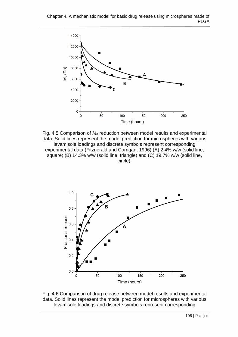
Chapter 4. A mechanistic model for basic drug release using microspheres made of PLGA
108 | P a g e
Fig. 4.5 Comparison of Mn reduction between model results and experimental data. Solid lines represent the model prediction for microspheres with various
levamisole loadings and discrete symbols represent corresponding experimental data (Fitzgerald and Corrigan, 1996) (A) 2.4% w/w (solid line, square) (B) 14.3% w/w (solid line, triangle) and (C) 19.7% w/w (solid line,
circle).
Fig. 4.6 Comparison of drug release between model results and experimental data. Solid lines represent the model prediction for microspheres with various
levamisole loadings and discrete symbols represent corresponding
C
B
A
A
B
C

Chapter 4. A mechanistic model for basic drug release using microspheres made of PLGA
109 | P a g e
experimental data (Fitzgerald and Corrigan, 1996) (A) 2.4% w/w (solid line, square) (B) 14.3% w/w (solid line, triangle) and (C) 19.7% w/w (solid line,
circle).
Under assumed interaction between drug and polymer matrix in the model, we
could adjust the three parameters, 𝑘3, 𝐷𝑑𝑟𝑢𝑔,0 and 𝐾𝑝 to fit the 61 data points in
Fig. 4.5 and Fig. 4.6. The model fits the experimental data, however, fittings for
Case B is relatively poor compared to Case A due to the self-imposed restriction.
If an independent set of 𝑘1, 𝑘2 and 𝐷𝑜𝑙0 were used a much better fitting can be
obtained. The fact that the model can capture the general trend as shown in Fig.
4.5 and Fig. 4.6 for drug loaded spheres using the same 𝑘1, 𝑘2 and 𝐷𝑜𝑙0 obtained
from blank polymers indicates that the assumed mechanism of interaction
between drug and polymer matrix is valid. The less satisfactory fitting in these
figures shows the complexity of the interaction. This complexity is a result of the
fact that drug release from biodegradable polymer is controlled by many factors,
including hydrophilicity-hydrophobicity, crystallization of drug and polymer, the
physicochemistry of drug, preparation method and etc. In the current model, we
only focused on the physicochemistry of basic drug and its interaction with the
polymer. And the model is capable of showing this interaction. It can be observed
from Fig. 4.5 and Fig. 4.6 that the model can indeed capture the strong effect of
drug loading on both polymer degradation and drug release.
The partition coefficient of drugs and carboxylic ends, 𝐾𝑝, determines the level of
degradation, therefore, degradation rate is very sensitive to the choice of 𝐾𝑝. The
effect of the partition coefficient on molecular weight is illustrated in Fig. 4.7 by
fixing the other parameters (e.g., oligomer and drug diffusivities, drug loading, k1,
k2, k3, m, α and β). As can be seen from the figure, the smaller partition coefficient
leads to the more enhanced degradation rate. This is reasonable, since as the
value of 𝐾𝑝 increases, the number of free carboxylic acids and drug molecules
would be reduced, therefore, the acid and base catalyst part of the chain scission
reaction would be less dominant. The partition coefficient is limited with the lower
and higher boundaries corresponding to 𝐾𝑝 =0 and 𝐾𝑝=1.0.

Chapter 4. A mechanistic model for basic drug release using microspheres made of PLGA
110 | P a g e
Fig. 4.7 The effect of partition parameter, Kp , on molecular weight
The mechanistic model presented above is tested using two sets of independent
experimental data taken from the literature. It is worth to highlight that our
emphasis is to explore the validity of the mechanism-based model. The idea is
that to make predictions for both blank spheres and drug-loaded spheres using
a common set of model parameters. If the model can indeed capture the
interaction between drugs and polyester, then the model calculation should fit
with the degradation rates of blank and drug-loaded spheres and the drug release
profile of the drug-loaded spheres well. Our numerical results showed that the
model could indeed capture the degradation behaviour and drug release profile
of the blank and loaded microspheres.
4.5 Conclusion
A comprehensive mechanism-based model is presented describing the polyester
degradation coupled with drug release from microspheres. The key issue in the
model is to consider the full ionic interaction between basic drugs and polymer
chain ends as well as the catalytic ef-fect of free acidic and basic species on
hydrolysis reaction. The model predictions are com-pared with the experimental
data from the literature with various basic drug types and several loadings. It is
shown that, the index of the polymer-drug interactions, , is the primitive factor
Higher Kp

Chapter 4. A mechanistic model for basic drug release using microspheres made of PLGA
111 | P a g e
controlling release of basic drugs. Together with our previous paper [24] on
micro-spheres loaded with acidic drugs, our work models the impact of various
drug types on poly-mer degradation for the first time from our knowledge. The
mechanistic model presented here can be used in the design of microsphere
systems as well as other drug loaded devices. The model can also facilitate the
understanding of the underlying physicochemistry responsible for the release of
basic drugs.

Part 3 A model by combination of hydrolytic degradation-erosion and its applications
112 | P a g e
Part 3
A model by combination of hydrolytic degradation-
erosion and its applications
Chapter 5. Combined hydrolytic degradation and erosion model for drug release
113 | P a g e
Chapter 5. Combined hydrolytic degradation and
erosion model for drug release
For many biodegradable polymers, there is a strong interplay between the
degradation and erosion processes – degradation leads to a certain decrease in
molecular weight which is the key process for erosion initiation. Eventually,
degradation leads to erosion and subsequently the loss of the material from the
polymer.
In this chapter, the reaction and diffusion equations provided in Section 2.2 are
combined with erosion models in the literature in order to identify and understand
how each mechanism is involved in the mass loss and how different mechanisms
dominate at different stages of the mass loss. Various kinetic mechanisms are
incorporated in the model in an attempt to explain every possible mass loss
behavior obtained from the experimental data. In the combined model, chain
scission, oligomer production, diffusion and microstructure evolution are modeled
together with surface erosion and interior erosion using a set of differential
equations and Monte Carlo technique. Oligomer diffusion is modeled using Fick’s
laws with a diffusion coefficient dependent on the porosity. The porosity of the
system is taken as dependent on the formation of cavities which is a result of
polymer collapse. Comparisons are made between the mass loss profiles of
individual mechanisms such as diffusion, surface erosion and interior erosion.
This way of representation has never been proposed in the literature before. The
model developed here has potential to deal with large mass losses, even up to
100%. This level of mass loss cannot be explained with a simple degradation-
diffusion model. It is also important to state that modeling PLA/GA degradation-
erosion is a pre-requirement for drug release modeling. The model constructed
here would be the basis of the drug release model which would be proposed in
Chapter 7. This part of the thesis has been published in Acta Biomaterialia.

Chapter 5. Combined hydrolytic degradation and erosion model for drug release
114 | P a g e
5.1 Introduction
Most of the biomedical applications benefit from the fact that the polymer
disappears after providing its function. Two major mechanisms are involved in
the process: degradation of the polymer chains and erosion of the polymer
matrix. Erosion leads to a visible change in microscopic and macroscopic level
(Gopferich and Langer, 1993) as well as the large increase in mass loss and drug
release. However, little is known about the basic principles of erosion process
and its link with the degradation. The number of parameters and complexity of
each process involved in the erosion hinder the development of new erosion
models.
According to the general knowledge in the literature, degradation is a chemical
process which can be explained by the chain cleavage. The degradation
products, monomers, and oligomers, are released by diffusion. Assuming that
chain cleavage is a random process affecting each bond with the equal
probability, the oligomers are produced from the beginning of the degradation. If
these products are released immediately from the beginning, there would be a
large mass loss from the beginning of the degradation (Gopferich, 1997).
However, the mass loss obtained by degradation is generally less than 5-10% of
the total molecular weight of the device and happens after a certain time of the
degradation. The level of mass loss that can be obtained with degradation is not
sufficient to explain all the observed mass loss behaviours in the literature.
Therefore, there must be other mechanisms causing a larger mass loss.
Recently Zhang et al. (Zhang et al., 2017) developed a combined degradation
and erosion model. This is an advanced model which follows oligomer diffusion
at the continuum scale and random chain scissions and polymer erosion at the
microscopic scale. However, the model is over-complicated for applications in
practical device design. The important autocatalytic effect of the hydrolysis
reaction was not considered, which means the model is unable to capture size
effect of the degradation. Gopferich (1997) suggested a two-phase mass loss
profile for an eroding polymer. During the first phase, no significant mass loss
can be obtained, while molecular weight is significantly reduced. This phase was

Chapter 5. Combined hydrolytic degradation and erosion model for drug release
115 | P a g e
designated as degradation. As soon as the molecular weight reaches a critical
level at which the polymer becomes water soluble, an erosion phase initiates and
the eroded material could be released into the surrounding medium leading to a
large mass loss (Husmann et al., 2002). In their work a mechanism based link
between the degradation and erosion processes was not made. Moreover, up to
date, there is no appropriate model to directly link erosion model with a solid
degradation model and the models are far from covering all the aspects of
erosion.
In summary, significant mass loss of the particles can be only observed when the
polymer erosion is the active mechanism. Therefore, polymer molecular weight
change is the measure for quantifying the degradation whereas mass loss is the
measure for quantifying erosion (Zhu and Braatz, 2015). It is assumed that
degradation is a necessary condition for the erosion and a degraded polymer can
only erode after it has contact to a pore of the matrix surface (Gopferich, 1997).
The objective of this chapter is to combine a hydrolytic degradation model with a
polymer erosion model so that the different behaviors of mass loss can be
captured in a single model. The reaction-diffusion equations previously
developed by Pan and his co-workers (2014, Wang et al., 2008) are adopted
which consider the autocatalytic effect and are valid for aliphatic polyesters such
as PLAs, PGAs and their copolymers. The degradation equations form the basis
of the current chapter and would be summarized clearly before they are linked
with the erosion model. These equations are coupled mechanistically with an
erosion model to provide a full picture of mass loss and drug release. It is shown
that all the observed trends such as biphasic and triphasic mass losses can be
obtained by using the combined model.
5.2 Hypothesis of the model and representation of the polymer
matrix
In formulating the algorithm, the composite and elementary events are
distinguished. The degradation and erosion mechanisms are assumed to be
elementary events which cannot be divided into simpler events, while transport

Chapter 5. Combined hydrolytic degradation and erosion model for drug release
116 | P a g e
of the degradation products is assumed to be the composite elements that can
be linked with the elementary events. A two-dimensional model is used for the
plates. To minimize the computational time, the symmetry about the vertical and
horizontal center lines are presented and quarter models are constrained in the
simulations. The polymer matrix is divided into xn x yn grid points and each
square pieces are called as pixels. The grid lines i= xn and j= yn represent the
surface of the plate in contact with aqueous media; i=1 and j=1 are the sides of
the plate which are not connected with the environment. Each pixel in the two-
dimensional grid represents a polymer chain and all pixels have the same size.
The following algorithm has been used to introduce the randomness of the
erosion, initial molecular weight has been distributed randomly to follow normal
distribution throughout the plate. Monte Carlo sampling method is used for the
random distribution. Initially, all pixels are assumed to be non-eroded except the
ones at the surface. Surface erosion starts at t=0, with a constant speed. To
simulate the overall polymer degradation, chain scission equations has been
defined at each pixel in the 2-dimensional grid system. Degradation produces
monomers and oligomers which are ready to diffuse out of polymer matrix.
Degradation also leads to a certain decrease in the molecular weight. As soon
as an inner pixel reaches to the critical molecular weight and contacts with an
eroded neighbour, it is assumed to be eroded instantaneously: this phenomenon
is named as interior erosion in the current chapter. The porosity of the matrix is
largely dependent on the cavities formed by erosion. The described algorithm
has been transformed into mathematical expressions in the following sections.
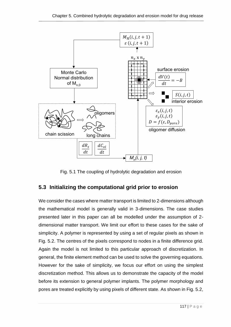
Chapter 5. Combined hydrolytic degradation and erosion model for drug release
117 | P a g e
Fig. 5.1 The coupling of hydrolytic degradation and erosion
5.3 Initializing the computational grid prior to erosion
We consider the cases where matter transport is limited to 2-dimensions although
the mathematical model is generally valid in 3-dimensions. The case studies
presented later in this paper can all be modelled under the assumption of 2-
dimensional matter transport. We limit our effort to these cases for the sake of
simplicity. A polymer is represented by using a set of regular pixels as shown in
Fig. 5.2. The centres of the pixels correspond to nodes in a finite difference grid.
Again the model is not limited to this particular approach of discretization. In
general, the finite element method can be used to solve the governing equations.
However for the sake of simplicity, we focus our effort on using the simplest
discretization method. This allows us to demonstrate the capacity of the model
before its extension to general polymer implants. The polymer morphology and
pores are treated explicitly by using pixels of different state. As shown in Fig. 5.2,
Monte Carlo Normal distribution
of Mn,0
chain scission
oligomers
long chains
Mn(i, j, t)
𝑑𝑉(𝑡)
𝑑𝑡= −𝐵
surface erosion
𝜀𝑥(𝑖, 𝑗, 𝑡) 𝜀𝑦(𝑖, 𝑗, 𝑡)
𝐷 = 𝑓(𝜀, 𝐷𝑝𝑜𝑟𝑒)
𝑑𝑅𝑠
𝑑𝑡
𝑑𝐶𝑜𝑙
𝑑𝑡
oligomer diffusion
𝑛𝑥 x 𝑛𝑦
interior erosion
𝑆(𝑖, 𝑗, 𝑡)
𝑀𝑛(𝑖, 𝑗, 𝑡 + 1)
𝜀 (𝑖, 𝑗, 𝑡 + 1)

Chapter 5. Combined hydrolytic degradation and erosion model for drug release
118 | P a g e
each pixel is identified by its indices (i,j) in the x- and y-directions. The state of
each pixel is defined by its number averaged molecular weight, 𝑀𝑛(𝑖, 𝑗, 𝑡), erosion
index, 𝑆(𝑖, 𝑗, 𝑡) and the local drug concentration 𝐶𝑑𝑟𝑢𝑔(𝑖, 𝑗, 𝑡). The erosion index is
defined as
𝑆𝑖,𝑗,𝑡 = {10
non−eroded pixeleroded pixel
(5.1)
Water diffusion is a fast process in comparison to polymer degradation and
erosion (Wang et al., 2008, Han and Pan, 2009). It is therefore assumed that
water molecules are always abundant in the polymer. The hydrolytic degradation
is reflected by the reduction in 𝑀𝑛 and polymer erosion is reflected by changes
of 𝑆(𝑖, 𝑗, 𝑡) from 1 to 0. The initial molecular weights of the pixels are set such that
they follow a normal distribution using a direct Monte Carlo technique. A random
number generator, R, is linked with a specified standard deviation to ensure that
the molecular weight follows a normal distribution such that
𝑀𝑛,0 = 𝑀𝑛,𝑚𝑒𝑎𝑛 + 𝑅 × 𝑀𝑛,𝑠𝑡_𝑑𝑒𝑣 (5.2)
in which 𝑀𝑛,𝑚𝑒𝑎𝑛 and 𝑀𝑛,𝑠𝑡_𝑑𝑒𝑣 represent the mean value and standard deviation
of the molecular weight distribution respectively.

Chapter 5. Combined hydrolytic degradation and erosion model for drug release
119 | P a g e
Fig. 5.2 Schematic illustration of discretised polymer
5.4 A brief summary of the reaction-diffusion model
After the grid is set up the rules, the hydrolytic degradation is the first phase prior
to the erosion which takes place in elementary level by cleavage of the backbone
chains. The detailed mechanism of degradation is provided in Section 2.2, a brief
summary of their model is provided here for the convenience of readers. The rate
of polymer chain scission follows the governing equation (Wang et al., 2008, Pan,
2014)
𝑑𝑅𝑠
𝑑𝑡= 𝐶𝑒,0 [1 − 𝛼 (
𝑅𝑠
𝐶𝑒,0)
𝛽
] (𝑘1 + 𝑘2 [𝐾𝑎 (𝐶𝑜𝑙
𝑚)]
0.5
). (5.3)
in which 𝑅𝑠, 𝐶𝑒,0 and 𝐶𝑜𝑙 represent the mole concentrations of chain scission,
initial ester bonds and short chains, 𝑘1 and 𝑘2, the kinetic rate constants for non-
catalytic and autocatalytic hydrolysis reactions, 𝛼 and 𝛽 are constants indicating
the nature of chain scissions (random or end scissions), 𝐾𝑎 represents the
equilibrium constant for acid disassociation of the carboxylic ends, and m, the
average degree of polymerization of the short chains which is generally taken as
.
x
y
j
i

Chapter 5. Combined hydrolytic degradation and erosion model for drug release
120 | P a g e
4 (Pan, 2014). The production rate of short chains due to polymer chain cleavage
is given by (Wang et al., 2008, Pan, 2014)
𝑑𝑅𝑜𝑙
𝑑𝑡= 𝛼𝛽 (
𝑅𝑠
𝐶𝑒,0)
𝛽−1𝑑𝑅𝑠
𝑑𝑡. (5.4)
in which 𝑅𝑜𝑙 is the concentration of ester bonds of all the short chains. The
average molecular weight 𝑀𝑛 of the polymer is calculated using (Wang et al.,
2008, Pan, 2014)
𝑀𝑛 = 𝑀𝑛,0
1 − 𝛼 (𝑅𝑠
𝐶𝑒,0)
𝛽
1 + 𝑁𝑑𝑝,0 (𝑅𝑠
𝐶𝑒,0−
𝛼𝑚 (
𝑅𝑠
𝐶𝑒,0)
𝛽
)
. (5.5)
in which 𝑀𝑛,0 is the initial molecular weight and 𝑁𝑑𝑝,0, the degree of
polymerisation of the polymer.
5.5 Surface erosion model
As stated in Section 1.3.2, polymer undergoes surface erosion causing the
material to shrink from its outer surface towards its center; maintaining the bulk
integrity. The speed of moving boundary is given by (Thombre and Himmelstein,
1984).
𝑑𝑉(𝑡)
𝑑𝑡= −𝐵.
(5.6)
in which 𝑑𝑉(𝑡)
𝑑𝑡 represents the volume of material lost per unit surface area per unit
time, and B is a material constant. For a pixel in contact with the surrounding
medium, 𝑆(𝑖, 𝑗, 𝑡) is set as zero when its volume is reduced to zero through Eq.
5.6.
5.6 Interior erosion model
Siepmann et al. (2002) used a Monte Carlo model to simulate the random
behavior of polymer erosion in which they are motivated from Gopferich’s study

Chapter 5. Combined hydrolytic degradation and erosion model for drug release
121 | P a g e
(1997). In their model, they treated erosion as a random process by assigning
individual lifetimes for each pixel. The lifetimes start to decrease upon contact
with water. The pixels counted to be eroded as soon as their lifetimes are
consumed. The interior erosion model is motivated by their study as well as the
criteria set by Gopferich (1997) which is discussed in section 5.1.
5.7 Combined hydrolytic degradation and erosion model
Degradation equations show the actual chemical equations in the plate. For each
cell (i, j) number average molecular weight, 𝑀𝑛, is obtained with the reaction
equations. In each iteration 𝑀𝑛 is being updated. As time proceeds, two main
criteria proposed by Gopferich (1997) must be satisfied for pixels to be eroded
from interior: molecular weight at the pixels must be below critical value, and
pixels should be in contact with an eroded neighbour. As a yield of the random
distribution of the initial molecular weight throughout the grid, each pixel will hit
to the critical molecular weight at different time. Once pixels satisfied both of the
criteria, they are assumed to fall apart instantaneously.
5.7.1 Rule of interior erosion
For computational reasons, we principally defined a temporary function, 𝑆𝑚 to
describe the current state of the pixels representing the temporary states of the
pixels
𝑆𝑚(𝑖, 𝑗, 𝑡) = 0 𝑀𝑛 < 𝑀𝑛,𝑐𝑟𝑖𝑡𝑖𝑐𝑎𝑙 (5.7)
in which 𝑀𝑛,𝑐𝑟𝑖𝑡𝑖𝑐𝑎𝑙 represents the critical molecular weight. However, a pixel
cannot be counted as eroded until it is in contact with an eroded neighbour. This
can be mathematically represented as
𝑆(𝑖, 𝑗, 𝑡) = 0 𝑖𝑓 𝑆𝑚(𝑖, 𝑗, 𝑡)
= 0 𝑎𝑛𝑑 𝑡ℎ𝑒 𝑝𝑖𝑥𝑒𝑙 ℎ𝑎𝑠 𝑎𝑛 𝑒𝑟𝑜𝑑𝑒𝑑 𝑛𝑒𝑖𝑔ℎ𝑏𝑜𝑢𝑟 (5.8)
Here, 𝑆(𝑖, 𝑗, 𝑡) is a function representing actual states of the pixels at time t- only
by action of interior degradation. This erosion model leads to a sudden release
Chapter 5. Combined hydrolytic degradation and erosion model for drug release
122 | P a g e
of oligomers when the critical molecular weight is reached. While some polymers
do show this sudden mass loss in the degradation experiment, other polymers
show a gentler trend in mass loss (Li et al., 1990a, Li et al., 1990b). The slow
mass erosion can be captured by introducing an incubation period, 𝑡𝑖𝑛𝑐, in the
model. A pixel of low molecular weight only changes its state from 𝑆 = 1 to 𝑆 = 0
after being in contact with an eroded neighbour for an incubation period of 𝑡𝑖𝑛𝑐.
5.7.2 Rule of surface erosion
The speed of the moving boundary is calculated in the same way with Thombre
and Himmelstein (1984) suggested. For a pixel in contact with the surrounding
medium, 𝑆(𝑖, 𝑗, 𝑡) is changed to zero when its volume is reduced to zero through
Eq. 5.6 which can be shown as
𝑉𝑐𝑒𝑙𝑙 = 𝑉𝑐𝑒𝑙𝑙 −
𝑑𝑉
𝑑𝑡𝐴 𝑑𝑡
(5.9)
𝑆(𝑖, 𝑗, 𝑡) = 0 𝑖𝑓 𝑉𝑐𝑒𝑙𝑙 = 0 (5.10)
5.7.3 Rate equation for oligomer and drug diffusion
Oligomers are capable to diffuse through the polymeric matrix. Assuming Fick’s
law for diffusion, the oligomer concentration, 𝐶𝑜𝑙, is governed by (Sevim and Pan,
2016)
𝜕𝐶𝑜𝑙
𝜕𝑡=
𝜕𝑅𝑜𝑙
𝜕𝑡+
𝜕
𝜕𝑥 (𝐷𝑜𝑙,𝑥
𝜕𝐶𝑜𝑙
𝜕𝑥) +
𝜕
𝜕𝑦 (𝐷𝑜𝑙,𝑦
𝜕𝐶𝑜𝑙
𝜕𝑦) (5.11)
in which 𝐷𝑜𝑙,𝑥 and 𝐷𝑜𝑙,𝑦 are the diffusion coefficients in x and y-directions. Here
the current oligomer concentration, 𝐶𝑜𝑙 is coupled back to Eq. 5.3.
The diffusion coefficients depend on the local porosity of the polymer matrix.
They are also hugely affected by the way in which the pores are connected
locally, i.e. the diffusion coefficients have very different values in different
directions. Two “porosities”, 𝜀𝑥 and 𝜀𝑦 are introduced to reflect the direction
dependence such that (Pan, 2014)

Chapter 5. Combined hydrolytic degradation and erosion model for drug release
123 | P a g e
𝐷𝑜𝑙,𝑥 = 𝐷𝑜𝑙,𝑝𝑜𝑙𝑦 + (1.3𝜀𝑥2 − 0.3𝜀𝑥
3)(𝐷𝑜𝑙,𝑝𝑜𝑟𝑒 − 𝐷𝑜𝑙,𝑝𝑜𝑙𝑦) (5.12)
and
𝐷𝑜𝑙,𝑦 = 𝐷𝑜𝑙,𝑝𝑜𝑙𝑦 + (1.3𝜀𝑦2 − 0.3𝜀𝑦
3)(𝐷𝑜𝑙,𝑝𝑜𝑟𝑒 − 𝐷𝑜𝑙,𝑝𝑜𝑙𝑦) (5.13)
in which 𝐷𝑜𝑙,𝑝𝑜𝑙𝑦 and 𝐷𝑜𝑙,𝑝𝑜𝑟𝑒 represents the diffusion coefficients in fresh bulk
polymer and in water filled pores respectively. A local “porosity” in a particular
direction is defined as the fraction of eroded pixels over a pre-defined number of
pixels, 2𝑛𝑟𝑎𝑛𝑔𝑒, vertical to that direction. 𝜀𝑥 and 𝜀𝑦 are therefore calculated as
𝜀𝑥(𝑖, 𝑗, 𝑡) =
1
2 × 𝑛𝑟𝑎𝑛𝑔𝑒 + 1∑ 𝑆(𝑖, 𝑗, 𝑡)
𝑗=𝑗+𝑛𝑟𝑎𝑛𝑔𝑒
𝑗=𝑗−𝑛𝑟𝑎𝑛𝑔𝑒
(5.14)
𝜀𝑦(𝑖, 𝑗, 𝑡) =
1
2 × 𝑛𝑟𝑎𝑛𝑔𝑒 + 1∑ 𝑆(𝑖, 𝑗, 𝑡)
𝑗=𝑗+𝑛𝑟𝑎𝑛𝑔𝑒
𝑗=𝑗−𝑛𝑟𝑎𝑛𝑔𝑒
(5.15)
The mass loss 𝑊𝑡 is calculated by summation of mass losses due to short chain
diffusion, 𝑊𝑑, and erosion, 𝑊𝑒, such as
𝑊𝑡 = 𝑊𝑑 + 𝑊𝑒 . (5.16)
5.8 The numerical procedure
This section provides the details of the computer implementation of the numerical
methods for determining a solution to the proposed model. Options can be
specified by turning on and off the certain portions of the code to investigate the
effects of the involved mechanisms separately. Switching between the reaction-
diffusion, surface erosion and bulk erosion are possible through the use of the
selections. The codes developed are provided in Appendix C.
The central finite difference scheme is used for spatial discretization of the
second term on the right hand side in Eq. 5.11. The time integration is performed

Chapter 5. Combined hydrolytic degradation and erosion model for drug release
124 | P a g e
by using the direct Euler scheme, i.e. values of 𝑅𝑠 and 𝐶𝐾 at t=t+∆𝑡 can be
calculated as
𝑅𝑠(𝑡 + ∆𝑡) = 𝑅𝑠 +𝑑𝑅𝑠
𝑑𝑡∆𝑡 (5.17)
𝐶𝑜𝑙(𝑡 + ∆𝑡) = 𝐶𝑜𝑙 +𝑑𝐶𝑜𝑙
𝑑𝑡∆𝑡 (5.18)
It is assumed that 𝐶𝑜𝑙(𝑖, 𝑗, 0) =0 and 𝑅𝑠(𝑖, 𝑗, 0) =0 at t=0. Perfect sink conditions
are assumed at the interface between the polymer and its surrounding medium,
which requires that 𝐶𝑜𝑙 = 0 at the interfaces. Numerical convergence is obtained
by gradually increasing the number of pixels and decreasing the time step.
The tablet domain is initially indicated by solid boundaries in Fig. 5.3. The moving
boundaries are indicated by dashed lines. Moving boundaries are only the case
when the surface erosion is in the game. New locations of the moving boundaries
are labelled as xe and ye in the figure. In the simulations, no new boundary has
been defined at new locations because of the characteristic of the problem. This
is because when we consider Eq. 5.12 and 5.13, the diffusion coefficients remain
at 𝐷𝑜𝑙,𝑝𝑜𝑟𝑒, for fully eroded surface, which is a very large number (taken by
consideration of diffusion of oligomers in water). This makes concentration at the
new boundary identical with the initial boundary. To sum up, the diffusion
coefficient acts as a state variable, preventing the need for a time dependent
boundary condition.

Chapter 5. Combined hydrolytic degradation and erosion model for drug release
125 | P a g e
Fig. 5.3 Moving boundaries at different times and boundary conditions
It is assumed that there is no oligomer at the grids initially and no chain scission
started at t=0, which can be represented mathematically as 𝐶𝑜𝑙(𝑖, 𝑗, 0) = 0 and
𝑅𝑠(𝑖, 𝑗, 0) =0. Moreover, it is assumed that a combination of random and end
chain cleavage occurred in degradation. By virtue of the boundary conditions only
upper and right side of the plate is exposed to the release medium. Perfect sink
conditions are assumed for these surfaces that requires 𝐶𝑜𝑙(𝑛𝑥, 𝑗, 𝑡) = 0 and
𝐶𝑜𝑙(𝑖, 𝑛𝑦, 𝑡) = 0. For the boundaries isolated from the solution it is assumed that,
𝐶𝑜𝑙(1, 𝑗, 𝑡) = 𝐶𝑜𝑙(2, 𝑗, 𝑡) and 𝐶𝑜𝑙(𝑖, 1, 𝑡) = 𝐶𝑜𝑙(𝑖, 2, 𝑡); 𝑅𝑠(1, 𝑗, 𝑡) = 𝑅𝑠(2, 𝑗, 𝑡) and
𝑅𝑠(𝑖, 1, 𝑡) = 𝑅𝑠(𝑖, 2, 𝑡).
With the defined initial and boundary conditions the equations are then solved
numerically by use of finite difference method and spatiotemporal evaluations of
the polymer matrix are determined. The simulated grid is spatially discretized into
nodes in order to apply central finite difference method and the time integration
is performed by use of direct Euler scheme. The plate is divided into i-space
intervals in x direction and into j-space intervals in y direction. A very small time
step is used in calculations (∆t=0.5s). Numerical convergence is tested by
gradually increasing the number of nodes and decreasing the time step. For each
grid point, polymer chains scission and oligomer production is modelled using
xi
xe
yi
ye
𝜕𝐶𝑜𝑙
𝜕𝑥
𝜕𝐶𝑜𝑙
𝜕𝑦
𝐶𝑜𝑙 = 0
𝐶𝑜𝑙 = 0
𝑦
𝑡 = 𝑡0 𝑡 = 𝑡1 𝑥

Chapter 5. Combined hydrolytic degradation and erosion model for drug release
126 | P a g e
degradation model mentioned above. Meanwhile, the surface erosion acts in a
way to constantly leads to plate shrinking. For the interior pixels, as soon as,
molecular weight reaches to a critical value, 𝑀𝑛,𝑐𝑟𝑖𝑡𝑖𝑐𝑎𝑙, and next to a hole, its
lifetime decreases and grid is counted as eroded when it consumes all the
volume. By considering the stated algorithm, concentration profiles, molecular
weight changes, porosities and mass losses at t=0+∆𝑡, 0+2∆𝑡 can be calculated
consecutively. The simulations are performed in supercomputer, which took
approximately 100 hours when utilizing 1 processor of the supercomputer. Fig.
5.4 shows the algorithm flow chart of the combined model developed in this
chapter. The codes of the FORTRAN program are provided in Appendix C.

Chapter 5. Combined hydrolytic degradation and erosion model for drug release
127 | P a g e
Fig. 5.4 Flow chart of the combined degradation-diffusion and erosion model
Chapter 5. Combined hydrolytic degradation and erosion model for drug release
128 | P a g e
5.9 Different behaviors of mass loss that can be obtained using
the combined model
The mathematical model developed here can be used to establish the conditions
under the each mechanism: degradation-diffusion, surface erosion, interior
erosion without incubation period, interior erosion with incubation period.
Scenarios for each mechanism or different combinations of the mechanisms are
shown in Fig. 5.5 to 5.10. An infinitively large plate is considered in the
simulations. The following model parameters are used to generate figures which
are broadly based on experimental data from Wang et al. (2006). The values of
molecular weights are set as 𝑀𝑛,𝑚𝑒𝑎𝑛=7.5x10⁴ g/mol, 𝑀𝑛,𝑠𝑡_𝑑𝑒𝑣=2.0x10⁴ g/mol,
𝑀𝑛,𝑐𝑟𝑖𝑡𝑖𝑐𝑎𝑙=2.7x10⁴ g/mol 𝑀𝑢𝑛𝑖𝑡=65 g/mol. The size of the representative unit of
the plate is taken as 80x320µm. 𝐷𝑜𝑙,𝑝𝑜𝑙𝑦=5.0x10⁻¹⁵ m2/week and 𝐷𝑜𝑙,𝑝𝑜𝑟𝑒=1.0x10-
8 m2/week. The rate of surface erosion is set as 𝐵 =6.5x10⁻¹⁴ m2/week and
hydrolysis reaction constants are set as 𝑘1=5.0x10⁻⁶ week-1, 𝑘2=2.0x10⁻² m3 mol-
1 week-1. The number of pixels in x- and y-directions, 𝑛𝑥 , 𝑛𝑦, are set as 250 x
1000. The values of parameter 𝐶𝑒,0, m, α and β were obtained from Pan et al.
(2014).
For the sake of comparison, all the simulations were terminated at 30 days. The
model is first established to calculate the mass loss from the reaction-diffusion
equations (Fig. 5.5). All other contributions to the mass loss are switched off in
order to assess the effect of diffusion on mass loss.

Chapter 5. Combined hydrolytic degradation and erosion model for drug release
129 | P a g e
Fig. 5.5 Mass loss due to diffusion of short chains
It can be observed from Fig. 5.5 that the short chain diffusion accounts for 0.3 %
of total polymer weight (0.3 wt. %). Sample shows a zero mass loss for a long
period followed by a rapid increase at week 10. This is attributed to the fact that
the soluble chains are unable to diffuse out of the matrix unless polymer is
degraded to a certain degree. However, even at the later stages of degradation,
short chains has only very little contribution to mass loss. The reason for such a
small contribution is due to the fact that diffusion coefficient through polymer bulk
is set as very small; which has been assigned deliberately by considering the
diffusion coefficients used in the literature for short chain diffusion in polymer
bulk.

Chapter 5. Combined hydrolytic degradation and erosion model for drug release
130 | P a g e
Fig. 5.6 Mass loss due to surface erosion
Fig. 5.6 shows mass loss due to surface erosion. Surface erosion starts at t=0,
with a constant speed which leads to shrinking of the device. 15% mass loss is
reached with the specified speed. The contribution of the surface erosion can be
controlled by changing the speed of moving boundary. The sudden jumps in the
figure are related to the characteristic of the surface erosion model and can be
explained with the theory that a pixel cannot be eroded until it consumes its
volume. The analyses are repeated with smaller mesh size and short time step
to reflect the convergence of the model.
Fig. 5.7 shows the mass loss when the interior erosion is in action. The sample
demonstrates a zero mass loss followed by a dramatic release of oligomers. The
zero mass loss at the early stages of interior erosion can be explained by the fact
that it takes time for chains to reach the critical molecular weight. The other
reason might be that although interior pixels reach to the critical molecular weight,
they need to be in contact with an eroded neighbour to be able to release. A soon
as both of the criteria are satisfied, the interior pixels erode swiftly leading to an
enormous mass loss.
0 5 10 15 20 25 30
0
2
4
6
8
10
Mass loss (
%)
Time (weeks)
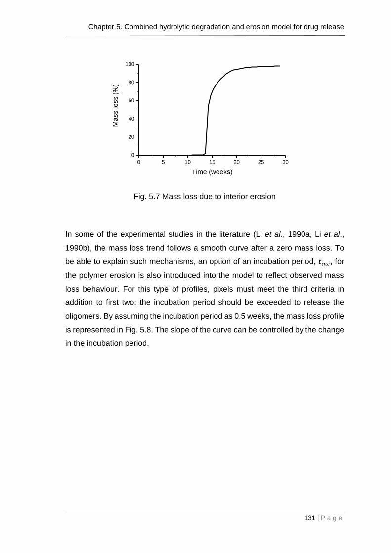
Chapter 5. Combined hydrolytic degradation and erosion model for drug release
131 | P a g e
Fig. 5.7 Mass loss due to interior erosion
In some of the experimental studies in the literature (Li et al., 1990a, Li et al.,
1990b), the mass loss trend follows a smooth curve after a zero mass loss. To
be able to explain such mechanisms, an option of an incubation period, 𝑡𝑖𝑛𝑐, for
the polymer erosion is also introduced into the model to reflect observed mass
loss behaviour. For this type of profiles, pixels must meet the third criteria in
addition to first two: the incubation period should be exceeded to release the
oligomers. By assuming the incubation period as 0.5 weeks, the mass loss profile
is represented in Fig. 5.8. The slope of the curve can be controlled by the change
in the incubation period.
0 5 10 15 20 25 30
0
20
40
60
80
100
Mass loss (
%)
Time (weeks)

Chapter 5. Combined hydrolytic degradation and erosion model for drug release
132 | P a g e
Fig. 5.8 Mass loss due to interior erosion with incubation period of 0.5 weeks
The introduction of an incubation period for interior erosion produces the mass
loss trend shown Fig. 5.8 that is most widely observed in the literature. The trend
is achieved by assuming that a polymer of very low molecular weight cannot
dissolve immediately when being in contact with water.
A summary of the mass loss profiles for individual mechanisms is plotted in Fig.
5.9. This kind of representation can be practical to assess the mechanisms
involved in a degrading-eroding polymer. However, the mass loss profiles in the
literature indicate that the various combinations of these mechanisms can be
required in order to explain the observed mass loss trends. Fig. 5.10 shows the
scenario for the combination of all the above mechanisms. These are
degradation, diffusion, surface erosion and interior erosion with incubation period
of 0.5 weeks. Up to week 13, surface erosion is dominated to the other
mechanisms by representing a characteristic linear mass loss. Beyond that,
surface erosion and interior erosion with incubation period are responsible with
the observed profile. Since more than one mechanism is involved, it is expected
to observe such a biphasic mass loss trend. By considering all the profiles
mentioned, it can be concluded that the bolus oligomer release towards the end
0 5 10 15 20 25 30
0
2
4
6
8
10
12
14
Mass loss (
%)
Time (weeks)
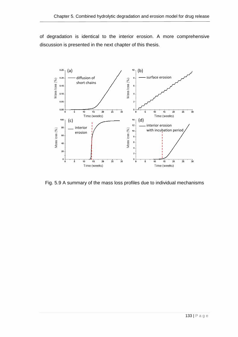
Chapter 5. Combined hydrolytic degradation and erosion model for drug release
133 | P a g e
of degradation is identical to the interior erosion. A more comprehensive
discussion is presented in the next chapter of this thesis.
Fig. 5.9 A summary of the mass loss profiles due to individual mechanisms
diffusion of short chains
surface erosion
interior erosion
interior erosion with incubation period
(a)
(c)
(b)
(d)

Chapter 5. Combined hydrolytic degradation and erosion model for drug release
134 | P a g e
Fig. 5.10 Combined effect of all the mechanisms on mass loss: degradation- diffusion (5.9(a)), surface erosion (5.9(b)), interior erosion with incubation
period of 0.5 weeks (5.9(d))
The combined model is able to capture the mass loss profiles of diffusion, surface
erosion, interior erosion or interior erosion with incubation period. The key point
here is to identify and understand particular mechanisms involved in the mass
loss. The contribution of that mechanisms can be more or less dominant or
completely uninvolved for the special cases. Often, more than one mechanism is
involved at a given time or different mechanisms can dominate at different stages
of mass loss as can be seen from Fig. 5.10. This has been succeed in the
simulations by switching on and off the relevant mechanisms and controlling the
speed of the involved mechanisms in the current model.
5.10 Conclusion
A combined mathematical model is developed in this chapter to simulate the
degradation-erosion process of PLA/GA polymers. In the model, surface erosion
and degradation initiates concurrently at t=0. Degradation equations feed
molecular weight values to the erosion part. As soon as a pixel reaches to the
critical molecular weight and has an eroded neighbor, interior erosion acts.
Heterogeneity of polymer matrix is also considered by calculation of the
porosities separately for each axial direction. The model calculates porosities in
Chapter 5. Combined hydrolytic degradation and erosion model for drug release
135 | P a g e
a range rather than averaging them along the axis. Using the model, chain
cleavage, diffusion, erosion and hole formation can be simulated in a single
model.
The key finding of this study is that, the early mass losses with constant rate is
an indicator of surface erosion, while the bolus mass losses after a certain time
are indicative of interior erosion. For the cases including bolus mass loss with a
smoother profile, one can claim that the interior erosion is functioning with an
incubation period. Incubation behaviour is a general and important factor that has
to be considered when understanding the degradation of aliphatic polyesters.
Diffusion individually does not have a big contribution to the mass loss. The
method used here is a very useful way to explain the different kind of mass loss
profiles by considering all the sources that can contribute to the mass loss.
Turning on and off the certain portions of the code provides a clear picture of how
each particular mechanism is involved in the mass loss.

Chapter 6. Case studies of polymer degradation using combined hydrolytic degradation and erosion model
136 | P a g e
Chapter 6. Case studies of polymer degradation using
combined hydrolytic degradation and erosion model
In this chapter, the full model presented in Chapter 5 was applied to several case
studies in the literature. For convenience, a summary of the combined model is
provided at the beginning of the chapter. The aim is to demonstrate the model
performance for the physically meaningful cases and provide an insight into the
possible mechanisms underlying each case. This has been achieved by
switching on and off the involved mechanisms and controlling the contribution of
each mechanism.
6.1 Summary of the experimental data by Grizzi et al. (1995) and
Lyu et al. (2007)
Grizzi et al. (1995) carried out a set of experiments using PLA50 in order to
compare the degradation behaviour of plates with different sizes. For this, large
and thin plates were allowed to age under iso-osmolar phosphate buffer solution,
pH 7.4 at 37oC. The thicknesses of the samples are given as 15x10x2 mm and
15x10x0.3 mm and 𝑀𝑛=20000 gmol-1 and 34000 gmol-1 for plates and films
respectively. The level of degradation is monitored by molecular weight and mass
loss change. Their experimental results are reproduced using the discrete
symbols in Fig. 6.3 and Fig. 6.4, in which number average molecular weight and
mass loss are shown as functions of time. The mass loss showed a sudden
increase after an initial zero mass loss. For thin device this trend is much smooth
compared to the thick plate. The greater thickness of the device showed a faster
degradation. A quantitative discussion was made which revealed considerable
insight into that degradation of the devices depends very much on size.
Lyu et al. (2007) studied the hydrolysis kinetics of amorphous poly(L-lactide-co-
L, D-lactic actide) (70/30) co-polymer. In their study, they compared the 2nd order
and 3rd order kinetic models with their experimental data. Moreover, the
temperature effect on the hydrolysis of PLA is tested over a range 37oC to 90oC
in a phosphate buffered solution (pH 7.4). Number average molecular weight of

Chapter 6. Case studies of polymer degradation using combined hydrolytic degradation and erosion model
137 | P a g e
the moulded samples is given as 290000 gmol-1. The test samples were discs
12.5 mm in diameter and 1 mm in thickness. The degradation results are shown
as the change in 𝑀𝑛 and mass loss as functions of time. The authors reported
that the experimental results do not follow 2nd or 3rd order reaction kinetics. It
has been suggested that the short chains does not have enough mobility in the
early stages of degradation to act as the catalysis for the hydrolysis reaction. This
suggestion was completed with the need for alternative models into the diffusion
limited degradation. Here we use the model presented in Chapter 5 to analyse
the underlying mechanisms of Grizzi et al. and Lyu et al.’s experimental data.
6.2 Summary of the combined model
The equations for combined degradation-erosion model are provided here for the
convenience of the reader
Chain scission
𝑑𝑅𝑠
𝑑𝑡= 𝐶𝑒,0 [1 − 𝛼 (
𝑅𝑠
𝐶𝑒,0)] (𝑘1 + 𝑘2 [𝐾𝑎 (
𝐶𝑜𝑙
𝑚)]
0.5
) (6.1)
𝑑𝑅𝑜𝑙
𝑑𝑡= 𝛼𝛽 (
𝑅𝑠
𝐶𝑒,0)
𝛽−1𝑑𝑅𝑠
𝑑𝑡 (6.2)
𝑀𝑛 = 𝑀𝑛,0
1 − 𝛼 (𝑅𝑠
𝐶𝑒,0)
𝛽
1 + 𝑁𝑑𝑝,0 (𝑅𝑠
𝐶𝑒,0−
𝑎𝑚
(𝑅𝑠
𝐶𝑒,0)
𝛽
)
(6.3)
Surface erosion
𝑑𝑉(𝑡)
𝑑𝑡= −𝐵 (6.4)
𝑉𝑐𝑒𝑙𝑙 = 𝑉𝑐𝑒𝑙𝑙 −𝑑𝑉
𝑑𝑡∗ 𝑑𝑡 (6.5)
𝑆(𝑖, 𝑗, 𝑡) = 0 𝑖𝑓 𝑉𝑐𝑒𝑙𝑙 = 0 (6.6)
Interior erosion

Chapter 6. Case studies of polymer degradation using combined hydrolytic degradation and erosion model
138 | P a g e
𝑆𝑚(𝑖, 𝑗, 𝑡) = 0 𝑖𝑓 𝑀𝑛 < 𝑀𝑛,𝑐𝑟𝑖𝑡𝑖𝑐𝑎𝑙 (6.7)
𝑆(𝑖, 𝑗, 𝑡) = 0 𝑖𝑓 𝑆𝑚(𝑖, 𝑗, 𝑡)
= 0 𝑎𝑛𝑑 𝑡ℎ𝑒 𝑝𝑖𝑥𝑒𝑙 ℎ𝑎𝑠 𝑎𝑛 𝑒𝑟𝑜𝑑𝑒𝑑 𝑛𝑒𝑖𝑔ℎ𝑏𝑜𝑢𝑟 (6.8)
Diffusion
𝜕𝐶𝑜𝑙
𝜕𝑡=
𝜕𝑅𝑜𝑙
𝜕𝑡+
𝜕
𝜕𝑥 (𝐷𝑜𝑙,𝑥
𝜕𝐶𝑜𝑙
𝜕𝑥) +
𝜕
𝜕𝑦 (𝐷𝑜𝑙,𝑦
𝜕𝐶𝑜𝑙
𝜕𝑦)
(6.9)
𝐷𝑜𝑙,𝑥 = 𝐷𝑜𝑙,𝑝𝑜𝑙𝑦 + (1.3𝜀𝑥2 − 0.3𝜀𝑥
3)(𝐷𝑜𝑙,𝑝𝑜𝑟𝑒 − 𝐷𝑜𝑙,𝑝𝑜𝑙𝑦) (6.10)
𝐷𝑜𝑙,𝑦 = 𝐷𝑜𝑙,𝑝𝑜𝑙𝑦 + (1.3𝜀𝑦2 − 0.3𝜀𝑦
3)(𝐷𝑜𝑙,𝑝𝑜𝑟𝑒 − 𝐷𝑜𝑙,𝑝𝑜𝑙𝑦) (6.11)
Equations 6.1 to 6.11 provide a summary of the model which combines chain
scission, surface erosion, interior erosion, and diffusion.
Eq. 6.1 gives the autocatalytic chain scission rate for the amorphous
polymer.
Eq. 6.2 relates oligomer production rate with the chain scission.
Eq. 6.3 relates the number of chain scission with the molecular weight.
Eq.s 6.4-6.6 determine whether a pixel is surface eroded or not by
considering the remaining volume of the cell. Pixels can be only surface
eroded if they are in contact with the aqueous medium.
Eq.s 6.7-6.8 determine whether a pixel is bulk eroded or not by checking
two main criteria of interior erosion: rather molecular weight is below the
critical value and pixels are in contact with an eroded neighbour.
Eq.s 6.9-6.11 are used to calculate the effective diffusion coefficient of the
oligomers taking into account the increasing porosity of the system. The
porosities 𝜀𝑥 and 𝜀𝑦 are based on the number of eroded pixels in each
direction.
6.3 Summary of the parameters used in the combined model
When analyzing the experimental data, a set of parameters can be found which
provides the best fitting with the model prediction. This set of parameters allows
identifying the underlying mechanisms of degradation and erosion. In this
section, the parameters have been varied to analyze two set of experimental

Chapter 6. Case studies of polymer degradation using combined hydrolytic degradation and erosion model
139 | P a g e
data. The selection of the case studies is done based on the fact that they require
different combinations of the mechanisms to attain the best fitting. This has been
established by switching on/off the mechanisms or controlling the contribution of
each mechanism. The model parameters used in the fittings are provided in
Table 6.1.
Table 6.1 Parameters used in the fittings
Model parameters
Units Case study A
(thick plate)
Case study A (thin plate)
Case study B
𝑀𝑛,𝑚𝑒𝑎𝑛 g mol-1 2x10⁴ 3.4x10⁴ 2.1x10⁵
𝑀𝑛,𝑠𝑡_𝑑𝑒𝑣 g mol-1 5x10³ 1.5x10³ 1.5x10⁵
𝑀𝑢𝑛𝑖𝑡 g mol-1 72 72 72
𝑘1 week-1 2.0x10⁻⁴ 7.0x10⁻⁵ 5.0x10⁻⁷
𝑘2 m3 mol-1 week-1 1.0x10⁻² 1.0x10⁻² 3.0x10⁻⁴
𝑚 no unit 4 4 4
α no unit 0.4 0.4 0.4
β no unit 1 1 1
𝐶𝑒,0 mol m-3 17300 17300 17300
𝐾𝑎 no unit 1.35x10⁻⁴ 1.35x10⁻⁴ 1.35x10⁻⁴
𝐵 m2 week-1 0 0
𝑀𝑛,𝑐𝑟𝑖𝑡𝑖𝑐𝑎𝑙 g mol-1 4.1x10³ 7.0x10³ 1.8x10⁴
𝐷𝑜𝑙,𝑝𝑜𝑙𝑦 m2 week-1 5.0x10⁻¹⁵ 5.0x10⁻¹⁵ 3.0x10⁻¹⁵
𝐷𝑜𝑙,𝑝𝑜𝑟𝑒 m2 week-1 1.0x10⁻⁵ 1.0x10⁻⁵ 1.0x10⁻⁵
Here, the parameter m, α and β are obtained from Pan et al. (2014). 𝐶𝑒,0, 𝑀𝑢𝑛𝑖𝑡
and 𝐾𝑎 are the standard data for the polymers in the issue. 𝑀𝑛,𝑚𝑒𝑎𝑛 is extracted
and 𝑀𝑛,𝑐𝑟𝑖𝑡𝑖𝑐𝑎𝑙 is estimated from the corresponding experimental data. The other
parameters such as 𝑘1, 𝑘2, 𝐵, 𝑀𝑛,𝑠𝑡_𝑑𝑒𝑣 and 𝐷𝑜𝑙,𝑝𝑜𝑙𝑦 are obtained by varying the
values systematically to give the best fit between the model prediction and
experimental data. 𝐷𝑜𝑙,𝑝𝑜𝑟𝑒 is set by considering the diffusivity of species in water
(Stewart, 2003). Two-dimensional plates are considered in the model. Initial
oligomer concentrations are 𝐶𝑜𝑙 = 𝐶𝑜𝑙,0= 0.035x𝐶𝑒,0 for thick plate; 0 for thin plate
for Case study A; and 0.015x𝐶𝑒,0 for Case study B. Symmetry is assumed across
the plates, therefore, quarter models are used in the simulations, therefore sizes
are set as a=1mm and b=5mm for thick plates and a=150µm and b=5mm for thin

Chapter 6. Case studies of polymer degradation using combined hydrolytic degradation and erosion model
140 | P a g e
plates in Case A. For case B, the values are a=500µm and b=6.25mm. Initial
molecular weight is randomly distributed throughout the plate considering the
mean values in the original study. 𝑀𝑛,𝑐𝑟𝑖𝑡𝑖𝑐𝑎𝑙 is estimated from the case studies
for amorphous polymer. In order to obtain a better fitting, a constant incubation
period of 0.5 week is added to interior erosion.
6.4 Fittings of the combined model to experimental data
Using the mathematical model provided in Section 6.2 and the parameters
provided in Section 6.3, it is now possible to suggest a mechanism for each case
study.
6.4.1 Case study A
Fig. 6.1 shows the model results of molecular weight distribution for thick plates
prior to degradation and at 1 week, 10 weeks and 13 weeks. The molecular
weight is distributed to follow normal distribution prior to degradation. The
distribution exhibits monomodal characteristic during the degradation and
erosion processes which indicate polymer to stay in amorphous phase during the
process. At t=0, the average molecular weight at the peak corresponds to the
20000. As time proceeds, the position of peaks is shifted to the left. The molecular
weight distribution of thin films is shown in Fig. 6.2 prior to degradation and at 10
weeks, 18, weeks and 27 weeks. Similarly, the peaks represent a monomodal
characteristic during the degradation and erosion processes.

Chapter 6. Case studies of polymer degradation using combined hydrolytic degradation and erosion model
141 | P a g e
Fig. 6.1 Molecular weight distributions of plates at various times during the degradation (a) t= 0 week; (b) t=1 week; (c) t=10 weeks and (d) t=13 weeks.
Molecular weight (Da)
time=0 week
time=10 weeks
(c)
time=1 week
time=13 weeks
(d)
(b) (a) F
req
uen
cy
Molecular weight (Da)
Fre
qu
en
cy
Molecular weight (Da) Molecular weight (Da)
Fre
qu
en
cy
Fre
qu
en
cy

Chapter 6. Case studies of polymer degradation using combined hydrolytic degradation and erosion model
142 | P a g e
Fig. 6.2 Molecular weight distributions of plates at various times during the degradation (a) t= 0 week; (b) t=1 week; (c) t=10 weeks and (d) t=13 weeks.
The best fit between the mathematical model and the experimental data is
presented in Fig. 6.3 and Fig. 6.4 both for films and plates. The parameters
𝑛𝑥 𝑥 𝑛𝑦 is set as 200 x 1000 for thick plates and 30 x 1000 for thin plates which
is compatible with the actual shape of the plates to ensure each pixel to be same
the size. For thick plates, both degradation, diffusion and interior erosion are
included in the numerical model. It can be observed that the model fits the
experimental data for the mass loss and average molecular weight. The best fit
is achieved by B=0, which indicates no surface erosion. This is reasonable since
the initial mass loss is zero when considering the experimental data. The interior
erosion without an incubation period is necessary for plates to produce the level
of mass loss observed in the experimental study. Results show that the thick
plate hits to the critical molecular weight is in 12 weeks. The greater amount of
Molecular weight (Da) Molecular weight (Da)
(c)
(b) (a)
time=0 week time=10 weeks
(d)
Fre
qu
en
cy
Fre
qu
en
cy
time=18 weeks time=27 weeks
Fre
qu
en
cy
Molecular weight (Da) Molecular weight (Da)
Fre
qu
en
cy
Chapter 6. Case studies of polymer degradation using combined hydrolytic degradation and erosion model
143 | P a g e
mass loss in later stages is identical for interior erosion and produce a bolus mass
loss in short period of time.
For thin plates, experimental results do represent no linear mass loss in early
times of degradation. Therefore, surface erosion is again switched off in the
numerical analysis for this case. However, it is obvious from the data that, there
is a sudden mass loss at t=0; which can be explained by the instant release of
fabrication excess in the matrix when exposed to the medium. This instant mass
loss is involved in the model; by setting 7% of initial mass loss at t=0. Similar to
the thick plates, a fitting to mass loss is only possible for thin plates if interior
erosion is included. However, the mass loss is much smooth for thin plates. The
smooth trend is explained by interior erosion with incubation period. The best
fitting is achieved by an incubation period of 0.2 weeks. As it can be observed
from the figure, the time at which device hits the critical molecular weight is 27
weeks. As a summary, it can be concluded that interior erosion is the main
mechanisms controlling mass loss from thick plates, while the interior erosion
with an incubation period is responsible for observed mass loss for thin plates of
Grizzi et al.’s study. A fitting to molecular weight is also presented in Fig. 6.3. The
model results are also proved to be accurate in capturing the size dependent
characteristic of degradation.

Chapter 6. Case studies of polymer degradation using combined hydrolytic degradation and erosion model
144 | P a g e
Fig. 6.3 Comparison of molecular weight change between model prediction and experimental data for samples with thickness of 0.3 mm and 2 mm. The solid and dashed lines represent the model predictions with the discrete symbols
representing the experimental data (Grizzi et al., 1995).
Fig. 6.4 Comparison of molecular mass loss between model prediction and experimental data for samples with thickness of 0.3 mm and 2 mm. The solid and dashed lines represent the model predictions with the discrete symbols
representing the experimental data (Grizzi et al., 1995)

Chapter 6. Case studies of polymer degradation using combined hydrolytic degradation and erosion model
145 | P a g e
Li et al. (1990c) conducted degradation experiments of PLA/GA specimens and
observed specimens to be heterogeneous after degradation. Fig. 6.5 shows the
cross section of their specimens after 10 days of degradation in distilled water.
They observed a clear whitish layer at the surface and the hollow structure inside
indicating a surface-centre differentiation of the specimens. The hollow structure
inside the specimens can be well explained by the model proposed in this
chapter. The time series of the representative thick plate that we obtained when
the procedure was applied is represented in Fig. 6.6. Here, white pixels represent
non-eroded polymer areas and black pixels, the eroded polymer areas.
Obviously, there is no interior erosion until week 11, since the pixels are above
critical molecular weight before that time. When grids reach to the critical value,
erosion starts from the surface and quickly connects to the more degraded inner
core. Fig. 6.6 shows that even after long erosion times there is still a clear skin
layer in the upper and right-side lines forming a clear shell for the grids in contact
with the aqueous environment. This finding agrees well with the experimental
data obtained by Li et al. (1990c). By expanding the grid into 3-dimension, it can
be visualized that the remainders form an interconnected network which is quite
porous. Burkersroda (2002) also discussed that issue with the break of the
surface layer at some point when a critical osmotic pressure builds up inside the
matrix due to the accumulation of degradation products. That theory is explained
with percolation phenomena which are based on the fact that degradation
products cannot leave the matrix unless a critical degree of degradation is
reached. The polymer then forms a network of pores to allow the release of
degradation products which are accumulated inside the matrix. Percolation
phenomena explain the hollow core surrounded by a whitish layer which is shown
in Fig. 6.6.

Chapter 6. Case studies of polymer degradation using combined hydrolytic degradation and erosion model
146 | P a g e
Fig. 6.5 Hollow structure of PLA37.5GA25 specimen after 10 days of degradation in distilled water (Li et al., 1990c) with permission via the Copyright
Clearance Centre.
Fig. 6.6 Temporal evaluation of simulated the polymer matrix
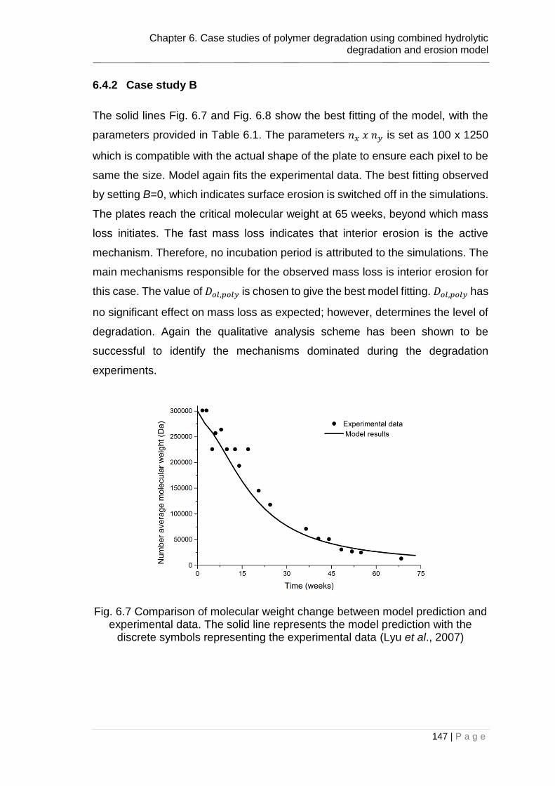
Chapter 6. Case studies of polymer degradation using combined hydrolytic degradation and erosion model
147 | P a g e
6.4.2 Case study B
The solid lines Fig. 6.7 and Fig. 6.8 show the best fitting of the model, with the
parameters provided in Table 6.1. The parameters 𝑛𝑥 𝑥 𝑛𝑦 is set as 100 x 1250
which is compatible with the actual shape of the plate to ensure each pixel to be
same the size. Model again fits the experimental data. The best fitting observed
by setting B=0, which indicates surface erosion is switched off in the simulations.
The plates reach the critical molecular weight at 65 weeks, beyond which mass
loss initiates. The fast mass loss indicates that interior erosion is the active
mechanism. Therefore, no incubation period is attributed to the simulations. The
main mechanisms responsible for the observed mass loss is interior erosion for
this case. The value of 𝐷𝑜𝑙,𝑝𝑜𝑙𝑦 is chosen to give the best model fitting. 𝐷𝑜𝑙,𝑝𝑜𝑙𝑦 has
no significant effect on mass loss as expected; however, determines the level of
degradation. Again the qualitative analysis scheme has been shown to be
successful to identify the mechanisms dominated during the degradation
experiments.
Fig. 6.7 Comparison of molecular weight change between model prediction and experimental data. The solid line represents the model prediction with the
discrete symbols representing the experimental data (Lyu et al., 2007)

Chapter 6. Case studies of polymer degradation using combined hydrolytic degradation and erosion model
148 | P a g e
Fig. 6.8 Comparison of mass loss between model prediction and experimental data. The solid line represents the model prediction with the discrete symbols
representing the experimental data (Lyu et al., 2007)
6.5 Conclusion
In this chapter, the mathematical model developed in Chapter 5 was validated by
two independent case studies from the literature. The case studies were chosen
considering that they require different combinations of degradation, diffusion,
surface erosion and interior erosion. The parameters were determined by varying
them in a range in order to obtain the best fitting. Therefore, one can claim that
the model presented in the chapter is a mechanistic model as well as being a
parameter estimation problem. The model proved to be accurate in predicting the
molecular weight distribution, change in molecular weight and mass loss
efficiently. The high level of fitting accuracy indicates the model’s ability to fit
various experimental data sets detailed in the literature. Moreover, the temporal
evolution of fragmentation stages of the polymer matrix is presented, which has
proved to be consistent with the theories demonstrated by literature. The method
used here effective to capture the large mass losses and the model results offer
physical insight into the experimental studies. Moreover, the computational
model presented here can be a useful tool in the estimation of the relation

Chapter 6. Case studies of polymer degradation using combined hydrolytic degradation and erosion model
149 | P a g e
between degradation and erosion processes and has shown to be a very useful
way to theoretically capture enormous mass losses.

Chapter 7. Case studies of drug release from stents using the combined hydrolytic degradation and erosion model
150 | P a g e
Chapter 7. Case studies of drug release from stents
using the combined hydrolytic degradation and erosion
model
The release kinetics of drugs dissolved within a polymeric matrix layer generally
follows a multiphasic release mechanism. This mechanism includes a diffusion
controlled phase, a degradation controlled phase and/or an erosion-controlled
phase. In this chapter, the full model presented in Chapter 5 is extended in a way
to cover the presence of drug. The modified model is validated with a case study
identifying the degradation and drug release from PLGA stent coating. Different
drug loadings are modelled to identify whether the model can indeed capture the
experimental results. The mathematical model is used to understand the
underlying mechanisms of drug-eluting stents.
7.1 Introduction
A coronary stent is a metal tube that is inserted into the arteries at the locations
of narrowing and acts as a supporting material to the blood vessels. The stents
can be either a balloon expandable or a self-expandable stent. The former
functions under the pressure of the balloon; while self-expandable stents work
when the sheath is retracted. For both of the cases, the stent provides support to
the artery and keeps the artery open (Migliavacca et al., 2004). The coronary
stents are generally grouped as bare metallic stents (durable stents), coated
metallic stents, biodegradable stents and drug eluting stent. Drug eluting stents
with durable polymer coatings reduce the rates of target lesion compared to the
durable stents. However, the problem of late stent thrombosis remains a high risk
in most of the populations (Bangalore et al., 2013).
The fully degradable drug eluting stents, in which the stent is made from
biodegradable polymers have great potential for delivering drugs into human
coronary arteries. The device enables prolonged delivery of the drugs. Currently,
sirolimus and paclitaxel are the only drugs used in drug eluting stents approved
by the Food and Drug Administration (Acharya and Park, 2006). Both are big

Chapter 7. Case studies of drug release from stents using the combined hydrolytic degradation and erosion model
151 | P a g e
molecules (Mw: 914.19 g/mol, sirolimus and 853.96 g/mol, paclitaxel (Ultra,
2001)) and have very low solubility in aqueous solution (logP: 4.3, sirolimus and
3.2, paclitaxel (Wishart et al., 2006)). Therefore, the release of these drugs from
the polymers are extensively governed by degradation and erosion mechanisms.
The polymers commonly used for that purpose include the PLA/GA group of
biodegradable polymers (Wang et al., 2006, Zhu et al., 2014). Particularly PLGA
copolymers are well recognized for their suitability in drug eluting stents due to
administering a complete drug release by virtue of degradation and erosion of
polymer matrix (Zhu and Braatz, 2015). There are several study in the literature
suggesting drug release mechanisms from biodurable stent coatings such as the
models considering the drug-vascular tissue interactions (Hossainy and Prabhu,
2008), analytical solutions for drug diffusion in one dimensional wall (Pontrelli and
de Monte, 2010) and mechanics and fluid dynamic simulations considering stent
expansion and interaction with coronary artery (Zunino et al., 2009). However,
there is limited work in mathematical models quantifying drug release from
biodegradable and bioerodible stents. Most of the models suggested so far
describe the drug release based on degradation only models. A broader
perspective has been recently adopted by Zhu and Braatz (2015). In their study,
Zhu and Braatz coupled degradation, erosion and drug release from PLGA stent
coating. They focused on the two stage release of PLGA drug release systems
involving an initial slow release followed by an enhanced release which is
obtained by erosion. Drug diffusion is achieved through polymer solid and liquid
filled pores. Drug release is modelled taking into account various factors such as
molecular weight change, diffusivity in polymer and liquid filled pores and drug
partitioning between solid and liquid phases. However, one major limitation of
their study is to propose an analytical expression for mass loss. The model would
have been more useful if they considered a mechanistic approach for erosion.
As repeatedly stated in Chapter 5 and Chapter 6, degradation and erosion
mechanism are fairly interconnected with each other. When designing a stent
system made of biodegradable polymers, it is important to understand these
particular mechanisms involved in the release process. Often, more than one
mechanisms are involved at a given time or different mechanisms may dominate

Chapter 7. Case studies of drug release from stents using the combined hydrolytic degradation and erosion model
152 | P a g e
at different stages of the drug delivery (Siegel and Rathbone, 2012). It is,
therefore, a very attractive proposition to suggest different mechanisms for a
specific device. In that perspective, the model proposed in Chapter 5 provides a
solid foundation for modelling drug release from biodegradable stents. In the
current chapter, the model provided in Chapter 5 is further improved to include
the drug term. So that drug release from stents is treated as a combination of
degradation, diffusion, surface erosion and interior erosion. The modified model
is then validated with a case study from the literature for in vitro sirolimus release.
By switching on and off the involved mechanisms, the model results giving the
best fit is represented.
7.2 Summary of the experimental data by Wang et al. (2006)
Wang et al. (2006) studied the release of sirolimus from bi-layer and tri-layer
biodegradable films made of supporting layer(s) and a drug eluting layer.
Supporting layer is made of PLLA and the drug-eluting layer is made of PLGA for
bi-layer films. For the case of tri-layer films, the drug eluting layer is kept between
two supporting layers: one layer made of PLLA and one mode of PLGA 50/50.
Diagrams of the bi-layer and tri-layer polymer matrix are shown in Fig. 7.1. These
layers are separately dissolved in DCM during the casting, thus, they can be
considered independently. 𝑀𝑛,0=75000 gmol-1; and 𝑀𝑢𝑛𝑖𝑡=65 gmol-1 (considering
53% PLA and 47% PGA wt/wt). 1% and 2% wt% drug loadings are studied to
analyse the effect of drug loadings on the final release profile. The layer
thicknesses are controlled within 60-80±5µm. Degradation and drug release
assessments are performed in the release medium (5% Dichloromethane
(DMSO)+95% pH 7.4 PBS) at 37 oC. The changes in molecular weight and mass
loss of drug-eluting layer is shown as functions of time. Moreover, drug release
and the micrographs of the surface morphology are monitored during the
degradation. The experimental results are reproduced using the discrete symbols
in Fig. 7.3, Fig. 7.4 and Fig. 7.5. It is shown that molecular weight decrease, mass
loss and drug release occur in two stages: an initial steady state and
subsequently a more drastic stage. They argued this trend by the relative
dominance of the mechanism during the degradation as a diffusion dominated

Chapter 7. Case studies of drug release from stents using the combined hydrolytic degradation and erosion model
153 | P a g e
phase and a degradation-erosion dominated phase. Moreover, it is concluded
that changing drug loading does not affect the release kinetics. This could be
attributed to the fact that the drug loadings studied are quite close to each other.
A further study with more loadings is therefore suggested.
Fig. 7.1 Diagrams of the bi-layer and tri-layer polymer films of Wang et al. (Wang et al., 2006) with the corresponding layer thicknesses (reproduced from
relevant study)
7.3 Modification of the combined degradation-erosion model to
include drug term
Fig. 7.2 shows the schematic of the stent and the drug loaded polymer coating
which is the topic of the mathematical model presented in this chapter. Once a
strut is in contact with a solvent, the solvent molecules (such as water) penetrate
80µm
80µm
Drug-eluting layer Supporting layer, PLLA
80µm
80µm
Drug-eluting layer Supporting layer, PLLA
60µm Supporting layer, PLGA 50/50

Chapter 7. Case studies of drug release from stents using the combined hydrolytic degradation and erosion model
154 | P a g e
into the polymer matrix leading to concurrent events: solubilization of drug
molecules depending on their kinetics and cleavage of polymer chains.
Fig. 7.2 a) Cross section of an implanted stent in a coronary artery; b) schematic of a single stent strut with drug-loaded polymer matrix; c) schematic
of the drug loaded polymer matrix which is modelled in the current chapter.
Two key components are considered in modelling drug release from PLGA stent:
1) capture the dynamic changes in the polymer matrix such as degradation,
erosion and corresponding porosity changes; 2) description of the drug diffusivity
based on the dynamic changes in the polymer matrix. The model presented in
Chapter 5 is applied for the calculation of PLA/GA degradation, erosion and the
corresponding porosity. The model is then modified considering the drug
transport in the coating which is proceeded by diffusion mechanism. Assuming
that the drug is uniformly dispersed in the polymer matrix initially, the drug release
is described by Fick’s law of diffusion such as
𝜕𝐶𝑑𝑟𝑢𝑔
𝜕𝑡=
𝜕𝑅𝑑𝑟𝑢𝑔
𝜕𝑡+
𝜕
𝜕𝑥(𝐷𝑑𝑟𝑢𝑔
𝜕𝐶𝑑𝑟𝑢𝑔
𝜕𝑥) +
𝜕
𝜕𝑦(𝐷𝑑𝑟𝑢𝑔
𝜕𝐶𝑑𝑟𝑢𝑔
𝜕𝑦). (7.1)
Here 𝐷𝑑𝑟𝑢𝑔 is the effective diffusivity that is dependent on the porosity of matrix.
Diffusion coefficient of drug changes significantly by generation of pores during
the degradation. Again, considering the heterogeneous structure within the
matrix which is largely based on erosion, the diffusion coefficient are calculated
separately for each direction. Eq. 5.22 is modified for the drug case such that

Chapter 7. Case studies of drug release from stents using the combined hydrolytic degradation and erosion model
155 | P a g e
𝐷𝑑𝑟𝑢𝑔,𝑥 = 𝐷𝑑𝑟𝑢𝑔,𝑝𝑜𝑙𝑦 + (1.3𝜀𝑥2 − 0.3𝜀𝑥
3)(𝐷𝑑𝑟𝑢𝑔,𝑝𝑜𝑟𝑒 − 𝐷𝑑𝑟𝑢𝑔,𝑝𝑜𝑙𝑦) (7.2)
and
𝐷𝑑𝑟𝑢𝑔,𝑦 = 𝐷𝑑𝑟𝑢𝑔,𝑝𝑜𝑙𝑦 + (1.3𝜀𝑦2 − 0.3𝜀𝑦
3)(𝐷𝑑𝑟𝑢𝑔,𝑝𝑜𝑟𝑒 − 𝐷𝑑𝑟𝑢𝑔,𝑝𝑜𝑙𝑦). (7.3)
Drug release is accomplished by combinations of several sources as drug
diffusion, surface erosion, and bulk erosion. The final drug release, 𝑀𝑡 can be
calculated by the sum of all the sources contributed:
𝑀𝑡 = 𝑀𝑑 + 𝑀𝑠 + 𝑀𝑏 (7.4)
𝑀𝑑, 𝑀𝑠 and 𝑀𝑏 are the drug release governed by drug diffusion, surface erosion
and bulk erosion respectively. The contribution of this mechanisms are controlled
by rather switching on/off the relevant bids in the simulations or changing the
domination of each mechanism.
7.4 Summary of the parameters used in case study
The set of parameters used in this section allows identifying the underlying
mechanisms of degradation, erosion and the drug release for the case study of
Wang et al. (2006). This has been established by switching on/off the
mechanisms or controlling the contribution of each mechanism. The selection of
the parameters is made based on targeting a good fitting. The model parameters
used in the fittings are provided in Table 6.1.
Table 7.1 Values of the model parameters used in the fittings
Model parameters Units Case study
𝑀𝑛,𝑚𝑒𝑎𝑛 g mol-1 7.5x10⁴
𝑀𝑛,𝑠𝑡_𝑑𝑒𝑣 g mol-1 2.0x10⁴
𝑀𝑢𝑛𝑖𝑡 g mol-1 65
𝑘1 week-1 5.0x10⁻⁶
𝑘2 m3 mol-1 week-1 2.5x10⁻²
𝑚 no unit 4 α no unit 0.4 β no unit 1 𝐶𝑒,0 mol m-3 20615
𝐾𝑎 no unit 1.35x10⁻⁴
𝑀𝑛,𝑐𝑟𝑖𝑡𝑖𝑐𝑎𝑙 g mol-1 2.0x10⁴

Chapter 7. Case studies of drug release from stents using the combined hydrolytic degradation and erosion model
156 | P a g e
𝐷𝑜𝑙,𝑝𝑜𝑙𝑦 m2 week-1 5.0x10⁻¹⁵
𝐷𝑜𝑙,𝑝𝑜𝑟𝑒 m2 week-1 1.0x10⁻⁵
𝐷𝑑𝑟𝑢𝑔,𝑝𝑜𝑙𝑦 m2 week-1 5.0x10⁻¹⁷
𝐷𝑑𝑟𝑢𝑔,𝑝𝑜𝑟𝑒 m2 week-1 1.0x10⁻⁵
Again, the parameter 𝐶𝑒,0, m, α and β is obtained from Pan et al. (2014).
𝑀𝑛,𝑚𝑒𝑎𝑛 is the initial molecular weight of the polymer prior to degradation, which
is taken from (Wang et al., 2006). 𝑀𝑛,𝑐𝑟𝑖𝑡𝑖𝑐𝑎𝑙 is estimated from the experimental
data representing 𝑀𝑛 reduction. 𝐷𝑜𝑙,𝑝𝑜𝑟𝑒 and 𝐷𝑑𝑟𝑢𝑔,𝑝𝑜𝑟𝑒 are the diffusion
coefficients in liquid filled pores for oligomers and drug respectively, which are
simply assumed to be big numbers considering the diffusivity of species in water
(Stewart, 2003). 𝐷𝑜𝑙,𝑝𝑜𝑙𝑦 is set as a very small number considering the diffusivity
of oligomers in fresh bulk polymer. The set of 𝑀𝑛,𝑠𝑡_𝑑𝑒𝑣, 𝑘1, 𝑘2 and 𝐷𝑑𝑟𝑢𝑔,𝑝𝑜𝑙𝑦 is
then obtained by fitting the model calculations with the experimental data.
The polymer matrix is simulated as a 2-dimensional plate. The parameters
𝑛𝑥 𝑥 𝑛𝑦 is set as 40 x 2500 which is compatible with the actual shape of the plate
to ensure each pixel to be square size. Quarter model is used in the simulations
because of the symmetry of the plates. Therefore, the sizes of the plate is set as
a=40µm and b=2.5mm. For the sake of a better fitting, an incubation period of
1.25 weeks is used with the interior erosion.
7.5 Fittings of the modified model with experimental data
Fig. 7.3, 7.4 and 7.5 shows the best fit between the model results and the
experimental data obtained by Wang et al. (2006). The model parameters used
in the fitting are provided in Table 7.1. The initial oligomer concentration is set as
𝐶𝑜𝑙,0=0. The experimental data gives the hint of a sudden mass loss at t=0; which
can be explained by the instant release of fabrication excess in the matrix when
exposed to the medium. This instant loss is involved in the model; by setting 3.8%
of initial mass loss at t=0. Surface erosion mechanism is switched off in the
simulations. The increased mass loss to the end of the degradation is
representative of the interior erosion. The gradual increase in the mass loss

Chapter 7. Case studies of drug release from stents using the combined hydrolytic degradation and erosion model
157 | P a g e
indicates the incubation for release of oligomers, therefore, we set an incubation
period of 1.25 weeks in the simulations.
Fig. 7.3 Comparison of molecular weight decrease of PLGA between model prediction and experimental data. The solid line represents the model
predictions with the discrete symbols representing the experimental data (Wang et al., 2006).
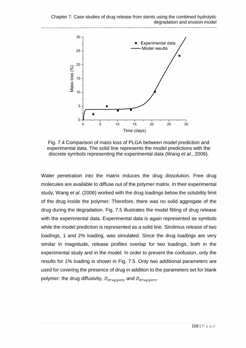
Chapter 7. Case studies of drug release from stents using the combined hydrolytic degradation and erosion model
158 | P a g e
Fig. 7.4 Comparison of mass loss of PLGA between model prediction and experimental data. The solid line represents the model predictions with the discrete symbols representing the experimental data (Wang et al., 2006).
Water penetration into the matrix induces the drug dissolution. Free drug
molecules are available to diffuse out of the polymer matrix. In their experimental
study, Wang et al. (2006) worked with the drug loadings below the solubility limit
of the drug inside the polymer. Therefore, there was no solid aggregate of the
drug during the degradation. Fig. 7.5 illustrates the model fitting of drug release
with the experimental data. Experimental data is again represented as symbols
while the model prediction is represented as a solid line. Sirolimus release of two
loadings, 1 and 2% loading, was simulated. Since the drug loadings are very
similar in magnitude, release profiles overlap for two loadings, both in the
experimental study and in the model. In order to prevent the confusion, only the
results for 1% loading is shown in Fig. 7.5. Only two additional parameters are
used for covering the presence of drug in addition to the parameters set for blank
polymer: the drug diffusivity, 𝐷𝑑𝑟𝑢𝑔,𝑝𝑜𝑙𝑦 and 𝐷𝑑𝑟𝑢𝑔,𝑝𝑜𝑟𝑒.
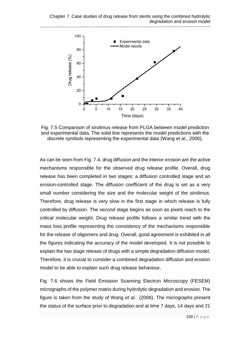
Chapter 7. Case studies of drug release from stents using the combined hydrolytic degradation and erosion model
159 | P a g e
Fig. 7.5 Comparison of sirolimus release from PLGA between model prediction and experimental data. The solid line represents the model predictions with the
discrete symbols representing the experimental data (Wang et al., 2006).
As can be seen from Fig. 7.4, drug diffusion and the interior erosion are the active
mechanisms responsible for the observed drug release profile. Overall, drug
release has been completed in two stages: a diffusion controlled stage and an
erosion-controlled stage. The diffusion coefficient of the drug is set as a very
small number considering the size and the molecular weight of the sirolimus.
Therefore, drug release is very slow in the first stage in which release is fully
controlled by diffusion. The second stage begins as soon as pixels reach to the
critical molecular weight. Drug release profile follows a similar trend with the
mass loss profile representing the consistency of the mechanisms responsible
for the release of oligomers and drug. Overall, good agreement is exhibited in all
the figures indicating the accuracy of the model developed. It is not possible to
explain the two stage release of drugs with a simple degradation diffusion model.
Therefore, it is crucial to consider a combined degradation diffusion and erosion
model to be able to explain such drug release behaviour.
Fig. 7.6 shows the Field Emission Scanning Electron Microscopy (FESEM)
micrographs of the polymer matrix during hydrolytic degradation and erosion. The
figure is taken from the study of Wang et al. (2006). The micrographs present
the status of the surface prior to degradation and at time 7 days, 14 days and 21

Chapter 7. Case studies of drug release from stents using the combined hydrolytic degradation and erosion model
160 | P a g e
days. As can be seen from the figure, cavities are formed during degradation and
erosion which links interior to the surface. The cavity formation is unclear up to
time 21 days. However, at 21 days, cavity formation is obvious in the matrix
surface which leads relatively significant mass loss (10%) and drug release
(30%) at that time.
Fig. 7.6 Micrographs of the surface morphology of degrading PLGA 53/47 taken from (Wang et al., 2006) (a) 0 days, (b) 7 days, (c) 14 days and (d) 21 days.
Fig. 7.7 shows the simulation results which represent the status of the drug
loaded polymer matrix at 21 days. Grey part in the figure represents the stent
strut which is excluded in the simulations and only represented here for a clear
picture. White pixels indicate the non-eroded polymer matrix whereas black
pixels represent the eroded polymer matrix. The status of the surface shown in
Fig. 7.7 fairly match with the FESEM micrographs represented in Fig. 7.6. This is

Chapter 7. Case studies of drug release from stents using the combined hydrolytic degradation and erosion model
161 | P a g e
because, model results validate the formation of microcavities which builds up a
network in the polymer and links the surface with the more degraded interior. The
microcavities are formed based on the erosion of the pixels which gives rise to
rapid oligomer and drug release. The level of matching between the model results
and experimental data confirms the validity of the model established. To
conclude, the oligomer and sirolimus release from PLGA polymer is divided into
two stages: a diffusion controlled stage which gives a constant slow release of
oligomer at initial times and an erosion-controlled stage which results in a rapid
release of oligomers an drug at later stages.
Fig. 7.7 Simulation results for drug loaded polymer matrix at t=21 days.
stent strut
matrix at t=21 days
Chapter 7. Case studies of drug release from stents using the combined hydrolytic degradation and erosion model
162 | P a g e
7.6 Conclusion
This chapter provides a complete model set for describing polymer degradation
and erosion and coupled drug release from a stent coating. Understanding the
degradation and erosion kinetics of biodegradable polymers such as PLGA is a
prerequisite for the design of a drug-eluting polymer stent. Considering this, the
mathematical model in Chapter 5 is modified and coupled with drug release with
an attempt to explain the number average molecular weight, mass loss and drug
release behaviour from the coating. The model results were then validated with
the experimental data from the literature.
Simultaneous drug diffusion from polymer matrix and liquid-filled pores was
modelled. Effective drug diffusivity was taken as dependent on the porosity of the
matrix which is a function of cavity formation. Erosion is the main mechanism
responsible for the formation of the cavities. The model was then verified for
sirolimus release from the stent coating and showed a good level of fitting. The
comparison between the model in this chapter and the degradation model
revealed that the multiple stages of drug release cannot be captured with a single
degradation model.

Chapter 8. Major conclusions and future work
163 | P a g e
Chapter 8. Major conclusions and future work
8.1 Major conclusions
In this thesis, several mathematical models were developed and used to predict
the drug release behaviour of PLA/GA polymers. The works in separate chapters
were motivated by experimental studies documented in the literature, which
demonstrated drug-polymer interaction within the polymer matrix, as well as two
stage degradation-erosion behaviour of polymers. The degradation models were
considered as autocatalytic because of the characteristics of PLA/GA polymers.
The reaction-diffusion models considered the pore evaluation and enhanced
diffusivity of oligomers and drugs during degradation and erosion. The models
were not developed to be valid for all cases for controlled drug delivery systems,
instead, they had been used to further understand the underlying background of
the experimental data.
The mathematical models presented in this thesis were based on previous
models from the group at the University of Leicester, they were either improved,
to include the further catalysts effects arising from drugs and the interactions with
the drug and polymer or coupled with erosion models, in order to capture the
enormous mass losses of polymers as well as multi-stage drug release
behaviour. The models were used to further understanding of the factors in
hydrolytic degradation and drug release.
The effect of drug incorporation on polymer degradation rate was presented by
considering the interaction between drugs and polymers as well as the catalyst
effect of free acidic and basic species. It was found that acidic drugs significantly
accelerates the polymer degradation by releasing protons during dissociation.
For the basic drugs, it was found that drugs can either accelerates or decelerates
the polymer degradation depending on the ionic interaction between basic drugs
and polymer chain ends. The index of the polymer - basic drug interactions, 𝐾𝑝,
was found to be the primitive factor controlling the release of basic drugs.
Namely, the increase in the value of 𝐾𝑝 resulted in a decrease in degradation

Chapter 8. Major conclusions and future work
164 | P a g e
rate, because of the decrease in the number of free carboxylic acids and drug
molecules.
A coupled mathematical model was also developed in this thesis to simulate the
hydrolytic degradation and erosion process of PLA/GA polymers. The key finding
of the study was that, the mechanism of diffusion has very small contribution to
the mass loss and drug release. Moreover, the early mass loss with constant rate
was an indicator of surface erosion, while the bolus mass losses after a certain
time were indicative of interior erosion. For the cases including bolus mass loss
with a smoother profile, it was found that the interior erosion is functioning with
an incubation period. The model well captured the mass loss, drug release and
microstructure evaluation for several case studies including the blank polymers
and a drug eluting stent.
From our knowledge, it is the first time in the literature to combine the
mechanisms of hydrolytic degradation, diffusion, surface and interior erosion into
a single mathematical model. Our study fills a gap in the literature by including
the autocatalysis into a probabilistic erosion model. The model highlight an issue
which has never been paid enough attention – it is important to link hydrolytic
degradation and erosion processes in order to understand different kinds of mass
loss and drug release trends. The method used here is effective to deal with large
mass loss as well as multiphasic drug release behaviour. Importantly, the model
results offer physical insight into the experimental studies. The practical
application of the model can be useful to guide the design of the polyester
materials with required properties.
Many mechanisms are involved in the progressive drug release from controlled
delivery systems. Moreover, experimental data gives the hint that release from
each controlled drug delivery system is dominated by different phenomena.
Therefore, it is not possible to propose models that would be valid for all the drug
delivery systems. The main aim of this thesis was offering possible mechanisms
to the experimental data rather than developing models that would be valid for all
the cases. The models developed in this thesis offered a physical insight into the
various experimental studies available in the literature. The good agreement

Chapter 8. Major conclusions and future work
165 | P a g e
between the model results and the experimental data showed that this target was
accomplished to a large extent.
8.2 Future work
Despite the number of experimental studies in controlled release systems in
recent years, the area of modelling controlled delivery systems is still under
development. As discussed in the previous chapters of this thesis, the models in
the literature are very simple and far from predicting the real data.
The mathematical modelling of drug delivery has a significant potential for
development of new products and helps to enlighten complex behaviour of
pharmaceutical dosage forms. With the developments in the information
technology the accuracy of the models developed are improved in a great extent.
Likewise the case for other disciplines, modelling drug delivery is expected to
become a part of the drug development. However, one obstacle with modelling
drug delivery systems is that it is challenging to establish a model which would
be applicable for all different kind of polymers and drugs. Mathematical models
are more likely to be applicable to specific devices with specific drug and polymer.
Another obstacle is that many assumptions are needed in order to develop the
models which decreases the convergence of the models to the reality. A fruitful
aspect will be to go towards development of models with decision trees which
identifies the appropriate model for specific kind of drug delivery systems. This
would help understanding the underlying drug release mechanism of a specific
system.
The other fruitful approach will be to combine these mathematical models for
quantifying the drug release in living organism, such as drug transport to the
different organs and cells. Yet, the drug release models predicts the resulting
drug release kinetics. However, the resulting drug concentration at human body
including the pharmacodynamics effects in patient is missing. The models
considering the drug distribution, drug metabolism and prediction of clearance
can provide valuable information to design new products.
References
166 | P a g e
References
ACHARYA, G. & PARK, K. 2006. Mechanisms of controlled drug release from drug-eluting
stents. Advanced Drug Delivery Reviews, 58, 387-401.
AGRAWAL, C. & RAY, R. B. 2001. Biodegradable polymeric scaffolds for musculoskeletal
tissue engineering. Journal of biomedical materials research, 55, 141-150.
AHOLA, M., RICH, J., KORTESUO, P., KIESVAARA, J., SEPPÄLÄ, J. & YLI-URPO, A. 1999. In
vitro evaluation of biodegradable ε-caprolactone-co-d,l-lactide/silica xerogel
composites containing toremifene citrate. International Journal of
Pharmaceutics, 181, 181-191.
ARIFIN, D. Y., LEE, L. Y. & WANG, C.-H. 2006a. Mathematical modeling and simulation of
drug release from microspheres: Implications to drug delivery systems.
Advanced drug delivery reviews, 58, 1274-1325.
ARIFIN, D. Y., LEE, L. Y. & WANG, C. H. 2006b. Mathematical modeling and simulation of
drug release from microspheres: Implications to drug delivery systems. Adv Drug
Deliv Rev, 58, 1274-325.
BALA, I., HARIHARAN, S. & KUMAR, M. R. 2004. PLGA nanoparticles in drug delivery: the
state of the art. Critical Reviews™ in Therapeutic Drug Carrier Systems, 21.
BANGALORE, S., TOKLU, B., AMOROSO, N., FUSARO, M., KUMAR, S., HANNAN, E. L.,
FAXON, D. P. & FEIT, F. 2013. Bare metal stents, durable polymer drug eluting
stents, and biodegradable polymer drug eluting stents for coronary artery
disease: mixed treatment comparison meta-analysis. BMJ : British Medical
Journal, 347.
BASTIOLI, C. 2005. Handbook of biodegradable polymers, iSmithers Rapra Publishing.
BATYCKY, R. P., HANES, J., LANGER, R. & EDWARDS, D. A. 1997. A theoretical model of
erosion and macromolecular drug release from biodegrading microspheres.
Journal of Pharmaceutical Sciences, 86, 1464-1477.

References
167 | P a g e
BERKLAND, C., KIM, K. K. & PACK, D. W. 2003. PLG microsphere size controls drug release
rate through several competing factors. Pharmaceutical research, 20, 1055-
1062.
BERKLAND, C., KING, M., COX, A., KIM, K. & PACK, D. W. 2002. Precise control of PLG
microsphere size provides enhanced control of drug release rate. Journal of
Controlled Release, 82, 137-147.
BODMEIER, R. & CHEN, H. G. 1989. Evaluation of biodegradable poly(lactide) pellets
prepared by direct compression. J Pharm Sci, 78, 819-22.
BODMER, D., KISSEL, T. & TRAECHSLIN, E. 1992. Factors influencing the release of
peptides and proteins from biodegradable parenteral depot systems. Journal of
Controlled Release, 21, 129-137.
BOSWORTH, L. A. & DOWNES, S. 2010. Physicochemical characterisation of degrading
polycaprolactone scaffolds. Polymer Degradation and Stability, 95, 2269-2276.
BUCHANAN, F. J. 2008. Degradation rate of bioresorbable materials: Prediction and
evaluation, Elsevier.
BURKERSRODA, F. V. & GOEPFERICH, A. An approach to classify degradable polymers.
MRS Proceedings, 1998. Cambridge Univ Press, 17.
CAI, H., DAVE, V., GROSS, R. A. & MCCARTHY, S. P. 1996. Effects of physical aging,
crystallinity, and orientation on the enzymatic degradation of poly(lactic acid).
Journal of Polymer Science Part B: Polymer Physics, 34, 2701-2708.
CAIRNS, D. 2012. Essentials of pharmaceutical chemistry, Pharmaceutical Press.
CASALINI, T., ROSSI, F., LAZZARI, S., PERALE, G. & MASI, M. 2014. Mathematical
modeling of PLGA microparticles: from polymer degradation to drug release.
Mol Pharm, 11, 4036-48.
CASCONE, M. G., SIM, B. & SANDRA, D. 1995. Blends of synthetic and natural polymers
as drug delivery systems for growth hormone. Biomaterials, 16, 569-574.
CHA, Y. & PITT, C. G. 1988. A one-week subdermal delivery system for l-methadone
based on biodegradable microcapsules. Journal of Controlled Release, 7, 69-78.

References
168 | P a g e
CHA, Y. & PITT, C. G. 1989. The acceleration of degradation-controlled drug delivery
from polyester microspheres. Journal of Controlled Release, 8, 259-265.
CHARLIER, A., LECLERC, B. & COUARRAZE, G. 2000. Release of mifepristone from
biodegradable matrices: experimental and theoretical evaluations. International
journal of pharmaceutics, 200, 115-120.
CLUGSTON, M. & FLEMMING, R. 2000. Advanced chemistry, Oxford University Press.
D’SOUZA, S., FARAJ, J. A., DORATI, R. & DELUCA, P. P. 2015. Enhanced Degradation of
Lactide-co-Glycolide Polymer with Basic Nucleophilic Drugs. Advances in
Pharmaceutics, 2015.
DANIELS, A., CHANG, M. K., ANDRIANO, K. P. & HELLER, J. 1990. Mechanical properties
of biodegradable polymers and composites proposed for internal fixation of
bone. Journal of Applied Biomaterials, 1, 57-78.
DEWICK, P. M. 2006. Essentials of organic chemistry: for students of pharmacy,
medicinal chemistry and biological chemistry, John Wiley & Sons.
DOMB, A. J. & KUMAR, N. 2011. Biodegradable polymers in clinical use and clinical
development, John Wiley & Sons.
DUNNE, M., CORRIGAN, O. I. & RAMTOOLA, Z. 2000. Influence of particle size and
dissolution conditions on the degradation properties of polylactide-co-glycolide
particles. Biomaterials, 21, 1659-1668.
ENGINEER, C., PARIKH, J. & RAVAL, A. 2011. Review on hydrolytic degradation behavior
of biodegradable polymers from controlled drug delivery system. Trends
Biomater Artif Organs, 25, 79-85.
FITZGERALD, J. F. & CORRIGAN, O. I. 1996. Investigation of the mechanisms governing
the release of levamisole from poly-lactide-co-glycolide delivery systems.
Journal of Controlled Release, 42, 125-132.
FORD, A. N., PACK, D. W. & BRAATZ, R. Multi-scale modeling of PLGA microparticle drug
delivery systems. 21st European Symposium on Computer Aided Process
Engineering: Part B, 2011a. Interscience New York, 1475-1479.

References
169 | P a g e
FORD, A. N., PACK, D. W. & BRAATZ, R. D. 2011b. Multi-Scale Modeling of PLGA
Microparticle Drug Delivery Systems. Computer Aided Chemical Engineering.
FORD VERSYPT, A. N., PACK, D. W. & BRAATZ, R. D. 2013. Mathematical modeling of
drug delivery from autocatalytically degradable PLGA microspheres — A review.
Journal of Controlled Release, 165, 29-37.
FRENNING, G. & STRØMME, M. 2003. Drug release modeled by dissolution, diffusion,
and immobilization. International Journal of Pharmaceutics, 250, 137-145.
GLEADALL, A., PAN, J., KRUFT, M.-A. & KELLOMÄKI, M. 2014. Degradation mechanisms
of bioresorbable polyesters. Part 1. Effects of random scission, end scission and
autocatalysis. Acta biomaterialia, 10, 2223-2232.
GLEADALL, A. C. 2015. Modelling degradation of biodegradable polymers and their
mechanical properties. Department of Engineering.
GOPFERICH, A. 1996. Mechanisms of polymer degradation and erosion. Biomaterials,
17, 103-114.
GOPFERICH, A. 1997. Polymer bulk erosion. Macromolecules, 30, 2598-2604.
GÖPFERICH, A. 1996. Mechanisms of polymer degradation and erosion. Biomaterials,
17, 103-114.
GOPFERICH, A. & LANGER, R. 1993. Modeling of polymer erosion. Macromolecules, 26,
4105-4112.
GRIZZI, I., GARREAU, H., LI, S. & VERT, M. 1995. Hydrolytic degradation of devices based
on poly(DL-lactic acid) size-dependence. Biomaterials, 16, 305-11.
HAN, X. 2011. Degradation models for polyesters and their composites. University of
Leicester.
HAN, X. & PAN, J. 2009. A model for simultaneous crystallisation and biodegradation of
biodegradable polymers. Biomaterials, 30, 423-430.
HAN, X., PAN, J., BUCHANAN, F., WEIR, N. & FARRAR, D. 2010. Analysis of degradation
data of poly(l-lactide–co-l,d-lactide) and poly(l-lactide) obtained at elevated and
References
170 | P a g e
physiological temperatures using mathematical models. Acta Biomaterialia, 6,
3882-3889.
HELLER, J. 1987. Controlled drug release from monolithic systems. Ophthalmic Drug
Delivery. Springer.
HELLER, J. & BAKER, R. 1980. Theory and practice of controlled drug delivery from
bioerodible polymers. Controlled release of bioactive materials. Academic Press
New York.
HIGUCHI, T. 1961. Rate of release of medicaments from ointment bases containing
drugs in suspension. Journal of pharmaceutical sciences, 50, 874-875.
HOLY, C. E., DANG, S. M., DAVIES, J. E. & SHOICHET, M. S. 1999. In vitro degradation of
a novel poly (lactide-co-glycolide) 75/25 foam. Biomaterials, 20, 1177-1185.
HOSSAINY, S. & PRABHU, S. 2008. A mathematical model for predicting drug release
from a biodurable drug-eluting stent coating. J Biomed Mater Res A, 87, 487-93.
HUANG, M.-H., LI, S. & VERT, M. 2004. Synthesis and degradation of PLA–PCL–PLA
triblock copolymer prepared by successive polymerization of ε-caprolactone and
dl-lactide. Polymer, 45, 8675-8681.
HUANG, X. & BRAZEL, C. S. 2001. On the importance and mechanisms of burst release
in matrix-controlled drug delivery systems. Journal of Controlled Release, 73,
121-136.
HUSMANN, M., SCHENDERLEIN, S., LÜCK, M., LINDNER, H. & KLEINEBUDDE, P. 2002.
Polymer erosion in PLGA microparticles produced by phase separation method.
International Journal of Pharmaceutics, 242, 277-280.
IKADA, Y. & TSUJI, H. 2000. Biodegradable polyesters for medical and ecological
applications. Macromolecular rapid communications, 21, 117-132.
JIANG, W., HAN, X. & PAN, J. 2008. Effective diffusion coefficient of biodegradation
polymers and its role in degradation. University of Leicester Research Report.
JOSHI, A. & HIMMELSTEIN, K. J. 1991. Dynamics of Controlled Release from Bioerodible
Matrices. Journal of Controlled Release, 15, 95-104.

References
171 | P a g e
KAMALY, N., YAMEEN, B., WU, J. & FAROKHZAD, O. C. 2016. Degradable controlled-
release polymers and polymeric nanoparticles: mechanisms of controlling drug
release. Chemical reviews, 116, 2602-2663.
KLOSE, D., SIEPMANN, F., ELKHARRAZ, K. & SIEPMANN, J. 2008. PLGA-based drug
delivery systems: Importance of the type of drug and device geometry.
International Journal of Pharmaceutics, 354, 95-103.
KULKARNI, A., REICHE, J. & LENDLEIN, A. 2007. Hydrolytic degradation of poly(rac-
lactide) and poly[(rac-lactide)-co-glycolide] at the air-water interface. Surface
and Interface Analysis, 39, 740-746.
LANGER, R. 1980. Invited review polymeric delivery systems for controlled drug release.
Chemical Engineering Communications, 6, 1-48.
LEE, W. K., LOSITO, I., GARDELLA, J. A. & HICKS, W. L. 2001. Synthesis and surface
properties of fluorocarbon end-capped biodegradable polyesters.
Macromolecules, 34, 3000-3006.
LI, S. 1999. Hydrolytic degradation characteristics of aliphatic polyesters derived from
lactic and glycolic acids. Journal of biomedical materials research, 48, 342-353.
LI, S., GARREAU, H. & VERT, M. 1990a. Structure-property relationships in the case of
the degradation of massive poly (α-hydroxy acids) in aqueous media. Journal of
Materials Science: Materials in Medicine, 1, 198-206.
LI, S., GIROD-HOLLAND, S. & VERT, M. 1996. Hydrolytic degradation of poly(dl-lactic
acid) in the presence of caffeine base. Journal of Controlled Release, 40, 41-53.
LI, S. & MCCARTHY, S. 1999. Influence of crystallinity and stereochemistry on the
enzymatic degradation of poly (lactide) s. Macromolecules, 32, 4454-4456.
LI, S. M., GARREAU, H. & VERT, M. Structure-property relationships in the case of the
degradation of massive aliphatic poly-(α-hydroxy acids) in aqueous media.
Journal of Materials Science: Materials in Medicine, 1, 123-130.

References
172 | P a g e
LI, S. M., GARREAU, H. & VERT, M. 1990b. Structure-property relationships in the case
of the degradation of massive aliphatic poly-(α-hydroxy acids) in aqueous media.
Journal of Materials Science: Materials in Medicine, 1, 123-130.
LI, S. M., GARREAU, H. & VERT, M. 1990c. Structure-property relationships in the case
of the degradation of massive poly(α-hydroxy acids) in aqueous media. Journal
of Materials Science: Materials in Medicine, 1, 131-139.
LOFTSSON, T. & BREWSTER, M. E. 1996. Pharmaceutical applications of cyclodextrins. 1.
Drug solubilization and stabilization. Journal of pharmaceutical sciences, 85,
1017-1025.
LYU, S., SCHLEY, J., LOY, B., LIND, D., HOBOT, C., SPARER, R. & UNTEREKER, D. 2007.
Kinetics and time-temperature equivalence of polymer degradation.
Biomacromolecules, 8, 2301-2310.
LYU, S. & UNTEREKER, D. 2009. Degradability of Polymers for Implantable Biomedical
Devices. International Journal of Molecular Sciences, 10, 4033.
MAKADIA, H. K. & SIEGEL, S. J. 2011. Poly lactic-co-glycolic acid (PLGA) as biodegradable
controlled drug delivery carrier. Polymers, 3, 1377-1397.
MALHOTRA, R. 2016. Empirical research in software engineering: concepts, analysis, and
applications, CRC Press.
MARK, H. 2004. Encyclopedia of Polymer Science and Technology, 12 Volume Set, Wiley-
Interscience, New York.
MATHIOWITZ, E., JACOB, J. S., JONG, Y. S., CARINO, G. P., CHICKERING, D. E.,
CHATURVEDI, P., SANTOS, C. A., VIJAYARAGHAVAN, K., MONTGOMERY, S. &
BASSETT, M. 1997. Biologically erodable microspheres as potential oral drug
delivery systems. Nature, 386, 410-414.
MAUDUIT, J., BUKH, N. & VERT, M. 1993a. Gentamycin/poly (lactic acid) blends aimed
at sustained release local antibiotic therapy administered per-operatively. III.
The case of gentamycin sulfate in films prepared from high and low molecular
weight poly (DL-lactic acids). Journal of Controlled Release, 25, 43-49.
References
173 | P a g e
MAUDUIT, J., BUKH, N. & VERT, M. 1993b. Gentamycin/poly(lactic acid) blends aimed at
sustained release local antibiotic therapy administered per-operatively. I. The
case of gentamycin base and gentamycin sulfate in poly(dl-lactic acid) oligomers.
Journal of Controlled Release, 23, 209-220.
MIDDLETON, J. C. & TIPTON, A. J. 2000. Synthetic biodegradable polymers as orthopedic
devices. Biomaterials, 21, 2335-2346.
MIGLIAVACCA, F., PETRINI, L., MASSAROTTI, P., SCHIEVANO, S., AURICCHIO, F. & DUBINI,
G. 2004. Stainless and shape memory alloy coronary stents: a computational
study on the interaction with the vascular wall. Biomechanics and Modeling in
Mechanobiology, 2, 205-217.
MIYAJIMA, M., KOSHIKA, A., OKADA, J. I. & IKEDA, M. 1999. Effect of polymer/basic drug
interactions on the two-stage diffusion-controlled release from a poly(l-lactic
acid) matrix. Journal of Controlled Release, 61, 295-304.
MIYAJIMA, M., KOSHIKA, A., OKADA, J. I., KUSAI, A. & IKEDA, M. 1998. Factors
influencing the diffusion-controlled release of papaverine from poly (l-lactic
acid) matrix. Journal of Controlled Release, 56, 85-94.
MOHAMMADI, Y. & JABBARI, E. 2006. Monte Carlo simulation of degradation of porous
poly (lactide) scaffolds, 1. Macromolecular theory and simulations, 15, 643-653.
MONTAUDO, G. & RIZZARELLI, P. 2000. Synthesis and enzymatic degradation of aliphatic
copolyesters. Polymer Degradation and Stability, 70, 305-314.
NAIR, L. S. & LAURENCIN, C. T. 2007. Biodegradable polymers as biomaterials. Progress
in Polymer Science, 32, 762-798.
NARAYANI, R. & PANDURANGA RAO, K. 1996. Gelatin microsphere cocktails of different
sizes for the controlled release of anticancer drugs. International Journal of
Pharmaceutics, 143, 255-258.
OKADA, H., DOKEN, Y., OGAWA, Y. & TOGUCHI, H. 1994. Preparation of three-month
depot injectable microspheres of leuprorelin acetate using biodegradable
polymers. Pharmaceutical research, 11, 1143-1147.

References
174 | P a g e
PAN, J. 2014. Modelling degradation of bioresorbable polymeric medical devices,
Elsevier.
PAN, J. & CHEN, X. 2015. 2 - Modelling degradation of amorphous biodegradable
polyesters: basic model. In: PAN, J. (ed.) Modelling Degradation of Bioresorbable
Polymeric Medical Devices. Woodhead Publishing.
PAN, J., HAN, X., NIU, W. & CAMERON, R. E. 2011. A model for biodegradation of
composite materials made of polyesters and tricalcium phosphates.
Biomaterials, 32, 2248-2255.
PARK, T. G. 1994. Degradation of poly (D, L-lactic acid) microspheres: effect of molecular
weight. Journal of Controlled Release, 30, 161-173.
PARK, T. G. 1995. Degradation of poly (lactic-co-glycolic acid) microspheres: effect of
copolymer composition. Biomaterials, 16, 1123-1130.
PAUL, D. R. & HARRIS, F. W. 1976. Controlled Release Polymeric Formulations,
AMERICAN CHEMICAL SOCIETY.
PERALE, G., AROSIO, P., MOSCATELLI, D., BARRI, V., MÜLLER, M., MACCAGNAN, S. &
MASI, M. 2009. A new model of resorbable device degradation and drug release:
Transient 1-dimension diffusional model. Journal of Controlled Release, 136,
196-205.
PHILIP, S., KESHAVARZ, T. & ROY, I. 2007. Polyhydroxyalkanoates: biodegradable
polymers with a range of applications. Journal of Chemical Technology and
Biotechnology, 82, 233-247.
PILLAI, O. & PANCHAGNULA, R. 2001. Polymers in drug delivery. Current Opinion in
Chemical Biology, 5, 447-451.
PITT, C. G. & GU, Z.-W. 1987. Modification of the rates of chain cleavage of poly(ϵ-
caprolactone) and related polyesters in the solid state. Journal of Controlled
Release, 4, 283-292.
PONTRELLI, G. & DE MONTE, F. 2010. A multi-layer porous wall model for coronary drug-
eluting stents. International Journal of Heat and Mass Transfer, 53, 3629-3637.
References
175 | P a g e
POSPıŠ́IL, J., HORÁK, Z., KRULIŠ, Z., NEŠPŮREK, S. & KURODA, S.-I. 1999. Degradation and
aging of polymer blends I. Thermomechanical and thermal degradation. Polymer
Degradation and Stability, 65, 405-414.
PROIKAKIS, C. S., MAMOUZELOS, N. J., TARANTILI, P. A. & ANDREOPOULOS, A. G. 2006.
Swelling and hydrolytic degradation of poly(d,l-lactic acid) in aqueous solutions.
Polymer Degradation and Stability, 91, 614-619.
RAMAN, C., BERKLAND, C., KIM, K. & PACK, D. W. 2005. Modeling small-molecule release
from PLG microspheres: effects of polymer degradation and nonuniform drug
distribution. Journal of Controlled Release, 103, 149-158.
RAMTEKE, K., JADHAV, V. & DHOLE, S. 2012. Microspheres: As carrieres used for novel
drug delivery system. IOSRPHR, 2, 44-48.
RANGA RAO, K. V. & PADMALATHA DEVI, K. 1988. Swelling controlled-release systems:
recent developments and applications. International Journal of Pharmaceutics,
48, 1-13.
RATNER, B. D., HOFFMAN, A. S., SCHOEN, F. J. & LEMONS, J. E. 2004. Biomaterials
science: an introduction to materials in medicine, Academic press.
REZAIE, H. R., BAKHTIARI, L. & ÖCHSNER, A. 2015. Biomaterials and Their Applications,
Springer.
SAHA, N. R., SARKAR, G., ROY, I., BHATTACHARYYA, A., RANA, D., DHANARAJAN, G.,
BANERJEE, R., SEN, R., MISHRA, R. & CHATTOPADHYAY, D. 2016. Nanocomposite
films based on cellulose acetate/polyethylene glycol/modified montmorillonite
as nontoxic active packaging material. RSC Advances, 6, 92569-92578.
SAMAMI, H. 2016. Solid Mechanics of Degrading Bioresorbable Polymers. Department
of Engineering.
SCOTT, G. 2002. Degradable polymers: principles and applications, Springer Science &
Business Media.
SEVIM, K. & PAN, J. 2016. A Mechanistic Model for Acidic Drug Release Using
Microspheres Made of PLGA 50: 50. Molecular Pharmaceutics, 13, 2729-2735.
References
176 | P a g e
SHAIKH, H. K., KSHIRSAGAR, R. & PATIL, S. 2015. Mathematical models for drug release
characterization: a review. WJPPS, 4, 324-338.
SIEGEL, R. A. & RATHBONE, M. J. 2012. Overview of controlled release mechanisms.
Fundamentals and Applications of Controlled Release Drug Delivery. Springer.
SIEGEL, S. J., KAHN, J. B., METZGER, K., WINEY, K. I., WERNER, K. & DAN, N. 2006. Effect
of drug type on the degradation rate of PLGA matrices. European Journal of
Pharmaceutics and Biopharmaceutics, 64, 287-293.
SIEPMANN, J., ELKHARRAZ, K., SIEPMANN, F. & KLOSE, D. 2005. How autocatalysis
accelerates drug release from PLGA-based microparticles: a quantitative
treatment. Biomacromolecules, 6, 2312-9.
SIEPMANN, J., FAISANT, N. & BENOIT, J. P. 2002. A new mathematical model quantifying
drug release from bioerodible microparticles using Monte Carlo simulations.
Pharmaceutical Research, 19, 1885-1893.
SIEPMANN, J., SIEGEL, R. A. & RATHBONE, M. J. 2011. Fundamentals and applications of
controlled release drug delivery, Springer Science & Business Media.
SIEPMANN, J. & SIEPMANN, F. 2012. Swelling Controlled Drug Delivery Systems. In:
SIEPMANN, J., SIEGEL, R. A. & RATHBONE, M. J. (eds.) Fundamentals and
Applications of Controlled Release Drug Delivery. Boston, MA: Springer US.
SIPARSKY, G. L., VOORHEES, K. J. & MIAO, F. 1998. Hydrolysis of Polylactic Acid (PLA) and
Polycaprolactone (PCL) in Aqueous Acetonitrile Solutions: Autocatalysis. Journal
of environmental polymer degradation, 6, 31-41.
SMITH, G. D. 1965. Numerical solutions of partial differential equations, Oxford
University Press London.
SPENLEHAUER, G., VERT, M., BENOIT, J. & BODDAERT, A. 1989. In vitro and in vivo
degradation of poly (D, L lactide/glycolide) type microspheres made by solvent
evaporation method. Biomaterials, 10, 557-563.
STEWART, P. S. 2003. Diffusion in Biofilms. Journal of Bacteriology, 185, 1485-1491.
References
177 | P a g e
TAMADA, J. & LANGER, R. 1993. Erosion kinetics of hydrolytically degradable polymers.
Proceedings of the National Academy of Sciences, 90, 552-556.
TANG, Y. & SINGH, J. 2008. Controlled delivery of aspirin: Effect of aspirin on polymer
degradation and in vitro release from PLGA based phase sensitive systems.
International Journal of Pharmaceutics, 357, 119-125.
TESTA, B. & MAYER, J. M. 2003. Hydrolysis in drug and prodrug metabolism, John Wiley
& Sons.
THOMBRE, A. & HIMMELSTEIN, K. 1985a. A simultaneous transport‐reaction model for
controlled drug delivery from catalyzed bioerodible polymer matrices. AIChE
Journal, 31, 759-766.
THOMBRE, A. G. & HIMMELSTEIN, K. J. 1984. Modelling of drug release kinetics from a
laminated device having an erodible drug reservoir. Biomaterials, 5, 250-254.
THOMBRE, A. G. & HIMMELSTEIN, K. J. 1985b. SIMULTANEOUS TRANSPORT-REACTION
MODEL FOR CONTROLLED DRUG DELIVERY FROM CATALYZED BIOERODIBLE
POLYMER MATRICES. AIChE Journal, 31, 759-766.
TSUJI, H. & IKADA, Y. 2000. Properties and morphology of poly(l-lactide) 4. Effects of
structural parameters on long-term hydrolysis of poly(l-lactide) in phosphate-
buffered solution. Polymer Degradation and Stability, 67, 179-189.
UHRICH, K. E., CANNIZZARO, S. M., LANGER, R. S. & SHAKESHEFF, K. M. 1999. Polymeric
systems for controlled drug release. Chemical reviews, 99, 3181-3198.
ULTRA, C. 2001. 6.0 and Chem3D Ultra. Cambridge Soft Corporation, Cambridge, USA.
VAN NOSTRUM, C. F., VELDHUIS, T. F., BOS, G. W. & HENNINK, W. E. 2004. Hydrolytic
degradation of oligo (lactic acid): a kinetic and mechanistic study. Polymer, 45,
6779-6787.
VENUGOPAL, J. & RAMAKRISHNA, S. 2005. Applications of polymer nanofibers in
biomedicine and biotechnology. Applied biochemistry and biotechnology, 125,
147-157.

References
178 | P a g e
VERT, M. 2009. Degradable and bioresorbable polymers in surgery and in pharmacology:
beliefs and facts. Journal of Materials Science: Materials in Medicine, 20, 437-
446.
VERT, M., LI, S., SPENLEHAUER, G. & GUÉRIN, P. 1992. Bioresorbability and
biocompatibility of aliphatic polyesters. Journal of materials science: Materials
in medicine, 3, 432-446.
VON BURKERSRODA, F., SCHEDL, L. & GOPFERICH, A. 2002. Why degradable polymers
undergo surface erosion or bulk erosion. Biomaterials, 23, 4221-4231.
WANG, X., VENKATRAMAN, S. S., BOEY, F. Y., LOO, J. S. & TAN, L. P. 2006. Controlled
release of sirolimus from a multilayered PLGA stent matrix. Biomaterials, 27,
5588-5595.
WANG, Y. 2009. Modelling degradation of bioresorbable polymeric devices. University
of Leicester.
WANG, Y., PAN, J., HAN, X., SINKA, C. & DING, L. 2008. A phenomenological model for
the degradation of biodegradable polymers. Biomaterials, 29, 3393-3401.
WARD, M. A. & GEORGIOU, T. K. 2011. Thermoresponsive Polymers for Biomedical
Applications. Polymers, 3, 1215.
WILSON, C. G. & CROWLEY, P. J. 2011. Controlled release in oral drug delivery, New York,
Springer.
WISE, D. L. 2000. Handbook of pharmaceutical controlled release technology, New York,
Marcel Dekker.
WISHART, D. S., KNOX, C., GUO, A. C., SHRIVASTAVA, S., HASSANALI, M., STOTHARD, P.,
CHANG, Z. & WOOLSEY, J. 2006. DrugBank: a comprehensive resource for in
silico drug discovery and exploration. Nucleic Acids Res, 34, D668-72.
XIANG, A. & MCHUGH, A. J. 2011. A generalized diffusion–dissolution model for drug
release from rigid polymer membrane matrices. Journal of Membrane Science,
366, 104-115.
References
179 | P a g e
YOU, S., YANG, Z. & WANG, C.-H. 2016. Toward Understanding Drug Release From
Biodegradable Polymer Microspheres of Different Erosion Kinetics Modes.
Journal of pharmaceutical sciences, 105, 1934-1946.
ZHANG, M. P., YANG, Z. C., CHOW, L. L. & WANG, C. H. 2003. Simulation of drug release
from biodegradable polymeric microspheres with bulk and surface erosions.
Journal of Pharmaceutical Sciences, 92, 2040-2056.
ZHAO, A., HUNTER, S. K. & RODGERS, V. 2010. Theoretical prediction of induction period
from transient pore evolvement in polyester‐based microparticles. Journal of
pharmaceutical sciences, 99, 4477-4487.
ZHU, X. & BRAATZ, R. D. 2015. A mechanistic model for drug release in PLGA
biodegradable stent coatings coupled with polymer degradation and erosion.
Journal of Biomedical Materials Research Part A, 103, 2269-2279.
ZHU, X., PACK, D. W. & BRAATZ, R. D. 2014. Modelling intravascular delivery from drug-
eluting stents with biodurable coating: investigation of anisotropic vascular drug
diffusivity and arterial drug distribution. Computer methods in biomechanics and
biomedical engineering, 17, 187-198.
ZILBERMAN, M. & MALKA, A. 2009. Drug controlled release from structured
bioresorbable films used in medical devices—a mathematical model. Journal of
Biomedical Materials Research Part B: Applied Biomaterials, 89, 155-164.
ZUNINO, P., D’ANGELO, C., PETRINI, L., VERGARA, C., CAPELLI, C. & MIGLIAVACCA, F.
2009. Numerical simulation of drug eluting coronary stents: mechanics, fluid
dynamics and drug release. Computer Methods in Applied Mechanics and
Engineering, 198, 3633-3644.
ZYGOURAKIS, K. 1990. Development and temporal evolution of erosion fronts in
bioerodible controlled release devices. Chemical Engineering Science, 45, 2359-
2366.

Appendices
180 | P a g e
Appendices

Appendix A
181 | P a g e
Appendix A
FORTRAN codes for the mechanistic model for acidic
drug release using microspheres made of PLGA
In this appendix we present the FORTRAN codes developed for the study in
Chapter 3.

Appendix A
182 | P a g e
! PROGRAM: Polymer hydrolytic degradation in the presence of acidic drugs
! PURPOSE: This program computes polymer hydrolytic degradation with respect
to the time and location
! in the presence of acidic drugs
! Author
! Kevser Sevim
! Ph.D. Dissertation 2017
! Department of Engineering
! University of Leicester
! DETAILS:
! ** Finite difference method has been used for numerical solution of chain
scission equations and diffusion equations
! ** Drug dissolution is instantaneous
! *************************************************************************
module variables
implicit none
integer, parameter:: z=1000
real*8, dimension(z) :: Rs !total number of chain scission
real*8, dimension(z) :: dRs_dt !time derivative of chain scission
real*8, dimension(z) :: Rol !number of ester chains of oligomers
real*8, dimension(z) :: Mn !number averaged molecular weight
real*8, dimension(z) :: Ce !concentration of ester bonds
real*8, dimension(z) :: dCol_dt !time derivative of oligomer concentration
real*8, dimension(z) :: Col ! oligomer concentration
real*8, dimension(z) :: Jr ! oligomer flux
real*8, dimension(z) :: dCdrug_dt !time derivative of drug concentration
real*8, dimension(z) :: dRol_dt !time derivative of number of ester chains
real*8, dimension(z) :: Jdrug ! drug flux and concentration
real*8, dimension(z) :: Cdrug !drug concentration
real*8, dimension(z) :: Rs_b ! normalised value of Rs with Ce0
real*8, dimension(z) :: r ! current radius
real*8, dimension(z):: Vpore !total porosity as a result of oligomer and drug
depletion
real*8, dimension(z):: Vpore_drug !porosity as a result of drug depletion
real*8, dimension(z):: Vpore_poly !porosity as a result of oligomer
real*8, dimension(z):: D !effective oligomer diffusivity
real*8, dimension(z):: Ddrug !effective drug diffusivity
real*8, dimension(z):: C1 !Ka*Col(i)/4.0
real*8, dimension(z):: C2 !Ka_drug*Cdrug(i)
real*8, dimension(z):: cf !factor of quadratic equation
real*8, dimension(z):: deltaaa !discrimant of the quadratic equation
real*8, dimension(z):: X2_2, X2_1 !dummy roots of the quadratic equation
real*8, dimension(z):: X2 ! root of the quadratic equation
real*8::Vshell !volume of microphere shell
real*8:: Col0 ! initial oligomer concentration in the polymer before chain
scission
real*8:: A1,A2 !area of the shells
real*8:: af, bf ! factors of quadratic equation
real*8:: Ho ! intial H+ from PBS
real*8:: k1 ! rate constant for non-catalysed hydrolysis
real*8:: k2 ! rate constant for acid catalysed hydrolysis

Appendix A
183 | P a g e
real*8:: Ka ! acid dissociation constant
real*8:: Cdrug_ent ! summation of the drug concentration at entire
real*8:: Cdrug_ave ! average drug concentration within the polymer
real*8:: Av_Mn ! average molecular weight
real*8:: CH_ave ! average proton concentration
real*8:: CH_ent ! summation of the drug concentration at entire polymer
real*8:: D_ent ! summation of the oligomer diffusivity at entire polymer
real*8:: Deff_ave ! average effective diffusivity
real*8:: Mn_ent ! summation of the oligomer molecular weight at entire polymer
real*8:: Ce0 ! initial ester concentration
real*8:: delta ! Cs, the saturation solubility of drug in the matrix, mol/m3
real*8:: Mn0 ! initial number average molecular weight
real*8:: Munit ! number average molecular weight of a polymer unit
real*8:: alpha, beta ! emprical parameters of the reaction
real*8:: Ndp0 !initial average degree of polymerisation
real*8:: m ! average polymerization degree of short chains
real*8:: b ! particle radius
real*8:: Ka_drug ! acid dissociation constant of drug
real*8:: Release !drug release
integer:: k ! number of mesh points in x direction
real*8 :: del_r ! spatial discretization size
integer:: nt ! total number of total time steps
integer:: it,i,Icount,Noutput,j !counters
real*8 :: del_t1 ! time step, week
real*8 :: t1 !time
real*8:: Dpoly !diffusion coefficient of oligomers in fresh bulk polymer
real*8:: Dpore !diffusion coefficient of oligomers in liquid filled pores
real*8:: Ddrug0 !diffusion coefficient of drug in fresh bulk polymer
real*8:: Cdrug0 !initial drug concentration
real*8:: fdrug0 !the volume ratio of drug to the polymer phase
real*8:: Dpore_drug !diffusion coefficient of drug in liquid filled pores
end module variables
!*****************************************************************************
program Ficks_diffusion
use variables
implicit none
open (6, file="fitsiepmann51.txt")
open (8, file="DrugAve51.txt")
open (10, file="MnAve51.txt")
open (11, file="Release51.txt")
open (20, file="pH.txt")
open (12, file="Effective_diffusivty.txt")
open (26, file="Cumulative_release.txt")
nt=1000000
k=1000
call
Initial_parameters(k1,k2,Ce0,alpha,beta,Mn0,m,Dpoly,Dpore,b,Col0,Ndp0,delta,Dd
rug0,Ka)
call
Initial_parameters_2(Ka_drug,Cdrug0,fdrug0,Dpore_drug,Ho)

Appendix A
184 | P a g e
del_t1=0.0000045
del_r=(b)/(k-1)
! Spatial discretization of the microsphere
r(1)=0.0
do i=2, k
r(i)=r(i-1)+del_r
end do
! Initial conditions of polymer matrix prior to degradation
do i=1,k
Col(i)=Col0
Rs(i)=0.0
Ce(i)=Ce0
Rol(i)=0.0
Vpore(i)=0.0
Vpore_drug(i)=0.0
Vpore_poly(i)=0.0
D(i)=Dpoly
Cdrug(i)=0.0
end do
! Initial condition of drug in polymer matrix prior to degradation
do i=1,k
Cdrug(i)=Cdrug0
end do
!*****************************************************************************
Noutput=120
Icount=0
t1=0.0
do it=1, nt
do i=1,k
! Solution of the second order quadratic equation for calculation of CH+
! Arrangement of Eq. 3.1, 3.3 and 3.4 leads to
! X2**2-Ho*X2-(C1(i)+C2(i))=0 (1)
! Here, (CH+)=X2; Ho refers to proton donated by the surrounding medium, CH+0,
constant
C1(i)=Ka*Col(i)/4.0
C2(i)=Ka_drug*Cdrug(i)
! The root of the Equation (1) gives the proton coconcentration
! the details are provided in Section 3.2.1
! The solution of the quadratic equation:
af=1
bf=-Ho
cf(i)=-(C1(i)+C2(i))
deltaaa(i)=(bf*bf)-(4.0*af*cf(i))
if(deltaaa(i).GT.0.0D0) then
X2_1(i)=(-bf-(sqrt(deltaaa(i))))/(2.0*af)

Appendix A
185 | P a g e
X2_2(i)=(-bf+(sqrt(deltaaa(i))))/(2.0*af)
if (((X2_2(i).LT.0.0D0).AND.(X2_1(i).LT.0.0D0))) then
print*,"The roots are complex"
else if ((X2_1(i).GT.0.0D0)) then
X2(i)=X2_1(i)
else if ((X2_2(i).GT.0.0D0)) then
X2(i)=X2_2(i)
else
Print*,"There are two positive roots"
end if
else
end if
dRs_dt(i)=k1*Ce(i)+k2*Ce(i)*X2(i)
Rs(i)=Rs(i)+dRs_dt(i)*del_t1
dRol_dt(i)=alpha*beta*(Rs(i)/Ce0)**(beta-1)*dRs_dt(i)
Rol(i)=Rol(i)+dRol_dt(i)*del_t1
Ce(i)=Ce0-Rol(i)
Vpore_poly(i)=1-(Ce(i)/Ce0)-(Col(i)/Ce0)
Vpore_drug(i)=1-(Cdrug(i)/Cdrug0)
Vpore(i)=Vpore_poly(i)*(1-fdrug0)+Vpore_drug(i)*fdrug0
D(i)=Dpoly+(1.3*Vpore(i)**2-0.3*Vpore(i)**3)*(Dpore-Dpoly)
Ddrug(i)=Ddrug0+(1.3*Vpore(i)**2-0.3*Vpore(i)**3)*(Dpore_drug-
Ddrug0)
end do
! Update oligomer concentration
call oligomer_flux(k,Col,D,r, & ! input
Jr) ! output
call calculate_dCol_dt(k,r,Jr, & ! input
dCol_dt) ! output
do i=1,k-1
Col(i)=Col(i)+dCol_dt(i)*del_t1+dRol_dt(i)*del_t1
end do
Col(k)=0.0 ! boundry condition
! Update drug concentration
call drug_flux(k,Cdrug,Ddrug,r & ! input
, Jdrug) ! output
call calculate_dCdrug_dt(k,r,Jdrug, & ! input
dCdrug_dt) ! output
! Update for drug concentration
do i=1, k-1
Cdrug(i)=Cdrug(i)+dCdrug_dt(i)*del_t1
end do
Cdrug(k)=0.0 ! boundry condition
! Calculate drug release
Cdrug_ent=0.0
do i=1, k-1
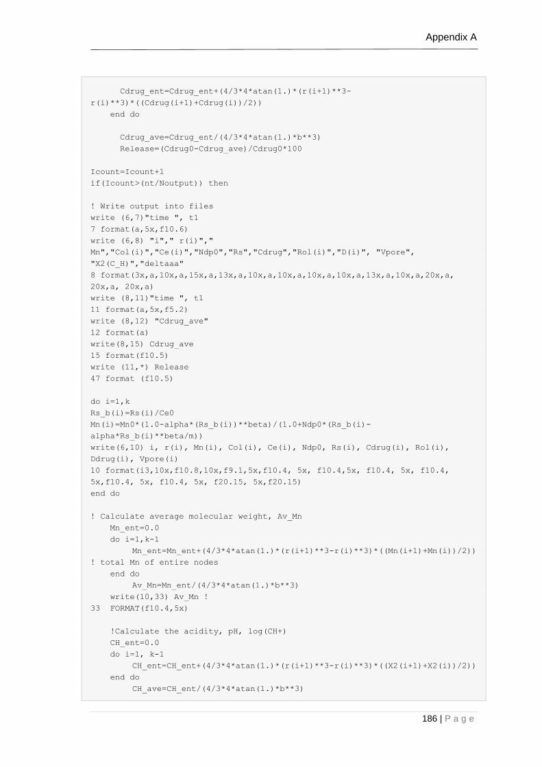
Appendix A
186 | P a g e
Cdrug_ent=Cdrug_ent+(4/3*4*atan(1.)*(r(i+1)**3-
r(i)**3)*((Cdrug(i+1)+Cdrug(i))/2))
end do
Cdrug_ave=Cdrug_ent/(4/3*4*atan(1.)*b**3)
Release=(Cdrug0-Cdrug_ave)/Cdrug0*100
Icount=Icount+1
if(Icount>(nt/Noutput)) then
! Write output into files
write (6,7)"time ", t1
7 format(a,5x,f10.6)
write (6,8) "i"," r(i)","
Mn","Col(i)","Ce(i)","Ndp0","Rs","Cdrug","Rol(i)","D(i)", "Vpore",
"X2(C_H)","deltaaa"
8 format(3x,a,10x,a,15x,a,13x,a,10x,a,10x,a,10x,a,10x,a,13x,a,10x,a,20x,a,
20x,a, 20x,a)
write (8,11)"time ", t1
11 format(a,5x,f5.2)
write (8,12) "Cdrug_ave"
12 format(a)
write(8,15) Cdrug_ave
15 format(f10.5)
write (11,*) Release
47 format (f10.5)
do i=1,k
Rs_b(i)=Rs(i)/Ce0
Mn(i)=Mn0*(1.0-alpha*(Rs_b(i))**beta)/(1.0+Ndp0*(Rs_b(i)-
alpha*Rs_b(i)**beta/m))
write(6,10) i, r(i), Mn(i), Col(i), Ce(i), Ndp0, Rs(i), Cdrug(i), Rol(i),
Ddrug(i), Vpore(i)
10 format(i3,10x,f10.8,10x,f9.1,5x,f10.4, 5x, f10.4,5x, f10.4, 5x, f10.4,
5x,f10.4, 5x, f10.4, 5x, f20.15, 5x,f20.15)
end do
! Calculate average molecular weight, Av_Mn
Mn_ent=0.0
do i=1,k-1
Mn_ent=Mn_ent+(4/3*4*atan(1.)*(r(i+1)**3-r(i)**3)*((Mn(i+1)+Mn(i))/2))
! total Mn of entire nodes
end do
Av_Mn=Mn_ent/(4/3*4*atan(1.)*b**3)
write(10,33) Av_Mn !
33 FORMAT(f10.4,5x)
!Calculate the acidity, pH, log(CH+)
CH_ent=0.0
do i=1, k-1
CH_ent=CH_ent+(4/3*4*atan(1.)*(r(i+1)**3-r(i)**3)*((X2(i+1)+X2(i))/2))
end do
CH_ave=CH_ent/(4/3*4*atan(1.)*b**3)

Appendix A
187 | P a g e
write(20,44) -LOG(CH_ave) !
44 FORMAT(f10.4,5x)
! Calculate average effective diffusivity
D_ent=0.0
do i=1, k-1
D_ent=D_ent+(4/3*4*atan(1.)*(r(i+1)**3-
r(i)**3)*((Ddrug(i+1)+Ddrug(i))/2))
end do
Deff_ave=D_ent/(4/3*4*atan(1.)*b**3)
write(12,22) Deff_ave !
22 FORMAT(f20.15)
!**************************************************************
Icount=0
end if
t1=t1+del_t1
end do
stop
!SUBROUTINES
Contains
Subroutine
Initial_parameters(k1,k2,Ce0,alpha,beta,Mn0,m,Dpoly,Dpore,b,Col0,Ndp0,delta,Dd
rug0,Ka)
implicit none
real*8:: Ce0,alpha,beta,Ka,Mn0,m,a,b,Col0,Ndp0,delta
real*8:: Dpoly,Dpore, Ddrug0, k1, k2
k1=8.D-4 !1/week
k2=0.1 !m3/mol.week
alpha=0.4 !constant
beta=1. !constant
m=4. !constant
Dpoly=1.D-12 !m2/week;
Dpore=1000D0*Dpoly
Ddrug0=1.5D-10 !m2/week
Ka=1.35D-4
b=75.D-6 !m; radius of the microsphere
Mn0=35640.5D0 !g/mol for microsphere
Munit=65.0D0 !g/mol
Ce0=20615.D0 !mol/m3
Col0=0.0*Ce0
Ndp0=Mn0/Munit
delta=9.7D0
End subroutine
Subroutine Initial_parameters_2(Ka_drug,Cdrug0,fdrug0,Dpore_drug,Ho)
implicit none

Appendix A
188 | P a g e
real*8:: Ka_drug, Ho, Cdrug0, fdrug0, Dpore_drug
Cdrug0=223.D0 !mol/m3
fdrug0=0.0524D0 !m3drug/m3unit
Dpore_drug=1000D0*Ddrug0 !m2/week
Ka_drug=6.31D-6 !acid dissociation constant
Ho=3.98D-8 !Initial H+ concentration in PBS
End subroutine
!*****************************************************************************
! Subroutines quantifying transport of drugs and oligomers
Subroutine oligomer_flux(k,Col,D,r & ! input
, Jr) ! output
Implicit none
integer, parameter:: z=1000
real*8, dimension(z):: r
real*8, dimension(z):: Jr
real*8, dimension(z):: Col
real*8, dimension(z):: D
integer:: k,i
Do i=1, k-1
Jr(i)=-D(i)*(Col(i+1)-Col(i))/(r(i+1)-r(i))
End do
End subroutine
!*****************************************************************************
Subroutine calculate_dCol_dt(k,r,Jr, & ! input
dCol_dt) ! output
Implicit none
integer, parameter:: z=1000
real*8, dimension(z):: dCol_dt
real*8, dimension(z):: Jr
real*8, dimension(z):: r
real*8::Vshell, A1,A2
integer:: k,i
dCol_dt(1)=-3*(Jr(1))/(r(2)/2.0)
Do i=2, k-1
del_r=(r(i+1)-r(i))/2+(r(i)-r(i-1))/2
A1=4* 4.*atan(1.)*(r(i-1)**2)
A2=4* 4.*atan(1.)*(r(i)**2)
Vshell=4/3* 4.*atan(1.)*((r(i)**3)-(r(i-1)**3))
dCol_dt(i)=(Jr(i-1)*A1-Jr(i)*A2)/Vshell
End do
End subroutine
!! DRUG DIFFUSION-
!! This two subroutine considers drug diffusion by Fick's law and matter
conversation

Appendix A
189 | P a g e
Subroutine drug_flux(k,Cdrug,Ddrug,r & ! input
, Jdrug) ! output
implicit none
real*8, dimension(z):: r
real*8, dimension(z):: Cdrug
real*8, dimension(z):: Jdrug
real*8, dimension(z):: Ddrug !m2/week
integer:: k, i
do i=1, k-1
Jdrug(i)=-Ddrug(i)*(Cdrug(i+1)-Cdrug(i))/(r(i+1)-r(i))
end do
End subroutine
Subroutine calculate_dCdrug_dt(k,r,Jdrug, & ! input
dCdrug_dt) ! output
Implicit none
integer, parameter:: z=1000
real*8, dimension(z):: dCdrug_dt
real*8, dimension(z):: Jdrug
real*8, dimension(z):: r
real*8:: Vshell, A1,A2
integer:: k,i
dCdrug_dt(1)=-3*(Jdrug(1))/(r(2)/2.0)
do i=2, k-1
del_r=(r(i+1)-r(i))/2+(r(i)-r(i-1))/2
A1=4* 4.*atan(1.)*(r(i-1)**2)
A2=4* 4.*atan(1.)*(r(i)**2)
Vshell=4/3* 4.*atan(1.)*((r(i)**3)-(r(i-1)**3))
dCdrug_dt(i)=(Jdrug(i-1)*A1-Jdrug(i)*A2)/Vshell
End do
End subroutine
End program
Appendix B
190 | P a g e
Appendix B
FORTRAN codes for the mechanistic model for acidic
drug release using microspheres made of PLGA
In this appendix we present the FORTRAN codes developed for the study in
Chapter 4.
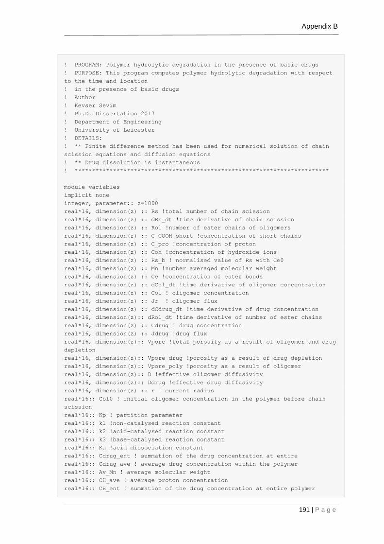
Appendix B
191 | P a g e
! PROGRAM: Polymer hydrolytic degradation in the presence of basic drugs
! PURPOSE: This program computes polymer hydrolytic degradation with respect
to the time and location
! in the presence of basic drugs
! Author
! Kevser Sevim
! Ph.D. Dissertation 2017
! Department of Engineering
! University of Leicester
! DETAILS:
! ** Finite difference method has been used for numerical solution of chain
scission equations and diffusion equations
! ** Drug dissolution is instantaneous
! *************************************************************************
module variables
implicit none
integer, parameter:: z=1000
real*16, dimension(z) :: Rs !total number of chain scission
real*16, dimension(z) :: dRs_dt !time derivative of chain scission
real*16, dimension(z) :: Rol !number of ester chains of oligomers
real*16, dimension(z) :: C_COOH_short !concentration of short chains
real*16, dimension(z) :: C_pro !concentration of proton
real*16, dimension(z) :: Coh !concentration of hydroxide ions
real*16, dimension(z) :: Rs_b ! normalised value of Rs with Ce0
real*16, dimension(z) :: Mn !number averaged molecular weight
real*16, dimension(z) :: Ce !concentration of ester bonds
real*16, dimension(z) :: dCol_dt !time derivative of oligomer concentration
real*16, dimension(z) :: Col ! oligomer concentration
real*16, dimension(z) :: Jr ! oligomer flux
real*16, dimension(z) :: dCdrug_dt !time derivative of drug concentration
real*16, dimension(z):: dRol_dt !time derivative of number of ester chains
real*16, dimension(z) :: Cdrug ! drug concentration
real*16, dimension(z) :: Jdrug !drug flux
real*16, dimension(z):: Vpore !total porosity as a result of oligomer and drug
depletion
real*16, dimension(z):: Vpore_drug !porosity as a result of drug depletion
real*16, dimension(z):: Vpore_poly !porosity as a result of oligomer
real*16, dimension(z):: D !effective oligomer diffusivity
real*16, dimension(z):: Ddrug !effective drug diffusivity
real*16, dimension(z) :: r ! current radius
real*16:: Col0 ! initial oligomer concentration in the polymer before chain
scission
real*16:: Kp ! partition parameter
real*16:: k1 !non-catalysed reaction constant
real*16:: k2 !acid-catalysed reaction constant
real*16:: k3 !base-catalysed reaction constant
real*16:: Ka !acid dissociation constant
real*16:: Cdrug_ent ! summation of the drug concentration at entire
real*16:: Cdrug_ave ! average drug concentration within the polymer
real*16:: Av_Mn ! average molecular weight
real*16:: CH_ave ! average proton concentration
real*16:: CH_ent ! summation of the drug concentration at entire polymer

Appendix B
192 | P a g e
real*16:: D_ent ! summation of the oligomer diffusivity at entire polymer
real*16:: Deff_ave ! average effective diffusivity
real*16:: Mn_ent ! summation of the oligomer molecular weight at entire
polymer
real*16:: Ce0 ! initial ester concentration
real*16:: delta ! Cs, the saturation solubility of drug in the matrix, mol/m3
real*16:: Mn0 ! initial number average molecular weight
real*16:: Munit ! number average molecular weight of a polymer unit
real*16:: alpha, beta ! emprical parameters of the reaction
real*16:: Ndp0 ! initial average degree of polymerisation
real*16:: m ! average polymerization degree of short chains
real*16:: Kb_drug ! base dissociation constant
real*16:: Release !drug release
real*16:: Col_ent ! summation of the oligomer concentration at entire polymer
real*16:: Col_ave ! average oligomer concentration
real*16:: Rol_ent ! summation of the oligomer production rate at entire
polymer
real*16:: Rol_ave ! average oligomer production rate
real*16 :: del_t1 ! time step, week
real*16 :: t1 !time
real*16:: Dpoly !diffusion coefficient of oligomers in fresh bulk polymer
real*16:: Dpore !diffusion coefficient of oligomers in liquid filled pores
real*16:: Ddrug0 !diffusion coefficient of drug in fresh bulk polymer
real*16:: Cdrug0 !initial drug concentration
real*16:: fdrug0 !the volume ratio of drug to the polymer phase
real*16:: Dpore_drug !diffusion coefficient of drug in liquid filled pores
real*16:: Cdrug_loading !initial drug loading
real*16:: Cchain0 !number of polymer chains per unit volume at the beginning
of the degradation
real*16 :: del_r !space step
real*16:: b !radius of the microsphere
integer:: k ! number of grids
integer:: nt ! total number of time steps
integer:: it,i,Icount,Noutput,j !counters
end module variables
program Loaded
use variables
implicit none
open (6, file="fitsiepmann_basic.txt")
open (8, file="DrugAve_basic.txt")
open (10, file="MnAve_basic.txt")
open (11, file="Release_basic.txt")
open (20, file="pH.txt")
open (12, file="Effective_diffusivity_basic.txt")
open (26, file="Cumulative_release_basic.txt")
open (27, file="weight_loss.txt")
nt=400000
k=1000
call
Initial_parameters(k1,k2,Ce0,alpha,beta,Mn0,m,Dpoly,Dpore,b,Col0,Ndp0,delta,Dd
rug0,Ka)
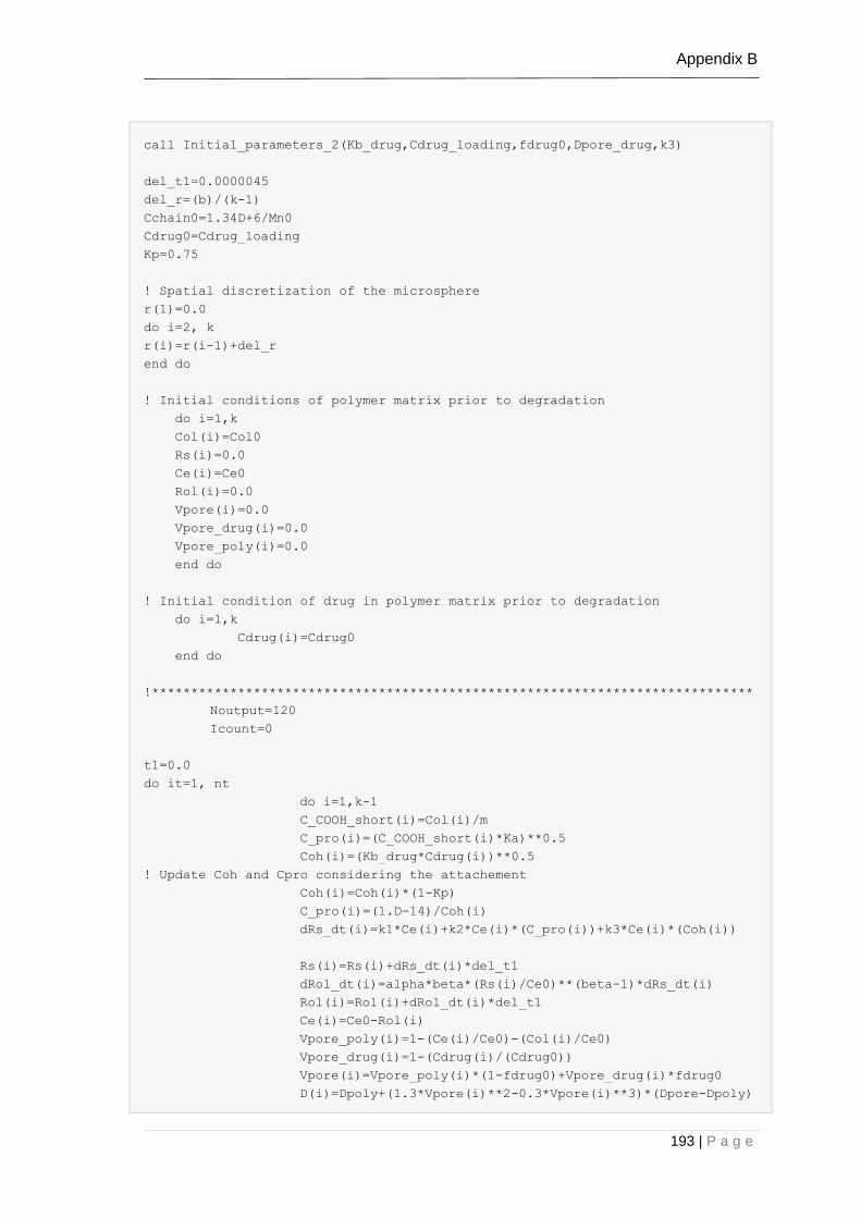
Appendix B
193 | P a g e
call Initial_parameters_2(Kb_drug,Cdrug_loading,fdrug0,Dpore_drug,k3)
del_t1=0.0000045
del_r=(b)/(k-1)
Cchain0=1.34D+6/Mn0
Cdrug0=Cdrug_loading
Kp=0.75
! Spatial discretization of the microsphere
r(1)=0.0
do i=2, k
r(i)=r(i-1)+del_r
end do
! Initial conditions of polymer matrix prior to degradation
do i=1,k
Col(i)=Col0
Rs(i)=0.0
Ce(i)=Ce0
Rol(i)=0.0
Vpore(i)=0.0
Vpore_drug(i)=0.0
Vpore_poly(i)=0.0
end do
! Initial condition of drug in polymer matrix prior to degradation
do i=1,k
Cdrug(i)=Cdrug0
end do
!*****************************************************************************
Noutput=120
Icount=0
t1=0.0
do it=1, nt
do i=1,k-1
C_COOH_short(i)=Col(i)/m
C_pro(i)=(C_COOH_short(i)*Ka)**0.5
Coh(i)=(Kb_drug*Cdrug(i))**0.5
! Update Coh and Cpro considering the attachement
Coh(i)=Coh(i)*(1-Kp)
C_pro(i)=(1.D-14)/Coh(i)
dRs_dt(i)=k1*Ce(i)+k2*Ce(i)*(C_pro(i))+k3*Ce(i)*(Coh(i))
Rs(i)=Rs(i)+dRs_dt(i)*del_t1
dRol_dt(i)=alpha*beta*(Rs(i)/Ce0)**(beta-1)*dRs_dt(i)
Rol(i)=Rol(i)+dRol_dt(i)*del_t1
Ce(i)=Ce0-Rol(i)
Vpore_poly(i)=1-(Ce(i)/Ce0)-(Col(i)/Ce0)
Vpore_drug(i)=1-(Cdrug(i)/(Cdrug0))
Vpore(i)=Vpore_poly(i)*(1-fdrug0)+Vpore_drug(i)*fdrug0
D(i)=Dpoly+(1.3*Vpore(i)**2-0.3*Vpore(i)**3)*(Dpore-Dpoly)

Appendix B
194 | P a g e
Ddrug(i)=Ddrug0+(1.3*Vpore(i)**2-
0.3*Vpore(i)**3)*(Dpore_drug-Ddrug0)
end do
! Update oligomer concentration
call oligomer_flux(k,Col,D,r, & ! input
& Jr) ! output
call calculate_dCol_dt(k,r,Jr, & ! input
& dCol_dt) ! output
do i=1,k-1
Col(i)=Col(i)+dCol_dt(i)*del_t1+dRol_dt(i)*del_t1
end do
Col(k)=0.0
call drug_flux(k,Cdrug,Ddrug,r & ! input
, Jdrug) ! output
call calculate_dCdrug_dt(k,r,Jdrug, & !input
dCdrug_dt) ! output
! Update for drug concentration
do i=1, k-1
Cdrug(i)=(Cdrug(i)+dCdrug_dt(i)*del_t1) !control it
end do
Cdrug(k)=0.0
! Calculate drug release
Cdrug_ent=0.0
do i=1, k-1
Cdrug_ent=Cdrug_ent+(4/3*4*atan(1.)*(r(i+1)**3-
r(i)**3)*((Cdrug(i+1)+Cdrug(i))/2))
end do
Cdrug_ave=Cdrug_ent/(4/3*4*atan(1.)*b**3)
Release=(Cdrug_loading-Cdrug_ave)/Cdrug_loading
!*****************************************************************************
Icount=Icount+1
if(Icount>(nt/Noutput)) then
write (6,7)"time ", t1
7 format(a,5x,f10.6)
write (6,8) "i","
r(i)","Mn","Col(i)","Ce(i)","Ndp0","Rs","Cdrug","Rol(i)","D(i)", "Vpore", "pH"
8
format(3x,a,10x,a,15x,a,13x,a,10x,a,10x,a,10x,a,10x,a,13x,a,10x,a,20x,a,
20x,a, 20x,a)
!
write (8,*) 7*24*t1
write (11,*) Release
do i=1,k
Rs_b(i)=Rs(i)/Ce0
Mn(i)=Mn0*(1.0-alpha*(Rs_b(i))**beta)/(1.0+Ndp0*(Rs_b(i)-
alpha*Rs_b(i)**beta/m))

Appendix B
195 | P a g e
write(6,10) i, r(i), Mn(i), Col(i), Ce(i), Ndp0, Rs(i), Cdrug(i),
Rol(i), C_pro(i),Coh(i)
10 format(i3,10x,f10.8,10x,f9.1,5x,f10.4, 5x, f10.4,5x, f10.4, 5x,
f10.4, 5x,f10.4, 5x, f10.4, 5x, f20.15, 5x,f20.15)
end do
! Calculate average molecular weight, Av_Mn
Mn_ent=0.0
do i=1,k-1
Mn_ent=Mn_ent+(4/3*4*atan(1.)*(r(i+1)**3-r(i)**3)*((Mn(i+1)+Mn(i))/2))
!total Mn of entire nodes
end do
Av_Mn=Mn_ent/(4/3*4*atan(1.)*b**3)
write(10,33) Av_Mn
33 FORMAT(f10.4,5x)
! Calculate average effective diffusivity, Deff
D_ent=0.0
do i=1, k-1
D_ent=D_ent+(4/3*4*atan(1.)*(r(i+1)**3-r(i)**3)*((Ddrug(i+1)+Ddrug(i))/2))
end do
Deff_ave=D_ent/(4/3*4*atan(1.)*b**3)
write(12,22) Deff_ave ! , AAA1, BBB1
22 FORMAT(f20.15)
Col_ent=0.0
do i=1, k-1
Col_ent=Col_ent+(4/3*4*atan(1.)*(r(i+1)**3-
r(i)**3)*((Col(i+1)+Col(i))/2))
end do
Col_ave=Col_ent/(4/3*4*atan(1.)*b**3)
Rol_ent=0.0
do i=1, k-1
Rol_ent=Rol_ent+(4/3*4*atan(1.)*(r(i+1)**3-
r(i)**3)*((Rol(i+1)+Rol(i))/2))
end do
Rol_ave=Rol_ent/(4/3*4*atan(1.)*b**3)
write(27,16) 1.0-((Rol_ave-Col_ave)/Ce0)
16 FORMAT(f10.4,5x,f10.4,5x,f10.4,5x) !,f10.4,5x,f10.4,5x,f20.10,5x,f20.10)
Icount=0
end if
t1=t1+del_t1
end do
stop
!SUBROUTINES
!*****************************************************************************
Contains
Subroutine
Initial_parameters(k1,k2,Ce0,alpha,beta,Mn0,m,Dpoly,Dpore,b,Col0,Ndp0,delta,Dd
rug0,Ka)
implicit none
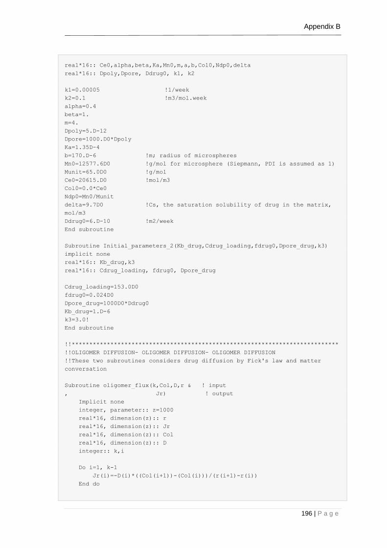
Appendix B
196 | P a g e
real*16:: Ce0,alpha,beta,Ka,Mn0,m,a,b,Col0,Ndp0,delta
real*16:: Dpoly,Dpore, Ddrug0, k1, k2
k1=0.00005 !1/week
k2=0.1 !m3/mol.week
alpha=0.4
beta=1.
m=4.
Dpoly=5.D-12
Dpore=1000.D0*Dpoly
Ka=1.35D-4
b=170.D-6 !m; radius of microspheres
Mn0=12577.6D0 !g/mol for microsphere (Siepmann, PDI is assumed as 1)
Munit=65.0D0 !g/mol
Ce0=20615.D0 !mol/m3
Col0=0.0*Ce0
Ndp0=Mn0/Munit
delta=9.7D0 !Cs, the saturation solubility of drug in the matrix,
mol/m3
Ddrug0=6.D-10 !m2/week
End subroutine
Subroutine Initial_parameters_2(Kb_drug,Cdrug_loading,fdrug0,Dpore_drug,k3)
implicit none
real*16:: Kb_drug,k3
real*16:: Cdrug_loading, fdrug0, Dpore_drug
Cdrug_loading=153.0D0
fdrug0=0.024D0
Dpore_drug=1000D0*Ddrug0
Kb_drug=1.D-6
k3=3.0!
End subroutine
!!****************************************************************************
!!OLIGOMER DIFFUSION- OLIGOMER DIFFUSION- OLIGOMER DIFFUSION
!!These two subroutines considers drug diffusion by Fick's law and matter
conversation
Subroutine oligomer_flux(k,Col,D,r & ! input
, Jr) ! output
Implicit none
integer, parameter:: z=1000
real*16, dimension(z):: r
real*16, dimension(z):: Jr
real*16, dimension(z):: Col
real*16, dimension(z):: D
integer:: k,i
Do i=1, k-1
Jr(i)=-D(i)*((Col(i+1))-(Col(i)))/(r(i+1)-r(i))
End do
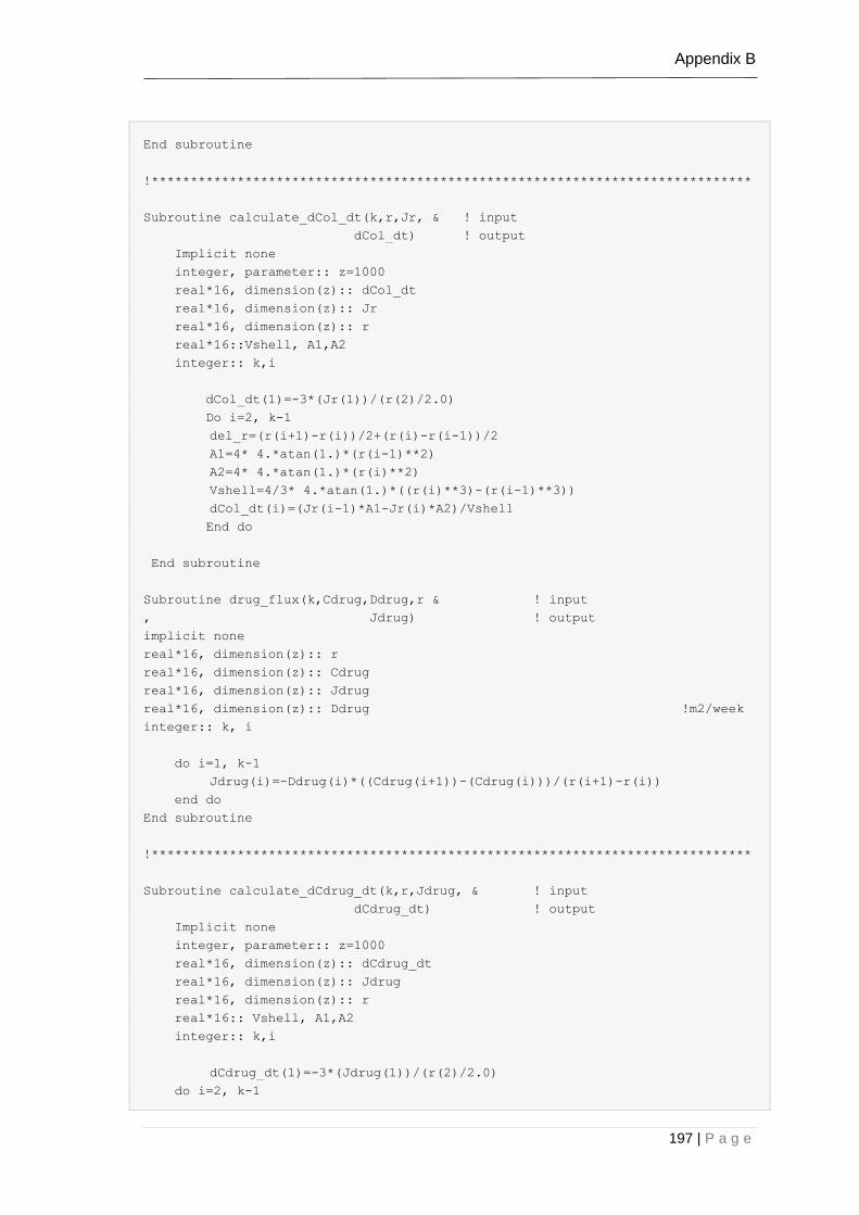
Appendix B
197 | P a g e
End subroutine
!*****************************************************************************
Subroutine calculate_dCol_dt(k,r,Jr, & ! input
dCol_dt) ! output
Implicit none
integer, parameter:: z=1000
real*16, dimension(z):: dCol_dt
real*16, dimension(z):: Jr
real*16, dimension(z):: r
real*16::Vshell, A1,A2
integer:: k,i
dCol_dt(1)=-3*(Jr(1))/(r(2)/2.0)
Do i=2, k-1
del_r=(r(i+1)-r(i))/2+(r(i)-r(i-1))/2
A1=4* 4.*atan(1.)*(r(i-1)**2)
A2=4* 4.*atan(1.)*(r(i)**2)
Vshell=4/3* 4.*atan(1.)*((r(i)**3)-(r(i-1)**3))
dCol_dt(i)=(Jr(i-1)*A1-Jr(i)*A2)/Vshell
End do
End subroutine
Subroutine drug_flux(k,Cdrug,Ddrug,r & ! input
, Jdrug) ! output
implicit none
real*16, dimension(z):: r
real*16, dimension(z):: Cdrug
real*16, dimension(z):: Jdrug
real*16, dimension(z):: Ddrug !m2/week
integer:: k, i
do i=1, k-1
Jdrug(i)=-Ddrug(i)*((Cdrug(i+1))-(Cdrug(i)))/(r(i+1)-r(i))
end do
End subroutine
!*****************************************************************************
Subroutine calculate_dCdrug_dt(k,r,Jdrug, & ! input
dCdrug_dt) ! output
Implicit none
integer, parameter:: z=1000
real*16, dimension(z):: dCdrug_dt
real*16, dimension(z):: Jdrug
real*16, dimension(z):: r
real*16:: Vshell, A1,A2
integer:: k,i
dCdrug_dt(1)=-3*(Jdrug(1))/(r(2)/2.0)
do i=2, k-1

Appendix B
198 | P a g e
del_r=(r(i+1)-r(i))/2+(r(i)-r(i-1))/2
A1=4* 4.*atan(1.)*(r(i-1)**2)
A2=4* 4.*atan(1.)*(r(i)**2)
Vshell=4/3* 4.*atan(1.)*((r(i)**3)-(r(i-1)**3))
dCdrug_dt(i)=(Jdrug(i-1)*A1-Jdrug(i)*A2)/Vshell
End do
End subroutine
End program

Appendix C
199 | P a g e
Appendix C
FORTRAN codes for the mechanistic model for acidic
drug release using microspheres made of PLGA
In this appendix we present the FORTRAN codes developed for the study in
Chapter 5.
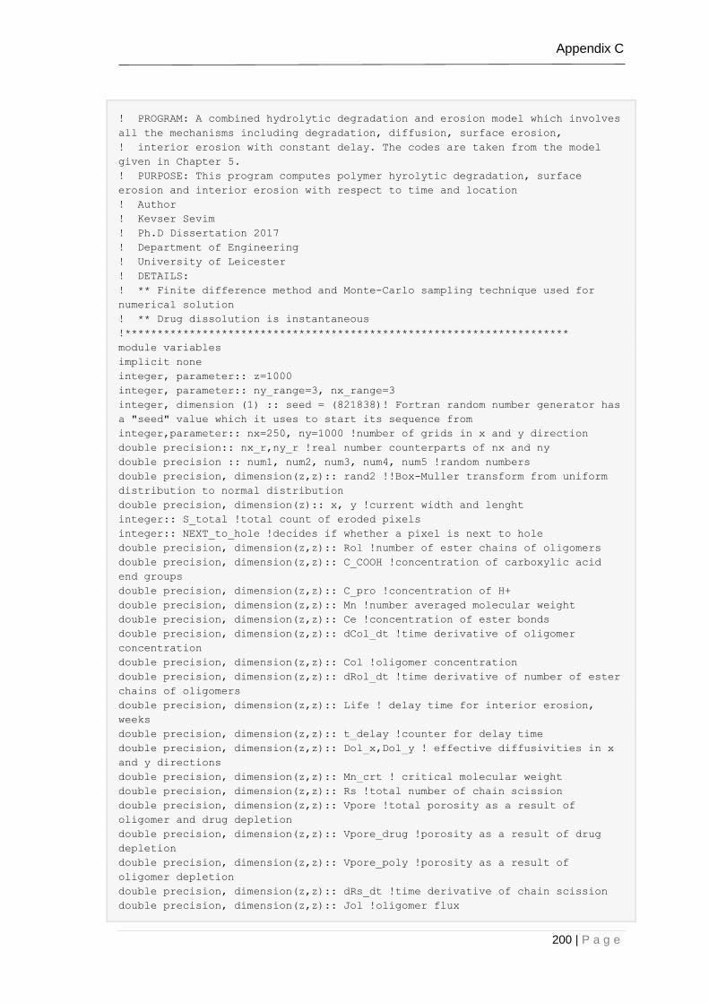
Appendix C
200 | P a g e
! PROGRAM: A combined hydrolytic degradation and erosion model which involves
all the mechanisms including degradation, diffusion, surface erosion,
! interior erosion with constant delay. The codes are taken from the model
given in Chapter 5.
! PURPOSE: This program computes polymer hyrolytic degradation, surface
erosion and interior erosion with respect to time and location
! Author
! Kevser Sevim
! Ph.D Dissertation 2017
! Department of Engineering
! University of Leicester
! DETAILS:
! ** Finite difference method and Monte-Carlo sampling technique used for
numerical solution
! ** Drug dissolution is instantaneous
!*********************************************************************
module variables
implicit none
integer, parameter:: z=1000
integer, parameter:: ny_range=3, nx_range=3
integer, dimension (1) :: seed = (821838)! Fortran random number generator has
a "seed" value which it uses to start its sequence from
integer,parameter:: nx=250, ny=1000 !number of grids in x and y direction
double precision:: nx_r,ny_r !real number counterparts of nx and ny
double precision :: num1, num2, num3, num4, num5 !random numbers
double precision, dimension(z,z):: rand2 !!Box-Muller transform from uniform
distribution to normal distribution
double precision, dimension(z):: x, y !current width and lenght
integer:: S_total !total count of eroded pixels
integer:: NEXT_to_hole !decides if whether a pixel is next to hole
double precision, dimension(z,z):: Rol !number of ester chains of oligomers
double precision, dimension(z,z):: C_COOH !concentration of carboxylic acid
end groups
double precision, dimension(z,z):: C_pro !concentration of H+
double precision, dimension(z,z):: Mn !number averaged molecular weight
double precision, dimension(z,z):: Ce !concentration of ester bonds
double precision, dimension(z,z):: dCol_dt !time derivative of oligomer
concentration
double precision, dimension(z,z):: Col !oligomer concentration
double precision, dimension(z,z):: dRol_dt !time derivative of number of ester
chains of oligomers
double precision, dimension(z,z):: Life ! delay time for interior erosion,
weeks
double precision, dimension(z,z):: t_delay !counter for delay time
double precision, dimension(z,z):: Dol_x,Dol_y ! effective diffusivities in x
and y directions
double precision, dimension(z,z):: Mn_crt ! critical molecular weight
double precision, dimension(z,z):: Rs !total number of chain scission
double precision, dimension(z,z):: Vpore !total porosity as a result of
oligomer and drug depletion
double precision, dimension(z,z):: Vpore_drug !porosity as a result of drug
depletion
double precision, dimension(z,z):: Vpore_poly !porosity as a result of
oligomer depletion
double precision, dimension(z,z):: dRs_dt !time derivative of chain scission
double precision, dimension(z,z):: Jol !oligomer flux
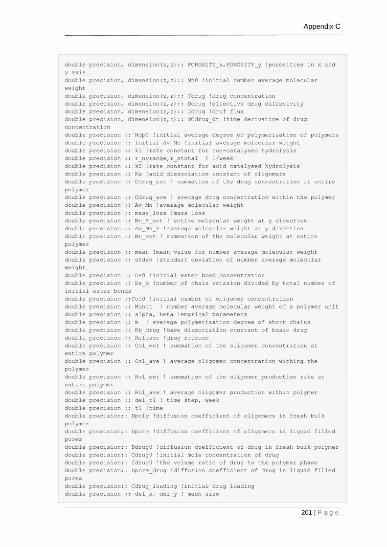
Appendix C
201 | P a g e
double precision, dimension(z,z):: POROSITY_x,POROSITY_y !porosities in x and
y axis
double precision, dimension(z,z):: Mn0 !initial number average molecular
weight
double precision, dimension(z,z):: Cdrug !drug concentration
double precision, dimension(z,z):: Ddrug !effective drug diffusivity
double precision, dimension(z,z):: Jdrug !druf flux
double precision, dimension(z,z):: dCdrug_dt !time derivative of drug
concentration
double precision :: Ndp0 !initial average degree of polymerisation of polymers
double precision :: Initial_Av_Mn !initial average molecular weight
double precision :: k1 !rate constant for non-catalysed hydrolysis
double precision :: r_nyrange,r_stotal ! 1/week
double precision :: k2 !rate constant for acid catalysed hydrolysis
double precision :: Ka !acid dissociation constant of oligomers
double precision :: Cdrug_ent ! summation of the drug concentration at entire
polymer
double precision :: Cdrug_ave ! average drug concentration within the polymer
double precision :: Av_Mn !average molecular weight
double precision :: mass_loss !mass loss
double precision :: Mn_Y_ent ! entire molecular weight at y direction
double precision :: Av_Mn_Y !average molecular weight at y direction
double precision :: Mn_ent ! summation of the molecular weight at entire
polymer
double precision :: mean !mean value for number average molecular weight
double precision :: stdev !standart deviation of number average molecular
weight
double precision :: Ce0 !initial ester bond concentration
double precision :: Rs_b !number of chain scission divided by total number of
initial ester bonds
double precision ::Col0 !initial number of oligomer concentration
double precision :: Munit ! number average molecular weight of a polymer unit
double precision :: alpha, beta !emprical parameters
double precision :: m ! average polymerization degree of short chains
double precision :: Kb_drug !base dissociation constant of basic drug
double precision :: Release !drug release
double precision :: Col_ent ! summation of the oligomer concentration at
entire polymer
double precision :: Col_ave ! average oligomer concentration withing the
polymer
double precision :: Rol_ent ! summation of the oligomer production rate at
entire polymer
double precision :: Rol_ave ! average oligomer production within polymer
double precision :: del_t1 ! time step, week
double precision :: t1 !time
double precision:: Dpoly !diffusion coefficient of oligomers in fresh bulk
polymer
double precision:: Dpore !diffusion coefficient of oligomers in liquid filled
pores
double precision:: Ddrug0 !diffusion coefficient of drug in fresh bulk polymer
double precision:: Cdrug0 !initial mole concentration of drug
double precision:: fdrug0 !the volume ratio of drug to the polymer phase
double precision:: Dpore_drug !diffusion coefficient of drug in liquid filled
pores
double precision:: Cdrug_loading !initial drug loading
double precision :: del_x, del_y ! mesh size
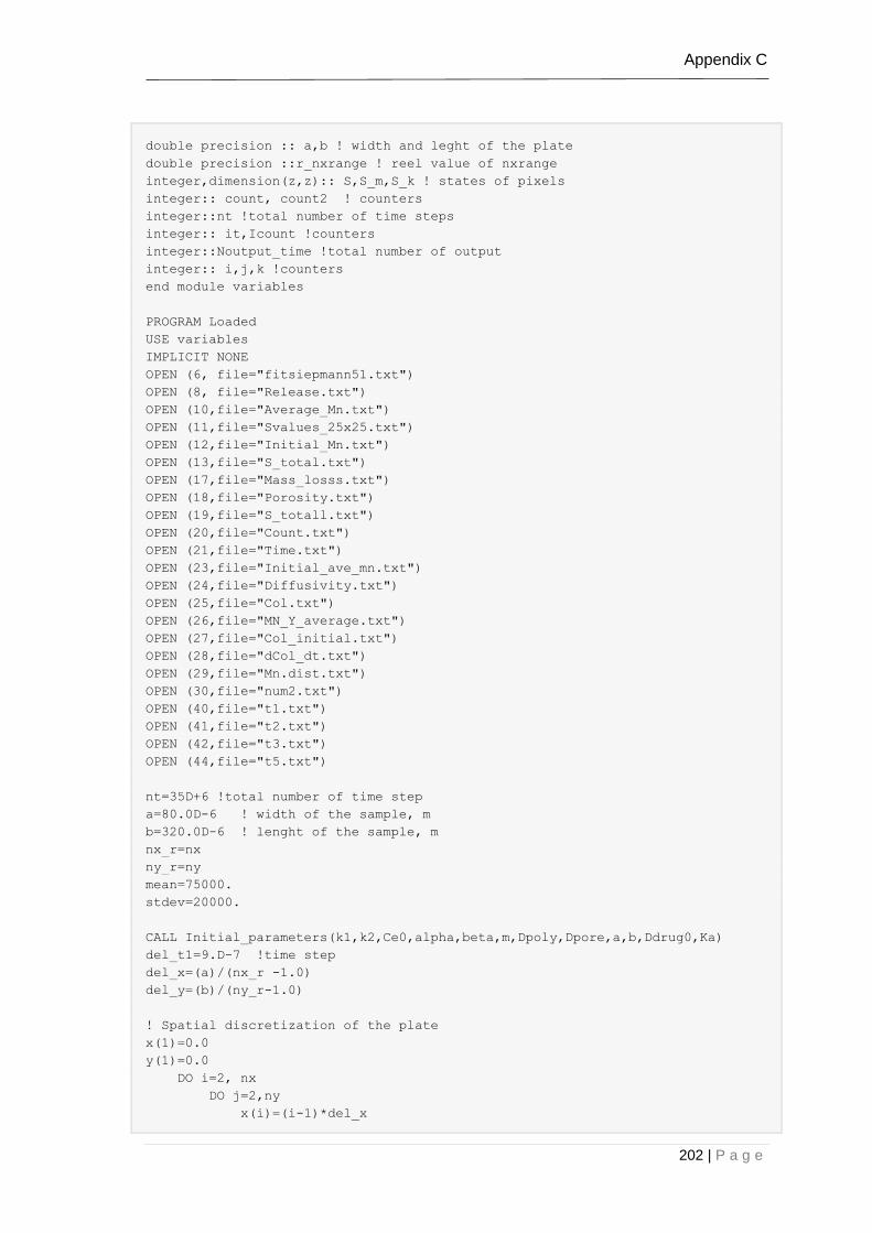
Appendix C
202 | P a g e
double precision :: a,b ! width and leght of the plate
double precision ::r_nxrange ! reel value of nxrange
integer,dimension(z,z):: S,S_m,S_k ! states of pixels
integer:: count, count2 ! counters
integer::nt !total number of time steps
integer:: it,Icount !counters
integer::Noutput_time !total number of output
integer:: i,j,k !counters
end module variables
PROGRAM Loaded
USE variables
IMPLICIT NONE
OPEN (6, file="fitsiepmann51.txt")
OPEN (8, file="Release.txt")
OPEN (10,file="Average_Mn.txt")
OPEN (11,file="Svalues_25x25.txt")
OPEN (12,file="Initial_Mn.txt")
OPEN (13,file="S_total.txt")
OPEN (17,file="Mass_losss.txt")
OPEN (18,file="Porosity.txt")
OPEN (19,file="S_totall.txt")
OPEN (20,file="Count.txt")
OPEN (21,file="Time.txt")
OPEN (23,file="Initial_ave_mn.txt")
OPEN (24,file="Diffusivity.txt")
OPEN (25,file="Col.txt")
OPEN (26,file="MN_Y_average.txt")
OPEN (27,file="Col_initial.txt")
OPEN (28,file="dCol_dt.txt")
OPEN (29,file="Mn.dist.txt")
OPEN (30,file="num2.txt")
OPEN (40,file="t1.txt")
OPEN (41,file="t2.txt")
OPEN (42,file="t3.txt")
OPEN (44,file="t5.txt")
nt=35D+6 !total number of time step
a=80.0D-6 ! width of the sample, m
b=320.0D-6 ! lenght of the sample, m
nx_r=nx
ny_r=ny
mean=75000.
stdev=20000.
CALL Initial_parameters(k1,k2,Ce0,alpha,beta,m,Dpoly,Dpore,a,b,Ddrug0,Ka)
del_t1=9.D-7 !time step
del_x=(a)/(nx_r -1.0)
del_y=(b)/(ny_r-1.0)
! Spatial discretization of the plate
x(1)=0.0
y(1)=0.0
DO i=2, nx
DO j=2,ny
x(i)=(i-1)*del_x

Appendix C
203 | P a g e
y(j)=(j-1)*del_y
END DO
END DO
CALL RANDOM_SEED (PUT=seed)
! Initial conditions of polymer matrix prior to degradation
DO i=1,nx
DO j=1,ny
Rs(i,j)=0.0
dRs_dt=0.0
dCol_dt=0.0
Ce(i,j)=Ce0
Rol(i,j)=0.0
dRol_dt(i,j)=0.0
C_COOH(i,j)=0.0
Jol(i,j)=0.0
Dol_x(i,j)=Dpoly
Dol_y(i,j)=Dpoly
C_pro(i,j)=0.0
Jol(i,j)=0.0
CALL RANDOM_NUMBER(num1)
CALL RANDOM_NUMBER(num2)
CALL RANDOM_NUMBER(num3)
CALL RANDOM_NUMBER(num4)
Col(i,j)=0.0
rand2=sqrt(-2*log(num3))*sin(2*3.14*num4) !Box-Muller transform
from uniform distribution to normal distribution
Mn0(i,j)=mean+stdev*rand2
Mn_crt(i,j)=27000.
Life(i,j)=0.5
t_delay(i,j)=0.0
POROSITY_x(i,j)=0.0
POROSITY_y(i,j)=0.0
Write(12,*) Mn_crt(i,j)
Write(27,*) Col(i,j)
END DO
END DO
! Assign the initial conditions of the pixels: surface pixels eroded at t=0
! All interior pixels are non-eroded at t=0
DO i=1,nx
DO j=1,ny
IF (i.EQ.nx .OR. i.EQ.nx-1) then
S(i,j)=0
S_m(i,j)=0
ELSE IF (j.EQ.ny .OR. j.EQ.ny-1) then
S(i,j)=0
S_m(i,j)=0
ELSE
S(i,j)=1
S_m(i,j)=1
END IF
END DO
END DO
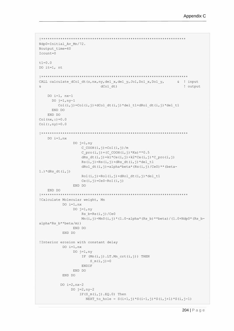
Appendix C
204 | P a g e
!********************************************************************
Ndp0=Initial_Av_Mn/72.
Noutput_time=60
Icount=0
t1=0.0
DO it=1, nt
!*********************************************************************
CALL calculate_dCol_dt(z,nx,ny,del_x,del_y,Jol,Dol_x,Dol_y, & ! input
& dCol_dt) ! output
DO i=1, nx-1
DO j=1,ny-1
Col(i,j)=Col(i,j)+dCol_dt(i,j)*del_t1+dRol_dt(i,j)*del_t1
END DO
END DO
Col(nx,:)=0.0
Col(:,ny)=0.0
!*********************************************************************
DO i=1,nx
DO j=1,ny
C_COOH(i,j)=Col(i,j)/m
C_pro(i,j)=(C_COOH(i,j)*Ka)**0.5
dRs_dt(i,j)=k1*Ce(i,j)+k2*Ce(i,j)*C_pro(i,j)
Rs(i,j)=Rs(i,j)+dRs_dt(i,j)*del_t1
dRol_dt(i,j)=alpha*beta*(Rs(i,j)/Ce0)**(beta-
1.)*dRs_dt(i,j)
Rol(i,j)=Rol(i,j)+dRol_dt(i,j)*del_t1
Ce(i,j)=Ce0-Rol(i,j)
END DO
END DO
!*********************************************************************
!Calculate Molecular weight, Mn
DO i=1,nx
DO j=1,ny
Rs_b=Rs(i,j)/Ce0
Mn(i,j)=Mn0(i,j)*(1.0-alpha*(Rs_b)**beta)/(1.0+Ndp0*(Rs_b-
alpha*Rs_b**beta/m))
END DO
END DO
!Interior erosion with constant delay
DO i=1,nx
DO j=1,ny
IF (Mn(i,j).LT.Mn_crt(i,j)) THEN
S_m(i,j)=0
ENDIF
END DO
END DO
DO i=2,nx-2
DO j=2,ny-2
IF(S_m(i,j).EQ.0) Then
NEXT_to_hole = S(i+1,j)*S(i-1,j)*S(i,j+1)*S(i,j-1)

Appendix C
205 | P a g e
IF(NEXT_to_hole.EQ.0) THEN
t_delay(i,j)=t_delay(i,j)+del_t1
ENDIF
ENDIF
END DO
END DO
DO i=2,nx-2
DO j=2,ny-2
IF(S_m(i,j).EQ.0) Then
IF(t_delay(i,j).GT.Life(i,j)) THEN
S(i,j)=0
ENDIF
ENDIF
END DO
END DO
!*******************************************************************
!Count the number of eroded pixels
nx_r=nx
ny_r=ny
Count=0.0
DO i=1,nx-2
DO j=1,ny-2
If(S(i,j).EQ.0) THEN
Count=Count+1.0
End If
END DO
END DO
!Calculate the local porosity
CALL porosity_diffusivity_x(ny,ny_range,S,Dpore,Dpoly, & !input
Dol_x,POROSITY_x)
!output
CALL porosity_diffusivity_y(nx,nx_range,S,Dpore,Dpoly, & !input
Dol_y,POROSITY_y)
!output
!*********************************************************************
Icount=Icount+1
IF(Icount>(nt/Noutput_time)) then
!*********************************************************************
Mn_ent=0.0
DO i=1,nx
DO j=1,ny
Mn_ent=Mn_ent+Mn(i,j)
END DO
END DO
Av_Mn=Mn_ent/(nx*ny)
write(10,33) Av_Mn
33 FORMAT(f12.4,5x)
! Calculate the average molecular weight
DO i=1,nx

Appendix C
206 | P a g e
Mn_Y_ent=0.0
DO j=1,ny
Mn_Y_ent=Mn_Y_ent+Mn(i,j)
END DO
Av_Mn_Y=Mn_Y_ent/ny
Write(26,*) Av_Mn_Y
END DO
! Calculare mass losss
Col_ent=0.0
DO i=1,nx
DO j=1,ny
Col_ent=Col_ent+Col(i,j)
END DO
END DO
Col_ave=Col_ent/(nx*ny)
Rol_ent=0.0
DO i=1,nx
DO j=1,ny
Rol_ent=Rol_ent+Rol(i,j)
END DO
END DO
Rol_ave=Rol_ent/(nx*ny)
Mass_loss=((Count/(nx_r*ny_r)))*100.
write(17,71) mass_loss
71 FORMAT(f10.4,5x,f10.3,5x)
Write(20,*) Count
!*********************************************************************
Icount=0
END IF
t1=t1+del_t1
!*********************************************************************
!Write to file at specified times
If (it==1200000) then
Do i=1,nx
Do j=1,ny
Write(40,*) i,j,S(i,j),Mn(i,j)
End do
End do
End if
If (it==12800000) then
Do i=1,nx
Do j=1,ny
Write(41,*) i,j,S(i,j),Mn(i,j)
End do
End do
End if
If (it==15000000) then
Do i=1,nx
Do j=1,ny
Write(42,*) i,j,S(i,j),Mn(i,j)
End do

Appendix C
207 | P a g e
End do
End if
If (it==22000000) then
Do i=1,nx
Do j=1,ny
Write(43,*) i,j,S(i,j),Mn(i,j)
End do
End do
End if
If (it==35000000) then
Do i=1,nx
Do j=1,ny
Write(44,*) i,j,S(i,j),S_m(i,j),Mn(i,j)
End do
End do
End if
!*********************************************************************
End Do
Stop
Contains
Subroutine
Initial_parameters(k1,k2,Ce0,alpha,beta,m,Dpoly,Dpore,a,b,Ddrug0,Ka)
implicit none
double precision:: Ce0,alpha,beta,m,a,b
double precision:: Dpoly,Dpore, Ddrug0, k1, k2, Ka
k1=0.5D-5 !1/week
k2=0.02 !m3/mol.week
Ka=1.35D-4
alpha=0.4
beta=1.
m=4.
Dpoly=5.0D-15 !m2/week;
Dpore=1.0D-8 !100.D-9
Ddrug0=0.0 !m2/week
a=80.0D-6 !m
b=320.0D-6 !m;
Munit=65.0D0 !g/mol
Ce0=20615.D0 !mol/m3
End subroutine
!*********************************************************************
Subroutine calculate_dCol_dt(z,nx,ny,del_x,del_y,Joll,Doll_x,Doll_y, &
! input
& dColl_dt) ! output
Implicit none
integer:: z
integer:: i,j,nx,ny
double precision, dimension(z,z):: dColl_dt,Joll,Doll_x,Doll_y
double precision::del_x,del_y
do i=2, nx-1
do j=2, ny-1

Appendix C
208 | P a g e
dColl_dt(i,j)=((Doll_x(i,j)/(del_x**2))*(Col(i+1,j)-
2*Col(i,j)+Col(i-1,j)))+&
((Doll_y(i,j)/(del_y**2))*(Col(i,j+1)-2*Col(i,j)+Col(i,j-1)))
end do
end do
End subroutine
!*********************************************************************
!This subroutine calculates local porosities and diffusivities in x direction
Subroutine porosity_diffusivity_x(ny,ny_range,S,Dpore,Dpoly, &
!input
Doll_x,POROSITYY_x)
!output
integer:: ny,S_total,i,j,k
integer:: ny_range
integer,dimension(z,z):: S
double precision, dimension(z,z)::POROSITYY_x
double precision::r_nyrange,r_stotal,Dpore,Dpoly
double precision, dimension(z,z) :: Doll_x
DO i=1,nx
DO j=ny_range+1,ny-ny_range
S_total=0.0
DO k=j-ny_range,j+ny_range
IF (S(i,k).EQ.0) THEN
S_total=S_total+1.0
ENDIF
END DO
r_nyrange= ny_range
r_stotal= S_total
POROSITYY_x(i,j)=((1.0/(2.0*r_nyrange+1.0))*r_stotal)
END DO
DO j=1,ny_range
POROSITYY_x(i,j)=POROSITYY_x(i,ny_range+1)
END DO
DO j=ny-ny_range+1,ny
POROSITYY_x(i,j)=POROSITYY_x(i,ny-ny_range)
END DO
END DO
DO i=1,nx
DO j=1,ny
Doll_x(i,j)=Dpoly+(1.3*POROSITYY_x(i,j)**2-
0.3*POROSITYY_x(i,j)**3)*(Dpore-Dpoly)
END DO
END DO
End subroutine
!*********************************************************************
!This subroutine calculates local porosities and diffusivities in y direction
Subroutine porosity_diffusivity_y(nx,nx_range,S, Dpore,Dpoly, & !input

Appendix C
209 | P a g e
Doll_y,POROSITYY_y)
!output
integer::nx,S_total,i,j,k
integer:: nx_range
integer,dimension(z,z):: S
double precision, dimension(z,z)::POROSITYY_y
double precision:: r_stotal,Dpore,Dpoly
double precision, dimension(z,z):: Doll_y
DO j=1,ny
DO i=nx_range+1,nx-nx_range
S_total=0.0
DO k=i-nx_range,i+nx_range
IF (S(k,j).EQ.0) THEN
S_total=S_total+1.0
ENDIF
END DO
r_nxrange= nx_range
r_stotal= S_total
POROSITYY_y(i,j)=((1.0/(2.0*r_nxrange+1.0))*r_stotal)
END DO
DO i=1,nx_range
POROSITYY_y(i,j)=POROSITYY_y(nx_range+1,j)
END DO
DO i=nx-nx_range+1,nx
POROSITYY_y(i,j)=POROSITYY_y(nx-nx_range,j)
END DO
END DO
DO i=1,nx
DO j=1,ny
Doll_y(i,j)=Dpoly+(1.3*POROSITYY_y(i,j)**2-
0.3*POROSITYY_y(i,j)**3)*(Dpore-Dpoly)
END DO
END DO
End subroutine
END PROGRAM
Copyright © 2022 FDOKUMEN