RESEARCH Open Access

Modelling local areas of exposure toSchistosoma japonicum in a limitedsurvey data environmentAndrea L. Araujo Navas1*, Ricardo J. Soares Magalhães2,3, Frank Osei1, Raffy Jay C. Fornillos4,Lydia R. Leonardo5 and Alfred Stein1

Abstract

Background: Spatial modelling studies of schistosomiasis (SCH) are now commonplace. Covariate values arecommonly extracted at survey locations, where infection does not always take place, resulting in an unknownpositional exposure mismatch. The present research aims to: (i) describe the nature of the positional exposuremismatch in modelling SCH helminth infections; (ii) delineate exposure areas to correct for such positionalmismatch; and (iii) validate exposure areas using human positive cases.

Methods: To delineate exposure areas to Schistosoma japonicum, a spatial Bayesian network (sBN) was constructed. Ituses data on exposure risk factors such as: potential sites for snails’ accessibility, geographical distribution ofsnail infection rate, and cost of the community to access nearby water bodies. Prior and conditional probabilities wereobtained from the literature and inserted as weights based on their relative contribution to exposure; these probabilitieswere then used to calculate joint probabilities of exposure within the sBN.

Results: High values of probability of S. japonicum exposure correspond to polygons where snails could potentially bepresent, for instance in wet soils and areas with low slopes, but also where people can easily access water bodies. Lowcorrelation (R2 = 0.3) was found between the percentage of human cases and the delineated probabilities of exposurewhen validation buffers are generated over the human cases.

Conclusions: The utility of a probabilistic method for the identification of exposure areas for S. japonicum, with widerapplication for other water-borne infections, was demonstrated. From a public health perspective, the schistosomiasisexposure sBN developed in this study could be used to guide local schistosomiasis control teams to specific potentialareas of exposure, and improve efficiency of mass drug administration campaigns in places where people are likely tobe exposed to the infection.

Keywords: Schistosomiasis, Spatial modeling, Bayesian network, Exposure uncertainty, Risk factors

BackgroundSchistosomiasis (SCH) is a water-borne neglected trop-ical disease of global public health significance [1, 2]. Itaffects more than 252 million people worldwide [3], es-pecially human populations living in places where cleanwater and sanitation are limited [4]. Schistosomiasis isknown to lead to anaemia, stunted growth and otherorgan pathologies in school-aged children [5, 6]. Three

schistosome species cause the infection: Schistosomamansoni, S. japonicum and S. haematobium. Schistosomajaponicum is presently endemic in China, Indonesia andthe Philippines, and is hard to control due to its zoo-notic life-cycle [7]. The life-cycle of S. japonicum in-cludes infection of an amphibious snail belonging toseveral subspecies of Oncomelania hupensis as the inter-mediate host, and humans and other mammalians as de-finitive hosts [8, 9].Traditionally, schistosomiasis risk mapping has en-

abled the identification of at risk populations for target-ing mass drug administration campaigns, thus increasing

* Correspondence: a.l.araujonavas@utwente.nl1Faculty of Geo-information Science and Earth Observation (ITC), Universityof Twente, PO Box 217, 7500 AE Enschede, The NetherlandsFull list of author information is available at the end of the article

© The Author(s). 2018 Open Access This article is distributed under the terms of the Creative Commons Attribution 4.0International License (http://creativecommons.org/licenses/by/4.0/), which permits unrestricted use, distribution, andreproduction in any medium, provided you give appropriate credit to the original author(s) and the source, provide a link tothe Creative Commons license, and indicate if changes were made. The Creative Commons Public Domain Dedication waiver(http://creativecommons.org/publicdomain/zero/1.0/) applies to the data made available in this article, unless otherwise stated.

Araujo Navas et al. Parasites & Vectors (2018) 11:465 https://doi.org/10.1186/s13071-018-3039-6

the efficiency of schistosomiasis disease control [10].Schistosomiasis mapping has been supported by the useof spatial information techniques, such as geographicalinformation systems (GIS), remote sensing and globalpositioning systems (GPS). Spatial information tech-niques allow the manipulation of spatially referenced in-fection data and data on the physical and biologicalenvironmental variables [11–14]. Modelling those datain combination allows studying the distribution of com-munities most at risk schistosomiasis and the role of thegeographical variation of environmental exposure factorson schistosomiasis risk [15].There are a number of errors inherent to spatial infor-

mation used in geographical epidemiological studies [4].Most of these errors involve positional measurement er-rors, where observation and prediction locations are af-fected by various factors such as GPS inaccuracies, thepresence of multiple addresses, geocoding errors, out-come or covariate aggregations, and misalignment be-tween covariates of exposure and disease outcomeestimates [15]. The last one is of our current interestand may occur when covariates of exposure are ex-tracted from locations where exposure has not occurred.Statistical modelling of the spatial distribution of schis-

tosome infections estimates empirical relationships be-tween morbidity indicators (e.g. prevalence or intensityof infection) and risk factors. Risk factors for schisto-some exposure include various environmental andsocio-economic covariates that help to interpolate thelevel of infection at unsampled locations [14, 16–18].Covariates and morbidity indicators are commonly ex-tracted from survey locations such as health centres,hospitals and schools. In most cases, exposure to infec-tion did not occur at survey data locations but at loca-tions where environmental and geographical conditions,together with the level of accessibility to contaminatedsites, are optimally exposed. Such exposure locations areusually unknown, resulting in positional mismatch of thesurveyed disease values, and the covariates in the model.To date, methods to account for this type of positional

misalignment are scarce. Several studies have used remotesensing data to determine biophysical features of habitats inrelation to snail prevalence [19–24], acknowledging that S.japonicum transmission is closely related to the distributionof its intermediate host in the environment [9]. Only onestudy [2] has used these habitats to correct for the pos-itional mismatch when modelling disease infection risk inhuman populations. Walz et al. [2] used high-resolution re-mote sensing data, environmental field measurements, andecological data, to model environmental suitability forschistosomiasis-related parasites and snail species. Theyrepresented environmental suitability as potential transmis-sion areas that could guide public health interventions toplaces where people could potentially be infected. Although

potential transmission areas were delineated, interactionsbetween humans, hosts, and suitable environments werenot taken into account.These studies suggest that ignoring positional mis-

match and its impact on spatial prediction remainslargely unquantified in schistosomiasis modelling. Fur-thermore, the extraction of covariate values in the pres-ence of positional mismatch is a significant source ofuncertainty that may influence the efficacy of schisto-somiasis control strategies [4]. Therefore, methods tocorrect for this positional mismatch need to be furtherinvestigated [1, 4].The objective of this study is to develop a schistosom-

iasis exposure sBN model that maps potential areas ofexposure to S. japonicum, taking into account human in-teractions with main sources of infection (i.e. water bod-ies). To accomplish this objective, we aimed to (i)describe the positional mismatch problem in modellingS. japonicum infection; (ii) delineate exposure areas thattake into consideration the accessibility cost of people tomain sources of infection, and that could be used to cor-rect for this positional mismatch; and to (iii) validate thedelineated exposure areas.

MethodsData on human and snail S. japonicum infectionIn the Philippines S. japonicum is endemic in 28 of its81 provinces [25], with approximately 1.8 million esti-mated infected people [26]. The disease affects children,adolescents and individuals with high-risk occupations,such as farmers and fishermen [26, 27]. In thePhilippines, the smallest administrative division is thebarangay, numbering about 22–50 in a municipality.We used data on human schistosomiasis and snail

prevalence of infection, collected in six barangays fromAlangalang municipality in Leyte Province in 2015 and2016. Data were collected by researchers from the Col-lege of Public Health and College of Science from theUniversity of the Philippines. Surveyors selected Alanga-lang municipality because it has the highest prevalenceof schistosomiasis (7.5%) from all the 43 municipalitiesof Leyte Province; within this municipality, they visitedthe barangays with the highest prevalence of infectionfrom the 54 barangays in Alangalang municipality.Human positive cases (12 records) were georeferenced

at household locations and snails surveys (8 records)were taken from water bodies in close proximity to sur-veyed households. The recording of all the human caselocations (also including negative cases) was not possibledue to a lack of manpower and material resources, suchas the availability of only one GPS device in the field.Diagnosis of schistosomiasis in humans was performed

using stool examination. Single stool sample was re-quested per participant with informed consent, coded

Araujo Navas et al. Parasites & Vectors (2018) 11:465 Page 2 of 15

and prepared following the Kato-Katz method. Eachslide prepared was read in the field using a microscopeand the presence of S. japonicum eggs indicated activeinfection.Infection among O. h. quadrasi snails was determined

by manually crushing the snails in aliquots on a glassslide. Each snail was placed in an aliquot droplet of dis-tilled water, usually three aliquots per glass slide. Snailswere gently crushed in between slides and were exam-ined under a conventional stereomicroscope (40×) usingforceps for separating snail tissues to detect the presenceof sporocysts or furcocercous cercariae characteristic ofS. japonicum.

Study areaFor the purpose of this study, it was decided to work ata local spatial scale in the Province of Leyte, due to thelocalized nature of the surveys and the high endemicityof the disease [28]. For the analysis, we identified a smallarea surrounding surveyed points (Fig. 1). This was donein order to select only surveyed barangays and to includeinformation of all risk factors, avoiding areas withoutsurvey information (Fig. 1).

Environmental and geographical dataExposure risk factors of SCH transmission are associatedwith the environment (i.e. moisture, temperature, rainfalland water characteristics), the topography (i.e. elevation,slope) of the area [2, 10, 20, 21, 29] and snail infection sta-tus [23, 24, 30, 31]. In the endemic provinces of thePhilippines, exposure to snails is mostly driven by thelocal topography, land use and the physical and chemicalcomponents of the water and soil [32]. We included eleva-tion, slope, land use, nearest distance to water bodies andsnail infection rates as exposure risk factors. Elevation wasobtained as a raster file from Aster GDEM version 2 fromUSGS [33]. Vector layers for land use, river and road net-work were obtained from the OpenStreetMap (OSM) pro-ject [34]. OSM land use and land cover products useinformation from GlobeLand30 (GL30), which is a newgeneration of 30 m land cover maps [35–37]. The OSMroad and river networks are incomplete and contain errorsin their connectivity. To account for this, we edited roadsand rivers, and digitalized footpaths using Google Earthimages. The vector layer for snail infection rate was ob-tained from the recorded surveys (Table 1). Slope was de-rived from elevation by using the Terrain Analysis toolfrom Quantum GIS version 2.6 [38].Distance to water bodies was calculated using the clos-

est facility network analysis tool from ArcGIS version 10[39]. Firstly, we corrected for topology errors such asduplicate lines, presence of dangles and multipart geom-etries in the river and road network. Secondly, commu-nities were loaded as incidents (261 points), and contact

river points as facilities (42 points). Thirdly, we used theclosest facility tool to find the nearest river from anurban area following a road. Finally, we interpolated thedistance to the nearest water source using ordinary kri-ging from the gstat package in R [40] and saved the mapas a raster file.

Snail infection rate mapWe constructed a trend surface that represents snail in-fection rate for the whole study area, thus using data ofall the points to predict at unknown locations (i.e. globalinterpolation). It fits a mathematically defined surfacethrough the data points (i.e. deterministic interpolation)to discover smoother (i.e. inexact interpolation)regional and local trends. It is similar to a three di-mensional regression surface obtained with linear re-gression, where coordinates si = (xi, yi) are used aspredictors. The interpolated value z(Si) for a first andsecond order polynomial is represented in equations1 and 2, respectively. z(Si) represents infection ratevalues (number of positive cases/number of sampledsnails) at location i.

z� sið Þ ¼ β0 þ β1xi þ β2yi ð1Þ

z� sið Þ ¼ β0 þ β1xi þ β2yi þ β3x2i þ β4y

2i þ β5xiyi ð2Þ

Figure 2a, b shows the resulting surfaces for the firstand second order polynomials, respectively. Figure 2ashows low risk probability values (Table 1), from -0.003to 0.008. These values do not match the original sur-veyed values. Figure 2b shows low and medium riskprobability values from -0.01 to 0.035. These valuesshow a better fit to the original surveyed values showedin red.To remove the occurring negative values, we fitted a

multiple linear regression by applying a generalized lin-ear regression model using equation 2. In this case z(Si)was the infection status for each location i, 1 indicatesan infected case and 0 a non-infected case. The resultingprediction from Fig. 3 shows only positive predictedvalues but very large standard errors (28.7 to 3e+13). Be-sides, none of the predictions approximate the originalsurveyed values. Finally, the second order trend surface(Fig. 2b) map was used for the analysis since it better fit-ted the original surveyed values.

Spatial Bayesian network of Schistosoma japonicumexposureWe have conceptually designed a model that representsthe positional mismatch between survey locations and

Araujo Navas et al. Parasites & Vectors (2018) 11:465 Page 3 of 15

exposure sites (Fig. 4). Locations s1and s2represent theschools, households, or other survey locations fromwhich morbidity indicators are extracted, while exmnre-presents the various exposure points where infectionscould have taken place, m is the corresponding numberof exposure points and n is the corresponding survey lo-cations related to the exposure.Exposure areas were delineated by using spatial Bayes-

ian networks (sBN) [41]. A Bayesian network (BN) is aprobabilistic graphical model that captures the variousconditional dependencies of a set of random variables(discrete or continuous) [42, 43], into a joint probabilitydistribution by means of a directed acyclic graph (DAG)[44, 45]. A BN for a set of random variables X is defined

by the pair (D, P). Here, D is the DAG and P is the set ofprobability distributions for all variables in the network.Each variable x with parents pa(x) has a conditionalprobability p(x| pa(x)). For a BN with a set of discrete (I)variables, the joint probability distribution factorizes intoequation 3 [42]. This is the joint probability distributionas the product of all conditional probabilities specifiedin a BN:

p Xð Þ ¼YI

i¼1p xijpa xið Þð Þ ð3Þ

The schistosomiasis exposure sBN defines exposureareas in a probabilistic way, by allowing the combination

Fig. 1 Selected study area

Araujo Navas et al. Parasites & Vectors (2018) 11:465 Page 4 of 15

Table

1Categ

orizationof

expo

sure

riskfactors

Risk

factor

(weigh

t)Spatialresolution

Tempo

ral

resolutio

nData

type

Coo

rdinate

system

Datasource

Hypothe

ticallink

Classificatio

nπweigh

tsBased

upon

Elevation(0.03)

~30

mat

equator

naRaster

EPSG

:4326

Aster

GDEM

V2fro

mUSG

SWhileelevationde

creases,

theriskof

infectionincreases

Highrisk:<900m

0.70

[32,51,

56]

Med

ium

risk:900–2300

m0.25

Low

risk:>2300

m0.05

Land

use(0.26)

~30

m2-3-2017

Vector

EPSG

:4326

Ope

nStreetM

approject

Wet

surfacesaremoresuitable

toahighe

rriskof

infection

Very

high

risk:wet

soils

0.42

[32,57]

Highrisk:water

bodies

0.29

Highandmed

ium

risk:Agriculture

land

andgrass

0.16

Med

ium

andlow

risk:forestand

naturalareas

0.08

Low

risk:barren

land

0.02

Very

low

risk:bu

iltland

0.03

Slop

e(0.13)

~30

mat

equator

naRaster

EPSG

:4326

Derived

from

elevation

Atmoreflatsurfacestheriskof

infectionincreases

Highrisk:<11

degrees

0.70

[49,51]

Med

ium

risk:11–30de

grees

0.23

Low

risk:>30

degrees

0.07

Distanceto

water

bodies

(0.50)

30m

2-3-2017

Raster

EPSG

:32651

Derived

from

roads,urban

areas,river

netw

orkand

water

bodies

from

the

Ope

nStreetM

approject

Whiledistance

towater

bodies

decreases,theriskof

infection

increases

Highrisk:<1000

m0.74

[51,52,

58]

Med

ium

risk:1000–5000m

0.21

Low

risk:>5000

m0.05

Snailinfectio

nrate

(0.06)

na2015–

2016

Vector

EPSG

:4326

Derived

from

recorded

surveys

Whilesnailinfectio

nrate

increases,theriskof

infection

increases

Highrisk:>3.6%

0.65

[23,24,30,

31]

Med

ium

risk:0.5–3.6%

0.28

Low

risk:<0.5%

0.07

Abb

reviation:

na,n

otap

plicab

le

Araujo Navas et al. Parasites & Vectors (2018) 11:465 Page 5 of 15

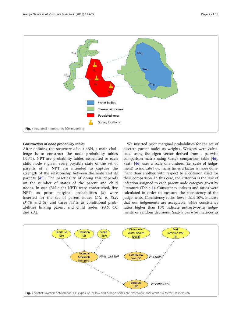
of various probability distributions from a set of randomspatial variables [44]. We have constructed a DAG forexposure areas (Fig. 5), where each random variable isrepresented as a node. Nodes are connected by directedlinks or edges that express probabilistic relationships be-tween the variables [43]. Three types of random vari-ables can be found including (i) an observable discretevariable [land use (LU)]; (ii) observable continuous vari-ables [elevation (E), slope (SLP), distance to water bodies(DWB) and snail infection rates (SI)]; and (iii) latent

discrete variables [potential accessible sites for snails(PAS), community cost (CC) and exposure (EX)]. Thedirection given in the link between variables, for in-stance from LU to PAS, encodes a direct causal depend-ence of PAS on LU; the node LU is known then as theparent of PAS [45].All continuous variables (E, SLP, DWB and SI) were

discretized into different categories, given that high orlow levels of exposure could occur at various rangesof risk factor values. We established hypothetical rela-tionships between the risk factors and the disease,and categorized the risk factors based on literature(Table 1).Exposure is a discrete child node, which has three

discrete parent nodes: PAS, CC and SI; its conditionalprobability is expressed as p(EX| PAS, CC, SI). PAS andCC are at the same time child nodes conditional ondiscrete parents. Their conditional probabilities are de-rived by p(PAS| LU, E, SLP) and p(CC|DWB), respect-ively. The joint probability distribution for our Bayesiannetwork is given as:

p Xð Þ ¼ p EXjPAS;CC; SIð Þ: p PASjLU ; E; SLPð Þ:p LUð Þ: p Eð Þ: p SLPð Þ:p CCjDWBð Þ: p DWBð Þ: p SIð Þ

ð4Þ

Equation 4 encodes assumptions of this researchabout direct dependencies between variables and indi-cates which node probability tables (NPT) need to bedefined [45].

Fig. 2 First order (a) and second order (b) polynomial trend surface. Red crosses represent the original surveyed snail infection locations

Fig. 3 Predicted probability of snail infection values usinggeneralized linear regression model. Colour scale representprobability values from 0 to 1. Snail survey locations are representedby white crosses

Araujo Navas et al. Parasites & Vectors (2018) 11:465 Page 6 of 15

Construction of node probability tablesAfter defining the structure of our sBN, a main chal-lenge is to construct the node probability tables(NPT). NPT are probability tables associated to eachchild node v given every possible state of the set ofparents of v. NPT are intended to capture thestrength of the relationship between the node and itsparents [45]. The practicality of doing this dependson the number of states of the parent and childnodes. In our sBN eight NPTs were constructed, fiveNPTs as prior marginal probabilities (π) wereinserted for the set of parent nodes (LU, E, SLP,DWB and SI) and three NPTs as conditional prob-abilities linking parent and child nodes (PAS, CCand EX).

We inserted prior marginal probabilities for the set ofdiscrete parent nodes as weights. Weights were calcu-lated using the eigen vector derived from a pairwisecomparison matrix using Saaty’s comparison table [46].Saaty [46] uses a scale of numbers (i.e. scale of judge-ment) to indicate how many times a factor is more dom-inant than another with respect to a criterion used fortheir comparison. In this case, the criterion is the risk ofinfection assigned to each parent node category given byliterature (Table 1). Consistency indexes and ratios werecalculated in order to measure the consistency of thejudgements. Consistency ratios lower than 10%, indicatethat our judgements are acceptable, while consistencyratios higher than 10% indicate untrustworthy judge-ments or random decisions. Saaty’s pairwise matrices as

Fig. 4 Positional mismatch in SCH modelling

Fig. 5 Spatial Bayesian network for SCH exposure. Yellow and orange nodes are observable and latent risk factors, respectively

Araujo Navas et al. Parasites & Vectors (2018) 11:465 Page 7 of 15

well as consistency indexes and ratios are included asAdditional file 1: Tables S1-S7. Prior marginal probabil-ities for the parent nodes are shown in Table 1.Latent variables PAS, CC and EX were divided into three

probability categories: high, medium and low risk. Condi-tional probabilities for these child nodes are associatedwith the edges that link them to the parent nodes, andwere also assigned using a pairwise comparison matrix.The criterion used to assign the scale of judgement is thestrength of the hypothetical link between the risk factorsand exposure. The strength of the hypothetical link wasevaluated based upon three studies that evaluated the riskfactors associated with schistosomiasis infection [47–49].Hu et al. [47] ranked the potential importance of

the schistosomiasis risk factors by means of a powerdetector. According to this detector, distance towater bodies is the most significant factor for diseaserisk, and elevation the least significant. Zhang et al.[48] used environmental, topographical and humanbehavioural factors to locate schistosomiasis activetransmission sites. Their predictor capacity was comparedby means of deviance analysis, used to determine the im-portant variables to be included in a generalized additivemodel. As in the previous study, distance to water bodieswas the most significant factor because of the smallest de-viance, and elevation the least significant. Finally, Ajakayeet al. [49] evaluated physical and environmental risk fac-tors to identify areas with suitable conditions for schisto-somiasis transmission. They used Saaty’s comparisonmatrix to assign weights to each risk factor. Distance towater bodies and land use were the most significantfactors, followed by elevation and slope as the leastsignificant.Weights obtained for each risk factor are shown in Table 1

and the conditional probabilities linking parent and childnodes are shown in Additional file 2: Tables S8-S10.

Deriving joint probabilitiesTo compute the probabilities for each category of thechild nodes, PAS, CC and EX, conditional and mar-ginal probabilities were used by applying equations 5,6 and 7, respectively. Joint probability values of ex-posure were calculated for each polygon of analysis.In order to update the prior marginal probabilities,evidence is inserted for each spatial polygon into theobservable variables (SI, LU, E, SLP,DWB). Bold facingindicates the insertion of evidence. Variables notationcan be found in Additional file 3: Table S11.

p PAS;LU ;E; SLPð Þ ¼X

LU ;E;SLPp LUð Þ � p Eð Þ � p SLPð Þ � p PASjLU ;E;SLPð Þ

ð5Þ

p CC;DWBð Þ ¼X

DWBp DWBð Þ � p CCjDWBð Þ

ð6Þ

p EX; PAS;CC; SIð Þ ¼�X

PAS;CC;SIp EXjPAS;CC; SIð Þ

�p SIð Þ�X

LU ;E;SLPp LUð Þ � p Eð Þ � p SLPð Þ

�p PASjLU ;E;SLPð Þ ÞX

DWBp DWBð Þ � p CCjDWBð Þ

� � �

ð7ÞFor the implementation, polygons of analysis were con-

structed based on the overlaying of each risk factor (i.e.parent node). To overlay all risk factors, they were firsttransformed into vectors and then corrected for topologyerrors. Topology errors included duplicated polygons,multipart geometries and overlapping polygons.Sensitivity analysis was used to see the relative influ-

ence of the risk factors on PAS and CC, and the relativeinfluence of PAS, CC and SI on exposure. We used thesensitivity function, calculated as the degree of entropyreduction. Degree of entropy reduction I is the degree ofchange or expected difference in information bits H be-tween a query variable Q (exposure) with q states andfindings variable F (risk factors) with f states [50] (equa-tion 8). A degree of entropy reduction of 0 means aquery variable is independent of the varying variable.

fI ¼ H Qð Þ−H Fð Þ ¼X

q

Xf

P q; fð Þ log2 P q; fð Þ½ �P qð ÞP fð Þ

ð8Þ

SoftwareTo work within the spatial domain we used the softwareNeticaTM 6.03 [41], which works with Bayesian net-works, decision nets and influence diagrams. Evidence isinserted as cases for each polygon of analysis, and priorand conditional probabilities are inserted as tables.

ValidationValidation was first performed by counting all surveyedpositive SCH human cases falling inside the various cat-egories of exposure in the map. However, this introducesa positional mismatch as the surveyed positive caseswere not necessarily acquired at those specific exposurepoints.As a second approach for validation, we defined po-

tential validation areas by constructing buffers aroundeach of the positive cases. We extracted the distance tothe nearest water body for each surveyed point using thedistance map previously generated. Extracted distancevalues were used as distance buffers generated around

Araujo Navas et al. Parasites & Vectors (2018) 11:465 Page 8 of 15

positive cases. Buffers completely containing otherbuffers were grouped. We counted the number ofpositive cases falling inside each group and calculatedthe mean probability of exposure within the groupedbuffers.

ResultsExposure networkHigh (> 50%), medium (35–50%), low (20–35%) and verylow (< 20%) probabilities of exposure were derived fromthe proposed exposure network. This is exemplified inFig. 6 for only one polygon. For this particular polygon,the probability is predominantly high (50.8%) for ahigh-risk elevation (< 900 m), DWB (< 1 km), and LU

(agriculture land and grass), a medium risk slope (11–30°), and a low risk SI (< 0.5%).Very low probability values of exposure (< 20%) were

found in built-up areas, medium risk DWB (1–5 km),slopes < 30° and low and medium (0.5–3.6%) risk ofsnail infection, but also in agriculture and grass landwith DWB > 5 km and slopes > 30° (Fig. 7). Low prob-abilities of exposure (20–35%) were found in built-upareas with slopes < 30°, low risk of snail infection, andwithin DWB < 1 km, but also in agriculture and grassland in DWB > 5 km. Medium probability values (35–50%) were found in agriculture and grass land and forestareas, in slopes > 11°, low risk of snail infection, andDWB < 1 km, but also in slopes < 30°, medium risk ofsnail infection and DWB from 1 to 5 km. High

Fig. 6 Probabilities of exposure in the Bayesian network

Araujo Navas et al. Parasites & Vectors (2018) 11:465 Page 9 of 15

probability of exposure values (> 50%) were found inwet soils with slopes < 30°, with DWB from 1 to 5 kmand medium risk of snail infection, but also in agricul-ture and grass land with DWB < 1 km and low risk ofsnail infection.Based on the degree of entropy reduction, our sensitiv-

ity results show that the risk factor with the highest de-gree of change is PAS followed by SI and CC. WithinPAS, land use has the highest degree of change and ele-vation has the lowest, showing that the most influentialrisk factors on exposure are land use, snail infection rateand distance to water bodies in that order, and the leastinfluential factors are slope and elevation (Table 2).

Fig. 7 a Probability of exposure map. b-f Risk factors of exposure: land use (b); slope (c); distance to water bodies (d); elevation (e); snail infectionrates (f)

Table 2 Sensitivity of exposure to risk factors using entropyreduction (variables are listed in order of influence on exposure)

Node Degree of entropy reduction % of influence to the network

PAS 0.07149 28.0

SI 0.06524 25.3

CC 0.04708 18.3

LU 0.04138 16.0

DWB 0.02868 11.1

SLP 0.00291 1.1

E 0.00066 0.2

Araujo Navas et al. Parasites & Vectors (2018) 11:465 Page 10 of 15

Our findings show that approximately 63% of thestudy area has high probability of exposure values (>50%). This is mainly explained by the predominance ofagricultural fields in the area (Fig. 7b) and the distanceto water bodies results, which indicate that approxi-mately 80% of the urban areas can access water bodiesfollowing routes < 500 m. Lowest and highest distancevalues between urban areas and water bodies are 7.6 mand 5.7 km, respectively, with a mean of 1.4 km (Fig. 8).

ValidationFor the first validation, the results show an increase inthe probability of exposure as the proportion of humancases also increases, except for 17% of human caseswhere a reduction in the probability of exposure of35.8% can be observed (Table 3). For the second valid-ation, four groups of buffers were observed: Group Awith one positive case, Group B with two positive casesand Groups C and D with four and five positive cases,respectively (Fig. 9). A low correlation was found be-tween probability of exposure and percentage of humancases within the groups (linear correlation, R2 = 0.3). Forthe first three groups (A, B and C) the probability of ex-posure increases while the percentage of human casesalso increases. For Group D, the group with more posi-tive cases, a minor decrease in the probability of expos-ure can be observed (Fig. 10). This could be explainedby the distance to water bodies that has a negative cor-relation (Group C: -0.3, Group D: -0.02) with the

probability of exposure values (0.47–0.55) calculatedfrom our sBN for groups C (R2 = 0.98) and D (R2 =0.96) (Fig. 11). For instance, for Groups A and B withone and two positive cases respectively, the distance towater bodies is higher for Group A (~980 m) than forGroup B (~177 m), with an average exposure value ofapproximately 0.47 and 0.48, respectively (Fig. 10). Like-wise, for Groups C and D, the distance to water bodiesis higher for Group D (~1100 m) than for Group C(~490 m), with an average probability of exposure valuesequal to 0.55 and 0.49, respectively (Fig. 10).

DiscussionSeveral studies have modelled snail distribution as inputinformation for risk prediction of schistosomiasis [2, 20,22, 47, 48, 51], in order to guide prevention (sanitaryand hygiene conditions of the population) and control(mass drug administration campaigns in the community)strategies for schistosomiasis infection. These ap-proaches are inadequate spatial decision support toolssince they have not accounted for snails’ infection statusor people’s exposure to infection (i.e. contact of peoplewith snails’ sites). In this study we demonstrate a novelapproach to delineate spatial areas of exposure to S.japonicum infection by accounting for the distributionof infected and non-infected snails, and considering thehuman interaction with active transmission sites. Thiswas done by accounting for the cost of the community

Fig. 8 Nearest route calculation from urban points to water bodies and DWB ordinary kriging interpolation

Araujo Navas et al. Parasites & Vectors (2018) 11:465 Page 11 of 15

to access water bodies and potential sites where snailsmay be present.Our results suggest that the predominance of high

probabilities of exposure values (> 50%) in the study areaare explained by the presence of wet soils and agricul-ture land in the zone, but also by the distance fromurban areas to nearby water bodies (< 5 km). This wasexpected given that land use is a highly influencing riskfactor on exposure after potential accessible sites(Table 2), and also because of the initial high weightsgiven to LU and DWB (Table 1).Our results demonstrate that for short distances to

water bodies, the probability of a community to be ex-posed to S. japonicum is high (Fig. 8). This was ex-plained by the probability of exposure map and therelative influence of DWB on exposure. Although DWBis the fifth influencing factor on exposure (Table 2), it isthe only influencing factor on community cost, which isthe third most important variable of the network(Table 2). Based on our results we propose that future

studies utilise the nearest distance to water bodies fol-lowing a road instead of the commonly used Euclideandistance [51–53], since the former provides a more ac-curate representation of community access to water bod-ies, as it accounts for the nearest path from humandwellings to potential infection foci.We postulated that the proportion of human S. japoni-

cum cases was higher in areas predicted to have a higherprobability of exposure. Our validation procedure usingoverlaying proportions in the four groups of buffers sur-rounding nearby S. japonicum cases, demonstrated a posi-tive correlation for three groups. Although the number ofvalidation points is somewhat low for a total validation,overlying proportions of exposure to schistosomiasis in-fection suggest a correlation between potential areas of ex-posure and the disease in the presence of limited surveydata.

Utility of modelling the geographical probability of S.japonicum exposureModelled schistosomiasis exposure areas account for thetransmission processes occurring between the environ-ment containing infective stages of S. japonicum or inter-mediary hosts (snails), and the susceptible hosts (humansand livestock). From a public health perspective, theprovision of maps that define the geographical limits ofprobability of exposure to S. japonicum infected areascould help target local schistosomiasis control strategiesto communities more likely to contact contaminated

Fig. 9 Buffers around surveyed human cases points. Letters show the grouped buffers based on points location

Table 3 Percentage of human cases falling within probabilitiesof high exposure values

No. of human cases % of human cases Probability of exposure

1 8.3 41.2

2 16.7 35.8

3 25.0 50.8

6 50.0 55.6

Araujo Navas et al. Parasites & Vectors (2018) 11:465 Page 12 of 15

environments and thereby improve the efficiency of massdrug administration campaigns. From a spatial modellingperspective, the availability of a predictive exposure mapcould serve as an important base map to obtain covariatevalues. By relating them to indicators of disease, we couldpossibly account for the positional mismatch between epi-demiological survey data and environmental covariates,and improve the statistical modelling of S. japonicuminfection.

Limitations of the studyA number of limitations should be accounted for in theinterpretation of our results. Firstly, estimates of the

probability of exposure are highly influenced by theavailability of snail infection estimates (Table 2). Dueto the localized nature of the study, it was difficultto generate an adequate surface map that couldproperly explain snail infection distribution, con-straining this map into a binary output with low andmedium risk values (Fig. 7f ). This might have an im-pact on the results and could be further improvedby an increase of the study extent, and the numberof survey points. In addition, whenever these data ornew knowledge becomes available, the sBN devel-oped in this study will enable a “rapid delineation”of potential exposure areas of S. japonicum by facili-tating a flexible integration of exposure data as riskfactors, and prior information derived from literatureor expert knowledge [54].Secondly, model validation procedures could be im-

proved by including positive and negative human cases.Collecting data on livestock infection [23, 24, 30, 31]could also serve for validation as livestock infection, par-ticularly carabao, has been suggested to play an import-ant role in the transmission of S. japonicum in thePhilippines [55].

ConclusionsIn conclusion, the present study describes the nature ofthe positional exposure mismatch in the modelling of S.japonicum infection. Results of the present study suggestthat the best way to address this mismatch should includethe extraction of covariate values from potential exposureareas. A probabilistic method to delineate exposure areasin the absence of sufficient empirical survey data is pro-posed. Unlike other studies, the present sBN is adequateto delineate exposure areas based upon the contact ofcommunities to water bodies and other potential sites ofinfection. We conclude that even with limited disease

Fig. 11 Distance to water bodies versus probability of exposure. Plottedvalues for a Group C and b Group D

Fig. 10 Probability of exposure vs percentage of human cases. Labels correspond to the grouped buffers visualized in Fig. 9

Araujo Navas et al. Parasites & Vectors (2018) 11:465 Page 13 of 15

survey data, it is possible to define potential exposureareas for schistosomiasis. Modelled exposure areas mightbe used to correct for positional mismatches and signifi-cantly improve disease predictions to better guide controlprograms to prevent and control schistosomiasis andother water-borne infections.

Additional files

Additional file 1: Table S1. Saaty’s pairwise comparison matrix for LandUse. Table S2. Saaty’s pairwise comparison matrix for Elevation. TableS3. Saaty’s pairwise comparison matrix for Slope. Table S4. Saaty’spairwise comparison matrix for Distance to water bodies. Table S5.Saaty’s pairwise comparison matrix for Snail infection rate. Table S6.Saaty’s pairwise comparison matrix for all risk factors. Table S7. Totalweights for all risk factors. Saaty’s pairwise comparison tables for therisk factors and their categories. This file also includes the calculation ofconsistency indexes and ratios. (XLSX 31 kb)

Additional file 2: Table S8. Conditional probabilities for Land Use.Table S9. Conditional probabilities for Community cost. Table S10.Conditional probabilities for Exposure. Node probability tables.Conditional probability tables used for each one of the latentvariable nodes: exposure (EX), potential accessible sites (PAS) andcommunity cost (CC). (XLSX 16 kb)

Additional file 3: Table S11. Abbreviations used in the manuscriptand variable notations. (XLSX 14 kb)

AbbreviationsBN: Bayesian network; DAG: Directed acyclic graph; GIS: Geographicalinformation systems; GPS: Global positioning systems; NPT: Node probabilitytables; sBN: Spatial Bayesian network; SCH: Schistosomiasis

AcknowledgementsWe would like to thank Dr Nicholas Hamm for his comments and contributionat the first stages of this manuscript.

FundingThe authors have indicated that no explicit funding was received for thiswork. ALAN’s doctoral research is funded by the University of Twente. Thehuman survey was funded by the Department of Science and Technology-Philippine Council for Health Research and Development (DOST-PCHRD).

Availability of data and materialsThe data supporting the conclusions of this article are included within thearticle and its additional files. The datasets used and/or analysed during thecurrent study are available from the corresponding author upon reasonablerequest.

Authors’ contributionsALAN, FO and RJSM contributed to conceptualization and study design. RJCFand LRL performed the field work and collected the data. ALAN analysedand interpreted the data. All authors were involved in drafting and revisingthe manuscript. All authors read and approved the final manuscript.

Ethics approval and consent to participateThe human survey protocol was reviewed and approved by the University ofthe Philippines Manila Research Ethics Board (UPMREB) granted with ethicalapproval code UPM REB Code 2011-098. Written informed consent for humancases was obtained from participants. For children under the age of 16,informed consent was obtained from their parents or legal guardians.

Consent for publicationNot applicable.

Competing interestsThe authors declare that they have no competing interests.

Publisher’s NoteSpringer Nature remains neutral with regard to jurisdictional claims in publishedmaps and institutional affiliations.

Author details1Faculty of Geo-information Science and Earth Observation (ITC), Universityof Twente, PO Box 217, 7500 AE Enschede, The Netherlands. 2UQ SpatialEpidemiology Laboratory, School of Veterinary Science, The University ofQueensland, QLD, Gatton 4343, Australia. 3Child Health and EnvironmentProgram, Child Health Research Centre, The University of Queensland, QLD,South Brisbane 4101, Australia. 4Institute of Biology, College of Science,University of the Philippines Diliman, 1101 Quezon, Philippines. 5Departmentof Parasitology, College of Public Health, University of the Philippines Manila,1000 Manila, Philippines.

Received: 28 February 2018 Accepted: 27 July 2018

References1. King CH, Dickman K, Tisch DJ. Reassessment of the cost of chronic

helmintic infection: a meta-analysis of disability-related outcomes inendemic schistosomiasis. Lancet. 2005;365:1561–9.

2. Walz Y, Wegmann M, Dech S, Vounatsou P, Poda J-N, N’Goran EK, et al.Modeling and validation of environmental suitability for schistosomiasistransmission using remote sensing. PLoS Neglect Trop D. 2015;9:e0004217.

3. Hotez PJ, Alvarado M, Basanez MG, Bolliger I, Bourne R, Boussinesq M, et al.The global burden of disease study 2010: interpretation and implications forthe neglected tropical diseases. PLoS Neglect Trop D. 2014;8:9.

4. Araujo Navas AL, Hamm NAS, Soares Magalhães RJ, Stein A. Mapping soiltransmitted helminths and schistosomiasis under uncertainty: a systematicreview and critical appraisal of evidence. PLoS Neglect Trop D. 2016;10:e0005208.

5. Leenstra T, Acosta LP, Langdon GC, Manalo DL, Su L, Olveda RM, et al.Schistosomiasis japonica, anemia, and iron status in children, adolescents,and young adults in Leyte, Philippines. Am J Clin Nutr. 2006;83:371–9.

6. Coutinho HM, McGarvey ST, Acosta LP, Manalo DL, Langdon GC, Leenstra T,et al. Nutritional status and serum cytokine profiles in children, adolescents,and young adults with Schistosoma japonicum-associated hepatic fibrosis, inLeyte, Philippines. J Infect Dis. 2005;192:528–36.

7. Jia TW, Zhou XN, Wang XH, Utzinger J, Steinmann P, Wu XH. Assessment ofthe age-specific disability weight of chronic schistosomiasis japonica. BullWorld Health Organ. 2007;85:458–65.

8. Tarafder MR, Balolong E, Carabin H, Belisle P, Tallo V, Joseph L, et al. A cross-sectional study of the prevalence of intensity of infection with Schistosomajaponicum in 50 irrigated and rain-fed villages in Samar Province, thePhilippines. BMC Public Health. 2006;6:10.

9. Yang K, Wang XH, Yang GJ, Wu XH, Qi YL, Li HJ, Zhou XN. An integratedapproach to identify distribution of Oncomelania hupensis, the intermediatehost of Schistosoma japonicum, in a mountainous region in China. Int JParasitol. 2008;38:1007–16.

10. Soares Magalhães RJ, Salamat MS, Leonardo L, Gray DJ, Carabin H, Halton K,et al. Geographical distribution of human Schistosoma japonicum infectionin The Philippines: tools to support disease control and further elimination.Int J Parasitol. 2014;44:977–84.

11. Herbreteau V, Salem G, Souris M, Hugot J-P, Gonzalez J-P. Thirty years of useand improvement of remote sensing, applied to epidemiology: from earlypromises to lasting frustration. Health Place. 2007;13:400–3.

12. Hay SI, Packer M, Rogers D. Review article: The impact of remote sensing onthe study and control of invertebrate intermediate hosts and vectors fordisease. Int J Remote Sens. 1997;18:2899–930.

13. Kalluri S, Gilruth P, Rogers D, Szczur M. Surveillance of arthropod vector-borne infectious diseases using remote sensing techniques: a review. PLoSPathog. 2007;3:e116.

14. Hamm NAS, Soares Magalhães RJ, Clements ACA. Earth observation, spatialdata quality, and neglected tropical diseases. PLoS Neglect Trop D. 2015;9:e0004164.

15. Zhang ZJ, Manjourides J, Cohen T, Hu Y, Jiang QW. Spatial measurementerrors in the field of spatial epidemiology. Int J Health Geogr. 2016;15:12.

16. Soares Magalhães RJ, Clements ACA, Patil AP, Gething PW, Brooker S. Theapplications of model-based geostatistics in helminth epidemiology andcontrol. Adv Parasitol. 2011;74:267–96.

Araujo Navas et al. Parasites & Vectors (2018) 11:465 Page 14 of 15

17. Cadavid Restrepo AM, Yang YR, McManus DP, Gray DJ, Giraudoux P, Barnes TS, et al.The landscape epidemiology of echinococcoses. Infect Dis Poverty. 2016;5:13.

18. Weiss DJ, Mappin B, Dalrymple U, Bhatt S, Cameron E, Hay SI, Gething PW.Re-examining environmental correlates of Plasmodium falciparum malariaendemicity: a data-intensive variable selection approach. Malar J. 2015;14:68.

19. Moodley I, Kleinschmidt I, Sharp B, Craig M, Appleton C. Temperature-suitability maps for schistosomiasis in South Africa. Ann Trop Med Parasitol.2003;97:617–27.

20. Stensgaard AS, Jorgensen A, Kabatereine NB, Rahbek C, Kristensen TK.Modeling freshwater snail habitat suitability and areas of potential snail-borne disease transmission in Uganda. Geospat Health. 2006;1:93–104.

21. Stensgaard AS, Utzinger J, Vounatsou P, Hurlimann E, Schur N, Saarnak CFL,et al. Large-scale determinants of intestinal schistosomiasis andintermediate host snail distribution across Africa: does climate matter? ActaTrop. 2013;128:378–90.

22. Guo JG, Vounatsou P, Cao CL, Utzinger J, Zhu HQ, Anderegg D, et al. Ageographic information and remote sensing based model for prediction ofOncomelania hupensis habitats in the Poyang Lake area, China. Acta Trop.2005;96:213–22.

23. Yang GJ, Vounatsou P, Tanner M, Zhou XN, Utzinger J. Remote sensing forpredicting potential habitats of Oncomelania hupensis in Hongze, Baima andGaoyou lakes in Jiangsu Province, China. Geospat Health. 2006;1:85–92.

24. Zhang ZJ, Bergquist R, Chen DM, Yao BD, Wang ZL, Gao J, Jiang QW.Identification of parasite-host habitats in Anxiang County, Hunan Province,China, based on multi-temporal China-Brazil Earth Resources Satellite(CBERS) Images. PLoS One. 2013;8:9.

25. Leonardo L, Rivera P, Saniel O, Solon JA, Chigusa Y, Villacorte E, et al. Newendemic foci of schistosomiasis infections in the Philippines. Acta Trop.2015;141:354–60.

26. Leonardo L, Acosta LP, Olveda RM, Aligui GDL. Difficulties and strategies inthe control of schistosomiasis in the Philippines. Acta Trop. 2002;82:295–9.

27. Zhou XN, Bergquist R, Leonardo L, Yang GJ, Yang K, Sudomo M, Olveda R.Schistosomiasis japonica: control and research needs. Adv Parasitol. 2010;72:145–78.

28. Olveda RM, Tallo V, Olveda DU, Inobaya MT, Chau TN, Ross AG. Nationalsurvey data for zoonotic schistosomiasis in the Philippines grosslyunderestimates the true burden of disease within endemic zones:implications for future control. Int J Infect Dis. 2016;45:13–7.

29. Liu Z, Li C, Tang L, Zhou X, Ma L, Liu C. Prediction of Oncomelania hupensis(vector of schistosomiasis) distribution based on remote sensing data andfuzzy information theory. In: Geoscience and Remote Sensing Symposium(IGARSS). 26–31 July 2015, Milan, Italy. Milan: IEEE International; 2015. p.4408–11.

30. Gao FH, Abe EM, Li SZ, Zhang LJ, He JC, Zhang SQ, et al. Fine scale spatial-temporal cluster analysis for the infection risk of schistosomiasis japonicausing space-time scan statistics. Parasit Vectors. 2014;7:578.

31. Yang K, Li W, Sun LP, Huang YX, Zhang JF, Wu F, Hang DR, et al. Spatio-temporal analysis to identify determinants of Oncomelania hupensisinfection with Schistosoma japonicum in Jiangsu Province, China. ParasitVectors. 2013;6:138.

32. Pesigan TP, Hairston NG, Jauregui JJ, Garcia EG, Santos AT, Santos BC, BesaAA. Studies on Schistosoma japonicum infection in the Philippines 2. Themolluscan host. Bull World Health Organ. 1958;18:481–578.

33. Geological Survey US. Global Data Explorer. 2017. https://gdex.cr.usgs.gov/gdex/. Accessed 1 Aug 2017.

34. Project OSM. Planet OSM. 2017. https://planet.osm.org. Accessed 21 Nov 2017.35. Schultz M, Voss J, Auer M, Carter S, Zipf A. Open land cover from

OpenStreetMap and remote sensing. Int J Appl Earth Obs. 2017;63:206–13.36. Fonte CC, Minghini M, Patriarca J, Antoniou V, See L, Skopeliti A. Generating

up-to-date and detailed land use and land cover maps usingOpenStreetMap and GlobeLand30. ISPRS Int J Geo-inf. 2017;6:125.

37. Chen J, Chen J, Liao A, Cao X, Chen L, Chen X, et al. Global land covermapping at 30 m resolution: A POK-based operational approach. ISPRS JPhotogramm. 2015;103:7–27.

38. Project OSGF. QGIS, a free and open source geographic information system.2018. https://www.qgis.org/en/site/. Accessed 29 Nov 2017.

39. ESRI. ArcGIS Desktop: Release 10. 2011. http://www.esri.com/news/releases/10_2qtr/arcgis10-download.html. Accessed 15 Dec 2017.

40. Pebesma E, Graeler B. Spatial and spatio-temporal geostatisticalmodelling, prediction, package ‘gstat’. In: The Comprehensive R ArchiveNetwork: R; 2017.

41. Corporation NS. NeticaTM application for belief networks and influencediagrams: User’s guide. Vancouver: Norsys Softwate Corporation; 1998.

42. Bottcher SG, Dethlefsen C. deal: a package for learning Bayesian networks. JStat Softw. 2003;8:20.

43. Bishop CM. Pattern recognition and machine learning. New York: SpringerScience and Business Media; 2006.

44. Nielsen TD, Jensen FV. Bayesian networks and decision graphs. New York:Springer Science and Business Media; 2009.

45. Fenton N, Neil M. Risk assessment and decision analysis with Bayesiannetworks. Boca Raton: CRC Press; 2012.

46. Saaty TL. Relative measurement and its generalization in decision makingwhy pairwise comparisons are central in mathematics for the measurementof intangible factors. The analytic hierarchy/network process. Rev Real AcadCienc. 2008;102:251–318.

47. Hu Y, Xia CC, Li SZ, Ward MP, Luo C, Gao FH, et al. Assessing environmentalfactors associated with regional schistosomiasis prevalence in AnhuiProvince, Peoples’ Republic of China using a geographical detector method.Infect Dis Poverty. 2017;6:8.

48. Zhang ZJ, Carpenter TE, Lynn HS, Chen Y, Bivand R, Clark AB, et al. Locationof active transmission sites of Schistosoma japonicum in lake and marshlandregions in China. Parasitology. 2009;136:737–46.

49. Ajakaye OG, Adedeji OI, Ajayi PO. Modeling the risk of transmission ofschistosomiasis in Akure North Local Government Area of Ondo State,Nigeria using satellite derived environmental data. PLoS Neglect Trop D.2017;11:e0005733.

50. Marcot BG, Steventon JD, Sutherland GD, McCann RK. Guidelines fordeveloping and updating Bayesian belief networks applied to ecologicalmodeling and conservation. Can J Forest Res. 2006;36:3063–74.

51. Zhu HR, Liu L, Zhou XN, Yang GJ. Ecological model to predict potential habitatsof Oncomelania hupensis, the intermediate host of Schistosoma japonicum in themountainous regions. China. PLoS Neglect Trop Dis. 2015;9:e0004028.

52. Clements ACA, Lwambo NJS, Blair L, Nyandindi U, Kaatano G, Kinung’hi S,et al. Bayesian spatial analysis and disease mapping: tools to enhanceplanning and implementation of a schistosomiasis control programme inTanzania. Trop Med Int Health. 2006;11:490–503.

53. Kabatereine NB, Brooker S, Tukahebwa EM, Kazibwe F, Onapa AW.Epidemiology and geography of Schistosoma mansoni in Uganda:implications for planning control. Trop Med Int Health. 2004;9:372–80.

54. Smith CS, Howes AL, Price B, McAlpine CA. Using a Bayesian belief networkto predict suitable habitat of an endangered mammal - the Julia Creekdunnart (Sminthopsis douglasi). Biol Conserv. 2007;139:333–47.

55. Gordon CA, Acosta LP, Gray DJ, Olveda RM, Jarilla B, Gobert GN, et al. Highprevalence of Schistosoma japonicum infection in Carabao from SamarProvince, the Philippines: implications for transmission and control. PLoSNeglect Trop D. 2012;6:7.

56. Steinmann P, Zhou XN, Li YL, Li HJ, Chen SR, Yang Z, et al. Helminthinfections and risk factor analysis among residents in Eryuan county,Yunnan Province, China. Acta Trop. 2007;104:38–51.

57. Head JR, Chang H, Li QN, Hoover CM, Wilke T, Clewing C, et al. Geneticevidence of contemporary dispersal of the intermediate snail host ofSchistosoma japonicum: movement of an NTD host is facilitated by land useand landscape connectivity. PLoS Neglect Trop Dis. 2016;10:e0005151.

58. Kloos H, Gazzinelli A, Van Zuyle P. Microgeographical patterns ofschistosomiasis and water contact behavior; Examples from Africa andBrazil. Mem Inst Oswaldo Cruz. 1998;93:37–50.

Araujo Navas et al. Parasites & Vectors (2018) 11:465 Page 15 of 15