Modelling and Assessing CSP and PV systems technical and ...

Department of Mechanical and Aerospace Engineering

Modelling and Assessing CSP and PV systems technical

and economic performances to supply power to a mining

context in Zimbabwe.

Author: Anesu Maronga

Supervisor: Dr Paul Tuohy

A thesis submitted in partial fulfilment for the requirement of degree in

Master of Science in Sustainable Engineering: Renewable Energy Systems and

the Environment

2020

2 Student No 201973483

Copyright Declaration

This thesis is the result of the author’s original research. It has been composed by the author

and has not been previously submitted for examination which has led to the award of a degree.

The copyright of this thesis belongs to the author under the terms of the United Kingdom

Copyright Acts as qualified by University of Strathclyde Regulation 3.50. Due

acknowledgement must always be made of the use of any material contained in, or derived

from, this thesis.

Signed: Anesu Maronga Date: 19/08/2020


Abstract The current electricity supply in Zimbabwe is not stable due to mainly drought that affected

the utility’s main hydro power station. This challenge resulted in load shedding something

that is not desirable to mining companies that require constant and reliable power for their

operations. Like any other power consumers in the country, mining companies are now

compelled to look for alternative ways to power their operations in an efficient, clean, and

cost-effective way. In this context, this report is aimed at evaluating the potential of

integrating Concentrated Solar Power (+ thermal storage) and Photovoltaics (+ battery

storage) to supply power at a typical mine in Zimbabwe.

The techno-economic analysis of the systems was carried out using System Advisory Model

(SAM) and PVSyst software packages. The climate data of the area was gathered together

with the typical annual demand profile which were then used as inputs to the designed

models. The PV system was designed and optimised based on the tilt angle, interrow

distance, and battery storage capacity. CSP system was designed and optimised based on the

solar multiple, design point direct normal irradiation value, and thermal energy storage

capacity. Two scenarios were simulated – base case with no exports to the grid and another

case where exports are allowed. The models were evaluated based on the generated

renewable energy offsetting the mine demand, energy exported, grid contribution, Localised

Cost of Energy and Net Present Value.

The addition of battery storage system to PV improved the percentage of load offset by

renewable system and the generated energy by the renewable system by almost double.

However, the installation cost, required land, LCOE, and simple payback also increased by

approximately a factor of 2 while the NPV reduced by nearly half. The addition of thermal

storage system to CSP increased the generated energy, capacity factor, and renewable energy

contribution by approximately a factor of 2. Also, the LCOE improved due to increase in

generated energy. However, the land required for development and installation costs also

nearly doubled.

The PV + Battery model performed better (hence recommended for implementation) on both

simulated scenarios offsetting about 63% of the annual mine load at a localised cost of US

cents 10.67/kWh (for no exports case) and US cents 9.4/kWh (for export case). The analysis

showed that the CSP system perform better when exports are allowed than with base case

scenario. The localised cost of energy of CSP + TES with no exports was predicted at US

cents 15.44/kWh while the one with exports case had a localised cost of energy at US cents

10.45/kWh and the annual mine load offset by the system was around 41%.


Acknowledgements Firstly, I wish to give my special appreciation to my dissertation supervisor, Dr Paul Tuohy,

for his continuous guidance and encouragement in making this dissertation complete.

Without his efforts, this dissertation would have not been the same as presented here.

I want to thank the Beit Trust Scholarship for the opportunity they gave me to study this

Master’s program. Without this scholarship, it would have been impossible for me to study

this course.

I am also indebted to my family who have been supportive to me during this time of Covid -

19 pandemic while I complete this dissertation. Thanks for their encouragement, love, and

emotional support that they have given me.

Finally, my appreciation goes to all my colleagues and others who contributed either directly

or indirectly in process to finish this dissertation.


Table of Contents Copyright Declaration ............................................................................................................................. 2

Abstract ................................................................................................................................................... 3

Acknowledgements ................................................................................................................................. 4

List of Figures ......................................................................................................................................... 9

List of Tables ........................................................................................................................................ 12

Nomenclature ........................................................................................................................................ 14

1.0 Introduction ................................................................................................................................... 15

1.1 Background ............................................................................................................................... 15

1.2 Aim ............................................................................................................................................. 16

1.3 Project Scope and Assumptions ............................................................................................... 16

1.4 Objectives................................................................................................................................... 16

1.5 Project Method .......................................................................................................................... 17

1.6 Tools and Resources ................................................................................................................. 17

1.7 Milestones .................................................................................................................................. 17

1.8 Risk management ...................................................................................................................... 18

2.0 Literature Review ......................................................................................................................... 19

2.1 Mining Power Systems and Renewable Energy ..................................................................... 19

2.1.1 Role of power in mines ....................................................................................................... 19

2.1.2 Demand profile ................................................................................................................... 19

2.1.3 Renewable energy integration in mines ........................................................................... 20

2.2 Concentrated Solar Power (CSP) ............................................................................................ 25

2.2.1 Technology Overview ........................................................................................................ 25

2.2.2 Types of CSP plants ........................................................................................................... 25

2.2.3 CSP System design ............................................................................................................. 30

2.3 Photovoltaic (PV) Plant ............................................................................................................ 35

2.3.1 PV Plant Overview ............................................................................................................. 35

2.3.2 System efficiency ................................................................................................................ 38

2.3.3 Parameter sizing ................................................................................................................. 40

2.3.4 PV LCOE ............................................................................................................................ 43

2.4 PV + Battery Storage ................................................................................................................ 43

2.4.1 Overview ............................................................................................................................. 43

2.4.2 Types and Uses of Batteries ............................................................................................... 44

2.4.3 PV + Batteries Configurations .......................................................................................... 45

2.4.4 Battery technologies ........................................................................................................... 48

2.4.5 PV + Battery system specifications ................................................................................... 51


2.4.6 PV + Battery Economics .................................................................................................... 51

2.5 Hybrid PV-CSP ......................................................................................................................... 52

2.5.1 Overview ............................................................................................................................. 52

2.5.2 PV-CSP Hybrid Types ....................................................................................................... 52

2.5.3 PV-CSP dispatch strategies ............................................................................................... 55

2.6 Software review for PV – CSP hybrid .................................................................................... 57

2.7 Comparison of PV + Battery vs CSP + TES ........................................................................... 60

3.0 Methodology .................................................................................................................................. 63

3.1 Model Description ..................................................................................................................... 63

3.2 Candidate mine ......................................................................................................................... 65

3.2.1 Mimosa Mining Company ................................................................................................. 65

3.2.2 Climate data ....................................................................................................................... 66

3.3 Mimosa Mine Demand Profile ............................................................................................. 67

3.3.1 Raw Data – Monthly profile 2015 ..................................................................................... 67

3.3.2 Synthesized hourly demand profile .................................................................................. 69

3.4 PV System .................................................................................................................................. 71

3.4.1 Plant Capacity .................................................................................................................... 71

3.4.2 Financial inputs for PV System ........................................................................................ 72

3.5 PV + Battery System ................................................................................................................. 73

3.5.1 Capacity design .................................................................................................................. 73

3.5.2 Battery dispatch ................................................................................................................. 74

3.5.3 Economic inputs to PV + Battery System ........................................................................ 74

3.5.4 Practical considerations of PV + Battery system ............................................................ 75

3.6 Concentrated Solar Power (CSP) ............................................................................................ 75

3.6.1 System design ..................................................................................................................... 75

3.6.2 Economic parameters for CSP .......................................................................................... 81

3.7 CSP + Thermal Energy Storage (TES) ................................................................................... 82

3.7.1 Capacity design .................................................................................................................. 82

3.7.2 Dispatch Control ................................................................................................................ 82

3.7.3 Parasitic losses for CSP + TES in SAM ........................................................................... 83

3.7.4 Practical considerations for CSP + TES plant ................................................................ 83

3.8 System with Exports ................................................................................................................. 86

3.8.1 Technical consideration ..................................................................................................... 86

3.8.2 Economic consideration ..................................................................................................... 87

4.0 Results and Discussion .................................................................................................................. 88

4.1 PV System Results ..................................................................................................................... 88


4.1.1 Tilt angle optimisation ....................................................................................................... 88

4.1.2 Azimuth angle optimisation .............................................................................................. 88

4.1.3 Interrow distance optimisation ......................................................................................... 89

4.1.4 Technical performance of optimised PV model .............................................................. 90

4.1.5 Comparing PVSyst and SAM ........................................................................................... 91

4.1.6 Economic performance of optimised PV model .............................................................. 92

4.2 PV + Battery Results ................................................................................................................. 93

4.2.1 Battery and PV plant capacities optimisation ................................................................. 93

4.2.2 Technical performance of the optimised PV + Battery System ..................................... 95

4.2.3 Economic performance of optimised PV + Battery System ........................................... 97

4.3 CSP Results................................................................................................................................ 98

4.3.1 Design point optimisation .................................................................................................. 98

4.3.2 Solar Multiple optimisation ............................................................................................... 99

4.3.3 Field subsections optimisation .......................................................................................... 99

4.3.4 Technical performance of the optimised CSP ............................................................... 100

4.3.5 Economic performance of optimised CSP system ......................................................... 101

4.4 CSP + TES Results .................................................................................................................. 102

4.4.1 Storage hours and Solar multiple optimisation ............................................................. 102

4.4.2 Technical performance of the optimised CSP + TES system ....................................... 104

4.4.3 Economic performance of optimised CSP + TES system ............................................. 106

4.5 Uncertainty and Sensitivity analysis for base case scenario ................................................ 107

4.5.1 PV System ......................................................................................................................... 107

4.5.2 PV + Battery system ......................................................................................................... 109

4.5.3 CSP System ....................................................................................................................... 110

4.5.4 CSP + TES ........................................................................................................................ 112

4.6 PV with Exports Results ......................................................................................................... 113

4.6.1 Desired PV Plant Optimisation ....................................................................................... 113

4.6.2 Technical performance of PV model .............................................................................. 114

4.6.3 Economic performance of PV model .............................................................................. 116

4.7 PV + Battery with exports ...................................................................................................... 117

4.7.1 Battery and PV plant capacity optimisation .................................................................. 117

4.7.2 Technical performance of PV + Battery ........................................................................ 118

4.7.3 Economic performance of the PV + Battery .................................................................. 120

4.8 CSP with exports results ........................................................................................................ 121

4.8.1 Solar multiple and Power output optimisation ............................................................. 121

4.8.2 Technical performance of optimised CSP...................................................................... 122


4.8.3 Economic performance of CSP ....................................................................................... 124

4.9 CSP + TES with Exports Results ........................................................................................... 125

4.9.1 Desired Power Output Optimisation .............................................................................. 125

4.9.2 Storage hours and Solar Multiple Optimization ........................................................... 125

4.9.3 Technical performance of CSP + TES ........................................................................... 126

4.9.4 Economic performance of CSP + TES ........................................................................... 128

4.10 Discussion of Results ............................................................................................................. 129

5.0 Conclusion ................................................................................................................................... 132

6.0 Future Work ................................................................................................................................ 133

References .......................................................................................................................................... 134

Appendix A ........................................................................................................................................ 139

Appendix B ........................................................................................................................................ 140

Appendix C ........................................................................................................................................ 141

Appendix D ........................................................................................................................................ 142

Appendix E ........................................................................................................................................ 144

Appendix F ........................................................................................................................................ 145

Appendix G ........................................................................................................................................ 146

Appendix H ........................................................................................................................................ 147

Appendix I ......................................................................................................................................... 148

Appendix J ......................................................................................................................................... 149

Appendix K ........................................................................................................................................ 150

Appendix L ........................................................................................................................................ 151

Appendix M ....................................................................................................................................... 152

Appendix N ........................................................................................................................................ 153

Appendix O ........................................................................................................................................ 154

Appendix P ........................................................................................................................................ 155

Appendix Q ........................................................................................................................................ 156


List of Figures Figure 2. 1: Typical power demand of Spencer copper mine, Chile (Bravo and Friedrich,

2018) ........................................................................................................................................ 20

Figure 2. 2: Installed renewable energy in mining sector (Rocky Mountains Institute, 2019) 20

Figure 2. 3: Cumulative commissioned plus announced renewable energy in mining sector

(Rocky Mountains Institute, 2019) .......................................................................................... 21

Figure 2. 4: Mostly used commercial arrangements in mining for renewables (Columbia

Center on Sustainable Investment, 2018) ................................................................................ 24

Figure 2. 5: Main parts and components of CSP plant (Islam et al, 2018) .............................. 25

Figure 2. 6: Types of CSP technology (Gharbi et al, 2011) .................................................... 26

Figure 2. 7: CSP technologies with their respective installed ratios (Islam et al, 2018) ......... 26

Figure 2. 8: Typical design of a two-tank molten salt storage system for PTC (Kuravi et al,

2013) ........................................................................................................................................ 27

Figure 2. 9: (a) Schematic diagram of LFR-CSP plant and (b)1.4 MW Power Plant at

Calasparra, Spain (Islam et al, 2018) ....................................................................................... 28

Figure 2. 10: Typical molten salt driven SPT-CSP plant......................................................... 29

Figure 2. 11: Typical arrangement of SPD-CSP plant (Islam et al, 2018) .............................. 30

Figure 2. 12: Relationship between capacity factor, thermal storage hours and solar multiple

of a typical 100MW PTC-CSP plant (IRENA, 2012).............................................................. 32

Figure 2. 13: Capacity factor trends for different configurations of CSP plants (IRENA, 2020)

.................................................................................................................................................. 33

Figure 2. 14: CSP LCOE trend (IRENA, 2020) ...................................................................... 34

Figure 2. 15: Effect of varying solar multiple and hours of thermal storage on LCOE

(IRENA, 2012) ......................................................................................................................... 35

Figure 2. 16: A basic PV system arrangement (Vidyanandan, 2017) ...................................... 35

Figure 2. 17: showing fixed, single, and double axis tracking systems (Fouad et al, 2017) ... 36

Figure 2. 18: Inverter configurations (International Finance Corporation, 2015) ................... 37

Figure 2. 19: Arrangement of micro-inverters (Vidyanandan, 2017) ...................................... 37

Figure 2. 20: Typical life span of PV modules (Vidyanandan, 2017) ..................................... 38

Figure 2. 21: Effect of temperature on solar cell (Vidyanandan, 2017) .................................. 39

Figure 2. 22: Typical relationship of tilt angle and energy yield (Bhattacharya et al, 2014) .. 40

Figure 2. 23: Different module configurations varying with tilt angle (Silver et al, 2020) ..... 41

Figure 2. 24: Impact on output energy with varying interrow distance (Silver et al, 2020) .... 42

Figure 2. 25: Global weighted average trend for PV capacity factor and LCOE, 2010-2019

(IRENA, 2020) ......................................................................................................................... 43

Figure 2. 26: Summary of services provided by FTM batteries (IRENA, 2019) .................... 44

Figure 2. 27: Summary of services offered by BTM batteries (IRENA, 2019)....................... 45

Figure 2. 28: Schematic of independent PV and storage systems (NREL, 2017) ................... 46

Figure 2. 29: Schematic of AC coupled PV + Battery system (NREL, 2017) ........................ 47

Figure 2. 30: Schematic of DC coupled PV + Battery systems (NREL, 2017) ....................... 47

Figure 2. 31: Chemical and principal components of lithium ion battery (May J.G. et al,

2018) ........................................................................................................................................ 48

Figure 2. 32: Chemistry and principal components of lead-acid battery (May J.G et al, 2018)

.................................................................................................................................................. 49

Figure 2. 33: Chemical and principal components of sulphur batteries. (May J.G. et al, 2018)

.................................................................................................................................................. 50

10 Student No 201973483

Figure 2. 34: Relationship between capacity factor and ILR with different amount of storage

(NREL, 2016) .......................................................................................................................... 51

Figure 2. 35: Classification of PV-CSP hybrid system (Ju et al, 2017)................................... 53

Figure 2. 36: Typical schematic flat PV-CSP hybrid plant (Starke et al, 2018) ...................... 54

Figure 2. 37: Pilot CPV-CSP with battery storage under construction in Italy (Ju et al, 2017)

.................................................................................................................................................. 55

Figure 2. 38: A typical dispatch strategy prioritising PV output (Bousselamti and Cherkaoui,

2019) ........................................................................................................................................ 56

Figure 2. 39: A typical independent strategy for PV – CSP (Zhai et al, 2017) ....................... 56

Figure 3. 1: The position of Mimosa mine on the Great dyke, Zimbabwe .............................. 65

Figure 3. 2: Satellite picture showing the position of mimosa mine (Google maps,2020)...... 66

Figure 3. 3: Monthly GHI and DNI for Mimosa mine ............................................................ 66

Figure 3. 4: Typical winter day (in June) profile at Mimosa mine .......................................... 67

Figure 3. 5: Typical summer day (In October) profile at Mimosa mine .................................. 67

Figure 3. 6: 2015 monthly energy consumption and maximum demand for Mimosa mine .... 68

Figure 3. 7: Time of Use monthly consumption of Mimosa mine in 2015 ............................. 68

Figure 3. 8: A pie chart showing 2015 Mimosa mine load distribution by time of use .......... 69

Figure 3. 9: Synthesized hourly profile for the month of April ............................................... 70

Figure 3. 10: Monthly energy consumption of raw data vs synthesized data .......................... 71

Figure 3. 11: Illustration of temperature variations influencing condenser pressure (NREL,

2011) ........................................................................................................................................ 77

Figure 3. 12: A single loop of 14 collector assemblies ............................................................ 80

Figure 3. 13: Dispatch control for CSP + TES in SAM .......................................................... 83

Figure 4. 1: Variation of annual energy and LCOE with tilt angle.......................................... 88

Figure 4. 2: Variation of annual energy and LCOE with azimuth angle ................................. 89

Figure 4. 3: Variation of annual energy and LCOE with Ground Cover Ratio ....................... 89

Figure 4. 4: Monthly variation of load vs generated PV energy .............................................. 90

Figure 4. 5: Typical two consecutive days with good PV production ..................................... 91

Figure 4. 6: Typical two consecutive days with bad PV production ....................................... 91

Figure 4. 7: Monthly electric bill with PV system vs without ................................................. 93

Figure 4. 8: Battery and PV plant capacities optimisation....................................................... 94

Figure 4. 9: 3D graph showing Battery and PV capacity optimisation ................................... 94

Figure 4. 10: Energy distribution of the PV + Battery System ................................................ 95

Figure 4. 11: Typical two consecutive days with good PV production ................................... 96

Figure 4. 12: Battery state of charge on two consecutive days with good PV production ...... 96

Figure 4. 13: Typical two consecutive days with bad PV production ..................................... 97

Figure 4. 14: Battery state of charge on two consecutive days with bad PV production ........ 97

Figure 4. 15: Monthly electric bill with PV + Battery system vs without ............................... 98

Figure 4. 16: Design point optimisation .................................................................................. 99

Figure 4. 17: Solar multiple optimisation ................................................................................ 99

Figure 4. 18: Number of field subsections optimisation ........................................................ 100

Figure 4. 19: Monthly generated CSP vs monthly demand ................................................... 100

Figure 4. 20: Typical two consecutive days with good CSP production ............................... 101

11 Student No 201973483

Figure 4. 21: Typical two consecutive days with bad CSP production ................................. 101

Figure 4. 22: Monthly electric bill with CSP system vs without ........................................... 102

Figure 4. 23: 3D graph showing optimisation of storage hours and solar multiple ............... 103

Figure 4. 24: Solar multiple and storage hours optimisation ................................................. 103

Figure 4. 25: Monthly generated energy from CSP + TES vs monthly load ......................... 104

Figure 4. 26: Typical two consecutive days with good CSP production ............................... 104

Figure 4. 27: TES state of charge on two consecutive days with good CSP production ....... 105

Figure 4. 28: Typical two consecutive days with bad CSP production ................................. 105

Figure 4. 29: TES state of charge on two consecutive days with bad CSP production ......... 106

Figure 4. 30: Monthly electric bill with CSP + TES system vs without ................................ 107

Figure 4. 31: Uncertainty analysis LCOE distribution for PV system .................................. 108

Figure 4. 32: Tornado chart showing the sensitivity analysis results for PV system ............ 108

Figure 4. 33: Uncertainty analysis LCOE distribution for PV + Battery system .................. 109

Figure 4. 34: Tornado chart showing the sensitivity analysis results for PV + Battery system

................................................................................................................................................ 110

Figure 4. 35: Uncertainty analysis LCOE distribution for CSP system ................................ 111

Figure 4. 36: Tornado chart showing the sensitivity analysis results for CSP system .......... 111

Figure 4. 37: Uncertainty analysis LCOE distribution for CSP + TES system ..................... 112

Figure 4. 38: Tornado chart showing the sensitivity analysis results for CSP + TES system

................................................................................................................................................ 113

Figure 4. 39: Desired PV plant size optimisation .................................................................. 114

Figure 4. 40: Generated PV Energy usage ............................................................................. 114

Figure 4. 41: Energy source distribution................................................................................ 115

Figure 4. 42: Typical two good days for PV production ....................................................... 115

Figure 4. 43: Typical two bad days for PV production.......................................................... 116

Figure 4. 44: Monthly electric bill with PV system vs without ............................................. 117

Figure 4. 45: Storage hours and PV plant optimisation for PV + Battery ............................. 117

Figure 4. 46: 3D Battery storage and PV plant optimisation ................................................. 118

Figure 4. 47: Generated PV Energy usage ............................................................................. 119

Figure 4. 48: Energy source distribution for PV + Battery .................................................... 119

Figure 4. 49: Typical two good days for PV production ....................................................... 120

Figure 4. 50: Typical two bad days for PV production.......................................................... 120

Figure 4. 51: Monthly electric bill with system vs without for PV + Battery ....................... 121

Figure 4. 52: Solar Multiple and Gross power output optimisation ...................................... 122

Figure 4. 53: Generated CSP Energy Usage .......................................................................... 122

Figure 4. 54: Energy source distribution for CSP .................................................................. 123

Figure 4. 55: Typical two good days for CSP production ..................................................... 123

Figure 4. 56: Typical two bad days for CSP production........................................................ 124

Figure 4. 57: Monthly electric bill with system vs without for CSP ..................................... 125

Figure 4. 58: Desired power output optimisation for CSP + TES ......................................... 125

Figure 4. 59: Storage hours and Solar Multiple optimisations for CSP + TES ..................... 126

Figure 4. 60: Generated CSP + TES Energy use ................................................................... 126

Figure 4. 61: Energy source distribution................................................................................ 127

Figure 4. 62: Typical two good days for CSP + TES production .......................................... 127

Figure 4. 63: Typical two bad days for CSP + TES production ............................................ 128

Figure 4. 64: Monthly electric bill with CEP +TES system vs without ................................ 129

12 Student No 201973483

List of Tables Table 1. 1: Project methodology .............................................................................................. 17

Table 1. 2: Project Milestones ................................................................................................. 17

Table 1. 3: Project Risk Management ...................................................................................... 18

Table 2. 1: High electric intensive activities typical at a mine (Australian Renewable Energy

Agency, 2018) .......................................................................................................................... 19

Table 2. 2: Key factors to consider when integrating renewable energy into a mine (Columbia

Centre on Sustainable Investment, 2018) ................................................................................ 21

Table 2. 3: Viability of renewable technologies in relation to life of mine (Australian

Renewable Energy Agency, 2018) .......................................................................................... 22

Table 2. 4: Typical coupling for PV + Batteries (NREL, 2017) .............................................. 45

Table 2. 5: Summary of key parameters between Lead-acid and Lithium ion (May J.G. et al,

2018) ........................................................................................................................................ 50

Table 2. 6: Estimated PV + Battery costs in 2020 (IRENA, 2019) ......................................... 51

Table 2. 7: Typical software packages and methodologies involving PV – CSP systems ...... 57

Table 2. 8: Key features of selected software packages for PV- CSP hybrid .......................... 59

Table 2. 9: Comparison of Capacity factors of different configurations of PV + Battery and

CSP + TES (NREL, 2016) ....................................................................................................... 60

Table 2. 10: Comparison of PV + Battery vs CSP + TES (Florin and Dominish, 2017) ........ 60

Table 3. 1: Methodology .......................................................................................................... 63

Table 3. 2: Key performance Indicators used for evaluation ................................................... 64

Table 3. 3: Time of use periods and corresponding tariff ........................................................ 69

Table 3. 4: Technical parameters for PV plant (SAM, 2020) .................................................. 72

Table 3. 5: Commercial parameters for PV module (Zurita et al, 2020) ................................. 72

Table 3. 6: Battery technical properties (SAM,2020) .............................................................. 74

Table 3. 7: Economic parameters for Battery storage (Zurita et al, 2020) .............................. 74

Table 3. 8: Potential practical challenges of PV + Battery system (NREL, 2018) .................. 75

Table 3. 9: Advantages and disadvantages of Air-cooled condenser over water condenser

(Padillar, 2011) ........................................................................................................................ 76

Table 3. 10: Properties of Heat Transfer Fluids (SAM, 2020) ................................................ 78

Table 3. 11: Technical parameters for CSP (SAM, 2020) ....................................................... 80

Table 3. 12: Economic parameters for CSP (Turchi et al, 2019) ............................................. 81

Table 3. 13: TES technical and Economic parameters (SAM, 2020) ...................................... 82

Table 3. 14: Parasitic losses for CSP + TES in SAM (NREL, 2011) ...................................... 83

Table 3. 15: Potential challenges and best practices on HTF (NREL, 2020) .......................... 84

Table 3. 16: Potential challenges and best practices on TES (NREL, 2020) ........................... 85

Table 3. 17: Typical challenges on CSP power cycle and balance of plant (NREL, 2020) .... 86

Table 3. 18: Methodology to simulate system with exports .................................................... 86

Table 4. 1: Comparison between PVSyst and SAM ................................................................ 92

Table 4. 2: Economic performance indicators for the PV system ........................................... 92

13 Student No 201973483

Table 4. 3: Economic performance indicators for the PV + Battery System ........................... 98

Table 4. 4: Economic performance indicators for the CSP System ....................................... 102

Table 4. 5: Economic performance indicators for the CSP + TES System ........................... 106

Table 4. 6: Uncertain parameters for PV system ................................................................... 107

Table 4. 7: Results of uncertainty analysis for PV system .................................................... 107

Table 4. 8: Uncertain parameters for PV + Battery system ................................................... 109

Table 4. 9: Results of uncertainty analysis for PV + Battery system .................................... 109

Table 4. 10: Uncertain parameters for CSP system ............................................................... 110

Table 4. 11: Results of uncertainty analysis for CSP system ................................................ 110

Table 4. 12: Uncertain parameters for CSP + TES system .................................................... 112

Table 4. 13: Results of uncertainty analysis for CSP + TES system ..................................... 112

Table 4. 14: Economic indicators for PV system .................................................................. 116

Table 4. 15: Economic indicators for PV + Battery .............................................................. 121

Table 4. 16: Economic indicators for CSP............................................................................. 124

Table 4. 17: Main economic indicators for CSP + TES ........................................................ 128

Table 4. 18: Summary of key results ..................................................................................... 130

14 Student No 201973483

Nomenclature Symbol Description

AC Alternating Current

CSP Concentrated Solar Power

DC Direct Current

DNI Direct Normal Irradiation

GHI Global Horizontal Irradiation

GWH Giga Watt Hour

kWh Kilo Watt Hour

kV Kilo Volt

Kg Kilo gram

LCOE Localised Cost Of Energy

MVA Mega Volt Amperes

M metres

MW Mega Watt

NPV Net Present Value

PV Photovoltaic

TES Thermal Energy Storage

USD United States Dollars

W Watts oC Degrees Celsius

15 Student No 201973483

1.0 Introduction

1.1 Background About 11% of the final worldwide energy consumption is attributed to the mining sector

according to the International Energy Agency (IEA) (IEA database, 2019). The energy

demand in mines is expected to increase by 36% by the year 2035 (Columbia Center on

Sustainable Investment, 2018). The industry, however, is currently powered predominantly

by convectional energy sources which contribute to greenhouse gas emissions (Australian

Renewable Energy Agency, 2017). Mining organisations including the International Council

on Mining and Metals (ICCM), South African Chamber of Mines, Minerals Council of

Australia among others have acknowledged the need to incorporate renewable energy

systems and improving efficiency in their operations to reduce greenhouse gas emissions

(Australian Renewable Energy Agency, 2017).

The current power situation in Zimbabwe is not favourable for mining companies who

require reliable power for their operations. According to the power utility 1st quarter figures

of 2020, the generated electricity was approximately 20% short from the target (Zimbabwe

Power Company, 2020). This was mainly caused by the low levels of water in Kariba dam

which is the main hydro power station and technical challenges at one of the thermal power

stations (Zimbabwe Power Company, 2020). Mining companies are now compelled to look

for alternative ways to supply power in case of load shedding from the utility. Renewable

energy systems, particularly solar, has the potential to provide an alternative solution to this

conundrum due to generally good solar resource in the country (Ziuku et al, 2014).

Renewable energy systems like Solar – Photovoltaic (PV) and Concentrated Solar Power

(CSP) - and wind have matured enough to be economically competitive to power mining

operations. The possibility of combining the systems with storage presents an opportunity to

solve the challenge of intermittence of renewable energy sources there by providing

predictable power. Thermal storage (in the case of CSP) and battery storage could be used as

technological enablers to help renewable energy systems to provide reliable and dispatchable

power. In addition, the hybrid renewable energy systems can have their dispatch automated to

provide high return on investment by supplying the lowest cost renewable electricity at any

given time.

Currently there is not much research available to access the possibility of powering mining

operations using hybrid renewable energy systems. However, a significant number of

scholars have evaluated quite diverse combinations of renewable systems to supply certain

needs. Zurita et al (2018) evaluated the hybrid CSP + PV + battery energy system to supply a

base load. One of the key results of the study was that integrating the battery storage would

make the system not economically competitive. Parrado et al (2016) projected the Localised

Cost of Energy (LCOE) of a hybrid PV-CSP located in Chile in the year 2050. The results

show that it is feasible to supply sustainable continuous electricity that could benefit

industries like mining. Green et al (2015) analysed factors that are important to have a high

capacity factor from a CSP-PV hybrid system. The analyses concluded that there is need of

an effective configuration, dispatch strategy and good sunlight to have high capacity factor

from the system.

16 Student No 201973483

Despite the high promise in the potential of hybrid renewable systems, there is still

uncertainty on whether the systems can reliably provide power to the mining sector while

providing economic benefit. Hybrid renewable energy systems in mining systems are

relatively still new and offtakers have no first-hand experience on their ability to reliably

provide power (Australian Renewable Energy Agency, 2017). Another limitation facing the

hybrid systems has to do with amortisation. There is usually a mismatch between the life of

the mine and the hybrid system asset life (Australian Renewable Energy Agency, 2017).

In this context, this project intends to analyse and propose renewable energy hybrid system

that can be technically and economically integrated into mining operations. The system

should be configured carefully to meet the electrical demand of the mine at most risk period

of load shedding at a lowest cost possible.

1.2 Aim The aim of the project is to evaluate the potential of integrating CSP + Thermal storage and

PV + Battery storage systems to supply power at a mine in Zimbabwe. The systems will be

optimised based on the following design parameters:

• Thermal energy storage capacity (CSP)

• Tilt angle (PV)

• Inter-row distance (PV)

• Solar multiple (CSP)

• Battery storage hours (PV)

The evaluation will be assessed based on energy generated and economic performance.

1.3 Project Scope and Assumptions The project scope will be limited to PV and CSP renewable technologies. Other potential

renewable energy sources such as wind and hydro will not be analysed. The project will

assume other development stages like Environmental Impact Studies and Grid impact studies

have been carried out and the results thereof will not affect the analysis. Also, the model

assumes that a Power Purchase Agreement (PPA) with the utility is in place in case of energy

exports. The land required to develop the hybrid system is assumed to be available near the

mine without restrictions.

1.4 Objectives The objective for this project is to simulate and evaluate/optimise the effect of:

• Tilt angle and interrow distance on PV system

• Thermal energy storage capacity on CSP system

• Battery capacity on PV system

• Solar multiple on CSP system

• Offsetting mine load with PV and PV + Battery systems

• Offsetting mine load with CSP and CSP + Thermal storage systems

17 Student No 201973483

1.5 Project Method The table 1.1 below shows the methodology to be used to deliver the outcomes of the project:

Table 1. 1: Project methodology

Item Description

Project definition Define the project title, aim, and expected outcomes

Literature review • Investigate the characteristics of general mine power systems

• Review the PV and CSP technologies

• Research about modelling software packages for CSP and PV

systems

Methodology • Gather the demand profile and weather data for the mine

• Identify economic metrices used to evaluate candidate

technologies

• Model and evaluate the impact of tilt angle, interrow distance,

and battery capacity on PV systems using SAM

• Model and evaluate the impact of thermal energy storage, and

solar multiple using SAM

• Design, model and evaluate the technical and economic

performance of PV, PV + Battery, CSP, CSP + Thermal

storage using SAM and PVSyst software packages

Result analysis • Analyse the results

1.6 Tools and Resources The list below shows the major tools and resources that will be used in the project:

• PVSyst – Used to evaluate PV systems

• SAM – Used to evaluate CSP and PV systems

• Weather data – the data for the case study to be purchased from Solcast and used by

SAM and PVSyst

• Demand profile – data from Mimosa mine in Zimbabwe as a case study to be used as

an input to the model

1.7 Milestones The schedule of key deliverables of the project is presented in the table 1.2 below:

Table 1. 2: Project Milestones

Deliverable Deliverable date

Project proposal 01/06/2020

Literature review 15/06/2020

PV and CSP Economic metrics 22/06/2020

Evaluation of key design parameters 06/07/2020

PV, PV + Battery models 13/07/2020

CSP, CSP + Thermal storage models 22/07/2020

First draft report 03/08/2020

Final report 17/08/2020

18 Student No 201973483

1.8 Risk management Potential obstacles to the completion of the project and their respective control strategies are

presented in the table 1.3 below:

Table 1. 3: Project Risk Management

Risk Control measure(s)

Change in scope or unsustainable

scope risking project

overrun/failure

• Define the scope boundaries and agree with

the supervisor early on

Inability to model the hybrid

technologies • Perform comprehensive literature review of

the technologies

• Make reasonable engineering assumptions

where necessary

Lack of key data /inaccurate data

like weather and demand profile • Use industrial links to source the demand

profile data

• Communicate with supervisor to identify

substitute data

• Find economical yet accurate weather data

accepted in the industry

• Make reasonable engineering assumptions

where there is no data

Lack of funding for software

licence and weather data • Try to use as much as possible free software

packages

• Communicate with the supervisor to explore

avenues available

Challenges with SAM and PVSyst

software • Learn in advance the functionality of these

software packages using YouTube and help

forums

Loss or corruption of project files • Always keep up to date back up files on

google drive and removable flash drive

Project time overrun • Adhere to the project timeline developed and

agreed by the supervisor

• Review progress weekly and adjust where

necessary with the consent of the supervisor

• Communicate with the supervisor every week

COVID-19 pandemic • Adhere to the given guidelines to stay safe

• Communicate with the supervisor/department

if anything happens

19 Student No 201973483

2.0 Literature Review

2.1 Mining Power Systems and Renewable Energy

2.1.1 Role of power in mines

In general, mines are high electrical power intensive sector requiring constant and reliable

electrical energy for its operations. Electrical cost constitutes about 15-40% of the total

annual operating expenditure (OPEX) of a typical mine with approximately 15% of a typical

capital expenditure (CAPEX) budget set aside for electrical infrastructure and equipment

(Australian Renewable Energy Agency, 2018). In most instances, the mining sector values

more the reliability and stability of the power than the marginal cost saving of its supply

(Australian Renewable Energy Agency, 2018).

The electricity consumed at the mine depends on the extend of processing required to liberate

the mineral from its ore (Australian Renewable Energy Agency, 2018). The table 2.1 below

shows some of the process that consumes a lot of electricity at a mine:

Table 2. 1: High electric intensive activities typical at a mine (Australian Renewable Energy

Agency, 2018)

Mine department High Electricity consumption activity

Mining Underground mining

• Mine ventilation

• Drilling

Open Cast mine

• Pumping

Processing Crushing plant

• can include primary, secondary, and tertiary crushers

• installed power capacity ranges from 0.2 – 1.2 MW per

crusher

Milling plant

• can consume up to 75% of the plant processing electrical

demand

• start-up power can be 1.5 times the rated power

• installed power capacity can range from 0.2 – 25 MW

per mill

• requires 24/7 operation

Benefaction

• smelting

Tailings • conveying or pumping

Product delivery • rail transport (electric)

2.1.2 Demand profile

The demand profile of mines both in the short term and long term has relatively the same

pattern. Mines usually operate 24/7 with very limited fluctuations in their daily profile hence

its relatively flat (Australian Renewable Energy Agency, 2018). The intra-day variability on

the demand profile is caused by maintenance activities. These include planned (scheduled or

condition based) or unplanned (faults) (Shahin et al, 2012). The figure 2.1 below shows a

typical demand profile (daily and annual) of Spencer copper mine in Northern Chile:

20 Student No 201973483

Figure 2. 1: Typical power demand of Spencer copper mine, Chile (Bravo and Friedrich,

2018)

The yearly demand profile, from above figure 2.1, shows that there is limited seasonal

variability with the major contributor being the maintenance strategy employed at the mine.

2.1.3 Renewable energy integration in mines

2.1.3.1 Technology

There has been a surge in interest in renewable power in the mining sector in recent years. By

November 2019, the total capacity of renewable energy either in construction or

commissioned was 5.032GW – total installed was 1.760GW and total announced was 3.272 –

spanning over 26 countries and 65 mining companies (Rocky Mountains Institute, 2019). The

graphs in figure 2.2 and 2.3 below show the renewable energy commissioned capacity in

mining by year and the cumulative commissioned plus announced renewable energy project

in mining.

Figure 2. 2: Installed renewable energy in mining sector (Rocky Mountains Institute, 2019)

21 Student No 201973483

Figure 2. 3: Cumulative commissioned plus announced renewable energy in mining sector

(Rocky Mountains Institute, 2019)

The trend is expected to continue to increase as the demand of minerals coupled with

reduction in ore grades will increase the required energy per output (Columbia Centre on

Sustainable Investment, 2018). In addition, mines are becoming automated and electrified

further increasing the potential of renewable integration. This also coincides with the falling

cost of renewables, renewable energy aligned polices from governments and increased

expertise of renewable energy that will further encourage the uptake of renewables into

mining (Columbia Centre on Sustainable Investment, 2018).

Before integrating renewables into mining industry there are several factors that need to be

considered to determine the scope of the power system and the design required. The table 2.2

below shows some of the factors needed to be considered when determining the renewable

power source to develop for use at a mine:

Table 2. 2: Key factors to consider when integrating renewable energy into a mine (Columbia

Centre on Sustainable Investment, 2018)

Factor Key questions

Potential for renewables • location of the mine

• demand profile

• power source options

Access and stability of grid • off or on grid

• grid stability

Stage of mine project • Exploration

• Operation

• Post closure

Regulation framework • Taxes and subsidies

• National utility

22 Student No 201973483

• Independent Power Producer (IPP)

opportunities

Beneficiaries • Mine

• Grid

• Community

Potential for renewables

Geographical characteristics around the mine will play a huge role in deciding the best

renewable energy mix to develop. This include weather conditions (things like wind profile,

radiation, and temperature) and the land terrain. The life of the mine and the load profile will

also help in designing the required renewable power source. The cost and reliability of the

available renewable source will be important factors to consider as well. (Columbia Centre on

Sustainable Investment, 2018)

Access and grid stability

Renewable power sources in the mining sector can be categorised as grid connected or off-

grid with the former further divided into central and distributed (Australian Renewable

Energy Agency, 2018). Central connected implies that renewable energy sources feeds into

the central grid (usually at transmission voltage levels) while distributed connected implies

that the renewable power source supply the on-site demand. Grid connected projects will

depend on technical capability of integrating them to the grid (Columbia Centre on

Sustainable Investment, 2018). This is usually assessed by carrying out the grid impact study.

On the other hand, off-grid systems are isolated from the central grid operating

autonomously.

Stage of project

Most renewables in mining sector have been integrated at the production stage of the mine.

There are however significant number of renewable projects integrated during exploration

and post closure (Columbia Centre on Sustainable Investment, 2018). Mine exploration is

usually done in remote areas which have limited grid access. Electrical power at this stage is

needed for drilling and domestic use in camps. PV modules provide an alternative clean

option to the diesel generators that are normally used at this stage (Columbia Centre on

Sustainable Investment, 2018).

At the end of life of the mine, companies are required to decommission and carryout

activities like reclamation, maintenance and monitoring the site (Columbia Centre on

Sustainable Investment, 2018). At this stage, these activities will be an expense to the

company hence renewable energy presents an opportunity to generate revenue from the site

(for example developing floating PV on tailings dams). The table 2.3 below shows the

viability of different renewable technologies in relation to the life of the mine:

Table 2. 3: Viability of renewable technologies in relation to life of mine (Australian

Renewable Energy Agency, 2018)

Power source Life of mine 3-7 years Life of mine >10 years

Diesel generator ✔

✔

23 Student No 201973483

PV ✔

✔

Wind ✘

✔

CSP ✘

✔

Regulation framework

Policy and regulation will determine the economies of scale of the renewable energy source

hence the viability thereof. These include the type of contracts (like power purchase

agreements), net metering, existence of feed in tariffs, among others (Columbia Centre on

Sustainable Investment, 2018).

Beneficiaries

The choice and design of the renewable power source will also depend on the target users.

Taking for example the demand profiles for a mine is different to that of the community and

in addition the infrastructure required to connect to the grid is different to that for off-grid

systems (Columbia Centre on Sustainable Investment, 2018).

2.1.3.2 System design

The design of renewable energy source should be compatible with the operations of the mine.

This means it is very important to know inherent characteristics of different renewable

resources and how they interact with the mine system (Australian Renewable Energy

Agency, 2018). Four key parameters that affect this system design are listed below

(Australian Renewable Energy Agency, 2018):

• Mine demand profile

• Characteristics of the renewable technology

• Operating control philosophy

• Commercial arrangements

Mine demand profile has been explained in section 2.1.2 above while the second point will be

explored in detail in the next sections

Operating control philosophy

The control philosophy basically has two nodes – load and generation – automated by

software to achieve stable and reliable power (Australian Renewable Energy Agency, 2018).

Load management involves controlling the demand to match power supply fluctuations. This

primarily involves load shifting and load shedding. Load shedding is the automatic

disconnection of load from supply feeders in response to a strain in the power supply network

(this could be a fault or intermittence of renewable energy). This form of control is not

encouraged at mine since it results in revenue loss if critical equipment is switched off. Load

shifting on the other hand, involves scheduling loads to coincide with available generation.

This could work in cases of non-critical, electrically intensive activities that can be scheduled

to capitalise solar PV output for instance. (Australian Renewable Energy Agency, 2018)

24 Student No 201973483

The other control node involves generation management. Spinning reserve and curtailment

are the typical methods used to control the generation side. Spinning reserve is extra online

generation capacity on stand-by to cover an increase in power demand due to either of the

following (Australian Renewable Energy Agency, 2018):

• Fault on one of the power sources

• Unexpected increase in demand

• Sudden increase in demand due to reduced generation from a variable renewable

source

In mining context, spinning reserve can be used to support start-up of large motors (like those

typically found at mills) and intermittent loads like conveyer belts. On the other hand, power

curtailment involves reducing the energy generated from the power source to enhance system

stability. In variable generation, power curtailment is used to provide voltage and frequency

control to improve the power quality supplied. (Australian Renewable Energy Agency, 2018)

Commercial arrangements

The economic viability of renewable energy systems is affected by the characteristics of the

mine including life of mine, legacy contracts, and source of project finance (Australian

Renewable Energy Agency, 2018). The figure 2.4 below shows mostly used commercial

arrangements for renewable energy in the mining sector. Power purchase agreements (PPA)

and self-generation are the most popular on the list (Columbia Center on Sustainable

Investment, 2018).

Figure 2. 4: Mostly used commercial arrangements in mining for renewables (Columbia

Center on Sustainable Investment, 2018)

25 Student No 201973483

2.2 Concentrated Solar Power (CSP)

2.2.1 Technology Overview

The cumulative installed CSP plants around the globe in 2019 was 6.3GW (IRENA, 2020).

Compared to other renewable energy systems, this number is in its infancy. The technology

however is expected to grow to the point of supplying 25% of global electricity in 2050

(Islam et al, 2018). The ability to provide dispatchable power on demand and firm capacity

coupled with decrease in generation costs, are some of the reasons expected to drive the

uptake of CSP systems (Islam et al, 2018).

CSP systems function by concentrating the sun’s rays using lenses or mirrors to produce heat

energy (IRENA, 2012). The produced heat is then transferred to a Heat Transfer Fluid (HTF)

which will be used to drive the steam cycle to produce electrical energy. Thermal energy

storage can be integrated to the system enabling the CSP system to operate continuously even

during the night or on a cloudy day. Generally, CSP plants consists of solar concentrators,

solar receivers, steam turbines, and generators (Islam et al, 2018). Figure 2.5 below shows the

main parts and components of CSP:

Figure 2. 5: Main parts and components of CSP plant (Islam et al, 2018)

2.2.2 Types of CSP plants

CSP plants can be categorised based on how they focus the sun rays (IRENA, 2020). The

solar concentrators can focus the solar rays either through line focussing or point focussing as

shown on the figure 2.6 below:

26 Student No 201973483

Figure 2. 6: Types of CSP technology (Gharbi et al, 2011)

The figure 2.7 below shows the installed ratios, by 2018, of the CSP technologies together

with the pictorial view of each of the systems:

Figure 2. 7: CSP technologies with their respective installed ratios (Islam et al, 2018)

2.2.2.1 Parabolic Trough Collector (PTC)

The PTC CSP system is the most widely used technology with the first plant have been

developed in Egypt in 1912 (Islam et al,2018). Currently most PTC plants are found in

United States of America (USA) and Spain. In 2018, there were 77 PTC plants in commercial

operation – 39 in Spain, 25 in USA, 3 in India, 2 in Morocco, 2 in Italy, 2 in South Africa, 1

in Canada, 1 in Egypt, 1 in United Arab Emirates and 1 in Thailand (Islam et al, 2018).

27 Student No 201973483

In a PTC system, U-shaped mirrors are used to reflect solar radiation onto a receiver. The

mirrors will be in a collector field placed in parallel to each other aligned in a north-south

axis (IRENA, 2012). The tracking mechanism will then be employed to track the sun from

East to West to maximise energy collection. The receiver is made up of an absorber tube –

usually a metal tube – inside an evacuated glass envelop. This stainless-steel tube is usually

painted with a coating that absorbs short wave irradiation well but emits very little long wave

irradiation to help reduce heat loss (IRENA, 2012).

The absorber tubes are filled by heat transfer fluid which is circulated to collect the solar

energy from the receiver and transfer it to the steam generator and/or heat storage system.

The fluid could be molten salts or synthetic oil or any other fluid that holds heat well (Islam

et al, 2018). The position of the absorption tube in the focal point of the trough and the

absorption coefficient of the tube are the two most important design parameters needed for

efficient heating of the transfer fluid (Islam et al, 2012). The temperature of the working fluid

will mainly depend on solar intensity, fluid flow rate and concentration ratio. Synthetic oils

can reach an upper limit temperature of 400oC (IRENA, 2012) while molten salts can reach

550oC (Islam et al, 2018).

When the trough system is coupled directly to the steam turbine, without thermal storage, the

system is called direct steam generation (Islam et al, 2018). The hot working fluid heats the

water through the heat exchanger turning it into steam used to drive a convectional Rankine

cycle. After the heat transfer, the working fluid is recycled again by pumping it to the

receiver to collect heat energy. The typical solar to electrical energy efficiency of this system

is 15% (Islam et al, 2018). The working fluid can also be stored and used at a latter stage

when there is no sunlight. The most used design is the two-tank molten salt storage system

shown in the figure 2.8 below:

Figure 2. 8: Typical design of a two-tank molten salt storage system for PTC (Kuravi et al,

2013)

28 Student No 201973483

2.2.2.2 Linear Fresnel Reflector (LFR)

Linear Fresnel reflector is a linear focusing CSP technology, like PTC, but much less

developed in comparison to PTC (IRENA, 2020). In 2018, there were only 7 operational

LFR-CSP plants (Islam et al, 2018). The highest installed capacity of this technology is in

India with a capacity of 125MW with designed generation capacity of 280GWh/year (Islam

et al, 2018).

LFR-CSP plants consists of an array of linear mirror strips that concentrate sun’s rays to a

receiver placed at height above them (IRENA, 2012). Figure 2.9 below show the schematic

of LFR-CSP plant and a typical plant in Spain with a capacity of 1.4MW.

Figure 2. 9: (a) Schematic diagram of LFR-CSP plant and (b)1.4 MW Power Plant at

Calasparra, Spain (Islam et al, 2018)

The system consists of reflectors, receivers, steam turbine, generator, and tracking system.

During the day, the reflectors are directed towards the sun and the solar irradiation is

reflected towards the receiver. The receiver is shaped like long cylinders containing tubes

filled with water (Islam et al, 2018). The solar energy will cause the water to evaporate under

pressure and this steam will be used in Rankine cycle to produce electricity. The solar to

electric efficiency is estimated to be 8-10% (Islam et al, 2018).

The advantages of LFR over parabolic trough systems are (IRENA, 2012):

• The glass mirrors used are cheaper

• The support structure is lighter – less steel and concrete required

• There is better structure stability due to smaller wind loads on LFR. This also reduce

mirror/glass breakages

• LFR have higher mirror surface per receiver. This is important since the receiver is

the most expensive component in both technologies

However, due to the geometric orientation of the LFR, the optical efficiency of LFR is lower

than that of PTC solar field (IRENA, 2012). There are higher cosine losses in the morning

leading to lower direct solar irradiation on the cumulated mirror aperture when compared to

PTC (IRENA, 2012).

2.2.2.3 Solar Power Tower (SPT)

The most widely developed focal point CSP technology is the solar power tower (IRENA,

2020). As of 2018, there were 13 operational SPT-CSP plants with a total capacity of around

618MW (Islam et al, 2018). The largest SPT-CSP plant currently is Ivanpah Solar Electric

29 Student No 201973483

generation located in USA with a design capacity of 392MW. It covers a land area of 3500

acres with energy generation capacity of about 1079GWh/year (Islam et al, 2018).

In a solar power tower, ground-based field of mirrors are used to focus direct solar irradiation

onto a receiver located at the top of a central tower (IRENA, 2012). At the receiver, the

directed light is captured and converted into heat energy. The receiver is usually made up of

metal or ceramics which are stable at high temperatures (Islam et al, 2018). The energy will

be transferred to the working fluid which will in-turn drive the Rankine cycle. Molten salt,

water/steam or air can be used as working fluid. The upper working temperature of the

working fluid ranges from 250-1000oC depending on the receiver design and heat transfer

fluid (molten salts can reach up to 600oC) (Islam et al, 2018).

The solar field consists of mirrors called heliostats arranged in a circle or semi-circle around

the central tower (IRENA, 2012). Each heliostat is programmed to track the sun, using two

axis tracker, to direct as much solar irradiation to the receiver at the top of the tower (IRENA,

2012). The figure 2.10 below shows the typical schematic of SPT-CSP plant:

Figure 2. 10: Typical molten salt driven SPT-CSP plant

As seen on figure 2.10 above, the system consists of thermal storage just like the parabolic-

trough system. However, SPT have a higher solar to electric efficiency ranging from 20 to

30% (Islam et al, 2018). Solar towers achieve higher concentration factors (ratio between

sunlight collected area and solar receiver where it is directed) which means higher potential

of achieving high operating temperatures (IRENA, 2012). This helps increase the steam cycle

efficiency, reducing the cost of thermal energy storage, reducing the cost of generation and

result in higher capacity factor. Unlike other CSP plants, SPT require large amounts of water

and the largest development land (IRENA, 2012).

2.2.2.4 Solar Parabolic Dish

Currently there is only one commercial operational SPD plant located at Tooele Army Deport

in Utah, USA. The design capacity is 1.5MW consisting of 429 solar dishes with a Stirling

engine. The plant supply 30% of the electrical load requirements at Tooele US army facility

(Islam et al, 2018).

30 Student No 201973483

A parabolic dish shaped point focus concentrator is used to reflect solar irradiation onto a

receiver at the focal point. The system requires two axis tracking and this help generate high

concentration ratio (IRENA, 2012). The working fluid upper limit temperature ranges from

700 to 750oC at 200 bars (Islam et al, 2018). A Stirling engine or micro turbine is placed at

the focal point to drive an electrical generator (Islam et al, 2018). A typical arrangement of

SPD-CSP system is shown in figure 2.11 below:

Figure 2. 11: Typical arrangement of SPD-CSP plant (Islam et al, 2018)

The diameters of the parabolic dishes range from 5m to 10m with surface area ranging from

40m2 to 120m2 (Islam et al, 2018). The dish should be constructed in a way to achieve high

solar reflectance (typical values of 90 – 94%). There are usually constructed with silver or

aluminium, with a thickness of 1µm, coated with plastic or glass. Typical generation capacity

of a single dish ranges from 0.01 - 0.5MW (Islam et al, 2018).

SPD systems with Stirling engine have efficiency that ranges between 25 – 30% (Islam et al,

2018). The curved mirrors always point to the sun unlike other CSP technologies which are

affected by cosine losses – reduced projected area. Another advantage of SPD system over

other CSP systems is that it does not need a level ground for development (IRENA, 2012).

The major characteristics and comparison of the 4 CSP technologies is given in the table in

Appendix A.

2.2.3 CSP System design

2.2.3.1 Efficiency

The generalised system efficiency of a CSP plant can be written as (Cirocco et al, 2014):

𝜂𝑠𝑦𝑠𝑡𝑒𝑚 = 𝜂𝑜𝑝𝑡𝑖𝑐𝑎𝑙 𝑥 𝜂𝑟𝑒𝑐𝑒𝑖𝑣𝑒𝑟 𝑥 𝜂𝑡𝑟𝑎𝑛𝑠𝑝𝑜𝑟𝑡 𝑥 𝜂𝑠𝑡𝑜𝑟𝑎𝑔𝑒 𝑥 𝜂𝑐𝑜𝑛𝑣𝑒𝑟𝑠𝑖𝑜𝑛𝑥 𝜂𝑒𝑙𝑒𝑐𝑡𝑟𝑖𝑐𝑎𝑙

31 Student No 201973483

Optical efficiency

This comprises of all the losses of the concentrator up to but not including the receiver. In the

case of solar power tower, these losses include cosine losses, atmosphere attenuation, spillage

losses, shading and blockage losses and mirror reflectivity

Cosine efficiency

For maximum energy interception by a heliostat, the frame thereof should be normal to the

sun’s rays (Arrif et al, 2018). Any deviation to this position will cause a decrease in the

intercepted energy which is proportional to the cosine angle (Arrif et al, 2018).

Atmospheric attenuation

This is the scatter of reflected radiation as it moves from the heliostat to the receiver. This

loss is dependent on distance between the receiver and the heliostat (Arrif et al, 2018).

Spillage loss

A fraction of reflected radiation loses its path and do not hit the receiver. This is mainly

caused by tracking accuracy and mirror quality (Eddhibi et al, 2015)

Blocking and shading loss

Blocking refers to when the heliostat behind its neighbour cannot reflect its whole surface to

the receiver. Shading is similar to blocking principle expect it refers to incident ray (Arrif et

al, 2018).

Mirror reflectivity

This the quality of the reflective surface. It depends on cleanliness and degradation of the

mirror (Eddhibi et al, 2015).

Receiver efficiency

This includes any losses associated with the receiver which include thermal losses (radiation

and convection from the receiver) and absorptivity (reflection of solar radiation from the

receiver surface) (Cirocco et al, 2014).

Transport efficiency

This refers to the efficiency of the heat transfer fluid and it also includes losses from heat

exchangers (Cirocco et al, 2014).

Thermal storage efficiency

This captures the charging and discharging efficiency of thermal energy storage (Cirocco et

al, 2014).

Conversion efficiency

This the heat to electrical efficiency which is theoretically limited to the Carnot efficiency of

the Rankine cycle (Cirocco et al, 2014).

32 Student No 201973483

Electrical efficiency

Any other losses like transformer losses, copper losses (I2R) in the conductors (Cirocco et al,

2014).

2.2.3.2 Parameter sizing

Solar field size, solar multiple and thermal storage are important parameters to consider when

designing CSP plant (IRENA, 2012). Thermal energy storage increases the costs but allows

the system to attain dispatchable generation and higher capacity factors. The increase in cost

is due to thermal system investment and increase in solar field size to cater for both plant

operation and storage. There is a trade-off between the incremental costs of the increased

solar field size and storage system against the anticipated revenue from increased production

and ability to dispatch power (IRENA, 2012).

Solar multiple is also important in plant optimisation. This is defined as the actual size of the

solar field relative to what is required to meet the rated electrical capacity at the design point

(IRENA, 2012). To ascertain that the power block is effectively being utilised, the solar

multiple value should be greater than 1 with typical value of 1.3 being used in industry

(IRENA, 2012). The solar multiple increase as the amount required for storage increases. The

figure below 2.12 shows the relationship between capacity factor and thermal storage for

different solar multiple at a good solar resource:

Figure 2. 12: Relationship between capacity factor, thermal storage hours and solar multiple

of a typical 100MW PTC-CSP plant (IRENA, 2012)

Finding the optimal design parameters is a challenge given that the goal is to minimise the

levelized cost of energy. There is need to strike the right balance as a smaller than optimal

solar size will under-utilize the thermal storage and designed power block. On the other hand,

33 Student No 201973483

a bigger than optimal solar field would increase the costs but with no guarantee of financial

gain (IRENA, 2020).

The overall cost of thermal storage has decreased due to decrease in cost of thermal energy

storage investment coupled with increased operating temperatures (IRENA, 2020). This

increased the optimal level at which storage can minimise localised cost of energy at a given

location. For a given DNI level and fixed plant configuration, a higher heat transfer fluid

temperature allows a bigger difference in temperatures between the hot and cold storage

tanks. This means greater energy can be extracted for a given physical storage size. In

essence, a smaller (hence cheaper) storage medium volume is now required to achieve a

given number of storage hours (IRENA, 2012).

2.2.3.3 CSP capacity factor

For a given location and technology, the capacity factor is largely depended on the quality of

the solar resource along with the configuration of the technology (IRENA, 2020). The

addition of thermal storage increases the capacity factor up to a certain point, given there are

diminishing marginal returns. The figure 2.13 below shows the trend of capacity factor for

different technologies and storage capabilities.

Figure 2. 13: Capacity factor trends for different configurations of CSP plants (IRENA, 2020)

2.2.3.4 Localised Cost of Energy (LCOE)

The International Renewable Energy Agency (IRENA) cost database shows that the weighted

average for LCOE is on a downward trend from USD 0.346 kWh in 2010 to USD 0.182 kWh

in 2019 as shown in figure 2.14 below:

34 Student No 201973483

Figure 2. 14: CSP LCOE trend (IRENA, 2020)

The downward trend can be attributed to several reasons including but not limited to projects

moving to areas with higher DNI, projects having higher storage capacity (both increase the

capacity factor) and reduced cost of thermal storage system (IRENA, 2020). The important

parameters when determining the LCOE of CSP plants are (IRENA, 2012):

• Initial investment cost – site development, components and system cost, assembly,

grid connection

• Plant capacity factor and efficiency

• Operations and maintenance cost

• Cost of capital and economy life

The amount of thermal energy storage and size of solar multiple, together with the location

DNI are important parameters to consider when reducing the LCOE (IRENA, 2012). The

figure 2.15 below shows the variation of LCOE in response to changes in solar multiple and

thermal energy storage:

35 Student No 201973483

Figure 2. 15: Effect of varying solar multiple and hours of thermal storage on LCOE

(IRENA, 2012)

2.3 Photovoltaic (PV) Plant

2.3.1 PV Plant Overview

By the year 2019, the cumulative installed solar PV System was over 580GW worldwide and

this is a 14-fold increase in capacity since 2010 (IRENA, 2020). One of the reasons for this

growth is due to decrease in the solar PV module costs. This has been attributed to more

efficient manufacturing processes and high efficiency gain in the modules. Higher efficiency

means a smaller area is required per unit watt hence reducing cost per watt of the module

together with that of balance of system (racking and mounting structures, cable, etc) (IRENA,

2020).

The basic building block of a photovoltaic plant system consist of solar arrays, mounting

structures, inverters, and transformers (in case of grid connected systems) as shown in the

figure 2.16 below:

Figure 2. 16: A basic PV system arrangement (Vidyanandan, 2017)

36 Student No 201973483

2.3.1.1 Solar PV modules

A PV module consist of individual solar cells connected in series. A solar cell is a

semiconductor responsible for converting solar irradiation into electrical energy

(Vidyanandan, 2017). Commonly used PV cells can be classified as silicon wafers or thin-

films technologies. These are further divided according to the long-range structure of the

semiconductor material – monocrystalline, polycrystalline, and amorphous material

(International Finance Corporation, 2015). In 2017, crystalline modules represent about 85%

of the market share due to reduced manufacturing cost and maturity of the technology

(Vidyanandan, 2017). Appendix B shows the most used technologies with their

characteristics.

2.3.1.2 Mounting structure

Mounting structures provides structural support and protection, and make sure modules are

oriented in the right direction. The structures can be classified as fixed or tracking:

• Fixed mounting – this maintains the modules at a fixed tilt angle and fixed angle of

orientation (azimuth). Optimum tilt angle is estimated to be equal to the latitude while

modules in a northern hemisphere should be geographical south facing and those in

south hemisphere should be geographical north facing (Fouad et al, 2017).

• Single axis tracker – the trackers either alters the tilt angle or the azimuth angle. Tilt

angle trackers follow the sun from east to west about the north-south axis. It might

also have backtracking to avoid interrow shading. Azimuth tracking rotates in a

horizontal plane altering the orientation angle (Fouad et al, 2017).

• Dual axis tracking – altering both the tilt angle (from east to west) and the orientation

angle (catering for seasonal variations). The figure 2.17 below shows the orientation

of the three systems. (Fouad et al, 2017)

Figure 2. 17: Fixed, single, and double axis tracking systems (Fouad et al, 2017)

Single axis trackers can improve the yield by a range of 15 – 30% while dual axis trackers

can increase the yield up to 45% (Fouad et al, 2017). However, trackers increase the capital

cost of installation and maintenance cost due to existence of moving parts.

37 Student No 201973483

2.3.1.3 Inverters

These are solid state electronic devises responsible to convert DC electricity from the PV

modules into AC electricity. They also perform the following functions in a solar power plant

(International Finance Corporation, 2015):

• Grid code compliance in a grid connected system (like adhering to voltage limits)

• Performance monitoring and data logging

• Protection from electrical faults and plant isolation and sectionalisation

• Optimising output through maximum power point tracking

There are basically two orientation in which inverters can be configured in a solar power

plant as shown in the figure 2.18 below:

Figure 2. 18: Inverter configurations (International Finance Corporation, 2015)

• Central inverters – the main advantage of central inverters is simplicity in installations

and lower cost per watt. However, they reduce the overall plant availability and lower

efficiency due to lack of performance optimisation - Maximum Power Point Tracker

(MPPT) (International Finance Corporation, 2015)

• String inverters – In contrast, string inverters provide MPPT function hence improved

efficiency. They also improve the overall plant availability as it makes it easier to

isolate and sectionalise a faulty part. However, string inverters have a higher cost per

watt.

Another inverter type configuration that is not popular in utility PV system due to high cost is

microinverters (Vidyanandan, 2017). These are connected to each module hence providing

effective optimisation than string inverters. Figure 2.19 below shows a typical connection of

such a system:

Figure 2. 19: Arrangement of micro-inverters (Vidyanandan, 2017)

38 Student No 201973483

2.3.2 System efficiency

There are a variety of factors that affect the performance of utility PV plants with some

related to the components while others are related to the operating conditions at a given

location:

(a) Module degradation

The performance of PV modules decreases with time due to mainly effects of module

exposure to irradiation, ambient temperature, humidity, and voltage bias effects. Crystalline

modules have a higher degradation rate during the first year of exposure to light and then

stabilises thereafter. This process is called light induced degradation and varies between 0.5 –

2%. Typical long-term degradation rate of crystalline modules is 0.4% per year (International

Finance Corporation, 2015).

Amorphous silicon cells on the other hand undergoes a process called Staebler-Wronski

effect. This degradation can cause between 10 - 30% reduced output during the 6 months of

exposure to light. The rate is expected to stabilise and continues at a rate between 0.7 – 1%

per annum (International Finance Corporation, 2015). Manufactures usually guarantees

module performance life of 25 years as shown in figure 2.20 below:

Figure 2. 20: Typical life span of PV modules (Vidyanandan, 2017)

(b) Irradiance Levels

The conversion efficiency of PV modules is affected by the level of irradiance falling on the

module. Low irradiance relative to standard test conditions (STC) of 1000 W/m2 will reduce

the performance of the module (Vidyanandan, 2017).

(c) Module temperature

PV modules characteristics are determined at 25oC (Vidyanandan, 2017). An increase in cell

temperature increases the current slightly but reduce the voltage significantly leading to

reduced power as shown in figure 2.21 below. The opposite occurs when temperature

decrease below 25oC – current falls slightly but voltage and power increases. Silicon cells

have a typical 0.5% loss in efficiency per degree (Vidyanandan, 2017). The impact of

temperature depends on the type of the module however, allowing conducive airflow behind

the panels helps to cool them (International Finance Corporation, 2015).

39 Student No 201973483

Figure 2. 21: Effect of temperature on solar cell (Vidyanandan, 2017)

(d) Soiling

Soiling can reduce the performance of a PV module by a range of 5 – 17% per year

depending on location (Vidyanandan, 2017). Accumulation of dust, dirty and other

contaminants affect the amount of incidence irradiance that reach the PV module.

Contaminants settlement on PV module will depend on weather (rain, snow, humidity, wind),

particle properties (size, shape, weight), location (coastal, desert, dusty), surface finish, tilt

angle, and operation and maintenance strategy (Vidyanandan, 2017).

(e) Air pollution

Air pollution from industries and agriculture can reduce the incident irradiation on PV

modules there by affecting the power output (International Finance Corporation, 2015).

(f) Shading

These are losses caused by obstruction on PV modules by objects in the vicinity. This can be

categorised into far shading, near shading, and mutual shading (International Finance

Corporation, 2015). Far shading involve shadow losses due to mountains or buildings on the

far horizon. Near shading is usually caused by trees, buildings, and other infrastructure close

by. Mutual shading refers to the shading between row modules. Common solutions include

due diligence in site selection, optimum row spacing, modelling near shading, and designing

modules and strings with bypass diodes (International Finance Corporation, 2015).

(g) Incident angle

This is reduced irradiation caused by reflection on PV modules of the incident radiation that

is not normal to the surface of the module. This means that the optimal position for PV

modules should always be facing the sun. This, however, is not possible due to daily and

seasonal variations in the sun’s position unless the system utilises tracking systems (Fouad et

al, 2017).

(h) Module mismatch

This is when modules connected in strings do not present same voltage and current profiles.

This usually caused by different properties of modules or different operating conditions

(International Finance Corporation, 2015). Average annual loss from module mismatch is

typically 2% (Fouad et al,2017).

40 Student No 201973483

(i) Inverter performance

The conversion efficiency from DC to AC will affect the output power of the PV system.

Typical datasheet values of inverter efficiency ranges from 94 – 98% for string inverters

(International Finance Corporation, 2015).

(j) Ohmic losses

These are power losses (I2R) in power cables (both DC and AC) and transformer which affect

the overall efficiency of the PV system (International Finance Corporation, 2015).

2.3.3 Parameter sizing

Designing a PV system usually involves finding the right balance between the yield and cost.

Most projects value reducing the LCOE hence any optimisation should be analysed to

ascertain the economic benefit is larger than the cost of implementing it (International

Finance Corporation, 2015).

Typical layout design will involve choosing the configuration, tilt angle, interrow distance

and orientation:

• Tilt angle – each location has an optimal tilt angle which lies +/-15o from the latitude

of the given location (Vidyanandan, 2017). However, there is need to take account of

the trade-off that exist between the tilt angle and interrow distance (hence capacity

density). It is also important to consider seasonal irradiation distribution when

choosing the tilt angle. Figure 2.22 below shows the typical relationship between tilt

angle and yield:

Figure 2. 22: Typical relationship of tilt angle and energy yield (Bhattacharya et al, 2014)

• Orientation – the rule of thumb in designing PV systems is that the modules should

face the equator. However, azimuth can be varied to optimise PV output at a certain

time – taking for example, a westly facing module has its peak late in the afternoon


• Configuration – PV modules can be configured in landscape or in portrait position.

PV module configurations are affected differently by shading. Modules in landscape

41 Student No 201973483

typically have less electrical shading losses (hence produce more as seen in Figure

2.23 below) since most bypass diodes are connected along the module’s length


Figure 2. 23: Different module configurations varying with tilt angle (Silver et al, 2020)

• Interrow space – this involves sticking the balance between reducing the interrow

shading and the area for development (hence cost). Interrow spacing can be calculated

using shadow analysis or the ground cover ratio (International Finance Corporation,

2015). Figure 2.24 below shows the typical impact of varying the pitch (distance

between rows) on output energy.

42 Student No 201973483

Figure 2. 24: Impact on output energy with varying interrow distance (Silver et al, 2020)

Typical electrical design of the plant will involve PV array design, inverter sizing and cable

sizing.

• PV Array design – the system architecture and inverter specifications will determine

the number of modules in a string. The maximum number of modules will depend on

the maximum allowable string voltage into the inverter. This voltage is the open

circuit voltage of the string on a coldest day (-10o used in Europe) (International

Finance Corporation, 2015). The maximum number of modules (N) will be

determined using the following relationship:

𝑉𝑜𝑐(𝑚𝑜𝑑𝑢𝑙𝑒 @ 𝑐𝑜𝑙𝑑𝑒𝑠𝑡 𝑜𝑝𝑒𝑟𝑎𝑡𝑖𝑛𝑔 𝑡𝑒𝑚𝑝𝑒𝑟𝑎𝑡𝑢𝑟𝑒)𝑥 𝑁 < 𝑉𝑚𝑎𝑥(𝐼𝑛𝑣𝑒𝑟𝑡𝑒𝑟 𝐷𝐶)

The minimum number of modules in a string depend on the operating MPPT range of

the inverter. If the string voltage drops below the MPPT lower limit, the inverter will

underperform with worst case scenario being switching off. The minimum operating

voltage on a typical hot day (70oC used in Europe) (International Finance

Corporation, 2015) is used to calculate the minimum number of modules (n) using the

following relationship:

𝑉𝑚𝑝𝑝(𝑚𝑜𝑑𝑢𝑙𝑒 @ ℎ𝑖𝑔ℎ𝑒𝑠𝑡 𝑚𝑜𝑑𝑢𝑙𝑒 𝑜𝑝𝑒𝑟𝑎𝑡𝑖𝑛𝑔 𝑡𝑒𝑚𝑝𝑒𝑟𝑎𝑡𝑢𝑟𝑒)𝑥 𝑛

> 𝑉𝑚𝑝𝑝(min 𝑖𝑛𝑣𝑒𝑟𝑡𝑒𝑟)

• Inverter sizing – the form factor is used to size an inverter. This is the ratio of DC

power from solar array to AC power produced by the inverter. Typical industrial

values used range between 1.1 – 1.2. A value greater than 1.2 will increase the

chances of clipping losses while a value less than 1 means the inverter is undersized

(which is not economical) (International Finance Corporation, 2015).

• Cable sizing – generally, cables should be sized according the cable voltage rating,

current carrying capacity and maximum allowable voltage drop.

43 Student No 201973483

2.3.4 PV LCOE

The weighted average of LCOE of PV plants at utility level dropped from USD 0.378/kWh in

2010 to 0.068/kWh in 2019 (IRENA, 2020) as shown in the figure 2.25 below:

Figure 2. 25: Global weighted average trend for PV capacity factor and LCOE, 2010-2019

(IRENA, 2020)

This decline in trend is attributed to reduced investment cost of PV system, increased

capacity factor – as shown in the graph above in figure 2.25 – and falling operation and

maintenance cost. The following parameters are important when determining the LCOE of

the PV plant (IRENA, 2020):

• Initial investment – land, modules, mounting systems, grid connection, balance of

system cost

• Operation and maintenance cost

• Energy produced – efficiency and power factor

• Financial terms

2.4 PV + Battery Storage

2.4.1 Overview

There is a growing push to take the advantage of declining cost for both PV and Energy

storage technologies to implement hybrid PV – Battery storage system (NREL, 2017). The

hybrid system has the potential to create a more flexible renewable energy system that can be

integrated in a flexible and reliable manner. The increase in flexibility is due to the unique

44 Student No 201973483

nature of batteries of being able to quickly absorb, hold, and reinject electricity (IRENA,

2019).

In 2017, the total worldwide stationery battery capacity was 11GWh and this value is

expected to increase to 167GWh by the year 2030 (IRENA, 2019). This increase is

anticipated due to the decline in the cost of battery storage technologies caused by the

growing consumer market, development of Electric Vehicles (including plug-in hybrid

Electric Vehicles), and increase in development of distributed renewable energy generation

together with development of smart grids (IRENA, 2019).

2.4.2 Types and Uses of Batteries

Batteries can be categorised as in-Front of the Meter (FTM) or Behind the Meter (BTM).

FTM batteries (sometimes called utility scale batteries) are connected to the distribution or

transmission network or in connection with generation asset. BTM batteries are

interconnected behind the utility meter of industrial, commercial, and residential customers,

primarily aimed to reduce the electricity bill through demand side management (IRENA,

2019).

FTM Batteries

Utility scale batteries can play a key role in energy transition to renewable energy. From

operational point view, battery storage system will facilitate grid services like frequency

response and ramp rate control (IRENA, 2019). It will also help in deferring investments in

peak generation and grid reinforcements. FTM can be an enabler of renewable energy

penetration into the grid by storing excess generation and firm the renewable energy output

(IRENA, 2019). Figure 2.26 below shows the summary of services that can be provided by

FTM batteries:

Figure 2. 26: Summary of services provided by FTM batteries (IRENA, 2019)

45 Student No 201973483

BTM batteries

A BTM battery is installed at the consumer premises to provide energy storage either from

the renewable energy system or from the distribution grid when the tariff is low (IRENA,

2019). The stored energy can be used to meet the local load or exported to the grid when the

price is high. The major enabler of deploying BTM batteries is to provide back-up power to

consumers in case of black outs occurring on the grid hence improving the power system

resilience and reliability (IRENA, 2019).

BTM batteries can play a key role in the development of renewable energy technologies. This

is done by facilitating integration of local renewable energy by maximising self-consumption

and its revenues (IRENA, 2019). In areas where time of use tariffs exist, consumers can

reduce the electricity bill by using the energy stored in batteries when the tariff is high

maximising the installed renewable energy. Just like the FTM batteries, BTM batteries can be

used to provide voltage and frequency support (IRENA, 2019). Figure 2.27 below shows the

summary of services offered by BTM batteries:

Figure 2. 27: Summary of services offered by BTM batteries (IRENA, 2019)

2.4.3 PV + Batteries Configurations

The table 2.4 below shows the typical configurations that currently exist to couple battery

systems:

Table 2. 4: Typical coupling for PV + Batteries (NREL, 2017)

Type of coupling Point of common coupling Energy stored

Independent - Grid

AC – coupled Transmission line/feeder Grid or PV

DC – coupled DC side of inverter Grid or PV

DC – tightly coupled DC side of inverter PV

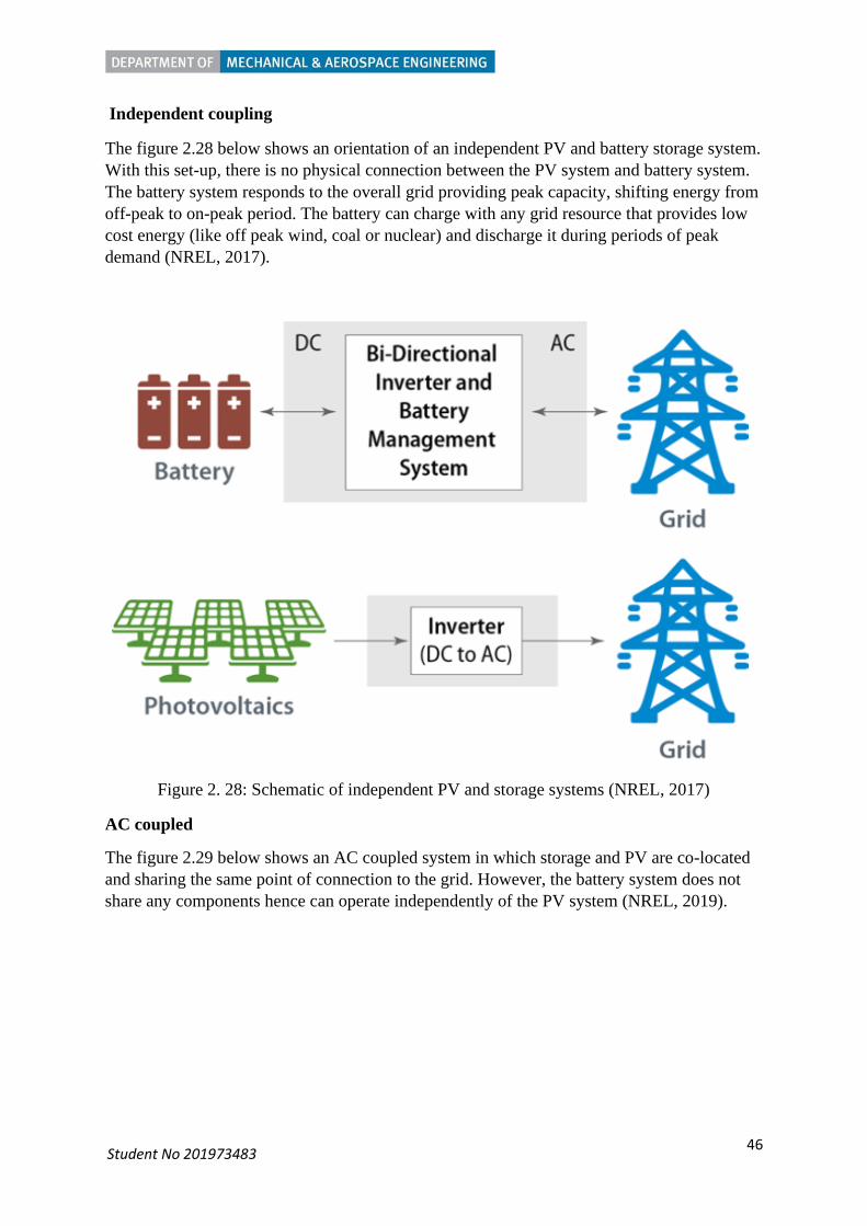
46 Student No 201973483

Independent coupling

The figure 2.28 below shows an orientation of an independent PV and battery storage system.

With this set-up, there is no physical connection between the PV system and battery system.

The battery system responds to the overall grid providing peak capacity, shifting energy from

off-peak to on-peak period. The battery can charge with any grid resource that provides low

cost energy (like off peak wind, coal or nuclear) and discharge it during periods of peak

demand (NREL, 2017).

Figure 2. 28: Schematic of independent PV and storage systems (NREL, 2017)

AC coupled

The figure 2.29 below shows an AC coupled system in which storage and PV are co-located

and sharing the same point of connection to the grid. However, the battery system does not

share any components hence can operate independently of the PV system (NREL, 2019).

47 Student No 201973483

Figure 2. 29: Schematic of AC coupled PV + Battery system (NREL, 2017)

DC Coupled systems

The figure 2.30 below shows both dc-coupled and tightly coupled battery systems. The DC

coupled systems include a bi-directional meter that enables battery system to be charged by

both the grid and PV system (NREL, 2017). The DC tightly coupled system can only be

charged by PV system and not from the grid. One advantage of DC coupled systems is that

they can store otherwise clipped energy that occurs when the inverter loading ratio exceeds 1

(NREL, 2017).

Figure 2. 30: Schematic of DC coupled PV + Battery systems (NREL, 2017)

48 Student No 201973483

2.4.4 Battery technologies

The mostly used battery technologies for FTM batteries include lithium ion, lead acid and

sodium sulphur while lithium ion and lead acid are mostly used for BTM batteries (IRENA,

2019). However, market growth is more in lithium ion technology as it constituted about 90%

of large-scale battery storage projects in 2017 (IRENA, 2019).

Lithium ion batteries

Lithium ion batteries consists of positive electrode materials made up of lithium compounds

capable of reversible intercalation of lithium ions (May J.G. et al, 2018). Negative electrodes

are made up of carbon or graphite that can accommodate lithium ions in solid state. Non-

aqueous electrolyte is used in lithium ion batteries and is made up of ionisable organic

solvents such as propylene carbonate with suitable lithium salts in solution (May J.G. et al,

2018). The cells also include separators which are microporous plastics films which may be

coated with ceramic particles to enhance the safety of the cells as shown in the figure 2.31

below:

Figure 2. 31: Chemical and principal components of lithium ion battery (May J.G. et al,

2018)

For small scale batteries, lithium cobaltite (LCO) is the most used as the positive electrode

material, however, this is too expensive for large scale storage systems. Low cost alternatives

are used instead which include nickel, mixed oxides of nickel - cobalt and aluminium (NCA),

and cobalt and manganese (NCM). For the anode, the most common material used is graphite

or carbon (May J.G. et al, 2018).

Lithium ion cells have a high energy density and organic electrolyte which is flammable

hence safety is a key issue (May J.G. et al, 2018). Thermal runaway is a huge challenge

hence the materials – cells, batteries, and charging systems – need to be carefully chosen to

49 Student No 201973483

reduce the risk. Battery monitoring systems with thermal sensors, voltage and current

measurements, and fuses are typically used for safe operation (May J.G et al, 2018).

Lead acid battery

Lead-acid cells are constructed from lead alloy grids which mechanically support the positive

and negative active materials and act as current collectors (May J.G et al, 2018). The grids

are stacked together as positive and negative plates and interleaved with a porous electrically

insulating separator as shown in the figure 2.32 below:

Figure 2. 32: Chemistry and principal components of lead-acid battery (May J.G et al, 2018)

There are two main types of positive plates namely flat pasted plates and tubular plates while

negative plates are always flat pasted type. The cells can also be categorised as flooded or

valve regulated lead acid (VRLA) type (May J.G et al, 2018). The positive active material is

highly porous lead dioxide and the negative material is finely divided lead. The electrolyte

comprises of a dilute aqueous sulphuric acid. One operational challenge associated with lead

acid batteries is the loss of water due to overcharging. This makes it imperative to control the

charging voltage of the battery. For flooded batteries, water loss (hence the need for adding

water during operation) can be reduced by correct selection of grid allows and charging

parameters (May J.G et al, 2018).

Sodium Sulphur batteries

Sodium sulphur batteries consist of molten liquid sodium and sulphur as the electrode

materials and operate between 300oC and 350oC (May J.G. et al, 2018). This is done to

maintain electrodes in liquid form and achieve good ionic conductivity in the electrolyte

which is a solid ceramic material. The advantages of these batteries over lead acid batteries is

50 Student No 201973483

that they have a higher energy density and a longer cycle life. However, safety is an issue in

sodium-sulphur batteries with the need for insulation, heat and thermal management which

make this type of batteries expensive (May J.G. et al, 2018). The figure 2.33 below shows the

chemical and principal components of sulphur batteries.

Figure 2. 33: Chemical and principal components of sulphur batteries. (May J.G. et al, 2018)

Lead acid battery vs Lithium ion battery

The table 2.5 below shows the summary of key parameters between the two technologies:

Table 2. 5: Summary of key parameters between Lead-acid and Lithium ion (May J.G. et al,

2018)

Parameter Lead acid Lithium ion

Energy density 35 – 40Wh/kg 150 – 180Wh/kg

Power density 250W/kg 800W/kg

High temperature performance To 40oC To 50oC

Low temperature performance To -30oC To -20oC

Charge acceptance Good Better

Circle life 1500 - 5000 1000 - 5000

Overall service life 15 years 10 – 15 years

Reliability Proven Needs to be accessed for

longer times

Sustainability Excellent Recovery methods

uneconomical

Safety Excellent Issues to be resolved

51 Student No 201973483

Cost (battery system only) 250/kWh 350/kWh

2.4.5 PV + Battery system specifications

The energy content (storage hours) and power capability of battery system are the most

important parameters in the design of battery storage (Hesse et al, 2017). For systems

integrated with PV, the inverter loading ratio (or DC – to - AC ratio) determines the size of

the PV plant. Parametric analysis is usually used to determine the right balance between the

investment cost, operational cost and the anticipated revenue based on the given load profile

and PV generation profile (Hesse et al, 2017).

The capacity factor of PV Battery plant can be increased by increasing the inverter loading

ratio – PV plant size relative to the desired output power – as shown in the figure 2.34 below

(NREL, 2016). Having very large inverter loading ratio (typical value of +2.4) means higher

chances of curtailing excess energy produced. However, having low Inverter Loading Ratio

(ILR) also translated to reduced capacity factor of the system as the plant rarely operates at

rated output (NREL, 2016).

Figure 2. 34: Relationship between capacity factor and ILR with different amount of storage

(NREL, 2016)

2.4.6 PV + Battery Economics

The table 2.7 below shows the anticipated cost from NREL Annual Technology Baseline for

PV + Battery systems. AC coupled battery systems are interpreted to be 10% lower than DC

coupled systems due to lesser equipment.

Table 2. 6: Estimated PV + Battery costs in 2020 (IRENA, 2019)

Component Cost

PV system 912/kW DC

PV Operation and Maintenance (O&M 11/kW-year

Batteries 217/kWh

Battery BOS 398/kW

Battery O&M 9/kW-year

52 Student No 201973483

2.5 Hybrid PV-CSP

2.5.1 Overview

The possibility of complementing CSP systems with PV systems promises to have high

returns both technically and economically. PV systems have matured in the market, but their

adoption is limited due to their instability caused by the intermittency nature of solar

radiation (Bousselamti and Cherkaoui, 2019). This challenge makes it very difficult for PV

systems alone to match demand. CSP systems on the other hand have the capability to match

demand and overcome the intermittency challenge by using thermal energy storage.

However, the current LCOE of CSP systems is more than double that of PV systems,

according to IRENA 2019 weighted averages (IRENA, 2020), which makes it unattractive to

developers (Singh and Singh, 2019).

There are a couple of PV-CSP commercial projects that are currently under development.

Cerro Dominador in Chile, Atacama Desert, is coupling 100MW PV plant with 110MW CSP

PTC with 17.5hours of thermal storage in molten salts (Bousselamti and Cherkaoui, 2019).

According to Cerro Dominador website, the PV plant is now operational (grid connected),

while the CSP is still in development (Cerro Dominador, 2020). There is also another plant in

Chile, Atacama Desert in Copiapo, which is still in development with a plan to combine

130MW CSP with 14hours molten salt storage with 150MW PV plant (Bousselamti and

Cherkaoui, 2019). The aim is to supply base load of 260MW 24/7 for local mining industries

(Ju et al, 2017). In South Africa, two PV plants – 96MW Jasper plant and 75MW Lesedi

plant – are planning to combine with a 100MW Redstone CSP plant that is currently under

development (Bousselamti and Cherkaoui, 2019).

2.5.2 PV-CSP Hybrid Types

PV-CSP hybrid plants can be categorised based on the characteristics of optical system,

system integration and operating temperature (Ju et al, 2017). Figure 2.35 below shows the

two types of PV-CSP hybrid systems - compact and non-compact. The two types are at

different stages of development with non-compact about to enter commercialisation while the

compact is still in research and pilot projects (Ju et al, 2017). This report will therefore focus

on non-compact PV-CSP.

53 Student No 201973483

Figure 2. 35: Classification of PV-CSP hybrid system (Ju et al, 2017)

2.5.2.1 Non-Compact PV-CSP hybrid

With a non-compact PV-CSP, PV system (both flat PV and concentrator PV) and CSP

system can be operated independently of each other (Ju et al, 2017). Typical schematic

diagram for a flat PV – CSP hybrid plant is shown in figure 2.36 below. The hybrid system is

then operated by a dispatch control system to optimise the power output. SolarReserve, which

is developing hybrid plants in Chile and South Africa, analysed the dispatch program they

intent to implement for the plant in Chile. They discovered that if the CSP plant follows the

output of PV plant, the capacity factor could reach a range of 80 – 90% (Ju et al, 2017). This

value is comparable to convectional thermal power plants and is way above for individual

CSP plants. The LCOE of the PV-CSP is expected to decline by a range of 8 – 13% when

compared to CSP alone with thermal storage (Ju et al, 2017).

54 Student No 201973483

Figure 2. 36: Typical schematic flat PV-CSP hybrid plant (Starke et al, 2018)

2.5.2.2 Addition of Battery Storage

Battery energy system can be added to the non-compact PV-CSP hybrid system to minimise

the variations of PV systems (Zurita et al, 2018). Currently, this type of system has only been

analysed by scholars and a few pilot projects are currently under development with non at

commercial level. A conceptual design to power Square Kilometre Array radio station

telescope project was proposed by the Institute of Fraunhofer. The system constituted of a

Concentrated PV (CPV) and linear Fresnel CSP combined with lithium and redox flow

batteries (Ju et al, 2017). In Italy, a CPV plant with a bank of Sodium Nickel batteries is

being coupled to linear Fresnel collector CSP system, with thermal oil as Thermal energy

storage, coupled to an organic Rankine cycle is being built as a pilot project (Zurita et al,

2018). The schematic diagram and pictorial view of the pilot plant are shown in figure 2.37

below:

55 Student No 201973483

Figure 2. 37: Pilot CPV-CSP with battery storage under construction in Italy (Ju et al, 2017)

Zurita et al (2018) performed a parametric study to analyse the impact of solar multiple, PV

size, Battery size and thermal storage size on PV-CSP hybrid with battery storage. The results

showed that investment costs of the battery need to fall by a range of 60 – 90% to make the

hybrid system competitive when compared to without battery system. The results were

echoed by Zhai et al (2018) who found out that the battery storage size must be very small to

make the hybrid system economically competitive.

2.5.3 PV-CSP dispatch strategies

2.5.3.1 Overview

An area of active study in the PV – CSP hybrid systems is to find the dispatch strategy that

will help optimise the two individual systems. The dispatch strategy has the potential to raise

the capacity factor of the hybrid system when compared to uncoordinated power generation

of the two systems (Pan and Dinter, 2017). There is also the potential to reduce the solar field

size (solar multiple) which leads to reduced LCOE (Pan and Dinter, 2017).

Zhai et al (2017) analysed the technical and economic performance of thermal storage of PV

– CSP when dispatched differently. The analyses showed that the LCOE reduced by 19%

when PV is prioritised for dispatch during the day than when using uncoordinated strategy.

The results also showed that the power output curve is more stable and fluid for coordinated

dispatch. Liu et al (2019) also concluded that independent dispatch strategy for PV – CSP has

a higher LCOE and less stead power output.

56 Student No 201973483

2.5.3.2 Typical dispatch strategies

There are typically two types of strategies from literature of dispatching PV – CSP hybrid

system– PV advanced and Independent (Zhai et al, 2017).

PV advanced strategy

With this dispatch strategy the PV system and CSP system are operating in synergy (Zhai et

al, 2017). When the PV output is larger enough to cover the load, the PV system operate

alone to satisfy the load while the thermal energy from CSP receiver is stored. If the PV

output is not enough, CSP will cover the missing section. When there is no sunlight, the

energy from the storage tank will be used to power the load as shown on the figure 2.38

below (Zhai et al, 2017):

Figure 2. 38: A typical dispatch strategy prioritising PV output (Bousselamti and Cherkaoui,

2019)

Independent strategy

With this strategy, the output from CSP system is summed up with that from the PV to

supply the load as shown in the figure 2.39 below (Zhai et al, 2017):

Figure 2. 39: A typical independent strategy for PV – CSP (Zhai et al, 2017)

57 Student No 201973483

2.6 Software review for PV – CSP hybrid Performance and financial modelling are very critical when designing PV – CSP hybrid

systems. Performance models are used to predict the expected output of the system at a given

location under expected operating conditions (Alsadi and Khatib, 2018). Financial models are

used to evaluate the economic performance of the system. Software packages differ in their

operations, but they generally perform one or more of designing, simulation, and optimising.

(Alsadi and Khatib, 2018). The table 2.7 below show different projects and approaches used

by some scholars to model and analyse PV – CSP systems:

Table 2. 7: Typical software packages and methodologies involving PV – CSP systems

Title Project Aim Methodology used Reference

“Combination of PV

and central receiver

CSP plants for base

load power

generation in South

Africa”

To simulate and

access if PV – CSP

can produce base

load in South Africa

• SAM software to

simulate PV and

CSP independently

• Modified the

thermal energy

storage dispatch to

emulate operational

strategy

• Combined the

systems in SAM

(Pan and

Dinter, 2017)

“Techno-Economic

Evaluation of

Renewable Energy

Projects using the

Software

GREENIUS”

Simulated the

performance of

50MW CSP and

50MW PV plant in

Jordan

• GREENIUS

software used to

simulate CSP and

PV plant

independently

• Added the two

outputs and

analysed

(Dieckmann

and Dersch,

2015)

“Optimal Design

Method of a Hybrid

CSP-PV Plant Based

on

Genetic Algorithm

Considering the

Operation Strategy”

To optimise the

design of PV – CSP

plant considering

operational strategy

• Modelled PV –

CSP hybrid

(performance and

economic) in

MATLAB

(Zhai et al,

2018)

“High capacity

factor CSP-PV

hybrid systems”

To investigate ways

in which

SolarReserve can

increase the capacity

factor of the hybrid

PV – CSP plant they

are constructing in

Chile

• PV plant was

modelled using

PVSyst

• CSP was modelled

using a proprietary

software belonging

to SolarReserve

company

• Dispatch strategy

was implemented

using an inhouse

(Green et al,

2015)

58 Student No 201973483

software

SmartDispatch

“Multi-objective

optimization of

hybrid PTC + PV

system using genetic

algorithm”

To develop a

methodology to

design and size PV –

CSP hybrid

• Used TRNSYS and

GenOpt to simulate

and optimise PV –

CSP system

respectively

• MATLAB used to

develop genetic

algorithm

(Starke et al,

2018)

“Techno-economic

evaluation of a

hybrid CSP + PV

plant integrated with

thermal energy

storage and a large-

scale battery energy

storage system for

base generation”

To investigate the

impact of PV size,

solar multiple,

thermal storage size,

and battery size on

technical and

economic

performance

• Used TRNSYS to

simulate thermal

and electric

performance of

hybrid system

• Optimisation of

heliostat field,

tower height,

receiver geometry

done using Solar-

Pilot an algorithm

from SAM

software

• 3 operational

strategies modelled

using a controller

in TRNSYS

software

(Zurita et al,

2018)

“Simulation of

hybrid solar power

plants”

To evaluate the

potential of software

GREENIUS to carry

out a techno –

economic evaluation

for hybrid solar

power plants

• Simulated the

hybrid system in

two simulations

using GREENIUS

software to

implement the


• First simulated

output for PV plant

• Modified the load

profile (base load –

PV output)

• Second simulation

involved CSP

following the

modified load

profile

(Dieckmann

and Dersch,

2017)

“Combined CSP –

PV plants for

MENA Region”

To investigate the

optimal

configuration of

solar power plants

• Simulated the

performance of

hybrid system

using INSEL tool

(Benitez et al,

2018)

59 Student No 201973483

for selected sites in

Jordan, Tunisia, and

Algeria

• Performed

parametric study,

optimisation,

economic

evaluation, and


implemented in

INSEL

From the above table, TRNSYS and INSEL are the two software packages with the capability

of simulating the PV – CSP hybrid system in its entirety. SAM and GREENIUS can

independently simulate PV and CSP and will need modifications to model PV – CSP as

whole system. The main features of the mentioned software packages are given in the table

2.8 below:

Table 2. 8: Key features of selected software packages for PV- CSP hybrid

Name and Developer Key features Technology

simulated

Reference

• SAM – System

Advisor Model

• National

Renewable

Energy

Laboratory

• Parametric

analysis,

stochastic

analysis,

probability of

Exceedance

analysis, LK

script, economic

evaluation

• Price – Free

• Comment – need

modifications to

simulate PV –

CSP, no global

weather data

PV (with option

for battery

storage), High

concentrated PV,

CSP, Wind,

Geothermal,

Biomass

combustion,

Convectional

thermal fossil

fuel, Water

heating

(SAM, 2020)

• TRNSYS –

Transient

System

Simulation

Program

• University of

Wisconsin,

TRANSSOLAR,

Thermal Energy

System

Specialist

• Parametric runs,

can model hybrid

PV – CSP

• Price – US$2530

for 10 users

• Comment – the

software is a

simulation

program and can

not perform

economic

evaluation and

optimisation

All thermal and

renewable

generation except

Nuclear, Wave,

Tidal, and Hydro

(TRNSYS,

2020)

60 Student No 201973483

• GREENIUS –

Green Energy

System Analysis

• German

Aerospace

Center (DLR)

• Economic

evaluation,

Performance

simulation

• Price – Free

• Comment –

Cannot perform

hybrid analysis,

No global

weather data

Solar thermal,

PV, Wind, Fuel

cells

(GREENIUS,

2020)

• INSEL –

Integrated

Simulation

Environment

Language

• University of

Oldenburg

• Worldwide

weather database,

ability to simulate

hybrid systems,

economic

evaluation,

performance

simulation

• Price – Free

PV, Solar thermal (INSEL, 2020)

2.7 Comparison of PV + Battery vs CSP + TES The tables 2.9 and 2.10 below show the comparison of two systems in terms of the important

parameters:

Table 2. 9: Comparison of Capacity factors of different configurations of PV + Battery and

CSP + TES (NREL, 2016)

Parameter CSP + TES PV + Battery

Typical capacity

factor (CF)

SM storage hrs CF / % ILR storage hrs CF / %

1.5 3 37 1.5 3 36.8

2 6 50 2.1 6 50

2.5 9 60 2.6 9 60

Table 2. 10: Comparison of PV + Battery vs CSP + TES (Florin and Dominish, 2017)

Parameter CSP + TES

PV + Battery

Lithium ion

(NMC) Lead acid Sodium - based

Energy

Efficiency

depend on steam

temperature and

capability of

storage material

withstanding

higher working

temperature

Mean roundtrip

efficiency = 90%

Mean roundtrip

efficiency = 82%

Mean roundtrip

efficiency = 81%

61 Student No 201973483

Lifecycle

greenhouse

efficiency

cradle to gate

(manufacturing

and production):

low

cradle to gate:

low

cradle to gate:

high

cradle to gate:

medium

5-25

kgCO2e/MWh 25 kgCO2e/MWh 75kgCO2e/MWh 50kgCO2e/MWh

20% from storage

system

mostly from

nickel and cobalt

Raw material

availability

potential

constraints in the

supply of silver

(used for

reflectors) and

silvering process

which uses cerium

which is a rare

earth material

presents of

graphite, cobalt

and fluorine not

easily accessed

lead is highly

recyclable hence

less critical

uses graphite

hence potential

issues

no issues with TES

potential issues in

the supply of

lithium

Material intensity relatively highly

intensive

high material

demand

high material

demand

low material

demand than

alternative battery

types

Recyclability

relatively long

lifespans (30yrs)

and rate of

degradation of

molten salts is very

slow minimal need

to refresh material

high potential of

recycling

high potential of

recycling

high potential of

recycling

Environmental

Impact

Significant water

usage

Air pollution

from graphite

dust

heavy metal

contamination of

water, soil, and

plants

air pollution from

graphite

land footprint is

relatively high

water pollution

from cobalt

Health and safety

relatively safe as it

has established

operating protocols

risk to consumers

of fire due to

thermal run away

potential

emission of

corrosive and

potential

explosive mix of

hydrogen and

oxygen in the last

stages of

charging

relatively safe

62 Student No 201973483

nitrate salts are

non-toxic

sulphuric acid as

electrolyte can

harm if exposed

63 Student No 201973483

3.0 Methodology

3.1 Model Description The techno-economic models for PV, PV + Battery, CSP, and CSP + Thermal Energy

Storage (TES) were developed for a typical mining load in Zimbabwe. Evaluation was based

on technical and economic performance using System Advisor Model (SAM) software. The

table 3.1 below describes the process taken:

Table 3. 1: Methodology

Stage System /

Description Aim Steps

1 Demand

profile

To develop typical

hourly load profile

from the given

monthly data

Understand the given load data and the billing

structure

Analyse the typical working pattern and use it

to develop hourly profile

2 PV

To analyse the

viability of integrating

Solar PV at Mimosa

mine

Design the capacity and optimise technical

parameters (tilt angle, orientation and interrow

distance)

Analyse technical and economic metrics of the

modelled results (annual energy produced,

LCOE, Savings, Net Present value)

3 PV +

Battery

To analyse the


Solar PV + Battery at

Mimosa mine

Design and determine the optimal size for PV

and Battery for a given dispatch



LCOE, savings, Net Present value)

4 CSP

To analyse the


CSP at Mimosa mine

Design the capacity and optimise technical

parameters (solar multiple, design point DNI)



LCOE, savings, Net Present value)

5

CSP +

Thermal

Energy

Storage

To analyse the


CSP + TES at

Mimosa mine

Design and determine the optimal size for CSP

and TES for a given dispatch



LCOE, savings, Net Present value

6

Repeat stage

2 to 5 but

considering

energy

export

To analyse the

techno-economic

performance of the

systems when exports

are allowed

Design and determine the optimal size for PV,

CSP and TES/Battery



LCOE, savings, Net Present value

64 Student No 201973483

The mentioned systems will be evaluated based on Key Performance Indicators (KPI) listed

in the table 3.2 below:

Table 3. 2: Key performance Indicators used for evaluation

KPI Calculation/Comment

Base case

Renewable Energy

Contribution

This is shown as a percentage energy offset by the

renewable energy system.

Calculated as 𝑁𝑒𝑡 𝑎𝑛𝑛𝑢𝑎𝑙 𝑒𝑛𝑒𝑟𝑔𝑦 𝑝𝑟𝑜𝑑𝑢𝑐𝑒𝑑 𝑏𝑦 𝑠𝑦𝑠𝑡𝑒𝑚

𝑎𝑛𝑛𝑢𝑎𝑙 𝑒𝑛𝑒𝑟𝑔𝑦 𝑑𝑒𝑚𝑎𝑛𝑑 𝑥 100%

Localised Cost of Energy

(LCOE) – applies to export

case

This metric will allow comparison of energy systems

being considered based on technical performance, capital

cost and operations and maintenance costs.

The formula used is given in Appendix C

Net Present Value (NPV) –

applies to export case

This will be used to analyse the profitability of the system

The formula used is given in Appendix C

Export case

Energy exported This shows the percentage of energy exported from the

system calculated as: 𝐴𝑛𝑛𝑢𝑎𝑙 𝑒𝑛𝑒𝑟𝑔𝑦 𝑓𝑟𝑜𝑚 𝑠𝑦𝑠𝑡𝑒𝑚 𝑡𝑜 𝑔𝑟𝑖𝑑

𝐴𝑛𝑛𝑢𝑎𝑙 𝑔𝑒𝑛𝑒𝑟𝑎𝑡𝑒𝑑 𝑒𝑛𝑒𝑟𝑔𝑦 𝑥 100%

Energy used locally This shows the percentage of energy used to meet local

generation from the system calculated as: 𝐴𝑛𝑛𝑢𝑎𝑙 𝑒𝑛𝑒𝑟𝑔𝑦 𝑓𝑟𝑜𝑚 𝑠𝑦𝑠𝑡𝑒𝑚 𝑡𝑜 𝑙𝑜𝑎𝑑

𝐴𝑛𝑛𝑢𝑎𝑙 𝑔𝑒𝑛𝑒𝑟𝑎𝑡𝑒𝑑 𝑒𝑛𝑒𝑟𝑔𝑦 𝑥 100%

Renewable Energy

contribution

This shows the percentage energy offset by the renewable

energy system calculated as: 𝐴𝑛𝑛𝑢𝑎𝑙 𝑒𝑛𝑒𝑟𝑔𝑦 𝑓𝑟𝑜𝑚 𝑠𝑦𝑠𝑡𝑒𝑚 𝑡𝑜 𝑔𝑟𝑖𝑑

𝐴𝑛𝑛𝑢𝑎𝑙 𝑚𝑖𝑛𝑒 𝑒𝑛𝑒𝑟𝑔𝑦 𝑑𝑒𝑚𝑎𝑛𝑑 𝑥 100%

Grid contribution (applies to

base case as well)

This shows the percentage of energy used to meet the mine

demand from the grid calculated as: 𝐴𝑛𝑛𝑢𝑎𝑙 𝑒𝑛𝑒𝑟𝑔𝑦 𝑓𝑟𝑜𝑚 𝑔𝑟𝑖𝑑 𝑡𝑜 𝑙𝑜𝑎𝑑

𝐴𝑛𝑛𝑢𝑎𝑙 𝑚𝑖𝑛𝑒 𝑒𝑛𝑒𝑟𝑔𝑦 𝑑𝑒𝑚𝑎𝑛𝑑𝑥 100%

System Advisor Model (SAM) software

The SAM software will be used to model the renewable energy systems under consideration.

This is a financial and performance model developed by National Renewable Energy

Laboratory (NREL) funded by US Department of Energy (SAM, 2020). The target users for

the software include:

• Project engineers and managers

• Developers

• Researchers

• Policy analyst

The model makes performance predictions and estimates energy cost for grid connected

systems referencing the installation and operations cost and the design parameters inputted to

the model (SAM, 2020). The projects can either be connected to:

65 Student No 201973483

• Customer side – buying and selling electricity at retail rates

• Utility side – selling electricity at a negotiated price through a power purchase

agreement

The models require input data to describe the performance characteristics of the system’s

physical equipment and project costs. One disadvantage of the software is that it does not

have weather database for the whole world hence there is need to source it from external if

the desired area is not covered (SAM, 2020).

3.2 Candidate mine

3.2.1 Mimosa Mining Company

Mimosa mine is a Platinum Group Metal (PGM) and base metal mining company located in

the Wedza sub-chamber of the Great Dyke of Zimbabwe (24 km west of Zvishavane town).

The two figures below (figure 3.1 and 3.2) show the geographical location of Mimosa mine

on the Great Dyke and the satellite picture (geographical coordinates with latitude -20.33 and

longitude 29.83). It involves underground mining and plant processing activities with an

estimated life of mine of 30 years. The output commodities of the mine include Platinum,

Palladium, Rhodium, Gold, Nickel and Copper.

Figure 3. 1: The position of Mimosa mine on the Great dyke, Zimbabwe

66 Student No 201973483

Figure 3. 2: Satellite picture showing the position of mimosa mine (Google maps,2020)

3.2.2 Climate data

The climate data used in this project was sourced from Solcast. This is a data services

company providing solar radiation data and solar forecasting globally using surface and

satellite measurements (Solcast, 2020). Three set of data were acquired – Typical

Meteorological Year (TMY) in csv format, data customised for SAM software and PVSyst.

Solcast data sets have been validated showing 0% and 0.3% bias on Global Horizontal

Irradiation (GHI) and Direct Normal Irradiation (DNI) data sets, respectively (Solcast, 2020).

Mimosa mine receives solar radiation of 2010 kWh/m2/year of DNI and 2034 kWh/m2/year

of GHI according to Solcast data. The DNI value shows that the site is technically feasible to

develop CSP as the minimum rule of thumb value required is between 1900 – 2000

kWh/m2/year (Bousselamti and Cherkaoui, 2019). The figure 3.3 below shows the variation

between monthly GHI and DNI for the candidate site - the site receives higher DNI values

than GHI between April and September.

Figure 3. 3: Monthly GHI and DNI for Mimosa mine

0.0

50.0

100.0

150.0

200.0

250.0

Mo

nth

ly s

ola

r ir

rad

iati

on

(kW

h/m

^2)

Monthly GHI and DNI for Mimosa mine, Zimbabwe

DNI GHI

67 Student No 201973483

The two figures below (figures 3.4 and 3.5) show the typical hourly variation of DNI, GHI

and temperature of a day in summer and winter at the candidate site. For both figures, the

GHI and DNI peak occurs around midday. The temperature in winter is below 25oC which

could help PV system to perform better. However, the temperature in summer has a peak

value of 35oC which could affect the performance of PV system.

Figure 3. 4: Typical winter day (in June) profile at Mimosa mine

Figure 3. 5: Typical summer day (In October) profile at Mimosa mine

3.3 Mimosa Mine Demand Profile

3.3.1 Raw Data – Monthly profile 2015

Currently, the mine is grid connected with annual consumption of 165GWh according to

2015 figures. The peak demand in that year was recorded in December with a value of

28.4MW. The figure 3.6 below shows the monthly variation of the consumed energy and the

corresponding peak power. The energy consumption graph has a minimum of 12.7GW (in

October) and a maximum value of 14.9GW in June. There is a variation from month to month

0

5

10

15

20

25

0

100

200

300

400

500

600

700

800

900

1000

00:00 02:00 04:00 06:00 08:00 10:00 12:00 14:00 16:00 18:00 20:00 22:00

TEM

PER

ATU

RE

(C)

HO

ULY

IRR

AD

IATI

ON

(WH

/M^2

)

Typical Winter day profile

DNI GHI Temperature

0

5

10

15

20

25

30

35

40

0

200

400

600

800

1000

1200

00:00 02:00 04:00 06:00 08:00 10:00 12:00 14:00 16:00 18:00 20:00 22:00

TEM

PER

ATU

RE

(C)

HO

UR

LY IR

RA

DIA

TIO

N (

WH

/M^2

)

Typical Summer day profile

DNI GHI Temperature

68 Student No 201973483

of energy consumed due to maintenance activities. Taking for example, in October there was

5-day plant shut down (planned maintenance) which corresponded to the minimum monthly

energy consumed that year.

Figure 3. 6: 2015 monthly energy consumption and maximum demand for Mimosa mine

The data for the year 2015 shows that the mine consumes most of its energy during peak

hours as shown in the figure 3.7 below. The table 3.3 below shows the time periods of on-

peak, standard and off-peak with the corresponding time of use tariff. The off-peak tariffs

show that the mine could benefit by load shifting to off-peak hours and by finding an

alternative cheaper source of electricity during peak hours.

Figure 3. 7: Time of Use monthly consumption of Mimosa mine in 2015

23

24

25

26

27

28

29

11.512

12.513

13.514

14.515

15.5

MA

XIM

UM

DEM

AN

D /

MW

ENER

GY

CO

NSU

MP

TIO

N /

GW

H

Monthly Energy Consumption and Maximum Demand in 2015

Energy consumed Maximum Demand

0

1

2

3

4

5

6

7

ENER

GY

CO

NSU

MP

TIO

N /

GW

H

Time of Use Monthly Consumption

On-Peak Standard Off-Peak

69 Student No 201973483

Table 3. 3: Time of use periods and corresponding tariff

The 2015 mine consumption figures show that 40% of the load was consumed during peak

times as illustrated by the pie chart (figure 3.8) below and this translates to high annual

electric bill. In addition, the electric bill also includes the maximum monthly demand charge

of USD2.6 per unit demand. The maximum demand charge is applied only during the peak

and standard period to encourage customers to load shift wherever possible and not strain the

system.

Figure 3. 8: A pie chart showing 2015 Mimosa mine load distribution by time of use

Lately, Zimbabwe has been facing power shortages which resulted in load-shedding with the

most shed period being between 4pm and 9pm. Such scenario causes the mine to add another

charge on the electric bill – uninterrupted demand charge of USD1.95 per unit demand on

each hour supposed to be on load shedding. This shows that the mine can benefit by

integrating reliable energy system that can offset or eliminate grid energy consumption

during these risk hours. The peak period is also coincidentally the high-risk period in terms of

load-shedding.

3.3.2 Synthesized hourly demand profile

Hourly demand profile for the mine was not provided (only monthly profile) hence there was

need to produce one to use in the analyses. The following assumptions and consumption

behaviours were used in estimating the hourly pattern from the given data:

• The hourly demand consumption is derived from time of use monthly consumption –

peak, off-peak and standard energy consumptions

• The assumption is that each day of the month follow the same pattern and the

cumulative total of energy consumption should be close to the given 2015 monthly

and time of use figures

Day of Week 0 1 2 3 4 5 6 7 8 9 10 11 12 13 14 15 16 17 18 19 20 21 22 23 Category Color Tariff/$USD per kWh

Sunday/Holiday Peak 0.13

Weekday Standard 0.07

Saturday Off-peak 0.04

Hours Legend

32%

40%

28%

Load distributed by time of use

offpeak load Peak load Standard load

70 Student No 201973483

• The time of use hourly periods for the weekday will be used in estimating the pattern

• The mine has 2 shifts a day – day shift which starts at 7am to 4:30pm and night shift

starting at 7pm up to 4am. The day shift consists of production and administrative

teams while the night shifts only comprises of production teams.

• There will be two shift changeovers one in the morning from 4am to 7am and the

other in the evening from 4:30pm to 7pm. During this time, key equipment that

operate 24/7 (like Mills and Ventilation fans for underground) will be running.

• During the shift change over, the underground operations will stop to allow for

blasting and no personal will be allowed underground for safety purposes. The

technical team in the process plant (above ground) will continue to operate.

• Other machinery (process pumps, crushers, conveyer belts) will be switched on at

8am to 9am and 8pm to 9pm by the morning and night shift teams, respectively. This

will correspond to peaks in the energy consumption pattern due to high starting

currents of large motors involved. The value of the peak demand is estimated from the

given maximum monthly demand from the 2015 data

• Each month will follow the same pattern but having different values as dictated by the

given data. Figure 3.9 below show the typical hourly profile synthesized for the

month of April:

Figure 3. 9: Synthesized hourly profile for the month of April

• The synthesized hourly profile has an annual energy consumption of 165.7GWh with

a peak demand of 28.4MW. The figure 3.10 below shows the monthly energy

consumption comparison for raw data and synthesized data:

0

5

10

15

20

25

30

00

:00

01

:00

02

:00

03

:00

04

:00

05

:00

06

:00

07

:00

08

:00

09

:00

10

:00

11

:00

12

:00

13

:00

14

:00

15

:00

16

:00

17

:00

18

:00

19

:00

20

:00

21

:00

22

:00

23

:00

DEM

AN

D /

MW

Synthesized houly Demand Profile

71 Student No 201973483

Figure 3. 10: Monthly energy consumption of raw data vs synthesized data

3.4 PV System

3.4.1 Plant Capacity

A PV plant differs from convectional electrical systems because their performance is

naturally connected to unique details of the site and the specifics of the plant design. This

makes it very difficult to calculate the required capacity of the plant. The equation used to

calculate power in HOMER software is going to be utilised to estimate the rated capacity of

this project (Homer, 2020). The rated capacity will assume that the modules are operating at

Standard Test Conditions (STC).

𝑃𝑜𝑤𝑒𝑟 = 𝑅𝑎𝑡𝑒𝑑 𝐶𝑎𝑝𝑎𝑐𝑖𝑡𝑦 𝑥 𝑁𝑒𝑡 𝑖𝑛𝑐𝑖𝑑𝑒𝑛𝑡 𝑟𝑎𝑑𝑖𝑎𝑡𝑖𝑜𝑛

𝑖𝑛𝑐𝑖𝑑𝑒𝑛𝑡 𝑟𝑎𝑑𝑖𝑎𝑡𝑖𝑜𝑛 𝑎𝑡 𝑆𝑇𝐶 𝑥 𝐷𝑒𝑟𝑎𝑡𝑖𝑛𝑔 𝑓𝑎𝑐𝑡𝑜𝑟

Where:

Power = peak load/demand required (from load profile)

Rated capacity = unknown

Net incident radiation = incident radiation at STC = 1000 W/m2 (Assumption)

Derating factor = 0.77 (NREL, 2013)

𝑅𝑎𝑡𝑒𝑑 𝐶𝑎𝑝𝑎𝑐𝑖𝑡𝑦 (𝐷𝐶) =𝑃𝑒𝑎𝑘 𝑙𝑜𝑎𝑑 𝑟𝑒𝑞𝑢𝑖𝑟𝑒𝑑

𝐷𝑒𝑟𝑎𝑡𝑖𝑛𝑔 𝑓𝑎𝑐𝑡𝑜𝑟

= 28.4 𝑀𝑊

0.77 = 36.88MW DC ~ 37MWDC

The recommended DC to AC ratio (form factor) to avoid inverter clipping losses is between

1.0 – 1.1 (PVSyst, 2020). The proposed form factor for the project is 1.05. The tilt angle,

azimuth angle and interrow space will be optimised through parametric analysis based on

energy produced and LCOE. The key technical parameters used for the model are given in

the table 3.4 below:

11.512

12.513

13.514

14.515

15.5EN

ERG

Y C

OM

SUM

PTI

ON

/ G

WH

Monthly Energy Consumption: Raw data vs Synthesized

Raw Data Synthesized

72 Student No 201973483

Table 3. 4: Technical parameters for PV plant (SAM, 2020)

Parameter Unit Value (and comment)

Module type - Polycrystalline

Module DC capacity W 345

Module Efficiency % 17.8

Inverter - String inverter

Inverter Capacity kW 40

Tilt angle degrees 0 – 60 (optimisation range)

Azimuth degrees 0 – 270 (optimisation range)

Module configuration - Landscape (based on literature review)

Far shading - Assumed no far shadings

DC / AC ratio - 1.05

Ground cover ratio - 0.05 – 0.95 (optimisation range to determine interrow distance)

Soiling loss % 5

DC losses % 4.4 (including module mismatch)

AC cabling losses % 2

Degradation %/year 0.5

3.4.2 Financial inputs for PV System

The commercial model will be used to simulate the financial analysis of the PV system in

SAM. This model assumes that the PV system will be developed, owned, and operated by

the entity and in this case the Mimosa mining company. With this model, the entity will be

able to buy and sell power at retail price. The metering and billing method to be used for this

analysis is the net metering. This allows the PV system to supply the load with the shortfall

being supplied from the grid. However, this type of system also mean excess generation of

the system will be fed into the grid hence there is need to design it in such a way there is

reduced excess generation. For the base case scenario, the excess generation will be curtailed

based on the assumption that there is no agreement with the utility company to export power.

The grid energy charges are based on the time of use for the weekday as defined in table 3.3

above in section 3.3.1.

The table 3.5 below shows the parameters to be used in the model to calculate LCOE, Net

Present Value (NPV) and pay-back period. The formulas on how these are calculated in SAM

are presented in Appendix C.

Table 3. 5: Commercial parameters for PV module (Zurita et al, 2020)

Parameter Unit Value

Direct Capital Cost

Module cost USD/Wdc 0.30

Inverter cost USD/Wac 0.05

Balance of System USD/Wdc 0.17

Installation cost USD/Wdc 0.10

Installer margin and overhead USD/Wdc 0.05

Contingency % 3

Indirect Capital Cost

Sales tax % 5

73 Student No 201973483

Land purchase USD/acre 11000

Operations and maintenance cost USD/kW-year 9

Analysis Parameters

Project life Years 25

Inflation % 2.5

Discount rate % 6.4

Interest rate % 5

3.5 PV + Battery System

3.5.1 Capacity design

The PV + Battery system in the model mainly aims to perform time of use arbitrage and to

reduce the risk of losing grid power due to load-shedding (or paying uninterrupted charge).

The AC connected behind the meter battery will utilise energy produced by PV system during

the day and discharging it during peak periods. The two main design parameters for the PV +

battery system are:

• Power to Energy ratio – this determines the battery storage hours

• PV size ratio – PV + battery plant capacity to PV (without storage) capacity. This

determines capacity of the PV plant to service both the load and the battery

A parametric analysis will be carried out to optimise the design parameters based on return

on investment (Net Present Value) and the ability of the system to supply the load during the

most risk period from load shedding on a typical good day for PV production. From the load

profile, the maximum energy required between 4am – 9pm is 138MWh (occurring in June)

and this will be used to calculate the minimum required battery capacity (Bayod-Rujula et al,

2013):

𝐸𝑐𝑎𝑝−𝑚𝑖𝑛(𝑀𝑊ℎ) = 110𝐸𝑟𝑒𝑞(𝑀𝑊ℎ/𝑑𝑎𝑦)𝑥𝐷

𝐷𝑂𝐷%

Where:

• Ecap-min = minimum battery capacity

• Ereq = peak energy consumption between 4pm and 9pm (inclusive) from load profile

• D = days of anatomy (1 will be used for estimation with parametric study to

determine the final)

• DOD = depth of discharge (80% will be used) (Petrollese and Daniele, 2016)

=110 𝑥 138 𝑥 1

80

= 189.75 ~ 190𝑀𝑊ℎ

Therefore, the minimum battery capacity for this model is 190MWh with rated power

capacity of 30MW (based on peak demand of 28.4MW). The technical parameters used to

model the battery are given in the table 3.6 below (the PV plant will use the same parameters

as described in the above section 3.4.1):

74 Student No 201973483

Table 3. 6: Battery technical properties (SAM,2020)

Description Unit Value

Battery type - Lithium ion: Nickel Manganese Cobalt Oxide

(NMC/Graphite)

Maximum charge power MWac 30

Maximum discharge power MWac 30

Life cycle at 80% DOD cycles 2500

Minimum State of Charge % 15

Maximum State of Charge % 95

Battery replacement

threshold capacity

% 50

DC – AC efficiency % 96

AC – DC efficiency % 96

3.5.2 Battery dispatch

A manual dispatch will be defined in SAM so as to input specific time frames, other than

using the automatic peak shaving dispatch. The battery will only be allowed to charge from

PV system (not from grid) and can only discharge during peak or standard period times (7am

– 9pm). The power generated from PV system prioritise the load first and will only charge

the battery when the generated PV is greater than the load. Just like with the PV system, the

excess generated power will not be exported to the grid and will be reported as losses. In case

the power from PV + Battery is not enough to supply the load: grid power will be used

instead.

3.5.3 Economic inputs to PV + Battery System

The commercial model used for this system is the same as with PV system described in

section 3.4.2 above. The table 3.7 below show the economic parameters for the battery

system to calculate the LCOE, Net Present Value and payback period (for PV they are the

same as described in the previous section 3.4.2):

Table 3. 7: Economic parameters for Battery storage (Zurita et al, 2020)


Battery Storage System

Cost of storage USD/kWh 209

Conversion system USD/kW 70

Balance of System USD/kW 80

Operations and Maintenance

(O/M)

Fixed O/M USD/kW-year 6.9

Variable O/M USD/MWh 2.1

Battery Replacement Cost USD/kWh 2/3 of Cost of Storage

Analysis Parameters


Inflation % 2.5

Discount rate % 6.4

Interest rate % 5

75 Student No 201973483

3.5.4 Practical considerations of PV + Battery system

The table 3.8 below shows typical practical challenges and corresponding best practises for a

PV + Battery system:

Table 3. 8: Potential practical challenges of PV + Battery system (NREL, 2018)

Subsection Challenge Best practice

Electrical and

Balance of plant • Degradation of

cables and cable ties

that are exposed to

direct sunlight

• Cables exposed to

animals (like rates,

snakes) which can

destroy/chew cable

insulation resulting

in faults

• Consider covering electrical

cables that are in open air

with conduits

• Employ animal

repellent/deterrent system

PV module

mounting • Modules mounted

too low causing

difficulties in

vegetation

management

• Consider intended vegetation

management during the

design stage of the project

Environmental • Hot spots from

uneven soiling like

bird droppings

• Flooding and soil

erosion

• Regular checking and

cleaning the PV modules –

also consider installing birds

spikes to prevent roosting

• Establish good drainage

system at the site

Battery system • Capacity

degradation and

shorter battery

usable life due to

operating outside

optimum

temperature range

• Effective and efficient (less

power consumption) thermal

management system of

battery units recommended

• Usually air cooling and

heating HVAC systems

employed

3.6 Concentrated Solar Power (CSP) The system chosen for primary analysis in this project is the Parabolic trough CSP system.

Based on the literature review, this is a more mature system (when compared to other CSP

systems) with commercial operational plants around the world including in Africa.

3.6.1 System design

The recommended methodology to design and model parabolic trough CSP plant in SAM is

given below (SAM, 2020):

• Define solar field design parameters

• Configure receiver and collector components

• Determine transport operational limits

• Configure the loop

76 Student No 201973483

• Specify power cycle design point

• Update cost and financials

• Optimise uncertain parameters – solar multiple, storage hours

The table 3.11 below shows the technical parameters used to develop the CSP parabolic

trough system for this project. Details of the most important parameters are described below:

Design point DNI

This is used to calculate the aperture area required to drive the power cycle at its design

capacity (SAM, 2020). Theoretically the value should be close to maximum DNI value of the

site. A low DNI value results in excessive dumped energy while a high reference DNI value

results in undersized solar field only operating at designed capacity for only few times (SAM,

2020). A parametric analysis will be used to determine the design point DNI.

Solar Multiple (SM)

This is defined as a multiple of aperture area required to operate the power cycle at its design

capacity (SAM, 2020). An SM value of 1 defines an aperture area that will generate (when

exposed to solar radiation equivalent to design point DNI) thermal energy required to drive

power block at its rated capacity. A parametric analysis will be used to determine the optimal

SM for this application.

Design turbine gross output

This is power cycle’s design output (not including parasitic losses) used to determine solar

field area (SAM, 2020). The value is determined from the maximum load required. The

maximum load from demand profile is 28.4MW hence the net estimated output at design

capacity is 29MW. The gross turbine output is determined using the following equation:

𝐸𝑠𝑡𝑖𝑚𝑎𝑡𝑒𝑑 𝑁𝑒𝑡 𝑂𝑢𝑡𝑝𝑢𝑡 𝑎𝑡 𝐷𝑒𝑠𝑖𝑔𝑛= 𝐷𝑒𝑠𝑖𝑔𝑛 𝑔𝑟𝑜𝑠𝑠 𝑜𝑢𝑡𝑝𝑢𝑡 𝑥 𝑒𝑠𝑡𝑖𝑚𝑎𝑡𝑒𝑑 𝑔𝑟𝑜𝑠𝑠 𝑡𝑜 𝑛𝑒𝑡 𝑐𝑜𝑛𝑣𝑒𝑟𝑠𝑖𝑜𝑛 𝑓𝑟𝑎𝑐𝑡𝑜𝑟

𝐷𝑒𝑠𝑖𝑔𝑛 𝑔𝑟𝑜𝑠𝑠 𝑜𝑢𝑡𝑝𝑢𝑡 = 𝐸𝑠𝑡𝑖𝑚𝑎𝑡𝑒𝑑 𝑛𝑒𝑡 𝑜𝑢𝑡𝑝𝑢𝑡

𝐸𝑠𝑡𝑖𝑚𝑎𝑡𝑒𝑑 𝑔𝑟𝑜𝑠𝑠 𝑡𝑜 𝑛𝑒𝑡 𝑐𝑜𝑛𝑣𝑒𝑟𝑠𝑖𝑜𝑛 𝑓𝑎𝑐𝑡𝑜𝑟

= 29𝑀𝑊

0.9(𝑆𝐴𝑀,2020) = 32MW

Heat rejection

One of the criticisms of the CSP plant is based on its extensive use of water. This model is

being proposed in area which is generally hot and dry with persistent droughts. In that regard,

air cooled condenser is chosen for this model rather than the water cooled. Some of the

advantages and disadvantages of air-cooled condenser over water condenser are given in the

table 3.9 below:

Table 3. 9: Advantages and disadvantages of Air-cooled condenser over water condenser

(Padillar, 2011)

Advantages Disadvantages

Reduced maintenance cost (no chemical

additives or periodic cleaning)

Forced air heat transfer is less effective than

evaporative heat transfer

77 Student No 201973483

Elimination of cooling tower plume Large heat exchange areas required to

achieve equivalent heat rejection

Reduced condensation on mirrors close to

the cooling tower plume thus increased

optical efficiency

Greater fan power required to achieve

equivalent heat rejection

The waste products (warm, clean air) are

environmentally friendly

Performance influenced by external

conditions – dry bulb temperature

Different types of dry cooling tower configurations are illustrated in Appendix D. In SAM

software, the air flow generated by the fans can be modelled either at 50% or 100% of the

designed air mass flow rate depending on the operating strategy (NREL, 2011). The strategy

allows for either using two fixed fans, each supplying 50% of the load or only one fan to

operate supplying 50% of the load. The air mass flow rate is calculated as (NREL, 2011):

𝑚𝑎𝑖𝑟 = 𝑄𝑟𝑒𝑗

𝐶𝑝,𝑎𝑖𝑟 𝑥 (𝑇𝐼𝑇𝐷 − Δ𝑇𝑜𝑢𝑡)

Where 𝑄𝑟𝑒𝑗 = 𝐻𝑒𝑎𝑡 𝑟𝑒𝑗𝑒𝑐𝑡𝑒𝑑 𝑎𝑡 𝑑𝑒𝑠𝑖𝑔𝑛, 𝐶𝑝,𝑎𝑖𝑟 = 𝑠𝑝𝑒𝑐𝑖𝑓𝑖𝑐 ℎ𝑒𝑎𝑡 𝑜𝑓 𝑎𝑖𝑟, 𝑇𝐼𝑇𝐷 =

𝑖𝑛𝑖𝑡𝑖𝑎𝑙 𝑡𝑒𝑚𝑝𝑒𝑟𝑎𝑡𝑢𝑟𝑒 𝑑𝑖𝑓𝑓𝑒𝑟𝑒𝑛𝑐𝑒 (𝑠𝑡𝑒𝑎𝑚 𝑡𝑜 𝑎𝑚𝑏𝑖𝑒𝑛𝑡), Δ𝑇𝑜𝑢𝑡 =

𝑡𝑒𝑚𝑝𝑒𝑟𝑎𝑡𝑢𝑟𝑒 𝑑𝑖𝑓𝑓𝑒𝑟𝑛𝑐𝑒 𝑎𝑡 𝑡ℎ𝑒 ℎ𝑜𝑡 𝑠𝑖𝑑𝑒 𝑜𝑓 𝑡ℎ𝑒 𝑐𝑜𝑛𝑑𝑒𝑛𝑠𝑒𝑟

The key performance indicators in dry cooled condensers are parasitic fan power and

condenser pressure. The condenser pressure is determined from the condenser temperature

which is illustrated in the figure 3.11 below:

Figure 3. 11: Illustration of temperature variations influencing condenser pressure (NREL,

2011)

78 Student No 201973483

From the figure 3.11 above:

𝑇𝑐𝑜𝑛𝑑 = 𝑇𝑑𝑏 + 𝑇𝐼𝑇𝐷

Where 𝑇𝐼𝑇𝐷 = Δ𝑇𝑜𝑢𝑡 + Δ𝑇𝑎𝑖𝑟 = Δ𝑇𝑜𝑢𝑡 + 𝑄𝑟𝑒𝑗

𝑚𝑎𝑖𝑟 𝑥 𝐶𝑝,𝑎𝑖𝑟 , 𝑇𝑑𝑏 = 𝑑𝑟𝑦 𝑏𝑢𝑙𝑏 𝑡𝑒𝑚𝑝𝑒𝑟𝑎𝑡𝑢𝑟𝑒 –

with selected temperature being 3-5% of maximum summer conditions (Padillar, 2011).

The fan power is proportional to the enthalpy increase across the fan. Assuming that the

ambient air behaves as ideal gas – no thermodynamic irreversibility – output isentropic

temperature of the fan is given as (NREL, 2011):

𝑇𝑓𝑎𝑛,𝑜𝑢𝑡,𝑠 = 𝑇𝑓𝑎𝑛,𝑖𝑛 𝑥 𝑟𝑝

𝑅𝐶𝑝,𝑎𝑖𝑟

Where 𝑇𝑓𝑎𝑛,𝑖𝑛 = 𝑇𝑑𝑏, 𝑅 = 𝑔𝑎𝑠 𝑐𝑜𝑛𝑠𝑡𝑎𝑛𝑡 𝑓𝑜𝑟 𝑎𝑖𝑟, 𝑟𝑝,𝑐𝑜𝑛𝑑 = 𝑐𝑜𝑛𝑑𝑒𝑛𝑠𝑜𝑟 𝑝𝑟𝑒𝑠𝑠𝑢𝑟𝑒 𝑟𝑎𝑡𝑖𝑜

The isentropic enthalpy at fan outlet is determined as a function of the isentropic temperature

and the actual outlet enthalpy is determined after considering the isentropic fan efficiency as

shown below:

ℎ𝑓𝑎𝑛,𝑜𝑢𝑡 = ℎ𝑓𝑎𝑛,𝑖𝑛 + ℎ𝑓𝑎𝑛,𝑜𝑢𝑡,𝑠+ ℎ𝑓𝑎𝑛,𝑖𝑛

𝜂𝑓𝑎𝑛,𝑠

Where 𝜂𝑓𝑎𝑛,𝑠 = 𝑖𝑠𝑒𝑛𝑡𝑟𝑜𝑝𝑖𝑐 𝑒𝑛𝑡ℎ𝑎𝑙𝑝𝑦 𝑓𝑎𝑛 𝑒𝑓𝑓𝑖𝑐𝑖𝑒𝑛𝑐𝑦 , ℎ𝑓𝑎𝑛,𝑖𝑛 = 𝑓𝑎𝑛 𝑖𝑛𝑙𝑒𝑡 𝑒𝑛𝑡ℎ𝑎𝑙𝑝𝑦,

ℎ𝑓𝑎𝑛,𝑜𝑢𝑡,𝑠 = 𝑖𝑠𝑒𝑛𝑡𝑟𝑜𝑝𝑖𝑐 𝑓𝑎𝑛 𝑜𝑢𝑡𝑙𝑒𝑡 𝑒𝑛𝑡ℎ𝑎𝑙𝑝

Therefore, the parasitic fan power is equal to:

𝑊𝑓𝑎𝑛 = 𝑚𝑎𝑖𝑟 𝑥 (ℎ𝑓𝑎𝑛,𝑜𝑢𝑡 − ℎ𝑓𝑎𝑛,𝑖𝑛)

𝜂𝑓𝑎𝑛

Where 𝜂𝑓𝑎𝑛 = 𝑎𝑐𝑡𝑢𝑎𝑙 𝑓𝑎𝑛 𝑒𝑓𝑓𝑖𝑐𝑖𝑒𝑛𝑐𝑒

Heat transfer fluid (HTF)

Majority of installed PTC solar power plants use an indirect system with the HTF (typically

synthetic oil) exchanging thermal energy to a secondary circuit (Batuecas et al, 2017).

Synthetic oil is limited on the operating temperature limits hence limiting the power cycle

efficiency. Direct systems use molten salts, which have higher operating temperature limits,

hence improved power cycle efficiency (Batuecas et al, 2017). In that regard, molten salts

(Hitec Solar Salt) will be used as the HTF for this project. The properties of the salt together

with that of a typically used synthetic oil (for comparison) are shown in the table 3.10 below:

Table 3. 10: Properties of Heat Transfer Fluids (SAM, 2020)

Name Type Minimum

operating

temperature /

oC

Maximum

operating

temperature /

oC

Freezing point

/ oC

Hitec Solar Salt Nitrate salt 238 593 238

Therminol VP-1 Mixture of

Biphenyl and

Diphenyl Oxide

12 400 12

79 Student No 201973483

However, one of the disadvantages of Hitec Solar Salt is the need for freezing point

protection which leads to increased operations and maintenance cost (by employing a

complicated HTF system which require power) and a drop in solar field efficiency.

Optimum mass flow for HTF in the field

The mass flow rate of the HTF determines the pressure exerted on the pipes/tubes with the

pressure drop above the allowable limit from the HTF has the ability burst the pipes (SAM,

2020). Also, the number of collectors in the loop (hence loop configuration) will depend on

the value of the mass flow rate. The procedure recommended in SAM help manual and

videos is to iteratively solve pressure loss equations of a pipe. The procedure is described as

follows (SAM, 2020):

1. Establish a reference pressure loss for a smooth pipe

The reference pressure loss for smooth pipes (at maximum allowable HTF velocity)

used in the SAM software to model CSP parabolic trough is 1610 Pa

2. Calculate HTF mass flow rate using energy balance equations

Absorption energy balance - 𝑄𝑙𝑜𝑜𝑝 = 𝐴𝑠𝑐𝑎𝑥 𝜂𝑠𝑐𝑎𝑥 𝑁𝑠𝑐𝑎𝑥 𝐼𝑏𝑛

Heat added to the loop - 𝑄𝑙𝑜𝑜𝑝 = 𝑚𝑠 𝑥 𝐶𝑠𝑝 𝑥 △𝑇

Rearranging gives - 𝑚𝑠 = 𝐴𝑠𝑐𝑎 𝑥 𝜂𝑠𝑐𝑎 𝑥 𝑁𝑠𝑐𝑎 𝑥 𝐼𝑏𝑛

𝐶𝑠𝑝 𝑥 Δ𝑇

Where: 𝐴𝑠𝑐𝑎 = 𝐴𝑟𝑒𝑎 𝑜𝑓 𝑐𝑜𝑙𝑙𝑒𝑐𝑡𝑜𝑟 , 𝜂𝑠𝑐𝑎 = 𝑐𝑜𝑙𝑙𝑒𝑐𝑡𝑜𝑟 𝑒𝑓𝑓𝑖𝑐𝑖𝑒𝑛𝑐𝑦 , 𝑁𝑠𝑐𝑎 =

𝑛𝑢𝑚𝑏𝑒𝑟 𝑜𝑓 𝑐𝑜𝑙𝑙𝑒𝑐𝑡𝑜𝑟𝑠 , 𝐼𝑏𝑛 = 𝑑𝑒𝑠𝑖𝑔𝑛 𝑝𝑜𝑖𝑛𝑡 𝐷𝑁𝐼 , 𝑚𝑠 = 𝑚𝑎𝑠𝑠 𝑓𝑙𝑜𝑤 𝑟𝑎𝑡𝑒 , 𝐶𝑠𝑝 =

𝑠𝑝𝑒𝑐𝑖𝑓𝑖𝑐 ℎ𝑒𝑎𝑡 𝑐𝑎𝑝𝑎𝑐𝑖𝑡𝑦 , Δ𝑇 = 𝑡𝑒𝑚𝑝𝑒𝑟𝑎𝑡𝑢𝑟𝑒 𝑑𝑖𝑓𝑓𝑒𝑟𝑒𝑛𝑐𝑒

The number collectors are initially estimated, and latter refined by iterations.

3. Calculate the reference length and iterate until convergence on reference

pressure

Velocity of mass flow rate - 𝑉𝑠 = 𝑚𝑠

𝜌𝑠 𝑥 𝜋 𝑥 (𝑅2) , where R is the radius of tube/pipe and

𝜌𝑠 = 𝑑𝑒𝑛𝑠𝑖𝑡𝑦 𝑜𝑓 𝐻𝑇𝐹 (𝑠𝑎𝑙𝑡 𝑖𝑛 𝑡ℎ𝑖𝑠 𝑐𝑎𝑠𝑒)

Calculate Reynolds number – 𝑅𝑒 = 𝜌𝑠 𝑥 𝑉𝑠 𝑥 2𝑅

𝜇𝑠 , where 𝜇𝑠 𝑖𝑠 𝑡ℎ𝑒 𝑣𝑖𝑠𝑐𝑜𝑐𝑖𝑡𝑦 𝑜𝑓 𝐻𝑇𝐹

Look up for friction factor on moody chart (given in Appendix E) for smooth pipe

Solve the pressure loss equation in a pipe for length - 𝐿 = Δ𝑃𝑟𝑒𝑓 𝑥 4𝑅

𝜌𝑠 𝑥 (𝑉𝑠2)𝑥 𝑓

, where L is the

reference length (used as a factor to scale the number of collectors), Δ𝑃𝑟𝑒𝑓 is reference

pressure and f is friction factor.

The new reference length is used to update the number of collectors and process

repeated until convergence on reference pressure.

80 Student No 201973483

The described above process was carried out in SAM official video tutorial for maximum

HTF flow rate and minimum HTF flow rate at 950W/m2 design point DNI using Hitec solar

salt as HTF and produced the following results:

• Number of collectors = 14

• Maximum HTF flow rate = 12.8 kg/s

• Minimum HTF flow rate = 1.75 kg/s

The figure 3.12 below shows the collector configuration (a single loop of 14 assemblies) used

for this model based on the parameters above:

Figure 3. 12: A single loop of 14 collector assemblies

The table 3.11 below shows most of the specifications used to model the parabolic trough

CSP system in SAM:

Table 3. 11: Technical parameters for CSP (SAM, 2020)

Subsection Parameter Description

Solar field Solar multiple

(Option 1)

Parametric analysis to determine – 1 to 4 with 0.25

steps

Number of field

subsections

Parametric analysis to determine – 1 to 12

HTF pump

efficiency

0.85

Irradiation at

design point

Parametric analysis to determine – 700 to 1000

W/m^2 with steps of 20

Design loop inlet

temperature / C

295

81 Student No 201973483

Design loop

outlet temperature

/C

550

Water usage per

wash (L/m^2)

0.7

Number of SCA

per loop

14

Collectors

(SCAs)

Configuration

type

Solargenix SGX-1

Receivers

(HCEs)

Configuration

type

Schott PTR80

Power cycle Design gross

output

32MW

Estimated gross

to net conversion

0.9

Rated cycle

conversion

efficiency

(Rankine)

0.4

Condenser type Air cooled

Ambient

temperature at

design point / C

32

3.6.2 Economic parameters for CSP

The commercial model used for this system is the same as with PV system described in

section 3.4.2 above. The table 3.12 below show the economic parameters for the CSP system

to calculate the LCOE, Net Present Value and payback period.

Table 3. 12: Economic parameters for CSP (Turchi et al, 2019)


Solar field USD/m2 150

Site improvements USD/m2 25

Heat Transfer Fluid USD/m2 60

Power plant USD/kW 910

Balance of Plant USD/kW 32

Contingency % 3

Land cost USD/acre 11000

Sales tax % 5

Operations and Maintenance

Fixed cost USD/kW-year 66

Variable cost by generation USD/MWh 4

Financial parameters


Inflation rate % 2.5

Discount rate % 6.4

Interest rate % 5

82 Student No 201973483

3.7 CSP + Thermal Energy Storage (TES)

3.7.1 Capacity design

Just like the PV + Battery system described in section 3.5, the main aim of adding thermal

energy storage is to assess the potential of performing time of use arbitrage and reducing the

risk of losing grid power due to load-shedding (or paying the uninterrupted charge). The

storage hours of the system and solar multiple are the two main design parameters of the CSP

+ TES system. A parametric analysis will be carried out optimise the two design parameters

based on LCOE and the ability of the system to supply the load during the risk period of load-

shedding on a typical good day for CSP production.

Besides the solar multiple, the CSP + TES will utilise the CSP technical and commercial

parameters as described in section 3.6. A direct system where molten salts are used both as a

heat transfer fluid and storage will be utilised for this project because of improved efficiency

advantage over indirect system. The table 3.13 below describes the TES technical (and

economic) parameters to be utilised:

Table 3. 13: TES technical and Economic parameters (SAM, 2020)

Parameter Units Value

Storage fluid - Hitec Solar Salt

Storage hours hrs Parametric analysis to determine – 1 to 14

with steps of 1

Solar Multiple - Parametric analysis to determine – 1 to 4

with 0.25 steps

Tank orientation - Parallel

Tank height m 15

Parallel tank pairs - 2

Cold tank heater

temperature set point

oC 238

Hot tank heater temperature

set point

oC 525

Economic parameter

Storage cost USD/kWht 62

3.7.2 Dispatch Control

The CSP + TES system will dispatch energy from 7am to 9pm (peak and standard periods)

with the off-peak period (11pm to 6am) - when the tariff is cheap - is left for the grid alone.

The figure 3.13 below shows the dispatch control for the system implemented in SAM –

period 1 shows when CSP + TES can dispatch power to the load with grid power able to fill

in the shortfall while period 2 show that the system output will be zero hence the grid

covering the load alone.

83 Student No 201973483

Figure 3. 13: Dispatch control for CSP + TES in SAM

3.7.3 Parasitic losses for CSP + TES in SAM

Several critical components require electrical energy to operate in a CSP plant which includes

tracking devises, fans, pumps, and site lighting (NREL, 2011). This power is siphoned off

from the plant generator output before it reaches the grid or load. If the plant is not actively

producing power (like at night or overcast periods), then this power must be sourced from the

grid or any other external source. The table 3.14 below shows losses accounted for in SAM in

a CSP + TES model:

Table 3. 14: Parasitic losses for CSP + TES in SAM (NREL, 2011)

Loss Sub-system

Tracking device power consumption Solar field

Solar field HTF pumps Solar field

Piping freezing protection Solar field

Storage HTF pumps Storage

Balance of plant Controller

Auxiliary heater operation Controller

Heat rejection equipment Power cycle

Storage heat trace heater Storage

3.7.4 Practical considerations for CSP + TES plant

3.7.4.1 Solar collector

The desired features of parabolic trough collectors are given below (NREL, 2020):

• High reliability and availability

84 Student No 201973483

• Good optical and thermal efficiency

• Stiff structure to maintain optical performance

• Strong enough to withstand adverse weather conditions like strong wind, earthquakes

• Low initial cost and maintenance requirements

The chosen SGX-1 collector for this model has the following practical advantages (NREL,

2007):

• 50% fewer parts than DS-1 collector

• 30% lighter

• Less time required for field assembly

• Low cost extruded parts

3.7.4.2 Receivers

The most important parameter of receivers are reliability and long lifespan. Receiver failure

rates can be attributed to breakages and hydrogen build-up (which increase thermal losses)

(NREL, 2011). Breakages are mainly caused by mirrors breaking and falling on the receiver,

torque from ball joints, and operational problems like HTF flow rate causing build-up of HTF

hence increasing the pressure on the receiver. Hydrogen from the breakdown of HTF tends to

build-up in the receiver’s vacuum annulus. Hydrogen is a good heat transfer medium hence

any build up will increase the thermal losses to the glass envelope (NREL, 2020).

The chosen receiver for this model, Schott PTR 80 is equipped with sufficient getter material

to capture hydrogen for at least 25 years (Schott Solar, 2020). The receiver has also improved

the glass to metal seal design to reduce breakages (Schott Solar, 2020).

3.7.4.3 HTF

The HTF system include the HTF pump, valves, piping, ullage system, instrumentation and

control, and auxiliary heating system (NREL, 2020). The table 3.15 below summarises the

common practical challenges of the HTF system and suggested best practices:

Table 3. 15: Potential challenges and best practices on HTF (NREL, 2020)

Subsection Potential challenge Best practice

HTF pumps • Pump failure affecting

plant availability

• Lack of variable frequency

drives (VFD) damaging

HTF control valves

• Installation of (n+1) pumps

to increase plant reliability

• VFD driven pumps reduce

the duty and stress of solar

field control valves

HTF valves • External valve leakage • Bellows sealed bonnet

valves preferred

• Shroud-less bellows seal

design valve

Ullage system • Inability to remove by-

products associated with

degradation of HTF like

hydrogen

• Installation of high and low

boilers and hydrogen

treatment design capable of

treating HTF for the life of

the project

85 Student No 201973483

• The system should have the

capability to remove water

in the HTF

HTF

instrumentation

and control

• HTF flowmeter

malfunction

• Installation of quality and

reputable brands

Auxiliary HTF

heaters • Wrong sizing • The heater should be

designed larger than the

minimum capacity required

to start up and maintain

load on turbine

3.7.4.4 TES

The table 3.16 below summarises potential challenges and best practises when using molten

salts as a TES:

Table 3. 16: Potential challenges and best practices on TES (NREL, 2020)

Subsection Potential Challenges Best practice

Chemical

composition • Corrosion issues due to

presents of chlorine

• Inorganic impurities

clogging pipes, valves,

pumps, and heat

exchangers

• Use salt consisting of a

total chloride concentration

below 0.1%

• The salt should free of

impurities

TES tank • Corrosion issues • Installation of corrosion

monitoring systems – like

ultrasound measurements

of tank wall thickness

Process design • Difficulty to control mass

flow rate of HTF during

start-up and during TES -

Solar transition

• Complexity and

availability challenges

from using external

heating system

• Installation of VFD salt

pumps and split ranges

controls to manage HTF

flow rates during transition,

start-up, and normal

operation

• Bayonet heaters installed in

tank walls preferred.

• Good salt circulation also

needed to mix and

distribute the heat

3.7.4.5 Power cycle and balance of plant

The table 3.17 below shows typical challenges and corresponding best practices for CSP

power block and balance of plant:

86 Student No 201973483

Table 3. 17: Typical challenges on CSP power cycle and balance of plant (NREL, 2020)

Subsection Potential Challenge Best practice

Steam generation • High stress on heat

exchangers during start

up

• Installation of bypasses on

high pressure feedwater

heaters recommended

Steam turbine • Low start-up efficiency • Consider thicker turbine

castings (hence hold heat

much better) to improve

start-up time

• Heating blankets can also

be considered but a cost

benefit analysis needed to

justify the investment

Generator • Complexity of

maintaining hydrogen

system at remote areas –

hence complicating

operations and

maintenance of hydrogen

cooled generators

• Consider using air cooled

generators

Electrical system • Lack of emergency

power system –

equipment in the solar

field could be damaged

due to loss of power

• Consider installing

Uninterruptable Power

System (UPS) or hydraulic

accumulators to power

solar field drive units in

case of loss of power

3.8 System with Exports

3.8.1 Technical consideration

The current transmission line supplying the mine is rated at 132kV, 100MVA feeding into 2 x

20MVA, 132kV/11kV transformers connected in parallel. The maximum demand (according

to 2015 figures) at the mine is 28.4MW. Taking these figures into consideration, the grid

exports from the renewable system will be limited to 60MW for this analysis. The table 3.18

below shows the procedures taken to analyse the systems:

Table 3. 18: Methodology to simulate system with exports

System Description

PV • The system will use the generic and optimised parameters

for the base case scenario as described in section 3.4

• The desired PV plant capacity will be determined by

parametric analysis. The analysed range is from 20MW to

120MW in steps of 5MW

PV + Battery • The system will inherit the generic and optimised

parameters for the base case scenario as described in section

3.5

• The battery being simulated is behind the meter hence

exports from the hybrid system will be from excess PV

87 Student No 201973483

generation. Behind the meter batteries in SAM are used to

meet the load and cannot export energy to the grid

• The desired battery capacity (storage capacity) and the

corresponding plant size will be determined by parametric

analysis. Battery storage size ranges from 2hours to 14hours

in steps of 1hr and PV plant size ranges from 55.5MWdc to

185MWdc in steps of 18.5MW

CSP • The system will inherit the generic and optimised


3.6

• The desired gross power output and solar multiple will be

determined by parametric analysis. Gross power output will

range from 20MW to 60MW with 10MW steps and solar

multiple will range from 1 to 4 with steps of 0.25

CSP + TES • The system will inherit the generic and optimised


3.7

• The desired gross power output, solar multiple and thermal

storage hours will be determined by parametric analysis.

Gross power output will range from 30MW to 75MW with

steps of 5MW, solar multiple will range from 1 to 4 with

steps of 0.25, and thermal storage hours will range from 1hr

to 14hrs in steps of 1hour

3.8.2 Economic consideration

Net billing will be used to compensate the energy generated by the renewable system. In

SAM, the difference between generated energy and load in each simulation time step over a

month is evaluated. For months with excess generation, the dollar value of the excess

generation is credited to the month’s bill with the value of credit determined by the sale rate.

The usual procedure to determine the sale rate is through Power Purchase Agreement with the

Utility provider. However, for this analysis an assumption will be made to equate the sale rate

and time of use tariff as described in section 3.3.1.

88 Student No 201973483

4.0 Results and Discussion

4.1 PV System Results

4.1.1 Tilt angle optimisation

A parametric study was performed to determine the optimum tilt angle for the site. The figure

4.1 below shows the variation of annual energy produced and LCOE for 37MW DC PV plant

with tilt angle. The annual energy increases with tilt angle increase (0 – 20o) from 53.1GWh

to 55.1GWh. Once the tilt angle is greater than 20o, the annual energy starts to decrease. The

curve for LCOE is a mirror image of the annual energy with its lowest value (US$0.048 /

kWh) at tilt angle of 20o. This result is consistent with literature review which pointed out

that the latitude of the site is usually the optimum angle hence the tilt angle of 20o will be

used in the model.

Figure 4. 1: Variation of annual energy and LCOE with tilt angle

4.1.2 Azimuth angle optimisation

The highest energy generated was found at azimuth angle of 00 (North facing) and together

with the lowest value of LCOE as shown in the figure 4.2 below. This is consistent with the

literature review that the best orientation for PV plants in the southern hemisphere should be

facing the North.

89 Student No 201973483

Figure 4. 2: Variation of annual energy and LCOE with azimuth angle

4.1.3 Interrow distance optimisation

The interrow distance is inversely proportional to the Ground Cover Ratio (GCR). This

defined as the area between PV modules and total ground area. The figure 4.3 below shows

the variation of annual energy generated and LCOE with GCR. The annual energy generated

shows that as the GCR reduces (hence interrow distance increases) the annual energy

increases steadily up to a GCR of 0.45 where it starts to flatten out. This means the lower the

interrow distance the more chances of shading leading to reduced generated energy. As the

interrow distance increases (GCR decreases), the generated energy will not vary much

because the factor of self-shading would have been eliminated.

Figure 4. 3: Variation of annual energy and LCOE with Ground Cover Ratio

The LCOE in the above figure 4.3 resembles a bowl or parabolic shape. Very low values of

GCR (high values of interrow distance) have a high LCOE even though the generated energy

is high. This is because the greater the interrow distance the more land area required thereby

90 Student No 201973483

increasing installation cost. On the other hand, high GCR values (low interrow distance)

mean more chances of self-shading leading to reduced generated energy which increases the

LCOE. The optimum GCR value is the point where annual energy starts to flatten showing

that the interrow distance is now just enough to eliminate interrow shading and on this case

its 0.45 giving interrow distance of 2.4m.

4.1.4 Technical performance of optimised PV model

The simulation of the optimised 37MW DC PV plant predicts an output of 55.13GWh during

the first year of operation (lifecycle output is shown in Appendix F). This is approximately

33.3% of the annual demand of the mine. The figure 4.4 below shows the monthly load vs the

generated PV energy. The graph for the generated energy shows limited seasonal variation

due to the optimisation of the tilt angle.

Figure 4. 4: Monthly variation of load vs generated PV energy

The expected capacity factor of the PV plant in the first year is 19% which compares with the

2019 weighted average capacity factor according to IRENA database (IRENA, 2020). The

performance ratio of the plant is predicted at 77% with major losses including soiling,

module mismatch and cable losses. The most significant loss however is that caused by grid

limit (generation exceeding load and no exporting power) which accounted for 10.3%. The

full loss diagram is given in Appendix F.

On a typical good PV production day, as shown in the figure 4.5 below, the PV plant is able

supply the mine load alone (on this day 23MW) for 4 hours between 9am to 1pm. However,

the morning spike is largely being covered by the grid because of the time it occurs (8am)

there will be not enough irradiation. The graphs show that on a typical good day, the PV

generated could be higher than the energy from the grid from 6am up to 3pm. As expected,

the load during the night is supplied from the grid.

0

2

4

6

8

10

12

14

16

GEN

ERA

TED

PV

EN

ERG

Y /

GW

H

Load vs Generated PV energy

Load Generated Energy

91 Student No 201973483

Figure 4. 5: Typical two consecutive days with good PV production

On a typical bad day for PV production, as shown in the figure 4.6 below, the generated PV

peak could be as low as 5MW with no point in time where the PV generated is higher than

the energy from the grid.

Figure 4. 6: Typical two consecutive days with bad PV production

4.1.5 Comparing PVSyst and SAM

For comparison purposes, the identical PV system (37MWdc, 1.05 DC/AC ratio, same PV,

and inverter efficiencies) was modelled in PVSyst software version 6.43. The only

adjustment that was made is on the grid limitation with the PVSyst allowed to export all the

generated energy without limitation from the load profile (the same adjustment was made to

the SAM model). The results show that the energy produced from the two software packages

differ by only 1.65% with the largest difference being on performance ratio as shown in the

table 4.1 below. The summary results from PVSyst simulation is given in Appendix G.

-5000

0

5000

10000

15000

20000

25000

30000

00

:00

02

:00

04

:00

06

:00

08

:00

10

:00

12

:00

14

:00

16

:00

18

:00

20

:00

22

:00

00

:00

02

:00

04

:00

06

:00

08

:00

10

:00

12

:00

14

:00

16

:00

18

:00

20

:00

22

:00

PO

WER

/W

Typical two clear days

Power from grid Power from PV to Load

-5000

0

5000

10000

15000

20000

25000

30000

00

:00

02

:00

04

:00

06

:00

08

:00

10

:00

12

:00

14

:00

16

:00

18

:00

20

:00

22

:00

00

:00

02

:00

04

:00

06

:00

08

:00

10

:00

12

:00

14

:00

16

:00

18

:00

20

:00

22

:00

PO

WER

/ W

Typical two cloudy days

Power from grid Power from PV to load

92 Student No 201973483

Table 4. 1: Comparison between PVSyst and SAM

Parameter SAM PVSyst % Difference with reference

to PVSyst

Produced Energy

(unlimited User)

61.5 GWh 60.5 GWh +1.65%

Specific production 1662

kWh/kW/year

1632

kWh/kW/year

+1.84%

Performance ratio 77% 74.5% +2.5%

4.1.6 Economic performance of optimised PV model

The installation cost of the project is predicted at USD 0.76 per DC Watt which is

comparable to the projects done in India in 2019 which had a weighted average installation

cost of USD 0.62 per DC Watt (IRENA, 2020). Similarly, the predicted LCOE of this PV

system is USD 0.048/kWh which is comparable to the weighted average LCOE of USD

0.045/kWh of projects done in India in 2019 (IRENA, 2020). The predicted Net Present

Value of the project is about USD 41Million with a pay-back period of 5.1 years reinforcing

the economic viability of this project. The table 4.2 below shows the main economic

indicators for this project:

Table 4. 2: Economic performance indicators for the PV system


Localised Cost of Energy USD/kWh 0.048

Annual Electric Bill without PV system USD 13.69 Million

Annual Electric Bill with PV system USD 8.021 Million

Net annual savings USD 5.672 Million

Net Present Value USD 41.39 Million

Simple pay back Years 5.1

The first-year figures show that the annual energy electric bill is reduced from USD13.7

million to 8.02 million. This means by reducing the annual load by about 33.3%, the system

will be able to save about 41.4% of the annual electric bill. The difference in two numbers is

caused by the fact that the PV System is offsetting the load during the peak and standard

tariff periods while the grid electricity is mainly used during off-peak hours. The figure 4.7

below shows the monthly bill of electricity with PV system and without.

93 Student No 201973483

Figure 4. 7: Monthly electric bill with PV system vs without

4.2 PV + Battery Results

4.2.1 Battery and PV plant capacities optimisation

A parametric analysis was carried out to determine the optimum storage hours (hence battery

capacity) and PV size based on the load profile, desired operation and return on investment.

The trend from the two figures (figure 4.8 and 4.9) below shows that in general, the smaller

the PV plant and the lower the storage hours the more viable the system. PV size ratios of 1.5

and 2 have a positive NPV value for the whole range of storage sizes simulated (2hrs to

12hrs) while the 2.5 PV size ratio is only viable up to 9hrs of battery storage. The PV size

ratios from 3 up to 5 are not viable for this designed application for all simulated storage

hours. For storage hours, the viability decreases with increase of storage size. The 2hour

storage battery has 3 PV sizes viable while the 12hour battery storage is only viable for 2 PV

sizes.

0

0.2

0.4

0.6

0.8

1

1.2

1.4

ELEC

TRIC

AL

BIL

L (U

SD/M

ILLI

ON

S)

Electrical bill with system vs without

Bill without PV system Bill with PV system

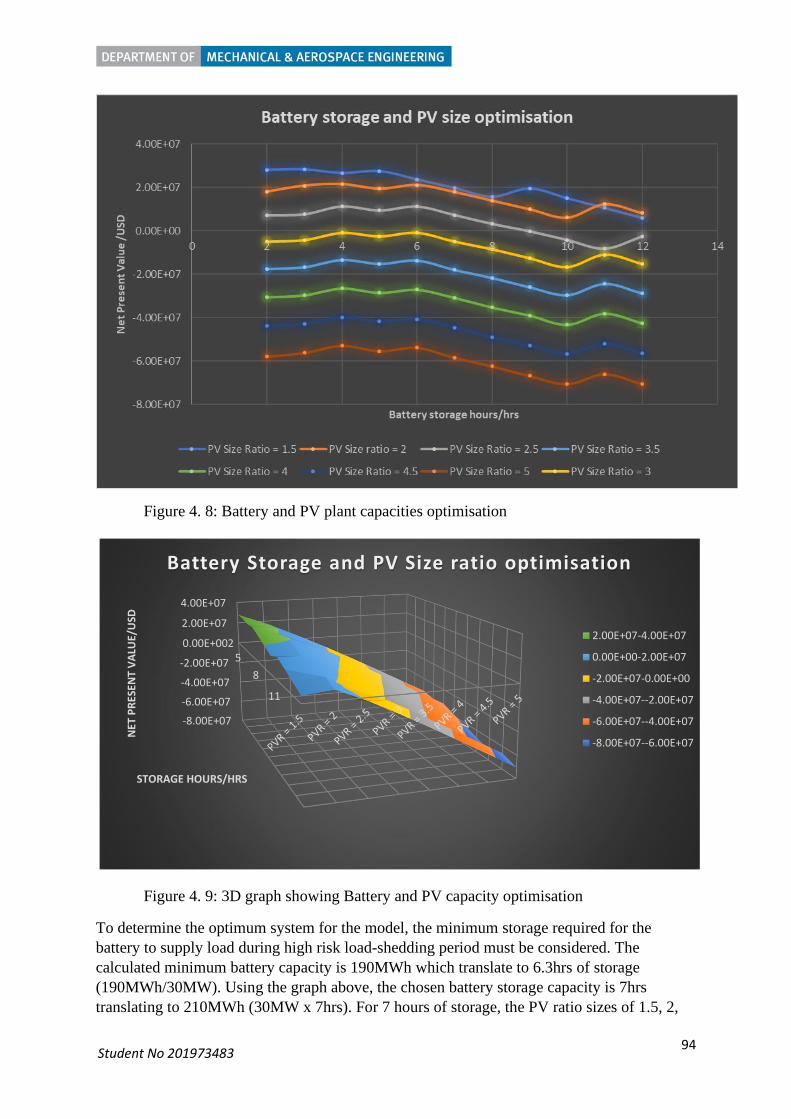
94 Student No 201973483

Figure 4. 8: Battery and PV plant capacities optimisation

Figure 4. 9: 3D graph showing Battery and PV capacity optimisation

To determine the optimum system for the model, the minimum storage required for the

battery to supply load during high risk load-shedding period must be considered. The

calculated minimum battery capacity is 190MWh which translate to 6.3hrs of storage

(190MWh/30MW). Using the graph above, the chosen battery storage capacity is 7hrs

translating to 210MWh (30MW x 7hrs). For 7 hours of storage, the PV ratio sizes of 1.5, 2,

-8.00E+07

-6.00E+07

-4.00E+07

-2.00E+07

0.00E+00

2.00E+07

4.00E+07

25

8

11

NET

PR

ESEN

T V

ALU

E/U

SD

STORAGE HOURS/HRS

Battery Storage and PV Size ratio optimisation

2.00E+07-4.00E+07

0.00E+00-2.00E+07

-2.00E+07-0.00E+00

-4.00E+07--2.00E+07

-6.00E+07--4.00E+07

-8.00E+07--6.00E+07

95 Student No 201973483

and 2.5 have a positive NPV value. The 2.5 PV size ratio was not chosen because the NPV

value was way below for the other two sizes. Although the 1.5 PV size ratio has a slight

better NPV value (by approximately USD2 million), the PV ratio of 2 performed better in

terms of annual energy produced hence chosen for the model.

The optimum combination chosen is:

• PV size ratio of 2 which translate to 2 x Peak power for PV without storage = 2 x

37MW DC (The designed PV system in section 3.3) = 74MW DC

• Power to Energy ratio of 1:7 translating to 7hrs of battery storage meaning battery

capacity of 210MWh

4.2.2 Technical performance of the optimised PV + Battery System

The simulation of the optimised 74MW DC PV plant + 210MWh of battery storage predicted

an annual energy output of 103GWh in the first year (lifecycle output is shown in Appendix

H). This is approximately 63% of the annual mine load – 41% from PV and 22% from

battery – as shown in the pie chart below (figure 4.10). The design was meant to cater for the

peak and standard periods which constitute about 68% of the load (from the load profile)

hence the system was 5% less from the target with the grid covering the slack.

Figure 4. 10: Energy distribution of the PV + Battery System

The expected capacity factor of the system is 18.6% with a performance ratio of 75% and a

battery roundtrip efficiency of 92.7%. The losses resembled that of the modelled PV with the

addition of the battery losses. As with the PV system, the most significant loss is the grid

connection limit with a value of around 13%. The full loss diagram is given in Appendix H.

On a typical good day of PV production, as shown in figure 4.11 below, the hybrid system is

able to supply the load over the designed periods (peak and standard). The PV plant will

supply the load alone from 7am to 2pm. The Battery and PV plant will supply the load from

2pm up to 5pm then the battery cover alone up to 9pm. The grid will then pick it up from

10pm to 6am which is off-peak period.

22%

37%

41%

Energy source distribution

Energy from battery Energy from Grid Energy from PV

96 Student No 201973483

Figure 4. 11: Typical two consecutive days with good PV production

The state of charge of the battery of the same period is shown in the figure 4.12 below. The

battery is charged by the PV plant between 7am to 12pm where it would have reached

maximum designed state of charge (95%). It would then discharge from 3pm to 9pm reaching

a state of charge of 40%.

Figure 4. 12: Battery state of charge on two consecutive days with good PV production

On a typical bad day (like cloudy day) for PV production, as shown in the figure 4.13 below,

the PV + Battery system only covers the load alone between 7am and 10am on the first day

of the period. The grid power will then be used thereafter with a little help from the PV plant

in the next day.

0

5000

10000

15000

20000

25000

30000

35000

40000

00

:00

02

:00

04

:00

06

:00

08

:00

10

:00

12

:00

14

:00

16

:00

18

:00

20

:00

22

:00

00

:00

02

:00

04

:00

06

:00

08

:00

10

:00

12

:00

14

:00

16

:00

18

:00

20

:00

22

:00

PO

WER

/W


PV to Battery Battery to Load Grid to Load PV to Load

0102030405060708090

100

00

:00

02

:00

04

:00

06

:00

08

:00

10

:00

12

:00

14

:00

16

:00

18

:00

20

:00

22

:00

00

:00

02

:00

04

:00

06

:00

08

:00

10

:00

12

:00

14

:00

16

:00

18

:00

20

:00

22

:00BA

TTER

Y S

TATE

OF

CH

AR

GE/

%

TIME/HRS

Typical battery state of charge on two clear days

97 Student No 201973483

Figure 4. 13: Typical two consecutive days with bad PV production

The state of charge of battery on the same period is shown in the figure 4.14 below. The PV

production is not enough to charge the battery and to cover the load. The battery will start

discharging from 44% up to 15% which is the minimum designed state of charge between

6am and 11am. The battery will stay in that state up until the PV production is high enough to

charge it again.

Figure 4. 14: Battery state of charge on two consecutive days with bad PV production

4.2.3 Economic performance of optimised PV + Battery System

The installed cost of PV + Battery system is USD 1.5/Wdc with the cost of storage

contributing 43.3%. The LCOE of the system is USD 0.106/kWh – this is more than double

than that of PV system alone. The predicted simple pay-back period is 10.8 years with an

0

5000

10000

15000

20000

25000

30000

PO

WER

/W


PV to Battery Battery to Load Grid to Load PV to Load

05

101520253035404550

00

:00

02

:00

04

:00

06

:00

08

:00

10

:00

12

:00

14

:00

16

:00

18

:00

20

:00

22

:00

00

:00

02

:00

04

:00

06

:00

08

:00

10

:00

12

:00

14

:00

16

:00

18

:00

20

:00

22

:00BA

TTER

Y S

TATE

OF

CH

AR

GE/

%

TIME/HRS

Typical battery state of charge on two cloudy days

98 Student No 201973483

NPV value of USD 19.26 Million. The table 4.3 below show the main economic indicators of

the project:

Table 4. 3: Economic performance indicators for the PV + Battery System



Annual Electric Bill without PV system USD 13.7 Million

Annual Electric Bill with PV system USD 3.0 Million




The first-year simulation results show that the annual electric bill is reduced from USD13.7

million to USD 3 million. This represents about 78% in electric bill reduction after offsetting

63% of the load. As with PV system, the difference in the two figures is because the grid

power is mainly used during off-peak period which is cheaper than the periods covered by the

PV + Battery system. The graph below (figure 4.15) shows the monthly bill of electricity

with PV + Battery and without.

Figure 4. 15: Monthly electric bill with PV + Battery system vs without

4.3 CSP Results

4.3.1 Design point optimisation

The graph below (figure 4.16) shows the variation of LCOE with design point DNI with

minimum LCOE occurring at 860W/m2. Values higher than this DNI have high LCOE

because the system is oversized and operates at design capacity for a limited time. Below

860W/m2, the LCOE is higher (even though the is more generated energy) because the solar

field area increase with low design point DNI hence increasing the installation cost.

0

0.2

0.4

0.6

0.8

1

1.2

1.4

Jan Feb Mar Apr May Jun Jul Aug Sep Oct Nov Dec

ELEC

TRIC

AL

BIL

L (U

SD/M

ILLI

ON

S)

Electrical Bill with System vs without

Bill with PV + Battery System Bill without Hybrid System

99 Student No 201973483

Figure 4. 16: Design point optimisation

4.3.2 Solar Multiple optimisation

The optimum solar multiple for the system from the graph (figure 4.17) below is 1.25. This

value is consistent with literature review that revealed that a solar multiple of 1.3 is a typical

optimum for no storage CSP system. Although the values higher than solar multiple 1.25

have higher energy produced, the increase in land size increases the LCOE.

Figure 4. 17: Solar multiple optimisation

4.3.3 Field subsections optimisation

The shape and location of header piping delivering heat to the power cycle is determined by

the number of field subsections. The orientation will directly affect the amount of heat loss in

the pipes. The graph below (figure 4.18) shows that the optimal number of subsections is 2

based on the lowest LCOE and highest generated energy.

16.2

16.4

16.6

16.8

17

17.2

17.4

700 720 740 760 780 800 820 840 860 880 900 920 940 960 980 1000

LCO

E (U

S C

ENTS

/KW

H)

DNI (W/M^2)

DNI Design point optimasation

0

5

10

15

20

25

1 1.25 1.5 1.75 2 2.25 2.5 2.75 3 3.25 3.5 3.75 4

LCO

E (U

S C

ENTS

/KW

H)

SOLAR MULTIPLE

Solar Multiple Optimisation

100 Student No 201973483

Figure 4. 18: Number of field subsections optimisation

4.3.4 Technical performance of the optimised CSP

The simulation of the optimised 32MW gross output, solar multiple of 1.25, and DNI design

point of 860W/m2 predicts a net annual electricity energy production of 39.3GWh during the

first year of operation (Summary results from SAM are given in Appendix I). This is

approximately 23.7% of annual demand of the mine with a capacity factor of 20.6%. The

predicted capacity factor compares with figures given in IRENA (2019) for no storage CSP

systems which has values ranging from 21% to 23%. The figure 4.19 below shows the

monthly production of CSP energy vs the monthly demand of the mine.

Figure 4. 19: Monthly generated CSP vs monthly demand

On a typical good day for CSP production, as shown in the figure 4.20 below, the system is

able to supply the load from 8:00am to 2:00pm. The grid power will start to compliment the

CSP after 2:00pm up until 4:00pm where CSP production will fall to zero. From then on, the

grid will supply the load up until the next day.

0

2

4

6

8

10

12

14

16

ENER

GY

/ G

WH

Load vs generated CSP energy

Load Generated CSP

101 Student No 201973483

Figure 4. 20: Typical two consecutive days with good CSP production

On a typical overcast day, as shown in the figure 4.21 below, the CSP system will be

absorbing power from the grid (for auxiliary circuits) instead of generating. The grid power

will supply the load during the day and night.

Figure 4. 21: Typical two consecutive days with bad CSP production

4.3.5 Economic performance of optimised CSP system

The installation costs of the system are predicted at USD 2479/kW. The IRENA renewable

cost database for CSP commissioned in 2019 showed installation costs ranging between USD

3704/kW and USD 8645/kW – with the exception that these figures are for systems with

storage hence higher. The predicted LCOE of the system is US cents 16.32/kWh which is

slightly lower to the weighted average of LCOE (US cents 18.2/kWh) of CSP system in 2019

(IRENA, 2019). However, the predicted NPV for the system is below zero making it

unattractive option to invest. The table 4.4 below show the main economic indicators of the

system:

-5000

0

5000

10000

15000

20000

25000

30000

00

:00

02

:00

04

:00

06

:00

08

:00

10

:00

12

:00

14

:00

16

:00

18

:00

20

:00

22

:00

00

:00

02

:00

04

:00

06

:00

08

:00

10

:00

12

:00

14

:00

16

:00

18

:00

20

:00

22

:00

PO

WER

/W


From Grid to load From CSP to Load

-5000

0

5000

10000

15000

20000

25000

30000

35000

00

:00

02

:00

04

:00

06

:00

08

:00

10

:00

12

:00

14

:00

16

:00

18

:00

20

:00

22

:00

00

:00

02

:00

04

:00

06

:00

08

:00

10

:00

12

:00

14

:00

16

:00

18

:00

20

:00

22

:00

PO

WER

/W

Typical two overcast days

From Grid to Load From CSP to Load

102 Student No 201973483

Table 4. 4: Economic performance indicators for the CSP System



Annual Electric Bill without CSP system USD 13.69 Million

Annual Electric Bill with CSP system USD 9.63 Million


Net Present Value USD -13.6 Million

Simple pay back Years Not available

The first-year simulation figures show that the annual electric bill is reduced from USD 13.69

million to 9.63 million. This represents a cost reduction of approximately 29.8% on the

annual electric bill after offsetting approximately 23.7% of the annual load. The figure 4.22

below shows the monthly bill of electricity with PV system and without.

Figure 4. 22: Monthly electric bill with CSP system vs without

4.4 CSP + TES Results

4.4.1 Storage hours and Solar multiple optimisation

A parametric analysis was carried out to determine the optimum storage hours and solar

multiple based on the load profile, location, desired dispatch and LCOE. The trends from the

two figures below (figure 4.23 and figure 4.24) show that for low values of SM (1 – 1.5) the

LCOE varies linearly, with a positive gradient, with TES storage hours. For solar multiple 2 –

4, low values of TES storage hours have high LCOE values which starts to decrease with

increase in storage hours. The optimum values of LCOE occur between storage hours

between 5 – 6 before the trend starts to increase gradually with increase in storage hours. This

is because at low values of storage hours, the energy produced will be too low to justify the

investment (the system will be undersized). At high values of storage hours, although the

energy produced will be high, the system will be oversized for the application hence higher

values of LCOE. From the analysis, optimum LCOE occurs at SM = 2.5 and storage hours of

5 hours.

0

0.2

0.4

0.6

0.8

1

1.2

1.4

ELEC

TRIC

AL

BIL

L (U

SD/M

ILLI

ON

S)


Without System With System

103 Student No 201973483

Figure 4. 23: 3D graph showing optimisation of storage hours and solar multiple

Figure 4. 24: Solar multiple and storage hours optimisation

For the system to cover the high-risk period from load shedding, the required storage hours

are 6.3 hours (calculated in section 4.2.1). Therefore, the optimum SM and storage hours

SM = 1

SM = 1.75

SM = 2.5

SM = 3.25

SM = 4

13

15

17

19

21

23

25

27

29

31

1 2 3 4 5 6 7 8 9 10 11 12 13 14

LCO

E (U

S C

ENTS

/KW

H)

STORAGE HOURS/ HRS

Storage hours and Solar Multiple optimisation

29-31

27-29

25-27

23-25

21-23

19-21

17-19

15-17

13-15

104 Student No 201973483

chosen for this project is 2.5 and 7 hours respectively – this combination has the lowest

LCOE at TES values greater than 6.3 hours.

4.4.2 Technical performance of the optimised CSP + TES system

The simulation of the optimised 32MW gross output, solar multiple of 2.5, storage hours of

7hrs at design point of 860W/m2 predicts an net annual electricity production of 68.4GWh

during the first year of operation (summary results from SAM are given in Appendix J). This

is approximately 41.3% of annual demand of the mine at a capacity factor of 40.5%. The

predicted capacity factor compares with figures given in IRENA (2012) for SM 2.5 and

storage of 7 which has values ranging from 42 – 45%. The figure 4.25 below shows the

monthly production of CSP + TES system vs the monthly demand of the mine:

Figure 4. 25: Monthly generated energy from CSP + TES vs monthly load

On a typically good day for CSP production, as shown in the figure 4.26 below, the CSP +

TES system is able to supply the load (without the grid) over the designed periods (7am to

9pm). The grid will supply the load during off-peak hours.

Figure 4. 26: Typical two consecutive days with good CSP production

0

2

4

6

8

10

12

14

16

ENER

GY

/ G

WH

Load vs Generated CSP + TES Energy

Load Generated CSP + TES

-5000

0

5000

10000

15000

20000

25000

30000

00

:00

02

:00

04

:00

06

:00

08

:00

10

:00

12

:00

14

:00

16

:00

18

:00

20

:00

22

:00

00

:00

02

:00

04

:00

06

:00

08

:00

10

:00

12

:00

14

:00

16

:00

18

:00

20

:00

22

:00

PO

WER

/W


Grid to Load CSP + TES to Load

105 Student No 201973483

The state of charge of TES on a typical good day is shown in figure 4.27 below. The graph

shows that the TES briefly discharges in the morning from 7am – 8am before being charged

from 8am to 12pm where it reaches a capacity just above 500 MWht. The TES will start to

discharge from 3pm to 10pm reaching a capacity of approximately 200MWht.

Figure 4. 27: TES state of charge on two consecutive days with good CSP production

On a typical overcast day, as shown in the figure 4.28 below, the CSP + TES system only

supply the load from 6am to 8am from storage before the grid power covers the slack. The

following day, the grid supplies the load without any contribution from CSP + TES system.

Figure 4. 28: Typical two consecutive days with bad CSP production

The state of charge of a typical overcast day is shown in the figure 4.29 below. The graph

shows that the TES discharges from a capacity of 100 MWht to zero between 6am to 8am.

The state of charge is maintained the following day up until the system receives direct

irradiation

0

100

200

300

400

500

600

00

:00

02

:00

04

:00

06

:00

08

:00

10

:00

12

:00

14

:00

16

:00

18

:00

20

:00

22

:00

00

:00

02

:00

04

:00

06

:00

08

:00

10

:00

12

:00

14

:00

16

:00

18

:00

20

:00

22

:00

STA

TE O

F C

HA

RG

E /

MW

HT

TIME/HRS

Typical TES state of charge on two clear days

-10000

-5000

0

5000

10000

15000

20000

25000

30000

35000

00

:00

02

:00

04

:00

06

:00

08

:00

10

:00

12

:00

14

:00

16

:00

18

:00

20

:00

22

:00

00

:00

02

:00

04

:00

06

:00

08

:00

10

:00

12

:00

14

:00

16

:00

18

:00

20

:00

22

:00

PO

WER

/W


From Grid to Load CSP + TES to Load

106 Student No 201973483

Figure 4. 29: TES state of charge on two consecutive days with bad CSP production

4.4.3 Economic performance of optimised CSP + TES system

The installation cost of the CSP + TES system is predicted at 5593.7/kW. This value is

comparable with IRENA database for CSP systems commissioned in 2019 which showed

installation cost ranging between USD 3704/kW and USD 8645/kW (IRENA, 2019). The

predicted LCOE of the system is US cents 15.44/kWh which is lower to the weighted average

LCOE (US cents 18.2/kWh) of CSP systems commissioned in 2019. However, the predicted

simple payback period is 20.9 years with a negative NPV value making the system

unattractive option to invest. The table 4.5 below shows the main economic indicators of the

system:

Table 4. 5: Economic performance indicators for the CSP + TES System






Net Present Value USD -17.3 Million


The first-year simulation figures show that the annual electric bill is reduced from 13.69

million to 6.54 million. This represents a cost reduction of approximately 52.2% on the

annual electric bill after offsetting approximately 41.3% of the annual load. The figure 4.30

below shows the monthly bill of electricity with CSP + TES system and without.

0

20

40

60

80

100

120

00

:00

02

:00

04

:00

06

:00

08

:00

10

:00

12

:00

14

:00

16

:00

18

:00

20

:00

22

:00

00

:00

02

:00

04

:00

06

:00

08

:00

10

:00

12

:00

14

:00

16

:00

18

:00

20

:00

22

:00

STA

TE O

F C

HA

RG

E /

MW

HT

TIME/HRS

Typical TES State of Charge on two overcast days

107 Student No 201973483

Figure 4. 30: Monthly electric bill with CSP + TES system vs without

4.5 Uncertainty and Sensitivity analysis for base case scenario Assumptions were made to the cost of parameters used in the above models. Uncertainty and

sensitivity analysis were carried out on each model to understand how uncertainty influence

the optimal design and to identify the most influential uncertain parameter. The parameters

were modelled over 100 samples using Monte Carlo technique in SAM software.

4.5.1 PV System

The table 4.6 below shows the cost parameters that were allowed to vary in the PV system:

Table 4. 6: Uncertain parameters for PV system

Parameter Base cost Distribution Standard deviation

Module cost USD 0.30/Wdc normal 50%

Inverter cost USD 0.05/Wac normal 20%

Balance of Plant cost USD 0.17/Wdc normal 15%

Land cost USD 11000/acre normal 50%

The table 4.7 and graph (figure 4.31) below show the results of the uncertainty analysis. The

90% confidence interval from the analysis ranges from US cents/kWh 3.12 to 6.05 for LCOE.

The NPV and simple pay back graphs are given in Appendix K.

Table 4. 7: Results of uncertainty analysis for PV system

Mean Variance P05 P95

LCOE (US cents/kWh) 4.76 0.77 3.12 6.05

NPV (USD) 4.14E+07 2.14E+13 34612505 50047255

Simple Pay Back (years) 5.13 1.20 3.08 6.74

0

0.2

0.4

0.6

0.8

1

1.2

1.4

ELEC

TRIC

AL

BIL

L (U

SD/M

ILLI

ON

)


Without System With System

108 Student No 201973483

Figure 4. 31: Uncertainty analysis LCOE distribution for PV system

The tornado chart from the sensitivity analysis is shown below (figure 4.32). The results

show that the PV module cost has the most influence on the LCOE followed by BOP cost

with the inverter cost having the least.

Figure 4. 32: Tornado chart showing the sensitivity analysis results for PV system

109 Student No 201973483

4.5.2 PV + Battery system

The table 4.8 below shows the cost parameters that were allowed to vary in the PV + Battery

system:

Table 4. 8: Uncertain parameters for PV + Battery system


Module cost USD 0.30/Wdc normal 50%

Inverter cost USD 0.05/Wac normal 20%

Battery cost USD 209/kWh normal 30%

Replacement cost USD 140/kWh normal 30%

Land cost USD 11000/acre normal 50%


90% confidence interval from the analysis ranges from US cents/kWh 7.95 to 12.64 for

LCOE. The NPV and simple pay back graphs are given in Appendix L.

Table 4. 9: Results of uncertainty analysis for PV + Battery system


LCOE (US cents/kWh) 10.67 1.83 7.95 12.64

NPV (USD) 1.93E+07 1.81096E+14 -301508 46345900

Simple pay back (years) 10.91 4.40 7.99 15.83

Figure 4. 33: Uncertainty analysis LCOE distribution for PV + Battery system

The tornado chart from the sensitivity analysis is shown in figure 4.34 below. The results

show that the Battery cost has the most influence on the LCOE followed by the module cost

with the inverter cost having the least.

110 Student No 201973483

Figure 4. 34: Tornado chart showing the sensitivity analysis results for PV + Battery system

4.5.3 CSP System

The table 4.10 below shows the cost parameters that were allowed to vary in the CSP system:

Table 4. 10: Uncertain parameters for CSP system


Solar Field cost USD 150/m2 Normal 30%

HTF cost USD 60/m2 Normal 20%

Power plant cost USD 910/kWe Normal 20%

Land cost USD 11000/acre Normal 50%



LCOE. The NPV graph is given in Appendix M.

Table 4. 11: Results of uncertainty analysis for CSP system


LCOE (US cents/kWh) 16.33 1.92 14.05 18.65

NPV (USD) -1.39E+07 2.82598E+13 -22795305 -5113653

111 Student No 201973483

Figure 4. 35: Uncertainty analysis LCOE distribution for CSP system

The tornado chart from the sensitivity analysis is shown (figure 4.36) below. The results

show that the Solar field cost has the most influence on the LCOE followed by the power

plant cost with the land cost having the least.

Figure 4. 36: Tornado chart showing the sensitivity analysis results for CSP system

112 Student No 201973483

4.5.4 CSP + TES

The table 4.12 below shows the cost parameters that were allowed to vary in the CSP + TES

system:

Table 4. 12: Uncertain parameters for CSP + TES system


Solar Field cost USD 150/m2 Normal 30%

HTF cost USD 60/m2 Normal 20%

Power plant cost USD 910/kWe Normal 15%

Storage cost USD 62/kWht Normal 30%

Land cost USD 11000/acre Normal 50%



LCOE. The NPV graph is given in Appendix M.

Table 4. 13: Results of uncertainty analysis for CSP + TES system


LCOE (US cents/kWh) 15.45 2.42 12.71 17.7

NPV -1.73E+07 1.07918E+14 -32378535 940789.3

Figure 4. 37: Uncertainty analysis LCOE distribution for CSP + TES system

The tornado chart from the sensitivity analysis is shown in figure 4.38 below. The results

show that the Solar field cost has the most influence on the LCOE followed by the storage

cost with the land cost having the least.

113 Student No 201973483

Figure 4. 38: Tornado chart showing the sensitivity analysis results for CSP + TES system

4.6 PV with Exports Results

4.6.1 Desired PV Plant Optimisation

A parametric study was carried out to determine the optimum size of the PV plant. The figure

4.39 below shows the variation of NPV with plant size. The NPV increases with increase of

plant size from 20MW to 60MW, where it peaks, before starting to decrease. From 20MW to

60MW, the PV plant is operating efficiently with the generated energy either being used for

local load or exported to the grid. After 60MW, although the energy produced is increasing,

the plant is no longer operating efficiently as some energy is being curtailed due to the grid

limit. From the analysis, the optimum PV plant size is 60MWdc hence chosen for the model.

114 Student No 201973483

Figure 4. 39: Desired PV plant size optimisation

4.6.2 Technical performance of PV model

The simulation of the optimised 60MWdc PV plant predicts an output of 99.7GWh during the

first-year operation (life cycle and loss diagram given in Appendix N). 65% of the generated

PV energy is used by the local mine load with the remaining 35% exported to the grid as

shown in the figure 4.40 below. However, most of the energy to supply the load is supplied

from the grid (61%) with the PV system only contributing 39% of the load as shown in the

figure 4.41 below.

Figure 4. 40: Generated PV Energy usage

65%

35%

Generated PV Energy Usage

PV to Load PV to Grid(Export)

115 Student No 201973483

Figure 4. 41: Energy source distribution

On a typical good day for PV production, as shown in the figure below 4.42, the PV system is

able to supply the mine load from 7:00am up to 2pm. During this period, the system will also

be exporting to the grid with a typical peak power exported reaching 25.5MW at 11am. By

around 3pm, there will no power being exported, and the grid power will start to compliment

the PV system to supply the mine load. From 4pm, the grid will be supplying the load alone

until the next day.

Figure 4. 42: Typical two good days for PV production

On a typical bad day for PV production, as shown in the figure 4.43 below, the generated PV

energy peak output is just above 5MW with no exports at any given point in time.

39%

61%

Energy Source distribution

PV to Load Grid to load

-5000

0

5000

10000

15000

20000

25000

30000

00

:00

02

:00

04

:00

06

:00

08

:00

10

:00

12

:00

14

:00

16

:00

18

:00

20

:00

22

:00

00

:00

02

:00

04

:00

06

:00

08

:00

10

:00

12

:00

14

:00

16

:00

18

:00

20

:00

22

:00

PO

WER

/W


Grid to load PV to Load PV to Grid (Export)

116 Student No 201973483

Figure 4. 43: Typical two bad days for PV production

4.6.3 Economic performance of PV model

The installation cost of the system is predicted at USD 0.76 per DC watt with the predicted

LCOE at US cents 4.34 per kWh. The NPV of the system is estimated at 47.7 million with a

simple pay-back period of 6.3 years. The table 4.14 below shows the main economic

indicators of the system:

Table 4. 14: Economic indicators for PV system








The simulation results show that the annual electric bill liable is reduced from USD 13.7

million to USD 6.17 million. This means by reducing the annual energy demand by 39% and

exporting 35% of the generated energy, the system is able to save about 55% of the annual

electric bill. The figure 4.44 below shows the monthly bill of electricity with PV system vs

without.

-5000

0

5000

10000

15000

20000

25000

30000

00

:00

02

:00

04

:00

06

:00

08

:00

10

:00

12

:00

14

:00

16

:00

18

:00

20

:00

22

:00

00

:00

02

:00

04

:00

06

:00

08

:00

10

:00

12

:00

14

:00

16

:00

18

:00

20

:00

22

:00

PO

WER

/ W


Grid to Load PV to load PV to Grid (Export)

117 Student No 201973483

Figure 4. 44: Monthly electric bill with PV system vs without

4.7 PV + Battery with exports

4.7.1 Battery and PV plant capacity optimisation

A parametric study was carried out to determine the optimum storage hours of the behind the

meter battery and corresponding PV size based on the load profile, desired operation, and

return on investment. The two figures below (figure 45 and 46) show that in general, the

smaller the PV plant size and the lower the storage hours the more viable the system. PV size

ratio of 5 is not viable for the whole range of storage hours while PV size ratio 1.5 to 3.5 is

viable for all analysed storage hours.

Figure 4. 45: Storage hours and PV plant optimisation for PV + Battery

0

0.2

0.4

0.6

0.8

1

1.2

1.4


ELEC

TRIC

AL

BIL

L (U

SD/M

ILLI

ON

)

Electricity bill with system vs without

Bill without system Bill with PV system

118 Student No 201973483

Figure 4. 46: 3D Battery storage and PV plant optimisation

To determine the optimum system, the minimum storage required for battery to supply load

during the high-risk load-shedding period must be considered. From section 4.2.1, the

minimum required storage hours are 7 hours. From the analysis, the PV size ratio with

maximum NPV at battery storage of 7 hours or more is 2. Therefore, the optimum battery

size is 210MWh with a PV plant size of 74MWdc.

4.7.2 Technical performance of PV + Battery

The simulation of the optimised 74MWdc PV plant + 210MWh of battery storage predicted

an annual output of 120.5 GWh in the first year (lifecycle and loss diagram are shown in

Appendix O). 55% of the generated energy by PV system is used to supply the load with 31%

used to charge the battery (and eventually supply the load) with the remaining 14% exported

to the grid as shown in figure 4.47 below. 63% of the load is supplied from local generation

(41% from PV and 22% from battery) with 37% supplied from the grid as shown in the figure

4.48 below.

PV

R =

1.5

PV

R =

2

PV

R =

2.5

PV

R =

3

PV

R =

3.5

PV

R =

4

PV

R =

4.5

PV

R =

5

-4.00E+07

-2.00E+07

0.00E+00

2.00E+07

4.00E+07

2

5

8

11

PV

SIZ

E R

ATI

O

NP

V /

USD

BATTERY STORAGE/HRS

Battery Storage and PV Size optimisation

2.00E+07-4.00E+07

0.00E+00-2.00E+07

-2.00E+07-0.00E+00

-4.00E+07--2.00E+07

119 Student No 201973483

Figure 4. 47: Generated PV Energy usage

Figure 4. 48: Energy source distribution for PV + Battery

On a typical good day of PV production, as shown in the figure 4.49 below, the hybrid

system is able to supply the load over the peak and standard periods. The PV plant will

supply the load alone from 7am to 2pm while at the same time charging the battery. Energy

exports starts -when the battery has reached full capacity – from 11 am up to 3pm. The

battery and PV plant will complement each other from 2pm to 5pm with the battery latter

suppling the load alone up to 9pm. The grid will supply the off-peak period from 10pm to

6am.

55%

14%

31%

Generated PV Energy Usage

PV to Load PV to Grid (Export) PV to Battery

41%

37%

22%


PV to Load Grid to Load Battery to Load

120 Student No 201973483

Figure 4. 49: Typical two good days for PV production

On a typical bad day for PV production, as shown in the figure 4.50 below, the hybrid system

only covers the load alone between 7am and 10am. The grid power will then be used

thereafter with a little help from PV plant in the next day. There will be no energy exports

during the period.

Figure 4. 50: Typical two bad days for PV production

4.7.3 Economic performance of the PV + Battery

The installation cost of the system is estimated at USD 1.5/Wdc with the predicted LCOE at

US cents 9.40 per kWh. The predicted NPV of the system is about USD 31.4 million with a

0

5000

10000

15000

20000

25000

30000

35000

40000

PO

WER

/WTypical two clear days

PV to Battery Battery to Load Grid to Load PV to Load PV to Grid (Export)

0

5000

10000

15000

20000

25000

30000

00

:00

02

:00

04

:00

06

:00

08

:00

10

:00

12

:00

14

:00

16

:00

18

:00

20

:00

22

:00

00

:00

02

:00

04

:00

06

:00

08

:00

10

:00

12

:00

14

:00

16

:00

18

:00

20

:00

22

:00

PO

WER

/W

Typical two cloudy day

PV to Battery Battery to Load Grid to load PV to Load PV to Grid(Export)

121 Student No 201973483

simple pay back of 9.7 years. The table 4.15 below shows the main economic indicators of

the system:

Table 4. 15: Economic indicators for PV + Battery








The first-year simulation results show that the annual electric bill liable is reduced from USD

13.7 million to USD 1.7 million. This means by reducing the annual load by 63% and

exporting 14% of the generated energy, the system is able to save about 86.6% of the annual

electric bill. The figure 4.51 below shows that in the month of October there will be a cash

inflow rather than outflow as far as electric bill is concerned.

Figure 4. 51: Monthly electric bill with system vs without for PV + Battery

4.8 CSP with exports results

4.8.1 Solar multiple and Power output optimisation

A parametric study was carried out to determine the optimum solar multiple and gross power

output. The figure 4.52 below shows that the LCOE reduces as SM varies from 1 to 1.75

before starting to increase. The variation of LCOE with gross output power is not significant

but the general trend is it is higher on the extremes (20MW and 60MW) and lowest between

40 – 50 MW. From the analysis, the lowest LCOE occurs at SM = 1.75 and gross power

output of 50MW.

-0.2

0

0.2

0.4

0.6

0.8

1

1.2

1.4


ELEC

TRIC

AL

BIL

L (U

SD/M

ILLI

ON

S)

Electricity bill with system vs without

Without system With system

122 Student No 201973483

Figure 4. 52: Solar Multiple and Gross power output optimisation

4.8.2 Technical performance of optimised CSP

The simulation of the optimised 50MW gross output, solar multiple of 1.75 and DNI design

point of 860W/m2 predicts a net annual electrical energy production of 94.7GWh during the

first-year operation (summary results from SAM are given in Appendix P). 49% of the

generated CSP energy is used to supply the load while 51% is exported to the grid as shown

in the figure 4.53 below. Energy supplied to the load covers 28% of the annual load with the

remaining 72% coming from the grid as shown below in figure 4.54.

Figure 4. 53: Generated CSP Energy Usage

20

30

40

50

6012.00

13.00

14.00

15.00

16.00

GR

OSS

PO

WER

OU

TPU

T /

MW

LCO

E (U

S C

ENTS

/KW

H)

SOLAR MULTIPLE

Solar Multiple and Gross Power Output Optimisation

15.00-16.00

14.00-15.00

13.00-14.00

12.00-13.00

49%51%

Generated CSP Energy Usage

CSP to load CSP to Grid (Export)

123 Student No 201973483

Figure 4. 54: Energy source distribution for CSP


able to supply the local load from 7:00am to 2pm. During this time, the system will also be

exporting power to the grid (with a typical peak power of 32MW). The energy exports stop at

around 3pm, with the grid power starting to compliment the CSP to supply the local load.

From 5pm, the grid power will be supplying the load alone up until the next day.

Figure 4. 55: Typical two good days for CSP production

On a typical bad day for CSP production, as shown in the figure 4.56 below, there will be

neither energy to cover the load nor to export to the grid. The grid will supply the load

(together with ancillary equipment like freeze protection heaters) during the day and night.

28%

72%


CSP to Load Grid to load

-5000

0

5000

10000

15000

20000

25000

30000

35000

00

:00

02

:00

04

:00

06

:00

08

:00

10

:00

12

:00

14

:00

16

:00

18

:00

20

:00

22

:00

00

:00

02

:00

04

:00

06

:00

08

:00

10

:00

12

:00

14

:00

16

:00

18

:00

20

:00

22

:00

PO

WER

/M

W


Grid to Load CSP to Load CSP to Grid (Export)

124 Student No 201973483

Figure 4. 56: Typical two bad days for CSP production

4.8.3 Economic performance of CSP

The installation cost of the system is predicted at 3347/kW with LCOE at US cents

12.13/kWh. The predicted NPV is USD 3.96 million with a simple pay-back period of 15.7

years. The main economic indicators of the system are given in the table 4.16 below:

Table 4. 16: Economic indicators for CSP








The first-year simulation results show that the amount of annual electric bill liable is reduced

from USD 13.69 million to 4 million. This means by reducing the annual load by 28% and

exporting 51% of the generated energy, the system is able to save about 70.6% of the annual

electric bill. The figure 4.57 below shows the monthly electric bill of the mine with system vs

without system:

-10000

-5000

0

5000

10000

15000

20000

25000

30000

35000

00

:00

02

:00

04

:00

06

:00

08

:00

10

:00

12

:00

14

:00

16

:00

18

:00

20

:00

22

:00

00

:00

02

:00

04

:00

06

:00

08

:00

10

:00

12

:00

14

:00

16

:00

18

:00

20

:00

22

:00

PO

WER

/ W



125 Student No 201973483

Figure 4. 57: Monthly electric bill with system vs without for CSP

4.9 CSP + TES with Exports Results

4.9.1 Desired Power Output Optimisation

A parametric study was carried out to determine the optimum output size for CSP + TES

system. As shown in the figure 4.58 below, there is little variation on LCOE with gross

power output. However, the analysis shows that the minimum LCOE occurs at power output

of 40MW.

Figure 4. 58: Desired power output optimisation for CSP + TES

4.9.2 Storage hours and Solar Multiple Optimization

The figure 4.59 below shows the results of the parametric analysis carried out to determine

the optimum solar multiple and storage hours. In general, the LCOE is higher for smaller

solar multiple values and decreases with increase in solar multiple reaching the trough at SM

= 2.25 to 2.75. For SM 1 to 1.5, the LCOE increases with increase in storage hours while for

SM 1.75 to 4, the LCOE is higher at the extremes of storage hours (1 and 14) with minimum

0

0.2

0.4

0.6

0.8

1

1.2

1.4


ELEC

TRIC

AL

BIL

L (U

SD /

MIL

LIO

NS)


Bill without System Bill with system

126 Student No 201973483

occurring between storage hours 5 and 7. The analysis shows that the optimum SM value is

2.5 and the minimum required storage hours for the system to supply the high risk period is

7hrs.

Figure 4. 59: Storage hours and Solar Multiple optimisations for CSP + TES

4.9.3 Technical performance of CSP + TES

The simulation of the optimised 40MW gross output, SM = 2.5, and storage hours of 7

predicts a net annual electrical energy of 127.4GWh during the first-year operation (summary

results from SAM are given in Appendix Q). 54% of the generated CSP + TES energy is used

to supply the local mine load with the remaining 46% exported to the grid as shown in the

figure 4.60 below. Energy supplied to the load covers 41% of the annual mine load with the

remaining 59% supplied from the grid as shown in the figure 4.61 below.

Figure 4. 60: Generated CSP + TES Energy use

SM =

1

SM =

1.5

SM =

2

SM =

2.5

SM =

3

SM =

3.5

SM =

4

10.0012.0014.0016.0018.0020.0022.0024.0026.00

1

3

5

7

9

11

13

LCO

E (U

S C

ENTS

/KW

H)

STORAGE HOURS/HRS

Storage hours and Solar Multiple optimisation

24.00-26.00

22.00-24.00

20.00-22.00

18.00-20.00

16.00-18.00

14.00-16.00

12.00-14.00

10.00-12.00

54%

46%

Generated CSP + TES Energy Use

CSP to load CSP to Grid (Export)

127 Student No 201973483

Figure 4. 61: Energy source distribution


able to supply the local mine load from 7am to 9pm while at the same time exporting to the

grid. The grid power is only used during off-peak period as per design.

Figure 4. 62: Typical two good days for CSP + TES production

On a typical bad day for CSP production, as shown in the figure 4.63 below, there will be

neither energy to cover the load nor to export to the grid. The grid will supply the load

(together with ancillary equipment like freeze protection heaters) during the day and night.

41%

59%

Energy Source distribution

CSP to Load Grid to load

-5000

0

5000

10000

15000

20000

25000

30000

00

:00

02

:00

04

:00

06

:00

08

:00

10

:00

12

:00

14

:00

16

:00

18

:00

20

:00

22

:00

00

:00

02

:00

04

:00

06

:00

08

:00

10

:00

12

:00

14

:00

16

:00

18

:00

20

:00

22

:00

PO

WER

/W



128 Student No 201973483

Figure 4. 63: Typical two bad days for CSP + TES production

4.9.4 Economic performance of CSP + TES

The installation cost of the system is predicted at USD 5546/kW with LCOE at US cents

10.45 per kWh. The predicted NPV is USD 28.6 million with simple pay back of 12.9 years.

The main economic indicators of the system are given in the table 4.17 below:

Table 4. 17: Main economic indicators for CSP + TES








The first-year simulation results show that the amount of annual electric bill liable is reduced

from USD 13.69 million to 0.472 million. This means by reducing the annual load by 41%

and exporting 46% of the generated energy, the system is able to save about 96.6% of the

annual electric bill. The CSP + TES system exports energy during the peak time where the

tariff is highest hence a higher return on investment. The figure 4.64 below shows 4 months

with cash inflows instead of outflows.

-10000

-5000

0

5000

10000

15000

20000

25000

30000

35000

00

:00

02

:00

04

:00

06

:00

08

:00

10

:00

12

:00

14

:00

16

:00

18

:00

20

:00

22

:00

00

:00

02

:00

04

:00

06

:00

08

:00

10

:00

12

:00

14

:00

16

:00

18

:00

20

:00

22

:00

PO

WER

/W


Grid to load CSP to Load CSP to Grid (Export)

129 Student No 201973483

Figure 4. 64: Monthly electric bill with CEP +TES system vs without

4.10 Discussion of Results The table 4.18 below shows the summary of key results from the analysis. The key points

from the results are:

• The addition of battery storage system to PV (on base case scenario) improved the

percentage of load offset by renewable system and the generated energy by the

renewable system by almost double. However, the installation cost, required land,

LCOE, and simple payback also increased by approximately a factor of 2 while the

NPV reduced by nearly half.

• The addition of thermal storage system to CSP (on base case scenario) increased the

generated energy, capacity factor, and renewable energy contribution by

approximately a factor of 2. Also, the LCOE improved due to increase in generated

energy. However, the land required for development and installation costs also nearly

doubled.

• For base case scenario, the CSP and CSP + TES system have a negative NPV making

them commercial unviable options. However, the two systems have positive NPV

values for export case. This concludes that CSP systems become more economically

viable as the size of the system (hence generated energy) increases.

• For both cases, PV system performed better than CSP system both on the technical

performance – generated energy, renewable energy contribution – and economic

performance – NPV, LCOE, and simple pay back

• In general, systems with exports performed better in terms of technical and economic

performance than base case scenarios. This is because the excess energy which could

have been clipped is exported gaining revenue in the process.

-0.4

-0.2

0

0.2

0.4

0.6

0.8

1

1.2

1.4

Jan Feb Mar Apr May Jun Jul Aug Sep Oct Nov DecELEC

TRIC

BIL

L (U

SD/M

ILLI

ON

S)

Electric bill with system vs without

Without system With system

130 Student No 201973483

Parameter No Export (base case) With Export

PV PV + Battery CSP CSP +

TES

PV PV + Battery CSP CSP +

TES

Installed capacity 37MWdc 74MW +

210MWh(7hrs)

32MW 32MW

+ 7hrs

60MWdc 74MW +

210MWh(7hrs)

50MW 40MW

+ 7hrs

Annual Energy generated (first year)/

GWh

55.1 104 39.3 68.4 99.7 121 94.7 127

Renewable Energy contribution (to

load)/ %

33.3 63 23.7 41.3 39 63 28 41

LCOE (US cents/ kWh) 4.76 10.67 16.32 15.44 4.34 9.4 12.13 10.45

NPV / USD Million 41.4 19.3 -13.9 -17.3 47.7 31.4 3.96 28.6

Energy Exported by System / % - - - - 35 14 51 46

Grid contribution (to load) / % 72.7 37 76.3 58.7 61 37 72 59

Installation Cost / USD 0.76/Wdc 1.5/Wdc 2.75/Wac 5.6/Wac 0.76/Wdc 1.5/Wdc 3.35/Wac 5.5/Wac

Land used / acres 114 228.2 178 355 185 228.2 383 437

Capacity Factor / % 19 18.6 20.6 40.5 19 18.6 24 40.4

Energy yield (kWh/kW) 1662 1629 1802 3552 1662 1629 2105 3540

Simple pay back / years 5.1 10.8 - 20.9 6.3 9.7 15.7 12.9

Annual Electric bill savings / USD

Million

5.67 10.7 4.1 7.15 7.52 12 9.68 13.2

Table 4. 18: Summary of key results

131 Student No 201973483

• For base case scenario PV + Battery system performed better than the CSP + TES

both technical and economic performance. With exports scenario, CSP + TES

generated more energy (which was largely exported) than the PV + Battery because

the simulated battery system was behind the meter hence exports were only limited to

excess energy generated by PV system. However, due to high installation costs of the

CSP + TES system, the PV + Battery performed better on the economic performance

regardless of producing less energy.

• In terms of renewable energy contribution and grid reliance, PV + Battery system out-

performed all other systems with 63% and 37% (on both scenarios) respectively. The

least performing system was CSP base case.

• In terms of NPV and LCOE, PV system with exports performed better than other

systems due to low installation cost and the ability to export energy (hence reduced

clipping and grid limit losses). CSP with no exports performed least on LCOE while

CSP + TES with no exports performed least as far as NPV is concerned.

• In terms of land use, the CSP + TES (with exports) required the biggest land for

development while PV base case required the least.

• As far as installation cost is concerned, CSP + TES has the highest cost while PV

system has the least. The sensitivity analyses showed that a reduction of about 30% in

installation costs will improve the economic performance of CSP + TES system.

From the analysis above, PV + Battery will be the recommended system for development.

This is mainly because the system was able to reduce the mine annual grid reliance to only

37% (considering that the dispatch design was not meant to include off-peak period which

constitute 32% of the annual mine load). CSP + TES has the potential to be competitive

economically if exports are allowed (hence bigger capacity) and installation cost reduce by at

least 30%.

132 Student No 201973483

5.0 Conclusion This research was aimed at analysing the technical and economic performance of CSP (+

thermal storage) and PV (+ battery storage) as applied to a typical mine in Zimbabwe. The

analysis showed that the PV + Battery models could offset about 63% of the annual mine

load. This is approximately double the contribution of PV system alone as the addition of

battery firmed up the generation of the renewable system. However, there is need to optimise

the PV size relative to the battery storage size (and load profile) as the analysis shows that the

larger the capacity of the two systems the lower the economic performance.

The CSP + TES system managed to offset about 41% of the annual mine load against 24%

(base case) of CSP alone. Design parameters like solar multiple, storage hours, design point

DNI, and solar field subsection need to be optimised based on the given demand profile. The

analysis shows that CSP systems performed better economically with exports allowed which

translates to bigger plant capacity.

Both the technical and economic performances of all the simulated models performed better

with the option to exporting to grid. For models with storage systems, the ability to export

energy during peak periods where the electricity tariff is highest certainly boosted the

economic performance thereof. With exports, CSP + TES LCOE was comparable to that of

PV + Battery (US cents 10.45/kWh vs 9.4/kWh respectively) something that was not the case

with no exports (US cents 15.44/kWh vs 10.67/kWh respectively).

The installation costs of CSP systems are currently still high when compared to PV systems.

For instance, CSP + TES installation cost was over double than that predicted for PV +

Battery. Also, the land required to develop the CSP technology is close to twice the land

required for PV systems.

The recommended system based on the analysis carried out will be the PV + Battery system.

The CSP + TES system shows great potential if the exports to the grid are allowed, bigger

load, and the installation cost thereof fall by at least 30%.

133 Student No 201973483

6.0 Future Work The exports scenario for PV + Battery was limited to behind the meter battery (due to

software limitation) hence did not fully utilise the potential of the battery system. When

simulating in-front of the meter battery in SAM there is no option for the system to supply

the local load. There is need to explore the PV + Battery (Infront of the meter hence battery

system can export to grid) where exports are allowed while suppling the local load. The

system promises to improve the economic performance and overall generated renewable

energy.

The combination of PV + CSP (+ Battery + TES) also need to be explored. The anticipated

benefits from theory include improved capacity factor and reduced LCOE. A dispatch

strategy will need to be formulated to exploit the unique characteristics of the systems. SAM

software can be used as it has a way to simulate combined cases and a platform to develop a

dispatch algorithm to control the combined cases.

The possibility of implementing demand side management at the mine like load shifting

while evaluating different renewable energy sources need to be analysed. For instance, the

possibility of utilising PV during the day to cover most of the load while reducing the peak

load but at the same time exporting energy from battery system (during peak period)

promises to have great economic benefits.

134 Student No 201973483

References Alsadi, S., Khatib, T., (2018), “Photovoltaic Power Systems Optimisation Research Status: A

Review of Criteria, Constrains, Models, Techniques, and Software tools”, Applied Sciences,

Vol. 8, page 1 – 30

Arrif, T., Benchabane, A., Germoui, M., Bezza, B., Belaid, A., (2018), ‘’Optimisation of

heliostat field layout for solar power tower systems using iterative artificial bee colony

algorithm: a review and case study’’, International Journal of Ambient Energy

Australian Renewable Energy Agency, 2017, ‘’Renewable Energy in the Australian mining

sector’’, available at https://arena.gov.au/knowledge-bank/renewable-energy-australian-

mining-sector/

Australian Renewable Energy Agency, (2018), ‘’Hybrid power generation for Australian off-

grid mines handbook, available at https://arena.gov.au/assets/2018/06/hybrid-power-

generation-australian-off-grid-mines.pdf

Batuecas, E., Mayo, C., Diaz, R., Perez, F.J., (2017), “Life cycle assessment of heat transfer

fluids in parabolic trough concentrating solar power technology”, Solar Energy Materials and

Solar Cells, Vol. 171, page 91- 97

Benitez, D., Kazantzidis, A., Al-Salaymeh, A., Bouaichaoui, S., Guizani, A., (2018),

“Combined CSP – PV plants for Mena Region”, GCREEDER 2018, Amman - Jordan, April

3rd – 5th 2018

Bhattacharya, P., Dey, S., Mustaphi, B., (2014), “Some analytical studies on the performance

of grid connected solar photovoltaic system with different parameters, Procedia Material

Science, Vol.6, page 1942-1950

Bousselamti, L., and, Cherkaoui, M., (2019), “Modelling and assessing the performance of

hybrid PV-CSP plants in Morocco: A Parametric study”, International Journal of

Photoenergy, Volume 2019, Article ID 5783927, 15 pages,

https://doi.org/10.1155/2019/5783927

Bravo, R. and Friedrich, D., (2018), ‘’Integration of energy storage with hybrid solar power

plant’’, Energy Procedia

Cerro Dominador website, (2020), https://cerrodominador.com/en/quienes-somos-en/

Cirocco, L., Belusko, M., Bruno, F., Boland, J., Pudney, P., (2014), ‘’Optimization of storage

for concentrated solar plants, Challenges, Vol. 5, page 473 – 503

Columbia Center on Sustainable Investment, (2018), ‘’The Renewable power of the mine –

Accelerating renewable energy integration’’, available at

http://ccsi.columbia.edu/files/2018/12/3418-CCSI-RE-and-mining-report-09-lr-reduced-

optmized-07-no-links.pdf

Dieckmann, S., Dersch, J., (2017), “Simulation of hybrid solar plants”, AIP Conference

Proceedings 1850, 16005 (2017), https://doi.org/10.1063/1.4984539

https://arena.gov.au/knowledge-bank/renewable-energy-australian-mining-sector/

https://arena.gov.au/knowledge-bank/renewable-energy-australian-mining-sector/

https://arena.gov.au/assets/2018/06/hybrid-power-generation-australian-off-grid-mines.pdf

https://arena.gov.au/assets/2018/06/hybrid-power-generation-australian-off-grid-mines.pdf

https://cerrodominador.com/en/quienes-somos-en/

http://ccsi.columbia.edu/files/2018/12/3418-CCSI-RE-and-mining-report-09-lr-reduced-optmized-07-no-links.pdf

http://ccsi.columbia.edu/files/2018/12/3418-CCSI-RE-and-mining-report-09-lr-reduced-optmized-07-no-links.pdf

https://doi.org/10.1063/1.4984539

135 Student No 201973483

Dieckmann, S., Dersch, J., (2015), “Techno – Economic evaluation of Renewable Energy

projects using software GREENIUS”, International journal of Thermal and Environmental

Engineering, Vol. 10 No. 1, page 17 – 24

Eddhibi, F., Amara B.M., Balghouthi, M., Guizani, A., (2015), ‘’Optimal study of solar tower

power plants’’, Journal of physics: Conference Series 596 (2015) 012018

Florin, N., Dominish, E., (2017), “Sustainability evaluation of energy storage technologies”,

Institute of Sustainable futures for the Australian Council of learned academics”, available at

https://acola.org/wp-content/uploads/2018/08/wp3-sustainability-evaluation-energy-storage-

full-report.pdf

Fouad, M.M., Shihata, A.L., Morgan, I.E., (2017), “An integrated review of factors

influencing the performance of photovoltaic panels”, Renewable Energy and Sustainable

Energy Reviews, Vol. 80, page 1499 – 1511

Gharbi, E.N, Derbal, H., Bouaichaoui, S., Said, H., (2011), ‘’A comparative study between

parabolic trough collector and linear Fresnel reflector technologies, Energy Procedia, Vol. 6,

page 565 – 572

Green, A., Diep, C., Dunn, R., Dent, J., (2015), ‘’High Capacity Factor CSP-PV Hybrid

Systems’’, Energy Procedia, Vol. 69, page 2049-2059

Green Energy System Analysis (GREENIUS), (2020), GREENIUS Manual Version

4.5.0.1052, DRL Solar Research, Available at

https://www.dlr.de/sf/de/Portaldata/73/Resources/sonstiges/greenius/Greenius_Manual.pdf

Hesse, C., H., Schimpe, M., kucevic, D., Jossen, A., “Lithium-ion battery storage system

design tailored for application in modern power grids, Energies, Vol 10, page 1-42

Homer help manual, (2020), https://www.homerenergy.com/products/pro/docs/index.html

IEA Energy Efficiency Indicators Database, (2019), ‘’Kew world energy statistics’’,

available at https://www.iea.org/reports/key-world-energy-statistics-2019

International Renewable Energy Agency (IRENA), (2012), ’’Renewable Energy

Technologies (CSP): Cost analysis series’’, Volume 1:Power sector, Issue 215, available at

https://www.irena.org/documentdownloads/publications/re_technologies_cost_analysis-

csp.pdf

International Renewable Energy Agency (IRENA), (2020), Renewable Power Generation

Costs in 2019’’ available at https://www.irena.org/publications

International Finance Corporation, (2015), “A project developer’s guide to utility-scale

photovoltaic power plants”, available at

https://www.ifc.org/wps/wcm/connect/topics_ext_content/ifc_external_corporate_site/sustain

ability-at-ifc/publications/publications_utility-scale+solar+photovoltaic+power+plants

International Renewable Energy Agency (IRENA), (2019), “Innovation landscape brief:

Behind-the-meter batteries”, available at https://www.irena.org/-

/media/Files/IRENA/Agency/Publication/2019/Sep/IRENA_BTM_Batteries_2019.pdf

https://acola.org/wp-content/uploads/2018/08/wp3-sustainability-evaluation-energy-storage-full-report.pdf

https://acola.org/wp-content/uploads/2018/08/wp3-sustainability-evaluation-energy-storage-full-report.pdf

https://www.dlr.de/sf/de/Portaldata/73/Resources/sonstiges/greenius/Greenius_Manual.pdf

https://www.homerenergy.com/products/pro/docs/index.html

https://www.iea.org/reports/key-world-energy-statistics-2019

https://www.irena.org/documentdownloads/publications/re_technologies_cost_analysis-csp.pdf

https://www.irena.org/documentdownloads/publications/re_technologies_cost_analysis-csp.pdf

https://www.irena.org/publications

https://www.ifc.org/wps/wcm/connect/topics_ext_content/ifc_external_corporate_site/sustainability-at-ifc/publications/publications_utility-scale+solar+photovoltaic+power+plants

https://www.ifc.org/wps/wcm/connect/topics_ext_content/ifc_external_corporate_site/sustainability-at-ifc/publications/publications_utility-scale+solar+photovoltaic+power+plants

https://www.irena.org/-/media/Files/IRENA/Agency/Publication/2019/Sep/IRENA_BTM_Batteries_2019.pdf

https://www.irena.org/-/media/Files/IRENA/Agency/Publication/2019/Sep/IRENA_BTM_Batteries_2019.pdf

136 Student No 201973483

International Renewable Energy Agency (IRENA), (2019), “Innovation landscape brief:

Utility scale batteries”, available at https://www.irena.org/-

/media/Files/IRENA/Agency/Publication/2019/Sep/IRENA_Utility-scale-batteries_2019.pdf

International Renewable Energy Agency (IRENA), (2020), Renewable Power Generation

Costs in 2019’’ available at https://www.irena.org/publications

INSEL website (2020), https://insel4d.ca/en/what-is-insel.html

Isalm, M.T., Huda, N., Abdullah, A.B., Saidur, R., (2018), ‘’A comprehensive review of state

of the art concentrating solar power technologies: Current status and research trends,

Renewable and Sustainable Energy Reviews, Vol. 91, page 987 – 1018

Ju, X., Xu, C., Hu, Y., Han, Y., Wei, G., Du, X., (2017), “A review on the development of

photovoltaic/Concentrated Solar (PV – CSP) hybrid system”, Solar Energy Materials and

Solar Cells, Vol. 161, page 305 – 327

Kuravi, S., Trahan, J., Goswam, Y.D., Rahman, M.M., Stefanokos, E.K., (2013), Thermal

energy storage technologies and systems for concentrating solar plants, Progress in Energy

and Combustion Science, page 1 – 35

Liu, H., Zhai, R., Fu, J., Wang, Y., Yang, Y., (2019), “Optimization study of thermal storage

PV – CSP integrated system based on GA – PSO algorithm”, Solar Energy, Vol. 184, page

391 – 409

Liu, M., Steven Tay, N.H., Bell, S., Belusko, M., Jacob, R., Will, W.S., Bruno, F., (2016),

‘’Review on concentrating solar plants and new developments in high temperature thermal

energy storage technologies’’, Renewable and Sustainable Energy Reviews, Vol. 53, pp

1411-1432

May, J., G., Davidson, A., Monahov, B., (2018), “Lead batteries for utility energy storage: A

review”, Journal of Energy Storage, Vol. 15, page 145 – 157

National Renewable Energy laboratory (NREL), (2013), Technical Report NREL/TP-6A20-

60272, available at https://www.nrel.gov/docs/fy14osti/60272.pdf

National Renewable Energy Laboratory, (2014), “Modelling Parabolic Trough systems”,

available at https://sam.nrel.gov/images/webinar_files/sam-webinars-2014-parabolic-trough-

systems.pdf

National Renewable Energy Laboratory, (2018), “Best practices for operation and

maintenance of photovoltaic and Energy Storage: 3rd Edition”, NREL/TP-7A40-73822,

available at https://www.nrel.gov/docs/fy19osti/73822.pdf

National Renewable Energy Laboratory, (2011), “Technical manual for the SAM physical

trough model”, NREL/TP-5500-51825, available at

https://www.nrel.gov/docs/fy11osti/51825.pdf

National Renewable Energy Laboratory, (2020), “Concentrating solar power best practice

study”, NREL/TP-5500-75763, available at https://www.nrel.gov/docs/fy20osti/75763.pdf

National Renewable Energy Laboratory, (2007), “Parabolic trough technology development”


https://www.irena.org/-/media/Files/IRENA/Agency/Publication/2019/Sep/IRENA_Utility-scale-batteries_2019.pdf

https://www.irena.org/-/media/Files/IRENA/Agency/Publication/2019/Sep/IRENA_Utility-scale-batteries_2019.pdf

https://www.irena.org/publications

https://insel4d.ca/en/what-is-insel.html


https://sam.nrel.gov/images/webinar_files/sam-webinars-2014-parabolic-trough-systems.pdf

https://sam.nrel.gov/images/webinar_files/sam-webinars-2014-parabolic-trough-systems.pdf





137 Student No 201973483

National Renewable Energy Laboratory (NREL), (2016), “Exploring the potential

competitiveness of utility-scale photovoltaics plus batteries with concentrating solar power,

2015-2030”, Technical report NREL/TP – 6A20 – 66592, available at


National Renewable Energy Laboratory, (2017), “Evaluating the technical and Economic

performance of PV plus storage power plants”, Technical report NREL/TP-6A20-68737,


Padilla, V.R., (2011), “Simplified methodology for designing parabolic trough solar power

plants”, available at

https://scholarcommons.usf.edu/cgi/viewcontent.cgi?referer=&httpsredir=1&article=4585&c

ontext=etd

Pan, C.A., Dinter, F., (2017), “Combination of PV and central receiver CSP plants for base

load power generation in South Africa”, Solar Energy, Vol. 146, page 379 – 388

Parrado, C., Girrard, A., Simon, F., Fuentealba, E., (2016), ‘’2050 LCOE projection for a

hybrid PV-CSP plant in the Atacama Desert in Chile’’, Energy, Vol 94, page 422-430

Petrollese, M., Cocco, D., (2016), “Optimal design of a hybrid CSP-PV plant for achieving

the full dispatchability of Solar Energy power plants”, Solar Energy, Vol. 137, page 447 –

489

PVSyst help manual, (2020), https://www.pvsyst.com/help/

Rocky Mountain Institute, (2019), ‘’Renewable resources at mine tracker’’, available at

https://rmi.org/our-work/industry-and-transportation/material-value-chains/renewable-

resources-at-mines-tracker/

SAM help manual, (2020), https://sam.nrel.gov/download.html

Schott solar, (2020), “Schott PTR 70 Receiver brochure” available at

https://www.schott.com/d/csp/370a8801-3271-4b2a-a3e6-

c0b5c78b01ae/1.0/schott_ptr70_4th_generation_brochure.pdf

Shahin, A., Shirouyehzad, H., Pourjavad, E., (2012), ‘’Optimal maintenance strategy: A case

study in mining industry’’, International Journal of Service and Operations Management, Vol

12, No.12, page 368-386

Singh, G., and, Singh, B.R., (2019), “Recent developments in hybrid solar power generation:

A review”, International Journal of Engineering research and technology, Vol. 8, Issue 06,

page 1019 – 1031

Solcast website, (2020), https://solcast.com/

Starke, A.R, Cardemil, D.M, Escobar, R., Lolle, S., (2018), “Multi-objective optimisation of

hybrid PTC + PV system using generic algorithm”, AIP Conference Proceedings 2033,

180011 (2018), https://doi.org/10.1063/1.5067183

TRNSYS website (2020), http://www.trnsys.com/index.html



https://scholarcommons.usf.edu/cgi/viewcontent.cgi?referer=&httpsredir=1&article=4585&context=etd

https://scholarcommons.usf.edu/cgi/viewcontent.cgi?referer=&httpsredir=1&article=4585&context=etd

https://www.pvsyst.com/help/

https://rmi.org/our-work/industry-and-transportation/material-value-chains/renewable-resources-at-mines-tracker/

https://rmi.org/our-work/industry-and-transportation/material-value-chains/renewable-resources-at-mines-tracker/

https://sam.nrel.gov/download.html

https://www.schott.com/d/csp/370a8801-3271-4b2a-a3e6-c0b5c78b01ae/1.0/schott_ptr70_4th_generation_brochure.pdf

https://www.schott.com/d/csp/370a8801-3271-4b2a-a3e6-c0b5c78b01ae/1.0/schott_ptr70_4th_generation_brochure.pdf

https://solcast.com/

https://doi.org/10.1063/1.5067183

http://www.trnsys.com/index.html

138 Student No 201973483

Turchi, Craig, S., Boyd, M., Kesseli, D., Kurup, P., Mehos, M., Neises, T., Sharan, P.,

Wagner, M., Wendelin, T., (2019).” CSP Systems Analysis – Final Project Report”, Golden,

CO: National Renewable Energy Laboratory. NREL/TP-5500-72856, available at


Vidyanandan, K.V., (2017), “An overview of factors affecting the performance of Solar PV

Systems”, Journal of Corporate planning, Issue 27, page 2-8

Zhai, R., Liu, H., Chen, Y., Yang, Y., (2017), “The daily and annual technical – economic

analysis of the thermal storage PV – CSP system into two strategies”, Energy conversion and

management, Vol. 154, page 56 – 67

Zhai, R., Chan, Y, Liu, H., Wu, H., Yang, Y., (2018), “Optimal design method of a hybrid

CSP-PV plant based on Generic Algorithm considering the operational strategy”,

International Journal of Photoenergy, Volume 2018, Article ID 8380276, 15 pages

https://doi.org/10.1155/2018/8380276

Ziuka, S., Seyetin, L., Mapurisa, B., Chikodzi, D., van Kuijk, K., (2014), ‘’Potential of

concentrated solar power (CSP) in Zimbabwe’’, Energy for sustainable development, No. 23,

pp 220-227

Zurita, A., Mata-Torres, C., Valenzuela, C., Felbol, C., Cardemil, J.M., Guzman, A.M,

Escobar, R.A, (2018), ‘’Techno-economic evaluation of a hybrid CSP + PV plant integrated

with thermal storage and a large scale battery energy storage system for base generation’’,

Solar Energy, Vol 173, page 1262-1277

Zurita, A., Mata-Torres, C., Cardemil, J.M., Escobar, A.R., (2020), “Assessment of time

resolution impact on the modelling of a hybrid CSP-PV plant: A case of study in Chile”,

Solar Energy, Vol. 202, page 553 – 570


139 Student No 201973483

Appendix A – Characteristics of CSP (Islam et al, 2018)

Parabolic-trough collector

(PTC)

Linear Fresnel

reflectors (LFR) Solar power tower (PTC)

Solar parabolic dishes

(SPD)

Capacity (MWe) 10-200 10-200 10-150 0.01-0.4

Concentration ratio 25-100 70-80 300-1000 1000-3000

Solar efficiency max 20% (expected) 21% (demonstrated) 20% (demonstrated) 35%

(expected) 29%(demonstrated)

Annual solar-to-electric efficiency 15% 8-10% 20-35% (concepts) 20-35%

Optical efficiency Medium Low Medium High

Collector concentration 70-80 suns > 60 suns (depends on

secondary reflector) > 1000 suns >1300 suns

Receiver/absorber Absorber attached to collector, moves

with collector, complex design

Fixed absorber, no

evacuation, secondary

reflector

External surface or cavity

receiver, fixed

Absorber attached to the

collector, moves with

collector

Area requirement (m²/MWh) 4 to 6 6 to 8 8 to 12 30 to 40

Thermal efficiency (%) 30-40 - 30-40 30-40

Plant peak efficiency (%) 14-20 18 23-35 ~30

Capital cost (US$/kW) 3972 - 4000+ 12578

Capital cost (US$/m^2) 424 234 476 -

Operation and maintenance cost ($/kW

h) 0.012 − 0.02 low 0.034 0.21

Basic plant cost (US$/W) 3.22 - 3.62 2.65

Land use (m^2/MW h/year) 6 to 8 4 to 6 8 to 12 8 to 12

Specific power (W/m2) 300 - 300 200

Water requirement (m^3/MWh)

3 (wet cooling), 0.3 (dry cooling) and

0.4-1.7 (hybrid) 3(wet cooling) and 0.2 (dry

cooling)

2-3 (wet cooling), 0.25 (dry

cooling) 0.05-0.1 (mirror washing)

Annual CF (%) 25-28 (no TES), 29-43 (7 h TES) 22-24 55 (10 h TES) 25-28

Grid stability Medium to high (TES or

hybridization)

Medium (back-up firing

possible) High (large TES) low

Operating temperature of solar field (°C) 290-550

250-390, possible up to

560° C 250-650 800

140 Student No 201973483

Appendix B – Type and Characteristics of PV Cells (International Finance

Corporation, 2015)

Technology Crystalline

Silicon

Heterojunction

with intrinsic

Thin-film

Layer

Amorphous

Silicon

Cadmium

Telluride

Copper

Indium

Gallium Di

Selenide

Category c-Si HIT a-Si CdTe CIGS or CIS

Current

commercial

efficiency

(Approx.)

13%-21% 18%-20% 6%-9% 8%-16% 8%-14%

Temperature co-

efficient for

power a (Typical)

-0.45%/oC 0.29%/oC -0.21%/oC -0.25%/oC -0.35%/oC

141 Student No 201973483

Appendix C – SAM Calculations for LCOE and NPV

Where:

• Qn (kWh) is the electricity generated by the system in year n

• N is the analysis period in years

• C0 is project equity investment amount

• Cn is project annual costs in year n

• dnominal is the discount rate

Where:

• Cn is the after-tax cash flow in year n

• N is the analysis period in years

• dnominal is the discount rate

•

Capacity factor in SAM

𝐶𝑎𝑝𝑎𝑐𝑖𝑡𝑦 𝑓𝑎𝑐𝑡𝑜𝑟 =𝑁𝑒𝑡 𝑎𝑛𝑛𝑢𝑎𝑙 𝐸𝑛𝑒𝑟𝑔𝑦 (𝑘𝑊ℎ𝑎𝑐/𝑦𝑒𝑎𝑟

𝑆𝑦𝑠𝑡𝑒𝑚 𝑐𝑎𝑝𝑎𝑐𝑖𝑡𝑦 (𝑘𝑊𝑑𝑐 𝑜𝑟 𝑘𝑊𝑎𝑐)𝑥 8760ℎ𝑟𝑠

142 Student No 201973483

Appendix D – Configurations of Air Cooled Condensers (Padilla, 2011)

A frame air cooled condensor

Air cooled heat exchanger using horizontal tubes: forced draft

143 Student No 201973483

Air cooled heat exchanger using horizontal tubes: induced draft

144 Student No 201973483

Appendix E – Moody Chart (NREL, 2014)

145 Student No 201973483

Appendix F – PV System Loss Diagram and Lifetime production

146 Student No 201973483

Appendix G – PVSyst Summary results

147 Student No 201973483

Appendix H– PV + Battery Loss diagram and Lifetime energy production

148 Student No 201973483

Appendix I – Summary results of CSP system

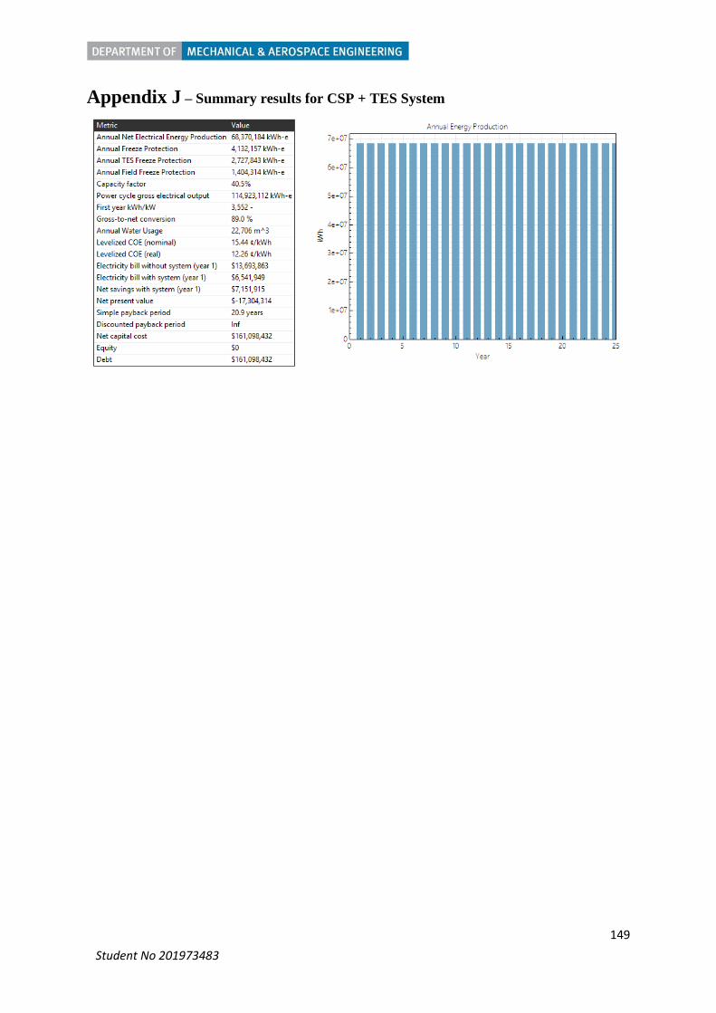
149 Student No 201973483

Appendix J – Summary results for CSP + TES System

150 Student No 201973483

Appendix K – Uncertainty Analysis for PV System

151 Student No 201973483

Appendix L – Uncertainty analysis for PV + Battery

152 Student No 201973483

Appendix M – Uncertainty analysis CSP and CSP + TES

153 Student No 201973483

Appendix N – PV with Exports loss diagram and lifetime production

154 Student No 201973483

Appendix O – PV + Battery with Exports loss diagram and lifetime production

155 Student No 201973483

Appendix P – Summary results for CSP with Exports

156 Student No 201973483

Appendix Q – Summary results for CSP + TES with exports

Modelling and Assessing CSP and PV systems technical and ...

Documents

Transcript of Modelling and Assessing CSP and PV systems technical and ...