Modelling and adaptive control ofaerobic continuous stirred tank reactorsP. Georgieva�, A. Ilchmanny, M.-F. WeirigzApril 2000AbstractA biotechnological aerobic process is modelled as an ordinary di�erential equationwhich, under mild assumptions, ensures invariance of the positive orthant and bound-edness of the concentrations. An adaptive controller is designed for this general classof processes so that the external substrate can be regulated by the dilution rate intoa prespeci�ed arbitrarily small neighbourhood of a constant setpoint reference. Theadaptive controller is robust, simple in its design without invoking any identi�cationmechanisms, and is based on output data only. It is shown that the prominent ex-ample of a baker's yeast fermentation belongs to this setup, and adaptive tracking isillustrated by simulations.Keywords: Adaptive control, input saturation, tracking, aerobic processes, yeast fer-mentation1 IntroductionThe purpose of the paper is threefold. First, it is a contribution to the general mod-elling of biotechnological aerobic processes including proofs which show that the intuitiveassumptions ensure mathematically what is expected from a real process. Secondly, weintroduce a simple adaptive controller with saturation which, under mild assumptions, isproved to achieve tracking of an external substrate within a prespeci�ed neighbourhood ofa setpoint. Thirdly, a well known example of baker's yeast fermentation is further inves-tigated and shown to be a special case of the proposed general model. Finally, adaptivetracking is illustrated for this example.

� Bulgarian Academy of Sciences, Institute of Control and System Research, P.O. Box 79, 1113 So�a,Bulgaria, pgeorgieva@iusi.bas.bgy Institute of Mathematics, Technical University Ilmenau, Weimarer Stra�e 25, 98693 Ilmenau, FRG,ilchmann@mathematik.tu-ilmenau.dez Alfred Wegener Institute for Polar and Marine Research, P.O. Box 120161, 27515 Bremerhaven, FRG,mweirig@awi-bremerhaven.de

We consider general biotechnological aerobic processes modelled by ordinary di�erentialequations of the form_x(t) = K '�x(t); O(t)� � D(t)x(t) � Qx(t) + F �D(t); xin(t)�;_O(t) = KO '�x(t); O(t)� � D(t)O(t) + �La[O� �O(t)]; (1.1)where, for n 2 N and n > m 2 N, the constants and variables denotex(t) = �x1(t); : : : ; xn(t)�T concentrations of the n chemical species at time t,O(t) concentration of dissolved oxygen at time t,K = [k1; : : : ; km] 2 Rn�m stoichiometric matrix,KO = [kO1; : : : ; kOm] 2 R1�m stoichiometric oxygen vector,Q = diagfq1; : : : ; qng 2 Rn�n�0 proportional gaseous out ow rates,�La[O� �O(t)] oxygen transfer rate with oxygen feed concentrationO� and oxygen mass transfer constant �La > 0,' = �'1; : : : ; 'm�T reaction rate vector, where'j(�; �) : Rn+1�0 ! R�0 are locally Lipschitz continuous functions,j = 1; : : : ;m,xin(�) : R�0 ! Rn�0 piecewise continuous and bounded function ofxin(t) = �xin1 (t); : : : ; xinn (t)�T n feed concentrations at time tD(�) : R�0 ! [0;Dsup] piecewise continuous function of dilution rate withDsup > 0.Furthermore, the following structural assumptions of (1.1) are assumed.(A1) There exists 2 Rn>0 such Tkj � 0 for all columnsk1; : : : ; km of the stoichiometric matrix K.(A2) F (t) = D(t)xin(t) for all t � 0.(A3) For j = 1; : : : ;m we have:'j(x;O) = �j(x;O) � Qi2Autj[Lj xifor locally Lipschitz continuous functions �j(�; �) : Rn+1�0 ! R�0 ;if 'j(x;O) = 0, then at least one of the components of (x;O) is 0;KO'(x; 0) = 0.Assumptions(A1)-(A3) are discussed in detail in Section 2.(A1) ensures that _x(t) = K '�x(t); O(t)� is dissipative. This replaces the classical as-sumption of Conservation of Mass. We do not suppose that the matrix K contains exactstoichiometric coe�cients. Our approach should encompass models which contain onlythe essential reactions and essential substrates, and we also allow for uncertainty of the2

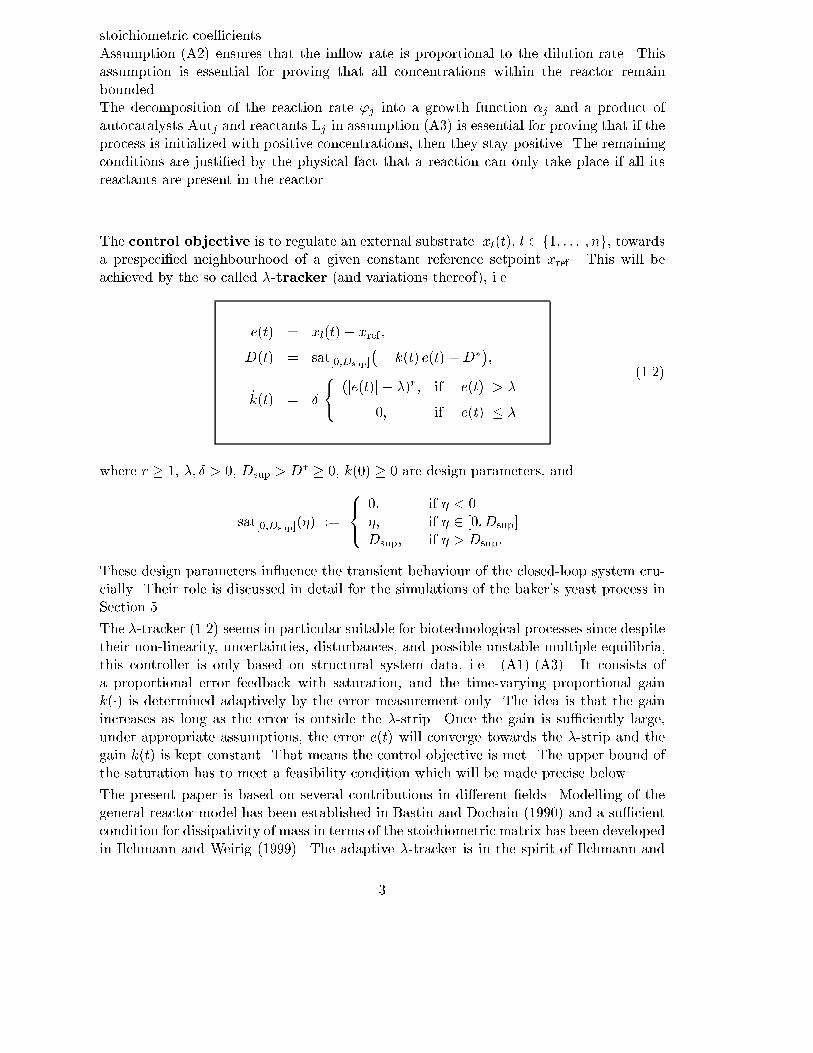
stoichiometric coe�cients.Assumption (A2) ensures that the in ow rate is proportional to the dilution rate. Thisassumption is essential for proving that all concentrations within the reactor remainbounded.The decomposition of the reaction rate 'j into a growth function �j and a product ofautocatalysts Autj and reactants Lj in assumption (A3) is essential for proving that if theprocess is initialized with positive concentrations, then they stay positive. The remainingconditions are justi�ed by the physical fact that a reaction can only take place if all itsreactants are present in the reactor.The control objective is to regulate an external substrate xl(t), l 2 f1; : : : ; ng, towardsa prespeci�ed neighbourhood of a given constant reference setpoint xref . This will beachieved by the so called �-tracker (and variations thereof), i.e.e(t) = xl(t)� xref ;D(t) = sat[0;Dsup]�� k(t) e(t) +D��;_k(t) = � ( (je(t)j � �)r; if je(t)j > �0; if je(t)j � � (1.2)where r � 1, �; � > 0, Dsup > D� � 0, k(0) � 0 are design parameters, andsat[0;Dsup](�) := 8<: 0; if � < 0�; if � 2 [0;Dsup]Dsup; if � > Dsup:These design parameters in uence the transient behaviour of the closed-loop system cru-cially. Their role is discussed in detail for the simulations of the baker's yeast process inSection 5.The �-tracker (1.2) seems in particular suitable for biotechnological processes since despitetheir non-linearity, uncertainties, disturbances, and possible unstable multiple equilibria,this controller is only based on structural system data, i.e. (A1)-(A3). It consists ofa proportional error feedback with saturation, and the time-varying proportional gaink(�) is determined adaptively by the error measurement only. The idea is that the gainincreases as long as the error is outside the �-strip. Once the gain is su�ciently large,under appropriate assumptions, the error e(t) will converge towards the �-strip and thegain k(t) is kept constant. That means the control objective is met. The upper bound ofthe saturation has to meet a feasibility condition which will be made precise below.The present paper is based on several contributions in di�erent �elds. Modelling of thegeneral reactor model has been established in Bastin and Dochain (1990) and a su�cientcondition for dissipativity of mass in terms of the stoichiometric matrix has been developedin Ilchmann and Weirig (1999). The adaptive �-tracker is in the spirit of Ilchmann and3

Ryan (1994), where it is introduced for linear systems and without any input saturations.In Ilchmann et al. (1998) adaptive �-tracking of an external substrate of a general reactormodel was achieved by using the feedrate as the input variable; it also was assumedthat the dilution rate is bounded away from zero. However, if aerobic continuous stirredtank reactors are modelled by lumping together the reaction equations in (1.1) to someddt(x;O)T = ~K'(x;O), then in this general form one cannot derive boundedness of theconcentrations of the general model. This is exactly the reason why the oxygen dynamicshave to be separated as in (1.1), and a new proof for �-tracking has to be developed. A�rst approach in this direction can be found in Weirig (1998).The paper is organised as follows. In Section 2 we introduce and motivate assumptions ofthe general model (1.1) so that it is su�ciently general to encompass relevant biochemicalprocesses, and su�ciently strict to derive mathematically properties of the process whichare intuitively expected. In Section 3 the adaptive feedback strategy to regulate an externalsubstrate to a prespeci�ed neighbourhood of the setpoint reference is introduced andproved to meet the control objective under certain assumptions. In Section 4 a wellknown model for baker's yeast fermentation is further investigated and shown that it fallsinto our general setup. This example is also used to illustrate the adaptive controller bysome simulations in Section 5.2 General modelling of bio-chemical aerobic processesAerobic biotechnological processes consist of a set of m reactions '1; : : : ; 'm involvingn + 1 concentrations x1; : : : ; xn+1 in the liquid phase of the reactor. Such a process iscommonly speci�ed by the following reaction scheme for each jth reaction:'jPi2Lj cij xi �! Pi2Rj cij xi; j = 1; : : : ;m: (2.1)Here Lj � f1; : : : ; n+ 1g; Lj 6= ;denotes the set of indices of the components xi which are the reactants of the jth reaction,Rj � f1; : : : ; n+ 1g; Rj 6= ;is the set of indices of the components xi which are the reaction products of the jthreaction.The quantities of each component involved in the reaction are speci�ed by the nonnegativestoichiometric coe�cients cij , sometimes also called yield coe�cients. The rate of con-sumption of the reactants, which is equal to the rate of formation of the reaction products,is called the reaction rate and denoted by 'j . For a comprehensive list of reaction ratessee for instance the Appendix in Bastin and Dochain (1990). The reaction rate 'j is often4

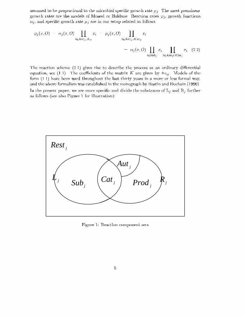
assumed to be proportional to the microbial speci�c growth rate �j. The most prominentgrowth rates are the models of Monod or Haldane. Reaction rates 'j , growth functions�j, and speci�c growth rate �j are in our setup related as follows.'j(x;O) = �j(x;O) Yi2Autj[Lj xi = �j(x;O) Yi2Autj[Catj xi= �j(x;O) Yi2Subj xi Yi2Autj[Catj xi (2.2)The reaction scheme (2.1) gives rise to describe the process as an ordinary di�erentialequation, see (1.1). The coe�cients of the matrix K are given by �cij . Models of theform (1.1) have been used throughout the last thirty years in a more or less formal way,and the above formalism was established in the monograph by Bastin and Dochain (1990).In the present paper, we are more speci�c and divide the substrates of Lj and Rj furtheras follows (see also Figure 1 for illustration):jRest

jAut

jSub jCatjProdjL

jR

Figure 1: Reaction component sets5

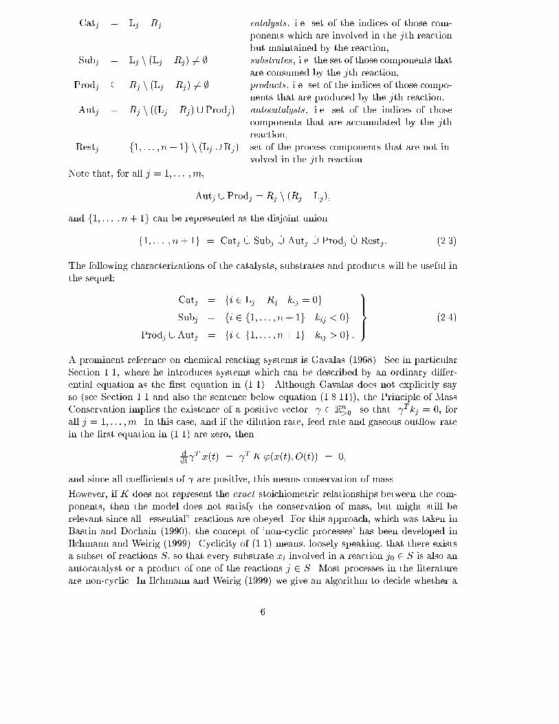
Catj = Lj \Rj catalysts, i.e. set of the indices of those com-ponents which are involved in the jth reactionbut maintained by the reaction,Subj = Lj n (Lj \Rj) 6= ; substrates, i.e. the set of those components thatare consumed by the jth reaction,Prodj � Rj n (Lj \Rj) 6= ; products, i.e. set of the indices of those compo-nents that are produced by the jth reaction,Autj = Rj n ((Lj \Rj) [ Prodj) autocatalysts, i.e. set of the indices of thosecomponents that are accumulated by the jthreaction,Restj = f1; : : : ; n+ 1g n (Lj [Rj) set of the process components that are not in-volved in the jth reaction.Note that, for all j = 1; : : : ;m,Autj [ Prodj = Rj n (Rj \ Lj);and f1; : : : ; n+ 1g can be represented as the disjoint unionf1; : : : ; n+ 1g = Catj _[ Subj _[ Autj _[ Prodj _[ Restj : (2.3)The following characterizations of the catalysts, substrates and products will be useful inthe sequel: Catj = fi 2 Lj \Rj j kij = 0gSubj = fi 2 f1; : : : ; n+ 1g j kij < 0gProdj [Autj = fi 2 f1; : : : ; n+ 1g j kij > 0g : 9>>=>>; (2.4)A prominent reference on chemical reacting systems is Gavalas (1968). See in particularSection 1.1, where he introduces systems which can be described by an ordinary di�er-ential equation as the �rst equation in (1.1). Although Gavalas does not explicitly sayso (see Section 1.1 and also the sentence below equation (1.8.11)), the Principle of MassConservation implies the existence of a positive vector 2 Rn>0 so that T kj = 0, forall j = 1; : : : ;m. In this case, and if the dilution rate, feed rate and gaseous out ow ratein the �rst equation in (1.1) are zero, thenddt T x(t) = T K '(x(t); O(t)) = 0;and since all coe�cients of are positive, this means conservation of mass.However, if K does not represent the exact stoichiometric relationships between the com-ponents, then the model does not satisfy the conservation of mass, but might still berelevant since all \essential" reactions are obeyed. For this approach, which was taken inBastin and Dochain (1990), the concept of `non-cyclic processes' has been developed inIlchmann and Weirig (1999). Cyclicity of (1.1) means, loosely speaking, that there existsa subset of reactions S, so that every substrate xi involved in a reaction j0 2 S is also anautocatalyst or a product of one of the reactions j 2 S. Most processes in the literatureare non-cyclic. In Ilchmann and Weirig (1999) we give an algorithm to decide whether a6

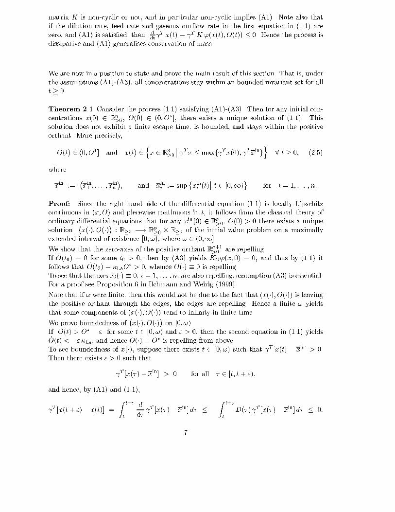
matrix K is non-cyclic or not, and in particular non-cyclic implies (A1). Note also thatif the dilution rate, feed rate and gaseous out ow rate in the �rst equation in (1.1) arezero, and (A1) is satis�ed, then ddt T x(t) = T K '(x(t); O(t)) � 0. Hence the process isdissipative and (A1) generalises conservation of mass.We are now in a position to state and prove the main result of this section. That is, underthe assumptions (A1)-(A3), all concentrations stay within an bounded invariant set for allt � 0.Theorem 2.1 Consider the process (1.1) satisfying (A1)-(A3). Then for any initial con-centrations x(0) 2 Rn>0 , O(0) 2 (0; O�], there exists a unique solution of (1.1). Thissolution does not exhibit a �nite escape time, is bounded, and stays within the positiveorthant. More precisely,O(t) 2 (0; O�] and x(t) 2 nx 2 Rn>0 �� Tx � maxf Tx(0); T xingo 8 t � 0; (2.5)wherexin := �xin1 ; : : : ; xinn �; and xini := sup�xini (t)�� t 2 [0;1) for i = 1; : : : ; n:Proof: Since the right hand side of the di�erential equation (1.1) is locally Lipschitzcontinuous in (x;O) and piecewise continuous in t, it follows from the classical theory ofordinary di�erential equations that for any xin(0) 2 Rn>0 , O(0) > 0 there exists a uniquesolution �x(�); O(�)� : R�0 �! Rn�0 � R�0 of the initial value problem on a maximallyextended interval of existence [0; !), where ! 2 (0;1].We show that the zero-axes of the positive orthant Rn+1>0 are repelling.If O(t0) = 0 for some t0 > 0, then by (A3) yields KO'(x; 0) = 0, and thus by (1.1) itfollows that _O(t0) = �LaO� > 0, whence O(�) � 0 is repelling.To see that the axes xi(�) � 0, i = 1; : : : ; n, are also repelling, assumption (A3) is essential.For a proof see Proposition 6 in Ilchmann and Weirig (1999).Note that if ! were �nite, then this would not be due to the fact that (x(�); O(�)) is leavingthe positive orthant through the edges, the edges are repelling. Hence a �nite ! yieldsthat some components of (x(�); O(�)) tend to in�nity in �nite time.We prove boundedness of �x(�); O(�)� on [0; !).If O(t) > O� + " for some t 2 [0; !) and " > 0, then the second equation in (1.1) yields_O(t) < �" �La, and hence O(�) � O� is repelling from above.To see boundedness of x(�), suppose there exists t 2 [0; !) such that T [x(t) � xin] > 0.Then there exists " > 0 such that T [x(�) � xin] > 0 for all � 2 [t; t+ ");and hence, by (A1) and (1.1), T [x(t+ ")� x(t)] = Z t+"t dd� T [x(�)� xin] d� � �Z t+"t D(�) T [x(�)� xin] d� � 0:7

Therefore, the bounds in (2.5) hold for all t 2 [0; !).Finally, since ! was chosen to be maximal and �x(�); O(�)� is bounded, it follows from thestandard theory of di�erential equations that ! =1. This completes the proof. 2Note that x(t) in (2.5) belongs to a bounded set which depends only on x(0); xin, and . Ifestimates of them are known and of O�, then Theorem 2.1 yields immediately a boundedset containing any trajectory of the system for any piecewise continuous bounded D(�).This is summarized in the following corollary.Corollary 2.2 Consider the process (1.1) satisfying (A1)-(A3). If bB � Rn>0 � R>0 �Rn>0 � Rn>0 is a bounded set and �x(0); O�; xin; � 2 bB, then this set determines anotherbounded set B � Rn>0 � R>0 , such that,�x(t); O(t)� 2 B for all t � 0: (2.6)B is independent of the choice of the piecewise continuous, bounded dilution rate D(�) in(1.1). 23 Adaptive �-setpoint control of external substratesIn this section we study the adaptive �-setpoint control of an external substrate, theoutput variable to be controlled. A substrate xl(�) of the reactor model (1.1) is deemedexternal if, and only if, l 2 m[j=1Subj n m[j=1 �Autj [ Prodj�: (3.1)We need to assume the following assumptions on the reaction rates with B as given in (2.6).(A4) 'j � sup�'j�x;O���� �x;O� 2 B are known for all j = 1; : : : ;m.Assumption (A4) is crucial for estimating the saturation bound. The need of this conditionis not surprising, the faster the reaction rates, the more exibility is needed in the input,and since the system parameters are not estimated in our setup, at least a rough upperbound for the reaction rates must be known. The set B in Corollary 2.2 might be wellknown in applications, and an upper bound 'j can be determined.

8

We are now in a position to prove the main result of this section.Theorem 3.1 Consider the process (1.1) satisfying (A1)-(A4) with bB and B as given inCorollary 2.2. Let xl(�) be an external substrate and suppose the following feasibilitycondition holdsinft�0 �xinl (t) := xinl > xref � � > 0; Dsup > Pmj=1 jklj j'j + ql[xref � �]xinl � [xref � �] : (3.2)Then the application of the �-tracker (1.2) to (1.1) yields, for any initial data �x(0); O(0)� 2bB, k(0) � 0, a closed-loop system with unique solution�x(�); O(�); k(�)� : R�0 �! B � R�0de�ned on the whole time axis R�0 and, moreover,(i) limt!1 k(t) = k1 2 R�0 , i.e. the gain adaptation converges,(ii) limt!1dist�xl(t); [xref � �; xref + �]� = 0, i.e. the external substrate xl(t) tends tothe �-neighbourhood of the reference setpoint xref as t!1. 2Proof: Since the right hand side of the closed-loop system (1.1), (1.2) is locally Lipschitzcontinuous in (x;O) and piecewise continuous in t, it follows from standard theory ofordinary di�erential equations that there exists a unique solution (x(�); O(�); k(�)) on amaximally extended interval of existence [0; !), ! 2 (0;1].By Theorem 2.1 (x(�); O(�)) is bounded, and so k(t) as the integral of a bounded functioncannot exhibit any �nite escape time. Therefore, ! =1, and applying Theorem 2.1 againyields �x(t); O(t); k(t)� 2 Rn>0 � R>0 � R�0 for all t � 0:Next we prove boundedness of k(�).In passing by note that by (3.1) and (2.4) we have klj � 0 for all j = 1; : : : ;m, and hence(1.1) gives _xl(t) = � mXj=1 jklj j'j�x(t); O(t)��D(t)xl(t)� ql xl(t) +D(t)xinl (t): (3.3)Now suppose that there exists t0 � 0 such that k(t0) > Dsup=�. (3.4)We show that there exists a �nite time t̂ � t0 such thatxl(t) 2 [xref � �; xref + �] for all t � t̂: (3.5)9

If xl(t) � xref + � and t � t0, then by (3.4) it follows that �k(t)[xl(t) � xref ] + D� ��k(t)�+D� < 0, and thus D(t) = 0, so that (3.3) yields,_xl(t) = � mXj=1 jklj j'j�x(t); O(t)� � ql xl(t):Since by (3.1) there exists j0 such that l 2 Subj0 , (2.4) yields klj0 < 0 and hence_xl(t) � �jklj0 j'j0�x(t); O(t)�:Now an application of LaSalle's Invariance Principle (see e.g. the version in Knobloch andKappel (1974)) shows that xl(t) decreases into the �-strip.If xl(t) � xref � � and t � t0, then by (3.4) it follows that �k(t)[xl(t) � xref ] + D� �k(t)�+D� > Dsup, and hence D(t) = Dsup. Now (3.3) yields_xl(t) � � mXj=1 jklj j'j � [Dsup + ql] [xref � �] +Dsup xinl ;and by (3.2) it follows that there exists " > 0 such that _xl(t) � ". This proves (3.5).Now we are in a position to prove boundedness of k(�). If (3.4) is satis�ed, then by (3.5),xl(t) reaches the interval [xref � �; xref + �] in �nite time, and stays within the intervalafter that. By the gain adaptation (1.2) this implies k(t) = k(t̂) for all t � t̂, whenceboundedness of k(�). If (3.2) is not satis�ed, then k(�) is obviously bounded.(i) is a simple consequence of monotonicity of t 7! k(t) and boundedness of k(�). It remainsto prove (ii).Using the distance functiond�(�) : R ! R�0 ; � 7! d�(�) := ( j�j � �; j�j � �0; j�j < �;it follows from the gain adaptation in (1.2) that (ii) is equivalent to d�(e(�)) 2 Lr(0;1;R).Since t 7! e(t) is absolutely continuous, and � 7! d�(�) is absolutely continuous and ofbounded variation, it follows (see e.g. Hewitt and Stromberg (1965)) that t 7! d�(e(t)) isabsolutely continuous. Hence for almost all t � 0 we havet 7! ddt d�(e(t)) � j _e(t)j :Now boundedness of t 7! ddt d�(e(t)) together with d��e(�)� 2 Lr(0;1;R) allows to applyBarb�alat's lemma (see, e.g., Khalil (1996)) to conclude that limt!1 d�(e(t)) = 0, whence(ii). This completes the proof of the theorem. 2Secondly, we also consider a non-adaptive version of (1.2) where the time-varying k(t) isreplaced by some constant k0 > 0. Although this non-adaptive strategy is restrictive sincek0 needs to be su�ciently large, the result is worth knowing due to its simplicity. Further-more, we give explicit lower bounds in terms of weak systems data, and it is ensured thatthe external substrate enters and stays within the �-strip around the reference setpointafter �nite time. 10

Theorem 3.2 Let D� 2 [0;Dsup) and supposek0 � Dsup=� (3.6)is known additionally to the assumptions in Theorem 2.1, then the non-adaptive feedbackcontroller D(t) = sat[0;Dsup]�k0 e(t) + D�� (3.7)applied to (1.1) yields, for any initial data �x(0); O(0)� 2 bB, k(0) � 0, a closed-loop systemwith unique solution �x(�); O(�); k(�)� : R�0 �! B � R�0de�ned on the whole time axis R�0 . Moreover, there exists t̂ � 0 such thatxl(t) 2 [xref � �; xref + �] for all t � t̂:Proof: Since (3.6) ensures that the condition in (3.4) is satis�ed, the proof is a straight-forward simpli�cation of the proof of Theorem 3.1. It is omitted. 24 Baker's yeast fermentation processThe following kinetic model for cellular productivity of a continuous culture of Saccha-romyces cerevisiae, more commonly known as baker's yeast, was introduced by Sonnleitnerand K�appeli (1986), and since then it has been used by numerous authors, see Chen et al.(1995), Ferreira and Feyo de Azevedo (1996), Pomerleau and Perrier (1990), and Sweereet a. (1988), to name but a few. The dynamical model is obtained from a mass balanceof the components, and it is assumed that the reactor is well mixed, the yield coe�cientsare constant, and the dynamics of the gas phase can be neglected. The yeast fermentationgoes through tree pathways: sugar oxidation, ethanol oxidation and sugar fermentationwith ethanol as an end product. The three reactions can occur simultaneously and theconsumption of glucose between them depends on the level of the glucose and oxygenconcentration.This process can be describes in the form (1.1) as follows.ddt 0BB@SXCE1CCA = 2664�c11 0 �c13c21 c22 c23c31 c32 c330 �c42 c43 37750@ �1(S;O)�2(S;O;E)�3(S;O) 1AX �D0BB@SXCE1CCA�0BB@ 00�CO2 C0 1CCA+0BB@DSin000 1CCA(4.1)ddtO = ��c01; �c02; 0�0@ �1(S;O)�2(S;O;E)�3(S;O) 1AO �DO + �La [O� �O];11

where the state variables areS(t) glucose (substrate) concentration in the reactor at time t (the output),X(t) yeast concentration in the reactor at time t,C(t) dissolved carbon dioxide concentration in the reactor at time t,E(t) ethanol concentration in the reactor at time t,O(t) dissolved oxygen concentration in the reactor at time t,and further variables and constants areD(t) dilution rate considered as the input,cij > 0 stoichiometric (or yield) coe�cients, corresponding to the productionof one unit of biomass (i.e. yeast) in each reaction,Sin glucose concentration in the feed,�La[O� �O(t)] gaseous oxygen transfer rate with oxygen mass transfer constant �Laand equilibrium concentration of dissolved oxygen O�,�CO2 C(t) gaseous carbon dioxide out ow rate proportional to C(t).The main objective is to keep the glucose concentration, which is considered as externalsubstrate, close to the reference value using the dilution rate as manipulating function.For technical reasons, the input must be bounded.The model is based on a limited oxidation capacity, which is a function of the oxygenconcentration in the liquid phase, see Sweere et al. (1988). If the oxidation capacity issu�ciently high to oxidize all glucose consumed, then no ethanol is produced. If in thissituation the ethanol is present in the medium as well, then co-consumption of ethanol ispossible. If not, then all glucose can be oxidized and the surplus glucose will be consumedaccording to the reductive metabolism, resulting in ethanol formation.The process of yeast growth on glucose with ethanol production is described by the fol-lowing three metabolic reactions. All constants involved are positive.The reaction rate of the respiratory growth on glucose respectively the speci�c growth rateis '1(S;O;X) = �1(S;O)X; �1(S;O) = 8<: c�111 qs;max SS+Ks OO+Kc ; if qs;max SS+Ks � qc;maxac�111 qc;maxa OO+Kc ; if qs;max SS+Ks � qc;maxa ;where qs;max and qc;max are the maximal speci�c uptake rates of glucose and oxygen, Ksand Kc are the saturation parameters for glucose uptake and oxygen uptake respectively,a is the stoichiometric coe�cient of the oxygen.After all glucose has been consumed, the yeast starts growing on ethanol. However,the amount of ethanol consumed is limited by the oxidation capacity, see Sweere et al.(1988). Since ethanol is not consumed under anaerobic conditions, the reaction rate ofthe respiratory growth on ethanol and the speci�c growth rate are'2(S;X;E;O) = �2(S;E;O)X; �2(S;E;O) = �e;maxEKe +E KiS +Ki OO + �o ;12

where �e;max is the maximal speci�c ethanol growth rate, Ki is the inhibition parame-ter (free glucose inhibits ethanol uptake), Ke is the saturation parameter for growth onethanol, and �o is the saturation parameter for the free respiratory capacity available.Finally, the reaction rate of the fermentative growth on glucose respectively the speci�cgrowth rate is'3(S;X;O) = �3(S;O)X; �3(S;O) = 8<: c�113 qs;max SS+Ks KcO+Kc ; if qs;max SS+Ks � qc;maxac�113 h qs;max SS+Ks � qc;maxa OO+Kc i ; if qs;max SS+Ks � qc;maxa :The process consists of 3 reactions involving 5 components (x;O) = (S;X;C;E;O), i.e.the concentrations in the liquid phase of the reactor. Using the notation introduced inSection 2, we see thatL1 = f1; 5g; L2 = f4; 5g; L3 = f1g; R1 = f2; 3g = R2 = f2; 3g; R3 = f2; 3; 4g;Catj = ;; Autj = f2g for j = 1; 2; 3Sub1 = f1; 5g; Sub2 = f4; 5g; Sub3 = f1g; Prod1 = Prod2 = f3g; Prod3 = f3; 4g:From (3.1) we see that possible external substrates are x1 and x5, and thus choosing S(t)as external substrate is allowed and l = 1. We are now in a position to factorise thereaction rates as in (2.2).Since Aut1 [ L1 = f1; 2; 5g, setting�1(S;O) = 8<: c�111O+Kc qs;maxS+Ks ; if qs;max SS+Ks � qc;maxac�111O+Kc qc;maxS�a ; if qs;max SS+Ks � qc;maxayields '1(S;O;X) = �1(S;O) Yi2Aut1[L1 xi = �1(S;O) � S � O �X:Since Aut2 [ L2 = f2; 4; 5g, setting�2(S;O;E) = �e;maxKe +E KIS +KI 1O + �oyields '2(S;O;X;E) = �2(S;O;E) Yi2Aut2[L2 xi = �2(S;O;E) � O �E �X:Finally, since Aut3 [ L3 = f1; 2g, setting�3(S;O) = 8<: c�113 KcO+Kc qs;maxS+Ks ; if qs;max SS+Ks � qc;maxac�113 � qs;maxS+Ks � OO+Kc qc;maxS�a �; if qs;max SS+Ks � qc;maxayields '3(S;O;X) = �3(S;O) Yi2Aut3[L3 xi = �3(S;O) � S �X:13

We check assumptions (A1)-(A4):(A1) is immediate from the special form of K in (4.1).(A2) is satis�ed since xin(�) � (Sin; 0; 0; 0)T .(A3) follows from the above factorisations and since KO = [�c01; �c02; 0].(A4) requires that for each 'j�x;O� an upper bound is known. The three reactions of theprocess (4.1) are autocatalytic and therefore the reaction rates are of the form 'j(x;O) =�j(x;O)X, j = 1; 2; 3. Since the growth capacity of a population of microorganisms isstrongly limited, the speci�c growth rates are bounded. The upper bounds are�1(S;O) � ��1 := c�111 qc;maxa ; �2(S;E;O) � ��2 := �e;max; �3(S;O) � ��3 := c�113 qc;maxa :Usually, the exact values of these parameters are not available but the range of theirvariations is well known, see Sonnleitner and K�appeli (1986). Therefore the maximalgrowth capacity of the yeast population in each reaction is known. Furthermore the upperbound of the biomass concentration X is usually known in applications, see Chen et al.(1995) and Feyo de Azevedo et al. (1995). Hence, �'j � ��jX are known for j = 1; 2; 3.By the above �ndings, the model of the baker's yeast fermentation process is a special caseof the general modell of bio-chemical aerobic processes analysed in Section 1 and 2, andmeets the assumptions required for the adaptive setpoint control introduced in Section3. Therefore, in the following Section 5 we will illustrate how the �-tracker works whenapplied to (4.1).5 SimulationsIn this section we simulate the application of the �-tracker (1.2) to the baker's yeastfermentation process (4.1). The output variable to be regulated within a neighbourhoodof a constant concentration is the glucose concentration. The following kinetic data aretaken from Sonnleitner and K�appeli (1986).qs;max = 3:5 [g�1gluch�1]; qc;max = 0:256 [g�1O2h�1]; �e;max = 0:17 [h�1];Ks = 0:2 [g=l]; Kc = 0:1 [mg=l]; Ke = 0:1 [g=l];Ki = 0:1 [g=l]; a = 0:4142 [gO2=ggluc]; �o = 0:003 [mg=l];where ggluc and gO2 denote gram glucose and gram oxygen, respectively.The constant yield coe�cients are chosen as in Pomerleau and Perrier (1990), so that thestoichiometric matrix K and the vector KO areK = 2664�2:04 0 �201 1 11:23 0:9 9:090 �1:39 10 3775 ; KO = ��0:83; �1:56; 0� :14

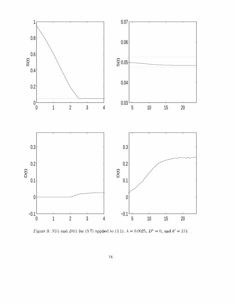
Following Feyo de Azevedo et al. (1992), the other constant process parameters are set�La = 100 [h�1]; O� = 0:007 [g=l]; Sin = 10 [g=l]:The initial values of the state variables areS(0) = 0:95; O(0) = 0:0066; X(0) = 0:1; C(0) = 0:000325; E(0) = 0:0001 [g=l]:The control objective is to regulate the glucose concentration S(t) into a �-neighbourhoodof the reference concentration Sref = 0:05. The tolerated error arround the referenceshould be below 5%, and hence we set � = 0:0025:According to Theorem 3.1 we need to determine an upper bound of the input saturationDsup. Recall that l = 1. Hence by the zero entries of K we need to determine upperbounds of the �rst and third reaction rate. Sonnleitner and K�appeli (1986) allow theparameters to vary within the following ranges0:24 � qc;max � 0:264; 0:47 � c�111 � 0:5; 0:05 � c�113 � 0:1:An upper bound for the biomass concentration, taken from Feyo de Azevedo et al. (1992),is X = 3 [g/l]. Hence the reaction rates are bounded by'1(S;O;X) � 0:3187; '3(S;X;O) � 0:0637:Now it is easy to see that the fraction on the right hand side in (3.2) is 0.3842. Therefore,we may choose Dsup = 0:385 satisfying (3.2).If the design parameters of the �-tracker (1.2) are � � 1 and r = � = 1, then for smallerror the growth of t 7! k(t) is \slow"; it is even slower if r > 1. To fasten this up, onehas to increase �. For this reason we choose � = 45, r = 1.Adaptive �-tracker (1.2) with di�erent o�sets applied to (4.1): The simulationsshow that the �-tracker is successful and what the e�ect of di�erent design parameters is.In the �rst run of simulations, depicted in Figure 2, we choose the o�set to be D� = 0(solid line). The gain increases rapidly until it is su�ciently large after 2 1/2 hours sothat the substrate is forced into the �-strip (dotted line) around the reference setpoint.The simulations are performed over a period of one day, and the �gures are divided intoan initial phase of 4 hours and the remaining 4-24 hours. Since S(t) remains inside the�-strip after t = 3 hours, the gain stays constant and also longer simulations have shownk(3) = k(200) = 49:73. Note also that S(t) as well as the control action D(t) behavesmoothly without any overshoots. Moreover, D(t) does not reach the upper saturationbound. The other variables - biomass, ethanol, oxygen, carbon dioxide - reach a 5%neighbourhood of their steady states within 17, 30, 15, 15 hours, respectively. We omit todepict them.In a second run we change the o�set to D� = 0:2 (dashed line). One may think thatthis should give a better behaviour since D� = 0:2, also depicted in Figure 2, is close tothe steady state value observed in the previous simulations. Although the results are not15

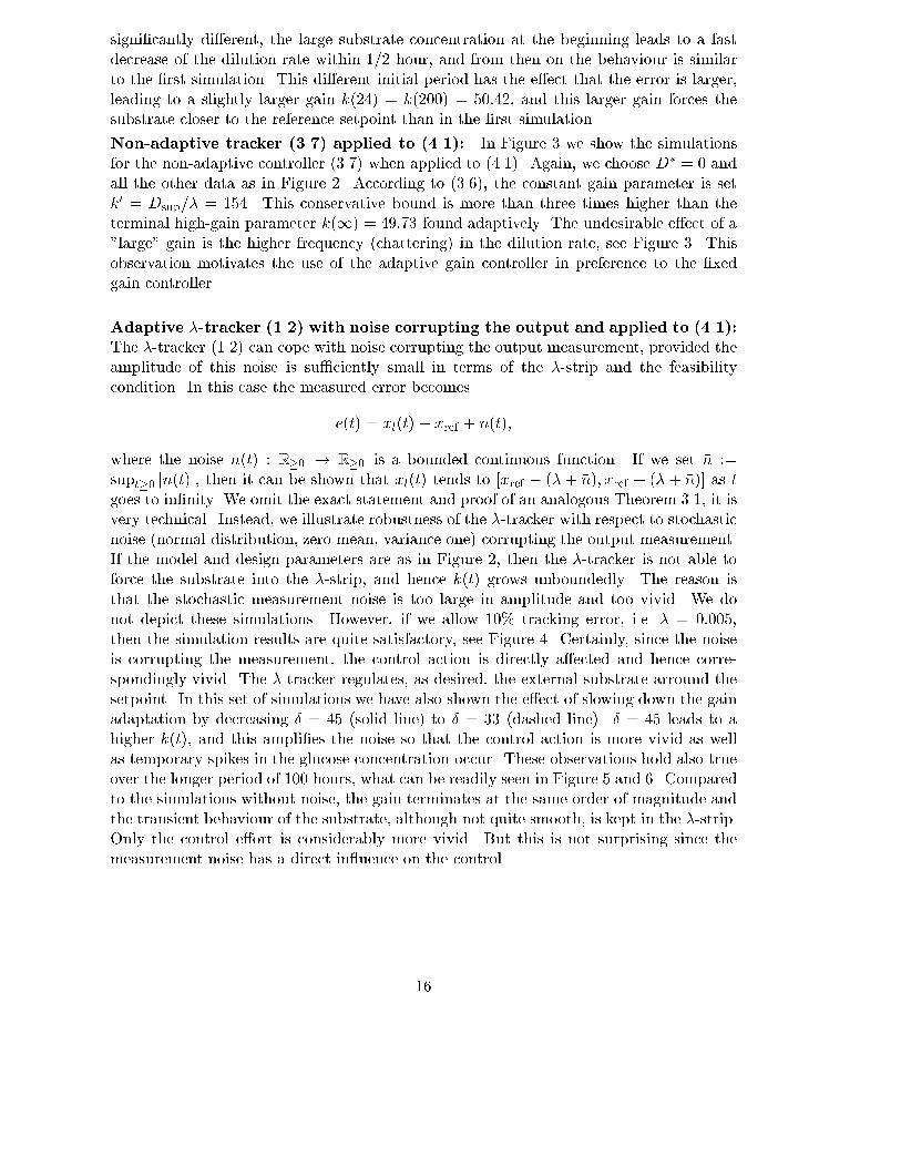
signi�cantly di�erent, the large substrate concentration at the beginning leads to a fastdecrease of the dilution rate within 1/2 hour, and from then on the behaviour is similarto the �rst simulation. This di�erent initial period has the e�ect that the error is larger,leading to a slightly larger gain k(24) = k(200) = 50:42, and this larger gain forces thesubstrate closer to the reference setpoint than in the �rst simulation.Non-adaptive tracker (3.7) applied to (4.1): In Figure 3 we show the simulationsfor the non-adaptive controller (3.7) when applied to (4.1). Again, we choose D� = 0 andall the other data as in Figure 2. According to (3.6), the constant gain parameter is setk0 = Dsup=� = 154. This conservative bound is more than three times higher than theterminal high-gain parameter k(1) = 49:73 found adaptively. The undesirable e�ect of a"large" gain is the higher frequency (chattering) in the dilution rate, see Figure 3. Thisobservation motivates the use of the adaptive gain controller in preference to the �xedgain controller.Adaptive �-tracker (1.2) with noise corrupting the output and applied to (4.1):The �-tracker (1.2) can cope with noise corrupting the output measurement, provided theamplitude of this noise is su�ciently small in terms of the �-strip and the feasibilitycondition. In this case the measured error becomese(t) = xl(t)� xref + n(t);where the noise n(t) : R�0 ! R�0 is a bounded continuous function. If we set �n :=supt�0 jn(t)j, then it can be shown that xl(t) tends to [xref � (�+ �n); xref + (� + �n)] as tgoes to in�nity. We omit the exact statement and proof of an analogous Theorem 3.1, it isvery technical. Instead, we illustrate robustness of the �-tracker with respect to stochasticnoise (normal distribution, zero mean, variance one) corrupting the output measurement.If the model and design parameters are as in Figure 2, then the �-tracker is not able toforce the substrate into the �-strip, and hence k(t) grows unboundedly. The reason isthat the stochastic measurement noise is too large in amplitude and too vivid. We donot depict these simulations. However, if we allow 10% tracking error, i.e. � = 0:005,then the simulation results are quite satisfactory, see Figure 4. Certainly, since the noiseis corrupting the measurement, the control action is directly a�ected and hence corre-spondingly vivid. The �-tracker regulates, as desired, the external substrate arround thesetpoint. In this set of simulations we have also shown the e�ect of slowing down the gainadaptation by decreasing � = 45 (solid line) to � = 33 (dashed line). � = 45 leads to ahigher k(t), and this ampli�es the noise so that the control action is more vivid as wellas temporary spikes in the glucose concentration occur. These observations hold also trueover the longer period of 100 hours, what can be readily seen in Figure 5 and 6. Comparedto the simulations without noise, the gain terminates at the same order of magnitude andthe transient behaviour of the substrate, although not quite smooth, is kept in the �-strip.Only the control e�ort is considerably more vivid. But this is not surprising since themeasurement noise has a direct in uence on the control.16

0 1 2 3 40

20

40k(t

)

0 1 2 3 40

0.5

1

S(t

)

0 1 2 3 4−0.1

0

0.1

0.2

0.3

D(t

)

5 10 15 2047

48

49

50

51

52

k(t

)

5 10 15 200.03

0.04

0.05

0.06

0.07

S(t

)

5 10 15 20−0.1

0

0.1

0.2

0.3

D(t

)

Figure 2: k(t), S(t) and D(t) for (1.2) applied to (4.1), � = 45, r = 1, � = 0:0025, D� = 0:2(dashed line), D� = 0 (solid line)17

0 1 2 3 40

0.2

0.4

0.6

0.8

1S

(t)

0 1 2 3 4−0.1

0

0.1

0.2

0.3

D(t

)

5 10 15 200.03

0.04

0.05

0.06

0.07

S(t

)

5 10 15 20−0.1

0

0.1

0.2

0.3

D(t

)

Figure 3: S(t) and D(t) for (3.7) applied to (4.1), � = 0:0025, D� = 0, and k0 = 15418

0 2 40

10

20

30

40

50

k(t

)

0 2 40

0.5

1

S(t

)

0 2 4−0.1

0

0.1

0.2

0.3

D(t

)

5 10 15 2036.96

36.965

36.97

delta=33

5 10 15 2047.65

47.655

47.66

delta=45

5 10 15 200.03

0.04

0.05

0.06

0.07

delta=33

5 10 15 200.03

0.04

0.05

0.06

0.07

delta=45

5 10 15 20−0.1

0

0.1

0.2

0.3

delta=33

5 10 15 20−0.1

0

0.1

0.2

0.3

delta=45

Figure 4: k(t), S(t) and D(t) for (1.2) applied to (4.1) in the presence of noise, r = 1,� = 0:005, � = 45 (solid line), � = 33 (dashed line)19

0 10 20 30 40 50 60 70 80 90 1000

10

20

30

40

50

k(t

)

0 10 20 30 40 50 60 70 80 90 1000

0.05

0.1

S(t

)

0 10 20 30 40 50 60 70 80 90 100−0.1

0

0.1

0.2

0.3

D(t

)

Figure 5: k(t), S(t) and D(t) for (1.2) applied to (4.1) in the presence of noise, r = 1,� = 0:005, � = 45; t = 100[h]20

0 10 20 30 40 50 60 70 80 90 1000

10

20

30

40

50

k(t

)

0 10 20 30 40 50 60 70 80 90 1000

0.05

0.1

S(t

)

0 10 20 30 40 50 60 70 80 90 100−0.1

0

0.1

0.2

0.3

D(t

)

Figure 6: k(t), S(t) and D(t) for (1.2) applied to (4.1) in the presence of noise, r = 1,� = 0:005, � = 33; t = 100[h]21

6 ConclusionsIn this paper, control of a wide class of aerobic continuous stirred tank reactors has beenachieved by a proportional error feedback controller with input saturations, where the gainis found adaptively. It is proved that regulation of external substrates to a neighborhoodof a constant reference concentration is possible under mild conditions. We have alsoworked out structural conditions of the general process model which are essential whenexploiting them mathematically. As a side result we show that proportional non-adaptiveerror feedback subjected to saturation is possible for the class of systems provided thesystem data satisfy a crude estimate. However, adaptive �-tracking results in a muchlower gain. The other clear advantage of the �-tracker over other approaches on control ofbiotechnological processes, such as PI or PID controllers as for example in Dairaku et al.(1982), or adaptive linearising control relying on system parameters or invoking estimatorsfor the system parameters (see for example Chen et al. (1995) or Ferreira and Feyo deAzevedo (1996)), is its simplicity. Only very limited information concerning the system isrequired and it readily tolerates noise corrupting the output measurement. The only priceto be paid is that setpoint tracking is not achieved asymptotically but in a neighbourhoodof the setpoint. However, the neighbourhood is prespeci�ed and arbitrarily small, whichsu�ces for practical purposes.Acknowledgements: This paper was initiated while P. Georgieva was visiting the Schoolof Mathematical Sciences, University of Exeter, and it was completed while A. Ilchmannand P. Georgieva were both on study leave at the Institute for Systems and Robotics,University of Porto. The hospitality is greatfully acknowledged, as well as the support ofA. Ilchmann by Portuguese Science Foundation, Praxis XXI/BCC/20279/99. P. Georgievaacknowledges the support received by the Portuguese Science Foundation, Praxis XXI, theNF \Scienti�c Investigations", contract No. TN-715/97 and Junior Project, contract No.I-4/98. We are indebted to A. Georgiev (So�a) for carefully working out the illustrationin Figure 1.References[1] Bastin G. and D. Dochain (1990): On-Line Estimation and Adaptive Control of Biore-actors; Elsevier Science Publishers B.V., Amsterdam and others[2] Chen L., G. Bastin and V. van Breusegem (1995): A case study of adaptive nonlinearregulation of fed-batch biological reactors; Automatica 31, 55{65[3] Dairaku K., E. Izimoto, H. Moriakawa, S. Shioya and T. Takamatsu (1982): Op-timal quality control of baker's yeast fed-batch culture using population dynamics;Biotechnology and Bioengineering 24, 2661-267422

[4] Ferreira E.C. and S. Feyo de Azevedo (1996): Adaptive linearizing control of biore-actors; pages 1184{1189 in: Proc. of the UKACC Int. Conf. on Control 1996 , Inst.of Electr. Engineers, London[5] Feyo de Azevedo S., P. Pimenta, F. Oliveira and E.C. Ferreira (1992): Computer-based studies on bioprocess engineering, II-tools for process operation; pp. 27{49 inA.R. Moreira and K.K. Wallace (eds.): Computer and information science applica-tions in bioprocess engineering , NATO ASI Series, Vol. 305[6] Gavalas G.R. (1968): Nonlinear Di�erential Equations of Chemically Reacting Sys-tems; Springer-Verlag, Berlin and others[7] Hewitt E. and K. Stromberg (1965): Real Analysis; Springer-Verlag, London[8] Ilchmann A. and E.P. Ryan (1994): Universal �-tracking for nonlinearly-perturbedsystems in the presence of noise; Automatica 30, 337{346[9] Ilchmann A. and M.-F. Weirig (1999): Modelling of general biotechnological pro-cesses; Mathematical Modelling of Dynamical Systems 5, 152{178[10] Ilchmann A., M.-F. Weirig and I.M.Y. Mareels (1998): Modelling of biochemical pro-cesses and adaptive control; pages 465{470 in: Proc. of 4th IFAC Nonlinear ControlSystems Design Symposium, NOLCOS '98, Eds.: H.J.C. Huijberts et al., Enschede,Netherlands[11] Khalil H.K. (1996): Nonlinear Systems second ed.; Prentice Hall, Upper Saddle River,NJ[12] Knobloch H.W. and F. Kappel (1974): Gew�ohnlich Di�erentialgleichungen; TeubnerVerlag, Stuttgart[13] Pomerleau Y. and M. Perrier (1990): Estimation of multiple speci�c growth rates inbioprocesses; AIChE Journal 36, 207{215[14] Sonnleitner B. and O. K�appeli (1986): Growth of Saccharomyces cerevisiae is con-trolled by its limited respiratory capacity:formulation and veri�cation of hypothesis;Biotechnology and Bioengineering 28, 927{937[15] Sweere A.P.J., J. Giesselbach, R. Barendse, R. Krieger, G. Honderd, K.C.M.A. Luy-ben (1988): Modelling the dynamical behaviour of saccharomyces cerevisiae and itsapplication in control experiments; Applied Microbiology and Biotechnology 28, 116{127[16] Weirig M.-F. (1998): Modelling and adaptive control of biotechnological processes;PhD thesis at the Faculty of Mathematics, Technical University Munich, Germany23