Estimation de paramètres et modélisation de piles au lithium ...
Upload
khangminh22Category
view
1download
0
HAL Id: tel-01132323https://tel.archives-ouvertes.fr/tel-01132323
Submitted on 17 Mar 2015
HAL is a multi-disciplinary open accessarchive for the deposit and dissemination of sci-entific research documents, whether they are pub-lished or not. The documents may come fromteaching and research institutions in France orabroad, or from public or private research centers.
L’archive ouverte pluridisciplinaire HAL, estdestinée au dépôt et à la diffusion de documentsscientifiques de niveau recherche, publiés ou non,émanant des établissements d’enseignement et derecherche français ou étrangers, des laboratoirespublics ou privés.
Modélisation des suies par méthode sectionnelle pour lasimulation RANS des moteurs Diesel
Damien Aubagnac-Karkar
To cite this version:Damien Aubagnac-Karkar. Modélisation des suies par méthode sectionnelle pour la simulation RANSdes moteurs Diesel. Mécanique des fluides [physics.class-ph]. Ecole Centrale Paris, 2014. Français.NNT : 2014ECAP0061. tel-01132323
THESE
presentee par
Damien AUBAGNAC-KARKAR
pour l’obtention du
GRADE de DOCTEUR
NUMERO D’ORDRE : 2014ECAP0061
Formation doctorale :
Energetique
Laboratoire d’accueil :
IFP Energies Nouvelles, Division : Techniques d’Applications Energetiques
et
Laboratoire d’Energetique Moleculaire
et Macroscopique, Combustion (EM2C)
du CNRS et de l’ECP
Sectional soot modeling for Diesel RANS simulations
Composition du jury:
Pr. Benedicte CUENOT CERFACS Rapporteur
Pr. Fabian MAUSS BTU Cottbus Rapporteur
Pr. Pascale DOMINGO CORIA Examinateur
Dr. Jerome HELIE Continental Examinateur
Pr. Christine ROUSSELLE Universite d’Orleans Examinateur
Dr. Olivier COLIN IFP Energies Nouvelles Examinateur
Pr. Nasser DARABIHA EM2C Examinateur
Dr. Jean-Baptiste MICHEL IFP Energies Nouvelles Examinateur


Remerciements
Mes premiers remerciements vont a mes encadrants de these, Nasser Darabiha de l’ecole Centrale
Paris, Olivier Colin et Jean-Baptiste Michel d’IFP Energies Nouvelles, qui m’ont guide et m’ont per-
mis de decouvrir les joies et les peines du metier de chercheur durant ces trois annees. Merci Nasser
pour ta patience, tes conseils toujours avises et les opportunites que tu m’as offertes pour completer
ma formation. Merci Olivier pour tes idees aussi nombreuses que pertinentes, pour m’avoir aide a
exprimer la rigueur de ma pensee en mots. Enfin, merci Jean-Baptiste pour ta presence reguliere,
pour la rigueur scientifique que tu caches sous ton style detache et pour l’aide que tu as su apporter
a chaque fois qu’il fallait finir des viennoiseries dans mon bureau.
Je souhaiterais aussi remercier les membres de mon jury de these pour avoir accepte d’evaluer
mon travail et pour avoir partage avec moi leurs opinions a son sujet. Merci a Madame Cuenot
et Monsieur Mauss pour avoir pris le temps de relire mon manuscrit en detail et avoir redige les
rapports. Merci a Mesdames Domingo et Rousselle ainsi qu’a Monsieur Helie pour avoir pris le
temps d’etudier mon travail.
Je remercie egalement Antonio Pires da Cruz qui m’a accueilli dans le departement qu’il dirigeait
durant mes trois annees de these, ainsi que Christian Angelberger; tous deux m’ont fait confiance
pour mener a bien cette these. Je suis aussi reconnaissant envers l’ensemble des ingenieurs et experts
du departement qui ont partage avec moi leurs savoir-faire et ont permis a ma these d’avancer au-dela
de certains points bloquants. Je remercie particulierement Andre Nicolle dont l’expertise en chimie
a debloque quelques situations. Et bien sur, je dois mentionner la patience et la competence de
Nicolas Gillet et Anthony Velghe, gardiens des temples que sont les codes du departement. Aurais-
je pu compiler C3D ne serait-ce qu’une fois si je n’avais pas paye mon tribut en pain au chocolat a
Anthony Velghe?
Ce travail n’aurait pas ete possible sans l’aide des equipes d’experimentateurs de la direction
R10. La base moteur fournie par l’equipe de Ludovic Noel a facililite la validation de mon modele.
La connaissance des methodes experimentales de l’ECN que l’equipe de Gilles Bruneaux a partage
avec moi a ete d’une grande aide.
Enfin, je vais parler du troisieme etage du batiment Claude Bonnier. Ma these aurait clairement
ete tres differente si elle ne s’etait pas deroulee a cet etage. Les soutiens et les moqueries d’une
troupe de thesards tous dans le meme bateau ont rythme mes journees pendant ces trois annees. Je
remercie les anciens pour leur accueil : Pauline dont je poursuivais les travaux, mais aussi Yohann,
Alexis, Julien, Carlo, Sullivan ou encore JB le tueur de cerfs ... Ensuite, je me dois de mentionner
specialement le bureau CB308, haut lieu de culture, de debat politique, philosophique et scientifique
iii

iv
anime durant ces trois annees par Sophie, Guillaume, Oguz, Jan, Bejoy et Betty, avant son depart
pour la lointaine contree du bureau voisin. Je remercie les autres thesards qui ont rendu ces trois
annees agreables avec quelques verres, parties de football ou autre sorties pour couper entre deux
calculs plein de bugs. Ainsi, merci a Haifa, Lama, Federico, Emre, Elias, Benjamin, Karl, Anthony,
Stephane, Adam, Nicolas ...
Enfin, je remercie ma famille qui m’a supporte avant cette these, durant ces trois annees et qui
va devoir continuer encore quelques temps. J’ai toujours ete soutenu dans mes projets aussi etranges
soient-ils (une these? quelle iee!), merci.

Abstract
Soot particles emitted by Diesel engines cause major public health issues. Car manufacturers need
models able to predict soot number and size distribution to face the more and more stringent norms.
In this context, a soot model based on a sectional description of the solid phase is proposed in this
work. First, the type of approach is discussed on the base of state of the art of the current soot
models. Then, the proposed model is described. At every location and time-step of the simulation,
soot particles are split into sections depending on their size. Each section evolution is governed by:
• a transport equation;
• source terms representing its interaction with the gaseous phase (particle inception, conden-
sation surface growth and oxidation);
• source terms representing its interaction with other sections (condensation and coagulation).
This soot model requires the knowledge of local and instantaneous concentrations of minor
species involved in soot formation and evolution. The kinetic schemes including these species are
composed of hundreds of species and thousands of reactions. It is not possible to use them in 3D-CFD
simulations. Therefore, the tabulated approach VPTHC (Variable Pressure Tabulated Homogeneous
Chemistry) has been proposed. This approach is based on the ADF approach (Approximated
Diffusion Flame) which has been simplified in order to be coupled with the sectional soot model.
First, this tabulated combustion model ability to reproduce detailed kinetic scheme prediction
has been validated on variable pressure and mixture fraction homogeneous reactors designed for this
purpose. Then, the models predictions have been compared to experimental measurement of soot
yields and particle size distributions of Diesel engines. The validation database includes variations
of injection duration, injection pressure and EGR rate performed with a commercial Diesel fuel as
well as the surrogate used in simulations. The model predictions agree with the experiments for
most cases.
Finally, the model predictions have been compared on a more detailed and academical case with
the Engine Combustion Network Spray A, a high pressure Diesel spray. This final experimental
validation provides data to evaluate the model predictions in transient conditions.
Keywords : Combustion, Simulation, Pollutant, Soot, Diesel, Tabulated chemistry
v

vi

Resume
Les particules de suies issues de moteur Diesel constituent un enjeu de sante publique et sont
soumises a des reglementations de plus en plus strictes. Les constructeurs automobiles ont donc
besoin de modeles capables de predire l’evolution en nombre et en taille de ces particules de suies.
Dans ce cadre, un modele de suies base sur une representation sectionnelle de la phase solide est
propose dans cette these. Le choix de ce type d’approche est d’abord justifie par l’etude de l’etat de
l’art de la modelisation des suies. Le modele de suies propose est ensuite decrit. A chaque instant
et en chaque point du maillage, les particules de suies sont reparties en sections selon leur taille et
l’evolution de chaque section est gouvernee par :
• une equation de transport;
• des termes sources modelisant l’interaction avec la phase gazeuse (nucleation, condensation,
croissance de surface et oxydation des suies);
• des termes sources collisionnels permettant de representer les interactions entre suies (conden-
sation et coagulation).
Ce modele de suies necessite donc la connaissance des concentrations locales et instantanees des
precurseurs de suies et des especes consommees par les schemas de reactions de surface des suies.
Les schemas fournissant ces informations pour des conditions thermodynamiques rencontrees dans
des moteurs Diesel comportant des centaines d’especes et des milliers de reactions, ils ne peuvent
etre utilises directement dans des calculs de CFD. Pour pallier cela, l’approche de tabulation de
la chimie VPTHC (Variable Pressure Tabulated Homogeneous Chemistry) a ete proposee. Cette
approche est basee sur l’approche ADF (Approximated Diffusion Flame) qui a ete simplifiee pour
permettre son emploi couple au modele de suies sectionnel.
Dans un premier temps, la capacite du modele tabule a reproduire la cinetique chimique a ete
validee par comparaison des resultats obtenus avec ceux de reacteurs homogenes avec loi de piston
equivalents. Finalement, le modele VPTHC, couple au modele de suies sectionnel, a ete valide sur
une base d’essais moteur dediee avec des mesures de distribution en taille de suies a l’echappement.
Cette base comporte des variations de duree d’injection, de pression d’injection et de taux d’EGR
a la fois pour un carburant Diesel commercial et pour le carburant modele utilise dans les calculs.
Les predictions des debits horaires de suies et des distributions a laechappement obtenues sont en
bon accord avec les mesures.
Ensuite, les resultats du modele ont ete compares avec les mesures plus academiques et detaillees
du Spray A de l’Engine Combustion Network, un spray a haute pression et temperature. Cette
seconde validation experimentale a permis l’etude du comportement du modele dans des regimes
transitoires.
vii

viii
Mots-clefs : Combustion, Simulation, Polluants, Suies, Diesel, Chimie Tabulatee
Contents
1 Introduction 1
1.1 Motivations . . . . . . . . . . . . . . . . . . . . . . . . . . . . . . . . . . . . . . . . . 1
1.1.1 Combustion in the world . . . . . . . . . . . . . . . . . . . . . . . . . . . . . 1
1.1.2 Automotive industry context . . . . . . . . . . . . . . . . . . . . . . . . . . . 2
1.2 Automotive industry context . . . . . . . . . . . . . . . . . . . . . . . . . . . . . . . 2
1.2.1 Reciprocating engines basics . . . . . . . . . . . . . . . . . . . . . . . . . . . 3
1.2.2 Number of Diesel powered cars . . . . . . . . . . . . . . . . . . . . . . . . . . 7
1.2.3 Norms . . . . . . . . . . . . . . . . . . . . . . . . . . . . . . . . . . . . . . . . 7
1.2.4 Control of emissions . . . . . . . . . . . . . . . . . . . . . . . . . . . . . . . . 9
1.3 Objectives of the present work . . . . . . . . . . . . . . . . . . . . . . . . . . . . . . 11
1.4 Turbulent flows modeling . . . . . . . . . . . . . . . . . . . . . . . . . . . . . . . . . 11
1.4.1 Different types of simulations . . . . . . . . . . . . . . . . . . . . . . . . . . . 11
1.4.2 RANS simulations basics . . . . . . . . . . . . . . . . . . . . . . . . . . . . . 12
1.5 Thesis outline . . . . . . . . . . . . . . . . . . . . . . . . . . . . . . . . . . . . . . . . 14
2 Soot modeling background 17
2.1 Soot formation mecanisms . . . . . . . . . . . . . . . . . . . . . . . . . . . . . . . . . 17
2.1.1 Gaseous precursor formation . . . . . . . . . . . . . . . . . . . . . . . . . . . 18
2.1.2 Smallest solid particles: particle inception . . . . . . . . . . . . . . . . . . . . 20
2.1.3 Collisional phenomena . . . . . . . . . . . . . . . . . . . . . . . . . . . . . . . 20
2.1.4 Soot surface chemistry . . . . . . . . . . . . . . . . . . . . . . . . . . . . . . . 22
2.2 Soot modeling approaches . . . . . . . . . . . . . . . . . . . . . . . . . . . . . . . . 22
2.2.1 Empirical correlations . . . . . . . . . . . . . . . . . . . . . . . . . . . . . . . 23
2.2.2 Semi-empirical models . . . . . . . . . . . . . . . . . . . . . . . . . . . . . . . 24
2.2.3 Detailed soot models . . . . . . . . . . . . . . . . . . . . . . . . . . . . . . . . 26
2.3 The proposed approach . . . . . . . . . . . . . . . . . . . . . . . . . . . . . . . . . . 28
3 The Sectional Soot Model 31
3.1 Soot modeling . . . . . . . . . . . . . . . . . . . . . . . . . . . . . . . . . . . . . . . . 31
3.1.1 Volume discretization . . . . . . . . . . . . . . . . . . . . . . . . . . . . . . . 32
3.1.2 Model variables . . . . . . . . . . . . . . . . . . . . . . . . . . . . . . . . . . . 33
3.1.3 Collisional source terms . . . . . . . . . . . . . . . . . . . . . . . . . . . . . . 33
3.1.4 Surface chemistry source terms . . . . . . . . . . . . . . . . . . . . . . . . . . 39
3.2 Homogeneous reactor and premixed flames validations . . . . . . . . . . . . . . . . . 42
3.2.1 Homogeneous reactor . . . . . . . . . . . . . . . . . . . . . . . . . . . . . . . 42
3.2.2 Laminar premixed flames . . . . . . . . . . . . . . . . . . . . . . . . . . . . . 46
ix

x CONTENTS
4 Diesel RANS simulations 51
4.1 Abstract . . . . . . . . . . . . . . . . . . . . . . . . . . . . . . . . . . . . . . . . . . . 51
4.2 Introduction . . . . . . . . . . . . . . . . . . . . . . . . . . . . . . . . . . . . . . . . . 52
4.3 Soot modeling . . . . . . . . . . . . . . . . . . . . . . . . . . . . . . . . . . . . . . . 54
4.3.1 Volume discretization . . . . . . . . . . . . . . . . . . . . . . . . . . . . . . . 55
4.3.2 Model variables . . . . . . . . . . . . . . . . . . . . . . . . . . . . . . . . . . . 56
4.3.3 Collisional source terms . . . . . . . . . . . . . . . . . . . . . . . . . . . . . . 57
4.3.4 Surface chemistry source terms . . . . . . . . . . . . . . . . . . . . . . . . . . 60
4.4 Turbulent Combustion Modeling . . . . . . . . . . . . . . . . . . . . . . . . . . . . . 62
4.4.1 The ECFM3Z model . . . . . . . . . . . . . . . . . . . . . . . . . . . . . . . . 62
4.4.2 The tabulated chemistry approach . . . . . . . . . . . . . . . . . . . . . . . . 63
4.5 Validation of the tabulated chemistry approach . . . . . . . . . . . . . . . . . . . . . 67
4.5.1 ECFM3Z-0D reactors description . . . . . . . . . . . . . . . . . . . . . . . . . 68
4.5.2 ECFM3Z-0D coupled to a kinetic solver . . . . . . . . . . . . . . . . . . . . . 69
4.5.3 Comparison between tabulated chemistry and kinetic solver . . . . . . . . . . 70
4.6 Soot impact on gaseous composition . . . . . . . . . . . . . . . . . . . . . . . . . . . 73
4.7 Evaluation on a Diesel engine . . . . . . . . . . . . . . . . . . . . . . . . . . . . . . . 76
4.7.1 Numerical set-up . . . . . . . . . . . . . . . . . . . . . . . . . . . . . . . . . . 76
4.7.2 Results . . . . . . . . . . . . . . . . . . . . . . . . . . . . . . . . . . . . . . . 78
4.8 Conclusions . . . . . . . . . . . . . . . . . . . . . . . . . . . . . . . . . . . . . . . . . 94
5 Diesel spray RANS simulation 97
5.1 Abstract . . . . . . . . . . . . . . . . . . . . . . . . . . . . . . . . . . . . . . . . . . . 97
5.2 Introduction . . . . . . . . . . . . . . . . . . . . . . . . . . . . . . . . . . . . . . . . 98
5.3 Models . . . . . . . . . . . . . . . . . . . . . . . . . . . . . . . . . . . . . . . . . . . 99
5.3.1 Turbulent combustion model: ADF-PCM . . . . . . . . . . . . . . . . . . . . 99
5.3.2 Sectional soot model . . . . . . . . . . . . . . . . . . . . . . . . . . . . . . . . 102
5.4 Results . . . . . . . . . . . . . . . . . . . . . . . . . . . . . . . . . . . . . . . . . . . 104
5.4.1 Experimental database . . . . . . . . . . . . . . . . . . . . . . . . . . . . . . . 104
5.4.2 Numerical configuration . . . . . . . . . . . . . . . . . . . . . . . . . . . . . . 105
5.4.3 Non-reactive case . . . . . . . . . . . . . . . . . . . . . . . . . . . . . . . . . . 106
5.4.4 Reference case . . . . . . . . . . . . . . . . . . . . . . . . . . . . . . . . . . . 109
5.4.5 Variations . . . . . . . . . . . . . . . . . . . . . . . . . . . . . . . . . . . . . . 116
5.5 Conclusion . . . . . . . . . . . . . . . . . . . . . . . . . . . . . . . . . . . . . . . . . 121
6 Conclusions and perspectives 123
6.1 Conclusions . . . . . . . . . . . . . . . . . . . . . . . . . . . . . . . . . . . . . . . . . 123
6.1.1 Soot modeling . . . . . . . . . . . . . . . . . . . . . . . . . . . . . . . . . . . 123
6.1.2 Diesel engine simulations . . . . . . . . . . . . . . . . . . . . . . . . . . . . . 124
6.1.3 Diesel Spray . . . . . . . . . . . . . . . . . . . . . . . . . . . . . . . . . . . . . 124
6.2 Perspectives . . . . . . . . . . . . . . . . . . . . . . . . . . . . . . . . . . . . . . . . . 125
6.2.1 Soot modeling . . . . . . . . . . . . . . . . . . . . . . . . . . . . . . . . . . . 125
6.2.2 Chemistry-turbulence interactions . . . . . . . . . . . . . . . . . . . . . . . . 126
6.2.3 Multi-physics modeling . . . . . . . . . . . . . . . . . . . . . . . . . . . . . . 126
6.3 Future works . . . . . . . . . . . . . . . . . . . . . . . . . . . . . . . . . . . . . . . . 127
Chapter 1
Introduction
1.1 Motivations
1.1.1 Combustion in the world
The mastery of combustion led to the industrial revolutions by providing the energy required for
mass production and transportation. Providing energy by combustion is a foundation of our current
society. Indeed, this process is currently involved in 90% of the energy production on Earth [1] and
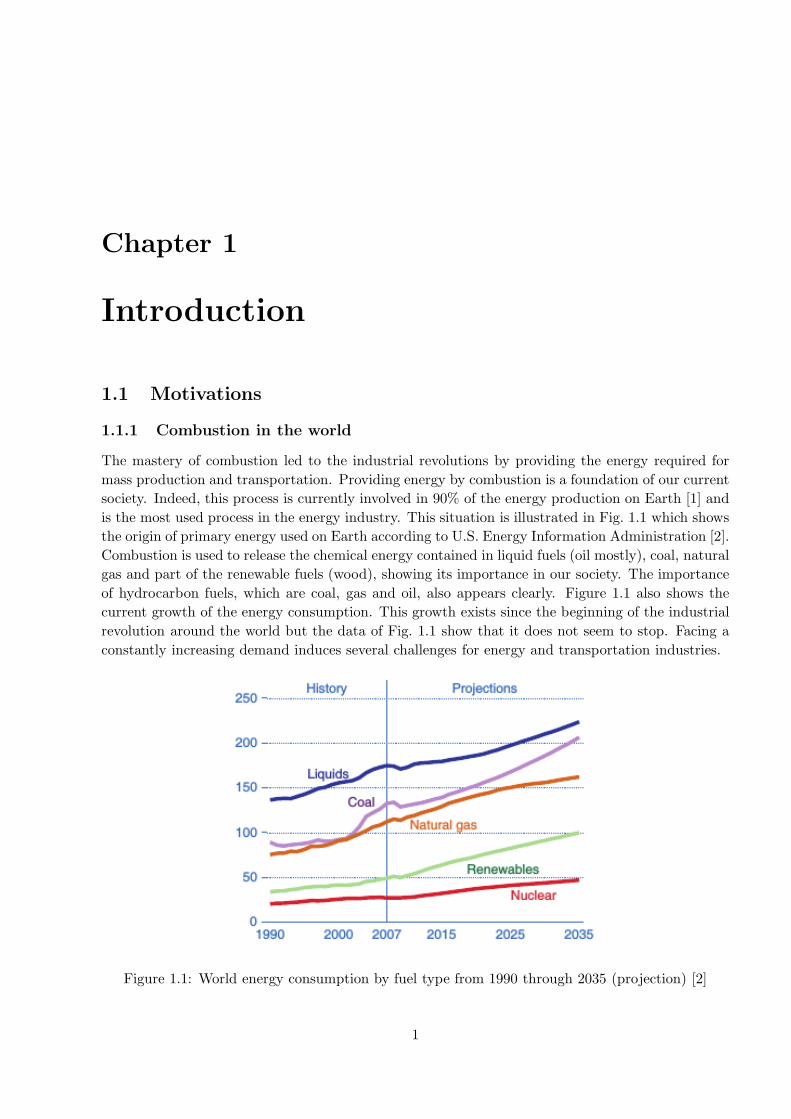
is the most used process in the energy industry. This situation is illustrated in Fig. 1.1 which shows
the origin of primary energy used on Earth according to U.S. Energy Information Administration [2].
Combustion is used to release the chemical energy contained in liquid fuels (oil mostly), coal, natural
gas and part of the renewable fuels (wood), showing its importance in our society. The importance
of hydrocarbon fuels, which are coal, gas and oil, also appears clearly. Figure 1.1 also shows the
current growth of the energy consumption. This growth exists since the beginning of the industrial
revolution around the world but the data of Fig. 1.1 show that it does not seem to stop. Facing a
constantly increasing demand induces several challenges for energy and transportation industries.
Figure 1.1: World energy consumption by fuel type from 1990 through 2035 (projection) [2]
1

2 CHAPTER 1. INTRODUCTION
This constantly increasing demand in energy causes strong stresses to both the ability of pro-
ducers to respond to it and to the environment. On the one hand, the scarcity of fuels becomes a
major economical and social issue with uncertain evaluation of hydrocarbon resources [2]. On the
other hand, one of the main combustion products, the carbon dioxide CO2, has a strong impact on
global warming. Incomplete combustion products, such as unburned hydrocarbons, carbon monox-
ide and soot particles, are considered as pollutants and have an impact on climate as well as they
cause health issues. Finally, the high temperatures reached during combustion also lead to nitrogen
oxides production, involved in tropospheric ozone creation which is very noxious to human beings.
1.1.2 Automotive industry context
Liquid fuels are one of the resources concerned by scarcity. Their consumption by sector is given in
Fig. 1.2, according to the U.S. Energy Information Administration [2]. The transportation domain
appears to be one of the largest energy consumers. It is also the domain where the use of different
sources of energy seems to be the more complicated. Indeed, many transportation devices, such as
cars or planes, have to transport their energy sources. In this context, the high energetic density of
liquid fuels is required. The number of vehicles is also constantly growing. For cars, it goes from
126 millions in 1960 to 1 billion in 2010 according to the US Department of Energy [3]. This trend
should not stop in the future because of the demand from the industrializing countries. Thus, the
car industry faces a challenge with a larger public to reach with less and less resources and emissions
that have to be controlled.
Figure 1.2: Consumption of liquid fuel in the world by sector from 2006 through 2030 (projection)
[2]
In this context, the transformation of the fuel latent energy into mechanical energy has to be
understood, mastered and controlled. This results in constant work to improve current engines
design.
1.2 Automotive industry context
Current car engines are internal combustion engines, most of them are piston engines, also known
as reciprocating engines. The release of the fuel energy as well as the pollutants emissions come
1.2. AUTOMOTIVE INDUSTRY CONTEXT 3
from the combustion inside these engines. The way this combustion is realized is also the main way
to classify cars.
1.2.1 Reciprocating engines basics
Most of the modern car engines are four-stroke engines. This means that they provide energy by
completing a five steps thermodynamical cycle realized during four strokes. They differ in the fact
that they can be either Compression Ignition (CI) engines, also called Diesel engines, or Spark
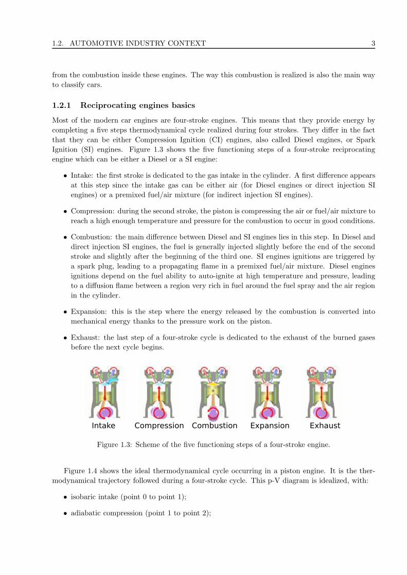
Ignition (SI) engines. Figure 1.3 shows the five functioning steps of a four-stroke reciprocating
engine which can be either a Diesel or a SI engine:
• Intake: the first stroke is dedicated to the gas intake in the cylinder. A first difference appears
at this step since the intake gas can be either air (for Diesel engines or direct injection SI
engines) or a premixed fuel/air mixture (for indirect injection SI engines).
• Compression: during the second stroke, the piston is compressing the air or fuel/air mixture to
reach a high enough temperature and pressure for the combustion to occur in good conditions.
• Combustion: the main difference between Diesel and SI engines lies in this step. In Diesel and
direct injection SI engines, the fuel is generally injected slightly before the end of the second
stroke and slightly after the beginning of the third one. SI engines ignitions are triggered by
a spark plug, leading to a propagating flame in a premixed fuel/air mixture. Diesel engines
ignitions depend on the fuel ability to auto-ignite at high temperature and pressure, leading
to a diffusion flame between a region very rich in fuel around the fuel spray and the air region
in the cylinder.
• Expansion: this is the step where the energy released by the combustion is converted into
mechanical energy thanks to the pressure work on the piston.
• Exhaust: the last step of a four-stroke cycle is dedicated to the exhaust of the burned gases
before the next cycle begins.
Intake Compression Combustion Expansion Exhaust
Figure 1.3: Scheme of the five functioning steps of a four-stroke engine.
Figure 1.4 shows the ideal thermodynamical cycle occurring in a piston engine. It is the ther-
modynamical trajectory followed during a four-stroke cycle. This p-V diagram is idealized, with:
• isobaric intake (point 0 to point 1);
• adiabatic compression (point 1 to point 2);
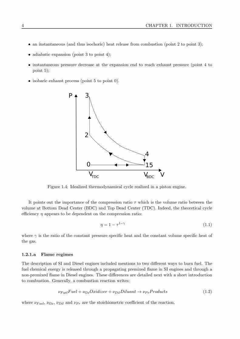
4 CHAPTER 1. INTRODUCTION
• an instantaneous (and thus isochoric) heat release from combustion (point 2 to point 3);
• adiabatic expansion (point 3 to point 4);
• instantaneous pressure decrease at the expansion end to reach exhaust pressure (point 4 to
point 5);
• isobaric exhaust process (point 5 to point 0).
P 3
2
4
150
VVVTDC BDC
Figure 1.4: Idealized thermodynamical cycle realized in a piston engine.
It points out the importance of the compression ratio τ which is the volume ratio between the
volume at Bottom Dead Center (BDC) and Top Dead Center (TDC). Indeed, the theoretical cycle
efficiency η appears to be dependent on the compression ratio:
η = 1− τ1−γ (1.1)
where γ is the ratio of the constant pressure specific heat and the constant volume specific heat of
the gas.
1.2.1.a Flame regimes
The description of SI and Diesel engines included mentions to two different ways to burn fuel. The
fuel chemical energy is released through a propagating premixed flame in SI engines and through a
non-premixed flame in Diesel engines. These differences are detailed next with a short introduction
to combustion. Generally, a combustion reaction writes:
νFuelFuel + νOxOxidizer + νDilDiluant → νPrProducts (1.2)
where νFuel, νOx, νDil and νPr are the stoichiometric coefficient of the reaction.

1.2. AUTOMOTIVE INDUSTRY CONTEXT 5
The exothermic reaction occurs when fuel and oxidizer are mixed with a ratio Φ (equivalence
ratio) not too high or too low with respect to the stoichiometric conditions and when the temperature
and pressure are high enough to trigger the reaction. The equivalence ratio writes:
Φ =
YFuel,0
YOx,0(YFuel,0
YOx,0
)st
=YFuel,0
YOx,0
νOxMOx
νFuelMFuel(1.3)
where YFuel,0 and YOx,0 are the initial mass fractions of fuel and oxidizer, MFuel and MOx are the
molar fractions of fuel and oxidizer and the subscript st refers to the value at the stoichiometric
conditions. The mixture is considered rich if Φ > 1 and lean if Φ < 1.
The ability of a mixture to burn is not only function of its equivalence ratio, temperature and
pressure but it also strongly depends on the fuel. Moreover, the fraction of dilutant gases which can
absorb heat and damper the ignition or propagation processes is also an important parameter.
These chemical reactions are realized in flows of fuel and oxidizer (usually air) which can be
mixed or not prior to combustion. The previously introduced two types of combustion differ in this
sense and the methods to define the flames vary in each case.
Premixed flames
Premixed flames are defined as a flame front separating a region of fresh premixed gases and a
region of burned gases. As illustrated in Fig. 1.5, this flame front can be separated in two zones. A
pre-heat zone where the fresh gases temperature is increased by thermal diffusion. In this region, the
fuel and oxidizer begin to react to create radicals required to complete the combustion reaction. The
reaction zone is the zone of the flame front where, when the temperature and quantity of radicals
are high enough, the reaction intensity increases and chemical heat is released.
Temperature
Oxidizer
Fuel
Reaction rate
Flame propagation
Preheat
zoneReaction
zone
Figure 1.5: Scheme of a premixed flame structure.
The evolution from the fresh gases to the burned ones can be described by a progress variable.
This progress variable can be defined from local temperature or species mass fractions. The main
characteristics defining a premixed flame will be its propagating speed and its thickness.

6 CHAPTER 1. INTRODUCTION
Non-premixed flames
Non-premixed (or diffusion) flames are defined as a reacting zone between a fuel region and an
oxidizer region. The structure of a non-premixed flame is shown in Fig. 1.6. The flame is controlled
by the mixing between fuel and oxidizer and is located at a position where the local equivalence ratio
is equal to unity. However, reactions take place in regions close to this location with high and low
equivalence ratios. This method is safer than premixed combustion because it prevents accidental
ignition or propagation. Indeed, most of the fuel is located in regions too rich for combustion
reactions to occur.
Temperature
Reaction rate
OxidizerFuel
Figure 1.6: Scheme of a non-premixed flame structure.
To describe these flames, a mixture fraction Z can be defined. This mixture fraction is equal
to 1 in the pure fuel region, 0 in the oxidizer region and evolves continuously in between without
effect due to the chemical reaction. Various definitions of the mixture fraction can be found in the
literature. The most used one is:
Z =1
Φ + 1
(Φ
YFu
YFu,0− YOx
YOx,0+ 1
)(1.4)
where YFu and YOx are respectively the local fuel and oxidizer mass fractions. YFu,0 and YOx,0 are
taken outside of the flame in their respective regions.
In this study, the mass fraction of the fuel tracer, which is a virtual species driven by the
transport equation of fuel without the chemical source term, is considered as the mixture fraction.
Such a species can be used as a mixture fraction because it is only convected and diffused by the
flow.
1.2.1.b Main differences
SI and Diesel engines face different limitations and issues. Standard SI engines efficiency is limited
by the possible auto-ignition of its mixture. This type of event, called knock, can destroy engines.
To avoid it, the compression ratio has to be lower and processes increasing the intake pressure (such
as turbochargers or superchargers, providing more torque and a better fuel efficiency) also have to
be used with caution. These limits do not exist on Diesel engines because the auto-ignition is used
to trigger the combustion. Auto-ignition can be used in Diesel engines because the fuel and air are
not premixed, unlike in SI engines. The energy release is then controlled by the fuel injection rate
and it is possible to build pistons able to resist the pressure and thermal strains it imposes.
1.2. AUTOMOTIVE INDUSTRY CONTEXT 7
1.2.2 Number of Diesel powered cars
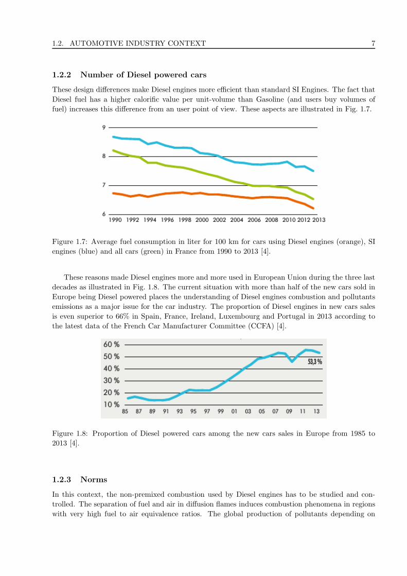
These design differences make Diesel engines more efficient than standard SI Engines. The fact that
Diesel fuel has a higher calorific value per unit-volume than Gasoline (and users buy volumes of
fuel) increases this difference from an user point of view. These aspects are illustrated in Fig. 1.7.
Figure 1.7: Average fuel consumption in liter for 100 km for cars using Diesel engines (orange), SI
engines (blue) and all cars (green) in France from 1990 to 2013 [4].
These reasons made Diesel engines more and more used in European Union during the three last
decades as illustrated in Fig. 1.8. The current situation with more than half of the new cars sold in
Europe being Diesel powered places the understanding of Diesel engines combustion and pollutants
emissions as a major issue for the car industry. The proportion of Diesel engines in new cars sales
is even superior to 66% in Spain, France, Ireland, Luxembourg and Portugal in 2013 according to
the latest data of the French Car Manufacturer Committee (CCFA) [4].
Figure 1.8: Proportion of Diesel powered cars among the new cars sales in Europe from 1985 to
2013 [4].
1.2.3 Norms
In this context, the non-premixed combustion used by Diesel engines has to be studied and con-
trolled. The separation of fuel and air in diffusion flames induces combustion phenomena in regions
with very high fuel to air equivalence ratios. The global production of pollutants depending on

8 CHAPTER 1. INTRODUCTION
equivalence ratio and temperature has been summarized by Pischinger et al. [5]. The diagram given
in Fig. 1.9 shows the different local conditions in temperature and equivalence ratio Φ required for
soot production and oxidation as well as NOx production. The conditions required to produce soot
particles are locally met in non-premixed flames. Accordingly, soot particles emissions are higher in
Diesel engines than in SI engines.
1/
Local temperature [K]
3000
2500
2000
1500
1000
500
0 0.5 1 1.5 2
Soot
formation
Figure 1.9: Diagram of soot and NOx formation and oxidation conditions depending on temperature
and equivalence ratio [5].
With a constantly growing number of Diesel cars in Europe and the soot emissions they generate,
soot particles became a major concern for the car industry. Indeed, the amount of soot particles
emitted grew larger as did the responsibility of the car industry for their emissions. In 2000, 25%
of the PM2.5 particles (particles with a diameter smaller than 2.5 µm) emitted in France were due
to road transportation [6] and 87% of it were emitted by Diesel engines [7]. In 2005, approximately
25% of the PM10 (particles with a diameter smaller than 10 µm) in France had their source in road
transportation [8].
These large emissions of soot particles due to Diesel engines raise public health issues. Indeed,
O’Connor et al. [9] have shown that exposing children to PM2.5 increases the risks of the children to
develop asthma or other pulmonary diseases. Globally, exposition to solid carbon particles increases
the risk of cancer and pulmonary inflammations [10, 11]. Moreover, the thinest particles, PM0.1
(particles with a diameter smaller than 100 nm), can infiltrate deep into the lungs according to
Donaldson et al. [11].
Solid particles in air also have an impact on the environment. PM2.5 are thin enough to be
transported by atmospheric events instead of deposing on the ground because of their weight. Thus,
they infect atmosphere and damage stratospheric ozone by reacting with it [12, 13]. Moreover, solid
particles also have an impact on greenhouse effect and are mentioned as the second cause of global
warming by Jacobson et al. [14]. Physical phenomena driving the interaction between particles and
the atmosphere are complex and depend on the particles aggregate structures according to Adachi
1.2. AUTOMOTIVE INDUSTRY CONTEXT 9
et al. [15]. This complexity and its uncertainties prevent the development of controls on particles for
climatic reasons as there are already for public health reasons. However, Diesel engines (as well as
residential burners) produce thin soot particles which are very probably involved in global warming
as shown by Bond et al. [16].
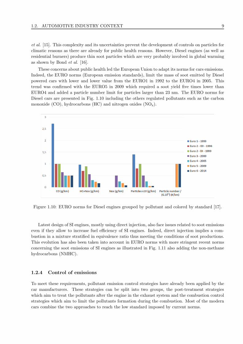
These concerns about public health led the European Union to adapt its norms for cars emissions.
Indeed, the EURO norms (European emission standards), limit the mass of soot emitted by Diesel
powered cars with lower and lower value from the EURO1 in 1992 to the EURO4 in 2005. This
trend was confirmed with the EURO5 in 2009 which required a soot yield five times lower than
EURO4 and added a particle number limit for particles larger than 23 nm. The EURO norms for
Diesel cars are presented in Fig. 1.10 including the others regulated pollutants such as the carbon
monoxide (CO), hydrocarbons (HC) and nitrogen oxides (NOx).
11
Figure 1.10: EURO norms for Diesel engines grouped by pollutant and colored by standard [17].
Latest design of SI engines, mostly using direct injection, also face issues related to soot emissions
even if they allow to increase fuel efficiency of SI engines. Indeed, direct injection implies a com-
bustion in a mixture stratified in equivalence ratio thus meeting the conditions of soot productions.
This evolution has also been taken into account in EURO norms with more stringent recent norms
concerning the soot emissions of SI engines as illustrated in Fig. 1.11 also adding the non-methane
hydrocarbons (NMHC).
1.2.4 Control of emissions
To meet these requirements, pollutant emission control strategies have already been applied by the
car manufacturers. These strategies can be split into two groups, the post-treatment strategies
which aim to treat the pollutants after the engine in the exhaust system and the combustion control
strategies which aim to limit the pollutants formation during the combustion. Most of the modern
cars combine the two approaches to reach the low standard imposed by current norms.

10 CHAPTER 1. INTRODUCTION
12
Figure 1.11: EURO norms for SI engines grouped by pollutant and colored by standard [17].
1.2.4.a Post-treatment
Most current SI engines use three-way catalyst (TWC) as their post-treatment system. It completes
the combustion reaction by:
• reducing nitrogen oxides into nitrogen and oxygen;
• oxidizing carbon monoxides to complete its transformation into carbon dioxide;
• oxidizing unburnt hydrocarbons (HC) to complete their reaction into carbon dioxide and water.
However, this method requires the mixture to be quasi-stoichiometric since it reduces and oxidizes
at the same time. The average mixture in Diesel engines is usually lean which cancels the ability to
reduce NOx.
To face this limit, Diesel engines can be equipped with several post-treatment systems. Most
Diesel engines use an Oxidation Catalyst (usually called DOC for Diesel Oxidation Catalyst) to
oxidize CO and HC into CO2 and water. DOC can also oxidize some soot particles. Nitrogen oxides
can be treated by NOx traps or using Selective Catalytic Reduction (SRC).
Finally, the soot particles are treated with a Particulate Filter (PF) in Diesel engines. This step
is optional in SI engines which produce less soot particles. However, new SI engines designs could
use PF since they produce more soot because of a combustion in a more stratified environment. PF
trap soot particles and oxidize them during their regeneration phases. These phases have to be done
regularly to keep the filter active between them. PF can reduce the soot emissions in mass of two
orders of magnitude. However, they have some limits:
• their use is complicated with regular regeneration phases which have to be done, otherwise
the PF can become unusable;
• they are expensive;
• they do not filter small particles smaller than a given diameter (usually 50 nm [18])

1.3. OBJECTIVES OF THE PRESENT WORK 11
1.2.4.b Combustion control
Pollutant emissions can be limited at the engine exhaust by using some methods to optimize the
combustion. For instance, the use of Exhaust Gas Recirculation (EGR) reduces the NOx formation
by reducing the temperature inside the cylinder. Indeed, a larger fraction of non-reactive gases with
high specific heat (mostly water and CO2) absorbs the heat release. However, this method also
increases the mixture equivalence ratio by reducing the quantity of oxygen inside the cylinder. This
leads to an increase of the soot formation.
Some other methods are specific to Diesel engines. For instance, multiple injections can be
done in the same cycle. This method uses the heat released by small injections before or after the
main one to reach better thermodynamical conditions either for the main combustion to occur or
to oxidize soot particles.
However, these methods are empirical and not yet fully understood. More studies have to be
done to improve their efficiency, including numerical studies which require models able to predict
the evolution of soot inside an engine cylinder.
1.3 Objectives of the present work
This study addresses the new issue of soot particle number in Diesel engines. The more and more
restrictive norms create a need of new engine designs among the car manufacturers. To develop these
new engines, soot formation and evolution models able to predict soot yield and size distribution in
3-D configurations are required. Indeed, numerical prediction of these data would help the design
process to converge to better engine geometries and settings to improve the combustion conditions
and reduce the raw-engine soot emissions. The 3-D aspect is also very important because of the
very heterogeneous conditions in Diesel engines combustion chambers.
In this context, the objective is to develop a soot model able to predict soot particles yield and
soot number density function (SNDF) in 3-D simulations of Diesel engines combustion chamber.
This model should:
• provide good enough predictions of soot yield and SNDF to allow the evaluation of parametric
variations from simulations;
• be adaptable to industrial 3-D CFD codes without too large cpu costs which would lower its
interest.
1.4 Turbulent flows modeling
1.4.1 Different types of simulations
The fuel and air flows in Diesel engines combustion chambers are turbulent. The codes used to
perform 3-D simulations of such engines require to represent or to model the turbulence effects.
Depending on the size of the domain and the objectives, different methods exist to model turbulence.
An illustration of the turbulence spectrum also showing which part of it are modeled by each method
is given in Fig. 1.12, along with an illustration of a typical simulated signal in each case. These
different approaches are:
• Direct Numerical Simulation (DNS): DNS represents all the scales of the turbulence spectrum
by directly solving the Navier-Stokes equations. It requires a very refined mesh to represent

12 CHAPTER 1. INTRODUCTION
effects down to the Kolmogorov scale. The time step and numerical methods needed to perform
a correct DNS are also very expensive in term of cpu cost. This method is not used for
combustion chambers simulations yet because of its high computational cost. It is mostly
used to study very local phenomena and to develop models for less accurate approaches.
• Large Eddy Simulation (LES): In LES, the smaller scales of turbulence are modeled and tur-
bulence is resolved down to scale ∆ (or up to a wavelength κc in the turbulence spectrum).
Even if part of the turbulence spectrum is modeled, LES allows to simulate variabilities due
to turbulence such as engine cycle to cycle variabilities [19]. The computational cost of LES
is still very high but combustion chambers simulations using LES can be performed.
• Reynolds Averaged Navier Stokes simulation (RANS): In RANS simulations, the complete tur-
bulence spectrum is modeled. This reduces strongly the computational cost but limits the
simulated data to averaged data. However, averaged data taking into account the effects of
turbulence is enough for many applications. Thus, RANS simulations are the most used for
combustion chambers and industrial applications generally. In these simulations, the influence
of the turbulence model as well as the coupling of other models (two-phases flows, combustion
...) is the most important compared to LES or DNS because everything is modeled.
Modeled in RANS
Computed in DNS
Computed in LESModeled in
LES
Signal
log( )log( )
E( )
timec
RANS
LES
DNS
Figure 1.12: Schematic presentation of the modeled and computed part of the turbulence spectrum
in RANS, LES and DNS (left) given with example of typical signal in time for the three methods
(right).
To perform 3-D simulations of Diesel engines using advanced combustion models coupled to a
detailed soot model, only RANS approach appears to be usable at this time. The progress of High
Performance Computing coupled to the implementation of advanced combustion models in LES
codes could make the use of LES possible in the near future.
1.4.2 RANS simulations basics
1.4.2.a Averaged equations
Any scalar X transported in a turbulent flow can be split into:
• a mean value X (Reynolds average)
• a fluctuation X ′ about its mean value, verifying X ′ = 0

1.4. TURBULENT FLOWS MODELING 13
Then, the scalar X writes:
X = X +X ′ (1.5)
To simplify the turbulence equations in compressible flows, Favre average X can be introduced
[20]:
X =ρX
ρ(1.6)
where ρ is the gas density. Fluctuation about X writes X ′′ and verifies X ′′ = 0.
The Navier-Stokes equations can then be averaged [1]. The averaged equations describe the
evolution of averaged values affected by turbulence. They read:
• Mass conservation:
∂ρ
∂t+
∂ρuj∂xj
= 0 (1.7)
• Momentum:
∂ρui∂t
+∂ρuiuj∂xj
= − ∂p
∂xi+
∂
∂xj
(τij − ρu′′i u
′′j
)(1.8)
where τij is the viscous stress tensor and ρu′′i u′′j is the Reynolds tensor which has to be modeled
in RANS. Boussinesq proposed a model which is usually used [21]:
−ρu′′i u′′j = µt
(∂ui∂xj
+∂uj∂xu
− 2
3
∂uk∂xk
δij
)− 2
3ρkδij (1.9)
where µt is the turbulent viscosity and k is the turbulent kinetic energy defined as k = u′′i u′′i .
Both µt and k have to be modeled.
• Species mass fraction:
∂ρYi
∂t+
ρYiuj∂xj
= − ∂
∂xj
(Vi,jYi + ρu′′jY
′′i
)+ ρ˜ωi (1.10)
where Yi is the ith species mass fraction, ˜ωi is the ith species production rate, Vi,jYi is the
laminar diffusion flux modeled by a Fick law:
Vi,jYi ≈ −ρDi∂Yi
∂xj(1.11)
whereDi is the species i diffusion coefficient. Usually, these diffusion coefficients are considered
equal for all species and written D. This approximation can be done because the turbulent
diffusivity is very dominant over the molecular diffusivity of all species. Finally, a closure is
required for the turbulent transport term:
ρu′′jY′′i = − µt
Sct
∂Yi
∂xj= −Dt
∂Yi
∂xj(1.12)

14 CHAPTER 1. INTRODUCTION
where Sct is the turbulent Schmidt number and Dt =µt
Sctthe turbulent diffusion. Then, the
transport equation of the ith species mass fraction writes:
∂ρYi
∂t+
ρYiuj∂xj
=∂
∂xj
((D +Dt
∂Yi
∂xj
)+ ρ˜ωi (1.13)
• Enthalpy:
∂ρhs∂t
+ρhsuj∂xj
=∂
∂xj
(µt
Prt
∂hs∂xj
)+ ˜ωh (1.14)
where Prt is the turbulent Prandtl number and ˜ωh is the enthalpy source term.
Similar transport equations can be written to represent variance X ′′2 of any scalar X.
1.4.2.b Turbulence modeling
Various models exist to compute turbulence effects in RANS simulations [1]. The ones used in
this study are two variations of the k-ǫ model: the standard one and the Re-Normalization Group
(RNG). Both models are based on two transport equations and a set of constants. First, the
turbulent viscosity, µt, writes:
µt = Cµρk2
ǫ(1.15)
where Cµ is a model constant.
The turbulent kinetic energy k is given by the following transport equation:
∂ρk
∂t+
ρkuj∂xj
=∂
∂xj
[(µ+
µt
σk
)∂k
∂xj
]+ Pk − ρǫ (1.16)
where σk is a modeling constant, Pk = −ρu′′i u′′j∂uj
∂xi. The turbulent energy dissipation rate ǫ is
deduced from a transport equation:
∂ρǫ
∂t+
ρǫuj∂xj
=∂
∂xj
[(µ+
µt
σǫ
)∂ǫ
∂xj
]+ Cǫ1
ǫ
kPk − Cǫ2ρ
ǫ2
k(1.17)
where σk and Cǫ1 are model constants. Cǫ2 is a model constant in the standard model and deduced
from an equation in the RNG model [22].
The constants for the standard k-ǫ model are taken from Jones and Launder [23]. The equivalent
set of constants as well as the relation giving Cǫ2 are taken from Yakhot et al. [22] for the k-ǫ RNG
model.
1.5 Thesis outline
This thesis is split into two parts, each one separated in two chapters:
• First, the soot formation and evolution is studied. A study of the physical phenomena involved
in soot life cycle and the existing methods to model soot particles is given in Chapter 2. It is
concluded by a definition of the modeling approach proposed in this study and an explanation
of its novelties with respect to the models existing in the literature. Then, the solid phase soot
model is detailed in Chapter 3. Finally, a first validation on academical cases is presented.

1.5. THESIS OUTLINE 15
• Then, two validation cases of the sectional soot model coupled with detailed chemistry turbu-
lent combustion models are presented with 3-D RANS simulations compared to experimental
measurements. In Chapter 4, Diesel engine cases are studied using an experimental database
of various operation points which have been simulated. The Chapter 5 contains a similar study
for Diesel sprays in a constant volume vessel with more detailed diagnostics and combustion
model. This vessel allows more measurements to be performed for validations than an actual
engine case would. The respective combustion models which are coupled with the soot model
are presented with each validation.
Global conclusions about the present work are given in the last chapter.

16 CHAPTER 1. INTRODUCTION

Chapter 2
Soot modeling background
Introduction
Soot particles are low diameter compounds (from nanometer to micrometer) of reactive flows usually
composed of aggregated elementary particles. They are created by the condensation of carbonic
species in the rich regions of flames. Although they are used since prehistory for Cave Art [24, 25],
their structures and the physical phenomena driving their evolutions are still open topics. Indeed,
soot formation is based on several phenomena strongly depending on local thermodynamic conditions
and gaseous composition which make them difficult to model.
In this chapter, the main phenomena of soot formation understood or predicted so far are
presented first. Then, the existing soot modeling approaches are presented. Finally, the proposed
model, which will be presented in Chapter 3, and its situation among the different approaches is
clarified as well as the soot modeling objectives of this study.
2.1 Soot formation mecanisms
Soot formation is a very complex phenomenon of conversion from gaseous hydrocarbon molecules
to solid agglomerates containing thousands of carbon atoms. The different phases of soot formation
are still uncertain but the global path leading to these agglomerates is known. These steps are
illustrated in Fig. 2.1 and detailed in this section.
Figure 2.1: Illustration of the main pathways for soot formation and evolution.
17

18 CHAPTER 2. SOOT MODELING BACKGROUND
2.1.1 Gaseous precursor formation
Polycyclic Aromatic Hydrocarbons (PAH) are considered as the main soot precursors. They are
reaction intermediates of combustion and their evolutions are still open topics. However, their
growth is usually based on single ring aromatic species such as benzene (C6H6), phenyl group
(C6H5) and cyclopentadienyl (cC5H5).
2.1.1.a First aromatic cycle formation
The representation of the first aromatic cycles formation is then a crucial step towards soot modeling
since they are the base of PAH block in kinetic schemes. Three main pathways have been identified
in the litterature to lead to the first benzene ring [26]:
• The C4 +C2 → C6 reactions:
A first way to create a benzene ring (C6H6) was proposed by Cole et al. [27] and Frenklach et
al. [28]:
C2H3 +C2H2 → C4H5 (2.1)
C4H5 +C2H2 → C6H6 +H (2.2)
However, Miller and Melius [29] have shown that these reactions cannot explain the amount
of benzene measured experimentally in some cases.
• The C3 +C3 → C6 reactions:
Kern and Xie [30] proposed a second way to form a benzene ring from smaller hydrocarbons.
This reaction, also mentioned by Miller and Melius [29], is the recombination of two propargyl
radicals (C3H3) into a benzene ring:
C3H3 +C3H3 → C6H6 (2.3)
C3H3 +C3H3 → C6H5 +H (2.4)
• The C5 +C1 → C6 reaction:
Another reaction has been proposed later by Melius et al.[31] and also validated by Ikeda et
al. [32]. This reaction is the addition of a methyl group on cyclopentadiene:
C5H5 +CH3 → C6H6 + 2H (2.5)
There are still studies to predict single ring aromatic species with more accuracy. Lamprecht et
al. [33] showed that the balance of the three proposed reactions to form benzene depended strongly
on thermodynamical conditions in acetylene and propene flames. A similar study of Gueniche et al.
[34] led on methane flames doped by unsaturated compounds also shows the sensitivity of benzene
formation to the different pathways.
Rasmussen et al. [35] studied the dominance of C3H3 +C3H3 → C6H5 +H reaction in the
propargyl recombination way. The C3 +C3 reactions rate constants are also evaluated in recent
works [36, 37].
Recently, Nawdiyal et al. [38] studied rich 1-hexene flames showing a dominance of the C5 +C1 →C6 reactions over the propargyl recombination, the C4 +C2 → C6 pathway being the less impor-
tant one. However, Bierkandt et al. [39] showed that the propargyl recombination is dominant in
acetylene flames. These recent results illustrate the importance of fuel for the first step leading to
soot formation.

2.1. SOOT FORMATION MECANISMS 19
2.1.1.b Polycyclic Aromatic Hydrocarbons formation
PAH formation models are still very uncertain due to the very low concentration and lifetime of
these species, making experimental measurements very complicated. However, the recent progress
in optical diagnostic could offer new possibilities and data to modelers [40].
Some pathways already exist to represent the growth from single ring aromatic species to Poly-
cyclic Aromatic Hydrocarbons. The two main pathways are presented in the following:
• Cyclopentadiene to naphthalene [31]:
The growth to PAH could begin with the cyclopentadiene recombination to naphthalene which
can be presented either in one or multiple step rearranging atoms to add a second aromatic
ring on the first cyclopentadiene:
C5H5 +C5H5 → Naphthalene + 2H (2.6)
This pathway is shown to be not dominant in the growth of larger aromatic species [41,
42]. However, Lindstedt and Rizos [43] also showed that this direct reaction would over-
predict naphthalene and a two-step sequence could not explain the amount of naphthalene
experimentally measured.
• The HACA cycle [26, 28, 44]:
The Hydrogen Abstraction Carbon Addition (HACA) cycle is a usual representation of growth
from benzene to larger PAH. The HACA cycle described by Francklach and co-workers [26,
28, 44] is based on two reactions occurring repetitively: Hydrogen Abstraction by a radical
hydrogen and Carbon Addition from acetylene, as illustrated in Fig. 2.2. This cycle is consid-
Figure 2.2: Illustration of the HACA cycle reactions
ered dominant for PAH growth by Appel et al. [45] but Bohm et al. [46] showed its limit to
predict some PAH species. Even if it is commonly used, the physical details of the reaction
represented in this cycle are still uncertain. This cycle is then used as a reference and a base to
develop growth cycle either by adding reactions or by using various sets of reaction rate con-
stants [47, 48]. Moreover, similar cycles are proposed such as the “phenyl addition/cyclization”
(PAC) and the “methyl addition/cyclization” (MAC) are studied [49].
20 CHAPTER 2. SOOT MODELING BACKGROUND
Frenklach [26] also mentioned the cyclopentadiene way as an addition to the HACA cycle. In
recent models, the two approaches are mixed with creditable results [50, 51]. However, the growth
of PAH is also still an open topic as explained by Wang [52], as well as the nascent soot physics
based on PAH.
2.1.2 Smallest solid particles: particle inception
The actual conditions on which carbon condenses into solid particles are not yet known [26, 53, 54].
Usually, the first solid particles correspond to a dimer PAH larger than pyrene [45]. This way to
model particle inception is usually used in soot models [55, 56, 57, 58]. Coronene is taken as a
reference by Richter et al. [59], leading to a similar size for the smallest solid particles. Another
approach exists, based on atomic mass unit amu, considering that carbon compounds are solid when
their atomic mass unit is larger than a constant criterion, varying from 800 to 2000 [60, 61].
For all considered sizes of the smallest solid particles, most of the representations of particle
inception are based on two phenomena:
• Solid particles formation from colliding precursors [26, 53] described by the Smoluchowski
equation [62],
• Growth of large enough carbon-based compounds from the HACA cycle [28].
In this context, two situations are isolated by Frenklach [26]. At low temperatures, chemical
bond can be created from collisions because there are only little thermodynamical limits to it. At
higher temperatures, the growth is controlled by the HACA cycle which is based on acetylene, a
thermodynamically stable species.
Recently, Eaves et al. [54] study also stressed the importance of taking into account the re-
versibility of the particle inception process. These results agree with the measurements of Sabbah
et al. [63] observing a too strong dissociation of pyrene dimerization for it to be a liable reaction
of particle inception. Accordingly, pyrene should only be used as an indicator of where particles
inception occurs and how it varies with respect to standard combustion parameters (equivalence
ratio, temperature, pressure...).
2.1.3 Collisional phenomena
2.1.3.a Light particle collisions
Two main phenomena are usually modeled as collisional phenomena:
• Condensation: PAH colliding with a solid soot particle;
• Coagulation: collision between two solid soot particles.
Condensation increases soot mass and size without impacting on the particle number, while
coagulation increases particle size and decreases particles number without impacting on soot mass.
Particle inception can also be considered as a collisional phenomenon [53, 55, 56]. The most common
approach has been proposed by Seinfeld [64] and also applied to the soot formation context by
Kazakov and Frenklach [65]. It describes collisional phenomena using the Smoluchowski equation:
Na,t =1
2
∫ a
0βa−b,bNb,tNa−b,tdb−
∫ ∞
0βa−b,bNa,tNb,tdb (2.7)

2.1. SOOT FORMATION MECANISMS 21
This equation provides the collisional source term for particles of size a: Na,t. βx,y represents the
collision frequency between particles of sizes x and y. It should be noticed that even if a represents
the size of solid particles, a− b and b can represent:
• two sizes of gaseous soot precursors leading to a solid particle of size a (particle inception)
• a gaseous soot precursor and a solid soot particle (condensation)
• two solid soot particles (coagulation)
The collision frequency βx,y depends on the Knudsen number Kn and thermodynamical condi-
tions. The Knudsen number reads:
Kn(x) =λgas
d(2.8)
where d is the diameter of the considered particle and λgas is the mean free path, written:
λgas =RT√
2d2gasNAP(2.9)
where P is the pressure, T is the temperature, NA is the Avogadro number, R the universal gas
constant and dgas the mean diameter of gas molecules.
Depending on the Knudsen number, three collision regimes can be established [64, 65]:
• If Kn ≫ 1 (Kn > 10 in [55, 56, 57]), the pressure is low enough and the particles are
small enough with respect to the temperature driven agitation for a free-molecular regime of
collision to be established. The particles can be considered as randomly moving spheres which
can collide within a very large free space between each of them. In this case, the collision
frequency βx,y writes:
βfmx,y =
(3
4π
) 1
6
√6kbT
ρsoot
√1
x+
1
y
(x
1
3 + y1
3
)2(2.10)
where kb is the Boltzmann constant, ρsoot is the solid soot density, x and y are the colliding
particles volume and T the gaseous temperature.
• If Kn ≪ 1 (Kn < 0.1 in [55, 56, 57]), the pressure is high enough and the particles are large
enough with respect to the temperature driven agitation for a continuum regime of collision
to be established. The amount of space taken by particles and their motions is large with
respect to the available space and collisions are more likely to occur. In this case, the collision
frequency βx,y writes:
βcx,y =
2kbT
3µ
(C(x)
x1
3
+C(y)
y1
3
)(x
1
3 + y1
3
)(2.11)
where µ is the gaseous dynamic viscosity and C(x) = 1 + 1.257Kn is the Cunningham slip
correction factor [66, 67].
• For intermediary cases, the collision frequency is written as the harmonic mean of the limit
values [65, 67, 68]:
βx,y =βfmx,y βc
x,y
βfmx,y + βc
x,y
(2.12)
22 CHAPTER 2. SOOT MODELING BACKGROUND
2.1.3.b Agglomeration
When the primary particles growth step is over, the particles grow by a collisional phenomenon
called agglomeration. They collide and bound to each other in order to form large chain structures
[26]. These agglomerates are the large particles measured at the exhaust of Diesel engines. However,
the agglomeration mechanisms are still unknown and defining their structure is a current research
topic [69, 70]. These structures are also studied for soot-in-oil to evaluate the effect of soot particles
over lubricant as in La Rocca et al. [71].
The collision rates are modeled as coagulation ones in most models models [57, 72, 73] but
multiple variables models can predict agglomerates structures [73].
2.1.4 Soot surface chemistry
Soot particles evolutions also depend on chemical phenomena. The gaseous phase composition
and thermodynamical conditions as well as the available soot surface and its ability to react are
parameters which lead to an increase or a decrease of the soot mass due to surface chemistry.
Frenklach proposed a soot surface chemistry controlled by the HACA cycle. This approach is
very commonly used to represent soot surface chemistry [52, 55, 56, 61, 74, 75, 76, 77, 78, 79, 80].
It is based on the assumption that C−H bounds are present on soot surface. The HACA cycle
could then occur at soot surface as it does for the gaseous PAH growth [26]. The HACA cycle
constants are not yet well defined [52] and various studies propose different sets of constants as
the one proposed by D’Anna and Kent [74, 75]. A version of the HACA cycle including a reverse
reaction on the carbon addition, named HACA Ring Closure (HACA-RC), has also been proposed
by Mauss [81] and used for soot modeling [55, 77, 78].
It has been shown that the chemical reaction rate of particle decreases with particle size [26, 82].
Two main causes have been identified to explain this phenomenon [26, 82]:
• Reaction sites at soot surface might not be active due to surface state.
• Gaseous hydrogen concentration could decrease, stopping the first step of the HACA cycle to
occur for most of the soot surface reactive sites.
The evaluation of soot surface composition is a major aspect of soot surface modeling [52].
Recent studies of Dworkin and co-workers [83, 84] proposed a representation of the proportion of
active sites depending on the thermal history of particles. This topic is also a source of research in
the field of atmospheric sciences [85].
2.2 Soot modeling approaches
To design engines able to match the more and more stringent norms of the 21th century, the car
manufacturers need models able to predict soot production of real engines. To reach these current
industrial targets for soot predictions, the previously introduced physical phenomena have to be
integrated into advanced numerical models. The complexity of these models depends on which type
of prediction is needed and on the tool it has to be implemented in.
There are three main types of soot models [86]: empirical models, semi-empirical models and
phenomenological models (or detailed models). These three different types of models are presented
in this section.

2.2. SOOT MODELING APPROACHES 23
2.2.1 Empirical correlations
Empirical correlations are very often used by the car industry. These models are based on corre-
lations between the soot mass production and the engine operating conditions. These correlations
were the first step towards soot modeling. For instance, Calcote and Manos [87] defined a Threshold
Soot Index (TSI) that ranks fuel from 0 to 100 depending on their soot production and proposed
a correlation between this TSI and the fuel molecular structure for premixed and diffusion flames.
This correlation has been studied by Olson et al. [88], providing a large database of case to widen
its possible applications.
More recent correlations can depend on more parameters such as the one proposed by Mehta
and Das [89], commonly used for engine simulations. They obtained a correlation depending on
six parameters: the spray mixing rate, the swirl mixing rate, the compression ratio, the injection
temperature, the injection velocity and the engine speed. As illustrated in Fig. 2.3, this correlation
gives decent predictions of soot production when compared to experimental measurements.
Figure 2.3: Prediction of a Diesel engine soot yield using Mehta and Das correlation [89] compared
to experimental measurements [89].
However, these correlations can only be used in conditions close to the one they were established
on. They also only provide global soot values, either mass or volume fraction. It is not possible to
describe the soot distribution in size using this type of correlation.
These correlations are also not usable in 3-D CFD code because they do not predict a time-
evolution of soot particles. Instead, they only predict a final value at exhaust for engine correlations,
or a value such as the TSI for flames correlations.
The use of these approaches is limited to global system simulations.
24 CHAPTER 2. SOOT MODELING BACKGROUND
2.2.2 Semi-empirical models
Semi-empirical models attempt to represent some physical phenomena driving soot time-evolution.
However, the different sizes of soot particles are not represented and global formation and oxidation
rates are applied to values representing the whole range of modeled particles. These global source
terms are usually applied to one or two variables and are designed to be applicable to turbulent
flames simulations as the model proposed by Leung et al. [90] which was recently used to model
soot evolution in Diesel sprays simulations by Bolla et al. [91] using a Conditional Moment Closure
approach. These models can also be coupled with detailed PAH modeling as proposed by Sukumaran
et al. [58].
The modeled variables can be different from one model to another. Three examples are given
to illustrate the different types of semi-empirical models from the more empirical to the more
phenomenological one:
• Said et al. [92] model: In this model, two transported variables are used to describe the soot
time-evolution. The first variable is an intermediary soot species mass fraction YI equivalent
to a soot precursor. The second variable is the total mass fraction of soot YS . These two
species are coupled as shown in their respective transport equations:
ωYI= kAYFY
αOxexp
(−TA
T
)− kByIY
βOx exp
(−TB
T
)− kI(T )YI (2.13)
ωYS= k1(T )YI −
kOρSdS
YOxYSPT−1/2 exp
(−TC
T
)(2.14)
where kA, kB , kO, α, β, TA, TC and TB are experimentally-obtained constants, kI and kS are
experimentally-correlated reaction rates, dS is an arbitrary-guessed particle diameter, ρS is
the density of solid soot, P is the pressure, T is the temperature and YOx and YF are the mass
fraction of oxidant and fuel respectively.
The intermediary soot species I is created by the fuel cracking and consumed by oxidation and
the creation of actual soot S. Here, the soot variable S is only formed from the intermediary
species and consumed by oxidation.
This model predicts a soot mass time-evolution in the context of a 3-D simulation but does
not include the representation of different phenomena such as coagulation, particle inception
or surface growth.
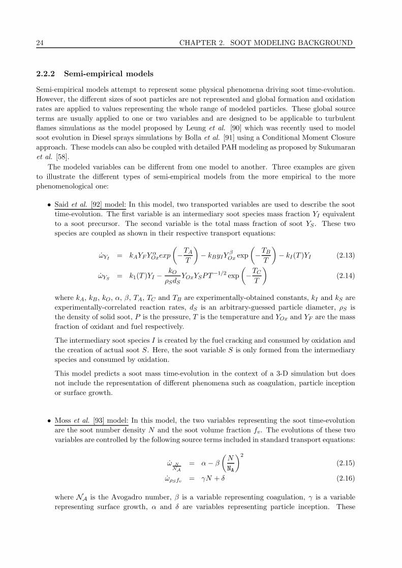
• Moss et al. [93] model: In this model, the two variables representing the soot time-evolution
are the soot number density N and the soot volume fraction fv. The evolutions of these two
variables are controlled by the following source terms included in standard transport equations:
ω NNA
= α− β
(N
NA
)2
(2.15)
ωρSfv = γN + δ (2.16)
where NA is the Avogadro number, β is a variable representing coagulation, γ is a variable
representing surface growth, α and δ are variables representing particle inception. These

2.2. SOOT MODELING APPROACHES 25
variables write:
α = Cαρ2T 1/2XC exp
(−Talpha
T
)(2.17)
β = CβT1/2 (2.18)
γ = Cγρ2T 1/2XC exp
(−Tgamma
T
)(2.19)
δ = CδT1/2 (2.20)
where ρ is the gas phase density, XC the fuel mole fraction and the Ci and Ti are prescribed
numerical constants.
The model of Moss et al. [93] represents particle inception and its effect on the soot volume
and number. The surface growth is also represented and its source term couples the soot
number density and volume fraction. Finally, the coagulation effect is only to reduce the soot
number density.
This model provides data on the soot volume fraction and number, thus also giving an average
particle size. It also takes into account most phenomena involved in soot evolutions but does
not include oxidation.
• Phenomenological Soot Kinetics (PSK) model [80]: In the PSK model, the evolution of two
variables, an intermediary soot variable “PR“ and a soot species ”Soot“ evolutions are driven
by a set of ten reactions:
CnHm
R1↔ n
2C2H2 +
m− n
2H2
C2H2R2↔ 2
nC,PRPR+H2
PR+ PRR3↔ soot
sooti +C2H2R4↔ sooti+2 +H2
sooti + PRR5↔ sooti+nC,PR
sooti + sootjR6↔ sooti+j
PR+nC,PR
2O2
R7↔ nC,PRCO
C2H2 +O2R8↔ 2CO + H2
H2 +1
2O2
R9↔ H2O
sooti +O2R10↔ 2CO + sooti−2
(2.21)
where nC,PR is the number of carbon atoms in a precursor, sooti is the soot species and sooti+j
does not represent a different soot species but indicates the fact that the reaction will add or
take the mass of j carbon atoms from the soot species.
This model represent all phenomena from fuel pyrolysis (R1) to soot oxidation (R10), includ-
ing PAH formation (R2), particle inception (R3), surface growth from precursors (R5) and
acetylene (R4), coagulation (R6) and oxidation of precursors (R7) and acetylene (R8,R9).

26 CHAPTER 2. SOOT MODELING BACKGROUND
The PSK model has been used for 3-D RANS modeling of engine cases [94, 95]. It provides a
prediction of the soot mass in 3-D RANS simulations by taking into account all phenomena
involved in soot formation and oxidation.
The use of only two variables at most in these semi-empirical approaches makes them unable to
predict soot size distributions. This limit is also a limit to their prediction of soot mass and number
time-evolution because many phenomena depend on particle size.
2.2.3 Detailed soot models
In order to predict the soot time-evolution with a better accuracy and to also predict SNDF, detailed
soot models have been developed. These models represent the dynamics of soot formation from the
smallest solid particle to large primary particles or agglomerates. They split into three main types,
described in the following.
2.2.3.a Stochastic approach
Stochastic approaches model molecules and particles structures and their evolutions using Monte-
Carlo method usually. The modeled particles structures evolve by the addition or abstraction of
atoms according to probabilistic considerations. Using presumed trajectories to represent the input
of their stochastic model, Balthasar and co-worker predicted complete SNDF with credible results
[96, 97]. The method has been used by Singh et al. to predict SNDF including data on particle age,
allowing to study numerically the evolution of some soot modeling parameter dependence to soot
aging [98].
These approaches also permit the modeling of molecular structures of soot precursors or particles.
Violi and co-workers modeled the physical properties of soot precursors and predicted characteristic
time for particle inception using these approaches [99, 100, 101]. Stochastic approaches also allow
the description of the type and number of available sites at PAH and nascent particles surface
[102, 103].
However, it is very complicated to direclty couple a gas phase solver and this type of soot model
[104]. Moreover, some of the features provided by these approaches, such as the site description, are
not directly usable with a complete population balance equation solver [103]. Some recent works
have been done to conceive this type of coupling in simple flows, mostly focusing on the issue of
coagulation modeling [105, 106, 107].
2.2.3.b Method of moments
The method of moments is a mathematical method used to describe dispersed phases in flows.
Based on an assumption on the dispersed phase distribution shape, the method of moment allows
to describe the distribution using its first characteristic moments. The dispersed phase can be
described by more than one variable, usually two variables are used to describe soot distributions
[73, 108, 109, 110] In this context, the order x in volume and y in surface moment of a distribution
writes:
Mn,y =∑
i
V xi S
yi Ni (2.22)
where Vi, Si and Ni are respectively the volume, surface and particle number density of size class i.
More complex closure can also be used to describe moments of soot distribution [108]. The physical

2.2. SOOT MODELING APPROACHES 27
phenomena are then represented by their effects on the different moments of the distribution as
detailed by Mueller et al. [108].
Balthasar and co-workers [97, 111] used a single variable method to describe soot volume fraction
evolutions in partially-stirred plug flow reactor and laminar flames. Single variable method has also
been used to model turbulent jet by Mauss et al. [112] showing good prediction of soot volume
fraction. This method has even been applied to 3-D RANS Diesel sprays simulations by Karlsson et
al. [113] and full engine simulations by Priesching et al. [114] but without quantitative comparisons
against the experimental measurements.
Laminar flames and counterflow diffusion flames have also been studied using a two variable
approach by Mueller et al. [108, 109]. Thanks to its low computation cost, the method of moments
have been used in 3-D CFD simulations, including LES [110, 115, 116] and DNS [73, 117, 118].
Flames simulated using a method of moments in a LES code show various results qualities in terms
of soot volume fraction with respect to the experimental measurements [110, 115]. However, Mueller
and Pitsch presented a complete LES simulation of an aircraft combustor, without experimental
comparison though [116].
Using an infinity of moments would describe the distribution totally. However, this is practically
impossible. A limited number of moments is then used to represent the distribution and this leads
to the assumption made on the distribution shape. Moreover, the data of the predicted SNDF is
rarely given and compared to experiment yet.
2.2.3.c SNDF resolution
In these approaches, the distribution in size of soot particles is split into different classes. Both
sectional dispersed phase models and chemical models representing soot particles as species are
included in this discussion. Indeed, these two approaches share the splitting in size of the SNDF
and only express it in different ways. The main difference between the two approaches lies on the
way the source terms are written.
• Chemical representation [72, 74, 119]: In this type of model, a detailed kinetic mechanism
describes the evolution of gaseous species during the combustion as well as large PAH species
which represent the solid phase. Usually, the switch from the standard gaseous reactions to the
solid phase reaction occurs for species constituted of more than 30 carbon atoms. The different
processes driving soot formation and evolution will all be written as chemical reactions. For
instance, in the model proposed by Richter et al. [119], the growth of the tenth size class soot
particles (called BIN10) by acetylene addition reads:
BIN10J + C2H2 → 0, 9998408 BIN10 + 0, 0001592 BIN11 + 0, 5414 H (2.23)
where BIN10J is a species representing the radical aromatic of size class 10, BIN10 and
BIN11 are the aromatic of size classes 10 (representing particles with mass from 102401 to
204800 amu) and 11 (representing particles with mass from 204801 to 409600 amu) respec-
tively.
This model has been used to simulate soot number density and average particle size in laminar
premixed benzene flames [119]. D’Anna and Kent also used this type of approach to simulate
soot volume fraction and mass in ethylene premixed and non-premixed laminar flames [74, 76]
and soot volume fraction in methane, ethylene and butene premixed laminar flames [75].

28 CHAPTER 2. SOOT MODELING BACKGROUND
These models require large computational resources because both the detailed kinetic scheme
has to be solved, including all the reactions between every ”BIN“. However, it has been used
for 3-D RANS Diesel simulations by Fraioli et al. [72] with decent results but a very high
computation cost as planned.
• Sectional method [55, 61, 77]: The sectional method describes the SNDF as a distinct dispersed
phase interacting with the gaseous phase. This dispersed phase is composed of a given amount
of scalars, representing the size classes of the distribution. Introduced by Gelbard et al.
for atmospheric aerosol studies [120], it has also been used to describe spray droplets by
Tambour and co-workers [121, 122]. The relevance of this method for spray simulations has
been contested by Laurent and Massot [123] because the various velocities and temperature
of same size droplets at the same locations cannot be represented. However, the method has
been applied to soot formation and is still considered relevant for these cases because these
issues are neglectable compared to soot formation and oxidation processes.
This method has been applied to ethylene laminar premixed flames [57, 124], to ethylene
nonpremixed laminar flames [79, 84] and to ethylene turbulent diffusion flames by Netzell et
al. [78]. A single Diesel engine case has also been simulated by Marchal et al. [125] showing
the method can be applied to complete engine simulations.
The source terms description can be very similar to the ones used with chemical representation
of soot as in Blacha et al. [61]. This study also includes a sectional representation of PAH
growth between the gaseous phase and the solid soot phase sectional model. This approach
shows good results on ethylene, propylene, kerosene surrogate and toluene premixed and non-
premixed laminar flames [61] for soot volume fraction and SNDF predictions. It has also been
applied to turbulent nonpremixed flames [126] with encouraging results.
Finally, the computation cost of this method can be high because of the large number of
scalars to transport (one per section) but its numerical implementation is simple. Moreover,
this method is not based on an assumption concerning the SNDF shape.
2.3 The proposed approach
In the present study, the proposed model only aims to represent the solid soot phase as the models
presented in Section 2.2. Empirical and semi-empirical models cannot be used in this study be-
cause the industrial requirements include the concept of particle size to match norms past EURO
5. Moreover, the target model has to be implemented in a 3-D CFD code in order to represent the
composition heterogeneities, which could not be done with an empirical model. However, most of
the detailed soot models currently developed have not been validated against experimental measure-
ments on 3-D cases. The few of them which have been validated, mostly with a sectional approach,
usually are only presented with one 3-D case. Moreover, all the referenced turbulent flames were
simulated with light fuels.
Accordingly, a detailed soot model has been developed. Among the different approaches to
model soot size distributions, only the sectional method and method of moments were suitable
for this study. Indeed, stochastic approaches can hardly be coupled to codes including spatial
heterogeneities and the chemical approach would require either to solve a complete kinetic scheme
or to tabulate every species representing solid soot particles which is practically impossible. Even

2.3. THE PROPOSED APPROACH 29
if the computation cost is higher for sectional models, this approach has been preferred over the
method of moments for three reasons:
• to avoid the presumption of the soot size distribution shape;
• because the method of moments requires specific numerical schemes to ensure moments real-
izability [127];
• because its numerical implementation does not require a reconstruction of the SNDF, thus
allowing a direct and easier study of the different locations of soot particles with respect to
their sizes in 3-D simulations.
However, similar works using the method of moments could be done in the future as a perspective
of the present study.
The gaseous phenomena described in Section 2.1.1 (growth of PAH) will not be studied and are
included in kinetics schemes taken from literature to represent the gaseous phase. A major aspect
of this work is to introduce the predictions of these kinetic schemes into 3-D RANS simulations
with a reasonable computation cost. The tabulated turbulent combustion models used to do so are
described in Chapter 4 and 5 prior to the description of the validation case they were used with.
In this context, the main objectives of this study are:
• to adapt a sectional soot model to Diesel conditions;
• to couple it with turbulent combustion models able to model heavy fuels combustion;
• to validate both the model and its coupling to a turbulent combustion model against experi-
mental data.
This leads to three main novelties presented in this study:
• the confirmation that tabulated approaches can be coupled to detailed soot solver, their ability
to reproduce the gaseous chemistry required by this type of soot model being shown;
• the validations of a detailed 3-D soot model against experimental data on 3-D turbulent cases
(engine cases and spray cases in a constant volume vessel);
• the validation of a detailed 3-D soot model on heavy fuels turbulent flames or engine cases.

30 CHAPTER 2. SOOT MODELING BACKGROUND

Chapter 3
The Sectional Soot Model
Introduction
The sectional soot model proposed in this study is first described in Section 3.1. To illustrate the
effects of the proposed changes to the reference model, comparisons to the reference model and to
academical experiments are presented in Section 3.2.
3.1 Soot modeling
The soot model introduced in the present study is based on the approach of Mauss [81, 128] followed
by the more recent work of Netzell et al. [55, 78], Marchal [56, 77] and Vervisch-Kljakic [57]. This
section describes its governing equations and the evolutions brought to the source terms estimation.
The soot particles population is evaluated by using a sectional method. The soot particles are
separated with respect to their volume into discrete sections. In contrast to Fraioli et al. [72] where
soot particles are considered as chemical species, the present approach considers that soot particles
are solid and modeled as a distinct dispersed phase, interacting with the gaseous phase. In the
turbulent reactive flow, each section i, representing the soot particles of a given volume range, is
governed by a standard transport equation for the soot mass fraction in this section, Ysoot,i:
∂ρYsoot,i
∂t+∇ · (ρuYsoot,i) = ∇ · (ρDt,soot∇Ysoot,i) + ρ˜ωsoot,i (3.1)
with ρ the gas phase density, u the gas velocity, Dt,soot the turbulent diffusion coefficient of soot
and ˜ωsoot,i the soot source term for section i.
We start with the presentation of the particle volume discretization and of the variables used to
represent soot particles in each section. Then, the different physical phenomena involved in the soot
formation process are described. These phenomena are illustrated in Fig. 3.1 and are introduced in
the following order:
• First, collisional source terms: particle inception, condensation and coagulation.
• Secondly, surface chemistry source terms: surface growth and oxidation.
31

32 CHAPTER 3. THE SECTIONAL SOOT MODEL
PAH PAH PAH+ + +
Combustion model(gaseous phase)
Sectional Soot Model(solid phase)
(PAH)
Polycyclic Aromatic
Hydrocarbon
Detailed chemistry
Fuel + Oxidizer
(+ Residual)
CO C2H2
H2 H20
O2 HCO
H OH
C2H2 + OH + O2+
Smallest solid
particle
Particle inception Condensation Coagulation
Surface growth Oxidation
Larger
particle
Surface chemistry
Collisional phenomena
Larger
particle
Larger
particle
Smaller
particle
Smaller
particle
Inte
rme
dia
tes a
nd
pro
du
cts
Figure 3.1: Illustration of the five phenomena representing soot formation and evolution with the
involved gaseous species.
3.1.1 Volume discretization
In this model, a fixed interval of volume [VMIN ;VMAX ] is divided into nsect sections. The smallest
volume of the considered particles is VMIN and is equal to the carbon-equivalent volume of the
number of carbon atoms of two soot precursors and two acetylene molecules. Carbon-equivalent
volume for two atoms of carbon is given by:
VC2=
2MC
NAρsoot(3.2)
where MC is the molar mass of carbon, NA the Avogadro number and ρsoot the soot density which
is assumed constant at a value of 1.86 · 103 kg.m−3 [55, 56].
Using pyrenyl (C16H9) as precursor as in [55, 56, 58, 78, 77], VMIN becomes equal to 18VC2
with a value of 3.857 · 10−28 m3 which is approximately the volume of a 0.9 nm diameter sphere. In
the case of a complete solid-gas coupling between the soot model and a kinetic solver, all hydrogen
atoms taken from the gas phase are then sent to H2 to close the hydrogen balance since all volumes
exchanged between phases are given with respect to the exchanged number of carbon atoms.
The largest modeled particles have a volume VMAX corresponding to the volume of a dMAX =
10µm diameter sphere. In Diesel engines, the particles produced are one or two orders of magnitude
smaller than this value dMAX in diameter [72, 129, 130, 131]. This VMAX value ensures that carbon
mass will not accumulate in the last section.
The first section represents soot particles of a constant volume range going from VMIN to VMIN+
VC2. The following sections are defined to fill the represented volume interval with nsect− 1 sections
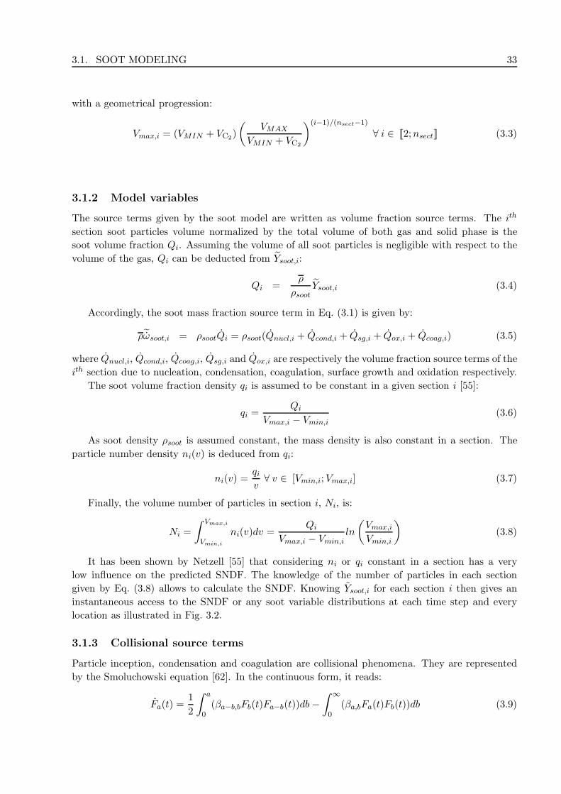
3.1. SOOT MODELING 33
with a geometrical progression:
Vmax,i = (VMIN + VC2)
(VMAX
VMIN + VC2
)(i−1)/(nsect−1)
∀ i ∈ J2;nsectK (3.3)
3.1.2 Model variables
The source terms given by the soot model are written as volume fraction source terms. The ith
section soot particles volume normalized by the total volume of both gas and solid phase is the
soot volume fraction Qi. Assuming the volume of all soot particles is negligible with respect to the
volume of the gas, Qi can be deducted from Ysoot,i:
Qi =ρ
ρsootYsoot,i (3.4)
Accordingly, the soot mass fraction source term in Eq. (3.1) is given by:
ρ˜ωsoot,i = ρsootQi = ρsoot(Qnucl,i + Qcond,i + Qsg,i + Qox,i + Qcoag,i) (3.5)
where Qnucl,i, Qcond,i, Qcoag,i, Qsg,i and Qox,i are respectively the volume fraction source terms of the
ith section due to nucleation, condensation, coagulation, surface growth and oxidation respectively.
The soot volume fraction density qi is assumed to be constant in a given section i [55]:
qi =Qi
Vmax,i − Vmin,i(3.6)
As soot density ρsoot is assumed constant, the mass density is also constant in a section. The
particle number density ni(v) is deduced from qi:
ni(v) =qiv
∀ v ∈ [Vmin,i;Vmax,i] (3.7)
Finally, the volume number of particles in section i, Ni, is:
Ni =
∫ Vmax,i
Vmin,i
ni(v)dv =Qi
Vmax,i − Vmin,iln
(Vmax,i
Vmin,i
)(3.8)
It has been shown by Netzell [55] that considering ni or qi constant in a section has a very
low influence on the predicted SNDF. The knowledge of the number of particles in each section
given by Eq. (3.8) allows to calculate the SNDF. Knowing Ysoot,i for each section i then gives an
instantaneous access to the SNDF or any soot variable distributions at each time step and every
location as illustrated in Fig. 3.2.
3.1.3 Collisional source terms
Particle inception, condensation and coagulation are collisional phenomena. They are represented
by the Smoluchowski equation [62]. In the continuous form, it reads:
Fa(t) =1
2
∫ a
0(βa−b,bFb(t)Fa−b(t))db−
∫ ∞
0(βa,bFa(t)Fb(t))db (3.9)

34 CHAPTER 3. THE SECTIONAL SOOT MODEL
Figure 3.2: Exemple of soot volume fraction distribution in size reconstruction
sect1 sect2 sect3 sect4 sect5 sect6
q1(v)
q2(v)
q3(v)
q4(v)
q5(v)
q6(v)
vMIN vMAX v
fvsoot(v)
where Fx(t) is the number of particles of size x, Fx(t) its variation rate and βx,y the collision
frequency between particles of size x and y.
The collision frequencies are obtained using the theory of aerosol science [64], applied to soot
formation by Kazakov and Frenklach [65]. These frequencies are evaluated for three different regimes
based on the value of the Knudsen number Kn defined as:
Kn(d) =λgas
d(3.10)
where d is the particle diameter and λgas the gas mean free path, computed for the bath gas N2.
3.1.3.a Inception and Condensation
Inception and condensation are the two phenomena related to precursors collisions. There can either
be collisions between precursors to create the smallest considered soot particles (particle inception),
or between precursors and soot particles to increase soot particles volume (condensation). The
precursor species used in these phenomena is a virtual species called PAH (for Polycyclic Aromatic
Hydrocarbons). PAH is the product of the pyrenyl radical polymerization by acetylene:
C16H9 +C2H2kpol−−→ PAH +H2 (3.11)
where kpol is the rate constant of reaction for this polymerization reaction.
The volume fraction reaction rate of PAH, rPAH , reads:
rPAH = NAkpol [C16H9] [C2H2]VPAH (3.12)
where VPAH is the volume of a precursor (18 carbon atoms).
Considering NPAH the volume number of PAH particles, volume fraction variation rate of the
smallest modeled soot QNucl comes from the Smoluchowski equation (3.9) coupled with Eq. (3.6)
and Eq. (3.7):
QNucl = 2VPAHβfmPAH,PAHN2
PAH (3.13)

3.1. SOOT MODELING 35
where βfmPAH,PAH is the molecular collision frequency for two precursors.
It is then possible to express the global volume amount of precursors that collide with all soot
particles per unit time QPAHCond:
QPAHCond = VPAHNPAH
imax∑
i=1
∫ Vmax,i
Vmin,i
βfmPAH,ini(v)dv (3.14)
where βfmPAH,i is the molecular collision frequency between precursors and soot particles of section i.
NPAH is calculated using a steady state assumption between the formation of PAH through
reaction (3.11) and its consumption by collision due to nucleation and condensation over all the
sections [55]:
rPAH = 2VPAHβfmPAH,PAH︸ ︷︷ ︸
kNucl
N2PAH +
(VPAH
imax∑
i=1
∫ Vmax,i
Vmin,i
βfmPAH,ini(v)dv
)
︸ ︷︷ ︸kCond
NPAH (3.15)
The positive roots of this polynomial equation are:
NPAH =−kCond +
√k2Cond + 4rPAHkNucl
2kNucl(3.16)
It is important to note that the inception reaction rate is directly read from Eq. (3.13) while for
condensation, the volume fraction computed from Eq. (3.14) represents the global volume fraction
transferred from gas phase to solid soot phase. This global volume fraction source term due to
condensation has therefore to be distributed correctly towards different sections as explained below.
Condensation reaction rates
The total amount of condensed soot in section i, QBDCond,i (BD for Before Distribution), which has
to be distributed into the SNDF reads:
QBDCond,i = NPAH
∫ Vmax,i
Vmin,i
βfmPAH,i (VPAH + v)ni(v)dv (3.17)
It can be split in two terms. The first term is the flux QoutCond,i of particles in section i that are
collided by the precursors:
QoutCond,i = NPAH
∫ Vmax,i
Vmin,i
βfmPAH,ini(v)vdv (3.18)
The second term is the volume of soot precursors colliding with particles of a given section i per
unit time QPAHCond,i obtained by:
QPAHCond,i = VPAHNPAH
∫ Vmax,i
Vmin,i
βfmPAH,ini(v)dv (3.19)

36 CHAPTER 3. THE SECTIONAL SOOT MODEL
This term is used previously to evaluate NPAH . In the previous versions of the model [55, 56, 57],
QPAHCond,i (Eq. (3.19)) was directly attributed to section i + 1 with a quantity of soot transferred
between sections i and i+ 1 calculated to ensure mass and number conservation.
Finally, QBDCond,i is distributed in the sections intersecting with the interval [Vmin,i+VPAH ;Vmax,i+
VPAH ]. Because the volume range represented by this interval is Vmax,i − Vmin,i, condensation only
makes particles larger and because the sections volume range is growing geometrically, only two
cases are possible:
• the volume interval is completely included in one section which will receive the complete
condensation reaction rate from section i,
• the interval intersects two different sections which will receive a part of the condensation
reaction rate from section i. In this case, section i can be one of those two sections.
Figure 3.3 illustrates these two steps to distribute the condensed mass of soot in the right
sections of the distribution. At first, the global amount of condensed soot in section i, QBDCond,i, is
evaluated. Then it is distributed with respect to particles volumes towards one or two sections. As
a consequence, the rate of volume fraction of soot received by a section j from the condensation
over section i, Qi→jCond, is the product of the volume fraction rate of soot distributed from section i,
QBDCond,i (including both the soot received from the gaseous phase and the one taken from the section
i), by a pre-tabulated matrix Gcond (defined in Section 3.1.3.c) representing the part of section i
condensation received by section j:
Qi→jCond = Gcond (i, j) Q
BDCond,i (3.20)
Finally, the condensation source term in section i is the sum of the volume fraction rates received
from all sections, with the volume fraction rate taken from section i (QoutCond,i) being withdrawn:
QCond,i = −QoutCond,i +
nsect∑
j=1
Gcond (j, i) QBDCond,j (3.21)
It is to be noticed that this method keeps the number of particles constant, as the condensation
phenomenon should. Indeed, the added volume fraction of soot is consistent with the transfer of
soot to the larger size of the distribution, thus conserving the number of particles computed with
Eq. (3.7).
3.1.3.b Coagulation
Coagulation is the collision between particles leading to larger particles. It is modeled with the same
two steps as condensation: first the global amount of volume fraction which coagulates is evaluated,
secondly this amount is distributed towards other sections with a distribution matrix. In contrast
with the condensation, it links any two sections i and j, sources of the colliding particles, with a
third section k receiving the coagulated particles. Since the volume density of particle number is
known for each section and that this value is used in the governing Eq. (3.9), coagulation is solved
in volume density of particle number.
The first step to model coagulation consists in evaluating the number of particles of section i
and j which collide. This comes directly from the Smoluchowski equation Eq. (3.9), which reads as
follows:
Noutij =
∫∫
∆vi∆vj
βijni(vi)nj(vj)dvidvj (3.22)

3.1. SOOT MODELING 37
QPAHCond,i
QoutCond,i
QBDCond,i
Section i
Vmin,i Vmax,i
v
Q
GAS
STEP 1
Qi→jCond Q
i→j+1Cond
Section j Section j + 1
Vmin,i + VPAH Vmax,i + VPAH
Vmin,j Vmax,j Vmax,j+1
v
Q
STEP 2
QBDCond,i
Figure 3.3: Illustration of condensation over section i. STEP 1: computation of QBDCond,i, the sum of
the condensed carbon from gaseous phase over section i and the volume fraction of section i colliding
with precursors. STEP 2: distribution of QBDCond,i in other sections.
where Noutij is the volume number rate of collisions between particles of sections i and j, ∆vi =
vmax,i − vmin,i the volume range represented by section i, and βij the coefficient frequency defined
by Kazakov et al. [65] and assumed constant for each pair of sections.
As for condensation, the second step in the coagulation modeling is to distribute the collided
particles in the interval [Vmin,i + Vmin,j;Vmax,i + Vmax,j ]. A 3-D pre-tabulated matrix Gcoag(i, j, k)
links two sections i and j to a third section k receiving a part of their collided particles. More details
on this matrix are given in Section 3.1.3.c.
Accordingly, the particle number rate received by a section k from sections i and j is the product
of the volume density of collision between particles of sections i and j, Noutij , by the matrix Gcoag:
N i,j→kCoag = Gcoag (i, j, k) N
outij (3.23)
As a consequence, the particle number rate in section i is equal to the particle rate received by
section i from all smaller sections N j,k→iCoag minus the rate of collision between particles of sections i
and all other sections. Using Eq. (3.8), the coagulation source term of section i reads:
QCoag,i =
i∑
j,k
N j,k→iCoag −
nsect∑
j=1
Noutij
Vmax,i − Vmin,i
ln(Vmax,i
Vmin,i
) (3.24)
The previous version of the model [55, 56, 57] used a similar approach with a simpler distribution
matrix Gcoag only equal to 1 if the receipting section volume interval included the middle of [Vmin,i+
Vmin,j ;Vmax,i + Vmax,j ] and equal to 0 otherwise.
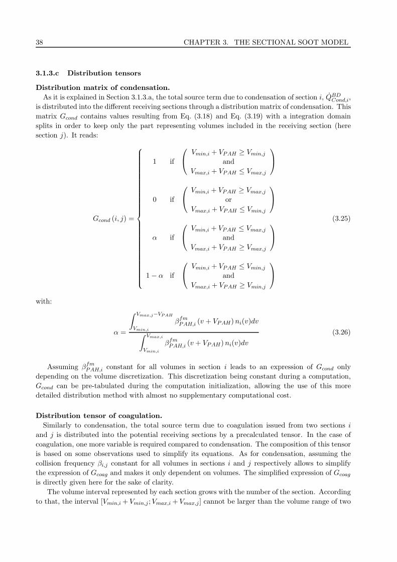
38 CHAPTER 3. THE SECTIONAL SOOT MODEL
3.1.3.c Distribution tensors
Distribution matrix of condensation.
As it is explained in Section 3.1.3.a, the total source term due to condensation of section i, QBDCond,i,
is distributed into the different receiving sections through a distribution matrix of condensation. This
matrix Gcond contains values resulting from Eq. (3.18) and Eq. (3.19) with a integration domain
splits in order to keep only the part representing volumes included in the receiving section (here
section j). It reads:
Gcond (i, j) =
1 if
Vmin,i + VPAH ≥ Vmin,j
and
Vmax,i + VPAH ≤ Vmax,j
0 if
Vmin,i + VPAH ≥ Vmax,j
or
Vmax,i + VPAH ≤ Vmin,j
α if
Vmin,i + VPAH ≤ Vmax,j
and
Vmax,i + VPAH ≥ Vmax,j
1− α if
Vmin,i + VPAH ≤ Vmin,j
and
Vmax,i + VPAH ≥ Vmin,j
(3.25)
with:
α =
∫ Vmax,j−VPAH
Vmin,i
βfmPAH,i (v + VPAH)ni(v)dv
∫ Vmax,i
Vmin,i
βfmPAH,i (v + VPAH)ni(v)dv
(3.26)
Assuming βfmPAH,i constant for all volumes in section i leads to an expression of Gcond only
depending on the volume discretization. This discretization being constant during a computation,
Gcond can be pre-tabulated during the computation initialization, allowing the use of this more
detailed distribution method with almost no supplementary computational cost.
Distribution tensor of coagulation.
Similarly to condensation, the total source term due to coagulation issued from two sections i
and j is distributed into the potential receiving sections by a precalculated tensor. In the case of
coagulation, one more variable is required compared to condensation. The composition of this tensor
is based on some observations used to simplify its equations. As for condensation, assuming the
collision frequency βi,j constant for all volumes in sections i and j respectively allows to simplify
the expression of Gcoag and makes it only dependent on volumes. The simplified expression of Gcoag
is directly given here for the sake of clarity.
The volume interval represented by each section grows with the number of the section. According
to that, the interval [Vmin,i + Vmin,j ;Vmax,i + Vmax,j ] cannot be larger than the volume range of two

3.1. SOOT MODELING 39
consecutive sections equal or larger than both sections i and j. Thus, half of the volume range
represented by this interval cannot be larger than the range of a section representing volume larger
than the one of sections i and j. Then, considering l the section number of the section including
the middle of the volume interval [Vmin,i + Vmin,j;Vmax,i + Vmax,j], the particles coagulated from
sections i and j belong to sections l − 1, l and l + 1. Gcoag can be written as follows:
Gcoag (i, j, k) =
0 if
k ≥ l + 2
or
k ≤ l − 2
∫ MIN(Vmax,i;Vmax,k−Vmin,j )
Vmin,i
ni(v)
(∫ Vmax,k−vi
Vmin,j
nj(v)dvj
)dvi
∫∫
∆i∆j
ni(v)nj(v)dvidvj
if (k = l − 1)
∫
∆i
ni(v)
(∫ MIN(Vmax,j ;Vmax,k−vi)
MAX(Vmin,j ;Vmin,k−vi)nj(v)dvj
)dvi
∫∫
∆i∆j
ni(v)nj(v)dvidvj
if (k = l)
∫ Vmax,i
MAX(Vmin,i;Vmin,k−Vmax,i)ni(v)
(∫ Vmax,j
Vmin,k−vi
nj(v)dvj
)dvi
∫∫
∆i∆j
ni(v)nj(v)dvidvj
if (k = l + 1)
(3.27)
3.1.4 Surface chemistry source terms
The HACA cycle (Hydrogen Abstraction Carbon Addition) developed by Frenklach [26] represents
the growth and oxidation of PAH. In the present work, surface chemistry of soot is modeled using a
variation of this cycle proposed by D’Anna and Kent [76]. This surface chemistry has been chosen
since it has been designed for engine conditions and previously validated by Fraioli et al. [72]. The
surface chemistry phenomena are described using eight gaseous species (H, H2, OH, H2O, C2H2,
O2, CO and HCO) in six reactions (given in table Tab.3.1) with the rate constants taken from [76]:
where Ai represents stable aromatic soot particles of section i, Ri represents radical soot particles of
section i, Apkrepresents stable aromatic soot particles product of a reaction that exchanges p carbon
atoms with the gaseous phase, and kin is the rate constant of nth reaction on particles of section i.
3.1.4.a Reaction rates
To evaluate the oxidation and surface growth reaction rates given by the surface chemistry reactions,
the total amount of particles in each section is first converted into a concentration ([Ai ] + [Ri ])
proportional to its surface Si. This value can be obtained from:
[Ai ] + [Ri ] =
∫ vmax,i
vmin,i
αHACA
λsoot
NASi(v)ni(v)dv (3.28)
where λsoot is the number of reactive sites per unit surface of soot and αHACA is the proportion of
these sites which are active.

40 CHAPTER 3. THE SECTIONAL SOOT MODEL
Ai
ki1↔ Ri +H
Ai +Hki2↔ Ri +H2
Ai +OHki3↔ Ri +H2O
Ri +C2H2ki4−→ A2
k +H
Ai +OHki5−→ A−1
k+HCO
Ri +O2ki6−→ A−2
k+ 2CO
Table 3.1: Reactions governing the soot surface chemistry [76].
The value of αHACA is often correlated to temperature [44, 132]. Because temperature dependent
expressions of αHACA are not completely validated today, we rather choose a constant value as
done in [55, 56] for instance. We choose αHACA = 0.27 which corresponds to the average value
of the correlation given by Markatou et al. [132] for a temperature interval of 1250K to 3000K.
Considering soot particles as spheres and considering that the smallest solid soot particle has only
one reactive site (λsootS1 = 1), as in [55, 56], the following relation appears:
λsootSi = λsootS1
(viVc2
) 2
3
=
(viVc2
) 2
3
(3.29)
The previous relation relies on the assumption of spherical particles, however a fractal dimension
should be introduced to correct the amount of soot surface available for reaction as in Forrest and
Witten [133]. The value and evolution depending on particle size, the fractal dimension of soot is
still uncertain [129, 130, 134, 135]. In this paper, a variable fractal dimension depending on particle
size has been chosen, as in [55], for all the Diesel surrogate calculations. For the calculations
presented here, θ = 2.0 for all particles with a diameter smaller than a given threshold and θ = 2.25
for all particles with a diameter larger than a second threshold and the fractal dimension evolves
linearly in between. These thresholds are adapted depending on the fuel used in the simulation,
since the growth of soot particles can be based on absorption of different sizes carbon species (PAH
or acetylene) depending on the burned fuel. Using Eq. (3.29) and the fractal dimension, the total
soot concentration becomes:
[Ai ] + [Ri ] =
∫ Vmax,i
Vmin,i
αHACA
ni(v)
NA
(v
Vc2
) θ3
dv (3.30)
As in [55, 56], a steady state assumption on active radical sites allows to write [Ri ] as a function
of [Ai ]:
[Ri ] =k1,i,f + k2,i,f [H] + k3,i,f [OH]
k1,i,b [H] + k2,i,b [H2] + k3,i,b [H2O] + k4,i [C2H2] + k6,i [O2][Ai ] (3.31)
The volume fraction reaction rates for surface growth (QgasSG,i) and oxidation (Qgas
Ox,i) in section i
are evaluated as in [55, 56]. These reaction rates represent the mass exchange between the gaseous

3.1. SOOT MODELING 41
phase and the solid phase. They read:
QgasSG,i = NAKSG,iVC2
(3.32)
QgasOx,i = NAKOx,iVC2
(3.33)
where KSG,i = k4,i [C2H2] [Ri ] and KOx,i = k6,i [O2] [Ri ] + k5,i [OH] [Ai ] /2.
These reaction rates respectively represent global surface growth and oxidation over all sections
and as for condensation and coagulation, they have to be distributed over the SNDF to complete
the modeling of the phenomena. In the previous versions of the model [55, 56, 57], QgasSG,i and Qgas
Ox,i
were directly attributed to section i + 1 and i − 1 respectively with a quantity of soot transferred
between sections i and i+ 1 or i− 1 calculated to ensure mass and number conservations.
3.1.4.b Surface growth
Surface growth is the carbon addition to soot particles from the gaseous phase. Its volume fraction
reaction rate is associated to a reference volume VC2to be consistent with the number of carbons
added by acetylene, which is the adsorbed species in the HACA mechanism. This phenomenon
implies only consecutive sections since it leads to a size variation of VC2which is the volume range
of the smallest section. Thus, the volume fraction rate of soot particles in section i which are growing
enough to switch to section i+ 1, QoutSG,i, needs to be modeled:
QoutSG,i = NAKSG,i
∫ Vmax,i
Vmax,i−VC2
(v + VC2)1
v
(v
Vc2
) θ3
dv (3.34)
In Eq. (3.34), the volume is (v + VC2) since the concerned particle has already received the volume
fraction from the gaseous phase and (1/v)(
vVc2
) θ3
represents the available reaction surface varia-
tion depending on the volume. The integration over the considered volumes in Eq. 3.34 can be
pre-tabulated as the ones for condensation, coagulation and the similar expression given next for
oxidation.
Finally, the surface growth source terms applied to each section write:
QSG,1 = −QoutSG,1 + Qgas
SG,1 (3.35)
QSG,i = QoutSG,i−1 − Qout
SG,i + QgasSG,i ∀i ∈ J2;nsect − 1K (3.36)
QSG,nsect = QoutSG,nsect−1 + Qgas
SG,nsect(3.37)
3.1.4.c Oxidation
The oxidation of soot particles is also part of the surface kinetic scheme where reactions with
dioxygen and hydroxyl take carbon from soot particles. Its modeling is similar to surface growth,
except that the concerned particle size is reduced by the associated volume VC2. The volume fraction
rate of soot transferred from section i to section i− 1 reads:
˙QoutOx,i = NAKOx,i
∫ Vmin,i+VC2
Vmin,i
(v − VC2)1
v
(v
Vc2
) θ3
dv (3.38)

42 CHAPTER 3. THE SECTIONAL SOOT MODEL
As for surface growth, the oxidation source terms applied to each section write:
QOx,1 = QoutOx,2 − Qgas
Ox,1 (3.39)
QOx,i = QoutOx,i+1 − Qout
Ox,i − QgasOx,i ∀i ∈ J2;nsect − 1K (3.40)
QOx,nsect = −QoutOx,nsect
− QgasOx,nsect
(3.41)
3.2 Homogeneous reactor and premixed flames validations
In order to validate the proposed changes to the sectional soot model, the current version of the model
has been compared to the reference version proposed by Vervisch-Kljakic [57]. These comparisons
are done on a homogeneous variable volume reactor and 1-D premixed flames. The reactor allows
to ensure the mass balance is closed during the interactions between the gaseous phase and the
solid soot phase. The flames are computed to verify the ability of the new model to predict SNDF
in these academical cases as the reference model. In order to ensure a comparison of the two
modeling approaches, these simulations have been ran using the HACA-RC cycle version used by
Vervisch-Kljakic [57].
3.2.1 Homogeneous reactor
This section presents the results obtained from the simulation of a homogeneous variable volume
reactor of n-heptane / air mixture at an equivalence ratio of Φ = 2, 5025. This simulation has been
run using the CLOE (CLosed hOmogeneous rEactor) code from the IFP-Kinetics package [136]
which includes the reference soot module and the proposed one.
The kinetic scheme proposed by Blanquart et al. [50] of 148 species and 928 reactions is used
to model the n-heptane combustion kinetic. The reactor volume law is a reciprocating motion law
defined by the engine-like conditions. The reactor initial conditions and the geometric parameters
defining the volume law are given in Table 3.2 with P0 and T0 the initial pressure and temperature,
RPM the rotating speed, VTDC the volume at the Top Dead Center (TDC) and τ the compression
ratio. The computation is done using 30 soot sections.
P0 [MPa] T0 [K] RPM VTDC [cm−3] τ
0, 1 600 1640 3, 026.10−5 17, 8
Table 3.2: Variable volume homogeneous reactor conditions.
Some modifications to the reference model, such as the addition of the exchanged hydrogen to
H2, are made in order to ensure mass conservation. Comparisons between the current version of
the model and the reference one have been done on the previously introduced homogeneous closed
reactor to illustrate the progress in mass conservation. Atoms balance are done to evaluate the mass
changes due to hydrogen or carbon loss. Even if the species interacting with the soot phase include
oxygen atoms, oxygen is not absorbed by soot in any of the HACA-RC cycle reaction. Thus, only
hydrogen and carbon mass have to be checked. These results are presented in the following.
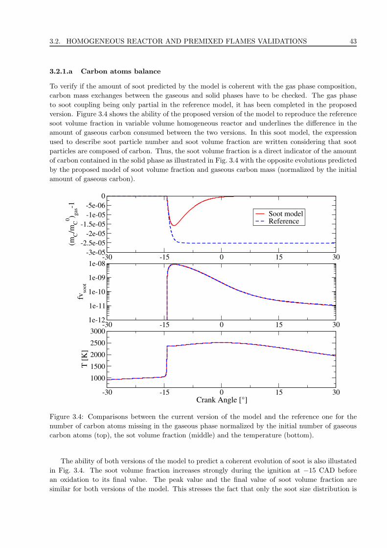
3.2. HOMOGENEOUS REACTOR AND PREMIXED FLAMES VALIDATIONS 43
3.2.1.a Carbon atoms balance
To verify if the amount of soot predicted by the model is coherent with the gas phase composition,
carbon mass exchanges between the gaseous and solid phases have to be checked. The gas phase
to soot coupling being only partial in the reference model, it has been completed in the proposed
version. Figure 3.4 shows the ability of the proposed version of the model to reproduce the reference
soot volume fraction in variable volume homogeneous reactor and underlines the difference in the
amount of gaseous carbon consumed between the two versions. In this soot model, the expression
used to describe soot particle number and soot volume fraction are written considering that soot
particles are composed of carbon. Thus, the soot volume fraction is a direct indicator of the amount
of carbon contained in the solid phase as illustrated in Fig. 3.4 with the opposite evolutions predicted
by the proposed model of soot volume fraction and gaseous carbon mass (normalized by the initial
amount of gaseous carbon).
-30 -15 0 15 30-3e-05
-2.5e-05
-2e-05
-1.5e-05
-1e-05
-5e-06
0
(mC/m
C
0) g
as-1
Soot modelReference
-30 -15 0 15 301e-12
1e-11
1e-10
1e-09
1e-08
fvso
ot
-30 -15 0 15 30Crank Angle [°]
1000
1500
2000
2500
3000
T [
K]
Figure 3.4: Comparisons between the current version of the model and the reference one for the
number of carbon atoms missing in the gaseous phase normalized by the initial number of gaseous
carbon atoms (top), the sot volume fraction (middle) and the temperature (bottom).
The ability of both versions of the model to predict a coherent evolution of soot is also illustated
in Fig. 3.4. The soot volume fraction increases strongly during the ignition at −15 CAD before
an oxidation to its final value. The peak value and the final value of soot volume fraction are
similar for both versions of the model. This stresses the fact that only the soot size distribution is

44 CHAPTER 3. THE SECTIONAL SOOT MODEL
modified. The absorption of carbon, and thus the evolution of the soot volume fraction (SVF), is
only indirectly modified by the different available surface due to different distribution in size.
A more detailed analysis of the carbon loss is given with Fig. 3.5. The difference between the
solid carbon mass in the soot model and the carbon mass lost by the gaseous phase is plotted along
with the SVF as indicator of the evolution of the solid phase depending on crank angle. The balance
between the gaseous and solid phase carbon of the proposed model is illustrated by the negligible
loss of carbon mass, more than three orders of magnitude smaller than the involved carbon mass
shown on Fig. 3.4. This loss cannot be null in this case because the gaseous and solid solver are
separated which will lead to a numerical error due the distinct resolutions of the two systems. Using
only one solver could prevent these errors in this specific case but this is not possible by the code
used for 3-D RANS simulation. Thus, the presented results are the ones obtained with two solvers
to validate an approach similar to the one used in 3-D RANS simulation.
-30 -15 0 15 301e-10
1e-09
1e-08
1e-07
1e-06
1e-05
(mC
0-m
C)/
mC
0 Soot modelReference
-30 -15 0 15 30Crank Angle [°]
1e-12
1e-11
1e-10
1e-09
1e-08
fvso
ot
Figure 3.5: Carbon mass lost by the total system normalized by the initial mass of carbon (top)
and soot volume fraction (bottom) as a function of crank angle.

3.2. HOMOGENEOUS REACTOR AND PREMIXED FLAMES VALIDATIONS 45
3.2.1.b Hydrogen atoms balance
Hydrogen mass balance validation has also been done on the same homogeneous reactor case. The
results are given in Fig. 3.6 with the hydrogen mass lost by the gaseous phase normalized by the
initial hydrogen mass and the SVF as indicator of the evolution of solid phase depending on crank
angle.
-30 -15 0 15 30
-6e-07
-4e-07
-2e-07
0
2e-07
4e-07
6e-07
(mH
/mH
0) g
az-1
Soot modelReference
-30 -15 0 15 30Crank Angle [°]
1e-12
1e-11
1e-10
1e-09
1e-08
fvso
ot
Figure 3.6: Hydrogen mass lost by the gaseous phase (top) and soot volume fraction (bottom) as a
function of crank angle.
Since the soot particles are considered as composed only of carbon, the gaseous hydrogen mass
should be constant in time during this simulation. This behavior is reproduced by the proposed
model. The variation of the gaseous hydrogen mass predicted by the reference model illustrates
the fact that soot is composed of hydrogen, as represented by the reactions modeling the formation
of precursor and the soot surface chemistry. This hydrogen is neglected in the evaluation of soot
volume and mass by both the reference and the proposed model. Considering this hydrogen could
lead to a different behavior of soot surface chemistry depending on the availability of hydrogen
at soot surface. It is to be noticed that the proposed solution is only a first step allowing mass
conservative simulations while the problem of soot surface chemistry is not solved.

46 CHAPTER 3. THE SECTIONAL SOOT MODEL
3.2.2 Laminar premixed flames
The laminar premixed flames measured by Zhao et al. [137] have been chosen to compare the
proposed model to the reference one [57]. These are laminar premixed flames of ethylene at an
equivalence ratio of 1.92. The fresh gases are diluted by nitrogen or argon. The molar composition
are given in Tab. 3.3. Different dilutants were used in order to reach different maximum temperatures
for a similar equivalence ratio and fresh gases velocity. The fresh gases velocity was also used as a
factor to control the maximum temperature. The conditions of the four flames simulated are given
in Tab. 3.4. These various flame temperatures lead to different SNDF by changing the dominance
of collisional or chemical phenomena.
C2H4 (% mol.) O2 (% mol.) Dilutant (% mol.)
24.2 37.9 37.9
Table 3.3: Fresh gases composition of Zhao et al. [137] experiments.
Flamme Dilutant Fresh gases velocity [cm/s] Tmax [K]
A1 Ar 7.0 1790
A3 Ar 10.0 1920
B1 N2 8.0 1790
B3 Ar 8.0 1840
Table 3.4: Dilutant species, fresh gases velocities and maximum temperature of Zhao et al. [137]
experiments flames.
These flames have been chosen because they were previously studied with the reference model.
The simulations were run with the 1-D laminar flame code STELLA from IFP-KINETICS library
[136], using the temperature profile, fresh gases composition and velocity as input parameters.
The kinetic scheme used to model ethylene combustion chemistry is the one proposed by Mauss
[128] including 82 species and 457 reactions, also used in the study with the reference model. The
simulations ran with the proposed model used the same set of modeling parameters as the ones ran
with the reference model to ensure that the differences were only due to the new modeling.
3.2.2.a Predicted SNDF
Figures 3.7 and 3.8 show the SNDF predicted by both models and compare them to the experimental
measurements for the two lower temperature flames A1 and B1. The difference between the two
versions can be seen with large soot predicted closer to the burner by the reference model for flame A1
with SNDF 5 mm and 7 mm above the burner in Fig. 3.7. It illustrates the difference of distribution
of surface growth and condensation for similar gaseous phase conditions. The predictions from the
proposed model are better at 5 mm and 7 mm above the burner for flame B1 as shown in Fig. 3.8
and also at 5 mm above the burner for flame A1 as shown in Fig. 3.7.
However, the predicted SNDF by both models at 10 mm and 12 mm above the burner for flames
A1 and B1 are very similar in these cases while the way the SNDF is formed closer to the burner is
different. As illustrated in Fig. 3.7 and Fig. 3.8, these predicted SNDF are also very different from
the measured ones at 10 mm and 12 mm above the burner. The modeling errors are assumed to

3.2. HOMOGENEOUS REACTOR AND PREMIXED FLAMES VALIDATIONS 47
be due to the representation of chemistry in these cases [57] and also to the fact that the collisional
particle inception mechanism is not dominant in these low temperature flames [137]. These aspects
impact as well the reference model and the proposed one abilities to predict SNDF for flames A1
and B1 since the difference between these models only lies on the way the particles are distributed
towards the sections.
1 4 16 6410
-3
10-2
10-1
100
101
(dN
p/d
log
Dp)/
Np
Zhao et al.Reference
Soot model
H=5 mm
1 4 16 6410
-3
10-2
10-1
100
101
H=7 mm
1 4 16 64Particle Diameter, D
p [nm]
10-3
10-2
10-1
100
101
(dN
p/d
log
Dp)/
Np
H= 10mm
1 4 16 64Particle Diameter, D
p [nm]
10-3
10-2
10-1
100
101
H=12 mm
Figure 3.7: Comparison between experimental measurements of Zhao et al. [137], reference model
predictions and current model predictions for flame A1; SNDF at four different heights above the
burner.
The SNDF predicted by the two models for the flame A3 are compared to those measured by
Zhao et al. [137] in Fig. 3.9. The final SNDF, at 12 mm above the burner, was reproduced well by
both the reference model and the proposed model. Even if there are slight differences between the
predicted SNDF at 5 mm, 7 mm and 10 mm above the burner by the two models, they all reproduce
well the measured SNDF as shown in Fig. 3.9.
Finally, comparisons between the SNDF predicted by the two models and the experimental
measurements for the flame B3 are presented in Fig. 3.10. Even if the presence of too large particles
is predicted by the current model at 7 mm after the burner, the global behavior of the SNDF with
respect to the height above the burner is well reproduced by the proposed model. The predicted
size of the larger particles at 5 mm and 12 mm above the burner are similar to the measured ones.
A clear progress also appears for the description of small particles at 10 mm and 12 mm above the
burner compared to the reference model. This case illustrates the benefit of using a more accurate

48 CHAPTER 3. THE SECTIONAL SOOT MODEL
1 4 16 6410
-3
10-2
10-1
100
101
102
(dN
p/d
log
Dp)/
Np
Zhao et al.Reference
Soot model
H=5 mm
1 4 16 6410
-3
10-2
10-1
100
101
102
H=7 mm
1 4 16 64Particle Diameter, D
p [nm]
10-3
10-2
10-1
100
101
102
(dN
p/d
log
Dp)/
Np
H=10 mm
1 4 16 64Particle Diameter, D
p [nm]
10-3
10-2
10-1
100
101
102
H=12 mm
Figure 3.8: Comparison between experimental measurements of Zhao et al. [137], reference model
predictions and current model predictions for flame B1; SNDF at four different heights above the
burner.
distribution of soot source terms towards the sections.
Globally, the proposed model results are at least equivalent to the reference ones on those flames.
Progresses are made in some specific cases but the flames A1 and B1 are still not well reproduced
by the sectional soot model. This emphasizes the role of the gaseous phase chemistry and the choice
of the soot surface chemistry. It illustrates the fact that gas phase modeling is crucial for soot
modeling.

3.2. HOMOGENEOUS REACTOR AND PREMIXED FLAMES VALIDATIONS 49
1 4 16 6410
-3
10-2
10-1
100
101
102
(dN
p/d
log
Dp)/
Np
Zhao et al.Reference
Soot model
H=5 mm
1 4 16 6410
-3
10-2
10-1
100
101
102
H=7 mm
1 4 16 64Particle Diameter, D
p [nm]
10-3
10-2
10-1
100
101
102
(dN
p/d
log
Dp)/
Np
H=10 mm
1 4 16 64Particle Diameter, D
p [nm]
10-3
10-2
10-1
100
101
102
H=12 mm
Figure 3.9: Comparison between experimental measurements of Zhao et al. [137], reference model
predictions and current model predictions for flame A3; SNDF at four different heights above the
burner.

50 CHAPTER 3. THE SECTIONAL SOOT MODEL
1 4 16 6410
-2
10-1
100
101
(dN
p/d
log
Dp)/
Np
Zhao et al.Reference
Soot model
H=5 mm
1 4 16 6410
-2
10-1
100
101
H=7 mm
1 4 16 64Particle Diameter, D
p [nm]
10-2
10-1
100
101
(dN
p/d
log
Dp)/
Np
H=10 mm
1 4 16 64Particle Diameter, D
p [nm]
10-2
10-1
100
101
H=12 mm
Figure 3.10: Comparison between experimental measurements of Zhao et al. [137], reference model
predictions and current model predictions for flame B3; SNDF at four different heights above the
burner.
Chapter 4
Diesel RANS simulations
This chapter is composed of the article “Sectional soot model coupled to tabulated chemistry for
Diesel RANS simulations” submitted to Combustion and Flames the 30th of July 2014. It includes
a description of the sectional soot model, followed by a description of the combustion model used
to represent the gaseous phase in 3D RANS simulation of Diesel engines. Section 4.3 was kept in
the article in order to save the article structure but it only contains a description of the sectional
soot model previously introduced in Chapter 3. The combustion model introduced in Section 4.4 is
the reference combustion model of this thesis. It is only replaced by a more advanced combustion
model in Chapter 5 in order to obtain a better prediction of lift-off in Diesel sprays simulations. This
reference model coupling with the proposed soot model is then validated on various cases. First, the
prediction of this combustion model is validated against a kinetic solver reference in Section 4.5. In
order to realize these comparisons in relevant conditions, specifically designed homogeneous reactors
have been proposed. These reactors, called ECFM3Z-0D reactors, reproduce conditions similar to
Diesel engines ones while being simple enough to be simulated with a detailed kinetic solver, allowing
the comparison between the reference combustion model and the kinetic solver. Finally, the model is
validated against experimental measurements in Section 4.7. For this purpose, a database of Diesel
operating conditions is described. Then, the comparisons between experimental measurements and
simulations are shown and analyzed.
However, this chapter contains a modified version of the article. In fact, more details are given
about the mass and enthalpy closure used in the tabulated approach in Section 4.4.2.c. Section 4.7.2.c
is also improved with in-cylinder iso-surfaces of different gaseous species, soot source terms and soot
section mass fractions used to illustrate the ability of the model to reproduce realistic evolutions
of the solid phase. The model validations against experiments in Section 4.7.2.d are completed
by time-evolutions of the mean soot mass fraction. Finally, supplementary results concerning the
possibility to include a pre-tabulated feedback from soot to the gaseous phase composition are also
given in Section 4.6.
4.1 Abstract
In future Euro norms, the soot volume fraction and the soot number density will be regulated. Car
manufacturers need therefore accurate soot models for piston engine emissions prediction in order
to develop future engine concepts. This paper addresses this question by coupling a sectional soot
model with a tabulated combustion model for RANS simulations of Diesel engines. The sectional
soot model, based on the work of Netzell et al. [K. Netzell, H. Lehtiniemi, F. Mauss, P. Combust.
51

52 CHAPTER 4. DIESEL RANS SIMULATIONS
Inst. 31 (2007), 1143-1155], is implemented in the IFP-C3D RANS CFD code. At each time
and location, transport equations are solved for several soot sections, including source terms for
collisional and chemical processes. The soot model is coupled to a tabulated combustion model
derived from the Engine Approximated Diffusion Flame one (EADF) [J-B. Michel, O. Colin, Int.
J. Engine Res. 15 (2013), 346-369]. It allows to represent the minor species required by the soot
model with a much lower computational cost than a kinetic solver. In order to evaluate the soot
model coupled to the resulting combustion model called Variable Pressure Homogeneous Tabulated
Chemistry (VPTHC), it is compared to the same soot model directly coupled to a complex chemistry
solver. As this comparison can hardly be performed on a real Diesel engine case due to the very high
CPU time involved by the chemical solver, it is performed on a variable volume and fuel/air ratio
case which retains the essential features of a Diesel engine. Results show that the proposed coupling
recovers with reasonable accuracy the evolution of the soot volume fraction and distribution. Finally,
an experimental database of Diesel operating points is simulated. The database includes points with
a commercial Diesel fuel and the computed surrogate (30% 1-Methylnaphthalene and 70% Decane
in liquid volume) to validate the models against the experiments. Soot yields predictions from the
model show an improvement against the current standards and reach industrial target of accuracy
for most of the database while the model also provides a good estimation of the soot particles
distributions in size.
4.2 Introduction
Soot particles are formed during the combustion of hydrocarbon/air mixtures in most combustion
devices related to transportation. They are regulated for Diesel engines since 1993 in Europe, and
will soon be for spark-ignition engines (SIE). Today, these regulations concern not only the soot
mass emission, but also the number of particles and finally the number of the smallest ones, which
have been identified as the most harmful [11]. Diesel engines are today equipped with particle
filters. However, even with such devices, there is still a strong interest in reducing soot emission at
the source for Diesel and SI engines in order to limit the emission of particles small enough to get
through particle filters.
In this context, engine manufacturers need experimental and numerical tools to evaluate the raw
engine-out Soot Volume Fraction (SVF) and Soot Number Density Function (SNDF). Besides, due to
the scarcity of fossil fuels, the contribution of bio-sourced fuels will increase in the future. A key issue
is then to be able to evaluate the impact of fuel composition on soot emissions. Several models can be
used to get soot emissions in Diesel engines in Reynolds Averaged Navier Stokes (RANS) calculations
[138], which are the most used 3-D simulations for combustion chamber designers. Among them,
the semi-empirical models [80, 139] are the most popular ones. This type of model is also used
for soot-turbulence interactions as in Bolla et al. [91]. It is usually based on two equations giving
access to a limited number of informations (total mass, mean diameter ...) whereas most advanced
models based on sectional [78, 61] or moment [108, 109, 97] methods are able to describe the SNDF.
However, only a few comparisons against experiments have been performed in 3-D cases with either
the sectional or the moment methods. Using the method of moments, 3-D RANS Diesel sprays
simulations have been presented by Karlsson et al. [113] and full engine simulations by Priesching
et al. [114] but without quantitative comparisons against the experimental measurements. Marchal
et al. [125] presented a single Diesel engine case simulation including a decent prediction of the
exhaust soot yield with respect to the experimental measurement using a sectional soot model.

4.2. INTRODUCTION 53
Fraioli et al. [72] simulated four Diesel cases with a sectional soot model coupled to a detailed
kinetic scheme. In this work, the sectional version [78, 124, 77] of models developed by Mauss
and co-workers [113, 112, 114] in previous studies is retained. This model accounts for inception,
condensation, surface growth, coagulation and oxidation processes and directly predicts the SNDF
at each time and location, in contrast to moment methods for which a post-processing is necessary.
The soot model requires the knowledge of local and instantaneous concentrations of the soot
precursor and the chemical species involved in the oxidation and surface growth processes. Kinetic
schemes able to correctly predict these concentrations under the whole range of thermodynamic and
chemical conditions encountered in Diesel engines are detailed chemical schemes including hundreds
of species and thousands of reactions [140, 141, 142, 143, 144]. As a consequence, transporting all
the species and solving the complete chemistry totally coupled with turbulent reactive flow balance
equations is very costly. It has been shown by Fraioli et al. [72] that a 3D RANS Diesel calculation
including a full kinetic scheme and soot sections (132 species and 2206 reactions) can take more than
a month which is simply unrealistic for industrial use. To overcome these difficulties we propose in
the present work a soot modeling strategy split into two parts as illustrated in Fig. 4.1:
• First, a tabulated combustion model is developed to compute the gaseous phase composition,
including the concentrations of soot precursor and of all other species involved in the soot
formation process.
• Then, the sectional soot model uses these data to estimate the different source terms related
to soot formation and destruction to determine the soot mass and SNDF.
Soot model inputs
Soot model ouputs
GAS PHASE
Tabulated
chemistry
Gaseous species SNDF(t)
Surface chemistry
+ Collisional phenomena
SNDF(t+dt)
Figure 4.1: Illustration of interactions between a combustion model with detailed chemistry and the
soot model.
The advantage of this tabulated strategy is clearly its very reduced CPU time compared to direct
chemistry resolution. On the other hand, its major limitation is that the exchange of mass between
solid and gaseous phases cannot be accounted for, which is equivalent to say that the impact of
the solid phase chemistry on the gaseous composition is negligible. Although this hypothesis is
strong, it cannot be avoided in a simple manner as soon as a tabulated approach is considered. The
results presented on an academic case and a Diesel engine in this paper show a posteriori that this
hypothesis seems acceptable for the practical cases of application targeted here.
In order to study the impact of fuel composition and chemical structure on the soot emissions,
one should introduce a complex chemistry mechanism in the turbulent combustion model used for
the gaseous phase. In this study, a simplification of the Engine Approximated Diffusion Flame
(EADF) combustion model [145] is proposed. Indeed, in EADF, homogeneous variable pressure

54 CHAPTER 4. DIESEL RANS SIMULATIONS
trajectories are first tabulated using complex chemistry. Then these trajectories are used in approx-
imate diffusion flame calculations at variable pressure to generate the final EADF table. This way,
EADF is able to account for both variable pressure and strain rate effects. For soot description,
additional minor species need to be added to the table, which would lead to a very large table which
is difficult to handle. Besides the EADF table generation itself requires a large CPU time. For
this reason, only the first homogeneous variable pressure table generated by EADF is retained here.
The simplified model using this table is called Variable Pressure Tabulated Homogeneous Chemistry
(VPTHC). In order to account for the local heterogeneity of mixture fraction, this homogeneous
table is inserted in the three Dirac mixture fraction description of the 3-Zones Extended Coherent
Flame Model (ECFM3Z) [146]. As this approach cannot account for the effect of strain on chemistry,
it must be considered as a first step towards a future coupling between EADF and the soot model.
The aim of this work is to present the complete modeling approach including the tabulated
chemistry model and the sectional soot model and to assess the ability of the resulting approach to
predict the soot emissions and size distributions of Diesel engine configurations. Since calculations
of 3D Diesel engine cases are too costly [72], comparisons based on these cases cannot be done
between tabulated chemistry and detailed kinetic solver results. For this reason, we propose a
comparison using a dedicated variable volume heterogeneous model reactor called ECFM3Z-0D.
This reactor is based on the three mixture fraction description of ECFM3Z and allows to mimic the
combustion process observed in a Diesel engine by imposing the mixing time-scale. In the mixed
zone of the reactor where combustion takes place, chemistry can be described using either VPTHC or
a kinetic solver. This finally allows a direct comparison between the two approaches using identical
mixing trajectories. Finally, a dedicated experimental Diesel engine database is used to evaluate
the potential of the proposed models. The database is described in Aubagnac-Karkar et al. [147]
along with an experimental validation of the proposed surrogate against commercial Diesel fuel and
a brief presentation of the 3-D simulations results obtained with the model detailed and validated
in this paper. It has been chosen because it provides SNDF measurements at exhaust for eleven
cases. This type of measurements being very complex, such databases of engine cases only exist at
exhaust for metal engines so far, restraining the validation to the exhaust SNDF and soot yields.
Section 4.3 describes the soot model and its adaptations to Diesel conditions. Then, Section 4.4
introduces the turbulent combustion model and its coupling with the soot model. The soot model is
validated in Section 4.5 on the ECFM3Z-0D test case. It is finally evaluated on the engine database
in Section 4.7.
4.3 Soot modeling
The soot model introduced in the present contribution is based on the previous work of Netzell et
al. [55, 78]. This section briefly describes its governing equations and the evolutions brought to the
source terms estimation.
The soot particles population is evaluated by using a sectional method. The soot particles are
separated with respect to their volume into discrete sections. In contrast to Fraioli et al. [72] where
soot particles are considered as chemical species, the present approach considers that soot particles
are solid and modeled as a distinct dispersed phase, interacting with the gaseous phase. In the
turbulent reactive flow, each section i, representing the soot particles of a given volume range, is

4.3. SOOT MODELING 55
governed by a standard transport equation for the mass fraction of soot in this section, Ysoot,i:
∂ρYsoot,i
∂t+∇ · (ρuYsoot,i) = ∇ · (ρDt,soot∇Ysoot,i) + ρ˜ωsoot,i (4.1)
with ρ the gas phase density, u the gas velocity, Dt,soot the turbulent diffusion coefficient of soot
and ˜ωsoot,i the soot source term for section i.
We start with an explanation of the particle volume discretization and of the variables used to
represent soot particles in each section. Then, the different physical phenomena involved in the soot
formation process are described. These phenomena are illustrated in Fig. 4.2 and are introduced in
the following order:
• First, collisional source terms: particle inception, condensation and coagulation.
• Secondly, surface chemistry source terms: surface growth and oxidation.
PAH PAH PAH+ + +
Combustion model(gaseous phase)
Sectional Soot Model(solid phase)
(PAH)
Polycyclic Aromatic
Hydrocarbon
Detailed chemistry
Fuel + Oxidizer
(+ Residual)
CO C2H2
H2 H20
O2 HCO
H OH
C2H2 + OH + O2+
Smallest solid
particle
Particle inception Condensation Coagulation
Surface growth Oxidation
Larger
particle
Surface chemistry
Collisional phenomena
Larger
particle
Larger
particle
Smaller
particle
Smaller
particle
Inte
rme
dia
tes a
nd
pro
du
cts
Figure 4.2: Illustration of the five phenomena representing soot formation and evolution with the
involved gaseous species.
4.3.1 Volume discretization
In this model, a fixed interval of volume [VMIN ;VMAX ] is divided into nsections sections. The
smallest volume of the considered particles is VMIN and is equal to the carbon-equivalent volume of
the number of carbon atoms of two soot precursors and two acetylene molecules. Carbon-equivalent
volume for two atoms of carbon is given by:
VC2=
2MC
NAρsoot(4.2)

56 CHAPTER 4. DIESEL RANS SIMULATIONS
where MC is the molar mass of carbon, NA the Avogadro number and ρsoot the soot density which
is assumed constant at a value of 1.86 · 103 kg.m−3 [55, 56].
Using pyrenyl (C16H9) as precursor as in [55, 56, 58, 78, 77], VMIN becomes equal to 18VC2
with a value of 3.857 · 10−28 m3 which is approximately the volume of a 0.9 nm diameter sphere. In
the case of a complete solid-gas coupling between the soot model and a kinetic solver, all hydrogen
atoms taken from the gas phase are then sent to H2 to close the hydrogen balance since all volumes
exchanged between phases are given with respect to the exchanged number of carbon atoms.
The largest modeled particles have a volume VMAX corresponding to the volume of a dMAX =
10µm diameter sphere. In Diesel engines, the particles produced are one or two orders of magnitude
smaller than this value dMAX in diameter [72, 129, 130, 131]. This VMAX value ensures that carbon
mass will not accumulate in the last section.
The first section represents soot particles of a constant volume range going from VMIN to VMIN+
VC2. The following sections are defined to fill the represented volume interval with nsections − 1
sections with a geometrical progression:
Vmax,i = (VMIN + VC2)
(VMAX
VMIN + VC2
)(i−1)/(nsections−1)
∀ i ∈ J2;nsectionsK (4.3)
All simulations presented in this paper have been realized with 30 sections. This value has been
chosen from the convergence study done with a similar model by Vervisch [57]. This value is a com-
promise which allows a limited CPU over-cost of the sectional model while giving an accuracy close
to a high resolution of typically 100 sections. It has been checked that these results were reproduced
by the proposed model. Moreover, 30 or 35 sections are commonly used in 3-D simulations using
soot sectional methods [57, 79, 84].
4.3.2 Model variables
The source terms given by the soot model are written as volume fraction source terms. The section i
soot particles volume normalized by the total volume of both gas and solid phase is the soot volume
fraction Qi. Assuming the volume of all soot particles is negligible with respect to the volume of
the gas, Qi can be deducted from Ysoot,i:
Qi =ρ
ρsootYsoot,i (4.4)
Accordingly, the soot mass fraction source term in Eq. (4.1) is given by:
˜ωsoot,i =ρsootρ
Qi =ρsootρ
(Qnucl,i + Qcond,i + Qsg,i + Qox,i + Qcoag,i) (4.5)
where Qnucl,i, Qcond,i, Qcoag,i, Qsg,i and Qox,i are respectively the volume fraction source terms of
section i due to nucleation, condensation, coagulation, surface growth and oxidation.
The soot volume fraction density qi is assumed to be constant in a given section i [55]:
qi =Qi
Vmax,i − Vmin,i(4.6)
As soot density ρsoot is assumed constant, the mass density is also constant in a section. The
particle number density ni(v) is deduced from qi:
ni(v) =qiv
∀ v ∈ [Vmin,i;Vmax,i] (4.7)
4.3. SOOT MODELING 57
Finally, the volume number of particles in section i, Ni, is:
Ni =
∫ Vmax,i
Vmin,i
ni(v)dv =Qi
Vmax,i − Vmin,iln
(Vmax,i
Vmin,i
)(4.8)
It has been shown by Netzell [55] that considering ni or qi constant in a section has a very low
influence on the predicted SNDF. The knowledge of the number of particles in each section given by
Eq. (4.8) allows to calculate the SNDF as illustrated in Fig. 4.35. Knowing Ysoot,i for each section i
gives an instantaneous access to the SNDF at each time step and every location.
4.3.3 Collisional source terms
Particle inception, condensation and coagulation are collisional phenomena. They are represented
by the Smoluchowski equation [62]. In the continuous form, it reads:
Fa(t) =1
2
∫ a
0(βa−b,bFb(t)Fa−b(t))db−
∫∞
0(βa,bFa(t)Fb(t))db (4.9)
where Fx(t) is the number of particles of size x, Fx(t) its variation rate and βx,y the collision
frequency between particles of size x and y.
The collision frequencies are obtained using the theory of aerosol science [64], applied to soot
formation by Kazakov and Frenklach [65]. These frequencies are evaluated for three different regimes
based on the value of the Knudsen number Kn defined as:
Kn(d) =λgas
d(4.10)
where d is the particle diameter and λgas the gas mean free path, computed for the bath gas N2.
In the present work, collision frequencies of soot precursors (either two soot precursors or a soot
precursor and a soot particle) are considered to occur in the molecular collision regime. The soot
particles collision regime is chosen as in Kazakov and Frenklach [65].
4.3.3.a Inception and Condensation
Inception and condensation are the two phenomena related to precursors collisions. It can either
be collisions between precursors to create the smallest considered soot particles (particle inception),
or between precursors and soot particles to increase soot particles volume (condensation). The
precursor species used in these phenomena is a virtual species called PAH (for Polycyclic Aromatic
Hydrocarbons). PAH is the product of the pyrenyl radical polymerization by acetylene:
C16H9 +C2H2kpol−−→ PAH +H2 (4.11)
where kpol is the rate constant of reaction for this polymerization reaction.
The volume fraction reaction rate of PAH rPAH reads:
rPAH = NAkpol [C16H9] [C2H2]VPAH (4.12)
where VPAH is the volume of a precursor (18 carbon atoms).

58 CHAPTER 4. DIESEL RANS SIMULATIONS
Considering NPAH the volume number of PAH particles, volume fraction variation rate of the
smallest modeled soot QNucl comes from the Smoluchowski equation (4.9) coupled with Eq. (4.6)
and Eq. (4.7):
QNucl = 2VPAHβfmPAH,PAHN2
PAH (4.13)
where βfmPAH,PAH is the molecular collision frequency for two precursors.
It is then possible to express the global volume amount of precursors that collide with all soot
particles per unit time QPAHCond:
QPAHCond = VPAHNPAH
imax∑
i=1
βfmPAH,i
∫ Vmax,i
Vmin,i
ni(v)dv (4.14)
where βfmPAH,i is the molecular collision frequency between precursors and soot particles of section i.
NPAH is calculated assuming a steady state assumption between the formation of PAH through
reaction (4.11) and its consumption by collision due to nucleation and condensation over all the
sections [55]:
rPAH = 2VPAHβfmPAH,PAH︸ ︷︷ ︸
kNucl
N2PAH +
(VPAH
imax∑
i=1
βfmPAH,i
∫ Vmax,i
Vmin,i
ni(v)dv
)
︸ ︷︷ ︸kCond
NPAH (4.15)
The positive roots of this polynomial equation being:
NPAH =−kCond +
√k2Cond + 4rPAHkNucl
2kNucl(4.16)
It is important to note that the inception reaction rate is directly read from Eq. (4.13) while
for condensation, the volume fraction computed from Eq. (4.14) represents the global volume frac-
tion transferred from gas phase to solid soot phase. This global condensation volume fraction has
therefore to be distributed correctly towards different sections as explained below.
Condensation reaction rates
The total amount of condensed soot in section i which has to be distributed into the SNDF QBDCond,i
(BD for Before Distribution) reads:
QBDCond,i = NPAH
∫ Vmax,i
Vmin,i
βfmPAH,i (VPAH + v)ni(v)dv (4.17)
It can be split in two terms. The first term is the flux QoutCond,i of particles in section i that are
collided by the precursors:
QoutCond,i = NPAH
∫ Vmax,i
Vmin,i
βfmPAH,ini(v)vdv (4.18)

4.3. SOOT MODELING 59
The second term is the volume of soot precursors colliding with particles of a given section i per
unit time QPAHCond,i obtained by:
QPAHCond,i = VPAHNPAH
∫ Vmax,i
Vmin,i
βfmPAH,ini(v)dv (4.19)
This term is used previously to evaluate NPAH . In the previous versions of the model [55, 56],
QPAHCond,i (Eq. (4.19)) was directly attributed to section i + 1 with a quantity of soot transferred
between sections i and i+ 1 calculated to ensure mass and number conservation.
Finally, QBDCond,i is distributed in the sections intersecting with the interval [Vmin,i+VPAH ;Vmax,i+
VPAH ]. Because the volume range represented by this interval is Vmax,i − Vmin,i, condensation only
makes particles larger and because the sections volume range is growing geometrically, only two
cases are possible:
• the volume interval is completely included in one section which will receive the complete
condensation reaction rate from section i,
• the interval intersects two different sections which will receive a part of the condensation
reaction rate from section i. In this case, section i can be one of those two sections.
Figure 4.3 illustrates these two steps to distribute the condensed mass of soot in the right
sections of the distribution. At first, the global amount of condensed soot in section i, QBDCond,i, is
evaluated. Then it is distributed with respect to particles volumes towards one or two sections. As
a consequence, the rate of volume fraction of soot received by a section j from the condensation
over section i, Qi→jCond, is the product of the volume fraction rate of soot distributed from section i,
QBDCond,i (including both PAH received from the gaseous phase and soot taken from the section i), by
a matrix Gcond (defined in Section 3.1.3.c) representing the part of section i condensation received
by section j:
Qi→jCond = Gcond (i, j) Q
BDCond,i (4.20)
Finally, the condensation source term in section i is the sum of the volume fraction rates received
from all sections, with the volume fraction rate taken from section i (QoutCond,i) being withdrawn:
QCond,i = −QoutCond,i +
nsections∑
j=1
Gcond (j, i) QBDCond,j (4.21)
It is to be noticed that this method keeps the number of particles constant, as the condensation
phenomenon should. Indeed, the added volume fraction of soot is consistent with the transfer of
soot to the larger size of the distribution, thus conserving the number of particles computed with
Eq. (4.7).
4.3.3.b Coagulation
The evaluation of the volume number rate of collisions between particles of sections i and j, Noutij ,
is done using the method proposed in [55, 56]. It is based on the collision frequency βij of sections
i and j defined by Kazakov and Frenklach [65].
As for condensation, the second step in the coagulation modeling is to distribute the collided
particles in the interval [Vmin,i+Vmin,j;Vmax,i+Vmax,j ]. A 3-D matrix Gcoag(i, j, k) links two sections

60 CHAPTER 4. DIESEL RANS SIMULATIONS
QPAHCond,i
QoutCond,i
QBDCond,i
Section i
Vmin,i Vmax,i
v
Q
GAS
STEP 1
Qi→jCond Q
i→j+1Cond
Section j Section j + 1
Vmin,i + VPAH Vmax,i + VPAH
Vmin,j Vmax,j Vmax,j+1
v
Q
STEP 2
QBDCond,i
Figure 4.3: Illustration of condensation over section i. STEP 1: computation of QBDCond,i, the sum of
the condensed carbon from gaseous phase over section i and the volume fraction of section i colliding
with precursors. STEP 2: distribution of QBDCond,i in other sections.
i and j to a third section k receiving a part of their collided particles. More details on this matrix
are given in the Section 3.1.3.c.
Accordingly, the particle number rate received by a section k from sections i and j is the product
of the volume density of collision between particles of sections i and j, Noutij , by the matrix Gcoag:
N i,j→kCoag = Gcoag (i, j, k) N
outij (4.22)
As a consequence, the particle number rate in section i is equal to the particle rate received by
section i from all smaller sections N j,k→iCoag minus the rate of collision between particles of sections i
and all other sections. Using Eq. (4.8), the coagulation source term of section i reads:
QCoag,i =
i∑
j,k
N j,k→iCoag −
nsections∑
j=1
Noutij
Vmax,i − Vmin,i
ln(Vmax,i
Vmin,i
) (4.23)
4.3.4 Surface chemistry source terms
The Hydrogen Abstraction Carbon Addition - Ring Closure cycle (HACA-RC) developed by Fren-
klach [26] represents the growth and oxidation of PAH. In the present work, surface chemistry of
soot is modeled using a variation of this cycle proposed by D’Anna and Kent [76]. This surface
chemistry has been chosen since it has been designed for engine conditions and previously validated
by Fraioli et al. [72]. The surface chemistry phenomena are described using eight gaseous species

4.3. SOOT MODELING 61
(H, H2, OH, H2O, C2H2, O2, CO and HCO) in six reactions (given in table Tab.3.1) with the rate
constants taken from [76].
Ai
ki1↔ Ri +H
Ai +Hki2↔ Ri +H2
Ai +OHki3↔ Ri +H2O
Ri +C2H2ki4−→ A2
k +H
Ai +OHki5−→ A−1
k+HCO
Ri +O2ki6−→ A−2
k+ 2CO
Table 4.1: Reactions governing the soot surface chemistry [76].
where Ai represents stable aromatic soot particles of section i, Ri represents radical soot particles
of section i, Apkrepresents stable aromatic soot particles product of a reaction that exchanged p
carbon atoms with the gaseous phase, and kin is the rate constant of reaction n on particles of
section i.
4.3.4.a Reaction rates
To evaluate the oxidation and surface growth reaction rates given by the surface chemistry reactions,
the total amount of particles in each section has to be converted into a concentration [Ai ] + [Ri ]
proportional to its available reactive surface. A steady state assumption on active radical sites
allows to distinguish [Ri ] from [Ai ]. These steps are realized as in [55, 56] to evaluate the volume
fraction reaction rates for surface growth QgasSG,i and oxidation Qgas
Ox,i in section i. These reaction
rates represent the mass exchange between the gaseous phase and the solid phase.
These reaction rates respectively represent global surface growth and oxidation over all sections
and as for condensation and coagulation, they have to be distributed over the SNDF to complete
the modeling of the phenomena.
4.3.4.b Surface growth
Surface growth is the carbon addition to soot particles from the gaseous phase. Its volume fraction
reaction rate is associated to a reference volume VC2to be consistent with the number of carbon
added by acetylene, which is the adsorbed species in the HACA mechanism. This phenomenon only
implies consecutive sections since it leads to a size variation of VC2which is the volume range of
the smallest section. Thus, the volume fraction rate of soot particles in section i which are growing
enough to switch to section i+ 1, QoutSG,i, needs to be modeled:
QoutSG,i = NAKSG,i
∫ Vmax,i
Vmax,i−VC2
(v + VC2)1
v
(v
Vc2
) θ3
dv (4.24)
where KSG,i = k4,i [C2H2] [Ri ] and KOx,i = k6,i [O2] [Ri ] + k5,i [OH] [Ai ] /2.
62 CHAPTER 4. DIESEL RANS SIMULATIONS
In Eq. (4.24), the volume is (v + VC2) since the concerned particle already received the vol-
ume fraction from the gaseous phase and (1/v)(v/Vc2 )θ/3 represents the available reaction surface
variation depending on the volume.
Finally, the surface growth source terms applied to each section write:
QSG,1 = −QoutSG,1 + Qgas
SG,1 (4.25)
QSG,i = QoutSG,i−1 − Qout
SG,i + QgasSG,i ∀i ∈ J2;nsect − 1K (4.26)
QSG,nsect = QoutSG,nsect−1 + Qgas
SG,nsect(4.27)
4.3.4.c Oxidation
The oxidation of soot particles is also part of the surface kinetic scheme used where reactions with
dioxygen and hydroxyl take carbon from soot particles. Its modeling is similar to surface growth,
except that the concerned particle size is reduced by the associated volume VC2. The volume fraction
rate of soot transferred from section i to section i− 1 reads:
˙QoutOx,i = NAKOx,i
∫ Vmin,i+VC2
Vmin,i
(v − VC2)1
v
(v
Vc2
) θ3
dv (4.28)
As for surface growth, the oxidation source terms applied to each section write:
QOx,1 = QoutOx,2 − Qgas
Ox,1 (4.29)
QOx,i = QoutOx,i+1 − Qout
Ox,i − QgasOx,i ∀i ∈ J2;nsect − 1K (4.30)
QOx,nsect = −QoutOx,nsect
− QgasOx,nsect
(4.31)
4.4 Turbulent Combustion Modeling
As mentioned in Section 4.2, a turbulent combustion model able to represent detailed chemistry in
non-premixed combustion is required to compute the species needed by the sectional soot model,
including soot precursors. In the present work, this is done by coupling the ECFM3Z model [146]
and a specifically developed tabulated chemistry model, VPTHC, to the IFP-C3D RANS code
[148, 149]. IFP-C3D, also used for the 3-D Diesel simulations and described in Section 4.7, is used
to simulate homogeneous cases in this section in order to validate the tabulated approach against a
reference solution provided by a detailed kinetic solver computation. The following section contains
a description of the mentioned models.
4.4.1 The ECFM3Z model
A detailed description of the model standard version is available in [146] for compression ignition
operating conditions. In order to represent the local mixing process, the ECFM3Z model includes
a description of the local mixture stratification by considering three homogeneous sub regions (see
Fig. 4.4): one region contains only pure fuel (region F), the second region contains fresh air plus any

4.4. TURBULENT COMBUSTION MODELING 63
additional EGR (region A) and the third region contains a mixture of the latter two (region M).
During injection, the evaporation of the spray droplets leads to a source of mass in region F. The
fuel and air (+EGR) from regions F and A mix to form region M. The mixing model is introduced
via the transport equation of region A oxygen and region F fuel tracers:
∂ρY FFu
∂t+∇.(ρuY F
Fu) = ∇.(ρ(Dt)∇Y FFu) + ρ˜SFu + ρ ˜E
F→M
Fu (4.32)
∂ρY AO2
∂t+∇.(ρuY A
O2) = ∇.(ρ(Dt)∇Y A
O2) + ρ ˜E
A→M
O2(4.33)
where ρ is the mean density, u the Favre mean velocity, Dt the turbulent diffusivity, Y FFu the
fuel tracer, Y AO2
the oxygen tracer, ˜SFu the source term of gaseous fuel mass fraction (from the
evaporation of liquid fuel droplets), ˜EF→M
Fu and ˜EA→M
O2the mixing source terms respectively from
region F to region M and from region A to region M.˜EF→M
Fu and ˜EA→M
O2evolutions are based on a characteristic mixing time τm:
˜EF→M
Fu = − 1
τmY FFu
(1− Y M
Fu
)(4.34)
˜EA→M
O2= − 1
τmY AO2
(1− Y M
O2
)(4.35)
where Y MFu and Y M
O2are respectively the fuel and oxygen mass fractions in region M. This mixing
time-scale τm is considered proportional to the turbulent time-scale given by the k − ǫ model,
τ−1m = ǫ
kC where C is a constant set to 0.6.
Potential EGR species are followed by tracers and their mixing is governed by that of oxygen
[146].
Finally, the auto-ignition and combustion in region M is described by the VPTHC approach
described in the following, as illustrated in Fig. 4.4.
Figure 4.4: Scheme of ECFM3Z coupled with the VPTHC combustion model.
4.4.2 The tabulated chemistry approach
In the EADF approach [145], approximated diffusion flames at variable pressure are used to generate
the look-up table. In this work, the turbulent mixing between fuel and air is described by the
ECFM3Z model and the look-up table is based on homogeneous reactors calculations at variable
pressure in the same manner as in [150]. This strategy allows the use of homogeneous tables
which are less demanding in terms of memory requirements compared to the EADF tables. This

64 CHAPTER 4. DIESEL RANS SIMULATIONS
tabulated chemistry approach is used in the mixed zone of ECFM3Z and gives a direct access
to the species evolutions. The resulting model is called VPTHC (Variable Pressure Tabulated
Homogenous Chemistry) and is very close to the model proposed by Jay and Colin [150] where
variable volume reactors were used instead of variable pressure reactors. As in [145], this model
uses two different tables generated respectively from constant pressure homogeneous reactors (HR)
and variable pressure reactors (VPR) computations. Both the HR and VPR are computed with
the IFP-Kinetics library solver [136] which is also used as the reference detailed chemistry solver to
validate the approach.
4.4.2.a Table generation
HR Table. The constant pressure table is used to represent the auto-ignition phase. It is built
from the calculation of a constant pressure HR database for several initial pressures P0, initial
temperatures T0, mixture fractions Z and mass fractions of dilutant YEGR as coordinates of the
database. The results are stored as a function of the progress variable which quantifies the transition
from fresh to burnt gases. This quantity is estimated here as c = Yc/Yeq where Yc = YCO + YCO2+
YH2O and Yeq is the value of Yc when the equilibrium at constant pressure and enthalpy is reached.
It has been verified that Yc grows bijectively with time in all reactors.
VPR Table. This table describes chemistry in the expansion phase. It is built from a database
of VPR at the same initial conditions as the HR table, with two additional coordinates which
are the progress variable at the beginning of the expansion Yc0 and the pressure time derivative
p. These reactors are constant pressure reactors until the progress variable reaches the value Yc0
when the pressure is forced to decrease with a constant rate p. Figure 4.5 illustrates how pressure
evolves depending on Yc0 and p, with the expansion trajectory from the initial pressure P0 to the
final pressure PF (here, 1 bar). This methodology allows tabulating species evolution in a model
trajectory which is close to the expansion trajectory encountered in a piston engine.
The parameters discretization of the HR and VPR tables are given in Tab.4.2.
Quantity Number of points Variation
c 100 [0; 1]
Z 25 [0; 0.5]
P0 [bar] 13 [1; 200]
T0 [K] 41 [600; 1200]
YEGR 3 [0; 0.5]
p [bar.s−1] 5 [−100;−100000]
c0 3 [0.05; 0.95]
Table 4.2: Discretizations of the tables used in this study.
4.4.2.b Model implementation
To compute species mass fractions in the combustion zone from the ones stored in the look-up table,
the input parameters described above need to be calculated. These parameters are the progress
variable Yc and the initial parameters of the reactors: Z, P0, T0, YEGR, p and Yc0 . These parameters
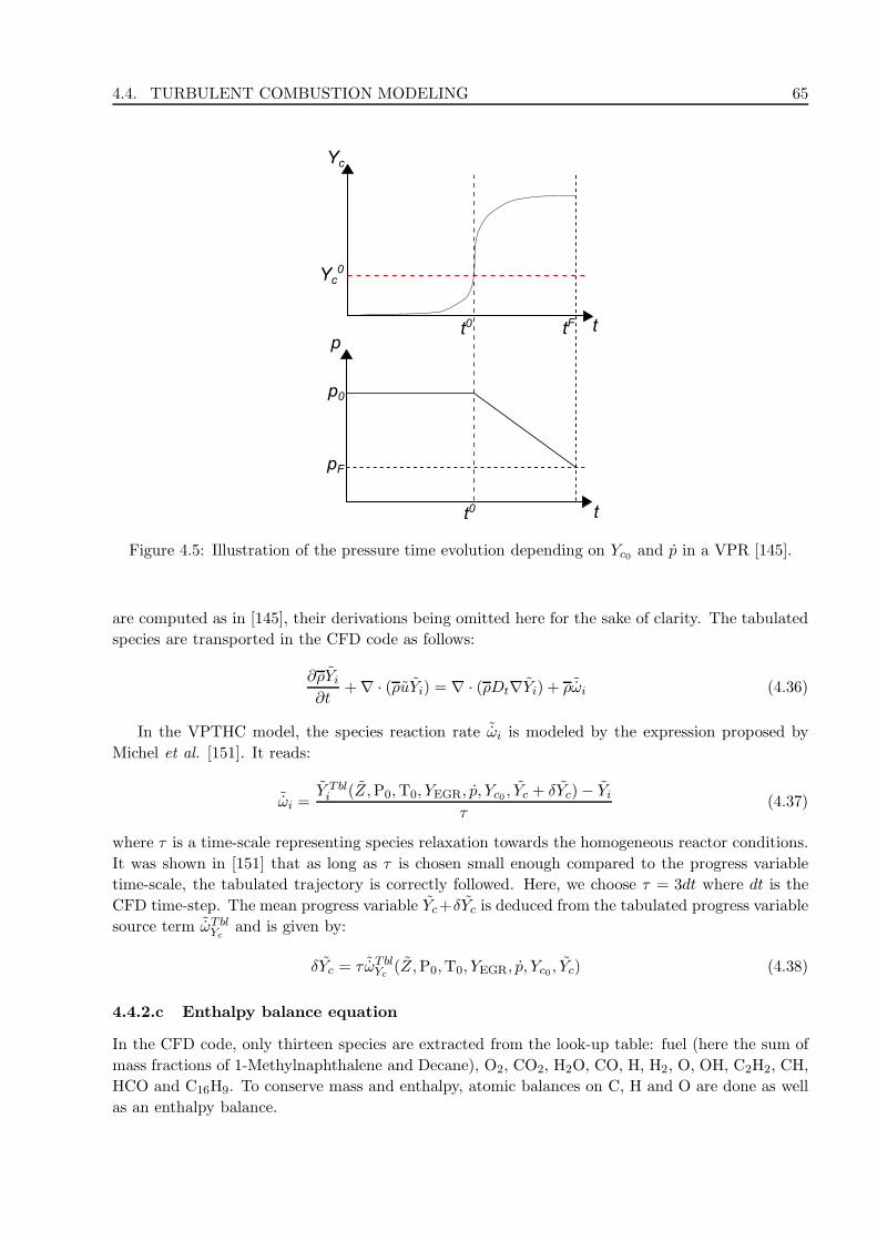
4.4. TURBULENT COMBUSTION MODELING 65
t
p
p0
pF
t0
Yc
Yc0
tt0 tF
Figure 4.5: Illustration of the pressure time evolution depending on Yc0 and p in a VPR [145].
are computed as in [145], their derivations being omitted here for the sake of clarity. The tabulated
species are transported in the CFD code as follows:
∂ρYi
∂t+∇ · (ρuYi) = ∇ · (ρDt∇Yi) + ρ ˜ωi (4.36)
In the VPTHC model, the species reaction rate ˜ωi is modeled by the expression proposed by
Michel et al. [151]. It reads:
˜ωi =Y Tbli (Z,P0,T0, YEGR, p, Yc0 , Yc + δYc)− Yi
τ(4.37)
where τ is a time-scale representing species relaxation towards the homogeneous reactor conditions.
It was shown in [151] that as long as τ is chosen small enough compared to the progress variable
time-scale, the tabulated trajectory is correctly followed. Here, we choose τ = 3dt where dt is the
CFD time-step. The mean progress variable Yc+δYc is deduced from the tabulated progress variable
source term ˜ωTblYc
and is given by:
δYc = τ ˜ωTblYc
(Z,P0,T0, YEGR, p, Yc0 , Yc) (4.38)
4.4.2.c Enthalpy balance equation
In the CFD code, only thirteen species are extracted from the look-up table: fuel (here the sum of
mass fractions of 1-Methylnaphthalene and Decane), O2, CO2, H2O, CO, H, H2, O, OH, C2H2, CH,
HCO and C16H9. To conserve mass and enthalpy, atomic balances on C, H and O are done as well
as an enthalpy balance.

66 CHAPTER 4. DIESEL RANS SIMULATIONS
The atomic balance of C and the enthalpy balance are closed by a pair of virtual carboneous
species C1 and C2. The atomic balances of H and O are closed by virtual species H2b and O2b (b
standing for balance) which have the same thermodynamic behaviors as their respective real species.
The balance of H includes the hydrogen from C1 and C2.
The merging of a two species surrogate fuel into a single species with a specific enthalpy defined
as the average specific enthalpy of both fuels in the initial proportion introduces a strong enthalpy
loss. Indeed, the proportion of each fuel evolves in time during combustion as illustrated in Fig. 4.6.
1-Methylnaphthalene being consumed faster than Decane, the fuel enthalpy becomes equal to the
Decane enthalpy beyond a given point of the reaction while it will be considered as equal to the
mixture enthalpy by the CFD code. This justifies the use of a fourth balance species to close the
enthalpy balance as well as the mass balance.
0 0,0001 0,0002 0,0003 0,0004 0,0005t [s]
0
0,02
0,04
0,06
0,08
0,1
0,12
0,14
Mas
s fr
acti
on
SumDecane1-Methylnaphthalene
Figure 4.6: Time-evolution of 1-Methylnaphthalene (red), Decane (blue) and their sum mass fraction
(black) in a constant pressure homogeneous reactor at 70 bar, with an initial temperature of 1000
K and an initial fuel mass fraction of 0.12
The two carboneous balance species are created with the atomic composition and the sensible
enthalpy of C2H3. Their specific enthalpies of formation have been chosen in order to conserve the
global mixture enthalpy by changing the ratio of C1 and C2 in the carbon mass required to complete
the atomic carbon balance. They are fixed as 3 · 106 J.mol−1 for C1 and −6 · 105 J.mol−1 for C2.
At every time step in every computed homogeneous reactors used to generate the look-up table,
CFD-like atomic balances are made with the species stored in the look-up table, H2b, O2b and a
virtual C2H3b species. From these balances and using the different enthalpies of formation of C1
and C2, the mass fractions YC1 and YC2 are evaluated considering that YC2H3b = YC1 + YC2 and by
closing the equation of enthalpy Eq. (4.39) by using a ratio x = YC1
YC2H3b:
H = htots +∑
i ∈ Ω
Yihi0 + YO2bh
O2
0 + YH2bhH2
0 + YC2H3bhC20 + xYC2H3b
(hC10 − hC2
0
)(4.39)
where H is the enthalpy of the mixture, htots the sensible enthalpy of all tabulated species and of

4.5. VALIDATION OF THE TABULATED CHEMISTRY APPROACH 67
the species used in atomic balances, Ω the ensemble of all tabulated species and hi0 the formation
enthalpy of species i.
x can be computed from Eq. (4.39). Thus, C1 is stored as C1 = xYC in the look-up table. For
every point of the table, the C2 computed to close the carbon atomic balance in the CFD code is
going to close the balance of enthalpy since the value of C1 has been computed in order to do this
on the homogeneous reactors.
This type of closure is required to predict auto-ignition with this surrogate. As illustrated in
Fig. 4.7, the enthalpy loss due to the error on the fuel enthalpy leads to a strong temperature
decrease. Auto-ignition still occurs in this constant pressure simulation because the conditions read
by the model in the look-up table are fresh gases conditions, which are not changed in a constant
pressure homogeneous reactor. In variable volume reactors or 3-D simulations, this type of enthalpy
loss would stop auto-ignition by switching the followed trajectory to a trajectory which does not
auto-ignites.
0 0,0005 0,001 0,0015 0,002t [s]
0
250
500
750
1000
1250
1500
1750
2000
2250
T [
K]
Kinetic solverVPTHC (complete)VPTHC (3 species balances)
Figure 4.7: Temperature time-evolution in a constant pressure homogeneous reactor at 70 bar, with
an initial temperature of 810 K and an initial fuel mass fraction of 0.14, for a solved chemistry
(black), a classical 3 species balances closure (blue) and the proposed 4 species balances closure
(red)
4.5 Validation of the tabulated chemistry approach
As explained in the introduction, the soot and VPTHC models are first compared to complex
chemistry on a simplified model reactor called ECFM3Z-0D, which is implemented in the IFP-C3D
code. This kind of reactor allows to use both the VPTHC tabulated model and a kinetic solver, which
allows a direct comparison of both approaches. For the present calculations, a mechanism of 590
species and 3890 reactions taken from the Model Fuels Consortium (MFC) thermo-kinetic database
[152] is used to build the VPTHC table and to run the detailed kinetic solver computations. The
fuel considered for these calculations is a Diesel surrogate composed of 30% 1-Methylnaphthalene

68 CHAPTER 4. DIESEL RANS SIMULATIONS
and 70% Decane (in liquid volume) which is also used for the 3D RANS simulation in Section 4.7.
The kinetic solver code coupled with IFP-C3D for these calculations comes from the IFP-Kinetics
package [136] as the code used to build the look-up tables.
In the following section, the principle of ECFM3Z-0D reactors is described first. Then, a reference
computation result of an ECFM3Z-0D reactor run with a detailed kinetic solver is given. Finally,
ECFM3Z-0D reactors results obtained with the tabulated approach and the detailed kinetic solver
are compared on various conditions.
4.5.1 ECFM3Z-0D reactors description
The global ECFM3Z-0D reactor is a variable volume reactor following piston motion equations.
Initially, fuel and air are separated in their respective zones. At a chosen crank angle CAstart, the
mixing begins. This crank angle corresponds to the beginning of injection in a real Diesel engine
computation. The mass flux from zone A (pure air) to zone M (homogeneous combustion zone) is
piloted by a time-scale τAm which represents the macro-scale mixing of air with the reactive gaseous
jet in a Diesel engine. In order to get a realistic fuel/air ratio in zone M during the mixing of
zones A and F, the mixing rate τFm of zone F is defined by fixing equivalence ratio ΦM in zone M
to an imposed value Φforce, a free parameter of the reactor. This mixing is illustrated in Fig. 4.8.
When the crank angle reaches CAstart, the ECFM3Z governing equations Eq. (4.34) and Eq. (4.35)
become:
˜EF→M
Fu =
(YFu
YO2
)
st
Φforce˜EA→M
O2(4.40)
˜EA→M
O2=
1
τmY AO2
(4.41)
Figure 4.8: Scheme of ECFM3Z-0D reactors.
Variable volume andequivalence ratio
homogeneous reactor
τAm
τFm = f(Φforce, τAm)
With this ECFM3Z-0D mixing model, region M can be seen as a variable-volume homogeneous
reactor. The reactor composition evolution is illustrated in Fig. 4.9. It shows how air is transferred
from zone A to zone M according to a constant time-scale τAm. The unmixed O2 (O2 in zone A)
decrease starts when the crank angle reaches CAstart = −15 CAD. Meanwhile, the fuel from zone
F (unmixed) mixes in order to keep ΦM = Φforce = 4.1 as long as there is fuel in zone F. When the
fuel contained in zone F is depleted, ΦM decreases to the average equivalence ratio of the reactor
here equal to 0.906 due to the mixing of O2 from zone A. Mixed quantities of O2 and fuel are limited
by their consumption from combustion.
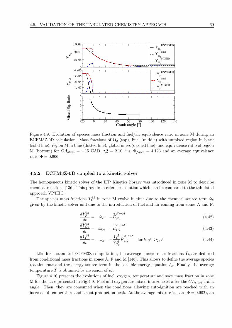
4.5. VALIDATION OF THE TABULATED CHEMISTRY APPROACH 69
0
5e-05
0.0001
0.0002
YO
2
YO
2
UNMIXED
YO
2
total
YO
2
MIXED
0
1e-05
2e-05
3e-05
4e-05Y
Fuel
YF
UNMIXED
YF
total
YF
MIXED
-20 0 20 40 60 80 100 120 140
Crank angle [°]
0
1
2
3
4
5
Mix
ed E
q.
Rat
io
Figure 4.9: Evolution of species mass fraction and fuel/air equivalence ratio in zone M during an
ECFM3Z-0D calculation. Mass fractions of O2 (top), Fuel (middle) with unmixed region in black
(solid line), region M in blue (dotted line), global in red(dashed line), and equivalence ratio of region
M (bottom) for CAstart = −15 CAD, τAm = 2.10−3 s, Φforce = 4.123 and an average equivalence
ratio Φ = 0.906.
4.5.2 ECFM3Z-0D coupled to a kinetic solver
The homogeneous kinetic solver of the IFP Kinetics library was introduced in zone M to describe
chemical reactions [136]. This provides a reference solution which can be compared to the tabulated
approach VPTHC.
The species mass fractions Y Mk in zone M evolve in time due to the chemical source term ωk
given by the kinetic solver and due to the introduction of fuel and air coming from zones A and F:
dY MF
dt= ωF + ˜E
F→M
Fu (4.42)
dY MO2
dt= ωO2
+ ˜EA→M
O2(4.43)
dY Mk
dt= ωk +
Y Ak
Y AO2
˜EA→M
O2for k 6= O2, F (4.44)
Like for a standard ECFM3Z computation, the average species mass fractions Yk are deduced
from conditional mass fractions in zones A, F and M [146]. This allows to define the average species
reaction rate and the energy source term in the sensible energy equation es. Finally, the average
temperature T is obtained by inversion of es.
Figure 4.10 presents the evolutions of fuel, oxygen, temperature and soot mass fraction in zone
M for the case presented in Fig.4.9. Fuel and oxygen are mixed into zone M after the CAstart crank
angle. Then, they are consumed when the conditions allowing auto-ignition are reached with an
increase of temperature and a soot production peak. As the average mixture is lean (Φ = 0.902), an

70 CHAPTER 4. DIESEL RANS SIMULATIONS
excess of oxygen is obtained at the end of the mixing process. This explains the partial oxidation
of soot at the beginning of the expansion stroke. Due to this expansion, temperature decreases
strongly which eventually leads to a freezing of all reactions, including soot oxidation.
0
1e-05
2e-05
3e-05
4e-05
5e-05Y
Mixed FuelMixed O
2
0
500
1000
1500
2000
2500
T [
K]
-140 -120 -100 -80 -60 -40 -20 0 20 40 60 80 100 120 140
Crank Angle [°]
1e-05
0.0001
0.001
0.01
Yso
ot
Figure 4.10: ECFM3Z-0D computation with the kinetic solver. Zone M fuel and oxygen mass
fractions (top), temperature (middle) and soot mass fraction (bottom) evolutions using CAstart =
−15 CAD, τAm = 2.10−3 s, Φforce = 4.123 and an average equivalence ratio of 0.906.
4.5.3 Comparison between tabulated chemistry and kinetic solver
In order to compare results obtained with the tabulated approach and the detailed kinetic solver,
four cases are presented in Tab.4.3, allowing three parametric studies. These calculations start at
−140 CAD with an initial pressure of 2 bar and an initial temperature of 400 K and run to +140
CAD. More parameter variations (EGR, initial temperature and pressure, rpm) have also been
tested with similar results (not presented here).
Case τm [s] Φforce average equivalence ratio
1 (ref) 2.10−3 4.123 0.906
2 10−3 4.123 0.906
3 2.10−3 2.311 0.906
4 2.10−3 4.123 1.151
Table 4.3: Conditions of the ECFM3Z-0D reactors studied for the parametric evaluation of VPTHC.
Pressure, temperature and soot mass fraction evolutions of the reference case 1 are given in
Fig. 4.11. The VPTHC approach shows a very good agreement with the kinetic solver for the
evolutions of temperature and pressure which confirms that tabulated chemistry can be used to
represent auto-ignition in variable volume environment. Soot mass fraction evolution is also qual-
itatively well predicted by VPTHC. Quantitatively, VPTHC underpredicts soot mass fraction by

4.5. VALIDATION OF THE TABULATED CHEMISTRY APPROACH 71
a factor two approximately. We consider this error as acceptable for two reasons at least. First,
the model trajectory followed by VPTHC (constant pressure and then constant expansion rate)
does not reproduce exactly the piston engine law followed by the kinetic solver. This induces small
differences in minor species relevant to soot formation which have a large impact on the final soot
yield. This error cannot be reduced as long as such a model trajectory is used. The solution would
be otherwise to employ directly the kinetic solver with the inconvenience of a very high CPU cost.
Secondly, as shown in the sectional soot model presentation, soot chemistry is still an open topic
of research today with large uncertainties on reaction constants, especially concerning inception. In
this context, a factor two of error added by the combustion model can be considered acceptable as
the uncertainty on chemistry is at least of the same order of magnitude on minor species required
for inception [77].
0
5e+06
1e+07
1.5e+07
P [
Pa]
VPTHCKinetic Solver
0
500
1000
1500
2000
2500
T [
K]
-140 -120 -100 -80 -60 -40 -20 0 20 40 60 80 100 120 140
Crank Angle [°]
1e-05
0.0001
0.001
0.01
Yso
ot
Figure 4.11: Pressure (top), temperature (middle) and soot mass fraction (bottom) evolutions on
the reference ECFM3Z-0D reactor with VPTHC tabulated chemistry (black) and the kinetic solver
(red) for the reference case.
Similar pressure and soot mass fraction evolutions have been computed for the three other test
cases and are given in Fig. 4.12 and Fig. 4.13. The agreement between tabulated and kinetic solver
chemistry is still good for pressure both for the auto-ignition delay and the maximum pressure. The
gap observed on soot mass fraction evolutions is still acceptable for soot modeling for every case.
Globally, soot sensitivity to parametric variations is well reproduced.

72 CHAPTER 4. DIESEL RANS SIMULATIONS
-10 -5 0 5 10 15 20
Crank Angle [°]
6e+06
8e+06
1e+07
1.2e+07
1.4e+07
1.6e+07
P [
Pa]
Kinetic solverReferenceCase 2Case 3Case 4
Figure 4.12: Pressure evolution for reference case (black), case 2 (τ inputm variation, triangle symbols),
case 3 (Φforce variation, red) and case 4 (average equivalence ratio variation, circle symbols) using
both the VPTHC approach (solid line) and the kinetic solver (dashed line).
-20 0 20 40 60 80 100 120 140
Crank Angle [°]
1e-08
1e-07
1e-06
1e-05
0.0001
0.001
0.01
0.1
Yso
ot
Kinetic solverReferenceCase 2Case 3Case 4
Figure 4.13: Soot mass fraction evolution for reference case (black), case 2 (τ inputm variation, trian-
gle symbols), case 3 (Φforce variation, red) and case 4 (average equivalence ratio variation, circle
symbols) using both the VPTHC approach (solid line) and the kinetic solver (dashed line).
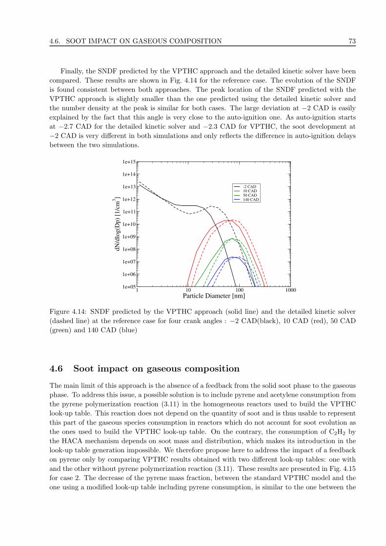
4.6. SOOT IMPACT ON GASEOUS COMPOSITION 73
Finally, the SNDF predicted by the VPTHC approach and the detailed kinetic solver have been
compared. These results are shown in Fig. 4.14 for the reference case. The evolution of the SNDF
is found consistent between both approaches. The peak location of the SNDF predicted with the
VPTHC approach is slightly smaller than the one predicted using the detailed kinetic solver and
the number density at the peak is similar for both cases. The large deviation at −2 CAD is easily
explained by the fact that this angle is very close to the auto-ignition one. As auto-ignition starts
at −2.7 CAD for the detailed kinetic solver and −2.3 CAD for VPTHC, the soot development at
−2 CAD is very different in both simulations and only reflects the difference in auto-ignition delays
between the two simulations.
1 10 100 1000
Particle Diameter [nm]
1e+05
1e+06
1e+07
1e+08
1e+09
1e+10
1e+11
1e+12
1e+13
1e+14
1e+15
dN
/dlo
g(D
p)
[1/c
m3]
-2 CAD10 CAD50 CAD140 CAD
Figure 4.14: SNDF predicted by the VPTHC approach (solid line) and the detailed kinetic solver
(dashed line) at the reference case for four crank angles : −2 CAD(black), 10 CAD (red), 50 CAD
(green) and 140 CAD (blue)
4.6 Soot impact on gaseous composition
The main limit of this approach is the absence of a feedback from the solid soot phase to the gaseous
phase. To address this issue, a possible solution is to include pyrene and acetylene consumption from
the pyrene polymerization reaction (3.11) in the homogeneous reactors used to build the VPTHC
look-up table. This reaction does not depend on the quantity of soot and is thus usable to represent
this part of the gaseous species consumption in reactors which do not account for soot evolution as
the ones used to build the VPTHC look-up table. On the contrary, the consumption of C2H2 by
the HACA mechanism depends on soot mass and distribution, which makes its introduction in the
look-up table generation impossible. We therefore propose here to address the impact of a feedback
on pyrene only by comparing VPTHC results obtained with two different look-up tables: one with
and the other without pyrene polymerization reaction (3.11). These results are presented in Fig. 4.15
for case 2. The decrease of the pyrene mass fraction, between the standard VPTHC model and the
one using a modified look-up table including pyrene consumption, is similar to the one between the

74 CHAPTER 4. DIESEL RANS SIMULATIONS
kinetic solver simulations with and without feedback from the soot phase. This shows that this
modification of the table generation succeeds in reproducing the impact of precursor consumption
by the inception process. It also appears that the acetylene mass fraction is not influenced by this
feedback in this case, even with a full feedback from the soot phase in the simulation run with a
kinetic solver.
0
2e-11
4e-11
6e-11
8e-11
YC
16H
9
VPTHC - without feedbackKinetic solver - without feedbackVPTHC - with feedbackKinetic solver - with feedback
-3 -2 -1 0 1Crank Angle [o]
0
1e-06
2e-06
3e-06
4e-06
YC
2H
2
Figure 4.15: Pyrene (top) and acetylene (bottom) mass fraction evolutions for case 2 with the soot
model coupled to the standard VPTHC model (black), a kinetic solver without feedback from the
solid phase (black dashed lines), the VPTHC model including pyrene and acetylene consumption
(red) and a kinetic solver with feedback from the solid phase (red dashed lines).
Similar results are obtained for the soot mass fraction evolution on the same case presented in
Fig.4.16. As for the pyrene mass fraction, the decrease of the soot mass fraction between simulations
with and without feedback is similar when using VPTHC or a kinetic solver. These first results show
the potential of this method to include the effect of soot particles on the gaseous phase in simulations.
It also underlines the dominance of the particle inception and condensation source terms over the
surface growth due to the HACA mechanism in this case. Indeed, including the effect of particle
inception and condensation over the gaseous phase in the tabulation approach allows to evaluate
the decrease of soot production correctly. These results must be considered specific to this case
and cannot be generalized at this point. To validate this modified table generation method, the
impact of oxidation and surface growth on the gaseous phase should also be evaluated for various
conditions. For this reason we preferred not to include this modified table generation in this study.

4.6. SOOT IMPACT ON GASEOUS COMPOSITION 75
-5 -2,5 0 2,5 5 7,5 10
Crank Angle [o]
0
5e-08
1e-07
1,5e-07
2e-07
2,5e-07
3e-07
Yso
ot
VPTHC - without feedbackKinetic solver - without feedbackVPTHC - with feedbackKinetic solver - with feedback
Figure 4.16: Soot mass fraction evolution for case 2 with the soot model coupled to the standard
VPTHC model (black), a kinetic solver without feedback from the solid phase (black dashed lines),
the VPTHC model including pyrene and acetylene consumption (red) and a kinetic solver with
feedback from the solid phase (red dashed lines).
The composition of the fuel which includes aromatic species might favor particle inception and
condensation compared to fuels composed of linear alkanes such as n-heptane. Finally, neglecting
the feedback of soot particles on the gaseous phase leads to an error of approximatively 25 % at the
soot peak on the present homogeneous case. This error is considered acceptable with respect to the
current accuracy of soot models. Although these effects were neglected in the present study, very
encouraging results were obtained on Diesel engine operating points, as seen in the next Section.

76 CHAPTER 4. DIESEL RANS SIMULATIONS
4.7 Evaluation on a Diesel engine
In order to evaluate the combustion and soot models, a complete database has been built at IFPEN
for a commercial and a surrogate Diesel fuel [147]. This surrogate fuel is the one presented in the
previous section. Using both fuels allows:
• to assess experimentally the difference in soot yield and SNDF between a real Diesel fuel and
a surrogate;
• to compare experiments and simulations using exactly the same surrogate fuel, thus avoiding
the error caused by the approximation of the real Diesel fuel by a surrogate.
The surrogate Diesel fuel is first validated against the commercial Diesel fuel for the pressure evolu-
tions, soot yields and SNDF at exhaust. Then, a detailed analysis of the simulations is presented. It
focuses on the time-evolution of soot distribution and source terms allowing a better understanding
of the model behavior in a real engine application.
4.7.1 Numerical set-up
Engine tests are performed on a single-cylinder Diesel engine of 500 cm3 with a compression ratio
of 16:1. A fast analyzer DMS 500 from Cambustion [153] is used to perform both particle size and
particle number measurements. The database includes two reference operating points from which
variations of Exhaust Gas Recirculation (EGR) rate (from 0% to 30%), injection duration (tinj),
injection pressure (Pinj) have been performed, both for the standard and the surrogate Diesel fuel.
The two reference operating points and all variations are reported in Tab. 4.4. The injection pressure
variation is performed around the reference case at 2200 rpm at partial load. It allows addressing
the effect of the spray characteristics on soot production. It is realized at constant equivalence ratio,
thus the injection duration is changed to keep the fuel injected mass constant between the three
cases. The EGR variation is also performed on the same reference case. It isolates the effect of the
EGR concentration on the soot yield and SNDF at exhaust for a constant mass of injected fuel.
Finally, the last variation concerns the equivalence ratio around the full load 4000 rpm reference
case.
The simulations are performed with the IFP-C3D RANS code [148, 149], a fully parallelized code
developed by IFP Energies Nouvelles for simulating compressible reactive flows. It solves the Navier
Stokes equations using the Arbitrary Lagrangian Eulerian formalism as described by Bohbot et al.
[148]. It integrates Lagrangian spray and liquid film models [154, 155] and a renormalization group
(RNG) k−ǫ model for turbulence description [156]. A turbulent wall law and a heat transfer law are
also required. Kays and Crawford law is used as proposed by Angelberger et al. [157]. Moving-mesh
strategies are integrated with all physical models needed to simulate internal combustion engines
[148, 149].
Before setting the initial conditions for the RANS simulations, the experimental data have been
verified with the set of tools presented in Martinez et al. [95]. The 3-D simulations start after
intake valve closing (IVC) and stop just before the exhaust valve opening (EVO) so that the com-
bustion chamber is closed during the computation. The field at 160 CAD before TDC is initiated
with the experimental pressure, recalculated temperature and species concentrations. The initial
swirl number is set to 1.9 based on previous studies on this engine (not presented here). The gas
composition depends on the equivalence ratio, the internal gas recirculation (IGR) rate, the EGR
rate and the air mass flow rate. The IGR mass ratio is set to 5% of the trapped mass. Equivalence

4.7. EVALUATION ON A DIESEL ENGINE 77
Case Variation Speed IMEP EGR tinj Pinj Equivalence ratio Legend
1 Reference 2200 rpm 8.29 bar 0% 636 µs 800 bar 0.48
2 EGR rate - 8.23 bar 10% 636 µs 800 bar 0.53
3 EGR rate - 8.14 bar 20% 636 µs 800 bar 0.58
4 EGR rate - 7.99 bar 30% 636 µs 800 bar 0.65
5 Pinj - 8.18 bar 0% 685 µs 700 bar 0.48
6 Pinj - 8.36 bar 0% 602 µs 900 bar 0.48
7 Reference 4000 rpm 22.21 bar 0% 1300 µs 1600 bar 0.85
8 Tinj - 21.58 bar - 1226 µs - 0.80
9 Tinj - 20.83 bar - 1100 µs - 0.75
10 Tinj - 19.95 bar - 1020 µs - 0.70
11 Tinj - 18.96 bar - 925 µs - 0.65
Table 4.4: Main characteristics of the Diesel operating points simulated.
ratio and mass flow rates are directly taken from experimental measurements. Only the following
species are present at the beginning of the simulation: O2, N2, CO2 and H2O. Their mass frac-
tions are determined assuming a perfect combustion at the selected equivalence ratio. The injection
rates are defined with a linear increase during 100 µs before a constant phase and finally a linear
decrease during 115 µs. The linear evolutions durations are based on previous studies on this engine
(not presented here). The constant phase duration and its amplitude are set for the total injection
duration and injected mass to be equal to the experimental ones given in Tab.4.4.
Wedge type calculations are performed (wedge is 51.43 degrees wide corresponding to a 7 holes
injector nozzle) thanks to the internal automatic mesh generation tool that uses 11 meshes with a
characteristic mesh size of 0.75mm. The number of nodes is 112500 at IVC (103377 cells) and 15408
(13260 cells) at TDC. An example of mesh used is given in Fig. 4.17.
Figure 4.17: Visualization of the computational mesh at 30 CAD

78 CHAPTER 4. DIESEL RANS SIMULATIONS
The same numerical and modeling parameters have been used for all points allowing to consider
these calculations as real blind tests to evaluate the model predictivity. These calculations have
been run on 8 processors and were 4 hours to 6 hours long.
4.7.2 Results
4.7.2.a Surrogate validation
A comparison of the experimental soot emissions obtained with the surrogate and commercial Diesel
fuel is given in Fig. 4.18 using the Filter Smoke Number (FSN) as an estimator of the emitted soot
mass. It shows that the surrogate offers a good estimation of the soot emissions. In addition, it has
been verified that this surrogate gives pressure evolutions very close to those of the Diesel fuel (not
shown here). Finally, the soot distribution at exhaust is very similar between the surrogate and the
commercial Diesel fuel as shown further in this section. In conclusion, these results show that this
surrogate composition constitutes a good approximation of a commercial Diesel fuel both in terms
of combustion properties (ignition delay and rate of heat release) and pollutants (soot).
Figure 4.18: Comparison of FSN obtained with the surrogate and commercial fuel. See Tab. 4.4 for
the legend.
4.7.2.b Mean cylinder pressure
Mean cylinder pressure results for some partial load operating points (cases 1 to 3) are presented in
Fig. 4.19 and compared with the surrogate fuel measurements. The results show a good prediction
of the pressure evolution for cases 1 to 3 (0% to 20% EGR) with a slight overestimation of the
maximum pressure but a good agreement between experiments and simulations for the crank angle
of maximum pressure. The apparent Heat Release Rate (HRR) is also well reproduced with less
than 5% of error on the integral of the apparent heat release rate between the measurements and the
simulations. The normalized apparent heat release rates are given in Fig. 4.20. The start of HRR
and the peak of HRR have been used to define the auto-ignition delay. These delays are presented
in Fig. 4.21 for all points. This figure shows that the auto-ignition delay defined as the start of
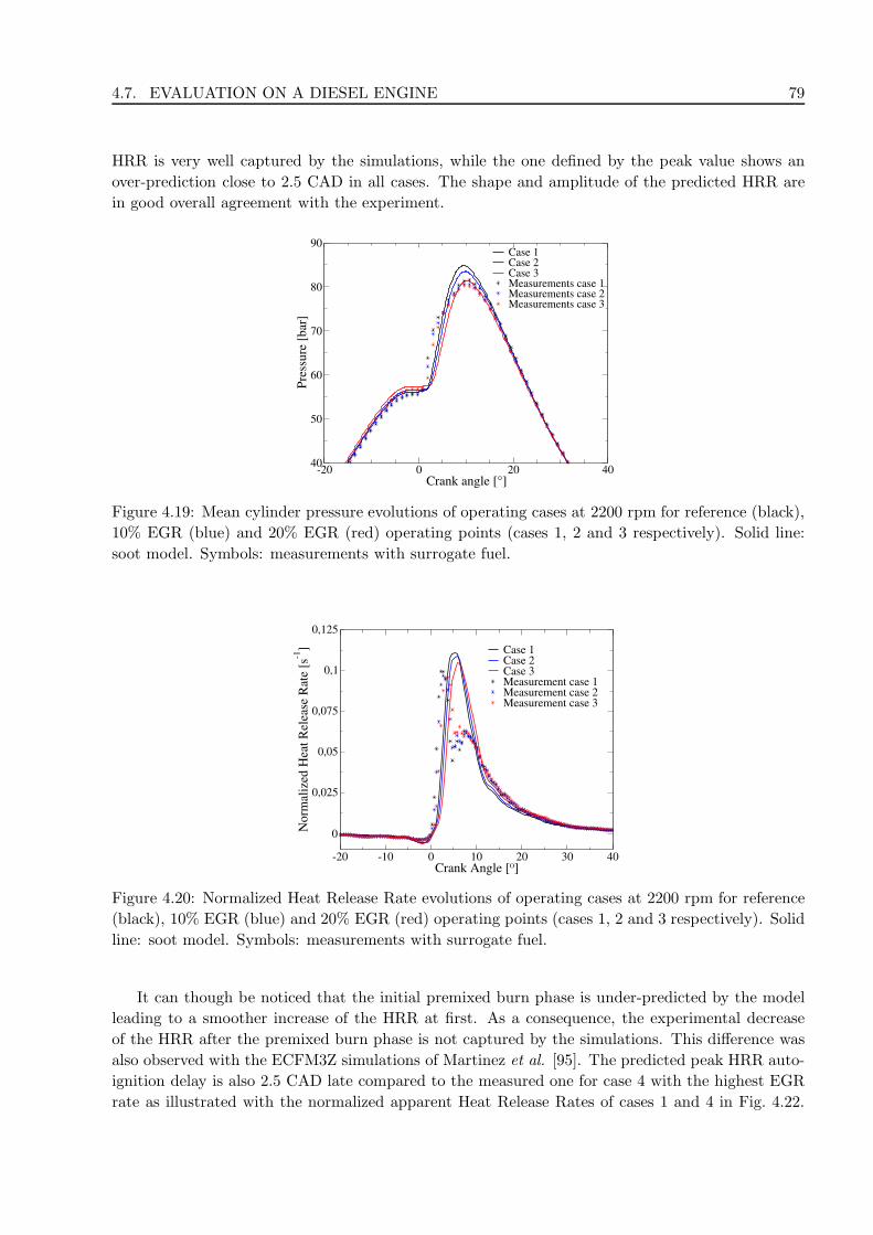
4.7. EVALUATION ON A DIESEL ENGINE 79
HRR is very well captured by the simulations, while the one defined by the peak value shows an
over-prediction close to 2.5 CAD in all cases. The shape and amplitude of the predicted HRR are
in good overall agreement with the experiment.
-20 0 20 40Crank angle [°]
40
50
60
70
80
90
Pre
ssure
[bar
]
Case 1Case 2Case 3Measurements case 1Measurements case 2Measurements case 3
Figure 4.19: Mean cylinder pressure evolutions of operating cases at 2200 rpm for reference (black),
10% EGR (blue) and 20% EGR (red) operating points (cases 1, 2 and 3 respectively). Solid line:
soot model. Symbols: measurements with surrogate fuel.
-20 -10 0 10 20 30 40Crank Angle [O]
0
0,025
0,05
0,075
0,1
0,125
Norm
aliz
ed H
eat
Rel
ease
Rat
e [s
-1] Case 1
Case 2Case 3Measurement case 1Measurement case 2Measurement case 3
Figure 4.20: Normalized Heat Release Rate evolutions of operating cases at 2200 rpm for reference
(black), 10% EGR (blue) and 20% EGR (red) operating points (cases 1, 2 and 3 respectively). Solid
line: soot model. Symbols: measurements with surrogate fuel.
It can though be noticed that the initial premixed burn phase is under-predicted by the model
leading to a smoother increase of the HRR at first. As a consequence, the experimental decrease
of the HRR after the premixed burn phase is not captured by the simulations. This difference was
also observed with the ECFM3Z simulations of Martinez et al. [95]. The predicted peak HRR auto-
ignition delay is also 2.5 CAD late compared to the measured one for case 4 with the highest EGR
rate as illustrated with the normalized apparent Heat Release Rates of cases 1 and 4 in Fig. 4.22.

80 CHAPTER 4. DIESEL RANS SIMULATIONS
Figure 4.21: Comparison of the experimental and simulated auto-ignition crank angle (CAD, dashed
line: +2 CAD and −2 CAD). See Tab. 4.4 for the legend, full symbol represent peak HRR delays
and blank symbol represent start of HRR delays.
Again, the integral of the apparent Heat Release Rate is well reproduced with less than 5% of error.
However, the error on the auto-ignition delay combined to a later ignition in case 4 leads to a slower
pressure increase and a larger error on the crank angle of maximum pressure as illustrated by the
mean cylinder pressure evolution of cases 1 and 4 in Fig. 4.23.
-20 -10 0 10 20 30 40Crank Angle [O]
0
0,025
0,05
0,075
0,1
0,125
Norm
aliz
ed H
eat
Rel
ease
Rat
e [s
-1] Case 1
Case 4Measurement case 1Measurement case 4
Figure 4.22: Normalized Heat Release Rate evolutions of operating cases at 2200 rpm for reference
(black) and 30% EGR (red) operating points (cases 1 and 4 respectively). Solid line: soot model.
Symbols: measurements with surrogate fuel.
The over-prediction of the auto-ignition delay based on the HRR peak for all cases can be

4.7. EVALUATION ON A DIESEL ENGINE 81
-20 0 20 40Crank angle [°]
40
50
60
70
80
90
Pre
ssure
[bar
]
Case 1Case 4Measurement case 1Measurement case 4
Figure 4.23: Mean cylinder pressure evolutions of operating cases at 2200 rpm for reference (black)
and 30% EGR (red) operating points (cases 1 and 4 respectively). Solid line: soot model. Symbols:
measurements with surrogate fuel.
explained by many causes. To our opinion, the most important one is the error on the complex
chemistry mechanism, as evidenced by the large variability of the auto-ignition delay and auto-
ignition reaction rate between different mechanisms as evidenced by the results obtained at ECN
for dodecane [158]. Besides, the kinetic scheme used to generate the look-up table, as all schemes
proposed for this fuel composition to our knowledge, has not been validated by its authors at the high
EGR rate, pressure and temperature characteristic of this operating point. Then the error on spray
modeling and turbulent mixing cannot be assumed negligible. It directly impacts the temperature
and mixture fraction in the reactive zone and consequently the auto-ignition delay. It also impacts
the amount of fresh gases that undergo the initial premixed burn phase, which directly pilots the
amplitude of the initial HRR. An experimental engine characterization of the spray and mixing was
not possible in the metal engine used in these experiments. It was therefore not possible to assess
the model prediction in this respect. Another error is the absence of strain effect in the ECFM3Z
model. As illustrated in Michel et al. [159], the absence of scalar dissipation in mixture fraction
space on an auto-igniting mixing layer leads to a restricted auto-ignition region close to the most
reactive mixture fraction. As ECFM3Z does not include scalar dissipation, this finding can explain
the fact that the amount of fresh gases undergoing the initial premixed-burn is under-predicted with
ECFM3Z compared to the experiment. Finally, the error cause by the EGR rate composition in
the homogeneous reactors used to generate the look-up table might also play a role, but to a lesser
extent as illustrated by the experiments of Colban et al. [160] and Kashdan and Thirouard [161].
Cases 5 to 6 represent a variation in injection pressure for 2200 rpm partial load operating
points and cases 7 to 11 correspond an injection duration variation for 4000 rpm full load operating
points. The simulations of these cases also show a good prediction of the auto-ignition delay, which
is presented in Fig. 4.21, and a good estimation of the maximum pressure (not presented here).

82 CHAPTER 4. DIESEL RANS SIMULATIONS
4.7.2.c In-cylinder soot fields
Global evolutions. Figure 4.24 shows soot mass fraction fields in the vertical plane containing
the spray axis. Four soot diameters are represented (1 nm, 20 nm, 100 nm and 260 nm) along with
the fields of the conditional fuel/air equivalence in region M and mean temperature. The first crank
angle shown in Fig. 4.24 is 0 CAD since it is the first angle at which a notable amount of 100 nm
particles has been created.
At 10 CAD, all soot formation mechanisms are active as illustrated with the 2D fields of the soot
mass fraction source terms in Fig. 4.25. Coagulation is not plotted since its sum over all sections
is null. Particle inception and condensation add carbon mass in the high equivalence ratio area
around the spray where the equivalence ratio is larger than two approximately. At the same time,
in a larger zone surrounding the spray and where temperature is still larger than 1700 K and the
equivalence ratio is lower than 1.5, oxidation reduces the amount of soot and limits its diffusion
in the combustion chamber. The surface growth source term is spread in a wider area around the
spray than particle inception and condensation because it is based on acetylene which is a species
more distributed in the combustion chamber than the soot precursor. As shown in Fig. 4.24, 100
nm diameter particles are present in these oxidazing areas but not 1 nm and 20 nm diameter ones
because these smaller particles are created next to the spray and are going to grow by condensation,
coagulation and surface growth as they move away from it.
After 35 CAD in the expansion phase, 1 nm and 20 nm diameter particles are no more present
close to the axis of the spray. This is due to the fact that fuel oxidation being almost finished
in this area, the inception reaction rate becomes null. Particles created previously have undergone
oxidation and coagulation, and have been convected outside the axis of the spray by the swirl motion.
Fig. 4.26 presents the different soot source terms at 35 CAD ATDC. Soot mass is still created by
surface growth but it is also limited by oxidation in the high temperature areas where soot already
exists and surface chemistry is still active. The fields corresponding to diameters of 100 nm and
260 nm at 35 CAD and 57 CAD in Fig. 4.24 show large amounts of soot in rich areas with lower
temperature and less soot in the stoichiometric or lean areas with the highest temperature where the
conditions are favorable to oxidation. As mentioned previously, particle inception and condensation
are null in the 2D views of Fig. 4.26 but these phenomena still exist in other areas of the combustion
chamber at 35 CAD. This last point also explains the presence of some small particles at 57 CAD.
The mean source terms evolutions are depicted in Fig. 4.27 for the reference 4000 rpm case (case
7). These evolutions split soot formation and evolution process into three main steps:
• First, the solid phase evolution is triggered by a large amount of small particles formed during
the ignition from −10 CAD and −5 CAD.
• Then, a transition phase occurs with a competition between the mass addition from precursors
(particle inception and condensation) in rich areas and the oxidation of particles which have
been transported to leaner areas as illustrated from −5 CAD and 30 CAD. This behavior is
also illustrated in Fig. 4.25.
• Finally, after 30 CAD, the soot production source terms vanish as the combustion ends.
Oxidation source term also decreases with the temperature decrease due to the expansion,
even if, as illustrated in Fig. 4.26, temperature is still high enough in some areas at 35 CAD
to oxidize particles. Once the temperature is too low to allow oxidation, the SNDF evolution
is only caused by coagulation.

4.7. EVALUATION ON A DIESEL ENGINE 83
0 CAD 10 CAD 20 CAD 35 CAD 57 CAD
Mixed region
Equivalence
Ratio
Temperature
[K]
Soot mass fraction
(1 nm diameter)
Soot mass fraction
(20 nm diameter)
Soot mass fraction
(100 nm diameter
Soot mass fraction
(260 nm diameter
Figure 4.24: 2D fields in the vertical plane containing the spray axis for the reference 4000 rpm case
(case 7). From top to bottom : fields of mixed region equivalence ratio, temperature and soot mass
fraction of four different diameters (1 nm, 20 nm, 100 nm and 260 nm) at five different crank angles
(from left to right, 0 CAD, 10 CAD, 20 CAD, 35 CAD and 57 CAD).

84 CHAPTER 4. DIESEL RANS SIMULATIONS
----
Figure 4.25: 2D fields in the vertical plane containing the spray axis for the reference 4000 rpm case
(case 7) at 10 CAD. Soot mass fraction source terms (s−1) for all sections: particle inception (top
left), condensation (top right), oxidation (bottom left), surface growth (bottom right).
----
Figure 4.26: 2D fields in the vertical plane containing the spray axis for the reference 4000 rpm case
(case 7) at 35 CAD. Soot mass fraction source terms (s−1) for all sections: oxidation (left), surface
growth (right).
Relative locations of species and soot particles. The location of the more important species
involved in soot formation and oxidation (pyrene, acetylene and hydroxyl) is shown in Fig. 4.28.
Carbon based species (pyrene and acetylene) are located in regions surrounding the spray initially.
The pyrene existence region is less spread than the acetylene one. These regions are then convected
by the swirl in the cylinder as illustrated in Fig. 4.28 with iso-surfaces from 10 CAD to 35 CAD.
Hydroxyl is located around the rich regions indicated by pyrene and acetylene. It exists in the
regions combining high temperatures with sufficiently oxidizing conditions.
The dispersed soot phase interacts with this gaseous composition and its location is very similar
as illustrated in Fig. 4.29. The particle inception location follows the pyrene one because pyrene

4.7. EVALUATION ON A DIESEL ENGINE 85
-20 -10 0 10 20 30 40 50 60 70Crank Angle [°]
-10
-5
0
5
10
15
Soot
mas
s fr
acti
on s
ourc
e te
rms
[s-1
]
Particle InceptionCondensationOxidationSurface Growth
Figure 4.27: Global soot mass fraction source terms (s−1) for the reference 4000 rpm case (case 7):
particle inception (solid, black), condensation (dashed, black), oxidation (solid, red), surface growth
(dashed, red).
0 CAD 10 CAD
20 CAD 35 CAD
Figure 4.28: Iso-surfaces taken at the half of the value range for pyrene (green), acetylene (pink)
and hydroxyl (blue) mass fractions at four different crank angles (0 CAD, 10 CAD, 20 CAD and 35
CAD)
is limiting reactant in its reaction with acetylene leading to particle inception. The soot volume
fraction appears to be further to the spray than the region where particle inception occurs. This
illustrate the ability of the model to reproduce a growth of soot in a reactive flow with particles

86 CHAPTER 4. DIESEL RANS SIMULATIONS
convected during their growth. Moreover, an oxidation region surrounds and limits the expansion
of the region where soot particles are.
0 CAD 10 CAD
20 CAD 35 CAD
Figure 4.29: Iso-surfaces taken at the half of the value range for particle inception (red) and oxidation
(blue) source terms and soot volume fraction (grey) at four different crank angles (0 CAD, 10 CAD,
20 CAD and 35 CAD)
Finally, the growth of soot particles within time and space is illustrated with iso-surface of
different particles sizes mass fraction in Fig. 4.30. At 0 CAD, the structure can be seen clearly with
the smallest particles next to the spray and the particles being further and further from the spray as
they grow before meeting the high oxidation reaction rate region. At contact between the particles
and the cylinder walls is predicted at 10 CAD. It results from the same contact of the carbon species
and the cylinder wall at the same time. However, interactions between the soot dispersed phase
and walls is not yet taken into account in this model. After 20 CAD, a new behavior appears for
large particles. Indeed, the 100 nm particles high density region (inside the volume limited by the
iso-surface) is further from the spray than the one of 260 nm particles. It illustrates a particle size
decrease predicted by the model along the trajectory followed by soot particles.

4.7. EVALUATION ON A DIESEL ENGINE 87
0 CAD 10 CAD
20 CAD 35 CAD
Figure 4.30: Iso-surfaces taken at the half of the value range for the oxidation source term (blue)
and the mass fractions of particles diameters 1 nm (light blue), 20 nm (yellow), 100 nm (red) and
260 nm (purple) at four different crank angles (0 CAD, 10 CAD, 20 CAD and 35 CAD)

88 CHAPTER 4. DIESEL RANS SIMULATIONS
4.7.2.d Soot model validation
In order to validate the soot model, a comparison of experimental (with surrogate fuel) and numerical
soot yield at EVO is first presented along with the predicted time-evolution of the soot mass in the
cylinder. Then, the numerical and experimental PSDF at EVO are compared.
Soot yield. The simulation results of soot emissions are presented in Fig. 4.31 and compared to
the measurements. These results show a good agreement with the experiments. Except for case 6,
all calculations predict the total mass with a relative error within −50% and +100%. The chosen
validation interval, of +100%/−50% is a common target used by engine manufacturers in the field of
soot modeling on piston engines. The variations of soot emissions with the injection duration (blue
symbols, cases 7 to 11) and with the EGR (red symbol, cases 1 to 4) are well predicted. For partial
load cases, the sensitivity to the injection pressure (red symbols, cases 1, 5 and 6) is underpredicted.
This could be explained by the fact that the soot model relies on species and temperature given by
the spray, evaporation, mixing and combustion models which do not represent the influence of the
injection pressure with a sufficient accuracy.
Figure 4.31: Comparison of the experimental and simulated soot emissions rate (g/h, dashed line:
+100% and -50%). See Tab. 4.4 for the legend.
The time-evolutions of the soot mass predicted by the sectional soot model (SSM) are shown
in Fig. 4.32 for cases 1, 7 and 11. The time-evolution of soot mass for case 1 only shows a first
formation phase from ignition at 1.5 CAD to 9 CAD after TDC before an oxidation phase leading to
the stabilized soot mass after 50 CAD after TDC. The soot mass evolutions are different for cases 7
and 11. The longer injection durations required to reach higher equivalence ratios (respectively 0.85
and 0.65 for cases 7 and 11) lead to a second phase of formation after the first soot production phase
due to the premixed auto-ignition. The differences in injection durations and injected fuel masses
between cases 7 and 11 induce the difference of duration of the second phase of soot formation. The
soot formation being longer and the rotating speed of the engine being faster, the soot oxidation is
still effective at the EVO in case 7.
Figure 4.33 shows the results obtained for the same cases with the Phenomenological Soot Kinet-

4.7. EVALUATION ON A DIESEL ENGINE 89
-20 0 20 40 60 80 100 120 140Crank Angle [°]
0
2.5e-07
5e-07
7.5e-07
1e-06
So
ot
mas
s [k
g]
SSM : Case 1SSM : Case 7SSM : Case 11
Figure 4.32: Soot mass (kg) evolutions predicted by the SSM function of the crank angle for cases
1 (black), 7 (red) and 11 (blue).
ics (PSK) model [80, 94], a semi-empirical two-equations model usually used for engine simulations
[95]. In comparison with Fig. 4.31, it illustrates the significant improvement obtained by the use
of a sectional approach. The injection duration variation at full load does not affect the soot mass
emission rate for the three lowest values before leading to a too important variation for the two
largest values. On the contrary, this effect is well reproduced with the sectional soot model with a
slight overestimation for all cases but with a relative variation close to the experimental ones. For
all the partial load cases, the PSK model strongly underestimates the soot yield unlike the sectional
soot model.
Figure 4.33: Comparison of the experimental and simulated with the PSK model soot emissions
rate (g/h, dashed line: +100% and -50%). See Tab. 4.4 for the legend.
These differences between the predictions of the PSK model and the SSM are illustrated with

90 CHAPTER 4. DIESEL RANS SIMULATIONS
the soot mass time evolutions of cases 1, 7 and 11 presented in Fig. 4.34. Although the soot
mass variations predicted by the PSK model are more important, the soot mass time evolutions are
qualitatively similar to the ones predicted by the SSM with one peak of soot production for case 1 and
two peaks for cases 7 and 11. These discrepancies can be first explained by the lack of information
on particles sizes in PSK. Indeed, in PSK, surface chemistry is based on an averaged surface for all
soot particles. The importance of this aspect is underlined by the inability of PSK to predict the
mean soot diameter for both cases. The second source of discrepancy is the simplified treatment of
chemistry in PSK where soot inception is based on ethylene instead of a PAH like pyrene. Ethylene
is itself given by a reduced four step mechanism and OH by an equilibrium computation instead of
complex chemistry in the present study [94].
-20 0 20 40 60 80 100 120 140Crank Angle [°]
0
2.5e-06
5e-06
7.5e-06
1e-05
1.25e-05
So
ot
mas
s [k
g]
SSM : Case 1SSM : Case 7SSM : Case 11PSK : Case 1PSK : Case 7PSK : Case 11
Figure 4.34: Soot mass (kg) evolutions predicted by the SSM (solid lines) and the PSK model
(dashed lines) function of the crank angle for cases 1 (black), 7 (red) and 11 (blue).
Predicted SNDF. SNDF simulation results at exhaust for the two reference cases 1 and 7 are
given in Fig. 4.35 and Fig. 4.36 respectively and compared to the experiments performed with
the surrogate fuel and to the average particle diameter predicted at exhaust by the PSK model.
These results are promising as the global amount of soot (in number) is predicted within an order
of magnitude compared to the experiments and the peak location of the size distribution is also
well reproduced. Some differences between the experiments and the simulations might come from
the fact that measurement of particles is quite difficult and could be strongly modified depending
on particle composition. However, the predicted SNDF offers a realistic view of the accumulation
mode at exhaust, matching the experiment on the median diameter and on the global shape of
the distribution for particle diameters larger than the 23 nm cut-off used for the definition of EU
emission standards. Note that the double peak of the SNDF observed experimentally for large
particles in Fig. 4.36 is certainly an artifact of the soot meter.
The average diameters predicted by the PSK model, 60 nm for case 1 and 6 nm for case 7,
illustrate the importance of modeling the SNDF. The large under-prediction on the average particle
diameter for case 7 is suspected to lead to an overestimation of the available reactive surface for
soot growth and oxidation. This value is here only compared to the SNDF at exhaust, because there
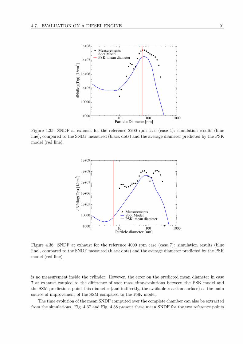
4.7. EVALUATION ON A DIESEL ENGINE 91
1 10 100 1000Particle Diameter [nm]
1000
10000
1e+05
1e+06
1e+07
1e+08
dN
/dlo
g(D
p)
[1/c
m3]
MeasurementsSoot ModelPSK: mean diameter
Figure 4.35: SNDF at exhaust for the reference 2200 rpm case (case 1): simulation results (blue
line), compared to the SNDF measured (black dots) and the average diameter predicted by the PSK
model (red line).
1 10 100 1000Particle diameter [nm]
1000
10000
1e+05
1e+06
1e+07
1e+08
1e+09
dN
/dlo
g(D
p)
[1/c
m3]
MeasurementsSoot ModelPSK: mean diameter
Figure 4.36: SNDF at exhaust for the reference 4000 rpm case (case 7): simulation results (blue
line), compared to the SNDF measured (black dots) and the average diameter predicted by the PSK
model (red line).
is no measurement inside the cylinder. However, the error on the predicted mean diameter in case
7 at exhaust coupled to the difference of soot mass time-evolutions between the PSK model and
the SSM predictions point this diameter (and indirectly, the available reaction surface) as the main
source of improvement of the SSM compared to the PSK model.
The time evolution of the mean SNDF computed over the complete chamber can also be extracted
from the simulations. Fig. 4.37 and Fig. 4.38 present these mean SNDF for the two reference points

92 CHAPTER 4. DIESEL RANS SIMULATIONS
(cases 1 and 7). At the ignition crank angle, the particle inception effect on the mean SNDF shape
is clearly represented with a large amount of very small particles. It is followed by a transfer of
small size particles to larger size particles due to coagulation. Finally, the established distribution
is partially oxidized which can be observed through the reduction of the soot peak concentration
(from 60 CAD up to the exhaust). A clear difference on the duration (in crank angles) of particle
inception can be seen between Fig. 4.37 and Fig. 4.38 with small soot disappearing earlier on the
2200 rpm reference case compared to the 4000 rpm reference case.
Figure 4.37: Particle volume number density depending on particle diameter and crank angle colored
by volume number density for the reference 2200 rpm case (case 1).
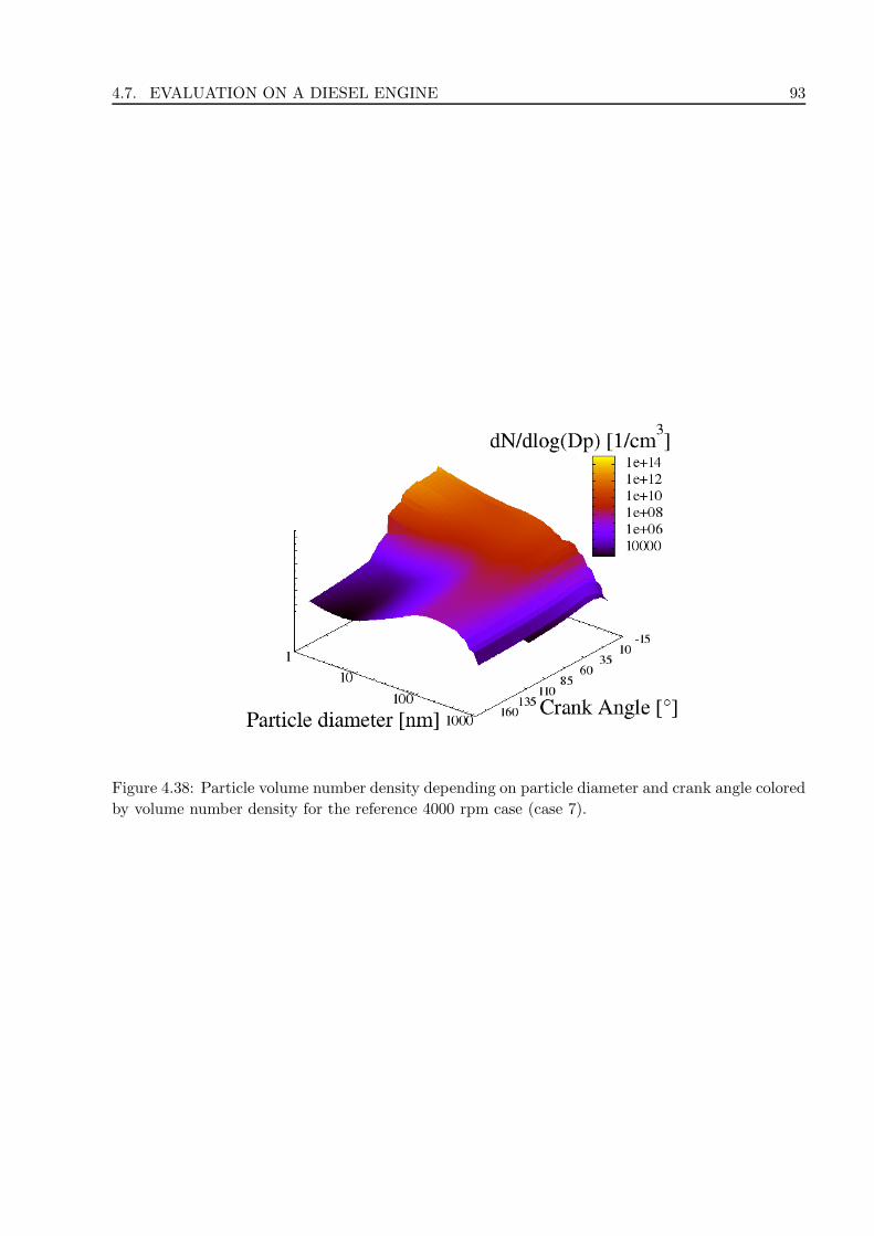
4.7. EVALUATION ON A DIESEL ENGINE 93
Figure 4.38: Particle volume number density depending on particle diameter and crank angle colored
by volume number density for the reference 4000 rpm case (case 7).

94 CHAPTER 4. DIESEL RANS SIMULATIONS
4.8 Conclusions
In this article, improvements brought to a sectional soot model are presented as well as its coupling
with the ECFM3Z [146] turbulent combustion model using a novel chemistry tabulation method
called VPTHC.
The sectional soot model is based on the description proposed in [77, 78, 124]. Two modifications
have been proposed in this work. First, a more accurate distribution of source terms through
the modeled SNDF is described. Secondly, a version of the HACA-RC cycle adapted to engine
calculations is employed [72].
This soot model requires as input parameters minor species mass fractions which are not available
using simplified kinetics. For this reason, a specific combustion model is proposed that allows to
describe these minor species. This model is based on the three mixing zones description of ECFM3Z
[146] and on the tabulated reaction rate model VPTHC. VPTHC (Variable Pressure Tabulated
Homogeneous Chemistry) is in fact a simplified version of the EADF combustion model [145].
It consists in the tabulation of species mass fractions and progress variable reaction rate using
constant and variable pressure homogeneous reactors. These outputs are used to calculate species
reaction rates in the reactive zone of ECFM3Z. VPTHC thus allows to include a complex chemistry
description at a low computational cost.
The ability of the VPTHC model to reproduce the detailed chemistry required by the soot model
is first evaluated on heterogeneous variable volume reactors (ECFM3Z-0D) specifically developed
to mimic Diesel combustion. Results show that the soot mass evolution during combustion is
qualitatively reproduced by VPTHC, even though a factor between two and three is found between
the tabulated method and the kinetic solver. This error is attributed to the VPTHC model trajectory
which only approximates the real engine trajectory: as minor species are extremely sensitive to this
trajectory, their prediction is much more difficult than for major combustion products like CO2. For
the time being, this error is considered acceptable because of the very large uncertainty linked to
the inception and surface chemistry and because the present model is devoted to an industrial usage
for which the limitation of the CPU cost is a major requirement. Clearly, the species description
proposed in VPTHC shall be improved in the future.
The soot and combustion models are finally evaluated on a Diesel engine database which includes
two operating points with parametric variations on EGR rate, injection pressure and duration. This
database [147] was acquired both for a commercial and a surrogate Diesel fuel which is also used
in the simulations (30% 1-Methylnaphthalene and 70% Decane in volume). Measurements provide
soot particle distributions at exhaust and soot yield. The main conclusions of this comparison are:
• The present surrogate offers a good representation of the commercial Diesel fuel for the rate
of heat release and for soot production (in terms of mass and distribution);
• The ECFM3Z/VPTHC model developed in this study reproduces with good accuracy the
auto-ignition delay and heat release rate for all the database;
• the soot yield obtained with the proposed model (sectional soot model coupled with ECFM3Z/VPTHC)
shows a good agreement with the experiments for the reference cases at 2200rpm and 4000rpm
and for the EGR and injection duration variations. In contrast, the effect of injection pressure
on the soot yield is underestimated.
• The soot particle distributions at exhaust correctly match the measurements in terms of dis-
tribution peak location and number density.

4.8. CONCLUSIONS 95
The underestimation of injection pressure influence on soot yield is yet an open topic. These sim-
ulations have been run with the standard modeling parameters of IFP-C3D without any calibration
between the operating points. It is well-known that spray models are not fully predictive yet. The
different sets of the k− ǫ model coefficients used by the different laboratories simulating the Engine
Combustion Network (ECN) Spray A (a Diesel-like spray in a constant volume vessel) illustrate this
fact. These coefficients are available in [158]. The inability of the spray model to reproduce a small
variation of injection pressure can be suspected to lead to the final error. Giving actual evidence of
this is difficult in this context because no data are available from this metal engine to validate the
spray model. Another possible explanation is the absence of strain effect in the ECFM3Z mixing
model: as the injection pressure is increased, larger gaseous velocities are expected, leading to larger
strain rates. As the strain rate increases, minor species concentrations like the soot precursor can
be strongly impacted as evidenced in the DNS of Bisetti et al. [73].
Future work will be devoted to improving the gaseous species description given by the VPTHC
model. This task might include the introduction of a feed-back model in the table representing
the impact of soot chemistry on the gaseous composition, and the introduction of specific transport
equations for minor species as proposed in Bisetti et al. [73].

96 CHAPTER 4. DIESEL RANS SIMULATIONS
Chapter 5
Diesel spray RANS simulation
This chapter is based on the current version of the article entitled “Combustion and soot modeling of
a high pressure and temperature Dodecane spray” to be submitted in November 2014. It contains
a description the Approximated Diffusion Flame (ADF) model which is coupled to the sectional
soot model for RANS simulations of Diesel sprays in a constant volume vessel. These simulations
provide a second validation of the model after the Diesel engines cases presented in the previous
chapter, using a more detailed combustion model and a different fuel. They also allow a more
detailed analysis of the soot formation and evolution predicted by the model.
First, the simulations were ran with the to ECFM3Z model coupled to the VPTHC model to
represent chemistry in the mixing region. However, this method is based on a simplified mixture
fraction stratification and it does not include strain effects. Even if the auto-ignition delay predic-
tions were acceptable with this approach, the lift-off lengths variations were underestimated. Since
one of the objectives of the Spray A simulations was to validate the ability of the model to predict
soot particles location, an approach able to predict the lift-off variations had to be used. Therefore,
the ADF model has been used for these simulations because it takes into account the strain effects
on the flame. These effects appeared to be necessary to represent the flame lift-off lengths. The
lift-off lengths predicted by the ADF model had a better agreement with the experimental ones.
Thus, the study of the soot particles location based on the gaseous phase predicted by the ADF
model was possible.
The sectional soot model used in the Spray A simulations is slightly different than the one
described in Chapter 3. The first simulations underestimated oxidation rates with very low variations
with respect to the temperature or dilutant mass fraction. This behavior was due to the value of
the coefficient from the quasi-steady state approximation in Eq. 3.31. It limited the oxidation by
hydroxyl and its variations. Therefore, a simpler method has been used. The reaction rates of
surface growth by acetylene and oxidation by oxygen and hydroxyl were directly obtained from the
surface chemistry reactions as in [73, 109]. These three reactions used for the Spray A simulations
are the same as the ones used for the other simulations of this work [76].
5.1 Abstract
Diesel engines are known to be one of the main sources of soot particle emission in the atmosphere.
The norms to restrain these emissions have created a need of accurate soot models for piston engine
emissions prediction in the automotive industry. This paper addresses this question by coupling
a sectional soot model with a tabulated combustion model for RANS simulations of the Engine
97

98 CHAPTER 5. DIESEL SPRAY RANS SIMULATION
Combustion Network (ECN) Spray A [L.M. Pickett, C.L. Genzale, G. Bruneaux, L-M. Malbec et al.
SAE Int. J. Engines 3 (2010) 156-181], a high pressure Dodecane spray with conditions very similar
to Diesel engines ones. The sectional soot model, which has already been used in Diesel engines
RANS simulations with a simpler combustion model in Aubagnac-Karkar et al. [D. Aubagnac-
Karkar, J-B. Michel, O. Colin, N. Darabiha, Combust. Flame (2015), In Press], is implemented in
the IFP-C3D RANS CFD code. At each time and location, transport equations are solved for several
soot sections, including source terms for collisional and chemical processes. The soot model is here
coupled to the Approximated Diffusion Flame - Presumed Conditional Moment model (ADF-PCM)
[J-B. Michel, O. Colin, D. Veynante, Flow Turb. Comb. 83 (2009), 33-60] which is a tabulated
combustion model. It allows to represent the minor species required by the soot model with a
much lower computational cost than a kinetic solver and includes complex turbulence-chemistry
interactions.
The predictions of these models agree with the experimental measurements for most of the Spray
A cases, for flame structure and soot production. These results show that detailed soot models can
be coupled to tabulated combustion models with good results in turbulent flames.
5.2 Introduction
A better understanding of soot particles formation and evolution is required to respond to the
stringent worldwide regulations on their emissions in the ground transport sector. In Europe, for
instance, EURO norms regulate particles emissions for Diesel engines since 1993 and will soon also
regulate them for spark-ignition engines (SIE). Even if Diesel engines are today equipped with parti-
cle filters, being able to predict soot particles number and size is still important to car manufacturers.
Indeed, some emitted particles are small enough to get through particle filters and the norms on
particles number will take them into account in the future. Moreover, particle filters are expensive
and a reduction of the raw-engine soot emissions would lead to a reduction of particle filters sizes
and costs.
In this context, engine manufacturers need experimental and numerical tools to evaluate the
raw engine-out Soot Volume Fraction (SVF) and Soot Number Density Function (SNDF). These
tools have to be implemented in RANS (Reynolds Averaged Navier Stokes) simulation codes, the
most used method for industrial combustion chamber simulation. Two main methods are used for
the prediction of SVF and SNDF in 3-D RANS simulations, the sectional method [61, 78, 162]
or the moment method [97, 108, 109]. In this work, a sectional soot model [162] derived from
models developed by Mauss and co-workers [112, 113, 114] is retained. It accounts for inception,
condensation, surface growth and oxidation processes and directly predicts the SNDF at each time
and location, in contrast to moment methods for which a post-processing is necessary.
Computing the local and instantaneous concentration of the soot precursors and the chemical
species involved in soot surface chemistry is required by detailed soot models, such as the one used
in the present paper. Kinetic schemes able to correctly predict these concentrations under the whole
range of thermodynamic and chemical conditions encountered in Diesel engines are detailed chemical
schemes including hundreds of species and thousands of reactions [140, 141, 142, 143, 144]. As a
consequence, transporting all the species and solving the complete chemistry totally coupled with
turbulent reactive flow balance equations is very costly. Thus, less expensive approaches have to be
used. Tabulated chemistry approaches have a very reduced CPU time compared to direct chemistry
resolution. Moreover, the sectional soot model has already been coupled to a tabulated turbulent

5.3. MODELS 99
combustion model derived of the Engine Approximated Diffusion Flame (EADF) [145] and used to
predict soot in RANS simulations of a Diesel engine with encouraging results [162]. In the present
work, a more complex model, the ADF-PCM model [151, 163], is used in order to include flame
structure effects to the gas phase modeling.
Relevant validation cases are required for these models. The closest academical set-up to Diesel
engines conditions is high pressure spray. In this study, the ability of the proposed sectional soot
model coupled to the ADF-PCM turbulent combustion model to predict SVF is evaluated against
measurements from the Dodecane Spray A [164, 165, 166] of the Engine Combustion Network (ECN).
The ECN Spray A is here retained because:
• it is a high pressure and temperature spray with conditions representative of those of a real
Diesel engine,
• Dodecane is a heavy fuel as Diesel fuel for which detailed chemical mechanisms are available,
• ECN provides large experimental databases with all variations required to validate a model.
The aim of this work is to assess the ability of the proposed combustion and soot models to
predict flame structure and soot production on the ECN Spray A cases. Section 5.3 describes
the ADF-PCM model used to compute the gaseous phase quantities and the sectional soot model
representing the soot particles formation and evolution. Then, the numerical configuration and
simulations results are given in Section 5.4.
5.3 Models
As mentioned in the introduction, a turbulent combustion model able to represent detailed chemistry
in non-premixed combustion is required to compute the species involved in the soot formation
process, including minor species such as soot precursors. In the present work, the ADF-PCM model
is used for that purpose. The two ADF-PCM and sectional soot models are described in the following
section.
5.3.1 Turbulent combustion model: ADF-PCM
In the ADF-PCM approach [151, 159, 163], approximated diffusion flames at various initial condi-
tions are used to generate a look-up table from which the species reaction rates are evaluated by
the CFD code. The generation of this look-up table splits into three parts:
• First, a chemistry database of autoigniting adiabatic homogeneous reactors is generated with
the IFP-Kinetics solver [136]. It allows the representation of pressure, temperature and dilu-
tant gases effects.
• Then, the flamelet equation of Peters [167] is solved for the progress variable only using the
chemical source terms extracted from the previous table in order to create a database of 1-D
approximated diffusion flames (ADF) which includes strain rate and temperature stratification
effects.
• Finally, the mixture fraction stratification is modeled with presumed pdf which are integrated
and stored in the ADF look-up tables.

100 CHAPTER 5. DIESEL SPRAY RANS SIMULATION
This method allows the representation of a detailed chemistry, required by the soot model, at a
very low computational cost. A similar approach was used for LES modeling of Diesel sprays with
good results in Tillou et al. [168].
5.3.1.a Homogeneous reactor table
This first table is built from the calculation of constant pressure autoigniting homogeneous reactors
for several pressures P , fresh gas temperatures T 0, mixture fractions Z and mass fractions of dilutant
YEGR as coordinates of the database. The results are stored as functions of the progress variable
which quantifies the transition from fresh to burnt gases. This quantity is here estimated as c =
Yc/Yeq where Yc = YCO + YCO2+ YH2O and Yeq is the value of Yc when the equilibrium at constant
pressure and enthalpy is reached. It has been verified that Yc evolves bijectively with time in all
computed reactors.
5.3.1.b Approximated diffusion flames calculations
In the ADF approach [151, 159, 163], the local and instantaneous structure of the reaction zone is
represented by autoigniting strained laminar diffusion flames which are tabulated. These flames are
defined by:
• A fresh gases mixture composition Yi,F and temperature T0F at the fuel saturated mixture
fraction Z = ZS
• A fresh gases mixture composition Yi,A and temperature T0A at mixture fraction Z = 0
The fresh gases composition and enthalpy evolve linearly with mixture fraction, thus defining the
fresh gases temperature though the flames.
The flamelet equation of Peters [167] is solved for the progress variable Yc:
∂Yc
∂t= χ
∂2Yc
∂Z2+ ωYc (5.1)
where χ is the scalar dissipation rate defined as:
χ = D |∇Z|2 (5.2)
where D is the diffusion coefficient. The strain rate, a, is used to characterize the scalar dissipation
rate, using the following relation for a counterflow diffusion flame [169]:
χ =aZs
2πexp
(−2
[erf−1
(1− 2
Z
Zs
)]2)= aF (Z) (5.3)
The progress variable reaction rate ωYc in the flamelet equation (5.1) is extracted from the
homogeneous reactors table in the ADF approach. Then, a database of flamelets computed with
this method can be generated for different values of T0F , T
0A and a as well as the values of YEGR and
P of the homogeneous reactors database.

5.3. MODELS 101
5.3.1.c Integration over a probability density function
Finally, the mixture fraction stratification is represented by a presumed β-PDF P (Z, Z, Z ′′) (here
written P (Z)) depending on the Favre average mixture fraction Z and its variance described in this
work with its segregation factor Sz = Z ′′/(Z(Zs − Z)). This presumed β-pdf is then applied to the
ADF progress variable source term and species computations to obtain the final table.
˜ωADF−PCMYc
(Z,P,T0F ,T
0A, YEGR, a, Sz, t) =
∫ Zs
Z=0ωflameletYc
(Z,P,T0F ,T
0A, YEGR, a, t)P (Z)dZ (5.4)
Y ADF−PCMi (Z,P,T0
F ,T0A, YEGR, a, Sz, t) =
∫ Zs
Z=0Y flameleti (Z,P,T0
F ,T0A, YEGR, a, t)P (Z)dZ (5.5)
where ωflameletYc
and Y flameleti are defined as:
ωflameletYc
(Z,P,T0F ,T
0A, YEGR, a, t) = ωHR
Yc(Z,P,T0
F ,T0A, YEGR, c(Z, t, a)) (5.6)
Y flameleti (Z,P,T0
F ,T0A, YEGR, a, t) = Y HR
i (Z,P,T0F ,T
0A, YEGR, c(Z, t, a)) (5.7)
where c(Z, t, a) = Yc(Z, t, a)/Yeqc (Z) is obtained from the flamelet equation solved for the progress
variable and the equilibrium value of the progress variable from the homogeneous reactor table.
Finally, ˜ωADF−PCMYc
and Y ADF−PCMi are stored in the final ADF-PCM table depending on the
flamelets initial conditions and c(Z, t, a) = Yc(Z, t, a)/Yeqc (Z).
5.3.1.d Model implementation
To extract species mass fractions in the combustion zone from the look-up table, the input param-
eters described above need to be calculated. These parameters are the progress variable Yc and the
initial parameters of the reactors: Z, P, T0F , T
0A, YEGR, a and Sz. The thermodynamic parameters
P, T0F , T
0A and YEGR derivations are detailed in [145]. The flame structure parameters Z, a and Sz
derivations are given in [163]. The tabulated species are transported in the CFD code as follows:
∂ρYi
∂t+∇ · (ρuYi) = ∇ · (ρ(D +Dt)∇Yi) + ρ˜ωYi
(5.8)
where ρ is the mean density, D an averaged diffusion coefficient and Dt the turbulent diffusivity.
It has been shown [151] that directly imposing species reaction rates from the look-up table leads
to uncontrolled deviations from the look-up table trajectories. Thus, another formulation [170, 171]
has been proposed by Michel et al. [151] for tabulated models species reaction rate ˜ωYi. It reads:
˜ωYi=
Y ADF−PCMi (Yc + δYc)− Yi
τ(5.9)
where τ is a time-scale representing species relaxation towards the homogeneous reactor conditions.
It was shown in [151] that as long as τ is chosen small enough compared to the progress variable
time-scale, the tabulated trajectory is correctly followed. Here, we choose τ = 3dt where dt is the
CFD time-step. The mean progress variable Yc+δYc is deduced from the tabulated progress variable
source term ˜ωADF−PCM
Ycand is given by:
δYc = τ ˜ωADF−PCMYc
(Z,P,T0F ,T
0A, YEGR, a, Sz , c) (5.10)

102 CHAPTER 5. DIESEL SPRAY RANS SIMULATION
where c = Yc/Yeqc with Yc here defined from the transported species.
In the CFD code, only thirteen species are extracted from the look-up table: n− C12H26, O2,
CO2, H2O, CO, H, H2, O, OH, C2H2, CH, HCO and C16H9. Therefore, the kinetic scheme inter-
mediary species atoms are missing. Three additional species are added to close the atomic balances
in carbon, hydrogen and oxygen: C2H3, H2b and O2b (b standing for balance) which have the same
thermodynamic properties as their respective real species as in [145, 162, 168].
5.3.2 Sectional soot model
The present soot model is identical to the one proposed in Aubagnac-Karkar et al. [162], which is
itself derived from the work of Netzell et al. [55, 78]. The present approach considers that soot
particles are solid and modeled as a distinct dispersed phase, interacting with the gaseous phase.
The soot particles population is evaluated by using a sectional method. The soot particles are
separated with respect to their volume into discrete sections. In the turbulent reactive flow, each
section i, representing the soot particles of a given volume range [Vmin,i;Vmax,i], is governed by a
standard transport equation for the mass fraction of soot in this section, Ysoot,i:
∂ρYsoot,i
∂t+∇ · (ρuYsoot,i) = ∇ · (ρDt,soot∇Ysoot,i) + ρ˜ωsoot,i (5.11)
with ρ the gas phase density, u the gas velocity, Dt,soot the turbulent diffusion coefficient of soot
here equal to the turbulent diffusivity Dt and ˜ωsoot,i the soot source term for section i.˜ωsoot,i is defined as the sum of five source terms describing the main processes of soot formation
and evolution. These different physical phenomena are described next. They are illustrated in
Fig. 5.1 and are introduced in the following order:
• Collisional source terms: particle inception, condensation and coagulation.
• Surface chemistry source terms: surface growth and oxidation.
5.3.2.a Collisional source terms
Particle inception, condensation and coagulation are collisional phenomena. They are represented
by the Smoluchowski equation [62]. In the continuous form, it reads:
Fa(t) =1
2
∫ a
0(βa−b,bFb(t)Fa−b(t))db−
∫ ∞
0(βa,bFa(t)Fb(t))db (5.12)
where Fx(t) is the number of particles of size x, Fx(t) its variation rate and βx,y the collision
frequency between particles of size x and y. The collision frequencies are obtained using the theory
of aerosol science [64], applied to soot formation by Kazakov and Frenklach [65].
Coagulation: Coagulation is the collision between particles, leading to larger particles. Its reac-
tion rate is directly evaluated from Eq. (5.12) and distributed among the sections.

5.3. MODELS 103
PAH PAH PAH+ + +
Combustion model(gaseous phase)
Sectional Soot Model(solid phase)
(PAH)
Polycyclic Aromatic
Hydrocarbon
Detailed chemistry
Fuel + Oxidizer
(+ Residual)
CO C2H2
O2 HCO
H OH
C2H2 + OH + O2+
Smallest solid
particle
Particle inception Condensation Coagulation
Surface growth Oxidation
Larger
particle
Surface chemistry
Collisional phenomena
Larger
particle
Larger
particle
Smaller
particle
Smaller
particle
Inte
rmed
iate
s a
nd p
roducts
Figure 5.1: Illustration of the five phenomena representing soot formation and evolution with the
involved gaseous species.
Inception and condensation; Inception and condensation are the two phenomena related to
precursors collisions. It can either be collisions between precursors to create the smallest considered
soot particles (particle inception), or between precursors and soot particles to increase soot particles
volume (condensation). The precursor species used in these phenomena is a virtual species called
PAH (for Polycyclic Aromatic Hydrocarbons). PAH is the product of the pyrenyl radical (C16H9),
a usual soot precursor [55, 56, 58, 78, 77], polymerization by acetylene as in [56, 77, 78, 162]:
C16H9 +C2H2kpol−−→ PAH +H2 (5.13)
where kpol is the rate constant of reaction for this polymerization reaction.
This precursor formation rate is balanced with its consumption rate by particle inception and
condensation which are evaluated using Eq. (5.12). This balance equation closes the problem of
particle inception and condensation by giving the number density of virtual precursors PAH, thus
leading to the final reaction rate of particle inception and condensation to be distributed in the
sections.
5.3.2.b Surface chemistry
Although the HACA-RC cycle (Hydrogen Abstraction Carbon Addition - Ring Closure) developed
by Frenklach [26] is commonly used to model soot surface chemistry [56, 75, 76, 78], the constants
for soot modeling in turbulent flame are still unsure [73]. Accordingly, considering only reaction
rates taken from literature for surface growth by acetylene addition, oxidation by hydroxyl radical
and oxidation by molecular oxygen is sufficient is turbulent combustion cases [73, 109]. In the
present work, these three surface chemistry reaction rates are taken from a variation proposed by
D’Anna and Kent [76] of the HACA-RC cycle. This surface chemistry scheme has been chosen as
a reference since it has been used with a similar sectional model in Diesel engine simulation [162]
104 CHAPTER 5. DIESEL SPRAY RANS SIMULATION
and was designed for Diesel engine conditions and previously validated by Fraioli et al. [72]. The
surface chemistry phenomena are described using six gaseous species (H, OH, C2H2, O2, CO and
HCO) in three reactions (given in table Tab.5.1) with the rate constants taken from [76]. In Tab.5.1,
Ci represents soot particles of section i, Cpkrepresents stable aromatic soot particles product of a
reaction that exchanged p carbon atoms with the gaseous phase, and kin is the rate constant of
reaction n on particles of section i.
Ci +C2H2ki4−→ C2
i +H
Ci +OHki5−→ C−1
i+HCO
Ci +O2ki6−→ C−2
i+ 2CO
Table 5.1: Reactions governing the soot surface chemistry [76].
To evaluate the oxidation and surface growth reaction rates given by the surface chemistry
reactions, the total amount of particles in each section is first converted into a concentration ([Ci ])
also proportional to the surface Si(v) of particles of volume v included in section i. This value can
be obtained from:
[Ci ] =
∫ vmax,i
vmin,i
αHACA
λsoot
NASi(v)ni(v)dv (5.14)
where NA is the Avogadro number, ni(v) is the number density of soot particle of volume v included
in section i, λsoot is the number of reactive sites per unit surface of soot and αHACA is the proportion
of these sites which are active.
The value of αHACA is often correlated to temperature [44, 132]. Because temperature dependent
expressions of αHACA are not completely validated up to now, we rather choose a constant value as
done in [55, 56]. We choose αHACA = 0.27 which corresponds to the average value of the correlation
given by Markatou et al. [132] for a temperature interval of 1250K to 3000K as in [55, 77, 78, 162].
The number of reactive sites available for reaction (λsootSi) is evaluated as in [55, 56]. Con-
sidering that the smallest solid soot particle has only one reactive site (λsootS1 = 1), the number
of reactive sites only depends on particles volume. Finally, the variation of the available surface
with particle volume is represented by correcting the surface of a sphere of equivalent volume by a
fractal dimension θ. For the calculations presented here, θ = 2.0 for all particles with a diameter
smaller than 20 nm and θ = 2.25 for all particles with a diameter larger than 60nm and the fractal
dimension evolves linearly in between as in [55, 77, 78, 162].
5.4 Results
5.4.1 Experimental database
The Spray A is a high-pressure Dodecane spray designed to reproduce Diesel sprays. In the Spray
A set-up [164], Dodecane is injected in a high-pressure constant volume vessel of 1150 cm3. The
initial composition of ambient gas is known as well as its thermodynamical conditions.
A large database of variations are available for the Spray A including different injection pressures
and ambient gas densities, compositions (with different molar fractions of oxygen) and temperatures.

5.4. RESULTS 105
This allows experimental studies on the effect of each of these parameters and offers validation cases
for models in conditions that are close to actual Diesel engines conditions and well documented.
Two of those variations include soot measurements and all the available cases of these variations
have been simulated. These different cases are summarized in Tab. 5.2 with the ambient temperature
Tamb, the ambient pressure Pamb, the molar fraction of oxygen XO2and the mass fraction of dilutant
YEGR. For all these cases, the fuel injection pressure difference to the ambient gas pressure is 150
bar, the injected fuel temperature is 363 K and the ambient gas density is 22.8 kg.m−3 (the pressure
is adapted to keep this density on the temperature sweep). The injections are 6.1 ms long and 14
mg of Dodecane are injected. For each value of XO2, a specific composition is provided including
CO2 and H2O. This justifies a non-zero value of YEGR for case 3 with 21% in mole of oxygen, the
dilutant mass fraction being evaluated with respect to pure air.
Case Variation Tamb Pamb XO2YEGR
1 Ref. 900 K 60 bar 15% 0.294
2 XO2900 K 60 bar 13% 0.387
3 XO2900 K 60 bar 21% 0.018
4 Tamb 750 K 49.3 bar 15% 0.294
5 Tamb 800 K 52.5 bar 15% 0.294
6 Tamb 850 K 56.1 bar 15% 0.294
7 Tamb 1000 K 66.2 bar 15% 0.294
8 Tamb 1100 K 73 bar 15% 0.294
9 Tamb 1200 K 79.4 bar 15% 0.294
Table 5.2: Main characteristics of the Spray A simulated cases.
5.4.2 Numerical configuration
The computations have been ran on a 1500000 hexahedral cells mesh illustrated in Fig 5.2. The
geometry is a cube of 1150 cm3, the volume of the experimental vessel, with a characteristic length
in the spray axis of 0.48 mm and 0.52 mm in the transverse directions at the injector nozzle. As
shown in Fig.5.2 with the OH mass fraction 5 ms after the beginning of injection (SOI) on the
reference case, the mesh has a better resolution area to correctly describe the spray.
The Dodecane chemistry is represented by a kinetic scheme proposed by Narayanaswamy et al.
[141] of 255 species and 1509 reactions used to generate the look-up table. The table is discretized
in order to cover all the simulated cases given in Tab.5.2 with:
• 7 couples of initial air temperature T0A and pressure P, one per point in the temperature sweep
(respectively 750 K/ 49.3 bar, 800 K/ 52.5 bar, 850 K/ 56.1 bar, 900 K/ 60 bar, 1000 K/ 66.2
bar, 1100 K/ 73 bar, 1200 K/ 79.4 bar);
• a fuel temperature T0F of 300 K and a saturated mixture fraction ZS constant at the value
of 0.5 obtained from a previous study of a single droplet evaporation [172] and usually used
with this model for Diesel spray simulations [145, 168, 95]. Moreover, combustion indicators
sensitivity to the value of ZS have been tested and is very low.
• 3 values of dilutant gases mass fraction YEGR, 0.387, 0.294 and 0 computed to reproduce the

106 CHAPTER 5. DIESEL SPRAY RANS SIMULATION
Figure 5.2: Visualization of the computational mesh in the plane containing the axis of the spray
colored by OH mass fraction 5.5 ms after the start of injection (SOI) on the reference case.
initial gaseous composition for the 3 values of ambient oxygen molar fractions respectively
13%, 15% and 21%;
• 30 progress variable c ranging from 0 to 1, 21 strain rates a from 0 s−1 to 20000 s−1, 100
average mixture fractions from 0 to 0.5 and 8 mixture fraction segregation factors Sz from 0
to 0.3 to described the possible flame structures with enough accuracy.
The sectional soot and the ADF-PCM models are implemented in the IFP-C3D RANS code
[148, 149], which is a fully parallelized code developed by IFP Energies Nouvelles for simulating
compressible reactive flows. It integrates Lagrangian spray and liquid film models [154, 155], and
a standard k-ǫ model for turbulence description. The simulations using the IFP-C3D RANS code
were 8 to 18 hours long on 128 processors with a CFD maximum time-step of 10−6 s and a temporal
subcycling for the soot sections.
5.4.3 Non-reactive case
First, a non reactive case has been simulated with ambient gas molar composition of 89.71% of
N2, 6.52% of CO2 and 3.77% of H2O, its other properties being identical to those of the reference
reactive case. This ensures that the IFP-C3D RANS code provides an acceptable representation of
the spray and its evaporation which is required by the combustion and soot models. The liquid and
vapor fuel penetrations are given in Fig. 5.3 and Fig. 5.4 respectively. Both predicted penetrations
agree with the experiments.
The fuel mass fraction axial and radial profiles are given in Fig. 5.5 and Fig. 5.6. The stabilized
axial profile of fuel mass fraction is compared to the mean experimental one in Fig. 5.5. The

5.4. RESULTS 107
0 1 2 3 4 5 6t [ms]
0
5
10
15
Liq
uid
Pen
etra
tio
n [
nm
]
MeasurementsIFP-C3D
Figure 5.3: Temporal evolution of the experimental and simulated liquid penetrations for the non-
reactive case.
0 1 2 3 4 5t [ms]
0
20
40
60
80
100
Vap
or
Pen
etra
tio
n [
mm
]
MeasurementsIFP-C3D
Figure 5.4: Temporal evolution of the experimental and simulated vapor penetrations for the non-
reactive case.
measured mean mass fraction uncertainties are given and the predicted fuel mass fraction along the
axis of the spray is in the uncertainties interval. Fig. 5.6 shows the fuel mass fraction radial profiles
simulated and measured at two distances from the injector orifice. The predicted profiles are slightly
wider than the measured ones but this error remains acceptable. The shapes of radial profiles agree
with the axial ones. Indeed, the angle of the gaseous phase of the spray is slightly too large, which
lowers the fuel mass fraction value along the spray axis and widens the radial profiles.
Globally, the agreement with the experiments in the range of distance from injector where it is
available is sufficient to allow further simulations in reactive cases.

108 CHAPTER 5. DIESEL SPRAY RANS SIMULATION
0 2 4 6 8 10Distance from injector orifice [cm]
0
0.05
0.1
0.15
0.2
0.25G
aseo
us
fuel
mas
s fr
acti
on
ExpIFP-C3D
Figure 5.5: Comparison between experimental (black with standard deviation in dashed line, avail-
able in a limited range of distances from injector orifice) and simulated gaseous fuel mass fraction
along the spray axis depending on the distance from the injector orifice.
-20 -10 0 10 20Radial distance to spray axis [mm]
0
0.05
0.1
0.15
0.2
Gas
eou
s fu
el m
ass
frac
tio
n
IFP-C3D - 2 cmMeasurements - 2 cmIFP-C3D - 4 cmMeasurements - 4 cm
Figure 5.6: Comparison between experimental and simulated fuel mass fraction at two distances
from the injector orifice depending on the distance from the spray axis.
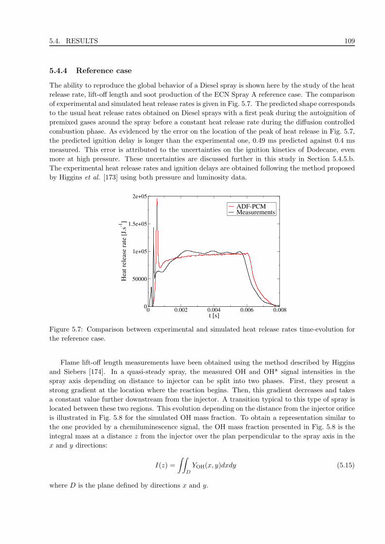
5.4. RESULTS 109
5.4.4 Reference case
The ability to reproduce the global behavior of a Diesel spray is shown here by the study of the heat
release rate, lift-off length and soot production of the ECN Spray A reference case. The comparison
of experimental and simulated heat release rates is given in Fig. 5.7. The predicted shape corresponds
to the usual heat release rates obtained on Diesel sprays with a first peak during the autoignition of
premixed gases around the spray before a constant heat release rate during the diffusion controlled
combustion phase. As evidenced by the error on the location of the peak of heat release in Fig. 5.7,
the predicted ignition delay is longer than the experimental one, 0.49 ms predicted against 0.4 ms
measured. This error is attributed to the uncertainties on the ignition kinetics of Dodecane, even
more at high pressure. These uncertainties are discussed further in this study in Section 5.4.5.b.
The experimental heat release rates and ignition delays are obtained following the method proposed
by Higgins et al. [173] using both pressure and luminosity data.
0 0.002 0.004 0.006 0.008t [s]
0
50000
1e+05
1.5e+05
2e+05
Hea
t re
leas
e ra
te [
J.s-1
]
ADF-PCMMeasurements
Figure 5.7: Comparison between experimental and simulated heat release rates time-evolution for
the reference case.
Flame lift-off length measurements have been obtained using the method described by Higgins
and Siebers [174]. In a quasi-steady spray, the measured OH and OH* signal intensities in the
spray axis depending on distance to injector can be split into two phases. First, they present a
strong gradient at the location where the reaction begins. Then, this gradient decreases and takes
a constant value further downstream from the injector. A transition typical to this type of spray is
located between these two regions. This evolution depending on the distance from the injector orifice
is illustrated in Fig. 5.8 for the simulated OH mass fraction. To obtain a representation similar to
the one provided by a chemiluminescence signal, the OH mass fraction presented in Fig. 5.8 is the
integral mass at a distance z from the injector over the plan perpendicular to the spray axis in the
x and y directions:
I(z) =
∫∫
DYOH(x, y)dxdy (5.15)
where D is the plane defined by directions x and y.

110 CHAPTER 5. DIESEL SPRAY RANS SIMULATION
The lift-off length definition is based on OH evolutions of the same type as the one presented
in Fig. 5.8. Arbitrary thresholds are defined to evaluate the experimental lift-off lengths in the
strong gradient area. A value of 50% of the chemiluminescence signal at the “knee” has been used
in experiments and the same threshold applied to OH mass fraction is used in the present study.
For the reference case, the measured lift-off length is 16.1 mm and the predicted one is 16.7 mm.
These results are illustrated in Fig.5.9 with OH mass fraction fields in the plane containing the
spray axis at four different times after SOI, also illustrating the ability of the model to reproduce a
quasi-steady flame structure. The experimental lift-off length is indicated by the vertical white line
to illustrate the global good prediction of the flame location.
0 0.025 0.05 0.075 0.1Distance to injector [m]
0
1e-06
2e-06
3e-06
4e-06
5e-06
Inte
gra
ted
OH
mas
s fr
acti
on
[m
2] 1 ms
2 ms3 ms4 ms5 ms6 ms
Figure 5.8: OH mass fraction integrated in a plane perpendicular to the spray axis depending on
the distance from the injector for the reference case.
Soot volume fraction (SVF) fields are also available from the experimental database. A 2-D field
of SVF in the plane containing the spray axis is available for this case, based on the integration
during the quasi-steady spray of SVF measured by soot optical extinction [165] or Laser Induced
Incandescence [166]. The soot mass contained in an experimental window going from a distance of
2 cm from the injector to 6.5 cm from the injector is also available. The evolution of this soot mass
is shown in Fig. 5.10 along with the model predicted soot mass in the given experimental windows.
The soot mass experimental measurement shows that soot processes are also in a quasi-steady state
from 3 ms after SOI through the end of injection at 6 ms after SOI. This quasi-steady state is well
reproduced by the model with a similar mass of soot. The very slow increase of soot between 4 ms
and 6 ms observed in this figure is due to a slight imbalance between the four source terms during
this period. These source terms are based on phenomena such as particle inception which are not
well defined yet. Therefore, this result is considered very acceptable for a complex case such as the
Spray A. Nevertheless, the initial peak of soot production is not predicted by the model. This can
be explained by two reasons. First, the RANS approach has a low ability to represent the steep
mixture fraction gradient observed experimentally and in LES [175, 176]: in the experiments, the
fluctuations from shot to shot of the position of this front lead to a smooth mean gradient as seen
in Fig.5.11. RANS recovers this mean gradient and represents the fluctuations with a fluctuations
modeling. Secondly, these mixture fraction fluctuations are included in ADF-PCM but they are

5.4. RESULTS 111
3ms
4ms
5ms
6ms
10
10
10
10
-10
-10
-10
-10
0
0
0
0
0 20 40 60 80Distance from injector ori ce [mm]
Figure 5.9: OH mass fraction fields in the plane containing the spray axis at four different times
after SOI (3 ms, 4 ms, 5 ms, 6 ms) for the reference case, with an indication of the experimental
lift-off length.
mostly interpreted in this model as a local heterogeneity of mixture fraction. On the contrary, LES
has the ability to represent this intermittency thanks to the simulation of many realizations of the
spray injection [176]. Last, even if the combustion model includes a fluctuations representation
of the mixture fraction distribution, the soot model itself is homogeneous. Thus, the soot phase
evolution is driven by the mean species concentrations read by the soot model. This impedes to
represent the strong production of soot within the real instantaneous gradient. This also explains
why the quasi-steady state soot mass predicted by the model occurs later than the experimental
one, the initial amount of soot being formed during a longer time.
The predicted SVF at four different times after SOI are compared with the time-averaged ex-

112 CHAPTER 5. DIESEL SPRAY RANS SIMULATION
0 0,002 0,004 0,006 0,008t [s]
0
5e-09
1e-08
1,5e-08
2e-08
2,5e-08
mso
ot [
kg]
MeasurementsSoot model
Figure 5.10: Comparison between the experimental and predicted soot mass integrated over the
experimental measurement windows as a function of time for the reference case.
Measurements LES
Average
Shots
Figure 5.11: Comparisons of experimental measurements (left) and LES predictions (right) of mix-
ture fractions in a Diesel-like spray 0.5 ms after the beginning of injection with two individual shots
of each (top) and the averaged value over 30 realizations (bottom) [176].
perimental SVF in Fig. 5.12. The predicted SVF are stabilized after 4 ms as indicated by the soot
mass. The stabilized predicted SVF location and width are similar to those of the experiments. The
absolute values of the SVF fields cannot be compared since the experimental one is averaged from
1.8 ms to 5.8 ms [165], including a first long duration without soot in the regions where negligible
SVF is observed, thus lowering the measured SVF. The predicted SVF fields in the plane containing
the spray axis are shaped by the balance between a strong soot production in the rich regions next to
the spray axis and oxidation in the regions with a large amount of hydroxyl on the side of the spray
and further from the injector nozzle as illustrated in Fig. 5.13. The shape of the particle inception

5.4. RESULTS 113
and condensation source terms are explained by the fact that these phenomena are controlled by
pyrene and acetylene which maxima are not located in the same regions of the spray as shown in
Fig.5.14.
3 ms
4 ms
5 ms
6 ms
0
0
0
0
10
10
10
10
-10
-10
-10
-10
Distance from injector orifice [mm]
Figure 5.12: SVF fields in the plane containing the spray axis at four different times after SOI (3
ms, 4 ms, 5 ms, 6 ms) compared to the time-averaged experimental SVF for the reference case
Finally, the dynamics of the soot production is analysed using the global source terms evolutions
presented in Fig. 5.15. The quasi-steady state corresponds to a balance between the surface growth
and condensation, in the one hand, and oxidation source term, in the other hand, for this spray
while particle inception only triggers the soot production processes. Further studies, for instance

114 CHAPTER 5. DIESEL SPRAY RANS SIMULATION
Particle
inception
Surface
growthOxidation
Condensation
Distance to injector orifice [mm]0 0
0
0
10
10
-10
-10
20 8040 6080604020
Figure 5.13: Soot mass fraction source terms (s−1) fields in the plane containing the spray axis
predicted by the soot model for the reference case 5.5 ms after SOI, including particle inception (top
left), condensation (top right), surface growth (bottom left) and oxidation (bottom right).
Distance to injector orifice [mm]
ene 0
0
0
10
10
-10
-10
20 40 60 80
Figure 5.14: Pyrene (top) and acetylene (bottom) mass fractions fields in the plane containing the
spray axis predicted by the ADF-PCM model for the reference case 5.5 ms after SOI.
on the version of Spray A with a fuel containing some aromatics species, could allow to figure out
if this balance is specific to these conditions and to Dodecane or if they are more universal. Indeed,

5.4. RESULTS 115
Dodecane is a heavy fuel but it does not contain aromatic species which are directly involved in soot
precursors kinetics.
0 0,002 0,004 0,006 0,008 0,01t [s]
-0,004
-0,003
-0,002
-0,001
0
0,001
0,002
0,003
0,004
0,005
So
ot
mas
s fr
acti
on
so
urc
e te
rms
[s-1
] Particle inception x500Condensation x100OxidationSurface growth
Figure 5.15: Time-evolution of the particle inception, condensation, surface growth and oxidation
source terms for the reference case.

116 CHAPTER 5. DIESEL SPRAY RANS SIMULATION
5.4.5 Variations
In the ECN database, the variations of dilutant mass fraction and of ambient gas temperature include
soot measurements. All the available variations have been simulated in this study and the results
are given in this section. These results underline the ability of the proposed models to reproduce
the effects of dilutant and ambient temperature on flame structure and soot production. The limits
of this modeling approach are also presented and discussed.
5.4.5.a EGR sweep
Combustion indicators. Figure 5.16 illustrates the ability of the ADF-PCM model to reproduce
lift-off lengths in the Spray A conditions for different dilutant mass fractions. The trends are well
reproduced with an acceptable error smaller than 1 mm between the experimental measurements
and the predicted lift-off lengths.
10 15 20 25% O
2
0
5
10
15
20
25
Lif
t O
ff L
eng
th [
mm
]
MeasurementADF-PCM
Figure 5.16: Evolution of the lift-off lengths with the oxygen molar fractions (cases 1 to 3).
Prediction of ignition delays for the same variations are showed in Fig. 5.17. As for the reference
case, the ignition delays for the two other initial compositions are too long. However, the global
trend is reproduced with predicted ignition delays which increase with the mass fraction of dilutant.
Soot production. The evolution of soot production is illustrated in Fig. 5.18 with the soot mass
time-evolution for the three different dilutant mass fractions. The model reproduces the apex of
the stabilized soot mass value for the reference case compared to the two other values of dilutant
mass fractions, which are 0.387 and 0.018 for cases 2 and 3 against 0.294 for the reference case.
This evolution depends on the dilutant mass fraction because of the competition between the soot
growth phenomena and oxidation as shown in Fig. 5.19. For case 3 where the dilutant mass fraction
is the lowest, the particle inception reaction rate increases due to the higher temperature reached,
which provides more particles in the surface growth regions compared to the two cases. The surface
growth is also increased by these conditions with twice the value of the reference case for a similar
mass of soot. However, this does not lead to a larger mass of produced soot particles because the

5.4. RESULTS 117
10 15 20 25X
O2
0
0.1
0.2
0.3
0.4
0.5
0.6
Ign
itio
n D
elay
[m
s]
MeasurementsADF-PCM
Figure 5.17: Evolution of the ignition delays with the oxygen molar fractions (cases 1 to 3).
high temperature combined to a more oxidizing gaseous composition also allows a higher oxidation
reaction rate. With the increase of the dilutant mass fraction, the reaction rates of these two
phenomena decrease. The oxidation is more limited than the soot growth phenomena between cases
1 and 3. This leads to an increase of the soot production as the dilutant mass fraction increases.
However, the evolution is different between cases 1 and 2 where the dilutant mass fractions are
higher. The main reason of this difference is that the soot particles, following the lift-off lengths,
get further downstream as the dilutant mass fraction increases. This locates a part of the soot mass
outside of the experimental measurement windows as illustrated for case 1 in Fig. 5.12 where a part
of the SVF is located outside of the measurement windows.
0 0,002 0,004 0,006 0,008 0,01t [s]
0
5e-09
1e-08
1,5e-08
2e-08
2,5e-08
mso
ot [
kg]
Measurements: case 1Measurements: case 2Measurements: case 3Simulation: case 1Simulation: case 2Simulation: case 3
Figure 5.18: Comparison between experimental and predicted soot mass time-evolution with three
different dilutant mass fractions (cases 1 to 3).

118 CHAPTER 5. DIESEL SPRAY RANS SIMULATION
0 0,002 0,004 0,006 0,008 0,011,0e-08
1,0e-07
1,0e-06
1,0e-05
1,0e-04
Soot
mas
s fr
acti
on r
eact
ion r
ate
[s-1
] Case 1Case 2Case 3
Particle inception
0 0,002 0,004 0,006 0,008 0,011,0e-08
1,0e-07
1,0e-06
1,0e-05
1,0e-04
Condensation
0 0,002 0,004 0,006 0,008 0,01
t [s]
0e+00
1e-03
2e-03
3e-03
4e-03
5e-03
6e-03
7e-03Surface Growth
0 0,002 0,004 0,006 0,008 0,01
t [s]
-7e-03
-6e-03
-5e-03
-4e-03
-3e-03
-2e-03
-1e-03
0e+00Oxidation
Figure 5.19: Comparison between the time-evolution of the space-averaged soot reaction rates of
particle inception (top left), condensation (top right), surface growth (bottom left) and oxidation
(bottom right) with three different dilutant mass fractions (cases 1 to 3).
5.4.5.b Ambient temperature sweep
Combustion indicators. The predicted lift-off lengths and ignition delays depending on ambient
gas temperatures are given in Fig. 5.20 and Fig. 5.21. The predicted lift-off lengths and ignition
delays for low temperature cases are well reproduced. The variation between the reference case and
case 7 is not correctly reproduced for the ignition delay as for the lift-off length. The most probable
explanation for this error is the lack of accuracy in the description of the NTC region by the detailed
mechanism. This point is detailed next.
700 800 900 1000 1100 1200 1300Ambient temperature [K]
0
10
20
30
40
50
60
Lif
t O
ff L
eng
th [
mm
]
MeasurementsADF-PCM
Figure 5.20: Lift-off lengths depending ambient gas temperatures.

5.4. RESULTS 119
700 800 900 1000 1100 1200 1300Ambient temperature [K]
0
1
2
3
Ign
itio
n D
elay
[m
s]
MeasurementsADF-PCM
Figure 5.21: Ignition delays depending ambient gas temperatures.
Dodecane ignition delay measurements in shock tubes are available in Vasu et al. [177]. These
measurements are compared with predicted ignition delays of constant volume reactors simulated
with the IFP-Kinetics library solver [136], using the kinetic scheme used to generate the look-
up table, proposed by Narayanaswamy et al. [141], and two other kinetic schemes which are the
JetSurF2.0 [178] and the scheme proposed by Malewicki and Brezinsky [179]. These results, given in
Fig. 5.22, cannot be taken as direct indications whether the ignition delay should be shorter or longer
at a given temperature since these cases are homogeneous and at initial pressures and temperatures
much lower than in the Spray A case. Still, they illustrate a chemical effect of dodecane combustion.
A very strong NTC occurs in a temperature range which is the one where the ADF-PCM combustion
model, based on source terms taken from homogeneous chemistry, provides less accurate results for
the Spray A simulations. Similar results are obtained by Pei et al. [180] for shock tubes simulations
as well as Spray A simulations using different kinetic schemes and combustion models. They also
illustrate the challenge that the Spray A modeling constitutes with high pressures and temperatures
conditions and a heavy fuel which combustion properties are not yet well modeled.
Soot production. Experimental soot mass time-evolutions are only available for cases 6 and 7
of the temperature sweep. A comparison between the predicted soot mass time-evolutions and the
measurements is given in Fig. 5.23. It shows that the effect of ambient temperature on the soot
yield is well reproduced from 850 K to 900 K but not from 900 K to 1000 K. This behavior was
predictable for case 7 at 1000 K. Indeed, this case is located in the NTC region of the employed
mechanism. As the lift-off length and auto-ignition delay are poorly reproduced at this temperature,
it can be inferred that the gaseous temperature and minor species are also poorly reproduced. In this
situation, one can not expect the soot model to predict correct soot profiles. This case illustrates the
importance of the gaseous phase representation in advanced soot modeling, and thus the importance
of the combustion model the soot model is coupled with.

120 CHAPTER 5. DIESEL SPRAY RANS SIMULATION
700 800 900 1000 1100 1200
T [K]
10
100
1000
10000
t AI [
µs]
Measurements: Vasu et al.JetSurf 2.0Brezinksy et al.Narayanaswamy et al.
Figure 5.22: Ignition delays of stoichiometric Dodecane/Air mixture depending on the initial tem-
peratures for constant volume homogeneous reactors at an initial pressure of 20 bar using different
kinetic schemes compared to shock tube ignition delays measurements. The reference Spray A tem-
perature (vertical black line) and the Spray A experiments temperature range (vertical orange lines)
are indicated.
0 0,002 0,004 0,006 0,008 0,01t [s]
0
1e-08
2e-08
3e-08
4e-08
5e-08
6e-08
7e-08
mso
ot [
kg]
Measurements: case 1Measurements: case 6Measurements: case 7Simulation: case 1Simulation: case 6Simulation: case 7
Figure 5.23: Comparison between experimental and predicted soot mass time-evolution with three
different dilutant mass fractions (cases 1 to 3).

5.5. CONCLUSION 121
5.5 Conclusion
In this article, the coupling of a sectional soot model with the ADF-PCM model is evaluated against
experimental measurements for the Spray A [164, 165, 166] of the Engine Combustion Network
(ECN), a high pressure Dodecane spray. The ability of the ADF-PCM model to reproduce the
flame structure is studied as well as the sectional soot model predictions for Soot Volume Fraction
(SVF) and total soot mass. The sectional soot model is based on the description proposed in [77, 78],
adapted to CFD in [162].
This soot model requires as input parameters minor species mass fractions which are not available
using simplified kinetics. For this reason, it can only be coupled with a combustion model which
describes these minor species. The ADF-PCM model [151, 163, 159] has been chosen since it allows
the representation of minor species at a low computational cost by tabulating very detailed kinetic
schemes (here the one proposed by Narayanaswamy et al. [141] of 255 species and 1509 reactions)
and also takes into account the diffusion flame structure and mixture fraction heterogeneities (thanks
to a probability density function).
In order to validate this approach in Diesel-like conditions, the ECN Spray A has been chosen as
a validation case. This choice is justified by the fact that a large experimental database, including
soot measurements, is available for this Dodecane spray in a constant volume vessel at high pressure.
Two parametric variations around the Spray A reference case have been simulated, representing
nine different cases including five cases with soot measurements. The results of these simulations are
promising with a good ability to reproduce both the main combustion indicators and the stabilized
soot production for most of these cases. The effects of dilutant mass fraction on the stabilized soot
mass are well reproduced. Initial temperature effects are also predicted with a good agreement
outside of the interval of 900 K to 1000 K. This interval corresponds to the NTC region of Dodecane
which seems to be over-predicted by the kinetic scheme used in the present study. However, the
predicted soot mass evolutions in time lack the first peak measured experimentally. They also raise
two fundamental issues of Diesel spray modeling:
• Heavy fuel chemistry is still uncertain and even if current schemes allow a good representation
of stabilized combustion, they still have a limited ability to model some transient effects such
as the ignition delays in high pressure cases.
• Soot chemistry is not yet fully understood and more work on soot modeling and coupling with
turbulent combustion models is required to represent the initial production of soot in sprays.
Future work will be devoted to the application of the present soot model to LES of the same
experiment possibly allowing to quantify the importance of spray intermittency on the soot average
production.

122 CHAPTER 5. DIESEL SPRAY RANS SIMULATION

Chapter 6
Conclusions and perspectives
6.1 Conclusions
The current concern on the effect of particulate matter on environment and public health has forced
the car industry to study not only the way to treat these particles in the exhaust pipe but also
their formation in the combustion chamber. Indeed, the arising question of the number and size
of soot particles cannot be solved by considering only the exhaust after-treatment systems. The
present work addresses the numerical aspect of this issue by proposing models to simulate the raw-
engine soot yield and size distribution that will allow engine manufacturers to develop cleaner engine
technologies.
After a detailed presentation of the industrial issue which includes global statistics as well as
the basics of the physical and technological topics involved, a state-of-the-art of the soot particles
modeling is presented. This review illustrates the complexity of modeling soot particles yield and
size distribution in the industrial context. Indeed, it requires:
• a detailed representation of the fuel cracking and carbon species evolutions during combustion
reactions;
• a detailed soot model which can interact with a detailed gas phase chemical reactions and
represent the soot size distribution evolutions;
• the ability to apply the two previously mentioned aspects in 3-D turbulent simulations to take
into account the spatial heterogeneities;
• a coupling of all these factors which provides results with an industrially reasonable CPU time.
6.1.1 Soot modeling
The sectional method appeared to be the method that best fits these objectives. Thus, a reference
sectional soot model previously validated on simulations of C2 fuels laminar flames was used as a
basis for this PhD work. Evolutions on the distribution of source terms among the sections were
proposed. These evolutions were validated against the same experiments as the reference model,
giving satisfactory results to allow further use of the modified model. Finally, a different set of
surface chemistry constants, taken from literature and previously used in Diesel engine simulations,
was used with this model for the 3-D RANS simulations.
123

124 CHAPTER 6. CONCLUSIONS AND PERSPECTIVES
6.1.2 Diesel engine simulations
6.1.2.a Specific developments
After these soot model developments, the major development work achieved in this thesis concerns
the coupling of the soot model with the gaseous phase description, that is, with the turbulent
combustion model. For this purpose, a tabulated approach dedicated to variable pressure combustion
was used and adapted from a previous work proposed by IFPEN [145]. This model allows a correct
description of essential minor species involved in the soot source terms. This constitutes a major
progress compared to available descriptions of the literature that always consider constant pressure
tabulations, thus leading to very important errors on the soot source terms during the expansion
stroke.
The soot model was also coupled to a kinetic solver to simulate a reference case for a first
validation of the coupling with the tabulated approach. This validation was done in specifically
developed variable volume and mixture fraction reactors which reproduce Diesel-like conditions
while allowing the reference simulation with the kinetic solver at a reasonable CPU time.
6.1.2.b Experimental validations
A database of Diesel engine operating conditions including measurements of soot size distributions
at exhaust was used. This database also allowed the validation of the Diesel surrogate because
all the conditions were done with a commercial Diesel fuel as well as the modeled surrogate (30%
1-Methylnaphthalene and 70% Decane in liquid volume) to ensure experimentally that the heat
release, soot yield and soot size distribution were similar. Then, the database was simulated using
the RANS code IFP-C3D. The soot modeling results, soot yields as well as soot size distributions,
showed a very good agreement with the experimental results on 9 of the 11 operating conditions
with only the variation in injection pressure which was not correctly predicted. These results were
also obtained with a very low CPU time (one operating conditions obtained in 4 to 8 hours on
8 processors) thanks to the tabulated chemistry which allows to include the results from kinetic
schemes with hundreds of species and thousands of reactions in 3-D RANS simulations.
6.1.3 Diesel Spray
A high pressure and temperature Diesel-like spray in a constant volume vessel was simulated. The
Spray A, a well documented spray operated by the various laboratories involved in the Engine
Combustion Network has been chosen as a reference. Among the variations performed on the Spray
A, variations of ambient gas temperature and composition included soot measurements.
6.1.3.a Specific developments
The first simulations were run using the same combustion and soot model as these of the Diesel en-
gine. However, the VPTHC coupled to ECFM3Z model underestimated the flame lift-off variations.
To validate the ability of the soot model to predict soot location, the flame lift-off predictions had
to match the experimental measurements. Thus, the soot model was coupled to the ADF model
[151], a more detailed tabulated model, which takes into account a more detailed mixture fraction
stratification and strain while being able to predict the minor species required by the soot model.

6.2. PERSPECTIVES 125
Moreover, the sectional soot model used in the Diesel engine simulations did not predict cor-
rectly the variations of the oxidation by hydroxyl reaction rate. This was shown to be due to the
quasi-steady state approximation used to couple the HACA mechanism to the sectional method to
represent soot surface chemistry. Thus, the surface chemistry reaction rates have been read directly
from the constants of the HACA mechanism. This solution provided a more physical evolution of
hydroxyl reaction rate in the spray.
6.1.3.b Experimental validations
After a validation of the ability of IFP-C3D to reproduce non-reactive spray characteristics, the
two variations including soot measurements were simulated. The predictions of the models were
good. First, the ADF model used to model the gas phase evolution predicted the main combustion
indicators (lift-off lengths and ignition delays) with a good accuracy. This stands as another vali-
dation of this model. Then, the sectional soot model predictions of soot volume fraction and total
soot mass showed a good agreement with the experimental measurements. These results validate
both the sectional soot model and the ability of the ADF model to predict species involved in soot
formation and oxidation. However, the predicted total soot mass evolutions in time lacked the first
peak measured experimentally. This difference was shown to be due to the RANS approach which
is unable, unlike LES, to predict the steep mixture fraction front at the leading point of the gaseous
jet.
6.2 Perspectives
The proposed sectional soot model and its coupling with two versions of a tabulated chemistry com-
bustion model provided satisfactory results against experiments. However, these two experimental
validations also pointed out the fact that soot modeling is a real challenge and many aspects of soot
particle formation and oxidation processes still have to be understood to obtain a universal model.
6.2.1 Soot modeling
This study illustrated the uncertainties concerning some phenomena involved in soot formation
and oxidation. Indeed, the reaction constants of pyrene polymerization used for the simulations of
the two experimental validations are different. The fractal dimensions used to link soot particles
surfaces to their volumes were also slightly different between the two experimental validations. Their
minimum and maximum values were the same but the threshold which separates them was different.
These differences are mostly attributed to the difference in the fuel components. Indeed, the fuel
molecular composition influences:
• The particle inception physics: the presence of aromatic species in the fuel might change the
balance between the physical phenomena involved in particle inception by facilitating different
reaction pathways to larger PAH. These new pathways might not include the specific species
(radical pyrene) used by the model as an indicator of soot particle inception, thus requiring
to change the rate of particle inception with respect to the radical pyrene concentration.
• The particles structure: the growth of particles should be different as pointed by Fig.4.27 for
the engine case and Fig.5.15 for the Spray A. With a fuel composition including aromatics, the
gain of carbon in the solid phase is mainly due to PAH (particle inception and condensation)

126 CHAPTER 6. CONCLUSIONS AND PERSPECTIVES
while for a pure alkane fuel it is mainly due to acetylene addition. The addition of a species
containing 18 carbon atoms should lead to different particle shape than the addition of a
species containing 2 carbon atoms. This difference is not yet taken into account by this model
and can only be guessed with the fractal dimension imposed as a parameter.
• The kinetic scheme used to represent chemistry: this indirect effect is due to the uncertain-
ties in the chemistry of large aromatics which can be predicted with orders of magnitude of
difference by two kinetic schemes for the same case. These uncertainties explain why ad-hoc
parameters are still required in the soot models to compensate these incertitudes. As most of
the time kinetic mechanisms are only validated for a reduced number of fuel species, this im-
plies to change the kinetic mechanism when changing the fuel formulation or to merge existing
mechanisms.
6.2.2 Chemistry-turbulence interactions
Detailed experiments of the Spray A have also pointed out that the coupling between the sectional
soot model and the turbulent reactive flow could be improved. In the proposed model, the dispersed
soot phase is homogeneous inside a mesh cell. Even if the combustion model takes into account the
mixture fraction stratification, the inputs of the model are also averaged on a cell. Some studies
already exist to treat these issues using the method of moments:
• Balthasar et al [111] proposed to include the soot moments involved in the PDF transport
approach computing the flow scalars. A similar approach has recently been used in LES
[109, 110, 115] showing that even in LES the subfilter interactions between soot particles and
the small turbulence structures influence the soot phase evolution.
• The resolution of the soot moments as conditionally-averaged scalars in a Conditional Moment
Closure (CMC) approach is also possible to take into account the soot evolution depending on
the mixture fraction. This approach, which is commonly used with semi-empirical approaches
[91, 181, 182], has recently been used with the method of moment by Lehtiniemi et al. [183].
These approaches can include differential diffusion effects on the soot phase. Indeed, large aromatic
species involved in particle inception have a large sensitivity to these effects according to recent DNS
results [73, 118]. Taking into account the mixture fraction stratification requires assumption about
the maximum mixture fraction. It is considered constant in the present work, but a more detailed
representation can be integrated, thus influencing the mixture fraction stratification and the scalar
dissipation rate, as in Netzell et al. [78].
6.2.3 Multi-physics modeling
All other phenomena involved in devices using combustion have to be modeled with a good ac-
curacy to capture soot particles formation and oxidation. This includes the ability to represent a
detailed chemistry in 3-D turbulent combustion which has been studied here and for which the use
of tabulated chemistry showed to be a viable solution.
It also means that the representation of the fluctuations, of mixture fraction and temperature
mostly, has to be accurate because the species involved in soot particle inception are very sensitive

6.3. FUTURE WORKS 127
to these parameters. Otherwise, improvements of the chemistry-turbulence interactions modeling
would not improve the final ability to predict the soot phase variations.
Finally, the mixture fraction heterogeneities also depend on the ability of the two-phase flow
models to predict the spray shape and variations with essential parameters. Most devices concerned
with soot norms employ a fuel injector located close to the combustion region which make the ability
to predict the spray a crucial need for properly modeling soot in industrial systems.
6.3 Future works
The previous perspectives indicate that pursuing the present modeling effort for Diesel engines is a
necessary task. In this direction, a PhD is today starting at IFPEN on the modeling of PAH and
particle inception.
In the field of gas turbines, the soot models used today in the industry are very similar to those
used for Diesel engines. For this reason, the model developed in this work will be adapted to the
LES of gas turbines in another PhD.

128 CHAPTER 6. CONCLUSIONS AND PERSPECTIVES

Bibliography
[1] T. Poinsot and D. Veynante. Theoretical and Numerical Combustion. 2012.
[2] U.S. Energy Information Administration. International energy outlook. 2010.
[3] S.C. Davis, S.W. Diegel, and R.G. Boundy. Transportation energy data book : Edition 33.
2014.
[4] CCFA. L’industrie automobile francaise. In Analyse et statistiques, 2014.
[5] F. Pischinger, H. Schulte, and J. Hansen. Grundlagen und entwicklungslinien des dieselmo-
torischen brennverfahren. In VDI-Berichte, editor, Die Zukunft des Dieselmotors, pages 61–93,
Dusseldorf, 1988.
[6] S. Barbusse and G. Plassat. Les particules de combustion automobile et leurs dispositifs
d’elimination. In ADEME : Donnees et references, 2005.
[7] M. Ba and J. Colosio. Qualite de l’air : une surveillance accrue des particules, mais des
concentrations a reduire d’ici l’an 2005. IFEN, les donnees de l’environnement, 58:1–5, 2000.
[8] Les dossiers du CCFA : Automobile et qualite de l’air, 2005.
[9] G. T. O’Connor, L. Neas, B. Vaughn, M. Kattan, H. Mitchell, E. F. Crain, R. Evans,
R. Gruchalla, W. Morgan, J. Stout, G. K. Adams, and M. Lippmann. Acute respiratory
health effects of air pollution on children with asthma in US inner cities. The Journal of
allergy and clinical immunology, 121:1133–1139, 2008.
[10] T. Nicolai, D. Carr, S.K. Weiland, H. Duhme, O. Von Ehrenstein, C. Wagner, and E. Von Mu-
tius. Urban traffic and pollutant exposure related to respiratory outcomes and atopy in a large
sample of children. European Respiratory Journal, 21:956–963, 2003.
[11] K. Donaldson, L. Tran, L.A. Jimenez, R. Duffin, D.E. Newby, N. Mills, W. MacNee, and
V. Stone. Combustion-derived nanoparticles: A review of their toxicology following inhalation
exposure. Part. Fibre Toxicol., 2:10, 2005.
[12] S. Kamm, O. Mohler, K.-H. Naumann, H. Saathoff, and U. Schurath. The heterogeneous
reaction of ozone with soot aerosol. Atmospheric Environment, 33:4651–4661, 1999.
[13] M. Shiraiwa, Y. Sosedova, A. Rouviere, H. Yang, Y. Zhang, J. P. D. Abbatt, M. Ammann,
and U. Poschl. The role of long-lived reactive oxygen intermediates in the reaction of ozone
with aerosol particles. Nature Chemistry, 3:291–295, 2011.
129

130 BIBLIOGRAPHY
[14] M. Jacobson. Control of fossil-fuel particulate black carbon and organic matter, possibly
the most effective method of slowing global warming. J. Geophys. Res., 107(D19):4410,
doi:10.1029/2001JD001376, 2002.
[15] K. Adachi, S. H. Chung, and P. R. Buseck. Shapes of soot aerosol particles and implications
for their effects on climate. J. Geophys. Res.-Atmos., 115(D15), 2010.
[16] T.C. Bond. Can warming particles enter global climate discussions? IOP Publishing, 2, 2007.
[17] Union Europeenne. REGLEMENT (CE) No 715/2007 DU PARLEMENT EUROPEEN ET
DU CONSEIL du 20 juin 2007 relatif a la reception des vehicules a moteur au regard des
emissions des vehicules particuliers et utilitaires legers (Euro 5 et Euro 6) et aux informations
sur la reparation et l’entretien des vehicules. In Journal officiel de l’Union Europeenne, 2007.
[18] J. Andersson, G. Barouch, R. Munoz-Bueno, E. Sandbach, and P. Dilara. Particle measure-
ment programme (pmp) light-duty inter-laboraty correlation exercice (ilce-ld) final report.
Technical report, European Commission - Joint Research Centre, 2007.
[19] A. Robert, S. Richard, O. Colin, L. Martinez, and L. De Francqueville. Les prediction and
analysis of knocking combustion in a spark ignition engine. Proc. Combust. Inst., In Press,
2014.
[20] A. Favre. Equations des ecoulements turbulents compressibles. Journal de mecanique, 1965.
[21] J. Boussinesq. Theorie de l’ecoulement tourbillonnant et tumultueux des liquides dans les lits
rectilignes a grande section. 1897.
[22] V. Yakhot, S.A. Orszag, S. Thangam, T.B. Gatski, and C.G. Speziale. Development of tur-
bulence models for shear flow by a double expansion technique. Phys. Fluids, 4(7):1510–1520,
1992.
[23] W.P. Jones and B.E. Launder. The prediction of the laminarization with 2-equations model
of turbulence. Int. J. Heat Mass Transfer, (15), 1972.
[24] M. Gradzinski, H. Hercman, M. Nowak, and P. Bella. Age of black coloured laminae within
speleothems from Domica Cave and its significance for dating of prehistoric human settlement.
Geochronometria, 28:39–45, 2007.
[25] F. Ospitali, D. C. Smith, and M. Lorblanchet. Preliminary investigations by Raman mi-
croscopy of prehistoric pigments in the wall-painted cave at Roucadour, Quercy, France.
Journal of Raman Spectroscopy, 36:1063–1071, 2006.
[26] M. Frenklach. Reaction mechanism of soot formation in flames. Phys. Chem. Chem. Phys.,
4:2028–2037, 2002.
[27] J. A. Cole, J. D. Bittner, J. P. Longwell, and J.B. Howard. Formation mechanisms of aromatic
compounds in aliphatic flames. Combust. Flame, 56:51–70, 1984.
[28] M. Frenklach, D. W. Clary, W.C Jr Gardiner, and S. E. Stein. Detailed kinetic modeling of
soot formation in shock-tube pyrolysis of acetylene. Proc. Combust. Inst., 20:887–901, 1985.

BIBLIOGRAPHY 131
[29] J.A. Miller and C. F. Melius. Kinetic and Thermodynamic Issues in the Formation of Aromatic
Compounds in Flames of Aliphatic Fuels. Combust. Flame, 91:21–39, 1992.
[30] R. D. Kern and K. Xie. Shock tube studies of gas phase reaction preceding the soot formation
process. Prog. Energ. Combust., 17:191–210, 1991.
[31] C. F. Melius, M. E. Colvin, N. M. Marinov, W. J. Pitz, and S. M. Senkan. Reaction mecha-
nisms in aromatic hydrocarbon formation involving the C5H5 cyclopentadienyl Moiety. Proc.
Combust. Inst., 26:685–692, 1996.
[32] E. Ikeda, R. S. Tranter, J. H. Kiefer, R. D. Kern, H.G. Singh, and Q. Zhang. The pyrolysis
of methylcyclopentadiene : isomerization and formation of aromatics. Proc. Combust. Inst.,
28:1725–1732, 2000.
[33] A. Lamprecht, B. Atakan, and K. Kohse-Hoinghaus. Fuel-rich propene and acetylene flames:
A comparison of their flame chemistries. Combust. Flame, 122:483–491, 2000.
[34] H.A. Gueniche, J. Biet, P.A. Glaude, R. Fournet, and F. Battin-Leclerc. A comparative study
of the formation of aromatics in rich methane flames doped by unsaturated compounds. Fuel,
88:1388–1393, 2009.
[35] C.L. Rasmussen, Skjøth-Rasmussen M.S., A.D. Jensen, and P. Glarborg. Propargy recombina-
tion: estimation of the high temperature, low pressure rate constant from flame measurements.
Proc. Combust. Inst., 30:1023–1031, 2005.
[36] Y. Giorgievskii, J.A. Miller, and S.J. Klippenstein. Association rate cconstant for rreaction
between resonance-stabilized radicals: c3h3+ c3h3, c3h3 + c3h5, and c3h5+ c3h5. Phys. Chem.
Chem. Phys., 9:4259–4268, 2007.
[37] R. S. Tranter, X. Yang, and J. H. Kiefer. Dissociation of c3h3i and rates of c3h3 combination
at high temperatures. Proc. Combust. Inst., 33:259–265, 2011.
[38] A. Nawdiyal, N. Hansen, T. Zeuch, L. Seidel, and F. Mauss. Experimental and modelling study
of speciation and benzene formation pathways in premixed 1-hexene flames. Proc. Combust.
Inst., In Press, 2014.
[39] T. Bierkandt, T. Kasper, E. Akyildiz, A. Lucassen, P. Oßwald, M. Kohler, and P. Hemberger.
Flame structure of a low-pressure laminar premixed and lightly sooting acetylene flame and
the effect of ethanol addition. Proc. Combust. Inst., In Press, 2014.
[40] P. Desgroux, X. Mercier, and K. A. Thomson. Study of the formation of soot and its precursors
in flames using optical diagnostics. Proc. Combust. Inst., 34:1713–1738, 2013.
[41] M.J. Castaldi, N. M. Marinov, C. F. Melius, J. Huang, S. M. Senkan, W.J. Pit, and C.K.
Westbrook. Experimental and modeling investigation of aromatic and polycyclic aromatic
hydrocarbon formation in a premixed ethylene flame. Proc. Combust. Inst., 26:693–702, 1996.
[42] N. M. Marinov, M. Castaldi, C. F. Melius, and W. Tsang. Aroflame and polycyclic aromatic
hydrocarbon formation in a premixed propane flame. Combust. Sci. Technol., 128:295–342,
1997.

132 BIBLIOGRAPHY
[43] R.P. Lindstedt and K.-A. Rizos. The formation and oxidation of aromatics in cyclopentene
and methyl-cyclopentadiene mixtures. Proc. Combust. Inst., 29:2291–2298, 2002.
[44] M. Frenklach and H. Wang. Detailed modeling of soot particle nucleation and growth. Proc.
Combust. Inst., 28:1559–1566, 1991.
[45] J. Appel, H. Bockhorn, and M. Frenklach. Kinetic Modeling of Soot Formation with Detailed
Chemistry and Physics: Laminar Premixed Flames of C2 Hydrocarbons. Combust. Flame,
121:122–136, 2000.
[46] H. Bohm, A. Lamprecht, B. Atakan, and K. Kohse-Hoinghaus. Modelling of a fuel-rich pre-
mixed propene-oxygen-argon flame and comparison with experiments. Phys. Chem. Chem.
Phys., 2:4956–4961, 2000.
[47] B.V. Unterreiner, M. Sierka, and R. Ahlrichs. Reaction pathways for growth of polycyclic
aromatic hydrocarbons under combustion conditions, a dft study. Phys. Chem. Chem. Phys.,
6:4377–4384, 2004.
[48] V. V. Kislov, N. I. Islamova, A. M. Kolker, S. H. Lin, and A. M. Mebel. Hydrogen Abstraction
Acetylene Addition and Diels-Alder Mechanisms of PAH Formation: A Detailed Study Using
First Principles Calculations. J. Chem. Theory Comput., 1:908–924, 2005.
[49] B. Shukla and M. Koshi. Comparative study on the growth mechanisms of PAHs. Combust.
Flame, 158:369–375, 2011.
[50] G. Blanquart, P. Pepiot-Desjardins, and H. Pitsch. Chemical mechanism for high tempera-
ture combustion of engine relevant fuels with emphasis on soot precursors. Combust. Flame,
158:588–607, 2009.
[51] N.A. Slavinskaya and P. Frank. A modelling study of aromatic soot precursors formation in
laminar methane and ethene flames. Combust. Flame, 156:1705–1722, 2009.
[52] H. Wang. Formation of nascent soot and other condensed-phase materials in flames. Proc.
Combust. Inst., 33:41–67, 2011.
[53] C.A. Schuetz and M. Frenklach. Nucleation of soot: molecular dynamics simulations of pyrene
dimerization. Proc. Combust. Inst., 29:2307–2314, 2002.
[54] N.A. Eaves, S.B. Dworkin, and M.J. Thomson. The importance of reversibility in modeling
soot nucleation and condensation processes. Proc. Combust. Inst., In Press, 2014.
[55] K. Netzell. Development and Application of Detailed Kinetic Models for the Soot Particle Size
Distribution Function. PhD thesis, Lund Institute of Technology, 2006.
[56] C. Marchal. Modelisation de la formation et de l’oxydation des suies dans un moteur automo-
bile. PhD thesis, Universite d’Orleans, 2008.
[57] P. Vervisch-Kljakic. Modelisation des oxydes d’azote et des suies dans les moteurs Diesel. PhD
thesis, Ecole Centrale Paris, 2011.

BIBLIOGRAPHY 133
[58] S. Sukumaran, Van Huynh C., and Kong SC. Numerical modeling of soot emissions in diesel
sprays based on detailed fuel and pah chemistry. Combust. Sci. Technol., 185(11):1696–1714,
2013.
[59] H. Richter and J.B. Howard. Formation of polycyclic aromatic hydrocarbons and their growth
to soot - a review of chemical reaction pathways. Prog. Energ. Combust., 26:565–608, 2000.
[60] B. Apicella, A. Carpentieri, M. Alfe, R. Barbella, A. Tregrossi, P. Pucci, and A. Ciajolo.
Mass spectrometric analysis of large PAH in a fuel-rich ethylene flame. Proc. Combust. Inst.,
31:547–553, 2007.
[61] T. Blacha, M. Di Domenico, P. Gerlinger, and M. Aigner. Soot predictions in premixed and
non-premixed laminar flames using a sectional approach for PAHs and soot. Combust. Flame,
159:181–193, 2011.
[62] M. V. Smoluchowski. Versuch einer mathematischen Theorie der Koagulationskinetik kolloider
Losungen., 1916.
[63] H. Sabbah, L. Bennier, S. Klippenstein, I.R. Sims, and B.R. Rowe. Exploring the role of pahs
in the formation of soot: Pyrene dimerization. J. Phys. Chem. Lett., 1:2962–2967, 2010.
[64] J. H. Seinfeld. Atmospheric Chemistry and Physics of Air Pollution. John Wiley & Sons,
1986.
[65] A. Kazakov and M. Frenklach. Dynamic Modeling of Soot Particle Coagulation and Ag-
gregation: Implementation With the Method of Moments and Application to High-Pressure
Laminar Premixed Flames. Combust. Flame, 114:484–501, 1998.
[66] S.W. Wang and S.K. Friedlander. The self-preserving particle size distribution for coagulation
by brownian motion: Ii. small particle slip correction and simultaneous shear flow. J. Colloid
Interface Sci., 24:170–179, 1967.
[67] S.E. Pratsinis. Simultaneous nucleation, condensation, and coagulation in aerosol reactors. J.
Colloid Interface Sci., 124:416–428, 1988.
[68] D.W. Mackowski, M. Tassopoulos, and D.E. Rosner. Aerosol Sci. Technol., 20:83–99, 1994.
[69] W.J. Menz and M. Kraft. The suitability of particle models in capturing aggregate structure
and polydispersity. Aerosol Sci. Technol., 47(7):734–745, 2013.
[70] J. Rissler, M.E. Messing, A.I. Malik, P.T. Nilsson, E.Z. Nordin, M. Bohgard, M. Sanati, and
J.H. Pagels. Effective density characterization of soot agglomerates from various sources and
comparison to aggregation theory. Aerosol Sci. Technol., 47(7):792–805, 2013.
[71] A. La Rocca, G. Di Liberto, P.J. Shayler, and M.W. Fay. The nanostructure of soot-in-oil
particles and agglomerates from an automotive diesel engine. Tribol. Int., 61:80–87, 2013.
[72] V. Fraioli, C. Beatrice, and M. Lazzaro. Soot particle size modeling in 3D simulations of diesel
engine combustion. Combust. Theor. Model., 15:863–892, 2011.
[73] F. Bisetti, G. Blanquart, M. Mueller, and H. Pitsch. On the formation and early evolution of
soot in tuburlent nonpremixed flames. Combust. Flame, 159:317–335, 2012.

134 BIBLIOGRAPHY
[74] A. D’Anna and J.H. Kent. Modeling of particulate carbon and species formation in coflowing
diffusion flames of ethylene. Combust. Flame, 144:249–260, 2006.
[75] A. D’Anna and J.H. Kent. A model of particulate and species formation applied to laminar,
nonpremixed flames for three aliphatic-hydrocarbon fuels. Combust. Flame, 152:573 – 587,
2008.
[76] A. D’Anna. Detailed Kinetic Modeling of Particulate Formation in Rich Premixed Flames of
Ethylene. Energy Fuels, 22:1610 – 1619, 2008.
[77] C. Marchal, Delfau J-L., Vovelle C., G. Moreac, Mounaım-Rousselle C., and F. Mauss. Mod-
elling of aromatics and soot formation from large fuel molecules. Proc. Combust. Inst., 32:753–
759, 2009.
[78] K. Netzell, H. Lehtiniemi, and F. Mauss. Calculating the soot particle size distribution function
in turbulent diffusion flames using a sectional method. Proc. Combust. Inst., 31:667–674, 2007.
[79] Q. Zhang. Detailed modeling of soot formation/oxidation in laminar coflow diffustion flames.
PhD thesis, University of Toronto, 2009.
[80] S. Martinot, P. Beard, J. Roesler, and A. Garo. Comparison and Coupling of Homogeneous
Reactor and Flamelet Library Soot Modeling Approaches for Diesel Combustion. SAE paper,
(2001-01-3684), 2001.
[81] F. Mauss, T. Schafer, and H. Bockhorn. Inception and Growth of Soot Particles in Dependence
on the Surrounding Gas Phase. Combust. Flame, 99:697–705, 1994.
[82] M. Frenklach. On surface growth mechanism of soot particles. Proc. Combust. Inst., 26:2285–
2293, 1996.
[83] A. Khosousi and S.B. Dworkin. Detailed modelling of soot oxidation by O2 and oh in laminar
diffusion flames. Proc. Combust. Inst., In Press, 2014.
[84] A. Veshkini, S.B. Dworkin, and M.J. Thomson. A soot particle surface reactivity model applied
to a wide range of laminar ethylene/air flames. Proc. Combust. Inst., In Press, 2014.
[85] J.C. Kaiser, N. Riemer, and D.A. Knopf. Detailed heterogeneous oxidation of soot ssurface in
a particle-resolved aerosol model. Atmos. Chem. Phys., 11:4505–4520, 2011.
[86] I.M. Kennedy. Models of soot formation and oxidation. Prog. Energy Combust. Sci., 23:95–132,
1997.
[87] H.F. Calcote and D.M. Manos. Effect of molecular structure on incipient soot formation.
Combust. Flame, 49:289–304, 1983.
[88] D.B. Olson, J.C. Pickens, and R.J. Gill. The effect of molecular structure on soot formation
ii. diffusion flames. Combust. Flame, 62:43–60, 1985.
[89] P. S. Mehta and S. Dast. A correlation for soot concentration in diesel exhaust based on
fuel-air mixing parameters. Fuel, 71:689–692, 1992.

BIBLIOGRAPHY 135
[90] K.M. Leung, R.P. Lindstedt, and W.P. Jones. A simplified reaction mechanism for soot
formation in nonpremixed flames. Combust. Flame, 87:289–305, 1991.
[91] M. Bolla, Y.M. Wright, K. Boulouchos, G. Borghesi, and E. Mastorakos. Soot formation
modeling of n-heptane sprays under diesel engine conditions using the conditional moment
closure approach. Combust. Sci. Technol., 185(5):766–793, 2013.
[92] R. Said, A. Garo, and R. Borghi. Soot Formation Modeling for Turbulent Flames. Combust.
Flame, 108:71–86, 1997.
[93] J. B. Moss, C. D. Stewart, and K. J. Young. Modeling Soot Formation and Burnout in a High
Temperature Laminar Diffusion Flame Burning under Oxygen-Enriched Conditions. Combust.
Flame, 101:491–500, 1995.
[94] S. Jay, P. Beard, and A. Pires Da Cruz. Modeling coupled processes of co and soot formation
and oxidation for conventional and hcci diesel combustion. SAE Paper, (2007-01-0162), 2007.
[95] L. Martinez, J-B. Michel, S. Jay, and O. Colin. Evaluation of Different Tabulation Techniques
Dedicated to the Prediction of the Combustion and Pollutants Emissions on a Diesel Engine
with 3D CFD. SAE paper, (2013-01-1093), 2013.
[96] M. Balthasar and M. Kraft. A stochastic approach to calculate the particle size distribution
function of soot particles in laminar premixed flames. Combust. Flame, 133:289–298, 2003.
[97] M. Balthasar and M. Frenklach. Detailed kinetic modeling of soot aggregate formation in
laminar premixed flames. Combust. Flame, 140:130–145, 2005.
[98] J. Singh, M. Balthasar, M. Kraft, and W. Wagner. Stochastic modeling of soot particle size
and age distribution in laminar premixed flames. Proc. Combust. Inst., 30:1457–1465, 2005.
[99] A. Violi, A. Kubota, T.N. Truong, W. J. Pitz, C.K. Westbrook, and A.F. Sarofim. A fully inte-
grated kinetic monte carlo/molecular dynamics approach for the simulation of soot precursors
growth. Proc. Combust. Inst., 29:2343–2349, 2002.
[100] A. Violi. Modeling of soot particle inception in aromatic and aliphatic premixed flames.
Combust. Flame, 139:279–287, 2004.
[101] A. Violi, G.A. Voth, and A.F. Sarofim. The relative rrole of acetylene and aromatic precursors
during soot particle inception. Proc. Combust. Inst., 30:1343–1351, 2005.
[102] M. Celnik, A. Raj, R. West, R. Patterson, and M. Kraft. Aromatic site description of soot
particles. Combust. Flame, 155:161–180, 2008.
[103] A. Raj, M. Celnik, R. Shirley, M. Sander, R. Patterson, R. West, and M. Kraft. A statistical
approach to develop a detailed soot growth model using pah characteristics. Combust. Flame,
2009.
[104] M. Celnik, R. Patterson, M. Kraft, and W. Wagner. Coupling a stochastic soot population
balance to gas-phase chemistry using operator splitting. Combust. Flame, 148:158–176, 2007.
[105] R.I.A. Patterson, W. Wagner, and M. Kraft. Stochastic weighted particle mmethod for pop-
ulation balance equations. J. Comput. Phys., 230:7456–7472, 2011.
136 BIBLIOGRAPHY
[106] R.I.A. Patterson. Convergence of stochastic particle systems underunder advection and coag-
ulation. Stoch. Anal. Appl., 31(5):800–829, 2013.
[107] W.J. Menz, J. Akroyd, and M. Kraft. Stochastic solution of population balance equations for
reactor networks. J. Comput. Phys., 256:615–629, 2014.
[108] M.E. Mueller, G. Blanquart, and H. Pitsch. Hybrid Method of Moments for modeling soot
formation and growth. Combust. Flame, 156:1143–1155, 2009.
[109] M.E. Mueller, G. Blanquart, and H. Pitsch. Modeling the oxidation-induced fragmentation of
soot aggregates in laminar flames. Proc. Combust. Inst., 33:667–674, 2011.
[110] P. Donde, V. Raman, M.E. Mueller, and H. Pitsch. Les/pdf based modeling of soot-turbulence
interactions in turbulent flames. Proc. Combust. Inst., 34:1183–1192, 2013.
[111] M. Balthasar, F. Mauss, A. Knobel, and M. Kraft. Detailed Modeling of Soot Formation in
a Partially Stirred Plug Flow Reactor. Combust. Flame, 128:395–409, 2002.
[112] F. Mauss, K. Netzell, and H. Lehtiniemi. Aspect of modeling soot formation in turbulent
diffusion flames. Combust. Sci. Technol., 178:1871–1885, 2006.
[113] A. Karlsson, I. Magnusson, M. Balthasar, and F. Mauss. Simulation of soot formation under
diesel engine conditions using a detailed kinetic soot model. SAE paper, (981022), 1998.
[114] P. Priesching, R. Tatschl, F. Mauss, F. Saric, K. Netzell, W. Bauer, M. Schmid, A. Leipertz,
S. S. Merola, and B. M. Vaglieco. Soot particle size distribution - a joint work for kinetic
modeling and experimental investigations. SAE paper, (2005-24-053), 2005.
[115] M.E. Mueller, Q.N. Chan, N.H. Qamar, B.B. Dally, H. Pitsch, Z.T. Alwahabi, and G.J.
Nathan. Experimental and computational study of soot evolution in a turbulent nonpremixed
bluff body ethylene flame. Combust. Flame, 160:1298–1309, 2013.
[116] M.E. Mueller and H. Pitsch. Large eddy simulation of soot evolution in an aircraft combustor.
Phys. Fluids, 25(110812), 2013.
[117] M.E. Mueller and H. Pitsch. Large eddy simulation subfilter modeling of soot-turbulence
interactions. Phys. Fluids, 23:na, 2011.
[118] A. Attili, F. Bisetti, M.E. Mueller, and H. Pitsch. Formation, growth, and transport of soot in
a three-dimensional turbulent non-premixed jet flame. Combust. Flame, 161:1849–1865, 2014.
[119] H. Richter, S. Granata, W. H. Green, and J.B. Howard. Detailed modeling of PAH and soot
formation in a laminar premixed benzene/oxygen/argon low-pressure flame. Combust. Flame,
30:1397–1405, 2005.
[120] F. Gelbard, Y. Tambour, and J. H. Seinfeld. Sectional representation for simulating aerosol
dynamics. J. Colloid Interface Sci., 76(2):541–556, 1980.
[121] Y. Tambour. Vaporization of polydisperse fuel spray in a laminar boundary layer flow: A
sectional approach. Combust. Flame, 58:103–114, 1984.
BIBLIOGRAPHY 137
[122] J.B. Greenberg, I. Silverman, and Y. Tambour. On the origin of spray sectional conservation
equations. Combust. Flame, 93:90–96, 1993.
[123] F. Laurent and M. Massot. Multi-fluid modelling of laminar polydisperse spray flames: origin,
assumptions and comparision of sectional and sampling methods. Combust. Theor. Model.,
5(4):537–572, 2007.
[124] C. Marchal, G. Moreac, K. Netzell, M. Kasper, and F. Mauss. The pressure dependence of
soot particle size distribution functions. Proceedings of the European Combustion Meeting,
2007.
[125] C. Marchal, G. Moreac, Vovelle C., Mounaım-Rousselle C., and F. Mauss. Soot modelling in
automotive engines. Proceedings of the European Combustion Meeting, 2009.
[126] M. Kohler, K-P. Geigle, T. Blacha, P. Gerlinger, and W. Meier. Experimental characterization
and numerical simulation of a sooting lifted turbulent jet diffusion flame. Combust. Flame,
159(8):2620–2635, 2012.
[127] D.L. Wright, R. McGraw, and D.E. Rosner. Bivariate extension of the quadrature method
of moment for modeling simultaneous coagulation and sintering of particle populations. J.
Colloid Interface Sci., 236(2):242–251, 2001.
[128] F. Mauss. Entwicklung eines kinetischen Modells der Russbildung mit schneller Polymerisa-
tion. PhD thesis, RWTH Aachen, 1998.
[129] H. Burtscher. Physical characterization of particulate emissions from diesel engines: a review.
J. Aerosol Sci., 36:896–932, 2005.
[130] S.J. Harris and M.M. Maricq. Signature size distributions for diesel and gasoline engine exhaust
particulate matter. J. Aerosol Sci., 32:749–764, 2001.
[131] M.M. Maricq, Podsiadlik D.H., and Chase R.E. Size distributions of motor vehicle exhaust
pm: A comparison between elpi and smps measurements. Aerosol Sci. Technol., 33:239–260,
2000.
[132] P. Markatou, H. Wang, and M. Frenklach. A computational study of sooting limits in laminar
premixed flames of ethane, ethylene, and acetylene. Combust. Flame, 93:467–482, 1993.
[133] S.R. Forrest and T.A. Jr Witten. Long-range correlations in smoke-particle aggregates. J.
Phys. A-Math. Gen., 12(5):–, 1979.
[134] R.K. Chakrabarty, H. Moosmuller, W. P. Arnott, M.A. Garro, G. Tian, J.G. Slowik, E.S.
Cross, J.-H. Han, P. Davidovits, T.B. Onasch, and D.R. Worsnop. Low fractal dimension
cluster-dilute soot aggregates from a premixed flame. Phys. Rev. Lett., 102:235504, 2009.
[135] D. Witkowski, Katsufumi K., Gokul V., and Rothamer D. Evaluation of the sooting properties
of real fuels and their commonly used surrogates in a laminar co-flow diffusion flame. Combust.
Flame, 160:1129–1141, 2013.
[136] A. Velghe, J. Bohbot, and S. Jay. A high efficiency parallel architecture dedicated to internal
combustion engine simulation coupled with chemical kinetic solver. 6th European Conference
on Computational Fluid Dynamics, 2014. In press.

138 BIBLIOGRAPHY
[137] B. Zhao, H. Yang, Z. Li, M. V. Johnston, and H. Wang. Particle size distribution function
of incipient soot in laminar premixed ethylene flames: effect of flame temperature. Combust.
Flame, 30:1441–1448, 2005.
[138] X.S. Bai, M. Balthasar, F. Mauss, and L. Fuchs. Detailed Soot modeling in turbulent jet
diffusion flames. Proc. Combust. Inst., pages 1623–1630, 1998.
[139] K. J. Syed, C. D. Stewart, and J. B. Moss. Modeling soot formation and thermal radiation in
buoyant turbulent diffusion flames. Proc. Combust. Inst., pages 1533–1541, 1991.
[140] J. M. Anderlohr, R. Bounaceur, A. Pires Da Cruz, and F. Battin-Leclerc. Modeling of au-
toignition and no sensitization for the oxidation of ic engine surrogate fuels. Combust. Flame,
156:505–521, 2009.
[141] K. Narayanaswamy, G. Blanquart, and H. Pitsch. A consistent chemical mechanism for oxi-
dation of substituted aromatic species. Combust. Flame, 157:1879–1898, 2010.
[142] H. P. Ramirez, K. Hadj-Ali, Dievart P., G. Dayma, C. Togbe, G. Moreac, and P. Dagaut.
Oxidation of commercial and surrogate bio-diesel fuels (b30) in a jet-stirred reactor at elevated
pressure: Experimental and modeling kinetic study. Proc. Combust. Inst., 33:375–382, 2011.
[143] H. P. Ramirez, K. Hadj-Ali, Dievart P., G. Moreac, and P. Dagaut. Kinetics of oxidation
of commercial and surrogate diesel fuels in a jet-stirred reactor: Experimental and modeling
studies. Energy Fuels, 24:1668–1676, 2010.
[144] N.A. Slavinskaya and P. Frank. A modeling study of aromatic soot precursors formation in
laminar methane and ethene flames. Combust. Flame, 156:1705–1722, 2009.
[145] J-B. Michel and O. Colin. A tabulated diffusion flame model applied to Diesel engine simula-
tion. Int. J. Engine Res., 15:346–369, 2013.
[146] O. Colin and A. Benkenida. The 3-Zones Extended Coherent Flame Model (ECFM3Z) for
Computing Premixed/Diffusion Combustion. Oil Gas Sci. Technol., 59:593–609, 2004.
[147] D. Aubagnac-Karkar, J.B. Michel, O. Colin, L. Noel, and N. Darabiha. A sectional soot model
for rans simulation of diesel engines. SAE paper, (2014-01-1590), 2014.
[148] J. Bohbot, N. Gillet, and A Benkenida. IFP-C3D: an Unstructured Parallel Solver for Reactive
Compressible Gas Flow with Spray. Oil Gas Sci. Technol., 64:309–335, 2009.
[149] A. Velghe, N. Gillet, and J. Bohbot. A high efficiency parallel unstructured solver dedicated
to internal combustion engine simulation. Comput. Fluids, 45:116–121, 2011.
[150] S. Jay and O. Colin. A variable volume approach of tabulated detailed chemistry and its
applications to multidimensional engine simulations. Proc. Combust. Inst., 33:3065–3072,
2011.
[151] J-B. Michel, O. Colin, and C. Angelberger. On the formulation of species reaction rates in the
context of multi-species CFD codes using complex chemistry tabulation techniques. Combust.
Flame, 157:701–714, 2010.

BIBLIOGRAPHY 139
[152] Reaction Design. Reaction design concludes model fuel consortium.
http://www.reactiondesign.com/news/3/95/Reaction-Design-Concludes-Model-Fuels-
Consortium/, November 2012.
[153] Cambustion. Dms 500 fast particle analyser. http://www.cambustion.com/products/dms500.
[154] P.J. O’Rourke and A. A. Amsden. A Particle Numerical Model for Wall Fluid Dynamics in
Port-Injected Engines. SAE paper, (961961), 1996.
[155] C. Habchi. A Comprehensive Model for Liquid Film Boiling in Internal Combustion Engines.
Oil Gas Sci. Technol., 65(2):331–343, April 2010.
[156] Z.Y. Han and R.D. Reitz. Turbulence modeling of internal combustion engines using rng
k-epsilon models. Combust. Sci. Technol., 106:267–295, 1995.
[157] C. Angelberger, T. Poinsot, and B. Delhaye. Improving near wall combustion and wall heat
transfer modeling in si engine computation. SAE Paper, (972881), 1997.
[158] Engine Combustion Network. Ecn workshop proceedings.
http://www.sandia.gov/ecn/workshop/ECN3.php, April 2014.
[159] J-B. Michel, O. Colin, and D. Veynante. Modeling ignition and chemical structure of partially
premixed turbulent flames using tabulated chemistry. Combust. Flame, 152:80–99, 2008.
[160] W.F. Colban, D. Kim, P.C. Miles, S. Oh, R. Opat, R. Krieger, D. Foster, R.P. Durrett, and
M.A. Gonzalez. A detailed comparison of emission and combustion performance between
optical and metal single-cylinder diesel engines at low temperature combustion conditions.
SAE Paper, (2008-01-1066), 2008.
[161] J.T. Kashdan and B. Thirouard. A comparison of combustion and emissions behaviour in
optical and metal single-cylinder diesel engines. SAE Paper, (2009-01-1963), 2009.
[162] D. Aubagnac-Karkar, J.B. Michel, O. Colin, and N. Darabiha. Sectional soot model coupled
to tabulated chemistry for diesel rans simulations. Combust. Flame, 2015. In Press.
[163] J-B. Michel, O. Colin, and D. Veynante. Comparison of differing formulations of the pcmmodel
by their application to the simulation of an auto-igniting h2 /air jet. Flow Turb. Combust.,
83:33–60, 2009.
[164] L.M. Pickett, C.L. Genzale, G. Bruneaux, L-M. Malbec, L. Hermant, C. Christiansen, and
J. Schramm. Comparison of diesel spray combustion in different high-temperature, high-
pressure facilities. SAE Int. J. Engines, 3:156–181, 2010.
[165] J. Manin, L Pickett, and S. Skeen. Two-color diffused back-illumination imaging as a diagnostic
for time-resolved soot measurements in reacting sprays. SAE Int. J. Engines, 6:1908–1921,
2013.
[166] E. Cenker, G. Bruneaux, L Pickett, and C. Schulz. Study of soot formation and oxidation
in the engine combustion network (ecn), spray a: Effects of ambient temperature and oxygen
concentration. SAE Int. J. Engines, 6:352–365, 2013.

140 BIBLIOGRAPHY
[167] N. Peters. Laminar diffusion flaflame models in non-premixed turbulent combustion. Prog.
Energ. Combust. Sci., 10:319–339, 1984.
[168] J. Tillou, J-B. Michel, C. Angelberger, and D. Veynante. Assessing les models based on
tabulated chemistry for the simulation of diesel spray combustion. Combust. Flame, 161:525–
540, 2014.
[169] N. Peters. Turbulent Combustion. Cambridge University Press., 2000.
[170] O. Colin, C. Pera, and S. Jay. Detailed chemistry tabulation based on a FPI approach adapted
and applied to 3-D internal combustion engine calculations. Proceedings of the European
Combustion Meeting, 2007.
[171] C. Pera, O. Colin, and S. Jay. Development of a fpi detailed chemistry tabulation methodology
for internal combustion engines. Oil Gas Sci. Technol., 64(3):243–258, 2009.
[172] S. Jay and O. Colin. Modelisation fpi detente en moteur - modelisation de la stratification en
temperature. Technical report, IFP Energies Nouvelles / GSM, 2008.
[173] B. Higgins, D. Siebers, and A. Aradi. Diesel-spray ignition and premixed-burn behavior. SAE
Paper, (2000-01-0940), 2000.
[174] B. Higgins and D. Siebers. Measurements of the flame lift-off location on di diesel sprays using
oh chemiluminescence. SAE Paper, (2001-01-0918), 2001.
[175] G. Bruneaux. Mixing process in high pressure diesel jets by normalized laser induced exciplex
fluorescence - part i: Free jet. SAE Paper, (2005-01-2100), 2005.
[176] C. Habchi and G. Bruneaux. LES and Experimental investigation of Diesel sprays. ICLASS
2012, 2012.
[177] S.S. Vasu, D.F. Davidson, Z. Hong, V. Vasudevan, and R.K. Hanson. n-dodecane oxidation
at hhigh-pressure: Measurements of ignition delay times and oh concentration time-histories.
Proc. Combust. Inst., 32:173–180, 2009.
[178] H. Wang, E. Dames, B. Sirjean, D.A. Sheen, R. Tangko, A. Violi, J.Y.W. Lai, F.N. Egolfopou-
los, D.F. Davidson, R.K. Hanson, C.T. Bowman, C.K. Law, W. Tsang, N.P. Cernansky, D.L.
Miller, and R.P. Lindstedt. A high-temperature chemical kinetic model of n-alkane (up top
n-dodecane), cyclohexane and methyl-, ethyl-, n-propyl and n-butyl-cyclohexane oxidation at
high ttemperature, jetsurf version 2.0, September 2010.
[179] T. Malewicki and K. Brezinsky. Experimental and modeling study on the pyrolysis and oxi-
dation of n-decane and n-dodecane. Proc. Combust. Inst., 34:361–368, 2013.
[180] Y. Pei, E.R. Hawkes, S. Kook, G.M. Goldin, and T. Lu. Modelling n-dodecane spray and
combustion with the trtransport probability density function method. Combust. Flame, 2015.
In Press.
[181] Yunardi, R.M. Woolley, and M. Fairweather. Conditional moment closure prediction of soot
formation in turbulent, nonpremixed ethylene flames. Combust. Flame, 152(3):360–376, 2008.

BIBLIOGRAPHY 141
[182] A. Kronenburg, R.W. Bilger, and J.H. Kent. Modeling soot formation in turbulent methane-air
jet diffusion flames. Combust. Flame, 121(1-2):24–40, 2000.
[183] H. Lehtiniemi, A. Borg, and F. Mauss. Conditional Moment Closure with a Progress Variable
Approach. COMODIA 2012, 2012.
Copyright © 2022 FDOKUMEN