Modélisation du transport des sédiments mixtes sable-vase et ...
200
Laboratoire d’Hyraulique Saint – Venant, Université Paris-Est (Unité de Recherche commune entre EDF R&D, le CETMEF, et l’Ecole des Ponts Paris-Tech) Ecole Doctorale N° 531 « Sciences, Ingénierie et Environnement » THÈSE Présentée pour l’obtention du grade de DOCTEUR DE L’UNIVERSITE PARIS-EST Par Lan Anh VAN Modélisation du transport des sédiments mixtes sable-vase et application à la morphodynamique de l’estuaire de la Gironde Spécialité Génie Côtier Composition du jury Rapporteur : Alan DAVIES (Prof. University of Bangor, UK) Rapporteur : Ping DONG (Prof. University of Dundee, UK) Examinateur : Mathieu MORY (Prof. Université de Pau, France) Examinateur : Jérome THIEBOT (Dr-Ing, Université de Caen, France) Directeur de thèse: Catherine VILLARET (Dr-Ing, HDR, EDF R&D) Co-encadrant de thèse: Damien PHAM VAN BANG (Dr-Ing, CETMEF)
-
Upload
khangminh22 -
Category
Documents
-
view
0 -
download
0
Transcript of Modélisation du transport des sédiments mixtes sable-vase et ...

Laboratoire d’Hyraulique Saint – Venant, Université Paris-Est
(Unité de Recherche commune entre EDF R&D, le CETMEF, et l’Ecole des Ponts Paris-Tech)
Ecole Doctorale N° 531 « Sciences, Ingénierie et Environnement »
THÈSE Présentée pour l’obtention du grade de
DOCTEUR DE L’UNIVERSITE PARIS-EST Par
Lan Anh VAN
Modélisation du transport des sédiments mixtes sable-vase et application à la
morphodynamique de l’estuaire de la Gironde
Spécialité
Génie Côtier
Composition du jury
Rapporteur : Alan DAVIES (Prof. University of Bangor, UK)
Rapporteur : Ping DONG (Prof. University of Dundee, UK)
Examinateur : Mathieu MORY (Prof. Université de Pau, France)
Examinateur : Jérome THIEBOT (Dr-Ing, Université de Caen, France)
Directeur de thèse: Catherine VILLARET (Dr-Ing, HDR, EDF R&D)
Co-encadrant de thèse: Damien PHAM VAN BANG (Dr-Ing, CETMEF)

ii
Thèse effectuée au sein du Laboratoire d’Hydraulique Saint-Venant c/o EDF R& D 6, quai Watier
BP 49 78401 Chatou cedex
France

iii
Abstract This study attempts to model sediment transport rates and the resulting bed evolution in a complex
estuarine environment: the Gironde estuary, characterized by a high hetereogeneity in the sediment bed composition, with the presence of both cohesive and non-cohesive sediments and sand/mud mixtures. Our main objective is to extend an existing 2D morphodynamic model developped by Huybrechts et al (2012b) for non-cohesive sediments, to account for the presence of mud and to draw some preliminary step for a fully mixed sediment morphodynamic model. Our framework is the finite element Telemac system (release 6.1), where the two-dimensional (depth averaged) approach has been selected for large scale and medium term simulations.
The first part of this work is devoted to the understanding of sedimentation-consolidation processes for pure mud, combining laboratory experiments and 1D vertical models. Cohesive processes are then integrated in the 2D (depth-averaged) large scale morphodynamic model of the Gironde estuary developed by Huybrechts et al. (2012b). Erosion/deposition experiments were performed at the RWTH laboratory (University of Aachen, Germany) to calibrate the erosion and deposition law parameters. Moreover, the effect of consolidation is taken into account through the implementation of a 1DV Gibson-based sedimentation-consolidation model (Thiebot et al., 2011) using analytical closure equations for permeability and effective stress. Special attention is paid to the initialisation of the bed structure. Comparisons between measurements and model results are achieved on both suspended sediment concentration records and on medium term (5-year) bed evolutions.
In the second part, a new 1DV model for the hindered settling of sand-mud mixtures has been developed based on the background of non-cohesive bi-disperse models. The numerical solution has been constructed by considering a high-order of accuracy in space via a Weighted Essentially Non Oscillatory (WENO) reconstruction technique and in time via a local space-time Discontinuous Galerkin (DG).The model is then validated against a large range of experimental data (mono-disperse sand, mud, non-cohesive bi-disperse and non-cohesive/cohesive mixture).
Keywords: Morphodynamic modelling, cohesive sediment, sedimentation, consolidation, hindered settling, sand-mud mixtures.
Résumé Cette étude tente de modéliser les taux de transport de sédiments et l’évolution du lit dans un milieu
estuarien complexe : l’estuaire de la Gironde, caractérisé par une grande hétérogénéité dans la composition des sédiments de lit, avec la présence de sédiments cohésifs et non-cohésifs ainsi que des mélanges sablo-vaseux. Notre objectif principal est d’étendre un modèle morphodynamique 2D développé par Huybrechts et al. (2012b) pour les sédiments non-cohésifs, afin de tenir compte de la présence de la vase et d’établir une étape préliminaire pour un modèle morphodynamique avec des sédiments mixtes. Notre outil d’étude est le système Telemac (version 6.1) où l’approche bi-dimensionnelle a été sélectionnée pour des simulations à grandes échelles spatiales (150 km) et moyen terme (5 ans).
La première partie de ce travail est consacrée à la compréhension des processus de sédimentation-consolidation de la vase pure, en combinant expériences et modèles 1D verticaux. Les processus du sédiment cohésif sont ensuite intégrés dans le modèle morphodynamique de l'estuaire de la Gironde. Des expériences d’érosion et de dépôt ont été réalisées au laboratoire RWTH (Université d’Aachen, Allemagne) pour calibrer les paramètres des lois d'érosion et de dépôt. En outre, l’effet de la consolidation est pris en compte à travers la mise en œuvre d'un modèle 1DV de sédimentation et consolidation basé sur la théorie de Gibson (Thiébot et al., 2011) en utilisant des équations de fermeture analytique pour la perméabilité et la contrainte effective. Une attention particulière est accordée à l’initialisation de la structure verticale du lit sédimentaire. Les mesures et les résultats du modèle sont comparés sur les concentrations des sédiments en suspension et sur l’évolution du fond à moyen terme (5 ans).
Dans la deuxième partie, un nouveau modèle 1DV pour la sédimentation entravée des mélanges sablo-vaseux a été développé sur la base de modèles formulés pour des mélanges bi-disperse de grains non-cohésifs. La solution numérique a été réalisée en prenant en considération un schéma de haute précision dans l'espace par la technique de reconstruction WENO et en temps par un Galerkin Discontinu local (DG). Le modèle est ensuite validé sur une large gamme de données expérimentales (mono-disperse sable, vase, non-cohésif bi-disperse et le mélange non-cohésif/cohesif).
Mots-clés: modélisation morphodynamique, sédiment cohésif, sédimentation, consolidation, sédimentation entravée, sédiment mixte sablo-vaseux.

iv
Acknowledgements
First, I acknowledge EDF R&D and Cetmef (French Ministry of Ecology, Sustainable Development and Energy) for their financial supports for my PhD.
I would like to gratefully and sincerely thank Dr. Catherine Villaret and Dr. Damien Pham Van Bang. Without their invaluable guidance and support, this dissertation work would have never been accomplished. They have not only been advisors, but also mentors to me. Their mentorship was and will be paramount in providing a well rounded experience for both the academic part of my career and other aspects of my life.
I would also like to thank Prof. Kim Dan Nguyen, Dr. Pierre Lehir and Dr. Jerome Thiébot which have followed my work since the very first day, and provided me with a great source of help and suggestion during two progress committee.
I would like to thank groups of LHSV and LNHE for their help and friendship. I offer my sincere regards to Dr. Nicolas Huybrechts – Researcher of CETMEF, which has contributed a lot to my dissertation and for being my good friend. I would like also to adresse my thanks to the administrative officers of Ecole Doctorale SIE and the Service to International Researchers BiCi of Université Paris-Est for their administrative help.
Special thanks are given to my husband Do Hoang Phuong and my daughter Do Nhat Vy. The encouragement, patience, support and unconditional love by him made me through the hard time. My little baby provided motivation for working. I also thank my mother Nguyen Thi Hong and my brother Van Xuan Anh, for their faith in me and unending encouragement and support to me. This dissertation is dedicated to the memory of my father Van Dinh An.

v
TABLE OF CONTENTS
Acknowledgements _________________________________________________________ iv
Introduction ______________________________________________________________ ix
Chapter 1: Description of study site_____________________________________________ 1
& experimental works _______________________________________________________ 1
1.1 Introduction __________________________________________________________ 1
1.2 The Gironde estuary ___________________________________________________ 2
1.2.1 Geographical context ________________________________________________ 2
1.2.2 Anthropological impacts _____________________________________________ 2
1.2.3 Morphological developments __________________________________________ 3
1.2.4 Hydrodynamic context _______________________________________________ 4
1.2.5 Fluvial hydrology ___________________________________________________ 7
1.2.6 Granulometry ______________________________________________________ 7
1.2.7 Suspended sediment dynamics _________________________________________ 7
1.3 Available data on the Gironde estuary ____________________________________ 9
1.3.1 Hydrodynamic data _________________________________________________ 9
1.3.2 Bathymetric evolution ______________________________________________ 13
1.3.3 Granolumetry _____________________________________________________ 17
1.3.4 Depth-averaged suspended concentration _______________________________ 19
1.4 New field campaign ___________________________________________________ 20
1.4.1 Field measurement _________________________________________________ 20
1.4.2 Sampling methods _________________________________________________ 20
1.4.3 Granulometry _____________________________________________________ 21
1.4.4 Sediment core sampling _____________________________________________ 22
1.5 Settling column experiment ____________________________________________ 24
1.5.1 Experimental device ________________________________________________ 24
1.5.2 Settling test results _________________________________________________ 27
1.6 Settling test in Owen tubes _____________________________________________ 28
1.7 Annular flume experiments ____________________________________________ 29
1.7.1 Description of the annular flume ______________________________________ 29
1.7.2 Erosion & deposition experiments _____________________________________ 29
1.8 Conclusions _________________________________________________________ 30
Chapter 2: 1DV modelling of sedimentation and consolidation for cohesive sediment ___ 33
2.1 Introduction _________________________________________________________ 34
2.2 Sedimentation-consolidation theory _____________________________________ 35
2.2.1 Sedimentation _____________________________________________________ 35
2.2.2 Gelling concentration _______________________________________________ 39
2.2.3 Self weight consolidation ____________________________________________ 41
2.2.4 Unified theory of sedimentation and self-weight consolidation ______________ 42
2.2.5 Typical functions of closure equations for permeability and effective stress ____ 43
2.3 Analytical solutions for closure equations ________________________________ 44
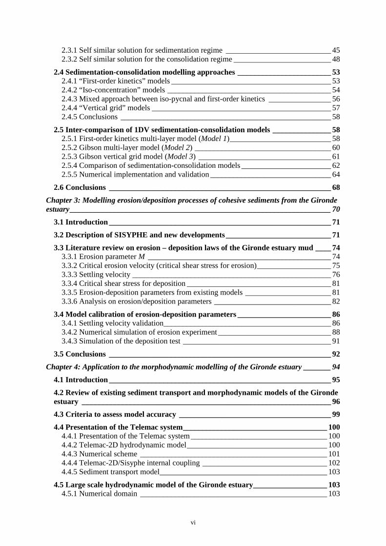
vi
2.3.1 Self similar solution for sedimentation regime ___________________________ 45
2.3.2 Self similar solution for the consolidation regime _________________________ 48
2.4 Sedimentation-consolidation modelling approaches ________________________ 53
2.4.1 “First-order kinetics” models _________________________________________ 53
2.4.2 “Iso-concentration” models __________________________________________ 54
2.4.3 Mixed approach between iso-pycnal and first-order kinetics ________________ 56
2.4.4 “Vertical grid” models ______________________________________________ 57
2.4.5 Conclusions ______________________________________________________ 58
2.5 Inter-comparison of 1DV sedimentation-consolidation models _______________ 58
2.5.1 First-order kinetics multi-layer model (Model 1) __________________________ 58
2.5.2 Gibson multi-layer model (Model 2) ___________________________________ 60
2.5.3 Gibson vertical grid model (Model 3) __________________________________ 61
2.5.4 Comparison of sedimentation-consolidation models _______________________ 62
2.5.5 Numerical implementation and validation _______________________________ 64
2.6 Conclusions _________________________________________________________ 68
Chapter 3: Modelling erosion/deposition processes of cohesive sediments from the Gironde estuary ___________________________________________________________________ 70
3.1 Introduction _________________________________________________________ 71
3.2 Description of SISYPHE and new developments ___________________________ 71
3.3 Literature review on erosion – deposition laws of the Gironde estuary mud ____ 74 3.3.1 Erosion parameter M _______________________________________________ 74
3.3.2 Critical erosion velocity (critical shear stress for erosion) ___________________ 75
3.3.3 Settling velocity ___________________________________________________ 76
3.3.4 Critical shear stress for deposition _____________________________________ 81
3.3.5 Erosion-deposition parameters from existing models ______________________ 81
3.3.6 Analysis on erosion/deposition parameters ______________________________ 82
3.4 Model calibration of erosion-deposition parameters ________________________ 86
3.4.1 Settling velocity validation___________________________________________ 86
3.4.2 Numerical simulation of erosion experiment _____________________________ 88
3.4.3 Simulation of the deposition test ______________________________________ 91
3.5 Conclusions _________________________________________________________ 92
Chapter 4: Application to the morphodynamic modelling of the Gironde estuary _______ 94
4.1 Introduction _________________________________________________________ 95
4.2 Review of existing sediment transport and morphodynamic models of the Gironde estuary ________________________________________________________________ 96
4.3 Criteria to assess model accuracy _______________________________________ 99
4.4 Presentation of the Telemac system _____________________________________ 100
4.4.1 Presentation of the Telemac system ___________________________________ 100
4.4.2 Telemac-2D hydrodynamic model ____________________________________ 100
4.4.3 Numerical scheme ________________________________________________ 101
4.4.4 Telemac-2D/Sisyphe internal coupling ________________________________ 102
4.4.5 Sediment transport model ___________________________________________ 103
4.5 Large scale hydrodynamic model of the Gironde estuary ___________________ 103
4.5.1 Numerical domain ________________________________________________ 103

vii
4.5.2 Initial and boundary conditions ______________________________________ 104
4.5.3 Physical & numerical parameters _____________________________________ 106
4.5.4 Calibration and validation results of hydrodynamic model _________________ 108
4.6 Cohesive sediment transport model _____________________________________ 109
4.6.1 Multi-layer consolidation algorithm __________________________________ 109
4.6.2 Initial & boundary conditions _______________________________________ 110
4.7 Calibration of erosion/deposition parameters ____________________________ 110
4.8 Initialisation of sediment bed structure _________________________________ 112
4.8.1 Measurement of the bed structure in the Gironde estuary __________________ 113
4.8.2 Bed structure initialisation __________________________________________ 114
4.8.3 Sensitivity analysis on erosion/deposition parameters _____________________ 117
4.8.4 Sensitivity analysis on concentration of topmost layer ____________________ 119
4.8.5 Effect of consolidation _____________________________________________ 119
4.9 Validation on depth-averaged suspended concentration measurements _______ 120
4.10 Morphodynamic modelling __________________________________________ 122
4.10.1 Calibration results on bathymetric evolution 1995-2000 __________________ 122
4.10.2 Validation results on bathymetric evolution 2000-2005 __________________ 127
4.10.3 Conclusions ____________________________________________________ 129
4.11 Discussion and conclusions ___________________________________________ 129
4.11.1 Main results ____________________________________________________ 129
4.11.2 Limitation of the present 2D morphodynamic model ____________________ 129
4.11.3 Future works ____________________________________________________ 130
Chapter 5: Hindered settling of sand/mud flocs mixtures: from model formulation to numerical validation _______________________________________________________ 133
5.1 Introduction ________________________________________________________ 137
5.2 Hindered settling theory for mixed sediment _____________________________ 139
5.2.1 Governing equations ______________________________________________ 139
5.2.2 Terminal velocity for mud flocs and sand particles _______________________ 139
5.2.3 Existing closure equations for cohesive and non-cohesive mixtures __________ 140
5.2.4 Modified MLB model for cohesive-non cohesive mixtures ________________ 141
5.2.5 Instability analysis ________________________________________________ 142
5.3 Numerical model ____________________________________________________ 144
5.3.1 Space-time finite volume ___________________________________________ 144
5.3.2 WENO4-DG numerical model _______________________________________ 145
5.3.3 Numerical validation on bi-disperse granular suspension __________________ 146
5.4 Simulation results on different sand-mud mixtures ________________________ 148
5.4.1 ‘Sand rich’ and ‘Mud rich’ test cases __________________________________ 149
5.4.2 Sand-kaolin mixture _______________________________________________ 151
5.5 Conclusions ________________________________________________________ 154
5.6 Acknowledgments ___________________________________________________ 155
General conclusions _______________________________________________________ 157
List of figures ____________________________________________________________ 162
References _______________________________________________________________ 165

viii
Appendices ______________________________________________________________ 172

ix
Introduction
Sediment in natural environments Sediment beds in estuaries and tidal basins often consist of both sand (non-cohesive)
and mud (cohesive). Cohesive and non-cohesive sediments are different from each other in two major properties: flocculation and consolidation of deposited material (with compaction of sediments).
One of the most characteristic properties of cohesive sediment is to form flocs: when individual fine sediment particles are transported in the water column, they undergo attractive forces (Van der Waals, electrochemical force…). Almost all cohesive sediment found in marine environment is flocculated. Floc formation affects the settling velocity and bed structure. Furthermore, the properties of flocs differ strongly from those of individual solid particles. This is due to the large water content of the flocs which tends to create a more open structure with densities only slightly higher than the density of the fluid (Winterwerp & Van Kesteren, 2004).
For concentrations larger than (1-10 g.l-1), flocs start to interact with each other during settling (Winterwerp and Van Kesteren, 2004). The interaction of floc particles can reduce the settling behaviour. This effect is called hindered settling. When sedimentation continues, more and more mud flocs accumulate on the bed. Pore water is driven out of flocs and out of the interstitial space between flocs, and sediment starts to be compacted. This process is known as self-weight consolidation, which results in large deformation of the vertical bed structure. During the hindered settling phase, flocs are supported by the upward fluid flow, while during the consolidation phase, flocs are supported primarily by particle interactions.
In the water column, fine sediments are transported in suspension by the mean and turbulent flow velocity. They follow therefore a classical advection and dispersion scheme, with an additional vertical advection velocity due to particle settling, modulated by flocculation and de-flocculation processes. In addition to their cohesive properties, fine sediments are often distinguished by their primary mode of transport, since they may remain in suspension for long periods of time.
The need for morphodynamic modelling Morphodynamic models are widely used in order to gain insight into the medium- and
long-term morphodynamic changes of a river, estuarine or coastal system.
However, morphodynamic modelling is challenging. Firstly, it is very difficult to account for all the natural variability of sediments and diversity of processes in numerical models. This is particularly crucial for estuarine applications characterised by the presence of mixed cohesive and non-cohesive sediments.
One particular difficulty is that the physical processes that drive morphological changes occur on much shorter time-scales than the morphological changes themselves. In other words, the bed form evolution is mostly altered during historical events (i.e. storm or flood), where the hydrodynamic forcing data is unavailable.
In reality, a morphodynamic model can never completely describe the complex sediment transport processes of natural systems and relies on simplifying assumptions regarding the hydrodynamic forcing terms as well as the nature of sediment, considered either
x
as purely cohesive or non-cohesive. In addition, the accuracy of morphodynamic models usually suffers from uncertainty in the definition of initial condition and of a numerous set of hydrodynamic and sediment parameters.
Site of interest The Gironde estuary is one of the largest estuaries in Europe, which is located south-
west of France. The watershed has a surface of 71.000 km². As one of the last European examples of a more or less undisturbed large estuary, the scientific study of the Gironde estuary is of particular importance and interest.
The Gironde macro-tidal estuary is characterised by strong tidal forcing, complex geo-morphology, high turbidity and heterogeneous sediment distribution (Allen, 1972, Castaing, 1981). This estuary has been studied for many years for numerous applications. In particular, in the central part, drastic bed evolutions have been reported as a result of sand bank formation and secondary mid-channel deposit despite activity of dredging management for the navigation channel and at the harbour of Bordeaux (second harbour in France).
Objectives The research objectives of this thesis are, first, to enhance our understanding of the
physical processes occurring in the cohesive sediment bed, and then, to develop a new process based 2D (depth-averaged) large scale morphodynamic model for cohesive sediments. This model will be applied to predict accurately the sediment dynamics and medium term bed evolution in the Gironde estuary.
Our framework is the Telemac hydro-informatic finite element system (release 6.1), where the two dimensional approach has been selected as a good compromise between CPU time and model accuracy.
Morphodynamic evolution is simulated by internal coupling of TELEMAC-2D for hydrodynamics and 2D morphodynamic model SISYPHE, (www.opentelemac.org, Villaret et al., 2011).
TELEMAC-2D
TELEMAC-2D is a program for the solution of the two dimensional Saint-Venant equations (Hervouet, 2007). The water depth and the velocity averaged on the vertical are the main variables, but the transport of a passive tracer as well as turbulence can be taken into consideration.
All modules of the Telemac system are based on unstructured grids and finite-element or finite volume algorithms. The method of characteristics, kinetic schemes and others can be applied to calculate the convective terms in the momentum equation. The use of implicit schemes enables relaxation of the CFL limitation on time steps (typically, values of CFL number up to 10 or 50 are acceptable).
The treatment of uncovered beds and dry zones are classically treated by limiting the value of the water depth to a threshold. However, this method induces disadvantages related to the conservation of mass and momentum. In TELEMAC, two novel methods are proposed. The first option treats the free surface gradient in an uncovered area as the bottom gradient

xi
and creates parasitic driving terms. The second solution consists of removing all elements which are not entirely wet from the calculation.
From release 6.1, TELEMAC can be run in parallel. This optimisation allows users to use simultaneously a cluster of computers, or a cluster of processors in the same computer, to solve a single problem. The domain decomposition is applied. This means that a part of the domain is assigned to each processor. The results of the other processors would help in determining artificial boundary conditions arising from the partition.
SISYPHE
SISYPHE is a process-based model: sediment transport rates, decomposed into bed-load and suspended load, are calculated as a function of the time-varying flow field and sediment properties at each node of the triangular grid (Sisyphe release v6p1, Villaret, 2010). The resulting bed evolution is determined by solving the Exner equation using either finite elements or finite volumes techniques.
Different processes can be accounted for, including the effect of combined waves and currents, non equilibrium flow conditions, the presence of rigid beds, tidal flats, cohesive and non-cohesive sediment properties.
SISYPHE can be either chained or internally coupled to the hydrodynamic models (TELEMAC-2D, -3D) or to the wave propagation model (TOMAWAC). It can be applied to diverse flow conditions including rivers, coastal and estuarine environments. An optimization of numerical schemes and use of parallel processors allow us to calculate the medium to long-term bed evolution of the order of decades, in basin scale models (10-100 km).
In previous attempts to model the bed evolution, only the non-cohesive behaviour was considered (Chini & Villaret, 2007, Villaret et al., 2009, Huybrechts et al., 2012b). This is the first time a 2DH morphodynamic model of cohesive sediment is built for the Gironde estuary.
The study focuses on the sedimentation-consolidation processes as well as erosion-deposition processes. Flocculation which governs the vertical repartition of sediments in the water column, is not considered in the present 2D approach. This process can be taken into account in a 3D model. However, the effect of flocculation is accounted for in the settling velocity which is an order of magnitude greater than the individual particle settling velocity and will be used as a calibration parameter. The effect of sedimentation-consolidation is taken into account by integrating existing 1DV Gibson-based sedimentation-consolidation models in the 2DH sediment transport model. The erosion-deposition behaviour of the Gironde mud is calibrated. A 2DH process-based cohesive sediment transport model is developed to predict the medium-term bed evolution in the Gironde estuary.
Moreover, with an attempt to account for the variability of natural sediments, the study also addresses the hindered settling of sand/mud mixtures.

xii
Applied approaches In sediment transport study, we traditionally distinguish four approaches:
1) In-situ study aims to collect sediment samples and to characterise external forces and factors (hydrodynamic, temperature, pressure, pH, bio-chemical factors…). This method also increases the understanding on the hydrologic and sedimentologic behaviours of the studied site. This study provides essential data for model initialisation, calibration and validation.
2) Laboratory studies, which characterize the sediment transport and deposition processes, allow us to study the rheologic behaviour of sediments. Empirical formulae of settling velocity, erosion and deposition fluxes, sedimentation and consolidation can be developed under well control experimental conditions. Those formulations cannot be applied to a whole range of sediment types and hydrodynamic forcing conditions, but are specific to the selected bed material and depend on the experimental conditions. Furthermore, care should be taken when applying those empirical formulae to simulate in-situ large scale conditions. Indeed the mechanism observed in laboratory under well control conditions in small scale flume and experimental devices may not be representative of the complex estuarine processes.
3) Numerical models are widely used by engineers as operational tools to simulate different scenarios and answer questions in which experimental and in situ studies cannot be applied. Indeed, the numerical modelling can be applied to investigate quantitatively the relative impact of hydrodynamic conditions on the sediment transport. However, laboratory studies are required to determine model parameters (like settling velocity, rheological characterization of the cohesive bed) and empirical laws embedded in the numerical model to determine the erosion/deposition fluxes.
4) Physical modelling can also be considered to investigate the problem with different scenarios. However, compared to numerical modelling, a major disadvantage of this type of study is the constraint on varying problem parameters that may not be easy to alter. Furthermore, physical models are very costly.
Within this study, the first three approaches are combined, in order to build a new morphodynamic modelling tool which accounts for the cohesive sediment behaviour.
Firstly, a sampling campaign is realised by Saint Venant Laboratory focusing on the central part of the Gironde estuary. Secondly, laboratory experiments are performed using bed materials issued from the campaign. The experiments comprise a granulometry analysis, and experiments performed in both settling column (at the Saint Venant Laboratory for Hydraulics) and recirculating flume experiments (at the RTWH laboratory, University of Aachen).
Thirdly, the 2DH morphodynamic model for cohesive sediment is built. The model parameters of the sedimentation - consolidation and the erosion – deposition processes are calibrated based on laboratory experimental results.
A hindered settling model is also developed both in theoretical and numerical aspects and validated by comparison with several sets of experimental data.

xiii
Outline of the thesis Chapter 1 presents a general description of the study area. It identifies available
hydrodynamic and sediment transport data, and focuses on new experimental works which were realised either by the Saint Venant Laboratory for Hydraulics (Université Paris-Est, France) or by the RWTH laboratory (University of Aachen - Germany) using bed materials issued from our new sampling campaign.
Chapter 2 gives the comparison and validation of two new sedimentation-consolidation models together with an existing semi-empirical model using our measured settling column of the Gironde mud. The objective of this chapter is to select the best model that enables the proper simulation of the physical settling process in cohesive sediment transport. These two models are then implemented in the morphodynamic model SISYPHE.
In the two new models, the sedimentation - consolidation modelling are based on the Gibson theory. Closure equations for bed permeability and effective stress are proposed based on a new method of space-time analysis of the measured concentration profiles. More importantly, the time dependence of the consolidation is introduced in the closure equation for effective stress.
Chapter 3 presents the simulation of the erosion – deposition experiments using the TELEMAC system: this modelling exercise allows us to calibrate the erosion and deposition parameters of the Gironde mud in laboratory conditions.
Chapter 4 aims at developing a realistic morphodynamic model which can be applied to predict the bed evolution in the central part of the estuary. The initial condition of the bed structure is studied attentively. This is the first time cohesive sediment is used in morphodynamic modelling of the Gironde estuary. This model together with the non-cohesive model of Villaret et al. (2012) can be considered as a starting point for sediment mixtures modelling of the Gironde estuary.
However, in order to extend our model to sediment mixtures, we need to consider specific process within sand-mud sediment mixtures. One key process is the segregation/trapping effect of sand inside mud suspension. The layering of bed samples issued from the measurement campaign has shown the evidence of this segregation process.
In chapter 5, a 1DV model for the hindered settling of sand-mud mixtures will be developed based on the background of non-cohesive bi-disperse models (in particular, Masliyah Lockett Bassoon model). The numerical solution has been constructed by considering a high order of accuracy in space via a Weighted Essentially Non Oscillatory (WENO) reconstruction technique and in time via a local space-time Discontinuous Galerkin (DG) which considers no time splitting. The model is then validated against a large range of experimental data (mono-disperse sand, mud, non-cohesive bi-disperse and non-cohesive-cohesive mixture).
In conclusion, we draw the lines for future work and for a fully mixed sediment transport and morphodynamic model of the Gironde estuary. The limitation of the present model will be discussed in order to increase the efficiency of the model. Besides, the hindered settling model is also expected to be generalised to both sedimentation-consolidation process of sand/mud mixtures. The integration of such a model in the sediment transport model SISYPHE could be a potential progress in mixed sediment transport modelling.

xiv
Intentionally left blank

Laboratoire d’Hyraulique Saint – Venant, Université Paris-Est
(Unité de Recherche commune entre EDF R&D, le CETMEF, et l’Ecole des Ponts Paris-Tech)
Chapter 1: Description of study site
& experimental works Contents ___________________________________________________________________________
1.1 Introduction __________________________________________________________ 2
1.2 The Gironde estuary ___________________________________________________ 2
1.3 Available data on the Gironde estuary ____________________________________ 9
1.4 New field campaign ___________________________________________________ 20
1.5 Settling column experiment ____________________________________________ 24
1.6 Settling test in Owen tubes _____________________________________________ 28
1.7 Annular flume experiments ____________________________________________ 29
1.8 Conclusions _________________________________________________________ 30
___________________________________________________________________________

Chapter 1. Description of study site and experimental works
2
1.1 Introduction Chapter 1 presents a general description of the study area and identifies the available
hydrodynamic and sediment transport data. It focuses on new experimental works which were performed using mud samples collected in the center part of the Gironde estuary.
Section 1.2 gives a description of both hydrological and morphological context of the Gironde estuary. In this section, physical characteristics of the estuary and major problems encountered in morphological model developments are briefly discussed. This allows to justify the required assumptions that will be made in chapter 4 for our numerical model.
Section 1.3 presents all available hydrodynamic and sediment data of the Gironde estuary, which will be used in chapter 4 for model calibration and validation purposes.
A new field campaign was carried out in February 2009. The objective of this sampling campaign was to collect sediment samples for the investigation of granulometry, sedimentation-consolidation processes, erosion and deposition processes.
Section 1.4 presents the field campaign associated with the granulometry and sediment core results. Section 1.5 gives the vertical concentration profiles obtained from a settling column. This result will be used in chapter 2 to calibrate and compare three consolidation models which will be integrated in the 2D depth-integrated (2DH) morphological model SISYPHE. Section 1.6 presents the erosion and deposition experiments in the annular flume and the settling test in Owen tubes. These experiments will be simulated in chapter 3 in order to illustrate that SISYPHE is able to represent both erosion and deposition processes for the Gironde mud.
1.2 The Gironde estuary The Gironde is the largest estuary in France and Western Europe, where economical
and ecological issues intersect. The Gironde estuary has been the subject of various studies such as hydrodynamics, geology, morphology and biogeochemistry. The mixing between freshwater and seawater induces here many phenomena in hydrological, sedimentary and biological characters. An exhaustive description of both geographical and environmental context of the Gironde estuary is presented in the PhD thesis of Allen (1972) and Castaing (1981). Summarised descriptions can also be found in recent numerical studies on this site (eg. Cancino & Neves, 1999; Sottolichio, 1999; Benaouda, 2008; Phan, 2002; Sottolichio et al., 2011).
1.2.1 Geographical context
The Gironde estuary, located southwest of France, extends over 70 km from the confluence of the Garonne and the Dordogne rivers to its mouth in the Bay of Biscay on the Atlantic coastline (Fig 1.1left). Its width varies from 10.5 km at the mouth to 3 km at its narrowest part at the confluence of the rivers (Bec d’Ambès) (Castaing, 1981).
1.2.2 Anthropological impacts
The estuary is considered to be rather natural but undergoes many human activities. The maritime traffic in the Gironde estuary has grown significantly (1700 commercial vessels per year, according to G.PM.B, 2002) due to the presence of the harbour of Bordeaux, located on the Garonne river, at KP 0 (i.e. KP signifies Kilometre Point: distance from Bordeaux in km).
Dredging is necessary to maintain the water depth in the navigation channel, and in the harbours of Bordeaux and Port Bloc (near Point de Grave, at the mouth). During the period of 1990-2000, the average annual dredging volume amounts approximately 8.4×10⁶ m3 of which
Chapter 1. Description of study site and experimental works
3
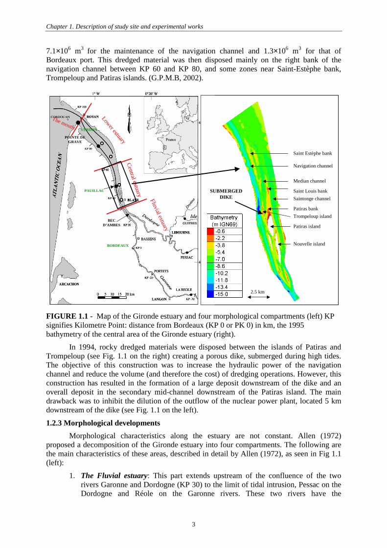
7.1×10⁶ m3 for the maintenance of the navigation channel and 1.3×10⁶ m3 for that of Bordeaux port. This dredged material was then disposed mainly on the right bank of the navigation channel between KP 60 and KP 80, and some zones near Saint-Estèphe bank, Trompeloup and Patiras islands. (G.P.M.B, 2002).
FIGURE 1.1 - Map of the Gironde estuary and four morphological compartments (left) KP signifies Kilometre Point: distance from Bordeaux (KP 0 or PK 0) in km, the 1995 bathymetry of the central area of the Gironde estuary (right).
In 1994, rocky dredged materials were disposed between the islands of Patiras and Trompeloup (see Fig. 1.1 on the right) creating a porous dike, submerged during high tides. The objective of this construction was to increase the hydraulic power of the navigation channel and reduce the volume (and therefore the cost) of dredging operations. However, this construction has resulted in the formation of a large deposit downstream of the dike and an overall deposit in the secondary mid-channel downstream of the Patiras island. The main drawback was to inhibit the dilution of the outflow of the nuclear power plant, located 5 km downstream of the dike (see Fig. 1.1 on the left).
1.2.3 Morphological developments
Morphological characteristics along the estuary are not constant. Allen (1972) proposed a decomposition of the Gironde estuary into four compartments. The following are the main characteristics of these areas, described in detail by Allen (1972), as seen in Fig 1.1 (left):
1. The Fluvial estuary: This part extends upstream of the confluence of the two rivers Garonne and Dordogne (KP 30) to the limit of tidal intrusion, Pessac on the Dordogne and Réole on the Garonne rivers. These two rivers have the
Lower estuary
Fluvial estuary
The mouth
POINTE DE GRAVE
BEC D’AMBES
Central estuaryPAUILLAC
Saint Estèphe bank
Navigation channel
Median channel
Saintonge channel
Saint Louis bank
Patiras bank
Trompeloup island
Patiras island
Nouvelle island
SUBMERGED DIKE
2.5 km
VERDON
BORDEAUX
Lower estuary
Fluvial estuary
The mouth
POINTE DE GRAVE
BEC D’AMBES
Central estuaryPAUILLAC
Saint Estèphe bank
Navigation channel
Median channel
Saintonge channel
Saint Louis bank
Patiras bank
Trompeloup island
Patiras island
Nouvelle island
SUBMERGED DIKE
2.5 km
Lower estuary
Fluvial estuary
The mouth
POINTE DE GRAVE
BEC D’AMBES
Central estuaryPAUILLAC
Saint Estèphe bank
Navigation channel
Median channel
Saintonge channel
Saint Louis bank
Patiras bank
Trompeloup island
Patiras island
Nouvelle island
SUBMERGED DIKE
2.5 km
VERDON
BORDEAUX

Chapter 1. Description of study site and experimental works
4
morphological features of meandering rivers: having a deep zone and bordered by a concave (erosive) bank and a convex (meandering, sedimentation) bank. Another characteristic of this part of estuary is that there is a single channel, islands and bifurcations are rare.
2. The Lower estuary extends 40 km from KP 60 to the mouth of the estuary (KP 100). The morphology of this area is simple compared to other compartments. Two channels (the navigation channel and the Saintonge channel) are well separated. The navigation channel runs along the left shore of the estuary in the upstream part, before deviating to the right bank, approaching the mouth (Fig 1.1 left). This deviation of the navigation channel is accompanied by a deepening of the depth from 15 m to a depth of 30 to 35 m. The two sections of the navigation channel merge near Royan (near the mouth, KP 95). One important point in the morphology of this area is the high elevation of banks of the estuary. On the right bank, formed by cliffs, intertidal zones extend over a width of 1 km and above 2 km on the left bank at KP 83.
3. The mouth, meanwhile, is subject to the interaction of waves and tidal currents. It consists of two channels separated by the presence of the central reef flat Cordouan.
4. The central estuary (Fig 1.1 right) is characterised by a complex geometry. Between KP 30 and KP 70, the bottom of the estuary is characterised by a complex network of channels defining longitudinal banks sometimes constantly immersed, thus giving rise to an island. There are three main channels:
- The navigation channel (left bank)
- The median channel
- The channel of Saintonge (right bank)
The depth of the navigation channel is maintained by dredging at an averaged depth of –12 m IGN69 (IGN69: mean sea level of France, determined by the tide gauge at Marseille).
The Saintonge channel and the median channel have an averaged depth of –8 m IGN69. Upstream of the Saintonge channel, there are different longitudinal banks and islands such as Nouvelle island, Bouchard bank… Downstream of KP 60, after the Patiras bank, the Saintonge channel widens to occupy the median channel.
The median channel extends from KP 49 to KP 60. It is separated from the navigation channel by the Trompeloup bank and the Saint-Estèphe bank, while both the Patiras and Saint Louis banks separate it from the Saintonge channel.
1.2.4 Hydrodynamic context
1.2.4.1 Propagation of tide
The Gironde estuary is classified as macro-tidal, hyper-synchronous and with an asymmetric tide (4 h for flood versus 8 h 25 for ebb).
According to Le Floch (1961), estuaries of hyper-synchronous type are characterised by an increase in tidal range and velocity of tidal currents from downstream to upstream.

Chapter 1. Description of study site and experimental works
5
Apparently, for a spring tide (coefficient1 110), the tidal range is 5 m at the mouth (Pointe de Grave), reaches 5.5 m at Pauillac (48 km from the mouth) and almost 6 m at Bordeaux (95 km from the mouth) (Fig. 1.2).
During mean tide and neap tide, the tidal range increases regularly from Verdon to 130 km upstream of the mouth where it reaches 4.7 m (at mean tide) and 4 m (at neap tide) (G.P.M.B, 2002). In the Dordogne, in contrast, the tidal range decreases slowly until Libourne and then rapidly after Libourne at the confluence between Isle and the Dordogne.
FIGURE 1.2 – Propagation of tidal wave in the Gironde estuary and deformation of tidal shapes (from Allen, 1972)
Moreover, while propagating upstream, tidal waves deform and become asymmetric. This asymmetry results in a longer duration of falling tide than rising tide. For example, in Fig. 1.2, the tide at the mouth (Pointe de Grave) is symmetric and further upstream it becomes asymmetric, in particular at Bordeaux. As a consequence, during the propagation upstream, flood duration decreases while ebb duration increases. Therefore flood currents are stronger and shorter than ebb currents.
In the estuary, according to Manen et al., (1878), Leveque (1936) and Glangeaud (1938) which were cited in Castaing (1981), the tidal limit is normally located at 120 km upstream of the mouth (Pointe de Grave). During low water, this limit can extend to 160 km. 1 Tidal coefficient is a term which is common used in France. It expresses the difference in height between the consecutive high tides and low tides in any given area. The highest possible tidal coefficient is 118. The average tidal coefficient is 70.
TIDE CURVES
Hours Hours
Hours
Met
ers
abo
ve m
ean
sea
leve
l
Me
ters
ab
ove
mea
n se
a le
vel
Met
ers
abo
ve m
ean
sea
leve
l
____ Spring tide
_ _ _ Neap tide
TIDE CURVES
Hours Hours
Hours
Met
ers
abo
ve m
ean
sea
leve
l
Me
ters
ab
ove
mea
n se
a le
vel
Met
ers
abo
ve m
ean
sea
leve
l
____ Spring tide
_ _ _ Neap tide

Chapter 1. Description of study site and experimental works
6
The tidal prism is defined as the volume of ocean water coming into an estuary on a flood tide plus the volume of river discharge mixing with that ocean water. This volume varies according to the coefficients of tide, river flows, and decreases upstream. According to Bonnefille et al. (1971), the sea water volume entering Bordeaux is only 5.2×10⁷ m3 at spring tide. At the mouth, for an average discharge, this volume is between 2×10⁹ m3 at spring tide and 1.1×10⁹ m3 at neap tide.
1.2.4.2 Tidal current
In the lower estuary (from KP 60 to the mouth KP 100), the mean velocity is higher at ebb tide than at neap and spring tides. Similarly, the velocities are larger in the channel of Saintonge than in the other two channels, this is particularly noticeable at spring tides. This is accompanied by a dominance of fresh water in the Saintonge channel, while sea water tends to be dominated in the left channel. According to Castaing (1981), during spring tides, the mean velocity can reach 1.25 m.s-1 near the surface, whereas during neap tides, it does not exceed 1 m.s-1. At the bottom, in the former case, it can reach 0.75 m.s-1, while in the latter case it never exceeds 0.5 m.s-1.
1.2.4.3 Residual circulation
FIGURE 1.3 – Residual circulation at the lowest water-level and mean tide (upper) and during flood and mean tide (lower) in the Gironde estuary (from Allen, 1972)
The residual currents are produced by horizontal advection linked to the vertical gradients of density. Those stratification effects reduce the vertical mixing of freshwater with salt water. The residual velocities are affected by the fluvial discharge, as well as by the topography of the estuary.

Chapter 1. Description of study site and experimental works
7
During lowest low water-level and mean tides, the residual circulation near the surface is directed downstream (Fig. 1.3 upper), while near the bottom it is directed upstream from KP 54 until the salt intrusion limit. The highest velocities are located in the navigation channel for the upstream part of the estuary and in the Saintonge channel for the downstream part. In the Gironde estuary, the residual velocity can reach 10, 15 cm.s-1 to 50 cm.s-1 near the bottom and more than 40 cm.s-1 on the surface (Allen, 1972).
In period of heavy flow and during mean tides, flows are dominant downstream both on the surface and near the bottom, except in the channels where the velocities at the bottom always orient upstream.
1.2.5 Fluvial hydrology
Flows in the estuary are also influenced by river discharges. The sum of river discharges of the two main tributaries of the Gironde (Garonne and Dordogne) can vary from 200 m3.s-1 during low water, to 5000 m3.s-1 during flood. The total annual average discharge is of the order of 1100 m3.s-1 in which 65 % from the Garonne and 35 % from the Dordogne (Sottolichio, 1999). The monthly mean values vary from 1.451 m3.s-1 in January to 235 m3.s-1 in August (Allen, 1972).
1.2.6 Granulometry
In the Gironde estuary, the composition of suspended material has been investigated by many authors. Here the granulometry results of Jouanneau & Latouche (1981) will be brieftly presented, which distinguishes between low flow and flood periods.
During low flow periods
Samples were collected on 23 and 24 October 1978 at twelve stations along the estuary between KP 44 and KP 90 (two days covered a period of neap tides, and flow of the Garonne, at that time, was about 50 m3.s-1). The results showed that:
• The fraction smaller than 16 µm is from 90 to 99 %.
• The fraction smaller than 2 µm (clay) is between 42 and 65 %
During flood periods
Samples were taken between KP 31 and KP 80 on 26 and 27 March 1979. Other samples were also taken at Pointe de Grave on 28th , at KP 25 on 20th , and at KP 20 on 21th of the same month. Samples on 20th and 21st March were realised after the passage of a big flood on 16th and 17th March (1950 and 1800 m3.s-1 for the Garonne). The sampling campaign on March 26th took place during spring tides and the flow of the Garonne was about 600 m3.s1. The sample analysis showed that there are two areas in which particle size is small. The first extends upstream of KP 20 and the second downstream from Saint Estèphe (KP 55). The central area between these two zones are characterised by larger grain sizes.
It is concluded that the muddy facies are predominant in the Gironde estuary. Out of flood periods, it covers ¾ of the estuarine bed. This explains the importance of the suspended transport in the Gironde estuary.
1.2.7 Suspended sediment dynamics
The Gironde estuary is characterised by its high turbidity: the suspended concentration, mainly composed of clays and silts of fluvial origin, can exceed 1 g.l-1 (Castaing, 1981).

Chapter 1. Description of study site and experimental works
8
Nagy (1993) estimated that the average annual discharge of suspended sediments entering the estuary from the rivers is about 2.5×10⁶ tonnes (from Phan, 2002). According to Allen (1971), this value varies from 1.5 to 3×10⁶ tonnes.
FIGURE 1.4 - Position of turbidity maximum as a function of fluvial discharge, based on the measurements between 1975 and 1976, during a neap tide (Allen, 1972)
According to measurements in 1975 and 1976, Castaing (1981) presented the position of turbidity maximum (TM) in the Gironde estuary according to three typical situations of fluvial flow rate (Fig. 1.4). For low flow rates, the turbidity maximum is from KP 10 to KP 60, about 70 km long, the centre is at KP 10, between Bordeaux and Le Bec d’Ambès. During mean flow rates, the turbidity maximum extends from KP 20 to KP 60, about 40 km long, the centre is situated at KP 40. During flood, the turbidity maximum appears in two positions, the first is located near the mouth from KP 80 to KP 100 (20 km long), and the second is identified at KP 30.
Castaing (1981) acknowledged that the existence of turbidity maximum dynamic in the Gironde estuary is due to the effects of tidal asymmetry. In Benadoua (2008), according to Fisher (1972), in partially stratified estuaries, which is the case of the Gironde estuary, the convective currents due to salinity gradients are negligible against those generated by the tide. Some authors refute the idea that only the density circulation is the origin of the formation of TM, and offers a complementary approach. It is to consider that the TM is caused by the asymmetry of the upstream tide. This results in strong currents during flood than ebb tide causing an important erosion and transport of suspended solids upstream. This sediment transport stops at the nodal point of the tide, which represents the dynamic limit of the tide, and beyond which fluvial current is directed downstream.
Migniot (1968) estimated the mass of turbidity maximum between 2.5×10⁶ tonnes and 4×10⁶ tonnes of fine sediments during spring tides. Jouanneau & Latouche (1981) gave a more accurate estimate from the turbidity measurement in water column and in fluid mud:
DOWNSTREAM UPSTREAM
Low flow
Flood
Mean flow
____ Turbidity (g/l)
------ Iso-line of 0.5 ‰
DOWNSTREAM UPSTREAM
Low flow
Flood
Mean flow
____ Turbidity (g/l)
------ Iso-line of 0.5 ‰

Chapter 1. Description of study site and experimental works
9
between 1.7×10⁶ tonnes and 2.3×10⁶ tonnes for the turbidity maximum and between 2.5×10⁶ tonnes to 3×10⁶ tonnes for fluid mud. These estimates were made during neap and mean tides, and during a period when the TM was in the middle of the estuary at mean flow rate.
The occurrence of fluid mud generally coincides with the presence of TM. The fluid mud undergoes a cycle of erosion and deposition related to tidal coefficient. Indeed, during low tides, current velocity decreases, the fluid mud accumulates gradually and reaches its maximum extension at neap tide. Conversely, during high tides, the tidal current velocity increases, the fluid mud is eroded and re-suspended in the TM at spring tide. According to the measurements by echo-sounder between 1983 and 1988 by G.P.M.B, Sottolichio (1999) showed that the fluid mud can exist in the upstream part for tidal coefficients greater than 100. The fluid mud is never observed downstream of Bordeaux for the same coefficients. However, for tidal coefficients below 100, the fluid mud is increased downstream of the estuary. The fluid mud is situated in between KP0 (Bordeaux) and KP 50 (Pauillac) for low river flows (< 1000 m3.s-1) and between KP 45 and KP 80 for high flow rates (>1000 m3.s-1) during flood (Fig. 1.5) (Allen, 1972).
FIGURE 1.5 - Seasonal movement of fluid mud between 1970-1971 (Allen, 1972)
1.3 Available data on the Gironde estuary 1.3.1 Hydrodynamic data Tide and water level
Water levels are measured every 5 minutes by G.P.M.B at 9 gauging stations: Verdon, Richard, Lamena, Pauillac, Fort Medoc, Ambès, Marquis, Bassens and Bordeaux. The measured water levels at 9 tide gauge stations are available for the year 1999. In between 2000 and 2007, water levels at only two stations Verdon and Pauillac are available.
Km
dow
nstr
eam
of B
orde
aux
Mea
nriv
er d
isch
arge
(m3 .
s-1 ) VARIATION OF FLUVIAL DISCHARGES
__________ Line of sounding Lens of fluid mud
Km
dow
nstr
eam
of B
orde
aux
Mea
nriv
er d
isch
arge
(m3 .
s-1 ) VARIATION OF FLUVIAL DISCHARGES
__________ Line of sounding Lens of fluid mud
VARIATION OF FLUVIAL DISCHARGES
__________ Line of sounding Lens of fluid mud

Chapter 1. Description of study site and experimental works
10
Since 2005, measurements of tide level are provided by MArel Gironde ESTuaire – The network of automated observation for monitoring water quality (Magest, www.magest.u-bordeaux1.fr) for the two stations Pauillac and Bordeaux. In 2009, the measurements at Port Bloc (which is located at the same location as Verdon) are operated by Service Hydrographique et Océanographique de la Marine (SHOM, www.shom.fr). The location of these three stations (Verdon, Pauillac, Bordeaux) are marked as green colour in Fig. 1.1.
Velocity measurement
FIGURE 1.6 - Location of three velocity measurement points in campaign 2006 (source: IXSurvey)
Recently, two field measurements were conducted by the Laboratoire National d’Hydraulique et d’Environnement (LNHE) in August 2006 (3 points) and in autumn 2009 (7 points).
In August 2006, velocity measurements, over a period of 22 days from 03/08/2006 to 24/08/2006, were performed using ADCP current profilers, at three points to investigate the spatial distribution of flow. These sensors were placed on the bottom of the three channels in the central part of the Gironde (Fig. 1.6).
2 1 3
NAVIGATION CHANNEL
MEDIAN CHANNEL
PATIRAS BANK SAINTONGE CHANNEL
POINT 1
FREE SURFACE
2 1 3
NAVIGATION CHANNEL
MEDIAN CHANNEL
PATIRAS BANK SAINTONGE CHANNEL
POINT 1
FREE SURFACE

Chapter 1. Description of study site and experimental works
11
FIGURE 1.7 – Velocity measurements at Point 1 in 2006 (Blue line: velocity amplitude in cm.s-1, Red line: Tidal coefficient; Brown points: Current direction in °, source: IXSurvey)
From measurements, the results (point 1 in Fig. 1.7, for point 2 and point 3, refer to IXSurvey, 2006) show that:
• Point 1 (Median channel) presents the smallest velocities. It can reach 160 cm.s-1 on the surface and 80 cm.s-1 at the bottom during high tidal coefficients. Maximum velocities are observed during periods of falling tide.
• Point 2 (Navigation channel): presents higher velocities than point 1. The maximum velocity is 180 cm.s-1 at 1m from the bottom and 260 cm.s-1 at the surface.
Vel
ocity
(cm
/s)
Vel
ocity
(cm
/s)
Ve
loci
ty (
cm/s
)D
irection (°)
Dire
ction (°)D
irection (°)
Velocity amplitude and direction at 2.8 m from the bottom
Velocity amplitude and direction on the surface
Velocity amplitude and direction at 1m from the bottom V
eloc
ity (
cm/s
)V
eloc
ity (
cm/s
)V
elo
city
(cm
/s)
Direction
(°)D
irection (°)
Direction
(°)
Velocity amplitude and direction at 2.8 m from the bottom
Velocity amplitude and direction on the surface
Velocity amplitude and direction at 1m from the bottom V
eloc
ity (
cm/s
)V
eloc
ity (
cm/s
)V
elo
city
(cm
/s)
Direction
(°)D
irection (°)
Direction
(°)
Velocity amplitude and direction at 2.8 m from the bottom
Velocity amplitude and direction on the surface
Velocity amplitude and direction at 1m from the bottom

Chapter 1. Description of study site and experimental works
12
• Point 3 (Saintonge channel): provides velocities greater than those of point 1, but lower than point 2. Maximum velocities are observed during rising tide periods. The average velocity is small (less than 10 cm.s-1).
FIGURE 1.8 - Location of 7 measurement points during the campaign of 2009 (left) and the measuring principle (source: IXSurvey, www.ixsurvey.com)
The measurement points of the 2009 campaign are shown in Fig. 1.8. Among seven measurement points by ADCP, two velocity profilers (Point 2 & point 6) have been lost during the campaign. Points 3 and 5 were located close to the water intake of the nuclear power plant, which is likely to introduce local disturbance to the flow. Points 1, 6 and 7 are located in areas where recent bathymetry is not available, and cannot be updated. Therefore, within this study, only the velocity measurements at point 4 are used to calibrate and validate the hydrodynamic model.
Water levels are also available from ADCP measurements, but are not correct. Indeed, the measured water level at Point 1 in campaign 2009 was compared to water gauge measurements at Port Bloc (these two points are close to each other) and is illustrated in Fig. 1.9. An offset of 25 cm is observed between the measured water level of IX-Survey and of tide gauge. According to Huybrechts et al. (2010) the observed difference can come from the wrong position of the device, or bathymetry changes. It is also possible that the ADCP technique induces some measurement errors. Indeed, the ADCP was moored on the bed and can only measure the center part of the water column. Two blanking areas are observed (Fig. 1.8 right): one near the bottom and the other at the surface. This is where the measurement is not valid, due to the lost of signal (IX-Survey). Therefore, within this study, the measured water level of IX-Survey will not be used to calibrate the hydrodynamic model.
Blanking distanceBlanking distanceBlanking distance

Chapter 1. Description of study site and experimental works
13
FIGURE 1.9 – Comparison between measured water level given by IX-Survey and those from tide gauge at Port Bloc on 25 September 2009 (blue: IX Survey; green: Tide gauge)
1.3.2 Bathymetric evolution
1.3.2.1 Bathymetry data
In general, the Gironde estuary can be divided into four areas corresponding to different sources of bathymetry data:
• Marine area
• Estuarine part
• Garonne river
• Dordogne river
The complete bathymetry is therefore a patchwork of data provided by various sources, from different periods and using different techniques (multi-beam and single-beam). Single beam echo-sounders use one emitting or receiving transducer, which releases a series of energy pulses in the form of sound waves to a small area underneath the boat. The time lag between the sound being emitted and its returning echo is used to calculate water depth beneath the boat. Multi-beam (Swathe) can transmit a broad acoustic pulse from a specially designed transducer across the full swathe acrosstrack then forming a receive beam (source: www.wikipedia.org). As technology has improved, multi-beam can now produce higher frequency suitable for higher resolution mapping.
First, bathymetric surveys of the Gironde estuary were conducted by the Grand Port Maritime de Bordeaux (G.P.M.B) between 1981 and 2005 using a single beam echo-sounder.
For the estuarine part, records prior to 2002 were digitised from SHOM maps (scale 1:50000) provided by G.P.M.B. Recent bathymetric data of 2002 and 2005 (scale 1:10000) of the central part of the Gironde estuary are provided by G.P.M.B. 2005 data from G.P.M.B (single beam) were integrated and complemented by measurements carried out by Division Technique Générale (DTG) of Electricité de France (EDF) using the denser multi-beam in the
Time (days, t = 0: 25 September 0h TU)
z (m
)
Time (days, t = 0: 25 September 0h TU)
z (m
)
Time (days, t = 0: 25 September 0h TU)
z (m
)
Time (days, t = 0: 25 September 0h TU)
z (m
)

Chapter 1. Description of study site and experimental works
14
area close to the nuclear power plant and the dike between the Patiras and Trompeloup islands (see Fig. 1.1).
For the maritime part and in both the Dordogne and Garonne rivers, the bathymetric data were provided respectively by SHOM and by the Direction Départementale de l’Equipement (DDE, www.reunion.developpement-durable.gouv.fr). These data are available until 1995. The bathymetry for the maritime part of 2009 and the data of the Garonne river of 2002 are also available. However, these two data will not be used in the bathymetry compilation to avoid a bathymetry consisted of several parts measured on different period of time.
Bed evolutions between 1981 and 1994 are marked by the progressive erosion of the Trompeloup bank, as well as the relative stability of the navigation channel (Villaret & Walther, 2008).
To quantify the recent developments after the construction of the dike, we use in this study bathymetric measurements from 1995 to 2005. The 1995 bathymetry is chosen as a reference bathymetry. For model comparison and initialization, the bathymetry is only updated in the estuarine part (from KP 30 to KP 60), while in the maritime and river parts, the bathymetry is considered constant as in 1995.
1.3.2.2 Bathymetry compilation
The bathymetric data exists in forms of papers (for the year 1995) and digitalised map (for the rest). From the raw bathymetric data, a process is systematically applied for 3 years: 1995, 2000, 2005 to interpolate the bathymetry on the geometry input file.
The preliminary step is only applied to the 1995 data set. Since the 1995 estuarine part bathymetry is only available in form of papers (four papers), all the maps are digitalised manually in order to convert the data to the digitalised form.
Second, the data of the maritime part and the two rivers are compiled with the estuarine part. The bathymetry data along the dike is also integrated in the bathymetry.
Third, levels are converted from zero-maritime to IGN69 taking into account the shift variation along the estuary.
This integrated data is then interpolated based on the grid. In order to accurately interpolate near the islands, the interpolation is not activated if the distance between two bathymetry data points greater than 150 m.
After interpolation stage, since the TELEMAC – 2D version 6.1 enables the treatment of tidal flat and dry zones, it is then not necessary to raise the border elevation to a fixed higher value of 2 m. This value was selected based on the tide characteristics of the Gironde estuary in order to ensure that this area is never suffered from inundation.
The compilation result is the bathymetry of the Gironde estuary extending from Portet (on the Garonne) and Libourne (on the Dordogne) at KP –20 until about 20 km outside the maritime area from the mouth of the estuary, as observed in Fig. 1.10.

Chapter 1. Description of study site and experimental works
15
FIGURE 1.10 – 1995 bathymetry of the Gironde estuary
1.3.2.3 Bathymetric evolution This section presents the evolution of bathymetry from 1995 until 2005 concentrated
on the central part of the estuary - our area of interest. Figure 1.11 shows the measured bathymetries between 1995 and 2005 in the central
part of the Gironde estuary. On these maps, three iso-lines are plotted (-1 m IGN69, -2 m IGN69, -5 m IGN69). Figure 1.12 shows the bathymetry differences produced between 2000 and 1995 and between 2005 and 2000. The –2 m IGN69 iso-contour is also presented on these maps.
It is observed from figures 1.11 and 1.12:
• The development of the Patiras bank downstream
• The erosion of the Trompeloup and Saint Louis banks
• The progressive deposition in the median channel
2 km2 km2 km

Chapter 1. Description of study site and experimental works
16
FIGURE 1.11 - Measured bathymetry in the central part of the Gironde estuary
a) 1995; b) 2000; c) 2002; d) 2005 + Iso-lines – 5 m, - 2 m, -1 m IGN69
The deposition of the Patiras bank started in 1995 after the construction of the dike between the Trompeloup and Patiras islands. In Fig. 1.12a, it can be observed through a 1 m deposition layer downstream of Patiras island. The position of the -2m iso-contour also moved downstream between 1995-2000. According to Chini & Villaret (2007), the deposition rate of the Patiras bank was at a speed of 360m/year during this period.
A widening of the Patiras bank is also observed, in particular to the left side of the bank. The deposition rate along the bank is approximately 22 cm/ year. In the next period, between 2005 and 2000, we observe a more stabilised development. Average deposition rate is less than 2 cm/year (Chini & Villaret, 2007).
It is observed that the downstream part of the median channel (next to the Saint Estèphe bank) has filled up between 1995 and 2000 (Fig. 1.12a), with a rate of about 20 cm/year. Between 2000 and 2005, deposits are widespread throughout the channel. These
Chapter 1. Description of study site and experimental works
17
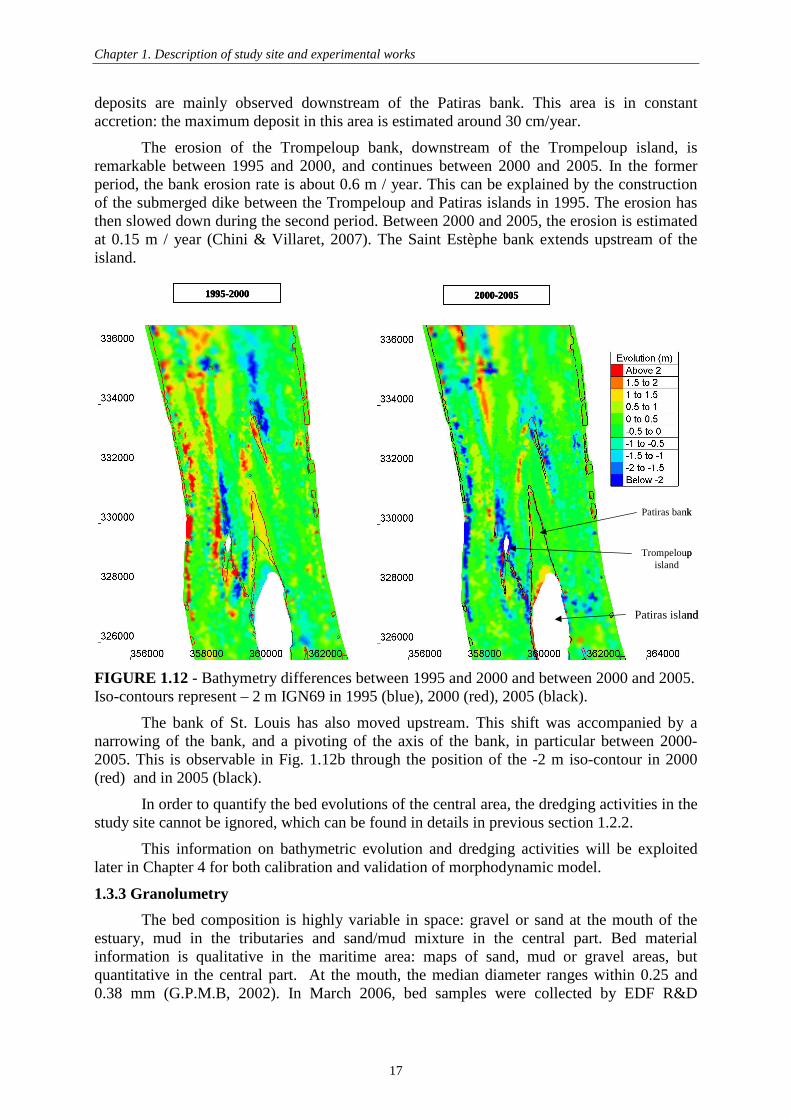
deposits are mainly observed downstream of the Patiras bank. This area is in constant accretion: the maximum deposit in this area is estimated around 30 cm/year.
The erosion of the Trompeloup bank, downstream of the Trompeloup island, is remarkable between 1995 and 2000, and continues between 2000 and 2005. In the former period, the bank erosion rate is about 0.6 m / year. This can be explained by the construction of the submerged dike between the Trompeloup and Patiras islands in 1995. The erosion has then slowed down during the second period. Between 2000 and 2005, the erosion is estimated at 0.15 m / year (Chini & Villaret, 2007). The Saint Estèphe bank extends upstream of the island.
FIGURE 1.12 - Bathymetry differences between 1995 and 2000 and between 2000 and 2005. Iso-contours represent – 2 m IGN69 in 1995 (blue), 2000 (red), 2005 (black).
The bank of St. Louis has also moved upstream. This shift was accompanied by a narrowing of the bank, and a pivoting of the axis of the bank, in particular between 2000-2005. This is observable in Fig. 1.12b through the position of the -2 m iso-contour in 2000 (red) and in 2005 (black).
In order to quantify the bed evolutions of the central area, the dredging activities in the study site cannot be ignored, which can be found in details in previous section 1.2.2.
This information on bathymetric evolution and dredging activities will be exploited later in Chapter 4 for both calibration and validation of morphodynamic model.
1.3.3 Granolumetry
The bed composition is highly variable in space: gravel or sand at the mouth of the estuary, mud in the tributaries and sand/mud mixture in the central part. Bed material information is qualitative in the maritime area: maps of sand, mud or gravel areas, but quantitative in the central part. At the mouth, the median diameter ranges within 0.25 and 0.38 mm (G.P.M.B, 2002). In March 2006, bed samples were collected by EDF R&D
1995-2000 2000-2005
Patiras island
Trompeloup island
Patiras bank
1995-2000 2000-20051995-2000 2000-2005
Patiras island
Trompeloup island
Patiras bank

Chapter 1. Description of study site and experimental works
18
downstream of the Patiras island. The location of the measuring points can be observed in Fig. 1.13.
FIGURE 1.13 – Location of sediment sampling points in the March 2006 campaign
TABLE 1.2 - Granulometry analysis of sampled sediments in the March 2006 campaign
Name of point Cohesive fraction Non-cohesive
fraction Diameter of sand
fraction (µm)
Upstream of Saint Estèphe bank 89.6% 10.3% 116
Upstream of Patiras bank 88.0% 11.9% 116
Upstream of median channel 77.4% 22.5% 185
Downstream of Saint Louis bank 58.1% 41.6% 331
Downstream of Patiras bank 25.2% 74.8% 240
Point E 4.2% 95.8% 271
Upstream of Trompeloup bank 0.1% 99.9% 390
Mean value 55% 45% 210
Table 1.2 summarizes the results of observation. The distinction between cohesive sediment (mud) and non-cohesive (sand) is revealed in the grain diameter. The mean diameter of the sand fraction in the area of interest is 0.210 mm
BATHYMETRY
DOWNSTREAM OFSAINT LOUIS BANK
UPSTREAM OFSAINT ESTEPHE BANK
DOWNSTREAM OF PATIRAS BANK
POINT E
UPSTREAM OF PATIRAS BANK
UPSTREAM OF MEDIAN CHANNEL
UPSTREAM OF TROMPELOUP ISLAND
BATHYMETRY
DOWNSTREAM OFSAINT LOUIS BANK
UPSTREAM OFSAINT ESTEPHE BANK
DOWNSTREAM OF PATIRAS BANK
POINT E
UPSTREAM OF PATIRAS BANK
UPSTREAM OF MEDIAN CHANNEL
UPSTREAM OF TROMPELOUP ISLAND

Chapter 1. Description of study site and experimental works
19
The composition of the bed in the median channel consists mainly of a mixture of sand and mud. On the Patiras bank and upstream of the rock dike, sediments are coarse. The intrusion limit of marine sediments in the estuary is at KP 70 (Jouanneau & Latouche, 1981). Above this limit, cohesive or non-cohesive sediments come from river flows. Analysis of these samples reveals that 55 % of the bed material is cohesive and 45 % is non-cohesive, with mean diameter d50 = 0.21 mm.
FIGURE 1.14 - Measurement of the granular distribution at the maritime area, yellow signifies sand, green signifies mud, red is rock, light yellow is fine sand, blue is sandy mud (source: SHOM)
At the mouth of the estuary and in rivers, information on the particle size is mainly available in qualitative form (fig. 1.14): map of areas of sand, sandy-mud or muddy bottoms (Allen 1971). Measurements given by the G.P.M.B (2002) indicate that in 1999, the mean diameter between Bordeaux and Verdon is about 10 to 20 µm. At the mouth, the mean diameter (d50) is between 250 and 380 µm. A qualitative sediment size distribution map at the mouth of the Gironde estuary is provided by SHOM (see Fig. 1.14). As shown on Fig. 1.14, the estuary is dominated by mud (blue colour) and the mouth is dominated by sand (yellow colour). In the southern part of the mouth, the sand is finer than the northern part (light yellow colour).
1.3.4 Depth-averaged suspended concentration
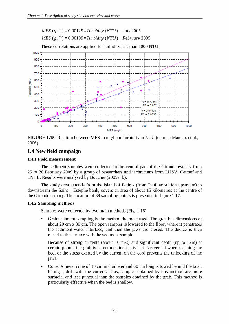
The time variation of the suspended load is measured every 10 min at four stations along the estuary (www.magest.u-bordeaux1.fr). Three stations are located in the tributaries whereas one is located in the estuary itself at Pauillac station. The turbidity is measured in NTU. In order to change the unit from NTU to mg.l-1, we use here the correlation in the 2005 activity report of Maneux et al. (2006) , which were proposed for two measuring campaigns in February 2005 (blue) and July 2005 (pink). Since our data was sampled in March (2006 campaign) and in February (campaign 2009, presented in next section 1.4), the correlation in February 2005 is selected.
Chapter 1. Description of study site and experimental works
20
1
1
( . ) 0.00129 ( ) 2005
( . ) 0.00109 ( ) 2005
MES g l Turbidity NTU July
MES g l Turbidity NTU February
−
−
= ×
= ×
These correlations are applied for turbidity less than 1000 NTU.
FIGURE 1.15- Relation between MES in mg/l and turbidity in NTU (source: Maneux et al., 2006)
1.4 New field campaign
1.4.1 Field measurement
The sediment samples were collected in the central part of the Gironde estuary from 25 to 28 February 2009 by a group of researchers and technicians from LHSV, Cetmef and LNHE. Results were analysed by Boucher (2009a, b).
The study area extends from the island of Patiras (from Pauillac station upstream) to downstream the Saint – Estèphe bank, covers an area of about 15 kilometres at the centre of the Gironde estuary. The location of 39 sampling points is presented in figure 1.17.
1.4.2 Sampling methods
Samples were collected by two main methods (Fig. 1.16):
• Grab sediment sampling is the method the most used. The grab has dimensions of about 20 cm x 30 cm. The open sampler is lowered to the floor, where it penetrates the sediment-water interface, and then the jaws are closed. The device is then raised to the surface with the sediment sample.
Because of strong currents (about 10 m/s) and significant depth (up to 12m) at certain points, the grab is sometimes ineffective. It is reversed when reaching the bed, or the stress exerted by the current on the cord prevents the unlocking of the jaws.
• Cone: A metal cone of 30 cm in diameter and 60 cm long is towed behind the boat, letting it drift with the current. Thus, samples obtained by this method are more surfacial and less punctual than the samples obtained by the grab. This method is particularly effective when the bed is shallow.

Chapter 1. Description of study site and experimental works
21
FIGURE 1.16 -Sampling campaign: a) Cone; b) Sampled sediments in the cone; c) Grab; d) Sediment core sampling
1.4.3 Granulometry
The machine used for granulometry analysis is granulometer LASER Cilas 1180.
Principle
The measuring range lies between 0.04 µm and 2.5 mm.
A small amount of sample is dispersed in a bowl with a mixer and an ultrasonic bath. Its content is drawn then passes through a quartz cell by two crossing laser beams. The photo detectors are placed behind the cell that records the diffraction pattern (Theory of Mie) of an incident laser beam: the finer the particles are, the more diffracted the ray is. To cover the entire range of measurement, two lasers are used: the first ray is perpendicular to the quartz cell, the second laser is at an angle of 45° with the first one. Hence, when the light of the first ray is diffracted outside the area of sensors, the second laser will be used. And there are always diffracted radiations on the detectors.
Because the quartz cell is 2.5 mm thick, it is essential to ensure that no particles could clog the cell, by sieving or filtering.
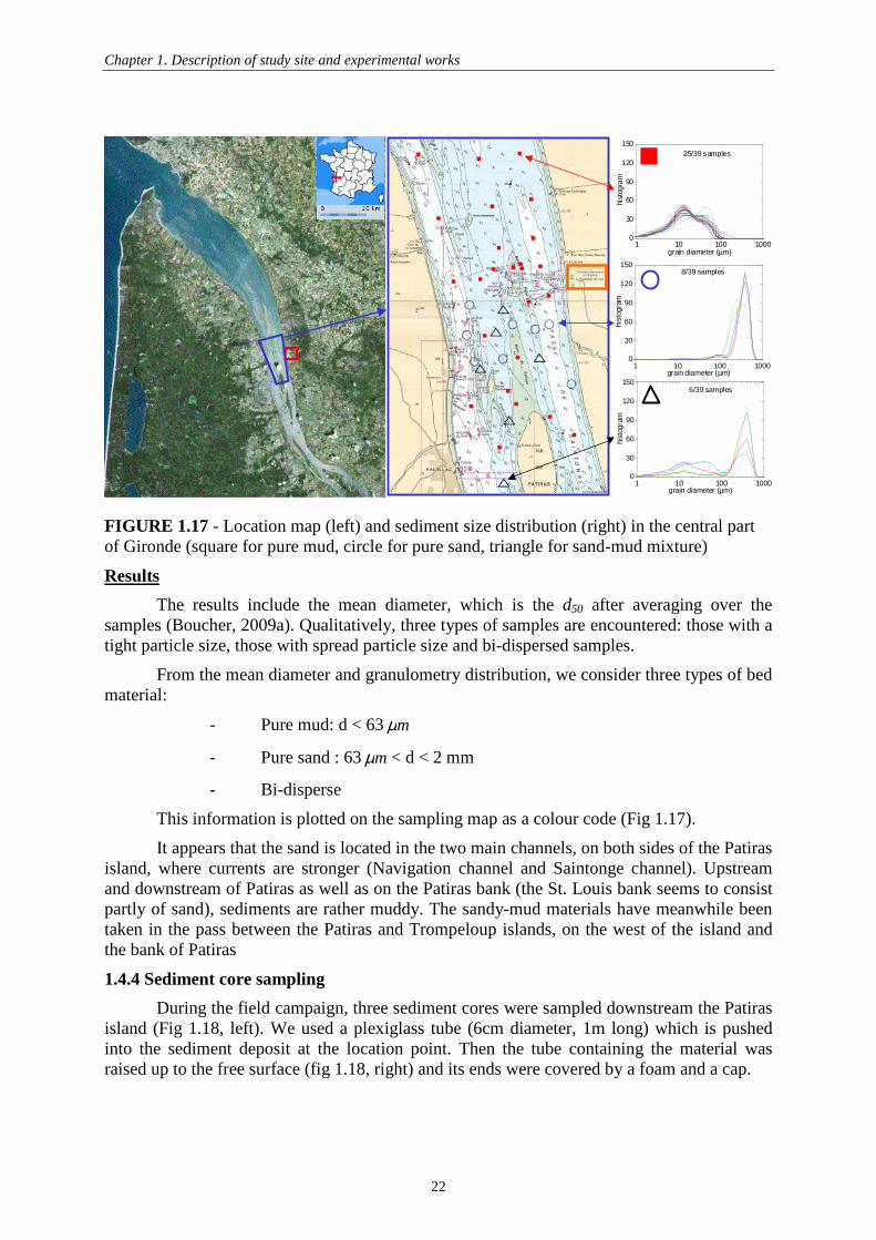
Chapter 1. Description of study site and experimental works
22
FIGURE 1.17 - Location map (left) and sediment size distribution (right) in the central part of Gironde (square for pure mud, circle for pure sand, triangle for sand-mud mixture)
Results
The results include the mean diameter, which is the d50 after averaging over the samples (Boucher, 2009a). Qualitatively, three types of samples are encountered: those with a tight particle size, those with spread particle size and bi-dispersed samples.
From the mean diameter and granulometry distribution, we consider three types of bed material:
- Pure mud: d < 63mµ
- Pure sand : 63mµ < d < 2 mm
- Bi-disperse
This information is plotted on the sampling map as a colour code (Fig 1.17).
It appears that the sand is located in the two main channels, on both sides of the Patiras island, where currents are stronger (Navigation channel and Saintonge channel). Upstream and downstream of Patiras as well as on the Patiras bank (the St. Louis bank seems to consist partly of sand), sediments are rather muddy. The sandy-mud materials have meanwhile been taken in the pass between the Patiras and Trompeloup islands, on the west of the island and the bank of Patiras
1.4.4 Sediment core sampling
During the field campaign, three sediment cores were sampled downstream the Patiras island (Fig 1.18, left). We used a plexiglass tube (6cm diameter, 1m long) which is pushed into the sediment deposit at the location point. Then the tube containing the material was raised up to the free surface (fig 1.18, right) and its ends were covered by a foam and a cap.
1 10 100 10000
30
60
90
120
150
25/39 samples
hist
ogra
m
grain diameter (µm)
1 10 100 10000
30
60
90
120
150
6/39 samples
hist
ogra
m
grain diameter (µm)
1 10 100 10000
30
60
90
120
150
8/39 samples
hist
ogra
m
grain diameter (µm)

Chapter 1. Description of study site and experimental works
23
FIGURE 1.18- Location of sediment core sampling points (left). P2B sediment core (right).
The sediment cores were carefully transported to the Saint Venant Laboratory for Hydraulics (LHSV) for analysis. First, the plastic tubes were cut by electric saw, then the sediment cores were cut in the longitudinal direction by metallic wire. The two resulting half-cylinders were then visually inspected (Figure 1.19). From these first observations, the core P1 is pure mud whilst cores P2 and P2B present thin layers of sand (targeted by red arrows).
FIGURE 1.19 - Visual inspection of sediment cores
We use the three cores to determine concentration of the cohesive bed in the field. We remove 2 cm thick layer at three points (top, middle, bottom) in each core and determine the sediment concentration after drying the material in an oven at 110°C during 24 hours. This method provides sediment concentration equal to 756 ± 100, 765 ± 50, 796 ± 20 g/l, respectively. However, since the analysis is performed only after several months of stacking, it may lead to a noticeable increase of sediment concentration.
The second half-cylinder is also used during the study. The half-core is cut into slices of thickness 10 cm and each one is submitted to laser granulometry. As an example, Table 1.3 presents the results of core P1 which corresponds to a pure cohesive bed. From the results, the core P1 should be considered as homogeneous along the vertical direction. The sediment from core P1 will be used later in the settling column experiment (section 1.5).
SurfaceL=70cm
L=47.5cm
L=51cm
P1
P2
P2B
Bottom SurfaceL=70cm
L=47.5cm
L=51cm
P1
P2
P2B
Bottom L=70cm
L=47.5cm
L=51cm
P1
P2
P2B
Bottom

Chapter 1. Description of study site and experimental works
24
TABLE 1.3 - Granulometry analysis for core P1
The sand fraction which is present in cores P2 and P2B is analysed. The laser granulometer gives a mean diameter equal to 280 µm.
These results are qualitative since the method used to sample bed sediments is very intrusive: the material is certainly disturbed during the sampling. Moreover, despite all the care we paid for the preservation and transport of samples, the top material has been evolved. The vibration during the transport and the maintenance time or condition before testing the material could modify its property in a non-negligible way.
Nevertheless, the segregation of sand-mud is clearly observed for cores P2 and P2B. This is an important phenomenon which is investigated in more details in Chapter 5 of this study.
1.5 Settling column experiment 1.5.1 Experimental device
FIGURE 1.20 - Principle of settling column experiment
Within this study, a settling column instrumented by X-ray techniques is used to obtain vertical concentration profiles at different times. This technique is selected since it has many advantages compared to existing techniques, as shown in Table 1.4 below.
d10 (µm) d50 (µm) d90 (µm) d10 (µm) d50 (µm) d90 (µm) d50/d10 d90/d50P1-1-a 2.5 12.06 40.53 2.57 12.65 41.54 4.92 3.28P1-1-b 2.64 13.24 42.55P1-2-a 2.58 12.08 38.11 2.58 12.03 38.04 4.66 3.16P1-2-b 2.58 11.98 37.97P1-3-a 2.75 14.49 46.14 2.76 14.57 46.26 5.29 3.17P1-3-b 2.76 14.65 46.37P1-4-a 2.82 15.59 49.14 2.86 15.57 49.05 5.44 3.15P1-4-b 2.9 15.54 48.95P1-5-a 2.37 10.86 32.85 2.37 10.89 33.09 4.60 3.04P1-5-b 2.36 10.92 33.33P1-6-a 2.46 12.23 39.37P1-6-b 2.41 12.1 39.15P1-7-a 2.72 14.46 46.21P1-7-b 2.8 14.63 47.32
60-70cm2.76 14.55 46.77 5.27 3.22
50-60cm2.44 12.17 39.26 5.00 3.23
40-50cm
30-40cm
20-30cm
10-20cm
0-10cm
WaterWater
++
MESMESRadioiso topeRadioiso tope
(radiation (radiation γγγγγγγγ et Xet X))
DetectorDetector
CaF2 / NaI(Tl)CaF2 / NaI(Tl)
(S) (D)

Chapter 1. Description of study site and experimental works
25
TABLE 1.4 - Advantages and disadvantages of existing techniques to measure concentration profiles in a settling column
Measuring technique Advantages Disadvantages
Optical Non-intrusive (not disturb the material)
Cannot applied for turbid zones
Acoustic Intrusive (direct contact with material)
Low resolution, depending on the number of sensors
Shear vane tester Simple, cheap
Very instrusive
Structure of sample is destroyed
Magnetic Resonance Imaging (MRI)
High resolution Small samples only
Costly
γ-Ray Non-intrusive, high resolution
Effective, cheap
Dangerous (radio source, high energy, cannot stop the source)
X-Ray Non-intrusive, high resolution
Effective as γ-Ray, cheap
More secure (radio generator, low energy)
The measurement principle is described in figure 1.20 and explained in Been and Sills (1981). An X-ray beam emerging from the source (S) is attenuated by the suspension (water + sediment). The intensity of the beam which is not absorbed or deviated by the suspension is measured by the detector (D). Here we use an X-ray generator and a NaI detector.
To improve the spatial resolution of the device, collimators are used behind the generator and before the detector. The first one allows to obtain a homogeneous beam at the entrance of the suspension recipient. The last one has an opening of 50mm x 5mm to select rays in a well-defined solid angle.
The source (S) and the detector (D) are aligned and attached. The displacement of the S-D system relatively to the sample allows to obtain different measurement points along the vertical axis, i.e. vertical profile of the X-ray beam attenuation.
The apparatus comes from the Commissariat à l’Energie Atomique (CEA, Saclay) and was tuned during this study (Fig. 1.21). The technique and its acquisition-piloting software are improved to enable automatic measurements (70 vertical points) every 3 minutes.
In our experimental set-up (Fig. 1.21), a step motor (g) is used to rotate an endless screw (h). The whole experimental process (control and data acquisition) is driven by a computer. The software, developed in Labview© environment, enables the switch on/off of the generator for its lifetime, the acquisition of vertical profile at different times. Thus the experimental system is totally autonomous and requires operator only at the beginning and end of the test.

Chapter 1. Description of study site and experimental works
26
FIGURE 1.21 - X-ray settling column device (CEA/DRT/LIST, Saclay) : a) supply of the X-Ray generator ; b) X-Ray generator ; c) collimator (5mm slot) ; d) photon detector ; e) computer controlled unit ; f) acquisition data unit ; g) step motor ; h) endless screw.
The transmitted intensity follows a classical exponential decay law (Klug &Alexander, 1954) :
0 exp ( )p p s pI I l l lα α = − − − (1.1)
where I0 is the intensity of the incident beam, αp and αs are the linear absorption coefficients of the particles and fluid respectively, l is the thickness of the suspension recipient (here is the diameter of the cylindrical column) and lp is the total equivalent thickness of particles crossed by the X-ray beam.
Then the X-ray intensity transmitted through the sample when filled up with clear fluid is:
[ ]0 expf sI I lα= − (1.2)
And the transmission factor is defined as:
( )0/ expf p s pT I I I lα α = = − − (1.3)
The system is calibrated by first filling the cell with pure fluid then with homogeneous mixture of fluid and particles at various concentrations (Fig. 1.22a).
By measuring the transmitted intensity I(z,t), the transmission factor is obtained with the corresponding solid fraction (Fig. 1.22b).

Chapter 1. Description of study site and experimental works
27
FIGURE 1.22 - Calibration curve of the system : a) 7 samples prepared at different concentrations (φ = 0.019, 0.03, 0.035, 0.04, 0.05, 0.061, 0.075); b) Transmission factor-concentration relationship where / sCφ ρ= .
1.5.2 Settling test results
Based on the obtained relationship between transmission factor and sediment concentration shown on Fig. 1.22b, the sediment concentration is easily obtained since the transmission factor is determined through calibration. In this study we perform two tests for two different initial concentrations (test 1: low initial concentration, test 2: high initial concentration). However, only test 1 is successfully ended and analysed. During test 2, the opening of the collimator is reduced from 5 to 2 mm in order to improve the spatial resolution

Chapter 1. Description of study site and experimental works
28
of the measurement. This, however, decreases the number of detected photons and gives a bad signal to noise ratio.
FIGURE 1.23 - Temporal evolution of concentration profiles of the Gironde mud
Test 1 concerns a sample of H = 20.7 cm height prepared at solid volume fraction φ of 2.96 % (i.e. C = 77 g/l). One vertical concentration profile (70 points, regularly spaced) is obtained every 3 minutes at the early stage. At the end of Test 1 (whose duration is 68h), the profiles are obtained every 1h. Figure 1.23 presents the temporal evolution of density profiles at short and long terms. One remark is that in figure 1.21a, the shape of the density profiles near the bottom are concave (upwards), while in figure 1.21b, one can observe the profiles becoming concave (downwards). This is a very important point to distinguish the sedimentation and the consolidation processes and will be discussed in details in chapter 2.
1.6 Settling test in Owen tubes
FIGURE 1.24 - Owen tubes results : tubes (left), weight percentage remaining in the tube (right)
The settling velocity of the Gironde mud is measured by Rheinisch Westfälische Techniche Hochschule (RWTH, Aachen, Germany) using Owen tubes (Owen, 1976). The tubes (120 cm high, 25 mm inner diameter) have an outlet tube of 8 mm (inner diameter) at the lower end (Fig. 1.24). For the present experiment, the Owen tubes are filled up to 100 cm with fresh water and sediments (5 g/l and 6.6 g/l). A mixing procedure (upside down mix) is

Chapter 1. Description of study site and experimental works
29
first applied to obtain a homogeneous suspension. Then, the tube is immediately placed in a rack and fixed in vertical position. The matter leaving the tube at the outlet tube is sampled over the time andthen the weight percentages remaining in the tube is determined (Fig. 1.24).
The investigated sediment in this experiment and the annular flume experiment was dredged from the Gironde estuary and was delivered by EDF by cooled transport. The material has a homogeneous composition and is coarse clay (Eisenbeis & Roger, 2011).
The test on suspension prepared at 6.6 g/l shows a decrease with time and is used to calibrate the settling velocity (which is presented in chapter 3). The last value of the 5.5 g/l measurement is considered as measurement error; therefore this result will not be used.
1.7 Annular flume experiments 1.7.1 Description of the annular flume
FIGURE 1.25 - Annular flume (RWTH, Aachen, Germany).
The annular flume (Fig. 1.25) of RWTH is used to perform measurements on erosion/deposition processes on the Gironde mud samples (July, 2010). It consists of a circular channel (mean diameter of 3.0 m), side walls (curved 8 mm glass segments) and a circular top lid. This latter is used to adjust the water depth by setting its position and to drive the flow (Couette type).
This type of flume offers a recirculating flow that is well-suited for investigation of cohesive sediment transport as no pumps or inflow/outflow conditions disturb the flocculation process (Schweim et al., 2001). A calibration procedure is done previously to set the ratio of rotational speeds of flume and lid in order to obtain optimal flow conditions, i.e. to minimise secondary flows.
1.7.2 Erosion & deposition experiments
The cohesive bed (4 cm high) is prepared at 300 g/l: 57 kg of moist mud is mixed with water (salinity 7.5 ‰ as estimates in real estuary) and pumped into the flume. The water level is kept at 35 cm level and the sediment is let to consolidate until it reaches the desired concentration of 300 g/l.
The experiment consists in reproducing schematically a tidal cycle with an increasing (erosion) and a decreasing phase (deposition) as illustrated by figure 1.25 (bottom right). The increasing (or decreasing) phase is realised in 8 steps (1 hour) of constant bottom shear stress from 0.1 to 0.8 N/m² (or 0.8 to 0.1 N/m²).
During the experiment, concentrations are measured by a Differential Turbidity Measurement Sensor (DTMS) which uses the transmitted light as a measure of turbidity and by sampling the suspension. The depth-averaged concentration is then calculated after the

Chapter 1. Description of study site and experimental works
30
calibration between measured concentrations by DTMS and by sampling method. The bottom shear stress has been measured previously during the calibration procedure from Laser Doppler Velocimetry (LDV) in clear water. Here we assume that the sediment transported in suspension does not affect the erosion and deposition test results.
FIGURE 1.26 - Concentration signal during the erosion test (left) and deposition test (right).
Figure 1.26 (left) presents the results with stepwise increase of bottom shear stress. Concentration measurements by sampling (noted concentration in figure 1.26) and turbidity measurements (noted continuous concentration) are compared on Fig 1.26. Two erosion processes which are commonly observed for cohesive bed are recovered. For bottom shear stress lower than 0.3Pa (t < 10800 s), floc erosion (or surface erosion) is observed. From 0.4 to 0.6 Pa the erosion rate is relatively low until mass erosion starts at a bottom shear stress of 0.7 Pa (t > 21600 s). Afterwards, the depth-averaged concentration is constant at 33.8 g/l. This phenomenon may due to the fact that there is no remaining sediment to be eroded.
Figure 1.26 (right) presents the concentration signal during the deposition test (stepwise decreasing stage) which is almost constant during the first steps. A slight reduction of concentration is observed for bottom shear stress smaller than 0.3 Pa and an important decrease from 33.8 g/l to approximate 25 g/l for values smaller than 0.2 Pa.
This data set will be used in Chapter 3 for model validation and determination of erosion – deposition parameters.
1.8 Conclusions This chapter presents an exhaustive compilation of available data of the study site.
These data are patchworks of results provided by different research teams, produced during different periods and in different conditions.
Here we focus our interest in the central part of the estuary, which is characterized by a complex geometry, sediment heterogeneity and strong hydrodynamic forcing.
In order to have a better description of the study site and to be able to calibrate and validate our morphodynamic model, we performed an additional sampling campaign in the central part. New experiments were performed including granulometry analysis, and the settling column experiments. In addition, erosion and deposition experiments were performed at University of Aachen annular flume. These experimental results will be used to validate our numerical work. The granulometry analysis gives us a general view on the sediment distribution in the estuary. This information is essential in the model construction step, stresses the needs of a model of mixing zones of sand and mud. The sediment core results confirm our hypothesis on the segregation of sand in a mud-sand mixture in chapter 5. The settling and the erosion – deposition are two main physical processes in sediment transport.

Chapter 1. Description of study site and experimental works
31
Using our experimental results, the ability of the sediment transport model in modelling physical sediment transport processes will be shown in chapters 2 and 3.
In conclusion, this chapter contains all the information to characterise the site: the hydrodynamic, morphological changes, bathymetry, sediment types and nature, properties which can be considered as a first brick to construct our study.

Chapter 1. Description of study site and experimental works
32
Intentionally left blank

Laboratoire d’Hyraulique Saint – Venant, Université Paris-Est
(Unité de Recherche commune entre EDF R&D, le CETMEF, et l’Ecole des Ponts Paris-Tech)
Chapter 2: 1DV modelling of sedimentation and consolidation for cohesive sediment Contents ___________________________________________________________________________
2.1 Introduction _________________________________________________________ 34
2.2 Sedimentation-consolidation theory _____________________________________ 35
2.3 Analytical solutions for closure equations ________________________________ 44
2.4 Sedimentation-consolidation modelling approaches ________________________ 53
2.5 Inter-comparison of 1DV sedimentation-consolidation models _______________ 58
2.6 Conclusions _________________________________________________________ 68 ___________________________________________________________________________

Chapter 2. 1DV modelling of sedimentation and consolidation of cohesive sediment
34
2.1 Introduction Consolidation is an important phenomenon which needs to be accounted for in
cohesive sediment transport models: indeed, the critical shear stress for erosion is strongly dependent on the strength and density of the cohesive sediment bed, which vary as a function of time under the effect of self-weight consolidation.
Two types of consolidation are usually considered: primary and secondary (Mehta et al., 1989). The primary consolidation begins when the self-weight of the sediment exceeds the seepage force induced by the upward flow of pore water from the underlying sediment. During this stage, the self-weight of the particles expels the pore water and forces the particles closer together. This process ends when the seepage force is completely dissipated. Secondary consolidation causes large deformations of the bed. It begins during the primary stage (several hours) and may last for several weeks or months.
In previous cohesive sediment transport models of the Gironde estuary (eg. Sottolichio, 1999 and Li et al., 1995), this important process has been ignored. In this chapter, two new consolidation models will be integrated in the sediment transport model Sisyphe (User manual - Villaret, 2010). These two consolidation models together with an existing semi-empirical multi-layer model will be validated by comparison with the new settling column experiment of the Gironde mud, presented in Chapter 1 (cf. §1.5). The best consolidation model will be selected for the morphodynamic application presented in Chapter 4.
Sedimentation is the process of particles settling in a suspension (Kynch, 1952). Historically, sedimentation and consolidation are used to be treated separately. Recently, sedimentation has often been treated as the consolidation of very loose soils, and then a unified theory has been proposed by Toorman (1996) to account for both consolidation and sedimentation based on the Gibson theory for large strains consolidation (Gibson et al., 1967). The Gibson equation allows to calculate the time-varying bed concentration for both primary and secondary consolidation stages. However, it introduces two additional parameters: the effective stress and bed permeability, which vary with bed density. Two additional constitutive equations are therefore needed to solve this equation.
Numerous studies have reported the problem associated with the closure of the Gibson equation (Bartholomeeusen et al., 2002; Toorman, 1999, ...). A method which is based on a least square fit analysis of the position of the water/sediment interface was proposed by Thiebot et al. (2011). This is rather empirical and can lead to inaccurate description of both closure parameters and therefore needs to be improved. We propose here a new procedure which is based on space-time analysis of the measured concentration profiles. More importantly, the time dependence of the consolidation is introduced in the closure equation for effective stress. This new method leads to an accurate determination of both permeabitily and effective stress parameters.
The structure of this chapter is as follows: in section 2.2, we start with a review of existing theoretical models, including the Gibson theory and the unified theory proposed by Toorman (1996). The new closure method for bed permeability and effective stress parameters is presented in section 2.3. Section 2.4 presents a review on existing consolidation algorithms. And finally in section 2.5, the three consolidation models, implemented in the morphodynamic model Sisyphe, are presented in details, and a comparison between these models is given.

Chapter 2. 1DV modelling of sedimentation and consolidation of cohesive sediment
35
More details on the numerical implementation and morphodynamic model itself can be found in the user manual for Sisyphe, devoted to the cohesive sediment transport development (cf. Villaret and Van, 2012).
2.2 Sedimentation-consolidation theory
FIGURE 2.1 - Diagram of different processes involved in the settling transport (left: non-cohesive, right : cohesive)
Sedimentation and consolidation are two different processes. Each of them has been originally studied separately using different approach, the sedimentation by Chemical Engineers (eg. Kynch, 1952) and the consolidation by Civil Engineers (eg. Terzaghi, 1923). In this part, we first follow the classical way of presenting them separately and then present the unified theory given by Toorman (1996) based on the Gibson theory (1967) (Fig. 2.1).
2.2.1 Sedimentation
Sedimentation is the process of particles settling in a suspension (Kynch, 1952). In the sedimentation theory of non-cohesive particles, the particle settling velocity is obtained from the terminal settling velocity of a single spherical particle in an infinite liquid medium and the hindrance function which takes into account the hydrodynamic interaction between particles.
In the case of cohesive sediments, the settling properties of cohesive sediments differ strongly from non-cohesive sediments. Due to the surfacial force which comes from the physico-chemistry properties, the primary particles form flocs.
At the dilute limit of suspension (C < 0.01g/l), the effect of particle interactions can be neglected and the settling velocity of flocs is equal to the terminal velocity2. (Thorn, 1981)
As the concentration of the suspension increases, the floc properties (size, density) vary and the settling velocity increases. In a given range of concentrations which varies with salinity, pH, physico-chemistry of water and mineralogy of cohesive particles, the settling velocity increases with concentration: this corresponds to the flocculation regime Ws ~ k1C
n in Thorn (1981) diagram, where k1 is an empirical constant equal to approximately 0.001 (Ws in m/s) depending on the type of sediment, and n is equal to approximately 1(Fig. 2.2).
2 In fluid mechanics, an object is moving at its terminal velocity if its speed is constant to the restraining force exterted by the fluid through which it is moving.
Terminal velocity regime
Flocculation regime
Hindered settling regimeof mud flocs
Terminal velocity regime
Hindered settling regimeof sand
Consolidation regimeNo consolidationof sand
Non cohesive Cohesive
Kyn
chG
ibso
n
Toor
man

Chapter 2. 1DV modelling of sedimentation and consolidation of cohesive sediment
36
FIGURE 2.2 - Relation between the settling velocity and the concentration in MES of cohesive sediment from Severn estuary, UK (adapted from Thorn, 1981)
A transition occurs for larger concentrations (C > 1 - 10 g/l): the settling velocity of the suspension decreases with concentrations larger than a transition value. This regime corresponds to the hindered regime for which Ws ~(1-k2C)β (Fig. 2.2), where k2 and β are determined constants equal to around 0.01 and 5 respectively (eg. Thorn, 1981).
2.2.1.1 Flocculation process
Flocculation is a process in which particles of clay and organic matter stick together, through chemical interactions, to form larger flocs. Flocculation influences the transport of the fine-grained sediment, and enhances its settling rate.
According to Kranenburg (1994), the differential (or excess) density fρ∆ of mud flocs
is given by:
3
( )fn
pf f w p w
f
D
Dρ ρ ρ ρ ρ
−
∆ = − = −
(2.1)
Where ρp, ρf, ρw are the densities of the primary particles, mud flocs, and water; Df, Dp are the diameters of the flocs and primary particles, respectively.
Measurement of the fractal dimension of flocs of cohesive sediment in the water column reveal typical values within estuarine and coastal areas ranging from nf = 1.7 -2.2, with an average value nf = 2.0 (Winterwerp & van Kesteren, 2004).
Therefore, the relation between the solid concentration C (kg/m3) and the volumetric concentration of flocs φf reads:
3 fn
p w ff
f w s s p
DC C
D
ρ ρφ
ρ ρ ρ ρ
− −
= = − (2.2)
Set t
ling
velo
city
(m
m/s
)
Concentration (g/l)
Flocculation
(C < 3 g/l)
Hindered settling
(C ≥≥≥≥ 3 g/l)
Set t
ling
velo
city
(m
m/s
)
Concentration (g/l)
Flocculation
(C < 3 g/l)
Hindered settling
(C ≥≥≥≥ 3 g/l)

Chapter 2. 1DV modelling of sedimentation and consolidation of cohesive sediment
37
2.2.1.2 Effect of flocculation on settling velocity
The Stokes velocity for single spherical grain falling in a quiescent liquid is commonly used for non-cohesive sediment having particulate Reynolds2 number lower than one. Based on the equilibrium between the drag (friction) forces and volume (buoyancy) forces, Stokes (1880) established the theoretical settling velocity:
( ) 2
18s w
st
gDV
ρ ρη
−= (2.3)
where ρs is the density of sand particles, η is the dynamic viscosity of the fluid.
Stokes law is subject to some limitation: • Spherical particles • The particle Reynolds number based on settling velocity and particle
diameter does not exceed one. • Laminar flow • Particles do not hinder with each other
The settling velocity formula of Stokes was then extended to natural sediment grains including mud flocs and non-spherical sand grains larger than 100 µm by considering the shape factor, the particle Reynolds corrections and the fractal dimension. Based on the fractal theory, Winterwerp (2002) proposed:
( ) 13
0 0.68718 1 0.15Re
f
f
np w n f
s pf
g Dw D
ρ ραβ µ
−−
− = +
(2.4)
where α, β are the shape factors, Ref the particle Reynolds number. It is worth noting that the Stokes velocity formula is recovered for small Reynolds particles, nf = 3 (i.e. Dp = Df) and spherical grains (α=β).
2.2.1.3 Hindered settling
For non-cohesive and well-sorted particles, Richardson and Zaki (1954) proposed an empirical formula to express the settling velocity’s decrease when concentration increases. Their empirical formula reads (Di Felice, 1999):
( )0
0.75p
1
4.70.175Re
2.35
RZn
s s s
RZ
RZ
w w
n
n
φ= −− =−
(2.5)
However, this popular expression of Richardson and Zaki has an important drawback: to obtain a zero settling velocity, the volume fraction φs should equal 1 which is an impossible value for a granular suspension. Indeed, for volume fraction larger than the random close packing value3 φmax which is typically of order 0.54-0.65, a granular skeleton is formed and the settling velocity turns to zero because of the jamming transition of the granular flow. For this reason, some authors (for instance, Camenen & Pham van Bang, 2011) proposed to replace the term φs by φs/φmax. This correction therefore increases the value of nRZ in order to obtain the same settling velocity (because φs/φmax >φs).For cohesive sediments, the hindered 2 A dimensionless number that gives a measure of the ratio of inertia forces to viscous forces and consequently quantifies the relative importance of these two types of forces for given flow conditions. 3 An empirical parameter used to characterise the maximum volume fraction of solids obtained when they are packed randomly.

Chapter 2. 1DV modelling of sedimentation and consolidation of cohesive sediment
38
settling regime occurs similarly. In the previous part (Fig. 2.2), the k2 coefficient plays a similar role as 1/φmax and β is similar to nRZ. However the value of 1/k2 is usually very low compared to φmax and β is very large in regards to nRZ. These differences could be explained by the different mechanisms which are responsible for the hindering effects (Winterwerp & Van Kesteren, 2004).
Nevertheless, the generic function of Richardson and Zaki was used by Kynch (1952) to propose his kinematics theory of sedimentation. Kynch (1952) showed that the knowledge of settling flux function of solid particles f is sufficient to determine the sedimentation process, i.e. the solution φ = φ(z,t), where z is the vertical axis for a given initial concentration φ0, and that the solution can be constructed by the method of characteristics. The mathematical problem is:
( )0
f
t z
φ φ∂ ∂+ =∂ ∂
0 Lz ≤≤ , 0t > (2.6)
With initial condition φ (z,0) = 0
max
0
0
0
for z L
for z L
for z
φφ
= < < =
And boundary conditions ( (0, ))f tφ max0 0for orφ φ φ= ≤ ≥
Such a problem is similar to a double Riemann problem4 at the lower and upper boundaries. Kynch applied the method of characteristics which construct the tangents of iso-concentration in the space-time plots in which the slope of tangents corresponding to the propagation speed of the wave at a fixed concentration. The relation between the mathematical properties of sedimentation flux, initial concentration and kinematics wave properties is further analysed in Burger & Tory (2000).
Figure 2.3 presents an illustration of a simple solid flux, i.e. presenting only one inflection point. Depending on the position of the initial concentration (φ0) relative to the inflection point (φi), three different wave patterns are produced. The authors remarked seven different wave patterns in the case of solid flux presenting two inflection points (see Burger & Tory, 2000). This observation gives rise to new modes of sedimentation as qualitative solutions of the batch sedimentation problem that had not been considered in previous studies.
4 A Riemann problem consists of a conservation law together with piecewise constant data having a single discontinuity.

Chapter 2. 1DV modelling of sedimentation and consolidation of cohesive sediment
39
FIGURE 2.3 - Three modes of sedimentation identified by Kynch (1952). From left to right, the flux curve with only one inflection point (Fi), the space-time diagram showing characteristics (red) and shock (blue) lines, and two concentration profiles (for t=t1 and t2). Time and flux curves are scaled to obtain the same slope between chords in the flux curves and shocks (blue lines in both figures), and between first derivative of the flux curves and characteristics (red lines in both figures), redrawn from Burger & Tory (2000).
The Kynch’s model is only applicable to non-Brownian suspension5, i.e. Brownian diffusion process is neglected or Peclet number6 is very large.
2.2.2 Gelling concentration
When volumetric concentration of flocs becomes unity, flocs form a space-filling network. This condition is known as gelling.
The gelling concentration (Cgel or φgel) is an important property. It marks the transition between the sedimentation phase where particles settle individually, but interactively through hindered settling/flocculation process and the consolidation phase where particles start to come in contact with each other and settle collectively under its own weight.
Applying the flocculation theory, Winterwerp (2002) proposed a relation between Cgel and the floc size Df:
5 Brownian motion is the presumably random moving of particles suspended in a fluid. 6 Peclet number is a dimensionless number defined by the rate of advection of a physical quantity by the flow to the rate of diffusion of the same quantity driven by an appropriate gradient. The large Peclet number refers to situations where variables in flow tend to become “one-way”.

Chapter 2. 1DV modelling of sedimentation and consolidation of cohesive sediment
40
3 fn
pgel p
f
DC
Dρ
−
=
(2.7)
In this formula, the floc size Df is difficult to measure, and can vary depending on the material and the salinity, pH, physico-chemistry of water.
FIGURE 2.4 - Determination of the gelling concentration from a settling curve (in Dankers, 2006)
Estimation of the gelling concentration is difficult but fundamental. According to Dankers (2006), there are two methods to determine the gel point. The first method is based on the mass balance of settling profile and from average concentrations above and below the lower interface (Fig. 2.4). The gelling concentration is then given by:
0 2 2
1gel
C h CC
δδ−= (2.8)
where C0 is the initial concentration, h is the initial height, C2 is the concentration in the area from the upper interface to the shock or lower interface, δ2 is the height from the top interface to the lower interface at time t1, δ1 is the height from the lower interface to the bottom of the column at time t1 and Cgel is the concentration between the 2nd interface and the bottom.
The calculated gelling concentration by this method can be higher than the actual value because the concentration of the suspension in layer δ1 is affected by consolidation.
The second mentioned method consists in measuring concentration profiles using a conductivity meter.
In our study, from the evolution of density profiles, differences in the shape of the density profiles at short and long terms are remarkable. During short term, the profiles near the bottom are concave (upwards), while in the long term one, the profiles become convex (downwards) (Fig. 1.23, section 1.5). This is a very important point to distinguish the sedimentation and the consolidation regimes. This phenomenon was also observed by Dankers (2006).At the early stage of settling, bed profiles are typically concave, indicating the presence of advection (permeability effects), while at consolidation stage, the convex shape
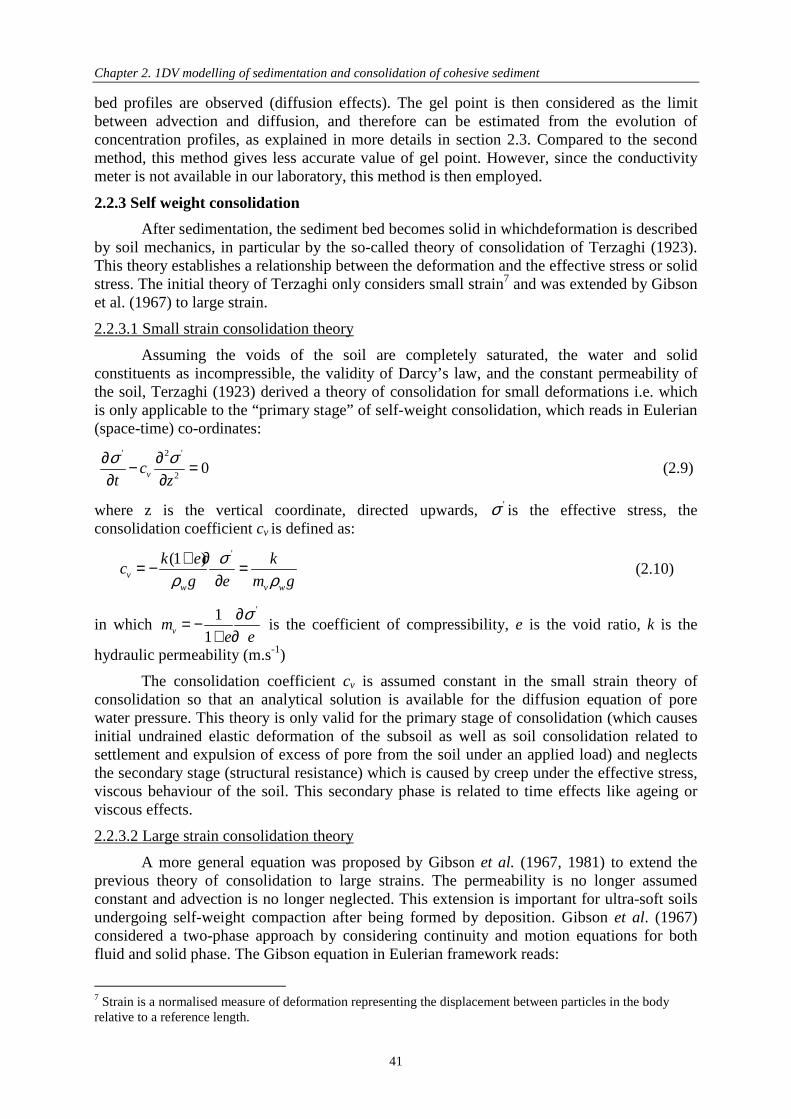
Chapter 2. 1DV modelling of sedimentation and consolidation of cohesive sediment
41
bed profiles are observed (diffusion effects). The gel point is then considered as the limit between advection and diffusion, and therefore can be estimated from the evolution of concentration profiles, as explained in more details in section 2.3. Compared to the second method, this method gives less accurate value of gel point. However, since the conductivity meter is not available in our laboratory, this method is then employed.
2.2.3 Self weight consolidation
After sedimentation, the sediment bed becomes solid in whichdeformation is described by soil mechanics, in particular by the so-called theory of consolidation of Terzaghi (1923). This theory establishes a relationship between the deformation and the effective stress or solid stress. The initial theory of Terzaghi only considers small strain7 and was extended by Gibson et al. (1967) to large strain.
2.2.3.1 Small strain consolidation theory
Assuming the voids of the soil are completely saturated, the water and solid constituents as incompressible, the validity of Darcy’s law, and the constant permeability of the soil, Terzaghi (1923) derived a theory of consolidation for small deformations i.e. which is only applicable to the “primary stage” of self-weight consolidation, which reads in Eulerian (space-time) co-ordinates:
' 2 '
20vc
t z
σ σ∂ ∂− =∂ ∂
(2.9)
where z is the vertical coordinate, directed upwards, 'σ is the effective stress, the consolidation coefficient cv is defined as:
'(1 )v
w v w
k e kc
g e m g
σρ ρ
+ ∂= − =∂
(2.10)
in which '1
1vme e
σ∂= −+ ∂
is the coefficient of compressibility, e is the void ratio, k is the
hydraulic permeability (m.s-1)
The consolidation coefficient cv is assumed constant in the small strain theory of consolidation so that an analytical solution is available for the diffusion equation of pore water pressure. This theory is only valid for the primary stage of consolidation (which causes initial undrained elastic deformation of the subsoil as well as soil consolidation related to settlement and expulsion of excess of pore from the soil under an applied load) and neglects the secondary stage (structural resistance) which is caused by creep under the effective stress, viscous behaviour of the soil. This secondary phase is related to time effects like ageing or viscous effects.
2.2.3.2 Large strain consolidation theory
A more general equation was proposed by Gibson et al. (1967, 1981) to extend the previous theory of consolidation to large strains. The permeability is no longer assumed constant and advection is no longer neglected. This extension is important for ultra-soft soils undergoing self-weight compaction after being formed by deposition. Gibson et al. (1967) considered a two-phase approach by considering continuity and motion equations for both fluid and solid phase. The Gibson equation in Eulerian framework reads:
7 Strain is a normalised measure of deformation representing the displacement between particles in the body relative to a reference length.

Chapter 2. 1DV modelling of sedimentation and consolidation of cohesive sediment
42
2 (1 )² '(1 ) 0
(1 )² 1s w
w w
e k e ke
t z e g z e z
ρ ρ σρ ρ
−∂ ∂ + ∂ ∂ + + + = ∂ ∂ + ∂ + ∂ (2.11)
or
'( 1) 0
w
kk s
t z z
φ σφ φγ
∂ ∂ ∂− − + = ∂ ∂ ∂ (2.12)
where φ stands for the sediment volume concentration =1/(1+e), s the density ratio between sediment and fluid (=ρs/ρw), γw the unit weight of fluid (kg.m-².s-²), (=gρw, g being the acceleration of gravity).
Numerical solution of this non-linear equation is difficult because of the moving upper interface (boundary condition). Therefore, it is common practice to rewrite (2.11) in a moving reference frame, the so-called material or Lagrange coordinate system. A vertical material coordinate ζ is introduced that represents the volume of solids.
0
'( , )
1 ( ', )
z dzz t
e z tζ =
+∫ (2.13)
With the assumption that k and 'σ are functions of e only, the classical Gibson equation in material co-ordinates is obtained:
'0
1 (1 )s w
w w
e d k e k d e
t de e g e de
ρ ρ σρ ζ ζ ρ ζ
−∂ ∂ ∂ ∂ + + = ∂ + ∂ ∂ + ∂ (2.14)
The equation of Gibson has been widely used in various numerical consolidation models (Been and Sills, 1981; Bartholomeeusen et al., 2002; Sanchez, 1992; Toorman, 1996; Thiebot, 2008; Pham Van bang et al., 2008 for instance) as well as compared with the experimental results.
2.2.4 Unified theory of sedimentation and self-weight consolidation
The Gibson theory has been intensively studied during the MAST European project. As pointed by Toorman (1996), the two terms in brackets in eq. 2.12 have physical interpretations in terms of hindered settling (first term) and consolidation (second term). On the one hand, Kynch theory (1952) is obtained if the second (or effective stress) term is neglected. On the other hand, Terzaghi theory (1923) is obtained when the first (or convective) term is withdrawn and the elasticity of the soil is assumed. Therefore the equation of Gibson will be solved in this study for the problem of sedimentation and consolidation since it is considered as the general one.
However, the Gibson equation needs two closure equations (one for the permeability, the other for the effective stress) to obtain the time evolution of vertical concentration profiles. These closure equations (material functions) are, however, difficult to obtain as reported by Toorman (1999) and Bartholomeeusen et al. (2002).
In 2002, Bartholomeeusen et al. set up a series of consolidation experiments using mud taken from the Scheldt River. The series of experiments consisted of two sub-sets. The measured interface level and vertical density profiles of four experiments were provided to establish the material functions. Next, the initial condition of the fifth experiment using the same mud was provided, and the consolidation process was predicted, using the material functions derived from the calibration tests. The measured interface level and density profiles were revealed only after the modelling exercise. The presented results of this fifth experiment

Chapter 2. 1DV modelling of sedimentation and consolidation of cohesive sediment
43
showed large differences between predictions and observations, in particular at the earlier stages of the consolidation process.
One of the reasons behind the unfavourable performance is the large sensitivity of both permeability and effective stress to the void ratio associated with the inaccuracy in measuring techniques: small variations in material functions yield large differences in consolidation behaviour. Another important remark of the authors is an observed significant time-dependent phenomenon of the effective stress, which is not yet incorporated in any existing consolidation model.
The following section reviews the existing semi-empirical closure equations of permeability and effective stress.
2.2.5 Typical functions of closure equations for permeability and effective stress
Up to now, the closure equations for permeability and effective stress have been derived by correlating experimental data with the following typical material functions (Eq. 2.15 & 2.16).
2.2.5.1 Closure equation for permeability k
Bartholomeeusen et al. (2002) introduced typical functions, in the form of either power or exponential, to relate the permeability k with the void ratio e:
2
2
1
1
1 2exp( )
A
As
k Ae
k A
k A A e
φ −
=
= = − +
(2.15)
The value of these coefficients A1, A2 depends on grain size distribution, organic content, biological activity and pore size distribution.
2.2.5.2 Closure equation for effective stress σ’
The similar way can be opted in the determination of )(' eσ , ( )(' Cσ , '( )σ φ ), which gives:
2
2
3
1 3
1
1 2
4 5
'
'
( ' )
' exp( )
B
Bs
B
e B B
B
e B B
B B e
σσ φ
σσ
−
= − +
=
= + = +
(2.16)
According to Winterwerp & van Kesteren (2004), the validity range of the power-type functions (eg. 2
1Ak Ae= , 2
1' BsBσ φ= ) is much larger than that of the exponential-type functions.
Moreover, there is a physical insight in the formulation of the power-type functions. Therefore, it is recommended to use power-type functions. However, two different power functions for permeability may be necessary to represent the two separate processes: sedimentation and consolidation.
2.2.5.3 Closure equations for sand-mud mixtures
At present, the accurate prediction of the consolidation behaviour of cohesive sediment is not possible due to the lack of good constitutive equations describing the effective stress and the permeability. Indeed, the difficulties arise in both the formulation and the parameters determination procedure. The right description of the effective stress cannot be

Chapter 2. 1DV modelling of sedimentation and consolidation of cohesive sediment
44
limited to functions of concentrations alone (Elder and Sills, 1984), but also depends on time or history effects (Toorman, 1999).
For sediment mixtures, there is an additional problem associated with the interaction between different sediment fractions during the settling process. Toorman (1992) argued that subdividing the sediment into many different fractions, according to the size distribution, is not necessary, but using two fractions (one represents coarse non-cohesive fraction, and the other fine cohesive one) is sufficient. In order to account for the mutual hindrance, the constitutive equations can be modified by working with the volume fractions relative to the estimated remaining space that is not occupied by the other fraction.
Furthermore, the proper determination of the closure equations for permeability and effective stress for each fraction when the other fraction is present is not easy. For instance, once trapped, sand particles could move at the same settling rate as the surrounding clay particles, unless their movement is hindered by the underlying sand particles that are touching each other.
From the settling and consolidation tests carried out on mud and sand mixtures, although there is no consolidation model which was successfully conducted, Torfs et al. (1996) gave some remarks on the future modelling strategy:
1) Experiments showed that segregation occurs for initial mud densities below the gel point. For many types of estuarine mud this transition takes place at a solid fraction φ of about 0.03 - 0.07 corresponding to an excess density of about 50 -110 kg/m3 or a sediment concentration of 80-180 g/l, depending on the type of sediment and the physico-chemistry of the water (Toorman and Berlamont, 1993).
2) An increasing amount of non-cohesive sediment in the mixture increases the apparent gel point density.
3) An increasing amount and supply rate of non-cohesive sediment increases the segregation process.
4) Segregation limits the increase of the settling rate and final mean concentration. The final thickness of a mixed sediment layer reaches a minimum and further increase in the sand content does not decrease this thickness anymore.
In our study, the hindered settling of sand-mud mixture is formulated based on the existing bi-disperse Masliyah–Lockett–Bassoon model (Lockett & Bassoon, 1979) and validated against the measurement. This will be presented in details in Chapter 5.
2.3 Analytical solutions for closure equations
If the self-weight consolidation is finely described by the so-called theory of Gibson (Gibson et al., 1967; Toorman, 1996), a huge amount of studies reported the problem associated with its closures and the poor predictive capacity (Bartholomeeusen et al., 2002; Toorman, 1999). This can be improved if an accurate determination procedure of parameters is defined. Thus, this section proposes a new procedure which is based on space-time analysis of concentration profiles instead of classical least square fit on water/sediment interface (Thiebot et al., 2011).
To obtain such an analytical expression of concentration profiles, we use self similar asymptotical method to separate the sedimentation regime from the self-weight consolidation regime.

Chapter 2. 1DV modelling of sedimentation and consolidation of cohesive sediment
45
2.3.1 Self similar solution for sedimentation regime
Hereafter, we follow the method of Kynch (1952). The non-linear advection problem of the sedimentation (Eq. 2.6) is solved by considering the theory of kinematics waves (Dankers & Winterwerp, 2007; Camenen & Pham Van Bang, 2011). If the concentration of the suspension is lower than a given threshold (the so-called gelling point φgel for cohesive sediment or the random packing concentration φmax for non-cohesive one), the inter-particle contacts are negligible, i.e. there is no solid (or effective) stress. In such a situation, the Gibson equation is simply reduced to the equation of Kynch:
[ ]( ) 0Vt z
φ φ φ∂ ∂− =∂ ∂
(2.17)
where V(φ) is the settling velocity of the suspension at concentration φ that is equal to k(s-1)φ in Eq. 2.12.
Considering the similarity variable ξ=z/t and solution X, i.e. φ(z,t)=X(ξ), equation (2.17) leads to:
0df dX
dX dξ
ξ − =
(2.18)
where f is the solid (or sedimentation) flux, which is equal to –V(φ)φ. The method of resolution is equivalent to the so-called method of characteristics
(Leveque, 2002). The iso-concentration pattern presents different straight lines in the space-time (z-t) plot. As confirmed by Kynch (1952) and Burger et al. (2000), shock waves, rarefaction or compound shock waves are supposed to occur depending on the position of initial concentration φ0 relatively to the inflection point fi (Fig. 2.3).
2.3.1.1 Closure equation for permeability k of Merckelbach and Kranenburg
As an illustration, we report the analytical results of Merckelbach and Kranenburg (2003) on sedimentation. In their model, the permeability closure was given as a power law equation which reads:
2( ) ( ) ( 1) nf V k sφ φ φ φ −= = − (2.19)
where n =2/(3-nf) , typical values of nf = 1.7 to 2.2.
Replacing the closure equation (2.19) in the non-linear hyperbolic equation (2.17) leads to:
1( 1)(2 )( ) 0nk s nt z
φ φφ −∂ ∂− − − =∂ ∂
(2.20)
Following the method of characteristics, they considered iso-concentration lines, i.e. lines in the space-time plot such as φ (z,t) is constant.
1( 1)(2 )( ) ndzk s n
dtφ −= − − (2.21)
Integration of (2.21) leads to:
11 nz
atφ
− =
with ( 1)(2 )a k s n= − − (2.22)

Chapter 2. 1DV modelling of sedimentation and consolidation of cohesive sediment
46
This analytical solution is dependent on the z/t ratio, i.e. the similarity variable ξ. Iso-concentration pattern can be illustrated by straight lines in the z-t plot.
2.3.1.2 Proposed closure equation for permeability k
We propose here a modified Richardson and Zaki expression for cohesive sediment, in order to account for the effect of concentrations up to the gel point. The modifications are:
• The term (1-φ) is added to account for the backflow8
• φ is replaced by φ/φgel to enable a zero settling velocity for concentrations close to the transition point, φgel.
The closure equation becomes:
( ) (1 ) 1
n
stgel
f Vφφ φ φ
φ
= − −
(2.23)
( )1
( )1 1 1 2 (1 )
n
stgel gel gel
df nV
d
φ φ φ φφ φφ φ φ φ
−
= − − − − − (2.24)
where Vst is the Stokes velocity of a single and spherical solid ‘representative’ sphere, φgel is the gelling concentration, n is the exponent.
Parameters φgel and n have physical meanings in terms of rheology (Pham Van Bang et al., 2007). Indeed, φgel is the concentration value from which the effective viscosity of the suspension diverges. And n is a parameter describing the settling rate (the smaller n is, the higher settling rate is). Such a closure does not diverge at zero concentration and its first derivative is easy to obtain.
FIGURE 2.5 - Granulometry of the tested material
8 A falling particle generates a return flow or a back flow. This phenomenon affects the settling velocity of the surrounding particles by decreasing it with a factor (1-φ).(Winterwerp and van Kesteren, 2004)
0
20
40
60
80
100
120
0,01 0,1 1 10 100 1000
Grain size (µm)
His
togr
am (
%)
Cumulative values (%)
Histogram (%)

Chapter 2. 1DV modelling of sedimentation and consolidation of cohesive sediment
47
In our study, the settling column experimental results presented in Chapter 1(§ 1.5) are used to propose a new closure equation for the bed permeability of the Gironde cohesive sediment.
First, the Stokes velocity Vst is calculated based on Eq. 2.3 assuming that the suspension is made of individual spherical solid particles having a ‘representative’ diameter d90 of 45 µm, as obtained from the grain size analysis of the tested material presented in Fig. 2.5 leading to Vst equal to 0.0018 m/s.
The gelling point φgel is determined based on differences in the shape of the vertical concentration profiles of the Gironde mud, (Fig 1.23) between the sedimentation (a) and the consolidation regimes (b). As observed in Fig. 1.23, the concentration profiles near the bottom during the short term are concave downward, while they become convex during the long-term evolution. As discussed previously in § 2.2.2, the gelling concentration marks the transition between concave profiles (advection or permeability) and convex profiles (diffusion or effective stress). Therefore, within our study, the gelling point is roughly determined from Fig 1.23 as φgel = 0.12 or Cgel = 312 g/l.
FIGURE 2.6 - Space-time based method to determine the sedimentation flux: a) iso-concentration plot; b) first derivative of sedimentation flux: blue line is first derivative of the sedimentation flux df/dφ, blue circles are measured slopes of iso-concentration lines on plot 2.6a
The exponent n is determined by correlating the first derivative of the sedimentation flux with the measured slopes of iso-concentration lines. From the obtained vertical concentration profiles of the Gironde mud (Fig. 1.23a), the space-time plot (Fig. 2.6a) is produced by plotting contours of different concentration φ within a z-t plot. Then, slopes of these iso-concentration lines in the space-time plot (Fig. 2.6a) are measured assuming that these lines are straight close to the bottom and have a unique slope. The mean slopes (as obtained by linear regression of the f(φ) data) correspond to the measured values of df/dφ (Eq. 2.24). In Fig. 2.6b, the line presents the first derivative of the sedimentation flux df/dφ and the corresponding points represent the measured slopes.
Knowing Vstokes = 0.0018 m/s, φgel = 0.12 and φ0 = 0.0295, the exponent n is finally obtained by calibration in order to reach the best fit agreement between the calculated and the measured slope values. The value n = 8 is obtained.
Then, the settling flux for the Gironde cohesive sediment is proposed hereby:
8
( ) 0.0018(1 ) 10.12
fφφ φ φ = − −
(2.25)
a) b)

Chapter 2. 1DV modelling of sedimentation and consolidation of cohesive sediment
48
The closure equation for permeability applied for the Gironde mud is then:
( ) ( ) 8
2
0.0018 11
( 1) ( 1) 0.12
fk
s s
φ φ φφ φ
− = = − − − (2.26)
In order to solve eq. (2.17), initial condition is needed. The measured initial concentration of the suspension is equal to C0 = 77 g/l, i.e. the initial volume concentration φ0 = 0.0295. In order to validate the closure equation, it will be implemented in the Gibson’s consolidation model and tested using two different numerical models (cf. Part 2.5).
Compared to previous relations proposed in the literature, this equation is supposed to better describe physical processes in terms of backflow and zero-settling velocity for concentrations near the gelling point. This will be demonstrated later in the numerical part (cf. part 2.5).
2.3.2 Self similar solution for the consolidation regime
2.3.2.1 Closure equation for effective stress σ’
For concentrations larger than the gel point, the convective term is negligible in comparison to the effective stress diffusion term in the Gibson equation (2.12). In such a situation, the Gibson equation is reduced to a non-linear diffusion equation:
( ) 0Dt z z
φ φφ∂ ∂ ∂ − = ∂ ∂ ∂ (2.27)
where the diffusion coefficient is defined as ( ) '
w
k dD
d
φ σφγ φ
= to match with Eq. 2.12.
NB: the sign is negative because the axis z is directed upwards (against gravity).
The classical approach is to consider explicitly a rheological law for the effective stress (for instance Terzaghi, 1923; Been and Sills, 1981). The use of simple rheological models is widespread, and they are useful description for slow, steady-state compaction of normally accumulating sediments from self-weight. However, this method does not produce time-dependent effective stress, which is an important point as argued by Toorman and Huysentruyt (1997).
In the present study, the non-linear diffusion coefficient is assumed to depend on concentration, time and space by an empirical power law, which is recommended by Winterwerp and van Kesteren (2004), i.e. D(φ)=D0φatbzc where a, b, c ≠ 0, a > 0 . Here the time dependence of the consolidation is introduced to mimic the thixotropic behaviour of mud (i.e. the mechanisms of structural recovery and shear thinning).
Using dimensionless variables*
*
2 10
/
/
/c b
z z H
t t T
D H T− +
= = =
where H is the initial water depth, T is the time scale, and D0 is a constant, the equation then becomes:
( )* * * ** * *
,a b ct z t z
t z z
φ φφ ∂ ∂ ∂= ∂ ∂ ∂
(2.28)

Chapter 2. 1DV modelling of sedimentation and consolidation of cohesive sediment
49
Introducing the similarity variable, χ=z*/t*θ with θ=(1+b)/(2+a-c) and solution y, i.e.
φ(z*,t*)=y( χ)/ t*θ in equation (2.28) leads to:
( ) ( ) 0c ad dyy y
d dχ χ θχ χ
χ χ
− =
(2.29)
The self-similar solution, y, is obtained by integrating the second-order differential equation 2.29. An analytical solution can be derived by:
( ) ( ) 0c a dyy y
dχ χ θχ χ
χ− = or 2( )
2a cy const
c
θχ χ −= +−
(2.30)
Scenario 1 is the general case where non-linear diffusion coefficient depends on space, time and sediment concentration (, , 0a b c≠ , and a > 0). In this scenario, there are two
solutions for c= 2 and c ≠ 2
( )
11/2 2
1
2
1/
(2 ) 0,
2( ) 2
(2 )0
( ) ln 2
ac c
c
a
a M cM for
c ay for c
M cfor
a
y M a for c
θχ χθ
χ
χθ
χ θ χ
− −
−
− − + ∈ − = ≠ − − ≥
= − =
(2.31)
M acts as a constant of integration, and is calculated from the total mass of sediment M*:
( )
1 1
2 2(2 ) (2 )1/1 1 2
2* * * *
0 0
, ( ) 1(2 )
c cM c caa a c
a ca
M z t dz y d M dc
θ θ θξφ χ χ ξ
− −− − − − ∞ −+
− = = = + − ∫ ∫ ∫ (2.32)
Scenario 2 is a particular case where the non-linear diffusion coefficient is dependent on concentration and time (c = 0)
11/2 2
1
2
(1 ) 2 (2 ) 0,
2(2 ) (1 )( )
2 (2 )0
(1 )
aa b M a
M fora a b
y
M afor
a b
χ χ
χ
χ
+ + − ∈ + + =
+ ≥ +
(2.33)
Scenario 3 The non-linear diffusion coefficient is only dependent on concentration
(b = c = 0)

Chapter 2. 1DV modelling of sedimentation and consolidation of cohesive sediment
50
11/2 2
12
2 (2 ) 0,
2(2 )( )
2 (2 )0
aa M a
M fora a
y
M afor
a
χ χ
χ
χ
+ − ∈ + = + ≥
(2.34)
The closure equation for effective stress can be obtained by determining the four variables T, a, b, c. H is the water depth. The following part is dedicated to the determination of these variables through the settling column experimental results (which were presented in § 1.5.5).
2.3.2.2 Parameter determination
The settling column presented in chapter 1 is used to calibrate the parameters.
As presented in the previous part, three scenarios can exist:
• General case , , 0a b c≠
• Case c=0
• Case b=c=0
FIGURE 2.7 - Computed and experimental concentration profiles (a): Measurement; b) Scenario 2; c) Scenario 3; d) Scenario 1 (Scenario 2 is selected)
The non-linear diffusion equation is transformed to dimensionless form as explained previously. The total mass M* is then kept equal to 1.0. All the three scenarios are tested.
a) c)
b) d)
a) c)
b) d)

Chapter 2. 1DV modelling of sedimentation and consolidation of cohesive sediment
51
Different set of values of a, b and c are applied by trial and error, in order to find the best set of parameters.
Figure 2.7 presents the measured concentration profiles (a) and the calculated concentration profiles corresponding to three scenarios (b, c, d).
It is observed that in the case of b = c = 0, the analytical results are very different from the measurements, both in terms of maximum concentrations at the bed and the lowest level of the water/sediment interface. Therefore this case is not selected. The shape of concentration profiles in Fig. 2.7b and 2.7d are similar to the measurements. A comparison between these two analytical results shows no significant difference. A slight difference arises in the lowest level of the supernatant/suspension interface (scenario 1 gives a lower level at about 4 cm, which corresponds better to our measurement). However, the effect of parameter c is also revealed in the shape of the concentration profiles near the bottom, as observed in Fig 2.7d. This increases the maximum concentration near the bottom to almost 0.18, which is much greater than the measured maximum concentration. Therefore, we restrict ourselves to scenario 2: the diffusion coefficient depends on both concentration and time:' ( , )f tσ φ= . A set of parameters (a = 12, b = - 3.4, c = 0) is obtained from this step. The following step is dedicated to validate our selection and determine the parameter T.
2.3.2.3 Parameter validation From the above analysis, the second scenario is selected. With the selected set of
parameters (a = 12, b = - 3.4, c = 0), a good agreement is observed between the modelled and the measured concentration profiles, as shown on Fig. 2.7a & b.
FIGURE 2.8 - Interface z*~t* plot (a,b: experiment, c,d: self-similar solution; a,c: normal scale, b,d: logarithmic scale). In figures b and c, the x axis signifies log(t*), and the y axis signifies the log(z*). In figure b, the red line represents the measured z~t plot, the blue one represents the z*~t* plot for the later stages of the consolidation process.

Chapter 2. 1DV modelling of sedimentation and consolidation of cohesive sediment
52
In order to validate the selected parameters, the experimental and self-similar values ofθ are calculated and compared. From the above part, it is seen that the value θ is in fact the slope of the plot z*~t*.
*
*
z
tθχ = , ( ) ( )**log logz tθ= where
1
2
b
a cθ +=
+ −
In the self-similar solution, we can determine from the concentration profiles the height of the water/sediment interface z* at different time t*. We can then draw the interface z*~t* plot (Fig. 2.8c). The slope θ is then obtained equal to – 0.165 by plotting the z*~t* plot in a logarithmic scale (Fig. 2.8d).
This value can be calculated manually from the values of a, b, c as:
1 1 ( 3.4)0.171
2 2 12 0
b
a cθ + + −= = = −
+ − + −
The same procedure is applied to the experimental results. However, by plotting the z*~t* plot in a logarithmic scale, we observe a line with different slopes (the red line in Fig. 2.8b). This can be explained by the presence of advection in the data. Indeed, those changes in slope are the signs of transition between the sedimentation regime dominated by advection to the consolidation regime dominated by diffusion process. In order to represent the consolidation only, we assume that diffusion occurs after a certain time, when the slope does not change anymore. The slope of the second half of the red line is found equal to – 0.1614 (linear regression). The calculated and experimental values of θ are found in reasonable agreement (θmeasured = −0.1614, θsimulated = −0.165). The selected set of parameters (a = 12, b = -3.4, c = 0) is therefore confirmed validated.
The next step is to determine parameter T. This parameter can be determined from the relationship between the dimensionless time t* and the real time t:
* 1 20; b ct Tt D T H+ −= =
FIGURE 2.9 - Determination of T: a) Correlation between experimental and modelled concentration profiles at the end of the consolidation process; b) Relation between dimensionless time t* and real time t and the best-fit line.
Several experimental and modelled profiles at different time t during consolidation regime are correlated, as observed in Fig. 2.9a. Then, the sampled dimensionless time t* and
a) b)a) b)

Chapter 2. 1DV modelling of sedimentation and consolidation of cohesive sediment
53
the real time t are plotted as different points in Fig. 2.9b. A best-fit line is applied in order to calculate T as the slope of the line in Fig. 2.9b (T = 10.3).
From the four determined parameters (T, b, c, H), D0 is calculated equal to 11.55. The diffusion equation is transformed back to initial form. However, since the correlation between φ(z*,t*) and φ(z,t) is unknown, it is recommended to keep that value in dimensionless form which is equal to φ/φ0 .
12.
3.4
0
'11.55
w
kt
z g z z z
φ σ φ φρ φ
− ∂ ∂ ∂ ∂ = − ∂ ∂ ∂ ∂
(2.35)
The closure equation for effective stress of the Gironde mud becomes:
12.
3.4
0
'11.55 wt
k
γσ φφ φ φ
− ∂ = − ∂
(2.36)
This closure equation for the effective stress will be implemented in the consolidation algorithms which will be applied in the morphodynamic model of the Gironde estuary.
2.4 Sedimentation-consolidation modelling approaches The above section gives a new procedure to determine the closure equations for
permeability and effective stress. This method which is based on analytical solutions has been applied to the Gironde mud. The constitutive equations for the bed permeability (Eq. 2.26) and effective stress (Eq. 2.36) will be implemented in the consolidation models.
This section is a literature review on existing modelling approaches, and part 2.5 will describe the consolidation models implemented in Sisyphe.
Several numerical models based on the equation of Gibson have been proposed in the litterature. Been and Sills (1981), Merckelbach (2000), Toorman (1996) proposed sedimentation-consolidation models for saturated material assuming both solid and fluid phases to be incompressible. Bürger et al. (2000), Bartholomeeusen et al. (2002), Pham Van Bang et al. (2008) used a finite difference numerical technique to capture shocks in order to describe the vertical propagation of concentration fronts.
Hereafter four modelling methods of sedimentation-consolidation are presented, and we emphasize their strengths and weaknesses.
1) First-order kinetics models
2) Iso-concentration models
3) Mixed models between first-order kinetics and iso-concentration approaches
4) Vertical-grid models
2.4.1 “First-order kinetics” models
According to Sanford (2008) the effect of consolidation can be approximated as a first-order relaxation (exponential approach) to an empirical defined equilibrium state. First-order kinetics models are then constituted of different layers of consolidating muddy bed. They calculate the concentration of each layer separately depending on the mean concentration of the deposition. This means there is no mixing between consecutive layers. The first-order kinetics equations have less parameters for calibration and can be used for any number of layers (even one layer), with any given concentration profile (even concentration

Chapter 2. 1DV modelling of sedimentation and consolidation of cohesive sediment
54
profile not monotonically increasing). Although this method has no physical insight, it has been used quite commonly because of the simplicity of the scheme.
It has been known that the mean concentration of consolidating muddy beds approaches its final value in an approximately exponential manner (Hayter, 1986, in Sanford, 2008). Assuming that the equilibrium concentration profile is known, then the mean concentration of the deposited bed is determined by the following equation:
( )1 exp
C t pt
tC ∞∞
= − −
(2.37)
where ( )C t is the mean concentration at time t ( sC ρ φ= × ), C∞ is the final maximum
concentration attained after a consolidation time t∞, p is the parameter depending on material.
And the concentration of sediment at depth z is calculated from the gradient of concentration within the sediment deposit.
( ) BC z H zA
HC
− =
(2.38)
where A and B are functions of consolidation time t and the relative depth z’ (=z/H).
Le Hir et al. (1988) proposed an empirical model in the form of a differential equation with respect to time:
( )0
CC C
tα ∞
∂ = −∂
(2.39)
where α0 is the coefficient depending on the type of bed material.
Hillebrand & Olsen (2011) and Sanford (2008) used a similar algorithm to Le Hir et al (1988) to model the effect of consolidation. In their approach, the concentration (density) of the respective bed layers is a time-dependent variable and is approaching an equilibrium state. The values for the kinetics coefficient α0 (s
-1) in Sanford (2008) is re-used in Hillebrand & Olsen (2011) and is reported in the range of [1.0e-5;3.5e-5].
This method is relatively simple and not too computationally expensive. However, this semi-empirical model does not account for the actual physics of consolidation.
2.4.2 “Iso-concentration” models
Bed structure
In “iso-concentration” models, the consolidating muddy bed is discretized in layers of increasing concentrations. The concentrations of each layer are constant and imposed by the users.
The concentration of different layers are fixed, the associated thicknesses are directly linked to the amount of sediment that they contain.
i i iM Ep C= × (2.40)
As sedimentation and consolidation progress, sediment bed mass is transfered from bed layers of low density to underlying layers with higher densities, thereby reducing the total bed height. The thickness of the top layers therefore decreases while the thickness of the underlying layers increases.

Chapter 2. 1DV modelling of sedimentation and consolidation of cohesive sediment
55
Compared to first-order kinetics models, this type of model needs at least two bed layers to work properly, and concentrations increase from the top surface to the bottom.
FIGURE 2.10 – Scheme of “iso-concentration” models Ci, Mi, Vsi, epi are the concentration, mass, settling velocity and thickness of layer i, respectively. Fi is the settling flux between layer i and under-layer i+1 . Zf is the level of sediment bed, Zr is the rigid bottom.
Sanchez (1992) presented a semi-empirical iso-concentration model, which was applied for the Loire. In this model, since the total stress was greater than the effective stress, the velocity of the solid phase could be equal to the sedimentation velocity (without effective stress regime). Otherwise, the velocity of the solid phase decreases corresponding to the consolidation regime. This model is described by several layers of fixed concentrations, and variable masses and thicknesses depending on the state of the suspension. The mass variation of a surface unit of the layer i reads:
( ) ( )
( )
( )
( )
1 0
'
0 '
'
1
0
gel
i
ii i i
ii i s i i
i
s iw
C
wi gel
s C
i gel
MF F M
tC
F C V C C ift
F if
k uV C
g z
u
g Cdz for C C
for C C
η
η
ησ σ
σ σ
ρσ σ
ρσρ
σ
−∂ = − ≥∂
∂= − × + >
∂= ≤
∂=∂
= −
= − ≥
= <
∫
(2.41)
C1, Vs1, M1, ep1
Ci, Vsi(t+∆t), Mi(t+ ∆t), epi(t +∆t)
Cimax, Vs,imax, Mimax, epimax
C1, Vs1, M1, ep1
…
Ci, Vsi(t), Mi(t), epi(t)
…
Cimax, Vs,imax, Mimax, epimax
ZF
F1
C1<Ci<Cimax
ZR
(t)
(t+∆t)
Fi
Fi-1
Fimax-1
C1, Vs1, M1, ep1
Ci, Vsi(t+∆t), Mi(t+ ∆t), epi(t +∆t)
Cimax, Vs,imax, Mimax, epimax
C1, Vs1, M1, ep1
…
Ci, Vsi(t), Mi(t), epi(t)
…
Cimax, Vs,imax, Mimax, epimax
ZF
C1, Vs1, M1, ep1
…
Ci, Vsi(t), Mi(t), epi(t)
…
Cimax, Vs,imax, Mimax, epimax
ZF
F1
C1<Ci<Cimax
ZRZR
(t)
(t+∆t)
Fi
Fi-1
Fimax-1

Chapter 2. 1DV modelling of sedimentation and consolidation of cohesive sediment
56
where η(C) is the level corresponding to the concentration Ci (m); σ is the total stress (Pa), σ’ is the effective stress (Pa). σ’ is calculated from closure equation for effective stress.
Recently, Thiébot et al. (2011) presented a “iso-concentration multi-layer” consolidation model. In his model, the mass conservation is ensured by requiring at each moment, in each layer, an equality between the mass Mi contained in a surface unit of layer i at time t + t∆ and the mass present in a surface unit of this layer at time t in which the outgoing mass was removed and the incoming mass was added (means the mass that crossed the upper and lower sections respectively during the time t∆ ).
1( ) ( ) ( ( ) ( ))i i i iM t t M t F t F t t−+ ∆ = + − ∆ (2.42)
The outgoing and incoming masses are taken into account by sediment flux noted Fi(t).
, , 1 1
1
( ( ) ( ))( ) s i s i i i
ii i
V t V t C CF t
C C+ +
+
−=
− (2.43)
in which Vs,i can be defined as:
,
,
1 1( )
'
s i i i i gels w
s i i gelw
V k C C If C C
kV k If C C
g z z
ρ ρσ σ
ρ
= − ≤
∂ ∂ = + − > ∂ ∂
(2.44)
The advantage of this iso-concentration model is to give an accurate description of the evolution of muddy sediment bed based on the Gibson’s theory with reasonable computation time. This model also takes into account high gradients of concentration. However, the discretization of the mud bed in layers of fixed concentrations is an over-simplification of in-situ conditions, where the bed structure can be highly variable.
2.4.3 Mixed approach between iso-pycnal and first-order kinetics
Villaret and Walther (2008) made a mixed approach based on iso-pycnal (or iso-concentration) and first-order kinetics models. Similar to the models proposed by Sanchez (1992) and Thiébot et al. (2011), this model computes the thickness of iso-concentration layers. The settling of sediment is then reproduced by the mass transfers between consecutive layers in the model. However, instead of calculating the sediment flux and the settling velocity based on the theory of Gibson, a set of mass transfer coefficients per layer ai are used. These coefficients are specified for each layer and maintained constant during consolidation process.
( ) ( ) ( ) ( )1 . ( )i ii i i i
M t t M tF t F t a M t
t −
+ ∆ −= − = −
∆ (2.45)
This method is simple, and not computational costly. It also allows to take into account high gradients of concentration. However this model is higly empirical and does not give any physical insight. Model results highly depend on the choice of empirical transfer coefficients which are poorly defined.
And the main problem is in the determination of model parameters. The calibration of the large number of empirical parameters (one per layer) is a difficult task. This model will be presented in details in section 2.5.1.

Chapter 2. 1DV modelling of sedimentation and consolidation of cohesive sediment
57
2.4.4 “Vertical grid” models
Bed structure
“Vertical-grid” models are models in which the consolidating bed is discretised in layers of the same initial concentration. The thicknesses of layers are constant and can be specified differently. Near the surface layer, increasing the number of layers will improve the representation of the results, but at a high computational cost. Concentration at these levels is calculated using numerical schemes.
The Gibson equation in Lagrange coordinate system (2.14) can be solved by applying different numerical schemes (either finite element or finite difference).
Finite element model
The first model (named 1D-FE-FCT) is a finite element model with a Flux Corrected Transport algorithm (Boris & Book, 1973, cited in Pham Van Bang et al., 2008) to avoid both the numerical diffusion of a first-order time scheme and the artificial oscillation of a second order time scheme. This model was developed by Pham Van Bang et al. (2006 & 2008).
Originally developed in a finite difference schemes applied to linear advection equation and to gas dynamical equations, the FCT technique was modified by Lohner et al. (1987) for finite element method and hydrodynamics (in Pham Van Bang et al., 2008). The basic concept of FCT is to generate a positive, high accuracy solution through a combination of high and low-order schemes:
lowii
highii
FCTi CCC )1( αα −+= (2.46)
where highiC (and low
iC ) are the concentrations computed from the high- (and low-)
order schemes at the node i, αi is a weighting coefficient (0 < αi < 1) and CFCT the corrected concentration. CFCT is restricted to the interval defined by the minimum and maximum concentration in the elements that contain node i at the previous time step.
Both schemes are combined such as the high-order scheme is employed (αi =1) in areas where the variables vary smoothly, a combination of the two schemes is used in a conservative manner, to ensure a monotonic solution in areas where the variables vary abruptly. In the 1D-FE-FCT code, the 6-step algorithm of Georghiou et al (2000) is implemented with the Zalesak’s Flux Limiter Procedure (in Pham Van Bang et al., 2006). For the high-order method, the time scheme is based on Lax-Wendroff’s method (second order in time); and for the low-order method, a lumped mass matrix formulation is used to make the computational cost associated with the FCT technique negligible.
Finite difference model
The second model which will be presented in details and validated later in section 2.5 was developed by Lenormant (1993) based on the Gibson equation (2.14) and applied to the Loire estuary. The constitutive laws which give the permeability k and effective stressσ’ as a function of the void ratio e are necessary to solve the equation.
To numerically solve Gibson equation including advection and diffusion terms, a 1D vertical mesh which discretises the bed into several layers is considered at each bottom point. Equation (2.14) is solved by applying the finite difference method with an implicit scheme (double-sweep scheme). The coefficients of both advection and diffusion terms are explicit in order to make this equation linear.

Chapter 2. 1DV modelling of sedimentation and consolidation of cohesive sediment
58
2.4.5 Conclusions
The above literature review gives a general overview on the process of sedimentation-consolidation and updates current knowledge on experimental and numerical models of these two processes.
In a layered model (first-order kinetics and iso-concentration models), the number of layers needs to be fixed. The main advantage is their computational cost. While the first-order kinetics models have no physical insight, the iso-concentration models are based on the Gibson theory. However, since the concentration of each layer is invariant, layered model cannot represent the in-situ conditions, where the bed structure can be highly variable. Moreover, this type of model cannot be developed to the case of sediment mixtures, where the concentration of each fraction varies depending on the percentage of each fraction in the mixture.
The “vertical grid” models represent more naturally the variation in the bed structure. They are the most appropriate choice of coastal models since they can more accurately resolve the top and bottom boundary layers by increasing the number of vertical points only within these areas. However, their disadvantage is the computational cost.
In the next part (cf §2.5), three sedimentation-consolidation models which represent three different types of model for cohesive sediment will be analysed. They will be compared against the experimental results of the settling column data of the Gironde mud, in order to select the most appropriate one to our research issue: the morphodynamic modelling of cohesive sediment.
2.5 Inter-comparison of 1DV sedimentation-consolidation models The consolidation effect in the morphodynamic model (Sisyphe release 6.1) is
accounted for by using an existing simplified multi-layer model. In order to correctly simulate the morphodynamic of cohesive sediments, two other physical-based sedimentation-consolidation models are implemented (Sisyphe, release 6.2) and validated against the settling column data of the Gironde mud. The following parts present these three models:
1) Semi empirical multi-layer model
2) Gibson multi-layer model
3) Gibson vertical grid model
The first two models are similar in modelling scheme: both models are based on a multi-layer iso-concentration scheme, but “Model 1” has no physical insight whereas “Model 2” follows the Gibson theory. Figure 2.10 (in section 2.4.2) presents the common scheme of these two models.
2.5.1 First-order kinetics multi-layer model (Model 1)
This model was originally developed by Villaret & Walther (2008) by mixing two approaches of iso-pycnal and first-order kinetics, as detailed previously. In this model, the muddy bed is discretised into a fixed number of layers (the maximum number of layers is 20). Each layer i is characterised by its mass concentration Ci (kg/m3), mass per unit surface Mi
(kg/m²), thickness epi and a set of mass transfer coefficient ai(s-1).
The thickness of the lower layers (higher concentration) increases by successive transfers from the upper layers. The mass balance in layer i is:
( ) ( ) ( ) ( )1 . ( )i ii i i i
M t t M tF t F t a M t
t −
+ ∆ −= − = −
∆ (2.47)

Chapter 2. 1DV modelling of sedimentation and consolidation of cohesive sediment
59
As the assumption of the model is to consider layers of fixed concentration over time, only the masses and thicknesses of these layers may vary. Thus, for a homogeneous bed section along the vertical axis, equation (2.47) becomes:
1
( ) ( )( ) ( ) ( )i i i i
i i i i i
ep t t C ep t CF t F t a C ep t
t −+ ∆ − = − = − × ×
∆ (2.48)
The transfer coefficients ai (i=1, n) are empirical coefficients which are determined by calibration in order to reproduce the time-varying concentration profiles.
At the first layer, there is only one interface between the first and second layers. Without the deposition, the thickness of the first layer decreases continuously as the mass is always transferred to the lower concentration layer. Here, the calculation of the transfer coefficient of the first layer (assumed not to be empty, ep1 cannot be equal to 0) is directly linked to the thickness of the sediment.
1 11
1
( ) ( )1
( )
ep t ep t ta
ep t t
− + ∆=∆
(2.49)
From layer 2 to imax-1 there are two interfaces: one with the upper layer, the other with the lower layer. Thus, the layer receives a sediment flux Fi-1 from the upper layer and transfers a mass flux Fi to the lower layer and the mass transfer coefficient ai is defined as:
11 1
1( ) ( ) ( ) i
i i i i ii i
Ca ep t ep t t a ep t t
C ep t−
− −
= − + ∆ + × × ∆ × ∆
(2.50)
A zero transfer coefficient of the last layer (an=0) is imposed to satisfy the requirement of impermeable bottom.
The mass transfer coefficients can be determined either from:
1. The most representative vertical concentration profiles: we select the most representative ones among the obtained vertical concentration profiles and determine the transfer coefficients based on equation (2.50). These values then need to be generalised in order to represent the whole test case.
2. The time evolution of the mean concentration (depth averaged over the whole
sediment column ( )C f t= . In fact, when a mass of sediment is subjected to the
consolidation, its height decreases when its mean concentration increases with time (Fig. 2.11). The multi-layer model should reproduce this phenomenon of consolidation. The principle of the latter case assumes a bed decomposed into a number of layers of fixed concentration and residence time. This method consists
of discretising the curve ( )C f t= into several layers of fixed concentration and
residence time. The mass transfer coefficient ai is calculated for each layer using equation 2.50.
In fact, 1/a is considered qualitatively as a characteristic time scale of inter-layer transfer or residence time per layer. The residence time increases (and therefor ai decreses)
when C increases. Therefore, the transfer coefficient should decrease when the layer concentration increase.This simple approach seems overly simplistic. In future, the formulation of the time dependence of the coefficient a, could be considered.

Chapter 2. 1DV modelling of sedimentation and consolidation of cohesive sediment
60
FIGURE 2.11 – Mass conservation during the consolidation process (upper, from Bugeat, 2008), evolution of the mean concentration with time (lower, from Thiebot, 2008), Ci is the mean concentration of layer i, Ti is the residence time of layer i, defined as the time which separates the layer of concentration Ci with the layer of concentration Ci+1.
2.5.2 Gibson multi-layer model (Model 2)
This is a 1DV sedimentation-consolidation « multi-layer » model, based on an original technique to solve the Gibson equation, developed by Thiebot et al. (2011). The advantage of this representation is that the flux of sedimentation and consolidation is calculated based on the Gibson theory.
The concentration of different layers are fixed, the associated thicknesses are directly linked to the amount of sediment that they contain.
The scheme of this model is similar to the “simple multi-layer” one, which is presented in previous section. However, instead of using the transfer coefficients which are arbitrary, this model is based on the Gibson’s theory for the definition of the settling velocity of solid grains and the determination of mass fluxes
The outgoing and incoming masses are taken into account by the sediment flux noted Fi(t).
Ti
Ci
Con
cent
ratio
n (g
/l)
Time (min)
Ti
Ci
Con
cent
ratio
n (g
/l)
Time (min)

Chapter 2. 1DV modelling of sedimentation and consolidation of cohesive sediment
61
, , 1 1
1
( ( ) ( ))( ) s i s i i i
ii i
V t V t C CF t
C C+ +
+
−=
− (2.51)
where
,
1,
1
1 1( )
( ) '( ) '( )1 1( )
1( ( ) ( ))
2
s i i i i gels w
i i is i i i i gel
s w wi i
V k C C C C
k C C CV k C C C C
g ep t ep t
ρ ρ
σ σρ ρ ρ
+
+
= − ≤
−= − + > +
(2.52)
The settling velocity and sediment flux of each layer are calculated based on the Gibson theory as a function of permeability k and effective stress σ’ by the model. They can be calculated once knowing the closure equations for permeability k and effective stress σ’ , which is specific to the type of mud. The constitutive laws need to be determined for each application.
For the Gironde mud we use equations (2.26) and (2.36) determined in previous section based on analytical solution and measured concentration analysis.
2.5.3 Gibson vertical grid model (Model 3)
This model is also based on Gibson equation (1967) of a saturated clay layer featured by its void ratio e. To numerically solve the Gibson equation, they consider a 1D vertical grid at each point of the bottom (i.e. at each point of 2D grid), which discretizes the muddy bottom in several layers.
FIGURE 2.12 - Scheme of “Model 3” at time step t and t+∆t
In order to describe the process, a new variable zs was introduced instead of using the variable z. It is associated with solid grains. sdz represents the solid volume of layer and dz
the total volume. They are related by the following relation:
dz= sdz (1+e) (2.53)
The constitutive laws for permeability and effective stress as a function of the void ratio are necessary to solve the equation (2.11).
Equation (2.11) is solved by applying the finite difference method with implicit scheme (double sweep algorithm) (Lenormant et al., 1993). The coefficients of both convection and diffusion terms are explicit in order to linearise the equation.
ZF eimax(t); ; zsimax(t)
eimax (t+∆t); zsimax (t+∆t)
ei(t+∆t); zsi(t+∆t)
e1 (t+∆t); zs1 (t+∆t)
…
e1(t); zs1(t)
ei(t); zsi(t)
imax
imax-1
i
1
dz = cst
dzs1 (t+∆t)
dzs1(t)
ZR
t t+∆tZF eimax(t); ; zsimax(t)
eimax (t+∆t); zsimax (t+∆t)
ei(t+∆t); zsi(t+∆t)
e1 (t+∆t); zs1 (t+∆t)
…
e1(t); zs1(t)
ei(t); zsi(t)
imax
imax-1
i
1
dz = cst
dzs1 (t+∆t)
dzs1(t)
ZR
t t+∆t

Chapter 2. 1DV modelling of sedimentation and consolidation of cohesive sediment
62
Discretisation results in a system of equations of the following form (see details in Appendix 2):
1 1 11 1
n n ni i i i i i iAe B e C e D+ + +
− ++ + = (2.54)
where i stands for the depth z, n stands for time t
Concerning the boundary, the bottom of the mud bed is impermeable, so there is no water source at the bottom layer. That gives the relationship between e1 and e2:
1 11 1 1 2 1
n nB e C e D+ ++ = (2.55)
At the water-mud bed interface, the void ratio is assumed to be constant:
1maxnie cst+ = (2.56)
The Gibson vertical grid model has the advantage that the equation reveals the consolidation process. However the specific closure equations of permeability and effective stress should be known. Moreover, this model was developed for the case of consolidation, which means it cannot be applied for concentration < gel point, i.e. without effective stress.
2.5.4 Comparison of sedimentation-consolidation models
The three presented models can be divided into two types in term of modelling schemes:
• Vertical-grid
• Multi-layer
And two types in term of modellling approach:
• Semi-empirical
• Physical based
The “vertical-grid” model uses an iterative method to solve the Gibson equation (2.11). The results are accurate but the computation time makes it impossible to use this model in the case of long-term sediment transport simulation because this equation requires to be solved at each point within the bed. It is more appropriate for coastal models since it can more accurately resolve the top and bottom boundary layers by locally refining the mesh at these areas.
For the “multi-layer” model, the main advantage is its simplicity and efficiency. However, since the concentration of each layer is invariant, it cannot give a good representation of the variation of sediment concentrations in the bed structure. Moreover, this type of model cannot be developed to the case of sediment mixtures (see chapter 5 for the development of hindered settling model for sediment mixtures).
One advantage of this representation is that the flux of erosion and deposition are easier to calculate than in a “vertical grid” model in which the layer thicknesses are fixed. If there is erosion, the thickness of the top surfacial layer decreases and vice versa, when there is deposition, the top layer thickness increases. In the “vertical grid” model, the thickness of the top layer is fixed. If there is erosion or deposition, it is necessary to redistribute the mud stock in order to take into account the gain or loss of sediments.
With “multi-layer” model, the accuracy of the concentration profiles depends on the choice of the concentration per layers. In reality, it is possible to take the concentration differences increasingly as we get close to the maximum concentration to maintain the

Chapter 2. 1DV modelling of sedimentation and consolidation of cohesive sediment
63
sufficient accuracy for the surface layers (less concentrated), i.e. those whose thicknesses vary rapidly under the effect of sedimentation, consolidation, erosion and deposition.
The “multi-layer” model allows to take into account the high gradients of concentration while if we use a vertical grid model with equidistant points, the accuracy can be limited in some areas of the deposit.
In term of physical processes, it would be preferable to use a “physical-based” approach since it gives accurate results. Furthermore, the volume of parameters to process in the case of “semi-empirical” approach is equal to the number of layers, which is much greater than the case of a “physical-based” model.
The following table gives the comparison between the descriptions of these three models.
TABLE 2.1 - Descriptions of three sedimentation-consolidation models Inputs Parameters Method Outputs Model 1 dC,dt aij =a(Ci,tj) Concentration profiles zij = z(Ci,tj) Model 2 dC,dt C, Cgel, n , Vstokes, σ’ Space-time plot zij = z(Ci,tj) Model 3 dz,dt C, Cgel, n , Vstokes, σ’ Space-time plot Cij = C(zi,tj)
On one hand, Model 1 uses the successive concentration profiles to obtain the time relaxations aij for each time step, tj while the last two use the space-time results to give simulations. On the other hand, the numerical strategy is different: the third one needs a vertical (Eulerian description) grid to compute the concentration whilst the first two consider a concentration grid to simulate the layer thicknesses (Lagrangian description). Finally, only the last two consider the continuity equation in accordance to Gibson theory.
The following table compares the strengths as well as the weaknesses of these models:
TABLE 2.2 - Strengths and weaknesses of three sedimentation-consolidation models Strengths Weaknesses Model 1 • Simplicity
• Computational cost • Stability
• Evolution of C is not realistic • No physical approach (based on heuristic
concept) • Accuracy depends on the number of layers • Too many parameters to be calibrated
Model 2 • Simplicity • Stability • Physical approach
• C of each layer is fixed • Difficulty in determination of constitutive
laws • Accuracy of C-profiles depends on the
number of layers Model 3 • C is not fixed
• Direct resolution method • Physical approach
• Instability (the model does not work for large time steps)
• Computational cost • Difficulty in determination of constitutive
laws • Accuracy of C-profiles depends on the
number of layers

Chapter 2. 1DV modelling of sedimentation and consolidation of cohesive sediment
64
2.5.5 Numerical implementation and validation
2.5.5.1 Validation test
The two above-presented models have been implemented in the numerical sediment transport model (SISYPHE) (cf. User-manual for cohesive sediment transport, SISYPHE v6p2, Villaret & Van, 2012), and are validated against our experimental settling column of the Gironde mud.
The validation test concerns the simulations of evolution of concentration profiles of sediment due to the sedimentation – consolidation processes. For this study, a conventional settling column instrumented by X-ray techniques is used to obtain vertical concentration profiles at different times (see §1.5 for the experiment).
The test concerns a settling column of H = 20.7cm height prepared at solid volume fraction of φ 2.96% (i.e. C = 77g/l; e = 32.77).
Numerical parameters
Geometry: to reproduce the settling column a square domain of 20 m x 20 m is selected.
Mesh: 4624 nodes, size: 0.3 m
Boundaries: Solid walls
Time step: ∆t = 60 s (Model 1 & Model 2) ; ∆t = 10 s (Model 3)
Simulation duration: 244800 sec (68 hours).
Number of layers for “Model 1” & “Model 2”: 20
Number of points for model “Model 3”: 21
Initial condition
TABLE 2.3 - Initial condition of “Model 1” & “ Model 2”
Layer 1 2 3 4 5 6 7 8 9 10
C (g/l) 77 80 93 109 125 141 157 173 186 204
H(cm) 20.7 0. 0. 0. 0. 0. 0. 0. 0. 0.
Layer 11 12 13 14 15 16 17 18 19 20
C (g/l) 220 236 252 268 284 300 316 332 348 364
H(cm) 0. 0. 0. 0. 0. 0. 0. 0. 0. 0.
TABLE 2.4 - Initial condition of “Model 3”
Layer 1 2 3 4 5 6 7 8 9 10
e (-) 32.77 32.77 32.77 32.77 32.77 32.77 32.77 32.77 32.77 32.77
H(cm) 1.035 1.035 1.035 1.035 1.035 1.035 1.035 1.035 1.035 1.035
Layer 11 12 13 14 15 16 17 18 19 20
e (-) 32.77 32.77 32.77 32.77 32.77 32.77 32.77 32.77 32.77 32.77
H(cm) 1.035 1.035 1.035 1.035 1.035 1.035 1.035 1.035 1.035 1.035

Chapter 2. 1DV modelling of sedimentation and consolidation of cohesive sediment
65
FIGURE 2.13 - Initial condition of consolidation model. Left: Model 1 & Model 2; Right: Model 3
Model parameters:
In Model 1, the set of parameters is the mass transfer coefficients a which correspond to each layer. The following table gives the obtained values of a, which is obtained by trial and error.
TABLE 2.5 - Calibrated parameters of Model 1
Layer 1 2 3 4 5 6 7 8 9 10
Coef. a 1×10⁻² 8×10⁻³ 6×10⁻³ 4×10⁻³ 2×10⁻³ 1×10⁻³ 8×10⁻⁴ 6×10⁻⁴ 4×10⁻⁴ 2×10⁻⁴
Layer 11 12 13 14 15 16 17 18 19 20
Coef. a 1×10⁻⁴ 8×10⁻⁵ 6×10⁻⁵ 4×10⁻⁵ 2×10⁻⁵ 1×10⁻⁵ 1×10⁻⁵ 1×10⁻⁵ 1×10⁻⁵ 0
In order to use the Model 2 and Model 3, the closure equations for permeability (k) and effective stress ( 'σ ) associated with the parameters (Vstokes, Cgel, egel, Cmax, emax, n) are needed. This procedure was presented in details in section 2.3. The obtained closure equations are given below:
C0 = 77 g/l
e1 = 32.77
e2 = 32.77
e3 = 32.77
e20 = 32.77
20 layers
ZF
ZR
C0 = 77 g/l
e1 = 32.77
e2 = 32.77
e3 = 32.77
e20 = 32.77
20 layers
ZF
ZR

Chapter 2. 1DV modelling of sedimentation and consolidation of cohesive sediment
66
TABLE 2.6 - Parameters of “Model 2” & “ Model 3”
Model Model 2 Model 3
Closure equation for k for C< Cgel
( ) (1 ) 11
n
st s
s gel
V C Ck C
s C C
ρρ
= − − −
( )1 1 1
n
gelste eV e
ks e e
φ− = − + +
Closure equation for k for C≥Cgel max
( ) (1 ) 11
n
st s
s
V C Ck C
s C C
ρρ
= − − −
max( )1 1 1
n
stV e eek
s e eφ − = − + +
Closure equation for σ’
12.
3.4
0
'11.55 wC
tC C kC
γσ − ∂ = − ∂
12.
3.401'11.55
1 /(1 )we
te e k e
γσ − +∂ = − ∂ + +
Vstokes (m/s) 0.0018 0.0018
Gel point 312 (g/l) 7.33 (-)
Maximum concentration
400 (g/l) 5.5(-)
Exponent n 8 8
2.5.5.2 Simulation results
FIGURE 2.14 - Validation results of “Model 1”: a) Sedimentation regime; b) Consolidation regime
a) b)a) b)

Chapter 2. 1DV modelling of sedimentation and consolidation of cohesive sediment
67
FIGURE 2.15 - Validation results of “Model 2”:a) Sedimentation regime; b) Consolidation regime
FIGURE 2.16 - Validation results of “Model 3”:Sedimentation regime; b) Consolidation regime
2.5.5.3 Computational cost
In order to compare the computational time, three simulations using three consolidation models are launched, with the time step is set equal to 10 s, and 60 s, respectively. For the sake of simplicity, the simulation is restricted to the sedimentation regime only (which is within 3 hours). The table below presents the computational consuming time for the three models using the same time step.
TABLE 2.7 – CPU time of three consolidation models for sedimentation regime with ∆t = 10 s, 60 s
CPU time Model 1 Model 2 Model 3
∆t = 10 s 5 s 18 s 51 s
∆t = 60 s 3 s 4 s Unstable
a) b)a) b)a) b)
a) b)a) b)

Chapter 2. 1DV modelling of sedimentation and consolidation of cohesive sediment
68
2.6 Conclusions Through the validation test, it can be seen that:
• “Model 1” gives good results in sedimentation regime. In consolidation regime, the modelled settling velocity seems smaller than the measured one. This can be explained by the small mass transfer coefficients of the lower layers. However, one important remark is the shape of the concentration profiles near the bottom. To my knowledge, in sedimentation regime, the shape of concentration profiles close to the bottom is convex, while in consolidation regime, they become concave due to the diffusion term. However, this phenomenon is not observed in figure 2.14. This means Model 1 does not give any physical insight. The correct results are just obtained from an appropriate selection of transfer coefficients a. The calibration procedure is time consuming (one coefficient for each layer).
• The results of “Model 2” are given in figure 2.15. At the beginning of the sedimentation regime, the model tends to give higher settling velocity and higher concentration at the bottom. However, after a certain time, an agreement between modelled and measured concentration profiles is observed both in sedimentation and consolidation processes. As was discussed above, the accuracy of “Model 2” & “Model 3” depends on the discretisation of the model, i.e. number of layers, points. It can be seen from figure 2.15b that the concentration curves near the bottom change from convex to concave, which represents the change from convection to diffusion term in the equation.
• Figure 2.16 gives the results produced by “Model 3”. This model was developed for consolidation regime only (with effective stress). In this validation test, in order to simulate the sedimentation, the diffusion term is added but the coefficient D0 (see section 2.2.2.1) is set equal to 0.002 (very small compared to the value in consolidation regime). In sedimentation regime, it gives good results in term of concentration at the bottom compared to the measurement. Concerning the descent of water/sediment interface, the model results are a little higher than the measured ones. This can be explained by the addition of the diffusion term, which retains the settling of the sediment particles. In consolidation regime, there is always a gap between the measured and the modelled concentration profiles. However, the trend of the modelled profiles are well concaved from t=5h.
• Regarding the instability of models, “Model 1” & “ Model 2” are stable, even with large time step such as ∆t = 60 s. In contrast, “Model 3” only runs with smaller time step (∆t = 10 s). For the same time step, “Model 1” consumes less CPU time, while “Model 3” needs much longer CPU time.
Comparing the results produced by 3 models, it is concluded that “Model 2” is most suitable for long-term simulations. First, it gives good results and is the most efficient in regards to computational time. Second, it is a physical-based model, with the access to both sedimentation and consolidation regimes. Moreover, the model does not produce the instability, even with large time step.

Chapter 2. 1DV modelling of sedimentation and consolidation of cohesive sediment
69
Intentionally left blank

Laboratoire d’Hyraulique Saint – Venant, Université Paris-Est
(Unité de Recherche commune entre EDF R&D, le CETMEF, et l’Ecole des Ponts Paris-Tech)
Chapter 3: Modelling erosion/deposition processes of cohesive sediments from the Gironde estuary Contents ___________________________________________________________________________
3.1 Introduction _________________________________________________________ 71
3.2 Description of SISYPHE and new developments ___________________________ 71
3.3 Literature review on erosion – deposition laws of the Gironde estuary mud ____ 74
3.4 Model calibration of erosion-deposition parameters _______________________ 86
3.5 Conclusions _________________________________________________________ 92 ___________________________________________________________________________

Chapter 3. Modelling of erosion/deposition processes of cohesive sediments from the Gironde estuary
71
3.1 Introduction Erosion and deposition laws are required as boundary conditions in morphodynamic
models. Numerous experiments have been performed on the Gironde mud, leading to a wide range of semi-empirical erosion/deposition parameters. These differences will be analysed in order to highlight possible differences coming from the composition of the mud which varies spatially within the estuary.
Additional experiments have been performed at the RWTH laboratory, in order to study the erosion behaviour of the Gironde mud. Measurements have been performed on pure mud issued from the Patiras bank in the central part of the estuary (Fig. 1.1). The description of the erosion and deposition experiments is given in sections 1.5 and 1.7. Experiments are then simulated using the TELEMAC - SISYPHE system: this modelling exercise allows to calibrate the erosion and deposition parameters in order to reproduce the raw data set (time-varying concentration for given water depth and imposed bed shear stress). This work has been published in ICSE proceedings (cf. Van et al., 2012).
This chapter presents a literature review on the calibration of erosion/deposition parameters of the Gironde mud. The numerical simulations of the new experiments aim to validate the capability of the morphodynamic model to represent the erosion/deposition processes for pure cohesive sediment. Our framework is the Telemac finite element hydro-informatic system (cf. www.opentelemac.org), release 6.1. The 2D hydrodynamics model, Telemac-2D is here coupled to the 2D morphodynamic model Sisyphe.
This chapter is organised as follows: Part 3.2 describes the numerical model and the governing equations of erosion-deposition. Part 3.3 reviews the experimental results on erosion-deposition parameters of the Gironde mud. Part 3.4 presents the model set up and calibration on the new data set (cf. § 1.5 - § 1.7). Part 3.5 gives the conclusions of this chapter.
3.2 Description of SISYPHE and new developments
FIGURE 3.1 - Sediment transport processes for cohesive and non-cohesive sediments in SISYPHE
SISYPHE is a 2DH process-based finite element morphodynamic model, which has been developed as part of the TELEMAC system (User manual of Sisyphe release 6.1, Villaret 2010). SISYPHE was first developed for uniform grain-size non-cohesive
ConsolidationConsolidation
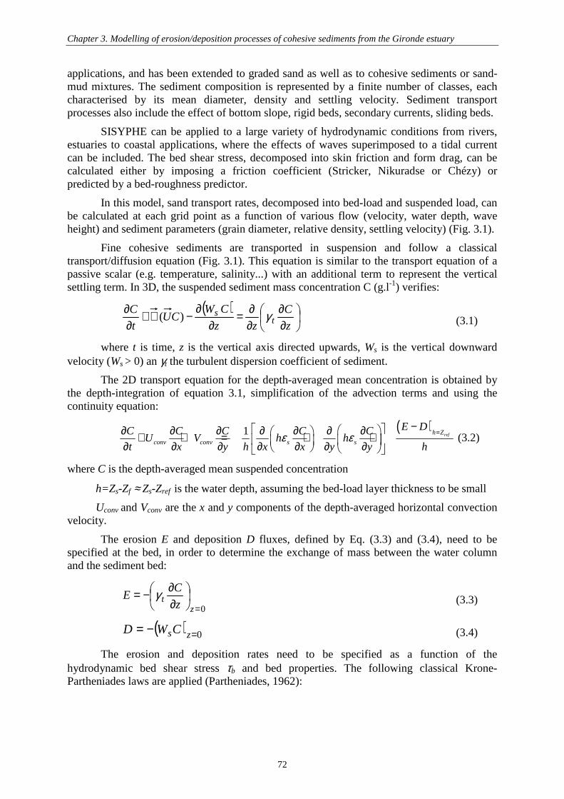
Chapter 3. Modelling of erosion/deposition processes of cohesive sediments from the Gironde estuary
72
applications, and has been extended to graded sand as well as to cohesive sediments or sand-mud mixtures. The sediment composition is represented by a finite number of classes, each characterised by its mean diameter, density and settling velocity. Sediment transport processes also include the effect of bottom slope, rigid beds, secondary currents, sliding beds.
SISYPHE can be applied to a large variety of hydrodynamic conditions from rivers, estuaries to coastal applications, where the effects of waves superimposed to a tidal current can be included. The bed shear stress, decomposed into skin friction and form drag, can be calculated either by imposing a friction coefficient (Stricker, Nikuradse or Chézy) or predicted by a bed-roughness predictor.
In this model, sand transport rates, decomposed into bed-load and suspended load, can be calculated at each grid point as a function of various flow (velocity, water depth, wave height) and sediment parameters (grain diameter, relative density, settling velocity) (Fig. 3.1).
Fine cohesive sediments are transported in suspension and follow a classical transport/diffusion equation (Fig. 3.1). This equation is similar to the transport equation of a passive scalar (e.g. temperature, salinity...) with an additional term to represent the vertical settling term. In 3D, the suspended sediment mass concentration C (g.l-1) verifies:
( )
∂∂
∂∂=
∂∂−∇+
∂∂
z
C
zz
CWCU
t
Ct
s γ)( (3.1)
where t is time, z is the vertical axis directed upwards, Ws is the vertical downward velocity (Ws > 0) an γt the turbulent dispersion coefficient of sediment.
The 2D transport equation for the depth-averaged mean concentration is obtained by the depth-integration of equation 3.1, simplification of the advection terms and using the continuity equation:
( )1 refh Z
conv conv s s
E DC C C C CU V h h
t x y h x x y y hε ε =
− ∂ ∂ ∂ ∂ ∂ ∂ ∂ + + = + + ∂ ∂ ∂ ∂ ∂ ∂ ∂ (3.2)
where C is the depth-averaged mean suspended concentration
h=Zs-Zf ≈ Zs-Zref is the water depth, assuming the bed-load layer thickness to be small
Uconv and Vconv are the x and y components of the depth-averaged horizontal convection velocity.
The erosion E and deposition D fluxes, defined by Eq. (3.3) and (3.4), need to be specified at the bed, in order to determine the exchange of mass between the water column and the sediment bed:
0=
∂∂−=
zt z
CE γ (3.3)
( ) 0=−= zsCWD (3.4)
The erosion and deposition rates need to be specified as a function of the hydrodynamic bed shear stress τb and bed properties. The following classical Krone-Partheniades laws are applied (Partheniades, 1962):

Chapter 3. Modelling of erosion/deposition processes of cohesive sediments from the Gironde estuary
73
2
2 2** *
*
1
0
b ce w ee
b ce
uE M if u u
u
E if
τ ρ τ ρ
τ τ
= − = > =
= <
(3.5)
where M is the erosion parameter (kgm-2s-1), u*e the critical erosion shear velocity (m.s-1), ceτ the critical shear stress for erosion (N.m-²) and ρw the density of water (kg.m-3).
The deposition rate is represented by the deposition law:
*
2
* **
* *
1
0
s dd
d
uD W C if u u
u
D if u u
= − <
= >
(3.6)
where Ws is the settling velocity (m.s-1) , u*d, the critical deposition velocity (m.s-1). The critical shear stress for deposition is determined equal to 2
*cd w duτ ρ= (N.m-²).
The development of cohesive sediment transport in SISYPHE is completed within this thesis by:
1) Implementation and validation of two sedimentation-consolidation models (a Gibson-based multi-layer model and a Gibson-based vertical grid model) in SISYPHE (cf. Chapter 2)
2) Validation of the cohesive sediment transport module by simulating the RTWH erosion – deposition experiments (Chapter 3)
There are many factors affecting the erosion-deposition parameters of cohesive sediments, including hydrodynamics, sediment characteristics (type of mud, its concentration and its composition - Migniot, 1968), vertical sediment bed structure and chemical and biological influences.
Here, the consolidation process is incorporated in SISYPHE by representing the bed with a number of layers, each having a specific thickness, concentration, and critical shear stress for erosion. In SISYPHE, the erosion occurs on the uppermost layer. Depending on the settling state of the sediment, the erosion rate can be high (un-consolidated sediment) or low (consolidated sediment).
On the other hand, the biological factors can affect the erodibility of sediments in a negative (decreasing sediment stability) or positive (increasing sediment stability) way. A positive effect on sediment stability is described as biostabilisation, which is defined as “a decrease in sediment erodibility caused directly or indirectly by biological action”. One of the most common negative effects of biological action is the reworking of the sediment by organisms known as bioturbation (a reworking or packaging of the sediment bed by organisms) (Paterson, 1997).
The settling velocity is also itself a function of the suspended concentration and the state of flocculation.
These parameters must be determined experimentally. Since there are many physical parameters affecting erosion and deposition processes, the determination of these parameters is crucial, in particular for the Gironde estuary which is characterized by a large heterogeneity in the sediment bed composition (see § 1.3 for more details on sediment bed distribution).
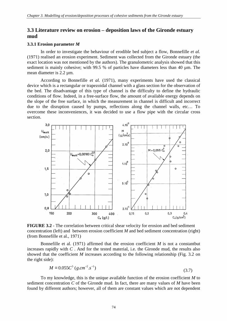
Chapter 3. Modelling of erosion/deposition processes of cohesive sediments from the Gironde estuary
74
3.3 Literature review on erosion – deposition laws of the Gironde estuary mud 3.3.1 Erosion parameter M
In order to investigate the behaviour of erodible bed subject a flow, Bonnefille et al. (1971) realised an erosion experiment. Sediment was collected from the Gironde estuary (the exact location was not mentioned by the authors). The granulometric analysis showed that this sediment is mainly cohesive; with 99.5 % of particles have diameters less than 40 µm. The mean diameter is 2.2 µm.
According to Bonnefille et al. (1971), many experiments have used the classical device which is a rectangular or trapezoidal channel with a glass section for the observation of the bed. The disadvantage of this type of channel is the difficulty to define the hydraulic conditions of flow. Indeed, in a free-surface flow, the amount of available energy depends on the slope of the free surface, in which the measurement in channel is difficult and incorrect due to the disruption caused by pumps, reflections along the channel walls, etc… To overcome these inconveniences, it was decided to use a flow pipe with the circular cross section.
FIGURE 3.2 - The correlation between critical shear velocity for erosion and bed sediment concentration (left) and between erosion coefficient M and bed sediment concentration (right) (from Bonnefille et al., 1971)
Bonnefille et al. (1971) affirmed that the erosion coefficient M is not a constantbut increases rapidly with C . And for the tested material, i.e. the Gironde mud, the results also showed that the coefficient M increases according to the following relationship (Fig. 3.2 on the right side):
3 2 10.055 ( . . )M C g cm s− −= (3.7)
To my knowledge, this is the unique available function of the erosion coefficient M to sediment concentration C of the Gironde mud. In fact, there are many values of M have been found by different authors; however, all of them are constant values which are not dependent

Chapter 3. Modelling of erosion/deposition processes of cohesive sediments from the Gironde estuary
75
on sediment concentrations. According to Phan (2002), the erosion coefficient M depends on the settling state of muddy bed, and is highly variable. Hence, this result of Bonnefille et al. (1971) significanty improves existing erosion models of the Gironde mud
Compared to other proposed constant values of M, this result is close to the values obtained by Harrison and Owen (1971) and by Migniot & Bellessort (1970). The formers proposed the value M = 1.7×10⁻⁴ g.cm-2.s-1 for an unknown concentration, but estimated equal to 200 g/l - the limited value obtained after 3 days of consolidation. This value of M corresponds to the concentration C = 140 g/l on Fig. 3.2. The latter proposed the value M = 4×10⁻⁴ g.cm-2.s-1 for mud concentration of 200 g/l which is equal to the value proposed by Bonnefille et al (1971) as can be observed in Fig. 3.2.
3.3.2 Critical erosion velocity (critical shear stress for erosion)
Regarding the critical erosion velocity, a comparison between the results of Migniot & Bellessort (1970), Cormault (1971) and Bonnefille et al. (1971) was given by Castaing (1981) in his PhD thesis.
According to him, similar experiments have shown certain limitations in a linear relationship between critical velocity for erosion * eu and sediment concentration C. Here are
three formulae developed from experiments in channels on the Gironde mud.
The first formula of Migniot & Bellessort (1970) has the form:
3* ( / ) 7.5 10eu cm s C−= × × with 200 450 /C g l≤ ≤ (3.8)
The second is the work of Cormault (1971) at Laboratoire National d’Hydraulique (L.N.H), which is presented in Fig. 3.3:
* ( / )eu cm s = 3 6 25.5 10 2.6 10C C− −× × + × × with 150 460 /C g l≤ ≤ (3.9)
FIGURE 3.3 - Critical erosion velocity of the Gironde mud versus sediment concentration (adapted from Cormault, 1971)
The third one is the experimental results of Bonnefille et al. (1971), which is illustrated in Fig. 3.2 on the left side:
1.2* ( / ) 0.00183eu cm s C= × for 192 / 362 /g l C g l< < (3.10)
u*e (cm/s)
Concentration (g/l)
Experimental limit of Cormault
u*e (cm/s)
Concentration (g/l)
Experimental limit of Cormault

Chapter 3. Modelling of erosion/deposition processes of cohesive sediments from the Gironde estuary
76
Most recently, in the “Navigation channel and Harbour Works” report of G.P.M.B (2002) a synthesis on different measured values of parameters was produced to establish a general function between the required friction velocity to start the erosion of a mud of a given concentration and the concentration. It is worth noting that this formula is generalised based on previous experimental works.
3(4.95.10 0.91)* ( / ) Ceu cm s e
− −= (3.11)
The limit of validity is relatively accurate. Cormault (1971) performed his experiments in a mud tube using mud of concentration ranging from 150 to 460 g/l (Fig. 3.3). Strictly speaking, this formula can only be used within this limit. Beyond 460 g/l, unpublished experiments of Laboratoire Central d’Hydraulique de France (L.C.H.F) show that the variation is no longer linear, * eu varies as a function of C². In fact according to Migniot &
Bellessort (1970), in order to erode a mud of concentration of 490 g/l, a critical erosion velocity * eu equal to 3.8 cm/s is needed, or to erode a mud of concentration of 540 g/l, * eu
needs to be greater than 6.2 cm/s.
3.3.3 Settling velocity
The settling velocity is the main parameter for sediment deposition flux modelling. The settling velocity is mainly determined by analysing the vertical distribution of concentrations in laboratory flumes. These methods give values varying between 0.1 and 5 mm/s for concentrations between 0.1 and 20 g/l (G.P.M.B 2002).
Effect of sediment concentration and salinity
FIGURE 3.4 - Measured settling velocity of the Gironde mud in quiescent condition, results of Migniot & Bellessort, 1970 (adapted from Davesne and Kovacs, 1979)
Sett
li ng
v elo
cit y
(m
m/s
)
Concentration (g/l)
Salinity of 5 ‰
Salinity (‰)
a) Influence of concentration b) Influence of salinity
Sett
li ng
v elo
cit y
(m
m/s
)
Concentration (g/l)
Salinity of 5 ‰
Salinity (‰)
a) Influence of concentration b) Influence of salinity

Chapter 3. Modelling of erosion/deposition processes of cohesive sediments from the Gironde estuary
77
In an attempt to reproduce the sediment transport of the Gironde mud in a scale model, Davesne & Kovacs (1979) first revised the measured settling velocity of the Gironde mud in quiescent condition with varying concentration (Fig 3.4a) and with varying salinity (b).
The results show that in quiescent water, the higher concentration of solid particles is, the higher settling velocity is, as long as the concentration does not exceed 17 g/l. The maximum velocity sW = 0.3 mm/s is reached when the suspended concentration C is equal to
17 g/l (salinity = 5‰). Beyond 17g/l, the settling velocity decreases (Fig. 3.4a).
For a known concentration, the settling velocity increases rapidly when the salinity increases from 0 to 3 ‰ (Fig. 3.4b). The settling velocity is multiplied by a factor of 20 when the salinity increases from 0 to 3 ‰ for a concentration of 10 g/l. The rate of increase is reduced for lower concentrations ( 5 g/l or 2 g/l).
Settling velocity determination using scale model
Later, Davesne & Kovacs (1979) simulated the sediment transport in their scale model. The schematic estuary characteristics were based on the Gironde estuary. The mud was represented by a light material, the gilsonite. The gilsonite has a density of 1.036 and a mean diameter around 45 µm. And the flocculation in the area of salt intrusion was reproduced by the addition of a salt flocculent. The objective of this experiment is to reproduce the turbidity maximum as observed in in-situ conditions.
The conducted result of Davesne & Kovacs is that the turbidity maximum can only be obtained if the settling velocity of particles in the scale model is greater than 0.5 mm/s (which corresponds to a settling velocity of 3.3 mm/s in nature). This value is then considered the measured settling velocity in turbulent flow. It will be compared against the measured in-situ settling velocity in the Gironde estuary given by Gratiot et al. (2005) and Sottolichio et al. (2011) later.
Settling velocity in quiescent conditions
Boutin (1993) correlated the existing formula of settling velocity (eg. diagram of Thorn, 1981) with the measured settling velocity in settling columns and annular flume to determine the settling velocity of the Gironde mud.
Two types of equipments were used: the settling columns equipped of sampling points and the annular flume. The columns are made of Plexiglas transparent glass, thermo-formed and capped one end. They are 2.00 m high, 10 cm outer diameter, and 4 mm thick. The flume is 20 m long. It is characterised by a fluid stream of constant section. The created velocity field is of uniform turbulent type.
The sediment used was the Gironde mud, which was collected at Bassens (KP 10, see Fig. 1.1), was screened to 100mµ and was then treated with permanganate to stop the proliferation of organic matters. In his experiments, the sediment was mixed with water from Grenoble city with pH = 7.
Based on the concentration profiles, the sediment flux and the settling velocity of different sediment concentrations were calculated through the mass conservation equation. Then, applying the formula of settling velocity proposed by Thorn (1981), the parameters were calibrated by correlating the measured settling velocity values with the law of Thorn (1981). Finally, the empirical formula of settling velocity of the Gironde mud was obtained:
50.37(1 0.01 )sW C= − (3.12)

Chapter 3. Modelling of erosion/deposition processes of cohesive sediments from the Gironde estuary
78
This result gives very low settling velocity values in quiescent environment. It will be compared against the results of other authors in section 3.3.6.
Effect of turbulence
Recently, the effect of turbulence on settling velocity was examined by Gratiot et al. (2005) and Sottolichio et al. (2011). They compared measurements of settling velocity in quiescent fluid and in turbulent flow. Experiments were performed in laboratory (Gratiot et al., 2005) and in-situ (Sottolichio et al., 2011).
In both experiments, mud was sampled at the centre of the Gironde estuary, close to the Pauillac station. While in Gratiot et al. (2005), it was chemically treated to limit the effect of organic matters, and was sieved at 100 µm, Sottolichio et al. (2011) used the natural sediment. The latter authors argued that the treatment of organic matters leads to much higher flocs density than the one of natural mud, which may increases the sediment settling flux.
In Gratiot et al. (2005), laboratrory experiments were performed in quiescent fluid, applying two methods:
• For C ≤ 5 g.l-1: four tests were performed in the range [0.2, 5.0] g.l-1. The sediment settling velocity and the concentration were recorded using the INSSEV video system after being well-mixed in a grid-stirred device.
• For high SSC: they applied the Kynch’s method to determine the settling velocity based on the position of the lutocline (cf. Kynch, 1952), which separates the fluid column into two distinct layers: the dilute suspension layer above ,and the fluid mud layer below (cf. Ross & Mehta, 1989).
In turbulent fluid, sediment settling flux was investigated in a turbulent-grid experiment (Fig. 3.5) in which turbulence is created inside the tank by a diffusive mechanism. The box is a square Perspex tank of 53 cm wide and 90 cm high. For all experiments, water depth is kept at H = 40 cm. The grid is fixed horizontally at hg = 5 cm above the bottom of the tank. The oscillations were made at frequency F (3, 4 or 6 Hz) with a stroke (twice the amplitude) S = 4.5 cm.
FIGURE 3.5 - Grid-stirred experiment procedure (from Gratiot et al., 2005)
Fourteen experiments were conducted with varying suspended sediment load and grid oscillation conditions. For each run, the settling flux in the turbulent mixed layer is obtained from the estimation of the position of the lutocline and the determination of the concentration

Chapter 3. Modelling of erosion/deposition processes of cohesive sediments from the Gironde estuary
79
C in the concentrated benthic suspension (CBS) layer at equilibrium state (where the settling flux of the fluid mud mixture is balanced by the upward turbulent flux).
From the experimental results, they concluded that the turbulence only increases the settling flux when the SCC exceeds 10 g.l-1. The settling flux can then be double for the highest concentrations. Besides, hindering effects observed under quiescent conditions when the concentration exceeds approximately 10 g.l-1 are considerably reduced in highly turbulent conditions.
FIGURE 3.6 - Sketch of the frame and the position of ADVs and OBSs instruments (from Sottolichio et al., 2011)
In Sottolichio et al. (2011) the measurement instrument is sketched in Fig. 3.6 and is detailed in Sottolichio et al. (2011). This combines two Acoustic Doppler Velocimeters (ADV Vector, Nortek) and two optical turbidity sensors (OBS) fixed at different levels above the sediment bed. Two OBS turbidimeters provided SSC data.
To determine settling flux in quiescent fluid, samples of turbid water and fluid mud were taken using a Niskin bottle, and carried out onboard immediately. The results were the time dependent vertical profiles of suspended sediment concentration C(z,t) measured by Bergen Nautik multi sensor system. The settling velocity ws(h,t) at a depth h < H below water surface was calculated from the equation of mass conservation, following the procedure by You (2004). The recirculation in the tank is neglected.
Mean turbulent settling fluxes determined from the ADV measurements are also plotted in Fig. 3.7. Fluxes were obtained from co-located 32 Hz records of velocity and SSC averaged over 3 minutes and 30 seconds, respectively.
The comparison between measured settlling fluxes of Gratiot et al. (2005) and Sottolichio et al. (2011) is illustrated in Fig. 3.7. Figure 3.7a gives the obtained settling fluxes in quiescent condition (line) and in turbulent flow (dots) of Gratiot et al., while figure 3.7b and 3.7c show the settling fluxes in quiescent condition (line + crosses) and in turbulent condition averaged over 3 mins (dots), and over 30 secs (circles).
Comparing to the laboratory experiments of Gratiot et al. (2005), in situ sediment fluxes averaged over 3 minutes were smaller. As discussed above, Sottolichio et al. (2011) argued that the treatment of organic matters can lead to an increase in flocs density, hence an increase in settling flux of sediment. The results in Fig. 3.7 confirm this argument.

Chapter 3. Modelling of erosion/deposition processes of cohesive sediments from the Gironde estuary
80
Averaging turbulent fluxes and SSC over shorter periods of 30s allowed to increase the mean SSC in the CBS layer up to 100 g.l-1. However, the large discrepancy between the results of settling fluxes over 3 minutes and 30 seconds need to be clarified and further investigated.
FIGURE 3.7 - Mean settling fluxes as a function of suspended sediment concentration. a) Results of Gratiot et al. (2005). Solid line: settling fluxes φ ( in quiescent condition; dots: in turbulent conditions; b) Sottolichio et al. (2011). Crosses and solid line: quiescent water; dots: turbulent fluxes determined from in-situ ADV measurements averaged over 3 mins; c) Sottolichio et al. (2011) circles: turbulent fluxes determined from in-situ ADV measurements averaged over 30 secs (in Sottolichio et al., 2011).

Chapter 3. Modelling of erosion/deposition processes of cohesive sediments from the Gironde estuary
81
3.3.4 Critical shear stress for deposition
Conversely to the large number of erosion experiments, measurements on the critical shear stress for deposition are scarse.
Recently, G.P.M.B (2002) reported that the experiments in flume in laboratory give the critical deposition velocity of the Gironde mud of 2
* 0.7.10 /du m s−= , which corresponds
to * 0.05 / ²d N mτ = . However the flume dimensions, measuring technique and mud treatment
procedure were not given in the report. Therefore, this value cannot be considered reliable.
3.3.5 Erosion-deposition parameters from existing models
In the 2DH depth-integrated model of Sottolichio (1999) the settling velocity was fixed to 1 mm/s. Using this high value, they assumed that the flocculation is implicitly taken into account. The critical shear stress for erosion and deposition were both imposed to 1 N/m². Therefore, they assumed that deposition and erosion do not occur simultaneously. It is also assumed that the hysteresis between the shear stress of erosion and deposition is minimal. This assumption is, however, not realistic since it has even been shown that deposition and erosion can take place simultaneously (Sanford and Halka, 1993, cited in Sanford, 2008).
Once deposited, the sediment is considered instantly. The erosion constant M was selected equal to 0.01 kg/m²/s, a relatively high value but fixed to ensure a strong flux of sediment in the water column. All erosion/deposition parameters were assumed to remain constant for the whole domain, which is an oversimplification of the natural heterogenieity of sediment and sediment transport processes.
FIGURE 3.8 - Longitudinal distribution of the critical bottom shear stresses and the erosion constant values (Li et al., 1995)
According to Li et al. (1995) the parameters must take a unique mean value along each cross-section in their 2DV width-integrated model (Fig. 3.8). The critical shear stress for erosion was set to 0.65 N/m² for areas of fluid mud, and equal to 2 N/m² for sandy areas. The critical shear stress for deposition* dτ and the erosion constant M were respectively taken from
0.3 - 0.5 N/m², and 2.10-3 – 3.10-3 kg/m²/s (fig 3.10). The settling velocity was calculated according to the results given by Thorn (1981) for Severn estuary:

Chapter 3. Modelling of erosion/deposition processes of cohesive sediments from the Gironde estuary
82
1.3
3 4.65
( / ) 0.513 3 /
( / ) 2.6 10 (1 0.008 ) 3 / 100 /
s
s
W mm s C C g l
W mm s C g l C g l−
= × ≤
= × × − < < (3.13)
More recently, Phan (2002) set up a 3D sediment transport model for the Gironde estuary based on the previous work of Li et al. (1995). The principle to calibrate deposition and erosion parameters was similar to the study of Li et al. (1995). The critical shear stress for erosion at the bed *eτ was characterised by the nature of bed material. The smaller values
correspond to fluid mud, and higher values for sandy bed. In his model, *eτ was chosen to be
varied between 0.7 and 2.5 N/m², depending on the nature of the bed. The erosion coefficient M was also chosen depending on the nature of the bed, and was varied in the estuary. The obtained values were between 5.10-4 and 1.8.10-3 kg/m²/s. The critical shear stress for deposition * dτ was selected between 0.1 and 0.4 N/m².
3.3.6 Analysis on erosion/deposition parameters
Erosion and deposition parameters from previous (modelling and experimental) studies of the Gironde mud are synthetised in Tables 3.1 and 3.2.
TABLE 3.1 - Review on erosion parameters of the Gironde mud Authors C (g.l-1) u*
e (cm.s-1) ττττ*e (N.m-²) M (g.cm-².s-1)
EXPERIMENT
Bonnefille et al. (1971)
192 < C < 362 1.20.00183 C×
30.055 C×
Cormault (1971) 150 < C < 460 3 6 25.5 10 2.6 10C C− −× × + × ×
2×10⁻³
Migniot & Bellessort (1970)
200< C < 450
37.5 10 C−× 4×10⁻⁴ for C = 200 g/l
Harrison & Owen (1971)
1.7× 10⁻⁴ for C = 200 g/l
G.P.M.B (2002) 3(4.95 10 0.91)Ce−× × −
MODEL
Li et al. (1995) 0.65 ÷ 2.0 2.10-4 ÷ 3.10-3 Sottolichio (1999) 1.0 0.001 Phan (2002) 0.70 ÷ 2.5 5.10-5 ÷ 1.8.10-4

Chapter 3. Modelling of erosion/deposition processes of cohesive sediments from the Gironde estuary
83
TABLE 3.2 - Review on deposition parameters for the Gironde mud Authors C (g.l-1) Ws (mm.s-1) u*
d (cm.s-1) ττττ*d (N.m-²)
EXPERIMENT Davesne & Kovacs (1979)
TM* 3.3
Migniot (1984) C = 17 0.3 Boutin (1993) 50.37(1 0.01 )C− ×
G.P.M.B (2002) 0.1 < C < 20 0.1 - 5.0 0.7 0.05 MODEL Li et al. (1995) C < 3
C = 3 C > 3
1.30.513 C× 2.0
3 4.652.6 10 (1 0.008 )C−× × − ×
Sottolichio (1999) 1.0 1.0 Phan (2002) 0.1 - 0.4 *: Turbidity maximum
Experimental results are compared on Fig 3.9 for the erosion coefficient M, Fig 3.10 for the critical erosion velocity * eu and Fig 3.11 for the settling velocity Ws versus sediment
concentration C. In those figures, symbols represent values which were defined at a constant concentration, while continuous lines represent values calculated from semi-empirical formulae depending on concentration.
FIGURE 3.9 - Erosion coefficient M versus sediment concentration C ( Gironde mud)
The first graph (Fig 3.9) presents the relationship between the erosion coefficient M and bed concentration C. Among of four authors, only Bonnefille et al. (1971) gives the dependence of M as a function of C, others only determined one value of M for a known C (Harrison & Owen, 1971, Migniot & Bellessort, 1970) or did not precise the applied range of sediment concentration (Cormault, 1971). It can be observed that the two values of M given by Harrision & Owen and Migniot & Bellessort agree with the M-curve provided by Bonnefille et al.(1971). Furthermore, it was confirmed by many authors that M should vary as
0,00E+00
5,00E-04
1,00E-03
1,50E-03
2,00E-03
2,50E-03
3,00E-03
100 150 200 250 300 350 400 450 500C (g/l)
M (
g/cm
2 /s)
Bonnefille et al. (1971)
Cormault (1971)
Harrison & Owen (1971)
Migniot & Bellessort (1970)

Chapter 3. Modelling of erosion/deposition processes of cohesive sediments from the Gironde estuary
84
a function of concentrations and on the consolidation state of the mud bed. Therefore, the results of Bonnefille et al. (1971) can be considered reliable for sediment transport modelling purpose.
FIGURE 3.10 - Critical erosion velocity versus sediment concentration C for the Gironde mud
FIGURE 3.11 - Settling velocity Ws versus sediment concentration C in quiescent water (Gironde mud)
In the case of critical erosion velocity* eu , an agreement is observed in Fig. 3.10
between plotted lines. However, (almost) all relations between the critical erosion velocity and sediment concentration are only valid for concentrations smaller than 460 g/l. This can be explained by the fact that, in laboratory conditions, the consolidation time is much shorter than in nature (e.g several hours compared to several years), therefore, the maximum
0
1
2
3
4
5
6
100 150 200 250 300 350 400 450 500
C (g/l)
u*e
(cm
/s)
Migniot & Bellessort (1970)
Bonnefille et al. (1971)
Cormault (1971)
G.P.M.B (2002)
Eisenbeis & Roger (2011)
0,001
0,01
0,1
1
0,1 1 10 100C (g/l)
Ws
(mm
/s)
Boutin (1993)Migniot & Bellessort (1970)Gratiot et al. (2005)Sottolichio et al. (2011)
Flocculation Hindering

Chapter 3. Modelling of erosion/deposition processes of cohesive sediments from the Gironde estuary
85
concentration that a sediment can attain in laboratory (460 g/l) can be lower than the value in nature conditions. On the other hand, unpublished experiments of Migniot & Bellessort (1970) affirmed that beyond 500 g/l the relation is no longer linear, but varies as a function of C², but the empirial coefficient is still un-defined. Therefore, within this study, we assume that these functions can be applied for concentrations greater than 460 g/l.
Figure 3.11 shows the relationship between the settling velocity Ws and sediment concentration C at quiescent condition, given by Migniot & Bellessort (1970), Boutin (1993), Gratiot et al. (2005) and Sottolichio et al. (2011). Among of them, the results of Boutin (1993) only concern the hindered settling regime. In comparison to the other experimental results, Boutin gives much lower settling velocity at high concentrations. Similar, for lower range of concentrations, the results provided by Migniot & Bellessort (1970) are much smaller than the values provided by Gratiot et al. (2005) and Sottolichio et al. (2011). The recent results provided by Gratiot et al. (2005) and Sottolichio et al. (2011) are close to each other, which give the maximum settling velocity of 0.5 mm/s for concentration of 5 g/l. However, because all these experiments were performed in quiescent conditions, these results cannot be applied in morphodynamic modelling where turbulence plays an important role in cohesive sediment transport.
FIGURE 3.12 - Settling velocity Ws versus sediment concentration C in turbulent environment (Gironde mud)
The settling velocity obtained in turbulent environments is given in figure 3.12. Comparing figure 3.11 and 3.12, the effect of turbulence is to increase the settling velocity. For example, at sediment concentration of 5 g.l-1, the settling velocity measured in quiescent water is about 0.5 mm/s, whereas in turbulent flow, this value can attain 3.3 mm/s approximately. This high value corresponds to the measured settling velocity in scale model of Davesne & Kovacs (1979).
Conclusion
Based on the above comparison and analysis, it can be concluded that the measurement results in laboratories are in fairly good agreeement, in particular for the critical velocity for erosion. However, a gap is observed between measurements in laboratories and in-situ through the experiments of Gratiot et al. (2005) and Sottolichio et al. (2011).
0,001
0,01
0,1
1
10
0,1 1 10 100C (g/l)
Ws
(mm
/s)
Gratiot et al. (2005)Sottolichio et al. (2011) averaged 3 minSottolichio et al. (2011) averaged 30 sec

Chapter 3. Modelling of erosion/deposition processes of cohesive sediments from the Gironde estuary
86
Furthermore, the discrepancy between experimental parameters and model parameters can be observed from table 3.1 and 3.2, in particular for critical velocity for erosion and deposition.
Considering the large variability in the parameters from the litterature, a calibration step is necessary, in order to verify that the selected modelling tool (SISYPHE) is able to correctly simulate the erosion/deposition processes, and that the selected set of erosion/parameters is adapted to the type of sediment and modelling tool.
3.4 Model calibration of erosion-deposition parameters Experiments were performed in 2011 at the RWTH laboratory (Germany), in order to
investigate the erosion and deposition behaviour of the Gironde estuary mud.
Measurements have been performed on pure mud issued from the Patiras bank in the central part of the estuary. The new experimental data was presented in § 1.5. This section only presents the model validation against the measurements. The objective of this validation test is to show that SISYPHE is able to represent the physical processes regarding the erosion and deposition. A comparison between the results of previous experiments and the new one is also made.
In this section, three experiments are simulated. The first simulation deals with a settling column with the objective of calculating the settling velocity. The two next simulations are to calibrate the parameters by producing the erosion and deposition tests. All simulations are carried out using SISYPHE (User manual -Villaret, 2010 ).
3.4.1 Settling velocity validation
3.4.1.1 Numerical parameters To model the settling experiment, we consider a uniform domain at rest with an initial
water depth of 1 m (for simplicity we assume a square domain of 20 m x 20 m with 4624 nodes, similar results would be obtained with a different geometry). All boundaries are solid walls. The initial concentration is set at 6.6 g/l and the bed concentration is set equal to 100 g/l. A time step of 1 second is selected.
Geometry: 20 m x 20 m
Mesh: 4624 nodes, size: 0.3 m
Boundaries: Solid walls
Time data: Time step = 1 sec.
Simulation duration : 6000 sec
In the model , we assume that:
• There is no critical shear stress for deposition ( the critical deposition velocity is set equal to 1000 m/s). This means that deposition always occurs.
• The erosion process is neglected by setting the erosion coefficient M equal to 0.
• The horizontal diffusion in the transport equation (3.2) is neglected in comparison to vertical diffusion term.
3.4.1.2 Settling simulation in quiescent fluid
Following Thorn (1981) we assume the general formulae:
(1 )
bs t
s t
W a C C C
W C C Cδα β= × <
= × − × > (3.15)
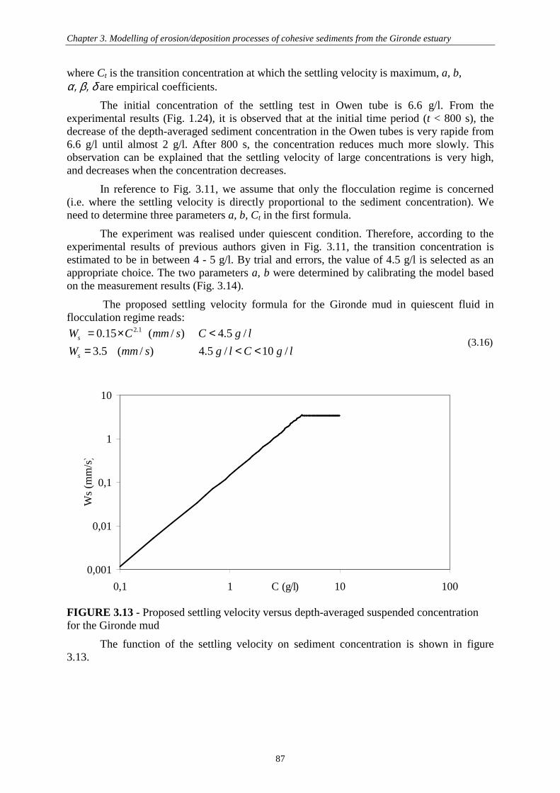
Chapter 3. Modelling of erosion/deposition processes of cohesive sediments from the Gironde estuary
87
where Ct is the transition concentration at which the settling velocity is maximum, a, b, α, β, δ are empirical coefficients.
The initial concentration of the settling test in Owen tube is 6.6 g/l. From the experimental results (Fig. 1.24), it is observed that at the initial time period (t < 800 s), the decrease of the depth-averaged sediment concentration in the Owen tubes is very rapide from 6.6 g/l until almost 2 g/l. After 800 s, the concentration reduces much more slowly. This observation can be explained that the settling velocity of large concentrations is very high, and decreases when the concentration decreases.
In reference to Fig. 3.11, we assume that only the flocculation regime is concerned (i.e. where the settling velocity is directly proportional to the sediment concentration). We need to determine three parameters a, b, Ct in the first formula.
The experiment was realised under quiescent condition. Therefore, according to the experimental results of previous authors given in Fig. 3.11, the transition concentration is estimated to be in between 4 - 5 g/l. By trial and errors, the value of 4.5 g/l is selected as an appropriate choice. The two parameters a, b were determined by calibrating the model based on the measurement results (Fig. 3.14).
The proposed settling velocity formula for the Gironde mud in quiescent fluid in flocculation regime reads:
2.10.15 ( / ) 4.5 /
3.5 ( / ) 4.5 / 10 /s
s
W C mm s C g l
W mm s g l C g l
= × <= < <
(3.16)
FIGURE 3.13 - Proposed settling velocity versus depth-averaged suspended concentration for the Gironde mud
The function of the settling velocity on sediment concentration is shown in figure 3.13.
0,001
0,01
0,1
1
10
0,1 1 10 100C (g/l)
Ws
(mm
/s)

Chapter 3. Modelling of erosion/deposition processes of cohesive sediments from the Gironde estuary
88
FIGURE 3.14 - Comparison between modelled and measured depth-averaged concentration versus time
Figure 3.14 presents the model results against measurements for the time-varying depth-averaged concentration. A good agreement is observed between measurements and model in figure 3.14 for the proposed formula (3.16). So we consider the proposed formula of settling velocity for low concentration to be satisfactory.
However, we emphasise that the objective of this simulation is to validate the ability of SISYPHE in physical modelling the settling of sediments. This result cannot be applied directly in morphodynamic modelling where the flow field is turbulent.
3.4.2 Numerical simulation of erosion experiment
3.4.2.1 Numerical parameters TABLE 3.3 – Assumptions made in numerical simulation of erosion-deposition experiment Experiment Simulation Flume Annular Straight Secondary currents Yes No Free surface No Fixed free surface Consolidation Yes No
A straight channel of 1 m width and 16 m length, with 891 nodes is built to model the erosion and deposition processes. The water level is set equal to 0.35 m as in the experiment.
Intial condition: a sediment concentration of 1 g/l is set up as observed in the measurement (see § 1.7).
Boundary condition: the two ends of the channel are considered as liquid boundaries with free evolution.
In order to reproduce the time-varying bottom shear stress, the flow mean velocity U is calculated using the following formula:
0
1
2
3
4
5
6
7
0 1000 2000 3000 4000 5000
Time (s)
C(g/l)
Measurement
Model
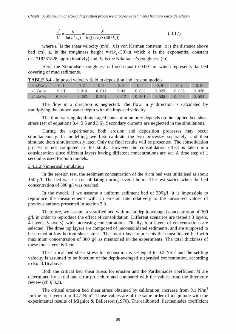
Chapter 3. Modelling of erosion/deposition processes of cohesive sediments from the Gironde estuary
89
*
0ln( / ) ln(( / ) (30 / ))s
u
U z z z e k
κ κ= =×
² ² ² ² ( 3.17)²
where u* is the shear velocity (m/s), κ is von Karman constant, z is the distance above bed (m), z0 is the roughness height = ( / 30)se k in which e is the exponential constant
(=2.718281828 approximativly) and ks is the Nikuradse’s roughness (m).
Here, the Nikuradse’s roughness is fixed equal to 0.001 m, which represents flat bed covering of mud sediments.
TABLE 3.4 - Imposed velocity field in deposition and erosion models τb²(N/m )² 0.1² 0.2² 0.3² 0.4² 0.5² 0.6² 0.7² 0.8²
u
*²
(m/s)² 0.01² 0.014² 0.017² 0.02² 0.022² 0.025² 0.026² 0.028²
U²(m/s)² 0.206² 0.292² 0.357² 0.412² 0.461² 0.505² 0.546² 0.584²
The flow in x direction is neglected. The flow in y direction is calculated by multiplying the known water depth with the imposed velocity.
The time-varying depth-averaged concentration only depends on the applied bed shear stress (set of equations 3.4, 3.5 and 3.6). Secondary currents are neglected in the simulations.
During the experiments, both erosion and deposition processes may occur simultaneously. In modelling, we first calibrate the two processes separately, and then simulate them simultaneously later. Only the final results will be presented. The consolidation process is not computed in this study. However the consolidation effect is taken into consideration since different layers having different concentrations are set. A time step of 1 second is used for both models.
3.4.2.2 Numerical simulation
In the erosion test, the sediment concentration of the 4 cm bed was initialised at about 150 g/l. The bed was let consolidating during several hours. The test started when the bed concentration of 300 g/l was reached.
In the model, if we assume a uniform sediment bed of 300g/l, it is impossible to reproduce the measurements with an erosion rate relatively to the measured values of previous authors presented in section 3.3.
Therefore, we assume a stratified bed with mean depth-averaged concentration of 300 g/l, in order to reproduce the effect of consolidation. Different scenarios are tested ( 3 layers, 4 layers, 5 layers), with increasing concentrations. Finally, four layers of concentrations are selected. The three top layers are composed of unconsolidated sediments, and are supposed to be eroded at low bottom shear stress. The fourth layer represents the consolidated bed with maximum concentration of 300 g/l as mentioned in the experiments. The total thickness of these four layers is 4 cm.
The critical bed shear stress for deposition is set equal to 0.3 N/m2 and the settling velocity is assumed to be function of the depth-averaged suspended concentration, according to Eq. 3.16 above.
Both the critical bed shear stress for erosion and the Partheniades coefficient M are determined by a trial and error procedure and compared with the values from the litterature review (cf. § 3.3).
The critical erosion bed shear stress obtained by calibration, increase from 0.1 N/m2 for the top layer up to 0.47 N/m2. Those values are of the same order of magnitude with the experimental results of Migniot & Bellessort (1970). The calibrated Partheniades coefficient

Chapter 3. Modelling of erosion/deposition processes of cohesive sediments from the Gironde estuary
90
M also varies with the concentration of the bed layer and results are summarized in Table 3.5. These values are equal to the measured values of Bonnefille et al. (1971), except for the last value. A possible explanation is that the parameters of the last layer represent the “mass-erosion”, which was not reported in previous experiments.
Erosion of cohesive soils refers to surface erosion (floc erosion), whereby individual particles or small aggregates are removed from the soil mass by hydrodynamic forces such as drag and lift. Mass erosion is determined by the soil’s undrained strength, or yield strength. Mass erosion occurs when the yield strength is exceeded such as a slip failure of a streambank or when large flakes of soil are eroded from the streambed. Studies have shown that there is a strength difference of one to three orders of magnitude between erosional strength and yield strength.
TABLE 3.5 - Bed structure and attached parameters in erosion model Layer Concentration (g/l) Thickness (cm) τ*e (N/m²) M(kg/m²/s) 1 150 0.4 0.1 1.86×10⁻³ 2 200 0.7 0.22 4.4×10⁻³ 3 250 0.4 0.35 8.0×10⁻³ 4 300 2.5 0.47 0.132
FIGURE 3.15 - Comparison between modelled and measured depth-averaged concentration in erosion test
Figure 3.15 presents a comparison between model results (in black) and measurements for the time-varying depth-averaged concentration. Using the calibrated values of the erosion parameters, we can achieve good agreement between the model results and measurement. Or the model is able to represent the two types of erosion which were mentioned in the experiment: “floc-erosion” and “mass-erosion”.
0
4
8
12
16
20
24
28
32
36
0 3600 7200 10800 14400 18000 21600 25200 28800
Time [s]
C (
g/l)
Measurement
Model
Floc erosion
Mass erosion

Chapter 3. Modelling of erosion/deposition processes of cohesive sediments from the Gironde estuary
91
3.4.3 Simulation of the deposition test
In the experiment, the deposition test was started after the occurrence of mass erosion, when the depth-averaged concentration reached 33.8 g/l and remained constant. This phenomenon can be explained either by the fact that the water column is saturated with suspended sediment or that the whole sediment bed layer is eroded.
Our numerical results confirm the latter hypothesis. At the end of the erosion test, all 4 cm-thickness of sediment bed is eroded, and there is no more sediment on the bottom.
In the simulation of the deposition experiment, the initial and boundary concentrations are fixed at 33.8 g/l as in the experiment. Because the information on bed sediment is not given, the bed concentration is fixed at 300 g/l since this is not an important parameter in this validation test.
As described in the measurement, the settling starts when the bottom shear stress is lower than 0.3 N/m². Within the first five hours (bedτ = 0.8-0.3 N/m²), there is no deposition.
During the next hour, it falls slowly, and then decreases sharply within 2 hours until the end of the test. From this analysis, the critical bed shear stress for deposition is assumed to be equal to 0.3 N/m², then the critical deposition velocity in the model is set equal to 0.016 m/s.
At the beginning of the deposition test, the high turbulent flow can induce the flocs break-up, leading to a reduction of the settling velocity . In the model, the settling velocity is calibrated equal to 30 µm/s at the first stage (6th hour) and rises up to 45 µm/s at the second stage (7th and 8th hour). These small values correspond to the settling velocity of primary mud particles.
FIGURE 3.16 - Comparison between modelled and measured concentration in deposion test
The calculated depth-averaged concentrations are compared against the measured values as seen in Fig. 3.16. In this figure, the decrease of the modelled concentration shows two steps as in the measurements. In general, the model captures well the decrease in the depth-averaged concentration. However, at t = 54400 s, after descending continuously, the
20
24
28
32
40000 47200 54400Time (s)
C (
g/l)
Measurement
Model

Chapter 3. Modelling of erosion/deposition processes of cohesive sediments from the Gironde estuary
92
depth-averaged concentration increases slightly and then continues to decrease. This is not observed in the model result. This can be explained by the fact that the previously deposited sediment is then eroded, which brings more sediment up into the water column. In the model, if we fixe the sediment bed concentration to a constant value of 300 g/l, erosion cannot take place at low bottom shear stress. Only the multi-layer bed structure, presenting a top layer of soft bed material, can succesfully reproduce the observed time-varying concentration, during the deposition experiment.
3.5 Conclusions The erosion and deposition laws are essential to calculate the bed evolution and
concentration in morphodynamic models. Parameters of these laws depend on the type of mud, its concentration and its composition. The settling velocity is itself also a function of concentration of the suspension and the state of flocculation. These parameters must be determined experimentally.
Sediment in the Gironde estuary is highly heterogeneous, and characterised by an alternate presence of pure sand (or sand dominant), pure mud (or mud dominant), (random debris) and sand-mud mixture. Several 2D or 3D hydro-sedimentary models have been constructed for Gironde estuary, however, the selected erosion/deposition parameters show a large variability (particularly in the choice of the Partheniades coefficient M and settling velocity Ws) based on a literature review. This can be explained by the high heterogeneity in the sediment bed composition as well as the use of different experimental device and possibly unreliable or not well defined experimental protocols.
To overcome this lack, the new experimental tests on the erosion and deposition processes were realised, which have been simulated to calibrate parameters. The good agreement between measured and modelled erosion and deposition fluxes was obtained . This gives access to better model the morphodynamic of the Gironde cohesive sediment which is presented in chapter 4.

Chapter 3. Modelling of erosion/deposition processes of cohesive sediments from the Gironde estuary
93
Intentionally left blank

Laboratoire d’Hyraulique Saint – Venant, Université Paris-Est
(Unité de Recherche commune entre EDF R&D, le CETMEF, et l’Ecole des Ponts Paris-Tech)
Chapter 4: Application to the morphodynamic modelling of the Gironde estuary Contents ___________________________________________________________________________
4.1 Introduction _________________________________________________________ 95
4.2 Review of existing sediment transport and morphodynamic models of the Gironde estuary ________________________________________________________________ 96
4.3 Criteria to assess model accuracy _______________________________________ 99
4.4 Presentation of the Telemac system _____________________________________ 100
4.5 Large scale hydrodynamic model of the Gironde estuary ___________________ 103
4.6 Cohesive sediment transport model _____________________________________ 109
4.7 Calibration of erosion/deposition parameters ____________________________ 110
4.8 Initialisation of sediment bed structure _________________________________ 112
4.9 Validation on depth-averaged suspended concentration measurements _______ 120
4.10 Morphodynamic modelling __________________________________________ 122
4.11 Discussion and conclusions ___________________________________________ 129
___________________________________________________________________________

Chapter 4. Application to the morphodynamic modelling of the Gironde estuary
95
4.1 Introduction Most estuaries and bays located on the French Atlantic seaside have endured strong
alluvial bed evolutions in the last decades. These bed evolutions may affect the morphodynamic equilibrium, with important consequences on various economical activities and environmental issues. The Gironde is a highly dynamical macro-tidal estuary characterized by complex geo-morphology, high turbidity and heterogeneous sediment distribution (Allen, 1972, Castaing, 1981). This estuary has been studied for many years for numerous applications: dredging management of the navigation channel from the mouth of the estuary down to the harbour of Bordeaux (second harbour in France), maintenance of the cooling system of the Blayais nuclear power plant (located 50 km downstream of Bordeaux, in the central part), flood prevention...
Most attention has been paid to the tide propagation (Huybrechts et al., 2012a) and the position of turbidity maximum in the estuary (Li et al., 1995, Sottolichio et al. 2011). Suspended sediment transport models have been developed in order to reproduce the position of turbidity maximum as a function of river discharges and tidal amplitude (Sottolichio & Castaing, 1999, Cancino & Neves, 1999, Li et al., 1995, Phan, 2002, Benaouda, 2008, Nguyen et al., 2009). The position of turbidity maximum and its extension vary seasonally: it moves upstream of Pauillac during summer droughts, and can be flushed out during flood events at the end of winter and spring time (Sottolichio & Castaing, 1999).
Under the combined action of tidal currents, waves and flow rates, large amounts of sediments can be transported as bed load and suspended load. From historical bathymetric records made by the ‘Grand Port Maritime de Bordeaux’ (G.P.M.B), drastic bed evolutions are observed in the central part of the estuary. Such bed evolutions may strongly affect the morphodynamic equilibrium. (cf Chapter 1)
Few models address the morphodynamic issues in this complex estuarine domain (Chini & Villaret, 2007; Villaret et al., 2012, Huybrechts et al., 2012b). For a schematized tidal basin, Hibma et al. (2004) showed that a 2D depth-averaged model (2DH) is sufficient to represent the morphological development of channel-shoal systems, in particular when the near bed velocities can be related to the depth-averaged velocity. The validity of the 2D assumption has been examined by Chini & Villaret (2007) based on ADCP velocity measurements taken in the central part of the estuary (on July 2006). According to their study, the depth-averaged velocity and the bottom velocity measured at 10 cm above the bed are in the same direction and their intensities proportional. The 2D (depth-averaged) hydrodynamic model can therefore be considered as a good compromise between model accuracy and CPU time for large scale and medium term morphodynamic applications.
This work attempts to develop a realistic 2D morphodynamic model which can be applied to predict the sediment dynamics and medium term bed evolution in the central part of the estuary. This is where drastic bed evolutions have been reported as a result of sand banks formation and secondary mid-channel deposit. As mentioned in Chapter 1, the Gironde estuary is composed of three types of sediments, non-cohesive sediments, cohesive sediments and sediment mixtures (cf. section 1.3.3). Previous large scale morphodynamic models assume purely non-cohesive sediments, either uniform (Chini & Villaret, 2007) or graded (Villaret et al., 2012, Huybrechts et al., 2012b). This is the first attempt to introduce cohesive sediment behaviour in morphodynamic modelling.
However, since the dredging and disposal strategy (see § 1.2.2), which affects the morphological developments of the Gironde estuary, is not accounted for in the model, and

Chapter 4. Application to the morphodynamic modelling of the Gironde estuary
96
due to other simplifying assumptions made in the model (neglect of wind, historical events, extreme events), the objectives of this study are then restricted to:
1. Modelling morphodynamic development tendency in the central part of the Gironde estuary
2. Evaluating the consolidation effects in long-term cohesive sediment transport modelling.
This chapter is organised as follows: we start in section 4.2 with a review of existing sediment transport and morphodynamic models of the Gironde estuary. Two criteria will be applied, the RMAE and BSS, to evaluate the model accuracy, as detailed in section 4.3. Section 4.4 presents the Telemac system and the 2DH modules Telemac-2D/Sisyphe which will be applied. The large scale hydrodynamic model of the Gironde estuary developed by Huybrechts et al. (2010) is presented in 4.5. The cohesive sediment transport model is given in section 4.6. In section 4.7, we discuss the calibration of the cohesive sediment transport model results. The initialization of the bed structure is considered an essential part in cohesive sediment transport modelling as described in section 4.8. A sensitivity analysis of model results on the various model parameters (erosion/deposition law, cohesive bed structure, and consolidation effects) is also addressed at the end of this section. The next two sections present the model results. In section 4.9, the calculated suspended sediment concentrations are compared with measurements. The next section 4.10 presents the morphodynamic model results including its calibration for the period (1995-2000) and validation for the period (2000-2005). A comparison with the non-cohesive morphodynamic model developed by Huybrechts et al. (2012a) is also given for the calibration step. The limitations of the present 2DH approach are discussed in section 4.11 where we draw the lines for future development.
4.2 Review of existing sediment transport and morphodynamic models of the Gironde estuary Review on sediment transport models
In 1995, Li et al. (1995) developed a two dimensional vertical (2DV) model in which the hydrodynamic, the sediment transport and the saline intrusion are coupled. It simulated the sediment transport and the formation and deplacement of turbidity maximum in the Gironde estuary during a period of 5 days for a realistic tidal condition. The model used a “k-L” turbulence model. The erosion and deposition fluxes were calculated using the formulae of Partheniades and Krone and Einstein. The movement of turbidity maximum was correctly simulated. However this type of model (2DV) induces some disadvantages such as: the difference on velocity on the cross section in very large areas cannot be simulated; the residual circulation in the horizontal plane cannot be taken into account; the erosion and deposition fluxes are not related to the nature of the bed since in a 2DV model, the topography of the bed is not account for.
In order to overcome the weaknesses of 2DV models, 3D models have been used. Cancino and Neves (1999) developed and applied a 3D model of sediment transport of the Gironde estuary to reproduce a situation observed in 1994 during a tidal cycle. The sigma coordinate discretization was adopted. The simulation of cohesive sediment transport processes was performed solving the 3D-conservative advection-diffusion equation. Flocculation, erosion and deposition of sediments are represented by using empirical formulations. The simulation showed that the maximum turbidity zone is in agreement with the known dynamics in the estuary.
In the same year, the model SIAM was used by Sottolichio (1999) for the 3D modelisation of turbidity maximum over the Gironde estuary. In the vertical, the real

Chapter 4. Application to the morphodynamic modelling of the Gironde estuary
97
coordinates were used. The validation of the model is only applied for hydrodynamic and for only one station (at PK 45). However, the validation of salinity and turbidity model is absent. The constant sediment parameters (critical shear stress for erosion, deposition, erosion parameter and settling velocity) were used for the whole domain.
Recently, Phan (2002) developed a 3D model (ECOMOD-3D) of sediment transport to simulate the exchange of sediment fluxes between the bed and the water column. This model was based on the work of Li et al. (1995). In this model, they used the classical laws of erosion and deposition (Krone & Partheniades), and the velocity is calculated depending on the concentration MES in order to distinguish the flocculation and hindered settling processes.
In order to represent the dynamic of turbidity maximum in the Gironde estuary, all of these sediment transport models use cohesive sediments. However, consolidation – a key parameter in the transport of cohesive sediment is lacked. Therefore, the application range of these models is restricted to several days or a tidal cycle, in which the effect of consolidation is not clearly observed
Review on non-cohesive morphodynamic models
FIGURE 4.1 - Grid of the large scale model (a) and small scale model (b) (in Chini & Villaret, 2007)
A 2DH morphodynamic model was previously developed by Chini and Villaret (2007) and Villaret et al. (2010) for the central part of the estuary, using the Telemac system. At that time, without the use of parallel processors, the key issue for long term evolution was to reduce CPU time. Therefore, they used a smaller scale model restricted to a 40 km-long section of the central part of the estuary (figure 4.1b), with a very refined grid of 20-250 m.
a) b)a) b)

Chapter 4. Application to the morphodynamic modelling of the Gironde estuary
98
An embedded model (figure 4.1a) strategy was chosen to impose the hydrodynamic boundary conditions under schematic forcing conditions, for a single neap-spring tidal cycle and constant mean flow rate. This method allowed to save computational time, but induced additional uncertainties related to the treatment of the boundary conditions.
Assuming a Strickler friction coefficient of 50 m1/3s-1 and a uniform grain size of 0.210 mm, the resulted 1 year-bed evolution was multiplied by a factor 5 assuming a linear extrapolation in order to obtain the 5-year bathymetric evolution and model results were compared against measurements in the period (1995-2000). However, this method overestimated the bed evolution (Chini & Villaret, 2007), since bathymetric evolution does not show a constant rate of bed changes.
In general, the model reproduced qualitatively the migration of the Patiras bank, but underestimated the deposition rate. Furthermore, the deposition in the navigation channel was not observed in the model results (Chini & Villaret, 2007).
FIGURE 4.2 - 5 year - bed evolution in the central part of the Gironde estuary (1995-2000) a) Measured differential bathymetry; b) Non-cohesive model (graded sediment, after Huybrechts et al. 2012b)
A large scale morphodynamic model of the whole estuary using graded non-cohesive sediment was developped by Huybrechts et al. (2012b), using parallel processors. The numerical domain was extended 30 - 40 km into the coastal zone (Fig. 4.3) in order to impose accurately the tide on the maritime boundary. This removed the uncertainties due to the treatment of the boundary in the small scale model. The unstructured triangular mesh comprised 22650 nodes (Huybrechts et al., 2012b).
This model will be developed for cohesive sediment and will be detailed in the following sections.
Based on the observed granulometry along the Gironde estuary (see section 1.3.3 and 1.4.3), the grain size distribution was schematized by assuming an initial uniform sediment size for each morphological compartments (section 1.2.2). The sediment size increased along
2 km
Patiras island
(a) (b)
Trompeloup island
2 km
Patiras island
(a) (b)
2 km
Patiras island
2 km
Patiras island
(a) (b)
Trompeloup island

Chapter 4. Application to the morphodynamic modelling of the Gironde estuary
99
the estuary, from silt (d50= 60 µm) in the upper river part to a mixture of 50 % of fine sand (d50= 210µm) and 50 % of silt (d50= 60µm) in the central part and medium sand (d50= 310 µm) in the maritime part. The model was then initialized by running a year of pre-simulation without bed evolution in order to determine the initial grain size distribution.
The predicted bed evolution was compared with the 5-year differential bathymetry, as shown in Fig. 4.2. The erosion and deposition areas were qualitatively reproduced in the model in comparison to measurements in the period (1995-2000). However, quantitatively, the deposition rates around the Patiras bank, the Trompeloup island and the Saint – Estèphe bank were over-estimated by roughly a factor 2. In the navigation channel (in the viccinity of Pauillac), the model results showed a high erosion rate whereas the measurements show deposition.
Model development strategy
The morphodynamic 2DH model, developed in this chapter, assumes pure cohesive sediments. This is the first attempt to account for cohesive sediment behaviourin morphodynamic modelling in the Gironde estuary. Our starting point is large scale hydrodynamic model developed and validated by Huybrechts et al. (2012a). We will compare our results to the non-cohesive morphodynamic model (cf. Huybrechts et al., 2012b) for graded sediments.
The multi-layer consolidation algorithm implemented in the sediment transport module SISYPHE (cf Chapter 2) will be applied here. Secondly, the erosion and deposition parameters for the Gironde mud are calibrated using a recent measurement of erosion and deposition (Chapter 3), knowing that these laboratory experiments were realised under well-controlled conditions which differ from the real situation
4.3 Criteria to assess model accuracy In order to evaluate the accuracy of the model in a more quantitative way, two criteria
from the literature are selected: the Relative Mean Absolute Error “RMAE” and the Brier Skill Score “BSS” (Sutherland et al., 2004a&b, van Rijn et al., 2003). The first one (RMAE) is classically applied for hydrodynamic (time-varying) model assessment, whereas the second one is generally used for morphodynamic (spatial variation) model assessment. The RMAE and BSS are thus given by:
Y X XRMAE
X
− − ∆= (4.1)
( )( )
2
21
Y X XBSS
B X
− − ∆= −
− (4.2)
where X (x1, …., xN) is a set of observations, Y the model predictions, ∆X is measurement error and B a baseline prediction, which is the measured bed level at the initial
condition. The mean value noted <> is defined by: ( )1
1 N
iiX x
N == ∑ .
Since all bathymetric surveys contain some errors in the measurements, those measurement errors should be accounted for. According to van Rijn et al., 2003, the measurement errors are ∆H = 0.1 m for wave height, ∆V = 0.05 m.s-1 for current velocity and ∆zb = 0.1 m for bed level in field conditions and 0.02 m for laboratory condition. The

Chapter 4. Application to the morphodynamic modelling of the Gironde estuary
100
measurement error for both tidal flow and suspended sediment concentration could not be found in the literature and are then considered to be zero.
TABLE 4.1 - Qualification of error ranges of process parameters (van Rijn et al., 2003) Qualification Wave height
RMAE Tidal flow
RMAE Velocity RMAE
Morphology BSS
Excellent < 0.05 < 0.20 < 0.1 1.0 - 0.8 Good 0.05 - 0.1 0.2 - 0.4 0.1 - 0.3 0.8 - 0.6
Reasonable 0.1 - 0.2 0.4 - 0.7 0.3 - 0.5 0.6 - 0.3 Poor 0.2 – 0.3 0.7 – 1.0 0.5 – 0.7 0.3 - 0.0 Bad > 0.3 > 1.0 > 0.7 < 0
Discussion on BSS values
Evaluating the performance of morphodynamic models is an essential but difficult part. The morphodynamic model often tends to produce different pattern/amplitude than reality. In the past, this has usually been done by comparing predicted with observed bed evolutions. Recently, the BSS which is commonly used in meteorology has already been applied to the modelling of coastal morphodynamics by Brady & Sutherland (2001), van Rijn et al., (2003), Sutherland et al. (2004b), Nguyen et al., (2010). However, almost all of the mentioned authors obtained the negative BSS score (Brady & Sutherland, 2001) or positive but low values of BSS (Sutherland et al., 2004).
4.4 Presentation of the Telemac system 4.4.1 Presentation of the Telemac system
Our framework is the finite element TELEMAC system, where the 2D approach is selected as a good compromise between model accuracy and computational cost (Hervouet, 2007). TELEMAC-2D has been developed for the solution of the two dimensional Saint-Venant equations (Hervouet, 2007). The water depth and the velocity averaged on the vertical are the main variables, but the transport of a passive tracer as well as turbulence can be taken into consideration.
All modules of the Telemac system are based on unstructured grids and finite-element or finite volume algorithms. The method of characteristics, kinetic schemes and others can be applied to calculate the convective terms in the momentum equation. The use of implicit schemes enables relaxation of the CFL limitation on time steps (typically, values of Courant numbers up to 10 or 50 are acceptable).
The uncovered beds and dry zones are classically treated by limiting the value of the water depth to a threshold. However, this method induces disadvantages related to the conservation of mass and momentum. In TELEMAC, two novel methods are proposed. The first option treats the free surface gradient in an uncovered area as the bottom gradient and creates parasitic driving terms. The second solution consists of removing all elements which are not entirely wet from the calculation.
From release 6.1, TELEMAC can be run in parallel. This optimisation allows to reduce largely computational cost, which is highly advantageous.
4.4.2 Telemac-2D hydrodynamic model
The hydrodynamic is described by the 2D shallow water equations of Saint-Venant (depth-integrated) written below in non-conservative form. The system of equations consists of the continuity equation (4.3) and momentum equation (4.4)

Chapter 4. Application to the morphodynamic modelling of the Gironde estuary
101
. 0th hU∂ + ∇ =
(4.3)
where h is water depth, which is equal to Zf -η (m), Zf and η are the bottom elevation and free surface respectively.
U
the depth-integrated velocity vector (ms-1)
1 1( )
2t H w dU U U g hU C U Uh
ς υ ρ∂ + ⋅∇ = − ∇ + ∆ −
(4.4)
where g is the gravity acceleration (m.s-2)
ζ is the free surface (m)
ρw the water density (kg.m-3)
ʋ the eddy diffusivity (m².s-1)
Cd the quadratic friction coefficient (-)
∆h the gradient of water depth (m)
The above Saint-Venant equations are obtained by depth-integrating the full 3D Navier-Stokes equations, considering the following assumptions:
• The fluid is Newtonian.
• The fluid is incompressible.
• The long wave approximation is adopted, and therefore, the pressure is assumed hydrostatic.
• The impermeability of both free surface and bottom is assumed, which means there is no transfer of water either through the bottom or from the surface
In equation (4.4) the Coriolis force is neglected in comparison to the advection term since the Rossby number, defined by the ratio of the advection term to the Coriolis force is less than 1 (Chini & Villaret, 2007).
Moreover, the effects of wind, atmospheric pressure and wind waves are not included in the present model. The effects of storm events (extreme winds, wind-induced waves, and atmospheric pressure) are thus currently neglected on both hydrodynamics and sediment transport. For example, the storm of December 1999 which caused huge damages and flooding to the estuary in general and to the nuclear power plant in particular is not simulated in our model.
4.4.3 Numerical scheme
Finite element schemes are advantageous than finite difference ones since the latter method is constrainted by the use of boundary fitted (orthogonal curvilinear horizontal cooridinate systems, sigma stretched vertical coordinates) which are only suitable for simplified geometry (Villaret et al. 2011).
TELEMAC-2D uses the finite element method in which the solution is calculated at a number of nodes for triangular unstructured grid. The time discretisation of the governing system of equations (4.3, 4.4) is semi-implicit, thus resulting in a system of 3N simultaneous algebraic equations to be solved at each time step, in which N being the number of nodes in the domain. This system is solved by conjugate gradient-like iterative techniques (GMRES).

Chapter 4. Application to the morphodynamic modelling of the Gironde estuary
102
Although in TELEMAC-2D, the formulation of equations is non-conservative (the main variable is the velocity, not the discharge), the discretisation ensures the exact conservation of the water body. In the equations of momentum, the hyperbolic part (advection term) can be treated using different numerical schemes, such as the method of characteristics, SUPG method, or kinetic schemes (PSI or N schemes). Here, the selected type of advection is characteristics on velocities and conservation plus modified S.U.P.G on depth.
TELEMAC-2D offers two radically different options for treating tidal flats (see Hervouet, 2007). The first consists of treating them integrally and in the entire domain, by correcting the term which are rendered obviously false because of the absence of water, as for example the gradient of the free surface. In an exposed area, this gradient becomes the gradient of the bottom and creates parasitic driving terms. The second option consists of removing from the calculations all the elements which are not entirely wet. Here, the first option is applied.
4.4.4 Telemac-2D/Sisyphe internal coupling
The 2D morphodynamic SISYPHE model can be internally coupled to TELEMAC-2D. At each instant, the calculated bed friction and all relevant hydrodynamic variables by hydrodynamic model are sent to sediment transport model which calculate the transport rate (bed load and suspended load) and send back to hydrodynamic model in order to update the bathymetry.
The bed shear stress is the most important hydrodynamic parameter regarding sediment transport applications. When the current-induced bed shear stress is greater than the critical shear stress for erosion, cohesive sediment particles start to be stirred up and transported as suspended load. The suspended load is defined as the depth- integrated flux of sediment concentration, from the bottom up to the free surface.
The bed shear stress exerted by the current on the sediment bed is expressed according to a quadratic friction law:
2 1 21( . . )
2 w dC U kg m sτ ρ − −= (4.5)
where ρw is the density of the liquid (kgm-3)
Cd is the quadratic friction coefficient (-)
U is the depth-averaged velocity (ms-1)
The coefficient Cd can be expressed by the use of a Strickler coefficient:
2 1/3
2d
t
gC
S h= (4.6)
where St is the Strickler coefficient (m1/3s-1)
g is the gravity acceleration (ms-2)
h is the water depth (m)
Different options are programed in SISYPHE to predict the total bed roughness. For waves and combined waves and currents, ripple dimensions are calculated as a function of wave parameters following the method of Wiberg and Harris (1994) (in Villaret et al., 2011). For currents only, the Van Rijn (2007) predictor has been implemented (cf. Huybrechts et al., 2010). The total bed roughness can be decomposed into a grain roughness, a small-scale ripple roughness, a mega-ripple and a dune roughness.

Chapter 4. Application to the morphodynamic modelling of the Gironde estuary
103
4.4.5 Sediment transport model
Non-cohesive sediments, consisting of sand, are characterised by their diameter and exhibit stable properties in time, while cohesive sediments, consisting of mud, silt and clay, are subject to consolidation and obey different laws of transport, erosion and deposition.
For non-cohesive sediment, the SISYPHE model calculates sand transport rates including both bed-load and suspended load. The bed-load is estimated by using a semi-empirical formula (e.g. Meyer-Peter Muller) whereas the suspended load is calculated by solving an additional transport equation for the depth-averaged sediment concentration. The erosion and deposition fluxes, which enter both the Exner equation and the suspended load transport equation, are expressed as a function of an equilibrium concentration (cf. SISYPHE release 6.1 user manual, Villaret, 2010).
Cohesive sediments are transported only in suspension (no bedload), such that the Exner equation for the bed evolution is no-longer solved. The bed evolution is obtained as a mass balance between the erosion and deposition fluxes, which are calculated through specific erosion/deposition properties (namely the Krone and Partheniades erosion/deposition laws: the erosion flux needs specific treatment in order to correctly account for the vertical increase in the bed shear strength as the bed gets eroded (User manual SISYPHE release 6.2, cf. Villaret and Van, 2012).
The effect of flocculation is not yet physically represented, a higher settling velocity parameter can be specified (order of magnitude greater than the individual particle settling velocity). The model presents different options to represent the effect of consolidation (cf. chapter 2).
The sand/mud mixture can be modelled in SISYPHE by defining two classes of non-cohesive and cohesive respectively. The vertical structure is similar to pure mud case, discretising into vertical layers. Each layer is characterised by a constant value of the mass concentration for the mud.
4.5 Large scale hydrodynamic model of the Gironde estuary The computational domain, mesh and hydrodynamic model are the same as in
Huybrechts et al. (2012b). The Telemac-2d hydrodynamic model has been calibrated and validated using measurements of water level and flow velocities (Huybrechts et al., 2012a). One advantage of the model is that it also includes a realistic representation of the hydrodynamic forcing, including seasonal variations in the river flow rates. It is also fully predictive, since the tidal signal along the maritime boundary is reconstructed from the 46 tidal components.
4.5.1 Numerical domain
The computational domain and the numerical mesh are issued from Huybrechts et al. (2012a, b). The domain extends from the Bay of Biscay to La Reole and Pessac, considered as the limit of the tidal influence in the tributaries. From the mouth of the estuary to the central part, the grid is refined progressively. The cell lengths range from 50 m in the refined central part and up to 2 km in the maritime boundary. Along the estuary, several areas are refined in order to better represent the hydrodynamic forcing. Near the entrance, the denser meshes were created near Verdon and in the navigation channel (Fig. 4.3). The mesh size here is 100 m. Upstream of Verdon, the mesh size is 400 m except in the navigation channel where the mesh is refined to 200 m. The densest meshes are found downstream of the Patiras island, which have the size of 50 – 75 m (Fig. 4.3). Small islands, such as Trompeloup, Pâte,

Chapter 4. Application to the morphodynamic modelling of the Gironde estuary
104
and Margot, which were neglected in the model of Chini & Villaret (2007), were added in the new bathymetry (Huybrechts et al., 2012a).
The numerical domain has been also extended into the coastal zone (30~40 km from Verdon station) by Huybrechts et al. (2012a) in order to impose the tide elevation in deep water. The tidal components are issued from a global oceanic model (Lyard et al., 2006, cited in Huybrechts et al., 2012a).
FIGURE 4.3 - Grid of morphodynamic model and zones of refined grid
The bathymetry of the large area dated before 1999. The latest complete survey of the estuary was in 1995. The recent bathymetric data is only available for the central area. Therefore, in this study, only the bathymetry of the central part, from KP 30 to KP 60 is updated. The 1995 bathymetry is used in the morphodynamic calibration test (1995-2000), and the 2000 bathymetry is used for the validation test (2000-2005). For the validation test on depth-averaged suspended concentration of 2007, the 2005 bathymetry is used.
4.5.2 Initial and boundary conditions
The initial condition is obtained by running the hydrodynamic model for 2 days (4 tides), knowing that the starting point is a constant free surface of 1.9 m over the whole estuary.
Flow discharges are imposed at the upstream boundary and the tide height at the maritime downstream boundary for the hydrodynamics. Daily variations of river discharges from January 1st 1995 to December 31st 2000 (for the calibration test) and from January 1st
Verdon
Bay of Biscay
Pessac
La Réole
Pâté
Margot
Verdon
Bay of Biscay
Pessac
La Réole
VerdonVerdon
Bay of Biscay
Pessac
La Réole
Pâté
Margot

Chapter 4. Application to the morphodynamic modelling of the Gironde estuary
105
2000 to December 31st 2005 (for the validation step) are imposed at both upstream boundaries for the Garonne and Dordogne rivers.
FIGURE 4.4 - Evolution of river discharge for both Dordogne and Garonne between 1995-2000 (upper) and between 2000-2005 (lower)
As observed in Fig. 4.4, the river discharges during the former period (1995-2000) are higher than the latter period (2000-2005). The total annual mean discharge is of the order of
0
500
1.000
1.500
2.000
2.500
3.000
3.500
4.000
4.500
5.000
jan
vier
-95
mar
s-9
5
juin
-95
sep
tem
bre
-95
no
vem
bre
-95
févr
ier-
96
mai
-96
juill
et-9
6
oct
ob
re-9
6
jan
vier
-97
mar
s-9
7
juin
-97
sep
tem
bre
-97
déc
emb
re-9
7
févr
ier-
98
mai
-98
aoû
t-9
8
oct
ob
re-9
8
jan
vier
-99
avri
l-9
9
juin
-99
sep
tem
bre
-99
déc
emb
re-9
9
mar
s-0
0
mai
-00
aoû
t-0
0
no
vem
bre
-00
Month-Year
Dis
char
ge (
m3 /s)
Garonne Dordogne
0
500
1.000
1.500
2.000
2.500
3.000
3.500
4.000
4.500
janv
ier-
00
avri
l-00
juill
et-0
0
sept
embr
e-00
déce
mbr
e-00
mar
s-01
mai
-01
août
-01
nove
mbr
e-01
févr
ier-
02
avri
l-02
juill
et-0
2
octo
bre-
02
déce
mbr
e-02
mar
s-03
juin
-03
août
-03
nove
mbr
e-03
févr
ier-
04
mai
-04
juill
et-0
4
octo
bre-
04
janv
ier-
05
mar
s-05
juin
-05
sept
embr
e-05
nove
mbr
e-05
Month-Year
Dis
char
ge (
m3 /s)
Garonne Dordogne
Chapter 4. Application to the morphodynamic modelling of the Gironde estuary
106
1000 m3.s-1. The minimum river discharge is about 100 ÷ 200 m3.s-1 during periods of low flow (July to September). The maximum river discharge can attain 4500 m3.s-1 in January.
The tidal range is imposed along the maritime border. Since water levels are not measured along the maritime boundary, the predicted tidal amplitudes and phases are then used to calculate the tidal signal. The tidal height is composed of 46 harmonic waves (cf. Huybrechts et al., 2012a), following the method of Simon (2007), cited in Huybrechts et al., 2012a. This method predicts the tide by a harmonic decomposition (Darwin, 1883, in Huybrechts et al., 2012a). Different long term harmonic components are annual Xa, monthly Xm, diurnal X1, semi-diurnal X2, quarter day X4…
[ ]cosn n n n n nn
h h H f t g V uσ= + − + +∑ (4.7)
The second term on the right side represents the amplitude of the tide. For harmonic wave n:
Hn is the amplitude
σn is the wave frequency
gn is the phase shift
fn is the nodal factor, correction of the amplitude
un is the nodal angle, correction of the phase
Vn is the phase
The values of the amplitude Hn and the phase gn can be obtained from the tide numerical model (global or oceanic extension). For the extended numerical domain, the harmonic constants of 46 tidal waves (mean amplitude and mean phase lag) are extracted from the oceanic model TUGO of Legos (cf. Huybrechts et al., 2010). Other terms σn, fn, un,
Vn, are calculated according to the method given by Schureman (1958) as cited in Huybrechts, 2010.
4.5.3 Physical & numerical parameters
Bed shear stress
Friction coefficients were calibrated and validated by comparison with water levels and velocities measurement in August 2006 and autumn 2009 surveys (Huybrechts et al., 2012). Four zones of constant Strickler coefficient were defined: the maritime zone includes the Bay of Biscay and the mouth, the central part from KP 20 to KP 80, the Garonneriver and the Dordogne river. The calibration of the friction coefficient was realized zone by zone.
The calibration procedure was based on the bed roughness predictor method, proposed by Van Rijn (2007). The predicted bed roughness, converted into Strickler, ensures that the selected set of Stricler coefficients is physically based. The predicted set of Strickler coefficients were then adjusted by trial and error, in order to get the best fit set of coefficients. This calibration procedure is explained in Villaret et al. (2010). Figure 4.5 below presents the four zones of calibrated Strickler coefficient:
In the maritime area, since the bed is composed of sand on which dunes can develop, the Strickler value is decreased to 37.5 m1/3.s-1.
In the central part, a Strickler coefficient of 67.5 m1/3.s-1 was selected, to account for the presence of cohesive sediments.

Chapter 4. Application to the morphodynamic modelling of the Gironde estuary
107
The original values of the Strickler coefficient on the fluvial parts (cf. Denot et al., 2000) were unchanged, with 70 m1/3.s-1 for the Garonne river and the 60 m1/3.s-1 Dordogne river, since our interest is mainly focused on the central part of the estuary. Figure 4.5 below presents the four zones of calibrated Strickler coefficient.
FIGURE 4.5 - Distribution of calibrated Strickler coefficient, and locations of water level and velocity stations used for calibration and validation steps
Time step
TELEMAC-2D offers unconditionally stable semi-implicit solution methods. However, it is recommended to adopt a time step such that the Courant number is not larger than 3 in general. Hence, the selected time step is equal to 60 s.
The Courant number is maximum where the grid is most refined (i.e. downstream of the Patiras island, in the navigation channel, in which the grid size ranges from 50 ÷ 75 m).
In order to calibrate the time step, based on the selected grid, the Courant number at a selected point in the navigation channel is plotted against time as seen in Fig. 4.6. Figure 4.6 shows that the Courant number ranges between 0 and 1.7, which is much lower than the recommended value of 3. Therefore, the model is considered stable using a time step of 60 s.
Verdon
Pauillac
P4P1
Bordeaux
Strickler coefficient
(m1/3.s-1)
37.5
67.5
70.0
60.0
Verdon
Pauillac
P4P1
Bordeaux
Strickler coefficient
(m1/3.s-1)
37.5
67.5
70.0
60.0

Chapter 4. Application to the morphodynamic modelling of the Gironde estuary
108
FIGURE 4.6 – Time varying Courant number for a time step equal to 60 s
Turbulence
The horizontal turbulence is represented by a constant diffusion coefficient, and is selected equal to 1 m²s-1 as the default value
4.5.4 Calibration and validation results of hydrodynamic model
FIGURE 4.7 - Calibrated results for neap event of August 2006 (t=0 corresponds to August 1st 0h UT). a) Water level at Verdon; b) Water level at Pauillac; c) Velocity at P1 (in Huybrechts et al., 2012a)
0
0,2
0,4
0,6
0,8
1
1,2
1,4
1,6
1,8
0 1000 2000 3000 4000 5000 6000 7000
Time (mins)
Cou
rant
num
ber
0
0,2
0,4
0,6
0,8
1
1,2
1,4
1,6
1,8
0 1000 2000 3000 4000 5000 6000 7000
Time (mins)
Cou
rant
num
ber
a) b)
c)
a) b)a) b)
c)
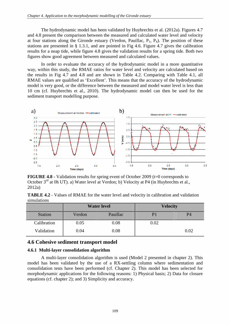
Chapter 4. Application to the morphodynamic modelling of the Gironde estuary
109
The hydrodynamic model has been validated by Huybrechts et al. (2012a). Figures 4.7 and 4.8 present the comparison between the measured and calculated water level and velocity at four stations along the Gironde estuary (Verdon, Pauillac, P1, P4). The position of these stations are presented in § 1.3.1, and are pointed in Fig 4.6. Figure 4.7 gives the calibration results for a neap tide, while figure 4.8 gives the validation results for a spring tide. Both two figures show good agreement between measured and calculated values.
In order to evaluate the accuracy of the hydrodynamic model in a more quantitative way, within this study, the RMAE ratios for water level and velocity are calculated based on the results in Fig 4.7 and 4.8 and are shown in Table 4.2. Comparing with Table 4.1, all RMAE values are qualified as ‘Excellent’. This means that the accuracy of the hydrodynamic model is very good, or the difference between the measured and model water level is less than 10 cm (cf. Huybrechts et al., 2010). The hydrodynamic model can then be used for the sediment transport modelling purpose.
FIGURE 4.8 - Validation results for spring event of October 2009 (t=0 corresponds to October 3rd at 0h UT). a) Water level at Verdon; b) Velocity at P4 (in Huybrechts et al., 2012a)
TABLE 4.2 - Values of RMAE for the water level and velocity in calibration and validation simulations Water level Velocity
Station Verdon Pauillac P1 P4
Calibration 0.05 0.08 0.02
Validation 0.04 0.08 0.02
4.6 Cohesive sediment transport model 4.6.1 Multi-layer consolidation algorithm
A multi-layer consolidation algorithm is used (Model 2 presented in chapter 2). This model has been validated by the use of a RX-settling column where sedimentation and consolidation tests have been performed (cf. Chapter 2). This model has been selected for morphodynamic applications for the following reasons: 1) Physical basis; 2) Data for closure equations (cf. chapter 2); and 3) Simplicity and accuracy.
a) b)a) b)

Chapter 4. Application to the morphodynamic modelling of the Gironde estuary
110
The advantage of this representation is that the flux of sedimentation and consolidation is based on the Gibson theory. If there is erosion, the thickness of the uppermost layer decreases, and vice versa, when there is deposition, it increases.
We use in this application 10 sediment layers, with fixed concentrations ranging from 100 g/l to 550 g/l (with ∆C = 50 g/l). The initial thickness of each layer is specified in order to represent a total bed thickness of 5 m (see Fig 4.11b for the initialization).
4.6.2 Initial & boundary conditions The averaged suspended concentration is set equal to zero as initial condition for the pre-run simulation.
For boundary conditions, concentrations need to be specified along both the upstream Dordogne and Garonne boundaries and the maritime boundary. In our study, we assumed zero sediment flux along the maritime boundary and on both rivers inlet. The specified fluxes are unknown, but the boundary limit is assumed to have no influence on the results in the center part where we focus our interest.
4.7 Calibration of erosion/deposition parameters The calibration of erosion/deposition parameters is a difficult task because these
parameters depend on the type of mud, its concentration and its composition. The erosion-deposition parameters in SISYPHE include the critical shear stress for erosion τ*
ce, the erosion parameter M, the critical velocity for deposition u*
d and the settling velocity Ws.
In chapter 3, new erosion-deposition experiments on the Gironde mud are simulated using SISYPHE. The erosion/deposition parameters which were determined from model calibration are in the same order of magnitude with previous studies (eg. Bonnefille et al., 1971, Migniot & Bellessort, 1970, Eisenbeis & Roger, 2011). However, we need to emphasize that the objective of chapter 3 was to demonstrate the ability of the numerical model to handle physical processes involved in cohesive sediment transport. All the simulations were set-up with well-controlled laboratory conditions which are different from in-situ conditions.
Differences between laboratory and in-situ conditions are well understood, in particular for cohesive sediments. In the field, very complex interactions between biology and physico-chemistry could strongly affect the transport parameters. On one hand, flocculation state can affect not only the settling properties but also the consolidation process. On the other hand, biological activities such as bio-deposition, bio-stabilisation, bio-destabilisation (Chapter 10, Winterwerp & Van Kesteren, 2004) cause significant seasonal variations in sediment properties, such as deposition rates and erodibility.
Indeed, it is commonly accepted that the erodability of the tidal mud flats is strongly influenced by physical, biological and chemical parameters. However, the treatment of sediments in laboratories such as mixing process, removing vegetal debris (Eisenbeis & Roger, 2011) reduces the cohesion between particles, changes the structure of the sediment bed.
Therefore, although the calibration of erosion and deposition parameters based on the experimental results shown in chapter 3 are satisfactory, it is necessary to adapt these values before applying our model to field conditions.
This part is dedicated to the calibration of erosion-deposition parameters for morphodynamic modelling. First, the calibrated set of parameters based on laboratory experiments (cf chapter 3) will be used as a starting point (Test 0 in Table 4.3). Preliminary

Chapter 4. Application to the morphodynamic modelling of the Gironde estuary
111
results show large scatter in comparison with in-situ measurements and further calibration is therefore needed before applying the model to in-situ conditions.
Figure 4.9 gives the schematic view of the modelled bed structure. The bed is comprised of 10 layers of concentration increasing progressively from 100 g/l to 550 g/l. Each layer is characterized by a critical shear stress for erosion and an erosion parameter issued from the given equations in figure 4.9. Since no data is available for the critical shear stress for deposition, it is fixed for the whole domain. In chapter 3, the settling velocity was calibrated as a function of depth-averaged suspended sediment concentration. However, it applies only for laboratory condition where the sediment bed is 4 cm. In-situ, averaging the sediment concentration along the water column decreases sharply the depth-averaged value. Therefore, in the Gironde model, the settling velocity is also kept constant.
FIGURE 4.9 - Schematic modelled bed structure with applied erosion-deposition parameters

Chapter 4. Application to the morphodynamic modelling of the Gironde estuary
112
FIGURE 4.10 – Water depth, velocity, bottom shear stress and depth-averaged concentration at Pauillac (KP 47, see Fig. 1.1) during a spring-neap tidal cycle
Figure 4.10 presents the bottom shear stress, water depth, velocity and depth-averaged concentration at Pauillac during a spring-neap tidal cycle using the calibrated set of erosion – deposition parameters presented in fig. 4.9.
4.8 Initialisation of sediment bed structure One of the difficulties in sediment transport modelling is the sensitivity of model
results to sediment parameters and bed composition. Most of those parameters are poorly defined because of the high inhomogeneity in the sediment bed composition. In particular, the bed structure in the estuary is generally unknown. Indeed, during the field campaign at the central part of the Gironde estuary (Boucher, 2009), three sediment cores were sampled in order to investigate the near-bed sediment structure (the sampling tube is 1 m long). Laboratory results show a homogeneous pure mud structure in one core while the two other cores present thin layers of sand (see §1.4.4 of this study). The concentration of the core of pure cohesive sediment gives a value of almost 756 ± 100 g/l. This high value is interpreted as being due to a long stacking duration of material before the analysis. According to Pham Van Bang(personal communication), an increase in the concentration of sediment of order of 100 g/l can be attained for a stacking duration of several months, which is our case. Therefore, in our model, the concentration of the most-consolidated layer is selected equal to 550 g/l.
- 3
- 2
- 1
0
1
2
3
4
0 5 0 1 0 0 1 5 0 2 0 0 2 5 0 3 0 0 3 5 0
H (
m)
- 0 , 8
- 0 , 6
- 0 , 4
- 0 , 2
00 , 2
0 , 4
0 , 6
0 , 8
1
0 5 0 1 0 0 1 5 0 2 0 0 2 5 0 3 0 0 3 5 0
Vel
ocity
(m
/s)
u ( m /s )
v ( m /s )
00 , 10 , 20 , 30 , 40 , 50 , 60 , 70 , 80 , 9
1
0 5 0 1 0 0 1 5 0 2 0 0 2 5 0 3 0 0 3 5 0
T im e ( h o u r s )
ME
S (
g/l)
00 , 10 , 20 , 30 , 40 , 50 , 60 , 70 , 80 , 9
1
0 5 0 1 0 0 1 5 0 2 0 0 2 5 0 3 0 0 3 5 0
Tbe
d (N
/m²)
T i m e ( h o u r s )

Chapter 4. Application to the morphodynamic modelling of the Gironde estuary
113
According to Toorman (1992), for concentrations less than 50 g/l, the physical properties of the suspension do not differ significantly from that of water and the fluid/mud mixture can be considered as a Newtonian fluid. In the transition range (from 50 to 100g/l), the fluid mud layer behaves as a non-Newtonian fluid with visco-plastic rheological behaviour (cf. Toorman, 1992). However, since the fluidization process is not accounted for in our model, the limit between the suspension considered as Newtonian fluid, and the bed over-topping layer is fixed arbitrarily at 100g/l. A sensitivity analysis on this value will be presented in section 4.8.3.
In order to initialise the sediment transport model, we assume two uniform bed structures for the maritime area and the estuary, and let the model run without bed evolution for a period of time and calculate transport rates and bed composition. This method has been also implemented by Waeles (2005) and Huybrechts et al., (2012b). The final result for the bed composition of this pre-simulation (one year in our study) is then used as initial conditions for the morphodynamic simulation.
4.8.1 Measurement of the bed structure in the Gironde estuary
According to Migniot (1984), there is always a concentration gradient between the surface and the bottom in a deposit, mud remains fluid on the surface and concentrated at the bottom. Depending on the nature and the size of particles, the physico-chemistry and biology of the aqueous medium, the excess pressure, the height of the deposits, the concentration of sediment in a deposit can vary from one to another.
For estuarine mud (Loire, Gironde, Mahury,…) concentration does not exceed 300 to 350 g/l after several days of settling, the concentration at the surface of the deposit remains very low (100-150 g/l). Figure 4.11 is an example of a conceptual concentration gradient for estuarine mud which was proposed by Migniot (1984).
Based on the concentration gradient proposed by Migniot (1984), the bed structure is schematized as shown in figure 4.11b. The total initial bed thickness is assumed to be equal to 5 m, and represented by 10 layers of concentration varying from 100 g/l (fluid mud) to 550 g/l (consolidated mud). The thickness of each layer is schematised based on the concentration gradient of Migniot (1984).
FIGURE 4.11 - a) Example of a conceptual concentration gradient in a deposit for estuarine mud (redrawn from Migniot, 1984) & b) Modelled bed structure at the initial condition
C1 = 100 g/l H1 = 0.25 mC2 = 150 g/l H2 = 0.25 m
C3 = 200 g/l H3 = 0.50 m
C4 = 250 g/l H4 = 1.0 m
C5 = 300 g/l H5 = 1.0 m
C8= 450 g/l H8 = 0.50 m
C6= 350 g/l H6 = 0.50 m
C7=400 g/l H7 = 0.50 m
C10= 550 g/l H10 = 0.25 mC9= 500 g/l H9 = 0.25 m
-3,5
-3
-2,5
-2
-1,5
-1
-0,5
0
0 100 200 300 400 500 600
C (g/l)
Z (
m)
Consolidating mud
Consolidated bed
Turbid zoneFluid mud
-3,5
-3
-2,5
-2
-1,5
-1
-0,5
0
0 100 200 300 400 500 600
C (g/l)
Z (
m)
Consolidating mud
Consolidated bed
Turbid zoneFluid mud
a) b) C1 = 100 g/l H1 = 0.25 mC2 = 150 g/l H2 = 0.25 m
C3 = 200 g/l H3 = 0.50 m
C4 = 250 g/l H4 = 1.0 m
C5 = 300 g/l H5 = 1.0 m
C8= 450 g/l H8 = 0.50 m
C6= 350 g/l H6 = 0.50 m
C7=400 g/l H7 = 0.50 m
C10= 550 g/l H10 = 0.25 mC9= 500 g/l H9 = 0.25 m
-3,5
-3
-2,5
-2
-1,5
-1
-0,5
0
0 100 200 300 400 500 600
C (g/l)
Z (
m)
Consolidating mud
Consolidated bed
Turbid zoneFluid mud
-3,5
-3
-2,5
-2
-1,5
-1
-0,5
0
0 100 200 300 400 500 600
C (g/l)
Z (
m)
Consolidating mud
Consolidated bed
Turbid zoneFluid mud
C1 = 100 g/l H1 = 0.25 mC2 = 150 g/l H2 = 0.25 m
C3 = 200 g/l H3 = 0.50 m
C4 = 250 g/l H4 = 1.0 m
C5 = 300 g/l H5 = 1.0 m
C8= 450 g/l H8 = 0.50 m
C6= 350 g/l H6 = 0.50 m
C7=400 g/l H7 = 0.50 m
C10= 550 g/l H10 = 0.25 mC9= 500 g/l H9 = 0.25 m
C1 = 100 g/l H1 = 0.25 mC2 = 150 g/l H2 = 0.25 m
C3 = 200 g/l H3 = 0.50 m
C4 = 250 g/l H4 = 1.0 m
C5 = 300 g/l H5 = 1.0 m
C8= 450 g/l H8 = 0.50 m
C6= 350 g/l H6 = 0.50 m
C7=400 g/l H7 = 0.50 m
C10= 550 g/l H10 = 0.25 mC9= 500 g/l H9 = 0.25 m
-3,5
-3
-2,5
-2
-1,5
-1
-0,5
0
0 100 200 300 400 500 600
C (g/l)
Z (
m)
Consolidating mud
Consolidated bed
Turbid zoneFluid mud
-3,5
-3
-2,5
-2
-1,5
-1
-0,5
0
0 100 200 300 400 500 600
C (g/l)
Z (
m)
Consolidating mud
Consolidated bed
Turbid zoneFluid mud
a) b)

Chapter 4. Application to the morphodynamic modelling of the Gironde estuary
114
Furthermore, during regular bathymetric survey of G.P.M.B (2002), vertical density profiles are also measured in order to clarify and complete bathymetric data. Density profiles are measured by Gamma-ray probes. The possibility of using these probes in-situ allows a rapid and complete knowledge of the density of mud deposits. Figure 4.12 gives an example of the measured vertical concentration profiles at the navigation channel using the acoustic sonar.
FIGURE 4.12- Measured vertical concentration profiles from Gamma-ray probes (in G.P.M.B, 2002)
It is observed that:
• The first echo corresponds to the roof of the deposit with a concentration of about 60 g/l. Above this level, from –6 m to –6.6 m is the water of highly suspended concentration (C = 10 - 50 g/l).
• The second echo at –7.3 m is marked by a high variation of concentration
• The third echo corresponds to “hard bed” represented by consolidated mud which the concentration of the order of 600 g/l.
The structure presented in Fig. 4.12 is not selected as the initial condition of the bed structure because it is not representative for the estuary where a lot of deposit is found. Indeed, the measurement was perfomed in the navigation channel, where currents are very strong, and the bed is mostly hard consolidated sediment (Fig 4.12).
The calibrated erosion and deposition parameters (u*e , M, τcd, Ws) in previous section (§ 4.6) are applied in the initialization of the model.
In order to validate the calculated bed structure, the computed vertical concentration profile at one point in the navigation channel will be compared against the measured profile (figure 4.12) in a qualitative way. This comparison is presented at the end of section 4.8.2.
4.8.2 Bed structure initialisation

Chapter 4. Application to the morphodynamic modelling of the Gironde estuary
115
In this section, the result of bed structure initialization is dicussed. The values of erosion and deposition parameters are presented in Fig. 4.9. The initial condition is given in Fig. 4.11b. It is worth noting that in the pre-run, the mass is not conservative since the erosion and deposision areas are formed without the calculation of the bed evolution.
FIGURE 4.13 - Initial thickness of the bottom layer for the pre-simulation (maritime part: 5 m = total sediment bed thickness; estuary: 0.25 m
As represented in table 1.3, figure 1.13, figure 1.16 (chapter 1), the bed material distribution in the Gironde estuary is a mixture between sand particles in the maritime part, mud and sand-mud mixture in the central part. In order to initialize the model for the pre-run simulation, we roughly divide the model into two parts: a maritime part (in red) and an estuarine part (in blue) (fig. 4.13).
Inside the estuary, 10 layers of cohesive sediments are set up with increasing concentrations from 100 g/l at the first top layer to 550 g/l at the bottom layer (as shown on Fig. 4.11b). At the mouth of the estuary, cohesive sediments are not observed. Therefore, a 5 m-layer of consolidated sediment (layer 10 of 550 g/l) is assumed in order to stabilize the bed in the maritime part.
The results of the pre-simulation for the bed structure are then produced after different periods of time (from one month up to three -, six -, eight -, ten months, one year) in order to verify if the bed structure attains a quasi-equilibrium state meaning that the thickness of the
5 m
0.25 m
2 km
5 m
0.25 m
2 km

Chapter 4. Application to the morphodynamic modelling of the Gironde estuary
116
bed layers does not vary with time. In this iso-picnal multi-layer model, the concentrations of the layers are fixed, but top layers may get entirely eroded.
FIGURE 4.14 - Evolution of concentration profiles at three points: point 1 downstream of Patiras island, point 2 in the navigation channel, point 3 in the median channel
In order to determine the minimum duration of the pre-run simulation, the time -evolution of the vertical concentration profiles is displayed in Figure 4.14 at three points: Point 1 at the Patiras bank, Point 2 in the navigation channel, and Point 3 in the median channel. It is observed that the concentration profiles at Point 2 and Point 3 in the channels evolve inversely to the concentration profiles at Point 1. While at Point 1, after one-year of pre-simulation, and the attained concentration of the top layer is about 250 g/l (corresponds to layer N°3), at Point 2 (in the navigation channel) the concentration of the top layer is much higher (400 g/l - layer N°5) than at Point 1. At Point 3, the concentration of the top layer also increases up to 300 g/l (layer N° 4).
A good agreement is observed when comparing the calculated concentration profile at Point 2 at the end of the 1-year of pre-simulation with the measured concentration profile in figure 4.12. The total thicknesses of both profiles are approximately 2 m, and the concentration ranges from 400 g/l to 550 g/l. One small difference between these two profiles is the observed fluid mud layer (10-50 g/l) at the surface of the deposit in figure 4.12, which cannot be observed in the model since the bed concentration starts from 100 g/l.

Chapter 4. Application to the morphodynamic modelling of the Gironde estuary
117
FIGURE 4.15 – Resulting map of the bed layer 4 (C = 250 g/l) and the bed layer 6 (C = 350 g/l) at the end of 1-year simulation a) Layer 4 over the whole estuary; b) Layer 4 in the central area; c) Layer 6 in the central area.
Regarding the sediment bed composition, at the end of 1-year simulation, in the central part, three top layers (which correspond to concentration of 100, 150 and 200 g/l) disappear, while at the mouth of the estuary, the thicknesses of the sediment bed layers keep constant (= 0 for layers 1-9, = 5 m for layer 10).
Inside the estuary, the sediment bed is composed of deposition and erosion zones, which are represented by the increase or decrease respectively of layer thicknesses in different zones (figure 4.15). For example, in zones of deposit (North of Patiras island, tidal flats) the thickness of the top layer increases (layer 4 - Cs= 250 g/l) and the bed is covered of soft mud, while in the navigation channel and in the Saintonge channel, where currents are stronger, the top layers are eroded and the sediment bed is made of consolidated mud (6th layer becomes the topmost layer: Cs= 350 g/l). This result is compared against the measured bathymetry in order to have a qualitative sediment bed distribution.
In conclusion, for morphodynamic simulations, an initialization period of one-year is sufficient in order to attain a quasi-equilibrium bed structure.
4.8.3 Sensitivity analysis on erosion/deposition parameters
The “best-fit” set of erosion-deposition parameters presented in Fig. 4.9 is obtained through a sensitivity test. This test consists in realizing the 10 simulations listed in Table 4.3: For each simulation, only one parameter is varied regarding the reference test (Test 0). The reference simulation (Test 0) corresponds to the set of parameters issued from the laboratory experiments simulation (cf. Chapter 3).
All simulation runs are performed for 1 year starting from the same initial state as schematized in Fig. 4.11b. The model results (the concentration of the topmost layer and the profile) are compared in a qualitative way with the measurement (eg. Fig 4.12). The most sensitive parameter is the critical erosion velocity, which reflects the erodability of the sediment bed.
a) b) c)a) b) c)

Chapter 4. Application to the morphodynamic modelling of the Gironde estuary
118
TABLE 4.3 – Applied range of parameters in the sensitivity analysis on erosion – deposition parameters (C is the mass concentration of the bed layer, in kg/m3)
Simulation u*e (cm/s) M (kg/m²/s) τcd (N.m-2) Ws (mm/s)
Test 0 (Chapter 3) 37.5 10 C−× × 30.55 C× 0.3 1.78
Test ue1 32 7.5 10 C−× × × 30.55 C× 0.3 1.78
Test ue2 33 7.5 10 C−× × × 30.55 C× 0.3 1.78
Test ue3 33.5 7.5 10 C−× × × 30.55 C× 0.3 1.78
Test ue4 34 7.5 10 C−× × × 30.55 C× 0.3 1.78
Test ud1 33.5 7.5 10 C−× × × 30.55 C× 0.5 1.78
Test ud2 33.5 7.5 10 C−× × × 30.55 C× 1.0 1.78
Test ud3 33.5 7.5 10 C−× × × 30.55 C× 1.5 1.78
Test ud4 33.5 7.5 10 C−× × × 30.55 C× 2.0 1.78
Test ws1 33.5 7.5 10 C−× × × 30.55 C× 1.5 2.50
Test ws2 33.5 7.5 10 C−× × × 30.55 C× 1.5 3.50
4.8.3.1 Critical erosion velocity (u*e )
Regarding erosion parameters, since the critical shear stress for erosion is a function of the degree of compaction of the sediments, which is much lower in laboratory conditions than in the field, it is justified to increase the calibrated value of the critical shear stress for erosion obtained in chapter 3. Different values (2, 3, 3.5, and 4) are multiplied to the calibrated function obtained in chapter 3. While a factor of 2 or 3 still gives much erosion in the whole estuary (the topmost layer is around 350-400 g/l), the sediment bed is not much evolved with a factor of 4. Therefore, a function for the critical velocity for erosion of 3.5× 37.5 10 C−× × is considered satisfactory.
4.8.3.2 Critical shear stress for deposition (τcd )
In 2DH models, the value of deposition parameters may be much higher than the measured one. This is due to the calculation of deposition flux in 2DH models is based on depth-averaged concentrations, but not the concentration of the sediment near the bed.
By trial and error, different values of critical shear stress for deposition (τcd = 0.7, 1.0, 1.5, 2.0) are tested. And the selected value is 1.5 N/m², which gives the critical velocity for erosion equal to 3.87 cm/s.
4.8.3.3 Settling velocity (Ws)
Three values of settling velocity are tested. The first value (Ws = 1.77 mm/s) is the calibrated settling velocity during the settling column test (chapter 2). The highest value (Ws = 3.5 mm/s) is the calibrated maximum velocity during the settling test in Owen tubes in chapter 3. The value of 2.5 mm/s is selected as the average of the two above values. The results do not show much impact on the bed evolution. The first value is then retained for morphodynamic simulation.
Chapter 4. Application to the morphodynamic modelling of the Gironde estuary
119
4.8.3.4 Erosion coefficient (M)
The erosion coefficient M, however, depends on the physico-chemical characteristics of bottom sediments. Because these properties are poorly known, this parameter is kept unchanged.
4.8.4 Sensitivity analysis on concentration of topmost layer
Another model is set up with 10 layers of sediments starting from 60 g/l at the top first layer (measurement value from G.P.M.B, 2002) until 550 g/l at the bottom layer. The resulting bed structure after 1-year simulation is exactly the same as the one in figure 4.14. This means that in our model, the concentration of the first layer is not a sensitive parameter to the model’s result.
4.8.5 Effect of consolidation
In order to evaluate the effect of consolidation, we compare here two simulations: one with the consolidation module, and the other one, without consolidation. The objective is to compare the 1-year bed evolution calculated by both models. The bed structure is built consisting of 10 layers from 100 g/l up to 550 g/l. The adopted pre-simulation is the same for the two simulations.
The calibrated erosion and deposition parameters (u*e , M, τcd, Ws) in previous section (§ 4.7) are applied in these simulations. The initial bed structure is obtained from section § 4.7. The model is run for 1 year to record the bed evolution.
Model results are presented in figure 4.16 for both models with (CS) and without consolidation (NCS). Figure 4.16a gives the bed evolution of the CS-model, and figure 4.16b presents the bed evolution of the NCS-model. It is observed that these two models give opposite results in terms of erosion and deposition areas. Indeed, downstream of the Patiras island, while the CS-model produces deposition along the Patiras bank (from 0.4 to 0.6 m/year), except for a small area closed to the Patiras island, the NCS-model gives deposition only in this area (about 0.8 m). Similarly, downstream of the Trompeloup island, while deposition is observed in the CS-model as well as in the measurement, the NCS-model tends to give erosion. This can be explained that without the consolidation model, the sediment is not transported in the vertical direction within the deposit. The sediment is then cumulated on the uppermost layer whenever deposition occurs. Later, in the period of erosion, because the sediment is not consolidated, all the recently-deposited sediment is supposed to be eroded easily. Therefore, both erosion and deposition thicknesses are over-estimated without the consolidation model.

Chapter 4. Application to the morphodynamic modelling of the Gironde estuary
120
FIGURE 4.16 – Modelled 1-year bed evolution: a) With consolidation (CS-model); b) Without consolidation (NCS-model). The initial bed structure is the same in both models.
These results confirm the necessity of consolidation model (CS-model) in cohesive sediment transport modelling, not only for the initialisation (pre-simultation) of the bed structure, but also for the long term morphodynamic modelling.
4.9 Validation on depth-averaged suspended concentration measurements For the two selected events in August 2007 (spring tide/ 01/08/2007-04/08/2007 and
neap tide 07/08/2007-10/08/2007), measurements of water levels are available at the mouth of the estuary (Verdon station) and in the central part (Pauillac station). Depth-averaged suspended sediment concentrations are also available at Pauillac station.
Using the set of calibrated erosion/depostion parameters as explained in previous paragraph, the calculated water level and concentration are compared against measurements. Differences between computed and measured water levels are lower than 10 cm which leads to RMAE within 0.09 to 0.15 (Table 4.4). These values correspond to “Excellent” agreement between measured and model results. This confirms the accuracy of the hydrodynamic model (cf. Huybrechts et al., 2012a).
2 km2 km
(a) (b)
2 km2 km
(a) (b)

Chapter 4. Application to the morphodynamic modelling of the Gironde estuary
121
FIGURE 4.17 - Time evolution of water level & depth-averaged suspended concentration at Pauillac. a) & c) Spring tide (t=0 corresponds to August 1st 0h TU 2007) ;b) & d) Neap tide (t=0 corresponds to August 7th 0h TU 2007)
TABLE 4.4 - Values of RMAE for the water level and the concentrations in suspension (neap and spring events of August 2007)
Criteria
Event
RMAE
H at Verdon
RMAE
H at Pauillac
RMAE
SSC at Pauillac
Spring tide 0.12 0.15 0.44
Neap tide 0.09 0.10 0.67
Time-varying concentrations calculated at the Pauillac station are shown in Fig 4.17 The model overall tends to underestimate the concentration peaks. In figure 4.17, we can observe that the prediction of the depth-averaged suspended concentration is in good agreement with observations. For the spring event (Fig 4.17 c), model results are close to measured values, except for the concentration peak values (around 10 g/l), which the model underestimates.
In addition, depth-averaged concentrations were estimated by measuring the turbidity at only 3 points in the vertical and therefore, the measurements include some uncertainty. Furthermore, the measured values can also be erroneous when applying the relation between MES and turbidity provided by Maneux et al. (2006) for turbidity greater than 1000 NTU (which is not valid). Considering the uncertainty in the data, the overall agreement between model results and measurements is satisfactory. This is confirmed by the RMAE for spring tide of 0.44.

Chapter 4. Application to the morphodynamic modelling of the Gironde estuary
122
During the neap tide event (Fig. 4.17d), however, the model under-estimates the concentration. The computed suspended concentration peaks are approximately three times lower than the measured values. This trend is also observed in non-cohesive results (Huybrechts et al., 2012). Here the RMAE of depth-averaged suspended concentration is 0.67 for neap tide, which is still considered “Poor”.
4.10 Morphodynamic modelling 4.10.1 Calibration results on bathymetric evolution 1995-2000
After the calibration and validation steps on water level and velocity and the validation on depth-averaged suspended concentration, the presented hydrodynamic model in § 4.5.4 is considered valid for the morphodynamic modelling. Concerning the tidal forcing, long term components as monthly components are included within the 46 harmonic components. Hourly variations of river discharges from January 1st 1995 to December 31st 2000 are imposed at both upstream boundaries for the Garonne and Dordogne rivers.
FIGURE 4.18 - Modelled 5-year bed evolution (1995-2000)
The 5-year bed evolution is plotted on Fig 4.18 for the whole estuary, including a zoom in the central area (small figure in the black square).
Within the maritime area, bed changes are small compared to the estuarine part. This is due to the fact that this part was initialized by a unique layer of consolidated sediment, in order to limit extra sources of sediment entering from the maritime boundary into the estuary.

Chapter 4. Application to the morphodynamic modelling of the Gironde estuary
123
Since measurements of bathymetry are not available in the maritime area, our calibration focuses on the central area.
Morphodynamic results of graded non-cohesive sediment (Huybrechts et al. 2012b) for the period of 1995-2000 are also compared in terms of bed evolutions and BSS values.
FIGURE 4.19 – Dumping areas (upper left) and zoom in 5-year bed evolutions in the central part (upper right: measured differential bathymetry, lower left: cohesive model, lower right: non-cohesive model). Orange rectangules indicates the dumping areas (zones 3.1, 2.4 and 2.2), black oval corresponds to area of high deposition rate in the measurements.
Figure 4.19 gives the comparison between the measured (fig 4.19 upper right) and computed bed changes (fig 4.19 lower). The bed evolution in cohesive sediment model is overall, in qualitative agreement with the 5-year differential bathymetry. The growth rate of the Patiras island and associated deposition rates of the fine particles downstream of the island are observed but under-estimated. The deposition is also observed along the right bank of the navigation channel, in particular close to the Trompeloup island in both measurement and
Differential bathymetry
Cohesive model
--
Non-cohesive model
Dumping areas Differential bathymetry
Cohesive model
--
Non-cohesive model
Dumping areas

Chapter 4. Application to the morphodynamic modelling of the Gironde estuary
124
model results, but is under-estimated in the model. This erroneous result can be explained by the ignorance of the dredging and dumping activities in this area (as discussed in part 4.10).
In the navigation channel, however, the model still gives slight erosion (in the order of –0.5 m), while the measurement clearly shows a tendency for deposition, such that the channel needs to be dredged. This erroneous result can be explained by the difficulty in modelling the sediment dynamics in the lutocline (i.e. the upper interface of the fluid mud layer, as discussed in § 4.9). Furthermore, the transportation activities in the navigation channel, which increase the re-suspension and the deposition of sediments, is ignored in our model.
Comparing the model results of non-cohesive (Fig. 4.19 lower right) and cohesive models (lower left), in general, in non-cohesive model, the deposition rate downstream of the Patiras island is over-estimated by roughly a factor two, while the erosion rate in the channels is higher than that observed in the bathymetry. Conversely, cohesive morphodynamic model tends to under-estimate the deposition rate in the whole estuary.
Furthermore, it is also observed that the non-cohesive model results produces areas of deposition more locally than the cohesive model as well as the measured bed evolutions. Indeed, downstream of the Patiras island, there is lots of deposition in the left hand side (in order of 5 m, double the measured value). This area corresponds to the area that sand particles are observed. However, on the Patiras bank, where cohesive sediments are dominant, the non-cohesive model predicts less deposition than the measurement.
FIGURE 4.20 - Location of measured profiles
To analyse in a more quantitative way, the same quality criteria are applied on six profiles localised in the central part of the estuary (Fig 4.20). For the BSS criterion (eq. 4.2), X is the measured final bathymetry, Y is the predicted final bathymetry and B is the initial bathymetry. The comparison between the measured bathymetric evolution and the calculated
L2
L1
L3
L4
L5
L6
L2
L1
L3
L4
L5
L6

Chapter 4. Application to the morphodynamic modelling of the Gironde estuary
125
evolution at selected profiles are presented in figure 4.21 for cohesive sediment model and in figure 4.22 for non-cohesive model. The corresponding BSS values are given in Table 4.5.
FIGURE 4.21 - Measured & modelled bed elevation in cohesive sediment model at selected profiles: the black line shows the model results and should be compared to the 2000 data set (in blue).
TABLE 4.5 - BSS score for control profiles in cohesive and non-cohesive models
Cohesive model Non-cohesive model
Control profile BSS Evaluation BSS Evaluation
L1 0.05 Poor < 0 Bad
L2 0.21 Poor < 0 Bad
L3 0.68 Good < 0 Bad
L4 0.24 Poor < 0 Bad
L5 < 0 Bad < 0 Bad
L6 < 0 Bad < 0 Bad
-3,5
-3
-2,5
-2
-1,5
-1
-0,5
0
0,5
1
328000 328500 329000 329500 330000 330500 331000 331500 332000
Y (m)
Z (
m)
-14
-12
-10
-8
-6
-4
-2
0
2
358000 359000 360000 361000 362000X (m)
Z (
m)
1995
2000
5-year model
-6
-5
-4
-3
-2
-1
0
359800 360000 360200 360400 360600 360800 361000
Y (m)
Z (
m)
-16
-14
-12
-10
-8
-6
-4
-2
0
358000 359000 360000 361000 362000X (m)
Z (
m)
L1 L2
L3 L4

Chapter 4. Application to the morphodynamic modelling of the Gironde estuary
126
FIGURE 4.22 - Measured & modelled bed elevation in non-cohesive model at four selected profiles
Qualitatively, figure 4.21 shows an overall agreement, in general, between measured and calculated evolutions. Four cross sections are plotted along the central part of the estuary. The results seem better upstream the estuary. Profiles L1, L2, L4 give positive BSS, in particular, the BSS score of profile L3 is qualified as good, while profiles L5, L6 give negative values.
Looking at L1, L2, L3, the deposition rate is better reproduced at the Patiras bank than in the median channel. This is because the model cannot simulate the sediment transported into the median channel from the dumping areas downstream. Therefore the model tends to give higher erosion rate in the median channel.
At L4, the model shows a deposition tendency of with a rate two times lower than the differential bathymetry. The model is unable to create a narrower area downstream of the bank as observed in the measurement (red arrow in figure 4.21).
Quantitatively, the model gives overall reasonable estimates of bed evolution, in particular the calculated shape of the deposit at the lee of the central island. This is where cohesive sediments are observed. Other areas where sand is dominated such as in the channels, downstream of the estuary, the model gives more erosion than the measurement. Therefore it would be interesting to compare results of cohesive model with non-cohesive model, and to see how to integrate the two types of sediments in one model (4.11). Moreover, since the dredging and dumping activities have a large impact on the equilibrium of the estuary, it is difficult to produce the same results as observed in the differential bathymetry.
-20
-15
-10
-5
0
5
358000 359000 360000 361000 362000X (m)
Z (
m)
1995
2000
5-year non-cohesivemodel
-20
-15
-10
-5
0
5
358000 359000 360000 361000 362000X (m)
Z (
m)
-6
-5
-4
-3
-2
-1
0
1
2
3
359800 360000 360200 360400 360600 360800 361000
Y (m)
Z (
m)
-3,5
-2,5
-1,5
-0,5
0,5
1,5
2,5
3,5
328000 328500 329000 329500 330000 330500 331000 331500 332000
Y (m)
Z (
m)
L1 L2
L4L3
-20
-15
-10
-5
0
5
358000 359000 360000 361000 362000X (m)
Z (
m)
1995
2000
5-year non-cohesivemodel
-20
-15
-10
-5
0
5
358000 359000 360000 361000 362000X (m)
Z (
m)
-6
-5
-4
-3
-2
-1
0
1
2
3
359800 360000 360200 360400 360600 360800 361000
Y (m)
Z (
m)
-3,5
-2,5
-1,5
-0,5
0,5
1,5
2,5
3,5
328000 328500 329000 329500 330000 330500 331000 331500 332000
Y (m)
Z (
m)
L1 L2
L4L3

Chapter 4. Application to the morphodynamic modelling of the Gironde estuary
127
Fig 4.22 presents the comparison between measured and simulated bed elevation from non-cohesive model at the same profiles as in cohesive model. The BSS values corresponding to non-cohesive morphodynamic model are negative for all selected profiles (Table 4.5). It is observed that the results of cohesive model are much better than of non-cohesive model.
4.10.2 Validation results on bathymetric evolution 2000-2005
Model validation is essential part of the model development process if models to be accepted and used to predict the bed evolution. In our study, the validation run is selected from 2000 to 2005 based on the measurement of bathymetry. The initial bathymetry is composed of 2000 bathymetry at the central area, and 1995 bathymetry of the rest of domain. This, however, can cause error in model results. The erosion and deposition parameters are kept the same as in the calibration test. The river discharges are imposed hourly from January 1st 2000 to December 31st 2005. All assumptions in the calibration test are applied in validation test. Since the validation result of the non-cohesive model is not available, there will be no comparison between cohesive and non-cohesive models as in calibration step.
FIGURE 4.23 - 5-year bed evolutions in the central part (left: measured, right: model)
Figure 4.23 gives 5-year measured and calculated bed evolution at the central part of the estuary. Similar to the results obtained for the calibration period (1995-2000), the model tends to give more erosion than the measured bathymetric evolution. Indeed, in the two channels (the navigation channel and the Saintonge channel), the measured bed evolution is of the order of 0.5-1 m, while erosion is obtained in the model. However, the elongation of the bank downstream the Patiras island is obtained in the model results. The deposition is also observed at the right bank of the navigation channel.
Measured ModelMeasured Model

Chapter 4. Application to the morphodynamic modelling of the Gironde estuary
128
FIGURE 4.24 - Measured & modelled bed elevation at selected profiles
Figure 4.24 presents the bed elevation in 2000, 2005 and the predicted bed elevation in 2005 at the same profiles as in calibration step. It is observed that compared to the period 1995-2000, during this period (2000-2005), the bed is more stabilised. In particular, at profiles L3 and L4, the measured bed evolution shows slight deposition rate, even in some areas (for example at the two sides of profile L3, the erosion is observed. The model results are considered reasonable at these two profiles.
TABLE 4.6 - BSS score for control profiles
Control profile BSS Evaluation
L1 < 0 Bad
L2 0.17 Poor
L3 0.31 Reasonable
L4 0.31 Reasonable
L5 < 0 Bad
L6 < 0 Bad
At the two cross sections L1 and L2, the model gives better results at the tidal flats. At the two median and Saintonge channel, the model gives more erosion. This decreases the BSS score of these two profiles. Actually, without available data, the critical shear stress for deposition is kept constant in the whole estuary. Since the Gironde estuary is characterised by its high turbidity, with the TM normally located in the main channels (Castaing, 1981), the critical shear stress for deposition in the channels should be higher than in tidal flat areas.
-6
-5
-4
-3
-2
-1
0
359800 360000 360200 360400 360600 360800 361000
Y (m)
Z (
m)
-3,5
-3
-2,5
-2
-1,5
-1
-0,5
0
0,5
1
328000 328500 329000 329500 330000 330500 331000 331500 332000
Y (m)
Z (
m)
L1 L2
L3 L4
-16
-14
-12
-10
-8
-6
-4
-2
0
358000 359000 360000 361000 362000X (m)
Z (
m)
-14
-12
-10
-8
-6
-4
-2
0
2
358000 359000 360000 361000 362000X (m)
Z (
m)
2000
2005
5-year model
-6
-5
-4
-3
-2
-1
0
359800 360000 360200 360400 360600 360800 361000
Y (m)
Z (
m)
-3,5
-3
-2,5
-2
-1,5
-1
-0,5
0
0,5
1
328000 328500 329000 329500 330000 330500 331000 331500 332000
Y (m)
Z (
m)
L1 L2
L3 L4
-16
-14
-12
-10
-8
-6
-4
-2
0
358000 359000 360000 361000 362000X (m)
Z (
m)
-14
-12
-10
-8
-6
-4
-2
0
2
358000 359000 360000 361000 362000X (m)
Z (
m)
2000
2005
5-year model

Chapter 4. Application to the morphodynamic modelling of the Gironde estuary
129
Better agreement could be probably obtained by further tuning different critical shear stress for deposition for different areas.
The dredging strategy is not yet available for this period. Therefore, it is difficult to evaluate properly the performance of the validation model.
4.10.3 Conclusions
Within this study, the BSS score is also applied to validate the 5-year bed evolution of the morphodynamic model. The obtained values are in general qualified as reasonable or poor. There is only one profile gives good BSS score. This is to conclude that the present morphodynamic model still consists of several uncertainties, which linked to the following limitations of our approach. In order to reproduce the observed morphological behaviour, suggestions are proposed hereafter.
4.11 Discussion and conclusions 4.11.1 Main results
In the Gironde estuary, drastic bed evolutions have been observed in the central part. This causes many impacts on the economical activities and environmental issues. Since morphodynamic is a difficult issue, in particular in this complex estuarine domain, few models investigate the morphodynamic problems. Recently, a morphodynamic study was developed using either uniform or graded non-cohesive sediment (Huybrechts et al., 2012b). Within this study, morphodynamic of the Gironde estuary is investigated using cohesive sediments, taking into account the consolidation effects. The results presented in this chapter, despite some ‘disappointing’ overall BSS scores in the central part clearly show
1. Significant improvement in comparison to previous ‘Non-cohesive’ models
2. The importance of the consolidation algorithm developed in chapter 2
3. An original method based on pre-simulation runs, in order to initialize properly the bed structure in the large scale simulation
4.11.2 Limitation of the present 2D morphodynamic model
3D effects:
For medium term and large scale application, 2DH process-based models are commonly used for investigating morphological changes at tidal inlets. However, 2DH models are based on simplifying assumptions (log velocity profiles, Rouse profiles) which are no-longer valid in the presence of recirculating flows and stratification effects.
For sediment transport application, the calculation of deposition flux in 2DH models is based on depth-averaged concentrations, which gives much lower value than the ones calculated from the near bed concentrated layer. A 3D model would be then necessary in order to represent the vertical concentration profile, as reported in the observations, and would significantly improve the model.
Dredging and disposal impact:
The navigation channel is maintained at a minimum depth of –12 m IGN69 to ensure the navigation until the harbour of Bordeaux by dredging.
According to Wang and Winterwerp (2001) which were cited in Jeuken and Wang (2010), there is a critical threshold for the amount of sediment dumping exists above which a channel system in equilibrium may become unstable and degenerate. The value of this

Chapter 4. Application to the morphodynamic modelling of the Gironde estuary
130
threshold is about 5 –10 % of the total sediment transport capacity. In the Gironde estuary, Allen (1972) gived an average annual discharge of suspended sediments entering the estuary from the rivers of approximately 1.5 to 3×10⁶ tonnes. As reported by G.P.M.B (2002) the total annual volume of dredging in the Gironde estuary since 1990 is approximate 8.4×10⁶ m3. The dredging and disposal activities in the Gironde estuary since 1990 have been over the limit of disequilibrium of the system. That is one of the reasons why the model cannot capture properly the morphological behaviour of the estuary.
The effect of dredging also appears clearly on the bed evolution. Figure 4.19 (upper left) presents three dumping zones in the central part which have been planned since 1990. The annual dumping volume on each zone was reported respectively by G.P.M.B (2002) as 250000 m3/year for zone 3.1, 1812000 m3/year for zone 2.4 and 2000 m3/year for zone 2.2. The comparison between the two upper figures shows an agreement between the dumping areas (the orange rectangular) and the high deposition rate zones of above 2 m (the black ovals). Indeed, this is not observed in the model results. Apart from these three dumping zones, downstream of the Gironde estuary, there is a chain of dumping areas in the median channel, which receives each year about 7×10⁶ m3/year of dredging material from the navigation channel. This brings a significant amount of sediments upstream the estuary and increases the amount of deposit.
4.11.3 Future works
Sediment mixtures:
The particle size analysis (chapter 1) shows that the bed of the Gironde estuary consists of a mixture of sand, mud and sand-mud sediments. In order to improve the model results, it is needed to take into account the mixing of cohesive and non-cohesive sediments. The physical processes associated with sand-mud mixtures is a subject of current researches. (van Ledden, 2003, Waeles, 2005). Among of them, the sedimentation-consolidation processes of sand-mud mixtures, the flocculation process of muddy sediments affect the sediment behaviour, and the specific properties of sand-mud mixtures. The following chapter presents our numerical work on hindered settling of sand-mud mixtures. A new formula to close the governing equations of hindered settling process of mixed sediment is proposed. The numerical model and the validation results will also be given in details.
Atmospheric forcings (wind storms and wind-waves)
This is a limitation of our model not including the effects of wind, atmospheric pressure and wind waves since the morphological developments normally occur after an extreme event (flood or storm). However, the effects of wind, atmospheric pressure and wind waves are not included in the present model. The effects of storm events (extreme winds, wind-inudced waves, and atmospheric depression) are thus currently neglected on the hydrodynamics and sediment transport, e.g. the storm of December 27 and 28, 1999 (which caused huge damages and flooding to the estuary in general, and to the nuclear power plant in particular) is not simulated in our model. Therefore, in order to improve the present model, it is needed to calibrate the morphodynamic model under a historical event.
Conclusions
The model, developed in this chapter for pure cohedive sediments, together with the previous large-scale non-cohesive morphodynamic model (cf. Huybrechts et al., 2012b) can be considered as preliminary steps towards the development of a complete morphodynamic model of the Gironde estuary which would also include mixed sediment processes.

Chapter 4. Application to the morphodynamic modelling of the Gironde estuary
131
Among different limitations of the model such as the vertical and horizontal gradient for sediment transport, the missing of flocculation and resuspension processes, the sediment mixture characteristic, and the atmospheric forcings, the effect of anthropological dredging and disposal strategy is believed to play a crucial role on the morphodynamic equilibrium and should be clearly accounted for.

Chapter 4. Application to the morphodynamic modelling of the Gironde estuary
132
Intentionally left blank

Laboratoire d’Hyraulique Saint – Venant, Université Paris-Est
(Unité de Recherche commune entre EDF R&D, le CETMEF, et l’Ecole des Ponts Paris-Tech)
Chapter 5: Hindered settling of sand/mud flocs mixtures: from model formulation to numerical validation
This chapter presents the content of the article entitled “Hindered settling of sand/mud flocs mixtures: from model formulation to numerical validation” which is published in Advances in Water Resources 53 (2013), pp. 1-11 (cf. Van and Pham Van Bang, 2013)
Contents
___________________________________________________________________________
5.1 Introduction ________________________________________________________ 137
5.2 Hindered settling theory for mixed sediment _____________________________ 139
5.3 Numerical model ____________________________________________________ 144
5.4 Simulation results on different sand-mud mixtures ________________________ 148
5.5 Conclusions ________________________________________________________ 154
5.6 Acknowledgments ___________________________________________________ 155
___________________________________________________________________________

Chapter 5. Hindered settling of sand/mud flocs mixtures: from model formulation to numerical validation
134
Motivation:
Natural sediments in estuaries and coastal areas are characterised by a mixture of water, sand, mud and organic matters. As discussed in the conclusion of chapter 4, in order to represent the heterogeneity of sediments of the Gironde estuary, a novel modelling strategy is needed, which takes into account the mixing of cohesive and non-cohesive sediments. This mixing characteristic can strongly affect all relevant processes (flocculation, erosion, hindered settling, and consolidation). Within this study, it is impossible to address all of these processes. As a continuation of chapter 2, the sedimentation-consolidation of sand/mud mixtures is supposed to be investigated in this chapter. However, due to difficulties associated with the problem, our study is limited to the hindered settling. An extension of our model to the consolidation process is expected in the future.
Main variables and definition sketch
A sand mud mixture is represented by two classes of bed material: Species 1 is for the slower settling species (mud fraction) and Species 2 for the faster settling species (sand fraction). The following figure sketches the sedimentation of a bi-disperse suspension (sand-mud mixture).
Sketch of the sedimentation of a bi-disperse suspension, where black and white circles represent small, slower settling species and heavier, faster settling species, respectively. (a) signifies the initial condition, (b) signifies the condition after a certain period. In figure (b), the top layer where heavy species are absent, is assigned by (+), the lower layers where both species exist, is assigned by (0).
Key processes:
The presence of a sand fraction in a mud suspension has a large impact on the settling process. The heavier sand particles settle faster and form a separate layer at the bottom of the column as long as the mud does not form a continuous network (as explained below). This process is called “segregation”. Segregation of sand is indicated by peaks in the density profiles, and occurs for initial mud densities below the gel point (Toorman and Berlamont, 1993).
(+)
(0)
(+)
(0)

Chapter 5. Hindered settling of sand/mud flocs mixtures: from model formulation to numerical validation
135
A continuous network is formed when the concentration of the mud fraction in the mixture exceeds the gel point and effective stresses develop. Once a structure is formed, sand segregation is limited or even impossible, the sand particles are trapped in the mud matrix. This process is called “trapping” (Torfs et al., 1996). The settling rates of the mud/sand mixture increase with increasing sand content.
The so-called “Smith effect” (Berres et al., 2005) describes the increases in the concentrations of slower-settling species in the upper regions. Considering the sedimentation of a bidisperse suspension, the uppermost region contains only the slower settling species assigned as species 2. Suppose that the solids concentrations of both species remain constant in the region above the packed bed. The faster settling species (assigned by 1) is absent from the top layer (assigned by +). Thus, the velocity of species 2 is ( )2 2v φ + . Below the interface
(assigned by 0), the velocities are ( )02v φ and ( )0
1v φ (where 1 2φ φ φ= + ). The mass balance
yields:
( ) ( ) ( ) ( )0 0 0 02 2 2 1 2 2 1v v v vφ φ φ φ φ φ+ + − = −
Species 2 settles more rapidly in the upper region than in the lower region of suspension. Since downward velocities are negative, ( )2 2v φ + < ( )0
2v φ , then 2φ + > 02φ .
Objective:
Our objective is to build a hindered settling model for sand-mud mixtures which can cover all of the above-mentioned key processes.
State of the art:
Regarding the existing hindered settling equations for sand/mud mixtures, we identify the works of Winterwerp and van Kesteren (2004), Cuthbertson et al.(2008). These formulae, however, are only valid for sand-mud mixtures of “mud-rich” type. Therefore, within this study, a new system of equations for hindered settling of sand/mud mixtures is developped based on the bi-disperse theory. Two existing bi-disperse models applying for high-concentrated suspensions are concerned: the Masliyah-Lockett-Bassoon (MLB) model and the Davis and Gecol (D&G) model. The following equations give the hindered settling velocity of solid suspensions settling within a bi-disperse environment.
MLB model:
( ) 2
,0 ,0
''1 (1 )
n jii i i j j
i w j w
w w wρ ρρ ρφ φ φ
ρ ρ ρ ρ− −−= − − − − −
where ρ’ is the density of the suspension (=ρiφi+ ρjφj+ ρwφw).
D&G model:
( ),0 1 1 ( ) 1,2iiS
i i ij ii jj i
w w S S iφ φ−
≠
= − + − =
∑

Chapter 5. Hindered settling of sand/mud flocs mixtures: from model formulation to numerical validation
136
where jφ φ=∑ is the total particle volume fraction. Its only parameters are the
sedimentation coefficients Sij determined from Batchelor’s theory. These parameters reduce to the Richardson and Zaki (1954) correlation nRZ for monodisperse suspensions. Values of sedimentation parameters were cited by Batchelor and Wen (1982).

Chapter 5. Hindered settling of sand/mud flocs mixtures: from model formulation to numerical validation
137
5.1 Introduction Sedimentation and consolidation of natural sediments are important processes in the
study of erosion and deposition processes that take place in estuarine environments. In order to predict bed evolution, knowledge of the vertical structure of the sediment is needed. Indeed, a freshly deposited mud is more easily eroded since the critical shear stress tends to be weaker than in a consolidated mud (Migniot, 1968). Moreover, for a given erosion flux, the computation of the erosion thickness should involve the sediment concentration in the uppermost layers of the deposit.
Most of existing studies use the Gibson’s model (Gibson et al., 1967; Gibson et al, 1981; Bartholomeeusen et al, 2002; Toorman, 1996) to compute the time evolution of vertical concentration profiles. As mentioned by Toorman in (Toorman, 1996 and Toorman, 1999), the Gibson’s model results from a unification of both theories on sedimentation (hindered settling) of Kynch (1952) and on consolidation (compression) of Terzaghi (1923). The sediment (solid) concentration φ is indeed obtained through a non linear convection-diffusion equation, which expresses the mass conservation of sediment.
'( / 1) 0s w
w
k dk
t z g d z
φ σ φρ ρ φ φρ φ
∂ ∂ ∂− − + = ∂ ∂ ∂ (5.1)
where k is the hydraulic permeability, sρ , wρ are the sediment and fluid density,
respectively, g is the acceleration of gravity and σ’ the effective stress.
Equation (5.1) of Gibson (Gibson et al., 1967; Gibson et al, 1981) requires two closure equations for: i) the hydraulic permeability, k, acting as a convection term to describe the sedimentation theory of Kynch (1952), and ii) the effective stress, σ’, as a diffusion term to take the consolidation theory of Terzaghi (1923) into consideration. Both are usually assumed depending on concentration and, more importantly, on mean characteristics of sediment such as density and size.
The Gibson’s equation can be applied for mono-disperse sediment, but is irrelevant for sediment mixtures such as muddy-sand or sandy-mud.
First, the physical processes during settling between these two types of sediment are different in two major aspects: flocculation and consolidation of deposited material. The most characteristic property of cohesive sediment is that it can form flocs when the attractive forces exceed the repulsive ones (see Migniot, 1968; Bartholomeeusen et al., 1981; Toorman, 1999 for instance) while non-cohesive grains are only subject to repulsive forces (contact). Properties of mud particles after forming flocs (density, size) differ strongly from those of primary particles. Moreover, cohesive sediment can be compacted (under consolidation) after the sedimentation process (as evidenced in Pham Van Bang et al., 2008), but non-cohesive sediment is only subject to sedimentation (or hindered settling).Second, sand grains fall in the presence of mud or in clear water differently and vice versa, the settling velocity of mud changes depending on the sand concentration (Migniot, 1968; Torfs et al., 1996; Cuthbertson et al., 2008; Dankers & Winterwerp, 2007).
Third, the possible segregation along the vertical generates difficulties in determining the mean characteristics of sediment in the whole column. Two Gibson equations should be then applied for two grain sizes. Such a coupled system looks promising to describe the role of the Smith effect (Berres et al., 2005, Bürger et al., 2011) on segregation and the trapping effect of sand grains in the muddy matrix (Migniot, 1968, Dankers & Winterwerp, 2007, Cuthbertson et al., 2008).

Chapter 5. Hindered settling of sand/mud flocs mixtures: from model formulation to numerical validation
138
From the above properties of mixed sediment whose density and size differ, a description of each constituent is necessary to simulate the hindered settling of sand-mud mixture (i.e. the first term in bracket of Eq. 5.1). This requires two non-linear mass conservation equations with coupled closures. To ensure the generality, these closure equations should: (i) cover pure mud and pure sand cases; (ii) describe the dependence of the settling velocity of one species on concentration of the other; (iii) describe the segregation or trapping effect in different mixtures.
This study presents new closure equations for sand-mud mixture – a modification of the Masliyah-Lockett-Bassoon (MLB) model, named mMLB. The MLB model was originally proposed for non-cohesive grains having difference in size and density (Berres et al., 2005).
First, following the idea of Cuthbertson et al. (2008), the buoyancy is corrected to express the influence of both species by the term( )1 p sφ φ− − , where φs and φp are the
volumetric concentration of sand particles and mud primary particles, respectively.
Second, we consider the suspension of sand-mud mixture as a system of two phases: sand phase and suspension phase, which is water-mud mixture. In the settling process, the viscous effect of the mud suspension reduces the falling velocity of sand-particles.
From stability point of view, compared to the modified Davis and Gecol (mD&G) model proposed by Cuthbertson et al. (2008) the mMLB model is advantageous because it never generates instability for particles of the same density, with whatever size ratios (cf. Bürger et al., 2000). However such a potential unstable behaviour has not been investigated (Migniot, 1968, Torfs et al., 1996, Cuthbertson et al., 2008, Dankers et al., 2007 for instance) for the sand/mud flocs system of interest. The formation of fingering or blobs in opaque solution is currently not accessible from the conventional and used measurement techniques. We consider therefore as a simplification that sandy-mud mixtures system is stable.
In order to construct solutions for the governing equations system and its proposed closures, a high-order accurate numerical scheme is proposed. The accuracy in space is obtained by using a Weighted Essentially Non Oscillatory (WENO) reconstruction technique, and in time via a local space-time Discontinuous Galerkin (DG), for which no time splitting is needed (Dumbser et al., 2008). The numerical technique is validated by comparing its results (WENO4-DG scheme) with those given by Bürger et al. (2011) (WENO5-RK3 scheme) on a bi-disperse granular suspension, in which the experiment was performed by Schneider et al. (1985). A good agreement is obtained. This proves the efficiency of the proposed technique in term of accuracy. Later, our numerical tests show the capacity of the present model to simulate the hindered settling process in different cases: (i) pure mono-disperse granular suspension (Pham Van Bang et al., 2008, Nguyen et al., 2009); (ii) pure cohesive suspension (Villaret et al., 2010); and (iii) cohesive-non cohesive mixture (Nguyen et al., 2007, Nguyen, 2008).
This paper is organised as follows. Section 5.2 presents the equations governing the hindered settling process of mixed sediment, as well as the available formulae to close the problem. The proposed formula is then described with justifications. Section 5.3 details the numerical scheme, which is used to construct numerical solutions and the validation. Finally Section 5.4 demonstrates the application of the mMLB model to different situations of sediment mixtures.

Chapter 5. Hindered settling of sand/mud flocs mixtures: from model formulation to numerical validation
139
5.2 Hindered settling theory for mixed sediment 5.2.1 Governing equations
We use a classical one-dimensional model, which expresses the mass conservation of each constituent of the sediment mixture. Here the equation is restricted to the case of two species, referred as species 1 and species 2. However the model is easy to extend to multi-(more than two) constituents as proposed by Bürger et al. (2011). The scope of this study devotes to hindered settling, thus consolidation phase is ignored. Defining the z upward vertical axis, the system of governing equations reads:
[ ]
[ ]
11 1 2 1
22 1 2 2
( , ) 0
( , ) 0
Vt z
Vt z
φ φ φ φ
φ φ φ φ
∂ ∂ + = ∂ ∂∂ ∂ + = ∂ ∂
(5.2)
where Vk, φk are the hindered settling velocity, the volumetric solids concentration of species k respectively.
The equation system (5.2) is considered as general throughout this paper because the hindered settling velocity Vk of species k depends on the concentration of both constituents. This is an essential point to enable the model capturing the physical processes associated with sand-mud suspension such as: i) the Smith effect (Berres et al., 2005), in which the upward motion of the lightest particles is induced by the falling motion of the heaviest ones (see Section 5.3.3); ii) the segregation of sand and mud particles if the mud fraction is lower than the gelling concentration; and iii) the trapping of sand grains in a gelled muddy matrix (Migniot, 1968, Torfs et al., 1996, Dankers & Winterwerp, 2007).
5.2.2 Terminal velocity for mud flocs and sand particles
For cohesive sediments, primary particles correspond to individual solid grains having density equal to 2.65 tons/m3 for quartz grains. They tend to aggregate or flocculate during inter-particle collisions and de-flocculate under shearing. The resulting aggregates or flocs have density much smaller than the density of primary particles.
The fractal theory (Winterwerp & Van Kesteren, 2004, Kranenburg, 1994) is commonly used to establish the mass-radius relationship and determine the density or fractal dimension of flocs based on the gelling concentration, which marks the transition between the sedimentation and consolidation (or compression) phases (Camenen & Pham Van Bang, 2011).
The following system of equations describes the relationship between the floc concentration (φf ), floc density (ρf ), floc diameter (Df) and the gelling concentration (φgel) given by Kranenburg (1994).
( )3
/
/f
f p gel
f w p w gel
n
gel p fD D
φ φ φ
ρ ρ ρ ρ φ
φ−
=
= + −
=
(5.3)
where nf is the fractal dimension, Dp and ρp are the diameter and density of primary mud particle, respectively.
The gelling concentration is difficult to determine accurately, as pointed out by Dankers & Winterwerp, 2007 and Camenen & Pham Van Bang, 2011. Once the gelling

Chapter 5. Hindered settling of sand/mud flocs mixtures: from model formulation to numerical validation
140
concentration is estimated, the concentration and density of mud floc can be easily determined using the first two equations in (5.3).
The diameter of mud floc is dependent on the gelling concentration, the primary particle diameter and fractal dimension. The primary particle size is determined experimentally. The fractal dimension is measured ranging from 1.4 to 2.2 for flocs of cohesive sediment in the water column, but can give higher values (2.6 ÷ 2.8) for bed sediment (Winterwerp & Van Kesteren, 2004).
For mud flocs with a fractal structure, the settling velocity of single mud floc in still water is proposed by Winterwerp and Van Kesteren (2004).
( ) 13
,0 0.68718 1 0.15Re
f
f
np w n f
sf pf
g Dw D
ρ ραβ µ
−−
− = +
(5.4)
where α, β are the shape factors, Ref the particle Reynolds number. It is worth noting that the Stokes velocity formula is recovered for small Reynolds non-cohesive particles, nf = 3 (i.e. Dp = Df ) and spherical grains (α=β). Therefore, the equation (5.4) can also be applied for non-cohesive sediments.
5.2.3 Existing closure equations for cohesive and non-cohesive mixtures
To solve the equation system (5.2), the closure equations are needed. For the most studied system (spherical bi-dispersed suspensions) we note a large variety of formulae in the literature (Batchelor & Wen, MLB, D&G as mentioned in Burger et al., 2011). Most of these studies propose formulations of type Vk(φ1,φ2) based on observations of the interface position between three zones (clear liquid, light component, and component 1-component 2 mixture). Since the Batchelor’s theory is applied to dilute suspensions (Berres et al., 2005), the following discussion concerns the two MLB and D&G models.
Stability analysis could be used as a useful tool for evaluating models of poly-disperse hindered settling. In order to conserve the hyperbolic property of the mathematical problem, Jacobian eigenvalues should remain real (section 5.2.4). This is a stability criterion. From this point of view, Burger et al. (2000) compared the D&G and MLB models. Their results show that the D&G model is limited to particles of the same density and with the ratio of particle sizes lower than 5. The MLB model is valid for grains, which are different in both size and density. For particles of the same density, the MLB model is proved always stable (Bürger et al., 2000). This statement is consistent with the experimental findings of Batchelor & Janse Van Rensburg (1986). The authors indeed observed that instability starts from a certain density ratio and manifests as the formation of fingering or blobs. For such a reason, the MLB model would be preferred in term of stability.
Few studies have been, however, proposed for cohesive and non-cohesive mixtures such as sand-mud one. On one hand, because of the opacity of the suspension it is very difficult to localise an interface inside a turbid zone. On the other hand, it is complicated to determine exactly the gelling concentration, the floc size and density, which are important parameters of cohesive sediment (Camenen & Pham Van Bang, 2011, Winterwerp & Van Kesteren, 2004). In such a specific case, we identify the analytical work of Cuthbertson et al. (2008) on formulae of Winterwerp & Van Kesteren (2004), and Cheng (1997). According to their analysis, those formulae are only valid for sand-mud mixtures of “mud-rich” type. They also proposed a formula based on the D&G model. Their new formula, named mD&G in the following, reads:

Chapter 5. Hindered settling of sand/mud flocs mixtures: from model formulation to numerical validation
141
( ) ( )( ) ( )
( 1)
,0
( 1)
,0
1 1 1 ( )
1 1 1 ( )
ss
ff
S
s s p s sf ss f
S
f f p s fs ff s
w w S S
w w S S
φ φ φ φ
φ φ φ φ
− +
− +
= − − − + −
= − − − + −
(5.5)
where wk,0 stands for the terminal settling velocity of sediment particle (subscript k is f for floc and s for sand), φp the volumetric concentration of primary mud particles (i.e. the mud volume fraction), φs the volume fraction of sand, φf the volume fraction of mud flocs, and φ (=φf+ φs) the total mixture volume fraction.
Compared to the original D&G model (Bürger et al., 2011), the mD&G model (Eq. 5.5) introduces two major modifications. First, the term ( )1 p sφ φ− − is explained by authors
as the correction for the buoyancy, which results from the sum of the volumetric particle concentration (Cuthbertson et al., 2008). More precisely, this effect of buoyancy or reduced gravity is explained by Winterwerp & Van Kesteren (page 129, Winterwerp & Van Kesteren, 2004) as a decrease in the effective settling velocity of the suspension by a factor (1 - φp) for a mono-disperse suspension. Hence, the settling velocity of a suspension of bi-disperse sand/mud types will decrease by a factor ( )1 p sφ φ− − .
Second, the computation of sedimentation parameters Sij (Eq. 5.6) takes into account the difference in particle density. This latter modification generalises the D&G model, which is originally only valid for particles of the same density.
( ) ( )
1.872.5 ² 3 1
1 0.0024 ²
/
/
ijij ij ij ij
ij
ij j i
ij j w i w
S
D D
λλ λ γ
λ
λ
γ ρ ρ ρ ρ
= − − + + − +
=
= − −
(5.6)
The mD&G model of Cuthbertson et al. (2008) needs four parameters Sij = [Sss ; Sff ; Ssf ; Sfs ]. Ssf and Sfs are related to particle diameter (λsf) and reduced density (γsf) ratios by Eq. 5.6 (Ha & Liu, 2002). The two remaining parameters, Sss and Sff, are equivalent to the exponent n in the classical phenomenological law of Richardson and Zaki (Richardson & Zaki, 1954).
The mD&G model extends the validity of the original one to particles of different densities. Indeed such an extension is crucial for sand grains and mud flocs mixtures, since the density of mud flocs strongly deviates from the density of sand. However, Cuthbertson et al. (2008) did neither study the stability of their model nor verify its validity against measured concentration profiles. In the present study, we propose another model (mMLB model) for the application of sand/mud mixtures in section 5.2.4. The instability analysis of these two models (mD&G and mMLB) is presented in section 5.2.5. Then the validation of the selected model against concentration profiles of different cases is given in section 5.4.
5.2.4 Modified MLB model for cohesive-non cohesive mixtures
Since the MLB model originallycan be applied for particles having differences in size and density, it is a good candidate for extending to sand-mud mixture cases.
In the MLB model (Berres et al., 2005), we recognize the effective density ratio inducing similar effects as γij in Eq. 5.6. The size ratio (parameters λij in Eq. 5.6) is implicit in the terminal velocity, wso and wf0.

Chapter 5. Hindered settling of sand/mud flocs mixtures: from model formulation to numerical validation
142
The proposed extension of the MLB model to sand-mud mixture cases comprises two important modifications in Eq. 5.7. First, the term, 1-φp- φs, which is the correction for the effect of buoyancy (Cuthbertson et al., 2008, Winterwerp & Van Kesteren, 2004) is added. Second, we consider a sand-mud mixture as a system of two phases: sand phase and mud-water phase. Each individual sand particle which falls in the remainder of the suspension has an increased relative viscosity, µ/µ0. This term reduces drastically the settling velocity of sand as the mud fraction in the suspension increases. This viscosity correction is not applied to mud particles, which are only considered to fall in water. For mud concentration close to the gel point, this term (µ0/µ) tends to approaching zero so that the settling velocity of sand, ws, could equal the settling velocity of mud, wf. This asymptotic situation corresponds to the trapping of sand particles in the gelled muddy matrix. Otherwise, the segregation occurs between sand and mud.
All of these considerations lead to the following mMLB model for sand-mud:
( )
( )
2 0,0 ,0
2 0,0 ,0
''1 (1 ) (1 )
' '1 (1 ) (1 )
n fss p s s s f f
s w f w
n f sf p s f f s s
f w s w
µw w w
µ
µw w w
µ
ρ ρρ ρφ φ φ φ φρ ρ ρ ρ
ρ ρ ρ ρφ φ φ φ φρ ρ ρ ρ
−
−
−−= − − − − − − −
− −= − − − − − − −
(5.7)
where 'ρ is the density of the suspension (= ρsφs+ ρfφf+ ρwφw). The exponent n is equivalent to the exponent of Richarson and Zaki (1954) for non-cohesive sediments, and can be much higher for cohesive sediments.
Here we use the semi-empirical model of Krieger-Dougherty to calculate the effective viscosity (Nguyen, 2008, Winterwerp & Van Kesteren, 2004, Camenen, 2005, Pham Van Bang et al., 2008). The mud-concentration-dependent viscosity relationship reads:
0
1 p
gel
αφµ
µ φ
−
= −
(5.8)
where µ0, µ are the dynamic viscosity of water and mud-water suspension, respectively, α expresses the divergence of the suspension viscosity at the gel point, φgel, vicinity. Its value is equal to 5/2 (with the assumption of 1gelφ = ) to agree with the theory of
Einstein for very dilute suspension of mono-dispersed spherical beads. For dense cohesive suspension, the empirical value of α can be much higher than the theoretical value.
Compare to the mD&G model, the mMLB model not only involves the effect of buoyancy but also can describe the segregation or trapping effect through the effective viscosity term.
5.2.5 Instability analysis
The sedimentation theory of Kynch (1952) concerns the case of mono-disperse granular suspension. Its theory of kinematic waves (shock waves, rarefaction waves and compound shock waves) during the sedimentation is well-established by the analytical solutions, which are obtained by the so-called method of characteristics. Such a method is only applicable for mathematical problems having strict hyperbolic property. However, this property is not guaranteed for the coupled equations (5.2) with the mD&G or mMLB closures.

Chapter 5. Hindered settling of sand/mud flocs mixtures: from model formulation to numerical validation
143
In order to investigate the possible loss of hyperbolic property in our problem, we apply here the instability criterion (Eq. 5.9) of Batchelor & Janse Van Rensburg (1986). This criterion states that instabilities may occur if the Jacobian, ( )ij j iJ f= ∂ , has a pair of complex-
conjugate eigenvalues and reads: 2
1 1 2 2 1 1 2 2
1 2 2 1
4 0V V V V
Iφ φ φ φφ φ φ φ
∂ ∂ ∂ ∂= − + < ∂ ∂ ∂ ∂ (5.9)
FIGURE 5.1 - Instability regions of two hindered settling models for sand-mud mixtures: a, b: mD&G model; c, d: mMLB model; a, c: density difference; b, d: size difference
If the criterion (Eq. 5.9) is fulfilled for a given instability region in the phase plane (φ1,φ2), the problem becomes elliptic with unstable solution. Figure 5.1 presents the instability regions of the mD&G and mMLB models. Instability regions of the original D&G and MLB models are detailed in Bürger et al. (2002).
Compared to the original D&G and MLB models, the instability regions are now strongly affected by the fractal dimension, nf, of mud flocs through the size (λ12) and density (γ12) ratios.
Figure 5.1a (5.1c) gives instability zones for particles of different densities. These zones concern ideal sand particles and mud flocs, whose density of mud flocs ranges from

Chapter 5. Hindered settling of sand/mud flocs mixtures: from model formulation to numerical validation
144
1033 kg/m3 (nf = 2 or γ=0.02) up to 1264 kg/m3 (nf = 2.6 or γ=0.16), which corresponds to estuarine mud. Comparing figure 5.1a (mD&G) with 5.1c (mMLB), the mD&G model produces larger instability zones than the mMLB model. The latter also presents smaller instability zones than the original MLB model (in Bürger et al., 2002). Indeed the modification of MLB model to account for the sand-mud property reduces the unstable regions. Such a comparison is not possible for theD&G model since it is inapplicable for particles of different densities.
Figure 5.1b (5.1d) presents the instability zones for particles of the same density but with different sizes of the mD&G model (the mMLB one, respectively). This ideal situation corresponds to extremely dense flocs (nf =3) so that the floc diameter becomes primary particle diameter (Df=Dp). The results in figure 5.1b (the mD&G model) are similar to those obtained by the original D&G model (Bürger et al., 2002): for size ratios larger than 5, instability zones are generated. Figure 5.1d demonstrates that neither the original nor the mMLB model presents unstable regions in the phase plane: both are stable for whatever size ratios. This observation is in agreement with the experimental results in Batchelor & Janse Van Rensburg (1986). These results indicate that the modifications brought to the original D&G and MLB models do not alter the stability results for particles of the same density. Therefore, from a stability point of view, the mMLB model could be preferred than the mD&G model proposed by Cuthbertson et al. (2008).
5.3 Numerical model This section presents the used numerical technique to solve the equation system (2),
associated with new closure for given initial and boundary conditions. The finite volume scheme of arbitrary high order of accuracy in space and time developed by Dumbser et al. (2008) is used.
5.3.1 Space-time finite volume
We first consider (Figure 5.2a) a space-time finite volume ] [ 11/ 2 1/ 2, × ,n n
i i ix x t tΩ +− + =
spanned by a spatial controlled volume (centered in xi and bounded by xi±1/2) and a temporal controlled volume (extending from the time level, tn, of known variables up to tn+1, time level of unknown variables).
Integrating over the Ωi space-time volume and after simplification by using the associated relative space-time, ξ−τ, coordinates which are defined in Figure 5.2c, Eq. 5.2 becomes:
( )
( )
1
1/ 2 1/ 2
1
0
1 1
11/ 20 0
with ( , 0)
and ( 1, ) (1, ), (0, )
n n
i i i ii
n
i
h i ii
tq q f f
x
q q d
f f d f q q d
ξ
τ τ
ξ τ ξ
ξ τ τ τ τ τ
+
+ −
=
++= =
∆= − −∆
= =
= = =
∫
∫ ∫
(5.10)
where q stands for the vector of conservative variables [φ1,φ2] and f(q) the flux vector [V1(φ1,φ2),V2(φ1,φ2)]. The superscript ‘bar’ (or ‘ tilde’) means the space (or time)-averaged value at a fixed time (or fixed interface respectively).

Chapter 5. Hindered settling of sand/mud flocs mixtures: from model formulation to numerical validation
145
FIGURE 5.2 - Principle of the WENO4-DG mathematical model: a) space-time mesh and control volume; b) assumption of piecewise constant solution (first order accurate finite volume method) and sketch of the WENO4 reconstruction procedure using stencil (stage I); c) space-time test and basis functions for Discontinuous Galerkin (DG) finite element method (stage II); d) five Gaussian integration points (stage III).
Reproducing the method of Dumbser et al. ( 2008), we also use the Rusanov flux, fh, as the numerical flux function and consider the boundary extrapolated value on the left side,
1/2 ( 1, )i iq q ξ τ−+ = = , and on the right side, 1/2 1(0, )i iq q τ+
+ += of the volume interface i+1/2. The
numerical solution is constructed in three stages.
5.3.2 WENO4-DG numerical model
Stage (I) corresponds to the ‘WENO reconstruction step’ in order to determine the
value q at xi±1/2 from space-averaged data n
iq and finally to compute 1/ 2if ± . We develop the
WENO4 and employ four reconstruction stencils (Figure 5.2b): 0,1iS (or 0,2
iS ) are the slightly
left-sided (or right-sided) central stencils, 3iS− (or 3iS ) is the entirely right-sided (or left-sided)
stencils. Each stencil contains four space-averaged data,n
iq , which are used to fit each
piecewise (spatial) polynomial of degree 3: we consider (see next stage) the rescaled Legendre polynomials (noted Ψ in what follows), which form an orthogonal basis on the unit
xL xR
tn
tn+1
xixi-1 xi+1
xi-1/2 xi+1/2
xixi-1 xi+1xi-2xi-3 xi+2 xi+3
tn
n
iq 1
n
iq +1
n
iq − 2
n
iq + 3
n
iq +2
n
iq −3
n
iq −
τ=0
τ=1
ξ=1ξ=0
xi-1/2 xi+1/2
1/ 2i i
n
x x x
t t t
ξτ
−= + ∆
= + ∆
0,1iS
0,2iS
3iS3
iS−
τ=0
τ=1
ξ=1ξ=02θ1θ 3θ 4θ
6θ5θ 7θ 8θ
10θ9θ 11θ 12θ
14θ13θ 15θ 16θa)
b) d)
c)

Chapter 5. Hindered settling of sand/mud flocs mixtures: from model formulation to numerical validation
146
interval, Ι=[0,1]. The final non-oscillatory reconstruction polynomials for each n
iq (noted wi in
Eq. 5.11) is obtained from a nonlinear weighting of the four mentioned stencil dependent polynomials. For the computation of the nonlinear weights, we strictly apply the relations proposed by Dumbser et al. (2008) with the same parameters values.
3
0
( , ) ( ) ( )i
n nki k
k
w t w tξ ξ=
= Ψ∑ (5.11)
where kΨ is the rescaled Legendre polynomial of degree k, i
kw is the coefficient
resulting from the weighting operation. The superscript ‘ ’ means component in the Ψ−basis (or θ−basis in the next stage).
Stage (II) corresponds to the ‘High order one-step time scheme’. The local space-time Discontinuous Galerkin (DG) finite element scheme is used to solve the element-local Cauchy problem at initial time, τ=0 (i.e. tn). The test functions ( , )kθ ξ τ (for k=1,16) are products of
scaled polynomials, ( ) ( )i jξ τΨ Ψ . Eq. 5.2 is transformed in coordinates of the reference
element (ξ,τ). Then it is multiplied by a local space-time test function following the classical finite element method. We integrate (5.10) by parts in time and insert there the initial solution wi obtained from Eq. 5.11. We expand the solution q and the flux f in the same basis functions
θk, i.e. ɵ( , ) : ( , )k kq qξ τ θ ξ τ= and ( , ) : ( , )k kf fξ τ θ ξ τ= , and rearrange the equation to obtain:
ɵ 1 0
1 1 11
0 0 0
1 1
0 0
10
0
( , )( ,1) ( ,1) ( , )
( , )( , )
( ,0) ( )
ii i
k kkl kl klk
kkl k l l
lkl k
kl k l
K u K f F
K d d d
with K d d
F d
ξ
ξ
ω
θ ξ τθ ξ θ ξ ξ θ ξ τ ξ ττ
θ ξ τθ ξ τ ξ τξ
θ ξ ξ ξ
+ =
∂= − ∂ ∂ = ∂ = Ψ
∫ ∫ ∫
∫ ∫
∫
(5.12)
The Eq. 5.12 is solved to determine the 16 element-local components,ɵi
ku , which are predictors of the solution at time τ=1 (i.e. tn+1). The nonlinear relation between fluxes and unknowns imposes an implicit resolution. We prepare the starting point for Newton method and inject the result into the iterative loop according to the procedure given by Dumbser et al. (2008).
Stage (III) corresponds to the ‘numerical integration’ in order to update the solution to
the new time tn+1. The computation of 1/ 2if + (or 1/ 2if − ) in Eq. 10 requires the time integration
of fluxes. The previously obtained solution (stage II) is used as a predictor and the time integration over each space-time volume is explicitly realized by considering five Gaussian integration points (figure 5.2d). The cell averages are updated and the algorithm restarts from stage I.
5.3.3 Numerical validation on bi-disperse granular suspension
The test case of batch settling of bi-disperse suspension in a vertical column of Schneider et al. (1985) was simulated by Bürger et al. (2011) to validate their numerical WENO5-RK3 method. Their numerical results (noted B-results in the following) are

Chapter 5. Hindered settling of sand/mud flocs mixtures: from model formulation to numerical validation
147
compared to the results provided by the previously detailed WENO4-DG model to validate our numerical code and verify the performance of the used numerical technique.
This test case concerns a batch settling test (0.3 m high column) of non-cohesive mixture composed of spherical solid grains of the same density (ρs=2790 kg/m3) but with different sizes (Ds1=0.496 mm and Ds2=0.125 mm). Initially, the mixture is homogeneous along the vertical at the concentration (φs1
0, φs20) of (0.2,0.05) in a Newtonian liquid
(µ0=0.02416 Pa.s, ρ0=1208 kg/m3). The solid fluxes of both species are set equal to zero at the (bottom and top) boundaries of the column to model the impermeable condition. This is realised by setting (φs1, φs2)=(0,0) at the top boundary and (V1, V2)=(0,0) at the bottom of the column.
For this test case, Bürger et al. (2011) consider the MLB model with the following physical parameters (maximum total concentration, φmax, equal to 0.68; Richardson-Zaki exponent, n, equal to 4.7 and gravity constant, g, equal to 9.81 m.s-2). In our case, we use the mMLB model (Eq. 5.7 & 5.8) which corresponds to the original MLB model for non-cohesive bi-disperse mixture (Df=Dp=Ds2, nf=3, ρf=ρs=2790 kg/m3, µ=µ0=0.02416 Pa.s, n=4.7). The same numerical parameters are used (6400 points along the vertical, CFL = 0.5).
FIGURE 5.3 - WENO4-DG solutions on batch settling of initially homogeneous bi-disperse and non cohesive case: a) t=50s; b) t =300s, with subscript 1 for numerical solutions for (φ1, φ2) and subscript 2 for total concentration.
Figure 5.3 presents the numerical solutions provided by our model at t = 50s and t = 300s (compare to Figs. 1 and 2 in Bürger et al., 2011). Our numerical results match perfectly

Chapter 5. Hindered settling of sand/mud flocs mixtures: from model formulation to numerical validation
148
the B-results as they reproduce exactly the same concentration profiles for species 1 and 2 at different considered time. Although small discrepancy in concentration gradient is observed near the supernatant-suspension interface, this small difference could be attributed to the difference in the polynomial reconstruction: our model considers a WENO4 while Bürger et al. (2011) use a WENO5. This small difference remains negligible so that our model and the model of Bürger et al. (2011) are considered equivalent in term of numerical precision.
A more important result in this test is the illustration of the Smith effect (Berres et al., 2005) in the bottom region of the column. This effect explains why smaller grains (of concentration φs2) are pushed upward during the downward falling movement of the bigger grains.
During the segregation, five zones are observed (noted A-E in Figure 5.3) along the column. From top to bottom, a clear fluid layer is first observed (zone A in Figure5.3 with zero concentration for both species) which is followed by zone B. In zone B, only small grains (φs1=0) are present since big ones have larger falling velocity: the concentration φs2 within this layer exceeds the initial value φ2
0. Zone C corresponds to the initial mixture with (φs1, φs2)=(φs1
0, φs20). Zone D is the transition layer above the packed bed (zone E). Both zones
D and E record small grains impoverishment (φs2 < φs20) and big grains enrichment (φs1
> φs10). Close to the bottom, zone E (packed) is observed but it is divided in 2 sub-regions.
The uppermost (zone E1 in Figure 5.3b1) is composed of small grains only and the bottom zone E2 is mainly composed of big grains but small grains are also present. The results show that we do not obtain a pure segregation at the bottom since small grains are still present. This issue will be discussed later in the case of sand-mud mixture.
5.4 Simulation results on different sand-mud mixtures In this section, we select 4 batch settling tests which were experimented by non-
intrusive techniques such as Magnetic Resonance Imaging (MRI) vertical prototype (Pham Van Bang et al., 2008), X-ray (Villaret et al., 2010) or Gamma-ray (Nguyen et al., 2007), (Nguyen, 2008) to validate our model. The simulation results are compared against experimental data on the time evolution of concentration profiles. This is the most valuable validation of sedimentation-consolidation models as argued by Toorman (1999).
The presentation of simulations gets progressively more difficult. First we consider asymptotical cases of mixture of i) pure non-cohesive sand (section 5.4.1.1) and ii) pure cohesive mud (section 5.4.1.2). These examples are essential to demonstrate that our sand-mud formula is able to cover the ‘sand-rich’ and ‘mud-rich’ cases. A cohesive-non cohesive mixture is thensimulated (section 5.4.2). The advantage of this case is the access to both preliminary test on pure cohesive sediment and the cohesive-non cohesive mixture (Nguyen et al., 2007, Nguyen, 2008). Based on the experimental results, we first calibrate the model on the cohesive fraction (section 5.4.2.1) and then adjust the parameters to simulate the sand-mud mixture case. A CFL condition of 0.5 is kept constant for all simulations. Table 5.1 presents the model parameters of all simulations. M signifies the number of points along the vertical.

Chapter 5. Hindered settling of sand/mud flocs mixtures: from model formulation to numerical validation
149
TABLE 5.1 - Summary of model parameters for every test case
The parameters describing the mud floc property (Df, nf, ρf, φf) are obtained through the calibration process, which is detailed previously in section 5.2.2. The exponent n is calibrated by correlating the measured and simulated concentration profiles.
5.4.1 ‘Sand rich’ and ‘Mud rich’ test cases
5.4.1.1 Asymptotic ‘sand rich’ case
FIGURE 5.4 - Modelled versus measured volume concentration profiles of mono-disperse polystyrene beads at different times
This case concerns the sedimentation of mono-dispersed spherical polystyrene beads (0.29 ± 0.03 mm diameter, 1.05 gcm-3 density) in Rhodorsil silicone oil (20 mPa.s viscosity

Chapter 5. Hindered settling of sand/mud flocs mixtures: from model formulation to numerical validation
150
and 0.95 gcm-3 density). The initial suspension is prepared in a cylindrical container (50 mm diameter, 100 mm height) at initial solid fraction of 0.48. A mixing procedure is applied to achieve the uniform initial concentration along the z-axis. The container is then covered and placed in MRI for automatic measurement on vertical concentration profile (∆z = 0.9 mm, ∆t = 2 min in Pham Van Bang et al., 2008). According to the experiment, the maximum volume concentration is equal to 0.60.This value is then inserted in the model. The exponent n is determined in order to obtain an agreement between the measured and modelled concentration profiles.
For this simple case, the mMLB model with Ds = 280 µm and n = 2 is simply reduced to:
,0
'(1 ) 1
0.6s s
s s ss w
w wρ ρ φφρ ρ
− = − − − (5.13)
Figure 5.4 presents the comparison between the modelled and measured vertical concentration profiles at different times. A good agreement is observed for the downward (supernatant/suspension) and upward moving (suspension/sediment bed) interfaces and the shape of the vertical profiles.
5.4.1.2 Asymptotic ‘mud rich’ case
FIGURE 5.5 - Modelled versus measured volume concentration profiles in sedimentation regime of the Gironde mud at different times
This test case concerns a batch settling test on mud which was sampled in the central part of the Gironde estuary (France). The suspension is prepared at initial solid fraction of

Chapter 5. Hindered settling of sand/mud flocs mixtures: from model formulation to numerical validation
151
2.96 % (i.e. 77 g/l) in a column (5 cm diameter, 20.7 cm height). X-ray technique is used to obtain vertical concentration profiles (∆z = 3 mm, in Villaret et al., 2010, Van & Pham Van Bang, 2011). Profiles are obtained every 3 minutes at the early stage of the sedimentation and every 1 hour during the consolidation stage.
The determination of sediment property follows the procedure described in section 5.2.2. First, the gelling concentration is estimated from the evolution of measured concentration profiles (Villaret et al., 2010). For short period (within 3 hours), the profiles near the bottom are concave, while in the long-term one (from 3 hours), the profiles become convex. Since the concave shape indicates the presence of advection scheme (permeability effect) and the convex one represents the diffusion scheme (effective stress) as analysed in Van & Pham Van Bang (2011), the gel point is estimated equal to 0.12. The floc density is then determined equal to 1192 kg/m3. The floc mean characteristics such as mean diameter (Df = 130 µm) and fractal dimension (nf = 2.39) are estimated knowing that the latter give values higher than 2.2 for sediment of high concentrations (Winterwerp & Van Kesteren, 2004). The determined sediment property gives the terminal settling velocity equal to 1.8 mm/s, assuming of spherical grains and small Reynolds number.
The exponent n is the last parameter needed to achieve calibration. The value of 9.5 is obtained from the fitting of computed concentration profiles on experimental data, which is presented in Fig. 5.5.
For this test case, the proposed mMLB model in the ‘mud rich’ case reads:
( ) 2
,0
'1 (1 ) (1 )
n ff f p f f
f w
w wρ ρ
φ φ φρ ρ
− −= − − −
− (5.14)
A good agreement is observed for concentration profiles obtained at the early stage (first hours) of the process, i.e. during the hindered settling regime.
5.4.2 Sand-kaolin mixture
This last test concerns a mixture of Kaolin and sand from Fontainebleau (France). It is a batch settling column (1.5 m height) which is instrumented by Gamma ray probe to measure the density profiles at different times. The test is detailed in Nguyen et al., 2007, Nguyen, 2008 from the University of Nantes (France). The Kaolin is a reference cohesive material with primary particle size of 2 µm. The sand of Fontainebleau (France) is also considered as a French reference material in soil mechanics. This sand has a mean diameter of 199 µm. In his study, the author performed two tests to highlight the difference between the case of pure cohesive sediment and the case of sand-mud mixture. This strategy enables us to validate our model for the pure cohesive case (same procedure as in section 5.4.1.2) then for the sand-mud case with the calibrated parameters for the mud.
5.4.2.1 Kaolin case
This preliminary test is a pure kaolin suspension which is prepared at initial concentration of 100 g/l, i.e. the volume fraction is 0.037. The gel point is determined equal to 0.20 by the author Nguyen et al., 2008. According to Aparcio et al. (2004), the fractal dimension for kaolin ranges in between 2.38 and 2.57, which is high compared to natural mud. In this case, the fractal dimension is calibrated equal to 2.41. Then the diameter of the kaolin flocs is determined equal to 30 µm according to Eq. 5.3 of Kranenburg (1994). The terminal settling velocity of kaolin is then calculated using Eq. 5.4 assuming of spherical grains and small Reynolds number. This gives the value of 0.164 mm/s.

Chapter 5. Hindered settling of sand/mud flocs mixtures: from model formulation to numerical validation
152
The exponent n is calibrated (n = 12.5) in order to obtain the best-fit between modelled and measured concentration profiles.
For this case, Eq. 5.14 is also used with the previously detailed physical parameters. Figure 5.6 presents the comparison between experimental and model concentration profiles for the first 2 hours. A good agreement is observed.
FIGURE 5.6 - Modelled versus measured vertical concentration profiles in sedimentation regime of Kaolin at different times
5.4.2.2 Kaolin-sand case
The next step is the simulation of sand-mud case. The mixture is also prepared at the initial total concentration of 100 g/l with 80 % kaolin (φp = 0.03) and 20 % sand (φs = 0.007). For the kaolin component, the same physical parameters (nf = 2.41, Df = 30µm, φgel = 0.20) are used, hence only sand parameters and the exponent n need to be calibrated.
Since the mean diameter, density of sand, and the initial concentration of both constituents are known (Table 5.1), the only parameter of the sand fraction which needs to be calibrated is the viscosity ratio, µ/µ0. This viscosity correction is a key modification in our model. As argued in section 5.2.3, this term enables the equality between ws and wf which is a necessary condition to simulate the trapping effect of sand particles in the muddy matrix. In this study, it is noticed that the settling velocities are overestimated without this viscosity correction.
The Krieger-Dougherty empirical model (Eq. 5.8) is used to calculate the effective viscosity. In Krieger-Dougherty model, two parameters (µ0, φgel) are provided as (0.001, 0.2). The parameter α is then calibrated in order to have good agreement between the simulation and experimental results. This is satisfactory achieved with α = 23 as illustrated in Figure 5.7.

Chapter 5. Hindered settling of sand/mud flocs mixtures: from model formulation to numerical validation
153
However, it is worth noting that the value of α can be strongly deviated depending on the calibrated gel point, φgel.
FIGURE 5.7 - Numerical solution versus measured total volume concentration profiles φ in sedimentation regime of the kaolin – sand mixture
Figure 5.7 compares the simulated and experimental total volume concentration profiles at different times. A good accordance is observed between the measurement and the model with the proposed values for the parameters of Krieger-Dougherty, i.e. (µ0, φgel, α) = (0.001, 0.2, 23). In this test case, these values correspond to a viscosity correction, µ0/µ, roughly equal to 1/43. This factor varies little during the experiment as explained in the following.
Figure 5.8 presents the time evolution of concentration profiles for each constituent. Since only total solid fraction are available from Gamma ray technique in Nguyen et al. (2007), Nguyen (2008), these results on concentration profiles for each species should be considered as predictions. They enable a similar analysis to that provided in figure 5.3 for bi-disperse granular suspension. As mentioned in section 5.3.3, different zones are observed along the vertical in figure 5.8 because of the segregation effects. If only small (light) grains are present in zone B, both types of grains are found in zones C-D. This means that the segregation of sand-mud is only partial, or the mud fraction in the bottom layer is not negligible. The model results on concentration profiles of mud constituent predicts that the mud concentration varies little at the bottom region and is lower than 0.09. As a first result, the viscosity correction is quite constant in this region. Furthermore, the kaolin concentration value is predicted lower than 0.09 and the sand concentration value within the range [0.006,

Chapter 5. Hindered settling of sand/mud flocs mixtures: from model formulation to numerical validation
154
0.3]. In other terms, the model predicts that the state vector (φ1, φ2) should always stay away from the unstable (elliptic) zone of Figure 5.1c.’
FIGURE 5.8 - Numerical solution for ,sand mudφ φ at different times of the kaolin – sand
mixture
5.5 Conclusions The purpose of this study is to propose a hindered settling model for sand-mud
mixtures. The self-weight consolidation (or compressibility) stage of the sediment bed is out of the objective. However, despite this simplification, the difference in physical processes during settling between the two types of sediment causes many complexities in modelling the evolution of concentration profiles.
From the bi-disperse environment, two existing models are analysed and compared in order to propose an extension to the case of cohesive-non cohesive mixtures. The mD&G model proposed by Cuthbertson et al. (2008) is one of the considered models. This model was originally developed by Davis & Gecol for the case of non-cohesive bi-disperse and then adapted for sand-mud mixture by Cuthbertson et al. (2008). However, this model has not been yet validated against experimental data.

Chapter 5. Hindered settling of sand/mud flocs mixtures: from model formulation to numerical validation
155
In this study, the MLB model is extended to the case of sand-mud mixtures through two main modifications. First is the correction for the effect ofbuoyancy resulting from the increase of the total volumetric particle concentration. Second is the viscosity correction for the sand component in suspension. The latter enables the equality of ws and wf which is a necessary condition to describe the trapping of sand grains in the gelled muddy matrix. This effect is not observed in the mD&G model.
Through the stability analysis, we conclude that compared to the mD&G modelthe mMLB model is more relevant for mud flocs and sand grains mixture since instability region is never observed for grains sharing the same density of whatever size ratios. For particles having the same size but differing in the fractal dimension or density, instability zones in the phase plane are produced for both models. From the two above points, the mMLB model is proved better than the mD&G model in terms of physical processes description and stability, and is validated against experimental data.
In this paper we present a one-dimension coupled numerical model for the hindered settling of sand-mud mixture. More specifically, we consider a shock capturing technique that is based on ADER-WENO algorithm combined with a local DG method to provide a sufficient accurate scheme (in space and in time). The algorithm was developed by Dumbser et al. (2008).
The novelty of this paper is the access to different sets of experimental data including pure sand (Pham Van Bang et al., 2008, Nguyen et al., 2009), pure mud (Villaret et al., 2010), bi-dispersed non cohesive mixture (Bürger et al., 2011) and cohesive-non cohesive mixture (Nguyen et al., 2007, Nguyen, 2008). Through these validation tests (from mono-disperse to bi-disperse, non-cohesive to cohesive) the model is proved to not only capture well the sand-mud mixture case but also cover a large range of applicability.
However, our model still induces some limitations. First, in this study, we assume a constant fractal dimension, nf. This is a classical assumption which is very practical for modelling. However, chemical engineers (who we are not) do not agree with this assumption. According to them, the fractal dimension should vary depending on the sediment concentration.
Second, the predictive capacity of the model has been not investigated. Within this study, only one test case of sand-kaolin mixture is considered for the calibration of the model. A second set of (φs
0, φf0) would be useful for a validation step.
Furthermore, the non intrusive technique used in the experiments measures the total solid fraction instead of the volumetric concentration of mud flocs and sand separately. In the near future, a more detailed measurement on cohesive-non cohesive mixture, with the access to volume concentration profiles of two species: sand and mud, is expected to provide a more accurate validation of the model.
5.6 Acknowledgments The first author acknowledges gratefully EDF R&D and Cetmef (French Ministry of
Ecology, Sustainable Development and Energy for their financial supports for her PhD.

Chapter 5. Hindered settling of sand/mud flocs mixtures: from model formulation to numerical validation
156
Intentionally left blank

157
General conclusions
Recall of the objective of the study Despite tremendous progress in the development of 2D morphodynamic models, the
numerical modelling of the complex interacting sediment transport processes and bed evolution remains a challenging task. This is particularly true for the Gironde estuary, characterized by strong tidal forcing and high heterogeneity in the sediment bed composition, with the alternate presence of mud, sand and sand/mud mixtures. Here we focus our interest on the central part of the estuary, where drastic bed evolutions have been observed, with important related economical issues and environmental impacts.
The present study emphasizes the importance of cohesive sediment transport processes, namely sedimentation-consolidation processes of cohesive sediment, in morphodynamics models. A new method is proposed here for sediment sedimentation and consolidation which has been validated for mud issued from the Gironde estuary. We propose also an extension to non-cohesive/cohesive sediment mixtures. The effect of cohesive sediment transport processes and more particularly, the effect of bed consolidation on medium term bed-evolution, has been highlighted. The modelling work is based on the open source finite element Telemac system (release 6.1) (cf. www.opentelemac.org).
Our main objective is to develop a 2D (depth-averaged) morphodynamic model for cohesive sediments which takes into account and predicts the cohesive sediment bed structure as consolidation proceeds. The key process of sedimentation-consolidation has been integrated in the 2DH sediment transport and morphodynamic model SISYPHE. This morphodynamic model is then applied to the central part of the Gironde estuary to estimate the effect of cohesive sediment processes on the morphodynamics. To accomplish this ambition, different physical processes of cohesive sediment are investigated, including the sedimentation-consolidation and erosion-deposition processes. We present also an original method to predict the natural variability of the cohesive sediment bed structure.
This morphodynamic model for pure cohesive sediment still needs to be combined with the pure non-cohesive sediment transport approach (cf. Huybrechts et al., 2012b) in order to achieve a fully realistic representation of the complex heterogeneous nature of the sediment bed. A general framework to account for specific processes of sand/mud mixtures (namely the segregation and trapping effect of sand in the muddy suspension) is finally presented.
Summary of the main achievements of this research work Achievement in modelling of sedimentation-consolidation of the Gironde mud
In this study, we present a novel approach to determine the closure equations for sedimentation-consolidation based on an analysis of experimental concentration profiles. The self-similar asymptotical method is used to separate the two sedimentation (convection) and consolidation (diffusion) regimes. For sedimentation regime, we extend the classical expression for hindered settling proposed by Richardson & Zaki (1954) to cohesive sediment in order to enable a zero settling velocity for concentrations close to the gelling point. And the method of characteristics is applied to solve the convection equation. For concentrations larger than the gel point, the problem becomes a non-linear diffusion equation. This is also

158
solved by self-similar solution. More importantly, the time dependence of the effective stress is introduced in our formula.
These proposed closure equations are then integrated in the sedimentation and consolidation models. Three different models are implemented in the morphodynamic model SISYPHE and tested against the settling column results performed at the Saint Venant Laboratory for Hydraulics (LHSV).
• Model 1: first order kinetics multi-layer model
• Model 2: Gibson multi-layer model
• Model 3: Gibson vertical grid model
An overall good agreement between the simulated and the measured vertical concentration profiles for all three models is observed. For “Model 1”, the correct results are obtained by choosing a good set of transfer coefficients a. However, one weakness of this model is the shape of concentration profiles obtained from this model does not change between sedimentation and consolidation regimes. For “Model 2” and “Model 3”, the good results confirm good closure equations of bed permeability and effective stress that we proposed. Moreover, the separation between the advection (permeability) and diffusion schemes (effective stress) is observed in the two process-based models through changes observed in the shape of the concentration profiles from convex to concave.
“Model 2” which is a “multi-layer iso-concentration model” has been selected for morphodynamic modelling purposes since it gives the best agreement with reasonable CPU time. More importantly, the framework is based on the Gibson equation and, can be applied to both sedimentation and consolidation regimes. The drawback of this model is, however, its dependency on the determination of the permeability and effective stress parameters (Thiebot et al., 2011).
Sand-mud mixtures modelling
As a first attempt to deal with sediment mixture, in Part 5, the effect of hindered settling on sand-mud mixtures is studied both theoretically and numerically. The flocculation of cohesive sediments is also involved in the model. The model is not only able to simulate sand-mud mixtures but can also cover a large range of applicability (from mono non-cohesive to cohesive sediments). An extension of the model to consolidation process of sand-mud mixtures is expected in the near future. This part has been submitted for publication in Advances in Water Resources.
Modelling of erosion – deposition of the Gironde mud
In Part 3, the erosion-deposition experiments performed in the annular flume at the RWTH laboratory are simulated. The major advantage of this flume is that it offers a recirculating flow which is best suited for investigation of cohesive sediment transport (Schweim et al., 2010). The tested mud is sampled from the Patiras bank in the center part of the Gironde estuary.
After calibration of depth-averaged suspended concentration, a good agreement between measured and modeled erosion and deposition fluxes is obtained. Through these simulations, a set of parameters for erosion and deposition is calibrated. However, we are aware that these parameters are obtained under well-controlled laboratory conditions which

159
are much different from estuarine conditions. Further adjustment of those erosion/deposition parameters is therefore necessary in the morphodynamic application.
Morphodynamic modelling
An existing 2DH morphodynamic model for the Gironde estuary developed by Huybrechts et al.( 2012a, b) for non-cohesive sediments is extended to account for cohesive sediment properties. The calibration of the erosion and deposition law parameters is based on the calibrated values for laboratory experiments as obtained in Part 3. Moreover, the effect of consolidation is taken into account through the implementation of a 1DV Gibson-based sedimentation-consolidation model (Thiebot et al., 2011). Special attention is paid to the initialization of the cohesive sediment bed structure. The spatial variability of the initial bed structure is predicted in the model by running the model for a 1-year pre-simulation considering both transport and consolidation processes, but no bed evolution. Comparisons between measurements and model results are achieved on both suspended sediment concentration records and medium term (5-year) bed level changes in the central part.
Qualitatively, the bed evolution is, overall, in good or medium agreement with the 5-year differential bathymetry. The exact locations of erosion areas (near the submerged dike) and deposition areas (downstream of the Patiras island, on the Trompeloup and the Saint-Estèphe banks) are observed in the models. Nevertheless, the deposition rate is under-estimated. Several sources of errors can be identified such as: the neglect of dredging and disposal activity, the limitation inherent to the 2DH approach, or the simplified assumption of a pure cohesive bed instead of cohesive and non-cohesive mixture as observed in situ.
Experimental work
This study combines both the numerical and experimental works. The first chapter gives a literature review on the available hydrodynamic and sediment data of the studied site. This part explains the necessity of a new campaign in order to get more detailed information on the sediment bed composition and to collect bed material in order to perform new laboratory experiments.
This chapter describes in details the experiments comprising the granulometry analysis, the settling column test and the erosion and deposition experiments. The objectives of this new series of experiment are:
• To achieve a better understanding of the sediment distribution along the estuary
• To provide a data set for calibrating the sedimentation-consolidation models
• And to determine a best fit set of erosion-deposition parameters
Outlook for future works Several improvements of the present 2D morphodynamic model could be accomplished to achieve a more accurate, complete description of sand/mud transport, and interacting processes. The main points are addressed below:
Dredging and disposal activity

160
Among different factors which increase the uncertainty of sediment transport modelling approach, the effect of human activities still needs to be accounted for in priority. In the Gironde estuary, since the dredging and dumping activities have an un-ignored impact on the morphological development of the estuary (G.P.M.B, 2002), it is recommended to take into account the volume and the location of dredged and dumped sediments in the model. Coupling with existing dredging monitoring tools like the DredgeSim (Maerker & Malcherek, 2010) module would significantly improve the model results.
2DH approach
Secondly, the limitation of our model is inherent to the 2D (depth-averaged) approach which does not allow to represent the vertical structure of the flow field and sediment concentration, and therefore to account properly for stratification effects. In the 2D approach, we assume logarithmic velocity profile and uniform sediment concentration, which is clearly not the case in the Gironde estuary.
In the Gironde estuary, the vertical gradient (which expresses the water stratification) is at its maximum in the Navigation channel (Jouanneau & Latouche, 1981). When the discharge is heavy, the mixture of freshwater/salt water is less marked, the salt stratification is more apparent and the vertical gradient is more pronounced. The maximum vertical gradient attained in the Navigation channel occupies a zone which oscillates according to fluvial discharge: around PK 68 at lowest water and downstream from PK 89 during flood.
This stratification effect is also observed in the formation of turbidity maximum in the central part of the estuary. Indeed, the minima are almost always located on the surface and the maxima on the bed. According to Jouanneau & Latouche (1981), during a two year period (1975-1976), the mean minima and maxima concentrations for the central part of the estuary (PK 35 to PK 80) were observed:
• Mean minima: 110 mg/l
• Mean maxima: 3300 mg/l
The large difference between those two extreme limits stresses the high stratification in concentration in the Gironde estuary.
The 2DH approach (Telemac-2d/Sisyphe) has the advantage in computational cost compared to the full Telemac-3D simulation. However, nowaday, since the TELEMAC system can be run in parallel mode, this optimisation reduces largely the computational time. The Telemac-3D model becomes more robust in both physical and numerical aspects, and should be applied to the Gironde estuary in order to capture the vertical structure of currents and estimate more accurately the resulting sediment transport rate
Sediment mixture
Finally, the Gironde estuary is characterised by large heterogeneity in the sediment bed composition, consisting of sand, mud and sand-mud mixtures. In order to simulate properly the sediment dynamics in the estuary, the interaction between both cohesive and non-cohesive sediments needs to be taken into account. Physical processes associated with sand-mud mixtures, such as the sedimentation-consolidation process, the flocculation - de-flocculation process and the specific property of sediment mixtures still need further development.

161

162
List of figures FIGURE 1.1 - Map of the Gironde estuary and four morphological compartments (left) KP signifies Kilometre
Point: distance from Bordeaux (KP 0 or PK 0) in km, the 1995 bathymetry of the central area of the Gironde estuary (right). ................................................................................................................................. 3
FIGURE 1.2 – Propagation of tidal wave in the Gironde estuary and deformation of tidal shapes (from Allen, 1972) .............................................................................................................................................................. 5
FIGURE 1.3 – Residual circulation at the lowest water-level and mean tide (upper) and during flood and mean tide (lower) in the Gironde estuary (from Allen, 1972) ................................................................................. 6
FIGURE 1.4 - Position of turbidity maximum as a function of fluvial discharge, based on the measurements between 1975 and 1976, during a neap tide (Allen, 1972) ............................................................................ 8
FIGURE 1.5 - Seasonal movement of fluid mud between 1970-1971 (Allen, 1972) ........................................... 9 FIGURE 1.6 - Location of three velocity measurement points in campaign 2006 (source: IXSurvey) ............... 10
FIGURE 1.7 – Velocity measurements at Point 1 in 2006 (Blue line: velocity amplitude in cm.s-1, Red line: Tidal coefficient; Brown points: Current direction in °, source: IXSurvey) ................................................ 11
FIGURE 1.8 - Location of 7 measurement points during the campaign of 2009 (left) and the measuring principle (source: IXSurvey, www.ixsurvey.com) ...................................................................................... 12
FIGURE 1.9 – Comparison between measured water level given by IX-Survey and those from tide gauge at Port Bloc on 25 September 2009 (blue: IX Survey; green: Tide gauge) ............................................................ 13
FIGURE 1.10 – 1995 bathymetry of the Gironde estuary ................................................................................... 15 FIGURE 1.11 - Measured bathymetry in the central part of the Gironde estuary ................................................ 16 a) 1995; b) 2000; c) 2002; d) 2005 + Iso-lines – 5 m, - 2 m, -1 m IGN69 ............................................................ 16
FIGURE 1.12 - Bathymetry differences between 1995 and 2000 and between 2000 and 2005. Iso-contours represent – 2 m IGN69 in 1995 (blue), 2000 (red), 2005 (black). ............................................................... 17
FIGURE 1.13 – Location of sediment sampling points in the March 2006 campaign ........................................ 18 FIGURE 1.14 - Measurement of the granular distribution at the maritime area, yellow signifies sand, green
signifies mud, red is rock, light yellow is fine sand, blue is sandy mud (source: SHOM) .......................... 19 FIGURE 1.15- Relation between MES in mg/l and turbidity in NTU (source: Maneux et al., 2006) ................ 20
FIGURE 1.16 -Sampling campaign: a) Cone; b) Sampled sediments in the cone; c) Grab; d) Sediment core sampling ...................................................................................................................................................... 21
FIGURE 1.17 - Location map (left) and sediment size distribution (right) in the central part of Gironde (square for pure mud, circle for pure sand, triangle for sand-mud mixture) ............................................................ 22
FIGURE 1.18- Location of sediment core sampling points (left). P2B sediment core (right). ........................... 23 FIGURE 1.19 - Visual inspection of sediment cores ........................................................................................... 23 FIGURE 1.20 - Principle of settling column experiment ..................................................................................... 24 FIGURE 1.21 - X-ray settling column device (CEA/DRT/LIST, Saclay) : a) supply of the X-Ray generator ; b)
X-Ray generator ; c) collimator (5mm slot) ; d) photon detector ; e) computer controlled unit ; f) acquisition data unit ; g) step motor ; h) endless screw. .............................................................................. 26
FIGURE 1.22 - Calibration curve of the system : a) 7 samples prepared at different concentrations (φ = 0.019, 0.03, 0.035, 0.04, 0.05, 0.061, 0.075); b) Transmission factor-concentration relationship where
/ sCφ ρ= . ................................................................................................................................................ 27
FIGURE 1.23 - Temporal evolution of concentration profiles of the Gironde mud ............................................ 28 FIGURE 1.24 - Owen tubes results : tubes (left), weight percentage remaining in the tube (right) .................... 28 FIGURE 1.25 - Annular flume (RWTH, Aachen, Germany). ............................................................................. 29 FIGURE 1.26 - Concentration signal during the erosion test (left) and deposition test (right). ........................... 30 FIGURE 2.1 - Diagram of different processes involved in the settling transport (left: non-cohesive, right :
cohesive) ...................................................................................................................................................... 35 FIGURE 2.2 - Relation between the settling velocity and the concentration in MES of cohesive sediment from
Severn estuary, UK (adapted from Thorn, 1981) ........................................................................................ 36
FIGURE 2.3 - Three modes of sedimentation identified by Kynch (1952). From left to right, the flux curve with only one inflection point (Fi), the space-time diagram showing characteristics (red) and shock (blue) lines, and two concentration profiles (for t=t1 and t2). Time and flux curves are scaled to obtain the same slope between chords in the flux curves and shocks (blue lines in both figures), and between first derivative of the flux curves and characteristics (red lines in both figures), redrawn from Burger & Tory (2000). ......... 39
FIGURE 2.4 - Determination of the gelling concentration from a settling curve (in Dankers, 2006) ................ 40
FIGURE 2.5 - Granulometry of the tested material ............................................................................................ 46

163
FIGURE 2.6 - Space-time based method to determine the sedimentation flux: a) iso-concentration plot; b) first derivative of sedimentation flux: blue line is first derivative of the sedimentation flux df/dφ, blue circles are measured slopes of iso-concentration lines on plot 2.6a ........................................................................ 47
FIGURE 2.7 - Computed and experimental concentration profiles (a): Measurement; b) Scenario 2; c) Scenario 3; d) Scenario 1 (Scenario 2 is selected) ...................................................................................................... 50
FIGURE 2.8 - Interface z*~t* plot (a,b: experiment, c,d: self-similar solution; a,c: normal scale, b,d: logarithmic scale). In figures b and c, the x axis signifies log(t*), and the y axis signifies the log(z*). In figure b, the red line represents the measured z~t plot, the blue one represents the z*~t* plot for the later stages of the consolidation process. .................................................................................................................................. 51
FIGURE 2.9 - Determination of T: a) Correlation between experimental and modelled concentration profiles at the end of the consolidation process; b) Relation between dimensionless time t* and real time t and the best-fit line. .................................................................................................................................................. 52
FIGURE 2.10 – Scheme of “iso-concentration” models ...................................................................................... 55 FIGURE 2.11 – Mass conservation during the consolidation process (upper, from Bugeat, 2008), evolution of
the mean concentration with time (lower, from Thiebot, 2008), Ci is the mean concentration of layer i, Ti is the residence time of layer i, defined as the time which separates the layer of concentration Ci with the layer of concentration Ci+1. .......................................................................................................................... 60
FIGURE 2.12 - Scheme of “Model 3” at time step t and t+∆t ............................................................................. 61 FIGURE 2.13 - Initial condition of consolidation model. Left: Model 1 & Model 2; Right: Model 3 ................. 65 FIGURE 2.14 - Validation results of “Model 1”: a) Sedimentation regime; b) Consolidation regime ................ 66
FIGURE 2.15 - Validation results of “Model 2”:a) Sedimentation regime; b) Consolidation regime ................ 67
FIGURE 2.16 - Validation results of “Model 3”:Sedimentation regime; b) Consolidation regime ..................... 67
FIGURE 3.1 - Sediment transport processes for cohesive and non-cohesive sediments in SISYPHE ................ 71
FIGURE 3.2 - The correlation between critical shear velocity for erosion and bed sediment concentration (left) and between erosion coefficient M and bed sediment concentration (right) (from Bonnefille et al., 1971) 74
FIGURE 3.3 - Critical erosion velocity of the Gironde mud versus sediment concentration (adapted from Cormault, 1971) ........................................................................................................................................... 75
FIGURE 3.4 - Measured settling velocity of the Gironde mud in quiescent condition, results of Migniot & Bellessort, 1970 (adapted from Davesne and Kovacs, 1979) ...................................................................... 76
FIGURE 3.5 - Grid-stirred experiment procedure (from Gratiot et al., 2005) ..................................................... 78 FIGURE 3.6 - Sketch of the frame and the position of ADVs and OBSs instruments (from Sottolichio et al.,
2011) ............................................................................................................................................................ 79 FIGURE 3.7 - Mean settling fluxes as a function of suspended sediment concentration. a) Results of Gratiot et
al. (2005). Solid line: settling fluxes φ ( in quiescent condition; dots: in turbulent conditions; b) Sottolichio et al. (2011). Crosses and solid line: quiescent water; dots: turbulent fluxes determined from in-situ ADV measurements averaged over 3 mins; c) Sottolichio et al. (2011) circles: turbulent fluxes determined from in-situ ADV measurements averaged over 30 secs (in Sottolichio et al., 2011). ......................................... 80
FIGURE 3.8 - Longitudinal distribution of the critical bottom shear stresses and the erosion constant values (Li et al., 1995) .................................................................................................................................................. 81
FIGURE 3.9 - Erosion coefficient M versus sediment concentration C ( Gironde mud) .................................... 83 FIGURE 3.10 - Critical erosion velocity versus sediment concentration C for the Gironde mud ....................... 84
FIGURE 3.11 - Settling velocity Ws versus sediment concentration C in quiescent water (Gironde mud) ......... 84
FIGURE 3.12 - Settling velocity Ws versus sediment concentration C in turbulent environment (Gironde mud) ..................................................................................................................................................................... 85
FIGURE 3.13 - Proposed settling velocity versus depth-averaged suspended concentration for the Gironde mud ..................................................................................................................................................................... 87
FIGURE 3.14 - Comparison between modelled and measured depth-averaged concentration versus time ........ 88
FIGURE 3.15 - Comparison between modelled and measured depth-averaged concentration in erosion test .... 90
FIGURE 3.16 - Comparison between modelled and measured concentration in deposion test ........................... 91
FIGURE 4.1 - Grid of the large scale model (a) and small scale model (b) (in Chini & Villaret, 2007) ............. 97
FIGURE 4.2 - 5 year - bed evolution in the central part of the Gironde estuary (1995-2000) a) Measured differential bathymetry; b) Non-cohesive model (graded sediment, after Huybrechts et al. 2012b) ........... 98
FIGURE 4.3 - Grid of morphodynamic model and zones of refined grid .......................................................... 104 FIGURE 4.4 - Evolution of river discharge for both Dordogne and Garonne between 1995-2000 (upper) and
between 2000-2005 (lower) ....................................................................................................................... 105
FIGURE 4.5 - Distribution of calibrated Strickler coefficient, and locations of water level and velocity stations used for calibration and validation steps ................................................................................................... 107
FIGURE 4.6 – Time varying Courant number for a time step equal to 60 s ..................................................... 108 FIGURE 4.7 - Calibrated results for neap event of August 2006 (t=0 corresponds to August 1st 0h UT). a) Water
level at Verdon; b) Water level at Pauillac; c) Velocity at P1 (in Huybrechts et al., 2012a) .................... 108

164
FIGURE 4.8 - Validation results for spring event of October 2009 (t=0 corresponds to October 3rd at 0h UT). a) Water level at Verdon; b) Velocity at P4 (in Huybrechts et al., 2012a) .................................................... 109
FIGURE 4.9 - Schematic modelled bed structure with applied erosion-deposition parameters ........................ 111 FIGURE 4.10 – Water depth, velocity, bottom shear stress and depth-averaged concentration at Pauillac (KP 47,
see Fig. 1.1) during a spring-neap tidal cycle ............................................................................................ 112
FIGURE 4.11 - a) Example of a conceptual concentration gradient in a deposit for estuarine mud (redrawn from Migniot, 1984) & b) Modelled bed structure at the initial condition ......................................................... 113
FIGURE 4.12- Measured vertical concentration profiles from Gamma-ray probes (in G.P.M.B, 2002) .......... 114
FIGURE 4.13 - Initial thickness of the bottom layer for the pre-simulation (maritime part: 5 m = total sediment bed thickness; estuary: 0.25 m ................................................................................................................... 115
FIGURE 4.14 - Evolution of concentration profiles at three points: point 1 downstream of Patiras island, point 2 in the navigation channel, point 3 in the median channel ....................................................................... 116
FIGURE 4.15 – Resulting map of the bed layer 4 (C = 250 g/l) and the bed layer 6 (C = 350 g/l) at the end of 1-year simulation a) Layer 4 over the whole estuary; b) Layer 4 in the central area; c) Layer 6 in the central area. ........................................................................................................................................................... 117
FIGURE 4.16 – Modelled 1-year bed evolution: a) With consolidation (CS-model); b) Without consolidation (NCS-model). The initial bed structure is the same in both models. ......................................................... 120
FIGURE 4.17 - Time evolution of water level & depth-averaged suspended concentration at Pauillac. a) & c) Spring tide (t=0 corresponds to August 1st 0h TU 2007) ;b) & d) Neap tide (t=0 corresponds to August 7th 0h TU 2007) .............................................................................................................................................. 121
FIGURE 4.18 - Modelled 5-year bed evolution (1995-2000) ............................................................................ 122 FIGURE 4.19 – Dumping areas (upper left) and zoom in 5-year bed evolutions in the central part (upper right:
measured differential bathymetry, lower left: cohesive model, lower right: non-cohesive model). Orange rectangules indicates the dumping areas (zones 3.1, 2.4 and 2.2), black oval corresponds to area of high deposition rate in the measurements. ......................................................................................................... 123
FIGURE 4.20 - Location of measured profiles .................................................................................................. 124
FIGURE 4.21 - Measured & modelled bed elevation in cohesive sediment model at selected profiles: the black line shows the model results and should be compared to the 2000 data set (in blue). ............................... 125
FIGURE 4.23 - 5-year bed evolutions in the central part (left: measured, right: model) .................................. 127 FIGURE 4.24 - Measured & modelled bed elevation at selected profiles ......................................................... 128 FIGURE 5.1 - Instability regions of two hindered settling models for sand-mud mixtures: a, b: mD&G model; c,
d: mMLB model; a, c: density difference; b, d: size difference ................................................................. 143 FIGURE 5.2 - Principle of the WENO4-DG mathematical model: a) space-time mesh and control volume; b)
assumption of piecewise constant solution (first order accurate finite volume method) and sketch of the WENO4 reconstruction procedure using stencil (stage I); c) space-time test and basis functions for Discontinuous Galerkin (DG) finite element method (stage II); d) five Gaussian integration points (stage III). ............................................................................................................................................................. 145
FIGURE 5.3 - WENO4-DG solutions on batch settling of initially homogeneous bi-disperse and non cohesive case: a) t=50s; b) t =300s, with subscript 1 for numerical solutions for (φ1, φ2) and subscript 2 for total concentration. ............................................................................................................................................ 147
FIGURE 5.4 - Modelled versus measured volume concentration profiles of mono-disperse polystyrene beads at different times ............................................................................................................................................ 149
FIGURE 5.5 - Modelled versus measured volume concentration profiles in sedimentation regime of the Gironde mud at different times ................................................................................................................................ 150
FIGURE 5.6 - Modelled versus measured vertical concentration profiles in sedimentation regime of Kaolin at different times ............................................................................................................................................ 152
FIGURE 5.7 - Numerical solution versus measured total volume concentration profiles φ in sedimentation
regime of the kaolin – sand mixture .......................................................................................................... 153
FIGURE 5.8 - Numerical solution for ,sand mudφ φ at different times of the kaolin – sand mixture ................ 154

165
References
Allen, G.P. , 1971, Relationship between grain size parameter distribution and current patterns in the Gironde estuary (France), Journal of Sedimentary Petrology, Vol. 41, No 1, P 74-88, Figs 1-16.
Allen, G.P., 1972, Etude des processus sédimentaires dans l’estuaires de la Gironde. Phd thesis. Université de Bordeaux 1.(310 p.).
Aparcio P., Pérez-Bernal, J.L., Galan, E.and Bello, M.A., 2004. Kaolin fractal dimension. Comparision with other properties, Clay Minerals 39, 75-84.
Bartholomeeusen, G., Sills, G.C., Znidarcic, D., van Kesteren, W., Merckelbach, L.M., Pyke, R., Carrier, W.D., Lin, H., Penumadu, D., Winterwerp, H., Masala, S. and Chan, D., 2002, Sidere: numerical prediction of large strain consolidation, Géotechnique 52, No. 9, 639-648.
Batchelor, G.K., Janse Van Rensburg, R.W., 1986, Structure formation in bidisperse sedimentation. J Fluid Mech, 166:379-407.
Batchelor, G.K., Wen, C.-S., 1982, Sedimentation in a polydisperse system of interacting spheres, Part 2. Numerical results. J. Fluid Mech., 124, 495-528.
Been, K. and Sills, G.C., 1981, Self weight consolidation of Soft Soils: an Experimental and Theoretical Study. Geotechnique, Volume 31, No.4, pp. 519-535.
Benaouda A., 2008, Dynamique saisonnière des sediments en suspension dans l’estuaire de la Gironde : modélisation opérationnelle de la réponse aux forcages hydrodynamiques, PhD Thesis. Université de Bordeaux 1. 295p.
Berres, S., Burger, R., Tory, E. M., 2005. Application of polydisperse sedimentation models, Chemical Engineering Journal 111, 105-117.
Bonnefille, R., Cormault, P., Kovacs, J. , 1971, Etude expérimentale de la dynamique des sédiments fins. Rapport no. 2 (Rapport HCO42/25 de LNH, EDF).
Boucher O., 2009a, Rapport technique sur les analyses granulométriques des sediments Girondins à proximité de la CNPE du Blayais, Rapport du Laboratoire d’Hydraulique Saint Venant.
Boucher, O., 2009b, Note sur les analyses de granulométrie Laser sur les échantillons de sédiments prélevés en Gironde. Rapport Cetmef.
Boutin, R., 1993, Etude et caracterisation des processus de dépôt, tassement et consolidation d’une vase de Gironde. D.E.A Report, Ecoles Nationale des Travaux Maritimes, 104 p.
Brady, A.J., and Sutherland, J., 2001, COSMOS modelling of COAST3D Egmond main experiment. HR Wallingford Report TR115.
Bugeat, P., 2008, Mise en place d’un modèle de tassement des sédiments au sein du logiciel morphodynamique Sisyphe, Rapport de fin d’étude, 80 pages.
Burger R. & Tory E. M., 2000, On upper rarefaction waves in batche settling, Powder Technology, 108, pp. 74-77.

166
Burger R., Karlsen, Tory, and Wendland, 2001. Model equations and instability regions for the sedimentation of polydisperse suspensions of spheres, Zeitschift fur Angewandte Mathematik und Mechanik 82(10) pp 699-722.
Bürger, R., Concha, F. Fjelde, K. and Hvistendahl Karlsen, K., 2000, Numerical simulation of the settling of polydisperse suspensions of spheres, Powder Technology 113, 30-54.
Bürger, R., Donat, R., Mulet, P., Vega, C. A., 2011. On the implementation of WENO schemes for a class of polydisperse sedimentation models, J. of Computational Physics 230, 2322-2344.
Camenen B. & Pham Van Bang D., 2011. Modelling the settling of suspended sediments for concentrations close to the gelling concentration, Cont. Shelf Res., 31, S106-S116.
Camenen B., 2005. Settling velocity of sediments at high concentration, Sediment and Ecohydraulics, INTERCOH conference.
Cancino, L., Neves, R., 1999, Hydrodynamic and sediment suspension modelling in estuarine system. Part II: Application to the Western Scheldt and Gironde estuaries, Journal of Marine Systems 22 (1999) 117-131.
Castaing, P., 1981, Le transfert à l’océan des suspensions estuariennes – Cas de la Gironde, PhD thesis, Unversity of Bordeaux I, 530 p.
Cheng N.S., 1997. Simplified settling velocity formula for sediment particle, J. Hydr. Eng., 123(2), 149-152.
Chini N., Villaret C., 2007, Numerical modelling of the bed evolution downstream of a dike in the Gironde estuary, Proceedings of the River, Coastal and Estuarine Morphodynamics Conference.
Cormault, P., 1971, Determination experiment du debit solide d’érosion des sediments fins cohésifs. IAHR XIV Congress.
Cuthbertson A., Dong P., King S., Davies P., 2008. Hindered settling velocity of cohesive/non cohesive sediment mixtures, Coastal Engineering, 55(12), 1197-1208
Dankers, P.J.T. and Winterwerp, J.C., 2007, Hindered settling of mud flocs: Theory and Validation. Continental Shelf Research 27 (2007) 1893-1907.
Dankers, PJ.T., 2006, On the hindered settling of suspensions of mud and mud-sand mixtures, PhD thesis, Technical University of Delft , 125 pages.
Davesne, M., Kovacs, J., 1979, Dynamique des vases - Rapport no.4 - Essais de suspension sur le modèle de l’estuaire schématique. HCO42/79.32, cf. LNH-EDF.
Denot, T ., Aelbrecht, D., Dribault, P., Courcier, P., 2000, CNPE du Blayais, modélisation hydrodynamique 2D de l’estuaire de la Gironde avec prise en compte des zones de débordement. Rapport EDF HP-72/2000/038/B
Di Felice, R., 1999, The sediment velocity of dilute suspensions of nearly monosized spheres. International Journal of Multiphase Flow 25 (1999) 559-574.
Dumbser M., Enaux C., Toro E. F., 2008. Finite volume schemes of very high order of accuracy for stiff hyperbolic balance laws, J. of Computational Physics 227, 3971-4001.
Eisenbeis & Roger, 2011, Study on the erosion of vegetal debris in the Gironde estuary clogging the coolant intake of a nuclear power plant –2nd phase, EDF Report.
167
Elder, D. MCG. and Sills, G.C., 1984, Time and stress dependent compression in soft sediment. In Sedimentation consolidation models, R.N. Yong and F.C. Townsend, editors, Proceedings of the A.S.C.E. Symposium , San Francisco, California, pp. 425-444.
Feltz, A., 2007, Contribution à l’étude du transport des mélanges sablo-vaseux, Master report, (54 pages).
G.P.M.B, 2002, Chenal de navigation et ouvrages portuaires : Demande d’autorisation pour l’entretien du chenal et des ouvrages portuaires et pour l’amélioration du chenal. Report.
Gibson, R.E., Englund, G. L. and Hussey, M. J. L., 1967, The theory of one-dimensional consolidation of saturated clay, I. Finite Non-Linear Consolidation of Thin Homogeneous Layers. Geotechnique, pp. 261-273
Gibson, R.E., Schiffman, R.L. and Cargill, K.W., 1981, The theory of One-dimensional Consolidation of Saturated Clays, II. Finite Nonlinear Consolidation of Thick Homogeneous Layers, Canadian Geotechnical Journal, Vol. 18, pp. 280-293.
Gratiot N., Michallet H, Mory M., 2005, On the determination of the settling flux of cohesive sediments in a turbulent fluid. Journal of Geophysical Research, Vol. 110, C06004
Ha Z. & Liu S., 2002. Settling velocities of polydisperse concentrated suspensions, The Canadian Journal of Chemical Engineering, Volume 80, 783-790.
Harrison and Owen, 1971, Siltation of fine sediments in estuaries, IAHR XIV Congress.
Hervouet, J.M., 2007, Hydrodynamics of free surface flow modelling with the finite element method. Wiley. (341 p.)
Hillebrand G. & Olsen N. R. B., 2011, Towards modelling consolidation of fine sediments upstream of the Iffezheim barrage, Upper Rhine River, Germany, RCEM 2011, Tsinghua University, China.
Hibma, A., Stive, M.J.F., Wang, Z.B., 2004, Estuarine morphodynamics, Coastal Engineering 5, 765-778.
Huybrechts, N., Hervouet, J.M., Villaret, C., 2010, Modélisation hydrodynamique de l’estuaire de la Gironde, LHSV Report (133 pages).
Huybrechts N., Villaret C., Lyard F., 2012a, Optimized predictive 2D hydrodynamic model of the Gironde estuary (France). Journal of Waterway, Coast, Port and Ocean engineering, 138 (4), 312-322.
Huybrechts N., Villaret C., Hervouet J. M., 2012b, Large scale morphodynamic modelling of the Gironde estuary. International Journal of Maritime Engineering (in press).
Jacobs, W., Le Hir, P., Van Kesteren, W. and Cann, P., 2010, Erosion threshold of sand-mud mixtures, Continental Shelf Research.
Jeuken, M.C.J.L. and Wang, Z.B., 2010, Impact of dredging and dumping on the stability of ebbflood channel systems, Coastal Engineering 57:6, 553.
Jouanneau, J.M. and Latouche, C., 1981, The Gironde estuary. Contribution to sedimentology. Book: ISBN 3 510 570103. 115 pages.
Klug, H.P., Alexander, L.E., 1954, X-ray diffraction procedure (Wiley Interscience)
Kranenburg C., 1994. On the fractal structure of cohesive sediment aggregates. Estuarine, Coastal and Shelf Science 39, 451-460.

168
Kynch, G. 1952. A theory of sedimentation, Transactions Faraday Society, 48, 166-176.
Le Floch, J.F., 1961, Propagation de la marée dynamique dans l’estuaire de la Seine et la Seine Maritime. PhD thesis, Paris, 507 pages.
Le Hir, P., Bassoulet, P., l’Yavanc, J., 1988, Modelling mud transport in a macrotidal estuary. IFREMER Report. 15 pages.
Lenormant, C., Lepeintre, F., Teisson, C., Malcherek, A., Markofsky, M., and Zielke, W., 1993, Three dimensional modelling of estuarine processes. In MAST Days and Euromar Market, Project Reports Volume 1.
Leveque, J., 2002, Finite-Volume Methods for Hyperbolics Problems, Cambridge Texts in Applied Mathematics, ISBN 0-511-04219-1 eBook.
Li, Z.H., Nguyen, K.D., Brun-cottan, J.C., Martin, J.M., 1995, Numerical simulation of the turbidity maximum transport in the Gironde estuary, Oceanological Acta, 17, 5 497-500.
Lockett, M.J., Bassoon, K.S., 1979, Sedimentation of binary particle mixtures, Powder Technology, 24, p 1-7.
Maneux, E., Castaing, P., Chabaud, G., Etcheber, H., 2006, Réseau Magest, mesures automatisées pour la surveillance de la Gironde. Rapport d’activité 2005. University of Bordeaux I . 46 pages.
Maerker, C., Malcherek, A., 2010, The simulation tool DredgeSim – Predicting dredging needs in 2- and 3-dimensional models to evaluate dredging strategies, River Flow 2010 – Dittrich, Koll, Aberle & Geisenhainer (eds), Bundesanstalt Für Wasserbau ISBN 978-3-939230-00-7.
Mehta, A.J., Hayter, W.R., Krone, R.B. and Teeter, A.M., 1989, Cohesive sediment transport I: Process description, Journal of Hydraulic Engineering, 115(8): p. 1076-1093.
Merckelbach , L.M. and Kranenburg, C., 2003, Equations for effective stress and permeability of soft mud-sand mixtures, Géotechnique 54, No. 4, 235-243.
Merckelbach, L.M, 2000, Consolidation and strength evolution of soft mud layers. PhD thesis, Delft University of Technology,Faculty of Civil Engineering and Geosciences. Communications on Hydraulic and Geotechnical Engineering, Report 00-2,ISSN 0169-6548 (151 pages).
Migniot , C , Bellessort, B ., 1970, Etude des propriétés physiques de la vase de la Gironde - Tassement et rigidité initiale - Laboratoire Central d'Hydraulique de France - February 1970.
Migniot C., 1968. A study of the physical properties of different very fine sediments and their behaviour under hydrodynamic action, La Houille Blanche 7, 591-620.
Migniot, C., 1984, Mesures des caractéristiques mécaniques des vases déposés dans les chenaux de navigation. XVIIIe Journées de l’Hydraulique.
Nguyen K.D., Phan, N.V., Guillou, S., 2009, A 3-D numerical study for the residual circulationand the sediment transport in the Gironde estuary, Congrès SHF N° 31, Morphodynamique et gestion des sediments dans les estuaries, baies et deltas, Paris, 8p.
Nguyen Q.D., Le Bras G., Barbry N., Alexis A., 2007. Caractérisation du début de

169
consolidation des sols de très forte teneur en eau, 25ème rencontres de l’AUGC, 23-25 mai 2007, Bordeaux, (France), 8p (in french).
Nguyen, D., Etri, T., Runte, K.H., Mayerle, R., 2010, Morphodynamic modelling of the medium-term migration of a tidal channel using process-based model. Proceedings of Coastal Engineering 2010.
Nguyen, Q.D., 2008, Etude expérimentale et numérique du début de consolidation de sols de très forte teneur en eau, PhD thesis, Université de Nanten Ecole Doctorale Sciences pour L’ingénieur, Géologie et Architecture, (208 pages).
Owen, M. W., 1976, Determination of the settling velocity of cohesive muds. In: Report No. IT 161, Hydraulics research station, Wallingford, England.
Partheniades, E., 1962, A study of erosion and deposition of cohesive soils in salt water. Ph.D thesis, University of California, Berkeley, 182 p.
Paterson , D.M., 1997, Biological mediation of sediment erodability: ecology and physical dynamics. In: Burt N., Parker R., Watts J. (eds) Cohesive sediments, Wiley, Chichester, pp 215-229.
Pham Van Bang D., Lefrançois E., Sergent P., Bertrand F., 2008. MRI experimental and finite elements modelling of the sedimentation-consolidation of mud, La Houille Blanche, n°3-2008, 39-44.
Pham Van Bang D., Ovarlez G., Tocquer L., 2007. Density and structural effects on the rheological characteristics of mud, La Houille Blanche, 2, 85-93.
Phan, N.V., 2002, Modélisation numérique tridimensionnelle de la circulation générale, de l’intrusion saline et du transport sédimentaire dans l’estuaire de la Gironde (France), PhD thesis, University of Caen, 298 p.
Richardson, J. F. and Zaki, W. N., 1954, Sedimentation and fluidisation. Part 1. Trans. Inst. Chem. Eng. 32: 35-53
Ross, M.A. and Mehta, A.J., 1989, On the mechanics of Lutoclines and Fluid mud. Journal of Coastal Research, Special Issue No. 5, Fort Lauderdale, Florida, pp. 51-61, ISSN 0749-0208.
Sanchez, M., 1992, Modélisation dans un estuaire à mare: Rôle du bouchon vaseux dans la tenue des sols sous marins. PhD thesis. University of Nantes (232 pages).
Sanford Lawrence P., 2008, Modelling a dynamically varying mixed sediment bed with erosion, deposition, bioturbation, consolidation, and armouring. Computers & Geosciences 34 (2008) 1263-1283
Schneider, W., Anestis, G., Schaflinger, U., 1985, Sediment composition due to settling of particles of different sizes, Int J Multiphase Flow, 11:419-423.
Schweim, C.; Prochonow, J.V.; and Köngeter, J., 2010, Combined experimental and numerical investigation of formulae for erosion and deposition of cohesive sediments. Internation Journal of Sediment Research, Vol. 16, No. 2: 258-267.
Sottolichio A., 1999, Modélisation de la dynamique des structures turbides (bouchon vaseux et crème de vase) dans l’estuaire de la Gironde, PhD thesis, Universtité de Bordeaux 1, p173.

170
Sottolichio A., Castaing P., 1999, A synthesis on seasonal dynamics of highly-concentrated structures in the Gironde estuary, C.R Acad. Sci. Paris, Earth & Planetary Sciences, Vol. 329, pp 795-800.
Sottolichio A., Hurther D., Gratiot N., Bretel P. (2011) Acoustic turbulence measurements of near-bed suspended sediment dynamic in highly turbid waters of a macrotidal estuary. Continental Shelf Research 31 S36-S49
Sutherland, J., Peet, A.H and Soulsby, R.L., 2004b, Evaluating the performance of morphological models, Coastal Engineering. 51, pp 917- 939.
Sutherland, J., Walstra, D.J.R, Chester, T.J., van Rijn, L.C and Southgate, H.N., 2004a, Evaluation of coastal area modelling systems at an estuary mouth. Coastal Engineering, 51; pp 119-142.
Terzaghi, K. 1923. Die Berechnung des Durchlassigkeitsziffer des Tones aus des Verlauf des hydrodynamischen Spannungerscheinungen, Sitz. Akad. Wissen. Wien, Math. Naturwiss. Kl., Abt IIa, 132, 125-138.
Thiébot J., 2008, Modélisation numérique des processus gouvernant la formation et la dégradation des massif vaseux (PhD thesis ENGREF- U.Caen), 130 p.
Thiebot, J., Guillou, S., Brun-Cottan, J-C., 2011, An optimisation method for determining permeability and effective stress relationships of consolidating cohesive sediment deposits, Continental Shelf Research 31 (2011) S117-S123.
Thorn, M.F.C., 1981, Physical processes of siltation in tidal inlets. Proceedings of Hydraulic Modelling applied to Maritime Engineering Problems, ICE, London, 47-55.
Toorman E. A., 1996, Sedimentation and self-weight consolidation: general unifying theory, Géotechnique 46, N° 1, pp. 101-113
Toorman E.A., Berlamont J.E., 1993, Settling and consolidation of mixtures of cohesive and non-cohesive sediments, Adv. Hydro-Sci.eng.1: pp. 606-613
Toorman, E.A., 1992, Modelling of fluid mud flow and consolidation, PhD thesis, Katholics University of Leuven (219 pages).
Toorman, E.A., 1999. Sedimentation and self-weight consolidation: constitutive equations and numerical modelling. Géotechnique, 49(6):709-726.
Toorman, E.A., Huysentruyt, H., 1997, Towards a new constitutive equation for effective stress in self-weight consolidation, Cohesive sediments, pp. 121-132, J. Wiley, Chichester.
Torfs H, Mitchener H., Huysentruyt H., Toorman E., 1996. Settling and consolidation of mud/sand mixtures, Coastal Engineering, 29(1-2), 27-45.
Van L.A., Pham Van Bang, D., 2011, On the self-weight consolidation of sediment mixtures. River, Coastal & Estuarine Morphodynamics: RCEM 2011, Beijing.
Van L.A., Villaret C., Pham van Bang D., Schüttrumpf H., 2012, Erosion and deposition of the Gironde mud, International Conference on Scour and Erosion, ICSE-6 – Paris- August 27-31, 2012.
Van L.A., Pham Van Bang D., 2012, Hindered settling of sand/mud flocs mixtures: from model formulation to numerical validation, Advances in Water Resources (accepted).
Van Ledden, M., 2003, Sand-mud segregation in estuaries and tidal basins. PhD thesis, Delft Technical University, The Netherlands.

171
Van Rijn L. C., 1984a, Sediment transport, part II: suspended load transport, J. Hydraul. Eng.-Asce, 110(11), 1613-1641.
Van Rijn, L.C., Walstra, D.J.R, Grasmeijer, B., Sutherland, J., Pan, S., Sierra, J.P., 2003, The predictability of cross-shore bed evolution of sandy beaches at the time scale of storms and seasons using process-based Profile models, Journal of Coastal Engineering 47, pp. 295-327.
Villaret C. and Walther R., 2008, Numerical modeling of the morphodynamic evolution of the Gironde estuary, Physics of Estuaries and Coastal Sediments, Liverpool, August 2008.
Villaret C., Hervouet J.M., Huybrechts N., Van L.A., Davies A.G., 2009, Effect of bed friction on morphodynamic modelling: Application to the central part of the Gironde estuary, Proceedings of the River, Coastal and Estuarine Morphodynamics Conference, pp 899-90
Villaret C., Huybrechts N., Davies A.G., 2012, A process based morphoydynamic model of the Gironde estuary. NCK days.
Villaret C., Van L.A., Huybrechts N., Pham Van Bang D., Boucher O., 2010. Consolidation effects on morphodynamics modelling: application to the Gironde estuary, La Houille Blanche, N° 6-2010, 15-24.
Villaret, C., 2010, User Manual of Sisyphe release 6.1
Villaret, C., Van, L.A., 2012, User Manual of cohesive sediment transport in Sisyphe release 6.2.
Villaret, C., Hervouet J.M., Kopmann R.,Merkel U., Davies, A.G., 2011, Morphodynamic modeling using the Telemac finite-element system. Computers & Geosciences, doi:10.1016/j.cageo.2011.10.004.
Waeles, B., 2005, Modélisation morphodynamique de l’embouchure de la Seine, PhD thesis, Université de Caen-Basse Normandie, Spécialité Terre Enveloppe Fluide (225 pages).
Winterwerp, J.C. and van Kesteren, W.G.M., 2004, Introduction to the physics of cohesive sediment in the marine environment, Development in Sedimentology 56, Elsevier (466 pages).
Winterwerp, J.C., 2002, Fine sediments dynamics in the marine environment. Book. ISBN: 9780080531663.
You, Z.-J., 2004, The effect of suspended sediment concentration on the settling velocity of cohesive sediment in quiescent water, Ocean Engineering 31, 1955-1965.
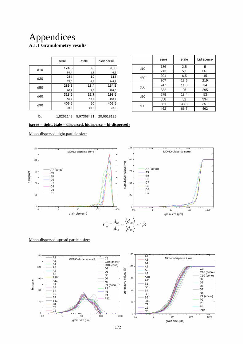
172
Appendices A.1.1 Granulometry results
(serré = tight, étalé = dispersed, bidisperse = bi-dispersed) Mono-dispersed, tight particle size:
Mono-dispersed, spread particle size:
174,5 3,8 9,6554,4 1,8 6,6
254 10 11775,0 4,9 144,2
289,5 18,4 164,560,1 9,3 184,6
318,5 22,7 193,555,9 13,2 198,7
406,5 50 406,578,5 23,6 78,5
Cu 1,8252149 5,97368421 20,0518135
d90
d10
d30
d50
d60
serré étalé bidisperse
136 2,5 5213 5,1 14,3201 6,5 15307 13,5 219247 11,8 34332 25 295279 13,4 53358 32 334351 33,3 351462 66,7 462
d90
serré étalé bidisperse
d10
d30
d50
d60
0,1 1 10 100 10000
30
60
90
120
150
MONO-disperse serré
hist
ogra
m
grain size (µm)
A7 (berge) A9 B8 C6 C7 C8 D8 P1
0,1 1 10 100 10000
25
50
75
100
125
MONO-disperse serré
cum
ulat
ive
valu
es (
%)
grain size (µm)
A7 (berge) A9 B8 C6 C7 C8 D8 P1
6060
10 10
1,8u
ddC
d d= ∼ ∼
0,1 1 10 100 10000
30
60
90
120
150
C9 C10 (ancre) C10 (cone) D2 D5 D6 D7 N5 P1 (ancre) P2 P3 P4 P12
MONO-disperse étalé
hist
ogra
m
grain size (µm)
A1 A3 A4 A5 A6 A7 A10 A11 B1 B3 B4 B5 B9 B11 C1 C3 C5
0,1 1 10 100 10000
25
50
75
100
125
C9 C10 (ancre) C10 (cone) D2 D5 D6 D7 N5 P1 (ancre) P2 P3 P4 P12
MONO-disperse étalé
cum
ulat
ive
valu
es (
%)
grain size (µm)
A1 A3 A4 A5 A6 A7 A10 A11 B1 B3 B4 B5 B9 B11 C1 C3 C5
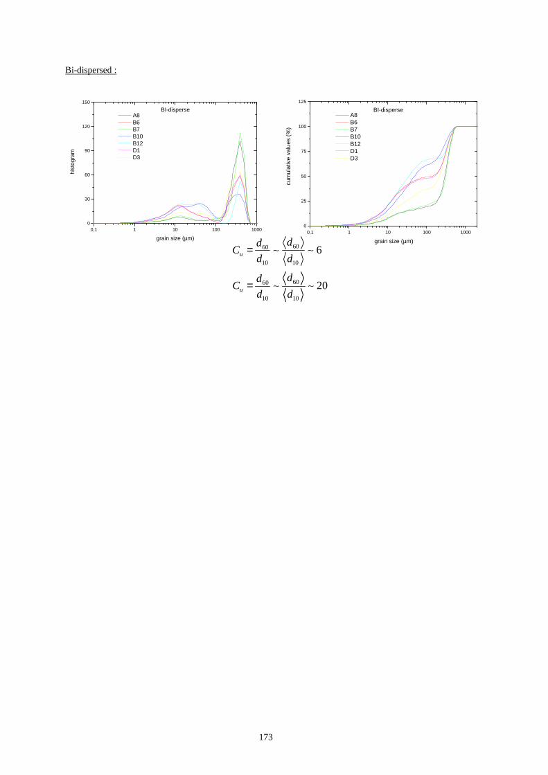
173
Bi-dispersed :
6060
10 10
6u
ddC
d d= ∼ ∼
0,1 1 10 100 10000
30
60
90
120
150
BI-disperse
hist
ogra
m
grain size (µm)
A8 B6 B7 B10 B12 D1 D3
0,1 1 10 100 10000
25
50
75
100
125
BI-disperse
cum
ulat
ive
valu
es (
%)
grain size (µm)
A8 B6 B7 B10 B12 D1 D3
6060
10 10
20u
ddC
d d= ∼ ∼

174
A.2.1 Fortran code of “Model 2” ! ********************** SUBROUTINE TASSEMENT_2 ! ********************** ! *(ZF,NPOIN,DTS,ELAY,DZF_TASS,T2,LT,XMVS,XMVE,G RAV,NOMBLAY, * ES,CONC_VASE,MS_VASE,XWC,COEF_N,CONC_GEL,CON C_MAX) ! !************************************************** ********************* ! SISYPHE V6P2 13/01/2012 !************************************************** ********************* ! !brief COMPUTES THE CONSOLIDATION BASED ON GIBSO N THEORY !+ ! !history Lan Anh Van (LHSV) !+ 10/01/2011 !+ V6P2 !+ First version in test (not yet called in curre nt version 6.2) !+ ! !~~~~~~~~~~~~~~~~~~~~~~~~~~~~~~~~~~~~~~~~~~~~~~~~~~ ~~~~~~~~~~~~~~~~~~~~~ !| COEF_N |-->| PERMEABILITY COEFFICIENT !| CONC_GEL |-->| GEL CONCENTRATION !| CONC_MAX |-->| MAXIMUM CONCENTRATION !| CONC_VASE |<->| MUD CONCENTRATION FOR EACH LAYER !| DTS |-->| TIME STEP FOR SUSPENSION !| DZF_TASS |-->| BED EVOLUTION DUE TO CONSOL IDATION !| ELAY |<->| THICKNESS OF EACH LAYER !| ES |<->| LAYER THICKNESSES AS DOUBLE PRECISION !| GRAV |-->| GRAVITY ACCELERATION !| LT |-->| ITERATION !| MS_VASE |<->| MASS OF MUD PER LAYER (KG/M 2) !| NOMBLAY |-->| NUMBER OF LAYERS FOR CONSOL IDATION !| NPOIN |-->| NUMBER OF POINTS !| T2 |<->| WORK BIEF_OBJ STRUCTURE !| XMVE |-->| WATER DENSITY !| XMVS |-->| SEDIMENT DENSITY !| XWC |-->| SETTLING VELOCITY !| ZF |-->| ELEVATION OF BOTTOM !~~~~~~~~~~~~~~~~~~~~~~~~~~~~~~~~~~~~~~~~~~~~~~~~~~ ~~~~~~~~~~~~~~~~~~~~~ ! USE BIEF USE DECLARATIONS_SISYPHE, ONLY : NLAYMAX USE INTERFACE_SISYPHE, EX_TASSEMENT_2 => TASS EMENT_2 ! IMPLICIT NONE INTEGER LNG,LU COMMON/INFO/LNG,LU ! !+-+-+-+-+-+-+-+-+-+-+-+-+-+-+-+-+-+-+-+-+-+-+-+-+- +-+-+-+-+-+-+-+-+-+-+ ! INTEGER,INTENT(IN) :: NPOIN INTEGER, INTENT(IN) :: LT,NOMBLAY DOUBLE PRECISION, INTENT(IN) :: DTS DOUBLE PRECISION, INTENT(IN) :: XMVS,XMVE, GRAV TYPE (BIEF_OBJ), INTENT(INOUT) :: DZF_TASS,E LAY,T2,ZF DOUBLE PRECISION, INTENT(INOUT) :: MS_VASE(NP OIN,NOMBLAY) DOUBLE PRECISION, INTENT(INOUT) :: ES(NPOIN,N OMBLAY) DOUBLE PRECISION, INTENT(IN) :: CONC_VASE( NOMBLAY)

175
DOUBLE PRECISION, INTENT(IN) :: XWC DOUBLE PRECISION, INTENT(IN) :: COEF_N,CON C_GEL,CONC_MAX ! !+-+-+-+-+-+-+-+-+-+-+-+-+-+-+-+-+-+-+-+-+-+-+-+-+- +-+-+-+-+-+-+-+-+-+-+ ! INTEGER I,J ! FALLING VELOCITY OF EACH LAYER DOUBLE PRECISION V_S(NLAYMAX) ! EFFECTIVE STRESS OF EACH LAYER DOUBLE PRECISION SIG_EFF(NLAYMAX) ! PERMEABILITY DOUBLE PRECISION KSED(NLAYMAX),KCONSO(NLAYMAX ) ! SEDIMENT FLUX BETWEEN TWO CONSECUTIVE LAYERS DOUBLE PRECISION FLUX(NLAYMAX) ! DIFFUSION TERM DOUBLE PRECISION DIFFU(NLAYMAX) ! ********************************************* ********************* ! * PROGRAM SIMULATING THE SEDIMENTATION-CONSOL IDATION * ! ********************************************* ********************* ! DO I =1,NPOIN T2%R(I)=0.D0 DO J=1,NOMBLAY T2%R(I)=T2%R(I)+ES(I,J) ENDDO c DEPENDING ON THE CLOSURE EQUATIONS, C THE INPUT CAN BE EFFECTIVE STRESS OF DIFFU SION TERM (= KC*DSIGMA/DC/(G*RHO_F)) c EFFECTIVE STRESS c ------------------------ ! DO J = 1,NOMBLAY ! SIG_EFF(J)= ! ENDDO C DIFFUSION TERM DO J = 1,NOMBLAY DIFFU(J)=11.55D0*(CONC_VASE(J)/(XMVS*0. 0296d0))**12.d0* & (LT*DTS)**(-3.4d0) ENDDO c PERMEABILITY c -------------- DO J=1,NOMBLAY-1 C SEDIMENTATION KSED(J)=XWC*(1.D0-CONC_VASE(J)/XMVS)* & (1.D0-(CONC_VASE(J)/CONC_GEL)) **COEF_N/ & ((XMVS-XMVE)*(CONC_VASE(J)/XMV S)/XMVE) C CONSOLIDATION KCONSO(J)=XWC*(1.D0-CONC_VASE(J)/XMVS) * & (1.D0-(CONC_VASE(J)/CONC_MAX)) **COEF_N/ & ((XMVS-XMVE)*(CONC_VASE(J)/XMV S)/XMVE) ENDDO c DO J=1,NOMBLAY-1 IF(LT*DTS.GT.11000.D0) THEN c c SEDIMENTATION AND CONSOLIDATION : c -------------------------------- C CALCULATE FROM DIFFU IF ((ES(I,J+1) + ES(I,J)).gt.1.d-8) THE N V_S(J) = & KCONSO(J) * CONC_VASE(J) * (1.D0/ XMVS - 1.D0/XMVE) & + DIFFU(J)/CONC_VASE(J)*
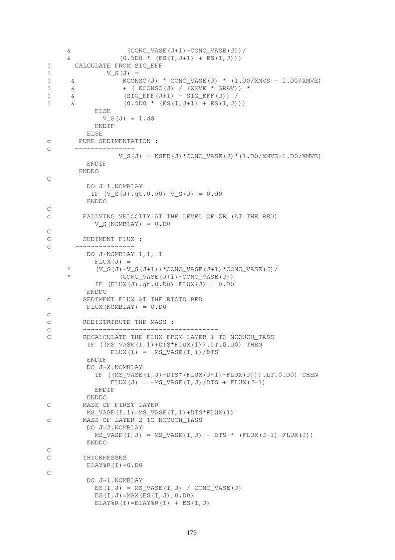
176
& (CONC_VASE(J+1)-CONC_VASE(J))/ & (0.5D0 * (ES(I,J+1) + ES(I,J))) ! CALCULATE FROM SIG_EFF ! V_S(J) = ! & KCONSO(J) * CONC_VASE(J) * (1.D0 /XMVS - 1.D0/XMVE) ! & + ( KCONSO(J) / (XMVE * GRAV)) * ! & (SIG_EFF(J+1) - SIG_EFF(J)) / ! & (0.5D0 * (ES(I,J+1) + ES(I,J))) ELSE V_S(J) = 1.d8 ENDIF ELSE c PURE SEDIMENTATION : c --------------- V_S(J) = KSED(J)*CONC_VASE(J)*(1. D0/XMVS-1.D0/XMVE) ENDIF ENDDO C DO J=1,NOMBLAY IF (V_S(J).gt.0.d0) V_S(J) = 0.d0 ENDDO C c FALLVING VELOCITY AT THE LEVEL OF ZR (AT T HE BED) V_S(NOMBLAY) = 0.D0 C C SEDIMENT FLUX : c --------------- DO J=NOMBLAY-1,1,-1 FLUX(J) = * (V_S(J)-V_S(J+1))*CONC_VASE(J+1)*CONC_V ASE(J)/ * (CONC_VASE(J+1)-CONC_VASE(J)) IF (FLUX(J).gt.0.D0) FLUX(J) = 0.D0 ENDDO c SEDIMENT FLUX AT THE RIGID BED FLUX(NOMBLAY) = 0.D0 c c REDISTRIBUTE THE MASS : c ---------------------------------- C RECALCULATE THE FLUX FROM LAYER 1 TO NCOUC H_TASS IF ((MS_VASE(I,1)+DTS*FLUX(1)).LT.0.D0) T HEN FLUX(1) = -MS_VASE(I,1)/DTS ENDIF DO J=2,NOMBLAY IF ((MS_VASE(I,J)-DTS*(FLUX(J-1)-FLUX(J ))).LT.0.D0) THEN FLUX(J) = -MS_VASE(I,J)/DTS + FLUX( J-1) ENDIF ENDDO C MASS OF FIRST LAYER MS_VASE(I,1)=MS_VASE(I,1)+DTS*FLUX(1) c MASS OF LAYER 2 TO NCOUCH_TASS DO J=2,NOMBLAY MS_VASE(I,J) = MS_VASE(I,J) - DTS * (FL UX(J-1)-FLUX(J)) ENDDO C C THICKNESSES ELAY%R(I)=0.D0 C DO J=1,NOMBLAY ES(I,J) = MS_VASE(I,J) / CONC_VASE(J) ES(I,J)=MAX(ES(I,J),0.D0) ELAY%R(I)=ELAY%R(I) + ES(I,J)

177
ENDDO C BED EVOLUTION DUE TO CONSOLIDATION DZF_TASS%R(I)=ELAY%R(I)-T2%R(I) ENDDO C END SUBROUTINE TASSEMENT_2 RETURN END
A.2.2 Fortran code of “Model 3” C C *********************** SUBROUTINE TASSEMENT_3 C *********************** C *(ZF,NPOIN,DTS,ELAY,DZF_TASS,T2,LT,XMVS,XMVE,G RAV,NOMBLAY, * ES,CONC_VASE,CONC,IVIDE,MS_VASE, XWC, COEF_N ,CONC_GEL,CONC_MAX) C C************************************************** ********************* C PROGRAMME APPELANT : SISYPHE C SIG_EFF et CHARGE: tableaux de travail additionne ls (TRA02 et TRA03) C PROGRAMMES APPELES : COEF,BISSEL C************************************************** ********************* C USE BIEF USE DECLARATIONS_SISYPHE, ONLY : NLAYMAX IMPLICIT NONE INTEGER LNG,LU COMMON/INFO/LNG,LU C C+-+-+-+-+-+-+-+-+-+-+-+-+-+-+-+-+-+-+-+-+-+-+-+-+- +-+-+-+-+-+-+-+-+-+-+ C INTEGER,INTENT(IN) :: NPOIN INTEGER, INTENT(IN) :: LT,NOMBLAY DOUBLE PRECISION, INTENT(IN) :: DTS DOUBLE PRECISION, INTENT(IN) :: XMVS,XMVE, GRAV TYPE (BIEF_OBJ), INTENT(INOUT) :: DZF_TASS,E LAY,T2,ZF DOUBLE PRECISION, INTENT(INOUT) :: MS_VASE(NP OIN,NOMBLAY) DOUBLE PRECISION, INTENT(INOUT) :: ES(NPOIN,N OMBLAY) DOUBLE PRECISION, INTENT(IN) :: XWC DOUBLE PRECISION, INTENT(IN) :: COEF_N,CON C_GEL,CONC_MAX ! DOUBLE PRECISION, INTENT(INOUT) :: CHARGE(NO MBLAY+1) DOUBLE PRECISION, INTENT(INOUT) :: CONC(NPOIN ,NOMBLAY) DOUBLE PRECISION, INTENT(INOUT) :: CONC_VASE( NOMBLAY) DOUBLE PRECISION, INTENT(INOUT) :: IVIDE(NPOI N,NOMBLAY+1) C DOUBLE PRECISION, INTENT(INOUT) :: SIG_EFF(N OMBLAY+1) C C+-+-+-+-+-+-+-+-+-+-+-+-+-+-+-+-+-+-+-+-+-+-+-+-+- +-+-+-+-+-+-+-+-+-+-+ C LOCAL VARIABLES INTEGER I,IPF,NDEB,J DOUBLE PRECISION DSIGMA,DSIG1 DOUBLE PRECISION PE,DPE,S DOUBLE PRECISION IVIDE_GEL, IVIDE_MAX DOUBLE PRECISION IVI_SED,IVI_CONSO,ECOUCH DOUBLE PRECISION TRA01(NOMBLAY+1,6) ! DOUBLE PRECISION SIG_EFF c-------------------------------------------------- --------------------- C CALCULATION OF THE VOID_RATIO AT GELLING POINT AND AT MAXIMUM CONCENTRATION S = XMVS/XMVE IVIDE_GEL=(XMVS-CONC_GEL)/CONC_GEL IVIDE_MAX=(XMVS-CONC_MAX)/CONC_MAX ! ! ----- CALCULATION OF EQUATION COEFFICIENTS ----- C DO I=1,NPOIN T2%R(I)=0.D0 DO J=1,NOMBLAY T2%R(I)=T2%R(I)+ES(I,J)
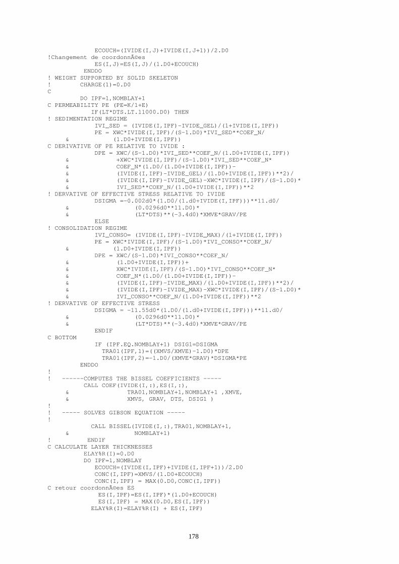
178
ECOUCH=(IVIDE(I,J)+IVIDE(I,J+1))/2.D0 !Changement de coordonnées ES(I,J)=ES(I,J)/(1.D0+ECOUCH) ENDDO ! WEIGHT SUPPORTED BY SOLID SKELETON ! CHARGE(1)=0.D0 C DO IPF=1,NOMBLAY+1 C PERMEABILITY PE (PE=K/1+E) IF(LT*DTS.LT.11000.D0) THEN ! SEDIMENTATION REGIME IVI_SED = (IVIDE(I,IPF)-IVIDE_GEL)/(1+ IVIDE(I,IPF)) PE = XWC*IVIDE(I,IPF)/(S-1.D0)*IVI_SED **COEF_N/ & (1.D0+IVIDE(I,IPF)) C DERIVATIVE OF PE RELATIVE TO IVIDE : DPE = XWC/(S-1.D0)*IVI_SED**COEF_N/(1. D0+IVIDE(I,IPF)) & +XWC*IVIDE(I,IPF)/(S-1.D0)*IVI_S ED**COEF_N* & COEF_N*(1.D0/(1.D0+IVIDE(I,IPF)) - & (IVIDE(I,IPF)-IVIDE_GEL)/(1.D0+I VIDE(I,IPF))**2)/ & (IVIDE(I,IPF)-IVIDE_GEL)-XWC*IVI DE(I,IPF)/(S-1.D0)* & IVI_SED**COEF_N/(1.D0+IVIDE(I,IP F))**2 ! DERVATIVE OF EFFECTIVE STRESS RELATIVE TO IVIDE DSIGMA =-0.002d0*(1.D0/(1.d0+IVIDE(I,I PF)))**11.d0/ & (0.0296d0**11.D0)* & (LT*DTS)**(-3.4d0)*XMVE*GRA V/PE ELSE ! CONSOLIDATION REGIME IVI_CONSO= (IVIDE(I,IPF)-IVIDE_MAX)/(1 +IVIDE(I,IPF)) PE = XWC*IVIDE(I,IPF)/(S-1.D0)*IVI_CON SO**COEF_N/ & (1.D0+IVIDE(I,IPF)) DPE = XWC/(S-1.D0)*IVI_CONSO**COEF_N/ & (1.D0+IVIDE(I,IPF))+ & XWC*IVIDE(I,IPF)/(S-1.D0)*IVI_CO NSO**COEF_N* & COEF_N*(1.D0/(1.D0+IVIDE(I,IPF)) - & (IVIDE(I,IPF)-IVIDE_MAX)/(1.D0+I VIDE(I,IPF))**2)/ & (IVIDE(I,IPF)-IVIDE_MAX)-XWC*IVI DE(I,IPF)/(S-1.D0)* & IVI_CONSO**COEF_N/(1.D0+IVIDE(I, IPF))**2 ! DERVATIVE OF EFFECTIVE STRESS DSIGMA = -11.55d0*(1.D0/(1.d0+IVIDE(I, IPF)))**11.d0/ & (0.0296d0**11.D0)* & (LT*DTS)**(-3.4d0)*XMVE*GRA V/PE ENDIF C BOTTOM IF (IPF.EQ.NOMBLAY+1) DSIG1=DSIGMA TRA01(IPF,1)=((XMVS/XMVE)-1.D0)*DPE TRA01(IPF,2)=-1.D0/(XMVE*GRAV)*DSIGM A*PE ENDDO ! ! ------COMPUTES THE BISSEL COEFFICIENTS ----- CALL COEF(IVIDE(I,:),ES(I,:), & TRA01,NOMBLAY+1,NOMBLAY+1 ,XM VE, & XMVS, GRAV, DTS, DSIG1 ) ! ! ----- SOLVES GIBSON EQUATION ----- ! CALL BISSEL(IVIDE(I,:),TRA01,NOMBLAY+1, & NOMBLAY+1) ! ENDIF C CALCULATE LAYER THICKNESSES ELAY%R(I)=0.D0 DO IPF=1,NOMBLAY ECOUCH=(IVIDE(I,IPF)+IVIDE(I,IPF+1))/2 .D0 CONC(I,IPF)=XMVS/(1.D0+ECOUCH) CONC(I,IPF) = MAX(0.D0,CONC(I,IPF)) C retour coordonnées ES ES(I,IPF)=ES(I,IPF)*(1.D0+ECOUCH) ES(I,IPF) = MAX(0.D0,ES(I,IPF)) ELAY%R(I)=ELAY%R(I) + ES(I,IPF)

179
ENDDO C BED EVOLUTION DUE TO CONSOLIDATION DZF_TASS%R(I)=ELAY%R(I)-T2%R(I) ENDDO C-------------------------------------------------- --------------------- C FIN SUBROUTINE TASSE_LENORMANT RETURN END CV 04/05/2010 CV AC(NSICLA) ! *************** SUBROUTINE COEF ! *************** ! & (IVIDE , ES_CLN, TRA01 ,NPFMAX, & IMAX, XMVE,XMVS,GRAV, & DTS , DSIG1 ) ! !************************************************** ********************* ! TELEMAC 3D VERSION 5.1 13/05/92 C LE NORMA NT (LNH)30 87 78 54 ! FORTRAN95 VERSION MARCH 1999 JACEK A. JANKOWSKI PINXIT !************************************************** ********************* ! ! FONCTION: CALCUL DES COEFFICIENTS ISSUS DE LA DISCRETISATION DE ! L'EQUATION DIFFERENTIELLE REGISSANT LA CONSOLIDATION ! DU FOND VASEUX- ! !-------------------------------------------------- --------------------- ! ARGUMENTS ! .________________.____.__________________________ _____________________ ! | NOM |MODE| ROLE ! |________________|____|__________________________ _____________________ ! | IVIDE | -->| INDICE DES VIDES AUX POI NTS DU MAILLAGE | ! | | | (MAILLAGE SELON UNE V ERTICALE) | ! | EPAI | -->| EPAISSEURS DES MAILLES | ! | TRA01 | -->| TABLEAU DE TRAVAIL | ! | NPFMAX | -->| NOMBRE MAXIMUM DE PLANS HORIZONTAUX | ! | | | DISCRETISANT LE FOND VAS EUX | ! | IMAX | -->| NOMBRE DE POINTS DU MAIL LAGE | ! | RHOS | -->| MASSE VOLUMIQUE DU SEDIM ENT | ! | GRAV | -->| ACCELERATION DE LA PESAN TEUR | ! | DTC | -->| PAS DE TEMPS DU PHENOMEN E DE CONSOLIDATION | ! | DSIG1 | -->| DERIVEE DE LA CONTRAINTE EFFECTIVE | ! | | | AU PREMIER POINT DU MAIL LAGE | ! |________________|____|__________________________ ___________________| ! MODE : -->(DONNEE NON MODIFIEE), <--(RESULTAT), < -->(DONNEE MODIFIEE) !-------------------------------------------------- --------------------- ! PROGRAMME APPELANT : TASSEM !************************************************** ******************** ! IMPLICIT NONE C C+-+-+-+-+-+-+-+-+-+-+-+-+-+-+-+-+-+-+-+-+-+-+-+-+- +-+-+-+-+-+-+-+-+-+-+ C INTEGER, INTENT(IN) :: IMAX,NPFMAX ! DOUBLE PRECISION, INTENT(INOUT) :: TRA01(NPF MAX,6) DOUBLE PRECISION, INTENT(IN) :: ES_CLN(NP FMAX-1) DOUBLE PRECISION, INTENT(IN) :: IVIDE(NPF MAX) DOUBLE PRECISION, INTENT(IN) :: GRAV,XMVS ,XMVE,DTS , DSIG1 C C+-+-+-+-+-+-+-+-+-+-+-+-+-+-+-+-+-+-+-+-+-+-+-+-+- +-+-+-+-+-+-+-+-+-+-+ C LOCAL VARIABLES INTEGER I,IPF , NDEB DOUBLE PRECISION A, D NDEB = 1 !================================================== ===================== ! -----INITIALISATION DES COEFFICIENTS-----

180
DO IPF=NDEB,IMAX TRA01(IPF,3)=0.D0 TRA01(IPF,4)=1.D0 TRA01(IPF,5)=0.D0 TRA01(IPF,6)=0.D0 END DO ! ! -----CALCUL DES COEFFICIENTS AUX POINTS DU M AILLAGE----- c ...POINT DE L'INTERFACE: TRA01(NDEB,6)=IVIDE(NDEB) ! ! ...POINTS INTERIEURS: DO IPF=NDEB+1,IMAX-1 IF (TRA01(IPF,1).GE.1.D-10) THEN A=TRA01(IPF,1)/ES_CLN(IPF-1) D=1.D0 ELSE A=TRA01(IPF,1)/ES_CLN(IPF) D=0.D0 ENDIF c TRA01(IPF,3)=DTS*(-D*A-(TRA01(IPF,2)+TRA01 (IPF-1,2))/ & ((ES_CLN(IPF-1)+ES_CLN(IPF))*ES_CLN(I PF-1))) c TRA01(IPF,5)=DTS*((1.D0-D)*A- & ((TRA01(IPF,2)+TRA01(IPF+1,2) )/ & ((ES_CLN(IPF-1)+ES_CLN(IPF))*ES_CLN(I PF)))) c TRA01(IPF,4)=1.D0-TRA01(IPF,3)-TRA01(IPF,5 ) c TRA01(IPF,6)=IVIDE(IPF) ENDDO ! ...POINT DU FOND: TRA01(IMAX,5)=-1.D0 TRA01(IMAX,6)=(XMVS-XMVE)*GRAV*ES_CLN(imax- 1)/DSIG1 RETURN END SUBROUTINE COEF !************************************************** ********************* ! ***************** SUBROUTINE BISSEL ! ***************** ! &(IVIDE,TRA01,NPFMAX,IMAX) ! !************************************************** ********************* ! TELEMAC 3D VERSION 5.7 18/07/06 NOEMIE DURAND ET SEBASTIEN BOURBAN ! C LE NORMA NT (LNH) 30 87 78 54 ! FORTRAN95 VERSION MARCH 1999 JACEK A. JANKOWSKI PINXIT !************************************************** ********************* ! ! FONCTION: RESOLUTION D'UN SYSTEME DE IMAX EQU ATIONS AVEC POUR ! INCONNUE E A L'INSTANT N+1- ! METHODE DITE DE DOUBLE BALAYAGE ! !-------------------------------------------------- --------------------- ! ARGUMENTS ! .________________.____.__________________________ _____________________ ! | NOM |MODE| ROLE ! |________________|____|__________________________ ____________________ ! | IVIDE |<-- | INDICE DES VIDES AUX PO INTS DU MAILLAGE | ! | | | (MAILLAGE SELON UNE VERTICALE) | ! | NPFMAX | -->| NOMBRE MAXIMUM DE PLANS HORIZONTAUX | ! | | | DISCRETISANT LE FOND VA SEUX | ! | IMAX | -->| NOMBRE DE POINTS DU MAI LLAGE DU FOND | ! | TRA01 | -->| TABLEAU DE TRAVAIL | ! |________________|____|__________________________ ___________________| ! MODE : -->(DONNEE NON MODIFIEE), <--(RESULTAT), < -->(DONNEE MODIFIEE) !-------------------------------------------------- ---------------------

181
! PROGRAMME APPELANT : TASSEM !************************************************** ******************** ! IMPLICIT NONE INTEGER LNG,LU COMMON/INFO/LNG,LU ! INTEGER, INTENT(IN) :: IMAX,NPFMAX ! DOUBLE PRECISION, INTENT(INOUT) :: IVIDE(NPFM AX) DOUBLE PRECISION, INTENT(INOUT) :: TRA01(NPFM AX,6) ! DOUBLE PRECISION VAR, N_VAR, N_IVIDE INTEGER K,I, NDEB, IPF DOUBLE PRECISION EPS ! !================================================== ==================== NDEB=1 ! ! THE FLOATING POINT EXCEPTIONS ARE NOW CHECKED BE FORE BEING USED EPS=1.D-8 DO IPF = IMAX-1,NDEB+1,-1 IF( ABS(TRA01(IPF-1,4)).LT.EPS ) THEN WRITE(LU,*) 'FLOATING EXCEPTION IN BISSEL (CALLED BY TASSEM)' CALL PLANTE(1) STOP ENDIF TRA01(IPF,4) = TRA01(IPF,4)-(TRA01(IPF,3)*T RA01(IPF+1,5)) & /TRA01(IPF+1,4) TRA01(IPF,6) = TRA01(IPF,6)-(TRA01(IPF,3)*T RA01(IPF+1,6)) & /TRA01(IPF+1,4) ENDDO ! IF(ABS(TRA01(NDEB,3)*TRA01(NDEB+1,5) & -TRA01(NDEB+1,4)*TRA01(NDEB,4)).LT.E PS ) THEN WRITE(LU,*) 'DIVISION BY ZERO IN BISSEL 1 ( CALLED BY TASSEM)' CALL PLANTE(1) STOP ENDIF ! IVIDE(NDEB)= & (TRA01(NDEB,6)*TRA01(NDEB+1,4)-TRA01(NDEB,3 )*TRA01(NDEB+1,6))/ & (TRA01(NDEB,4)*TRA01(NDEB+1,4)-TRA01(NDEB,3 )*TRA01(NDEB+1,5)) C DO IPF = NDEB+1,IMAX IF( ABS(TRA01(IPF,4)).LT.EPS ) THEN WRITE(LU,*) 'DIVISION BY ZERO IN BISSEL 2 (CALLED BY TASSEM)' CALL PLANTE(1) STOP ENDIF IVIDE(IPF)=(TRA01(IPF,6)-TRA01(IPF,5)*IVIDE (IPF-1))/TRA01(IPF,4) ENDDO C !-------------------------------------------------- --------------------- ! RETURN END SUBROUTINE BISSEL A.2.3 Test case of ”Model 1” /PROCESSEURS PARALLELES : 1 / CAS TEST DE TASSEMENT POUR MODELE DE TASSEMENT NO 1 / MATERIAU: VASE DE LA GIRONDE / /++++++++++++++++++++++++++++++++++++++++++++++++++ ++++++ / FICHIER DE DECLARATION DES MOTS CLES DU CODE SIS YPHE
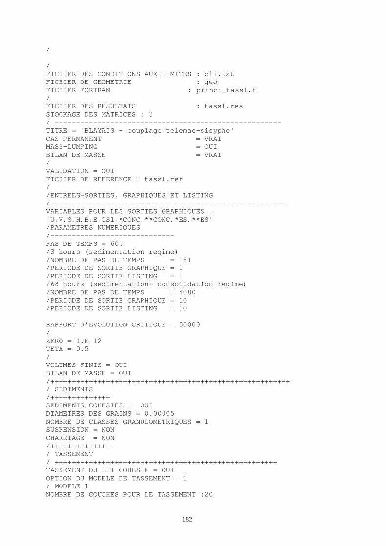
182
/ / FICHIER DES CONDITIONS AUX LIMITES : cli.txt FICHIER DE GEOMETRIE : geo FICHIER FORTRAN : princi_tass1.f / FICHIER DES RESULTATS : tass1.res STOCKAGE DES MATRICES : 3 / ------------------------------------------------- ---- TITRE = 'BLAYAIS - couplage telemac-sisyphe' CAS PERMANENT = VRAI MASS-LUMPING = OUI BILAN DE MASSE = VRAI / VALIDATION = OUI FICHIER DE REFERENCE = tass1.ref / /ENTREES-SORTIES, GRAPHIQUES ET LISTING /-------------------------------------------------- ----- VARIABLES POUR LES SORTIES GRAPHIQUES = 'U,V,S,H,B,E,CS1,*CONC,**CONC,*ES,**ES' /PARAMETRES NUMERIQUES /----------------------------- PAS DE TEMPS = 60. /3 hours (sedimentation regime) /NOMBRE DE PAS DE TEMPS = 181 /PERIODE DE SORTIE GRAPHIQUE = 1 /PERIODE DE SORTIE LISTING = 1 /68 hours (sedimentation+ consolidation regime) /NOMBRE DE PAS DE TEMPS = 4080 /PERIODE DE SORTIE GRAPHIQUE = 10 /PERIODE DE SORTIE LISTING = 10 RAPPORT D'EVOLUTION CRITIQUE = 30000 / ZERO = 1.E-12 TETA = 0.5 / VOLUMES FINIS = OUI BILAN DE MASSE = OUI /++++++++++++++++++++++++++++++++++++++++++++++++++ ++++++ / SEDIMENTS /++++++++++++++ SEDIMENTS COHESIFS = OUI DIAMETRES DES GRAINS = 0.00005 NOMBRE DE CLASSES GRANULOMETRIQUES = 1 SUSPENSION = NON CHARRIAGE = NON /++++++++++++++ / TASSEMENT / +++++++++++++++++++++++++++++++++++++++++++++++++ +++ TASSEMENT DU LIT COHESIF = OUI OPTION DU MODELE DE TASSEMENT = 1 / MODELE 1 NOMBRE DE COUCHES POUR LE TASSEMENT :20

183
/ CONCENTRATIONS DU LIT DE VASE : 77.;80.;93.;109.;125.;141.;157.;173.;186.;204.;220. ;236.; 252.;268.;284.;300.;316.;332.;348.;364.0 / TRANSFERT DE MASSE PAR COUCHE: 1.D-02;8.D-03;6.D-03;4.D-03;2.0D-03;1.D-03;8.D-04;6 .D-04; 4.0D-04;2.0D-04;1.0D-04;8.0D-05;6.0D-05;4.0D-05;2.0 D-05; 1.0D-05;1.0D-05;1.0D-05;1.0D-05;0.d0 / / &ETA A.2.4 Test case of « Model 2 » /PROCESSEURS PARALLELES : 1 / CAS TEST DE TASSEMENT POUR MODELE DE TASSEMENT NO 2 / MATERIAU: VASE DE LA GIRONDE / /++++++++++++++++++++++++++++++++++++++++++++++++++ ++++++ / FICHIER DE DECLARATION DES MOTS CLES DU CODE SIS YPHE / / FICHIER DES CONDITIONS AUX LIMITES : cli.txt FICHIER DE GEOMETRIE : geo FICHIER FORTRAN : princi_tass2.f / FICHIER DES RESULTATS : tass2.res STOCKAGE DES MATRICES : 3 / ------------------------------------------------- ---- TITRE = 'BLAYAIS - couplage telemac-sisyphe' CAS PERMANENT = VRAI MASS-LUMPING = OUI BILAN DE MASSE = VRAI / /VALIDATION = OUI /FICHIER DE REFERENCE = tass2.ref / /ENTREES-SORTIES, GRAPHIQUES ET LISTING /-------------------------------------------------- ----- VARIABLES POUR LES SORTIES GRAPHIQUES = 'U,V,S,H,B,E,CS1,*ES,**ES' /PARAMETRES NUMERIQUES /----------------------------- PAS DE TEMPS = 60. /3 hours (sedimentation regime) /NOMBRE DE PAS DE TEMPS = 1086 /PERIODE DE SORTIE GRAPHIQUE = 6 /PERIODE DE SORTIE LISTING = 6 / NOMBRE DE PAS DE TEMPS = 4080 PERIODE DE SORTIE GRAPHIQUE = 10 PERIODE DE SORTIE LISTING = 10

184
RAPPORT D'EVOLUTION CRITIQUE = 30000 / ZERO = 1.E-12 TETA = 0.5 / VOLUMES FINIS = OUI BILAN DE MASSE = OUI /++++++++++++++++++++++++++++++++++++++++++++++++++ ++++++ / SEDIMENTS /++++++++++++++ SEDIMENTS COHESIFS = OUI DIAMETRES DES GRAINS = 0.00005 NOMBRE DE CLASSES GRANULOMETRIQUES = 1 SUSPENSION = NON CHARRIAGE = NON /++++++++++++++ / TASSEMENT / +++++++++++++++++++++++++++++++++++++++++++++++++ +++ TASSEMENT DU LIT COHESIF = OUI OPTION DU MODELE DE TASSEMENT = 2 / MODELE 2 COEFFICIENT DE PERMEABILITE =8. CONCENTRATION GEL = 312. CONCENTRATION MAXIMALE = 400. / VITESSES DE CHUTE = 0.0017658 / MASSE VOLUMIQUE DU SEDIMENT = 2600. MASSE VOLUMIQUE DE L'EAU =1000. CONCENTRATION MASSIQUE = OUI CONCENTRATIONS PAR CLASSE AUX FRONTIERES = 0.;0. / NOMBRE DE COUCHES POUR LE TASSEMENT :20 CONCENTRATIONS DU LIT DE VASE : 77.;80.;93.;109.;125.;141.;157.;173.;186.;204.;220. ;236.; 252.;268.;284.;300.;316.;332.;348.;364.0 /CONTRAINTE CRITIQUE D'EROSION DE LA VASE : /0.00816605;0.0264398;0.05477861;0.0930092;0.140985 92; /0.19862961;0.29816415;0.46425147;0.68695285;0.8215 7461 / / &ETA A.2.5 Test case of “Model 3” / TASSEMENT DU LIT COHESIF = OUI OPTION DU MODELE DE TASSEMENT = 3 / NOMBRE DE COUCHES POUR LE TASSEMENT :20 SUSPENSION = NON / /PROCESSEURS PARALLELES : 8 / CAS TEST DE TASSEMENT POUR MODELE DE TASSEMENT NO 2 / MATERIAU: VASE DE LA GIRONDE

185
/DEBUGGER = 1 /++++++++++++++++++++++++++++++++++++++++++++++++++ ++++++ / FICHIER DE DECLARATION DES MOTS CLES DU CODE SIS YPHE /EFFET DE PENTE : OUI CORRECTION DU CHAMP CONVECTEUR = OUI FORME DE LA CONVECTION : 1 /REFERENCE / FORME DE LA CONVECTION : 2 OPTION DE SUPG : 2 / FORME DE LA CONVECTION : 6 /SCHEMA PSI/ / FORME DE LA CONVECTION : 8 / VOLUMES FINIS / FICHIER DES CONDITIONS AUX LIMITES : cli.txt FICHIER DE GEOMETRIE : geo FICHIER FORTRAN : princi_tass3.f FICHIER DES RESULTATS :tass3.res STOCKAGE DES MATRICES : 3 / ------------------------------------------------- ---- TITRE = 'BLAYAIS - couplage telemac-sisyphe' CAS PERMANENT = VRAI MASS-LUMPING = OUI BILAN DE MASSE = VRAI / /ENTREES-SORTIES, GRAPHIQUES ET LISTING /-------------------------------------------------- ----- VARIABLES POUR LES SORTIES GRAPHIQUES = 'U,V,S,H,B,E,*ES,**ES,*CONC,**CONC' /PARAMETRES NUMERIQUES /----------------------------- PAS DE TEMPS = 10 / /3 hours (sedimentation regime) NOMBRE DE PAS DE TEMPS = 1086 PERIODE DE SORTIE GRAPHIQUE = 6 PERIODE DE SORTIE LISTING = 6 / /68 hours (consolidation regime) /NOMBRE DE PAS DE TEMPS = 4080 /PERIODE DE SORTIE GRAPHIQUE = 10 /PERIODE DE SORTIE LISTING = 10 RAPPORT D'EVOLUTION CRITIQUE = 300000 / ZERO = 1.E-12 TETA = 0.5 / VOLUMES FINIS = OUI BILAN DE MASSE = OUI /++++++++++++++++++++++++++++++++++++++++++++++++++ ++++++ / SEDIMENTS /++++++++++++++ SEDIMENTS COHESIFS = OUI DIAMETRES DES GRAINS = 0.00005 NOMBRE DE CLASSES GRANULOMETRIQUES = 1 CHARRIAGE = NON SUSPENSION = NON /++++++++++++++

186
/ TASSEMENT / COEFFICIENT DE PERMEABILITE =8. CONCENTRATION GEL = 312. CONCENTRATION MAXIMALE = 365. / VITESSES DE CHUTE = 0.0017658 / MASSE VOLUMIQUE DU SEDIMENT = 2600. MASSE VOLUMIQUE DE L'EAU =1000. CONCENTRATION MASSIQUE = OUI CONCENTRATIONS PAR CLASSE AUX FRONTIERES = 0.;0. / CONCENTRATIONS DU LIT DE VASE : 77.;77.;77.;77.;77.;77.;77.;77.;77.;77.; 77.;77.;77.;77.;77.;77.;77.;77.;77.;77. / /------------------------------ / &ETA