Modeling potential movements of an ash threat

581

Advances in Threat Assessment and Their Application to Forest and Rangeland Management

Louis R. Iverson, Anantha Prasad, Jonathan Bossenbroek, Davis Sydnor, and Mark W. Schwartz

Louis R. Iverson, research landscape ecologist, and Anantha Prasad, ecologist, USDA Forest Service, North-ern Research Station, Delaware, OH 45015; Jonathan Bossenbroek, assistant professor, University of Toledo, Department of Earth, Ecological and Environmental Sciences, Lake Erie Center, Oregon, OH 43618; Davis Sydnor, professor, Ohio State University, School of Natural Resources, Columbus, OH 43210; and Mark W. Schwartz, professor University of California-Davis, Department of Environmental Science and Policy, Davis, CA 95616-8573.

AbstractThe emerald ash borer (EAB, Agrilus planipennis Fair-maire) is threatening to decimate native ashes (Fraxinus spp.) across North America and, so far, has devastated ash populations across sections of Michigan, Ohio, Indiana, and Ontario. We are attempting to develop a computer model that will predict EAB future movement by adapting a model developed for the potential movement of tree species over a century of climate change. We have two model variants, an insect-flight model and an insect-ride model to assess potential movement.

The models require spatial estimates of EAB abun-dance and ash abundance. The EAB abundance map shows a zone of initial infestation in the western suburbs of Detroit, with ash trees first dying about 1998. The fine-scale (270-m cells) ash basal area maps show highly variable values, but woodlots often have very high levels of ash. At the coarse scale (20-km cells) for the Eastern United States, available ash is high throughout the northern part of the country.

With the flight model, probability of movement is dependent on EAB abundance in the source cells, the quantity of ash in the target cells, and the distances between them. With the insect-ride model, we used geographic infor-mation system data to weight factors related to potential human-assisted movements of EAB-infested ash wood or just hitchhiking insects. We are developing a gravity model

that considers traffic volumes and routes between EAB source areas and various distances to campgrounds.

Preliminary results from a test strip through northern Ohio show (1) the insect-flight model creates a relative probability of colonization that decreases quickly from the EAB range boundary edge; and (2) the insect-ride model provides occasions for long-distance transport via human-aided dispersals.

Keywords: Ash, dispersal, emerald ash borer, invasive, Ohio.

IntroductionThe emerald ash borer (EAB), Agrilus planipennis Fair-maire (Coleoptera: Buprestidae), poses a serious threat to all ash trees in North America. The larvae feed on phloem, producing galleries that eventually kill large trees in 3 to 4 years and small trees in as little as 1 year (Poland and McCullough 2006). A native of Northeastern China, Korea, Japan, Mongolia, Taiwan, and Eastern Russia, the species was first identified in the United States near Detroit, Michi-gan, in July 2002 (Haack 2006). The borer was probably imported into Michigan in the early 1990s via infested ash crating or pallets (Herms and others 2004).

The impact of EAB may be enormous. An estimated 8 billion ash trees exist in the United States, comprising roughly 7.5 percent of the volume of hardwood sawtimber, 14 percent of the urban leaf area (as estimated across eight U.S. cities), and with a value exceeding $300 billion (Poland and McCullough 2006).

Research into the spatial distribution of the host ash species helps us better understand the resource at risk and the potential for EAB spread. The USDA Forest Service’s Forest Inventory and Analysis (FIA) units continually conduct inventories across more than 100,000 plots in the Eastern United States (Miles and others 2001). This invalu-able data source provides the information critical to the assessment of the ash resource, including the work reported here. For a detailed look, we rely on 30-m Landsat data that have been classified into forest types with associated ground samples to calculate ash content.

Modeling Potential Movements of the Emerald Ash Borer: the Model Framework

Previous

582

GENERAL TECHNICAL REPORT PNW-GTR-802

There are a variety of approaches for using computer models to predict the risk and spread of invasive insects (e.g., Rykiel and others 1988, Sharov and Liebhold 1998, Sharov and others 1997, Sturtevant and others 2004, Turchin 2003). To summarize, modeling insect movement is a complicated venture, especially in heterogeneous landscapes. BenDor and Metcalf (2006) and BenDor and others (2006) have initiated a dynamic modeling approach to learn more about EAB spread and possible mechanisms to retard it. These authors also call for high resolution data on the ash resource and human-assisted components such as campgrounds to move this work forward. In this paper, we present a slightly different approach using higher resolution databases.

The objectives of this work are to (1) evaluate the ash quantity across the Eastern United States at a coarse level and in Ohio at a fine scale; (2) assess EAB spread and rate of spread through the region so far; and (3) begin to model future spread through the two modeling approaches of insects flying and insects riding with humans.

MethodsDistribution of AshFraxinus (ash) is the only genus that EAB has attacked in North America. There is no observed host expansion. Consequently, we mapped ash availability as a resource for EAB spread, at a coarse resolution for the Eastern United States (20- by 20-km cell) and at a fine resolution for Ohio (30- by 30-m cell size).

Coarse-Level Analysis of Ash for the Eastern United States—We used FIA data (Miles and others 2001) to determine ash distribution and abundance for 9,782 cells over the Eastern United States. We created these data sets for a climate change atlas (Iverson and others 1999) and have made these data available (Prasad and Iverson 2003). We summed the data for four species of ash that comprise the vast majority of ash in the Eastern United States: Fraxinus americana L. (white ash), F. pennsylvanica Marsh. (green ash), F. nigra Marsh. (black ash), and F. quadrangulata Michx. (blue ash). This effort produced maps of relative availability of rural

ash (FIA does not sample urban areas well) to the EAB. The methodology used data from the 100,000+ forested plots to calculate the basal area (BA) of ash per plot, then calculated average BA of ash per unit area based on all the plots within the 20- by 20-km cell. One drawback of this methodology is that in some cells with small quantities of forest, no FIA plots were established so that the average ash BA is calcu-lated as zero for that cell. In reality (as seen in the fine-scale analysis), every cell in the Midwest has at least some forest (and, most likely, some ash). Another drawback is that the urban forest resource is underrepresented in the FIA data. (There is an ongoing effort within our group to conduct surveys to better understand the forest resource in certain urban areas.)

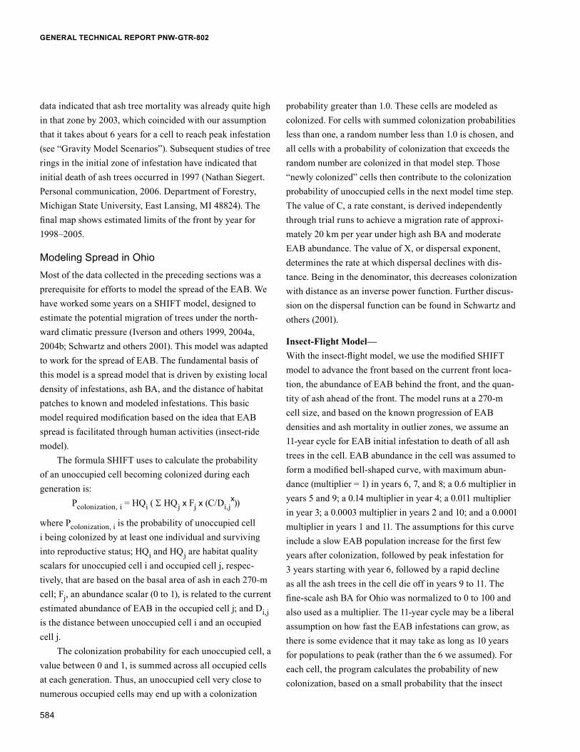
The next step was to create a map of percentage of for-est cover by 20- by 20-km-grid cell. We acquired classified 30 m Landsat TM-interpreted data from Riitters and others (2002). The data were reclassified into forest or nonfor-est and tallied by 20- by 20-km cell to yield an estimated percentage of forest cover for each cell.

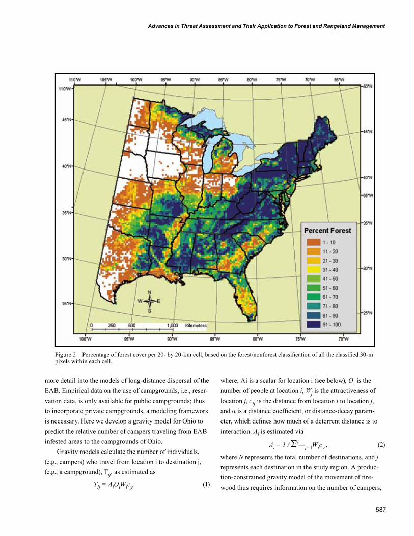
Data from the average BA map was multiplied by the percentage of forest cover per 20- by 20-km cell, providing an estimate of the total availability of the ash resource to the invasive species, in thousands of square feet of BA per 20 by 20 km.

Fine-Scale Analysis of Ash in Ohio—For a detailed estimate of ash resource availability in Ohio, we combined estimates of ash BA per FIA plot with a Landsat TM-based classification of forest types. We acquired the landcover data from the Ohio Gap Analysis Program (GAP) (Ramirez and others 2005). This data set contains vegetation classes based on leaf-on and leaf-off imagery from 1999 to 2002 (Ramirez and others 2005), at 30-m resolution. Vegetation classes conform to the NatureServe’s Ecological Classification system (Comer and others 2003). We attempted to establish ash percentages for 28 classes, including the following classes important in northwestern Ohio: row crop, open water, low density urban, high density urban, urban forested, grassland, evergreen forest, North-Central Interior Dry Oak For-est and Woodland (CES202.047), North-Central Interior Floodplain (CES202.694), North-Central Interior Wet

583


Flatwoods (CES202.700), and North-Central Oak Barrens (CES202.727).

To estimate ash BA in each landcover type, 2,298 FIA plots were overlaid on the Ohio GAP data set by Elizabeth LaPoint, FIA geographic information system (GIS) Service Center. Due to the restriction on releasing FIA plot coordi-nates, Ms. LaPoint performed the overlay and reported the average ash BA per class. However, only a portion of the plot coordinates (ca 40 percent) were global positioning sys-tem (GPS) corrected so that locational error is present in the overlay (which caused, for example, some plots to appear in open water). For certain classes, including the urban classes, row crop, and oak barrens, we believed, based on number of FIA plots available and ancillary information, the data reported for southern Michigan by McFarlane and others (2005) better represented the quantity of ash present in the types. So, the McFarlane and others data were substituted for the FIA estimates.

Finally, an EAB habitat availability map was prepared by applying the estimated BA of ash per class. To prepare a smoother map, which was needed for the modeling effort, we calculated the mean ash BA per 270-m pixel (a 9 by 9 cell average). This product was used for mapping and modeling, which requires estimates of ash quantities per cell (see “Modeling Spread in Ohio”).

Mapping Estimated EAB Spread, 1998–2005To model potential future spread and assess observed spread rates, a preliminary map of historical spread was created. For this, multiple data sets and GIS manipulations were used, and for the most part, represent the spread of visible damage to ash trees rather than the initial infestation of EAB. The Michigan Department of Natural Resources (DNR) mapped pest outbreaks, which estimated the range of EAB-damaged ash in 2002 and 2003. These were accepted as accurate. We also used data from interstate highway exit surveys for 2003 and 2004, with 10 ash trees per exit tallied for death/life (irrespective of what killed the ash) by Smitley (2005) and Smitley and others (2005). These data were useful to show where ash death first occurred in the region. A Michigan ash damage survey from September 2004 also was used (Michigan State University, 2006) along

with the actual locations and density of extent of known EAB locations as of December 2005, obtained from the Cooperative Emerald Ash Borer Project (2006). In addition, multiple dates of these national EAB positive maps were acquired to detect additional finds temporally. Finally, our own field work on ash tree assessment in northern Ohio and southern Michigan during the summers of 2004 and 2005 yielded additional spatial information, particularly on ash not yet visually affected by EAB. Again, most of the data were based on visual observations of damage, which can be delayed for several years after EAB colonization in otherwise healthy, larger ash trees. It should also be noted that girdled detection trees were used in Michigan in 2004 and 2005, which increased detection capability over that available from visual inspection alone. Thus, this new survey method may have artificially expanded the estimated front in 2004 and 2005 over what would have been detected with only observable symptoms. It definitely expanded the number of outliers detected outside the main front.

Known EAB locations were inputted into ArcGIS (GRID - focalsum commands), and four EAB abundance classes were derived based on the number of EAB positives recorded within three spheres of influence around each point: 1, 2.5, and 5 km. Each 270-m cell within the study area was assigned EAB abundance class 0 (no EAB posi-tives within 5 km), 1 (1 to 5 positives within 5 km), 2 (1 to 3 positives within 2.5 km or 6 to 10 positives within 5 km), or 3 (1 to 38 positives within 1 km, or 4 to 100 positives within 2.5 km, or 11 to 110 positives within 5 km). The resulting map presented the best summary of EAB concentration areas as of December 2005.

Armed with all the above data sets overlaid in ArcGIS, we manually drew estimated boundaries of the EAB-dam-aged ash front for 2005, 2004, 2001, 2000, 1999, and 1998. Lines were drawn to encompass the higher EAB density zones, the mortality estimates, and the nearby new finds for each year. For 2002 and 2003, we used the pest maps from Michigan DNR mentioned above. Although EAB probably entered the United States prior to 1998 and was likely present in these trees prior to that date, we started with 1998 as the first year to estimate the visual damage front based primarily on the Smitley (2005) data. These

584


data indicated that ash tree mortality was already quite high in that zone by 2003, which coincided with our assumption that it takes about 6 years for a cell to reach peak infestation (see “Gravity Model Scenarios”). Subsequent studies of tree rings in the initial zone of infestation have indicated that initial death of ash trees occurred in 1997 (Nathan Siegert. Personal communication, 2006. Department of Forestry, Michigan State University, East Lansing, MI 48824). The final map shows estimated limits of the front by year for 1998–2005.

Modeling Spread in OhioMost of the data collected in the preceding sections was a prerequisite for efforts to model the spread of the EAB. We have worked some years on a SHIFT model, designed to estimate the potential migration of trees under the north-ward climatic pressure (Iverson and others 1999, 2004a, 2004b; Schwartz and others 2001). This model was adapted to work for the spread of EAB. The fundamental basis of this model is a spread model that is driven by existing local density of infestations, ash BA, and the distance of habitat patches to known and modeled infestations. This basic model required modification based on the idea that EAB spread is facilitated through human activities (insect-ride model).

The formula SHIFT uses to calculate the probability of an unoccupied cell becoming colonized during each generation is:

Pcolonization, i = HQi ( S HQj x Fj x (C/Di,jx))

where Pcolonization, i is the probability of unoccupied cell i being colonized by at least one individual and surviving into reproductive status; HQi and HQj are habitat quality scalars for unoccupied cell i and occupied cell j, respec-tively, that are based on the basal area of ash in each 270-m cell; Fj, an abundance scalar (0 to 1), is related to the current estimated abundance of EAB in the occupied cell j; and Di,j is the distance between unoccupied cell i and an occupied cell j.

The colonization probability for each unoccupied cell, a value between 0 and 1, is summed across all occupied cells at each generation. Thus, an unoccupied cell very close to numerous occupied cells may end up with a colonization

probability greater than 1.0. These cells are modeled as colonized. For cells with summed colonization probabilities less than one, a random number less than 1.0 is chosen, and all cells with a probability of colonization that exceeds the random number are colonized in that model step. Those “newly colonized” cells then contribute to the colonization probability of unoccupied cells in the next model time step. The value of C, a rate constant, is derived independently through trial runs to achieve a migration rate of approxi-mately 20 km per year under high ash BA and moderate EAB abundance. The value of X, or dispersal exponent, determines the rate at which dispersal declines with dis-tance. Being in the denominator, this decreases colonization with distance as an inverse power function. Further discus-sion on the dispersal function can be found in Schwartz and others (2001).

Insect-Flight Model—With the insect-flight model, we use the modified SHIFT model to advance the front based on the current front loca-tion, the abundance of EAB behind the front, and the quan-tity of ash ahead of the front. The model runs at a 270-m cell size, and based on the known progression of EAB densities and ash mortality in outlier zones, we assume an 11-year cycle for EAB initial infestation to death of all ash trees in the cell. EAB abundance in the cell was assumed to form a modified bell-shaped curve, with maximum abun-dance (multiplier = 1) in years 6, 7, and 8; a 0.6 multiplier in years 5 and 9; a 0.14 multiplier in year 4; a 0.011 multiplier in year 3; a 0.0003 multiplier in years 2 and 10; and a 0.0001 multiplier in years 1 and 11. The assumptions for this curve include a slow EAB population increase for the first few years after colonization, followed by peak infestation for 3 years starting with year 6, followed by a rapid decline as all the ash trees in the cell die off in years 9 to 11. The fine-scale ash BA for Ohio was normalized to 0 to 100 and also used as a multiplier. The 11-year cycle may be a liberal assumption on how fast the EAB infestations can grow, as there is some evidence that it may take as long as 10 years for populations to peak (rather than the 6 we assumed). For each cell, the program calculates the probability of new colonization, based on a small probability that the insect

585


will fly from an occupied cell to an unoccupied cell, for all surrounding cells within a specified search window (40 km in this case). Once selected for colonization, the cell starts the 11-year cycle of EAB increasing and then decreasing as ash dies out.

Insect-Ride Model—To develop the insect-ride model, we used GIS data to weight factors related to potential human-assisted move-ments of EAB-infested ash wood or just hitchhiking insects: roads, urban areas, various wood products industries, popu-lation density, and campgrounds. Each of these five factors was converted into weighting layers that became multipliers for the ash BA component of the insect-ride model. That is, the increase in probability of EAB infestation by the insect-ride factors is made manifest by increasing the amount of ash available in those cells. Thus, if no ash exists in the cell, it matters not whether there is an escaped EAB from one of the human-assisted vectors, but if there is a large ash component, an escaped EAB could quickly find a place to colonize.

To register the increased probability of insects riding on windshields, radiators, or otherwise attached to vehicles moving down the road, we assigned weights to two widths of major road corridors. We used the U.S. Geological Survey major roads data and created buffers of 1 and 2 km, with a scoring of 10 for 0 to 1 km and 5 for 1 to 2 km distance from the roads.

For urban areas, where there is much more vehicular density and opportunity for EAB transport, we assigned values of 7 if the urban center size was less than the median size and 10 if greater than the median. We therefore assume larger cities will have greater chance of EAB infestation via human movement. Data were acquired for the State of Ohio urban centers from the Department of Transportation Office of Technical Services (Ohio Department of Transportation 2006).

Related to the urban areas, weighting is the population density scoring by zip code. This factor creates a wall-to-wall scoring and distinguishes rural from more urbanized areas. Data were acquired from the U.S. Census Bureau, which included population estimates for 2001 by zip code

area. Population densities were divided into six classes with scoring as follows: 1 = 1 to 100 people/km2; 2 = 101 to 200; 4 = 201 to 800; 6 = 801 to 2,000; 8 = 2,001 to 4,000; 10 = 4,001 to 16,582.

Wood products industries also have been responsible for some EAB movement, so a scheme was developed to weight buffers around individual businesses dealing in wood products. We performed an analysis of potential industries carrying wood products, based on the listing of SIC codes from Dunn and Bradstreet. We scored each industry for likelihood of EAB getting to the site and emerging based on our estimate of the amount and status of ash used in the industry: 0 = none; 2 = small likelihood; 4 = somewhat likely; 6 = higher likelihood. For example, forest nurseries and wood pallet industries scored a 6, whereas manufacturers of decorative woodwork or wooden desks scored a 4 (mostly used kiln-dried wood), and manufactur-ers of pressed logs of sawdust or woodchips scored a 2. Movement of material from nurseries historically has been a source for several infestations, which are not accounted for in this model. Presumably, this source has been slowed recently via quarantine regulation. Next, buffer distances around the businesses were created based on the number of employees (surrogate for size or volume of wood) working at the facility. For 1 to 10 employees, the buffer of 0 to 1 km scored 8, and the 1 to 2 km buffer scored 3; for 11 to 50 employees, the buffer of 0 to 1.5 km scored 9, and the 1.5 to 3 km buffer scored 4; and if the facility had more than 50 employees, the 0 to 2 km buffer scored 10, and the 2 to 4 km buffer scored 5. Because facilities could be within each other’s buffer space, scores were added, and the maximum score over the study area was 22.

Finally, campgrounds were considered likely destina-tions of human-assisted EAB transport, primarily through the (mostly illegal) movement of firewood. The general public is the primary vector, so it is much more difficult (relative to industry vectors) to achieve education, regula-tion, and enforcement goals related to stopping EAB spread. Campgrounds were treated in two ways: through the weighting scheme described here and the gravity model described in the next section. Campground locations were acquired from Dunn & Bradstreet (unpublished data

586


purchased by Iverson) and the AAA Travel and Insurance Company (unpublished data provided to Bossenbroek). Similar to that described for wood products industries, we base the weighting on both distance (from the camp headquarters) and number of campsites. For campgrounds with less than 50 campsites, the buffer of 0 to 0.5 km scored 10, and the buffer of 0.5 to 1 km scored 5; for 51 to 200 campsites, the equivalent buffers were 0 to 1 (10 points) and 1 to 2 km (5 points); for 201 to 400 campsites, buffers were 0 to 1.5 and 1.5 to 3 km; for 401 to 600 campsites, buf-fers were 0 to 2 km and 2 to 4 km; and for more than 600 campsites, buffers were 0 to 2.5 km and 2.5 to 5 km.

Gravity Model Scenarios—In the second approach used with campgrounds, we are developing a gravity model (Bossenbroek and others 2001) that considers traffic volumes and routes between EAB source areas and various distances to campgrounds (Muirhead and others 2006). Muirhead and others (2006) presented an initial model predicting human-mediated dis-persal of the EAB through the movement of campfire wood. Given the rapid spread of the EAB and a need for a quick response, simple models based on simple assumptions, such as developed by Muirhead and others (2006), are an essen-tial step. One of the goals of this project is to incorporate

Figure 1—Ash basal area (square feet per acre for 20- by 20-km cells) across the Eastern United States, from Forest Inventory and Analysis data for white, green, black, and blue ash.

587


more detail into the models of long-distance dispersal of the EAB. Empirical data on the use of campgrounds, i.e., reser-vation data, is only available for public campgrounds; thus to incorporate private campgrounds, a modeling framework is necessary. Here we develop a gravity model for Ohio to predict the relative number of campers traveling from EAB infested areas to the campgrounds of Ohio.

Gravity models calculate the number of individuals, (e.g., campers) who travel from location i to destination j, (e.g., a campground), Tij, as estimated as

Tij = AiOiWicy (1)

where, Ai is a scalar for location i (see below), Oi is the number of people at location i, Wj is the attractiveness of location j, cij is the distance from location i to location j, and α is a distance coefficient, or distance-decay param-eter, which defines how much of a deterrent distance is to interaction. Ai is estimated via N Ai = 1 / S —j=1Wicy

, (2)

where N represents the total number of destinations, and j represents each destination in the study region. A produc- tion-constrained gravity model of the movement of fire-wood thus requires information on the number of campers,

Figure 2—Percentage of forest cover per 20- by 20-km cell, based on the forest/nonforest classification of all the classified 30-m pixels within each cell.

588


the residency of the campers, the location of potential destinations (i.e., campgrounds), the attractiveness of those destinations, and the distribution of the EAB (i.e., source locations). The spatial resolution of our gravity model is based on ZIP code regions for the residency of campers and the point locations of campgrounds.

Based on data from Dunn & Bradstreet and the AAA Travel and Insurance Company, we identified the location of 241 public and private campgrounds in Ohio. For a measure of attractiveness for each campground (w) we initially are using the number of camp sites at each location. Other factors, such as proximity to boating, fishing, and hiking,

are likely to influence the attractiveness of individual campgrounds, but these data are unavailable on a regional and consistent basis. The distance between a ZIP code and a campground (c) was calculated as the road network dis-tance between these locations. For simplification, the road network is based on all roads with either a State or Federal designation and excludes local roads. The point of origin for each ZIP code was determined as the road location near-est the centroid of the ZIP code region. Likewise, for each campground, the point location was determined as the point on the nearest road to the campground. The result of the gravity model is a prediction of the number of campers that

Figure 3—Amount of ash available (square foot basal area of ash per 20- by 20-km cell) to the emerald ash borer. It is the product of Figures 1 (basal area of ash) and 2 (percent forest).

589


travel from an area of EAB infestation to each particular campground.

To estimate the distance coefficient (α), we compared our gravity model with reservation data obtained from the Ohio Division of Parks and Recreation for 58 state parks. These records contained the number of reservations for each campground summed by ZIP code of the camper’s residence. We used sum of squares to measure goodness-of-fit between model predictions and the observed data. To identify the best-fit model, the value of α was systematically assessed over a range from 0.1 to 10. By fitting the model to the reservation data for Ohio state parks, we assume that campers using private and public campgrounds behave in

the same manner, i.e., distance and attraction affect their travel decisions in the same manner.

Once the gravity model was parameterized, we used the estimated distance coefficient value to determine the expected number of campers that would travel to all 241 campgrounds within Ohio. We reported the percentage of campers coming from EAB-infested ZIP codes (as of 2003) traveling to each campground in Ohio to give a relative estimate of risk.

Results and DiscussionThis project is a work in progress, and consequently, results presented in sections 3.1 and 3.2 could change pending new

Figure 4—Proportion of various genera of trees, based on basal area as calculated from data depicted in Figure 3. The propor-tions of ash are highest in the Northern States.

590


data or analysis or both. Results reported in “Modeling Spread in Ohio” are very preliminary.

Distribution of AshAnalysis of the distribution of ash at two scales showed two facts: there is a lot of ash available to the insect, and it is distributed throughout the Eastern United States. Consequently, the EAB threat is real for most communities and rural locations throughout the region.

Coarse-Level Analysis of Ash for Eastern United States—The map of ash BA (including white, green, black, and blue ash) per unit area of forest shows there is a great deal of ash in the woodlots and small forests common within the cur-rent range of the EAB (southern Michigan, northern Ohio,

northeastern Indiana) (Figure 1). However, the amount of forest in that zone is limited (Figure 2), so the total available ash is less compared to the more forested regions (Figure 3). Of major concern is the large amount of ash available just south of Lake Erie (northeast Ohio, northwest Pennsylvania) and Lake Huron (western New York). The western edge of this zone is just now being reached by the EAB.

These maps show a high level of ash availability in the zones surrounding the borer’s current range, indicating a difficult control task ahead.

Figure 4 shows a map with the proportions of various genera of trees in each State of the Eastern United States. Ash comprises a significant proportion of basal area across the Northern States, but is less prevalent in the Southeastern States.

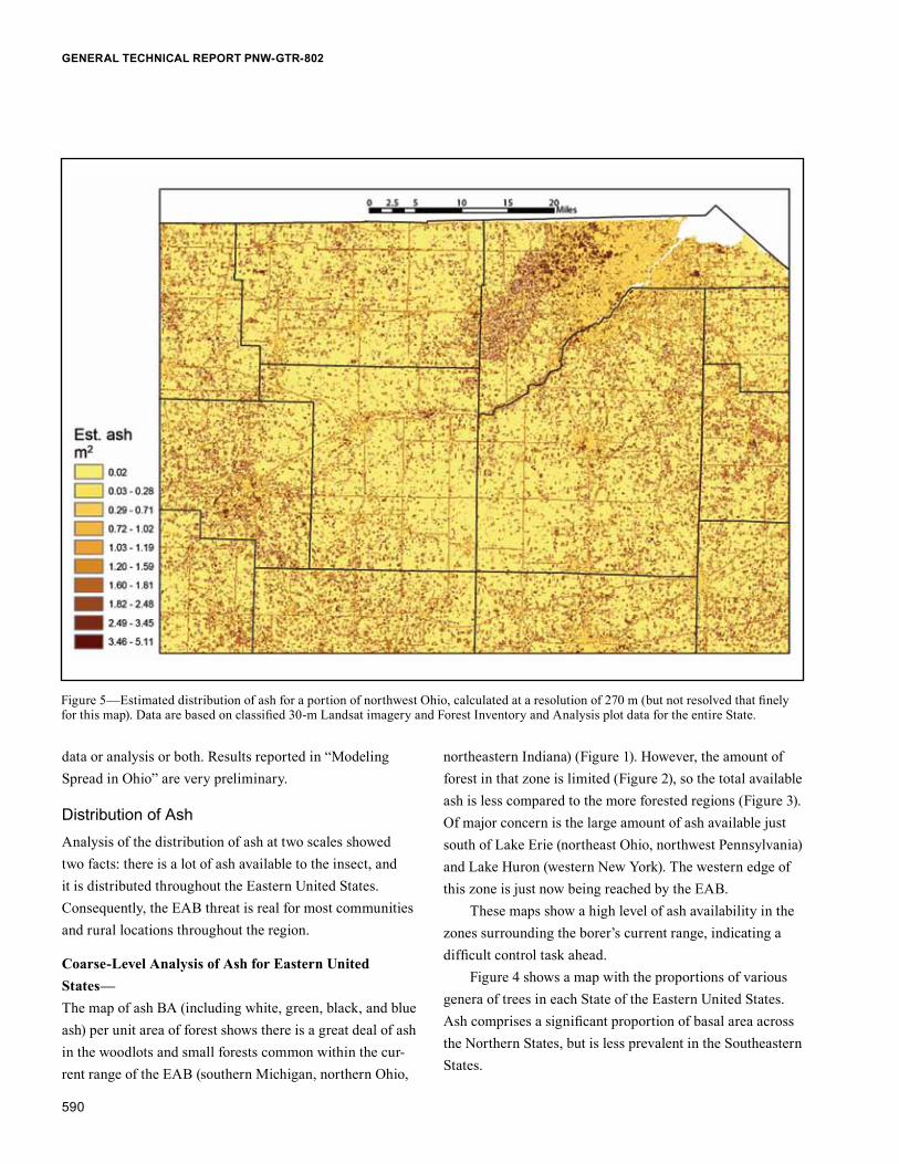
Figure 5—Estimated distribution of ash for a portion of northwest Ohio, calculated at a resolution of 270 m (but not resolved that finely for this map). Data are based on classified 30-m Landsat imagery and Forest Inventory and Analysis plot data for the entire State.

591


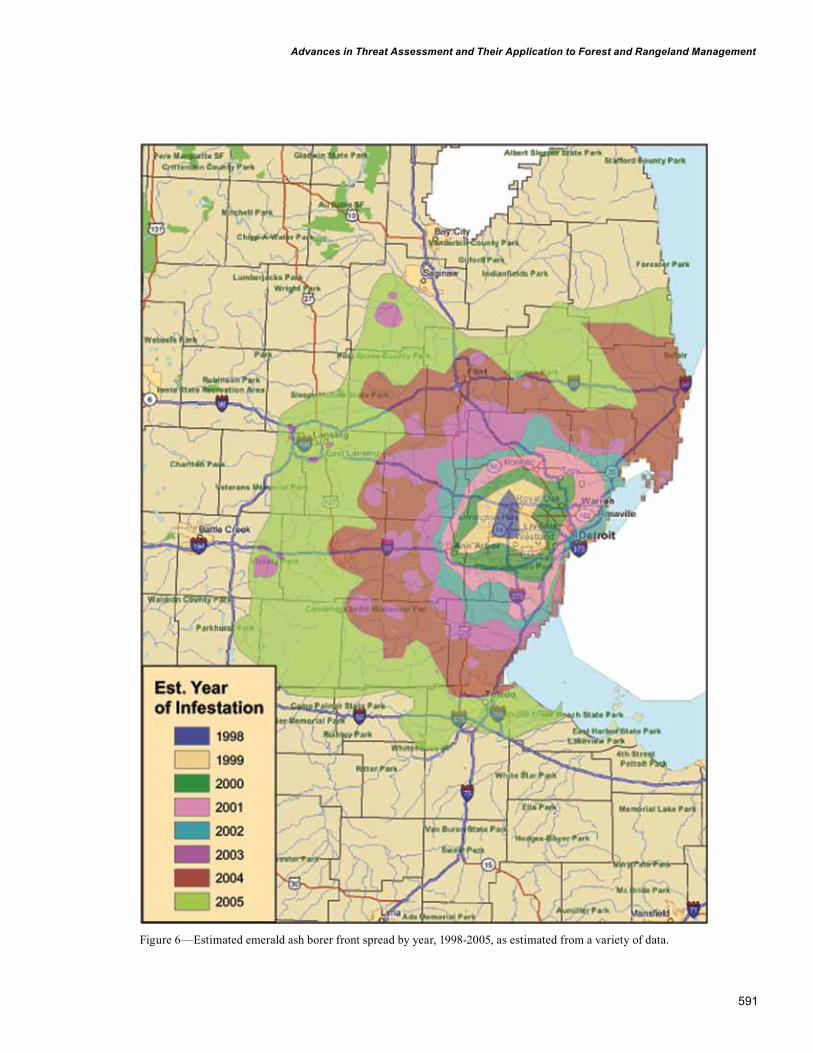
Figure 6—Estimated emerald ash borer front spread by year, 1998-2005, as estimated from a variety of data.

592


Fine-Scale Analysis of Ash for Ohio—The fine-scale analysis for Ohio, using 30-m data and plot information, shows an estimate of the urban and riparian zones with levels of ash (BA) (Figure 5). Most of the area shown in Figure 5 is agricultural land, but ash is maintained in the landscape even in these croplands along roadsides, ditches, and small wetlands. There are also numerous woodlots, many of which contain high proportions of ash.

Mapping Estimated EAB Spread, 1998–2005The map of estimated EAB front locations was required for two reasons: (1) to create a baseline from which our spread modeling will commence; and (2) to estimate the average historical rate of spread that will help calibrate the model. The resulting map (Figure 6) shows expansion from a core area in western Detroit, with substantial concentric

movement each year. Using these data, and assuming a start date of 1998, we calculated an average spread rate of approximately 20 km/yr for the years 1998 through 2005. This expansion rate is much faster than the field and labora-tory dispersal (flight) studies that have been presented thus far of 1 km/yr (McCullough and others 2005) to 4.8 km/yr (Taylor and others 2005), respectively. Clearly, much of the historical movement of the front, as we detected it here, is hastened by shorter human-assisted movements, and the two mechanisms (flight vs. ride) cannot be clearly distin-guished from each other in the real world.

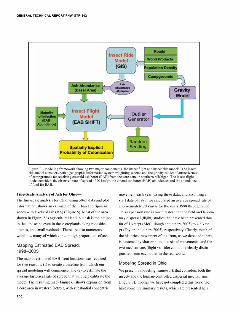
Modeling Spread in OhioWe present a modeling framework that considers both the insect- and the human-controlled dispersal mechanisms (Figure 7). Though we have not completed this work, we have some preliminary results, which are presented here.

Figure 7—Modeling framework showing two major components–the insect flight and insect ride models. The insect ride model considers both a geographic information system weighting scheme and the gravity model of attractiveness of campgrounds for receiving emerald ash borer (EAB) from the core zone in southern Michigan. The insect flight model considers the observed rate of spread of 20 km/yr, the emeral ash borer (EAB) abundance, and the abundance of food for EAB.

593


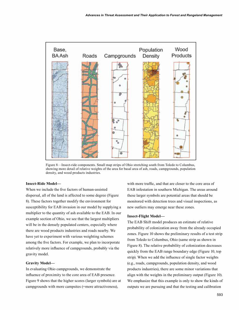
Insect-Ride Model—When we include the five factors of human-assisted dispersal, all of the land is affected to some degree (Figure 8). These factors together modify the environment for susceptibility for EAB invasion in our model by supplying a multiplier to the quantity of ash available to the EAB. In our example section of Ohio, we see that the largest multipliers will be in the densely populated centers, especially where there are wood products industries and roads nearby. We have yet to experiment with various weighting schemes among the five factors. For example, we plan to incorporate relatively more influence of campgrounds, probably via the gravity model.

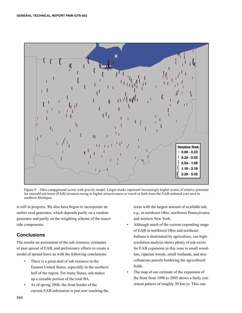
Gravity Model—In evaluating Ohio campgrounds, we demonstrate the influence of proximity to the core area of EAB presence. Figure 9 shows that the higher scores (larger symbols) are at campgrounds with more campsites (=more attractiveness),

with more traffic, and that are closer to the core area of EAB infestation in southern Michigan. The areas around these larger symbols are potential areas that should be monitored with detection trees and visual inspections, as new outliers may emerge near these zones.

Insect-Flight Model—The EAB Shift model produces an estimate of relative probability of colonization away from the already occupied zones. Figure 10 shows the preliminary results of a test strip from Toledo to Columbus, Ohio (same strip as shown in Figure 8). The relative probability of colonization decreases quickly from the EAB range boundary edge (Figure 10, top strip). When we add the influence of single factor weights (e.g., roads, campgrounds, population density, and wood products industries), there are some minor variations that align with the weights in the preliminary output (Figure 10). We emphasize that this example is only to show the kinds of outputs we are pursuing and that the testing and calibration

Figure 8—Insect-ride components. Small map strips of Ohio stretching south from Toledo to Columbus, showing more detail of relative weights of the area for basal area of ash, roads, campgrounds, population density, and wood products industries.

594


is still in progress. We also have begun to incorporate an outlier seed generator, which depends partly on a random generator and partly on the weighting scheme of the insect-ride components.

ConclusionsThe results on assessment of the ash resource, estimates of past spread of EAB, and preliminary efforts to create a model of spread leave us with the following conclusions:

• There is a great deal of ash resource in the Eastern United States, especially in the northern half of the region. For many States, ash makes up a sizeable portion of the total BA.• As of spring 2006, the front border of the current EAB infestation is just now reaching the

areas with the largest amount of available ash, e.g., in northeast Ohio, northwest Pennsylvania, and western New York.• Although much of the current expanding range of EAB in northwest Ohio and northeast Indiana is dominated by agriculture, our high- resolution analysis shows plenty of ash exists for EAB expansion in this zone in small woodlots, riparian woods, small wetlands, and mis- cellaneous parcels bordering the agricultural fields.• The map of our estimate of the expansion of the front from 1998 to 2005 shows a fairly consistent pattern of roughly 20 km/yr. This rate

Figure 9—Ohio campground scores with gravity model. Larger marks represent increasingly higher scores of relative potential for emerald ash borer (EAB) invasion owing to higher attractiveness or travel or both from the EAB-infested core area in southern Michigan.

595


of expansion would necessarily have to include both the biological dispersal capacity of the insect and some short-distance movement assisted by humans (e.g., on or in vehicles, plant material, wood material, etc.).• The components of the insect-ride model (roads, campgrounds, wood products industries, population density, and urban centers) have been acquired and processed to create a weighting scheme based on various factors, including buffer distances and number of people involved in the endeavor. When combined, every 270-m

pixel in the study area has been scored for its likelihood of enhancing EAB spread.• The gravity model yielded a relative scoring of potential EAB invasion among campgrounds based on traffic from the core EAB zone and attractiveness of the campgrounds.• Preliminary test results of movement of the front from the EAB shift model shows the probability of colonization diminishes quickly away from the front, and that the insect-ride components modify those results through the multiplier effects.

Figure 10—Combined model outputs using single-factor weights. These maps show preliminary results on the Toledo (left side) to Columbus (right side) test strip of the emerald ash borer Shift base run, and then with single-factor multipliers for roads, campgrounds, population density, and wood products industries. Numbers correspond to relative colonization probabilities after 11 years of runs. It does not include random or directed outlier generation that may occur through the insect-ride or gravity modeling components.

596


• We hope to use these data along with GIS and modeling tools to better understand the potential rate of spread, which could inform management decisions that will hopefully slow the spread of this destructive pest.

AcknowledgmentsThanks to Doug Bopp of the Cooperative Emerald Ash Borer Project for providing data on EAB infestation locations. We are grateful to Elizabeth LaPoint from the FIA GIS Support Center for overlaying the Ohio FIA plots with the Ohio GAP data to estimate ash BA. We thank the Ohio Center for Mapping, especially Lawrence Spencer, for creating and providing the Ohio GAP data. We thank Matthew Swanson and Matthew Peters for their help in various aspects of the study. We thank Michael Kilpatrick of Ohio State University for his support with the EAB Web server. Also, we thank the reviewers of this manuscript for the improvements they have made.

Literature CitedBenDor, T.K.; Metcalf, S.S. 2006. The spatial dynamics of

invasive species spread. System Dynamics Review. 22: 27–50.

BenDor, T.K.; Metcalf, S.S.; Fontenot, L.E. [and others]. 2006. Modeling the spread of the emerald ash borer. Ecological Modelling. 197: 221–236.

Bossenbroek, J.M.; Kraft, C.E.; Nekola, J.C. 2001. Prediction of long-distance dispersal using gravity models: zebra mussel invasion of inland lakes. Ecological Applications. 11: 1778–1788.

Comer, P.; Faber-Langendoen, D.; Evans, R. [and others]. 2003. Ecological systems of the United States: a working classification of U.S. terrestrial systems. Arlington, VA: NatureServe. 83 p.

Cooperative Emerald Ash Borer Project. 2006. www.emeraldashborer.info/files/TriState_EABpos.pdf. [Date accessed unknown].

Haack, R.A. 2006. Exotic bark- and wood-boring Coleoptera in the United States: recent establishments and interceptions. Canadian Journal of Forest Research. 36: 269–288.

Herms, D.A.; McCullough, D.G.; Smitley, D.R. 2004. Under attack. American Nurseryman. October: 20–26.

Iverson, L.R.; Prasad, A.M.; Schwartz, M.W. 1999. Modeling potential future individual tree-species distributions in the Eastern United States under a climate change scenario: a case study with Pinus virginiana. Ecological Modelling. 115: 77–93.

Iverson, L.R.; Schwartz, M.W.; Prasad, A. 2004a. How fast and far might tree species migrate under climate change in the Eastern United States? Global Ecology and Biogeography. 13: 209–219.

Iverson, L.R.; Schwartz, M.W.; Prasad, A.M. 2004b. Potential colonization of new available tree species habitat under climate change: an analysis for five Eastern U.S. species. Landscape Ecology. 19: 789–799.

MacFarlane, D.W.; Friedman, S.K.; Rubin, B.D. 2005. Assessing the spatial distribution of ash trees for increased efficiency in sampling for the emerald ash borer. East Lansing, MI: Michigan State University. 45 p.

McCullough, D.G.; Siegert, N.W.; Poland, T.M. [and others]. 2005. Dispersal of emerald ash borer at three outlier sites: three case studies. In: Mastro, V.; Reardon, R., comps. Emerald ash borer research and technology development meeting. FHTET-2005-15. Morgantown, WV: U.S. Department of Agriculture, Forest Service, Northeastern Area State and Private Forestry: 58–59.

Michigan State University. 2006. Emerald ash borer. www.emeraldashborer.info/files/ashdamage4_05.pdf. [Date accessed unknown].

Miles, P.D.; Brand, G.J.; Alerich, C.L. [and others]. 2001. The forest inventory and analysis database: database description and users manual version 1.0. Gen. Tech. Rep. NC-218. St. Paul, MN: U.S. Department of Agriculture, Forest Service, North Central Research Station. 130 p.

597


Muirhead, J.R.; Leung, B.; van Overdijk, C. [and others]. 2006. Modeling local and long-distance dispersal of invasive emerald ash borer Agrilus planipennis (Coleoptera) in North America. Diversity & Distributions. 12: 71–79.

Ohio Department of Transportation. 2006. Statewide Digital Data. www.dot.state.oh.us/techservsite/availpro/GIS_Mapping/gisdata sets/data sets.htm. [Date accessed unknown].

Poland, T.M.; McCullough, D.G. 2006. Emerald ash borer: invasion of the urban forest and the threat to North America's ash resource. Journal of Forestry. 104(April/May): 118–124.

Prasad, A.M.; Iverson, L.R. 2003. Little’s range and FIA importance value database for 135 Eastern U.S. tree species. http://www.fs.fed.us/ne/delaware/4153/global/littlefia/index.html. [Date accessed unknown]. Delaware, OH: U.S. Department of Agriculture, Forest Service, Northeastern Research Station.

Ramirez, J.R.; Spencer, L.; Huang, M. 2005. Ohio GAP land cover map: final report. Columbus, OH: The Ohio State University, Center for Mapping. 55 p.

Riitters, K.H.; Wickham, J.D.; O’Neill, R.V. [and others]. 2002. Fragmentation of continental United States forests. Ecosystems. 5: 815–822.

Rykiel, E.J.; Coulson, R.N.; Sharpe, P.J.H. [and others]. 1988. Disturbance propagation by bark beetles as an episodic landscape phenomenon. Landscape Ecology. 1: 129–139.

Schwartz, M.W.; Iverson, L.R.; Prasad, A.M. 2001. Predicting the potential future distribution of four tree species in Ohio, U.S.A., using current habitat availability and climatic forcing. Ecosystems. 4: 568–581.

Sharov, A.A.; Liebhold, A.M. 1998. Model of slowing the spread of gypsy moth (Lepidoptera: Lymantriidae) with a barrier zone. Ecological Applications. 8: 1170–1179.

Sharov, A.A.; Liebhold, A.M.; Roberts, E.A. 1997. Methods for monitoring the spread of gypsy moth (Lepidoptera: Lymantriidae) populations in the Appalachian Mountains. Journal of Economic Entomology. 90: 1239–1266.

Smitley, D.R. 2005. Map of ash mortality for 2003. www.emeraldashborer.info/images/ashsurvey.gif. [Date accessed unknown].

Smitley, D.R. [and others]. 2005. Map of ash mortality for 2004. www.emeraldashborer.info/images/EAB-04dieback_map.jpg. [Date accessed unknown].

Sturtevant, B.R.; Gustafson, E.J.; Lib, W.; He, H.S. 2004. Modeling biological disturbances in LANDIS: a module description and demonstration using spruce budworm. Ecological Modelling. 180: 153–174.

Taylor, R.A.J.; Bauer, L.S.; Miller, D.L.; Haack, R.A. 2005. Emerald ash borer flight potential. In: Mastro, V.; Reardon, R., comps. Emerald ash borer research and technology development meeting. FHTET-2005-15. Morgantown, WV: U.S. Department of Agriculture, Forest Service, Northeastern Area State and Private Forestry: 15–16.

Turchin, P. 2003. Complex population dynamics. Princeton, NJ: Princeton University Press. 450 p.

Continue

Modeling potential movements of an ash threat

Documents

Transcript of Modeling potential movements of an ash threat