PREDICTING FLY ASH PERFORMANCE IN

CONCRETE FROM PARTICLE CHARACTERISTICS

By

SHINHYU KANG

Bachelor of Science in Materials Science and

Engineering

Kyonggi University

Suwon, Republic of Korea

2010

Master of Science in Materials Science and Engineering

Kyonggi University

Suwon, Republic of Korea

2012

Submitted to the Faculty of the

Graduate College of the

Oklahoma State University

in partial fulfillment of

the requirements for

the Degree of

DOCTOR OF PHILOSOPHY

May, 2020

ii

PREDICTING FLY ASH PERFORMANCE IN

CONCRETE FROM PARTICLE CHARACTERISTICS

Dissertation Approved:

Dr. M. Tyler Ley

Dissertation Adviser

Dr. Bruce W. Russell

Dr. Julie A. Hartell

Dr. Nicholas F. Materer

iii

Acknowledgements reflect the views of the author and are not endorsed by committee members

or Oklahoma State University.

ACKNOWLEDGEMENTS

First, I greatly appreciate my advisor, Dr. Tyler Ley for giving me a chance to work with

him during my Doctorate. This degree would have not happened without your support,

patience, encouragement, and guidance. I will forever be indebted to you. I also would

like to thank my committee members, Dr. Bruce Russell, Dr. Julie Hartell, and Dr.

Nicholas Materer who generously agreed to serve on my committee and support me. The

professional knowledge and encouragement that they shared made me keep going on my

research.

I would like to extend my thanks to all my colleagues and friends at Oklahoma State

University. I would especially like to thank Dr. Taahwan Kim for helping and supporting

me mentally and physically to get over those days. I would like to thank Dr. Daniel Cook

for reviewing all my papers and giving me valuable comments to enhance them. Jeffrey

M. Davis, Dr. Qinang Hu, Dr. Mehdi Khanzadeh, Zane Lloyd, Mark Finnell, Nick

Seader, Nathaniel Morris, Mayra Salazar, Anna Rywelski, and Amir Behravan; it was a

pleasure to work with all of you on my research. I would also like to thank all of the

undergraduate students that helped me during my doctorate research.

I would like to express my sincere thankfulness to my beloved and supportive family,

especially my parents for unconditionally loving, encouraging, supporting and believing

in me. A special thank you must go to my best friend as well as my beautiful and

wonderful wife, Eunyoung, for her love, trust, and support over the years. I would like to

give my special thanks to my precious and adorable daughter, Joey. Thank you for

coming to this world as my daughter at the end of my degree. I could not have done this

journey without my family.

iv

Name: SHINHYU KANG

Date of Degree: MAY, 2020

Title of Study: PREDICTING FLY ASH PERFORMANCE IN CONCRETE FROM

PARTICLE CHARACTERISTICS

Major Field: CIVIL ENGINEERING

Abstract: While fly ash is widely used as supplementary cementitious material (SCM) in

concrete, the demands of fly ash have been increased in producing high-performance

concrete. Fly ash can contribute to the strength gain and improve the durability of

concrete because of its pozzolanic and cementitious properties. Even though fly ash can

be classified either Class C or Class F based on the contents of CaO according to ASTM

C618, this classification has not always shown to be useful to predict performance in

concrete. Because of the unpredictability of the performance of fly ash this limits the

amount of fly ash used in concrete. This study aims to develop predictive models for the

compressive strength, electrical resistivity and apparent diffusion coefficient of fly ash

concrete materials. A novel approach called the Particle Model is employed to construct

the predictive models for different curing dates and replacement levels. This includes

investigating thousands of fly ash particles using automated scanning electron

microscopy (ASEM) and classifying them into nine distinct groups based on the

characteristics of the individual particle with the help of machine learning. This work has

given promising linear predictive equations and important insights into how different fly

ash particles contribute to the compressive strength, electrical resistivity and apparent

diffusion coefficient of concrete over time. These are an important step to build accurate

predictive models for fly ash performance in concrete. In addition, the possibility of

predicting the apparent diffusion coefficient using electrical resistivity was evaluated by

investigating the practical relationship between two performances. The results in this

dissertation could be of interest to a broad readership seeking more knowledge about the

impacts of fly ash on compressive strength, electrical resistivity and apparent diffusion

coefficient in concrete, usage of fly ash in concrete, and advanced technique for

predicting the performances of concrete with by-products.

v

TABLE OF CONTENTS

Chapter Page

I. INTRODUCTION ........................................................................................................ 1

1.1 Introduction ............................................................................................................... 1

1.2 Research objectives ................................................................................................... 2

1.3 Overview of dissertation ........................................................................................... 3

References ....................................................................................................................... 5

II. PREDICTING THE COMPRESSIVE STRENGTH OF FLY ASH CONCRETE

WITH THE PARTICLE MODEL ................................................................................ 7

Abstract ........................................................................................................................... 7

2.1 Introduction ............................................................................................................... 8

2.2 Experimental Method ................................................................................................ 9

2.2.1 Raw materials ..................................................................................................... 9

2.2.2 Fly ash particle investigation with the ASEM .................................................. 10

2.2.3 Sample preparation for compressive strength testing ....................................... 11

2.2.3.1 Concrete mixture design ............................................................................ 11

2.2.3.2 Concrete mixing procedure and sample preparation ................................. 12

2.2.3.3 Sample preparation and testing .................................................................. 13

2.2.4 Particle Model Development ............................................................................ 13

2.2.5 Bootstrapping.................................................................................................... 15

2.3 Results and discussion ............................................................................................. 15

2.3.1 PSD and bulk chemical composition of raw fly ash from ASEM .................... 15

2.3.2 Data processing................................................................................................. 18

vi

Chapter Page

2.3.2.1 Determination of distinct groups ............................................................... 18

2.3.2.2 Predicting compressive strength ................................................................ 20

2.3.3 Accuracy of the Particle Model ........................................................................ 22

2.3.4 Effects of each individual group on compressive strength ............................... 26

2.3.4.1 Discussion of Group 2, 3, 5, and 7 ............................................................. 27

2.3.4.2 Discussion of Group 9 ............................................................................... 28

2.3.4.3 Discussion of Group 4, 6, and 8 ................................................................. 29

2.3.4.4 Discussion of Group 1 ............................................................................... 29

2.3.5 Practical Implications ....................................................................................... 30

2.4 Conclusion ............................................................................................................... 30

Acknowledgments ......................................................................................................... 32

Reference ....................................................................................................................... 32

III. USING THE PARTICLE MODEL TO PREDICT ELECTRICAL RESISTIVITY

PERFORMANCE OF FLY ASH IN CONCRETE .................................................... 39

Abstract ......................................................................................................................... 39

3.1 Introduction ............................................................................................................. 40

3.2 Experimental Method .............................................................................................. 42

3.2.1 Materials ........................................................................................................... 42

3.2.2 Investigation of fly ash particles with the ASEM............................................. 43

3.2.3 Concrete specimen preparation ........................................................................ 44

3.2.3.1 Concrete mixture design ............................................................................ 44

3.2.3.2 Concrete mixing procedure and sample preparation ................................. 44

vii

Chapter Page

3.2.4 Testing of concrete samples ............................................................................. 45

3.2.5 The Particle Model development ...................................................................... 46

3.2.6 Bootstrapping.................................................................................................... 47

3.3 Result and Discussion ............................................................................................. 48

3.3.1 Investigation of bulk chemical composition ..................................................... 48

3.3.2 Investigation of the PSD ................................................................................... 49

3.3.3 Determination of distinct groups of fly ash particles ....................................... 52

3.3.4 The accuracy for predicting electrical resistivity ............................................. 54

3.3.5 Effects of each group on electrical resistivity .................................................. 58

3.3.5.1 Discussion for Group 4, 5, 7 and 8 on the electrical resistivity ................. 60

3.3.5.2 Discussion for Group 1 and 9 on the electrical resistivity ......................... 61

3.3.5.3 Discussion for Group 2, 3, and 6 on the electrical resistivity .................... 62

3.3.6 Practical implications and future applications .................................................. 63

3.4 Conclusion ............................................................................................................... 63

Acknowledgment .......................................................................................................... 65

Reference ....................................................................................................................... 65

IV. PREDICTING ION DIFFUSION IN FLY ASH CEMENT PASTE THROUGH

PARTICLE ANALYSIS ............................................................................................. 72

Abstract ......................................................................................................................... 72

4.1 Introduction ............................................................................................................. 73

4.2 Experimental Method .............................................................................................. 75

4.2.1 Raw materials ................................................................................................... 75

viii

Chapter Page

4.2.2 Fly ash particle characterization by using ASEM method ............................... 76

4.2.3 Fly ash-cement paste sample preparation ......................................................... 77

4.2.4 Ion penetration test and TXM data analysis ..................................................... 78

4.2.5 Particle Model development ............................................................................. 79

4.2.6 Bootstrapping.................................................................................................... 80

4.3 Result and discussion .............................................................................................. 81

4.3.1 KI diffusion test ................................................................................................ 81

4.3.2 Relationship between particle size of fly ash and the paste performances ....... 82

4.3.3 Bulk chemical composition of raw fly ashes by using ASEM ......................... 84

4.3.4 Evaluation of the test results and the predictive models .................................. 86

4.3.6 Discussion for the contribution of each group .................................................. 89

4.3.6.1 Discussion for Group 2 and 5 .................................................................... 90

4.3.6.2 Discussion for Group 1, 3, 6, 8, and 9 ....................................................... 91

4.3.6.3 Discussion for Group 4 and 7 .................................................................... 93

4.3.7 Practical implications and future applications .................................................. 93

4.4 Conclusion ............................................................................................................... 94

Acknowledgments ......................................................................................................... 95

Reference ....................................................................................................................... 96

V. THE RELATIONSHIP BETWEEN THE APPARENT DIFFUSION COEFFICIENT

AND ELECTRICAL RESISTIVITY OF FLY ASH CONCRETE ......................... 104

Abstract ....................................................................................................................... 104

5.1 Introduction ........................................................................................................... 105

ix

Chapter Page

5.2 Raw materials and experimental methods ............................................................. 107

5.2.1 Raw materials ................................................................................................. 107

5.2.2 Diffusion test for developing apparent diffusion coefficient (Dic) ................. 108

5.2.2.1 Sample preparation .................................................................................. 108

5.2.2.2 TXM ion penetration test and data analysis ............................................. 108

5.2.3 Concrete sample preparation .......................................................................... 109

5.2.4 Surface electrical resistivity (ρsr) with the Wenner probe .............................. 110

5.2.5 Investigation of the correlation between ρsr and Dic ....................................... 111

5.3 Result and discussion ............................................................................................ 111

5.3.1 Bulk chemical composition ............................................................................ 111

5.3.2 Correlation between ρsr and Dic ...................................................................... 112

5.3.2.1 Correlations between ρsr and Dic with and without fly ash ...................... 113

5.3.2.2 Impact of the type of fly ash on the relationships between the ρsr and Dic

.............................................................................................................................. 115

5.3.3 Calculate Dic cement paste with fly ash through the ρsr ................................. 117

5.3.4 Practical implication ....................................................................................... 118

5.4 Conclusion ............................................................................................................. 118

Acknowledgments ....................................................................................................... 119

Reference ..................................................................................................................... 120

VI. CONCLUSION ......................................................................................................... 126

6.1 Predicting the Compressive Strength of Fly Ash Concrete with the Particle Model

..................................................................................................................................... 126

x

Chapter Page

6.2 Using the Particle Model to Predict Electrical Resistivity Performance of Fly Ash

in Concrete .................................................................................................................. 127

6.3 Predicting Ion Diffusion in Fly Ash Cement Paste through Particle Analysis ..... 128

6.4 The Relationship between the Apparent Diffusion Coefficient and Electrical

Resistivity of Fly Ash Concrete .................................................................................. 129

6.5 Future Work .......................................................................................................... 130

APPENDICES ................................................................................................................ 131

Appendix A. Consistency of the ASEM method ........................................................ 131

Appendix B. Bulk chemical composition comparison between the results of XRF and

ASEM .......................................................................................................................... 132

Appendix C. The comprehensive procedure of ASEM method .................................. 133

Appendix D. Determination of the maximum spectral angle...................................... 135

Appendix E. The procedure for the model analysis with the ANOVA for the

compressive strength ................................................................................................... 139

Appendix F. Determine the nine distinct groups from SOM analysis ........................ 141

Appendix G. The comprehensive results of the coefficient values for the predictive

models of the compressive strength ............................................................................ 144

Appendix H. The procedure for simplifying the prediction model for the surface

electrical resistivity ..................................................................................................... 145

Appendix I. The comprehensive results of the coefficient values for the predictive

models of surface electrical resistivity ........................................................................ 147

Appendix J. Experimental settings for the KI diffusion test ....................................... 148

Appendix K. The procedure for the model analysis with the ANOVA for apparent

iodide diffusion coefficient ......................................................................................... 149

Appendix L. Comprehensive results of the coefficient values for the predictive models

of apparent iodide diffusion coefficient ...................................................................... 151

xi

Chapter Page

Appendix M. Concrete mixing procedure ................................................................... 152

References for appendix .............................................................................................. 153

xii

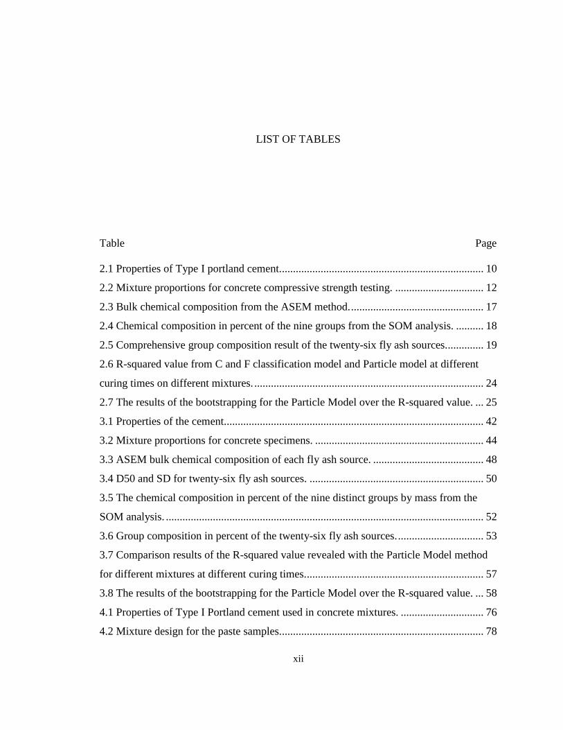
LIST OF TABLES

Table Page

2.1 Properties of Type I portland cement.......................................................................... 10

2.2 Mixture proportions for concrete compressive strength testing. ................................ 12

2.3 Bulk chemical composition from the ASEM method. ................................................ 17

2.4 Chemical composition in percent of the nine groups from the SOM analysis. .......... 18

2.5 Comprehensive group composition result of the twenty-six fly ash sources.............. 19

2.6 R-squared value from C and F classification model and Particle model at different

curing times on different mixtures. ................................................................................... 24

2.7 The results of the bootstrapping for the Particle Model over the R-squared value. ... 25

3.1 Properties of the cement.............................................................................................. 42

3.2 Mixture proportions for concrete specimens. ............................................................. 44

3.3 ASEM bulk chemical composition of each fly ash source. ........................................ 48

3.4 D50 and SD for twenty-six fly ash sources. ............................................................... 50

3.5 The chemical composition in percent of the nine distinct groups by mass from the

SOM analysis. ................................................................................................................... 52

3.6 Group composition in percent of the twenty-six fly ash sources. ............................... 53

3.7 Comparison results of the R-squared value revealed with the Particle Model method

for different mixtures at different curing times. ................................................................ 57

3.8 The results of the bootstrapping for the Particle Model over the R-squared value. ... 58

4.1 Properties of Type I Portland cement used in concrete mixtures. .............................. 76

4.2 Mixture design for the paste samples.......................................................................... 78

xiii

Table Page

4.3 Bulk chemical composition by using the ASEM method. .......................................... 85

4.4 R-squared value of the predictive models for the Dic at different hydration times. .... 88

4.5 Bootstrapping for the Particle Model over the R-squared value. ................................ 89

5.1 Chemical and phase properties of Type I ordinary portland cement. ....................... 107

5.2 Mixture design for the paste specimen. .................................................................... 108

5.3 Concrete mixture proportions of specimens for ρsr test. ........................................... 110

5.4 Bulk chemical composition from the ASEM. ........................................................... 112

5.5 K and R-squared values for samples with fly ash for each hydration date. .............. 115

5.6 K and R-squared values for different types of fly ash. ............................................. 117

A.1 The average standard deviation for three times ASEM investigation of 50 fly ash

particles on the same sample........................................................................................... 131

B.1 Chemical composition of fly ashes by XRF and ASEM (C: Class C fly ash and F:

Class F fly ash)................................................................................................................ 132

C.1 Summary of instrument settings, scanning settings, and EDS settings used for ASEM.

......................................................................................................................................... 134

D.1 Statistical analysis results with different max spectral angles. ................................ 136

D.2 R-squared value of each linear regression model on different hydration time data

with different max spectral angle used. .......................................................................... 137

E.1 The initial model result with ANOVA for predicting the compressive strength of 20%

fly ash concrete at 28d curing. ........................................................................................ 140

E.2 Particle Model result for predicting the compressive strength of 20% fly ash concrete

at 28d curing time using seven significant groups. ......................................................... 141

F.1 Chemical composition of determined nine distinct groups with SOM analysis. ...... 143

F.2 The standard error for each chemical for nine groups. ............................................. 143

G.1 Coefficients for each group at different curing times. ............................................. 144

H.1 The initial model result with ANOVA for predicting the resistivity of 40% fly ash

concrete at 28d curing. .................................................................................................... 145

H.2 Particle Model result for predicting the resistivity of 40% fly ash concrete at 28d

curing time using seven significant groups. .................................................................... 146

xiv

Table Page

I.1 Coefficient values for each of the nine groups at different curing times for 20% and

40% fly ash replacement rates. ....................................................................................... 147

J.1 Summary of TXM instrument setting [10]. ............................................................... 148

K.1 The initial model result with ANOVA for predicting the diffusion coefficient at 90

days of hydration............................................................................................................. 150

K.2 Particle Model result for predicting the diffusion coefficient at 90 days of hydration

using six significant groups. ........................................................................................... 151

L.1 Coefficients of each group on the predictive models for Dic. ................................... 152

xv

LIST OF FIGURES

Figure Page

2.1 The schematic diagram of the overall progress. ........................................................... 9

2.2 Comparison of the particle size distribution by number fraction of (a) Cumulative

PSDs for fourteen Class C fly ashes and (b) Cumulative PSDs for eleven Class F fly

ashes. ................................................................................................................................. 16

2.3 The cumulative plot for chemicals of determined nine groups................................... 19

2.4 Comparison results between actual and predicted compressive strength with the type

of fly ash used: (a) 20% fly ash replacement concrete and (b) 40% fly ash replacement

concrete. ............................................................................................................................ 21

2.5 Comparisons of (a) Bulk chemical composition, (b) Particle groups, (c) Compressive

strength change for C1 vs. C2, and (d) Compressive strength change for F5 and IF1. .... 22

2.6 The relationship between the predicted and measured value for strength by using the

Particle Model for (a) 20% fly ash concrete and (b) 40% fly ash concrete. ..................... 23

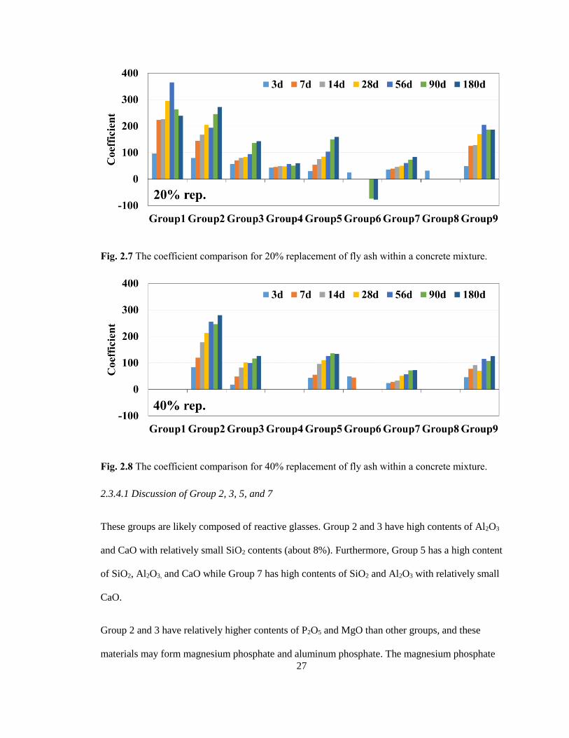
2.7 The coefficient comparison for 20% replacement of fly ash within a concrete mixture.

........................................................................................................................................... 27

2.8 The coefficient comparison for 40% replacement of fly ash within a concrete mixture.

........................................................................................................................................... 27

3.1 The schematic diagram of the overall procedure of the work in this study. ............... 41

3.2 Comprehensive cumulative particle size distribution for fifteen Class C fly ashes and

eleven Class F fly ashes. ................................................................................................... 50

3.3 Relationship between the D50 and the measured electrical resistivity from concrete

with nineteen fly ash sources at different times: (a) 20% and (b) 40% fly ash replacement

concrete. ............................................................................................................................ 51

xvi

Figure Page

3.4 The cumulative plot of the chemical composition of the nine distinct groups. .......... 53

3.5 Comparison between the measured and average values of resistivity with the type of

fly ash used: (a) 20% fly ash replacement concrete and (b) 40% fly ash replacement

concrete. ............................................................................................................................ 55

3.6 Comprehensive relationship between the calculated and experimental resistivity for

(a) 20% fly ash replacement and (b) 40% fly ash replacement. ....................................... 56

3.7 Coefficient comparison for 20% fly ash replacement at different times for each group.

........................................................................................................................................... 59

3.8 Coefficient comparison for 40% fly ash replacement at different times for each group.

........................................................................................................................................... 60

4.1 Comprehensive schematic diagram of the process for investigating the diffusion

properties........................................................................................................................... 75

4.2 Dic at different days of hydration. ............................................................................... 82

4.3 Cis at different days of hydration. ............................................................................... 82

4.4 Comparison of the frequency of the PSDs for (a) fourteen Class C fly ashes and (b)

eleven Class F fly ashes. ................................................................................................... 83

4.5 Relationships between the average particle size compared to (a) Dic and (b) Cis. ...... 84

4.6 Comparison between actual and predicted Dic with the type of fly ash used. ............ 86

4.7 Comparison between the calculated and measured value for Dic. .............................. 88

4.8 Coefficients of predictive models of each group at different hydration times for Dic. 90

5.1 Comprehensive correlation between the ρsr and Dic for samples with fly ash and OPC.

......................................................................................................................................... 114

5.2 Correlation between the ρsr and Dic for Class C fly ashes. ....................................... 116

5.3 Correlation between the ρsr and Dic for Class F fly ashes. ........................................ 117

C.1 The schematic of the ASEM procedure. .................................................................. 133

D.1 Comprehensive results of the linear regression model analysis with different max

spectral angles on different hydration time data. ............................................................ 139

J.1 Schematic diagram of the diffusion test setup [10]. .................................................. 148

1

CHAPTER I

INTRODUCTION

1.1 Introduction

Fly ash is currently being used in many places as one of the supplementary cementitious materials

(SCMs) in concrete. Fly ash is fine spherical particles resulting from the combustion of

pulverized coal in the power plants. About 12.5 million tons or 35% of the total fly ash produced

in the United States in 2018 was used as a partial replacement of portland cement in concrete [1].

Any improvements to the utilization of fly ash or understanding of fly ash properties could help

not only for the environment but also in economic impact.

ASTM C618 [2] is widely used to classify fly ash as either Class C or F based on the bulk

chemical composition, and past studies of the reactivity of fly ash largely relied on bulk

characterization methods, such as X-ray fluorescence (XRF) or X-ray diffraction (XRD) [3-5].

While understanding the bulk chemical composition is useful, it only describes the average

behavior of the system. Practically, each coal particle independently undergoes different physical

and chemical changes during the combustion process at the power plant. Therefore, the

composition of each individual particle of fly ash is a result of all these processes [6]. Because of

this, there is no universal method to predict the performance of fly ash in concrete [2-5].

2

However, there may be more to learn about the performance of fly ash by studying individual

particles. A method for a better understanding of the characteristics of fly ash and its performance

would greatly benefit in the concrete industry.

A technique using automated scanning electron microscopy (ASEM) is able to rapidly measure the

physical and chemical information of thousands of individual particles within a reasonable timeframe

[6-11]. This can provide potential insights into the performance of fly ash in cement-based materials

through the study of the individual fly ash particles. In addition, the ASEM allows the investigation of

the impacts of particle size and chemical composition of fly ash in performances and helps to study

the relationship among the performances.

A novel approach called the Particle Model is introduced to predict the compressive strength of fly

ash concrete [8]. The Particle Model uses a machine learning, self-organizing map (SOM), to classify

thousands of fly ash particles in distinct groups based on the particle information and construct the

linear model for predicting the performance of cement-based materials including fly ash. This can be

applied to a specific period of hydration date and other concrete performance such as electrical

resistivity and diffusion. Furthermore, the coefficients from the derived predictive models can provide

important insights into the effectiveness of different fly ash particles over time into the performances

of concrete materials. The work presented provides new insights into creating predictive models for

the performance of fly ash in concrete. This could help users better characterize different fly ash

sources and use even higher volumes of fly ash in concrete.

1.2 Research objectives

The main tasks of this dissertation are to:

- Develop a statistical approach to classify the fly ash particles into distinct groups using a

machine learning method based on the characteristics of the individual fly ash particles.

3

- Develop and extend the application of a novel approach to drive the predictive models for the

compressive strength, electrical resistivity and diffusion coefficient of the cement-based

materials including fly ash at different hydration times and replacement levels called the

Particle Model.

- Investigate the impacts of fly ash on each performance by using the determined groups of fly

ash particles and the predictive models.

- Study the correlation between electrical resistivity and the iodide diffusion coefficient.

1.3 Overview of dissertation

In this dissertation, work is presented in six chapters in the paper-based format including the first

chapter which is the introduction of the dissertation.

The second chapter presents the usefulness of the Particle Model to predict the compressive strength

of fly ash concrete. The Particle Model uses machine learning through a Self-Organizing Map (SOM)

algorithm to classify the thousands of fly ash particles into distinct groups. Predictive models for

compression strength of 20% and 40% fly ash replacement levels are developed for seven different

curing times between 3 and 180 days. This chapter in the present format was submitted for

publication in Cement and Concrete Research.

In the third chapter, the Particle Model is applied to predict the surface electrical resistivity of fly ash

concrete. Predictive models for predicting the surface electrical resistivity are presented for each 20%

and 40% fly ash replacement levels at seven different curing times between 3 and 180 days. This

chapter in the present format was submitted for publication in Construction and Building Materials.

The fourth chapter extends the use of the Particle Model to investigate the diffusion properties of fly

ash-cement paste. Predictive models for predicting the apparent I diffusion coefficient for 20% fly ash

4

replacement level are developed at three different curing times which are 45, 90, and 135 days. This

chapter in the present format was prepared for publication in Cement and Concrete Composites.

The fifth chapter describes the empirical correlation between the surface electrical resistivity and the

apparent iodide diffusion coefficient by employing the Nernst-Einstein equation for the concrete

materials with partially replacing the cement to fly ash. The possibility of determining of apparent

diffusion coefficient through the electrical resistivity is evaluated for service life prediction. This

chapter in the present format was prepared for publication in Construction and Building Materials.

Finally, in chapter six, the major conclusions of this dissertation are summarized followed by the

recommendations for future research.

The research presented in this dissertation is based on work performed by the author at Oklahoma

State University.

Contributors/co-authors to this study are: Dr. Mohammed Aboustait, Dr. Taehwan Kim, Jeffrey

Davis, Dr. Qinang Hu, Zane Lloyd, and Dr. Tyler Ley.

Dr. Aboustait developed the ASEM method to analyze the fly ash particles, and Dr. Kim improved

the reliability of the ASEM method by employing the data correction process by using CalcZAF to

complete the chemical analysis of the individual particles. The data of seven out of twenty-six fly ash

sources were analyzed by Dr. Aboustait and Dr. Kim. Jeffrey Davis developed the SOM analysis with

the R program for determining distinct groups of the fly ash particles and classifying the individual

particles into the groups. Furthermore, he developed the code for multiple linear regression (MLR)

modeling by using the R program to help derive the predictive models of fly ash concrete. Dr. Hu

created the code using MATLAB for calculating the apparent iodide diffusion coefficient and surface

concentration of the radiographs of the paste samples. Zane Lloyd measured and collected all the data

of compressive strength and surface electrical resistivity for 40% fly ash concrete. Dr. Ley is the

5

advisor, and he guides the directions of the dissertation and papers. Their contributions are

acknowledged and greatly appreciated.

References

[1] A. C. A. Association, "2018 Production and Use Survey Results News Release," American

Coal Ash Association, Washington, D.C.2019.

[2] ASTM C618, Standard Specification for Coal Fly Ash and Raw or Calcined Natural Pozzolan

for Use in Concrete, 2019.

[3] S. Diamond, "On the Glass Present in Low-Calcium and in High-Calcium Flyashes," (in

English), Cement and Concrete Research, vol. 13, no. 4, pp. 459-464, 1983.

[4] L. X. Du, E. Lukefahr, and A. Naranjo, "Texas Department of Transportation Fly Ash

Database and the Development of Chemical Composition-Based Fly Ash Alkali-Silica

Reaction Durability Index," (in English), Journal of Materials in Civil Engineering, vol. 25,

no. 1, pp. 70-77, Jan 2013.

[5] S. C. White and E. D. Case, "Characterization of fly ash from coal-fired power plants,"

Journal of Materials Science, vol. 25, no. 12, pp. 5215-5219, 1990/12/01 1990.

[6] M. Aboustait, T. Kim, M. T. Ley, and J. M. Davis, "Physical and chemical characteristics of

fly ash using automated scanning electron microscopy," (in English), Construction and

Building Materials, vol. 106, pp. 1-10, Mar 1 2016.

[7] T. Kim, M. Moradian, and M. T. Ley, "Dissolution and leaching of fly ash in nitric acid using

automated scanning electron microscopy," Advances in Civil Engineering Materials, vol. 7,

no. 1, pp. 291-307, 2018.

[8] T. Kim, J. M. Davis, M. T. Ley, S. Kang, and P. Amrollahi, "Fly ash particle characterization

for predicting concrete compressive strength," (in English), Construction and Building

Materials, vol. 165, pp. 560-571, Mar 20 2018.

6

[9] S. Ghosal, J. L. Ebert, and S. A. Self, "Chemical composition and size distributions for fly

ashes," Fuel processing technology, vol. 44, no. 1-3, pp. 81-94, 1995.

[10] Y. Chen, N. Shah, F. E. Huggins, G. P. Huffman, W. P. Linak, and C. A. Miller, "Investigation

of primary fine particulate matter from coal combustion by computer-controlled scanning

electron microscopy," Fuel Processing Technology, vol. 85, no. 6-7, pp. 743-761, 2004.

[11] T. Kim, M. T. Ley, S. Kang, J. M. Davis, S. Kim, and P. Amrollahi, "Using particle

composition of fly ash to predict concrete strength and electrical resistivity," Cement and

Concrete Composites, vol. 107, p. 103493, 2020/03/01/ 2020.

7

CHAPTER II

PREDICTING THE COMPRESSIVE STRENGTH OF FLY ASH CONCRETE WITH

THE PARTICLE MODEL

Abstract

A novel approach called the Particle Model is used to predict the compressive strength of fly ash

concrete. Thousands of fly ash particles are classified into the nine groups based on the chemical

information of each particle based on the Particle Model. Predictive models for compression

strength for 20% and 40% fly ash replacement levels are developed for seven different curing

times between 3 and 180 days. The R-squared value for the compressive strength prediction of

the Particle Model is ≈ 0.99, while the Class C and F classification model is < 0.50. Furthermore,

the results show that the Particle Model is able to predict the compressive strength within +/- 10%

for 95% of all measurements at 20% fly ash replacement and for 81% of all measurements at 40%

replacement. The coefficients in the derived predictive models give important insights into the

effectiveness of different fly ash particles over time. This work shows that the Particle Model is a

promising method to make predictions of the performance of fly ash in concrete.

Keywords: Fly ash; Concrete; Compressive strength; ASEM; Particle Model; SOM

8

2.1 Introduction

Fly ash is a fine powder from the combustion of pulverized coal. About 14.1 million tons or 36%

of the total fly ash produced in the United States in 2017 was used as a partial replacement of

portland cement in concrete [1]. Fly ash can improve the overall performance and economy of

concrete [2-5]. Fly ash is typically used at a 15-35% replacement level by mass in concrete [6].

This rate of fly ash replacement is typically limited to 20% as it is hard to predict the performance

of fly ash in concrete and so this replacement level typically produces acceptable performance.

Since fly ash is a waste product that would typically be landfilled if not used in concrete [7],

higher replacement levels in concrete allow significant improvements in the sustainability of

these mixtures. However, tools are needed to help practitioners realize when they can use higher

replacement levels and how this might impact the properties and performance of the concrete.

The bulk characterization methods such as X-ray fluorescence (XRF) has been used in the

previous studies to investigate the properties of fly ash and predict performance [8-11].

Unfortunately, some fly ashes with similar bulk chemical compositions can have dramatically

different performance [12]. Thus, the bulk chemical composition alone cannot fully explain the

fly ash properties and cannot be used to predict the performance of fly ash concrete. Previous

research showed that fly ash particles are not uniform but do have repeating patterns in

composition [13, 14]. Further studies using scanning electron microscopy (SEM) and automated

scanning electron microscopy (ASEM) with energy dispersive X-ray spectrometry (EDS) have

identified nine repeating patterns in the chemical composition of fly ash particles [14-17].

After investigating thousands of particles from different sources a method to organize and predict

the performance of the fly ash was developed called the Particle Model [18]. Fig. 2.1 provides an

overview of the entire process. The Particle Model uses machine learning through a Self-

Organizing Map (SOM) algorithm to classify the numerous fly ash particles into nine distinct

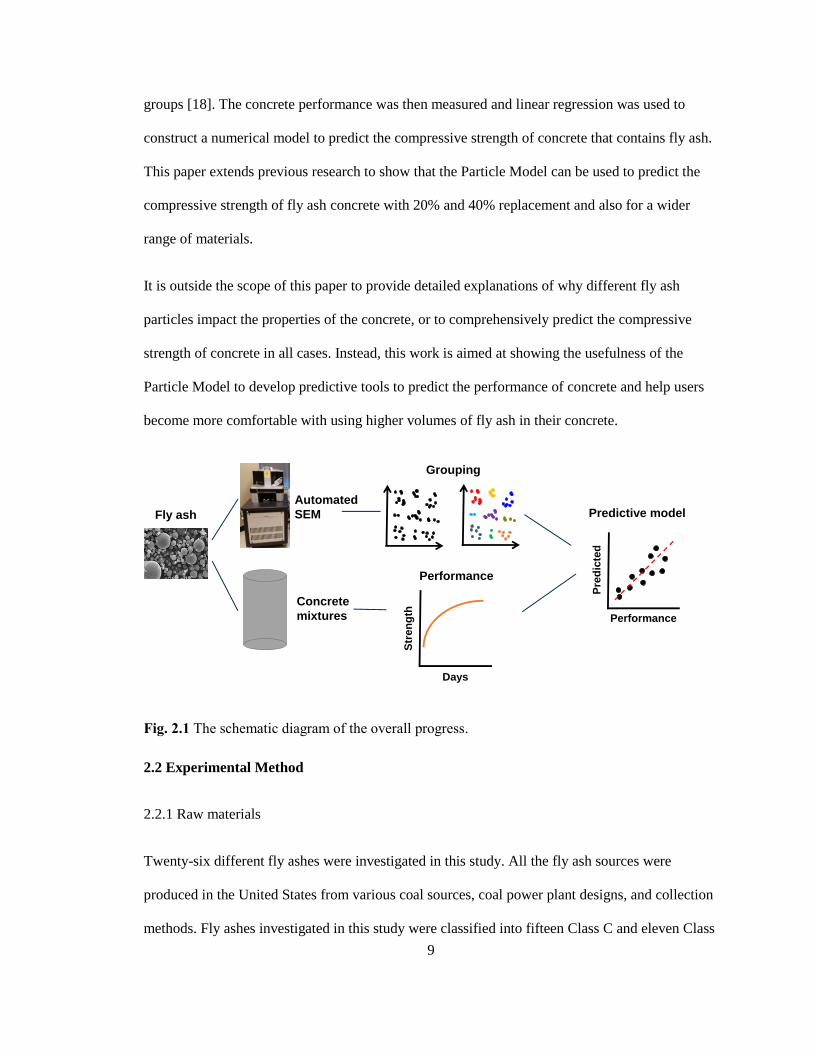
9

groups [18]. The concrete performance was then measured and linear regression was used to

construct a numerical model to predict the compressive strength of concrete that contains fly ash.

This paper extends previous research to show that the Particle Model can be used to predict the

compressive strength of fly ash concrete with 20% and 40% replacement and also for a wider

range of materials.

It is outside the scope of this paper to provide detailed explanations of why different fly ash

particles impact the properties of the concrete, or to comprehensively predict the compressive

strength of concrete in all cases. Instead, this work is aimed at showing the usefulness of the

Particle Model to develop predictive tools to predict the performance of concrete and help users

become more comfortable with using higher volumes of fly ash in their concrete.

Fig. 2.1 The schematic diagram of the overall progress.

2.2 Experimental Method

2.2.1 Raw materials

Twenty-six different fly ashes were investigated in this study. All the fly ash sources were

produced in the United States from various coal sources, coal power plant designs, and collection

methods. Fly ashes investigated in this study were classified into fifteen Class C and eleven Class

Fly ash

Automated

SEM

Concrete

mixtures

Performance

Grouping

Predictive model

Str

en

gth

Days

Pre

dic

ted

Performance

10

F fly ashes according to ASTM C618 [19]. The ASEM method was used to collect a large

collection of data by analyzing each individual fly ash particle. ASTM C150 Type I [20] ordinary

portland cement (OPC) was used for all concrete mixtures. Table 2.1 shows the chemical and

phase composition of cement used in this study. Limestone and natural sand from the state of

Oklahoma were used as coarse and fine aggregate, respectively. The specific gravities for the

coarse and fine aggregate were the same as 2.60, and the absorptions were 0.64% and 0.55%,

respectively.

Table 2.1 Properties of Type I portland cement.

Element Composition (%) Phase Composition (%)

SiO2 20.77

C3S 52.13 Al2O3 4.57

Fe2O3 2.62

CaO 62.67

C2S 20.22 MgO 2.37

SO3 3.18

Na2O 0.19

C3A 7.68 K2O 0.32

TiO2 0.34

P2O5 0.14

C4AF 7.97 SrO 0.22

BaO 0.07

2.2.2 Fly ash particle investigation with the ASEM

The ASEM method was used to investigate the properties of all twenty-six fly ashes. This method

uses SEM-EDS (Aspex Explorer PSEM-EDS) with an image analysis operating system and has

important advantages over the conventional analysis of bulk chemistry using conventional XRF

11

[13, 21, 22]. One of the primary advantages of the ASEM is that the method can investigate the

chemical composition, size and shape of approximately 500 particles per hour without human

intervention. This means that the ASEM can rapidly measure the physical and average chemical

information of thousands of individual particles within a reasonable timeframe. Two thousand

particles were examined from each fly ash and grouped based on the eleven elements. Two

thousand particles have been shown to be a representative sample for fly ash [13].

Since fly ash particles are not flat this violates one of the fundamental assumptions of classical

quantitative EDS analysis. The correction models have been developed by Armstrong and Love-

Scott [23, 24] and Armstrong – Buseck [25, 26] to take into account the shape of the particle and

make corrections to the collected k-ratios of 11 elements (Si, Al, Fe, Ca, Mg, S, Na, K, Ti, P, and

Sr). A previous study measured the chemical composition for 50 Class C fly ash particles three

times. The results showed that the highest standard deviation (SD) was 1.60% [18]. This indicates

the analysis results using ASEM was consistent. More detailed results for the consistency of the

ASEM method can be found in Appendix A. The accuracy, reliability, and repeatability of the

ASEM method when compared to XRF analysis have been presented in other publications and

shown to be < 5% absolute difference for > 90% of comparisons [13, 18, 27]. This indicates that

the two methods agree. Comparisons for the materials in this work are presented in Appendix B.

Furthermore, the particle size distribution (PSD) has been compared between ASEM and acoustic

attenuation spectroscopy and found to be similar [28]. More details over the ASEM method,

sample preparation, analysis with ASEM and data processing, can be found in Appendix C.

2.2.3 Sample preparation for compressive strength testing

2.2.3.1 Concrete mixture design

Twelve Class C and seven Class F were used for concrete mixtures. Fly ash sources were chosen

based on a wide range of different chemical compositions. To investigate the fly ash

12

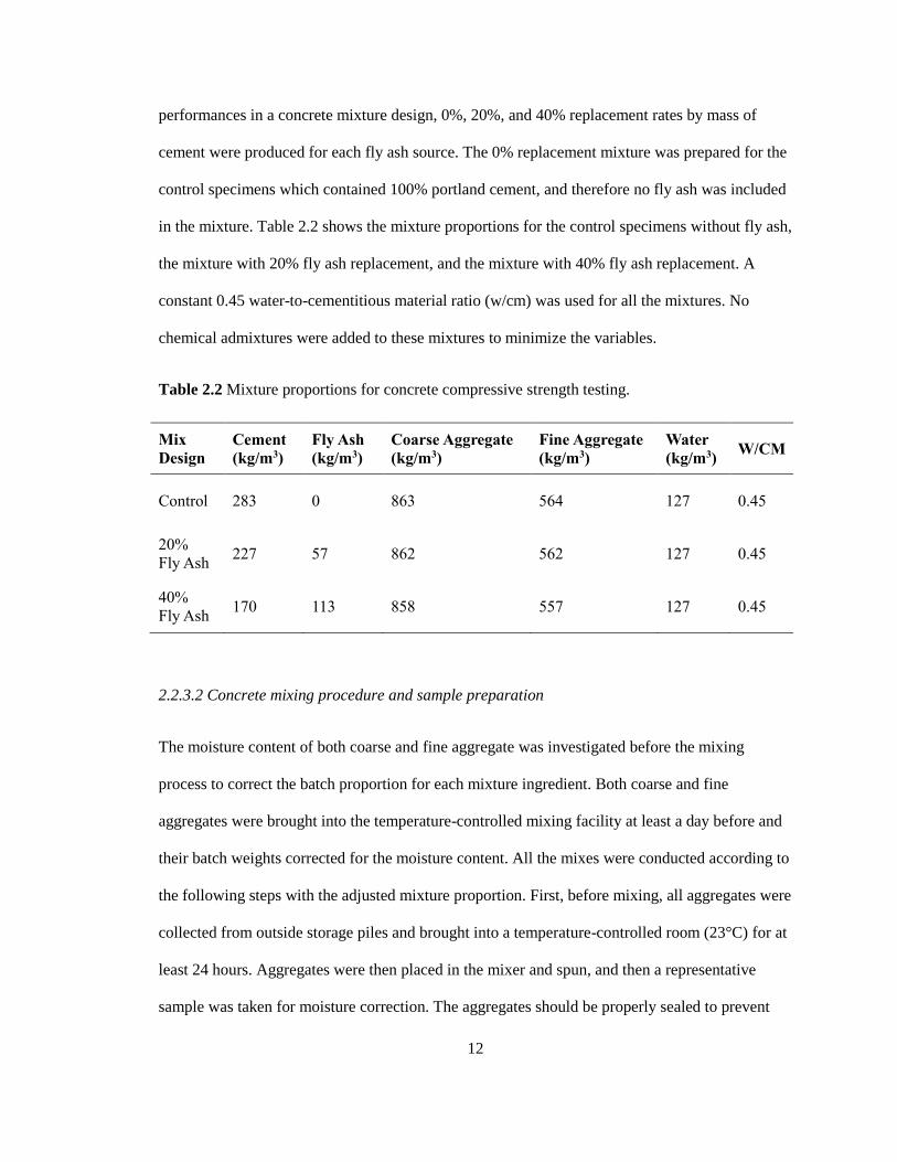
performances in a concrete mixture design, 0%, 20%, and 40% replacement rates by mass of

cement were produced for each fly ash source. The 0% replacement mixture was prepared for the

control specimens which contained 100% portland cement, and therefore no fly ash was included

in the mixture. Table 2.2 shows the mixture proportions for the control specimens without fly ash,

the mixture with 20% fly ash replacement, and the mixture with 40% fly ash replacement. A

constant 0.45 water-to-cementitious material ratio (w/cm) was used for all the mixtures. No

chemical admixtures were added to these mixtures to minimize the variables.

Table 2.2 Mixture proportions for concrete compressive strength testing.

Mix

Design

Cement

(kg/m3)

Fly Ash

(kg/m3)

Coarse Aggregate

(kg/m3)

Fine Aggregate

(kg/m3)

Water

(kg/m3) W/CM

Control 283 0 863 564 127 0.45

20%

Fly Ash 227 57 862 562 127 0.45

40%

Fly Ash 170 113 858 557 127 0.45

2.2.3.2 Concrete mixing procedure and sample preparation

The moisture content of both coarse and fine aggregate was investigated before the mixing

process to correct the batch proportion for each mixture ingredient. Both coarse and fine

aggregates were brought into the temperature-controlled mixing facility at least a day before and

their batch weights corrected for the moisture content. All the mixes were conducted according to

the following steps with the adjusted mixture proportion. First, before mixing, all aggregates were

collected from outside storage piles and brought into a temperature-controlled room (23°C) for at

least 24 hours. Aggregates were then placed in the mixer and spun, and then a representative

sample was taken for moisture correction. The aggregates should be properly sealed to prevent

13

water loss until the mixing. At the time of mixing, all aggregate and approximately one half of the

mixing water was loaded into the mixer and mixed for three minutes. This allows the aggregates

to approach the saturated surface dry (SSD) condition and ensures that the aggregates were

evenly distributed. Then, all the materials (the cement, fly ash, and the remaining water) were

added into the mixer and mixed for three minutes. The mixture was rested for two minutes while

the sides of the mixing drum were scraped. After this time, the mixer was started to mix the

concrete for another three minutes.

2.2.3.3 Sample preparation and testing

The unit weight, slump, and air content were measured for each mixture [29-31]. The results are

reported in other publications [32]. Using ASTM C31 [33], samples were cast in 100 mm x 200

mm cylindrical containers and cured at 23°C and 100% RH for 24 hours in the curing room after

sealing the container. The samples were then demolded and placed back into the curing room

until the sample was ready for compressive strength testing according to ASTM C39 [34]. Three

samples were tested at the curing times of 3, 7, 14, 28, 56, 90, and 180 days.

2.2.4 Particle Model Development

Two thousand particles were collected from each fly ash, and thus 52,000 fly ash particles from

twenty-six fly ashes were collected by using ASEM. Each particle has 12 different variables,

including eleven pieces of chemical composition data (Na2O, MgO, Al2O3, SiO2, P2O5, SO3, K2O,

CaO, TiO2, Fe2O3, and SrO2) and its average diameter. This means that 624,000 pieces of data

were collected through the ASEM particle analysis.

The SOM analysis was completed 200 times to determine the distinct groups. The SOM method

is a useful way to deal with a large database and find distinct groups [35]. A previous study found

14

a nine group geometry worked best for the clustering analysis [18], and therefore, a nine group

geometry was continued to be used for this work.

Each particle was grouped by using a spectral angle analysis. This has been discussed in previous

publications and additional information is provided in Appendix D. A threshold or maximum

spectral angle of 0.4 rad is used to exclude particles that do not fit any of the groups. Each

particle was placed in the group with the lowest spectral angle.

These nine groups were used to derive predictive models for the compressive strength at 3, 7, 14,

28, 56, 90, and 180 days. The percentage of each group was used to conduct a multiple linear

regression (MLR) analysis. In addition, the model analysis was applied not only for 20% but also

for 40% fly ash replacement to predict the compressive strength. Therefore, the initial

multivariable linear model equation was derived with the format of Eq.(2.1):

Compressive Strength = {a(Group 1) + b(Group 2) + c(Group 3) + d(Group 4) + e(Group 5)

+ f(Group 6) + g(Group 7) + h(Group 8) + i(Group 9)} / Z Eq.(2.1)

where Z is a conversion factor to determine the units of the compressive strength. The unit of

strength is psi when the Z is 1 (one) and the value of Z is 145.03 if the desired units of strength

are MPa. The lowercase letters represent the determined coefficients from the model analysis.

Each of the coefficients reflects the effect of the individual groups on compressive strength at a

specific curing time, where the potential influence of the remaining independent variables on the

groups has been taken into account.

The probability value (Pr(>|t|)) from the MLR was then used to determine the statistical

significance of variables on the results. This was done because there were concerns of overfitting

the data with these nine groups and the Pr(>|t|) allowed the groups to be reduced to only those

that are statistically significant. The R-squared value of each model was investigated for 20% and

40% fly ash replacement concrete at all individual curing times to evaluate the linear fit to the

15

model. The detailed procedure of the MLR analysis is found in Appendix E. All the data and

model processing was conducted using the R programming environment [36, 37].

2.2.5 Bootstrapping

To evaluate the robustness of the derived predictive models, the bootstrap method was applied.

Ideally, the data can be collected by repeating a large number of mixtures for the same

experiment to evaluate the validity of the derived predictive models, but this is impractical.

Instead, the bootstrap was implemented to investigate the robustness of the Particle Model over

the R-squared value. The bootstrapping is a resampling method where the data are sampled with

replacement from the original sample to generate simulated results [36]. This allows creating

many R-squared values by running the predictive models with simulated samples in a timely

manner. Furthermore, the results from the bootstrapping can be used to calculate a variety of

sample statistics such as the mean (average) and SD of the created R-squared values to compare

the R-squared value of the original model.

The size of the bootstrapping sample was the same as the original dataset and is chosen at random

from the existing data set. This means that some data points can be chosen multiple times in the

simulated sample while others may not be selected at all. This procedure has been used by others

[38]. The bootstrapping was conducted with 500 times for each model. Then, the mean of the R-

squared values from the bootstrapping was investigated and compared with the R-squared value

of the derived predictive model. This was applied to each curing time for both 20% and 40%

replacement.

2.3 Results and discussion

2.3.1 PSD and bulk chemical composition of raw fly ash from ASEM

16

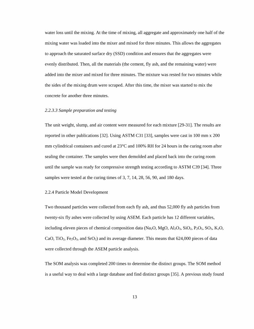
Fig. 2.2 shows the cumulative PSDs of fifteen Class C and eleven Class F fly ashes investigated

in this study. Most of the fly ash particles ranged between 0.5 μm and 30 μm in diameter. The

range of D50 for Class C fly ashes is between 1.5 μm to 3 μm while Class F is between 1.5 μm to

2.5 μm. Previous research investigated the effect of fly ash mean particle size on the compressive

strength at 7d, 28d, and 120d, and the results showed that there were no significant changes in the

compressive strength for fly ash with a mean particle size between 2 to 5 μm [39]. The largest

and smallest mean particle size in this study is 4.3 μm (C10) and 1.9 μm (C1). Because of this,

the particle size information of the fly ashes was not included in the model.

(a) Cumulative PSDs for Class C fly ashes

(b) Cumulative PSDs for Class F fly ashes

Fig. 2.2 Comparison of the particle size distribution by number fraction of (a) Cumulative PSDs

for fourteen Class C fly ashes and (b) Cumulative PSDs for eleven Class F fly ashes.

All the fly ashes are classified as either Class C or F fly ash according to ASTM C618. This

means that Class C fly ash has > 18% of CaO while Class F fly ash has < 18% of CaO [19]. Table

2.3 shows the bulk chemical composition result from the ASEM method for twenty-six fly ash

17

sources. The fly ashes with “C#” and “IC#” represent Class C fly ash while the fly ashes with

“F#” and “IF#” represent Class F fly ash.

Table 2.3 Bulk chemical composition from the ASEM method.

Source SiO2 Al2O3 Fe2O3 CaO MgO SO3 Na2O K2O TiO2 P2O5 SrO

C1 36.20 21.72 5.35 23.15 5.38 0.67 3.58 1.01 0.80 1.90 0.23

C2 35.82 19.18 5.60 26.88 5.49 0.98 3.00 0.88 0.73 1.25 0.18

C3 25.32 19.26 5.22 32.50 7.76 2.60 3.42 0.63 1.08 1.89 0.32

C4 36.70 22.82 4.53 22.45 4.33 1.19 3.44 0.95 1.28 1.09 1.22

C5 31.25 22.46 5.38 26.06 5.95 0.56 4.30 0.84 0.84 2.11 0.23

C6 27.66 22.88 4.23 21.54 4.52 2.55 12.61 0.76 1.27 0.67 1.32

C7 35.28 20.61 4.74 24.72 4.93 0.74 4.26 1.23 1.64 0.82 1.00

C8 40.11 22.61 4.54 19.45 5.72 0.76 3.74 0.91 0.64 1.42 0.10

C9 31.49 24.02 5.96 25.71 5.35 0.99 3.72 0.61 0.94 1.12 0.10

C10 36.04 19.30 5.06 22.70 7.77 1.97 4.78 0.57 1.03 0.32 0.47

C11 30.96 20.77 6.38 27.15 7.14 1.59 3.45 0.73 0.78 0.83 0.23

IC1 31.82 22.87 5.68 28.24 5.52 1.08 2.28 1.02 0.78 0.46 0.25

IC2 25.15 21.20 6.22 30.47 7.78 1.04 4.02 0.56 1.22 2.18 0.15

IC3 29.66 21.03 5.92 30.29 5.35 1.87 2.22 0.55 1.04 1.61 0.46

IC4 29.85 17.66 4.73 31.75 9.32 1.19 2.57 0.76 0.83 1.08 0.24

F1 48.76 23.79 7.39 12.53 2.97 0.48 0.86 2.05 0.78 0.09 0.29

F2 50.40 20.91 3.89 17.09 3.69 0.54 1.04 1.37 0.70 0.05 0.32

F3 48.81 26.62 6.65 9.30 1.95 0.28 1.75 1.93 1.46 0.14 1.10

F4 45.34 27.39 4.00 14.61 3.59 0.70 1.48 0.65 1.09 0.37 0.76

F5 53.18 25.36 11.21 2.06 0.19 0.89 0.97 4.43 0.71 0.03 0.96

F6 51.87 25.71 12.32 2.50 0.32 0.67 1.61 4.13 0.66 0.05 0.16

F7 51.92 26.31 8.01 3.28 0.54 1.69 4.04 2.53 0.87 0.61 0.14

F8 56.90 23.94 3.38 6.21 2.11 0.10 4.05 1.70 0.34 1.20 0.07

F9 48.27 25.01 5.86 12.59 3.32 0.49 1.33 1.77 1.12 0.18 0.06

18

F10 53.59 27.76 2.79 10.53 2.50 0.47 0.33 1.27 0.45 0.28 0.02

IF1 58.33 21.87 6.87 3.67 1.42 0.59 2.17 4.25 0.22 0.36 0.24

2.3.2 Data processing

2.3.2.1 Determination of distinct groups

Table 2.4 shows the nine different groups were found with unique chemical compositions. The

standard error of each group after 200 independent SOM analyses is < 0.10%. This is quite low,

indicating that the nine different groups are representative compositions obtained from 52,000

particles. More details about the SOM analysis and error analysis are found in Appendix F.

Table 2.4 Chemical composition in percent of the nine groups from the SOM analysis.

Group SiO2 Al2O3 Fe2O3 CaO MgO SO3 Na2O K2O TiO2 P2O5 SrO

Group 1 10.56 5.42 77.81 2.80 0.72 0.98 0.91 0.18 0.28 0.20 0.10

Group 2 8.35 33.41 6.35 33.71 6.62 2.06 0.47 0.01 0.81 6.96 1.14

Group 3 8.67 15.83 8.17 42.63 9.34 6.21 0.23 0.03 2.00 6.49 0.28

Group 4 38.35 31.09 4.48 6.65 2.89 1.29 12.13 1.95 0.56 0.20 0.37

Group 5 36.16 26.69 4.64 20.99 6.55 0.43 2.35 0.13 1.29 0.30 0.43

Group 6 23.86 21.54 4.80 34.81 7.90 1.54 0.45 0.01 1.70 2.90 0.43

Group 7 48.75 32.36 6.39 3.82 1.65 0.42 2.97 2.85 0.43 0.02 0.32

Group 8 60.58 14.82 4.75 7.11 2.75 0.33 5.90 2.83 0.46 0.04 0.39

Group 9 84.46 5.43 2.03 2.19 0.51 0.20 2.62 2.06 0.10 0.00 0.38

Fig. 2.3 shows a graphical comparison of the different particle groups. All individual groups

show a unique composition of the eleven oxides. For example, Group 1 shows extremely high

contents of Fe2O3 (77.81%) while Group 9 is mainly composed of SiO2 (84.46%) which is

19

presumably crystalline quartz. More details about different groups will be discussed later in the

paper.

Fig. 2.3 The cumulative plot for chemicals of determined nine groups.

The amount of each group in the twenty-six fly ash sources is shown in Table 2.5. The results

indicate that this approach is able to sort > 91% for each fly ash source into one of the nine

groups. Excluded particles are not used in the compressive strength models.

Table 2.5 Comprehensive group composition result of the twenty-six fly ash sources.

Source Group

1

Group

2

Group

3

Group

4

Group

5

Group

6

Group

7

Group

8

Group

9 Total

C1 0.50 8.75 16.20 13.10 21.00 21.75 4.55 5.40 5.35 96.60

C2 0.15 8.25 23.80 18.70 12.80 17.65 1.40 6.80 7.60 97.15

C3 0.30 8.55 32.20 10.30 11.80 21.25 0.25 4.90 2.90 92.45

C4 0.10 8.65 15.70 21.40 21.00 19.00 4.00 2.95 3.05 95.85

C5 0.25 7.70 27.90 21.80 12.90 16.95 0.90 3.20 4.05 95.65

C6 0.30 11.85 7.20 37.80 13.55 13.60 0.00 5.30 1.80 91.40

C7 0.15 10.05 22.90 17.25 11.95 18.55 2.40 6.35 7.50 97.10

C8 0.20 9.35 6.85 18.35 25.65 18.95 4.15 7.30 5.05 95.85

20

C9 0.20 11.65 10.00 20.15 25.85 21.05 0.70 3.50 3.05 96.15

C10 0.20 14.40 14.35 10.75 15.85 26.70 0.90 5.75 5.60 94.50

C11 0.15 12.60 19.85 13.80 15.50 22.75 1.30 4.95 5.10 96.00

IC1 0.25 5.75 15.30 11.70 20.70 20.45 11.00 6.70 5.15 97.00

IC2 0.00 10.75 22.40 13.95 15.35 25.40 0.05 5.15 3.30 96.35

IC3 0.25 6.70 26.00 16.70 14.50 19.45 4.65 4.15 4.05 96.45

IC4 0.05 7.60 30.25 5.95 11.35 30.10 0.80 3.60 2.65 92.35

F1 1.10 0.95 7.15 0.50 22.60 11.75 39.85 8.65 6.10 98.65

F2 0.40 0.60 6.55 0.40 22.30 13.75 36.70 11.30 6.15 98.15

F3 5.80 0.60 2.55 0.35 15.40 4.05 51.15 11.85 1.85 93.60

F4 0.30 5.05 11.95 1.65 18.45 13.15 37.45 4.30 3.90 96.20

F5 1.80 0.15 0.25 0.05 1.05 0.30 75.20 7.50 8.60 94.90

F6 2.55 0.35 0.55 0.10 1.30 0.70 71.80 8.60 8.70 94.65

F7 1.80 0.10 0.15 36.00 1.00 0.55 43.15 4.70 6.50 93.95

F8 0.80 0.95 0.30 6.50 8.50 1.60 48.80 13.45 12.35 93.25

F9 0.50 2.55 6.45 0.85 20.40 13.00 37.55 7.50 7.90 96.70

F10 0.25 0.55 1.50 0.35 14.70 4.45 56.90 10.25 7.65 96.60

IF1 1.80 0.35 0.75 0.85 2.45 1.70 51.95 20.90 11.15 91.90

2.3.2.2 Predicting compressive strength

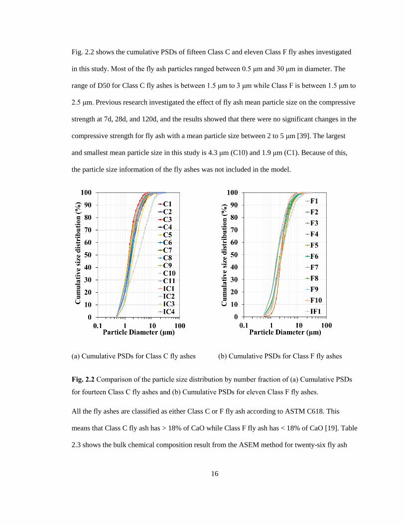
The ASTM C618 [19] classification method is widely used to approximately compare the

performance of different fly ashes despite this not being recommended. Fig. 2.4 shows the

comparison between the measured strength and the average values for Class C or F fly ash at 20%

and 40% replacement rates. The actual measured values were shown as points on the plot with the

same color as the matching trend line. Despite having similar bulk chemical classification as per

ASTM C618 the strength performance was variable. This further shows the challenge of using

ASTM C618 classification methods to predict the compressive strength of concrete containing fly

ash.

21

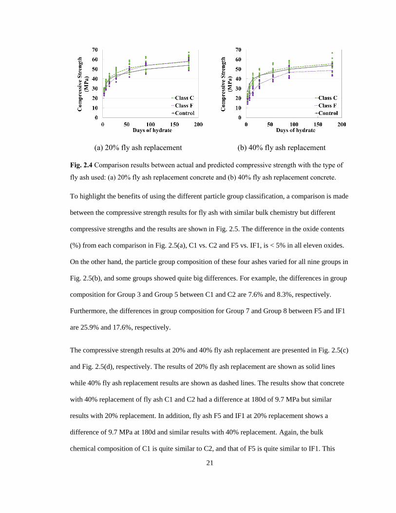
(a) 20% fly ash replacement (b) 40% fly ash replacement

Fig. 2.4 Comparison results between actual and predicted compressive strength with the type of

fly ash used: (a) 20% fly ash replacement concrete and (b) 40% fly ash replacement concrete.

To highlight the benefits of using the different particle group classification, a comparison is made

between the compressive strength results for fly ash with similar bulk chemistry but different

compressive strengths and the results are shown in Fig. 2.5. The difference in the oxide contents

(%) from each comparison in Fig. 2.5(a), C1 vs. C2 and F5 vs. IF1, is < 5% in all eleven oxides.

On the other hand, the particle group composition of these four ashes varied for all nine groups in

Fig. 2.5(b), and some groups showed quite big differences. For example, the differences in group

composition for Group 3 and Group 5 between C1 and C2 are 7.6% and 8.3%, respectively.

Furthermore, the differences in group composition for Group 7 and Group 8 between F5 and IF1

are 25.9% and 17.6%, respectively.

The compressive strength results at 20% and 40% fly ash replacement are presented in Fig. 2.5(c)

and Fig. 2.5(d), respectively. The results of 20% fly ash replacement are shown as solid lines

while 40% fly ash replacement results are shown as dashed lines. The results show that concrete

with 40% replacement of fly ash C1 and C2 had a difference at 180d of 9.7 MPa but similar

results with 20% replacement. In addition, fly ash F5 and IF1 at 20% replacement shows a

difference of 9.7 MPa at 180d and similar results with 40% replacement. Again, the bulk

chemical composition of C1 is quite similar to C2, and that of F5 is quite similar to IF1. This

22

indicates that the compressive strength is not accurately predicted by bulk chemical composition

in this example. More in-depth analysis is needed to compare how the fly ash groups perform.

(a) Bulk chemical composition

(b) Particle groups

(c) Compressive strength change for

two Class C fly ashes

(d) Compressive strength change for

two Class F fly ashes

Fig. 2.5 Comparisons of (a) Bulk chemical composition, (b) Particle groups, (c) Compressive

strength change for C1 vs. C2, and (d) Compressive strength change for F5 and IF1.

2.3.3 Accuracy of the Particle Model

Fig. 2.6 shows the relationship between the measured and predicted value using the Particle

Model for all curing times on 20% and 40% fly ash replacement. The detailed results of the

predictive models for 20% and 40% fly ash replacement at different hydration time is found in

Appendix G. The slope of the trend line for 20% and 40% replacement are 1.00 and 0.99

respectively, and the R-squared value of each trend line for 20% and 40% replacement are 0.95

23

and 0.93. This shows the compressive strength is accurately predicted by using the Particle Model

for each curing time.

According to ASTM C39, the acceptable range of three individual cylinder strengths for the test

of 100 by 200 mm (4 by 8 inch) cylinders made from a well-mixed sample of concrete under

laboratory conditions is 10.6% [34]. This is a helpful number to evaluate the accuracy of the

Particle Model. Values of +/- 10% are shown in Fig. 2.6 as dashed red lines. For the 20% fly ash

replacement shown in Fig. 2.6(a), 127 out of 133 measurements or 95% of all measurements are

within +/- 10%, and the remaining 6 predictions are within +/- 15%. For the concrete with 40%

fly ash replacement in Fig. 2.6(b), 108 out of 133 or 81% of the measurements are within +/- 10%

and the 94% predictions are within +/- 15%. This indicates that the Particle Model works well,

and the derived equations are reliable to predict the compressive strength from periods between

3d and 180d with both 20% and 40% replacement.

(a) 20% fly ash replacement

(b) 40% fly ash replacement

* Red dash line: The range of +/‒ 10% of the predicted and measured strength.

Fig. 2.6 The relationship between the predicted and measured value for strength by using the

Particle Model for (a) 20% fly ash concrete and (b) 40% fly ash concrete.

24

With the Particle Model, a model based on the current ASTM C618 classification method (Class

C or F) was created for each day of hydration. It should be noted that Class C and F model did not

use any of the fly ash particle data from ASEM or the nine groups. The R-squared value of Class

C and F classification model was investigated for 20% and 40% fly ash replacement concrete at

all individual curing time and compared to the R-squared value from Particle Model. Table 2.6

shows the R-squared value comparison results between Class C and F model and Particle Model

results for all the analyses. Low R-squared value indicates a weak linear fit for the model while

high R-squared value indicates the model explains all the variability of the response data around

its mean. The R-squared value for all the Particle Models is close to 0.99 while the Class C and F

classification model had R-squared values < 0.50 for all the measurements. These high R-squared

values show that the Particle Model closely matches the measured compressive strength results.

Table 2.6 R-squared value from C and F classification model and Particle model at different

curing times on different mixtures.

Days of

hydration

20% replacement 40% replacement

C-F Model Particle Model C-F Model Particle Model

3 days 0.494 0.997 0.458 0.992

7 days 0.423 0.996 0.495 0.989

14 days 0.478 0.998 0.438 0.988

28 days 0.256 0.997 0.397 0.991

56 days 0.065 0.997 0.365 0.992

90 days 0.000 0.996 0.184 0.993

180 days 0.000 0.996 0.318 0.993

Table 2.7 shows the results of the bootstrapping for the Particle Model over the R-squared value.

The mean of 500 R-squared values through the bootstrap method is compared with the R-squared

value of the derived predictive model in Table 2.6 at each measurement time for both 20% and

25

40% fly ash concrete. It should be noted here again that this helps to determine the robustness of

the Particle Model. The results present that the mean R-squared value from the bootstrapping

shows the same or almost the same each other to the R-squared value of the derived predictive

model. The maximum, minimum and SD are also investigated over the R-squared values from the

bootstrapping. It shows that the range of difference between the maximum and minimum R-

squared value is from 0.002 to 0.014 which is quite narrow. Furthermore, all the investigated SDs

are under 0.003 which indicates the variance of the bootstrap results is quite small. Thus, the

Particle Model can be considered as a robust tool to predict the compressive strength of fly ash

concrete for the materials investigated.

Table 2.7 The results of the bootstrapping for the Particle Model over the R-squared value.

Mixture Days of

hydration

The mean of the

R-squared values Max Min SD

20%

Fly ash

3 days 0.997 0.999 0.995 0.0006

7 days 0.997 0.998 0.994 0.0007

14 days 0.998 0.999 0.997 0.0004

28 days 0.997 0.999 0.994 0.0007

56 days 0.997 0.999 0.995 0.0006

90 days 0.997 0.999 0.995 0.0007

180 days 0.997 0.999 0.994 0.0008

40%

Fly ash

3 days 0.993 0.997 0.987 0.0014

7 days 0.990 0.995 0.984 0.0016

14 days 0.988 0.996 0.981 0.0026

28 days 0.991 0.996 0.988 0.0013

56 days 0.992 0.996 0.986 0.0015

90 days 0.993 0.997 0.989 0.0013

180 days 0.993 0.997 0.990 0.0013

26

2.3.4 Effects of each individual group on compressive strength

Fig. 2.7 and 2.8 show the coefficients of each group for the linear model used to predict the

compression strength between 3 and 180 days for 20% and 40% replacement. The value of > 0

indicates that the group helps to increase the compressive strength while ages without a value for

a coefficient mean that those groups did not affect the strength at that time period. For example,

since Group 6 and 8 have a coefficient of zero between 7 and 56 days for 20% fly ash

replacement, these groups are found to not be statistically significant during these periods of time

(from 7 days to 56 days). The numerical value for each group shows how significant it is at each

time. Positive values are shown to increase strength and negative values will decrease strength.

Further discussion over the contribution of each group will be discussed later in this paper.

The impacts of Group 2, 3, 5, 7, and 9 for both 20% and 40% replacement show a steady increase

over time. This means that these groups continue to contribute to strength over time. At 20%

replacement Group 4 did not show an improvement in strength after 3 days, and at 40%

replacement, it did not contribute to strength. Groups 6 and 8 show either no meaningful

contribution or a decrease in strength for both 20% and 40% replacement. Finally, Group 1 shows

a difference in performance at 20% and 40% replacement. At 20% replacement Group 1 shows an

increase in contribution up to 56 days and then a decrease in strength after that, but no

contribution of Group 1 was found at 40% replacement.

27

Fig. 2.7 The coefficient comparison for 20% replacement of fly ash within a concrete mixture.

Fig. 2.8 The coefficient comparison for 40% replacement of fly ash within a concrete mixture.

2.3.4.1 Discussion of Group 2, 3, 5, and 7

These groups are likely composed of reactive glasses. Group 2 and 3 have high contents of Al2O3

and CaO with relatively small SiO2 contents (about 8%). Furthermore, Group 5 has a high content

of SiO2, Al2O3, and CaO while Group 7 has high contents of SiO2 and Al2O3 with relatively small

CaO.

Group 2 and 3 have relatively higher contents of P2O5 and MgO than other groups, and these

materials may form magnesium phosphate and aluminum phosphate. The magnesium phosphate

28

can decrease set, increase early strength, and show good durability including resistance to

chemical attack and permeation [40]. Aluminum phosphate will also increase strength [41].

It is also possible that several glassy phases can exist in these four groups such as calcium-rich

aluminosilicates, aluminosilicate and calcium silicates. Those glassy phases have been found in

fly ash in several previous studies and suggested as reactive glassy phases [5, 42-45]. Durdziński

et al. [43] studied the reactivity of four glassy phases in fly ash for 365 days of hydration. They

have shown calcium-rich aluminosilicates were the most reactive, and the aluminosilicates also

had a high reactivity [43]. It is well known that the calcium-rich glassy phases are much more

reactive than those with low or moderate calcium content phases [43, 45]. Thus, Group 2, 3, 5 and

7 are likely more reactive phases than other groups.

2.3.4.2 Discussion of Group 9

Group 9 has ≈ 85% SiO2 content. Previous studies over fly ash have shown a silicon-rich phase

containing almost no impurities was mainly observed as crystalline silica which is quartz [46, 47].

Quartz is commonly observed in fly ash [5]. Furthermore, on both 20% and 40% fly ash concrete,

Group 9 relatively has a high impact on the compressive strength than other groups for the first

180d of hydration. Further, the impact was almost constant after 56d of hydration.

Popovics has suggested the strength increase on the fly ash concrete could be either attributed to

the reduction in initial porosity of the paste by fine particles of fly ash and quartz powder, or to

the acceleration of hydration of the cement phase due to nucleation effects from fly ash particles

for C-S-H gel [48]. It is also possible that some soluble silica exists in Group 9. The soluble silica

could react with the aluminum to form a C-A-S-H gel with a dense microstructure. This would

lower the porosity and create a finer gel pore system [49].

29

2.3.4.3 Discussion of Group 4, 6, and 8

The particles in these groups show a poor reactivity. Even though these groups have a similar

chemical composition to the calcium-rich alumino-silicate (Group 6) and aluminum silicate

(Group 4 and 8), there may be some reason that these particles have a poor reactivity. Previous

studies have found low reactive materials such as mullite (a crystalline aluminosilicate) in low

calcium fly ashes [50]. Group 4 has a high percentage of SiO2 and Al2O3 with a CaO content of

about 6%. Therefore, Group 4 may contain high amounts of mullite. Group 8 contains high SiO2

(≈ 60%) and some Na2O and K2O. This material is more likely a conglomerate of non-reactive

phases like feldspar (K, Na)A1Si3O8, mullite, and quartz [51].

Group 6 has higher CaO and MgO content than the other groups and also has some SiO2 and

Al2O3. Group 6 seemed to have a similar chemical composition to Group 3 but there is about a

15% difference in SiO2 content. The chemical composition of Group 6 could be gehlenite

Ca2Al(AlSiO7) and akermanite Ca2Mg(Si2O7) which have shown to not be chemically active in

concrete [5]. Merwinite (Ca3Mg(SiO4)2), a non-reactive phase that is commonly found in high-

calcium fly ash may also be found in Group 6 [5]. It is also possible that the MgO causes an

unsoundness problem in the concrete. This might be why these materials are observed to have a

negative coefficient or a loss in strength over time.

2.3.4.4 Discussion of Group 1

Group 1 contains 77.81% of Fe2O3 content and this particle has the largest coefficient for 3, 7, 14,

28, and 56 days on 20% replacement while there is no impact at all to the strength over time for

40% replacement. Furthermore, the impact of Group 1 at 20% fly ash replacement concrete

decreases after 56d while the impact of other groups increases. Previous studies used Fe-rich

materials such as iron powder and iron waste as the partial replacement of cement to investigate

the impact on the compressive strength [52-55]. The studies have found that the Fe-rich material

30

increased the first 28 days of hydration. One reason for this may be the strong electrostatic

attractive forces of the Fe-rich particle. This has been suggested as a cause for the increase in

strength at early ages [52]. This work went on to show that there is no impact on the properties

after the optimum amount of Fe-rich material was reached [52]. Thus, it is possible that a 40%

replacement of fly ash provides an excessive amount of this material and so there is no impact on

the measured strength.

2.3.5 Practical Implications

This work builds on previous studies to show that understanding the reactivity of the individual

fly ash particles is a helpful tool to predict and ultimately understand the performance of fly ash

within concrete. The Particle Model takes this concept and creates a numerical tool for prediction.

This work has given useful predictive equations that can be used at both 20% and 40%

replacement volume of fly ash within the concrete and should help build confidence in the use of

higher replacement levels of fly ash. This work also shows that it is possible to build accurate

predictive models for fly ash performance in concrete.

Because of the change in coal-fired power plant emissions, the supply of fly ash has been reduced

in some regions. Because the Particle Model is performance-based then it may allow greater

usage of fly ash that does not meet current specifications. Further, the Particle Model may be able

to serve as the basis for a performance-based classification system for fly ash beyond the current

bulk composition analysis in ASTM C 618.

2.4 Conclusion

Twenty-six fly ash sources were investigated by using the ASEM to collect the properties of

52,000 fly ash particles. The Particle Model was used to investigate the fly ash concrete with

nineteen fly ash sources and predict compressive strength at 20% and 40% replacement in

31

concrete after 3, 7, 14, 28, 56, 90, and 180 days of curing. Insights about each fundamental type

or group are made as well as their contribution to the compressive strength over time.

The following contributions were made:

1. Over 91% of the fly ash particles can be classified into nine groups based on the chemical

composition data.

2. The Particle Model is able to predict the compressive strength within +/- 10% for 95% of

all measurements at 20% fly ash replacement and for 81% of all measurements at 40%

replacement.

3. The R-squared value for the compressive strength prediction of the Particle Model is ≈

0.99, while the Class C and F classification model is < 0.50 for the time periods

investigated and for 20% and 40% fly ash replacement.

4. Group 2, 3, 5, 7, and 9 are correlated with strength gain for both 20% and 40% fly ash

replacement and show similar trends at both replacement levels.

5. Group 4, 6, and 8 have a poor contribution or a reduction to the compressive strength for

20% and 40% replacement.

6. Group 1 showed the largest contribution coefficient over the first 56 days for 20%

replacement while there is no impact for the compressive strength for 40% replacement.

This paper presents a useful approach to fly ash classification and accurate prediction of

performance in concrete at 20% and 40% replacement levels. This work also shows that these

contributions depend on the replacement levels, the chemical composition of each type of

particle, and the age of curing.

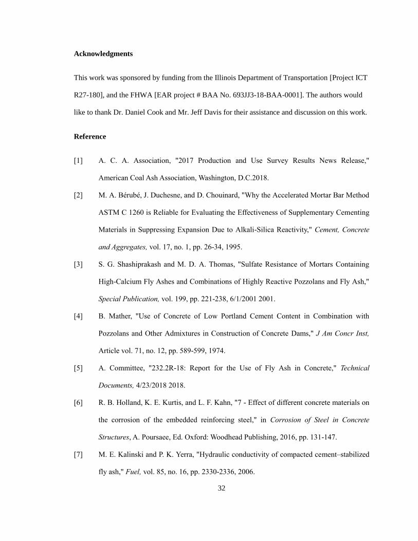
32

Acknowledgments

This work was sponsored by funding from the Illinois Department of Transportation [Project ICT

R27-180], and the FHWA [EAR project # BAA No. 693JJ3-18-BAA-0001]. The authors would

like to thank Dr. Daniel Cook and Mr. Jeff Davis for their assistance and discussion on this work.

Reference

[1] A. C. A. Association, "2017 Production and Use Survey Results News Release,"

American Coal Ash Association, Washington, D.C.2018.

[2] M. A. Bérubé, J. Duchesne, and D. Chouinard, "Why the Accelerated Mortar Bar Method

ASTM C 1260 is Reliable for Evaluating the Effectiveness of Supplementary Cementing

Materials in Suppressing Expansion Due to Alkali-Silica Reactivity," Cement, Concrete

and Aggregates, vol. 17, no. 1, pp. 26-34, 1995.

[3] S. G. Shashiprakash and M. D. A. Thomas, "Sulfate Resistance of Mortars Containing

High-Calcium Fly Ashes and Combinations of Highly Reactive Pozzolans and Fly Ash,"

Special Publication, vol. 199, pp. 221-238, 6/1/2001 2001.

[4] B. Mather, "Use of Concrete of Low Portland Cement Content in Combination with

Pozzolans and Other Admixtures in Construction of Concrete Dams," J Am Concr Inst,

Article vol. 71, no. 12, pp. 589-599, 1974.

[5] A. Committee, "232.2R-18: Report for the Use of Fly Ash in Concrete," Technical

Documents, 4/23/2018 2018.

[6] R. B. Holland, K. E. Kurtis, and L. F. Kahn, "7 - Effect of different concrete materials on

the corrosion of the embedded reinforcing steel," in Corrosion of Steel in Concrete

Structures, A. Poursaee, Ed. Oxford: Woodhead Publishing, 2016, pp. 131-147.

[7] M. E. Kalinski and P. K. Yerra, "Hydraulic conductivity of compacted cement–stabilized

fly ash," Fuel, vol. 85, no. 16, pp. 2330-2336, 2006.

33

[8] S. K. Das and Yudhbir, "A simplified model for prediction of pozzolanic characteristics of

fly ash, based on chemical composition," (in English), Cement and Concrete Research,

vol. 36, no. 10, pp. 1827-1832, Oct 2006.

[9] S. Diamond, "On the Glass Present in Low-Calcium and in High-Calcium Flyashes," (in

English), Cement and Concrete Research, vol. 13, no. 4, pp. 459-464, 1983.

[10] L. X. Du, E. Lukefahr, and A. Naranjo, "Texas Department of Transportation Fly Ash

Database and the Development of Chemical Composition-Based Fly Ash Alkali-Silica

Reaction Durability Index," (in English), Journal of Materials in Civil Engineering, vol.

25, no. 1, pp. 70-77, Jan 2013.

[11] S. C. White and E. D. Case, "Characterization of fly ash from coal-fired power plants,"

Journal of Materials Science, vol. 25, no. 12, pp. 5215-5219, 1990/12/01 1990.

[12] S. Schlorholtz, K. Bergeson, and T. Demirel, "Monitoring of Fluctuations in the Physical

and Chemical Properties of a High-Calcium Fly Ash," MRS Proceedings, vol. 113, p.

107, 1987, Art. no. 107.

[13] M. Aboustait, T. Kim, M. T. Ley, and J. M. Davis, "Physical and chemical characteristics

of fly ash using automated scanning electron microscopy," (in English), Construction and

Building Materials, vol. 106, pp. 1-10, Mar 1 2016.

[14] Q. Hu, M. Aboustait, M. T. Ley, J. C. Hanan, V. Rose, and R. Winarski, "Combined three-

dimensional structure and chemistry imaging with nanoscale resolution," (in English),

Acta Materialia, vol. 77, pp. 173-182, Sep 15 2014.

[15] Q. Hu, M. T. Ley, J. Davis, J. C. Hanan, R. Frazier, and Y. Zhang, "3D chemical

segmentation of fly ash particles with X-ray computed tomography and electron probe

microanalysis," Fuel, vol. 116, pp. 229-236, 2014.

[16] T. Kim, Q. Hu, M. T. Ley, M. Aboustait, and J. W. Bullard, "Using Particle

Characterization to Study Fly Ash Dissolution and Leaching in Water and KOH

34

Solution," ACI Materials Journal, vol. 116, no. 4, 2019.

[17] T. Kim, M. Moradian, and M. T. Ley, "Dissolution and leaching of fly ash in nitric acid

using automated scanning electron microscopy," Advances in Civil Engineering

Materials, vol. 7, no. 1, pp. 291-307, 2018.

[18] T. Kim, J. M. Davis, M. T. Ley, S. Kang, and P. Amrollahi, "Fly ash particle

characterization for predicting concrete compressive strength," (in English), Construction

and Building Materials, vol. 165, pp. 560-571, Mar 20 2018.

[19] ASTM C618, Standard Specification for Coal Fly Ash and Raw or Calcined Natural

Pozzolan for Use in Concrete, 2019.

[20] ASTM C150, Standard Specification for Portland Cement, 2019.

[21] R. P. Gupta, T. F. Wall, I. Kajigaya, S. Miyamae, and Y. Tsumita, "Computer-controlled

scanning electron microscopy of minerals in coal - Implications for ash deposition," (in

English), Progress in Energy and Combustion Science, vol. 24, no. 6, pp. 523-543, 1998.

[22] C. A. O'Keefe, T. M. Watne, and J. P. Hurley, "Development of advanced scanning

electron microscopy techniques for characterization of submicron ash," (in English),

Powder Technology, vol. 108, no. 2-3, pp. 95-102, Mar 20 2000.

[23] J. T. Armstrong, "Quantitative Elemental Analysis of Individual Microparticles with

Electron Beam Instruments," in Electron Probe Quantitation, K. F. J. Heinrich and D. E.

Newbury, Eds. Boston, MA: Springer US, 1991, pp. 261-315.

[24] G. Love and V. D. Scott, "Evaluation of a New Correction Procedure for Quantitative

Electron-Probe Microanalysis," (in English), Journal of Physics D-Applied Physics, vol.

11, no. 10, pp. 1369-1376, 1978.

[25] J. T. Armstrong and P. R. Buseck, "Quantitative Chemical-Analysis of Individual

Microparticles Using Electron-Microprobe - Theoretical," (in English), Analytical

Chemistry, vol. 47, no. 13, pp. 2178-2192, 1975.

35

[26] J. T. Armstrong and P. R. Buseck, "A General Characteristic Fluorescence Correction for

the Quantitative Electron Microbeam Analysis of Thick Specimens, Thin-Films and

Particles," (in English), X-Ray Spectrometry, vol. 14, no. 4, pp. 172-182, 1985.

[27] M. Aboustait et al., Innovative prediction of fly ash performance in concrete. Midwest

City, OK: Oklahoma Transportation Center, 2013.

[28] C. P. Aichele et al., "A comparison of automated scanning electron microscopy (ASEM)

and acoustic attenuation spectroscopy (AAS) instruments for particle sizing," Colloids

and Surfaces A: Physicochemical and Engineering Aspects, vol. 479, pp. 46-51,

2015/08/20/ 2015.

[29] ASTM C138, Standard Test Method for Density (Unit Weight), Yield, and Air Content

(Gravimetric) of Concrete, 2017.

[30] ASTM C143, Standard Test Method for Slump of Hydraulic-Cement Concrete, 2015.

[31] ASTM C231, Standard Test Method for Air Content of Freshly Mixed Concrete by the

Pressure Method, 2017.

[32] Z. Lloyd, "Investigation of the Quality Control of Waste Products for Concrete," Master,

Civil Engineering, Oklahoma State University, Stillwater, OK, 2019.

[33] ASTM C31, Standard Practice for Making and Curing Concrete Test Specimens in the

Field, 2019.

[34] ASTM C39, Standard Test Method for Compressive Strength of Cylindrical Concrete

Specimens, 2018.

[35] T. Kohonen, Self-Organizing Maps, Third ed. (Springer Series in Information Sciences).

Springer, Berlin, Heidelberg, 1997.

[36] M. J. Crawley, The R Book, Second ed. Imperial College London at Silwood Park, UK:

John Wiley & Sons Ltd, 2012.

[37] R. C. Team, "R: a language and environment for statistical computing. Vienna, Austria: R

36

Foundation for Statistical Computing; 2015. R Foundation for Statistical Computing," ed,

2016.

[38] M. Kuhn and K. Johnson, Applied predictive modeling. Springer, 2013.

[39] G. Li and X. Wu, Influence of fly ash and its mean particle size on certain engineering

properties of cement composite mortars. 2005, pp. 1128-1134.

[40] Z. Li, Z. Ding, and Y. Zhang, "Development of sustainable cementitious materials," in

Proceedings of the international workshop on sustainable development and concrete

technology, 2004, vol. 1, no. 1, pp. 55-76: Iowa State University.

[41] N. Abdel-Rahman and N. M. Naghoj, "Silica Phosphate in Engineering Materials," in

Challenges of Concrete Construction: Volume 6, Concrete for Extreme Conditions, 2002,

pp. 101-107.

[42] D. M. Roy, K. Luke, and S. Diamond, "Characterization of fly ash and its reactions in

concrete," MRS Online Proceedings Library Archive, vol. 43, 1984.

[43] P. T. Durdzinski, C. F. Dunant, M. Ben Haha, and K. L. Scrivener, "A new quantification

method based on SEM-EDS to assess fly ash composition and study the reaction of its

individual components in hydrating cement paste," (in English), Cement and Concrete

Research, vol. 73, pp. 111-122, Jul 2015.

[44] K. L. Aughenbaugh, "Fly ash-based geopolymers: identifying reactive glassy phases in

potential raw materials," Doctor of Philosophy, Civil, Architectural, and Environmental

Engineering, The University of Texas at Austin, The University of Texas at Austin, 2013.

[45] K. L. Aughenbaugh, R. T. Chancey, P. Stutzman, M. C. Juenger, and D. W. Fowler, "An

examination of the reactivity of fly ash in cementitious pore solutions," Materials and

Structures, vol. 46, no. 5, pp. 869-880, 2013.

[46] V. M. Malhotra and P. K. Mehta, High-performance, high-volume fly ash concrete :

materials, mixture proportioning, properties, construction practice, and case histories.

37

Ottawa, Canada: Supplementary Cementing Materials for Sustainable Development, Inc.,

2002.

[47] K. Kiattikomol, C. Jaturapitakkul, S. Songpiriyakij, and S. Chutubtim, "A study of

ground coarse fly ashes with different finenesses from various sources as pozzolanic

materials," (in English), Cement & Concrete Composites, vol. 23, no. 4-5, pp. 335-343,

Aug-Oct 2001.

[48] S. Popovics, "A Model for Estimation of the Contribution of Fly Ash to Concrete

Strength in Blended Cements in Construction," vol. Blended cements in construction, no.

Elsevier Applied Science, ed. by R. N. Swamy, 1991.

[49] Y. Ma, J. Hu, and G. Ye, "The effect of activating solution on the mechanical strength,

reaction rate, mineralogy, and microstructure of alkali-activated fly ash," Journal of

Materials Science, vol. 47, no. 11, pp. 4568-4578, 2012/06/01 2012.

[50] S. Gomes, M. François, M. Abdelmoula, P. Refait, C. Pellissier, and O. Evrard,

"Characterization of magnetite in silico-aluminous fly ash by SEM, TEM, XRD,

magnetic susceptibility, and Mössbauer spectroscopy," Cement and Concrete Research,

vol. 29, no. 11, pp. 1705-1711, 1999/11/01/ 1999.

[51] D. Stark and M. S. Y. Bhatty, "Alkali-Silica Reactivity: Effect of Alkali in Aggregate on

Expansion," V. H. Dodson, Ed. West Conshohocken, PA: ASTM International, 1986, pp.

16-30.

[52] P. Sikora, E. Horszczaruk, K. Cendrowski, and E. Mijowska, "The Influence of Nano-

Fe3O4 on the Microstructure and Mechanical Properties of Cementitious Composites," (in

English), Nanoscale Research Letters, vol. 11, Apr 11 2016.

[53] S. Ghannam, H. Najm, and R. Vasconez, "Experimental study of concrete made with

granite and iron powders as partial replacement of sand," (in English), Sustainable

Materials and Technologies, vol. 9, pp. 1-9, Sep 2016.

38

[54] M. A. Largeau, R. Mutuku, and J. Thuo, "Effect of Iron Powder (Fe2O3) on Strength,

Workability, and Porosity of the Binary Blended Concrete," Open Journal of Civil

Engineering, vol. Vol.08No.04, p. 15, 2018, Art. no. 88279.

[55] K. Noori and H. Ibrahim, Mechanical Properties of Concrete Using Iron Waste as a

Partial Replacement of Sand. 2018.

39

CHAPTER III

USING THE PARTICLE MODEL TO PREDICT ELECTRICAL RESISTIVITY

PERFORMANCE OF FLY ASH IN CONCRETE

Abstract

The electrical resistivity performance of fly ash in concrete is not easy to predict due to the

diverse sources of fly ash and their varying reactivity. This paper aims to develop predictive

models for the electrical resistivity of fly ash concrete by applying the Particle Model. The

Particle Model rapidly examines individual fly ash particles without human intervention and is

used to derive predictive models for 20% and 40% fly ash replacement levels in concrete at seven

different periods of hydration. The R-squared values of predictive models in the Particle Model

show significant improvement over using the classification method based on Class C and F for

both fly ash replacement at all investigated time periods. The derived predictive models are able

to accurately estimate the electrical resistivity within +/- 10% for 80% of all measurements at

20% fly ash replacement and within +/- 10% for 75% of all measurements at 40% fly ash

replacement. These investigations provide important insights into how the Particle Model can

help predict the electrical resistivity of fly ash concrete at different mixtures and hydration times.

Keywords: Electrical resistivity; Fly ash; Concrete; ASEM; Particle Model; Grouping; SOM

40

3.1 Introduction

Electrical resistivity gives direct insight into the rate of corrosion within concrete once the

chloride threshold level has been exceeded and corrosion has been initiated [1]. Furthermore, the

corrosion process of steel in reinforced concrete can be evaluated with the help of electrical

resistivity of concrete, and the correlations between the electrical resistivity of concrete and the

corrosion have been found in other studies [2-6]. Electrical resistivity is also being evaluated as a

means to evaluate mass transport into concrete and has been proposed as a quality control tool for

concrete [7-9]. Several factors influence the performance of electrical resistivity including:

cement chemistry, the cement content, water-to-cement ratio, admixtures, and supplementary

cementitious materials such as fly ash [10].

Fly ash is used as a partial replacement of the portland cement to improve the overall durability of

concrete [11-14] and is generally used at 15-35% replacement of cement by mass because this

range has been found to be an acceptable level of replacement without major negative effects on

the performance [15]. Previous studies have investigated the impacts of fly ash in concrete and

tried to predict the performance of fly ash by using bulk chemical characterization methods such

as X-ray fluorescence (XRF) [16-19]. However, fly ash sources with similar bulk chemistry can

have dramatically different performance [20]. This indicates that bulk chemical characteristics are

not always useful to predict the properties of concrete. Furthermore, it is hard to predict the

performance of higher replacement levels of fly ash in concrete. These higher replacement levels

can reduce the overall cost, possibly increase durability, and improve the sustainability of the

concrete [13]. Thus, a technique is needed to provide accurate predictions for the electrical

resistivity performance of fly ash concrete. This has the ability to increase the usage of fly ash in

concrete and improve the service life of concrete structures.

41

While bulk chemistry does not provide predictable insights into the performance of the fly ash in

concrete, studies with scanning electron microscopy (SEM) and automated scanning electron

microscopy (ASEM) show that there are repeating patterns in chemical composition found within

fly ash particles [21, 22]. To gain more insights, a method called the Particle Model is developed

in a previous study to produce predictive models for compressive strength [23]. This is based on

using an ASEM to classify thousands of individual fly ash particles [23-28] and then machine

learning with the Self-Organizing Map (SOM) algorithm was applied to classify the fly ash

particles into nine distinct groups based on these few major repeatable patterns of chemical

compositions [23]. These groups are then able to predict the compressive strength at different

times with 90% of the predicted values within +/- 10% of the measured values [29].

The current work expands the application of the Particle Model by predicting electrical resistivity

as demonstrated in Fig. 3.1. The aim of this work is to provide important insights into how the

application of the Particle Model can be extended on the electrical resistivity prediction at 20%

and 40% replacement by mass at different hydration times. This paper provides some important

insights to evaluate the impact of fly ash in concrete and improve the durability of concrete,

although a full investigation is outside the scope of this work.

Fig. 3.1 The schematic diagram of the overall procedure of the work in this study.

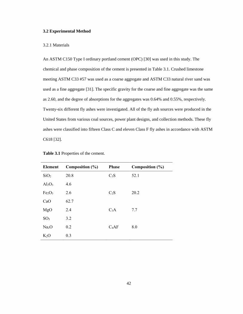
42

3.2 Experimental Method

3.2.1 Materials

An ASTM C150 Type I ordinary portland cement (OPC) [30] was used in this study. The

chemical and phase composition of the cement is presented in Table 3.1. Crushed limestone

meeting ASTM C33 #57 was used as a coarse aggregate and ASTM C33 natural river sand was

used as a fine aggregate [31]. The specific gravity for the coarse and fine aggregate was the same

as 2.60, and the degree of absorptions for the aggregates was 0.64% and 0.55%, respectively.

Twenty-six different fly ashes were investigated. All of the fly ash sources were produced in the

United States from various coal sources, power plant designs, and collection methods. These fly

ashes were classified into fifteen Class C and eleven Class F fly ashes in accordance with ASTM

C618 [32].

Table 3.1 Properties of the cement.

Element Composition (%) Phase Composition (%)

SiO2 20.8 C3S 52.1

Al2O3 4.6

Fe2O3 2.6 C2S 20.2

CaO 62.7

MgO 2.4 C3A 7.7

SO3 3.2

Na2O 0.2 C4AF 8.0

K2O 0.3

43

3.2.2 Investigation of fly ash particles with the ASEM

The ASEM was used to investigate the properties of fly ash and to collect thousands of individual

fly ash particle data. The ASEM method used SEM-EDS (Aspex Explorer PSEM-EDS) with the

image analysis operating system. Two thousand particles were analyzed from each fly ash

because this amount of particles has been shown to be a representative sample for fly ash [25].

One of the important advantages of the ASEM over the conventional analysis of bulk chemistry is

the effectiveness of measurement time [25, 33, 34]. The ASEM method enabled researchers to

investigate the chemical composition, size, and shape of approximately 500 particles per hour

without human intervention. This means that the ASEM can rapidly measure the physical and

average chemical information of thousands of individual particles within a reasonable timeframe.

One challenge with the ASEM method was that the fly ash particle has a spherical shape, but not

a flat shape; so this violated one of the assumptions of the classical quantitative EDS analysis.

The correction models developed by Armstrong and Love-Scott [35, 36] and Armstrong – Buseck

were used to address this [37, 38]. These models took into account the shape of the particle and

make corrections in the collected k-ratios of eleven investigated elements (Na, Mg, Al, Si, P, S,

K, Ca, Ti, Fe, and Sr). Furthermore, the particle size distribution (PSD) was compared between

ASEM and acoustic attenuation spectroscopy and found to be similar [39]. The consistency of the

ASEM method was discussed in the previous study [23], and details can be found in Appendix A.

The accuracy, reliability, and repeatability of the ASEM method when compared to XRF analysis

were presented in other publications and shown to be less than a 5% absolute difference for >

90% of comparisons [23, 25, 40]. More details over the ASEM method, sample preparation,

analysis with ASEM, and data processing can be found in Appendix C.

44

3.2.3 Concrete specimen preparation

3.2.3.1 Concrete mixture design

Based on a wide range of different chemical composition, twelve Class C and seven Class F fly

ash sources were chosen for concrete mixtures. The 20% and 40% fly ash replacement rates by

mass of cement were produced for each fly ash source to investigate the fly ash performances in a

concrete mixture design. In addition, a concrete mixture with 100% portland cement or 0% of fly

ash replacement was prepared as the control specimens for performance. Table 3.2 shows mixture

proportions for the mixtures with different fly ash replacement levels. A constant 0.45 water-to-

cementitious material ratio (w/cm) was used for all the mixtures. To minimize the variables, no

chemical admixtures were used in any mixtures.

Table 3.2 Mixture proportions for concrete specimens.

Mixture

design W/C

Cement

(kg/m3)

Fly ash

(kg/m3)

Water

(kg/m3)

Coarse

aggregate

(kg/m3)

Fine

aggregate

(kg/m3)

Control 0.45 283 0 127 863 564

20% fly ash 0.45 227 57 127 862 562

40% fly ash 0.45 170 113 127 858 557

3.2.3.2 Concrete mixing procedure and sample preparation

The moisture content for both coarse and fine aggregates was determined before the mixing

process and the batch proportions for the aggregates and water were adjusted. Both aggregates

were brought into the temperature-controlled mixing facility at least a day before conducting the

moisture correction, and their batch weights were corrected for the moisture content. After

adjusting the mixture proportion, all the mixtures were mixed according to the following steps.

All aggregates were collected from the outside storage piles, and they were stored in a

45

temperature-controlled room (23°C) for at least 24 hours. The aggregates were then placed in the

mixer and spun; after that, a representative sample was taken for moisture correction. It should be

noted here that aggregates have to be properly sealed to prevent water loss before the mixing. At

the time of mixing, all aggregates and approximately one half of the mixing water were loaded

into the mixer; they were being mixed for three minutes. This allowed the aggregates to approach

the saturated surface dry (SSD) condition and to ensure that the aggregates were evenly

distributed. All the materials (the cement, fly ash, and the remaining water) were added into the

mixer and were being mixed for three minutes. Then the mixture was rested for two minutes

while the sides of the mixing drum were scraped. After that, the mixer was started to mix the

concrete for three more minutes as well.

3.2.4 Testing of concrete samples

The unit weight, slump, and air content were measured for each mixture [41-43]. The results were

reported in the previous publication [44]. Concrete samples were then formed in 100 mm by 200

mm cylindrical containers according to ASTM C31 [45]; they were being cured at 23°C and

100% RH for 24 h in the curing room after sealing the container. The samples were demolded and

placed into the curing room until the samples were ready for the surface resistivity test.

A non-destructive surface resistivity test, the four-point Wenner probe, was performed to

measure the electrical resistivity of the concrete according to AASHTO T358 [46] at 3, 7, 14, 28,

56, 90, and 180 days of hydration. Before the measurement, four lines were marked on the

circular face of each concrete cylinder at 0, 90, 180, and 270 degrees for measurement. Three

cylinders were measured so that twelve measurements were collected for each fly ash concrete at

each chosen curing time. The average value of twelve measurements was used as the

representative electrical resistivity for each fly ash at specific curing time. All the specimens were

in the saturated surface dry (SSD) status while the resistivity test was conducted.

46

3.2.5 The Particle Model development

The SOM algorithm and the maximum spectral angle method were used for the model

development process of the Particle Model. The SOM helped to determine nine distinct groups of

fly ash particles with unique chemical makeup. The data of the 52,000 particles were extracted

from twenty-six sources of fly ashes, and each particle had eleven pieces of chemical composition

data (Na2O, MgO, Al2O3, SiO2, P2O5, SO3, K2O, CaO, TiO2, Fe2O3, and SrO2). The maximum

spectral angle method helped to classify the fly ash particles into the determined nine groups.

More details of the maximum spectral angle method can be found in the previous publication [18]

and Appendix D.

A multiple linear regression (MLR) analysis was conducted by using the percentage of each of

the nine groups found within fly ash to derive predictive models for the electrical resistivity at 3,

7, 14, 28, 56, 90, and 180 days of hydration. This model analysis was applied to both 20% and

40% fly ash replacement of the concrete. The initial linear model to predict the electrical

resistivity was derived as the format of Eq.(3.1):

Resistivity (kΩ·cm) = a(Group 1) + b(Group 2) + c(Group 3) + d(Group 4)

+ e(Group 5) + f(Group 6) + g(Group 7) + h(Group 8) + i(Group 9) Eq.(3.1)

Where, lowercase from “a” to “i” in the equation indicates the coefficient of each group

determined from statistical analysis. The group # indicates the percentage of each group of fly

ash.

The initial model was evaluated with the probability value (Pr(>|t|)) from the MLR to

determine the statistical significance of the variables. The R-squared value of each model was

investigated for 20% and 40% fly ash replacement concrete at all individual curing times to

47

evaluate the linear fit to the model. More details can be found in Appendix H. All the data and

model processing was conducted within the R programming environment [47, 48].

3.2.6 Bootstrapping

The robustness of the derived predictive models was evaluated with the help of the bootstrap

method. Ideally, the data can be collected by repeating a large number of mixtures for the same

experiment to evaluate the validity of the generated predictive models, but this is impractical.

Instead, bootstrapping was used to investigate the robustness of the Particle Model over the R-

squared value. Bootstrapping is a resampling method where the data are sampled with

replacement from the original sample to generate simulated results [47]. This allowed creating

numerous R-squared values by running predictive models with simulated samples. Furthermore,

the results from the bootstrapping were used to calculate a variety of sample statistics such as the

mean (average) and standard deviation (SD) of the created R-squared values to compare the R-

squared value of the original model.

The size of the bootstrapping sample was the same as the original dataset and is chosen at random

from the existing data set. This means that some data points can be chosen multiple times in the

simulated sample while others may not be selected at all. This procedure has been used in

previous publications [49, 50]. The bootstrapping was conducted with 500 times for each model.

Then, the mean of the R-squared values from the bootstrapping was investigated and compared

with the R-squared value of the derived predictive model. This was applied to each curing time

for both 20% and 40% replacement.

48

3.3 Result and Discussion

3.3.1 Investigation of bulk chemical composition

Table 3.3 shows the result of the bulk chemical composition involving the use of ASEM for

twenty-six fly ashes. The fly ashes with “C#” and “IC#” represent Class C fly ash, while the fly

ashes with “F#” and “IF#” represent Class F fly ash. The fly ash that has greater than 18% of CaO

is classified as Class C and the fly ash that has 18% or less of CaO is attributed to Class F

according to ASTM C618 [32].

Table 3.3 ASEM bulk chemical composition of each fly ash source.

Source SiO2 Al2O3 Fe2O3 CaO MgO SO3 Na2O K2O TiO2 P2O5 SrO

C1 36.2 21.7 5.4 23.2 5.4 0.7 3.6 1.0 0.8 1.9 0.2

C2 35.8 19.2 5.6 26.9 5.5 1.0 3.0 0.9 0.7 1.3 0.2

C3 25.3 19.3 5.2 32.5 7.8 2.6 3.4 0.6 1.1 1.9 0.3

C4 36.7 22.8 4.5 22.5 4.3 1.2 3.4 1.0 1.3 1.1 1.2

C5 31.3 22.5 5.4 26.1 6.0 0.6 4.3 0.8 0.8 2.1 0.2

C6 27.7 22.9 4.2 21.5 4.5 2.6 12.6 0.8 1.3 0.7 1.3

C7 35.3 20.6 4.7 24.7 4.9 0.7 4.3 1.2 1.6 0.8 1.0

C8 40.1 22.6 4.5 19.5 5.7 0.8 3.7 0.9 0.6 1.4 0.1

C9 31.5 24.0 6.0 25.7 5.4 1.0 3.7 0.6 0.9 1.1 0.1

C10 36.0 19.3 5.1 22.7 7.8 2.0 4.8 0.6 1.0 0.3 0.5

C11 31.0 20.8 6.4 27.2 7.1 1.6 3.5 0.7 0.8 0.8 0.2

IC1 31.8 22.9 5.7 28.2 5.5 1.1 2.3 1.0 0.8 0.5 0.3

IC2 25.2 21.2 6.2 30.5 7.8 1.0 4.0 0.6 1.2 2.2 0.2

IC3 29.7 21.0 5.9 30.3 5.4 1.9 2.2 0.6 1.0 1.6 0.5

IC4 29.9 17.7 4.7 31.8 9.3 1.2 2.6 0.8 0.8 1.1 0.2

F1 48.8 23.8 7.4 12.5 3.0 0.5 0.9 2.1 0.8 0.1 0.3

F2 50.4 20.9 3.9 17.1 3.7 0.5 1.0 1.4 0.7 0.1 0.3

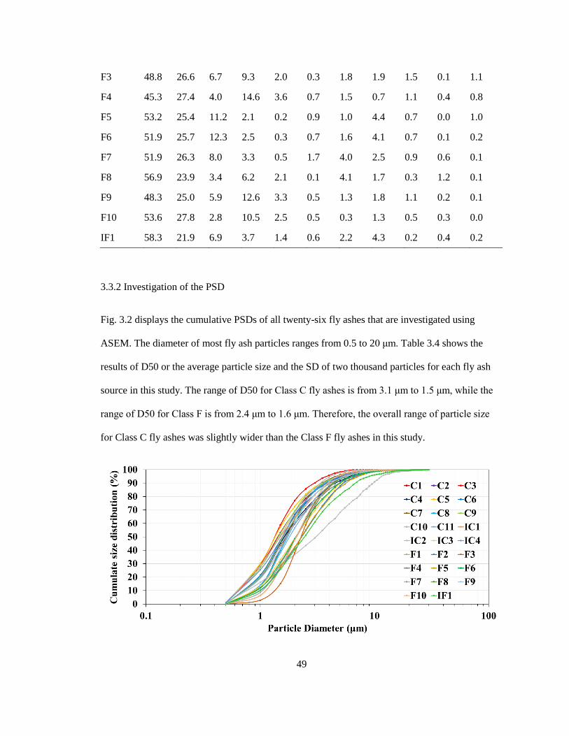
49

F3 48.8 26.6 6.7 9.3 2.0 0.3 1.8 1.9 1.5 0.1 1.1

F4 45.3 27.4 4.0 14.6 3.6 0.7 1.5 0.7 1.1 0.4 0.8

F5 53.2 25.4 11.2 2.1 0.2 0.9 1.0 4.4 0.7 0.0 1.0

F6 51.9 25.7 12.3 2.5 0.3 0.7 1.6 4.1 0.7 0.1 0.2

F7 51.9 26.3 8.0 3.3 0.5 1.7 4.0 2.5 0.9 0.6 0.1

F8 56.9 23.9 3.4 6.2 2.1 0.1 4.1 1.7 0.3 1.2 0.1

F9 48.3 25.0 5.9 12.6 3.3 0.5 1.3 1.8 1.1 0.2 0.1

F10 53.6 27.8 2.8 10.5 2.5 0.5 0.3 1.3 0.5 0.3 0.0

IF1 58.3 21.9 6.9 3.7 1.4 0.6 2.2 4.3 0.2 0.4 0.2

3.3.2 Investigation of the PSD

Fig. 3.2 displays the cumulative PSDs of all twenty-six fly ashes that are investigated using

ASEM. The diameter of most fly ash particles ranges from 0.5 to 20 μm. Table 3.4 shows the

results of D50 or the average particle size and the SD of two thousand particles for each fly ash

source in this study. The range of D50 for Class C fly ashes is from 3.1 μm to 1.5 μm, while the

range of D50 for Class F is from 2.4 μm to 1.6 μm. Therefore, the overall range of particle size

for Class C fly ashes was slightly wider than the Class F fly ashes in this study.

50

Fig. 3.2 Comprehensive cumulative particle size distribution for fifteen Class C fly ashes and

eleven Class F fly ashes.

Table 3.4 D50 and SD for twenty-six fly ash sources.

Class C D50 (μm) SD (μm) Class F D50 (μm) SD (μm)

C1 1.4 1.5 F1 1.6 1.7

C2 1.6 1.6 F2 2.3 2.3

C3 1.3 1.0 F3 2.3 1.6

C4 1.6 2.0 F4 1.7 2.1

C5 1.3 1.7 F5 2.3 2.4

C6 1.6 1.6 F6 2.1 2.0

C7 1.7 1.4 F7 2.1 1.7

C8 1.7 1.5 F8 2.0 1.7

C9 1.4 1.6 F9 1.7 1.7

C10 3.1 4.0 F10 2.1 1.6

C11 1.8 1.7 IF1 2.4 3.0

IC1 1.5 1.7

IC2 1.5 1.2

IC3 2.0 2.1

IC4 1.6 1.6

Fig. 3.3(a) and 3.3(b) describes the relationship between the D50 and the measured resistivity of

nineteen sources of fly ash concrete at different curing times comprised of 20% and 40% fly ash

replacement rates, respectively. R-squared values of the linear trend line for each relationship are

presented below the legend of each hydration time in the figures. All the R-squared values except

for 180 days are shown as < 0.5 for 20% fly ash replacement concrete which means the

relationship between D50 and the measured electrical resistivity is quite poor. The R-squared

values of the linear trend line appear to be < 0.3 for seven curing times in the case of the 40% fly

51

ash replacement concrete. Thus, the particle size information of the fly ash is not regarded as

significant in this study. This means the analysis will focus on the different groups of fly ash

particles.

(a) 20% fly ash replacement

(b) 40% fly ash replacement

Fig. 3.3 Relationship between the D50 and the measured electrical resistivity from concrete with

nineteen fly ash sources at different times: (a) 20% and (b) 40% fly ash replacement concrete.

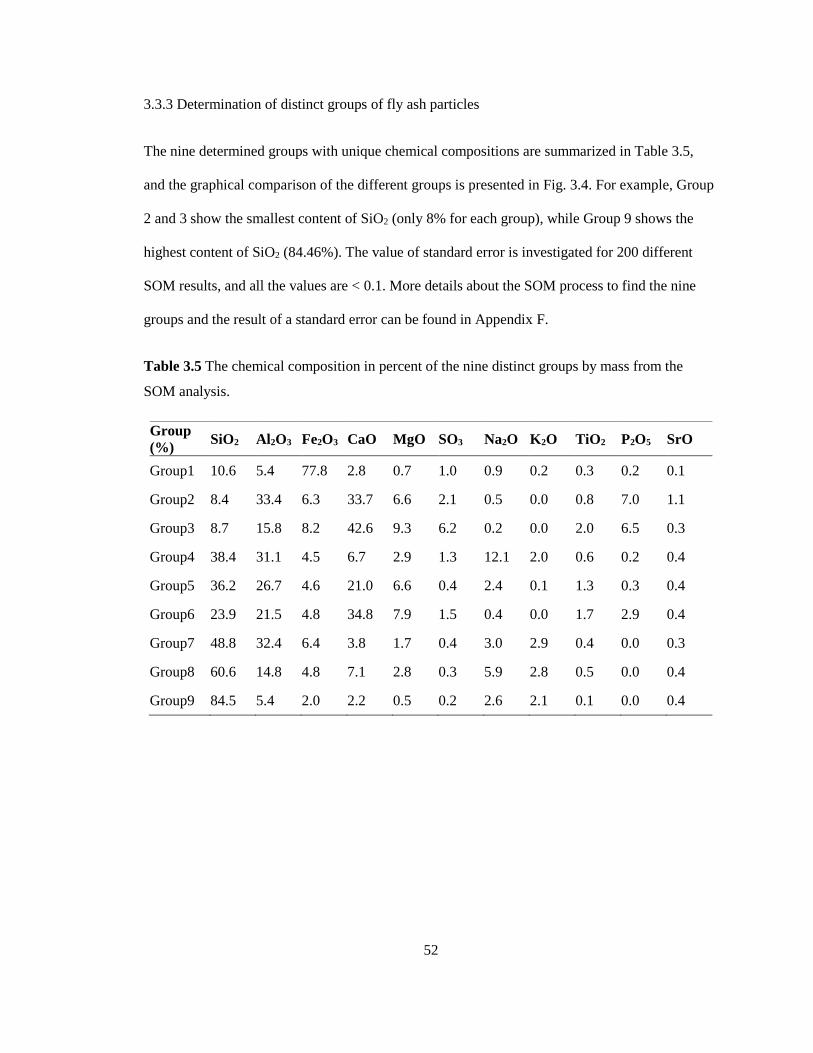
52

3.3.3 Determination of distinct groups of fly ash particles

The nine determined groups with unique chemical compositions are summarized in Table 3.5,

and the graphical comparison of the different groups is presented in Fig. 3.4. For example, Group

2 and 3 show the smallest content of SiO2 (only 8% for each group), while Group 9 shows the

highest content of SiO2 (84.46%). The value of standard error is investigated for 200 different

SOM results, and all the values are < 0.1. More details about the SOM process to find the nine

groups and the result of a standard error can be found in Appendix F.

Table 3.5 The chemical composition in percent of the nine distinct groups by mass from the

SOM analysis.

Group

(%) SiO2 Al2O3 Fe2O3 CaO MgO SO3 Na2O K2O TiO2 P2O5 SrO

Group1 10.6 5.4 77.8 2.8 0.7 1.0 0.9 0.2 0.3 0.2 0.1

Group2 8.4 33.4 6.3 33.7 6.6 2.1 0.5 0.0 0.8 7.0 1.1

Group3 8.7 15.8 8.2 42.6 9.3 6.2 0.2 0.0 2.0 6.5 0.3

Group4 38.4 31.1 4.5 6.7 2.9 1.3 12.1 2.0 0.6 0.2 0.4

Group5 36.2 26.7 4.6 21.0 6.6 0.4 2.4 0.1 1.3 0.3 0.4

Group6 23.9 21.5 4.8 34.8 7.9 1.5 0.4 0.0 1.7 2.9 0.4

Group7 48.8 32.4 6.4 3.8 1.7 0.4 3.0 2.9 0.4 0.0 0.3

Group8 60.6 14.8 4.8 7.1 2.8 0.3 5.9 2.8 0.5 0.0 0.4

Group9 84.5 5.4 2.0 2.2 0.5 0.2 2.6 2.1 0.1 0.0 0.4

53

Fig. 3.4 The cumulative plot of the chemical composition of the nine distinct groups.

Table 3.6 shows the comprehensive result of the group composition for the twenty-six fly ash

sources. The average of the sum is 95.4% and so, roughly 5% of fly ash particles cannot be

considered as one of the nine groups, and are not used in further model analysis.

Table 3.6 Group composition in percent of the twenty-six fly ash sources.

Source Group

1

Group

2

Group

3

Group

4

Group

5

Group

6

Group

7

Group

8

Group

9 Total

C1 0.5 8.8 16.2 13.1 21.0 21.8 4.6 5.4 5.4 96.6

C2 0.2 8.3 23.8 18.7 12.8 17.7 1.4 6.8 7.6 97.2

C3 0.3 8.6 32.2 10.3 11.8 21.3 0.3 4.9 2.9 92.5

C4 0.1 8.7 15.7 21.4 21.0 19.0 4.0 3.0 3.1 95.9

C5 0.3 7.7 27.9 21.8 12.9 17.0 0.9 3.2 4.1 95.7

C6 0.3 11.9 7.2 37.8 13.6 13.6 0.0 5.3 1.8 91.4

C7 0.2 10.1 22.9 17.3 12.0 18.6 2.4 6.4 7.5 97.1

C8 0.2 9.4 6.9 18.4 25.7 19.0 4.2 7.3 5.1 95.9

C9 0.2 11.7 10.0 20.2 25.9 21.1 0.7 3.5 3.1 96.2

C10 0.2 14.4 14.4 10.8 15.9 26.7 0.9 5.8 5.6 94.5

54

C11 0.2 12.6 19.9 13.8 15.5 22.8 1.3 5.0 5.1 96.0

IC1 0.3 5.8 15.3 11.7 20.7 20.5 11.0 6.7 5.2 97.0

IC2 0.0 10.8 22.4 14.0 15.4 25.4 0.1 5.2 3.3 96.4

IC3 0.3 6.7 26.0 16.7 14.5 19.5 4.7 4.2 4.1 96.5

IC4 0.1 7.6 30.3 6.0 11.4 30.1 0.8 3.6 2.7 92.4

F1 1.1 1.0 7.2 0.5 22.6 11.8 39.9 8.7 6.1 98.7

F2 0.4 0.6 6.6 0.4 22.3 13.8 36.7 11.3 6.2 98.2

F3 5.8 0.6 2.6 0.4 15.4 4.1 51.2 11.9 1.9 93.6

F4 0.3 5.1 12.0 1.7 18.5 13.2 37.5 4.3 3.9 96.2

F5 1.8 0.2 0.3 0.1 1.1 0.3 75.2 7.5 8.6 94.9

F6 2.6 0.4 0.6 0.1 1.3 0.7 71.8 8.6 8.7 94.7

F7 1.8 0.1 0.2 36.0 1.0 0.6 43.2 4.7 6.5 94.0

F8 0.8 1.0 0.3 6.5 8.5 1.6 48.8 13.5 12.4 93.3

F9 0.5 2.6 6.5 0.9 20.4 13.0 37.6 7.5 7.9 96.7

F10 0.3 0.6 1.5 0.4 14.7 4.5 56.9 10.3 7.7 96.6

IF1 1.8 0.4 0.8 0.9 2.5 1.7 52.0 20.9 11.2 91.9

3.3.4 The accuracy for predicting electrical resistivity

Fig. 3.5(a) and 3.5(b) compares the accuracy of predicting the electrical resistivity using the Class

C and F classification method with 20% and 40% replacement rates. The measured values are

indicated as the points with the same color as the matching dashed line which is the average

values for Class C and F fly ashes at seven different curing times, respectively. Overall, the 40%

fly ash replacement concrete shows higher electrical resistivity than the concrete with a 20% fly

ash replacement. Furthermore, despite having a similar bulk chemical classification as per ASTM

C618, the variability of electrical resistivity is quite high to predict the performance using this

classification method. Even though the ASTM C618 classification method is widely used to

compare the performance of different fly ashes, these comparison results present the drawbacks

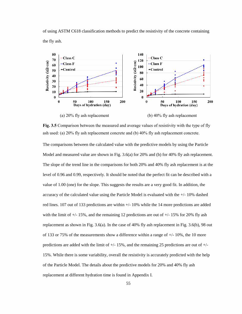
55

of using ASTM C618 classification methods to predict the resistivity of the concrete containing

the fly ash.

(a) 20% fly ash replacement (b) 40% fly ash replacement

Fig. 3.5 Comparison between the measured and average values of resistivity with the type of fly

ash used: (a) 20% fly ash replacement concrete and (b) 40% fly ash replacement concrete.

The comparisons between the calculated value with the predictive models by using the Particle

Model and measured value are shown in Fig. 3.6(a) for 20% and (b) for 40% fly ash replacement.

The slope of the trend line in the comparisons for both 20% and 40% fly ash replacement is at the

level of 0.96 and 0.99, respectively. It should be noted that the perfect fit can be described with a

value of 1.00 (one) for the slope. This suggests the results are a very good fit. In addition, the

accuracy of the calculated value using the Particle Model is evaluated with the +/- 10% dashed

red lines. 107 out of 133 predictions are within +/- 10% while the 14 more predictions are added

with the limit of +/- 15%, and the remaining 12 predictions are out of +/- 15% for 20% fly ash

replacement as shown in Fig. 3.6(a). In the case of 40% fly ash replacement in Fig. 3.6(b), 98 out

of 133 or 75% of the measurements show a difference within a range of +/- 10%, the 10 more

predictions are added with the limit of +/- 15%, and the remaining 25 predictions are out of +/-

15%. While there is some variability, overall the resistivity is accurately predicted with the help

of the Particle Model. The details about the predictive models for 20% and 40% fly ash

replacement at different hydration time is found in Appendix I.

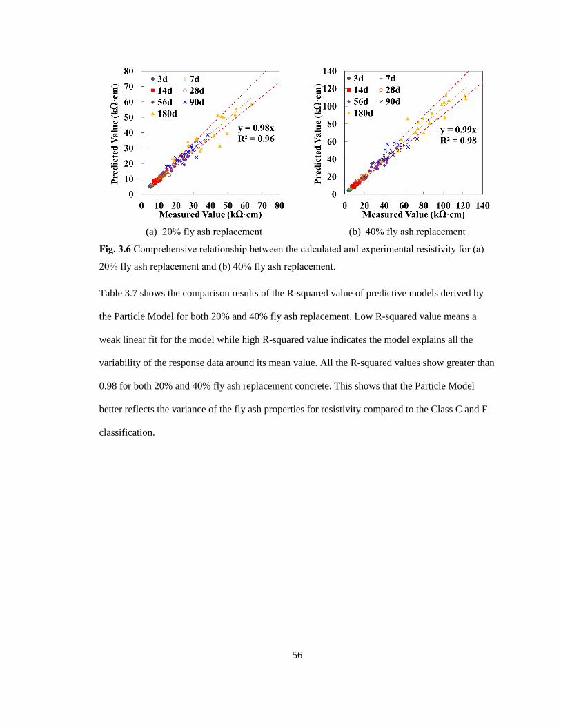
56

(a) 20% fly ash replacement (b) 40% fly ash replacement

Fig. 3.6 Comprehensive relationship between the calculated and experimental resistivity for (a)

20% fly ash replacement and (b) 40% fly ash replacement.

Table 3.7 shows the comparison results of the R-squared value of predictive models derived by

the Particle Model for both 20% and 40% fly ash replacement. Low R-squared value means a

weak linear fit for the model while high R-squared value indicates the model explains all the

variability of the response data around its mean value. All the R-squared values show greater than

0.98 for both 20% and 40% fly ash replacement concrete. This shows that the Particle Model

better reflects the variance of the fly ash properties for resistivity compared to the Class C and F

classification.

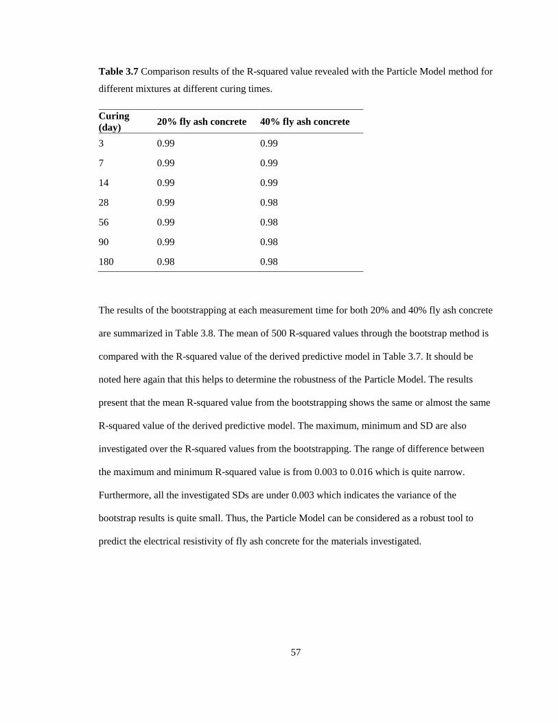
57

Table 3.7 Comparison results of the R-squared value revealed with the Particle Model method for

different mixtures at different curing times.

Curing

(day) 20% fly ash concrete 40% fly ash concrete

3 0.99 0.99

7 0.99 0.99

14 0.99 0.99

28 0.99 0.98

56 0.99 0.98

90 0.99 0.98

180 0.98 0.98

The results of the bootstrapping at each measurement time for both 20% and 40% fly ash concrete

are summarized in Table 3.8. The mean of 500 R-squared values through the bootstrap method is

compared with the R-squared value of the derived predictive model in Table 3.7. It should be

noted here again that this helps to determine the robustness of the Particle Model. The results

present that the mean R-squared value from the bootstrapping shows the same or almost the same

R-squared value of the derived predictive model. The maximum, minimum and SD are also

investigated over the R-squared values from the bootstrapping. The range of difference between

the maximum and minimum R-squared value is from 0.003 to 0.016 which is quite narrow.

Furthermore, all the investigated SDs are under 0.003 which indicates the variance of the

bootstrap results is quite small. Thus, the Particle Model can be considered as a robust tool to

predict the electrical resistivity of fly ash concrete for the materials investigated.

58

Table 3.8 The results of the bootstrapping for the Particle Model over the R-squared value.

Mixture Days of

hydration

The mean of the

R-squared values Max Min SD

20%

Fly ash

3 days 0.994 0.996 0.992 0.0006

7 days 0.994 0.996 0.992 0.0006

14 days 0.991 0.994 0.988 0.0009

28 days 0.990 0.995 0.986 0.0014

56 days 0.986 0.991 0.982 0.0014

90 days 0.988 0.991 0.984 0.0014

180 days 0.978 0.984 0.972 0.0021

40%

Fly ash

3 days 0.990 0.992 0.986 0.0009

7 days 0.988 0.991 0.984 0.0011

14 days 0.989 0.992 0.986 0.0009

28 days 0.985 0.989 0.979 0.0014

56 days 0.984 0.987 0.978 0.0016

90 days 0.980 0.986 0.970 0.0024

180 days 0.983 0.988 0.978 0.0018

3.3.5 Effects of each group on electrical resistivity

The impacts of each group on the electrical resistivity are investigated by comparing the

coefficients from predictive models at different hydration times, and the comparison results for

20% and 40% fly ash replacement concrete are shown in Fig. 3.7 and Fig. 3.8, respectively. The

coefficients show how different groups impact the electrical resistivity of the concrete at a

specific time period, and moreover, further discussion over the impact of each group will be

provided. A value > 0 indicates that the group helps to increase the electrical resistivity while the

group with the value of < 0 decreased the electrical resistivity at that time period. Ages without a

value for a coefficient mean that those groups do not contribute to the electrical resistivity at that

59

time period. For example, Group 1 shows a coefficient of zero between 3 and 28 days for 20% fly

ash replacement, this group is found to not be statistically significant at this curing time. The

impacts of Group 4, 5, 7, and 8 show a similar trend of change over time. These groups increase

the electrical resistivity between 3 and 180 days of hydration. Group 1 and 9 show almost no

meaningful impacts at early age while the significant contribution occurs at later ages. Group 2

shows less than zero coefficients at 20% replacement while it presents > 0 at 40% replacement for

all the measured hydration times. Group 3 seems to have a similar trend of coefficient change

over time for both replacement to Group 2, but the contribution is negligible as the coefficients

are quite small. On the contrary, Group 6 shows relatively small effects to increase the resistivity

at 20% replacement while it decreases the resistivity at 40% replacement between 3 and 180 days

of hydration.

Fig. 3.7 Coefficient comparison for 20% fly ash replacement at different times for each group.

60

Fig. 3.8 Coefficient comparison for 40% fly ash replacement at different times for each group.

3.3.5.1 Discussion for Group 4, 5, 7 and 8 on the electrical resistivity

Although Group 5 shows quite small negative coefficient (almost zero) at 3 and 7 days at 20%

replacement, overall Group 4, 5, 7, and 8 increase the electrical resistivity at rest of all

measurement times at both 20% and 40% replacement and the magnitude of their contribution

also increases. It is possible that several glassy phases can exist in these groups such as calcium-

rich aluminosilicates (especially for Group 5), aluminosilicate and calcium silicates based on the

chemical information in Table 3.5. Those glassy phases have been found in fly ash in several

previous studies [13, 51-54], and it is well known that the calcium-rich glassy phases are much

more reactive than those with low or moderate calcium content phases [52, 54]. Furthermore,

these four groups show quite high contents of SiO2. This means Group 4, 5, 7, and 8 might have a

good source to form C-S-H with the portland cement particles. The electrical resistivity is

improved by increasing C-S-H phases and decreasing capillary porosity and connectivity of

capillary pores [55]. Thus, hydration products with the particles of these groups can increase the

resistivity of fly ash concrete.

61

3.3.5.2 Discussion for Group 1 and 9 on the electrical resistivity

Group 1 shows the largest coefficient at later ages for both 20% and 40% fly ash replacement

rates while there were no impacts on early ages (3d, 7d, 14d, and 28d for 20%, and 3d and 7d for

40%). Group 1 has 77.8% of iron oxide (Fe2O3), which Fe-rich phases such as magnetite (Fe2O3)

and hematite (Fe2O3) have been found in fly ash and have been known to be largely inert [13, 56].

In addition, a ferrite phase could exist in this group. It is reported that the ferrite particles fill the

pores between cement particles resulting in finer pore structure, and more C-S-H gel can be

formed because of the reaction between the ferrite particles and the Ca(OH)2 in the hydrating of

cement [57, 58]. This could improve the electrical resistivity after 28 days of hydration and be a

possible reason why Group 1 does not have any impact at early age for both fly ash replacement.

The impact of Group 9 is almost zero until the 90d of hydration, and then a significant impact is

observed for 180 days of hydration for both the 20% and 40% fly ash replacement. This indicates

Group 9 affects more on the electrical resistivity at later ages. Group 9 contained 84.5% SiO2, and

this could be a good source of either quartz or a more reactive silicate. Quartz has been observed

in almost all fly ashes [13], and a silicon-rich phase containing almost no impurities was found in

some previous studies [59, 60]. Furthermore, it should be noted that the reactivity of the quartz

and silicate phase is very low and slow [52, 61]. Ehsan et al. [62] have reported the electrical

resistivity changes with adding SiO2 powder (1%, 3%, and 5% of the cementitious materials) with

25% fly ash replacement concrete. The study found that the resistivity increased by increasing the

SiO2 powder at 90 days of hydration while additional Al2O3 powder decreases the electrical

resistivity [62]. Another study has reported the SiO2 powder is helpful to improve the water

permeability resistance of concrete [63] which means that this could be a possible reason for the

impact of Group 9 on resistivity at later ages.

62

3.3.5.3 Discussion for Group 2, 3, and 6 on the electrical resistivity

Groups 2 and 3 show less than zero or zero coefficients on the resistivity at 20% replacement

while the results appear > 0 at 40% replacement between 3 and 180 days of hydration. The

coefficients for Group 3 are quite small for both replacements at all the hydration times

investigated. On the contrary, Group 6 shows relatively small effects to increase the resistivity at

20% replacement while it decreases the resistivity at 40% replacement between 3 and 180 days of

hydration.

Group 2 shows the lowest SiO2 contents among the nine groups while the contents of CaO, MgO,

and SO3 are relatively higher than the other groups. In addition, the content of Al2O3 for Group 2

is the highest among the nine groups. Group 6 also shows relatively higher content of CaO than

the other groups and similar content of SiO2 and Al2O3. Various crystalline and glassy phases

could exist in those group particles. Several glassy phases such as calcium-rich aluminosilicates,

aluminosilicate and calcium silicates can exist in these two groups. Merwinite (Ca3Mg(SiO4)2), a

common phase in high-calcium fly ash and at the early stages of the devitrification of Mg-

containing glasses, could also be considered a phase of Group 6. This material is non-reactive in

concrete at normal temperatures [13]. Furthermore, these three groups could be a good source for

producing the melilite group which includes Gehlenite Ca2Al(AlSiO7) and Akermanite

Ca2Mg(Si2O7) phases; these phases are not chemically active in concrete [13]. Thus, investigating

the reason for the different trends of Group 2 and Group 6 at different replacement rates is an area

of future work.

As discussed, there is almost no contribution from Group 3 on resistivity for both replacements at

all the measurement times. This means that the particles in Group 3 can be mainly composed of

non-reactive phases although it has some oxides that can possibly be a source of some of the

reactive phases.

63

3.3.6 Practical implications and future applications

The use of fly ash in concrete is typically limited because of the unpredictability of the material.

This work has given useful predictive equations that can be used at both 20% and 40%

replacement volume of fly ash within the concrete and emphasize that the Particle Method

showed a clear path forward for future research efforts that could ultimately make significant

changes to predict the electrical resistivity of fly ash concrete. While previous studies have been

used the Particle Model to predict the compressive strength with the impact of fly ash particles,

this work shows the application of the Particle Model can be extended on accurately predicting

the electrical resistivity of the fly ash concrete within 180 days of hydration. This indicates that

the Particle Model can not only allow greater usage of fly ash to allow the usage of fly ash that

does not meet current specifications by ASTM C618 but also be implemented on predicting other

performance of fly concrete.

3.4 Conclusion

The Particle Model is used to create predictive models for the electrical resistivity for 19 different

fly ash sources at 20% and 40% replacement of cement in concrete after 3, 7, 14, 28, 56, 90, and

180 days of hydration. With this massive data set, the predicted electrical resistivity values are

compared with the measured values and the coefficients from the predictive models were used to

interpret the measured chemical consistency of the individual groups. The following contributions

are made:

1. The Class C and F classification method does not accurately predict resistivity

performance in concrete.

2. The electrical resistivity and the median particle size are not related as all R-squared

values of the investigated trend lines are < 0.5 at 20% replacement and < 0.3 for 40%

replacement.

64

3. The electrical resistivity is accurately predicted by the Particle Model within +/- 10% for

80% of all measurements at 20% fly ash replacement and +/- 10% for 75% of all

measurements at 40% replacement.

4. The R-squared value is > 0.98 for both 20% and 40% fly ash replacement levels for the

Particle Model.

5. Overall, Group 4, 5, 7, and 8 increase the resistivity between 3 and 180 days of hydration

at both 20% and 40% replacement. The impact of these groups further increases with

additional hydration.

6. Group 1 has the largest coefficient at the later ages for both 20% and 40% replacement

while there is no impact at an early age. The impact of Group 9 is ≈ 0 until 90 days of

hydration while it has a big impact at 180 days of hydration for both 20% and 40%

replacement.

7. Group 2 decreases the resistivity at 20% replacement and increases the resistivity at 40%

replacement between 3 and 180 days of hydration. Although the actual value of

coefficients for Group 3 is quite small for all the measured hydration times for 20% and

40% fly ash replacement levels, it shows a similar trend of coefficient change to Group 2.

On the other hand, Group 6 increases the resistivity at 20% replacement while it

decreases the resistivity at the 40% replacement.

Despite there still existing many unknowns, several new insights are found by applying the

Particle Model to these fly ashes. This paper offers a novel way to facilitate investigations of fly

ash properties in concrete and lead to a better classification of fly ash at both early and later ages

at different replacement levels.

65

Acknowledgment

This work was sponsored by funding from the Illinois Department of Transportation [Project ICT

R27-180], and the FHWA [EAR project # BAA No. 693JJ3-18-BAA-0001]. The authors would

like to thank Dr. Daniel Cook and Mr. Jeff Davis for their assistance and discussion on this work.

Reference

[1] K. Hornbostel, C.K. Larsen, M.R. Geiker, Relationship between concrete resistivity and

corrosion rate–a literature review, Cement and Concrete Composites 39 (2013) 60-72.

[2] O. Sengul, O.E. Gjørv, Electrical resistivity measurements for quality control during concrete

construction, ACI Materials Journal 105(6) (2008) 541.

[3] W. Morris, A. Vico, M. Vázquez, Chloride induced corrosion of reinforcing steel evaluated by

concrete resistivity measurements, Electrochimica Acta 49(25) (2004) 4447-4453.

[4] B.B. Hope, A.K. Ip, D.G. Manning, Corrosion and electrical impedance in concrete, Cement

Concrete Res 15(3) (1985) 525-534.

[5] C. Alonso, C. Andrade, J.A. González, Relation between resistivity and corrosion rate of

reinforcements in carbonated mortar made with several cement types, Cement Concrete Res 18(5)

(1988) 687-698.

[6] W. López, J.A. González, Influence of the degree of pore saturation on the resistivity of

concrete and the corrosion rate of steel reinforcement, Cement Concrete Res 23(2) (1993) 368-

376.

[7] O. Gjorv, Durability design and construction quality of concrete structures, PRO 32:

International Conference on Advances in Concrete and Structures-ICACS 2003 (Volume 1),

RILEM Publications, 2003, p. 309.

[8] C. Andrade, The limit of service life of concrete structures, Encontro Nacional Betão

Estrutural (2004) 1-25.

66

[9] B. Silva, S. Jalali, R. Ferreira, Estimating electrical resistivity based on early age

measurements, Proceedings of the international RILEM workshop performance based evaluation

and indicators for concrete durability, Madrid, 2006.

[10] P.C. Silva, R.M. Ferreira, H. Figueiras, Electrical resistivity as a means of quality control of

concrete–influence of test procedure, XII International Conference on Durability of Building

Materials and Components, FEUP Edições, Porto: Distrito de Porto (PT), 2011.

[11] M.A. Bérubé, J. Duchesne, D. Chouinard, Why the Accelerated Mortar Bar Method ASTM C

1260 is Reliable for Evaluating the Effectiveness of Supplementary Cementing Materials in

Suppressing Expansion Due to Alkali-Silica Reactivity, Cement, Concrete and Aggregates 17(1)

(1995) 26-34.

[12] B. Mather, Use of Concrete of Low Portland Cement Content in Combination with

Pozzolans and Other Admixtures in Construction of Concrete Dams, J Am Concr Inst 71(12)

(1974) 589-599.

[13] A. Committee, 232.2R-18: Report for the Use of Fly Ash in Concrete, Technical Documents

(2018).

[14] S. Shashiprakash, M. Thomas, Sulfate resistance of mortars containing high-calcium fly

ashes and combinations of highly reactive pozzolans and fly ash, Special Publication 199 (2001)

221-238.

[15] R.B. Holland, K.E. Kurtis, L.F. Kahn, 7 - Effect of different concrete materials on the

corrosion of the embedded reinforcing steel, in: A. Poursaee (Ed.), Corrosion of Steel in Concrete

Structures, Woodhead Publishing, Oxford, 2016, pp. 131-147.

[16] S.K. Das, Yudhbir, A simplified model for prediction of pozzolanic characteristics of fly ash,

based on chemical composition, Cement Concrete Res 36(10) (2006) 1827-1832.

[17] S. Diamond, On the Glass Present in Low-Calcium and in High-Calcium Flyashes, Cement

Concrete Res 13(4) (1983) 459-464.

67

[18] L.X. Du, E. Lukefahr, A. Naranjo, Texas Department of Transportation Fly Ash Database

and the Development of Chemical Composition-Based Fly Ash Alkali-Silica Reaction Durability

Index, J Mater Civil Eng 25(1) (2013) 70-77.

[19] S.C. White, E.D. Case, Characterization of fly ash from coal-fired power plants, Journal of

Materials Science 25(12) (1990) 5215-5219.

[20] S. Schlorholtz, K. Bergeson, T. Demirel, Monitoring of Fluctuations in the Physical and

Chemical Properties of a High-Calcium Fly Ash, MRS Proceedings 113 (1987) 107.

[21] Q. Hu, M.T. Ley, J. Davis, J.C. Hanan, R. Frazier, Y. Zhang, 3D chemical segmentation of

fly ash particles with X-ray computed tomography and electron probe microanalysis, Fuel 116

(2014) 229-236.

[22] Q. Hu, M. Aboustait, M.T. Ley, J.C. Hanan, V. Rose, R. Winarski, Combined three-

dimensional structure and chemistry imaging with nanoscale resolution, Acta Mater 77 (2014)

173-182.

[23] T. Kim, J.M. Davis, M.T. Ley, S. Kang, P. Amrollahi, Fly ash particle characterization for

predicting concrete compressive strength, Constr Build Mater 165 (2018) 560-571.

[24] T. Kim, M. Moradian, M.T. Ley, Dissolution and leaching of fly ash in nitric acid using

automated scanning electron microscopy, Advances in Civil Engineering Materials 7(1) (2018)

291-307.

[25] M. Aboustait, T. Kim, M.T. Ley, J.M. Davis, Physical and chemical characteristics of fly ash

using automated scanning electron microscopy, Constr Build Mater 106 (2016) 1-10.

[26] S. Ghosal, J.L. Ebert, S.A. Self, Chemical composition and size distributions for fly ashes,

Fuel processing technology 44(1-3) (1995) 81-94.

[27] Y. Chen, N. Shah, F.E. Huggins, G.P. Huffman, W.P. Linak, C.A. Miller, Investigation of

primary fine particulate matter from coal combustion by computer-controlled scanning electron

microscopy, Fuel Processing Technology 85(6-7) (2004) 743-761.

68

[28] T. Kim, M.T. Ley, S. Kang, J.M. Davis, S. Kim, P. Amrollahi, Using particle composition of

fly ash to predict concrete strength and electrical resistivity, Cement and Concrete Composites

107 (2020) 103493.

[29] S. Kang, Z. Lloyd, T. Kim, M.T. Ley, Predicting the Compressive Strength of Fly Ash

Concrete with the Particle Model, Manuscript submitted for publication.

[30] ASTM C150, Standard Specification for Portland Cement, American Society for Testing and

Materials, West Conshohocken, PA, 2019.

[31] ASTM C33, Standard Specification for Concrete Aggregates, American Society for Testing

and Materials, West Conshohocken, PA, 2018.

[32] ASTM C618, Standard Specification for Coal Fly Ash and Raw or Calcined Natural

Pozzolan for Use in Concrete, American Society for Testing and Materials, West Conshohocken,

PA, 2019.

[33] R.P. Gupta, T.F. Wall, I. Kajigaya, S. Miyamae, Y. Tsumita, Computer-controlled scanning

electron microscopy of minerals in coal - Implications for ash deposition, Prog Energ Combust

24(6) (1998) 523-543.

[34] C.A. O'Keefe, T.M. Watne, J.P. Hurley, Development of advanced scanning electron

microscopy techniques for characterization of submicron ash, Powder Technol 108(2-3) (2000)

95-102.

[35] J.T. Armstrong, Quantitative Elemental Analysis of Individual Microparticles with Electron

Beam Instruments, in: K.F.J. Heinrich, D.E. Newbury (Eds.), Electron Probe Quantitation,

Springer US, Boston, MA, 1991, pp. 261-315.

[36] G. Love, V.D. Scott, Evaluation of a New Correction Procedure for Quantitative Electron-

Probe Microanalysis, J Phys D Appl Phys 11(10) (1978) 1369-1376.

[37] J.T. Armstrong, P.R. Buseck, Quantitative Chemical-Analysis of Individual Microparticles

Using Electron-Microprobe - Theoretical, Anal Chem 47(13) (1975) 2178-2192.

69

[38] J.T. Armstrong, P.R. Buseck, A General Characteristic Fluorescence Correction for the

Quantitative Electron Microbeam Analysis of Thick Specimens, Thin-Films and Particles, X-Ray

Spectrom 14(4) (1985) 172-182.

[39] C.P. Aichele, D. Venkataramani, J.E. Smay, M.H. McCann, S. Richter, M. Khanzadeh-

Moradllo, M. Aboustait, M.T. Ley, A comparison of automated scanning electron microscopy

(ASEM) and acoustic attenuation spectroscopy (AAS) instruments for particle sizing, Colloids

and Surfaces A: Physicochemical and Engineering Aspects 479 (2015) 46-51.

[40] M. Aboustait, Q. Hu, R. Frazier, Y. Zhang, B. Tabb, M. Ley, J. Hahan, Innovative prediction

of fly ash performance in concrete, Oklahoma Transportation Center, Midwest City, OK, 2013.

[41] ASTM C231, Standard Test Method for Air Content of Freshly Mixed Concrete by the

Pressure Method, American Society for Testing and Materials, West Conshohocken, PA, 2017.

[42] ASTM C138, Standard Test Method for Density (Unit Weight), Yield, and Air Content

(Gravimetric) of Concrete, American Society for Testing and Materials, West Conshohocken, PA,

2017.

[43] ASTM C143, Standard Test Method for Slump of Hydraulic-Cement Concrete, American

Society for Testing and Materials, West Conshohocken, PA, 2015.

[44] Z. Lloyd, Investigation of the Quality Control of Waste Products for Concrete, Civil

Engineering, Oklahoma State University, Stillwater, OK, 2019.

[45] ASTM C31, Standard Practice for Making and Curing Concrete Test Specimens in the Field,

American Society for Testing and Materials, West Conshohocken, PA, 2019.

[46] AASHTO T 358:2015Method Of Test For Surface Resistivity Indication Of Concrete'S

Ability To Resist Chloride Ion Penetration, 2015.

[47] M.J. Crawley, The R Book, Second ed., John Wiley & Sons Ltd, Imperial College London at

Silwood Park, UK, 2012.

[48] R.C. Team, R: A Language and Environment for Statistical Computing, Vienna, Austria,

70

2016.

[49] M. Kuhn, K. Johnson, Applied predictive modeling, Springer2013.

[50] B. Efron, R.J. Tibshirani, An introduction to the bootstrap, CRC press1994.

[51] D.M. Roy, K. Luke, S. Diamond, Characterization of fly ash and its reactions in concrete,

MRS Online Proceedings Library Archive 43 (1984).

[52] P.T. Durdzinski, C.F. Dunant, M. Ben Haha, K.L. Scrivener, A new quantification method

based on SEM-EDS to assess fly ash composition and study the reaction of its individual

components in hydrating cement paste, Cement Concrete Res 73 (2015) 111-122.

[53] K.L. Aughenbaugh, Fly ash-based geopolymers: identifying reactive glassy phases in

potential raw materials, Civil, Architectural, and Environmental Engineering, The University of

Texas at Austin, The University of Texas at Austin, 2013, p. 292.

[54] K.L. Aughenbaugh, R.T. Chancey, P. Stutzman, M.C. Juenger, D.W. Fowler, An examination

of the reactivity of fly ash in cementitious pore solutions, Materials and Structures 46(5) (2013)

869-880.

[55] Z. Liu, Y. Zhang, Q. Jiang, Continuous tracking of the relationship between resistivity and

pore structure of cement pastes, Constr Build Mater 53 (2014) 26-31.

[56] G. McCarthy, J. Solem, O. Manz, D. Hassett, Use of a database of chemical, mineralogical

and physical properties of North American fly ash to study the nature of fly ash and its utilization

as a mineral admixture in concrete, Materials Research Society Symposium Proceedings 178

(1990) 3-34.

[57] M.A. Ahmed, Y.A. Hassanean, K.A. Assaf, M.A. Shawkey, The Effect of Incorporation of

Ferrite Nano-particles on Compressive Strength and Resistivity of Self-Compacting Concrete,

Open Journal of Civil Engineering 5(01) (2015) 131.

[58] M.A. Largeau, Effect of iron powder patially used as portland cement replacement on the

structural properties of concrete, JKUAT-PAUSTI, 2018.

71

[59] V.M. Malhotra, P.K. Mehta, High-performance, high-volume fly ash concrete : materials,

mixture proportioning, properties, construction practice, and case histories, Supplementary

Cementing Materials for Sustainable Development, Inc., Ottawa, Canada, 2002.

[60] K. Kiattikomol, C. Jaturapitakkul, S. Songpiriyakij, S. Chutubtim, A study of ground coarse

fly ashes with different finenesses from various sources as pozzolanic materials, Cement

Concrete Comp 23(4-5) (2001) 335-343.

[61] P.T. Durdzinski, R. Snellings, C.F. Dunant, M. Ben Haha, K.L. Scrivener, Fly ash as an

assemblage of model Ca-Mg-Na-aluminosilicate glasses, Cement Concrete Res 78 (2015) 263-

272.

[62] E. Mohseni, B.M. Miyandehi, J. Yang, M.A. Yazdi, Single and combined effects of nano-

SiO2, nano-Al2O3 and nano-TiO2 on the mechanical, rheological and durability properties of

self-compacting mortar containing fly ash, Constr Build Mater 84 (2015) 331-340.

[63] M.R. Sharbaf, S.M. Hejazi, An investigative study on the effects of nano-SiO 2 on

compressive strength and permeability of concrete, 5th International Conference on Advanced

Computer Theory and Engineering, Cape Town, South Africa, 2012.

72

CHAPTER IV

PREDICTING ION DIFFUSION IN FLY ASH CEMENT PASTE THROUGH

PARTICLE ANALYSIS

Abstract

Mass transport in concrete is an important factor to control the durability of concrete structures.

Fly ash is commonly used as an additive to help reduce the mass transport of concrete. Since fly

ash is a waste product, it is challenging to predict the performance of fly ash in concrete. This

work uses a technique called the Particle Model to predict the reactivity and modification of the

diffusion coefficient of the paste with fly ash at a 20% replacement level. The results show 81%

of all measurements for the diffusion coefficient can be predicted within the reported variation of

the test method (+/- 30%). This work provides a deeper understanding of the impacts of fly ash

on the properties of concrete to more accurately predict the performance of the diffusion

coefficient at different hydration times.

Keywords: Diffusion coefficient; Surface concentration; Fly ash; Cement paste; ASEM; The

Particle Model;

73

4.1 Introduction

The apparent diffusion coefficient (Dc) is an important factor to control the durability of concrete

structures because outside chemicals such as natural chlorides, deicer salts, and sulfate ions will

penetrate into concrete and deteriorate the rebar or the concrete matrix itself [1, 2]. Because of the

importance of this parameter, performance-based durability specifications commonly use Dc [3,

4]. Fly ash is used as a partial replacement of the portland cement to improve the overall economy,

sustainability, and often the durability of the concrete [5-8]. It is known that many fly ashes are

helpful to produce concrete with a low Dc in concrete [9-11]. This is achieved through both

pozzolanic and secondary cementitious reactions [12, 13].

Fly ash is generally used at 15-35% replacement of cement by mass because this range has been

found to be an acceptable level of replacement without major negative effects on the performance

[14]. Previous studies have investigated the impacts of fly ash in concrete and tried to predict the

performance of fly ash by using bulk chemical characterization methods such as X-ray

fluorescence (XRF) [15-18]. However, it is reported that fly ash sources with similar bulk

chemistry can have dramatically different performance [19]. In other words, bulk chemical

characteristics are not always useful to predict the properties of concrete.

While bulk chemistry does not provide predictable insights into the performance of the fly ash in

concrete, studies with scanning electron microscopy (SEM) and automated scanning electron

microscopy (ASEM) show that there are repeating patterns in chemical composition found within

fly ash particles [20, 21]. To gain more insights, this study applies a method called the Particle

Model that is developed in a previous study to produce predictive models for the performance of

cement-based materials such as compressive strength and electrical resistivity [22]. This is based

on using an ASEM to classify thousands of individual fly ash particles [22-27] and then machine

learning with the Self-Organizing Map (SOM) algorithm was applied to classify the fly ash

74

particles into nine distinct groups based on these few major repeatable patterns of chemical

compositions [22]. The predictive models through these groups are then able to predict 90% of

the predicted compressive strength and 80% of the predicted electrical resistivity values within

+/- 10% of the measured values at different hydration times [28, 29].

To investigate ion diffusion of the fly ash-cement paste, a novel approach using transmission X-

ray microscopy (TXM) is applied in this work. This technique is useful as it is non-destructive

and rapid to investigate the Dc and surface concentration (Cs). This approach has been used in

previous studies to image the movement of the ions in cement-based materials using the

potassium iodide (KI) solution as a tracer or contrast agent [30, 31]. Iodide (I) is a great tracer for

two reasons; (1) it is strongly X-ray attenuating because of its high atomic number and (2) iodide

and chloride ions have been shown similar concentration profiles and about 10% difference of

apparent Dc and Cs in the experiments [30, 31]. The current work examines the cement paste to

investigate ion diffusion properties such as the apparent iodide Dc and the iodide Cs as the pore

structure of the cement paste matrix is related to the ion diffusion in concrete [32]. Moreover,

using cement paste is helpful to minimize intervention from aggregates [31]. In all of this work,

the term Dic and Cis will refer to the iodide diffusion coefficient and iodide surface concentration,

respectively.

The current work expands the application of the Particle Model by predicting the Dic of the fly

ash-cement paste as demonstrated in Fig. 4.1. The aim of this work is to provide important

insights into how the application of the Particle Model can be extended to predict Dic at 20% fly

ash replacement by mass at different hydration times. This paper provides some important

insights to evaluate the impact of fly ash in cement-based materials and improve the durability of

concrete, although providing detailed interpretations of why different fly ash particles impact the

properties of the cement paste is outside the scope of this work.

75

Fig. 4.1 Comprehensive schematic diagram of the process for investigating the diffusion

properties.

4.2 Experimental Method

4.2.1 Raw materials

A Type I ordinary portland cement (OPC) by ASTM C150 [33] was used. Table 4.1 shows the

chemical and phase composition of cement which was used in this study. Twenty-six different fly

ashes were investigated in this study as the replacement material. All the fly ashes were produced

from various coal sources, boiler designs, and collection conditions in the United States. Fly

ashes in this study were classified into fifteen Class C and eleven Class F fly ashes according to

ASTM C618.

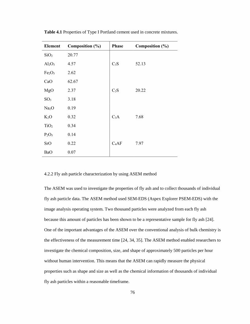
76

Table 4.1 Properties of Type I Portland cement used in concrete mixtures.

Element Composition (%) Phase Composition (%)

SiO2 20.77

C3S 52.13 Al2O3 4.57

Fe2O3 2.62

CaO 62.67

C2S 20.22 MgO 2.37

SO3 3.18

Na2O 0.19

C3A 7.68 K2O 0.32

TiO2 0.34

P2O5 0.14

C4AF 7.97 SrO 0.22

BaO 0.07

4.2.2 Fly ash particle characterization by using ASEM method

The ASEM was used to investigate the properties of fly ash and to collect thousands of individual

fly ash particle data. The ASEM method used SEM-EDS (Aspex Explorer PSEM-EDS) with the

image analysis operating system. Two thousand particles were analyzed from each fly ash

because this amount of particles has been shown to be a representative sample for fly ash [24].

One of the important advantages of the ASEM over the conventional analysis of bulk chemistry is

the effectiveness of the measurement time [24, 34, 35]. The ASEM method enabled researchers to

investigate the chemical composition, size, and shape of approximately 500 particles per hour

without human intervention. This means that the ASEM can rapidly measure the physical

properties such as shape and size as well as the chemical information of thousands of individual

fly ash particles within a reasonable timeframe.

77

Since fly ash particles are not flat, this violates one of the fundamental assumptions of classical

quantitative EDS analysis. The correction models have been developed and presented in previous

publications [36-39]. These models have taken into account the shape of the particle and make

corrections in the collected k-ratios of eleven investigated elements (Na, Mg, Al, Si, P, S, K, Ca,

Ti, Fe, and Sr). A previous study discussed the consistency of the ASEM method with measuring

the chemical composition for 50 Class C fly ash particles three times and the results showed that

the highest standard deviation (SD) was 1.60% [22], and more details of the results can be found

in Appendix A. The accuracy, reliability, and repeatability of the ASEM method when compared

to XRF analysis have been presented in other publications and shown to be less than 5% absolute

difference for greater than 90% of comparisons which indicates that the two methods largely

agree [22, 24, 40]. Comparisons for the materials in this work are presented in Appendix B. The

result of the particle size distribution (PSD) with data from ASEM has been compared to acoustic

attenuation spectroscopy, and has been found to be similar [41]. Detailed procedure over the

ASEM method, sample preparation, analysis with ASEM, and data processing are discussed in

Appendix C.

4.2.3 Fly ash-cement paste sample preparation

Nineteen fly ashes were chosen based on a wide range of different chemical compositions for the

paste sample preparation. Table 4.2 shows the mixture design of the paste samples. These

mixtures have a 0.45 water to cement ratio (w/cm) at a 20% fly ash replacement rate by mass of

cement. Thus, a total of twenty mixtures were prepared including one control with 100% OPC

and nineteen mixtures with 20% fly ash replacement. All the mixtures were prepared as per

ASTM C305 [42].

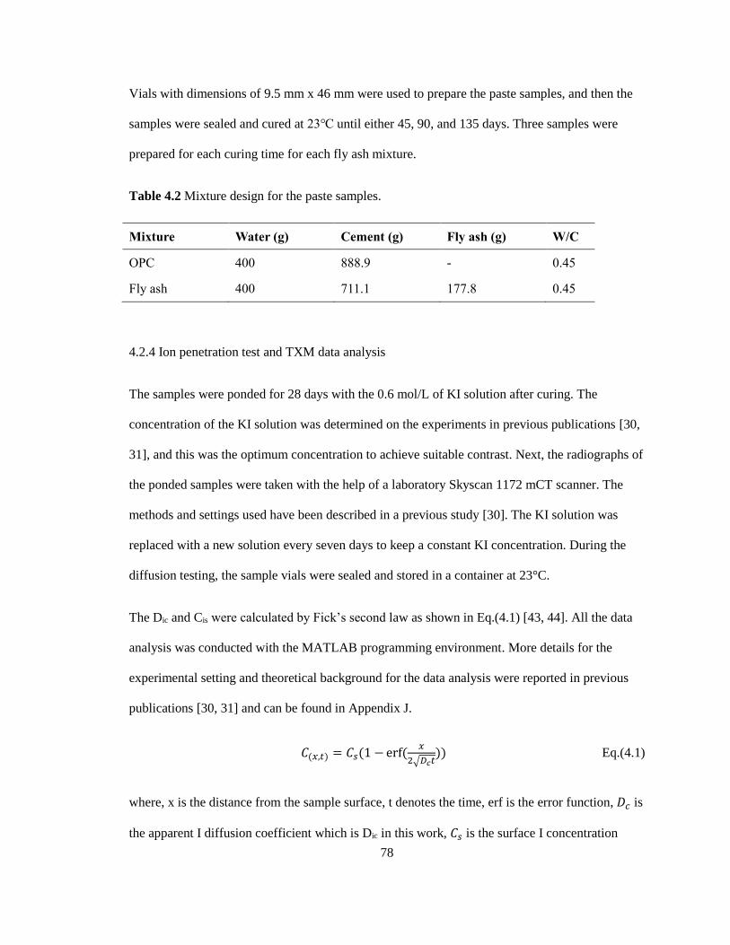
78

Vials with dimensions of 9.5 mm x 46 mm were used to prepare the paste samples, and then the

samples were sealed and cured at 23℃ until either 45, 90, and 135 days. Three samples were

prepared for each curing time for each fly ash mixture.

Table 4.2 Mixture design for the paste samples.

Mixture Water (g) Cement (g) Fly ash (g) W/C

OPC 400 888.9 - 0.45

Fly ash 400 711.1 177.8 0.45

4.2.4 Ion penetration test and TXM data analysis

The samples were ponded for 28 days with the 0.6 mol/L of KI solution after curing. The

concentration of the KI solution was determined on the experiments in previous publications [30,

31], and this was the optimum concentration to achieve suitable contrast. Next, the radiographs of

the ponded samples were taken with the help of a laboratory Skyscan 1172 mCT scanner. The

methods and settings used have been described in a previous study [30]. The KI solution was

replaced with a new solution every seven days to keep a constant KI concentration. During the

diffusion testing, the sample vials were sealed and stored in a container at 23°C.

The Dic and Cis were calculated by Fick’s second law as shown in Eq.(4.1) [43, 44]. All the data

analysis was conducted with the MATLAB programming environment. More details for the

experimental setting and theoretical background for the data analysis were reported in previous

publications [30, 31] and can be found in Appendix J.

𝐶(𝑥,𝑡) = 𝐶𝑠(1 − erf(𝑥

2√𝐷𝑐𝑡)) Eq.(4.1)

where, x is the distance from the sample surface, t denotes the time, erf is the error function, 𝐷𝑐 is

the apparent I diffusion coefficient which is Dic in this work, 𝐶𝑠 is the surface I concentration

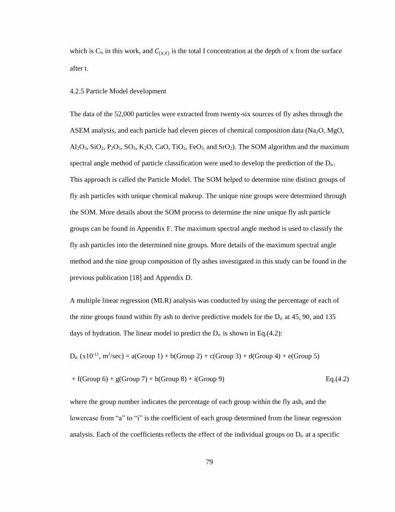
79

which is Cis in this work, and 𝐶(𝑥,𝑡) is the total I concentration at the depth of x from the surface

after t.

4.2.5 Particle Model development

The data of the 52,000 particles were extracted from twenty-six sources of fly ashes through the

ASEM analysis, and each particle had eleven pieces of chemical composition data (Na2O, MgO,

Al2O3, SiO2, P2O5, SO3, K2O, CaO, TiO2, FeO3, and SrO2). The SOM algorithm and the maximum

spectral angle method of particle classification were used to develop the prediction of the Dic.

This approach is called the Particle Model. The SOM helped to determine nine distinct groups of

fly ash particles with unique chemical makeup. The unique nine groups were determined through

the SOM. More details about the SOM process to determine the nine unique fly ash particle

groups can be found in Appendix F. The maximum spectral angle method is used to classify the

fly ash particles into the determined nine groups. More details of the maximum spectral angle

method and the nine group composition of fly ashes investigated in this study can be found in the

previous publication [18] and Appendix D.

A multiple linear regression (MLR) analysis was conducted by using the percentage of each of

the nine groups found within fly ash to derive predictive models for the Dic at 45, 90, and 135

days of hydration. The linear model to predict the Dic is shown in Eq.(4.2):

Dic (x10-11, m2/sec) = a(Group 1) + b(Group 2) + c(Group 3) + d(Group 4) + e(Group 5)

+ f(Group 6) + g(Group 7) + h(Group 8) + i(Group 9) Eq.(4.2)

where the group number indicates the percentage of each group within the fly ash, and the

lowercase from “a” to “i” is the coefficient of each group determined from the linear regression

analysis. Each of the coefficients reflects the effect of the individual groups on Dic at a specific

80

curing time, where the potential influence of the remaining independent variables on the groups

has been taken into account.

The initial model was evaluated with the probability value (Pr(>|t|)) from the MLR to

determine the statistical significance of the variables. To evaluate the linear fit to the model, the

R-squared value of each model was investigated at the individual curing times. More details can

be found in Appendix K. All the data and model processing was conducted within the R

programming environment [45, 46].

4.2.6 Bootstrapping

The robustness of the derived predictive models was evaluated with the help of the bootstrap

method. Ideally, the data can be collected by repeating a large number of mixtures for the same

experiment to evaluate the validity of the generated predictive models, but this is impractical.

Instead, bootstrapping was used to investigate the robustness of the Particle Model over the R-

squared value. Bootstrapping is a resampling method where the data are sampled with

replacement from the original sample to generate simulated results [45]. This allowed creating

numerous R-squared values by running predictive models with simulated samples. Furthermore,

the results from the bootstrapping were used to calculate a variety of sample statistics such as the

mean (average) and SD of the created R-squared values to compare the R-squared value of the

original model.

The size of the bootstrapping sample was the same as the original data set and is chosen at

random from the existing data set. This means that some data points can be chosen multiple times

in the simulated sample while others may not be selected at all. This procedure has been used in

previous publications [47, 48]. The bootstrapping was conducted with 500 times for each model.

81

Then, the mean of the R-squared values from the bootstrapping was investigated and compared

with the R-squared value of the derived predictive model.

4.3 Result and discussion

4.3.1 KI diffusion test

Fig. 4.2 and Fig. 4.3 describe the diffusion test results for Dic and Cis at different days of

hydration for the fly ash sources investigated. The Dic is decreased with increased days of

hydration for all the fly ash sources except for C6. While it is well known that the fly ash helps to

reduce the permeability by refining the pore structure of concrete [49], it should be noted that the

value of Dic for some of the fly ashes is higher values compared to the OPC. Specifically, at 45

and 90 days of hydration, 8 of the 12 Class C fly ashes show a greater iodide diffusion coefficient

than OPC, and at the 135 days of hydration, the number of Class C fly ashes decreases into 6.

This means that some of the Class C ashes can have worse performance than OPC when it comes

to Dic.

In the case of Cis, almost all the fly ash data, except for C6 and C11, show similar values to the

OPC. Furthermore, the Cis shows similar values with changing the days of hydration for each

mixture. Since the Cis values do not change significantly, and this is caused by using the same

concentration of the KI solution for all the test samples, the Particle Model is not be applied to

predicting the Cis.

82

Fig. 4.2 Dic at different days of hydration.

Fig. 4.3 Cis at different days of hydration.

4.3.2 Relationship between particle size of fly ash and the paste performances

Fig. 4.4 shows the frequency of PSDs for fifteen Class C and eleven Class F fly ashes by using

ASEM, respectively. The fly ashes with “C#” and “IC#” represent Class C fly ash while the fly

ashes with “F#” and “IF#” represent Class F fly ash. The results show most of fly ash particles

have a size within the range of 0.5 μm and 20 μm in diameter, and the distribution for most fly

ashes show a similar trend. D50 mean particle size for all fly ashes are investigated, and the

differences between the largest and smallest D50 in Class C and Class F fly ashes are 1.6 μm and

0.8 μm, respectively. Furthermore, the largest and smallest average particle size among twenty-

six fly ashes are 4.3 μm (C10) and 1.8 μm (IC2), respectively.

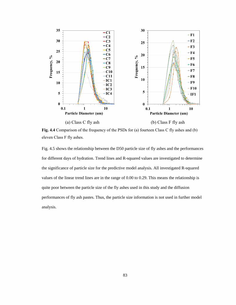
83

(a) Class C fly ash

(b) Class F fly ash

Fig. 4.4 Comparison of the frequency of the PSDs for (a) fourteen Class C fly ashes and (b)

eleven Class F fly ashes.

Fig. 4.5 shows the relationship between the D50 particle size of fly ashes and the performances

for different days of hydration. Trend lines and R-squared values are investigated to determine

the significance of particle size for the predictive model analysis. All investigated R-squared

values of the linear trend lines are in the range of 0.00 to 0.29. This means the relationship is

quite poor between the particle size of the fly ashes used in this study and the diffusion

performances of fly ash pastes. Thus, the particle size information is not used in further model

analysis.

84

(a) D50 vs. Dic

(b) D50 vs. Cis

Fig. 4.5 Relationships between the average particle size compared to (a) Dic and (b) Cis.

4.3.3 Bulk chemical composition of raw fly ashes by using ASEM

The bulk chemical composition of twenty-six fly ash sources from the ASEM method is

investigated, and the results are shown in Table 4.3. The fly ashes are classified as either Class C

for greater than 18% of CaO or Class F less than 18% of CaO according to ASTM C618 [50].

85

Table 4.3 Bulk chemical composition by using the ASEM method.

Source SiO2 Al2O3 Fe2O3 CaO MgO SO3 Na2O K2O TiO2 P2O5 SrO

C1 36.2 21.7 5.4 23.2 5.4 0.7 3.6 1.0 0.8 1.9 0.2

C2 35.8 19.2 5.6 26.9 5.5 1.0 3.0 0.9 0.7 1.3 0.2

C3 25.3 19.3 5.2 32.5 7.8 2.6 3.4 0.6 1.1 1.9 0.3

C4 36.7 22.8 4.5 22.5 4.3 1.2 3.4 1.0 1.3 1.1 1.2

C5 31.3 22.5 5.4 26.1 6.0 0.6 4.3 0.8 0.8 2.1 0.2

C6 27.7 22.9 4.2 21.5 4.5 2.6 12.6 0.8 1.3 0.7 1.3

C7 35.3 20.6 4.7 24.7 4.9 0.7 4.3 1.2 1.6 0.8 1.0

C8 40.1 22.6 4.5 19.5 5.7 0.8 3.7 0.9 0.6 1.4 0.1

C9 31.5 24.0 6.0 25.7 5.4 1.0 3.7 0.6 0.9 1.1 0.1

C10 36.0 19.3 5.1 22.7 7.8 2.0 4.8 0.6 1.0 0.3 0.5

C11 31.0 20.8 6.4 27.2 7.1 1.6 3.5 0.7 0.8 0.8 0.2

IC1 31.8 22.9 5.7 28.2 5.5 1.1 2.3 1.0 0.8 0.5 0.3

IC2 25.2 21.2 6.2 30.5 7.8 1.0 4.0 0.6 1.2 2.2 0.2

IC3 29.7 21.0 5.9 30.3 5.4 1.9 2.2 0.6 1.0 1.6 0.5

IC4 29.9 17.7 4.7 31.8 9.3 1.2 2.6 0.8 0.8 1.1 0.2

F1 48.8 23.8 7.4 12.5 3.0 0.5 0.9 2.1 0.8 0.1 0.3

F2 50.4 20.9 3.9 17.1 3.7 0.5 1.0 1.4 0.7 0.1 0.3

F3 48.8 26.6 6.7 9.3 2.0 0.3 1.8 1.9 1.5 0.1 1.1

F4 45.3 27.4 4.0 14.6 3.6 0.7 1.5 0.7 1.1 0.4 0.8

F5 53.2 25.4 11.2 2.1 0.2 0.9 1.0 4.4 0.7 0.0 1.0

F6 51.9 25.7 12.3 2.5 0.3 0.7 1.6 4.1 0.7 0.1 0.2

F7 51.9 26.3 8.0 3.3 0.5 1.7 4.0 2.5 0.9 0.6 0.1

F8 56.9 23.9 3.4 6.2 2.1 0.1 4.1 1.7 0.3 1.2 0.1

F9 48.3 25.0 5.9 12.6 3.3 0.5 1.3 1.8 1.1 0.2 0.1

F10 53.6 27.8 2.8 10.5 2.5 0.5 0.3 1.3 0.5 0.3 0.0

IF1 58.3 21.9 6.9 3.7 1.4 0.6 2.2 4.3 0.2 0.4 0.2

86

4.3.4 Evaluation of the test results and the predictive models

Fig. 4.6 shows the comparison between the measured Dic and the average values for Class C or F

fly ash. The actual measured values are shown as points on the plot with the same color as the

matching trend line. The results show that the value of Dic varies depending on the fly ash, and

Class C fly ash has a much wider range of Dic than Class F fly ash. For example, in the results of

90 days of hydration, the difference between the highest Dic and lowest Dic for Class C fly ashes

is 1.02 x 10⁻¹¹ m²/sec while the difference for Class F fly ashes is 0.23 x 10⁻¹¹ m²/sec. This means

that it is much harder to predict the Dic of Class C fly ash than Class F fly ash. Furthermore,

despite having similar bulk chemical classification as per ASTM C618 the diffusion property is

variable. This further shows the challenge of using ASTM C618 classification methods to predict

the Dic of concrete containing fly ash.

Fig. 4.6 Comparison between actual and predicted Dic with the type of fly ash used.

The comparisons between the predicted Dic from the Particle Model and measured Dic is

described in Fig. 4.7. The slope of the trend line in the comparisons is 0.96 with the R-squared

value of 0.80. It should be noted that the perfect fit can be described with a value of 1.00 (one) for

87

the slope. This means that overall the Dic can be closely predicted with the Particle Model. It

should be noted that some of the predictions are quite different results to the measured values. For

example, the measured Dic of the pastes with C11 fly ash at 135 days of hydration is 0.60 x 10⁻¹¹

m²/sec while the predicted value is 0.24 x 10⁻¹¹ m²/sec.

Tang [51] has evaluated the precision of diffusion coefficient through various test methods such

as immersion test (Nordtest method NT build 492), rapid migration test (Nordtest method NT

build 443), and measurement of chloride ion ingress test (EN 13396), and the study suggests the

CV of the reproducibility of these tests are 24%, 28%, and 36%, respectively. The average CV is

29.3% or close to 30% for this work. Moreover, ASTM C1556 (bulk chloride diffusion test)

provides 39.8% as the limit of CV to evaluate the precision (single laboratory) of determining the

apparent Dc of cementitious mixtures [52]. Even though the test method in this study is different

from those methods, these numbers could be a good guideline to evaluate the test results of the

current study. A value of +/- 30% has been added as the dashed blue line as a conservative

estimate for the variability of the test method. The comparison between the predicted and

measured values for the Dic for 57 samples is shown in Fig. 4.7, and 81% of comparisons are

within +/- 30%. The detailed results of the predictive models for different hydration time can be

found in Appendix L.

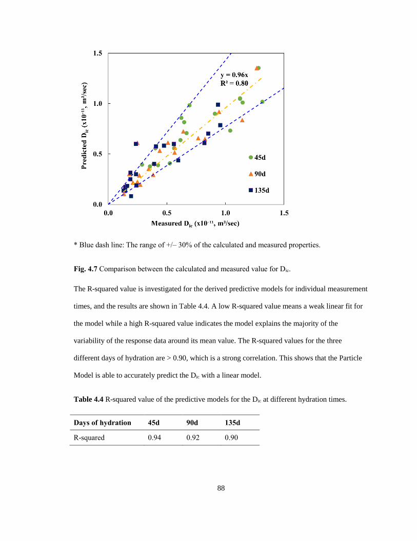
88

* Blue dash line: The range of +/‒ 30% of the calculated and measured properties.

Fig. 4.7 Comparison between the calculated and measured value for Dic.

The R-squared value is investigated for the derived predictive models for individual measurement

times, and the results are shown in Table 4.4. A low R-squared value means a weak linear fit for

the model while a high R-squared value indicates the model explains the majority of the

variability of the response data around its mean value. The R-squared values for the three

different days of hydration are > 0.90, which is a strong correlation. This shows that the Particle

Model is able to accurately predict the Dic with a linear model.

Table 4.4 R-squared value of the predictive models for the Dic at different hydration times.

Days of hydration 45d 90d 135d

R-squared 0.94 0.92 0.90

89

The results of the bootstrapping at each measurement time are presented in Table 4.5. It should be

noted here again that this helps to determine the robustness of the Particle Model. The mean of

500 R-squared values through the bootstrap method is compared with the R-squared value of the

derived predictive model in Table 4.4. The results present that the mean R-squared value from the

bootstrapping shows the same or almost the same R-squared value of the derived predictive

model. The maximum, minimum, and SD of the R-squared values from the bootstrapping are also

investigated. The range of difference between the maximum and minimum R-squared value is

from 0.07 to 0.14, and all the investigated SDs are under 0.025 which indicates the variance of

the bootstrap results is quite small. This means that the Particle Model can be considered as a

robust tool to predict the Dic of 20% fly ash cement paste.

Table 4.5 Bootstrapping for the Particle Model over the R-squared value.

Days of hydration The mean of the

R-squared values Max Min SD

45d 0.94 0.98 0.91 0.012

90d 0.92 0.97 0.86 0.018

135d 0.90 0.97 0.83 0.023

4.3.6 Discussion for the contribution of each group

The contribution of each group to the Dic for each time period can be investigated by examining

the change in the coefficient over time. The groups with a coefficient value greater than 0

increase the Dic while groups with a coefficient value lesser than 0 decrease the Dic. This means

that the groups with the negative coefficient will decrease or improve the Dic while the groups

with the positive coefficient values will increase or impair the Dic. The groups that do not have a

coefficient mean that those groups did not affect the performance at that time period.

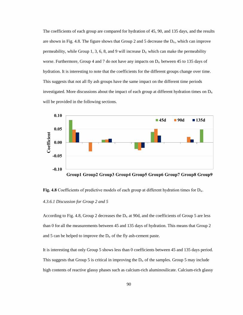
90

The coefficients of each group are compared for hydration of 45, 90, and 135 days, and the results

are shown in Fig. 4.8. The figure shows that Group 2 and 5 decrease the Dic, which can improve

permeability, while Group 1, 3, 6, 8, and 9 will increase Dic which can make the permeability

worse. Furthermore, Group 4 and 7 do not have any impacts on Dic between 45 to 135 days of

hydration. It is interesting to note that the coefficients for the different groups change over time.

This suggests that not all fly ash groups have the same impact on the different time periods

investigated. More discussions about the impact of each group at different hydration times on Dic

will be provided in the following sections.

Fig. 4.8 Coefficients of predictive models of each group at different hydration times for Dic.

4.3.6.1 Discussion for Group 2 and 5

According to Fig. 4.8, Group 2 decreases the Dic at 90d, and the coefficients of Group 5 are less

than 0 for all the measurements between 45 and 135 days of hydration. This means that Group 2

and 5 can be helped to improve the Dic of the fly ash-cement paste.

It is interesting that only Group 5 shows less than 0 coefficients between 45 and 135 days period.

This suggests that Group 5 is critical in improving the Dic of the samples. Group 5 may include

high contents of reactive glassy phases such as calcium-rich aluminosilicate. Calcium-rich glassy

91

phases are much more reactive than those with low or moderate calcium content phases [53, 54].

Furthermore, Group 5 might be a good source to produce C-S-H with a pozzolanic reaction that

causes the reduction of capillary production and interconnected pores.

Group 2 shows the lowest SiO2 content as 8.4%, and only this group has over 30% contents of

Al2O3 and CaO among the nine groups. In addition, a relatively high amount of MgO is included

in Group 2. Various crystalline and glassy phases could exist in those particles. Several glassy

phases such as calcium-rich aluminosilicates, aluminosilicate, and calcium silicates can exist in

these two groups. Non-reactive phases at normal temperatures such as Merwinite Ca3Mg(SiO4)2,

Gehlenite Ca2Al(AlSiO7), and Akermanite Ca2Mg(Si2O7) phases [7] could also be considered a

phase of Group 2. Merwinite is a common phase in high-calcium fly ash and at the early stages of

the devitrification of Mg-containing glasses [7]. Calcium hydroxide in the cement paste can react

with the reactive Mg-phases to form the insoluble magnesium hydroxide Mg(OH)2 that is capable

of reducing the porosity of the cement paste [49]. Thus, investigating the reason for Group 2

about decreasing Dic only at 90 days of hydration is an area of future work.

4.3.6.2 Discussion for Group 1, 3, 6, 8, and 9

Group 1, 3, and 6 show a positive coefficient during all three measurement periods. More

specifically, Group 1 and 6 show relatively higher coefficients than the other groups between 45

to 135 days of hydration. This means that the particles in Group 1 and 6 impact the Dic the most.

Group 8 shows a positive coefficient at 90d and 135d, and the coefficient is decreased from 90d

to 135d while Group 9 increases the Dic at 45d, and it is zero after 45d.

Group 1 has 77.8% of Fe2O3, and Fe-rich phases such as magnetite and hematite have been found

in fly ash, which is not chemically reactive [7]. Moreover, a ferrite phase could exist in this group.

It is reported that the ferrite particles fill the pores between cement particles resulting in finer pore

structure, and more C-S-H gel can be formed because of the reaction between the ferrite particles

92

and the Ca(OH)2 in the hydrating of cement [55, 56]. This could improve the diffusion property,

and since this happens after 28 days of hydration, this is a possible reason why the coefficient of

Group 1 decreased with increasing hydration time.

Group 3 and 6 have > 6% MgO which is significantly higher than the other groups. Furthermore,

these groups have relatively higher CaO and lower Al2O3 than Group 2. This can be a good

source to form Merwinite which is a common phase in high-calcium fly ash and it is non-reactive

in concrete at normal temperatures and it may exist in the particles of these two groups [7]. While

Group 3 has a high content of CaO, it also shows the lowest SiO2 with a quite high content of

P2O5 among the nine groups. The content of P2O5 in Group 6 is also higher than other groups, and

the contents of SiO2 and Al2O3 in Group 6 are quite comparable to each other as about 20%. The

contents and distribution of pores in concrete can be influenced by high P2O5 content fly ash

particles because the high contents of P2O5 can decompose C3S forming a series of solid solutions

between C2S and 3CaO·P2O5 [57, 58]. Besides, Group 6 can be a source of the melilite group

including Gehlenite and Akermanite phases which are not chemically reactive in concrete [7].

Thus, even though further investigation is needed for the phase characterization of each group,

the findings in this study provide important insights for the use of fly ash in concrete to improve

the Dic.

Group 8 contains high SiO2 (roughly 60%) and some Na2O and K2O. This material is more likely

a conglomerate of non-reactive phases like feldspar (K, Na)AlSi3O8, mullite (a crystalline

aluminosilicate), and quartz [59]. Furthermore, the previous study has found low reactive

materials such as mullite (a crystalline aluminosilicate) in low calcium fly ashes [60]. Group 9

could be a good source of either quartz or reactive chemical forms such as silicate or

aluminosilicate because of the high SiO2 content as 84.46%, and those phases have been observed

in almost all fly ashes [7]. It has been known that the reactivity of quartz and silicate phase is very

93

low [53, 61]. Those properties could affect the characteristics of pores in fly ash concrete.

Practically, the change of the total porosity has been investigated in previous studies by using

mercury intrusion porosimetry for the mortar with using the Fe2O3 and SiO2 powder as additives

and found the mortar with the additives had higher total porosity than the control mortar with no

additives [62, 63].

4.3.6.3 Discussion for Group 4 and 7

Group 4 and 7 have no impacts on Dic between 45d and 135d hydration. Group 4 and 7 show

relatively low CaO content with high content SiO2 and Al2O3. Meanwhile, these groups show

high contents of alkalis (Na2O and K2O) compared to the other groups. Even though the siliceous

glass can help to reduce the availability of alkalis for the alkali-silica reaction [7], excessive

content of alkali hydroxide can affect the porosity. A previous study reported the evolution of the

mercury porosity with a 28 days maximum age of the cement paste which used NaOH and KOH

solution [64]. The study found that the cement paste with NaOH and KOH showed higher

porosity (22% and 24%, respectively) than the control cement paste (17.5%) which used

deionized water as the solution [64]. Besides, additional water-soluble alkalis from the fly ash can

cause expansion and damage to the concrete [65].

4.3.7 Practical implications and future applications

This study shows the usefulness of the Particle Model to predict the Dic between 45 and 135 days

of hydration for 20% replacement of fly ash paste. This shows that the Particle Model could be a

useful tool to evaluate the fly ash powder and predict the performance in hardened concrete. This

prediction could be used to help practitioners make wise decisions in choosing a fly ash source

that will help them obtain the desired property. This could lead to a new approach to concrete

performance design. Furthermore, this approach can be used to determine the interrelationships

94

among the different fly ash particles and how they contribute to the ultimate properties of the

concrete.

4.4 Conclusion

A novel characterization and analysis method called the Particle Model has been used to classify

the fly ash particles into nine distinct groups. The predictive models for apparent diffusion

coefficient and surface concentration of iodide into cement paste with a 20% replacement of fly

ash at 45, 90, and 135 days of hydration. The accuracy of the predictive models is evaluated with

the comparison results between the calculated and measured values from the paste samples using

nineteen fly ash sources. The impacts of each group on the diffusion coefficient are discussed by

interpreting the coefficient changes over time and the measured chemical consistency of the

individual groups.

The following contributions are drawn in this study:

1. Between 45 and 135 days of hydration, the apparent iodide diffusion coefficient is

decreased over time for all the fly ash sources except for C6. Furthermore, iodide

surface concentration shows similar values to the OPC for all the investigated fly

ash sources.

2. At 45 and 90 days of hydration, 8 of the 12 Class C fly ashes show a greater

iodide diffusion coefficient than OPC, and at the 135 days of hydration, the

number of Class C fly ashes decreases into 6.

3. The R-squared values of the relationship between the measured values and mean

particle size of nineteen fly ashes are less than 0.3 which means the mean particle

size showed poor correlation over the apparent iodide diffusion coefficient.

4. For the apparent iodide diffusion coefficient, all the R-squared values of

95

predictive models are > 0.95.

5. The predicted and measured apparent iodide diffusion coefficient in paste shows

that 81% of all measurements can be predicted within the variation of the test

method (+/- 30%) between 45 to 135 days of hydration at 20% fly ash

replacement.

6. Group 2 and 5 decreases the apparent iodide diffusion coefficient which means

these groups help to improve the mass transport of the sample. Group 5 is the only

particle group that showed improvement at all measurement periods while Group

2 showed improvement at 90d.

7. Group 1, 3, and 6 increase the apparent iodide diffusion coefficient between 45

and 135 days of hydration. Group 8 increases the apparent iodide diffusion

coefficient at 90d and 135d while Group 9 increases the apparent iodide diffusion

coefficient at only 45d. Group 4 and 7 have no impacts on the apparent iodide

diffusion coefficient between 45d and 135d hydration.

Future work should be done to better understand the different fly ash groups and also

investigate higher replacement levels of fly ash.

Acknowledgments

This work was sponsored by funding from the Illinois Department of Transportation [Project ICT

R27-180], and the FHWA [EAR project # BAA No. 693JJ3-18-BAA-0001]. The authors would

like to thank Dr. Daniel Cook and Mr. Jeff Davis for their assistance and discussion on this work.

96

Reference

[1] X. Li, Q. Xu, S. Chen, An experimental and numerical study on water permeability of

concrete, Constr Build Mater 105 (2016) 503-510.

[2] S. Sadati, M. Arezoumandi, M. Shekarchi, Long-term performance of concrete surface

coatings in soil exposure of marine environments, Constr Build Mater 94 (2015) 656-663.

[3] O. Sengul, Probabilistic Design for the Durability of Reinforced Concrete Structural Elements

Exposed to Chloride Containing Environments, Teknik Dergi 22 (2011) 5409-5423.

[4] V. Å rskog, O. Sengul, O. Gjørv, Performance-based quality control for concrete durability,

Proceedings of International RILEM Workshop on Performance Based Evaluation and Indicators

for Concrete Durability. Madrid, 2006, pp. 223-27.

[5] M.A. Bérubé, J. Duchesne, D. Chouinard, Why the Accelerated Mortar Bar Method ASTM C

1260 is Reliable for Evaluating the Effectiveness of Supplementary Cementing Materials in

Suppressing Expansion Due to Alkali-Silica Reactivity, Cement, Concrete and Aggregates 17(1)

(1995) 26-34.

[6] B. Mather, Use of Concrete of Low Portland Cement Content in Combination with Pozzolans

and Other Admixtures in Construction of Concrete Dams, J Am Concr Inst 71(12) (1974) 589-

599.

[7] A. Committee, 232.2R-18: Report for the Use of Fly Ash in Concrete, Technical Documents

(2018).

[8] S. Shashiprakash, M. Thomas, Sulfate resistance of mortars containing high-calcium fly ashes

and combinations of highly reactive pozzolans and fly ash, Special Publication 199 (2001) 221-

238.

97

[9] M. Thomas, Marine performance of PFA concrete, Magazine of Concrete Research 43(156)

(1991) 171-185.

[10] O. Al-Amoudi, M. Maslehuddin, I.M. Asi, Performance and correlation of the properties of

fly ash cement concrete, Cement, Concrete and Aggregates 18(2) (1996) 71-77.

[11] R.K. Dhir, E.A. Byars, PFA concrete: chloride diffusion rates, Magazine of Concrete

Research 45(162) (1993) 1-9.

[12] R.C. Joshi, R. Lohita, Fly ash in concrete: production, properties and uses, CRC Press1997.

[13] K.O. Ampadu, K. Torii, M. Kawamura, Beneficial effect of fly ash on chloride diffusivity of

hardened cement paste, Cement Concrete Res 29(4) (1999) 585-590.

[14] R.B. Holland, K.E. Kurtis, L.F. Kahn, 7 - Effect of different concrete materials on the

corrosion of the embedded reinforcing steel, in: A. Poursaee (Ed.), Corrosion of Steel in Concrete

Structures, Woodhead Publishing, Oxford, 2016, pp. 131-147.

[15] S.K. Das, Yudhbir, A simplified model for prediction of pozzolanic characteristics of fly ash,

based on chemical composition, Cement Concrete Res 36(10) (2006) 1827-1832.

[16] S. Diamond, On the Glass Present in Low-Calcium and in High-Calcium Flyashes, Cement

Concrete Res 13(4) (1983) 459-464.

[17] L.X. Du, E. Lukefahr, A. Naranjo, Texas Department of Transportation Fly Ash Database

and the Development of Chemical Composition-Based Fly Ash Alkali-Silica Reaction Durability

Index, J Mater Civil Eng 25(1) (2013) 70-77.

[18] S.C. White, E.D. Case, Characterization of fly ash from coal-fired power plants, Journal of

Materials Science 25(12) (1990) 5215-5219.

98

[19] S. Schlorholtz, K. Bergeson, T. Demirel, Monitoring of Fluctuations in the Physical and

Chemical Properties of a High-Calcium Fly Ash, MRS Proceedings 113 (1987) 107.

[20] Q. Hu, M.T. Ley, J. Davis, J.C. Hanan, R. Frazier, Y. Zhang, 3D chemical segmentation of

fly ash particles with X-ray computed tomography and electron probe microanalysis, Fuel 116

(2014) 229-236.

[21] Q. Hu, M. Aboustait, M.T. Ley, J.C. Hanan, V. Rose, R. Winarski, Combined three-

dimensional structure and chemistry imaging with nanoscale resolution, Acta Mater 77 (2014)

173-182.

[22] T. Kim, J.M. Davis, M.T. Ley, S. Kang, P. Amrollahi, Fly ash particle characterization for

predicting concrete compressive strength, Constr Build Mater 165 (2018) 560-571.

[23] T. Kim, M. Moradian, M.T. Ley, Dissolution and leaching of fly ash in nitric acid using

automated scanning electron microscopy, Advances in Civil Engineering Materials 7(1) (2018)

291-307.

[24] M. Aboustait, T. Kim, M.T. Ley, J.M. Davis, Physical and chemical characteristics of fly ash

using automated scanning electron microscopy, Constr Build Mater 106 (2016) 1-10.

[25] S. Ghosal, J.L. Ebert, S.A. Self, Chemical composition and size distributions for fly ashes,

Fuel processing technology 44(1-3) (1995) 81-94.

[26] Y. Chen, N. Shah, F.E. Huggins, G.P. Huffman, W.P. Linak, C.A. Miller, Investigation of

primary fine particulate matter from coal combustion by computer-controlled scanning electron

microscopy, Fuel Processing Technology 85(6-7) (2004) 743-761.

99

[27] T. Kim, M.T. Ley, S. Kang, J.M. Davis, S. Kim, P. Amrollahi, Using particle composition of

fly ash to predict concrete strength and electrical resistivity, Cement and Concrete Composites

(2019) 103493.

[28] S. Kang, Z. Lloyd, T. Kim, M.T. Ley, Predicting the Compressive Strength of Fly Ash

Concrete with the Particle Model, Manuscript submitted for publication.

[29] S. Kang, M.T. Ley, Z. Lloyd, T. Kim, Using the Particle Model to Predict Electrical

Resistivity Performance of Fly Ash in Concrete, Manuscript submitted for publication.

[30] M. Khanzadeh Moradllo, M.T. Ley, Comparing ion diffusion in alternative cementitious

materials in real time by using non-destructive X-ray imaging, Cement and Concrete Composites

82 (2017) 67-79.

[31] M.K. Moradllo, Q. Hu, M.T. Ley, Using X-ray imaging to investigate in-situ ion diffusion in

cementitious materials, Constr Build Mater 136 (2017) 88-98.

[32] K. Stanish, R.D. Hooton, M.D. Thomas, Testing the Chloride Penetration Resistance of

Concrete: A Literature Review, United States. Federal Highway Administration, 2001.

[33] ASTM C150, Standard Specification for Portland Cement, American Society for Testing and

Materials, West Conshohocken, PA, 2019.

[34] R.P. Gupta, T.F. Wall, I. Kajigaya, S. Miyamae, Y. Tsumita, Computer-controlled scanning

electron microscopy of minerals in coal - Implications for ash deposition, Prog Energ Combust

24(6) (1998) 523-543.

[35] C.A. O'Keefe, T.M. Watne, J.P. Hurley, Development of advanced scanning electron

microscopy techniques for characterization of submicron ash, Powder Technol 108(2-3) (2000)

95-102.

100

[36] J.T. Armstrong, Quantitative Elemental Analysis of Individual Microparticles with Electron

Beam Instruments, in: K.F.J. Heinrich, D.E. Newbury (Eds.), Electron Probe Quantitation,

Springer US, Boston, MA, 1991, pp. 261-315.

[37] G. Love, V.D. Scott, Evaluation of a New Correction Procedure for Quantitative Electron-

Probe Microanalysis, J Phys D Appl Phys 11(10) (1978) 1369-1376.

[38] J.T. Armstrong, P.R. Buseck, A General Characteristic Fluorescence Correction for the

Quantitative Electron Microbeam Analysis of Thick Specimens, Thin-Films and Particles, X-Ray

Spectrom 14(4) (1985) 172-182.

[39] J.T. Armstrong, P.R. Buseck, Quantitative Chemical-Analysis of Individual Microparticles

Using Electron-Microprobe - Theoretical, Anal Chem 47(13) (1975) 2178-2192.

[40] M. Aboustait, Q. Hu, R. Frazier, Y. Zhang, B. Tabb, M. Ley, J. Hahan, Innovative prediction

of fly ash performance in concrete, Oklahoma Transportation Center, Midwest City, OK, 2013.

[41] C.P. Aichele, D. Venkataramani, J.E. Smay, M.H. McCann, S. Richter, M. Khanzadeh-

Moradllo, M. Aboustait, M.T. Ley, A comparison of automated scanning electron microscopy

(ASEM) and acoustic attenuation spectroscopy (AAS) instruments for particle sizing, Colloids

and Surfaces A: Physicochemical and Engineering Aspects 479 (2015) 46-51.

[42] ASTM C305, Standard Practice for Mechanical Mixing of Hydraulic Cement Pastes and

Mortars of Plastic Consistency, American Society for Testing and Materials, West

Conshohocken, PA, 2014.

[43] J. Crank, The mathematics of diffusion, Oxford university press1979.

101

[44] S. Sadati, M.K. Moradllo, M. Shekarchi, Long-term durability of onshore coated concrete —

chloride ion and carbonation effects, Frontiers of Structural and Civil Engineering 10(2) (2016)

150-161.

[45] M.J. Crawley, The R Book, Second ed., John Wiley & Sons Ltd, Imperial College London at

Silwood Park, UK, 2012.

[46] R.C. Team, R: A Language and Environment for Statistical Computing, Vienna, Austria,

2016.

[47] M. Kuhn, K. Johnson, Applied predictive modeling, Springer2013.

[48] B. Efron, R.J. Tibshirani, An introduction to the bootstrap, CRC press1994.

[49] D. Manmohan, P. Mehta, Influence of pozzolanic, slag, and chemical admixtures on pore

size distribution and permeability of hardened cement pastes, Cement, Concrete and Aggregates

3(1) (1981) 63-67.

[50] ASTM C618, Standard Specification for Coal Fly Ash and Raw or Calcined Natural

Pozzolan for Use in Concrete, American Society for Testing and Materials, West Conshohocken,

PA, 2019.

[51] L. Tang, Guideline for practical use of methods for testing the resistance of concrete to

chloride ingress, CHLORTEST-EU funded Research Project’Resistance of concrete to chloride

ingress-from laboratory tests to in-field performance’G6RD-CT-2002-00855, Deliverable D23

(2008).

[52] ASTM C1556, Standard Test Method for Determining the Apparent Chloride Diffusion

Coefficient of Cementitious Mixtures by Bulk Diffusion, American Society for Testing and

Materials, West Conshohocken, PA, 2016.

102

[53] P.T. Durdzinski, C.F. Dunant, M. Ben Haha, K.L. Scrivener, A new quantification method

based on SEM-EDS to assess fly ash composition and study the reaction of its individual

components in hydrating cement paste, Cement Concrete Res 73 (2015) 111-122.

[54] K.L. Aughenbaugh, R.T. Chancey, P. Stutzman, M.C. Juenger, D.W. Fowler, An

examination of the reactivity of fly ash in cementitious pore solutions, Materials and Structures

46(5) (2013) 869-880.

[55] M.A. Ahmed, Y.A. Hassanean, K.A. Assaf, M.A. Shawkey, The Effect of Incorporation of

Ferrite Nano-particles on Compressive Strength and Resistivity of Self-Compacting Concrete,

Open Journal of Civil Engineering 5(01) (2015) 131.

[56] M.A. Largeau, Effect of iron powder patially used as portland cement replacement on the

structural properties of concrete, JKUAT-PAUSTI, 2018.

[57] D.J. Naus, C.H. Mattus, L.R. Dole, Assessment of Potential Phosphate Ion-Cementitious

Materials Interactions, Citeseer, 2007.

[58] Z. Li, Z. Ding, Y. Zhang, Development of sustainable cementitious materials, Proceedings of

the international workshop on sustainable development and concrete technology, Iowa State

University, 2004, pp. 55-76.

[59] D. Stark, M.S.Y. Bhatty, Alkali-Silica Reactivity: Effect of Alkali in Aggregate on

Expansion, in: V.H. Dodson (Ed.), ASTM International, West Conshohocken, PA, 1986, pp. 16-

30.

[60] S. Gomes, M. François, M. Abdelmoula, P. Refait, C. Pellissier, O. Evrard, Characterization

of magnetite in silico-aluminous fly ash by SEM, TEM, XRD, magnetic susceptibility, and

Mössbauer spectroscopy, Cement Concrete Res 29(11) (1999) 1705-1711.

103

[61] P.T. Durdzinski, R. Snellings, C.F. Dunant, M. Ben Haha, K.L. Scrivener, Fly ash as an

assemblage of model Ca-Mg-Na-aluminosilicate glasses, Cement Concrete Res 78 (2015) 263-

272.

[62] M.Á .S. Barbudo, C.A. Lucio, J.C.G. Ruiz, E.R. Pozo, Combined effect of nano-SiO2 and

nano-Fe2O3 on compressive strength, flexural strength, porosity and electrical resistivity in

cement mortars, Materiales de construcción (329) (2018) 8.

[63] E. Mohseni, B.M. Miyandehi, J. Yang, M.A. Yazdi, Single and combined effects of nano-

SiO2, nano-Al2O3 and nano-TiO2 on the mechanical, rheological and durability properties of

self-compacting mortar containing fly ash, Constr Build Mater 84 (2015) 331-340.

[64] G. Sant, A. Kumar, C. Patapy, G. Le Saout, K. Scrivener, The influence of sodium and

potassium hydroxide on volume changes in cementitious materials, Cement Concrete Res 42(11)

(2012) 1447-1455.

[65] A.D. Buck, K. Mather, Methods for Controlling Effects of Alkali-Silica Reaction in

Concrete, ARMY ENGINEER WATERWAYS EXPERIMENT STATION VICKSBURG MS

STRUCTURES LAB, 1987.

104

CHAPTER V

THE RELATIONSHIP BETWEEN THE APPARENT DIFFUSION COEFFICIENT

AND ELECTRICAL RESISTIVITY OF FLY ASH CONCRETE

Abstract

Electrical resistivity is a factor that has been suggested as a method to predict mass transport in

concrete. This would be of great value because of the low cost, speed, and convenience of

electrical resistivity. This study employs the Nernst-Einstein equation to estimate the apparent

iodide diffusion coefficient (Dic) by using the surface electrical resistivity (ρsr) of fly ash concrete.

The empirical relationship between the Dic and ρsr is investigated at three different hydration dates

for 19 different fly ash sources at 20% fly ash replacement of the cement. A factor K which

shows the correlation between ρsr and Dic is calculated using the Nernst-Einstein equation, and the

regression line is investigated to evaluate the relationship. Comparisons between Dic and ρsr are

made with both Class C and Class F fly ash, and the R-squared values of the regression line for

each comparison are examined. This work shows that there is not a single relationship between

Dic and ρsr for the materials and mixtures investigated. However, the results show an accurate

prediction of the Dic for class F fly ash is reasonable.

Keywords: Apparent iodide diffusion coefficient, Surface electrical resistivity, Fly ash

105

5.1 Introduction

The mass transport of outside chemicals into concrete is widely used to evaluate the lifespan of

concrete structures. The resistance of concrete against ion ingress is one of the most important

factors for designing durable concrete structures [1-3]. Furthermore, the degradation mechanism

in reinforced concrete due to the chloride-induced corrosion of reinforcement can cause several

structural problems such as cracking, spalling, and delaminating of concrete cover. Previous

studies have employed the apparent diffusion coefficient (Dc) as one of the primary parameters to

predict the time to corrosion initiation of the reinforcing steel in concrete [4-6]. According to the

service life prediction model such as Life-365 and DuraCrete, the model predicts the initiation

period assuming diffusion to be the dominant mechanism [7, 8]. There are many papers

describing this approach [9-12]. Thus, Dc is a useful tool to evaluate the service life of concrete

structures.

The current work focuses on estimating the Dc in fly ash concrete through the electrical resistivity

of concrete. Fly ash has been widely used as supplementary cementitious material (SCM) in

concrete to improve the durability of concrete. Moreover, the incorporation of fly ash in concrete

can significantly reduce the Dc of chloride into cement paste, mortar, or concrete [13-15]. The

chloride penetration has also been evaluated by accounting for the chloride binding for the

cement paste using fly ash [16-18]. Specifically, Thomas et al. [16] have studied one Class C and

one Class F fly ash with a 25% replacement rate of cement paste. In addition, Qiao et al. [17]

investigate the chloride biding of the cement paste for 20%, 40% and 60% replacement rates of a

Class C fly ash while Ishida et al. [18] uses a Class F fly ash at 20% and 40% replacement rates to

examine the chloride binding. All of these publications found that while fly ash does affect the

chloride binding capacity of the cement paste, the results in those studies show that the binding of

the chlorides is insignificant when the chloride concentration is around 1.0 mol/L regardless of

106

the fly ash source and replacement rate [16-18]. Because of this, the salt concentrations in this

study are limited to 0.6 mol/L.

Recent studies employ electrical resistivity techniques to improve the estimation of the Dc of

concrete [4, 19-23]. These efforts have used the Nernst-Einstein equation to investigate the

interrelationship between the electrical resistivity [1, 5, 24, 25]. The Nernst-Einstein equation has

been reported as a helpful approach to predict Dc since this equation applies to electrolytes, for

ion travel can be likened to that of electrical charges [21, 26]. However, those studies mainly

focus on studying concrete with fly ash of limited chemistry. Because of this, a study is needed

about investigating the correlation between Dc and electrical resistivity in cement paste, as it is a

simpler system, with a large number of fly ashes by applying the Nernst-Einstein equation.

In this study, an approach using the transmission X-ray microscopy (TXM) is applied to examine

the Dc for a cement paste containing fly ash. This technique is useful as it is non-destructive and

rapid to investigate the apparent Dc and surface concentration (Cs). This approach has been

presented in previous studies to image the movement of the ions in concrete materials using the

potassium iodide (KI) solution as a tracer or contrast agent [27, 28]. The current work examines

the cement paste to investigate the apparent iodide diffusion coefficient (Dic) as the pore structure

of the cement paste matrix is related to the ion diffusion in concrete [29]. Moreover, using cement

paste is helpful to minimize intervention from aggregates [28]. The surface electrical resistivity

(ρsr) is also investigated in the current study for fly ash concrete using the four-point Wenner

probe measurements as per AASHTO T 358 [30]. In all of this work, the term Dic and ρsr will

refer to the apparent iodide diffusion coefficient of the paste and the surface electrical resistivity

of the concrete, respectively.

This study aims to evaluate the possibility of determining Dic using ρsr in concrete materials

including fly ash and provides insights into the relationship between Dic and ρsr for 20% fly ash

107

replacement at 45, 90, and 135 days of hydration by using the Nernst-Einstein equation. This

provides important insights into the relationship between the electrical resistivity and Dc in

concrete structures.

5.2 Raw materials and experimental methods

5.2.1 Raw materials

ASTM C150 Type I ordinary portland cement (OPC) [31] was used as a cement, and the

properties of OPC are described in Table 5.1. Limestone and natural sand from Oklahoma were

prepared as coarse and fine aggregate, respectively. The specific gravities of coarse and fine

aggregate were the same as 2.60, and the absorption for each aggregate was shown as 0.64% and

0.55%, respectively. No chemical admixtures were used in any mixtures to minimize the

variables.

Nineteen different fly ash sources were investigated in this study. The fly ashes were produced

from various coal sources, boiler designs, and collection conditions in the United States. The fly

ashes were classified into twelve Class C and seven Class F fly ashes according to ASTM C618

[32]. The properties of fly ash, bulk oxides, and particle information were investigated with the

automated scanning electron microscopy (ASEM) method. Details about the ASEM method was

presented in previous chapters and publications [33-36].

Table 5.1 Chemical and phase properties of Type I ordinary portland cement.

Chemical composition (%) Phase Composition (%)

SiO2 Al2O3 Fe2O3 CaO MgO SO3 Na2O K2O C3S C2S C3A C4AF

20.8 4.6 2.6 62.7 2.4 3.2 0.2 0.3 52.1 20.2 7.7 8.0

108

5.2.2 Diffusion test for developing apparent diffusion coefficient (Dic)

5.2.2.1 Sample preparation

Paste samples were prepared for the ion penetration test, and the mixture design of the paste

samples is shown in Table 5.2. A total of twenty mixtures was prepared including one mixture

with 100% OPC and nineteen mixtures with 20% fly ash replacement by mass. A 0.45 water-to-

cement ratio was used at the 20% fly ash replacement rate by mass of cement for all the mixtures.

Any chemical admixtures were not incorporated into the mixtures to minimize the potential

variables. All the mixtures were prepared as per ASTM C305 [37]. Vials with a 9.5 mm diameter

and 46.0 mm height were used for the paste samples, and then these samples were sealed and

cured in the curing room (100% relative humidity at 23℃) until either 45, 90, or 135 days. Three

samples were prepared for each hydration date for each mixture.

Table 5.2 Mixture design for the paste specimen.

Mixture Water (g) Cement (g) Fly ash (g) W/C

OPC 400 888.9 - 0.45

20% Fly ash 400 711.1 177.8 0.45

5.2.2.2 TXM ion penetration test and data analysis

The 0.6 mol/L of KI solution was used as a tracer of the moisture penetration to investigated the

Dic of fly ash paste. The concentration of the KI solution was determined because the preliminary

experiments in the previous study showed this was the optimum concentration to attain suitable

contrast between the paste and solution [28]. As presented in the introduction, other publications

have shown that the chloride binding capacity with the 0.6 mol/L solution was not affected by

different fly ash sources [16-18]. Furthermore, previous studies found that the diffusion profiles

109

for iodide and chloride in paste were quite comparable, and the difference in the calculated

diffusion coefficient at 28 days of ponding for each solution was about 10% [27, 28].

After curing, all the samples were ponded with the KI solution for 28 days. Then the radiographs

of the ponded samples were taken with a Skyscan 1172 mCT scanner. The KI solution was

replaced with a new solution every seven days to keep a constant KI concentration. While

ponding, the sealed vials were stored in a container at 23°C.

The Dic was calculated by approximating Fick’s second law with an error function as shown in

Eq.(5.1) [38, 39]. All the data analysis was conducted with the MATLAB programming

environment. More details for the experimental settings and theoretical background for the data

analysis were reported in previous publications [27, 28] and can be found in Appendix J. The

equation used is:

𝐶(𝑥,𝑡) = 𝐶𝑖𝑠(1 −erf(𝑥

2√𝐷𝑖𝑐𝑡)) Eq.(5.1)

where, x is the distance from the sample surface, t is the denotes time, erf is the error function,

𝐷𝑖𝑐 is the apparent iodide diffusion coefficient, 𝐶𝑖𝑠 is the iodide surface concentration, and 𝐶(𝑥,𝑡)

is the total iodide concentration at the depth of x from the surface after t.

5.2.3 Concrete sample preparation

The concrete mixtures used 20% of the binder as fly ash by mass except for one mixture with 100%

portland cement. Table 5.3 shows the mixture proportions for the mixtures. A 0.45 water-to-

cementitious material ratio (w/cm) was used for all the mixtures. No chemical admixtures were

used in any mixtures to minimize the variables. Details for the concrete mixing procedure can be

found in Appendix M.

110

After mixing, concrete samples were formed in 100 mm by 200 mm cylindrical containers

according to ASTM C31 [40]; they were being cured at 23°C and 100% RH for 24 h in the curing

room after sealing the container. The samples were then demolded and placed into the curing

room until the samples were ready for the surface electrical resistivity test.

Table 5.3 Concrete mixture proportions of specimens for ρsr test.

Mixture

design W/C

Cement

(kg/m3)

Fly ash

(kg/m3)

Water

(kg/m3)

Coarse aggregate

(kg/m3)

Fine aggregate

(kg/m3)

OPC 0.45 283 0 127 863 564

20%

Fly ash 0.45 227 57 127 862 562

5.2.4 Surface electrical resistivity (ρsr) with the Wenner probe

A non-destructive electrical resistivity test, the four-point Wenner probe, was performed to

measure the ρsr of the concrete according to AASHTO T358 [30] at 3, 7, 14, 28, 56, 90, and 180

days of hydration. Four lines were marked on the circular face of each concrete cylinder at 0, 90,

180, and 270 degrees before the measurement. The ρsr was measured at each angle. This means

that 12 measurements were collected at each time period. The average value of twelve

measurements was used as the representative ρsr for each fly ash at specific curing time. All

specimens were in the saturated surface dry (SSD) status while the resistivity test was conducted.

The ρsr values for 45 and 135 days of hydration were linearly interpolated from the measured data.

This helped to eliminate the time variable in the comparison of ρsr and Dic. The values of ρsr for

45 days of hydration were interpolated by using the measured values of 28 and 56 days of

hydration, while the values of ρsr for 135 days of hydration were interpolated by using the

measured values of 90 and 180 days of hydration for each fly ash.

111

5.2.5 Investigation of the correlation between ρsr and Dic

The Nernst-Einstein equation in Eq.(5.2) was used to investigate the correlation between ρsr and

Dic. This approach has been widely used because the test method for the electrical resistivity is

quick, easy and non-destructive to measure, and it helps to avoid the time-consuming grinding of

the samples [4, 22, 23, 41]. This means that theoretically the service life of the concrete structure

can be simply estimated from the resistivity of the concrete.

The constant value K was calculated by using all the dataset, only Class C fly ash dataset and

only Class F fly ash dataset. Then it was used to interpret the relationship between two

performances under different use of datasets. Furthermore, the R-squared value for each derived

equation was investigated to discuss the correlation between the two properties. The Nernst-

Einstein equation is:

Dic = K/ρsr Eq.(2)

where, Dic is the apparent iodide diffusion coefficient [x10-11, m2/s]; ρsr is the surface electrical

resistivity of the concrete sample [kΩ·cm]; K is a factor that shows the correlation between Dic

and ρsr.

5.3 Result and discussion

5.3.1 Bulk chemical composition

Table 5.4 shows the bulk chemical composition result from the ASEM method for nineteen fly

ash sources used in the mixtures. The fly ashes with “C#” and “IC#” represent Class C fly ash

while the fly ashes with “F#” and “IF#” represent Class F fly ash. All the fly ashes are classified

as either Class C or F fly ash according to ASTM C618 which means Class C fly ash has > 18%

of CaO while Class F fly ash has < 18% of CaO [32].

112

Table 5.4 Bulk chemical composition from the ASEM.

Source SiO2 Al2O3 Fe2O3 CaO MgO SO3 Na2O K2O TiO2 P2O5 SrO

C1 36.20 21.72 5.35 23.15 5.38 0.67 3.58 1.01 0.80 1.90 0.23

C2 35.82 19.18 5.60 26.88 5.49 0.98 3.00 0.88 0.73 1.25 0.18

C3 25.32 19.26 5.22 32.50 7.76 2.60 3.42 0.63 1.08 1.89 0.32

C4 36.70 22.82 4.53 22.45 4.33 1.19 3.44 0.95 1.28 1.09 1.22

C5 31.25 22.46 5.38 26.06 5.95 0.56 4.30 0.84 0.84 2.11 0.23

C6 27.66 22.88 4.23 21.54 4.52 2.55 12.61 0.76 1.27 0.67 1.32

C7 35.28 20.61 4.74 24.72 4.93 0.74 4.26 1.23 1.64 0.82 1.00

C11 30.96 20.77 6.38 27.15 7.14 1.59 3.45 0.73 0.78 0.83 0.23

IC1 31.82 22.87 5.68 28.24 5.52 1.08 2.28 1.02 0.78 0.46 0.25

IC2 25.15 21.20 6.22 30.47 7.78 1.04 4.02 0.56 1.22 2.18 0.15

IC3 29.66 21.03 5.92 30.29 5.35 1.87 2.22 0.55 1.04 1.61 0.46

IC4 29.85 17.66 4.73 31.75 9.32 1.19 2.57 0.76 0.83 1.08 0.24

F1 48.76 23.79 7.39 12.53 2.97 0.48 0.86 2.05 0.78 0.09 0.29

F2 50.40 20.91 3.89 17.09 3.69 0.54 1.04 1.37 0.70 0.05 0.32

F3 48.81 26.62 6.65 9.30 1.95 0.28 1.75 1.93 1.46 0.14 1.10

F4 45.34 27.39 4.00 14.61 3.59 0.70 1.48 0.65 1.09 0.37 0.76

F5 53.18 25.36 11.21 2.06 0.19 0.89 0.97 4.43 0.71 0.03 0.96

F6 51.87 25.71 12.32 2.50 0.32 0.67 1.61 4.13 0.66 0.05 0.16

IF1 58.33 21.87 6.87 3.67 1.42 0.59 2.17 4.25 0.22 0.36 0.24

5.3.2 Correlation between ρsr and Dic

The value of K in Eq.(5.2) can be varied depending on the test method for determining the Dic,

the pore solution composition, the use of SCM in concrete materials, etc [4]. Since diffusivity is

higher and electrical resistivity is lower in the more porous materials, the value of K tends to

increase with concrete porosity [21].

113

5.3.2.1 Correlations between ρsr and Dic with and without fly ash

To describe the effect of fly ash on the relationship between the ρsr and Dic, Fig. 5.1 presents the

comparison results between the ρsr and Dic for all the measurements of samples with fly ash and

without fly ash. A total of 57 comparisons are made for the samples with fly ash and three

mixtures with only OPC. The mixtures with OPC do not show changes in Dic or ρsr between 45 d

and 135 d. However, the samples with fly ash showed that 19 out of 57 or 33% of the Dic are

higher than the Dic of OPC. This is surprising as every ρsr value is higher for fly ash than OPC.

However, once the ρsr > 25 kΩ·cm, the Dic values are < 0.5 x 10-11 m2/s of the value for OPC. This

is true for 22 out of 26 or 85% of the samples. This indicates two important things; (1) when the

ρsr is > 25 kΩ·cm there is a high possibility to improve the Dic, and (2) when the ρsr < 25 kΩ·cm

then the performance is quite variable.

Since OPC samples show quite consistent value on both the ρsr and Dic for all the measurements,

the K value is not examined for OPC. On the contrary, the K value is calculated as 13.16 by

employing all the measurements for the samples with fly ash, and the black curve is shown in Fig.

5.1 with a K value of 13.16; however, a poor correlation is found with 0.67 R-squared value.

The variability of the apparent diffusion coefficient has been reported in several studies by using

the coefficient of variation (CV). Tang [42] has evaluated the precision of diffusion coefficient

through various test methods such as immersion test (Nordtest method NT build 492), rapid

migration test (Nordtest method NT build 443), and measurement of chloride ion ingress test (EN

13396). This work showed that the CV of these tests is 24%, 28%, and 36%, respectively.

Moreover, ASTM C1556 (bulk chloride diffusion test) provides 39.8% as the limit of CV to

evaluate the precision (single laboratory) of determining the apparent diffusion coefficient of

cementitious mixtures [43]. Based on the test results of those studies, this work uses +/- 30%

value to determine the variability of predicting Dic.

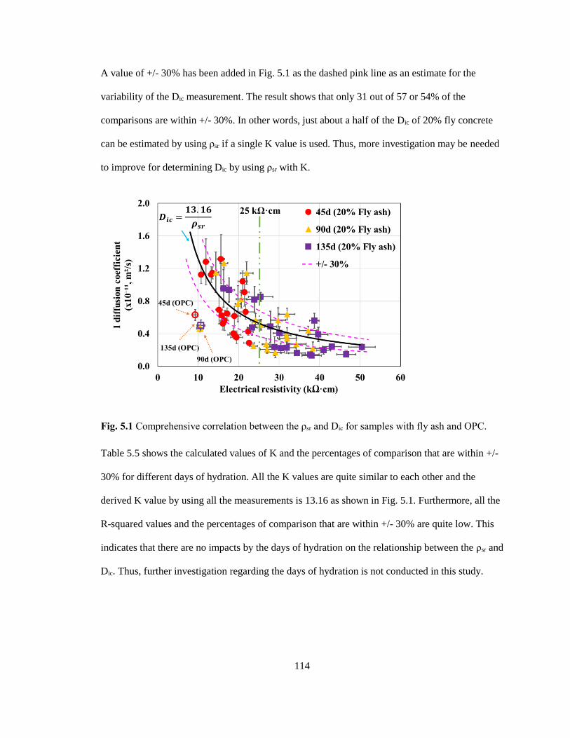
114

A value of +/- 30% has been added in Fig. 5.1 as the dashed pink line as an estimate for the

variability of the Dic measurement. The result shows that only 31 out of 57 or 54% of the

comparisons are within +/- 30%. In other words, just about a half of the Dic of 20% fly concrete

can be estimated by using ρsr if a single K value is used. Thus, more investigation may be needed

to improve for determining Dic by using ρsr with K.

Fig. 5.1 Comprehensive correlation between the ρsr and Dic for samples with fly ash and OPC.

Table 5.5 shows the calculated values of K and the percentages of comparison that are within +/-

30% for different days of hydration. All the K values are quite similar to each other and the

derived K value by using all the measurements is 13.16 as shown in Fig. 5.1. Furthermore, all the

R-squared values and the percentages of comparison that are within +/- 30% are quite low. This

indicates that there are no impacts by the days of hydration on the relationship between the ρsr and

Dic. Thus, further investigation regarding the days of hydration is not conducted in this study.

115

Table 5.5 K and R-squared values for samples with fly ash for each hydration date.

Days of hydration

(days) K (95% confidence intervals) R-squared

Percentage within

+/- 30%

45 12.56 (10.48, 14.58) 0.41 63%

90 14.41 (11.63, 17.19) 0.53 58%

135 13.26 (10.74, 15.78) 0.61 42%

5.3.2.2 Impact of the type of fly ash on the relationships between the ρsr and Dic

The relationships between the ρsr and Dic with considering the type of fly ash are investigated

further. Fig. 5.2 shows the comparison between the ρsr and Dic of Class C fly ashes while Fig. 5.3

shows the comparison for Class F fly ashes. Overall, the Class F fly ashes exhibit a higher ρsr and

lower Dic than that of Class C fly ashes. The values of K and R-squared values of each

comparison, as well as the number of points within +/-30%, are summarized in Table 5.6. Poor

correlations have been found in each comparison between the ρsr and Dic with the R-squared value

of 0.53 for Class C and 0.60 for Class F. The value of K is calculated as 14.42 and 9.22 for the

comparison of Class C fly ash and Class F fly ash, respectively. A value of +/- 30% to the

regression line of Class C and Class F fly ash has been added respectively in Fig. 5.2 and Fig. 5.3

as the dashed pink line as a conservative estimate for the variability of the results. For Class C fly

ash, 18 out of 36 or 50% comparisons are within +/- 30%, while 16 out of 21 or 76% comparisons

are within +/- 30% for Class F fly ash. The results indicate that the K value is affected by the type

of fly ash so that different K values might be used for different types of fly ash. Further, the

results provide some insights that even though the Dic could not be accurately predicted to use a

single regression through the ρsr for Class C fly ash, an accurate prediction of the Dic using ρsr for

class F fly ash is reasonable.

116

While the Class F fly ash shows a lower variability than Class C fly ash, the Dic values have a low

variability after 25 kΩ·cm of ρsr. For the data points with ρsr > 25 kΩ·cm, the Dic is between 0.13

x 10-11 m2/s and 0.44 x 10-11 m2/s, which is quite narrow. On the other hand, the ρsr shows a

significant change from 26.82 kΩ·cm to 50.46 kΩ·cm in the same comparisons. In other words,

Dic for Class F fly ash is almost not changed after about 25 kΩ·cm, and so practically it is not

necessary to use ρsr to estimate the Dic.

Fig. 5.2 Correlation between the ρsr and Dic for Class C fly ashes.

117

Fig. 5.3 Correlation between the ρsr and Dic for Class F fly ashes.

Table 5.6 K and R-squared values for different types of fly ash.

Class of fly ash K (95% confidence intervals) R-squared Percentage within

+/- 30%

Class C 14.42 (12.84, 16.00) 0.53 50%

Class F 9.22 (8.02, 10.42) 0.60 76%

5.3.3 Calculate Dic cement paste with fly ash through the ρsr

The current study focuses on examining the possibility of determining the Dic through the ρsr by

applying the Nernst-Einstein equation, and investigating the empirical relationship between Dic of

the fly ash-cement paste and ρsr from fly ash concrete. It has been published that the pore solution

composition can affect the electrical resistivity, and therefore, these factors should be considered

to accurately predict Dc [44, 45]. This has been done by controlling the pore solution chemistry of

the concrete through a chosen soak solution or from measuring the pore solution chemistry and

calculating a term called the formation factor [17, 46, 47]. The formation factor may improve the

118

ability to predict the Dc; however, the results in this study show that ρsr seems to be accurate for

Class F fly ash.

5.3.4 Practical implication

In this study, the possibility of applying the Nernst-Einstein equation to estimate Dic of 20% fly

ash replacement of cement paste by using the ρsr at 45, 90 and 135 days of hydration. The results

show that it is not recommended to use a single K value to interpret the empirical relationship

between Dic and ρsr of fly ash concrete. Although the correlations between two performances are

quite poor, both Class C and Class F, employing the Nernst-Einstein equation on different types

of fly ash provide insights that the variability of the comparison Dic and ρsr could be affected by

the type of fly ash used. However, the work shows that a single K value for class F fly ash is

more reliable. Further, the work shows that the Dic improved to be better than OPC when the ρsr is

> 25 kΩ·cm. However, this occurred with all of the Class F fly ash after 90 d of hydration.

5.4 Conclusion

The present work employs the Nernst-Einstein equation to investigate the empirical relationship

between the surface electrical resistivity and apparent diffusion coefficient for 20% fly ash

replacement concrete materials between 45 and 135 days of hydration. This study shows that it is

not accurate to use single regression analysis to relate the apparent iodide diffusion coefficient

and the surface electrical resistivity. However, an accurate prediction of the apparent iodide

diffusion coefficient for class F fly ash is reasonable.

The following conclusions can be made:

1. A poor correlation (0.67 R-squared value) and only 54% of the data is within +/- 30% of

the predicted values when all fly ash is investigated with one equation for predicting the

apparent iodide diffusion coefficient by using the surface electrical resistivity. This did

119

not improve when investigating different days of hydration.

2. A poor correlation (0.53 R-squared value) and only half (50%) of the data is within +/-

30% of the predicted values when Class C fly ash is investigated with one equation for

predicting the apparent iodide diffusion coefficient by using the surface electrical

resistivity.

3. While a poor correlation (0.60 R-squared value) is found when Class F fly ash is

investigated with one predictive equation, 76% of the data is within +/- 30% of the

predicted values one predictive equation which means that using a single predictive

equation can be possible for Class F fly ash.

4. The apparent iodide diffusion coefficient becomes quite low and consistent for fly ash

concrete for an electrical resistivity value > 25 kΩ·cm.

This work provides a practical application of the approach using the Nernst-Einstein equation to

predict the diffusion coefficient. Future works studying the pore structure, ion types and

concentration of pore solution in concrete for combining with the approach in this work should be

done to better understand the relationship between the electrical resistivity and diffusion

coefficient of fly ash concrete.

Acknowledgments

This work was sponsored by funding from the Illinois Department of Transportation [Project ICT

R27-180], and the FHWA [EAR project # BAA No. 693JJ3-18-BAA-0001]. The authors would

like to thank Dr. Daniel Cook for the assistance and discussion of this work.

120

Reference

[1] R. Van Noort, M. Hunger, P. Spiesz, Long-term chloride migration coefficient in slag cement-

based concrete and resistivity as an alternative test method, Constr Build Mater 115 (2016) 746-

759.

[2] R. He, H. Ye, H. Ma, C. Fu, X. Jin, Z. Li, Correlating the Chloride Diffusion Coefficient and

Pore Structure of Cement-Based Materials Using Modified Noncontact Electrical Resistivity

Measurement, J Mater Civil Eng 31(3) (2019) 04019006.

[3] L. Basheer, J. Kropp, D.J. Cleland, Assessment of the durability of concrete from its

permeation properties: a review, Constr Build Mater 15(2-3) (2001) 93-103.

[4] Y. Liu, F.J. Presuel-Moreno, M.A. Paredes, Determination of Chloride Diffusion Coefficients

in Concrete by Electrical Resistivity Method, ACI Materials Journal 112(5) (2015).

[5] X. Lu, Application of the Nernst-Einstein equation to concrete, Cement Concrete Res 27(2)

(1997) 293-302.

[6] A.A. Torres-Acosta, F. Presuel-Moreno, C. Andrade, Electrical Resistivity as Durability Index

for Concrete Structures, ACI Materials Journal 116(6) (2019) 245-253.

[7] B. Violetta, Life-365 service life prediction model, Concrete international 24(12) (2002) 53-

57.

[8] A. Siemes, C. Edvardsen, Duracrete: service life design for concrete structures, Ottawa: NRC

Research Press1999.

[9] E.P. Nielsen, M.R. Geiker, Chloride diffusion in partially saturated cementitious material,

Cement Concrete Res 33(1) (2003) 133-138.

121

[10] A. Ababneh, F. Benboudjema, Y. Xi, Chloride penetration in nonsaturated concrete, J Mater

Civil Eng 15(2) (2003) 183-191.

[11] A.V. Saetta, R.V. Scotta, R.V. Vitaliani, Analysis of chloride diffusion into partially

saturated concrete, Materials Journal 90(5) (1993) 441-451.

[12] M. Masi, D. Colella, G. Radaelli, L. Bertolini, Simulation of chloride penetration in cement-

based materials, Cement Concrete Res 27(10) (1997) 1591-1601.

[13] M. Thomas, Marine performance of PFA concrete, Magazine of Concrete Research 43(156)

(1991) 171-185.

[14] O. Al-Amoudi, M. Maslehuddin, I.M. Asi, Performance and correlation of the properties of

fly ash cement concrete, Cement, Concrete and Aggregates 18(2) (1996) 71-77.

[15] R.K. Dhir, E.A. Byars, PFA concrete: chloride diffusion rates, Magazine of Concrete

Research 45(162) (1993) 1-9.

[16] M. Thomas, R. Hooton, A. Scott, H. Zibara, The effect of supplementary cementitious

materials on chloride binding in hardened cement paste, Cement Concrete Res 42(1) (2012) 1-7.

[17] C. Qiao, P. Suraneni, T.N.W. Ying, A. Choudhary, J. Weiss, Chloride binding of cement

pastes with fly ash exposed to CaCl2 solutions at 5 and 23° C, Cement and Concrete Composites

97 (2019) 43-53.

[18] T. Ishida, S. Miyahara, T. Maruya, Chloride binding capacity of mortars made with various

Portland cements and mineral admixtures, Journal of Advanced Concrete Technology 6(2) (2008)

287-301.

[19] W.J. McCarter, G. Starrs, T.M. Chrisp, Electrical conductivity, diffusion, and permeability

of Portland cement-based mortars, Cement Concrete Res 30(9) (2000) 1395-1400.

122

[20] R.J. Kessler, R.G. Powers, E. Vivas, M.A. Paredes, Y.P. Virmani, Surface resistivity as an

indicator of concrete chloride penetration resistance, 2008 Concrete Bridge ConferenceFederal

Highway AdministrationNational Concrete Bridge CouncilMissouri Department of

TransportationAmerican Concrete Institute (ACI), 2008.

[21] P. Linares-Alemparte, C. Andrade, D. Baza, Porosity and electrical resistivity-based

empirical calculation of the oxygen diffusion coefficient in concrete, Constr Build Mater 198

(2019) 710-717.

[22] C. Andrade, R. d’Andrea, N. Rebolledo, Chloride ion penetration in concrete: The reaction

factor in the electrical resistivity model, Cement and Concrete Composites 47 (2014) 41-46.

[23] L. Xiao, Z. Ren, W. Shi, X. Wei, Experimental study on chloride permeability in concrete by

non-contact electrical resistivity measurement and RCM, Constr Build Mater 123 (2016) 27-34.

[24] O. Sengul, O.E. Gjørv, Electrical resistivity measurements for quality control during

concrete construction, ACI Materials Journal 105(6) (2008) 541.

[25] C. Andrade, Calculation of chloride diffusion coefficients in concrete from ionic migration

measurements, Cement Concrete Res 23(3) (1993) 724-742.

[26] E.J. Garboczi, Permeability, diffusivity, and microstructural parameters: a critical review,

Cement Concrete Res 20(4) (1990) 591-601.

[27] M. Khanzadeh Moradllo, M.T. Ley, Comparing ion diffusion in alternative cementitious

materials in real time by using non-destructive X-ray imaging, Cement and Concrete Composites

82 (2017) 67-79.

[28] M.K. Moradllo, Q. Hu, M.T. Ley, Using X-ray imaging to investigate in-situ ion diffusion in

cementitious materials, Constr Build Mater 136 (2017) 88-98.

123

[29] K. Stanish, R.D. Hooton, M.D. Thomas, Testing the Chloride Penetration Resistance of

Concrete: A Literature Review, United States. Federal Highway Administration, 2001.

[30] AASHTO T 358:2015Method Of Test For Surface Resistivity Indication Of Concrete'S

Ability To Resist Chloride Ion Penetration, 2015.

[31] ASTM C150, Standard Specification for Portland Cement, American Society for Testing and

Materials, West Conshohocken, PA, 2019.

[32] ASTM C618, Standard Specification for Coal Fly Ash and Raw or Calcined Natural

Pozzolan for Use in Concrete, American Society for Testing and Materials, West Conshohocken,

PA, 2019.

[33] Q. Hu, M. Aboustait, M.T. Ley, J.C. Hanan, V. Rose, R. Winarski, Combined three-

dimensional structure and chemistry imaging with nanoscale resolution, Acta Mater 77 (2014)

173-182.

[34] Q. Hu, M.T. Ley, J. Davis, J.C. Hanan, R. Frazier, Y. Zhang, 3D chemical segmentation of

fly ash particles with X-ray computed tomography and electron probe microanalysis, Fuel 116

(2014) 229-236.

[35] T. Kim, Q. Hu, M.T. Ley, M. Aboustait, J.W. Bullard, Using Particle Characterization to

Study Fly Ash Dissolution and Leaching in Water and KOH Solution, ACI Materials Journal

116(4) (2019).

[36] T. Kim, M. Moradian, M.T. Ley, Dissolution and leaching of fly ash in nitric acid using

automated scanning electron microscopy, Advances in Civil Engineering Materials 7(1) (2018)

291-307.

124

[37] ASTM C305, Standard Practice for Mechanical Mixing of Hydraulic Cement Pastes and

Mortars of Plastic Consistency, American Society for Testing and Materials, West

Conshohocken, PA, 2014.

[38] J. Crank, The mathematics of diffusion, Oxford university press1979.

[39] S. Sadati, M.K. Moradllo, M. Shekarchi, Long-term durability of onshore coated concrete —

chloride ion and carbonation effects, Frontiers of Structural and Civil Engineering 10(2) (2016)

150-161.

[40] ASTM C31, Standard Practice for Making and Curing Concrete Test Specimens in the Field,

American Society for Testing and Materials, West Conshohocken, PA, 2019.

[41] E. Ryan, E. Burdette, R. Ankabrandt, R. Nidiffer, B. Buchanan, Comparison of two methods

to assess the resistance of concrete to chloride ion penetration, J Mater Civil Eng 26(4) (2014)

698-704.

[42] L. Tang, Guideline for practical use of methods for testing the resistance of concrete to

chloride ingress, CHLORTEST-EU funded Research Project’Resistance of concrete to chloride

ingress-from laboratory tests to in-field performance’G6RD-CT-2002-00855, Deliverable D23

(2008).

[43] ASTM C1556, Standard Test Method for Determining the Apparent Chloride Diffusion

Coefficient of Cementitious Mixtures by Bulk Diffusion, American Society for Testing and

Materials, West Conshohocken, PA, 2016.

[44] P. Gao, J. Wei, T. Zhang, J. Hu, Q. Yu, Modification of chloride diffusion coefficient of

concrete based on the electrical conductivity of pore solution, Constr Build Mater 145 (2017)

361-366.

125

[45] C. Shi, Effect of mixing proportions of concrete on its electrical conductivity and the rapid

chloride permeability test (ASTM C1202 or ASSHTO T277) results, Cement Concrete Res 34(3)

(2004) 537-545.

[46] W.J. Weiss, T.J. Barrett, C. Qiao, H. Todak, Toward a specification for transport properties

of concrete based on the formation factor of a sealed specimen, Advances in Civil Engineering

Materials 5(1) (2016) 179-194.

[47] W.J. Weiss, R.P. Spragg, O.B. Isgor, M.T. Ley, T. Van Dam, Toward performance

specifications for concrete: linking resistivity, RCPT and diffusion predictions using the

formation factor for use in specifications, High tech concrete: Where technology and engineering

meet, Springer2018, pp. 2057-2065.

126

CHAPTER VI

CONCLUSION

The research presented in this dissertation provides an advanced approach of the Particle Model

that predicts the performances of the fly ash in concrete by using the individual fly ash particle

characteristics. The 52,000 particles from 26 fly ash sources are investigated using the automated

scanning electron microscope. Nine distinct groups of fly ash particles are provided through

machine learning that is used for deriving predictive models. The fitting coefficients in the

derived predictive models give important insights into the varying effects of different fly ash

particles over time. Furthermore, the empirical correlation between the electrical resistivity and

the diffusion coefficient is provided for the materials with partially replaced fly ash to cement.

These are an important step to build accurate predictive models for fly ash performance in

concrete.

The main conclusions of this dissertation are:

6.1 Predicting the Compressive Strength of Fly Ash Concrete with the Particle Model

Overall, over 91% of the fly ash particles investigated are classified into nine groups

based on the chemical composition of each particle.

About 95% of all measurements at 20% fly ash replacement and 81% of all

127

measurements at 40% replacement of the compressive strength are predicted within +/-

10% through the predictive models through the Particle Model method.

The R-squared value for the compressive strength prediction of the Particle Model is ≈

0.99, while the Class C and F classification model is < 0.50 for 20% and 40% fly ash

replacement between 3 to 180 days of hydration.

Group 2, 3, 5, 7, and 9 are correlated with strength gain for both 20% and 40% fly ash

replacement and show similar trends at both replacement levels.

Group 4, 6, and 8 have a poor contribution or a reduction to the compressive strength for

20% and 40% replacement.

Group 1 showed the largest coefficient over the first 56 days for 20% replacement while

there is no impact for the compressive strength for 40% replacement.

6.2 Using the Particle Model to Predict Electrical Resistivity Performance of Fly Ash in

Concrete

The Class C and F classification method does not work well to predict electrical

resistivity of fly ash concrete.

There are no correlations found between the electrical resistivity and the median particle

size as all R-squared values of the investigated trend lines are < 0.5 and < 0.3 at 20% and

40% fly ash replacement level, respectively.

The Particle Model can predict the electrical resistivity within +/- 10% for 80% of all

measurements at 20% replacement and 75% of all measurements at 40% replacement.

The R-squared value for the electrical resistivity prediction of the Particle Model is >

0.98 for both 20% and 40% fly ash replacement between 3 to 180 days of hydration.

Group 4, 5, 7, and 8 increased the resistivity between 3 and 180 days of hydration at both

20% and 40% replacement.

128

Group 1 has the largest coefficient at the later ages for both 20% and 40% replacement

while there was no impact at an early age. The impact of Group 9 is ≈ 0 until 90 days of

hydration while it has a big impact at 180 days of hydration for both 20% and 40%

replacement.

Group 2 decreases the resistivity at 20% replacement and increases the resistivity at 40%

replacement between 3 and 180 days of hydration. Although the actual value of

coefficients for Group 3 is quite small for all the measured hydration times for 20% and

40% fly ash replacement levels, it showed a similar trend of coefficient change to Group

2. On the other hand, Group 6 increases the resistivity at 20% replacement while it

decreases the resistivity at the 40% replacement.

6.3 Predicting Ion Diffusion in Fly Ash Cement Paste through Particle Analysis

Between 45 and 135 days of hydration, the apparent iodide diffusion coefficient is

decreased over time for all the fly ash sources except for C6. Furthermore, iodide surface

concentration shows similar values to the OPC for all the investigated fly ash sources.

At 45 and 90 days of hydration, 8 of the 12 Class C fly ashes show a greater iodide

diffusion coefficient than OPC, and at the 135 days of hydration, the number of Class C

fly ashes decreases to 6.

The R-squared values of the relationship between the measured values and mean particle

size of nineteen fly ashes are less than 0.3 which means the mean particle size showed

poor correlation over the apparent iodide diffusion coefficient.

For the apparent iodide diffusion coefficient, all the R-squared values of predictive

models are > 0.95.

The predicted and measured apparent iodide diffusion coefficient in paste shows that

81% of all measurements can be predicted within the variation of the test method (+/-

129

30%) between 45 to 135 days of hydration at 20% fly ash replacement.

Groups 2 and 5 decrease the apparent iodide diffusion coefficient which means these

groups help to improve the mass transport of the sample. Group 5 is the only particle

group that showed improvement at all periods while Group 2 showed improvement at

90d.

Group 1, 3, and 6 increase the apparent iodide diffusion coefficient between 45 and 135

days of hydration. Group 8 increases the apparent iodide diffusion coefficient at 90d and

135d while Group 9 increases the apparent iodide diffusion coefficient at only 45d.

Group 4 and 7 have no impacts on the apparent iodide diffusion coefficient between 45d

and 135d hydration.

6.4 The Relationship between the Apparent Diffusion Coefficient and Electrical Resistivity

of Fly Ash Concrete

A poor correlation (0.67 R-squared value) and only 54% of the data is within +/- 30% of

the predicted values when all fly ash is investigated with one equation for predicting the

apparent iodide diffusion coefficient by using the surface electrical resistivity. This did

not improve when investigating different days of hydration.

A poor correlation (0.53 R-squared value) and only half (50%) of the data is within +/-

30% of the predicted values when Class C fly ash is investigated with one equation for

predicting the apparent iodide diffusion coefficient by using the surface electrical

resistivity.

While a poor correlation (0.60 R-squared value) is found when Class F fly ash is

investigated with one predictive equation, 76% of the data is within +/- 30% of the

predicted values one predictive equation which means that an accurate prediction of the

apparent iodide diffusion coefficient for class F fly ash is reasonable.

130

The apparent iodide diffusion coefficient becomes quite low and consistent for fly ash

concrete for an electrical resistivity value > 25 kΩ·cm.

6.5 Future Work

Even though this research focuses on the fly ash performance on compressive strength, surface

electrical resistivity, and diffusion, the application of the Particle Model can be extended to

predict the fly ash performance in different concrete performances and longer hydration times.

The following is a list of proposed future work:

The Particle Model method can be used to predict the different durability mechanisms

such as the alkali-silica reaction of fly ash concrete over time. Furthermore, the

developed methods can be applied to investigate the impact of fly ash in fresh concrete

properties such as slump and air contents.

The suggested nine fly ash particle groups can be used to predict the longer period (after

180 days) of fly ash concrete performance.

The suggested nine groups of fly ash and the Particle Model method can be used to more

accurately predict the performance of blended fly ash in concrete.

The reactivity and the phase composition of each group should be studied for more

understanding of the nine groups of fly ash particles. This can help to improve the

reliability and accuracy or the Particle Model.

Studying the pore structure, ion types and concentration of pore solution in concrete for

combining with the approach using the Nernst-Einstein equation should be done to better

understand the relationship between the electrical resistivity and diffusion coefficient of

fly ash concrete.

131

APPENDICES

Appendix A. Consistency of the ASEM method

Table A.1 shows the results of the average SD for three times the ASEM investigation of 50 fly

ash particles on the same sample [1]. The SD of three times investigation was relatively small

which means that the results from the ASEM method were quite consistent.

Table A.1 The average standard deviation for three times the ASEM investigation of 50 fly ash

particles on the same sample.

Element SD (%)

Silicon, Si 0.3

Aluminum, Al 0.4

Iron, Fe 0.7

Calcium, Ca 0.8

Magnesium, Mg 0.3

Potassium, K 0.6

Sodium, Na 0.6

Sulfur, S 0.2

Phosphorus, P 1.6

Morphology SD

Average diameter (μm) 0.1

Perimeter (μm2) 0.4

132

Appendix B. Bulk chemical composition comparison between the results of XRF and ASEM

Table B.1 shows the comparison results of the eleven oxides between the result obtained with the

ASEM method and the XRF method for twenty fly ashes. It showed that 96% of the comparisons

were shown less than a 5% absolute difference between them. This suggests that the two

methods agree well with each other.

Table B.1 Chemical composition of fly ashes by XRF and ASEM (C: Class C fly ash and F:

Class F fly ash).

Fly ash Chemical composition (% by mass) SiO2 Al2O3 Fe2O3 CaO MgO SO3 Na2O K2O TiO2 P2O5 SrO

C1 XRF 38.4 19.8 6.2 21.9 5.3 1.4 1.8 0.6 1.4 1.7 0.4

ASEM 36.2 21.7 5.3 23.2 5.4 0.7 3.6 1.0 0.8 1.9 0.2

C2 XRF 36.2 19.9 6.7 24.0 5.2 1.4 1.7 0.5 1.4 1.4 0.4

ASEM 35.8 19.2 5.6 26.9 5.5 1.0 3.0 0.9 0.7 1.2 0.2

C3 XRF 33.2 17.0 5.8 28.1 7.0 1.9 1.9 0.4 1.4 1.4 0.4

ASEM 25.3 19.3 5.2 32.5 7.8 2.6 3.4 0.6 1.1 1.9 0.3

C4 XRF 37.6 23.2 5.5 21.8 4.2 1.0 1.7 0.6 1.6 1.6 0.4

ASEM 36.7 22.8 4.5 22.4 4.3 1.2 3.4 1.0 1.3 1.1 1.2

C5 XRF 37.9 19.5 5.7 22.9 5.6 0.9 2.0 0.5 1.4 1.5 0.4

ASEM 31.3 22.5 5.4 26.1 6.0 0.6 4.3 0.8 0.8 2.1 0.2

C6 XRF 37.0 20.6 5.3 15.6 3.6 2.9 9.2 0.7 1.3 0.7 0.7

ASEM 27.7 22.9 4.2 21.5 4.5 2.5 12.6 0.8 1.3 0.7 1.3

C7 XRF 39.1 20.0 6.2 22.3 4.9 1.0 1.8 0.7 1.4 1.1 0.4

ASEM 35.3 20.6 4.7 24.7 4.9 0.7 4.3 1.2 1.6 0.8 1.0

C8 XRF 40.0 20.9 5.9 21.5 5.0 0.8 1.6 0.7 - - -

ASEM 40.1 22.6 4.5 19.4 5.7 0.8 3.7 0.9 0.6 1.4 0.1

C9 XRF 36.0 22.4 5.5 24.0 4.8 1.2 1.7 0.5 - - -

ASEM 31.5 24.0 6.0 25.7 5.3 1.0 3.7 0.6 0.9 1.1 0.1

C10 XRF 35.9 18.0 6.7 25.8 6.1 1.8 1.8 0.4 1.2 0.8 0.5

ASEM 36.0 19.3 5.1 22.7 7.8 2.0 4.8 0.6 1.0 0.3 0.5

F1 XRF 56.3 20.1 5.7 10.3 3.0 0.5 0.6 1.4 1.2 0.1 0.3

ASEM 48.8 23.8 7.4 12.5 3.0 0.5 0.9 2.1 0.8 0.1 0.3

F2 XRF 52.0 16.4 4.4 18.7 2.9 0.9 0.8 0.9 1.0 0.3 0.2

ASEM 50.4 20.9 3.9 17.1 3.7 0.5 1.0 1.4 0.7 0.1 0.3

F3 XRF 59.2 24.4 6.2 4.0 1.2 0.4 1.4 1.1 1.1 0.1 0.1

ASEM 48.8 26.6 6.6 9.3 2.0 0.3 1.7 1.9 1.5 0.1 1.1

F4 XRF 49.7 24.2 4.7 12.9 3.3 0.7 1.0 0.6 1.7 0.5 0.3

ASEM 45.3 27.4 4.0 14.6 3.6 0.7 1.5 0.6 1.1 0.4 0.8

133

F5 XRF 51.5 23.2 11.9 3.9 1.1 0.9 0.9 2.4 1.3 0.2 0.1

ASEM 53.2 25.4 11.2 2.1 0.2 0.9 1.0 4.4 0.7 0.0 1.0

F6 XRF 49.0 20.9 16.1 4.9 0.9 1.6 1.1 2.5 1.1 0.1 0.0

ASEM 51.9 25.7 12.3 2.5 0.3 0.7 1.6 4.1 0.7 0.1 0.2

F7 XRF 47.7 24.9 14.7 3.7 0.9 0.7 0.7 1.7 1.3 0.3 0.1

ASEM 51.9 26.3 8.0 3.3 0.5 1.7 4.0 2.5 0.9 0.6 0.1

F8 XRF 56.9 22.6 4.6 7.3 2.3 0.3 1.7 1.2 - - -

ASEM 56.9 23.9 3.4 6.2 2.1 0.1 4.1 1.7 0.3 1.2 0.1

F9 XRF 53.5 19.2 6.3 13.2 3.1 0.6 0.6 1.1 - - -

ASEM 48.3 25.0 5.9 12.6 3.3 0.5 1.3 1.8 1.1 0.2 0.1

F10 XRF 57.7 24.5 4.1 8.1 2.0 0.3 0.2 0.9 - - -

ASEM 53.6 27.8 2.8 10.5 2.5 0.5 0.3 1.3 0.4 0.3 0.0

Appendix C. The comprehensive procedure of ASEM method

ASEM method has been introduced and published [2] and was processed with three steps as

shown below in Fig. C.1.

a) Sample preparation b) ASEM analysis c) Data Collection

Fig. C.1 The schematic of the ASEM procedure.

The first step was the sample preparation. A fly ash sample of 16.5mg (±1.5mg) was taken and

placed in a plastic vial with 50 ml of alcohol solution. Since fly ash is a reactive material with

water, it is important using a non-reactive solution for dispersion of fly ash particles without any

reactions. The vial was capped, sealed, and sonicated for 30 min to disperse the fly ash particles

and keep them in the suspension. Then, three to four droplets of the suspension with dispersed fly

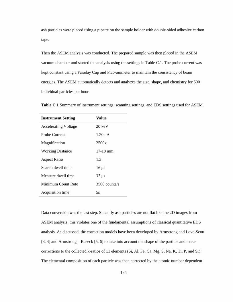
134

ash particles were placed using a pipette on the sample holder with double-sided adhesive carbon

tape.

Then the ASEM analysis was conducted. The prepared sample was then placed in the ASEM

vacuum chamber and started the analysis using the settings in Table C.1. The probe current was

kept constant using a Faraday Cup and Pico-ammeter to maintain the consistency of beam

energies. The ASEM automatically detects and analyzes the size, shape, and chemistry for 500

individual particles per hour.

Table C.1 Summary of instrument settings, scanning settings, and EDS settings used for ASEM.

Instrument Setting Value

Accelerating Voltage 20 keV

Probe Current 1.20 nA

Magnification 2500x

Working Distance 17-18 mm

Aspect Ratio 1.3

Search dwell time 16 μs

Measure dwell time 32 μs

Minimum Count Rate 3500 counts/s

Acquisition time 5s

Data conversion was the last step. Since fly ash particles are not flat like the 2D images from

ASEM analysis, this violates one of the fundamental assumptions of classical quantitative EDS

analysis. As discussed, the correction models have been developed by Armstrong and Love-Scott

[3, 4] and Armstrong – Buseck [5, 6] to take into account the shape of the particle and make

corrections to the collected k-ratios of 11 elements (Si, Al, Fe, Ca, Mg, S, Na, K, Ti, P, and Sr).

The elemental composition of each particle was then corrected by the atomic number dependent

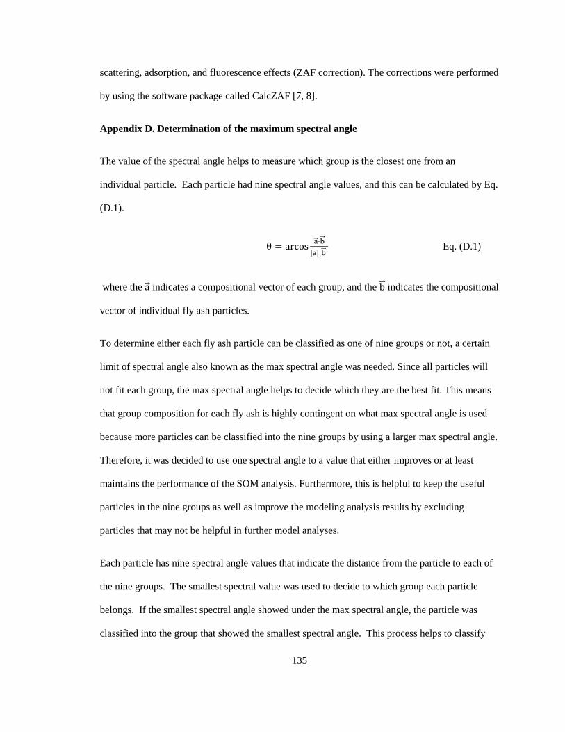
135

scattering, adsorption, and fluorescence effects (ZAF correction). The corrections were performed

by using the software package called CalcZAF [7, 8].

Appendix D. Determination of the maximum spectral angle

The value of the spectral angle helps to measure which group is the closest one from an

individual particle. Each particle had nine spectral angle values, and this can be calculated by Eq.

(D.1).

θ = arcosa⃗ ·b⃗⃗

|a⃗ ||b⃗⃗ | Eq. (D.1)

where the a⃗ indicates a compositional vector of each group, and the b⃗ indicates the compositional

vector of individual fly ash particles.

To determine either each fly ash particle can be classified as one of nine groups or not, a certain

limit of spectral angle also known as the max spectral angle was needed. Since all particles will

not fit each group, the max spectral angle helps to decide which they are the best fit. This means

that group composition for each fly ash is highly contingent on what max spectral angle is used

because more particles can be classified into the nine groups by using a larger max spectral angle.

Therefore, it was decided to use one spectral angle to a value that either improves or at least

maintains the performance of the SOM analysis. Furthermore, this is helpful to keep the useful

particles in the nine groups as well as improve the modeling analysis results by excluding

particles that may not be helpful in further model analyses.

Each particle has nine spectral angle values that indicate the distance from the particle to each of

the nine groups. The smallest spectral value was used to decide to which group each particle

belongs. If the smallest spectral angle showed under the max spectral angle, the particle was

classified into the group that showed the smallest spectral angle. This process helps to classify

136

fly ash particles into one of the nine groups if they are in a reasonable range of the chemistry

reported in Table 2.4. The ones that do not fit any of the nine groups were recorded as

unclassified fly ash particles. Therefore, the percentage of classified particles for each fly ash

also could be changed by using different maximum spectral angles.

The following process was conducted to determine the optimum maximum spectral angle.

52,000 particles, were classified by using different thresholds. The threshold was changed from

0.10 rad then increased incrementally by 0.10 rad interval to 0.60 rad so that six thresholds were

investigated as a potential maximum spectral angle (0.10, 0.20, 0.30, 0.40, 0.50, and 0.60 rad).

Since twenty-six fly ashes were investigated in this study, twenty-six percentage values were

calculated based on the number of classified particles for each fly ash (2,000 is 100% for each fly

ash). Then the comprehensive percentage of classified particles and SD of twenty-six fly ash

percentage values were calculated for each investigated potential maximum spectral angle.

Table D.1 shows the changes for the comprehensive percentage of classified particles and

STDEV of twenty-six fly ash percentage values on each different max spectral angle. The results

of the STDEV from 0.1 rad to 0.3 rad showed significant changes with changing the max spectral

angle but it turned to a highly consistent level after the point of 0.3 rad. The lower STDEV by

using over 0.4 rad implied that the data might have higher stability in expecting the modeling

analysis. Furthermore, the difference of the comprehensive percentage of classified particles

between 0.3 rad and 0.4 rad was about 6% which means more particles can be included in nine

groups if 0.4 rad is used as a max spectral angle rather than 0.3 rad.

Table D.1 Statistical analysis results with different max spectral angles.

Spectral Angle (θ, rad) 0.10 0.20 0.30 0.40 0.50 0.60

The percentage of

classified particles (%) 14.17 65.38 88.99 95.36 97.91 98.80

SD (%) 6.10 14.38 5.31 1.93 1.33 1.02

137

To determine which value performs the best for predicting the compressive strength, the linear

regression analysis was conducted with 0.3, 0.4 and 0.5 rad as the max spectral angle. Fig. D.1

shows the comprehensive comparison results of the significance of the probability of each nine

groups for each model with different maximum spectral angles on different performance data. It

shows how each group is significant in its model. 3d, 28d, and 180d of 20% fly ash concrete

performance data were investigated for the linear regression analysis using nine groups on

compressive strength (Fig. D.1(a)). 28d and 180d at 20% fly ash concrete data were investigated

for the linear regression analysis using nine groups on the electrical resistivity (Fig. D.1(b)). The

linear regression analysis using nine groups at 45d of DiC and CiS was investigated (Fig. D.1(c)).

Each model was derived using all nine groups with the significance of variables from the MLR

analysis and compared. The R-squared value of each model also compared and the results are

shown in Table D.2. All the R-squared values showed over 0.99 which is quite high for all the

analyses. This means that all of these potential maximum spectral angles did a good job on the

modeling. The results with 0.3 rad max spectral angle showed some differences to modeling

results with 0.4 rad and 0.5 rad max spectral angle. On the other hand, the significance of each

group between 0.4 rad and 0.5 rad was almost the same as each other. The results indicate that

about 6% of particles between 0.3 rad and 0.4 rad spectral angle affect the result of the modeling

analysis. In other words, these particles cannot be excluded for further modeling analysis because

of the reliability. Furthermore, the particles that showed over a 0.4 rad spectral angle may not

affect the model analysis results so that these particles can be considered as outliers and excluded

from nine groups. Thus, 0.4 rad was used as the max spectral angle in this study.

Table D.2 R-squared value of each linear regression model on different hydration time data with

different max spectral angle used.

138

Max spectral angle 3d 28d 180d

0.3 rad 0.995 0.995 0.995

0.4 rad 0.997 0.996 0.996

0.5 rad 0.997 0.997 0.996

(a) Compressive strength

(b) Electrical resistivity

139

(c) Diffusion

Fig. D.1 Comprehensive results of the linear regression model analysis with different max

spectral angles on different hydration time data.

Appendix E. The procedure for the MLR analysis for the compressive strength

While the model could be returned that uses all nine groups, it was possible that some of the

identified groups do not have any influence on concrete performance. The significance of the

variables was investigated from the MLR analysis to determine which, if any, of the groups are

significant to the analysis. The variable which showed over 0.10 was not considered as a

significant value from the result. The significance of value was tested by determining the t-value

of the coefficient. The t-value can be simply calculated by dividing the coefficient by the

standard error which is shown in the 2nd (Coefficient) and 3rd (Std. Error) column in Table E.1.

As an example, Table E.1 showed the initial model performance with all nine groups for 20% fly

ash concrete at 28d curing with the result of the MLR.

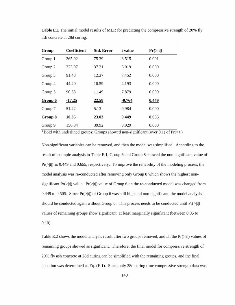
140

Table E.1 The initial model results of MLR for predicting the compressive strength of 20% fly

ash concrete at 28d curing.

Group Coefficient Std. Error t value Pr(>|t|)

Group 1 265.02 75.39 3.515 0.001

Group 2 223.97 37.21 6.019 0.000

Group 3 91.43 12.27 7.452 0.000

Group 4 44.40 10.59 4.193 0.000

Group 5 90.53 11.49 7.879 0.000

Group 6 -17.25 22.58 -0.764 0.449

Group 7 51.22 5.13 9.984 0.000

Group 8 10.35 23.03 0.449 0.655

Group 9 156.84 39.92 3.929 0.000

*Bold with underlined groups: Groups showed non-significant (over 0.1) of Pr(>|t|)

Non-significant variables can be removed, and then the model was simplified. According to the

result of example analysis in Table E.1, Group 6 and Group 8 showed the non-significant value of

Pr(>|t|) as 0.449 and 0.655, respectively. To improve the reliability of the modeling process, the

model analysis was re-conducted after removing only Group 8 which shows the highest non-

significant Pr(>|t|) value. Pr(>|t|) value of Group 6 on the re-conducted model was changed from

0.449 to 0.505. Since Pr(>|t|) of Group 6 was still high and non-significant, the model analysis

should be conducted again without Group 6. This process needs to be conducted until Pr(>|t|)

values of remaining groups show significant, at least marginally significant (between 0.05 to

0.10).

Table E.2 shows the model analysis result after two groups removed, and all the Pr(>|t|) values of

remaining groups showed as significant. Therefore, the final model for compressive strength of

20% fly ash concrete at 28d curing can be simplified with the remaining groups, and the final

equation was determined as Eq. (E.1). Since only 28d curing time compressive strength data was

141

used in the analysis, the model does not require a time element. The R-squared value of the final

model showed as 0.997 (R-squared value of the initial model was 0.996) after the equation was

simplified.

Table E.2 Particle Model result for predicting the compressive strength of 20% fly ash concrete

at 28d curing time using seven significant groups.

Group Coefficient Std. Error t value Pr(>|t|)

Group 1 295.66 55.86 5.293 0.000

Group 2 204.69 27.66 7.400 0.000

Group 3 83.82 7.57 11.073 0.000

Group 4 48.29 9.13 5.289 0.000

Group 5 84.72 7.02 12.068 0.000

Group 7 50.46 4.81 10.491 0.000

Group 9 170.09 25.82 6.588 0.000

Compressive Strength of 20% fly ash concrete at 28d (psi)

= 295.66(%Group1) + 204.69(%Group2) + 83.82(%Group3) + 48.29(%Group4) +

84.72(%Group5) + 50.46(%Group7) + 170.09(%Group9) Eq. (E.1)

Appendix F. Determine the nine distinct groups from SOM analysis

As discussed, 52,000 fly ash particles data from twenty-six fly ashes were collected by using

ASEM, and each particle has eleven pieces of chemical composition data (Na2O, MgO, Al2O3,

SiO2, P2O5, SO3, K2O, CaO, TiO2, Fe2O3, and SrO2). The SOM was used to determine distinct

groups [9]. To conduct the SOM analysis, a certain model geometry should be selected to

determine the number of datum points to classify the fly ash particles, and nine geometry was

used in this study based on the result of previous publication [1].

142

The main purpose of using SOM was not just grouping fly ash particles into nine groups, but to

find a representative set of nine groups to classify the fly ash particles and apply these nine

groups to model analysis. The representative nine groups were determined through the following

three steps: 1) Running SOM 200 times with the 52,000 particle database so that 200 possible

sets of nine groups were derived. 2) Pick one set and compare all nine groups with nine groups

from all the other 199 sets. Each group can be identified with the composition of eleven

chemistry provided from ASEM analysis. 3) Collect all the groups that showed similar chemical

composition from 200 sets as one. The average and standard error for each chemical composition

were calculated for each group.

Table F.1 (same as Table 2.4) showed the chemical composition of each group, and each group

showed a unique composition of eleven chemicals. The standard error was investigated for the

200 comparisons on each chemical for each group, and the result is shown in Table F.2. The

result showed that just one result was 0.10, and all the other values were under 0.06. These

values were quite low, and this means that nine groups derived by using the SOM method were

quite repeatable and consistent. Therefore, nine groups in Table F.1 were determined as the

representative nine groups.

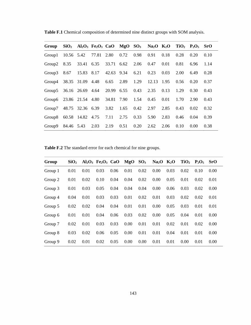
143

Table F.1 Chemical composition of determined nine distinct groups with SOM analysis.

Group SiO2 Al2O3 Fe2O3 CaO MgO SO3 Na2O K2O TiO2 P2O5 SrO

Group1 10.56 5.42 77.81 2.80 0.72 0.98 0.91 0.18 0.28 0.20 0.10

Group2 8.35 33.41 6.35 33.71 6.62 2.06 0.47 0.01 0.81 6.96 1.14

Group3 8.67 15.83 8.17 42.63 9.34 6.21 0.23 0.03 2.00 6.49 0.28

Group4 38.35 31.09 4.48 6.65 2.89 1.29 12.13 1.95 0.56 0.20 0.37

Group5 36.16 26.69 4.64 20.99 6.55 0.43 2.35 0.13 1.29 0.30 0.43

Group6 23.86 21.54 4.80 34.81 7.90 1.54 0.45 0.01 1.70 2.90 0.43

Group7 48.75 32.36 6.39 3.82 1.65 0.42 2.97 2.85 0.43 0.02 0.32

Group8 60.58 14.82 4.75 7.11 2.75 0.33 5.90 2.83 0.46 0.04 0.39

Group9 84.46 5.43 2.03 2.19 0.51 0.20 2.62 2.06 0.10 0.00 0.38

Table F.2 The standard error for each chemical for nine groups.

Group SiO2 Al2O3 Fe2O3 CaO MgO SO3 Na2O K2O TiO2 P2O5 SrO

Group 1 0.01 0.01 0.03 0.06 0.01 0.02 0.00 0.03 0.02 0.10 0.00

Group 2 0.01 0.02 0.10 0.04 0.04 0.02 0.00 0.05 0.01 0.02 0.01

Group 3 0.01 0.03 0.05 0.04 0.04 0.04 0.00 0.06 0.03 0.02 0.00

Group 4 0.04 0.01 0.03 0.03 0.01 0.02 0.01 0.03 0.02 0.02 0.01

Group 5 0.02 0.02 0.04 0.04 0.01 0.01 0.00 0.05 0.03 0.01 0.01

Group 6 0.01 0.01 0.04 0.06 0.03 0.02 0.00 0.05 0.04 0.01 0.00

Group 7 0.02 0.01 0.03 0.03 0.00 0.01 0.01 0.02 0.01 0.02 0.00

Group 8 0.03 0.02 0.06 0.05 0.00 0.01 0.01 0.04 0.01 0.01 0.00

Group 9 0.02 0.01 0.02 0.05 0.00 0.00 0.01 0.01 0.00 0.01 0.00

144

Appendix G. The comprehensive results of the coefficient values for the predictive models of

the compressive strength

The coefficients of each group for the model used for predicting the compressive strength are

shown in Table G.1. The predictive models were constructed by applying the coefficient values

to the Eq. (2) for both 20% and 40% fly ash replacements at seven specific times.

Table G.1 Coefficients for each group at different curing times.

Mixture Curing Group

1

Group

2

Group

3

Group

4

Group

5

Group

6

Group

7

Group

8

Group

9

20%

Fly ash

3 days 96.50 79.40 56.94 42.92 29.85 25.06 35.35 32.19 49.30

7 days 222.86 144.55 71.05 45.91 54.44 - 39.54 - 125.45

14 days 226.16 167.32 80.02 49.40 75.67 - 46.17 - 128.52

28 days 295.66 204.69 83.81 48.29 84.72 - 50.46 - 170.09

56 days 364.94 193.79 94.85 56.72 103.25 - 60.91 - 204.87

90 days 262.89 245.19 136.83 50.55 150.02 -74.03 73.67 - 186.76

180 days 239.32 272.40 142.75 60.05 159.46 -77.40 83.75 - 186.45

40%

Fly ash

3 days - 83.52 17.62 - 43.87 49.25 24.06 - 45.82

7 days - 119.63 48.95 - 55.15 44.48 28.65 - 77.55

14 days - 178.06 82.00 - 95.84 - 32.88 - 91.57

28 days - 212.96 102.60 - 110.01 - 51.25 - 69.28

56 days - 254.92 99.78 - 125.77 - 56.89 - 114.86

90 days - 246.19 116.46 - 135.93 - 71.30 - 107.35

180 days - 280.54 126.19 - 134.31 - 72.56 - 125.26

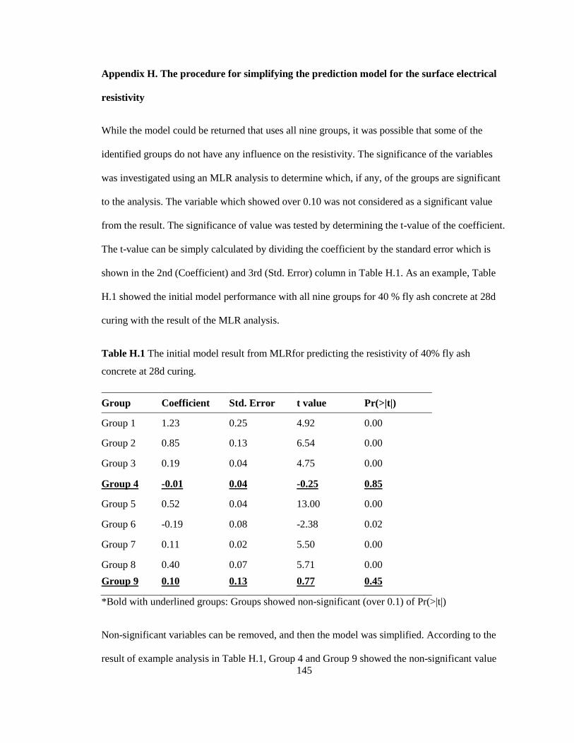
145

Appendix H. The procedure for simplifying the prediction model for the surface electrical

resistivity

While the model could be returned that uses all nine groups, it was possible that some of the

identified groups do not have any influence on the resistivity. The significance of the variables

was investigated using an MLR analysis to determine which, if any, of the groups are significant

to the analysis. The variable which showed over 0.10 was not considered as a significant value

from the result. The significance of value was tested by determining the t-value of the coefficient.

The t-value can be simply calculated by dividing the coefficient by the standard error which is

shown in the 2nd (Coefficient) and 3rd (Std. Error) column in Table H.1. As an example, Table

H.1 showed the initial model performance with all nine groups for 40 % fly ash concrete at 28d

curing with the result of the MLR analysis.

Table H.1 The initial model result from MLRfor predicting the resistivity of 40% fly ash

concrete at 28d curing.

Group Coefficient Std. Error t value Pr(>|t|)

Group 1 1.23 0.25 4.92 0.00

Group 2 0.85 0.13 6.54 0.00

Group 3 0.19 0.04 4.75 0.00

Group 4 -0.01 0.04 -0.25 0.85

Group 5 0.52 0.04 13.00 0.00

Group 6 -0.19 0.08 -2.38 0.02

Group 7 0.11 0.02 5.50 0.00

Group 8 0.40 0.07 5.71 0.00

Group 9 0.10 0.13 0.77 0.45

*Bold with underlined groups: Groups showed non-significant (over 0.1) of Pr(>|t|)

Non-significant variables can be removed, and then the model was simplified. According to the

result of example analysis in Table H.1, Group 4 and Group 9 showed the non-significant value

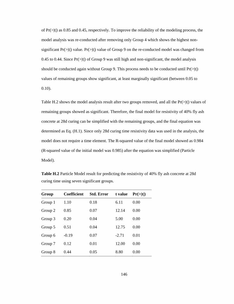
146

of Pr(>|t|) as 0.85 and 0.45, respectively. To improve the reliability of the modeling process, the

model analysis was re-conducted after removing only Group 4 which shows the highest non-

significant Pr(>|t|) value. Pr(>|t|) value of Group 9 on the re-conducted model was changed from

0.45 to 0.44. Since Pr(>|t|) of Group 9 was still high and non-significant, the model analysis

should be conducted again without Group 9. This process needs to be conducted until Pr(>|t|)

values of remaining groups show significant, at least marginally significant (between 0.05 to

0.10).

Table H.2 shows the model analysis result after two groups removed, and all the Pr(>|t|) values of

remaining groups showed as significant. Therefore, the final model for resistivity of 40% fly ash

concrete at 28d curing can be simplified with the remaining groups, and the final equation was

determined as Eq. (H.1). Since only 28d curing time resistivity data was used in the analysis, the

model does not require a time element. The R-squared value of the final model showed as 0.984

(R-squared value of the initial model was 0.985) after the equation was simplified (Particle

Model).

Table H.2 Particle Model result for predicting the resistivity of 40% fly ash concrete at 28d

curing time using seven significant groups.

Group Coefficient Std. Error t value Pr(>|t|)

Group 1 1.10 0.18 6.11 0.00

Group 2 0.85 0.07 12.14 0.00

Group 3 0.20 0.04 5.00 0.00

Group 5 0.51 0.04 12.75 0.00

Group 6 -0.19 0.07 -2.71 0.01

Group 7 0.12 0.01 12.00 0.00

Group 8 0.44 0.05 8.80 0.00

147

The resistivity of 40% fly ash concrete at 28d (kΩ·cm)

= 1.10(%Group1) + 0.85(%Group2) + 0.20(%Group3) + 0.51(%Group5) - 0.19(%Group6) +

0.12(%Group7) + 0.44(%Group8) Eq. (H.1)

Appendix I. The comprehensive results of the coefficient values for the predictive models of

surface electrical resistivity

The coefficients of each group for the model used for predicting the electrical resistivity are

shown in Table I.1. The predictive models were constructed with applying the coefficient values

to the Eq.(3.2) for both 20% and 40% fly ash replacements at seven specific times.

Table I.1 Coefficient values for each of the nine groups at different curing times for 20% and

40% fly ash replacement rates.

Mixture Curing Group

1

Group

2

Group

3

Group

4

Group

5

Group

6

Group

7

Group

8

Group

9

20%

Fly ash

3 days - -0.07 0.02 0.09 -0.02 0.18 0.06 0.16 -0.06

7 days - -0.06 0.01 0.13 -0.02 0.22 0.08 0.18 -0.09

14 days - -0.18 -0.05 0.26 0.02 0.32 0.10 0.20 -0.14

28 days - -0.18 -0.04 0.37 0.10 0.33 0.14 0.42 -0.37

56 days 0.99 -0.67 -0.07 0.59 0.28 0.43 0.22 0.45 -

90 days 1.09 -0.60 - 0.61 0.45 0.36 0.30 0.73 -

180 days 1.47 -0.58 - 0.61 0.63 0.31 0.44 1.04 0.79

40%

Fly ash

3 days - - 0.02 0.04 0.07 0.07 0.04 0.06 0.08

7 days - 0.23 0.04 - 0.10 0.06 0.06 0.06 0.11

14 days 0.92 0.33 0.05 - 0.24 0.06 0.02 -0.09 0.58

28 days 1.10 0.85 0.20 - 0.51 -0.19 0.12 0.44 -

56 days 2.34 1.23 0.17 0.28 0.99 -0.40 0.28 0.81 -

90 days 3.75 2.24 0.36 0.31 1.65 -1.14 0.47 1.34 -

180 days 3.64 1.20 - 1.09 2.13 -0.46 0.90 - 4.09

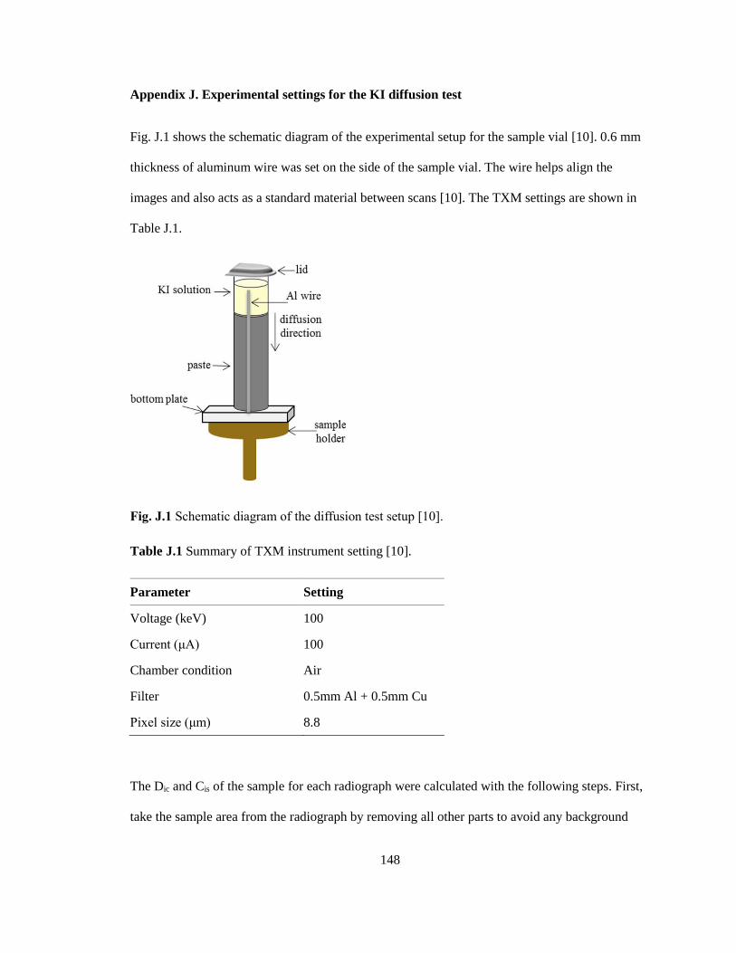
148

Appendix J. Experimental settings for the KI diffusion test

Fig. J.1 shows the schematic diagram of the experimental setup for the sample vial [10]. 0.6 mm

thickness of aluminum wire was set on the side of the sample vial. The wire helps align the

images and also acts as a standard material between scans [10]. The TXM settings are shown in

Table J.1.

Fig. J.1 Schematic diagram of the diffusion test setup [10].

Table J.1 Summary of TXM instrument setting [10].

Parameter Setting

Voltage (keV) 100

Current (μA) 100

Chamber condition Air

Filter 0.5mm Al + 0.5mm Cu

Pixel size (μm) 8.8

The Dic and Cis of the sample for each radiograph were calculated with the following steps. First,

take the sample area from the radiograph by removing all other parts to avoid any background

149

attenuation effect. Next, match the height of the surface between the reference paragraph and the

28d ponding time radiograph to measure the gray value from the same area. Then, measure the

hundreds of lines of the specified area in several seconds, and calculate the Dic and Cis. Beer-

Lambert Law (Eq.(J.1)) [11, 12] was applied to calculate a change in attenuation due to I (Δμ) at

different depths of the sample.

(𝛥𝜇)𝑥 = ln(𝐼𝑟𝑒𝑓)𝑥− ln(𝐼𝑡)𝑥 Eq.(J.1)

where, (𝐼𝑟𝑒𝑓)𝑥 is the gray value at depth x on the reference profile, and (𝐼𝑡)𝑥 is the gray value at

the same location at a future time.

Then the Dic and Cis were calculated with the help of Fick’s second law (Eq.(4.1)) [13, 14]. All

the data analysis was conducted with the MATLAB programming environment.

Appendix K. The procedure for the MLR analysis for apparent iodide diffusion coefficient

Even though the model could be returned that uses all nine groups, some of the groups cannot

have any influence on the diffusion coefficient or surface concentration. The significance of the

variables was used to determine the groups which are significant to the model. The variable

which showed the probability (Pr(>|t|)) over 0.10 was not considered as a significant value from

the result. The significance of value was tested by determining the t-value of the coefficient.

Table K.1 provides MLR analysis results for the initial model performance with all nine groups of

the diffusion coefficient at 90 days of hydration.

150

Table K.1 The initial model result of MLR for predicting the diffusion coefficient at 90 days of

hydration.

Group Coefficient Std. Error t value Pr(>|t|)

Group 1 0.049 0.039 1.256 0.216

Group 2 - 0.038 0.018 - 2.111 0.041

Group 3 0.010 0.006 1.667 0.128

Group 4 0.001 0.005 0.200 0.792

Group 5 - 0.030 0.006 - 5.000 0.000

Group 6 0.053 0.011 4.818 0.000

Group 7 0.001 0.003 0.333 0.869

Group 8 0.014 0.011 1.273 0.215

Group 9 0.008 0.020 0.400 0.693

*Bold with underlined groups: Groups showed non-significant (over 0.1) of Pr(>|t|)

The model was simplified by removing the non-significant variables. According to the result of

example analysis in Table K.1, Group 1, 3, 4, 7, 8, and 9 showed the non-significant Pr(>|t|) value.

To improve the reliability of the model process, the model analysis was re-conducted after

removing a group that showed the highest non-significant Pr(>|t|) value which is Group 7 in Table

K.1. Group 4 showed the highest Pr(>|t|) value among the remaining eight groups as 0.808 which

is non-significant. The model analysis was conducted after removing the Group 4, and Group 9

showed the highest Pr(>|t|) among the remaining seven groups as 0.429 which is non-significant.

The model analysis was conducted again after removing the Group 9, and then all the Pr(>|t|)

value of the remaining six groups were < 0.1. The process was conducted until Pr(>|t|) values of

remaining groups show significant, at least marginally significant (between 0.05 to 0.10).

Table K.2 shows the final model analysis result after three groups removed. Thus, the predictive

model for the diffusion coefficient at 90 days of hydration can be derived using the result, and the

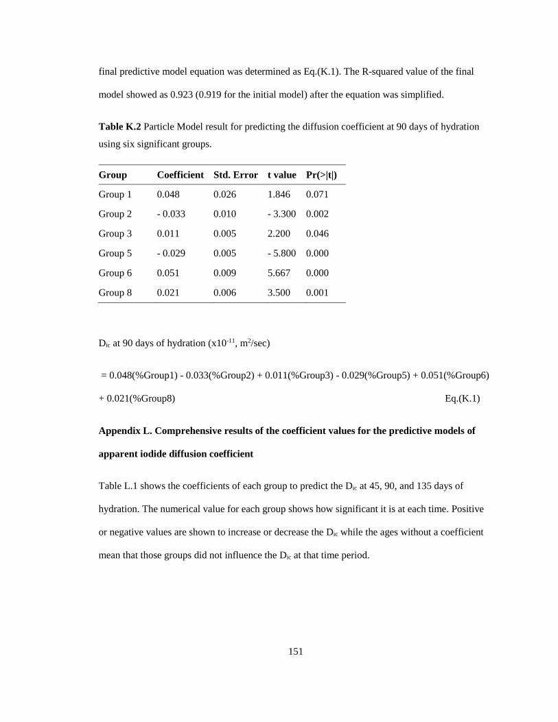
151

final predictive model equation was determined as Eq.(K.1). The R-squared value of the final

model showed as 0.923 (0.919 for the initial model) after the equation was simplified.

Table K.2 Particle Model result for predicting the diffusion coefficient at 90 days of hydration

using six significant groups.

Group Coefficient Std. Error t value Pr(>|t|)

Group 1 0.048 0.026 1.846 0.071

Group 2 - 0.033 0.010 - 3.300 0.002

Group 3 0.011 0.005 2.200 0.046

Group 5 - 0.029 0.005 - 5.800 0.000

Group 6 0.051 0.009 5.667 0.000

Group 8 0.021 0.006 3.500 0.001

Dic at 90 days of hydration (x10-11, m2/sec)

= 0.048(%Group1) - 0.033(%Group2) + 0.011(%Group3) - 0.029(%Group5) + 0.051(%Group6)

+ 0.021(%Group8) Eq.(K.1)

Appendix L. Comprehensive results of the coefficient values for the predictive models of

apparent iodide diffusion coefficient

Table L.1 shows the coefficients of each group to predict the Dic at 45, 90, and 135 days of

hydration. The numerical value for each group shows how significant it is at each time. Positive

or negative values are shown to increase or decrease the Dic while the ages without a coefficient

mean that those groups did not influence the Dic at that time period.

152

Table L.1 Coefficients of each group on the predictive models for Dic.

Group Dic

45d 90d 135d

Group 1 0.084 0.048 0.038

Group 2 - -0.033 -

Group 3 0.010 0.011 0.012

Group 4 - - -

Group 5 -0.024 -0.029 -0.020

Group 6 0.039 0.051 0.027

Group 7 - - -

Group 8 - 0.021 0.011

Group 9 0.049 - -

Appendix M. Concrete mixing procedure

The moisture content for both coarse and fine aggregates was determined before the mixing

process and the batch proportions for the aggregates and water were adjusted. Both aggregates

were brought into the temperature-controlled mixing facility at least a day before conducting the

moisture correction, and their batch weights were corrected for the moisture content. After

adjusting the mixture proportion, all the mixtures were mixed according to the following steps.

All aggregates were collected from the outside storage piles, and they were stored in a

temperature-controlled room (23°C) for at least 24 hours. The aggregates were then placed in the

mixer and spun; after that, a representative sample was taken for moisture correction. It should be

noted here that aggregates have to be properly sealed to prevent water loss before the mixing. At

the time of mixing, all aggregates and approximately one half of the mixing water were loaded

into the mixer; they were being mixed for three minutes. This allowed the aggregates to approach

the saturated surface dry (SSD) condition and to ensure that the aggregates were evenly

153

distributed. All the materials (the cement, fly ash, and the remaining water) were added into the

mixer and were being mixed for three minutes. Then the mixture was rested for two minutes

while the sides of the mixing drum were scraped. After that, the mixer was started to mix the

concrete for three more minutes as well.

References for appendix

[1] T. Kim, J.M. Davis, M.T. Ley, S. Kang, P. Amrollahi, Fly ash particle characterization for

predicting concrete compressive strength, Constr Build Mater 165 (2018) 560-571.

[2] M. Aboustait, T. Kim, M.T. Ley, J.M. Davis, Physical and chemical characteristics of fly ash

using automated scanning electron microscopy, Constr Build Mater 106 (2016) 1-10.

[3] J.T. Armstrong, Quantitative Elemental Analysis of Individual Microparticles with Electron

Beam Instruments, in: K.F.J. Heinrich, D.E. Newbury (Eds.), Electron Probe Quantitation,

Springer US, Boston, MA, 1991, pp. 261-315.

[4] G. Love, V.D. Scott, Evaluation of a New Correction Procedure for Quantitative Electron-

Probe Microanalysis, J Phys D Appl Phys 11(10) (1978) 1369-1376.

[5] J.T. Armstrong, P.R. Buseck, Quantitative Chemical-Analysis of Individual Microparticles

Using Electron-Microprobe - Theoretical, Anal Chem 47(13) (1975) 2178-2192.

[6] J.T. Armstrong, P.R. Buseck, A General Characteristic Fluorescence Correction for the

Quantitative Electron Microbeam Analysis of Thick Specimens, Thin-Films and Particles, X-Ray

Spectrom 14(4) (1985) 172-182.

[7] M. Aboustait, Q. Hu, R. Frazier, Y. Zhang, B. Tabb, M. Ley, J. Hahan, Innovative prediction

of fly ash performance in concrete, Oklahoma Transportation Center, Midwest City, OK, 2013.

154

[8] J.T. Armstrong, J. Donovan, P. Carpenter, CALCZAF, TRYZAF and CITZAF: The Use of

Multi-Correction-Algorithm Programs for Estimating Uncertainties and Improving Quantitative

X-ray Analysis of Difficult Specimens, Microscopy and Microanalysis 19(S2) (2013) 812-813.

[9] T. Kohonen, Self-Organizing Maps, Third ed., Springer, Berlin, Heidelberg1997.

[10] M. Khanzadeh Moradllo, M.T. Ley, Comparing ion diffusion in alternative cementitious

materials in real time by using non-destructive X-ray imaging, Cement and Concrete Composites

82 (2017) 67-79.

[11] V.C. Tidwell, L.C. Meigs, T. Christian-Frear, C.M. Boney, Effects of spatially

heterogeneous porosity on matrix diffusion as investigated by X-ray absorption imaging, Journal

of Contaminant Hydrology 42(2) (2000) 285-302.

[12] L. Cavé, T. Al, Y. Xiang, P. Vilks, A technique for estimating one-dimensional diffusion

coefficients in low-permeability sedimentary rock using X-ray radiography: Comparison with

through-diffusion measurements, Journal of Contaminant Hydrology 103(1) (2009) 1-12.

[13] J. Crank, The mathematics of diffusion, Oxford university press1979.

[14] S. Sadati, M.K. Moradllo, M. Shekarchi, Long-term durability of onshore coated concrete —

chloride ion and carbonation effects, Frontiers of Structural and Civil Engineering 10(2) (2016)

150-161.

VITA

Shinhyu Kang

Candidate for the Degree of

Doctor of Philosophy

Dissertation: PREDICTING FLY ASH PERFORMANCE IN CONCRETE FROM

PARTICLE CHARACTERISTICS

Major Field: Civil Engineering

Biographical: Shinhyu Kang was born in Iksan, Jeollabuk-do, Republic of Korea on July

4th, 1983

Education:

Completed the requirements for the Doctor of Philosophy in Civil Engineering at

Oklahoma State University, Stillwater, Oklahoma in May 2020.

Completed the requirements for the Master of Science in Materials Science and

Engineering at Kyonggi University, Suwon, Gyeonggi-do, Republic of Korea in 2012.

Completed the requirements for the Bachelor of Science in Materials Science and

Engineering at Kyonggi University, Suwon, Gyeonggi-do, Republic of Korea in 2010.

Experience:

Graduate Research Assistant, Oklahoma State University, Stillwater, OK, 2015-2020.

Development Engineer & Research Assistant, Iljin Diamond Co., Ltd., Eumseong,

Republic of Korea 2011-2014

Graduate Research Assistant, Kyonggi University, Suwon, Gyeonggi-do, Republic of

Korea, 2010-2011

Professional Memberships:

American Concrete Institute (ACI)

American Coal Ash Association (ACAA)

American Ceramic Society (ACerS)

American Society of Civil Engineers (ASCE)