Developing an Alternate Backing System Made of Fly Ash Composite for Nickel Shell Moulds

Fouad Fayez Kamaieddine

A thesis submitted in conformity with the requirements for the degree of Doctor of' Phibsophy

Graduate De partment of Civil Engineering University of Toronto

O Copyright by Fouad bnaleddine 2001

National Library ml . c m BibliothPque nationale du Canada

Acquisitions and Acquisitions et Bibliographie Services services bibliographiques 395 Weüington Street 395. rue Wellingtan Ottawa ON K1A ON4 Ottawa ON K I A ON4 Canada Canada

The author has granted a non- exclusive licence aiiowing the National Library of Canada to reproduce, loan, distriiute or seli copies of this thesis in microform, paper or electronic formats.

The auîhor retains ownership of the copyright in this thesis. Neither the thesis nor substantial extracts fiom it may be priuted or otherwise reproduced without the author's permission.

L'auteur a accordé une licence non exclusive peunettant à la Bibliothèque nationaie du Canada de reproduire, prêter, distribuer ou vendre des copies de cette thèse sous la fome de microfiche/füm, de reproduction sur papier ou sur format électronique.

L'auteur conserve la propriété du droit d'auteur qui protège cette thèse. Ni la thèse ni des extraits substantiels de celle-ci ne doivent être imprimés ou autrement reproduits sans son autorisation.

Abstract

Some injection and compression moulds are made uing thin nickel sheIls, which

require proper backing to withstand the pressures imposed by the mouiding process. The

main disadvantage of conventional backing fillers is the difficulty of rebuilding the

mould in the event that the thermal lines need to be repaired or reconiïgured. This thesis

proposes an alternative backing system made of a tly ash:cement:sand composite.

The operationai factors that constrain the design of nickel vapor deposited (NVD)

shells are F i t quantified and summarized in the form of design guidelines. The stiffness

and strength behavior of the nickel shell is then investigated using experimental bearn-

bending and axial compression/tension tests, based on which a constitutive model is

introduced. Mechanical testing is considered for nvo conventionai backing materials:

epoxy and polymer-concrete composites. Triaxial compression tests were conducted on

epoxy composite specimens and a material model is proposed. Unia~ial compression

strength tests were carried out on polymer-concrete (type HTSOS) specimens, and a

strength envelope is presented.

Design parameters of NVD backing fillers are illusuated in the conmt of strength

versus stiffness considerations. Mechanical properties of different fly ash mixes are

investigated for strength and stiffness behaviour using experimental testhg. Based on the

test results, a proposed mix design is engineered to meet the following properties: ease of

placement, rapid curing, appropriate mechanical and thermal performance, and easy

removal For mould repair. A numericd finite element technique is used to successfully

caiibrate a materiai model for the proposed backing based on triaxial test resuits.

The new backing was then used in a prototype triai. Both sides (Top and Bottom)

of a new mould were backed with the fly ash composite, and instnrmented for strain,

temperature* and displacement. Production part quaiity and the performance of the

mouid were monitored during the production triais, Test results show that the new fly ash

composite backing is both mechanically and thennally suitable for backing nickel shells,

under the conditions of the mouIding process used. Mould performance was compared to

3D finite element models, which assisted in the interpretation of the collected prototype

performance data, and in gaining better insight into the pedormance of the NVD mould

(nickel shell+fly ash backing+frame) as a whole. Both experimental and numerical

resuits are consistent in presenting the behaviour of the nickel shell mould under the

conditions of the production trial.

Acknowledgement

1 would like to express my sincere thankç and appreciation to my supervisor, Professor M.W. Grabinsky, for his invaluable support, guidance, and most of al1 patience throughout this project. Thanks for every vaLuabLe advice that helped to give the project direction in d i c u l t situations.

I am also grateful for the helphl suggestions and comments of Professors K.D. Pressnail, M.D.A. Thomas. and R.D. Venter.

Thanks are due to Professor P.R. Frise of the University of Windsor for reviewing this manuscript and giving his usehl and valuable comrnents.

Part of the experimental work was carried out at the Structural Laboratories of the Deparunent of Civil Engineering. The help of R. Basset. G. Buueo, J. MacDonald and in particular P. Heliopoulos in developing and conducting the experimental work is geatiy appreciated. Another part of the experimentd work was conducted at the Geotechnical Laboratory, and my thanks are due to A. Rygren for his help and technical expertise.

1 would like to extend my sincere thanks to Mr. L. Schwenteck, Blanco Canada, for granting me the oppominity to conduct the prototype triai at Blanco's manufacturing complex. The help of R. iacobucci and F. Lannes in the test instrumentation is greatly acknowledged.

1 would also like to thank ail my colleagues in the Geotechnical group, in particular Hossein Bidhendi for his fnendship and support.

The financiai support provided by the N a d Sciences and Engineering Research Council of Canada (NSERC), the Industrial Research and Development Institute (mi), Materiais and Manufacturing OncmÏo (MMO), and the Uaiversity of Toronto is grateîülly acknowledged.

Thanks to my Parents for their unlimired love. You believed in me and I did not put you down.

Last but not least, 1 wodd Lie to deeply thank my lovely wife. Nada, for her continuous love, support and encouragement during the course of this work. A speciai mention also goes to my beautiful son, Laith. fur bringing in lots of joy and happiness into our lives. To you both 1 dedicate this thesis.

Table of Contents

. . .AB STR4CT ..................................................................................................................... i i

............................................................................................. ACKNO WLEDGEMENTS iv

LIST OF TABLES ........................................................................................................ ix

LIST OF F I G W S ......................................................................................................... xi

..................................................................................................... 1 . INTRODUCTION 1 1.1 Background .................... ,. ........................................................................... 1

1 1 1 Overview of Nickel Vapour deposition (NVD) Tooling ................... L 1.1.2 Advantages of NVD Moulds ............................................................. 2 1 . 1.3 Backing NVD hrioulds ........................................... .. ............. 2

1.7 Objectives ......................................................................................................... 2 ..................................................................................................... 1.3 Methodology 3

......................................................................................... 1.4 Outline of the Thesis 4

................................................. 2 . MECHANICAL BEWAVIOUR OF W D SHELLS 7 .......................................................... 2.1 Bearn Bending Test on NVD Specimens 7

2.1.1 Test Procedures .................................................................................. 7 2.1.2 Test Results .................................................................................... 8

2.2 Modelling the Mechanical Behaviour of NVD Materiai .................................. I O 2.2.1 Mechanical Behaviour Based on Previous Test Results .................... Il 2.2.2 Constitutive Mode1 for the Compression/Tension Test Results ........ 12 3.2.3 Application of the Constitutive Model to the Beam Bending ProblemlS 2.2.4 Modelling ResuIts ........................................................................... IS 2-23 Application of the Constitutive Mode1 in NVD Mould Design ......... 18

2.3 Conclusions ........................ ,., .......................................................................... 20

3 . DESIGN OF BACKiNG SYSTEMS FOR NVD MOüLDS .................................... 22 3 1 Conventionai Bücking Systems ................... .. ................................................ 22

3.1.1 Solid Steel Backing .......................................................................... 23 j . 1.2 Rib Structure Backing ...................................................................... 23 3-1 -3 Rib Structure a d Resin Epoxy Combination Backing ...................... 23 3.1. Mass-Cast Backing ............................................................................ 24

3.2 Modelling NVD Mouids ................................................................................. 26 3 2.1 Modelling Sotid Steel Backing ...................... ,.. ......................... 26 3.2.2 Modelling Rib Structure Backing: Flat SheUs ................................... 27 3.2.3 Modelling Rib Structure Backing: Curved Sheils ............................. 29 3.2.4 Modeiiing Rib Structure and Resin Epoxy Combination Backing .... 30 3 2 Modeliing Mass-Cast Backing .................................................... 36

6 Conclusions on the Design oEExisting Backing Systems ................. 40 ............................................................ 3.3 Mechanical Behaviour of Resin Epoxy 41

3 . 3 1 Triaxiai Compressive Strength Test ............................................. 41 3.3.2 Test Results ........................................................................................ 42 7 - I - l ............................. 3 3 . 3 General Interpretation ..................................... 42

3.4 Proposed Constitutive Mode1 for the Resin Epoq ........................................ 45 3.5 Material Properties of Polymer Modified concrete (HTS05 Mix) .................... 47

3.5.1 Introduction to HTSOS Concrete ........................................................ 47 3.5.2 Ovemiew of Polymer Concrete ........................................................ 47

....................................................................... 3 3 Experimental Program 48

4 . USiNG GRANULAR COMPOSITES FOR BACKING NICKEL SHELL MOLDS 4.1 Introduction ....................................................................................................... 51

............................................ 4.1.1 Design Parameters of Composite Fillers 51 4.12 Options for Composite Mix Design ................................................... 53

4.2 Literature Review of Fly Ash ........................................................................... 53 4 . 2 Origin of Fly Ash ................ ,.. ..................................................... 53 4.2.2 Materiai Properties of Fly Ash ......................................................... 54

................................................................................... 4.2.3 Use of Fly Ash 57 4.2.4 Engineering Applications of Fly Ash as a Soi1 Stabiliser .................. 60

...................................................................................... 4.3 Experimental Program 62 4.3.1 Objectives .......................................................................................... 62 4.3.2 Materiais and Mixture Proportions .................................................... 62 4.3.3 Esperimentai Program ...................................................................... 63 4.3.4 Test Results and Discussion ............................................................... 66 4.3 . Selecting the Optimal Mix Design ................. .. ...................... 68 4.3.6 Conclusions ................................................................................ . 70

4.4 Numerical Modelling of Fly Ash Composites Using TriaxiaI Data ................. 85 4.4.1 Finite Element Mode1 ........................................................................ 85 44.3 Dnicker-Prager Mode1 for Geoiogicai Materials ............................... 85 4.4.3 Ovemiew of the Dmcker-Prager Material Models in ABAQUS ....... 87 4.4.4 Using Linear Drucker-Prager Material Mode1 ................................... 89 4.4.5 Using Hyperbolic Drucker-Prager Material Mode1 ........................... 93 4.4.6 Using Generai Exponent Dnicker-Prager Matenal Mode1 ................ 95

3 . PRODUCTION TRIAL TEST OF A MCKEL MOULD WlTH FLY ASH COMPOSITE BACKING .......................................................................................... 98 5 . 1 Objective ......................................................................................................... 98

.................................................................. 5.2 Description of the Production Trial 99 5.2 1 MethodoIogy ............................................................, 99

............................................................................... 5-22 Moulding Process 99 5.2.3 Fly Ash Mix Design ........................................................................... IO 1

5.3 Test instrumentation ....................................................................................... 103 5.3. 1 Thermocouples ................................................................................... 103 - ? 2 Potentiometers ..................

- 9 - 3 J . J Strain Gauges ..................................................................................... 1 04 5.3 -4 S hell Mould Backing Systerns ....................................................... 107

5.4 Conducting the Trial Test ................................................................................. 110 5-41 Starting the Test ................................................................................. 110 5.4.2 Observing the Test ................... ... ............................................. 110 5-43 Storing the Data .............................................................................. 111 5.4.4 Completing the Test ........................................................................... 111

5.5 Production Test Results and Discussion ........................................................... 111 - . 3.3.1 Strain bIeasurements .......................................................................... 111 ............................................. 3.5.2 Measurement of flexural Deformations 113

* . 3 . s . 3 Temperature Measurements ............................................................. 113 5.5.4 Production Party Qudity ................................................................... 115

6 Conclusions ....................................................................................................... 115

6 . iNTERPRETATION OF PRODUCTION T'MAL TESTS ....................................... l j 9 Numerical Modelling Using ABAQUS ............................................................. 139

6.1.1 2D Modelling ..................................................................................... 139 6.1.2 Sensitivity Study ................................................................................ 142 6.1.3 Results and Conclusions .................................................................... 143

6.2 3D Modeliing ............................................................................................... 144 6.2.1 ABAQUSICAE Part Module ............................................................ 151 6.2.2 Section Properties ............................................................................. 151 6.2.3 Shell-Backing Interaction ............................................................. 152 6.2.4 Load and Displacement Boundary Conditions ................................. 152 6.2.5 Assembly Mesh Generation ............................................................. 154 . - 6.2.6 Submitting the Job ............................................................................ l m

6.3 Modelling Results ............................................................................................. 155 6.3.1 NVD Shell: Top Mould ................................................................... 155 6.3.2 NVD Shell: Bottom Mould ............................................................. 156 6 . 3 Checking Strains Locked into the Nickel Shell ............................... 156 6-34 Stresses in the Fly Ash Backing .................................................. 157 6 3 Result Validation .............................................................................. 158

6.4 Conclusions ....................................................................................................... 160

7 . CONCLUSIONS AND RECOMMENDATION ...................................................... 167 7.1 Summary ........................................................................................................... 167 7.2 Conclusions ....................................................................................................... 168 7.3 Conmbutions of the Thesis to Science and Industry ........................................ 170

................... 7.3.1 investigating the Mechanical Behaviour of NVD Shells 170 7.3.2 Guidelines for Backing NVD MouIds ............................................... 170 7.3.3 lnvestigating the Mechanicd Properties of Conventionai Backing

FiIlers ................................................................................................. 170 7-34 Characterising the Appropriate Matend Properties for Proposed

Nickel Shell Backing ......................................................................... 171 ................. 7 Studying the Matenai Properties of Fly Ash Composites 171

7.3.6 SeIecting an Optimai Mix Design ...................................................... 172

vii

7.3.7 Production Trial Test ...................................................................... 172 7.4 Recornmendations ............................................................................................ 172

REFERENCES ...................................... .. ................................................................ 174

APPENDIX A ............................................................................................................ Al

APPENDLX B ........................ .. ........... .,. . B1

APPENDIX C .................................... .... .................................................................... C l

APPENDIX D .................................... .... .................................................................... Dl

List of Tables

Chaprer 2

Table 2.1

Chaprer 3

Table 3.1 Table 3.2

Table j . 3 Table 3.4 Table 3.5

Chnprer 4

Table 4.1

Table 4.2 Table 4.3 Table 4.4

Chaprer 5

Table 5 . I

Chaprer 6

Table 6.1 Table 6.3

Appendix A

Table A . 1 Table A 2 Table A.3 Table AA Table A.5

Appendk B

Table 0.1 Table EL2 Table B.3

Mechanical Properties of NVD. pure Nickel. and AISE P20 Steel ......... 11

Effect of Epoxy Thickness on Moment and Deflection ......................... 33 Values of Bending Moments for Two Backing S ysterns: (1) Rib and Epoxy, and (2) Mas-Cast Epoxy ..................................... ................... 37 PhysicaI Properties of Epoxy Spechens ...................,.... ... .......... 41 Triavial Test Results ........................................................................... 44 Vahes of ul Using Hoek-Brown Criterion ........................................... 16

Normal Range of Chemical Composition for Fly Asti Produced h m Different Cod Types .................................... ,... ....................................... 56 Chernical composition of the Lingan and Edgewater Fly Ashes ............ 63 Typical Resuits of' Proctor T s t s on Different FIy Ash Mixes ................ 66 Triauial Test Resuits for ~bliwire 2 ...................................... ..., ................ 69

................ Chemical composition of the Cumberland (Type F) Fly Ash 102

.......... Stresses in the Fly Ash Backing reIation to the failure Enveiope 157 Comparing S train Vdues between Experimentd and Numerical Resdts 159

Integd Vdues for Eqziarion 2.10 ..................... ., ..... .. ................... A2 Moment Values fcr Test #l ..................... .. ...................................... A2 Moment Values for Test #2 ................... ... .................................... A3

................................ ....................... Defiection Vaiues for Test #1 ... A4 Defiection Values for Test #2 ...................... ,. ................................ A5

Inputs (red) and Outputs (Grey) for Solid Backing Design ..................... B3 Inputs (red) and Outputs (Grey) for Beam Design ............................... B4 Inputs (red) and Outputs (Grey) for Rib Design ...................... .. ..,....... B4

List of Tables

Table 8.4 Inputs (red) and Outputs (Grey) for Backing Design of Sphencal NVD Shells ..................................................................................................... B6

Table B.5 Inputs (red) and Outputs (Grey) for Backing Design of Ellipsoidai NVD Shells ...................... .. ........................................................................ B7

Table B.6 Inputs (red) and Outputs (Grey) for Backing Design of Paraboloic NVD Shells ....................................................................................................... B8

Table 8.7 Inputs (red) and Outputs (Grey) for Backing Design of Conical NVD Shells ....................................................................................................... BI0

Table B.8 Inputs (red) and Outputs (Grey) for Backing Design ~~Cylinciricai (Circular) NVD Shells ............................ ......,.. ...................................... B 1 1

Table B.9 Inputs (red) and Outputs (Grey) for Backing Design of Cylindrical (Parabolic) NVD ShelIs .....................................~..................................... B 12

List of Figures

Chapter 2

Figure 2.1 Figure 3.3 Figure 2.3 Figure 2.4 Figure 2.5 Figure 2.6

Figure 2.7 Figure 3.8

Figure 2.9

Beam Bending Test Set-up ................................................................... 8 Dimensions of NVD Specimens and Testing Set-up ............................ 8 Load-Deformation Behaviour of Beam Bending Test #1 ...................... 9 Load-Deformation Behaviour of Beam Bending Test #2 ..................... 9 Hyperbolic Representation of Load-Deformation Curve ...................... 10 Complete Stress-Strain Curve olTension~Compression Tests on NVD Specimens ........................................................................................ I l Stress-Strain Behaviour (Part I) of the Tension/Cornpression Test ...... 12 Experimencal and Predicted Stress-Strain Cumes for Tension/Compression Tests ..................................................................................................... 14

CompIete Stress-Strain Curves of Both Experimentai and Predicted Results ................................................................................................. 15

........................ Figure 2.10 Bending Moments in 4-Point Beam Bending Structure 16 Figure 2.1 1 Load-Deformation Curves for Experimental (Test 1) versus Predicted

Results of Bearn Bending Modei .................................................... 20 Figure 2 . 12 Load-Deformation Curves for Experimental (Test 2) versus Predicted

Results of Beam Bending Mode1 ........................ ... ................. 21 Figure 2.13 Expected Behaviour of NVD Sheli during Moukding Cycles ............... 31

Figure 3.1 Solid SteeI Backing ............................................................................. 23 Figure 3.2 Rib Structure Backing .............................. ,.. .............................. 24 Figure 3.3 Rib Structure and Epoxy Combination Backing .................................... 25

................................................................................. Figure 3.4 Mass-Cast Backing 25 Figure 3.5 ModeIIincg Soiid Steel Backing System ............................................ . 27 Figure 3.6 Schematic and Modelling of Rib Structure Backing Flat Shells ............ 28 Figure 3.7 Exarnples of Simplified Surface Curved SheIIs ..................................... 30 Figure 3.8 Schematic Representation of the Rib and Epoxy Backing Systems ...... 3 1 Figure 3.9 Modehg of Rib Epoxy ................................................................. 32 Figure 3.10 Bending Moments versus Shell Thickness Results for Rib and Epoxy

Mode1 ................................................................................................... 34 Figure 3.1 1 Shell Deformation versus Shell Thickness Results for Rib and Epoxy

Mode1 ...................................................................................................... 34 Figure 3.12 Bending Moments versus Epoxy Thickness Resdts for Rib and Epoxy

................................................................ ..................... Mode1 ...,...,. 35 Figure 3.13 SheU Deformation versus Epoxy Thickness Resdts for Rib and Epoq

...................................................................................................... Mode1 35 Figure 3-14 Modelling of Mass-Cast Backing .......................................................... 36

List of Figura

Figure 3-15

Figure 3.16

Figure 2.17

Figure 3.18

Figure 3.19 F igiue 3 -20 Figure 3 -2 L Figure 3 -22

Figure 2-22

Chapter 4

Figure 4.1

Figure 4.3 Figure 4.3 Figure 4.4 Figure 4.5 Figure 4. 6 Figure 4.7 Figure 4.8 Figure 4.9 Figure 4.1 O

Figure 4.1 1

Figure 4.12

Figure 4.13

Bending Moments versus Shell Thickness Results for Mas-Cast Backing Model ................................................................................................... 38 Shell Deformation versus Shell Thickness Results for Mass-Cast Backing

...................................................................................................... Mode1 35 Bending Moments versus Epoxy Thickness Results for Mass-Cast Backing Mode1 ......................................................................................... 39 Shell Deformation versus Epoxy Thickness Results for Mass-Cast Backing Model ............................. ... ................................................ 39

.......................................... Axial Suess-Suain Resuits of Resin Epo'cy 43 Mohr Circles for Triaxial Test Results .................................................. 46 Hoek-Brown Failure Envelope ............................................................. 46 Axial Stress-Strain Behaviour of two HTSOS-Concrete Specirnens Tested

.................................................................................... after Seven Days 49 Mean Compressive Strength versus Age at Testing for HTSOS Concrete Specimens ............................. .... ...................................................... 50

Production of Fly Ash in a Dry-Bottom Utility Boiler with Electrostatiç ........................................................................................ Precipitation 54

Hock-Cell Apparatus ...............................~.............................................. 71 ............... Applying Confining Stress Using a Manual Hydrriulic Pump 72

................................. TypicaI F1y Ash Composite Specimen (Mirfure i) 72 ....................................................... Test Set-up Showing Two LVDT's 73

............................................................. O v e d l View of the Test Ser-up 73 ......... Compaction Curve for Fly Ash Composites: Mixtures 1' 2, and 3 74

.... Effect of Tirne on the Thermal Conductivity of Fly Ash Composites 74 ................................. Dry Density versus Thermal Conductivity Results 75

28' Day Uniaxial Compressive Strength for Màtirre I Composite Having ................................................. 15% and 35% Fly Ash to Cernent Ratio 75

2gU' Day Uniaxial Compressive Strength for itlixtirre 2 Composite Having ............... 1 :IO: 10, I:IO:lSI and 1: 10:20 of Cement:Fly AskSand Ratio 76

28' Day Unimial Compressive Strength for iLIixfwe 3 Composite aving 7% arïd 10% Cernent to Fly Ash Ratio ................................................ 76 Effect of Curing Age on Uniaxial Compressive Strength of Mixlure I

.................. Composite Having 15% and 25% Fly Ash to Cernent Ratio 77 Figure 4.14 ~ f f e c t of Curing Age on Uniaxial Compressive Strength of Mixrtrre 2

Composite Having 1: 10: 10. 1: 10: 15. and 1: 10:?0 Cement:Fly Ash:Sand ............................................. ............................................ Ratio - 77

Figure 4-15 Effect of Curing Age on Uniaxial Compressive Strength of Mimire 3 ..................... Composite Having 7% and 10% Cernent to F1y Asti Ratio 78

Figure 4-16 Tria!~ial Compression Test Data for MLrture I Composite with 15% Fly .............................................................................. Ash to Cernent Ratio 79

Figure 4.17 Axial versus Volumetric Strains for Mirfure 1 Composite with 15% Fly .......................... ............................................. Ash to Cernent Ratio .., 79

Figure 4-18 Triaxial Compression Test Data for ~Mfxlure I Composite with 25% F1y .............................................................................. Ash to Cernent Ratio 80

List of Figures

Figure 4.19 h i a l versus Volumetric Strains for Mirture I Composite with 35% Fly ............................................................................... Ash to Cement Ratio 80

Figure 4.30 Triavial Compression Test Data for Mixture 2 Composite with 1 :IO: 10 ................................................................... Cement:Fly Ash:Sand Ratio 81

Figure 4.21 Axial versus Volumetric Strains for 1Mixtiire 2 Composite with 1: 10:lO ................................................................... Cement:Fly Ash:Sand Ratio 81

Figure 4.22 Triaxial Compression Test Data for Mirtiire 2 Composite with 1 : 10: 15 Cement:Fly Ash:Sand Ratio ................................................................... 82

Figure 4.23 Axial versus Volumetric Strains for ~Llirtzrre 2 Composite with l:IO:15 ................................................................... Cement:Fly Ash:Sand Ratio 82

Figure 4.24 Triaviai Compression Test Data for ~Mi'crure 2 Composite with 1 : 1020 ................................................................... Cement:Fly Ash:Sand Ratio 83

Figure 4.25 Axial versus Volumetric Strains for Mirture 2 Composite with 1:10:20 Cement:Fly Ash:Sand Ratio .................................................................... 83

Figure 4.26 Triaviai Compression Test Data for lblirtrcre 3 Composite with 10% Cement to Fly Ash Ratio ....................................................................... 84

Figure 4.27 Axial versus Volumetric Strains for Mrrrtire 3 Composite with IO% Cement to Fly Ash Ratio ..................................................................... 84

Figure 4.28 Triaxial Specimen Mode1 ...............................,..................................... . 86 Figure 4.29 Axisymrnetric Finite Element Mode1 .................................................... 86 Figure 4.30 Linear Drucker-Prager Mode1 .......................................................... 88 Figure 4.3 1 Hyperbolic Drucker-Prager Model ........................................................ 88 Figure 4.32 Exponent Drucker-Prager Mode1 ............... ,.., ..................................... 88 Figure 4.33 Simulating the HardeningBoftening Behaviour of ~tlixntre 2 Using Five

Point Selection ........................................................................................ 89 Figure 4.34 Axial cr-E Behaviour From Triaxial Data ............................................. 91 Figure 4.35 A-id-Volumetric Strain Behaviour fiom Triavial Data .......................... 91 Figure 4.36 ABAQUS Axial a-& Results for Linear D-P Mode1 .............................. 92 Figure 4.37 ABAQUS Axial-Volumetric Strain Results for Linear D-P ModeL ........ 92 Figure 4.38 ABAQUS Axial a-& Results for Hyperbolic D-P Mode1 ..................... 94 Figure 4.39 ABAQUS Axial-Volurnetric Strain Results for Hyperbotic D-P Model . 94 Figure 4.40 M3AQUS Axial o-E Results for Exponential D-P Mode1 ...................... 96 Figure 4.41

Chupter 5

Figure 5 . l Figure 5.2 Figure 5.3 Figure 5.4

Fi-we 5.5

Figure 5.6 Figure 5.7

Figure 5.8

ABAQUS Axial-Volumeûic Strain ~esul ts for Exponential D-P Madel 96

Face of the Nickel Shell of Type Moen 2 Mould by Blanco .................. 116 Section View through the Top Half of the Moen 2 Mould ................... I I 6 Moen 2 Mould Placed on the Carrier .................................................... 117 Schematic Layout of the Data Acquisition Systern of the Thennocouples and Potentiometers .................................................................................. 117 Location of Strain Gauges, Thermocouples and Potentiometers in the Top Half of the Mould .................................................................................... 118 Schematic Layout of the Data Acquisition System of the Strain Gauges 1 18 Apparent Strain for Type CEA Strain Gauges by the Strain Gauge Manufacturer ......................................................................................... 1 19 Thermal Lines at the Back of the Nickel SheII ........................ ... ..... 119

............ Figure 5.9 Thermal Lines after lnstaliation at the Back of the Nickel Shell 120

............ Figure 5.10 Surface Preparation Using a Disc Sander for Gauge hstaIlation 120 ......................................... Figure 5.1 1 Tenon Tape Cover to Protect Strain Gauges -121

...... Figure 5.13 Applying Type .J Coating to Protect Strain Gauges and Lead Wires 121 ...................... Figure 5.13 Type J Coating Protection Covered with Alurninurn Foi1 122

................................................ Figure 5 . 14 Vinyl Sleeves Used for Wire Protection 122 .................................... F i e 5.15 Steel Wire Collection Box Welded to the Frame 123 ................... Figure 5-16 Wires Driven out of the Mould through the Frame ....... 123

................................................. Figure 5.17 Design for Potentiometer Installation 124 ................ Fi,w e 5.18 One of the Two Potentiometers Installed for the Top Mould 124

........... Figure 5-19 Casting Fly Ash Composite into the Mould ................... ,... -125 .......... Figure 5.20 Two Vibrators Used for Mix Compaction ....................... .,, 2

.................. Figure 5.2 1 Strain Results for Bottom Half of the Mould during Run # I 126

.................. Figure 5.23, Strain Results for Bottom Half of the Mould duRng Run #2 126

.................. Figure 5.7; Strain Resuits for Bottom Half of the Mould during Run if3 127 Figure 5.24 Strain Results for Bottom Half of the Mould during Run #4 .................. 127 Figure 5.25 Strâin Results for Bottom Half of the Mould during Run #S .................. 128 Figure 5.26 Strain Results for Bottom Half of the MouId during Run #6 .................. 128 Figure 5.27 Strain ResuIts for Top Haif of the Mould during Run if1 ........................ 129 Figure 5.28 Strain ResuIts for Top Haif of the Mould during Run #2 ........................ 129 Figure 5.29 Strain ResuIts for Top Half of the Mould during Run if2 ........................ 130 Figure 5.30 Strain Resuits for Top Half of the Mould during Run if4 ........................ 130 Figure 5.2 1 Strain Results for Top Half of the Mould during Run #5 ........................ 131 Figure 5.32 Strain ResuIts for Top Haif of the Mould during Run if6 ........................ 131 Fi_me 5.3 Cornparison of Temperature Measurements for Top and Bottom Kalves of

the Mould during Different Runs ..................... .. ................................. 132 Figure 5.34 Temperature Measurements Results for Bonorn Haif of the Mould during

Run #1 ...................... .......,...,...., ............................................................... 133 Figure 5.35 Temperature Measurements Results for Bottom Half of the Mould during

Run $2 .................. ,. ............................................................................... 133 Figure 5.36 Temperanire Measurements Resuits for Bottorn Half of the MouId during

Run $3 .......................... ,. ..................................................................... 134 Figure 5.37 Temperanire Measurements Results for Bottom Half of the Mould during

U Run ~4 .................. ,... ........................................................................ 134 Figure 5.38 Temperature Measurements Resuits for Bottom Half of the Mould during

Run #5 .................... ,. ............................................................................ 135 Figure 5.39 Temperature Measurements Results for Bottom Hdf of the Mould during

Rua X6 ........................ ,. ...................................................................... 135 Figure 5.30 Temperature Measurements Results for Top Hdf of the MouId during Run

YI ............................................................................................................. 136 Figure 5.41 Temperanire Measurements Results for Top H&of the Mouid during Rün

E ............................................................................................................. 136 Figure 5.42 Temperature Measurements Results for Top Haif of the MouId duhg Run

#3 .......................................................................................................... 137 Figure 5.43 Temperature Measurements Results for Top Halfof the MouId during Run

List of Figures

Figure 5.44 Temperature Measurernents Results for Top HaIf of the Mould during Run #5 ............................................................................................................. 138

Figure 5.45 Temperature Measurernents ResuIts for Top Half of the Mould during Run #6 .................................... ... ................................................................ 138

Chupier 6

Figure 6.1 Section View dong the Length of the Model Representing the Bottom ....................................................................... Haif of the Trial Modd 140

Figure 6.2 Section View almg the Width of the ModeI Representing the Bottom ................ Mould (Left) . and a 2D Meshed Mode1 of the Mould (Right) 140

.... Figure 6.3 Boundary Conditions of the 2D mode1 sirnurathg the Bottom mouid 142 ...... Figure 6.4 Resuhs of 7D ModeIs Representing Actual Geometry of ihe Mould 145 ....... Figure 6.5 Results of 3D ModeIs with Round Edges and Triangular Elements 146

... Figure 6.6 Results of 2D Models with Round Edges and Quadrilateral Elements 147 ....... Figure 6.7 Resuits of 2D Models with Round Edges and Fine Mesh Eiements 148

Figure 6.8 Results a€ 2D Models with Chamfered Edges ........................................ 149 Figure 6.9 Modelling Top and Bottom Moulds Using CAD Software ................... ISO Figure 6.10 Two Vietvs Shawing the Mode1 of the Top mould .............................. 150 Figure 6.1 1 Two Views S howing the Mode1 of the Bottorn mould ........................... 151 Figure 6.12 Boundary conditions of the 3D Models: 1) displacement DOF consûained .

2) rotational DOF constrained, and 3) syrnrnetry boundary conditions applied to the faces ................................................................................. 153

Figure 6.13 FEA Mesh Simdating the Bottom Half of the Mould ............................ 161 Figure 6.14 FEA Mesh Simulating the Top Half of the Mould ............................... 161 Figure 6.15 Contour Plots Representing Axial Strain, EI i , in the Nickel Sheil of the

Top Mould ............................................................................................... 162 Figure 6.16 Contour Plots Representing Axial Strain, EZ, in the Nickel Shell of the

Top MouId ........................................... 162 Figure 6.17 Contour Plots Representing Flemal Deformations, U, in the Nickel Shell

of the Top Mould ................................................................................... 162 Figure 6.18 Contour Plots Representing AxiaI Strain. EI 1, in the Nickel Shell of the

Bottom Mould .......................................................................................... 163 Figure 6.19 Contour Plots Representing Axid Strain . €2, in the NickeI Sheii of the

Bottom Modd .......................................................................................... 163 Fig~re 6.20 Contour Plots Representing Flexural Deformations, U, in the Nickel Sheli

of the Bottom Mould . .............................. ............................................. 163 Figure 6.21 Stresses in the Fly Ash Backing of Both Top and Borroni Moulds in

Relation to their Failure Envelope ........................................................... 164 Figure 6.22 Averaged Strain Curves of Six Runs (above) and Strain Curves during

Intervd 1200-1 400 second (below) for the Bortom Half of the Mould ... 165 Figure 6.23 Avenged Strain Curves of Six Runs (above) and Strain Curves during

interval 1300-1400 second (below) for the Top Haif of the Mouid ........ 166

Figure B-L Spacing between Studs in a Solid SteeL Backing System ........................ B2 Figure 3.2 Boundary Conditions in Rib Structure Backing .................... ,.. ....... B3

List of Figures

Figure B.3 Diagram of a Shell of Revolution ........................................................ Bj Figwe B.4 Diagram of a Conicai Section ............................................................ B8

Figure C. 1 Figure C.2 Figure C.3 Figure C.4

Figure C.5 Figure C.6

Figure C.7 Figure C.8

Axial Stress-Strain for Uniaxial Test .................................................... C2 Volumetric strain-axial strain for uniaxial compression test .................. C2 Axial Stress-Strain for Triaxial Compression Test #3 (a3 = 10 MPa) ..... C3 Volumetric-Axial Strain for Triaxial Compression Test ff3 (c3 = 10 bPa) ................... ,.,, ............. * . . . * ............................................ . . C3 A?cial Stress-Strain for Triaxial Compression Test #4 (a; = 10 MPa) ..... C4 Voiumetric-Axial Strain for Triaxial Compression Test ##4 (a3 = 10 MPa). . . ...................~................................................................ C4 Axial Stress-Strain for Triaxial Compression Test #5 (a3 = 20 MPa) ..... C5 Volumetric-Axial Strain for Triaxial Compression Test X5 (a3 = 20 ml) ........................ - ..... *..* ...... ...-.-----...... *.* .... *.* .....-............ *...*...*. . - C5

Figure C.9 Asial Stress-Strain for Triaxial Compression Test #6 (m3 = 20 MPa) ..... C6 Figure C. 10 Volumetric-AxiaI Suain for Triaxial Compression Test #6 (03 = 20

MPa). . .......................................................................................... C6 Figure C.11 Axial Stress-Strain for Triaxial Compression Test #7 (oj = 30 MPa) ..... C7 Figure C. 12 Volumetric-Axial Strain for Triaxial Compression Test fC7 (5, = 30

MPa) ................................................................................................ C7 Figure C. 13 Axial S tress-S train for Triaxial Compression Test $8 (u3 = 30 MPa) ..... CS Figure C.14 Volumetric-hiai Strain for Triaxial Compression Test #8 (a3 = 30

kü?a). . , ...................~..~~........................................................ CS

Introduction

1.1 Background

Some injection and compression plastic pms manufacniring moulds are made

using thin rnetal shells. which must then be backed (supported) to withstand the pressures

imposed by the moulding process. The most comrnon meta1 sheil moulds in the

rnoulding industry are nickel shell moulds. which are made either by electroforming or by

vapor deposition. Electroforming is the technique of creating exact, minor image copies

of uniquely shaped objects by electrodepositing a layer of heaw metal ont0 an original

and subsequentiy sepanting the two. Nickel is the logical choice for electroformed

tooling, as it is among the erisiest metals to electroplate out of environmentally benign

aqueous solutions. Nickel is also sufficiently strong. hard and tarnish-resistant to

withstand the moulding conditions encountered in the processing of many popular

plastics. Moreover. it is aIso easily macliined. brazed and welded.

Nickel vapor deposition (NVD) tooling, on the other hand is a relatively new

technology that can be used to produce mould shells for low and hi@-pressure

applications. NVD moulding has been increasing si,g$ficantLy in the 1st few years in the

plastic industry due to certain advantages it possesses over conventional dl-steel and

electroformed nickel moulds.

1.1.1 Ovrrview oJlVicke1 Vapor Deposition (rm,) Tuoling

NVD shells are made by depositing nickel ions onto a mandrel. which is put

inside a pressunzed and heated chamber (177 O C ) . Nickel carbonyl gas is injected into

the chamber, where it becornes deposited on the heated rnandrel, conforming to the shape

of the fmai part. Once the desired thickness is reached. the process is stopped, and the

nickel shell is stnpped off the mandrel. Other characteristics of the NVD process are:

lnrroducrion 7

NVD is a chemical vapor process. capable ofproducing uniform thickness

nickel shells

a The nickel shell is high quality, 99.98% pure nickel fiee fiom sulfur

The nickel is deposited at a rate of 0.25 mm/hr

a The deposition occurs %tom by atom" creating an exact replication of the

mandrel surface to the micron Ievel

The mandrel can be used for muItiple depositions

1.1.2 Advarrtages of NVD ~kfoulds

The advantages of NVD over conventional steel moulds are [IRDI. 19971:

Eliminating CNC machining for muLtip1e tools: once the mandrel has been

manufactured. it can be reused to produce more tools

Faster deposition cornpared to other deposition processes: the deposition of

the shell can be done in days

Superior tool deliveries as compared to other fabrication methods

Reduced cycle time and greater temperature uniformity across the mould

surtàce compared to most production tools

.4ccurate reproduction of authentic texture (tvoodgain. leathergrain. etc.) in a

hard mould surface.

1.1.3 Backirtg hYû Morridr

y-. - . 1 i ~ h e l shells have been produced frorn I O to 25 mm thick. and are currently in

production for low to hi& pressure rnoulding applications (up to 70 MPa). An adequate

backing system must therefore be attached to the rear of the nickel shells in order to

provide adequate suppoa açainst imposed pressures. Designing the optimal backing for

NVD shell mouids is the main object of this study.

1.2 Objectives

Critical considerations in the design of any mould should include its mechanical

and thermal performance. time efficiency and cost. OpumiPng the mouId design

requires an ability to analyze the induced stresses in the rnould shell as well as those

passed on to the mould mounts and their supporting fiame-

At the beginning of this projecc mechanicd design approaches Pertaining (0 shdl

moulds were largely empirical. due ta the many operational constrains h t mus[ be

accounted for. Consequently, in order to advance the state of the art in shell mould

design. the project had the following objectives:

1. Quantifj the operational factors that constrain the design of NVD m ~ l d s and

summarize them in the f o m of guidelines:

2. h a l y z e existing backing design approaches. and develop a general mdysis

strategy to be incorporated into a handbook to assist mould designers in

conducting a rationai stress anaiysis for any NVD t00uld;

3. Investigate the mechanicaI behavior of NVD shells:

4. Study the material properties of conventional composite fillers used for nickel

shell backing:

5. Consider the alternative approach of designing backing systems for NVD

shell moulds using tly ash composite fillers: and

6. Recommend a framework that will enable mould designers to engineer tly ash

composite backing systems compatible with their moulds and production

processes.

1.3 Methodology

The follotving steps were taken to~vards realizing the above objectives:

1. h a l y z e existing backing systems of NVD shell modds in t m - ~ ~ s of suesses

and deformations using either simpiified analytical models (beam or shell

theory) or numerical (FEA) method for dose apprdmation. depending on the

type of the backing system used.

2. Conduct a beam-bending test on NVD shells to chrrractenze their mechanical

properties and develop a material mode1 based on Ihe test results.

3. Carry out triauid tests on resin-epoxy rnix (used i~ conventionai backing of

NVD shell moulds). and fmd a constitutive mode[ that best simdates its

materid behavior.

4. Consider ily ash composite filler as an alternative backing matend and

determine its mechanicd and themai behavior fiom labo rat or^ tesTing-

Inrroducrion 4

5. Simulate the material properties of Ay ash tiom triaxial test data using non-

linear Druker-Prager capped material models as implemented in the

ABAQUSIStandard f i t e dernent proumam.

6. Carry out a production trial test to monitor the thermal and mechanical

performance of a nickel shel1 mould using the proposed fly ash composite

backing.

7. Constnict a complete finite element mode1 of the production trial mould using

Cm and ABAQUS/C& software. and perform the analysis in

ABAQUS/Standard sobvare.

8. Analpze and compare the production trial data with the numerical modelling

predictions to interpret and validate the results.

1.4 Outline of the Thesis

The following topics will be included in this thesis:

1. !&chciniccd Behavior clf'NVD Shells (Chapter 2)

The tirst part of this Chapter describes the beam-bending test that was

conducted on specimens machined from an NVD shell. The second part discusses

modelling the mechanical behavior of NVD material based on the test resuIts.

2. Design of Backing Systemsjor NVD Morilds (Chapter 3)

This Chapter andyses the mechanicd behavior of NVD shell moulds

using conventional backing systems. Some of the existing backing systems are

examined using analytical solutions and principles that are derived from

engineering mechanics. as in the case of flat and curved shell moulds with steel

rib backing and flat shell moulds with solid steel backing. Other convenùonal

backing systems are analyzed using numerical simulations. for example, sheil

moulds with rib and resin-epoxy backing and resin-epoxy mas-cast backing

systems. The Iast part of this Chapter discusses the results of two experimentai

tests conducted on two mas-cast backing filles: 1) a t r i a d compression test

conducted on resin-epoxy specimens, based on which a proposed constitutive

mode1 is suggested: 2) a uniauid compression strength test conducted on HT-SOS

polymer concrete specirnens to find their stiffness and strength properties.

3. Using Fly Ash Compositesfor Backing Nickel Shell rnozdak (Chapter 4)

First. a literature review is presented on high volume fly ash composites,

their mix design and their engineering applications. The chapter next discusses

the design of hi& volume fly ash composite mixes for potential use in shell

mould backing. The resuits of testing the material properties of fly ash

composites using thermal conductivity tes&. Proctor compaction tests. and

unconfined and confined compression tests are then given. Constitutive models

are then assigned for the optimal fly ash miu design using ABAQUSIStandard

software. based on triaxial test results.

4. Triai Production Test ut Blanco (Chapter 5 )

The trial began with the selection of the appropriate tly ash mix design for

the prototype NVD mould. folowed by setting up and instrumenting the NVD

shell mould and pIacing the composite backing. The instrumentation part

required installing strain gauges. thennocouples. and displacement transducers at

specific monitoring locations at the back of the nickel shells. This chapter also

covers the results of monitoring mould performance in production,

j. Interpretdon of'ProcI~~cfion Trial Tests (Chapter 6 )

Numencal rnodelling of the NVD mouId required consuucting two

complete 3D-models representing both halves of the mould. The main

coinponents of each model are the nickei shell. the tly ash composite backing and

the steel frarne. Due to the complicated geometry of the mould, some

simplifications were necessary with regard to the 3D model designs. Such

simplifications were based on a sensitivity study using 2D models that

investigated the influence of certain panmeters on the final mode1 design.

Numerical simulation of the selected mod:! and backing required buiIding a 3D

model of the whole mould using CAD software, and importing it in iGES format

into i\BAQUSICAE for modelIing. The model was then analyzed using

ABAQUS/Standard Solver. Modeiling results are presented, investigated. and

compared to the production trial data.

6. Strmmuiy and Conclusions (Chapter 7 )

introduction 6

A surnmary of the main results and conclusions are given, followed by a

description of the main contributions of the thesis to both science and indus..

Recommendations for future work are also provided.

Mechanical Behavior of NVD Shells

The first part of this chapter describes the procedures and results of the beam-

bending test canied out on machined specimens From an NVD shell mould. The second

part gives an interpretation of the test data in terms of a constitutive mode1 for the NVD

material.

2.1 Beam Bending Tests on NVD Specimens

Microstructunl analyses of NVD shells suggest that they are virtually tiee from

any residual stress. Early results of axial tensile/cornpression tests on NVD specimens

showed that non-linear plastic deformations may occur after the first load cycle: before

the material reaches its ultimate yield stress [Bansa]. Because of this. the main objective

of the beam-bending laboratory tests is to gain a better understanding of the mechanical

behavior of the nickel specimens. particularly their elastic/elasto-plastic behavior with

respect to stiffness and strength.

2.1.1 Test procedures

$-point beam-bending tests of NVD beams were conducted rit the stnictural

labontory of the University of Toronto. The key aspect of the test is in the application of

load-unload-reload cycles to elucidate the material elastic/plastic behavior. Specimen

deformations were measured using a linear variable differential transducer (LVDT)

clamped to the bottom of the NVD beams at mid-span (Figure 7.1). Applied Ioad was

measured using load cells. Only two samples with dimensions: 20-mm (h) x 40-mm (w)

x 200-mm (4 were tested. as per F i p e 2.2.

Mechanical Behavior ofNVD sheils 8

Figure 2.1: Bram bending rest-setiip

Figure 7.2: Dimensions [mm] o j ' W D specimen und [esring serup

2.1.2 Test Results

The collected data were first recorded in text-fonn and then transferred to a

spreadsheet. !GIS ~ r c r l ? in order to plot the material behavior in terrns of load-flexurai

defomations. P- y, relations (Figzirrs 2.3 and 24).

The resuits of the beam bending test show that the mechanical behavior of the

NVD specirnens exhibit non-Iinear strain hardening from the fist load cycle, while

during unloading, the behavior is close to linear elastic (Figures 2.3 and 2.4). The beam

bendiig results also show noticeable breaks in the hardening behavior at the beginning of

the loading cycles (Fisires 7.3 and 7.4. This rnight be attributed to artifact mors nther

iVechunical Behavior of NVD shells 9

than due to materiai failure. since these beaks are less evident in the stress-strain resuk

of the axial tensile tests (Figure 2.7).

BEAM BENDING (TEST 1)

Figure 1.3: Loud-deformurion behuvior of beam bending tesr + I

BEAM BENDING (TEST 2)

Figure 2.k Loud-de$ormion behavior of beam bending resr $2

~tlechanical Behavior of NVD shells IO

The Load-deformation curves c m be described or modelled as hyperbolic, bound

by ttvo asymptotes, El, (initial dope or tangent modulus) and o; (asymptouc or ultimate

stress), as shown in Figzrre 2.5.

Figure 2.5: Hvperbolic represenration of-load-deformarion cttrve

2.2 Modelling the Mechanical Behavior of NVD Material

Simple constitutive laws based on Linear elasticity, such as Hooke's law.

are only valid for certain classes of materials. Most engineering sjrstems.

however. are non-linear and complex [Desai. 19841. The intluence of non-linrar

responses becomes more prominent in materials that are influenced by factors

such as state of stress. residual or initial stress. volume changes under shear. stress

paths. inherent and induced anisotropy. change of physical state, and fluid in

pores.

As noted earlier. the main objective of the beam test is to gain insight into

the elasto-plastic behavior of NVD material with respect to stifiess and strength.

This was accomplished by findine a constitutive mode1 that best fits the stress-

strain results of the a i a I tension/compression tests, then incorporating this mode1

Mechonical Behavior of NVD sheils I I

into a bem bending analysis, The validity of the constitutive mode1 was checked

by comparing the beam-bending modelling results to those found experimentally.

2.2.1 Mechanical Behavior Based on Previous Test Results

Complete stress-strain results (Le.. until ultimate failure) of the

tensile/compressive tests on NVD specimens show. at the tirst glance. a close to

elastic-strain hardening-perfectly plastic behavior: where the elastic region is

denoted by Part I. the strain hardening part by Parr II. and the perîèctly plastic by

Parr III [Bansa]. The results also show that yielding of the material occurs at Y =

438 MPa (Figure 2.6).

Tuble 2.1 shows the mechanical properties of the NVD rnatenal in

cornparison to other metaIs used in the moulding industry.

Tuble 2.1: LCfechanical Properrtes uf W D , Pirrr :Vickel, und.41SI P20 Srrel front the Onlinr ~llarrriuls inforniarion Rrsorrrce: inc7v.niohvrb.comj

II AISI ~ 2 0 steel 1 1350 MPa I 205 GPa II

METAL

NVD

Pure Nickel

Figure 2.6: Cornpiete stress-sfrain curve of U ~ Ï L I X I Q ~ remion tests on lVvD specimens

YiELD STRESS i YOUNG'S MODULUS

438 MPa

59 W a

90 GPa

I 107 GPa

Mechanical Behavior of NVD shells II

A closer look at the assumed elastic part (Parr I ) shows that the initiai behavior is

not linear-elastic, but rather non-linear strain hardening (Figure 2. ï), with an initiai

tangentid Young's modulus of E,, = 120 GPa, and a constant modulus during unloading

of E = 90 GPa. This hardening-behavior (Parr 1) continues up to the point initially

identified as yield point (cr= 438 MPa). Subsequenrly, a noticeable change in the

hardening behavior occurs (Part Il), cbatacterized by a sharp decrease in the dope of the

stress-strain curve until stresses reach a maximum value of 565 MPa. The material then

assumes a perfectly plastic behavior (Part Ili). Accordingly, any constitutive mode1

proposed to simulate the behavior ofthe NVD materid should take into account the two

distinct regions in the stress-strain curve. i.e.. Parts 1 and II.

Airtal Tenston Test

Figure 2.7: Stress-main behavior (Part 4 of the remion lest [Bansa] OZ,,: initial rangenrial r l l ~ d t t l ~ ; E: Linear moduiw during tinload-reloa4

2.2.2 Constitutive Mode1 for the Tension/Compression Test Results

Modeiiing the test results requires a mathematical h c t i o n that will simulate the

stress-strain response of NVD fiom uniavid tension test (Figures 2.6 and 2.7). For non-

linear anaiysis. the moduii are usually computed as tangents or first derivatives of the

functions representing the stress-strain cuves. In the mode1 used, the stress-strain curve

(Figure 2.6) is first expressed as a mathematical function, after which the moduli are

calculated as the first derivatives of the function at given points relevant to given

increments.

The given stress-strain curve (Parr I ) resulting from the axial

tension/compression tests of NVD specimens (Figure 3.7) can be simulated with a

hyperbolic hnction that was proposed by Kondner (1963). as illustrated in Figure 2.j.

[t is given by:

where a1 and b1 are reiated to the initial slope or tangent modulus. E,,? and the asymptote -

stress. cru . respectively, of the curve as:

1 E,, = - .................................................................. (-.-

~ I I ' ')

The value of slope or tangent modulus at a point c m be found by differentiating

Eqiiurion 2.1 with respect to E as

From Figrrre 2.7 and Eqliarion 7.1. it was tiound that the values of ci, and b, are

1 I and - . respectively. Using Equarions 2.3 and 2.4. the values of E,, and

150.000 800 '

T w e r e caiculated as 150 GPa and 800 MPa. respectively.

Figure 2.8 shows both experimentai and predicted stress-strain curves for the

axial tension test.

The second strain-hardening part (Pmr II) of the stress-strain curve. Figure 2 . o

resuiting fiom the aviai tensionlcompression tests of NVD specimens can be simulated

using the following hyperbolic function:

lCIechanical Behavior of iVVD shells 14

where Y is the yield point.

Substituting the values ofa,, b,,and Y from Parr I. and itpplying stress-strain

values Forn Figure 2.6 into Equarion 2.5, the value of n is round to be equal to 0.45.

Complete tension/compression stress-main curves of both experimental and

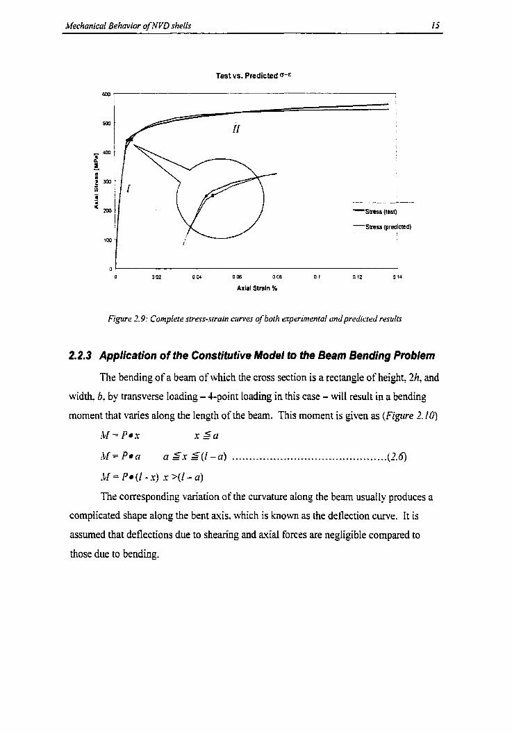
predicted results are depicted in Fignre 7.9.

fest vs. ~redfcted Data

ao

Figure 2.8: Erperirnenraf crndpredicredsness-srrain aimes for the ai41 [enrion tesr

ibfechanical Behavior of NVD shells I j

Test vs. Predicted 0-E

mo i

Figure 7.9: Complere srrrss-srruin cimes of borh experinrenful undpredi~.led resulrs

2.2.3 Application of the Constitutive Mode1 to the Beam Bending Problem

The bending of a beam of which the cross section is a rectangle of height, 2h, and

width. b. by transverse Ioading - Cpoint Loading in this case - will result in a bending

moment that varies along the length of the beam. This moment is given as (Figure 2. IO)

!1.I = P.x x s u

!Cf = P.a a S x S ( i - a ) .....,.......,,,............-.-...... ...,..... ..... Q-6-I

-11 = P . ( [ - x ) x > ( / - a )

The corresponding variation ofthe curvature dong the beam usually produces a

complicated shape along the bent axis. which is knom as the detlection curve. It is

assurned that deflections due to sheâring and axial forces are negligible compared to

those due to bending.

Mechanical Behavior of NVD shells 16

Figure 2. IO: Bending niomenr in 4-poinr brom brnding srnicrirrr

The downward displacement. y. of any pmicle on the longitudinal a ~ i s of the

bearn is assurned to be srnall compared with the dimensions of its cross section. Then the

local curvature olthe bent avis is numerically equal to 9. to a close approximation. If 2.r -

# denotes the counter clockwise single which the tangent to the deflectïon c u v e makes

with the x axis. then

The second expression is consistent with the fact that the curvature is positive

when the bent b e m is concave upward. Since the moment. 1M. is a known tùnction of ..c,

the shape of the deflection cuve can be determined by direct integration of th2

differentid equation, if possible.

We have seen from Eqziations 2.1 and 2.5 that the material suain-hardens

according to the law

Mechunical Behavior of NVD shells 17

where E,. is the main related to the stress at the assurned yield point, the point at the end

of Part 1 ( Figiirr 1.6).

In view of the symmetry of the cross section. the bending moment at any stage is

given by,

h

M = 2 b 1 a - y - d y O

v but E =-.3 y =E-R.and r[v = R a d &

R

The value of the moment, MI. from Eqziuiion 2.8 can be calculated as

which gives ML as a function of EI, Le.. =A&!)-

The second part of the expression of moment. hi~: in Equation 2.9, cannot be

gïven in a cIosed forrn, and the software ~ t l a t h d PLUS. Version 6.0 is used to

Mechanical Behavior ofiVVD shells 18

nurnerically solve this integral. The answers are put in tabuIar t o m for certain vaIues of

6,. Once the second part of Eqzrafion 2.9 is reached, the tirst part is easily catcdated by

substituting the vaIue of E, (from Figure 2.6) into Eqirurion 2.10.

From Equations 2.9 and 2.10' finding &as a hnction of hf, -the inverse of the Ml

funcrion? f "(LW, j or hf2 is not easily accomplished. The problem is analyzed in tabular

fom, yielding discrete values of E, = f "(M,,). The latter will give discrete values of the

1 local curvature - .

R

1 By ~ l a t i n g the discrete values of - to that of Eqirnrion 2. ;i. and applying the

R

Finite Difference k h o d and the bending moments. hl,, from Eqrrufion 2.6. the values of

bearn deflections. y,, for diilèrent points dong the span of the bearn can be easily round.

Detailed tabuIar calculations of the values of b e m deflections. y,, are givsn in Appendix

A*

2.2.4 Modelling Resuits

The behavior of the load-deformation curves of the beam-bending problem, based

on the constitutive Iaws described earlier. shows satisfactory results once cornpared CO

those found experimentally. Figwes 2. Z i and 2-12 show predicted vs. experimental

resuIts at the mid-spans of the beams for Tests 1 and 7.

2.2+5 Application of the Constitutive Model in NVD Mould Design

It is imponant to note that the nickel sheII is mainiy exposed to pressures exened

by the moulded (injected) matenal. which is dependent on the process used. Wu (199 1)

divided the pressure profile of an injection cycle according to the moulding phases and

showed that peak loding occurs during the phase associated with the mould fil1 up.

compression applications. on the other hand. e.xhibit pressure profiies that can be

considered constant tfiroughout the cycle. For mechanical mould design, cavity pressure

is assurned uniformly distributed on the projected mouid areas wenges, 19931. Based on

this assumption, as we11 as on the constitutive mode1 derived in Section 2.2, the behavior

of the W D shelI is projected as (Figure 2.13):

iMechanica1 Behavior of NVD shells 19

1. During first load, the NVD shell exhibits an elasto-plastic behavior and

follows the AB curve until it reaches its peak loading phase;

2. While unloading, the sheli's response is linear and follows line BC. At this

stage? some strains, E ~ , are locked in the shell and the backing system;

3. [f the process exerts the same peak loads during mould filling, then the

nickel material will stabilize after the first rinload. and assume a linear

response thereafter. This is represented by the unloati-refond Iine (Line

BO. 4. If the peak load is not constant, the highest value reached in any moulding

cycle will be considered as the peak Ioad. M e r this point the behavior of

the NVD shell is assurned linear (as in Part 3).

In modelling. it would be preferable to assume linear behavior (line BC) for the

nickel shell. As discussed above. this will not account for plastic strains Iocked into the

sheii on initial peak loading. However. a process for approxirnating the magnitude of this

plastic behavior can be developed. as follows:

1. Examine the results of the Iinear model in terms of stresses and strains

applied to the nickel shell:

2. Locate critical stresses in the nickel shell:

3. Substitute the critical stresses from ( 2 ) in the constitutive model

(Equations 2.1 and 2.9 and calculate the values of k i r corresponding

total strains:

4. Compare the calculated strains From (3). G. to the predicted strains From

(l)? sm, and find the (plastic) mains, E,, locked in the nickeI sheIl as

Ep = E, -&,

5. Check ifthe values of E, meet the mould specifications.

If the manufacturer uses acceptability criterion based on strains. the above process

may be used direcdy. However. if the acceptability criterion is based on deflection.

plastic strains, q,, need to be integrated to obtain deformations, y,? similar to the mamer

Mechanical Behavior of iVVD shells 20

demonstrated in Section 3.3.3, but modified to account for the boundary conditions

particular to the manufacturer's mould geometry and production process,

2.3 Conclusions

The main objective of this work is to gain better insight into the elasto-plastic

(strain hardening) behavior of NVD material seen in the mess-strain curves of

some axial tensionkompression tests. This was accompIished by tinding a

constitutive Iaw that best fit the stress-strain results of the a i a i

tension/compression tests (Section 2.2.2). thsn incorporating this model into the

results fiom the beam bending tests (Section 2.2.3). The modeiling results

showed good agreement with those found sxperimentdly. Some guidelines are

given for using the constitutive model in NVD mould designs.

O 0.5 t 1 5 Z 25 1 3 5 4 a 5 5

h l o m a b n [mm]

Figure Z 1 I I : Load-dclJomarim ~lrries for erperin~entul (Test lj ïs. prrdicredresrrI~s of beum bending mode!

!Clechunical Behavio of NVD shells 71

Predicted va. Experimental Load-Oefonnation (TEST 2)

BO -- - - - - I

O as t 7 5 2 t5 3 3 5 i 4 s 5

üefonnatlon [mm]

Figure 2.17: Load-deformution ciirves for rrperimenrul (Tesr 2) vs. predicred resulrs of benm

bending mode1

Design of Backing 2 Systems for NVD Moulds

The fmt part of this chapter analyses the mechanical behavior of NVD shell-

moulds depending on the design of their backing systems. This part surnmarizes nvo

chapters that were previously contributed by the author to a manual handbook on NVD

mould design [IRDI. 19971. The second part discusses the experimental testing carried

out on nvo NVD backing-tillers. resin epoxy and polymer concrete. A triaiciai test was

conducted on resin epoxy specimens. based on which a proposed constitutive mode1 is

given. An overview of polymer modified concrete is also given. followed by the results

of uniaxial compressive strength tests.

3.1 Conventional Backing Systems

The first step into analyzing the backing systems of NVD moulds is to quanti@

the operational factors that constrain any mould design in generai. and NVD moulds in

particular. This was accomplished by approaching a goup of experienced modd

designers who were able to identifj some of the important pararneters affecting the

backing design of NVD moulds. which c m be summarized as.

materi id composition of the moulded product

Pressure and temperature used in the moulding process

Geometry of the she1I

Size of the product and. consequently, size of the shell

Depending on these pararneters, four types of NVD backing systems are currently

used in the industry. ïhese are: soIid steel backing, rib structure backing, rib structure

and epoxy backing, and mass-cast epoxy backing systems.

Design of Backing Sysrems for 1VVD rl.lou1ds 73

3.1.1 Solid Steel Backing

A solid steel backing system utilizes a block of steel on the back of a sheI1 to

provide adequate support. The back of the shell is first machined flat then integrated into

the steel block either by welding or with threaded studs. This system can be used for

shells with simple (flat) geometry so that it is easy to machine and instdl the solid steel

backing while keeping a good contact with the shell (Figure 3.1).

Figure 3.1 : Solid Steel Backing

3.1.2 Rib Structure Backing

This system is nortnally used for relatively srnaIl moulds and for low-pressure

processes. The advantage of the rib structure is that it is easy to install on the back of a

sheii ~14th slightly irregular geometry (Figure 3.2). However. support provided is notas

good as in the case of solid steel backing. [n addition. if the geometry of the shell is very

irreguiar, it becomes inconvenient to fit the rib structure to the given curvature.

3. f.3 Rib Structures and Resin Epoxy Combination Backing

composite system is usually used for large modds and cornpiex geornetry in

high-pressure applications. The resin epoxy is used to Fi11 the small gaps or deep holes

Design of Backing Systems for NVD ~bloulds 24

that cause dificulties in installing steel ribs. In order to guarantee minimum deformation

of the sheil, epoxy fillers are normally backed by mounting steel kames or ribs on them

(Figure 3.3).

3.1.4 Mass-Cast Backing

Mass-cast backing consists of a relatively rigid steel box containing a nickel shelI

of irregular shape and a backing Filler. The box is itself backed by the platens (Figure

3.4). This system is more flexible than rib and epoxy backing, and thus fits a wide range

of applications in which steel ribs are not capable of providing enough conveniently

installed support. The type of filler used for mass-cast backing varies with the rnoulding

process. for example. resin eposy is used for high-pressure applications (over 10 MPa)

and polymer modified concrete is used for low-pressure applications.

AFTER INJECTION

PLANE -A-

i l- ?.., ,.

PLANE -0-

Figure 3.7: Rib stnicture backing

Design of Backing Systemsfor NVD ltfolifds 25

BEFORE INJECTION PLANE -A-

/ Prrsiurm-

AFTER INJECTION PLANE -8-

Figrire 3.3: Rib srrnctrrres und rpo.ry combincition bncking

Non Octonninq Structurn (Bock Plot.)

BEFORE INJECTION FRONT VlEW

\ -. \ j i r ! v ; ! i r -s lutc

AFTER INJECTION FRONT YiEW

Design of Bwking Sysrems for IVVD ~Wurdds 26

3.2 Modelling NVD Moulds

As a general principle, moulds must be designed with their permissible

deformation in mind. Since deformations m u t be small, computing the static behavior is

sufficient. Complex configurations make most moulds statically indeterminate systems;

however, calculations of the expected deformations and stresses requires the use of either

simplified analytical rnodels (bearn or shell theory) or numerical finite element analysis

(FEA) for close approximation, depending on the type of backing system used. For

example. analytical approaches are applied to solid steel backing and rib structure

backing systerns, while FEA simulations are utilized for rib and epoxy backing and mass-

cast backing systerns.

3.2.1 Modelling Solid Steel Sacking

This system is mainly used for backing NVD moulds in compression applications.

Since the system is comprised of a llat steel plate backing a flat nickel shell (Figure 3. i),

the shear stresses çan be ignored and the stresses dictating the behavior ofboth the steel

plate and nickel shell are only compressive. Analyzing the mode1 in compression is not

required. since no tàilure is expected to occur under the given loading and boundary

conditions.

The critical issue in this mode1 is the stiction force generated during dernoulding -

when the two moulds are puiied apart by means of'uniform' clamping f0rce.p. but the

moulded part sticks to the mouid faces. thus generating an elastic force called stiction

force (Figtcre 3.9. The main concern is to check the stresses and deformations in the

nickel shell due to this force.

After applying the loading and b o u n d q conditions. the problem becomes

equivaient to that of a sotid plate on an elastic foundation: the plate is supported

continuousIy dong its bottom by a foundation, which itself experiences eIastic

deformations. The foundation reaction forces. stiction forces in this case, are assumed to

be linearijproportional to the pIate deflection at any point, Le.. (y k), where y is the

Design of Backing Systems for iVVD hfo1tldr 27

plate deflection and k is a constant, termed as the modzrlus of thefiundation or bedding

constant, which, in this case is a characteristic of the moulded material. The bedciing

constant. k. has the dimensions of force per unit area of plate per unit deflection (e.g.,

Pdm).

The above principles lead to equations. which are easiIy input into a ~Wicrosoft

~wl" spreadsheet. The input parameters are the thickness of the NVD shell, r . the pitch

ofthe studs in two directions. clx b. and k. The output results are found in tenns of the

mavimum moments. h$, mcc~imurn deflections. y. and maximum stresses. ~ ( s e e

Appendix B for output details).

Figrrre 3.5: .LIodrIling soiid bucking system

3.2.2 Modelling Rib Structure Backing: Flat Shells

1. Analysis of Nickel Shells

The problem is that of a fiat plate under a uniformly distributed load, supported by

continuous ribs which are equaily spaced. Due to the symmetry in Ioading and boundary

conditions. the plate c m be modelled in a two-lever arrangement: loads acting on the

mould are f i s t received by the sheli surface, then transferred to the secondary members

(nbs), which, in tumt t r a d e r them to the platens (Figzire 3.6). The problem cm thus be

modeIIed using a simplified beam theory, by anaIysing the system as a continuous beam

Design of Backing Sysems for NFD MoulrLF 8

(NVD shell) on periodically spanned steel ribs. First, the section of the beam and the rib

spacing are defined, atier which the section of the ribs is determined.

2. Analysis of Ribs

Ribs are modelled as compression members. Dependig on their height, the ribs

could fail either by crushing (short colurnns) or by instability, also knovm as buckling

(long cohnns).

L Non Dcforming

Structure (Platen) \ t-1

N V D

Figure R 6: Schrmutic und rnodelling of Rib Strircrurc Bucking:/lut shefis wifh ribs

3. Results and Discussion

As in the design ol'any continuous beam. it is important to ensure the foilowing:

1. The member is capable of withstanding the given moments (stresses)

associated with the Loading and boundary conditions;

7. The maximum defiection of the member has to conform to the allowabIe

defonnations; and

3. The size of the structure at any specsc point shodd be based on the criticai

Ioading.

Based on these factors, the rib structure backing mode1 is anaiyzed and

programmed into a illicroso$ ~xcel@ spreadsheet? having the thickness of the nickel sheIl

Design of Backing Sysrems for NVD rbfouldî 29

and the span between the ribs as input parameters. The output results are expressed in

terms of hiy. y, and u(see Appendix B).

3.2.3 Modelling Rib Structure Backing: Curved Shells

In order to be able to handle curved shells analytically, simplified versions must

be considered. In practice, a shell surface may assume virtually any shape, but shells

with complex designs can be decomposed into simpler foms of localized curvatures, to

which a simplified shell theocy can be applied, provided that both loading and boundary

conditions are satisfied. Common forms of curvature include rotational surfaces

genented by the rotation of a curve about an axis (e-g., surface of revolution: spherical,

eiiiptical. parabolic etc.), translational surfaces generated by sliding a circle along an avis

(e.g.. cylindrical surfaces). and other complex surfaces formed by various combinations

of rotations1 and translational surfaces. Figure 3.7 shows two sxamples of curved shells.

surface of revolution and cylindrical surface.

Loads applied to shell surfaces are camed to the ground supports by the

development of compressive. (ensile. and shear stresses acting in the in-plane direction of

the surtàce. NVD shells are analyzed as :hin shell structures. which are uniquely suited

to carrying distributed loads. but usually unsuited to carrying concentrated loads.

Results and Discussion

Based on previously noted factors on beam design (Section 3.2.2, Part 3), the

input parameters of this models are the NVD shelI thickness. t. the angle Frorn the verticai

to the end of the shell. 4. and the radius of curvature in the section. r,. The output results

are d~scribed in terms of the ma~imurn a ~ i d forces. N. shell deilection. y. and mavimurn

nomai stresses. ~ ( s e e Appendix B).

Rib structures are modelIed as compression members similar to those of flat sheUs

(Section 3.2.2. Part 2).

Design of Backing System for NVD ~Moulds 30

a) Sheil ot'revolution

b) Cyiindrical surface with parabolic section

Figure 3 . 7 E~umples of simpiijed c i i d sheiis

3.2.4 Modelling Rib Structures and Epoxy Combination Backing

More emphasis in this Chapter is given to the mechanical behavior of nickel shell

rnoulds backed by epoxy FiIlers. Due to the compiexity ofthese structures, the analysis of

the composite beam (NVD sheIl + epov-backing) cannot be handIed analytically and a

numerical FEA approximation is considered using ABAQUSIStandard to study the

mode[.

Design of Backing SystemsfOr NVD ~Llotrids 3 1

1. Modelling of the Rib and Epoxy Backing Systern

This model studies the behavior of NVD sheI1s in bending, due to uniform-

injection pressure, using the rib and epoxy backing. The system problem comprises a

composite flat plate under a uniformly distnbuted load, supported by continuous ribs

spaced at equal spans. Loads acting on the mould are first taken by the NVD shell

surface and then transferred to the epoxy-fitler. wtiich transfers the load to the secondary

members (ribs). then to the platens (Figure 3.8 and 3.9). The problem is thus simulated

as a continuous composite-bearn (NVD shell+ epoxy) on periodically spaced ribs.

Moments. their consequent stresses, and shell deformations are analyzed in this

model. The main three parameters in this design are the NVD shell thickness. fshe/[, the

epoy thickness, tep,,, and the spacing between ribs. 1. A sensitivity study is also

conducted to check the effect of these parameters on the bending behavior of the nickel

shell.

The steel rib structures are considered as members in compression. and their

analysis is canied out (analytically) as before.

Non Ddorming

StmctuqPlaren)

Figure 3.8: Schemaric representacion of rhe ri6 and epoq backing system

Design of Backing Systems fir W D Moiilh 32

Pressure

Figure 3.9: iClodelling of rib and epo-ry structure

2. Geometric Modelling

This model considers flat sheil geometry. although the srme principles apply to

curved shells. In this model of uniforrn loading and a tlat surface. a simple mesh will

suffrce. The NVD shell is modelled using beam section with rectangular cross-section of

type B21. two node linesir beam, with three degrees of freedom. 1.2. and 6 at the nodes.

These elernents use Simpson's rule as the integration method with !ive points through the

shell's thickness. which is adequate to give a reasonably smooth response. The resin

eposy filler is modelled using contincum plane stmin element type CPES. which is a 4-

node bilinear quadrilateral element with two degrees of Freedom and four integration

points. Material properties are defined using elastic parameters. which are given in terrns

of Young's modulus. EvrD = 90 GPa and Eepo.rv = 23 GPa , and Poisson's ratio. V , V I ~ 0.3

and vepo.v= 0.21 4. for the .ND shell and resin epoxy fillers. respectively.

The number of elements in the model depends on the length of the NVD sheII and

the thickness of the epoxy, rnaintaining the sarne aspect ratio for the continuum solid

elernents.

3. Results and Discussion

Based on previously noted factors on beam design (Section 2-22 Part 2), bending

moments and deflections are fust checked to study the effect of the epoxy backing,

Results show that the epoxy fiIIer significantly increases the capabüity ofNVD sheiis, as

Design of Backing Systems for NVD rbloulds 33

compared to rib structure backing without epoxy. Table 3.1 illustrates a sample of these

results.

Table 3.1: Effecc! of r p o . ~ ~hickness on moment and deflecrion

[ Pressure 1 Span 1 NVû Shell thickness 1 Epoxy thickness 1 Moment 1 Deflection /I

4. Sensitivity Study As mentioned earlier. the three parneters affecthg the backing design are the

thickness of the NVD shell. the thickness of the epoxy and the span between the ribs. In

order to check the influence of each of these parameters. a sensitivity study was carried

out a!j follows.

1. Different shell thickness values were modelled (r,h,(l= 10. 1 5 70. 25, und 30

mm). and results show that increasing the thickness of the shell increases the

bending moment. but significantly decreases the deflection of the member

(Figrire 3.10 and 3.11).

2. Different epoxy thickness values are considered (tep,= 0, JO, 100, und 150

mm). showing that increasing the thickness of the epoxy will decrease the

bending moment in the nickel shell. as wel1 as its deflection (Figzire 3.11 and

3.12).

3. The mode1 is tested using diffecent spans between steel nbs (l=IjO, 200, 300,

jO0 mm). Results show that increasing the span increases both the moments

and the deflections of the member.

Design of Backing Systenis for lVVD hfoul& 34

Bending Moment vs. Span between Ribs

lm,

Figrire 3. IO: B e n h g niamenu vs. spun ben~een ribs for dtflerent shell rhicknessa in u rib und rpo-v

ntorlrl (rib spacing = 300 mm)

Deformation v a Span between Ribs

O 1w

Figrire 3.1 Ir Shell Defontarions vs. span benwen ribs for diffuent shell thicknesses in a rib and epoxy

modef (rib spacing = 300 mm)

Design of Backing Sysrems for NVD ibfurrlds 33

Bending Moment vs. Shell Thickness

Shell Thickneu (mm)

Figwe 3.12: Btinding monrenrs W. ski1 ihickness for dfferent e p o q rhicknrssrs in u rib urd q u . ~ niudd

/ri& spacing = 3011 mm)

Deformation W. Shell Thlcknisi

Shat Thlckness (mm1

Figure 3.13: SheII dejororarcons vs. sheif rhtckness for differenr q0.y rhicknesses in a rib and e p q model

(rib spacing = 300 mm)mnz)

Design of Backing Systems for IVVD ibfoulak 36

3.2.5 Modelling Mass-cast backing

This model is comprised of a rigid steel box backed with fillers that shouid give

sufficient support to the nickel shell. The box is itself backed by the platens. The actual

problem and its model are illustrated in Figure 3.14.

The type of backing filler depends on the type of moulding process used: some

manufacturers use resin epoxy composites for hi&-pressure applications (over 10 MPa),

while others use polymer concrete composites for low-pressure moulding applications.

The mass-cast system is modelled as fol~ows: loads acting on the mould are first

taken by the NVD shell surface. then transferred to the backing filler. The latter transfers

the loads to the steel box-laterally to the walls of the box. and vertically to the base of the

box-which in tum will transfer the loads to the piatens (Figure 3.14).

Resuits are given in terms of moments, their consequent stresses. and shell

deformations. The main three parameters in the design of the mode1 are the NVD shell

thickness. the thickness of the fiIler or the height of the box. h, and the Iength of the

shell. 1. A sensitivity study was also conducted to check for the effect of these parameters

on the bending behavior of the NVD shell.

Pressure Steel Frameiûox

Plate

Figure 3.13: :tlodeffing oj'mass-cul backing

Design of Backing Systems for iVYD hiou/& 3 7

1. Geametric Modelling

The mass-cast backing rnodel is comprised of the following: the NVD shell,

which is modelled as a beam element: two steel beams simularing the wails ot'the steel

box; and the backing-filler, which is modelled as continuum plane strain elements. For

the type of dements and their materiai properties please refer to Section 3.2.5, Part 2.

The boundary conditions are such that the bottom of the steel box. which is in

contact with the platens. is asurned to be rigid. and hence, the bottom of the backing-

filler is considered fixed.

2. Results

Bending moments and detlections in resin e p o y mas-cast backing are tirst

checked for a given load of 70 MPa. Compared to the resuits ofthe rib and rpoxy

system, and for a given set of parameters. the mass cast backing system showed relatively

inferior resdts. as ilusrrated in Table 3.2.

Table 3.1 I/ulues 01-hending moments und deflections jor nvo backing systems: f 1) rib and epary, und (2) mus-cmt rpo.np.

No. 1 Pressure / Length 1 NVD thickness 1 Epoxy thickness 1 Moment 1 Deflection I/

3. Sensitivity Study

As mentioned earlier. the parameters considered in the mas-cast backing mode1

are the thickness of the NVD shell. the thickness of the epoliy or the height of the steeI

box and the length of the NVD shell. To determine the influence of each of these

parameters, a sensitivity smdy is carrïed out as foIlows:

1, Different nickel shell thickness values are rnodelled (t= IO, 15, 203 25, and 30

mm), Results show that increasing the thickness of the shell inmases the

bending moment as expectedf but sIightly affects the deflections in the member

(Fignres 3-15 and 3.16).

Design of Backing Systems for NVD Mouldr 38

Moment for Different NVD Shell Length

Figure 3 .15 Bending moment vs. lengrh ofNVD Shell for diffeenr shell thickness in a mass-cast backing

mode1

Deformation vs. NVD Shetl Length

a20 ! Span (mm)

Design of'Bocking Systems for NVD Morrlds 39

Figure 3. 16: Shell defirmarions vs. lengrh of NVD Shellfor dlrerenr shell rhickness in a m m - c a r backing

nrodel

Moment vs. Shell Thickness (Pressure = 70 Mpa)

-epoxy ihickness -200 mm

- epoxy ihickness = 300 mm

epoxy ihickness = 400 mm

- epoxy ihickness = 500 mm -... ~ - - ~ ~ ~ -- -- ~.

" . . -

10 12 14 16 la 20 22 Z4 26 26 30 Shell Thickness (mm)

Figure 3.17: Momenr vs. shell thickness for diffirenr rp0.v thicknessrrs in a muss-cas[ bucking mode!

Deformation vs. Shell Thicknesae (Pnrssure-79 MPa)

,a -. . - - - . --- .

. .- . . . . . - . . --- - -..p.- A--

lm. .- .. . .. . ," .A -- -. .

i m :

- epoxy lhicknes = 4üû mm

- epoxy mickneu = 5W mm - - - - - -. - - -

am t I la t t 14 16 :a zo 22 24 2s 28 y1

Shell Thickness (mm)

Figure 3.18: Shell deformutions vs. shell thickness for dflerenr epo-ry rhickneirsees in a mass-casr

backing model

Design of Backing Sysrems for NVD iMouids 40

2. Different epoxy thickness values are also considered (tl= 200.300,400, and

500 mm). ResuIts show that increasing the thickness of the epoxy increases

the bending moment of the nickel sheII. but decreases its deflection (Figures

3.17 and 3.18).

3. The mode1 is tested for different sheII lengths (1=500,700, 1000, and 1500

mm). Results show that increasing the span increases both the moments and

the deflections of the member.

4. Analysis of the Steel Frame Box

The objective of this analysis is to assure the rigidity and stability of the box walls

to minimize lateral deflection. The box walls are modelled as compression members.

a d . depending on their height. they rnight fail either by crushing or by instability, which

is also known as buckling,

Results obtained in terms of bending moments and lateral (horizontal) box wail

deflections. show that increasing the thickness of the corumn (Le., its moment of inertia,

I) increases its bearing capacity.

Since the height of the column depends on the epoxy thickness. the instability of

the Frame is also analyzed, dong with the influence of the epoxy thickness on the bending

moments and deflections of the shell. Results show an increase in the moments and

deflections of the shell with an increase in the epoxy thickness. This agrees tvith Euler's

buckiing method.

3.2.6 Conclusions on fhe Design of ExMing Backing Systems

Modelling results show that the epoxy-fillers in rib + epoxy and mm-cast

backing systems significantly improve the behavior of NVD shells. The main parameters

that affect the design of the epoxy-fiiied backing are the thickness and the length of the

nickel sheil. and the thickness of the epoxy. A sensitivity study on the effect of these

parameters on the backing design, show that increasing the thickness of the sheII

increases the bending moment. but decreases the deflection in the member. increasing the

Design of Backing Svsrems for NVD Morrlds 3 1

thickness of the epoxy in a rib and epoxy system decreases the bending moment in the

nickel shell and decrease its deflection. whereas relatively littie effect on the shell

dehrmations was apparent in the mass cast epoxy system. The length of the shell has

also a major effect on the design. Modelling results indicate that increasing the length

increases both the moments and deflections in the shell. When compared to the results of

the rib and epoxy backing system, and for a given set of parameters, the mas-cast

backing system showed relatively inferior results in terms of NVD shell deforrnations.

3.3 Mechanical Behavior of Resin epoxy

3.3.1 Triaxial Compressive Sfrengfh Test

The main objective of running the trimial tests is to obtain the mechanical properties and

a failure mode1 of the resin epoxy through axial stress-strain (o-E) and axial-vohmetric

strain relations. Two sarnples were used at each of four confining pressures (c3 = 00, 10,

20 and 30 MPa) for a total of eight samples. The tests were carried out at the CANMET

laboratory facilities in Ottawa. The tested epoxy specimens had the following physical

properties (Table 3.3):

Table 3.3: Physical properries oftpoxy specimem

Design of Backing Systems for NVD hloulds 47

3.3.2 Test Results

Collected data were given in table format and analyzed using a crosofr ~xcel"

spreadsheet. Resdts are presented in the forrn of mial stress-axial strain, cri-€1, axial

strain-volumetric strain. E1-EV. for different confining stresses. a;. Material behavior is

also analyzed in tenns of a ~ i a l stress-confining stress! al - O:, for points of peak a i a l

stresses (ultimate strength). These charts are shown in Figures C. 1 ro C. 14. Appendix C,

Test results were also checked t'or failure analysis using both Mohr and Hoek-Brown

criteria.

3.3.3 General lnterpretation

The stress-strain curves of the resin epoxy show a brittle materiai behavior in the

case of no confining pressure. and an increase in ductility as confining stress ( lem

compressive principal stress) increases. [ncreasing confining stress also yields an

increase in both material stiî'fness and strength.

h i a i stress-axial strain relations show elastic linear behüvior up to the initial

yield stress (a,) level. Beyond this point. the material adopts a non-Iinear hardening

behaviour. and non-recoverable plastic strains occur. As stated earlier. test results show

thar the value ofo, increases with increasing conîïning stress. that is. increasing the

material strength as confïning pressure increases. The stress-strain curres show

hardening behavior up to a maximum value-ultimate strength (US), beyond which the

materiai starts softening.

Volumetnc strain and volurnetric strain deviation fiorn Iinear elasticity allow the

determination of stress levels associated with materiai crack growth. Resuits show initial

linear elastic behaviour, foIIotved by non-linear volurnetric strain increase. which is

usuaily associated with stable crack growth. At low confinement (O and 10 MPa), the

materiai did not exhibit any significant volumetric compression, while at higher

confinement (20 and 30 MPa) the materiai showed noticeable volumetric compression,

followed by Linear expansion. Results also show sharp increase in volurnetric strains (as

compared to axial strains), once the materid reaches its peak strength (see Appendi. C)

Design of Backing Sysrrms for rVVD rbfouldr -13

1. Uniaxial strength

The peak unia~ial compressive strength of the resin epoxy specimens was

detennined fkom the raw data to be 1 15 MPa (Figure 3.19).

Axial Stress-Axial Strain (Sigma 3 = O MPa) 'Test UT-2'

140

O ' O.OOE*CQ LW€-O3 4 WE-03 4.CQE.03 6.WE.03 1 WE.02 1 20E-02 l aE.02 1 BOL02 t 80E.02

Axial Slrain Ph]

Figure 3-19: .-i.riul srress-aria1 main for tmiurial lest (sre ulso Figure C. 1 )

In order to achieve the complete axial stress-strain curves of the materiai.

a servo-controlled and displacement based testing machine was used to conduct

the triaxial tests. Axial displacement is programmed to Vary in a predetermined

rnanner, generally monotonically increasing with time [Brady and Bro~m. 19931.

The measured and programmed vaiues are compared electronicaIIy several

thousands of times a second, and a servo valve adjusts the pressure within the

actuator to produce the desired equivalence- Cycles of Ioading and unIoadmg are

thus produced whenever the servo valve reveais the onset of yieIding (Figzrre

3.19).

Design of Backing Sysrems for NVD Mouldr 44

2. Triaxial strength

Data contained in Table 3.4 show that in triaxial tests the ultimate strength

(US) of the epoxy specimens increases with increasing confining pressure fiom

US=115MPaa ta3=OuptoUS=170~aa tc r j=30MPa.

3. Initial Yield Stress

Results show that the initial yield stress, a,, of the epoxy specimens

increases with increasing conEining stress. Table 3.4 shows that the initial yield

stress changes fiom o, = 96 MPa at oj = O up to a, = 108 MPa at o; = 30 MPa.

Initial yield is determined graphicaily using a spreadsheet.

4. Young's Modulus

Young's Modulus was determined as the average of the values o, in the El

linear elastic part of the unia~ial test. It is also taken as the average of the values

a, -Zv <r,

"1 in the linear part of the triztuiai tests, taking into account the

"strengthening" effecc of a;. Test Results show that Young's Modulus does not

change considerably with increasing confining pressure. For example. Young's

moduIus t'or unimial compression. E = 27.32 GPa. while for triaxial compression

(cr; = 30 MPa). E = 22.45 GPa.

Table 3.4: Triuriul (est ratilts

Sample l Confining Stress

No. I

[MPal

1 O

1 O

3 IO

4 10

5 20

Failure Load

rw

A

Peak Stnin

ml

15927

184.9

170.4

6

7

8

Yield Stress

W a l

N/A

Ultimate Strength

[ M W

NIA NIA NIA

10 1 34316

115.4

131.62

143.64

14729

249. 14

185.56

309.06

3 16.78

1-17

116

I.39

30

30

114.39

143.3 1

108.65

399-05

5683 1

0.77 96.03

1-17

1.77

1.73

86.52

115.10

107.68

Design of Backing Systemsfir NVD MouIrLF 45

3.4 Proposed Consfitutive Mode1 for the Resin Epoxy

Two failure envelopes are used to check for the results of rhis test: Mohr circles

and the Hoek and Brown criterion.

inspection of the Mohr circles (Figure 3.20) generated fiom ai and 0 3 data

indicate that a curved envelope analysis method might best describe the failure

envelopes. The Hoek and Brown method which is usually intended for the analysis of

rock-type material was therefore used.

Trimiai and uniaxial tests are usually used in the Hoek and Brown Mure

criterion. The triaxial strength values provided in Tuble 3.4 are therefore used to

determine the failure envdope for each test.

The relationship between the major principal stresses at filure is defined by the

Hoek and Brown criterion as ttollows [Hoek and Brown. 19941:

0, =O* + , / m c p , +su: ...-................-..-.............................. (3.1)

where.

ol = major principal stress at failure

c3 = minor principai stress at failure

oc = unia~ial compressive strength

m, s = material constants depend on material properties.

The Hoek and Brown resuIts are depicted in Figtcre 3.21, and the test results seem

to be in good agreement with those computed theoreticaily, fiom Equation 3.1.

Checking the test resuits and the relation between CI and 0 3 in Eqztarion 3.1, the

average value of m was found fiom each mi related to each c o n f i ï g pressure. This

range of m is typical for brittle materials [Hoek and Brown? 19941. Averaged m was

found to be equd to 2.33. Substituting the vaiue of m back into Eqziarion 3.1 wiIL give

the required values of al ( see Table 3.9.

Design of Backing Systemsfir :VVD iCfoddr -16

Table 3.5: Values of a, rtsing Hoek-Brown criterion

Nomat Stress [MPal

8

Fipre 3.20: Mohr circles for ri axial l e m

m

NIA

NIA

1.48

al (Test)

NIA

115.4

132.67

tr

1

2

3

Figure 3.2 1: Hoek-Brown failwe envelope

o@oek-Brown)

NlA

II5.4

136.67

SIGMA3

O

O

1 O

3.92 1 136.67 4

176.64 30

10

1 70.4

rn (Average)

143.64

1.84

2.36

Design of Backing Sysfems for iVVD rbfoirlJs 47

3.5 Material Properties of Polymer Modified Concrete (HTSOS

Mix)

3.5.1 Introduction to HTSOS Concrete

The industrial partner in this smdy. Blanco Canada Inc., and other moulding

manufacturers, fabricate moulds using NVD sheils backed with polymer-modified

concrete (known as HTSOS concrete). A major disadvantage of this backing is that. in

the event that a mould needs to be repaired or retrotitted due to deficiencies of the

thermal lines. the concrete is so strong and adhesive that the entire backing and thermal

line systems must be stripped and replaced. Minor changes to the shell itself can also

occur during this process- The replacement process is also labor intensive and c m result

in lost production time on the order of weeks.

HTSOS cernent is available in 40 kg-bags in a ready-mix fonn. Due to the lack of

information on the material properties of HTSO5 concrete. an experimental testing

program was recommended to study some of its mechanical properties. mainly its

stiffness and strength characteristics through stress-strain behavior.

3.5.2 Ovewiew of Polymer Concrete

Polymer-modified or polyrner cernent mortar and concrete are a category of

concrete-polymer composites which are made by partially repiacing the cernent hydrate

binders of conventional cernent concrete with suengthening polymer admixtures. Several

types of polyrner admixtures are currently produced in the f o m of latexes, redispersable

polymer powders, water-soluble polymers. etc. Of these, the latex polymers are by far

the most widely used as cement modifiers.

Polymer Latexes and Recitrpersible Polymer Powders

Polymer concrete made Erom latex-modified cernent and cement modified by

redispersibIe polymer powders contain equivaient miu proportions and exhibit similar

material properties. In general. these composites show a noticeable increase in the tensile

Design of Backing Systems for NVD ithdds 48

and f l e x d strengths but IittIe improvement in the compressive strength as compared to

o r d i n q cement mortar and concrete [Fontana et al., 1996; Oharna, 19951.

GeneralIy, redispersibIe polyrner potvders are dry-blended with cernent and

aggregate mixtures. The propenies of the resulting concrete depend on the nature of the

polymer and polymer-cernent ratio. Increasing the latter wil1 improve the materia1

performance.

Objectives

The main objective of this test is to investigate the mechanical properties

of the HTSO5 mix and analyze its suitability as a backing material for nickel shell-

moulds. Specific objectives are to:

1. Determine the uncontined compressive strength of the hardened composite.

3. Decemine the stress-strain behavior of the materid. and

3. Analyze the hydration process by checking the influence of curing age on the

compressive strength.

2, Materials and Mixture Proportions

KTSOS mortar/concrete is easily prepared by using a conventionai mortar

batch mixerhiender. The waterl(cement + aggregate) ratio of 0.25 is used by

Blanco Canada for mould backing purposes. and the speed and tirne of mixing are

selected to avoid unnecessary entrapment of air [Blanco. 19981.

The HTSO5 monar handIes more easily during nkuing than ordiiary

cernent mortars, which rnay be attriiuted to the mix containhg a certain

percentage of water-soluble polymers.

For the sake of our test, the mixed rnortar was placed in 50.8-mm inner

diameter x 110-mm hi& mouids made of ABS pipes. The specimens were then

Design of Backing Spenis for NYD iMo~f& 49

sealed md placed in a room maintained at a temperature of 21' C and 100%

relative humidity for unconfined compression tssting at 2,3,5.7, and 14 days.

Test Results

The unconfined compressive suen+@ tests were conducted in accordance

with ASTM D 1633. Test results show that HTS03 is a high strength concrete

capable of attaining a uniavial compression strength of 40 MPa after two days of

curing. Only elastic and hardening parts of the stress-strain behavior were

deduced from the tests. Test results show a close-to-linear behavior that is

generally ductile up to the peak load-point of rupture (Figure 3.27). Test data

dso indicated an average uniaxial strength cf 45 MPa (at 7 days) with a Young's

modulus in the range 0123.0-37.0 GPa.

The effect of age on compression strength values is s h o w in Figure 3-23.

The unconfined compressive stren-gth does not change markedly with additional

curing time becomins mari); constant at the age ofthree days.

Figwe 3.27: Aria/ stress-srrain behmior of nvo HTSO5 concreze specimens iested 4ter 7 days

curing

Design of Backing Systemfor NVD ~Moufdr 50

Uniaxial StressStrain

5 m . .

am O 2 1 6 3

Curing Aga pays]

Figure 3.23: Mean compressive srrengfh LX uge ut resfing Jor HTSûS cuncrefr specimens

Usina Fly Ash Composites for Backing

Nickel Shell-Moulds

4.1 Introduction So Far. only conventionaI NVD mould backing systems have been examined, with

emphasis on high-pressure applications, among which mas-cast backing is considered

the most flexible system For handling cornplicated mould geornetry. While some

manufacturers have used concrete and resin-epoxy composites as mas-cast backing

fillers. their main design consideration appears to be srrengrh of the filler material. In

fact, it was s h o w from the compression test results (Chapter 3) that the average

unconfined compressive strength of resin-epoxy and polyner concrete is 1 10 MPa and 45

MPa. respectively. However. for moulds subjected to predominantly compressive

stresses. the main design considention of the backing fillers should be srifjness. This

notion was the cornerstone to the proposed aiternative backing filler for NVD shells. that

is îly ash cmposite backing.

Knowing that fly ash composite is a rnix of fly a h ' cement, smdt and waeer, the

probiem is to define the optimal rnix design for a given rnould and moulding application.

This requires extensive experimentai cesting on different fly ash composite mixes,

varying the ratios of: fly a h . cement. and sand. Experimental testing was aimed at

studying both thermal conductivity and mechanical stimisss/strength properties.

4.1.1 Design Parameters of Composite Fillers

As noted in Chapter 3, the industrial parmer in this study, Blanco Canada, uses

polymer-concrete b a c h g for their proprïetary modding application. Net ~\/lorilding.

The main disadvantage in usine concrete rnass backing is the difficulty rebuilding the

modd in the event that the therrnd Iines need to be repaired or reconfigured. The

disadvantages are that:

Using FIy Ash Composites for Backing Nickel Shell-Moulds j2

1. The moulds are very time consuming to build and break (40-80hs);

2. There is a high risk of darnage to the nickel shell (cost $20,00OS30,000):

3. No partial repair or replacement of one thermal line is possible;

4. The concrete backing c m crack during its expected life time; and

5. Insufficient heat insulation and consequently, higher thermal diffusion than

required by the process.

The main design pararneters of the proposed fly ash composite fillers are

therefore:

1. Provide adequate structural support for the nickel shell;

2. Provide thermal performance appropriate to the manufacturing process:

2. Ensure easy placement in the mould's irregular geometry,

4. Ensure npid curing; and

5 . Make the backing easily removable for repair or reconfiguration of the

rnould's thermal lines.

Based on the above listed pararneters. the proposed composite filler should

possess the following properties (appropriate values for each parameter are based on

andysis from Section 3.4. modified to account for any differences in the Net Mouiding

process) :

Mechanical Properties

1. Relatively High Stifiess: the proposed mix should have a minimal buIk

modulus of 2 GPa for adequate stiffness:

2. Relarively Low Srrengrh: the uniaxial strength of the new backing shodd

range between 5 to 8 MPa to allow better extraction during rnould rebuilds;

3. High Eurly Srrengrh: the proposed mix should be abIe to cure rapidIy and

reach a uniaxial strength of 5 MPa in a few days;

4. High triuxial strength: the proposed mix should exhibit notabIe uicrease in

both s t f i e s s and strength under high conhement.

2. Physical Properties

1. Maximum density upon compaction

Using Fly Ash Composites for Backing Nickel Shell-iGloitlk 53

2. Low water content

These properties can be investigated using compaction tests. Mixes with high

densities and low water content upon compaction are preferred.

3. Thermal properties

1. Compatible with the Net Morrlding process, which requires the mix to have a

w thermal conductivity less than 1 -

"C.m

4.1.2 Options for Composite Mix Design

Based on a Literature review, tly ash composite couid be utilised in any of the

following ways:

1. Fly-ash-stabilised sand mixture.

2. Fly ash-sand-cement composites. and

3. Compacted tiy ash stabilised with lime or cement.

4.2 Literature Review of Fly Ash

4.2.1 Origin of Fly Ash

Fly ash is a by-product of coal combustion in power plants which is produced in

large quantities in many counuies. Fly ash produced from the burning of pulverized coal

in a coal-tired boiler is a fine-grained, powdery particulate material that is carried off in

the flue gas and usually collected from the flue gas by means of electrostatic

precipitators, baghouses. or mechanical collection devices such as cyclones. In general,

there are three types of cod-fired boiler furnaces used in the electric utility industry.

They are referred to as dry-bottom boilers, wet-bottom boilers, and cyclone furnaces.

The most common type of coal burning furnace is the dry-bottom h a c e . A general

flow diagram of fly ash production in a drybottom coal-fired utility boiler operation is

presented in Figure 4. i.

Using Fly Ash Compositesfor Backing !Vickel Shell-Moulls 54

Figure 4.1: Production o f j y ash in a dry-bortom uriliy hoikr rvith electrostaric precipifution Urom

Bubcock and Wilco,~, 1978)

Fly ash to be used in Portland cernent concrete (PCC) must meet the requirements

of ASTM C 6 18. Ttvo classes of fly ash are defined in ASTM C6 18: 1) Class F fly ash.

and 2) Class C ily ash. Fly ash that is produced from the burning of anthracite or

biturninous coal is typically pozzolanic and is referred to as a Class F fly ash if it meets

the chemicai composition and physical requirements specified in ASTM C618.

Materials with pozzolanic properties contain glassy silica and alumina that will, in the

presence of water and tiee Lime. react with the calcium in the lime to produce calcium

silicate hydrates (cementitious compounds). Fly ash that is produced from the burning

of Iignite or subbituminous coal. in addition to having pozzolanic properties. also has

some self-cementing properties (ability to harden and gain men,@ in the presence of

water alone). When this fly ash meets the chemicai composition and physical

requirements outlined in ASTM C618. it is referred to as a Class C tly ash. Most Class C

fly ashes have self-cementing properties.

4.2.2 Material Properties of Fly Ash

1 - Physical Properties

Fly ash consists of fine, powdery particles that are predominantly

sphericd in shape, either soiid or hoUow, and mostly giassy (amorphous) in

Using Fly Ash Composimfor Backing Nickel SheU-Moul& 55

nature. The carbonaceous materid in fly ash is composed of angular particles.

The particle size distribution of most biruminous coai fly ashes is generally

similar to that of a silt (less than a 0.073' mm or No. 200 sieve). Although

subbituminous coal fly ashes are also silt-sized, they are generally slightiy coarser

than bituminous coal fl y ashes [DiGioia, 19721.

The specific gravity of fly ash usuaily ranges from 2.1 to 3.0, while its

specific surface area (measured by the Blaine air permeability method) may range

h r n 170 to 1000 m'/kg [ASTM C204,1994]. The color of fly ash can vary

frorn tan to gray to black. depending on the arnount of unburned carbon in the ash.

The lighter the color. the lower the carbon content. Lignite or subbituminous fly

ashes are usuaily light tan to butT in color. indicating relatively low amounts of

carbon as well as the presence of some lime or calcium. Bituminous fly ashes are

usually some shade of gray. with the lighter shades of gray generaily indicating a

higher quality of ash.

C hemical Properties

The chemical properties of fly ash are infiuenced to a great extent by those

of the coal burned and the techniques used for handling and storage. There are

basically four types. or ranks, of coal. each of which varies in terms of its heating

value. its chemical composition. ash content. and geologicai origin. The four

types. or ranks. of coai are anthracite. biturninous, subbituminous, and lignite. In

addition to being handled in a dry. conditioned. or wet form. fly ash is also

sometimes classified according to the type of coai fiom which the ash was

derived.

The principal cornponents of bituminous cod fiy ash are silica, durnina

iron oxide, and calcium. with varying amounts of carbon. as measured by the loss

on ignition (LOT). Lignite and sub bituminous coal fly ashes are charactenzed by

higher concentrations of calcium and magnesium oxide and reduced percentages

of silica and iron oxide, as well as a Iower carbon content, compared with

Using Fly Ash Composites/or Backing Nickel Shell-Moulds 56

bitminous coal fly ash weyers, 19761, Very little anthracite coal is b m e d in

utility boiiers. so there are only smail amounts of anthracite coal fly ash.

Table 4.1 compares the normal range of the chemical constituents of biturninous

coai fly ah with those of lignite coal îly ash and subbituminous coal fly ash

[ACAA. 19961. From the table, it is evident that lignite and subbituminous coal

fly ashes have a higher calcium oiride content and lower loss on ignition than £Iy

ashes from bitwninous coals. Lignite and subbituminous coal fly ashes may have

a higher concentration of sulfate cornpounds than bituminous coal fly ashes.

Tuble 4. Ir Normal range of chemical composirion forjly ash producedfrom d~rereni coal types(erpressed as percent by rveight).

11 COMPONENT I BITUMINOUS 1 SUBBITUMINOUS 1 LIGNITE]^

The chief difference between Class F and Class C fly ash is in the amount

of cdciurn and the silica, alwnina and iron content in the ash [ASTM C204.

19941. In Class F fly ash. total calcium typically ranges from 1 to 12 percent,

Na10 KzO LOI

mostIy in the form of calcium hydroxide, calcium sutfate, and glassy components

in combination with silica and alumina. In contrast, Class C fly ash may have

reported calcium oxide contents as high as 30 to 40 percent McKerall. 199821.

Another difference between Class F and Class C is that the amount of alkalis

0-4 0-3 0-1 5

(combined sodium and potassium) and sulfates (SOJ) are generally higher in the

Class C fly ashes than in the Class F fly ashes.

Althou@ the CIass F and CIass C designations strictly apply only to fly

ash meeting the ASTM C618 specification, these terms are ofien used more

0-2 0-4 0-3

J

0-6 0-4

-

0-5

Using Fly rlsh Composites for Backing Nickel Shell-ibloulh 57

generally to apply to fly ash on the basis of its original coal type or Ca0 content.

It is important to recognize that not al1 fly ashes are able to meet ASTFvr Cd 18

requirements, which are necessary for PCC applications.

The loss on ignition (LOI). which is a measurement of the amount of

unburned carbon remaining in the fly ash. is one of the most significant chemical

properties of fly ash, especially as an indicator of suitability for use as a cernent

replacement in concrete.

4.2.3 Use of Fly Ash

1. Fly Ash as Admixture to Concrete

Fly ash has been successtùlly used as a minerai admixture in PCC for

various purposes for nearly 60 years. This is the largest single use of fly ash. It

can aIso be used as a feed materiai for producing Portland cernent and as a

component of a Portland-pozzolan blended cement.

Fly ash must be in a dry form when used as a mineral admixture, Fly ash

quaiity must be closely monitored when the material is used in PCC. Fineness,

loss on ignition. and chemical content are the most important characteristics of fly

a h affecthg its use in concrete. Fly ash used in concrete must aiso have sUfEcient

pozzolanic reactivity and must be of consistent quality.

Fly ash has been used extensively in mass concrete structures like dams,

nucIear reactors and other important structures al1 over the world. Moreover' fly

ash has been investigated and used for mass concrete structures exposed to

elevated temperatures. Marzouk (1979) tested mass concrete containhg

Saskatchewan fly ash and showed that temperatures have only minor effects on

both strength and elasticity up to 71' C, resulting in an increase in strength for the

temperature range of 121 to 149 C. Marzouk attributed this increase in strength

to the secondary hydration process, which takes place between the hydrated üme

and fly ash to form a new, highly cementitious tobemorite geI.

bsing Fiy dsh Conrposiresfor Backing ~Vickd Shell-i\.lottlds j8

Asphalt Concrete - Minera1 Fill

Fly ash has been used as a substitute mineral filIer in asphalt paving

mixtures for many years. Mineral filler in asphalt paving mixtures consists of

particles, less than 0.075 mm (No. 300 sieve) in size. that fil1 the voids in a paving

mix and serve to improve the cohesion of the binder (asphalt cement) and the

stability of the mixture. Most fly ash sources are capable of meeting the gradation

(minus .O75 mm) requirements and other pertinent physical (nonplastic) and

chemical (organic content) requirements of mineral filler specifications.

Fly ash must be in a dry form for use as a minerai filler. Fly ash that is

collected dry and stored in silos requires no additional processing. It is possible

that some sources of fly ash that have a hi& lime (Cao) content may also be

useful as an antistripping agent in asphalt paving mixes.

Flowable Fill- Aggregate or Supplementary Cementitious material

Flowable fiII is a slurry mixture consisting of sand or other fine aggregate

materiai and a cementitious binder that is norrnally used as substituts for a

compacted eartii backfill. Fly ash has been used in flowable fil1 applications as a

fine aggregate and (because of its pozzolanic properties) as a supplement to or

replacement for the cernent. Either pozzolanic or self-cementing fly ash can be

used in flowable fil1 [ACI, 19941. When large quantities of pozzolanic fly ash are

added. the tly ash can act as both fine aggregate and part of the cementitious

matrix. Self-cementing fly ash is used in smaller quantities as part of the binder in

place of cement.

The quaiity of fly ash used in flowable fiIl applications need not be as

strictly controlkd as in other cementitious appIications. 00th dry and reclaimed

ash fiom settiing ponds c m be used. No speciai processing of fly ash is required

pnor to use.

Usinrr Flv Ash Composires for Backing ~Vickel Shell-Mouldr 59

Embankment and Fill Matenal

Fly ash has been used for several decades as an embankment or structurai fiil

material, particularly in Europe. There has been relatively limited use of fly ash LX

an embankment material in North America. although its use in this application is

becoming more widely accepted.

As an embankment or fil1 materid. fly ash is used as a substitute for natural

soils. Fly ash in this application must be stockpiled and conditioned to its

optimum moisture content to ensure that the materia1 is not too dry and dusty or

too wet and unmanageable. When fly a h is at or near its optimum moisture

content. it can be compacted to its maximum density and will perform in an

equivalent manner to well-compacted soil

4. Fly Ash as Soil Stabilizer - Supplementary Cementitious Material

Stabilized bases or subbases are mixtures of aggregates and binders. such as

Portland cernent. which increase the strength, bearing capacity. and durability of a

pavement substructure. Because fly ash may exhibit pozzolanic properties, or self-

cementing properties. or both. it c m and has been successhlly used as part of the

binder in stabilized base construction applications. When pozzolanic-type fly ash

is used. an activaror must be added to initiate the povolanic reaction. Self-

cementing fly ash does not require an activator. The most commonly used

activators or chernical binders in pozzolan-stabilized base (PSB) mixtures are

lime and Portland cement, aithough cernent h l n dusts and lime kiln dusts have

also been used with varying degrees of success. Sometimes. combinations of lime,

Portland cernent. or kiln dusts have aIso been used in PSB mixtures.

The successfu1 performance of PSB mixtures depends on the development of

strength within the matrl,~ formed by the pozzolanic reaction between the fly ash

and the activator. This cementitious mantu acts as a binder that hoIds the

aggregate partides togethe. simiIar in many respects to a low-strength concrete.

The effectiveness of using fly ash in problematic soil stabiiization has

been discussed by several investigators [Joshi and Nagaraj, 1987 lndraratna et al-?

Using Fiy .4sh Composiresfor Bucking Nickel Shell-Moulds 611

1992: and others]. Although encouraging results of using coal ash for raising

embankmsnts have been docurnented in the past po th et al., 19881, problems

associated with using fly ash as a structural till have also been reported [Arber,

19851. The main dnwback in geotechnical practice is that it has not been

possible to propose effective or universal specifications to select or reject a given

fly ash for a particular project. This is because the engineering behavior of one

fly ash can be considerably different from another. depending upon the type of

h a c e , efficiency of tiring process and the method of coal preparation.

Therefore. in order to establish the suitability of a given Ely ash as a structural fiIl,

a thorough experimental study of the stress-strain behavior and failure

mechanisms of the given tly ash is recommended,

4.2.4 Engineering Applications of Fly Ash as a Soi1 Stabilizer

1. Fly Ash-Stabilized Sand Mixtures

Fly ash-sand mixtures were tested by many investigators [Taha and

Pmdeep. 1997: Indrantna and Nutalaya. 199 1 : Toth et. Al.. 1988;; and others]

for use as capping materials for landfills and other structural fi11 projects. ResuIts

show that sand mixtures stabilized with 15% to 20% Class C fly ash will result in

increased unconfined compressive strength. increased stiffness. and reduced

permeability.

2. Low Strength Cernent Composites

Use of fly ash in concrete is an age-old concept. In recent years, a

number ~Fresearchers have s h o w that a much higher proportion of fly ash can be

utilized in concrete than was previously done. The advent of hi@ range water

reducing admixtures (superplasticizers) made it possible to use higher percentages

of fly ash without increasing the water content in the mixture. Recently. many

researchers focused on maximum utilization of fly ash deaiing with relatively dry

mixes, which can be used in compacted forrn. BaIagm (1966) and Funston

(1984) tested low-strength filler material using cement-composite m i m e s

containing Iarge sand: fly ash ratios. Maher and B a l a p (1993) tested hi&-

Llsing Fly Ash Composires for Backing Nickel Shell-Motrldr 61

volume fly ash-cement composites to be used as waste-disposal site liners and

backfills. Their results showed that hi&-volume Ely ash composites can be

proportioned to obtain compressive strengths as high as 2 1 MPa at 180 days. For

applications requiring strengths less than 3 MPa, mixtures with a fly ash-cement

ratio of 10 and sand-cement ratio of 20 were used.

3. Compacted Fly Ash

Compacted. stabilized fly ash has been used successfully in many

i m p o m t structures, including structurai fills and highway embankrnents, road

sub-bases? airport runway sub-bases and others. Fly ashes respond to compaction

much the same as any fine-grained soil. Properly compacted and stabilized fly

ash is just as strong and durable as conventional. compacted earthfills [Gray and

Lin, 19721. Gray and Lin tested samples of compacced fly ash (ASTM Type F)

using the Modified AASHO procedure. Their resuIts show maximum dry density

of fly ash ranging from 1 185 gkm3 to 1685 dcm3 with optimum water content

ranging between 17% and 2% resulting in a low unconfined compressive

strength between 0.1 MPa and 0,4 MPa.

Gray and Lin (1972) also reported the effect of Iime treatrnent on the

unconfined compressive strength of compacted fly ashes. ï h e addition of a few

percent-hydrated lime (up to 10% by weight) increased the compressive strength

of the compacted tly ashes more than 10-fold after one month of moist curing.

Reported values of 2.5 MPa and 5 m a was given to hr cement and lime treated

mixtures. It is important to point out that the cure rate and uhirnate strength of

lime treated Ely ashes are very sensitive to curing temperatures mates, 19641.

Mi.utures treated with 8% lime and cured at 60" C exhibited strengths of 8.5 MPa

and 1 1.25 MPa at 7 and 28 days, respectively, as opposed to 1.5 MPa and 2.5

MPa for samples cured at 20" C.

Using Fly Ash Composites for Backing iVickel Shell-itlorilds 62

Sutherland et al. (1970) have reported that although cement stabilized

ashes are stronger than lime stabilized ashes at early stages, the difference is

generaily eliminated within three months for most ashes.

4.3 Experimental Program

4.3.1 Objectives

The main objective of the esperimental program is to investigate the suitability of

using tly ash composites as a backing material for NVD shell-moulds. Specific

objectives are to:

1. Characterize the composite mix design. Le., the proportions of fly

ash:sand:cement in the mixture:

3. Determine the optimum water requirement and maximum density of the mixes.

3. Determine the stiffness properties of the mixes:

4. Determine the uncontined compressive strength for different composite blends.

5. Determine the volurnetric/~~ial strain behavior and the failure mechanism of

different composite mixes during triaxial compressive tests; and

6. Using the trizxiai test data. develop a constitutive model that best represents the

material behavior of tly ash composite mixes. Subsequently, apply this model to

simulate the behavior of' the composites when used as backing fillers under the

conditions of the "Net hfodding'' process.

4.3.2 Materials and Mixture Proportions

The materiais used in this experimentd program were Portland cement (ASTM

Type I), concrete sand, and ASTM Type F (Iow-calcium) and Type C (high-calcium) fly

ash. Fly ash (Type F) was obtained fiom Lingan, Cape Breton County, Nova Scotia, and

Fly ash (Type C) was obtained from Edgewater, Sheboygan, Wisconsin. The fineness of

the Lingan and Edgewater fly ashes were 17.8% and 15.14% (retaïned on sieve # 325),

respectively. Chernical composition o fboh types of fly ash is presented in Table 42.

Using Fly Ash Composites for Backing Nickel Shell-Moirids 64

laboratories in Newmarket. Ontario. The following three fly ash mixtures were tested:

Mi.r~ure 1 with 15 percent fly ash by weight, Mrilrre 2 with 1:10:20 percent by weight of

cement:fly ash:sand, respectively. and Mirtirre 3 with a cement ratio of 10 percent by

weight.

3. Unconfined Compression test

The objective of this test is to study the influence of fly ash content and curing

age on the mechanical propenies of different fly ash mixes.

The unconfined compressive strength tests were conducted in accordance with

ASTM D 1633 - 96: Test Method for Compressive Strength of Mouided Soil-Cernent

Cylinders). A.Uial deformations, and consequently strains. were measured using

deformation indicators (dia1 gauges) in accordance with A S W D2166 - 98a: Test

Method for Unconîïned Compressive Strength of Cohesive Soils. Fly ash mixes were

prepared at their optimum moisnue contents and compacted in 50.8 mm (2-in.) imer

diameter by 1 10 mm (4-in.) high rnoulds made of US-pipes in accordance with ASTEvl

D698 - 98: Test Method for Laboratory Compaction Characteristics of Soils Using

Standard Effort. The specimens were then sealed and placed in a room rnaintained at a

temperature of 22" C and 100% relative hurnidity for testing at 7. 14.28, and 90 days.

Duplicate specimens were prepmed for each mixture.

4. Triaxial Compression test

The objective of this test is to study materiai propenies. specifically triaxial

stiffness and strength,

Fly ash specimens were prepared in a similar fashion to those of the unconfined

compression tests described above- The program included testing 50 specimens fiom

Mirttlres I , ? and 3. Testing \vas carried out at the age of 90 days and at four levels of

c o n f i g stress: 0, I,2, and 5 MPa. The t r iad test program was designed at the

University of Toronto and used a Hoek-ceIi (a staidess-steel chambeq bound in the

interior by a cylindricai membrane. ~vhich hosts the fly ash specimen (Figrire 4.2).

Using Fly Ash Coniposites for Backing Nickel Shell-Morrlds 65

C o n f i g stress was applied using a manual hydraulic puiip connected to a pressure

gauge to monitor the pressure in the ce11 (Figure 3.3).

An MTS servo-controlled loading fiame was used in this test program to axially

load the specimen. The fiame is capable of applying loads to the specimen under either

Ioad or displacement control. In this program. al1 the tests were performed under

displacement control. Loads were applied through upwards vertical movement of the

lower loading platen of the loading frame. which has a maximum stroke of 2.5 inch from

its centre point. The test set-up is shown in Figures 3.54.6-

Two LVDT's (Linear Variable Differential Transducers) with S.5 mm maximum

stroke were used to measure the axial displacements of the specimens through the test

(Figzm 4.4.

Determining radial (and consequently volurnetric) strains is critical for anaiyzing

the behavior of fly ash composites under the condition of compression loading. None of

the found Litenture anaiyzed this aspect in fly ash composite testing. Measuring radial

strains inside the Hoek-Ce11 is the most difficult task of the criaxial testing. The

measuring device had to meet the following criteria [Imran. 19941:

1. Capable of measuring the radial strain in the post-peak regimi- or during

plastic flow:

2. Capable of averaging the radial strain measurement. rather than sense a

Iocalized effect.

Based on these criteri. it was decided to use special main gauges with high range of

strain limit. which can be glued to the surface of the fly ash composite specimen. Radial

strains were therefore measured using post-yield TML-gages (type YL-90) with a strain

limit of Iû-?O%, and a nominal resistance of 1201T0.3Q. These gauges were 90 mm

long, which helped them to obtain average rather than local strain measurements (Figzrre

4.4).

Using FLv .4sh Composites for Backing Nickel Shell-Motilch 66

Test results are given in t ems of axial stress-strain and axial-volumetric strain

behavior. Based on the stifiess and strength behavior of the tested samples, an optimal

composite-mix will be selected for backing the prototype mould for the production triai

(see Chapter 5).

4.3.4 Test Resulfs and Discussion

1. Compaction

Compaction curves for different fly ash composite-mixtures are depicted in

Figure 4.7. which show that for Mxnire I with 15 percent fly ash (Type C) by weight,

the optimal water content and maximum dry density w r e 6.4 % and 2059 kg/m3,

respectively. For iblixm-e 2 with 1 : 1 O : l O percent by weight of cement /fly ashlsand,

respectively, the optimal water content and mavimum dry density were 8.3 % and 2120

kg/m3? respectively. For hlix~rrre 3 with a cernent ratio of 10 percent by weight, the

optimal water content and maximum dry density were 15.5 % and 1660 kg/m3.

respectively. Surnmary of the compaction results is given in Table 4.3.

2. Thermal Conductivity

Tuble 4.3: Tvpicul rtinùts of Proctor tests on differentflv ash nrixes

Test results on thermal conductivity of three fly ash mixtures are presented in

r

Figure 4.8. which show no si_enificant decrease in thermal conductivity with curing age is

apparent for either mixture. However, thermal conductivity seems to be dependent on

the density of the fly ash mI.utures (Figure 4.8). Within the range tested, the thermai

Pvt ix

Fly Ash (Type C) and Sand

Fly Ash (Type F). Cernent. and Sand

Fly Ash (Type F) and Cement

FIy Ash Ratio by Dry Weight

C%l 15

JO I

90

Maximum Dry Density

[km'] 3059.0

2120.0

1660.0

8.3

I 15.5

Water Content

[NI 6.4

7

Using Fly -4sh Composites for Backing iVickd Shell-Moiil& 67

FV conductivity of the Ely ash mixtures ranged benveen 0.8 co 1.6 - , but can be

"C-nt

engineered to meet the process parameters (see Section 4.1), by decreasing the sand

content of the mixtures.

3. Unconfined Compression

The prirnary test variables for al1 the composites were the ratios of the ingredients,

and the curing age at testing (7-90 days). The response variables were given in tems of

compressive strength and stress-straui behavior in compression. Typicd stress-strain

behaviiir (at 28 days) for specimens selected from ibïhtrire 1, 1 and 3 is presented in

Figires 4.lû-4.17. some of which show two general regions tôr each stress-strain curve.

The initial region is attributed to the fact that avid defonnations. and consequently

strains. werc measured using diai gauges that were attached to the bottom platen of the

testing machine. With initia1 application of the axial load, any pre-existing gaps benveen

the specimens and the bottom platen begin to close. The second region begins to ciose

once the aforementioned gaps have closed, and M e r compression produces axial

deformations in the specimens. This region is considered for computing the stiffriess of

the fly ash mixtures.

Test resu1t.s for ~iditftve 1 and ~blirrirre 2 show an increase in strength results with

the increase in 8y ash content. For example !îdLr.rrrlre I showed an increase in strength of

more than 2-fold after 28 days of moist curing when the fly ash content was increased

from 1 5% to 25%. (Figrire 4.8). :CiLrfure 3 on the other hand. which is made of cernent

and t-ly ash (T-pe F) showed a noticeable increase in strength with the decrease in fly ash

content. which is attnbuted to the increase in cernent content (Figure 4.12).

In general, resdts show that the stiflhess of the composites increased substantiatly

with increase in both fly ash content and curing age. The linear portion of the stress-

strain curve increased with an increase in stren-gh. n i e results dso show that the 28-day

strength was slightly iower than the 90-day stren-gh and thedore should not be used as a

design parameter. Within the range tested, the 90-day uniaviai compressive strength of

Using Fiy llsh Composites for Backing Nickel Shrll-itloulds 68

tly asti mixes ranged between 5 and 20 ma (Figures 4- 13-4-131 and their elastic moduli

ranged between 2 and 6 GPa.

4. Triaxial Compression

As noted earlier, the main objective of running the triaxial test is to b t able to

formulate appropriate constitutive models for different fly ash composites. This includes

studying the mechmical properties through o-E rdations. fmding the limit of linear

elasticity in terms of mial and volumetric strains. and analyzing the failure criteria (post

peak behavior). Test results in terms of a d stress-auial/radial main and wial strain-

volumetric strain behavior For specimens made of ~tkrrtres I f 2- 3 are presented in

Figrires 4.16-4.2 7 .

Generally. results s hotv more ductility in the stress-strain behavior and an increase

in both stiffness and strength associated with an increase in the confining stress. This

c m be attributed to the fact that deveIopment of IateraI (or volurnetric) expansion was

impeded by the presence of the lateral stress. Figiire 4.17 and Figure 4.19 show that

volumeuic growth in Mixttrrr I becomes Iess pronounced as the Iateral stress increases,

The same results are concluded for iblirtlires 2 and 3. FaiIure modes observed during the

tests reveal the transition tkom brittle to ductile response as conhement increases.

Specimens subjected to Iow Ievels of laterd conhement experienced macrocracking

similar to that observed in unconfined tests, while al high stress IrveI formation of

macrocracks was impeded by the presence of lateral compressive stress.

4.3.5 Selecting the Optimal Mix Design

it was mentioned in Section 4.1.1 that the proposed composite mi. for backing

nickel shell moulds in the Net Morrkiing application should possess the follotving

properties: m~uimum dry density. appropriate structurai suppoa. kgh early strength. and

hi@ triaxiai srrength. Based on the test resdts (Section 4.3.4), it was concluded that

Mirtzrre 3 with ratio of 1: 10: 15 representing cement:fly ash:sand, respectively, is the most

desirable composite-mix to fit the requirements of NVD mould backing in the Net

Mozdding application, taking. into account the following considerations:

Using Fly Ash Composites for Backing Nickel Sheii-Mouldr 69

1. Appropriate stn~cti~rul szrpporr: this requirement is also bound by another

propeq: easy extraction of the composites for mould cebuilding.

Prelirninary modelling results showed that the right composite mixture

should have a uniaxial strength in the range of 5-8 MFa and a bulk

modulus over 3 GPa (for adequate stifiess). Kence, it was f o n d that

Mirizrre 2 with cement:fly ash:sand ratio of I:lO:Ljt respecuveiy~ meets

al1 of these requirements (Figure 4. II).

2. High Eurly Srrength: knowing that the proper backing filler should cure

rapidly. and that the curing process of fly ash is considerably slower than

that of cernent. then the only mixture that c m be engineered to anain high

early strength is the one having cernent mong its ingredients-ibfi~tt~re 2

in this case.

3 High triarial strengrh: from the t n a d test data, Mi;rrzirr 2 shows

substantiai increases in both stiffness and strençth associared with an

increase in confining stress. In fact? the mults show that by increasing

the conlining pressure to 5 MPa. this mixture could attrtin a compressive

strength in the mge of 32-26 MPa. Triaxid test results are shown in

Tuble 4.4: Triarial test results for Mirturr 7

4 MiiixÎrnirrn Dry Densiry: within the range of mixtures tested, Mixture 2

gave the highest dry density-2120 ke/m3 (Figzire 4 7). This is attributed

CO the fact that this composite is a mix of cernent, fly ash and a high

content of sand, It had k e n docurnented that thar mixes of fly ash and

san& stabilized with iime, cernent in this case, wouid result in excellent

compaction properties [Gray et al.. 19721.

Mixture Ingredient Ratio

Confining Stress

No. / C\FA\S [MPa] O 1 2 5

2

Failure Load

1:10:15

[KNl 12.975 40.765 56.56 84.35

Peak Strain

M 1 [ M W , [ M W

Yield Stress

Ultimate Strength

,

0.005 1 4.13 1 7.345 0.0066 9.564 0.011 1 13.04

14.234 24.355

0.016 1 17.354 1 34.234

Using Fly Ash Composites for Backing iVickel Shell-ilfoulds 70

4.4 Conclusions From the uniaxiai compression test data, it is shown that fly ash composites can

be engineered to reach a unaxial compressive strength up to 20 MPa, and a bulk rnodulus

up to 5 GPa. Triaxial test data on the other hand show that composite strength is

noticeably affected by the value of confinhg pressure, changing fiorn 10 MPa to 40 MPa

upon increasing the confuiing pressure fÏorn O to 5 MPq respectively. Depending on the

type of composite mixture. compaction test data show that the maximum dry density of

the composites could range between 1660-2 120 kgim'.

The test results also showed that !bIix~rrre 2 with ratio of 1: 10:lj representing

cement:îly ash:sand, respectively, is the most desirable composite-rnix to fit the

requirernents of NVD mould backing in the Nef Moidiiing application.

UsingJly ash composites for backing IVVD moulak 71

Hardened and graund steel spherical seou

\

i Specimen jacket

Figure 4 2 : Hoek-Cell =Ipparatus Cfrom EL E International Catalogue)

Usingj'y ash composites for backing NVD mouldr 72

Figure 4.3: Applying confining stress irsing a mantrol hydrrnrlic prtnip (showed inside square)

Figure 4.4: Typicaf fly ash composite spccimen (~Ciirture I )

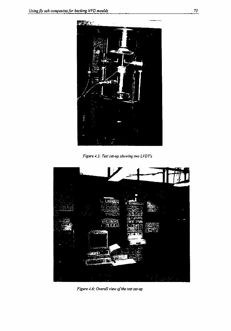
Usingfly ash composiresfor backing NVD mouid 73

Figure 4.5: Tesr set-up shoiving nvo L VD T's

Figure 4.6: Overall view of rhe tesi set-up

Usingfly ash composites for backing NYD mouldF 74

Figure 4.7: Compaction curvefirjly ash campasites -Mixtures 1. 2 and 3

Thermal Conductivity vs. Time

Figrrre 4.8: Efect oftirne an the thermal conduct~ity offly asIr compasiles

Usingjly ash composites for backing NVD moulh 75

1500 1600 1700 1800 1900 2000 2100 2200

Dry ûensity [kglm31

Figure 4.9: Dry demis, versus thermal conductiv@ resiilts of fly mh composites

Uniaxial Compression - 28' Day

.., -A--. A- 1 - +Mixture 1:15% Fly Ash

+ Mixture 1: 25% Fly Ash

1 .O0

0.00 0.00% 0.10% 0.20%

Uniaxial Strains tO/o]

Figure 4-10: 2 f h day irniaxiaf compressÏve strength for ii4irrure I compasire having 15% and 75%flv a h ta sand ratio

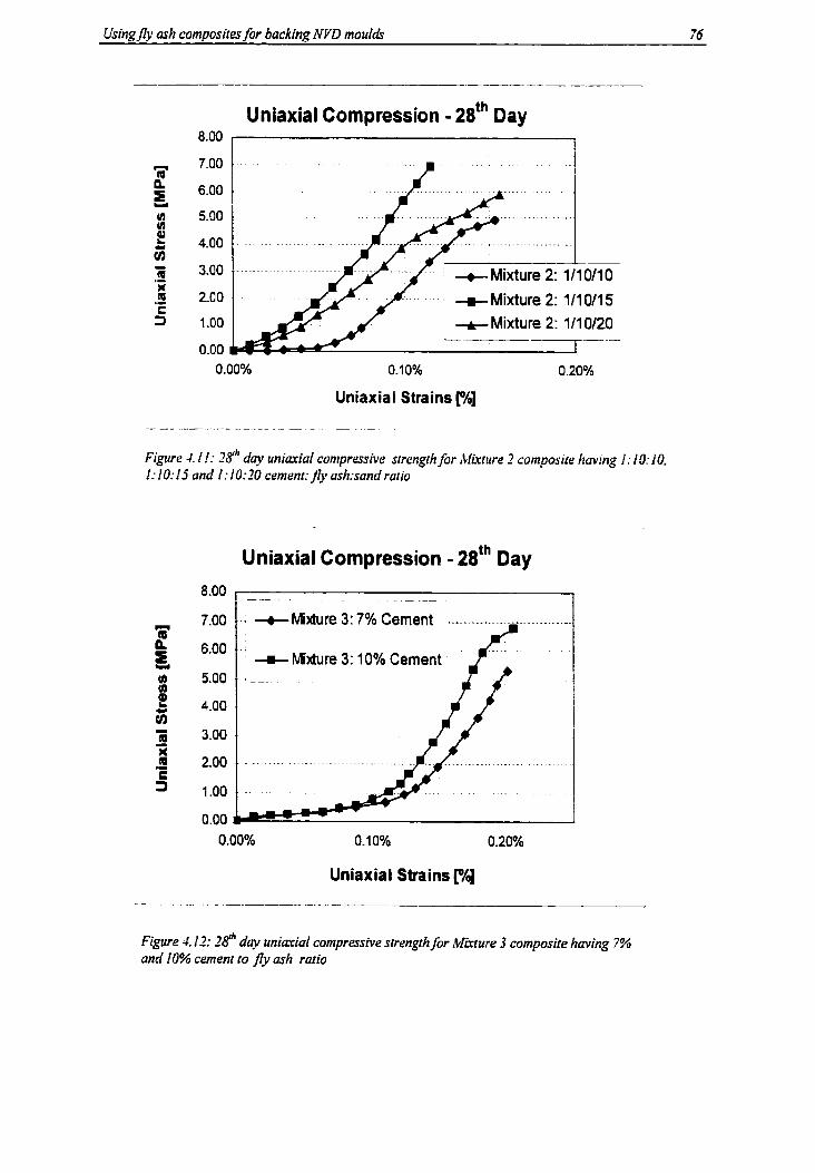
Usingfly ash composites for backing NVD moula% 76

Uniaxial Compression - 28th ~a~

I--

/ t Mixture 2: 1H 011 0

-e Mixture 2: 111 0120 --

0.00% 0.10% 0.20%

Uniaxial Strains Ph]

Figure 4 I f : 2 t h day uniaxial compressive strength for Blixture 2 composire having 1: 10:10. 1: IO: 15 and 1: 1 Or20 cement: j1y ush:sand rario

Uniaxial Compression - 28th ~a~

-a- Mixture 3: 10% Cernent f . *

Uniaxial Strains ["/d

Figure 4.12: 7gh day uniaxial compressive strengthjôr kICrture 3 composite huuing 7% and IO% cement IO fly a h ratio

Usingfly ash composires fir backing NVD moulds 77

+ 25% Fly & h

Figure 4.13: Effect of c'tuing uge on irnuxtaf compressive srrengrh of ibfirture 1 composite having 15% und 25% f iy ush ro randrurio

Strength vs. Curing Age (Mixture 2)

Figure 4.14: Effect of curing age on ~marial compressive strength of ilfimue 7 coniposite having 1: 10: 10. 1:lO:ISand 1: IO:70 cement:f!v a h : sand rurios

(lsingjly esh compositesfir backing NVD moulak 78

- - - . --

Strength vs. Curing Age (Mixture 3) 10.00 -- - - -- -- -

/- + 10% Cernent

Figure 4.15: Ejyect of nrring age on unmial compressive sfrengfh of Mitture 3 composire having 7% and 1 O% cernent roj& a h ratios

Using Fiy Ash Composiresfor Backing NVD Mouldr 79

Stress-Strain [15% fly ash]

Axial Strain Radial Strain

Figure 4.16: TricrriaI compression test data for iblirrurr 1 rotnposite wirh Ij%j(v u h IO

cernent ratio

Axial Strain - Volumetric Strain [15%fly ash]

4.02 - - - -

Axial Stnin

Figure 4. I 7: riririal vs. volurnerric strains f i r Mlrture f composite with Ij%fly arh ro cemenr ratio

Using Fly dsh Composites for Backing NVD Mou!& 80

Axial Strain Radial Strain

Figure 4.18:Triaxial (est durajar :bfkture f camposire wiih X%f{v ash ratio

Axial Strain - Volumetric Strain (FA(C)-ZS-S]

\

-4.02-

Axial SWin

Figure 4. I9:..triul W. volumesric slraimfor ibfirrttre I composite wirh 55% jly ash racio

Using Fly Ash Composites for Backing iVVD ii4ouldr 81

Stress-Strain [C$A(F)40-S]

4-

35

m U

-0.025 -0.015 -0.005 0.005 0.015 0.025

Axial Strain Radial Strain

Figure 4.20: Tricrriul tesr clrrrufi~r .\.tixture 2 composire ivirh 1: IO: 10 crmrnt$,v ashrsand ratio

Axial Stnin - Volumetric Strain [C-FA(F)-3041

-0.006 .

-&cm Axial Strain

Figure 4.2 1:-LriaI vs. volumefric srrainr /or Mkture 2 composite with 1: IO: IO cemenr:jly ashxand ratio

Using Flv ilsh Composites for Backina NVD Mouluk 87

Stress-Strain [C-FA(F)40S]

Axial Strain Radial Strain

Figrire 4.22:Triariul test dura for Mkrure 2 composite with 1: IO: 15 r.rment:fly ash:sand ratio

Axial Strain - Volumetric Strain [C-FA(F)-4041

-.--- Axial Strain

Figue 4.23: ..Lrial vs. vofitnrrtricsrrainî for ~Mirrure 2 composite ivith I : IO:IS cementrflv ashrsand ratio

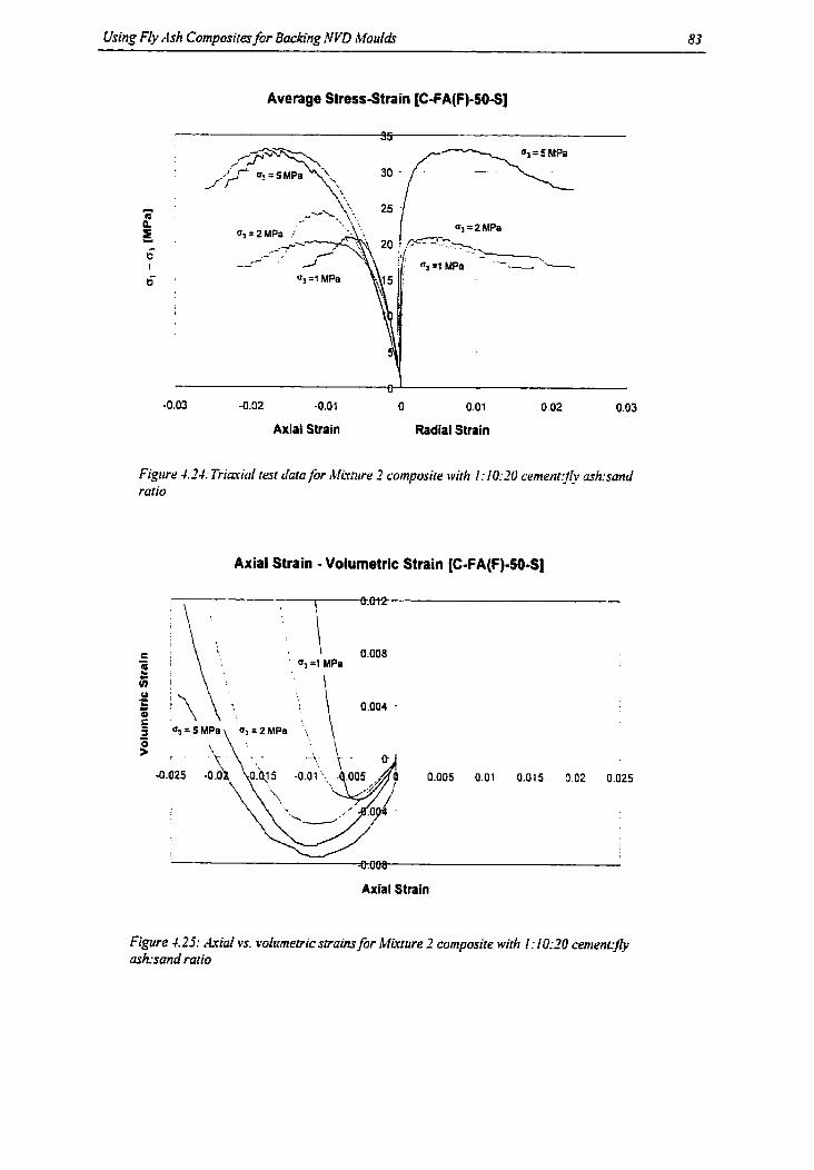
Using Fly Ash Composites for Backing NVD ibfoula3 83

Average StressStrain [C-FA(F)-SOS]

Axial Strain Radial Strain

Figure -1.74: Triariuf (est duta for ~Clirture 2 composire ivirh 1: IO:70 cenient$v uksand rurio

Axial Strain - Volumetric Strain [C-FA(F)-50-SI

0.005 O 0.015 0.02 0.025

I

Axial Strain

Figure 4.25: k i a f vs. volumetric srraitufor ibfirrure 2 composire ivilir I r 1O:IO ceniencfly ash:sand ratio

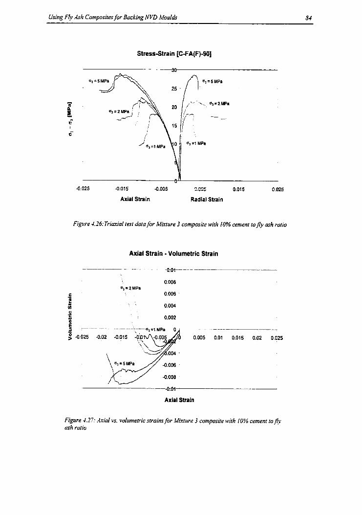
Using F& .4sh Coniposites for Backing NVD :I.loulds 84

-0.025 -0.015 -0.005 n *.vwW nnc 0.015 0.025

Axial Strain Radial Strain

Figure 4.76: Trimial test data for rCILrlure 3 composite with 10% cement rojly ash ratio

Axial Strain - Volumetric Strain

.@,M -- -

0.008 a3 = 2 MPa

0.006

-W.",

Axial Strain

Figure 4.27: ..lriui vs. volumetric srrains for ~bfixture 3 composite with IO% cment rof7y ah ratio

Using Fly Ash Composires jar Backing Nickel SheII-Mouldr 85

4.4 Numerical Modelling of Fly Ash Composites Using Triaxial

Data

The aim of this section is to formulate a f i t e eiement mode1 with appropriate

constitutive relationship for the triaxial testing of fly ash composites. as described in

Section 4.3. This was achieved using M3AQUS finite element software with various

built-in types of Drucker-Prager materiai model.

4.4. i Finite Element Model

Due ta the geometry of the triaxial specimen. which is a cylinder with a 2:l height

to diameter ratio, the finite element c m be implemented using axisyrnmetric solid

(continuum) elements (Figure 428). The model uses stress/displacement elements

without twist of the 4-node bilinear axisymrnetric (CAX4) type with 4 integration points.

These elements are fonnulated using 4 corner nodes. that have rwo degrees of freedom:

one in the radial and one in the longitudinal direction. The mode1 consists of one such

elernent of unit dimension. The conventional counter-clockwise nodal and face

numbering is employed as shown in Figure 4.29. dong with the generai element

configuration. The loading of the specimen is implemented using a distributed load

(*DLOAD) on the (P2) face to simulate the corifinhg pressure acting on the side of the

cylinder. The axial loading is simulated by incremental displacements

(DISPLACEMENT) of the top (P3) face over a range of straui increments to achieve the

required stress-strain behaviour of the materiai. The auial stress is obtained from the

output of the anaiysis that contains the stresses in al1 h e directions (radial, a~ial . and

hoop) and the conesponding strains. The important values are the axial stress. axial

strain and the volumetric strain given by the summation of the three principal strains.

Axial loading is s h d a t e d by prescribing a displacement at the top of the specimen. since

the post-peak behaviour is expected. which can Iead to two different axial strain values if

the loading is applied by pressure.

4.4.2 Drucke~Prager Model for Geological Materials

The Drucker-Prager model is suitable for modelling a \vide range of geoiogical

materials that are fnctional in nature and exhibit pressure dependent yield, such as soils,

Using Fly Ash Composites for Bading Nickel Shell-Mauldr 86

granular materials and rock types. The model is formulated using the invariants of the

stress tensor? more precisely the t'irst invariant of the stress tensor, Ji, and the second

invariant of the deviatoric stress tensor, JiD. The original mode1 is a straight line in the

J, - & space defined by cohesion, k, and an angle, ,f?. Thus the general equation has

the following form:

The criterion plots as a circula cone in the three-dimensional stress space, thus in

the ïi-plane the surface is a Mises circle.

Figure 4 2 : Triurid specimen model

Figure 4-29: ..ttisyrnmetricjinire element mode1

Using Fly itsh Composites for Backing Nickel Shell-Moulds 87

4.4.3 Ovenliew of the Drucker-Prager Material Models in ABAQUS

Since ABAQUS incorporates the Extended Drucker-Prager material model, a

choice of three different yield criteria is provided. The differences are based on the shape

of the yield surface in the meridional, J I - J ~ D or p-t(q) using ABAQUS notation of plane.

The yieid surface can have a linear form, a hyperbolic form. or a general exponent

fom modelled with or without experimentai test data.

The linear model is intended for cases when stresses are mainly compressive. If

the Mohr-Coulomb Ection angle and cohesion are known, it is possible to convert this

data and use the Linear Drucker-Prager model. The parameters used in the linear rnodel

and the model itself are shown in Figure 4.30.

The hyperbolic mode1 is useful for brittle materials for both triaxial compression

and tension, The hyperbolic model uses a von Mises circle cross-section in the deviatonc

plane. At hi& confining stresses. the hyperbolic model is asymptotic to the linear model

with angle, fi, as shown in Figure -1.31.

The most generai mode1 is the exponent model, providing the most flexibility for

matching triaxial test data (Figure -1.32). ABAQUS is capable of detennining the

parameters from the triaxial data using a least square technique.

The Dmcker-Prager mode1 implementation in ABAQUS enables the user to

de fine a hardening behaviour of the materiai. A hardening then so ftening (afier the peak)

strength can be modelled as well. The hardening behaviour is captured by selecting

points on the laboratory stress-strain curve and finding the yield stresses and the

correspondhg plastic strains as s h o w on Figzrre 433 for the case of !Mixture 2 fly ash

composite, This approach is used in this section to define the hardening behaviour of the

model. The hardening behaviour is defined using five points.

Using Fly Ash Composites for Backing Nickel Shell-hfoulrFF 88

Figure 4.30: Linear Drucker-Prager mode!: F=t-p. tanp-d'd

Figure 431: Hyperbdic Drzicker-Proger >nodei F = &lo -pi lo m p)' + s2 - p . m p - d*= O

Figure C32: Erponeni Drucker-Prager model: -p -p, =O

Using Fly Ash Composites for Backing Nickel Sheii-iUoulc& 89

In addition to the above, ABAQUS allows for rate-dependent behaviour and

creep. These factors were d e d not important for the case of this study, however.

StressStrain (SIGMA 3 = 5 MPa)

-0.02 -0.018 4.016 4.014 0.012 -0.01 -0.Oû8 4.OM (-0.004 4.002 O

Axial Strain pi] 1 J E ~ ;

Figure 4.33: Simularing the hardenindmfiening behaviour of~LIirture I usingjîve-

point se/ection

4.4.4 Using Linear Drucker-Prager Material Mode1

The numerical procedure using a linear Drucker-Prager mode1 is accomplished

using the experimental data provided. The first step is to select yield points on the

surface for various confinhg pressures. The analyst has the choice to select the initial

yield or the peak suength. For our purposes. the peak strength and the corresponding

strains were used in al1 modelling. Once the faiIure and confinhg stresses are

determined, the values must be converted to the p-r plane using the foilowing formulas,

adapting a tension positive system:

and

Using Fb Ash Composites for Backing Nickel ShelI-rtCouldr 90

on the condition that KI the parameter de€ining the shape of the yield surface in the

deviatonc plane is equal to 1.0 (von Mises circle).

The p-r pairs used in a linear regession yielded vaiues of d and b of 6.444 and

59.214 degrees. respectively. The angle of dilation was set to the angle b associated

flow. The complete ABAQUS input file is given in Appendix D.

The results of the analgsis are shown in Figzires 4364 .37 . and can be compared

to the original labontory results (Figure 4.344.3.7)

Since the initial elastic behaviour is smail. there was no concern about it, and both

the model and the actuai data show close behaviour up to the peak strength of the

material. ABAQUS models also simulated the post peak behaviour. and modelling

results show softening behaviour at low confinement sirnilar to that found in the

experimental data.

Both the model and the experirnental data are consistent in showing the axial-

volurnetric strain behaviour: initial volurnetric compression with increasing mial strain,

and close to the peak strength, the materid starts to dilate. expand until the specimen

breaks up in the test data and the material Bows according to the associated flow mle in

the ABAQUS model.

By Iooking at the individud stress-strain and volumemc versus axial diagrams for

each confining pressure, it can be concluded that the mode1 gives a better approximation

to the actual curves at low confining pressures, meanwhile the predicted contraction is

much less than that experienced during the test. however the two curves area closely

match.

in concIusion, the linear Drucker-Prager model can be used to model the

behaviour of the fly ash composites, if enough experimental data is gathered and the post

Using Fly rlsh Composites for Backing Nickel Shell-Mouldç 9 1

peak curves are established in order to specify the hardening or softening behaviouc of

the materiai.

-0.025 -0.015 -0.005

Axial Strain Radial Strain

Figure 4.34: rlxial D-E behaviourffom iriarial tesr data

Axial Strain - Volumetric Strain [C-FA(F)40S]

Axial Stnin

Figure 4 -32 i.Lriai-volumetric stain behaviourfiom rrimial test data

Using Ffy Ash Composites fi?- Bucking Nickel Shell-ibloulds 92

Axial Stress-Strain (Linear Drucker-Prager)

n

2 z ô * Ci

- - - - - -s3=0 MPa

-s3=1 MPa

-s3=2 MPa

-s3=5 MPa -

Axial Sîrain [O/o]

Figure -1.36: ..LBAQLSmial o-~resulrsfor linear D-P model

Axial-Volumetric Strain (Linear Drucker Prager)

-s3=0 MPa

-s3=1 MPa

- s3=2 MPa

Figure 4 . 3 7 =IBAQUS axiai-volt~metric srru& resuf~sjor linear 0-P mode1

Using Fly Ash Composites for Backing Nickel Shrll-MouIds 93

4.4.5 Using Hyperbolic Drucker-Prager Material Mode1

The hyperbolic model is a continuous combination of the ma~irnum tensile stress

condition of Rankine (tensile cut-off) and the linear Drucker-Prager condition at high

codining stress. The hyperbolic yield critenon in ABAQUS is defmed similar to the

linear model, however this model c m accommodate a non-linear envelope at low

conhing pressures, thus correct the probkm with the linear model. The hyperbolic

model has the following Form:

where the d' parameter is similar to the d in the Iinear modei. and the angle h defines the

envelope at high confining pressures. The model requires the above angle plus the angle

of dilation, which is assumed to be the same for associated tlow, however a third

parameter is required, the tensile strength of the material. p,. it will be assumed in this

modelling that the composite has a tensiIe strength of 1 MPa, The mode1 requires the

sarne hardening specifications and the loading is achieved with the same method.

Figures X 3 9 4 . 3 9 show the material response predicted by hyperbolic model.

It is evident from the stress-strain curves. that the envelope is no longer linear, but

has a curvature that is closer to the actuai observed material response. In this model, the

hardening parameters were changed to enable the results to exhibit more elongated post-

peak behaviour. If the first point aFter the peak strength is moved closer to the peak. a

steeper decline will result in the region following the peak strength. The approximation

of' the post peak behaviour is thus better than the Iinear rnodel results.

The volumemc versus axial strain behaviour of the mode1 is very similar to the

linear mode1 resuits, where the curves predict initial contraction then dilation responses

similar to the actuaI curves.

Using Fly .4sh Composites /or Backing Nickel Shell-Mord& 91

In conclusions, the hyperbolic model seems a better approximation than the linear

model, with the sarne effort in the preparation of the input fiIes.

Axial StressStrain (Hyperbolic Drucker-Prager)

C< m L

O - a3=0 MPa

-d=l MPa

- fl=2 MPa

-s3=5 MPa

" .a 02s -0 02 -0 01s -o a i -0 a05 O

Axial Strain [%]

Figure 4.38. : A4B,4QL!S axiul stress-srruin results for hyperbolic D-P model

Axial-Volumetric Stnin (Hyperbolic Drucicer Pnger)

O - b - PI --

5 -s3=0 MPa - g - s 3 4 MPa

-s3=2 MPa

-0m-

Axial Strain

Figure 4.39: .4 8rlQU.T arial-volumerric srruin renilts/or hyperbolic D-P n~odel

Using Fly .4sh Composiies for Backing Nickel Shell-Moulds 95

4.4.6 Using General Exponent Drucker-Prsger Material Mode1

The most general and most cornplicated model to use in Ai3AQUS is the general

elcponent form. It c m assume linear, hyperbolic and more complex shapes. The general

forrn of the model is as follows: h F = a - q - p - p , = O

where constants a and b are found using non-linear regression and p, is the [ensile

strength of the materiai. For the purpose of this work it is assumed to be equal to 1 MPa.

The material parameters a and b are found using a non-linear regression

technique. For the case of the best fit parameters a and b were found to be equal to

0.2015 and 1.2661' respectively. tf b is equal to 1.0 the model degrades to a linear

Drucker-Prager model.

The general exponent rnodel is a non-associated flow model. since the curve is

changing constmtly in the meridional plane.

The results of analysis are surnrnarised in Figures X-1O-l. 41 for axial stress-strain

and aial-voIurnetnc strain. respectively, and are cornpared to the corresponding

laboratory test data.

The parameters for this version of the extended Dmcker-Prager model were

retined to sirnulate the sharp Ml-off after the peak strength has reached, This effect was

reached by selecting a plastic deformation for the stress point after the peak in the

defrnition of the hardening law.

From che models presented, this model simulates the Iaboratory behaviour of the

fly ash composite to the highest degree of accuracy. The initial curved envelope with the

sadual deciiie after the peak is properly predicted by the model. k

The volumerric versus axial strain behaviour of the mode1 is very sirnilar to the

hyperbolic model resuits, where the curves predict initial contraction then dilation

responses simiIar to that of the actual curves.

Using Fly Ash Compositesfor Backing iVicke1 Shell-M~ulds 96

Axial Stress-Strain (Exponential Dnicker-Prager)

/ -

-Q=O MPa

-s3=1 MPa

- s3=2 MPa I

-s3=5 MPa

Axial Stnin ph]

Figure 4. -IO: A BA QUS axial stress-strain resultsfir exponenrial D P mode1

Axial-Volumetric Strain (Exponential Drucker-Prager)

-s3=2 MPa

Figure 4.41: .-I BAQUS mial-voiumerric srruin resultsfor e.rponmtia/ D-f nrodei

Using Fly As11 Composi~es for Backing fiickel Sheli-rbloulk 97

4.5 Conclusions

It was shown and supported by actual analysis results, that it is possible to model

the behaviour of fly ash composites using a finite element package such as ABAQUS.

The extended Drucker-Prager is suitable to capture the matenal response under triaxial

loading. Starting with the simplest Linear modeI, the results were of the same magnitude

as the eliperimental, the hyperbolic model added the non-linear yield envelop to a better

approximation and finaily the general exponent model was used to fine-tune the material

behaviour. Considering the complexity in obtaining the best material model parameters

and the resulting material response. the exponentiai mode1 is recornmended. If the

labontory data is sufficientiy detailed and complete, the general exponent model can be

used with or without the inclusion of the test data to caiculate the model.

Production Trial Test of a

Nickel Mould with Fly Ash

Composite Backing

in the previous chapter. the strength/stiffness behaviour of fly ash composites was

simulated using the ABAQUS tinite element program by applying a modifred built-in

non-Iinear Dmcker-Prager capped material model. Subsequently, this material mode1

was incorporated into the simplified 2D-mode1 that was previously used for modelling

mass-cast backing systems (Section 3.4). Preliminary results from this mode1 show that,

within the pressure range of the 1Ve.r iblortlding application. fly ash composite backing is

mechanically suitable for the process. This chapter describes the use of fly ash

composites in a prototype trial to analyse their performance and veriSl their capabilities

in backing shell-moulds. The trial took place at the industriai partner's (Blanco Canada

Inc.) rnanufacniring comple'r.

5.1 Objective

The main objective of mnning the production trial test is ta investigate the

suitability of using fly ash composite backing for nickel shell-mouids. This objective

could be accomplished by:

Determining the mechanical behaviour of the nickei shell by monitoring its mains

and flexurai deformations at various presurned-critical locations,

Checking thermal behaviour in ternis of temperature measurements at various

points on the shell, and

Comparing triai data Erom above to numericai modelling resuits using the finite

element anaiysis (FEA) method.

Production Trial Test of a Nickel Shell-mould with Fiy ctsh Composite Backing 99

5.2 Description of the Production Trial

5.2.1 Methodology

In order to achieve the objectives noted eadier, the theory underlying the

developed composite design had to be tested in practice. A new NVD shell-mould was

built at Blanco Canada's manufacturing facilities in Etobicoke, Ontario. It was equipped

with the following instrumentation:

Strain gauges to monitor stnins in the nickel shi-II,

Potentiometers (transducers) to control shell displacements. and

Thennocoupies to measure temperatures at different shell locations.

Both halves of the mould were instrumented and then filled with composite

backing. The mould was put into pre-production triah for caiibration of the moulding

process to produce the **perfect pan". During these trials the mould pertormance was

rnonitored. as was the qudity of the trial parts.

The monitored mould performance was then compared to the performance

predicted by FEA models cdtlibrated with material data fiom niavia1 laboratory tests (see

Chapter 6).

1. Mould Description

The mould used for this trial is type hhoen 2 !Mottld by Blanco Canada which uses

Blanco's proprïetary !Vet Motrlding process for manufacturing double-bowl kitchen si&

(Figure 5-2). The mould consists of nvo haIves (Top and Bottom representing core and

cavity, respectively), each encompassed by a cigid steel box made oftvelded HSS

90x50~9 fiame, filled with the composite filIer to back the nickel shell-mould. The

bottom side of the box is contains a steel cover made of 15-mm (Bottom half) and 18-mm

(Top half) thick plates for better backing support (Figure 5.2)-

Production Trial Test ofa Nickel Shell-mould ivith Fly Ash Composite Backing 100

2. Mould Construction

The process of building a new mould by Blanco Canada Inc. requires the

following steps [Blanco. 19981:

1. Preparing drawings and ordering the nickel shell, dong with the Çarnes and

parts;

2. tnspecting the shell and frame according to the drawings upon arriva1 at

Blanco's headquarters:

3. Preparing and pre-assembling the shell and frame;

4. Checking mould alignment and thickness;

5 . Preparing thermal copper Lines;

6. Building thema1 copper lines;

7. Applying copper powder paste between the thermal copper lines and the

nickel shell:

8. Attaching the rnould to the shells:

9. Filling the gap between the mould and the fiame with epoxy;

10. Connecting watw pipes to the manifolds:

1 1. Assembling the ejectors to the moulds and Frames;

12. Placing concrete/composites into the mould;

13. Letting the concrete/composites set for 48 hours:

14. Connecting the ejectors Iine to the air manifolds:

15. Mounting the gasket holder and the gasket;

16. Putting Top and Bottom haives of the mould together;

17. Installing the completed mould on the mouid carrier:

18. Transferring the r n d d to the production area to make test parts; and

19. Checking the thickness and the weight of tfit moulded part and adjusting it if

necessary.

3. Net-Moulding Process Description

During production, the mouid is placed on a specially designed carrier (Figure

5-3). The Top haif is instded on the carrier using two brackets that are attached to its top

Production Triol Tesr of a Nickel Shell-mould ivith Fly Ash Composite Backing 101

cover-piate. The Bortom half sits on a series of air hoses or bags, whkh are comected to

an air compressor.

The followings are the major steps for rnould operation planco, 1998):

1. From the open position, bring down the Top half of the mould until it stops - once

it reaches the Bottom mould;

2. Close the mould clamps to keep the Top and Bottom halves of the mouId together

and apply air pressure to the air bags undemeath the Bottom rnould;

3. Detlate the air bags and get the mould ready to be fiIled:

4. Comect the filling and overflow pipes to their proper valves:

5 . Tilt the mould to its vertical position;

6. Close the valves once the mould is full;

7. Rerurn the mould back to its horizontal position;

8. Apply pressure through the air bags under the Bortom mould:

9. Once the curing cycle is complete, turn on the top ejector to separate the Top

mould fiom the sink;

10. Open the mould and raise the Top half to its top position; and

I 1. Dernould the sink and clean the rnould.

4, Properties of the Net Moulding Process

The main parameters for Blanco's proprietary Net Moulding process in relation to

conventional plastic parts rnoulding processes are:

Relativeiy low temperature (between 30 OC to 105 OC).

Long cycle tirne: about 30 minutes.

Low Pressure: between 6 and 8 bars (600-800 kPa).

5.2.3 Fly Ash Mix Design

Based on the results of the material properties of fly ash composites (Chapter 4),

as weii as on the parameters of the Net ~Vonlding process, a preliminary rnix design was

identified for this tria1 to meet the fol!owing criteria:

The Eesh mix is fluid enough to easily place it in a complicated, three

dimensional mould geometry,

Production Trial Test of rr Nickel Shell-mould wilk Fly Ash Composile Backing 102

The mix hardens quickly, and its stifiess and strength adequately support the

shell against the pressure irnposed during rnanutàcturing,

The as-placed mix is thermally insulating (a requirement for the particular

process), and

The hardened rnaterial is &able enough that it may be removed using hand tools.

thereby permitting selective repair of thermal lines in an isolated portion of the

mould.

As noted earlier. the ingredients of the composite are cernent. fly ash, and sand-

The mix was designed with the ratio of 2: IO: 15 representing the ratio of cement:fly

ash:sand, respectively. The water content considered for this rnix is 14% of the dry

weight. Laboratory resuIts show that this mix c m attain a uniaial strength of 6 MPa and

a bulk stiffness of 3.4 GPa at a curing agc of four days.

The mis ingredients were High Early Strength Cement (ASTM Type III).

concrete sand (industriai quartz. 10% retained on sieve #20), and ASTM Type F (low-

calcium) tly ash. This fly ash was obtained fiom Holnam Inc, Chesterfield, MO. The

source of the fly ash is the Tennessee VaIIey Power Station, Cumberland City, TN. USA.

The fineness of this fly ash is 16.2% (retained on sieve #325), and its chernical

composition is presented in Table-j. II.

Table-5.1: Chernical composition of the Cumberland (Qpe FlXv ash

5.3 Test Instrumentation

The first part of this section describes the instrumentation procedure, inctudiog

the set up and running of the hardware (measurement devices, data acquisition, etc.) and

Pulaterial

Cumberland

Fly Ash

Sioz

49.8

F103

17.76

Ca0

5.74

M@

0.94

SOI

1-72

K20

2.30

Na@

0.66

alzOj

19.73

TiOz

0.84

c

034

Production Trial Test of a Nickel Shell-mould with Fly clsh Composite Backing IO3

s o h a r e considered for the triai. The second part covers the monitoring procedure,

including data collection and analysis, of the mould in production trials.

5.3.1 Thennocouples

Thermocouples used for mould instrumentation were PVC insulated wires and

connectors of the following t-yes:

I . FVires

Thermocouple wires Type PP-T-24-1000 by Ornega Technologies, with PVC

insulation.

2. Connecrors

Connectors includs rugged glas-tilled shells Type OST-M or F (male or female),

dong with Type 'Tt connectors that are made of '-ve' constantan copper-nickel

and '+vet copper leads.

1. Data Acquisition System

The data acquisition system consists of a computer with a General Purpose

Interface Board (GPIB) controlhg a HP-3421A data acquisition unit. Figure j -4 shows

the connection between the system and the mould. The data acquisition and control unit

used in this set. was set up for making temperature readings for the thennocouples and

DC-voltage readings fiom the potentiornenters.

2. The Cornputer Program Freeze-Thaw

The computer prograrn Freeze-Thmv was used here for data collection. This

prograrn was initiaily written as part of a freeze-thaw investigation on some cernent-

treated soils, carried out at the University of Toronto [Lee, 19991.

3. Calibrating the Therrnocouples

The F r e e z e - h v program requires that di newly installed thermocoupIes be

calibrated before data collection. For the sake of this trialt two temperature points were

considered: ice point and boiling point temperatures. i.e., O O C and 100 "C [Lee. 19991.

Production Trial Tesr of u Nickel Shell-mould ivirh Fly Ash Composite Backing 104

5.3.2 Potentiometers

The potentiometers used for this test are Type KL 250 SEF by Omega

Technologies, with a cross-section of 13 x 13 cm, and a measuring tolerance less than

0.05 mm.

The sarne data acquisition system, and the Freeze-Thmv program mentioned

earlier in the thermocouple section were used for the potentiometers (see Figure 5-4).

The Freeze-Thmv program also requires calibrating newly installed

potentiometers before data collection [Lee. 19991.

5.3.3 Strain gauges

Strain gauges used for this test are Type CEA Micro-Measurement gauges

supplied with hlly encapsuhted gids and exposed copper-coated integral solder tabs.

The gauges have a normal temperame range behveen -75 to 205 "C. and stnin Limits of

approximately 5%.

1. Lead Wires

Based on preliminary computer simulations, strains in the shell-mould were

expected in the order of 200-500 p. Thus. Omega Type TFCP-005 copper wires was

used to provide adequate sensor performance. Lead wires are Teflon-insulated to

withstand the environmental conditions expected in the test.

2. Setup

Monitoring points for strain gauge installation were sekcted in locations where

stressistrain gradients are expected to be minimum. Displacement transducers, on the

other hand, were installed at points where f lexud deformations are expected to be hi&.

The Location of the strain gauges, transducers and thermocoupIes are shown in Figure

5.5. Each gauge, thermocouple, and displacement m s d u c e r are IabelIed by suffix letters

"SG" and "TC" and "TR", respectively, and a number. A total of eight strain gauges and

eight adjacent thermocoupIes were instaiied on each haif of the mouid. Two additional

displacement transducers were instaiied on the Top half of the mould.

Production Trial Tesr of a Nickel Shell-mould with Fiy .4sh Camposile Backing 105

3. Data Acquisition System

Figzire 5.6 shows the connection between the data acquisition system and the

mould. The data acquisition (and controI unit) from Sciemetrics Instments Inc. is used

for strain measurements. It consists of an lntegrating AJD Module (Model 23 1) dong

with Model 25 1A with 16-Channel analogue-expansion module that provides support for

I /J and % bridge strain measurements with shunt calibration. A !4 bridge connection,

which is considered in this test. is usually u sd if a raw unconditioned strain gauge is to

be measured directly. In this case the gauge is c o ~ e c t e d as one of the four resistors that

fomi the bridge circuit, whiIe the three completion resistors are provided by the Model

251A.

4. The computer unit

The computer program GVingen version 1.1 was used for suain data collection.

bVingen is issued by Sciemetric Instruments ta support their modular measurement and

control systems.

5. Shunt Calibration

Shunt calibration allows a bridge output to be temporarily increased (or

decreased) by shunting a resistor across one m of the bridge. Since this shunt

connection changes the resistance of the m. the output of the bridge will tip slightly up

or d o m . This calibration method allows the integrity of the connections. excitation. and

data acquisition to be checked quickly without acmdly changing the sensor input. The

precision resistor is typically quite large (cg., 120 ici2 for $4 bridge) so the output of the

bridge only changes by a few millivolts, simulating a typical response fÏom the gauge.

Push button switches are provided with the Mode1 251A to allow any channel to be

shunted manually. When the minianire push button switch on each side is pressed, one of

two gIobal shunt resistors is placed behveen the input terminal and ground. The known

vdue can be compared to the change in value read by the data acquisition system, using

the Wingen program, and a d j m e n t s can be made to correct the errors.

Production Trial Test of a Mckel Shell-mould wizh Fiy Ash Composite Backing 106

6. Temperature Effect

Ideally the resistance of the strain gauge would change only in response to the

strain induced in the test specimen. However, the sensitivity and the strain resistivity of

ail known strain sensitive materials vary tvith temperature. This rneans that the gage

resistance and the gage factor will change when the temperature changes. This change in

resistance with temperature for a mounted strain gauge is a Function of the difference in

the thermal expansion coefficients between the gauge and the specimen and of the

thermal coefficient of resistance of the gauge alloy. Self-temperature compensating

gaugcs are produced for specific materials by processing the main sensitive alloy such

that it has thermal resistance characteristics that cornpensates for the effects of the

mismatch in thermal expansion coefficients between the gauge and the specific material.

The compensation is effective over a limited temperature range given by the gauge

manufacturer in the form of an Apparent Strain Curve. This is a plot of temperature-

induced apparent srrain versus temperature. for the gauge, mounted on a specific material

with a specified coefficient of thermal expansion. Gauges o f Type CEA are supplied by

Micro-Measurement as self-temperature compensating gauges. The Apparent Strain

Curve of'this gauge is provided by the manufacturer and depicted in Figire 5.7. and its

squation is given by.

4 5 E,,, =-3.83~10' +3.01 x1o0T-6 .54~ 10-'T' i L 5 0 x 1 0 T - 4 . ~ 8 x 1 0 - ' ~ ' ( ~ C ) ( j . l )

where: T = measured temperature

ET^ = uncorrected main measurement as registered by the strain indicator

By monitoring the temperature of the gauge during the strain rneasurement, we can solve

this equation to compensate for the temperature-induced strain- The fwst step in the

correction procedure is to refer to the gaph (fiom Figtire 5.7 or Equarion 1) and read the

apparent strain correspondhg to the test temperature. Then, assurning that the strain

indicator was balanced to zero strain at room temperature (the reference temperature with

respect to which the apparent main data were rneasured), subtract the apparent strain

(including correction due to gauge factor) from the strain measurernent at the test

temperature. This procedure can be expressed as,

Production Trial Test of a Nickel Shell-mould ivifh F[y Ash Composite Backing 107

where: c= corrected strain indication

&Pp = apparent strain at temperature Tl, from graph or Equation (5.1)

F' = gauge factor at room temperature. as given by the manufacturer

F ~ ' = gauge factor at test temperature

Equation (22) can be introduced into a spreadsheet to calculate after data for are

collected.

5.3.4 Shell-Mould Backing Sysfem

1. Thermal Line Installation

The back of the nickel shell is usually plumbed with a network or circuit of

thermal lines. made of 10-mm diameter copper pipes. To achieve maximum heat transfer

and temperature uniformity across the rnould Face, the distance between pipes is between

12-20 cm. Thus. the selection and installation of the strain gauges were highly dictated

by the location of the copper pipes and their pit distance. To enhance heat transfer, the

gap between the pipe and the nickel shell is filled with copper paste (Figures 5.8 and

5.9). This paste is a mix of copper powder + Catalyst ( T p e LLH 6930) + Resin (Type

CLR 1190), al1 produced by Cross Line Technology. The ratio of the copper

powderlcatalystlresin is 40130130. respectively.

2. Strain Gauge Installation

Since the validity and usefulness of the test results are measured by the success of

the suain gauge installation, a speciai attention was given to this part of the project,

Gauge installation was achieved in stages as follows:

1. Surface Prepararion

To properly bond strain gauges, ail sufaces involved must be absolutely clean

and chemicalIy inert before applying adhesive. Depending upon the initiai

conditions of the surface and the finish desired for the gauge installation, the

Producrion Trial Test of a Nickel Shell-mould wirh Fiy Ash Composite Backing 108

abrading operation could be done using silicon-carbide paper of the appropriate

grit. For extremely rough surface a disc sander or grinder might be needed in

order to leave the required srnoothness (Figure j. 1 O) . Final surface preparation is

accomplished with M-prep Conditioner A immediately followed by M-Prep

Neutraiizer 5. Conditioner A is a mild phosphoric acid compound, which acts as

a mild etching agent that accelerates the cleaning process. Neutralizer 5 is an

amrnonia-based mateciai. which neutrabes any chemicai reaction introduced by

the Conditioner A and produces optimum surface conditions for strain gauge

adhesives.

2. rldhesive

Adhesive Type CN from Texas Measurements inc. was used for gauge

bonding to the Nickel shell. CN adhesive is a transparent, low-viscosity glue,

made of Cyanoacrylate. with a normal temperature application between -30 and

+120 OC. The tirne required to bond the gage is extremely short and handling is

very easy. The thin bonding layer dlows adhesion to nearly any object. in the

case of the CEA gauges, CN adhesive kvas applied to form a uniform coat on the

surîàce of the strain gauge and terminai. Curing time under normal conditions is

20 to 60 seconds

3. Gnuge-Lead Frire Jrmncrion

Solder type 570-20s was used to solder lead wires to gauge terminais. This

solder provides hi& electricaI conductivity and excellent mechanical strength. it

is usually recommended for hi& temperature connections.

3. =Ipplying Protrctive Coctting

Gauges are easily degraded by any chernical attack, including moisture,

fingerpcïnts, etc. Thus strain gauge installation requires varying degrees of

protection to prevent gauge instability and mechanical darnage. M-Coat Type J

from Micro-Measmement was used for this purpose. M-coat Type J is a two-part

polysulfide Iiquid polymer compound usudy used for environmental protection

of strain gauge installations, When M y cured, it forms a mbber-like covering

that provides an effective banier against moisture, and also protects against

mechanical darnage. Pnor to the application of M-Coat J, exposed electrical

Producrion Trial Tesr of a Nickel Shell-mouid with Fiy Ash Composite Bockinn 109

connections and the exposed foi1 of the open-Caced gauges are first covered with a

layer of Teflon tape (Figure j.11). This provides insulation against electrical

leakage, and minimises gauge resistance shiRs during the cure cycle. To prevent

tluid migration dong lead \vires and into the gauge instailation, protective

coatings must encapsulate the lead wires to a minimum distance of 1 in (25 mm)

fiom the installation (Figtrre j.12).

To minimise moisture Ieaks and provide a uniform protective coating, the

M-Coat Type-J coating is covered tvith aluminurn foi[ (Figzrrr j. 13).

The Teflon insdated Lead wires used in bis test must be prepared for

bonding before a protective coating c m be applied. TEC-1 Tetra Etch compound

was used to treat the Teflon for bonding. M-Coat J then bonded to the treated

Teflon without requiring an intemediate primer coating.

3. Wiring Techniques

To protect lead wires fiom moisture and mechanicd damage. they were inserted

into protective viny1 sleeves (Figure j. 14). AI1 wires (lead wires and thermocouples)

were colIected togeher and passed through fitting ddled holes into a specially designed

steel station or boxf which was weided to the mould's steel fiame (Figure 5.1.5). From the

bottom of the box. t i res were driven out of the mould through ehe frarne-tube using two

90" .4BS elbows (Figrtre 3.16).

4. Thermocouple Installation

ThennocoupIe installation %-as achieved by preparing the surface as in Section

4-52: Part I l Strain Gauge InstalIation). followed by the bonding of the thermocouples to

the nickel sheIl using copper paste.

5. Potentiometer Installation

in accordance with the specifications of the potentiometer and the geometry of the Top

haif of'the mould, a specid design for the installation procedure was required. This

procedure required that the potentiometer be fastened using two screws to a steel angle,

Production Trial Tea of a Nickel Shell-mould with Fly Ash Composite Backing II0

which was welded to the cover plate. A IO-mm diarneter hole was drilled in the cover

plate to instaii a protective pipe sleeve (Figures 5-17 and j- 118). This sleeve helped to

protect the shaft of the potentiometer fiom any friction with the composite. The tip end

of the shaft extended to the back of the nickel shell.

6. Placing Composite Backing in the mould

in accordance with the rnk design descnbed earlier (Section 4.4), the fresh

composite was fluid enough to be easily placed into the back of the mould using a

standard electricaI concrete mixer (Figrire j. 19). In order to reach maximum mix

consolidation. nvo vibrators were placed on top of the mould Erarne (Figure 5.20).

The two haives of the mould were then left for a minimum of four days for the

sake of giving the backing composite enough time to cure,

7. Connecting Data Acquisition Systems to the Mould

At this stage. all wires (thennocouples. potentiometers. and gauges) coming out of

the two halves of the mould were comected to their data acquisition systems. Channel

ranges in both systems were set in accordance with the recornrnendations given by the

manufacturers.

5.4 Conducting the Trial Test

5.4. i Sfarting the Test

The data acquisition systems (along with the PC's) of both the thermocoupies and

the strain gauges are tumed on at ieast an hour before the test begins, to assure accurate

data collection. A manual data scan is tried fist on the thermocouple, potentiorneter, and

gauge channels to ensure that al1 devices are funçtioning properiy. Both software

programs: Freeze-Thcnv and Wingen are then put in "Start" mode ready for monitoring.

5.4.2 Observing the Test

Upon cIicking the "Staa" buttons on both programs, the monitoring process is

started once the mouId is ready to be filled. During the cycle, the change in the strain and

Production Trial Test of a ~Vickel Shell-mould wilh Fiy Ash Composite Backing I I I

temperature vdues are periodically monitored to check if d l channels are transferring

data properly.

5.4.3 Storing the Data

The scanning of the temperature and displacement readings from the Freeze-ï'hmv

program and for suain readings from the tVingen program is autornatically set at 18 sec.

This interval largely depends on the speed of the module and the nurnber of channels

acquired by the data acquisition system. The recorded data are then saved as separate

files for each moulding cycle (30 minutes). Al1 saved files are in ASCII text format.

which can be opened by spreadsheet sohvare for ediung.

5.4.4 Completing the Test

At the end of the last trial m. disconnect al1 the wires and phgs to the data

acquisition units. then turn them offalong with their PC units.

5.5 Production Test Results and Discussion

This section presents and discusses the production test results. Mechanical

properties of the shell-mould are investigated using collecteci strain and tle'rural

deformation data at différent monitoring points throughout the shell through the cycle

time. Thermal behaviour is checked by measuring shell surface temperature at similar

monitoring points in the mould. Production part quality is aiso checked according to the

quality requirements set by Blanco Canada.

5.5.1 Strain Measurements

Strains measuernents were collected for both-Top and Bottom-halves of the

mould in terms of strain vs. time. Each run extended about 30 minutes. which represents

the cycIe time of the Net ~bfoufding process.

1. Bottom Half

Results tiom the Bottom ha& in terms of strain measurements vs. the. show that

strain curves are not smooth but tend to zigzag. These 'ups and downs' in the strain-

Production Triai Tesr of a Nickel Sheli-mould with Fiy Ash Composite Backing 112

c w e s are probably attributed to factors such as air bag and machine vibrations, chernical

reactions in the injected materiai, and others, aithough more investigations might be

required to reach a m e understanding into the cause of this behaviour. The general trend

in the strain behaviour shows an initial increase in the strain values, durhg the first

hvelve minutes after pressure application. after which strains start to stabilise and Say

steady till the end of the cycle.

Measured strain values ranged between -255 to 270 micro-strains, depending on

the location of the monitoring points. Apparent strains were then calculated depending

on measured temperatures (see Section 4.3.6) using Equation 5. I : 4 5 E,, = - 3 . 8 3 x 1 0 ' + 3 . O 1 x 1 0 ~ ~ - 6 . 5 4 x 1 0 - ~ ~ ~ + 3 . 5 0 x 1 O T - 4 . 2 8 x 1 0 - ' ~ ' ' ( ~ C )

where T is the measured temperature. which ranged between 72 O C and 105 OC. inducing

apparent strains, ETO, in the range of -50 to -90 micro-strains. The corrected strain was

then calculated by Eqzrarion 2 as:

Corrected strains. c;., ranged behveen -165 to 360 micro-strains. and are shown in Figzrrrs 5.21-

j.26 for six monitored runs.

2. Top Half

Results £iom the Top half show strain-cuves that are 'smoother' than those fouad

in the Bottom half. Strain curves exhibited similar trend behaviour. exhibiting s h q

initial increase in strain values dunng the tirst 5 minutes after pressure application. then

stabilising and staying stable till the end of the cycle.

Measured strain values ranged between -340 to 160 micro-strains, depending on

the location of the monitoring points. Apparent strains were caicuiated Ekom measured

temperatures - ranging between 33 OC and 102 O C - using Eqzration 1. inducing apparent

strains' ETO, in the range of-90 to 20 micro-strains. The corrected strains, c;, ranged

between -250 to 250 micro-strains, and are shown in Figures 5.27-532 for six monitored

m.

Producrion Trial Tes[ of a Nickel Shell-mould ivith Fly Ash Composite Backing 113

5.5.2 Measurement of FIexural Deforma fions

As stated earlier, NO potentiometers were installed on presumed critical points on

the Top half of the moulds. Results showed flexural deformations in the order of 3-5

x IO-' mm' which is less than the measuring tolerance of the potentiometen, stated by the

manufacturer as 0.05 mm. Thus. the actuai deflections are likely much Iess than 0.05

mm, the implications of which are considered in the next chapter.

5.5.3 Temperature Measurements

Results of measured temperatures show that the hvo halves of the mould elihibit

different heating regimes throughout the moulding cycle (Figzire 5.33). Results also

show that temperature differences between the maximum and minimum temperatures

arnong rnonitored points are not identical throughout the cycle. and largely depend upon

the temperature of the mould surfàce. Temperature differences may be attributed to the

chernical reaction taking place in the mould. They appear to reach a minimal value once

the moulded part starts solidifying,

1. Bottom Half

Results of the Bortom half show an increase in temperature from about 74-76 O C

to about 101-101 O C from the beginning to the end of the moulding cycle. The

temperature increase and the differences in temperature values between various

monitoring points are not steady throughout the cycle time. and four stages of

temperature behaviour can be distinguished during the cycle (Figures 5.34-5.39):

I" Period takes place in the first bvo minutes aller the mould is filled and shows

an insignificant decrease in its surface temperature - fiom 78 O C to 74

O C . This period aiso shows minor temperature differences among

different monitoring points.

2" Period: occurs over a period of 11-12 minutes. Mouid temperame increases

rapidly, reaching a value of 96 OC in the first eight minutes. After that

temperature keeps increasing at a lower rate: stabilising at a vatue of 98

O C by the end of the period. This period also shows the highest

Production Trial Test of a Nickel Sheil-mould with Fly Ash Composire Backing 1 14

temperature difference among monitoring points, fiom 5.5 OC in the first

half to 2.8 "C in the second half of the period.

3" Period extends for an interval of 7-8 minutes. In the h s t two minutes, the

temperature keeps steady at an average value of 98 OC. Then it increases

slowly till it reaches a peak value of 104-105 OC at the jh minute,

decreasing gradually to stabilise at 101-102 "C at the end of the period.

Temperature differences among monitoring points in this penod are Iess

marked than during the 1" Period. with an average difference of 2 O C .

4" Period extends till the end of the cycle. Mould temperature is stable at an

average vaiue of 10 1 OC. Temperature differences among sensors during

this period are minimal.

Results of the Top half show an increase in temperature fiom about 34 "C to about

101-102 "C from the beginning to the end of the moulding cycIe. The rate of

temperature increase and the differences in temperature values among various monitoring

points are also changeable throughout the cycle. Three stages of temperature behaviour

c m be distinguished during the cycle (Figures 5.40-5.45):

1" Period occurs for an interval of 13 minutes after the mould is fiIled, This

period shows some fluctuations of minor periodic temperature increases

and decreases, aithough the overall behaviour shows no noticeable

change in temperature measurements. The first half of this penod shows

smaii temperature difference among monitoring points, but this

difference tends to increase till it reaches a value of up to 5 OC by the

end of the period.

2" Period- continues for a duration of 7-8 minutes. Fim, mould temperature

increases rapidly, reaching an average value of 100 OC in five minutes.

M e r that, the temperature starts decreasing gradually until it stabilises

at 98-99 O C at the end of the period, This perïod also shows the highest

Production Trial Tesr o f a Nickel Shell-motrld with Flv k h Com~osite Backim II5

temperature difference among m o n i t o ~ g points, up to 5.5 OC at the 18"

minute since the beginning of the cycle.

3"' Period extends till the end of the cycle. Mould temperature is stable at an

average value of 99 OC. Temperature differences during this period are

minimal.

5.5.4 Production Part Qualiîy

Production part quality was tested by the quaiity control team at Blanco Canada.

This test required the foilowings:

1. Measuring the thickness of the production parts (measurement tolerance

up to O. 1 mm), and

2. Ensuring that the surface of each part is glossy and free from blernishes.

Test results show that the prototype produced parts of hi& quality, passing

successfully al1 qudity requirements set by Blanco Canada.

5.6 Conclusions

Experimental results show that fiy ash composite backing is mechanically and

thermaily suitable for backing nickel shell-moulds for the Mer ililotdding application. The

results reveal that that strain values in the nickel shell are relativeiy insignificant (less

than 250 micro-strains) and that flexurai deformations are considerably small ( l e s than

j x IO-' mm)' which means that the composite backing is capable of withstanding the

process-imposed stresses without undergoing any permanent deformation. Themai

results, on the other hand, show relatively srnaII dif5erences in temperature values

between various monitoring points. Temperature distribution dong the nickel shell

surface cari therefore be considered uaiform. Test results clearly show the adequacy of

fly ash composites for shell-mould backing under the conditions of the Net ~llottlding

process. Further modelling simdations are required at this stage to check the poteutid of

this backing to be engineered for other mouids and production processes.

Producrion Trial Test of a Nickel Shell Mouid with Fly dxh Composire Backing 116

HSS STIFFHERS FOR COVER PLATE (TYPICAL)

HSS oQX3OX9 F R N I E ?O HM STEEL PLATE

CONCRETE SACKING

I I

SECTION

Figure 5-2: Secrion viav through the top halfoffhe itlaen 2 mouid

Production Trial Test of a Nickel Shell Motdd with Ft'y Ash Composite Backing 117

F i p e 5.3: Moen 2 ~tfoldpluced on the carrier

Trial MoId

HP 3421A Data Acquisition and

Control Unit

Figure 5-4: Schematic fayourfor the Dam Acquisition

Sysrem of the rhermocoupfes artdpotentiomerers

Production Trial Test of a Nickel Shell Mould wirh Fly dsh Composite Backing 118

Displacemcnt Tmnsducers for rncajurinq lateml gap closure ( h o rquired)

/ l

Section L CE4 Type gauga to rneosura

longitudinal and lbkml stmins in the shell (one per cach diredion)

TOP H A U

SC: Stmin Gauge DT: Dixplacernent Tmnsducer

Figwr j. j: Locurion of srruin gariges and ~hrrrnocotipl~s in iop huij-of [hr ntotrld

Trial Mould I Sciemetric

Made1 231 ND & Mode1251 A

Modules

I L

Cornputer Unit I I I

i - - - - - - - - - - - - - - - - - - - - - - - - - - - - - - - - - - - - - - I

Figure 5.6: Schemaric Iayour fit- the Daru

A cquisicion Sj~srern of ihe main gauges

Producrion Trial Test of a Nickel Shell iClorrld with Fly Ash Composite Backing 119

Apparent Stnin

' O O i

- - -- - - -- - - -- - -

3~ / I

g m 1

r - 1 ; l m ;

k 1 5 * O ; i \ ,.. 6 -lM , V> Y C 2 Ip 2 -2131 i i ! - - . . .

-1 -** uiiRa

1

l

.m -100 .50 O 50 100 150 MO W1 m

Temperature CC]

Figure 5.7: Apparent srrain for Type CE4 Srrain gauges iby main g a g e manufacnuer)

Figure 58: Thermal fines ut the back of the nickel shell

Production Trial Test of a Nickel Shell Mould ivith Fiv Ash Cam~osite Backin~ 120

Figrre 5.9: Thermd linrs ufrer insrallution ut the bock ofthe nickel shell

1' 1

Figure L IO: Surfce preparation uing dkc sanderfir g a g e installation

Production Trial Tesr of a Nickel Shell Mould wirh Fly Ash Composite Backing II I

Figure 5- I I : Tejlon tape cover ro prorecr srruin p ige s

Figure 5- 12: Appiying Type J coafing fo prorecr gages and lead wires

Production - - li.iul T e ~ t of a Nickel Shell Mold wirh Fly Ash Composite Backing 122

Figure 5. f 3: Type J coaiingprorecrion covered wirh aluminumfiil

Figure 5.14.- Vityl sleeves used for rvire prorection

Producrion Trial Test of a Nickel Shell Mold with FIy Ash Composite Backing 123

Figure 5. 15: Steel ivire collection bo.r iveldedro theframe

Figure 5.16: Wires are &ken out of the rnould through the frome

Production Trial Test of a Nickel Sheli Mofd w i h Fly Ash Composite Backing 12 J

-RI sni 7

Figure j. i 7: Design for poienriomerer imrallarion

Figure 5-18: One of che ovo poien!iomeiers instafiedjor rhe Top mouId

Production Trial Test of a Nickel Shell MoId with Fiy Ash Composite Backing 125

Figure 5.19: Casf ingjiy ash composite into ;the mofd

Figure ir211: Two vibrators (nrunbered 1 and 2) usedfor mir compaction

Production Trial Test of a Nickel Shell hfould with Fly Ash Composite Backing 126

Figure j.2 Strain resultsfor Bottom harfdwing Rm #1

Production T'riaf Tesi of a Nickel Shell Mould with Fb Ash Composite Backing 127

Figtirr 5.23: S m i n ranilts jar Botrom haif of ihe molci cluring Rtin #3

Figure 5.24: Snain remltsfir Bottom haro[ fie mold during Run M

Production Trial Test of a Nickel Shell Mould with Fly Ash Composite Backing 128

Figure 5.25: Srrain reiîulrs for Bortom halfof the mold during Run f 5

Figure 5-26: Strain restdrs for Botrom halfof the mold durïng Run #6

Production Trial Test of a Nickel Shell M0ü1d ivith Fiy clsh Composite Zacking 129

0- y.---

-Sm2 (ml) - S i 3 (ml)

4dCQX19 - -- - - - - - -- - -

l'hm (*l

Figurr 5.27: Strain remlrs for Top halfof the mold dwtng Run #l

Ttmc-Airlai S ( n h (Top Hall')

Figure 5.28: Strain resufts for Top haif of the mdd during Rwi $2

Production Trial Test of a Nickel Shell Mould with Fiy Ash Composite Backing 130

Figure 5.29: Strnin results fbr Top halfqf'rhe mold during Rirn ii3

ffmedxlrl Slraln (Top Han)

Figure 5-30: Strain resulrsfir Top halfof the mold during Run M

Production Triai Tesr of a ~Vickel Shell iMouid wirh Fiy &h Composite Backing 131

4.W03CQ

nm. [sas1

Fiyrrrr 5. J I : Struin rrsrihs for Top hulfoj'rhe moid during Run ij

mm.-Mil Stnh vop Hiif)

Figrrre 5-32. SfraÏn results for Top harof the moid during Run $6

Prodrrciion Trial Test of a Akkel Shell Mould with Fly Ash Composite Backing 132

Producion Trial Test of a Nickel Shell Mould rvith Fly Ash Composite Backing 133

frmpsnrun Rang* (Roitom Hiif, Fint Run)

Figure 5.34: Tmperurirre meantremenr resttlrs for Borrom halj'of rire ~riould during Rut1 R I

Tlllp.nIun Rang* (Botmm HaW. Run I Z )

Figure 5-35: Temperature measuremenr resultsfor Botrom halfof the mould during Run i2

Production Trial Test of a LVickel SheU ~Woirld ivirh Fiy dsh Camposite Backing 134

L

Figure j.36: Temperature meusurement resulrs for Borroni harof rhr mouid during Run $3

Figure 5-3 7: Temperature measirement r m l t s for Bottom ha l f f the mordd during Rwt %

Production Trial Test of a Nickel Shell ~bfouid ivith Fly Ash Composite Backing 135

a.

X I .

0 -

n m [%cl

Figure 5.38: Temperature meusurement results for Bottoni half'of'the morild during Rurt + j

Figure 5.39: Temperature memurement results for Bottom halfof the mould during Run #6

Production Trial Test of a Nickel Shell Mould rvith Fly Ash Composite Bucking 136

Figure 5-40: Temperature memuremenl results for Top hou of the mould during Run $1

Tempntun Range (Top Hmlf. Slcond Run)

Figure 5.4 I: Temperature memurement results for Top ha(fof the mouid during Run B

Production Trial Tesr of a Nickel Shell Mould ivith Fly Ash Composite Backing 137

Figue Id3: Temperature meanirement resdtsfir Top halfof the mould during Run fü

Production Trial Test of a Nickel Shell Modd rvih Fiy Ash Composite Backing 138

.

Tsrnprnhrn Range Vop H a W , F i i Run)

Figure j.44: Temperarure memurernent resriltsfar Top halfof the moaid dtirirtg Rirn #j

Figure 5-45 Temperature meanrremerrt resuh fur Top halfof the mould during Run +6

Interpretation of Production

Trial Test Results

While the previous chapter examined the performance of fly ash composites in

backing NVD moulds using a production nia i test. this chapter considers numerical

simulations a s a means to vaiidate the test data and to gain a better insight h to the overail

performance of fly ash composites in shelr backing. DetaiIed 3D Models of the whole

mould (nickel shell+composite backing+steel kame) are carried out using finite element

analysis with ABAQUSICAE and Standard software. Numerical results shows the

adequacy ofthe fly ash composite backing for the Net ibfurtlding process and its potential

to be engineered for other moulds and production processes.

6.1 Numerical Modelling Using ABAQUS

Numerical modelling of the NVD mould required constructing two complete 3D

Models representing the Top and Bottom halves of the mould. The main components of

each model are the nickel shell. the fly ash composite backing and the steel frarne.

Because of the complexity of the rnodels. some revisions were necessary to avoid

memory problems in the cornputer system or convergence problems in the

.4E4AQUS/Solver during analysis. This required the introduction of some simplifications

of the geometry of the mould and choosing suitable types of modelling elements that are

easy to manipulate during 30 Modelling. A sensitivity study using 2D Modelling is

necessary at this stage in order to investigate the influence of these revisions on the frnai

mode1 design.

6.1.f 20 Modelling

Since 2D Modelling is considered only to investigate the intluence of some design

parameters on the f - 3D Model, it is not necessary to model both hahes of the mouid.

Hence, only the Bottom half is presented here. Also, due to the symrneq in the

eeometry, load and boundary conditions of the Bottom mould, only haif of its 2D -

Interpretation of Producrion Trial Tesr Rrsul~ 140

section is modelled. Figures 6.1 and 6.2 show two cross-sections of the trial mould and a

view of its 2D-meshed model, respectively. This model consists of the following parts:

FI: P r r f i ~ r c Due Lu Uije~zeci &:erinl F-t Pressure DUC tO .Aar f ies

Figure 6.1: Secrion vtew dong the lengzh of the model representing the Bortom

halfof the trial mould

Figure 6.7: Secrion view along the rvidth of the modelrepresenring the Borrom mould (lefi,

and a SD-meshed model of the mortld kighq

1. The 1WD shell: the nickel shelI is modeIIed using Euler-Bernouli beam section

with a rectangular cross-section of type B23 (two node cubic beam) tvith three

degrees of freedom (two dispiacement, rix and ri,, and one rotational, &) at the

fnterpretation of Production Triol Test Results I I I

nodes, These elements use Simpson's rule as the integration method with 5

integration points along the thickness of the beam. Material properties of the

NVD shelI are defined using linear eIastic parameters ( E 4 O GPa and v=0.3),

which were determined based on compression/tension tests (see Chapter 2).

The Sreelfime: this is modelled using homogeneous continuum

stress/displacement plane strain elements. Two types of elements are used for the

sensitivity study (Section 6.1.2): 3-node linear triangular elements of type CPE3

and cl-node bilinear quadriiateral elements with reduced integration and hourglass

control type CPE4R. Both elements have two degrees of fieedom (displacement)

with one integration point.

Linear elastic material parameters of standard structural steel are used to

define the material properties of the frames (E=204 GPa and d . 3 ) .

3. The jly ush composirefiller: this is modelled using the same elemcnt sections and

types as thosc of the steel frme. The material behavior, on the other hand, is

simulated using a general exponent Drucker-Prager materiai rnodel, based on a

numerical modelling approach using triaxial test data and ABAQUSIStandard

sothvare (see Section 4.4).

The load is applied as a uniform distributed load (*DLOAD) with a value of 0.8

MPa to the front face of the Borrom mould. Another distnbuted load (0.8 MPa) is

applied to the boaom face of the Bottom mould due to rhe air pressure exerted by the air

bags (hoses).

Boundary conditions are such that the node where the steel frarne of the Borrom

mould is clamped to the frame of the mouid-carrier is considered fixed, Le., ail degrees of

keedom (DOF) are constrained at the specified point. In addition, the nodes of the NVD

shel that are in contact with the steel frame have their rotational DOF constrained

(Figure 6,3).

Inrerpreration of Production Trial Test Results II2

Contact Arw beheen N M Shdl cnd Steel Fmme:

odes with Rototianal OOF Canstrained

Boundory

Point rhore Stesl Frame is Clarnped to Mould-Carrier: blodc with Fixed Boundary Conditions " : ;

Bottom Half

Figure 6.3: Boundary Conditiom ofthe 2D model simularing the Botrom mould

6.1.2 Sensitivity Sfudy

Parameters that influence the model design are:

1. Geometry of the Mouid

Round vs. chamfered edges: edgeslcomers of the NVD Shell (in the

triai mould) are ail curved. with various radii of curvature throughout

the rnould. This adds to the complexity of the model. A solution to

this problem is to use chamfered corners instead. Hence, 2D

Modelling results of curved verse chamfered edges are checked to see

if chamferhg the edges could adversely effect the integrity of the

results.

Tapered vs. straight sides: the sides/walls of the mal mould are tapered

with an average angle of inclination Eiom vertical of 5.86 degrees.

The model design can be simplified by using verticd wails.

Therefore, modeiling resdts are checked and compared between

moulds with tapered and verticai sides.

2. Tnangdar vernis @radrilateral Elements

ABAQUSICAE uses an automatic Free Meshing technique that uses

triangular and tetrahedral elements only. This technique can be appIied

to alrnost any 2D or 3D Mode1 shape (see Section 6.2.5 for details).

Interprerarion of Production Trial Test Reiîulrs IJ3

Therefore, the effect of using tnangular eIements in the simulations is

checked. which requires studying 20 modets using

triangular/quadrilaterai elements and comparing their modelling results.

3. Size of Elemenfs

Mesh density is an important factor in fuiite eternent modelling.

Consequently, the size of the modelling elements is checked in order to

reach the optimal element size for the final 3D models. Elements that are

2.5. 10, and 20 mm long at each side are tested in this study.

6.1.3 Results and Conclusions

As noted earlier. the objective of the sensitivity study is to investigate the

influence of introducing some revisions to the model design. Several 2D models with

different design parameters were made as follows:

1. A 2D model representing the actual geometry of the nickel shell was first made.

Results show that the direct strains (dong the Iength) of the nickel shelI are in the

range of -3.749 xloJ to 2.45 IO-'. Flexural defomations, on the other hand,

reached a maximum value of 3.5~ 10'~ mm. Compared to the models with

simplified geometry (straight walls and chamfered edges). this models shows

minimal stress concentration at corners and edges (Figiire 6.4).

2. A simplified mode1 with vertical walls and round edges was next made using both

quadrilateral and triangular continuum elements to simulate the backing system.

Both models show dose results in terms of their strains and flexurai deformations.

Models with triangdar and quadrilateral elements show maximum flexural

deformations of 3.1 J8x 10" mm and 3.822~ 1 O-' mm, respectively. Axial strains

in both models are in the range of -4.54 x 1 O+ to 2.624~ 1 O-'.

3. The size of modelling elements is checked using a simplified mode1 with

quadrilaterd continuum eiements that are 2.5, 10, and 20 mm long at each side.

The fine mesh (2.5 mm) model shows improved results compared to the coarse

mesh (20 mm) model in tenns of stresdstrain concentration at the corners

(Figures 6.7). Nevertheless, the range of the strain and deformation resdts is

matchîng in aii three models.

lnterpretation of Production Trial Test Results 144

4. Finally, a simplified ?D model with vertical walls and chamfered edges was

made. blodelling results show similar behavior in terms of stress and strain

distribution, for both chamfered edges and curved edges. Axial strains in the

nickel shell are found to be ic t ie range of -5.34~ lo4 to 3 .Qx 10". Flexural

deformations in the nickel shell are a bit higher than before, reaching a mavimurn

value of 4.2 1 x 1 O-' mm (Figirre 6.8).

From these results. differences were assessed to be acceptable for this work. Thus

the simplitied geometry will be used in the final 3D Mode1 design. As for the density of

the mesh. results show that fine meshing is required in areas close to edges and corners,

but a coarser mesh will suffice elsewhere. A good strategy in Our modelling scheme is

therefore to seed the 3D rnodels biased totvard the edges or vertices. This will result in

increasing the density of the mesh toward the edges (element size in the range of 2 to 3

mm), while keeping coarser rneshes in other areas where stresslstrain gradient is minimal

(element size in the range of 10 to 20 mm),

6.2 3D Modelling

Geometry data representing the two haIves of the mould (Top and Bottom) were

tirst built in AutoCAD Release14 (by Autodesk) using 3D solid modelling (Figire 6.9).

This model was saved in .sut (ASCII) file format - ACIS format. ACIS is an object-

onented toolkit designed for use as a geometry engine for modelling applications and is

considered the industry standard for geornetry modeIling. The ACIS files were then

imported into ABAQUSKAE, an MAQUS environment providing a user-fnendly

interface for creating, submitting, monitoring, and evaluating results fiom

ABAQUSIStandard and ABAQUSExplicit simulations. ABAQUSICAE is divided into

moduIes that define the main logical aspects of the modeIlhg process. such as defming

the geometry, defining materiai and section properties, and generathg the mesh.

A8AQUSICAE c m also be used to read the output database and view the results of the

anaiysis.

interprerarion of Production Trial Tert Resirlfs 145

Figure 6.4: Resuirs of a I D mode1 representing actr~af geometry of the rnould: a) miai straim, 4, 6) f l e x ~ v d deformationr, U c) Mises Siruser

fnrerpreration of Production Trial Tar Remlts 1-16

Figure 6.5.- Reniits of a ZR madel rvih round edges and rrianguIar efemenfs: a) a i a f straiw, b) jeturu1 d~ormations. U c) iMises Stresses

Interpretation of Prudttction Trial Test Remlts 147

Figure 6.6: Rm11s of a 7D mode1 with round edges and quacùiIatera1 elemenrs: a) miuisnuins. ES, 6)flertiral deformatiom, iJ c) Mises Stresser

Inrerpreration of Production Trial Test Results 148

Figure 6.7: RerrrIts of a ZD mode1 with round edges andfine mesh elemenrs (2.5-mm): a) a ia l strains. E,, b)/Ierur~l deformations, Cl c) Mises Strmses

lnrerpreration of Production Trial Test Resuits 119

Figure 6.8: Results of a 70 mode1 with chamfered edges: a) axial srraim. .CI,

b) fiexural deformariom. U c) Mises Stresses

Interpretation of Production Trial Tesr Results 1 30

Due to the symmetry in the geometry, loading and boundary conditions of bath

Top and Bottom models. only one quarter ofeach model is simulated and analyzed

(Figures 6. IO and 6.1 1).

Figure 6.9: Modrling Top and Bottom Mouldr ttsing C.4 D sofnvare

Figure 6.10: Front and rear vieivs of ihe FE model of the Top rnould

lnterpretarion of Producrion Trid Tesr Reszilts 151

Figure 6.1 Ir Fronr and rear views ofrhe FE model of the Bottom moidd

6.2.1 ABAQUSKAE Part Module

Parts are the building blocks of an ABAQUSKAE model. and are usualiy created

in or irnported into the Part moduIe, For example, the CAD drawing was irnported (in

ACIS format) into the Part module [O create the mould-part. This module aIso gives

some "properties" to the parts like "part modelling space" (three-diensiona1) and "part

type" (deformable).

6.2.2 Section Properties

The nickel shell is modelied using a hornogeneous 3D shell section with 6-node

triangdar stress/dispIacement elements of type STEü65 with five degrees of ûeedom

(three displacement and two rotational) at the nodes. These elements use Simpson's nile

as the integration method with 5 integration points aIong the thickness of the shell.

Material properties of the NVD sheI1 are defined using linear eiastic parameters ( E d o

GPa and d - 3 ) , which were determined baed on compressiodtension tests (see Chapter

2). However, an approximation to the strains locked into the shell wiII be checked

afierwards, using the procedure described in Section 2.2.5.

SteeI frames are modelled using a homogeneous 3D solid section with modified

quaciratic tetrahedrd stress/displacement elements of the type C3DlOM. Each element

has 10 nodes with three degrees of kedorn (displacement), and four integration points-

Tetrahedrai elements are geornetricaliy versade and convenient to mesh complex shapes

Interpretation of Production Trial Tesr Results 152

and are usuaily used in automatic meshing algorithm. Second-order elements usualIy

provide higher accuracy than fmt order elements for "smooth" problems that do not

involve complex contact conditions. They capture stress concentrations more effectively

and are better for modelling geometric features. The "modified tetrahedral elements, on

the other hand, are often used in contact problems because the contact forces are

consistent with the direction of contact.

Linear elastic material properties of standard structural steel are used to define

this material, Le.? E=204 GPa and 4 . 3 .

The tly ash composite Mer is modelled using a homogeneous 3D solid section

with tetrahedral stress/displacement elements of type C3D 1OM. The material behavior is

simulated using a general exponent Drucker-Prager material model based on numerical

material modelling using ABAQUSIStandard sofnitare (see Section 4.4).

6.2.3 Shell-Backing Interaction

ABAQUS/CAE contains the Interaction module that allows users to define and

manage different types of interactions between regions of a model or between a region of

a model and its sunoundings. In our model, the interaction between the NVD shell and

the fly ash backing is simulated using the TiedSuSace Interaction. which allows the user

to fuse together two regions even though the meshes created on the surfaces of the

regions may be dissimilar. Creating a Tied S ~ i ~ c e Interaction in ABAQUS/CAE is

anaiogous to including *CONTACT PAR. TIED option in a solver input file.

6.2.4 Load and Displacement Boundary Conditions

Load and displacement boundary conditions are applied to the model using the

Load/BC/IC module in ABAQUSEAE. The m o d e h g technique adopted in this mode1

is similar to that used earlier for modeliing the mass-cast backing (Section 3.75). The

system is modelled as such: Loads acting on the shell-mould fiom the injected materiai are

first taken by the NVD sheIl surface. then transferred to the composite filler, which

transfers the loads to the steel fiamelbox. This load is appIied as a uniformiy distributed

Interpretarion of Production Trial Test Results 153

load oFO.8 MPa to the front faces of the two halves of the rnoulds. Another load -due

to the air pressure exerted by the air bags (hoses) - is applied as a distributed load of 0.8

MFa to the bottorn face of the Bottom half of the rnould, as shown in Figure 6.1.

Boundary conditions are such that the points where the steel fiame of bath halves

of the mould are clamped to the fiame of the carrier are considered fixed, i.e., al1 degrees

of tieedom (DOF) are constrained (shown as boundary condition rype 1 in Figure 6.12).

Points on the NVD shell that are in contact with the steel frame have theu rotational DOF

constrained (ope 2) . Symmetry boundary conditions are applied to hvo faces of each

mode1 (ype 3).

Figure 6. IL: Boundary conditions of the 30 Mode1s.- 1) displacement DOF consrrained, 2)

rotational DOF conrrrained, and 3) synrmetry boundary conditions applied to the faces

Inrerpretation of Production Trial Test Results 154

6.2.5 Assembly Mesh Generstion

ABAQUSICAE is capable of generating meshes in the Mesh module with various

levels of mesh control and automation to meet the needs of the analysis. ABAQUSICAE

c m use a variety of meshing techniques to mesh models of different topologies:

1. Smtctured meshing: this technique uses hexahedrar and quadrilateral elements for

three and hvo-dimensional models, receptively. It applies pre-established mesh

patterns to particular models. however most unpartitioned models are too complex

to be meshed using this pattem, Therefore, the user is prompted to partition

complex models into simple regions with topologies for which structured meshing

patterns exist.

2. S~vepf meshing intemally generates a mesh on an edge or face and then

extrudes that mesh dong a sweep path or revolves the mesh around an a ~ i s (of

revolution). Like structured meshing, swept meshiiig uses hexahedral and

quadrilateral elements for three and two-dimensional models, receptively, and is

limited to models with specific topologies and geometries.

3. Free Meshing uses tetrahedral and triangular elements for three and two-

dimensional models, receptively. It is the most flexible meshing technique. Free

meshing uses no pre-estabrished mesh pattern and can be applied to almost any

model shape.

Since the geometry of both Top and Bottom moulds is complex. using structured

and swept meshing required adding different types of partitions to simplifj the models,

The resulting meshes were too stiff and their qudity was unsatisfactory. Free meshing

was selected as a better alternative. Modified quadratic tetrahedrd elements of type

C3DlOM were used to generate the rneshes. Mesh density was adjusted using the Seed

command in the Mesh module. Seeds are markers placed dong the edges of a region to

speciQ the target mesh density in that region. ABAQUSiCAE generates meshes that

match these seeds as closely as possible. For our model, mesh-seed distribution was

generaily biased toward the edges, increasing mesh densities in those regions, and

generating finer meshes for more accurate results in areas where stress gradients are

Inrerpreiation of Prodiction Trial Test Results 155

elcpecied to be high. The final mesbes of the Top and Bortom moulds are illustrated in

Figures 6.13 and 6.14.

6.2.6 Submiffing the Job

The next step is to submit the job to ABAQUSiSkmdard for analysis. Once the

analysis is completed successfully, AE3AQUSICAE automatically generates an input file

for the job. dong with other files associated with the anaiysis (the output database, the

message file, the status file, etc.).

ABAQUS/CAE uses a Vistiaiisation module tu view the model and the results of

its anaiysis. tt plots the deformed and undeformed shapes of the model. the results in

contour foms or in the form 0f.r-y graphs. etc.

6.3 Modelling Results

One of the advantages of using numerical simulations is the ability to andyze a

wide range of variables. some of which are not possible to obtain fiom experimentd

testing. For exarnple. during the trial test, field variables that were feasible to monitor on

the nickel shell were axial strains, temperature, and flexural deformations. Hence,

numericai modelling dlows better understanding of the collected prototype performance

data.

For the sake of vaiidating and interpreting the trial test data. rnodelling results are

presented in this section in terms of miai strains and flexural deformations in the nickel

s hells of both the Top and Boriom moulds.

6.3.1 NVD Shelk Top Mould

ModeIling resdts show that direct &us, CI and E?, in the nickel sheU of the Top

mould ranged between -255 to 395 and -298 to 365 micro-strains, respectiveiy (Figures

6-15 and 6.16). F l e d deformations, on the other hand, are in the range of 2x10~-

5x10" mm (Figure 6.1 7). The mode1 dso shows that the Top mouid exhibited oniy

h e a r behavior tiirough the trial since plastic strains at any point were equd to zero.

Interprerarion of Producrion Triai Test Results 156

Figures 6.16 and 6.17 also show that strain gradients at the monitoring points

(locations of strain gauges in the production trial) are in the range of 6-8xl0-'- These

gradients are considered insignificant' and clearly validate our notion on the location of

the motoring points that was described in Section 5.3.3.

6.3.2 NVD Shell: Boîtom Mould

Modelling results show that direct strains in the nickel shell of the Bottom mould

are in the range between -165 to 775 micro-strains for E,, and -65 to 172 micro-strains

for EZZ (Figures 6.18 and 6.19). FIexural deformations, on the other hand, are

considerably lower han those seen in the Top portion. ranging in value fiom 1 . 5 ~ 10'' to

4% 1 o4 mm (Figure 6.20). The Bottom mould also exhibited linear behavior with no

plastic strains s h o w at any point in the model.

Figzrres 6.18 and 6.19 also show insignificant strain gradients ( M x 10-~) at al1

monitoring locations pertaining to strain gauge installation in the Bottom Mould.

6.3.3 Checking Strains Locked into the Nickel Shell

The NVD material was modeiled as being linear elastic. This did not account for

the plastic strains locked into the nickel sheI1 on initia1 peak loading. However, an

approximation to the magnitude ofthe plastic behavior was described in Section 2.2.5.

which can be applied here by.

1. C hecking critical stress (O-) and strain (E-) resdts in the nickel shells

for both Top and Bottom moulds. These results are found as,

cm, =38 .5~Wa 1 for the Top mould, and E,, = 2.38 x IO-"

O,, = 25.4 ~bPa for the Boitom mould

E,, = 1.668 x 10"

2. Finding the total strains (G,,~,) corresponding to the critical stresses in (1)

using either Eqzration 2.1 or the chart given in Figure 1.7.

= E,,~~ = 2-70x 104 (for the Top mould), and

lnrerpretation of Production Tria! Test Resulrs 157

E,,~ = 1.75 x 10 (for the Bottom mouid).

3. Findimg the plastic (+) strains iocked into the nickel shell as,

3 s, =1.16x 10" (for the Top mould), and

,cP = 8.09 x 1 O 4 (for the Boitom mould).

Plastic strains are relatively small and represent only 4.32% and 4.6% of

the tom1 strains in the Top and Bortom moulds, respectively.

6.3.4 Stresses in the Fly Ash Backing

Stresses in the fly ash composite backing are checked at two critical nodes in each

half of the mould. Critical stress values are selected using the tabular data report in

ABAQWCAE by assigning ma~imum value summaries for the Borrom and Top Parts.

Maximum stress results are then andyzed in tems of Mises stress (or second deviatoric

stress invariant, G) vernis fira stress invariant, J!, and compared to the material

faihre enverope (see Chapter 4). Modelhg resdts show that stresses in the fly ash

backing in the Top and Bortom rnodds are less than 22% and 12%: respectively. of their

critical values. i.e.. the faiIure lirnit. These results are shown in Table 6.1 and Figtire

Table 6.1: Stresses in the Boitom mould in relation ro iheir failure limit

.

TOP MOüLD

Mises S t 1 h [ S; 1 J [ %oflitnit

lntrrprerarion of Producrion Trial Test Resulfs 158

6.3.5 Result Validation

tt was noted in Chapter 5 that triai test results showed f lemai deformations

below that of the measuring tolerance range of the potentiorneters (stated by the

manufacturer as 0.05 mm). This obsenration was confirmed by the modelling results,

which show deforrnations on the order of 4.jxl0-'-5xl0-~ mm. Thus, result validation

will not consider deformation test data and will be Iimited to strain results.

1. Selecting Strain Values from Trial Data for Result Validation

tt was shown from production tria1 data (Figures j.21-5-32) that strain

curves are not smooth but have many 'ups and downs'. FE modelling, on the other

hand. results in constant strain values determined at the last increment of tirne or

last r u . Therefore. For the sake of comparing modelling to triai test results,

certain values have to be chosen from the trial strain curves. This is accornplished

b y,

1. Finding averaged strain curves from different trial Runs. for both

Botrom and Top moulds. An example of this is shown in Figtres 6.22

and 6.23;

2. Checking the time corresponding to minimai temperature differences

m o n g the monitoring points in both moulds (Figure 5.33);

3. Checking the time corresponding to minimal ternperature difference

benveen the Bortom and Top moutds (Figure 5-33);

4. Choosing a short duration (1 50-200 sec) on the strain c w e s (Figures

6.32 and 6.23) where the strain behavior is relatively smooth; and

5. Analyzing strain values during this period.

Following steps 1 to 5, the interval fiom1200 to 1400 seconds was chosen for

evaluating the strain values. Minimal and maximal strain vaiues for each gauge,

dong with their corresponding modelliig results are shown in Table 6.2. Strain

curves during this interval are aIso depicted in Figures 6-24 and 6.25.

Inreroretation of Prodimion Trial Test Resulrs 159

2. Comparing Modelling to Trial Data

From Table 6.2 and Figures 6.24 and 6.2j, comparing experimental to modelling

data shows the following:

Table 6.2: Comparing strain values benveen erperimenral and numerical resulrs

Percentage 1 Point # 1 ~ x ~ e r i m e n î s Modeling

EI I

1.67E-O4

1.67E-04

1.67E-04

1.67E-O4

-1.1 1 E-O4

4.18E-05

4.1 8E-05

6.18E-05

2.54E-04

2.54E-04

2.54E-04

7.54E-O4

7.85E-05

-8.Q E-05

7.85E-05

7.85E-O5

&=

Min

-1,lSE-O4

-9.80E-05

Min

2.60E-O4

2.47E-04

EI i

M a

3.63E-O4

?.SE-O4

-?.ME-05

8.9 1 E-05

1 .23 E-O4

9.06E-05

iMax

4.3 8E-O4

4.02E-04

1 -4OE-O4

-1.51E-04

1.61E-04

1.73 E-04

€ 1 1

Bottom I Min

EZ

-2.43E-04

-2.42E-04

-2.42E-04

-2.42E-O4

7.95E-05

-1.65E-04

- 1.65E-04

-1.42E-04

1.94E-O4

1.94E-04

I.94E-04

1.94E-04

2.42E-O4 - ~

2.64E-O4

2.42E-04

2.42E-04

EE

M a

-1.53E-04

-1.19E-O4

Max

2.77E-04

3.64E-O4

I I

Exp/Mod

7 I.?6%

63.17%

7 1.72%

4929%

match

match

match

match

63*62%

74.66%

69.5 1%

78.87%

63.86% - -

71.14%

52.16%

49.47%

2.35E-04

. ? l 3

4

5

3.33E-04

-1.06E-04

j 6 1 -5.40E-O5

7

8

TOP

9

?.OSE-O5

6.02E-05

Min

3.99E-04

Io 1 I 1 1 3.65E-O4

12

13

14

15

I6

1.73E-O4

-1.19E-O4

' 1.31E-04

1 .BE-04

lnrerpreration of Production Trial Tesr Resulrs 160

1. For direct strains, E[ , (dong the iength of the shell), experimental results at

monitoring points 13: and 9-1 6 are larger than their modelling counterparts

by a margin of 50-72% (shown in boid in the Percentage column of Table

6.7).

2. For direct strains, (dong the width of the shell), experimentai data at

monitoring points 2 and 4 are smaller than their modelling counterparts by a

margin of jO-62%.

3. Monitoring points 5 to 8 (located on the sides of the nickel shell) showed

direct strains. E,,, that are consistent with the modelling results.

6.4 Conclusions

It is shown that, qualitatively. experimental and modelling results are consistent in

representing the overall strain behavior of the nickel shell rnould under the imposed

conditions of the production trial. These results may agree or differ by a margin of + 5C-

70% depending on the iocation of their monitoring points.

Whiie experimentai data show that composite backing is both mechanicaily and

thermally suitable for the Net iidorrlling process. modeIling results helped validate these

results and elucidate the performance of the NVD mould as a whole (nickel shellifly ash

backing+fame). Modelling resuIts also show insignificant strain gradients (in the order

of 2-8x 10-7 at al1 monitoring points where strain gauges were installed in the production

trial. These results validated our notion on proper selection of the rnotoring points.

The mode1 clearly shows that tly ash composite backing is capable of

withstanding the process-applied stresses without undergoing any permanent

deformation. in fact, results show that deformations in the nickel sheiis are extremely

smaiI, and that stresses in the composites are relatively insignificant- Iess than 12 and

22% of their limit of failure for the Bortorn and Top rnoulds, respectively.

Interpretarion of the Trimiol Test Resrrhs 161

Figure 6- 13: F U mesh simulaiing the Bottom harof the rnould

Figure 6.14: F U mesh simulaiing rhe Top hayofrhe mouid

Inrerprerarion of the Trial Tesr Results 162

Figure 6.15: Contour plots representing a i a i strains, E,,, in the Nickel shell of the Top mozrld

Figure 6.16: Contour plots representing mial strains, 63 in the Nickel shell of the Top mould

Figure 6.17: Contour plots reprnrentingflerr~ral deformations. II. in the Nickel shell of the Top moufd

Interpretation of the Trial Test Resulfs 163

Figure 6.18: Contorr plors representing axial strains, KI,,, in the Nickel shell of the bottorn niould

Figure 6.19: Contourplon representing aria! strains, &a. in the Nickel shell of the botrom moulii

Figure 6.20: Contour plots representingfrmral deformafions, U in the Nickel shell of the bottorn mould

Interpretation of the Trial Test Results 164

Dnicker-Pager Exponent Criterion 50 -

First Stress Invariant, JI

Figure 6.2 1: Stresses in rhejiy a h backing of bath Top and Bottom Motil& in relation ro rheirfaiiirre envelope

Interpretalion of ihe Triai Test Reszilts 16j

Time-Axial Strain (Bottorn HaII) --

-SGl (amage) - SG2 (amge)

a.fm-x ,- - - S Q (amrage) - SG4 (amrage) 1 -SG5 (awnge) -SG6 (aierage)

- SGï (average) Oooo4 i - S a (amrage)

Tirne-Axial Stnin (Bottom Half)

a m ---- --

L .

Time [Sec]

Figure 6.22: rlveruged strain ninies of sir Runr (above), andstrain m e s during intewal 1700-1400 second(be1oru) for the Botrom halfof the mould

Time-Axial Strain (Top Hait')

Time pec]

lime-Axial Stnin (Top Haif)

1

a, 1

O- 2 . .

Figure 6.23: Averagedsrrain curves of sir Rttm (above), and srruin m e s during interval 1200- 1400 second (below) for the Top haifof rhe mould

Conclusions and J Recommendations

7.1 Summary

This thesis proposes a new technique for using fly ash composite fillers to back

nickel shell-moulds. First, the properties and behavior of the nickel shell were

investigated using experimental beam-bending and axial compression~tension tests.

Based on the test results a constitutive mode1 was introduced that simulates the

mechanical behavior of NVD material. Subsequently, a general study of conventional

backing systems for nickel shells was carried out using both analytical and numerical

approaches. Meanwhile, mechanical testing was considered for two conventional

backing materials: epo'ry and polyrner-concrete composites. Triavial compression tests

were conducted on epoxy composite specimens. based on which a constitutive mode1 is

proposed. Uniâuial compression strength tests were carried out on polyrner-concrete

(type HTSOS) specimens to find the material's stiffness and strength behavior.

The project then proposed using fly ash composites for backing nickel shell-

moulds. The material properties of the fly ash composite mixtures were therefore tested

experimentally for strength, stifmess and thermal behavior through Proctor compaction

tests, unconi'ned and confined compression tests, and thermal conductivity tests.

The fly ash composite backing was then studied in the context of the parameters

of the industrial p m e r ' s Net Moitlding process. A preliminary fly ash mix design was

identified to meet the criteria of placement and repair, stiffness, strength, and thennai

performance. Constitutive models were assigned and calibrated for the selected fly ash

composite miu design using ABAQUS finite elernent software.

Conclusions and Recommendarions 168

The next stage in the project wu to use the selected fly a h composite backing in

a production trial test of a prototype NVD mould. This included setting up and

instnunenting the modd so that its performance can be monitored during the production

triai. Mould instrumentation included uistailing strain gauges, thennocouples, and

displacement transducers at different monitoring points on the back of the nickel shelI.

Production trial data were then colIected, analyzed and incorporated into special tables

and charts.

NVD mould performance was then simulated using 3D finite element models

using ABAQUSICAE and ABAQUS/Standard software. Some simplifications were

considered for the 3D-mode1 based on a sensitivity study (using 2D-modelling) that

investigated the influence of these simplifications on the mode1 design. Modelling results

were then presented, analyzed, and compared to the production trial data.

7.2 Conclusions

The main disadvantage of conventionai backing fillers (Le.. epoxy and concrete

composites) for nickel shell moulds is the dificuiw of rebuilding the mould in the event

that the themai lines need to be repaired or reconfigured. This project proposes an

alternative backing system made of cementdi y ash:sand composite. Properties of the

new fly ash composite backing are: ease of placement. rapid curing, appropriate

mechanical and thermal performance. and easy removal for mould repair. This means

that the fly ash mix should have reIatively low strength (in the range of 5-8 MPa) and a

reiatively high b u k stifiess (over 2 GPa).

Expenmentai test results show that fly ash composites can be engineered to reacit

a uniauid compressive stren-gh up to LS-20 MPa, and a bulk modulus in the range of 5-7

GPa. Test data also show that composite strength is noticeably affected by the value of

confining pressure, increasing 3 4 fold upon increasing the confining pressure fiom O to

5 MPa.

ConcIusions and Recommendarions 169

Based on the test results, a composite mix design (Mixture 2) is recommended

that fits the requirements of the Ner Moulding process. The selected mix is a combination

of cernentzfly ash:sand in the ratio of 1 : 10: 15. respectively. The recommended mix has

the following properties:

1. Relarively High Densiry: the mix gave the highest r n a e u m dry density

among the mixes tested (2120 kg/m3);

2- =Ippropriare srrtrcrrtral support: the rnix c m be engineered to attain a uniaxial

strength in the range of 5-8 MPa and a bulk modulus over 2 GPa (for

adequate stiffness);

3. High Early Strength: test results show that if early strength cernent (Type 30)

is used as the cement component. the proposed mix could attain a unimiai

strength of 4-5 MPa in a rnatter of 3 4 days; and

4. High iriarial sfrengrh: From the tris~viai test data, ~bfirtirre 2 shows a

substantial increase in both stiffness and strength associated with increase in

the conf~ning stress.

Experimental data from the production trial show that the selected fly ash

composite is both mechanically and therrnally suitable for backing NVD shells under the

conditions of the Nef Moulding process. Modelling resuits validate the experimental

results and eIucidate the behavior of the composite backing and the performance of the

entire NVD mouid (nickel shelh-fly ash backing+frarne). Both experimental and

numerical resuIts are in good agreement in presenting the behavior of the nickel shell

under the imposed conditions of the production trial. The mode1 clearly shows that the

fly ash composite backing is capable of withstanding the process-applied stresses without

undergoing any permanent deformation of engineering significance. Modelling results

show that deformations in the nickel shells are very small, and that stresses in the

composites are only 10-1 5% of their limits of failure.

Both modeIlhg and test results clearly show the adequacy of using fly ash

composites for backing nickel sheii-mouids, under the conditions of the Net Motilding

procesa Results aIso show that composite backing can be engineered to provide a wider

Conclusions and Recommendations 1 70

range of properties that would make it compatible with other moulds and production

processes.

7.3 Contributions of the Thesis to Science and Industry

7.3.1 Invesîigating the Mechanical Behaviour of hWD Shells

1 Contribution to science

This project enabled us to gain a better insight into the behavior of NVD shells,

particularly their elasto-plastic behavior with respect to strength and stiffness. This was

accomplished by finding a constitutive law chat best fits the stress-strain results of the

&.uial tension/compression tests (Section 2.2.2). then incorporating this model into the

results fiom the beam bending tests (Section 2.2.3).

7. Contribution to inhstry

A process was developed for determining the suitability of analysis results based

on assumed nickel shell behavior (Section 2.23) .

7.3.2 Guidelines for Backing h W Moulds

1. Contribution to industry

At the begiming of this project. mechanical design approaches pertaining to shell

mouids were Largely empirical, due to many operational constrains that must be

accounted for. This project was able to quantify the operationai factors that constrain the

design of NVD moulds and summarized them in the form of guidelines. These

guidelines were incorporated into a handbook on NVD mould design [IRDI, 19971, For

assisting mould designers in conducung a rationai Suess anaiysis of any NVD mould.

7.3.3 Investigating the Mechanical Properties of Conventional Backing Fillers

I. Contribution to science

This project conducted two experirnental programs on bvo existing NVD backing

fiIlers, resin epoxy and polymer concrete. Triaxial tests were conducted on resin epoxy

specimens, based on which a constitutive model is proposed (Section 3.3.3). A uniaxial

compressive test program \vas then conducted on polymer concrete specimens, and

Conclusions and Recommendarions 171

results of which were analyzed in terms of stress-strain behavior, and a strength envelope

was proposed (Section 3.4.3).

1. Concribucion to indmry

Mechanical properties of resin epoxy and polymer concrete were previously

unknown to the industry. The resin epoxy constitutive mode1 was used to quanti& the

behavior of existing backing systems of NVD moulds [IRDI, 19971. The polymer

concrete uniaxial test results, on the other hand, were usehl in demonstrating to the

industrial partner (Blanco Canada) that the concrete is unsuccessfully strong with the

detrimental sequence of being difficult to remove in the event of a mouid rebuild.

7.3.4 Characterizing the Appropriate Material for Proposed Nickel SIiell Backing

Several manufacnirers, aside from Blanco Canada, use mould backings of "hi&

tech" concrete and epoxy composites. The manufacturers' main consideration appears to

be the strength of the backing materiai. However, for moulds subjected to predorninantly

compressive stresses, the main design consideration for the backing should be stiffness.

Illustrating the significance between strength and stiffness in the context of shell mould

backing is one of the major contributions of this thesis.

The advantage of the proposed fly ash composite is that it has high stiffness, yet it

is easy to remove because of its relatively low stren,&. This enables selective repair of

the mould in which only a portion of the backing bas to be rernoved to repair or rebuild

the thermal lines in a locaiized area of mouid imperfection. In contrast, conventional

moulds, in the event of thermal line damage, generaliy have to be totally stripped off their

backing and then rebuilt. Repairs of the fly ash backing are also much faster than

conventional backing, and may even be carried out on the production floor. This is

particularly important in terrns of rninimizing Iost production time for the client, which is

ofien more expensive than the cost of the repair itself.

7.3.5 Studying the Material Properties of Fly Ash Composites

I. Conrribttrion ro Science

While many researchers have investigated the material properties of fly ash

composites, non of the found literature examined radia1 strain results. Measuring radial

Conclusions and Recommendatiom 1 72

(and consequently voiumeuic) strains is critical for studying the triaxial strength and

stifhess properties of the materiai, yet it is the most difficult aspect of the triaxial testing.

This project was able to design and conduct successful triaxial compression tests on fly

ash mixes made with different ratios of fly a h , cernent and sand. The test results clearly

show the effect of initial cracking leading to volumetric dilation and subsequent failure of

the sarnples. Based on the test results, a numerical finite element technique was used to

successfully calibrate a material mode1 for the fly ash composite (Section 4.4).

2. Contribution to Industry

This part is useful in showing mould manufacturers how to use materiai testing

and modelling to analyse composite fillers.

7.3.6 Selecting an Optimal Design

In the context of the Net ~lfoulding process, the thesis gives a systematic approach

for selecting an optimal mis design for the composite backing. This approach may be

generaiised for other moulding applications. assuming addition of iürther test data for

parameters relevant to the considered process.

7.3.7 Prodrrction Trial Test

1. Contribution to indtlsrry

This project included the design and set up of a production trial test that

monitored the performance of a prototype nickel shell mould during production using

scrain gauges. displacement transducers and therrnocouples. The author then used

extensive 3D finite element modelling to interpret and validate the collected tria1 data.

Both expenrnental and numerical resuits are consistent in representing the behavior of the

nickeI shell during the production trial. The industrial partner. Blanco Canada, decided

on adopting the same concept of instrumentation to monitor the performance of their

future moulds.

7.4 Recommendations

Although the fly ash composite performed well backing nickel sheii mouids for

Blanco's proprietary Net Moulding process, more research is recommended to anaiyze

other aspects of this process, and to M e r understand and predict the properûes of fly

Conclusions and Recommendarions 1 73

ash composites and their potentiai For other future applications. Specific

recornrnendations can be sumrnarïzed as,

Studying the effect of temperature and moisture on the properties of fly ash

composites, in particular, the creep effect;

Studying the hiluence of cyclic pressure and temperature on both fatigue and creep

propenies of fly ash composites.

Conducting a non-destructive testing program to analyze hrther material properties

of the composite, and to check the existence of any thermal or mechanical cracks in

the matrix:

Studying the potential for engineering fly ash composites for other more conventional

manufacturing processes;

Conducting a destructive test program on fly ash composite backing to check the ease

of extraction in the case of mould rebuild. This program should also inspect partiai

removal and re-packing of the composite backing in cases where a repair or rebuild of

the thermal lines is required in a localised area of mould imperfection.

ABAQUS Version 5.8, User's and Theory Manrids. Hibbitt. Karisson & Sorensen Inc., 1998.

ABAQUSICAE Version 2, Cher's ~tfanual, Hibbitt, Karlsson & Sorensen Inc., 1998.

Arnerican Concrete Institute. "ControUed Low Strength Materiais (CLSM)", Special Reporr by rhe ACf Commisree 279,1994, pp. 729R1-229Rl3.

her ican Cod Ash Association (ACAA), Coal Conibrrstion Prodzict-Prodrrction and Use. Alexandria Virginia 1996.

Amencan Concrete Institue. " Pol'ers in Concrere", Publication SP-58, Detroit, Michigan, USA, 1978.

Arber. N.R. "Cracking of PuIverized Fly Ash Embankment over Safi Ailuvium", Symposizim on Failirre in Earthvorh, Thomas TeIfold Ltd., London, 1985. pp. 137-140.

ASTM C618-97a. "Standard Specification for Fly Ash and Raw or Calcined Natural Pozzolan for Use as Minerai Admixture in Portland Cernent Concrere," Amencan Society for Testing and Materiah, Anmiai Book of ASTM Standards, Volume 04.02, West Conshohocken, Pennsylvania, 1994.

ASTM C204. "Test Method for Fineness of Portland Cernent by Air Permeability Apparatus," h e r i c a n Society for Testing and Materiais, Annual Book of ASTM Srnndards, Volume 04.02. West Conshohocken, Penns y lvania. L 994.

Babcock and Witcox Company. Sfeum. ILS Generarion and Use. New York, NY,lW8.

Balaguru, P. "Utilization of Fly Ash in High Volumes for Low Strength Cernent Composites", ASCE on Soif iwechanics and Forrndation Division, SM4, 1966, pp. 30& 3 19.

Bansa Patrice, Property Characterizarion ofCVD Nickel* M.A.Sc. ïhesis, University of Toronto (Work in Progress).

Brady B.H.G.' and E.T. Brown, Rock ibfechanics for Undergrozrnd ~llining, Second Edition, Chapmau and Hall, United Kingdom 1993.

Chakrabarty, J., fieory of Plastici&, McGraw-WI, hc.? New York, USA, 1976.

Desai, C. S., and H. J. Siriwardane, Constitutive Lavs for Engineering ~llnerials, with Emphasis on Geologic rbfarerials, Prentice Hall, Inc., Englewood Cliffs, New Jersey, 1984.

Design manrial for NVD Shell Molds, Industrial Research and Devekopment Institute. Midland. Ontario. 1998.

DiGioia. Anthony M.. Jr. and William L. Nuzzo, "Fly Ash as Sfmctural Fill," Proceedings o f the American Society of Civil Engineers, Journal of the Potver Division, New York, NY, June 1972.

Fontana. J.. Kaeding, A., Krauss, P. "Properties and Uses ofpolymers in Concrere", AC1 Publication SP- 166. Detroit. Michigan, USA, 1996.

Ghali, A.. and A. M. Neville, Strt(etzira1 Analysis, A Unified Classical And Marrix Appvoach. Fourth Edition, E & FN Spon. London, UK, 1997.

Gray, D. and Lin Y. "Engineering Properties of Compacted Fly Ash", Journal of Soi1 Mechanics and Foundation Division, SM4, April. 1972, pp. 2 6 1-3 80.

Hoek, E. and E.T. Brown, Urzderground Ercavcition in Rock, E & FN Spon, London, W. 1994.

Indraratna, B. " Problems related to Disposai of Fly Ash and its Utilization as a Structural FiIl", W d e itfurerials Utilizarion, ASCE, New York, N.Y.. 1992, pp. 274- 285.

IRDt "Design Manrralfor 1WD Nickel SheIl Morrlds", Industrial Research & Development tnstitute, Midiand, Ontario, 1997.

Joshi. R.C. md Nagaraj, T. "Fly Ash Utilkation for Soi1 Improvement", Infernafional Symposium on Environmrnrrcl Grofechnics and Problematic Soils and Rocks, Balasubrarnaniam A.S. (editor), BaIkema, Rotterdam, pp. 15-24.

Kondner, R. L., "Hyperbolic Stress-Strain Response: Cohesive Soil." J Soii Mech. Found. Dïv.,ASCE, VoI. 89, No. SMI! Jan. 1963, pp. 115-143.

Labline Series, Hardtvare User Guide, Sciemethic Instruments hc., 1994

Lee Warren, A fieeze Thmv Tesr on Halron Hill Treated wirh Cernent Kiln Dtist? M.A.Sc. Thesis, University of Toronto, 1999

Maher, M. and Balagunr, P. "Properties of FlowabIe High-Volume FIy Ash-Cernent Composite", ASCE Joztrnal of Civil Engineering Mareriais? No. 2,1993, pp. 2 12-225.

~ ~ o u k , H. "The Effect of High Temperatures on the Properties of Mass Concrefe

Appendix A

Detailed Tabular Calculations on Finding the Modelling Results of Beam Deflections

Detailed Tabtdar Calcularions on Finding the Modeliing Resulrs of Beam Dejlectiom A 2

Detailed Tabular Calculations on Finding the Modelling Results of Beam Deflections

A. 1 Table of Values of Integral, "'" ] - dt , of Equation 2. I O TV (a, + b, - &)O..'S

Using numencal integration in Matï~cad PLUS (Ver. 6.0) sofhvare, the

results evaluating the summarised Table as:

1 A.2 Values oJ Momerits Mt and iv.r.t. the Values of E and -

R Values of moments !Cf, and !Lfi (Equations 2.9 and 2. IO) and their

1 corresponding values of E and - are summarised in Tables A 2 and A.3.

R - -

Table A 2 Moments for Test #i 1 train 1 Moment 1 1 IR 1

Continiued next page..

Derailed TubrtIar Calculafions on Finding the Modelling Results of Beam Deflecfions A3

Table A.2: Moments for Test # I (Conrinued)

Table A.3: Momenrsfor Test #2

continued next page..

Strain 0.0000 15 0.000 1

Moment 5987.372066 39445.80775

1 IR 0.00000 15 0.0000 1

Deroiled Tabiilar Calculaiions on Finding ~ h e Modelling Resufts of Beam Deflecrions A4

Table A.3: ~Mornentsfor Test #2 (Conrinued)

Values of Beam Deflrctions for Dwferent Points along the Span Due to the symrnetry of the model, only half of the beam is checked for

detlection (y,: end-point,-v5: mid-span). This is show in Tables A.4 and A.5.

Table A.4: Dejlectionsfor tesr # I

continued next page..

Derailed Tabular Calarlations on Finding the tkfodeliing Raru11s of Beam DeJecrions AS

Table A.4: Deflections for test #I (Conrinuedl a a

Distance Over Span [mm1 1 O 1 17 1 34 1 51 1 85

Table A.5: DeJectionsfor test iC2 1 Distance Ouer Soan rmml 1

continued next page..

Detailed Tabular Calculations on Finding I ~ Ê Modehg Resulls of Beam Defections A6

Table A.j: Deflecrionsfor test fF7 (Continzted) 1 Oistance Over Soan tmml 1

Appendix B

Results of Modelling Existing Backing Systems of NVD Moulds

Resiilrs ofModelling Exisring Backing Sysrems of IVVD Mod& 32

Results of Modelling Existing Backing Systems of NVD Moulds

6.1 Modeling Results of Solid Steel Backing

This mode1 checks the deformations of the nickel shell due to the applied

concentrated force. P, acting at one of its edges and pulling the plate upwards. Force P is

demouldinç force.

The deflection y of a rectangular plate subjected to a load P can be found by the

equation:

rvhere, D = ~ - r '

E(1- v L )

where n is Poisson's constant and E

is the Young's modulus of elasticity.

Bending moments and stresses c m also be found as,

Results of Modelling Erisring Backing Syslems of NVD hfoul~5 8.3

Modelling results are presented in tabular f o n using bficrosoft ~xcel? as illustrated in

Table B. I .

Table B. 1: Inpurs (red) and orifpuis (grqlfor solid backing design

Max of My (N.mm) Max of sx (MPa) Max of sy (MPa)

B.2 Modeling Results of Flat Nickel Shells Using Rib Structure Backing

- -

Figure B.2: Bozindary condilions in rib structure backing

Design of ~Vickel Shell

The problem is modelled as a flac plate under uniform distributed load, and

supported by continuous and equally spaced ribs. The nickel shell is analysed using

beam theory. Modelling results are presented in ternis ofmaximum stresses in the beam

section and mz~imurn deflection aiong the beam axis, as shown in Table B-2-

Table B.2: Inputs (re4 and ourputs (gray) for beam design

Design oj'Steel Ribs

Ribs are rnodeled as compression members under the effect of axial and buckling

Ioads. Modelling results in table form using a spreadsheet is shown in Table B.3.

Table B. 3: Inputs (rr4 and outpuis (gray) for Rib design

k i b Heiaht. h 1500 1 Iwr (mm) 112 I

linput: 1 Data [Total 1 - -

1 in of Pcr (NI

B.3 Modeling Results of Curved Nickel Shells Using Rib Structure Backing

Design of Svmmetrically loaded shelis of revolution

In a..isymmetric problems invotving shells of revolution, no shear forces exist

and there are only two unknown membrane forces per unit length, iVq and Nf The

goveming equations for these forces are derived from two equilibrium conditions. One

of the basic relations for the axisymmetricatly loaded shell is found as follows [Ugural,

19881,

Results of Modelling Etisting Backing Sysrems of I V W hloulds B5

1

Figure 8.3: Diagram of a shdl of revolinion

From equilibrium of forces in the vertical direction,

where F represents the resultant of al1 external Ioading applied to the shell.

Sphericul Shells

For spherical shetls one can set the mean radius a = r f = r l . Then Equarions B.4 and

B.5 appear in the fom:

Nq f iVf= -p=a

But since the onIy applied load is interna1 pressurep, thenp = p 3 and F = -paIp.

Results of il/lodelling Eristing Backing Sysiems of NVD MoulrFF B6

Inasmuch as any section rhrough the center results in the identical free body, Nq = L V ~

=iV. The stress from Eqimtion B. 7 is therefore,

Applying Hook's law, the expansion of the sphere can be found byo

Results are presented in a spreadsheet f o m as per Table B.4

Tabk B.4: Inputs (pet() und outputs (gr#) /or backittg design of spherical NVD shells

Data [Total I

Maximum Maximum

Tangential Force Moment Stress Defl ection

In a similar rnanner to the discussion stated for the spherical shells, the

membrane forces can be written as,

where a and b are the semi axes, and p is the intensity Load. Equations B.I0 and B.II

lead to the membrane stresses.

Resulrs of Modelling Eristing Backing Sysfems of NVD MoulrLF 8 7

Applying Hook's Iaw, the expansion ofthe sphere can be found by,

Results are presented in a spreadsheet fonn as in Table B.5.

Table 8.5: [nprus Ire4 and oiiipuis (grcy) /or backing design@ ellipoidal Nt'D shells

Maximum Maximum Maximum

Apply ing the conditions of parabolic curvature to Eqzmions B.6 and B. 7. the

membrane forces c m be written as.

where ro is the horizontal projection on .r-auis, and p is the intensity Ioad.Equutions B.15

and B. l6 lead to the membrane stresses,

Remlts of ~llodelling Eristing Backing Systems of NVD Moula3 88

Applying Hook's law, the expansion of the paraoloid can be found by,

Results are presented in a spreadsheet form as in Table B.6.

Table 8.6: Inpurs (re4 and ourputs ( g r a f i r backing design for paraboloidal iVVD shells

Maximum s(phi) Maximum theta ta) Maximum w

In this case. angle f is a constant (rl =a} and c m no longer serve as a coordinate

on the meridian. Instead we introduce coordinate S. the distance of a point of the

midsurface. uswl!v measuredfiiom rhe verre-r, dong the geneentor (Figure B.9).

Figure B.#: Dingrum of a conicaf secrion

ResuI~s of Modelling Eristing Backing Systems of NVD kfouldr B9

Accordingly, the length of a mendional element ds = r l df: Hence,

Also,

r o = s c o s f r?=scor f Ns=iVf ................... (B.21)

These relationships. when introduced into Equations B.6 and B. 7. lead to,

- t' and M, = ................................................ (B-13)

31r-7, .sin4

i For the case of uniform radial pressure, F = - Pmo-.

P.r" N , =- ......................................................... (8 .24) sin 4

where r, is the horizontal projection on .Y-ais, and p is the intensip load. Equarions

B.13 and B.24 lead to the membrane stresses,

P-5, ................................................................... CT, =- .--(B.26) r-sin4

AppIying Hook's law. the expansion of the cone can be found by,

p - ru2 s, = ( 1 - ") ."""..".."""..".".."....""...'.............( B.,

2 - E-[-sin4 ' 7)

Resuits are presented in a spreadsheet f o m as in Table B. 7.

Results of Modelling Erisring Backing Systems of NVD ~Moulds BI0

Table B. 7: lnprrts (red) and ourputs (grq.) for backing design for conical iVVD sheils

Maximum theta ta) Maximum s(s) Maximum w

To obtain the stress resultants in a circuiar cylindrical sheil, one can begin with

the cone equations. setting

f = p/2. pz = p, and mean radius cr = r, = consrunr. Wence Equutions B. 6 and B. 7

becomes.

In which .u is measured in the x~ial direction.

Case of constant intemal pressure, p = - pr and F = - p a3 p. Then Equalions

8-28 and B.19 yield the folluwing a..ial and hoop stresses:

Applying Hook's law, the expansion of the cone can be found by,

ResuIts are presented in a spreadsheet fonn as in Table B.8.

Raulcs of Madelhg Eristing Backing Systems of NVD hfouldr BI I

TabIe 8.8: Inpiifs (red) und outputs (gray) fir backing design& cylindricai (circuiar) IVVD shells

Data ITotal

Parabolic Cvlinder

tf ro is the radius of curvature of the parabola at its origin, then the radius of

curvature at any point can be expressed as,

Applying the conditions of parabolic curvature to Equations B.6 and B. 7. the membrane

forces can be written as,

Eqwtions B. 33 and B. 34 lead to the membrane stresses,

P q =-(L 4 .................................................. 2 . r;, . t (3.36)

Applying Hook's law, the expansion of the parabolic cylinder cm be found by.

Results are presented in a spreadsheet form as in Table B.!?.

Resuh of ~~fodeiling Existing Bucking Systems of NVD rtlouldî BI2 - ~

Tabie B.9: Inputs tre4 and autputs (gray)& backing design for cyIin&ical (parabolic) NVD shells

1 Data ITotaI

Appendix C

Triaxial Compressive Strength Results of Resin Epoxy

Triaxial Compressive Strrngih Resulfs of Resin Epary C2

Axial Stress-Axial Strain (Sigma 3 = O MPa) Test UT-2'

1 1

h i a i Strain (%1

Figure C. 1: ..t\ial stress-main for ziniarial tesi

Axial strain-Volumetric Strain (Sigma 3 = O MPa) 'Test UT-2'

0.00E100 200E-03 4.WE-93 6.0OE-03 BOOE-03 l.OOM2 t.ZüE-02 i.4OE-02 1.60E-02 1.80E-02 200E-02

Axial Strain %

Figure C.2: Voiumerric-mial siruin for unirnid compression r a t

Triarial Compressive Strengrh Resrtlts o . Resin E p a y C3

Axial Stress-Axial Strain (Sigma 3 = 10 MPa) 'Test U T 4

0.WE-W 5 00E43 t .ME42 t .SE42 ZWE.02 ZME-02

Axial Smln fil

Axialstrain-Votumeüic Strain (Sigma 3 = 10 MPa)

Test UT-3

- - - - - - -- - --

-

- - - - -

- - - - -

Figure C4: Volumetric-arid snainfor rriminl cornprasion test (oj = IO MPaJ

Tri& Compressive Sfrength Resulfs of Resin EPOXJV CJ

Axial Stress-Axial Stnin (Sigma 3 = 10 MPa) 'Test UT4

Figure C.5: .-ixial stress-svuin for riar rial compression lest (ûj = CO MPa)

Axial Stain-Volumetric Strain (Sigma 3 = 10 MPa) 'Test U T 4

~.WEOO I W E ~ t . w ~ - 0 2 1 . ~ 0 ~ 0 2 ZOOE-OZ ZSOE-~Z ~.WEQZ XSOEQZ

Axial Strain pi]

Figure C-6: Volumefric-axial s~raittjàr [rimial compression test (q = 20 MPa)

Triariid Compressive Strength Rmtlts of Rein Epoxy CS

Axial Stress-Axial Strain (Sigma 3 = 20 MPa) 'Test U T 4

Axial Strain rh]

Figure î. 7: A.ria1 stress-strain for trimiai compression tesr /aJ = 10 W u )

Axial Strain-Volumetric Strain (Sigma 3 = PO MPa) 'Test UT-5'

Triasial Compressive Srrengrh Resulis of Resirr Epo-sy C6

Axial Stress-Axial Stnin (sigma3 = 20 MPa) 'Test UT-6'

Figure C. 9: .Wu1 mess-main for triaxial compression resr (aJ = 20 MPu)

Axlal stain-Volumetric Strain (Sigma 3 = 20 MPa) 'Test UT-&

Figure CAO: Volumenic - axiaf strainj'or triariaf compression test (cq = 10 MPa)

Appendix D

Numerical Modelling of Fly Ash Composites Using ABAQUS (Input Files)

iVtrmericn1 ~lladrlling of Fly Ash Composites Using ABrlQUS (Inpur Files) D2

* HEADMG Modeling specimen #20 from 'Pufixture 3'- fly ash composite with 40% fly ash, using linear D- P Model *PREPRiNT, ECHO=YES, HISTORY=NO, MODEL=NO 'RESTART, WRiTE *NODE I.O..O. 7,l .,o. 3,1.,L. 4,O.. 1. *NSET. NSET=TOP 3,4 *ELEMENT. TYPE=CAXJ. ELSET=FA 1 ? 1 3 , 4 'BOUNDARY 1.1.2 2.2 4 1 *SOLID SECTION. ELSET=FA. MAT=FA *MATERIAL. NAME=FA *ELASTIC, TYPE=ISOTROPIC 6430.0,0.1 ** **Drucker Pnger Material Model *DRUCKER PRAGER. SHEAR CRITERION=LINEAR 59.2514, 1.0.59.3514.0.0 *DRUCKER PRAGER HARDENING 5.039.0.0 1 I.O83',O.OOO492 l3.623,O.OO 127 12.706,0.00213 9.072.0.00347 ** 'STEP 'STATIC * 'Confining stress sigma 1 and sigma 3 => hydrostat ic *DLOAD 1. P?, 0.0 1. P3,O.O *BOüNDARY. TYPE=DISPLACEMENT TOP,2,2,-0.000 125 *ELPRMT, FREQ= 1 00, SUMMARY=NO *NODE PRMT, FKEQ=O *END STEP * * * S E P *STATIC *BOWDARY, TYPE=DISPLACEMENT TOP,2,2,-0.00025 *ELPRiNT. FREQ=100. SUMMARY=NO *NODE P M t FEEQ=O *END STEP

** * S E P *STATIC *BOCMDARY, TYPE=DISPLACEMENT TOP,2,2,-0.000375 *ELPRMT, FREQ=100, SUMMARY=NO *NODE PRMT, FREQ=O *END STEP ** * S E P 'STATIC *BOUNDARY, TYPE=DISPLACEMENT TOP,1,.2,-0.0005 *ELPRMT, FREQ=100, SUMMARY=NO *NODE PRINT, FREQ=O *END STEP * * 'STEP 5TATIC 'BOüNDARY, NPE=DISPLACEMENT TOP.22.-0.000625 *ELPRiNT, FREQ-100, SUMMARY=NO *NODE PRINT. FREQ=O *END STEP

* S E P 'STATIC *BOUNDARY, TYPE=DISPLACEMENT TOP,27,-0.00075 'ELPRINT, FREQ=100, SUMMARY=NO 'NODE PRMT. FREQ=O 'END S E P * * * S E P STATIC

*BOUNDARY. TYPE=DISPLACEMENT TOP,2.2,-0.000875 'ELPRINT, FREQ=100, SUMMARY=NO *NODE PRMT, FREQ=O 'END STEP * * * S E P STATIC BOCMDARY, NPE=DISPLACEMENT

TOP,2,2,-0.00 1 *ELPRMT, FREQ=100, SUMMARY=NO *NODE PRMT, FREQ=O 'END STEP ** * S m *STATIC *BOüNDARY, TYPE=DISPLACEMENT TOP1,2,-0.00 1 125 *ELPRMT, FREQ=100, SüMMARK=NO *NODE PRiNT, FREQ=O *END STEP

Numericaf hfodelling of Fly Ash Composira Using ABAQUS (Input Files) D3

* *STEP *STATIC *BOüNDARY, TYPE=DiSPLACEMENT TOP,^,^,-0.00 125 *ELPRïNT, FREQ=lOO, SUMMARY=NO *NODE PRMT, FREQ=O *END STEP * * *STEP *STATK *BOüNDARY, TYPE-DISPLACEMENT TOP,2,2,-0.00 1375 *ELPRiNT, FREQ= 100. SUMMARY=NO *NODE PRiNT. FREQ=O *END STEP ** *STEP 'STATIC 'BOüNDARY, TY PE=DISPLACEMENT TOP.1.2,-0.00 15 IELPRINT, FREQ= L 00, SUMMARY=NO *NODE PRiNT, FREQ=O *END STEP * * %TEP 'STATIC *BOüNDARY. TYPE=DISPLACEMENT TOP3.2.-0.00 1 6 3 'ELPRINT, FREQ= t 00, SUMMARY=NO *NODE PRiNT. FREQ=O *END STEP * * *STEP 'STATIC *BOLMDARY. iYPE=DISPLACEMENT TOP,1.1,-0.00 175 * ELPRINT. FREQ=IOO. SUMMARY=NO *NODE PRiNT. FREQ=O *END STEP ** 'STEP *STATIC 'BOLMDARY. NPE=DISPLACEMENT TOP32,-O.OO 1875 *ELPRiNT, FREQ=IOO, SUMMARY=NO *NODE PRiNT. FREQ=O *END STEP 2 5

S E P STATIC

*BOLMDARY, TYPE=DISPLACEMENT TOP,2,2,-0.003, *ELPRINT, FREQ=IOO, SüMMARY=NO *NODE PRiNT. FREQ=O *END S E P

I * *STEP *STATIC 'BOUNDARY, TYPE=DISPLACEMENT TOP3,2,-0.002 175 *ELPRiNT, FREQ= 100, SUMMARY=NO 'NODE PI2.iNT, FREQ=O *END STEP * * *STEP * STATIC *BOUNDARY, TYPE=DISPLACEMENT TOP,7,2.-0.00225 *ELPRiNT, FREQ=IOO, SUMMARY=NO *NODE PI2.iNT. FREQ=O *END STEP * * *STEP *STATIC *BOUNDARY, TYPE=DISPLACEMENT TOP.23,-0.007375 *ELPRiNT, FREQ=100, SUMMARY=NO *NODE PRMT. FREQ=O 'END STEP * * *STEP *STATIC *BOUNDARY. NPE=DiSPLACEMENT TOP,X?,-0.0025 'ELPRINT, FREQ400, SUMMARY=NO *NODE PRMT. FREQ=O *END STEP * * *STEP 'STATIC *BOUNDARY. TYPE=DiSPLACEMMT TOP,23,-0.002615 *ELPRiNT. FREQ=100, SUMMARY=NO *NODE PRiNT, FREQ=O *END S E P ** *STEP *STATIC *BOUNDARY, TYPE=DISPLACEMENT TOP,2,2,-0.00275 *ELPRiNT, FREQ=lOO. SUMhfARY=NO *NODE PEüNT, FREEQ-O *END STEP ** * S E P *STATIC *BOüNDARY, TYPE=DlSPLACEMENT TOP,&2,-0.002873 *ELPRINT, FREQ=100, SUMMARY=NO *NODE PRiNT, FREQ=O *END STEP

Numerical hlodelling of Fly clsh Composites Using ABAQUS (Input Files) QQ

** *STEP 'STATIC *BOüNDARY, TYPE=DISPLACEMENT TOP,&&-0.003 *ELPRMT, FREQ= LOO, SUMMARY=NO *NODE P m , FREQ=O *END STEP ** *STEP *STATtC *BOUNDARY, TYPE=DISPLACEMENT TOP,2,2,-0.003 LIS *ELPFüNT, FREQ=100. SUMMARY=NO *NODE PRlNT. FREQ=O *END STEP * * *STEP *STATIC *BOüNDARY, TYPE=DISPLACEMMT TOP2.2.-0.00325 *ELPRiNT, FREQ-100. SUPV[MARY=NO *NODE PRMT. FREQ=O *END S E P * STEP

*STATIC *BOüNDARY, NPE=DISPLACEMENT TOP,2,2,-0.003375 *ELPRMT, FREQ= IOO. SUMMARY=NO *NODE PRMT. FREQ=O 'END STEP ' 8

*STEP *STATIC *BOUNDARY. TYPE=DiSPLACEMENT TOP,2,2.-0.0035 *ELPRINT, FREQ=lOO, SUMMARY-NO *NODE PRINT. FREQ=O * M D STEP * * * S E P *STATIC *BOüNDARY, TYPE=D[SPLACEMENT TOP22,-0.003675 'ELPRMT, FREQ= IOO. SUMMARY=NO *NODE PRMT, FREQ=O *END S E P * * * STEP *STATIC *BOCMDARY, -M'E=D[SPLACEMENT TOP,2,2.-0.00375 'ELPRINT. FREQ=lOO, SUMMARY=NO *NODE PRMT, FREQ=O *END STEP

* STEP *STATIC *BOüNDARY. TYPE=DISPLACEMENT TOP,7,2,-0.003875 *ELPiUNT, FREQ=LOO, SUMMARY=NO *NODE PRiNT, FREQ=O * M D STEP * * *STEP *STATIC *BOUNDARY, TYPE=DISPLACEMENT TOP,32,-0.004 *ELPRMT, FREQ=I 00, SUMMARY=NO 'NODE PRtNT, FREQ=O *END STEP * * 'STEP * STATIC *BOIJNDARY, TYPE=DiSPLACEMENT TOP,32,-0.004 175 *ELPRMT. FREQ=I00, SUMMARY=NO *NODE PRMT. FREQ=O * M D STEP * * *STEP *STATlC *BOüNDARY, TYPE=DISPLACEMENT TOPJ.2,-0.00425 *ELPRINT, FREQ=IOO. SUMMARY=NO *NODE PRiNT. FREQ=O 'END STEP * 'STEP 'STATIC 'BOüNDARY, TYPE=DISPLACEMEM TOP,3,2,-0.004375 *ELPRMT, FREQ= LOO. SUMMARY=NO *NODE PRiNT, FREQ=O *END STEP * * 'STEP *STATIC *BOtJNDARY, TYPE=DiSPLACEMENT TOP,2,2,-0.0045 *ELPEüNT. FREQ=100, SUMMARY=NO *NODE PRiNT. FREQ=O *END STEP ** *STEP *STATIC *BOüNDARY, TYPE=DISPLACEMEM TOP,2,2,-0.004625 *ELPiüNT, FREQ=t 00. SCTMMARY=NO *NODE PFüNT, FREQ--O *END STEP

Numerical Modelling of Fly Ash Composites Using ABAQUS (Input Files) D5

t * * STEP *STATIC *BOUNDARY, TYPE=DISPLACEMENT TOP.22,-0.00475 *ELPRMT, FREQ= 100, SUMMARY=NO *NODE PRMT. FREQ=O *END STEP * * *STEP *STATIC * BOUNDARY, TYPE=DISPLACEMENT TOP.22,-0.004875

ELPRiNT, FREQ= IOO. SUMMARY=NO *NODE PRMT, FREQ=O *END STEP ** * S E P

STATIC *BOUNDARY. TYPE=DISPLACEMENT T0P12,2,-0.O05 * ELPRNT, FREQ= IOO. SUMMARY=NO *NODE PRMT. FREQ=O * N D STEP ** * S E P STATIC *BOUNDARY. TYPE=DISPLACEMENT TOP.12.-0.005 125 *ELPRMT. F E Q = 100. SUMMARY=NO *NODE PRINT, FREQ=O *END STEP ** *STEP 'STATIC *BOCMDARY. TYPE=DISPLACEMENT TOP,71,-0.00525 'ELPRMT, FREQ=I00. SUMMARY=NO *NODE PRMT. FREQ=O *END STEP ** *STEP * STATIC *BOUNDARY, TYPE=DiSPLACEMENT TOP,2,2.-0.00535 * ELPRMT, FREQ= 100, SUMMARY=NO *NODE PIUNT. FREQ=O * M D S E P ** * S E P *STATIC *BOCMDARY, TYPE=DISPLACEMENT TOP,??,-0.0055 *ELPRMT, FREQ=100, S U W Y = N O *NODE P m . FREQ=O *END S E P

* * * S E P *STATIC *BOLMDARY, TYPE=DISPLACEMENT TOP,2,2,-0.005625 *ELPRiNT, FREQ=100, SUMMARY=NO *NODE PRiNT, FREQ=O *END S E P * * *STEP *STATIC *BOüNDARY, TYPE=DISPLACEMENT TOP,2,2,-0.00575 *ELPRiNT, FREQ=IOO, SUMMARY=NO *NODE PRiNT, FREQ=O *END STEP ** *STEP 'STATIC *BOUNDARY, Ti PE=DISPLACEMENT TOP,27,-0.005875 *ELPRMT, FREQ=100. SUMMARY=NO 'NODE PRMT, FREQ=O *END STEP * * *STEP 'STATIC *BOUNDARY, TYPE=DISPLACEMENT TOP,2,1,-0.006 *ELPRMT, FREQ=f 00, SUMMARY=NO *NODE PRiNT. FREQ=O *END STEP

Numerical Modelling of Fiy A h Composites Using ABAQUS (Input Files) 06

* HEADMG Modeling specimen $20 fiom 'Mixture 1'- fly ash composite with 40% tly ash, using hyperbolic D-P Mode1 * PREPRiNT, ECHO=YES, HISTORY=NO, MODEL=NO *RESTART, WRITE *NODE 1 ,o.,o. 2.1 .,o. 5.1.,1. +O., 1. *NSET, NSET=TOP 5,4 *ELEMENT. TYPE=CAX4, ELSET=FA 1,1,23.4 'BOUNDARY 1.1.2 1,1 4. I 'SOLID SECTION. ELSEPFA, MAT=FA * MATERIAL, NAME=FA * ELASTIC. TYPE=ISOTROPIC 6430.0.0.2 ** **Drucker Prager Material Modei *DRUCKER PRAGER, SHEAR CRITERION=HYPERBOLIC 59.2514.0.0.0.0.59.25 140.0 'DRUCKER PRAGER HARDENiNG 5.039.0.0 1 1.085,0.000491 13.613.0.00177 17.706,0.00243 9.072,0.00342 ** * S E P 'STATIC **Confining stress sigma I and sigma 3 => hydrostatic * DLOAD 1, P2,o.o 1, P3,O.O *BOLJNDARY, TYPE=DISPLACEMENT TOP,&&-0.000 175 *ELPRMT, FREQ= 100, SüMMARY=NO *NODE P M , FREQ=O * M D STEP ** * S E P *STATIC *BOUNDARY, TYPE=D[SPLACEMENT ToP,.2,2,-o.ooozs *ELPRMT, FREQ=IOO, SUMMARY=NO *NODE P M T I FREQ=O *END STEP

** *STEP *STATIC *BOüNDARY, TYPE=DISPLACEMENT TOP,2,2,-0.000375 *ELPRMT, FREQ=IOO, SUMMARY=NO *NODE PiUNT, FREQ=O *END STEP ** *STEP *STATIC *BOüNDARY, NPE=DISPLACEMENT TOP,2,2,-0.0005 *ELPRMT, FREQ=100, SUMMARY=NO *NODE PRMT. FREQ=O *END STEP ** *STEP 'STATIC 'BOüNDARY, TYPE=DISPLACEMENT TOP,2,2,-0.000625 *ELPWT, FREQ= 100, SUMMARY=NO *NODE PRMT, FREQ=O *END STEP ** *STEP *STATIC *BOLJNDARY, WPE=DISPLACEMENT TOPd7,-0.00075 *ELPRMT, FREQ400, SUMMARY=NO 'NODE PRiNT. FREQ-O *END STEP .* *STEP *STATIC 'BOUNDARY, TYPE=DISPLACEMENT TOP,2J,-0.000875 *ELPRINT, FREQf100. SUMMARY=NO *NODE PRMT. FREQ=O 'END STEP ** *STEP *STATIC *BOWDARY, TYPE=DISPLACEMENT TOP,2,2,-0.00 1 *ELPRMT, FREQ=100, SUMMARY=NO *NODE P m , FREQ=O *END STEP * *STEP *STATIC *BOCMDARY, TYPE=DISPLACEMENT TOP,2,2,-0.00 1125 *ELPRiNT, FREQ=100, SUMMARY=NO *NODE P m I FREQ=O *END S E P

iVumericu1 Modelling of Fly Ash Composites Using ..i BAQUS (Input Files) 07

** *STEP *STATIC *BOLMDARY, TYPE=DISPLACEMENT TOP 22,-0.00 125 *ELPRMT, FREQ= LOO, SUMMARY=NO *NODE PRiNT, FREQ=O *END STEP * * * S E P *STATIC *BOUNDARY. TYPE=DISPLACEMENT TOP,1,2,-0.001575 *ELPRiNT, FREQ= LOO, SUMMARY=NO *NODE PRMT. F REQ=O *END STEP * * *STEP *STATIC *BOüNDARY, TYPE=DISPLACEMENT TOP.7.2.-0.00 15 *ELPRINT. FREQ= IOO. SUMMARY=NO *NODE PRMT. FREQ=O *END STEP ** *STEP *STATIC *BOUNDARY, TYPE=DISPLACEMENT TOP.22.-0.00 1625 *ELPRiNT, FREQ=lOO. SUMMARY=NO 'NODE PRMT. FREQ=O *END STEP * * ' S E P *STATIC *BOiJNDARY. TYPE=DISPLACEMENT TOP,7.2,-0.00 175 'ELPRINT. FREQ= 100. SUMMARY=NO *NODE PIUNT. FREQ=O * M D STEP ** *STEP *STATIC *BOüNDARY. TYPE=DISPLACEMENT TOPr.2,-0.00 1873' *ELPRMT, FREQ=IOO, SUMMARY=NO *NODE PRINT. FREQ=O *END STEP 5 2

*STEP *STATIC 'BOUNDARY. TYPE=DISPLACEMENT TOP,2,2,-0.002 *ELPRiNT, FREQ=100, SUMMARY=NO *NODE P W T , FREQ=O *END STEP

* *STEP *STATIC *BOüNDARY, TYPE=DISPLACEMENT TOP,2,2,-0.002125 *ELPRMT, FREQ=lOO. SUMMARY=NO *NODE PRiNT. FREQ=O *END STEP * * *STEP 'STATIC *BOUNDARY. TYPE=DISPLACEMENT TOP,2,7,-0.0015 * ELPRMT, FREQ=lûO, SUMMARY=NO *NODE PRMT. FREQ=O

END STEP v

'STEP *STATIC 'BOüNDARY. TY PE=DlSPLACEMENT TOP,2,2,-0.002375 *ELPRINT. FREQ=100. SUMMARY=NO *NODE PRMT, FREQ=O 'END STEP *

' S E P 'STATIC *BOüNDARY, TYPE=DISPLACEMENT TOP 12.-0.0075 'ELPRMT, FREQ=100. SUMMARY=NO *NODE PRiNT, FREQ=O *END STEP 5 2

*STEP 'STATIC *BOüNDARY, TYPE=DISPLACEMENT TOP,2,2,-0.001625 *ELPRMT, FREQ=IOO, SUMMARY=NO *NODE PRiNT. FREQ=O *MD STEP * 'STEP STATIC

*BOUNDARY, TYPE=DISPLACEMENT TOP,22,-0.00275 *ELPRINT, FREQ=100, SUMMARY=NO *NODE PRMT, FREQ=O *END STEP * * *STEP STATIC

*BOUNDARY, TYPE=DISPLACEMENT TOP=,-0.007875 *ELPR[NT, FREQ= 100, SUMMARY=NO *NODE PRMT, FREQ=O *END S E P

iVunierica1 Modelling of FIy Ash Composixes Using ABAQOS (Input Files) D8

** * STEP *STATIC *BOLJNDARY, TYPE=DiSPLACEMENT TOP,2,2,-0.003 * E L P W T , FREQ=100, SUMMARY=NO *NODE PRMT, FREQ=O *END STEP * * *STEP *STATIC 'BOLJNDARY, TYPE=DISPLACELIENT TOP.2.2,-0.003 125 *ELPRiNT. FREQ=lOO, SUMMARY=NO 'NODE PRiNT, FREQ=O *END S E P * * *STEP *STATIC *BOUNDARY, TYPE=DISPLACEMENT TOP.2.7.-0.00375 'ELPRMT. FREQ=IOO. SUMMARY=NO *NODE PRMT. FREQ=O *END STEP ** *STEP *STATIC *BOüNDARY, TY PE=D [SPLACEMENT TOP,2,2,-0.003375 *ELPRiNT. FREQ= 100, SUMMARY=NO *NODE PRiNT. FREQ=O *END STEP * * * STEP *STATIC *BOüNDARY. TYPE=DISPLACEMENT TOP,2,2.-0.0035 +ELPRiNT, FREQ=I 00. SUMMARY=NO *NODE PRiNT. FREQ=O *END STEP * * *STEP *STATIC *BOWDARY, TYPE=DISPLACEMENT TOP.2,2,-0.003625 *ELPRiNT, FREQ=I 00, SUMMARY=NO *NODE PRMT. FREQ=O * M D STEP ** *STEP *STATIC * BOüNDARY, TYPE=DISPLACEMENT TOP,2,2,-0.00375 *ELPRMT, FREQ= 100, SüMMARY=NO *NODE PRiNT, FREQ=O *END STEP

*STEP STATIC

*BOIMDARY. TYPE=DISPLACEMENT TOP.22.-0.003875 *ELPRiNT, FREQ=100, SUMMARY=NO *NODE PRMT, FREQ=O *END STEP *

*STEP *STATIC *BOUNDARY, TYPE=DISPLACEMENT TOP.2.2,-0.004 *ELPRiNT, FREQ=lOO, SUMMARY=NO *NODE PRINT, FREQ=O *END STEP * 8

*STEP * STATIC *BOUNDARY, TYPE=DISPLACEiMENT TOP,?,?,-0.004 115 *ELPRiNT, FREQ=lOO, SUMMARY=NO *NODE PRMT, FREQ=O *END STEP * * * STEP STATIC

*BOWDARY, TYPE=DISPLACEMENT TOP,?,&-0.00425 *ELf RMT, FREQ= 100, SUMMARY=NO *NODE PRMT. FREQ=O *END STEP ** * S E P "STATIC *BOuNDARY, TYPE=DISPLACEMENT TOP.2.2,-0.004375 'ELPRiNT, FREQ=100, SUMMARY=NO *NODE PRINT, FREQ=O *END STEP ** 'STEP 'STATIC * BOüNDARY, TYPEzDISPLACEMENT TOP,2,2,-0.0045 *ELPRiNT, FREQ= 100, SUMMARY=NO *NODE PRMT, FREQ=O *END STEP ** * STEP * STATIC 'BOUNDARY, TYPE=DISPLACEMENT TOP,22,-0.004625 *ELPRiNT, FREQ=100, SUMMARY=NO *NODE PRMT, FREQ=O *END STEP

Nrrmericd Modeiling of Fiy dsh Composites Using ABAQUS (Input Files) 179

*STEP 'STATIC *BOUND ARY, TYPE=D[SPLACEMENT TOP,3,2,-0.00475 "ELPRINT, FREQ=IOO, SUMMARY=NO *NODE PRiNT, FREQ=O *END STEP 8 1

* STEP 'STATIC *BOLTNDARY, TYPE=DISPLACEMENT TOP,2,2.-(i.O04875 *ELPRINT, FREQ= 100, SUMMARY=NO *NODE PRINT. FREQ=O +END STEP * *STEP 'STATIC *BOCMDARY. TYPE=DISPLACEMENT TOP,7,2,-0.005 'ELPRMT. FREQ= IOO. SUMMARY=NO *NODE PRiNT. FREQ=O *END STEP ** *STEP * STATIC *BOIMDARY. TYPE=DISPLACEMENT TOP.37,-0.005125 *ELPRMT. FREQ= 100, SUMMARY=NO *NODE PRMT, FREQ=O *END STEP 8 * *STEP * STATiC *BOUNDARY, TYPE=DISPLACEMENT TOP2.2,-0.00535 * ELPR.INT. FREQ= IOO. SUMMARY=NO *NODE PRiNT. FREQ=O * M D STEP 1 8

* S E P *STATiC *BOUNDARY, TYPE=DISPLACEMENT TOP,2,2,-0.005i75 *ELPR.INT, FR.EQ=lOO, SUMMARY=NO *NODE PRiNT. FREQ=O *END STEP * * *STEP *STATtC *BOUNDARY, TYPE=DISPLACEMENT TOP,2,2,-0.0055 *ELPR.iNT, FREQ=100. SüMh4ARY=NO *NODE PRiNT. FREQ=O *END S E P

* * *STEP *STATIC *BOUNDARY, TYPE=D[SPLACEMENT TOP.22,-0.005625 *ELPRiNT, FREQ- 100, SUMMARY=NO *NODE PRiNT, FREQ=O *END STEP * * *STEP 'STATIC *BOüNDARY, TYPE=DtSPLACEMENT TOP.7.7,-0.00575 *ELPRMT, FREQ= 100, SUMMARY=NO *NODE PRMT. FREQ=O *END STEP ** * S E P *STATIC *BOUNDARY, TYPE=DISPLACEMENT TOP,3,2,-0.005875 *ELPRMT, FREQ=lOO. SUMMARY=NO *NODE PRMT, FREQ=O *END STEP ** *STEP *STATtC *BOüNDARY, TYPE=DISPLACEMENT TOP.I.2,-0.006 *ELPR[NT. FREQ=100, SUMMARY=NO *NODE PRMT. FREQ=O *END STEP

Numerical Modelling of Fiy Ash Composites Using ABAQUS DI0

* HEADMG Modeling specimen $20 Eom 'Maure 2'- fly ash composite with 40% t7y ash. using exponent D-P Model *PREPRiNT, ECHO=YESI HISTORY=NO, MODEL=NO RESTART, WRITE

*NODE l,O.,O* Il 1 ..o. 3,1.,1. 4,0..1. *NSET. NSET=TOP 3 *4 *ELEMENT, TYPE=CAXJ, ELSET=FA l,l,2$,4 *BOUNDARY IV12 2'2 4.1 *SOLID SECTION. ELSET=FA. MAT=FA *MATERIAL, NAME=FA * ELASTIC, TYPE=ISOTROPiC 6430.0,0.1 t * ** Drucker Prager Material Mode1 *DRUCKER PRAGER SHEAR CRITERION=EXPONENT FORM 0.2015. L.1661.0.0. 59.2514. 0.0 "DRUCKER PRAGER HARDENMG 5.039,O.O 1 1.085,0.000492 13.623,O.OO 127 12.706,0.00243 9.077,0.00342 ** *STEP * STATIC **Contining stress sigma 1 and s i p a 3 => hydrostatic *DLOAD 1. P2,o.o 1, P3, 0.0 *BOüNDARY, P(PE=DISPLACEMENT TOP,lJ,-0.000 I l 3 *ELPRiNT, FREQ=IOO, SUMMARY=NO 'NODE F'R.iNT. FREQ4 *END STEP * t 'STEP *STATIC *BOüNDARY, TYPE=DISPLACEMENT TOP,2,2,-0.00025 *ELPiUNïl FREQ=IOO, SüMMARY=NO *NODE PRiNT? FREQ=O *END S E P

' S E P *STATIC

BOUNDARY. ïYPE=DISPLACEMENT TOP,2,2,4.000375 * ELPRMT, FREQ=100, SUMMARY=NO *NODE PRMT, FREQ=O *END STEP * * * S E P +STATIC *BOUNDARY, TYPE=DISPLACEMENT TOP,2,2,-0.0005 *ELPRiNT. FREQ=IOO, SUMMARY=NO *NODE P m , FREQ=O *END S E P ** * S E P 'STATIC *BOüNDARY, TYPE=DISPLACEMENT TOP,3,2.-0.000625 *ELP[UNT, FREQ=100, SUMMARY=NO *NODE PRiNT, FREQ=O * M D STEP ** "STEP *STATIC +BOWDARY. TYPE=DiSPLACEMENT TOP23.-0.00075 *ELPRMT, FREQ=IOO, SUMMARY=NO l NODE PRMT, FREQ=O * END STEP t * * STEP *STATIC *BOIMDARY, TYPE=D[SPLACEMENT TOP23,-0.000875

ELPRMT. FREQ=I 00, SCIMMARY=NO *NODE PRiNT. FREQ=O 'END S E P ** * STEP 'STATIC * BOUNDARY, TYPE=D[SPLACEMENT TOP,?,?,-0.00 i *ELPRINT, FREQ= 100, SUMMARY=NO *NODE f RiNT, FREQ=O *END STEP t *

*NO DE f EUNT, FUEQ=O *END STEP

Numerical Modelling of FIy Ash Composites Using ABAQUS DI1

* *STEP 'STATIC *BOüNDARY. TYPE=DISPLACEMENT TOP,2,2,-0.00 1 3 * ELPRINT, FREQ= 100, SUMMARY=NO +NODE PRINT. FREQ=O *END STEP ** *STEP *STATIC *BOUNDARY, TYPE=DISPLACEMENT TOP.?,?,-0.00 1375 * ELPRINT, FREQ=IOO. SUMMARY=NO *NODE PRiNT. FREQ=O *END STEP * * *STEP *STATlC 'BOüNDARY, TYPE=DISPLACEMENT TOP,?3,-0.00 15 'ELPRMT, FREQ=100. SUMMARY=NO *NODE PRMT. FREQ=O 'END STEP ** 'STEP *STATIC 'BOLMDARY, TYPE=DISPLACEMENT TOP.2,?,-0.00 1625 'ELPRiNT, FREQ= IOO. SUMMARY=NO *NODE PRINT. FREQ=O *END STEP L*

'STEP *STATIC *BOUNDARY. TYPE=DISPLACEMf3T TOP,2,2,-0.00 175 *ELPRiNT. FREQ=100. SUMMARY=NO *NODE PRINT. FREQ=O *END STEP ** *STEP *STATIC *BOüNDARY. TYPE=DISPLACEMENT TOPJJ,-0.00 1875 *ELPRiN. FREQ=IOO, SUMMARY=NO *NODE PRiNT. FREQ=O *END STEP * * * STEP * STATIC 'BOüNDARY. TYPE=DISPLACEMENT TOP,2,2;0.002 *ELPRiNT, FREQ=100, SUMMARY=NO *NODE PRiNT. FREQ=O *END S E P

*STEP * STATIC *BO[MDARY, TYPE=DISPLACEMENT TOP,2,2,-0.002 125 *ELPRiNT, FREQ=100, SUMMARY=NO *NODE PRMT, FREQ=O *END STEP * * * S E P *STATlC *BOUNDARY, TYPE=DISPLACEMENT TOP,2,2,-0.00225 *ELPRiNT, FREQ=100, SUMMARY=NO 'NODE PRiNT, FREQ=O *END STEP * * * STE P *STATIC *BOUNDARY, TYPE=DISPLACEMENT TOP.3.2,-0.002375 * ELPRINT, FREQ= IOO. SUMMARY=NO *NODE PRMT, FREQ=O MD STEP

* * * S E P *STATIC *BOUNDARY, TYPE=DISPLACEMENT TOP&?,-0.0025 *ELPWNT. FREQ= 100. SUMMARY-NO 'NODE PRMT, FREQ=O *END STEP * * *STEP *STA'tiC 'BOüNDARY, TYPE=DISPLACEMENT TOP?,2,-0.002635 *ELPRMT, FREQ-100, SUMMARY=NO *NODE PRiNT. FREQ=O *END STEP ** *STEP *STATiC *BOWDARY, TYPE=DISPLACEMENT TOPJ,2,-0.00275 *ELPRINT, FREQ=IOO, SüMMARY=NO *NODE PRMT, FREQ=O *END STEP ** *S'TEP *STATIC *BOtJNDARY, NPE=DISPLACEMENT TOP,2~,-0.002875 * E L P M , FREQ=lOO, SLJMMARY=NO *NODE P W , FREQ=O *END STEP

Numerical Modelling of Fly Ash Composites Using ABAQUS D 12

* S E P *STATIC *BOCMDARY. TYPE=DISPLACEMENT TOP,2,2,-0,003 *ELPRMT, FREQ=lOO, SUMMARY=NO *NODE PRMT, FREQ=O * M D STEP * 8

*STEP *STATIC *BOüNDARY. TYPE=DISPLACEMENT TOP2.2.-0-003 175 *ELPiUNT. FREQ= IOO. SUMMARY=NO *NODE PRINT, FREQ=O *END STEP * * *STEP *STATIC *BOIMDARY, TYPE=DISPLACEMENT TOP.22,-0.00325 *ELPRiNT. FREQ= 100. SUMMARY=NO *NODE PRINT, FREQ=O *END STEP II

*STEP 'STATIC *BOWDARY, TYPE=DISPLACEMENT TOP.2.3.-0.003375 *ELPRMT, FREQ=lOO. SUMMARY=NO 'NODE PRINT. FREQ=O *END STEP *

*STEP *STATIC 'BOCMDARY, TYPE=DISPLACEMENT TOP2.2,-0.0035 * ELPEWT, FREQ= 100. SUMMARY=NO *NODE PRLNT. FREQ=O *END STEP *

*STEP 'STATIC *BOUNDARY, TYPE=DISPLACEMENT TOP,22,-0.003625 * E L P M , FREQ= 100, SUMMARY=NO *NODE PRiNT, FREQ=O *END STEP ** * S E P *STATiC *BOüNDARY. TYPE=DISPLACEMENT TOP23.4.00375 *ELPRiNTf FREQ= f 00. SüMMARY=NO *NODE PRINT, FREQ=O *END S E P

I * %TEP * STAT tC *BOüNDARY, TYPE=DISPLACEMENT TOP,2,2,-0.003875 *ELPEüNT, FREQ=100, SUMMARY=NO *NODE PRiNT, FREQ=O *END S E P * * *STEP *STATIC *BOWDARY, TYPE=DISPLACEMENT TOP2,2.-0.004 *ELPRiNT, FREQ=lOO, SUMMARY=NO *NODE PRiNT, FREQ=O *END STEP *

*STEP 'STATIC *BOüNDARY, TYPE=DISPLACEMENT TOP,2,2,-0.004 175 "ELPRiNT, FREQ=100, SUMMARY=NO *NODE PRMT, FREQ=O +END STEP * * * STEP *STATIC *BOüNDARY, ïYPE=DISPLACEMENT TOP2.7.-0.00425 * ELPRiNT. FREQ- LOO. SUMMARY=NO *NODE PRINT. FREQ=O *END STEP * * 'STEP 'STATIC *BOüNDARY. TYPE=DISPLACEMENT TOP,?>,-0.004375 *ELPRNï, FREQ=100, SLJMMARY=NO *NODE PIUNT, FREQ=O *END STEP * * * S E P *STATIC *BOUNDARY, TYPE=DtSPLACEMEM TOP,2,?,-0.0045 *ELPRMT, FREQ=100, SüMMARY=NO *NODE P m , FREQ=O *END S E P ** *STEP *STATIC *BOUNDARY. TYPE=DISPLACEMJ%T TOP,2,2,-0.004625 *ELPRINT, FREQ= LOO, SUMMARK=NO *NODE PRMT, FREQ=O *END STEP

Numerical Modellrno of Fly Ash Com~osites Usincl ABAQUS Dl3

* * *STEP *STATIC *BOWDARY, TYPE=DISPLACEMENT TOP,2,2,-0.00475 *ELPRïNT. FREQ= 100, SUMMARY=NO *NODE PRiNT, FREQ=O *END STEP ** *STEP *STATIC *BOUNDARY, TYPE=DISPLACEMENT TOP,2,2,-0.004875 *ELPRiNT. FREQ=100, SUMMARY=NO *NODE PRMT. FREQ=O *END STEP ** *STEP *STATIC *BOUNDARY, TYPE=D[SPLACEMENT TOP,2,2,-0.005 *ELPiüNT. FREQ-IOO. SUMMARY=NO *NODE PRMT. FREQ=O *END STEP * * *STEP *STATIC *BOUNDARY, TYPE=DISPLACEMENT TOP,23,-0.005 125 *ELPR[iJT, FREQ=IOO, SUMMARY=NO *NODE PRINT. FREQ-9 *END STEP * * STE P

'STATIC 'BOUNDARY. TYPE=DISPLACEMENT TOP12z,-0.00575 *ELPiüNTI FREQ=i00. SUMMARY=NO *NODE PRINT, FREQ=O *END STEP ** *STEP *STATIC 'BOLMDARY, TYPE=DISPLACEMENT TOPJ7,-0.005375 *ELPRMT, F E Q = 100, SUMMARY=NO *NODE PRINT. FREQ=O *END STEP * * * S E P 'STATIC *BOIMDARY, TYPE=DISPLACEMENT TOP,23,-0.0055 *ELPRMT, FREQ= 100, SUMMARY=NO *NODE P W T , FREQ=O *END STEP

* * *STEP *STATIC *BOUNDARY, ïYPE=DISPLACEMENT TOP,2,2,-0.005625 *ELPRiNT, FREQ=lOO. SUMMARY=NO *NODE P M , FREQ=O *END STEP * * *STEP *STATIC *BOüNDARY, TYPE=DISPLACEMENT TOP3.2,-0.00575 *ELPRMT, FREQ=100, SUMMARY=NO *NODE PRMT, FREQ=O *END STEP ** * STEP *STATIC *BOUNDARY, TYPE=DISPLACEMENT TOP,2.2,-0,005875 *ELPRINT. FREQ=100. SUMMARY-NO "NODE PRINT. FREQ=O 'END STEP t * *STEP 'STATIC *BOUNDARY, TYPE=DISPLACEMMT TOP,?.?,-0.006 *ELPRMT, FREQ= IOO. SUMMARY=NO "NODE PRMT. FREQ=O *END STEP

Numerical Modelling of Fly Ash Composites Using ABAQUS 014

* HEADMG ModeIinp specimen #20 from 'Mixture 1- fly ash composite with 40% tly ash', using rxponent D-P Model with trixxial data input *PREPR[NT. ECHO=YES, HISTORY=NO, MODEL=NO *RESTART. WRITE *NODE l.O.,O. 2,1.,0. 3?l.,I* 4.0.. 1. *%SET. NSET=TOP 3.4 * ELEMENT, TYPE=CAX4, ELSET=FA 1,1,2.3.4 *BOüNDARY 1,lJ 2.2 4.1 'SOLID SECTION, ELSET=FA. MAT=FA *MATERIAL. NAME=FA ELASTIC. TYPE=iSOTROPIC

6430.0,0.1 * * **Drucker Pnger Material Model *DRUCKER PRAGER SHEAR CRITERION-EXPONENT FORM, TEST DATA , . ,5425 14.0.0 *TRIAXIAL TEST DATA. A=0.70 15, B= 1.266 IO7 0.0. -13.684 0.0, -10.291 0.0. -9.878 -1.0, -17.691 -1.0, -14.851 -1.0, -1 1.924 -2.0, -24.335 -2.0, -27.9 17 -3.0. -16.1876 -3.0. -32.435 -5.0. -30.978 -5-0. -78.343 * * * S E P *STATIC

'Confining stress sigma 1 and sigma 3 => hydrostatic *DLOAD 1' P1,o.o 1: P3,O.O *BOüNDI1RY, TYPE=DISPLACEMENT TOP=,-0.000 123 * ELPRiNT, FREQ=lOO, SüMMARY=NO *NODE PRINT, FREQ=O

*END STEP * * *STEP *STATiC *BOIMDARY, TYPE=DISPUCEMENT TOP,2,2;0.00025 *ELPRMT, FREQ=lOO, SUMMARY=NO *NODE PRINT, FREQ=O *END S E P ** *STEP *STATIC *BOIMDARY. TYPE=DiSP WCEMENT TOPJ7,-0.000375 *ELPRMT, FREQ=I 00, S U W Y = N O *NODE PRMT, FREQ=O *END STEP *

*STEP 'STATIC 'BOüNDARY. TYPE=DISPLACEMENT TOP.23.-0.0005 *ELPRINT. FREQ=I 00, SUMMARY=NO *NODE PRINT. FREQ=O *END STEP * * %TEP *STATIC *BOüNDARY, ïYPE=DISPLACEMENT TOP,2,2,-0.000625 *ELPRMT, FREQ=100, SLJMMARY=NO *NODE PRINT. FREQ=O *END STEP *

*STEP *STATIC *BOüNDARY. TYPE=DISPLACEMENT TOP,22.-0.00075 'ELPRiNT, FREQ=100. SUMMARY=NO 'NODE PRiNT. FREQ=O

END STEP ** *STEP *STATIC 'BOüNDARY, TYPE=DISPLACEMENT TOP,22,-0.000875 *ELPRiNT, FREQ=100, SUMMARY=NO *NODE P M . FREQ=O *END STEP ** STEP

*STATIC *BOüNDARY, RPE=DISPLACEMENT TOP2 J;0.00 1 *ELPRiNT, FREQ=lOO, SüMMARY=NO *NODE P m , FREQ=O

I 1

Numerical Modelling of Fly Ash Composites Using ABAQUS DI5

* M D STEP * * 'STEP *STATIC *BOUNDARY. TYPE=DISPLACEMENT TOP,23,-0.00 1 133 *ELPRiNT, FREQ= LOO, SUMMARY=NO *NODE PRMT, FREQ=O *END S E P * * * S E P 'STATIC *BOLMDARY, TYPE=DISPLACEMENT TOP2.2,-0.00 115 *ELPRINT, FREQ=100, SUMMARY=NO 'NODE PRMT, FREQ=O * M D STEP ** %TEP *STATlC 'BOUNDARY, TYPE=D[SPLACEMENT TOP.32.-0.00 1375 *ELPRiNT. FREQ=100, SUMMARY=NO *NODE PRiNT. FREQ=O *END STEP * * *STEP *STATIC *BOüNDARY, TYPE=DISPLACEMMT TOP,2,2,-0.00 15 *ELPRMT, FREQ= IOO. SUMMARY=NO *NODE PRMT. FREQ=O *END S E P * * * S E P *STATIC *BOüNDARY, TYPE=DISPLACEMENT T O P ~ ~ . - O . O O 1625 *ELPRiNT, FREQ=lOO. SUMMARY=NO 'NODE PRINT, FREQ=O *END STEP * * 'STEP 'STATIC *BOüNDARY, TYPE=DISPLACEMENT TOP,22,-0.00 175 'ELPNNT. FREQ= LOO, SUMMARY=NO *NODE PRiNT, FREQ=O * END S E P ** 'STEP *STATIC *BOUNDARY, TYPE-DISPLACEMENT TOP,^,^,-0.00 1875 *ELPRiNT, FREQ=100, SUMMARY=NO 'NODE PRMT. FREQ=O

*END STEP ** %TEP *STATIC *BOUNDARY, NPE=DISPLACEblENT TOP,22,-0.002 *ELPRMT, FREQ=100, SUMMARY=NO *NODE PRiNT, FREQ=O *END STEP * * *STEP *STATIC *BOIMDARY, TYPE=DISPLACEMENT TOP,7,2.-0.002 135 *ELPRiNT. FREQ=100. SUMMARY=NO *NODE PRiNT. FREQ-O *END STEP * *STEP ' STATIC *BOüNDARY, NPE=DISPLACEMENT TOP,2,2,-0.00225 *ELPRINT. FREQ=100, SUMMARY=NO 'NODE PRMT, FREQ=O *END STEP ** 'STEP 'STATIC 'BOUNDARY, TYPE=DISPLACEMENT TOP,7,1,-0.002375 'ELPRMT. FREQ=100, SUMMARY=NO *NODE PRMT. FREQ=O *END STEP * * STEP

'STATIC *BOüNDARY, TYPE=DISPLACEMENT TOP2,2,-0.0025 *ELPRiNT. FREQ=I 00. SUMMARY=NO *NODE PRMT, FREQ=O *END STEP ** * S E P *STATtC *BOCIM)ARY, TYPE=DISPLACEMENT TOP,77,-0.002633 *ELPiüNT, FREQ=lOO. SUMMARY=NO *NODE PRMT, FREQ=O *END STEP ** *SEP *STATiC *BOWDARY, TYPE=DISPL,ACEMENT

*NODE PRiNT, FREQ=O

Numerical Modelling of FIy Ash Composites Using ABAQUS 016

*END STEP * * *STEP *STATK 'BOUNDARY, TYF'E=D[SPLACEMENT TOP,2,2,-0.003875 *ELPRiNT, FREQ=100, SUMMARY=NO 'NODE PRINT, FREQ=O

END STEP * 'STEP %TATIC *BOüNDARY. TYPE=D[SPWCEMENT TOP,2,2,-0.003 *ELPRMT, FREQ= 100, SUMMARY=NO *NODE PFüNT, FREQ=O *END STEP

* 'STEP * STATIC 'BOUNDARY. TYPE=DISPLACEMENT TOP71.-0.003 125 'ELPRMT, FREQ= LOO, SUMMARY=NO *NODE PRiNT, FREQ=O *END STEP * * *STEP *STATIC 'BOLFNDARY. TYPE=DISPLACEMENT TOP.7.2.-0.0033 *ELPRMT. FREQ=100. SUMMARY=NO *NODE PRiNT. FREQ=O *END STEP *+ *STEP 'STATIC *BOUNDARY. TYPE=DISPLACEMENT TOP2.2.-0.005375 +ELPRiNT, FREQ= 100. SUMMARY=NO *NODE PRINT. FREQ=O *END STEP * * 'STEP *STATIC *BOUNDARY, TYPE=DISPLACEMENT TOP,12;0.0053 *ELPRiNT, FREQ=IOO, SUMMARY=NO *NODE PRMT. FREQ=O *END STEP ** * S E P 'STATIC *BOUNDARYy TYPE=DISPLACEMENï TOP,2&,-0.003625 *ELPR[NT, FREQ= LOO, SüMMARY=NO *NODE PRiNT, FREQ=O

*END STEP * * 'STEP *STATIC *BOüNDARY, TYPE=DISPLACEMENT TOP,?,?,-0.00375 *ELPiüNT, FREQ=100, SUMMARY=NO *NODE PRMT, FREQ=O *END STEP ** *STEP *STATIC *BOUNDARY, TYPE=DISPLACEMENT TOP,2,2;0.003875 *ELPRiNT, FREQ=100, SUMMARY=NO *NODE PRINT, FREQ=O * M D STEP ** * S E P *STATIC *BOUNDARY. TYPE=DISPLACEMENT TOPZ.2.-0.004 *ELPRïNT, FREQ=100, SUMMARY=NO *NODE PRiNT, FREQ=O *END STEP ** * S E P *STATIC *BOUNDARY. TYPE=DiSPLACEMENT TOP.23.-0.004 135

ELPRiNT. FREQ= 100, SUMMARY=NO *NODE PfUNT, FREQ=O * M D STEP ** STEP

*STATIC *BOUNDARY. TYPE=DISPLACEMENT TOPf .Z-O.OOQj *ELPRiNT, FREQ=lOO, SUMMARY=NO *NODE PRiNT, FREQ=O * M D STEP * * *STEP *STATIC *BOCMDARY, TYPE=DISPLACEMENT TOPf f ,-O.O043?5 *ELPRiNT, FREQ= 100, SUMMARY=NO *NODE P W T I FREQ=O 'END S E P 8 f

* S E P 'STATIC *BOüNDARY, TYPE=DLSPLACEMMT 'ïOPJ,2,-0.0045 * E L P W , FREQ=100, SUMMARY=NO *NODE PRiNT, FREQ=O

Numerical Modelling of Fly Ash Com~osites Using ABAQUS Dl7

*END STEP * * * S E P *STATIC *BOüNDARY, TYPE=DISPLACEMENT TOP,2,2.-0.004625 *ELPRiNT, FREQ=LOO. SUMMARY=NO *NODE PRMT, FREQ=O *END STEP * * *STEP 'STATIC *BOUNDARY, TYPE=DISPLACEMENT TOP,7,2,-0.00475 *ELPRMT, FREQ=100, SUMMARY=NO *NODE PRiNT, FREQ=O 'END STEP ** *STEP *STATIC *BOüNDARY, TYPE=DISPLACEMENT TOP,2.2,-0.004875 * ELPRMT, FREQ=I 00, SUMMARY=NO *NODE PRINT. FREQ=O * M D STEP ** *STEP *STATIC *BOüNDARY. TYPE=DlSPLACEMENT TOP??.-0.005 ' ELPRiNT, FREQ= LOO. SUMMARY=NO *NODE PEUNT. FREQ=O * M D STEP * * *STEP * STATIC *BOüNDARYI TYPE=DISPLACEMENT TOP.22.-0.005 12 5 *ELPRINT. FREQ=100. SUMMARY=NO *NODE PRMT. FREQ=O *END STEP f *

*STEP *STATIC * B O W A R Y , TYPE=DISPLACEMENT TOP,2,2'-0.00525 *ELPRMT, FREQ=100. SüMMARY=NO *NODE PRiNT. FREQ=O *END STEP ** * S E P *STATiC *BOüNDAEtY, TYPE=DISPLACEMENT TOP,2,2,-0.005375 *ELPRMT, FREQ= 100, SUMMARY=NO *NODE PRiNT. FREQ=O

*END STEP *+ *STEP *STATIC *BOüNDARY, TYPE=DISPLACEMENT TOP,2,2,-0.O05j *LL?iüNT, FREQ= LOO, SUMMARY=NO *NODE PRMT, FREQ=O *END STEP * * *STEP *STATIC *BOWDARY, TYPE=DISPLACEMENT TOP2,2,-0.005675 *ELPRMT, FREQ=l00, SUMMARY=NO *NODE PRMT, FREQ=O *END STEP * * *STEP * STATIC *BOWDARY. TYPE=DISPLACEMENT TOP.22.-0.00575 'ELPRMT. FREQ=lOO. SUMMARY=NO *NODE PRMT, FREQ=O * M D STEP ** * S E P 'STATIC *BOUNDARY. TYPE=DISPLACEMENT TOP.22,-0.005872 *ELPRiNT, FREQ= 100, SUMMARY=NO *NODE PRMT. FREQ=O *END S E P * * 'STEP * STATiC 'BOUNDARY, TYPE=DISPLACEMENT TOP,2,2,-0.006 'ELPRMT. FREQ=lOO. SUMMARY=NO *NODE P W T , FREQ=O * M D S E P