JOURNAL OF GEOPHYSICAL RESEARCH, VOL. 105, NO. D1, PAGES 1599-1610, JANUARY 20, 2000

Modeling of the transport and diffusion of a tracer in the Freiburg-Schauinsland area

F. Fiedler, I. Bischoff-GauB, N. Kalthoff, and G. Adrian Institut ffir Meteorologie und Klimaforschung, Forschungszentrum Karlsruhe/Universitiit Karlsruhe, Karlsruhe, Germany

Abstract. In June 1996, the Schauinsland Ozone Precursor Experiment (SLOPE) was performed in the area of Freiburg-Schauinsland (Germany). A major objective of this experiment was to investigate the behavior of ozone and its precursors of the city plume of Freiburg on the way from Freiburg to Schauinsland [Volz-Thomas et al., this issue]. Meteorological [Kalthoff et al., this issue] and chemical measurements [Piitz et al., this issue; Kolahgar et al., this issue] were carried out at several stations along the expected transport path between Freiburg and Schauinsland. In order to separate the contribution of transport and diffusion from that of chemical reaction, to calculate the transport time and dilution factor, the inert tracer SF 6 was released at the beginning of the transport path [Kalthoff et al., this issue; M. M611mann-Coers et al., unpublished data, 1999 (hereinafter referred to as M99)]. The results from the model calculations were first compared with the observations at different measurement sites. Then the calculations were used to provide interpretation support with regard to the mesoscale meteorological phenomena observed. Finally, they delivered explanations for the observed temporal development and spatial distribution of the tracer concentrations between Freiburg and Schauinsland.

1. Introduction

The meteorological conditions in hilly terrain are character- ized by the formation of secondary circulation systems, which exhibit typical periodic daily variations [Atkinson, 1981]. In addition, a mixing layer develops over hilly terrain, which is subject to strong time and spatial variations over the day [de Wekker, 1995; Kalthoff et al., 1998; Kossmann, 1998]. These meteorological phenomena strongly influence the transport and diffusion of air pollutants. Because of the complex struc- ture of many mountainous regions, measurements of the vary- ing circulation systems on all relevant scales are very difficult, if not impossible. Often, the interpretation of the meteorolog- ical phenomena observed is aggravated, as the secondary cir- culation systems may influence each other [Bosserr et al., 1989; Barry, 1992]. In this case, model calculations may give inter- pretation support. It is important, however, that the model provides for a sufficient spatial resolution of the relevant me- teorological processes. A useful approach is the so-called nesting approach [Kurihara et al., 1979; Koch and McQueen, 1987]. Here computation grids of varying scales are put into each other. Thus the influences of the processes taking place on the regional scale on those of the mesoscale can be taken into consideration.

The problem described above, i.e., the occurrence of a com- plex mesoscale wind field structure and its influence on the pollutant transport, has already been known for the Freiburg area for a long time [Lossnitzer, 1942]. The valley winds are suspected to transport pollutant-loaded air masses from Freiburg up to the summits of the Black Forest during the day. Therefore the Schauinsland Ozone Precursor Experiment (SLOPE) was carried out in June 1996. This experiment was

Copyright 2000 by the American Geophysical Union.

Paper number 1999JD900911. 0148-0227/00/1999 J D900911 $09.00

aimed at investigating the transport, diffusion, and the chem- ical transformation of ozone and its precursors of the city plume of Freiburg between Freiburg and Schauinsland, a sum- mit in the Black Forest. For the determination of advection

and diffusion processes, information about the meteorological conditions (onset of the valley winds, mixing heights, transport path) is necessary. Therefore several meteorological surface stations and vertical profiling systems were installed [Kalthoffet al., this issue]. To separate the effect of transport and diffusion from that of the chemical reaction processes on the behavior of the chemical components with time, an inert tracer was re- leased in addition (M99). The meteorological and tracer data were used to determine the transport path, the transport time, and the influence of the mixing processes [Kalthoff et al., this issue]. Several chemical measurements were performed to an- alyze ozone and its precursors on the way from Freiburg to Schauinsland [Piitz et al., this issue; B. Kolahgar et al., unpub- lished data, 1999]. From the two intensive measuring cam- paigns, June 5 was chosen for the common analysis because only on this day, clear air conditions led to the necessary up-valley winds, a prerequisite for the transport of air pollutants from Freiburg via the Grosses Tal to Schauinsland. To support the meteorological and tracer measurements, model calculations were performed with the objective (1) to obtain a survey of the meteorological phenomena as a whole and (2) to provide inter- pretation aids for the analysis of the tracer and pollutant concen- trations observed. The present contribution is therefore divided into the following sections: Section 2 contains a short description of the meteorological and tracer data available and required among others for model initialization. In section 3, the three- dimensional mesoscale model KAMM and the nesting procedure are described. In section 4, the model results are compared with the meteorological measurements for various locations. Finally, section 5 deals with the analysis of the tracer transport paths between Freiburg and Schauinsland at various times of the day.

1599

1600 FIEDLER ET AL.: TRANSPORT AND DIFFUSION MODELING

0 20 40 60 80 100 120 140 88 90 '92 94 96 98 100 102 104 t06

x in km x in km

Figure 1. Model area with the three nested submodel areas (left). The nested model area with the finest spatial resolution of 18.5 km x 18.5 km and the measurement stations (right). The tracer collectors are marked by numbers; the measurement stations are indicated by letters (see text). The three tracer release points are marked by inverted triangles.

2. Available Meteorological Data and Tracer Concentration Measurements

2.1. Site Description

Freiburg is located at the eastern edge of the Rhine valley at the entrance to the Zarten Basin (Figure 1). In this area the Rhine valley has a width of about 40 km. The Zarten Basin is oriented from the west to the east. The length of the Zarten Basin is about 12 km, its width about 3.5 km. Various smaller

side valleys, such as the Grosses Tal and the Bruggatal run into the Zarten Basin. The Grosses Tal, which is oriented toward the south, is about 8 km long and ends at Schauinsland (1284 m mean sea level (msl)). The width of the valley, i.e., the distance from the western to the eastern ridge, is more than 1 km at the entrance and about 500 m at the outlet. More

information about the experimental area and the climatologi- cal conditions is given by Volz-Thomas et al. [this issue].

2.2. Meteorological Measurements

During the intensive measurement campaign from June 4 to 6, surface measurements were carried out at seven different

locations (Figure l): in the Zarten Basin near Ebnet (EB) (327 m msl), in the Grosses Tal near Kappel (KA) (354 m msl), Marxenhof (MA) (630 m msl), Kohlengrund (KG) (810 m msl), and at Schauinsland (SL). Another measurement station was located on a mountain ridge near Rappeneck (RE) (1000 m msl). This mountain ridge separates the western Grosses Tal from the eastern Bruggatal. In Bruggatal, another station was installed on the western slope near Oberried (OR) (575 m msl). At all stations the wind velocity, wind direction, temper- ature, and air humidity were measured continuously at one altitude at least. The measurement height for the wind speed varied between 7 and 10 m, except at Oberried (3 m). In addition, the energy balance components, the radiation bal- ance components, and the air pressure were recorded at the stations of Ebnet and Oberried. The data were aggregated into

10 min mean values. The data of these stations were used for

the comparison with the model results (section 4). The vertical structure of the meteorological components of temperature, air humidity, wind direction, and wind velocity was recorded by means of a radiosonde system (radiotheodolite from AIR) in the Zarten Basin near Ebnet (EB). The system delivers data every 2 s. In the Grosses Tal at the stations of Maierhof (MH), Molzhof (MO) (450 m msl), and Kohlengrund (KG), tether- sondes (AIR) were applied for the determination of the me- teorological parameters over the area of the boundary layer. At Maierhof and Molzhof the data were continuously collected during the ascents, at Kohlengrund the 1 min mean values were collected at different heights. Sodar measurements (remtech PA 2) of the wind velocity and wind direction were performed at Kappel (KA). A detailed description of the avail- able observations and the analysis of the wind field is done by Kalthoff et al. [this issue].

2.3. Tracer Experiment

For the analysis of the pollutant transport between Freiburg and Schauinsland the SF 6 tracer was applied. The optimum release sites were obtained from precalculations with the help of model simulations with KAMM (M99). On June 5 the re- lease took place simultaneously from 0900 CET (central Eu- ropean time) to 1030 CET in the Zarten Basin at the three stations marked by inverted triangles in Figure 1 in about 4 m altitude. At each site the release rate was 1.9 g s-1. The tracer was collected with sampling bags at 15 locations (Figure 1). The integration time for the collectors amounted to 30 min. A background concentration of 4.5 parts per trillion (ppt) was found for the area and subtracted from the observations

(M99). The sampling at the different sites started with the expected arrival of the plume. To determine the spatial distri- bution of the tracer concentration in the Grosses Tal, the collectors were distributed on several traverses perpendicular

FIEDLER ET AL.: TRA2qSPORT AND DIFFUSION MODELING 1601

Ebnet

360 !! ........................................ ] ......................................... i .................................... "";' ................ : ........................................................................................................ i .......................................... i .......................................... i ....................................... i .......................................... i ....................................................

-o 180 i i i • • J • . • •

4

ß • 2

1

Marxenhof 360 ............................. i ..................................... i ..................... "6 .............. ! .......................................... il ..................................................................................... i ........................................... i' .......................................... i .......................................... i .......................................... ! .......................................... i ........................................... i ..........

270-1 ............................ ; ......................................... • ................. o ................ i .......................................... i ........................................... i ........................................... ! ........................................... • .......................................... i .......................................... i ...................................... ...,,• ...................................... i .......................................... i ..........

180 ........................................................................... ""•' 90 .............................. i ......................................... ! ...................................... V ...................................... i ...................................................................................... (,......o. ......................... i .......................................... i ......................................... " .......................................... ! ....................................... i ...................................... .V

3 '

E 2

>1

Schauinsland

270

i • • • • • • • ...... 180

9o- O' • i • '•'o

8

._

• .........

2 4 6 8 10 12 14 16 18 20 22 24

CET

Figure 2. Comparison of the modeled and the observed daily variations of the wind speed Vh and wind direction a at the stations Ebnet (EB), Marxenhof (MA), and Schauinsland (SL) on June 5, 1996. The modeled wind direction is represented by inverted triangles, the observed wind direction by circles. The modeled wind speed is indicated by a dashed line, the observed wind speed by a solid line.

to the valley axis (Figure 1). The analysis of the tracer exper- iment can be found in the work of Kalthoff et al. [this issue].

3. Model Description and Initialization 3.1. Simulation Model KAMM

During the work presented here, the numerical simulation model KAMM (Karlsruhe Atmospheric Mesoscale Model) was applied [Fiedler, 1993]. The entire model consists of four

components: (1) the atmospheric model [Adrian and Fiedler, 1991], (2) the soil vegetation model [Schiidler et al., 1990], (3) the transport and diffusion model DRAIS [Baer and Nester, 1992], and (4) the chemistry model RADM2 [Chang et al., 1987].

The three-dimensional nonhydrostatic numerical simulation model KAMM solves the momentum, heat, and humidity equations. The inelastic form is applied to filter out the sound waves. The equations are transformed to a coordinate system that follows the terrain. The model was conceived for the

1602 FIEDLER ET AL.: TRANSPORT AND DIFFUSION MODELING

mesoscale 3/and the microscale •. It is driven by a large-scale or synoptic basic state which is given geostrophically and hy- drostatically. Parameterization of the turbulent fluxes takes place in analogy to the molecular exchange according to the eddy diffusivity concept. It is assumed that the stress tensor is proportional to the deformation of the velocity field with the turbulent diffusion coefficient being applied as a proportion- ality factor. In the case of stable thermal stratification the diffusion coefficient is determined by means of functions ac- cording to Businger et al. [1971]. They are dependent on the local Richardson number. In the case of convective conditions, a nonlocal closure of Degrazia [1988] is applied. In this case the turbulent diffusion coefficient is determined as a function of

the boundary layer height for which an additional prognostic equation has to be solved.

The soil vegetation model integrated in KAMM consists of two parts. In the first part, the soil model serves to determine prognostic equations for the soil temperature and the soil water content in a sufficiently thick soil layer. The second part, the vegetation model, corresponds to the one-layer model of Deardorff[1978]. This means that the vegetation is not resolved in the vertical direction but considered to be a homogeneous layer or so-called big leaf between the ground surface and the lower atmosphere.

The DRAIS model (three-dimensional regional diffusion simulation model) simulates the transport, diffusion and dep- osition of air pollutants for a given location and intensity of the various emission sources. The production and loss rates occur- ring in the equation for the individual species due to chemical reactions are determined by means of the chemistry model RADM2 (regional acid deposition model) which was also in- tegrated in KAMM [Vogel et al., 1995].

As input data, the model requires large-scale meteorological data driving the processes in the simulation area, the terrain altitude as a function of the geographical location, data on soil and vegetation types, as well as emission data. The large-scale flow is described by the components of the geostrophic wind and the large-scale field of the potential temperature.

The model outputs are space- and time-dependent distribu- tions of wind (horizontal and vertical components), potential temperature, specific humidity, concentrations, and deposi- tion. The model version used here is a nested KAMM version.

The horizontal grid spacing is reduced to half the value in the next smaller area; that is, the nesting ratio is 1:2. The number of grid points in the horizontal and vertical direction is the same for all areas; that is, the surface of the simulation areas is reduced to one fourth from area to area. In the western part of the outermost model area the Vosges Mountains, in the center the upper Rhine valley, and in the eastern part the Black Forest are located. In Figure 1 the three internal partial areas are marked by a frame each. The horizontal mesh widths Ax and Ay of the outermost area are 2000 m. Having 75 x 75 grid points in the horizontal direction, an area of 148 x 148 km 2 is obtained. The internal partial areas are put into the southern part of the upper Rhine valley or the Black Forest with a horizontal mesh width of 1000, 500, and 250 m, respectively. The innermost area is 18.5 km x 18.5 km in dimension.

The upper limit of the model areas and the resolution in vertical direction are the same for all areas. The number of

computation levels in the vertical direction is 35. The vertical grid spacing is not equidistant and varies from about 10 m near the ground to about 300 m at the upper edge of the model area at 5000 m altitude.

The topography of an external area is selected to agree with the terrain heights of the internal area at the corresponding locations. As far as the transfer of the boundary values is concerned, this means that along the edge of the internal area, every second value of the internal area can be taken over directly from the external area at any altitude. The lacking intermediate value is interpolated linearly from the adjacent values of the external model area. The time step At for the time integration is recalculated for each time step and each partial area, with the minimum of the time steps determined for the individual areas being then used for all areas.

3.2. Model Initialization

The model calculations were performed for the intensive measurement day June 5, 1996. As far as the categories of land use are concerned, six types of vegetation were distinguished. These are grass, areas for agricultural use, mixed forest, conif- erous forest, thinly and densely populated areas, and water. Regarding the type of soil, four categories were distinguished: loam, sandy loam, populated areas, and water. The model is driven by a geostrophic wind according to the large-scale weather conditions. On June 5, !996, the center of a high- pressure area was located over eastern Germany. It resulted in a large-scale airflow from the southeast and a largely cloudless sky. Only in the afternoon, cumulus clouds developed over the mountains of the Black Forest with a degree of coverage of 1/8-2/8. The strength of the geostrophic wind was set to v a =

q in g kg '• v, in ms" 0 5 10 15 0 5 10 5 20

2.5 ! ?

0'0/ ............ I 292 296 300 304 308

S • -- slrnulat•on I q in g kg '• e • 0 5 10 15

30 ,•,,I,,,,I,•,•1 -measurements; •- I

2.5 ' ';;" i • . ............. simulation -- measurements I 2.0 ?:x•: :;

vE 1.5 "• sim•lat,on ß • o measurements

-- s•mulatlon

-- measurements 0.5 •

296 300 304 308 0 90 180 270 360

(• in K a in degree

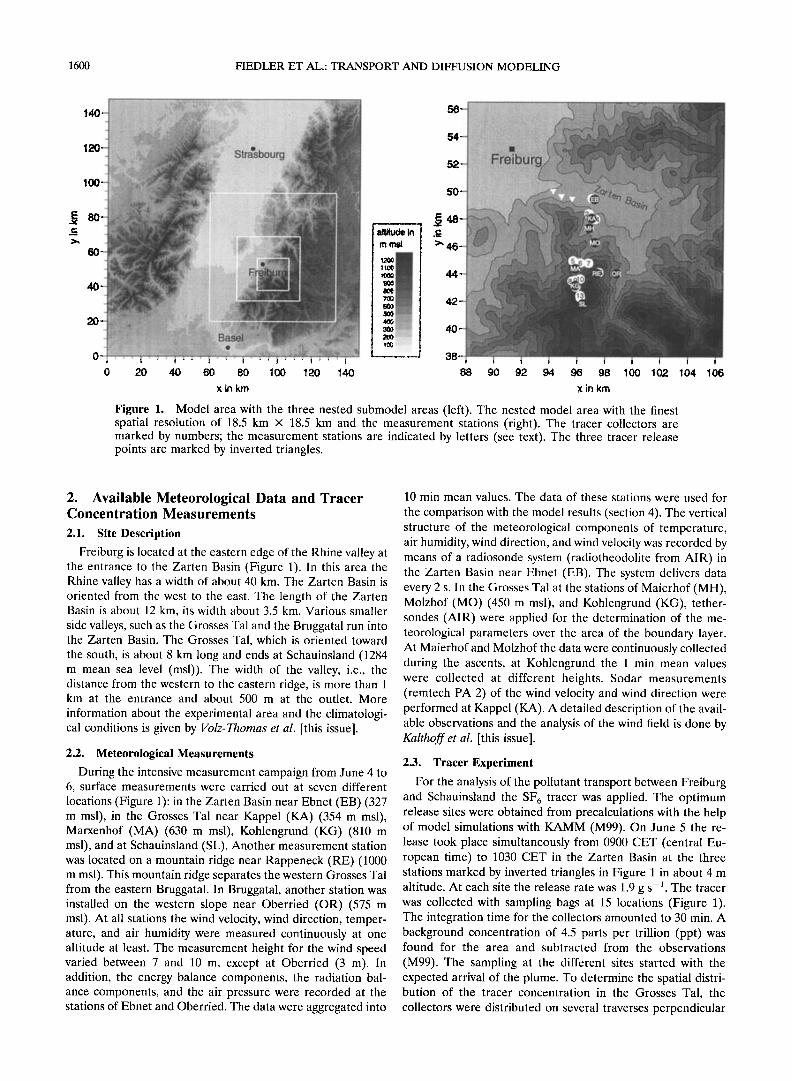
Fisure 3. Comparison of the modeled and the observed ver- tical profiles of the potential temperature 6), the specific hu- midit 7 •, the wind speed •, and the wind direction • at the Ebnet (EB) Station on June 5, 1996, at 0900 and 1:300 CET.

FIEDLER ET AL.: TRANSPORT AND DIFFUSION MODELING 1603

5 m s -• according to the measurements and was kept constant during the whole day. The vertical profiles of the temperature and the specific humidity at the beginning of the simulation were obtained from the radiosonde data of the Ebnet Station

and interpolated to the whole simulation area. The simulation run was started on June 5 at 0000 CET.

4. Meteorological Conditions in the Area Investigated

The model calculations provide the daily variation of the three-dimensional structure of the meteorological parameters for the entire model area. At first, the results of these calcu- lations will be compared with the data measured at the differ- ent observation stations. For comparison, the station in the Zarten Basin (Ebnet), a station in the Grosses Tal (Marxen- hof), and the Schauinsland were selected. The comparison shows the daily variation of the wind velocity and wind direc- tion for these three stations (Figure 2). The major character- istic of airflow is that the valley wind first develops in the side valleys, such as the Grosses Tal and the Bruggatal, whereas valley wind formation is delayed in the Zarten Basin [Kalthoff et al., this issue]. The veering of the wind observed between 0500 and 0600 CET in the Grosses Tal (Marxenhof) is de-

46-

44•

42-•

38-•-,. • I ' • ' • ' • ' • 88 90 92 94 96 98 t00 102 104 106

56-

E 48

• 46-

44 - 900 ..' •.'

42 - 7•

40-

88 90 92 94 96 98 100 102 104 106

x in km

Figure 4. Modeled surface wind field at 1000 CET (top) and 1300 CET (bottom). The wind vectors provided with a frame show the wind measured at the surface stations

1.8

1,4

1.0-

0.8

0.6

0.2 ' ,T•T,-'•r?T.. ½ ." .'- , , ':-• , , . ",. 0 1 2 3 4 5 6 ;• 8 '9 10 11 12 13 t'4 15 16 17 NW km SE

ß . .

• •-- •'7

Figure 5. Vertical cross sections of the simulated wind and potential temperature ©, fields from the northwest to the southeast via Freiburg in the Rhine valley (at 1 km) and Schauinsland in the Black Forest (at 11.5 km) on June 5, 1996 at 0900 CET (top) and 1300 CET (bottom). The wind arrows indicate the wind component in the cutting plane.

scribed correctly by the model. The difference consists in the veering of the wind observed taking place more rapidly. The change from mountain to valley wind was observed between 0800 and 0900 CET in the Zarten Basin, a little later than described by the model. For the Zarten Basin the best agree- ment is obtained for the wind velocity. The modeled and ob- served nocturnal mountain wind is about I m s-•. The valley wind amounts to about 4 m s-•. At the Schauinsland the wind

changes from east to northeast between 0900 and 1000 CET. This change reflects the arrival of the valley wind at the Schauinsland. At 1200 CET the wind changes to northwest and west. This change of the wind from eastern to western direc- tion is also described by the model calculations. A detailed description of the phenomenon will be given below together with the development of the wind field in the entire area. The varying flow conditions at the Schauinsland are of importance for the pollutant transport and will be dealt with in section 5.

In Figure 3 the vertical profiles of the wind speed, wind direction, potential temperature, and the specific humidity as obtained for Ebnet in the Zarten Basin on June 5, 1996, at 0900 and 1300 CET are compared. A special feature at 0900 CET is the development of an inversion at the upper edge of the valley wind layer at 600 m msl. This inversion is attributed to the horizontal advection of cold air from the Rhine valley

1604 FIEDLER ET AL.' TRANSPORT AND DIFFUSION MODELING

into the Zarten Basin and warm air above [Kalthoff et al., this issue]. Within this valley wind layer of about 300 m in thick- ness, a nearly altitude-constant northwestern wind prevails. At the upper edge of the valley wind layer, the wind changes with height by nearly 180 ø to a geostrophic eastern wind within a few

54

52

>'46

44

42

40-*

ß

E48 ©

.,

ß ,,;:. •. • '<.

ß , . •, .•:..r:•. • ,2 •.'.'.•". ,..// • • ß .•...• , •,•. • •.•...., .:.,. ½ • •

92 94 96 98 1• 102 104 106

x in km

Figure 6. Modeled surface wind field during the transition hours in the morning of June 5, 1996, at 0400, 0600, and 0800 CET.

•....• • ..•...• ..... .. ,...: ..:..: .........• ........ . ..... • .... ....... • ...... ......

50.

• •' .•.

40'". ::.•;.•:::•:"•.•,..•,½t'i¾•/z • ,:;• ..... '9½.,,•..'•4) • i • .:•"• '•f '•;'•'":T'• ' •" ':'•'•"':•"•% ........ -.. -:.-......'.N.....

'• •- • .• ½ ..... •..•,:-., ,.• .• •..• •.• • • ½ ½ • .....

b• .- • .- -•)g•:•.•;.•2%• •"• t:;• ...... •;; :•. ...... • ".'• ::.• .:....•:. ß . [• ...... """•r• • -':•s:• ............

•:•)-

• •..•••:•:•.•;.•. :•F•.:•..•:•r•.•F•:•..•. •.• . •........:L• ..

•.•-••.,:;•?..':..•)•.•.::..,....:.',:• .%'.•. '. _"-' ..• :':-•-•.:..•::...:?...:•,..,•,•. "" ::'t•,•½:.•- -%: .............. . • :/-•'•.•t':'!i•'.s•'..•.:•ii.'..:•..-"•.•'• • • "•_t•.,,.*' "-•'"•"• • Z'• • : 5• " •"• '•: .)%

--"•"•?•?""'•'•-'• :•e,-:.•', • ,, // :. ..,•?•..- '(/z'/,•-' .,'%4-}'. :½%.•::•".'•:•.•.':•-:'..•; '•' '"'•'•:• 40- ::'.:.•:?. •..•.'•

ß •;•';,•"'•.H•:':•'""•:•"::':2 ß '.:J".:•"'•

88 90 92 94 96 98 100 102 104 106

x in km

Figure 7. Modeled surface wind field for the transition hours in the evening of June 5, 1996, at 1800, 2000, and 2200 CET.

decameters. Measurement and model results are in agreement as far as the description of the valley wind structure at 0900 CET is concerned. Until 1300 CET, the valley wind layer has grown to about 900 m msl. It is obvious from both the mea- surements and the model calculations that this valley wind layer is associated with a wind speed maximum of about

FIEDLER ET AL.: TRANSPORT AND DIFFUSION MODELING 1605

................... •" .- 52 :-> ? ........... ;...."" _ _ t ..... 3oo•. '" .................................. : "Oo.":'"'""'..--.• ....... '"

50•...•:• ......... . "- ........... ' ........... ',.. )....--" ..'i (' • 48 ;::77"\/,: .......... ;"E :'/ C ti: q • i / -:."'""\ ..... /'/"5: - ß - 4 .• ...-- i : ..: • .-------..... v ...--------....:= ---. 6 ..... i ....' • • •:.-:.:"...:::: ,.--' :...., t.: ..--' .• ..... \ '... ..... ;.--<_

>' ..... ........... • 44-• ,..' ._• ............ :.'....:....:,•.*•

{ ........ : .... -":-:. %7 42 1 /"'"::::'"::'--• '! t._:., .... ::'......"-'7 )•.....:57 ':•i:i!:!;!?ii!.!iiC-'?::::?;;:};'(i;.:,( ..........

ti ...'"-.., :. ............ ;....' :.'.._ • ....... ',: • • :...:::::: _.. '"--':.:-.:::..; .......... : ..... .z. ZOo"::--;'... :.'-':5-'"" .- 40 ........... :.. :.,'-., ,, ......... ß ........ . ...... .....-..- .... - ....... •'::: ......

38

56 ._....i';) C 54 (': ............... '"' !'"'"' •=- '-'"'"' •'½':!::?:"'"'""':="::::-'i?-:;"'-"'""" :' ,._.1 50- ..•oo.:_ '-..-, .... ',oo_.!':.'"';...::, ..... I

,/ 48-

.•_

:

46-

44-

42-

40-

38

88 90 92 94 96 98 100 102 104 106

' ..-.- 700 -'-:

_ ... •760- '--- : ':'- "- ..... "- '" .'"'--..; .'5-: :. ".'.':--L-• -•: 88 90 92 94 96 98 100 102 104106

X in km x in km

ppt I Above 1600 • 96o - 1600

I• ....... I

I ---..• ....... I

Figure 8. Simulated concentration distribution of the SF•, tracer in the bottom computation layer for June 5, 1996, from 0900 to 1100 CET. The dotted lines indicate the altitudes in meters msl. The locations of the SFr, measurement sites are marked by numbers (see Figure 1).

5 m s -• At thc upper edge of the valley wind layer, the modeled and observed wind speed shows a local minimum. Above, the geostrophic eastern wind predominates. Larger differences are found between the modeled and the observed

mixing layer height; that is, the mixing layer height at this time is overestimated by the model. In total, the comparison of the time and spatial behavior of the valley wind systems in the different valleys allows the conclusion that the modeled and the observed structures are in good agreement. Hence the model calculations can also be used for the interpretation of the still unclear phenomena observed.

In Figure 4 the modeled surface wind fields of June 5, 1996, at 1000 and 1300 CET are represented. In both horizontal space directions, only every second calculated wind vector is indicated. In addition, the winds observed at the ground sta- tions at this time are plotted. At 1000 CET the valley winds in the individual valleys are fully developed. Over some mountain ridges, in particular in the southern part of the model area, convergence lines can be noticed. For the Rhine valley the model calculation indicates a northern airflow, and at the Black Forest slopes of the Rhine valley, upslope winds of northwestern direction develop. At this time, a northeastern wind still prevails at Schauinsland. Until 1300 CET, the struc- ture of the valley winds remains more or less the same. As described in Figure 2, however, the wind at Schauinsland has changed to the northwestern direction. The model calculations

now show that the upslope winds at the slopes of the Rhine valley have penetrated further to the east of the Black Forest. They are responsible for the veering of the wind at Schauins- land. To obtain information with regard to the vertical extent of these upslope winds, vertical cross sections were made from the northwest to the southeast, i.e., from Freiburg at I km in the Rhine valley to the Black Forest via Schauinsland at 11.5 km, for the times of 0900 and 1300 CET (Figure 5). At 0900 CET a northwestern wind layer up to about 600 m msl can be found in the Rhine valley. The upper edge of this flow corre- sponds to the altitude of a cold air pool that had developed over night in the Rhine valley. At this time, the upslope winds at the Black Forest slopes of the Rhine valley have not yet reached the mountain ridge. In southeastern Bruggatal, at 13.5 km, upslope winds have developed on both slopes. Above about 1000 m in the Rhine valley and 1200 m in the Black Forest, geostrophic eastern wind prevails. Until 1300 CET the cold air pool in the Rhine valley has vanished, and a mixing layer of about 1000 m in thickness has developed. Over the area of this layer, the northwestern wind has moved upward. At this time, the upslope winds at the Black Forest slopes of the Rhine valley have already penetrated beyond the Schauin- sland further to the east. The thickness of this upslope wind layer is about 300 m. Only at the western slope of Bruggatal, a thin upslope wind layer with an eastern wind component can be observed. According to the measurements, these upslope

1606 FIEDLER ET AL.' TRANSPORT AND DIFFUSION MODELING

winds generated at the Black Forest slopes of the Rhine valley penetrate even further to the Black Forest during the after- noon and interfere with the valley wind systems in Grosses Tal and Bruggatal [Kalthoff et al., this issue]. The convergence areas above the mountain ridges (Figure 4), which are gener- ated by the slope wind systems, cause strong vertical winds (Figure 5) and the ventilation of air pollutants into the free atmosphere. This phenomenon is also known as the mountain chimney effect [e.g., Lu and Turco, 1994] or mountain venting. This effect also influences the tracer transport (section 5). An additional basis for the interpretation of the concentration distribution of air pollutants is the surface wind field. There- fore its spatial distribution is indicated for the transition times from 0400 to 0800 CET (Figure 6) and from 1800 to 2200 CET (Figure 7). Besides the already mentioned flow properties, the following features will be emphasized. During the night (0400 and 2200 CET) a heterogeneous wind field develops. Its struc- tures are determined by the local orography. The highest wind speeds are encountered at the slopes and valley outlets. The "H611entiiler" wind, a well-known valley wind system at the outlet of the Zarten Basin [Lossnitzer, 1942; Rudloff, 1980; Gross, 1989], is well developed. In the morning, at 0800 CET, the strongest winds have developed on the western slopes under sunshine. Until the evening (1800 CET) the convergence of the wind field over the mountain ridges can be noticed. Be- tween 2000 and 2200 CET the valley winds are replaced by moun- tain winds. The upslope winds at the Black Forest slopes of the Rhine valley have given way to downslope winds.

5. Tracer Propagation The tracer released is subject to the transport and diffusion

processes resulting from the meteorological conditions de- scribed in section 4. In Figure 8 the simulated concentration distribution is represented for the time intervals, during which the tracer measurements were performed. The simulated con- centration distribution holds for the bottom computation layer which corresponds to an average altitude of about 5 m. It is obvious that the tracer first (0900 to 0930 CET) spreads toward the east and fills the southern part of the Zarten Basin accord- ing the valley wind existing there. However, during the next time interval, between 0930 and 1000 CET, it can be noticed that a part of the tracer is also transported toward the south into the Grosses Tal. With the valley branching into the Grosses Tal and Kleines Tal, the tracer splits up and enters both valley arms. As will be demonstrated below, this is one of the reasons for the strong differences of the SF 6 concentration between the Kappel and Marxenhof Stations. In the further course of the morning (1000 to 1030 CET) the tracer extends over the entire southern part of the Zarten Basin, its eastern and southern slopes, and its southern side valleys, such as the Bruggatal valley. Between 1030 and 1100 CET the highest surface concentrations are found at the southern slopes of the Zarten Basin and in the eastern area of the Grosses Tal. Even

the mountain ridge between Grosses Tal and Bruggatal is reached by the tracer.

The observed and modeled concentration behaviors of the

000-

900 -

800 -

700 -

600 -

500-

400 -

300 -

200 -

100-

0

8

1000-

900 -

800 -

700 -

600 -

500-

400 -

300 -

200 -

100-

0

8

i

10 11 12

CET

Kappel

' I ' I

13 14

000-

900 -

800 -

700 -

600 -

500-

400 -

300 -

200 -

100-

0

8

Kohlengrund

10 11 12 13

Marxenhof

9 10 11 12 13 14

CET

1000-

900 -

800 -

700 -

600 -

• 500-

400 -

300 -

200 -

100-

i i o i i ' i i i i 9 14 8 9 10 11 12 13 14

CET CET

Schauinsland

I measurements simulation

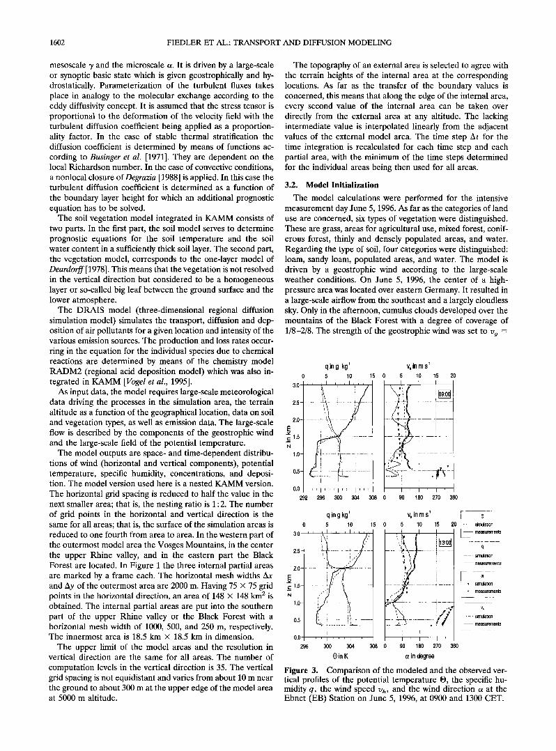
Figure 9. Comparison of the observed and modeled concentration distributions at the four valley cross sections of Kappel (KA), Marxenhof (MA), Kohlengrund (KG), and Schauinsland (SL). For the comparison the observation data and the model results were averaged over the respective valley cross section.

FIEDLER ET AL.' TRANSPORT AND DIFFUSION MODELING 1607

300 - simulation

300 - measurements

I P5

200 -

100 -

0 ' I 8 9 10 11

200-

100-

' I ' I ' I 0 12 13 14 8 10 11 12 13 14

CET CET

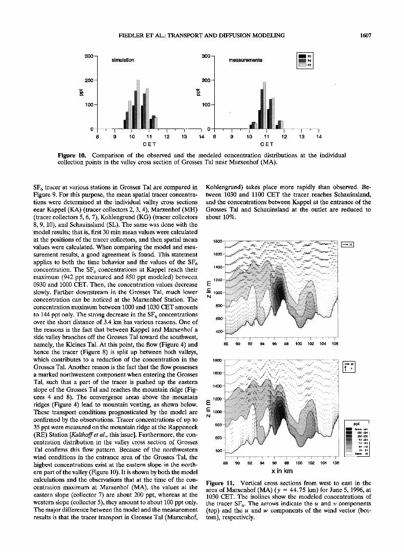
Figure 10. Comparison of the observed and the modeled concentration distributions at the individual collection points in the valley cross section of Grosses Tal near Marxenhof (MA).

SF 6 tracer at various stations in Grosses Tal are compared in Figure 9. For this purpose, the mean spatial tracer concentra- tions were determined at the individual valley cross sections near Kappel (KA) (tracer collectors 2, 3, 4), Marxenhof (MH) (tracer collectors 5, 6, 7), Kohlengrund (KG) (tracer collectors 8, 9, 10), and Schauinsland (SL). The same was done with the model results; that is, first 30 min mean values were calculated at the positions of the tracer collectors, and then spatial mean values were calculated. When comparing the model and mea- surement results, a good agreement is found. This statement applies to both the time behavior and the values of the SF6 concentration. The SF 6 concentrations at Kappel reach their maximum (942 ppt measured and 850 ppt modeled) between 0930 and 1000 CET. Then, the concentration values decrease slowly. Farther downstream in the Grosses Tal, much lower concentration can be noticed at the Marxenhof Station. The

concentration maximum between 1000 and 1030 CET amounts

to 144 ppt only. The strong decrease in the SF 6 concentrations over the short distance of 3.4 km has various reasons. One of

the reasons is the fact that between Kappel and Marxenhof a side valley branches off the Grosses Tal toward the southwest, namely, the Kleines Tal. At this point, the flow (Figure 4) and hence the tracer (Figure 8) is split up between both valleys, which contributes to a reduction of the concentration in the

Grosses Tal. Another reason is the fact that the flow possesses a marked northwestern component when entering the Grosses Tal, such that a part of the tracer is pushed up the eastern slope of the Grosses Tal and reaches the mountain ridge (Fig- ures 4 and 8). The convergence areas above the mountain ridges (Figure 4) lead to mountain venting, as shown below. These transport conditions prognosticated by the model are confirmed by the observations. Tracer concentrations of up to 35 ppt were measured on the mountain ridge at the Rappeneck (RE) Station [Kalthoff et al., this issue]. Furthermore, the con- centration distribution in the valley cross section of Grosses Tal confirms this flow pattern. Because of the northwestern wind conditions in the entrance area of the Grosses Tal, the highest concentrations exist at the eastern slope in the north- ern part of the valley (Figure 10). It is shown by both the model calculations and the observations that at the time of the con-

centration maximum at Marxenhof (MA), the values at the eastern slope (collector 7) are about 200 ppt, whereas at the western slope (collector 5), they amount to about 100 ppt only. The major difference between the model and the measurement results is that the tracer transport in Grosses Tal (Marxenhof,

Kohlengrund) takes place more rapidly than observed. Be- tween 1030 and 1100 CET the tracer reaches Schauinsland, and the concentrations between Kappel at the entrance of the Grosses Tal and Schauinsland at the outlet are reduced to

about 10%.

800

600 --•"- 400

200 000 -

800 -

400-

' I ' I ' I ' I ' I ' I ' I ' I ' I

88 90 92 94 96 98 100 102 104 106

1800 I .,• - // -.- _ \ _ -/ vxx, ---,.

t"--- ... ,,-_ 1600 -L._•.? ..

j ----.>. -,,,,,- ... -

1400 -•.• -----' '" ::"••.i:•:,.-,,,.,,,•,,,,/: ' -. .... -.,._, E .' .... , .....

-- • ooo- •.•.,..,>:.:::':' I:??-:(.'• . . .? '•¾- , -:•.'(:-. • ' '

oo- t ' ' t ,, t t t :;•½;:,:.,.=..:• , :..;.

600- ,•' ,",','•"•' :;; ..• , , • t ,,, t;; • --:•,.•¾•½-? "':--.:

400- : ';':"' ' "• ' I ' I ' I ' I ' I ' I ' I ' I ' I

88 90 92 94 96 98 1 O0 102 104 106

x in km

ppt above 304 I

•56- 304 I •o,•- •.• I .•o- •o,• I

64-112 I ,•- •, I

Below 16 J

Figure 11. Vertical cross sections from west to east in the area of Marxenhof (MA) (y = 44.75 kin) for June 5, 1996, at 1030 CET. The isolines show the modeled concentrations of

the tracer $F 6. The arrows indicate the u and v components (top) and the u and w components of the wind vector (bot- tom), respectively.

1608 FIEDLER ET AL.: TRANSPORT AND DIFFUSION MODELING

105

2000 • •oo•-••

ppt

x in krn I At,ore 100 95 90 I 256- 304 • I 208 - 256

' I 160 - 208 • 112 - 160

64 112

; ' r--'l Below 16

Schauinsland

Zarten Basin

s

ooo

000 '-- N

,00

105

: 90 100 95

x in krn Figure 12. Vertical cross sections from east to west at y = 41.75 km, y = 43.5 km, y = 44.75 km, and y = 48.5 km with isolines of the modeled SF 6 concentrations for June 5, 1996, at 1130 CET.

The convergent flow near the ground in the area of the mountain ridges (Figure 4) suggests that an upward airflow prevails in these areas for continuity reasons, and that this upward flow is accompanied by venting of the tracer from the valley atmosphere to the free atmosphere. Figure 11 shows a vertical cross section through the model area from the west to the east in the latitude of Marxenhof (MA) together with the modeled SF 6 concentration distribution as well as the u and w components and the u and v components of the wind vector, respectively. From the v component of the wind it is evident that the valley wind in the Grosses Tal (96 km) reaches up to an altitude of about 950 m msl, which corresponds to about the altitude of the eastern ridge of the Grosses Tal. On the other hand, it is also obvious that vertical winds of about 1 m s -• occur over the mountain ridges east of Grosses Tal. They result in a vertical transport of the tracer out of the valley atmo- sphere. The tracer is moved upward up to the upper inversion at about 1400 m msl (Figure 3). Consequently, the tracer reaches altitudes where eastern wind prevails and thus is en- trained in western direction toward the Rhine valley. These conditions are summarized in an overview by the representa- tion of vertical cross sections of the modeled SF 6 concentra- tions at different places in the simulation area (Figure 12). Similar transport processes have already been observed during other experiments in the transition area between the Rhine valley and the Black Forest [e.g., Kossmann et al., 1998].

A special feature of the Schauinsland Station is that the wind direction changes several times during the day. Because of the western wind replacing the valley wind at noon (Figures 4, 5, and 6) the air masses are expected to reach Schauinsland on two different ways in the morning and in the afternoon. For this reason, the trajectories were calculated for these two time intervals. Figure 13 shows the trajectories for air parcels which

were started at 0930 CET in the area of the three tracer release

stations in the Zarten Basin. These air parcels were mainly transported from the Zarten Basin along the eastern slope of the Grosses Tal toward the south and reached Schauinsland

via the valley outlet. Because of the eastern upper airflow the air parcels then were transported toward the Rhine valley in the west. In the afternoon the air parcels, started in the area of Freiburg at 1130 CET, did no longer reach Schauinsland via the Zarten Basin and Grosses Tal but were transported via the Black Forest slopes to Schauinsland. Also in this case, the air parcels above Schauinsland are returned to the Rhine valley south of Freiburg when entering the eastern upper airflow.

6. Conclusions

In June 1996 the SLOPE experiment was carried out in the area of Freiburg-Schauinsland. This experiment was aimed at studying the city plume of Freiburg [I/olz-Thomas et al., this issue]. Therefore chemical, meteorological, and tracer mea- surements were performed between Freiburg and Schauins- land. The meteorological secondary circulation systems in their complexity and the associated diffusion and transport of air pollutants between Freiburg and Schauinsland were analyzed by Kalthoff et al. [this issue]. In principle, field experiments allow local measurements only. Because of this limited spatial resolution the SLOPE measurements gave rise to questions which could not or only hardly be answered on the basis of the measurement results. Model calculations represent a suitable means to facilitate interpretation. As a prerequisite, the model has to provide for the necessary spatial and time resolution for all scales to be taken into account. This requirement was com- plied with by the use of a multinested model. The resolution in

FIEDLER ET AL.: TRANSPORT AND DIFFUSION MODELING 1609

Schauinsland

Freiburg

Zarten Basin

qo oø _

Figure 13. Modeled trajectories for the air parcels released in the Zarten Basin at 0930 CET (top) and in the area of Freiburg at 1130 (bottom). The release points are marked by inverted triangles. The time difference between two points on the trajectory is 10 min.

the outermost model area was 2 km. The smallest nested

model area had a resolution of 250 m.

At first, the daily variations and vertical profiles computed with the model were compared with the measurements. It was thus demonstrated that the valley wind systems in the different valleys can be reproduced by the model. Then, tracer transport could be calculated. The most important modeling results are as follows:

1. The northern valley wind observed until noon over Schauinsland is replaced by a northwestern wind arriving at the Black Forest summits. These northwestern winds developed on the Black Forest slopes of the Rhine valley. In the course of the morning, these upslope winds reach the edge of the Black

Forest slopes and penetrate farther toward the east into the Black Forest.

2. As a result of this penetration of the larger-scale north- western flow, the transport of air masses does no longer take place via the valley wind systems from Freiburg to Schauins- land, i.e., via the Zarten Basin and the Grosses Tat but from the Rhine valley over the Black Forest slopes to Schauinstand.

3. The SF 6 tracer released in the Zarten Basin on June 5, 1996, exhibited a marked decrease over a short distance in the entrance area of the Grosses Tat. It is demonstrated by the model calculations that this decrease is to be attributed to (1) the flow splitting up into the Grosses Tat and a side valley of the Grosses Tal, namely, the Kleines Tal, and to (2) the flow in

1610 FIEDLER ET AL.: TRANSPORT AND DIFFUSION MODELING

the entrance area of the Grosses Tal not being parallel to the valley but pushed up over the eastern slope to the mountain ridge by the northwestern wind prevailing there. The conver- gence line along the mountain ridges also results in a ventila- tion effect or the so-called mountain chimney effect. Conse- quently, the tracer is removed from the valley atmosphere up into the eastern upper airflow. This effect also contributes to the reduction of the tracer concentration.

Both the measurement and the model calculation give a clear picture of the meteorological phenomena in the area of Freiburg-Schauinsland. Furthermore, they provide the inter- pretation support for understanding the tracer concentration behaviors. This allows to determine the influence of transport and diffusion on the air mass flow from Freiburg to Schauin- sland. Only then the chemical reaction processes can be sep- arated from the transport and diffusion processes. The model results together with the meteorological and tracer measure- ments [Kalthoff et al., this issue] are used for the interpretation of the chemical reaction processes [Volz-Thomas et al., this issue; Volz-Thomas and Kolahgar, this issue].

Acknowledgments. The authors would like to thank all groups involved in the SLOPE experiment. The measurements were sup- ported by the Baden-Wfirttemberg State Ministry for Science and Research under contract no. 1499Tit. Gr.74 within the framework of

the Regio-Klima-Project (REKLIP) and by the Hermann von Helm- holtz-Gemeinschaft Deutscher Forschungszentren (HGF).

References

Adrian, G., and F. Fiedler, Simulation of unstationary wind- and tem- perature fields over complex terrain and comparison with observa- tions, Contrib. Phys. Atmos., 64, 27-48, 1991.

Atkinson, B. W., Mesoscale Atmospheric Circulations, 495 pp., Aca- demic, San Diego, Calif., 1981.

Baer, M., and K. Nester, Parameterization of trace gas dry deposition velocities for a regional mesoscale diffusion model, Ann. Geophys., 10, 912-923, 1992.

Barry, R. G., Mountain Weather and Climate, 402 pp., Routledge, New York, 1992.

Bossert, J. E., J. D. Sheaffer, and E. R. Reiter, Aspects of regional- scale flows in mountainous terrain, J. Appl. Meteorol., 28, 590-601, 1989.

Businger, J. A., J. C. Wyngaard, Y. Izumi, and E. F. Bradley, Flux profile relationships in the atmospheric boundary layer, J. Atmos. Sci., 28, 181-189, 1971.

Chang, J. S., R. A. Brost, I. S. A. Isaksen, S. Madronich, and P. Middleton, A three-dimensional Eulerian acid deposition model: Physical concepts and formulation, J. Geophys. Res., 92, 14,681- 14,700, 1987.

Deardorff, J. W., Efficient prediction of ground surface temperature and moisture with inclusion of a layer of vegetation, J. Geophys. Res., 83, 1889-1903, 1978.

Degrazia, G. A., Anwendung von J•hnlichkeitsverfahren auf die tur- bulente Diffusion in der konvektiven und stabilen Grenzschicht, 99 pp., Ph.D. thesis, Univ. Karlsruhe, Karlsruhe, 1988.

Fiedler, F., Development of meteorological computer models, Inter- disciplinary Sci. Rev., 18, 192-198, 1993.

Gross, G., Numerical simulation of the nocturnal flow systems in the Freiburg area for different topographies, Contrib. Phys. Atmos., 62, 57-72, 1989.

Kalthoff, N., H.-J. Binder, M. Ko13mann, R. V6gtlin, U. Corsmeier, F. Fiedler, and H. Schlager, Temporal evolution and spatial variation of the boundary layer over complex terrain, Atmos. Environ., 32, 1179-1194, 1998.

Kalthoff, N., V. Horlacher, U. Corsmeier, A. Volz-Thomas, B. Kolah- gar, H. Geiss, M. M611mann-Coers, and A. Knaps, The influence of valley winds on transport and dispersion of airborne pollutants in the Freiburg-Schauinsland area. J. Geophys. Res., this issue.

Koch, S. E., and J. T. McQueen, A survey of nested grid techniques and their potential for use within the MASS weather prediction mode, NASA Tech. Memo. 87808, 25 pp., 1987.

Kossmann, M., Einflu13 orographisch induzierter Transportprozesse auf die Struktur der atmosphfirischen Grenzschicht und die Vertei- lung von Spurengasen, 193 pp., Ph.D. thesis, Univ. Karlsruhe, Karlsruhe, 1998.

Kossmann, M., R. V6gtlin, U. Corsmeier, B. Vogel, F. Fiedler, H.-J. Binder, and N. Kalthoff, Aspects of the convective boundary layer structure over complex terrain, Atmos. Environ., 32, 1323-1348, 1998.

Kurihara, Y., G. J. Tripoli, and M. A. Bender, Design of a movable nested-mesh primitive equation model, Mon. Weather Rev., 107, 239-249, 1979.

Lossnitzer, H., Einige Bemerkungen zum Klima Freiburgs im Breis- gau, Z. Angew. Meteorol. "das Wetter," 59, 37-42, 1942.

Lu, R., and R. P. Turco, Pollutant transport in a coastal environment, Part 1, Two-dimensional simulations of sea breeze and mountain effects, J. Atmos. Sci., 51, 2285-2308, 1994.

Pfitz, H.-W., et al., Measurements of trace gases and photolysis fre- quencies during SLOPE 96 and a course estimate of the local OH concentration from NHO3 formation, J. Geophys. Res., this issue.

v. Rudloff, H., Besonderheiten im Klima yon Freiburg, Bad. Landesver. Naturschutz, NF, 5, 237-254, 1980.

Sch•idler, G., N. Kalthoff, and F. Fiedler, Validation of a model for heat, mass and momentum exchange over vegetated surfaces using LOTREX-10E/HIBE88 data, Contrib. Phys. Atmos., 63, 85-100, 1990.

Vogel, B., F. Fiedler, and H. Vogel, Influence of topography and biogenic volatile organic compounds emission in the state of Baden- Wtirttemberg on ozone concentrations during episodes of high air temperatures, J. Geophys. Res., 100, 22,907-22,928, 1995.

Volz-Thomas, A., and B. Kolahgar, On the budget of hydroxyl radicals at Schauinsland during SLOPE96, J. Geophys. Res., this issue.

Volz-Thomas, A., H. Geiss, N. Kalthoff, The Schauinsland Ozone Precursor Experiment (SLOPE96): Scientific background and main results, J. Geophys. Res., this issue.

de Wekker, S. F. J., The behaviour of the convective boundary layer height over orographically complex terrain, diploma thesis, Dep. Meteorol. Wageningen Agric. Univ. and Meteorol. Inst., Univ. Karlsruhe, Karlsruhe, 1995.

G. Adrian, I. Bischoff-Gaul:3, F. Fiedler, and N. Kalthoff, Institut ftir Meteorologie und Klimaforschung, Forschungszentrum Karlsruhe/ Universit•it Karlsruhe, Postfach 3640, D-76021 Karlsruhe, Germany. (inge.bischoff-gauss@imk.fzk. de)

(Received April 12, 1999; revised August 19, 1999; accepted August 25, 1999.)