Modeling methane production from beef cattle using linear and nonlinear approaches

Moore, R. Christopherson, G. K. Murdoch, B. W. McBride, E. K. Okine and J. FranceJ. L. Ellis, E. Kebreab, N. E. Odongo, K. Beauchemin, S. McGinn, J. D. Nkrumah, S. S.

Modeling methane production from beef cattle using linear and nonlinear approaches

doi: 10.2527/jas.2007-0725 originally published online December 19, 20082009, 87:1334-1345.J ANIM SCI

http://jas.fass.org/content/87/4/1334the World Wide Web at:

The online version of this article, along with updated information and services, is located on

www.asas.org

by guest on September 27, 2011jas.fass.orgDownloaded from

http://jas.fass.org/

ABSTRACT: Canada is committed to reducing its greenhouse gas emissions to 6% below 1990 amounts between 2008 and 2012, and methane is one of several greenhouse gases being targeted for reduction. Methane production from ruminants is one area in which the agriculture sector can contribute to reducing our global impact. Through mathematical modeling, we can fur-ther our understanding of factors that control methane production, improve national or global greenhouse gas inventories, and investigate mitigation strategies to re-duce overall emissions. The purpose of this study was to compile an extensive database of methane produc-tion values measured on beef cattle, and to generate linear and nonlinear equations to predict methane pro-duction from variables that describe the diet. Extant methane prediction equations were also evaluated. The linear equation developed with the smallest root mean square prediction error (RMSPE, % observed mean) and residual variance (RV) was Eq. I: CH4, MJ/d = 2.72 (±0.543) + [0.0937 (±0.0117) × ME intake, MJ/d] + [4.31 (±0.215) × Cellulose, kg/d] − [6.49 (±0.800) × Hemicellulose, kg/d] − [7.44 (±0.521) × Fat, kg/d]

[RMSPE = 26.9%, with 94% of mean square prediction error (MSPE) being random error; RV = 1.13]. Equa-tions based on ratios of one diet variable to another were also generated, and Eq. P, CH4, MJ/d = 2.50 (±0.649) − [0.367 (±0.0191) × (Starch:ADF)] + [0.766 (±0.116) × DMI, kg/d], resulted in the smallest RMSPE values among these equations (RMSPE = 28.6%, with 93.6% of MSPE from random error; RV = 1.35). Among the nonlinear equations developed, Eq. W, CH4, MJ/d = 10.8 (±1.45) × (1 − e[−0.141 (±0.0381) × DMI, kg/d]), performed well (RMSPE = 29.0%, with 93.6% of MSPE from ran-dom error; RV = 3.06), as did Eq. W3, CH4, MJ/d = 10.8 (±1.45) × [1 − e{−[−0.034 × (NFC/NDF) + 0.228] × DMI, kg/d}] (RMSPE = 28.0%, with 95% of MSPE from random error). Extant equations from a previous publication by the authors performed comparably with, if not bet-ter than in some cases, the newly developed equations. Equation selection by users should be based on RV and RMSPE analysis, input variables available to the user, and the diet fed, because the equation selected must account for divergence from a “normal” diet (e.g., high-concentrate diets, high-fat diets).

Key words: beef cattle, greenhouse gas, methane production, modeling

©2009 American Society of Animal Science. All rights reserved. J. Anim. Sci. 2009. 87:1334–1345 doi:10.2527/jas.2007-0725

INTRODUCTION

As a result of signing the Kyoto protocol in 1998, Canada is committed to reducing its greenhouse gas emissions to 6% below 1990 amounts between 2008 and 2012 (Environment Canada, 2005), and this includes gases such as CO2, N2O, and CH4. Methane production from ruminants is one area in which the agriculture sector can contribute to reducing overall greenhouse

Modeling methane production from beef cattle using linear and nonlinear approaches1

J. L. Ellis,*2 E. Kebreab,† N. E. Odongo,*‡ K. Beauchemin,§ S. McGinn,§ J. D. Nkrumah,# S. S. Moore,# R. Christopherson,# G. K. Murdoch,#‖

B. W. McBride,* E. K. Okine,# and J. France*

*Centre for Nutrition Modeling, Department of Animal and Poultry Science, University of Guelph, Guelph, Ontario, N1G 2W1, Canada; †National Centre for Livestock and Environment, Department of Animal Science,

University of Manitoba, Winnipeg, Manitoba, R3T 2N2, Canada; ‡Animal Production and Health Section, Department of Nuclear Sciences and Applications, International Atomic Energy Agency, PO Box 100,

Wagramer Strasse 5, A-1400 Vienna, Austria; §Agriculture and Agri-Food Canada, Lethbridge Research Centre, Lethbridge, AB, T1J 4B1, Canada; #Department of Agricultural, Food and Nutritional Science,

University of Alberta, Edmonton, Alberta, T6G 2P5, Canada; and ‖Animal and Veterinary Science, University of Idaho, Moscow 83844

1 Funding was provided in part by the Canada Research Chairs Program (Ottawa, Ontario, Canada), the Natural Sciences and En-gineering Research Council Strategic Grants Program (Ottawa, On-tario, Canada), and BIOCAP Canada (Ottawa, Ontario, Canada).

2 Corresponding author: [email protected] November 13, 2007.Accepted December 3, 2008.

1334



gas emissions because CH4 from ruminants accounts for 72% of the total CH4 emissions of Canada (Environ-ment Canada, 2005).

Country- and world-wide inventories are based on mathematical models that are also important in devel-oping mitigation strategies to reduce emissions. Both mechanistic and regression models aid in improving our understanding of CH4 production by animals and al-low evaluation of the causes of change and variation in CH4 production. Although several CH4 regression equations exist in the literature (Kriss, 1930; Axelsson, 1949; Blaxter and Clapperton, 1965; Moe and Tyrrell, 1979; Mills et al., 2003), some require input variables that are not commonly available, whereas others were developed for different classes of animals (e.g., dairy vs. beef) or feeding regimens (as reviewed by Ellis et al., 2007). Equations developed by Ellis et al. (2007), based on a North American and Canadian beef and dairy cattle literature database, performed better than other extant CH4 prediction equations. The purpose of the current study is to 1) collect an extensive north-ern United States and Canadian beef cattle database of CH4 emissions, consisting of individual animal data as opposed to treatment averages available in the lit-erature; 2) to generate linear and nonlinear equations containing combinations of variables that describe the diet, including ratios of nonfiber to fiber carbohydrate components, to determine whether any improvements in CH4 prediction over the beef equations of Ellis et al. (2007) could be obtained; and 3) to challenge the beef cattle equations developed by Ellis et al. (2007) with the current database.

MATERIALS AND METHODS

Animal Care and Use Committee approval was not required for this study because the data were obtained from an existing database, as outlined in Table 1.

Database

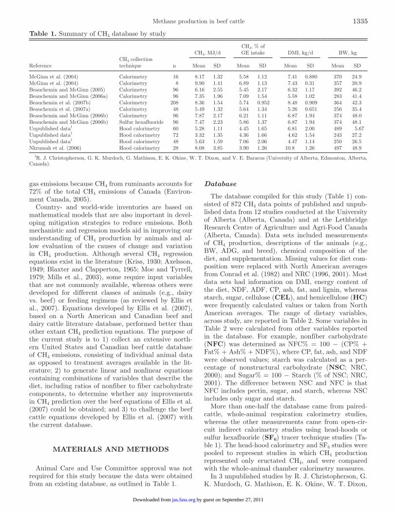
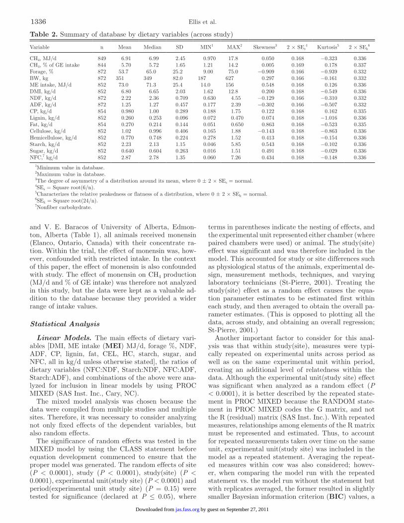
The database compiled for this study (Table 1) con-sisted of 872 CH4 data points of published and unpub-lished data from 12 studies conducted at the University of Alberta (Alberta, Canada) and at the Lethbridge Research Centre of Agriculture and Agri-Food Canada (Alberta, Canada). Data sets included measurements of CH4 production, descriptions of the animals (e.g., BW, ADG, and breed), chemical composition of the diet, and supplementation. Missing values for diet com-position were replaced with North American averages from Conrad et al. (1982) and NRC (1996, 2001). Most data sets had information on DMI, energy content of the diet, NDF, ADF, CP, ash, fat, and lignin, whereas starch, sugar, cellulose (CEL), and hemicellulose (HC) were frequently calculated values or taken from North American averages. The range of dietary variables, across study, are reported in Table 2. Some variables in Table 2 were calculated from other variables reported in the database. For example, nonfiber carbohydrate (NFC) was determined as NFC% = 100 − (CP% + Fat% + Ash% + NDF%), where CP, fat, ash, and NDF were observed values; starch was calculated as a per-centage of nonstructural carbohydrate (NSC; NRC, 2000); and Sugar% = 100 − Starch (% of NSC; NRC, 2001). The difference between NSC and NFC is that NFC includes pectin, sugar, and starch, whereas NSC includes only sugar and starch.

More than one-half the database came from paired-cattle, whole-animal respiration calorimetry studies, whereas the other measurements came from open-cir-cuit indirect calorimetry studies using head-hoods or sulfur hexafluoride (SF6) tracer technique studies (Ta-ble 1). The head-hood calorimetry and SF6 studies were pooled to represent studies in which CH4 production represented only eructated CH4, and were compared with the whole-animal chamber calorimetry measures.

In 3 unpublished studies by R. J. Christopherson, G. K. Murdoch, G. Mathison, E. K. Okine, W. T. Dixon,

Table 1. Summary of CH4 database by study

ReferenceCH4 collection technique n

CH4, MJ/dCH4, % of GE intake DMI, kg/d BW, kg

Mean SD Mean SD Mean SD Mean SD

McGinn et al. (2004) Calorimetry 16 8.17 1.32 5.58 1.12 7.41 0.880 370 24.9McGinn et al. (2004) Calorimetry 8 9.90 1.41 6.89 1.13 7.43 0.31 357 20.9Beauchemin and McGinn (2005) Calorimetry 96 6.16 2.55 5.45 2.17 6.32 1.17 392 46.2Beauchemin and McGinn (2006a) Calorimetry 96 7.35 1.96 7.09 1.54 5.58 1.02 283 41.4Beauchemin et al. (2007b) Calorimetry 208 8.36 1.54 5.74 0.952 8.48 0.909 364 42.3Beauchemin et al. (2007a) Calorimetry 48 5.49 1.32 5.64 1.34 5.26 0.651 256 35.4Beauchemin and McGinn (2006b) Calorimetry 96 7.87 2.17 6.21 1.11 6.87 1.94 374 48.0Beauchemin and McGinn (2006b) Sulfur hexafluoride 96 7.47 2.23 5.86 1.37 6.87 1.94 374 48.1Unpublished data1 Hood calorimetry 60 5.28 1.11 4.45 1.65 6.81 2.00 489 5.67Unpublished data1 Hood calorimetry 72 3.32 1.35 4.36 1.66 4.62 1.54 243 27.2Unpublished data1 Hood calorimetry 48 5.63 1.59 7.06 2.06 4.47 1.14 250 26.5Nkrumah et al. (2006) Hood calorimetry 28 8.08 3.85 3.90 1.26 10.8 1.26 497 48.9

1R. J. Christopherson, G. K. Murdoch, G. Mathison, E. K. Okine, W. T. Dixon, and V. E. Baracos (University of Alberta, Edmonton, Alberta, Canada).

Methane production in beef cattle 1335



and V. E. Baracos of University of Alberta, Edmon-ton, Alberta (Table 1), all animals received monensin (Elanco, Ontario, Canada) with their concentrate ra-tion. Within the trial, the effect of monensin was, how-ever, confounded with restricted intake. In the context of this paper, the effect of monensin is also confounded with study. The effect of monensin on CH4 production (MJ/d and % of GE intake) was therefore not analyzed in this study, but the data were kept as a valuable ad-dition to the database because they provided a wider range of intake values.

Statistical Analysis

Linear Models. The main effects of dietary vari-ables [DMI, ME intake (MEI) MJ/d, forage %, NDF, ADF, CP, lignin, fat, CEL, HC, starch, sugar, and NFC, all in kg/d unless otherwise stated], the ratios of dietary variables (NFC:NDF, Starch:NDF, NFC:ADF, Starch:ADF), and combinations of the above were ana-lyzed for inclusion in linear models by using PROC MIXED (SAS Inst. Inc., Cary, NC).

The mixed model analysis was chosen because the data were compiled from multiple studies and multiple sites. Therefore, it was necessary to consider analyzing not only fixed effects of the dependent variables, but also random effects.

The significance of random effects was tested in the MIXED model by using the CLASS statement before equation development commenced to ensure that the proper model was generated. The random effects of site (P < 0.0001), study (P < 0.0001), study(site) (P < 0.0001), experimental unit(study site) (P < 0.0001) and period(experimental unit study site) (P = 0.15) were tested for significance (declared at P ≤ 0.05), where

terms in parentheses indicate the nesting of effects, and the experimental unit represented either chamber (where paired chambers were used) or animal. The study(site) effect was significant and was therefore included in the model. This accounted for study or site differences such as physiological status of the animals, experimental de-sign, measurement methods, techniques, and varying laboratory technicians (St-Pierre, 2001). Treating the study(site) effect as a random effect causes the equa-tion parameter estimates to be estimated first within each study, and then averaged to obtain the overall pa-rameter estimates. (This is opposed to plotting all the data, across study, and obtaining an overall regression; St-Pierre, 2001.)

Another important factor to consider for this anal-ysis was that within study(site), measures were typi-cally repeated on experimental units across period as well as on the same experimental unit within period, creating an additional level of relatedness within the data. Although the experimental unit(study site) effect was significant when analyzed as a random effect (P < 0.0001), it is better described by the repeated state-ment in PROC MIXED because the RANDOM state-ment in PROC MIXED codes the G matrix, and not the R (residual) matrix (SAS Inst. Inc.). With repeated measures, relationships among elements of the R matrix must be represented and estimated. Thus, to account for repeated measurements taken over time on the same unit, experimental unit(study site) was included in the model as a repeated statement. Averaging the repeat-ed measures within cow was also considered; howev-er, when comparing the model run with the repeated statement vs. the model run without the statement but with replicates averaged, the former resulted in slightly smaller Bayesian information criterion (BIC) values, a

Table 2. Summary of database by dietary variables (across study)

Variable n Mean Median SD MIN1 MAX2 Skewness3 2 × SEs4 Kurtosis5 2 × SEk

6

CH4, MJ/d 849 6.91 6.99 2.45 0.970 17.8 0.050 0.168 −0.323 0.336CH4, % of GE intake 844 5.70 5.72 1.65 1.21 14.2 0.005 0.169 0.178 0.337Forage, % 872 53.7 65.0 25.2 9.00 75.0 −0.909 0.166 −0.939 0.332BW, kg 872 351 349 82.0 187 627 0.297 0.166 −0.161 0.332ME intake, MJ/d 852 73.0 71.3 25.4 14.0 156 0.548 0.168 0.126 0.336DMI, kg/d 852 6.80 6.65 2.03 1.62 12.8 0.200 0.168 −0.549 0.336NDF, kg/d 872 2.22 2.36 0.709 0.630 4.55 −0.129 0.166 −0.310 0.332ADF, kg/d 872 1.25 1.27 0.457 0.177 2.39 −0.302 0.166 −0.507 0.332CP, kg/d 854 0.980 1.00 0.289 0.188 1.75 0.122 0.168 0.162 0.335Lignin, kg/d 852 0.260 0.253 0.096 0.072 0.470 0.074 0.168 −1.016 0.336Fat, kg/d 854 0.270 0.214 0.144 0.051 0.650 0.863 0.168 −0.523 0.335Cellulose, kg/d 852 1.02 0.996 0.406 0.165 1.88 −0.143 0.168 −0.863 0.336Hemicellulose, kg/d 852 0.770 0.748 0.224 0.278 1.52 0.413 0.168 −0.154 0.336Starch, kg/d 852 2.23 2.13 1.15 0.046 5.85 0.543 0.168 −0.102 0.336Sugar, kg/d 852 0.640 0.604 0.263 0.016 1.51 0.491 0.168 −0.029 0.336NFC,7 kg/d 852 2.87 2.78 1.35 0.060 7.26 0.434 0.168 −0.148 0.336

1Minimum value in database.2Maximum value in database.3The degree of asymmetry of a distribution around its mean, where 0 ± 2 × SEs = normal.4SEs = Square root(6/n).5Characterizes the relative peakedness or flatness of a distribution, where 0 ± 2 × SEk = normal.6SEk = Square root(24/n).7Nonfiber carbohydrate.

Ellis et al.1336



statistical criterion used for model selection, indicating a better fit of the model (SAS Inst. Inc.).

If, when running the model, the random covariance or the random slope was not significant (P > 0.05), it was removed from the model (St-Pierre, 2001). The joint distribution of random effects was assumed to be multivariate normal and the dual quasi-Newton tech-nique was used for optimization, with adaptive Gauss-ian quadrature as the integration method. Analysis was performed with the assumption that variance distribu-tion for the estimates followed a multivariate normal distribution.

Nonlinear Models. Biological relationships are seldom linear over a wide range of values; therefore, nonlinear relationships between CH4 production (MJ/d) and dietary variables (Table 2) were also considered. The PROC NLMIXED in SAS was used to parameter-ize either a modified nonlinear Mitscherlich (Mits; rise to plateau; Eq. 1) or a Gaussian (rise to peak; Eq. 2) equation to describe the relationship:

CH4 (MJ/d) = a − (a + b)e(−cx), [1]

CH4 (MJ/d) = aexp{−0.5[(x − x0)/b]2}, [2]

where, for the Mits equation, parameter a represents the maximum potential CH4 production, parameter b was fixed at zero to represent zero methanogenesis at zero intake, and parameter c controls the rate of change with variable x. For the Gaussian equation, parameter a represents the maximum potential CH4 production, parameter b controls the rate of change of CH4 pro-duction with x, and x0 indicates where the peak in the curve occurs. Parameters a, b, c, and x0 were fitted to the beef database by using the NLMIXED procedure.

The NLMIXED procedure does not accommodate both random and repeated statements; therefore, ob-servations made on the same experimental unit with the same treatment were averaged. This procedure re-duced the overall sample size from 879 to 424. A random statement was included within the NLMIXED code to account for the effect of study, but nesting could not be evaluated.

To account for the study effect, an additive random term was added to Eq. 1 and 2. Additive random terms should have been added to parameters a and c (Eq. 1) separately, on top of the fixed effects, but attempts to do this resulted in nonconvergence of the models. Consequently, the model across studies has an implicit (0,0) intercept, but the regressions for each study do not have this property. They are sets of parallel curves with intercepts shifted according to the BLUP for the effect of each study.

In addition to these simple nonlinear equations, pa-rameter c in the Mits equation was replaced with a linear equation containing a ratio (e.g., NFC:NDF) that will control the rate of increase of the curve rela-tive to DMI, similar to the work described by Mills et al. (2003). Dry matter intake was selected to scale

the model (parameter x) over MEI because of conver-gence problems with MEI in the linear modeling sec-tion. The data were first divided into 4 equal groups, each representing an increase in the average ratio value (NFC:NDF, starch:NDF, NFC:ADF, or starch:ADF). A Mits curve was then fitted to each of the 4 subsets of data separately, using DMI as the x variable, and a and c values were determined. The relationship between the average ratio for each of the 4 groups and the c values for each of the 4 groups was then plotted, and linear equations were developed. These linear equations, con-taining one of the above ratios, were then put into the Mits equation in place of the c variable.

Extant Models. The predictive ability of some simple CH4 prediction equations developed in an earlier study (Ellis et al., 2007), as well as equations by Kriss (1930), Axelsson (1949), Blaxter and Clapperton (1965; as modified by Wilkerson et al., 1995), Moe and Tyrrell (1979), and Mills et al. (2003) were challenged with this database. The extant equations are presented in Table 3. These equations were selected for comparison be-cause they are commonly used and their input variables were obtainable from the compiled database.

Model Evaluation. Residual variance (RV) and BIC values were reported for the developed equations as an indicator of the goodness of model fit. Variance attributable to the study effect (SV) was also reported. Models developed in this study and extant models were also evaluated using the mean square prediction error (MSPE), calculated as

MSPE = -( )=å O P ni ii

n 2

1

/ , [3]

where Oi is the observed value, and Pi is the predicted value. Square root of the MSPE (RMSPE), expressed as a proportion of the observed mean, gives an esti-mate of the overall prediction error. Root MSPE values are expressed relative to the observed mean so that comparisons of RMSPE (%) values can be made be-tween equations with different predicted means, and so that deviations from observed values can be evaluated. The RMSPE was decomposed into random error (ED), error attributable to deviation of the regression slope from unity (ER), and error attributable to overall bias (ECT; Bibby and Toutenburg, 1977).

Concordance correlation coefficients (CCC; Lin, 1989) were also calculated as an evaluation of the pre-cision and accuracy of predicted vs. observed values for the models. The CCC estimate is the product of 2 components: 1) the R, which is a measure of precision (deviation of observations from the best fit line), and 2) a bias correction factor (Cb), which indicates how far the regression line deviates from the line of unity (ac-curacy). Another estimate (µ) that measures location shift relative to the product of 2 SD is also reported, where a negative value indicates underprediction and a positive value indicates overprediction of observed val-ues by the model.




RESULTS AND DISCUSSION

Methane Collection Method

The effect of CH4 collection method (whole-animal calorimetry vs. SF6 and hood calorimetry) within the PROC MIXED model of SAS was not significant when CH4 was expressed in megajoules per day (P = 0.12) or as a percentage of GE intake (P = 0.15). Because there was no difference between measurement techniques, whole-animal calorimetry, hood calorimetry, and SF6 data were pooled in this study and were not evaluated separately.

Linear Regression Models

As a follow-up to the study by Ellis et al. (2007), in this study regression analysis was conducted, using the MIXED model described above, on a more exten-sive database of animal data, which included dietary variables not available previously. Ellis et al. (2007) examined both beef and dairy data, whereas this study focused on only beef cattle data. Although many more equations and variable combinations were evaluated in this study than those presented, for simplicity, equa-tions duplicating those developed in Ellis et al. (2007) are not reported, and only the top 12 equations from the analysis are reported here.

Considerably less use of North American averages for diet variables was required for the current study com-pared with those used by Ellis et al. (2007). The list of available variables used in this regression analysis is reported in Table 2. Although book variables are likely to contain more error than measured values, the variables NFC, starch, HC, and CEL were frequently significantly related to CH4 production and were there-fore generally included in the regression equations in this study. All diet-based linear regression equations developed in this study are reported in Table 4, and all equation parameters were significant at P ≤ 0.05.

Previous work by Moe and Tyrrell (1979) revealed that NFC, HC, and CEL were good predictors of CH4 production. However, Ellis et al. (2007) found that MEI, forage percentage, NDF, and ADF were also strongly related to CH4 production, and were good alternative predictors when accurate estimates of NFC, starch, HC, and CEL were not available. One of the challenges faced by Ellis et al. (2007) was that within the equa-tion used to calculate NFC, many input variables were North American averages. Because each average will contain some degree of error, combining them within this equation resulted in considerable error in the cal-culated NFC value; thus, NFC, or any value calculated from it, was not used for regression analysis in that study. In contrast, only observed values were used to calculate NFC in this study; thus, the value of NFC contains considerably less error. The minimum and

Table 3. Extant CH4 prediction equations developed in, or evaluated by, Ellis et al. (2007)

Source Equation1

Ellis et al. (2007), Eq. 1b CH4 (MJ/d) = 4.38(±1.46) + 0.0586(±0.0175) × MEI (MJ/d)Ellis et al. (2007), Eq. 2b CH4 (MJ/d) = 3.96(±1.18) + 0.561(±0.130) × DMI (kg/d)Ellis et al. (2007), Eq. 3b CH4 (MJ/d) = 4.79(±1.98) + 0.0492(±0.0219) × Forage (%)Ellis et al. (2007), Eq. 4b CH4 (MJ/d) = 5.263(±1.57) + 6.93(±2.66) × Lignin (kg/d)Ellis et al. (2007), Eq. 5b CH4 (MJ/d) = 5.58(±1.12) + 0.848(±0.266) × NDF (kg/d)Ellis et al. (2007), Eq. 6b CH4 (MJ/d) = 5.70(±1.64) + 1.41(±0.550) × ADF (kg/d)Ellis et al. (2007), Eq. 7b CH4 (MJ/d) = 3.05(±1.21) + 0.0371(±0.0170) × MEI (MJ/d) + 0.801(±0.223) × NDF (kg/d)Ellis et al. (2007), Eq. 8b CH4 (MJ/d) = 3.31(±1.27) + 0.0382(±0.0178) × MEI (MJ/d) + 1.05(±0.384) × ADF (kg/d)Ellis et al. (2007), Eq. 9b CH4 (MJ/d) = 0.357(±2.04) + 0.0591(±0.0164) × MEI (MJ/d) + 0.0500(±0.0193) × Forage (%)Ellis et al. (2007), Eq. 10b CH4 (MJ/d) = −1.02(±1.86) + 0.681(±0.139) × DMI (kg/d) + 0.0481(±0.0173) × Forage (%)Ellis et al. (2007), Eq. 11b CH4 (MJ/d) = 2.30(±1.05) + 1.12(±0.197) × DMI (kg/d) − 6.26(±2.12) × Lignin (kg/d)Ellis et al. (2007), Eq. 12b CH4 (MJ/d) = 2.70(±1.38) + 1.16(±0.271) × DMI (kg/d) − 15.8(±6.86) × EE (kg/d)Ellis et al. (2007), Eq. 13b CH4 (MJ/d) = 0.183(±1.85) + 0.0433(±0.0170) × MEI (MJ/d) + 0.647(±0.244) × NDF (kg/d) +

0.0372(±0.0186) × Forage (%)Ellis et al. (2007), Eq. 14b CH4 (MJ/d) = 2.94(±1.16) + 0.0585(±0.0201) × MEI (MJ/d) + 1.44(±0.331) × ADF (kg/d) − 4.16(±1.93)

× Lignin (kg/d)Kriss (1930) CH4 (MJ/d) = 75.42 + 94.28 × DMI (kg/d) × 0.05524 (MJ/g of CH4)Axelsson (1949) CH4 (MJ/d) = −2.07 + 2.636 × DMI (kg/d) − 0.105 × DMI (kg/d)2

Blaxter and Clapperton (1965) CH4 (MJ/d) = 5.447 + 0.469 × (energy digestibility at maintenance intake, % of GE) + multiple of maintenance × (9.930 − 0.21 × (energy digestibility at maintenance intake, % of GE)/100 × GEI (MJ/d)

Moe and Tyrrell (1979) CH4 (MJ/d) = 0.341 + 0.511 × NSC (kg/d) + 1.74 × HC (kg/d) + 2.652 × CEL (kg/d)Mills et al. (2003), Linear 1 CH4 (MJ/d) = 5.93 + 0.92 × DMI (kg/d)Mills et al. (2003), Linear 2 CH4 (MJ/d) = 8.25 + 0.07 × MEI (MJ/d)Mills et al. (2003), Linear 4 CH4 (MJ/d) = 1.06 + 10.27 × forage proportion + 0.87 × DMI (kg/d)Mills et al. (2003), Mits2 Eq. 1 CH4 (MJ/d) = 56.27 − (56.27 + 0) × e[−0.028 × DMI (kg/d)]

Mills et al. (2003), Mits2 Eq. 2 CH4 (MJ/d) = 45.98 − (45.98+ 0) × e[−0.003 × MEI (MJ/d)]

Mills et al. (2003), Mits2 Eq. 3 CH4 (MJ/d) = 45.98 − (45.98+ 0) × e{−[−0.0011 × (Starch:ADF) + 0.0045] × MEI (MJ/d)}

1MEI = ME intake, EE = ether extract, GEI = GE intake, NSC = nonstructural carbohydrate (starch + sugar); HC = hemicellulose; CEL = cellulose.

2Mits = Mitscherlich.

Ellis et al.1338



maximum values as well as skewness and kurtosis esti-mators of the database were examined (Table 2). The minimum and maximum values indicate an acceptable range of values. The skewness and kurtosis values indi-cate the degree of asymmetry of a distribution around its mean and characterize the relative peakedness or flatness of a distribution compared with a normal dis-tribution, respectively (Table 2). For each skewness and kurtosis value, 0 ± 2 × SE represents “normal” distri-butions. Results indicate that some variables have non-normal distributions, and this may have contributed to nonconvergence of some models.

Residual variance (MJ/d) and BIC were used to evaluate how well the models in Table 4 described the database. In both cases (RV and BIC), smaller values indicate a better fit. It seems, however, that the BIC values were more strongly influenced by the structure of the MIXED model used than by the equations devel-oped themselves. For example, Eq. D and K had excep-tionally low BIC values, which were due to removal of nonsignificant random slopes. The random slopes were kept in for the other equations, however. The equa-tions reported in Tables 4 and 5 are those that had the smallest RV values, in combination with the smallest RMSPE values, of the approximately 25 equations de-veloped.

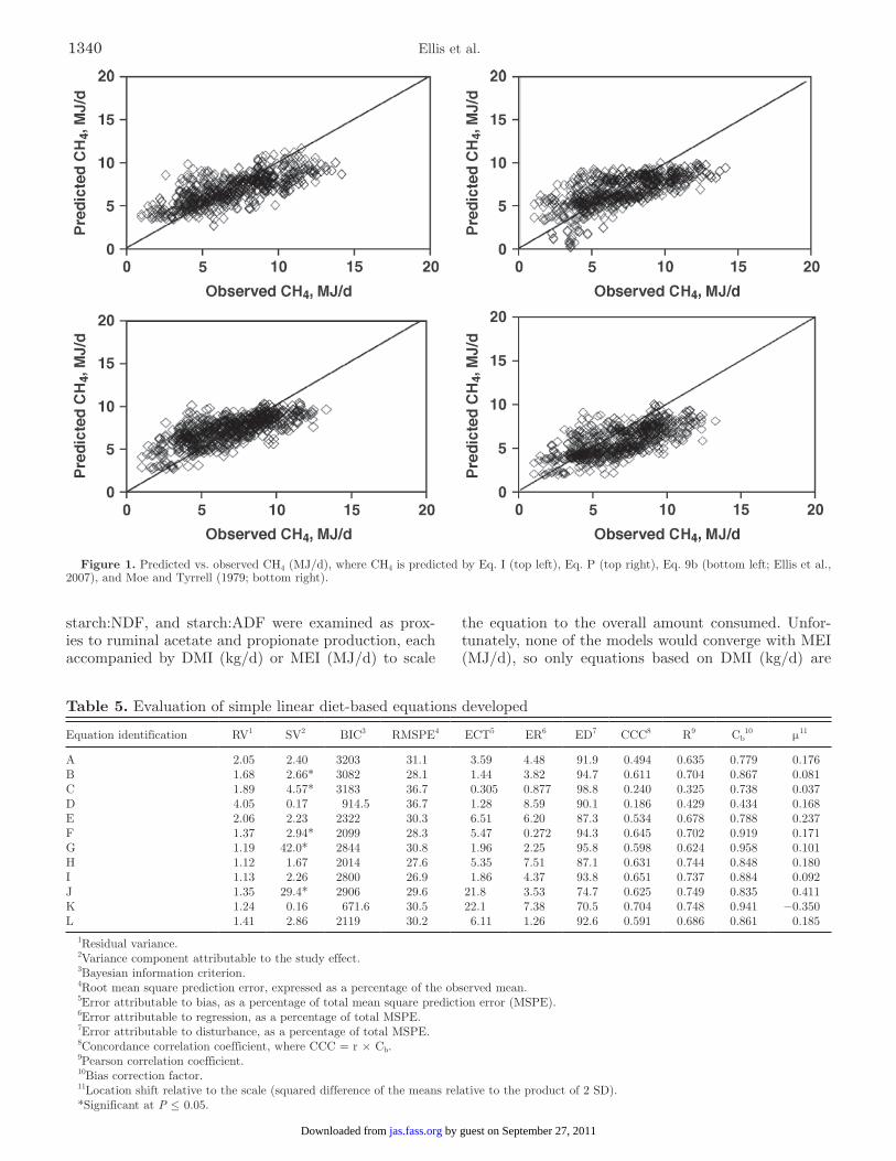
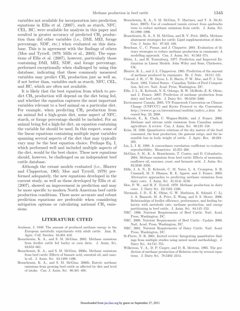
In this study, many calculated variables (e.g., NFC, CEL, HC, starch) in the equations gave rise to smaller RV and RMSPE values (Tables 4 and 5). Results showed that Eq. H and I resulted in the smallest RMSPE val-ues (27.6 and 26.9, respectively) and the smallest RV values (1.12 and 1.13, respectively), and 87 and 94% of RMSPE, respectively, was attributable to random error (Table 5). Equation H also had one of the smallest BIC values of those reported (Table 5), and Eq. I had one of the smallest CCC values (next to Eq. K). Each had a tendency for a slight overestimation, as indicated by the small positive µ value (Table 5). These 2 equations include the variables sugar and forage percentage (Eq. H), and MEI, CEL, HC, and fat (Eq. I). For each of these equations, SV was small and nonsignificant. A

plot of predicted vs. observed CH4 for Eq. I is presented in Figure 1.

Many of the simpler equations resulted in compara-bly low RMSPE and RV values (Table 5). For example, Eq. B contains only CEL and has a RMSPE value of 28.1, 95% of which is due to random error (Table 5). It does, however, have a larger RV value (1.68). In ad-dition, Eq. G, containing NDF and starch, has a low RV (1.19), a comparably low RMSPE (30.8), and 96% of RMSPE attributable to random error. Equation G did, however, have a high and significant SV estimate. Equation selection should be based on what variables are available, how well the equations have been shown to perform, and possibly by specific dietary scenari-os; for example, if high concentrations of fat are being supplemented in the diet, an equation containing the variable fat would be desirable (i.e., Eq. I). With lipid supplementation of diets, the effect of fat can override naturally occurring rumen fermentation; thus, an equa-tion that does not include fat may not accurately pre-dict CH4 production.

In addition to the dietary variables examined above, it was also of interest to investigate relative propor-tions of dietary variables in determining CH4 produc-tion. Mills et al. (2003) attempted this with a nonlinear equation using a starch:ADF ratio to predict CH4 pro-duction in dairy cattle, and this equation is evaluated in a subsequent section of this study. It is well known that high-forage diets promote acetate production in the rumen, which results in H production that can then be used for methanogenesis (Kebreab et al., 2006). In contrast, high-grain diets promote propionate produc-tion in the rumen, which competes with methanogens for available H. It seems that the proportion of these 2 types of substrates has a large influence on the amount of CH4 produced in the rumen. This could also explain why forage percentage showed up in one of the better fitting simple linear models from the previous section (Eq. H). Because of this, ratio-based linear equations that account for these proportions were also devel-oped (Table 6). The ratios of NFC:NDF, NFC:ADF,

Table 4. Summary of simple linear equations developed from dietary variables

Equation identification Equation1

A CH4 (MJ/d) = 2.29(±0.576) + 0.670(±0.104) × DMI (kg/d)B CH4 (MJ/d) = 3.05(±0.577) + 3.71(±0.573) × Cellulose (kg/d)C CH4 (MJ/d) = 4.72(±0.706) + 1.13(±0.478) × Starch (kg/d)D CH4 (MJ/d) = 6.01(±0.514) + 0.345(±0.158) × NFC (kg/d)E CH4 (MJ/d) = 3.46(±0.567) + 5.06(±1.14) × Sugar (kg/d)F CH4 (MJ/d) = 3.32(±0.607) − 1.23(±0.363) × Starch (kg/d) + 9.48(±0.634) × Sugar (kg/d)G CH4 (MJ/d) = −1.01(±2.01) + 2.76(±0.844) × NDF (kg/d) + 0.722(±0.0578) × Starch (kg/d)H CH4 (MJ/d) = 2.26(±0.607) + 5.02(±1.19) × Sugar (kg/d) + 0.0236(±0.0112) × Forage (%)I CH4 (MJ/d) = 2.72(±0.543) + 0.0937(±0.0117) × MEI (MJ/d) + 4.31(±0.215) × Cellulose (kg/d) − 6.49(±0.800) ×

Hemicellulose (kg/d) − 7.44(±0.521) × Fat (kg/d)J CH4 (MJ/d) = 0.310(±1.693) + 2.88(±0.196) × Cellulose (kg/d) + 4.15(±1.64) × CP (kg/d) − 3.97(±0.534) × Fat (kg/d)K CH4 (MJ/d) = 0.561(±0.427) + 5.86(±0.273) × Cellulose (kg/d) + 0.526(±0.0895) × NFC (kg/d)L CH4 (MJ/d) = 2.61(±0.630) + 0.0687(±0.0148) × MEI (MJ/d) + 5.99(±0.860) × Sugar (kg/d) − 2.15(±0.127) × Starch

(kg/d)1NFC = nonfiber carbohydrate; MEI = ME intake.




starch:NDF, and starch:ADF were examined as prox-ies to ruminal acetate and propionate production, each accompanied by DMI (kg/d) or MEI (MJ/d) to scale

the equation to the overall amount consumed. Unfor-tunately, none of the models would converge with MEI (MJ/d), so only equations based on DMI (kg/d) are

Table 5. Evaluation of simple linear diet-based equations developed

Equation identification RV1 SV2 BIC3 RMSPE4 ECT5 ER6 ED7 CCC8 R9 Cb10 µ11

A 2.05 2.40 3203 31.1 3.59 4.48 91.9 0.494 0.635 0.779 0.176B 1.68 2.66* 3082 28.1 1.44 3.82 94.7 0.611 0.704 0.867 0.081C 1.89 4.57* 3183 36.7 0.305 0.877 98.8 0.240 0.325 0.738 0.037D 4.05 0.17 914.5 36.7 1.28 8.59 90.1 0.186 0.429 0.434 0.168E 2.06 2.23 2322 30.3 6.51 6.20 87.3 0.534 0.678 0.788 0.237F 1.37 2.94* 2099 28.3 5.47 0.272 94.3 0.645 0.702 0.919 0.171G 1.19 42.0* 2844 30.8 1.96 2.25 95.8 0.598 0.624 0.958 0.101H 1.12 1.67 2014 27.6 5.35 7.51 87.1 0.631 0.744 0.848 0.180I 1.13 2.26 2800 26.9 1.86 4.37 93.8 0.651 0.737 0.884 0.092J 1.35 29.4* 2906 29.6 21.8 3.53 74.7 0.625 0.749 0.835 0.411K 1.24 0.16 671.6 30.5 22.1 7.38 70.5 0.704 0.748 0.941 −0.350L 1.41 2.86 2119 30.2 6.11 1.26 92.6 0.591 0.686 0.861 0.185

1Residual variance.2Variance component attributable to the study effect.3Bayesian information criterion.4Root mean square prediction error, expressed as a percentage of the observed mean.5Error attributable to bias, as a percentage of total mean square prediction error (MSPE).6Error attributable to regression, as a percentage of total MSPE.7Error attributable to disturbance, as a percentage of total MSPE.8Concordance correlation coefficient, where CCC = r × Cb.9Pearson correlation coefficient.10Bias correction factor.11Location shift relative to the scale (squared difference of the means relative to the product of 2 SD).*Significant at P ≤ 0.05.

Figure 1. Predicted vs. observed CH4 (MJ/d), where CH4 is predicted by Eq. I (top left), Eq. P (top right), Eq. 9b (bottom left; Ellis et al., 2007), and Moe and Tyrrell (1979; bottom right).

Ellis et al.1340



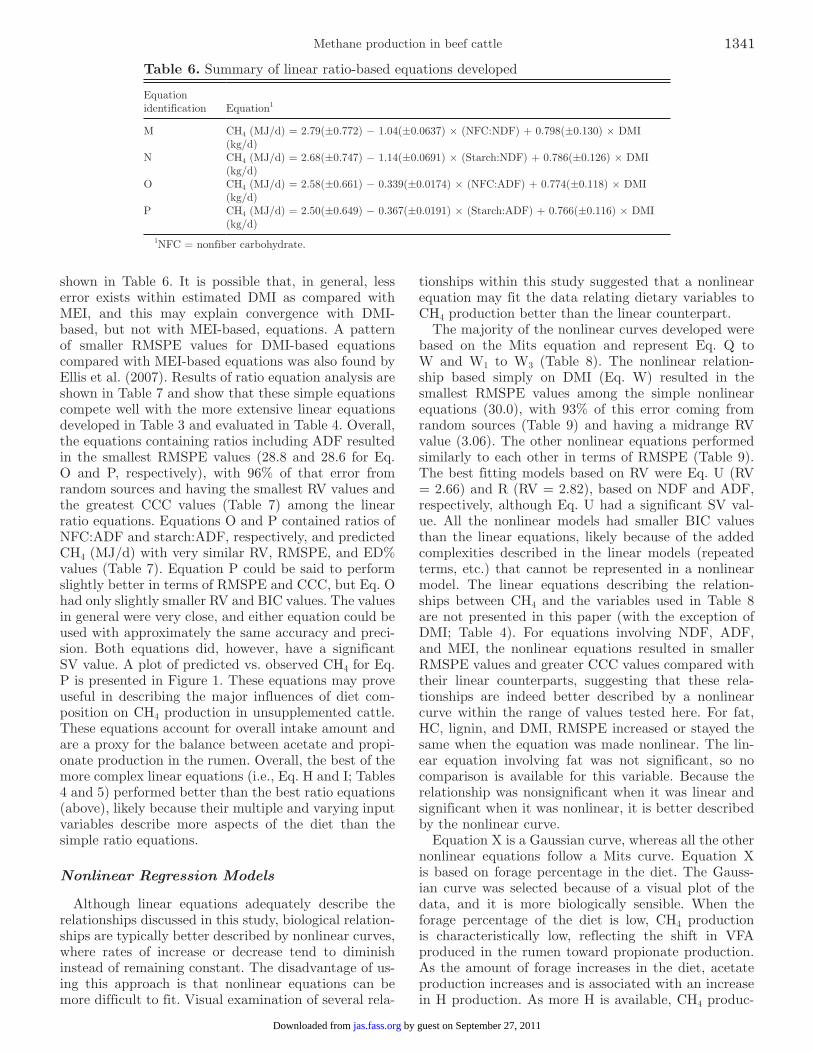
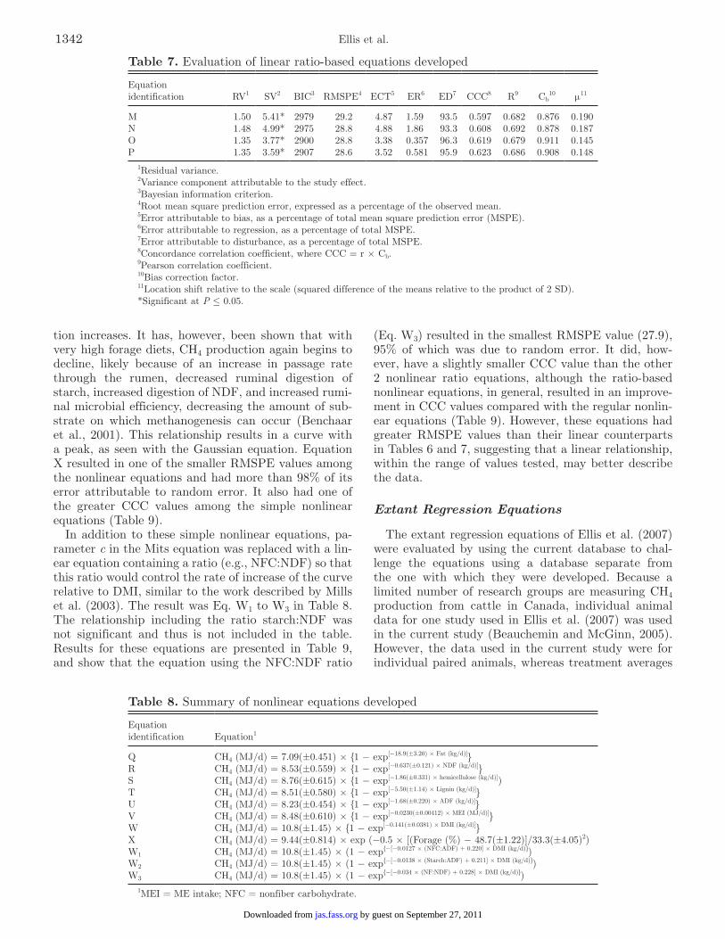
shown in Table 6. It is possible that, in general, less error exists within estimated DMI as compared with MEI, and this may explain convergence with DMI-based, but not with MEI-based, equations. A pattern of smaller RMSPE values for DMI-based equations compared with MEI-based equations was also found by Ellis et al. (2007). Results of ratio equation analysis are shown in Table 7 and show that these simple equations compete well with the more extensive linear equations developed in Table 3 and evaluated in Table 4. Overall, the equations containing ratios including ADF resulted in the smallest RMSPE values (28.8 and 28.6 for Eq. O and P, respectively), with 96% of that error from random sources and having the smallest RV values and the greatest CCC values (Table 7) among the linear ratio equations. Equations O and P contained ratios of NFC:ADF and starch:ADF, respectively, and predicted CH4 (MJ/d) with very similar RV, RMSPE, and ED% values (Table 7). Equation P could be said to perform slightly better in terms of RMSPE and CCC, but Eq. O had only slightly smaller RV and BIC values. The values in general were very close, and either equation could be used with approximately the same accuracy and preci-sion. Both equations did, however, have a significant SV value. A plot of predicted vs. observed CH4 for Eq. P is presented in Figure 1. These equations may prove useful in describing the major influences of diet com-position on CH4 production in unsupplemented cattle. These equations account for overall intake amount and are a proxy for the balance between acetate and propi-onate production in the rumen. Overall, the best of the more complex linear equations (i.e., Eq. H and I; Tables 4 and 5) performed better than the best ratio equations (above), likely because their multiple and varying input variables describe more aspects of the diet than the simple ratio equations.

Nonlinear Regression Models

Although linear equations adequately describe the relationships discussed in this study, biological relation-ships are typically better described by nonlinear curves, where rates of increase or decrease tend to diminish instead of remaining constant. The disadvantage of us-ing this approach is that nonlinear equations can be more difficult to fit. Visual examination of several rela-

tionships within this study suggested that a nonlinear equation may fit the data relating dietary variables to CH4 production better than the linear counterpart.

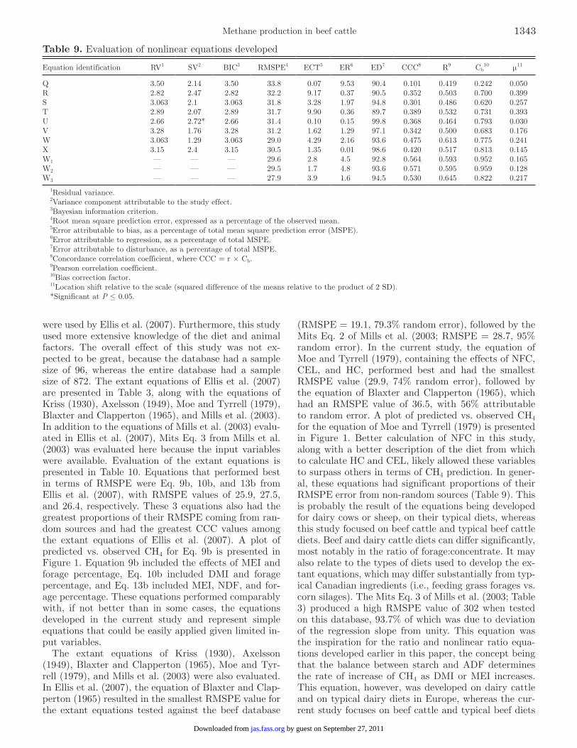
The majority of the nonlinear curves developed were based on the Mits equation and represent Eq. Q to W and W1 to W3 (Table 8). The nonlinear relation-ship based simply on DMI (Eq. W) resulted in the smallest RMSPE values among the simple nonlinear equations (30.0), with 93% of this error coming from random sources (Table 9) and having a midrange RV value (3.06). The other nonlinear equations performed similarly to each other in terms of RMSPE (Table 9). The best fitting models based on RV were Eq. U (RV = 2.66) and R (RV = 2.82), based on NDF and ADF, respectively, although Eq. U had a significant SV val-ue. All the nonlinear models had smaller BIC values than the linear equations, likely because of the added complexities described in the linear models (repeated terms, etc.) that cannot be represented in a nonlinear model. The linear equations describing the relation-ships between CH4 and the variables used in Table 8 are not presented in this paper (with the exception of DMI; Table 4). For equations involving NDF, ADF, and MEI, the nonlinear equations resulted in smaller RMSPE values and greater CCC values compared with their linear counterparts, suggesting that these rela-tionships are indeed better described by a nonlinear curve within the range of values tested here. For fat, HC, lignin, and DMI, RMSPE increased or stayed the same when the equation was made nonlinear. The lin-ear equation involving fat was not significant, so no comparison is available for this variable. Because the relationship was nonsignificant when it was linear and significant when it was nonlinear, it is better described by the nonlinear curve.

Equation X is a Gaussian curve, whereas all the other nonlinear equations follow a Mits curve. Equation X is based on forage percentage in the diet. The Gauss-ian curve was selected because of a visual plot of the data, and it is more biologically sensible. When the forage percentage of the diet is low, CH4 production is characteristically low, reflecting the shift in VFA produced in the rumen toward propionate production. As the amount of forage increases in the diet, acetate production increases and is associated with an increase in H production. As more H is available, CH4 produc-

Table 6. Summary of linear ratio-based equations developed


M CH4 (MJ/d) = 2.79(±0.772) − 1.04(±0.0637) × (NFC:NDF) + 0.798(±0.130) × DMI (kg/d)

N CH4 (MJ/d) = 2.68(±0.747) − 1.14(±0.0691) × (Starch:NDF) + 0.786(±0.126) × DMI (kg/d)

O CH4 (MJ/d) = 2.58(±0.661) − 0.339(±0.0174) × (NFC:ADF) + 0.774(±0.118) × DMI (kg/d)

P CH4 (MJ/d) = 2.50(±0.649) − 0.367(±0.0191) × (Starch:ADF) + 0.766(±0.116) × DMI (kg/d)

1NFC = nonfiber carbohydrate.




tion increases. It has, however, been shown that with very high forage diets, CH4 production again begins to decline, likely because of an increase in passage rate through the rumen, decreased ruminal digestion of starch, increased digestion of NDF, and increased rumi-nal microbial efficiency, decreasing the amount of sub-strate on which methanogenesis can occur (Benchaar et al., 2001). This relationship results in a curve with a peak, as seen with the Gaussian equation. Equation X resulted in one of the smaller RMSPE values among the nonlinear equations and had more than 98% of its error attributable to random error. It also had one of the greater CCC values among the simple nonlinear equations (Table 9).

In addition to these simple nonlinear equations, pa-rameter c in the Mits equation was replaced with a lin-ear equation containing a ratio (e.g., NFC:NDF) so that this ratio would control the rate of increase of the curve relative to DMI, similar to the work described by Mills et al. (2003). The result was Eq. W1 to W3 in Table 8. The relationship including the ratio starch:NDF was not significant and thus is not included in the table. Results for these equations are presented in Table 9, and show that the equation using the NFC:NDF ratio

(Eq. W3) resulted in the smallest RMSPE value (27.9), 95% of which was due to random error. It did, how-ever, have a slightly smaller CCC value than the other 2 nonlinear ratio equations, although the ratio-based nonlinear equations, in general, resulted in an improve-ment in CCC values compared with the regular nonlin-ear equations (Table 9). However, these equations had greater RMSPE values than their linear counterparts in Tables 6 and 7, suggesting that a linear relationship, within the range of values tested, may better describe the data.

Extant Regression Equations

The extant regression equations of Ellis et al. (2007) were evaluated by using the current database to chal-lenge the equations using a database separate from the one with which they were developed. Because a limited number of research groups are measuring CH4 production from cattle in Canada, individual animal data for one study used in Ellis et al. (2007) was used in the current study (Beauchemin and McGinn, 2005). However, the data used in the current study were for individual paired animals, whereas treatment averages

Table 7. Evaluation of linear ratio-based equations developed

Equation identification RV1 SV2 BIC3 RMSPE4 ECT5 ER6 ED7 CCC8 R9 Cb

10 µ11

M 1.50 5.41* 2979 29.2 4.87 1.59 93.5 0.597 0.682 0.876 0.190N 1.48 4.99* 2975 28.8 4.88 1.86 93.3 0.608 0.692 0.878 0.187O 1.35 3.77* 2900 28.8 3.38 0.357 96.3 0.619 0.679 0.911 0.145P 1.35 3.59* 2907 28.6 3.52 0.581 95.9 0.623 0.686 0.908 0.148


Table 8. Summary of nonlinear equations developed


Q CH4 (MJ/d) = 7.09(±0.451) × {1 − exp[−18.9(±3.20) × Fat (kg/d)]}R CH4 (MJ/d) = 8.53(±0.559) × {1 − exp[−0.637(±0.121) × NDF (kg/d)]}S CH4 (MJ/d) = 8.76(±0.615) × {1 − exp[−1.86(±0.331) × hemicellulose (kg/d)])T CH4 (MJ/d) = 8.51(±0.580) × {1 − exp[−5.50(±1.14) × Lignin (kg/d)]}U CH4 (MJ/d) = 8.23(±0.454) × {1 − exp[−1.68(±0.220) × ADF (kg/d)]}V CH4 (MJ/d) = 8.48(±0.610) × {1 − exp[−0.0230(±0.00412) × MEI (MJ/d)]}W CH4 (MJ/d) = 10.8(±1.45) × {1 − exp[−0.141(±0.0381) × DMI (kg/d)]}X CH4 (MJ/d) = 9.44(±0.814) × exp (−0.5 × [(Forage (%) − 48.7(±1.22)]/33.3(±4.05)2)W1 CH4 (MJ/d) = 10.8(±1.45) × (1 − exp{−[−0.0127 × (NFC:ADF) + 0.220] × DMI (kg/d)})W2 CH4 (MJ/d) = 10.8(±1.45) × (1 − exp{−[−0.0138 × (Starch:ADF) + 0.211] × DMI (kg/d)})W3 CH4 (MJ/d) = 10.8(±1.45) × (1 − exp{−[−0.034 × (NF:NDF) + 0.228] × DMI (kg/d)})

1MEI = ME intake; NFC = nonfiber carbohydrate.

Ellis et al.1342



were used by Ellis et al. (2007). Furthermore, this study used more extensive knowledge of the diet and animal factors. The overall effect of this study was not ex-pected to be great, because the database had a sample size of 96, whereas the entire database had a sample size of 872. The extant equations of Ellis et al. (2007) are presented in Table 3, along with the equations of Kriss (1930), Axelsson (1949), Moe and Tyrrell (1979), Blaxter and Clapperton (1965), and Mills et al. (2003). In addition to the equations of Mills et al. (2003) evalu-ated in Ellis et al. (2007), Mits Eq. 3 from Mills et al. (2003) was evaluated here because the input variables were available. Evaluation of the extant equations is presented in Table 10. Equations that performed best in terms of RMSPE were Eq. 9b, 10b, and 13b from Ellis et al. (2007), with RMSPE values of 25.9, 27.5, and 26.4, respectively. These 3 equations also had the greatest proportions of their RMSPE coming from ran-dom sources and had the greatest CCC values among the extant equations of Ellis et al. (2007). A plot of predicted vs. observed CH4 for Eq. 9b is presented in Figure 1. Equation 9b included the effects of MEI and forage percentage, Eq. 10b included DMI and forage percentage, and Eq. 13b included MEI, NDF, and for-age percentage. These equations performed comparably with, if not better than in some cases, the equations developed in the current study and represent simple equations that could be easily applied given limited in-put variables.

The extant equations of Kriss (1930), Axelsson (1949), Blaxter and Clapperton (1965), Moe and Tyr-rell (1979), and Mills et al. (2003) were also evaluated. In Ellis et al. (2007), the equation of Blaxter and Clap-perton (1965) resulted in the smallest RMSPE value for the extant equations tested against the beef database

(RMSPE = 19.1, 79.3% random error), followed by the Mits Eq. 2 of Mills et al. (2003; RMSPE = 28.7, 95% random error). In the current study, the equation of Moe and Tyrrell (1979), containing the effects of NFC, CEL, and HC, performed best and had the smallest RMSPE value (29.9, 74% random error), followed by the equation of Blaxter and Clapperton (1965), which had an RMSPE value of 36.5, with 56% attributable to random error. A plot of predicted vs. observed CH4 for the equation of Moe and Tyrrell (1979) is presented in Figure 1. Better calculation of NFC in this study, along with a better description of the diet from which to calculate HC and CEL, likely allowed these variables to surpass others in terms of CH4 prediction. In gener-al, these equations had significant proportions of their RMSPE error from non-random sources (Table 9). This is probably the result of the equations being developed for dairy cows or sheep, on their typical diets, whereas this study focused on beef cattle and typical beef cattle diets. Beef and dairy cattle diets can differ significantly, most notably in the ratio of forage:concentrate. It may also relate to the types of diets used to develop the ex-tant equations, which may differ substantially from typ-ical Canadian ingredients (i.e., feeding grass forages vs. corn silages). The Mits Eq. 3 of Mills et al. (2003; Table 3) produced a high RMSPE value of 302 when tested on this database, 93.7% of which was due to deviation of the regression slope from unity. This equation was the inspiration for the ratio and nonlinear ratio equa-tions developed earlier in this paper, the concept being that the balance between starch and ADF determines the rate of increase of CH4 as DMI or MEI increases. This equation, however, was developed on dairy cattle and on typical dairy diets in Europe, whereas the cur-rent study focuses on beef cattle and typical beef diets

Table 9. Evaluation of nonlinear equations developed

Equation identification RV1 SV2 BIC3 RMSPE4 ECT5 ER6 ED7 CCC8 R9 Cb10 µ11

Q 3.50 2.14 3.50 33.8 0.07 9.53 90.4 0.101 0.419 0.242 0.050R 2.82 2.47 2.82 32.2 9.17 0.37 90.5 0.352 0.503 0.700 0.399S 3.063 2.1 3.063 31.8 3.28 1.97 94.8 0.301 0.486 0.620 0.257T 2.89 2.07 2.89 31.7 9.90 0.36 89.7 0.389 0.532 0.731 0.393U 2.66 2.72* 2.66 31.4 0.10 0.15 99.8 0.368 0.464 0.793 0.030V 3.28 1.76 3.28 31.2 1.62 1.29 97.1 0.342 0.500 0.683 0.176W 3.063 1.29 3.063 29.0 4.29 2.16 93.6 0.475 0.613 0.775 0.241X 3.15 2.4 3.15 30.5 1.35 0.01 98.6 0.420 0.517 0.813 0.145W1 — — — 29.6 2.8 4.5 92.8 0.564 0.593 0.952 0.165W2 — — — 29.5 1.7 4.8 93.6 0.571 0.595 0.959 0.128W3 — — — 27.9 3.9 1.6 94.5 0.530 0.645 0.822 0.217





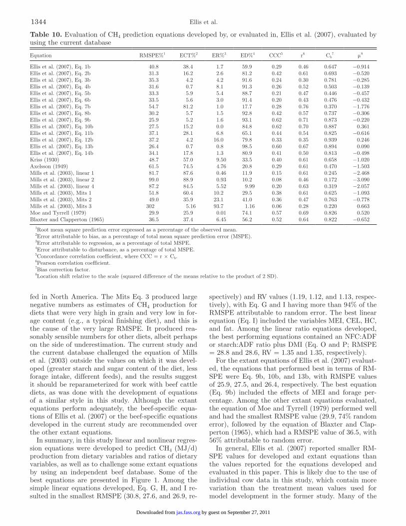
fed in North America. The Mits Eq. 3 produced large negative numbers as estimates of CH4 production for diets that were very high in grain and very low in for-age content (e.g., a typical finishing diet), and this is the cause of the very large RMSPE. It produced rea-sonably sensible numbers for other diets, albeit perhaps on the side of underestimation. The current study and the current database challenged the equation of Mills et al. (2003) outside the values on which it was devel-oped (greater starch and sugar content of the diet, less forage intake, different feeds), and the results suggest it should be reparameterized for work with beef cattle diets, as was done with the development of equations of a similar style in this study. Although the extant equations perform adequately, the beef-specific equa-tions of Ellis et al. (2007) or the beef-specific equations developed in the current study are recommended over the other extant equations.

In summary, in this study linear and nonlinear regres-sion equations were developed to predict CH4 (MJ/d) production from dietary variables and ratios of dietary variables, as well as to challenge some extant equations by using an independent beef database. Some of the best equations are presented in Figure 1. Among the simple linear equations developed, Eq. G, H, and I re-sulted in the smallest RMSPE (30.8, 27.6, and 26.9, re-

spectively) and RV values (1.19, 1.12, and 1.13, respec-tively), with Eq. G and I having more than 94% of the RMSPE attributable to random error. The best linear equation (Eq. I) included the variables MEI, CEL, HC, and fat. Among the linear ratio equations developed, the best performing equations contained an NFC:ADF or starch:ADF ratio plus DMI (Eq. O and P; RMSPE = 28.8 and 28.6, RV = 1.35 and 1.35, respectively).

For the extant equations of Ellis et al. (2007) evaluat-ed, the equations that performed best in terms of RM-SPE were Eq. 9b, 10b, and 13b, with RMSPE values of 25.9, 27.5, and 26.4, respectively. The best equation (Eq. 9b) included the effects of MEI and forage per-centage. Among the other extant equations evaluated, the equation of Moe and Tyrrell (1979) performed well and had the smallest RMSPE value (29.9, 74% random error), followed by the equation of Blaxter and Clap-perton (1965), which had a RMSPE value of 36.5, with 56% attributable to random error.

In general, Ellis et al. (2007) reported smaller RM-SPE values for developed and extant equations than the values reported for the equations developed and evaluated in this paper. This is likely due to the use of individual cow data in this study, which contain more variation than the treatment mean values used for model development in the former study. Many of the

Table 10. Evaluation of CH4 prediction equations developed by, or evaluated in, Ellis et al. (2007), evaluated by using the current database

Equation RMSPE%1 ECT%2 ER%3 ED%4 CCC5 r6 Cb7 µ8

Ellis et al. (2007), Eq. 1b 40.8 38.4 1.7 59.9 0.29 0.46 0.647 −0.914Ellis et al. (2007), Eq. 2b 31.3 16.2 2.6 81.2 0.42 0.61 0.693 −0.520Ellis et al. (2007), Eq. 3b 35.3 4.2 4.2 91.6 0.24 0.30 0.781 −0.285Ellis et al. (2007), Eq. 4b 31.6 0.7 8.1 91.3 0.26 0.52 0.503 −0.139Ellis et al. (2007), Eq. 5b 33.3 5.9 5.4 88.7 0.21 0.47 0.446 −0.457Ellis et al. (2007), Eq. 6b 33.5 5.6 3.0 91.4 0.20 0.43 0.476 −0.432Ellis et al. (2007), Eq. 7b 54.7 81.2 1.0 17.7 0.28 0.76 0.370 −1.776Ellis et al. (2007), Eq. 8b 30.2 5.7 1.5 92.8 0.42 0.57 0.737 −0.306Ellis et al. (2007), Eq. 9b 25.9 5.2 1.6 93.1 0.62 0.71 0.873 −0.220Ellis et al. (2007), Eq. 10b 27.5 15.2 0.0 84.8 0.62 0.70 0.887 0.361Ellis et al. (2007), Eq. 11b 37.1 28.1 6.8 65.1 0.44 0.54 0.825 −0.616Ellis et al. (2007), Eq. 12b 37.2 4.2 16.0 79.8 0.33 0.35 0.939 0.246Ellis et al. (2007), Eq. 13b 26.4 0.7 0.8 98.5 0.60 0.67 0.894 0.090Ellis et al. (2007), Eq. 14b 34.1 17.8 1.3 80.9 0.41 0.50 0.813 −0.498Kriss (1930) 48.7 57.0 9.50 33.5 0.40 0.61 0.658 −1.020Axelsson (1949) 61.5 74.5 4.76 20.8 0.29 0.61 0.470 −1.503Mills et al. (2003), linear 1 81.7 87.6 0.46 11.9 0.15 0.61 0.245 −2.468Mills et al. (2003), linear 2 99.0 88.9 0.93 10.2 0.08 0.46 0.172 −3.090Mills et al. (2003), linear 4 87.2 84.5 5.52 9.99 0.20 0.63 0.319 −2.057Mills et al. (2003), Mits 1 51.8 60.4 10.2 29.5 0.38 0.61 0.625 −1.093Mills et al. (2003), Mits 2 49.0 35.9 23.1 41.0 0.36 0.47 0.763 −0.778Mills et al. (2003), Mits 3 302 5.16 93.7 1.16 0.06 0.28 0.220 0.663Moe and Tyrrell (1979) 29.9 25.9 0.01 74.1 0.57 0.69 0.826 0.520Blaxter and Clapperton (1965) 36.5 37.4 6.45 56.2 0.52 0.64 0.822 −0.652

1Root mean square prediction error expressed as a percentage of the observed mean.2Error attributable to bias, as a percentage of total mean square prediction error (MSPE).3Error attributable to regression, as a percentage of total MSPE.4Error attributable to disturbance, as a percentage of total MSPE.5Concordance correlation coefficient, where CCC = r × Cb.6Pearson correlation coefficient.7Bias correction factor.8Location shift relative to the scale (squared difference of the means relative to the product of 2 SD).

Ellis et al.1344



variables not available for incorporation into prediction equations in Ellis et al. (2007), such as starch, NFC, CEL, HC, were available for analysis in this paper and resulted in greater accuracy of predicted CH4 produc-tion than did other variables (i.e., DMI, MEI, forage percentage, NDF, etc.) when evaluated on this data-base. This is in agreement with the findings of others (Moe and Tyrrell, 1979; Mills et al., 2003). The equa-tions of Ellis et al. (2007), however, particularly those containing DMI, MEI, NDF, and forage percentage, performed exceptionally when challenged by using this database, indicating that these commonly measured variables may predict CH4 production just as well as, if not better than, variables such as starch, NFC, CEL, and HC, which are often not available.

It is likely that the best equation from which to pre-dict CH4 production will depend on the diet being fed, and whether the equation captures the most important variables relevant to a beef animal on a particular diet. For example, when predicting CH4 production from an animal fed a high-grain diet, some aspect of NFC, starch, or forage percentage should be included. For an animal being fed a high-fat diet, an equation containing the variable fat should be used. In this respect, some of the linear equations containing multiple input variables spanning several aspects of the diet that may typically vary may be the best equation choice. Perhaps Eq. I, which performed well and included multiple aspects of the diet, would be the best choice. These new equations should, however, be challenged on an independent beef cattle database.

Although the extant models evaluated (i.e., Blaxter and Clapperton, 1965; Moe and Tyrrell, 1979) per-formed adequately, the new equations developed in the current study, as well as those developed by Ellis et al. (2007), showed an improvement in prediction and may be more specific to modern North American beef cattle production conditions. These more accurate and robust prediction equations are preferable when considering mitigation options or calculating national CH4 emis-sions.

LITERATURE CITED

Axelsson, J. 1949. The amount of produced methane energy in the European metabolic experiments with adult cattle. Ann. R. Agric. Coll. Sweden 16:404–419.

Beauchemin, K. A., and S. M. McGinn. 2005. Methane emissions from feedlot cattle fed barley or corn diets. J. Anim. Sci. 83:653–661.

Beauchemin, K. A., and S. M. McGinn. 2006a. Methane emissions from beef cattle: Effects of fumaric acid, essential oil, and cano-la oil. J. Anim. Sci. 84:1489–1496.

Beauchemin, K. A., and S. M. McGinn. 2006b. Enteric methane emissions from growing beef cattle as affected by diet and level of intake. Can. J. Anim. Sci. 86:401–408.

Beauchemin, K. A., S. M. McGinn, T. Martinez, and T. A. McAl-lister. 2007b. Use of condensed tannin extract from quebracho trees to reduce methane emissions from cattle. J. Anim. Sci. 85:1990–1996.

Beauchemin, K. A., S. M. McGinn, and H. V. Petit. 2007a. Methane abatement strategies for cattle: Lipid supplementation of diets. Can. J. Anim. Sci. 87:431–440.

Benchaar, C., C. Pomar, and J. Chiquette. 2001. Evaluation of di-etary strategies to reduce methane production in ruminants: A modelling approach. Can. J. Anim. Sci. 81:563–574.

Bibby, J., and H. Toutenburg. 1977. Prediction and Improved Es-timation in Linear Models. John Wiley and Sons, Chichester, UK.

Blaxter, K. L., and J. L. Clapperton. 1965. Prediction of the amount of methane produced by ruminants. Br. J. Nutr. 19:511–521.

Conrad, J. H., C. W. Deyoe, L. E. Harris, P. W. Moe, and P. J. Van Soest. 1982. United States—Canadian Tables of Feed Composi-tion. 3rd rev. Natl. Acad. Press, Washington, DC.

Ellis, J. L., K. Kebreab, N. E. Odongo, B. W. McBride, E. K. Okine, and J. France. 2007. Prediction of methane production from dairy and beef cattle. J. Dairy Sci. 90:3456–3466.

Environment Canada. 2005. UN Framework Convention on Climate Change (UNFCCC) and Kyoto Protocol to the Convention. http://www.ec.gc.ca/international/multilat/unfccc_e.htm Ac-cessed Sep. 23, 2008.

Kebreab, E., K. Clark, C. Wagner-Riddle, and J. France. 2006. Methane and nitrous oxide emissions from Canadian animal agriculture: A review. Can. J. Anim. Sci. 86:135–158.

Kriss, M. 1930. Quantitative relations of the dry matter of the food consumed, the heat production, the gaseous outgo, and the in-sensible loss in body weight of cattle. J. Agric. Res. 40:283–295.

Lin, L. I. K. 1989. A concordance correlation coefficient to evaluate reproducibility. Biometrics 45:255–268.

McGinn, S. M., K. A. Beauchemin, T. Coates, and D. Colombatto. 2004. Methane emissions from beef cattle: Effects of monensin, sunflower oil, enzymes, yeast, and furmaric acid. J. Anim. Sci. 82:3346–3356.

Mills, J. A. N., E. Kebreab, C. M. Yates, L. A. Crompton, S. B. Cammell, M. S. Dhanoa, R. E. Agnew, and J. France. 2003. Alternative approaches to predicting methane emissions from dairy cows. J. Anim. Sci. 81:3141–3150.

Moe, P. W., and H. F. Tyrrell. 1979. Methane production in dairy cows. J. Dairy Sci. 62:1583–1586.

Nkrumah, J. D., E. K. Okine, G. W. Mathison, K. Schmid, C. Li, J. A. Basarab, M. A. Price, Z. Wang, and S. S. Moore. 2006. Relationships of feedlot efficiency, performance, and feeding be-havior with metabolic rate, methane production, and energy partitioning in beef cattle. J. Anim. Sci. 84:145–153.

NRC. 1996. Nutrient Requirements of Beef Cattle. Natl. Acad. Press, Washington, DC.

NRC. 2000. Nutrient Requirements of Beef Cattle—Update 2000. Natl. Acad. Press, Washington, DC.

NRC. 2001. Nutrient Requirements of Dairy Cattle. Natl. Acad. Press, Washington, DC.

St-Pierre, N. R. 2001. Invited review: Integrating quantitative find-ings from multiple studies using mixed model methodology. J. Dairy Sci. 84:741–755.

Wilkerson, V. A., D. P. Casper, and D. R. Mertens. 1995. The pre-diction of methane production of Holstein cows by several equa-tions. J. Dairy Sci. 78:2402–2414.




Related Articleshttp://jas.fass.org/content/animalsci/87/5/1849.full.htmlA related article has been published:

Supplementary Materialhttp://jas.fass.org/content/suppl/2009/03/17/jas.2007-0725.DC1.htmlSupplementary material can be found at:

Referenceshttp://jas.fass.org/content/87/4/1334#BIBLThis article cites 18 articles, 6 of which you can access for free at:

Errata

http://jas.fass.orgor:

next pageAn erratum has been published regarding this article. Please see



1849

doi:10.2527/jas.2009-87-5-1849

The article “Modeling methane production from beef cattle using linear and nonlinear approaches” (J. Anim. Sci. 87:1334–1345) has a few corrections shown below in bold text. The authors regret the errors.

On page 1337, bottom of the second column, the sentence should read, “Another estimate (µ) that measures location shift relative to the product of 2 SD is also reported, where a negative value indicates overprediction and a positive value indicates underprediction of observed values by the model.”

On page 1339, bottom of the first column, the sentences should read, “Equation H also had one of the smallest BIC values of those reported (Table 5), and Eq. I had one of the greatest CCC values (next to Eq. K). Each had a tendency for a slight underestimation, as indicated by the small positive µ value (Table 5).”

Erratum



Modeling methane production from beef cattle using linear and nonlinear approaches

Documents

Transcript of Modeling methane production from beef cattle using linear and nonlinear approaches