Pedigree analysis of eight Spanish beef cattle breeds

Genet. Sel. Evol. 35 (2003) 43–63 43© INRA, EDP Sciences, 2003DOI: 10.1051/gse:2002035

Original article

Pedigree analysis of eight Spanish beefcattle breeds

Juan Pablo GUTIÉRREZa∗, Juan ALTARRIBAb,Clara DÍAZc, Raquel QUINTANILLAd∗∗,

Javier CAÑÓNa, Jesús PIEDRAFITAd

a Departamento de Producción Animal, Facultad de Veterinaria,Universidad Complutense de Madrid, 28040 Madrid, Spain

b Departamento de Anatomía y Genética, Facultad de Veterinaria,Universidad de Zaragoza, 50013 Zaragoza, Spain

c Departamento de Mejora Genética Animal, INIA, Carretera de la Coruña,Km 7, 28040 Madrid, Spain

d Departament de Ciència Animal i dels Aliments, Facultat de Veterinària,Universitat Autònoma de Barcelona,08193 Bellaterra, Barcelona, Spain

(Received 16 November 2001; accepted 7 August 2002)

Abstract – The genetic structure of eight Spanish autochthonous populations (breeds) of beefcattle were studied from pedigree records. The populations studied were: Alistana and Say-aguesa (minority breeds), Avileña – Negra Ibérica and Morucha (“dehesa” breeds, with a scarceincidence of artificial insemination), and mountain breeds, including Asturiana de los Valles,Asturiana de la Montaña and Pirenaica, with extensive use of AI. The Bruna dels Pirineusbreed possesses characteristics which make its classification into one of the former groupsdifficult. There was a large variation between breeds both in the census and the number of herds.Generation intervals ranged from 3.7 to 5.5 years, tending to be longer as the population sizewas larger. The effective numbers of herds suggest that a small number of herds behaves as aselection nucleus for the rest of the breed. The complete generation equivalent has also beengreatly variable, although in general scarce, with the exception of the Pirenaica breed, with amean of 3.8. Inbreeding effective population sizes were actually small (21 to 127), especially inthe mountain-type breeds. However, the average relatedness computed for these breeds suggeststhat a slight exchange of animals between herds will lead to a much more favourable evolutionof inbreeding. The effective number of founders and ancestors were also variable among breeds,although in general the breeds behaved as if they were founded by a small number of animals(25 to 163).

beef breeds / inbreeding / probability of gene origin / conservation

∗ Correspondence and reprintsE-mail: [email protected]∗∗ Present address: Station de génétique quantitative et appliquée, Inra, 78352 Jouy-en-JosasCedex, France

44 J.P. Gutiérrez et al.

1. INTRODUCTION

Domestic animal diversity is an integral part of global biodiversity, whichrequires sound management for its sustainable use and future availability [19].The knowledge of genetic diversity of the population is the basis for effectiveselection and/or conservation programmes. According to Vu Tien Khang [22],genetic variability can be studied through the estimation of the genetic varianceof quantitative traits, the analysis of pedigree data and the description ofvisible genes and markers in the population, such as microsatellite markers.Demographic analysis allows us to describe the structure and dynamics ofpopulations considered as a group of renewed individuals. Genetic analysisis interested in the evolution of the population’s gene pool. Since the historyof genes is fully linked to that of individuals, demography and populationgenetics are complementary matters. Pedigree analysis is an important tool todescribe genetic variability and its evolution across generations. The trend ininbreeding has been the most frequently used parameter to quantify the rate ofgenetic drift. Inbreeding depresses the components of reproductive fitness innaturally outbreeding species [10]. In beef cattle, the effects of inbreeding wererelatively minor at lower levels of inbreeding, and animals that had inbreedingcoefficients higher than 20% were more affected by inbreeding than thosehaving milder levels of inbreeding (see review of Burrow, [5]).

There is a direct relationship between the increase in inbreeding and thedecrease in heterozygosity for a given locus in a closed, unselected and pan-mictic population of finite size [24]. In domestic animal populations, however,some drawbacks may arise with this approach [4]. A complementary approachis to analyse the probabilities of gene origin [12,22]. In this method, thegenetic contribution of the founders, i.e., the ancestors with unknown parents,of the current population is measured. As proposed by Lacy [13], these foundercontributions could be combined to derive a synthetic criterion, the “founderequivalents”. In addition, Boichard et al. [4] have proposed to compute theeffective number of ancestors that accounts for the bottlenecks in a pedigree.

Compared to the number of European beef cattle breeds, there are onlya few studies regarding the genetic structure of European local beef cattlepopulations and most of them concern only one breed or a small numberof breeds [1,4,8,20]. Furthermore, some of the Spanish populations havestarted programmes of genetic evaluation through the BLUP animal modelmethodology. Verrier et al. [21] have argued that the use of the animalmodel in populations of limited effective size leads to profound changes inthe structure of the population and cannot be the optimum selection criterionneither in terms of the cumulated genetic progress or maintenance of geneticvariability. In this context, the objective of this study was to analyse theherdbooks in order to know the gene flows, population structure and potential

Pedigree analysis in beef breeds 45

danger for losing genetic variability of eight Spanish local beef cattle breeds.Population structures were analysed in terms of census, generation interval,effective number of herds, pedigree completeness level, inbreeding coefficient,average relatedness, effective population size and effective number of founders,ancestors and founder herds.

2. MATERIALS AND METHODS

2.1. Breeds and data available

Eight Spanish breeds were involved in this analysis: Alistana (Ali), Asturi-ana de la Montaña (AM), Asturiana de los Valles (AV), Avileña – Negra Ibérica(A-NI), Bruna dels Pirineus (BP), Morucha (Mo), Pirenaica (Pi) and Sayaguesa(Say). Herdbook data available from the foundation up to the year 1996 wereused for this study. Data registered in the herdbook were assumed to berepresentative of the whole breed although, for most of the breeds, registeredanimals represent only a low percentage of the population.

These breeds are different in many aspects but, in order to discuss the results,they were classified into three main groups. The first one was composed ofminority breeds: Ali and Say, with fewer than 500 registered calves per year.A second group, the mountain breeds (AM, AV, and Pi), was defined as thosewith a geographical location in mountain areas and wide use of some animalsas parents, usually by artificial insemination (AI). The third group was the“dehesa”breeds, and was made up of A-NI and Mo. The BP breed should havebeen classified into the group of mountain breeds, but due to the scarce use ofAI and its sparse pedigree knowledge, this breed cannot be properly assignedto any of the previous groups.

2.2. Analysis of pedigree structure and inbreeding

The objective of this part was to obtain significant insight in the recent geneticand current status of the breeds regarding breeding practices and effectivepopulation sizes. The work was carried out from two main points of view:inbreeding and analysis of the founders. Specific FORTRAN codes werewritten to compute all of the parameters shown below.

2.2.1. Generation interval

It is defined as the average age of parents when their progeny, upon becomingparents themselves, are born. It is computed only for the animals who areparents in the four years previous to the last year analysed. In order to knowthe evolution of this parameter, generation intervals were also computed withthe same criteria from a sample of animals born ten years before in a block offour consecutive years.


2.2.2. Effective number of herds

Robertson [17] defined the CS parameter as the probability that two animalstaken at random, have the sire in the same herd. We can, in a similar way, obtainthe CSS parameter to give the probability for sires of sires, and successivelythe CSSS parameter, and so on. The inverse of these values (HS,HSS, . . . ) willbe the effective number of herds supplying sires, grand sires, great-grandsires,and so on.

2.2.3. Pedigree description

Average inbreeding coefficients vary among breeds for several reasons thatmay lead to difficult interpretations. The most important reasons are the sizeof the population, pedigree completeness level, and breeding policy. Amongthem, pedigree completeness level is the cause that could make drawing con-clusions from the available data difficult. Two ways were used to describethe pedigree completeness level: (1) computing the proportion of parents,grandparents and great-grandparents known and (2) estimating the completegeneration equivalent value [3,4]. This parameter was estimated in each breedby averaging over the sum of (1/2)n, where n is the number of generationsseparating the individual from each known ancestor.

2.3. Inbreeding coefficient

The inbreeding coefficient of an individual (F) is the probability of havingtwo genes which are identical by descent [23]. A modification of the Meuwissenand Luo [15] algorithm was used to compute the inbreeding coefficients.

2.3.1. Average relatedness

Inbreeding is a consequence of mating relatives, but this parameter does notexplain the reason for this kind of mating. Average relatedness (AR) [9] amongall animals in the population tends to be higher too, when all animals are highlyrelated and there is no chance of mating unrelated or slightly related individuals.Nevertheless, a low average relatedness coupled with a high average inbreedingsuggests a wide use of within-herd matings. AR coefficients were chosenbecause this parameter provides complementary information to that providedby the inbreeding coefficient.

The average relatedness [9] of each individual is the average of the coeffi-cients in the row corresponding to the individual in the numerator relationshipmatrix (A). AR has been preferred to the mean kinship parameter [2] because itis much easier to compute and both parameters show basically the same conceptfor practical purposes. However, AR indicates the percentage of representation


of each animal in a whole pedigree, while mean kinship is not useful fordescription purposes.

The average inbreeding coefficient of a population is frequently used as ameasure of its level of homozygosity. All of the information on inbreedingcoefficients is included in the diagonal elements of the numerator relationshipmatrix. If, for instance, there is a subdivision of the population, animals aremated within subpopulations and a decrease in inbreeding coefficients mightbe possible by mating animals from different families. Furthermore, the ARcoefficient also addresses the chance of recovery of the breed, since it alsotakes coancestry coefficients into account, not only for the animals of the samegeneration but also for those of previous generations whose genetic potentialcould be interesting to preserve.

2.3.2. Effective population size

The effective size of a population (Ne) is defined as the size of an idealisedpopulation which would give rise to the rate of inbreeding (∆F). The effectivepopulation size was calculated as in Wright [23]:

Ne = 1

2∆F

where ∆F is the relative increase in inbreeding by generation. This formula,however, usually fits poorly to real populations, giving an overestimate ofthe actual effective population size [4], mainly when the degree of pedigreeknowledge is scarce.

The relative increase in inbreeding by generation (∆F), i.e., the relativedecrease of heterozygosity between two generations, was defined followingWright [24] as:

∆F = Fn − Fn−1

1− Fn−1

Fi being the average inbreeding in the ith generation.The increase in inbreeding between two generations (Fn−Fn−1) was obtained

from the regression coefficient (b) of the average inbreeding over the year ofbirth obtained in the last 8 years, and considering the average generation interval(`) as follows:

Fn − Fn−1 = `× b

Fn−1 being computed from the mean inbreeding in the last year studied (Fly)as:

Fn−1 = Fly − `× b.


2.3.3. Effective number of founders and effective number of ancestors

When we wish to describe the population structure after a small number ofgenerations, parameters derived from the probability of gene origin are veryuseful [4]. These parameters can detect recent significant changes in breedingstrategy, before their consequences appear in terms of inbreeding increase. Theparameters are useful both when the breeding objective is the maintenance of agene pool (conservation programmes), and when analysing the consequencesof selection in small populations.

The effective number of founders, fe [13], is the number of equally contrib-uting founders that would be expected to produce the same genetic diversity asin the population under study. It is computed as:

fe = 1f∑

k=1

q2k

where qk is the probability of gene origin of the k ancestor. The effectivenumber of ancestors ( fa) is the minimum number of ancestors, founders or not,necessary to explain the complete genetic diversity of the population understudy [3]. For this purpose a reference population was defined as the animalsborn in three consecutive and significant years (1993–1995). The effectivenumber of ancestors was computed by following the algorithm described byBoichard et al. [4].

2.3.4. Effective number of founder herds

Finally, the initial contribution of founders can be added into each herdfounder contribution, and the inverse of their added squared value gives aneffective number of founder herds.

3. RESULTS

3.1. Census

Table I shows the evolution of some demographic parameters in the analysedbreeds: the number of cows registered in the breed association (when thisparameter was available), number of calves born, number of herds recordingcalvings, and calves/herd rate. This table shows that recording began duringthe last decade, with the exception of Pi and A-NI. In general, the breeds tendedto increase their census over time. The apparent decrease in the Mo censusmust be interpreted as a delay in the registering of cows at the time of the study.


Table I. Evolution of the number of registered cows, number of registered calves,number of herds (left) and calves/herd (right) in eight Spanish beef cattle breeds.

Breed Number Number Number

of registered cows of registered calves of herds (calves/herd)

1985 1990 1995 1985 1990 1995 1985 1990 1995

Ali – – – 104 184 157 9 11.6 5 36.8 6 26.2

AM – 1 809 4 629 233 508 1 075 106 2.2 182 2.8 204 5.3

AV – 1 554 7 863 1 948 3 320 6 310 970 2.0 1 411 2.4 1 798 3.5

A-NI 2 506 4 009 4 060 2 535 4 125 4 841 49 51.7 115 35.9 104 46.5

BP – 2 061 2 809 – 824 1 707 – – 140 6.0 102 18.2

Mo 4 289 – – 912 869 – 104 8.8 90 9.7 – –

Pi 12 823 11 892 13 117 2 376 2 949 5 019 558 4.3 541 5.4 486 10.3

Say – – – 53 57 64 9 5.9 10 5.7 11 5.8

Population size, estimated as the number of calves born in a year, showed awide range of variation among breeds. For instance, in 1995 calving recordingin the Say breed reached 64 animals, while AV records were up to a hundredtimes this number (6310). There are breeds still growing in the number ofcalving records, as in AM, AV, Pi, and Say, while there are other breeds whichremain in an approximate constant number (Ali, A-NI, BP, Mo). The evolutionof the census reflects which breeds are still growing.

There were some breeds where the number of herds tended to decreasewhile the number of calves increased or remained constant (A-NI, Pi), showingan increase in the herd size. The calves/herd rate reflects herd size and isparticularly interesting in terms of breeding management. A large dehesapopulation with a relatively long history, like A-NI, had a very high valueshowing that the herd size is greater than in other breeds.

3.2. Generation interval

Generation intervals for the four last effective years of recording and forfour other consecutive years, ten years before the first four used, are presentedin Table II. The estimates ranged from 3.70 to 6.08 years in the referencepopulations. In the sire-offspring pathway, the generation interval was alwayslower because sires were replaced early and, so, the AM and AV breeds tendto present greater differences with respect to those intervals ten years before,because of the introduction and widespread use of artificial insemination.

In addition, the longest generation intervals corresponded to the largestpopulations, perhaps due to the need of quickly replacing breeding animalsin small populations. The values estimated in the minority breeds, however,


Table II. Generation intervals (years) estimated from the parents of the calf-crop forthe years 1985 and 1995 in eight Spanish beef cattle breeds.

Sire/Son Sire/Daughter Dam/Son Dam/Daughter Average

1985 1995 1985 1995 1985 1995 1985 1995 1985 1995

Ali 3.07 3.11 2.94 3.09 6.23 5.69 5.69 5.51 4.04 4.08

AM 4.65 3.49 3.85 3.66 7.31 4.81 7.33 5.57 5.88 4.55

AV 4.09 3.22 4.06 3.26 6.10 4.91 6.32 5.00 5.28 4.31

A-NI 4.10 3.60 4.20 3.60 4.30 3.80 4.50 3.90 4.30 3.70

BP – 5.20 – 4.45 – 6.49 – 5.94 – 5.52

Mo 4.52 4.37 4.57 4.01 6.38 4.52 5.47 4.57 4.93 4.76

Pi 7.75 5.02 6.61 4.49 8.52 7.26 7.48 7.09 7.39 6.08

Say 2.87 2.86 2.68 3.35 6.40 4.00 5.75 4.21 4.07 3.75

must be observed with caution due to the small number of records used intheir computation. Furthermore, generation intervals were shorter than thoseestimated with data obtained ten years before. Among other causes, thisdifference could be due to an improvement of reproductive management, shorterlongevity and the use of genetic evaluations for replacement decisions.

3.3. Effective number of herds

The actual and effective number of herds supplying sires (HS), grand-sires(HSS), and great-grandsires (HSSS) are shown in Table III. In general, theeffective number of herds was smaller than the actual number of herds inall breeds. This means that an unbalanced contribution of the herds to thegene pool exists, since a small number of herds behave as a selection nucleussupplying sires to the rest of the population.

Whereas the actual number of herds supplying ancestors decreases withthe number of generations considered, the effective number of herds tends toremain almost constant in many of the breeds, leading one to think that theherds supplying the genetic stock are always the same.

3.4. Pedigree structure

An indepth analysis of the pedigree completeness level of the breeds isimportant since all results in terms of inbreeding and relationship are dependentupon it. The percentages of parents, grandparents and great-grandparentsknown are shown in Figure 1. The breed with the highest pedigree completenesslevel was Pi followed by A-NI, both in terms of the complete generation equi-valent (Tab. IV) and also the percentage of known ancestors in the most recent


Table III. Actual and effective number of herds contributing sires (HS), grand-sires(HSS) and great-grandsires (HSSS), following the Robertson (1953) methodology ineight Spanish beef cattle breeds.

Sires Grandsires Great-grandsires

Actual HS Actual HSS Actual HSSS

Ali 14 3 13 4 9 4

AM 303 77 293 75 272 74

AV 2 636 631 2 472 692 1 990 548

A-NI 61 13 39 7 23 3

BP 41 10 15 3

Mo 218 89 198 90 167 81

Pi 1 813 341 1 741 353 1 655 349

Say 16 6 14 6 12 5

Table IV. Estimates of average inbreeding and average relatedness in eight Spanishbeef cattle breeds.

Breed Completeequivalentgenerations

Average F(%) in the

wholepedigree

Averagerelatedness

(%)

Inbredanimals

(%)

Average F(%) of inbred

animals

Ali 1.53 1.09 0.73 10.97 9.98

AM 1.56 1.55 0.68 15.7 9.86

AV 1.08 0.48 0.26 3.7 13.27

A-NI 2.23 2.50 0.10 32.0 7.80

BP 0.81 0.25 0.35 1.73 14.22

Mo 1.22 2.20 0.30 16.5 13.36

Pi 2.97 1.60 1.58 48.3 3.33

Say 1.73 3.13 1.70 25.0 13.56

generations. BP was the breed in the worst state of pedigree completenesslevel with a very low percentage of great-grandparents known. AV and BPhave a similar aspect in Figure 1, but the complete generations equivalent ofAV was 1.08, instead of 0.81 for BP. The difference between these two breedsis that there were some animals, usually widely used sires, in the AV breedwith a high number of equivalent generations, a fact not present in the BPbreed.

For most of the breeds, the pedigree completeness level was higher in thedam pathway when considering recent generations, but it improved in the


Alistana

25%GGS

35%GGD

46%GS

15%GGS

29%GGD

52%GD

68%Sire

13%GGS

18%GGD

28%GS

5%GGS

16%GGD

45%GD

80%Dam

3447animals

�� Montaña

11%GGS

11%GGD

29%GS

10%GGS

10%GGD

28%GD

63%Sire

10%GGS

10%GGD

27%GS

8%GGS

8%GGD

27%GD

63%Dam

9316animals

��Ibérica

56%GGS

56%GGD

65%GS

43%GGS

43%GGD

64%GD

73%Sire

46%GGS

46%GGD

53%GS

33%GGS

33%GGD

52%GD

76%Dam

96042animals

�� !�Valles

3%GGS

3%GGD

18%GS

4%GGS

4%GGD

18%GD

59%Sire

3%GGS

3%GGD

19%GS

4%GGS

4%GGD

18%GD

58%Dam

53515animals

"�� !��Pirineus

3%GGS

3%GGD

23%GS

4%GGS

8%GGD

23%GD

49%Sire

4%GGS

4%GGD

12%GS

3%GGS

5%GGD

20%GD

63%Dam

2545animals

Morucha

21%GGS

19%GGD

40%GS

14%GGS

13%GGD

39%GD

60%Sire

16%GGS

15%GGD

31%GS

11%GGS

10%GGD

29%GD

57%Dam

26576animals

Pirenaica

79%GGS

79%GGD

84%GS

54%GGS

65%GGD

85%GD

89%Sire

64%GGS

66%GGD

70%GS

45%GGS

53%GGD

75%GD

91%Dam

78118animals

Sayaguesa

29%GGS

36%GGD

49%GS

23%GGS

28%GGD

55%GD

68%Sire

28%GGS

32%GGD

40%GS

18%GGS

23%GGD

47%GD

79%Dam

1189animals

Figure 1. Pedigree completeness level in the whole pedigree data files, in eight Spanishbeef cattle breeds.

sire pathway when the generations considered are distant. This could be aconsequence of a good pedigree completeness level in the valuable sires of the


Pi and A-NI breeds. The AV and AM breeds have a more balanced patternbetween the sire and dam pathways where the percent of ancestor knowledgein the first generation was about 60%.

3.5. Inbreeding and average relatedness

The average inbreeding value and the overall mean average relatedness (AR)values in the whole pedigree are presented in Table IV. Since the inbreedingcoefficient is a relative value that greatly depends on pedigree completenesslevel, the complete generation equivalents together with the percentage ofinbred animals with its mean inbreeding value are also shown in Table IV.A graph describing the evolution of the inbreeding per year of birth, both inall animals and only in inbred animals, is drawn in Figure 2. The averagecoefficient of inbreeding was found to be variable among the different breeds.The breeds with the highest average inbreeding coefficient were Say, A-NI andMo, followed by Pi and AM. The first of these breeds, Say, is the breed ofthe smallest census and has an acceptable pedigree completeness level. Thus,difficulties will be found when trying to avoid matings between relatives; thiscircumstance is reflected in the higher AR coefficient in the breed studied,which shows a high degree of relationship among all the individuals in thepedigree.

The next two breeds in terms of comparatively higher inbreeding coefficientwere A-NI and Mo. Their AR coefficients, nevertheless, were very low,especially for the A-NI breed, showing the typical breeding management of thedehesa breeds in which the sires utilised are usually born in the same herd andthe interchange of animals with other herds is not frequently carried out. Inthese breeds, there are subpopulations composed of several herds with an inter-change of animals between them. In populations with low average relatedness,inbreeding would dramatically decrease if migration among subpopulationstook place. The comparatively high inbreeding coefficient in the Pi breed was,however, related to the high degree of pedigree completeness level, which alsoled to a high AR coefficient.

The percentage of inbred animals together with their average inbreedingcoefficient were also computed, showing their evolution over the year of birth(Fig. 2). Common ancestors were rarely found when few generations wereknown and, thus, the percentage of inbred animals was very low. In our data,common ancestors belonged to very close generations in the pedigree, for whichinbreeding coefficients were relatively high in their offspring. It will be notedin Figure 2 that the inbreeding coefficient of inbred animals decreases whilethe percentage of inbred animals and the inbreeding in the whole populationincrease. This is because the chance of finding common ancestors increasesalong with the pedigree completeness level, but these ancestors are foundmore in distant generations. The two breeds having the highest pedigree


Alistana

0

0,05

0,1

0,15

0,2

0,25

0,3

1981 1985 1989 1993 1997#%$'&�(*),+,-/. ( 0 1

Inbreeding

2 3 4 5 6 7�8�3 9 :�; < =

>%?'@ A,B C D�E,DGFHGI DGJLK,E,@ D�M/D

0

0,05

0,1

0,15

0,2

1976 1981 1985 1989 1993 1997NOH�D�BPK/Q,R,C B @ S

Inbreeding

T U V W X Y�Z�U [ \�] ^ _

`%a'b c/d e f�g/fih,jGk l/aimPf'k k j'a

0

0,05

0,1

0,15

0,2

1976 1980 1984 1988 1992 1996n%j'f�d*l,o,p/e d b q

Inbreeding

r s t u v w�x�s y z�{ | }

>%~�C I H'M,Di�,�OH��/B Di� R,�'B C �'D

0

0,05

0,1

0,15

0,2

0,25

0,3

1971 1975 1979 1983 1987 1991 1995N%H'D�BPK/Q,R,C B @ S

Inbreeding

T U V W X Y�Z�U [ \�] ^ _

�%� �/�,�i�,�'� �i�� /��,�

0

0,05

0,1

0,15

0,2

0,25

0,3

1981 1985 1989 1993�O��*�,�,�/� � � �

Inbreeding

� � � � � �� ¡

Morucha

0

0,05

0,1

0,15

0,2

0,25

0,3

1972 1976 1980 1984 1988 1992¢%£'¤�¥*¦,§/¨,© ¥ ª «

Inbreeding

¬ ® ¯ ° ±�²� ³ ´�µ ¶ ·

Pirenaica

0

0,05

0,1

0,15

0,2

1940 1946 1952 1958 1964 1970 1976 1982 1988 1994¸O¹�º�»P¼/½,¾,¿ » À Á

Inbreeding

Â Ã Ä Å Æ Ç/È�Ã É Ê�Ë Ì ÍSayaguesa

0

0,05

0,1

0,15

0,2

0,25

0,3

1982 1984 1986 1988 1990 1992 1994 1996¢%£'¤�¥P¦,§/¨,© ¥ ª «

Inbreeding

¬ ® ¯ ° ±�²� ³ ´�µ ¶ ·

Figure 2. Evolution of inbreeding in the whole population and in inbred animals only,in eight Spanish beef cattle breeds.

completeness level were also those with the highest percentage of inbredanimals, which present, in their turn, the lowest inbreeding coefficient of inbredanimals. Conversely, the breed with the lowest pedigree completeness level,BP, also had the highest inbreeding coefficient in inbred animals.

Only three breeds (AV, BP and Pi) showed an increase of the inbreeding pergeneration below 1%, whereas Say surpassed 2% (Tab. V). The evolution ofthe coefficient of inbreeding is shown in Figure 2. In general, this coefficient


Table V. Relative increase of inbreeding per year and generation, and estimates ofeffective population size in eight Spanish beef cattle breeds.

Breed Annual ∆F(%)

Average generationinterval

∆F by generation(%)

Ne

(= 1/2∆F)

Ali 0.3317 4.08 1.3539 36

AM 0.3087 4.55 1.4046 35

AV 0.1300 4.30 0.5590 89

A-NI 0.2170 5.70 1.2369 40

BP 0.0940 5.52 0.5200 95

Mo 0.3606 4.93 1.7762 27

Pi 0.0654 6.08 0.3973 123

Say 0.5867 3.75 2.2005 21

tended to decrease. The Pi breed, though, showed a particular pattern. Itsaverage inbreeding increased up to the decade of the nineteen fifties but thendecreased to begin a new increase several years later. This could probably bedue to the fact that matings were usually carried out within the herd up to thenineteen fifties until the use of AI sires began to spread the genes of a smallnumber of bulls.

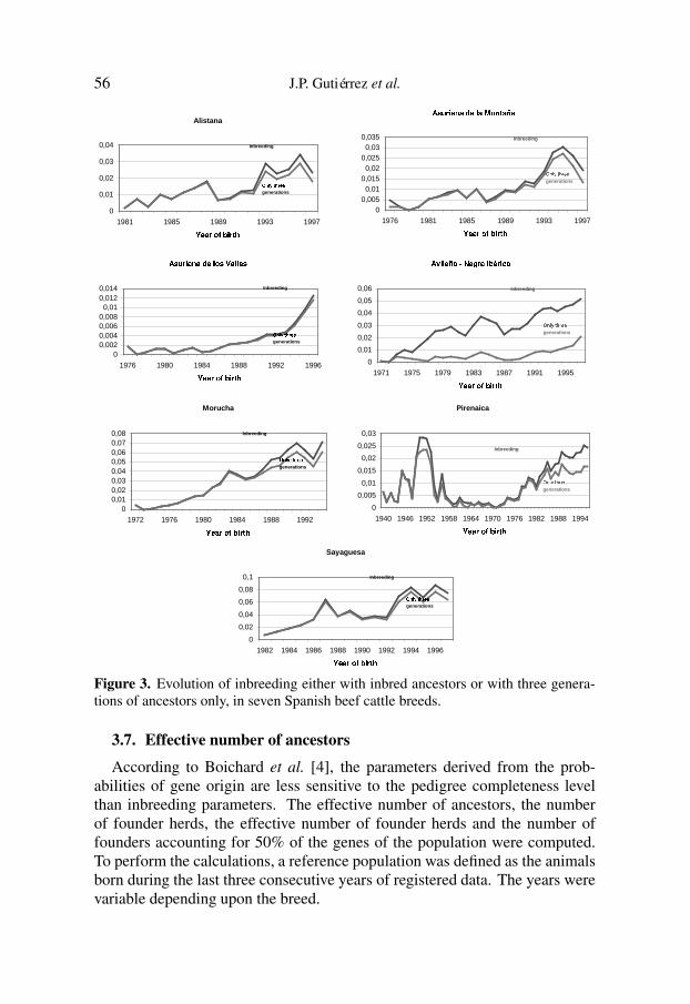
In order to distinguish between recent and cumulated inbreeding, the evolu-tion of this parameter per year of birth was also computed taking into accountonly the last three generations (Fig. 3). All breeds exhibited a similar patternshowing that inbreeding was mainly due to the recent generations, in most of thecases because a historical knowledge of the pedigree is lacking. A-NI had animportant cumulated inbreeding due to both a good knowledge of its historicalpedigree and to the typical breeding management as a dehesa breed. The Pibreed, however, changed the usual breeding management with the use of AIin the last several years not showing much difference between the evolution oftotal inbreeding and that provided by only the last three generations considered.

3.6. Effective population size

The effective population size, Ne, is the number of breeding animals thatwould lead to the actual increase in inbreeding if they contributed equally to thenext generation. In general, Ne was rather low in the Spanish breeds, rangingfrom 21 to 123 (Tab. V). Again, the dehesa breeds were those with the lowesteffective population size due to their particular intra-herd breeding policy.Subdivided populations can originate increases in inbreeding comparable to thatof smaller populations. For mountain breeds, the larger breeds also showedthe larger effective population size because of a dissemination of the morefrequently used animals among herds.


Alistana

0

0,01

0,02

0,03

0,04

1981 1985 1989 1993 1997ÎPÏ'Ð�Ñ,Ò�Ó*Ô�Õ Ñ Ö ×

Inbreeding

Ø�Ù Ú ÛÝÜ Þ ß à àgenerations

áPâ�ã�ä å æ�ç�æéè/êìë æìíiî,ç'ï æ�ð'æ

00,0050,01

0,0150,02

0,0250,03

0,035

1976 1981 1985 1989 1993 1997ñPê'æ�ä,î�ò*ó�å ä ï ô

Inbreeding

õ÷ö ø ùÝú û ü ý ýgenerations

þPÿ�� ÿ�� ÷ÿ

00,0020,0040,0060,0080,01

0,0120,014

1976 1980 1984 1988 1992 1996��

Inbreeding

�� ! !generations

"�#�$ % &�'�()�*�&�+�, (.- /�0�, $ 1�(

0

0,01

0,02

0,03

0,04

0,05

0,06

1971 1975 1979 1983 1987 1991 19952�&�(�,43�5�/�$ , 6 7

Inbreeding

8:9 ; <�= > ? @ @generations

Morucha

00,010,020,030,040,050,060,070,08

1972 1976 1980 1984 1988 1992ACB:D�E�F�G�H�I E J K

Inbreeding

L:M N O�P Q R S Sgenerations

Pirenaica

0

0,005

0,01

0,015

0,02

0,025

0,03

1940 1946 1952 1958 1964 1970 1976 1982 1988 1994T�U�V�W�X�Y�Z�[ W \ ]

Inbreeding

^:_ ` a�b c d e egenerations

Sayaguesa

0

0,02

0,04

0,06

0,08

0,1

1982 1984 1986 1988 1990 1992 1994 1996fCg:h�i�j�k�l�m i n o

Inbreeding

p�q r s�t u v w wgenerations

Figure 3. Evolution of inbreeding either with inbred ancestors or with three genera-tions of ancestors only, in seven Spanish beef cattle breeds.

3.7. Effective number of ancestors

According to Boichard et al. [4], the parameters derived from the prob-abilities of gene origin are less sensitive to the pedigree completeness levelthan inbreeding parameters. The effective number of ancestors, the numberof founder herds, the effective number of founder herds and the number offounders accounting for 50% of the genes of the population were computed.To perform the calculations, a reference population was defined as the animalsborn during the last three consecutive years of registered data. The years werevariable depending upon the breed.


These parameters explain how an abusive use of certain individuals as breed-ing animals can lead to a considerable reduction in the genetic stock. The upperbounds of these parameters are the actual number of founder animals/herds andthey decrease since their contribution is more unbalanced.

Estimates for the parameters of gene origin are presented in Table VI,whereas the evolution of the percentage of the explained population by thenumber of ancestors considered is shown in Figure 4 for all breeds. As before,it is possible to find some differences among breeds in the pattern shown by eachbreed, which would be explained by different mating policies and would leadto different advice in terms of controlling future inbreeding and relatedness.

The effective number of founders and ancestors ranged from 48 to 846 and25 to 163, respectively. These values were higher in the larger populations,especially when the size of their founder population was initially high, and werenot directly dependent upon the size of their populations of reference. In thelarger breeds, the size of the founder population was large when the pedigreecompleteness level was sparse, as in the AV breed. In the minority breeds,when the genealogy knowledge was sparse, the size of the founder populationwas still higher than the reference population, even twice as much, due to thefact that animals with unknown ancestors automatically became founders.

The number of founders accounting for 50% of the population genes rangesfrom 10 to 43, except for AV. Eight-point-three percent of the founders accoun-ted for half of the population in BP, but this number was considerably lowerin the other breeds, mainly in those with a larger historical genealogy, as A-NI(0.8%) and Pi (1.1%). It must be noted that these values indicate how muchof the inbreeding is caused by an abusive use of certain founders through theirdescendants. The differences between the effective number of founders and theeffective number of ancestors reflect the existence of bottlenecks in the pedigreeof several breeds. Furthermore, a bottleneck is logically more frequent in pop-ulations with a long historical pedigree knowledge such as Pi. This comparisonalso reflects the existence of important bottlenecks in Ali, AV, Pi and Say.

The evolution of the number of founders accounting for different percentagesof the populations can be observed in Figure 4. Breeds having the largest pop-ulation sizes (AV, A-NI, Mo, Pi) had the largest size of the founder populationand, consequently, showed a similar pattern. In the largest breeds, the numberof ancestors that accounts for the population diversity increased very quicklyat the beginning, but slower than in the other breeds later; in other words,several ancestors explained a high percentage of the population, but the rest ofthe population was explained by many others. This particular trend was morepronounced if the genealogy was well known (A-NI, Pi). On the contrary,minority populations (Ali, Say) as well as a breed with a sparse knowledge ofgenealogy (BP) tended to exhibit a more linear pattern than the other breeds.The extrapolation of these results to more generations in the past suggests


Tabl

eV

I.E

stim

ates

ofpa

ram

eter

sof

prob

abili

tyof

gene

orig

inin

eigh

tSpa

nish

beef

cattl

ebr

eeds

.

Bre

edR

efer

ence

popu

latio

nN

umbe

rof

foun

ders

Eff

ectiv

enu

mbe

rof

foun

ders

Eff

ectiv

enu

mbe

rof

ance

stor

s

Foun

ders

expl

aini

ng50

%

Num

ber

offo

unde

rhe

rds

Eff

ectiv

enu

mbe

rof

foun

der

herd

s

Ali

513

120

726

556

2220

2

AM

307

129

511

983

4042

750

AV

1650

910

107

846

163

415

293

530

4

A-N

I13

034

430

168

5936

137

59

BP

259

327

4840

27

Mo

119

399

013

010

543

225

76

Pi8

604

327

915

358

3661

554

Say

235

407

116

2510

135


Asturiana de los Valles

Number of founders: 10107 Founders explaining 50% : 415

100 2 00 3 00 4 00 5 00 6 00 7 00 8 00 9 00 1000

Number of anc est ors

0

2 0

4 0

6 0

8 0

100 E xplained perc ent age

Asturiana de la M ontañ a

Number of founders: 12 9 5 Founders explaining 50% : 40

100 2 00 3 00 4 00 5 00 6 00 7 00 8 00 9 00 1000


0

2 0

4 0

6 0

8 0


Av ileñ a - N eg ra I b é ric a

Number of founders: 43 01 Founders explaining 50% : 3 6

100 2 00 3 00 4 00 5 00 6 00 7 00 8 00 9 00 1000


0

2 0

4 0

6 0

8 0


Alistana


3 0 6 0 9 0 12 0 15 0 18 0 2 10


0

2 0

4 0

6 0

8 0

100

B runa dels P irineus


2 0 4 0 6 0 8 0 100 12 0 14 0 16 0 18 0


0

2 0

4 0

6 0

8 0


S ay ag uesa

Number of founders: 407 Founders explaining 50% : 10

10 2 0 3 0 4 0 5 0


0

2 0

4 0

6 0

8 0


M oruc h a

Number of founders: 9 9 0 Founders explaining 50% : 43

100 2 00 3 00 4 00 5 00 6 00 7 00 8 00 9 00 1000


0

2 0

4 0

6 0

8 0


P irenaic a

Number of founders: 3 2 79 Founders explaining 50% : 3 6

100 2 00 3 00 4 00 5 00 6 00 7 00 8 00 9 00 1000


0

2 0

4 0

6 0

8 0


Figure 4. Cumulative contribution of the ancestors to the genes of the referencepopulation, in eight Spanish beef cattle breeds.

that matings may have been carefully managed in small populations to avoidinbreeding consequences.


The analysis of the number of founder herds and their effective number leadsto similar conclusions in terms of abusive use of some breeding animals andloss of genetic diversity of populations. The effective number of founder herdsin relation to the total number of founder herds, was clearly larger in the dehesabreeds (A-NI and Mo, around 40%) than in the mountain breeds (AM, AV andPi, around 10%). This difference could be due to the low rate of migrationbetween herds in the dehesa breeds. Two of the minority breeds, Ali and Say,appeared equally founded by the animals of two and five herds, respectively,which indicates the potentially endangered state of these populations.

4. DISCUSSION

The estimates of generation intervals range from 3.70 to 6.08 years in thereference populations. In the sire-offspring pathway, the generation intervalwas always lower because sires were replaced earlier. A longer generationinterval in females than in males has been previously reported in other breeds,for example, in Australian Shorthorn [11] or British Hereford [16], and also inA-NI [20], and AM and AV [8].

Inbreeding has been shown to have an adverse effect on all performancetraits of beef cattle, although the effects of the inbreeding depression weremore severe in populations developed under rapid inbreeding systems, andparticularly in animals with inbreeding coefficients higher than 20% [5]. Inour populations, the average inbreeding was low, in the range of 1% to 3%, sothey can be considered far from dangerous values. Even the inbred animals inrecent generations did not approach the limit mentioned above.

When looking at the future, however, the effective population size in generalwas rather low in the Spanish breeds, ranging from 21 to 123. In five breeds(Ali, AM, A-NI, Mo and Say) that parameter did not reach the minimumrecommended value [14] to prevent a considerable loss of genetic variability.Boichard et al. [4] have shown that when the pedigree information is incom-plete, the computed inbreeding is biased downwards and the realised effectivesize is overestimated. Given the very low degree of pedigree knowledge inmost of the breeds studied, the true effective size would be even lower, whichwould worsen the situation in terms of maintenance of genetic variability.

Boichard et al. [3,4] have also found low population sizes (below 50) inseveral French breeds, such as Holstein, Normande, and Tarentaise. Ourresults, however, cannot be compared to the results of these authors becausethe complete generation equivalent value was, in general, much lower in theSpanish breeds and the information used to estimate ∆F was different. Fur-thermore, these authors [4] have shown that the trend in inbreeding was veryunstable between replicates of a simulation experiment, especially when thepedigree was not complete. Given the sparse pedigrees of most of the Spanish


breeds studied, our estimates may have a high degree of uncertainty. It becomesevident that an intensive effort of pedigree recording will be needed in orderto develop an appropriate monitoring of the genetic variability in most of theSpanish breeds. This situation is particularly critical for the Ali and Say breeds,in which a more indepth analysis of their population structure will allow for theestablishment of optimal criteria for choosing and mating the breeding animals.

Migrations between subpopulations when there is a low average relatednessvalue, i.e. in dehesa breeds, in order to dramatically decrease inbreeding has alogical appeal. This strategy should be tested in the future in different scenariosagainst the results that can be obtained by different mating methods, such asfactorial and compensatory matings (see review of Caballero et al. [6]), or min-imum coancestry mating with a maximum of one offspring per mating pair [18].

The effective number of ancestors takes into account the possible bottle-necks in the pedigree, such as those originated by AI schemes, and, thus, thisparameter tends to present values lower than the effective number of founders(Boichard et al. [4]). This parameter will be equivalent to the average pairwisecoancestry of a given group of N individuals (see equation (5) in [7]). Usually,historical pedigrees tend to provide low values of both effective numbers offounders and ancestors. When we compared the effective number of foundersto the effective population size, and the effective number of founder herdsin contrast to the HS parameter that measures the effective number of herdssupplying sires per generation, BP appeared to be the breed with the lowesteffective number of founders and ancestors, but it ranked second in terms ofthe effective population size estimated from the increase of inbreeding pergeneration. This figure, nevertheless, could be related to the low completenesslevel of the pedigree. On the contrary, Ali had approximately the same effectivenumber of founders as AV, but the number of effective founder herds was 2for Ali against 304 for AV. The breed with the highest pedigree completenesslevel (Pi) had a discrete effective number of founders but the highest effectivepopulation size and a very low effective number of founder herds. Eachgroup of breeds was shown to have its own particular pattern regarding all theparameters analysed and, even within group, each breed was shown to have itsown particular situation.

5. CONCLUSIONS

The main conclusion to be drawn from our study is that the genetic statusregarding the maintenance of genetic variability differs among breeds, and asingle practical recommendation does not exist. The causes of these differencescould be related to population size, breeding policy, and probably in somebreeds to empirical selection objectives.


The subdivision carried out at the beginning of this paper leads to differentconclusions for the dehesa versus the mountain breeds. Inbreeding is higherin the dehesa breeds than in the mountain breeds, whereas the opposite is truefor average relatedness.

There is clear evidence that Ali and Say populations have a small effectivesize from a genetic point of view. As a consequence, a more indepth analysisof the genetic structure of each breed and its mating policy is necessary in orderto recommend, on an individual basis, the most convenient breeding practicesto maintain genetic diversity. The A-NI and Mo breeds, with a small effectivesize but showing a low mean average relatedness coefficient, are not in danger.

Most of the breeds need an important recording effort in order to achievebetter genealogy knowledge, particularly AV, BP and Mo, and to be able toproperly carry out the monitoring of inbreeding. This situation is critical forBP because the two other breeds have animals which have made an importantcontribution to the population and with a well known genealogy. Pi is differentfrom the others, presenting a wide historical pedigree.

The effective number of founders is considerably higher than the effectivenumber of ancestors in mountain and minority breeds when compared to dehesabreeds, as a consequence of their particular breeding system.

ACKNOWLEDGEMENTS

This research has been funded by the EU - FAIR1 CT95 0702 and AGF95–0576 projects, the last one granted by the “Comision Interministerial de Cienciay Tecnología” of the Spanish government. We acknowledge the collaborationof the breed societies for recording and providing the data. The English ofthis manuscript was revised and corrected by Chuck Simmons, instructor ofEnglish at the UAB.

REFERENCES

[1] Altarriba J., Ocáriz J.M., Estudio genético-reproductivo de la raza Pirenaica apartir del registro genealógico de Navarra, ITEA 7 (1987) 67–69.

[2] Ballou J.D., Lacy R.C., Identifiyng genetically important individuals for manage-ment of genetic variation in pedigreed populations, in: Ballou J.D., Gilpin M.,Foose T.J. (Eds.), Population management for survival and recovery, ColumbiaUniversity Press, New York, 1995, pp. 76–111.

[3] Boichard D., Maignel L., Verrier E., Analyse généalogique des races bovineslaitières françaises, INRA Prod. Anim. 9 (1996) 323–335.

[4] Boichard D., Maignel L., Verrier E., The value of using probabilities of geneorigin to measure genetic variability in a population, Genet. Sel. Evol. 29 (1997)5–23.


[5] Burrow H.M., The effects of inbreeding in beef cattle, Anim. Breed. Abstr. 61(1993) 737–751.

[6] Caballero A., Santiago E., Toro M.A., Systems of mating to reduce inbreedingin selected populations, Anim. Sci. 62 (1996) 431–442.

[7] Caballero A., Toro M.A., Interrelations between effective population size andother pedigree tools for the management of conserved populations, Genet. Res.Camb. 75 (2000) 331–343.

[8] Cañón J., Gutiérrez J.P., Dunner S., Goyache F., Vallejo M., Herdbook analysisof the Asturiana beef cattle breeds, Genet. Sel. Evol. 26 (1994) 65–75.

[9] Dunner S., Checa M.L., Gutiérrez J.P., Martín J.P., Cañón J., Genetic analysisand management in small populations: the Asturcon pony as an example, Genet.Sel. Evol. 30 (1998) 397–405.

[10] Falconer D.S., Mackay T.F.C., Introduction to Quantitative Genetics, Longman,Harlow, 1996.

[11] Herron N.D., Pattie W.A., Studies of the Australian Illawarra Shorthorn breed ofdairy cattle. II., Austr. J. Agric. Res. 28 (1977) 1119–1132.

[12] James J.W., Computation of genetic contributions from pedigrees, Theor. Appl.Genet. 42 (1972) 272–273.

[13] Lacy R.C., Analysis of founder representation in pedigrees: founder equivalentsand founder genome equivalents, Zoo. Biol. 8 (1989) 111–123.

[14] Meuwissen T.H.E., Operation of conservation schemes, in: Oldenbroek J.K.(Ed.), Genebanks and the conservation of farm animal genetic resources, DLOInstitute for Animal Science and Health, Lelystad, 1999, pp. 91–112.

[15] Meuwissen T.H.E., Luo Z., Computing inbreeding coefficients in large popula-tions, Genet. Sel. Evol. 24 (1992) 305–313.

[16] Özkütük K., Bichard M., Studies of pedigree Hereford cattle breeding. 1. Herd-book analyses, Anim. Prod. 24 (1977) 1–13.

[17] Robertson A., A numerical description of breed structure, J. Agric. Sci. 43 (1953)334–336.

[18] Sonesson A.K., Meuwissen T.H.E., Non-random mating for selection withrestricted rates of inbreeding and overlapping generations, Genet. Sel. Evol.34 (2002) 23–29.

[19] United Nations Environment Programme, Convention on Biological Diversity,Environmental Law and Institutions Programme Activity Centre, 1992, pp. 1–52.

[20] Vassallo J.M., Díaz C., García-Medina J.R., A note on the population structureof the Avileña breed of cattle in Spain, Livest. Prod. Sci. 15 (1986) 285–288.

[21] Verrier E., Colleau J.J., Foulley J.L., Le modèle animal est-il optimal à moyenterme ?, in: Foulley J.L., Molénat M. (Eds.), Séminaire modèle animal, Inra,Paris, 1994, pp. 57–66.

[22] Vu Tien Kang J., Méthodes d’analyse des données démographiques et généalo-giques dans les populations d’animaux domestiques, Génét. Sél. Évol. 15 (1983)263–298.

[23] Wright S., Mendelian analysis of the pure breeds of livestock. I. The measurementof inbreeding and relationship, J. Hered. 14 (1923) 339–348.

[24] Wright S., Evolution in Mendelian populations, Genetics 16 (1931) 97–159.

Pedigree analysis of eight Spanish beef cattle breeds

Documents

Transcript of Pedigree analysis of eight Spanish beef cattle breeds