Complex pedigree analysis to detect quantitative trait loci in ...
126
Complex pedigree analysis to detect quantitative trait loci in dairy cattle
-
Upload
khangminh22 -
Category
Documents
-
view
2 -
download
0
Transcript of Complex pedigree analysis to detect quantitative trait loci in ...
Complex pedigree analysis
to detect quantitative trait loci
in dairy cattle
Promotoren: dr. ir. E.W. Brascamp
hoogleraar in de veefokkerij
dr. R.L. Quaas
professor animal science, Cornell University, US
Co-promotor: dr. ir. J.A.M, van Arendonk
Persoonlijk hoogleraar bij de leerstoelgroep fokkerij en genetica
<?4 7 f
Complex pedigree analysis
to detect quantitative trait loci
in dairy cattle
Marco (M.C.A.M.) Bink
Proefschrift
ter verkrijging van de graad van doctor op gezag van de rector magnificus van de Landbouwuniversiteit Wageningen, dr. C.M. Karssen, in het openbaar te verdedigen op vrijdag 4 september 1998 des namiddags te twee uur dertig in de Aula
\bfc ™ß''

CIP-GEGEVENS KONINKLIJKE BIBLIOTHEEK, DEN HAAG
Bink, Marco
Complex pedigree analysis to detect quantitative trait loci in dairy cattle / Marco C.A.M. Bink
Thesis Wageningen. - With ref. - With summary in Dutch.
ISBN: 90-5485-897-4
Subject headings: genetic markers; quantitative trait locus; dairy cattle; genetics
Abstract
Bink, M.C.A.M., 1998. Complex pedigree analysis to detect quantitative trait loci in dairy cattle. Doctoral thesis, Wageningen Agricultural University, P.O. Box 338, 6700 AH Wageningen, The Netherlands.
This thesis considers development of statistical methodology for detection of
quantitative trait loci (QTL) in outbreeding dairy cattle populations. Information on genetic
markers is used to study segregation of chromosomal segments from parents to offspring. The
presence of complex pedigrees and incompleteness of genetic marker information seriously
complicate the statistical analysis of QTL mapping experiments in livestock populations. In
this thesis, a Bayesian approach to QTL detection and mapping is developed, which makes
use of Markov chain Monte Carlo (MCMC) methodology to perform the otherwise intractable
computations. The Bayesian approach combined with the MCMC computing methodology,
proved very flexible in the construction of a realistic model for the analysis of livestock data.
Methodology was tested empirically by Monte Carlo simulation and was successfully applied
to data on Dutch dairy cattle, identifying chromosomal regions likely containing QTL for
traits of biological importance.
BIBLIOTHEEK LANDBOUWUNIVERSITEIT
WAGENINGEN

Voorwoord
Het onderzoek dat in dit proefschrift wordt beschreven is uitgevoerd in het kader van
een assistent in opleiding (aio) projekt. De was die aio. Echter, zonder de hulp van vele
anderen was ik mogelijk niet die aio geweest of was de inhoud van dit proefschrift niet zoals
die nu voor u ligt. Het aio projekt is uitgevoerd bij de vakgroep veefokkerij, hedendaags
bekend als leerstoelgroep fokkerij en genetica. Ik wil alle huidige en ex-medewerkers van
deze groep bedanken voor de prettige en stimulerende werksfeer en samenwerking. Zonder
anderen te kort te willen doen, wil ik toch enkele mensen met name noemen.
Johan, je was degene die me op het juiste spoor zette voor dit aio projekt en ook
tijdens het aio projekt was je een perfekte begeleider die me zelfvertrouwen en vrijheid in het
onderzoek gaf. Pim, Henk, Luc, Ab, Michel en Theo, bedankt voor jullie bijdragen aan de
discussies in de begeleidingscommissie. Ant, hoewel we aardig verschillend waren, was het
aangenaam om je deze vier jaar als kamergenoot te hebben. Sijne, het was erg prettig om
tegen je aan te mogen kletsen en zeuren, tevens bedankt voor je kritische feedback. Richard,
thanks for the enjoyable discussions and workouts.
Dick, it all started with a memorable discussion after my oral presentation at the Dairy
Science meeting in 1995. This contact led to a very pleasant and fruitful cooperation,
especially during my six-month stay at Cornell University in 1996. I also like to thank family
Ducrocq, Susan and John Herbert, the members of the animal breeding group, and my
housemates at Watermargin for making my stay at Cornell.
Mijn aio projekt was onderdeel van het zogenaamde MILQTL projekt. Met name
tijdens de jaarlijkse scientific reviews, werd mijn horizon weer breder door inbreng van
mensen van Holland Genetics, Livestock Improvement en vooral de Universiteit van Luik.
Een niet onbelangrijk deel van mijn sociale leven in Wageningen is bepaald door
Dijkgraaf 4-la. Beland in 1990, eerst in onderhuur op de kamer van mijn 'nichtje' Ine, en er
daarna er blijven hangen omdat het er toch best gezellig was. In 1994 was het moment daar
om samen met drie afdelingsgenoten (in wisselende samenstelling) te verkassen naar
Asterstraat. Marion, Lutzen, Jeroen, Peter, en Frouwkje, bedankt voor de leuke tijd op A39.
Lieve Agnes, bedankt voor je rotsvaste vertrouwen, je steun en vooral geduld. Als
laatste wil ik mijn ouders bedanken voor hun steun en belangstelling tijdens mijn studie. Aan
hen draag ik dit werk op.
Marco

Contents
Chapter 1 General introduction
Chapter 2 Breeding value estimation with incomplete data
Chapter 3 Bayesian estimation of dispersion parameters with a reduced
animal model including polygenic and QTL effects 27
Chapter 4 Markov chain Monte Carlo for mapping a quantitative trait locus
in outbred populations 53
Chapter 5 Detection of quantitative trait loci in outbred populations with
incomplete marker data 69
Chapter 6 General discussion 95
Summary
Samenvatting
117
121
Curriculum vitae 127

Stellingen
1. Het benutten van maternale en patemale relaties tussen half-sib families in een
granddaughter design leidt tot een grotere statistische power om QTL's op te sporen.
Dit proefschrift
2. De toepassing van data-augmentatie om te komen tot bekende verdelingen van trekkingen
voor de Gibbs sampler, leidt tot inefficiente menging van modelparameters indien er
relatief veel data aangevuld moet worden.
Dit proefschrift
3. Schattingsmethoden waarin een genetisch model met random effecten voor het QTL
wordt verondersteld, zijn geschikt voor gesimuleerde data waarin het QTL slechts 2
allelen bevat, maar andersom is dit niet het geval.
Hoeschele et al. Genetics, 1997,147:1445-1457
4. De in de data aanwezige informatie over een modelparameter kan eenvoudig worden
bestudeerd door de veronderstelde voorkennis over deze parameter te variëren.
Dit proefschrift
5. Het direkte gebruik van waarnemingen van de dochters leidt tot nauwkeurigere
schattingen van variantiecomponenten dan het gebruik van zogenaamde Daughter Yield
Deviations.
Dit proefschrift; Van Arendonk et al. J Dairy Sei (1998, accepted); Grignola et al. (1996) Genet Sel Evol
28:491-504; Thaller & Hoeschele (1996) Theor Appl Genet 93:1167-1174; Uimari et al. (1996) Genetics
143:1831-1842
6. Aangezien veefokkers een beter idee hebben van verhoudingen van variantiecomponenten
dan van de variantiecomponenten zelf, ligt het meer voor de hand om in een Bayesiaanse
analyse de voorkennis over genetische parameters te definieren in termen van deze
verhoudingen.

7. Bayesiaanse modelbepaling is de beste statistische methode voor de bestudering van het
aantal QTL's dat aanwezig is binnen een gemarkeerd chromosoomsegment.
Satagopan & Yandell (1996) Special contributed paper session on genetic analysis of quantitative traits and
complex diseases, Biometrie section, Joint Statistical Meetings, Chicago, IL.; Uimari & Hoeschele (1997)
Genetics 146:735-743; Sillanpaa & Arjas (1998) Genetics 148:1373-1388
8. Voor het opsporen van QTL's voor kenmerken waarop fenotypisch selectie moeizaam
verloopt, is het verzamelen van fenotypische gegevens cruciaal.
9. Het succes van merker-ondersteunde selectie in een fokprogramma hangt in sterke mate af
van het vinden van nieuwe QTL's.
Meuwissen & Goddard (1996) Genet Sel Evol 28:161-176
10. In tegenstelling tot de situatie bij de handel in aandelen wordt het in een Bayesiaanse
analyse zeer gewaardeerd wanneer aanwezige voorkennis zo goed mogelijk wordt benut.
11. Het succes van het zogenaamde polder-model heeft geen betrekking op het aantal
Wageningse carpoolers dat uiteindelijk in Lelystad gaat wonen.
12. Universiteiten en professionele voetbalclubs in Nederland hebben gemeen dat ze prima in
staat zijn om talent op te leiden maar tevens dat ze dit talent daarna niet weten te
behouden.
13. Life is what happens to you while you're busy making other plans.
John Lennon
Stellingen behorende bij het proefschrift
"Complex pedigree analysis to detect quantitative trait loci in dairy cattle",
Marco Bink,
Wageningen, 4 september 1998.

Chapter 1
General Introduction

General introduction
In dairy cattle, phenotypic variation can be observed in many traits, such as milk
yield, fertility and disease resistance. For breeding purposes, analysis of this phenotypic
variation and uncovering the contribution of genetic factors is very important. The observed
variation results from the combined action of multiple segregating genes and environmental
factors. An intrinsic feature of such traits is, however, that the individual genes contributing
to the quantitative genetic variation can hardly be distinguished. The detection of the
individual gene is hampered by their generally small effects, and the fact that segregation of
alleles from parents to offspring cannot be followed. Therefore, the genetics of such traits
until recently were studied in general terms of classical quantitative genetics, e.g., heritability
and covariances between relatives, rather than in terms of individual gene effects (Falconer
and MacKay 1996). Developments in molecular genetics during the last decade, however,
have opened the way to follow segregation of chromosomal segments in families. Through
the use of these genetically marked chromosomal segments, it has become possible to detect
and locate the genes affecting quantitative traits ("quantitative trait loci" or "QTL"). After
successful identification of QTL, the genetic markers linked to the QTL can be used to
improve selection schemes.
Without markers, prediction of genetic merit of animals and selection decisions are
entirely based on phenotypic and pedigree information. Phenotypic information to identify
within family genetic differences only becomes available after measurement on the animal or
its offspring. For example, with milk production traits information on within family genetic
differences between brothers comes available when the bulls are 5 years old, i.e. when their
offspring have completed their first lactation. Genetic markers linked to QTL can be used to
improve prediction of genetic merit and selection of animals. The transmission of alleles at
the QTL from parents to offspring can be traced based on the genotypes of linked markers.
Marker information is available very soon after birth or even at the embryo level and
facilitates early identification of genetic differences within a family. Information on genetic
markers can be used to select animals at a younger age and/or to improve the accuracy of
prediction of genetic merit. Additional genetic improvement from marker assisted selection
in dairy cattle breeding programs has been reported (Soller and Beckmann 1983; Kashi et al.
1990; Meuwissen and VanArendonk 1992).

4 Chapter 1
UTILIZATION OF FIELD DATA TO DETECT QTL IN DAIRY CATTLE
The structure of commercial dairy cattle breeding programs, where sires have a large
number of offspring, can be utilized to detect QTL directly in commercial populations.
Weiler et al. (1990) investigated the daughter and granddaughter design for detection of QTL
in dairy cattle populations. In a daughter design, sires and their daughters are scored for
markers and the daughters are measured for the quantitative trait. In a granddaughter design,
grandsires and their sons are genotyped for markers, while the daughters of the sons (i.e., the
granddaughters) are measured for the trait. The granddaughter design makes use of the
generally large amount of phenotypic data that are routinely collected in dairy cattle
populations, while minimizing the genotyping effort (Weiler et al. 1990).
In the statistical analysis of granddaughter design data grandsires are usually assumed
to be unrelated and the sons only related through their (grand) sire. This assumption often
does not hold since additional relationships are often present. For example, bull dams may
have multiple sons tested in a breeding program, or bull dams are sired by a grandsire. A full
pedigree analysis, accounting for all relationships, can improve the power to detect QTL
since more segregation events are included. Low power implies a small probability of
detecting a QTL. The additional increase in power is especially beneficial when the size of
the granddaughter design is limited by the progeny test capacity of breeding programs. A full
pedigree analysis will include individuals (bull dams) that do not have marker genotypes
observed. Furthermore, breeding programs are ongoing and new generations of individuals
can be added to detect more QTL or to confirm previously detected QTL.
In summary, complex pedigrees of individuals in a granddaughter design for dairy
cattle and the incomplete marker data require sophisticated statistical methods for analysis.
These methods are currently not available, since most methods used to date, only use a single
kind of relationship and assume that all individuals have observed marker genotypes (see
reviews by Bovenhuis et al. 1997; Hoeschele et al. 1997). Markov chain Monte Carlo
(MCMC) methods may offer the opportunity to utilize all pedigree information in QTL
analysis in complex pedigrees. In this thesis, MCMC methods will be used to make Bayesian
inferences and in the following section the essentials of Bayesian methods is briefly
introduced.

General introduction
BAYESIAN DATA ANALYSIS AND MARKOV CHAIN MONTE CARLO
The essential characteristic of Bayesian methods are their explicit use of probability
for quantifying uncertainty in inferences based on statistical data analysis (Gelman et al.
1995). Bayesian data analysis starts with setting up a full probability model - a joint
probability distribution for all observable and unobservable quantities in a problem. For
example, trait phenotypes are assumed to follow a normal distribution, but also the
distributions of variance components are specified a priori. Bayesian statistical inference is
concerned with drawing conclusions about quantities that are not observed, after combining
prior knowledge on all unobserved quantities with information from the observed data.
Bayesian inferences about a particular parameter are made in terms of probability statements
or probability distributions. Marginal posterior distributions take into account uncertainty in
a single parameter due to uncertainty in all other parameters in the model. This treatment of
uncertainty involves complicated integration of the joint posterior density, and analytical
integration is often impossible due to the high-dimensional complexity of the problem.
In the 1990's, the interest in Bayesian analysis has increased rapidly due to the
increasing availability of inexpensive, high-speed computing, and the advent of methods
based on Markov chain Monte Carlo (MCMC) algorithms, i.e., Monte Carlo integration
using Markov chains. Monte Carlo integration draws samples from the required distribution
(the joint posterior density), and Markov chain Monte Carlo draws these samples by running
a cleverly constructed Markov chain for a long time. The Markov chain has an equilibrium
distribution equal to the joint posterior distribution being approximated. One can construct
these chains in many ways, but all of them, including the Gibbs sampler (Geman and Geman
1984), are special cases of the general framework of Metropolis et al. (1953) and Hastings
(1970). Recommendations for further reading on Bayesian data analysis and MCMC
methodology are Gelman et al. (1995) and Gilks et al. (1996), respectively.
AIM AND OUTLINE OF THIS THESIS
The aim of this thesis is to contribute to the efficient utilization of data on genetic
markers and quantitative traits to detect and utilize QTL in complex outbred pedigrees in
dairy cattle breeding programs. Due to the lack of flexible and efficient statistical methods to
analyze such data, presentation of statistical methods developed forms the core of this thesis.
Methodology is based on Bayes theory and implemented via MCMC algorithms.
6 Chapter 1
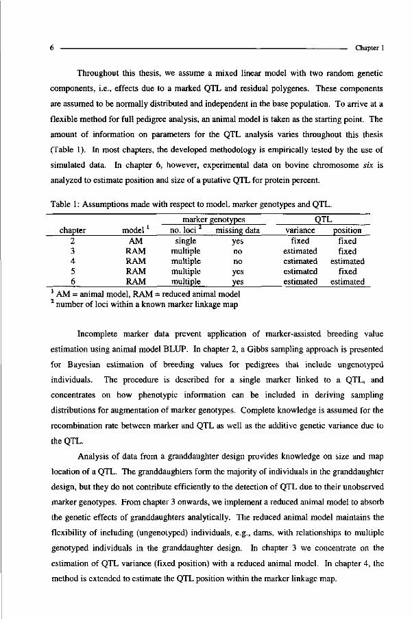
Throughout this thesis, we assume a mixed linear model with two random genetic
components, i.e., effects due to a marked QTL and residual polygenes. These components
are assumed to be normally distributed and independent in the base population. To arrive at a
flexible method for full pedigree analysis, an animal model is taken as the starting point. The
amount of information on parameters for the QTL analysis varies throughout this thesis
(Table 1). In most chapters, the developed methodology is empirically tested by the use of
simulated data. In chapter 6, however, experimental data on bovine chromosome six is
analyzed to estimate position and size of a putative QTL for protein percent.
Table 1 : Assumptions made with respect to model, marker genotypes and QTL.
chapter 2 3 4 5 6
modell
AM RAM RAM RAM RAM
marker no. loci 2
single multiple multiple multiple multiple
genotypes missing data
yes no no yes yes
QTL variance
fixed estimated estimated estimated estimated
position fixed fixed
estimated fixed
estimated 1 AM = animal model, RAM = reduced animal model 2 number of loci within a known marker linkage map
Incomplete marker data prevent application of marker-assisted breeding value
estimation using animal model BLUP. In chapter 2, a Gibbs sampling approach is presented
for Bayesian estimation of breeding values for pedigrees that include ungenotyped
individuals. The procedure is described for a single marker linked to a QTL, and
concentrates on how phenotypic information can be included in deriving sampling
distributions for augmentation of marker genotypes. Complete knowledge is assumed for the
recombination rate between marker and QTL as well as the additive genetic variance due to
the QTL.
Analysis of data from a granddaughter design provides knowledge on size and map
location of a QTL. The granddaughters form the majority of individuals in the granddaughter
design, but they do not contribute efficiently to the detection of QTL due to their unobserved
marker genotypes. From chapter 3 onwards, we implement a reduced animal model to absorb
the genetic effects of granddaughters analytically. The reduced animal model maintains the
flexibility of including (ungenotyped) individuals, e.g., dams, with relationships to multiple
genotyped individuals in the granddaughter design. In chapter 3 we concentrate on the
estimation of QTL variance (fixed position) with a reduced animal model. In chapter 4, the
method is extended to estimate the QTL position within the marker linkage map.
General introduction
In chapter 5, the methodology of handling ungenotyped animals (chapter 2) and the
reduced animal model (chapter 3) are combined to estimate model parameters in
granddaughter designs, where ungenotyped dams of sons provide additional relationships
between genotyped elite sires and sons.
The general discussion (chapter 6) contains four sections. First, the method described
in chapter 5 was extended to estimate QTL position in a way similar to that described in
chapter 4. Secondly, results are presented from QTL analysis of experimental data for
chromosome six in dairy cattle. Thirdly, the developed Bayesian method for QTL analysis in
complex pedigrees is compared to literature. Finally, practical implications of marker-
assisted genetic evaluation in dairy cattle breeding programs are briefly addressed.
REFERENCES
Bovenhuis H, Van Arendonk JAM, Davis G, Elsen JM, Haley CS, Hill WG, Baret PV, Hetzel DJS, Nicholas FW (1997) Detection and mapping of quantitative trait loci in farm animals. Livest Prod Sei 52:135-144
Falconer DS, Mackay TFC (1996) Introduction to Quantitative Genetics. Longman Group Ltd, Essex, United Kingdom
Gelman A, Carlin JB, Stern HS, Rubin DB (1995) Bayesian Data Analysis. Chapman & Hall, Suffolk, United Kingdom
Geman S, Geman D (1984) Stochastic relaxation, Gibbs distributions and the Bayesian restoration of images. IEEE Trans Pattern Anal Machine Intelligence 6:721-741
Gilks WR, Richardson S, Spiegelhalter DJ (1996) Markov chain Monte Carlo in practice. Chapman & Hall, Suffolk, United Kingdom
Hastings WK (1970) Monte Carlo sampling methods using Markov chains and their applications. Biometrika 57:97-109
Hoeschele I, Uimari P, Grignola FI, Zhang Q, Gage KM (1997) Advances in statistical methods to map quantitative trait loci in outbred populations. Genetics 147:1445-1457
Kashi Y, Hallerman E, Soller M (1990) Marker-assisted selection of candidate bulls for progeny testing programmes. Anim Prod 51:63-74
Metropolis N, Rosenbluth AW, Rosenbluth MN, Teller H, Teller E (1953) Equations of state calculations by fast computing machines. J Chem Physics 21:1087-1091
Meuwissen THE, Van Arendonk JAM (1992) Potential improvements in rate of genetic gain from marker assisted selection in dairy cattle breeding schemes. J Dairy Sei 75:1651-1659
Soller M, Beckmann JS (1983) Genetic polymorphism in varietal identification and genetic improvement. Theor Appl Genet 67:25-33
Weiler JI, Kashi Y, Soller M (1990) Power of daughter and granddaughter designs for determining linkage between marker loci and quantitative trait loci in dairy cattle. J Dairy Sei 73:2525-2537
Chapter 2
Breeding Value Estimation with Incomplete Marker Data
Marco C. A. M. Bink , Johan A. M. van Arendonk and Richard L. Quaas
'Animal Breeding and Genetics Group, Wageningen Institute of Animal Sciences, Wageningen Agricultural University, PO Box 338,6700 AH Wageningen, The Netherlands
"Department of Animal Science, Cornell University, Ithaca, NY 14853, USA
Published in Genetics Selection Evolution 30:45-58 (1998)
Reproduced by permission of Elsevier/INRA, Paris

Incomplete marker data 11
ABSTRACT
Incomplete marker data prevents application of marker-assisted breeding value
estimation using animal model BLUP. We describe a Gibbs sampling approach for Bayesian
estimation of breeding values, allowing incomplete information on a single marker that is
linked to a quantitative trait locus. Derivation of sampling densities for marker genotypes is
emphasized, because reconsideration of the gametic relationship matrix structure for a
marked quantitative trait locus leads to simple conditional densities. A small numerical
example is used to validate estimates obtained from Gibbs sampling. Extension and
application of the presented approach in livestock populations is discussed.
INTRODUCTION
Identification of a genetic marker closely linked to a gene (or a cluster of genes)
affecting a quantitative trait, allows more accurate selection for that trait (Goddard 1992).
The possible advantages from marker-assisted genetic evaluation have been described
extensively (e.g., Soller and Beekman 1982; Smith and Simpson 1986; Meuwissen and Van
Arendonk 1992).
Fernando and Grossman (1989) demonstrated how Best Linear Unbiased Prediction
(BLUP) can be performed when data is available on a single marker linked to quantitative
trait locus (QTL). The method of Fernando and Grossman has been modified for including
multiple unlinked marked QTL (Van Arendonk et al. 1994), a different method of assigning
QTL effects within animals (Wang et al. 1995); and marker brackets (Goddard 1992). These
methods are efficient when marker data is complete. However, in practice, incompleteness of
marker data is very likely because it is expensive and often impossible (when no DNA is
available) to obtain marker genotypes for all animals in a pedigree. For every unmarked
animal, several marker genotypes can be fitted, each resulting in a different marker genotype
configuration. When the proportion or number of unmarked animals increases, identification
of each possible marker genotype configuration becomes tedious and analytical computation
of likelihood of occurrence of these configurations becomes impossible.
Gibbs sampling (Geman and Geman 1984) is a numerical integration method that
provides opportunities to solve analytically intractable problems. Applications of this
12 Chapter 2
technique have recently been published in statistics (e.g. Gelfand and Smith 1990; Geyer
1992) as well as animal breeding (e.g., Wang et al. 1993; Sorensen et al. 1994). Janss et al.
(1995) successfully applied Gibbs sampling to sample genotypes for a bi-allelic major gene,
in absence of markers. Sampling genotypes for multiallelic loci, e.g., genetic markers, may
lead to reducible Gibbs chains (Thomas and Cortessis 1992; Sheehan and Thomas 1993).
Thompson (1994) summarizes approaches to resolve this potential reducibility and concludes
that a sampler can be constructed that efficiently samples multiallelic genotypes on a large
pedigree.
The objective of this paper is to describe the Gibbs sampler for marker-assisted
breeding value estimation for situations where genotypes for a single marker locus are
unknown for some individuals in the pedigree. Derivation of the conditional, discrete,
sampling distributions for genotypes at the marker is emphasized. A small numerical example
is used to compare estimates from Gibbs sampling to true posterior mean estimates.
Extension and application of our method are discussed.
METHODOLOGY
Model and Priors
We consider inferences about model parameters for a mixed inheritance model of the
form
y = Xß + Zu + Wv + e [1]
where y and e are «-vectors representing observations and residual errors, ß is a p-vector of
'fixed effects', u and v are q and 2^-vectors of random polygenic and QTL effects,
respectively, X is a known n x p matrix of full column rank, and Z and W are known nx q
and n x 2q matrices, respectively. For each individual we consider three random genetic
effects, i.e., 2 additive allelic effects at a marked QTL ( v' and v], see Figure 1) and a residual
polygenic effect («,-). Here e is assumed to have the distribution Nn (O, \<s\), independently of
ß, u and v. Also u is taken to be Nq (O, Aa2u ), where A is the well-known numerator
relationship matrix. Finally, v is taken to be N2q(o,GaJ), where G is the gametic
relationship matrix (2q x 2q) computed from pedigree, a full set of marker genotypes and the
known map distance between marker and QTL (Wang et al. 1995). In case of incomplete

Incomplete marker data- 13
marker data, we augment genotypes for ungenotyped individuals. We then denote m^ and
G(k) as the marker genotype configuration k and as the corresponding gametic relationship
matrix. Further, ß, u, v, and missing marker genotypes are assumed to be independent, a
priori. We assume complete knowledge on variance components and map distance between
marker and QTL.
Linkage between Marker and QTL
M s i -
Q s 1 -
- M s2 Md ' -
- Q s 2 Qd1 -
M j 1 -
Q i 1 -
- M d2
- Q d 2
- M j 2
- Q i 2
Figure 1 : Linkage between marker and quantitative trait locus (QTL) alleles. Assignment of QTL alleles is based on marker alleles. Given a known recombination rate, r, the probability that the first QTL allele of animal i is identical to the second QTL allele of its sire is given as P( Q) = Q2) = ( l - r ) xP (M ' = M2) + {r)xP(M) = M]), where M = marker allele; Q = QTL allele; i = individual, s = sire; and d = dam.
Joint Posterior Density and Full Conditional Distributions
The conditional density of y given ß, u, and v for the model given in [1] is
proportional to exp{->£ <7~2 (y - Xß - Zu - Wv)'(y - X/? - Zu - Wv)}, so the joint posterior
density is given by
p(ß,u,vlCT^,aJ,oe2,mobs,r,y)
- exp{- /2 c;2 (y - Xß - Zu - Wv) (y - Xß - Zu - Wv)}
xexp{-Xa;2(u'A_1u)}
XH |G("k)Gv2| 'expt-^o^v'GloVjjxpipaolm,*,) [2]
The joint posterior density includes a summation (nc) over all consistent marker genotype
configurations (n^k)). In the derivation of the sampling densities for marked QTL effects,

14 Chapter 2
however, one particular marker genotype configuration, ni(k), is fixed. The summation needs
to be considered only when the sampling of marker genotypes is concerned.
To implement the Gibbs sampling algorithm, we require the conditional posterior
distributions of each of ß, u, and v given the remaining parameters, the so-called full
conditional distributions, which are as follows
(frlß-i,o,v,y)
~ N [ (x /x J -y ( y - X . ^ - Z u - W v M V x J - y ]
(u ilu. i,ß,v,y)
N (z/Zi+aX)"1 z X y - X ß - Z ^ - W v ^ J a X U i j .W^+^aJa,
[3]
[4]
(Vilv.,,ß,u,m (k),y)
N (wjwi+g^ocj1 w ; (y -Xß-Zu-W_,v . i ) -£a v gf k ) v j ,(w;Wi+gji
k)av )r'ae2
where, a'j ,gjjk) is the (i,))th element of A" and G(k), respectively, <xu = % , a
[5]
and
2«
2^a,JotuUy, and Xav£(k)v; a r e m e corrections for polygenic and gametic covariances in the
pedigree, respectively. Note that the means of the distributions [3], [4], and [5] correspond to
the updates obtained when mixed model equations are solved by Gauss-Seidel iteration.
Methods for sampling from these distributions are well known (e.g., Wang et al. 1993; or
VanTassell et al. 1995).
Sampling Densities for Marker Genotypes
Suppose m is the current vector of marker genotypes, some observed and some of
which were augmented (e.g., sampled by the Gibbs sampler). Let m.j denote the complete set
except for the ith (ungenotyped) individual, and let gm denotes a particular genotype for the
marker locus. Then the posterior distribution of genotype gm is the product of 2 factors
P(mi =gm lm-i,ß>u.v,mobs,r,y)
« P f o ^ gm 'm- Jxp^ lm j =g r a ,m_ i ,o ' ,r) [6]
with,
p(vlm i=gm,m_,,^,r)=|G( i;)a;2fexp{-XG;2(v'G(k1
)v)j [7]
Incomplete marker data 15
where, G^j corresponds to marker genotype set {m.j, mi =gm). So, equation [7] shows that
phenotypic information needed for sampling new genotypes for the marker is present in the
vector of QTL effects (v).
Now, it suffices to compute equation [6] for all possible values of gm, and then
randomly select one from that multinomial distribution (Thomas and Cortessis 1992). In
practice considering only those gm that are consistent with m.j and Mendelian inheritance, can
minimize the computations. Furthermore, computations can be simplified because
"transmission of genes from parents to offspring are conditionally independent given the
genotypes of the parents..." (Sheehan and Thomas 1993). Adapting notation from Sheehan
and Thomas (1993), let Sj denote the set of mates (spouses) of individual i and Oy be the set
of offspring of the pair i and j . Furthermore, the parents of individual i are denoted by ^ (sire)
and d (dam). Then, equation [6] can be more specifically written as
p(m( =gm ,m_ ilv,a' ,mobs ,r)
K P K =g jm s ,m d ) xp (v i l v s , v d , m i =g m ,m s ,m d , c ' , r )
[8] x n n W m i l m i =gm.mj)xp(vl IVi.Vj.irii =gro,mj,m1,a',r)}
jeS, leO,,
When parents of individual i are not known, then the first 2 terms on the right-hand side of
[8] are replaced by 7i(mi), which represents frequencies of marker genotypes in a population.
The probability p ^ = gm I ms,md) corresponds to Mendelian inheritance rules for
obtaining marker genotype gm given parental genotypes ms and m<i, similar for
p(m, Inij =gm ,mj). The computation of p[\i I vs,vd,mi,ms,md,r} (and
p{v,lvi,vj,mi,mJ,m,,r}) can efficiently be done by utilizing special characteristics of the
matrix G~'.
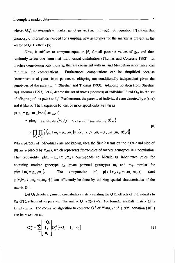
Let Qi denote a gametic contribution matrix relating the QTL effects of individual i to
the QTL effects of its parents. The matrix Qj is 2(i-l)x2. For founder animals, matrix Qi is
simply zero. The recursive algorithm to compute G"1 of Wang et al. (1995, equation [18] )
can be rewritten as,
G? =L l2 Dj-'t-Qi' I2 0,] [9] 0,

16 Chapter 2
where D~' = (C; -Q j 'G^Qj) ' 1 (which reduces to D~' = (lf -Q , 'Q , ) ' with no inbreeding),
Oj is a 2(q-i)x2 null matrix. The off-diagonals in Ci equal the inbreeding coefficient at the
marked QTL (see Wang et al. 1995). Equation [8] shows the similarity to Henderson's rules
for A"1 (Henderson 1976). The nonzero elements of G~' pertaining to an animal arise from its
own contribution plus those of its offspring. So, when sampling the Ith animal's marker
genotype, only those contribution matrices need to be considered that contain elements
pertaining to animal i. These are the individual's own contributions and those of its progeny
when i appears as a parent.
( v ' G - ' v ) . ^ 1 -Qi '
Dil-Qi' I2 Ojv + X I v ' jeS, lsOM
D : ' [ - Q ; I2 Ojjv
=k -QX -QfvjDr'h -Q,svs -QfvJ
+SE[v,-Q;vi-Qjvj]Dr1[v,-Qivi-Q;vJ] *sS, kO, j
[10]
where, Vk is the vector of animal k's two marked QTL effects, andQ£ denotes the rows of Qk
pertaining to P, one of fc's parents. Again, we recognize each term in the sum is the kernel of a
(bivariate) normal which are p{v i lv , ,v d ,m i ,m, ,m d , r}orp{v 1 lv i ,v j ,m i ,m j )m 1 , r} .
Running the Gibbs Sampling
The Gibbs sampler is used to obtain a sample of a parameter from the posterior
distribution and can be seen as a chained data augmentation algorithm (Tanner 1993). So,
one augments data (y and niobs) with parameters (0) to obtain, for example, p(Q\ I 02 , . . . ,
0d , y). For the purpose of breeding value estimation, Gibbs sampling works as follows:
1) Set arbitrary initial values for 0[O], we use zeros for fixed and genetic effects and
for each unmarked animal, we augment a genotype that is consistent with
pedigree, Mendelian inheritance, and observed marker data.
2) Sample 0|t+1! from
[3], i =1,2,..,p; for fixed effects,
[4], i =p+l,p+2,..,p+q; for polygenic effects,
[5], i =p+q+l,p+q+2,..,p+q+2q; for marked QTL effects, or
[6], i =p+3q+l,p+3q+2,..,p+3q+t; for marker genotypes,

Incomplete marker data- 17
and replace e[Tl with 6|T+11.
3) repeat 2) N (length of chain) times.
For any individual parameter, the collection of n values can be viewed as a simulated
sample from the appropriate marginal distribution. This sample can be used to calculate a
marginal posterior mean or to estimate the marginal posterior distribution. For small
pedigrees with only a few animals missing observed marker genotypes, posterior means can
be evaluated directly using
E(Q'\ol,ol,olmobs,r,y) = £ E ( 8 * I G ( k ) , c r » ^ y ) x p(G(k)lmobs,r,y) [11]
where 6* is a fixed, polygenic or marked QTL effect.. This provides a criterion to compare
the estimates obtained from Gibbs sampling.
Pedigree of Numerical Example
Sire (01) y = . . . gm = AB
1 FS (03,04,05) y = + 20 gm = BC
Animal 09 y = +20
Dam (02) y = . . .
Animal 10 y = -20 Sm =
| FS (06,07,08) y = -20 gm = AD
Figure 2: Pedigree of numerical example. Two parents, sire 01 and dam 02, have eight offspring. The sire and dam have observed marker genotypes, AB and CD, respectively, but do not have phenotypes observed. Three full sibs (FS 03,04,05) have marker genotype BC and phenotype +20; three other full sibs (FS 06, 07, 08) have marker genotype AD and phenotype - 20. Animals 09 and 10 have no marker genotypes but have phenotypes + 20 and -20, respectively.

18 Chapter 2
NUMERICAL EXAMPLE
A small numerical example is used to verify the use of the Gibbs sampler to obtain
posterior mean estimates and illustrate the effect of the data on the estimates obtained from
two different estimators, i.e., a posterior mean and the well-known BLUP estimator (by
solving the MME given in Appendix). Pedigree and data of the example are in Figure 2. Both
sire (01) and dam (02) have observed marker genotypes, AB and CD, respectively, but do not
have phenotypes observed.
Three full sibs have a marker genotype BC and a phenotype +20 (denoted FS
03,04,05); three other full sibs have a marker genotype AD and a phenotype - 20 (denoted FS
06, 07, 08). Both animals 09 and 10 have no marker genotypes but have a phenotype + 20
and -20, respectively. Complete knowledge was assumed on variance components and
recombination rate between marker and MQTL (Table 1). The thinning factor in Gibbs
sampling chain was 50 cycles and the burn in period was twice the thinning factor, and 20000
thinned samples were used for analysis.
Table 1 : Population genetic parameters, used in numerical example.
Parameter Value Phenotypic variance 1000 Polygenic variance 300 Marked quantitative trait locus variance 50 Recombination rate 0.05
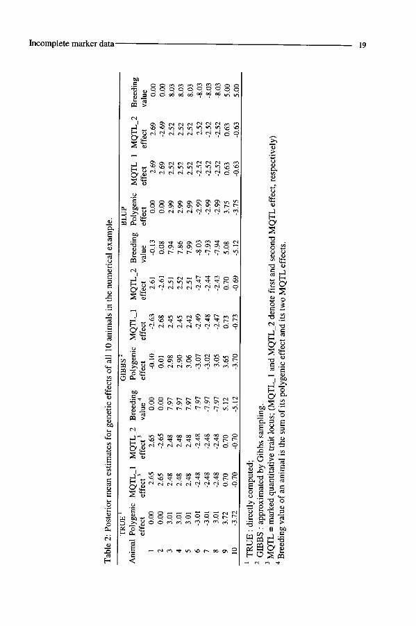
Estimates for genetic effects. The posterior estimates obtained from Gibbs sampling
were similar to the TRUE posterior estimates, as shown in Table 2. The posterior estimates
of MQTL effects of animals 09 and 10 (± 0.70) were much less divergent than those of their
full sibs that had their marker genotypes observed (± 2.48). These less divergent values
reflect the uncertainty on marker genotypes of animals 09 and 10. The TRUE and GIBBS
posterior densities for an MQTL effect of animal 09 were also very similar (Figure 3). The
posterior variance was 52.3, which was larger than the prior variance (CTJ =50) and reveals the
data are not decreasing the prior uncertainty on MQTL effects for animals 09 and 10 in this
situation.
Incomplete marker data- 19
o
o o.
X> c3
H
p o o o o P P P p p
03 >
H u
& S J « r i ( N i M r i « M c j d Q
o 'E <u
CL, bfl — D >> « J o & 03 CL, OJ
M
0 0 0 \ O v O \ î î î i n | T
3 o ö M ^ \o o 2 « 3 o o\ oo a\ v °^ °^ o —:
i/i "? CQ
f—1 ^ ^n *0 i ~
H _ rsi (N c4 ^ ™ ^
H u
c u m S u m -s <Ä
O _ o o Cr ^ ^
ró f ?
M
T3
m
I
O O O o
3 O Ö
r - t - t - , t - r - c - csi CN
H . , >/->''_' o o o o o o 0 ° c o o o 0 o
^ V I M O O M ^ M M Q O *_. ^ ^O
o o o P P P t - - ^
- N m ^ V ) ^ h o o ! > ^
_ w D DS H
M o o
8>« =? p .•? O ° ° o fc
OH O
T3
§ id o o c/> H-H
-o C
U
H o
ü o
g ü
1 c
S fc -a u
=< S I b û
E - 1 S * - < C A
bO i=
I'S o c o .£ >-. X
• 3 O
• S &
•3 ^
.'S <u ni J 3
'•3 'S C ei
H a
•a o
tH 3
e ed >
II gp J ^
S PQ
20 Chapter 2
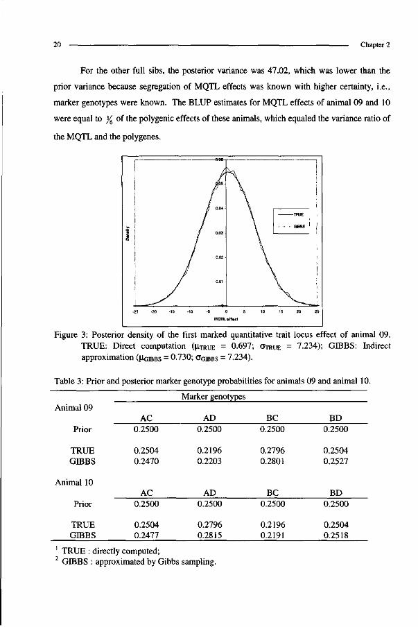
For the other full sibs, the posterior variance was 47.02, which was lower than the
prior variance because segregation of MQTL effects was known with higher certainty, i.e.,
marker genotypes were known. The BLUP estimates for MQTL effects of animal 09 and 10
were equal to /6 of the polygenic effects of these animals, which equaled the variance ratio of
the MQTL and the polygenes.
Figure 3: Posterior density of the first marked quantitative trait locus effect of animal 09. TRUE: Direct computation (u.TRUE = 0.697; OTRUE = 7.234); GIBBS: Indirect approximation (UGIBBS = °-730; OGIBBS = 7.234).
Table 3: Prior and posterior marker genotype probabilities for animals 09 and animal 10.
Animal 09
Prior
TRUE GIBBS
Animal 10
Prior
TRUE GIBBS
AC 0.2500
0.2504 0.2470
AC 0.2500
0.2504 0.2477
Marker genotypes
AD 0.2500
0.2196 0.2203
AD 0.2500
0.2796 0.2815
BC 0.2500
0.2796 0.2801
BC 0.2500
0.2196 0.2191
BD 0.2500
0.2504 0.2527
BD 0.2500
0.2504 0.2518
TRUE : directly computed; GIBBS : approximated by Gibbs sampling.

Incomplete marker data 21
Marker genotype probabilities. In the following marker genotype AB represents both
AB and BA. In the latter case, alleles for both marker and MQTL are reordered, maintaining
linkage between marker and MQTL alleles within an animal. So, 4 marker genotypes were
possible for animals 09 and 10 (Table 3). Based on pedigree and marker data solely, each of
these 4 genotypes was equally likely (prior probability = 0.25). After including phenotypic
data, (posterior) probabilities changed: marker genotype BC and AD for animal 09 became
more and less probable, respectively. The reverse was true for animal 10. The estimates from
the Gibbs sampler were very similar to the TRUE posterior probabilities. Complete
phenotypic and marker information on 6 full sibs gave the MQTL effects linked to marker
alleles B and C positive values and marker alleles A and D negative values. Note that
probabilities (TRUE) for marker genotypes AC and BD also (slightly) changed after
considering the phenotypic data.
DISCUSSION
Marker-assisted breeding value estimation in livestock has been hampered by
incomplete marker data. Previously described methods (Fernando and Grossman 1989; Van
Arendonk et al. 1994; and Wang et al. 1995) can accommodate ungenotyped individuals that
do not have offspring themselves as was shown by Hoeschele (1993). However, they do not
provide the flexibility to incorporate parents with unknown genotypes, which results in the
loss of information for estimating marker-linked QTL effects. The described Gibbs sampling
algorithm now provides this required flexibility. The innovative step in our approach is the
sampling of genotypes for a marker locus that is closely linked to QTL with normally
distributed allelic effects. Normality of QTL effects is a robust assumption to allow
segregation of many alleles throughout a population and allow changes in allelic effects over
generations, e g, due to mutations and interactions with environments (Jansen 1996). In
sampling missing genotypes information from marker genotypes as well as phenotypes of
animals in the pedigree are used. Jansen et al. (1998) indicate that, as a result of the use of
phenotypic information, unbiased estimates of effects at the QTL can be obtained in situations
where animals have been selectively genotyped.

22 Chapter 2
In this paper we have concentrated on the use of information from a single marker
locus. Using information from multiple linked markers can increase accuracy of predicting
genetic effects at the QTL. The principles applied here have been extended to situations
where genotypes for all the linked markers are known for all individuals (Goddard 1992;
Uimari et al. 1996). In order to incorporate individuals with unknown genotypes, the method
presented in this paper needs to be extended to a multiple marker situation. In extending the
method to multiple markers, the problem of reducibility deserves special attention.
Reducibility of Gibbs chains can arise when sampling genotypes for a locus with more than
two alleles (Thomas and Cortessis 1992). The reducibility problems will become more
severe when sampling genotypes for multiple linked markers. Thompson (1994) suggested
several, workable, approaches to guarantee irreducibility of the Gibbs chain. These
approaches make use of Metropolis-coupled samplers (Lin 1993), importance sampling, with
0/1 weights (Sheehan and Thomas 1993), and "heating" in the Metropolis- Hastings steps
(Lin et al. 1993). Alternatively, Jansen et al. (1998) sampled IBD values for all marker loci
indicating parental origin of alleles instead of actual alleles to avoid the reducibility problem.
In extending the method to multiple linked markers, attention also needs to be paid to an
efficient scheme for updating haplotypes or genotypes at the linked loci. Updating of
genotypes at closely linked loci will be more efficient when genotypes at the linked loci are
updated together ('in blocks') in order to reduce auto-correlation in the Gibbs sampler (Janss
etal. 1995).
For posterior inferences on the breeding value of an animal a minimum of 100 effective
samples may suffice (Uimari et al. 1996). In the numerical example this minimum would
correspond to a chain of 5000 cycles which required 8 seconds of CPU at a HP9000 K260
server. It has been found that computing requirements increase more or less linearly with the
number of animals (Janss et al. 1995). The presented method can be applied to data originating
from nucleus populations which comprises the relatively small number of genetically superior
animals from the population. In a marker assisted selection scheme marker genotypes will be
collected largely on these animals. Straightforward application in large commercial populations
with thousands of marker genotypes missing, is not a valid option because of computational
requirements of Markov chain Monte Carlo (MCMC) algorithms like Gibbs sampling. Hybrid
schemes will need to be developed to incorporate information from the commercial population
into the marker-assisted prediction of breeding values of nucleus animals. Similar schemes
Incomplete marker data 23
have been implemented to incorporate foreign information into national evaluations in dairy
cattle.
Our Bayesian approach can also be considered as a first step towards a MCMC
algorithm, not necessarily Gibbs sampling, that can estimate dispersion parameters, which were
held constant in this study. The next step, therefore, comprises estimation of variance
components, both marked QTL and polygenic, given a fixed map position of the QTL. And,
eventually, one could estimate the most likely position of the QTL within a linkage map
containing multiple markers. The complete MCMC algorithm can then be used for the analysis
QTL mapping experiments in outbred populations with complex pedigree structures.
ACKNOWLEDGMENT
Valuable suggestions by S. van der Beek and anonymous reviewers are gratefully
acknowledged. The financial support of Holland Genetics is highly appreciated.
REFERENCES
Fernando RL, Grossman M (1989) Marker-assisted selection using best linear unbiased prediction. Genet Sel Evol 21:467-477
Gelfand AE, Smith AFM (1990) Sampling-based approaches to calculating marginal densities. J Am Stat Assoc 85:398-409
Geman S, Geman D (1984) Stochastic relaxation, Gibbs distributions and the Bayesian restoration of images. IEEE Trans Pattern Anal Machine Intelligence 6:721-741
Geyer CJ (1992) A practical guide to Markov chain Monte Carlo. Stat Sei 72:320-339
Goddard ME (1992) A mixed model for analysis of data on multiple genetic markers. Theor Appl Genet 83:878-886
Henderson CR (1976) A simple method for computing the inverse of a numerator relationship matrix used in prediction of breeding values. Biometrics 32:69-83
Hoeschele I (1993) Elimination of quantitative trait loci equations in an animal model incorporating genetic marker data. J Dairy Sei 76:1693-1713
Jansen RC (1996) Complex plant traits: time for polygenic analysis. Trends Plant Sei. 3:73-103
Jansen RC, Johnson DL, Van Arendonk JAM (1998) A mixture model approach to the mapping if quantitative trait loci in complex populations with an application to multiple cattle families. Genetics 148:391-399
Janss LLG, Thompson R, Van Arendonk JAM (1995) Application of Gibbs sampling for inference in a mixed major gene-polygenic inheritance model in animal populations. Theor Appl Genet 91:1137-1147
Lin S (1993) Markov chain Monte Carlo estimates of probabilities on complex structures. PhD dissertation, University of Washington
24 Chapter 2
Lin S, Thompson EA, Wijsman E (1993) Achieving irreducibility of the Markov chain Monte Carlo method applied to pedigree data. IMA J Math Appl Med Biol 10:1-17
Meuwissen THE, VanArendonk JAM (1992) Potential improvements in rate of genetic gain from marker-assisted selection in dairy cattle breeding schemes. J Dairy Sei 75:1651-1659
Schaeffer LR, Kennedy BW (1986) Computing strategies for solving mixed model equations. J Dairy Sei 69:575-579
Sheehan N, Thomas A (1993) On the irreducibility of a Markov chain defined on a space of genotype configurations by a sampling scheme. Biometrics 49:163-175
Smith C, Simpson SP (1986) The use of genetic polymorphisms in livestock improvement. J Anim Breed Genet 103:205-217
Soller M, Beckmann JS (1982) Restricted fragment length polymorphisms and genetic improvement. Proc 2nd
World Congress Genet Appl Livest Prod, Madrid, Editorial Garsi, Madrid, vol 6:396-404
Sorensen DA, Wang CS, Jensen J, Gianola D (1994) Bayesian analysis of genetic change due to selection using Gibbs sampling. Genet Sel Evol 26:333-360
Tanner MA (1993) Tools for Statistical Inference. Springer-Verlag, New York, NY
Thomas DC, Cortessis V (1992) A Gibbs sampling approach to linkage analysis. Hum Hered 42:63-76
Thompson EA (1994) Monte Carlo likelihood in genetic mapping. Stat Sei 9:355-366
Uimari P, Thaller G, Hoeschele I (1996) The use of multiple markers in a Bayesian method for mapping quantitative trait loci. Genetics 143:1831-1842
VanArendonk JAM, Tier B, Kinghorn BP (1994) Use of multiple genetic markers in prediction of breeding values. Genetics 137:319-329
VanTassell CP, Casella G, Pollak EJ (1995) Effects of selection on estimates of variance components using Gibbs sampling and restricted maximum likelihood. J Dairy Sei 78:678-692
Wang CS, Rutledge JJ, Gianola D (1993) Marginal inferences about variance components in a mixed linear model using Gibbs sampling. Genet Sel Evol 25:41-62
Wang T, Fernando RL, VanderBeek S, Grossman M, Van Arendonk JAM (1995) Covariance between relatives for a marked quantitative trait locus. Genet Sel Evol 27:251-272

Incomplete marker data- 25
APPENDIX
Computation of average G with incomplete marker data. Wang et al. (1995) suggested computing an average G, here denoted G , as
G = Z,GwxP{mm\mohs) m d ) = '
where G<k) is the gametic relationship matrix given a particular marker genotype configuration m^; and p(ni(k) Imobs) is the probability of m^) given mobs- This equation is not conditioned on phenotypic information.
Marker-assisted Best Linear Unbiased Prediction of Breeding Values. Mixed model equations (MME) to obtain BLUE for fixed effects and BLUP for random effects are,
XX
Z'X
W'X
X'Z
Z'Z + A-'a,,
W'Z
X'W
Z'W
W'W + G-'a
F û
V
= "X'y"
zy W y
2 / 2 / where, a = "/ i , a = '/ 2 and G are all known. Solutions can be obtained by iteration
on the data (Schaeffer and Kennedy 1986). These equations can be used in three situations. First, G is unique (complete marker data). Second, with missing markers, a linear estimator is obtained by taking G = G. Third, with G = G(k), they are used to compute E ( 0 I G ( k ) , a » e
2 , y ) .

Chapter 3
Bayesian Estimation of Dispersion Parameters with a Reduced
Animal Model including Polygenic and QTL effects
Marco C. A. M. Bink', Richard L. Quaas and Johan A. M. van Arendonk
Animal Breeding and Genetics Group, Wageningen Institute of Animal Sciences, Wageningen Agricultural University, PO Box 338,6700 AH Wageningen, The Netherlands
"Department of Animal Science, Cornell University, Ithaca, NY 14853, USA
Published in Genetics Selection Evolution 30:103-125 (1998)
Reproduced by permission of Elsevier/INRA, Paris

Reduced animal model and dispersion parameters 29
ABSTRACT
In animal breeding Markov chain Monte Carlo algorithms are increasingly used to
draw statistical inferences about marginal posterior distributions of parameters in genetic
models. The Gibbs sampling algorithm is most commonly used and requires full conditional
densities to be of a standard form. In this study, we describe a Bayesian method for the
statistical mapping of quantitative trait loci (QTL), where the application of a reduced animal
model leads to non-standard densities for dispersion parameters. The Metropolis Hastings
algorithm is used to obtain samples from these non-standard densities. The flexibility of the
Metropolis Hastings algorithm also allows changing the parameterization of the genetic
model. Alternatively to the usual variance components, we use one variance component
(^residual) and two ratios of variance components, i.e., heritability and proportion of genetic
variance due to the QTL, to parameterize the genetic model. Prior knowledge on ratios can
more easily be implemented, partly by absence of scale effects. Three sets of simulated data
are used to study performance of the reduced animal model, parameterization of the genetic
model, and testing the presence of the QTL at a fixed position.
INTRODUCTION
The wide availability of high-speed computing and the advent of methods based on
Monte Carlo simulation, particularly those using Markov chain algorithms, have opened
powerful pathways to tackle complicated tasks in (Bayesian) statistics (Gelfand and Smith
1990: Gelfand 1994). Markov chain Monte Carlo (MCMC) methods provide means for
obtaining marginal distributions from a complex non-standard joint density of all unknown
parameters (which is not feasible analytically). There are a variety of techniques for
implementation (Gelfand 1994) of which Gibbs sampling (Geman and Geman 1984) is most
commonly used in animal breeding. The applications include univariate models, threshold
models, multi-trait analysis, segregation analysis and QTL mapping (Wang et al. 1993; Wang
et al 1997; Van Tassell and VanVleck 1996; Janss et al 1995; Hoeschele 1994).
Because Gibbs sampling requires direct sampling from full conditional distributions,
data augmentation (Tanner and Wong 1987) is often used so that 'standard' sampling densities
are obtained. Often, however, this is at the expense of a substantial increase in number of
30 Chapter 3
parameters to be sampled. For example, the full conditional density for a genetic variance
component becomes standard (Inverted Gamma distribution) when a genetic effect is sampled
for each animal in the pedigree, as in a (Full) Animal Model (FAM). The dimensionality
increases even more rapidly when the FAM is applied to the analysis of granddaughter
designs (Weiler et al. 1990) in QTL mapping experiments, i.e., marker genotypes on
granddaughters are not known and need to be sampled as well. In addition, absence of
marker data hampers accurate estimation of genetic effects within granddaughters, which
form the majority in a granddaughter design. This might lead to very slow mixing properties
of the dispersion parameters (see also Sorensen et al. 1995).
The reduced animal model (RAM, Quaas and Pollak 1980) is equivalent to the FAM,
but can greatly reduce the dimensionality of a problem by eliminating effects of animals with
no descendants. With a RAM, however, full conditional densities for dispersion parameters
are not standard. Intuitively, RAM, used to eliminate genetic effects and concentrate
information, is the antithesis of data augmentation, used to arrive at simple standard densities.
For the Metropolis-Hastings (MH) algorithm (Metropolis et al. 1953, Hastings 1970),
however, a standard density is not required, in fact, the sampling density needs to be known
only up to proportionality. Another alternative for the FAM is the application of a sire model
which implies that only sires are evaluated based on progeny records. With a sire model, the
genetic merit of the dam of progeny is not accounted for and only the phenotypic information
on offspring is used. The RAM offers the opportunity to include maternal relationships,
offspring with known marker genotypes and information on grand-offspring. As a result the
RAM is better suited for the analysis of data with a complex pedigree structure.
The flexibility of the MH algorithm also allows for a greater choice of the
parameterization (variance components or ratios thereof) of the genetic model. If Gibbs
sampling is to be employed, the parameterization is often dictated by mathematical
tractability - to get the simple sampling density. The MH algorithm readily admits much
flexibility in modeling prior belief regarding dispersion parameters which is an advantageous
property in Bayesian analysis (e.g., Hoeschele and VanRaden 1993).
In this paper, we present MCMC algorithms that allow Bayesian linkage analysis with
a RAM. We study two alternative parameterizations of the genetic model and use a test
statistic to postulate presence of a QTL at a fixed position relative to an informative marker
bracket. Three sets of simulation data using a typical granddaughter design are used.

Reduced animal model and dispersion parameters 31
METHOD
Genetic Model
The additive genetic variance ( o\ ) underlying a quantitative trait is assumed to be due
to two independent random effects, due to a putative QTL and residual independent
polygenes. The QTL effects (v) are assumed to have a N(0,Gal) prior distribution where G
is the gametic relationship matrix (e.g., Fernando and Grossman 1989, Bink et al. 1998a), and
rjj is the variance due to a single allelic effect at the QTL. Matrix G depends upon one
unknown parameter, the map position of the QTL relative to the (known) positions of
bracketing (informative) markers. Here we consider the location of the QTL to be known.
The polygenic effects (u) have a N(0,\a2u) prior distribution, where A is the numerator
relationship matrix. The genetic model underlying the phenotype of an animal is
yj = xlb + ui +Vj' +vf+ej,
where Xj is an incidence vector relating fixed effects to yu b is the vector with fixed effects, vj
and vf are the two (allelic) QTL effects for animal i, and e; ~ N(Q,\a2t). (QTL effects within
individual are assigned according to marker alleles, as proposed by Wang et al. 1995). The
sum of the three genetic effects is the animal's breeding value (a). In addition to genetic
effects, location parameters comprise fixed effects that are, a priori, assumed to follow the
proper uniform distribution: f(b) ~ u l b ^ . b ^ J , where bmin and bmax are the minimum and
maximum values for elements in b.
Reduced Animal Model (RAM)
The RAM is used to reduce the number of location parameters that need to be
sampled. The RAM eliminates the need to sample genetic effects of animals with no
descendants nor marker genotypes, i.e., ungenotyped non-parents. The phenotypic
information on these animals can easily be absorbed into their parents without loss of
information. Absorption of non-parents that have marker genotypes becomes more complex
when position of QTL is unknown; it is therefore better to include them explicitly in the
analysis. In the remainder of the paper, it is assumed that marker genotypes on non-parents
are not available. The genetic effects of non-parents can be expressed as linear functions of
the parental genetic effects by the following equations (Cantet and Smith 1991),

32 Chapter 3
Unon-parents = "parentsUparents "•" Pnon-parents H J
and
V non-parents = ViparentsVparents "" Ynon-parcnts L^J
where each row in P contains at most 2 non-zero elements, (= 0.5), and each row in Q has at
most 4 non-zero elements (Wang et al. 1995), the terms (pnon-parems and <)>non-parents pertain to
remaining genetic variance due to Mendelian segregation of alleles. In a granddaughter
design, the P and Q for granddaughters, not having marker genotypes observed nor
augmented, have similar structures,
Q = P®iJ 2 x 2 , [3]
where <8> denotes the Kronecker product, and J is a unity matrix (Searle 1982). This equality
does not hold if marker genotypes are augmented, since phenotypes contain information that
can alter the marker genotype probabilities for ungenotyped non-parents (Bink et al. 1998a).
The phenotype for a quantitative trait can now be expressed as,
y, =x jb + Piu + Qiv + ei [4]
for row vectors P; and Qj (possibly null), and
ol=c2e+(ui(a
2u+2ü2
v), [5]
where C0i reflects the amount of total additive genetic variance that is present in a2 . Based on
the pedigree, four categories of animals are distinguished in the RAM (Table 1). The vectors
Pi and Qj contain partial regression coefficients. For parents, the only nonzero coefficients
pertain to the individual's own genetic effects (ones); for non-parents, the individual's
parents' genetic effects (halves). Note that Pj and Qi are null for a non-parent with unknown
parents, and that non-parents' phenotypes in this category contribute to the estimation of fixed
effects and phenotypic (residual) variance only.
Table 1 : Categories of animals in a reduced animal model and values for C0j for each category.
Category No. of parents known cas '
1 non-parent 0 1 2 non-parent 1 % 3 non-parent 2 /2
_4 parent ^ 0 1 without inbreeding 2 not relevant

Reduced animal model and dispersion parameters 33
Parameterization
Let 0 denote the set of location parameters (b, u, and v) and dispersion parameters.
We consider the following two parameterizations for the dispersion parameters,
0vc : b, u, v, a], o], and cs]
eRT : b, u, v, a), h2, and y
where
h2=^for , a " + , 2 ° v , .with 0< h2<\, [6]
and
Y = - f o r ; wi thO<y<l. [7] °a Ou+20v
In the first, 0yc, the parameters are the variance components (VC). This is the usual
parameterization. A difficulty with this is that it is problematic for an animal breeder to elicit
a reasonable prior of the genetic VC. Animal breeders, it seems to us, are much more likely
to have, and be able to state, prior opinions about such things as heritabilities. Consequently,
in 0RT, parameter h2 is the heritability of a trait, and parameter y is the proportion of additive
genetic variance due to the putative QTL. This parameterization allows more flexible
modeling of prior knowledge because h2 and y do not depend on scale. Theobald et al. (1997)
used a variance ratio, G 2 / a 2 , parameterization but noted that the animal breeder may prefer
to think in terms of heritability. We prefer the part-whole ratios h2 and y. The components
a\ and a j can be expressed in terms of a2e, h
2 and y
(1-AZ) o ' = a - Y ) T 7 ^ T I 7 0 , 2 ' a n d [8]
h2 2 / c- -> " 2
O-fc2) < = C 5 x y ) T — — a t . [9]
Priors
We now present the prior knowledge on dispersion parameters, priors for location
parameters have been given earlier. In earlier studies, two different priors are often used to
describe uncertainty on VC. The inverted gamma (IG) distribution, or its special case the
inverted chi-square distribution, is common because it is often the conjugate prior for the VC
if the FAM (or sire model) is applied. Hence, the full conditional distribution for VC will

34 Chapter 3
then be a "posterior" updating of a standard prior (Gelfand 1994). This simplifies Gibbs
sampling. We will use the IG as the prior for ax - though with a RAM it is not conjugate,
f ^ l c ^ ß j o c ^ - ' e x p J_J_ [10]
where x = e, u, or v. The rhs of [10] constitute the kernel of the distribution. The mean (\i) of
an IG(a,ß) is ((a-l)ß)~' , and the variance equals ((oc-l)2(a-2)ß2)"'. Van Tassell et al.
(1995) suggests setting a = 2.000001 and ß = (fi)"1 for an 'almost flat' prior with a mean
corresponding to prior expectation (u,). The IG distributions for three different prior
expectations are given in Figure 1.
\ E[ IG(<J*) ] = 5
11(0,200)
80
Figure 1: Inverted Gamma and Uniform densities that are used to represent (lack of) prior knowledge on variance components.
When the prior expectation is close to zero (|A = 5.0), the distribution is more peaked and has
less variance because mass accumulates near zero. When the prior expectation is relatively
high (\i = 60), the probability of a2 being equal to zero is very small, which might be
undesirable and/or unrealistic for o 2 . An alternative prior distribution for a2 is
f(°i)< k 0 < a ; < a 2
x.max [11]
10 otherwise
which is a proper prior for a2 with a uniform density over a pre-defined large, finite interval,
for example from zero to 200 (Figure 1). These prior distributions for VC are used mainly to

Reduced animal model and dispersion parameters 35
represent prior uncertainty (e.g., Wang et al. 1993, Van Tassell et al. 1995, Sorensen et al.
1995).
Corresponding to [10] ([11]) there is an equivalent prior distribution for h2 (and y).
However, because neither [10] nor [11] were chosen for any intrinsic "rightness" we prefer a
simpler alternative of using Beta distributions for the ratio parameters h2 and y to represent
prior knowledge,
f(x|ax,ßJoc(xr"-'(l-xr--' [12]
where x = h2 or y. When prior distribution parameters ocx and ßx are both set equal to 1, the
prior is a uniform density between 0 and 1 (Figure 2), i.e., flat prior. Alternatively, a* and ßx
can be specified to represent prior expectations for parameter of interest. For example, center
the density for heritability of a yield trait in dairy cattle around the prior expectation (=0.40),
with a relatively flat (Beta (2.5, 3.75) ) or peaked (Beta (30.0, 45.0) ) distribution when prior
certainty is moderate or strong, respectively. Furthermore, prior knowledge on y, proportion
of additive genetic variance due to a putative QTL, can be modeled to give relatively high
probabilities of values close to zero, e.g., (Beta(0.9, 2.7). Another option, suggested by a
reviewer, would be to put vague priors on ctx and ßx as in Berger (1985).
8
Beta(1,1)
0.0 0.1 0.2 0.3 0.9 1.0
Figure 2: Beta densities that are used to represent (lack of) prior knowledge on (part whole) ratios of variance components.
36 Chapter 3
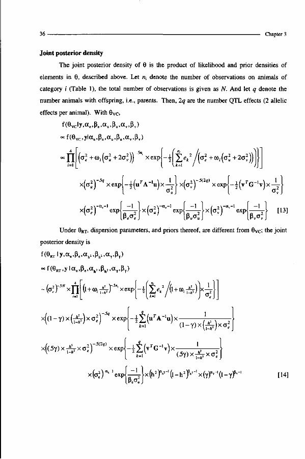
Joint posterior density
The joint posterior density of 0 is the product of likelihood and prior densities of
elements in 6, described above. Let n\ denote the number of observations on animals of
category i (Table 1), the total number of observations is given as N. And let q denote the
number animals with offspring, i.e., parents. Then, 2q are the number QTL effects (2 allelic
effects per animal). With 8Vc.
f ( 9 v c l y . « e ' ß e . « u . ß U . « v . ß v )
ocf(evc ,ylae ,ßc ,au ,ßu ,av ,ßv)
n (o.1 + co,(a> +2oî))- * x e x p j - l ^ 2 / ^ +co,(c> + 2a>))j
x(oiy* xexpj-l^A-uJx-Lj x(a^5<2î) xexpj-^G-'vJx-L}
^^Aû}*^ tl3]
Under 0RT, dispersion parameters, and priors thereof, are different from 6vc; the joint
posterior density is
f(eRTly,ac,ße,ah2,ßh2,a rßT)
°=f(eRT)ylae,ße,ah2,ßh2,arßY)
^^xeJ-tâeï & + »,£) ~&rNxn
xfd-^x^Jxa^^xexp -^(urA-'u)x-( ! - ^ x t e ) x a e
x N ^ x ^ P ' xexJ-it(YrG-'T)x- l 1 [ k=\ '
(5y)x^xa2e
*te^^f?\*b2T*^-*1J*Myr(i-yr- [14]

Reduced animal model and dispersion parameters 37
Full Conditional Densities
From the joint posterior densities [13] and [14], the full conditional density for each
element in 8 can be derived by treating all other elements in 0 as constants and selecting the
terms involving the parameter of interest. When this leads to the kernel of a standard density,
e.g., Normal for location parameters or an IG distribution, e.g., variance components with
FAM, Gibbs sampling is applied to draw samples for that element in 8. Otherwise, the full
conditional density is non-standard and sampling needs to be done by other techniques. (All
full conditional densities are given in the Appendix).
Sampling non-standard densities by Metropolis-Hastings algorithm
Sampling a non-standard density can be done a variety of ways, including various
rejection sampling techniques (Devroye 1986, Gilks and Wild 1992, Chib and Greenberg
1995, Gilks et al. 1995), and Metropolis-Hastings sampling within Gibbs sampling (Chib and
Greenberg 1995). We use the Metropolis-Hastings algorithm (MH). Let TT(X) denote the
target density, the non-standard density of a particular element in 8, and let <?(x,y) be the
candidate generating density. Then, the probability of move from current value x to
candidate value y for 6j is,
[l otherwise.
When y is not accepted, the value for 8j remains equal to x, at least until the next update for
8i. Chib and Greenberg (1995) described several candidate generating densities for MH. We
use the random walk approach in which candidate y is drawn from a distribution centered
around the current value x. To ensure that all sampled parameters are within the parameter
space the sampling distribution, q(x,y), was U(BL, By) with
BL =max(0,x-f) for a2,a2u,a
2,h2, y
„2 „2 „2 i x f I. 11)1 I
B U - 1 • /, . , A - . 2 x + t for o2,a2
u, a;
lmin(l,x + f) for h ,y
where t is a positive constant determined empirically for each parameter to give acceptance
rates between 25 and 50 %, (Tierney 1994; Chib and Greenberg 1995). For each of the non
standard densities, an univariate MH was used. We perform univariate MH iterations (10
times) within a MCMC cycle to enhance mixing in the MCMC chain, as suggested by Uimari
etal. (1996).

38 Chapter 3
Comparison to a Full Animal Model (FAM)
From the conditional densities presented, two hybrid MCMC chains can be used to
obtain samples of all unknown parameters (9vc or 6RT) using a RAM. For comparison, the
equivalent FAM can be used with similar parameterization (0vc and 8RT)- The conditional
densities for the FAM are a special case of RAM (see Table 1): all animals are in category 4
and co, = 0. In case of 9yc the conditional densities for G\,G\, and CTJ are now recognizable
IG distributions and Gibbs sampling can be used to draw samples from these densities
directly. In case of 9RT the conditional densities for h2 and y remain non-standard and MH is
used to draw samples. Table 2 gives the four constructed MCMC sampling schemes.
Table 2: Sampling algorithms for location and dispersion parameters for alternative models (RAM versus FAM) and parameterizations (0Vc versus 0RT).
RAM 8 vc 9 RT
FAM 9yç 9RT
ß u V
GS GS GS
GS GS GS
GS GS GS
GS GS GS
h
y
MH
MH
MH
GS
MH
MH
GS
GS
GS
GS
MH
MH
GS = Gibbs sampling 2 MH = Metropolis Hastings algorithm
Post MCMC Analysis
Depending on the dispersion parameterization (9vc or 0RT), three out of five
parameters were sampled (Table 2). In each MCMC cycle, however, the remaining two were
computed, using [6] and [7] or [8] and [9], to allow comparison of results of different
parameterizations. For parameter X, the auto-correlation of a sequence of samples was
m-I
calculated as ^^[ (JC,- -&-x\xM - ji^)]/*2 where m = number of samples, p.x and sx are
posterior mean and standard deviation, respectively. The correlation among samples for

Reduced animal model and dispersion parameters 39
m
parameters x and z, within MCMC cycles, were computed as^-^[(jt,. — p-^Xz, - M - Z ) ] / [ M Z ] -
For each parameter an effective sample size (ESS) was computed which estimates the number
of independent samples with information content equal to that of the dependent samples
(Sorensen et al. 1995).
The null hypothesis that y = 0 - the QTL explains no genetic variance - was tested via
mode{p(y)j an odds ratio ;—=—T-^->20 following Janss et al. (1995). They suggest that this
MY = °) criterion, however, may be quite stringent. The 90 % Highest Posterior Density regions
(HPD90) (e.g., Casella and George 1990), were also computed for parameter y.
SIMULATION
In this study, granddaughter designs were generated by Monte Carlo simulation. The
unrelated grandsire families each contained 40 sires that were half sibs. The number of
families was 20 except in simulation HI where designs with 50 families were simulated as
well (Table 3). Polygenic and QTL effects for grandsires, were sampled from N (0 ,G*) and
N(0,O"J), respectively. The polygenic effect for sires was simulated as u^ = y(uGS)+<|>,
where UGS is the grandsire's polygenic effect, and <|), Mendelian sampling, is distributed
independently as N (0,Var(<|>)) with Var(<|>) = .75 x GJ (no inbreeding). The sires inherited
one QTL at random from its (grand) sire. The maternally inherited QTL effect for a sire was
drawn from N (0,aj). Each sire had 100 daughters with phenotypes observed, that were
generated as
y - w{.5usirc + pvjirc + ( l -p)v 2r e , .750-;; + G2 + G2},
where p is a 0/1 variable. In all simulations the phenotypic variance and the heritability of the
trait were 100 and 0.40, respectively. The proportion of genetic variance due to the QTL (= y)
was by default 0.25, or 0.10 in simulation HI (Table 3). Two genetic markers bracketing the
QTL position at lOcM (Haldane mapping function), were simulated with 5 alleles at each
marker, with equal frequencies over alleles per marker. For grandsires, the marker genotypes
were fully informative, i.e., heterozygous, and the linkage phase between marker alleles is
assumed to be known, a priori. The uncertainty on linkage phase in sires can be included in

40- Chapter 3
8, but we did not. All possible linkage phases within sires were weighted by their probability
of occurrence and one average relationship matrix between grandsires' and sires' QTL effects
was used.
Table 3: Simulation of Granddaughter designs and MCMC chains.
No. grandsires proportion QTL (y) ' No. replicates
Purpose
MCMC chains Length Thinning factor Stored samples
Simulation I 20 0.25 1
Comparison RAM versus FAM
500,000 250
2000
Simulation II 20 0.25 5
Comparison 9vc versus 0RT
250,000 250
1000
Simulation in 20,50 0.10,0.25
25
Hypothesis testing Power for detection
200,000 1000 200
proportion QTL = proportion of additive genetic variance due to the QTL.
RESULTS & DISCUSSION
Simulation I Comparison RAM versus FAM
For each of the four MCMC algorithms that are given in Table 2, a single MCMC
chain run and 2000 thinned samples were used for post-MCMC analysis (Table 3). In case of
9vc, prior distributions for o2e,o
2u,andaj were "flat" IG's (Figure 1) with expected means
equal to 60, 30 and 5 (values used for simulation), respectively. In case of 0RT, prior for a\
was again an IG and priors for h2 and y were Beta(2.5, 3.75) and Beta(0.9, 2.7), respectively.

Reduced animal model and dispersion parameters 41
100000 200000 300000 cycle
400000 500000
12 -J
10 -o g 8 «J
<5 6
ë 4
2
C
lil H W» JW
YTL /*• ™
1 100000
I k H w AA/WI "yvr W V T>
1 ' 200000 300000 cycle
i À ÀMS v ' SjM^ T ' y
' 400000
K* VA 500000
Figure 3: Two-thousand thinned samples for parameter o j , from MH algorithm (RAM, top)
and from Gibbs sampling (FAM, bottom) (Simulation I).
Figure 3 presents the mixing properties for parameter a2v within the chains for the
RAM-0VC and FAM-Gvc alternatives and points to slower mixing when using the FAM. This
slow mixing is also indicated by high auto correlation (=1) among samples for parameters c j
and y when the FAM was used (Table 4). With the same thinning, the auto-correlation among
samples in the RAM is <0.70. The estimates for posterior mean and coefficient of variation,
derived from samples of the four chains, are given in Table 5. These estimates are very
similar over models (RAM and FAM) and parameterizations (0vc and 0RT). The coefficients
of variation for o\ and y are relatively large and indicate that a posteriori knowledge on
these parameters remains small, while estimates for a] and h are accurate.

42 Chapter 3
Table 4: Sampling correlation and effective sample size for alternative models (RAM versus FAM) and parameterizations (9vc versus 6RT) from Simulation I (see Table 3).
9vc °l °l <
0RT
°l h2
Y
RAM
auto
0.07 0.34 0.60
0.05 0.06 0.71
correlation '
°l
-0.47 -0.29
-0.98 -0.19
<
-0.69
0.20
ESS2
1880 856 611
1481 1571 350
FAM correlation auto
0.29 0.61 0.97
0.57 0.59 0.99
<
-0.57 -0.18
-0.99 -0.17
<
-0.67
0.17
ESS
1635 133 62
654 604 29
1 auto-correlation = between subsequent samples for the same parameter; otherwise correlation between samples for different parameters within cycle.
2 ESS = effective sample size.
Table 5: Estimates of posterior mean and standard deviation for dispersion parameters, for alternative models (Reduced AM versus Full AM) and parameterizations (9vc versus 9RT) from Simulation I. (see Table 3).
9vc <
°l Ov
h2
Y ORT
<
< ö2v
h2
J-
RAM mean
62.7 30.5
2.8
0.37 0.16
62.6
30.3 3.0 0.37 0.17
CV
0.03 0.09 0.44
0.05 0.42
0.03
0.11 0.53 0.05 0.54
FAM mean
62.7 30.0
3.1
0.37 0.17
62.3
29.9 3.4 0.37 0.18
CV
0.03
0.09
0.35
0.05 0.34
0.03
0.12 0.51 0.07 0.49
1 Parameters underlined were actually sampled in that parameterization.
Reduced animal model and dispersion parameters 43
The magnitude of the sampling correlation among parameters within MCMC cycles
was very similar for both models and parameterizations. The samples for a2 and a2 showed
a moderately high negative correlation (-0.7), while the sampling correlation between h2 and y
was relatively low and positive (0.2). The correlation among samples for a2 and h2 was very
high but apparently did not adversely affect the auto-correlation of these parameters. Taking
100 ESS as a minimum (Uimari et al. 1996) the MCMC chain was rather short for statistical
inferences for y in FAM-8RT. However, running a longer MCMC chain was not practical
since the FAM-9VC MCMC chain needed 68593 minutes CPU (47 days) on a HP 9000-
735(125Hz) workstation. This was almost 100 times the 11 hours that were needed to run the
RAM with similar chain length.
The slow mixing of parameters for a FAM was likely due to the lack of marker data
on granddaughters. Distinction between polygenic and QTL effects within these animals is
hardly possible. Consequently, they provide little information regarding dispersion but
because they are so numerous they dominate the distribution from which the next sample for
the dispersion parameter is drawn. Heuristically, one first generates u and v with variances
reflecting current a2. Subsequently one samples a new a2 from a peaked distribution with a
mean near the sample variance of the u and v. Not surprisingly one gets back a a2 very
similar to the previous, as a result of which the chain is slowly mixing.
The data from Simulation I was also used to examine the effect of priors on posterior
inferences on the proportion of QTL when 0RT was used. Four different priors for y were
used, ranging from a "flat" (but not a "non-informative") uniform prior to a density at peaked
zero. The latter reflects the prior expectation that the genetic variance due to the QTL is
small or equal to zero. Figure 4 presents both prior and posterior densities. The uniform and
the "peaked-at-zero" prior resulted into the highest (0.20) and lowest posterior mean estimate
(0.10), respectively. For this design, the information from the data is not overwhelming the
prior knowledge. All priors studied, however, showed consistency for the posterior
probability of 7^0, i.e., the data supported the presence of a QTL at the studied position of the
chromosome.

44 Chapter 3
20 T 18 16 14 12 10 8 6 4 2 0
posterior
prior mean = 0.50 (0.30) posterior mean = 0.20 (0.09)
pnor
1 1 1 I T 1— 1 1 1 0.0 0.1 0.2 0.3 0.4 0.5 0.6 0.7 0.8 0.9 1.0
Y
18 • 16 • 14 12 • 10 8 6 4 • 2 0 -
^ _ - ^ posterior
— 1 1 1
prior
— r - i i
prior mean = 0.25 (.20) posterior mean = 0.17 (.09)
T I 1
20 7
18 16 14 12 10 8 6 4 2 0
0.0 0.1 0.2 0.3 0.4 0.5 0.6 0.7 0.8 0.9 1.0 Y
..prior
"v posterior
_j_l^==r==-—|—__, 1
prior mean = 0.10 (.09) posterior mean = 0.14 (.07)
H 1 1 0.0 0.1 0.2 0.3 0.4 0.5 0.6 0.7 0.8 0.9 1.0
Y
18 1fi 14 12 10 8 6 4 -2 0 H
\ prior
Z. 1
\posterior
— ^ ^ i i " i i 1 1 1
prior mean = 0.05 (.05) posterior mean = 0.10 (.05)
H 1 1 1 0.0 0.1 0.2 0.3 0.4 0.5 0.6 0.7 0.8 0.9 1.0
Y
Figure 4: Effect of prior knowledge on posterior densities (RAM - 6RT, Simulation I).
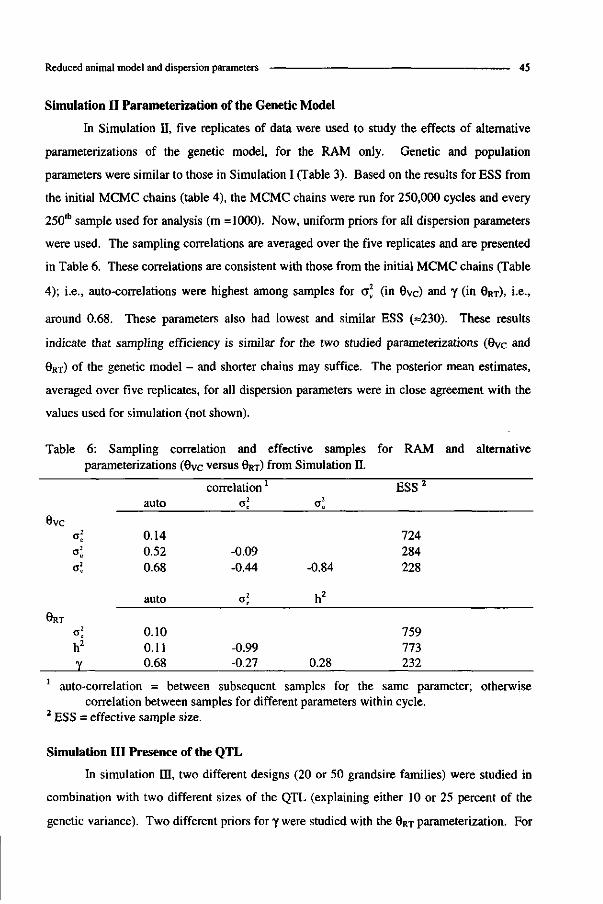
Reduced animal model and dispersion parameters 45
Simulation II Parameterization of the Genetic Model
In Simulation E, five replicates of data were used to study the effects of alternative
parameterizations of the genetic model, for the RAM only. Genetic and population
parameters were similar to those in Simulation I (Table 3). Based on the results for ESS from
the initial MCMC chains (table 4), the MCMC chains were run for 250,000 cycles and every
250th sample used for analysis (m =1000). Now, uniform priors for all dispersion parameters
were used. The sampling correlations are averaged over the five replicates and are presented
in Table 6. These correlations are consistent with those from the initial MCMC chains (Table
4); i.e., auto-correlations were highest among samples for a] (in 0Vc) and y (in 9RT), i.e.,
around 0.68. These parameters also had lowest and similar ESS (=230). These results
indicate that sampling efficiency is similar for the two studied parameterizations (Ovc and
0RT) of the genetic model - and shorter chains may suffice. The posterior mean estimates,
averaged over five replicates, for all dispersion parameters were in close agreement with the
values used for simulation (not shown).
Table 6: Sampling correlation and effective samples for RAM and alternative parameterizations (9vc versus 0RT) from Simulation H.
correlation ' ESS 2
auto 6vc
al 0.14 724 o\ 0.52 -0.09 284 <sl 0.68 -0.44 -0.84 228
auto o ] h2
9RT 0.10 759 0.11 -0.99 773 0.68 -0.27 0.28 232
h2 0.11 -0.99 773
_ï 1 auto-correlation = between subsequent samples for the same parameter; otherwise
correlation between samples for different parameters within cycle. 2 ESS = effective sample size.
Simulation III Presence of the QTL
In simulation HI, two different designs (20 or 50 grandsire families) were studied in
combination with two different sizes of the QTL (explaining either 10 or 25 percent of the
genetic variance). Two different priors for y were studied with the 9RT parameterization. For

46 Chapter 3
each combination of design and y, test runs preceding the 25 replicates were used to
empirically determine values for t in the MH algorithm, in order to achieve the desired
acceptance rates. From the marginal posterior density an odds ratio was computed and the
presence of the QTL was accepted only if this ratio exceeded a critical value of 20. Using this
test statistic we postulated the power of detecting the QTL for specific designs and using
different priors (Table 7).
Table 7: Power' for detection of QTL for RAM and parameterization ÖRT from Simulation HI.
Design 2
20x40
50x40
QTL(Y)3
0.10
0.25
0.10
0.25
prior on y = Beta(l,l)
0.24
0.64
0.80
1.00
prior on y = Beta(l ,19)
0.28
0.56
0.68
1.00
1 Power is defined as the acceptance rate for a QTL, for an odds ratio, mode{p(y)}/p(y=0), exceeds 20. For each "design - QTL" combination, 25 replicates were simulated.
2 Design is defined as 20 (50) grandsire families, each family contains 40 sons. 3 QTL (y) is the proportion of genetic variance due to the QTL.
The small design (20x40) has low power of QTL detection, i.e., only 25 %, for a QTL
that explain 10 % of the genetic variance. Power increased when either the QTL explained
more genetic variance or when a large design (50x 40) was used. For the large design with a
relatively large QTL, power of detection is 100%, for both priors considered. The use of the
"peaked-at-zero" prior reduced power in the two intermediate cases but increased power in
the small design with the small QTL. Estimates for posterior mode, mean and HPD90 were
averaged over the 25 replicates and these averages are presented Figure 5. When the
"peaked-at-zero" prior was used, point estimates are lower compared to using the uniform
prior. This prior also led to shorter - and closer to zero - HPD90 region in all combinations
of design and y but the impact was more noticeable for the small design.

Reduced animal model and dispersion parameters 47
0.50
0.45
0.40
0.35
p! 0.30
o o 0.25 't a. 0.20 o a.
0.15
0.10
0.05
0.13
0.28
0.00 design_». 2 0 x 4 0
1-*- 0.10 prior on •»—>• B ( 1 , 1 )
• mean
• mode
110.26
0.09 0.08
0.20- 0.19
20x40 0.10
B(1,19)
20x40 0.25
B(1,1)
20x40 0.25
B(1,19)
50x40 0.10
B(1,1)
50x40 0.10
B(1,19)
50x40 0.25
B(1,1)
50x40 0.25
B(1,19)
Figure 5: Estimates for posterior mode, mean and 90 % Highest Posterior Density (HPD90) region. Estimates are averages over 25 replicates (Simulation LET).
CONCLUSIONS
We presented MCMC algorithms, using the Gibbs sampler and the MH algorithm,
which facilitate Bayesian estimation of location and dispersion parameters with a RAM. The
RAM proved to be superior to the FAM; RAM required much less computational time
because of the greatly reduced number of location parameters and also better mixing of the
dispersion parameters. Information on individual phenotypes led to accurate estimation of
both residual variance and heritability, as was similar to Van Arendonk et al. (1998). On the
contrary, Daughter Yield Deviations (Wiggans and VanRaden 1993) may result into poor
estimation of polygenic and residual variances (e.g., Uimari and Hoeschele 1997). The use of
0RT allows a better representation of prior belief about dispersion parameters while sampling
efficiency was similar to the usual 0vc parameterization.
Considering ratios of variance components rather than variance components
themselves in sampling procedures, has been previously proposed (Theobald et al. 1997).
However, our ratios can be interpreted directly and have implicit boundaries (zero and one),
where Theobald et al. (1997) needed a specific restriction on their ratio. The representations
of prior knowledge in the two parameterizations were not equivalent and differences in

48 Chapter 3
posterior estimates can be expected. However, the use of vague priors (absence of prior
knowledge) in the two parameterizations lead to very similar results.
In this study, position of the QTL was assumed known. Extension of the MCMC
algorithm to allow estimation of QTL position has been studied and implemented (Bink et al.
1998b). Currently, the method of Bink et al. (1998a) to sample genotypes for a single marker
is being extended to multiple markers linked to a normally distributed QTL. Then, a robust
MCMC method becomes available for linkage analysis in multiple generation pedigrees
allowing incomplete information on both trait phenotypes and marker genotypes.
ACKNOWLEDGMENT
The authors wish to thank Luc Janss and George Casella for stimulating discussions
and suggestions. Comments from anonymous reviewers and the editor considerably
improved the paper. The first author acknowledges financial support from NWO while on
research leave at Cornell University, Ithaca NY. The financial support of Holland Genetics is
gratefully acknowledged.
REFERENCES
Berger JO (1985) Statistical decision theory and Bayesian analysis, 2" edition. Springer-Verlag ,New York, NY
Bink MCAM, VanArendonk JAM, Quaas RL (1998a) Breeding value estimation with incomplete marker data. Genet Sel Evol 30:45-58
Bink MCAM, Janss LLG, Quaas RL (1998b) Mapping a poly-allelic quantitative trait locus using simulated tempering. Proc 6* World Congr Genet Appl Livest Prod, Armidale, Australia 26:277-280
Cantet RJC, Smith C (1991) Reduced animal model for marker assisted selection using best linear unbiased prediction. Genet Sel Evol 23:221-233
Chib S, Greenberg E (1995) Understanding the Metropolis Hastings algorithm. Am Stat 49:327-335
Devroye L, (1986) Non-uniform Random Variate Generation. Springer-Verlag Ine, New York
Fernando RL, Grossman M (1989) Marker-assisted selection using best linear unbiased prediction. Genet Sel Evol 21:467-477
Gelfand AE (1994) Gibbs Sampling (A Contribution to the Encyclopedia of Statistical Sciences). Technical Report, Department of Statistics, University of Connecticut
Gelfand AE, Smith AFM (1990) Sampling-based approaches to calculating marginal densities. J Am Statist Assoc 85:398-409
Geman S, Geman D (1984) Stochastic relaxation, Gibbs distributions and the Bayesian restoration of images. IEEE Trans Pattern Anal Machine Intelligence 6:721-741
Gilks WR, Wild P (1992) Adaptive rejection sampling for Gibbs sampling. Appl Stat 41:337-348

Reduced animal model and dispersion parameters 49
Gilks WR, Best NG, Tan KKC (1995) Adaptive rejection Metropolis sampling within Gibbs sampling. Appl Stat 44:455-472
Hastings WK (1970) Monte Carlo sampling methods using Markov chains and their applications. Biometrika 57:97-109
Hoeschele I (1994) Bayesian QTL mapping via the Gibbs Sampler. Proc 5th World Congr Genet Appl Livest Prod 21:241-244, Guelph, Canada
Hoeschele I, Van Raden PM (1993) Bayesian analysis of linkage between genetic markers and quantitative trait loci, I Prior knowledge. Theor Appl Genet 85:953-960
Janss LLG, Thompson R, Van Arendonk JAM (1995) Application of Gibbs sampling for inference in a mixed major gene-poly genie inheritance model in animal populations. Theor Appl Genet 91:1137-1147
Metropolis N, Rosenbluth AW, Rosenbluth MN, Teller H, Teller E (1953) Equations of state calculations by fast computing machines. J Chem Physics 21:1087-1091
Quaas RL, Pollak EJ (1980) Mixed model methodology for farm and ranch beef cattle testing programs. J Anim Sei 51:1277-1287
Searle SR (1982) Matrix Algebra Useful For Statistics. John Wiley & Sons, New York, NY
Sorensen DA, Andersen S, Gianola D, Korsgaard I (1995) Bayesian inference in threshold models using Gibbs sampling. Genet Sel Evol 27:229-249
Tanner MA, Wong WH (1987) The calculation of posterior distributions by data augmentation. J Am Stat Assoc 82:528-540
Theobald CM, Firat MZ, Thompson R (1997) Gibbs sampling, adaptive rejection sampling and robustness to prior specification for a mixed linear model. Genet Sel Evol 29:57-72
Tierney L (1994) Markov chains for exploring posterior distributions (with discussion). Ann Stat 22:1701-1762
Uimari P, Thaller G, Hoeschele I (1996) The use of multiple markers in a Bayesian method for mapping quantitative trait loci. Genetics 143:1831-1842
Uimari P, Hoeschele I (1997) Mapping-linked quantitative trait loci using Bayesian analysis and Markov chain Monte Carlo algorithms. Genetics 146:735-743
VanArendonk JAM, Tier B, Bink MCAM, Bovenhuis H (1998) Restricted maximum likelihood analysis between genetic markers and quantitative trait loci for a granddaughter design. J Dairy Sei (accepted)
VanRaden PM, Wiggans GR (1991) Derivation, calculation and use of national animal model information. J Dairy Sei 74:2737-2746
Van Tassell CP, Casella G, Pollak EJ (1995) Effects of selection on estimates of variance components using Gibbs sampling and restricted maximum likelihood. J Dairy Sei 78:678-692
Van Tassell CP, VanVleck LD (1996) Multiple-trait Gibbs sampler for animal models: flexible programs for bayesian and likelihood-based (Co)variance component Inference. J Anim Sei 74:2586-2597
Wang CS, Rutledge JJ, Gianola D (1993) Marginal inferences about variance components in a mixed linear model using Gibbs sampling. Genet Sel Evol 25:41-62
Wang, CS, Quaas RL, Pollak EJ (1997) Bayesian analysis of calving ease scores and birth weights. Genet Sel Evol 29:117-143
Wang T, Fernando RL, VanderBeek S, Grossman M, Van Arendonk JAM (1995) Covariance between relatives for a marked quantitative trait locus. Genet Sel Evol 27:251-272
Weiler JI, Kashi Y, Soller M (1990) Power of daughter and granddaughter designs for determining linkage between marker loci and quantitative trait loci in dairy cattle. J Dairy Sei 73:2525-2537

50- Chapter 3
APPENDIX
Full Conditional Densities Location parameters The conditional densities for location parameters are the same
with either sets of dispersion parameters (0vc or 9RT). When sampling genetic effects, the ratios of VC needed can be computed from either parameterizations, i.e.,
a"1 = f = ((1 - y) x -j^-J, and cc~' = •% = Uy x - ^ r ) . In this study we considered only one
fixed effect, an overall mean \i, for which the conditional density becomes ( • ( 4 n, \ / ' \ - ' A
M.ie_u,y ~ N 4 n, \ f 4
X X Pk • XniGE",
where, pk equals yk corrected for genetic effects, following the categorization in Table 1.
The conditional variance of this overall mean is an weighted average over categories. Again,
for phenotypes on animals in category 1 to 3, the residual variance, <s\ , contains parts of the
genetic variances. The conditional density for the polygenic effect of animal 7' can be given as
"jM-u^-Nfcj/djtf/dj) where
keo (j) leo• (j) i'=l
dj -rij+a 8J +
*S'V(J)
where y, is the ith phenotype for animal j , corrected for all effects, other than polygenic, y,. is the average of phenotypes on non-parent /, also corrected for all effects other than polygenic, op(j) represents the offspring of animal j , which are parents themselves, onp(j) represents the offspring of animal j , which are non-parents. Furthermore, uM,k is the polygenic effect of the other (if known) parent (mate of animal j) of offspring k, nj is the number of phenotypes for
animal j , 8j,= 1, %, 2 when 0, 1, or 2 parents of j are identified (with no inbreeding), (ôy1 is
the fraction o2u in the sampling term fy.) Finally, q); is the reciprocal of the amount of variance
present in the residuals of phenotypes on animal /, and can be calculated as,
<p, = ( « , - ' + a : V + a 7 l l ï D / l 2 ) where n; is the number of observations on animal /, and D; = I2 - Q;xQ/T (with no inbreeding, see also Bink et al. 1998a). The conditional density for the xlh QTL effect of animal j can be given as
v , * i e_ v ; , y~Ar (c , 7 j ; , 0^ ; ) , x= i , 2
where
^ X * + a, *-,vlJ+dafvlJ+dqfvlJ + <WA<j)
+a. • X K + dq?vl -dqd3k*v[
MJ -dqdt^lj)
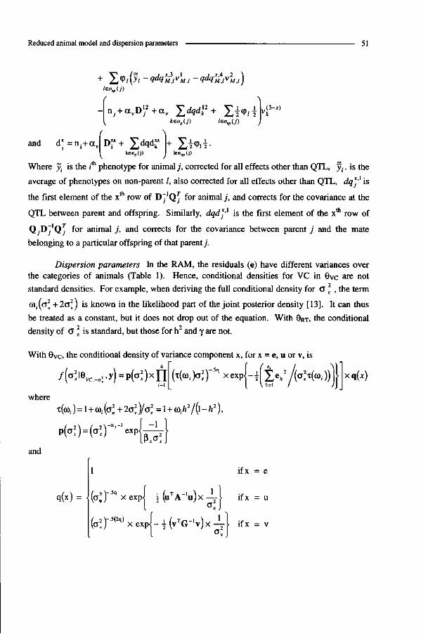
Reduced animal model and dispersion parameters 51
,(3-x)
and dx = ^ +0^ kso.(j)
1
teo„,(j)
Where y,- is the ith phenotype for animal j , corrected for all effects other than QTL, yt. is the
average of phenotypes on non-parent /, also corrected for all effects other than QTL, dq j ' 1 is
the first element of the xth row of D ^ ' Q J for animal j , and corrects for the covariance at the
QTL between parent and offspring. Similarly, dqd*'1 is the first element of the Xth row of
QjD~'Qy for animal j , and corrects for the covariance between parent j and the mate
belonging to a particular offspring of that parent ƒ
Dispersion parameters In the RAM, the residuals (e) have different variances over the categories of animals (Table 1). Hence, conditional densities for VC in 9vc are not standard densities. For example, when deriving the full conditional density for O e , the term
00;(oI +2a2v) is known in the likelihood part of the joint posterior density [13]. It can thus
be treated as a constant, but it does not drop out of the equation. With 8RT, the conditional
density of CT 2 is standard, but those for h2 and y are not.
With 9vc. the conditional density of variance component x, for x = e, u or v, is ( », / >
/H i evc,-o-y)=p(^)xn
where
and
x(co,)= l + (of(oj + 2av2)/o2 = l + co,7z2/(l-/z2),
p (o ' ) = (a2)"a '_1exp V*<
q(x) = tar ta)
x exp, 2
5(2q) ^
x exp
(iTA-'u):
(vTG-'v):
( T ( c o , ) a 2 p ' x e x p - | X ^ 7 ( ^ M ^ ) ) V*=i
ifx = e
ifx = u
ifx = v
xq(x)

52- Chapter 3
With ORT, the conditional density for a \ is IG(r, s) distribution with
s = IX: 2 A uTA"'u v rG- 'v
ße 2{tiÙA°>,)) 2 (1-Y)x^ 2-5yx^_ where N is the total number of phenotypes.
4 <n ^r-xexJ-ifj^/^K) / J .
x(T^r5<"2î,xexP-i[(u^A-'u/(l-Y))+(v^G-'v/.5y)]xi^
where T(©,.)=1 + (Ö1.Ä2/(I-A2).
/(Tie^T,y)oc(Yr-,(l-Y)ß-1
x(l-T)-5( ' )x(y)-5(2 ' )xexp{-i[(u^A-'u/(l-y))+(v^G-'v/.5y)]xl^;
Chapter 4
Markov Chain Monte Carlo for Mapping a Quantitative Trait Locus
in Outbred Populations
Marco C. A. M. Bink , Luc L. G. Janss and Richard L. Quaas
'Animal Breeding and Genetics Group, Wageningen Institute of Animal Sciences,
Wageningen Agricultural University, PO Box 338, 6700 AH Wageningen, The Netherlands
"institute for Animal Science and Health, PO Box 65, 8200 AB Lelystad, The Netherlands
'"Department of Animal Science, Cornell University, Ithaca, NY 14853, USA
Submitted for publication to Genetical Research

Mapping a QTL in outbred populations 55
ABSTRACT
A Bayesian method for identification of the most likely marker bracket interval
containing a quantitative trait locus (QTL) with normally distributed effects, is presented.
Parameter estimation was implemented via Markov chain Monte Carlo (MCMC) algorithms.
Parameters of the mixed model are residual variance, heritability, proportion of genetic
variance due to QTL, and QTL position on a linkage map. Straightforward implementation of
a Metropolis Hastings algorithm to sample QTL position results in a reducible chain, i.e., the
chain does not move away from the initial marker interval. This is due to a different set of
marker brackets that are used in computing the gametic relationship matrix for QTL effects
when the candidate QTL position is in a different marker interval as the current QTL position.
A relatively new MCMC technique, simulated tempering, is implemented to improve mixing
of QTL position. Although computer intensive, the simulated tempering sampler yields
proper mixing of QTL position. Inferences on the most likely position of the QTL are based
on marginal posterior probabilities.
INTRODUCTION
Mapping loci responsible for variation in quantitative traits (quantitative trait loci or
QTLs) in humans, animals and plants has rapidly become a major area of interest. Due to
high density of molecular markers now available, segregation and transmission of
chromosomal segments can be accurately followed throughout a population. A variety of
methods are used for identification of marker-QTL associations (e.g., Weiler et al. 1986;
Knott and Haley 1992; Zeng 1994). Most were developed assuming simple pedigrees, e.g.,
backcrosses or F2s. They cannot fully account for the more complex data structures of
outbred populations such as found in domestic animals.
Markov Chain Monte Carlo (MCMC) algorithms (Metropolis et al. 1953; Hastings
1970) provide a powerful computational tool for analysis of complex data structures, either in
a maximum likelihood or Bayesian context. Ideas of a Bayesian analysis for QTL detection
were described in Hoeschele and VanRaden (1993a, 1993b), and implemented, via MCMC
algorithms, in contributions by Thaller & Hoeschele (1996); Satagopan et al. (1996), Uimari
et al. (1996); Uimari & Hoeschele (1997); and Sillanpää & Arjas (1998). Most of these

56 Chapter 4
Bayesian methods assume a bi-allelic QTL model (Hoeschele et al. 1997). Though
reasonable for a cross of inbred strains it is less so for a population such as the Holstein breed
of dairy cattle. Outside of North America, populations typically resulted from several crosses
of the North American breed on the local strain of black and white cattle. Currently the gene
flow among countries continues unabated. A population with such varied origins is a long
way from inbred strains; a polyallelic model seems more appropriate.
In this paper a Bayesian approach is presented for estimating position and contribution
to variance of a random, normally distributed QTL together with additive polygenic and
residual variance components. We show that a straightforward implementation of a
Metropolis-Hastings (MH) algorithm to shuffle the QTL position within the linkage map
leads to an effectively reducible Markov chain, i.e., not all possible positions are reached
from a given starting position of the QTL. We suggest a modified MCMC scheme, which is
simulated tempering (Marinari & Parisi 1992; Geyer & Thompson 1995), to solve the mixing
problem for QTL position. The presented MCMC scheme is empirically evaluated for
simulated data from a granddaughter design (Weiler et al. 1990). In a granddaughter design,
marker genotypes are available on elite sires and their sons and trait phenotypes are observed
on daughters of sons. The extension and application of the Bayesian method presented to
complex pedigree analysis to detect QTL in outbred populations are discussed.
METHOD AND APPLICATION
Mixed linear model: Fernando and Grossman (1989) derived best linear unbiased
prediction (BLUP) of normally distributed QTL allelic effects. The animal model including
QTL effects and residual polygenic effects (QTL not linked to marker map under study) of
Fernando and Grossman (1989) is:
y = Xb + Zu + ZTv + e
with VflKu) = Acr„2,VaKv) = G(Tv2,Var(e) = RcTe
2 [1]
where y is an N x 1 vector of phenotypes, b is a vector of fixed effects, X is a
design/covariate matrix relating b to y, u is a q x 1 random vector of residual additive
(polygenic) effects, Z is an incidence matrix relating records in y to individuals, v is a 2q x 1
random vector of QTL allelic effects, T is an incidence matrix relating each individual to its
two QTL alleles, e is a vector of random residuals, A is the additive genetic relationship

Mapping a QTL in outbred populations 57
matrix (Henderson 1976), a] is the polygenic variance, Ge 2 ' s m e variance-covariance
matrix of the QTL allelic effects conditional on marker information, a2 is half the additive
genetic variance explained by the QTL, R is a known diagonal matrix, and a2 is the residual
variance. Matrix G is the gametic relationship matrix for the QTL with size 2q x 2q, where
the (i,j) element represents the probability of QTL allele i being identical by descent (IBD) to
QTL allele j . The IBD probabilities for QTL effects are computed given marker data and a
map position, (IQ, of the QTL. Parameters related to the marker map (marker distances and
allele frequencies) are assumed to be known. In this study we apply the recursive method of
Wang et al. (1995) to construct matrix G and its inverse. For animals with many genotyped
offspring, the linkage phase is assumed known a priori, for the remaining animals an
averaged linkage phase, i.e., weighting each possible linkage phase by its probability of
occurrence, is taken. The model in [1] is parameterized in terms of the unknown heritability
(h2 = a2 la1) with additive genetic errand phenotypic variance a2p, proportion of the
additive genetic variance due to the QTL (y = a1 la]), residual variance a2, and QTL
position CIQ.
Estimation of location and dispersion parameters: Bayesian inferences about the
parameters are based on the posterior distribution of parameters given the observed data (y)
and marker data (m). The missing data are the fixed effects (b), and random QTL (v) and
polygenic (u) effects. Priors for b are assumed to be uniform over a large but fixed interval.
The polygenic and QTL effects are a priori Normal (0, ACT2 ), Normal (0, G a2 ), respectively.
Now let 0 denote {b,u,v,h2,y,o2}. Given the position of the QTL relative to the set of
available linked markers, the sampling distributions for all elements in 8 are similar to those
in Bink et al. (1998b). For the location parameters b, u, and v sampling distributions are
Normal. The sampling distribution for oj is a scaled inverted chi-squared distribution with
df equal to dim(e) - 2, resulting from the use of uniform prior on [0, °°). Beta distributions
were used to specify prior knowledge on both h2 and y. The resulting sampling distributions
for h2 and y are non-standard and a Metropolis Hastings (MH)-algorithm is used to obtain
samples for these parameters (Bink et al. 1998b).
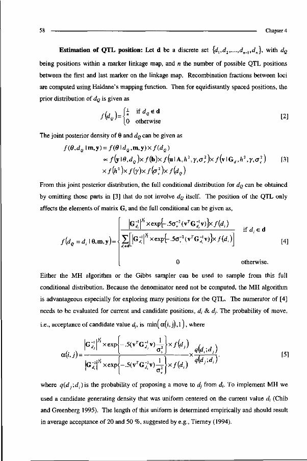
58 Chapter 4
Estimation of QTL position: Let d be a discrete set {d{,d2,....,dn_x,dn}, with dQ
being positions within a marker linkage map, and n the number of possible QTL positions
between the first and last marker on the linkage map. Recombination fractions between loci
are computed using Haldane's mapping function. Then for equidistantly spaced positions, the
prior distribution of dQ is given as
f\do)= V 0 otherwise
[2]
The joint posterior density of 9 and dQ can be given as
f(8,dQ \m,y) = f(d\dQ,m,y)xf(dQ)
~f(y\6,dQ)xf{b)xf{u\A,h2,Y,(j>)xf{y\Ga,h2,Y,<Jï) [3]
xf{h2)xf(y)xf{a2)xf{dQ)
From this joint posterior distribution, the full conditional distribution for JQ can be obtained
by omitting those parts in [3] that do not involve dQ itself. The position of the QTL only
affects the elements of matrix G, and the full conditional can be given as,
f{dQ=di\Q,m,y) =
IG"' r x expf .5a;2 ( vTG "' v)}x f(di )
; xexp{ - . 5o \ 2 ( v r G»}x / (< ) if d; e d
[4]
0 otherwise.
Either the MH algorithm or the Gibbs sampler can be used to sample from this full
conditional distribution. Because the denominator need not be computed, the MH algorithm
is advantageous especially for exploring many positions for the QTL. The numerator of [4]
needs to be evaluated for current and candidate positions, dt & dj. The probability of move,
i.e., acceptance of candidate value dj, is min( cc(i, j), 1 ) , where
a(i,j)--'f{dj)
\% xexp - .5 (v rG>)— x ƒ(</.)
M\dj) Adj-.d.y
[5]
where q{df,dt)is the probability of proposing a move to dj from dt. To implement MH we
used a candidate generating density that was uniform centered on the current value d, (Chib
and Greenberg 1995). The length of this uniform is determined empirically and should result
in average acceptance of 20 and 50 %, suggested by e.g., Tierney (1994).

Mapping a QTL in outbred populations 59
Effectively reducible MCMC chain: A candidate position for the QTL in another
marker interval usually involves a different set of marker loci (and genotypes). Consequently,
very different IBD patterns are used to compute G"1. A different G"1 will result in
(vTGj'v » vTGj'v) (equation [5]) because values for v were sampled conditional on G^1.
This gives a relatively very small value for the numerator in [5], and, for large pedigrees, the
probability of move in [5] is virtually zero. Consequently, the QTL position remains within the
starting marker interval, independent of which starting position is chosen, i.e., effectively
reducible. However, density [4] remains useful to find the most likely position of the QTL
within a marker bracket.
Simulated tempering: Simulated tempering was first described by Marinari & Parisi
(1992) and in the modified form used here by Geyer & Thompson (1995). It is a procedure to
improve the mixing properties of a chain such as described above. A set of unnormalized
densities, rather than just one, is sampled from; one being the original and the others
modifications with (expected) better mixing properties. One such modification is to "heat" the
target density. This flattens the distribution, making it easier for the chain to move around in the
parameter space. A simulated tempering scheme includes an index to the current distribution as
part of the state of the Markov chain. With this index, a new stage is added to the sampling
scheme outlined previously. When the chain is sampling the target - "cold" - distribution it
will explore within a local mode; when it is sampling from the hot distributions it should be able
to move easily around in the parameter space. Each time the chain moves from the hot
distributions to the cold distribution, it has the potential to enter a different local mode.
Because differences in the inverse matrices computed for current and candidate marker
interval causes the non-mixing for parameter CIQ, the heated distributions were obtained by
modifying G '. The elements of G ' are recursively computed by using, for each individual,
an IBD probability matrix Q (= q in [17] in Wang et al. 1995). For each individual with 2
identified parents, nonzero elements (< 8) in Q are computed from the individual's and
parental marker genotypes and recombination fractions between QTL and adjacent marker
loci. Now, let Qlrue denote the Q matrix conditional on marker data and true recombination
fractions between QTL and adjacent marker loci. And let Qfree denote a matrix Q where the
QTL is not linked to any markers. That is, recombination fractions between QTL and
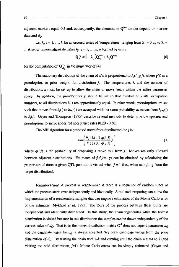
60 Chapter 4
adjacent markers equal 0.5 and, consequently, the elements in Qfree do not depend on marker
data and dQ.
Let Xj,j= 1,..., k, be an ordered series of 'temperatures' ranging from X\ = 0 up to Xk =
1. A set of unnormalized densities A,-, j= 1, ..., k, is formed by using
QÎ ;= ( i - ^X j r + ^Q f r e e [6]
for the computation of GT in the numerator of [4].
The stationary distribution of the chain of X's is proportional to A/.) g(j), where g(j) is a
pseudoprior, or prior weight, for distribution j . The temperatures X and the number of
distributions k must be set up to allow the chain to move freely within the entire parameter
space. In addition, the pseudopriors g should be set so that number of visits, occupation
numbers, to all distributions A/ s are approximately equal. In other words, pseudopriors are set
such that moves from A/.) to A/+/(.) are accepted with the same probability as moves from A7+/(.)
to A/.). Geyer and Thompson (1995) describe several methods to determine the spacing and
pseudopriors to arrive at desired acceptance rates (0.20 - 0.50).
The MH algorithm for a proposed move from distribution i toy' is:
'hjUgiflq&j) min ,1 [7]
{ A((.)g(0 qU;0 )
where q(rj) is the probability of proposing a move to i from j . Moves are only allowed
between adjacent distributions. Estimates of /(rf^lm, y) can be obtained by calculating the
proportion of times a given QTL position is visited when j = 1 (i.e., when sampling from the
target distribution).
Regeneration: A process is regenerative if there is a sequence of random times at
which the process starts over independently and identically. Simulated tempering can allow the
implementation of a regenerating sampler that can improve estimation of the Monte Carlo error
of the estimates (Mykland et al. 1995). The tours of the process between these times are
independent and identically distributed. In this study, the chain regenerates when the hottest
distribution is visited because in this distribution the samples can be drawn independently of the
current value of dQ. That is, in the hottest distribution matrix G ' does not depend parameter dQ
and the candidate value for dç> is always accepted. We draw candidate values from the prior
distribution of dQ. By starting the chain with j=k and running until the chain returns to k (and
visiting the cold distribution, j= 1), Monte Carlo errors can be simply estimated (Geyer and

Mapping a QTL in outbred populations 61
Thompson 1995). Estimating Monte Carlo errors with a standard MCMC scheme is much
harder due to the dependency between samples (Geyer 1992). The method described by Geyer
and Thompson to estimate Monte Carlo errors was used in this study.
Simulated data: Monte Carlo simulation was used to generate granddaughter designs
comprising 20 unrelated grandsire families each having 40 sires (paternal half sibs). This
approximately reflects a Dutch granddaughter experiment design as described by Spelman et
al. (1996). Polygenic and QTL effects for grandsires, were sampled from N(0,a2u) and
N(0,O2v), respectively. The polygenic effect for a sires was simulated a su s = ^ (uGS)+()>,
where us is the grandsire's polygenic effect, and (j), Mendelian sampling, is distributed
independently as N(Q,Vai(§)) with Var(<t>) = .75 x G2U (no inbreeding). Each sire inherited one
QTL allele at random from its grandsire. The maternally inherited QTL effect for a son was
drawn from N(0, c2,). Each sire had 100 daughters with phenotypes observed, that were
generated as
y ~ N{{±US + pvi + (1 -p)v2\(X2 + < + <)).
where p is a 0/1 variable. The phenotypic variance and the heritability of the trait were 100
and 0.40, respectively. The proportion of genetic variance due to the QTL (= y) was 0.25,
except for data II where y = 0.00 (table I). Data II was chosen to verify that absence of a QTL
within the linkage map was also detected by the MCMC method.
Table 1 :Characteristics of simulation of DATA 1 _
DATA y QTL position heterozygosity
1 Ö25 90 cM 100%
H 0.00 - 100%
m 0.25 90 cM 60%
IV 0.25 50 cM 60%
1 Position of QTL relative the map position of first marker in linkage group; 2 Heterozygosity is the percentage of heterozygous marker genotypes for grandsires.
Marker data was generated for all grandsires and sons. Six markers were spaced
equidistantly (20 cM, Haldane's mapping function) with the first marker being the origin of
the linkage map. Each marker locus contained five alleles with equal frequencies. For
62 Chapter 4
grandsires, the informativeness of marker genotypes, i.e., heterozygous, was arbitrarily set
equal to 100% or 60% (table I). The 100% heterozygosity is the ideal situation; 60% is a
level found in practice (e.g., chromosome six in dairy cattle, Spelman et al. 1996).
MCMC simulation: In the analysis, we restricted the set of QTL positions to 5 for
program coding reasons. These positions were the middle of each marker bracket, i.e., 10, 30
50, 70, and 90 cM. The five possible positions of the QTL had equal prior probabilities
(=0.20). In the analysis, Beta(l,l) (= uniform) prior distributions were used for parameters h2
and y. Initial values for location parameters were zero, while starting values fora2, h2, and y
were 60.0, 0.40, and 0.25, respectively. The simulated tempering sampler always started in
the hottest distribution (Xk =1)- Due to independent sampling of d in this distribution, the
starting value for d was not relevant. For each of the four data sets, one final long MCMC
chain was run (after fine-tuning the number of distributions with their spacing and
pseudopriors in the simulated tempering scheme). The length of each MCMC run was
arbitrarily set at 5,000,000 iterations. Total CPU-time per MCMC run was about 40 hours on
a HP 9000-k260 server. In each iteration (in chronological order), b, u, v, and a2 were
updated by Gibbs sampling, while h2, y, d, and \ were updated by MH algorithms. (To
decrease the number of elements in u and v, a reduced animal model was fit (Bink et al.
1998b).) The samples for parameters a2 h2, y, and d were stored when the cold distribution
(kj = 0) was visited.
RESULTS AND DISCUSSION
Parameter Estimation: The four data sets yielded similar, firm, posterior knowledge
on h2 and a2 i.e., peaked symmetric densities centered on values very close to the values
(0.40, and 60) used for simulation (results not shown). Marginal posterior densities for the
proportion QTL variance (y) for all 4 data sets are presented in Figure 1. These densities are
not very peaked, but do indicate presence of a QTL in the three data sets where a QTL was
simulated (I, H, and IV) and absence of a QTL in II where none was simulated. This was
supported by the estimated 90% Highest Posterior Density (HPD90) regions, [0.03, 0.34],
[0.00, 0.19], [0.05, 0.42] and [0.03,0.42] for data I, H, m, and IV, respectively.

Mapping a QTL in outbred populations 63
. •
f Y posterior
/ prior x
mode = 0.147 mean = 0.192 stdv =0.103
0.2 0.4 0.6 0.8 proportion QTL ( y )
9
8
7
fi -5
4
3
2
0 -
\ posterior
prior V
mode = 0.017 mean = 0.089 stdv = 0.074
1 — ^ * * —i 1 1
0.2 0.4 0.6 0.8 proportion QTL ( y )
9
8
7
6
5
4
3
2
1 / prior
V posterior
mode = 0.135 mean = 0.230 stdv =0.126
) 0.2 0.4 0.6 proportion QTL ( y
0.8 1
)
.
•
f *» posterior
/ prior X * .
mode = 0.163 mean = 0.230 stdv = 0.130
- ' 1 H — — ^ = = T > — 1
0.2 0.4 0.6 0.8 proportion QTL ( y )
1.0
0.8
0.6
0.4
0.2
0.0
30 50 70 position QTL (d)
1.0 -,
0.8
0.6 -
0.4 -
0.2 -
0.0 -
0 36
10
0.47
WË 0.08 0.08
30 50 70 position QTL (d)
0.02
90
50 70 90
position QTL(d)
30 50 position QTL (d)
Figure 1 : Marginal posterior densities for proportion QTL (y), and probabilities for position of the QTL (d) relative to origin of linkage map, after analyzing DATA I, II HI, and IV. Uniform priors were assumed for both parameters.

64 Chapter 4
Computed odds ratios - marginal posterior density at mode divided by marginal
posterior density at zero - were decisive for data I, n and HI, i.e., 180.9, 1.4, and 57.0,
respectively. The odds ratio for data IV equaled 17.8, which is below but very close to the
critical value of 20 (as suggested by Janss et al. 1995), and presence of the QTL seems
justified.
Estimation of QTL position within marker linkage map: The total length of the
MCMC chains was arbitrarily set to 5,000,000 iterations, under the presumption that this was
sufficient to minimize Monte Carlo error on the estimated QTL position. When only 500,000
iterations were used for data I, the MC error on the estimated position was zero because only
1 of the possible positions, i.e., 90 cM, was visited. After 5,000,000 iterations only position
30 cM was not sampled. Posterior probabilities for positions other than 90 cM were below
0.02 (Figure 1). Based on the marginal posterior density for proportion QTL (y) the presence
of the QTL within the marker linkage map was rejected for data H In this case the position is
meaningless though the chain did not visit all intervals equally as might have been expected.
The most likely position for the QTL in data III was at 70 cM (Figure 1), what was not in
agreement with the value (90 cM) used in simulation. This may be because the QTL was
simulated at the end of the chromosome and the sixth marker (at 100 cM) was informative for
only 10 of the 20 grandsire families, single marker information is less powerful than marker
bracket information (e.g., Haley and Knott 1992). In addition, Van Arendonk et al. (1998)
showed that estimated QTL position is biased towards "informative regions" of the marker
linkage map. In addition, lack of information on the fifth marker (at 80 cM) for some
grandsires caused the same markers to be used for both position 70 cM and 90 cM to compute
IBD probabilities, although with different recombination rates. In data IV the most likely
position of the QTL was at 50 cM, which was in agreement with the value used in simulation.
The probability for position 30 cM was almost half of the probability for 50 cM. These
results point to a rather low power for estimation of QTL position when markers are only
partially informative for grandsires. Uimari et al. (1996) and VanArendonk et al. (1998)
found similar results.
Mixing of QTL position: For data I and II the simulated tempering sampler needed
35 (modified) distributions to move from hot to cold and reverse. In data III and IV fewer
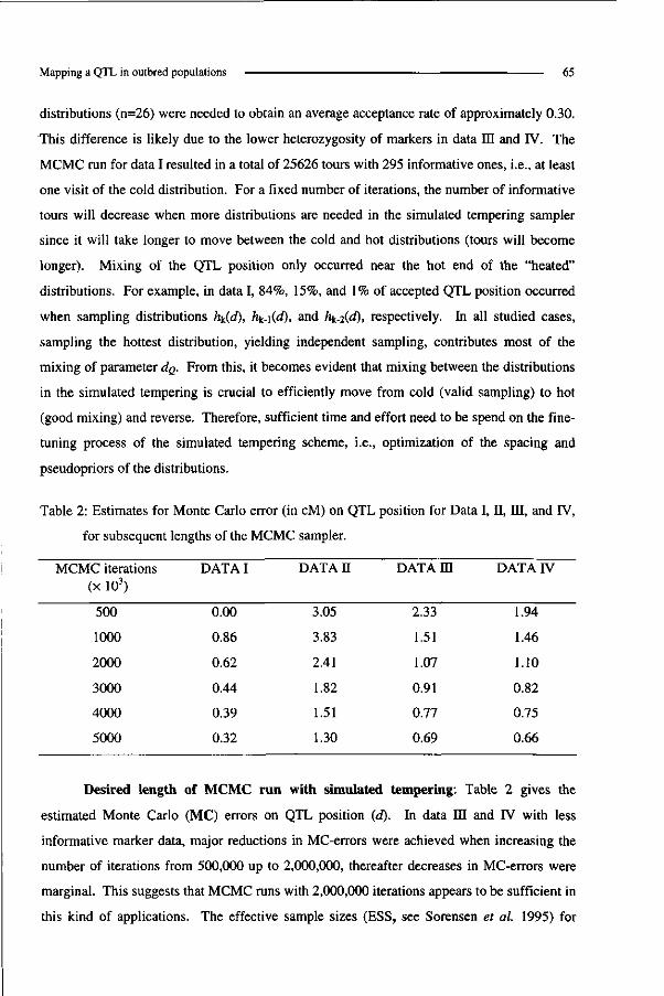
Mapping a QTL in outbred populations 65
distributions (n=26) were needed to obtain an average acceptance rate of approximately 0.30.
This difference is likely due to the lower heterozygosity of markers in data HI and IV. The
MCMC run for data I resulted in a total of 25626 tours with 295 informative ones, i.e., at least
one visit of the cold distribution. For a fixed number of iterations, the number of informative
tours will decrease when more distributions are needed in the simulated tempering sampler
since it will take longer to move between the cold and hot distributions (tours will become
longer). Mixing of the QTL position only occurred near the hot end of the "heated"
distributions. For example, in data I, 84%, 15%, and 1% of accepted QTL position occurred
when sampling distributions h^{d), h^.\{d), and h^d), respectively. In all studied cases,
sampling the hottest distribution, yielding independent sampling, contributes most of the
mixing of parameter <1Q. From this, it becomes evident that mixing between the distributions
in the simulated tempering is crucial to efficiently move from cold (valid sampling) to hot
(good mixing) and reverse. Therefore, sufficient time and effort need to be spend on the fine-
tuning process of the simulated tempering scheme, i.e., optimization of the spacing and
pseudopriors of the distributions.
Table 2: Estimates for Monte Carlo error (in cM) on QTL position for Data I, E, HI, and IV,
for subsequent lengths of the MCMC sampler.
MCMC iterations (x 103)
500
1000
2000
3000
4000
5000
DATAI
0.00
0.86
0.62
0.44
0.39
0.32
DATA II
3.05
3.83
2.41
1.82
1.51
1.30
DATA m
2.33
1.51
1.07
0.91
0.77
0.69
DATA IV
1.94
1.46
1.10
0.82
0.75
0.66
Desired length of MCMC run with simulated tempering: Table 2 gives the
estimated Monte Carlo (MC) errors on QTL position (d). In data HI and IV with less
informative marker data, major reductions in MC-errors were achieved when increasing the
number of iterations from 500,000 up to 2,000,000, thereafter decreases in MC-errors were
marginal. This suggests that MCMC runs with 2,000,000 iterations appears to be sufficient in
this kind of applications. The effective sample sizes (ESS, see Sorensen et al. 1995) for

66 Chapter 4
dispersion parameter y were 2623 and 2882 for data HI and IV, respectively (ESS for h2 were
4 times larger). Minimum values for ESS of about 100 were suggested by Uimari et al.
(1996).
CONCLUDING REMARKS
We presented an MCMC technique to identify the most likely marker bracket interval
for a normally distributed QTL within a marker linkage map in a Bayesian analysis. Using
simulated data from a granddaughter design we empirically tested the method. Because
straightforward sampling of QTL position by an MH algorithm results in a non-mixing chain,
we applied simulated tempering to improve mixing of QTL position. In this study we only
focused on the most likely interval. A second grid search within most likely interval, using
the initially proposed MH algorithm, could more precisely locate the QTL relative to markers
with known positions.
The use of the simulated tempering sampler is not new in genetics. Geyer and
Thompson (1995) applied it to compute the probability distribution of carrier status of a lethal
recessive disease over a pedigree in Hutterites. Heath (1997) used the simulated tempering
sampler to improve mixing in the analysis of haploid radiation hybrid mapping data. In these
studies, mixing properties of important parameters in the Markov chain were insufficient
without the implementation of the simulated tempering sampler. When the simulated
tempering scheme regenerates, tours from different MCMC runs can be combined. This
means that a large analysis could be run on several processors (or personal computers), and
the results simply combined. Alternatively, a second MCMC run could be produced if the
precision obtained from an initial MCMC run was not enough. There are, however, several
technical difficulties with using simulated tempering schemes, particularly with regard to
setting up the modified densities and their pseudopriors. Simplification of that process will
allow a widespread use of methods using simulated tempering schemes in practice.
For the analysis discussed in this study only paternal relationships within unrelated
grandsire families were considered and model assumptions might have been much simpler.
However, we are currently working on methodology for complex pedigree analysis where
ungenotyped individuals provide additional ties between members of different families. This
methodology is based on the ideas of Bink et al. (1998a) for sampling genotypes for a single
marker that is linked to a random normally distributed QTL, and on the ideas of Jansen et al.
Mapping a QTL in outbred populations 67
(1998) to improve mixing of IBD values for marker loci. Examples of ungenotyped
individuals are dams that have sons in multiple grandsire families, or dams of sons that are
sired by a grandsire. Allowing these ungenotyped individuals will increase the number of
segregation events in the analysis and thereby likely improve the power and accuracy of QTL
detection and mapping. The Bayesian analysis presented is primarily described for detection
of QTL in outbred animal populations, but can also be applied to complex pedigrees in
humans or plants.
ACKNOWLEDGMENTS
The authors thank George Casella and Johan van Arendonk for stimulating discussion
and helpful comments to improve the manuscript. Marco Bink acknowledges financial
support from Holland Genetics.
REFERENCES
Bink MCAM, VanArendonk JAM, Quaas RL (1998a) Breeding value estimation with incomplete marker data. Genet Sel Evol 30:45-58
Bink MCAM, Quaas RL, VanArendonk JAM (1998b) Bayesian estimation of dispersion parameters with a reduced animal model including polygenic and QTL effects. Genet Sel Evol 30:103:125
Chib S, Greenberg E (1995) Understanding the Metropolis Hastings algorithm. Am Stat 49: 327-335
Fernando RL, Grossman M (1989) Marker-assisted selection using best linear unbiased prediction. Genet Sel Evol 21: 467-477.
Geyer CJ (1992) Practical Markov chain Monte Carlo (with discussion). Stat Sei 7:467-511.
Geyer CJ, Thompson EA (1995) Annealing Markov chain Monte Carlo with applications to ancestral inference. J Am Stat Assoc 90: 909-920
Haley CS, Knott SA (1992) A simple regression method for mapping quantitative trait loci in line crosses using flanking markers. Heredity 69: 315-324
Hastings WK (1970) Monte Carlo sampling methods using Markov chains and their applications. Biometrika 57: 97-109
Heath SC (1997) Markov chain Monte Carlo methods for radiation hybrid mapping. J Comp Biol 4:505-515
Henderson CR (1976) A simple method for computing the inverse of a numerator relationship matrix used in prediction of breeding values. Biometrics 32:69-83
Hoeschele I, Vanraden PM (1993a) Bayesian analysis of linkage between genetic markers and quantitative trait loci: I Prior knowledge. Theor Appl Genet 85: 953-960
Hoeschele I, Vanraden PM (1993b) Bayesian analysis of linkage between genetic markers and quantitative trait loci: II Combining prior knowledge with experimental evidence Theor Appl Genet 85: 946-952
Hoeschele I, Uimari P, Grignola FE, Zhang Q, Gage KM (1997) Advances in statistical methods to map quantitative trait loci in outbred populations. Genetics 147:1445-1457

68 Chapter 4
Jansen RC, Johnson DL, VanArendonk JAM (1998) A mixture model approach to the mapping of quantitative trait loci in complex populations with an application to multiple cattle families. Genetics 148:391-399
Janss LLG, Thompson R, VanArendonk JAM (1995) Application of Gibbs sampling in a mixed major gene -polygenic inheritance model in animal populations. Theor Appl Genet 91: 1137-1147
Knott SA, Haley CS (1992) Aspects of maximum likelihood methods for the mapping of quantitative trait loci in line crosses. Genet Res Camb 60:139-151
Marinari E, Parisi G (1992) Simulated tempering: a new Monte Carlo scheme. Europhysics Letters 19: 451-458
Metropolis N, Rosenbluth AW, Rosenbluth MN, Teller H, Teller E (1953) Equations of state calculations by fast computing machines. J Chem Physics 21: 1087-1091
Mykland P, Tierney L, Yu B (1995) Regeneration in Markov chain samplers. J Am Stat Assoc 90:233-241
Satagopan JM, Yandell BS, Newton MA, Osborn TC (1996) A Bayesian approach to detect quantitative trait loci using Markov chain Monte Carlo. Genetics 144: 805-816
Sillanpää MJ, Arjas E (1998) Bayesian mapping of multiple quantitative trait loci from incomplete inbred line cross data. Genetics 148:1373-1388
Sorensen DA, Andersen S, Gianola D, Korsgaard I (1995) Bayesian inference in threshold models using Gibbs sampling. Genet Sel Evol 27:229-249
Spelman RJ, Coppieters W, Karim L, VanArendonk JAM, Bovenhuis H (1996) Quantitative trait loci analysis for five milk production traits on chromosome six in the Dutch Holstein-Friesian population. Genetics 144: 1799-1808
Thaller G, Hoeschele I (1996) A Monte Carlo method for Bayesian analysis of linkage between single markers and quantitative trait loci : I. Methodology. Theor Appl Genet 93:1161 -1166
Tierney L (1994) Markov chains for exploring posterior distributions (with discussion). Ann Stat 22: 1701-1762
Uimari P, Hoeschele I (1997) Mapping-linked quantitative trait loci using Bayesian analysis and Markov chain Monte Carlo algorithms. Genetics 146: 735-743
Uimari P, Thaller G, Hoeschele I (1996) The use of multiple markers in a Bayesian method for mapping quantitative trait loci. Genetics 143: 1831-1842
Van Arendonk, JAM, Tier B, Bink MCAM, Bovenhuis H (1998) Restricted maximum likelihood analysis of linkage between genetic markers & quantitative trait loci for a granddaughter design. J Dairy Sei (accepted)
Wang T, Fernando RL, Vanderbeek S, Grossman M, VanArendonk JAM (1995) Covariance between relatives for a marked quantitative trait locus. Genet Sel Evol 27: 251-272
Weller JI (1986) Maximum likelihood techniques for the mapping and analysis of quantitative trait loci with the aid of genetic markers. Biometrics 42: 627-640
Weiler JI, Kashi Y, Soller M (1990) Power of daughter and granddaughter designs for determining linkage between marker loci and quantitative trait loci in dairy cattle. J Dairy Sei 73: 2525-2537
ZengZ-B (1994) Precision mapping of quantitative trait loci. Genetics 136:1457-1468
Chapter 5
Detection of Quantitative Trait Loci in Outbred Populations
with Incomplete Marker Data
Marco C. A. M. Bink and Johan A. M. van Arendonk
Animal Breeding and Genetics Group, Wageningen Institute of Animal Sciences,
Wageningen Agricultural University, PO Box 338,6700 AH Wageningen, The Netherlands
Submitted for publication in Genetics

Detection of QTL with incomplete marker data 71
ABSTRACT
Augmentation of marker genotypes for ungenotyped individuals is implemented in a
Bayesian method for QTL detection via the use of Markov chain Monte Carlo techniques.
Marker data on relatives, and phenotypes are combined to compute conditional posterior
probabilities for marker genotypes of ungenotyped individuals. Accommodating
ungenotyped individuals allows the analysis of complex pedigrees to detect segregating QTL.
Allelic effects at the QTL were assumed to follow a normal distribution with a covariance
matrix based on known QTL position and identity-by-descent probabilities derived from
flanking markers. The Bayesian approach estimates variance due to the single quantitative
trait locus, together with polygenic and residual variance. The method was empirically tested
through analyzing simulated data from a complex granddaughter design. Ungenotyped dams
were related to one or more sons or grandsires in the design. Heterozygosity of the marker
loci and size of QTL were varied. Simulation results indicated a significant increase in power
when all relationships were included in the analysis.
INTRODUCTION
Recent advances in molecular genetics technology have lead to the availability of
moderate resolution genetic marker maps for plant and livestock species (e.g., Barendse et al.
1994). Animal and plant breeders are currently using these genetic markers to identify
chromosomal regions containing quantitative trait loci (QTL) (e.g., Paterson et al. 1988;
Stuber et al. 1992; Andersson et al. 1994; Georges et al. 1995). The power of QTL detection
is an important factor in the analysis of experiments, that is, maximize the chance of detecting
QTL and minimize the risk on false-positives.
Weiler et al. (1990) outlined the granddaughter design to map QTL in dairy cattle. In
this design, marker genotypes are determined for grandsires and their sons (paternal half
sibs), and quantitative trait phenotypes are measured on daughters of sons. This scheme
capitalizes on the existing structure in dairy cattle populations and minimizes the amount of
marker genotypes for a given power of detection (Weiler et al. 1990). Traditional methods
such as (multiple) linear regression and maximum likelihood interval mapping assume
unrelated elite sire families and only 2 generations of genotyped individuals. However,
relationships between families, such as related grandsires and maternal grandsons frequently

72 Chapter 5
occur in outbred populations. Furthermore, available data may involve multiple generations
of genotyped or phenotyped individuals. Exploiting all relationships between individuals and
all information collected over generations seems a very appropriate approach to increase
power of QTL detection.
Parameter estimation in complex animal (and plant) breeding pedigrees may be
tackled by Bayesian analysis, a comprehensive overview is given by Wang (1998). In
Bayesian analysis, prior assumptions and the likelihood of the data at hand form the joint
posterior density of all unknown variables in a model underlying the observed phenotypes.
Markov chain Monte Carlo (MCMC) methods provide means for exploration of complex
non-standard joint densities, and marginal posterior densities for parameters of interest can be
approximated. There are a variety of techniques for their implementation (Gelfand 1994) of
which Gibbs sampling (Geman and Geman 1984) is the most commonly used. Bayesian
linkage analysis in combination with MCMC methods have been applied in human genetics
(e.g., Thomas and Cortessis 1992; Heath 1997a), in plant genetics (e.g., Satagopan et al.
1996; Sillanpää and Arjas 1998), and in animal genetics (e.g., Thaller and Hoeschele 1996a;
Uimariefa/. 1996; Hoeschele et al. 1997).
A second assumption in methods currently employed for QTL linkage analysis of
half- sib or full-sib designs, is that all individuals have observed marker genotypes. The
incompleteness of marker data may be due to genotyping expenses or lack of DNA. This has
hampered the implementation of a full pedigree evaluation in QTL mapping. Augmentation
of missing genotypes via the Gibbs sampler has been suggested (e.g., Thomas and Cortessis
1992). However, the Gibbs samper may be theoretically reducible, i.e., not be able to reach
all permissible genotypes from the starting configuration, when genotypes are missing on
parents and the locus has more than 2 alleles (e.g., Sheehan and Thomas 1993). This
reducibility problem does not occur if at least one parent has observed marker genotypes,
which may hold for dairy cattle data, where semen of sires is stored for artificial insemination
and available for DNA typing.
In this study a Bayesian approach is presented that estimates variance due to a single
quantitative trait locus, together with polygenic and residual variance, allowing ungenotyped
individuals. We adapt the method of Jansen et al. (1998) to describe marker information on
an individual in terms of allelic constitution of its homologues and identity-by-descent (IBD)
values. We extend the genotype sampling approach of Bink et al. (1998a) from single marker

Detection of QTL with incomplete marker data 73
to multiple linked markers. The described approach will be used for the analysis of simulated
data from a granddaughter design with many maternal ties between sons, and between sires
and sons. Emphasis is on the accuracy of estimates of dispersion parameters. The position of
the QTL relative to multiple linked markers is fixed in this study, possibilities to estimate this
parameter are discussed. We also discuss an extension of our approach to pedigrees with no
restrictions on incompleteness of marker data.
MATERIALS AND METHODS
Marker genotypes: Consider a q member population on which marker scores are
observed. Let gt denote the i'h individual's genotype at all marker loci (excluding the QTL
genotype). The genotype g includes full multi-locus information about alleles and their
identity-by-descent (IBD) pattern, but this information can be observed only partially. For
each possible genotypic configuration g on the population (that is, being consistent with
observed marker scores) a scalar probability of occurrence may be calculated. The number of
possible genotypic configurations exponentially increases when considering marker data on
many individuals for many marker loci, and containing many missing marker scores. The
Gibbs sampler has been successfully used to explore a large number of genotypic
configurations and their probability of occurrence (e.g., Guo and Thompson 1992; Janss et al.
1995). Jansen et al. (1998) introduced different descriptions of the genotype of founders (that
is, individuals with both parents unknown) and non-founders in the population. They
specified the genotypic state of any founder by the alleles at each of its homologues, and they
expressed the state of any non-founder by IBD values indicating parental origin of its alleles.
For illustration, consider a small pedigree in Table 1. Two founder individuals had observed
marker scores and the linkage phase was assumed to be known for convenience (limits the
number of genotypic configurations that are consistent with observed marker scores). Marker
alleles of these individuals are arbitrarily assigned to their first and second homologues,
where first and second correspond to paternally and maternally inherited gametes,
respectively. Based on observed marker scores, three genotypes were allowed for the
ungenotyped non-founder. For completeness, alleles of non-founders' homologues are also
given. Marker data may provide full information on the IBD pattern, e.g., the paternally
inherited alleles of individuals 4 and 5, respectively. More often the IBD patterns are not
constant, due to allelic switches in parent or offspring. Note that for a homozygous parent,
the IBD value of alleles transmitted to its offspring can be either 1 or 2.
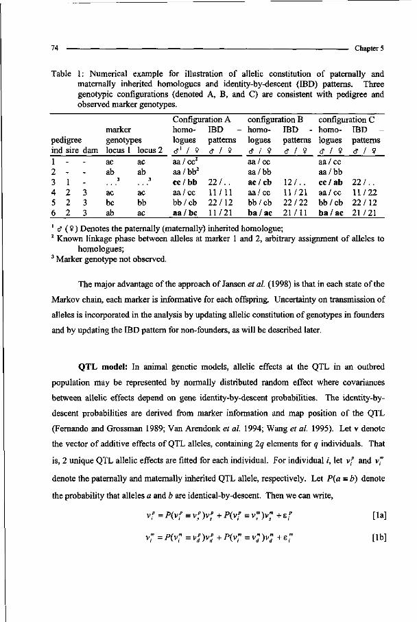
74 Chapter 5
Table 1: Numerical example for illustration of allelic constitution of paternally and maternally inherited homologues and identity-by-descent (IBD) patterns. Three genotypic configurations (denoted A, B, and C) are consistent with pedigree and observed marker genotypes.
pedigree ind sire dam 1 - -2 - -3 1 -4 2 3 5 2 3 6 2 3
marker genotypes locus 1 ac ab
3
ac be ab
locus 2 ac ab
3
ac bb ac
Configuration A homologues dl 1 9 aa/cc2
aa/bb2
cc/bb aa/cc bb/cb aa/bc
IBD -patterns a / 9
2 2 / . . 11/11 22/12 11/21
configuration B homologues a 1 9 aa/cc aa/bb ac/cb aa/cc bb/cb ba/ac
IBD -patterns d- / 9
1 2 / . . 11/21 22/22 21/11
configuration C homologues <? / 9 aa/cc aa/bb cc/ab aa/cc bb/cb ba/ac
IBD -patterns a 1 9
2 2 / . . 11/22 22/12 21/21
1 <5 ( 9 ) Denotes the paternally (maternally) inherited homologue; 2 Known linkage phase between alleles at marker 1 and 2, arbitrary assignment of alleles to
homologues; 3 Marker genotype not observed.
The major advantage of the approach of Jansen et al. (1998) is that in each state of the
Markov chain, each marker is informative for each offspring. Uncertainty on transmission of
alleles is incorporated in the analysis by updating allelic constitution of genotypes in founders
and by updating the IBD pattern for non-founders, as will be described later.
QTL model: In animal genetic models, allelic effects at the QTL in an outbred
population may be represented by normally distributed random effect where covariances
between allelic effects depend on gene identity-by-descent probabilities. The identity-by-
descent probabilities are derived from marker information and map position of the QTL
(Fernando and Grossman 1989; Van Arendonk et al. 1994; Wang et al. 1995). Let v denote
the vector of additive effects of QTL alleles, containing 2q elements for q individuals. That
is, 2 unique QTL allelic effects are fitted for each individual. For individual i, let vf and v™
denote the paternally and maternally inherited QTL allele, respectively. Let P(a = b) denote
the probability that alleles a and b are identical-by-descent. Then we can write,
v," = Piyf m vƒ )vf' + P(v," m v," )vsm + s,' [la]
v," = W S V ; K +P(v,m = v ; )v ; +8," [it>]

Detection of QTL with incomplete marker data 75
where, s, d denote the sire and dam of the individual, and ef ,e" are residuals. When the
QTL is located between marker k and k + 1 and IBD pattern for these markers is known, then
the probability of IBD for the QTL can be represented as,
IBDikx IBD,
(1 ~h,qa ) * ( l -V* + i ) l
1 P(vf , ) * (l-r*,,„)x(V,*+i)
K , « ) x ( l - V w ) 2
(r*,„,)x(v*+i) 2
i,t+l,Jt
1
2
1
2
[2]
where, x = p, or m if the parent considered is the sire or dam, respectively, and r^q„ is the
recombination fraction between marker k and the QTL. For example, IBDiXp=\ means that
for individual i at the A* marker the paternally inherited allele is identical by descent to the
first allele in its sire (where the latter is the paternal allele within the sire). For simplicity, we
assume recombination fractions to be equal in males and females. The
probabilityP(v' = vmpareM) equals 1-P(v' = vp
parenl). The residuals ef,s™ are bivariate
normally distributed, that is
N 0 of 0
[3]
where
1 - \p(vr = v;)f + {2 x P(vf = vf) x P(v," = v,") x P{yps = v,")} + {p(vf = V;)}2>
vl _ {P(vr ^ v;)j2 + j 2 x PW = v;) x Ptf = v,7) x P(V> S vj)} + {P(v," ^ vj)}:
and, a I is half the additive genetic variance explained by the QTL. When a parent is not
inbred at the QTL, the second probability drops out, (P{vps =v™) = 0 and/or P(yp =VJ) = 0),
and when parent x is unknown, 5 ' = 1. Our model is an approximation to a mixture model in
which the QTL allelic effect is exactly identical to one of the parental QTL allelic effects (see
also Hoeschele et al. 1997 and Jansen et al. 1998). Changes in allelic effects between parent
and (grand) offspring might be due to mutations, or to the fact that a QTL represents a cluster
of closely linked QTL, or to epistatic effects.
Let G denote the gametic relationship matrix for the QTL (2q x 2q) where the (ij)
element represents the probability of QTL allele i being identical by descent to QTL allele j .
Then, the conditional density of v can be given,

76 Chapter 5
( v I G . a ^ l G G ^ x e x p l - X c ^ V G - ' v } [4]
Van Arendonk et al. (1994) presented a recursive algorithm to efficiently construct matrix G
and its inverse G' . Matrix G"1 has a nice sparse structure: The non-zero elements in G"1
pertaining to an individual's QTL allelic effect arise from its own contribution (to its parents)
plus those of its offspring, i.e., its neighborhood set (e.g., Sheehan and Thomas 1993). The
determinant of G"1 and the term vrG"'v can be efficiently computed using partitioned matrix
theory (Searle 1982). After some algebra, the conditional density of v is,
/»(v|G,oj)
«n(|(sr)>|(srr|)xexp|-KcT;2|:((ôrr x(v; -?>?+&y x(v; -v;)2)J
where v/ = P(yxk = v^Jv^ + P(vx
k = v™ renl )v™ rml with parent being a sire or dam for x
being the paternal or maternal derived allele of the individual, respectively. And, for
example, the full conditional density of the paternal QTL effect of male i, v ' ,
/ ,(< I G .aJ)« |(6f Y|xexpf-/2a;2(ôf )'' x{vf -v(')2}
r f xnk)"'|xexp -K^2 +Z(ôf)"' x(v,' -v,')
[5]
where O, represents the set of offspring for male /. Equation [5] shows that the full
conditional density for a QTL effect can efficiently be computed and only involves the IBD
patterns of the individual itself and those of its offspring. Equations [2], [3] and [5] are used
to draw samples for elements in v and to compute conditional probabilities in updating
marker genotypes (see also Bink et al. 1998a, equation [6]).
Updating of marker genotypes
Three classes of individuals are distinguished when updating genotypic information:
(1) Genotyped founders (with offspring); (2) Genotyped non-founders; and (3) Ungenotyped
parents (ungenotyped non-parents are not considered). Examples in Table 1 of each category
are individual 1 and 2, individual 4,5 and 6, and individual 3, respectively. The sampling of
genotypes is described for each of these categories in the subsequent section.
Category 1: genotyped founders. In order to take all possible linkage phases in the
genotypes of genotyped founders into account, linkage phases are sampled interval by
Detection of QTL with incomplete marker data 77
interval and founder by founder, as suggested by Jansen et al. (1998). For a particular set of 2
neighboring markers, e.g., j and (/' + 1), one can use information on the individual and its
offspring (their IBD values) to calculate the conditional probabilities for two options "phase
switch" and "no phase switch" and subsequently sample one of the options. In case of a
phase switch, the distal part of its homologue 1 (marker j+\ to end) is attached to the
proximal part of homologue 2 (map origin to marker j) and vice versa. Also, the IBD values
at the distal part of the chromosome in its offspring are switched (1 becomes 2 and vice
versa).
Updating of linkage phase for the marker interval containing the QTL actually
involves two interval updates, i.e., the interval "left flanking marker - QTL" and "QTL - right
flanking marker". The conditional probabilities of the two linkage phases now also include
information from the random QTL, using equation [5] (the QTL has no IBD patterns). For
the left interval, the option "phase switch" involves a switch in founder QTL effects. This
affects the computation of equation [5] and in case of a phase switch the founder QTL effects
do switch (nothing changes for the QTL effects in its offspring). For the right interval, order
of QTL effects within a founder is unaffected.
Category 2: genotyped non-founders. To generate complete genotypes of non-
founders, one can sample a new IBD pattern given the genotypes of parents. This can be
done individual by individual and marker locus by marker locus. If we update the IBD at a
certain marker locus, then the two flanking marker loci (with "known" IBD) are fully
informative and no other marker loci are needed. One considers at most 4 IBD patterns (2 per
known parent), discarding the ones inconsistent with the individual's marker score. The IBD
values of the individual's offspring are used when one of the consistent IBD patterns for the
individual involves an allelic switch in the individual. When only one parent is known,
population allelic frequencies are used. When the individual's alleles are switched
(heterozygous), its offspring' IBD values are switched as well (1 becomes 2 and vice versa).
When a marker flanks the QTL, the conditional probabilities include information of
the QTL by using equation [5] for each consistent IBD pattern.
Category 3: ungenotyped parents. This is the most complicated category since genotypes
should not be updated individual by individual. To illustrate this, suppose a sire with
genotype a / b, an ungenotyped dam, and their two offspring (g0, = a / b, go2 = a / c). Starting
with gd = b / c, the first offspring will have a / b, i.e., the a-allele at its paternal homologue
and the b-allele at its maternal homologue. Then, updating individual by individual will not

78 Chapter 5
allow a switch to the configuration gd = a / c that would be consistent with the first offspring
having b / a instead of a / b. To avoid this problem, we update an ungenotyped parent and its
offspring in a block, allowing an allelic switch in the offspring. This allelic switch needs of
course to be consistent with the other parent's marker genotype. The genotype for the
ungenotyped parent is sampled from its marginal (w.r.t. its offspring) distribution, and the
IBD of its offspring is subsequently updated from its full conditional (w.r.t. parent)
distribution. Updates are done marker locus by marker locus. When one or both parents (of
the ungenotyped parent) are unknown, the conditional probabilities also involve population
allelic frequencies. Note that for an augmented homozygous genotype, the offspring's IBD
value may equal 1 or 2 and both values are taken into account. This also holds for an
augmented heterozygous genotype when parent and offspring have the same alleles. When a
marker flanks the QTL, the conditional probabilities include information from the QTL using
equation [5]. After updating an ungenotyped parent, its genotyped offspring are updated (as
described under category 2).
Allele frequencies. The allelic frequencies at a particular marker locus in a
population are likely unknown and can be treated as such. Let r\mi denote the counts of allele
i at marker locus m at "founder" homologues, i.e., homologues of founders plus the non-
parental homologue of non-founders with only one parent identified. Then, allelic
frequencies at each marker locus can be sampled from a Dirichlet distribution with
parameters r\mi+ 1 (for Dirichlet distribution, see p.482 - Gelman et al. 1995).
Mixed linear model: Let b be a vector of fixed effects, and let u be an q x 1 vector of
residual additive (polygenic) effects (not linked to the marker linkage group under
consideration). Then the model underlying the phenotypes is given as,
y = Xb + Zu + ZTv + e [6]
with b ~ i/[bmin,bmaJ,u ~ JV(0, Aa>),v ~ N(0,Ga2v),e ~ N{0,Ro2
e)
where y is an N x 1 vector of phenotypes, X, Z are known design matrices relating records in
y to fixed effects and to q individuals, T is a known incidence matrix relating each individual
to its two QTL alleles, e is a vector of residuals, bmin, b^ are vectors with minimum and
maximum values for fixed effects, A is the additive genetic relationship matrix (e.g.,

Detection of QTL with incomplete marker data 79
Henderson 1988), a 2 is the polygenic variance, R is a known diagonal matrix, a 2 is the
residual variance.
The model is parameterized in terms of the heritability(A2 =cr2 / a 2 ) , proportion of
the additive genetic variance due to the QTL (y = 2a 2 / a 2 ) and residual variance ( c 2 ) ,
wherea2 is the additive genetic anda2 is the phenotypic variance. In the remainder of the
paper y will be referred to as proportion QTL. In this study, the QTL position relative to the
origin of the marker map is assumed known, but this assumption may be removed as shown
by Bink et al. (1998c).
Prior knowledge on dispersion parameters: Different priors may be useful to explore
the amount of information coming from the data for a particular parameter in the model. In a
previous study, Bink et al. (1998b) showed that the posterior density of y was clearly affected
by using different Beta distributions to represent prior knowledge on the proportion of QTL (
y), indicating lack of information on y from the data. In this study, two Beta distributions are
considered to represent prior knowledge on y. A Beta (1,1) prior is uniform between 0 and 1
with mean equal to 0.5, and will be denoted UNIFORM. A Beta (1,9) prior has the mode at
zero with mean equal to 0.10, and will be denoted PEAKED AT ZERO. Based on Bink et al.
(1998b), priors on h2 and a] were taken uniform over the interval [0,l] and [0,oo),
respectively.
Implementation of MCMC sampling: Bayesian inferences about the parameters are
here computed using the Gibbs sampler and the Metropolis Hastings (MH) algorithm
(Metropolis et al. 1953; Hastings 1970) based on the joint posterior distribution of the
missing data and the parameters given the observed data (y) and marker data (m). The
missing data are the fixed effects (b), the random QTL (v) and polygenic (u) effects, and
marker genotypes (i.e., linkage phase between alleles at the markers and marker scores for
ungenotyped individuals). Now let 9 denote |b,u, v, h2,y,a2}.
To reduce the number of genetic effects that must be sampled (in a granddaughter
design), a Reduced Animal Model (RAM, Quaas and Pollak 1980) is used. That is, the
genetic effects of ungenotyped granddaughters are absorbed into the parental genetic effects,
as described by Bink et al. (1998b).
The sampling distributions for all elements in 6 are similar to those in Bink et al.
(1998b). For location parameters b, u, and v, the full conditional densities are Normals and

80 Chapter 5
values are drawn by using the Gibbs sampler. A scalar-wise sampling strategy may lead to
slow convergence of the Markov chain (Smith and Roberts 1993), especially when elements
in 0 are highly correlated. A full block sampling strategy, i.e., sample all correlated elements
in 0 at once, may improve convergence significantly (Liu et al. 1994), but may also be hard
to implement in animal breeding applications (Garcia-Cortes and Sorensen 1996). Within the
RAM, block sampling, as proposed by Janss et al. (1995) is applied to polygenic effects of
grandsires together with those of their sons. Block sampling (again within the RAM) is also
applied to the QTL effects of grandsires together with the paternally derived QTL effects in
their sons and also to the QTL effects of elite dams together with maternally derived QTL
effects of their sons. First a new realization is drawn for the parental effect from the reduced
conditional density, after absorption of genetic effects of sons. Secondly, new realizations are
drawn for the sons, conditional on the new value of the parental genetic effect.
The full conditional density for a2e is an inverse chi-squared distribution with degrees
of freedom equal to (dim(e) - 2), and sampling is done via the Gibbs sampler. The sampling
distributions for h2 and y are non-standard and samples of these parameters are obtained using
MH-algorithms (Bink et al. 1998b). In the MH algorithms for updating h2 and y, we used the
random walk approach as candidate generating density (Chib and Greenberg 1995). Length
of sampling intervals in the random walk need to be empirically determined to arrive at
desired acceptance rates, e.g., between 0.20 and 0.50 (see Chib and Greenberg 1995).
Data simulation: In this study, we simulated the segregation of a QTL in a
granddaughter design. The pedigree material consisted of 20 unrelated grandsires, 400 elite
dams, and 800 sons, equally distributed over the 20 grandsires. Two hundred elite dams were
daughters of randomly assigned grandsires and the remaining 200 were unrelated to the
grandsires. There were no maternal relationships between dams. Dams may have 1, 2, 3, 4, 5,
or 6 sons with probability 0.50, 0.25, 0.10, 0.075, 0.050 and 0.025, respectively (relaxing
fixed probabilities, a truncated Poisson distribution may apply). Mating of dams with
grandsires was at random, but father-daughter mating was avoided. As a result of this
strategy approximately 300 dams are related to at least 2 males in the pedigree (e.g., multiple
sons and/or elite sire). About 400 sons are also maternal grandsons of grandsires. These
numbers approximately reflect a Dutch granddaughter experiment design as described by
Spelman et al. (1996). Polygenic and QTL effects for grandsires and founder-dams, were

Detection of QTL with incomplete marker data 81
sampled from N(0,CT^) and N(0,CTJ), respectively. The polygenic effect of individual i is
simulated as u-L = \ [us ; + wD, )+ <j>, where uSi and uDi are the polygenic effects of the sire and
dam of individual i, respectively. When individual i has unknown parents, zeros are
substituted for usi and uDi. The term <j> represents Mendelian sampling that follows a Normal
distribution with mean zero and variance equal to .50 a2,, .75a], or I.OCT2,, when 2, 1 or 0
parents are known. Inheritance of QTL effects (and the linked marker alleles) from parent to
offspring occurred at random. When a parent is unknown the QTL effect is drawn from N (0,
a I ). Individual phenotypes, observed on 100 daughters for each son, were generated as
v~ N[{^US +pvls +(i-p)v^(iCT2 +al + a2)),
where p is a 0/1 variable. No phenotypes were simulated for dams. The phenotypic variance
and the heritability of the trait were equal to 100 and 0.40, respectively. The proportion of
genetic variance due to the QTL (= y) was equal to 0.10 or 0.25, representing a small and
large QTL, respectively (Table 2).
Table 2: Sets of parameters used in simulation.
Proportion alleles per marker QTL' locus 2
Small QTL, high informative markers 0.10 4 Large QTL, high informative markers 0.25 4 Large QTL, low informative markers 0.25 2
1 Proportion of genetic variance explained by the QTL (y); 2 Alleles have equal frequencies.
For each individual a lOOcM chromosome was simulated with 6 markers at 20 cM
intervals. The position of the QTL was 30 cM from the origin of the linkage group. Each
marker contained either 2 (low informative markers) or 4 (high informative markers) alleles
with equal frequencies, assuming Hardy-Weinberg equilibrium within marker alleles and
linkage equilibrium between alleles of different markers (Table 2).
Approaches to analyze data from granddaughter designs: Marker data in
granddaughter design typically comprise marker genotypes for grandsires and their sons.
Three different approaches for analysis are presented in Table 3. The first approach (denoted
PATRLT) considers only paternal relationships between males in the pedigree, all with
marker genotypes. The second approach (denoted ALL_RLT) considers all relationships
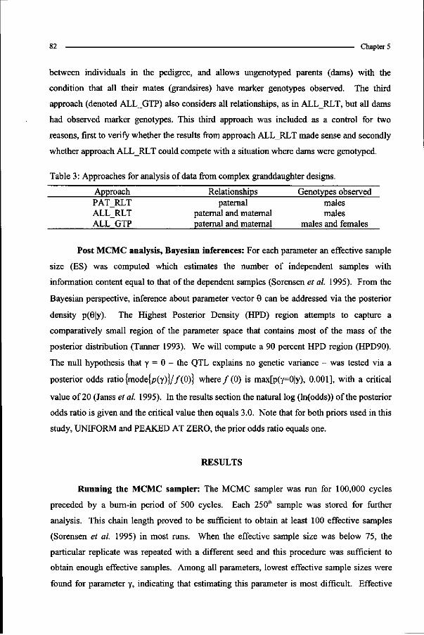
82 Chapter 5
between individuals in the pedigree, and allows ungenotyped parents (dams) with the
condition that all their mates (grandsires) have marker genotypes observed. The third
approach (denoted ALLGTP) also considers all relationships, as in ALL_RLT, but all dams
had observed marker genotypes. This third approach was included as a control for two
reasons, first to verify whether the results from approach ALLRLT made sense and secondly
whether approach ALL_RLT could compete with a situation where dams were genotyped.
Table 3: Approaches for analysis of data from complex granddaughter designs.
Approach Relationships Genotypes observed PATRLT paternal males ALLRLT paternal and maternal males ALL GTP paternal and maternal males and females
Post MCMC analysis, Bayesian inferences: For each parameter an effective sample
size (ES) was computed which estimates the number of independent samples with
information content equal to that of the dependent samples (Sorensen et al. 1995). From the
Bayesian perspective, inference about parameter vector 0 can be addressed via the posterior
density p(0|y). The Highest Posterior Density (HPD) region attempts to capture a
comparatively small region of the parameter space that contains most of the mass of the
posterior distribution (Tanner 1993). We will compute a 90 percent HPD region (HPD90).
The null hypothesis that y = 0 - the QTL explains no genetic variance - was tested via a
posterior odds ratio {mode{p(y)}/ f (0)} where ƒ (0) is max[p(Y=0|y), 0.001], with a critical
value of 20 (Janss et al. 1995). In the results section the natural log (ln(odds)) of the posterior
odds ratio is given and the critical value then equals 3.0. Note that for both priors used in this
study, UNIFORM and PEAKED AT ZERO, the prior odds ratio equals one.
RESULTS
Running the MCMC sampler: The MCMC sampler was run for 100,000 cycles
preceded by a burn-in period of 500 cycles. Each 250th sample was stored for further
analysis. This chain length proved to be sufficient to obtain at least 100 effective samples
(Sorensen et al. 1995) in most runs. When the effective sample size was below 75, the
particular replicate was repeated with a different seed and this procedure was sufficient to
obtain enough effective samples. Among all parameters, lowest effective sample sizes were
found for parameter y, indicating that estimating this parameter is most difficult. Effective

Detection of QTL with incomplete marker data 83
sample sizes decreased for smaller QTL and for lower informative markers (Table 4). The
prior density of y did not seriously affect the effective sample size (Table 4). The MCMC
sampler was run on a HP 9000 K260 server, computing time of a single chain for approach
PATRLT, ALLRLT, and ALL_GTP were 23 minutes, 2 hours 12 minutes, and 1 hour 1
minute, respectively. This indicates that the updating marker haplotypes and IBD patterns for
ungenotyped individuals was the most time consuming part of the MCMC sampler.
Parameter estimates: Heritability. In all replicates, estimates for parameters h2 and
a2 were very accurate, independent of approach or size of y. For example, for data with a
large QTL and low informative markers, the posterior mean estimates of h2 (simulated 0.40)
were, averaged over 10 replicates, 0.393, 0.394, and 0.394 for approach PAT_RLT,
ALL_RLT, and ALLGTP, respectively. The averages of estimates of the posterior standard
deviation were 0.023, 0.022, and 0.023 for approach PAT_RLT, ALL_RLT, and ALL_GTP,
respectively. Similar levels of accuracy were found for estimates of the residual variance.
The use of individual phenotypes allows a clear dissection of the phenotypic variance into
genetic and residual components. This result was also found by Bink et al. (1998b) and Van
Arendonk et al. (1998), but was not found by others (Thaller and Hoeschele 1996b; Uimari et
al. 1996; and Uimari and Hoeschele 1997) which used the average phenotype of daughters of
a sire instead of all individual phenotypes.

84 Chapter 5
Table 4: Average effective samples (ES), average posterior mean estimates (mean), average posterior standard deviations (mean), and the average In of the odds ratio test statistic (ln(odds)) across 10 replicates for proportion QTL (y). Simulated proportion QTL was small (y=0.10) or large (y=0.25), and information content per marker was high (n=4) or low (n=2). Prior knowledge on proportion QTL (y) was UNIFORM or PEAKED AT ZERO.
prior (y) = UNIFORM ES mean sd
Small QTL, high informative markers PAT RLT 134 0.15 0.08 ALL RLT 101 0.12 0.06 ALL GTP 132 0.12 0.05
Large QTL, high informative markers PAT RLT 192 0.29 0.12 ALL RLT 280 0.25 0.07 ALL GTP 253 0.25 0.07
Large QTL, low informative markers PAT RLT 110 0.29 0.15 ALL RLT 121 0.26 0.09 ALL GTP 158 0.27 0.08
ln(odds)1'2
2.69 5.58 6.53
5.67 8.31 8.68
3.46 7.04 8.50
(7) (3) (1)
(2) (0) (0)
(5) (0) (0)
prior ES
117 106 119
179 218 211
113 110 149
(y) = PEAKED AT ZERO mean
0.10 0.10 0.10
0.19 0.21 0.21
0.15 0.19 0.20
sd
0.06 0.04 0.04
0.07 0.06 0.06
0.08 0.07 0.07
ln(odds)1'2
2.20 (7) 5.18 (3) 6.16 (1)
6.09 (1) 8.47 (0) 8.88 (0)
3.04 (6) 7.09 (0) 7.22 (1)
1 ln(odds) = ln(posterior mode (y) / posterior (y=0)); 2 Number of replicates with ln(odds) below the critical value of 3.0.
Small QTL, high informative markers: The marginal posterior density was flatter and
shifted towards the mean of the UNIFORM prior (0.5), when using only paternal
relationships compared to using all relationships (Figure 1). The posterior density for
PATRLT was more similar to those of the other two approaches when using the PEAKED
AT ZERO prior. Including all relationships lead posterior densities with a smaller standard
deviation, that is higher accuracy of estimates. Including genotypes for dams (ALLGTP) did
not further improve the accuracy. Including all relationships lead to smaller estimated
HPD90 regions for Y (Figure 1). The HPD90 regions were smaller when the PEAKED AT
ZERO prior was used, especially when only paternal relationships were considered. Averaged
over 10 replicates, the posterior mean of y for approach PAT_RLT and the UNIFORM prior
was 0.15, which was clearly larger than the simulated value (0.10). Apparently, the data did
not provide sufficient information to reduce the effect of the UNIFORM prior, which has an
expected mean of 0.5. When the PEAKED AT ZERO prior on y was used, estimated
posterior mean was equal to the simulated value, which is also the expected mean of the prior.
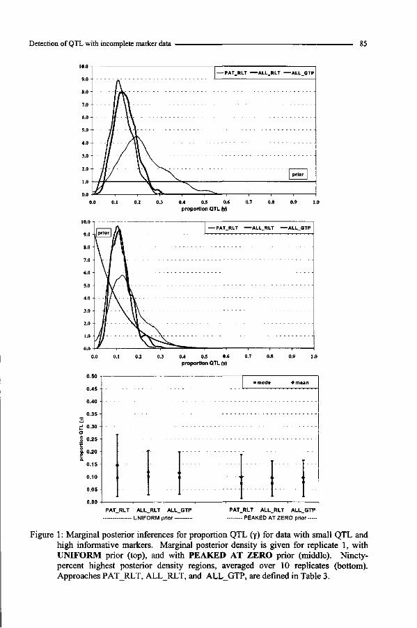
Detection of QTL with incomplete marker data 85
0.50
0.45
0.40
0.35 -
J 0.30 O | 0.25
| ° '20 Q.
0.15
0.10
0.05
0.00
0.4 0.5 0.6 proportion QTL (y)
•
• mode • mean
i
' 1 •
- -> <-
PAT_RLT ALL_RLT ALL_GTP UNIFORM prior
PAT_RLT ALL_RLT ALL_GTP PEAKED AT ZERO prior-—
Figure 1 : Marginal posterior inferences for proportion QTL (y) for data with small QTL and high informative markers. Marginal posterior density is given for replicate 1, with UNIFORM prior (top), and with PEAKED AT ZERO prior (middle). Ninety-percent highest posterior density regions, averaged over 10 replicates (bottom). Approaches PATRLT, ALL_RLT, and ALLGTP, are defined in Table 3.

86 Chapter 5
proportion QTL (7)
0.50 -
0.45 -
0.40 -
0.35-
J 0.30 -O g 0.25 c I 0.20 0.
0.15 -
0.10 -
0.05 -
0.00 -
-
- i f I 1
• mode «mean
r •
1
1
1 ' • • • 1 1
PAT.RLT ALL_RLT ALL_GTP UNIFORM prior
PAT_RLT ALL_RLT ALL_GTP PEAKED AT ZERO prior
Figure 2: Marginal posterior inferences for proportion QTL (y) for data with large QTL and high informative markers. Marginal posterior density is given for replicate 1, with UNIFORM prior (top), and with PEAKED AT ZERO prior (middle). Ninety-percent highest posterior density regions, averaged over 10 replicates (bottom). Approaches PAT_RLT, ALL_RLT, and ALL_GTP, are defined in Table 3.

Detection of QTL with incomplete marker data 87
0.50
0.45
0.40
0.35
fj 0.30 O | 0.25
o o °-20
a 0.15
0.10
0.05
0.00
] , '
• mode •mean
I
I
i
I
I
I
PAT RLT ALL RLT ALL GTP PAT_RLT ALL.RLT ALL_GTP
- U N I F O R M prior - - PEAKED AT Z E R O prior -
Figure 3: Marginal posterior inferences for proportion QTL (y) for data with large QTL and low informative markers. Marginal posterior density is given for replicate 1, with UNIFORM prior (top), and with PEAKED AT ZERO prior (middle). Ninety-percent highest posterior density regions, averaged over 10 replicates (bottom). Approaches PATRLT, ALLRLT, and ALL_GTP, are defined in Table 3.
88 Chapter 5
Large QTL, high informative markers: In approach PAT_RLT, the marginal posterior
density for parameter y was relatively flat when the UNIFORM prior was used (Figure 2).
The marginal posterior density for y was clearly shifted towards zero when applying the
PEAKED AT ZERO prior in approach PATRLT. The other two approaches (ALLRLT
and ALLGTP) gave similar and more stable densities with the two priors for y, indicating
more information coming from the data compared to PAT_RLT. The HPD90 region was
largest for approach PATRLT with an UNIFORM prior (Figure 2). The PEAKED AT
ZERO prior led to a downward shift of the HPD90 regions, in particular for approach
PATRLT. The PEAKED AT ZERO prior led also to estimated posterior mean that were
smaller than the simulated values for all approaches (Table 4). The UNIFORM prior led to
an upward bias in the estimated posterior mean for approach PAT_RLT but not for the other
approaches.
Large QTL, low informative markers: Low informative markers (2 alleles per locus)
resulted in relatively flat posterior densities for y (Figure 3), but differences were observed
between the three approaches. The use of all relationships improved the accuracy, but in this
case the use of all genotypes gave an additional improvement over ALL_RLT. The
PEAKED AT ZERO prior led to posterior densities that were closer to zero in all approaches
but especially for PAT_RLT. The estimated HPD90 region was again largest for approach
PATRLT with the UNIFORM prior. The HPD90 regions for approaches ALLGTP and
ALLRLT were very similar for UNIFORM prior. However, the HPD90 region for approach
ALLRLT was shifted more towards zero than the region for approach ALL_GTP with the
PEAKED AT ZERO prior (Figure 3). The posterior mean estimates were all higher than the
simulated value for the UNIFORM prior and below the simulated value for the PEAKED AT
ZERO prior. Differences between estimated and simulated value were largest for approach
PAT_RLT.
Hypothesis testing, detection of QTL: The hypothesis of the presence of a QTL at a
particular position in a linkage map was tested via a posterior odds ratio. For a small QTL
the ln(odds), averaged over 10 replicates, for approach PATREL was 2.69, which was below
the critical threshold of 3.0. For approach PATREL only 3 out of 10 replicates yielded
significant evidence for the presence of a QTL (Table 4). This was very similar to the power
of QTL detection found by Bink et al. (1998b). Approach ALLRLT resulted in an average

Detection of QTL with incomplete marker data 89
ln(odds) of 5.58 and the QTL was significantly detected in 7 out of 10 replicates. Approach
ALLGTP only failed to significantly detect the small QTL in one of the replicates.
For a large QTL and high informative markers, approach PAT_RLT was detected the
QTL in at least 8 out of 10 replicates, i.e., 2 and 1 failures for UNIFORM and PEAKED AT
ZERO prior, respectively (Table 4). The approaches ALL_RLT and ALL_GTP detected the
QTL in all replicates. The average ln(odds) was clearly higher for the large QTL. Note that
the posterior odds of approach ALL_RLT for a small QTL (ln(odds)=5.64) was even a little
higher than the posterior odds of approach PATRLT for a large QTL (ln(odds)=5.58), when
high informative markers were considered.
Reducing heterozygosity of the markers resulted in lower averaged estimates of the
ln(odds) for all cases. The detection rate for approach PATRLT with low informative
marker was 50 percent or lower depending on the prior (Table 4). In all except one case, the
QTL was still significantly detected by approaches ALLRLT and ALL_GTP.
DISCUSSION
A variety of statistical gene mapping methods have been developed and applied to
outbred populations (see Bovenhuis et al. 1997; Hoeschele et al. 1997). Computationally
inexpensive methods, such as regression interval mapping, allow data permutation to
determine genome-wide threshold values for test statistics and can be extended more easily to
incorporate multiple QTLs; however, these methods can only use certain types of relatives
(e.g., half-sibships or full-sibships). Bayesian analysis is computationally more demanding
but takes fully account of the uncertainty associated with all unknowns in the QTL mapping
problem and offers the opportunity to analyze general pedigree data and to fit other random
components such as polygenic effects (e.g. Thaller and Hoeschele 1996a). Bayesian linkage
analysis has been applied in animals (e.g. Thaller and Hoeschele 1996a; Uimari et al. 1996),
plants (e.g. Satagopan et al. 1996) and humans (e.g., Thomas and Cortessis 1992).
Application of these methods to large pedigrees with missing genotypes, as described in this
paper, has not been explored in depth (Hoeschele et al. 1997). The procedures of Janss et al.
(1995), i.e., block sampling of ungenotyped dams and their offspring, and Jansen et al.
(1998), i.e., sampling IBD patterns, were implemented in order to achieve good mixing of the
sampler in the full pedigree analysis with incomplete marker information. To accommodate
missing marker data, special precautions need to be taken for the sampling procedure to avoid

90 Chapter 5
reducibility, i.e. not all possible genotype configurations can be reached from any valid
starting configuration. Reducibility especially occurs in situations in which offspring are
genotyped but both parents are not. In livestock, the number of offspring per sire is usually
large and genetic material from males is often stored which facilitates genotyping of the male
parent. When genetic material is not available, genotypes of males can often be inferred from
its offspring. In the present study, it is assumed that marker genotypes on at least one parent
are known. This is assumption is not limiting the application of the presented approach to
livestock, but it might be limiting in situations where family sizes are smaller. Sheehan and
Thomas (1993) allowed non-Mendelian segregation of alleles (e.g., genotype AB transmitting
allele C) to solve the theoretical reducibility. Inferences were based on samples from only
those Gibbs cycles with strict Mendelian segregation, which may be an inefficient procedure
in large animal breeding populations. Instead of fixing the non-Mendelian segregation
probability, one may implement a simulated tempering scheme (Geyer and Thompson 1995)
that allows this probability to randomly increase from and decrease to zero.
Uimari et al. (1996), Grignola et al. (1996b) and Hoeschele et al. (1997) investigated
the effect of ignoring relationships among families on estimates of QTL location and genetic
parameters. Virtually no difference was found between analyses with and without
relationships between families for situations with much and little information about the QTL.
In our study a large impact of including additional relationships was found (Table 4). This
apparent discrepancy with literature can be explained by the relationships considered. In the
earlier studies, relationships between the grandsires were included which leads to additional
information on estimating the paternally inherited QTL alleles. In the present study, the
ungenotyped dams of the sons were included which provides information for estimating the
maternally inherited QTL alleles. The impact of including additional relationships is clearly
demonstrated in Figures 1 to 3. Including additional relationships resulted in improved
estimates of parameter y, i.e., lower posterior standard deviations and smaller HPD90 regions,
(Table 4, Figure 1 to 3). These results strongly suggest that including all relationships in
complex pedigrees does improve power of QTL detection.
The pedigree we analyzed consisted of close to 100,000 individuals. The largest
proportion of individuals was offspring of sires that only had phenotypic records. The
dimensional complexity of the problem was reduced by applying a reduced animal model
(Quaas and Pollak 1980) in which genetic effects of ungenotyped non-parents are absorbed
into those of their parents as presented by Bink et al. (1998b). The procedure presented in
Detection of QTL with incomplete marker data 91
this paper which applies a reduced animal model, offers the opportunity to combine the
information from different experimental designs, e.g., a granddaughter design, a grand-
granddaughter design (Coppieters et al. 1998), or a daughter design and also the information
collected with a closed breeding population spanning several generations. Despite higher
computational requirements, the application of a RAM in a Bayesian context more naturally
treats missing genotypes than the restricted maximum likelihood procedures described by
Grignola et al. (1996a).
In this study, we assumed a fixed QTL position relative to known markers. Bink et al.
(1998c) showed that the position of the QTL can be included as an additional parameter in the
model. Appropriate sampling of QTL position was facilitated through the use of simulated
tempering (Geyer and Thompson 1995). Simulated tempering, which has also been applied
in radiation hybrid mapping (Heath 1997b), proved especially useful to improve mixing by
relaxing the distance between closely linked loci. An alternative approach to estimate QTL
location within a marker linkage map was presented by George et al. (1998). They
implemented the reversible jump sampler (Green 1995) to order a bi-allelic QTL relative to
multiple markers via model choice.
In conclusion, the work presented shows that detection of QTL in data from
complex pedigrees is feasible by the use of MCMC and Bayesian analysis. It is shown that
utilizing all existing relationships increases the power of detection and the accuracy of the
estimates. This work also lays the foundation to study the number of QTL and their relative
positions within marker linkage maps.
ACKNOWLEDGMENTS
The authors thank Ritsert Jansen, Luc Janss, Henk Bovenhuis, and Dick Quaas for
stimulating discussion. The authors acknowledge financial support from Holland Genetics.
REFERENCES
Andersson L, Haley CS, Ellegren H, Knott SA, et al. (1994) Genetic mapping of quantitative trait loci for growth and fatness in pigs. Science 263:1771 -1774
Barendse W, Armitage SM, Kossarek LM, Shalom A, et al. (1994) A genetic linkage map of the bovine genome. Nature Genetics 6:227-235
92 Chapter 5
Bink MCAM, Van Arendonk JAM, Quaas RL (1998) Breeding value estimation with incomplete marker data. Genet Sel Evol 30:45-58
Bink MCAM, Quaas RL, Van Arendonk JAM (1998b) Bayesian estimation of dispersion parameters with a reduced animal model including polygenic and QTL effects. Genet Sel Evol (accepted)
Bink MCAM, Janss LLG, Quaas RL (1998c) Mapping a Polyallelic Quantitative Trait Locus using Simulated Tempering. Proc 6lh World Congr Genetics Appl Livest Prod Sei, Armidale, Australia 26: 277-280
Bovenhuis H, Van Arendonk JAM, G Davis G, Elsen JM, et al (1997) Detection and mapping of quantitative trait loci in farm animals. Livest Prod Sei 52:135-144
Chib S, Greenberg E (1995) Understanding the Metropolis Hastings algorithm. Am Stat 49: 327-335
Coppieters W, Kvasz A, Arranz JJ, Grisart B, Riquet J, et al. (1998) The grand-granddaughter design: a simple strategy to increase the power of a granddaughter design, (submitted)
Fernando RL, Grossman M (1989) Marker-assisted selection using best linear unbiased prediction. Genet Sel Evol 21:467-477
Garcia-Cortes LA, Sorensen D (1996) On a multivariate implementation of the Gibbs sampler. Genet Sel Evol 28:121-126
Gelfand AE, (1994) Gibbs sampling (A contribution to the Encyclopedia of Statistical Sciences). Technical Report, Department of Statistics, University of Connecticut
German A, Carlin JB, Stern HS, Rubin DB (1995) Bayesian data analysis. Chapman & Hall, London, UK
Geman S, Geman D (1984) Stochastic relaxation, Gibbs distributions and the Bayesian restoration of images. IEEE Trans Pattern Anal Machine Intelligence 6:721-741
George AW, Mengersen KL, Davis GP (1998) A Bayesian analysis of a QTL under a half-sib design. Proc 6lh
World Congr Genetics Appl Livest Prod Sei, Armidale, Australia 26:225-228
Georges M, Nielsen D, Mackinnon M, Mishra A, Okimoto R et al (1995) Mapping quantitative trait loci controlling milk production in dairy cattle by exploiting progeny testing. Genetics 139:907-920
Geyer CJ, Thompson EA (1995) Annealing Markov chain Monte Carlo with applications to ancestral inference. J Am Stat Ass 90:909-920
Green PJ (1995) Reversible jump Markov chain Monte Carlo computation and Bayesian model determination. Biometrika 82:711-732
Grignola FE, Hoeschele I, Tier B (1996a) Mapping quantitative trait loci via Residual Maximum Likelihood: I. Methodology. Genet Sel Evol 28:479-490
Grignola FE, Hoeschele I, Zhang Q, Thaller G (1996b) Mapping quantitative trait loci via Residual Maximum Likelihood: II. A simulation study. Genet Sel Evol 28:491-504
Guo SW, Thompson EA (1992) A Monte Carlo method for combined segregation and linkage analysis. Am J HumGenet51:llll-1126
Hastings WK (1970) Monte Carlo sampling methods using Markov chains and their applications. Biometrika 57:97-109
Heath SC (1997a) Markov chain Monte Carlo segregation and linkage analysis for oligogenic models. Am J Hum Genet 61:748-760
Heath SC (1997b) Markov chain Monte Carlo methods for radiation hybrid mapping. J Comp Biology 4:505-515
Henderson CR (1988) Theoretical basis and computational methods for a number of different animal models. J DairySci71:(Suppl2) 1-16
Hoeschele I, Uimari P, Grignola FE, Zhang Q, Gage KM (1997) Advances in statistical methods to map quantitative trait loci in outbred populations. Genetics 147:1445-1457
Jansen, RC, Johnson DL, Van Arendonk JAM (1998) A mixture model approach to the mapping of quantitative trait loci in complex populations with an application to multiple cattle families. Genetics 148:391-399
Janss LLG, Thompson R, Van Arendonk JAM (1995) Application of Gibbs sampling in a mixed major gene -polygenic inheritance model in animal populations. Theor Appl Genet 91:1137-1147

Detection of QTL with incomplete marker data 93
Lander ES, Botstein D (1989) Mapping Mendelian factors underlying quantitative traits using RFLP linkage maps. Genetics 121:185-199
Liu JS, Wong WH, Kong A (1994) Covariance structure of the Gibbs sampler with applications to the comparisons of estimators and augmentation schemes. Biometrika 81:27-40
Metropolis N, Rosenbluth AW, Rosenbluth MN, Teller H, Teller E (1953) Equations of state calculations by fast computing machines. J Chem Physics 21:1087-1091
Paterson AH, Lander ES, Hewitt JD, Peterson S, Lincoln SE, et al. (1988) Resolution of quantitative traits into Mendelian factors by using a complete linkage map of restriction fragment polymorphisms. Nature 335:721-726
Quaas RL, Pollak EJ ( 1980) Mixed model methodology for farm and ranch beef cattle testing programs. J Anim Sei 51:1277-1287
Satagopan JM, Yandell BS, Newton MA, Osborn TC (1996) A Bayesian approach to detect quantitative trait loci using Markov chain Monte Carlo. Genetics 144:805-816
Searle SR ( 1982) Matrix algebra useful for statistics. John Wiley & Sons, New York, NY
Sheehan N, Thomas A (1993) On the irreducibility of a Markov chain defined on a space of genotype configurations by a sampling scheme. Biometrics 49:163-175
Sillanpää MJ, Arjas E (1998) Bayesian mapping of multiple quantitative trait loci from incomplete inbred line cross data. Genetics 148:1373-1388
Smith AFM, Roberts GO (1993) Bayesian computation via the Gibbs sampler and related Markov chain Monte Carlo methods. J R Stat Soc B 55:3-23
Sorensen DA, Andersen S, Gianola D, Korsgaard I (1995) Bayesian inference in threshold models using Gibbs sampling. Genet Sel Evol 27:229-249
Spelman RJ, Coppieters W, Karim L, Van arendonk JAM, et al. (1996) Quantitative trait loci analysis for five milk production traits on chromosome six in the Dutch Holstein-Friesian population. Genetics 144:1799-1808
Stuber CW, Lincoln SE, Wolff DW, Helentjaris T, et al. (1992) Identification of genetic factors contributing to heterosis in a hybrid from two elite maize inbred lines using molecular markers. Genetics 132:823-839
Tanner MA (1993) Tools for Statistical Inference. Ed 2 Springer-Verlag, Berlin
Thaller G, Hoeschele I (1996a) A Monte Carlo method for Bayesian analysis of linkage between single markers and quantitative trait loci: I. Methodology. Theor Appl Genet 93:1161-1166
Thaller G, Hoeschele I, (1996b) A Monte Carlo method for Bayesian analysis of linkage between single markers and quantitative trait loci: II. A simulation study. Theor Appl Genet 93:1167-1174
Thomas DC, Cortessis V (1992) A Gibbs sampling approach to linkage analysis, Hum Hered 42:63-76
Uimari P, Thaller G, Hoeschele I (1996) The use of multiple markers in a Bayesian method for mapping quantitative trait loci. Genetics 143:1831-1842
Uimari P, Hoeschele I (1997) Mapping-linked quantitative trait loci using Bayesian analysis and Markov chain Monte Carlo algorithms. Genetics 146:735-743
Van Arendonk JAM, Tier T, Kinghorn BP (1994) Use of multiple genetic markers in prediction of breeding values. Genetics 137:319-329
Van Arendonk, JAM, Tier B, Bink MCAM, Bovenhuis H (1998) Restricted maximum likelihood analysis of linkage between genetic markers and quantitative trait loci for a granddaughter design. J Dairy Sei (accepted)
Vilkki HJ, De Koning DJ, Elo K, Velmala R, Maki-Tanilla A (1997) Multiple marker mapping of quantitative trait loci in Finnish dairy cattle by regression. J Dairy Sei 80:198-204
Wang CS (1998) Implementation issues in Bayesian analysis in animal breeding. Proc 6'h World Congr Genetics Appl Livest Prod Sei, Armidale, Australia 25:481-488
Wang T, Fernando RL, Van der Beek S., Grossman M, Van Arendonk JAM (1995) Covariance between relatives for a marked quantitative trait locus. Genet Sel Evol 27:251-272

94 Chapter 5
Weller JI, Kashi Y, Soller M (1990) Power of daughter and granddaughter designs for determining linkage between marker loci and quantitative trait loci in dairy cattle. J Dairy Sei 73:2525-2537

Chapter 6
General Discussion

General discussion 97
INTRODUCTION
In this thesis statistical tools have been developed to identify linkage between markers
and quantitative trait loci (QTL) in outbred populations. A Bayesian method for detection of
a segregating QTL in complex pedigrees has been described stepwise. The method has been
implemented via the use of Markov chain Monte Carlo (MCMC) algorithms. First, a method
was proposed for prediction of breeding values when data on a single marker was incomplete,
the size of the QTL and its distance to the marker were known with certainty (chapter 2). It
was shown that for incomplete marker data, the marginal posterior mean estimates for
breeding values differ from the BLUP values. These differences arose because in a Bayesian
analysis, phenotypic trait information contributes to the estimation of conditional
probabilities for marker genotypes, while in BLUP only marker information is used.
When the size and position of the QTL are unknown, these parameters should be
included as unknowns in the genetic model. In chapter 3, the interest was in estimating the
size of the QTL in terms of the proportion of genetic variance explained. A reduced animal
model (RAM) was proposed to facilitate a full pedigree analysis in a granddaughter design
setting, making full use of all information on the genotyped individuals. The genetic effects
of ungenotyped final offspring that only provided trait phenotypes, were absorbed. In chapter
4, the position of the QTL was estimated via implementation of a modified MCMC scheme to
ensure correct mixing of this parameter through its parameter space. In chapter 3 and 4,
restrictions were imposed on the genotypic uncertainties, i.e., it was assumed that all
individuals in the RAM analysis had marker genotypes and that the linkage phase in parents
was known with certainty. In chapter 5, a Bayesian method was described that accounts for
ungenotyped animals and uncertainty on all parameters in the mixed linear model, except the
position of the QTL. In this chapter, the theory developed in chapters 2 and 3 was combined,
and the proposed Bayesian method was empirically tested on simulated data.
In this chapter we first complete the Bayesian method for QTL detection by
combining theory of chapters 4 and 5, and apply this method to four simulated data sets. In a
second section, experimental data from chromosome six in dairy cattle is analyzed for
presence of QTL for milk production traits. Furthermore, the developed Bayesian method for
QTL analysis in complex pedigrees is compared to literature. A brief section on practical
implications for dairy cattle breeding programs completes this chapter.
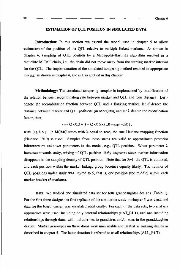
98 Chapter 6
ESTIMATION OF QTL POSITION IN SIMULATED DATA
Introduction: In this section we extend the model used in chapter 5 to allow
estimation of the position of the QTL relative to multiple linked markers. As shown in
chapter 4, sampling of QTL position by a Metropolis-Hastings algorithm resulted in a
reducible MCMC chain, i.e., the chain did not move away from the starting marker interval
for the QTL. The implementation of the simulated tempering method resulted in appropriate
mixing, as shown in chapter 4, and is also applied in this chapter.
Methodology: The simulated tempering sampler is implemented by modification of
the relation between recombination rate between marker and QTL and their distance. Let r
denote the recombination fraction between QTL and a flanking marker, let d denote the
distance between marker and QTL positions (in Morgans), and let X denote the modification
factor, then,
r = (A.)x0.5 + (l-A,)x0.5x(1.0-exp{-2d}),
with 0 < X < 1. In MCMC states with X equal to zero, the true Haldane mapping function
(Haldane 1919) is used. Samples from these states are valid to approximate posterior
inferences on unknown parameters in the model, e.g., QTL position. When parameter X
increases towards unity, mixing of QTL position likely improves since marker information
disappears in the sampling density of QTL position. Note that for X=l, the QTL is unlinked,
and each position within the marker linkage group becomes equally likely. The number of
QTL positions under study was limited to 5, that is, one position (the middle) within each
marker bracket (6 markers).
Data: We studied one simulated data set for four granddaughter designs (Table 1).
For the first three designs the first replicate of the simulation study in chapter 5 was used, and
data for the fourth design was simulated additionally. For each of the data sets, two analysis
approaches were used: including only paternal relationships (PAT_RLT), and one including
relationships through dams with multiple ties to grandsires and/or sons in the granddaughter
design. Marker genotypes on these dams were unavailable and treated as missing values as
described in chapter 5. The latter situation is referred to as all relationships (ALL_RLT).

General discussion 99
Table 1 : Sets of parameters used in simulation
alleles per QTL position Proportion QTL l marker locus 2 (cM)3
Large QTL, high informative markers Large QTL, low informative markers Small QTL, high informative markers Small QTL, low informative markers
0.25 0.25 0.10 0.10
4 2 4 2
30 30 30 30
1 Proportion of genetic variance explained by the QTL (y); 2 Alleles have equal frequencies. 3 Position relative to origin of marker linkage group.
Markov chain Monte Carlo: In total 8 individual MCMC chains (4 data sets x 2
approaches) were run. In the simulated tempering sampler, 44 modified versions were added
to the target density (X = 0), i.e., 45 X's were defined, spanning the interval from 0 to 1. The
values of X's (distances between modified densities) were empirically determined and kept
equal in all MCMC chains. The relative weights (or pseudopriors) of modified densities were
empirically determined for each MCMC chain separately to obtain proper mixing between
the (modified) densities. The equal number and distances between modified densities,
resulted in differences in average acceptance rate of moves between densities. The length of
each MCMC chain was arbitrarily set to 2,000,000 cycles. Computing time per MCMC
chain was 15 and 48 hours on a HP 9000 K260 server, for approach PAT_RLT and
ALL_RLT, respectively.
Sampling densities of other parameters in the model were equal to those in chapter 5.
A PEAKED AT ZERO prior on y (proportion additive genetic variance explained by QTL)
was used in each MCMC chain. The effective sample size (Sorensen et al. 1995) was always
lowest for parameter y and ranged from 357 to 1392.
Results: The presence of a QTL within the marker linkage group was tested via the
posterior odds ratio of p(mode(y)ly) and p(y=0ly) (as previously described in chapters 3, 4
and 5). Presence of a QTL was declared when the ln(odds) statistic exceeded the critical
value of 3.0. Based on this criterion, the presence of a small QTL in the data, with low
informative markers was rejected in the PAT_RLT analysis (ln(odds) of y was 1.5). Table 2
presents the posterior probabilities for QTL position in the four data sets analyzed by the two
approaches. For highly informative markers (4 alleles), the position of the QTL was
accurately estimated, especially for the large QTL. For the latter case, the posterior
probability for the true position (30 cM) was 100% for both PATJRLT and ALL_RLT.

100 Chapter 6
Reduction of the number of alleles at the markers led to less accurate estimation of the QTL
position, especially for the small QTL. Including all relationships improved the accuracy of
QTL position estimates in all cases. When marker heterozygosity decreased, approach
ALL_RLT tended to position the QTL more to the origin of the linkage group, whereas the
approach PAT_RLT tended to position the QTL more to the middle of the linkage group.
The reason for this difference is unclear and might be due to chance since only one replicate
was studied.
Table 2: Posterior probabilities on QTL position.
]
QTL large
large
small
small
Data set marker info
high
low
high
low
approach 2
PAT RLT ALL RLT
PAT RLT ALL RLT
PAT RLT ALL RLT
PAT RLT ALL_RLT
0.10
.00
.00
.07
.35
.02
.04
.05
.34
QTL positi 0.30
1.00 1.00
.41
.60
.79
.88
.26
.47
on (in 0.50
.00
.00
.43
.05
.15
.04
.35
.02
Morgan) ' 0.70
.00
.00
.09
.00
.03
.02
.27
.13
0.90
.00
.00
.00
.00
.01
.01
.07
.04 1 Position relative to origin of marker linkage group. 2 Approaches: PAT_RLT = analysis includes paternal relationships only;
ALL_RLT = analysis includes all relationships, marker genotypes on males.
Discussion: After implementation of the simulated tempering method, mixing of QTL
position over different locations within the marker linkage group was established. For data
with a large QTL and highly informative markers, the MCMC sampler only visited the true
QTL position when sampling from the target density, irrespective of the approach used. For
this data set, one could study the QTL position within the marker bracket. For the other data
sets, one could study multiple positions within several marker brackets, providing more
knowledge on the most likely position of the QTL. Further improvements of the simulated
tempering sampler will allow widespread use. For example, the guidelines provided by
Geyer and Thompson (1995) to determine distances (A,'s) between and weights on modified
densities may be implemented in a software package. This will allow application by less
experienced MCMC users, and less manual efforts in the fine-tuning process.
The results further support the findings in chapter 5 that using all relationships results
in more accurate estimation of QTL parameters. Sophisticated statistical methods that

General discussion 101
naturally treat missing data such as unobserved marker genotypes, are an important
supplement to the analysis of phenotypic and marker data for QTL detection.
DETECTION OF PUTATIVE QTL FOR CHROMOSOME SIX IN DAIRY CATTLE
Introduction: Georges et al. (1995) reported five chromosomes that gave evidence
for the presence of a QTL affecting milk yield in the American Holstein population.
Chromosome six was one of the five chromosomes identified. The QTL on chromosome six
affected milk yield but not fat or protein yield and as a result influenced protein and fat
percent. Bovenhuis and Weiler (1994) reported effects of casein loci and an effect for fat
percent that was linked to the casein locus, which is also found on chromosome six. Spelman
et al. (1996) analyzed data from 20 Dutch Holstein-Friesian families, with a total of 715 sires,
in a granddaughter design for marker-QTL associations. They reported a QTL for protein
percent, significant at the 1 % level. Approximately the same data was released to the animal
breeders community for further analysis and the results on this have been reported by
Bovenhuis et al. (1997). The data for the current study stems from the same granddaughter
experiment, but information from additional sons is available since their daughters obtained
trait phenotypes. First the data is analyzed by the multi-marker approach of Knott et al.
(1994), as extended by Spelman et al. (1996). Secondly, the data on protein percent are
analyzed with the ALL_RLT and PAT_RLT approaches as described earlier. In this study,
we limit ourselves to including relationships via ungenotyped dams, relationships between
grandsires were not included.
Data: Twenty-two grandsire families, with 922 sons, were included in the analysis
(Table 3). All available sons were included, i.e., no correction was made for selection among
sons, or sons not being informative at any marker. Small families were not excluded which
allowed maternal links between members of these families and other families. The data
contained 455 (elite) dams with direct links to at least two male individuals. Fourteen
grandsires were also sires of 399 dams, with a range of 2 to 99 per sire. As a result of this,
these grandsires had in total 653 maternal grandsons. The average number of sons per dam
was 1.8 with a range of 1 to 12.
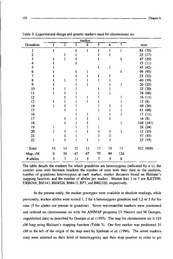
102 Chapter 6
Table 3: Experimental design and genetic markers used for chromosome six.
Grandsire
1 2 3 4 5 6 7 8 9 10 11 12 13 14 15 16 17 18 19 20 21 22
Total Map, cM # alleles
1 1
1
15 0 3
2
1 1
1
14 29 7
3
1 1 1 1
1 1 1 1 1 1 1 1 1 1 1 1 1 1 1 1 1
21 47 11
marker 4
1
1 1 1 1
1 1
1 1 1 1 1
1
13 67 5
5
17 75 7
6
1 1
1
1 1 1 1 1
1 1 1 1
1 1 1
15 89 5
7
1
1
1
1
1 1 1 1 1
1
1
11 124 8
sons
84 (70) 25 (17) 47 (29) 15 (11) 45 (42) 99 (95) 25 (22) 40 (39) 26 (25) 22 (20) 74 (68) 16 (11) 13 (6) 40 (36) 61 (60) 17 (11) 16 (8)
148 (141) 28 (24) 11 (10) 47 (45) 23 (19)
922 (809)
The table details the markers for which grandsires are heterozygous (indicated by a 1), the number sons with between brackets the number of sons with their dam in the analysis, number of grandsires heterozygous at each marker, marker distances based on Haldane's mapping function, and the number of alleles per marker. Marker loci 1 to 7 are ILSTS90, URB016, BM143, BM4528, BM415, BP7, and BM2320, respectively.
In the present study, the marker genotypes were available in absolute readings, while
previously, marker alleles were scored 1, 2 for a heterozygous grandsire and 1,2 or 3 for his
sons (3 for alleles not present in grandsire). Seven microsatellite markers were positioned
and ordered on chromosome six with the ANIMAP programs (D Nielson and M Georges,
unpublished data) as described by Georges et al. (1995). The map for chromosome six is 124
cM long using Haldane's mapping function (Table 3). Our first marker was positioned 31
cM to the left of the origin of the map used by Spelman et al. (1996). The seven markers
used were selected on their level of heterozygosity and their map position in order to get

General discussion 103
more or less equal coverage of the chromosome (Table 3). For these seven markers, 152, 34,
14, 3, and 2 sons did not have marker genotypes available for 1, 2, 3, 4, or 5 loci,
respectively. In the analysis, these missing genotypes are augmented within the MCMC
procedure using both marker and phenotypic information on linked marker loci and related
individuals.
Five traits are analyzed for putative QTL on chromosome six: milk, fat, and protein
yield and fat and protein percent. Only daughters who resulted from the young bull
inseminations (based on date of birth) were included in the analysis. In the analysis, records
on individual daughters, as stored during the animal evaluations conducted by the Royal
Dutch Cattle Syndicate, were used. All records were adjusted for fixed effects and
heterogeneity of variance between herds. In the case of multiple lactations, the permanent
environmental effect was subtracted. For each individual, the average yield over lactations
(maximum of three) and the number of lactations was stored. For the analysis, however,
information on individual lactation production is needed. The sum of squared daughter
deviation can not be determined directly from the average production. Data were adjusted to
account for the reduced variance in mean production with increased number of lactations, and
for permanent environmental effects. Within sire deviations for daughters with two or three
lactations were multiplied with 1.55 and 2.10, respectively. These factors were based on
heritability of 0.33 and repeatability of 0.55 for yield traits. The percentage traits were
calculated from the adjusted yield deviations and the population means (6365 kg milk, 4.42
%fat and 3.45% protein). Information on daughters was weighted to account for the
repeatability of observations on the same animal by using factors 1.000, 1.625 and 1.772
when the daughter produced 1, 2, and 3 lactations, respectively.
Results: An across-family regression analysis (similar to Spelman et al. 1996) for
five traits again revealed a possible QTL for protein percent positioned at 47 cM, i.e., the
location of the third marker (Figure 1). This is the same position as reported by Spelman et
al. 1996). At position 47 cM, test statistics for milk, fat, and fat percent also showed peaks,
however, the effects were not significant. No significant QTL was found for protein percent
or for other traits at other positions.
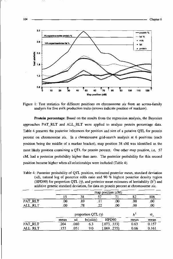
104 Chapter 6
•a 2.3
50 60
Map position (cM)
Figure 1: Test statistics for different positions on chromosome six from an across-family analysis for five milk production traits (arrows indicate position of markers).
Protein percentage: Based on the results from the regression analysis, the Bayesian
approaches PAT_RLT and ALL_RLT were applied to analyze protein percentage data.
Table 4 presents the posterior inferences for position and size of a putative QTL for protein
percent on chromosome six. In a chromosome grid-search analysis at 6 positions (each
position being the middle of a marker bracket), map position 38 cM was identified as the
most likely position containing a QTL for protein percent. One other map position, i.e, 57
cM, had a posterior probability higher than zero. The posterior probability for this second
position became higher when all relationships were included (Table 4).
Table 4: Posterior probability of QTL position, estimated posterior mean, standard deviation (sd), natural log of posterior odds ratio and 90 % highest posterior density region (HPD90) for proportion QTL (y), and posterior mean estimates of heritability (h2) and additive genetic standard deviation, for data on protein percent at chromosome six.
PAT_RLT ALL RLT
PAT_RLT ALL_RLT
15 .00 .00
mean .204 .153
map position (cM) 38 57 .89 .11 .78 .22
proportion QTL (y)
71 .00 .00
sd ln(odds) HPD90 .080 6.3 [.073, .051 9.0 [.069,
.333]
.235]
82 .00 .00
h2
mean 0.63 0.66
106 .00 .00
o . mean 0.157 0.161

General discussion 105
The high natural log posterior odds ratios, 6.3 and 9.0 for PAT_RLT and ALL_RLT,
respectively, clearly declared the presence of a QTL within the linkage map. The posterior
mean estimate for proportion QTL (y), was lower, and more accurate, when all relationships
were included in the analysis (Table 4).
0.45 -
0.4
0.35 -
i °-3
• | 0.25 -o Q. S 0.2 -Q.
0.15
0.1 -
0.05
0
I I I I
I I
I
I I
I I I
57 71 Map position (cM)
106
57 71 Map position (cM)
Figure 2: Marginal posterior mean estimates and 90% Highest Posterior Density regions for the proportion QTL for protein percent on different fixed positions at chromosome six, using only paternal relationships (top) or using all relationships (bottom).
The analyses for 6 individual fixed map positions, using approaches PAT_RLT and
ALL_RLT, revealed 3 and 5 positions, respectively, with significant posterior odds ratios for
proportion QTL (Table 5). For these significant positions the posterior mean estimate for
proportion QTL was highest at position 38 cM in both analyses. For approach PAT_RLT, no
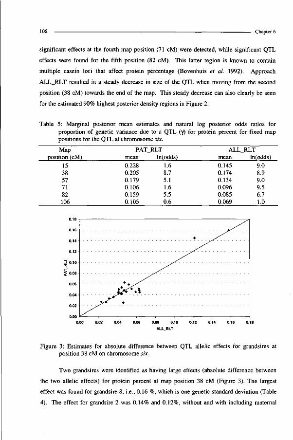
106 Chapter 6
significant effects at the fourth map position (71 cM) were detected, while significant QTL
effects were found for the fifth position (82 cM). This latter region is known to contain
multiple casein loci that affect protein percentage (Bovenhuis et al. 1992). Approach
ALL_RLT resulted in a steady decrease in size of the QTL when moving from the second
position (38 cM) towards the end of the map. This steady decrease can also clearly be seen
for the estimated 90% highest posterior density regions in Figure 2.
Table 5: Marginal posterior mean estimates and natural log posterior odds ratios for proportion of genetic variance due to a QTL (y) for protein percent for fixed map positions for the QTL at chromosome six.
Map position (cM)
PAT_RLT mean ln(odds)
ALL_RLT mean ln(odds)
15 38 57 71 82 106
0.228 0.205 0.179 0.106 0.159 0.105
1.6 8.7 5.1 1.6 5.5 0.6
0.145 0.174 0.134 0.096 0.085 0.069
9.0 8.9 9.0 9.5 6.7 1.0
Figure 3: Estimates for absolute difference between QTL allelic effects for grandsires at position 38 cM on chromosome six.
Two grandsires were identified as having large effects (absolute difference between
the two allelic effects) for protein percent at map position 38 cM (Figure 3). The largest
effect was found for grandsire 8, i.e., 0.16 %, which is one genetic standard deviation (Table
4). The effect for grandsire 2 was 0.14% and 0.12%, without and with including maternal

General discussion 107
relationships, respectively. Grandsire 2 was the sire of many dams and including maternal
relationships can explain the difference in estimated effects for this sire.
The differences between QTL effects in grandsires were in general smaller for the
QTL at 82 cM (casein locus) when compared to the QTL at 38 cM (Figure 4). The
correlation between differences at the two positions was not high, i.e., 0.53.
0.08 0.10
position 38 cM
Figure 4: Estimates for absolute difference between QTL allelic effects within grandsires for position 38 cM and 82 cM on chromosome six.
Discussion: Bayesian analysis fully accounts for uncertainty in parameters in the
model and data in a full pedigree analysis. The marker data was incomplete since all dams
were ungenotyped but also a number of sons did not have complete data on all seven
markers. Our normal-effects QTL model directly estimated the proportion of additive genetic
variance due to a QTL. A technical difficulty occurred in estimating the difference in QTL
effects for founders (grandsires). For these individuals the updating of the allelic constitution
of their two marker haplotypes may also involve switches of QTL effects (see chapter 5).
Estimates of allelic QTL effects can be improved by linking them to alleles at flanking
markers. Here we simply computed the absolute difference between their two QTL allelic
effects to identify individuals heterozygous for the QTL. At map position 38 cM, two
grandsires were identified with large effects for protein percentage. Grandsire 2 was known
to be the sire of grandsire 8, although this relationship was not used in the analysis. Including
ancestral information on grandsires and dams can further improve the estimation of QTL
variance and QTL effects of individuals.
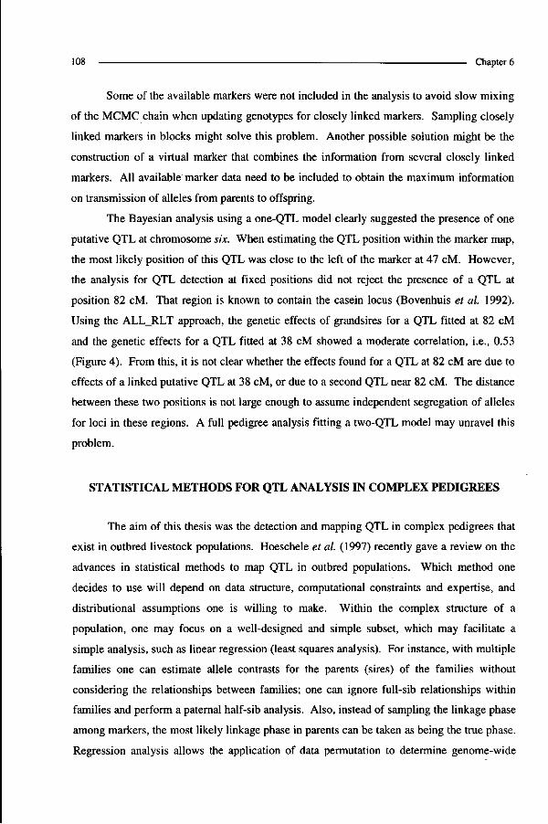
108 Chapter 6
Some of the available markers were not included in the analysis to avoid slow mixing
of the MCMC chain when updating genotypes for closely linked markers. Sampling closely
linked markers in blocks might solve this problem. Another possible solution might be the
construction of a virtual marker that combines the information from several closely linked
markers. All available marker data need to be included to obtain the maximum information
on transmission of alleles from parents to offspring.
The Bayesian analysis using a one-QTL model clearly suggested the presence of one
putative QTL at chromosome six. When estimating the QTL position within the marker map,
the most likely position of this QTL was close to the left of the marker at 47 cM. However,
the analysis for QTL detection at fixed positions did not reject the presence of a QTL at
position 82 cM. That region is known to contain the casein locus (Bovenhuis et al. 1992).
Using the ALL_RLT approach, the genetic effects of grandsires for a QTL fitted at 82 cM
and the genetic effects for a QTL fitted at 38 cM showed a moderate correlation, i.e., 0.53
(Figure 4). From this, it is not clear whether the effects found for a QTL at 82 cM are due to
effects of a linked putative QTL at 38 cM, or due to a second QTL near 82 cM. The distance
between these two positions is not large enough to assume independent segregation of alleles
for loci in these regions. A full pedigree analysis fitting a two-QTL model may unravel this
problem.
STATISTICAL METHODS FOR QTL ANALYSIS IN COMPLEX PEDIGREES
The aim of this thesis was the detection and mapping QTL in complex pedigrees that
exist in outbred livestock populations. Hoeschele et al. (1997) recently gave a review on the
advances in statistical methods to map QTL in outbred populations. Which method one
decides to use will depend on data structure, computational constraints and expertise, and
distributional assumptions one is willing to make. Within the complex structure of a
population, one may focus on a well-designed and simple subset, which may facilitate a
simple analysis, such as linear regression (least squares analysis). For instance, with multiple
families one can estimate allele contrasts for the parents (sires) of the families without
considering the relationships between families; one can ignore full-sib relationships within
families and perform a paternal half-sib analysis. Also, instead of sampling the linkage phase
among markers, the most likely linkage phase in parents can be taken as being the true phase.
Regression analysis allows the application of data permutation to determine genome-wide
General discussion 109
significance thresholds. This can be used as the first step in the analysis of QTL experiments.
Due to the approximations involved, the application of most simple methods is limited to
certain designs (e.g., a number of large half-sib families). At the second stage, one may want
to relax the simplifying assumptions to explore the data in more detail in order to get more
accurate estimates of QTL at interesting chromosomal regions, at the expense of higher
computational requirements. For example, linkage phases in parents and allele frequencies at
marker loci can be included as unknowns in the model. This second stage analysis may be
performed with methods that make less assumptions and account for model uncertainties.
To avoid a repetition of reviews given by Hoeschele et al. (1997), Bovenhuis et al.
(1997), and Jansen et al. (1998), we compare the Bayesian method presented in this thesis to
statistical methods previously described by Grignola et al. (1996a), Uimari et al. (1996), and
Jansen et al. (1998). Occasionally other methods will be mentioned. Comparisons are made
with respect to handling genetic marker information, assumptions on the genetic model for
the QTL, possibility for correction for other QTL, and hypothesis testing.
Genetic marker information: For QTL mapping in outbreeding livestock
populations moderately dense genetic maps based on molecular genetic markers are
available. Recombination frequencies between marker loci are often assumed to be known as
we did, however, these can be included as unknowns in the analysis (e.g., Uimari et al. 1996).
The number of alleles and allele frequencies in the (base) population for marker loci are
typically unknown for outbreeding species. Data might not provide complete information on
genotypic status of animals at the marker loci. The marker genotypes may be observed on
only a subset of the population, e.g., due to selective genotyping. In addition to unobserved
marker data, marker data might not be fully informative about the actual marker genotype,
e.g., when markers are dominant. In that case, a heterozygous genotype cannot be
distinguished from one of the homozygous genotypes. In addition, only a fraction of parents
are usually heterozygous for a marker locus. Homozygous marker genotypes in parents
complicate the identification of parental origin of alleles at a linked QTL. A special case of
unknown parental origin of marker alleles arises when an offspring and both its parents are
heterozygous, carrying the same alleles, at a marker locus. Therefore, it is important to use
all available marker information simultaneously to study segregation of chromosomal
segments from parents to offspring. A priori, the linkage phase between marker alleles in
parents is unknown. Phenotypes contain information on QTL genotypes, and when a marker
is linked to a QTL, the phenotypes also contain information about incomplete marker
110 __ Chapter 6
genotypes. The impact of including phenotypes in the calculation of genotype probabilities
increases with the size of the QTL and likely decreases with the amount of marker data
available. The Bayesian method (chapter 2 and 5) takes into account marker plus phenotype
information to calculate marker genotype probabilities. In contrast, in the REML approach of
Grignola et al. (1996a), the probabilities are calculated on the basis of marker data only and
this calculation precedes the QTL analysis. Furthermore, the computation of the variance-
covariance matrix of the QTL effects in the REML approach of Grignola et al. (1996a)
becomes inefficient when applied to pedigrees where individuals are related through both
paternal and maternal relationships and when genotypes are missing. Grignola et al. (1996b)
considered data for half-sib designs, i.e., ignored maternal links between animals, and
assumed that for a parent the most likely linkage phase was the true phase.
In summary, statistical methods for QTL mapping by full pedigree analysis should
consider all uncertainties with respect to marker information. The Bayesian approach allows
for individuals with no or partial data for marker loci. Partial data may for example occur
when animals are genotyped for different subsets of marker loci. Augmentation of genotypes
was implemented via a Gibbs sampler. The Gibbs sampler may be further improved to
circumvent reducibility problems that may occur when sampling genotypes for two
ungenotyped parents and when sampling genotypes for closely linked marker loci. The latter
will be crucial since marker maps in outbred species are becoming more and more dense
(e.g., Barendse et al. 1996).
Assumption of the genetic model: The genotype at the QTL is typically unknown in
outbred populations. The number of alleles in the population and their frequencies of
occurrence are also unknown. In mixture models and mixed inheritance models it is usually
assumed that the QTL is biallelic (e.g., Guo and Thompson 1992, Uimari et al. 1996, Jansen
et al. 1998). Except for potential computational problems (e.g., number of parameters in the
likelihood) there is no basic problem in extending the number of QTL alleles in these models
(Hoeschele et al. 1997). The problem remains that the number of alleles should be inferred
and preferably models with different numbers of alleles should be compared. On the other
hand, the models with expected covariance matrix of random QTL effects make no specific
assumptions with respect to the number of QTL alleles. The biallelic model will likely
perform badly if there are three or more alleles, all at reasonable frequencies and with
measurable differences in effects. A situation with two closely linked QTL might be
observed as one QTL with multiple alleles. For data simulated under a biallelic model,

General discussion 111
Hoeschele et al. (1997) reported that a Bayesian analysis fitting a normal-effects (mixture)
model provided more accurate estimates of QTL variance than the Bayesian analysis fitting a
biallelic model. For data simulated under the normal-effects model, the analysis fitting the
biallelic model underestimated QTL variance substantially, while the QTL variance was
accurately estimated with the normal effects QTL analysis.
Our genetic model for the QTL is identical to that of Grignola et al. (1996a).
Individuals have two random additive allelic effects with covariance matrix composed of
elements equal to probabilities of allele identity by descent conditional on marker information
(Fernando and Grossman 1989). This can be viewed as an approximation of the model where
all base individuals have two random allelic effects and the QTL effect inherited from a
particular parent is exactly identical to one of the parental effects. This latter model is a
normal-effects mixture model as used by Uimari et al. (1996) and Hoeschele et al. (1997).
The approximate expectation model can accommodate QTL clusters and mutations in the
sense that the QTL effect inherited from a particular parent is modeled as a weighted average
of the two parental QTL effects plus a residual. In addition, this model transforms to a
polygenic model when marker information is low. Further research is needed to compare
both procedures in multiple generation pedigrees - which should involve a study of the
evolution of QTL effects over time.
In a full pedigree analysis with biallelic (or multi-allelic) QTL in a mixture model,
univariate genotype sampling causes slow or non-sufficient mixing of the Gibbs sampler.
Block sampling of genotypes is useful for parents with large progeny groups (Janss et al.
1995). Sampling identity-by-descent values at the QTL for non-founders as proposed by
Jansen et al. (1998) also improves mixing of QTL genotypes in unrelated half-sib family
analysis. Further research is needed to compare computational and mixing properties of the
approximate expectation model and the exact mixture model for normal QTL effects in a full
pedigree analysis.
Correction for other QTL: In this thesis, we considered one QTL within a marked
chromosomal segment. The QTL at other chromosomes were accounted for via a residual
polygenic effect for each individual, which was independent of the marked QTL. In crosses
from inbred lines background QTL can be taken into account by including linked markers as
cofactors in the model, as first proposed by Jansen (1992). In livestock species, a QTL can
be segregating in some families, whereas, the linked marker is not and vice versa. Then a
marker linked to a putative QTL can not be used as the cofactor in the model. In such cases,

112 Chapter 6
the QTL itself should be included instead of the marker as cofactor in the model, as suggested
by Spelman et al. (1996). Grignola et al. (1997) and Uimari and Hoeschele (1997) presented
methods to include two linked QTL in the model for a REML and Bayesian approach,
respectively. A polygenic component was still included to account for (unlinked) QTL at
other chromosomes.
Hypothesis testing: The presence of a single QTL in the REML approach of Grignola
et al. (1996a) was done by comparing the likelihood under the null hypothesis of zero
variance due to the QTL versus the likelihood of the estimated variance due to the QTL. The
distribution of this test statistic is unknown, but is a chi-square distribution with between 1
and 2 degrees of freedom (Xu and Atchley 1995). Computational requirements of the REML
method prohibited the use of data permutation (Churchill and Doerge 1994) to obtain the
distribution of the likelihood ratio statistic and calculation of genome-wide significance
thresholds (Grignola et al. 1996a,b).
The test statistic for presence of a QTL in the Bayesian approach was the odds ratio
between the posterior mode and the density at zero for the proportion additive genetic
variance due to the QTL. The prior odds ratio of this parameter equaled one for both a
UNIFORM prior and a PEAKED AT ZERO prior. The PEAKED AT ZERO prior reflects
the prior expectation that the genome contains very few genes with large effects, some genes
with moderate effects, and many genes with small effects (as was reported by Shrimpton and
Robertson (1988) for experimental populations). The PEAKED AT ZERO prior appeared to
be useful in the analyses of data with low informative markers. When markers are not very
informative, the variance-covariance matrix of QTL effects and that for the residual
polygenic effects have an almost identical structure. This hampers accurate estimation of the
variance due to the QTL from the data and the posterior density will be similar to its prior. A
PEAKED AT ZERO prior will therefore regress the posterior towards zero, while a
UNIFORM prior allows any estimate between zero and one with equal probability and
'regresses' towards 0.5 (the prior mean).
Uimari et al. (1996) in their Bayesian analysis used an indicator variable representing
either nonlinkage or linkage of the QTL to the marker group. Thaller and Hoeschele (1996)
and Satagopan et al. (1996) performed QTL model selection based on Bayes factors, which
were estimated using different MCMC algorithms. Thaller and Hoeschele (1996) found that
MCMC sampling with model indicators gave much more stable results than MCMC
estimates of Bayes factors. In this thesis, the application of Bayes factors for model selection
General discussion 113
has been studied for two situations, i.e., a model with or without the QTL, and for the
position of the QTL relative to multiple markers. However, we were not successful in
obtaining stable estimates for the Bayes factors and we used alternative procedures, i.e., a
posterior odds ratio and the simulated tempering sampler, to draw inferences about presence
and position of the QTL, respectively. For our test statistic, the critical significance value
was arbitrarily set to 20 (or the natural log equal to 3.0), as suggested by Janss et al. (1995).
A recent development to Bayesian model selection via MCMC is the use of a
reversible jump sampler (Green 1995). In the reversible jump sampler, jumps are made
possible between models with different parameter spaces within a single Markov chain. This
reversible jump sampler has already been implemented to obtain posterior probabilities for
models with none, one or multiple linked QTL, within a marker linkage group for plants
(Satagopan and Yandell 1997), animals (Uimari and Hoeschele 1997) and humans (Heath
1997). The reversible jump sampler has also been implemented for ordering a biallelic QTL
relative to multiple linked markers (George et al. 1998). Based on these studies, the
reversible jump sampler contributes to the potential and flexibility of the MCMC framework
for Bayesian model selection and analysis in QTL mapping. Developments in this area will
contribute to more realistic models and a better understanding of the genetics underlying
quantitative traits.
MARKER ASSISTED PREDICTION OF BREEDING VALUES
For the application of genetic markers in a dairy cattle selection scheme, prediction of
breeding values is an essential component. We may envision a dairy cattle breeding program
with a nucleus breeding scheme producing young bulls that are progeny tested in commercial
populations. Here, we outline a procedure, using both schemes, to include marker
information in the genetic evaluation and selection.
At this moment, the high costs for marker genotyping prohibit the routinely
genotyping of large numbers of animals. Among individuals with missing marker genotypes,
two categories of individuals can be distinguished. The first category comprises the (grand)
daughters of young bulls that only contribute phenotypic information in a granddaughter
design type of analysis. The second category comprises the ungenotyped-parents of
genotyped nucleus individuals, e.g., elite dams. In this thesis we described methodology to
handle both categories. The genetic effects of ungenotyped granddaughters are absorbed in

114 Chapter 6
the reduced animal model (chapter 3). The marker genotypes for ungenotyped parents are
treated as missing values in the Bayesian analysis where the Gibbs sampler is used to
augment the genotypes (chapter 2 for single marker and chapter 5 for multiple markers). In
an open nucleus system, parents of nucleus individuals may be present in the commercial
population. Procedures to incorporate information from these parents (without including
them explicitly in the analysis) need to be developed similar to procedures that incorporate
foreign information in national genetic evaluation of dairy cattle.
In prediction of genetic effects at marked QTL, we may assume to have accurate
estimates for the QTL location and the QTL variance. This would greatly reduce the
computational requirements. Initially, the number of animals within the nucleus scheme
having observed marker genotypes is probably too small for accurate estimation of QTL
parameters. In that case, the parameter estimates obtained from a granddaughter design
analysis, exploiting the progeny-testing scheme, seem most appropriate. The amount of
information within the nucleus, however, will increase over time and this may enable
estimation of the genetic parameters from the current breeding population. Spelman and Van
Arendonk (1997) have investigated the consequences of inaccurate estimation of variance
and location of the QTL on genetic response to marker-assisted selection. They concluded
that the loss in genetic response due to errors in parameters could be reduced when the
parameters were re-estimated over time. Instead of assuming that the parameters are known,
a complete Bayesian analysis can be conducted in which uncertainty about genetic
parameters is accounted for explicitly. In a Bayesian analysis, results from other QTL
experiments, described in literature, can be used as prior knowledge on position and size of
putative QTL. Furthermore, data from the nucleus and a granddaughter design can be
combined in a Bayesian analysis for parameter estimation via the use of the reduced animal
model and MCMC algorithms. Close relationships between sires in the granddaughter design
and nucleus individuals will provide accurate predictions of breeding values of selection
candidates in the nucleus.
In conclusion, breeding values are derived from the phenotypic information collected
on all animals in the population and genotypic information on a selected group of animals.
The Bayesian procedure for predicting marker assisted breeding values combines the
genotypic and phenotypic information in an optimal manner. The accuracy of predicted
breeding values and the response to marker assisted selection will depend on the type and
number of relatives of the selection candidates on which genotypic and phenotypic is
collected. The reduced animal model no longer puts a restriction on the type of relatives to

General discussion 115
be genotyped and, therefore, opens new opportunities to capitalize on this new source of
information. The prediction of breeding values in a dairy cattle population with complex
pedigrees forms a very important step towards the application of marker assisted selection in
dairy cattle populations.
ACKNOWLEDGMENTS
I am indebted to Johan van Arendonk for his guidance and encouragement. I thank
Henk Bovenhuis, Richard Spelman Luc Janss, Ab Groen, and Pim Brascamp for helpful
discussions. I am grateful to Holland Genetics and Livestock Improvement for financial
support and data access. Chris Schrooten, Sijne van der Beek, and Bart Ducro are
acknowledged for the preparation of data on bovine chromosome six.
REFERENCES
Barendse W, Vaiman D, Kemp SJ, Sugimoto Y, Armitage SM, et al. (1996) A medium-density genetic linkage map of the bovine genome. Mamm Genome 8(l):21-28
Bovenhuis H, Van Arendonk JAM, Korver S (1992) Associations between milk protein polymorphisms and milk production traits. J Dairy Sei 75:2549-2559
Bovenhuis H, Weller JI (1994) Mapping and analysis of dairy cattle quantitative trait loci by maximum likelihood methodology using milk protein genes as genetic markers. Genetics 137:267-280
Bovenhuis H, Van Arendonk JAM, Davis G, Elsen J-M, et al. (1997) Detection and mapping of quantitative trait loci in farm animals. Livest Prod Sei 52:135-144
Churchill GA, Doerge RW (1994) Emperical thresholds values for quantitative trait mapping. Genetics 138:963-971
Fernando RL, Grossman M (1989) Marker-assisted selection using best linear unbiased prediction. Genet Sel Evol 21:467-477
George AW, Mengersen KL, Davis GP (1998) A Bayesian analysis of a QTL under a half-sib design. Proc 6th
World Congr Genetics Appl Livest Prod Sei, Armidale, Australia 26:225-228
Georges M, Nielsen D, Mackinnon M, Mishra A, Okimoto R, et al. (1995) Mapping quantitative trait loci controlling milk production in dairy cattle by exploiting progeny testing. Genetics 139:907-920
Geyer CJ, Thompson EA (1995) Annealing Markov chain Monte Carlo with applications to ancestral inference. J Am Stat Ass 90:909-920
Green PJ 1995 Reversible jump Markov chain Monte Carlo computation and Baysian model determination. Biometrika 82:711-732
Grignola FE, Hoeschele I, Tier B (1996a) Mapping quantitative triat loci via Residual Maximum Likelihood: I. Methodology. Genet Sel Evol 28:479-490
Grignola FE, Hoeschele I, Zhang Q, Thaller G (1996b) Mapping quantitative triat loci via Residual Maximum Likelihood: II. A simulation study. Genet Sel Evol 28:491-504
Grignola FE, Zhang Q, Hoeschele I (1997) Mapping linked quantitative trait loci via residual maximum likelihood. Genet Sel Evol 29:529-544
Guo SW, Thompson EA (1992) A Monte Carlo method for combined segregation and linkage analysis. Am J HumGenet51:llll-1126
116 Chapter 6
Haidane JBS (1919) The combination of linkage values and the calculation of distances between the loci of linked factors. J Genet 2:3-19
Heath SC (1997) Markov chain Monte Carlo segregation and linkage analysis for oligogenic models. Am J Hum Genet 61:748-760
Hoeschele I, Uimari P, Grignola FE, Zhang Q, Gage KM (1997) Advances in statistical methods to map quantitative trait loci in outbred populations. Genetics 147:1445-1457
Jansen RC (1992) A general mixture model for mapping quantitative trait loci by using molecular markers. Theor Appl Genet 85:252-260
Jansen RC, Johnson DL, Van Arendonk JAM (1998) A mixture model approach to the mapping of quantitative trait loci in complex populations with an application to multiple cattle families. Genetics 148:391-399
Janss LLG, Thompson R, Van Arendonk JAM (1995) Application of Gibbs sampling in a mixed major gene -polygenic inheritance model in animal populations. Theor Appl Genet 91:1137-1147
Knott SA, Elsen JM, Haley CS (1994) Multiple marker mapping of quantitative trait loci in half sib populations. Proc 5,h World Congr Genetics Appl Livest Prod Sei, Guelph, Canada 21:33-36
Satagopan JM, Yandell BS, Newton MA, Osborn TC (1996) A Bayesian approach to detect quantitative trait loci using Markov chain Monte Carlo. Genetics 144:805-816
Satagopan JM, Yandell BS (1997) Estimating the number of quantitative trait loci via Bayesian model determination. Proc Section Bimetrics, Am Stat Assoc, Alexandria, VA (in press)
Shrimpton AE, Robertson A (1988) The isolation of polygenic factors controlling bristle score in Drosphila melanogaster. II. Distribution of third chromosome bristle effects within chromosome sections. Genetics 118:445-459
Sorensen DA, Andersen S, Gianola D, Korsgaard I (1995) Bayesian inference in threshold models using Gibbs sampling. Genet Sel Evol 27:229-249
Spelman RJ, Coppieters W, Karim L, Van Arendonk JAM, et al. (1996) Quantitative trait loci analysis for five milk production traits on chromosome six in the Dutch Holstein-Friesian population Genetics 144:1799-1808
Spelman RJ, Van Arendonk JAM (1997) Effect of inaccurate parameter estimates on genetic response to marker-assisted selection in an outbred population. J Dairy Sei 80:3399-3410
Thaller G, Hoeschele I (1996) A Monte Carlo method for Bayesian analysis of linkage between single markers and quantitative trait loci: II. A simulation study. Theor Appl Genet 93:1167-1174
Uimari P, Thaller G, Hoeschele I (1996) The use of multiple markers in a Bayesian method for mapping quantitative trait loci. Genetics 143:1831-1842
Uimari, P, Hoeschele I (1997) Mapping-linked quantitative trait loci using Bayesian analysis and Markov chain Monte Carlo algorithms. Genetics 146:735-743
Xu S, Atchley WR (1995) A random model approach to interval mapping of quantitative trait loci. Genetics 141:1189-1197
117
Summary
In dairy cattle, many quantitative traits of economic importance show phenotypic
variation. For breeding purposes the analysis of this phenotypic variation and uncovering the
contribution of genetic factors is very important. Usually, the individual gene effects
contributing to the quantitative genetic variation can not be distinguished. Developments in
molecular genetics, however, have resulted in the identification of polymorphic sites in the
genome, which are called genetic markers. Genetic markers have opened the way to follow
segregation of chromosomal segments in families. Through the use of these genetically
marked chromosomal segments, detection and mapping the genes affecting quantitative traits
("quantitative trait loci" or "QTL") becomes possible. After identifying QTL, genetic
markers may, for example, be used to select animals at a younger age and/or to improve the
accuracy of predictions of genetic merit.
The aim of this thesis is to contribute to the efficient utilization of genetic marker and
quantitative trait data in detecting and utilizing single QTL in complex pedigrees in dairy
cattle breeding programs. Implementation of marker-assisted selection in dairy cattle has
been hampered by the lack of identified QTL, and the lack of efficient methods for marker-
assisted genetic evaluation for situations with incomplete marker data. The development of
statistical methods forms the core of this thesis. Methodology is based on Bayes theory and
implemented via Markov chain Monte Carlo algorithms, such as the Metropolis-Hastings
algorithm and the Gibbs sampler.
Throughout this thesis, a mixed linear model with two random genetic components,
i.e., effects due to a marked QTL and residual polygenes, was assumed. These components
are assumed to be normally distributed and independent in the base population. To arrive at a
flexible method for full pedigree analysis, an animal model is taken as the starting point.
Covariances among genetic effects of related individuals are taken into account via the
numerator relationship matrix for polygenes and the gametic relationship matrix for QTL. In
most chapters, the developed methodology is empirically tested by the use of simulated data.

118
In chapter 6, however, experimental data on bovine chromosome six is analyzed to estimate
the position and size of a putative QTL for protein percent.
Incomplete marker data hinders application of marker-assisted breeding value
estimation using animal model BLUP. In chapter 2, Gibbs sampling is applied to facilitate
Bayesian estimation of breeding values with incomplete information on a single marker that
is linked to a QTL. Gibbs sampling is a Markov chain Monte Carlo procedure to
approximate the joint posterior distribution of data and all unknowns. Exact knowledge on
position and size of the QTL is assumed in estimating the breeding values. Derivation of
sampling densities for marker genotypes is emphasized, because a study of the structure of
reconsideration of the gametic relationship matrix structure for a marked QTL leads to simple
conditional densities. In the Bayesian procedure, the posterior probabilities of marker
genotypes are based on trait phenotypes as well as observed marker genotypes of the animal
and its relatives. Due to computational requirements, the presented Bayesian approach is less
applicable to large populations with many ungenotyped individuals, but may be used in
nucleus breeding schemes with relatively small numbers of ungenotyped individuals.
In chapter 3, a Bayesian method is presented for the statistical detection of QTL,
where the application of a reduced animal model leads to non-standard densities for
dispersion parameters. The Gibbs sampling algorithm requires full conditional densities to be
of a standard form and, therefore, an alternative technique, i.e. the Metropolis-Hastings
algorithm, is used to obtain samples from these non-standard densities. The flexibility of the
Metropolis-Hastings algorithm also allows studying the parameterization of the genetic
model. Alternatively to a parameterization in terms of the usual variance components, we
also parameterized the genetic model in terms of one variance component (=residual) and two
ratios of variance components, i.e., heritability and proportion of genetic variance due to the
QTL. Prior knowledge on variance ratios rather than variances can more easily be
implemented, partly due to the absence of scale effects. Three sets of simulated data are used
to study performance of the reduced animal model, parameterization of the genetic model,
and testing for the presence of the QTL at a fixed position.
In absence of exact knowledge on the size and position of the QTL, these parameters
can be included as unknowns in the model. In chapter 3, exact knowledge is assumed about
the position of the QTL relative to multiple linked markers. In chapter 4, the previously
119
described Bayesian method is extended for the identification of the most likely marker
bracket containing a QTL. Parameters to be estimated in the mixed linear model are residual
variance, heritability, proportion of genetic variance due to QTL, and QTL position on a
linkage map. Straightforward implementation of a Metropolis-Hastings algorithm to sample
QTL position results in practical reducibility of the chain, i.e., the chain does not move away
from the initial marker bracket. Candidate positions for the QTL in adjacent marker brackets
are not accepted. The non-mixing of the chain is caused by the large changes in the gametic
relationship matrix for QTL effects when moving QTL position from one bracket to the next.
To overcome this non-mixing problem, a relatively new MCMC technique, simulated
tempering is implemented. Although computer intensive, the simulated tempering sampler
yields proper mixing of QTL position among marker brackets when empirically tested on
simulated data. Inferences on QTL position can be based on marginal posterior probabilities.
In chapter 3 and 4, restrictions are imposed on the genotypic uncertainties, i.e., it is
assumed that all individuals in the reduced animal model analysis have observed marker
genotypes and the linkage phase in parents is known with certainty. In chapter 5, the Bayesian
method is further extended to account for ungenotyped animals and uncertainty on all
parameters of the mixed linear model except the position of the QTL. Augmentation of
marker genotypes for ungenotyped individuals is implemented. Marker data on relatives, and
phenotypes are combined to compute conditional posterior probabilities on marker genotypes
for ungenotyped individuals. Accommodating ungenotyped individuals allows QTL analysis
in populations with complex pedigrees and missing marker data. The method is empirically
tested by analyzing simulated data from a complex granddaughter design. Ungenotyped dams
are related to one or more sons and/or to a grandsire in the design. Information per marker
locus and size of QTL is varied. Results from Monte Carlo simulations indicate a significant
increase in power of QTL detection when all relationships are included in the analysis.
In chapter 5, exact knowledge on QTL position is assumed, i.e. this parameter is not
estimated. The general discussion (chapter 6) starts with combining theory of chapter 4 and
chapter 5, to complete the Bayesian method that estimates both position and size of a QTL
with complex pedigree data. The method is then empirically tested on four simulated data
sets. The second section of the general discussion describes the QTL analysis on
chromosome six in dairy cattle. The data stems from the Holland Genetics/Livestock
Improvement QTL experiment. Approximately the same data have been analyzed previously

120
by Spelman and co-workers who identified a QTL for protein percentage. Our data
comprised 22 Dutch Holstein-Friesian families, with a total of 922 sons, and 455 elite dams
with direct links to at least two male genotyped individuals. Fourteen grandsires were also
sires of 399 elite dams, corresponding with a total of 653 maternal grandsons. A QTL for
protein percent was identified. The most likely position of this QTL is similar to that
previously reported by Spelman and co-workers. The presence of a second putative QTL for
protein percent is uncertain and requires further research probably with a two-QTL model. In
the third section of the general discussion, the presented Bayesian method is compared to
other methods for QTL analysis in complex pedigrees. Our method at this moment is unique
in being able to handle complex pedigrees in outbred populations with missing marker data.
The general discussion is completed with a brief review of issues related to practical
implications for marker-assisted genetic evaluation in dairy cattle breeding schemes.

121
Samenvatting
Veel kwantitatieve eigenschappen bij melkvee vertonen fenotypische variatie. In de
veefokkerij is de analyse van deze fenotypische variantie en het blootleggen van de
genetische factoren erg belangrijk. Normaliter kunnen de individuele effecten van genen die
bijdragen aan de kwantitatieve genetische variatie, niet worden onderscheiden. Echter,
recente ontwikkelingen in de moleculaire genetica hebben geleid tot de identificatie van
polymorfe posities op het genoom welke ook wel genetische merkers worden genoemd.
Genetische merkers bieden de mogelijkheid om de segregatie van segmenten van
chromosoom te volgen in families. Met behulp van gemerkte chromosoomsegmenten, kan
men bepalen welke segmenten genen bevatten die bijdragen aan de genetische variatie van
kwantitatieve kenmerken. Eén zo'n gen wordt in de veefokkerij ook wel aangeduid met de
engelse term quantitative trait locus (afgekort tot QTL). Zodra een QTL opgespoord is, kan
men genetische merkers gebruiken om bijvoorbeeld dieren op een jongere leeftijd te
selecteren of om de genetische verschillen tussen dieren nauwkeuriger te schatten.
Het doel van het in dit proefschrift beschreven onderzoek was het verbeteren van het
gebruik van alle beschikbare data (genetische merkers en kwantitatieve kenmerken) voor het
opsporen en benutten van QTL in melkveepopulaties. De implementatie van
merkerondersteunde selectie is op dit moment niet mogelijk door het ontbreken van
geïdentificeerde QTL en het ontbreken van efficiënte methoden voor het uitvoeren van
merkerondersteunde fokwaardeschatting in situaties waarin niet alle dieren getypeerd zijn
voor merkers. Een belangrijk deel van dit proefschrift wordt in beslag genomen door de
presentatie en testen van nieuwe methoden. De ontwikkelde methoden zijn gebaseerd op de
Bayesiaanse theorie en maken gebruik van Monte-Carlo-Markov-keten algoritmen, zoals de
Gibbs sampler en het Metropolis-Hastings algoritme. Door deze algoritmen is uitvoeren van
complexere genetische analyses mogelijk geworden.
In dit proefschrift wordt uitgegaan van een gemengd lineair model met 2 genetische
componenten, te weten effecten van het gemerkte QTL en effecten van de resterende

122
(achtergrond) genen (ookwel polygenen genoemd). We veronderstellen dat deze effecten een
normale verdeling volgen en onafhankelijk van elkaar zijn in de basispopulatie. Om rekening
te houden met de co-varianties tussen genetische effecten van verwante dieren, bijvoorbeeld
ouder - nakomeling, wordt in de veefokkerij vaak gebruik gemaakt van het diermodel. Dit
model vormt het vertrekpunt voor de complete stamboom analyse beschreven in dit
proefschrift. In vrijwel alle hoofdstukken, worden de ontwikkelde methoden getest door
gesimuleerde data te analyseren. In Hoofdstuk 6 wordt ook een analyse beschreven van
experimentele data gericht op het opsporen van genen / QTL voor productiekenmerken op
chromosoom zes in melkvee.
Onvolledige merker data belemmert het gebruik van het diermodel voor de toepassing
van merkerondersteunde fokwaardeschatting. In Hoofdstuk 2 wordt de toepassing van Gibbs
sampling beschreven om fokwaarden volgens de Bayesiaanse methode te schatten. Deze
methode kan worden toegepast wanneer de informatie voor een merker, gekoppeld aan het
QTL, onvolledig is. Met deze benadering wordt een marginale a-posteriori verdeling geschat
middels trekkingen uit de werkelijke marginale a-posteriori verdeling. Voor het genereren
van de gewenste trekkingen wordt een Monte Carlo Markov keten geconstrueerd. In
Hoofdstuk 2 veronderstellen we volledige kennis over de positie en de grootte van het QTL.
De nadruk ligt op het afleiden van de verdelingen waaruit genotypes afgeleid kunnen worden
voor dieren met ontbrekende merker genotypen. Het blijkt dat de specifieke structuur van de
gametische relatiematrix van het QTL benut kan worden om te komen tot eenvoudige
verdelingen voor merker genotypen. In de Bayesiaanse benadering, dragen waarnemingen
aan het kenmerk ook bij aan de a-posteriori kansen voor de merker genotypen van een niet-
getypeerd individu. Uitbreiding en toepassing van de beschreven benadering in grote
populaties van landbouwhuisdieren worden bediscussieerd.
Vanaf Hoofdstuk 3 staat de detectie en positionering van QTL centraal. Hierbij wordt
allereerst onderzocht of een significant deel van de genetische variantie verklaard wordt door
het QTL. Vervolgens wordt aandacht besteed aan het bepalen van de meest waarschijnlijke
plaats van het QTL op een gemerkt stuk chromosoom bepaald. Er wordt steeds uitgegaan van
een (deel van het) chromosoom waarop meerdere merker loei voorkomen op bekende
posities. In de veefokkerij worden Monte-Carlo-Markov-keten algoritmen steeds vaker
gebruikt om statistische conclusies te trekken over marginale a-posteriori verdelingen van
parameters in het gebruikte genetische model. De Gibbs sampling wordt hierbij het meest

123
gebruikt en vereist dat de conditionele kansverdelingen van een standaard vorm zijn,
bijvoorbeeld een Normale verdeling. In Hoofdstuk 3 beschrijven we een Bayesiaanse
benadering voor het statistisch opsporen van QTL, waarbij het gebruik van het gereduceerde
dier model leidt tot verdelingen van dispersie parameters die niet standaard zijn. In dat geval
wordt het Metropolis-Hastings algoritme gebruikt om trekkingen te verkrijgen uit deze niet-
standaard verdelingen. Het Metropolis-Hastings algoritme biedt tevens mogelijkheden om
verschillende parameterizaties van het genetisch model te bestuderen. Als alternatief voor de
parameterizatie in termen van variantiecomponenten, gebruiken we ook een parameterizatie
in termen van één variantie component en twee ratios van variantie componenten, te weten de
erfelijkheidsgraad en de proportie genetische variantie verklaard door het QTL. In
vergelijking tot de variantie componenten, is het implementeren van voorkennis is in het
geval van ratios gemakkelijker dan in het geval van variantie componenten, mede door de
afwezigheid van schaaleffecten. De eigenschappen van het gereduceerde diermodel zijn
bestudeerd door analyse van drie verschillende sets van gesimuleerde gegevens. Hierin komt
naar voren dat door het gebruik van het gereduceerde diermodel de rekentijd enorm wordt
verkort terwijl eigenschappen van schatters gelijk zijn aan die van volledig diermodel.
In Hoofdstuk 3 is de kaartpositie van het QTL bekend verondersteld. In Hoofdstuk 4,
wordt de eerder beschreven Bayesiaanse methode uitgebreid om ook de meest waarschijnlijke
positie (merker interval) voor het QTL te bepalen. Echter, simulaties toonden aan dat een
Metropolis Hastings algoritme voor het trekken van nieuwe QTL posities niet toereikend was
om de positie over een kaart met meerdere merker loei te bepalen. Vanuit een willekeurige
startpositie kwam de keten nooit in een andere merker interval, een probleem wat bekend
staat als onvolledige menging. Deze onvolledige menging wordt veroorzaakt door de
gametische relatie matrix voor de QTL effecten. Om dit probleem op te lossen, is een relatief
nieuwe MCMC techniek, simulated tempering, geïmplementeerd. Hoewel simulated
tempering computer intensief is, resulteert het wel in adequate mixing van de QTL positie
over de verschillende merker intervallen. Conclusies over de meest waarschijnlijke QTL
positie kunnen nu gebaseerd worden op marginale a-posteriori kansen.
In Hoofdstuk 3 en 4 is uitgegaan van een populatie alle (ouder-)dieren in het
reduceerde dier model bekende merker genotypes hebben en verder is aangenomen dat de
koppelingsfase van merker allelen volledig bekend is. In Hoofdstuk 5 wordt de Bayesiaanse
benadering uitgebreid om rekening te houden met niet-getypeerde dieren en met onzekerheid

124
over alle parameters in het gemengde lineaire model, met uitzondering van de positie van het
QTL. Het aanvullen van merker genotypen voor niet-getypeerde dieren is geïmplementeerd
een Bayesiaanse benadering en MCMC technieken. Merker informatie van verwante dieren
en fenotypische informatie worden gecombineerd om a-posteriori kansen voor merker
genotypen uit te rekenen. Het kunnen meenemen van niet-getypeerde dieren in de analyse
biedt de mogelijkheden tot QTL analyse in populaties met complexe stamboomstructuren en
ontbrekende merker gegevens. De ontwikkelde methode is empirisch getest door
gesimuleerde gegevens te analyseren voor een complex granddaughter design. In een
granddaughter design wordt vaak uitgegaan van ongerelateerde half-sib families bestaande uit
stiervaders en hun (proefstier)zonen. In fokprogramma's, is er naast deze vader zoon relaties
nog sprake van vele andere (maternale) familie relaties tussen dieren. Deze relaties lopen
deels via niet-getypeerde stiermoeders. Door alle niet-getypeerde dieren op te nemen in de
analyse wordt het onderscheidingsvermogen voor QTL detectie vergroot. Dit blijkt uit
resultaten gepresenteerd in hoofdstuk 5 waarin het voordeel van meenemen van alle relaties is
gekwantificeerd aan de hand van gesimuleerde data.
In Hoofdstuk 5 werd volledige kennis over de positie van het QTL verondersteld. In
de algemene discussie wordt de procedure beschreven in Hoofdstuk 5 gecombineerd met de
procedure in Hoofdstuk 4 voor het schatten van de positie van het QTL. Hierdoor ontstaat
een Bayesiaanse benadering die zowel positie als grootte van het QTL kan schatten welke kan
worden toegepast in populaties met complexe stamboomstructuren. Deze methode is ook
empirisch getest met Monte Carlo simulatie. Vervolgens zijn praktijkgegevens uit het
Holland Genetics/Livestock Improvement QTL experiment geanalyseerd. In een eerdere
analyse van deze gegevens door Spelman en medewerkers is een QTL voor eiwit% gevonden.
De hier geanalyseerde gegevens omvatten 22 Nederlandse Holstein-Friesian families met in
totaal 922 zonen, en 455 stiermoeders met relaties naar tenminste 2 manlijke getypeerde
individuen. Veertien stiervaders zijn tevens de vader van 399 stiermoeders, wat
correspondeert met in totaal 653 maternale kleinzonen. In de analyse wordt opnieuw het
QTL voor eiwit percentage gevonden, waarbij de meest waarschijnlijk positie van dit QTL
goed overeenkomt met de positie die eerder gevonden is. Door het meenemen van de extra
familierelaties is het mogelijk om een nauwkeurige uitspraak te doen over de grootte en de
positie van het QTL. Tevens zijn er aanwijzingen gevonden voor de aanwezigheid van een
mogelijk tweede QTL en een nadere analyse, mogelijk met een zogenaamd 2-QTL model, is

125
gewenst. In het derde deel van de algemene discussie wordt de ontwikkelde Bayesiaanse
benadering vergeleken met andere, in de literatuur beschreven, methoden voor QTL analyse
in populaties met complexe stambomen. Op dit moment is de in dit proefschrift beschreven
methode uniek omdat het een analyse mogelijk maakt van complexe stamboomstructuren
waarin niet alle dieren getypeerd zijn voor merker loei. Tenslotte worden in de algemene
discussie enige aspecten van de praktische implementatie van merker ondersteunde evaluatie
van fokprogramma's behandeld.

127
Curriculum Vitae
Marinus Cornells Alloysius Maria (Marco) Bink werd op 15 augustus 1968 geboren te
Raamsdonk. Na het behalen van het diploma HAVO aan het Dongemond College te
Raamsdonksveer, begon hij in 1985 aan de studie Nederlandse Landbouw aan de Agrarische
Hogeschool van de K.N.B.T.B. te 's-Hertogenbosch, welke in 1989 succesvol werd
afgesloten. Van september 1989 tot november 1990 vervulde hij zijn militaire dienstplicht als
onderofficier Intendance. Ondertussen werd in september 1990 begonnen met het
doorstroomprogramma Zootechniek aan de Landbouw universiteit te Wageningen. In
augustus 1993 sloot hij deze studie af, met als afstudeervakken Veefokkerij en Agrarische
Bedrijfseconomie. Vervolgens was hij gedurende drie maanden werkzaam bij de vakgroep
Veefokkerij als toegevoegd onderzoeker. In november 1993 begon hij als AIO (assistent in
opleiding) met het promotieonderzoek waarvan het thans voor u liggende proefschrift het
resultaat is. Vanaf maart 1998 werkt hij als onderzoeker bij het DLO - Centrum voor
Plantenveredelings- en Reproduktieonderzoek (CPRO-DLO) en bij het DLO - Instituut voor
Dierhouderij en Diergezondheid (ID-DLO).