Modeling Chip Formation in Orthogonal Metal Cutting using ...
115
Mississippi State University Mississippi State University Scholars Junction Scholars Junction Theses and Dissertations Theses and Dissertations 8-3-2002 Modeling Chip Formation in Orthogonal Metal Cutting using Finite Modeling Chip Formation in Orthogonal Metal Cutting using Finite Element Analysis Element Analysis Jaton Nakia Wince Follow this and additional works at: https://scholarsjunction.msstate.edu/td Recommended Citation Recommended Citation Wince, Jaton Nakia, "Modeling Chip Formation in Orthogonal Metal Cutting using Finite Element Analysis" (2002). Theses and Dissertations. 3139. https://scholarsjunction.msstate.edu/td/3139 This Graduate Thesis - Open Access is brought to you for free and open access by the Theses and Dissertations at Scholars Junction. It has been accepted for inclusion in Theses and Dissertations by an authorized administrator of Scholars Junction. For more information, please contact [email protected].
-
Upload
khangminh22 -
Category
Documents
-
view
0 -
download
0
Transcript of Modeling Chip Formation in Orthogonal Metal Cutting using ...
Mississippi State University Mississippi State University
Scholars Junction Scholars Junction
Theses and Dissertations Theses and Dissertations
8-3-2002
Modeling Chip Formation in Orthogonal Metal Cutting using Finite Modeling Chip Formation in Orthogonal Metal Cutting using Finite
Element Analysis Element Analysis
Jaton Nakia Wince
Follow this and additional works at: https://scholarsjunction.msstate.edu/td
Recommended Citation Recommended Citation Wince, Jaton Nakia, "Modeling Chip Formation in Orthogonal Metal Cutting using Finite Element Analysis" (2002). Theses and Dissertations. 3139. https://scholarsjunction.msstate.edu/td/3139
This Graduate Thesis - Open Access is brought to you for free and open access by the Theses and Dissertations at Scholars Junction. It has been accepted for inclusion in Theses and Dissertations by an authorized administrator of Scholars Junction. For more information, please contact [email protected].
MODELING CHIP FORMATION IN ORTHOGONAL METAL CUTTING
USING FINITE ELEMENT ANALYSIS
By
Jaton Nakia Wince
A Thesis Submitted to the Faculty of Mississippi State University
in Partial Fulfillment of the Requirements for the Degree of Master of Science
in Mechanical Engineering in the Department of Engineering
Mississippi State, Mississippi
August 2002
MODELING CHIP FORMATION IN ORTHOGONAL METAL CUTTING
USING FINITE ELEMENT ANALYSIS
By
Jaton N. Wince
Approved: ______________________________________ ________________________________________ Dr. Judy Schneider Dr. Christopher Eamon Assistant Professor of Mechanical Engineering Assistant Professor of Civil Engineering (Director of Thesis) (Committee Member) ______________________________________ _________________________________________ Dr. John T. Berry Dr. Rogelio Luck Professor of Mechanical Engineering Graduate Coordinator of the Department (Committee Member) of Mechanical Engineering
______________________________________ Dr. A. Wayne Bennett Dean of the College of Engineering
Name: Jaton Nakia Wince Date of Degree: August 3, 2002 Institution: Mississippi State University Major Field: Mechanical Engineering Major Professor: Dr. Judy Schneider Title of Study: MODELING CHIP FORMATION IN ORTHOGONAL METAL CUTTING USING FINITE ELMENT ANALYSIS Pages in Study: 104 Candidate for the Degree of Master of Science
This thesis presents the simulation of chip formation in orthogonal metal cutting to evaluate the
predictive capabilities of finite element code DYNA 3D. The Johnson and Cook constitutive model for
materials, OFHC Copper, Aluminum 2024 T351, and Aluminum 6061 T6 alloy were incorporated into the
simulation to account for the effects of strain hardening, strain rate hardening, and thermal softening effects
during machining. Calculated values for the Johnson and Cook constitutive constants for Aluminum 6061
T6 alloy were determined from the literature. The model was compared to experimentally measured shear
angles, chip thickness, chip velocity, and forces from the literature to evaluate the accuracy of the finite
element code for a range machining strain rates. In an attempt to determine the predictive capabilities of
DYNA 3D a strain rate regime of 10+3 s -1 to 10+4 s -1 was defined as the optimal strain rate regime for the
orthogonal metal cutting application.

- ii -
DEDICATION
I would like to dedicate this research to my daughter Infinity and my parents.
- iii -
ACKNOWLEDGEMENTS
The author would like to first of all give honor to his Heavenly Father and Jesus Christ his
personal Lord and Savior for without them none of this would have been possible. The author would also
like to express his sincere gratitude to the Department of Mechanical Engineering for providing the
opportunity to conduct this research at Mississippi State University. Expressed appreciation is also due to
Dr. Judy Schneider, and members of the author’s committee. Finally, special thanks to Dr. Christopher
Eamon in the Department of Civil Engineering at Mississippi State University for providing support with
the computational resources.
- iv -
TABLE OF CONTENTS
Page
DEDICATION ...................................................................................................................................................... ii
ACKNOWLEDGEMENTS ................................................................................................................................ iii LIST OF TABLES ............................................................................................................................................... v LIST OF FIGURES .............................................................................................................................................. vi CHAPTER
I. INTRODUCTION ........................................................................................................................... 1
Background ....................................................................................................................................... 2 Metallurgical Fundamentals ........................................................................................................... 2 Principal of Metal Cutting .............................................................................................................. 11 Principles of Finite Element Modeling ......................................................................................... 21 Literature Review ............................................................................................................................. 23 Analytical Models ................................................................................................................. 24 Numerical Models ................................................................................................................. 24 Research Approach .......................................................................................................................... 28
II. Finite Element Modeling ................................................................................................................ 30
Finite Element Method ................................................................................................................... 31 Material Model ................................................................................................................................ 32 Equation of State ............................................................................................................................. 33 Hourglass Control ........................................................................................................................... 34
Orthogonal Cutting Model ............................................................................................................. 35
III. Determining the Material Properties for Aluminum 6061-T6 for Implementation in the Johnson and Cook Constitutive Equation for Predicting Dynamic Materia l Behavior .... 41
Introduction ....................................................................................................................................... 41
Evaluation of Constitutive Equation ............................................................................................. 42 Determination of Constitutive Constants ...................................................................................... 43 Validation of Constitutive Parameters .......................................................................................... 47 Conclusion ......................................................................................................................................... 51
IV. Orthogonal Metal Cutting Model Analysis of Chip Formation for Two Different Face Centered Cubic Materials ........................................................................... 52
Introduction ....................................................................................................................................... 52
Effect of Machining Parameters on Chip Thickness .................................................................. 53
- v -
CHAPTER Page
Results ................................................................................................................................................ 54 Discussion of Results ....................................................................................................................... 65
Conclusion ........................................................................................................................................ 66
V. Conclusion ......................................................................................................................................... 68
Discussion of Results ........................................................................................................................ 68 Conclusion ......................................................................................................................................... 69 Directions to Future Research ........................................................................................................ 71
REFERENCES ...................................................................................................................................................... 72
APPENDIX
A CREATING METAL CUTTING SIMULATION USING DYNA 3D ............................... 76
B INGRID INPUT FILE FOR CHAPTER III AL 6061-T6 SIMULATION ......................... 79
C INGRID INPUT FILE FOR CHAPTER IV AL 2024-T351 SIMULATION ..................... 84
D INGRID INPUT FILE FOR CHAPTER IV OFHC COPPER 10102 SIMULATION ..... 89
E INGRID INPUT FILE FOR VALIDATION OF MATERIAL MODEL RESPONSE ..... 95
F COMPILING DYNA 3D CODES ON SGI WORKSTATION ............................................. 100
G MODIFICATIONS MADE TO DYNA 3D INPUT FILE “INGRIDO” ............................ 102
- vi -
LIST OF TABLES
TABLE Page
1.1 Proposed Geometry of Orthogonal Machining ........................................................................................ 26
1.2 Comparison of Finite Element Models for Orthogonal Metal Cutting ................................................ 27
2.1 Schematic Classification of Testing Techniques According to Strain Rates ...................................... 32
2.2 Slide Surface Supported in DYNA 3D Version 4.0.14 .......................................................................... 39
2.3 Simulation Normal and Shear Failure Stresses used for Slide Surface Type 9 .................................. 40
3.1 Johnson/Cook Tabulated Constitutive Parameters for Al 6061 T6 ...................................................... 47
3.2 Results (Experimental, FEA, & Deviation) .............................................................................................. 50
4.1 Parameter for Orthogonal Metal Cutting Simulation .............................................................................. 55
4.2 Results of Orthogonal Metal Cutting Experiment and Simulation (Al 6061 T6) .............................. 62
4.3 Results of Orthogonal Metal Cutting Experiment and Simulation (OFHC Copper 10102) ............ 64
5.1 DYNA 3D Strain Rate Operation Range for Metal Cutting Simulations ........................................... 70
- vii -
LIST OF FIGURES
FIGURE Page
1.1 Cubic Structure ............................................................................................................................................ 3
1.2 Face Centered Cubic Structure .................................................................................................................. 4
1.3 1.3. Body Centered Cubic Structure ......................................................................................................... 4
1.4 Classical Idea of Slip ................................................................................................................................... 4
1.5 Critical Resolved Shear Stress Diagram .................................................................................................. 5
1.6 (111) Plane of FCC Crystal ........................................................................................................................ 6
1.7 The (111) Slip Plane for FCC showing 3 Slip <110> Directions ....................................................... 6
1.8 Stereographic Projection of a Cubic Crystal – (Note: Tensile axis is out of plane) ......................... 7
1.9 Schematic Model of a Stacking Fault ...................................................................................................... 8
1.10 Stacking Fault of FCC Lattice ................................................................................................................... 8
1.11 Flow Curve for FCC Single Crystals ....................................................................................................... 10
1.12 Orthogonal Cutting Model ......................................................................................................................... 12
1.13 3D Orthogonal Metal Cutting Model ....................................................................................................... 13
1.14 Velocity and Shear Plane Angle Relationship Diagram ....................................................................... 14
1.15 Forces on Tool and Shear Plane ................................................................................................................ 15
1.16 Merchant’s Stack of Cards Model ............................................................................................................ 17
1.17 Schematic Representation of Material Flow to Shear Plane and Front Angles ................................ 18
1.18 Schematic Diagram showing basic Crystal Orientation with respect to Cutting Direction (CD) and the Chip Flow Direction (CFD) ....................................................... 19 1.19 Schematic Diagram of Cross Slip in Orthogonal Cutting Model ........................................................ 20
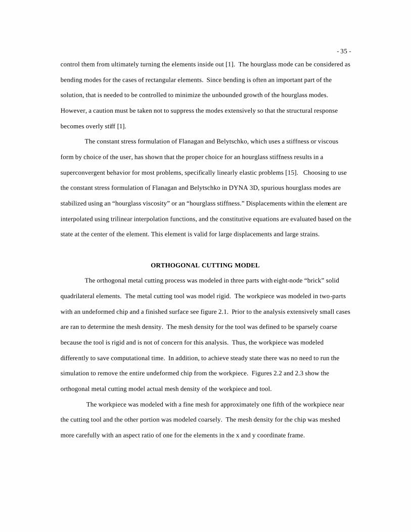
2.1 Schematic of Finite Element Model .......................................................................................................... 36
2.2 3-D Orthogonal Metal Cutting Model Mesh ............................................................................................ 36
- viii -
FIGURE Page
2.3 3-D Orthogonal Metal Cutting Model Mesh Density and Boundary Constraints ............................. 37
3.1 Yield Strength vs. Log Strain Rate (Al 6061-T6) ................................................................................... 44
3.2 True Stress Strain Plot (Al 6061-T6) ........................................................................................................ 45
3.3 Shear Stress and Shear Strain Plot (Al 6061-T6) .................................................................................... 46
3.4 Stress vs. Plastic Strain (Al 6061-T6) ....................................................................................................... 47
3.5 Orthogonal Metal Cutting Simulation of Chip Velocity ........................................................................ 48
3.6 Orthogonal Metal Cutting Simulation of Chip Velocity ........................................................................ 49
3.7 Chip Velocity vs. Simulation Time .......................................................................................................... 49
4.1 Simulation No. 2 Al 6061 T6 with α = 20o ............................................................................................. 56
4.2 Simulation No. 3 Al 6061 T6 with α = 30o ............................................................................................. 57
4.3 Simulation No. 4 Al 6061 T6 with α = 40o ............................................................................................. 58
4.4 Rake Angle vs. Shear Plane Angle for Al 6061 T6 ............................................................................... 59
4.5 Rake Angle vs. Shear Front Angle for Al 6061 T6 ............................................................................... 60
4.6 Rake Angle vs. Chip Thickness for Al 6061 T6 .................................................................................... 61
4.7 Rake Angle vs. Chip Velocity Plot for Al 6061 T6 ............................................................................... 62
4.8 Simulation No. 8 OFHC Copper 10102 with α = 25o ........................................................................... 63
4.9 Machining Forces vs. Tool Advance for OFHC Copper 10102 .......................................................... 64
- 1 -
CHAPTER I
INTRODUCTION
There are two distinct types of manufacturing processes that rely on the behavior of the material
past the yield point to form net shape components from a work piece. The first is a deformation process,
which produces the required shape by plastic deformation of the material while conserving mass. The
second process and the focus of this project is the machining process, which forms the net shape workpiece
by removing material. Traditional machining uses a cutting tool to perform milling, drilling, sawing,
abrasive, or broaching operations. Machining can also include non-traditional processes in which the
material is removed by other means such as electrically, chemically, or optically. In traditional machining,
where a tool mechanically cuts, or shears the material to failure, the resulting chip formation process can be
modeled with a simple orthogonal metal cutting model in which a local region of the work piece is strained
to fracture. The intent of this study was to study the chip formation in orthogonal metal cutting from a
continuum perspective through the finite element method and correlate the results to observations in the
literature by using the predictive capabilities of DYNA 3D.
Many studies of machining have been investigated over the years, however the phenomenon of
chip formation is still not completely understood. The complex dynamic behavior of chip formation is due
to the shearing process by which small sizes of chip are produced. Studying the process of chip formation
can give relatively important insights in conventional machining applications. The study of this metal
cutting process by which chips are formed considers how the properties of both the work piece and tool are
effected by friction, strain rate, and thermal effects generated during the machining process. The materials
chosen for this study were two face centered cubic materials (FCC), Oxygen Free High Conductivity
(OFHC) copper 10102, aluminum alloy 6061 T6, and aluminum alloy 2024 T351. These two FCC
materials were chosen due to their difference in stacking fault energy (SFE). Through the advancement of
technology in computing power, numerical modeling, and finite element analysis, allows researchers to
- 2 -
characterize and analyze the machining process by manipulating control parameters in order to
increase the understanding of chip formation in metal cutting.
The remainder of this chapter is organized into several sections. The first section
contains background information for the study specifying the fundamentals of plastic deformation or
shearing in metal cutting. The second section provides the groundwork for understanding the background
of the orthogonal metal cutting model. The third section summarizes the application of finite element
modeling to the metal cutting process. Finally, the last two sections focus on the previous research
obtained from literature review and the research approach.
BACKGROUND
This study concentrates on the continuum plasticity theory of chip formation in metal
cutting and dislocation theory from a microscopic point of view, which provides an understanding of
plastic deformation during metal cutting. The theory of plasticity deals with the nonlinear behavior of
materials at strains where Hooke’s Law is no longer valid [13]. The irreversible process known as plastic
deformation is centered on the effect of metallurgical principles, crystalline structure, and lattice
imperfections on the dynamic deformation behavior. Plasticity is a phenomenon that is affected by various
rate-controlling processes in the generation and interactions of dislocation movement across a wide range
of scales [32]. To gain a better understanding of the fundamental mechanism of plastic deformation in
cutting of metallic FCC materials, the mechanics of the microstructure must be qualitatively understood.
The next section gives an extensive overview of metallurgical fundamentals of plastic deformation of FCC
crystals and the correlation to metal cutting.
METALLURGICAL FUNDAMENTALS
Dislocation theory will be introduced to give a qualitative understanding of the modern
concept of plastic deformation. Much of the fundamental work on plastic deformation of metals has been
analyzed with single crystal specimens to eliminate the complicating effects of grain boundaries and the
- 3 -
restraints imposed by neighboring grains and second phase particles [1]. Although in reality significant
engineering materials are polycrystalline solids, the single crystal will be discussed for simplicity.
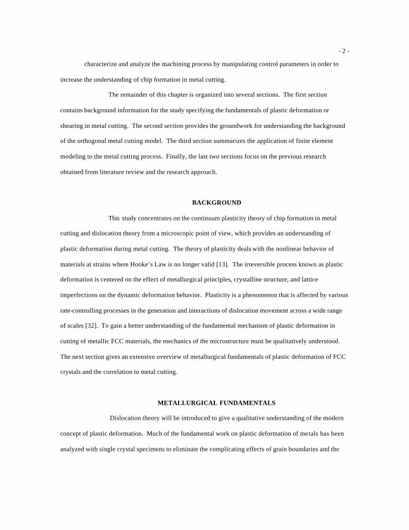
The atom arrangements of crystalline metals are visualized as a three dimensional lattice
in which atoms are portrayed as solid balls located at prescribed locations in a geometrical arrangement.
Figure 1.1 describes this crystal lattice by superimposing a right hand coordinate system of axes with the
origin at the intersection. In the FCC system, the lengths of each side are equal and the axes are
perpendicular. Miller Indices are used to specify the crystallographic planes and directions with respect to
these axes. A crystallographic plane can be described in this system, relative to the intersection of the
atoms.
Figure 1.1 Cubic Structure [13]
In the Miller Indices system the specific plane is denoted as (hkl) and the family of planes as
{hkl}. For example, the plane shown in figure 1.1 would be the (011) plane. Crystallographic directions in
this system are indicated by integers in brackets [uvw]; with the family of crystallographic equivalent
direction would be designated as <uvw>. Many of the common engineering metals such as aluminum and
copper have a face centered cubic (FCC) crystal structure and materials such as steel have a body centered
cubic (BCC) crystal structure represented in figures 1.2 and 1.3 respectively [13].
- 4 -
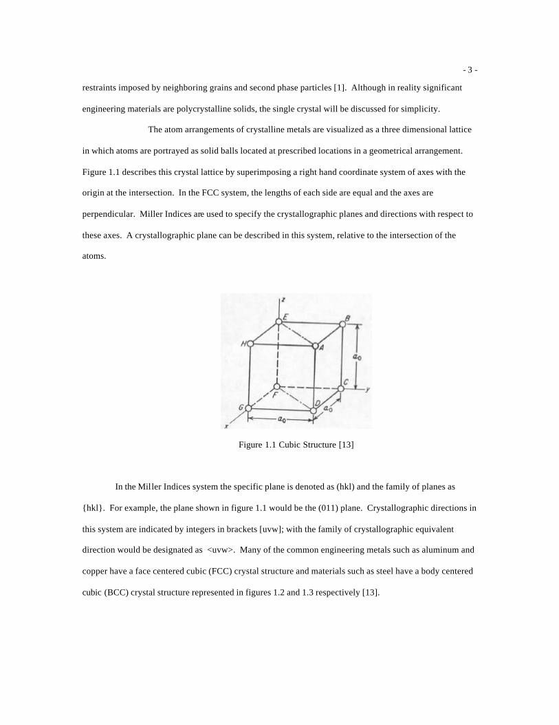
Figure 1.2 Face Centered Cubic Structure [13] Figure 1.3 Body Centered Cubic Structure [13]
Plastic deformation in metals occurs on slip planes by which the sliding of rows of atoms
over one another along definite crystallographic plane or slip planes. Slip occurs most readily in certain
specific directions on certain individual crystallographic planes. It is common for the slip plane to have the
greatest atomic density and the slip direction is the closest packed direction within the slip. The resistance
to slip is generally less for those planes with the greatest atomic density because they are widely spaced.
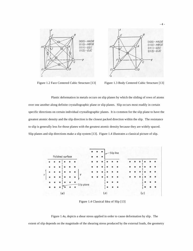
Slip planes and slip directions make a slip system [13]. Figure 1.4 illustrates a classical picture of slip.
Figure 1.4 Classical Idea of Slip [13]
Figure 1.4a, depicts a shear stress applied in order to cause deformation by slip. The
extent of slip depends on the magnitude of the shearing stress produced by the external loads, the geometry
- 5 -
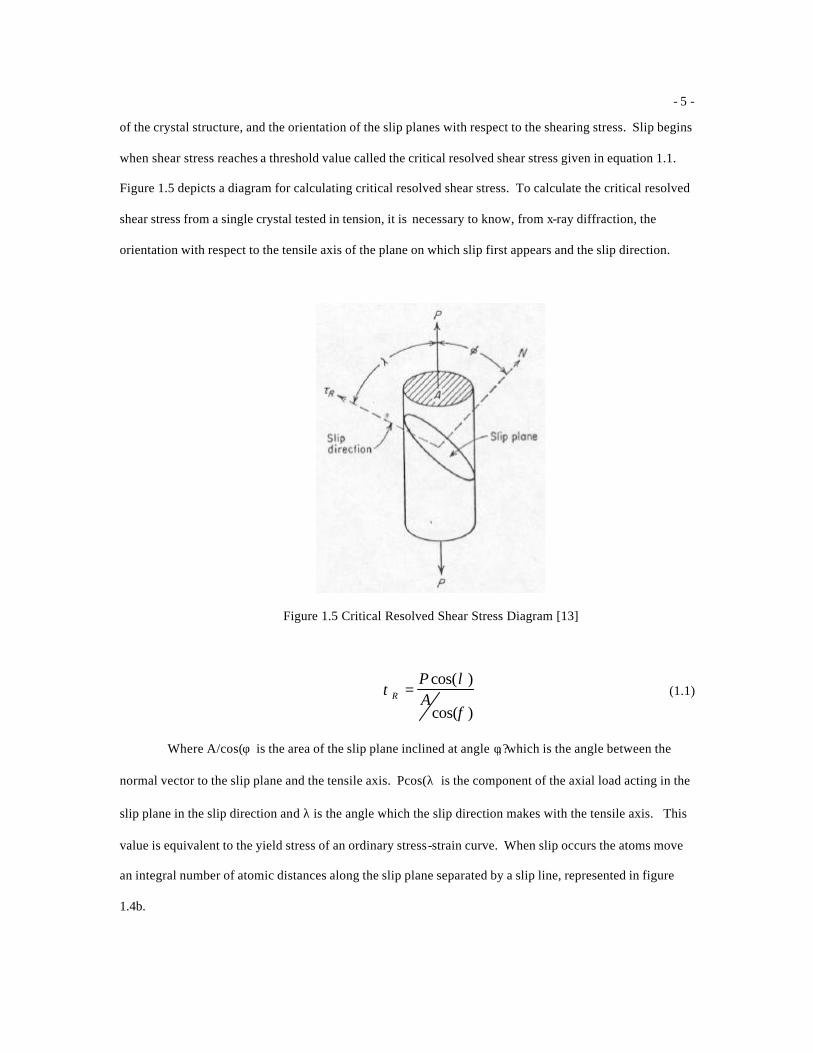
of the crystal structure, and the orientation of the slip planes with respect to the shearing stress. Slip begins
when shear stress reaches a threshold value called the critical resolved shear stress given in equation 1.1.
Figure 1.5 depicts a diagram for calculating critical resolved shear stress. To calculate the critical resolved
shear stress from a single crystal tested in tension, it is necessary to know, from x-ray diffraction, the
orientation with respect to the tensile axis of the plane on which slip first appears and the slip direction.
Figure 1.5 Critical Resolved Shear Stress Diagram [13]
)cos(
)cos(
φ
λτ
AP
R = (1.1)
Where A/cos(φ) is the area of the slip plane inclined at angle φ,? which is the angle between the
normal vector to the slip plane and the tensile axis. Pcos(λ) is the component of the axial load acting in the
slip plane in the slip direction and λ is the angle which the slip direction makes with the tensile axis. This
value is equivalent to the yield stress of an ordinary stress-strain curve. When slip occurs the atoms move
an integral number of atomic distances along the slip plane separated by a slip line, represented in figure
1.4b.
- 6 -
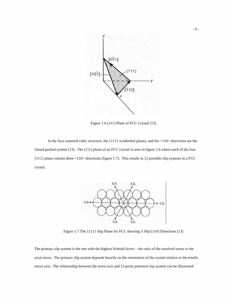
Figure 1.6 (111) Plane of FCC Crystal [13]
In the face centered cubic structure, the {111} octahedral planes, and the <110> directions are the
closed packed system [13]. The (111) plane of an FCC crystal is seen in figure 1.6 where each of the four
{111} plane contain three <110> directions (figure 1.7). This results in 12 possible slip systems in a FCC
crystal.
Figure 1.7 The {111} Slip Plane for FCC showing 3 Slip [110] Directions [13]
The primary slip system is the one with the highest Schmid factor – the ratio of the resolved stress to the
axial stress. The primary slip system depends heavily on the orientation of the crystal relative to the tensile
stress axis. The relationship between the stress axis and 12-point potential slip system can be illustrated
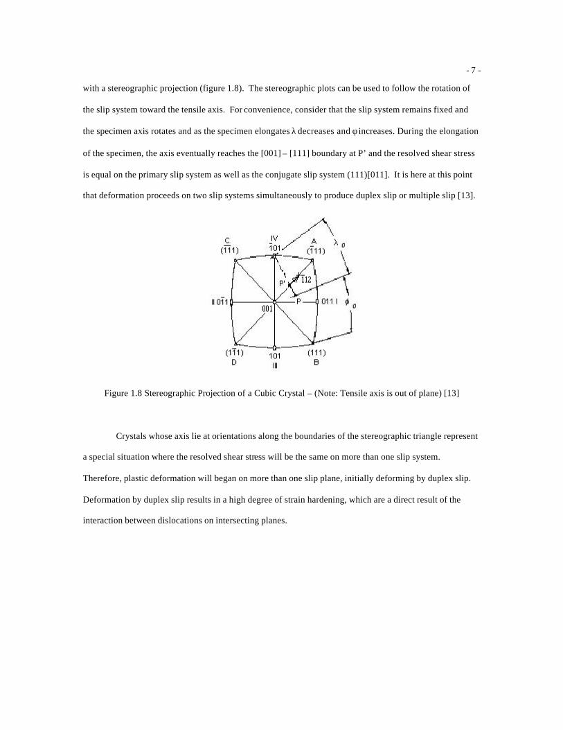
- 7 -
with a stereographic projection (figure 1.8). The stereographic plots can be used to follow the rotation of
the slip system toward the tensile axis. For convenience, consider that the slip system remains fixed and
the specimen axis rotates and as the specimen elongates λ decreases and φ increases. During the elongation
of the specimen, the axis eventually reaches the [001] – [111] boundary at P’ and the resolved shear stress
is equal on the primary slip system as well as the conjugate slip system (111)[011]. It is here at this point
that deformation proceeds on two slip systems simultaneously to produce duplex slip or multiple slip [13].
Figure 1.8 Stereographic Projection of a Cubic Crystal – (Note: Tensile axis is out of plane) [13]
Crystals whose axis lie at orientations along the boundaries of the stereographic triangle represent
a special situation where the resolved shear stress will be the same on more than one slip system.
Therefore, plastic deformation will began on more than one slip plane, initially deforming by duplex slip.
Deformation by duplex slip results in a high degree of strain hardening, which are a direct result of the
interaction between dislocations on intersecting planes.
- 8 -
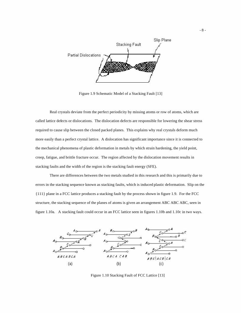
Figure 1.9 Schematic Model of a Stacking Fault [13]
Real crystals deviate from the perfect periodicity by missing atoms or row of atoms, which are
called lattice defects or dislocations. The dislocation defects are responsible for lowering the shear stress
required to cause slip between the closed packed planes. This explains why real crystals deform much
more easily than a perfect crystal lattice. A dislocation has significant importance since it is connected to
the mechanical phenomena of plastic deformation in metals by which strain hardening, the yield point,
creep, fatigue, and brittle fracture occur. The region affected by the dislocation movement results in
stacking faults and the width of the region is the stacking fault energy (SFE).
There are differences between the two metals studied in this research and this is primarily due to
errors in the stacking sequence known as stacking faults, which is induced plastic deformation. Slip on the
{111} plane in a FCC lattice produces a stacking fault by the process shown in figure 1.9. For the FCC
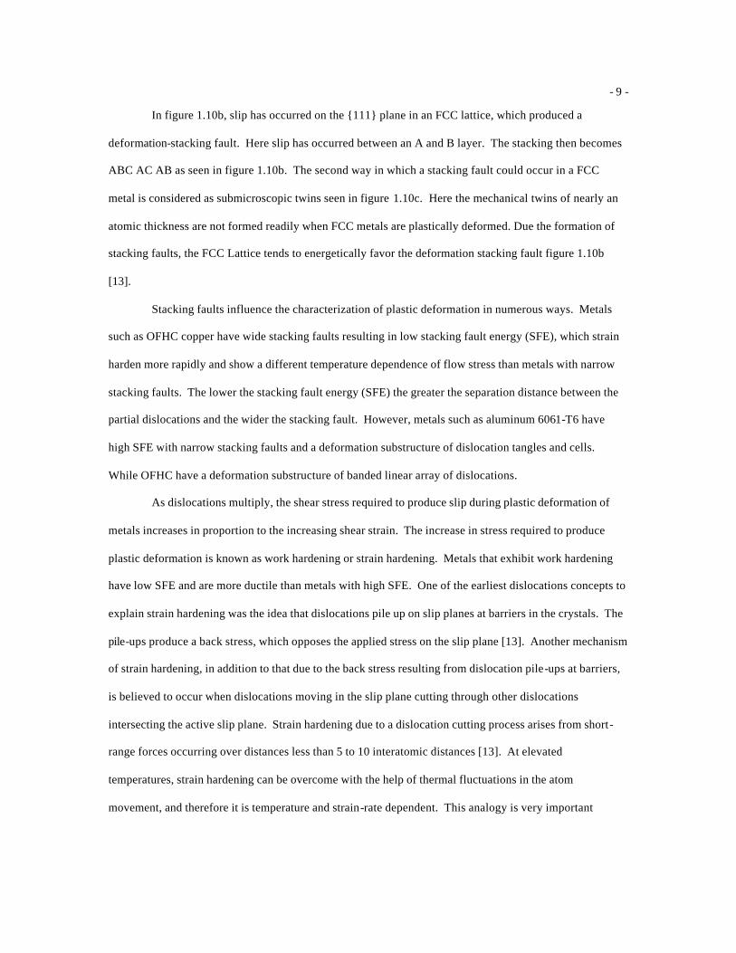
structure, the stacking sequence of the planes of atoms is given an arrangement ABC ABC ABC, seen in
figure 1.10a. A stacking fault could occur in an FCC lattice seen in figures 1.10b and 1.10c in two ways.
Figure 1.10 Stacking Fault of FCC Lattice [13]
- 9 -
In figure 1.10b, slip has occurred on the {111} plane in an FCC lattice, which produced a
deformation-stacking fault. Here slip has occurred between an A and B layer. The stacking then becomes
ABC AC AB as seen in figure 1.10b. The second way in which a stacking fault could occur in a FCC
metal is considered as submicroscopic twins seen in figure 1.10c. Here the mechanical twins of nearly an
atomic thickness are not formed readily when FCC metals are plastically deformed. Due the formation of
stacking faults, the FCC Lattice tends to energetically favor the deformation stacking fault figure 1.10b
[13].
Stacking faults influence the characterization of plastic deformation in numerous ways. Metals
such as OFHC copper have wide stacking faults resulting in low stacking fault energy (SFE), which strain
harden more rapidly and show a different temperature dependence of flow stress than metals with narrow
stacking faults. The lower the stacking fault energy (SFE) the greater the separation distance between the
partial dislocations and the wider the stacking fault. However, metals such as aluminum 6061-T6 have
high SFE with narrow stacking faults and a deformation substructure of dislocation tangles and cells.
While OFHC have a deformation substructure of banded linear array of dislocations.
As dislocations multiply, the shear stress required to produce slip during plastic deformation of
metals increases in proportion to the increasing shear strain. The increase in stress required to produce
plastic deformation is known as work hardening or strain hardening. Metals that exhibit work hardening
have low SFE and are more ductile than metals with high SFE. One of the earliest dislocations concepts to
explain strain hardening was the idea that dislocations pile up on slip planes at barriers in the crystals. The
pile-ups produce a back stress, which opposes the applied stress on the slip plane [13]. Another mechanism
of strain hardening, in addition to that due to the back stress resulting from dislocation pile-ups at barriers,
is believed to occur when dislocations moving in the slip plane cutting through other dislocations
intersecting the active slip plane. Strain hardening due to a dislocation cutting process arises from short-
range forces occurring over distances less than 5 to 10 interatomic distances [13]. At elevated
temperatures, strain hardening can be overcome with the help of thermal fluctuations in the atom
movement, and therefore it is temperature and strain-rate dependent. This analogy is very important
- 10 -
because it gives rise to constitutive models that are strain rate dependent and temperature dependent for the
plastic regime.
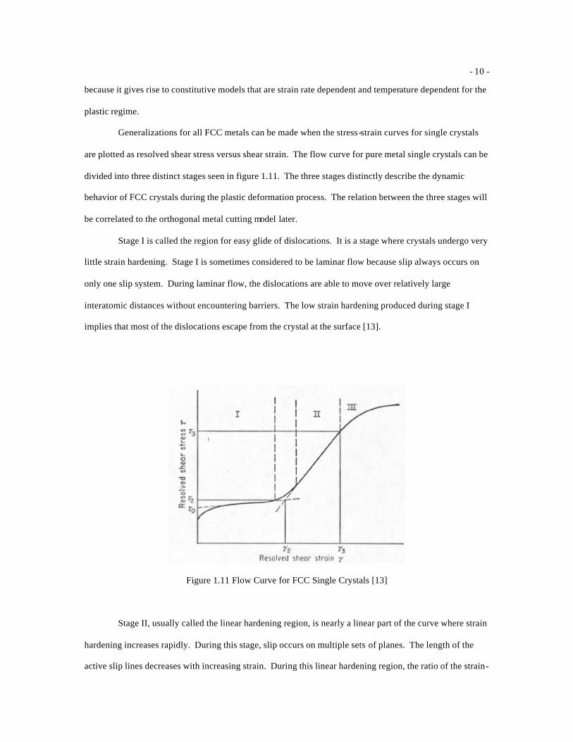
Generalizations for all FCC metals can be made when the stress-strain curves for single crystals
are plotted as resolved shear stress versus shear strain. The flow curve for pure metal single crystals can be
divided into three distinct stages seen in figure 1.11. The three stages distinctly describe the dynamic
behavior of FCC crystals during the plastic deformation process. The relation between the three stages will
be correlated to the orthogonal metal cutting model later.
Stage I is called the region for easy glide of dislocations. It is a stage where crystals undergo very
little strain hardening. Stage I is sometimes considered to be laminar flow because slip always occurs on
only one slip system. During laminar flow, the dislocations are able to move over relatively large
interatomic distances without encountering barriers. The low strain hardening produced during stage I
implies that most of the dislocations escape from the crystal at the surface [13].
Figure 1.11 Flow Curve for FCC Single Crystals [13]
Stage II, usually called the linear hardening region, is nearly a linear part of the curve where strain
hardening increases rapidly. During this stage, slip occurs on multiple sets of planes. The length of the
active slip lines decreases with increasing strain. During this linear hardening region, the ratio of the strain-
- 11 -
hardening coefficient to the shear modulus is nearly independent of stress and temperature, as well as being
independent of crystal orientation and purity. The fact that the slope of the flow curve in stage II is nearly
independent of temperature agrees with the theory that assumes the chief strain-hardening mechanism to be
pile-up of groups of dislocations. As a result of slip on several slip systems, lattice irregularities are
formed. Dislocation tangles begin to develop which result in the formation of dislocation forests or cell
structures [13].
Stage III, often called the parabolic hardening region, is characterized by a work hardening rate
that decreases with continuous increasing strain until fracture. The parabolic region can also be called
dynamical recovery. This region of the flow curve is strongly temperature dependent. With increasing
temperature, dislocations are able to climb from one slip plane to another where dislocation interactions of
opposite signs result in annihilation restoring order to the crystalline structure. Cross slip is believed to be
the chief process by which dislocations can escape and reduce the internal-strain field. This temperature
dependence suggests that the intersection of forests of dislocations, with dislocations threading through the
active slip plane, is the primary strain-hardening mechanism in the parabolic hardening region (stage III)
[13].
Concluding that for a given resolved shear stress value the strain decreases with increasing
temperature. So, with increasing temperature both stage I and II decrease in extent until at a high
temperature the stress-strain curve shows entirely a parabolic hardening (stage III) behavior.
PRINCIPLES OF METAL CUTTING
Metal cutting is classified as the secondary process by which material is removed to acquire a part
with a certain shape, size, high dimensional tolerance, and a good surface finish. Traditional machining
applications are accomplished by mechanically straining a local region of the work piece to fracture. The
theory of machining is concerned with the various features of the cutting process including the forces,
strain and strain rates, temperatures, and wear of cutting tools [21]. All metal cutting operations such as
turning, drilling, boring, milling, grinding, reaming, and other metal removal processes produce chips in a
similar fashion. Therefore, analysis of chip formation can give a better understanding to the mechanics of
- 12 -
the machining process. Although, the formation of chips is perhaps the most important aspect, as it affects
surface finish, it is also the least understood [25]. This is due to the comple xity of the problem during the
plastic deformation process. For this study, tool wear will not be investigated and the chip formation of
orthogonal metal cutting process will be the focus of this thesis.
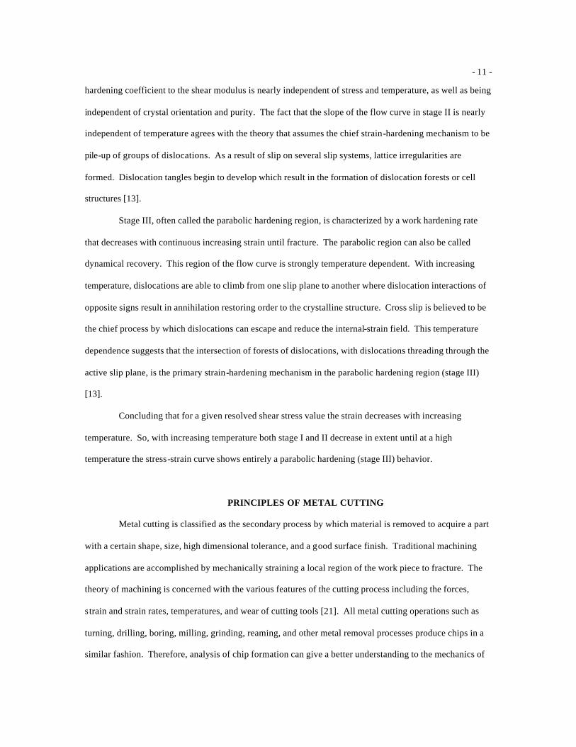
Figure 1.12 Orthogonal Cutting Model
A simple two-dimensional orthogonal metal cutting model is seen in figure 1.12. The tool is a
single point tool that is characterized by the rake angle α and the trailing edge of the tool, the clearance
angle θ.??? When the rake face of the tool is in the clockwise position from the work piece the rake angle is
considered to be positive and if counter clock wise negative. Different rake angles are used for different
cutting conditions and the small clearance angle is generally used to keep the tool from damaging the
finished surface of the work piece. The rake face of the tool is the surface over which the chip flows and
has a contact length lc, which is the chip and tool contact interaction. The prescribed velocity V, known as
the cutting speed is in the feed direction. The localized straining in the work piece enforced by the tool
causes plastic deformation of the undeformed chip t, which proceeds to the deformed chip thickness tc. The
- 13 -
chip thickness are related by the shear plane angle φ, which is an important characteristic parameter in
metal cutting that varies with cutting conditions and work piece materials.
There are three deformation zones that result during the plastic deformation or chip formation the
primary shear zone, secondary shear zone and the tertiary shear zone. The primary shear zone extends
from the tool tip to the free surface of the work piece, the secondary shear zone exists in the region where
the chip is in contact with the cutting tool, and the tertiary zone is the zone perpendicular to tool tip
clearance face. The primary shear zone is the region that experiences large localized strain whereas the
friction between the chip and cutting tool affects the secondary zone. The tertiary shear zone is a result of
the immediate removal of undeformed chip by the tool, which is also a local region for residual stresses.
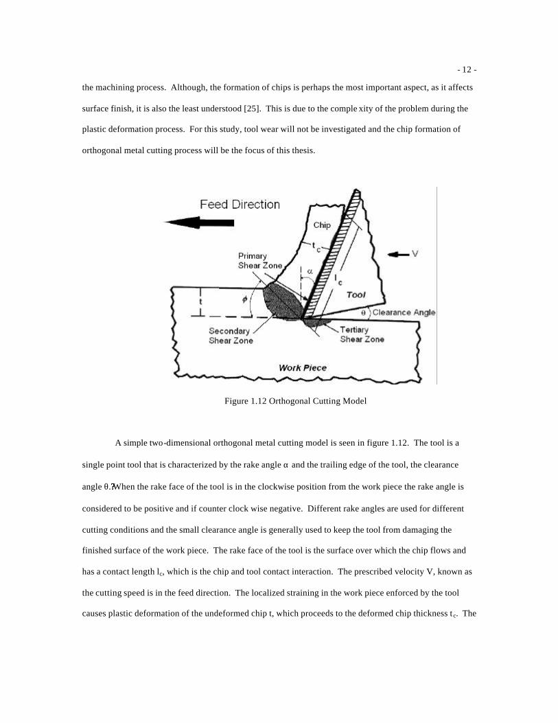
Figure 1.13 3D Orthogonal Metal Cutting Model
Figure 1.13 shows a three-dimensional view of the same orthogonal cutting model.
Assuming an incompressible material, the chip thickness ratio, also cutting ratio, can be derived from the
general continuity equation, where ρ is the material density and V is the velocity vector,
0)( =+∂∂
Vdivt
ρρ
(1.2)

- 14 -
which reduces to divergence(V)= 0 [2]. With the assumption that b1 = b2, the chip does not
deform laterally during the cutting process and the chip thickness ratio rc can be expressed as
CC
F rtt
VV
==2
1 (1.3)
Since the chip thickness ratio is easily determined from the chip thickness measurements
taken after the cut (t2) is made, the shear angle existing during the cut can be estimated using equation (1.4).
Figure 1.13 shows the relationship between the cutting velocity VC and shear velocity, which is the vector
sum of the cutting velocity VC and chip velocity VF.
)sin(1)cos(
)sin()cos(
)tan(α
αα
αφ
C
C
FC
F
rr
VVV
−=
−= (1.4)
Figure 1.14 Velocity and Shear Plane Angle Relationship Diagram
Much work has been done for estimating the shear plane angle, which can give a relative
estimation of chip formation. The most dominant effect on the shear front angle is the material hardness
and the second is the feed rate [2]. The shear front angle decreases with increasing hardness as the shear
zone (figure 1.12), which extends the width of the undeformed chip b1 and perpendicular to the cutting tool
rake face tip , approaches a fracture plane.
Large forces are generated during the machining process, which are shown in figure 1.15.
The cutting force FC acts in the direction of the cutting velocity and the thrust force FT act normal to the
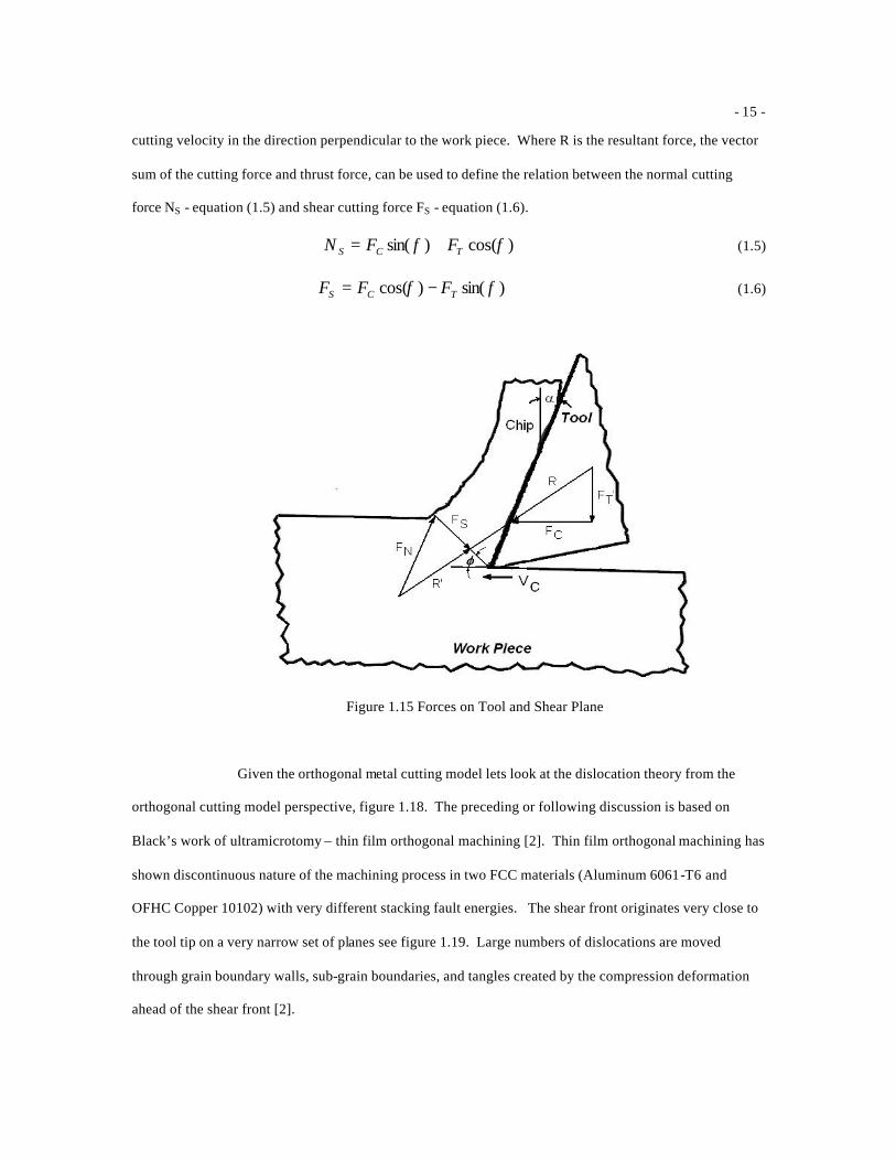
- 15 -
cutting velocity in the direction perpendicular to the work piece. Where R is the resultant force, the vector
sum of the cutting force and thrust force, can be used to define the relation between the normal cutting
force NS - equation (1.5) and shear cutting force FS - equation (1.6).
)cos()sin( φφ TCS FFN += (1.5)
)sin()cos( φφ TCS FFF −= (1.6)
Figure 1.15 Forces on Tool and Shear Plane
Given the orthogonal metal cutting model lets look at the dislocation theory from the
orthogonal cutting model perspective, figure 1.18. The preceding or following discussion is based on
Black’s work of ultramicrotomy – thin film orthogonal machining [2]. Thin film orthogonal machining has
shown discontinuous nature of the machining process in two FCC materials (Aluminum 6061-T6 and
OFHC Copper 10102) with very different stacking fault energies. The shear front originates very close to
the tool tip on a very narrow set of planes see figure 1.19. Large numbers of dislocations are moved
through grain boundary walls, sub-grain boundaries, and tangles created by the compression deformation
ahead of the shear front [2].
- 16 -
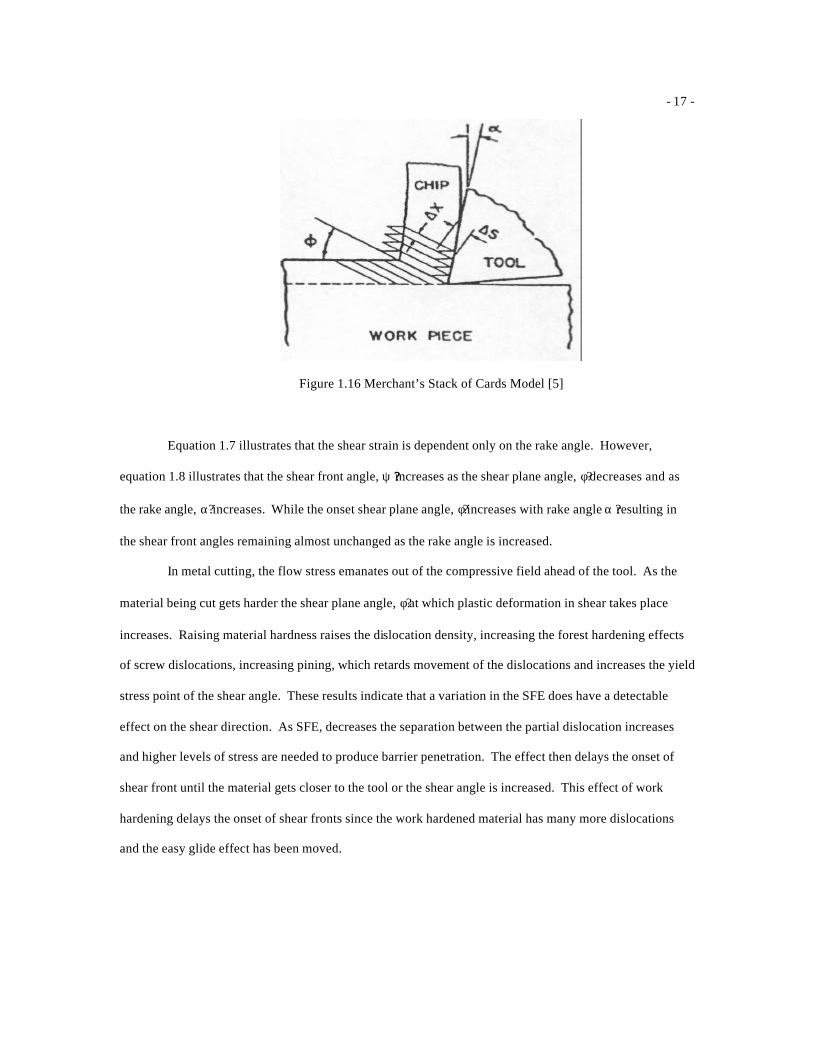
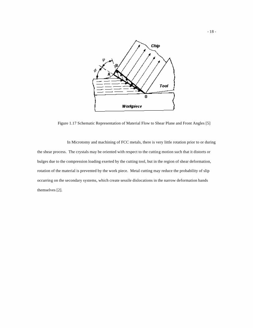
Shear strain, along with shear stress, are important para meters for describing the plastic
deformation in metal cutting [5]. The shear strain has a tremendous effect on the flow stress, shear energy,
temperature and chip morphology. The material flow process during a metal cutting process is
schematically represented in figure 1.17, relating the shear plane angle and shear front angle to the material
flow [5]. This model was developed to predict shear strain and the shear front angle. In figure 1.17, a
particle in the work piece moves toward the cutting tool along the cutting direction, which approaches the
shear zone [5]. As the particle encounter plane OA, it changes direction and flows at an inclination angle,
ψ? to the plane. Once the particle reaches, plane OB the shear process stops and the particle changes
direction again and flows in parallel direction to the tool rake face. A number of particles encounter the
plane OA simultaneously and as a result, they shear in mass, which defines the simultaneous onset of
multiple shear fronts [5]. An expression of shear strain for the new shear strain model was derived by
Black and Huang by developing a new stack of cards model equations 1.7 and 1.8, which expresses the
shear strain and shear front angle relation [5].
))sin(1()cos(2
αα
γ+
= (1.7)
245
αφψ +−= o (1.8)
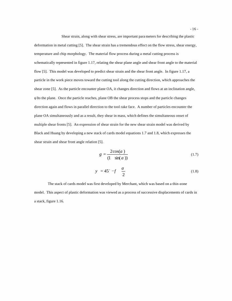
The stack of cards model was first developed by Merchant, which was based on a thin-zone
model. This aspect of plastic deformation was viewed as a process of successive displacements of cards in
a stack, figure 1.16.
- 17 -
Figure 1.16 Merchant’s Stack of Cards Model [5]
Equation 1.7 illustrates that the shear strain is dependent only on the rake angle. However,
equation 1.8 illustrates that the shear front angle, ψ ??increases as the shear plane angle, φ? decreases and as
the rake angle, α? increases. While the onset shear plane angle, φ? increases with rake angle α ?resulting in
the shear front angles remaining almost unchanged as the rake angle is increased.
In metal cutting, the flow stress emanates out of the compressive field ahead of the tool. As the
material being cut gets harder the shear plane angle, φ? at which plastic deformation in shear takes place
increases. Raising material hardness raises the dislocation density, increasing the forest hardening effects
of screw dislocations, increasing pining, which retards movement of the dislocations and increases the yield
stress point of the shear angle. These results indicate that a variation in the SFE does have a detectable
effect on the shear direction. As SFE, decreases the separation between the partial dislocation increases
and higher levels of stress are needed to produce barrier penetration. The effect then delays the onset of
shear front until the material gets closer to the tool or the shear angle is increased. This effect of work
hardening delays the onset of shear fronts since the work hardened material has many more dislocations
and the easy glide effect has been moved.
- 18 -
Figure 1.17 Schematic Representation of Material Flow to Shear Plane and Front Angles [5]
In Microtomy and machining of FCC metals, there is very little rotation prior to or during
the shear process. The crystals may be oriented with respect to the cutting motion such that it distorts or
bulges due to the compression loading exerted by the cutting tool, but in the region of shear deformation,
rotation of the material is prevented by the work piece. Metal cutting may reduce the probability of slip
occurring on the secondary systems, which create sessile dislocations in the narrow deformation bands
themselves [2].
- 19 -
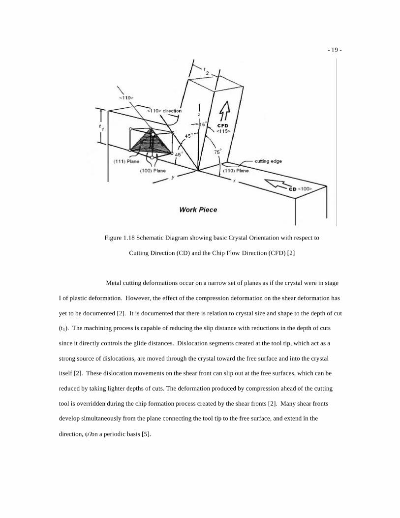
Figure 1.18 Schematic Diagram showing basic Crystal Orientation with respect to
Cutting Direction (CD) and the Chip Flow Direction (CFD) [2]
Metal cutting deformations occur on a narrow set of planes as if the crystal were in stage
I of plastic deformation. However, the effect of the compression deformation on the shear deformation has
yet to be documented [2]. It is documented that there is relation to crystal size and shape to the depth of cut
(t1). The machining process is capable of reducing the slip distance with reductions in the depth of cuts
since it directly controls the glide distances. Dislocation segments created at the tool tip, which act as a
strong source of dislocations, are moved through the crystal toward the free surface and into the crystal
itself [2]. These dislocation movements on the shear front can slip out at the free surfaces, which can be
reduced by taking lighter depths of cuts. The deformation produced by compression ahead of the cutting
tool is overridden during the chip formation process created by the shear fronts [2]. Many shear fronts
develop simultaneously from the plane connecting the tool tip to the free surface, and extend in the
direction, ψ? on a periodic basis [5].
- 20 -
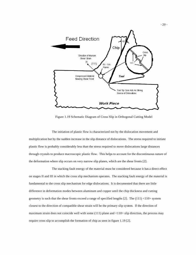
Figure 1.19 Schematic Diagram of Cross Slip in Orthogonal Cutting Model
The initiation of plastic flow is characterized not by the dislocation movement and
multiplication but by the sudden increase in the slip distance of dislocations. The stress required to initiate
plastic flow is probably considerably less than the stress required to move dislocations large distances
through crystals to produce macroscopic plastic flow. This helps to account for the discontinuous nature of
the deformation where slip occurs on very narrow slip planes, which are the shear fronts [2].
The stacking fault energy of the material must be considered because it has a direct effect
on stages II and III in which the cross slip mechanism operates. The stacking fault energy of the material is
fundamental to the cross slip mechanism for edge dislocations. It is documented that there are little
difference in deformation modes between aluminum and copper until the chip thickness and cutting
geometry is such that the shear fronts exceed a range of specified lengths [2]. The (111) <110> system
closest to the direction of compatible shear strain will be the primary slip system. If the direction of
maximum strain does not coincide well with some (111) plane and <110> slip direction, the process may
require cross slip to accomplish the formation of chip as seen in figure 1.19 [2].
- 21 -
The intermittent fashion of the chip formation process may be explained by the classical
continuum plasticity theory and dislocation theory. The large-scale dislocation activity occurring in the
work piece due to the compression loading by the cutting tool presents evidence that the tool tip is a very
strong source of dislocation generation. An alteration of the surface morphology was observed between the
sides and top of the deformed chips indicating a shift from plane stress on the side to plane strain in the
bulk of the chip. The shear fronts were observed to extend to the very bottom of the chip [2].
PRINCIPLES OF FINITE ELEMENT MODELING
Finite element analysis is a numerical approximation method of analysis that breaks a
complex structure into discrete components, resulting in an idealized structure that can be mathematically
solved. The finite element method provides a systematic procedure for the derivation of the approximation
functions over sub-regions of the domain called finite elements. The approximation functions are derived
using the idea that any continuous functions that are derived can be expressed by a linear combination of
algebraic polynomials, which are obtained by satisfying the governing equations, usually in a weighted-
integral sense over each element. Numerically solving for the variables at specified points called nodes on
each element and applying the calculated finite solutions to the whole geometry determines the solution to
the problem. The finite element method proves useful by producing approximations of the exact solution
for problems that would be difficult or impossible to solve analytically.
Discretization of the geometry is the first step in finite element analysis and it is in this
step that the geometry is divided into finite elements. Next, the element properties are defined in which
different types of elements such as bricks, triangular, or shell elements are used depending on the
requirements of the analysis. Using the element properties, the stiffness matrix, which describes the force –
displacement relationship of the element under loading, is derived. Following the derivation of the stiffness
matrix, the loading conditions, such as pressure, forces, and velocities, are defined along with the boundary
conditions at specified nodes. Finally, the element descriptions, applied loads, and boundary conditions are
assembled as a set of equations in matrix form. The set of equations are then solved numerically for the
- 22 -
unknown values. Stresses, strains, and other quantities of interest can be calculated based on the resulting
nodal displacements.
For a general linear and/or nonlinear static problem the equilibrium equations for a finite
element analysis are expressed as
}]{[}{ UKF = (1.9)
where F is the vector matrix for the forces on the element, K is the stiffness matrix, and U is the
vector of nodal displacements to be determined. However, for time dependent dynamic problems the
equation requires the form for a dynamic analysis as represented by equation (9).
}]{[}]{[}]{[)}({ 21 UMUMUKtF &&& ++= (1.10)
Where K is the stiffness matrix, U is the nodal displacement vector, which is updated as time
changes, M1 is the damping matrix, U’ are the nodal displacements with respect to first order time
derivative (i.e. nodal velocity), M2 is the mass matrix, and U’’ are the nodal displacements with respect to
second order time derivative (i.e. nodal acceleration).
The finite element formulation used in DYNA 3D is a Lagrangian formulation. The
central finite difference rule is used to integrate the equation of motion. DYNA 3D uses a lumped mass
formulation for efficiency, which produces a diagonal mass matrix that renders the solution of the
conservation of momentum equation. In an explicit analysis code, there are many small time steps, so it is
important that the number of operations performed at each time step is minimized [42]. This consideration
has largely motivated the use of elements with one-point Gauss quadrature for the element integration.
This approach gives rise to spurious zero energy deformation modes, or hourglass modes within the
element [42]. The element must then be stabilized to eliminate the spurious modes while retaining
legitimate deformation modes.
There are two ways in which a continuous medium can be described: Eulerian and
Lagrangian [42]. In a Lagrangain referential, the computational grid deforms with the material where as in
a Eulerian referential it is fixed in space. This paper will only make mention of the Lagrangian formulation
for the purpose of the code’s use of this formulation. The Lagrangian calculation embeds a computational
- 23 -
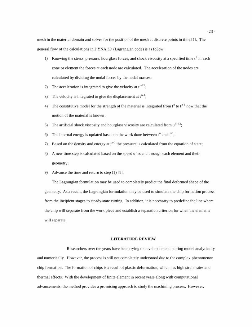
mesh in the material domain and solves for the position of the mesh at discrete points in time [1]. The
general flow of the calculations in DYNA 3D (Lagrangian code) is as follow:
1) Knowing the stress, pressure, hourglass forces, and shock viscosity at a specified time tn in each
zone or element the forces at each node are calculated. The acceleration of the nodes are
calculated by dividing the nodal forces by the nodal masses;
2) The acceleration is integrated to give the velocity at tn-1 2 ;
3) The velocity is integrated to give the displacement at tn-1;
4) The constitutive model for the strength of the material is integrated from tn to tn-1 now that the
motion of the material is known;
5) The artificial shock viscosity and hourglass viscosity are calculated from un-1 2;
6) The internal energy is updated based on the work done between tn and tn-1;
7) Based on the density and energy at tn-1 the pressure is calculated from the equation of state;
8) A new time step is calculated based on the speed of sound through each element and their
geometry;
9) Advance the time and return to step (1) [1].
The Lagrangian formulation may be used to completely predict the final deformed shape of the
geometry. As a result, the Lagrangian formulation may be used to simulate the chip formation process
from the incipient stages to steady-state cutting. In addition, it is necessary to predefine the line where
the chip will separate from the work piece and establish a separation criterion for when the elements
will separate.
LITERATURE REVIEW
Researchers over the years have been trying to develop a metal cutting model analytically
and numerically. However, the process is still not completely understood due to the complex phenomenon
chip formation. The formation of chips is a result of plastic deformation, which has high strain rates and
thermal effects. With the development of finite element in recent years along with computational
advancements, the method provides a promising approach to study the machining process. However,
- 24 -
development of finite element models to understand the complex phenomenon requires extensive time and
effort along with an understanding of the machining process and the development of finite element codes.
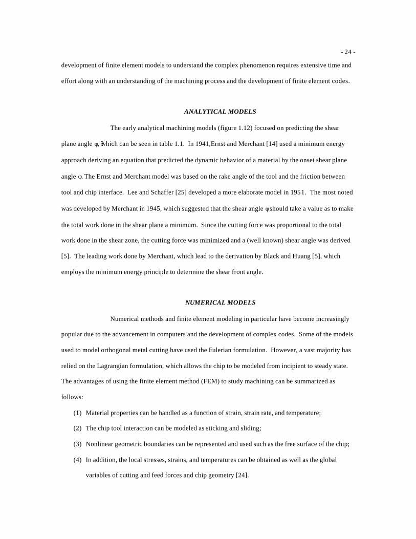
ANALYTICAL MODELS
The early analytical machining models (figure 1.12) focused on predicting the shear
plane angle φ, ??which can be seen in table 1.1. In 1941,Ernst and Merchant [14] used a minimum energy
approach deriving an equation that predicted the dynamic behavior of a material by the onset shear plane
angle φ. The Ernst and Merchant model was based on the rake angle of the tool and the friction between
tool and chip interface. Lee and Schaffer [25] developed a more elaborate model in 1951. The most noted
was developed by Merchant in 1945, which suggested that the shear angle φ should take a value as to make
the total work done in the shear plane a minimum. Since the cutting force was proportional to the total
work done in the shear zone, the cutting force was minimized and a (well known) shear angle was derived
[5]. The leading work done by Merchant, which lead to the derivation by Black and Huang [5], which
employs the minimum energy principle to determine the shear front angle.
NUMERICAL MODELS
Numerical methods and finite element modeling in particular have become increasingly
popular due to the advancement in computers and the development of complex codes. Some of the models
used to model orthogonal metal cutting have used the Eulerian formulation. However, a vast majority has
relied on the Lagrangian formulation, which allows the chip to be modeled from incipient to steady state.
The advantages of using the finite element method (FEM) to study machining can be summarized as
follows:
(1) Material properties can be handled as a function of strain, strain rate, and temperature;
(2) The chip tool interaction can be modeled as sticking and sliding;
(3) Nonlinear geometric boundaries can be represented and used such as the free surface of the chip;
(4) In addition, the local stresses, strains, and temperatures can be obtained as well as the global
variables of cutting and feed forces and chip geometry [24].
- 25 -
The finite element models found in the literature have been compared in Table 1.2, which are list
of the various finite element models generated for orthogonal metal cutting.
Klamecki developed one of the first finite element models of machining in 1973 [13].
This model of the incipient chip formation was a three-dimensional model in metal cutting. Another early
model was developed by Tay [14]. The drawback of this two-dimensional model used to calculate
temperature distributions in steady-state orthogonal cutting was the requirement of experimental strain rate
data. Moreover, in the past decade or so vast improvements in modeling orthogonal metal cutting has been
developed by a number of researchers. Strenkowski and Carroll [38] developed a finite element model
based on the Lagrangian formulation that modeled the chip formation from incipient to steady state cutting.
This model included the effects of friction and heat generation, as well as a separation criterion based on
effective plastic strain.
Strenkowski and Carroll also employed a Eulerian formulation to model steady-state orthogonal
metal cutting [16]. The Eulerian formulated model calculated the heat generated by friction and plastic
deformation. Another model of the Eulerian formulation was developed by Strenkowski and Moon which
predicted the tool-chip contact length as well as the temperature distributions in the work piece, chip, and
tool [37]. Shih developed an orthogonal cutting model in 1990, which included the effects of sticking and
sliding friction, strain rate, and heat generation [38]. This model utilized a separation criterion based on the
distance between the tool tip and the nodes of the work piece being cut. Moreover, many other researchers
have developed similar models to study the effects of tool wearing, varying rake angles, and chip-tool
interface contact [21 –23].
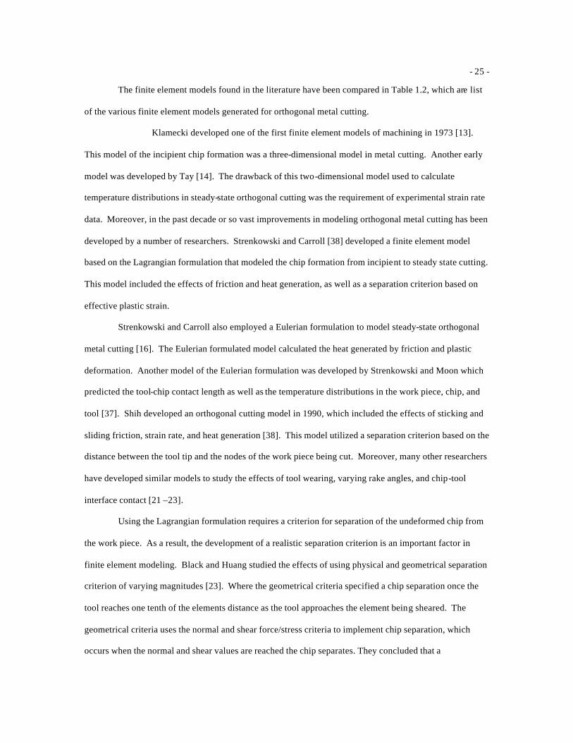
Using the Lagrangian formulation requires a criterion for separation of the undeformed chip from
the work piece. As a result, the development of a realistic separation criterion is an important factor in
finite element modeling. Black and Huang studied the effects of using physical and geometrical separation
criterion of varying magnitudes [23]. Where the geometrical criteria specified a chip separation once the
tool reaches one tenth of the elements distance as the tool approaches the element being sheared. The
geometrical criteria uses the normal and shear force/stress criteria to implement chip separation, which
occurs when the normal and shear values are reached the chip separates. They concluded that a
- 26 -
combination of both physical and geometric criteria provided the most realistic simulation for metal
cutting. For this study, the physical separation criterion will only be used.
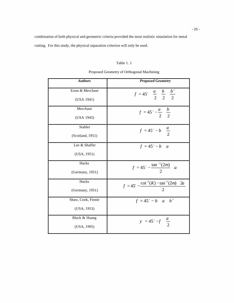
Table 1. 1
Proposed Geometry of Orthogonal Machining
Authors Proposed Geometry
Ernst & Merchant
(USA 1941) 22245
ββαφ
′+++= o
Merchant
(USA 1945) 2245
βαφ +−= o
Stabler
(Scotland, 1951) 245
αβφ +−= o
Lee & Shaffer
(USA, 1951)
αβφ +−= o45
Hucks
(Germany, 1951) α
µφ +−=
−
2)2(tan
451
o
Hucks
(Germany, 1951) 22)2(tan)(cot
4511 αµ
φ+−
−=−− Ko
Shaw, Cook, Finnie
(USA, 1953)
ηαβφ ′++−= o45
Black & Huang
(USA, 1995) 245
αφψ +−= o

- 27 -
Table 1.2
Comparison of Finite Element Models for Orthogonal Metal Cutting
Authors Material
Model
Chip-Tool
Interaction
Special
Features
Experimental
Comparison
Klamecki [13]
(1973)
Elastic-plastic
bilinear-strain curve
Frictionless sticking
as B.C.
Initial contact
simulation (3D)
Shape of the chip cross
section
Shirakashi, Usui [40]
(1974, 1982)
Elastic-plastic true
stress curve at
different strain rates
and temperatures
Frictional force as a
function of normal
force as B.C.
Steady-state
simulation
Temperature
Interfacial stress
Lajczok [23] (1980) Elastic-plastic
bilinear stress-strain
curves
Pre-applied B.C. Experimental data:
cutting force, feed
force, shear angle
Residual strain
Residual stress on the
machined surface
Iwata, Osakada,
Teraska [16] (1984)
Rigid-plastic flow
stress as function of
strain
Frictional stress as a
function of normal
stress as B.C.
Micro machining
simulation at steady-
state assumed const.
Cutting force feed force
chip-tool contact length
Strenkowski, Carroll
[34] (1985)
Elastic-plastic A const. coeff. of
friction at interface
Simulate whole chip
Chip separation
None
Strenkowski, Carroll,
Moon [41] (1986)
Visco-plastic Not discussed Eulerian formulation
for steady-state
None
Strenkowski, Carroll,
Moon [38] (1990)
Elasto-plastic Not discussed Coupled Lagrangian-
Eulerian formulation
Cutting force
Mean interface temp.
Shih, Chadrasekar,
Yang [46] (1990)
Elastic-viscoplastic
stress-strain curves at
different temperatures
Constant coeff. of
friction in sticking
region, linearly
decaying in sliding
region
Simulate whole chip
formation process,
chip separation,
automatic remesh,
sticking sliding
region
Cutting force
Feed force
- 28 -
RESEARCH APPROACH
To validate finite element model and results, the machining conditions and data from
experiments conducted by Black [2] and [5] and Zhang [45] will be used to simulate the model and
compare results. Finite element models of the chip formation process for orthogonal metal cutting were
developed for this study. The simulation analysis was performed using Lawrence Livermore National
Laboratory’s (LLNL) FEM code DYNA 3D version 4.0.14 licensed for research and education [42].
DYNA 3D is an explicit, nonlinear, finite element code intended for transient dynamic analysis as well as
quasi-static analysis of three dimensional solids and structures [42]. DYNA 3D is also referred to as a
hydro-code, which uses complex material models incorporating strength, rate dependence, and thermal
effects as well as failure models to solve large-scale numerical computational problems such as a dynamic
deformation processes. In addition, the hydro-code has a sophisticated contact interface capability,
including frictional sliding and single surface contact, to handle arbitrary mechanical interactions between
independent bodies or between two portions of one body. Details on creating metal cutting models of
simulation are included in the appendix.
The pre-processing was done with LLNL software INGRID, which writes a DYNA 3D
input file in ASCII format that may be modified and edited if required. The DYNA 3D analysis writes
binary plot files, restart files, and an ASCII output file that are post-processed using LLNL’s GRIZ. The
finite element modeling and modeling techniques will be discussed in the next chapter. To validate the
simulation analysis of the two FCC materials, OFHC Copper, Aluminum Alloy 6061 in the T6 condition
and Aluminum Alloy 2024 in the T351 condition, obtained from the FEM code. Black’s and Zhang’s
experimental work on two FCC materials will be used to compare FEA and experimental results.
FCC materials aluminum and copper were chosen because of the difference in their stacking fault
energy. Stacking faults influence the plastic deformation of metals in a number of ways. Aluminum has
high stacking fault energy (SFE), which has narrow stacking faults, twin easily on annealing, and a
deformation substructure of dislocation tangles and cells. Copper has a low stacking fault energy (SFE),
which has wider stacking faults and strain-harden more rapidly, and show a different temperature
dependence of flow stress than metals with narrow stacking faults. Low-SFE also shows a deformation

- 29 -
substructure of banded, linear arrays of dislocations. This type of finite element modeling is considered to
be in the continuum theory of plasticity, in addition, the question arises whether modeling in the continuum
captures the realistic behavior from a dislocation theory perspective at the macroscopic level.
- 30 -
Chapter II
Finite Element Modeling
INTRODUCTION
The typically engineering analysis process begins with a physical description of some problem or
system to be studied. The next step before finite element modeling is to not only understand the behavior
of the structure to be modeled but to know what is needed from the analysis such as deflections, reactions,
and stresses as well as failure load and failure mode. Generally, the process of idealizing the structure
mathematically using FEM requires the understanding of what type of elements to use, the behavior of the
elements, material models to be used, where can the mesh be coarse and or fine, what special FEA
techniques may apply, such as rigid regions or multipoint constraints. Also a basic understanding of how
the program solver affects accuracy, and the how the results are calculated. The last step would be to
balance accuracy with the resources available. This step is one of the most important because time,
manpower, and cost are of importance in determining how much detail should be included in the model.
Deciding when time savers for solutions can be used such as reduced integration schemes, modeling only
certain portions of the structure, and large time steps, defines what degree of accuracy is acceptable.
In order to assure a successful analysis the preceding steps must be taken into consideration.
There are a few things that may help develop a thorough routine for analysis which are as follow: checking
program documentation; running small test problems; using the simplest elements and material constitutive
relationships that can accurately represent the behavior to be modeled; paying attention to mesh density;
being cautious of idealized supports, and thoroughly understanding how the load can be idealized.
Thoroughly understanding the above issues will increase the chances for the analysis to converge to the
exact solution within a certain degree of accuracy. This chapter will give an extensive overview of the
modeling technique developed for the metal cutting model.
- 31 -
FINITE ELEMENT METHOD
Utilizing the finite element method for analyzing the chip formation in metal cutting requires a
number of assumptions. These assumptions aid in defining the problem to be solved as well as the
boundary and loading conditions. The orthogonal metal cutting model (figure 1.13) requires a three-
dimensional coordinate frame and time for the full description of the problem. The following assumptions
were made in regard to this model:
(1) The cutting speed is constant.
(2) The width of cut b1 is much larger then the feed t1, and both are constant.
(3) The tool is perfectly sharp.
(4) The chip is a continuous ribbon for ductile materials.
(5) The cutting velocity vector Vc is normal to the cutting edge.
(6) The work piece material is a homogeneous polycrystalline, isotropic, and incompressible solid.
(7) The work piece is at a reference temperature usually room temperature (298.15 – 300 degrees K).
(8) The cutting is performed in air with no liquid coolants.
(9) There is no tool wear.
(10) The tool is rigid (no deformation)
(11) The steady state of cutting has been reached during the process.
Implementing these assumptions and defining the strain rate testing range from table 2.1, as well
as an extensive understanding of how FCC materials behave during plastic deformation gives insight for
choosing the proper modeling technique as well as the proper material model. To capture the dynamic
behavior of the model a constitutive equation must be chosen that couples strain rate and thermal effects.
The stress in metals varies as a function of strain, strain rate, and temperature. The Johnson and Cook
constitutive equation is one of the first models to incorporate both strain rate effects and thermal effects
[28]. For this study the Johnson and Cook constitutive equation was used to model the material behavior of
the two selected FCC materials. During the orthogonal machining process the effects of thermal softening
and strain-rate hardening are discussed in detail in chapter 3.
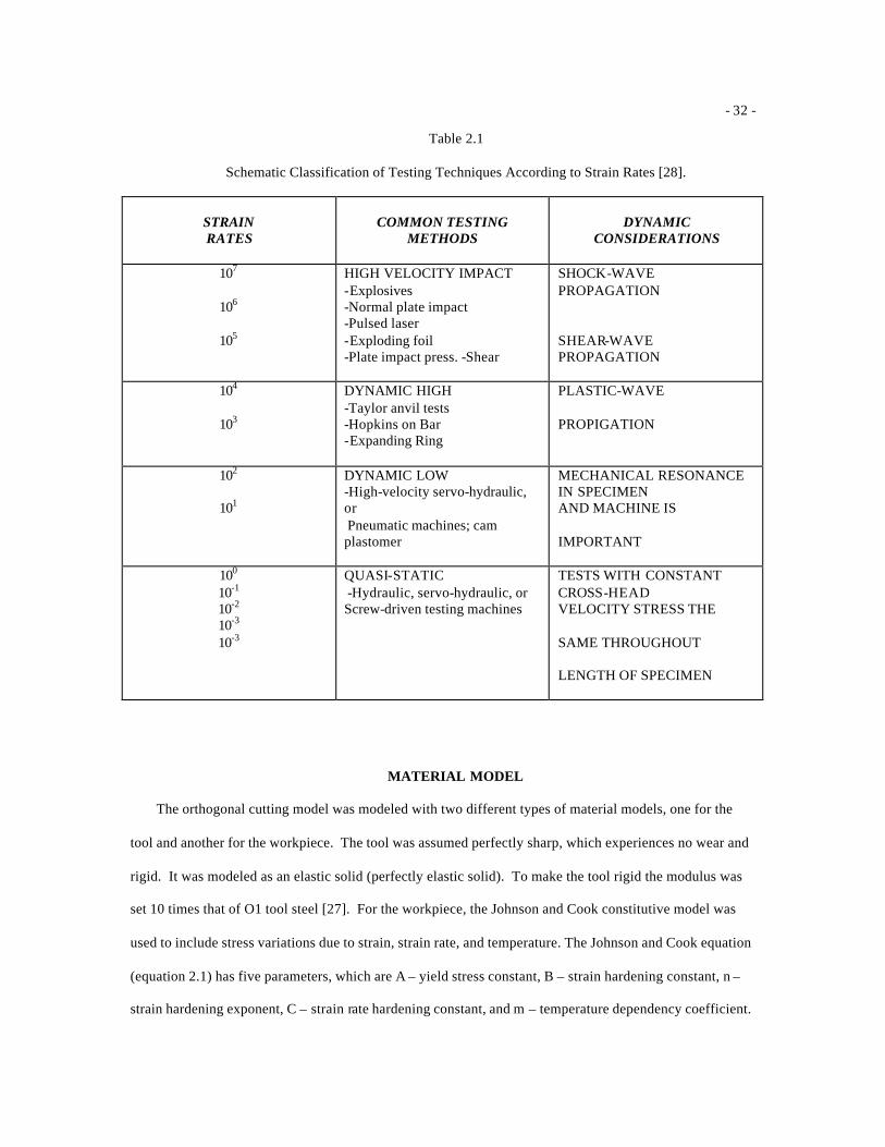
- 32 -
Table 2.1
Schematic Classification of Testing Techniques According to Strain Rates [28].
STRAIN RATES
COMMON TESTING
METHODS
DYNAMIC
CONSIDERATIONS
107
106
105
HIGH VELOCITY IMPACT -Explosives -Normal plate impact -Pulsed laser -Exploding foil -Plate impact press. -Shear
SHOCK-WAVE PROPAGATION SHEAR-WAVE PROPAGATION
104
103
DYNAMIC HIGH -Taylor anvil tests -Hopkins on Bar -Expanding Ring
PLASTIC-WAVE
PROPIGATION
102
101
DYNAMIC LOW -High-velocity servo-hydraulic, or Pneumatic machines; cam plastomer
MECHANICAL RESONANCE IN SPECIMEN AND MACHINE IS
IMPORTANT
100 10-1 10-2 10-3 10-3
QUASI-STATIC -Hydraulic, servo-hydraulic, or Screw-driven testing machines
TESTS WITH CONSTANT CROSS-HEAD VELOCITY STRESS THE
SAME THROUGHOUT
LENGTH OF SPECIMEN
MATERIAL MODEL
The orthogonal cutting model was modeled with two different types of material models, one for the
tool and another for the workpiece. The tool was assumed perfectly sharp, which experiences no wear and
rigid. It was modeled as an elastic solid (perfectly elastic solid). To make the tool rigid the modulus was
set 10 times that of O1 tool steel [27]. For the workpiece, the Johnson and Cook constitutive model was
used to include stress variations due to strain, strain rate, and temperature. The Johnson and Cook equation
(equation 2.1) has five parameters, which are A – yield stress constant, B – strain hardening constant, n –
strain hardening exponent, C – strain rate hardening constant, and m – temperature dependency coefficient.
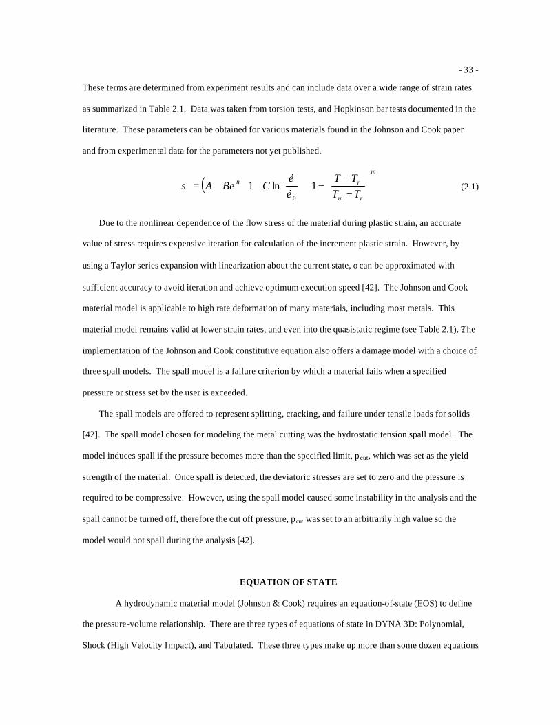
- 33 -
These terms are determined from experiment results and can include data over a wide range of strain rates
as summarized in Table 2.1. Data was taken from torsion tests, and Hopkinson bar tests documented in the
literature. These parameters can be obtained for various materials found in the Johnson and Cook paper
and from experimental data for the parameters not yet published.
( )
−−
−
++=
m
rm
rn
TTTT
CBA 1ln10ε
εεσ
&&
(2.1)
Due to the nonlinear dependence of the flow stress of the material during plastic strain, an accurate
value of stress requires expensive iteration for calculation of the increment plastic strain. However, by
using a Taylor series expansion with linearization about the current state, σ can be approximated with
sufficient accuracy to avoid iteration and achieve optimum execution speed [42]. The Johnson and Cook
material model is applicable to high rate deformation of many materials, including most metals. This
material model remains valid at lower strain rates, and even into the quasistatic regime (see Table 2.1). ?The
implementation of the Johnson and Cook constitutive equation also offers a damage model with a choice of
three spall models. The spall model is a failure criterion by which a material fails when a specified
pressure or stress set by the user is exceeded.
The spall models are offered to represent splitting, cracking, and failure under tensile loads for solids
[42]. The spall model chosen for modeling the metal cutting was the hydrostatic tension spall model. The
model induces spall if the pressure becomes more than the specified limit, pcut, which was set as the yield
strength of the material. Once spall is detected, the deviatoric stresses are set to zero and the pressure is
required to be compressive. However, using the spall model caused some instability in the analysis and the
spall cannot be turned off, therefore the cut off pressure, pcut was set to an arbitrarily high value so the
model would not spall during the analysis [42].
EQUATION OF STATE
A hydrodynamic material model (Johnson & Cook) requires an equation-of-state (EOS) to define
the pressure-volume relationship. There are three types of equations of state in DYNA 3D: Polynomial,
Shock (High Velocity Impact), and Tabulated. These three types make up more than some dozen equations
- 34 -
of state to be used with hydrodynamic material model for solid elements in DYNA 3D. When using the
Johnson & Cook Plasticity Model, you can define two of three types of equations of state: Linear
Polynomial and Gruneisen equations of state.
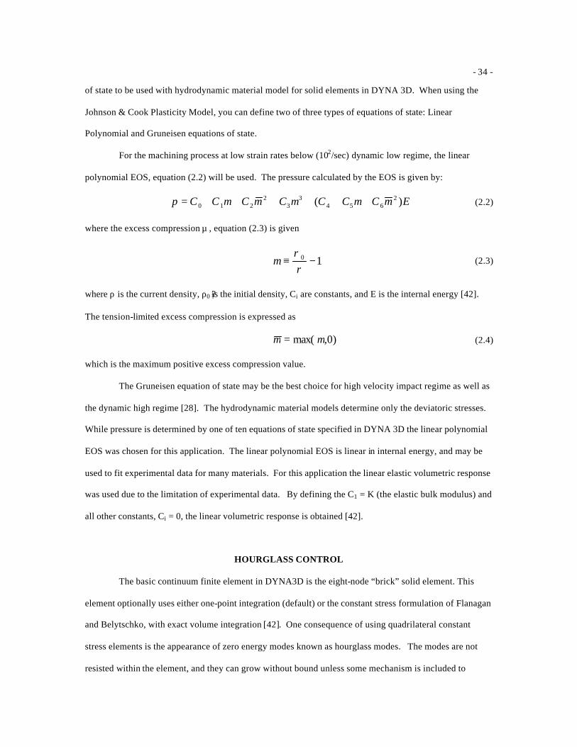
For the machining process at low strain rates below (102/sec) dynamic low regime, the linear
polynomial EOS, equation (2.2) will be used. The pressure calculated by the EOS is given by:
ECCCCCCCp )( 2654
33
2210 µµµµµ ++++++= (2.2)
where the excess compression µ , equation (2.3) is given
10 −≡ρ
ρµ (2.3)
where ρ is the current density, ρ0 ??is the initial density, Ci are constants, and E is the internal energy [42].
The tension-limited excess compression is expressed as
)0,max( µµ = (2.4)
which is the maximum positive excess compression value.
The Gruneisen equation of state may be the best choice for high velocity impact regime as well as
the dynamic high regime [28]. The hydrodynamic material models determine only the deviatoric stresses.
While pressure is determined by one of ten equations of state specified in DYNA 3D the linear polynomial
EOS was chosen for this application. The linear polynomial EOS is linear in internal energy, and may be
used to fit experimental data for many materials. For this application the linear elastic volumetric response
was used due to the limitation of experimental data. By defining the C1 = K (the elastic bulk modulus) and
all other constants, Ci = 0, the linear volumetric response is obtained [42].
HOURGLASS CONTROL
The basic continuum finite element in DYNA3D is the eight-node “brick” solid element. This
element optionally uses either one-point integration (default) or the constant stress formulation of Flanagan
and Belytschko, with exact volume integration [42]. One consequence of using quadrilateral constant
stress elements is the appearance of zero energy modes known as hourglass modes. The modes are not
resisted within the element, and they can grow without bound unless some mechanism is included to
- 35 -
control them from ultimately turning the elements inside out [1]. The hourglass mode can be considered as
bending modes for the cases of rectangular elements. Since bending is often an important part of the
solution, that is needed to be controlled to minimize the unbounded growth of the hourglass modes.
However, a caution must be taken not to suppress the modes extensively so that the structural response
becomes overly stiff [1].
The constant stress formulation of Flanagan and Belytschko, which uses a stiffness or viscous
form by choice of the user, has shown that the proper choice for an hourglass stiffness results in a
superconvergent behavior for most problems, specifically linearly elastic problems [15]. Choosing to use
the constant stress formulation of Flanagan and Belytschko in DYNA 3D, spurious hourglass modes are
stabilized using an “hourglass viscosity” or an “hourglass stiffness.” Displacements within the element are
interpolated using trilinear interpolation functions, and the constitutive equations are evaluated based on the
state at the center of the element. This element is valid for large displacements and large strains.
ORTHOGONAL CUTTING MODEL
The orthogonal metal cutting process was modeled in three parts with eight-node “brick” solid
quadrilateral elements. The metal cutting tool was model rigid. The workpiece was modeled in two-parts
with an undeformed chip and a finished surface see figure 2.1. Prior to the analysis extensively small cases
are ran to determine the mesh density. The mesh density for the tool was defined to be sparsely coarse
because the tool is rigid and is not of concern for this analysis. Thus, the workpiece was modeled
differently to save computational time. In addition, to achieve steady state there was no need to run the
simulation to remove the entire undeformed chip from the workpiece. Figures 2.2 and 2.3 show the
orthogonal metal cutting model actual mesh density of the workpiece and tool.
The workpiece was modeled with a fine mesh for approximately one fifth of the workpiece near
the cutting tool and the other portion was modeled coarsely. The mesh density for the chip was meshed
more carefully with an aspect ratio of one for the elements in the x and y coordinate frame.
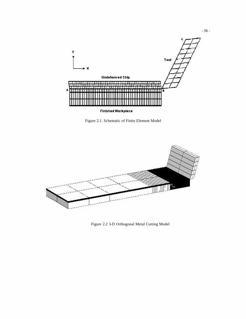
- 36 -
Figure 2.1. Schematic of Finite Element Model
Figure 2.2 3-D Orthogonal Metal Cutting Model
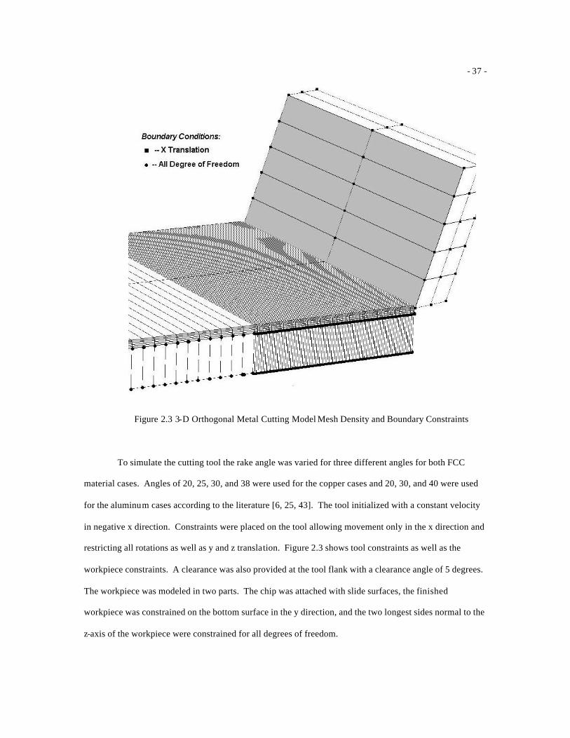
- 37 -
Figure 2.3 3-D Orthogonal Metal Cutting Model Mesh Density and Boundary Constraints
To simulate the cutting tool the rake angle was varied for three different angles for both FCC
material cases. Angles of 20, 25, 30, and 38 were used for the copper cases and 20, 30, and 40 were used
for the aluminum cases according to the literature [6, 25, 43]. The tool initialized with a constant velocity
in negative x direction. Constraints were placed on the tool allowing movement only in the x direction and
restricting all rotations as well as y and z translation. Figure 2.3 shows tool constraints as well as the
workpiece constraints. A clearance was also provided at the tool flank with a clearance angle of 5 degrees.
The workpiece was modeled in two parts. The chip was attached with slide surfaces, the finished
workpiece was constrained on the bottom surface in the y direction, and the two longest sides normal to the
z-axis of the workpiece were constrained for all degrees of freedom.
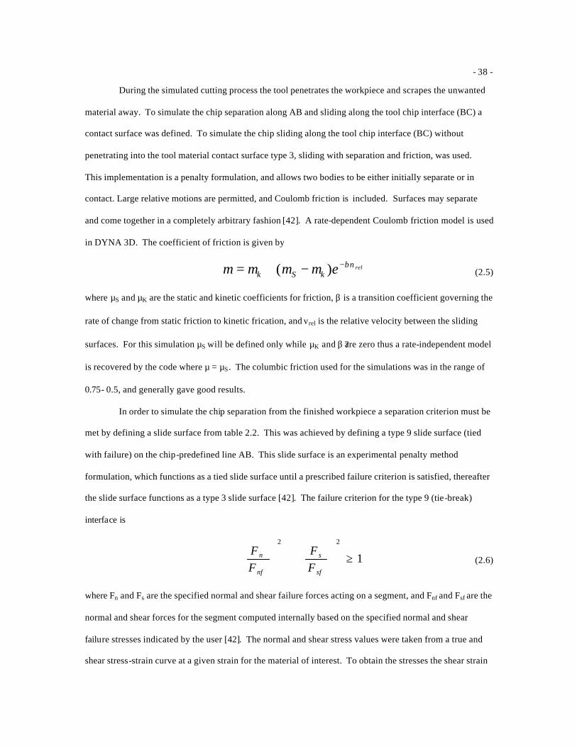
- 38 -
During the simulated cutting process the tool penetrates the workpiece and scrapes the unwanted
material away. To simulate the chip separation along AB and sliding along the tool chip interface (BC) a
contact surface was defined. To simulate the chip sliding along the tool chip interface (BC) without
penetrating into the tool material contact surface type 3, sliding with separation and friction, was used.
This implementation is a penalty formulation, and allows two bodies to be either initially separate or in
contact. Large relative motions are permitted, and Coulomb friction is included. Surfaces may separate
and come together in a completely arbitrary fashion [42]. A rate-dependent Coulomb friction model is used
in DYNA 3D. The coefficient of friction is given by
relekSkβνµµµµ −−+= )( (2.5)
where µS and µK are the static and kinetic coefficients for friction, β is a transition coefficient governing the
rate of change from static friction to kinetic frication, and νrel is the relative velocity between the sliding
surfaces. For this simulation µS will be defined only while µK and β ?are zero thus a rate-independent model
is recovered by the code where µ = µS . The columbic friction used for the simulations was in the range of
0.75- 0.5, and generally gave good results.
In order to simulate the chip separation from the finished workpiece a separation criterion must be
met by defining a slide surface from table 2.2. This was achieved by defining a type 9 slide surface (tied
with failure) on the chip-predefined line AB. This slide surface is an experimental penalty method
formulation, which functions as a tied slide surface until a prescribed failure criterion is satisfied, thereafter
the slide surface functions as a type 3 slide surface [42]. The failure criterion for the type 9 (tie-break)
interface is
1
22
≥
+
sf
s
nf
n
FF
FF
(2.6)
where Fn and Fs are the specified normal and shear failure forces acting on a segment, and Fnf and Fsf are the
normal and shear forces for the segment computed internally based on the specified normal and shear
failure stresses indicated by the user [42]. The normal and shear stress values were taken from a true and
shear stress-strain curve at a given strain for the material of interest. To obtain the stresses the shear strain
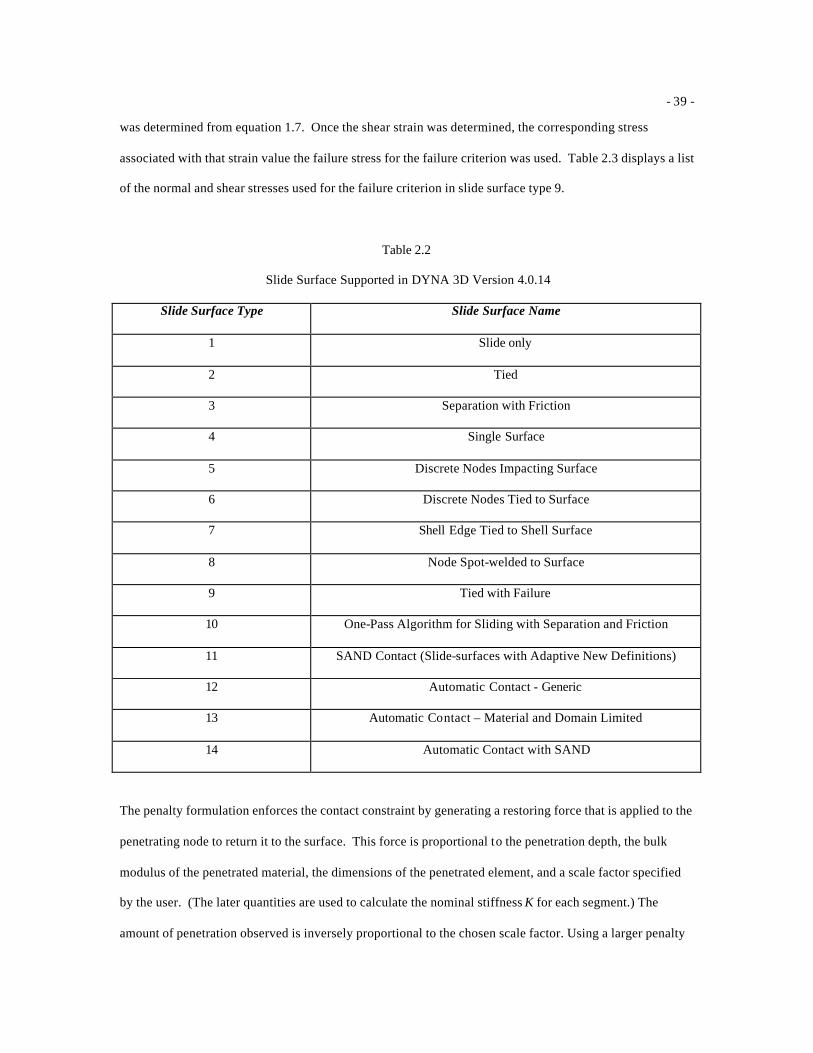
- 39 -
was determined from equation 1.7. Once the shear strain was determined, the corresponding stress
associated with that strain value the failure stress for the failure criterion was used. Table 2.3 displays a list
of the normal and shear stresses used for the failure criterion in slide surface type 9.
Table 2.2
Slide Surface Supported in DYNA 3D Version 4.0.14
Slide Surface Type Slide Surface Name
1 Slide only
2 Tied
3 Separation with Friction
4 Single Surface
5 Discrete Nodes Impacting Surface
6 Discrete Nodes Tied to Surface
7 Shell Edge Tied to Shell Surface
8 Node Spot-welded to Surface
9 Tied with Failure
10 One-Pass Algorithm for Sliding with Separation and Friction
11 SAND Contact (Slide-surfaces with Adaptive New Definitions)
12 Automatic Contact - Generic
13 Automatic Contact – Material and Domain Limited
14 Automatic Contact with SAND
The penalty formulation enforces the contact constraint by generating a restoring force that is applied to the
penetrating node to return it to the surface. This force is proportional to the penetration depth, the bulk
modulus of the penetrated material, the dimensions of the penetrated element, and a scale factor specified
by the user. (The later quantities are used to calculate the nominal stiffness K for each segment.) The
amount of penetration observed is inversely proportional to the chosen scale factor. Using a larger penalty
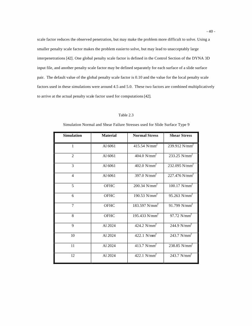
- 40 -
scale factor reduces the observed penetration, but may make the problem more difficult to solve. Using a
smaller penalty scale factor makes the problem easier to solve, but may lead to unacceptably large
interpenetrations [42]. One global penalty scale factor is defined in the Control Section of the DYNA 3D
input file, and another penalty scale factor may be defined separately for each surface of a slide surface
pair. The default value of the global penalty scale factor is 0.10 and the value for the local penalty scale
factors used in these simulations were around 4.5 and 5.0. These two factors are combined multiplicatively
to arrive at the actual penalty scale factor used for computations [42].
Table 2.3
Simulation Normal and Shear Failure Stresses used for Slide Surface Type 9
Simulation Material Normal Stress Shear Stress
1 Al 6061 415.54 N/mm2 239.912 N/mm2
2 Al 6061 404.0 N/mm2 233.25 N/mm2
3 Al 6061 402.0 N/mm2 232.095 N/mm2
4 Al 6061 397.0 N/mm2 227.476 N/mm2
5 OFHC 200.34 N/mm2 100.17 N/mm2
6 OFHC 190.53 N/mm2 95.263 N/mm2
7 OFHC 183.597 N/mm2 91.799 N/mm2
8 OFHC 195.433 N/mm2 97.72 N/mm2
9 Al 2024 424.2 N/mm2 244.9 N/mm2
10 Al 2024 422.1 N/mm2 243.7 N/mm2
11 Al 2024 413.7 N/mm2 238.85 N/mm2
12 Al 2024 422.1 N/mm2 243.7 N/mm2
- 41 -
Chapter III
Determining the Material Parameters for Aluminum 6061-T6
for Implementation in the Johnson and Cook Constitutive
Equation for Predicting Dynamic Material Behavior
INTRODUCTION
Finite element analysis has proven useful for predicting the performance of components. To
operate acceptably, there can be no permanent deformation of the part in response to the applied stress.
This is called the elastic behavior of a material and Hooke’s Law is used to model the stress versus strain
relationship. In contrast, the use of finite element analysis to predict material behavior during the
fabrication process is much more difficult in that the part is required to undergo permanent plastic
deformation. The stress strain relationship for plastic deformation is no longer linear and varies as a
function of the amount of strain, the rate of strain applied, and temperature. Collapsing the stress versus
strain relationship into one equation to use in numerical analysis methods has resulted in a variety of
constitutive equations. One of the most commonly used empirically based equations is the Johnson and
Cook constitutive equation.
There have been a number of equations used to characterize the plastic behavior of materials,
however during recent years and even now, the Johnson & Cook constitutive equation has been used in a
number of computer codes. The Johnson and Cook equation relates the strain rate dependence of flow
stress as a function of temperature and strain rate, which is necessary to predict the dynamic behavior of
materials in hydrodynamic codes [28]. This constitutive equation was formulated for computational
purposes in an attempt to characterize materia l behavior with laboratory experiments so the initial
- 42 -
computations could be used with more confidence. As a result, the parameters could be extracted
from the experiments for a more efficient design cycle, which would increase the understanding of the
complicated process, which occurs during impulsive loading conditions [18].
EVALUATION OF CONSTITUTIVE EQUATION
Constitutive equations often describe strain-rate plastic deformation of materials by relating stress
as a function of strain, strain rate, and temperature. The stress can be expressed as
),,( Tf εεσ &= (3.1)
where ε is the strain, and ε& ?is the strain rate, and T is the temperature. A successive constitutive equation
collapse data into a single equation and have the ability to extrapolate and interpolate data [13]. At low
constant strain rates, materials such as metal work harden along the relationship called parabolic hardening,
equation (3.2).
nκεσσ += 0 (3.2)
The parabolic hardening equation has three terms where σ0 is the yield stress; n is the work hardening
exponent, and κ ?is the pre-exponential factor [13]. The effects of temperature and strain rate on flow stress
can also be expressed separately, equations (3.3) and (3.4).
−−
−=m
rm
rr TT
TT1σσ (3.3)
( )εασ &ln= (3.4)
In equation (3.3.) σr is a reference stress, T (degrees Kelvin) is the temperature of the material for which
stress is calculated, Tr is the reference temperature, and Tm is the melting point of the material. In equation
(3.4) α is the strain rate dependence factor [13]. Johnson and Cook used the basic ingredients of equations
(3.2), (3.3), and (3.4) to empirically propose what is known as the Johnson and Cook constitutive equation.
The Johnson/Cook constitutive equation is expressed as the model for dynamic flow stress, -
presented in equation (3.5):
- 43 -
( )
−−
−
++=
m
rm
rn
TTTT
CBA 1ln10ε
εεσ
&&
(3.5)
where ε is equivalent for plastic strain, ε& /? 0ε& is the dimensionless plastic strain rate and 0ε& =1.0 s -1 is the
reference strain rate and ε& is the strain rate for which the stress is calculated, T is the temperature of the
specimen, Tr is the reference temperature, and Tm is the melting temperature of the specimen.
The Johnson/Cook constitutive equation has five experimentally determined material constants A,
B, n, C, and m. The definitions of each material constant are as follow: A - yield stress constant, B - strain
hardening coefficient, n - strain hardening exponent, C - strain rate dependence coefficient, and m -
temperature dependence coefficient. The first bracket in the constitutive equation is the strain hardening
term, the second is the strain rate hardening term, and the third is the thermal softening term. Assuming
adiabatic deformation at high strain rates, the third term allows for reduction in strength corresponding to
the increase in temperature due to plastic work. While the first term accounts for the strain hardening of the
material for isothermal conditions, and the second term allows the combination of strain rate and thermal
softening to be evaluated at large strain rates.
DETERMINATION OF CONSTITUTIVE PARAMETERS
The Johnson/Cook constitutive equation seen above in equation (3.5) has five material constants
which were determined from stress strain data digitized from the literature using digitizing software [17].
The yield stress constant was determined from a plot of yield strength versus log strain rate for strain rates
of 10-3 s -1 to 103 s -1. The data was a result of a uniaxial tensile test conducted by the collaborative effort of
Chatfield and Rote [9]. Figure one was used to extrapolate the plot of effect of strain rate on yield strength
of the test material used to determine the yield strength of Al 6061-T6. The yield stress constitutive
parameter was determined as 325 MPa.
The constitutive parameters B-strain hardening coefficient and n-strain hardening exponent were
determined using the work of D. Lee [24]. The true stress strain data was gathered from a uniaxial tensile
test with a reference strain rate of 3.3x10⁻⁴ s -1. The value of B is the true stress at ε? = 1. The strain
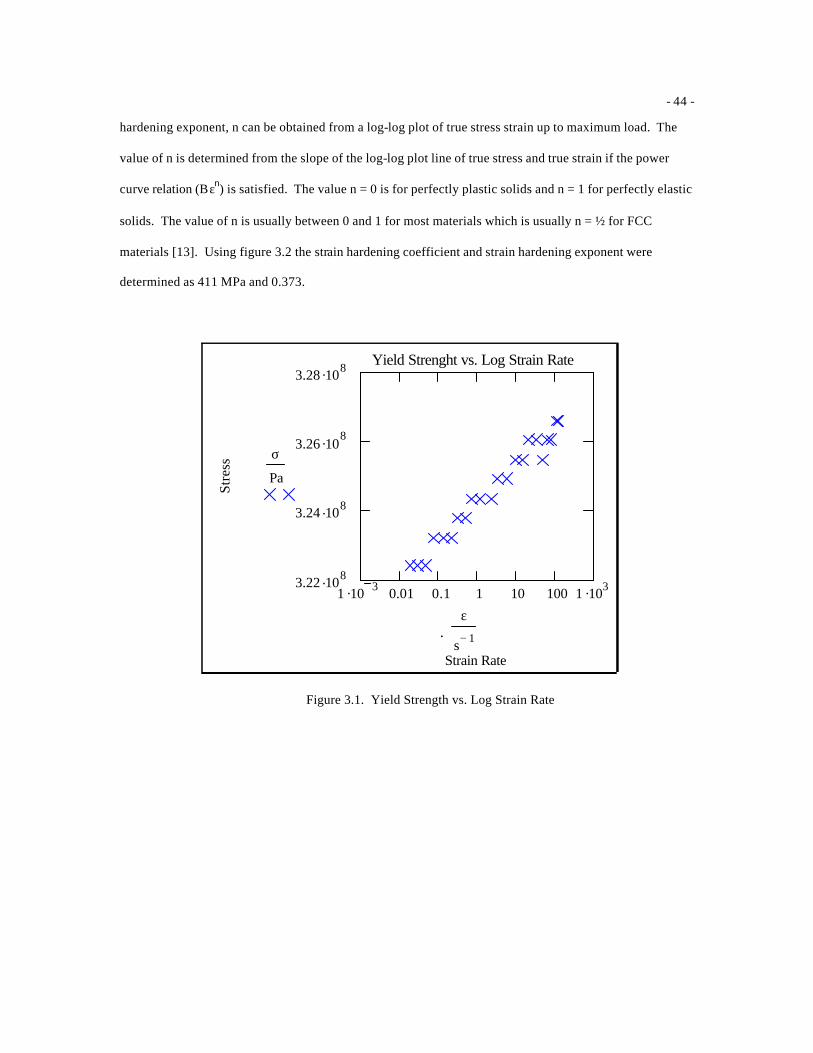
- 44 -
hardening exponent, n can be obtained from a log-log plot of true stress strain up to maximum load. The
value of n is determined from the slope of the log-log plot line of true stress and true strain if the power
curve relation (Βεn) is satisfied. The value n = 0 is for perfectly plastic solids and n = 1 for perfectly elastic
solids. The value of n is usually between 0 and 1 for most materials which is usually n = ½ for FCC
materials [13]. Using figure 3.2 the strain hardening coefficient and strain hardening exponent were
determined as 411 MPa and 0.373.
1 .10 3 0.01 0.1 1 10 100 1 .1033.22 .108
3.24 .108
3.26 .108
3.28 .108 Yield Strenght vs. Log Strain Rate
Strain Rate
Stre
ss
σ
Pa
ε
s 1−.
Figure 3.1. Yield Strength vs. Log Strain Rate
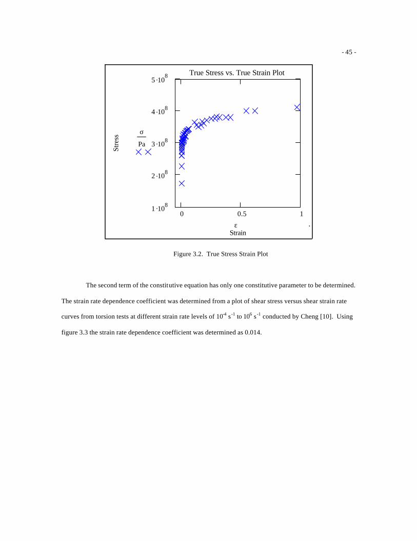
- 45 -
0 0.5 11 .108
2 .108
3 .108
4 .108
5 .108 True Stress vs. True Strain Plot
Strain
Stre
ss
σ
Pa
ε .
Figure 3.2. True Stress Strain Plot
The second term of the constitutive equation has only one constitutive parameter to be determined.
The strain rate dependence coefficient was determined from a plot of shear stress versus shear strain rate
curves from torsion tests at different strain rate levels of 10-4 s -1 to 106 s -1 conducted by Cheng [10]. Using
figure 3.3 the strain rate dependence coefficient was determined as 0.014.
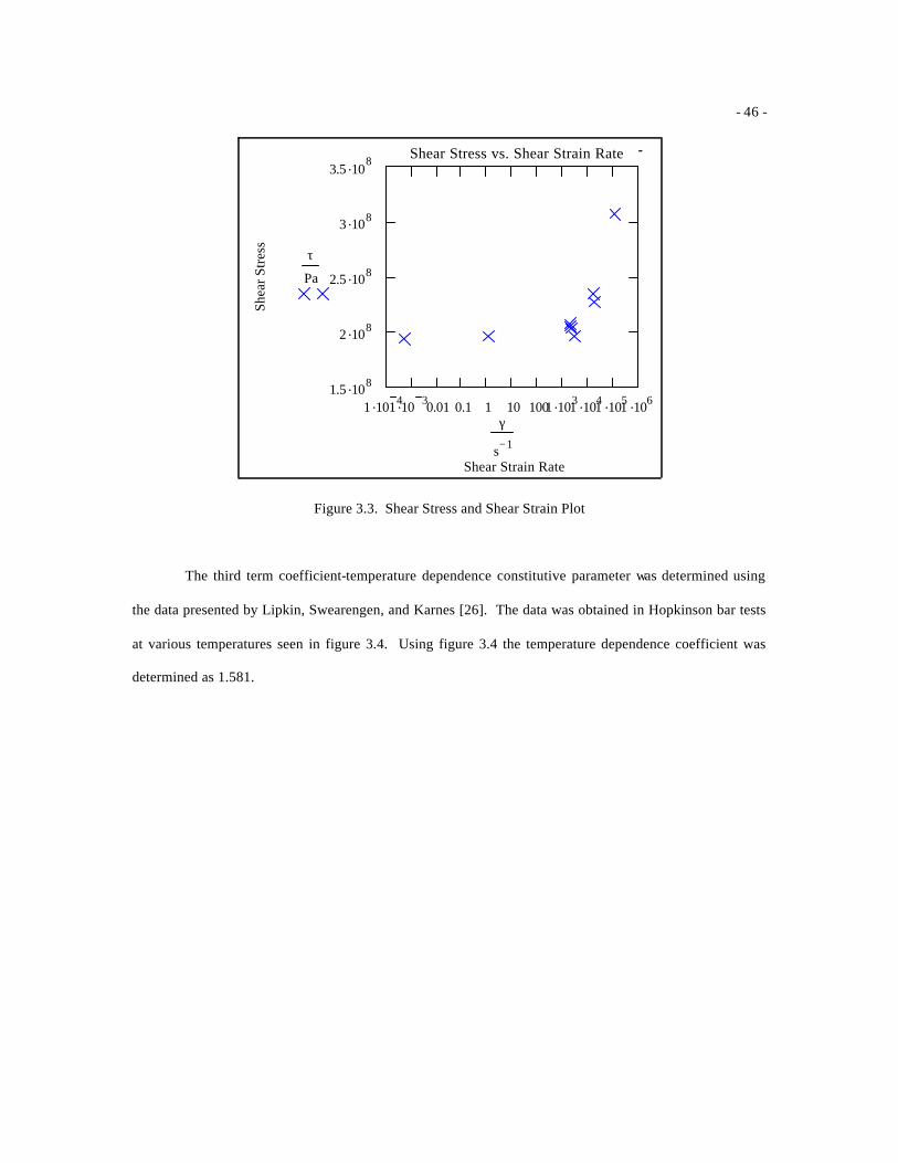
- 46 -
1 .10 41 .10 30.01 0.1 1 10 1001 .1031 .1041 .1051 .1061.5 .108
2 .108
2.5 .108
3 .108
3.5 .108 Shear Stress vs. Shear Strain Rate
Shear Strain Rate
Shea
r Str
ess
τ
Pa
γ
s 1−
-
Figure 3.3. Shear Stress and Shear Strain Plot
The third term coefficient-temperature dependence constitutive parameter was determined using
the data presented by Lipkin, Swearengen, and Karnes [26]. The data was obtained in Hopkinson bar tests
at various temperatures seen in figure 3.4. Using figure 3.4 the temperature dependence coefficient was
determined as 1.581.
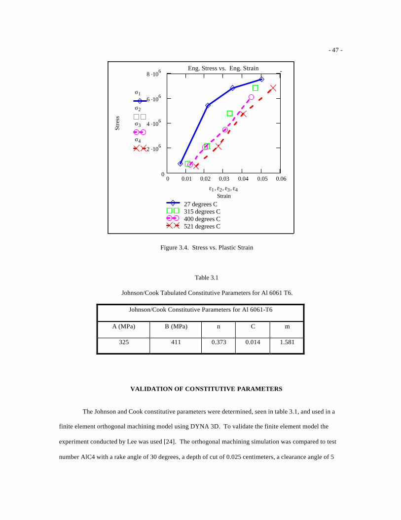
- 47 -
0 0.01 0.02 0.03 0.04 0.05 0.060
2 .106
4 .106
6 .106
8 .106
27 degrees C315 degrees C400 degrees C521 degrees C
Eng. Stress vs. Eng. Strain
Strain
Stre
ss
σ1
σ2
σ3
σ4
ε1 ε2, ε3, ε4,
-
Figure 3.4. Stress vs. Plastic Strain
Table 3.1
Johnson/Cook Tabulated Constitutive Parameters for Al 6061 T6.
Johnson/Cook Constitutive Parameters for Al 6061-T6
A (MPa) B (MPa) n C m
325 411 0.373 0.014 1.581
VALIDATION OF CONSTITUTIVE PARAMETERS
The Johnson and Cook constitutive parameters were determined, seen in table 3.1, and used in a
finite element orthogonal machining model using DYNA 3D. To validate the finite element model the
experiment conducted by Lee was used [24]. The orthogonal machining simulation was compared to test
number AlC4 with a rake angle of 30 degrees, a depth of cut of 0.025 centimeters, a clearance angle of 5
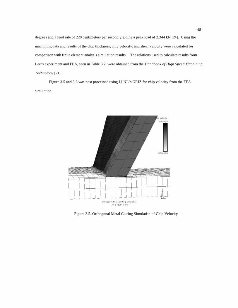
- 48 -
degrees and a feed rate of 220 centimeters per second yielding a peak load of 2.344 kN [24]. Using the
machining data and results of the chip thickness, chip velocity, and shear velocity were calculated for
comparison with finite element analysis simulation results. The relations used to calculate results from
Lee’s experiment and FEA, seen in Table 3.2, were obtained from the Handbook of High Speed Machining
Technology [21].
Figure 3.5 and 3.6 was post processed using LLNL’s GRIZ for chip velocity from the FEA
simulation.
Figure 3.5. Orthogonal Metal Cutting Simulation of Chip Velocity
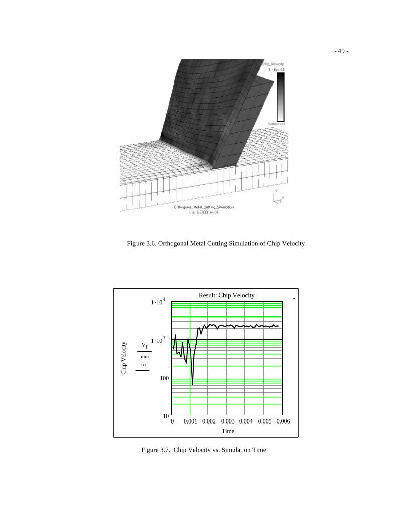
- 49 -
Figure 3.6. Orthogonal Metal Cutting Simulation of Chip Velocity
0 0.001 0.002 0.003 0.004 0.005 0.00610
100
1 .103
1 .104Result: Chip Velocity
Chi
p V
eloc
ity Vfmm
sec
Time
-
Figure 3.7. Chip Velocity vs. Simulation Time
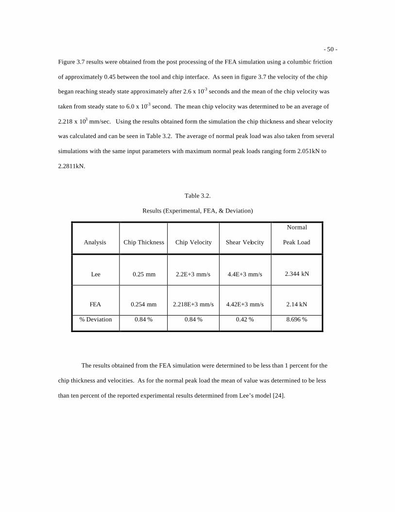
- 50 -
Figure 3.7 results were obtained from the post processing of the FEA simulation using a columbic friction
of approximately 0.45 between the tool and chip interface. As seen in figure 3.7 the velocity of the chip
began reaching steady state approximately after 2.6 x 10⁻³ seconds and the mean of the chip velocity was
taken from steady state to 6.0 x 10⁻³ second. The mean chip velocity was determined to be an average of
2.218 x 103 mm/sec. Using the results obtained form the simulation the chip thickness and shear velocity
was calculated and can be seen in Table 3.2. The average of normal peak load was also taken from several
simulations with the same input parameters with maximum normal peak loads ranging form 2.051kN to
2.2811kN.
Table 3.2.
Results (Experimental, FEA, & Deviation)
Analysis Chip Thickness Chip Velocity Shear Velocity
Normal
Peak Load
Lee 0.25 mm 2.2E+3 mm/s 4.4E+3 mm/s
2.344 kN
FEA 0.254 mm 2.218E+3 mm/s 4.42E+3 mm/s
2.14 kN
% Deviation 0.84 % 0.84 % 0.42 % 8.696 %
The results obtained from the FEA simulation were determined to be less than 1 percent for the
chip thickness and velocities. As for the normal peak load the mean of value was determined to be less
than ten percent of the reported experimental results determined from Lee’s model [24].
- 51 -
CONCLUSION
The Johnson and Cook constitutive model was presented here in an attempt to understand the
origins of the five material constants and apply the constants for various materials for computational
models implemented in computational codes such as DYNA 3D. The constitutive equation is modeled as
dynamic flow stress, which includes the effects of strain hardening, strain rate hardening, and thermal
softening of a material. An explicit finite element analysis using DYNA 3D proved to give reliable
computational results for an orthogonal machining application using the Johnson and Cook constitutive
equation.
- 52 -
Chapter IV
Orthogonal Metal Cutting Model Analysis of Chip Formation
For Two Different Face Centered Cubic Materials
INTRODUCTION
Metal cutting is a highly nonlinear and coupled thermo mechanical process, where the coupling is
introduced through localized heating and temperature rise in the workpiece, which is caused by the rapid
plastic flow in the workpiece and by the friction along the tool-chip interface. In the last two decades, the
finite element method and analytical models have been developed and applied to study the chip formation
process. Metal cutting also known as machining, which is one of many manufacturing processes affected
by many complex factors, including the type of work material, machine tools, cutting tools, cutting
operations, and cutting conditions. The difficulty of machining can be evaluated by three criteria such as
tool life, precision and surface finish of machined parts, and chip control. For this study the effect of the
cutting tool and the precision and surface finish were not investigated. Three main factors affect chip
control, and that have an influence on the cutting process. These are the chip thickness, the radius of
curvature of chips, and the mechanical properties of the material being machined. The focus of this study
concentrates on the chip thickness. The factors affecting chip thickness are cutting speed, depth of cut,
lubricants, tool normal rake angle, tool cutting edge angle, and the hardness of the work material [46].
Using DYNA 3D will allow
To perform a complete analysis machining data was obtained from references [5] and [7], which
were published by Black [6, 25] and Zhang [45]. Utilizing the machining data from Black and Zhang the
machining conditions and cutting operations were implemented into a finite element procedure to simulate
orthogonal metal cutting using an explicit finite element code, namely DYNA 3D. In addition, the
machining results obtained from the literature and the finite element analysis such as chip thickness, shear
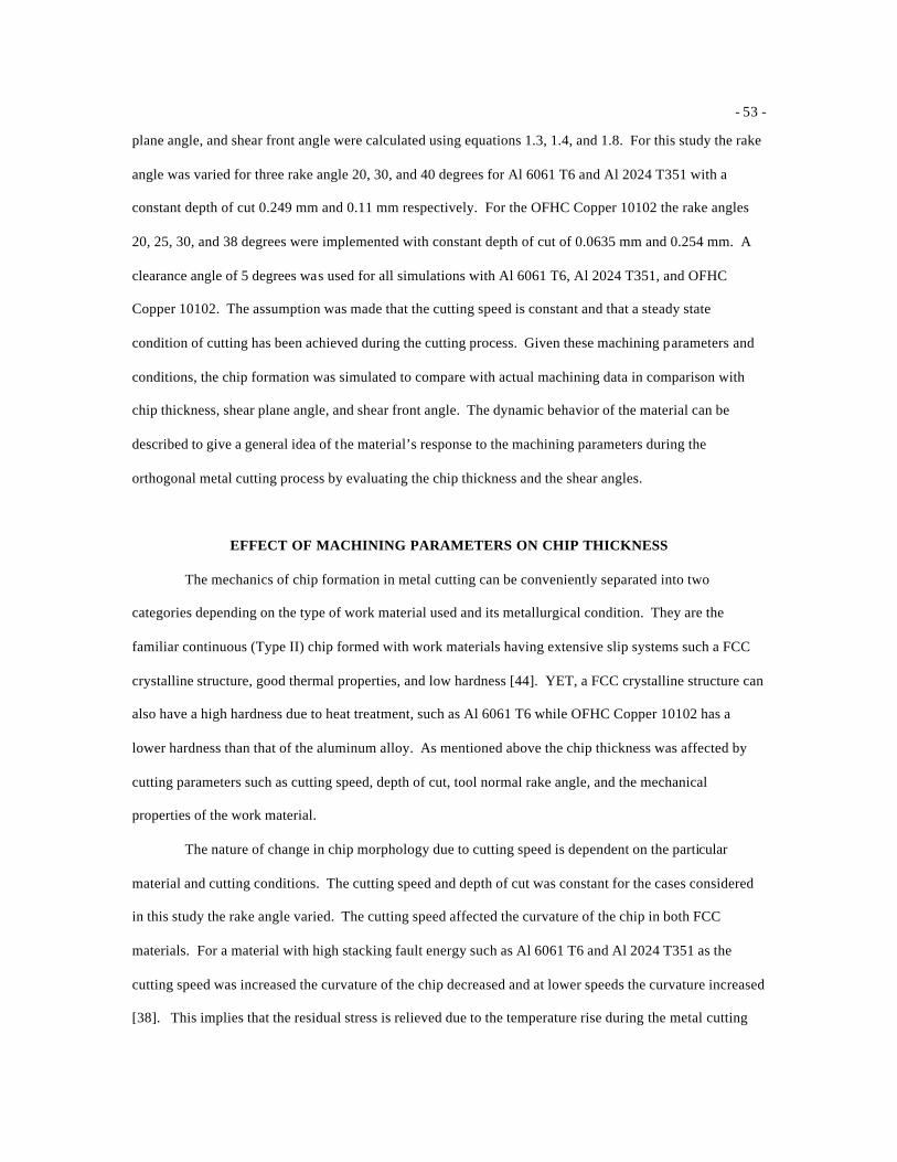
- 53 -
plane angle, and shear front angle were calculated using equations 1.3, 1.4, and 1.8. For this study the rake
angle was varied for three rake angle 20, 30, and 40 degrees for Al 6061 T6 and Al 2024 T351 with a
constant depth of cut 0.249 mm and 0.11 mm respectively. For the OFHC Copper 10102 the rake angles
20, 25, 30, and 38 degrees were implemented with constant depth of cut of 0.0635 mm and 0.254 mm. A
clearance angle of 5 degrees was used for all simulations with Al 6061 T6, Al 2024 T351, and OFHC
Copper 10102. The assumption was made that the cutting speed is constant and that a steady state
condition of cutting has been achieved during the cutting process. Given these machining parameters and
conditions, the chip formation was simulated to compare with actual machining data in comparison with
chip thickness, shear plane angle, and shear front angle. The dynamic behavior of the material can be
described to give a general idea of the material’s response to the machining parameters during the
orthogonal metal cutting process by evaluating the chip thickness and the shear angles.
EFFECT OF MACHINING PARAMETERS ON CHIP THICKNESS
The mechanics of chip formation in metal cutting can be conveniently separated into two
categories depending on the type of work material used and its metallurgical condition. They are the
familiar continuous (Type II) chip formed with work materials having extensive slip systems such a FCC
crystalline structure, good thermal properties, and low hardness [44]. YET, a FCC crystalline structure can
also have a high hardness due to heat treatment, such as Al 6061 T6 while OFHC Copper 10102 has a
lower hardness than that of the aluminum alloy. As mentioned above the chip thickness was affected by
cutting parameters such as cutting speed, depth of cut, tool normal rake angle, and the mechanical
properties of the work material.
The nature of change in chip morphology due to cutting speed is dependent on the particular
material and cutting conditions. The cutting speed and depth of cut was constant for the cases considered
in this study the rake angle varied. The cutting speed affected the curvature of the chip in both FCC
materials. For a material with high stacking fault energy such as Al 6061 T6 and Al 2024 T351 as the
cutting speed was increased the curvature of the chip decreased and at lower speeds the curvature increased
[38]. This implies that the residual stress is relieved due to the temperature rise during the metal cutting
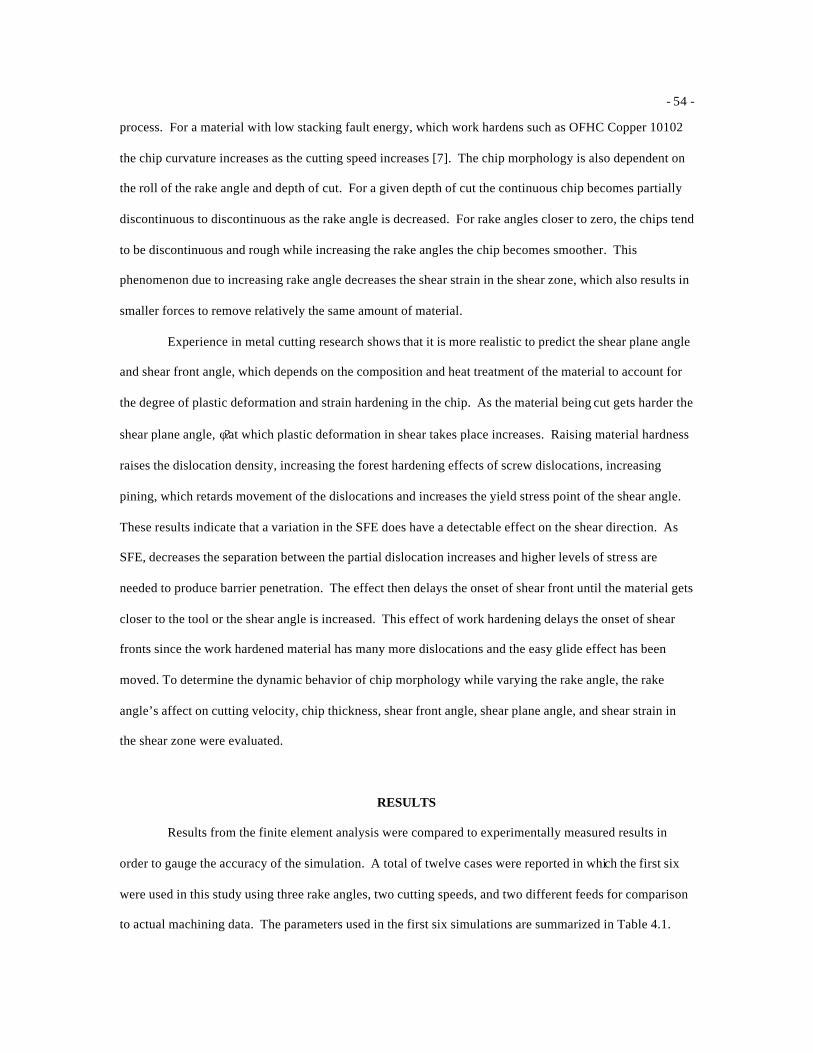
- 54 -
process. For a material with low stacking fault energy, which work hardens such as OFHC Copper 10102
the chip curvature increases as the cutting speed increases [7]. The chip morphology is also dependent on
the roll of the rake angle and depth of cut. For a given depth of cut the continuous chip becomes partially
discontinuous to discontinuous as the rake angle is decreased. For rake angles closer to zero, the chips tend
to be discontinuous and rough while increasing the rake angles the chip becomes smoother. This
phenomenon due to increasing rake angle decreases the shear strain in the shear zone, which also results in
smaller forces to remove relatively the same amount of material.
Experience in metal cutting research shows that it is more realistic to predict the shear plane angle
and shear front angle, which depends on the composition and heat treatment of the material to account for
the degree of plastic deformation and strain hardening in the chip. As the material being cut gets harder the
shear plane angle, φ? at which plastic deformation in shear takes place increases. Raising material hardness
raises the dislocation density, increasing the forest hardening effects of screw dislocations, increasing
pining, which retards movement of the dislocations and increases the yield stress point of the shear angle.
These results indicate that a variation in the SFE does have a detectable effect on the shear direction. As
SFE, decreases the separation between the partial dislocation increases and higher levels of stress are
needed to produce barrier penetration. The effect then delays the onset of shear front until the material gets
closer to the tool or the shear angle is increased. This effect of work hardening delays the onset of shear
fronts since the work hardened material has many more dislocations and the easy glide effect has been
moved. To determine the dynamic behavior of chip morphology while varying the rake angle, the rake
angle’s affect on cutting velocity, chip thickness, shear front angle, shear plane angle, and shear strain in
the shear zone were evaluated.
RESULTS
Results from the finite element analysis were compared to experimentally measured results in
order to gauge the accuracy of the simulation. A total of twelve cases were reported in which the first six
were used in this study using three rake angles, two cutting speeds, and two different feeds for comparison
to actual machining data. The parameters used in the first six simulations are summarized in Table 4.1.
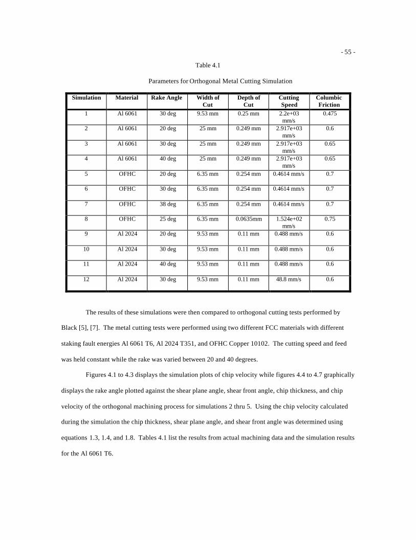
- 55 -
Table 4.1
Parameters for Orthogonal Metal Cutting Simulation
Simulation Material Rake Angle Width of Cut
Depth of Cut
Cutting Speed
Columbic Friction
1 Al 6061 30 deg 9.53 mm 0.25 mm 2.2e+03 mm/s
0.475
2 Al 6061 20 deg 25 mm 0.249 mm 2.917e+03 mm/s
0.6
3 Al 6061 30 deg 25 mm 0.249 mm 2.917e+03 mm/s
0.65
4 Al 6061 40 deg 25 mm 0.249 mm 2.917e+03 mm/s
0.65
5 OFHC 20 deg 6.35 mm 0.254 mm 0.4614 mm/s 0.7
6 OFHC 30 deg 6.35 mm 0.254 mm 0.4614 mm/s 0.7
7 OFHC 38 deg 6.35 mm 0.254 mm 0.4614 mm/s 0.7
8 OFHC 25 deg 6.35 mm 0.0635mm 1.524e+02 mm/s
0.75
9 Al 2024 20 deg 9.53 mm 0.11 mm 0.488 mm/s 0.6
10 Al 2024 30 deg 9.53 mm 0.11 mm 0.488 mm/s 0.6
11 Al 2024 40 deg 9.53 mm 0.11 mm 0.488 mm/s 0.6
12 Al 2024 30 deg 9.53 mm 0.11 mm 48.8 mm/s 0.6
The results of these simulations were then compared to orthogonal cutting tests performed by
Black [5], [7]. The metal cutting tests were performed using two different FCC materials with different
staking fault energies Al 6061 T6, Al 2024 T351, and OFHC Copper 10102. The cutting speed and feed
was held constant while the rake was varied between 20 and 40 degrees.
Figures 4.1 to 4.3 displays the simulation plots of chip velocity while figures 4.4 to 4.7 graphically
displays the rake angle plotted against the shear plane angle, shear front angle, chip thickness, and chip
velocity of the orthogonal machining process for simulations 2 thru 5. Using the chip velocity calculated
during the simulation the chip thickness, shear plane angle, and shear front angle was determined using
equations 1.3, 1.4, and 1.8. Tables 4.1 list the results from actual machining data and the simulation results
for the Al 6061 T6.
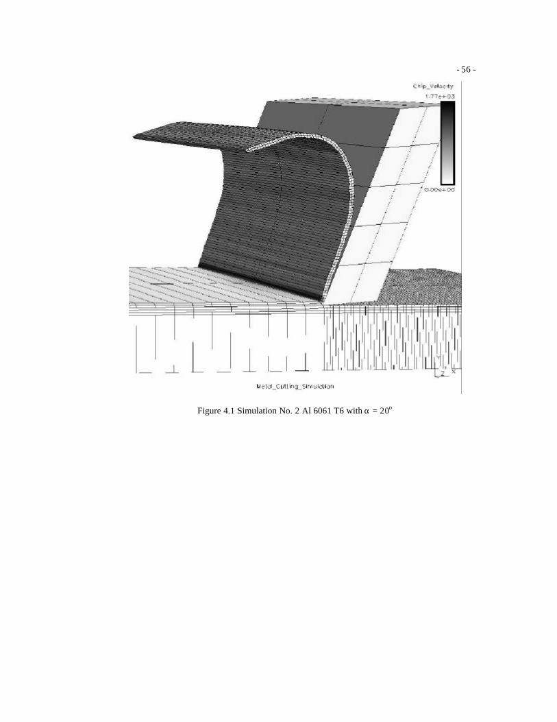
- 56 -
Figure 4.1 Simulation No. 2 Al 6061 T6 with α = 20o
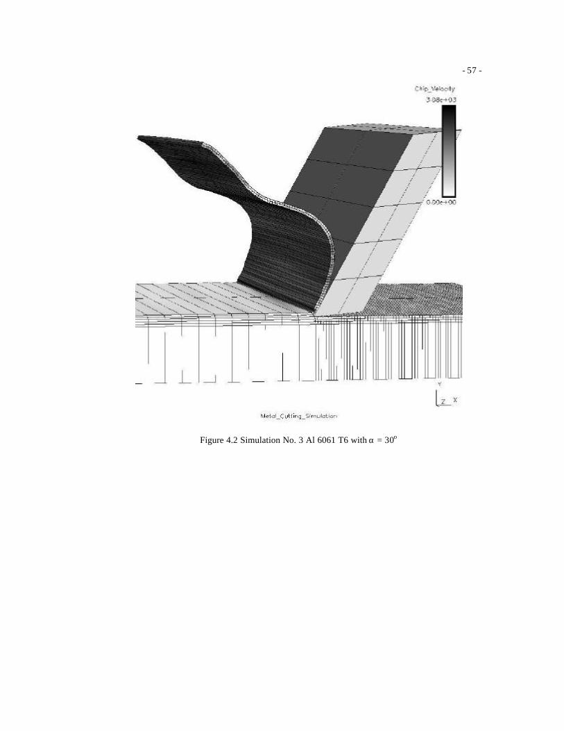
- 57 -
Figure 4.2 Simulation No. 3 Al 6061 T6 with α = 30o
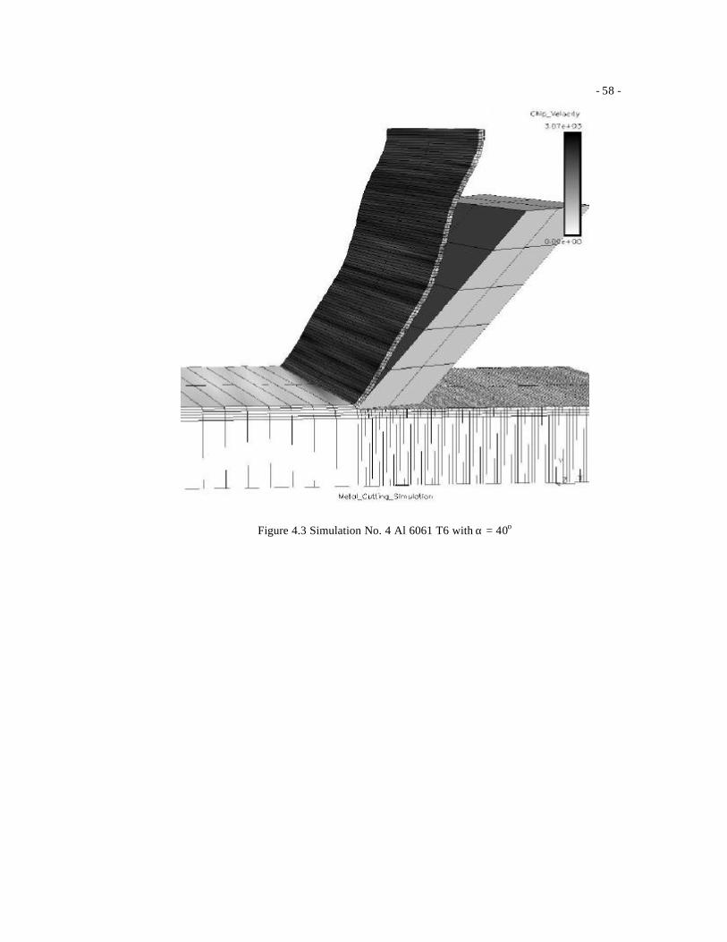
- 58 -
Figure 4.3 Simulation No. 4 Al 6061 T6 with α = 40o
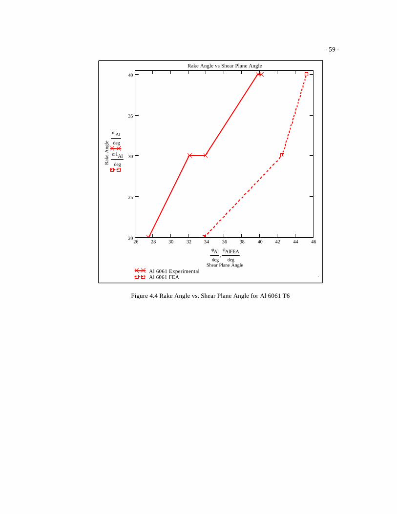
- 59 -
26 28 30 32 34 36 38 40 42 44 4620
25
30
35
40
Al 6061 Experimental Al 6061 FEA
Rake Angle vs Shear Plane Angle
Shear Plane Angle
Rak
e A
ngle
αAl
deg
α1Al
deg
φAl
deg
φAlFEA
deg,
.
Figure 4.4 Rake Angle vs. Shear Plane Angle for Al 6061 T6
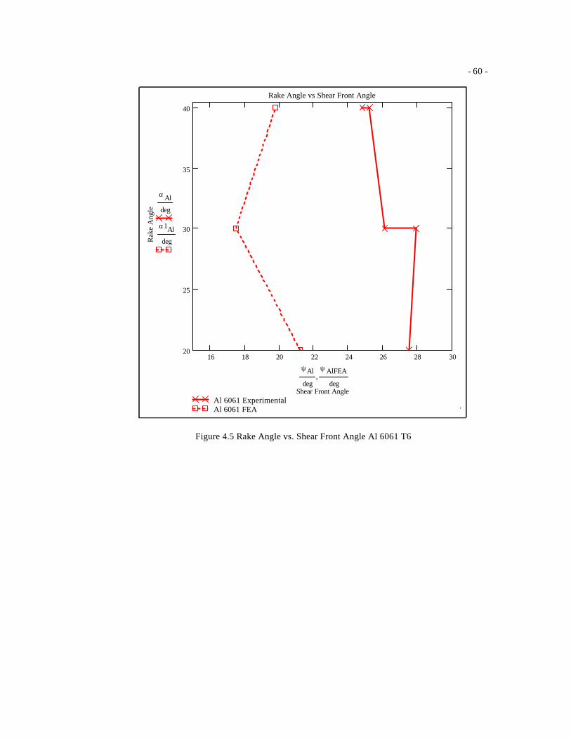
- 60 -
16 18 20 22 24 26 28 3020
25
30
35
40
Al 6061 ExperimentalAl 6061 FEA
Rake Angle vs Shear Front Angle
Shear Front Angle
Rak
e A
ngle
α Al
deg
α1Al
deg
ψAl
deg
ψ AlFEA
deg,
.
Figure 4.5 Rake Angle vs. Shear Front Angle Al 6061 T6
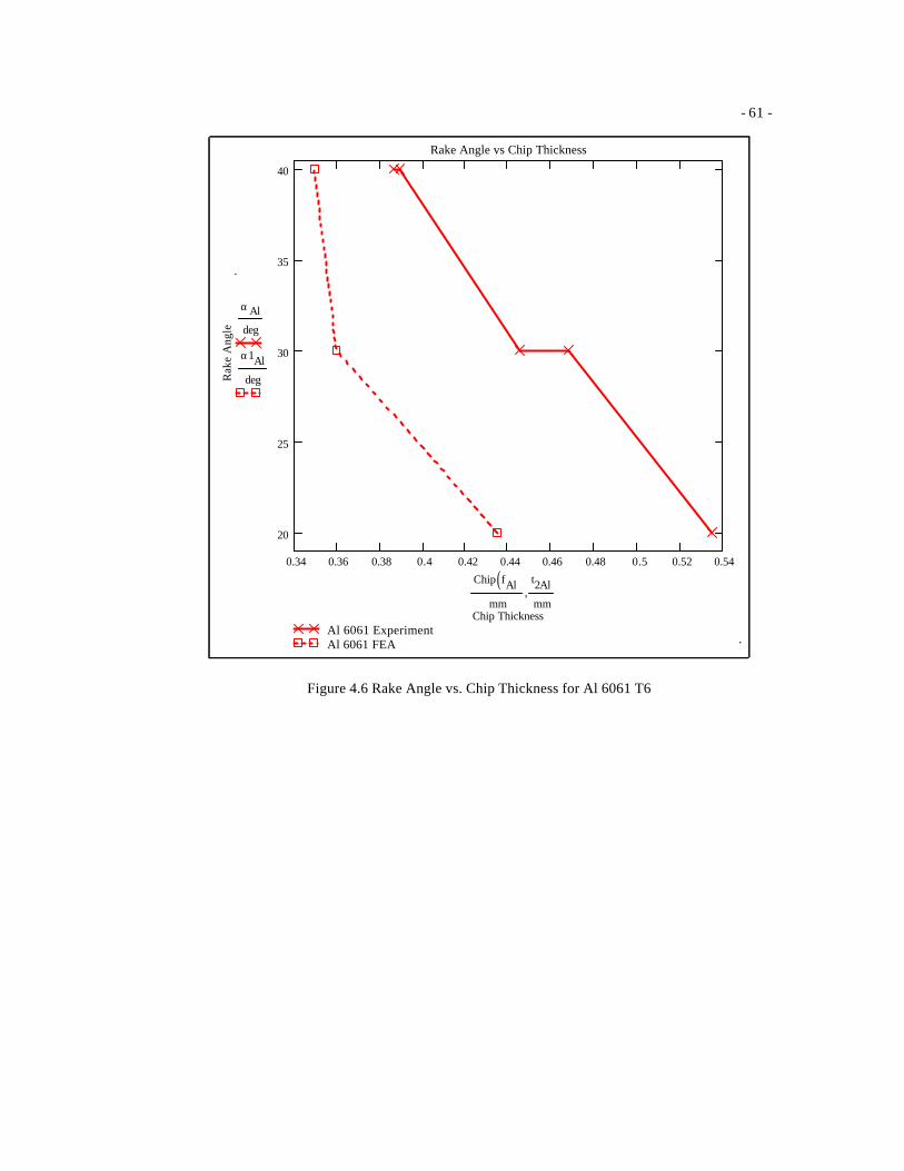
- 61 -
0.34 0.36 0.38 0.4 0.42 0.44 0.46 0.48 0.5 0.52 0.54
20
25
30
35
40
Al 6061 ExperimentAl 6061 FEA
Rake Angle vs Chip Thickness
Chip Thickness
Rak
e A
ngle
α Al
deg
α1Al
deg
Chip fAl( )mm
t2Al
mm,
.
.
Figure 4.6 Rake Angle vs. Chip Thickness for Al 6061 T6
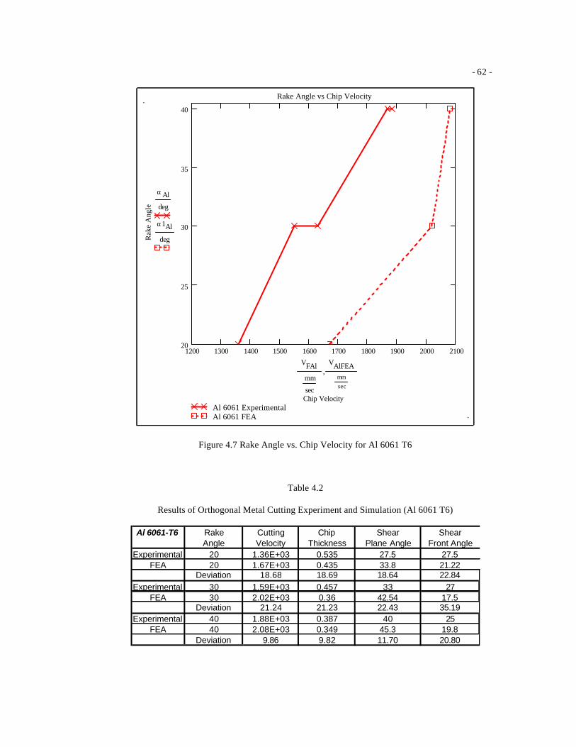
- 62 -
1200 1300 1400 1500 1600 1700 1800 1900 2000 210020
25
30
35
40
Al 6061 ExperimentalAl 6061 FEA
Rake Angle vs Chip Velocity
Chip Velocity
Rak
e A
ngle
α Al
deg
α1Al
deg
VFAl
mm
sec
VAlFEAmmsec
,
.
.
Figure 4.7 Rake Angle vs. Chip Velocity for Al 6061 T6
Table 4.2
Results of Orthogonal Metal Cutting Experiment and Simulation (Al 6061 T6)
Al 6061-T6 Rake Cutting Chip Shear ShearAngle Velocity Thickness Plane Angle Front Angle
Experimental 20 1.36E+03 0.535 27.5 27.5FEA 20 1.67E+03 0.435 33.8 21.22
Deviation 18.68 18.69 18.64 22.84Experimental 30 1.59E+03 0.457 33 27
FEA 30 2.02E+03 0.36 42.54 17.5Deviation 21.24 21.23 22.43 35.19
Experimental 40 1.88E+03 0.387 40 25FEA 40 2.08E+03 0.349 45.3 19.8
Deviation 9.86 9.82 11.70 20.80
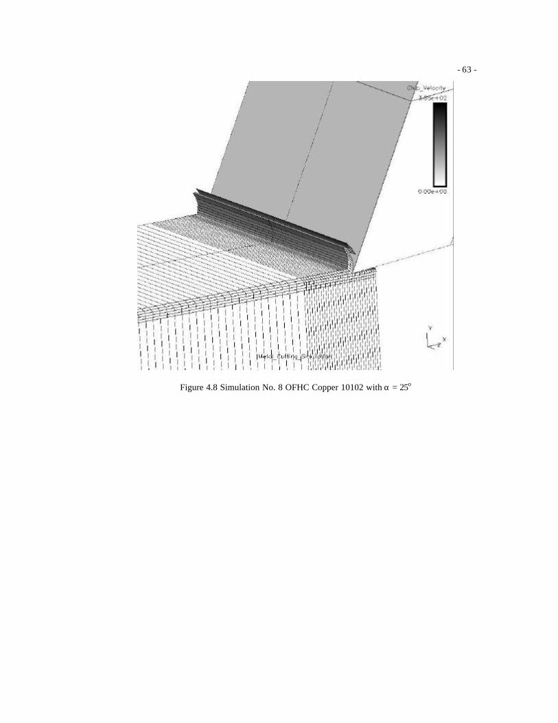
- 63 -
Figure 4.8 Simulation No. 8 OFHC Copper 10102 with α = 25o
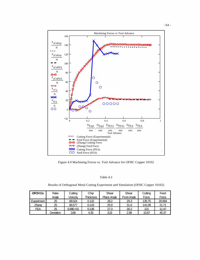
- 64 -
0 0.2 0.4 0.6 0.8 120
0
20
40
60
80
100
120
140
160
Cutting Force (Experimental)Feed Force (Experimental)(Zhang) Cutting Force(Zhang) Feed ForceCutting Force (FEA)Feed Force (FEA)
Machining Forces vs Tool Advance
Tool Advance
FxCuExp
N
FyCuExp
N
FxCuFEA
N
FyCuFEA
N
FcCu
N
FtCu
N
DExp1
mm
DExp2
mm,
DFEA1
mm,
DFEA2
mm,
DFEA
mm,
DFEA
mm,
.
.
Figure 4.9 Machining Forces vs. Tool Advance for OFHC Copper 10102
Table 4.3
Results of Orthogonal Metal Cutting Experiment and Simulation (OFHC Copper 10102)
OFCH Cu Rake Cutting Chip Shear Shear Cutting FeedAngle Velocity Thickness Plane Angle Front Angle Force Force
Experiment 25 68.024 0.132 28.2 29.3 135.75 20.994Zhang 25 66.577 0.143 25.9 31.6 141.09 21.71FEA 25 6.99E+01 0.138 27.3 30.2 121 11.47
Deviation 2.68 4.35 3.19 2.98 10.87 45.37
- 65 -
DISCUSSION
Results from simulations 5 thru 7 and 9 thru 12 were not reported in this study due to the ability of
the code to solve those class of problems. The deviations found in those simulations were a result of some
numerical instabilities and/or the material model in the finite element code. Considering that a finite
element code has two parts that would contribute to deviations it was believed that majority of it was
contributed by the numerical scheme in the finite element code. The simulation results reported in this
study resulted in excessive deformation or zero spurious deformation at low strain rates especially in the
quasi-static regime.
Considering if valid results were obtained from those listed simulations within a certain degree of
accuracy with that of actual machining results, the simulations would provide better insight of rake angle
configuration in chip formation. The effect of the rake angle on chip formation would show that as the rake
angle increases the chip thickness decreases. In addition, also as the rake angle increased the chip velocity
and shear plane would increase while the shear front angle would either decrease of increase depending on
which face centered cubic (FCC) material being machined. As stated in chapter one variations in stacking
fault energy (SFE) have a detectable effect on the shear direction. As the SFE increases the separation
between partial dislocations decreases thus lowering levels of stress required to produce slip. This effect
causes the onset of the shear front to decrease, as the material gets closer to the tool. The shear plane and
shear front angle describes the plastic deformation of the material during the metal cutting process by
indicating the increase in shear plane angle indicates an increase in dislocation density with a decrease in
shear front angle which results in no work hardening for the aluminum alloy. However, for OFHC copper
a decrease in the shear plane angle results in work hardening due to the low SFE. This work hardening is a
result of dislocation multiplying and increasing the shear stress required to produce slip during plastic
deformation of metals in proportion to the increase in shear strain.
As seen in figure 4.4 and 4.5 increasing the rake angle for Al 6061-T6 the shear plane angle
increases while the shear front angle decreases depicts that the material does not plastically flow very well
during the metal cutting process. Decreasing the rake angle for the aluminum alloy yields a discontinuous
chip formation. The simulation results in figures 4.1 to 4.3 illustrate the dynamic behavior of chip
- 66 -
formation during the machining process. Usually decreasing the rake angle requires larger forces to
remove the same amount of material, which also increases tool wear. In figure, 4.6 increasing the rake
angle decrease the chip thickness, which produces a smoother chip. The objective of most machining
applications would be to control the feed rate, depth of cut, and cutting velocity for a given rake angle to
produce continuous smooth chip formation if possible. In figure 4.7 the chip velocity increases as the rake
angle increases which indicates that the chip surface between the tool chip interface would be much
smoother than those machined at lower rake angles.
For OFHC Copper 10102 as the rake angle increases the shear front angle would increases as
shear plane angle would decreases, which indicates that the dislocation density increases as the SFE
decrease. This increase in dislocation density and decrease in SFE results in a material that plastically
deforms until work hardening occurs during the cutting application. Increasing the rake angle also increase
tool wear thus shortening the tool life [7]. Yet increasing the rake also decreases the cutting forces during
cutting thus decreasing the shear strain in the primary shear zone. Figure 9 displays a plot of machining
forces and cutting tool displacement. In figure 9 the machining forces plotted are the cutting force and feed
force, see figure 1.14. According to the simulation results at a tool displacement of 5.334x10⁻⁴ mm the
cutting force deviated by more than ten percent in comparison to experimental data, however the simulated
feed force showed a very large deviation. Seen in figure 8 is graphic plot of chip velocity for OFHC
Copper 10102 with an average chip velocity of 69.9 mm/sec. Table 4.3 contains simulation, experimental,
and Zhang FEA results.
CONCLUSION
The simulations developed for this study were not able to predict the experimentally measured
chip thickness, chip velocity, shear plane and shear front angles for a class of metal cutting problems below
the dynamic high strain rate regime. In addition, it was determined that both the material model as well as
the numerical scheme could contribute to the error in simulations 5 thru 7 and 9 thru 12. A study was
conducted with simple materials models to determine whether the material model contributed to the error
and the simulation results were approximately the same, yielding zero deformation modes. Evaluating
- 67 -
various simple material models such as elastic-plastic with failure and kinematic/isotropic elastic-plastic
material model, the conclusion was drawn that the instability occurs at low machining strain rates yielding
zero deformation modes with excessive deformation. Chapter 5 will g ive better insight to what regions
DYNA 3D were capable of predicting agreeable results with that of actual machining data found in the
literature.
The simulations performed with Al 6061 T6 with an increasing rake angle, captured the dynamic
behavior of chip formation within a certain degree of accuracy of actual machining data. Simulation No. 4
yielded the best results when compared to the actual machining results. The degree of accuracy for the
simulation results for Al 6061 T6 ranged from approximately 9% to 35%. Theses results tend to be
random, however they could be improved by increasing the Columbic friction to decrease the chip velocity,
which would yield closer results for chip thickness, shear plane and shear front angle. An investigation to
determine actual friction values to use in the simulation would eliminate randomly increasing the Columbic
friction value to obtain the desired simulated chip velocity.
The simulation of OFHC Copper 10102 returned agreeable results for chip thickness, chip
velocity, shear plane and shear front angle. The largest deviation was in the simulated feed force results in
comparison with experimental results. One reason for this deviation could be the material model, element
formulation, or numerical solution scheme. However, in performing this simulation the undeformed chip
thickness was 0.0635 mm. This undeformed chip thickness causes the chip to undergo zero deformation
modes due to the very thin chip thickness. One problem with this very thin undeformed chip thickness
causes zero deformation with very few elements. So by increasing the number of elements the aspect ratio
was resolved, thus increasing solution time by two orders of magnitude and reducing the zero deformation
modes substantially. However, as seen in figure 8 there is still remnants of zero deformation modes to
some degree, which can affect the solution. Increasing the chip thickness would reduce the zero
deformation modes for this problem, which gives the notion that element formulation and the material
model could be the cause of this deformation mode. The machining force deviations could also be a result
of the material model’s inadequate ability to account for heat conduction or specific heat variation with
temperature.
- 68 -
Chapter V
Conclusion
DISCUSSION OF RESULTS
The objective presented in this paper was to study the relationship between modeling an
orthogonal metal cutting process in a continuum finite element analysis using predictive tool such as
DYNA 3D. Provided with machining data the characterization and behavior of an orthogonal metal cutting
process could be analyzed for a better understanding of chip formation in a face centered cubic material,
namely Al 6061 T6, Al 2024 T351, and OFHC Copper 10102. Utilizing and understanding the mechanics
of chip formation from dislocation theory provides a clear understanding of the dynamic behavior of two
different FCC materials with different staking fault energies. The theory of dislocation provided insight of
the mechanics of plastic deformation form a microscopic point of view. The two FCC materials behave
very differently from a microscopic point of view and with equations derived by previous researchers,
which simplify and quantify the evaluation of the dynamic behavior of a material. Utilizing the equations
that determine chip thickness, shear plane and front angles, and shear strain gives researchers the ability to
model the phenomenon of chip formation during metal cutting to gain a better understanding of an area that
is still not yet fully known.
The simulations presented in this thesis represent two stages in the development of an accurate
finite element machining model. In chapter III the Johnson and Cook constitutive constants for the Johnson
and Cook constitutive equation were determined for Al 6061 in the T6 condition. The intent of chapter 3
was to utilize the literature to obtain the necessary data to determine the constitutive constants for the
Johnson and Cook equation. Validation of the constants required implementation of a finite element code,
namely DYNA 3D, to simulate an orthogonal metal cutting process and compare simulation results with
- 69 -
actual experimental results. The machining results reported by Lee [27] and the finite element
simulation proved to give good results.
In the second portion of this thesis, the work done by Black [6, 25] and Zhang [45] was used to
compare with simulation results. The distinctions between the two FCC materials Al 6061 T6 and OFHC
Copper 10102 were investigated do determine the metallurgical and dynamic behavior of both materials.
To distinguish the difference in the material behavior the chip thickness, shear front angle, and shear plane
angle were determined from both experimental and simulation results. However, there were some
instabilities discovered while using DYNA 3D to simulate the metal cutting process. Through multiple
simulations at various cutting speeds, an operation range was defined for a class of problems in which
DYNA 3D will yield agreeable results for the specified parameters in Table 4.1. Table 5.1 gives a brief
summary of the strain rate regime operation range for a metal cutting simulation using the specified
parameters in DYNA 3D.
CONCLUSION
This thesis has detailed the development of a finite element model of orthogonal metal cutting
simulation to study the phenomenon of chip formation. Although the metal cutting process is a quite
complex subject the finite element method proves to be a useful tool in study the metal cutting process for
strain rates ranging from 103 s -1 – 104 s -1, see Table 5.1. To validate the study conducted in Table 5.1, more
than 100 simulations were implemented at different rake angles, depth of cut, cutting speed, and with
different material models, such as kinematic/isotropic elastic-plastic material model. The simulations were
also implemented with a full eight-point integration hourglass mode and Flanagan- Belytschko stiffness
hourglass mode. This study provided valuable insight that at low strain rates the zero spurious deformation
and/or excessive noise would dominate the solution giving an inaccurate approximation or result. The
operation range defined in the Table 5.1 proves to give agreeable results and a realistic behavior of chip
formation during a metal cutting process.
Yet future work is needed to create a more responsive and accurate machining model. The
simulations performed in this study prove to give poor results for low strain rates and good results for strain
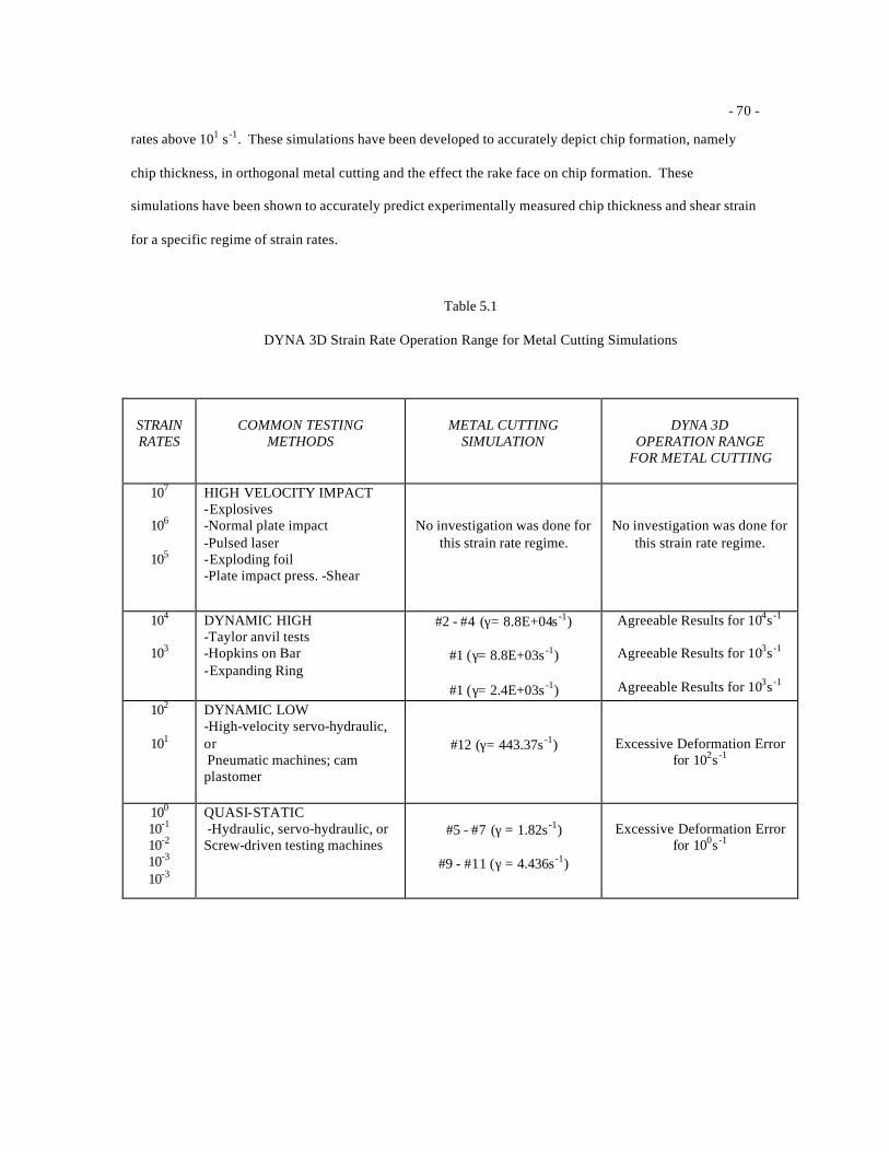
- 70 -
rates above 101 s -1. These simulations have been developed to accurately depict chip formation, namely
chip thickness, in orthogonal metal cutting and the effect the rake face on chip formation. These
simulations have been shown to accurately predict experimentally measured chip thickness and shear strain
for a specific regime of strain rates.
Table 5.1
DYNA 3D Strain Rate Operation Range for Metal Cutting Simulations
STRAIN RATES
COMMON TESTING
METHODS
METAL CUTTING
SIMULATION
DYNA 3D
OPERATION RANGE FOR METAL CUTTING
107
106
105
HIGH VELOCITY IMPACT -Explosives -Normal plate impact -Pulsed laser -Exploding foil -Plate impact press. -Shear
No investigation was done for
this strain rate regime.
No investigation was done for this strain rate regime.
104
103
DYNAMIC HIGH -Taylor anvil tests -Hopkins on Bar -Expanding Ring
#2 - #4 (γ= 8.8E+04s -1)
#1 (γ= 8.8E+03s -1)
#1 (γ= 2.4E+03s -1)
Agreeable Results for 104s -1
Agreeable Results for 103s -1
Agreeable Results for 103s -1
102
101
DYNAMIC LOW -High-velocity servo-hydraulic, or Pneumatic machines; cam plastomer
#12 (γ= 443.37s -1)
Excessive Deformation Error for 102s -1
100 10-1 10-2 10-3 10-3
QUASI-STATIC -Hydraulic, servo-hydraulic, or Screw-driven testing machines
#5 - #7 (γ = 1.82s -1)
#9 - #11 (γ = 4.436s -1)
Excessive Deformation Error
for 100s -1
- 71 -
FUTURE WORK
Development of an accurate metal cutting model is a complex task, which requires a very good
understanding of the mechanical response of the material and the numerical modeling. There are three
general aspects, which make up numerical modeling: the material model (constitutive equation and/or
equation of state), element formulation, and the numerical algorithm that performs the numerical analysis.
Either of these areas can contribute to errors experienced during a simulation and to validate each area
requires further investigation. The first issue that should be addressed should be the choice of algorithm
used to solve this type of problem. This can be resolved by solving the same problem with different
numerical schemes and algorithms such as a forward difference vs. central difference method. As a result
of using DYNA 3D, noise tends to be generated at low strain rates ranging from 102s -1 to the quasi-static
regime, which would require some technique to dampen the excess noise, which would reduce majority of
the error produced in the metal cutting simulation. Element formulation such as shape functions and
derivational theory, as well as basic modeling issues should be investigated to improve the accuracy of a
finite element code.
Another concern is the code’s ability to account for the thermo -mechanical modeling of the
problem. DYNA 3D does not account for heat conduction or variations in the value of specific heat, yet it
has the ability to perform thermo analysis with the necessary input. In addition, it would be worthwhile to
investigate other software packages, such as LS-DYNA and ABAQUS, which might be faster and more
reliable than DYNA 3D.
The simulations proposed in paper assumed the tool was rigid and perfectly sharp. Although these
are common assumptions for theoretical purposes, they are not completely true. In reality the tool is not
rigid, and tool wear will occur over time with repeated use during machining. In actuality, the tool is not
perfectly sharp, but has a small radius at the tool tip. These are both factors that should be considered for
future studies.

NOTE TO USER
Page(s) not included in the original manuscriptare unavailable from the author or university. The
manuscript was microfilmed as received.
72
This reproduction is the best copy available
- 73 -
REFERENCES CITIED
1. Benson, D. J., “Computational Methods in Lagrangian and Eulerian Hydrocodes,” Computer Methods in Applied Mechanics and Engineering, Vol. 99, 1992, pp. 235 – 394.
2. Black, J. T., “On the Fundamental Mechanism of Large Deformation: Electron Microscopy of
Metal Cutting Chips,” Journal of Engineering for Industry, May 1971, pp. 507 – 526. 3. Black, J. T., Breneiser, D. and Mitchell, H. B., 1975, “Dynamic Shear Stress Constancy with
Respect to Deformation Texture in Al 6061-T6 Aluminum and Alpha Brass,” 3rd NAMRC. 4. Black, J.T., 1979, “Flow Stress Model in Metal Cutting,” ASME Journal of Engineering for
Industry, Vol. 101, p. 403 – 415. 5. Black, J. T., Huang, J. M., “Shear Strain Model in Metal Cutting,” ASME Manufacturing Science
and Engineering , Vol. 2 – 3, 1995, pp. 283 – 302. 6. Black, J. T., Huang, J. M., “An Evaluation of Chip Separation Criteria for the FEM Simu lation of
Machining,” Journal of Manufacturing Science and Engineering, Vol. 118, 1996, pp. 545 – 553. 7. Black, J. T., Payton, L. N., 2000, “Orthogonal Machining of Copper with a Hardness Gradient,”
Transaction of NARMC. 8. Buryta, D., Sowerby, R., Yellowely, I., 1994, “Stress Distribution on the Rake Face During
Orthogonal Machining,” International Journal pf Machine Tools Manufacturing, Vol. 34, No. 5, pp. 721-739.
9. Chatfield, D. A., Rote, R. R., 1974, “Strain Rate Effects on the Properties of High Strength, Low
Alloy Steels, SAE Preprints No. 740177, pp. 1 – 12. 10. Cheng, Ching-Shan, 1999, “Material Characterization at High Rates of Plastic Deformation:
Experiments and Numerical Modeling,” Ph. D. thesis, Ohio State University, Columbus, Ohio. 11. Christon, M. A., Dovey, Donald, 1992, “INGRID: A 3D Mesh Generator for Modeling Nonlinear
Systems – User Manual,” Lawrence Livermore National Laboratory Report UCID-20506.
12. Cook, N., 1966, “Manufacturing Analysis,” Addison-Wiley, Massachusetts. 13. Dieter, George E., 1986, “Mechanical Metallurgy,” McGraw-Hill, New York. 14. Ernst, H., Merchant, M. E., 1941, “Chip Formation, Friction and Finish,” Cincinnati Milling
Machine Company, Ohio. 15. Flanagan, D. P., Belytschko, T., “A Uniform Strain Hexahedron and Quadrilateral With
Orthogonal Hourglass Control,” International Journal of Numerical Methods In Engineering , Vol. 17, 1981, pp. 679-706.
16. Iwata, K., Osakada, K., Terasaka, Y., “Process Modeling of Orthogonal Cutting by the Rigid-
Plastic Finite Element Method,” ASME Journal of Engineering Materials and Technology, Vol. 106, 1984, pp. 132 - 138.
17. James, Mark, “DigXY Application,” 1994 – 1998, Version 1.0.1.
- 74 -
18. Johnson, G. R. and Cook, W. H., 1983, “A constitutive model and data for metals subjected to
large strains, high strain rates and temperatures,” 7th International Symposium on Ballistics, the Hague, the Netherlands, p. 541
19. Kaneko, Junichi, 1977, “Thermo mechanical Treatment of the 6061 Aluminum Alloy,” Journal of
Japan Institute of Light Metals, Vol. 27, pp. 49 – 56. 20. Kim, K. W., Sin, H., 1995, “Development of A Thermo-Viscoplastic Cutting Model Using Finite
Element Method,” International Journal of Machine Tools Manufacturing , Vol. 36, No. 3, pp. 379-397.
21. King, Robert I., 1985, “Handbook of High Speed Machining Technology,” Chapman and Hall,
New York. 22. Klamecki, B. E., 1973, Incipient Chip Formation in Metal Cutting – A Three-Dimension Finite
Element Analysis,” Ph. D. dissertation, University of Illinois at Urbana-Champaign. 23. Lajczok, M. P., 1980, ‘A Study of Some Aspects of Metal Machining Using Finite Element
Method,” Ph. D. Dissertation, North Carolina State University. 24. Lee, D., 1985, “The Effect of Cutting Speed on Chip Formation Under Orthogonal Machining,”
Journal of Engineering for Industry, Transactions ASME, Vol. 107, p. 55 – 63. 25. Lee, E. H., Schaffer, B. W., “The Theory of Plasticity Applied to a Problem of Machining,” ASME
Journal of Applied Mechanics, vol. 18, 1951, pp. 405 –413. 26. Lipkin, J., Swearengen, J. C., Karnes, C. H., 1973,“Mechanical Properties of 6061 Al-Mg-Si
Alloy After Very Rapid Heating.” Journal of the Mechanics and Physics of Solids, Vol. 21, pp. 91 – 112.
27. McClain, B., Thean, W., Maldonado, G. I., Fang, X. D., 2000 “Finite Element Analysis of Chip
Formation in Grooved Tool Metal Cutting,” Machining Science and Technology, Vol. 4, pp. 305 –316.
28. Meyers, Marc A., 1994, “Dynamic Behavior of Materials,” John Wiley & Sons, New York. 29. Nakayama, K, 1962,“A Study of Chip Breaking,” Bulletin of the Japan Society of Precision
Engineering, Vol. 5, pp. 142 – 150. 30. Nakayama, K, 2000,“Chip Control in Metal Cutting,” Bulletin of the Japan Society of Precision
Engineering, Vol. 18, p. 315 – 316. 31. Reddy, J. N., 1993, “An Introduction to The Finite Element Method,” McGraw-Hill, New York. 32. Reed-Hill, Robert E., 1994, “Physically Metallurgy Principles,” PWS Publishing Company,
Boston. 33. Sato, Shiro, 1973, “Effect of Specimen Shape and Dimension on Elongation of Tensile Test Pieces
of 6061 and 7075 Alloy Sheets,” Journal of Japan Institute of Light Metals, Vol. 23, pp. 368 – 375.
34. Shi, G., Deng, X., Shet, C., 2002, “A finite element study of the effect of friction on orthogonal
metal cutting,” Finite Elements in Analysis and Design, pp. 863 – 883.
- 75 -
35. Shih, A. J. M., Chadrasekar, S., Yang, H. T., “Finite Element Simulation of Metal Cutting Process
with Strain Rate and Temperature Effects,” Fundamental Issue in Machining, ASME Publication, PED-Vol. 43, 1990, pp. 11 – 24.
36. Strenkowski, J. S., Carroll, J. T., “A Finite Element Model of Orthogonal Metal Cutting,” ASME Journal of
Engineering for Industry, Vol. 107, Nov., 1985, pp. 349. 37. Strenkowski, J. S., Carroll, J. T., “An Orthogonal Metal Cutting Model Based on an Eulerian Finite Element
Method,” Manufacturing Processes, Machines and Systems, Conference on Production Research and Technology, 13th, 1986, p. 261.
38. Strenkowski, J. S., Moon, K. J., “Finite Element Predications of Chip Geometry and Tool/Workpiece
Temperature Distribution in Orthogonal Metal Cutting,” ASME Journal of Engineering for Industry, Vol. 112, 1990, p. 213.
39. Tay, A. O., Stevenson, M. G., de Vahl, Davis G., “Using Finite Element Method to Determine
Temperature Distributions in Orthogonal Machining,” Proceedings of the Institute of Mechanical Engineers, Vol. 188, 1974, pp. 627 – 638.
40. Thean, W. K., McClain, B., Maldonado, G. I., Fang, X. D., 1999, “Finite Element Analysis of
Chip Formation in Grooved Tool Metal Cutting,” ASME Journal of Manufacturing Science and Engineering, Vol. 3-1, pp. 245-258.
41. Tucker, A. B., 1998, “Modeling Temperature and Strain Rate History Effects in OFHC Cu,” Ph.
D. thesis, Georgia Institute of Technology, Georgia. 42. Whirley, R. G., Engleman, B. E., Lin, J. I., 1999, “A Nonlinear, Explicit, Three-Dimensional
Finite Element Code For Solid and Structural Mechanics – User Manual,” Lawrence Livermore National Laboratory Report UCRL-MA-10752.
43. Wince, J. and Schneider, J., 2002 “Determining the Material Properties for Aluminum 6061-T6
for Implementation in the Johnson and Cook Constitutive Equation for Predicting Dynamic Material Behavior,” Proceedings of the ASME Southeastern Region XI Technical Conference, Vol. 1, No. 1, pp. 12.1-12.5.
44. Worthington, B., “The Effect of Rake Face Configuration on The Curvature of The Chip in Metal
Cutting,” International Journal of Machine Tool Design, Vol. 15, p. 223 – 239. 45. Zhang, B., Bagchi, A., 1994, “A Study of Chip Separation Criteria for the FEM Simulation of
Machining,” Journal of Manufacturing Science and Engineering, Vol. 118, pp. 545-555. 46. Zhang, Y. P., 1980, “Chip Curl, Chip Breaking and Chip Control of the Difficult to Cut
Materials,” CIRP Annals … Manufacturing Technology, pp. 79 – 83.

- 76 -
APPENDIX A
CREATING METAL CUTTING SIMULATION USING DYNA 3D
- 77 -
CREATING METAL CUTTING SIMULATION USING DYNA 3D
The contents of this appendix explain in detail the method used to create models and run
simulations using DYNA 3D. To generate the simulations and view the results three programs are
required. The preprocessor, Ingrid, creates a finite element mesh and generates an input file to be used by
DYNA 3D. DYNA 3D does the actual numerical analysis, calculating the final deformation of the chip and
workpiece and any other desired information such as forces. Finally, the results are viewed with the
postprocessor, called Griz.
The first step in the simu lation process is to create an input file for the Ingrid processor. This file
is a text file defining the geometry of the problem, along with input parameters and boundary conditions.
Sample Ingrid input files for several simulations are found in Appendices B – D. Once the input file is
generated, Ingrid is started by using the following command at the Unix prompt:
Ingrid i=filename
where filename is the name of the input file. Many commands are available in the preprocessor for viewing
the mesh of the metal cutting simulation. The commands used to generate the output file to implement in
DYNA 3D is typing continue at the prompt. Ingrid will then generate the input file called ingrido, which
can be read by DYNA 3D. The simulation can be ran by typing the following command at the Unix
prompt:
dyna3d i=ingrido.
DYNA 3D will perform all the calculations for the simulation and generate several output files
such as binary data files including files with nodal forces acting on specified surfaces. When DYNA 3D
completes the analysis it will generate a restart file called d3dump01. If desired, the simulation may be
continued or restarted by issuing the following command at the Unix prompt:
dyna3d i=d3dump01.
- 78 -
Once DYNA 3D has generated the binary data files, the results may be viewed using the
postprocessor Griz. Griz creates the visual display of the simulation results. It is possible to view the
deformed geometry along with contours of specified important data, such as velocity magnitude and shear
strain. Griz is implemented by typing the following command at the Unix prompt:
griz –i d3plot.
CORRECTING THE DYNA 3D INPUT FILE
The Ingrid input file for the simulations using Johnson and Cook constitutive equation for the
material model will not generate all the information needed to run the simulation with DYNA 3D properly.
As a result, it is necessary to manually modify the DYNA 3D input file ingrido. The modified portion of
the file is shown in Appendix E. The first value that must be modified is the strain rate sensitivity
coefficient C. One other flag in the ingrido file must be modified if it is desired to update the stress first
order, second order, or exponential map and mid step geometry.

- 79 -
APPENDIX B
INGRID INPUT FILE FOR CHAPTER III Al 6061 T6 SIMULATION
- 80 -
INGRID INPUT FILE FOR CHAPTER III Al 6061 T6 SIMULATION
Note: This input file is for the simulation in Chapter III Al 6061-T6 simulation # 1.
Orthogonal Metal Cutting Simulation (kg mm sec) c Simulation title. All units are given in SI units: kg, mm, and seconds. c Simulation for Aluminum 6061 T6 alpha = 30 degrees t1 = 0.25 millimeters c . c .********************* INITIAL INPUT PARAMETERS **************************** c . c Input file generated for DYNA 3D. dn3d c Metal cutting simulation terminates at 5.75e-3 seconds. term 5.75e-3 c . c Data will be stored in intervals of 2.5e-4 sec for graphics and 2.5e -4 sec c for printing in the metal cutting simulation. plti 2.5e-4 c . prti 2.5e-4 c . c . c Define number of iteration between convergence checks for dynamic relaxation. itrx 250 c . c Define convergence tolerance for dynamic relaxation. tolrx 1e -4 c . c Define dynamic relaxation. facrx 0.995 c . c Define hourglass viscosity type. ihg 5 c . c Define hourglass viscosity coefficient. qh 0.101 c . c Set the scale factor for dynamic relaxation. scftrx 1.0 c Specify the time step scale factor. tssf 1.0 c Set the linear bulk viscosity coefficient. q2 0.06 c . c Set the quadratic bulk viscosity coefficient, q1 1.5 c . c . c.**************** SLIDE SURFACE/LOAD CURVE DEFINITIONS ********************* c . c Define 3 slide surfaces: #1 - sliding with separation and friction c slide surface with columbic friction of 0.5, #2 - tied with failure slide c surface to model separation of chip from workpiece, #3 - sliding with separation c and friction slide surface for bottom of tool. si 1 sv fric 0.475 kfric 0.0 mfif pnlts 1.0 pnltm 1.0; c . si 2 break fric 0.0 kfric 0.0 pnlts 5.0 pnltm 5.0; c . si 3 dummy fric 0.0 kfric 0.0 pnlts 0.0 pnltm 0.0; c . c . c Define load curve #1 with a value of 1 at time 0 to time 5.8e -3 c (constant load). Will be used to define tool velocity. lcd 1 3 0 1 0.01 1 5.8e-3 1 c . c .
- 81 -
c . c .********************* MATERIAL DEFINITIONS ********************************** c . c Define material models for tool and the 2 part work piece. c . c ************************ Elastic Material Model ************************************ c . c Define material #1 to be a Type 1 (Elastic) material. mat 1 1 c . c Define material #1 material properties: Young's Modulus of Elasticity (e), c density (ro), Possion's ratio (pr). Note: Young's modulus was defined as c an arbitrarily high number (5 X Modulus of O1 Tool Steel)to make the tool rigid. ro 7.801e -06 c . e 1.079e+06 c . pr 0.30 c . c End of material #1 definition. endmat c . c . c ******************* Johnson/Cook Elastic-Plastic Model ****************************** c . c Define material #2 material properties for Johnson/Cook Elastic-Plastic c model: Modulus of Rigidity (G), Density (ro), Yield constant (A), c Strain hardening coefficient (B), Strain hardening exponent (n), c Strain rate dependence coefficient (C), Temperature dependence c exponent (m), Melt Temperature (Tm), Room Temperature (Tr), Reference c strain rate (XO), Specific Heat (SH), Pmin or Failure Stress (PMIN), c Plastic Strain Iteration Flag (iterate), Damage Parameters (D1, D2, D3, D4, c D5) Spall Type (spall). c . mat 2 15 c . ro 2.71260e-06 c . g 25842.418640 c . a 324.585800 c . b 411.371000 c . n 0.373 c . C 0.014 c . m 1.581 c . tm 902.289 c . tr 300.15 c . x0 1.0 c . sh 875 c . pmin -1.079e+11 c . spall 3.0 c . iterate 1.0 c . d1 –0.969 d2 2.68 c . d3 4.94 c . d4 5.145e-04 c . d5 0.656 c . c End of material definition #2. endmat c . c . c .**************** EQUATIONS-OF-STATE DEFINITION *************************** c .
- 82 -
c Define equations of state for material type 15 Johnson/Cook to be Linear c Polynomial: C0 - C6 are constants used in the pressure calculation and c E0 initial internal energy, V0 initial relative volume. eos 2 1 c . c0 0 c . c1 69224.470815 c . c2 0 c . c3 0 c . c4 0 c . c5 0 c . c6 0 c . e0 0 c . v0 1 c . c End of equations of state for material definition #2. endeos c . c . c ********************** GEOMETRY DEFINITIONS ***************************** c . c *************************** CUTTING TOOL ********************************* c . c Start defining tool for simulation. start c . c Define part as block with 3 nodes in x, 6 nodes in y, and 3 nodes in z c direction. 1 3; 1 6; 1 2 3; c Coordinates for nodes 1 and 3 in x, 1 and 11 in y, and 1 and 2 in z. c directions. 0 2.5 c . 0 8.0 c . 0 -4.765 -9.53 c . c Rotate front face of tool -30 degrees around z-axis. rr 1 1 1 1 2 3 rz -30; c . c Translate back of tool -2.5mm in the x direction, rotate 30 degrees, c and translate back. rr 2 1 1 2 2 3 mx -2.5 rz -30 mx 2.5; c . c Rotate bottom of tool 5 degrees about z-axis. rr 1 1 1 2 1 3 rz 5; c . c Translate top of tool -8.0mm in y direction, rotate 5 degrees, and c translates back. rr 1 2 1 2 2 3 my -8.0 rz 5 my 8.0; c . c Constrain movement of tool to the x direction only. b 1 1 1 2 2 3 011111 c . c Translate tool 0.10mm in the x direction. mb 0 0 0 0 0 0 x 0.10 c . c Define front of tool as master surface for sliding interface of contact length of tool c to chip interface. sii 1 1; 1 2; 1 3; 1 m c . c Define bottom of tool as master surface for sliding interface #3. sii 1 2; 1 1; 1 3; 3 m c . c Define velocity of tool in -x direction equal to 2.2e+03 times c load curve #1 (constant velocity of 2.2e+03 mm/sec). Velocity in c the y and z directions are zero. fv 1 1 1 2 2 3 1 2.2e+03 -1 0 0 c . c Define tool material from material definition #1.
- 83 -
mate 1 c . c End of tool definition. end c . c . c ********************** UNDEFORMED WORKPIECE (CHIP) ********************** c . c Define the undeformed chip of the workpiece. start c . c Define as block with 115 nodes in the x direction, 3 nodes in y c direction, and 3 nodes in the z direction. 1 5 20 111 115; 1 3; 1 2 3; c . c Coordinates of nodes in the x direction, y direction and z direction. -76.2 -25.4 -12.7 –0.67 0 c . 0 0.254 c . 0 -4.765 -9.53 c . c Define as slave surface for sliding interface #1. sii 1 4; 1 1; 1 3; 1 s c . c Define bottom of chip as slave surface of sliding interface #2. The terms c 515.54 and 297.647 indicates the normal and shear failure stress in c N/mm^2 for use with the element failure separation criterion. sii 1 3; 1 1; 1 3; 2 s 515.54 297.647 c . sii 3 4; 1 1; 1 3; 2 s 515.54 297.647 c . sii 4 5; 1 1; 1 3; 2 s 515.54 297.647 c . c Undeformed workpiece (chip) is defined as material definition #2. mate 2 c . c End of undeformed workpiece (chip) definition. end c . c . c *************************** WORKPIECE ************************************* c . c Define finished surface of the workpiece. start c . c Define block for nodes as before. 1 5 20 111 115; 1 3 4 5; 1 2 3; c . c Coordinates of nodes in the x direction, y direction and z direction. -76.2 -25.4 -12.7 –0.67 0 c . 0 -0.254 -0.381 -2.54 c . 0 -4.765 -9.53 c . c Apply boundary conditions fixing the workpiece location. b 1 4 1 5 4 3 010000 c . (bottom of workpiece) b 1 1 1 5 4 1 111111 c . (plane #1 of workpiece + z direction) b 1 1 3 5 4 3 111111 c . (plane #2 of workpiece - z direction) c Define the top of the finished workpiece as master surface for sliding c interface #2 for tied slide surface. sii 1 3; 1 1; 1 3; 2 m c . sii 3 4; 1 1; 1 3; 2 m c . sii 4 5; 1 1; 1 3; 2 m c . c Define top of part as slave surface of sliding interface #3 for interface of c bottom of tool. sii 1 5; 1 1; 1 3; 3 s c . c Finished part of workpiece is defined as material definition #3 mate 2 c . c End of finished workpiece definition. end c .

- 84 -
APPENDIX C
INGRID INPUT FILE FOR CHAPTER IV AL 2024-T351 SIMULATION
- 85 -
INGRID INPUT FILE FOR CHAPTER IV AL 2024-T351 SIMULATION
Note: This input file is for the simulation in Chapter IV for Al 2024 T351 simulation # 10.
Metal Cutting Simulation c Simulation title. All units are given in SI units: kg, m, and seconds. c Simulation for Aluminum 2024 T351 alpha = 30 degrees t1 = 2.49e -1 millimeters c . c .************************ INITIAL INPUT PARAMETERS ************************** c . c Input file generated for DYNA 3D. dn3d c Metal cutting simulation terminates at 17.9 seconds. term 17.9e c . c Data will be stored in intervals of 1e-01sec for graphics and 1e-01 sec c for printing in the metal cutting simulation. plti 1e-01 c . prti 1e-01c . c Specify the time step scale factor. tssf 1.0 c . c Define number of iteration between convergence checks for dynamic relaxation. itrx 250 c . c Define convergence tolerance for dynamic relaxation. tolrx 1e -4 c . c Define dynamic relaxation. facrx 0.995 c . c Set the scale factor for dynamic relaxation. scftrx 1.0 c Define hourglass viscosity type. ihg 5 c . c Define hourglass viscosity coefficient. qh 0.10 c . c Set the bulk viscosity to the default. ibq 1 c . c Set the linear bulk viscosity coefficient. q2 0.06 c . c Set the quadratic bulk viscosity coefficient, q1 1.5 c . c.**************** SLIDE SURFACE/LOAD CURVE DEFINITIONS ******************* c . c Define 3 slide surfaces: #1 - sliding with separation and friction c slide surface with columbic friction < 0.5, #2 - tied with failure slide c surface to model separation of chip from workpiece, #3 - sliding with separation c and friction slide surface for bottom of tool #4 - tied slide surface. si 1 sv fric 0.6 kfric 0.0 mfif pnlts 1.5 pnltm 1.5; c . si 2 break fric 0.0 kfric 0.0 pnlts 3.0 pnltm 3.0; c . si 3 dummy fric 0.0 kfric 0.0 pnlts 0.0 pnltm 0.0; c . c Define load curve #1 with a value of 1 at time 0 and at time 18.0 c (constant load). Will be used to define tool velocity. lcd 1 3 0 1 0.1 1 18.0 1 c . c .
- 86 -
c .********************** MATERIAL DEFINITIONS *************************** c . c Define material models for tool and the 2 part work piece. c . c ********************** Elastic Material Model ******************************** c . c Define material #1 to be a Type 1 (Elastic) material. mat 1 1 c . c Define material #1 material properties: Young's Modulus of Elasticity (e), c density (ro), Possion's ratio (pr). Note: Young's modulus was defined as c an arbitrarily high number (5 X Modulus of O1 Tool Steel)to make the tool rigid. ro 7.801e -06 c . e 1.079e+06 c . pr 0.30 c . c End of material #1 definition. endmat c . c . c ****************** Johnson/Cook Elastic-Plastic Model ************************** c . c Define material #2 material properties for Johnson/Cook Elastic-Plastic c model: Modulus of Rigidity (G), Density (ro), Yield constant (A), c Strain hardening coefficient (B), Strain hardening exponent (n), c Strain rate dependence coefficient (C), Temperature dependence c exponent (m), Melt Temperature (Tm), Room Temperature (Tr), Reference c strain rate (XO), Specific Heat (SH), Pmin or Failure Stress (PMIN), c Plastic Strain Iteration Flag (iterate), Damage Parameters (D1, D2, D3, D4, c D5) Spall Type (spall). c . mat 2 15 c . ro 2.768e -06 c . g 25842.418640 c . a 265.0c . b 426.0 c . n 0.34 c . C 0.015 c . m 1.00 c . tm 775.0 c . tr 300.15 c . x0 1.0 c . sh 875 c . pmin -2.7579e+11 c . spall 3.0 c . iterate 1.0 c . d1 –0.969 d2 2.68 c . d3 4.94 c . d4 5.145e-04 c . d5 0.656 c . c End of material definition #2. endmat c . c . c .***************** EQUATIONS-OF-STATE DEFINITION ************************* c . c Define equations of state for material type 15 Johnson/Cook to be Linear
- 87 -
c Polynomial: C0 - C6 are constants used in the pressure calculation and c E0 initial internal energy, V0 initial relative volume. eos 2 1 c . c0 0 c . c1 69224.470815 c . c2 0 c . c3 0 c . c4 0 c . c5 0 c . c6 0 c . e0 0 c . v0 1 c . c End of equations of state for material definition #2. endeos c . c . c . c *********************** GEOMETRY DEFINITIONS ****************************** c . c ************************** CUTTING TOOL ************************************* c . c Start defining tool for simulation. start c . c Define part as block with 3 nodes in x, 6 nodes in y, and 3 nodes in z c direction. 1 3; 1 6; 1 3; c Coordinates of nodes in the x direction, y direction and z direction. 0 2.5 c . 0 10.0 c . 0 -25.0 c . c Rotate front face of tool -30 degrees around z-axis. rr 1 1 1 1 2 2 rz -30; c . c Translate back of tool -2.5mm in the x direction, rotate 30 degrees, c and translate back. rr 2 1 1 2 2 2 mx -2.5 rz -30 mx 2.5; c . c Rotate bottom of tool 10 degrees about z-axis. rr 1 1 1 2 1 2 rz 10; c . c Translate top of tool -10.0mm in y direction, rotate 10 degrees, and c translates back. rr 1 2 1 2 2 2 my -10.0 rz 10 my 10.0; c . c Constrain movement of tool to the x direction only. b 1 1 1 2 2 2 011111 c . c Translate tool 0.10mm in the x direction. mb 0 0 0 0 0 0 x 0.10 c . c Define front of tool as master surface for sliding interface #1 sii 1 1; 1 2; 1 2; 1 m c . c Define bottom of tool as master surface for sliding interface #3. sii 1 2; 1 1; 1 2; 3 m c . c Define velocity of tool in -x direction equal to 4.88e-01 times c load curve #1 (constant velocity of 4.88e-01 mm/sec). Velocity in c the y and z directions are zero. fv 1 1 1 2 2 2 1 0.488 -1 0 0 c . c Define tool material from material definition #1. mate 1 c . c End of tool definition.
- 88 -
end c . c . c *********************** UNDEFORMED WORKPIECE (CHIP) ********************** c . c Define the undeformed chip of the workpiece. start c . c Define as block with 95 nodes in the x direction, 3 nodes in y c direction, and 3 nodes in the z direction. 1 2 5 91 95; 1 3; 1 4; c . c Coordinates of nodes in the x direction, y direction and z direction. -50.0 -12.7 -10.16 -0.56 0 c . 0 0.249 c . 0 -25.0 c . c Translate top of the part 4.35e-2 millimeters in the -x direction (tilts the elements) mb 1 2 1 5 2 2 x -4.35e -2 c . c Define as slave surface for sliding interface #1. sii 1 5; 1 1; 1 2; 1 s c . c Define bottom of chip as slave surface of sliding interface #2. The terms c 402.0e -01 and 232.095e -01 indicates the normal and shear failure stress in c N/mm^2 for use with the element failure separation criterion. sii 1 5; 1 1; 1 2; 2 s 422.1 243.7 c . c Undeformed workpiece (chip) is defined as material definition #2. mate 2 c . c End of undeformed workpiece (chip) definition. end c . c . c *************************** WORKPIECE *********************************** c . c Define finished surface of the workpiece start c . c Define block for nodes as before. 1 2 5 91 95; 1 2 3 4 5; 1 3; c . c Coordinates of nodes in the x direction, y direction and z direction -50.0 -12.7 -10.16 -0.56 0 c . 0 -1.24e-01 -2.49e-1 -3.8e-1 -3.8 c . 0 -25.0 c . c Apply boundary conditions fixing the workpiece location b 1 5 1 5 5 2 010000 c . (bottom of workpiece) b 1 2 1 5 5 1 111111 c . (plane #1 of workpiece) b 1 2 2 5 5 2 111111 c . (plane #2 of workpiece) c Define the top of the finished workpiece as master surface for sliding c interface #2 for tied slide surface. sii 1 5; 1 1; 1 2; 2 m c . c Define top of part as slave surface of sliding interface #3 for interface of c bottom of tool. sii 1 5; 1 1; 1 2; 3 s c . c Finished part of workpiece is defined as material definition #3 mate 2 c . c End of finished workpiece definition. end c .

- 89 -
APPENDIX D
INGRID INPUT FILE FOR CHAPTER IV OFHC COPPER 10102 SIMULATION
- 90 -
INGRID INPUT FILE FOR CHAPTER IV OFHC COPPER 10102 SIMULATION
Note: This input file is for the simulation in Chapter IV for OFHC Copper simulation #6.
Metal Cutting Simulation c Simulation title. All units are given in SI units: kg, mm, and seconds. c Simulation for OFHC Cooper alpha = 30 degrees t1 = 2.54e -1 millimeters c . c .************************ INITIA L INPUT DEFINITIONS ****************************** c . c Input file generated for DYNA 3D. dn3d c Metal cutting simulation terminates at 18.7 seconds. term 18.7 c . c Data will be stored in intervals of 1e-1 sec for graphics and 1e-1 sec c for printing in the metal cutting simulation. plti 1e-1 c . prti 1e-1 c . c Specify the time step scale factor. tssf 1.0 c . c Define number of iteration between convergence checks for dynamic relaxation. itrx 250 c . c Define convergence tolerance for dynamic relaxation. tolrx 1e -4 c . c Define dynamic relaxation. facrx 0.995 c . c Set the scale factor for dynamic relaxation. scftrx 1.0 c Define hourglass viscosity type. ihg 5 c . c Define hourglass viscosity coefficient. qh 0.10 c . c Set the bulk viscosity to the default. ibq 1 c . c Set the linear bulk viscosity coefficient. q2 0.06 c . c Set the quadratic bulk viscosity coefficient, q1 1.5 c . c.****************** SLIDE SURFACE/LOAD CURVE DEFINITIONS *********************** c . c Define 3 slide surfaces: #1 - sliding with separation and friction c slide surface with columbic friction < 0.7, #2 - tied with failure slide c surface to model separation of chip from workpiece, #3 - sliding with separation c and friction slide surface for bottom of tool. si 1 sv fric 0.7 kfric 0.0 mfif pnlts 1.5 pnltm 1.5; c . si 2 break fric 0.0 kfric 0.0 pnlts 3.0 pnltm 3.0; c . si 3 dummy fric 0.0 kfric 0.0 pnlts 0.0 pnltm 0.0; c . c . c Define load curve #1 with a value of 1 at time 0 and at time 18.8 c (constant load) will be used to define tool velocity. lcd 1 3 0 1 0.1 1 18.8 1 c .
- 91 -
c . c .************************* MATERIAL DEFINITIONS ********************************* c . c Define material models for tool and the 2 part work piece. c . c *************************** Elastic Material Model ************************************ c . c Define material #1 to be a Type 1 (Elastic) material. mat 1 1 c . c Define material #1 material properties: Young's Modulus of Elasticity (e), c density (ro), Poisson’s ratio (pr). Note: Young's modulus was defined as c an arbitrarily high number (5 X Modulus of O1 Tool Steel)to make the tool rigid. ro 7.801e -06 c . e 1.079e+06 c . pr 0.30 c . c End of material #1 definition. endmat c . c . c *********************** Johnson/Cook Elastic-Plastic Model ******************************* c . c Define material #2 material properties for Johnson/Cook Elastic-Plastic c model: Modulus of Rigidity (G), Density (ro), Yield constant (A), c Strain hardening coefficient (B, Strain hardening exponent (n), c Strain rate dependence coefficient (C), Temperature dependence c exponent (m), Melt Temperature (Tm), Room Temperature (Tr), Reference c strain rate (XO), Specific Heat (SH), Pmin or Failure Stress (PMIN), c Plastic Strain Iteration Flag (flag), Damage Parameters (D1, D2, D3, D4, c D5) Spall Type (spall). c . c ***************** Original values for OFHC Cooper from Johnson/Cook paper ****************** c (JC Constants used for Simulation No. 8) c mat 2 15 c . c ro 8.968e-06 c . c g 4.4064e+04 c . c a 90 c . c b 292 c . c n 0.31 c . c C 0.025 c . c m 1.09 c . c tm 1356 c . c tr 300.15 c . c x0 1.0 c . c sh 383 c . c pmin -1.596e+31 c . c spall 3.0 c . c iterate 1.0 c . c d1 –0.54 c . c d2 4.89 c . c d3 3.03 c . c d4 0.014 c . c d5 1.12 c . c End of material definition #2. c endmat c . c .
- 92 -
c ************* Optimized values for Johnson/Cook from Thesis by A. B. Tanner **************** mat 2 15 c . ro 8.968e -06 c . g 4.4064e+04 c . a 0 c . b 470 c . n 0.44 c . c 0.027 c . m 0.78 c . tm 1356 c . tr 300.15 c . x0 1.0 c . sh 383 c . pmin -1.596e+11 c . spall 3.0 c . iterate 1.0 c . d1 –0.54 c . d2 4.89 c . d3 3.03 c . d4 0.014 c . d5 1.12 c . c End of material definition #2. endmat c . c . c .************************** EOS DEFINITION ********************************* c . c Define equations of state for material type 15 Johnson/Cook to be Linear c Polynomial: C0 - C6 are constants used in the pressure calculation and c E0 initial internal energy, V0 initial relative volume. eos 2 1 c . c0 0 c . c1 114912.621553 c . c2 0 c . c3 0 c . c4 0 c . c5 0 c . c6 0 c . e0 0 c . v0 1 c . c End of equations of state for material definition #2 endeos c . c . c ************************ GEOMETRY DEFINITIONS ************************** c . c **************************** CUTTING TOOL ******************************* c . c Start defining tool for simulation. start c . c Define part as block with 3 nodes in x, 6 nodes in y, and 3 nodes in z c direction. 1 3; 1 6; 1 3; c Coordinates of nodes in the x direction, y direction and z direction 0 2.5 c . 0 10.0 c .
- 93 -
0 -6.35 c . c Rotate front face of tool -30 degrees around z-axis. rr 1 1 1 1 2 2 rz -30; c . c Translate back of tool -2.5mm in the x direction, rotate 30 degrees, c and translate back rr 2 1 1 2 2 2 mx -2.5 rz -30 mx 2.5; c . c Rotate bottom of tool 10 degrees about z-axis. rr 1 1 1 2 1 2 rz 10; c . c Translate top of tool -10.0mm in y direction, rotate 10 degrees, and c translate back. rr 1 2 1 2 2 2 my -10.0 rz 10 my 10.0; c . c Constrain movement of tool to the x direction only. b 1 1 1 2 2 2 011111 c . c Translate tool 0.10mm in the x direction. mb 0 0 0 0 0 0 x 0.10 c . c Define front of tool as master surface for sliding interface #1-rake face & c contact length of tool to chip sii 1 1; 1 2; 1 2; 1 m c . c Define bottom of tool as master surface for sliding interface #3. sii 1 2; 1 1; 1 2; 3 m c . c Define velocity of tool in -x direction equal to 4.61433e-1 times c load curve #1 (constant velocity of 4.61433e-1 mm/sec). Velocity in c the y and z directions are zero. fv 1 1 1 2 2 2 1 4.61433e-1 -1 0 0 c . c Define tool material from material definition #1. mate 1 c . c End of tool definition. end c . c . c *********************** UNDEFORMED WORKPIECE(CHIP) ********************* c . c Define the undeformed chip of the workpiece. start c . c Define as block with 95 nodes in the x direction, 3 nodes in y c direction, and 3 nodes in the z direction. 1 2 5 91 95; 1 3; 1 3; c . c Coordinates of nodes in the x direction, y direction and z direction -50.8 -12.7 -10.16 -0.58 0 c . 0 0.254 c . 0 -6.35 c . c Translate top of the part -4.32e-2mm in the x direction (tilts the elements). mb 1 2 1 5 2 2 x -4.32e -2 c . c Define as slave surface for sliding interface #1. sii 1 5; 1 1; 1 2; 1 s c . c Define bottom of chip as slave surface of tied sliding interface #3. The terms c used in tied slide surface are 190.52559 and 95.26279 indicates the normal and c shear failure stress in N/mm^2 for use with the element failure separation criterion. sii 1 5; 1 1; 1 2; 2 s 190.52559 95.26279 c . c Undeformed workpiece (chip) is defined as material definition #2. mate 2 c . c End of undeformed workpiece definition. end c . c . c **************************** WORKPIECE ************************************
- 94 -
c . c Define finished surface of the workpiece start c . c Define block for nodes as before. 1 2 5 91 95; 1 2 3 4 5; 1 3; c . c Coordinates of nodes in the x direction, y direction and z direction -50.8 -12.7 -10.16 -0.58 0 c . 0 -1.27e-1 -2.54e-1 -3.81e-1 -3.8 c . 0 -6.35 c . c Apply boundary conditions fixing the workpiece location b 1 5 1 5 5 2 010000 c . (bottom of workpiece) b 1 2 1 5 5 1 111111 c . (plane #1 of workpiece) b 1 2 2 5 5 2 111111 c . (plane #2 of workpiece) c Define the top of the finished workpiece as master surface for sliding c interface #2 for tied slide surface. sii 1 5; 1 1; 1 2; 2 m c . c Define top of part as slave surface of sliding interface #3 for interface of c bottom of tool. sii 1 5; 1 1; 1 2; 3 s c . c Finished part of workpiece is defined as material definition #3 mate 2 c . c End of finished workpiece definition. end c . end c .

- 95 -
APPENDIX E
INGRID INPUT FILE FOR VALIDATION OF MATERIAL MODEL RESPONSE
- 96 -
INGRID INPUT FILE FOR VALIDATION OF MATERIAL MODEL RESPONSE
Note: This input file is for validating material model response.
Metal Cutting Simulation c Simulation title. All units are given in SI units: kg, mm, and seconds. c Simulation for OFHC Cooper alpha = 30 degrees t1 = 2.54e -1 millimeters c . c .************************ INITIAL INPUT DEFINITIONS ****************************** c . c Input file generated for DYNA 3D. dn3d c Metal cutting simulation terminates at 18.7 seconds. term 18.7 c . c Data will be stored in intervals of 1e-1 sec for graphics and 1e-1 sec c for printing in the metal cutting simulation. plti 1e-1 c . prti 1e-1 c . c Specify the time step scale factor. tssf 1.0 c . c Define number of iteration between convergence checks for dynamic relaxation. itrx 250 c . c Define convergence tolerance for dynamic relaxation. tolrx 1e -4 c . c Define dynamic relaxation. facrx 0.995 c . c Set the scale factor for dynamic relaxation. scftrx 1.0 c Define hourglass viscosity type. ihg 5 c . c Define hourglass viscosity coefficient. qh 0.10 c . c Set the bulk viscosity to the default. ibq 1 c . c Set the linear bulk viscosity coefficient. q2 0.06 c . c Set the quadratic bulk viscosity coefficient, q1 1.5 c . c.****************** SLIDE SURFACE/LOAD CURVE DEFINITIONS *********************** c . c Define 3 slide surfaces: #1 - slid ing with separation and friction c slide surface with columbic friction < 0.7, #2 - tied with failure slide c surface to model separation of chip from workpiece, #3 - sliding with separation c and friction slide surface for bottom of tool. si 1 sv fric 0.7 kfric 0.0 mfif pnlts 1.5 pnltm 1.5; c . si 2 break fric 0.0 kfric 0.0 pnlts 3.0 pnltm 3.0; c . si 3 dummy fric 0.0 kfric 0.0 pnlts 0.0 pnltm 0.0; c . c . c Define load curve #1 with a value of 1 at time 0 and at time 18.8 c (constant load) will be used to define tool velocity. lcd 1 3 0 1 0.1 1 18.8 1 c .
- 97 -
c . c .************************* MATERIAL DEFINITIONS ********************************* c . c Define material models for tool and the 2 part work piece. c . c *************************** Elastic Material Model ************************************ c . c Define material #1 to be a Type 1 (Elastic) material. mat 1 1 c . c Define material #1 material properties: Young's Modulus of Elasticity (e), c density (ro), Poisson’s ratio (pr). Note: Young's modulus was defined as c an arbitrarily high number (5 X Modulus of O1 Tool Steel)to make the tool rigid. ro 7.801e -06 c . e 1.079e+06 c . pr 0.30 c . c End of material #1 definition. endmat c . c . c ********************* Kinematic/Isotropic Elastic-Plastic Model ***************************** c . c Define material #2 material properties for Kinematic/Isotropic Elastic-Plastic c model: Young ‘s Modulus (E), Density (ro), Poisson’s Ratio (pr), Yield Stress (sigy) c Tangent Modulus (etan), and Hardening Parameter (beta). c . c mat 2 3 c . c e 1.172e+05 c ro 8.968e-06 c . c pr 0.33 c etan 1.1e+05 c sigy 90 c . c beta 0.31 c . c End of material definition #2. c endmat c . c . c ************************ GEOMETRY DEFINITIONS ************************** c . c **************************** CUTTING TOOL ******************************* c . c Start defining tool for simulation. start c . c Define part as block with 3 nodes in x, 6 nodes in y, and 3 nodes in z c direction. 1 3; 1 6; 1 3; c Coordinates of nodes in the x direction, y direction and z direction 0 2.5 c . 0 10.0 c . 0 -6.35 c . c Rotate front face of tool -30 degrees around z-axis. rr 1 1 1 1 2 2 rz -30; c . c Translate back of tool -2.5mm in the x direction, rotate 30 degrees, c and translate back rr 2 1 1 2 2 2 mx -2.5 rz -30 mx 2.5; c . c Rotate bottom of tool 10 degrees about z-axis. rr 1 1 1 2 1 2 rz 10; c .
- 98 -
c Translate top of tool -10.0mm in y direction, rotate 10 degrees, and c translates back. rr 1 2 1 2 2 2 my -10.0 rz 10 my 10.0; c . c Constrain movement of tool to the x direction only. b 1 1 1 2 2 2 011111 c . c Translate tool 0.10mm in the x direction. mb 0 0 0 0 0 0 x 0.10 c . c Define front of tool as master surface for sliding interface #1-rake face & c contact length of tool to chip sii 1 1; 1 2; 1 2; 1 m c . c Define bottom of tool as master surface for sliding interface #3. sii 1 2; 1 1; 1 2; 3 m c . c Define velocity of tool in -x direction equal to 4.61433e-1 times c load curve #1 (constant velocity of 4.61433e-1 mm/sec). Velocity in c the y and z directions are zero. fv 1 1 1 2 2 2 1 4.61433e-1 -1 0 0 c . c Define tool material from material definition #1. mate 1 c . c End of tool definition. end c . c . c *********************** UNDEFORMED WORKPIECE(CHIP) ********************* c . c Define the undeformed chip of the workpiece. start c . c Define as block with 95 nodes in the x direction, 3 nodes in y c direction, and 3 nodes in the z direction. 1 2 5 91 95; 1 3; 1 3; c . c Coordinates of nodes in the x direction, y direction and z direction -50.8 -12.7 -10.16 -0.58 0 c . 0 0.254 c . 0 -6.35 c . c Translate top of the part -4.32e-2mm in the x direction (tilts the elements). mb 1 2 1 5 2 2 x -4.32e -2 c . c Define as slave surface for sliding interface #1. sii 1 5; 1 1; 1 2; 1 s c . c Define bottom of chip as slave surface of tied sliding interface #3. The terms c used in tied slide surface are 190.52559 and 95.26279 indicates the normal and c shear failure stress in N/mm^2 for use with the element failure separation criterion. sii 1 5; 1 1; 1 2; 2 s 190.52559 95.26279 c . c Undeformed workpiece (chip) is defined as material definition #2. mate 2 c . c End of undeformed workpiece definition. end c . c . c **************************** WORKPIECE ************************************ c . c Define finished surface of the workpiece start c . c Define block for nodes as before. 1 2 5 91 95; 1 2 3 4 5; 1 3; c . c Coordinates of nodes in the x direction, y direction and z direction -50.8 -12.7 -10.16 -0.58 0 c . 0 -1.27e-1 -2.54e-1 -3.81e-1 -3.8 c .
- 99 -
0 -6.35 c . c Apply boundary conditions fixing the workpiece location b 1 5 1 5 5 2 010000 c . (bottom of workpiece) b 1 2 1 5 5 1 111111 c . (plane #1 of workpiece) b 1 2 2 5 5 2 111111 c . (plane #2 of workpiece) c Define the top of the finished workpiece as master surface for sliding c interface #2 for tied slide surface. sii 1 5; 1 1; 1 2; 2 m c . c Define top of part as slave surface of sliding interface #3 for interface of c bottom of tool. sii 1 5; 1 1; 1 2; 3 s c . c Finished part of workpiece is defined as material definition #3 mate 2 c . c End of finished workpiece definition. end c . end c .

- 100 -
APPENDIX F
COMPILING DYNA3D CODES ON SGI WORKSTATION
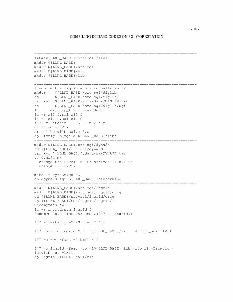
-101-
COMPILING DYNA3D CODES ON SGI WORKSTATION
======================================================================= setenv LLNL_BASE /usr/local/llnl mkdir ${LLNL_BASE} mkdir ${LLNL_BASE}/src-sgi mkdir ${LLNL_BASE}/bin mkdir ${LLNL_BASE}/lib ======================================================================= #compile the diglib -this actually works mkdir ${LLNL_BASE}/src-sgi/diglib cd ${LLNL_BASE}/src-sgi/diglib/ tar xvf ${LLNL_BASE}/cds/dyna/DIGLIB.tar cd ${LLNL_BASE}/src-sgi/diglib/Sgi ln -s devindep_f.sgi devindep.f ln -s x11_f.sgi x11.f ln -s x11_c.sgi x11.c f77 -c -static -O -G 0 -n32 *.f cc -c -O -n32 x11.c ar r libdiglib_sgi.a *.o cp libdiglib_sgi.a ${LLNL_BASE}/lib/ ======================================================================= mkdir ${LLNL_BASE}/src-sgi/dyna3d cd ${LLNL_BASE}/src-sgi/dyna3d tar xvf ${LLNL_BASE}/cds/dyna/DYNA3D.tar vi dyna3d.mk change the LBPATH = -L/usr/local/llnl/lib change .....????? make -f dyna3d.mk SGI cp ddyna3d.sgi ${LLNL_BASE}/bin/dyna3d ======================================================================= mkdir ${LLNL_BASE}/src-sgi/ingrid mkdir ${LLNL_BASE}/src-sgi/ingrid/orig cd ${LLNL_BASE}/src-sgi/ingrid/orig cp ${LLNL_BASE}/cds/ingrid/Ingrid/* . uncompress *Z ln -s ingrid.sun ingrid.f #comment out line 253 and 29947 of ingrid.f f77 -c -static -O -G 0 -n32 *.f f77 -n32 -o ingrid *.o -L${LLNL_BASE}/lib -ldiglib_sgi -lX11 f77 -c -O4 -fast -libmil *.f f77 -o ingrid -fast *.o -L${LLNL_BASE}/lib -libmil -Bstatic -ldiglib_sgi -lX11 cp ingrid ${LLNL_BASE}/bin

- 102 -
APPENDIX G
MODIFICATIONS MADE DYNA 3D INPUT FILE “INGRIDO”

- 103 -
MODIFICATIONS MADE DYNA 3D INPUT FILE
“INGRIDO”
SPECIFING STRESS UPDATE ORDER
In order to specify the stress update order from first order to second order or exponential map mid
step geometry it is necessary to modify control card nine. Issuing a two for second order or three for
exponential map will flag DYNA 3D to update stress in second order or by exponential map. The default is
one or first order.
Unmodified portion of input file (Control Card 9):
*-------------------------- CONTROL CARD #9 ---------------------------* * * plane stress plasticity[1] printout flag[2] number of 1Dslidelines[3] 1 0 0 *
Modified portion of input file (Control Card 9):
*-------------------------- CONTROL CARD #9 ---------------------------* * * plane stress plasticity[1] printout flag[2] number of 1Dslidelines[3] 1 0 0 2 *
ADDITION OF MATERIAL CONSANT
Due to a program error in the preprocessor Ingrid, the constitutive constant C for strain rate
sensitivity coefficient of the Johnson and Cook constitutive equation does not write out properly. Ingrid
interprets the letter “C” as comment command. As a result it is necessary to manually enter the value for
“C” in ingrido under the material cards section. For Al 6061-T6 the value of C is 0.014, Al 2024-T351 the
value of C is 0.015, and OFHC Copper is 0.25 (value form Johnson and Cook paper) and 0.27 (value from
Tanner for lower strain rates), and it may be entered by modifying one entry as follow:
Unmodified portion of input file (Material Card):
*--------------------------- MATERIAL CARDS ---------------------------* * material type #15(Johnson/Cook Strain and Temperature Sensitive Plasticity) 4.406E+04 0.000E+00 4.700E+02 4.400E-01 0.000E+00 7.800E-01 1.356E+03 3.001E+02 Modified portion of input file (Control Card 9):

- 104 -
material type #15(Johnson/Cook Strain and Temperature Sensitive Plasticity) 4.406E+04 0.000E+00 4.700E+02 4.400E-01 2.700E-02 7.800E-01 1.356E+03 3.001E+02