Model of coupled liquid water flow and heat transport with phase change in a snowpack

AcattwitTemEatmlmdslrSd

D

CI

F

1

pro2

Download

Model for Coupled Liquid Water Flowand Heat Transport with Phase Change

in a Snowpack

Ronald P. Daanen1 and John L. Nieber2

bstract: The flow of liquid water in a snowpack is complex because of theoupled processes involved, including the phase change between liquid and solid,nd the latent and sensible heat transfer processes. To properly describe the de-ails of spatial and temporal changes in a snowpack it is necessary to includehese coupled processes. This paper presents a numerical model of coupled liquidater flow and heat transport in a snowpack. The model is intended to quantify

nfiltration into a snowpack, and evaluate the potential for the formation of dis-inct heterogeneities in liquid water and heat transport properties in a snowpack.he numerical model solves the two-dimensional form of the governing coupledquations using a finite difference scheme. The governing equations assume ther-odynamic equilibrium between the solid and liquid phases in the snowpack.quations describing the metamorphosis of ice grains during liquid water flowre applied within the model, and the heat and liquid water transport properties ofhe snow are treated with relations identical to those used for mineral porousedia. Sample solution results for an alternative formulation taken from the

iterature are used to test the present solution, and it is found that the presentodel yields similar results but with some distinct differences. The effect of

irect coupling of the temperature with the liquid water pressure is presented in aimple horizontal freezing simulation, which is compared with the Stefan prob-em where liquid water is not redistributed. Overall the direct coupling and wateredistribution is found to lead to greater front penetration in comparison to thetefan formulation. For infiltration with gravity it is shown that grain size growthuring infiltration leads to increased wetting front penetration.

OI: 10.1061/�ASCE�0887-381X�2009�23:2�43�

E Database subject headings: Snow; Snowmelt; Water flow; Models;nfiltration.

1Research Fellow, Geophysical Institute, Univ. of Alaska Fairbanks, 903 Koyukuk Dr.,airbanks, AK 99775-7320 �corresponding author�. E-mail: [email protected]

2Professor, Dept. of Bioproducts and Biosystems Engineering, Univ. of Minnesota,390 Eckles Ave., St. Paul, MN 55108-6005.

Note. This manuscript was submitted on December 7, 2004; approved on July 1, 2008;ublished online on May 15, 2009. Discussion period open until November 1, 2009; sepa-ate discussions must be submitted for individual papers. This paper is part of the Journalf Cold Regions Engineering, Vol. 23, No. 2, June 1, 2009. ©ASCE, ISSN 0887-381X/
009/2-43–68/$25.00.
J. COLD REG. ENGRG. © ASCE / JUNE 2009 / 43

ed 09 Jun 2009 to 128.101.98.21. Redistribution subject to ASCE license or copyright; see http://pubs.asce.org/copyright

I

Sott1ttholnsfnhi

qdwpsdptdmsst

pwpTsMttqm

sJ1

4

Download

ntroduction

nowfall dominates winter weather in many regions of the world, and the varietyf conditions in which this snow forms a snowpack is extensive. Snowmelt fromhese snowpacks is consequently extremely variable, spatially and temporally inerms of the quantity of water released �Harrington et al. 1996; Williams et al.999; Lundquist and Dettinger 2005�. For example, Marsh and Woo �1985� statedhat flow at the bottom of small areas of arctic snow covers can vary from 0o 240% spatially compared to the average flow. This variability of melt releaseas an impact on the timing of floods and sustained flows, and also on the qualityf water in streams and rivers. In pristine environments snowmelt can causeethal damage to aquatic life, due to potentially high concentrations of contami-ants �Harrington et al. 1996� deposited with snowfall. Wania et al. �1998�howed that snow is more efficient at removing hydrophobic organic chemicalsrom the atmosphere than rain, thereby leading to the concentration of contami-ants in a snowpack. The release of these contaminants with snowmelt can alsoave detrimental impacts on the source of drinking water for humans. Thus it ismportant to understand the process of melt water release from snowpacks.

Simple computational models use snow water equivalent measurements touantify the amount of water that will be released out of a seasonal snowpackuring spring ablation. The quantity and timing of this water release is critical forater supply or flood prediction in many parts of the world. This approach for therediction of melt water release is in many situations a satisfactory tool. Theuccess of these models depends entirely on a good calibration and reliable inputata. For instance, Daanen �1997� found a simple modeling approach able toredict surface water runoff from snow melt about 70% accurate, after calibra-ion. He found that the accuracy dropped to 50% when predicting an independentata set for the same area. There are many causes for inaccuracies of simplerodels, but one might be that those models do not account for the complex

tructures that can form within a snowpack. Without directly accounting for suchtructures it is impossible that a model will provide reliable predictions of con-aminant release or even melt release.

Marsh and Woo �1985� provide a conceptual description of the varied flowaths that exist in a melting snowpack. The description clearly shows that liquidater does not move in a diffuse manner within the snowpack, but throughreferential flow paths formed by heterogeneities in the snowpack properties.hese heterogeneities are manifested in terms of spatially variable snow grainize and snow packing density, sloping dense layers, and vertical flow channels.ore recently Waldner et al. �2004� showed the importance of snow structure on

he liquid water flow distribution and preferential flow paths. To be able to predicthe movement of liquid water within a snowpack containing these features re-uires a more complete description of flow mechanisms than those available withost current modeling formulations.Several physically based models for simulating liquid water flow within a

nowpack have been developed over the last few decades �Colbeck 1972, 1978;ordan 1983, 1991; Illangasekare et al. 1990; Wigmosta et al. 1994; Tseng et al.
994; Tuteja and Cunnane 1997; Stähli and Jansson 1998�. The principles under-
4 / J. COLD REG. ENGRG. © ASCE / JUNE 2009


lfpt1wti

�d�mwpn�lpats

sesgftlw

T

Ticmetmipp

st

Download

ying these models are very similar to the soil physics principles of Darcian flowor unsaturated conditions, and depending on the modeling approach, the cou-ling with heat transport with the water flow is also considered. Many applica-ions have neglected capillary effects since they are generally small �Wankiewicz979� during fast ablation of snow, and also have not considered the couplingith heat transport. However, both capillarity and heat transport may be impor-

ant during preablation snowmelt which can influence the formation of ice layersn the snowpack.

A model that is now applied widely is the SNTHERM model by Jordan1991�. The model treats the water flow and heat transport processes as being oneimensional and is based on the mixture theory presented by Morland et al.1990�. This theory combines four constituents �ice, water, vapor, and air� in oneixture. Illangasekare et al. �1990� described a model for the infiltration of meltater in subfreezing snow. The model treats the water flow and heat transportrocess as being two dimensional and it is capable of treating a nonisothermalonhomogeneous snowpack. The SNOWPACK model by Bartelt and Lehning2002� also needs to be mentioned here, that while it does not directly deal withiquid water flow in snow, it does quantify many relevant snow microstructuralroperties such as temporal changes in grain size. The model is designed forvalanche forecasting and therefore it contains a very detailed description ofhe microstructure of snow and how this relates to the internal strength of thenowpack.

In this paper we present a model of coupled water flow and heat transport innow. The formulation is similar to that presented by Illangasekare et al. �1990�xcept that in our model we impose thermodynamic equilibrium between theolid and liquid phases of water, and the model also includes the process of snowrain growth. The purpose for the development of the model was to provide a toolor simulating the formation of heterogeneities in snowpacks. This paper presentshe background development of the model and illustrates a few applications, buteaves the application to detailed analysis of snow structure formation to futureork.

heory of Liquid Water Flow in Snow

he governing equations for the coupled processes of mass and energy transportn a snowpack will now be presented. These coupled processes are represented byoupled equations for each of the fluid masses, including the conservation ofass equations, the conservation of thermal energy equations, constituent flux

quations, and relations for thermodynamic equilibrium. We note from the starthat in the present application we neglect the contribution of water vapor to theass balance of water and the thermal energy balance. The justification underly-

ng this choice is explained in the “Discussion” section. Note that in addition toresenting the definition of terms where they first appear in the text, we alsoresent definitions in the “Notation.”

Snow is composed of three components: ice, liquid water, and air. The con-ervation of mass principle for water is applied to both water phases to yield
he following equations:


L

I

w�ll

pf

L

I

A

wTaoQ

ti

w

a�

4

Download

iquid water

��l�l��t

= − � · ��lql� + Ei,l �1�

ce

��i�i��t

= − Ei,l �2�

here �l and �i=densities of liquid water and ice, respectively; �l andi=volumetric contents of liquid water and ice, respectively; ql=Darcy flux foriquid water; Ei,l=mass of water involved in the change of phase from ice toiquid water; and t=time.

The conservation of heat energy principle is applied to each of the waterhases and the air phase. The resulting conservation equations are given by theollowing equations:

iquid water

�lCl

�Tl

�t= − � · qh

l + Qha,l + Qh

i,l �3�

ce

�iCi

�Ti

�t= − � · qh

i − Qhi,l − LfEi,l �4�

ir

�aCa,p�Ta

�t= − � · qh

a − Qha,l �5�

here Cl, Ci, and Ca,p=specific heats for liquid water, ice and air, respectively;

l, Ti, and Ta=temperatures of the liquid water, ice, and air, respectively; qhl , qh

i ,nd qh

a=heat fluxes in the liquid water, ice, and air, respectively; Lf =latent heatf fusion; Qh

i,l=sensible heat exchange between the ice and liquid water; and

ha,l=sensible heat exchange between the air and the liquid water.

Under conditions of thermal equilibrium the temperatures will be equal amonghe phases at a point �Tl=Ti=Ta�, so a bulk thermal energy conservation equations obtained by combining Eqs. �3�–�5� to yield

��bCvT��t

= − � · qh − LfEi,l �6�

here qh=vector sum given as

qh = qhl + qh

i + qha �7�

nd we have �b=�l�l+�i�i+�a�a, Cv=�lCl+�iCi+�aCa,p, and the constraint
l+�i+�a=1, where �a=air content of the snowpack.


P

TwoidMt

b�h�sa

waslwmTl

uttfag

m�patocc

p

Download

hase Change

hermal equilibrium for snow is derived assuming that there is always a liquidater film surrounding ice crystals. This assumption can be justified if the theoryf Dash et al. �1995� is followed. He suggested that the surface molecules ofce always behave like a liquid. We should note that this is different than theiscussion of Colbeck �1978� who indicated that within the pendular regime �seearsh 1991� there should be an interface between the water vapor and the ice. In

his study we assume the air-ice interfacial area to be negligible.

The thermodynamic principles at the basis of phase change can be describedy equilibrium thermodynamics expressed in the General–Clapeyron equationP= ��H /T�V��T, where �P=pressure departure for the mixture; �H=latenteat of fusion; �V=specific volume change or reciprocal density change; andT=temperature departure �Spaans 1994�. We assume that the temperature is the

ame over the two phases and the ice pressure is the reference pressure. Inddition we use P=��g to convert the pressure to pressure heads, resulting in

�l = � Lf

273.15g�T + �i, T � 0 ° C �8�

here �l and �i=liquid water and ice pressure heads; g=acceleration of gravity;nd T=equilibrium temperature �°C�. Eq. �8� states that if the liquid water pres-ure is less than the ice pressure, the freezing temperature of the liquid will beess than 0°C, while if the liquid water pressure is greater than the ice pressure itill freeze at 0°C. The term in parentheses equals approximately 123.2 m°C−1,eaning that at −1°C the pressure difference, ��l−�i�, will be about −123 m.his large negative pressure is a result of internal molecular forces that act on the

iquid water �Spaans and Baker 1996�.

In the environment water pressure will not usually be less than the ice pressurenless it is contained in a porous media such as soil or snow. We therefore assumehat Eq. �8� may be used to relate the liquid water pressure, the ice pressure, andhe temperature of the snow. To apply Eq. �8� to snow it is necessary to accountor the effect of the geometry of the pores and the surface tension between the icend the liquid water. The explanation for the correction for this pore geometry isiven in the following paragraph.

For isothermal metamorphism it has been shown, physically as well as experi-entally, that liquid water migrates toward the larger crystals in the medium

Colbeck 1973, 1982�. To realize this behavior we corrected the liquid waterressure head for crystal size. We do not attempt to derive a more elegant relationmong crystal size, equilibrium temperature, and the liquid water pressure headhrough the use of first principles, but rather we use a more empirical correctionn the Clausius–Clapeyron equation �Eq. �8��. For future studies we hope toonsider the use of a first principle based approach to relate temperature andrystal curvature to the liquid water pressure head.

The correction ��gr� to the Clausius–Claperon equation, an internal ice crystal
ressure head, is formulated similarly to the external ice pressure head �also


krg

wrTdi

T

W

ItctgtmdfTCsssbenttt

rrtc

4

Download

nown as overburden� so that under isothermal conditions �l is more negative inegions of a heterogeneous snowpack containing coarser grains. This correction isiven in the Young–Laplace equation as

�gr = 2�i,l

�lg� 1

ri,l� �9�

here the radius of curvature is taken positive for this relation and equalsi,l=� /2; �=grain size; and �i,l=surface tension between ice and liquid water.his correction is added to the right hand side of Eq. �8� and the whole equationivided by the temperature, so that the function to convert the snow temperaturento the liquid water pressure corrected for this curvature effect is expressed by

�l

T= �T→�l

= � Lf

273.15g� +

�i

T+

�gr

T, T � 0 ° C �10�

he liquid water pressure is therefore given by

�l = �T→�l T �11�

ater Retention Curve for Snow

n porous media like soil, the relationship between the liquid water content andhe air-water interfacial capillary pressure is represented by the water retentionurve. The same type of relationship is assumed here to exist for snow. In general,he relationship depends on the size of the pores which are the result of snowrain size and packing of the grains. While the measurement of the water reten-ion curve for soils is a matter of routine, for snow it is extremely difficult toake such a measurement because the snow grains need to be kept from melting

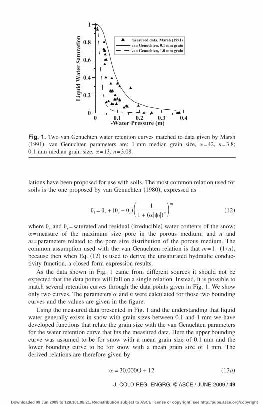
uring the measurement. Even so, an example of a water retention curve relationor snow was presented by Marsh �1991�, and the relation is presented in Fig. 1.he data points shown in the figure were acquired by Marsh from reports byolbeck �1973, 1974�, Wankiewicz �1979�, and Jordan �1983�. In the figure we

ee a cluster of points between 0.05 and 0.15 m on the pressure scale where theaturation changes from 0.1 to 0.8. According to Marsh, the water contents innow samples were measured by calorimetry and the pressure was measuredased on the sample location taken at an elevation over a static water table. Thexact grain shape and size distribution of the snow grains in the experiments wereot given. For the construction of the water retention curves in Fig. 1 we assumedhat most premelt snowpacks have grain sizes around 0.1 mm, which results inhe upper curve in the figure and during the melt period the average size can growo several millimeters, which results in the lower curve of Fig. 1.

For modeling purposes it is common practice to express the water retentionelation by an equation. Those relations are then used many times to deriveelations between unsaturated hydraulic conductivity and liquid water content ofhe porous medium based on the use of Poiseuille’s law for laminar flow in
apillary tubes. Quite a variety of empirical water content-capillary pressure re-


ls

wmcbt

emoc

wdfcld

F�0

Download

ations have been proposed for use with soils. The most common relation used foroils is the one proposed by van Genuchten �1980�, expressed as

�l = �r + ��s − �r�� 1

1 + ��l��n�m

�12�

here �s and �r=saturated and residual �irreducible� water contents of the snow;=measure of the maximum size pore in the porous medium; and n and=parameters related to the pore size distribution of the porous medium. The

ommon assumption used with the van Genuchten relation is that m=1− �1 /n�,ecause then when Eq. �12� is used to derive the unsaturated hydraulic conduc-ivity function, a closed form expression results.

As the data shown in Fig. 1 came from different sources it should not bexpected that the data points will fall on a single relation. Instead, it is possible toatch several retention curves through the data points given in Fig. 1. We show

nly two curves. The parameters and n were calculated for those two boundingurves and the values are given in the figure.

Using the measured data presented in Fig. 1 and the understanding that liquidater generally exists in snow with grain sizes between 0.1 and 1 mm we haveeveloped functions that relate the grain size with the van Genuchten parametersor the water retention curve that fits the measured data. Here the upper boundingurve was assumed to be for snow with a mean grain size of 0.1 mm and theower bounding curve to be for snow with a mean grain size of 1 mm. Theerived relations are therefore given by

0 0.1 0.2 0.3 0.4-Water Pressure (m)

0

0.2

0.4

0.6

0.8

1

LiquidWaterSaturation

measured data, Marsh (1991)

van Genuchten, 0.1 mm grain

van Genuchten, 1.0 mm grain

ig. 1. Two van Genuchten water retention curves matched to data given by Marsh1991�. van Genuchten parameters are: 1 mm median grain size, =42, n=3.8;.1 mm median grain size, =13, n=3.08.

= 30,000� + 12 �13a�



Aga

wv

H

Tat

wTs

ov

w

A

L

TDaa

5

Download

n = 800� + 3 �13b�

verage grain size �� can be related to the volume of ice and the number ofrains. The average grain size is calculated based on the ice content by volumend the number of grains in the domain, that is

� = 2�3Vgr

4��1/3

�14a�

Vgr =�iVt

Ngr�14b�

here Vgr=volume of ice grains in a control volume; Vt=volume of the contrololume; and Ngr=number of grains in the control volume.

ydraulic Conductivity

he saturated hydraulic conductivity function varies with grain size distributionnd the viscosity of the liquid water, which is temperature dependent. The rela-ion used in the present study is the equation of Shimizu �1970�, and is given as

Ks = 0.077��lg

��2 exp�− 7.8

�b

�l� �15�

here Ks=saturated hydraulic conductivity; and �=viscosity of the liquid water.he saturated hydraulic conductivity is reported to be anywhere between 0.0 forolid ice and 3.910−3 m s−1 for low density snow according to Shimizu.

The unsaturated hydraulic conductivity is a monotonically decreasing functionf the effective saturation of the porous medium. Based on the use of Eq. �12�,an Genuchten �1980� proposed the function given by

K = KsSe0.5�1 − �1 − �Se

�1/m��m�2 �16�

here Se = � �l − �r

�s − �r� is effective saturation

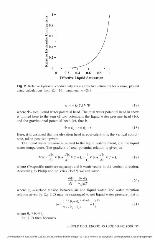
plot of Eq. �16� is given in Fig. 2 to illustrate this function.

iquid Water Flux

he classic way to describe water movement in porous media is the use ofarcy’s law. This description can be applied to many porous media, and here we

ssume that Darcy’s law is applicable to liquid water flow in snow. This samessumption has been applied by many others �Marsh 1991�.

Darcy’s equation for unsaturated porous media is expressed as



wia

Hn

w

wA

wr

w

Fu

Download

ql = − K�Se� � �17�

here =total liquid water potential head. The total water potential head in snows limited here to the sum of two potentials: the liquid water pressure head ��l�,nd the gravitational potential head �e�, that is

= �l + e = �l + z �18�

ere, it is assumed that the elevation head is equivalent to z, the vertical coordi-ate, taken positive upward.

The liquid water pressure is related to the liquid water content, and the liquidater temperature. The gradient of total potential relation is given as

� =d�l

d�l� �l +

d�l

dT� T + k =

1

C� �l +

d�l

dT� T + k �19�

here C=specific moisture capacity; and k=unit vector in the vertical direction.ccording to Philip and de Vries �1957� we can write

d�l

dT=

�l

�a,l

d�

dT�20�

here �a,l=surface tension between air and liquid water. The water retentionelation given by Eq. �12� may be rearranged to get liquid water pressure, that is

�l =1

�� l − �r

�s − �r�−�1/m�

− 1�1/n

�21�

here �r��l��s.

0 0.2 0.4 0.6 0.8 1

Effective Liquid Saturation

0

0.2

0.4

0.6

0.8

1

RelativeHydraulicConductivity

ig. 2. Relative hydraulic conductivity versus effective saturation for a snow, plottedsing calculations from Eq. �16�; parameter m=2 /3

Eq. �17� then becomes



A

ws

M

Ti

H

Tte

w

scagTpstsr

wplcs

5

Download

ql = −K

C� �l − K

�l

�a,l

d�s

dT� T − Kk �22�

fter terms are collected and expressed as diffusivities Eq. �22� becomes

ql = − D�C � �l − DT � T − Kk �23�

here D�=isothermal diffusivity for liquid water; and DT=nonisothermal diffu-ivity for liquid water.

ass Balance Equation for Water

he mass balance equation for liquid water in snow is now derived by substitut-ng Eq. �23� into the combined Eqs. �1� and �2�. The result is

��l

�t+

�i

�l

��i

�t= � · �D�C � �l� + � · �DT � T� + Kk �24�

eat Flux

he flux of heat occurs by both conduction through the pore space and throughhe ice grains, and by convection with the moving liquid water. This flux isxpressed by

qh = − � � T + Cl�l�T − T0�ql �25�

here �=thermal conductivity of the bulk media; and T0=reference temperature.The thermal conductivity in snow was reported to range between 0.028 for dry

now and 2.23844 J m−1 s−1 °C−1 for pure ice �Singh and Singh 2001�. This valuean be estimated in a number of ways, but depends largely on the snow densitynd the connection between grains. Density is important because ice has a muchreater thermal conductivity than air, and it is about twice that of liquid water.he approach presented by de Vries �1966� for thermal conductivity estimation oforous media was originally applied for estimating the thermal conductivity ofoils. The calculation is based on the geometry of the pore space and the connec-ion between the solid grains. We assume that the same approach can be used fornow. The thermal conductivity, calculated according to de Vries �1966� forounded crystals, is given by the relation

� =kva�1 − �l − �i��a + kvl�l�l + kvi�i�i

kva�1 − �l − �i� + kvl�l + kvi�i�26�

here �a, �l, and �i=thermal conductivities of the air, liquid water, and icehases, respectively; and kva, kvl, and kvi=geometric shape factors for the air,iquid water, and ice phases, respectively. The liquid water phase is assumed to beontinuous, because of the liquid-like layer on the ice crystals. The geometric
hape factors are given by


wct

At

w

H

Cwt

Tot

N

EttWpms

Download

kv j =1

3�a,l,i

�1 + � � j

�0− 1�ga�−1

j = a,l,i �27�

here ga=thermal conductivity constant; and �0= thermal conductivity of theontinuous medium �taken to be liquid water in this case�. The thermal conduc-ivity of the individual phases can be calculated as

�l = �1.32 + 0.00559T − 0.0000263T2�/0.2389

�a = �0.0566 + 0.000153T�/0.2389

�i = 2.1 �28�

s an alternative way to compute the bulk thermal conductivity of snow we havehe empirical relations presented by Illangasekare �1990�

� = 0.000307�b + 1.964 10−6�b2, �b � 450 kg m−3

� = 0.00298�b − 0.805, �b � 450 kg m−3 �29�

here �b=917�i+1,000�l=bulk density of the snow.In the above relations all thermal conductivities have units of J m−1 s−1 °C−1.

eat Balance Equation

ombining Eq. �25� with the conservation of thermal energy equation, Eq. �6�,e get the equation for heat balance, assuming thermodynamic equilibrium be-

ween the phases. The heat balance equation is given by

��bCvT��t

= � · �� T� + � · �qlT� − LfEi,l �30�

he last term on the right, which is the latent heat term associated with latent heatf fusion, can be replaced by a term containing the rate of change of ice content,hat is we use LfEi,l=Lf�i��i /�t, to yield

��bCvT��t

+ Lf�i

��i

�t= � · �� T� + � · �qlT� �31�

umerical Solution of Governing Equations

qs. �24� and �31� along with the relationships for the transport parameters andhe equations for solid-liquid phase equilibrium constitute the governing equa-ions for the coupled flow of liquid water flow and heat transport in a snowpack.

hen initial conditions and boundary conditions are specified for a particularroblem of interest, those equations can be solved by either analytical solutionethods for simplified conditions or by numerical methods for more complex

ituations. In this paper a numerical solution scheme is applied to solve these



ees

bbodwfetwitp

�tn

onmtntetGhts

cfp

1

2

3

5

Download

quations for several initial and boundary conditions, and we note that thesequations are solved in two space dimensions. A brief overview of the numericalolution scheme is now presented.

The governing differential equations were discretized using a fully implicit,lock-centered finite difference scheme for the spatial derivatives and a standardackward difference scheme for the temporal derivatives. The temporal derivativef liquid water content in Eq. �24� was treated with the modified-Picard proce-ure described by Celia et al. �1990�, which results in replacement of the liquidater content by the water pressure as the unknown in the equation. As a result,

or these discretizations there are three primary unknowns at each finite differ-nce node point: the water pressure head, the ice content, and the bulk tempera-ure. Since we assume thermodynamic equilibrium between the ice and the liquidater, the water pressure is uniquely related to the temperature, therefore allow-

ng us to replace the pressure by the temperature using Eq. �11�. The result is thathe final set of discretized equations have only ice content and temperature asrimary unknown variables.

The substitution of temperature for water pressure requires the coefficient

T→�lfrom Eq. �10�. In this paper the ice pressure is assumed to be zero, and the

erm for �gr can be computed from Eqs. �9�, �14a�, and �14b�, and the determi-ation of Ngr as described in the next paragraph as Eq. �32�.

To best manage the memory and solution requirement to solve a large systemf algebraic equations the finite difference grid cells in the solution domain wereumbered in sequence along each column. After gathering all like terms into aatrix form it is found that the global matrix for the system of discretized equa-

ions is symmetric and sparse. Even with the sparse nature of the matrix, eachode added in the vertical to the grid adds six diagonals to the sparse matrix dueo the horizontal flux terms in the equations. To reduce this memory cost thequations were solved by iterating on these horizontal flux terms by moving themo the right side of the equations. With this format the matrix had a block form.aussian elimination is used to invert the matrix for solution, but since theorizontal fluxes are iterated upon an iterative procedure is needed. In this studyhe block Jacobi method �Remson et al. 1971� was used to perform the iterativetep. Considerable computational savings were realized by using this procedure.

Since the equations are nonlinear it is necessary to update the coefficients afterompletion of each linear iteration step. The Picard procedure was used to per-orm this nonlinear iteration. All simulations were performed on a Pentium-IVersonal computer.

The computations for a solution were performed by the following steps:. Read the files for input data, which specify the geometry, initial conditions,

boundary conditions, duration of the simulation, and snow parameters in-cluding the initial size of snow grains. The number of snow grains in a unitvolume is then determined based on the specified initial ice content and thegrain sizes;

. During any given time step, the matrix equations are constructed and solvedusing the block Jacobi method for the linear matrix solution step, and Picarditeration to update the nonlinear parameters;

. The water retention curve parameters are updated after every Picard itera-



4

5

R

C

Agpss�F�

twlwt

ii

Download

tion. These parameters are dependent on the mean size of the snow grains,which is calculated with Eqs. �14a� and �14b�, where the number of snowgrains is updated with Eq. �32� based on the amount of ice calculated for therepresentative elementary volume for the previous iteration

Ngr = Ngrold ��i � 0

Ngr = Ngrold�0.01� + 0.9999 − � �t

86,400� − ��i� ��i � 0 �32�

These relations are empirically based and were fitted together with Eqs.�14a� and �14b� to match the expected crystal sizes for a hypothetical snow-pack undergoing a melt period, growing from 0.001 to 0.01 m in a day, with�t much smaller than 86,400 s;

. Convergence of the Picard iterations were considered complete at a relativeerror of 10−8. After convergence of the Picard iteration steps, the solution ischecked for mass balance error. The allowable mass balance error was set to10−6 in relative terms; and

. When the mass balance is satisfied, the solution moves to the next time step,the size of which is based on the number of Picard iterations required in thecurrent time step. When more than 15 Picard iterations are required toachieve convergence, the next time step is set to one half of the current timestep, while if the number of iterations are less than five, then the next timestep is set to twice the current time step.

esults

omparison Simulation

comparison of our model is given with respect to results obtained by Illan-askare et al. �1990�. Their model was developed for a similar type of ap-lication. The problem of interest involves the infiltration of water into a coldnowpack of 0.5 m depth. The infiltration rate into the top of the snowpack waspecified as 1 mm /h. The van Genuchten parameters used for the snow were

according to Eq. �13a� and n according to Eq. �13b�, =42, n=3.8,r=110−8, the values corresponding to the lower bounding curve shown inig. 1. The value of Ks is calculated according to Shimizu �1970�, Eq. �15�, andis calculated according to Eqs. �29� �Illangasekare et al. 1990�.The top boundary of the snowpack had the infiltration flux and a specified

emperature of 0°C, while the bottom boundary was considered impermeable toater and had a specified temperature of −10°C. The initial conditions were:

inear temperature profile with 0°C at the top and −10°C at the bottom; liquidater content given by the van Genuchten function for the given initial tempera-

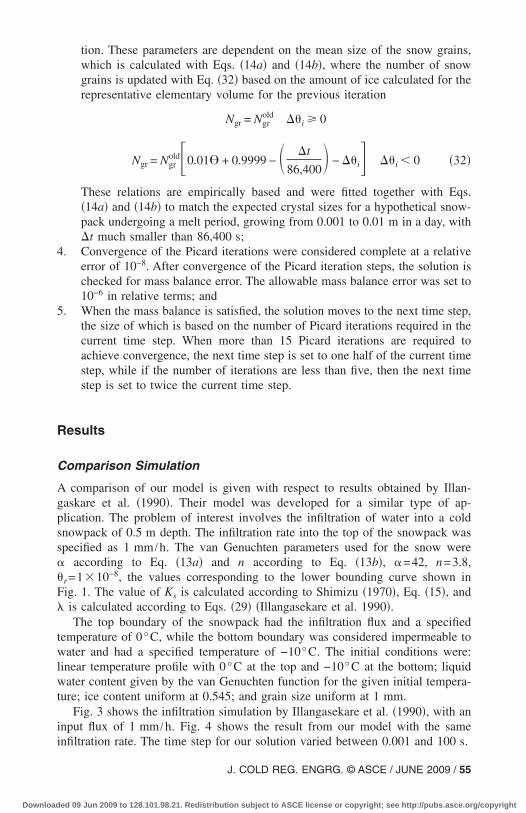
ure; ice content uniform at 0.545; and grain size uniform at 1 mm.Fig. 3 shows the infiltration simulation by Illangasekare et al. �1990�, with an

nput flux of 1 mm /h. Fig. 4 shows the result from our model with the same
nfiltration rate. The time step for our solution varied between 0.001 and 100 s.


tfistuootw

ccccau

Fit

5

Download

The results seen in this comparison are different in the saturation profile and inhe porosity profile. The saturation profile derived from our solution is differentrom the Illangasekare et al. �1990� solution in that our solution exhibits anncreasing saturation with depth behind the wetting front instead of a constantaturation as derived by Illangasekare et al. This seems counterintuitive, becausehe water is added at the top of the profile and one would expect that with aniform porous medium that the saturation profile would be uniform. However,f course the snow is not uniform as the infiltration progresses because freezingccurs as the front moves downward, thus decreasing the porosity. So the ques-ion then arises as to why the Illangasekare et al. result shows a uniform liquidater profile while our solution does not.

The difference between the saturation profiles can be explained based on theharacter of the relation between effective saturation and unsaturated hydrauliconductivity. The effective saturation is given by Se= �S−Sr� / �1−Sr�, and in thease of the Illangasekare et al. �1990� model the residual saturation was set to aonstant value of 0.05, while in our model the residual water content is constantnd therefore the residual saturation varied inversely with porosity. In effect, the

(b)(a)

(c)

0 0.02 0.04 0.06 0.08Liquid Water Saturation

0.4

0.3

0.2

0.1

0

Depth(m)

0.42 0.43 0.44 0.45 0.46Porosity

0.4

0.3

0.2

0.1

0

Depth(m)

3 hours

6.0 hours

9.0 hours

12 hours

-8 -6 -4 -2 0Temperature (oC)

0.4

0.3

0.2

0.1

0

Depth(m)

ig. 3. Data from Illangasekare et al. �1990� for their simulation of water infiltratingnto cold snowpack. Infiltration rate was 1 mm /h. Shown are depth dependent varia-ions of porosity, liquid water saturation, and temperature.

nsaturated hydraulic conductivity of the Illangasekare et al. model is therefore



gToc

rsnd

owmbw

Fid

Download

reater at lower porosity and lower at higher porosity than that in our model.hese differences in the tendencies of the unsaturated hydraulic conductivitiesf the two models should produce the observed differences in the liquid waterontent profiles.

To confirm this explanation for the difference between the two models, theesidual saturation parameter was set to a constant of 0.05 in our model and theame simulation was performed. The result was that the saturation profile, whileot exactly the same as the one shown in Fig. 3, was so close that it would beifficult to distinguish in a plot.

The difference in the porosity profiles can be explained based on the fact thatur model assumed thermodynamic equilibrium between the two water phases,hile in the Illangasekare et al. �1990� model this was not the case. Thus in ourodel, water at the wetting front will freeze immediately if the temperature is

elow the freezing point, while in the Illangasekare et al. model some liquid

(b)

0.5

-10 -8 -6 -4 -2 0

Temperature (oC)

0.4

0.3

0.2

0.1

0

Depth(m)

0 0.02 0.04 0.06

Liquid Water Saturation

0.5

0.4

0.3

0.2

0.1

0

Depth(m)

0.41 0.42 0.43 0.44 0.45 0.46

Porosity

0.5

0.4

0.3

0.2

0.1

0

Depth(m)

3 hours

6 hours

9 hours

12 hours

(a)

(c)

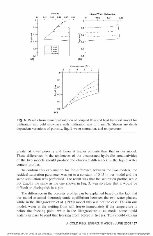
ig. 4. Results from numerical solution of coupled flow and heat transport model fornfiltration into cold snowpack with infiltration rate of 1 mm /h. Shown are depthependent variations of porosity, liquid water saturation, and temperature.

ater can pass beyond that freezing front before it freezes. This should explain



wts

fcit

F

Tcttlwtcfl−wta

stFsgttF

tlsS

g

Ef

5

Download

hy the porosity profile generated by our model is so sharp at the front while forhe Illangasekare et al. model the front is more diffuse while still being quiteteep.

The results for both models show that the porosity decreases as the wettingront progresses downward. This occurs because as the front moves closer to theonstant temperature boundary the temperature gradient increases, thus increas-ng the ability for latent heat to be carried away from the freezing front. Thishereby increases the amount of ice accumulation at a given depth.

reezing Simulation

his simulation is intended to demonstrate the freezing of water in a 0.55 m longolumn of snow laid horizontally to eliminate the effect of gravity. This simula-ion is not a representation of a natural situation, but rather a simplified case toest whether liquid water migrates to the freezing front and forms a dense iceayer as is often observed in snowpacks. The absence of gravity in the simulationas expected to increase the chance that a dense ice layer forms. In this case

he snow was initially at a uniform temperature of −0.0005°C. The initial iceontent was 0.50. Both boundaries are considered to be impermeable to waterow. At the beginning of the simulation one boundary suddenly was set to10°C. The opposing boundary was insulated. The van Genuchten parametersere set to: =42, n=3.8, �r=110−8, with Ks according to Eq. �15� and a fixed

hermal conductivity �=0.8 J m−1 s−1 °C−1. For the given retention parametersnd the initial temperature the initial water content is 0.046.

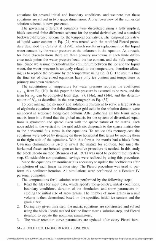
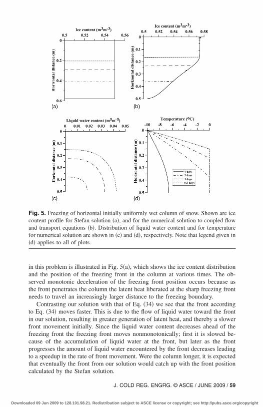
The simulation was performed for a period of 4 days. The results of theimulation are illustrated in Fig. 5. The ice content profile is given in Fig. 5�b�,he liquid water content profile in Fig. 5�c�, and the temperature profile inig. 5�d�. The results show that the freezing front moves into the profile as aharp front, but the ice content distribution is nonuniform, with the content beingreater toward the freezing boundary. This nonuniform distribution of ice forma-ion occurs because of the migration of liquid water toward the freezing front,hereby lessening the water content ahead of the freezing front as illustrated byig. 5�c�.

For comparison it should be interesting to evaluate the rate of movement ofhe freezing front for this case in comparison to the rate that would occur if theiquid water were not to migrate to the front. The rate of movement for ourolution is compared to the rate using a sharp front approximation given by thetefan equation

dxf

dt=

1

2�2��T

Lf�l�l�1/2

t−1/2 �33�

iving for the position of the front

xf = �2��T

Lf�l�l�1/2

t1/2 �34�

q. �34� indicates that the speed of the freezing front decreases monotonically
or the Stefan formulation. The result for this formulation for the parameters used


iastn

tiffcpttc

Fcaf�

Download

n this problem is illustrated in Fig. 5�a�, which shows the ice content distributionnd the position of the freezing front in the column at various times. The ob-erved monotonic deceleration of the freezing front position occurs because ashe front penetrates the column the latent heat liberated at the sharp freezing fronteeds to travel an increasingly larger distance to the freezing boundary.

Contrasting our solution with that of Eq. �34� we see that the front accordingo Eq. �34� moves faster. This is due to the flow of liquid water toward the frontn our solution, resulting in greater generation of latent heat, and thereby a slowerront movement initially. Since the liquid water content decreases ahead of thereezing front the freezing front moves nonmonotonically; first it is slowed be-ause of the accumulation of liquid water at the front, but later as the frontrogresses the amount of liquid water encountered by the front decreases leadingo a speedup in the rate of front movement. Were the column longer, it is expectedhat eventually the front from our solution would catch up with the front position

ig. 5. Freezing of horizontal initially uniformly wet column of snow. Shown are iceontent profile for Stefan solution �a�, and for the numerical solution to coupled flownd transport equations �b�. Distribution of liquid water content and for temperatureor numerical solution are shown in �c� and �d�, respectively. Note that legend given ind� applies to all of plots.

alculated by the Stefan solution.



hvsstrfm

cmafiba

G

Iodmi

cgot

a0ttgcwrFsKE

gbi

6

Download

Although graphical results are not shown here we note that when the saturatedydraulic conductivity is set to zero for our model the predicted freezing front isery similar to that for the Stefan solution. The front is not as sharp as the Stefanolution because our model accounts for freezing point depression, leading to ateep, but slightly diffuse front. The resulting ice content profile is identical tohat for the Stefan solution because for this case the liquid water freezes in placeather than moving toward and accumulating at the freezing front. This resulturther emphasizes the importance of the liquid water flow in affecting the move-ent of the freezing front and the ultimate ice content profile.Producing a solid layer of ice within the column requires an ice content in-

rease to a value equal to 1.0. This would of course require that the freezing frontove slowly enough into the column such that the migrating liquid water can

ccumulate to a high enough value �in this case an increase of 0.5� to completelyll the initial porosity with ice upon freezing. This result does not occur howeverecause the freezing front is not slow enough to allow this amount of waterccumulation to occur.

rain Size Variation during Infiltration

t is expected that the size of grains in the snow should have a significant effectn the movement of liquid water in a snowpack, since both the saturated hy-raulic conductivity of the snow, and the retention of liquid water by the snowedium are strongly affected by grain size. We now show a case of vertical

nfiltration into a snowpack to demonstrate this effect.Two cases of infiltration are tested: one into a homogeneous medium with

hanging snow grain size and the other into a homogeneous medium with fixedrain size. The test shows that there is not only an effect of spatial heterogeneityf water in the snow; there is also a temporal effect of changing snow grains onhe melt water distribution.

The short melt water infiltration event starts during the third hour of the daynd lasts for 1 h with an intensity of 1.8 mm /h continuing with 1 h at.36 mm /h. Therefore, the infiltration ends after the fourth hour and is zero forhe remainder of the simulation. The initial van Genuchten parameters were es-imated according to the initial grain size of 1.0 mm with Eqs. �13a� and �13b�,iving values of =42, n=3.8, �r=110−8. These parameters will of coursehange for the case where the snow grains vary with time. The bottom boundaryas set to be impermeable to water flow and insulated, while the upper boundary

eceived a variable liquid water flux and the temperature was set to −0.001°C.or initial conditions: temperature, liquid water content, ice content, and grainize are all uniform at −1°C, 0.0, 0.30, and 1.0 mm, respectively. The values fors are according to Eq. �15� and � according to the thermal conductivity given byqs. �29�.

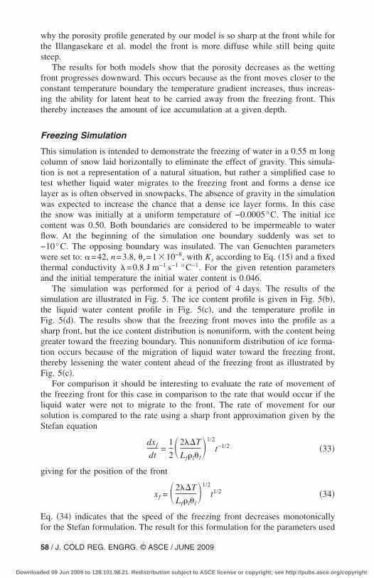
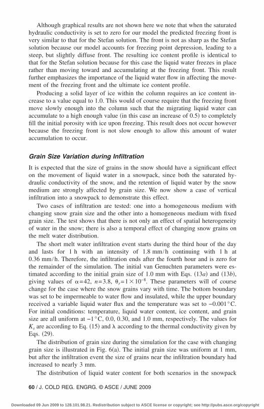
The distribution of grain size during the simulation for the case with changingrain size is illustrated in Fig. 6�a�. The initial grain size was uniform at 1 mm,ut after the infiltration event the size of grains near the infiltration boundary hadncreased to nearly 3 mm.

The distribution of liquid water content for both scenarios in the snowpack



dorFahbt

D

Tpiwtb

F�fi

Download

uring the simulation is illustrated in Figs. 6�b and c�. Here we see that the effectf changing grain size on liquid water distribution is dramatic, even while weealize that the overall change in liquid water content is not large �about 0.5%�.or the case of changing snow grains, the front of liquid water content penetratedbout 10 cm deeper into the snowpack, and the liquid water content is about 15%igher at the wetting front. The dramatic difference in water distribution occursecause of the increased hydraulic conductivity and decreased water retentionhat occurs with grain growth.

iscussion

he model developed for the work presented in this paper is similar to thatresented by Nassar and Horton �1992�. One main difference between the modelss that they considered the phase change between liquid water and water vapor,hile we ignored water vapor and considered the phase change from liquid water

o ice. We justified neglecting water vapor contributions to the transport of water

0 0.004 0.008 0.012 0.016 0.02

Liquid water content (m3m-3)

0.5

0.4

0.3

0.2

0.1

0

Depth(m)

0.5 days

0.4 days

0.3 days

0.2 days

0.0012 0.0016 0.002 0.0024 0.0028

Mean grain size (m)

0.5

0.4

0.3

0.2

0.1

0

Depth(m)

0 0.004 0.008 0.012 0.016 0.02

Liquid water content (m3m-3)

0.5

0.4

0.3

0.2

0.1

0

Depth(m)

(b)(a)

(c)

ig. 6. Grain size distribution for simulation where grain size was allowed to changea�; melt water content distribution after pulse of melt water entered snowpack forxed snow grain size �b�; and changing grain size �c�

ased on a dimensional analysis that indicated water vapor to be a minor player



ddwaflvbi

ltlepetutigmzh

w2w1awmbbcf

flheSlSTcd

6

Download

uring infiltration and redistribution �Daanen 2004�. However, it might be thaturing long-term freezing processes that water vapor would be important andould be required in the model. A second major difference between our model

nd the model of Nassar and Horton is that we did not consider solute in theormulation. We should mention that Daanen �2004� did provide a model formu-ation for the full suite of variables including liquid water, temperature, waterapor, ice, and solute. The presentation in this paper was somewhat simplifiedecause we were interested only in infiltration and short-term freezing processesn the snowpack.

To summarize the model, it includes a mass balance equation for water in theiquid and solid phase, a heat balance equation including the latent heat exchangehat occurs with phase change, equation for thermodynamic equilibrium betweeniquid water and ice, expressions for quantifying the growth of ice grains, and anxpression for water retention and unsaturated hydraulic conductivity of the snoworous medium. These many features of the model provide it with the capacity toxamine the details of liquid water flow, freezing, and melting along with heatransfer processes in a snowpack. It is different than other models that have beensed for simulating liquid water flow in snowpacks through the fact that it relateshe snow temperature directly with the liquid water pressure, through explicitncorporation of thermodynamic equilibrium. This approach generates pressureradients in the snowpack that produce liquid water fluxes ignored in most otherodels of liquid water flow in snow. These fluxes are demonstrated in the hori-

ontal freezing simulation, and may prove important for future studies related toeterogeneous snowpacks and fluxes along impermeable ice layers.

Other models for liquid water flow in snow include the class of kinematicave models �Colbeck 1972; Bengtsson 1982; Marsh and Woo 1985; Sellers000�, the Richards equation type model �Jordan 1983�, and models for coupledater flow, heat transport, and phase change �Jordan 1991; Illangasekare et al.990; Tseng et al. 1994�. The kinematic wave models are applied under thessumption that gravitational force is dominant over the capillary force, and thisill most likely be the case for most snowmelt events �Wankiewicz 1979�. Theseodels consider only the flow of the liquid water and treat the porous snow as

eing passive to the presence of liquid water, that is, the snow does not respondack to the flux of the water. The Richards equation type of models again do notonsider any feedback from the snowpack to the liquid water, but they do accountor capillarity as a driving mechanism for flow.

The model presented by us is closest to the various types of coupled waterow and heat transport models listed above. There are still some differencesowever. The SNTHERM model �Jordan 1991� accounts for thermodynamicquilibrium, as done in our model, but the thermodynamic equilibrium for theNTHERM model is expressed in terms of a relation between temperature and

iquid water content. Liquid water pressure does not enter into the calculations ofNTHERM because it assumes that the flow of liquid water is by gravity only.he models of Illangasekare et al. �1990� and Tseng et al. �1994� both account forapillarity as well as gravity in the flow, but their models do not assume thermo-ynamic equilibrium as we do in our model.

The procedure given for updating of grain size based on the number of grains



Essft�swf

slloT�em

mpamCmdra

mpiwasbmnw

icutHlw

Download

q. �32� was derived from trial-and-error simulations and tended to fit the grainizes that have been observed in the field. However, it might appear from the dataummarized by Marsh �1991� for experiments performed by Wakahama �1968�or snow at low water content, that the growth rates simulated with our model areoo high. The growth rates we simulated might be reasonable for saturated snowMarsh 1991; Wakahama 1974�, but our modeling results were for quite lowaturations. As grain size is very important to the penetration depth of liquidater, it is important to have a representative model of grain size dynamics. This

eature will require additional work.It has been demonstrated by Illangasekare et al. �1990� that heterogeneities in

now properties within a snowpack will significantly affect the distribution ofiquid water migration within the snowpack. They showed that the presence of iceenses will interrupt the downward flow of water and lead to a lateral movementf liquid water and concentration of downward flow along the edges of the lenses.his concentrated flow has been observed in the field and is described by Marsh

1991�. Based on the results shown in our last example one can also imagine theffect of more subtle features such as variations in grain size on the downwardovement of water.To date there has not been a successful attempt to fully simulate the develop-

ent of strong layering or other types of structures of heterogeneity in a snow-ack. A recent attempt was reported by Gustafsson et al. �2004� in which theuthors applied the SNTHERM model �Jordan 1991�, and the SNOWPACKodel �Bartelt and Lehning 2002; Lehning et al. 2002� in conjunction with theOUP model �Jansson and Moon 2001� which is a soil-plant-atmosphere transferodel. The authors simulated conditions for a monitored snowpack in which

istinct ice layering was observed, but the simulation models were not able toeproduce the development of the distinct layers, some of which reached densitiess high as 500 kg m−1.

We expect that a model similar to the one we present might be capable ofimicking the conditions leading to the formation of strong layering in a snow-

ack. We hypothesize the conditions that will lead to the formation of this layer-ng involve repeated infiltration events, grain growth, concentration of infiltratedater into certain positions within the snowpack, freezing of the infiltrated water,

nd of course pack consolidation. With the initial discrimination of a layer sub-equent infiltration will again be held up by the layer and with freezing the layerecomes denser. With repeated infiltration the layer will build up with ice andight eventually become impermeable, or nearly so. Additional work will be

ecessary with the developed model to discover the conditions that potentiallyill lead to the formation of these layers.

The use of the van Genuchten �1980� type of water retention curve expressions somewhat limiting because the lower limit water content is the residual waterontent, rather than zero water content. The residual water content is a constructsed in most analytical water retention curve expressions to account for the facthat hydraulic conductivity is rather small �taken as zero� at low water contents.owever, even at extremely low water content there is still some conductance of

iquid water, and although it is quite small it is completely conceivable that liquid
ater flow even at low rates can have a significant effect on water flow toward a


frrws

C

Tfcepg

t1

2

3

oad

N

T

6

Download

reezing front. Also, water at low water contents is susceptible to freezing, butetention functions that use the residual water content parameter do not allow theesidual water to freeze. Several models �Rossi and Nimmo 1994� that extend theater retention curve to zero could quite easily be adopted into our model. This

hould be done in future work.

onclusion

he model presented in this study is fundamentally different from other modelsor flow of liquid water in snow. Its distinguishing features are that it fullyouples the mass flow and heat transport processes and enforces thermodynamicquilibrium between the liquid and solid phases, and capillarity is included asart of the force for driving liquid water flow. The model also accounts for therowth of snow grains during infiltration events.

The numerical solution was applied to three case studies. A brief description ofhe case study and the conclusions from those case studies are summarized below.. The problem of vertical infiltration into a cold snowpack as described by

Illangasekare et al. �1990� was simulated with our model. The simulatedprofiles of ice content, liquid water content, and temperature were found tobe very similar to those presented by Illangasekare et al., but there weredistinct differences. The differences were explained in terms of the assump-tion of thermal nonequilibrium used in their model;

. The freezing from one end of a horizontal initially uniformly wet column ofsnow was shown to cause migration of liquid water toward the freezingfront, thereby reducing the liquid water content ahead of the front, and in-creasing the ice content behind the front, which is a direct result of couplingthe temperature to the liquid water pressure; and

. The problem of vertical infiltration into a uniformly dry snowpack was usedto test the effect of grain size growth on the depth of wetting. The simulationallowing for grain growth led to a 37% increase in wetting depth in com-parison to the case where the grain size was kept constant. This increase inwetting depth occurred because the increase in grain size increased the satu-rated hydraulic conductivity and decreased the liquid water retention of thesnow.

The model should be suited to investigate the processes underlying the devel-pment of strong layering in snowpacks and heterogeneous liquid water flow. Inddition, the process of water vapor transport should be included in futureevelopments/applications of the model.

otation

he following symbols are used in this paper:C � specific moisture capacity �m−1�;Cl � specific heat of liquid water �J kg−1 °C−1�;

−1 −1
Cv � bulk heat capacity �J kg °C �;


Download

DTl � thermal moisture diffusivity for liquid water �m2 s−1 °C−1�;

D�l � isothermal moisture diffusivity for liquid water �m2 s−1�;

Ei,l � freeze/melt mass transfer �kg s−1 m−3�;e � elevation potential head �m�;g � acceleration of gravity 9.81 �m s−2�;

ga � thermal conductivity constant �-�;K � unsaturated hydraulic conductivity �m s−1�;

Ks � saturated hydraulic conductivity �m s−1�;k � unit vector in the vertical �-�;

kva � thermal conductivity parameter for air phase �-�;kvi � thermal conductivity parameter for ice phase �-�;kvl � thermal conductivity parameter for liquid water phase �-�;Lf � latent heat of fusion: 0.33E+6 �J kg−1�;

n ,m � van Genuchten parameters related to pore size distribution �-�;ngr � number of ice grains in control volume �-�;

Qhi,l � sensible heat exchange between liquid and ice phases �J s−1 m−3�;

qha � sensible heat flux in air phase �J s−1 m−2�;

qh � total sensible heat flux in bulk snow �J s−1 m−2�;qh

i � sensible heat flux in ice �J s−1 m−2�;qh

l � sensible heat flux in liquid water �J s−1 m−2�;ql � flux for liquid water �m s−1�;Se � effective saturation of liquid water �-�;

Tl ,Ti � temperature for liquid water and ice �°C�;T0 � reference temperature �°C�;

t � time �s�;Vgr � volume of ice grains in control volume �m3�;Vt � volume of control volume �m3�;z � coordinate axis �positive upward� �m�; � van Genuchten parameter alpha �m−1�;�s � surface tension of water �N m−1�;� � mean size of snow grains �m�;�a � volumetric air content �-�;�i � volumetric ice content �-�;�l � volumetric liquid water content �-�;�r � volumetric residual liquid water content �-�;�s � volumetric saturated liquid water content �-�;� � thermal conductivity of bulk snow �J m−1 s−1 °C−1�;

�l ,�i ,�a � thermal conductivity for liquid water, ice, and air, respectively�J m−1 s−1 °C−1�;

�b � bulk density of snow �kg m−3�;�i � density of ice=918 �kg m−3�;�l � density of liquid water �kg m−3�; � total potential head for liquid water �m�;�i � ice pressure head �m�;�l � liquid water pressure head �m�; and

�T→�l� freezing point depression variable �m T−1�.



R

B

B

C

C

C

C

C

C

D

D

D

d

G

H

I

J

J

J

L

6

Download

eferences

artelt, P., and Lehning, M. �2002�. “A physical SNOWPACK model for the Swiss ava-lanche warning. Part I: Numerical model.” Cold Regions Sci. Technol., 35�3�, 123–145.

engtsson, L. �1982�. “Percolation of meltwater through a snowpack.” Cold Regions Sci.Tech., 6, 73–81.

elia, M. A., Bouloutas, E. T., and Zarba, R. L. �1990�. “A general mass-conservativenumerical solution for the unsaturated flow equation.” Water Resour. Res., 26, 1483–1496.

olbeck, S. C. �1972�. “A theory of water percolation in snow.” J. Glaciol., 11, 369–405.

olbeck, S. C. �1973�. “Theory of metamorphism of wet snow.” Cold Region ResearchEngineering Lab., Res. Rep. No. 313, Hanover, N.H.

olbeck, S. C. �1974�. “The capillary effects on water percolation in homogeneous snow.”J. Glaciol., 13, 85–97.

olbeck, S. C. �1978�. “Physical aspects of water flow through snow.” Adv. Hydrosci., 11,165–206.

olbeck, S. C. �1982�. “An overview of seasonal snow metamorphism.” Rev. Geophys.Space Phys., 20�1�, 45–61.

aanen, R. P. �1997�. “A one dimensional model study on the movement of water out ofthe snowpack into the soil, during winter and spring in Sjökulla Finland.” MS thesis,Univ. of Wageningen, Wageningen, The Netherlands.

aanen, R. P. �2004�. “Modeling liquid water flow in snow.” Ph.D. dissertation, Univ. ofMinnesota, St. Paul, Minn.

ash, J. G., Fu, H., and Wettlaufer, J. S. �1995�. “The premelting of ice and its environ-mental consequences.” Rep. Prog. Phys., 58, 115–167.

e Vries, D. A. �1966�. “Thermal properties of soils.” Physics of plant environment, W. R.van Wijk, ed., North-Holland, Amsterdam, The Netherlands.

ustafsson, D., Waldner, P., and Stähli, M. �2004�. “Factors governing the formation andpersistence of layers in subalpine snowpack.” Hydrolog. Process., 18�7�, 1165–1183.

arrington, R., Bales, R. C., and Wagnon, P. �1996�. “Variability of meltwater and solutefluxes from homogeneous melting snow at the laboratory scale.” Hydrolog. Process.,10, 945–953.

llangasekare, T. H., Walter, R. J., Meier, M. F., and Pfeffer, W. T. �1990�. “Modeling ofmeltwater infiltration in subfreezing snow.” Water Resour. Res., 26�5�, 1001–1012.

ansson, P. E., and Moon, D. �2001�. “A coupled model of water, heat and mass transferusing object orientation to improve flexibility and functionality.” Environ. Modell. Soft-ware, 16�1�, 37–46.

ordan, P. �1983�. “Meltwater movement in a deep snowpack. 2: Simulation model.” WaterResour. Res., 19, 979–985.

ordan, R. �1991�. “A one-dimensional temperature model for a snow-cover.” TechnicalDocumentation for SNTHERM.89. Special Rep. No. 91-16, U.S. Army Cold RegionsResearch Laboratory, Hanover, N.H.

ehning, M., Bertelt, P., Brown, B., Fierz, C., and Satyawali, P. �2002�. “A physicalSNOWPACK model for the Swiss avalanche warning. Part II: Snow microstructure.”
Cold Regions Sci. Technol., 35, 147–167.


L

M

M

M

N

P

R

R

S

S

S

S

S

S

T

T

v

W

W

W

W

Download

undquist, J. D., and Dettinger, M. D. �2005�. “How snowpack heterogeneity affects diur-nal streamflow timing.” Water Resour. Res., 41, W05007.

arsh, P. �1991�. “Water flux in melting snow covers.” Advances in porous media, M. Y.Corapcioglu, ed., Elsevier, Amsterdam, Vol. 1, 61–124.

arsh, P., and Woo, M. �1985�. “Melt water movement in natural heterogeneous snowcovers.” Water Resour. Res., 21, 1710–1716.

orland, L. W., Kelly, R. J., and Morris, E. M. �1990�. “A mixture theory for phase-changing snowpack.” Cold Regions Sci. Technol., 17, 271–285.

assar, I. N., and Horton, R. �1992�. “Simultaneous transfer of heat, water and solute inporous media. I: Theoretical development.” Soil Sci. Soc. Am. J., 56, 1350–1356.

hilip, J. R., and de Vries, D. A. �1957�. “Moisture movement in porous materials undertemperature gradients.” Trans., Am. Geophys. Union, 38, 222–232.

emson, I., Hornberger, G. M., and Molz, F. J. �1971�. Numerical methods in subsurfacehydrology, Wiley-Interscience, New York.

ossi, C., and Nimmo, J. R. �1994�. “Modeling of soil water retention from saturation tooven dryness.” Water Resour. Res., 30, 701–708.

ellers, S. �2000�. “Theory of water transport in melting snow with a moving interface.”Cold Regions Sci. Tech., 31, 47–57.

himizu, H. �1970�. “Air permeability of deposited snow.” Contribution No. 1053, Instituteof Low Temperature Science, Sapporo, Japan.

ingh, P., and Singh, V. P. �2001�. Snow and glacier hydrology, Kluwer, Dordrecht, TheNetherlands.

paans, E. J. A. �1994�. “The soil freezing characteristic: Its measurement and similarityto the soil moisture characteristic.” Ph.D. dissertation, Univ. of Minnesota, St. Paul,Minn.

paans, E. J. A., and Baker, J. M. �1996�. “The soil freezing characteristic: Its measurementand similarity to the soil moisture characteristic.” Soil Sci. Soc. Am. J., 60�1�, 13–19.

tähli, M. D., and Jansson, P. E. �1998�. “Test of two SVAT snow submodels duringdifferent winter conditions.” Agric. Forest Meteorol., 92, 29–41.

seng, P.-H., Illangasekare, T. H., and Meier, M. F. �1994�. “A 2D finite element methodfor water infiltration in a subfreezing snowpack with a moving surface boundary duringmelting.” Adv. Water Resour., 17, 205–219.

uteja, N. K., and Cunnane, C. �1997�. “Modeling coupled transport of mass and energyinto the snowpack model development, validation and sensitivity analysis.” J. Hydrol.,195, 232–255.

an Genuchten, Th. M. �1980�. “A closed form equation for predicting the hydraulic con-ductivity of unsaturated soil.” Soil Sci. Soc. Am. J., 44, 892–898.

akahama, G. �1968�. “The metamorphism of wet snow.” Int. Assoc. Sci. Hydrol., 79,370–379.

akahama, G. �1974�. “The role of meltwater in densification processes of snow and firn.”Int. Assoc. Sci. Hydrol., 114, 66–72.

aldner, P. A., Sneebeli, M., Schultze-Zimmermann, U., and Flüher, H. �2004�. “Effectof snow structure on water flow and solute transport.” Hydrolog. Process., 18, 1271–1290.

ania, F., Hoff, J. T., Jia, C. Q., and Mackay, D. �1998�. “The effects of snow onthe environmental behavior of hydrophobic organic chemicals.” Environ. Pollut., 102,
25–41.


W

W

W

6

Download

ankiewicz, A. �1979�. “A review of water movement in snow.” Proc., Modelling Snow-

cover Runoff, Cold Reg. Res. Eng. Lab., Hanover, N.H., 222–252.

igmosta, M. S., Vail, L. S., and Lettenmaier, D. P. �1994�. “A distributed hydrology-

vegetation model for complex terrain.” Water Resour. Res., 30, 1665–1680.

illiams, M. W., Sommerfeld, R., Massman, S., and Rikkers, M. �1999�. “Correlation

lengths of meltwater flow through ripe snowpacks.” Hydrolog. Process., 13, 1807–

1826.



Model of coupled liquid water flow and heat transport with phase change in a snowpack

Documents

Transcript of Model of coupled liquid water flow and heat transport with phase change in a snowpack